Analytical solution of a class of network dynamics with ...math.gmu.edu/~harbir/PInetwork.pdf · Analytical solution of a class of network dynamics with mechanical and nancial applications

Analytical solution of a class of network dynamicswith mechanical and financial applications

P. Krejcı,1 H. Lamba,2 S. Melnik,3 and D. Rachinskii4, 5

1Institute of Mathematics, Academy of Sciences of the Czech Republic, Prague, Czech Republic2Department of Mathematical Sciences, George Mason University, Fairfax, USA

3MACSI, Department of Mathematics & Statistics, University of Limerick, Ireland4Department of Applied Mathematics, University College Cork, Ireland

5Department of Mathematical Sciences, University of Texas at Dallas, Richardson, USA

We show that for a certain class of dynamics at the nodes the response of a network of anytopology to arbitrary inputs is defined in a simple way by its response to a monotone input. Thenodes may have either a discrete or continuous set of states and there is no limit on the complexity ofthe network. The results provide both an efficient numerical method and the potential for accurateanalytic approximation of the dynamics on such networks. As illustrative applications, we introducea quasistatic mechanical model with objects interacting via frictional forces, and a financial marketmodel with avalanches and critical behavior that are generated by momentum trading strategies.

PACS numbers: 89.75.Hc, 75.60.Ej, 89.65.Gh, 89.75.Fb, 64.60.aq

I. INTRODUCTION

Dynamical processes on networks are used to model awide variety of phenomena such as the spreading of opin-ions through a population [1], propagation of infectiousdiseases [2], neural signaling in the brain [3], and cascad-ing defaults in financial systems [4]. Similar dynamicalprocesses on regular lattices are used for modeling phasetransitions and critical phenomena in statistical mechan-ics [5], avalanches and propagation of cracks in earth-quake fault systems [6], percolation phenomena [7, 8],crackling noise [8, 9] and hysteresis in constitutive re-lationships of various materials [10]. The structure ofthe underlying network may strongly influence the dy-namics, the response of the network to variations of theinput and parameters, and the critical values of parame-ters such as the critical temperature of the random fieldIsing spin-interaction model [11], or the epidemic thresh-old for disease-spread models [12–14]. Prediction of theresponse of a network to variations of the input or initialstate is thus an important problem, which remains openfor many real-world and randomly generated networks(e.g., networks with arbitrary degree distribution) [15].

Nodes of the above networks are often assumed tohave a binary response modeled by Heaviside step func-tions [16]. In this paper, we consider networks with adifferent type of nodes characterized as Prandtl-Ishlinskii(PI) operators.1

1 The classical Prandtl-Ishlinskii model of plasticity and fric-tion [17, 18] introduced independently by Prandtl (1928) andIshlinskii (1944) is obtained by the linear superposition of sim-ple hysteresis operators (stops) that model non-interacting fiberswith possibly different physical properties. Recently, the modelhas found new applications in such areas as control of sensors andactuators [19, 20]. The celebrated Preisach model used in mod-eling ferromagnetism [21, 22], magnetostriction [23], and porousmedia flow [24], can also be considered as a nonlinear generaliza-

We present an almost explicit solution for the input-state-output relationship for networks of PI operators atthe nodes. Essentially, we demonstrate that the networkof PI nodes is also a PI operator with, possibly, a dis-continuous response. This fact sets a limitation on theclass of systems that can be modeled by a network ofconnected PI nodes while simultaneously providing us

��

u

k1 k1

1

2

3

(a) (b)

FIG. 1. (Color online) (a) A mechanical analogy of the stopoperator: an ideal spring and an object on a dry surface con-nected in series. When the spring stress σ is within the range(−r, r), variations of the displacement x cause linear changesin σ while the object remains stationary on the surface. Thespring stress clamps at a value of ±r whereas the object movesrelative to the surface following x. (b) A mechanical modelwith three nodes, each attached to a fixed left plate and amoving right plate by two elastic springs, with interactionsmodeled by stop operators as in (a).

tion of the Prandtl-Ishlinskii model. The PI operator introducedin this paper generalizes the classical Prandtl-Ishlinskii modelby including a possibility of discontinuous response that modelsavalanches. The objective of this paper is twofold: firstly, topresent a new method for solving dynamics on networks (witharbitrary complex topology); and secondly, to explore how thestandard models of hysteretic phenomena which in most casesassume no interaction between elementary hysteresis operatorswill be affected by the interaction of these operators.

2

with an effective tool for mapping the network topologyto its dynamics. Two motivating examples, one with amechanical and one with a financial background, will beconsidered.

II. MECHANICAL EXAMPLE

In a mechanical context, the PI model describes thehysteretic relationship between strain x and stress σ inelasto-plastic materials [25]. The simplest example isPrandtl’s elastic-perfect plastic element [17], which com-bines the restriction −r ≤ σ ≤ r with the assumptionthat Hooke’s law is obeyed when |σ| < r. The oper-ator Sr that transforms the input time series x(t) intothe output time series σ(t) = Sr[x](t) of Prandtl’s ele-ment is called a stop. Figure 1(a) shows the underlyingmechanical model as a cascade connection of a Coulombfriction element and an ideal elastic element, as well asthe parallelogram-shaped hysteresis loops in the (x, σ)plane. In the Coulomb friction model the force σ in-creases without motion until it reaches the limit valueσ = ±r at which point motion starts and the force re-mains constant.

In the general PI model stops with different limits rare superposed so that σ(t) =

∫∞0Sr[x](t) dµ(r), where

µ is some cumulative distribution function. According tothis relationship, a new hysteresis loop is initiated in the(x, σ) plane each time the input x makes a turning point,see Fig. 2. Like the Ising and Preisach models [26, 27],the PI model has return point memory, which means thatthe moment the input repeats its past extremum valuea hysteresis loop closes and the dynamics proceeds as ifthere were no such loop [17]. Moreover, the shape of allloops is defined explicitly by the primary response (PR)

function R(x) = 2∫ x/20

(µ(∞) − µ(r))dr. Namely, forevery loop, the arc where the input increases is a shiftedinitial segment of the graph of the PR function, whilethe arc of the loop where the input decreases is centrallysymmetric to the arc where the input increases, see Fig. 2.These properties allow one to map an arbitrary piecewisemonotone input x(t) to the output σ(t) graphically verysimply using the PR curve. Equivalently, one can usethe sequence of running main extrema Xk(t) of the inputx(t) (see [28])

σ(t) =R(2X1(t))

2+∑k≥1

(−1)kR(|Xk+1(t)−Xk(t)|

), (1)

where we assume zero initial output of each stop Srand a non-negative input with x(0) = 0. Here,the running main extrema are defined consecutively asXk(t) = maxτk−1≤τ≤t x(τ) for odd k ≥ 1 and Xk(t) =minτk−1≤τ≤t x(τ) for even k ≥ 1, where τ0 = 0 and τk isthe last moment prior to t when x(τk) = Xk.

For any, possibly discontinuous, function R(x) withR(0) = 0 that has bounded variation, the input-outputrelationship defined by Eq. (1) (equivalently, by Fig. 2)

���

x

σ

FIG. 2. (Color online) Loops of the PI operator obtainedfrom the PR curve which is shown by the thick line. Eachhysteresis branch (dotted, dashed, solid curves) is a shiftedor shifted-and-rotated image of the corresponding segment ofthe PR curve.

will be called the PI operator IR with PR function Rand will be denoted σ(t) = IR[x](t). The stop and thePI model are PI operators.

In the PI model the stops do not interact but interac-tions are necessary for producing more complicated hys-teresis loops. Examples of complex hysteretic responsesdue to interactions include spin-interaction models [5, 6],the moving Preisach hysteresis model [29], and networksof non-ideal relays [25]. Such interactions make the mod-els far less tractable as well as making identification ofmodel parameters extremely difficult. Hence the absenceof interactions between the elementary hysteretic com-ponents of the model (such as stops or relays) has beenconsidered a necessary simplification in the majority ofphenomenological models of hysteresis. However, we willshow that networks of PI operators (including systems ofinteracting stops) are analytically tractable under broadand well-defined assumptions.

We now proceed with an example of a network of in-teracting stops modeling quasistatic one-dimensional dy-namics of a mechanical system that consists of N rigidfibers elongated along the x direction and interacting dueto friction between them. The fibers are stretched be-tween two plates; the left plate is fixed, the right plateis subject to a time dependent quasistatic loading. InFig. 1(b), each fiber is represented by a node (N = 3)attached to two plates by linear springs. The interactionbetween the nodes is modeled by Maxwell-slip frictionelements [30]. The balance of forces at each node can bewritten as

−kiξi + ki(u− ξi) +∑

j=1,...,N ; j 6=i

aijSrij [ξj − ξi] = 0, (2)

where: ξi are displacements of the nodes; the displace-ment u of the right plate is the input; ki and ki are stiff-nesses of the springs attached to the left and right platesrespectively; all the initial displacements and forces arezero. According to the action-reaction principle the ma-trix rij and the adjacency matrix aij , which quantify thestrength of the interactions between the nodes via stic-tion and kinetic friction, are symmetric and nonnegative.The system dissipates energy due to friction and the in-ternal energy of the system is U = 1

2

∑i(kiξ

2i + ki(u −

ξi)2) + 1

2

∑i

∑j<i aij(Srij [ξj − ξi])2.

3

Our main observation is that if in response to an in-creasing input u each distance |ξi − ξj | correspondingto a nonzero aij grows monotonically, then the rela-tionship between each displacement ξi and the input uis described by a PI operator IRi for all possible in-puts u(t). This fact is rooted in the composition for-mula [31] which ensures that the cascade connectionσ = IR1 [IR2 [u]] of two PI operators with PR functionsR1, R2 where R2 is monotone, is itself a PI operatorIR1◦R2 with the PR function (R1 ◦R2)(u) = R1(R2(u)).Substituting the relations ξi(t) = IRi [u](t) in Eq. (2), us-ing the composition formula, and replacing PI operatorswith their PR functions, we obtain the algebraic systemkiu−(ki+ki)Ri(u)+

∑j 6=i aijφrij (Rj(u)−Ri(u)) = 0 for

the PR functions Ri of the PI operators IRi describingthe displacements of the nodes where φr is the PR func-tion of the stop Sr = Iφr , see Fig. 3(a). The Browder-Minty property [32] of these equations ensures that all thePR functions Ri are continuous and increasing. Thesefunctions are measurable from the system’s response toan increasing input u since ξi(u) = Ri(2u)/2.

FIG. 3. PR curves R(x) versus input x for several examplesof PI operators: (a) stop; (b) play; (c) binary PI operator;(d) continuous approximation of a binary PI.

Monotonicity of the relative displacements ξi−ξj withincreasing u is a substantial condition for ensuring the PIrelationships ξi(t) = IRi [u](t) between the displacementsof nodes and plates in system (2) for arbitrary inputsu(t). Even in a system of 3 nodes the differences ξi − ξjcan be non-monotone in u, in which case the relationshipbetween ξi and u loses the return point memory propertyand becomes more complex. Fig. 4 presents an exampleof such behavior. Here the relative displacement ξ1 − ξ2between the nodes 1 and 2 changes non-monotonicallywhen the input increases (decreases), see the lower panel.As a result the relationship between the input u and dis-placement ξ1 time series is not of a PI form: when theinput u changes, for example, from −100 to −80 andback to −100 the hysteresis loop does not close as shownby the bold line in the upper panel (see Appendix A fordetails).

However, if all the friction forces are relatively smallcompared to the forces of the springs, then the distancesξi − ξj are monotone and ξi(t) = IRi [u](t). For example,Fig. 5 presents a system of 3 interacting fibers (nodes)where all three relative displacements |ξi−ξj | grow mono-tonically in response to an increasing (decreasing) inputu (see the lower panel). Hence, the position of each nodeξi is related to the displacement of the right plate u bya PI operator ξi(t) = IRi [u](t). Indeed, all the hysteresis

−100 −95 −90 −85 −80 −75

−2

−1

0

1

Input u

ξ 1

−7 −6 −5 −4 −3 −2 −1 0−1

0

1

2

3

4

Input u

ξ i–ξ j

ξ1 – ξ2ξ2 – ξ3ξ1 – ξ3

FIG. 4. (Color online) An example where ξ1 − ξ2 is non-monotone for a decreasing input u (the lower panel) and so therelationship between u and ξ1 loses the return point memoryproperty (the non-closed loop shown by the bold line on theupper panel). In this example the system has three fibers(nodes). Each node interacts with the other two and theforces of interaction between them are 1 (i.e., all aij = 1). Allthe nodes have the same rij = 1. The left springs’ stiffnessparameters are k1 = 1, k2 = 10, k3 = 1 and the right springs’stiffness parameters are k1 = 0, k2 = 1, k3 = 10. Initially alldisplacements are zero.

loops in Fig. 5 (see the upper panel) are closed and cen-trally symmetric, which is the characteristic property ofPI operators.

−100 −95 −90 −85 −80 −75

−2

−1

0

1

2

Input u

ξ 1

−7 −6 −5 −4 −3 −2 −1 00

1

2

3

4

Input u

ξ i–ξ j

ξ1 – ξ2ξ2 – ξ3ξ1 – ξ3

FIG. 5. (Color online) An example where ξi−ξj are monotonein u, hence ξi(t) = IRi [u](t). The network structure, param-eters and the variation of u are the same as in Fig. 5 exceptthat k1 = k2 = k3 = 1. The upper panel shows variationsof the position ξ1 of the first node in response to the input uwhich starts at 0 and varies monotonically between the fol-lowing turning points: {0,−100,−80,−100,−90,−97,−75}.Plots of ξ2, ξ3 against u (not shown), as well as plots of anyweighted sum of ξi, also demonstrate symmetric loops. Thelower panel shows the monotonic growth of the displacements|ξi − ξj | for a decreasing input u starting at 0.

In other words, weak interactions merely correspond toparameter changes in the Prandtl-Ishlinskii model and

4

so cannot induce any extra complexity in the modelresponse. This scenario provides a plausible explana-tion for why the simplified phenomenology underlyingthe Prandtl-Ishlinskii model gives good approximationsacross multiple applications [17–20]. However strongerinteractions generate more complex responses as in theexample in Fig. 4 which exhibits the phenomenon ofratcheting (accumulating non-closed hysteresis loops)which cannot occur in any Prandtl-Ishlinskii model. Notethat that standard models of ratcheting used, for exam-ple, in the study of fatigue and damage (see e.g. Section5.4.4 of [33]) combine the Prandtl-Ishlinskii model withan additional nonlinearity.

An algorithm for the simulation of systems such as (2)is presented in Appendix A.

III. FINANCIAL EXAMPLE

In this section, we use PI networks (with discontin-uous PR functions) to model momentum-based tradingstrategies within a financial market. We start by describ-ing the simplest version of the model in which traderssell/buy when the ratio of the price and a running maxi-mum/minimum of the price hit certain threshold values.This wholely price-based strategy is a plausible proxyfor an important subset of real-world traders — so-calledmomentum traders2 who either a) believe that the recentprice history is signaling an upcoming change or rever-sals in market ‘sentiment’ [34, 35], or b) have been onthe wrong side of the recent price history and feel enoughpressure to have to switch their position [36]. Momentumtraders tend to act as a source of positive feedback thatexaggerates recent price moves and can induce, in a plau-sible manner, both the long-term mispricings and suddenreversals that are characteristic of financial systems.

We then generalize the model by supposing that themarket participants also have a network structure andeach agent now reacts not only to the price but to thestates of their network neighbors. Once the effect ofagents changing investment positions is allowed to feedback into the price the network model makes full use ofthe results outlined in Section II.

A. Momentum trading strategies as PI operators

We consider N traders with the state χi of trader ibeing either 1 or −1. The ‘long’ state χi = 1 indicatesthat the i-th trader owns the asset and the ‘short’ stateχi = −1 means the trader does not own the asset.

Other traders, not modeled directly, play two impor-tant roles. Firstly, many operate on short timescales,

2 Fundamentalist traders on the other hand trade based upon cal-culations of whether a stock is over- or under-valued accordingto some model of the fair/correct price.

comparable with the arrival of new exogenous informa-tion, and translate this information into price changes.This allows us to consider the system as being slowlydriven through metastable states. Secondly, they providea pool of potential trading partners so that buyers andsellers amongst the N traders do not need to be matched(as occurs in kinetic theory models of financial systems).

The following drawup/drawdown rule [34] for the Ntraders mimics strategies that try to identify a nascenttrend and are used in actual trading algorithms3 (see,e.g., [35]).

After switching to the long state χi = 1 (purchas-ing the asset) at time τ , the ith trader tracks the as-set price p(t) and the running maximum maxτ≤s≤t p(s)since time τ . The trader switches back to the shortstate χi = −1 at the first time θ > τ when the in-equality p(t)/maxτ≤s≤t p(s) ≤ α−i is satisfied for somethreshold value α−i ∈ (0, 1). For example, if α−i = 0.9,then the trader sells at the moment when the pricedrops from its peak value by 10%. Using the log-price r(t) = ln(p(t)/p(0)) gives the selling conditionθ = min{t > τ : r(t) − maxτ≤s≤t r(s) ≤ lnα−i }. Thistrader then adopts a similar strategy for deciding when tobuy again. The trader tracks the ratio p(t)/minθ≤s≤t p(s)and switches to the state χi = 1 when it exceeds a valueα+i > 1.

Following [36], the aggregated quantity σ =∑Ni=1 µiχi

represents the overall sentiment of the market where theweights µi > 0 are a measure of the market impact ofeach trader.

To use the results of Sec. II we must make the mildassumption that lnα+

i = − lnα−i := ρi for each trader.Then the relationship between r(t) and the state χi(t)of each trader is defined by the binary PI operatorχi(t) = IHi [r](t) whose PR function is the shift Hi(r) =H(r − ρi) of the step function H(r) (see Fig. 3(c)).Moreover, the sentiment is related to the log-price bythe PI operator σ(t) = IR[r](t) with the PR function

R(r) =∑Ni=1 µiHi(r).

So far each agent’s PI operator reacts to the same in-put, namely the log-price r(t). We now introduce cou-pling between the traders by replacing the log-price r inthe trading strategy of the i-th trader with the aggre-

gated quantity ξi =∑Nj=1 aijχj + bir. This leads to the

network model

χi(t) = IHi

[ N∑j=1

aijχj(t) + bir(t)]; σ =

N∑j=1

µjχj , (3)

where bi, µi ≥ 0. The coefficients aij ≥ 0 measure the(attracting) influence of the j-th trader upon the deci-sion making of the i-th trader. Using the composition

3 The strategy described below, or minor variations of it, are im-plementable on some trading platforms by placing a trailing stoporder.

5

formula for PI operators (as in the above mechanical ex-ample), the solution of model (3) takes the form of thePI operator relationship χi(t) = IHi [r](t) between thestate of each trader and the log-price r, where the setof thresholds of the step response functions Hi is a sub-set of the set of thresholds ρi of the functions Hi. Thecomposition formula for PI operators with continuous PRfunctions [31] requires justification when applied to (3)with discontinuous Hi but can be derived using Kurzweil

integral theory [37]. The PR curve R(r) =∑Ni=1 µiHi(r)

of the PI relationship σ(t) = IR[r](t) between the log-price and the sentiment can be obtained by testing (3)with an increasing input r(t) (see Fig. 6), or by solvingthe algebraic system

Hi(r) = H[ N∑j=1

aijHj(r) + bir − ρi]

(4)

derived from (3). A large jump in the PR curve R inFig. 6 corresponds to an avalanche: a change in the stateof one node causes other nodes to change their states (vianetwork connections) triggering a cascade.

If we replace the binary PI operator χi(t) = IHi [ξi](t)at the nodes of model (3) by the simple input-outputrelationship χi(t) = H(ξi(t) − ρi) (a memoryless idealswitch), the response of the network to increasing inputs,i.e. the PR function, remains the same. Hence, the manyresults describing PR functions of networks of Heavisideswitches (such as the statistics of avalanches and criti-cal parameters, see e.g. [5]) are equally valid for PI net-works (3); see Fig. 6(b). The equation σ(t) = IR[r](t)then explicitly describes the response of the PI networkto arbitrary inputs in terms of its PR function R, whileEq. (4) links the network topology (in terms of its adja-

cency matrix) with the PR function R =∑Ni=1 µiHi. In

particular, the network of binary PI nodes can be set toproduce the same response to increasing inputs as anygiven Ising spin model. However, the response of theIsing model to non-monotone inputs is more complicatedthan that of the PI network.

We now compute an example of the network model (3)for interacting momentum traders, see Fig. 6 for the pa-rameters of the network. Figure 6(a) presents the PRcurve of the PI relationship σ(t) = IR[r](t) between thelogarithmic asset price and the market sentiment (a solu-tion of the model). This PR curve has been obtained sim-ply by testing system (3) with an increasing input r(t).The histogram in Fig. 6(b) shows statistics of avalanchesizes for the PR curve calculated from 1000 realizationsof random networks and node thresholds. A large jumpin the PR curve corresponds to a big avalanche involvingmany nodes.

We stress that (large) jumps of the network PR curveR are due to avalanches (caused by interactions betweennodes) rather than the discontinuity of the response func-tion Hi at the nodes. A similar discontinuous PR curveR can be generated by a network of the PI nodes withcontinuous state, where each node has the continuous PR

curve shown in Fig. 3(d) (PI models of investment (sup-ply) strategies with a continuous PR curve, such as theone shown in Fig. 3(b), have been proposed in the eco-nomics literature [38]). The counterpart of Eq. (4) for anetwork model with such nodes can result in a PI opera-tor with a discontinuous response caused by avalanches.

4 5 6 7 8−10000

−5000

0

5000

10000

r

σ

(a)

100

102

104

10−6

10−4

10−2

100

Avalanche size

Probability

(b)

FIG. 6. (Color online) (a) PR curve of a network (3) of binaryPI operators whose PR curves are as in Fig. 3(c) (momentumtraders). To define the adjacency matrix aij we use, as anexample, an undirected unweighted Erdos-Renyi network (i.e.,a graph in which each pair of nodes is connected by an edgewith equal, independent probability) of N = 104 nodes withmean degree 5. Threshold values ρi for the nodes are takenfrom the normal distribution with mean 7 and variance 1.Other parameters are µi = 1 and bi = 1 for all i. We startwith r = 0 and all nodes in state −1; we then increase r untilall nodes reach state 1. (b) Size distribution of avalanchesexhibited by the same system. The statistics is calculatedfrom 1000 realizations of random networks and ρi. The spikein the distribution for large avalanche sizes corresponds to thelarge jump in (a).

It is worth noting that the PR function of the stop op-erator shown in Fig. 3(a) generates clockwise hysteresisloops. This is in contrast to the counterclockwise hystere-sis loops produced by the play operator whose PR func-tion is shown in Fig. 3(b). PI operators of momentumtraders (Fig. 3(c)) generate loops with both orientations.

B. Pricing models

We can now feed changes in the overall sentiment backinto the price to generate asset pricing models. We startwith a simple mean-field feedback case where the follow-ing simplifying assumptions allow us to compute analyt-ical solutions and describe how the transition from con-tinuous to discontinuous PR curves dramatically changesthe market dynamics.

It is reasonable to reinterpret r(t) in the definition ofξi as being an exogenous Brownian information streamrather than the log-price. The log-price, now denotedr∗(t), is assumed to be modified by the sentiment in aproportional way leading to r∗(t) = r(t) + κσ(t) wherethe parameter κ > 0 quantifies the effect of momentumtraders on the price (if, say, more momentum tradersenter the market then κ will increase). We chooseµi = 1/N, aij = κ/N and bi = 1 so that χi(t) = IHi [r

∗](t)

6

−1

−0.5

0

0.5

1

1.5

Dai

ly l

og−

pri

ce

(a)

0 10 20 30 40

−0.1

−0.05

0

0.05

0.1

Time (years)

Dai

ly c

han

ge

in l

og−

pri

ce

(b)

10−4

10−2

PD

F

(c)

0 0.1 0.2 0.3 0.4

10−4

10−2

| Daily change in log−price |

PD

F

(d)

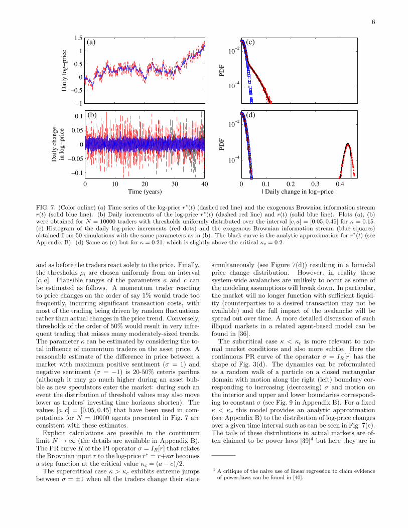
FIG. 7. (Color online) (a) Time series of the log-price r∗(t) (dashed red line) and the exogenous Brownian information streamr(t) (solid blue line). (b) Daily increments of the log-price r∗(t) (dashed red line) and r(t) (solid blue line). Plots (a), (b)were obtained for N = 10000 traders with thresholds uniformly distributed over the interval [c, a] = [0.05, 0.45] for κ = 0.15.(c) Histogram of the daily log-price increments (red dots) and the exogenous Brownian information stream (blue squares)obtained from 50 simulations with the same parameters as in (b). The black curve is the analytic approximation for r∗(t) (seeAppendix B). (d) Same as (c) but for κ = 0.21, which is slightly above the critical κc = 0.2.

and as before the traders react solely to the price. Finally,the thresholds ρi are chosen uniformly from an interval[c, a]. Plausible ranges of the parameters a and c canbe estimated as follows. A momentum trader reactingto price changes on the order of say 1% would trade toofrequently, incurring significant transaction costs, withmost of the trading being driven by random fluctuationsrather than actual changes in the price trend. Conversely,thresholds of the order of 50% would result in very infre-quent trading that misses many moderately-sized trends.The parameter κ can be estimated by considering the to-tal influence of momentum traders on the asset price. Areasonable estimate of the difference in price between amarket with maximum positive sentiment (σ = 1) andnegative sentiment (σ = −1) is 20-50% ceteris paribus(although it may go much higher during an asset bub-ble as new speculators enter the market: during such anevent the distribution of threshold values may also movelower as traders’ investing time horizons shorten). Thevalues [a, c] = [0.05, 0.45] that have been used in com-putations for N = 10000 agents presented in Fig. 7 areconsistent with these estimates.

Explicit calculations are possible in the continuumlimit N → ∞ (the details are available in Appendix B).The PR curve R of the PI operator σ = IR[r] that relatesthe Brownian input r to the log-price r∗ = r+κσ becomesa step function at the critical value κc = (a− c)/2.

The supercritical case κ > κc exhibits extreme jumpsbetween σ = ±1 when all the traders change their state

simultaneously (see Figure 7(d)) resulting in a bimodalprice change distribution. However, in reality thesesystem-wide avalanches are unlikely to occur as some ofthe modeling assumptions will break down. In particular,the market will no longer function with sufficient liquid-ity (counterparties to a desired transaction may not beavailable) and the full impact of the avalanche will bespread out over time. A more detailed discussion of suchilliquid markets in a related agent-based model can befound in [36].

The subcritical case κ < κc is more relevant to nor-mal market conditions and also more subtle. Here thecontinuous PR curve of the operator σ = IR[r] has theshape of Fig. 3(d). The dynamics can be reformulatedas a random walk of a particle on a closed rectangulardomain with motion along the right (left) boundary cor-responding to increasing (decreasing) σ and motion onthe interior and upper and lower boundaries correspond-ing to constant σ (see Fig. 9 in Appendix B). For a fixedκ < κc this model provides an analytic approximation(see Appendix B) to the distribution of log-price changesover a given time interval such as can be seen in Fig. 7(c).The tails of these distributions in actual markets are of-ten claimed to be power laws [39]4 but here they are in

4 A critique of the naive use of linear regression to claim evidenceof power-laws can be found in [40].

7

fact close to a sum of different Gaussian and error func-tions. For completeness of the mathematical analysis wenote that as κ approaches κc, the distribution becomesbimodal as in Fig. 7(d) where the smaller mode corre-sponding to large changes of the price separates from themain Gaussian mode.

The existence of a critical value together with thepossibility of κ varying in time suggests a mechanismfor extreme market volatility and the associated bub-bles/crashes and fat tails. As a particular asset classreceives increased attention or is perceived to be undergo-ing some fundamental positive change, the price will riseand attract more momentum traders/short-term specu-lators. This will cause κ to increase through the criticalvalue and the system to evolve with σ at or close to +1until changes in the process r∗(t) trigger the drawdownprocess and a (at least theoretical) system-wide down-ward cascade.

It is not our aim here to match the fat tails gener-ated by the simple model above with the approximatepower laws measured in real, highly complex, financialmarkets. Rather, we have demonstrated theoretically aplausible mechanism for generating fat tails. The modelalso predicts that as the proportion of traders who usesuch a strategy increases the system will pass through acritical point beyond which a systemic market failure isinevitable. We believe that this model, due to its simplic-ity and theoretical tractability, complements other het-erogeneous agent-based models (see [41] for examples),that also generate cascades and fat tails but rely solelyon numerical simulations.

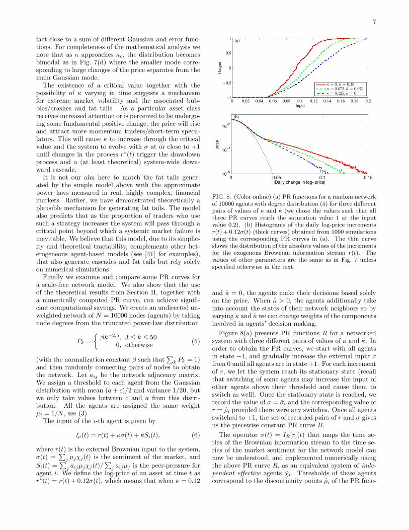
Finally we examine and compare some PR curves fora scale-free network model. We also show that the useof the theoretical results from Section II, together witha numerically computed PR curve, can achieve signifi-cant computational savings. We create an undirected un-weighted network of N = 10000 nodes (agents) by takingnode degrees from the truncated power-law distribution

Pk =

{βk−2.5, 3 ≤ k ≤ 50

0, otherwise(5)

(with the normalization constant β such that∑k Pk = 1)

and then randomly connecting pairs of nodes to obtainthe network. Let aij be the network adjacency matrix.We assign a threshold to each agent from the Gaussiandistribution with mean (a+ c)/2 and variance 1/20, butwe only take values between c and a from this distri-bution. All the agents are assigned the same weightµi = 1/N , see (3).

The input of the i-th agent is given by

ξi(t) = r(t) + κσ(t) + κSi(t), (6)

where r(t) is the external Brownian input to the system,σ(t) =

∑j µjχj(t) is the sentiment of the market, and

Si(t) =∑j aijµjχj(t)/

∑j aijµj is the peer-pressure for

agent i. We define the log-price of an asset at time t asr∗(t) = r(t) + 0.12σ(t), which means that when κ = 0.12

0 0.02 0.04 0.06 0.08 0.1 0.12 0.14 0.16 0.18 0.2−1

−0.5

0

0.5

1

Input

Output

(a)

κ = 0, κ = 0.18κ = 0.072, κ = 0.072κ = 0.125, κ = 0

0 0.05 0.1 0.1510

−6

10−4

10−2

|Daily change in log−price|

PD

F

(b)

FIG. 8. (Color online) (a) PR functions for a random networkof 10000 agents with degree distribution (5) for three differentpairs of values of κ and κ (we chose the values such that allthree PR curves reach the saturation value 1 at the inputvalue 0.2). (b) Histograms of the daily log-price incrementsr(t) + 0.12σ(t) (thick curves) obtained from 1000 simulationsusing the corresponding PR curves in (a). The thin curveshows the distribution of the absolute values of the incrementsfor the exogenous Brownian information stream r(t). Thevalues of other parameters are the same as in Fig. 7 unlessspecified otherwise in the text.

and κ = 0, the agents make their decisions based solelyon the price. When κ > 0, the agents additionally takeinto account the states of their network neighbors so byvarying κ and κ we can change weights of the componentsinvolved in agents’ decision making.

Figure 8(a) presents PR functions R for a networkedsystem with three different pairs of values of κ and κ. Inorder to obtain the PR curves, we start with all agentsin state −1, and gradually increase the external input rfrom 0 until all agents are in state +1. For each incrementof r, we let the system reach its stationary state (recallthat switching of some agents may increase the input ofother agents above their threshold and cause them toswitch as well). Once the stationary state is reached, werecord the value of σ = σi and the corresponding value ofr = ρi provided there were any switches. Once all agentsswitched to +1, the set of recorded pairs of r and σ givesus the piecewise constant PR curve R.

The operator σ(t) = IR[r](t) that maps the time se-ries of the Brownian information stream to the time se-ries of the market sentiment for the network model cannow be understood, and implemented numerically usingthe above PR curve R, as an equivalent system of inde-pendent effective agents χi. Thresholds of these agentscorrespond to the discontinuity points ρi of the PR func-

8

tion, while the weight of the i-th agent is equal to halfthe change in the value of the PR function at the i-thdiscontinuity point, µi = (σi − σi−1)/2 (that is µi is thesum of the weights of all the agents in the network modelthat switch collectively when exposed to an increasing in-put as it reaches the value ρi). All effective agents areindependent of each other, i.e., the input of each effec-tive agent is just the Brownian information stream r(t)(cf. Eq. (6)). When we replace all agents of the origi-nal networked model with the effective agents, the sys-tem σ(t) =

∑i µiχi(t) that we obtain will be equivalent

to the original networked system (both systems producethe same output σ in response to any realization of theinput r). In other words, we no longer need to considerthe network structure because its effect is embedded inthe thresholds and weights of the effective agents. Thisgives us a substantial computational advantage: not onlythe number of agents is reduced, but there is no need forcomputationally expensive calculation of peer pressure,and since the system no longer exhibits cascades of acti-vations it immediately reaches a stationary state for eachvalue of r.

Figure 8(b) presents histograms of the daily log-priceincrements for the network model; they correspond tothe PR curves shown in Fig. 8(a). We define log-priceas r(t) + 0.12σ(t) and run 1000 simulations (here we cal-culate the increments using the system of independenteffective agents, and not the original system of interact-ing agents as in Fig. 7(c)). In this example, the fattesttail of the log-price returns distribution is achieved whenthe pressure of network neighbors has the strongest effecton the decision making of the agents (the largest κ). Theleast-fat tail occurs when the network structure is absentand agents react solely to the price.

IV. CONCLUSIONS

To summarize, we have considered input-driven dy-namics on networks with PI operators at the nodes. Ex-amples of such nodes are provided by models of plasticityand friction and some common trading strategies. Wehave shown that no matter how complex the network, itsresponse to arbitrary variations of the input is describedby an effective PI operator and hence can be deduced ina simple and explicit way from the network’s responseto a monotonically increasing input. Using these resultswe have shown that one-dimensional models of frictionand plasticity with interacting elastic and dry friction ele-ments can be reduced, in case of not-too-strong coupling,to the standard PI model without interactions. We havealso derived the analytical form of the fat-tailed price re-turns induced by momentum-based trading in a financialmarket. Extending the analysis to allow for the varyinginfluence of momentum traders (the parameter κ) mayyield new insights into the approximate power-law scal-ings claimed for actual markets. Finally, the numericalmethod used for our simulations provides a computation-

ally efficient alternative for solving the dynamics on net-works of PI operators of arbitrary complexity and witharbitrary inputs.

ACKNOWLEDGMENTS

We thank A. Amann, M. Dimian and B. Hanzon foruseful discussions. This work was funded in part byGACR Grant P201/10/2315 and RVO: 67985840 (P.K.),the Irish Research Council (New Foundations grant,S.M.) co-funded by Marie Curie Actions under FP7 (IN-SPIRE fellowship, S.M.), and Science Foundation Ireland(11/PI/1026, S.M.).

Appendix A: Simulation of the mechanical model

In this section we consider in more detail the mechan-ical model schematically illustrated in Fig. 1(b) and de-scribed by Eq. (2). This model can be used to representa bunch of one-dimensional rigid fibers (shown as nodesin Fig. 1(b)) elongated along the horisontal axis, whoseleft and right ends are attached (by springs) respectivelyto the left and the right plates. The displacement offiber i relative to the left plate is ξi. We assume per-fect elastic interactions between each fiber i and the left(and the right) plate with coefficients ki (and ki corre-spondingly). Furthermore, we assume that each fiber isin contact with some other fibers along its length andthere is Maxwell friction when they move with respect toone another. We model the friction force acting on thei-th fiber due to its relative displacement with respect tothe j-th fiber by aijSrij [ξj − ξi], where fiber interactionstrengths aij are non-negative, and Srij denotes the stopoperator of half-width rij ≥ 0 (see Fig. 1(a)) with in-put ξj − ξi. Initially, all forces and displacements in thesystem are 0. The time-varying input of the system isthe displacement u of the right plate relative to its initialposition (see Fig. 1(b)); the left plate does not move. Allthe motions are quasistatic.

Equation (2), which describes the balance of forces forfiber i, can be written as

(ki + ki)ξi +∑j∈Ni

aijSrij [ξi − ξj ] = kiu, (A1)

where Ni denotes the set of indices j for which aij > 0(i.e., Ni is the set of fibers interacting with fiber i or,using different terminology, the set of neighbors of nodei in the network with the adjacency matrix aij whereeach fiber is represented by a node).

Equation (A1) represents a piecewise linear system,which we can solve in each of the linear regimes whiletracking the transitions from one linear regime to an-other. A switch between linear regimes occurs when anyof the stop operators Srij saturates (i.e., when the magni-tude of the friction force between any pair of fibers i and

9

j achieves its maximal possible value rij) or de-saturates(the magnitude of the friction force becomes smaller thanrij); we describe this by saying that link ij saturates orde-saturates. Before we consider the transitions betweenlinear regimes in more detail, let us write Eq. (A1) in theform of a linear matrix equation

Mξ = Ku+ D, (A2)

where ξ = {ξ1, . . . , ξn} and K = {k1, . . . , kn}. Thematrix M and vector D take specific values (given byEqs. (A5) and (A6) below) for each of the linear regimes.

We introduce a new quantity Oij which denotes thecurrent reference point (the origin) for the interactionSrij [ξi−ξj ] between nodes i and j. Specifically, Oij is thevalue of ξi − ξj at which Srij [ξi − ξj ] = 0, provided thatthe relative displacement ξi − ξj approaches the valueOij monotonically from its current value. Notice thatOij = −Oji. We also introduce a binary quantity lij torepresent the current state of link ij (interaction betweenfibers i and j),

lij =

{1 , if link ij is unsaturated0 , if link ij is saturated

. (A3)

We assume that initiallyOij = 0 for all the links and lij =1 (all links are unsaturated). These quantities will be

updated according to the rules described below when thevariations in the input parameter u become sufficientlylarge.

If a link ij is unsaturated (lij = 1), then the value ofSrij is given by (ξi − ξj − Oij). In the case when linkij is saturated (lij = 0), the value of Srij is given byrij sgn(ξi − ξj − Oij). Therefore, using the notation Oijand lij , we can rewrite Eq. (A1) as

(ki + ki)ξi+∑j∈Ni

lijaij(ξi − ξj −Oij)+ (A4)

∑j∈Ni

(1− lij)aijrij sgn(ξi − ξj −Oij) = kiu.

Equation (A4) can be written in matrix form (A2) wherethe elements of M and D are given by

Mij =

{−aij lij , if i 6= j

ki + ki +∑j∈Ni aij lij , if i = j

. (A5)

and

Di =∑j∈Ni

aij (lijOij − (1− lij)rijsgn(ξi − ξj −Oij)) .

(A6)

For example, if we consider three fibers connected as inFig. 1(b), then Eq. (A2) takes the form

k1 + k1 +

∑j∈N1

a1j l1j −a12l12 −a13l13

−a21l21 k2 + k2 +∑j∈N2

a2j l2j −a23l23

−a31l31 −a32l32 k3 + k3 +∑j∈N3

a3j l3j

ξ1ξ2ξ3

=

k1k2k3

u+

∑j∈N1

a1j [l1jO1j − (1− l1j)r1jsgn(ξ1 − ξj −O1j)]∑j∈N2

a2j [l2jO2j − (1− l2j)r2jsgn(ξ2 − ξj −O2j)]∑j∈N3

a3j [l3jO3j − (1− l3j)r3jsgn(ξ3 − ξj −O3j)]

. (A7)

Suppose we want to calculate the values of ξi as theinput u varies. The solution of Eq. (A2) is given by

ξ = M−1(Ku+ D). (A8)

However, we need to update M and D each time a linksaturates or de-saturates.

The condition for the saturation of an unsaturated linkij is ξi − ξj = Oij ± rij . We note that when we checkthis condition for all pairs of i and j, then it is sufficientto consider only one of the two cases, for example,

ξi − ξj = Oij + rij , (A9)

since the other case is captured due to Oij − rij =−(Oji + rji). Using the link saturation condition (A9)and Eq. (A8) we obtain the values of uij at which thelink between nodes i and j saturates:

uij =Oij + rij + (M−1D)i − (M−1D)j

(M−1K)i − (M−1K)j. (A10)

Hence, we can calculate ξi from Eq. (A8) for all u (with-out the need to update M and D) until u passes throughany of uij values. When u reaches any of uij , this willindicate that we transition to a new linear regime, andthus have to calculate new M and D as lij changes from1 to 0 at this point.

10

The de-saturation of a saturated link ij occurs whenξi − ξj has a turning point (passes through a local max-imum or minimum value). There are two ways this canhappen. First, due to complex interactions between thenodes, a link ij may de-saturate due to the saturation ofanother link mn (this happens in the example shown inFig. 4 as described in steps 6 and 13 of Table I). Second,saturated links may de-saturate when the input u has aturning point. (Interestingly, saturated links may remainsaturated when u makes a turning point; this happens inthe example shown in Fig. 4 as described in step 4 ofTable I where Sr12 does not de-saturate.) In both cases,we need to determine whether ξi− ξj has a turning pointby evaluating the sign of the derivative of ξi − ξj withrespect to u. The derivative is obtained from Eq. (A8)and is given by

(ξi − ξj)′u = (M−1K)i − (M−1K)j . (A11)

In the first case, we need to evaluate the sign of (ξi −ξj)′u before and after the saturation of mn. Moreover, a

change in lij will affect matrix M and therefore furtherchanges in (ξi − ξj)′u (and thus in lij) are possible. Thismeans that we need to iterate the evaluation of (ξi−ξj)′u,lij and M until lij reaches a steady state.

In the second case, we need to find a partition of pre-viously saturated links into a set of links that remainsaturated and a set that becomes de-saturated. Thesesets should ensure the consistency condition on (ξi−ξj)′uwhen u makes a turning point, that (ξi − ξj)

′u should

change the sign for links that remain saturated, and notfor links that become de-saturated. Similar to the firstcase, finding the set of de-saturating links may be notstraightforward because of the dependency of (ξi − ξj)′uon lij . However, this can be done numerically by simplylooping through all possible partitions and finding theone that leads to consistency.

Finally, for the resulting set of links that became de-saturated we calculate the new Oij from ξi− ξj , rij , andthe current Oij :

Onewij = ξi − ξj − sgn(ξi − ξj −Oij)rij . (A12)

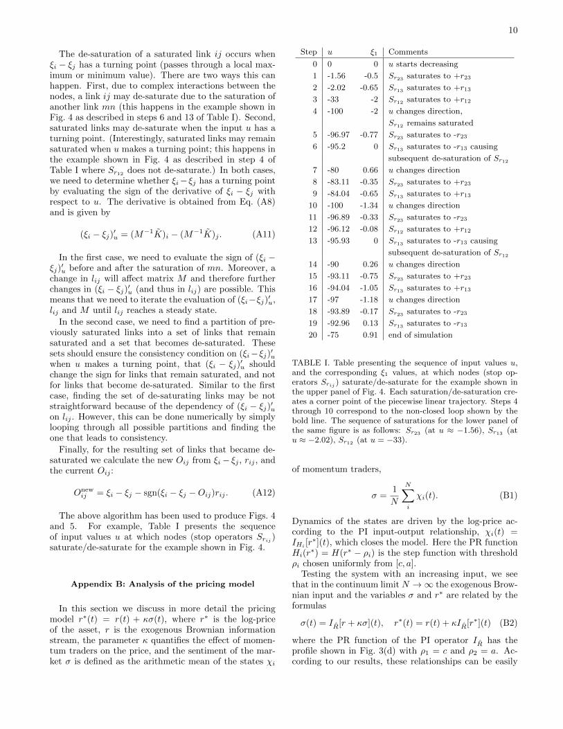
The above algorithm has been used to produce Figs. 4and 5. For example, Table I presents the sequenceof input values u at which nodes (stop operators Srij )saturate/de-saturate for the example shown in Fig. 4.

Appendix B: Analysis of the pricing model

In this section we discuss in more detail the pricingmodel r∗(t) = r(t) + κσ(t), where r∗ is the log-priceof the asset, r is the exogenous Brownian informationstream, the parameter κ quantifies the effect of momen-tum traders on the price, and the sentiment of the mar-ket σ is defined as the arithmetic mean of the states χi

Step u ξ1 Comments

0 0 0 u starts decreasing

1 -1.56 -0.5 Sr23 saturates to +r23

2 -2.02 -0.65 Sr13 saturates to +r13

3 -33 -2 Sr12 saturates to +r12

4 -100 -2 u changes direction,

Sr12 remains saturated

5 -96.97 -0.77 Sr23 saturates to -r23

6 -95.2 0 Sr13 saturates to -r13 causing

subsequent de-saturation of Sr12

7 -80 0.66 u changes direction

8 -83.11 -0.35 Sr23 saturates to +r23

9 -84.04 -0.65 Sr13 saturates to +r13

10 -100 -1.34 u changes direction

11 -96.89 -0.33 Sr23 saturates to -r23

12 -96.12 -0.08 Sr12 saturates to +r12

13 -95.93 0 Sr13 saturates to -r13 causing

subsequent de-saturation of Sr12

14 -90 0.26 u changes direction

15 -93.11 -0.75 Sr23 saturates to +r23

16 -94.04 -1.05 Sr13 saturates to +r13

17 -97 -1.18 u changes direction

18 -93.89 -0.17 Sr23 saturates to -r23

19 -92.96 0.13 Sr13 saturates to -r13

20 -75 0.91 end of simulation

TABLE I. Table presenting the sequence of input values u,and the corresponding ξ1 values, at which nodes (stop op-erators Srij ) saturate/de-saturate for the example shown inthe upper panel of Fig. 4. Each saturation/de-saturation cre-ates a corner point of the piecewise linear trajectory. Steps 4through 10 correspond to the non-closed loop shown by thebold line. The sequence of saturations for the lower panel ofthe same figure is as follows: Sr23 (at u ≈ −1.56), Sr13 (atu ≈ −2.02), Sr12 (at u = −33).

of momentum traders,

σ =1

N

N∑i

χi(t). (B1)

Dynamics of the states are driven by the log-price ac-cording to the PI input-output relationship, χi(t) =IHi [r

∗](t), which closes the model. Here the PR functionHi(r

∗) = H(r∗ − ρi) is the step function with thresholdρi chosen uniformly from [c, a].

Testing the system with an increasing input, we seethat in the continuum limit N →∞ the exogenous Brow-nian input and the variables σ and r∗ are related by theformulas

σ(t) = IR[r + κσ](t), r∗(t) = r(t) + κIR[r∗](t) (B2)

where the PR function of the PI operator IR has theprofile shown in Fig. 3(d) with ρ1 = c and ρ2 = a. Ac-cording to our results, these relationships can be easily

11

solved explicitly:

σ(t) = IR[r](t), r∗(t) = r(t) + κσ(t) (B3)

and two cases are possible. In the subcritical case,κ < κc = (a − c)/2, the PR function R in these rela-tionships also has the shape shown in Fig. 3(d) with thesame ρ1 = c, but with a smaller ρ2 = a − 2κ > ρ1. Inthe supecritical case κ > κc, the function R is the stepfunction with the threshold c. That is, in the supercriti-cal case, due to a global avalanche, all the traders switchtheir state simultaneously causing σ jump between thevalues ±1. The statistics of the intervals between jumpscan be found by solving an exit time problem.

We first consider the subcritical case which is morerelevant to normal market conditions and more interest-ing. Our objective is to calculate the profile of the dailylog-price increments histogram shown in Fig. 7(c). Forthis purpose, we first find the stationary distribution ofthe stochastic process σ(t) = IR[r](t). The shape of thePR curve R allows us to describe this process as a ran-dom walk of a particle in a rectangle, where the verticalcoordinate of the particle is σ, while the horizontal coor-dinate is an auxiliary variable w, see Fig. 9. The motionof the particle (w(t), σ(t)) is driven by the Brownian in-put r(t). For simplicity, we describe the random walkin a discrete time/state setting. In this case, the parti-cle lives on a rectangular mesh with nx columns and nyrows and the Brownian input is represented by a randomwalk r which at every time step with equal probabilitymakes one step left or one step right along a uniformmesh on the real line. First assume that the input rmoves left at some moment. Then, if the particle wasnot on the left side of the rectangle (left column of themesh), it also moves one step left to a neighboring node;it moves one step down from any node of the left side,except from the lower corner; and, if the particle was inthe lower left corner of the rectangle, it remains there.Similarly, when r moves right, so does the particle if itwas not on the right side of the rectangle; it moves onestep up from any node of the right side, except from theupper corner; and, it remains in the upper right cornerif it was there (see Fig. 9). In this model, the horizon-tal and vertical step of the rectangular mesh are relatedby |∆w| = (κc − κ)|∆σ|, the horizontal step equals thestep of the input mesh, |∆w| = |∆r|, and the numberof rows and columns in the rectangular mesh are relatedby cny = 2(κc − κ)nx. These relationships ensure thatthe increment of the log-price equals ∆r∗ = ∆r + κ∆σwhere ∆r and ∆σ are the increments of the input andthe vertical coordinate of the particle at the same timestep, respectively.

A simple calculation shows that the probability densityof the stationary distribution for the random walk (w, σ)linearly decreases on the lower (upper) side of the rectan-gle from the lower left to the lower right (upper right toupper left) corner and is uniform on the rest of the rect-angle. In the continuous time/state limit (nx, ny →∞),when the input r(t) becomes the continuous Brownian

motion, the density function of the stationary probabil-ity distribution for the random process (w(t), σ(t)) on therectangle Π = {0 ≤ w ≤ c, 0 ≤ σ ≤ 2} is

ρst(w, σ) =(c− w)δ(σ) + wδ(σ − 2) + κc − κ

c(a− 2κ), (B4)

where δ denotes the Dirac delta function. We note that inthe continuum limit the process w becomes the reflectedBrownian motion on the interval [0, c] (with reflectingboundary condition at both ends).

FIG. 9. Rectangular random walk (w, σ). At each time step,a particle makes one of two possible moves with equal prob-ability as shown by arrows. It moves either to a neighboringnode or, if it is at the upper right or lower left corner, possiblyto the same node.

Calculations of the profile of the histogram for dailylog-price increments ∆r∗n = r∗(tn + τ) − r∗(tn), whereτ = 1 day is a fixed time interval and tn = nτ , will be per-formed in the continuous time/state setting. Assumingergodicity, statistics of the increments ∆rn obtained froma typical long trajectory of the processes r and (w, σ) canbe approximated by the probability density function ofthe random variable

∆r∗ = r∗(τ)− r∗(0) = r(τ) + κ(σ(τ)− σ(0)), (B5)

where the stationary process (w(t), σ(t)) bounded by therectangle Π is driven by the Brownian input r(t) (withr(0) = 0) and has the law (B4). The following calcu-lations are based on the assumption that the maximalincrement of the Brownian input r during one day re-mains bounded by the quantity c/2 with a probabilityclose to 1:

P

(max0≤t≤τ

|r(t)| ≥ c/2)� 1. (B6)

For the plots shown in Fig. 7, the variance of the Brow-nian input r(T ) at the end of the time interval T = 40years (with 250 trading days per year) has been set to1. Hence, for one trading day r(τ) ∼ N(0,Σ2) with thestandard deviation Σ = 0.01. Since c/2 = 2.5Σ for theseplots, P (|r(τ)| ≤ c/2) = 0.988, which agrees with (B6).We will consider only those input trajectories that satisfy

12

|r(t)| < c/2 on the whole time interval 0 ≤ t ≤ τ . Thecorresponding trajectories of the process (w, σ) cannotreach both left and right sides of the rectangle Π duringthe same time interval. Trajectories for which this occurswill be disregarded.

Thus, let us consider trajectories (w(t), σ(t)) corre-sponding to different realizations of the Brownian r(t)on the time interval 0 ≤ t ≤ τ and different initial data(w(0), σ(0)), restricting our attention to initial data fromthe right half of the rectangle Π, i.e., with c/2 ≤ w(0) ≤c, 0 ≤ σ(0) ≤ 2. (Trajectories starting at the left halfof Π can be treated similarly). Since we assume thatr(t) > −c/2 for all 0 ≤ t ≤ τ (other inputs are disre-garded due to (B6)), a trajectory starting from the righthalf of Π never reaches the left side of the rectangle. Forsuch trajectories, the log-price increment (B5) can be eas-ily expressed in terms of the variables w(0), σ(0), r(τ),and m(τ) = max0≤t≤τ r(t), the maximum input value,where the probability density of the joint distribution forthe Brownian motion and its running maximum is de-fined by the relation

ρbr(r,m) =

{2(2m−r)τ√2πτ

e−(2m−r)2

2τ , m ≥ 0,m ≥ r,0, otherwise.

(B7)

The two-dimensional random variable (r(τ),m(τ)) andthe two-dimensional variable (w(0), σ(0)), which has the

law (B4), are independent. As the expression for ∆r∗

depends on relations between these variables, we classifytrajectories into a few groups.

If σ(0) = 2, then the trajectory remains on the upperboundary of the rectangle Π all the time (σ(t) = 2 forall 0 ≤ t ≤ τ), hence the log-price increment (B5) equalsthe increment of the input, ∆r∗ = r(τ). Since r(τ) isnormally distributed, so is ∆r∗ for such trajectories:

ρ(∆r∗ = y, σ(0) = 2) =3c

8(a− 2κ)· e− y

2

2τ

√2πτ

, (B8)

where P = 3c/(8(a− 2κ)) is the total probability to findthe point (w(0), σ(0)) on the right half of the upper sideof the rectangle, see (B4).

Another class consists of trajectories that start belowthe upper side of the rectangle Π and never reach its rightside during the day. This class is defined by the relations

0 ≤ σ(0) < 2; c/2 ≤ w(0) < c−m(τ). (B9)

For such trajectories, σ(t) = σ(0) for all 0 ≤ t ≤ τ andhence ∆r∗ = r(τ), as in the previous case. Integratingthe product of the probability densities ρst(w, σ)ρbr(r,m)over domain (B9) with respect to the variables w(0) =w, σ(0) = σ and m(τ) = m, we obtain the probabilitydensity function of the log-price increment for this class oftrajectories. After some manipulations, this probabilitydensity can be presented as the integral

ρ(∆r∗ = y, σ(0) < 2, w(0) < c−m(τ)) =1

2c(a− 2κ)

∫ c/2

max{0,y}ρbr(y,m)

( c2−m

)( c2

+m+ 4(κc − κ))dm, (B10)

which can be expressed explicitly in terms of the Gaus-sian and the error function.

The next set of conditions,

m(τ) +w(0) > c;m(τ) + w(0)− c

κc − κ< 2− σ(0), (B11)

ensures that a trajectory reaches the right side, but notthe upper side of the rectangle Π. For such trajectories,

∆r∗ = r(τ) +κ

κc − κ(m(τ) + w(0)− c). (B12)

Hence, we obtain the probability density functionρ(∆r∗ = y) of the log-price increment for this class by in-tegrating the product ρst(w, σ)ρbr(r,m) where r = r(τ) isrelated to the variables w = w(0), σ = σ(0),m = m(τ) byformula (B12) with ∆r∗ = y kept fixed; relations (B11)define the domain of integration in the product of the do-main Π of the pair (w, σ) and the line m. The resultingtriple integral can be reduced to the sum of the followingtwo terms:

ρ(∆r∗ = y, 0 < σ(0) < σ(τ) < 2) = c0

∫ 2

max{0,(y−c/2)/κc}(2− p) dp

∫ c/2

max{0,y−κcp}ρbr(y − κp, q + (κc − κ)p

)dq, (B13)

ρ(∆r∗ = y, 0 = σ(0) < σ(τ) < 2) =c0

κc − κ

∫ 2

max{0,(y−c/2)/κc}dp

∫ c/2

max{0,y−κcp}q ρbr

(y − κp, q + (κc − κ)p

)dq, (B14)

where c0 = (κc − κ)2/(c(a− 2κ)). Finally, there are trajectories starting below the upper

13

side of the rectangle that reach the upper side during theday. This class is defined by the conditions

0 < 2− σ(0) <m(τ) + w(0)− c

κc − κ(B15)

and the corresponding log-price increment equals ∆r∗ =∆r + κ(2 − σ(0)). For the subcritical parameter set weconsider, the probability of having such trajectories issmall and their contribution has almost no effect on theprofile of the probability density plot. Hence, we havediscarded a correction to the probability density functionof ∆r∗ due to such trajectories.

Thus, denoting the sum of contributions (B8), (B10),(B13), (B14) from different classes of trajectories startingin the right half of Π by ρr(y), the symmetrized sum

ρ(∆r∗ = y) = ρr(y) + ρr(−y) (B16)

provides an analytic approximation to the probabilitydensity function of the log-price daily increments, see thetheoretical curve in Fig. 7(c). The term ρr(−y) accountsfor trajectories starting in the left half of Π.

We now look at the critical value κ = κc. In the criti-cal case, each trajectory that reaches the right side of therectangle, immediately jumps to its upper side. Hence,ρr(y) is the sum of expressions (B8) and (B10) only (withno terms of the form (B13), (B14)). The symmetrizedsum (B16) describes the main central mode of the prob-ability density distribution shown in Fig. 7(d). One smallside mode appears due to trajectories that start on thelower side of the rectangle and reach (jump to) the up-per side, that is trajectories that have been disregardedin the subcritical case. The profile of the side modes isdescribed by the left and right shifts ρside(±(y + 2κ)) ofthe function

ρside(y) =1

2c2

∫ c/2

max{y,0}m2ρbr(y,m) dm. (B17)

Hence, the central mode and side modes can be explicitlyexpressed as a combination of the Gaussian and the errorfunction.

In the supercritical case κ > κc, the central mode isthe same as in the critical case, while the side modes havethe same shape as in the critical case but shift further toleft and right.

[1] R. Pastor-Satorras and A. Vespignani, Phys. Rev. Lett.86, 3200 (2001).

[2] C. Castellano, S. Fortunato, and V. Loreto, Rev. Mod.Phys. 81, 591 (2009).

[3] C. J. Honey, O. Sporns, L. Cammoun, X. Gigandet, J. P.Thiran, R. Meuli, and P. Hagmann, Proc. Natl. Acad.Sci. U.S.A. 106, 2035 (2009).

[4] A. G. Haldane and R. M. May, Nature (London) 469,351 (2011).

[5] J. P. Sethna, K. Dahmen, and C. R. Myers, Nature (Lon-don) 410, 242 (2001).

[6] K. Dahmen and Y. Ben-Zion, in Encyclopedia of Com-plexity and System Science, Vol. 5, edited by R. Meyers(Springer, 2005) p. 5021.

[7] R. A. Guyer and K. R. McCall, Phys. Rev. B 54, 18(1996).

[8] M. Schroder, S. H. Ebrahimnazhad Rahbari, and J. Na-gler, Nat. Commun. 4, 2222 (2013).

[9] A. M. Alencar, S. V. Buldyrev, A. Majumdar, H. E. Stan-ley, and B. Suki, Phys. Rev. Lett. 87, 088101 (2001).

[10] The Science of Hysteresis, edited by I. Mayergoyz andG. Bertotti (Elsivier, 2005).

[11] S. N. Dorogovtsev, A. V. Goltsev, and J. F. F. Mendes,Phys. Rev. E 66, 016104 (2002).

[12] R. Parshani, S. Carmi, and S. Havlin, Phys. Rev. Lett.104, 258701 (2010).

[13] C. Castellano and R. Pastor-Satorras, Phys. Rev. Lett.105, 218701 (2010).

[14] J. P. Gleeson, Phys. Rev. Lett. 107, 068701 (2011).[15] A. Barrat, M. Barthelemy, and A. Vespignani, Dynamical

Processes on Complex Networks (Cambridge Univ. Press,2008).

[16] D. J. Watts, Proc. Natl. Acad. Sci. U.S.A. 99, 5766

(2002).[17] M. Brokate and J. Sprekels, Hysteresis and Phase Tran-

sitions (Springer, 1996).[18] M. A. Janaideh, S. Rakheja, and C.-Y. Su, IEEE/ASME

Trans. Mechatronics 16, 734 (2011).[19] K. Kuhnen, Europ. J. Control 9, 407 (2003).[20] M. A. Janaideh, S. Rakheja, and C.-Y. Su, IEEE/ASME

Trans. Mechatronics 16, 734 (2011).[21] I. Mayergoyz, Mathematical Models of Hysteresis

(Springer, 1991).[22] G. Radons, Phys. Rev. Lett. 100, 240602 (2008).[23] D. Davino, P. Krejcı, and C. Visone, Smart Materials

Struct. 22, 095009 (2013).[24] B. Appelby, D. Flynn, H. McNamara, P. O’Kane, A. Pi-

menov, A. Pokrovskii, D. Rachinskii, and A. Zhezherun,IEEE Control Systems Mag. 29, 44 (2009).

[25] M. A. Krasnosel’skii and A. V. Pokrovskii, Systems withHysteresis (Springer, 1989).

[26] J. P. Sethna, K. Dahmen, S. Kartha, J. A. Krumhansl,B. W. Roberts, and J. D. Shore, Phys. Rev. Lett. 70,3347 (1993).

[27] I. Mayergoyz, Mathematical Models of Hysteresis andTheir Applications (Elsevier, 2003).

[28] P. Krejcı, Math. Z. 193, 247 (1986).[29] M. Brokate, Math. Method. Appl. Sci. 15, 145 (1992).[30] D. D. Rizos and S. D. Fassois, IEEE Trans. on Control

Systems Technology 17, 153 (2009).[31] P. Krejcı, Hysteresis, Convexity and Dissipation in Hy-

perbolic Equations (Gakkotosho, Tokyo, 1996).[32] F. E. Browder, Bull. Amer. Math. Soc. 69, 862 (1963).[33] J. Lemaitre and J.-L. Chaboche, Mechanics of solid ma-

terials (Cambridge University Press, 1990).[34] S. J. Grossman and Z. Zhou, Mathemat. Finance 3, 241

14

(1993).[35] https://www.quantopian.com.[36] H. Lamba, Eur. Phys. J. B 77, 297 (2010).[37] P. Krejcı, J. Phys.: Conf. Ser. 55, 144 (2006).[38] M. Gocke, J. Econ. Surveys 16, 167188 (2002).[39] P. Gopikrishnan, V. Plerou, L. A. Nunes Amaral,

M. Meyer, and H. E. Stanley, Phys. Rev. E 60, 5305(1999).

[40] A. Clauset, C. R. Shalizi, and M. E. J. Newman, SIAMReview 51, 661 (2009).

[41] B. LeBaron, J. Economic Dynamics Control 24, 679(2000).