Analytical integrations in 2D BEM elasticity

INTERNATIONAL JOURNAL FOR NUMERICAL METHODS IN ENGINEERINGInt. J. Numer. Meth. Engng 2002; 53:1695–1719 (DOI: 10.1002/nme.359)

Analytical integrations in 2D BEM elasticity

Alberto Salvadori∗;†

Department of Civil Engineering; University of Brescia, Via Branze 38; 25123 Brescia; Italy

SUMMARY

In the context of two-dimensional linear elasticity, this paper presents the closed form of the integralsthat arise from both the standard (collocation) boundary element method and the symmetric Galerkinboundary element method. Adopting polynomial shape functions of arbitrary degree on straight elements,<nite part of Hadamard, Cauchy principal values and Lebesgue integrals are computed analytically,working in a local coordinate system. For the symmetric Galerkin boundary element method, a study onthe singularity of the external integral is conducted and the outer weakly singular integral is analyticallyperformed. Numerical tests are presented as a validation of the obtained results. Copyright ? 2001 JohnWiley & Sons, Ltd.

KEY WORDS: integral equations; boundary element methods; analytical integrations; Hadamard’s <nitepart; Cauchy’s principal value

1. INTRODUCTION

In the framework of linear elasticity problems modelled by means of boundary integral equa-tions (BIEs) [1], the present work concerns analytical integrations on polygonal domainsin R2. As a reference problem, a homogeneous solid with polygonal domain D⊂R2 and withboundary E=Eu ∪Ep is considered. Assuming small strains and displacements, consider thefollowing quasi-static external actions: tractions Gp(x) on Ep, displacements Gu(x) on Eu anddomain forces Gf(x) in D; the constitutive law is assumed to be isotropically linear elastic.The assumed problem is a prototype of a broad class of engineering applications. In fact, BIEsof linear elasticity, can be easily arranged to describe various engineering problems, amongothers: potential problems [2]; fracture mechanics problems [3], with internal pressure [4] andfrictional contact [5]; multidomain problems [6; 7], even in the case of non-linear interfaces[8]; steady Stokes Jow of an incompressible newtonian Juid [9].

∗Correspondence to: Alberto Salvadori, Department of Civil Engineering, University of Brescia, Via Branze 38,25123 Brescia, Italy

†E-mail: [email protected] 28 January 2000

Copyright ? 2001 John Wiley & Sons, Ltd. Revised 9 April 2001

1696 A. SALVADORI

The boundary integral formulation of a linear elastic problem was proposed by Rizzo [10],stemming from Somigliana’s identity, which is the boundary integral representation of dis-placements in the interior of the domain x∈D. Somigliana’s identity is based on Green’sfunctions (also called kernels) which represent components ui of the displacement vector u ina point x due to: (i) a unit force concentrated in space (point y) and acting on the unboundedelastic space D∞ in direction j (such functions are gathered in matrix Guu(x−y)); (ii) a unitrelative displacement concentrated in space (at a point y), crossing a surface with normal l(y)and acting on the unbounded elastic space D∞ (in direction j) (gathered in matrix Gup(x−y))(Appendix A).Since all the above-introduced kernels are in<nitely smooth in their domain, which is the

whole space R2 with exception of the origin (that is x �= y), the traction operator can be appliedto Somigliana’s identity, thus obtaining the boundary integral representation of tractions on asurface of normal n(x) in the interior of the domain [11]. Such representation formula (bysome authors named ‘hypersingular identity’ [12]) involves Green’s functions (collected inmatrices Gpu and Gpp) which describe components (pi) of the traction vector p on a surfaceof normal n(x) due to: (i) a unit force concentrated in space (point y) and acting on theunbounded elastic space D∞ in direction j; (ii) a unit relative displacement concentrated inspace (at a point y), crossing a surface with normal l(y) and acting on the unbounded elasticspace D∞ (in direction j).BIEs for the linear elastic problem can be derived from the aforementioned two represen-

tation formulae performing the boundary limit D�x→xo ∈E. For the hypersingular identity,the boundary limit must be considered at a smooth point xo with a well-de<ned normal vec-tor n(xo) [13]. The two integral equations, usually referred to as displacements and tractionequations, are also called ‘dual’ BIEs [14].In the limit process, singularities of Green’s functions are triggered oO. Kernel Guu shows an

integrable singularity (named ‘weak’) O(r−1); kernels Gup and Gpu present a strong singularityof O(r−2); kernel Gpp is usually named hypersingular, since it shows a singularity of O(r−3)greater than the dimension of the integral [15].By the approach of [16], all singular terms cancel out in the limit process (and without

recourse to any a-priori interpretation in the <nite part sense). However, there exists an inti-mate relationship between hypersingular BIEs and <nite part integrals (HFPs) in the sense ofHadamard [17]. In References [15; 18] among others, it has been proved that a hypersingularintegral can be interpreted as a HFP in the limit as an internal point source approaches theboundary. In Reference [19], the same conclusion has been obtained by an alternate de<nitionof HFP, without the need for a limiting process. Making recourse to the distribution theory,in Reference [14] the dual BIEs are obtained by the application of a trace operator to therepresentation formulae. In such an approach, the strongly singular and hypersingular integralscan be expressed by means of discontinuity jumps (also named as ‘free terms’) of these inte-grals on the boundary summed with the values of the integrals on the boundary existing onlyin the sense of the Cauchy principal value (CPV) or in the sense of the HFP. By exploitingGreen’s functions properties, the commutativity of the two operations of traction and tracehas also been proved, showing the consistency of all diOerent approaches of derivations ofthe BIEs.As mentioned above, strongly singular kernels Gup and Gpu generate free terms, C(xo) and

D(xo), respectively, that hold 12I for smooth boundaries [13; 20; 21]) in the limit process. It

has been shown [16] that the hypersingular kernel generates a free term when the boundary

Copyright ? 2001 John Wiley & Sons, Ltd. Int. J. Numer. Meth. Engng 2002; 53:1695–1719

ANALYTICAL INTEGRATIONS IN 2D BEM ELASTICITY 1697

curvature and the tangent vector to the boundary are not smooth. Discarding these conditions,the BIEs of the linear elastic problem read as follows [14]:

C(x)u(x) +−∫EpGup(r; l(y))u(y)d dy+−

∫EuGup(r; l(y))Gu(y)dy

=∫EuGuu(r)p(y) dy+

∫EpGuu(r)Gp(y) dy+

∫DGuu(r)Gf(y) dy; x∈E (1)

D(x)p(x) + =∫EpGpp(r; n(x); l(y))u(y) dy+=

∫EuGpp(r; n(x); l(y))Gu(y) dy

=−∫EuGpu(r; n(x))p(y) dy+−

∫EpGpu(r; n(x))Gp(y) dy+−

∫DGpu(r; n(x))Gf(y) dy; x∈E

(2)

having set r=x − y. After imposing the ful<llment of Equation (1) on Eu and of Equation(2) on Ep, one obtains a linear boundary integral problem whose operator is symmetric withrespect to the classical bilinear form (see [22–25]). Accordingly, the problem admits of avariational formulation [26; 27] and its solution is shown to be a saddle-point of a givenfunctional �(u; p), whose expression can be found for instance in Reference [28]. Energyimplications have been largely investigated (see [29] among others).Let u(y), p(y) be discrete approximations of the displacement <eld u(y) and of the traction

<eld p(y), respectively. The discretization of the unknown <elds permits to transform the BIEsinto sets of algebraic equations. Two main techniques have been successfully developed tothis aim: the collocation [2] and the symmetric Galerkin [30] methods (SGBEM).The collocation approach requires the ful<llment of the displacement equation onto a se-

lected set of collocation points, x∗i ∈E, after having substituted u(y) and p(y) with the discreteapproximations u(y), p(y). In this technique, one has to deal with integrals of the followingform: ∫

EsGrs(x∗i − y) h(y) dE(y) r= u; s= u; p (3)

denoting with h(y) shape functions that model the unknown <elds on the boundary.After having substituted u(y) and p(y) with the discrete approximations u(y), p(y) into the

functional �(u; p), the SGBEM approach is obtained by performing the <rst variation withrespect to the (discrete) unknowns. In this formulation, one has to deal with integrals of thefollowing form: ∫

Er k(x)

∫EsGrs(x − y) h(y) dE(y) dE(x); r; s= u; p (4)

where k(x), h(y) are, respectively, test and shape functions that model the displacementand traction <elds on the boundary. The evaluation of (3) and (4) is not a trivial task, be-cause of the involved singularities, especially for the hypersingular kernel. Several techniques,


1698 A. SALVADORI

collectable in three principal groups, have been proposed for their evaluation: (i) regularizationtechniques, (ii) numerical integrations, (iii) analytical integrations.By a regularization procedure, the strongly singular and hypersingular integrals are analyt-

ically manipulated to convert them into, at most, weakly singular integrals, which can thenbe computed throughout diOerent quadrature schemes. Regularization procedures have beenobtained by means of simple solutions [31; 32]; by applying the Stokes theorem [18; 33]; viaintegration by parts [34–36].Numerical methods for the evaluation of the CPV were proposed <rst in Reference [37].

There is nowadays an extensive literature on this subject (see, among others [38–44]). A hugeamount of literature concerns the numerical evaluation of hypersingular integrals: among others[15; 18; 19; 38; 45–47].Analytical integrations have been basically performed towards two schemes. In the <rst

scheme (see e.g. [12; 16; 45; 46; 48]), the source point is <xed, while the boundary aroundthe source point is temporarily deformed to allow an analytical evaluation of contributionsfrom singular kernels, and then the limit is taken as the deformed boundary shrinks back tothe actual boundary. In the second approach, see among others [40; 49; 50], the source pointx is <rst moved away from the boundary; integrals are evaluated analytically and a limitprocess is then performed to bring the source point back to the boundary. In all the afore-mentioned papers, analytical integrations are provided for all singular integrals, while standardquadrature formulae are used for non-singular integrals. A complete analytical integration of2D elastostatic kernels has been provided in Reference [51] for linear shape functions onpolygonal domains, directly evaluating HFP and CPV.The present note provides a further contribution in the context of analytical integrations.

It is focused on the analytical evaluation of the single integration process pertaining to thecollocation technique (3) and of the double integration process (4) pertaining to the SGBEM,when the domain is an open polygon. Discretization is here considered by means of straightelements adopting polynomial test and shape functions of arbitrary degree. This allows for ah- as well as a p- and h-p approximation technique.In Section 2, the problem is shortly formulated, making reference to [8] for further de-

tails. By introducing a local orthogonal coordinate system, an eOective representation of theinvolved integrals is given. In Section 3, the analytical integration of (3) is carried out.The Cauchy principal values and Hadamard’s <nite parts are computed both directly andby a limit process. In this last case, well-known free terms [16; 18] naturally arise. Theperformed analytical integrations are exhaustive for every formulation that entails only oneintegration process, with exception of corners. In the frame of the Galerkin approach, thesingularity analysis in the outer integration process is required and developed in Section 4.The outer integration process is proved to involve at most weak singularities; this prop-erty allows the use of numerical quadrature rules with high eTciency and accuracy [52; 53]that require large computational eOort, though. As an alternative, computationally advanta-geous in some circumstances, the analytical integration of the weakly singular integrals isperformed in Section 5. In Section 6, two applications are given to validate the proposedresults. As <rst a Dirichlet problem on a disk is proposed, where the p-technique reveals tobe very eTcient both for the collocation and the SGBEM. Furthermore, a multizone prob-lem with rigid interface is proposed and solved via the SGBEM. A pure integration test is alsoconducted, comparing analytical integration with recently proposed numerical integrationschemes [42].



2. PROBLEM FORMULATION

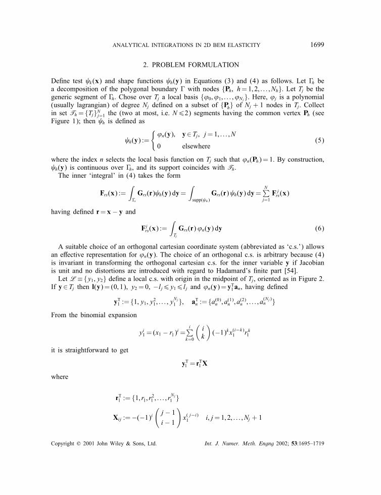
De<ne test k(x) and shape functions h(y) in Equations (3) and (4) as follows. Let Eh bea decomposition of the polygonal boundary E with nodes {Ph; h=1; 2; : : : ; Nh}. Let Tj be thegeneric segment of Eh. Chose over Tj a local basis {’0; ’1; : : : ; ’Nj}. Here, ’j is a polynomial(usually lagrangian) of degree Nj de<ned on a subset of {Ph} of Nj + 1 nodes in Tj. Collectin set Th= {Tj}Nj=1 the (two at most, i.e. N62) segments having the common vertex Ph (seeFigure 1); then h is de<ned as

h(y) :=

{’n(y); y∈Tj; j=1; : : : ; N

0 elsewhere(5)

where the index n selects the local basis function on Tj such that ’n(Ph)=1. By construction, h(y) is continuous over Eh, and its support coincides with Th.The inner ‘integral’ in (4) takes the form

Frs(x) :=∫EsGrs(r) h(y) dy=

∫supp( h)

Grs(r) h(y) dy=N∑

j=1F jrs(x)

having de<ned r=x − y and

Fjrs(x) :=∫TjGrs(r)’n(y) dy (6)

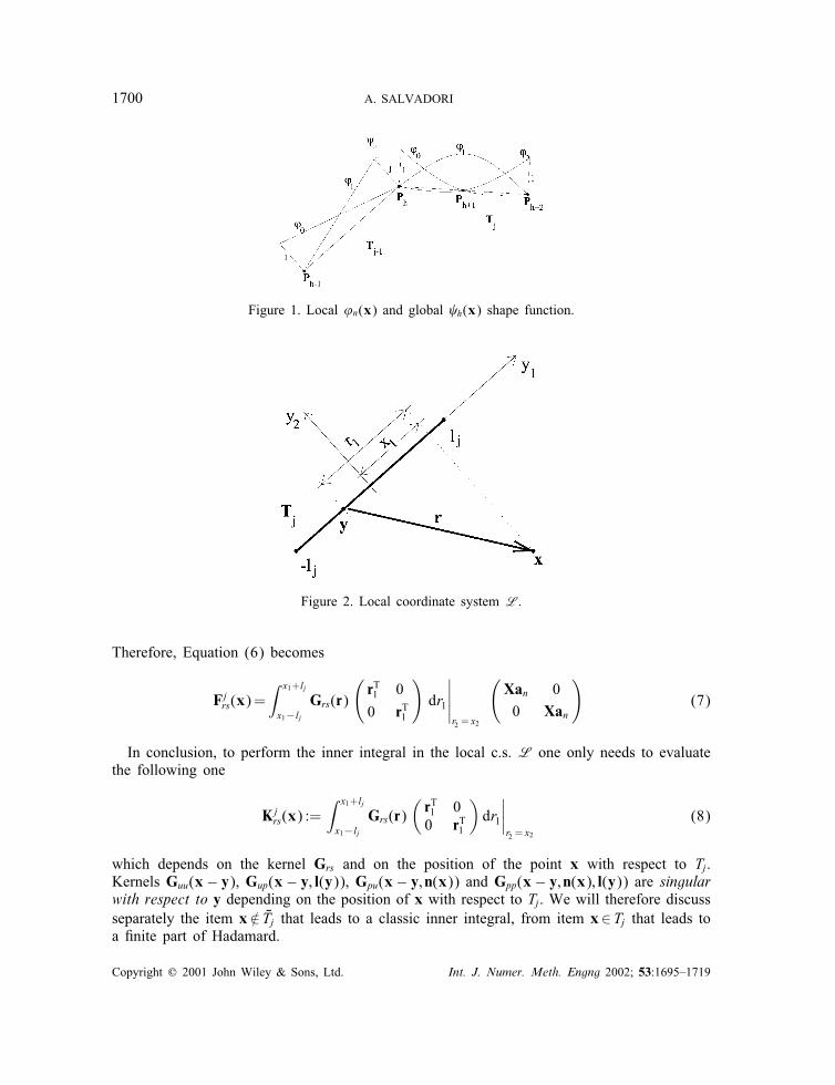
A suitable choice of an orthogonal cartesian coordinate system (abbreviated as ‘c.s.’) allowsan eOective representation for ’n(y). The choice of an orthogonal c.s. is arbitrary because (4)is invariant in transforming the orthogonal cartesian c.s. for the inner variable y if Jacobianis unit and no distortions are introduced with regard to Hadamard’s <nite part [54].Let L≡{y1; y2} de<ne a local c.s. with origin in the midpoint of Tj, oriented as in Figure 2.

If y∈Tj then l(y)= (0; 1), y2 = 0, −lj6y16lj and ’n(y)= yT1an, having de<ned

yT1 := {1; y1; y21 ; : : : ; yNj

1 }; aTn := {a(0)n ; a(1)n ; a(2)n ; : : : ; a(Nj)n }

From the binomial expansion

yi1 = (x1 − r1)

i=i∑

k=0

(ik

)(−1)kx(i−k)

1 rk1

it is straightforward to get

yT1 = rT1X

where

rT1 := {1; r1; r21 ; : : : ; rNj

1 }

Xij :=−(−1)i(

j − 1i − 1

)x( j−i)1 i; j=1; 2; : : : ; Nj + 1


1700 A. SALVADORI

Figure 1. Local ’n(x) and global h(x) shape function.

Figure 2. Local coordinate system L.

Therefore, Equation (6) becomes

Fjrs(x)=∫ x1+lj

x1−ljGrs(r)

(rT1 0

0 rT1

)dr1

∣∣∣∣∣r2 = x2

(Xan 00 Xan

)(7)

In conclusion, to perform the inner integral in the local c.s. L one only needs to evaluatethe following one

Kjrs(x) :=

∫ x1+lj

x1−ljGrs(r)

(rT1 00 rT1

)dr1

∣∣∣∣r2 = x2

(8)

which depends on the kernel Grs and on the position of the point x with respect to Tj.Kernels Guu(x − y), Gup(x − y; l(y)), Gpu(x − y; n(x)) and Gpp(x − y; n(x); l(y)) are singularwith respect to y depending on the position of x with respect to Tj. We will therefore discussseparately the item x =∈ GTj that leads to a classic inner integral, from item x∈Tj that leads toa <nite part of Hadamard.



3. INNER ANALYTICAL INTEGRATION

3.1. Lebesgue integrals

Easy algebraic manipulations (see [8]) lead from integral (8) to the following basic integrals:

∫ x1+lj

x1−ljr k1 log(r) dr1;

∫ x1+lj

x1−lj

r k1

r2dr1;

∫ x1+lj

x1−lj

r k1

r4dr1;

∫ x1+lj

x1−lj

r k1

r6dr1

that have been analytically solved when x =∈ GTi (results in Appendix B). Collecting all com-mon terms, the following compact expressions are the outcome for integrals (8) in the localcoordinate system L:

Kjuu(x) =

18�

1G(1− �)

[log(r2)Luu + arctan

(r1x2

)Auu + Puu

]r1=x1+lj

r1=x1−lj

(9)

Kjup(x) =

14�

11− �

[log(r2)Lup + arctan

(r1x2

)Aup +

1r2Sup + Pup

]r1=x1+lj

r1=x1−lj

(10)

Kjpu(x) =

14�

11− �

[log(r2)Lpu + arctan

(r1x2

)Apu +

1r2Spu + Ppu

]r1=x1+lj

r1=x1−lj

(11)

Kjpp(x) =

G4�

11− �

[log(r2)Lpp + arctan

(r1x2

)App +

1r2Spp +

1r4Hpp + Ppp

]r1=x1+lj

r1=x1−lj

(12)

where r2 = r21 +x22 and Luu; Auu; Puu, Lup; Aup; Sup, Pup; Lpu; Apu, Spu; Ppu; Lpp, App; Spp; Hpp

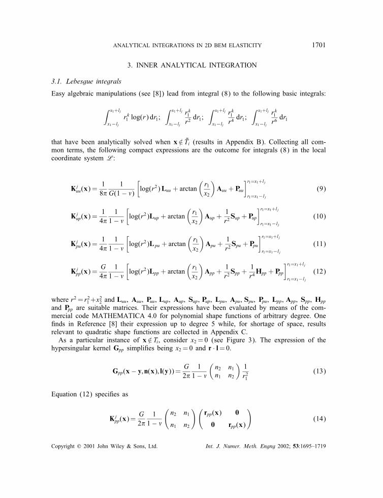
and Ppp are suitable matrices. Their expressions have been evaluated by means of the com-mercial code MATHEMATICA 4.0 for polynomial shape functions of arbitrary degree. One<nds in Reference [8] their expression up to degree 5 while, for shortage of space, resultsrelevant to quadratic shape functions are collected in Appendix C.As a particular instance of x =∈Ti, consider x2 = 0 (see Figure 3). The expression of the

hypersingular kernel Gpp simpli<es being x2 = 0 and r · l=0.

Gpp(x − y; n(x); l(y))= G2�

11− �

(n2 n1n1 n2

)1r21

(13)

Equation (12) speci<es as

Kjpp(x)=

G2�

11− �

(n2 n1

n1 n2

)(rpp(x) 0

0 rpp(x)

)(14)


1702 A. SALVADORI

Figure 3. x �∈Ti, but x2 = 0.

having set

rpp(x) :=

(− 1r1; log |r1|; · · · rk−1

1

k − 1; · · ·)∣∣∣∣∣

r1=x1+lj

r1=x1−lj

(15)

Again in the case of x2 = 0, the expression of the strongly singular kernel Gpu simpli<es as

Gpu(x − y; n(x))= − 14�

11− �

((3− 2�)n1 (1− 2�)n2−(1− 2�)n2 (1− 2�)n1

)1r1

(16)

When x =∈Ti, Equation (11) turns out to be

Kjpu(x)= − 1

4�1

1− �

((3− 2�)n1 (1− 2�)n2−(1− 2�)n2 (1− 2�)n1

)(rpu(x) 0

0 rpu(x)

)(17)

having set

rpu(x) :=

(log |r1|; · · · rk−1

1

k − 1; : : :

)∣∣∣∣∣r1=x1+lj

r1=x1−lj

(18)

Similarly, it holds

Gup(x − y; l(y))= − 14�1− 2�1− �

(0 1

−1 0

)1r1

(19)

and Equation (10) holds

Kjup(x)= − 1

4�1− 2�1− �

(0 rpu(x)

−rpu(x) 0

)(20)



3.2. Hadamard’s /nite part

De/nition 1. Let � → I(�) denote a complex-valued function which is continuous in (0; �0)and assume that

I(�)= I0 + I1 log(�) +m∑

j=2Ij�1−j + o(1); �→ 0

where Ij ∈C. Then I0 is called the <nite part of I(�).

In dealing with integrals, the <nite part I0 of a (usually) divergent integral∫ +∞−∞ �(t) dt is

denoted by the symbol =∫ +∞−∞ �(t) dt.

Consider

I(�) :=∫ x1−�

−lj

1r21rT1 dy1 =

− 1

r1

∣∣∣∣−�

x1−lj

; log |r1||−�x1−lj ; · · · rk−1

1

k − 1

∣∣∣∣∣−�

x1−lj

; · · ·

By means of de<nition 1 and making use of the additive property of the <nite part ofHadamard, one obtains

=∫ lj

−lj

1r21rT1 dy1 = rpp(x) (21)

with rpp(x) de<ned in Equation (15). By means of (21) and setting n(x)= (0; 1) in Equation(13) one obtains the following expression of the <nite part of Hadamard of the integral (8),when x∈Tj

Kjpp(x)=

G2�

11− �

(rpp(x) 0

0 rpp(x)

)(22)

As a diOerent approach, perform the limit process Kjpp(z) s.t. Tj =� z→x∈Tj. By taking

x2→ 0−, it holds

limx2→0−

Lpp =G

4�(1− �)

[0 1 0 : : : 0 0 0 0 : : : 00 0 0 : : : 0 0 1 0 : : : 0

]

limx2→0−

App = 0

limx2→0−

Spp =− Gr12�(1− �)

[1 0 0 : : : 0 0 0 0 : : : 00 0 0 : : : 0 1 0 0 : : : 0

]

limx2→0−

Hpp = 0

limx2→0−

Ppp[1; 1] =Ppp[2; 2]=G

2�(1− �)[ 0 0 r1 r21 =2 : : : r k

1 =k ]

limx2→0−

Ppp[1; 2] =Ppp[2; 1]= 0

and Equation (22) is obtained immediately from (12).


1704 A. SALVADORI

One concludes therefore that when x =∈ GTj, the hyper singularities in integral (8) are nottriggered oO and Kj

pp(x) is a Lebesgue integral. On the contrary, as x∈Tj the ‘integral’ (8)does not exist in a Lebesgue sense but it can be seen in the <nite part of Hadamard sensefor the hypersingular kernel Gpp. This property actually holds not only for (8) but for thetraction boundary integral equation itself. Following the approach of [16], all singular termscancel out in the limit process (and without recourse to any a-priori interpretation in the <nitepart sense). Although, there exists an intimate relationship between hypersingular boundaryintegral equations and <nite part integrals in the sense of Hadamard: in References [15] and[18] among others, it has been proved that a hypersingular integral can be interpreted in the<nite part sense in the limit process of an internal source point that approaches the boundary.In Reference [19], the same conclusion has been obtained by a diOerent de<nition of <nitepart, without the need for any limit process.Finally, it is worth stressing the equivalence between (14) and (22): this implies that when

x2 = 0, ‘wherever x is placed (inside or outside Ti)’, Kjpp assumes the same expression. In a

distribution and in a more correct sense, we obtain that the function Kjpp (not the value of

Kjpp(x)!) does not depend on x.

3.3. Cauchy principal value

De/nition 2. The CPV of the (usually) divergent integral∫ +∞−∞ (�(t)=t) dt is the <nite

quantity

−∫ +∞

−∞

�(t)tdt := lim

�→0+

(∫ −�

−∞

�(t)tdt +

∫ +∞

�

�(t)tdt)

Proposition. It is straightforward [55] to prove that

−∫ +∞

−∞

�(t)tdt= =

∫ 0

−∞

�(t)tdt +=

∫ +∞

0

�(t)tdt (23)

Property (23) permits to extend the concluding remarks of the previous section to the stronglysingular kernels Gup and Gpu. In particular, it is possible to state that when x∈Tj the ‘integral’(8) can be considered in the CPV sense [55] for the strongly singular kernels Gup and Gpu.The equivalence between the limit process approach and the CPV interpretation is proved inwhat follows.From the De<nition 1 and Property (23), one has

−∫ lj

−lj

1r1rT1 dy1 = rpu(x) (24)

and by setting n(x)= (0; 1) in Equations (16) and (19) one obtains

Kjpu(x)=K

jup(x)= − 1

4�1− 2�1− �

(0 rpu(x)

−rpu(x) 0

)(25)



Through a limit process, by taking x2→ 0− in (11), one has

limx2→0−

Lpu =−1− 2�2

[0 0 : : : 0 1 0 : : : 0−1 0 : : : 0 0 0 : : : 0

]

limx2→0−

Apu =−2(1− �)[1 0 : : : 0 0 0 : : : 00 0 : : : 0 1 0 : : : 0

]

limx2→0−

Spu = 0

limx2→0−

Ppu[1; 1] = limx2→0−

Ppu[2; 2]= 0

limx2→0−

Ppu[1; 2] =−(1− 2�)[ 0 r1 r21 =2 : : : r k1 =k ]

limx2→0−

Ppu[2; 1] = (1− 2�)[ 0 r1 r21 =2 : : : r k1 =k ]

and Equation (11) becomes

Kjpu(x)= − 1

4�1− 2�1− �

(0 rpu(x)

−rpu(x) 0

)+14

[1 0 : : : 0 0 : : :0 0 : : : 1 0 : : :

]sgn(r1)

∣∣∣∣r1=x1+lj

r1=x1−lj

(26)

If x1¡−lj or x1¿lj then sgn(r1)|r1=x1+ljr1=x1−lj =0 so that (26) coincides with (17). On the contrary,

when −lj¡x1¡lj, it holds sgn(r1)|r1=x1+ljr1=x1−lj =2 and the second addend in Equation (26) turns

out to be

12

[1 0 : : : 0 0 0 : : : 00 0 : : : 0 1 0 : : : 0

](27)

Substituting (27) into (7) gives the discrete counterpart of the free-term for smooth boundaries

12

[1 0 : : : 0 0 0 : : : 00 0 : : : 0 1 0 : : : 0

](Xan 0

0 Xan

)=12’n(x)I

4. OUTER INTEGRATION SINGULARITY ANALYSIS

In this section, it will be proved that the external integral in Equation (4)

∫Ep k(x)

N∑j=1Kj

pp(x)

(X(x)an 0

0 X(x)an

)dx (28)

has a meaning in a Lebesgue sense even for the hypersingular kernel. For the sake of sim-plicity, suppose x∈T1⊂ supp( k) and use the following notation: (i) take as the absolute


1706 A. SALVADORI

coordinate system the local reference on the element T1 and denote it by R; (ii) denote byx( j) the <eld point x when it is expressed in the local coordinate system L on the genericelement Tj; (iii) omit the apex (1) when x is expressed in R, i.e. x≡x(1); (iv) take k(x) and h(x) of Section 2 as the Lagrangian test and shape functions.Consider as <rst the ‘easy’ case of supp( h)≡T1. Equation (22) becomes:

K1pp(x)=G2�

11− �

(rpp(x) 0

0 rpp(x)

)(29)

From the De<nition (15) of rpp(x), it is clear that all terms in Equation (29) are Lebesgueintegrable with respect to x1, except

rpp(x)(e1 ⊗ e1)Xan= − 1r1

∣∣∣∣r1=x1+l1

r1=x1−l1

’n(x1)

As a consequence, the terms that ‘can be singular’ in (28) are the following:

G2�

’n(l1)1− �

∫T1 k(x)

1x1 − l1

dx1I; − G2�

’n(−l1)1− �

∫T1 k(x)

1x1 + l1

dx1I (30)

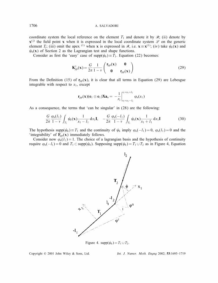
The hypothesis supp( h)≡T1 and the continuity of h imply ’n(−l1)=0, ’n(l1)=0 and the‘integrability’ of Fpp(x) immediately follows.Consider now ’n(l1)=1. The choice of a lagrangian basis and the hypothesis of continuity

require ’n(−l1)=0 and T1⊂ supp( h). Supposing supp( h)=T1 ∪T2 as in Figure 4, Equation

Figure 4. supp( h)=T1 ∪T2.



(28) becomes

2∑j=1

∫Tj k(x)Kj

pp(x( j))

(X(x( j))an 0

0 X(x( j))an

)dx (31)

About K1pp, from Equation (30), singularities may arise only from the term

G2�

11− �

∫T1 k(x)

1x1 − l1

dx1

About K2pp, from identity (12) one notes that all terms are Lebesgue integral with exceptionof [

1r2Spp +

1r4Hpp

]r1=x1+l2((e1 ⊗ e1)X(2)an 0

0 (e1 ⊗ e1)X(2)an

)(32)

In order to compare singularities, the factor (32) must be expressed in the absolute coordinatesystem R. The reference change between the L on T2 and R reads as

x(2) =R(x −O(2)); n(2) =Rn (33)

having set

R=

(cos� − sin�sin� cos�

); O(2) =

(l1 + l2 cos�

l2 sin�

)

By means of (33), factor (32) becomes

− 12�

G1− �

’n(−l2)1

x1 − l1I

By noting that ’n(−l2)=1 for the continuity of h(x), one <nally states that K2pp generatesthe following singular integral:

− 12�

G1− �

∫T1 k(x)

1x1 − l1

dx1

It is so self shown that even if none of the two ‘integrals’∫Ep k(x)F1pp(x

(1))dx;∫Ep k(x)F2pp(x

(2))dx

has a meaning in a Lebesgue sense, integral (28) is well de<ned.

5. WEAKLY SINGULAR INTEGRALS

In this section, it will be shown that all weakly singular integrals of (4) can be deduced fromthe following integral: ∫

zh log[z2 + c2] dz (34)


1708 A. SALVADORI

where c∈R, h∈N. Moreover, the following closed form can be proved by induction on h

∫zh log[z2 + c2] dz − C =

zh+1

h+ 1log[z2 + c2]

+ (1−M2[h])

[(−1)h=2 2c

h+1

h+ 1arctan

( zc

)

−h=2∑j=0(−1)(h−2j)=2 2ch−2jz2j+1

(h+ 1)(2j + 1)

]

+M2[h]

[(−1)(h−1)=2 ch+1

h+ 1log(z2 + c2)

−(h+1)=2∑j=1

(−1)h−j ch+1−2jz2j

(h+ 1)j

]

where C ∈R and M2[h] stands for the remainder of the (integer) division h÷ 2.In order to prove that all weakly singular integrals of (4) can be deduced from (34), one

de<nes test functions k(x) as in Equation (5), denoting x1:= {1; x1; x21 ; : : : ; xNi1 }, am:= {a(0)m ;

a(1)m ; a(2)m ; : : : ; a(Ni)m } and ’m(x)= aTmx1. Using Equations (7) and (8) integral (4) takes the

following form for the generic kernel Grs:

M∑i=1

N∑j=1

∫Ti

(aTmx1 Kjrs(x

(j))

(X(j)an 0

0 X(j)an

)dx (35)

Here the apex (j) states that x is written in with respect to a local reference on Tj. Withthe aim of simplifying the notation, when not explicitly indicated by the apex (j), x will beexpressed in the local reference on Ti and the apex (i) omitted.In view of identities (9)–(12), the external weakly singular integral in Equation (35)

reads as

∫ li

−li

(x1 0

0 x1

)[log(r21 + (x

(j)2 )

2)Lrs]r1=x( j)1 +ljr1=x( j)1 −lj

(X(j) 0

0 X(j)

)dx1 (36)

After mapping x(j) and X(j) in the local reference on Ti by means of a reference change,easy algebraic manipulations lead from Equation (36) to

∫ li

−li

(x1 ⊗ x1 0

0 x1 ⊗ x1

)log[x21 + a(%)x1 + b(%)] dx1�rs(%)

∣∣∣∣∣%=lj

%=−lj

where �rs(%) is a suitable matrix, a; b∈R depends on lj, with b¿0. As a conclusion, toperform the integration of the weakly singular part of (4), one has to solve the following



integral:

∫ li

−lixk1 log[x

21 + ax1 + b] dx1 =

k∑h=0

(kh

)(−a2

)k−h∫ (a=2)+li

(a=2)−lizh log[z2 + c2] dz

where the following variable change has been used:

z= x1 + a=2; c2 = b− a2=4

6. APPLICATIONS

6.1. A pure integration test

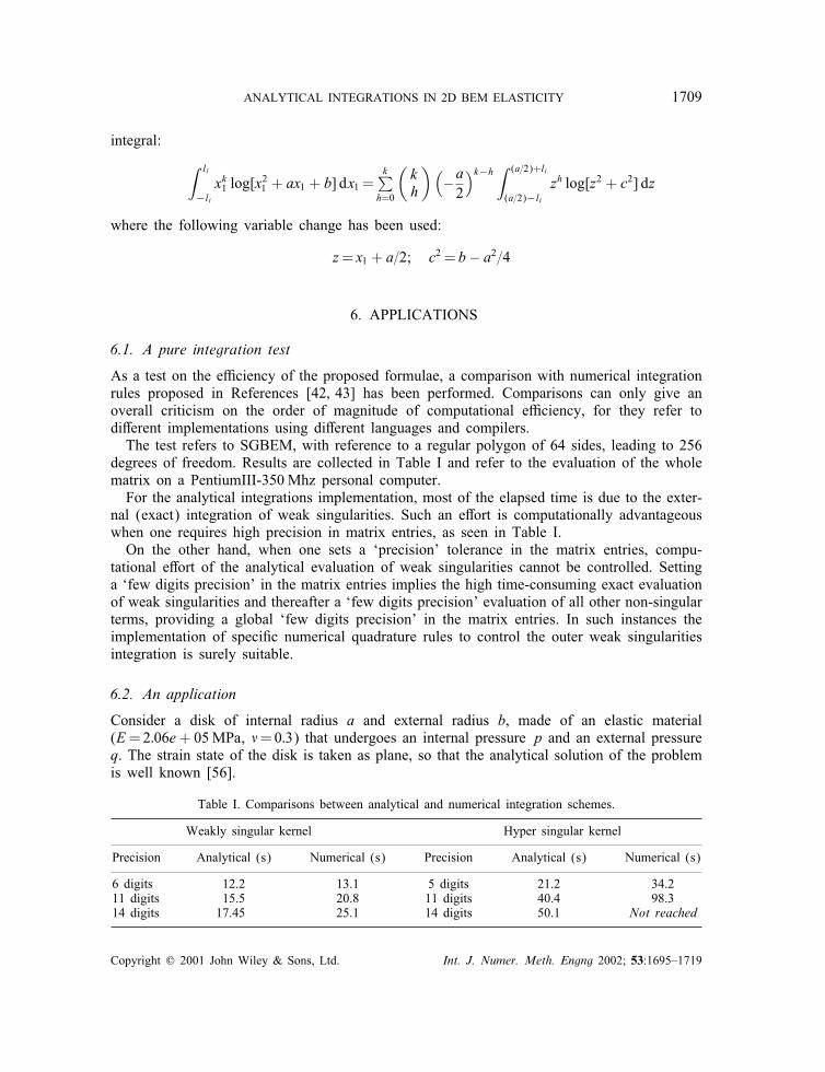
As a test on the eTciency of the proposed formulae, a comparison with numerical integrationrules proposed in References [42; 43] has been performed. Comparisons can only give anoverall criticism on the order of magnitude of computational eTciency, for they refer todiOerent implementations using diOerent languages and compilers.The test refers to SGBEM, with reference to a regular polygon of 64 sides, leading to 256

degrees of freedom. Results are collected in Table I and refer to the evaluation of the wholematrix on a PentiumIII-350 Mhz personal computer.For the analytical integrations implementation, most of the elapsed time is due to the exter-

nal (exact) integration of weak singularities. Such an eOort is computationally advantageouswhen one requires high precision in matrix entries, as seen in Table I.On the other hand, when one sets a ‘precision’ tolerance in the matrix entries, compu-

tational eOort of the analytical evaluation of weak singularities cannot be controlled. Settinga ‘few digits precision’ in the matrix entries implies the high time-consuming exact evaluationof weak singularities and thereafter a ‘few digits precision’ evaluation of all other non-singularterms, providing a global ‘few digits precision’ in the matrix entries. In such instances theimplementation of speci<c numerical quadrature rules to control the outer weak singularitiesintegration is surely suitable.

6.2. An application

Consider a disk of internal radius a and external radius b, made of an elastic material(E=2:06e+ 05MPa, �=0:3) that undergoes an internal pressure p and an external pressureq. The strain state of the disk is taken as plane, so that the analytical solution of the problemis well known [56].

Table I. Comparisons between analytical and numerical integration schemes.

Weakly singular kernel Hyper singular kernel

Precision Analytical (s) Numerical (s) Precision Analytical (s) Numerical (s)

6 digits 12.2 13.1 5 digits 21.2 34.211 digits 15.5 20.8 11 digits 40.4 98.314 digits 17.45 25.1 14 digits 50.1 Not reached


1710 A. SALVADORI

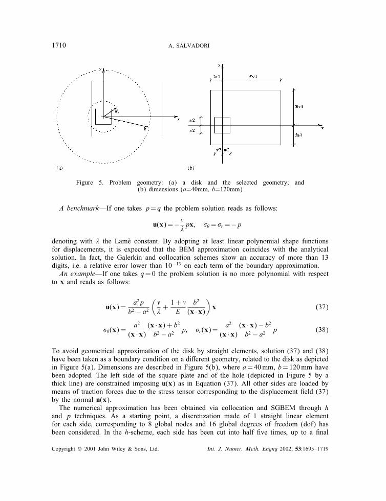
Figure 5. Problem geometry: (a) a disk and the selected geometry; and(b) dimensions (a=40mm, b=120mm)

A benchmark—If one takes p= q the problem solution reads as follows:

u(x)=− �*px; +,=+r =−p

denoting with * the LamWe constant. By adopting at least linear polynomial shape functionsfor displacements, it is expected that the BEM approximation coincides with the analyticalsolution. In fact, the Galerkin and collocation schemes show an accuracy of more than 13digits, i.e. a relative error lower than 10−13 on each term of the boundary approximation.An example—If one takes q=0 the problem solution is no more polynomial with respect

to x and reads as follows:

u(x) =a2p

b2 − a2

(�*+1+ �E

b2

(x ·x))x (37)

+,(x) =a2

(x ·x)(x ·x) + b2

b2 − a2p; +r(x)=

a2

(x ·x)(x ·x)− b2

b2 − a2p (38)

To avoid geometrical approximation of the disk by straight elements, solution (37) and (38)have been taken as a boundary condition on a diOerent geometry, related to the disk as depictedin Figure 5(a). Dimensions are described in Figure 5(b), where a=40mm, b=120mm havebeen adopted. The left side of the square plate and of the hole (depicted in Figure 5 by athick line) are constrained imposing u(x) as in Equation (37). All other sides are loaded bymeans of traction forces due to the stress tensor corresponding to the displacement <eld (37)by the normal n(x).The numerical approximation has been obtained via collocation and SGBEM through h

and p techniques. As a starting point, a discretization made of 1 straight linear elementfor each side, corresponding to 8 global nodes and 16 global degrees of freedom (dof) hasbeen considered. In the h-scheme, each side has been cut into half <ve times, up to a <nal



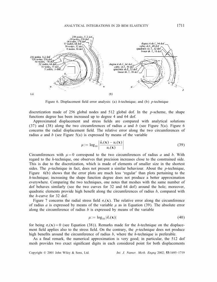
Figure 6. Displacement <eld error analysis: (a) h-technique; and (b) p-technique

discretization made of 256 global nodes and 512 global dof. In the p-scheme, the shapefunctions degree has been increased up to degree 4 and 64 dof.Approximated displacement and stress <elds are compared with analytical solutions

(37) and (38) along the two circumferences of radius a and b (see Figure 5(a). Figure 6concerns the radial displacement <eld. The relative error along the two circumferences ofradius a and b (see Figure 5(a) is expressed by means of the variable

- := log10

∣∣∣∣ ur(x)− ur(x)ur(x)

∣∣∣∣ (39)

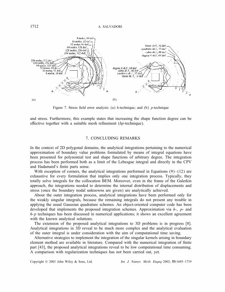
Circumferences with -=0 correspond to the two circumferences of radius a and b. Withregard to the h-technique, one observes that precision increases close to the constrained side.This is due to the discretization, which is made of elements of smaller size in the shortestsides. The p-technique in fact, does not present a similar behaviour. About the p-technique,Figure 6(b) shows that the error plots are much less ‘regular’ than plots pertaining to theh-technique; increasing the shape function degree does not produce a better approximationeverywhere. Comparing the two techniques, one notes that meshes with the same number ofdof behaves similarly (see the two curves for 32 and 64 dof) around the hole; moreover,quadratic elements provide high bene<t along the circumferences of radius b, compared withthe h-curve for 32 dof.Figure 7 concerns the radial stress <eld +r(x). The relative error along the circumference

of radius a is expressed by means of the variable - as in Equation (39). The absolute erroralong the circumference of radius b is expressed by means of the variable

- := log10 |+r(x)| (40)

for being +r(x)=0 (see Equation (38)). Remarks made for the h-technique on the displace-ment <eld applies also to the stress <eld. On the contrary, the p-technique does not producehigh bene<ts around the circumference of radius b, where the h-technique is preferable.As a <nal remark, the numerical approximation is very good; in particular, the 512 dof

mesh provides two exact signi<cant digits in each considered point for both displacements


1712 A. SALVADORI

Figure 7. Stress <eld error analysis: (a) h-technique; and (b) p-technique

and stress. Furthermore, this example states that increasing the shape function degree can beeOective together with a suitable mesh re<nement (hp-technique).

7. CONCLUDING REMARKS

In the context of 2D polygonal domains, the analytical integrations pertaining to the numericalapproximation of boundary value problems formulated by means of integral equations havebeen presented for polynomial test and shape functions of arbitrary degree. The integrationprocess has been performed both as a limit of the Lebesgue integral and directly in the CPVand Hadamard’s <nite parts sense.With exception of corners, the analytical integrations performed in Equations (9)–(12) are

exhaustive for every formulation that implies only one integration process. Typically, theytotally solve integrals for the collocation BEM. Moreover, even in the frame of the Galerkinapproach, the integrations needed to determine the internal distribution of displacements andstress (once the boundary nodal unknowns are given) are analytically achieved.About the outer integration process, analytical integrations have been performed only for

the weakly singular integrals, because the remaining integrals do not present any trouble inapplying the usual Gaussian quadrature schemes. An object-oriented computer code has beendeveloped that implements the proposed integration schemes. Approximation via h-, p- andh-p techniques has been discussed in numerical applications; it shows an excellent agreementwith the known analytical solutions.The extension of the proposed analytical integrations to 3D problems is in progress [8].

Analytical integrations in 3D reveal to be much more complex and the analytical evaluationof the outer integral is under consideration with the aim of computational time saving.Alternative strategies to implement the integration of the singular kernels arising in boundary

element method are available in literature. Compared with the numerical integration of <nitepart [43], the proposed analytical integrations reveal to be low computational time consuming.A comparison with regularization techniques has not been carried out, yet.



Besides computational eTciency, the availability of the closed form for the approximateddisplacement and stress <elds entails the possibility of analytical manipulations which arehardly possible with alternative approaches. Typically, the possibility of <nding the extremalvalues of the principal stress <eld is a major task in studying fracture initiation in unnotchedstructure. Furthermore, fracture propagation in bimaterial interfaces may have great advantagesover the proposed analytical integrations. In these contexts, work is in progress.

APPENDIX A: GREEN’S FUNCTIONS FOR LINEAR ELASTICITY

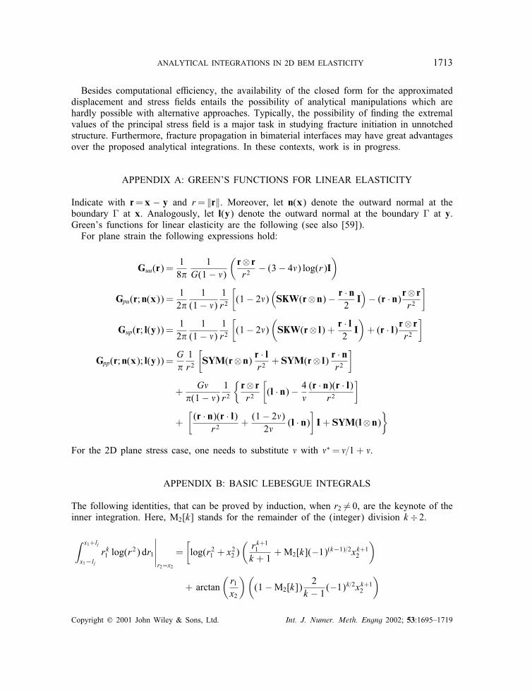
Indicate with r=x − y and r= ‖r‖. Moreover, let n(x) denote the outward normal at theboundary E at x. Analogously, let l(y) denote the outward normal at the boundary E at y.Green’s functions for linear elasticity are the following (see also [59]).For plane strain the following expressions hold:

Guu(r) =18�

1G(1− �)

(r⊗ rr2

− (3− 4�) log(r)I)

Gpu(r; n(x)) =12�

1(1− �)

1r2

[(1− 2�)

(SKW(r⊗ n)− r · n

2I)− (r · n)r⊗ r

r2

]

Gup(r; l(y)) =12�

1(1− �)

1r2

[(1− 2�)

(SKW(r⊗ l) + r · l

2I)+ (r · l)r⊗ r

r2

]

Gpp(r; n(x); l(y)) =G�1r2

[SYM(r⊗ n) r · l

r2+ SYM(r⊗ l) r · n

r2

]

+G�

�(1− �)1r2

{r⊗ rr2

[(l · n)− 4

�(r · n)(r · l)

r2

]

+[(r · n)(r · l)

r2+(1− 2�)2�

(l · n)]I+ SYM(l⊗ n)

}

For the 2D plane stress case, one needs to substitute � with �∗= �=1 + �.

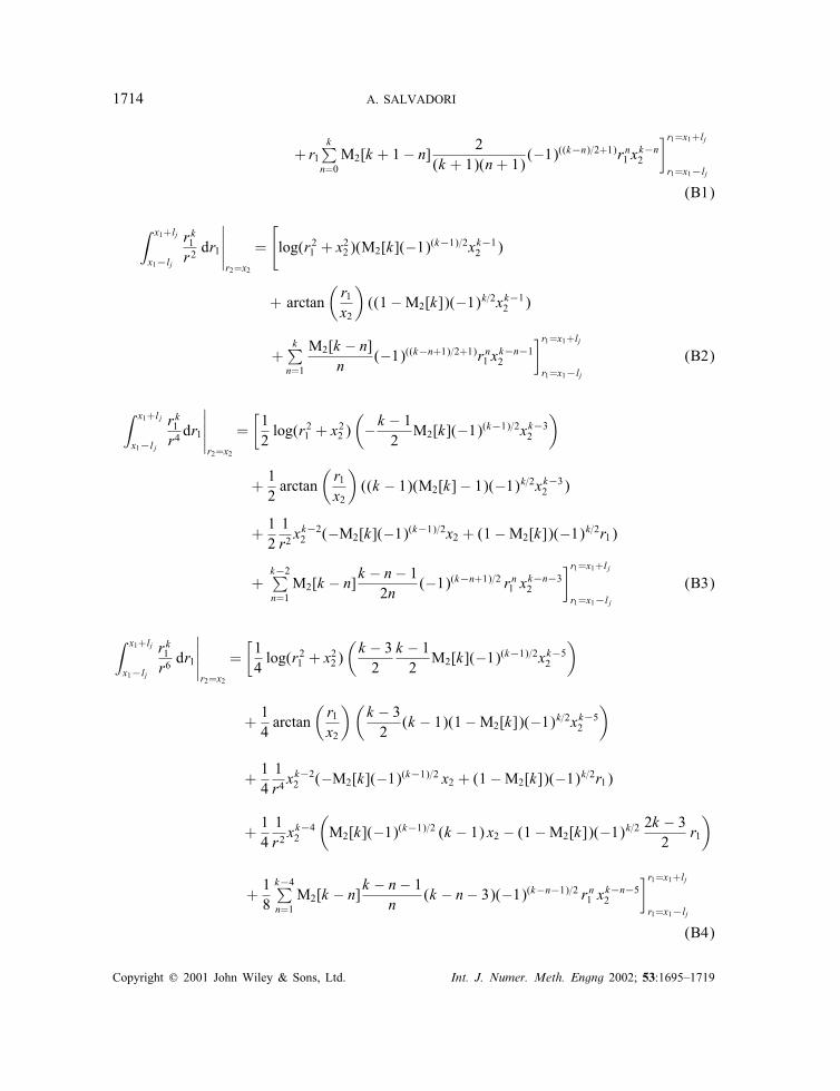
APPENDIX B: BASIC LEBESGUE INTEGRALS

The following identities, that can be proved by induction, when r2 �=0, are the keynote of theinner integration. Here, M2[k] stands for the remainder of the (integer) division k ÷ 2.

∫ x1+lj

x1−ljr k1 log(r

2) dr1

∣∣∣∣∣r2=x2

=[log(r21 + x22 )

(rk+11

k + 1+M2[k](−1)(k−1)=2xk+1

2

)

+ arctan(r1x2

)((1−M2[k])

2k − 1(−1)

k=2xk+12

)


1714 A. SALVADORI

+ r1k∑

n=0M2[k + 1− n]

2(k + 1)(n+ 1)

(−1)((k−n)=2+1)rn1 x

k−n2

]r1=x1+lj

r1=x1−lj

(B1)

∫ x1+lj

x1−lj

r k1

r2dr1

∣∣∣∣∣r2=x2

=

[log(r21 + x22)(M2[k](−1)(k−1)=2xk−1

2 )

+ arctan(r1x2

)((1−M2[k])(−1)k=2xk−1

2 )

+k∑

n=1

M2[k − n]n

(−1)((k−n+1)=2+1)rn1 x

k−n−12

]r1=x1+lj

r1=x1−lj

(B2)

∫ x1+lj

x1−lj

r k1

r4dr1

∣∣∣∣∣r2=x2

=[12log(r21 + x22 )

(−k − 1

2M2[k](−1)(k−1)=2xk−3

2

)

+12arctan

(r1x2

)((k − 1)(M2[k]− 1)(−1)k=2xk−3

2 )

+121r2

xk−22 (−M2[k](−1)(k−1)=2x2 + (1−M2[k])(−1)k=2r1)

+k−2∑n=1M2[k − n]

k − n− 12n

(−1)(k−n+1)=2 rn1 xk−n−3

2

]r1=x1+lj

r1=x1−lj

(B3)

∫ x1+lj

x1−lj

r k1

r6dr1

∣∣∣∣∣r2=x2

=[14log(r21 + x22)

(k − 32

k − 12M2[k](−1)(k−1)=2xk−5

2

)

+14arctan

(r1x2

)(k − 32(k − 1)(1−M2[k])(−1)k=2xk−5

2

)

+141r4

xk−22 (−M2[k](−1)(k−1)=2 x2 + (1−M2[k])(−1)k=2r1)

+141r2

xk−42

(M2[k](−1)(k−1)=2 (k − 1) x2 − (1−M2[k])(−1)k=2 2k − 3

2r1

)

+18

k−4∑n=1M2[k − n]

k − n− 1n

(k − n− 3)(−1)(k−n−1)=2 rn1 xk−n−5

2

]r1=x1+lj

r1=x1−lj

(B4)



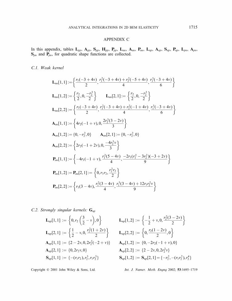
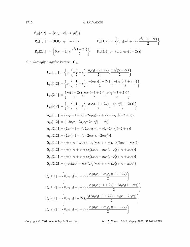
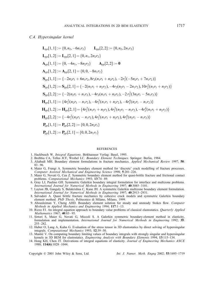
APPENDIX C

In this appendix, tables Lpp, App, Spp, Hpp, Ppp, Luu, Auu, Puu, Lup, Aup, Sup, Pup, Lpu, Apu,Spu and Ppu, for quadratic shape functions are collected.

C.1. Weak kernel

Luu[1; 1] :={r1(−3 + 4�)

2;r21 (−3 + 4�) + r22 (−5 + 4�)

4;r31 (−3 + 4�)

6

}

Luu[1; 2] :={r22; 0;

−r322

}Luu[2; 1] :=

{r22; 0;

−r322

}

Luu[2; 2] :={r1(−3 + 4�)

2;r21 (−3 + 4�) + r22 (−1 + 4�)

4;r31 (−3 + 4�)

6

}

Auu[1; 1] :={4r2(−1 + �); 0;

2r32 (3− 2�)3

}

Auu[1; 2] := {0;−r22 ; 0} Auu[2; 1] := {0;−r22 ; 0}

Auu[2; 2] :={2r2(−1 + 2�); 0; −4r

32 �3

}

Puu[1; 1] :={−4r1(−1 + �);

r21 (5− 4�)4

;−2r1(r21 − 3r22 )(−3 + 2�)

9

}

Puu[1; 2] :=Puu[2; 1] :={0; r1r2;

r21 r22

}

Puu[2; 2] :={r1(3− 4�); r

21 (3− 4�)4

;r31 (3− 4�) + 12r1r22 �

9

}

C.2. Strongly singular kernels: Gup

Lup[1; 1] :={0; r2

(32− �); 0}

Lup[1; 2] :={−12+ �; 0;

r22 (3− 2�)2

}

Lup[2; 1] :={12− �; 0;

r22 (1 + 2�)2

}Lup[2; 2] :=

{0;

r2(1− 2�)2

; 0}

Aup[1; 1] := {2− 2�; 0; 2r22 (−2 + �)} Aup[1; 2] := {0;−2r2(−1 + �); 0}Aup[2; 1] := {0; 2r2�; 0} Aup[2; 2] := {2− 2�; 0; 2r22 �}Sup[1; 1] := {−(r1r2); r32 ; r1r32 } Sup[1; 2] := Sup[2; 1]= {−r22 ;−(r1r22 ); r42}


1716 A. SALVADORI

Sup[2; 2] := {r1r2;−r32 ;−(r1r32 )}

Pup[1; 1] := {0; 0; r1r2(3− 2�)} Pup[1; 2] :={0; r1(−1 + 2�); r

21 (−1 + 2�)

2

}

Pup[2; 1] :={0; r1 − 2r1�; r

21 (1− 2�)2

}Pup[2; 2] := {0; 0; r1r2(1− 2�)}

C.3. Strongly singular kernels: Gpu

Lpu[1; 1] :={n1

(−32+ �);n2r2(−3 + 2�)

2;n1r22 (5− 2�)

2

}

Lpu[1; 2] :={n2

(−12+ �);−(n1r2(1 + 2�))

2;−(n2r22 (1 + 2�))

2

}

Lpu[2; 1] :={n2(1− 2�)

2;n1r2(−3 + 2�)

2;n2r22 (−3 + 2�)

2

}

Lpu[2; 2] :={n1

(−12+ �);n2r2(−1 + 2�)

2;−(n1r22 (1 + 2�))

2

}

Apu[1; 1] := {2n2(−1 + �);−2n1r2(−2 + �);−2n2r22 (−2 + �)}Apu[1; 2] := {−2n1�;−2n2r2�; 2n1r22 (1 + �)}Apu[2; 1] := {2n1(−1 + �); 2n2r2(−1 + �);−2n1r22 (−2 + �)}Apu[2; 2] := {2n2(−1 + �);−2n1r2�;−2n2r22 �}Spu[1; 1] := {r2(n2r1 − n1r2);−r22 (n1r1 + n2r2);−r32 (n2r1 − n1r2)}Spu[1; 2] := {r2(n1r1 + n2r2); r22 (n2r1 − n1r2);−r32 (n1r1 + n2r2)}Spu[2; 1] := {r2(n1r1 + n2r2); r22 (n2r1 − n1r2);−r32 (n1r1 + n2r2)}Spu[2; 2] := {−r2(n2r1 − n1r2); r22 (n1r1 + n2r2); r32 (n2r1 − n1r2)}

Ppu[1; 1] :={0; n1r1(−3 + 2�); r1(n1r1 + 2n2r2)(−3 + 2�)2

}

Ppu[1; 2] :={0; n2r1(−1 + 2�); r1(n2r1(−1 + 2�)− 2n1r2(1 + 2�))2

}

Ppu[2; 1] :={0; n2r1(1− 2�); r1(2n1r2(−3 + 2�) + n2(r1 − 2r1�))

2

}

Ppu[2; 2] :={0; n1r1(−1 + 2�); r1(n1r1 + 2n2r2)(−1 + 2�)2

}



C.4. Hypersingular kernel

Lpp[1; 1] := {0; n2;−6n1r2} Lpp[2; 2] := {0; n2; 2n1r2}Lpp[1; 2] :=Lpp[2; 1]= {0; n1; 2n2r2}App[1; 1] := {0;−4n1;−8n2r2} App[2; 2] := 0

App[1; 2] :=App[2; 1]= {0; 0;−8n1r2}Spp[1; 1] := {−2n2r1 + 6n1r2; 8r2(n1r1 + n2r2);−2r22 (−5n2r1 + 7n1r2)}Spp[1; 2] := Spp[2; 1]= {−2(n1r1 + n2r2);−4r2(n2r1 − 2n1r2); 10r22 (n1r1 + n2r2)}Spp[2; 2] := {−2(n2r1 + n1r2);−4r2(n1r1 + n2r2);−2 r22 (3n2r1 − 5n1r2)}Hpp[1; 1] := {4r22 (n2r1 − n1r2);−4r32 (n1r1 + n2r2);−4r42 (n2r1 − n1r2)}Hpp[1; 2] :=Hpp[2; 1]= {4r22 (n1r1 + n2r2); 4r32 (n2r1 − n1r2);−4r42 (n1r1 + n2r2)}Hpp[2; 2] := {−4r22 (n2r1 − n1r2); 4r32 (n1r1 + n2r2); 4r42 (n2r1 − n1r2)}Ppp[1; 1] :=Ppp[2; 2] := {0; 0; 2n2r1}Ppp[1; 2] :=Ppp[2; 1]= {0; 0; 2n1r1}

REFERENCES

1. Hackbusch W. Integral Equations. Birkhaeuser Verlag: Basel, 1995.2. Brebbia CA, Telles JCF, Wrobel LC. Boundary Element Techniques. Springer: Berlin, 1984.3. Aliabadi MH. Boundary element formulations in fracture mechanics. Applied Mechanical Review 1997; 50:83–96.

4. Maier G, Frangi A. Symmetric boundary element method for ‘discrete’ crack modelling of fracture processes.Computer Assisted Mechanical and Engineering Science 1998; 5:201–226.

5. Maier G, Novati G, Cen Z. Symmetric boundary element method for quasi-brittle fracture and frictional contactproblems. Computational Mechanics 1993; 13:74–89.

6. Gray LJ, Paulino GH. Symmetric Galerkin boundary integral formulation for interface and multizone problems.International Journal for Numerical Methods in Engineering 1997; 40:3085–3101.

7. Layton JB, Ganguly S, Balakrishna C, Kane JH. A symmetric Galerkin multizone boundary element formulation.International Journal for Numerical Methods in Engineering 1997; 40:2913–2931.

8. Salvadori A. Quasi brittle fracture mechanics by cohesive crack models and symmetric Galerkin boundaryelement method. PhD Thesis, Politecnico di Milano, Milano, 1999.

9. Abousleiman Y, Cheng AHD. Boundary element solution for steady and unsteady Stokes Jow. ComputerMethods in Applied Mechanics and Engineering 1994; 117:1–13.

10. Rizzo FJ. An integral equation approach to boundary value problems of classical elastostatics. Quarterly AppliedMathematics 1967; 40:83–95.

11. Sirtori S, Maier G, Novati G, Miccoli S. A Galerkin symmetric boundary-element method in elasticity,formulation and implementation. International Journal for Numerical Methods in Engineering 1992; 35:255–282.

12. Huber O, Lang A, Kuhn G. Evaluation of the stress tensor in 3D elastostatics by direct solving of hypersingularintegrals. Computational Mechanics 1993; 12:39–50.

13. Manti[c V. On computing boundary limiting values of boundary integrals with strongly singular and hypersingularkernels in 3D BEM for elastostatics. Engineering Analysis with Boundary Elements 1994; 13:115–134.

14. Hong KH, Chen JT. Derivations of integral equations of elasticity. Journal of Engineering Mechanics ASCE1988; 114(6):1028–1044.


1718 A. SALVADORI

15. Diligenti M, Monegato G. Finite-part integrals, their occurence and computation. Rendiconti del CircoloMatematico di Palermo 1993; 33(II):39–61.

16. Guiggiani M. Hypersingular boundary integral equations have an additional free term. Computational Mechanics1995; 16:245–248.

17. Hadamard J. Lectures on Cauchy’s Problem in Linear Partial Di;erential Equations. Yale Univ. Press:New Haven, Conn, 1923.

18. Krishnasamy G, Rizzo FJ, Rudolphi TJ. Hypersingular Boundary Integral Equations, Their Occurrence,Interpretation, Regularization and Computation. In Developments in Boundary Element Methods, vol. 7,Banerjee PK, Kobayashi S (eds). Elsevier Applied Science Publishers: Amsterdam, 1991.

19. Toh K, Mukherjee S. Hypersingular and <nite part integrals in the boundary element method. InternationalJournal of Solid Structures 1994; 31:2299–2312.

20. Manti[c V. A new formula for the C-matrix in the Somigliana identity. Journal of Elasticity 1993; 33:191–201.21. Hartmann F. The Somigliana identity on a piecewise smooth surface. Journal of Elasticity 1981; 11(4):

403–423.22. Nedelec JC, Planchard J. Une methode variationelle d’elements <nis pour la resolution numerique d’un problem

exterieur dans R3. RAIRO Analyse Numerique 1973; 7:105–129.23. Hsiao GC, Wendland WL. A <nite element method for some integral equations of the <rst kind. Journal of

Mathematical Analysis and Applications 1977; 58:449–481.24. Sirtori S. General stress analysis by means of integral equation and boundary elements. Meccanica 1979; 14:

210–218.25. Hartmann F, Katz C, Protopsaltis B. Boundary elements and symmetry. Ingenieur-Archiv 1985; 55:440–449.26. Wendland WL. Variational methods for BEM. In Boundary Integral Methods (Theory and Applications),

Morino L, Piva R (eds). Springer: Berlin, 1990.27. Polizzotto C, Zito M. A variational approach to boundary element methods. In Boundary Elements Methods in

Applied Mechanics, Tanaka M, Cruse T (eds). Pergamon Press: Oxford, 1989; 13–24.28. Carini A, Salvadori A. Implementation of a symmetric Galerkin boundary element method in quasi-brittle fracture

mechanics. Proceeding of IUTAM=IACM=IABEM 1999 Symposium. Kluwer Academic Press: Dordrecht, MA,1999.

29. Polizzotto C. An energy approach to the boundary element method. Part I, Elastic solids. Computer Methodsin Applied Mechanics and Engineering 1988; 69:167–184.

30. Bonnet M, Maier G, Polizzotto C. Symmetric Galerkin boundary element method. Applied Mechanical Review1998; 51:669–704.

31. Kane JH, Balakrishna C. Symmetric Galerkin boundary formulations employing curved elements. InternationalJournal for Numerical Methods in Engineering 1993; 36:2157–2187.

32. Rudolphi TJ. The use of simple solutions in the regularization of hypersingular boundary integral equations.Mathematical Computational Model 1991; 15:269–278.

33. Bonnet M. A regularized Galerkin symmetric BIE formulation for mixed 3D elastic boundary values problems.Boundary Elements Abstracts and Newsletters 1993; 4:109–113.

34. Sladek V, Sladek J. Transient elastodynamic three dimensional problems in cracked bodies. AppliedMathematical Model 1984; 8:2–10.

35. Frangi A, Novati G. Symmetric BE method in two-dimensional elasticity, evaluation of double integrals forcurved elements. Computational Mechanics 1996; 19:58–68.

36. Frangi A, Novati G. Regularized symmetric Galerkin BIE formulations in the Laplace transform domain for 2Dproblems. Computational Mechanics 1998; 22:50–60.

37. Kutt HR. The numerical evaluation of principal value integrals by <nite-part integration. Numerical Mathematics1975; 24:205–210.

38. Monegato G. The numerical evaluation of hypersingular integrals. Journal of Computational and AppliedMathematics 1994; 50:9–31

39. Aimi A. New numerical integration schemes for solution of (hyper) singular integral equations with GalerkinBEM. PhD Thesis. Universita‘ degli Studi di Milano, Milano, 1997.

40. Balakrishna C, Gray LJ, Kane JH. ETcient analytic integration of symmetric Galerkin boundary integralsover curved elements, thermal conduction formulation. Computational Mathematics and Applied Mechanicsin Engineering 1994; 111:335–355.

41. Aimi A, Carini A, Diligenti M, Monegato G. Numerical integration schemes for evaluation of (hyper)singularintegrals in 2D BEM. Computational Mechanics 1998; 22:1–11.

42. Aimi A, Diligenti M, Monegato G. New numerical integration schemes for applications of Galerkin Bem to 2Dproblems. International Journal for Numerical Methods in Engineering 1997; 40:1977–1999.

43. Aimi A, Diligenti M, Monegato G. Numerical integration schemes for the BEM solution of hypersingular integralequations. International Journal for Numerical Methods in Engineering 1999; 45:1807–1830.

44. Elliott D, Paget DF. Gauss type quadrature rules for Cauchy principal value integrals. Mathematics ofComputation 1979; 33(145):301–309.



45. Guiggiani M, Krishnasamy G, Rudolphi TJ, Rizzo FJ. A general algorithm for the numerical solution ofhypersingular boundary integral equations. Journal of Applied Mechanics 1992; 59:604–614.

46. Holzer S. How to deal with hypersingular integrals in the symmetric BEM. Communications and AppliedNumerical Methods 1993; 9:219–232.

47. Hui CY, Shia D. Evaluations of hypersingular integrals using Gaussian quadrature. International Journal forNumerical Methods in Engineering 1999; 44:205–214.

48. Guiggiani M. Hypersingular formulation for boundary stress evaluation. Engineering Analysis with BoundaryElements 1994; 13:169–179.

49. Gray LJ, Martha LF, IngraOea AR. Hypersingular integrals in boundary element fracture analysis. InternationalJournal for Numerical Methods in Engineering 1990; 29:1135–1158.

50. Gray LJ, Soucie CS. A Hermite interpolation algorithm for hypersingular boundary integrals. InternationalJournal for Numerical Methods in Engineering 1993; 36:2357–2367.

51. Carini A, Diligenti M, Maranesi P, Zanella M. Analytical integrations for two-dimensional elastic analysis bythe symmetric Galerkin boundary element method. Computational Mechanics 1999; 23(4):308–323.

52. Mori M. Quadrature formulas obtained by variable transformation and the DE-Rule. Journal of Computationaland Applied Mathematics 1985; 12:119–130.

53. Monegato G, Scuderi L. Numerical integration of functions with boundary singularities. Journal ofComputational and Applied Mathematics 1999; 112:201–214.

54. Schwab C, Wendland WL. Kernel properties and representations of boundary integral operators. MathematischeNachrichten 1998; 156:187–218.

55. Zemanian AH. Distribution Theory and Transform Analysis. Dover: New York, 1987.56. Corradi Dell’Acqua L. Meccanica delle Strutture. McGraw-Hill: Milano, 1992 (in Italian).57. Banerjee PK, Butter<eld R. Boundary Element Method in Engineering Science. McGraw-Hill: New York, 1981.58. Press WH, Flannery BP, Teukolsky SA, Vetterling WT. Numerical Recipes. The Art of Scienti/c Computing.

Cambridge University Press: Cambridge, 1986.59. Carini A, De Donato O. Fundamental solutions for linear viscoelastic continua. International Journal for Solids

Structures 1992; 29:2989–3009.


Analytical integrations in 2D BEM elasticity

Documents