ANALYTICAL AND NUMERICAL SOLUTIONS FOR PILE FOUNDATIONS by Wei Dong Guo BE(Civil), M. Eng.(Geotechnical) This dissertation is submitted for the degree of Doctor of Philosophy of The University of Western Australia Department of Civil Engineering December 1996

Welcome message from author
This document is posted to help you gain knowledge. Please leave a comment to let me know what you think about it! Share it to your friends and learn new things together.
Transcript
ANALYTICAL AND NUMERICAL SOLUTIONS FOR PILE FOUNDATIONS
by
Wei Dong Guo
BE(Civil), M. Eng.(Geotechnical)
This dissertation is submitted for the degree of Doctor of Philosophy
of The University of Western Australia
Department of Civil Engineering
December 1996
1
ABSTRACT
This research has investigated the performance of piles in non-homogeneous elastic-
plastic media subject to vertical or torsional loading, the time-dependent response of a
vertically loaded pile due to either creep or reconsolidation subsequent to pile driving,
and the behaviour of vertically loaded pile groups. Closed form solutions have been
established accordingly, and numerical programs, G A S P I L E and G A S G R O U P have
been developed.
The closed form solutions were firstly developed for vertically loaded single piles.
Secondly, in a similar manner, solutions for single piles subject to torsion were
generated, in light of a newly established torsional load transfer model. The effect of
non-linear soil stress-strain properties modelled using a hyperbolic stress-strain law, has
been investigated through the program, GASPILE, for both vertical and torsional
loading. Thereafter, the solutions for vertically loaded piles were extended to account
for visco-elastic response, with a newly established visco-elastic model.
All the solutions have been developed to incorporate accurate modelling of the soil
stiffness profile described by a power law of depth, and also with appropriate attention
to the gradual development of slip between pile and soil.
Although the solutions are based on the load transfer approach, treating each soil layer
independently from neighbouring layers, the accuracy has been extensively checked by
more rigorous numerical approaches, against which load transfer factors have been
extensively calibrated. Appropriate load transfer factors have been developed, allowing
for the effect of the following parameters: pile slenderness ratio, ratio of the depth of
underlying rigid layer to pile length, soil Poisson's ratio, and non-homogeneous soil
profile.
One of the major concerns has been the variation of soil properties with time following
pile installation. This variation has been simulated through a newly established visco-
elastic radial consolidation theory.
ii
The solutions for a single pile have then been eventually extended to evaluate settlement
behaviour of large pile groups, in light of the principle of superposition.
All the solutions established have been substantiated by previous numerical and
experimental results. Parametric analyses were undertaken extensively and a number
conclusions were drawn.
In particular, non-linear analysis using a hyperbolic stress-strain model does not lead to
appreciable differences from a simple elastic, perfectly plastic analysis. Therefore, the
closed form solutions based on an elastic-plastic model can be applied directly to the
non-linear case, without significant lose of accuracy.

iii
DECLARATION
I certify that, except where specific reference is made in the text to the work of others,
the content of this thesis are original and have not been submitted to any other
university or institute. This thesis is the result of m y o w n work and contains nothing
which is the outcome of work done in collaboration.
Wei Dong Guo
iv
ACKNOWLEDGMENTS
I would like to express my sincere thanks to my supervisor, Professor Mark Randolph
for his insight guidance and encouragement throughout the course of this study. His
sincere assistance beyond the research is much appreciated.
I would also like to thank Vickie Goodall for her sincere help all the time. Mr. Wayne
Griffioen for his friendly discussion and assistance on computer issues. Dr. Anthony De
Nicola, Mr. Joyis Thomas and Mr. Fujiyasu Yoshimasa for their friendly gossip. Craig
Sampson, Simon Kelly for their assistance whenever the computer becomes unbearable.
Simone Gjergjevica for her regular automotive backup of m y computer. Dr. Deepak
Adhikary for his friendly jokes and encouragement. Dr. Patrick Clancy for a nice copy
of his Ph.D thesis. Davide Bruno is also thanked for proof reading the first draft of the
thesis. I also would like to thank all other staff and students in the Civil Engineering
Department for their friendship.
Thanks should also go to Professor Qian Jia Huan for his early guidance when I was
doing research in Hohai University, China. His sudden passing way was a shock to me.
Thanks should be given to Professor Qian Hon Jin for his time and constant
encouragement, Professor Yin Zon Ze for his confidence and interest in m y professional
ability, Professor Arun Valsangkar for his suggestions and discussions on a number of
issues from practical points of views, and finally Professor W a n g J. X. for his
information from China.
Without the initial financial support from the Geomechanics group at UWA, I would
probably not have had the opportunity to come to such a nice place. None of this could
have happened without the Overseas Postgraduate Research Studentship provided by
the Commonwealth Government of Australia, the research scholarship from the
University of Western Australia and the Geomechanics Studentship.
Finally, I must thank my wife and daughter for their support and understanding over the
course of the research. I also thank m y parents for their support in all m y endeavours,
thank m y brothers for their constant encouragement and concern for m y study, and
thank m y parents in law for their constant information from China.
Wei Dong Guo December 12, 1996
V
TABLE OF CONTENTS
ABSTRACT
DECLARATION
ACKNOWLEDGEMENTS
TABLE OF CONTENTS
NOTATION
1. INTRODUCTION 1-1
1.1 BACKGROUND 1-1
1.2 OBJECTIVES 1-2
1.3 CLOSED FORM SOLUTIONS AND NUMERICAL VERIFICATIONS 1-3
1.4 ORGANISATION OF THE DISSERTATION 1-4
2. LITERATURE REVIEW 2-1
2.1 INTRODUCTION 2-1
2.2 VERTICALLY LOADED SINGLE PILES 2-1
2.2.1 Load Transfer Approach 2-2
2.2.1.1 Empirical (ID) Load Transfer Approaches 2-2
2.2.1.2 Theoretical (2D) Load Transfer Models 2-3
2.2.2 Closed Form Solutions 2-8
2.2.2.1 Based on Mindlin' Solution 2-8
2.2.2.2 Based on Empirical (ID) Model 2-8
2.2.2.3 Based on Theoretical (2D) Model 2-9
2.2.3 Numerical Solutions Based on Discrete Element 2-10
2.2.3.1 Load Transfer Approach 2-10
2.2.3.2 Direct Hyperbolic Load Transfer Approach 2-11
2.2.4 Rigorous Numerical Analysis based on Continuum Media 2-12
2.2A. 1 Boundary Element Approach Based on Mindlin's Solution 2-12
2.2.4.2 Boundary Element Approach Based on Chan's Solution 2-14
2.2.4.3 Finite Element Method 2-14
2.2.4.4 Variational Element Method 2-15
2.2.5 Consideration of Non-homogeneity 2-15
2.2.5.1 Based on Shear Modulus 2-16
2.2.5.2 Based on Stress Distribution 2-16
2.2.5.3 Pile-Soil Relative Stiffness Factor 2-20
2.3 TIME-DEPENDENT EFFECT 2-20
2.3.1 Soil Strength 2-20
2.3.2 Excess Pore Pressure 2-21
2.3.3 Reconsolidation Process 2-22
VI
2.3.4 Visco-elastic Behaviour 2-25
2.3.5 Time-dependent Load Settlement Behaviour 2-27
2.4 VERTICALLY LOADED GROUP PILES 2-28
2.4.1 Empirical Approaches 2-29
2.4.2 Interaction Factor and Superposition Principle 2-30
2.4.3 Displacement Field Around a Single (Group) Pile 2-31
2.4.3.1 A Single Pile 2-31
2.4.3.2 Two Piles 2-31
2.4.3.3 Muti-Piles 2-32
2.4.4 Simple Closed Form Approaches 2-33
2.4.5 Numerical Approaches 2-34
2.4.5.1 Boundary Element (Integral) Approach 2-34
2.4.5.2 Infinite Layer Approach 2-35
2.4.5.3 Non-linear Elastic Analysis 2-35
2.4.5.4 Discrete Element Analysis - Layer Model 2-36
2.4.5.5 Hybrid Load Transfer Approach 2-37
2.4.6 Influence of Non-homogeneity 2-39
2.4.6.1 Vertical Non-homogeneity 2-39
2.4.6.2 Horizontal Non-homogeneity 2-39
2.4.6.3 Shear Stress Non-homogeneity 2-39
2.5 TORSIONAL PILES 2-40
2.5.1 Load Transfer Analysis 2-40
2.5.2 Continuum Based Numerical Approach 2-41
2.6 S U M M A R Y 2-41
2.6.1 Single Piles 2-41
2.6.2 Time-Dependent Effect 2-42
2.6.3 Pile Groups 2-43
2.6.4 Torsional Piles 2-43
3. VERTICALLY LOADED SINGLE PILES 3-1
3.1 INTRODUCTION 3-1
3.2 LOAD TRANSFER MODELS 3-2
3.2.1 Expressions of Non-homogeneity 3-2
3.2.2 Elastic Stiffness 3-3
3.2.2.1 Shaft Load Transfer Model 3-4
3.2.2.2 Base Pile -Soil Interaction Model 3-5
3.3 OVERALL PILE SOIL INTERACTION 3-6
3.3.1 Elastic Solution 3-6
3.3.2 Elastic-Plastic Solution 3-8
3.4 PILE RESPONSE WITH HYPERBOLIC SOIL M O D E L 3-10
vii
3.4.1 A Program for Non-linear Load Transfer Analysis 3-10
3.4.2 Shaft Stress-Strain Non-linearity Effect 3-10
3.4.3 Base Stress-Strain Non-linearity Effect 3-11
3.5 VERIFICATION OF THE THEORY 3-11
3.5.1 FLAC Analysis 3-11
3.5.2 Pile-head Stiffness and Settlement Ratio 3-12
3.5.3 Load Settlement 3-13
3.6 SETTLEMENT INFLUENCE FACTOR 3-14
3.6.1 Settlement Influence Factor 3-14
3.6.2 Pile Slenderness Ratio Influence. 3-15
3.6.3 Pile-Soil Relative Stiffness Effect 3-15
3.7 CASE STUDY 3-15
3.7.1 Load Displacement Distribution Down a Pile 3-16
3.8 CONCLUSIONS 3-16
4. LOAD TRANSFER IN FINITE LAYER MEDIA 4-1
4.1 INTRODUCTION 4-1
4.2 RATIONALITY OF LOAD TRANSFER APPROACH 4-2
4.2.1 Calibration Procedures 4-2
4.2.2 FLAC Analysis 4-3
4.2.3 Variation of Shaft Load Transfer Factor WithDepth 4-5
4.3 EXPRESSIONS FOR LOAD TRANSFER FACTORS 4-5
4.3.1 Base Load Transfer Factor 4-6
4.3.2 Shaft Load Transfer Factor 4-7
4.3.3 Accuracy of Load Transfer Approach 4-8
4.3.3.1 Using 'A=2.5' for a Pile in an Infinite Layer 4-9
4.3.3.2 Effect of Base Load Transfer Factor 4-9
4.4 VALIDATION OF LOAD TRANSFER APPROACH 4-10
4.4.1 Comparison with Existing Solutions 4-10
4.4.1.1 Slenderness Ratio Effect 4-10
4.4.1.2 Soil Poisson's Ratio Effect 4-11
4.4.1.3 Finite Layer Effect 4-11
4.5 EFFECT OF SOIL PROFILE BELOW PILE BASE 4-11
4.7 CONCLUSIONS 4-13
5. NON-LINEAR VISCO-ELASTIC LOAD TRANSFR MODELS FOR PILES 5-1
5.1 INTRODUCTION 5-1
5.2 SHAFT BASE PILE-SOIL INTERACTION 5-2
5.2.1 Non-linear Visco-elastic Stress-Strain Model 5-2
5.2.2 Shaft Displacement Estimation 5-5
viii
5.2.2.1 Visco-elastic Shaft Estimation Formula 5-5
5.2.2.3 Discussion on Local Shaft Stress-Displacement Relationship 5-8
5.2.2.4 Verification of the Shaft Load Transfer Model 5-10
5.2.3 Base Pile-Soil Interaction Model 5-12
5.3 VALIDATION OF THE THEORY 5-12
5.3.1 Closed Form Solutions 5-12
5.3.2 Validation 5-14
5.4 COMPARISON BETWEEN THE TWO KINDS OF LOADING 5-15
5.5 APPLICATION 5-15
5.5.1 Case 1: Tests reported by Konrad and Roy (1987) 5-16
5.5.2 Case II: Visco-elastic Property Predominated Compressive Loading.... 5-16
5.6 CONCLUSIONS 5-17
6. PERFORMANCE OF A DRIVEN PILE IN VISCO-ELASTIC MEDIA 6-1
6.1 INTRODUCTION 6-1
6.2 NON-LINEAR VISCO-ELASTIC STRESS-STRAIN MODEL 6-3
6.3 GOVERNING DIFFUSION EQUATION FOR RECONSOLIDATION 6-4
6.3.1 Volumetric Stress-strain Relation of Soil Skeleton 6-4
6.3.2 Flow of Pore Water and Continuity of Volume Strain Rate 6-6
6.4 BOUNDARY CONDITIONS 6-7
6.5 GENERAL SOLUTION 6-8
6.5.1 Direct Solution of the Diffusion Equation 6-8
6.5.2 Rigorous Solutions for the Radial Reconsolidation 6-11
6.5.3 Solution By Correspondence Principle 6-11
6.6 CONSOLIDATION FOR LOGARITHMIC VARIATION OF U0 6-12
6.7 VISCO-ELASTIC BEHAVIOUR 6-14
6.7.1 Parameters for the Creep Model 6-14
6.7.2 Prediction of the Ratio of Modulus and Limiting Shaft Stress 6-14
6.7.2.1 Example Study 6-15
6.8 CASE STUDY 6-17
6.8.1 Tests reported by Seed and Reese (1955) 6-17
6.8.2 Tests reported by Konrad and Roy (1987) 6-18
6.8.3 Comments on the Current Predictions 6-20
6.9 CONCLUSIONS 6-20
7. SETTLEMENT OF PILE GROUPS IN NON-HOMOGENEOUS SOIL 7-1
7.1 INTRODUCTION 7-1
7.2 ANALYSIS OF A SINGLE PILE IN A GROUP 7-2
7.3 INTERACTION FACTOR 7-4
7.4 PILE GROUP ANALYSIS 7-4
IX
7.4.1 GASGROUP Program 7-4
7.4.2 Verification of the GASGROUP Program 7-5
7.4.2.1 Small Pile Groups in an Infinite Layer 7-6
7.4.2.2 Small Pile Groups in a Finite Layer 7-6
7.4.2.3 Large Pile Groups in an Infinite Layer 7-7
7.5 APPLICATIONS 7-8
7.5.1 Full Scale Tests (Cooke, 1974) 7-8
7.5.2 Molasses Tank (Thorburn et al, 1983) 7-9
7.5.3 19-storeyR. C. Building (Koerner andPartos, 1974) 7-10
7.5.4 Ghent Grain Terminal (Goosens and Van Impe, 1991) 7-10
7.5.6 5-Storey Building (Yamashita et al. 1993) 7-11
7.5.7 General Comments From the Case Study 7-11
7.6 CONCLUSIONS 7-11
8. TORSIONAL PILES IN NON-HOMOGENEOUS MEDIA 8-1
8.1 INTRODUCTION 8-1
8.2 TORQUE-ROTATION TRANSFER BEHAVIOUR 8-1
8.2.1 Non-homogeneous Soil Profile 8-2
8.2.2 Non-linear Stress-Strain Response 8-2
8.2.3 Shaft Torque-Rotation Response 8-3
8.3 OVERALL PILE RESPONSE 8-4
8.3.1 Critical Pile Length and Pile-Soil Stiffness Ratio 8-4
8.3.2 Elastic Solution 8-5
8.3.3 Elastic-Plastic Solution 8-7
8.4 VALIDATION OF THEORY 8-8
8.4.1 Relationship with Previous Published Elastic Solutions 8-9
8.4.2 Elastic-Perfectly Plastic Response 8-11
8.5 PILE RESPONSE WITH HYPERBOLIC SOIL MODEL 8-11
8.5.1 Rigid Piles 8-11
8.5.2 Flexible Piles 8-12
8.6 CASE STUDY 8-12
8.7 CONCLUSIONS 8-14
9. CONCLUSIONS 9-1
9.1 VERTICALLY LOADED SINGLE PILES 9-1
9.2 VERTICALLY LOADED SINGLE PILES IN A FINITE LAYER 9-2
9.3 VISCO-ELASTIC RESPONSE OF SINGLE PILES 9-4
9.4 PERFORMANCE OF DRIVEN PILES 9-4
9.5 VERTICALLY LOADED PILE GROUPS 9-5
X
9.6 TORSIONAL PILES 9-6
9.7 RECOMMENDATIONS FOR FURTHER RESEARCH 9-7
9.8 CONCLUDING REMARKS 9"7
APPENDIX A GASPILE: A SPREADSHEET PROGRAM A-l
A. 1 INTRODUCTION A-l
A.2 LOAD TRANSFER MODELS A-l
A.2.1 The Similarity A-l
A. 2.2 The Difference A-3
A.3 STRUCTURE OF THE PROGRAM A-4
A.4 VERIFICATION OF THE PROGRAM A-5
A.5 SUMMARY AND CONCLUSIONS A-5
APPENDIX B VERTICAL PILES IN HOMOGENEOUS SOIL B-l
B.l ELASTIC SOLUTION B-l
B.2 ELASTIC-PLASTIC SOLUTION B-2
APPENDIX C NON-DIMENSIONAL RESPONSE OF SINGLE PILES C-1
Cl INTRODUCTION C-l
C.2 LOAD TRANSFER ANALYSIS C-l
C.2.1 The Soil Concerned. C-l
C.2.2 Load Transfer Models C-l
C.3 NEW CLOSED FORM SOLUTIONS C-2
C.3.1 Elastic Solution C-2
C.3.2 Plastic Solution C-4
C.3.3 Combined Solutions C-5
APPENDIX D DETERMINATION OF CREEP PARAMETERS D-l
APPENDIX E RADIAL CONSOLIDATION E-l
E.l SOLUTION FOR THE TIME-DEPENDENT EQ. (6-17) E-l
E.2 SOLUTION FOR RADIAL NON-HOMOGENOUS CASE E-2
E.3 CONSOLIDATION FOR LOGARITHMIC VARIATION OF U0 E-4
APPENDDC F TORQUE AND TWIST PROFILE F-l
REFERENCES
FIGURES
xi
NOTATION
Roman
A = a coefficient for estimating shaft load transfer factor;
A(t) = time-dependent part of the shaft creep model;
A2 = a parameter from rate process theory;
A c = a parameter for the creep function of J(t);
A g = constant for soil shear modulus distribution;
A h = a coefficient for estimating 'A', accounting for the effect of H/L;
A n = coefficients for predicting excess pore pressure;
Aoh = the value of A ^ at a ratio of H/L = 4;
A p = cross-sectional area of an equivalent solid cylinder pile;
A t = a constant for shaft friction profile;
A v = a constant for shaft limit stress distribution;
B = a coefficient for estimating shaft load transfer factor;
B2 = a parameter from rate process theory;
B c = a parameter for the creep function of J(t);
Ct(z) = a function for assessing torsional stiffness at a depth of z;
Cto = the limiting value of Ct(zt) as zt approaches zero;
cv = coefficient of soil consolidation ;
Cv(z) = a function for assessing pile stiffness at a depth of z, under vertical loading;
C v 0 = limiting value of the function, Cv(z) as z approaches zero;
CV2 = limiting value of the function, CV2(z) as z approaches zero;
C ^ = a coefficient for estimating 'A', accounting for the effect of X;
d(r0) = diameter (radius) of a pile;
E = Young's modulus of soil;
E2 = Young's modulus of soil for spring 2 (Chapter 2);
E p = Young's modulus of an equivalent solid cylinder pile;
EJL = initial Young's modulus of soil at pile base level;
E L = Young's modulus of soil at pile base level;
fbii = the displacement influence coefficient for the node at the pile base;
fbi = the displacement influence coefficient at the pile base;
fsy = the flexibility coefficient for pile shaft in layer k due to unit load the layer k
in the same pile i;
fSij = the average settlement flexibility coefficient for shaft elements at pile i due to
unit head load at pile j.
fk = the displacement influence coefficient for pile shaft in layer k denoting the S1J
settlement of the shaft at pile i due to a unit load at pile j, within the layer k;
F(t) = the creep compliance derived from the generalised creep model;
xii
[Fsk 1 = flexibility matrix of order ng x ng for layer k;
F^ = modification factor accounting for pile-soil relative slip;
G = scant shear modulus at radius, r (Chapters 3 and 8);
G = elastic shear modulus (Chapters 2 and 6);
Gave = average shear modulus over the pile embedded depth;
G b = shear modulus at just beneath pile base level;
G c = soil shear modulus at a depth of z = Lc;
Gi = initial soil shear modulus;
G L = shaft soil shear modulus at just above the pile base level;
Gib = initial shear modulus at just beneath pile base level;
Gib(t) = time-dependent initial shear modulus at just beneath pile base level;
Gibj = initial shear modulus at just beneath pile base level for spring j (j = 1, 2);
GiL = initial shaft soil shear modulus at just above the pile base level;
GiL/2 = initial soil shear modulus at depth of L/2;
Gy = the instantaneous and delayed initial shear modulus for elastic spring j (j = 1,
3); Gio = initial soil shear modulus at mudline level;
Grj = shear modulus at distance, r away from the pile axis for elastic spring j;
Gro = initial soil shear modulus at pile-soil interface;
G p = shear modulus of an equivalent solid cylinder pile;
G D = shear modulus for deviatoric stress-strain relationship;
G v = shear modulus for volumetric stress-strain relationship;
Gy = initial soil shear modulus at strain y;
GYj = initial soil shear modulus at strain 75 for spring j (j = 1, 3) within the creep
model;
G i % = shear modulus at a shear strain of 1 %;
H = the depth to the underlying rigid layer;
I = settlement influence factor for single piles subjected to vertical loading;
IG = settlement influence factor for pile groups subjected to vertical loading;
Im, Im-i = Modified Bessel functions of the first kind of non-integer order, m and m-1
respectively;
IpP, Ips = new settlement influence factors for estimating base settlement;
1+ = torsional influence factor;
J = a creep parameter defined as: J = 1/Gyi+ 1/GY2
J(t) = a creep function defined as / Gu;
Jj = Bessel functions of the first kinds and of order i (i = 0, 1);
Jp = polar moment of inertia of a pile;
k = permeability of soil;
xiii
kj = a factor representing soil non-linearity of elastic spring j;
ks = a factor representing pile-soil relative stiffness;
ksL = non-dimensional shaft stiffness factor;
kt = ratio of pile length, L, to the critical pile length, Lc;
Kb = relative pile-soil stiffness ratio between Young's modulus of a pile and the
initial soil Young's modulus at just above the base level, E/En;
K m = Modified Bessel functions of the second kind of non-integer order, m;
Km-i = Modified Bessel functions of the second kind of non-integer order, m-1;
K p = pile-head stiffness defined as Pt/wt;
K T = relative pile-soil torsional stiffness ratio;
1 = pile segment length;
L = embedded pile length;
Li = the depth of transition from elastic to plastic phase, the slip part length of a
pile under vertical or torsional loading;
L2 = length of the elastic part of a pile under a given load;
L c = the critical pile length of a pile under torsion;
m = l/(2+n);
nic = a creep parameter for the empirical creep model;
m 2 = ratio of shear moduli, Gyi/GY2;
m3 = ratio of shear moduli, Gyi/GY3;
N = S P T value;
N = the average value of the SPT values over a pile embedded depth;
n = power of the shear modulus distribution, non-homogeneity factor;
nc = power of a creep model (Chapter 2);
ng = total number of piles in a group;
nrnax = m a x i m u m ratio of pile head load and the ultimate shaft load (Appendix C);
np = ratio of pile head load and the ultimate shaft load (Appendix C) ;
P10 = the pile-head load required to cause a head settlement of 1 0 % of pile
diameter;
Pb = load of pile base;
Pbj (Pbi) = base load at pile j (i);
P(z) = axial force of pile body at a depth of z;
Pe = axial load at the depth of transition (Lj) from elastic to plastic phase;
Pf(Puit) = ultimate pile bearing load;
Pfb = ultimate base load;
PfS = ultimate shaft load of a pile;
Pj = load on pile j, which is in a group of ng;
P G = load excerted on a pile group;
XIV
Ps = shaft load of a pile;
Ps(z) = shaft load at a depth of z;
PSL = total shaft load of a pile;
[ Psk 1 = shaft load vector for layer k;
pSj (
Psi) = shaft load at layer k at Pile i W;
Pt = load acting on pile head;
Puit = the ultimate total pile capacity;
R = the radius beyond which the excess pore pressure is initially zero;
R b = ratio of settlement between that for pile and soil caused by Pb, base
settlement ratio (Appendix C ) ;
R f = failure ratio of a hyperbolic model, curve-fitting constant;
Rft = a hyperbolic curve-fitting constant for pile base load settlement curve;
R g = a hyperbolic curve-fitting constant, Tfj/xuitj, for the elastic element j within
the creep models;
Rfs = ratio of limiting and ultimate shaft shear stress;
Rs = settlement ratio for pile groups;
r = distance from normal axis of pile body;
rg = semi-width of the pile groups;
r0 = pile radius;
rm = radius of zone of shaft shear influence;
rmg = radius of zone of shaft shear influence for pile groups;
r* = the radius at which the excess pore pressure, by the time they reach there,
are small and can be ignored;
s = argument of the Laplace transform;
s = pile centre-centre spacing;
sy = pile centre-centre spacing between pile i and pile j;
Sy = deviatoric stress;
su = undrained shear strength of soil;
t (t*) = time elapsed;
ti = normalising time constant;
t = power of the shaft friction distribution (Chapter 8);
tk = a critical time at which the Voigt element 2 starts to work;
T50, T90 = non-dimensional times for 5 0 % and 9 0 % degree of consolidation
respectively;
T = relaxation time, r|/Gi2;
T 2 = relaxation time, r)y2/GY2;
T 3 = relaxation time, nY3/Gy3;
XV
Tb = torque at the pile base;
T(z) = torque in the pile body at a depth of z;
T e = torque at the depth of transition ( L ^ from plastic to elastic phase;
Tn(t) = the time for the reconsolidation theory;
Tt = torque acting on a pile head;
T u = ultimate torque acting on a pile head;
u(z) = axial pile deformation;
u = vertical displacement along depth (Chapter 5 only);
u = pore water pressure (Chapter 6 only);
u = radial soil movement (Chapter 8 only);
Uo = initial pore water pressure (Chapter 6 only);
Uo(r) = initial excess pore water pressure at radius r;
v = circumferential movement (Chapter 8 only);
Vj = cylinder function of i-th order;
w = local shaft deformation at a depth of z;
wi = settlement of a single pile under unit head load;
Wb = settlement of pile base;
wbi = the overall settlement of the soil at the base of pile i due to loading on itself
and on neighbouring piles;
(wjj)2 = base settlement of a pile in a group of two piles;
(wb)j = base displacement of they'th pile;
w c = the creep part of the local deformation;
we(w*) = limiting elastic shaft displacement calculated by using tm a x;
W Q = settlement of a pile group;
Wj = settlement of any pile i in a group;
w p = displacement of a pile under head load, with rigid base resistance only;
w p p = settlement of the base by the load transmitted at the pile base;
w p s = settlement of the base due to the load transmitted along the pile shaft;
w s = shaft displacement;
(ws)2 = shaft settlement of a pile in a group of two piles;
(ws)j = shaft displacement of they'th pile;
w k = the overall settlement of the soil at the pile shaft of pile i within a soil layer,
k due to loading on itself and on neighbouring piles;
w t = pile-head settlement;
w(r) = settlement at a distance of r away from the pile axis;
w(z) = deformation of pile body at a depth of z for a given time;
[ws 1 = sriaft displacement vector for layer k;
yR = a radius beyond which the excess pore pressure is initially zero;
XVI
Yj = Bessel functions of the second kinds and of order i (i = 0, 1);
z = depth.
Greek
a = average pile-soil adhesion factor in terms of total stress;
aby = base interaction factor between pile i and pile j;
etc = non-dimensional creep parameter for standard linear model;
otc = a parameter for the empirical creep model (Chapter 2);
ay = interaction factor between pile i and pile j;
a p P (aps) = interaction factors for assessing base settlement;
as = ratio of the total shaft and pile-head load;
aSij = shaft interaction factor between pile i and pile j;
ai2 = pile-pile interaction factor;
oty = a creep parameter obtained from rate process theory;
P = average pile-soil adhesion factor in terms of effective stress (Chapter 6);
P = non-dimensional shaft stiffness factor (= JKI);
P = non-dimensional shaft stiffness factor, p(l - u) (Appendix B ) ;
Pb = ratio of pile base and head load;
pc = a parameter for the empirical creep model;
P* = modified non-dimensional shaft stiffness factor, 1.15(3 (Chapter 2);
py = a creep parameter obtained from rate process theory;
y = shear strain;
yi = shear strain at time ti (Chapter 2);
Yj = shear strain for elastic spring j;
yw = the unit weight of water;
y = shear strain rate;
y • = shear strain rate for elastic spring j;
80 = mean total stress;
8o\ (8a e ) = increments of the effective stress during consolidation in radial and
circumferential directions;
A = stress distribution factor;
At = time increment;
Aua = an ambient component of excess pore pressure due to pile driving,
Aus = a shearing component of excess pore pressure due to pile driving,
A w = displacement increment;
£r, e0, ez = shear strain in the radial, circumferential and depth directions;
ev = the volumetric strain;
xvii
e2 ( E 2 ) = shear strain and its rate (Chapter 2);
C, = shaft load transfer factor;
Cfi = a non-dimensional creep function (Chapter 5 only);
£j = non-linear measure of the influence of load transfer for spring j (j = 1, 2)
within the creep models;
C,2 = shaft load transfer factor for two piles (Chapter 7 only);
TI = homogeneity factor by Poulos (Chapter 3 only);
r\ = creep parameter for the visco-elastic model, shear viscosity for the dash;
TI i, T|2 = viscosity parameters for the model by K o m a m u r a and Huang (1974);
r|y2 = shear viscosity for the dash at strain Y2;
r|y3 = shear viscosity for the dash at strain Y3;
TID = shear viscosity of the dash for deviatoric stress-strain relationship;
n v = shear viscosity of the dash for volumetric stress-strain relationship;
0 = power of the depth for limiting shaft stress profile;
K = radial shear modulus non-homogeneity factor;
X = relative stiffness ratio between pile Young's modulus and the initial soil
shear modulus at just above the base level, Ep/GiL;
X = relative stiffness ratio between pile shear modulus and the initial soil shear
modulus at the depth of one pile radius, X = G p /(Agr0n) (torsional case);
Xn = the n-th root for the Bessel functions;
Xr = Pio/Puit, load capacity reduction factor;
|j, = degree of pile-soil relative slip;
vp = Poisson's ratio of a pile;
vs = Poisson's ratio of soil;
t, = shaft stress softening factor, when w > we;
£b = pile base shear modulus non-homogeneous factor, GJL/GJIJ;
^r = outward radial movement;
n\ = normalised pile displacement (Appendix C ) ;
7tj* = normalised local limiting displacement (Appendix C ) ;
jt2 = normalised depth with pile length (Appendix C ) ;
7:3 = normalised pile-soil relative stiffness factor (Appendix C ) ;
7t4 = normalised pile-soil relative stiffness for plastic case (Appendix C ) ;
7i2p = normalised depth with slip length (Appendix C ) ;
7^ = non-dimensional relative torsional stiffness factor;
p g = ratio of soil shear moduli at depths L/2 and L;
a, c0 = total stress and its critical value (Chapter 2);
CT2 = stress acted on the dashpot for the model by Murayama & Shibata (1961);
a = effective stress;
xviii
a ^ = volumetric stress;
rjvo = effective overburden pressure;
T( T) = shear stress (shear stress rate); T(Tre) = shear stress due to torsional loading;
ij = shear stress rate for spring 1 in the creep model; Tave = average shear stress for equivalent homogeneous case;
xc = the fraction of shear stress causing flow;
if = limiting local shaft stress;
tfj = ( m a x i m u m ) unchained (pile-soil) adhesion (j = 1 , 3 ) ;
ij = shear stress on elastic spring j (j = 1, 3);
x0 = shear stress on pile soil interface;
x0(t) = shear stress on pile soil interface at the time oft;
x0j = shear stress on pile-soil interface at elastic spring j (j = 1, 2);
T P = peak shear stress (Chapter 2);
Tuit = ultimate local shaft stress;
Tt = ultimate local shaft stress for torsional case (Chapter 2);
Tuitj = ultimate (soil) shear stress for spring j (j = 1, 3) respectively;
<|> = a fictitious stress system (Chapter 2);
ij) = local angle of twist of a pile;
<(>(z) = angle of twist of pile at a depth of z;
<j)b = angle of twist of pile base;
(|>e = limiting elastic shaft rotation;
<|)t = pile head rotation or rotation at the transition level, z = L\;
X = a ratio of shaft and base stiffness factors for torsional loading;
Xv = a ratio of shaft and base stiffness factors for vertical loading;
Xv2 = a ratio of shaft and base stiffness factors for a pile in a group of two piles;
v|/ = non-linear factor (T0RfS/xf), stress level due to torsional loading;
i|/j = non-linear stress level for spring j (j = 1 , 3 ) within the creep models;
vj/0 = non-linear factor (T0Rfs/Tf), stress level;
i|/oj = non-linear factor (TojRf/Tmax )> stress l e v e l o n Pile son interface for spring j (j
= 1,2);
co = a pile base shape and depth factor;
Gob = an empirical base modification factor;
(Oh = a coefficient for estimating 'co', accounting for the effect of H/L;
cooh = the value of ©h at a ratio of H/L = 4;
cov = a coefficient for estimating 'co', accounting for the effect of vs;
coov =thevalueofcovataratioofvs= 0.4;
XIX
co 2 = base load transfer factor for two piles.
Principal subscripts
ave
b
e
f
max
i
j
P
s
t
ult
= average value
= value for pile base;
= at the transition depth from elastic to plastic zones;
= failure;
= maximum;
= initial;
= element number for the creep models;
= pile;
= soil;
= pile head;
= ultimate value.
Chapter 1 1.1 Introduction
1. INTRODUCTION
1.1 BACKGROUND
Many n imerical approaches and various closed form solutions have been proposed for
analysis of single piles and, more particularly, for pile groups. However, for analysing a
large pile group, it is rarely practicable, and in many cases impossible, to use rigorous
numerical analysis alone, due to limitations in computing capacity, and time and cost
constraints. Therefore hybrid load transfer numerical approaches have been proposed,
which take advantage of the strength of numerical and analytical solutions to produce a
complete numerical analysis. Such approaches are generally more efficient than other
methods currently available. However, the approaches rely on the availability and
accuracy of closed form solutions, which are of tremendous importance to practical pile
group analysis.
Closed form solutions for a single pile subjected to vertical (or torsional) loading have
been based either on point load solutions, e.g. Mindlin's solution (and Chan's solution),
which is strictly only valid for homogeneous (and layered homogeneous), and elastic
soil conditions, or on load transfer relationships relating the shear stress mobilised along
the pile shaft to the local displacement. The load transfer approach appears to offer
adequate accuracy and greater flexibility for considering visco-elasticity, non-linearity
and heterogeneity of soil. The approach can be readily adapted to estimate pile group
behaviour as well, and it requires much less computer storage compared with other
approaches based on point load solutions. Therefore the development of closed form
solutions should mainly be based on this approach.
Early empirical approaches for estimating load transfer curves have been extended and
linked to more fundamental soil properties through the use of elastic or hyperbolic
stress-strain models for the soil and the concentric cylinder approximation of shearing
around the pile. However, the link is dominated by the load transfer factor, which in
turn is significantly influenced by the following four factors: (a) non-homogeneous soil
profile, (b) soil Poisson's ratio, (c) pile slenderness ratio, and (d) the relative ratio of
embedment depth of the underlying rigid layer to the pile length. Therefore, it is
essential to explore the effect of these four factors, so as to facilitate the application of
load transfer analysis.
Chapter 1 1.2 Introduction
For a pile in a non-homogeneous soil, whether it is subjected to vertical or torsional
loading, no exact closed form solutions are available except for a pile in an infinite
homogeneous and/or Gibson soil.
In practical applications, piles may be subjected to time-varying loading, hence visco-
elastic or creep response of the soil m a y be important. A s shown by numerous
experimental results, the deformation and strength of a soft soil is significantly time-
dependent, due to the pronounced visco-elastic or creep properties. Similar response is
demonstrated for piles in a clay, particularly at high load levels. The effect of load levels
on the time-dependent response of piles needs to be clarified and quantified.
Driven piles normally generate excess pore pressures in the surrounding soil.
Dissipation of the pore pressures following driving is predicted currently by available
elastic theory. However, viscosity is pronounced for many soft clays, therefore its effect
should be suitably accounted for. The gradual increase in pile capacity is dominated by
the dissipation of excess pore pressure as has been widely explored both experimentally
and theoretically. To predict the load-settlement response, the variation of pile-soil
stiffness with the dissipation of pore pressure must also be quantified.
Currently available closed form solutions for assessing the settlement of pile groups are
not unified in respect of either the pile-soil relative stiffness or the number of piles
within a group (as shown in Chapter 2). The solutions are generally limited to piles in
infinitely deep layer. The effect of a finite depth of compressible soil is not included.
Non-homogeneity of the soil profile has been considered approximately, but needs to be
handled more accurately, since a slight difference in estimating pile-soil-pile interaction
factors m a y have considerable effect on the prediction of the overall response of large
pile groups.
It is not yet fully clear how the torsional pile response is affected by the non-
homogeneous soil profile and elastic-plastic soil response. Therefore some efforts are
devoted to this direction.
1.2 OBJECTIVES
The aim of this research was to tackle the problems referenced above, specifically to
establish:
Chapter 1 1.3 Introduction
(1) closed form solutions for a pile in non-homogenous elastic-plastic media under
vertical loading, in terms of load transfer models;
(2) formulae for estimating load transfer factors, calibrated against more rigorous
roimerical analysis, particularly to explore the rationality of the load transfer
approach;
(3) a non-linear visco-elastic load transfer model, which is a logical extension of the
elastic model, allowing the elastic solutions established previously to be readily
extended to account for visco-elastic effects;
(4) visco-elastic soil consolidation theory for the radial dissipation of pore water
pressure following pile installation, so that the overall performance of a pile during
the phase of reconsolidation may be quantified;
(5) unified exact solutions for estimating the settlement of (large) pile groups enabling
the effects of the four factors discussed in Section 1.1 to be considered;
(6) closed form solutions for a pile subjected to torsional load in non-homogeneous
elastic-plastic soil.
The particular form of soil non-homogeneity addressed in the thesis is that the soil shear
modulus and limiting shaft shear stress vary as a power of depth. For vertically loaded
piles, the new load transfer factors have been calibrated against more rigorous
numerical analysis for a variety of soil and pile parameters, allowing the closed form
solutions to be automatically extended to most cases of practical interest.
1.3 CLOSED FORM AND NUMERICAL SOLUTIONS
The closed form solutions are all expressed in the form of Bessel functions, for which,
the numerical estimation in this thesis has been performed by Mathcad and newly
designed spreadsheet programs operating in Windows E X C E L .
A non-linear load transfer analysis operating in Windows EXCEL has been developed,
which enables the overall response of a single pile to be predicted for the instances of
either vertical or torsional loading. The program has been utilised to verify the closed
form solutions, and explore the influence of non-linearity of soil stress-strain.
Chapter 1 1.4 Introduction
To verify pile-head stiffness predicted by the closed form solutions outlined above,
numerical analysis has been performed using the finite-difference program F L A C
(Itasca, 1992). Load transfer factors have been back-figured extensively to consider the
effect of the four factors discussed in Section 1.1, through comparisons between the
F L A C analysis and the closed form solutions. The back-estimation has been undertaken
through a program written in F O R T R A N . In light of the back-figured load transfer
factors, the rationality of the load transfer approach has therefore been extensively re
examined.
1.4 ORGANISATION OF THE DISSERTATION
A review of the literature pertaining to this research is presented in Chapter 2, which
covers the performance of single piles subjected to vertical and torsional loading and
pile groups subjected to vertical loading, with particular attention being paid to time-
dependant, non-homogeneous soil properties.
Closed form solutions for vertically loaded piles in non-homogeneous elastic-plastic
media have been established and compared extensively with previous numerical
analyses as shown in Chapter 3. Non-linear stress-strain effect has been explored
numerically.
Load transfer factors have been extensively calibrated using FLAC analysis, and have
been provided in simple formulae in Chapter 4. The influence of different soil and pile
parameters on the values of load transfer factors, and the sensitivity of pile-head
stiffness to the load transfer factors have been explored. Finally, the rationality of the
load transfer analysis has been clarified.
A non-linear visco-elastic load transfer approach has been proposed in Chapter 5. Both
closed form and numerical solutions for single pile response are generated and
compared with more rigorous numerical analysis. The effect of the time-scale of loading
has been explored.
New closed form solutions governing visco-elastic soil consolidation around a driving
pile have been produced in Chapter 6. In terms of several case studies, the effect of
reconsolidation on the pile-soil interaction stiffness has been explored, allowing the
time-dependant load-settlement response to be identified.
Chapter 1 1.5 Introduction
Pile group behaviour in non-homogenous media has been explored by a new unified
approach, focusing particularly on the settlement of large pile groups. This is provided
in Chapter 7.
Closed form solutions for torsional pile response in non-homogenous media have been
established in a similar form to those for vertically loading piles, and are presented in
Chapter 8. The effect of non-linear soil stress-strain response is explored as well.
The major conclusions and recommendations arising from this research are summarised
in Chapter 9. Areas that may be studied further are highlighted
A number of relevant algebraic details have been provided in Appendix A to F. In
particular, a program called G A S P I L E has been designed, which is shown in Appendix
A, for estimating the load-settlement behaviour of a pile subjected to either vertical or
torsional loading. The difference and similarity of the pile responses due to the two
kinds of loading are explored. Non-dimensional closed form solutions for vertically
loaded piles in strain-softening soil have been provided in Appendix C. Closed form
solutions for radial consolidation in a radially non-homogeneous medium has been
illustrated in Appendix E.
Chapter 2 2.1 Literature Review
2. LITERATURE REVIEW
2.1 INTRODUCTION
Analysis of piles can be broadly classified into: (1) empirical methods, (2) numerical
methods, (3) closed form solutions, and (4) a combination of these methods, (e.g, the
hybrid method, which is a combination of (2) and (3)). Empirical methods and
numerical approaches have been widely proposed, developed and refined.
Nevertheless, relatively few closed form solutions have been proposed.
This thesis aims at the development of closed form solutions for piles, as mentioned in
Chapter 1, that can capture the non-linear, non-homogeneous and visco-elastic
properties of soil. In order to achieve such solutions, it is necessary to perform a review
of the relevant literature, which has been organised according to the problems listed in
the previous chapter. Particularly, key numerical and empirical methods will be
summarised, as these will be used for comparison and verification of the current
research.
2.2 VERTICALLY LOADED SINGLE PILES
A number of procedures have been proposed for predicting overall pile response,
namely:
(1) Numerical analyses or simple closed form solutions based on either empirical
load transfer curves or theoretical load transfer curves derived using a concentric
cylinder approach.
(2) Numerical procedures based on hypothetical shaft and base load-settlement
relationship respectively.
(3) Various rigorous numerical approaches, e.g. finite element analysis (FEM),
boundary element method ( B E M ) , and variational method ( V M ) .
The research performed so far has been generally concerned with the pile-head
stiffness, and the load and settlement distribution along the pile and the manner in
which these quantities are affected by (a) non-homogeneity of either the soil shear
modulus profile or the assumed shaft stress distribution, (b) the pile-soil relative
stiffness, (c) relative thickness of the compressive soil layer compared with the pile
length, (d) non-linear soil stress-strain response, and (e) slip development along the
pile-soil interface.
Chapter 2 2.2 Literature Review
The load transfer approach will be addressed first.
2.2.1 Load Transfer Approach
Load transfer analysis is an uncoupled approach that treats the shaft and base as
independent elastic springs, Fig. 2-1(a). The behaviour of the elastic springs can be
based on either empirical or theoretical relationships, referred to conventionally as t-z
(shaft) and q-z (base) load transfer curves.
2.2.1.1 Empirical (ID) Load Transfer Approaches
The load transfer approach was originally based on direct measurement of local load-
displacement response at different depths along the pile-soil interface (Fig. 2-lb) as
reported by many researchers, e.g. Seed and Reese (1957), Coyle and Reese (1966),
Coyle and Sulaiman (1967). Various functions have been proposed to fit the measured
shaft and base load displacement data, namely:
(1) exponential functions by Kezdi (1957), Liu and Meyerhof (1987), Vaziri and Xie
(1990), Georgiadis and Saflekou (1990);
(2) empirical functions by Reese et al. (1969), and Vijayvergiya (1977);
(3) elastic, perfectly plastic model by Satou (1965), and Fujita (1976);
(4) hyperbolic functions by Hirayama (1990);
(5) tri-linear function by Frank and Zhao (1982), Frank, et al. (1991), Zhao (1991),
Tan and Johnston (1991), and Kodikara and Johnston (1994);
(6) Ramberg-Osgood function, as shown in Fig. 2-2, by many researchers, e.g.
Abendroth and Greimann (1988), Armaleh and Desai (1987), O'Neill and Raines
(1991).
Some of these transfer functions have been summarised in Tables 2-1 and 2-2 for axial
pile analysis. The coefficients governing these functions are adjusted to simulate the
measured data. However, as evidenced later, the local load transfer behaviour is mainly
affected by the following four factors:
(a) soil Poisson's ratio;
(b) relative layer thickness ratio, that is the ratio of the depth of the underlying stiff
stratum below the groundline, H to the pile length, L, H/L;
(c) shear modulus value and its variation with depth;
(d) pile geometry (e.g., pile slenderness ratio).
Chapter 2 2.3 Literature Review
Therefore, in principle, those factors should be used as variables to fit the measured
data rather than the irrelevant empirical curve fitting coefficients. In addition, all those
empirical curves based on fitting measurement on the pile-soil interface reaction cannot
reflect the soil reaction around the pile. Thereby, these curves obtained from a single
pile test should not be utilised to predict behaviour of pile groups. Therefore, the
analysis based on these groups of curves can be regarded as one-dimensional (ID)
empirical approach.
By directly using a measured load transfer curve, a satisfactory evaluation of the pile
behaviour might be obtained, compared with that measured (Coyle and Reese, 1966).
(Note: that is probably why so many empirical functions have been proposed, as shown
in Table 2-1.) However, the good comparison is the adoption of an correct value of the
tangential shaft stiffness, T/W for the specific cases. For subsequent reference, the shear
modulus and/or limiting shaft shear stress might be back-figured from the measured
load transfer curves, and should suitably account for the effect of the four factors.
2.2.1.2 Theoretical (2D) Load Transfer Models
(a) Shaft Model
The early empirical approaches shown in Table 2-1 have been extended and linked to
more fundamental soil properties through a load transfer function. This function for the
shaft may be derived from the stress-strain response of the soil using the concentric
cylinder approach, which itself is based on a simple 1/r variation of shear stress around
the pile (where r is the radius), (e.g. Frank, 1974; Cooke, 1974; Randolph and Wroth,
1978). For a hyperbolic stress-strain model, the local stress and displacement
relationship can be expressed as (Randolph, 1977; Kraft et al. 1981)
w = ^ (2-1)
where
; = ln[(rmAo-Vo)/(l-Vo)] (2-2)
where G is shear modulus at any depth; C, is the shaft load transfer factor; T0 is the local
shaft shear stress; r0 is the pile radius; v|/0 = Rfsx0 / Tf, which is the stress level on the
pile-soil interface; RfS = Tf /Tujt, a parameter which controls the degree of non-
linearity; TUH is the ultimate local shaft stress; rm is the m a x i m u m radius of influence of
Chapter 2 2.4 Literature Review
the pile beyond which the shear stress becomes negligible, and may be expressed in
terms of the pile length, L, as
rm=Apg(l-vs)L + Br0 (2-3)
where pg is non-homogeneity factor, A = 2 to 2.5 (Randolph and Wroth, 1978, 1979a),
B = 0 to 5 (Randolph, 1994). The value of A may be adjusted to allow for the effect of
an underlying rigid layer, with the value decreasing as the depth to the rigid layer
decreases. Randolph (1994) has suggested increasing the value of B from 0 (applicable
for most piles) to 5 for piles where the length to diameter ratio is less than 10.
When the shear stress at the pile-soil interface exceeds the limiting shaft stress, Tf, the
relationship between the shear stress and displacement has generally been determined
by the following ways: (1) direct shear simulation (Kraft et al. 1981); (2) an assumed
strain-softening curve (Randolph, 1986); (3) an assumed constant of £,if, (0 < £ < 1).
For instance if £, - 1, an ideal plastic load transfer is assumed upon reaching the plastic
stage, as demonstrated in Fig. 2-3; (4) an extension from the elastic empirical curves as
shown in Table 2-1.
Singh and Mitchell (1968) proposed an empirical creep model. For pile analysis, it has
been re-cast in the form (Ramalho Ortigao and Randolph, 1983)
Aw = Pcw*(At/t)mc exp(ctcT0/Tf) (2-4)
where Aw is displacement increment, At is time increment, w* is the displacement to
mobilise peak skin friction (at the load transfer curve). Typical values for the constants
are: ac = 6 - 8, rrie = 0.75 - 1.2, pc = 0 - 0.01 (Singh and Mitchell, 1968; Randolph,
1986). As illustrated in Fig. 2-4, the creep process has been regarded as a stress
relaxation process, and therefore the load transfer curve is shifted by a small amount
over each time increment. However, the creep is assumed to occur only above the yield
point (T0 4TP> X P = Peak stress), as implemented in load transfer analysis of R A T Z
(Randolph, 1986).
Chapter 2 2.5 Literature Review
(b) Base Interaction Model
The base settlement can be estimated from the solution of a rigid punch resting on an
elastic half-space
Ptfah (2-5) 4r 0 G b
where Gbis the shear modulus just below the pile tip level; Pb is the mobilised base
load; co is the pile base shape and depth factor, referred to as base load transfer factor,
which is generally chosen as unity (Randolph and Wroth, 1978; Armaleh and Desai,
1987).
(c) Comments on the Load Transfer Factors
The shaft stiffness, T/W can be expressed explicitly by an equivalent value of G; /r0 C, as
from Eq. (2-1). The shear modulus can also be back-figured by Eq. (2-1), once the
factor, C, and the stiffness, T/W are known. The effect of the four factors, listed eariler in
the section 2.2.1.1, on the assessment of shear modulus (or stiffness) can be explicitly
accounted for by C,. Therefore Eq. (2-1) is preferred to other empirical (ID) functions.
The key factors of C, and co, referring to Eqs. (2-1) and (2-5), should be back-figured in
terms of the stress and displacement obtained from more rigorous numerical analysis,
(e.g., a continuum based Fast Lagrangian Analysis of Continua (FLAC) (Itasca, 1992)).
As shown previously, Randolph and Wroth (1978) provides the simple way of
estimating the shaft load transfer factor by Eq. (2-3), taking co = 1, which normally
predicts pile-head stiffness sufficiently accurate in terms of their simplified formula,
namely Eq. (2-7) as shown later, for a pile in a infinite layer. However it does not
accurately reflect the distribution of pile load and settlement along the pile (Rajapakse,
1990) or the behaviour of an end-bearing pile subjected to downdrag (Lim et al. 1993).
As explored later in Chapter 4, load transfer factors are considerably influenced by the
listed factors of (a) to (d) (section 2.2.1.1), and even the closed form equation (accurate
or approximate). Therefore, the suitability of the load transfer factors should be
examined with respect to the corresponding closed form solution compared with
continuum based numerical analysis under the desired conditions.
Chapter 2 2.6 Literature Review
(d) Shaft Limiting Stress and Stiffness
The shaft model expressed by Eq. (2-1) represents a two dimensional (2D) simulation
of pile-soil interaction, which considers the horizontal non-linear soil contribution by
the integrated factor, C,. For the vertical dimension, two key facets of pile-soil
interaction need to be accounted for, namely: the profiles of stiffness and limiting
strength on the pile-soil interface. The former parameter controls the pile elastic
response, while the latter offers evaluation of the limiting shaft displacement, hence the
plastic pile-soil interaction.
Prediction of the limiting strength on the pile-soil interface is one of the most popular
subjects. A number of empirical formulas have been proposed, as summarised
previously by many researchers (e.g., Kraft et al. 1981; Poulos, 1989), which are briefly
described here as:
(1) a total stress method (a-method), in which the shaft stress is correlated to the
undrained shear strength, su through the empirical parameter a (e.g. Woodward
andBoitano, 1961; Tomlinson, 1957, 1970; Flaate, 1972; McClelland, 1974);
(2) an effective stress method (P-method), where the shaft stress is correlated to the
initial effective overburden stress, CTVO in terms of the empirical parameter p
(Zeevaert, 1959; Eide et al. 1961; Chandler, 1968; Clark and Meyerhof, 1972,
1973; Burland, 1973; Mayerhof, 1976; Flaate and Seines, 1977; Burland and
Twine, 1988);
(3) the Lambda method, as proposed by Vijayvergiya and Focht (1972), which is
related to a combination of su and o'vo; and
(4) empirical formula considering the overconsolidation effect (Randolph and
Murphy, 1985; Azzouz et al. 1990).
Generally these formulae are deduced from the equilibrium of a rigid pile, and are
mainly concerned about the soil behaviour, (e.g. the strength, overconsolidation ratio
and overburden vertical stress). To account for pile length effect, Kraft (1981)
correlated the X value (the Lambda method) to a non-dimensional pile-soil relative
stiffness ratio proposed by Murff (1980), on the basis that decreasing capacity with
increasing length was associated with a strain-softening load transfer curve and
progressive failure. Poulos (1982) has argued that the length effect noted from pile load
test may be largely attributed to the definition of failure at a pile-head displacement of
1 0 % of the pile diameter. This is illustrated in Fig. 2-5. In the figure, XT is the load
capacity reduction factor
Chapter 2 2.7 Literature Review
^=P,o/Pu.t (2-6)
where Pio is the pile-head load required to cause a head settlement of 10% of pile
diameter, Puit is the ultimate total pile capacity. Randolph (1983) found that the length
effect is largely attributed to the development of pile-soil relative slip, combining with
the pile-soil relative stiffness (Fig. 2-6).
As a consequence, a realistic value of the limiting strength might be back-figured,
based on known soil modulus and measured pile load-settlement response, through
sophisticated numerical or closed form approaches, which should account for:
(1) equilibrium of a pile-soil system;
(2) pile-soil deformation compatibility;
(3) realistic pile-soil load transfer behaviour.
Such numerical or analytical approaches have been established in Chapter 3.
Soil shear modulus can be estimated through field tests, for example, standard
penetration test (SPT), Cone penetration test (CPT), self-boring pressuremeter tests,
screw plate tests and seismic methods. Laboratory tests generally give lower values
than from field tests. Many researchers have attributed this difference to sampling
disturbance, although there is also a significant sample size effect, which can affect the
stress condition within the sample and hence the measured stiffness (Yin et al. 1994).
The effect of pile size (dimensions) on response of a loading test might be simulated
through the % " in Eq. (2-1) in the load transfer approach.
In short, the main challenge in predicting the axial performance of piles lies in
establishing the load transfer functions for the shaft and base, which are linked to
fundamental properties of the soil and yet which allow for non-homogeneity, non-
linearity and time dependence of the soil response; and the challenge in generating load
transfer factors suitable for various conditions, which result in close agreement with
results from continuum based numerical analysis, similar to the analysis by Randolph
and Wroth (1978) for a pile in an infinite layer.
The load transfer approach based on the 2D model can lead to closed form solutions for
a pile in a non-homogeneous media, and the solutions for estimating pile group
behaviour. Similarly, the solutions for a single pile can also be implemented into
Chapter 2 2.8 Literature Review
hybrid analysis, allowing for analysis of large pile groups. All these will be reviewed in
later relevant sections.
2.2.2 Closed Form Solutions
Establishment of solutions for vertically loaded single piles in closed form has been
based on Mindlin's (1936) solution and load transfer approach.
2.2.2.1 Based on Mindlin' Solution
Nishida (1957), Przystanski (1963) developed approximate elastic solutions for piles,
based on Mindlin's solution for a vertical point load in a homogeneous, isotropic elastic
half-space. D'Appolonia and Romudladi (1963) explored load transfer mechanism of
end-bearing piles, using Mindlin's solution. Mindlin's solutions later formed the basis
for numerical solutions for pile response, as discussed in detail in section 2.2.4.
2.2.2.2 Based on Empirical (ID) Model
Solutions based on the (ID) load transfer model first appeared in the middle of the
1960s. With a linear elastic, perfectly plastic shaft and base model, closed form
solutions for single piles in homogeneous soil media were systematically derived, (e.g.
Satou, 1965; Murff, 1975). The solutions required homogeneous soil constants, with
uniform pile-soil shaft interaction stiffness and limiting shaft stress. For non-
homogeneous case, equivalent values of stiffness and limiting stress had to be found.
To obtain these values of stiffnesses and limiting stresses for non-homogeneous soil,
Fujita (1976) generated empirical formulae as shown in Table 2-1, based on a database
of about 30 pile loading tests and corresponding in situ SPT test results.
Some progress in the ID based load transfer approach has been attempted during the
past 20 years, in considering "non-linear" and stress-strain softening behaviour (e.g.
Murff, 1980; Kodikara and Johnston, 1994). However, none of the approaches
proposed so far can handle accurately the effect of a non-homogeneous soil profile.
Murff (1975) generated non-dimensional closed form solutions for a pile in a
homogeneous elastic-plastic media. Later, he extended it to account for strain softening
behaviour (Murff, 1980) by taking the shaft stress as £cf, (0< % <1), once the stress
exceeds the peak shaft strength, Tf.
Chapter 2 2.9 Literature Review
Kodikara and Johnston (1994) extended the solutions by Murff (1980) to account for a
tri-linear shaft load transfer model as shown in Fig. 2-7, where three different stages
have to be considered along the pile, Fig. 2-8.
Motta (1994) reported a consideration of elastic-plastic behaviour for a pile in Gibson
soil. A number of assumptions made are listed here: (1) Tip resistance is ignored; (2)
Pile-soil interface stiffness, T/W is taken as an equivalent constant, which is an average
value for the upper length of 25 pile diameters; (3) a sufficiently large extent of elastic
zone exists. A s long as the above conditions are satisfied, the approximate solution
(Motta, 1994) can be used, and the accuracy will be within 2 0 % (Motta, 1994) for the
prediction of the pile-head response. A s a matter of fact, the solutions are essentially
identical to those proposed by Satou (1965).
Castelli et al. (1993) proposed solution for a single pile in a homogeneous elastic media
in a new form, which is essentially identical to those given by Satou (1965) and Murff
(1975). They suggested to account for non-linear pile-soil interaction by decreasing the
global shaft load transfer factor, which is equivalent to the " .^TC^ " by Murff (1975), as
pile-head load level increases. The load level is defined as the ratio of pile-head load to
the sum of the ultimate shaft and base load. The pile-head load-settlement can be
predicted numerically by this approach. However, the global factor is generally reduces
with the development of pile-soil relative slip as shown in Appendix B.
2.2.2.3 Based on Theoretical (2D) Model
From the mid 1970s to the early 1980s, the load transfer mechanism was explored both
theoretically (e.g. Randolph and Wroth, 1978; and Kraft et al. 1981) and
experimentally (e.g. Cooke, 1974). This work led to the theoretical load transfer
relation, Eq. (2-1), that empirically links the gradient of the load transfer curve to the
elastic shear modulus of the soil. Randolph and Wroth (1978) also provided an
approximate estimation of the pile-head stiffness, which is defined as1
1 Note that except where specified, pile-head stiffness will be referred to as the value of Pt/(GLr0wt) in
this thesis.
Chapter 2 2.10 Literature Review
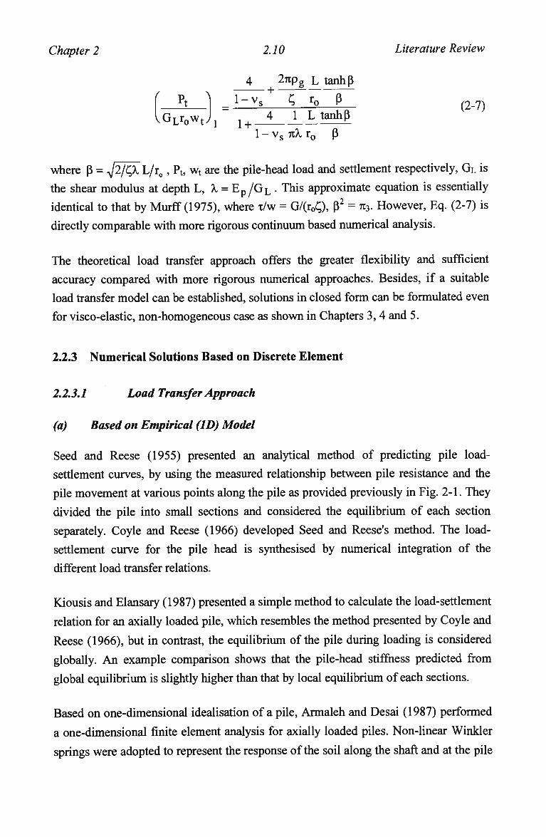
Pt )
GLr0wJi
4 27ipg L tanhp
l-vs C, r0 p 4 1 L tanhp
1 - vs nX r0 p
(2-7)
where p = J2/Q L/r0, Pt, w t are the pile-head load and settlement respectively, G L is
the shear modulus at depth L, X = E p / G L . This approximate equation is essentially
identical to that by Murff (1975), where T/W = G/(r0Q, p2 = n3. However, Eq. (2-7) is
directly comparable with more rigorous continuum based numerical analysis.
The theoretical load transfer approach offers the greater flexibility and sufficient
accuracy compared with more rigorous numerical approaches. Besides, if a suitable
load transfer model can be established, solutions in closed form can be formulated even
for visco-elastic, non-homogeneous case as shown in Chapters 3, 4 and 5.
2.2.3 Numerical Solutions Based on Discrete Element
2.2.3.1 Load Transfer Approach
(a) Based on Empirical (ID) Model
Seed and Reese (1955) presented an analytical method of predicting pile load-
settlement curves, by using the measured relationship between pile resistance and the
pile movement at various points along the pile as provided previously in Fig. 2-1. They
divided the pile into small sections and considered the equilibrium of each section
separately. Coyle and Reese (1966) developed Seed and Reese's method. The load-
settlement curve for the pile head is synthesised by numerical integration of the
different load transfer relations.
Kiousis and Elansary (1987) presented a simple method to calculate the load-settlement
relation for an axially loaded pile, which resembles the method presented by Coyle and
Reese (1966), but in contrast, the equilibrium of the pile during loading is considered
globally. A n example comparison shows that the pile-head stiffness predicted from
global equilibrium is slightly higher than that by local equilibrium of each sections.
Based on one-dimensional idealisation of a pile, Armaleh and Desai (1987) performed
a one-dimensional finite element analysis for axially loaded piles. Non-linear Winkler
springs were adopted to represent the response of the soil along the shaft and at the pile
Chapter 2 2.11 Literature Review
tip. A generalised Ramberg-Osgood model, as shown in Fig. 2-2, was used to simulate
the shaft and base non-linear response. Good comparison with measured load-
settlement curves resulted for piles in sand. In a similar way, Abendroth and Greimann
(1988) carried out F E M studies which includes material and geometric non-linearity,
utilises two-dimensional beam elements for the pile, and uncoupled non-linear Winkler
soil springs for shaft and tip response. Based on curve-fitting measured strain data, they
also developed the soil resistance and the displacement relationship in the form of
Ramberg-Osgood expressions. The Ramberg-Osgood model does offer a flexible
fitting for shaft and base load transfer behaviour (Armaleh and Desai, 1987; Abendroth
and Greimann, 1988; O'Neill and Raines, 1991), but the t-z function generally varies
with the four factors shown in the section 2.2.1.1, even within the same site. Therefore,
it is difficult to choose suitable coefficients for the model for future design.
(b) Based on Theoretical (2D) Model
Randolph (1986) developed a load transfer based program, RATZ in which the
theoretical load transfer models of Eqs. (2-1) and (2-6) are adopted. The predicted load-
settlement relationships normally compare well with more rigorous continuum based
analysis. The advantage of this analysis is that
(1) The parameters, e.g., soil shear modulus, can be directly obtained;
(2) Based on measured load-settlement relationships, shear modulus of soil can be
back-figured through the program.
However, the program is confined to Fortran environment, therefore a spreadsheet
program operating in E X C E L has been developed in this research.
2.2.3.2 Direct Hyperbolic Load Transfer Approach
Fleming (1992) proposed a numerical procedure for estimating pile load-settlement
behaviour based on separate hyperbolic laws (Chin, 1970; Chin and Vail, 1973) for the
shaft and base responses, the responses were then combined making due allowances for
elastic shortening of the pile. A program called C E M S E T was developed to facilitate
the analysis. Although the predictions are satisfactory, compared with the measured
response of many piles, several concerns need to be explored
(1) A hyperbolic soil stress-strain relationship (Duncun and Chang, 1970) does not
lead to a hyperbolic load transfer curve (Kraft et al. 1981; Randolph, 1994);
Chapter 2 2.12 Literature Review
hence, particularly for a rigid pile, it cannot result in an integrated shaft load-
displacement that may be modelled as a hyperbolic curve.
(2) The consequence of using hyperbolic models for shaft and base respectively leads
to a result that violates the hyperbolic load-settlement relationship (Chin, 1970;
Chin and Vail, 1973; Poskitt et al. 1993).
(3) The parameters used in the model are not directly related to soil properties,
therefore the parameters have to be back-figured through the program only;
(4) Due to (3), C E M S E T analysis is difficult to be directly checked with a more
rigorous analysis.
(5) The method cannot be used to predict load distribution down a pile.
In essence, the principle of this method is identical to the "Empirical (ID) Load
Transfer Approach", but uses one element for the whole pile shaft.
2.2.4 Rigorous Numerical Analysis based on Continuum Media
As it is well known, a number of numerical procedures have been developed, and
applied in the analysis of axial pile response.
2.2.4.1 Boundary Element Approach Based on Mindlin's Solution
(a) Butterfield and Banerjee (1971)
The essence of the boundary element approach is to find a fictitious stress system (j)
which, when applied to the boundaries of the figure inscribed in the half space, will
produce displacements of the boundaries which are identical to the specified boundary
conditions of a real pile system of the same geometry and also satisfy identically the
stress boundary conditions on the free surface of the half space. The stress (j) are
fictitious in that they are to be applied to the boundaries of the fictitious half space
figure and are therefore not necessarily the actual stresses acting on the real pile
surfaces. However, once the <|> values have been determined it is a simple matter to
calculate the actual stresses and displacements they produce anywhere in the half space,
including those on the real pile boundaries. The total vertical and radial displacements
at a point due to a pile loaded vertically are expressed through integral equations as
functions of <{> and coefficients derived from Mindlin's solution (Butterfield and
Banerjee, 1971). Radial displacement compatibility is ignored, since it generally
produces negligible effects on the total load required for a given settlement. The
integral equations are then estimated numerically, in a way that the pile shaft is divided
Chapter 2 2.13 Literature Review
into n equal segments and the base into m rings. With this approach, Butterfield and
Banerjee, (1971) provided the relationships between pile-head stiffness and the pile
slenderness ratios for single piles and different pile groups.
(b) Banerjee and Davies (1977)
Banerjee and Davies (1977) reported non-dimensional load displacement behaviour of
axially loaded pile embedded in Gibson soil by utilising a boundary integral method
(BI). They showed the substantial effect of soil profiles on pile-head stiffness, load
distribution down the pile and pile-soil-pile interaction factors, and hence pile group
behaviour. The approach, however based on Mindlin's (1936) solutions are not strictly
valid for a non-homogeneous, elastic half space.
(c) Poulos (1979)
Poulos (1979) adopted a boundary element approach (BEM) to analyse a single pile in
non-homogeneous soil. A s shown in Fig. 2-9, the method involves division of the pile
into a number of elements, each acted upon by an unknown interaction stress. The
vertical displacements of the pile at each location are expressed in terms of the
unknown interaction stresses and the pile properties while the soil displacements are
expressed in terms of the interaction stresses and the soil properties. If no slip occurs at
the pile-soil interface, the expressions for pile-soil displacement can be equated and the
resulting equations solved for the interaction stresses, the displacement along the pile
can then be evaluated. The displacement influence factor may be evaluated by
integration of the Mindlin equation for vertical displacement due to a vertical
subsurface point load acting within a semi-infinite mass.
For the non-homogeneous condition, an equivalent value of shear modulus has been
adopted, which is an average of the soil modulus at elements i and j. The soil non-
homogeneous property below the pile tip has been considered approximately by an
extension of the Steinbrenner approximation (1934). This analysis is generally
consistent with that by BI analysis (Banerjee and Davies, 1977), except for short piles.
In fact, for short piles, the BI analysis is reported to overestimate the pile-head stiffness
by 2 0 % (Rajapakse, 1990). Shear stress distribution along a pile is considerably
affected by the soil profile, as shown in Fig. 2-10. However, for a stiff pile, the
distribution of the shear stress down the pile is similar to the shear modulus profile,
implying uniform shear strain with the depth. The settlement influence factor is
Chapter 2 2.14 Literature Review
generated for given pile-soil relative stiffness of various slenderness ratio in a soil layer
of vs = 0.3, H/L = 2 (H is depth of rigid layer).
(d) Poulos (1989)
Poulos (1989) reported an analysis of a pile load-settlement behaviour in a
homogeneous soil based on the boundary element ( B E M ) analysis described above.
Three different interface models have been adopted, namely: an elasto-plastic
continuum based interface model, a hyperbolic continuum based interface model, and a
load transfer model respectively. The analyses showed that except for the case of
extremely high pile Young's modulus (e.g. Ep = 30,000 GPa), load transfer analysis
provides an excellent prediction of pile load-settlement compared with the continuum
based approaches and also the F E M analysis by Jardine et al. (1986).
2.2.4.2 Boundary Element Approach Based on Chan's Solution
Chin et al. (1990) reported a simplified elastic continuum boundary element method, in
which the soil flexibility coefficients were evaluated using the analytical solutions for a
layered elastic half space (Chan et al. 1974). The use of such solutions is theoretically
more correct than the approximate procedures using Mindlin's homogeneous solutions.
Radial displacement compatibility at the pile-soil interface was not included as it does
not influence significantly the pile response (Mattes, 1969). T w o kinds of idealisations
of the pile-soil forces were adopted; a circular "patch" load over the cross-sectional
area at the pile nodes and that of a "ring" load over the outer circumferential area of the
pile elements. The pile-head stiffness against the pile slenderness ratio was provided
for both homogeneous and Gibson soil by both "patch and ring" approaches. Finite
layer effect was also explored and expressed as settlement influence factor against pile
slenderness ratio.
2.2.4.3 Finite Element Method
Randolph and Wroth (1978) performed a comprehensive numerical exploration of load
transfer behaviour of a single pile. In particular, two kinds of numerical analyses for
rigid piles are: (1) Integral equation analysis for a rigid pile of various slenderness
ratios in a soil of two Poisson's ratios: vs = 0, 0.5; and (2) Finite element analysis for a
rigid pile in a soil of Poisson's ratio: vs = 0.4, and a profile of either homogeneous or
Gibson types. Pile-head stiffness and its radial distribution away from the pile axis
Chapter 2 2.15 Literature Review
have been presented. Shear stress distribution for the two types of soil profiles has been
explored. The effect of Poisson's ratio and non-homogeneity of soil profile on a pile
response has been investigated. For instance, for a rigid pile embedded in a Gibson
soil, at the midpoint of the pile, the shear stress is of the order of half that for the
homogeneous case. Therefore, they inferred that the horizontal influenced radius, rm, is
about half its value for the homogeneous case. This analysis led to the simple equation
of Eq. (2-3) for the load transfer factor. Later, through a finite element analysis, they
(Randolph and Wroth, 1979a) improved the equation to account for the effect of non-
homogeneity and end-bearing on pile-head stiffness. However, the influenced radius
could be more accurately calibrated by the comparison between numerical analysis and
closed form solution.
Three dimensional FEM analysis has been performed by Trochanis et al. (1991), which
included interface elements for representing slippage and pile-soil separation, based on
an elasto-plastic (a generalised Drucker-Prager) model. The analysis showed that pile-
soil slippage is practically the only source of non-linear behaviour under purely axial
loading.
2.2.4.4 Variational Element Method
Rajapakse (1990) proposed a variational formulation (VM) coupled with a boundary-
integral representation of the linearly increasing shear modulus with depth (non-
homogeneous), and incompressible soil medium. H e found that the approximate
solution, Eq. (2-7) provides an estimation of pile-head stiffness sufficiently accurate for
slenderness ratio exceeding 20. However, appreciable differences are noted in the
prediction of pile base load, and hence, the load distribution down the pile.
In a word, the results from the BEM, VM and FEM analyses are generally consistent
with each other except those reported by Banerjee and Davies (1977), which gives
higher stiffness than others reported. The non-linear pile-soil interaction can be
considered by pile-soil relative slip alone for purely axial loading.
2.2.5 Consideration of Non-homogeneity
Numerical analysis for elastic case (Banerjee and Davies, 1977; Poulos, 1979) showed
that the non-homogeneity of shear modulus has significant influence on the pile-head
stiffness, and load distribution down the pile. For a slender pile, relative pile-soil slip
Chapter 2 2.16 Literature Review
could be developed (Randolph, 1983). Therefore, the non-homogeneity of the shaft
limiting stress gains importance. Analysis of a pile should generally embrace the non-
homogeneity of both the shear modulus and the limiting shaft shear stress.
Consideration of non-homogeneity in closed form solutions is currently confined to
elastic stage and based on either shear modulus non-homogeneous factor or shaft stress
distribution factor.
2.2.5.1 Based on Shear Modulus
Owing to the fact that given identical conditions, shaft stiffness defined as PSL/(GLr0wt)
(PsL = shaft load) of a rigid pile in a non-homogeneous soil will be reduced by a factor
of pg compared with that in homogeneous soil. Randolph and Wroth (1978) suggested
to use the factor to predict approximately the head stiffness of a compressible pile, as
shown in Eq. (2-7). This treatment gives sufficiently accurate prediction of the stiffness
as evidenced by the F E M analysis. Probably due to the fact that as long as A. is high, as
illustrated in Fig. 2-10 for X - 2600, the similarity between the profiles of shear stress
and modulus exists, similar to that for a rigid pile. However, for lower X, the similarity
no longer exists, as demonstrated by the results from Rajapakse (1990). Therefore, the
accuracy of the treatment for predicting the pile-head stiffness decreases as pile-soil
relative stiffness reduces. Obviously, the treatment is not feasible for evaluating load
and settlement distribution down the pile.
2.2.5.2 Based on Stress Distribution
(a) Bearing Capacity Estimation
Current design of single piles, particularly for offshore structure, is generally based on
API Recommended Practice 2A, which, however, underpredicts the capacities of short
piles and overpredicts the capacities of long piles (Olson, 1990). Many factors can
attribute to the misleading prediction (Iskander and Olson, 1992). Mainly speaking, the
API recommended practice,
(1) adopts the simplified approach of setting upper limits on side shear and end
bearing, which however, should vary with depth (Vesic, 1967; Kulhaway, 1984;
Briaud et al. 1987; Toolan et al. 1990; Kraft, 1991; Randolph et al. 1994), and
take as non-homogeneous media;
(2) takes no account of pile-soil relative slip;
Chapter 2 2.17 Literature Review
(3) concerns nothing about the load settlement behaviour.
For piles in sand, there is no plunging failure load, load and displacement just continue
increasing; while for piles in clay, as it happens for most conventional onshore
development, with the main purpose to satisfy a serviceability of deformation, the
settlement prediction becomes more important than that of bearing capacities (Khan et
al. 1992).
(b) Settlement Prediction
Based on an assumed load distribution down a pile, Vesic (1965, 1970, 1977)
suggested a very simple way of predicting pile-head displacement. H e considered pile
settlement as three components: (1) the axial deformation of the pile shaft, ws, induced
by axial load along a pile; (2) settlement of the base, wps, by the load transmitted along
the pile shaft; and (3) settlement of the pile base, wpp, due to the load transmitted at the
base. Therefore, pile-head settlement, wt, equals
w, = ws + wpp + wps (2-8)
Shaft displacement, ws is expressed by the elastic shortening of a pile under a load of Pt
Vesic (1965)
ws=(asA + pb)-P^ (2-9)
where Pt = PsL + Pb, Pt, Pb are the total head and base load respectively; as = PsL/Pt ,
PSL is the total shaft load; and P b = Pb/Pt • The non-uniform distribution of shaft load
(stress) is represented by a constant called stress distribution factor A, which has been
rewritten in a general form by Chen and Song (1991)
A=fl(i-¥^)dz <2-10) L o ^sL
where Ps(z) is the shaft load at depth z. For friction distribution of triangle, inverse-
triangle and rectangle, A is found to be 0.67, 0.33, and 0.5 respectively (Vesic, 1977).
For a two layered soil profile, the A has been generated by Leonards and Lovell (1979)
for the two cases as shown in Figs. 2-11 and 2-12 for the two different shaft friction
patterns and relative thickness. The solution has been extended to a three-layered soil
Chapter 2 2.18 Literature Review
system as well (Schmertmann, 1987). This stress distribution factor is, in fact, a
representation of the non-homogeneity.
More practically, given a ratio of pile-head load Pt and ultimate load Puit, the
distribution figure of skin friction along a pile can be approximately represented by a
number of small sections, which are trapezoidal, rectangular or triangular. The distance
of the geometrical centre of each figure from the ground surface can be estimated. The
stress distribution factor defined by Eq. (2-10) is estimated to be the ratio of the
distance of the geometrical centre of the whole figure to the corresponding pile length.
Following this procedure, based on measurement from a database of 84 instrumented
piles, Chen and Song (1991) recently deduced the pile shaft distribution factor at load
levels of Pt/Puit = 0.5 and 1 for concrete driven piles, steel piles, and bored piles
respectively.
The base displacement, which consists of the last two components in Eq. (2-8), may be
given by the following empirical equation
wb=a)bPbL/ApEp (2-11)
where ©b is an empirical base modification factor (Chen and Song, 1991). More
rigorously, the base displacement may be estimated by the following equations
wpp=PbdIpp/ApEs (2-12)
wps=TavedIps/Es (2-13)
where Tave is the average shaft friction; Ipp, Ips are the new settlement influence factors
as given by Polo and Clemente (1988). Pile-head and base displacements have been
obtained by F E M analysis for the following four different pile shaft stress distributions
(Polo and Clemente, 1988), which are triangular decreasing with depth, triangular
increasing with depth, parabolic and uniform with depth. F E M analysis has been
undertaken by the following procedures:
(1) idealising the pile as a hollow cylinder, and treating the soil as a homogeneous,
linear elastic, isotropic half-space;
(2) applying the different stress distribution along the inner surface of the pile.
The displacement obtained is then split into the three components. Thereby, with Eqs.
(2-9), (2-12) and (2-13), the factors are back-figured respectively. A s would be
Chapter 2 2.19 Literature Review
expected, the factors achieved are shown to be different from those derived from
Mindlin's solutions, due to the idealisation of the pile and the stress condition.
The major concern for the FEM analysis is the fact that the stress distributions assumed
are not always compatible with the shear modulus profile used. The effect of this
incompatibility m a y need to be clarified. Although many empirical stress distribution
profiles have been reported (Vesic, 1967; Toolan et al. 1990; Kraft, 1991; Randolph et
al. 1994), these are generally suggested for predicting pile capacity, rather than for
settlement. A s shown later in Chapter 3, settlement prediction is much more sensitive
to the stress profile than bearing capacity prediction. For instance, settlement is a
parabolic function of the stress at full pile-soil slip case, (see later, Eq. (3-14)).
Therefore, using error analysis, it may be shown that the accuracy for estimating
settlement m a y be more readily attained if using the shear modulus profile rather than
using a stress profile. In fact, only for a rigid pile, can this approach based on stress
distribution ensure compatibility between shear modulus and shear stress. Hence the
prediction is theoretically reliable.
Following the above arguments, the key for using the approach is to choose a suitable
stress distribution factor. The following effects may need to be considered beforehand.
(1) The distribution factor varies with load levels. Particularly for a slender pile
and/or a higher ratio of Pt/Puit, pile-soil relative slip might be developed.
Therefore, the distribution factor is a coupled reflection of the stress distribution
non-homogeneity of the elastic and the plastic parts.
(2) The distribution factor changes with the pile Young's modulus or the total pile
deformation (Van Impe, 1988). Once the pile-soil relative stiffness or head
displacement changes, the shear stress distribution is bound to be different.
However, using shear modulus based analysis (Chapter 3), the above concerns m a y be
avoided.
As stated previously, the shear modulus non-homogeneity causes both stress and strain
distribution alteration. Whether the shear modulus non-homogeneity factor (or the
reduction factor), or the stress distribution factor mentioned previously can not be
applied to the slip part. Thus a suitable formulation should be developed to account for
the shear modulus non-homogeneity prior to slip and the shaft stress non-homogeneity
posterior to the slip.
Chapter 2 2.20 Literature Review
2.2.5.3 Pile-Soil Relative Stiffness Factor
The pile-soil relative stiffness factor is normally defined as a ratio of pile Young
modulus and soil Young or shear modulus at the pile base level (Banerjee and Davies,
1977; Poulos, 1979; Randolph and Wroth, 1978). Pile-head stiffness, in terms of this
definition as shown in Eq. (2-7), can be considerably altered for different degree of
non-homogeneity (Banerjee and Davies, 1977; Randolph and Wroth, 1979), due to a
corresponding difference in the average soil shear modulus over the whole pile
embedded depth.
Poisson's ratio, vs> in fact, represents compressibility of a soil (e.g. a value of vs = 0.5
implies that the soil is incompressible). Its variation could lead to significant change in
pile-head stiffness (as explored in Chapter 4). To avoid this effect, as argued by
Randolph and Wroth (1978), pile-soil relative stiffness might be suitably defined by the
shear modulus rather than Young's modulus.
If the influence of shear modulus distribution alone on a pile behaviour is to be
explored, pile-soil relative stiffness might be more reasonably defined as the ratio of
pile Young modulus to the average soil shear modulus over the pile length.
Accordingly, the shear modulus of " G L " in Eq. (2-7) should be replaced by the average
shear modulus as well.
2.3 TIME-DEPENDENT EFFECT
2.3.1 Soil Strength
The disturbance of clays as a result of pile driving was first detailed by Casagrande
(1932). A s a result of this remoulding and subsequent reconsolidation, settlements and
negative skin friction would develop on the pile. Investigating a large pile group driven
through soft clay, Cummings et al. (1950) found that the effect of remoulding was
limited and the reduction of strength was rapidly eliminated as a result of
reconsolidation. They also found that strength observed 1 month after driving was
about equal to the strength of the intact clay, and after 11 months it was considerably
greater. Generally the undrained shear strength of soft clays is reduced immediately
following driving, followed by subsequent increase in the strength with time after the
end of driving, resulting in strengths equal to or greater than the initial values (Orrje
and Broms, 1967; Flaate, 1972; Fellenius and Samson, 1976; Bozozuk et al. 1978).
Chapter 2 2.21 Literature Review
Such a remoulding and strength variation are accompanied with the radial soil
movement at constant volume (Francescon, 1983).
There are no solutions for predicting variation of soil strength due to reconsolidation.
However, the theory of reconsolidation for pore pressure dissipation may be directly
used with sufficient accuracy to simulate the variation as detailed in Chapter 6.
2.3.2 Excess Pore Pressure
The pore pressure caused by driving a pile in clay was first observed by Bjerrum et al.
(1958). Generally the maximum excess pore pressures immediately after driving were
equal to or exceeded the total overburden pressure in overconsolidated clays (Orrje and
Broms, 1967; Koizumi and Ito, 1967; Clark and Meyerhof, 1972; Fellenius and
Samson, 1976). The maximum pore pressures occur only in a limited volume of soil in
the immediate vicinity of the pile wall. The magnitude of the driving pore pressures
decreases rapidly with the distance from the pile wall, and becomes negligible at a
distance in the order of 10-20 pile diameters (Bjerrum and Johannessen, 1960; Lo and
Stermac, 1965).
The maximum excess pore pressure may be obtained through (1) a triaxial test-based
empirical equation; (2) a cylinder expansion theory; and (3) strain path method.
The increase in pore pressure may be divided into an ambient component, Aua, and a
shearing component, Aus, which are caused respectively by an increase in the ambient
total stress and the shearing of the soil to large strains around the pile. The maximum
ambient component, Aua, may be taken as the difference between vertical and
horizontal effective stresses (Lo and Stermac, 1965). The maximum shearing
component, Aus, may be taken as a product of vertical effective stress and a normalised
maximum pore pressure, with the normalised value being estimated by consolidated-
undrained triaxial tests. This approach gives very good comparison with field
measurements for normally consolidated clay (Lo and Stermac, 1965). As for
overconsolidated clays, the maximum shearing component, Aus, may be taken as a
product of preconsolidation pressure and the normalised maximum pore pressure (Roy
etal. 1981).
The maximum pore pressure can be reasonably predicted by a cylinder expansion
(Randolph and Wroth, 1979b; Roy et al. 1981), which is based on the expansion of a
Chapter 2 2.22 Literature Review
cylinder cavity from zero radius to a radius of r0 (r0, the radius of the pile) in an ideal
elastic, perfectly plastic material, characterised by a shear modulus, G and an undrained
shear strength, su. The theory was originally employed in the analysis of pressuremeter
tests (Gibson and Anderson, 1963), but the suitability to simulate the installation of a
pile has been extensively explored by Randolph and Wroth (1979b), Carter et al.
(1979), in particular for overconsolidated soil by Randolph et al. (1979).
The maximum excess pore pressure may also be obtained by strain path method
(Baligh, 1985a), which is based on a kinematically admissible soil deformation around
a simple pile. The method can well account for the effects of the strain history on the
principal stress directions of inelastic soils, but cannot ensure equilibrium everywhere
in the soil (Baligh, 1986a; Teh and Houlsby, 1991). Therefore, the results from this
method are generally considered to be approximate.
Analysis using strain path method by Baligh (1986b) shows that around pile shafts,
cylindrical cavity expansion solutions can provide reasonable estimates of the soil
conditions in the far field, where inelastic soil behaviour is negligible. Near the shaft,
cylindrical expansion solutions may be used as well, except that they tend to
overpredict the excess pore pressure.
2.3.3 Reconsolidation Process
The rate of pore pressure dissipation in a clay around a pile after driving is a radial
reconsolidation process. Similar to any consolidation process (Randolph and Wroth,
1979b; Randolph et al. 1979), the radial reconsolidation will generally be affected by
the following factors:
(1) non-linear soil stress-strain relationship;
(2) soil viscosity property;
(3) soil (shear modulus) non-homogeneity.
Davis and Raymond (1965) developed a non-linear theory of consolidation for an ideal
normally consolidated soil by assuming a linear relationship between void ratio and
log a (a'= effective pressure) rather than a linear relationship between void ratio and
a as adopted by Terzaghi (1943). They demonstrated that at high ratios of final to
initial effective pressure, the pore pressure in a normally consolidated soil can be
expected to be considerably higher at any particular time than that predicted by the
Terzaghi theory.
Chapter 2 2.23 Literature Review
Later, Vaid (1985) extended the non-linear theory of consolidation to the case of
constant rate of loading. The difference between the results from linear and non-linear
theories has been explored with regard to the rate of loading, sample thickness, and the
value of effective stress from where the consolidation is initiated.
Merchant (1939) (referenced via Christie, 1964) first proposed the theory of visco-
elastic consolidation in his thesis by using a standard linear model. Later, Gibson and
Lo (1961) presented similar solutions for visco-elastic consolidation, using an identical
soil model (Visco-elastic analysis based on other models has been reviewed in section
"Visco-elastic behaviour"). A s is well known, these kinds of theories were developed
to simulate secondary compression.
Schiffman and Gibson (1964) explored the effect of non-homogeneous soil properties
on consolidation behaviour. The analytical and numerical analyses showed that the
difference in time-settlement relationship due to consolidation is quite appreciable
between a nonhomogeneous soil and homogeneous soil.
For radial consolidation, so far there are no publications dealing with the effect of the
(1) to (3) factors. To account for the effect of the three factors, a new non-linear visco-
elastic model has been proposed by using hyperbolic stress-strain law coupled with the
Mediant's model. The new model is then used to established new closed form
solutions for radial consolidation. The radial soil (shear modulus) non-homogeneity
must affect radial consolidation of soil following pile driving, To assess this effect,
closed form solutions have been established by assuming the shear modulus is a power
of the radial distance away form pile axis, which have been detailed in Appendix E.
In addition to the above-mentioned three factors, radial consolidation is significantly
affected by the following two factors:
(4) soil shear stiffness expressed by a rigidly index as •yJG/su ;
(5) overconsolidation ratio.
Teh and Houlsby (1991) showed that the initial excess pore pressure (hence the
consolidation process) is significantly dependent on soil shear stiffness (A/G/su ). In
order to provide a consistent pore pressure dissipation curve for different values of the
soil shear stiffness, they introduced a new time factor.
Chapter 2 2.24 Literature Review
Randolph et al. (1979) reported that the maximum pore pressure (normalised by su)
decreases slightly as the overconsolidation ratio ( O C R ) increases. The time process of
consolidation was reported to be affected slightly by the value of O C R , depending on
the shear modulus.
Two basic approaches are commonly used for analysing consolidation problems. The
first was developed from diffusion theory by e.g. Terzaghi (1943) and Rendulic
(reported by Murray, 1978). The second was developed from elastic theory by e.g. Biot
(1941), and more recently by Randolph and Wroth (1979b) for dissipation of pore
pressure generated due to pile driving.
The diffusion theory is generally less rigorous than the elastic theory. However, the
diffusion theory is mathematically much simpler to apply, and can be readily extended
to account for complex conditions, e.g. soil visco-elasticity, soil shear modulus non-
homogeneity. In fact, the diffusion theory is different from the elastic theory in that (1)
the mean total stress is assumed constant in the diffusion theory; (2) the coefficients of
consolidation derived for the two theories are generally different (Murray, 1978).
However, for radial consolidation, the rate of change of mean total stress happens to be
zero for elastic soil response (Chapter 6); thus, the only difference between the two
theory is the coefficients of consolidation. Therefore, using a coefficient from elastic
theory to replace the coefficient in the solution of the diffusion theory, the solution
from the diffusion theory is readily converted into a rigorous solution.
Soderberg (1962) first proposed a numerical solution of the reconsolidation process.
Later, Torstensson (1975) developed a solution based on a combination of the theory of
cavity expansion and of Terzaghi's consolidation theory. Randolph and Wroth (1979b)
proposed a closed form solution for reconsolidation, with the initial excess pore
pressure around a pile described by a law of logarithmic variation away from the pile
axis, which itself is obtained from the theory of cylinder expansion.
Once the dissipation process of pore pressure is known, the variation of pile capacity
with the process can be readily deduced. The experiments by Fellenius (1972) showed
that a significant negative skin friction develops on the pile during reconsolidation. The
rate of development of this negative friction in the clay appears closely related to the
rate of pore pressure dissipation in the clay in the vicinity of the pile. The analyses by
Soderberg (1962), Randolph and Wroth (1979b) showed that the measured rate of
development of pile capacity in clay appears to be consistent with the rate of pore
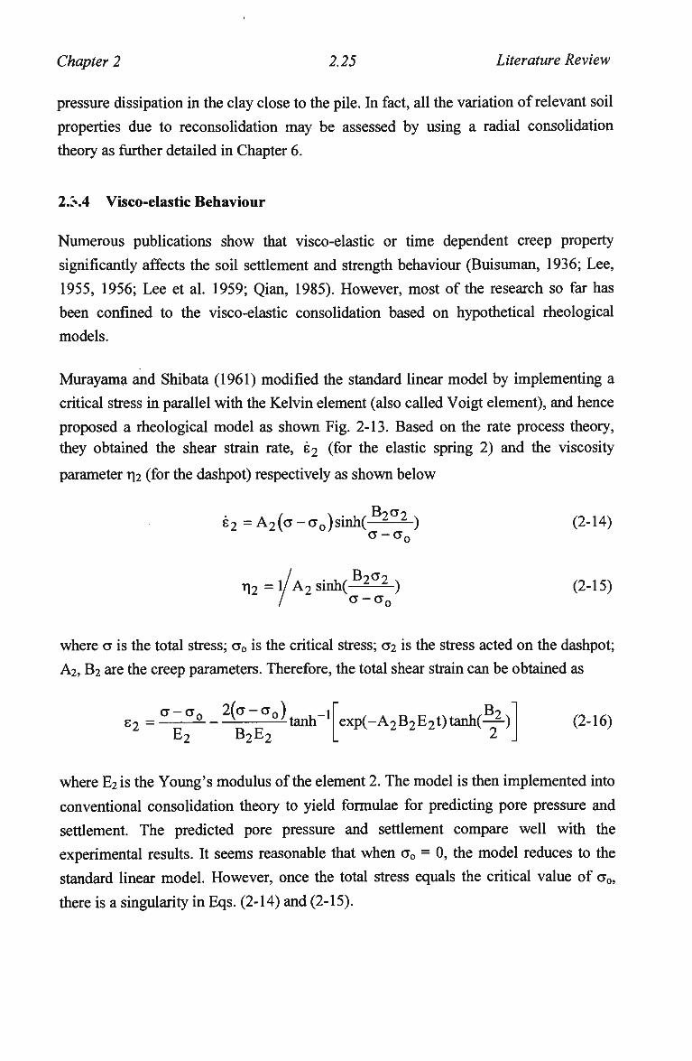
Chapter 2 2.25 Literature Review
pressure dissipation in the clay close to the pile. In fact, all the variation of relevant soil
properties due to reconsolidation may be assessed by using a radial consolidation
theory as further detailed in Chapter 6.
2.>.4 Visco-elastic Behaviour
Numerous publications show that visco-elastic or time dependent creep property
significantly affects the soil settlement and strength behaviour (Buisuman, 1936; Lee,
1955, 1956; Lee et al. 1959; Qian, 1985). However, most of the research so far has
been confined to the visco-elastic consolidation based on hypothetical rheological
models.
Murayama and Shibata (1961) modified the standard linear model by implementing a
critical stress in parallel with the Kelvin element (also called Voigt element), and hence
proposed a rheological model as shown Fig. 2-13. Based on the rate process theory,
they obtained the shear strain rate, e2 (for the elastic spring 2) and the viscosity
parameter r|2 (for the dashpot) respectively as shown below
e2 =A2(cr-c70)sinh(—=^= a-o\
• )
(2-14)
r,2 = l/A2 sinh(^=-) CT-CX,
(2-15)
where a is the total stress; a0 is the critical stress; o~2 is the stress acted on the dashpot;
A2, B2 are the creep parameters. Therefore, the total shear strain can be obtained as
Eo = G-G, 2(<7-CT0)
BoE tanh"
2n2 exp(-A 2B 2 E 2 t)tanh(% (2-16)
where E2 is the Young's modulus of the element 2. The model is then implemented into
conventional consolidation theory to yield formulae for predicting pore pressure and
settlement. The predicted pore pressure and settlement compare well with the
experimental results. It seems reasonable that when cr0 = 0, the model reduces to the
standard linear model. However, once the total stress equals the critical value of a0,
there is a singularity in Eqs. (2-14) and (2-15).
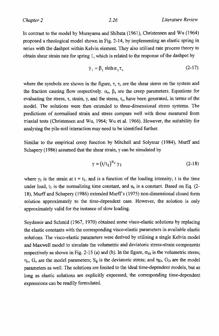
Chapter 2 2.26 Literature Review
In contrast to the model by Murayama and Shibata (1961), Christensen and W u (1964)
proposed a rheological model shown in Fig. 2-14, by implementing an elastic spring in
series with the dashpot within Kelvin element. They also utilised rate process theory to
obtain shear strain rate for spring 1, which is related to the response of the dashpot by
y, =pY sinharTc (2-17)
where the symbols are shown in the figure, T, TC are the shear stress on the system and
the fraction causing flow respectively, o ,, PY are the creep parameters. Equations for
evaluating the stress, T, strain, y, and the stress, TC, have been generated, in terms of the
model. The solutions were then extended to three-dimensional stress systems. The
predictions of normalised strain and stress compare well with those measured from
triaxial tests (Christensen and W u , 1964; W u et al. 1966). However, the suitability for
analysing the pile-soil interaction may need to be identified further.
Similar to the empirical creep function by Mitchell and Solymar (1984), Murff and
Schapery (1986) assumed that the shear strain, y can be simulated by
y =(t/t1)ncYi (2-18)
where yi is the strain at t = tj, and is a function of the loading intensity, t is the time
under load, tj is the normalising time constant, and nc is a constant. Based on Eq. (2-
18), Murff and Schapery (1986) extended Murff s (1975) non-dimensional closed form
solution approximately to the time-dependent case. However, the solution is only
approximately valid for the instance of slow loading.
Soydemir and Schmid (1967, 1970) obtained some visco-elastic solutions by replacing
the elastic constants with the corresponding visco-elastic parameters in available elastic
solutions. The visco-elastic parameters were derived by utilising a single Kelvin model
and Maxwell model to simulate the volumetric and deviatoric stress-strain components
respectively as shown in Fig. 2-15 (a) and (b). In the figure, akk is the volumetric stress;
nv, G v are the model parameters; Sy is the deviatoric stress; and r\D, G D are the model
parameters as well. The solutions are limited to the ideal time-dependent models, but as
long as elastic solutions are explicitly expressed, the corresponding time-dependent
expressions can be readily formulated.
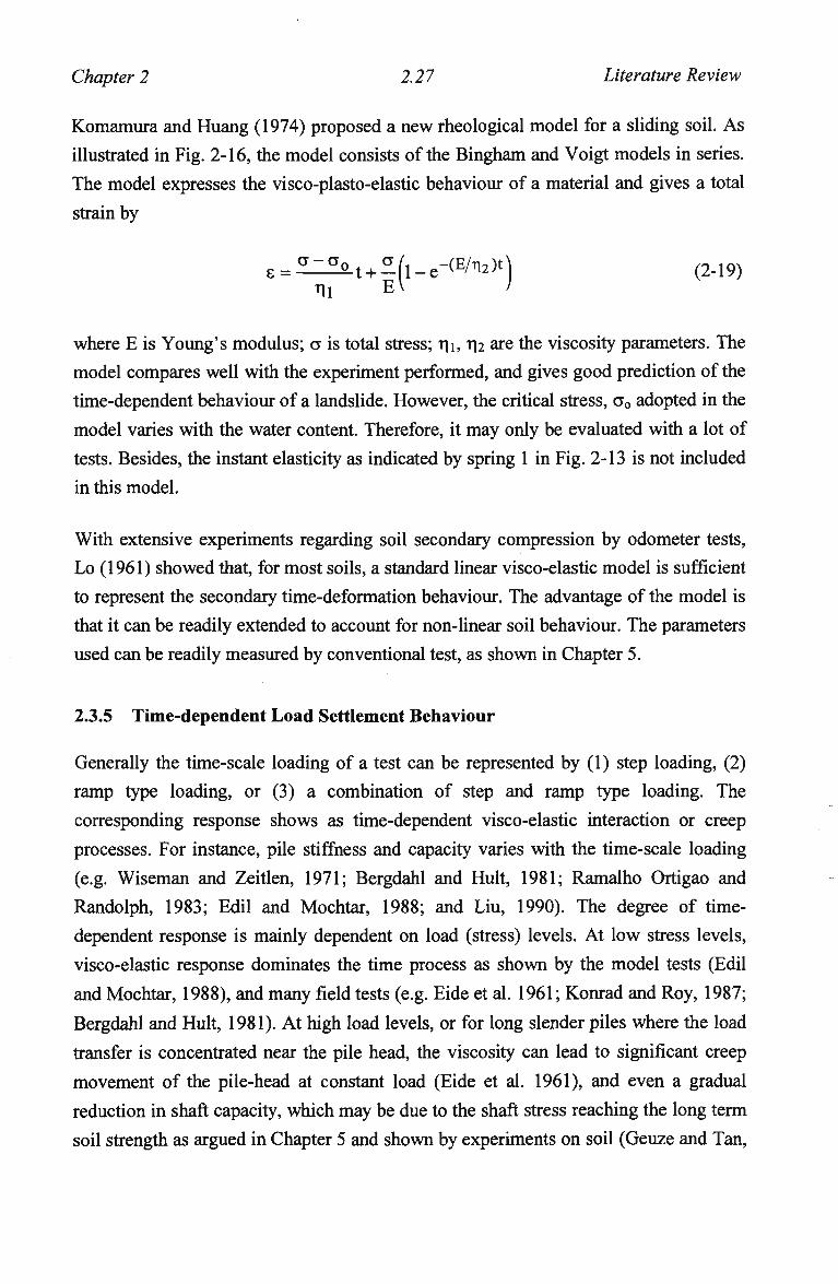
Chapter 2 2.27 Literature Review
Komamura and Huang (1974) proposed a new rheological model for a sliding soil. As
illustrated in Fig. 2-16, the model consists of the Bingham and Voigt models in series.
The model expresses the visco-plasto-elastic behaviour of a material and gives a total
strain by
^^^t + ^l-e"^)*) (2-19) ri! EV /
where E is Young's modulus; a is total stress; rji, r|2 are the viscosity parameters. The
model compares well with the experiment performed, and gives good prediction of the
time-dependent behaviour of a landslide. However, the critical stress, a0 adopted in the
model varies with the water content. Therefore, it may only be evaluated with a lot of
tests. Besides, the instant elasticity as indicated by spring 1 in Fig. 2-13 is not included
in this model.
With extensive experiments regarding soil secondary compression by odometer tests,
Lo (1961) showed that, for most soils, a standard linear visco-elastic model is sufficient
to represent the secondary time-deformation behaviour. The advantage of the model is
that it can be readily extended to account for non-linear soil behaviour. The parameters
used can be readily measured by conventional test, as shown in Chapter 5.
2.3.5 Time-dependent Load Settlement Behaviour
Generally the time-scale loading of a test can be represented by (1) step loading, (2)
ramp type loading, or (3) a combination of step and ramp type loading. The
corresponding response shows as time-dependent visco-elastic interaction or creep
processes. For instance, pile stiffness and capacity varies with the time-scale loading
(e.g. Wiseman and Zeitlen, 1971; Bergdahl and Hult, 1981; Ramalho Ortigao and
Randolph, 1983; Edil and Mochtar, 1988; and Liu, 1990). The degree of time-
dependent response is mainly dependent on load (stress) levels. At low stress levels,
visco-elastic response dominates the time process as shown by the model tests (Edil
and Mochtar, 1988), and many field tests (e.g. Eide et al. 1961; Konrad and Roy, 1987;
Bergdahl and Hult, 1981). At high load levels, or for long slender piles where the load
transfer is concentrated near the pile head, the viscosity can lead to significant creep
movement of the pile-head at constant load (Eide et al. 1961), and even a gradual
reduction in shaft capacity, which may be due to the shaft stress reaching the long term
soil strength as argued in Chapter 5 and shown by experiments on soil (Geuze and Tan,
Chapter 2 2.28 Literature Review
1953; Murayama and Shibata, 1961; Leonard, 1973). Ramalho-Ortigao and Randolph
(1983) reported an apparent difference of some 30 % in the tension capacity of a pile
loaded at a constant displacement rate leading to failure in about 40 seconds, compared
with a similar pile subjected to a maintained load test over a period of 40 days.
A few numerical analyses are available for the pile creep analysis (Booker and Poulos,
1976; Yuan, 1994). A simple empirical approach has been recently proposed (England,
1992).
Booker and Poulos (1976) implemented the standard linear visco-elastic model into
Mindlin's solution for boundary element analysis of the creep behaviour of a single
pile. Non-dimensional charts of the settlement influence factor have been produced for
step loading case.
England (1992) extended the hyperbolic approach of pile analysis described by
Fleming (1992) to allow the effects of time to be incorporated into axial pile analysis,
with separate hyperbolic laws being used to describe the time-dependency of the
(average) shaft and base response. This phenomenological approach is limited by the
difficulty of linking the parameters required for the model to fundamental and
measurable properties of the soil.
Time-dependent behaviour can arise from either reconsolidation due to disturbance
from installation of a pile or consolidation induced by loading. However, the current
research level is not permitting the distinguishing of the effect of the reconsolidation
from that of the consolidation.
A realistic prediction of creep behaviour, above all, should be a logical extension from
an elastic solution but also linked to fundamental soil properties.
2.4 VERTICALLY LOADED GROUP PDLES
A large body of information is available for analysing pile groups. Generally the
performance of pile groups can be predicted by the following procedures
(1) empirical methods (Terzaghi, 1943; Skempton, 1953; Meyerhof, 1959; Vesic,
1967; Kaniraj, 1993);
Chapter 2 2.29 Literature Review
(2) load transfer approaches, based on either simple closed form solutions (Randolph
and Wroth, 1978, 1979; Lee, 1993a) or discrete layer approach (Chow, 1986b;
Lee, 1991);
(3) elastic continuum based methods, e.g. boundary element analysis (Poulos, 1968;
Butterfield and Banerjee, 1971; Chin et al. 1990), infinite layer approach (Guo et
al. 1987; Cheung et al. 1988); F E M analysis (Ottaviani, 1975; Valliappan et al.
1974; Pressley and Poulos, 1986);
(4) hybrid load transfer approach (O'Neill et al. 1977; Chow, 1986a; Lee, 1993b;
Clancy and Randolph, 1993), which takes advantage of both numerical and
closed form approaches, renders the possibility of analysing large group piles.
2.4.1 Empirical Approaches
A number of non-dimensional parameters have been introduced to describe pile group
behaviour. One of the parameters is the settlement ratio, Rs, which was defined as the
ratio of the average group settlement to the settlement of a single pile carrying the
same average load (Poulos, 1968). For this particular parameter, empirical formulae
were proposed by several researchers (e.g. Skempton, 1953; Meyerhof, 1959).
The empirical formulae were generally established from the comparison of full-scale or
model test results between the settlement of a single pile group and that of a single pile
in sands (Skempton, 1953; Meyerhof, 1959), but only the group geometry was taken
into account. In addition, test results (Kaniraj, 1993) show that the settlement ratios
generally decrease as the pile spacing decreases, but the empirical formulae (Skempton,
1953; Meyerhof, 1959) indicated an opposite trend. Therefore, the empirical formulae
may be used only for the cases where the overall conditions are similar to those on
which these formulae are based.
Kaniraj (1993) modified the definition of settlement ratio by Poulos (1968), and
defined a new settlement ratio as a ratio of the settlement of a pile group to that of a
single pile when the average stress on their respective load transmitting area is
identical. The load transmitting area is the area at the pile base level, estimated through
the dispersion angle (* 7° as reported by Berezantzev et al. 1961) as illustrated in Fig.
2-17. This new settlement ratio was presented in the form of semi-empirical equations,
and was compared with the measured values. The equations give better estimations of
the settlement ratios than the previous empirical formulae (e.g. Skempton, 1953;
Chapter 2 2.30 Literature Review
Meyerhof, 1959), although generally the estimations are higher than the measured
values.
In fact, as has been partly explored by different numerical analyses published,
settlement ratio is dependent on the following factors: pile spacing, the number of piles
in a group, pile-soil relative stiffness, the depth of the underlying rigid layer, and the
profile of shear modulus both vertically and horizontally. Therefore, the empirical
formulae may need to be improved to account for these factors, as shown in Chapter 7.
2.4.2 Interaction Factor and Superposition Principle
The influence of the displacement field of a neighbouring identical pile was
represented by an interaction factor between pairs of incompressible piles (Poulos,
1968). The interaction factor reflects the increase in settlement of a pile due to the
displacement field of a similarly loaded neighbouring pile, which can be expressed as
Pile - head stiffness of a single pile , a H = — — 1 (2-20)
Pile - head stiffness of a pile in a group of two
where ay is the interaction factor between pile i and pile j. The interaction factor
originally defined for two identical piles is then extended to unequally loaded piles.
The shaft displacement increase due to a displacement field of a similarly loaded
neighbouring pile m a y be represented by (Lee, 1993 a)
Shaft displacement for a pile in a group of two
Shaft displacement for a single pile uiia.±i ui3uiai>uiu/in xv/i a, uuv 111 a tiuuu \JJ. iwv , ._ _ , .
asu = „, ,. ,. , — 7 r-5;—rt (2-21)
where asy is the shaft interaction factor between pile i and pile j. Similarly, a base
interaction factor m a y be defined. In fact, the interaction factor can be defined in other
forms depending on the manner used for estimating displacements. For instance,
consistent with the settlement prediction for a single pile using Eq. (2-8), Polo and
Clemente (1988) introduced two pile-pile interaction factors, a^s and a^p for base
settlement estimation: the interaction factor, a l , reflects an increase in the settlement
at the base of pile j due to the load transmitted along the shaft of pile i; the interaction
factor, a^p, reflects an increase in the settlement at the base of pile j due to the load
transmitted at the base of pile i.
Chapter 2 2.31 Literature Review
With a known displacement field or pile-soil-pile interaction factors, the behaviour of a
pile in a group can be readily evaluated, using the principle of superposition. The
results using the principle of superposition are generally the same as those by analysing
the entire pile group. Even for general pile group analysis, the principle of
superposition is approximately valid (Clancy, 1993). The validity of the superposition
approach both to the estimation of the pile settlement and to the determination of the
load carried by each pile was confirmed by Cooke et al. (1980) through a number of
field tests. In the following sections, it may be noticed that the principle of
superposition is utilised for all the load transfer based analyses.
2.4.3 Displacement Field Around a Single (Group) Pile
2.4.3.1 A Single Pile
From a vertically loaded single pile analysis, it was shown that (Cooke, 1974; Frank,
1974; Randolph and Wroth, 1978), the settlement around the pile shaft is given by
w(r) = ^ln(rm/r) (2-22)
The settlement at the pile base level away from the pile axis is approximated by
w(r) = wb-^°- (2-23) n r
2.4.3.2 Two Piles
Using the superposition principle, the displacement field for a pile in a group of two
may be obtained by superimposing the local displacement field (Randolph and Wroth,
1979c); therefore the settlement around each of the pile shafts, (ws)2, is given by:
(w.)2 =^HWr0) + ln(rmg/s)) (2-24)
where s is pile centre-centre spacing; rmg = rm + rg; rg is the half the maximum distance
between any two piles in the group. The base settlement of each of the pile base, (wb)2,
is
Chapter 2 2.32 Literature Review
4r„G V n s. 0
Lee (1993a) modified Eq. (2-7) and gave the following equation for the average shaft
displacement, (ws)2, around each pile in a group of two
^-d^iWwoW^)) (2"26)
With Eq. (2-26), the shaft interaction factor by Eq. (2-21) may be expressed as
a-=—r-^ rlnfr /s~) (2-27) ln(rmg/r0)
where sy is pile centre-centre spacing between pile i and j, sy = r0 for i = j. And the
base interaction factor may be expressed as
abij=2r0/7rSij (2-28)
where aby is base interaction factor for two piles corresponding to spacing between pile
i and pile j; sy = IXJTI for i = j.
2.4.3.3 Muti-Piles
Generally, for a group of ng piles, shaft displacement of the y'th pile, (ws)j, may be
obtained by Eq. (2-29) (Randolph and Wroth, 1979c)
Wj-^Wto, •»('.,/»•) (2-29) ^ i = l
Similarly, the base displacement, (wb)j, fory'th pile may be given by
( \ $( \ (1-vs)2^(pb)i n-m
i=l
The shaft and base displacements for each pile are estimated separately.
Chapter 2 2.33 Literature Review
2.4.4 Simple Closed Form Approaches
Randolph and Wroth (1979c) provided a simple approach for predicting settlement of
pile groups of ng piles. The ng values of pile shaft displacement, ws, was related to the
ng values of T 0 by Eqs. (2-29) to give a matrix equation of
WS=[FS]T0 (2-31)
Similarly, from Eq. (2-30), a base matrix may be formulated as
w„ = [F„]P„ (2"32)
For rigid piles, w s = w b, and for a rigid pile cap, (ws)i = (wb)j. Therefore, it is
straightforward to obtain shaft stress and base load for a given pile cap displacement by
inverting the shaft and base matrices. The method generally furnishes good predictions
compared with more rigorous numerical analyses (e.g. Butterfield and Banerjee, 1970).
However, for compressible pile groups, the shaft displacement, ws, and base
displacement, Wb, for each pile is different, therefore an additional equation is needed
for each pile to correlate these two displacements. This approach treating the shaft and
base interaction effects separately generally requires an iteration for analysing
compressible pile groups. However, should the shaft and base displacements be dealt
with together, the analysis will be greatly simplified as shown in Chapter 7.
Lee (1993a) assumed the denominator of Eq. (2-7) as unity, but tried to compensate the
assumption by replacing the p with p* (= 1.15p); therefore the stiffness of a single pile
is a simple sum of total base and shaft stiffness as
P 4 2np L tanhp* ._ __. + —r1" ^r~ (2-33) GLr0wt 1-v, C r0
The shaft stiffness is then implemented into Eq. (2-22) to yield an average
displacement field around the pile, as given by Eq. (2-26). Therefore, the total stiffness
for each pile in a group of two piles, (P/G Lr 0w t) 2, can be obtained as
'—-L—1 4 1 ^TtPgL tanhp 1
loLr0wtJ2 l-vsl + 2r0/7ts r0 P J ^ + m f r
ro
mg
\ S J
Chapter 2 2.34 Literature Review
With the stiffness by Eq. (2-34) and that for a single pile by Eq. (2-33), the interaction
factor defined by Eq. (2-20) was expressed explicitly and compared with more rigorous
numerical analyses (Lee, 1993a). In turn, with this interaction factor, pile group
behaviour was predicted, using the superposition principle. The predictions were then
compared with more rigorous numerical analyses and field test results.
Using the average displacement field of Eq. (2-26), the approach only partly accounts
for the effect of pile-soil relative stiffness, although the effect of the stiffness might be
limited as shown later in Chapter 7. Another major concern is that even though Eq. (2-
7) has been modified as Eq. (2-33), the resulting interaction factor still does not always
compare satisfactorily with more rigorous numerical analysis as the pile centre to
centre space changes.
In fact, load transfer factors embracing the neighbouring pile effect may be
implemented directly into Eq. (2-7), to achieve pile-head stiffness of a pile in a group
of two. In this manner, pile-pile interaction factor by Eq. (2-20) may be obtained as
illustrated in Chapter 7.
2.4.5 Numerical Approaches
2.4.5.1 Boundary Element (Integral) Approach
Using the BEM (BI) approaches described in Section 2.2.4:
(1) Butterfield and Banerjee (1971) explored extensively pile-head stiffness for
different pile groups of rigid cap at various pile slenderness ratios, and pile-soil
relative stiffness;
(2) Poulos (1968) introduced the pile-soil-pile interaction factor as mentioned earlier.
With the interaction factor, values of the settlement ratio, Rs, and load
distribution within a group have been obtained. The influence of pile spacing,
pile length, type of group, depth of layer and Poisson's ratio of the layer on the
settlement behaviour of pile groups was examined;
(3) Chin et al. (1990) reported pile-soil-pile interaction factors, in terms of Chan's
solution (Chan et al. 1974) for various pile spacing, relative stiffness and
slenderness ratios.
Chapter 2 2.35 Literature Review
2.4.5.2 Infinite Layer Approach
Guo et al. (1987) and Cheung et al. (1988) proposed an infinite layer approach. The
stress analysis for a single pile embedded in layered soil was performed through a
cylindrical co-ordinate system. Each soil layer was represented by an infinite layer
element and the pile by a solid bar. The displacements of the soil layer were given as a
product of a polynomial and a double series. The strain-displacement and stress-strain
relations were established from the displacement fields and therefore the total stiffness
matrix could be readily formed.
The interaction between two piles, which are called pile 1 and 2 respectively as shown
in Fig. 2-18, is simulated through the following procedure:
(1) Replacing pile 2 with a soil column of the same properties as the surrounding soil.
The settlement of pile 1 as well as the soil due to the action of unit load on the pile
is then computed by the single pile model. Ignoring the change in the displacement
field due to the existence of pile 2, the force acting along pile 2 can be readily
calculated by multiplying the displacement vector and the stiffness matrix of pile
2. The differences between the forces on the pile and those computed from the
infinite layer model are regarded as residual forces, which are applied in the
opposite direction along pile 2 to maintain the equilibrium of the whole system.
(2) If the forces are applied to pile 2, pile 1 is replaced by a soil column. Similarly, the
soil movement and residual forces induced in pile 1 are computed.
(3) The whole procedure (1) to (2) is repeated by applying the residual forces of each
step on pile 1 and pile 2 accordingly until the changes in the displacement of both
piles due to the loading are negligible. By this analysis, the resulting interaction
factors for two identical piles embedded in homogenous soil were found to be
generally consistent with those by Poulos (1968).
2.4.5.3 Non-linear Elastic Analysis
Trochanis et al. (1991) studied the response of a single pile and pairs of piles by
undertaking a 3-dimensional F E analysis using an elastoplastic model. The results
demonstrated that as a result of the non-linear behaviour of the soil, the pile-soil
interface interaction, especially under axial loading, is reduced greatly compared to that
for an elastic soil bonded to piles. The commonly used methods for evaluating pile-
soil-pile interaction, which are based on the assumption of purely elastic behaviour, can
substantially overestimate the degree of interaction in realistic situations. In load
Chapter 2 2.36 Literature Review
transfer analysis, this non-linear effect may be modelled by using elastic interaction
factors and adding non-linear components afterwards (Randolph, 1994; Caputo and
Viggiani (1984) referenced via Mandolini and Viggiani (1996)).
2.4.5.4 Discrete Element Analysis - Layer Model
"Layer model" for analysing pile groups is illustrated in Fig. 2-19(a) (Chow, 1986b).
The piles are modelled using discrete elements with an axial mode of deformation, and
the soil is treated as independent horizontal layers; therefore the interaction between
piles takes place within each soil layer only. Assuming that the shear stress remains
constant within each pile segment, 1, the deformation at a radius of r from the axis of a
vertically loaded single pile is approximated by Eq. (2-22) ( T 0 = Ps/7idl, Ps is the pile
shaft load). Eq. (2-22) is applicable to each of the N L layers along the pile shaft.
For any pile i in a group of ng piles, the overall settlement of the soil at the pile shaft of
a particular pile within a soil layer, k, due to loading on itself and on neighbouring
piles, w k , is given by
<=t^i (2-35) j=i
where Psk (Ps
k) is the shaft load at layer k at pile j (i); fsk is the displacement influence
coefficient for pile shaft in layer k denoting the settlement of the shaft at pile i due to a
unit load at pile j, within the layer k. f^ may be obtained from Eq. (2-22) (Chow,
1986b). Eq. (2-35) may be written for each of the ng piles in the group giving the
following matrix equation
K}=[Fsk]{Ps
k} (2-36)
where [wk j is shaft displacement vector for layer k; [Fkl is flexibility matrix of order
ngxng for layer k; and |Psk j is shaft load vector for layer k. This procedure is repeated
for each soil layer along pile shaft i.e. for k = 1, 2,..., N L .
For any pile i in a group of ng piles, the overall settlement of the soil at the base of pile
i due to loading on itself and on neighbouring piles, Wbi, is given by
Chapter 2 2.37 Literature Review
wbi=£fbijPbj (2-37) j=i
where Pbj (PbO is the base load at pile j (i); fbij denotes the displacement influence
coefficient at the pile base. For i = j, fbij may be obtained from Eq. (2-5) and for i * j,
from Eq. (2-23). Eq. (2-37) may be written for each of the ng piles in the group giving
the following matrix equation, similar to Eq. (2-32)
K} = [Fb]{Pb} (2-38)
where {wb} is base displacement vector; [Fb] is flexibility matrix of order ngx ng for
pile base; and {Pb} is base load vector.
The stiffness matrices of the soil layers and that of the soil at the pile base are
assembled together with the pile discrete element matrices to yield the total stiffness
matrix of the pile group system governing pile load and displacement relationship. In
this manner, the soil stratification can be dealt with, but the continuity of the soil
medium is ignored. Generally the approach tends to underestimate the interaction
except for piles with large slenderness ratios (Chow, 1986b).
2.4.5.5 Hybrid Load Transfer Approach
In the 'layer model', if the pile-soil-pile interaction between different layers is taken
into account, the model is referred to as a continuum model (Chow, 1986a), which is
illustrated in Fig. 2-19(b). The approach based on this model is more popularly called
"hybrid load transfer approach" (O'Neill et al. 1977; Clancy and Randolph, 1993; Lee,
1991), and is a simple efficient method for analysing pile groups.
In the hybrid load transfer approach, the displacements given by Eqs. (2-35) and (2-37)
may be decomposed into two components respectively
<=Yj^l=^+TS«?> (2-39) j=i j=i
wbi=i;fbuPbj=fbiiPbl+E
fbijPj (2-40) j=i j=i
Chapter 2 2.38 Literature Review
where fsk is the flexibility coefficient for the pile shaft in layer k due to unit load at the
layer k in the same pile i; fsy is the average settlement flexibility coefficient for shaft
elements in pile i due to unit head load at pile j. The factor, fsk may be estimated by
(Chow, 1986a)
f^ = ln(r JO/27CG1 (2-41)
and similarly, the flexibility coefficients for the node at the pile base is given by
fbii=(l-vs)/4GLr0 (2-42)
While f kj = 0 for loadings at nodes j which are associated with the same pile as node i,
and for j * i; the coefficients, f^ (fby), may generally be estimated by utilising the
analytical point load solutions for soil displacement at each element along pile i due to
the loading acting at each element along every pile j (i * j). The point load solutions
may be based on Mindlin's solution for a vertical point in a homogeneous, isotropic
elastic half-space (Chow, 1986a). The "hybrid" approach based on Mindlin's solution
maintains the continuity of the soil, but handles the soil non-homogeneity in an
approximate way. Lee (1991) reported the application of the "hybrid" method (Chow,
1986a) in analysing piles in layered soil media.
The interaction between pile i and j may be also accounted for by the displacement
field arould a pile of Eq. (2-24). Lee (1993b) found that the two components, fsy, fby, of
displacement influence coefficients in Eqs. (2-39) and (2-40) may be predicted by
fsi^w^ (2-43)
fbij = w,abij (2-44)
where wi is the settlement of a single pile under unit load in a group. More importantly,
Lee (1993b) found that the coefficient, fsy, may be assumed to be the same for all the
shaft elements in pile i due to unit head load at pile j. Therefore, the computer storage
required and the computing time reduces substantially, in comparison with the
evaluation by utilising the analytical point load solutions. Besides, using the new
coefficient, fsy, the analysis can furnish sufficiently accurate results.
The average shaft and base flexibility coefficients have been evaluated by either
Mindlin's solution (Chow, 1986a), or the pile-soil-pile interaction factors (Lee, 1993b).
Chapter 2 2.39 Literature Review
Both solutions yield satisfactory results compared with more rigorous numerical
approaches, using the continuum model (Fig. 2-19(b)). Therefore, the core of the
hybrid analysis is to find an accurate, simple solution for pile-soil-pile interaction,
which is able to account for various soil properties, e.g. non-homogeneity, and the
effect of finite layer depth.
2.4.6 Influence of Non-homogeneity
2.4.6.1 Vertical Non-homogeneity
Vertical soil non-homogeneity significantly affects pile group behaviour (Guo and
Randolph, 1996a), although it has limited effect on single pile response (Motta, 1994;
Chapter 3), provided the average shear modulus along the pile depth is identical. Fig.
2-20 presents a comparison of the interaction factors for homogeneous soil by Poulos
and Davis (1980) and Gibson soil by Lee (1993b). The differences in the pile-pile
interaction factor may be partly attributed to the variation of the average shear
modulus, and partly to the fact that the influenced zone is about twice as large for a
homogeneous soil compared with a Gibson soil (Randolph and Wroth, 1978).
2.4.6.2 Horizontal Non-homogeneity
Horizontal non-homogeneity considered so far has been limited to the shear modulus
alteration caused by pile installation (Randolph and Wroth, 1978; Poulos, 1988). This
alteration leads to a significant change in the load transfer factor, and therefore
normally results in a lower value of the pile-pile interaction factor as noted
experimentally by O'Neill et al. (1977), and obtained numerically by Poulos (1988),
Lee and Poulos (1990). Horizontal non-homogeneity may be readily incorporated into
the %" (refer to Eq. (2-1)), in a manner used by Randolph and Wroth (1978).
Therefore, closed form solutions as developed in this thesis may be directly used to
account for the non-homogeneity.
2.4.6.3 Shear Stress Non-homogeneity
Using the interaction factors defined earlier in section 2.4.2, equations for analysing
settlement of pile groups have been produced (Polo and Clemente, 1988).
Chapter 2 2.40 Literature Review
Current elastic analyses for pile groups generally adopt an implicit assumption that
shaft load over point load ratio is a constant throughout loading of individual piles. The
assumption, however, is not realistic at high load levels. Based on measurements of the
shaft loads of a single pile as it is loaded, and the new settlement interaction factors,
Ipp, and Ips, by Polo and Clemente, (1988), Clemente (1990) proposed a method to
capture the effect of the variation of the ratio of shaft load over the base load on
predicting settlement of pile groups. The method is based on known shaft stress
distribution. However, pile-shaft stress distribution is significantly affected by the soil
shear modulus profile and the pile-soil relative stiffness (Rajapakse, 1990). Therefore,
how to choose a suitable stress profile consistent with the soil shear modulus profile is
a major concern, prior to using this approach.
2.5 TORSIONAL PILES
2.5.1 Load Transfer Analysis
Similar to the analysis for vertical loading, the load transfer analysis for a pile
subjected to torsion can be based on either analytical or numerical approaches.
The analytical approach was first proposed by Randolph (1981). Load transfer models
were established in a similar way to that for vertical loading. With the models, closed
form solutions for piles subjected to torsion in both elastic-plastic homogeneous and
Gibson soil have been generated. Pile-head stiffness is defined and presented in a
closed form solution. However, the head-stiffness is dependent on pile slenderness
ratios. Randolph's (1981) solutions were extended into two layered soil cases (Hache
and Valsankar, 1988), but the numerical results for the two layered soil were expressed
in two new non-dimensional factors, namely, pile-soil relative stiffness and pile-head
torsional influence factors. The advantage is that the relationship between the two new
factors is independent of the pile slenderness ratio. However, the relationship is
sensitive to the soil non-homogeneity; therefore a more accurate modelling is essential.
A discrete element approach was proposed by Chow (1985). The pile is discretized into
a series of elements connected at the nodes. The soil is treated as horizontal layers,
each with a modulus of subgrade reaction. In other words, the approach is an
uncoupled analysis. However, as would be expected, the approach provides excellent
comparison with that from finite element analysis. This gives further confidence to
develop the solutions based on a load transfer approach as shown in Chapter 8.
Chapter 2 2.41 Literature Review
2.5.2 Continuum Based Numerical Approach
Poulos (1975) proposed a boundary element approach (BEM) for analysing a
torsionally loaded pile, which is similar to that for analysing a pile under vertical
loading. The pile is discretized into a number of elements. The soil rotation at the
midpoint of each element is obtained from elastic theory (Mindlin's solution for a
horizontal subsurface point load) in terms of the unknown interaction stress. The
corresponding pile rotation is then expressed in terms of these interaction stresses by
considering the pile as a circular cylinder. While conditions at the pile-soil interface
remain elastic, the expressions for soil and pile rotations can be equated and solved,
together with the equilibrium equation, to obtain the interaction stresses and thus pile
rotation. To allow for the possibility of pile-soil slip, limiting shaft and base skin
friction are specified. W h e n the shaft stress, T reaches or exceeds the limiting value xt,
the rotation compatibility equation for that element is replaced by the condition of, T =
Tt and the solution is recycled until T < Tt at all elements.
The rotation behaviour of a pile in both a uniform soil and a Gibson soil, in which
shear modulus and pile-soil adhesion increase linearly with depth, has been analysed.
Design charts for torsional influence factor were provided, but unfortunately, were
presented in different pile-soil relative stiffnesses for elastic and plastic stages
respectively. Also the relation between the influence factor and pile-soil stiffness is
dependent on the slenderness ratio. Therefore for practical design, a trial and error
approach is needed. This approach is strictly not valid for non-homogeneous soil.
2.6 SUMMARY
Following the literature review presented in this Chapter, a number of weaknesses in
the existing approaches have been revealed, as briefly summarised below.
2.6.1 Single Piles
(1) None of the current empirical formulas for prediction of pile capacity and/or
settlement can accurately account for soil non-homogeneity, and pile-soil relative
slip.
(2) The theoretical load transfer approach based on concentric cylinder approach
approximates the pile-soil interaction in a simple 2-dimensional form, and it is
readily comparable with other rigorous numerical approaches. Therefore, it is
preferred to all other curve fitting approaches. Only with the load transfer model
Chapter 2 2.42 Literature Review
can accurate closed form solutions be formulated, which can be readily extended
to other cases as well.
(3) Settlement prediction methods are preferred to be based on shear modulus non-
homogeneity than the stress distribution factor. Since using a stress distribution
factor, the stress distribution along a pile cannot be ensured to be compatible with
the shear modulus profile. In addition, the stress distribution factor can be readily
obtained by closed form solutions based on shear modulus.
(4) If the influence of the shear modulus distribution is to be considered alone, then
the definition of pile-soil relative stiffness should be based on an average shear
modulus along a pile, rather than the modulus at the tip level.
In view of the above points (1), (2) and (3), closed form solutions for vertically loaded
single piles have been established as shown in Chapter 3. The effect of point (4) has
also been explored.
(5) The load transfer factors are dependent on the four factors listed earlier in section
2.2.1.1.
Following point (5), a comprehensive investigation of the suitability and rationality of
load transfer analysis has been undertaken in Chapter 4. Load transfer factors have
been calibrated against more rigorous numerical (FLAC) analysis, and have been
provided in statistical forms in respect of the four factors.
2.6.2 Time-Dependent Effect
(6) Time dependent behaviour of a pile is governed by visco-elastic soil response
when at lower load levels and/or for a short pile, or by creep when at high load
levels and/or for a long pile (hence by long term soil strength).
(7) The available analysis on step loading cases shows a significant time-dependent
pile response; however, the effect of other time-scale loading on pile behaviour
remains to be further explored.
Following points (6) and (7), a visco-elastic shaft model has been developed which can
well account for the effect of stress levels, and yet is a logical extension of an elastic
load transfer model. This study can be found in Chapter 5.
(8) The effect of visco-elastic soil properties on pile capacity and settlement
following driving is not yet clear. H o w to predict the overall pile response due to
the installation of the pile in a clay is left to be explored.
Chapter 2 2.43 Literature Review
Following point (8), a rigorous radial consolidation theory has been established in
Chapter 6. A number of predictions accounting for time effects have been provided.
2.6.3 Pile Groups
(9) Numerical analysis is generally expensive and confined to the analysis of small
pile groups. Hybrid analysis has the potential to be applied for analysing large
pile groups, but it relies on the feasibility and availability of the closed form
solutions.
(10) Non-homogeneity of the soil shear modulus has considerable effect on the pile-
soil-pile interaction, and therefore the overall pile group response.
(11) The methods of using stress distribution factors to estimate the settlement of pile
groups is subject to further research, since the effect of the incompatibility
between shear modulus and stress distribution is not yet known.
Following points (9), (10) and (11), a rigorous closed form solution for pile-soil-pile
interaction factor has been proposed. Settlement of (large) pile groups has been
investigated extensively using the interaction factors, as detailed in Chapter 7.
2.6.4 Torsional Piles
(11) Current design charts for the torsional response of piles is dependent on
slenderness ratios. Therefore, an trial and error is needed for practical design.
(12) The non-homogeneity effect of the soil profile has been explored only for the
cases of homogeneous and Gibson soil.
An ideal approach should reflect any degree of non-homogeneity, and elastic-plastic
behaviour but be independent of slenderness ratios. Such solutions have been
established in Chapter 8.
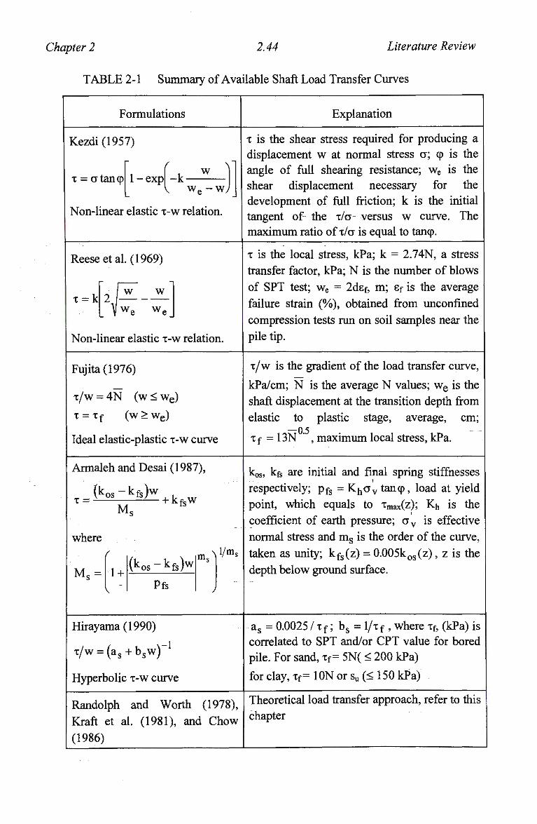
Chapter 2 2.44 Literature Review
T A B L E 2-1 Summary of Available Shaft Load Transfer Curves
Formulations Explanation
Kezdi (1957)
T = CTtancp r
1-exp -k w \
V we-w;
Non-linear elastic T-W relation.
T is the shear stress required for producing a
displacement w at normal stress a; op is the
angle of full shearing resistance; w e is the
shear displacement necessary for the
development of full friction; k is the initial
tangent of the T/CT versus w curve. The
maximum ratio of X/G is equal to tancp.
Reese etal. (1969)
x = k w
w.
w
wf
Non-linear elastic T-W relation.
T is the local stress, kPa; k = 2.74N, a stress
transfer factor, kPa; N is the number of blows
of SPT test; w e = 2d6f, m; Sf is the average
failure strain (%), obtained from unconfined
compression tests run on soil samples near the
pile tip.
Fujita(1976)
T/W = 4N (w < we)
T = Tf (w>We)
Ideal elastic-plastic T-W curve
T / W is the gradient of the load transfer curve,
kPa/cm; N is the average N values; w e is the
shaft displacement at the transition depth from
elastic to plastic stage, average, cm;
Tf = 13N ' , maximum local stress, kPa.
Armaleh and Desai (1987),
(kos-kfs)w
T =
where
M, + kfsw
f
M s = 1 + (kos-kfs)w
Pfs
mr\Vm»
koS, kfS are initial and final spring stiffnesses i
respectively; Pfs = K^CTy tancp, load at yield
point, which equals to Tmax(z); Kh is the
coefficient of earth pressure; CTV is effective
normal stress and m s is the order of the curve,
taken as unity; kfs(z) = 0.005kos(z), z is the
depth below ground surface.
Hirayama(1990)
T/W = (as + bsw)~
Hyperbolic T-W curve
as = 0.0025 / Tf; bs = 1/Tf , where Tf, (kPa) is
correlated to SPT and/or C P T value for bored
pile. For sand, Tf = 5N( < 200 kPa)
for clay, Tf= ION or su (< 150 kPa)
Randolph and Worth (1978),
Kraft et al. (1981), and Chow
(1986)
Theoretical load transfer approach, refer to this
chapter
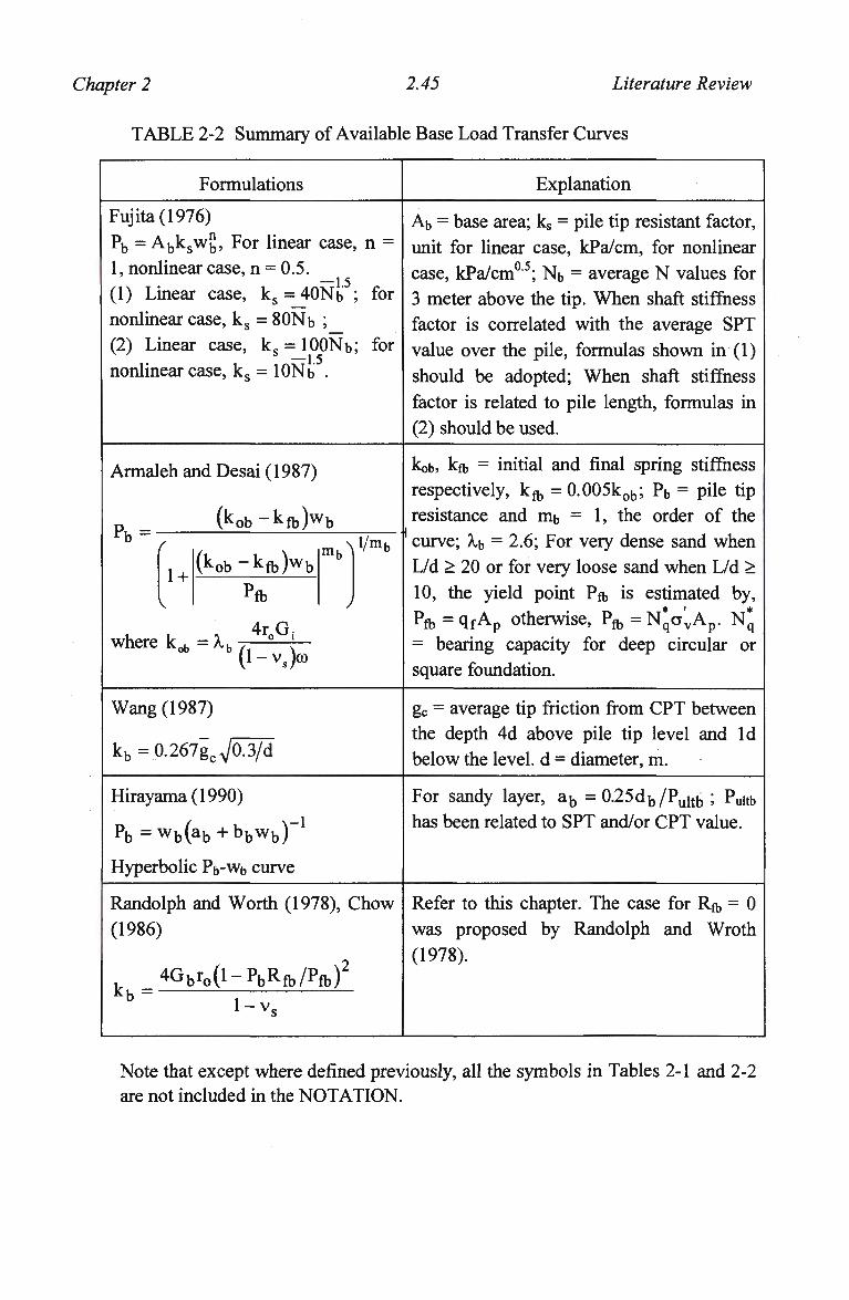
Chapter 2 2.45 Literature Review
T A B L E 2-2 Summary of Available Base Load Transfer Curves
Formulations Explanation
Fujita(1976)
Pb = A b k s w b , For linear case, n =
1, nonlinear case, n = 0.5. 1.5
(1) Linear case, k s = 4 0 N b ; for
nonlinear case, ks = 80Nb ;
(2) Linear case, kK = lOONb; for —15
nonlinear case, ks = 10Nb .
Ab = base area; ks = pile tip resistant factor,
unit for linear case, kPa/cm, for nonlinear
case, kPa/cm°5; Nb = average N values for
3 meter above the tip. When shaft stiffness
factor is correlated with the average SPT
value over the pile, formulas shown in (1)
should be adopted; When shaft stiffness
factor is related to pile length, formulas in
(2) should be used.
Armaleh and Desai (1987)
(kob-kfb)wb Ph =
(kob-kfb)wb 1 +
V 'ft
where k . = Xt kot> — / V / b (l-v.) CO
kob» kfb = initial and final spring stiffness
respectively, kft = 0.005kob; Pb = pile tip
resistance and nib = 1, the order of the
curve; X\> = 2.6; For very dense sand when
L/d > 20 or for very loose sand when L/d >
10, the yield point PA, is estimated by, pfb = q f A
P otherwise, Pft = N*o\A p . N*
= bearing capacity for deep circular or
square foundation.
Wang (1987)
kb=0.267gcVa3/d
gc = average tip friction from CPT between
the depth 4d above pile tip level and Id
below the level, d = diameter, m.
Hirayama(1990)
pb = w b ( a b + b b w b ) "
Hyperbolic Pb-Wj, curve
For sandy layer, ab = 0.25db/Pultb ; Pukb
has been related to SPT and/or CPT value.
Randolph and Worth (1978), Chow
(1986)
kh = ^Gbrpft-PbRfb/Pfb)2
Refer to this chapter. The case for Rft, = 0
was proposed by Randolph and Wroth
(1978).
l-v.
Note that except where defined previously, all the symbols in Tables 2-1 and 2-2
are not included in the NOTATION.
Chapter 3 3.1 Vertically Loaded Single Piles
3. VERTICALLY LOADED SINGLE PILES
3.1 INTRODUCTION
The load-settlement response of single piles and pile groups is significantly affected by
non-homogeneity in stiffness and strength of the ground. Three aspects of the response
may be identified: (a) the pile-head settlement at working load; (b) the distribution of
load down the pile; and (c) the degree of the interaction between piles within a group.
While, for piles of moderate slenderness ratio, the settlement under working load is
primarily a function of the average stiffness of the ground over the depth of embedment
of the pile, variations in stiffness and limiting shaft friction with depth have an
increasing influence as the slenderness of the pile increase. For all piles, however, the
relative homogeneity of the soil is critical in determining the load distribution along the
pile and also interaction between piles.
Analytical methods for piles fall into two main categories: continuum-based, such as the
boundary or finite element methods; or load transfer approaches. The latter category
quantifies interaction between pile and soil through a series of independent springs
distributed along the pile and at the base (Coyle and Reese, 1966). For pile groups and
piled rafts, increasing use is being made of a so-called 'hybrid' approach, where load
transfer springs are used to obtain the response of each single pile, while a continuum
model is used to assess effects of interaction between different piles and with the pile
cap or raft (Chow, 1986a, 1986b; Clancy and Randolph, 1993).
The load transfer approach is attractive in its flexibility, enabling non-linear and
heterogeneous soil conditions to be incorporated easily. At the other extreme, closed
form solutions may be obtained for homogeneous elastic-perfectly plastic load transfer
spring stiffness (Murff, 1975; Kodikara and Johnston, 1994; Motta, 1994), which may
also be related to the elastic properties of the soil in order to simulate continuum-based
solutions (Randolph and Wroth, 1978).
The present chapter addresses the response of axially loaded piles in a generic non-
homogeneous soil where stiffness and strength vary monotonically with depth. The
main aims of the chapter are:
(1) to calibrate the relationship between load transfer spring stiffness and elastic soil
properties, extending the work of Randolph and Wroth (1978) to consider the
effect of non-homogeneity on the relationship;
Chapter 3 3.2 Vertically Loaded Single Piles
(2) to present new closed form solutions for the case of elastic-perfectly plastic soil
response with stiffness and strength varying as a power law of depth.
(3) to develop a spreadsheet program called GASPILE, which is then adopted to
explore the difference between non-linear elastic-plastic and the elastic-perfectly
plastic analyses.
The study uses continuum analyses from previous published work, and from an
extensive parametric study undertaken using the finite difference program, F L A C
(Itasca, 1992), to verify the closed form solutions. The solutions are also used to back-
analyse field data, allowing comparison of computed and measured load distributions.
3.2 LOAD TRANSFER MODELS
3.2.1 Expressions of Non-homogeneity
The soil profile concerned and the relevant non-dimensional parameters adopted in this
chapter are briefly described below.
(1) The initial soil shear modulus (Gj) distribution down a pile is assumed as a power
function of depth (Booker et al., 1985)
Gi=Agzn (3-1)
where A„ and n are constants; z is the depth below the ground surface. The
average shear modulus down the pile can be estimated by
Gave=AgDV(n + l) (3-2)
where L is the pile embedded length. Below the pile tip level, the shear modulus
is kept as a constant, Gjb. Therefore, the pile base shear modulus jump is
expressed by the ratio, £b (= Gii/Gib)> where G j L is shear modulus just above the
pile base level; t^ is referred to as the end-bearing factor, which is assumed to be
unity in this chapter except where specified. Fig. 3-1 shows examples of the shear
modulus distribution.
(2) Generally, it is assumed that the ratio of the limiting shaft friction to shear
modulus falls into a narrow range (Randolph and Wroth, 1978), particularly for a
Chapter 3 3.3 Vertically Loaded Single Piles
given soil and pile combination. The limiting shaft friction may be expressed, in a
similar manner to the shear modulus, as
Tf = Avz9 (3-3)
where Av and 0 are constants. In this thesis attention will be restricted to the case
of n being equal to 9. Therefore, the ratio of modulus to limiting shaft stress is
invariant with the depth, and is equal to Ag/Av.
(3) Non-homogeneity factor is expressed by, (a) pg = Gave/GiL = l/(n +1), which
was referred to as the shaft non-homogeneity factor (Randolph and Wroth, 1978);
(b) t| = G J O / G J L (Poulos, 1979), where G j 0 = shear modulus at the mudline level.
This definition is suitable for a Gibson soil, in which the soil modulus increases
linearly with depth; or (c) simply by the power n.
(4) Pile-soil relative stiffness ratio may be expressed as (a) the ratio of pile Young's
modulus, E p and the base level soil Young's modulus, EJL (Poulos, 1979), i.e.
K b = E p / E i L (3-4)
or (b) the ratio of Ep, to the shear modulus at pile base level, GJL, (Randolph and
Wroth, 1978), i.e.
X = E p / G i L (3-5)
As discussed in Chapter 2, the non-homogeneity factor n, and the relative stiffness
factor X are adopted in the current research. For ease of comparison, the previously
published results will be converted and expressed in terms of these non-dimensional
parameters later.
3.2.2 Elastic Stiffness
Theoretical load transfer models were developed for a homogeneous or Gibson soil
(Randolph and Wroth, 1978), where the stiffness of the load transfer relationship for
soil along the pile shaft and at the pile base was expressed in terms of the elastic
properties of the soil. These models are extended further to more general non-
homogeneous soil profile as described below.
Chapter 3 3.4 Vertically Loaded Single Piles
3.2.2.1 Shaft Load Transfer Model
The shaft displacement, w is related to the local shaft stress, x0, and initial shear
modulus, Gi by (Randolph and Wroth, 1978)
w = ^L£ (3-6) Gi
where r0 is the radius of the pile and £ is a parameter given by
; = inpi- (3-7)
where the parameter, rm, represents the maximum radius of influence of the pile beyond
which the shear stress becomes negligible, and is discussed further below and in
Chapter 4. Using a hyperbolic law to model the soil stress-strain relationship, the
parameter, £, then can be expressed as (Randolph, 1977; Kraft et al. 1981)
(^-v|/0)/(l-M>0) (3-8) 5 = In
where the term, i|/0 (^o = Rfsxo I xf )•> represents the non-linear stress level at the pile-
soil interface (the limiting stress being assumed to be equal to the failure shaft stress);
Rfs is a parameter controlling the degree of non-linearity.
The critical value of the maximum radius of influence of the pile beyond which the
shear stress becomes negligible was expressed in terms of the pile length, L, as
(Randolph and Wroth, 1978)
rm=2.5pg(l-vs)L (3-9)
where vs is the Poisson's ratio. This estimation of rm is generally valid for a pile
embedded in an infinite layer. More generally, it can be expressed as
rra = A^L + Br0 (3-10) 1 + n
Values of A and B for different pile geometry, pile-soil stiffness, and various thickness
of finite soil layer are explored in Chapter 4.
Chapter 3 3.5 Vertically Loaded Single Piles
The purpose of this chapter is to establish closed form solutions, using the load transfer
approach. The assessment of the load transfer method, and the suitability of Eq. (3-10)
are explained in detail in Chapter 4, where it is shown that the load transfer factor, C, can
be taken as approximately constant with depth.
As the pile-head load increases, the mobilised shaft shear stress will reach the limiting
value (Tf). The local limiting displacement can be expressed as
we=Cr0^- (3-11) A g
Thereafter, as the pile-soil relative displacement exceeds the limiting value, the shear
stress is kept as Tf (i.e., an ideal elastic, perfectly plastic load transfer response is
assumed). Due to the assumed similarity of the limiting shaft stress and the shear
modulus distribution, the limiting shaft displacement is a constant down the pile.
The load transfer response may be taken as elastic, by assuming a constant value of \\f0 ,
(referred to as 'simple linear analysis (SL)'). Alternatively, non-linearity may be
incorporated, expressing the parameter i|/0 as a function of stress level and the constant
Rfs in Eq. (3-8) (hence, C, is dependent on stress level). This is referred to as non-linear
(NL) analysis. A s an example, Fig. 3-2 shows the non-dimensional shear stress versus
displacement relationship for N L (Rfs = 0.9) and SL (C, = constant with vj/0 = 0.5)
analyses, with Tf/Gj = 350, L/r0 = 100, and vs = 0.5. Note that full mobilisation of shaft
friction occurs at a displacement of 1 - 2 % of the pile radius, which accords with
experimental evidence (Whitaker and Cooke, 1966)
3.2.2.2 Base Pile -Soil Interaction Model
The base settlement can be estimated through the solution for a rigid punch acting on an
elastic half-space, as suggested by Randolph and Wroth (1978)
wb = M-v> (3-12) b 4r0Gib
where Pb is the mobilised base load; co is the pile base shape and depth factor which is
generally chosen as unity (Randolph and Wroth, 1978; Armaleh and Desai, 1987). This
parameter will be assessed in detail in Chapter 4. Using a hyperbolic model, the base
load displacement relationship can be given by (Chow, 1986b)
Chapter 3 3.6 Vertically Loaded Single Piles
wb = Pb(1-V> ! 5- (3-13)
4r0Gib (1-RftPb/Pfb)2
where Pfl, is the limiting base load; Rft, is a parameter controlling the degree of non-
linearity.
3.3 OVERALL PILE SOIL INTERACTION
Generally, a pile is assumed to behave elastically, with constant diameter and Young's
modulus. Therefore, the governing equation for pile-soil interaction can be written as
(Randolph and Wroth, 1978)
d2u(z) = 7tdT0 £_14^
d2z E p Ap
where Ep, Ap are the Young's modulus and its cross-sectional area of an equivalent
solid cylinder pile, and u(z) is the axial pile deformation.
3.3.1 Elastic Solution
Within the elastic stage, the shaft stress in Eq. (3-14) can be expressed by the local
displacement as prescribed by Eq. (3-6), in which the load transfer factor, C, is estimated
by Eq. (3-8) with \y0 = 0. Therefore, the basic differential equation governing the axial
deformation for a pile fully embedded in the non-homogeneous soil described by Eq. (3-
1) is found to be
d2u(z) Ag 2TC _ , , ,. 10 —-^-£ = — § znw(z) (3-15) d2z E p A p C,
The axial pile displacement, u(z) should equal the pile-soil relative displacement, w(z)
when ignoring any external soil subsidence. Normally the load transfer factor C, can be
taken as a constant along a pile depth (Randolph and Wroth, 1978). Therefore, Eq. (3-
15) can be solved in terms of Bessel functions of non-integer order
w(z) = (^J (A,Im(y) + B1Km(y)) (3-16)
Chapter 3 3.7 Vertically Loaded Single Piles
dw(z) P(z) 1/2
dz EpAp •Hi zn/2(A,Im.1(y)-B1Km_1(y)) (3-17)
where w(z), P(z) are the displacement and load at a depth of z (0 < z < L);
m = l/(n + 2). The variable y is
rQ \X^KL;
l/2m
(3-18)
and the stiffness factor kg
s i^V^VL
l/2m
(3-19)
The constants Ai and Bi can be found in terms of the stress and deformation
compatibility conditions at the pile base
w(L) = w b
~dz~
Pb 1 w b
z=L A p EP (l-vs)oo7i£bk r0
(3-20)
(3-21)
where P b has been expressed in terms of wb, through Eq. (3-12). Therefore, the
coefficients Ai, Bi can be expressed respectively as
Al = wb (Km-i " X^m)K^m-\lm + XvKmIm-l)
B^Wbpnj^+XvImJAKm-^m+XvKmlm-i)
(3-22)
(3-23)
where Im, Im.i, Km_i and K m are the values of the Bessel functions for z = L. The ratio
Xv is given by
2>/2 5Cv=^?VA
ksLn/2+1; wb EpAp
K(l-vs)co^b \X (3-24)
Substituting the expressions for Ai and Bi into Eqs. (3-16) and (3-17), the displacement
and load at any depth of z can be expressed respectively as
Chapter 3 3.8 Vertically Loaded Single Piles
w ( z ) = w b f ^ "2 f C 3 ( Z ) + XvC4(Z)
^--^^Hfi^iM^
(3-25)
(3-26)
where
Ci(z) = -K^I^rfy) + K^Cy)^., C2(z) = KmIm_1(y) + Km_1(y)Ira
C3(z) = Km_1Im(y) + Km(y)Im_1
C4(z) = -K mI m(y) + Km(y)Im
(3-27)
At any a depth z, the stiffness can be derived as
P(z) = *j2n l—Cv(z)
GiLw(z)r0 "V C,
where
(3-28)
c (z)_ci(z)+xvC2(z)rz
>| v^ C,(Z) + YXZI(Z)ILJ
n/2 (3-29)
At the ground surface, where z = 0, it is necessary to take the limiting value of Cv(z) as z approaches zero. This will be referred to as Cvo- From Eqs. (3-25) and (3-26), the base settlement can be written as a function of pile load and displacement as well. The accuracy of the above closed form solutions (CF) have been checked by Mathcad™.
Further corroboration by continuum-based finite difference analysis is shown later.
3.3.2 Elastic-Plastic Solution
As the pile-head load increases, pile-soil relative slip is assumed to commence from the
ground level and at any stage during loading may be taken to have developed to a depth called transition depth (Lj), at which the shaft displacement, w, corresponds to the local
limiting displacement. The upper part of the pile, above the transition depth, is in a
plastic state, while the lower part below this depth is in an elastic state. Within the
plastic state, the shaft shear stress in Eq. (3-14) should be replaced by the limiting shaft
Chapter 3 3.9 Vertically Loaded Single Piles
stress Eq. (3-3). Pile-head load and settlement are, therefore, expressed respectively as a
sum of the elastic part represented by letters with subscript of "e", and the plastic part
Pt=Pe + 27tr°AvLl+ (3-30)
1 e e + i
w t = w e + EpAp
r27tr0AvL\+e ^
1 + 0 % (3-31)
where u, = Lj/L is defined as the degree of slip (0 < p, < 1); Lj + L 2 = L; L 2 is the
length of the lower elastic part, which equals L(l - JI) . The pile load at the transition
depth is written as Pe. Since w(z) = w e at the transition depth of Li, Pe = P(Lj) can be
readily estimated from Eq. (3-28), therefore, Eq. (3-30) can be rewritten as
P, = weksE„ApL"/2Cv(nL) f ^W
1" (3-32) 1 + O
Similarly, as a result of Eq. (3-31), and substituting for Pe, the pile-head settlement is
expressed as
w t = w e l + uksL
n/2+1Cv(uL) 2nr0Av QiL)
2 ^ 3
E p A p 2 + 0
These solutions provide three important results as shown below:
(1) For a given degree of slip, the pile-head load and settlement can be estimated by
Eqs. (3-32) and (3-33) respectively, therefore the full pile-head load-settlement
relationship may be obtained;
(2) For a given pile-head load, the corresponding degree of slip of the pile can be
back-figured by Eq. (3-32);
(3) The distribution profile of either load or displacement can be readily obtained, at
any stage of the elastic-plastic development. Within the upper plastic part, at any
depth of z,
(i) from Eq. (3-30), the load, P(z) can be predicted by
(uL)e + 1-z 1 + 0
P(z) = Pe + 27tr0Av > (3-34) b +1
(ii) from Eq. (3-31), the displacement, w(z) can be obtained by
Chapter 3 3.10 Vertically Loaded Single Piles
f-2+e ^.^)z(ML)^i+(1.Qv..Tx2+e>>
(l + 0)(2 + 0)
W l ^ - W , Pc(ML-z) 27rroA vfz2 + e-(2 + 0)z(^L)9+1+(l + 0 ) ( ^
E p A p ^ p A p V
(3-35)
The current analysis is limited to the case of n = 0, but the physical implications of n
(related to elastic stage) and 0 (to plastic stage) are completely different, therefore, both
parameters are presevered in the equations.
3.4 PILE RESPONSE WITH HYPERBOLIC SOIL MODEL
3.4.1 A Program for Non-linear Load Transfer Analysis
A program operating in Windows EXCEL called GASPILE has been developed to
allow analysis of pile response in non-linear soil. The analytical procedure is similar to
that proposed by Coyle and Reese (1966) for computing load-settlement curves of a
single pile under axial load. The pile is discretised into elements, each of which is
connected to a soil load transfer spring. The load transferred is divided into two parts:
the shaft where Eq. (3-6) is adopted; and the base where Eq. (3-13) is employed. The
input parameters include (1) limiting pile-soil friction distribution down the pile; (2)
initial shear modulus distribution down the pile; (3) the end-bearing factor and soil
Poisson's ratio; and (4) the dimensions and Young's modulus of the pile. Comparison
(referred to in Appendix A ) shows that the results from GASPILE are consistent with
those from R A T Z (Randolph, 1986).
To explore the effect of the non-linear soil model, GASPILE has been used to analyse a
typical pile-soil system: The pile is assumed to have dimensions of L = 25 m, r0 = 0.25
m and E p = 2.9 GPa, in a soil of Ga v e = 20 MPa, Poisson's ratio, vs = 0.4; the ratio of
modulus and strength, Gj/Tf = 350; The end-bearing factor has been taken as, = 1 and
the ultimate base load as, Pfb = 1.2 M N . The pile is discretized into 20 segments,
although in practice the results are very similar to those using 10 segments.
3.4.2 Shaft Stress-Strain Non-linearity Effect
GASPILE analyses have been performed respectively by using both the non-linear
model (NL, RfS = constant) model and the simple linear model (SL, vj/0 = constant) as
described previously and shown in Fig. 3-2. To explore the difference in the shaft
component of the pile response between the analyses using N L and SL models, for both
analyses the base soil models have been taken identically by using a value, Rfl, of 0.9.
Chapter 3 3.11 Vertically Loaded Single Piles
Fig. 3-3 shows that the analyses from the NL (Rfs = 0.9) and SL (\|/0 = 0.5) models are
generally consistent for (1) non-dimensional load and displacement distribution down
the pile (two different base displacement, w b = 1.5, 3.0 are provided), and (2) the pile-
head response (note that base behaviour is identical). This is probably because the shaft
N L and SL models, as illustrated in Fig. 3-2, are generally consistent with each other for
stress levels below about 0.6 to 0.7. The difference in load transfer due to the variation
of the degree of non-homogeneity can be sufficiently reflected by the simplified model
(SL). For most realistic cases, the effect of non-linearity is expected to be significant
only at load levels close to failure (e.g. Fig. 3-3(c) for which Rfs = 0.9). Therefore, it is
generally sufficient to use the simplified model (SL) resulting in a constant value of C,.
3.4.3 Base Stress-Strain Non-linearity Effect
The influence of base stress level is obvious only when a significant settlement occurs
(Poulos, 1989). If the base settlement, w b is less than the local limiting displacement,
we, the base soil is generally expected to behave elastically except when the underlying
soil is less stiff than the soil above the pile base level (£b > 1)- However, in the case of
^b > 1, the base contribution becomes less important. Therefore an elastic consideration
of the base interaction before full shaft slip is generally adequate.
The effect of the non-linear stress-strain relationship on pile-head response is further
illustrated in Fig. 3-4 for soil of different profiles, with the results presented separately
for clarity. Each presentation provides the comparison between closed form solutions
with two constant values of i|/0 = 0, 0.5 and the N L (Rfs = 0.9) analyses by GASPILE.
3.5 VERIFICATION OF THE THEORY
To verify the elastic solutions outlined previously, a continuum-based numerical
analysis was performed with the finite-difference program F L A C , while the elastic-
plastic solutions were substantiated by the available continuum-based solutions (Poulos,
1989;Jardineetal. 1986).
3.5.1 FLAC Analysis
For the current FLAC analysis, a typical axisymmetric grid generated is shown in Fig.
3-5. The width of the grid was the m a x i m u m of 2.5L and 75r0. The effect of the ratio of
the depth to the underlying rigid layer, H and the pile length, L has been explored. As
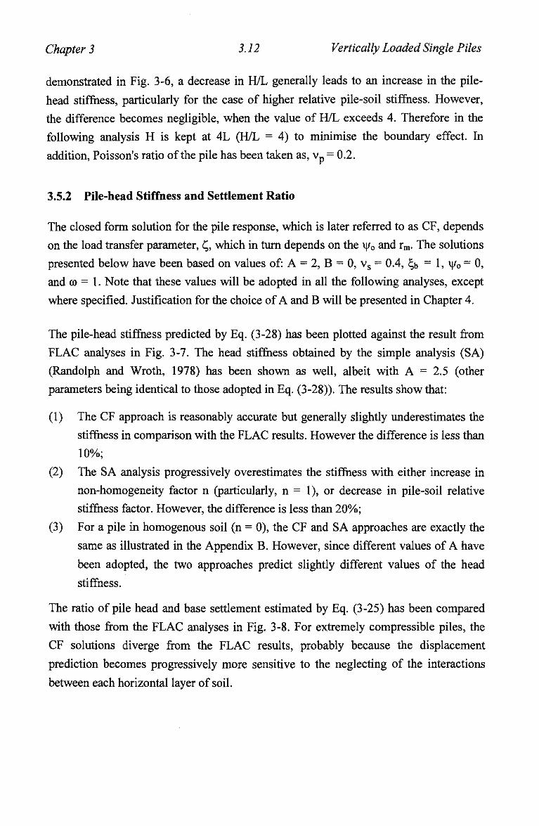
Chapter 3 3.12 Vertically Loaded Single Piles
demonstrated in Fig. 3-6, a decrease in H/L generally leads to an increase in the pile-
head stiffness, particularly for the case of higher relative pile-soil stiffness. However,
the difference becomes negligible, when the value of H/L exceeds 4. Therefore in the
following analysis H is kept at 4L (H/L = 4) to minimise the boundary effect. In
addition, Poisson's ratio of the pile has been taken as, v p = 0.2.
3.5.2 Pile-head Stiffness and Settlement Ratio
The closed form solution for the pile response, which is later referred to as CF, depends
on the load transfer parameter, C„ which in turn depends on the v|/0 and rm. The solutions
presented below have been based on values of: A = 2, B = 0, vs = 0.4, £$ = 1, vj/0 = 0,
and co = 1. Note that these values will be adopted in all the following analyses, except
where specified. Justification for the choice of A and B will be presented in Chapter 4.
The pile-head stiffness predicted by Eq. (3-28) has been plotted against the result from
F L A C analyses in Fig. 3-7. The head stiffness obtained by the simple analysis (SA)
(Randolph and Wroth, 1978) has been shown as well, albeit with A = 2.5 (other
parameters being identical to those adopted in Eq. (3-28)). The results show that:
(1) The CF approach is reasonably accurate but generally slightly underestimates the
stiffness in comparison with the F L A C results. However the difference is less than
10%;
(2) The S A analysis progressively overestimates the stiffness with either increase in
non-homogeneity factor n (particularly, n = 1), or decrease in pile-soil relative
stiffness factor. However, the difference is less than 2 0 % ;
(3) For a pile in homogenous soil (n = 0), the C F and S A approaches are exactly the
same as illustrated in the Appendix B. However, since different values of A have
been adopted, the two approaches predict slightly different values of the head
stiffness.
The ratio of pile head and base settlement estimated by Eq. (3-25) has been compared
with those from the F L A C analyses in Fig. 3-8. For extremely compressible piles, the
C F solutions diverge from the F L A C results, probably because the displacement
prediction becomes progressively more sensitive to the neglecting of the interactions
between each horizontal layer of soil.
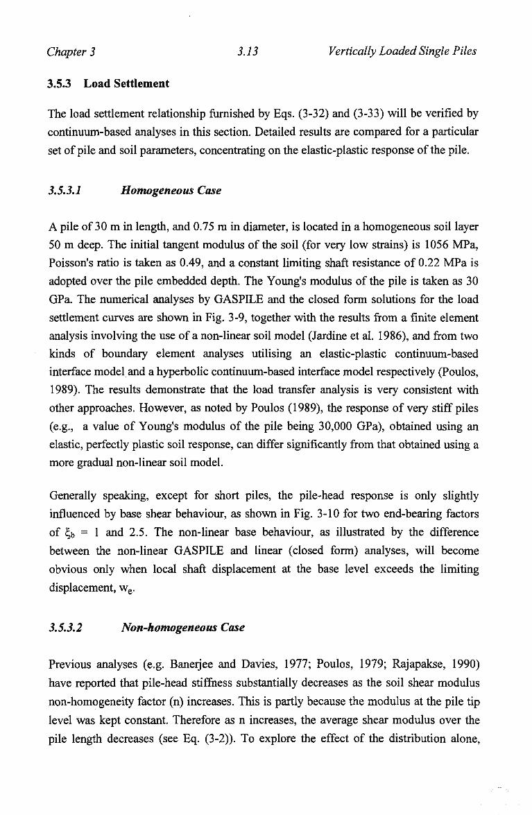
Chapter 3 3.13 Vertically Loaded Single Piles
3.5.3 Load Settlement
The load settlement relationship furnished by Eqs. (3-32) and (3-33) will be verified by
continuum-based analyses in this section. Detailed results are compared for a particular
set of pile and soil parameters, concentrating on the elastic-plastic response of the pile.
3.5.3.1 Homogeneous Case
A pile of 30 m in length, and 0.75 m in diameter, is located in a homogeneous soil layer
50 m deep. The initial tangent modulus of the soil (for very low strains) is 1056 MPa,
Poisson's ratio is taken as 0.49, and a constant limiting shaft resistance of 0.22 M P a is
adopted over the pile embedded depth. The Young's modulus of the pile is taken as 30
GPa. The numerical analyses by GASPILE and the closed form solutions for the load
settlement curves are shown in Fig. 3-9, together with the results from a finite element
analysis involving the use of a non-linear soil model (Jardine et al. 1986), and from two
kinds of boundary element analyses utilising an elastic-plastic continuum-based
interface model and a hyperbolic continuum-based interface model respectively (Poulos,
1989). The results demonstrate that the load transfer analysis is very consistent with
other approaches. However, as noted by Poulos (1989), the response of very stiff piles
(e.g., a value of Young's modulus of the pile being 30,000 GPa), obtained using an
elastic, perfectly plastic soil response, can differ significantly from that obtained using a
more gradual non-linear soil model.
Generally speaking, except for short piles, the pile-head response is only slightly
influenced by base shear behaviour, as shown in Fig. 3-10 for two end-bearing factors
of b = 1 and 2.5. The non-linear base behaviour, as illustrated by the difference
between the non-linear G A S P I L E and linear (closed form) analyses, will become
obvious only when local shaft displacement at the base level exceeds the limiting
displacement, we.
3.5.3.2 Non-homogeneous Case
Previous analyses (e.g. Banerjee and Davies, 1977; Poulos, 1979; Rajapakse, 1990)
have reported that pile-head stiffness substantially decreases as the soil shear modulus
non-homogeneity factor (n) increases. This is partly because the modulus at the pile tip
level was kept constant. Therefore as n increases, the average shear modulus over the
pile length decreases (see Eq. (3-2)). To explore the effect of the distribution alone,
Chapter 3 3.14 Vertically Loaded Single Piles
when the non-homogeneity factor (0 = n) is changed, the average shaft shear modulus
should be kept as a constant and also all the other parameters be identical. In such a
way, the closed form prediction by \j/0 = 0 (linear elastic-plastic case) has been shown in
Fig. 3-11 (a). In this particular case, only about 3 0 % difference due to variation in the n
is noted within the elastic stage. Both the pile-head load and settlement, at which slip is
initiated, decreases as n increases, as demonstrated in Fig. 3-11 (b) and (c). Once pile-
soil relative slip develops (u, > 0), the pile-head load and displacement for 0 = 1
increases with the slip degree, u, at a higher gradient than that for 0 = 0. Therefore at
some degree of the slip, the load will be identical irrespective of the shaft stress non-
homogeneity factor, 0. For a purely frictional pile, the degree is unity. However,
generally due to the base contribution, the degree is less than unity, and the
corresponding load occurs before the full development of the pile-soil slip.
3.6 SETTLEMENT INFLUENCE FACTOR
The above analysis is further substantiated for different slenderness ratio and relative
pile-soil stiffness cases.
3.6.1 Settlement Influence Factor
The settlement influence factor, I is defined as the inverse of a pile-head stiffness,
therefore
I.^Iffil (3-36) P,
where I is the settlement influence factor. While within the elastic stage, the factor can
be derived directly from Eq. (3-28)
1 = I— (3-37) W2CvoU
It is also straightforward to obtain an elastic-plastic formula for the factor, in terms of
Eqs. (3-32) and (3-33). The settlement influence factor is mainly affected by pile
slenderness ratio, pile-soil relative stiffness factor, the degree of the non-homogeneity
of the soil profile, and the degree of pile-soil relative slip.
Chapter 3 3.15 Vertically Loaded Single Piles
3.6.2 Pile Slenderness Ratio Influence
Fig. 3-12 shows the settlement influence factor for a pile of different slenderness ratios
in a Gibson soil, at a constant relative stiffness factor (X = 3000), together with the
B E M analysis based on Mindlin's solution (Poulos, 1989), B E M analysis of three
dimensional solids (Banerjee and Davies, 1977), and the approximate closed form
solution by Randolph and Wroth (1978). The effect of slenderness ratio on the
settlement influence factor reflected by the closed form solution is generally consistent
with those provided by the other approaches.
3.6.3 Pile-Soil Relative Stiffness Effect
Using identical values as mentioned previously, the settlement influence factor, I was
estimated by Eq. (3-37) for a list of given X, which are shown in Fig. 3-13 for four
different slenderness ratios, in comparison with the boundary element ( B E M ) analysis
by Poulos (1979) and the current F L A C analysis. The B E M analysis is for the case of
H/L = 2, while this C F solution is corresponding to the case of H/L = 4. As presented
early in Fig. 3-4, increase in the value of H/L can lead to decrease in pile-head stiffness
and thus an increase in the settlement influence factor. For the case of L/r0 = 50, X =
26,000 (Kb = 10,000), n = 0, an increase in H/L from 2 to infinity can lead to an
increase in the settlement factor by up to 2 1 % (Poulos, 1979). In view of the H/L effect,
the closed form solutions are generally quite consistent with the numerical analysis.
3.7 CASE STUDY
The non-homogeneous soil property and the pile-soil relative slip can be readily taken
into account by the established solutions. A n example analysis is demonstrated as
follows. The test reported by Gurtowski and W u (1984) describes the detailed measured
response of a pile. The pile was 0.61 m wide octagonal prestressed concrete hollow pile
with a plug at the base, and was driven to a depth of about 30 m. For the current
analysis, the parameters used by Poulos (1989) have been adopted directly as shown
below: Young's modulus of the pile was 35 GPa; soil Young's modulus is approximated
by 4 N M P a (N = SPT value); N increases almost linearly with depth from 0 at ground
surface to 70 at a depth of 30 m. The limiting shaft stress is taken as 2 N kPa, the base
limiting stress is 0.4 MPa, and the soil Poisson's ratio is 0.3. The pile-head and base
load-settlement predictions by GASPILE with Rfs = 0.9, Gj/Tf = 769.2 Rft = 0.9 and by
the closed form solutions with \|/0 = 0.5 are shown in Fig. 3-14 together with those
Chapter 3 3.16 Vertically Loaded Single Piles
predicted by boundary element analysis (Poulos, 1989). Good comparisons have been
demonstrated between the current predictions and the measured results, except at failure
load levels. The divergence at high load levels between the current predictions and
those of Poulos (1989) is because the assumed ultimate base stress of 0.4 M P a in the
current GASPILE and closed form analyses is different from that used in the boundary
element analysis.
3.7.1 Load Displacement Distribution Down a Pile
Load and displacement distribution below and above the transition depth may be
estimated in terms of the elastic and elastic-plastic solutions. Under a given pile-head
load, the depth of the transition is expressed by the degree of slip, and can be estimated
by Eq. (3-32) (i.e., by using Mathcad), which is also affected by the non-homogeneity
factor n. At a depth below the transition point, the local shaft displacement must be less
than the limit displacement, we. Therefore, the distributions may be estimated by Eqs.
(3-25) and (3-26) respectively. Otherwise, with an estimated \i, the distribution of load
and displacement within the upper plastic zone can be evaluated by Eqs. (3-34) and (3-
35) respectively. If a pile-head load exceeds the load corresponding to the full shaft slip,
then the difference should be attributed to the base load.
For this typical example, the degrees of slip at P^ = 1.8 MN are 0.058, 0.136, 0.202,
0.258, and 0.305 for n = 0, 0.25, 0.5, 0.75, and 1.0 respectively. For Pt = 3.45 M N , [i =
0.698, 0.723, 0.743, 0.758, 0.771 correspondingly. For Pt = 4.52 M N , the base should
take a load of 1.07 M N . The closed form predictions of load and displacement
distributions down the pile are generally consistent with those from non-linear
GASPILE analysis. For the three different soil profiles of n = 0, 0.5 and 1.0, the
settlement (only at two load levels) and load transfer are shown in Fig. 3-15 together
with the those from GASPILE. A summary of the closed form solutions and that from
GASPILE (n = 1 case only) are shown in Fig. 3-16 a, b, c in conjunction with those by
Poulos (1989) and the measured data. The results show that the linear correlations of the
soil strength and shear modulus with the values of SPT (n = 1) yield reasonable
predictions of the pile response in comparison with the measured.
3.8 CONCLUSIONS
The analysis outlined in this chapter has attempted to provide a more rigorous approach
to the analysis of a pile in a non-homogenous soil medium. The accuracy of the
Chapter 3 3.17 Vertically Loaded Single Piles
solutions based on the load transfer approach is very good compared with those from
continuum and non-linear load transfer analyses. The following conclusions can be
drawn:
(1) A non-linear elastic-plastic analysis makes only a slight difference from that of the
simplified linear elastic-plastic analysis. Therefore the newly established closed
form solutions based on the simplified elastic-plastic soil response are sufficiently
accurate even for estimation of the non-linear response.
(2) The previously reported significant influence of n on pile-head stiffness or
settlement influence factor is partly caused by the alteration of average shear
modulus over the pile length, and partly by the distribution. For a constant
average shear modulus, the influence of the n on the pile-head stiffness become
relatively minor.
(3) The effect of the pile-soil relative slip on estimating load-settlement behaviour
including the load and displacement distributions down the pile can be readily
simulated by the newly established theory.
From the second conclusion, it may be inferred that even for a complicated shear
modulus profile, the non-homogeneity factor, n m a y be adjusted to fit the general trend
of the modulus with depth. The solution presented here m a y thus still be applied with
reasonable accuracy.
Chapter 4 4.1 Load Transfer Factors
4. LOAD TRANSFER IN FINITE LAYER MEDIA
4.1 INTRODUCTION
Load transfer analysis is an uncoupled analysis, which treats the pile-soil interaction
along the shaft and at the base as independent springs (Coyle and Reese, 1966). The
stiffness of the elastic springs, expressed as the gradient of the local load transfer
curves, m a y be correlated to the soil shear modulus by load transfer factors (Randolph
and Wroth, 1978). Given suitable load transfer factors, the analysis provides a close
prediction to a continuum based numerical analysis as reported by Randolph and Wroth
(1978) for piles in an infinite elastic half-space. The question is whether the load
transfer factors are significantly affected by a number of features: (a) non-homogeneous
soil profile, (b) soil Poisson's ratio, (c) pile slenderness ratio, and (d) the relative ratio of
the depth of any underlying rigid layer to the pile length. H o w these features affect the
final pile prediction has not yet fully explored. In addition, the assumption of
proportionality of load transfer gradient to the soil shear modulus, uniformly down the
pile, has not been rigorously explored.
Ideally, load transfer analysis should give identical results to that of a continuum based
numerical analysis. Therefore, continuum based analysis should be used to calibrate the
load transfer factors.
This purpose of this chapter is devoted to (1) investigating the adequacy of the load
transfer approach; (2) calibrating the load transfer factors by undertaking Fast
Lagrangian Analysis of Continua (FLAC) (Itasca, 1992) considering the above
mentioned (a) to (d) conditions. The results are then expressed in statistical formulae.
The back-figured factors are thereafter adopted in the new closed form (CF) solutions to
estimate pile-head stiffness, and the ratio of pile base and head load over a wide range
of slenderness ratios, finite layer ratios, soil Poisson's ratios, non-homogeneity and
relative pile-soil stiffness factor, with the purpose to re-examine the suitability and the
accuracy of the load transfer approach through comparison with previous publications
and the current F L A C analysis.
Chapter 4 4.2 Load Transfer Factors
4.2 RATIONALITY OF LOAD TRANSFER APPROACH
4.2.1 Calibration Procedures
The core of the closed form (CF) solutions is the two critical load transfer factors, C, and
co, which are essentially dependant on each other. A s stated later, the shaft load transfer
factor can reasonably be assumed as a constant with depth. It is thus reasonable to back-
estimate the two factors with the C F solutions through comparison with a more rigrous
numerical (FLAC) analysis. The base behaviour will be calibrated uniquely against Eq.
(3-12), while the shaft load transfer factor can be calibrated against a number of non-
dimensional ratios, e.g.
(a) pile-head stiffness, defined as Pt^GLWtr,,)1;
(b) the ratio of base and head loads;
(c) the ratio of pile head and base settlement.
If the load transfer approach is accurate compared with the F L A C analysis, then
identical values of C, and co should be obtained irrespective of the ratios used for the
calibration.
For the calibration against pile-head stiffness (referred to as matching pile-head
stiffness), the procedure can be detailed as:
(i) Using a desired set of soil and pile parameters, FLAC analysis is performed.
(ii) In terms of the F L A C analysis, pile-head stiffness, and the ratio of base to head
loads can be obtained. Therefore, co may be obtained by Eq. (3-12).
(iii) For the same problem, using a guessed initial value of C„ a pile-head stiffness can
be estimated by Eq. (3-28), with the 'co' obtained above.
(iv) The initial value of C, may be adjusted iteratively, so that the estimated pile-head
stiffness can match (within a desired accuracy) with that obtained from F L A C
analysis. Therefore, C, is obtained.
This process has been fulfilled through a purpose written program in F O R T R A N 77. To
examine the accuracy of the load transfer approach, calibration against the load ratio
between pile base and head (referred to as load ratio) has been performed as well. This
approach is similar to that of matching pile-head stiffness. However, in steps (iii) and
(iv), load ratio rather than stiffness has been estimated by Eq. (3-26), and matched
against that from F L A C analysis.
Except where specified, all the symbols are identical to those defined previously in the thesis.
Chapter 4 4.3 Load Transfer Factors
4.2.2 FLAC Analysis
A continuum based finite difference (FLAC) analysis has been used to explore the
validity of the load transfer approach, and to assess optimum values of load transfer
factors, C, and co. In the simulation of the problem, two kinds of boundary conditions
were used
(a) normal boundary: For the radial boundary, the radial displacements of all the
nodes are restrained, while for the base boundary, only vertical displacements are
constrained;
(b) fixed boundary: The vertical and radial displacements of the nodes along the
boundary are restrained.
Prior to any analysis being performed, a number of factors affecting the load transfer
factors and pile head-stiffhess have been explored for a pile embedded in a soil with
shear modulus described by Eq. (3-1). Except where specified, this pre-exploration was
based on the following conditions:
• The mesh adopted was a 21 x 50 grid, which is identical to that used in Chapter 3.
• Normal boundary was adopted.
• The width of the grid was chosen as the maximum of 2.5L and 75r0.
This pre-exploration gave the following points
(1) The effect of the Poisson's ratio of the pile on this analysis may be ignored as
illustrated in Table 4-1.
(2) The width of the 21 x 50 grid may affect the pile-head stiffness. Table 4-2 shows
that pile-head stiffness obtained from using a width of mesh of 2.5 L is barely
different from that using 75r0. However, as shown in Fig. 4-1 (in the figure, the
current equation is referred to Eq. (4-5) as shown later), the width of the mesh
should be increased to 2.5L (L/r0 > 40) to avoid the effect on back-estimated C,.
(3) A width of 2.5L may be used to avoid the boundary effect. To show the effect of
the width of the mesh combining with boundary condition, a radial width of 75r0
for the mesh has been adopted for a set of analysis based on fixed boundary. As
shown in Fig. 4-2, the fixed boundary comes into effect as pile slenderness ratio
(L/r0) exceeds 40, and results in lower values of C, than those from the normal
boundary with 2.5L. However, as long as the width of the mesh is sufficient, the
boundary effect can be ignored.
Chapter 4 4.4 Load Transfer Factors
(4) Boundary conditions become important when the ratio of H/L exceeds about 4.
Fig. 4-3 shows a comparison of the effect of the boundary on pile-head stiffness
and the ratio of head and base settlements (The widths of the meshes are identical,
with a value of 2.5L.) W h e n the ratio of H/L exceeds 4, fixed boundary offers
constant values of pile-head stiffness, and ratio of head and base settlements.
Therefore, the fixed boundary seems to be a reasonable assumption for the
prediction of the pile-soil response rather than the normal boundary, which has
been further substantiated by the following points:
(a) As illustrated in Fig. 4-3(a), as the ratio of H/L increases, pile-head stiffness
obtained from using a normal boundary keeps decreasing (for lower values of n),
which does not seem to be real, in contrast with that obtained from using fixed
boundary.
(b) Fig. 4-3 (b) shows that the ratios of pile head and base settlements from using a
normal boundary diverge progressively (when H/L > 4), which does not seem
realistic.
(5) As the ratio of H/L increases, the effect of the density of the mesh becomes
obvious. Fig- 4-4 shows the results obtained by using two different kinds of grids.
A grid of 21 x 100 will give accurate value of shaft and base load transfer factors.
Using a grid of 21 x 50, reasonable values of shaft factors may be obtained for H/L
< 4, but incorrect trends for the base load transfer factor are evident for larger
values of H/L.
(6) FLAC analysis gives a slightly higher pile-head stiffness. Table 4-3 shows
comparisons among boundary element analysis (BEM, Randolph and Wroth,
1978), variational method (VM, Rajapakse, 1990) and the F L A C analysis for
single piles in homogeneous soil (n = 0, H/L = 4). The F L A C and B E M analyses
were based on a Poisson's ratio of 0.4, while in the V M analysis, the soil
Poisson's ratio was selected as 0.5. Since a higher Poisson's ratio generally leads
to higher stiffness (as shown later), the stiffness from F L A C analysis is slightly
higher than the predictions from the other approaches. Table 4-4 shows a further
comparison between F E M analysis (Randolph and Wroth, 1978), and the F L A C
analysis for both homogeneous (n = 0) and Gibson soil (n = 1). Note that the
results shown in Table 4-4 were based on a constant shear modulus below the pile
base level.
In terms of the above exploration, in the present FLAC analysis
(i) generally a grid of 21 x 50 was used, following point (5);
Chapter 4 4.5 Load Transfer Factors
(ii) the Poisson's ratio of the pile was taken as vp = 0.2, following point (1);
(iii) the width of the grid was chosen as the maximum of 2.5L and 75r0, following
points (2) and (3);
(iv) when the ratio of H/L is less than 4, the normal boundary was used, otherwise the
fixed boundary was adopted, following point (4);
(v) base load transfer factor was estimated in terms of a grid of 21 x 100, following
point (5).
The analyses have explored the effect of the four factors discussed earlier.
4.2.3 Variation of Shaft Load Transfer Factor With Depth
FLAC analysis is utilised to find the base and shaft load transfer factors. The base
factor, co is directly back-figured by Eq. (3-12), in which the base load, Pb was estimated
through linear extrapolation from the stresses of the last two segments from the base of
the pile, and the base displacement, Wb was taken as the node displacement of the pile
base. The shaft load transfer factor has been evaluated in terms of the shaft load transfer
model and the closed form solutions for single pile (Chapter 3) as described respectively
below.
(1) Variation of C, with depth: With the shaft shear stress and displacement along a
pile obtained by F L A C analysis, the shaft load transfer factor has been back-
figured by using Eq. (3-6), as represented by ' F L A C in Fig. 4-5(a).
(2) Average value of C, over the pile embedded depth: Taking £ as a constant with
depth, the value of the factor, C, has been back-figured in light of the calibration
procedures described previously in section 4.2.1, and has been illustrated in Fig.
4-5(a) as matching 'load ratio' and pile head 'stiffness'.
Fig. 4-5(a) shows that the variation of C, with depth can be approximately taken as a
constant. With average values of C„ the predicted loads and displacements along the
pile, using Eqs. (3-25) and (3-26) respectively, are very close to those from the F L A C
analysis, as illustrated in Fig. 4-5 (d) and (e) respectively. Therefore, the shaft factor, C„
can generally be assumed as a constant with depth.
4.3 EXPRESSIONS FOR LOAD TRANSFER FACTORS
As just mentioned in section 4.2, the base factor, co may be back-figured directly from
Eq. (3-12). The shaft load transfer factor may be taken as a constant with depth, and so
may be backfigured directly by either matching 'load ratio' or pile-head 'stiffness'.
Chapter 4 4.6 Load Transfer Factors
With these approaches, load transfer factors have been obtained in terms of the FLAC
analysis, and have been given in the form of simple expressions.
4.3.1 Base Load Transfer Factor
Load distribution prediction is sensitive to the base load transfer factor. Thus, a more
accurate value of the factor has been provided here as
G)=^L^LG>0 (4-1) cooh coov
where Oh, cov are the parameters that reflect the effect of H/L and soil Poisson's ratio;
©ov is cov at vs = 0.4, co0h is coh at H/L = 4.
The inverse of the factor 'co' reflects the base stiffness (Pb(l-vs)/(4Gbr0Wb)). Therefore,
all the figures will be illustrated in the form of '1/co' to be consistent with that for pile-
head stiffness. The following conclusions have been observed:
(1) The ratio of' 1/co' generally increases slightly with the pile slenderness ratio, when
the ratio of L/r0 is higher than 20, as shown in Fig. 4-6. As the non-homogeneity
factor, n increases from 0 to 1, the factor '1/co' increases by about 0.15. Therefore,
it can be approximated by
1/co 0 = 0.67 - 0.0029 L/r0 + 0.15n (L / r0 < 20)
1/co 0 = 0.6 + 0.0006 L/r0 + 0.15n (L / r0 > 20) (4-2)
(2) As Poisson's ratio increases, '1/co' decreases slightly. However, once vs exceeds
0.4, it increases as shown in Fig. 4-7. Thereby
l/cov = 1/coo+ 0.3(0.4-v.) (vs<0.4)
1/co v = 1/co o + L2(v, - 0.4) (v, > 0.4) (4-3)
(3) The ' 1/co' calibrated is sensitive to the grid used for the case of different values of
H/L, as described previously. Following careful exploration, it maybe concluded
that '1/co' can be predicted by the following equation
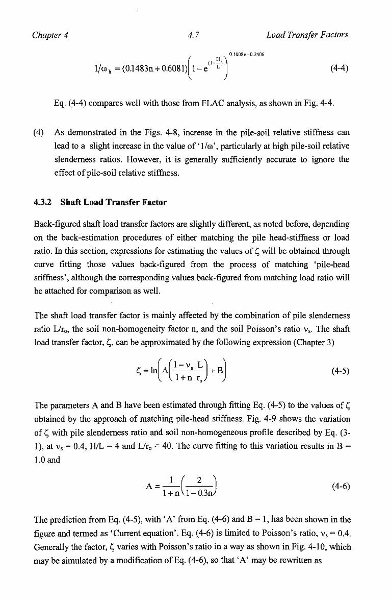
Chapter 4 4.7 Load Transfer Factors
x 0.1008n-0.2406
1/co h = (0.1483n + 0.6081) 1 - e L (4-4)
v )
Eq. (4-4) compares well with those from F L A C analysis, as shown in Fig. 4-4.
(4) As demonstrated in the Figs. 4-8, increase in the pile-soil relative stiffness can
lead to a slight increase in the value of '1/co', particularly at high pile-soil relative
slenderness ratios. However, it is generally sufficiently accurate to ignore the
effect of pile-soil relative stiffness.
4.3.2 Shaft Load Transfer Factor
Back-figured shaft load transfer factors are slightly different, as noted before, depending
on the back-estimation procedures of either matching the pile head-stiffness or load
ratio. In this section, expressions for estimating the values of C, will be obtained through
curve fitting those values back-figured from the process of matching 'pile-head
stiffness', although the corresponding values back-figured from matching load ratio will
be attached for comparison as well.
The shaft load transfer factor is mainly affected by the combination of pile slenderness
ratio L/r0, the soil non-homogeneity factor n, and the soil Poisson's ratio vs. The shaft
load transfer factor, £, can be approximated by the following expression (Chapter 3)
( A „ TA ^ ; = in
l-v
I 1 + n rj + B (4-5)
J
The parameters A and B have been estimated through fitting Eq. (4-5) to the values of C,
obtained by the approach of matching pile-head stiffness. Fig. 4-9 shows the variation
of t, with pile slenderness ratio and soil non-homogeneous profile described by Eq. (3-
1), at vs = 0.4, H/L = 4 and L/r0 = 40. The curve fitting to this variation results in B =
1.0 and
A=-L(-U (4.6) l + nvl-0.3n/
The prediction from Eq. (4-5), with 'A' from Eq. (4-6) and B = 1, has been shown in the
figure and termed as 'Current equation'. Eq. (4-6) is limited to Poisson's ratio, vs = 0.4.
Generally the factor, C, varies with Poisson's ratio in a way as shown in Fig. 4-10, which
may be simulated by a modification of Eq. (4-6), so that 'A' may be rewritten as
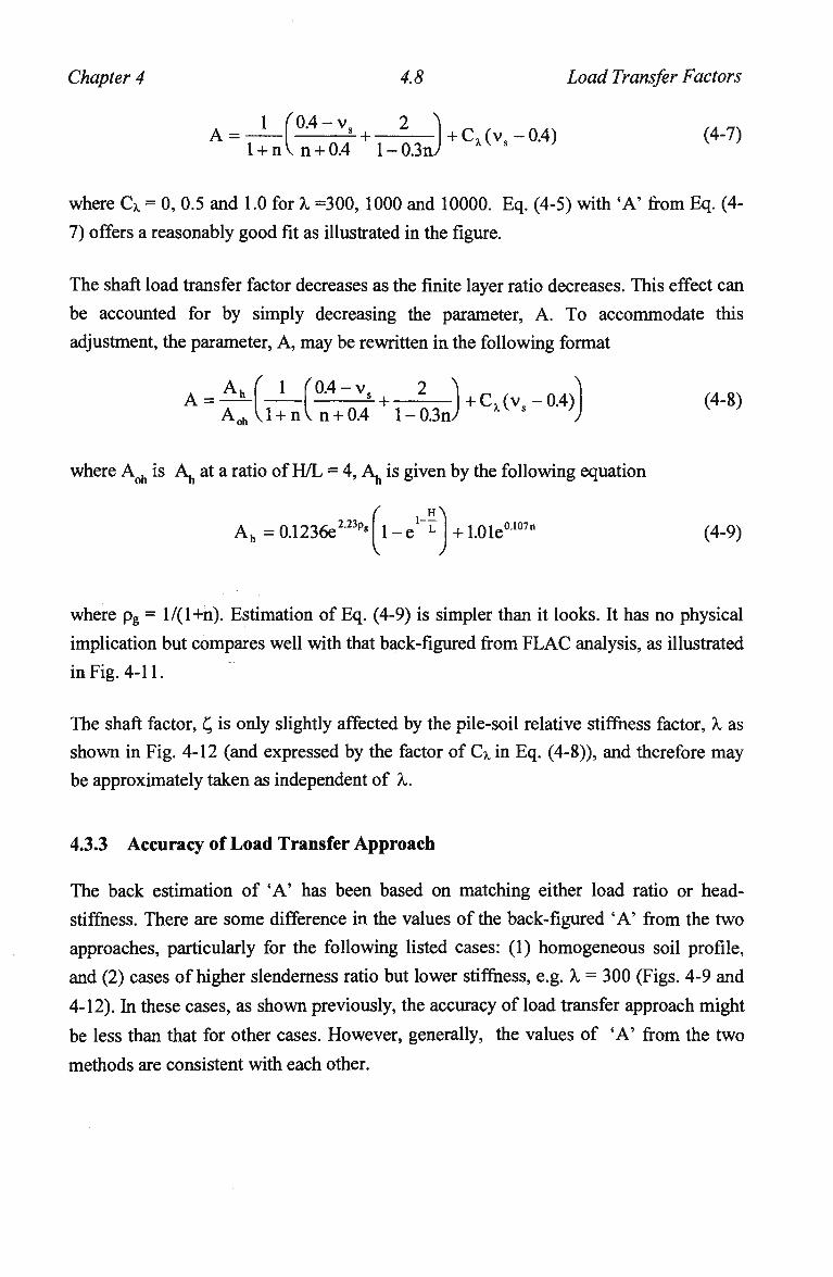
Chapter 4 4.8 Load Transfer Factors
A = J—(^Zl± + -J—) +Cx(vs -0.4) (4-7) l + nln + 0.4 l-0.3nJ s
where Cx = 0, 0.5 and 1.0 for X =300, 1000 and 10000. Eq. (4-5) with 'A' from Eq. (4-
7) offers a reasonably good fit as illustrated in the figure.
The shaft load transfer factor decreases as the finite layer ratio decreases. This effect can
be accounted for by simply decreasing the parameter, A. To accommodate this
adjustment, the parameter, A, may be rewritten in the following format
A=A'' l
AohU + n ^—~ + — ^ — 1 + Cx (vs - 0.4)] (4-8) l n + 0.4 l-0.3nJ x s )
where AQh is A^ at a ratio of H/L = 4, Ah is given by the following equation
... ( ,_HA + 1.01e0107n (4-9) A h = 0.1236e
223p« 1-e L
where pg = l/(l+n). Estimation of Eq. (4-9) is simpler than it looks. It has no physical
implication but compares well with that back-figured from F L A C analysis, as illustrated
in Fig. 4-11.
The shaft factor, C, is only slightly affected by the pile-soil relative stiffness factor, A, as
shown in Fig. 4-12 (and expressed by the factor of Cx, in Eq. (4-8)), and therefore may
be approximately taken as independent of X.
4.3.3 Accuracy of Load Transfer Approach
The back estimation of 'A' has been based on matching either load ratio or head-
stiffness. There are some difference in the values of the back-figured 'A' from the two
approaches, particularly for the following listed cases: (1) homogeneous soil profile,
and (2) cases of higher slenderness ratio but lower stiffness, e.g. X = 300 (Figs. 4-9 and
4-12). In these cases, as shown previously, the accuracy of load transfer approach might
be less than that for other cases. However, generally, the values of 'A' from the two
methods are consistent with each other.
Chapter 4 4.9 Load Transfer Factors
4.3.3.1 Using 'A=2.5'for a Pile in an Infinite Layer
When the ratio of H/L is less than 4, boundary (fixed or normal) conditions have
negligible effect on the analysis of pile response. However, once the ratio H/L exceeds
4, boundary conditions progressively affect the final pile-head stiffness (Fig. 4-3 (a)),
and affect significantly the values of 'A', as shown in Fig. 4-13 for case I (shear
modulus by Eq. (3-1) across the entire depth, H ) at X = 1000. It has been argued before
that at a higher ratio of H/L ( > 4), analysis using fixed boundary is more realistic,
which gives a value of 'A = 2.1 (n = 0)' for infinite layer case (H/L = oo). Therefore, for
the case of H/L = oo and n = 0, a discrepancy arises between the value of 'A = 2.1' by
the current calibration and the previous suggestion of 'A = 2.5' (Randolph and Wroth,
1978). Many researchers have reported that a value of 'A = 2.5 (n = 0)' gave excellent
comparison with most of the available numerical approaches for single piles (shown late
in this chapter) and pile groups (shown in Chapter 7). It may be due to the fact that
F L A C analysis gives a higher pile-head stiffness for a pile in an infinite layer than most
of other approaches, and therefore gives a lower value of 'A = 2.1 (n = 0)'.
Using (incorrect) normal boundary, as H/L increases from 2 to 12, a significant increase
in the back-figured 'A' of about 90 and 1 0 % individually for n = 0 and 1 is noted.
However, corresponding to which, the head stiffness changes only about 11 and 0.5%
respectively for n = 0 and 1 (Table 4-5). Therefore, using an ultimate 'A' value of 2.5
(corresponding to the incorrect normal boundary), when H/L > 2, should generally
underestimate the stiffness by less than 1 1 % (n = 0) compared with that obtained by
F L A C analysis using (correct) fixed boundary. In view of this fact and that F L A C
analysis generally overestimates the head stiffness for a pile in an infinite layer, a value
of 'A = 2.5' may still be taken.
Generally even a 30% difference in choice of 'A' value, leads to a less than 10%
difference in the prediction of head stiffness from Eq. (3-28). However, the accuracy of
'A' becomes important when estimating pile-pile interaction factors, as noted by Guo
and Randolph (1996a) and further explored in Chapter 7.
4.3.3.2 Effect of Base Load Transfer Factor
The base load transfer factor can generally be taken as unity for predicting pile-head
stiffness. As shown above, 1/co varies generally between 0.6 and 1.0, with an average of
about 0.8. The base contribution to the pile-head stiffness is generally less than 10%.
Therefore, taking co as a unity will result in less than 6 % difference in the predicted pile-
Chapter 4 4.10 Load Transfer Factors
head stiffness. Fig. 4-14 shows an example for two extreme cases of higher (L/r0 = 80)
and lower (L/r0 = 10) values of co, and the prediction by the current equation, Eq. (4-5).
4.4 VALIDATION OF LOAD TRANSFER APPROACH
The current solutions of pile head-stiffness and the load ratio are in the form of
modified Bessel functions as illustrated in Chapter 3. The numerical evaluation of the
solutions have been performed through a spreadsheet program, which operates through
a macro sheet in Microsoft E X C E L , with the shaft load transfer factor given by Eq. (4-
7) and the base load transfer factor generally given by Eq. (4-1). Except for comparison
with the F L A C analyses, a value of unity for base load transfer factor has been used. All
the following C F solutions result from this program.
4.4.1 Comparison with Existing Solutions
Table 4-6 shows that the predicted pile-head stiffness by Eq. (3-28) and the ratio of pile
base and head load by Eq. (3-26) are shown to be consistent with those from other
approaches. However, soil Poisson's ratio was selected as 0.4 in the current F L A C and
CF analyses, rather than 0.5 as used in the other approaches. In view of the effect of the
Poisson's ratio, the F L A C analysis offers a slightly higher head stiffness. Particularly, at
higher pile-soil relative stiffness (e.g., X > 10000), the F L A C and current C F approaches
yield appreciably (about 10%) higher stiffness than those from other approaches as
shown in Table 4-7.
4.4.1.1 Slenderness Ratio Effect
Fig. 4-15(a) shows the variation of pile-head stiffness with slenderness ratio obtained
for a pile in a homogeneous, infinite half space by Butterfield and Banerjee (1971),
Chin et al. (1990). To simulate the infinite half space condition, a value of 2.5 for the
'A' is assumed in the closed form prediction of Eq. (3-28), which offers a very good
comparison of pile-head stiffness with those from the more rigorous numerical
approaches shown in the figure. Fig. 4-15(b) provides a further comparison of the head
stiffness for a pile in a Gibson soil (n = 1) obtained by C h o w (1989), Banerjee and
Davies (1977) and the present closed form solutions. Increase in slenderness ratio as
shown in Fig. 4-15 can lead to an increase in pile-head stiffness, but this tendency is
limited to a certain value, beyond which any an increase in the slenderness ratio will
lead to an negligible difference in the pile-head stiffness.
Chapter 4 4.11 Load Transfer Factors
4.4.1.2 Soil Poisson's Ratio Effect
Poisson's ratio reflects the compressibility of a soil, the more incompressible (higher
Poisson's ratio) the soil is, the higher is the pile-head stiffness, as shown in Fig. 4-16.
The difference in the stiffness due to variation of Poisson's ratio between 0 and 0.5 can
be as high as 2 5 % .
4.4.1.3 Finite Layer Effect
The finite layer ratio, H/L can influence the pile response, if it is less than a limiting
value (e.g., H/L = 4 when L/r0 = 40). The limiting value of H/L is affected by the critical
pile slenderness ratio, beyond which any increase in the pile slenderness ratio results in
negligible increase in pile-head stiffness. Fig. 4-17 shows that as the ratio of H/L
increases from 1.25 to 4, the head stiffness incurs about 1 5 % reduction, but only a slight
decrease in base load is noted (not shown). At this particular slenderness ratio (L/r0 =
40), the percentage in reduction of stiffness with H/L is consistent with those reported
by Poulos (1974) and Valliappan et al. (1974) (not shown). The effect of the ratio of
H/L can be well represented for different slenderness ratios by the current load transfer
factors, as illustrated in Fig. 4-18, together with the predictions by Butterfield and
Douglas (1981).
The overall comparison demonstrates that Eq. (4-1) for co and Eq. (4-5) for C, are
sufficiently accurate for load transfer analysis.
4.5 EFFECT OF SOIL PROFILE BELOW PILE BASE
The above analysis is generally based on the shear modulus described by Eq. (3-1)
across the entire depth, H, and is referred to as case I. If the modulus is taken as a
constant below the tip level, it will be referred to as case II.
For piles of different slenderness ratios embedded in a soil profile of H/L = 4, Poisson's
ratio = 0.4, F L A C analysis for case I and II shows that
(1) For short piles (L/r0 < 20), the pile-head stiffnesses diverge progressively for the
two cases, as n increases (Fig. 4-19(a));
(2) The ratio of head and base settlement differs more obviously in case II than case I
for different non-homogeneity factors (Fig. 4-19(b)), but the difference is minor.
Chapter 4 4.12 Load Transfer Factors
(3) The difference in the values of the load transfer factor, 'A' (as the gradient of the
plot in Fig. 4-20) between case II and I becomes progressively more pronounced
as the value of 'n' increases. To accommodate this effect, 'B' may still be taken as
unity, and Eq. (4-6) may be replaced with,
A = 2.1 - (4-10) 3.53n-0.03
Eq. (4-10) is based on H/L = 4 and X = 1000, which offers a close prediction of
the C, variation as shown in Figs. 4-21 (a) to (d) represented by 'Equation for case
IF.
(4) For case II (X = 3000), 'A' decreases as H/L reduces (Fig. 4-22). Particularly,
when H/L < 2, 'A' decreases very sharply. At higher values of H/L, 'A'
approaches a constant. The variation of 'A' for the case II may be simulated by the
following equation (to replace Eq. (4-9) for case I),
A h = 0.9064e04172p« l-e"L
V J + 0.6429e°™ (4-11)
This 'A' based on X. = 3000 is generally about 1 0 % (for n = 0) lower than that
obtained by Eq. (4-10), as illustrated in Fig. 4-23. The effect of pile-soil relative
stiffness (X = 1000 for case I, X = 3000 for case II) on C, is relative small as
illustrated in Fig. 4-22 for the case of n = 0. Therefore, the effect of the soil profile
below pile base level is assessed to be obvious as clearly demonstrated by the
figure for the case of n = 1.
In summary, generally the 'A' for case II may be estimated by
A = A h
( 1 fO.4-0 f\. n ^ >
Aoh + 2.1-—- — - +Cx(vs-0.4) (4-12)
U + n V n + 0.4 / V 3.53n - 0.03,
where Aoh is Ah at a ratio of H/L = 4, Ah is given by Eq. (4-11).
(5) The base load transfer factor (1/co) for case II generally lies in the range 0.55 to
1.0 (not shown), increasing with L/r0, H/L (for H/L > 2) and pile-soil stiffness
ratio, X, and decreasing as vs increases. The values of '1/co' are about 2 0 % lower
than those previously reported (Guo and Randolph, 1996a), because a new mesh
of 21x100 grid has been adopted in the present analysis, rather than a grid of 21 x
50 as used previously.
Chapter 4 4.13 Load Transfer Factors
4.7 CONCLUSIONS
In this Chapter, an extensive numerical analysis has been undertaken using the FLAC
program. With these numerical results, the suitability and rationality of load transfer
analysis has been explored extensively.
Preliminary numerical check showed that a grid of 21 x 100 was necessary to obtain
accurate estimation of the base load transfer parameter, co. Also, while the radial
boundary condition made no difference for H/L < 4, fixed boundary was essential for
H/L > 4. With the fixed boundary, it was found that H/L = 4 may be considered as
effectively an infinite deep soil layer.
The numerical analysis shows that the effect of choosing soil Poisson's ratio can be
equally as important as the ratio of H/L and should be taken into consideration. The
finite layer ratio of H/L can only lead to about 1 5 % increase in head stiffness when H/L
decreases from 4 to 1.25, but the increase in soil Poisson's ratio from 0 to 0.499 can
result in about a 2 5 % increase in pile-head stiffness.
The calibration using load transfer model shows that, generally, shaft load transfer
factor can be taken as constant with depth. With average values of the shaft load
transfer factor, the load transfer approach yielded close predictions of overall pile
response compared with those obtained by F L A C analysis.
The calibration using the closed form solutions demonstrates that shaft load transfer
factor (1) increases with increase in pile slenderness ratio; (2) decreases with increase in
Poisson's ratio; (3) increases slightly with increase in the ratio of H/L (H/L < 4), but (4)
is nearly independent of the pile-soil relative stiffness.
The difference in the values of shaft load transfer factors, calibrated against pile-head
stiffness and ratio of base and head load, implies that the load transfer approach is less
accurate in the cases of (1) homogeneous soil profile; and (2) higher pile slenderness
ratio but lower pile-soil relative stiffness. However, an appreciable (e.g. 30%)
difference in selection of the value of 'A' generally leads to a slight (e.g. about 10%)
difference in the predicted pile-head stiffness of a single pile. Therefore, generally load
transfer analysis is sufficiently accurate for practical analysis.
The backfigured load transfer factors have been expressed in the form of simple
formulas and also implemented in a spreadsheet program. In comparison with the
current F L A C analysis and relevant rigorous numerical approaches, the simple formulas
Chapter 4 4.14 Load Transfer Factors
can well account for the effects of various relative thickness ratio of H/L (< 4),
Poisson's ratio and pile slenderness ratio. In the case of an infinite layer, it seems that a
value of 'A = 2.5' gives good comparison with most of the available numerical
predictions.
The shear modulus distribution below the pile tip level can significantly alter the value
of the shaft load transfer factor. To account for this effect, (1) for the case of shear
modulus varying as a power law of depth across the entire depth, H, Eq. (4-8) may be
used, otherwise (2) for the case of a constant value below the tip level, Eq. (4-12) may
be used.
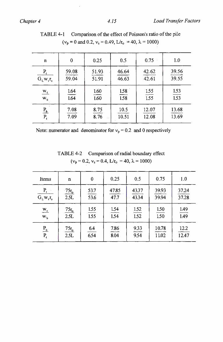
Chapter 4 4.15 Load Transfer Factors
T A B L E 4-1 Comparison of the effect of Poisson's ratio of the pile
(vp = 0 and 0.2, vs = 0.49, L/r0 = 40, X = 1000)
n
P, GL Wt ro
w t
Pb p.
0
59.08
59.04
1.64
1.64
7.08
7.09
0.25
51.93
51.91
1.60
1.60
8.75
8.76
0.5
46.64
46.63
1.58
1.58
10.5
10.51
0.75
42.62
42.61
1.55
1.55
12.07
12.08
1.0
39.56
39.55
1.53
1.53
13.68
13.69
Note: numerator and denominator for vp = 0.2 and 0 respectively
T A B L E 4-2 Comparison of radial boundary effect
(vp = 0.2, vs = 0.4, L/r0 = 40, X = 1000)
Items
P, GLwtr0
w t
w b
P„
Pt
n
75r0 2.5L
75r0 25L
75r0
25L
0
53.7
53.6
1.55
1.55
6.4
654
0.25
47.85
47.7
1.54
1.54
7.86
8.04
0.5
43.37
43.34
1.52
1.52
9.33
954
0.75
39.93
39.94
1.50
1.50
10.78
11.02
1.0
37.24
37.28
1.49
1.49
12.2
12.47
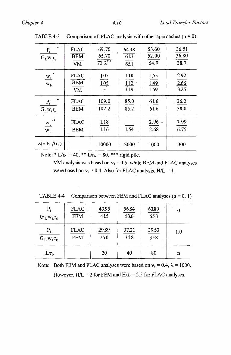
Chapter 4 4.16 Load Transfer Factors
T A B L E 4-3 Comparison of FLAC analysis with other approaches (n = 0)
P. * GLw,r0
w b
P. ** GLwtr0
*«
w t
w b
A(=Ep/GL)
FLAC BEM VM
FLAC BEM VM
FLAC BEM
FLAC BEM
69.70 65.70
72.2
1.05
1.05
109.0
102.2
1.18
1.16
10000
64.38 61.3
65.1
1.18
1.12 1.19
85.0
85.2
1.54
3000
53.60 52.00
54.9
1.55
1.49 1.59
61.6
61.6
2.96
2.68
1000
36.51
36.80
38.7
2.92
2.66 3.25
36.2
38.0
7.99
6.75
300
Note: * L/r0 = 40, ** L/r0 = 80, *** rigid pile.
V M analysis was based on vs = 0.5, while B E M and FLAC analyses
were based on vs = 0.4. Also for FLAC analysis, H/L = 4.
T A B L E 4-4 Comparison between F E M and FLAC analyses (n = 0, 1)
Pt
G L w t r 0
Pt
G L w t r 0
L/r0
FLAC FEM
FLAC FEM
43.95
41.5
29.89
25.0
20
56.84
53.6
37.21
34.8
40
63.89
65.3
39.53
35.8
80
0
1.0
n
Note: Both F E M and FLAC analyses were based on vs = 0.4, X = 1000.
However, H/L = 2 for F E M and H/L = 2.5 for FLAC analyses.
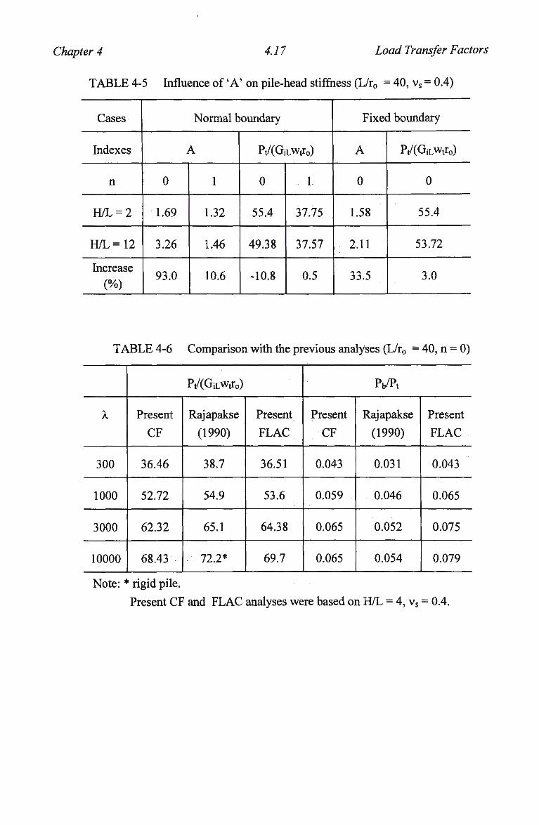
Chapter 4 4.17 Load Transfer Factors
TABLE 4-5 Influence of 'A' on pile-head stiffness (L/r0 = 40, vs = 0.4)
Cases
Indexes
n
H/L = 2
H/L = 1 2
Increase
(%)
Normal boundary
A
0
1.69
3.26
93.0
1
1.32
1.46
10.6
Pt/(GiLwtr0)
0
55.4
49.38
-10.8
1
37.75
37.57
0.5
Fixed boundary
A
0
1.58
2.11
33.5
Pt/(GiLwtr0)
0
55.4
53.72
3.0
T A B L E 4-6 Comparison with the previous analyses (L/r0 = 40, n = 0)
X
300
1000
3000
10000
Pt/(GiLwtro)
Present
CF
36.46
52.72
62.32
68.43
Rajapakse
(1990)
38.7
54.9
65.1
72.2*
Present
F L A C
36.51
53.6
64.38
69.7
Pb/Pt
Present
CF
0.043
0.059
0.065
0.065
Rajapakse
(1990)
0.031
0.046
0.052
0.054
Present
F L A C
0.043
0.065
0.075
0.079
Note: * rigid pile.
Present CF and F L A C analyses were based on H/L = 4, vs = 0.4.
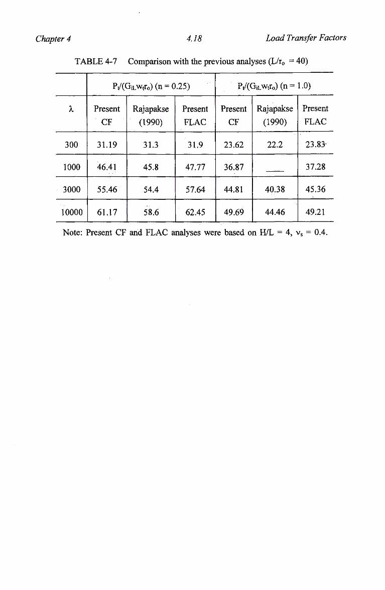
Chapter 4 4.18 Load Transfer Factors
TABLE 4-7 Comparison with the previous analyses (L/r0 = 40)
X
300
1000
3000
10000
Pt/(GiLwtro)(n = 0.25)
Present
CF
31.19
46.41
55.46
61.17
Rajapakse
(1990)
31.3
45.8
54.4
58.6
Present
F L A C
31.9
47.77
57.64
62.45
Pt/(GiLwtro)(n=1.0)
Present
CF
23.62
36.87
44.81
49.69
Rajapakse
(1990)
22.2
40.38
44.46
Present
F L A C
23.83
37.28
45.36
49.21
Note: Present CF and F L A C analyses were based on H/L = 4, vs = 0.4.
Chapter 5 5.1 Visco-elastic Load Transfer Models
5. NON-LINEAR VISCO-ELASTIC LOAD TRANSFR MODELS FOR PILES
5.1 INTRODUCTION
Numerical solutions for axial pile response, based on elasticity, have been extended to
allow for non-homogeneity of the soil (e.g. Banerjee and Davies, 1977; Poulos, 1979),
relative slip between pile and soil (e.g. Poulos and Davis, 1980), and visco-elastic
response of soil (Booker and Poulos, 1976). However, a load transfer approach appears
to offer adequate accuracy and distinctly much greater flexibility to yield unified
compact closed form solutions to take into account all of these factors (Randolph and
Wroth, 1978; Guo and Randolph, 1996c).
Time can have an important effect on the response of piles in clay. For driven piles,
dissipation of the excess pore pressures generated during driving leads to an increase in
shaft friction and in the stiffness of the surrounding soil (e.g. Bergdahl and Hult, 1981;
Trenter and Burt, 1981). In addition, creep or viscoelastic response of the soil leads to
variations in stiffness and capacity depending on the time-scale of loading. At high load
levels, or for long slender piles where the load transfer is concentrated near the pile
head, creep can lead to significant pile head movement at constant load, and even a
gradual reduction in shaft capacity. Ramalho-Ortigao and Randolph (1983) report an
apparent difference of some 30 % in the tension capacity of a pile loaded at a constant
displacement rate leading to failure in about 40 seconds, compared with a similar pile
subjected to a maintained load test over a period of 40 days.
England (1992) has extended the hyperbolic approach of pile analysis described by
Fleming (1992) to allow the effects of time to be incorporated into axial pile analysis,
with separate hyperbolic laws being used to describe the time-dependency of the
(average) shaft and base response. This phenomenological approach is limited by the
difficulty of linking the parameters required for the model to fundamental and
measurable properties of the soil.
Creep displacement can be induced by any of the following factors: (1) a prolonged step
loading; (2) a vibration or (3) a change of temperature. For conventional pile loading
tests (e.g, Maintained loading test and Constant rate load test), the time-scale of loading
can be simulated sufficiently accurately by the two kinds of commonly encountered
loading: 1-step loading, and ramp (linear increase followed by sustained) loading. In the
present chapter, visco-elastic shaft and base load transfer models have been proposed
for the two types loading respectively. With the models, the previous closed form
Chapter 5 5.2 Visco-elastic Load Transfer Models
solutions for a pile in an elastic-plastic non-homogeneous media (Chapter 3) have been
extended to account for visco-elastic response. A previously designed program called
GASPILE has been extended to allow the time-dependent pile response to be computed.
The solutions have been compared extensively with the numerical analysis by Booker
and Poulos (1976) for the case of 1-step loading. The overall pile response for the two
commonly encountered loading types has been explored. Finally, two example analyses
are compared with measured pile responses to illustrate the validity of the proposed
theory to practical applications.
5.2 SHAFT BASE PILE-SOIL INTERACTION
The main challenge in predicting the axial performance of piles lies in establishing load
transfer functions for the shaft and base, which are linked to fundamental properties of
the soil and yet which allow for non-linearity and time dependence of the soil response.
Load transfer functions for the shaft may be derived from the stress-strain response of
the soil using the concentric cylinder approach, which itself is based on a simple 1/r
variation of shear stress around the pile (where r is the distance from pile axis) (e.g.
Frank, 1974; Cooke, 1974; Randolph and Wroth, 1978). The treatment below extends
those functions to allow for visco-elastic response of the soil.
5.2.1 Non-linear Visco-elastic Stress-Strain Model
A pile in clay under a sustained load usually undergoes additional settlement, the
amount of which varies from soil to soil and which is thought to be due to changes in
the stress-strain behaviour with aging (Mitchell and Solymar, 1984). Such creep
behaviour, which occurs in the soil surrounding the pile as well as on the pile-soil
interface itself, has been well recognised (Edil and Mochtar, 1988). A model consisting
of Voigt and Bingham elements in series can account well for the creep behaviour of
several soils (Komamura and Huang, 1974). However determination of the slider
threshold value for the Bingham model is difficult, and an alternative is to adopt a
hyperbolic stress-strain model as shown by experiment (Zen, 1991; Feda, 1992). Such a
treatment can lead to a modified intrinsic time dependent non-linear creep model (Fig.
5-1(a)), which can be expressed as
y = y , + y 2 (5-1)
x j=Y jG i j k j (5-2)
*3=T1Y3Y3 (5-3)
Chapter 5 5.3 Visco-elastic Load Transfer Models
Tl =X2 +X3 (5"4)
where yj is the shear strain for the elastic spring 1, 2 and dashpot 3 (j = 1, 2 and 3)
respectively; y is the total shear strain; Gy is the instantaneous and delayed initial elastic
shear modulus (j = 1, 2) respectively; y^ is the shear strain rate for the dashpot (73 = Y2);
r|y3 is the shear viscosity at a strain rate of 3; tj is the shear stress acted on spring 1, 2
and dashpot 3 (j = 1, 2 and 3) respectively; kj is the coefficient for considering non-
linearty of elastic springs 1 and 2 (j = 1, 2) respectively.
In terms of rate process theory, the shear strain rate, y, can be expressed in different
forms related to absolute temperature and/or deviatoric shear stress (Murayama and
Shibata, 1961; Mitchell, 1964; Christensen and Wu, 1964; Mitchell, et al. 1968).
However, none of the expressions available can account for the non-linearity of the soil
creep. A non-linear hyperbolic model of soil shear stress-strain relationship can offer a
good comparison with the measured stress-strain relationship at different time (Feda,
1992); therefore, the model is employed as expressed by Eq. (5-5), where the coefficient
kj is expressed as
kj=l-\|/j (5-5)
where VJ/J = RgXj /xf] (j = 1, 2), and Rg is originally defined as xs/xultj (xuitj, xg are the
ultimate and failure local shaft stress for spring 1 and 2 respectively) for the hyperbolic
model only (Duncan and Chang, 1970).
From Eqs. (5-1) to (5-4), it follows that
T ^3 1 . "H 3 . TiJ + 7 ^ 7 ^ x i = 7 + 7 7 ^ 7 (5-6)
Gy2 Gyl Gy 2
where J = l/Gyi+l/Grc; Gyj (= Gykj), is the instantaneous and delayed elastic shear
modulus at a strain of yj (j = 1, 2) respectively; x 1, y are the shear stress rate and shear
strain rate respectively. Integration of Eq. (5-6) with respect to time, considering the
initial conditions: t = 0, y = 0, leads to
y=^[> + ^{^expf-^(t-t-)U (5-7) GTl I GV2 ^ 3 * Xl I "Y3 J J
Chapter 5 5.4 Visco-elastic Load Transfer Models
where xi, xi(t*) are the soil shear stress at time t and t* respectively. The total shear
strain in Eq. (5-7), obtained from the non-linear soil model by Eqs. (5-1) to (5-4),
reflects two types of responses to stress: instantaneous elasticity (G;i) and delayed
elasticity (Gi2). At the onset of loading, only the elastic part of shear strain exists, but as
time passes, some creep displacement (delayed elasticity) on and/or around the pile-soil
interface is anticipated.
Generally speaking, secondary compression of all remoulded and undisturbed clays
obtained by oedometer tests can be sufficiently accurately predicted by the model of Eq.
(5-7) for the elastic case (\\fi = v|/2 = 0), except for a soil of loose structure that is
susceptible to breakdown, where a Voigt element has to be added in series with
Mediant's model (Lo, 1961). A s for pile foundations, since remoulding of the soil
around the piles is inevitable due to construction, the model proposed herein and
expressed by Eqs. (5-1) to (5-4) may be adequate to simulate the creep behaviour as
shown later.
In pile analysis, xg is taken as xuitj, and the Rg is used as a parameter to control the
degree of non-linearity for spring 1 and 2 (j = 1, 2) respectively. Strictly speaking, the
limiting value of shear stress at the pile-soil interface, xuiti, may be larger than the
failure shear stress, xfl, in the hyperbolic model of the soil response. Appropriate values
of xn (xuiti) may be correlated with the shear strength of the soil, or with the effective
overburden stress (e.g., API RP2A; Tomlinson, 1970; Randolph and Murphy, 1985), or
estimated through the correlation to the CPT, S P T (e.g. Hirayama, 1990) and vane shear
test (Tomlinson, 1970; McClelland, 1974; Meyerhof, 1976).
Normally, as time passes, the stress initially taken by the dashpot redistributes to the
elastic spring 2 (Fig. 5-1 a), until finally all the stress is transferred, and the time
dependent creep ceases. During the transferring process, if the shear stress on spring 2
exceeds the failure stress, the spring will yield and a larger fraction of the stress has to
be endured by the dashpot, which could lead to a non-terminating creep and eventually
trigger a failure. Therefore, the stress XQ. (xuit2) must be the long term value, which is
lower than xn (xuiti), as reported by many researchers, e.g. Geuze and Tan (1953),
Murayama and Shibata (1961), Leonard (1973). Reduction in soil strength is linearly
related to the logarithmic time elapsed (Casagrande and Wison, 1951), which has also
been formulated by Leonard (1973). Based on a number of creep tests at an approximate
constant rate of loading, Murayama and Shibata (1961) report that the ratio of xc/xfi(xuit2
/xuiti) is about 0.71, while the values themselves xo(xuit2), n('Cuiti) increase
logarithmically as the water content decreases.
Chapter 5 5.5 Visco-elastic Load Transfer Models
5.2.2 Shaft Displacement Estimation
5.2.2.1 Visco-elastic Shaft Estimation Formula
Local shaft displacement can be predicted through a concentric cylinder approach,
which itself is based on elastic theory (Randolph and Wroth, 1978; Kraft et al. 1981).
The correspondence principle (Lee, 1955; Lee et al. 1959) states that the analysis of
stress and displacement field in a linear visco-elastic medium can be treated in terms of
the analogous linear elastic problem having the same geometry and boundary
conditions. However, for the case of non-linear elastic soil, the principle is invalidated.
Therefore, a shaft model reflecting non-linear visco-elastic response might have to be
directly obtained from the generalised visco-elastic stress strain relationship of Eq. (5-
7), with suitable shear modulus. Model pile tests show that load transfer along a model
pile shaft leads to a nearly negligible volume change (or consolidation) in the
surrounding soil (Edil and Mochtar, 1988). Approximately, the vertical displacement, u
along depth, z ordinate may be ignored. Therefore it follows that
du dw dw y = — + — » — (5-8)
& Sr 9r
where w is the local displacement of shaft element at time t. Based on the concentric
cylinder approach, the shaft displacement is obtained by integration from r0 to the
m a x m u m radius of influence, rm
"•dw w JS* w dr
With the shear stress, xj at a distance of r away from the pile axis given by, x, = x0r0 /r,
and substituting Eq. (5-7) into the above equation
w = Y^J_dr + ^L fr}l^X_Lexp(_^l(t_t*))dt*dr (5_10) r f Grl ^3 V r Gr2 nY3
where x0, x0(t*) are the shear stress on the pile soil interface at time t and t* respectively.
Grj is the shear modulus at distance, r away from the pile axis for elastic spring 1 and 2
(j = 1, 2). Although the shear modulus and the viscosity parameter are functions of the
stress level, the relaxation time, Gy2/r|y3 may be taken as a constant as shown in the
Chapter 5 5.6 Visco-elastic Load Transfer Models
experiment by Lo (1961). Hence it is replaced with 1/T, (1/T = GJ2/TI, n = the value of r|y3
at strain y3 = 0%).
Due to the inverse linear reduction of shear stress away from a pile (Frank, 1974;
Cooke, 1974; Randolph and Wroth, 1978), with Eq. (5-5), a variation of shear modulus
with distance, r can be resulted and expressed as
Gd=Gfl(l-^) (5-11)
where r0 is the pile radius; vj/oj = RfjXoj / xfi , which is the non-linear stress level on the
pile-soil interface; x0j is the shear stress on pile-soil interface (j = 1, 2).
With the shear modulus variation rule of Eq. (5-11), Eq. (5-10) can be simplified as
w = T ° r ° < G ; > GI+<;2-iLA(t) (5-12)
G n V Gi2 )
with the time dependent part A(t) being related to stress level by
i r*.(t')„_, (t-f). A(t) = i f i ^ e x p ( - * ^ i i ) d t - (5-13) T * x„ T
The radial shear influence can be determined by
^mAo-Yoj'1 5j=ln
1"M>0J (5-14)
where Q is a measure of the shear influence for stress level, vj/0j is the non-linear stress
level for elastic springs 1 and 2 (j = 1,2) respectively; rm = the maximum radius of
influence of the pile beyond which the shear stress becomes negligible, and may be
expressed in terms of the pile length, L, as (Randolph and Wroth, 1978; Chapter 3)
rm=A^L + Br0 (5-15) 1 + n
where generally A = 2, B = 0, as shown in Chapters 3 and 4; vs is Poisson's ratio of the
soil; L is the embedded pile length; GJL, Gib are the initial shear moduli of the soil just
above the level of the pile tip, and that beneath the pile tip, with the ratio given by b =
Chapter 5 5.7 Visco-elastic Load Transfer Models
GiL/Gib (referred to as the end-bearing factor); n is the power of the depth, z for shear
modulus distribution.
The estimation of A(t) depends on the shear stress-time relationship. For most practical
loading tests, the shear stress is likely caused by a ramp type loading, which is a
combination of constant rate of loading (addition of load, even though it might be
limited to a short duration of tc Fig. 5-1(c)) and sustained loading (corresponding to a
creep process). Within the elastic stage, the shear stress should follow a similar pattern
of time-dependency to the loading. Therefore at any time, t* in between 0 and tc, it
follows that
T0(O/x0(t) = t*/t (5-16)
Afterwards, when t* > tc, the stress ratio stays at unity. Therefore, if the total loading
time, t exceeds tc, Eq. (5-13) may be integrated, allowing A(t) to be written as
t„ ( t-O T ( / t-O ( t t-t.
AW=t^-^j-Ti-n-rM-expi-?jj+,-=n-VJ (5"17)
Otherwise, if t < tc, it follows that
A(t) = l-l(l-exp(~)} (5-18)
where tc is the time at which a constant load commences. If tc = 0, it is reduced to 1-step
loading (Fig. 5-1(b)), which can be simply described by
A(t) = l-exp(-t/T) (5-19)
The non-dimensional local displacement and stress level for non-linear visco-elastic
case (NLVE) is shown in Fig. 5-2, for a pile of L/r0 = 50 in a clay of xg/Gy = 0.04 (j = 1,
2), vs = 0.5, n = 1, Gn/Gi2 = 1, and pile-soil interaction factors ofCpJC,\ = 1, and = 1.
The creep is supposed to be initiated at a stress level of (TO/XA =) 0.5 for 1-step loading,
or initiated at the beginning and held at a prolonged load level of 0.8 from time tc (Fig.
5-1) for ramp loading. The results from linear elastic (LE) and non-linear elastic (NLE)
load transfer model have been illustrated in the Fig. 5-2 as well. For ramp type loading,
the relative ratio of the duration of constant rate of loading, tc and total loading time, t
can have significant effect on the stress-displacement response, particularly as tc
Chapter 5 5.8 Visco-elastic Load Transfer Models
approaches t. This effect has been further explored in Fig. 5-3 by giving a constant of
tc/T but varying t/T.
5.2.2.3 Discussion on Local Shaft Stress-Displacement Relationship
From Eq. (5-12), a shaft displacement can be expressed by
w^CCo (5-20) G n
where
;c = l + ^-A(t) (5-21) Si Gi2
Eq. (5-20) is called non-linear visco-elastic load transfer (t-z) model. Estimation of the
shear measure of influence is divided into two entities which can be evaluated
separately in a rational and systematic manner. The displacement calculation embracing
non-linear visco-elastic behaviour still retains the simplicity and pragmatism of the
previous formulas suggested by Randolph and Wroth (1978), and Kraft et al. (1981).
As discussed by Randolph and Wroth (1978), typical values of the parameter ^ are
about 4 for i|/ = 0. Fig. 5-4 shows how the parameter varies with the shear stress level,
v|/. It may be seen that, at failure, the secant stiffness of the load transfer curve is
approximately half the initial tangent value for values of Rf in the region of 0.9, and in
fact the whole shape of the curve may be approximated closely by a parabola
(Randolph, 1994). The pile behaviour within the time taken for consolidation of 9 0 %
degree under working load might normally be treated by elastic analysis (C,c = 1 ) , which
has been explored earlier (Chapter 3).
Except where specified in this chapter, the ratio of C^l^x is assumed to be unity, which is
based on the correspondence principle for linear visco-elastic media, with identical shaft
failure stress for both springs 1 and 2. Accordingly only secondary deformation of clay
is concerned. Generally, as evidenced by experiments (Geuze and Tan, 1953; Murayama
and Shibata, 1961), x„it2 is lower than xU|ti. Therefore, the stress level on spring 2 must
be higher than that on spring 1 at the same degree of shaft displacement mobilization.
W h e n the pile-soil interface stress level reaches the limiting shear stress xuit2 (but lower
than xuiti), the parameter C,2 estimated by Eq. (5-14) can be significantly larger than C,\.
Chapter 5 5.9 Visco-elastic Load Transfer Models
At this stage, the pile would not yield, but significant creep displacement can be
induced, particularly for long piles.
The variation of the creep modification factor, C,c with non-dimensional time t/T for
various modulus ratios, Gu/Gi2 is shown in Fig. 5-5 (a) for step loading. The effect of
the tc/t of the ramp loading (giving Gn/Gj2 = 1) on the value of C,c is illustrated in Fig. 5-
5(b). W h e n t > tc, the increase in C,c with time is accelerated compared with that of t < tc
case.
Particularly for the step loading case, in terms of Eq. (5-19), a creep function J(t) in a
general form can be inferred
J(t) = Ac + Bce"t/T (5-22)
where Ac = 1/Gn + ^2/Gj2^j; Bc = -£2/Gi2^,. The function is equivalent to that
adopted by Booker and Poulos (1976), and will be used later for comparison. In
addition, comparing Eq. (5-21) with (5-22), it follows that,
J(t) = ;c/Gn (5-23)
This relationship enables Eq. (5-20) to be written as a function of J(t) as well:
w = x0r0c;iJ(t) (5-24)
From Eqs. (5-20) and (5-21), the creep part of displacement for step loading case can be
expressed as
wc =^2A(t) = ^^;2fl-exp(-ir)l (5-25) Gi2
Rf 2 G i 2 V T J
where wc is the local creep displacement at time t. In terms of Eq. (5-25), the rate of
creep displacement of a frictional pile is proportional to the diameter of the pile and the
stress ratio, which has also been well founded theoretically and/or empirically in
previous publications (Edil and Mochtar, 1988; Mitchell, 1964). It seems plausible that
pile slenderness ratio, the shaft non-homogeneity factor and Poisson's ratio (expressed
by ^2) could have some influence on creep behaviour. The time-displacement
relationship given by Eq. (5-25) is different from the statistical formula by Edil and
Chapter 5 5.10 Visco-elastic Load Transfer Models
Mochtar (1988). However the next section will demonstrate that it does well fit to the
experimental data.
5.2.2.4 Verification of the Shaft Load Transfer Model
The shaft displacement can be easily determined from Eq. (5-20) which includes the
non-linear elastic part obtained by using £c =1 and the creep part, e.g. by Eq. (5-25) for
step loading. Since the theoretical verification for non-linear case has been made
previously (Randolph and Wroth, 1978; Kraft et al. 1981; Guo and Randolph, 1996c),
only experimental verifications of Eq. (5-25) are given below. To allow such a
comparison, the following parameters need to be known: (a) the initial elastic and
delayed shear moduli; (b) the ultimate (failure) shaft shear stress for the springs 1 and 2;
(c) the relaxation time; and (d) the geometry and elastic property of the pile.
Evaluation of ultimate (failure) shaft shear stress, Xfi and XQ has been described
previously.
To assess Gn, the most reasonable way is by fitting the measured local shear stress-
displacement relationship with Eq. (5-20). A s a first approximation, the following
principle might be used as proposed by Kuwabara (1991): The equivalent modulus to
evaluate a pile settlement of 1 % of the pile radius can be taken as three times the shear
modulus at a shear strain of 1%. W h e n pile settlement is larger than 1 % of the pile
radius, a smaller value should be taken. For normally consolidated clays, the shear
modulus at a shear strain of 1%, (Gi<>/0) and 0 % (Cm) can be obtained respectively as
G1o/o = (80~90)su (5-26)
and
Gii = (400~900)su (5-27)
whether using non-linear elastic or elastic form (vj/ = 0) of Eq. (5-20) generally results in
a slight discrepancy of the overall pile response over a loading level between 0 and 0.75
(Chapter 3). Therefore, initial shear modulus, Gii can generally be chosen as 1 to 3
times the corresponding shear modulus estimated by field measurement or empirical
formulas (e.g. by Fujita, 1976).
For estimating the development of the local displacement with time, the rate factor, 1/T,
should be ascertained for a range of relevant loading level. Three examples from
laboratory tests (Edil and Mochtar, 1988) are cited here. Settlement time relationships
Chapter 5 5.11 Visco-elastic Load Transfer Models
from the tests are presented for the head of the piles. The local shaft displacement time
relationship at the top level may be assumed to be identical to these relationships, since
the model piles are relatively short and rigid. Comparison between the predicted and the
measured behaviour has been shown in Fig. 5-6 where the "calculated" represents the
prediction by Eq. (5-25), for which the corresponding adopted parameters and
information are given in Table 5-1. The initial part of the comparison is not good
irrespective of fitting with Eq. (5-25) or Edils and Mochtar's statistical formula, which
implies a possible existence of non-linear elastic displacement in the creep tests and
reflects the hydrodynamic period of consolidation process (Lo, 1961). The relaxation
time of 1/T back-figured is quite consistent with those from other publications, e.g.
values of 1/T, (1.71 to 3.29)xl0"5 s_1 (second*1, simplified as s_1) have been adopted by
Qian et al. (1992) in estimation of vacuum preloading.
It is also convenient to back-estimate the creep parameters for a given load from
measured settlement versus time relationship of a load test, which is similar to that
proposed by Lee (1956). In terms of Eq. (D-l) (referred to Appendix D ) , an example of
the fitting between the data reported by Ramalho Ortigao and Randolph (1983) and that
calculated by Eq. (5-25) is plotted in Fig. 5-7 for two load levels, and a very similar
range of values of 1/T are duduced, in the range of 0.36 to 0.664(xl0"5s_1).
Based on a comprehensive study of the secondary compression of Sodium Bentonite
clay, remoulded London clay, Grangemonth clay and both undisturbed and remoulded
Fornebu clay, Lilla Edet clay, Lo (1961) shows that generally the rate factor, 1/T lies in
between 0.2 and 0.4 (xl0"5s_1), and is a constant for a definite clay. The compressibility
index ratio, GJI/GJ2, lies in between 0.05 and 0.2, and is only slightly influenced by the
soil water content. Variation of the above two ratios (factors) with stress level is
negligible, except that for clay of loose structure such as Lilla Edet clay, the value of
GJI/GJ2 increases, e.g. a value of 1.4 to 1.6 is recorded, when the consolidated pressure
exceeds slightly the soil preconsolidated pressure. However, the individual values of
Gii, Gi2 and r\ vary with load (stress) level. Parametric analysis on settlement time
relationship under given load levels shows that an average value of 1/T over a zone of
working load should be assessed and employed in Eq. (5-20); such a simplification does
not affect very much pile-soil response over the range of pile working load.
Chapter 5 5.12 Visco-elastic Load Transfer Models
5.2.3 Base Pile-Soil Interaction Model
The base settlement can be estimated through a rigid punch as shown in Chapter 3.
Supposing that a hyperbolic model for base load settlement is adopted, it follows
(Chow, 1986b)
= pb(i-v> 1 (5.28) 4r0Gib(t) (1-R.PJP.)
2
where Pb is the mobilised base load; co is the pile base shape and depth factor, which is
generally chosen as 1.0 (Randolph and Wroth, 1978; Armaleh and Desai, 1987), but
more accurately can be estimated by the empirical equations shown in Chapters 3 and 4;
r0 is the pile radius; PA, is the limiting base load; RA, is a parameter which controls the
degree of non-linearity. The time dependent shear modulus can be estimated by
Gib (t) = ^ (5-29) 'b l + Gibl/Gib2A(t)
where G^i, Gib2 are the shear modulus just beneath the pile tip level for spring 1 and 2
respectively. The ratio of Gjbi and Gib2 can be taken the same as that of Gii/G(2.
5.3 VALIDATION OF THE THEORY
5.3.1 Closed Form Solutions
Closed form solutions for a pile in an elastic-plastic non-homogeneous soil have been
generated in Chapter 3. Under the circumstance of a constant of C,c, these solutions can
be readily extended to account for visco-elastic response of soil by simply replacing: (a)
the non-linear elastic load transfer, C,\ with the new load transfer factor, CJ^x; (b) the
base shear modulus, Gib with the time dependent Gib(t). Therefore, load ratios of pile
base and head can be predicted by
P' (1"V')%FA ",2fZ'Y fCl(-.) + X.Cz(z,)^
where Ep, Ap are Young's modulus,and its cross-sectional area of an equivalent solid
cylinder pile.
Chapter 5 5.13 Visco-elastic Load Transfer Models
C1(z) = -Km_1Im_1(y) + Km_1(y)Im_1
C2(z) = KmIm_1(y) + Km_1(y)Im
C3(z) = Km_1Im(y) + Km(y)Im_1
C4(z) = -K mI m(y) + Km(y)Im
with the modified Bessel functions Im(y), Im-i(y), Km.i(y), and Km(y) being written as
Im, Im-i, Km.i, and K m at z = L. The ratio %v is given by
7t(l-vs)o>£b V X
The variable y is given by
x . . ^ f f J £ S T (5-32)
L 2 /
r0 \ KA
and the stiffness factor, ks is provided by
z l/2m
y=2m-i^rr-^Y:J (5_33)
l/2m
The settlement influence factor, I, can be estimated by
K-±kMU 34)
I = G j t w ^ = _ J _ _ ^
Pt 7tCv(zt)V2A. }
where GJL is the shear modulus at the level just above the pile tip. The coefficient of
Cv(zt) is given by
c,(Z|)+x,c2(z,)^r "'" C,(z,) + x„C4(zt)<,lJ >
As the pile head load increases, the mobilised shaft shear stress will reach the limiting
shaft stress, Xf
t f = A v z9 (5-37)
Chapter 5 5.14 Visco-elastic Load Transfer Models
where Av is a constant for limit shear stress distribution, 0 is a constant determining the
shaft limiting stress distribution, normally taken as equal to the constant n. Therefore,
the local limiting displacement, w e can be obtained from Eq. (5-20) as
we=^4^ (5-38)
Pile-head load, Pt and settlement, wt can be expressed as the slip degree, p. = Li/L (Li =
slip length) by
(HL) i+e
Pt = w e k s E A Ln / 2 C v ( u L ) + 7idAv — (5-39)
p p 1 + 0
wt =we[l + ksL"-1Cv^L)] + i g ^ (5-40)
For the pile at high stress levels and/or of a higher slenderness ratio, C,c is no longer a
constant. Therefore, Eqs. (5-39) and (5-40) are no longer valid. In this case, it is
desirable to use a numerical analysis, e.g. the GASPILE program, to account for the
variation of c.
5.3.2 Validation
Booker and Poulos (1976) have incorporated a linear visco-elastic model into Mindlin's
solution for analysing creep behaviour of a vertically loaded pile. They show the
variation of the settlement influence factor and the ratio of base and head loads affected
by the following three variables: (a) pile-soil relative stiffness; (b) the ratio of long-term
and short-term soil response J(oo)/J(o), and (c) non-dimensional time, t/T. Except that
the effect of the viscosity on the Poisson's ratio has been ignored, the numerical analysis
is rigorous and hence has been adopted to validate the current closed form prediction.
Fig. 5-8 shows a comparison of the settlement influence factor for the case of two
different relative stiffnesses at a ratio of J(oo)/J(o) = 2. Fig. 5-9 illustrates that the ratio
of base and head load predicted by Eq. (5-30), both considering and ignoring the effect
of base creep. Base creep significantly affects the load ratio, but it has negligible effect
on the settlement influence factor as shown in Fig. 5-10. For a higher ratio of J(oo)/J(o),
for instance, a value of 10 (corresponding to a ratio of Gji/Gj2 = 9), the difference
between the response predicted by Eq. (5-35) and the numerical solution (Booker &
Poulos, 1976) becomes apparent (Fig. 5-10). Fortunately, the ratio of Gu/Gi2 is normally
Chapter 5 5.15 Visco-elastic Load Transfer Models
lower (Lo, 1961) and generally less than 5 as backfigured from a few different field
tests.
Fig. 5-11 shows that the pile-head load and settlement predicted by Eqs. (5-39) and (5-
40) respectively is normally consistent with the numerical prediction by GASPILE.
5.4 COMPARISON BETWEEN THE TWO KINDS OF LOADING
The time dependent behaviour of a pile subjected to 1-step and ramp loading has been
examined. Comparison of the settlement influence factor using the closed form solution,
Eq. (5-35) for the two types of loading has been presented in Fig. 5-12 (a), (b). It
demonstrates that a larger settlement occurs for the case of step loading as would be
expected. The relative time ratio of XjX has significant effect on the pile settlement. By
controlling the time tc (hence the loading rate), significant secondary pile settlement can
be prevented. Similarly, a slightly higher percentage of base load over the head load for
the step loading case in comparison with that for the ramp loading as predicted by Eq.
(5-30) is demonstrated, which has been illustrated in Fig. 5-13 (a), (b).
5.5 APPLICATION
In general, two kinds of time dependent loading tests on piles are frequently reported:
(1) A series of loading tests are performed at different time intervals following
installation of a pile. For each step of the loading tests, a sufficient time is given.
(2) Only one loading test is performed and will be undertook only when the
destructed soil around the pile has been fully reconsolidated. However, when the
test is undertaken, the time for each step of loading is allowed as required.
The first kind of test reflects the recovery of the soil strength (modulus) with
reconsolidation, its simulation will be discussed in Chapter 6. Whereas the second kind
of test reflects purely the pile response due to loading. The response can be simulated by
either the closed form solutions of Eqs. (5-39), (5-40) or the numerical G A S P I L E
program. Normally, if the test time for each step loading is less than that required for a
9 0 % degree of consolidation t^ for the soil, the pile response has been assumed to
behave elastically. While the effect of an extra long time has been attributed to the
visco-elastic response. Unfortunately, the current criteria for stopping each step of a
loading test is based on the settlement rate (e.g. Maintained Loading Test) rather than
Chapter 5 5.16 Visco-elastic Load Transfer Models
the degree of consolidation tpo- This criterion incurs some difficulty in classifying the
consolidation and creep settlements as shown in the following examples.
5.5.1 Case 1: Tests reported by Konrad and Roy (1987)
Konrsd and Roy (1987) reported the results of an instrumented pile loaded to failure at
intervals after driving. The closed-ended steel pipe pile of outside radius 0.219 m , 8.0
m m thick wall was jacked vertically to a depth of 7.6 m below the ground level. The
Young's modulus was 2.07xl05 M P a and the cross sectional area was 53.03 cm2.
Therefore the equivalent pile modulus can be inferred as 29,663 MPa. The test was
performed at a site consisting of 0.4 m of topsoil, 1.2 m of weathered clay crust, 8.2 m
of soft silty clay of marine origin, 4.0 m of very soft clayey silt and a deep layer of dense
sand extending from a depth of 13.7 m to more than 25 m. The profile of the soil
undrained shear strength, Su increased nearly linearly from 18 kPa at a depth of 1.8 m to
28 kPa at 9 m. The pile was loaded to failure in 10 to 15 increments of 6.67 kN. Each
load was maintained for a period of 15 min. The soil shear modulus is taken as 270 Su.
With the data tabulated in Table 5-2, the elastic prediction of load-settlement
relationship by GASPILE and the closed form solutions are shown in Fig. 5-14, together
with the immediate elastic response measured at different days. At a load level higher
than about 7 0 % , a non-linear relationship between the initial load and settlement
prevails with increasing curvature as failure approaches. This non-linearity principally
reflects the effect of the base non-linearity, since by simply using a non-linear base
model (Rfl, = 0.95 in Eq. (5-28)), an excellent prediction using GASPILE is achieved.
Time dependent creep predictions for the test at 33 days after completion of the driving
have been obtained by the visco-elastic analysis, with Gi/G2= 2. As shown in Fig. 5-15,
the analytical results are generally very good compared with those measured at a
number of time intervals, 0, 15 and 90 minutes. However, at higher load levels, the
factor, Qi, is not a constant as adopted in the prediction, or else the effect of the base
non-linearity becomes important; thus, the closed form solution cannot furnish a good
prediction.
5.5.2 Case II: Visco-elastic Property Predominated Compressive Loading
Two driven wooden piles were tested in a site about 20 km west of Stockholm (Bergdhl
and Hult, 1981), in which the subsoil consisted mainly of postglacial organic clay. The
undrained shear strength was 9 kPa at a depth of 4 to 5 m and increased almost linearly
to 25 kPa at 14 m. Both piles (termed as Bj and B2) were 100 m m square sections and
15 m lengths. The two piles gave consistent results, therefore only pile Bj will be
Chapter 5 5.17 Visco-elastic Load Transfer Models
analysed herein. The Young's modulus of the piles is taken as 104 MPa. Other relevant
information for the analysis has been tabulated in Table 5-3 for numerical G A S P I L E
analysis. A n equivalent shear modulus distribution of G a v e = 755.6 kPa, n = 0.75 is
obtained to perform the closed form predictions. The load settlements predicted by the
non-linear elastic analyses both by numerical G A S P I L E program and the closed form
solutions are compared with the measured data in Fig. 5-16(a). The creep behaviour was
monitored by maintained load tests, with the load increased in steps of 1/16th of the
estimated bearing capacity of the pile every 15 minutes. This creep displacement is
obtained theoretically as the difference between the non-linear visco-elastic (NLVE)
and the non-linear elastic (NLE) analysis. It has been shown in Fig. 5-16 (c) in
comparison with the measured creep displacement. The corresponding load distribution
down the pile is illustrated in Fig. 5-16 (b). In this instance, the secondary deformation
due to the viscosity of the soil can be sufficiently accurately predicted by a visco-elastic
analysis over a loading level of 7 5 % of the ultimate bearing capacity as determined by
constant rate of penetration (CRP) test. Afterwards, considerable creep occurs as shown
in the tests.
5.6 CONCLUSIONS
The proposed shaft and base pile soil interaction models can account well for non-linear
visco-elastic soil property at any stress levels. Based on these analytical models, the
overall pile response under 1-step and the ramp type loading can be readily estimated
through either the closed form solutions or the G A S P I L E program. Nevertheless, the
closed solutions are only valid for normal working loads, e.g. less than 7 0 % of ultimate
load level (hence for estimation of the secondary consolidation), because a constant load
transfer factor, C,c is adopted. At a higher stress level, £c is no longer a constant.
Therefore, numerical analysis (e.g. by GASPILE analysis) of the creep behaviour is
necessary. The ratio of initial and delayed elastic shear moduli, and the relaxation time
factor can be ascertained from measurements of time settlement relationships of a pile
under a load or from soil creep tests. Both the variation of the shear modulus, and
failure shear stress with depth, might be simply obtained from current empirical
formulas or more accurately by field tests. A suitable control of the ramp type loading
can avoid excessive secondary settlement. Step loading should be avoided wherever
possible.
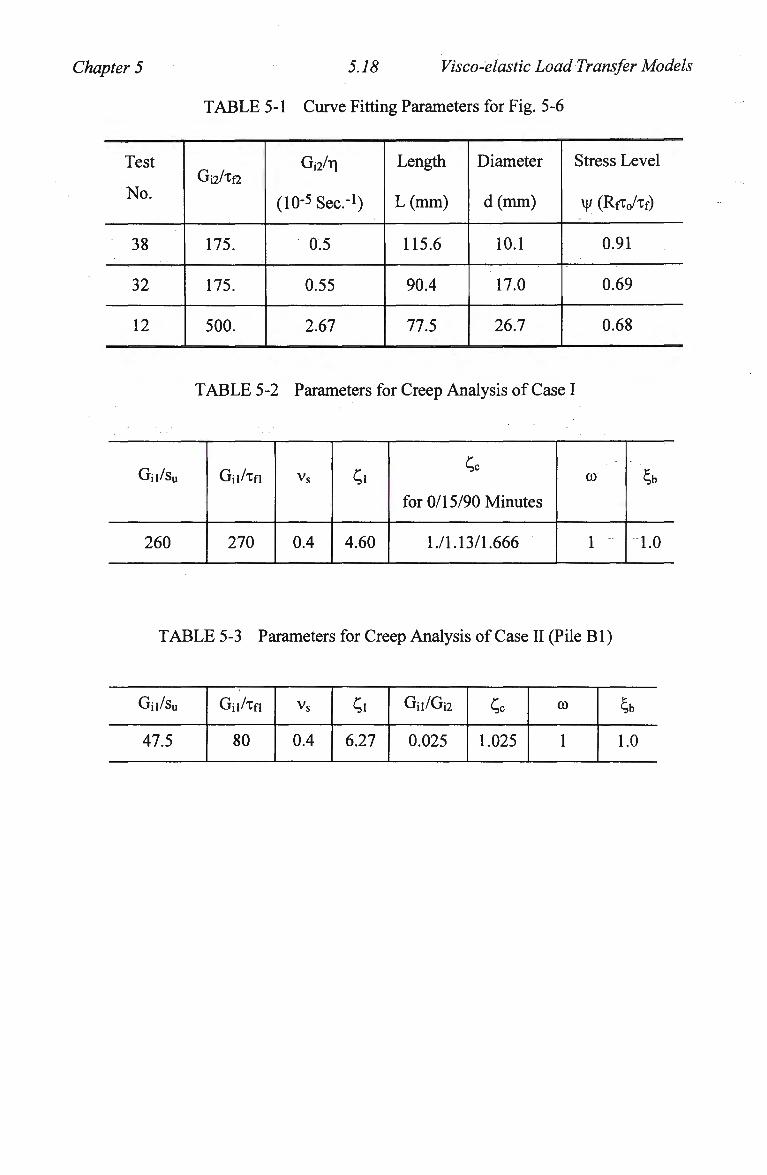
Chapter 5 5.18 Visco-elastic Load Transfer Models
TABLE 5-1 Curve Fitting Parameters for Fig. 5-6
Test
No.
38
32
12
Gi2/Xf2
175.
175.
500.
GoAi
(10-5 Sec."1)
0.5
0.55
2.67
Length
L(mm)
115.6
90.4
77.5
Diameter
d(mm)
10.1
17.0
26.7
Stress Level
\|/ (RfXo/xf)
0.91
0.69
0.68
T A B L E 5-2 Parameters for Creep Analysis of Case I
Gii/su
260
Gii/xfl
270
vs
0.4
Gi
4.60
Co
for 0/15/90 Minutes
l./l.13/1.666
CO
1
^
1.0
T A B L E 5-3 Parameters for Creep Analysis of Case II (Pile B1)
Gii/su
47.5
Gii/xfl
80
vs
0.4
Ci
6.27
Gii/Gi2
0.025
Co
1.025
CO
1
b
1.0
Chapter 6 6.1 Visco-elastic Consolidation
6. PERFORMANCE OF A DRIVEN PILE IN VISCO-ELASTIC MEDIA
6.1 INTRODUCTION
Installation of a driven pile in a clay generally leads to a remoulding of the soil, some
loss in the strength and an increase in pore water pressure in the vicinity of the pile.
Increase in strength with time, subsequent to driving, results in the final soil strength
being equal to, or greater than the initial value (Orrje and Broms, 1967; Flaate, 1972;
Fellenius and Samson, 1976; Bozozuk et al. 1978), accompanied by a gradual decrease
in water content in the clay adjacent to the pile, and increase in the bearing capacity of
the pile (Seed and Reese, 1955).
The maximum pore pressure occurs immediately following driving, and may
approximately equal, or exceed the total overburden pressure in overconsolidated soil
(Koizumi and Ito, 1967; Flaate, 1972). The magnitude of the pore pressures induced due
to driving decreases rapidly with distance from the pile wall, and becoming negligible at
a distance of 5 to 10 pile diameters. This distribution of excess pore pressure around a
driven pile may be simulated with sufficient accuracy using the cylindrical cavity
expansion analogy (Randolph and Wroth, 1979b) or the strain path method (Baligh,
1985, 1986a, 1986b). The former theory, though, is a one-dimensional analysis, has
generally provided sufficient accuracy, compared with the latter analysis. A particular
advantage of the approach is that it can be readily extended to the case of visco-elastic
soil response.
Using a radial consolidation theory, Soderberg (1962), Randolph and Wroth (1979b)
show that the measured rate of development of pile capacity in soft clay appears to be
consistent with the rate of pore pressure dissipation. Therefore, with the assumption of
an impervious pile, the problem of predicting the variation of capacity becomes one of
predicting the hydrostatic excess pressures at the pile shaft as a function of time.
Dissipation of the excess pore pressures generated during driving leads to an increase
not only in shaft friction but also in the stiffness of the surrounding soil (e.g. Eide et al.
1961; Flaate, 1972; Flaate and Seines, 1976; Bergdahl and Hult, 1981; Trenter and Burt,
1981). Accurate prediction of pile behaviour requires determination of the profile of
pile-soil interaction stiffness and limiting shaft friction, which are generally treated as
invariants with time. However, the soil strength is normally significantly altered by pile
driving, which means that the overall pile-soil interaction should be treated as a time-
Chapter 6 62 Visco-elastic Consolidation
dependent problem. Many researchers have emphasised the importance of predicting the
load-settlement behaviour (Olson, 1992; Fleming, 1992; Randolph, 1994), particularly
where piles act as settlement reducers. However, most research conducted to date has
concentrated on the time-dependent bearing capacity, rather than h o w the overall
response is affected by soil reconsolidation following pile driving.
Two basic approaches are commonly used for analysing consolidation problems. The
first was developed from diffusion theory by e.g. Terzaghi (1943) and Rendulic
(reported by Murray, 1978). The second was developed from elastic theory by e.g. Biot
(1941), and more recently by Randolph and Wroth (1979b) for dissipation of pore
pressure generated due to pile driving.
The diffusion theory is generally less rigorous than the elastic theory. However, the
diffusion theory is mathematically much simpler to apply, and can be readily extended
to account for complex conditions, e.g. soil visco-elasticity, soil shear modulus non-
homogeneity. In fact, the diffusion theory is different from the elastic theory in that (1)
the mean total stress is assumed constant; (2) the coefficients of consolidation derived
for the two theories are generally different (Murray, 1978). If the mean total stress
change happens to be zero, the only difference between the two theory is in the
coefficients of consolidation. Therefore, a coefficient from elastic theory m a y be used to
replace the coefficient in the solution of the diffusion theory, then the solution is
converted into a rigorous solution.
In this chapter:
(1) A generalised non-linear visco-elastic stress-strain model is first generated.
(2) A governing equation from the diffusion theory is established for radial
reconsolidation of a visco-elastic medium. By comparing with an available
rigorous elastic solution (Randolph, 1977), a rigorous solution for a visco-elastic
medium is obtained by using a suitable coefficient of consolidation. Alternatively,
rigorous visco-elastic solutions have been obtained by using the correspondence
principle (Mase, 1970), in light of the available elastic solutions.
(3) Equations for radial consolidation for a given logarithmic variation of initial pore
pressure are provided.
(4) Three case studies are described to illustrate the time variation of pore pressure,
pile capacity, average pile shaft cohesion, and average shear modulus.
Chapter 6 6.3 Visco-elastic Consolidation
6.2 NON-LINEAR VISCO-ELASTIC STRESS-STRAIN MODEL
A non-linear visco-elastic model (simply called Mediant's model) has already been
described in Chapter 5 as illustrated in Fig. 6-1(a). In principle, the model is directly
adopted herein, except that a Voigt element is added in series with Mediant's model.
This addition leads to a generalised visco-elastic model, as detailed in Fig. 6-1(b). For a
prolonged constant loading, the stress-strain relationship for the generalised model can
be expressed by
y = xF(t) (6-1)
where x, y are the total shear stress and strain respectively for the model. The creep
compliance, F(t) is given by (Lo, 1961)
F(t) = -!-(l + m2 (1 - exp(- t/T2)) + m3 (l - exp(- (t - tk )/T3))) (6-2)
where m2 = Gyl/Gy2; m3 = Gyl/GY3 ;1/T2 = Gy2/riY2 ; 1/T3 = GY3/r|Y3 ; r^, x\n are
the shear viscosity at visco elements 2 and 3 respectively; G?j is the shear modulus for
each of the elastic springs; tk is a critical time used to determine when the Voigt element
is in action. The value of tk can be assessed by experiment (Lo, 1961). If the elapsed
time, t is less than tk, the Voigt element 2 is not in effect. Therefore, 013 is zero, and the
generalised model reduces to the Mediant's standard linear model as shown in Fig. 6-
1(a).
To account for the soil non-linear response, the shear modulus for each of the elastic
springs, GYj is derived through using a hyperbolic stress-strain model, and may be
expressed by
where kj = 1 - vj/j, v|/j = R^Xj / xf], kj is the coefficient for considering the non-linear
effect on the shear moduli of the elastic springs 1, 2 and 3 (j = 1, 2, and 3) respectively;
Rg is a parameter, which controls the degree of non-linearity for springs 1 to 3
respectively; Xj is the shear stress on element j; xg is the local failure shaft stress for
springs 1 to 3; Gy and Gyj are the initial and the average secant shear modului up to a
strain level of zero and yj respectively for each of the springs 1 to 3.
Chapter 6 6.4 Visco-elastic Consolidation
A number of conclusions about using Mediant's model have been obtained in Chapter
5. These conclusions as described below are generally valid for the current generalised
model as well; as such they are directly adopted in this Chapter:
(1) The limiting shaft stress, xuitj and the failure stress, xg are assumed identical.
(2) A n appropriate value of xuiti can be correlated with the shear strength of the soil,
or with the effective overburden stress (e.g. API RP2A; Tomlinson, 1970;
Randolph and Murphy, 1985). The failure stresses of Xf2, and xo may be assessed
through experiments, and the stresses are generally correlated with the x« e.g. xc
was reported to be approximately equal to 0.7xfi (Geuze and Tan, 1953;
Murayama and Shibata, 1961).
(3) With the model, two types of responses to stress are reflected: instantaneous
elasticity (Gyi) and delayed elasticity (GY2 and/or GY3). At any given time, e.g. at
the onset of loading, the stress-strain response may be modelled as a non-linear
hyperbolic curve. Under a specified stress, the displacement develops as a creep
process.
(4) According to the experiment by Lo (1961), generally secondary deformation of all
remoulded and undisturbed clays can be modelled sufficiently accurately by the
linear standard model, with ni3 = 0. For a soil of loose structure, the generalised
model may be used, with the values of tk and ni3 determined by experiment.
6.3 GOVERNING DIFFUSION EQUATION FOR RECONSOLDDATION
The effect of driving a pile into clay can be simulated by expansion of a long cylindrical
cavity under undrained conditions in an ideal visco-elastic, perfectly plastic material,
characterised by the shear moduli, Gyj (j = 1, 2 and 3) and the undrained shear strength,
su. Experiment shows that the expansion is a plane strain problem for the middle part of
the pile (Clark and Meyerhof, 1972). The soil properties and the stress state
immediately following pile driving have been simplified and illustrated in Fig. 6-2.
6.3.1 Volumetric Stress-strain Relation of Soil Skeleton
In this section, volumetric effective stress-strain relationship is first given for an elastic
medium and then the relationship is converted into that for a visco-elastic medium. The
plane strain version of Hooke's law is
Chapter 6 6.5 Visco-elastic Consolidation
e' = [ ( 1 ~ v - ) 8 c , ' ~ v ' 8 o « ] e 9 = ^ [ - v s 8 a r + ( l - v s ) 8 a e ] (6-4)
E Z = 0
where G is the elastic soil shear modulus; bGt, 8GQ, 8CTZ are the increments of the
effective stresses during consolidation in the radial, circumferential and depth
directions, with 5crz = vs(8ar + 8 a 9 ) . Combining Eq. (6-4) and the effective stress
principle, the volumetric effective stress-strain relationship for plain strain cases may be
written as
ev=i^(80-(u-uo)) (6-5)
where vs is the Poisson's ratio of the soil; 80 is the total mean stress change,
80 = O.5(8ar + 8 a 9 ) ; u is the excess pore pressure; UQ is the initial value following
driving (Randolph and Wroth, 1979b).
Eq. (6-5) is valid for an elastic medium. Similar volumetric expression for visco-elastic
media may be directly transformed from Eq. (6-5), using the correspondence principle
(Mase, 1970), by the following procedures:
(1) applying the Laplace transform to Eqs. (6-1) and (6-2) respectively, allowing the
shear modulus G , to be related to the compliance, F(t) by
F(tj = l/(sG) (6-6)
(2) applying the Laplace transform to Eq. (6-5), and using F(t) to replace the
transformed modulus, G , to give
Ty = (1 - 2vs)sF(t)(o0 - (u^uj) (6-7)
where s is the argument of the Laplace transform.
(3) applying the inverse Laplace transform to Eq. (6-7), to obtain the final expression
of the volumetric strain for visco-elastic media as
Chapter 6 6.6 Visco-elastic Consolidation
l-2v f , N „ V/cn , ^1 dF(t-x) sv GYl
8 0 - ( u - u o ) + G y l j (80-(u-u o ) )| t - ^—-^dx (6-8) d(t - x) )
where sv is the volumetric strain.
The Poisson's ratio is regarded as a constant, and the effect of this assumption is
generally ignored even for numerical analysis (Booker and Poulos, 1976). In fact,
considering the viscous effect on Poisson's ratio would lead to a formidable inverse
Laplace transform.
The total mean stress change, 80 is generally not zero (a constant) with time during
consolidation (Mandel, 1957; Oyer, 1963; Murray, 1978). However, taking it as a
constant (zero) as assumed by Terzaghi (1943) and Rendulic (1936), will significantly
simplify the solution of the problem, and the solution generally compares very well with
the corresponding rigorous solution (Davis and Poulos, 1968; Christian and Boehmer,
1970; Murray, 1978). In fact, as noted by Murray (1978), many of the currently popular
theories are based on this assumption, for instance, the sand drain problem solved by
Barron (1948).
To simply the current problem, it is assumed that 80 = 0. In terms of Eq. (6-8), the
changing rate of volumetric strain may then be expressed by
^ - O ^ v V 1 fdu+ VaudF(t-x)d; U YlJ& d(t-x) .
(6-9) at " G T I
It worth noting that Eq. (6-9) is derived from the stress-strain relationship.
6.3.2 Flow of Pore Water and Continuity of Volume Strain Rate
The volumetric strain rate may be obtained by considering the flow of pore water and
continuity of volume. The pore water velocity may be related to the pressure gradient by
Darcy's law. For continuity, the rate of volumetric strain must be related to the flow of
pore water into and out of any region by (Randolph and Wroth, 1979b)
0e„ k 1 d ( du V
di y w r dr V dr r — (6-10)
where k is the permeability of the soil; and yw is the unit weight of water.
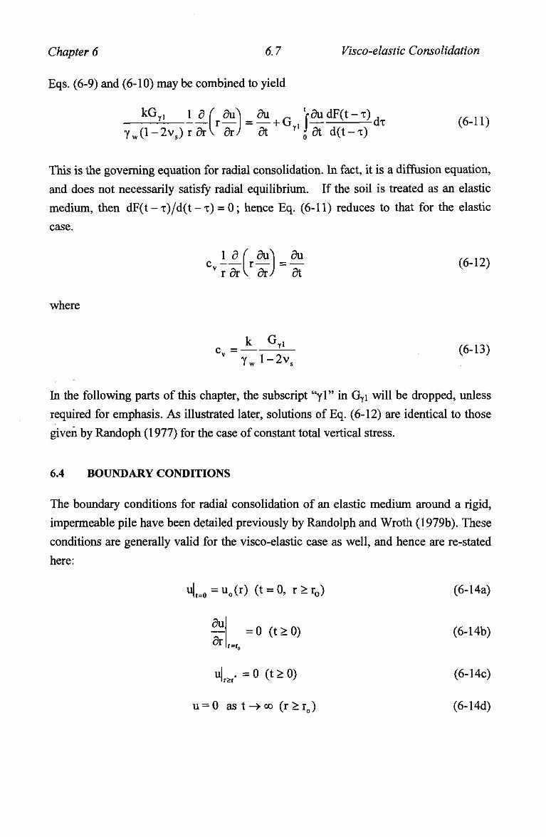
Chapter 6 6.7 Visco-elastic Consolidation
Eqs. (6-9) and (6-10) may be combined to yield
kGyl la^p JJIJFH^ y w ( l - 2 v s ) r d A dr) dt yl
0J dt d(t-x)
This is the governing equation for radial consolidation. In fact, it is a diffusion equation, and does not necessarily satisfy radial equilibrium. If the soil is treated as an elastic
medium, then dF(t - x)/d(t - x) = 0; hence Eq. (6-11) reduces to that for the elastic
case.
1 d ( du] du (, .„ c-7alr¥J = aT (6"12)
where
7w l-2v,
In the following parts of this chapter, the subscript "yl" in GYi will be dropped, unless required for emphasis. As illustrated later, solutions of Eq. (6-12) are identical to those
given by Randoph (1977) for the case of constant total vertical stress.
6.4 BOUNDARY CONDITIONS
The boundary conditions for radial consolidation of an elastic medium around a rigid,
impermeable pile have been detailed previously by Randolph and Wroth (1979b). These
conditions are generally valid for the visco-elastic case as well, and hence are re-stated
here:
<=o=uo(r) (t = 0, r>r0) (6-14a)
= 0 (t>0) (6-14b) du dr
u|rsr. = 0 (t>0) (6-14c)
u = 0 as t->oo (r>r0) (6-14d)
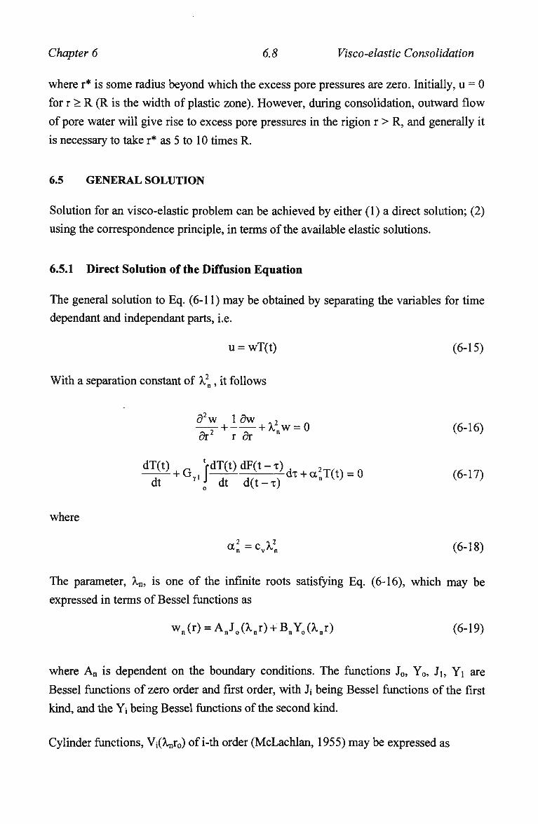
Chapter 6 6.8 Visco-elastic Consolidation
where r* is some radius beyond which the excess pore pressures are zero. Initially, u = 0
for r > R (R is the width of plastic zone). However, during consolidation, outward flow
of pore water will give rise to excess pore pressures in the rigion r > R, and generally it
is necessary to take r* as 5 to 10 times R.
6.5 GENERAL SOLUTION
Solution for an visco-elastic problem can be achieved by either (1) a direct solution; (2)
using the correspondence principle, in terms of the available elastic solutions.
6.5.1 Direct Solution of the Diffusion Equation
The general solution to Eq. (6-11) may be obtained by separating the variables for time
dependant and independant parts, i.e.
u = wT(t) (6-15)
With a separation constant of X2n, it follows
5 w 1 dw ,2 dr x dt
dT(t) + r i fdT(t)dF(t-x)
+ - — + X.„w = 0 (6-16)
* M^f^+^>=° where
<=*X (6-18)
The parameter, Xn, is one of the infinite roots satisfying Eq. (6-16), which may be
expressed in terms of Bessel functions as
wn(r) = AnJ0(A.nr) + BnY0(?,nr) (6-19)
where A n is dependent on the boundary conditions. The functions J0, Y0, Ji, Yi are
Bessel functions of zero order and first order, with Jj being Bessel functions of the first
kind, and the Yj being Bessel functions of the second kind.
Cylinder functions, Vj(A,nr0) of i-th order (McLachlan, 1955) may be expressed as
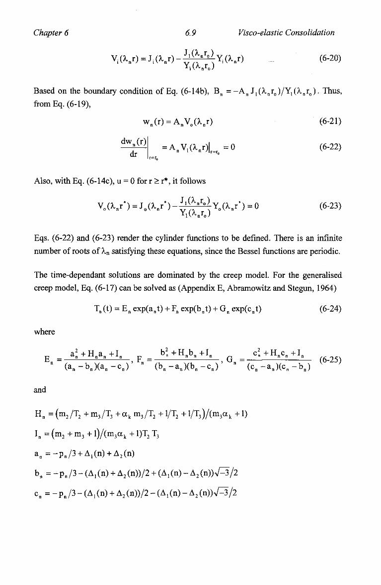
Chapter 6 6.9 Visco-elastic Consolidation
V i M ^ i M - ^ ^ M (6-20) Yi(A.nr0)
Based on the boundary condition of Eq. (6-14b), Bn = -An J,(A,nr0)/Y,(A,nr0). Thus,
from Eq. (6-19),
wn(r) = AnV0(A,nr) (6-21)
dwn(r)
dr = AnV,(A.nr)|r=r = 0 (6-22)
Also, with Eq. (6-14c), u = 0 for r > r*, it follows
V.(V) = J0(V*) ~ V7^HY°(?°nr,) = 0 (6'23) YiO„r0)
Eqs. (6-22) and (6-23) render the cylinder functions to be defined. There is an infinite
number of roots of Xn satisfying these equations, since the Bessel functions are periodic.
The time-dependant solutions are dominated by the creep model. For the generalised
creep model, Eq. (6-17) can be solved as (Appendix E, Abramowitz and Stegun, 1964)
Tn (t) = En exp(ant) + Fn exp(bnt) + Gn exp(cnt) (6-24)
where
a2+Ha +1 b2„+Hnbn+L c2„+Hncn+L
P _ "n x x n n n p _ _ _ n n n - _ ^^j> n n n ,£• rjr\
(an - bn )(an - cn) (bn - an)(bn - cn) (cn - an)(cn - bn)
and
Hn = (m2/T2 + m3/T3 + «k m3/T2 + 1/T2 + l/T3)/(m3cck +1)
K = (m2 + m3 + l)/(m3«k + 1)T2 T3
a„=-P„/3 + A1(n) + A2(n)
bn=-p„/3-(A1(n) + A2(n))/2 + (A1(n)-A2(n))V::3/2
cn=-pn/3-(A,(n) + A2(n))/2-(A1(n)-A2(n))V=3/2
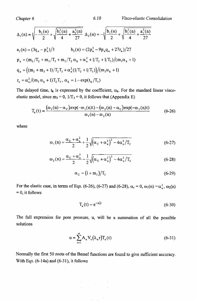
Chapter 6 6.10 Visco-elastic Consolidation
A, ( n ) H ).^+j^)+^> &Aa),-f-f+JMiE)+5M ax(n) = (3qn -pJ)/3 bT(n) = (2p
3n -9Pnqn +27rn)/27
pn = (m2/T2 + m3/T3 + m3/T2 ak + a2 + 1/T2 + l/T3)/(m3ak +1)
qn =((m2 +m3 +1)/T2T3 +a2n(l/T2 +l/T3))/(m3ak +1)
rn = «a Am3 <*k + 1)T2T3, ak = 1 - exp(tk /T3)
The delayed time, tk is expressed by the coefficient, ak. For the standard linear visco-
elastic model, since m3 = 0, I/T3 = 0, it follows that (Appendix E)
Tm (co1(n)-ac)exp(-co1(n)t)-(co2(n)-ac)exp(-co2(n)t) 1 n (t) = — — (6-26)
co,(n)-co2(n)
where
«>i(n) = ^ + ( a c + a ; )2 - 4 a ; / T 2 (6-27)
»2(n) = ^y^-^(ac+a2n)
2-4a2/T2 (6-28)
ac=(l + m2)/T2 (6-29)
For the elastic case, in terms of Eqs. (6-26), (6-27) and (6-28), ac = 0, ©i(n) =a2, co2(n)
= 0, it follows
Tn(t) = e-a"t (6-30)
The full expression for pore pressure, u, will be a summation of all the possible
solutions
u = I>nV0MTn(t) (6-31) n=l
Normally the first 50 roots of the Bessel functions are found to give sufficient accuracy.
With Eqs. (6-14a) and (6-31), it follows
Chapter 6 6.11 Visco-elastic Consolidation
An = Ju0(r)V0(rt..)rdr / }v2(r^n)rdr (6-32)
6.5.2 Rigorous Solutions for the Radial Reconsolidation
For the elastic case, the above established solutions reduce to the rigorous solutions
from the elastic theory by Randoph (1977) for the case of constant total vertical stress.
The difference in the solutions from the current diffusion theory and the elastic theory
(by Randolph and Wroth, 1979b) is just the coefficient of consolidation, since 80 = 0.
Therefore, the above solutions may be readily transformed into the case of plane strain
deformation by simply replacing the cv of Eq. (6-13) with
k 2(l-v.)GT, c v = — (6-33)
Yw l"2vs
Considering non-linear soil stress-strain response, a lower value of the shear modulus
will generally result, as shown by Eq. (6-3). Therefore, the consolidation time increases
by a factor of 1/(1 -i|/j) as demonstrated by Eq. (6-30). The stress level, VJ/J here is an
average value for the domain concerned. For convenience, it may be taken as 0.5 as
argued previously in Chapter 3.
6.5.3 Solution By Correspondence Principle
The above visco-elastic solutions may be readily obtained, in terms of the elastic
solutions, by the correspondence principle. From Eq. (6-31)
u = EAnt;V0(^nr) (6-34) n=l
For the visco-elastic analysis given by the standard linear model, the time-dependant
part should be replaced with (Appendix E),
t7 = S-±^£ (6_35) (s + co,(n)Xs + co2(n))
For the elastic analysis, the time-dependant part should be replaced with
T~n=l/(s + al) (6-36)
Chapter 6 6.12 Visco-elastic Consolidation
The inverse Laplace transform of Eqs. (6-35) and (6-36) (referred to Appendix E) leads
to Eqs. (6-26) and (6-30) respectively. That is to say, the visco-elastic solutions can be
formulated by simply replacing the time-dependent part of the elastic solutions with that
for the visco-elastic case.
6.6 CONSOLIDATION FOR LOGARITHMIC VARIATION OF u0
The initial stress state for radial consolidation of a visco-elastic medium around a rigid,
impermeable pile is similar to that of an elastic medium (Randolph and Wroth, 1979b),
as described below:
(1) For a cavity expanded from zero radius to a radius of r0 (pile radius), the stress
change, 80 within the plastic zone (r0 < r < R as shown in Fig. 6-2) is given by
80 = su(ln(G/su)-21n(r/ro)) (6-37)
(2) The width of the plastic zone is given by
R = r0(G/su)1/2 (6-38)
(3) Under undrained conditions, if the mean effective stress remains constant, the
initial excess pore pressure distribution away from pile wall varies according to
u0(r) = 2suln(R/r) r0<r<R ((J_39)
u0 = 0 R < r < r*
where R is the radius, beyond which the excess pore pressure is initially zero.
In light of the initial pore pressure distribution of Eq. (6-39), the coefficients can be
simplified as
4s, V.fr.Q-V.fr.R)
»?. r-2V,>(V)-rX(V0)
With these values of An, the pore pressure can be readily estimated with Eq. (6-31).
Evaluation of these functions has been carried out in a spreadsheet.
Chapter 6 6.13 Visco-elastic Consolidation
With the correspondence principle, the elastic solution of the outward radial movement,
£r by Randolph and Wroth (1979b) can be extended to the visco-elastic case as
$< =
Sr =
1 2G' Xn \ V r yRJ) n=l
2G" VA°T-(t)V-^Akh(4)-r:^) n=l
R.
R* jo
( r 0 < r < R ) (6-41)
(R < r < r*) (6-42)
where G* = G T l /(l-2v,), R* = R V e . The T„(t) is given by Eqs. (6-24), (6-26) and
(6-30) respectively, dependent on which model is adopted.
The rate of consolidation may be expressed by the following non-dimensional variable
(Soderberg, 1962),
T = cvt/r02
The visco-elastic effect may be represented by the factor,
Tc=(l + m2)/(T2cv)
(6-43)
(6-44)
A parametric study has been undertaken for the solutions based on standard linear
model. Fig. 6-3 shows the consolidation expressed as u(r0)/su (u(r0) is the pore pressure
on pile-soil interface) for a soil with Gyi/su = 50, but at different ratios of primary and
secondary shear moduli, Gyi/Gy2 and various values of the viscosity factor, Tc. Provided
that other input parameters are identical, variation of the relaxation factor, I/T2 can only
shift the dissipation curve of pore pressure at the middle stage of the process, but not the
initial or the final stages. Generally speaking, the viscosity effect becomes obvious only
at a later stage.
Fig. 6-4 shows a set of plots of the non-dimensional times for 50% (T50) and 90% (T90)
degree of consolidation to occur at different values of Uo(r0)/su and Gyi/Gy2 (Uo(r0) is the
initial pore pressure on pile-soil interface immediately following pile installation).
Considering the secondary consolidation by the ratio of Gyi/Gy2, higher values of T50
and T90 are obtained compared with those from elastic analysis (Gyi/Gy2 = 0).
Accordingly longer consolidation times and higher displacements occur compared with
the elastic case.
Chapter 6 6.14 Visco-elastic Consolidation
The rules shown in Figs. 6-3 and 6-4 are applicable for both cases of constant total
stress and plane strain deformation. The corresponding coefficient of consolidation, cv,
may be used for each case.
6.7 VISCO-ELASTIC BEHAVIOUR
6.7.1 Parameters for the Creep Model
The magnitude of the relaxation time has been provided in Table 6-1, based on the
relevant publications (Edil and Mochtar, 1988; Qian et al. 1992; Ramalho Ortigao and
Randolph, 1983).
In particular, as reviewed in the previous chapter, the experiment by Lo (1961) showed
that
(1) The rate factor, Gy2/rjY2, is generally a constant for a given clay. For the clays
tested, it lies between 0.2 and 0.4 (xlO'V1).
(2) The compressibility index ratio, Gyi/Gy2, is only influenced by the soil water
content, and generally lies between 0.05 and 0.2, except for a soil of loose
structure.
(3) The individual values of Gyi, Gy2 and t|y2, however, vary with load (stress) level.
6.7.2 Prediction of the Ratio of Modulus and Limiting Shaft Stress
Experimental results (Clark and Meyerhof, 1972) show that:
(1) during a loading test, the change in pore water pressure along the shaft of the pile
is insignificant;
(2) the magnitude of the total and effective radial stress surrounding the pile is
primarily related to the stress changes brought about when the pile is driven and
during subsequent consolidation. Changes with time due to loading are
insignificant relative to the initial values.
Therefore, the ratio of Gyi/xn may generally be assumed to be a constant during a
loading test, so that it can be estimated from the measured load-settlement curve by
fitting theoretical solutions (e.g. by GASPILE). Soil stress-strain non-linearity has only
limited effect on such a back-analysis. Because the overall response of a pile by elastic
analysis are barely different from that by a non-linear elastic as shown in Chapter 3.
Chapter 6 6.15 Visco-elastic Consolidation
6.7.2.1 Example Study
The recovery of the soil strength and modulus during reconsolidation was investigated
previously (e.g. Trenter and Burt, 1981) by a series of loading tests performed at
different time intervals following installation of a pile. Through fitting the measured
load-settlement curve with the theoretical solutions (GASPILE analysis), the soil
strength and modulus are back-figured. From the series of loading test results, a series
of the strength and the corresponding shear modulus are obtained corresponding to the
test time interval; and then these values of strength and modulus are normalised by the
initial values respectively.
Test Reported by Trenter and Burt (1981)
Four driven open ended pile load tests were performed in Indonesia, mainly by
maintained load procedure (Trenter and Burt, 1981). The basic pile properties are
shown in Table 6-2; Young's modulus of the pile is assumed as 29,430 M P a (the effect
of this assumption is explored later). The undrained shear strength of the subsoil at the
site varies basically according to s„ = 1.5z (su, kPa; z, depth, m ) . The initial shear
modulus is taken as a multiple of the undrained shear strength, su, the ratio G/su being
back-analysed from the test data. There is no information about the values of the creep
parameters. However, based on previous publications, shear modulus ratio, Gyi/Gy2,
may be reasonably taken as 0.15, and rate factor, Gy2/r|y2, taken as, 0.5xl0"5 (s"1). Using
these assumed values, the variation of normalised soil strength and shear modulus with
with time during consolidation is not affected, as justified later.
The accuracy of the load transfer factor, C,\ given by Eq. (3-7) has been testified (against
the available rigorous numerical solutions shown in Fig. 4-15 in Chapter 4) up to a
slenderness ratio, L/r0, of 180. As for a higher slenderness ratio, the slenderness ratio
used in the Eq. (3-7) may be replaced with a critical pile slenderness ratio, which is
defined as 3y/X (Fleming et al. 1992), but this definition is recursive. For the current
example, the interest is to find the normalised variations of shear strength and modulus
with time. Therefore, the accuracy of the load transfer factor becomes relatively
unimportant. For convenience, the load transfer factor is simply estimated with A = 2.5
(for infinite layer case), and the pile slenderness ratios. The input parameters have been
detailed in Table 6-2. Using G A S P I L E analysis, the relevant average values are back-
figured and shown in Tables 6-3 to 6-5. From the measured load-settlement curves, pile-
head displacements have reached 4 % and 6.3% of the diameter for pile 4 and 3
Chapter 6 6.16 Visco-elastic Consolidation
respectively, when the piles reaches their ultimate capacities. Therefore, according to
Eq. (5-26) in Chapter 5, the value of Gyi/xfi for pile 3 (Table 6-4) should be lower than
that for pile 4 (Table 6-3).
In light of the measured data, the back-analysis of the overall pile response by
G A S P I L E program has been illustrated in Fig. 6-5 (pile 2), Fig. 6-6 (pile 4) and Fig. 6-7
(pile 3) individually. A list of the abbreviations used in the figures has been detailed in
Table 6-6. For pile 4 at 1.7 and 10.5 days, the following analyses have been undertaken:
non-linear elastic (NLE), non-linear visco-elastic (NLVE), linear elastic (LE), and linear
visco-elastic (LVE). However the difference amongst these analyses are so small, as
shown in Fig. 6-5, that only non-linear visco-elastic and linear elastic analyses are
shown in the other cases.
The shaft resistance was analysed in terms of total and effective stress using the
following expressions
xfl=asu (6-42)
t„ = Pa'vo (6-43)
where aw is the effective overburden pressure; xn is the limiting shaft stress, a is the
average pile soil adhesion factor in terms of total stress; p" is the average pile soil
adhesion factor in terms of effective stress. The corresponding parameters (a, P) have
been estimated by Trenter and Burt (1981) as tabulated in Table 6-7. Using each of the
estimated data at 1.7 days to normalise the rest, a consistency between the increase in
the non-dimensional strength and shear modulus with consolidation of soil is
demonstrated as shown in Table 6-8. More generally, strength increases logarithmically
with time (Bergdahl and Hult, 1981; Sen and Zhen, 1984), but obviously the increase
should be limited.
Analysis shows that to fit a measured load-settlement curve by GASPILE analysis
through selecting (1) different Young's modulus of a pile, (2) different ratio of creep
moduli, Gyi/Gy2, and even (3) the load transfer factor, £, only the initial shear modulus
needs to be changed. Young's modulus of the pile, creep moduli and the load transfer
factor have been taken constants for each of pile at different stages of consolidation, in
the back-analysis of initial shear modulus from the load-settlement curves; hence, the
obtained relationships of non-dimensional values versus time, as shown in Table 6-8,
are not affected by the selected values.
Chapter 6 6.17 Visco-elastic Consolidation
This example demonstrates that (1) the pile-soil interaction stiffness increases
simultaneously as soil strength regains; (2) secondary compression of clay only accounts
for a small fraction of the settlement of the pile.
6.8 CASE STUDY
Theoretical prediction of the pore pressure dissipation is provided using the radial
consolidation theory, and compared with the following non-dimensional parameters:
(1) the difference of the measured (if available) pore pressure, UQ-U normalised by the
initial value, Uo;
(2) the back-figured shear modulus normalised by the value at tc>o;
(3) the back-figured limiting shear strength normalised by the value at t9o-
(4) the measured time-dependent pile bearing capacity normalised by the value at tgo.
The shear modulus and limiting strength with time have been back-analysed in a similar
manner as described in section 6.7.2.1, using the measured load-settlement curves at
different times following pile driving. Also the values at t9o were obtained through
interpolation. The theoretical predictions are based on assumption of plane strain
deformation for each case study and are expressed in the form of (uo-u)/u0.
6.8.1 Tests reported by Seed and Reese (1955)
To assess the change in pile bearing capacity with reconsolidation of soil following pile
installation, Seed and Reese (1955) performed instrumented pile loading tests at
intervals after driving. The pile, of radius 0.0762 m, was installed through a sleeve,
penetrating the silty clay from a depth of 2.75 to 7 m. The Young's modulus is 2.07x
10 M P a and the cross sectional area is 9.032 c m . Therefore, the equivalent pile
modulus can be inferred as 10,250 MPa.
Through fitting the measured load-settlement response by the GASPILE program
analysis (Fig. 6-8), values of Gyi, xn were back-figured from each load-settlement
curves. These values are tabulated in Table 6-9. In terms of Poisson's ratio, vs = 0.49,
permeability k = 2x10" m/s, cv = 0.0529 m /day, the 9 0 % degree of reconsolidation is
estimated to occur at t9o = 8.76 days (T90 = 74.43, Gyi/xn = 350). From Table 6-9, at the
time of tgo, the shear modulus is about 3.55 MPa, which is less than 9 0 % of the
maximum value of 4.5 M P a at 33 days. The shaft friction is estimated as about 11.6 kPa
Chapter 6 6.18 Visco-elastic Consolidation
compared with the final pile-soil friction of 12.6 kPa, which is a fraction of the initial
soil strength of 18 kPa, due to soil sensitivity.
The back-figured shear modulus and the limiting strength have been normalised by the
values at tgo and plotted in Fig. 6-9(a) together with the normalised measurements and
predicted dissipation of pore water pressure.
Assuming Gyi/Gy2 = 1, the visco-elastic analysis leads to tgo = 16.35 days (Tgo= 148.85,
Gyi/xfi = 350). Also from Table 6-9, at this t9o, the corresponding shear modulus is
about 4.06 M P a , which is about 9 0 % of the final value, 4.5 M P a at 33 days. The shaft
friction is about 12.54 kPa. The normalised data by these visco-elastic estimations are
shown in Fig. 6-9(b) together with the measurement and predictions.
Elastic analysis can give reasonable predictions of shear strength or pile capacity
variation, but not the overall pile behaviour, particularly the deformation, as further
explored in the next case study.
6.8.2 Tests reported by Konrad and Roy (1987)
Konrad and Roy (1987) reported the results of an instrumented pile, loaded to failure at
intervals after driving. The pile, of outside radius 0.219 m, and wall thickness 8.0 m m ,
was jacked closed-ended to a depth of 7.6 m below ground level. The Young's modulus
is 2.07x10 M P a and the cross sectional area is about 53.03 c m . Therefore, the
equivalent pile modulus is inferred as 29,663 MPa.
The increase in shaft capacity was reported by Konrad and Roy (1987) and has been
normalised by that at 2 years after installation. The normalised values are shown to be
generally consistent with the normalised dissipation of pore pressure measured at three
depths of 3.05,4.6, and 6.1 m as illustrated in Fig. 6-10(a) and (b).
In terms of conventional elastic analysis, from the initial load-settlement response
measured at different time intervals after pile installation, an initial value of Gyi/su =
270 has been back-analysed (Chapter 5). From the final load-settlement relationships at
different time intervals, the values of Gyi/su are found to be almost a constant of 210-
230, with a value of Gyi/GY2 = 2. The shear modulus and the shear strength (being
assumed to increase linearly with depth) have been back-figured through fitting the
Chapter 6 6.19 Visco-elastic Consolidation
measured response with the visco-elastic GASPILE analysis, and are tabulated in Table
6-10.
The visco-elastic analysis gives a satisfactory agreement with the measured response at
b w load levels of about 7 0 % ultimate load (Fig. 6-11). The visco-elastic analysis gives
a better prediction than the elastic analysis (Fig. 6-12) in comparison with the measured
response, particularly at higher load levels (being greater than 7 0 % ) . Due to the marked
non-linear soil response of the base (Chapter 5), the visco-elastic analysis is still
significant different from the measured response at high load levels. The prediction may
be improved, if the non-linear base response and the variation of C,\ with load level is
accounted for. However, the current analysis is sufficiently accurate for assessing the
interested values: the variation of shear strength and modulus with reconsolidation.
The value of the coefficient of consolidation has been estimated as cv = 0.0423 m /day
(vs = 0.45, Konrad and Roy, 1987). Using elastic analysis, the time factor for 9 0 %
degree of consolidation, T90, is about 65, with Gyi/su = 230 from Fig. 6-4; hence, tgo «
18 days. From Table 6-10, at the time of t9o, the shear strength at the pile base level is
estimated to be 22.4 kPa, which is in good agreement with the value of 23.0 kPa
obtained as 9 0 % of limiting stress, xn (xn = 25.64 kPa); while the corresponding
modulus is 4.79 M P a , which is slightly lower than 5.08 M P a obtained as 9 0 % of the
maximum shear modulus (5.64 MPa). Using visco-elastic analysis, with Gyi/GY2 = 2, T90
= 205.1, tgo is estimated to be about 57 days, the corresponding values are xn = 23.99
kPa and Gyi = 5.16 M P a by interpolation from the data given in Table 6-10.
With the above estimated values at tgo, the normalised variations are plotted in Fig. 6-
11(a) and (b) respectively for elastic and visco-elastic analyses, together with the
theoretical curves of dissipation of pore water pressure. The predicted values at the
initial stage are lower than the measured data, probably due to the radial soil non-
homogeneity (Appendix E). Radial non-homogeneity can also retard the regain in the
average shear modulus (at some distance away from the pile axis). Therefore, a
comparatively higher value of t9o for the modulus regain is expected than the current
prediction. Using modulus at the t9o (interpolated by Table 6-10) to normalise the rest
values can only lead to a lower trend than the current prediction as shown in the figure.
Soil strength may increase due to reconsolidation, but it may also decrease due to creep
(Creep causes soil strength reduce, until finally the strength approaches to a long term
strength, which is about 7 0 % of the soil strength). The effect of reconsolidation and
Chapter 6 6.20 Visco-elastic Consolidation
creep on the soil strength may offset in this particular case. However, since the creep
leads to an increase in settlement, only with a visco-elastic analysis, (e.g. with a value of
Gyi/Gy2 = 2 for the current example), can an excellent prediction be made as shown in
Fig. 6-11 for final settlement and Fig. 5-15 (Chapter 5) for a time-dependent process.
6.8.3 Comments on the Current Predictions
The back-figured values of Gyi/Gy2 for the two case studies are higher than those
reported by Lo (1961). The reason for this may be that the former are based on field
tests, while the latter are based on confined compression (oedometer) tests. The current
radial consolidation theory is based on a homogeneous medium. However, as just
argued, radial non-homogeneity can alter the shape of the time-dependent curve at
initial stage and increase the time for regain of shear modulus.
6.9 CONCLUSIONS
The research outlined here has attempted to offer a prediction of the overall response of
a pile following driving, rather than just the pile capacity. A number of important
conclusions can be drawn:
(1) Visco-elastic solutions can be obtained by (a) solving diffusion theory and then
using an accurate coefficient of consolidation; or (b) the available elastic solutions
using the correspondence principle.
(2) The viscosity of a soil can significantly increase the consolidation time, hence
increase the pile-head settlement. However, it has negligible effect on soil
strength or pile capacity.
(3) Almost all the case studies show that the variation of the normalised pile-soil
interaction stiffness (or soil shear modulus) due to reconsolidation is consistent
with that of the pore pressure dissipation on the pile-soil interface and that of
increase in soil strength. Therefore, the time-dependent properties following pile
installation can be sufficiently accurately predicted by the radial consolidation
theory. With the predicted time-dependent parameters, it is also straightforward to
obtain load-settlement response at any times following driving by either
GASPILE analysis or the previous closed form solutions (Chapters 3, 4 and 5).
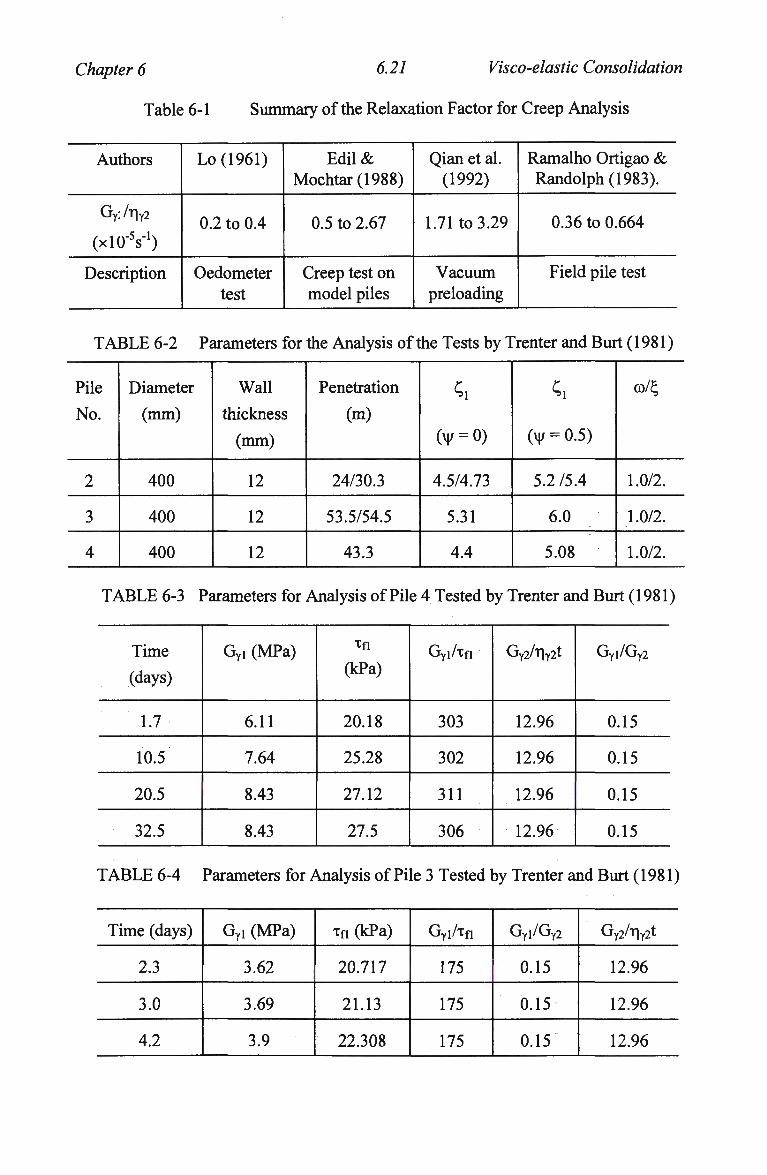
Chapter 6 6.21 Visco-elastic Consolidation
Table 6-1 Summary of the Relaxation Factor for Creep Analysis
Authors
Gy;/ny2
(xl0V)
Description
Lo(1961)
0.2 to 0.4
Oedometer test
Edil& Mochtar (1988)
0.5 to 2.67
Creep test on model piles
Qian et al. (1992)
1.71 to 3.29
Vacuum preloading
Ramalho Ortigao & Randolph (1983).
0.36 to 0.664
Field pile test
T A B L E 6-2 Parameters for the Analysis of the Tests by Trenter and Burt (1981)
Pile
No.
2
3
4
Diameter
(mm)
400
400
400
Wall
thickness
(mm)
12
12
12
Penetration
(m)
24/30.3
53.5/54.5
43.3
Si
(V = 0)
4.5/4.73
5.31
4.4
S,
(v|/ = 0.5)
5.2 /5.4
6.0
5.08
co/4
1.0/2.
1.0/2.
1.0/2.
T A B L E 6-3 Parameters for Analysis of Pile 4 Tested by Trenter and Burt (1981)
Time
(days)
1.7
10.5
20.5
32.5
Gyi (MPa)
6.11
7.64
8.43
8.43
Xfl
(kPa)
20.18
25.28
27.12
27.5
GYi/xfi
303
302
311
306
GY2/riY2t
12.96
12.96
12.96
12.96
GYi/GY2
0.15
0.15
0.15
0.15
T A B L E 6-4 Parameters for Analysis of Pile 3 Tested by Trenter and Burt (1981)
Time (days)
2.3
3.0
4.2
GYi (MPa)
3.62
3.69
3.9
xn (kPa)
20.717
21.13
22.308
Gyi/xfi
175
175
175
Gyi/GY2
0.15
0.15
0.15
GY2/nY2t
12.96
12.96
12.96
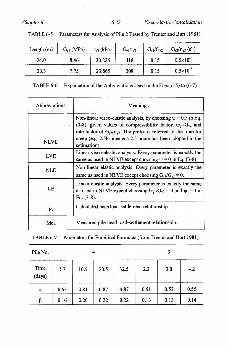
Chapter 6 6.22 Visco-elastic Consolidation
TABLE 6-5 Parameters for Analysis of Pile 2 Tested by Trenter and Burt (1981)
Length (m)
24.0
30.3
GYi (MPa)
8.46
7.75
Tfi (kPa)
20.225
23.865
GYi/xfi
418
308
GYi/GY2
0.15
0.15
Gy2/riY2 (s"1)
0.5xl0"5
0.5xl0"5
T A B L E 6-6 Explanation of the Abbreviations Used in the Figs.(6-5) to (6-7)
Abbreviations
NLVE
LVE
NLE
LE
Pb
Mea
Meanings
Non-linear visco-elastic analysis, by choosing \|/ = 0.5 in Eq.
(3-8), given values of compressibility factor, GYi/GY2 and
rate factor of GY2/r|Y2. The prefix is referred to the time for
creep (e.g. 2.5hr means a 2.5 hours has been adopted in the
estimation).
Linear visco-elastic analysis. Every parameter is exactly the
same as used in N L V E except choosing u/ = 0 in Eq. (3-8).
Non-linear elastic analysis. Every parameter is exactly the
same as used in N L V E except choosing GYi/GY2 = 0.
Linear elastic analysis. Every parameter is exactly the same
as used in N L V E except choosing Gyi/Gy2 = 0 and i|/ = 0 in
Eq. (3-8).
Calculated base load-settlement relationship
Measured pile-head load-settlement relationship.
T A B L E 6-7 Parameters for Empirical Formulas (from Trenter and Burt 1981)
Pile No.
Time
(days)
a
P
4
1.7
0.63
0.16
10.5
0.81
0.20
20.5
0.87
0.22
32.5
0.87
0.22
3
2.3
0.51
0.13
3.0
0.53
0.13
4.2
0.55
0.14
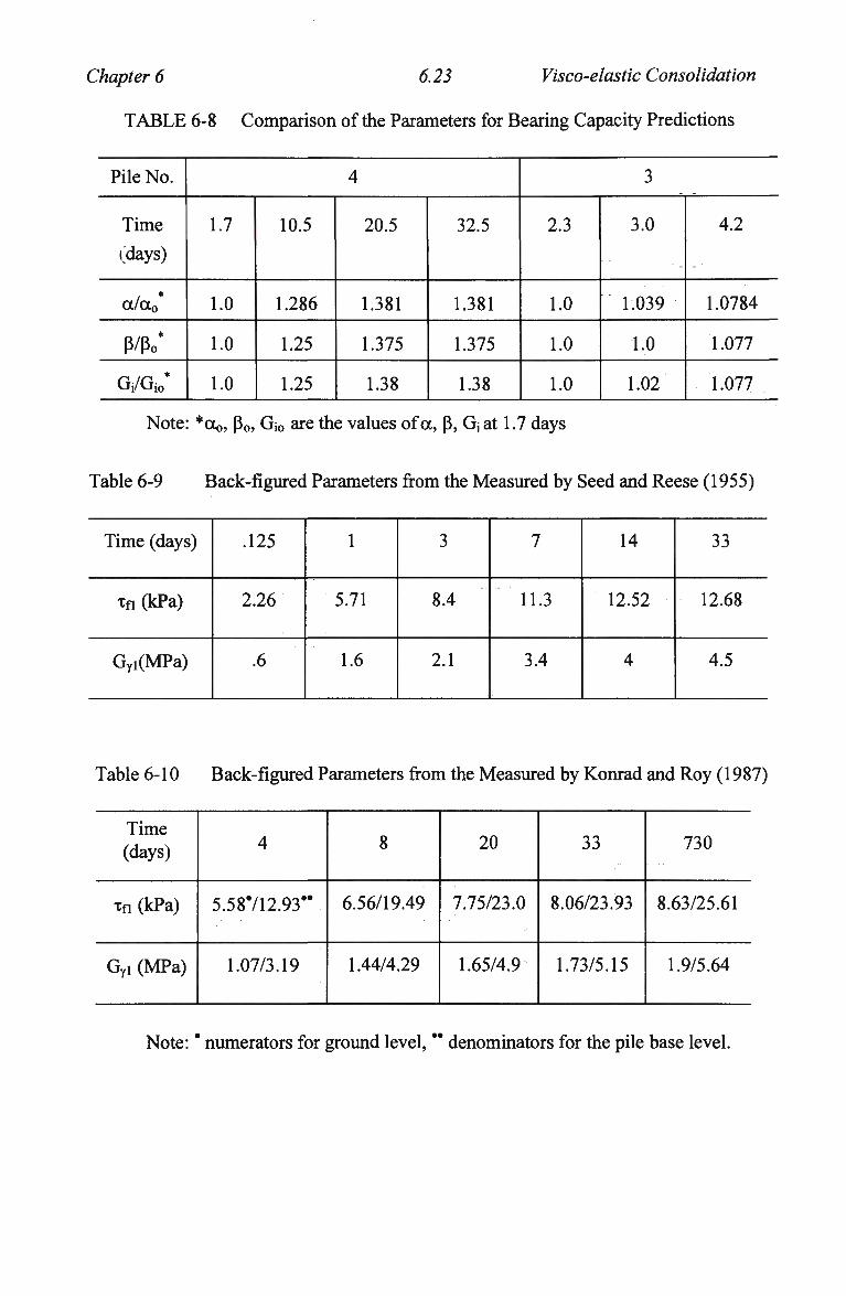
Chapter 6 6.23 Visco-elastic Consolidation
TABLE 6-8 Comparison of the Parameters for Bearing Capacity Predictions
Pile No.
Time
(days)
a/a0
P/Po*
Gj/Gjo
4
1.7
1.0
1.0
1.0
10.5
1.286
1.25
1.25
20.5
1.381
1.375
1.38
32.5
1.381
1.375
1.38
3
2.3
1.0
1.0
1.0
3.0
1.039
1.0
1.02
4.2
1.0784
1.077
1.077
Note: *a0, po, Gj0 are the values of a, P, Gj at 1.7 days
Table 6-9 Back-figured Parameters from the Measured by Seed and Reese (1955)
Time (days)
xn (kPa)
Gyi(MPa)
.125
2.26
.6
1
5.71
1.6
3
8.4
2.1
7
11.3
3.4
14
12.52
4
33
12.68
4.5
Table 6-10 Back-figured Parameters from the Measured by Konrad and Roy (1987)
Time (days)
xn (kPa)
Gyi (MPa)
4
5.58712.93"
1.07/3.19
8
6.56/19.49
1.44/4.29
20
7.75/23.0
1.65/4.9
33
8.06/23.93
1.73/5.15
730
8.63/25.61
1.9/5.64
Note: * numerators for ground level, " denominators for the pile base level.
Chapter 7 7.1 Settlement of Pile Groups
7. SETTLEMENT OF PILE GROUPS IN NON-HOMOGENEOUS SOIL
7.1 INTRODUCTION
Various numerical approaches have been proposed for analysing the settlement of pile
groups. Generally, the approaches are based on either (a) a direct and complete analysis
of the whole pile group, or (b) the superposition principle through using interaction
factors.
Direct analysis is generally achieved through boundary element approach, for example,
Butterfield and Banerjee, (1971), and Butterfield and Douglas, (1981). The analysis is
relatively accurate and rigorous, but requires long computation time and large computer
storage space. Therefore, so far, only relative small groups, e.g., 8 x 8 , have been
analysed. The approach is therefore limited for practical analysis of large piled groups.
Using interaction factors (e.g. Poulos and Davies, 1980), analysis based on the
superposition principle is generally more efficient and straightforward. However, at
present, a numerical technique such as the boundary element approach ( B E M ) is usually
adopted for direct analysis of two equally loaded piles, so as to obtain the interaction
factors. Randolph and Wroth (1979c) suggested a simple way to estimate the interaction
factors. However, in their approach, the shaft and base components were considered
separately; thus, an iterative procedure is needed for compressible pile groups. Based on
simple solutions by Randolph and Wroth (1978), Lee (1993a) gave an approximate
equation for direct evaluation of the interaction factors for both rigid and compressible
pile groups.
Mandolini and Viggiani (1996) proposed a numerical approach for estimating the
settlement of large piled groups. They also used B E M analysis to obtain the value of the
pile-pile interaction factors, from which the superposition principle is then utilised to
estimate the settlement of each pile in a group, assuming either a rigid or fully flexible
pile cap.
For a pile group in a finite layer, the pile-pile interaction should reduce significantly due
to the reduction of the shaft load transfer factors. However, none of the closed solutions
available can account for the reduction.
Chapter 7 7.2 Settlement of Pile Groups
This chapter presents
(1) an extension of the exact closed form solutions for the response of single piles
(Chapter 3) to piles within a group, with the soil stiffness increasing with some
power of depth (Booker et al. 1985);
(2) closed form expression for interaction factors for two identical piles;
(3) a numerical program, GASGROUP, for analysing large piled groups, using the
superposition principle, with interaction factors being given by the closed form
expression;
(4) a number of case studies.
The expression of interaction factors based on load transfer approach is verified
extensively by the results from more rigorous numerical analyses provided by Poulos
and Davis (1980), Cheung et al. (1988), Chin et al. (1990) and Lee (1993a). Pile group
stiffness obtained by the G A S G R O U P program is compared with that from the more
rigorous numerical approach by Butterfield and Banerjee (1971), Banerjee and Davies
(1977), and Poulos (1989) for groups in an infinite layer; and by Butterfield and
Douglas (1981) for pile groups embedded in different finite layers.
7.2 ANALYSIS OF A SINGLE PILE IN A GROUP
Closed form solutions for a pile in a non-homogeneous soil have been generated in
Chapter 3 for the case where the elastic shear modulus of the soil varies with depth
according to
G = Agzn (7-1)
where n is the power of the depth variation (referred to as the shaft non-homogeneity
factor) and A g determines the magnitude of the shear modulus. The shear modulus
below the base of the pile is assumed constant at Gb = GJt^ (with a value of £& = 1 in
this chapter).
In order to allow for the presence of neighbouring piles, following Randolph and Wroth
(1979c), the resulting load transfer factors for a pair of piles are
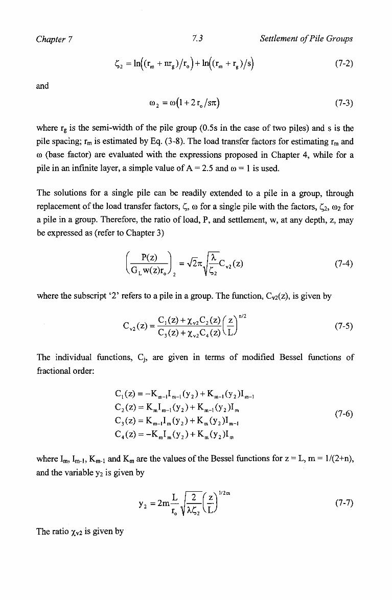
Chapter 7 7.3 Settlement of Pile Groups
;2 = ln((rm + nrg )/r0) + ln((rm + rg )/s) (7-2)
and
co2 =co(l + 2r0/s7t) (7-3)
where rg is the semi-width of the pile group (0.5s in the case of two piles) and s is the
pile spacing; rm is estimated by Eq. (3-8). The load transfer factors for estimating rm and
co (base factor) are evaluated with the expressions proposed in Chapter 4, while for a
pile in an infinite layer, a simple value of A = 2.5 and co = 1 is used.
The solutions for a single pile can be readily extended to a pile in a group, through
replacement of the load transfer factors, , co for a single pile with the factors, Qi, ©2 for
a pile in a group. Therefore, the ratio of load, P, and settlement, w, at any depth, z, may
be expressed as (refer to Chapter 3)
P(z) = V27tl^Cv2(z) (7-4)
.GLw(z)r0.
where the subscript '2' refers to a pile in a group. The function, CV2(z), is given by
C3(z) + Xv2C4(z)VLy
The individual functions, Cj, are given in terms of modified Bessel functions of
fractional order:
Ci(z) = -Km_1Im_1(y2) + Km_1(y2)Im_1
C2(z) = KmIm_1(y2) + Km_1(y2)Im
C3(z) = Km_1Im(y2) + Km(y2)Im_1
C4(z) = - K m I m ( y 2 ) + Kra(y2)Im
where Im, Im-i, Km.i and Km are the values of the Bessel functions for z = L, m = l/(2+n),
and the variable y2 is given by
l/2m
^ t l f e v l J The ratio %V2 is given by
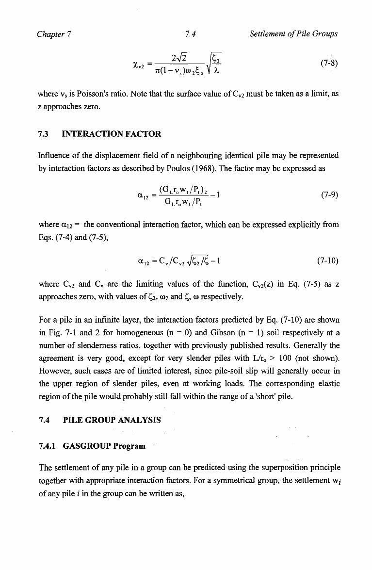
Chapter 7 7.4 Settlement of Pile Groups
^-i^krJf (7-8)
where vs is Poisson's ratio. Note that the surface value of CV2 must be taken as a limit, as
z approaches zero.
7.3 INTERACTION FACTOR
Influence of the displacement field of a neighbouring identical pile may be represented
by interaction factors as described by Poulos (1968). The factor may be expressed as
(GLr0w,/P,)
GLr0w,/P,
where an = the conventional interaction factor, which can be expressed explicitly from
Eqs. (7-4) and (7-5),
a,2=Cv/Cv2V^7c;-l (7-10)
where CV2 and Cv are the limiting values of the function, CV2(z) in Eq. (7-5) as z
approaches zero, with values of £2, ©2 and C,, co respectively.
For a pile in an infinite layer, the interaction factors predicted by Eq. (7-10) are shown
in Fig. 7-1 and 2 for homogeneous (n = 0) and Gibson (n = 1) soil respectively at a
number of slenderness ratios, together with previously published results. Generally the
agreement is very good, except for very slender piles with L/r0 > 100 (not shown).
However, such cases are of limited interest, since pile-soil slip will generally occur in
the upper region of slender piles, even at working loads. The corresponding elastic
region of the pile would probably still fall within the range of a 'short' pile.
7.4 PILE GROUP ANALYSIS
7.4.1 GASGROUP Program
The settlement of any pile in a group can be predicted using the superposition principle
together with appropriate interaction factors. For a symmetrical group, the settlement WJ
of any pile / in the group can be written as,
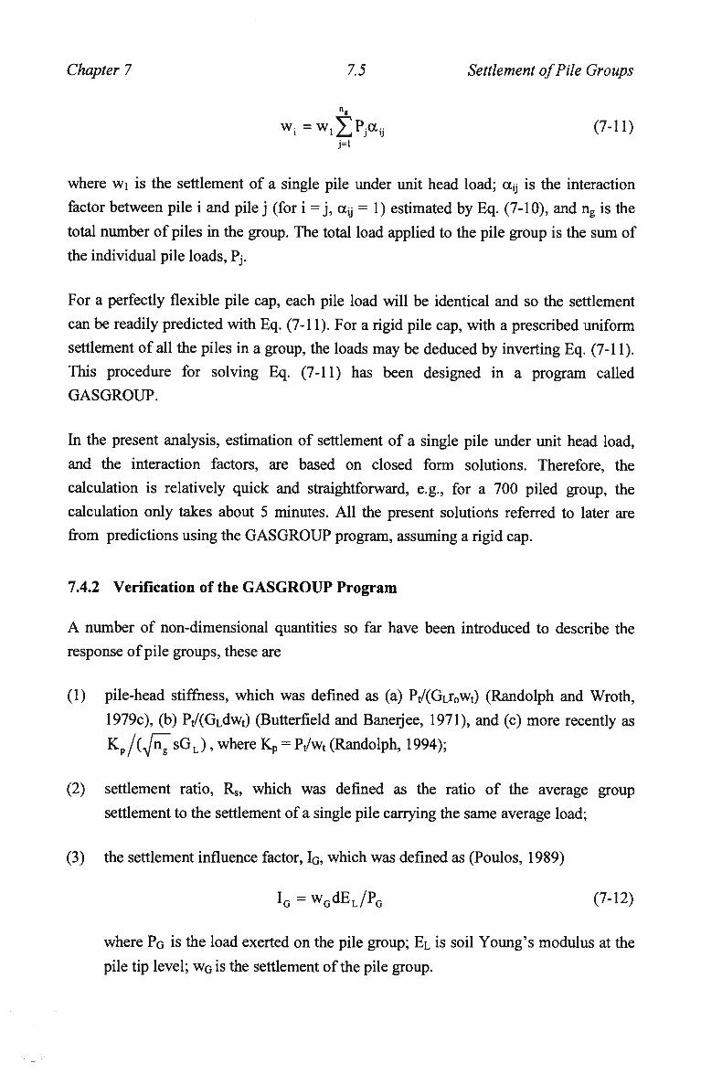
Chapter 7 7.5 Settlement of Pile Groups
wi=w12]Pjaa (7-11) j=i
where wi is the settlement of a single pile under unit head load; ay is the interaction
factor between pile i and pile j (for i = j, ay = 1) estimated by Eq. (7-10), and ng is the
total number of piles in the group. The total load applied to the pile group is the sum of
the individual pile loads, Pj.
For a perfectly flexible pile cap, each pile load will be identical and so the settlement
can be readily predicted with Eq. (7-11). For a rigid pile cap, with a prescribed uniform
settlement of all the piles in a group, the loads may be deduced by inverting Eq. (7-11).
This procedure for solving Eq. (7-11) has been designed in a program called
GASGROUP.
In the present analysis, estimation of settlement of a single pile under unit head load,
and the interaction factors, are based on closed form solutions. Therefore, the
calculation is relatively quick and straightforward, e.g., for a 700 piled group, the
calculation only takes about 5 minutes. All the present solutions referred to later are
from predictions using the G A S G R O U P program, assuming a rigid cap.
7.4.2 Verification of the GASGROUP Program
A number of non-dimensional quantities so far have been introduced to describe the
response of pile groups, these are
(1) pile-head stiffness, which was defined as (a) Pt/(GLr0Wt) (Randolph and Wroth,
1979c), (b) Pt/(GLdwt) (Butterfield and Banerjee, 1971), and (c) more recently as
K p / C ^ S G L ) , where K p = Pt/wt (Randolph, 1994);
(2) settlement ratio, Rs, which was defined as the ratio of the average group
settlement to the settlement of a single pile carrying the same average load;
(3) the settlement influence factor, IG, which was defined as (Poulos, 1989)
IG=wGdEL/PG (7-12)
where PG is the load exerted on the pile group; EL is soil Young's modulus at the
pile tip level; W G is the settlement of the pile group.
Chapter 7 7.6 Settlement of Pile Groups
These non-dimensional factors are used in the following comparisons.
7.4.2.1 Small Pile Groups in an Infinite Layer
For pile groups embedded in a homogeneous soil profile, the present solution was
compared with that obtained using the boundary integral approach (BI) by Butterfield
and Banerjee (1971) and is presented in
(1) Fig. 7-3 for the pile-head stiffness of three symmetrical pile groups at different
pile-soil relative stiffness; and
(2) Fig. 7-4 for the sharing of load among the piles in a 3x3 symmetrical pile groups.
For pile groups embedded in a Gibson soil, the present solution is compared with that
obtained using the boundary element approach of Lee (1993a), as illustrated in Fig. 7-5,
which gives the sharing of load within a 3x3 pile group.
Values of settlement ratio, Rs, were estimated and compared with those obtained by
Butterfield and Banerjee (1971), as shown in
(1) Fig. 7-6 for different spacing ratios, s/r0 for three symmetrical pile groups.
(2) Fig. 7-7 for a symmetrical four pile group, accounting for the effect of the pile-
soil stiffness ratio, X.
Available values of settlement influence factor, IG, were used to substantiate the present
solution for pile groups in a Gibson soil, as shown in Fig. 7-8.
All the above comparisons show that for pile groups in an infinite layer, the closed form
approach as used in the G A S G R O U P program is capable of predicting a very similar
response of different pile groups to those obtained previously by various numerical
approaches.
7.4.2.2 Small Pile Groups in a Finite Layer
The most comprehensive rigorous analysis of pile groups in a finite layer is probably
that provided by Butterfield and Douglas (1981). Using the P G R O U P program
(Banerjee and Driscoll, 1978 referenced via Randolph, 1994), Butterfield and Douglas
(1981) obtained flexibility factors (the inverse of stiffness factors) for pile groups in
homogeneous, finite (H/L =1.5 and 3.0) and infinite layers, with the pile cap being
treated as rigid and at ground level, but with no contact between the pile cap and the
soil.

Chapter 7 7.7 Settlement of Pile Groups
The normalised stiffness, Kp/c/n^~sGL), obtained from the present solution is first
compared with those obtained by Butterfield and Douglas (1981) for 2-pile groups at
different centre-centre spacing embedded in an infinite layer, as shown in Fig. 7-9. The
normalised stiffness obtained by the present solution is then compared with those
obtained by Butterfield and Douglas (1981) for groups in homogenous soil layers of
various values of H/L (= 1.5, 3.0 and infinite layer) at pile centre-centre spacing of s/d =
2.5 and 5. The later comparison for symmetrical pile groups is presented individually in
a) Fig. 7-10 for 2x2 pile groups; b) Fig. 7-11 for 3x3 pile groups;
c) Fig. 7-12 for 4x4 pile groups; d) Fig. 7-13 for 8x8 pile groups;
e) Fig. 7-14 for 4x2 pile groups; f) Fig. 7-15 for 8x2 pile groups.
The comparison shows that
(1) Generally the present solution is consistent with that of P G R O U P analysis;
(2) For large group of piles, e.g. 8x8, and at lower values of H/L, e.g. 1.5, differences
between the present solution and the P G R O U P analysis become obvious. The
P G R O U P analysis for these cases was found to be unreliable (Butterfield and
Douglas, 1981). The results from P G R O U P analysis are independent of pile
slenderness ratio, which do not seem to be realistic, while comparatively, the
current prediction gives a reasonable trend.
7.4.2.3 Large Pile Groups in an Infinite Layer
For large pile groups, previous solutions are available only for groups embedded in an
infinite layer. Fig. 7-16 shows a comparison of the solutions obtained by the following
computer codes:
(1) The analysis by Fleming et al (1992), based on the PIGLET program (Randolph,
1987);
(2) The interaction factor approach derived from analysis using DEFPIG program
(Poulos and Davis, 1980);
(3) The most rigorous numerical results by Butterfield and Douglas (1981), based on
the full B E M analysis incorporated in the P G R O U P program.
The average of the first two approaches appears to offer reasonably accurate solutions
(Randolph, 1994). The present solution is quite consistent with this average trend for
close pile spacing (s/d = 2.5) as illustrated in Fig. 7-16(a), and approaches a limiting
normalised stiffness of 4.5 corresponding to that of a shallow foundation. However, for
a large pile centre-centre space (s/d = 5), the normalised stiffness by the present
Chapter 7 7.8 Settlement of Pile Groups
GASGROUP analysis as shown in Fig. 7-16 (b) tends to decrease and becomes lower
than that for a shallow foundation. Probably as noted by Cooke (1986), at a large pile
centre-centre space (e.g. greater than 4d), the pile group performs in a different way
from that of a densely spaced pile group.
7.5 APPLICATIONS
Settlements of a number of actual pile groups have been analysed using the present
G A S G R O U P program. These cases are
(1) full scale pile tests by Cooke (1974);
(2) a tank supported by 55 piles, embedded in silt and very silty clay (Thorburn et al.
1983);
(3) a 19-storey building supported by a group of 132 piles, embedded in sandy layer
(Koerner and Partos, 1974);
(4) a block of 40 cylindrical silos supported by a large group of 697 piles, embedded
in a layer of interbedded sands and stiff clays (Goosens and Van Impe, 1991);
(5) a 5-storey building supported by a group of 20 piles, embedded in a layer of stiff
clays underlain by a medium to dense sand (Yamashita et al. 1993).
Input parameters for each analysis include (i) soil shear modulus distribution down the
pile, Poisson's ratio, and the ratio of H/L; (ii) the dimensions and Young's modulus of
the pile; (iii) the number of piles in the foundation and pile centre-centre space. There is
no practical difficulty in estimating the exact centre-centre spacing for each pair of
piles. However, for convenience, equivalent average pile spacing has been assessed and
used for large pile groups. In the prediction of Rs, the irregular plans of large groups
were converted to equivalent rectangular plans.
7.5.1 Full Scale Tests (Cooke, 1974)
Cooke (1974) reported the results of full scale tests on vertically loaded single piles, and
a row of three piles spaced at s = 6r0, embedded in London clay at Hendon. The tubular
steel piles, of external radius 84 m m and wall thickness 6.4 m m , were jacked to a depth
of 4.5 m. The equivalent Young's modulus of the piles is E p = 30.8 GPa.
The load distribution in the piles as well as the vertical displacements at different levels
below the ground surface were measured. From the test results of the central pile of the
row of three piles, which was loaded before the installation of the two flanking piles,
Chapter 7 7.9 Settlement of Pile Groups
the pile-head stiffness Pt/wt is 127,800 kN/m, and also from Cooke (1979), the shear
modulus may be simulated by Eq. (7-1) with n = 0.85, A g = 12.48 M P a rn"085, which
leads to a pile-soil relative stiffness factor, X = 687.1. Other relevant parameters have
been estimated as presented in Fig. 7-17.
With these parameters, the predicted pile-pile interaction factors agree well with the
measured values reported by Cooke (1979, 1980) (Fig. 7-17). This may be attributed to
the more accurate selection of the A value of 1.66 for H/L = 2, as backfigured by F L A C
analysis shown in Chapter 4. This 'A' value gives an excellent estimation of the
maximum radius of influence of the pile-shaft shear, and the corresponding theoretical
predictions of displacement are consistent with those measured, as shown in Fig. 7-18
for the single pile, and Figs. 7-19 (a) and (b) for pile groups of equal pile load and rigid
pile cap respectively. The prediction of pile-head load-displacement relations are
illustrated in Figs. 7-20 (a) and (b) for equal pile load and rigid pile cap respectively.
7.5.2 Molasses Tank (Thorburn et al, 1983)
The Molasses tank described by Thorburn et al (1983) was 12.5 m in diameter, and was
supported by 55 precast concrete piles, each 0.25 m square, and 27 m long (effective
length), laid out on a triangular grid at a spacing of 2.0 m. The strength profile of the
subsoil may be written as
su (kPa) = 6 + 1.8z (m) (7-13)
and the shear modulus was estimated as
G (MPa) = 1.5 + 0.45z (m) (7-14)
From the single pile test, the measured initial elastic stiffness of Pt/wt was 88 MN/m.
Young's modulus of the pile was measured as 26 GPa. Therefore, with an assumed
value of n = 1, the backfigured shear modulus was G (MPa) = 0.54z (m).
By the GASGROUP analysis, taking the group as a rectangular array of 7x8, the
estimated settlement ratio, Rs, was 5.43. Alternatively, taking the group as rectangular, 5
x 11, the estimated settlement ratio, Rs, was 6.08. At the average load per pile of 440
kN, the predicted elastic displacement of the single pile was 5 m m . Therefore, the
predicted settlement of the pile group was in the range of 27.2 to 30.4 m m . This
compares well with the measured settlements in the range of 29 - 30 m m .
Chapter 7 7.10 Settlement of Pile Groups
7.5.3 19-storey R. C. Building (Koerner and Partos, 1974)
The 19-storey building described by Koerner and Partos, (1974) was founded on 132
permanently cased driven piles, covering an approximately rectangular area, about 24 m
by 34 m. The piles were cased 0.41 m diameter and 7.6 m long, with an expanded base
of 0.76 m. Dividing the total area by 132 piles results in a mean area of 6.18 m per pile,
and a pile 'spacing' of 2.48 m.
The SPT varies approximately with depth by a power of n = 0.5. From the single pile
loading test results, a secant stiffness of Pt/wt = 3 5 0 k N / m m was obtained. With the
ratio of H/L = 2.2, the shear modulus variation with depth may be approximated by
G (MPa) = 16.43z05 (7-15)
Young's modulus of the pile was measured as 30 GPa. With these parameters, the
G A S G R O U P analysis gave a value of the settlement ratio, Rs of 19.85. The single pile
settlement was computed to be 3.3 m m for the average load of 1.05 M N . Thus the
average group settlement was computed to be 65.5 m m . The measured values ranged
between a maximum of 80 m m near the centre, to 37 m m near the corners of the
building, with an average of about 64 m m . The predicted settlement is therefore close to
the average measured value.
7.5.4 Ghent Grain Terminal (Goosens and Van Impe, 1991)
A block of 40 cylindrical reinforced concrete grain silo cells was erected in Ghent,
covering a rectangular area 34 m by 84 m, within a new terminal for storage and transit
(Goosens and Van Impe, 1991). Each of the cells is 52 m high and 8 m in diameter. The
silos were built on a 1.2 m thick slab, which in turn rested on a total of 697 driven cast
in situ reinforced concrete piles. The piles are of 13.4 m in length, 0.52 m in shaft
diameter, and incorporating an expanded base, which was estimated to be 0.8 m in
diameter. The average working load for each pile was about 1.3 M N .
The average shear modulus near the centre of the site may be regarded as uniform with
depth, with a value of 28.6 M P a (Poulos, 1993). Young's modulus of the pile was
assumed as 30 GPa. The average area per pile was estimated to be 4.1 m2, giving a 'pile
spacing' of 2.02 m. Using the G A S G R O U P analysis, the settlement ratio, Rs, was
estimated to be 59.15. At the average working load of 1.3 M N , the single pile
displacement was estimated to be 3.15 m m . Therefore, the predicted settlement of the
Chapter 7 7.11 Settlement of Pile Groups
pile group was 186.3 mm. At completion of the building, the measured settlement was
185.0 m m . The predicted settlement is quite consistent with the measured value.
7.5.6 5-Storey Building (Yamashita et al. 1993)
A piled raft foundation has been adopted in Japan for a five-storey building with plan
area measuring 24 m by 23 m. A total of 20 piles were utilised to reduce the potential
settlement (Yamashita et al. 1993). The piles were 16 m in length and 0.7 and 0.8 m in
diameter, with pile centre to centre spacing of 6.3 to 8.6 times the pile diameter. The
total working load was 47.5 M N .
The shear modulus profile adopted by Yamashita et al (1993) may reasonably be
approximated by
G (MPa) = 9.5z08 (7-16)
Young's modulus of the pile was assumed as 9.8 GPa. Using the GASGROUP analysis,
the settlement ratio, Rs, was estimated to be 2.7. At the average working load of 2.4
M N , the single pile showed about 5.0 m m displacement. Therefore, the predicted
settlement of the pile group was 13.5 m m . At completion of the building, the measured
settlements were in the range of 10 to 20 m m , with an average of about 14 m m . The
predicted settlement is quite consistent with the measured value.
7.5.7 General Comments From the Case Study
Generally speaking, using an assumed pile Young's modulus, the corresponding initial
soil modulus may be backfigured, in terms of single pile test results. The parameters
from the single pile analysis may then be used directly to predict the settlement of the
pile group. In the case of using enlarged pile base (section 7.5.3), a secant stiffness from
single pile test results may be used. Where an inclined underlain rigid layer exists, since
the ratio of H/L varies across the pile group, different values of H/L may be used to
assess the possible displacement range of the foundation.
7.6 CONCLUSIONS
This chapter was aimed at establishing a simple efficient approach for predicting
settlement of large pile groups. A closed from expression for estimating pile-pile
interaction factors was established, which was then used to predict behaviour of large
Chapter 7 7.12 Settlement of Pile Groups
pile groups embedded in non-homogeneous, finite layer media. The current solutions
have been compared extensively with the previous numerical analyses. A number of
actual pile groups have been analysed. The main conclusions from this research are:
(1) The new closed form expression for interaction factors, using the modified load
transfer factors, gives very good agreement with those obtained by more rigorous
numerical analyses.
(2) The current approach for estimating pile group stiffness yields very good
agreement with those obtained by rigorous numerical analysis for a range of
different layer thickness ratio, H/L.
(3) The current program, GASGROUP, gives reasonable prediction in comparison
with both rigorous numerical analyses and measured data. The program is very
quick, efficient and can be readily run on a personal computer. Therefore, it may
be used for practical engineering design.
(4) Some guidelines for estimating settlement of pile groups have been provided,
using G A S G R O U P program for a variety of different subsoil profiles.
Chapter 8 8.1 Torsional Piles
8. TORSIONAL PILES IN NON-HOMOGENEOUS MEDIA
8.1 INTRODUCTION
Numerical and analytical solutions have been published for piles subjected to torsion,
where the piles are embedded in elastic soil with either homogeneous modulus, or
modulus proportional to depth (Poulos, 1975; Randolph, 1981). A more general, and
often appropriate, class of soil is one where the depth variation of modulus may be
described by a simple power law (see later, Eq. (8-1)), as investigated for shallow
foundations by Booker et al. (1985). The nature of the power law, which encompasses
the homogeneous and proportionally varying cases as well, can have a significant effect
on the calculated pile head stiffness, particularly as the torsional load transfer is
generally concentrated in the upper part of the pile (Poulos, 1975).
This chapter describes new analytical solutions for the torsional response of piles in
non-homogenous soil deposits where the stiffness profile is modelled as a power law of
depth. The solutions are expressed in terms of Bessel functions of non-integer order,
and have been evaluated using Mathcad and also using a spreadsheet approach with the
Bessel functions approximated by polynomial functions. Expressions for the critical
pile length, beyond which the pile length no longer affects the pile head stiffness, are
presented. The solutions have also been extended into the non-linear range, using a
hyperbolic stress-strain response for the soil. At one extreme of the hyperbolic model,
the stress-strain response becomes elastic, perfectly plastic, and for that case analytical
solutions are presented giving the pile head response right up to complete torsional
failure of the pile. Simple non-dimensional charts have been presented to facilitate
hand calculation of the pile response.
In all the above solutions, a load transfer approach has been used, where each horizontal
layer of soil is considered as independent of neighbouring layers. The resulting
solutions have been checked against the more rigorous, continuum, solutions of Poulos
(1975) for the extreme cases of uniform modulus and modulus proportional to depth.
8.2 TORQUE-ROTATION TRANSFER BEHAVIOUR
Torque transfer models have been presented by Randolph (1981) for elastic conditions,
and incorporated into closed form solutions for the pile head response, assuming either
uniform soil modulus, or modulus varying proportionally with depth. Here, those
Chapter 8 8.2 Torsional Piles
solutions are extended for more general non-homogeneity of the soil, and also for non
linear soil response using a hyperbolic stress-strain law.
8.2.1 Non-homogeneous Soil Profile
The soil modulus profile is taken as a power law variation of depth, given by
Gi=Agzn (8-1)
where Gj is the initial (tangent) shear modulus at depth z; Ag is a modulus constant;
and n is the depth exponent, referred to here as the non-homogeneity factor. Typically,
the factor will lie in the range 0 (uniform soil) to 1 (stiffness proportional to depth).
The limiting shaft friction, Xf, can also be expressed as a power law variation with
depth, as
x f = A t zt (8-2)
where At is a constant that determines the magnitude of shaft friction, and t is the
corresponding non-homogeneity factor. In this chapter, attention will be restricted to
situations where the shear modulus and shaft friction profiles are similar (with n = t).
The ratio of modulus to shaft friction is then constant through the profile, and equal to
Ag/At.
8.2.2 Non-linear Stress-Strain Response
Non-linear response of the soil may be modelled using a hyperbolic stress-strain law,
where the secant shear modulus, G, is given by
( x\ G = Gj 1-Rf— (8-3)
V if)
where Rf is the hyperbolic parameter that controls the ratio of the secant modulus at
failure, to the initial tangent modulus, Gj. Note that it is assumed here that the limiting
shear stress in the soil is the same as the limiting pile-soil shaft friction. While this is a
simplification, the hyperbolic approach has sufficient flexibility to provide realistic non
linear response.
The 'concentric cylinder approach' (Frank, 1974; Randolph and Wroth, 1978; Randolph,
1981) may be used to estimate the radial variation of shear stress around a pile subjected
Chapter 8 8.3 Torsional Piles
to torsion. Assuming that the stress gradients longitudinally (parallel to the pile) are
small by comparison with radial stress gradients, it may be shown that the shear stress
(formally, Xj-e, but the double subscript is omitted here) at any radius, r, is given by
x = x0 \ (8-4) rz
where r0 is the pile radius and x0 is the shear stress mobilised at the pile. Combining
this equation with Eq. (8-3) gives the radial variation of secant shear modulus as
G = Gj l-y\ (8-5) V r J
where v|/ = RfXo/xf, which defines the relative mobilisation of shaft friction at the pile
surface. Note that Rf = 0 corresponds to a linear elastic case, while the upper limit on
Rf is unity.
The above relationships are similar to those derived for axial loading of a pile (Kraft et
al. 1981). However, the effect of non-linearity is much more localised close to the pile
for the torsional case, as shown by Fig. 8-1 where the normalised shear modulus, G/Gj,
is plotted as a function of radius, r/r0, for the two types of loading.
8.2.3 Shaft Torque-Rotation Response
The shear strain, yj-e, around a pile subjected to torsion may be written as (Randolph,
1981),
Xrfi 1 du d (v\ rry G r50 dr\r)
(8-6)
where u is the radial soil movement, v is the circumferential movement, and 0 is the
angular polar co-ordinate. From symmetry, du/dQ is zero, and so this equation may be
combined with (8-4) to give
Substituting (8-5) and integrating this with respect to r from r0 to oo yields the angle of
twist at the pile as
Chapter 8 8.4 Torsional Piles
4>Jl) =J*o_(-Wl-V)} (8.8) \v)0 2Gjl V J
This equation may be transformed into
•-^db-H*-'1')] (8-9)
which shows that the angle of twist depends logarithmically on the relative shear stress
level.
Again, the form of the torque-twist relationship is similar to that for axial loading.
However, as shown in Fig. 8-2, the degree of non-linearity (for a given Rf value) is
somewhat more for the torsional case (w in the figure is the shaft displacement for
vertical loading, while d is the pile diameter and C, is a load transfer parameter).
8.3 OVERALL PILE RESPONSE
The governing equations for the overall pile response have been documented by
Randolph (1981), and may be written:
where (GJ)p is the torsional rigidity of the pile. It is also helpful to introduce an
equivalent shear modulus for a solid pile, Gp, where
2(GJ)n G D = - ^ (8-11) 'P 7ir0
8.3.1 Critical Pile Length and Pile-Soil Stiffness Ratio
For slender piles, transfer of torque is concentrated in the upper part of the pile, at least
at low load levels, and the torque-twist stiffness of the pile is not affected by the overall
pile length. It is useful to introduce the concept of a critical pile length, and hence a
pile-soil stiffness ratio defined in terms of the pile length relative to that critical pile
length. Randolph (1981) defined the critical pile length as that length beyond which the
pile head torque-twist stiffness became independent of the overall pile length. The
critical pile length was defined as
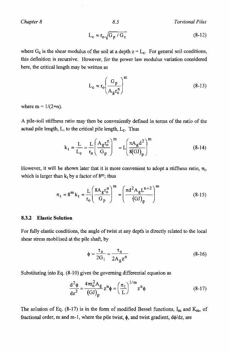
Chapter 8 8.5 Torsional Piles
L c * r 0 > / G p / G ( (8-12)
where G c is the shear modulus of the soil at a depth z = Lc. For general soil conditions,
this definition is recursive. However, for the power law modulus variation considered
here, the critical length may be written as
Lc *roi G, m
A rn (8-13)
where m = l/(2+n).
A pile-soil stiffness ratio may then be conveniently defined in terms of the ratio of the
actual pile length, L, to the critical pile length, Lc. Thus
L L k t= — = —
Lc ro
/ „ \ m
' A rn >
V G P ; = L
17iA0d2 ^
8(GJ) (8-14)
pJ
However, it will be shown later that it is more convenient to adopt a stiffness ratio, 7tt,
which is larger than kt by a factor of 8m; thus
7it = 8m k t =
"8Agr0n>
v G P ,
r 7 r d 2 A g Ln + 2 ^
(GJ) (8-15)
P /
8.3.2 Elastic Solution
For fully elastic conditions, the angle of twist at any depth is directly related to the local
shear stress mobilised at the pile shaft, by
• = 2Gj 2 A g z
n (8-16)
Substituting into Eq. (8-10) gives the governing differential equation as
d2<j) 47tr2Ag n
dz (GJ), z> = Hi.
v.L
1/m z <p (8-17)
The solution of Eq. (8-17) is in the form of modified Bessel functions, I m and K m , of
fractional order, m and m-1, where the pile twist, <|), and twist gradient, d<j>/dz, are
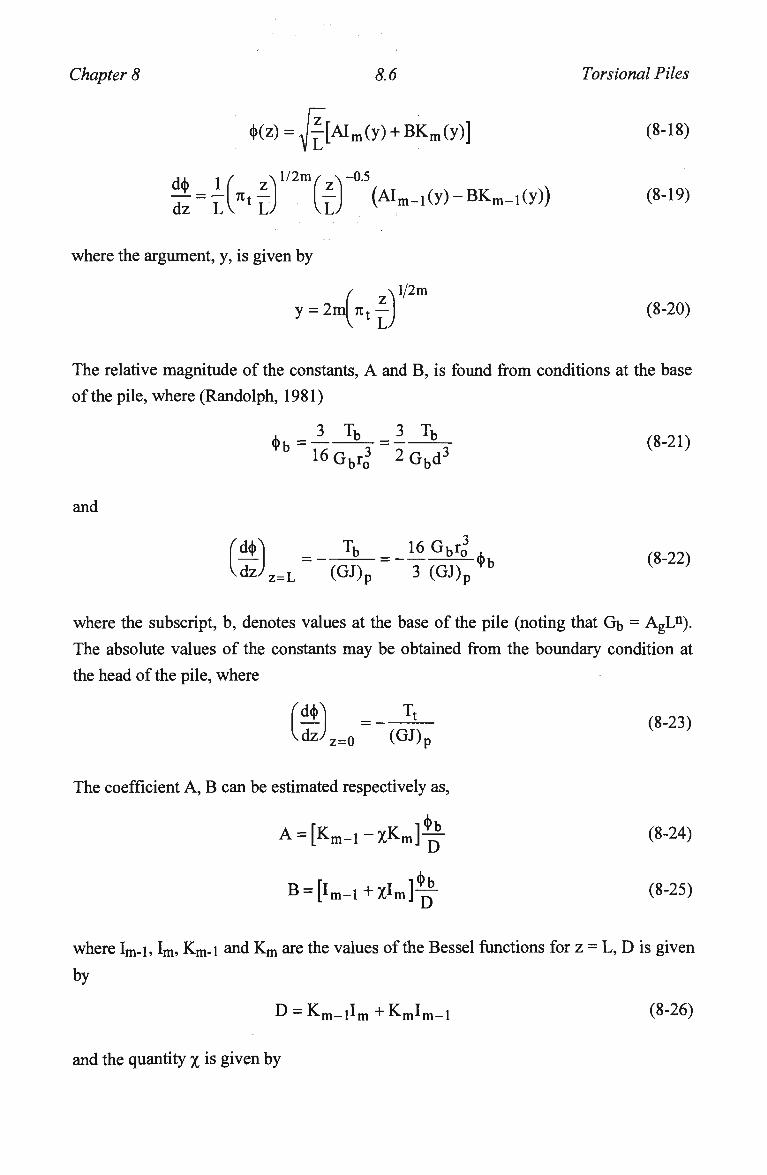
Chapter 8 8.6 Torsional Piles
<Kz) = ^[AIm(y) + BKm(y)] (8-18)
/ \l/2m/ \-0.5
h r J I D (AIm-i(y)-BKm-i(y)) (8-19) dz L
where the argument, y, is given by
=2n(K<i l/2m
(8-20)
The relative magnitude of the constants, A and B, is found from conditions at the base of the pile, where (Randolph, 1981)
*b=-Jkr = -JLr (8-20 16Gbr0
3 2Gbd3
and
(») Zl ^Gfc^.+b (8-22) VdzJ z = L (GJ)p 3 ( G J ) p
T b
where the subscript, b, denotes values at the base of the pile (noting that Gb = AgLn).
The absolute values of the constants may be obtained from the boundary condition at the head of the pile, where
*) =--3L- (8-23) d z ; z = 0 (GJ)p
The coefficient A, B can be estimated respectively as,
A = [Km_,-XKm]^- (8-24)
B = [lm_i+Xlm]^- (8-25)
where Im-i, Im> Kna-1 and Km are the values of the Bessel functions for z = L, D is given
by
D = K m _ 1 I m + K m I m _ 1 (8-26)
and the quantity % is given by
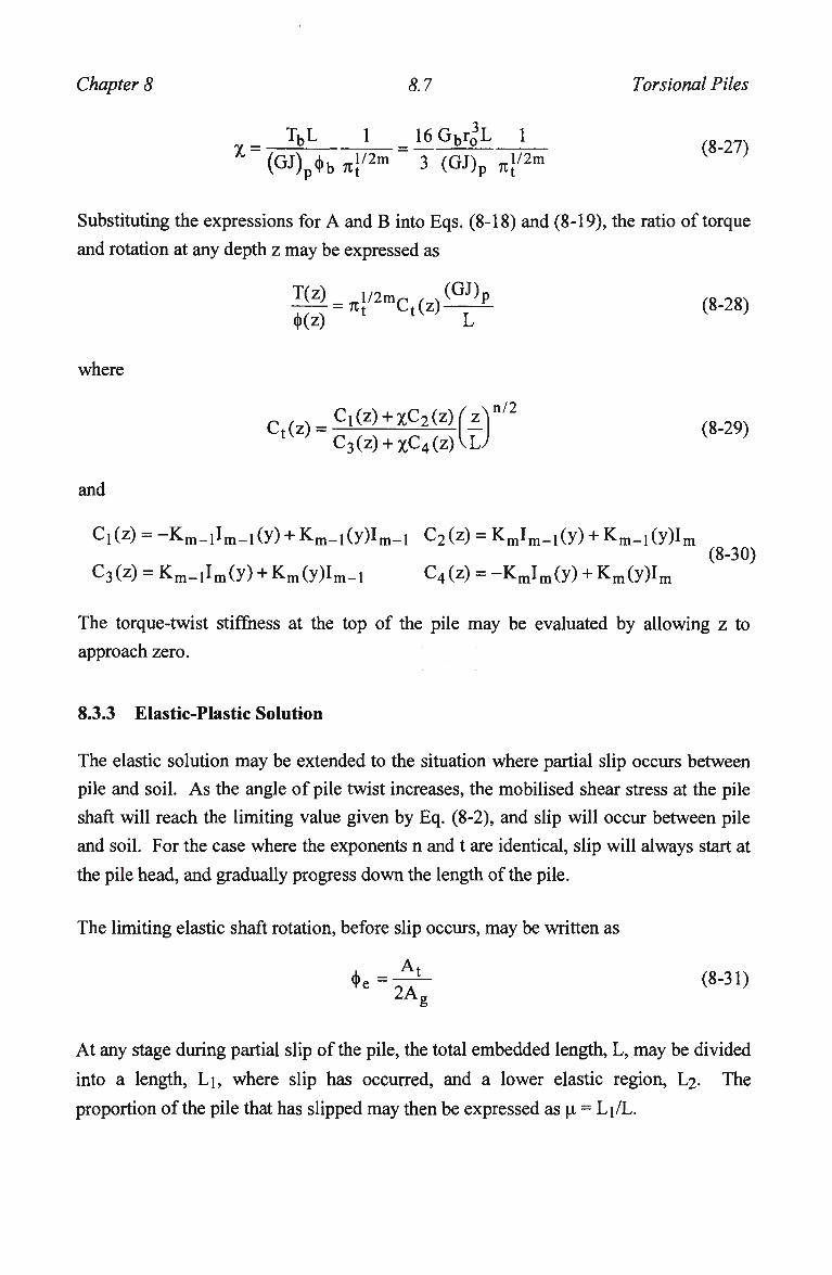
Chapter 8 8.7 Torsional Piles
T b L 1 ^16G b r 03 L 1
( G J ) p H n\/2m 3 (GJ)p n\
/2m
Substituting the expressions for A and B into Eqs. (8-18) and (8-19), the ratio of torque
and rotation at any depth z may be expressed as
T(z)=7t{/2mCt(z)^P. (8-28)
<Kz)
where
cl(z)+xc2(Z)rzy/2
C 3 ( Z ) + X C 4 ( Z ) I L J
and
C1(z) = -Km_1Im_1(y) + Km_1(y)Im_1 C2(z) = KmIm_1(y) + Km_1(y)Im (8-30)
C3(z) = K m _ 1 I m ( y ) + K m ( y)I m _ 1 C4(z) = - K m I m ( y ) + K m ( y ) I m
The torque-twist stiffness at the top of the pile may be evaluated by allowing z to
approach zero.
8.3.3 Elastic-Plastic Solution
The elastic solution may be extended to the situation where partial slip occurs between
pile and soil. As the angle of pile twist increases, the mobilised shear stress at the pile
shaft will reach the limiting value given by Eq. (8-2), and slip will occur between pile
and soil. For the case where the exponents n and t are identical, slip will always start at
the pile head, and gradually progress down the length of the pile.
The limiting elastic shaft rotation, before slip occurs, may be written as
4>e=^ (8-31) ZAg
At any stage during partial slip of the pile, the total embedded length, L, may be divided
into a length, Li, where slip has occurred, and a lower elastic region, L2. The
proportion of the pile that has slipped may then be expressed as u. = Lj/L.
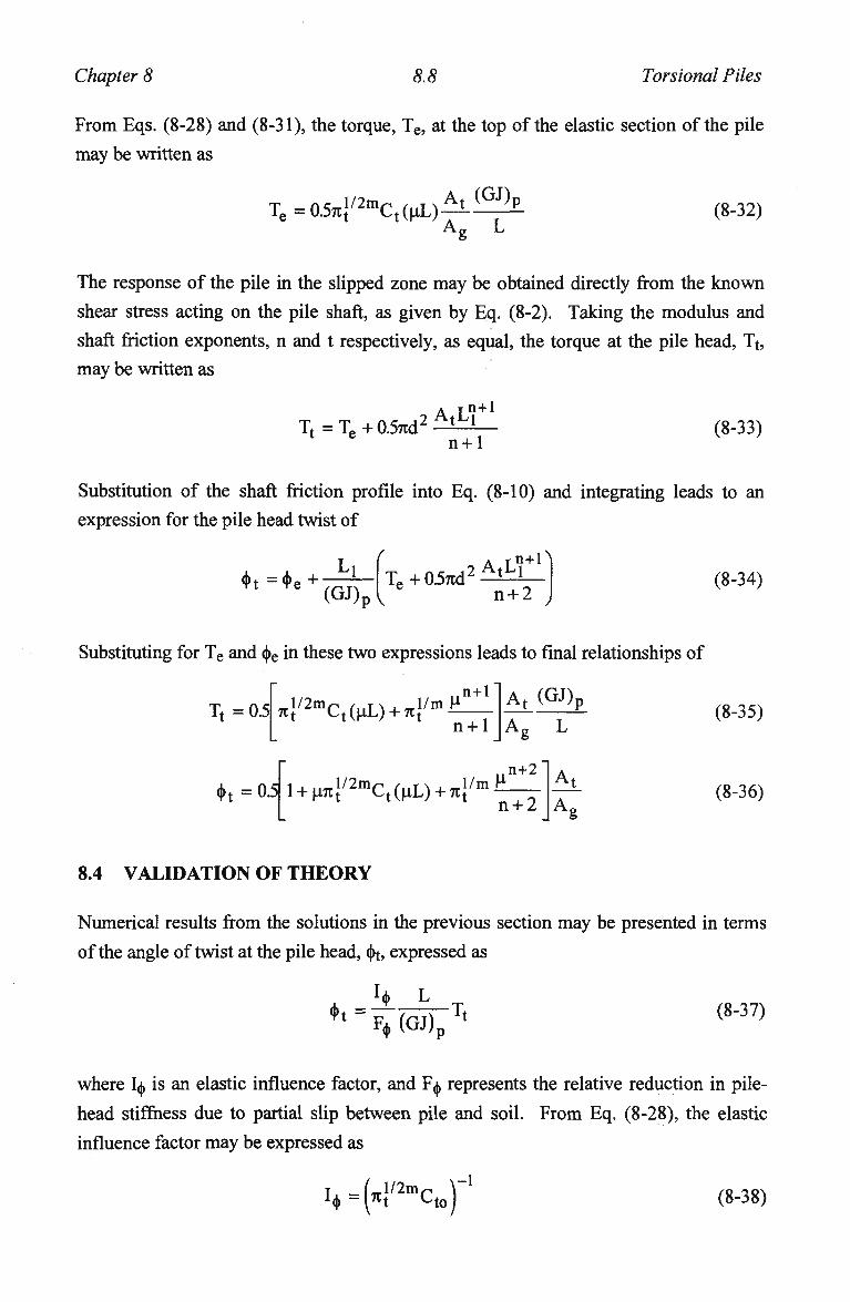
Chapter 8 8.8 Torsional Piles
From Eqs. (8-28) and (8-31), the torque, Te, at the top of the elastic section of the pile
may be written as
T e =0.5nl/ 2 m C t ( ^L)
A t ( G J ) p
A g L (8-32)
The response of the pile in the slipped zone may be obtained directly from the known
shear stress acting on the pile shaft, as given by Eq. (8-2). Taking the modulus and
shaft friction exponents, n and t respectively, as equal, the torque at the pile head, Tt,
may be written as
Tt = Te + 0.57td 2 AtL'j n+1
n + 1 (8-33)
Substitution of the shaft friction profile into Eq. (8-10) and integrating leads to an
expression for the pile head twist of
< h =<t>e + (GJ),
X. + 05nd 2 AtL
]! n+A
V n + 2 (8-34)
Substituting for Te and <|>e in these two expressions leads to final relationships of
Tt = 0.5 n\/2mCt(uL) + n\/mli
n+1
n + 1
A t (GJ)p
Ag L
<Pt =0.5 l + U7t{/2mCt(uL) + 7r;
/mi n+2
n + 2 J Ag
(8-35)
(8-36)
8.4 VALIDATION OF THEORY
Numerical results from the solutions in the previous section may be presented in terms
of the angle of twist at the pile head, (J>t, expressed as
*' = E* (GJ)p Tt
(8-37)
where I is an elastic influence factor, and F§ represents the relative reduction in pile-
head stiffness due to partial slip between pile and soil. From Eq. (8-28), the elastic
influence factor may be expressed as
L = [nt ctoj (8-38)
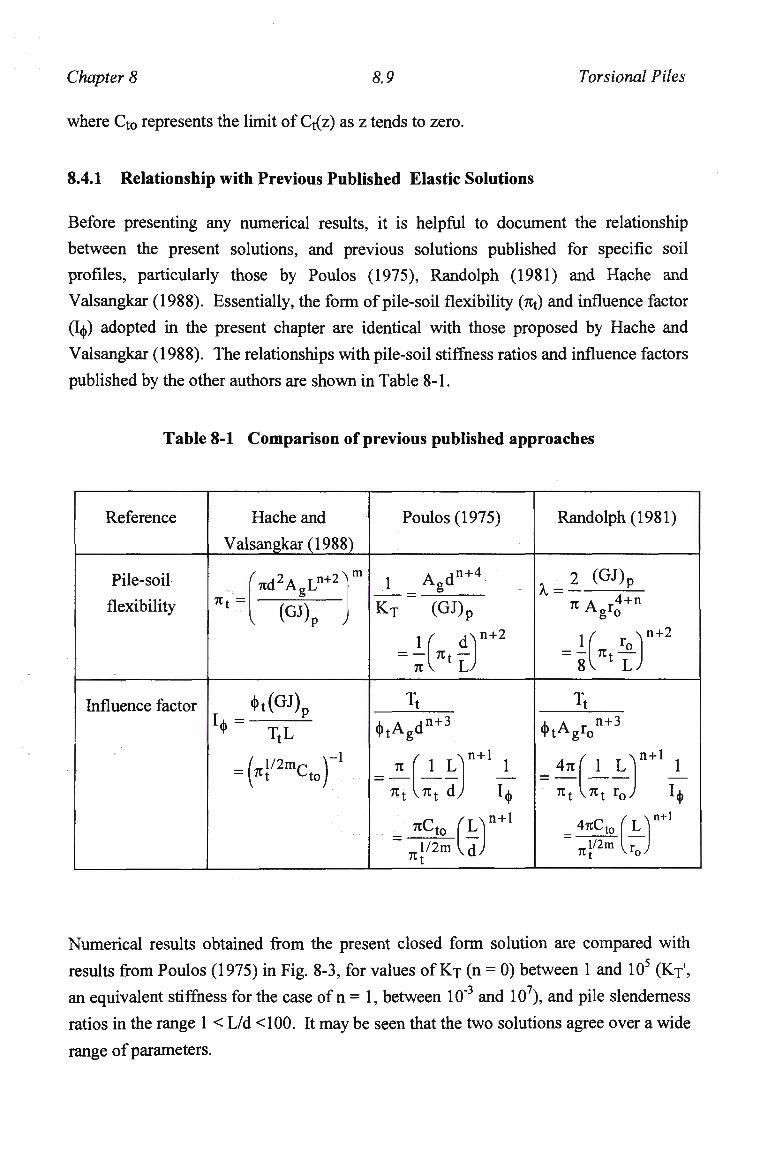
Chapter 8 8.9 Torsional Piles
where Q o represents the limit of Q(z) as z tends to zero.
8.4.1 Relationship with Previous Published Elastic Solutions
Before presenting any numerical results, it is helpful to document the relationship
between the present solutions, and previous solutions published for specific soil
profiles, particularly those by Poulos (1975), Randolph (1981) and Hache and
Valsangkar (1988). Essentially, the form of pile-soil flexibility (Ttt) and influence factor
(I,),) adopted in the present chapter are identical with those proposed by Hache and
Valsangkar (1988). The relationships with pile-soil stiffness ratios and influence factors
published by the other authors are shown in Table 8-1.
Table 8-1 Comparison of previous published approaches
Reference Hache and
Valsangkar (1988)
Poulos (1975) Randolph (1981)
Pile-soil
flexibility 7tt = ^d 2A g L"^
m
(GJ)t
1 A„d n+4
X = K^ (GJ)
n I 7Tt —
P
d
2 (GJ)p
* A gr 04 + n
\ n+2 = - 7li
n+2
L.
Influence factor <t>t(GJ)t
^ " TtL
172m,
Tt Tt
<t>tAgd
=H / 2 m c t 0 )_ 1 7t
711
(
n+3
1 L
<t>tAgr0 n+3
n+1 1 4TC
nt d)
KC -to 71 l/2m ^d
n+1
7t
1 L n+1
VTtt roJ
4TCC to
TC l/2m vr0
n+1
Numerical results obtained from the present closed form solution are compared with
results from Poulos (1975) in Fig. 8-3, for values of K r (n = 0) between 1 and 105 (Kf,
an equivalent stiffness for the case of n = 1, between 10"3 and 107), and pile slenderness
ratios in the range 1 < L/d <100. It may be seen that the two solutions agree over a wide
range of parameters.
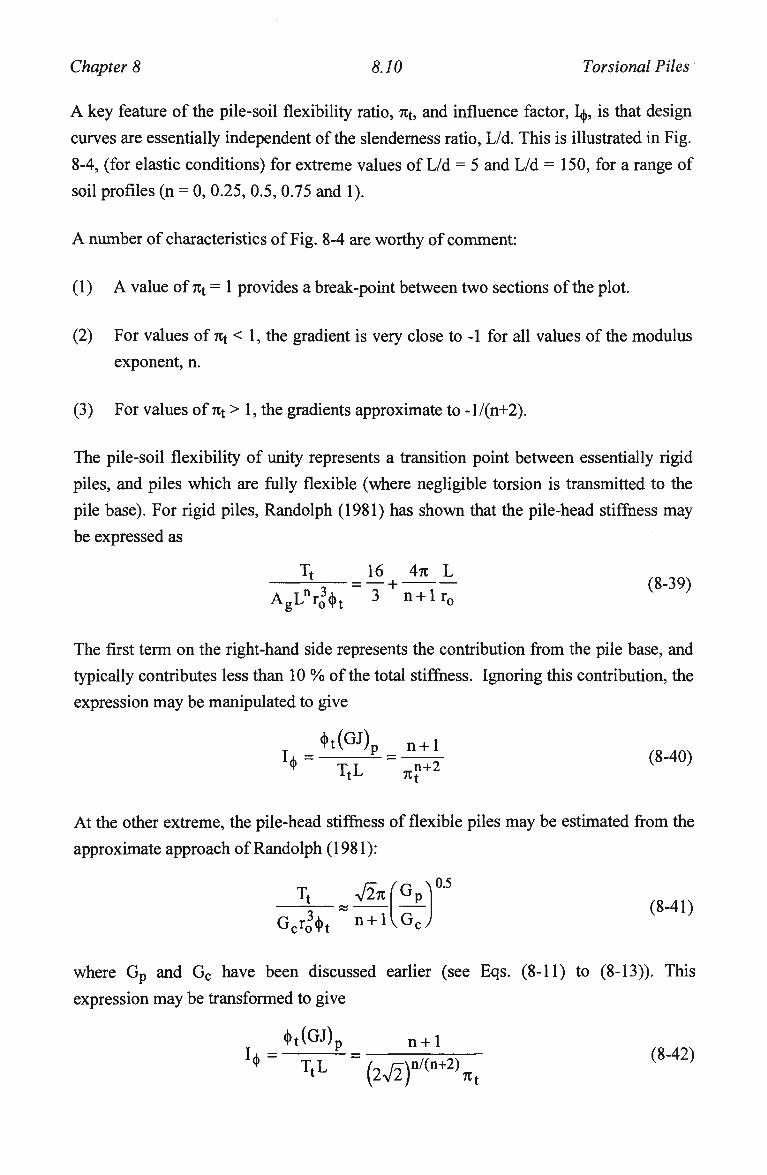
Chapter 8 8.10 Torsional Piles
A key feature of the pile-soil flexibility ratio, 7tt, and influence factor, l§, is that design
curves are essentially independent of the slenderness ratio, L/d. This is illustrated in Fig.
8-4, (for elastic conditions) for extreme values of L/d = 5 and L/d = 150, for a range of
soil profiles (n = 0, 0.25, 0.5, 0.75 and 1).
A number of characteristics of Fig. 8-4 are worthy of comment:
(1) A value of 7tt = 1 provides a break-point between two sections of the plot.
(2) For values of 7it < 1, the gradient is very close to -1 for all values of the modulus
exponent, n.
(3) For values of Tit > 1, the gradients approximate to -l/(n+2).
The pile-soil flexibility of unity represents a transition point between essentially rigid
piles, and piles which are fully flexible (where negligible torsion is transmitted to the
pile base). For rigid piles, Randolph (1981) has shown that the pile-head stiffness may
be expressed as
Tt 16 4TC L ^-T- = V + 7 ~ (8-39)
AgLnr0
3<|>t 3 n + lr0
The first term on the right-hand side represents the contribution from the pile base, and
typically contributes less than 10 % of the total stiffness. Ignoring this contribution, the
expression may be manipulated to give
*t(GJ)p n+1 h = L = - ^ r (8-40) * TL ,rn+2
1 t J j 7tt
At the other extreme, the pile-head stiffness of flexible piles may be estimated from the
approximate approach of Randolph (1981):
Tt V^pf5
(8-41) Gcr0(|>t h. n + 1 vGcy
where G p and G c have been discussed earlier (see Eqs. (8-11) to (8-13)). This
expression may be transformed to give
4>t(GJ)p n + 1
'*= TtL = (2V2)"
/(n+2)xt ( '
Chapter 8 8.11 Torsional Piles
This expression matches the curves shown in Fig. 8-4 very closely.
8.4.2 Elastic-Perfectly Plastic Response
The torque-twist relationship where partial slip occurs along the pile shaft may be
obtained from the expressions for Tt and (|>t in Eqs. (8-35) and (8-36). The yield
correction factor to the elastic flexibility coefficient, l^, may be written as
n + 2
where uL is the depth to which slip has occurred. This may be related to the proportion
of the ultimate capacity, T u = 0.57td2AtLn+1/(n+l) + Tt,, where Tb is the base torque
taken as (7td3/12)AtLn, by
Tt (l + n)7tr1/2mCt(uL) + p.
1+n
=r- = ~ — i ^ (8-44) T u 1 + n d v ' u 1 + -
6 L
Fig. 8-5 shows the variation of F<j> with Tt/Tu, for different values of the flexibility ratio,
7tt. The above solution is compared with values published by Poulos (1975), with the
two sets of results showing excellent agreement. A fuller set of design curves for the
correction factor, F^, is given in Fig. 8-6. It may be seen that the correction factor is
essentially independent of the slenderness ratio, L/d, of the pile.
8.5 PILE RESPONSE WITH HYPERBOLIC SOIL MODEL
The previous section presented solutions for partial slip along the pile, where the soil
response was modelled as elastic-perfectly plastic. Here, the effect of a hyperbolic
stress-strain response of the soil is explored.
8.5.1 Rigid Piles
For rigid piles, the angle of twist, <|>, will be uniform down the pile, and so the torque-
twist response at the pile head may be obtained directly by integrating the local torque
transfer curve given by Eq. (8-9). The overall torsional stiffness may be written in the
form adopted by Randolph (1981) as
Chapter 8 8.12 Torsional Piles
Tt 16 4TI L -\I/ 4—= T + 7 T^-^ (8-45)
AgLnr0
3(j>t 3 n + lr 0 ^ n ( l_y)
8.5.2 Flexible Piles
For flexible piles, it is necessary to adopt a numerical approach in order to implement
the non-linear torque transfer curve. A spreadsheet program, GASPILE, originally
developed for axial loading (Chapter 3; Guo and Randolph, 1996c), has been extended
to torsional loading. With it, non-linear analyses have been performed for hyperbolic
soil response, as given by Eq. (8-9) taking Rf = 0.95. At low load levels, the computed
influence factor, I,),, is essentially identical to the closed-form results, as indicated in Fig.
8-4(b). For the hyperbolic model, the overall torque-twist relationship for the pile head
is indistinguishable from that obtained using an elastic-perfectly plastic model with the
same initial shear modulus. This result, which has been noted for axial loading by
Poulos (1989) is illustrated below in the case study.
8.6 CASE STUDY
An example analysis is given here, for torsional load tests reported by Stoll (1972). The
two piles were steel pipes of external diameter 0.273 m, and wall thickness 6.3 m m ,
back-filled with concrete. Stoll (1972) reports the torsional rigidity (GJ)p of the two
piles as 12.8 M N m 2 .
Pile A-3 was driven to a penetration of 17.4 m through soil where the SPT value (N)
varied approximately linearly with depth according to,
N «1.38z (8-46)
where z is the depth in m. The other pile, pile V-4, was driven to 20.7 m at a location
where the SPT value in the upper 2.4 m was very low, and below 2.4 m it varied
linearly with depth according to
N«2.62(z-2.4) (8-47)
The SPT profiles suggest distributions of shear modulus and shaft friction which vary
linearly with depth, giving n = 1. For pile V-4, an artificial ground surface at z = 2.4 m
has been assumed, and the calculated pile head flexibility has been increased
accordingly.
The ultimate torques measured in each case were 29.3 kNm and 52.1 kNm for piles A -
3 and V - 4 respectively. These lead to values of A t of 1.66 kPa/m and 2.66 kPa/m
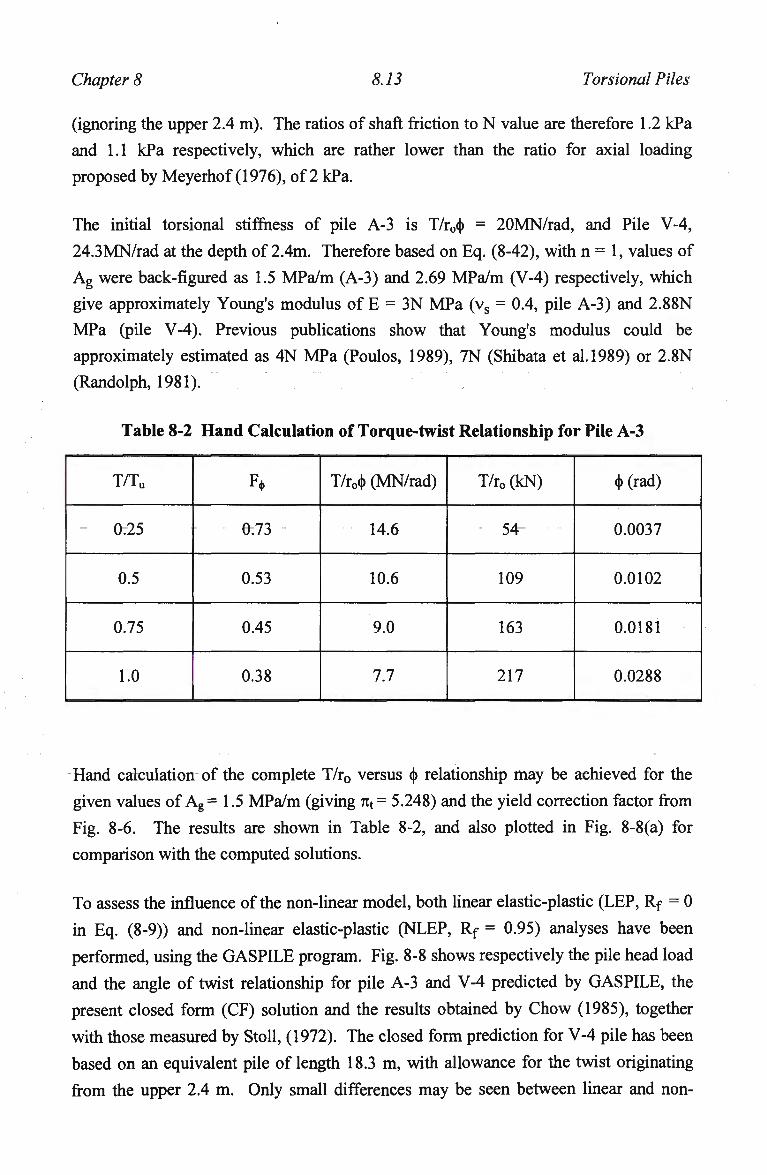
Chapter 8 8.13 Torsional Piles
(ignoring the upper 2.4 m). The ratios of shaft friction to N value are therefore 1.2 kPa
and 1.1 kPa respectively, which are rather lower than the ratio for axial loading
proposed by Meyerhof (1976), of 2 kPa.
The initial torsional stiffness of pile A-3 is T/r0<|> = 20MN/rad, and Pile V-4,
24.3MN/rad at the depth of 2.4m. Therefore based on Eq. (8-42), with n = 1, values of
A g were back-figured as 1.5 MPa/m (A-3) and 2.69 MPa/m (V-4) respectively, which
give approximately Young's modulus of E = 3N M P a (vs = 0.4, pile A-3) and 2.88N
M P a (pile V-4). Previous publications show that Young's modulus could be
approximately estimated as 4 N M P a (Poulos, 1989), 7N (Shibata et al.1989) or 2.8N
(Randolph, 1981).
Table 8-2 Hand Calculation of Torque-twist Relationship for Pile A-3
T/Tu
0.25
0.5
0.75
1.0
F*
0.73
0.53
0.45
0.38
T/r0(j) (MN/rad)
14.6
10.6
9.0
7.7
T/r0(kN)
54
109
163
217
<|> (rad)
0.0037
0.0102
0.0181
0.0288
Hand calculation of the complete T/r0 versus ty relationship m a y be achieved for the
given values of A g = 1.5 M P a / m (giving 7tt= 5.248) and the yield correction factor from
Fig. 8-6. The results are shown in Table 8-2, and also plotted in Fig. 8-8(a) for
comparison with the computed solutions.
To assess the influence of the non-linear model, both linear elastic-plastic (LEP, Rf = 0
in Eq. (8-9)) and non-linear elastic-plastic (NLEP, Rf = 0.95) analyses have been
performed, using the G A S P I L E program. Fig. 8-8 shows respectively the pile head load
and the angle of twist relationship for pile A-3 and V-4 predicted by G A S P I L E , the
present closed form (CF) solution and the results obtained by C h o w (1985), together
with those measured by Stoll, (1972). The closed form prediction for V-4 pile has been
based on an equivalent pile of length 18.3 m , with allowance for the twist originating
from the upper 2.4 m . Only small differences m a y be seen between linear and non-
Chapter 8 8.14 Torsional Piles
linear elastic-plastic analyses. However, none of the computed solutions provides a
very good match with the measured data. The computed stiffness at loads of 50 % of
the ultimate is too low, and even increasing the soil modulus by a factor of 10 makes
little difference, owing to the occurrence of slip at low load levels. A possible
explanation lies in the choice of torsional rigidity of the piles, which may have been
affected by load level, due to cracking of the concrete.
Fig. 8-9 shows profiles of shear stress, load (T/r0) and displacement (<|>r0) down the pile,
predicted from non-linear and linear elastic-plastic numerical G A S P I L E analysis, and
also by the closed form equations (see Appendix F). All profiles are very similar.
8.7 CONCLUSIONS
The analysis outlined in this chapter has attempted to provide a comprehensive
approach for the analysis of piles subjected to torsion. Solutions have been presented
for piles embedded in a non-homogeneous medium, where the shear modulus and
limiting shaft friction are taken as power law functions of depth. Consideration has also
been given to the form of torque-twist relationship arising from a hyperbolic stress-
strain response of the soil.
The rapid decay of shear stress with distance from the pile entails that non-linear effects
in the soil are limited to the immediate vicinity of the pile. The resulting torque-twist
curve may be closely approximated by elastic-perfectly plastic response, even where the
stress-strain response of the soil is markedly non-linear.
A general closed-form solution has been developed for elastic-perfectly plastic soil
response. The solution is written in terms of fractional Bessel functions, and has been
evaluated using Mathcad. A n alternative numerical solution, which can handle more
general non-homogeneous and non-linear stress-strain response of the soil, has been
implemented in a spreadsheet program, GASPILE. Both solutions have been shown to
agree with each other, and with solutions published previously for the limiting cases of
soil with either uniform stiffness or stiffness proportional to depth.
Design charts have been presented in non-dimensional form for the pile-head influence
coefficient, l§, and a modifying factor, F§, to allow for partial slip down the pile. Both
factors are a function primarily of the pile-soil flexibility ratio, 7tt, and are essentially
independent of the slenderness ratio, L/d. A flexibility ratio of unity marks a transition
point between very stiff piles, where the twist is uniform down the pile, and fully
flexible piles where the torque at the pile base is negligible.
Chapter 8 8.15 Torsional Piles
The solutions have been applied to a case study, where two piles were loaded
torsionally to failure. The soil parameters (shear modulus and shaft friction) back-
analysed from the initial stiffness and ultimate torque capacity were found to be
consistent with c o m m o n practice. However, the overall agreement between calculated
and measured response curves was relatively poor, indicating that some aspect of the
pile-soil system was incorrectly modelled, possibly due to progressive cracking of the
concrete interior of the pile.
Chapter 9 9.1 Conclusions
9. CONCLUSIONS
Closed form solutions have been established for a pile subject to either vertical or
torsional loading in non-homogeneous media, where the shear modulus and limiting
shaft friction are taken as power law functions of depth. The rationality and suitability
of load transfer approaches have been extensively checked corresponding to various
boundary conditions. Simple statistical formulas for estimating load transfer factors
were given. Closed form solutions have been generated respectively to account for the
effect of soil elastic-plastic, visco-elastic properties, and the reconsolidation due to pile
installation. A load transfer analysis program, GASPILE, has been newly developed, to
explore the effect of non-linearity and visco-elastic soil properties on a pile response for
the instance of either vertically or torsional loading. A closed form expression for pile-
pile interaction has been generated. Therefore, the solutions for analysing a single pile
are then extended to that for pile groups. A numerical program called G A S G R O U P has
been designed to facilitate estimation of settlement of large piled groups. Extensive
comparisons with the previously publications have been made for every theories
established. Relevant design charts have been produced. Case studies for each theories
have been undertaken to illustrate the strength of the current research. Detailed
conclusions arising from the research have been presented in each of the previous
chapters, and the main findings are briefly summarised below.
9.1 VERTICALLY LOADED SINGLE PILES
Analytical solutions have been established for a pile in a non-homogenous elastic-
plastic media. The accuracy of the solutions, which are based on the load transfer
approach, is very good compared with those from more rigorous continuum based
numerical analyses and the numerical load transfer analysis, GASPILE. The following
conclusions were drawn
• A non-linear elastic-plastic analysis (NL) shows only slight differences from a
simplified linear elastic-plastic analysis (SL); therefore the closed form solutions
established based on the simplified elastic-plastic model can be directly utilised for
the non-linear case.
• The significant influence of non-homogeneity of the soil profile on pile-head
stiffness or settlement influence factor maybe attributed partly to the non-
Chapter 9 9.2 Conclusions
homogeneity and partly to the variation of the average soil modulus over the pile
length. In other words, the influence of non-homogeneity originated partly from the
definition of relative pile-soil stiffness in terms of the soil modulus at the pile tip
level.
• For a given average shear modulus over the pile length, but different distribution (n
different), the final elastic pile-head stiffness (or the settlement influence factor) is
not significantly different (e.g. less than 2 0 % ) .
• For a long pile, pile-soil relative slip should be considered when estimating load-
settlement behaviour and load distribution down the pile. A case study has shown
that the pile response can be modelled well by the closed form solutions, right up to
full shaft slip.
• Though only vertical non-homogeneity is considered in the current load transfer
model, radial non-homogeneity due to disturbance from pile installation can be
taken into account as well by a modification of the shaft load transfer factor.
• The power of the depth (refer to Eq. (3-1)) may be adjusted to fit more complicated
shear modulus profile, allowing the analysis proposed here still to be used.
9.2 VERTICALLY LOADED SINGLE POLES IN A FINITE LAYER
Load transfer factors have been back-figured through FLAC analysis subject to a variety
of boundary conditions. The suitability and rationality of load transfer analysis has been
explored extensively. The following conclusions have been demonstrated
• A preliminary numerical check showed that a grid of 21 x 100 was necessary to
obtain accurate estimation of the base load transfer parameter, to. Also, setting a
radial boundary at a distance of 2.5L, the radial boundary condition made no
difference for H/L < 4, while fixed boundary was essential for H/L > 4. With the
fixed boundary, it was found that H/L = 4 may be considered effectively as an
infinitely deep soil layer.
• The numerical analysis shows that the effect of choosing soil Poisson's ratio can
be equally as important as the ratio of H/L and should be taken into consideration.
The finite layer ratio of H/L can only lead to about 1 5 % increase in head stiffness
Chapter 9 9.3 Conclusions
when H/L decreases from 4 to 1.25, but an increase in soil Poisson's ratio from 0 to
0.499 can result in about a 2 5 % increase in pile-head stiffness, when using a
constant value of relative stiffness ratio defined as the ratio of pile Young's
modulus to soil shear modulus.
• Calibration using the load transfer model shows that, generally, the shaft load
transfer factor can be taken as constant with depth. With average values of the shaft
load transfer factor, the load transfer approach yielded close predictions of overall
pile response compared with those obtained by F L A C analysis.
• Calibration using the closed form solutions demonstrates that shaft load transfer
factor (1) increases with increase in pile slenderness ratio; (2) decreases with
increase in Poisson's ratio; (3) increases slightly with increase in the ratio of H/L
(H/L < 4), but (4) is nearly independent of the pile-soil relative stiffness.
• The difference in the values of shaft load transfer factors, calibrated against pile-
head stiffness and ratio of base and head load, implies that the load transfer
approach is less accurate in the cases of (1) homogeneous soil profile; and (2)
higher pile slenderness ratio or lower pile-soil relative stiffness. However, an
appreciable (e.g. 3 0 % ) difference in selection of the value of 'A' (referred to Eq. (4-
5)) generally leads to a slight (e.g. about 10%) difference in the predicted pile-head
stiffness of a single pile. Therefore, generally load transfer analysis is sufficiently
accurate for practical analysis.
• The backfigured load transfer factors have been expressed in the form of simple
formulas and also implemented in a spreadsheet program. In comparison with the
current F L A C analysis and relevant rigorous numerical approaches, the simple
formulas can well account for the effects of various relative thickness ratio of H/L
(< 4), Poisson's ratio and pile slenderness ratio. In the case of an infinite layer, it
seems that a value of 'A = 2.5' gives good comparison with most of the available
numerical predictions.
• The shear modulus distribution below the pile tip level can significantly alter the
value of the shaft load transfer factor. To account for this effect, (1) for the case of
shear modulus varying as a power law of depth across the entire depth, H, Eq. (4-8)
may be used, otherwise (2) for the case of a constant value below the tip level, Eq.
(4-12) m a y b e used.
Chapter 9 9.4 Conclusions
9.3 VISCO-ELASTIC RESPONSE OF SINGLE PILES
A new load transfer model has been established and substantiated by available rigorous
numerical analysis. The numerical program, GASPILE, has been extended to account
for the non-linear visco-elastic response. The major conclusions from this study were:
• The new non-linear visco-elastic shaft load transfer (t-z) model compares well with
published field and laboratory test data.
• Generally, the numerical GASPILE program and the closed form solutions may be
utilised to undertake creep analysis. However, at high stress levels (e.g. higher than
7 0 % of ultimate pile capacity), shaft load transfer factor is no longer a constant,
hence, the closed form solutions are no longer valid.
• At high load levels, pile response is mainly affected by soil long-term strength,
while at lower load levels, the response is affected by the soil delayed (secondary)
elastic shear property.
• Parametric studies on the two extreme types of time-scale loading, namely: step and
ramp (linear increase followed by sustained) loading, show that the former incurs
significantly higher displacement than the latter does, should other conditions be
identical.
• The case studies show that excellent comparison with measured response can be
made with the proposed theory.
9.4 PERFORMANCE OF DRIVEN POLES
A visco-elastic radial consolidation has been established and compared with previous
theory for elastic case. A number of case studies have been undertaken. The study
showed that:
• Visco-elastic consolidation theory can be obtained by (a) solving the diffusion
theory and then using an accurate coefficient of consolidation; or (b) adapting the
available elastic solutions using the correspondence principle;
• Viscosity of soil can significantly increase the reconsolidation time, hence increase
the final pile settlement. However, it has negligible effect on soil strength or pile
Chapter 9 9.5 Conclusions
capacity, which may be attributed to the offset between the reduction in the strength
to the long terms value due to creep, and the increase in strength due to
reconsolidation.
• The case studies show that normalised pile-soil interaction stiffness (shear
modulus) variation, due to reconsolidation, is consistent with dissipation of pore
pressure and increase in soil strength on the pile-soil interface. The time-dependent
parameters for analysing a driven pile following installation can be sufficiently
accurately predicted by radial consolidation theory. Therefore with the parameters
predicted, it is straightforward to predict the load-settlement response for piles
tested at different times following driving, by either G A S P I L E analysis or the
previous closed form solutions (Chapters 3 and 5).
9.5 VERTICALLY LOADED PILE GROUPS
The new closed form solutions for single piles have been extended to the analysis of
pile groups. Closed form expressions for pile-pile interaction factor have been
established, yielding a unified approach for analysing pile group behaviour by means of
the superposition principle. A number of analyses have led the following conclusions:
• The closed form expression for interaction factors gives very good comparison with
those obtained by more rigorous numerical analyses, using the modified load
transfer factors.
• The current approach yields very good comparison of the pile group stiffness with
those obtained by rigorous numerical analysis, over a range of layer thickness
ratios.
• The current program, GASGROUP, gives reasonable prediction in comparison with
either more rigorous numerical analyses or measured data. The program is very
quick, efficient and can be readily run in a personal computer. Therefore, it may be
used for practical engineering design.
• Guidelines for estimating settlement of (large) pile groups have been provided,
using G A S G R O U P program for a variety of different subsoil profiles.
Chapter 9 9.6 Conclusions
9.6 T O R S I O N A L POLES
A comprehensive approach for analysing piles subjected to torsion has been attempted.
Solutions have been presented for piles embedded in a non-homogeneous medium. The
study showed that:
• The rapid decay of shear stress with distance from the pile entails that non-linear
effects in the soil are limited to the immediate vicinity of the pile. The resulting
torque-twist curve may be closely approximated by elastic-perfectly plastic
response, even where the stress-strain response of the soil is markedly non-linear.
• A general closed-form solution has been developed for elastic-perfectly plastic soil
response. The solution is written in terms of fractional Bessel functions, and has
been evaluated using Mathcad . A n alternative numerical solution, which can
handle more general non-homogeneous and non-linear stress-strain response of the
soil, has been implemented in a spreadsheet program, GASPILE. Both solutions
have been shown to agree with each other, and with solutions published previously
for the limiting cases of soil with either uniform stiffness or stiffness proportional
to depth.
• Design charts have been presented in non-dimensional form for the pile-head
influence coefficient, and a modifying factor, to allow for partial slip down the pile.
Both factors are a function primarily of the pile-soil flexibility ratio, TI\, and are
essentially independent of the slenderness ratio, L/d. A flexibility ratio of unity
marks a transition point between very stiff piles, where the twist is uniform down
the pile, and fully flexible piles where the torque at the pile base is negligible.
• The solutions have been applied to a case study, where two piles were loaded
torsionally to failure. The soil parameters (shear modulus and shaft friction) back-
analysed from the initial stiffness and ultimate torque capacity were found to be
consistent with c o m m o n practice. However, the overall agreement between
calculated and measured response curves was relatively poor, indicating that some
aspect of the pile-soil system was incorrectly modelled, possibly due to progressive
cracking of the concrete interior of the pile.
Chapter 9 9.7 Conclusions
9.7 RECOMMENDATIONS FOR FURTHER RESEARCH
The current research enables pile behaviour to be predicted under a range of working
conditions as shown above. A direct extension of this research m a y be directed toward
the following subjects:
• The solutions for vertical loading may be implemented directly into "hybrid
analysis" for analysing pile-raft foundation in a non-homogeneous soil.
• For a pile in a layered or radially non-homogeneous soil, the load transfer factors
may be back-figured, although using a value of load transfer factor predicted by the
formulae shown in Chapter 3 may give a satisfactory result.
• Elastic-plastic response of a pile group might be investigated, adapting the current
closed form solutions for a single pile under vertical loading.
• By prescribing a stress distribution along a pile, numerical analysis, similar to that
by Polo and Clemente (1988), may be performed for a pile in a medium of a desired
shear modulus profile, so that new values of load transfer factors may be back-
figured. Therefore, the affect of incompatibility between the assumed stress
distribution and the shear modulus profile might be examined.
9.8 CONCLUDING REMARKS
The current research has led to various closed form solutions. The suitability of the
theoretical load transfer approach has been clarified. The overall pile response has been
explored extensively focusing on the effect of non-homogeneous soil profiles, the
development of pile-soil relative slip, visco-elastic pile-soil interaction, and soil
reconsolidation subsequent to pile driving. The response of pile groups in a non-
homogeneous medium has been modelled accurately by the new closed form solutions.
Solutions for torsional pile-soil interaction have been achieved using an elastic-plastic
soil model in combination with the non-homogeneous soil profile. The effect of non
linear soil response on the pile behaviour has been investigated in regards to both
vertical and torsional loading by the newly developed load transfer programs.
Appendix A A.l A Spreadsheet Load Transfer Analysis
APPENDIX A GASPILE: A Spreadsheet Program
A.1 INTRODUCTION
Load transfer approach refers to simulating the pile-soil interaction by a series of
independent linear (or non-linear) elastic-plastic spring down the pile shaft and at the
pile base, with the spring stiffness being evaluated by either direct experimental
measurement (Coyle and Reese, 1966), or the theoretical load transfer model (Randolph
and Worth, 1978; Kraft et al. 1981). Particularly, the theoretical load transfer approach
can offer sufficient accuracy compared with more rigorous numerical analyses.
Therefore it has been widely utilised to predict pile load settlement behaviour (e.g.
Randolph and Wroth, 1978; Kraft et al. 1981; Lee, 1991). The advantage lies in its
simplicity and valid to a variety of loading conditions, e.g. vertical, torsional loading,
and group pile case as well. For linear, elastic-plastic case, analytical solutions have
been established in the current thesis. But for the non-linear case, the prediction has to
recourse to numerical approach. A few numerical programs have been developed
previously (Coyle and Reese, 1966; Randolph and Wroth, 1978; Kraft et al. 1981;
Kiousis and Elansary, 1987), but generally they are based on a sophisticated Language,
(e.g. Fortran), and therefore restricted to the special environment. The post-analysis is
generally time-consuming compared with a routine spreadsheet analysis. In addition,
none of the analyses can account for the torsional behaviour.
This appendix aims at (1) exploring the difference and similarity between the torsional
and vertical loading; (2) developing a spreadsheet program, which can be readily
utilised to predict pile behaviour under either torsional or vertical loading. The newly
designed program is apparently more efficient and accessible to design engineers.
A.2 LOAD TRANSFER MODELS
As may be seen from Chapters 3 and 8, there is a striking similarity of the governing
equations between vertical and torsional loaded piles. Therefore, firstly, a general
procedure and principle of load transfer analysis for either vertical or torsional loading
is briefly presented, then the difference between the two kinds of loadings is explored.
A.2.1 The Similarity
The pile is discretised into a number of sections. For each sections, the pile-soil
interaction is represented by a shaft (or base) load transfer model. The shaft model
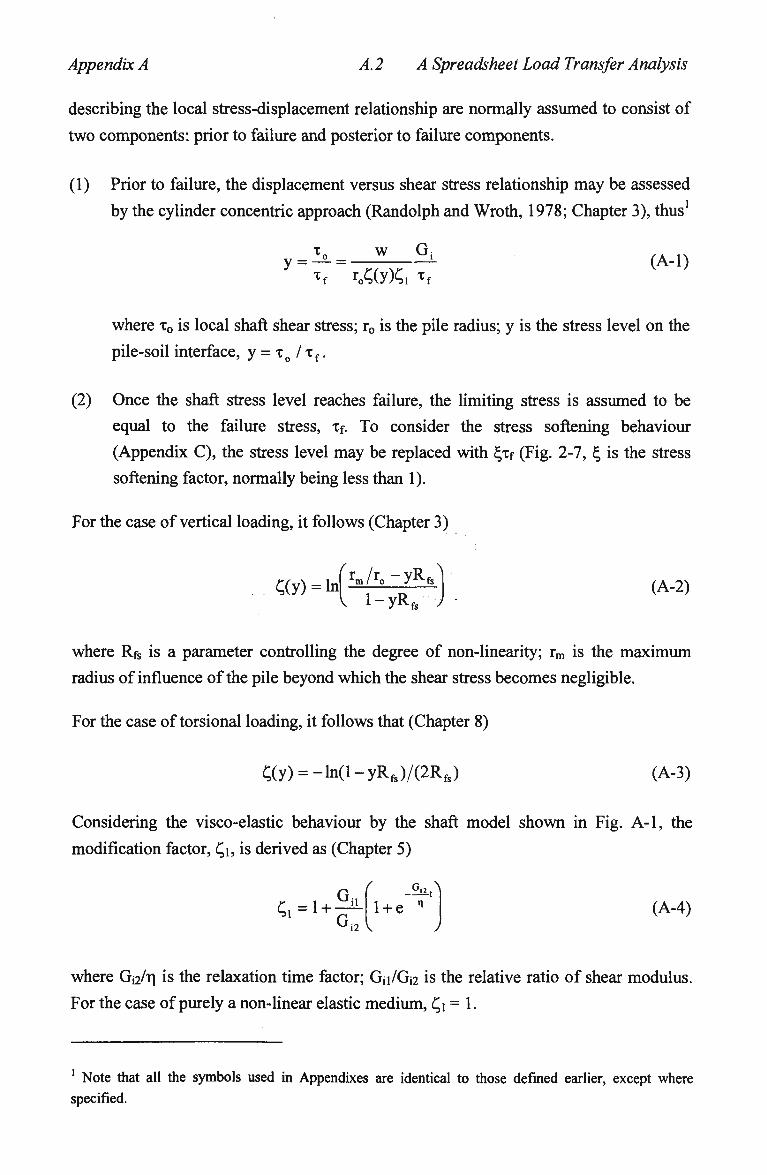
Appendix A A.2 A Spreadsheet Load Transfer Analysis
describing the local stress-displacement relationship are normally assumed to consist of
two components: prior to failure and posterior to failure components.
(1) Prior to failure, the displacement versus shear stress relationship may be assessed
by the cylinder concentric approach (Randolph and Wroth, 1978; Chapter 3), thus1
y = -^ = ^l_^ (A-l) tf r0C(yKi
Tf
where x0 is local shaft shear stress; r0 is the pile radius; y is the stress level on the
pile-soil interface, y = x0 / xf.
(2) Once the shaft stress level reaches failure, the limiting stress is assumed to be
equal to the failure stress, Xf. To consider the stress softening behaviour
(Appendix C ) , the stress level may be replaced with £xf (Fig. 2-7, t, is the stress
softening factor, normally being less than 1).
For the case of vertical loading, it follows (Chapter 3)
rm/
ro-yR* ^(y) = In
i-yRfs J (A-2)
where Rfs is a parameter controlling the degree of non-linearity; rm is the m a x i m u m
radius of influence of the pile beyond which the shear stress becomes negligible.
For the case of torsional loading, it follows that (Chapter 8)
;(y) = -ln(l-yRfs)/(2Rfs) (A-3)
Considering the visco-elastic behaviour by the shaft model shown in Fig. A-l, the
modification factor, C,i, is derived as (Chapter 5)
c, = i 3 Gi2
( -—A 1 + e n
(A-4)
where Gi2/r| is the relaxation time factor; Gn/Gi2 is the relative ratio of shear modulus.
For the case of purely a non-linear elastic medium, C,i = 1.
1 Note that all the symbols used in Appendixes are identical to those denned earlier, except where specified.
Appendix A A. 3 A Spreadsheet Load Transfer Analysis
As shown in Fig. A-2, the increment of displacement, Aw arising from the midpoint of
the segment n to that of n+1 consists of two parts
Aw = Aw^ + AwBC (A-5)
These parts may be estimated by (Coyle and Reese 1966)
A w = wa n + T°7td"L° L" (A-6)
8 [EA]n V J qn
with
2[EA]n 8 [EA] w • Q^_+Q.., + 3Q. L •
where Q n is the axial force, subscript "n" for segment "n", [EA]n is the pile rigidity for
segment n; Ln, Ln+i are the segment lengths for segment n and n+1 respectively; dn, d„+i are the segment diameters for segment n and n+1 respectively. The total shaft displacement of the segment is given by
w = won + Aw (A-8)
where won is the initial displacement at the segment of AC.
Within the elastic stage, displacement by Eq. (A-l) should equal that by Eq. (A-8). Therefore, it follows
F(y) = wOT+wqn+^d„L„-^^ = 0 (A.9)
The load transfer factor, <^(y), is dependent on shear stress level, and is given by the
following local stress-displacement relationship for a non-linear visco-elastic medium
f(y) = C,;(y)-—— = o (A-io) yr0
Tr
where w is the relative pile-soil movement at the midpoint of the segment, AC.
A.2.2 The Difference
The difference between torsional and vertical loading has been summarised in Table A-
i, which is an extension of the analysis presented in the Chapters 3 and 8.
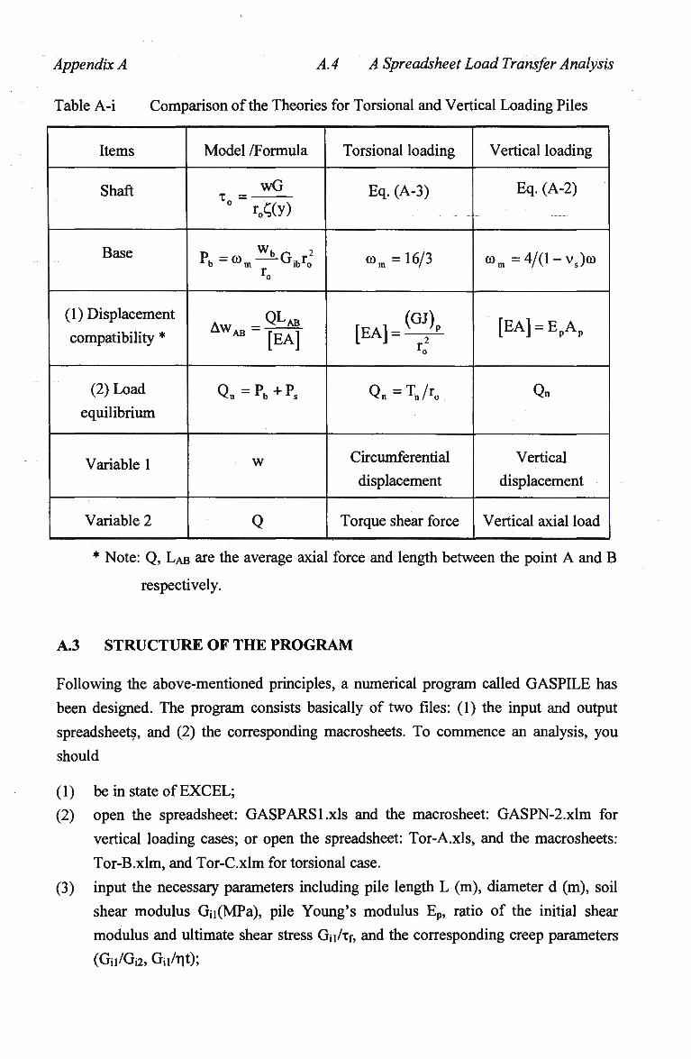
Appendix A A.4 A Spreadsheet Load Transfer Analysis
Table A-i Comparison of the Theories for Torsional and Vertical Loading Piles
Items
Shaft
Base
(1) Displacement
compatibility *
(2) Load
equilibrium
Variable 1
Variable 2
Model /Formula
wG T° " r0«y)
w Pb=«>m^-Gibr0
2
A w = ^ L A B
** [EA]
Q„ = P b + P s
w
Q
Torsional loading
Eq. (A-3)
com=16/3
(GJ)
0
Q„=Tn/r0
Circumferential
displacement
Torque shear force
Vertical loading
Eq. (A-2)
<Dm=4/(l-V,)(0
[EA] = EpAp
Qn
Vertical
displacement
Vertical axial load
* Note: Q, LAB are the average axial force and length between the point A and B
respectively.
A.3 STRUCTURE OF THE PROGRAM
Following the above-mentioned principles, a numerical program called GASPILE has
been designed. The program consists basically of two files: (1) the input and output
spreadsheets, and (2) the corresponding macrosheets. To commence an analysis, you
should
(1) be in state of EXCEL;
(2) open the spreadsheet: GASPARSl.xls and the macrosheet: GASPN-2.xlm for
vertical loading cases; or open the spreadsheet: Tor-A.xls, and the macrosheets:
Tor-B.xlm, and Tor-C.xlm for torsional case.
(3) input the necessary parameters including pile length L (m), diameter d (m), soil
shear modulus Gn(MPa), pile Young's modulus Ep, ratio of the initial shear
modulus and ultimate shear stress Gu/xf, and the corresponding creep parameters
(Gii/Gi2, Gn/Tit);
Appendix A A. 5 A Spreadsheet Load Transfer Analysis
(4) input the value for base property, Rb, which was defined originally for vertically
loaded pile by Murff (1975) and rewritten as (Appendix C)
Rb = PbL/[EA]wb (A-ll)
where the base load Pb and the stiffness [EA] has been provided in Table A-i.
A.4 VERIFICATION OF THE PROGRAM
Comparisons between GASPILE analyses and the previous analyses for vertical loading
and torsional loading are presented in Chapters 3, 5 and 8. However, as an illustration,
an example analysis by GASPILE is provided here, in comparison with the results from
R A T Z analysis (Randolph, 1986).
The analysed pile is assumed of Ep = 20 GPa; L = 40 m, r0 = 1.0 m, and embedded in a
soil of shear modulus, G varying in such a way that the non-homogeneous factor equals
2/3. Given an average shear modulus, Gave = kL, (k = the gradient of the linearly
increasing shear modulus with depth), then the shear modulus at the ground level is, Gj0
= l/2kL, and that at the pile tip level is, GJL = 3/2kL. The value of pile-soil relative
stiffness therefore equals X - Ep/GaVe = 500/k. For a number of X, the pile-head load-
settlement relationships have been predicted by GASPILE program, and are shown in
Fig. A-3, together with the results by R A T Z program. Obviously, as would have
expected, the two programs gives reasonable consistent predictions.
A.5 SUMMARY AND CONCLUSIONS
Pile response could be readily predicted by simply changing the input data in the »
spreadsheet of the GASPILE program. The results are automatically generated and
presented in form of both data and charts, which encompass:
(1) Pile-head load and settlement relationship.
(2) Load and displacement distribution down the pile.
(3) Pile shaft load transfer curves (up to 5 depths).
The program GASPILE may be modified to account for (1) negative friction caused by
external subsidence; (2) the effect of the reconsolidation based on the theory presented
in Chapter 6; (3) group pile interaction based on the theory illustrated in Chapter 7.
Appendix B B.l Theory for Homogeneous Soil
APPENDIX B VERTICAL PILES IN H O M O G E N E O U S SOIL
This appendix shows that the solutions for a pile in a homogeneous soil published
previously can be achieved readily from the new theory established the Chapter 3.
B.l ELASTIC SOLUTION
For a pile in an ideal non-linear homogeneous soil subject to vertical loading, since n =
0, the coefficients in Eq. (3-27) can be simplified as following
C!(z) = C4(z) = -L Jisinhks(L-z) KQ L v z
(B-l) C2(z) = C3(z) = - 1 - -coshks(L- z)
ksL V z
Shaft displacement, w(z), and axial load, P(z), of the pile body at depth of z are
expressed as
w(z) = wb(cosh ks(L - z) + xv smh ks(L - z)) (B-2)
P(z) = ksEpApwb(xv coshks(L - z) + sinhks(L - z)) (B-3)
where EpAp is the cross-sectional rigidity of an equivalent solid cylinder pile. Supposing
load acted on the pile head is Pt, thereby a clear understanding of the relationship among
the force on a pile base and head, the base settlement, Wb and the shaft (base) settlement
ratio can be established as by Eq. (B-3)
Pb cosh p + ksEpApwb sinh p = Pt (B-4)
Note that on the head of a pile (z = 0), from Eq.(3-23), pile settlement wt
wt = wb(cosh P + xv sinn P) (B_5)
where P = ksL. With Eq.(3-28), the non-dimensional relationship between the head load
Pt (hence deformation, wp) and settlement wt is derived as
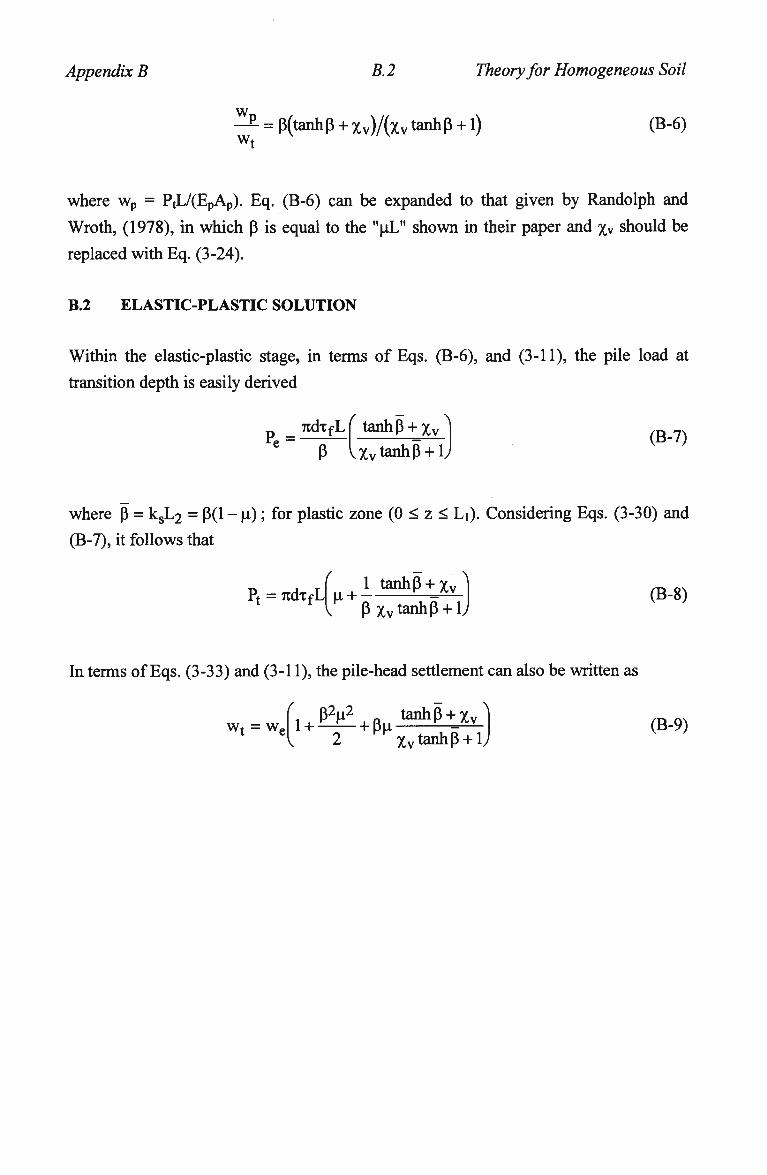
Appendix B B.2 Theory for Homogeneous Soil
w r
w t
= P(tanhp + Xv)/(Xv tanhp+ 1) (B-6)
where w p = PtL/(EpAp). Eq. (B-6) can be expanded to that given by Randolph and
Wroth, (1978), in which p is equal to the "uL" shown in their paper and Xv should be
replaced with Eq. (3-24).
B.2 ELASTIC-PLASTIC SOLUTION
Within the elastic-plastic stage, in terms of Eqs. (B-6), and (3-11), the pile load at
transition depth is easily derived
TidxfL( tanhp + Xv
p \%y tanhp + \) (B-7)
where p = ksL2 = P(l - u); for plastic zone (0 < z < Li). Considering Eqs. (3-30) and
(B-7), it follows that
(
Pt = 7rdxfL H + 1 tanhp+ xv
PXv tanhp + 1) (B-8)
In terms of Eqs. (3-33) and (3-11), the pile-head settlement can also be written as
w t = w e I P ^ 2 i Ru t a n h P ^ v
2 PKxvtanhp + lJ (B-9)
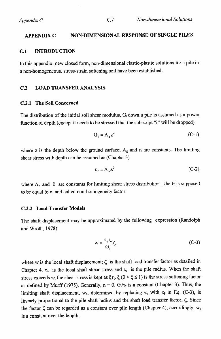
Appendix C C.l Non-dimensional Solutions
APPENDIX C NON-DIMENSIONAL RESPONSE OF SINGLE PILES
C.l INTRODUCTION
In this appendix, new closed form, non-dimensional elastic-plastic solutions for a pile in
a non-homogeneous, stress-strain softening soil have been established.
C.2 LOAD TRANSFER ANALYSIS
C.2.1 The Soil Concerned
The distribution of the initial soil shear modulus, Gj down a pile is assumed as a power
function of depth (except it needs to be stressed that the subscript "i" will be dropped)
G-V (C-l)
where z is the depth below the ground surface; Ag and n are constants. The limiting
shear stress with depth can be assumed as (Chapter 3)
xf=Avze (C-2)
where Av and 0 are constants for limiting shear stress distribution. The 9 is supposed
to be equal to n, and called non-homogeneity factor.
C.2.2 Load Transfer Models
The shaft displacement may be approximated by the following expression (Randolph
and Wroth, 1978)
w = ^C (C-3) G ;
where w is the local shaft displacement; ^ is the shaft load transfer factor as detailed in
Chapter 4. x0 is the local shaft shear stress and r0 is the pile radius. W h e n the shaft
stress exceeds xf, the shear stress is kept as £xf. £ (0 < £ < 1) is the stress softening factor
as defined by Murff (1975). Generally, n = 0, Gj/xf is a constant (Chapter 3). Thus, the
limiting shaft displacement, we, determined by replacing x0 with Xf in Eq. (C-3), is
linearly proportional to the pile shaft radius and the shaft load transfer factor, C,. Since
the factor C, can be regarded as a constant over pile length (Chapter 4), accordingly, w e
is a constant over the length.
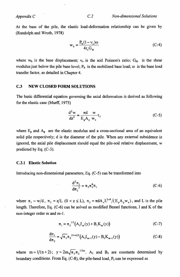
Appendix C C.2 Non-dimensional Solutions
At the base of the pile, the elastic load-deformation relationship can be given by
(Randolph and Wroth, 1978)
P ± ( l - v > b 4r0Gib
where Wb is the base displacement; vs is the soil Poisson's ratio; Gjb is the shear
modulus just below the pile base level; Pb is the mobilised base load; co is the base load
transfer factor, as detailed in Chapter 4.
C.3 NEW CLOSED FORM SOLUTIONS
The basic differential equation governing the axial deformation is derived as following
for the elastic case (Murff, 1975)
dV=^d_^y_Tf (C5) dz E p A p w e
where Ep and Ap are the elastic modulus and a cross-sectional area of an equivalent
solid pile respectively; d is the diameter of the pile. When any external subsidence is
ignored, the axial pile displacement should equal the pile-soil relative displacement, w
predicted by Eq. (C-3).
C.3.1 Elastic Solution
Introducing non-dimensional parameters, Eq. (C-5) can be transformed into
5- = 7r37C27ti (C-6) d7t2
where 7t, = w/d, n2 = z/L (0 < z < L), n3 = 7tdAvL2 + 9/(EpApwe), and L is the pile
length. Therefore, Eq. (C-6) can be solved as modified Bessel functions, I and K of the
non-integer order m and m-1.
".^"'(A.UyHB.KJy)) (c-7)
g- = ^2<l«"2(A,Im.,(y)-B,Knl_1(y)) (C-8)
where m = l/(n + 2); y = 2myfn^n2xl2m. Ai and Bi are constants determined by
boundary conditions. From Eq. (C-8), the pile-head load, Pt can be expressed as
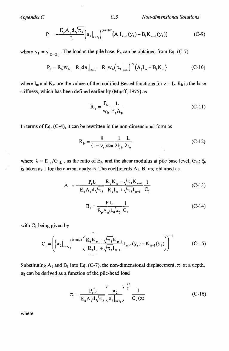
Appendix C C.3 Non-dimensional Solutions
EAAJTU I , \(n+l)/2 Pt=~
P PLV (^U) (AII^I(yt)-B1KB.1(yt)) (C-9)
where y t = yl . The load at the pile base, Pb can be obtained from Eq. (C-7) 'Z=Z
Pb = R b w b = R.dn.l^ = Rbwb(7r2|z=L) (A,Im + B,Km) (C-10)
where Im and Km are the values of the modified Bessel functions for z = L. Rb is the base
stiffness, which has been defined earlier by (Murff, 1975) as
R.= P> L
w b E p A p
(Oil)
In terms of Eq. (C-4), it can be rewritten in the non-dimensional form as
8 1 L Rb = (l-vs)7i(o^b 2r0
(C-12)
where X = E p / G { L , as the ratio of Ep, and the shear modulus at pile base level, GJL; b
is taken as 1 for the current analysis. The coefficients Ai, Bi are obtained as
A , = PtL RbKm-V7t7Km_, 1
EpApd^ Rblm+V^m-l Cl
B,= P«L
E p A p d ^ C,
with Ci being given by
c,= ( l RbKm-V7t7Km_,
I 1 .
Rblm+V^I.
^
,(y,) + KB_I(yt) Lm-1
(C-13)
(C-14)
(C-15)
Substituting Ai and Bi into Eq. (C-7), the non-dimensional displacement, TCJ at a depth,
7C2 can be derived as a function of the pile-head load
71, = P.L
EpApd^TtT
71-
1+n
V n2\ J \ zlz=z, /
1 Cv(z)
(C-16)
where
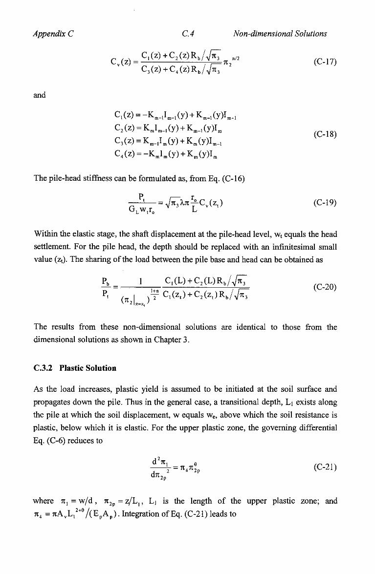
Appendix C C.4 Non-dimensional Solutions
C1(z) + C2(z)Rb/77t7_ n/2 Cv(z) = 7-7=rc2 (C-17)
C3(z) + C4(z)Rb/V7x7
and
C1(z) = -Km_1Im_1(y) + Kra_1(y)Im_1
C2(z) = KmIm.1(y) + Km_1(y)Im
C3(z) = Km_,Im(y) + Km(y)Im_1
C4(z) = -K mI m(y) + Km(y)Im
The pile-head stiffness can be formulated as, from Eq. (C-l6)
(C-18)
P, = V7t7A.7t^Cv(zt) (C-19) G L w t r 0 L
Within the elastic stage, the shaft displacement at the pile-head level, wt equals the head
settlement. For the pile head, the depth should be replaced with an infinitesimal small
value (zt). The sharing of the load between the pile base and head can be obtained as
Pb_ 1 C^LHC^R./VTTT
p. (n\ ^C.CzJ + C^zJR,,/^ ^ 2 7=7_. /
The results from these non-dimensional solutions are identical to those from the
dimensional solutions as shown in Chapter 3.
C.3.2 Plastic Solution
As the load increases, plastic yield is assumed to be initiated at the soil surface and
propagates down the pile. Thus in the general case, a transitional depth, Li exists along
the pile at which the soil displacement, w equals we, above which the soil resistance is
plastic, below which it is elastic. For the upper plastic zone, the governing differential
Eq. (C-6) reduces to
^ =nAnl (C-21) 2 -'M'^p d * 2 P
where nx=w/d, 7t2p=z/L,, Li is the length of the upper plastic zone; and
7t4 = nAyLx2+e /(E A ). Integration of Eq. (C-21) leads to
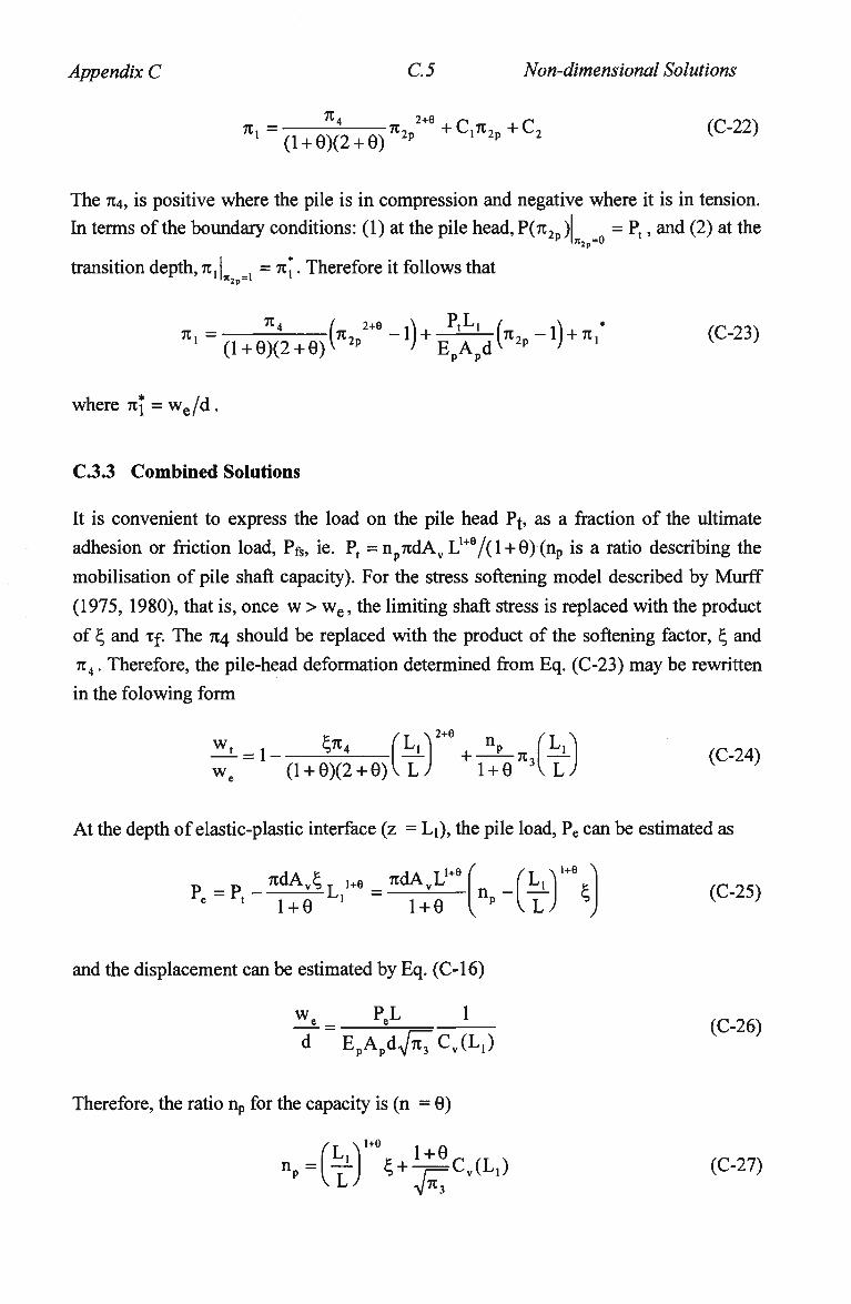
Appendix C C.5 Non-dimensional Solutions
TI, = ^ Tt 2+e + C,TC2P + C 2 (C-22) 1 (l + 0)(2 + 0) 2p ' 2p 2
The 714, is positive where the pile is in compression and negative where it is in tension. In terms of the boundary conditions: (1) at the pile head, P(7t2 ) = Pt, and (2) at the
ljt2p=0
transition depth, TI,^ = TC*. Therefore it follows that
TC, = ^ L *+•_!) +JJLJ_(W _i) + w; (C-23) 1 (l + 0)(2 + 0)V 2p I E pA p d
v 2p ] '
where TC* = we/d.
C.3.3 Combined Solutions
It is convenient to express the load on the pile head Pf, as a fraction of the ultimate adhesion or friction load, PfS, ie. Pt =np7tdAvL
1+e/(l + 0)(np is a ratio describing the
mobilisation of pile shaft capacity). For the stress softening model described by Murff
(1975, 1980), that is, once w > w e, the limiting shaft stress is replaced with the product
of and xf. The 714 should be replaced with the product of the softening factor, £, and 7t4. Therefore, the pile-head deformation determined from Eq. (C-23) may be rewritten in the folowing form
2+e )• n II w. . &< (LA™ , n
we (l + 0)(2 + 0) i - ^ - d - 1 (C-24)
VL) 1+0 3VLJ V }
At the depth of elastic-plastic interface (z = Li), the pile load, Pe can be estimated as
p = p ^ d A ^ 1+e = 7tdAvL i+e ( fT \i+e "\
1+0 X 1+0 L n p - | ^ l § (C-25)
and the displacement can be estimated by Eq. (C-l6)
w. PX 1 d EpApd^Cv(L,)
Therefore, the ratio np for the capacity is (n = 0)
(C-26)
np=(y+Vj7=Cv(L1) (C-27)
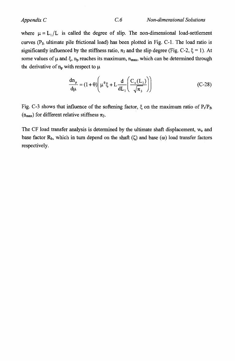
Appendix C C.6 Non-dimensional Solutions
where u. = L,/L is called the degree of slip. The non-dimensional load-settlement
curves (Pf, ultimate pile frictional load) has been plotted in Fig. C-l. The load ratio is
significantly influenced by the stiffness ratio, 7C3 and the slip degree (Fig. C-2, t, = 1). At
some values of p and \, np reaches its maximum, nmax, which can be determined through
the derivative of np with respect to p
dnp
dp = (1 + 0) HVL
'cv ( L l ) vi
dL, v /
(C-28)
Fig. C-3 shows that influence of the softening factor, % on the maximum ratio of Pt/PfS
(nmax) for different relative stiffness 713.
The C F load transfer analysis is determined by the ultimate shaft displacement, w e and
base factor Rb, which in turn depend on the shaft (Q and base (co) load transfer factors
respectively.
Appendix D D.l Determination of Creep Parameters
APPENDIX D DETERMINATION OF CREEP PARAMETERS
This appendix shows how to back-estimate creep parameters from a maintained pile
loading test by matching the time dependent settlement with that predicted by the
theoretical load transfer model. From Eqs. (5-12) and (5-25), the creep settlement rate
may be expressed as
d w c
dt rp» JrV T ^ !°J<Lr Gi2
(D-l)
For a given sustained load at the pile top, the variation of the creep settlement rate
log(dWc/dt) can be plotted against time. The response can be fitted by Eq. (D-l), and
usually results in a straight line. Thus creep parameters are back estimated. A n example
is illustrated below:
A pile called pile I was tested in clay up to failure in an increment sustained tensile
loading pattern (Ramalho Ortigao and Randolph, 1983). It was a closed ended steel pipe
pile of 203 m m diameter and 6.4 m m wall thickness driven 9.5 m into a stiff
overconsolidated clay. Young's modulus for the pile body was 2.1xl05 MPa. Soil shear
modulus was about 12 M P a from back estimation with the load settlement curve, and
the failure shaft friction was about 41.5 kPa for the pile. The creep parameters for this
pile I has been back-figured as illustrated below.
For estimation of the non-linear elastic load transfer measure, C„ an average pile stress
level is used. From the loading tests, the ultimate load of pile I is 280 kN; thus the
corresponding stress (load) level for the pile under loads of 200 and 240 k N would be
0.714 and 0.857 respectively. With the stress levels, the pile geometry, a soil Poisson's
ratio of 0.3, the non-linear elastic measure, as predicted by Eq. (5-14), is 6.35 at load
level 1 of 200 k N (referred to as (£2)0 and 7.04 at level 2 of 240 k N (referred to as
(£2)2) respectively.
Based on the measurement of pile I by Ramalho Ortigao and Randolph (1983), a plot of
the log creep settlement rate and time relationship shown in Fig. 5-7 demonstrates that
for the pile under two different loading levels of 200 and 240 kN, the corresponding -6 -6 -1
relaxation times, 1/Ti and I/T2 are equal to 6.64x10 and 3.6x10 s respectively. The intersections in the creep settlement rate ordinate for the two loading levels are 0.00018
and 0.00035 mm/min.
Appendix D D.2 Determination of Creep Parameters
In terms of these parameters and Eq. (D-l), at loading level 1,
x„r„ \(Q \ i (^).lJl£^ \-JL — = 0.00018 (mm/min) (D-2)
with \|/i = 0.714, (£2)i, = 6.35, r0= 101.5 mm, 1/Ti = 6.64x10V and xf= 41.5 kPa
therefore Gji/Gi2= 0.2839, (Gi2)i = 42.27 MPa.
At loading level 2,
(^y^H \^A ^- = 0.00035 (mm/min) (D-3) v G n ; 2 ^G i 2 ; 2 T 2
with \j/2 = 0.857, (£2)2 = 7.04, r0 = 101.5 mm, 1/T2 = 3.6x10V and xf = 41.5 kPa
therefore GJI/GJ2= 0.7653, (G,2)2 = 15.68 MPa. The initial shear modulus, Gii generally
increases with the process of consolidation of the soil, but can be regarded as a constant,
once the primary consolidation is complete. The creep parameters, Gj2 and rj normally
vary with the loading (hence stress) level (Fig. 5-7). For this particular example, a value
of 2.69 is obtained for the ratio of delayed shear moduli between load level 1, (Gi2)i and
level 2, (Gj2)2. However, the ratio of Gu/Gi2 and Gi2/r) are nearly constants within
normal working load level, e.g. less than 7 0 % of failure load level, of a pile of normal
length. At higher load levels or for a long pile, the ultimate shaft stress for spring 2 is
normally about 7 0 % of that of spring 1, therefore, a higher value of 2 than that of £, is
generally resulted even if the pile does not yield, which may accompany by a higher
value of GJI/GJ2. The ratio, Gj2/r| influences the duration of creep time rather than the
final pile head response. Therefore it can roughly be taken as a constant over the zone of
general working load.
Appendix E El Radial Consolidation
APPENDIX E RADIAL CONSOLIDATION
This appendix gives
(1) the solution of the time-dependent equation, Eq. (6-17) for visco-elastic case;
(2) elastic solution for radial non-homogeneous case; and
(3) elastic solution for radial non-homogeneous case, with logarithmic variation of
initial pore pressure distribution.
E.l SOLUTION FOR THE TIME-DEPENDENT EQ. (6-17)
The following time-dependent governing equation is solved in this section.
«.«. + 0..f«kWdF(lzx)(h + a j T t) = „ dt J
o dt d(t-x) (E-l)
In terms of Laplace transform, it follows
[sTn - Tn (0)] + Gy][(sTn - Tn (0))(sF - F(0)) + <Tn=0 (E-2)
Due to Tn(0) = 1, Eq. (E-2) can be written as
T= Gyl(sF-F(0)) + l
" Gyl(s2F-sF(0)) + a; + s
(E-3)
The flexibility factor, F(t), is given by Eq. (6-2), hence, the Laplace transform of F(t) is
F = G Yl
+ m. 1 1
Is s + 1/T2 + m,
1 exp(tk/T3)N
s s+l/T3 y (E-4)
Therefore
GYl(s2F-F(0)) = ^ ^ + S a ^ 3 + m 3 / T
Yl^ I s+l/T s+l/T, V-(E-5)
This equation enables Eq. (E-3) to be written as
m 2 /(T2 s +1) + (sa k m 3 T3 + m 3 )/(sT3 +1) +1 T =
s[m2/(T2s + l) + (sakm3T3 +m3)/(sT3 +l)] + a2 +s
(E-6)
To facilitate the inverse Laplace transform, Eq. (E-6) is rewritten as
Appendix E E.2 Radial Consolidation
- s'+H„s + l„ (E.7) " (s-a„)(s-b„)(s-c„)
where all the parameters have been defined in the Chapter 6. Eq. (E-7) may be divided
into tliree parts according the denominator, for each parts, an inverse Laplace transform can be readily obtained (Abramowitz and Stegun, 1964), Finally, Eq. (E-7) can be transformed into Eq. (6-24).
If m3 = 0,1/T3 = 0, ak = 0, then
TB= , / + (1 + m2^ _ (E-8)
s2+(a2n+(m2+l)/T2)s + a
2n/T2
The inverse of Eq. (E-8) is Eq. (6-26). Otherwise, if m 2 = m 3 = 0, 1/T2 = 1/T3 = 0, ak = 0, then Eq. (E-6) reduces to the following format
T7 = l/(s + a2n) (E-9)
The inverse of Eq. (E-9) is Eq. (6-30).
E.2 SOLUTION FOR RADIAL NON-HOMOGENOUS CASE
For elastic case, from Eq. (6-2), dF/dt = 0. Therefore, if taking Gy, =GrorK, (Gro =
shear modulus at pile-soil interface. In the following parts, the subscript "ro" may be
dropped, unless it need stressing; K is a constant, 0 < K < 1), Eqs. (6-16) and (6-17) may be rewritten as
a2w iaw ., .. „
where
dr r + r
dT(t) dt
a
Cv =
+ X2nr~K
dr
+ a2nT(t) =
2 = X 2 c n n v
k Gro
rw l~2vs
w =
= 0 (E-ll)
(E-12)
(E-13)
The parameter, Xn, is one of the infinite roots satisfying Eq. (E-10), which may be
expressed in terms of the Bessel functions as
Appendix E E.3 Radial Consolidation
wn(r) = AnJ0(^ny) + BnY0(^ny) (E-14)
where A„ is dependent on the boundary conditions. The functions J0, Y0, Ji, Yi are
Bessel functions of zero order and first order, with Jj being Bessel functions of the first
kind, and the Yj being Bessel functions of the second kind. The variable, y, is given by
y = —r(2-K)/2 (E-15) 2-K
and the corresponding boundary value at r = r0 is
yl =yo=-?-r0(2-K)/2 (E-16)
•,lr=r0 2 — K
Cylinder functions, Vi(A,ny0) of i-th order (McLachlan, 1955) may be expressed as
Vi(A.By) = Jl(A.By)-i^y-lYi(\11y) (E-l 7) Y,O ny 0)
Based on the boundary condition of Eq. (6-14b), Bn = -An J,(^ny0)/Y,(A.ny0). Thus,
fromEq. (E-14),
wn(y) = AnV0(A,ny) (E-18)
dwn(y) = A.V1(Xny)l = 0 (E-19)
y=y, y=y»
dr
Also, with Eq. (6-14c), u = 0 for y > y* (r > r*), it follows
vo(^ny,) = J0(^ny
,)-!;(^nyo)Y0(^ny,) = o (E-20)
Yi(^ny0)
Eqs. (E-19) and (E-20) render the cylinder functions to be defined.
The solution of Eq. (E-l 1) is
Tn(t) = e-a"< (E-21)
The full expression for pore pressure, u will be a summation of all the possible solutions
u=lAnV0(^ny)Tn(t) (E-22) n=l
Appendix E E.4 Radial Consolidation
Normally the first 50 roots of the Bessel functions are found to give sufficient accuracy.
With Eqs. (6-14a) and (E-22), it follows
* / *
An = ju0 (y)V0 (yXn )ydy / Jv2 (yXn )ydy (E-23)
y» / y0
E.3 CONSOLBDATION FOR LOGARITHMIC VARIATION OF u 0
The initial stress state for radial consolidation of an elastic non-homogeneous medium
around a rigid, impermeable pile is similar to that of an elastic medium, which are
described below:
(1) The width of the plastic zone given by Eq. (6-3 8) may be rewritten as
yL = y R = ~^o VG/\ )(2_K)/2 (E-24)
(3) The initial excess pore pressure distribution by Eq. (6-39) may be rewritten as
u0(r) = —^—suln|^-| 2 - K l y r | y 0 ^ y ^ y R (E-25)
u0 = 0 yR < y < y*
where yR is the radius, beyond which the excess pore pressure is initially zero.
In light of the initial pore pressure distribution of Eq. (E-25), the coefficients, An, can be
simplified as
A = 2 4su V0(X,yD)-V0(X,ya)
2 - K XD y V,(A,ny )-y0V0 (XDy0)
With these values of A„, the pore pressure can be readily estimated using Eq. (E-22).
Fig. E-l shows an example of the effect of radial non-homogeneity on the dissipation of
excess pore pressure. It demonstrates that radial non-homogeneity has significant effect
on the value of the ratio, u(r0)/su, during the initial stage of the consolidation, but has
negligible effect at the late stage of the consolidation process.
Appendix F F.l Torque and Twist Profile
APPENDIX F TORQUE AND TWIST PROFILE
This appendix shows the closed form solutions for the assessment of the torque and
twist angle profile along a pile, the consistency of the stiffness prediction of the
solutions shown in Chapter 8 with the previous solution for homogeneous cases.
Profiles of torque and twist angle down the pile, for elastic conditions have been
formulated as
<Kz) = -| 4>b 1/2
C3(z) + xC4(z)
c3(L) (F-l)
T(z)
(GJ)D
= Tc|/2m -(l+n)/2
L
C,(z) + xC2(z)
C3(L) (F-2)
Within the plastic zone, it follows that
T(z) = Te+(GJ)p<|>eTc;/2m
l+n „l+n L'^-z l + n
(F-3)
L -z <Kz) = <!>e+-r—-+K
n
l+n , „2+n 1/2 m
(GJL e'"t
(l + n)L/1+n-(2 + n)zL',+n + z
(l + n)(2 + n) (F-4)
If the non-homogeneity factor n = 0, the coefficients can be simplified as follows
C,(z) = C4(z) = — - sinh7ct(l - f ) 7tt V z L
= —./—cosh 71, 71, V Z
(F-5)
C2(z) = C3(z) = — J — <•-!>
Therefore, shaft rotation, <|>(z), and axial torque, T(z), of the pile body at depth of z are
expressed respectively as
<j>(z) = f cosh7c, 1 1 +xsinh7ttl 1- — (F-6)
T(z) = (GJ)p7ct x — ; <Pt sinhTcJ 1 j+xcoshTCt '-£ (F-7)
Appendix F F.2 Torque and Twist Profile
From the definition shown in Table 8-1 column 3 (Chapter 8), with Eq. (8-28), the pile-
head stiffness can be rewritten as
Tt = (GJ)p7tt x + tanh(7ct)
G ^ f Agr03 L l + xtanh(Tc.)
Using the relationship between TCt and X relationship shown in Table 8-1 and Eq. (8-27),
the form of Eq. (F-8) can be transformed into an identical one to that for the linear case
obtained by Randolph, (1981).
R. 1 References
REFERENCES
Abendroth, R. E., and Greimann, L. F. (1988). "Pile Behaviour Established from
Model Tests." J. ofGeotech. Engrg. Div., ASCE, 116(4), 571-588.
Abramowitz, M., and Stegun, I. A. (1964). Handbook of Mathematical Functions with
Formulas, Graphs and Mathematical Tables. National Bureau of Standards
Applied Mathematics Series, 55. U.S. Government printing office, Washington,
D. C. 20402.
API RP2A: recommended practice for planning, designing and constructing fixed
offshore platforms, (1987). American Petroleum Institute (API), Washington,
D.C.
Armaleh, S., and Desai, C. S. (1987). "Load Deformation Response of Axially Loaded
Piles." J. ofGeotech. Engrg. Div., ASCE, 113(12), 1483-1499.
Azzouz, A. S., Baligh, M. M., and Whittle, A. J. (1985). "Shaft Resistance of Piles in
Clay." J. ofGeotech. Engrg. Div., ASCE, 116(2), 205-221.
Baligh, M. M. (1985). "Strain Path Method." J. ofGeotech. Engrg. Div., ASCE,
111(9), 1108-1136.
Baligh, M. M. (1986a). "Undrained Deep Penetration, I: Shear Stresses."
Geotechnique, 36(4), 471-485.
Baligh, M. M. (1986b). "Undrained Deep Penetration, II: Pore Pressure."
Geotechnique, 36(4), 487-501.
Banerjee, R. (1978). "Analysis of Axially and Laterally Loaded Pile Groups." In
Developments in Soil Mechanics (Ed. C. R. Scott), Applied Science Publishers,
U.K.
Banerjee, P. K., and Davies, T. G. (1977). "Analysis of Pile Groups Embedded in
Gibson Soil." Proc. of 9th ICSMFE, Tokyo, Japan, 1, 381-386.
Barron, R. (1948). "Consolidation of Fine Grained Soils by Drain Wells." Trans.
Amer. Soe. Civ. Engrs. 113, 718-742.
Berezantzev, V. G., Khristoforov, V. S., and Golubkov, V. N. (1961). "Load Bearing
Capacity and Deformation of Piled Foundation," Proc. 5th ICSMFE, Paris, 2.
11-15.
Bergdahl, U., and Hult, G. (1981). "Load Tests on Friction Piles in Clay." Proc. of the
XICSMFE, Stockhom: Balkema, 2, 625-630.
Biot, M. A. (1941). "General Theory of Three-dimensional Consolidation." J. ofAppl.
Phys. 12, 155-164.
R.2 References
Bjerrum, L., Brinch Hansen, J., and Sevalason, R. (1958). "Geotechnical Investigations
for a Quay Structure in Horten." Norwegian Geotechnical Institute, Publ. No. 28,
1-18.
Bjerrum, L., and Johannessen, I. (1960). "Pore Pressures Resulting form Driving Piles
in Soft Clay." Proc. of Conf. on Pore Pressure and Suction in Soils, London,
108-111.
Booker, J. R., and Poulos, H. G. (1976). "Analysis of Creep Settlement of Pile
Foundations."./ ofGeotech. Engrg. Div, ASCE, 102(1), 1-14.
Booker, J. R., Balaam, N., and Davis, E. H. (1985). "The behaviour of an elastic non-
homogeneous half-space, Parts I & II." Int. J. Numer. and Analy. Methods in
Geomechanics, 9(4), 353-367, 369-381.
Bozozuk, M., Fellenius, B. H., and Samson, L. (1978). "Soil Disturbance from Pile
Driving in Sensitive Clay." Can. Geotech. J., 15(3), 346-361.
Briaud, J. L., Anderson, J., and Perdomo, D. (1987). "Evaluation of API Method Using
98 Vertical Pile Load Tests." Proc. 19th Annual OTC, Houston, Paper O T C
5411,447-451.
Buisuman, K. (1936). "Results of Long Duration Settlement Tests." Proc. 1st
ICSMFE, 1, 103-106.
Burland, J. B. (1973). "Shaft Friction of Piles in Clay - A Simple Fundamental
Approach." Ground Engineering, 6(3), 30-32.
Burland, J. B., and Twine, D. (1988). "The Shaft Friction of Bored Piles in Terms of
Effective Strength." Deep Foundations on Bored and Augered Piles, Balkema,
Rotterdam, 411-420.
Butterfield, R., and Banerjee, R. (1970). "A Note on the Problem of a Pile-reinforced
Half-space." Geotechnique, 20(1), 100-103.
Butterfield, R., and Banerjee, R. (1971). "The Elastic Analysis of Compressible Piles
and Pile Groups." Geotechnique, 21(1), 43-60.
Butterfield, R., and Douglas, R. A. (1981). "Flexibility Coefficients for the Design of
Piles and Pile Groups." CIRIA: Technical Note 108, London, CIRIA.
Carter, J. P., Randolph, M. F., and Wroth, C. P. (1979). "Stress and Pore Pressure
Change in Clay during and after the Expansion of a cylinder Cavity." Int. J.
Numer. and Analy. Methods in Geomechanics, 3, 305-322.
Casagrande, A. (1932). "The Structure of Clay and its Importance in Foundation
Engineering." J. of Boston Society of Civil Engineering, reprinted in contribution
to soil mechanics 1925-1940, 72-113.
R.3 References
Casagrande, A., and Wison, S. (1951). "Effect of Rate Loading on the Strength of
Clays and Shales at Constant Water Content." Geotechnique, 2(3).
Castelli, F., Maugeri, M., and Motta, E. (1993). Discussion of "A New Method for
Single Pile Settlement Prediction and Analysis." by Fleming, W . G. K. (1992),
Geotechnique, 43(4), 615-619.
Chan, K. S., Karasudhl, P., and Lee, S. L. (1974). "Force at a Point in the Interior of
Layered Elastic Half-space." Int. J. Solids Struct., 10(11), 1179-1199.
Chandler, R. J. (1968). "The Shaft Friction of Piles in Cohesive Soils in Terms of
Effective Stress." Civ. Engng. Publ. Wks. Rev. Jan. 48-50.
Chen, Z. C, and Song, R. (1991). "A study on Compression of Shaft of Individual
Pile." 4th Int. DFIConf, Balkema, Rotterdam, 343-348.
Cheung, Y. K., Tham, L. G., and Guo, D. J. (1988). "Analysis of Pile Group by Infinite
Layer Method." Geotechnique, 38(3), 415-431.
Chin, F. K. (1970). "The Inverse Slope as a Prediction of Ultimate Bearing Capacity of
Piles." Proc. 3rd S. E. Asian Conf. on Soil Engrg., Singapore, 11-15, June, 81-
90.
Chin, F. K., and Vail, A. J. (1973). "Behaviour of piles in alluvium." Proc, 8th
ICSMFE, Vol. 2.1, Moscow, U.S.S.R., 47-52.
Chin, J. T., Chow, Y. K., and Poulos, H. G. (1990). "Numerical Analysis of Axially
Loaded Vertical Piles and Pile Groups." Computers and Geotechnics, 9(4), 273-
290.
Christensen, R. W., and Wu, T. H. (1964). "Analyses of Clay Deformation as a Rate
Process." J. ofSoilMech. and Found. Engrg. Div. 90(6), 125-157.
Christian, J. T., and Boehmer, J. W. (1972). "Plane Strain Consolidation by Finite
Elements."./ ofSoilMech. and Found. Engrg. Div. 96(4), 1435-1457.
Christie, I. F. (1964). "A Re-appraisal of Mediant's Contribution to the Theory of
Consolidation.", Geotechnique, 14(4), 309-320
Chow, Y. K. (1986a). "Analysis of Vertically Loaded Pile Groups." Int. J. Numer. and
Analy. Methods in Geomechanics, 10(1), 59-72.
Chow, Y. K. (1986b). "Discrete Element Analysis of Settlement of Pile Groups."
Computer & Structures, 24(1), 157-166.
Chow, Y. K. (1985). "Torsional Response of Piles in Nonhomogeneous Soil" J. of
Geotech. Engrg. Div., ASCE, 111(7), 942-947.
R.4 References
Chow, Y. K. (1989). "Axially Loaded Piles and Pile Groups Embedded in a Cross-
anisotropic Soil." Geotechnique, 39(2), 203-211.
Clancy, P. (1993). Numerical Analysis of Piled Raft Foundation. Ph. D thesis, The
University of Western Australia.
Clancy, P., and Randolph, M. F. (1993). "An Approximate Analysis Procedure for
Piled Raft Foundations." Int. J. Numer. and Analy. Methods in Geomechanics,
17(12), 849-869.
Clark, J. I., and Meyerhof, G. G. (1972). "The Behaviour of Piles Driven Clay. I An
Investigation of Soil Stress and Pore Water Pressure as Related to Soil
Properties." Can. Geotech. J., 9(4), 351-373.
Clark, J. I., and Meyerhof, G. G. (1973). "The Behaviour of Piles Driven Clay. II An
Investigation of Bearing Capacity Using Total and Effective Strength
Parameters." Can. Geotech. J., 10(1), 86-100.
Clemente, J. M. (1990). "Analysis of Pile Groups with Variable Shaft-Load and Point-
Load Ratios." J. ofGeotech. Engrg. Div., ASCE, 116(4), 692-697.
Cooke, R. W. (1974). "The Settlement of Friction Pile Foundations." Proceedings,
Conference on Tall Buildings, Kuala Lumpur, Malaysia.
Cooke, R. W., Price, G., and Tarr, K. (1979). "Jacked Piles In London Clay: A Study
of Load Transfer and Settlement under Working Conditions." Geotechnique,
29(4), 461-468.
Cooke, R. W., Price, G., and Tarr, K. (1980). "Jacked Piles In London Clay:
Interaction and Group Behaviour under Working Conditions." Geotechnique,
30(2), 97-136.
Cooke, R. W. (1986). "Pile Raft Foundations on Stiff Clays - A Contribution to
Design Philosophy." Geotechnique, 36(2), 169-203.
Coyle, H. M., and Reese, L. C. (1966). "Load Transfer for Axially Loaded Piles In
Clay." J. of Soil Meek and Found. Engrg. Div. 92(2), 1-26.
Coyle, H. M., and Sulaiman, I. H. (1967). "Load Transfer for Axially Loaded Piles In
Clay." J. ofSoilMech. and Found. Engrg. Div. 93(6), 261-278.
Cryer, C. W. (1963). "A Comparison of the Three-Dimensional Consolidation
Theories of Biot and Terzaghi," Quart. J. Mech. and Math. 16, 401-412.
Cummings, A. E., Kerkhoff, G. O., and Peck, R. B. (1948). "Effect of Driving Piles
into Soft Clay.", Proceedings, ASCE, 74,1553-1563.
Davis, E. H., and Poulos, H. G. (1972). "Rate of Settlement Under Two- and Three-
dimensional Conditions.", Geotechnique, 22(1), 95-114.
R.5 References
Davis, E. H., and Raymond, G. P. (1965). "A Non-linear Theory of Consolidation.",
Geotechnique, 15(2), 161-173.
D'Appolonia, D., and Romudladi, J. P. (1963). "Load Transfer in End-Bearing Steel H-
Piles." J. Soil Meek and Found. Engrg, ASCE, 89(2), 1-25.
Duncan, J. M., and Chang, C. Y. (1970). "Non-linear Analysis of Stress and Strain in
Soils." J. Soil Meek and Found. Engrg., ASCE, 96(5), 1629-1652.
England, M. (1992). "Pile Settlement Behaviour: an accurate model." Application of
the Stress Wave Theory to Piles. Rotterdam, Balkema, 91-96.
Edil, T. B., and Mochtar, I. B. (1988). "Creep Response of Model Pile in Clay." J. of
Geotech. Engrg. Div, ASCE, 114(11), 1245-1259.
Eide, O., Hutchinson, J. N., and Landva, A. (1961). "Short and Long Term Test
Loading of a Friction Pile in Clay." Proc. 5th ICSMFE, Paris, 2, 45-53.
Feda, J. (1992), Creep of Soils and Related Phenomena. Developments in
Geotechnical Engineering 68, Publishing House of the Czechoslovak Academy
of Sciences, Prague.
Fellenius, B. H. (1972). "Down-drag on Piles in Clay due to Negative Skin Friction."
Can. Geotech. J., 9(4), 323-337.
Fellenius, B. H., and Samson, L. (1976). "Testing of Drivability of Concrete Piles and
Disturbance to Sensitive Clay." Can. Geotech. J., 13(2), 139-160.
Flaate, K. (1972). "Effects of Pile Driving in Clay." Can. Geotech. J., 9(1), 81-88.
Flaate, K., and Seines, P. (1977). "Side Friction of Piles in Clay." Proc. of 9th
ICSMFE, Tokyo, Japan, 1, 517-522.
Fleming, W. G. K., Weltman A. J., Randolph, M. F., and Elson, W. K. (1992). Piling
Engineering (2nd Edition). Surrey University Press, Glasgow, Halst Press, N e w
York.
Fleming, W. G. K. (1992). "A New Method for Single Pile Settlement Prediction and
Analysis." Geotechnique, 42(3), 411-425.
Francescon, M. (1983). "Model Pile Tests in Clay: Stress and Displacements due to
Installation and Axial Loading." Ph. D Thesis, Cambridge University.
Frank, R (1974). "Etude Theorique du Comportement des Pieux sous Charge
Verticale. Introduction de la Dilatance," Doctor-Engineer Thesis, University
Paris, France.
R. 6 References
Frank, R., and Zhao, S. R. (1982). "Estimation par les parametres pressiometriques de
l'enfoncementt soud charge axiale de pieux fores dans des sols fins." Bull.
Liaison Labo. P. et Ck, No.l 19, 17-24, (in French).
Frank, R., Kalteziotis, N., Bustamante, M., Christoulas, S., and Zervogiannis, H.
(1991). "Evaluation of Performance of Two Piles Using Pressuremeter Method."
J. ofGeotech. Engrg. Div., ASCE, 117(5),695-713.
Fujita, H. (1976). "Study on Prediction of Load vs. Settlement Relationship for a
Single Pile." Special report of Hazama-Gumi, Ltd, No.l (in Japanese).
Georgiadis, M., and Saflekou, S. (1990). "Piles Under Axial and Torsional Loads."
Computers and Geotechnics, 9, 291-305.
Gibson, R. E., and Anderson, W. F. (1963). "In-situ Measurement of Soil Properties
with the Pressuremeter." Civ. Eng. and Public Work Rev., 56, No. 658.
Goosens, D., and Van Impe, W. F. (1991). "Long Term Settlements of a Pile Group
Foundation in Sand, Overlying a Clayey Layer." Proc. 10th ECSMFE, Florence,
1,425-428.
Geuze, E. C. W. A., and Tan. T. K. (1953). "The Mechanical Behaviour of Clays."
Proc. 2nd Int. Congress on Rheology.
Guo, D. J., Tham, L. G., and Cheung, Y. K. (1987). "Infinite Layer for the Analysis of
a Single Pile." Computers and Geotechnics, 3(4), 229-249.
Guo, W. D., and Randolph, M. F. (1996a). "Settlement of Pile Groups in Non-
homogeneous Soil." Proc. 7th ANZ Conference on Geomechnics, 1, 631-636
Guo, W. D., and Randolph, M. F. (1996b). "Torsional Piles in Non-homogeneous
Media." Accepted by Computers and Geotechnics for publication.
Guo, W . D., and Randolph, M. F. (1996c). "Vertically Loaded Piles in Non-
homogeneous Media." Accepted by International. J. Num. & Analy. methods in Geomechanics for publication.
Gurtowski, T. M., and W u , M. J. (1984). "Compression Load tests on Concrete Piles
in Alluvium." Anal, and Design of Pile Foundations, Am. Soe. Civ Engrs. 138-
153.
Hache, R. A. G., and Valsangkar, A. J. (1988). "Torsional Resistance of Single Pile in
Layered Soil." J. ofGeotech. Engrg Div, ASCE, 114(2), 216-220.
Hirayama, H. (1990). "Load-Settlement Analysis for Bored Piles Using Hyperbolic
Transfer Functions." Soils and Foundations, JSSMFE. 30(1), 55-64.
Iskander, M., and Olson, R. E. (1992). "Review of API Guidelines for Pipe Piles in
Sand." Proc. of Int. Conf. Civil Engineering in the Oceans V, Texas, Nov. 2-5,
798-812.
R. 7 References
Itasca (1992). "FLAC - Users' Manual." Itasca Consulting Group, Minneapolis.
Jardine, R. J., Potts, D. M., Fourie, A. B., and Burland, J. B. (1986). "Studies of the
Influence of Non-linear Stress-Strain Characteristics in Soil-Structure
Interaction." Geotechnique, 36(3), 377-396.
Kaniraj, S. R. (1993). "A Semi-empirical Equation for Settlement Ratio of Pile
Foundations in Sand." Soils and Foundations, JSSMFE. 33(2), 82-90.
Kezdi, A. (1975). Chapter 19, Pile Foundations. Foundation Engineering Handbook,
Ed. by Winterkorn, H. F. and Fang, H. Y., Van Nostrand Reinhold Company,
N e w York, N. Y., 567.
Khan, N. I., Templeton, J. S., and O'Neill, M. W. (1992). "Skin Friction Distribution
on Piles in Sand." Proc. of Int. Conf. Civil Engineering in the Oceans V, Texas,
Nov. 2-5, 783-797.
Kiousis, P. D., and Elansary, A. S. (1987). "Load Settlement Relationship for Axially
Loaded Piles." J. ofGeotech. Engrg. Div, ASCE, 113(6), 655-661.
Kodikara, J. K., and Johnston, I. W. (1994). "Analysis of Compressible Axially
Loaded Piles in Rock." Int. J. Numer. and Analy. Methods in Geomechanics, 12,
427-437.
Koerner, R. M., and Partos, A. (1974). "Settlement of Building on Pile Foundation in
Sand." J. ofGeotech. Engrg. Div, ASCE, 100(3), 265-278.
Koizumi, Y., and Ito, K. (1967). "Field Tests with Regard to Pile Driving and Bearing
Capacity of Piled Foundations." Soils and Foundations, 7(3), 30-53.
Komamura, F., and Huang, R. J. (1974). "New Rheological Model for Soil
Behaviour." J. ofGeotech. Engrg. Div., ASCE, 100(7), 807-824.
Konrad, J.-M., and Roy, M. (1987). "Bearing Capacity of Friction Piles in Marine
Clay." Geotechnique, 37(2), 163-175.
Kraft, L. M., Focht, J. A., and Amerasinghe, S. F. (1981). "Frictional Capacity of Piles
Driven into Clay." J. ofGeotech. Engrg. Div, ASCE, 107(11), 1521-1541.
Kraft, L. M., Ray, R. P., and Kagawa, T. (1981). "Theoretical t-z Curves." J. of
Geotech. Engrg. Div, ASCE, 107(11), 1543-1561.
Kraft, L. M. (1991). "Performance of Axially Loaded Pipe Piles in Sand." J. of
Geotech. Engrg. Div, ASCE, 117(2), 272-296.
Kulhawy, F. H. (1984). "Limiting Tip and Side Resistance: Fact or Fallacy?." Analysis
and Design of Pile Foundation, ASCE, N e w York. 80-98.
R.8 References
Kuwabara, F. (1991). "Settlement Behaviour of Nonlinear Soil Around Single Piles
Subjected to Vertical Loads." Soils and Foundations, JSSMFE, 31(1), 39-46.
Lee, C. Y. (1991). "Axial Response Analysis of Axially Loaded Piles and Pile
Groups." Computers and Geotechnics, 11(4), 295-313.
Lee, C. Y. (1993a). "Settlement of Pile Group-Practical Approach." J. ofGeotech.
Engrg. Div, ASCE, 119(9), 1449-1461.
Lee, C. Y. (1993b). "Pile Group Settlement Analysis by Hybrid Layer Approach." J. of
Geotech. Engrg. Div, ASCE, 119(6), 984-997.
Lee, C. Y., and Poulos, H. G. (1990). "Axial Response Analysis of Piles in Vertically
and Horizontally Loaded Non-homogeneous Soils." Computers and Geotechnics,
9(3), 133-148.
Lee, E. H. (1955). "Stress Analysis in Viscoelastic Bodies." Quart. Appl. Math. 13,
183.
Lee, E. H. (1956). "Stress Analysis in Viscoelastic Bodies." J. of Applied Physics
27(7), 665-672.
Lee, E. H., Radok, J. M., and Woodward, W. B. (1959). "Stress Analysis for Linear
Viscoelastic Materials." Transactions, Society of Rheology, 3, 41-59.
Leonards, Z. (1973), Foundation Engineering for Difficult Subsoil Condition. Van
Norstrand Reinhold Company.
Leonards, G. A., and Lovell, D. (1979). "Interpretation of Load Tests on High-
Capacity Driven Piles." Behaviour of Deep Foundations ASTM STP 670,
Raymond Lundgen, Ed., A S T M , 388-415.
Lim, C. H., Chow, Y. K., and Karunaratne, G. R. (1993). "Negative Skin Friction on
Single Piles in a Layered Half-Space." Int. J. Numer. and Analy. Methods in
Geomechanics, 17, 625-645.
Liu, J. L. (1990). Pile Foundation Design and Calculation. China Construction
Industry Press House, Beijing, 264-268, (in Chinese).
Liu, Q. F., and Meyerhof, G. G. (1987). "New Method for Nonlinear Analysis of Rigid
Piles in Clay." Computers and Geotechnics, 3,185-212.
Lo, K. Y. (1961). "Secondary Compression of Clays." J. of Soil Meek and Found.
Engrg. Div. 87(4), 61-87.
Lo, K. Y., and Stermac, A. G. (1965). "Induced Pore Pressures during Pile Driving
Operations." Proc. 6th ICSMFE, Montreal, 2.
R.9 References
Mandel, J. (1957). "Consolidation des Couches D'argiles." Proc. 4th ICSMFE,
England, 1, 360-367.
Mandolini, A., and Viggiani, C. (1996). "Settlement of Piled Foundation." Submitted
to Geotechnique.
Mase, G. E. (1970). "Theory and Problems of Continuum Mechanics." Schaum's
Outline Series, McGram-Hill Book Company.
Mattes, N. S. (1969). "The Influence of Radial Displacement Compatibility on Pile
Settlements." Geotechnique, 19(1) 157-159.
McClelland, B. (1974). "Design of Deep Penetration Piles for Ocean Structures." J. of
Geotech. Engrg. Div, ASCE, 100(7), 105-1 Al.
McLachlan, N. W. (1955), Bessel Functions for Engineers, Oxford University Press,
N e w York.
Meyerhof, G. G. (1959). "Compaction of Sands and Bearing Capacity of Piles." J. of
Soil Meek and Found. Engrg. Div. 85(6), 1-30.
Meyerhof, G. G. (1976). "Bearing Capacity and Settlement of Pile Foundation" J. of
Geotech. Engrg. Div, ASCE, 102(3), 197-228.
Mindlin, R. D. (1936). "Force at a Point in the Interior of a Semi-Infinite Solid."
Physics, 1, 197-202.
Mitchell, J. K. (1964). "Shearing Resistance of Soils as a Rate Process." J. of Soil
Meek and Found. Engrg. Div. 90(1), 29-61.
Mitchell, J. K, Campanella, R. G., and Singh, A. (1968). "Soil Creep as a Rate
Process." J. ofSoilMech. and Found. Engrg. Div. 94(1), 231-253 .
Mitchell, J. K., and Solymar, Z. V. (1984). "Time-dependent Strength Gain in Freshly
Deposited or Densified Sand." J. ofGeotech. Engrg. Div, ASCE, 110(10), 1559-
1576.
Motta, E. (1994). "Approximate Elastic-Plastic Solution for Axially Loaded Piles." J.
ofGeotech. Engrg. Div, ASCE, 120(9), 1616-1624.
Murayama, S., and Shibata, T. (1961). "Rheological Properties of Clays." Proc. of 5th
ICSMFE, 6, Paris, France, 269-273.
Murff, J. D. (1975). "Response of Axially Loaded Piles." J. ofGeotech. Engrg. Div.,
ASCE, 101(3), 357-360.
Murff, J. D. (1980). "Pile Capacity in a Softening Soil." Int. J. Numer. and Analy.
Methods in Geomechanics, 4, 185-189.
R.10 References
Murff, J. D., and Schapery, R. A. (1986). "Time Dependence of Axial Pile Response",
Int. J. Numer. and Analy. Methods in Geomechanics, 10, 449-458.
Murray, R. T. (1978). "Developments in Two- and Three-Dimensional Consolidation
Theory." In Developments in Soil Mechanics (Ed. C. R. Scott), Applied Science
Publishers, U. K., 103-147.
Nishida, Y. (1957). "An estimation of the Point Resistance of a Pile." J. of Soil Meek
and Found. Engrg, ASCE, 83(2), 1-7.
O'Neill, M. W., and Dutt, R. N. (1976), Discussion of "Torsional Response of Piles."
by H. G. Poulos, J. ofGeotech. Engrg. Div, ASCE, 102(6), 658-660.
O'Neill, M. W., Ghazzaly, O. I., and Ha, H. B. (1977). "Analysis of Three-Dimensional
Pile Groups with Non-linear Soil Response and Pile-Soil-Pile Interaction." Proc.
9th Annual OTC, Houston, Paper O T C 2838,245-256.
O'Neill, M. W., Hawkins, R. A., and Mahar, L. J. (1982). "Load Transfer Mechanisms
in Piles and Pile Groups." J. ofGeotech. Engrg. Div, ASCE, 108(12), 1605-
1623.
O'Neill, M. W., and Raines, R. D. (1991). "Load Transfer for Pipe Piles in Highly
Pressured Dense Sand", J. ofGeotech. Engrg. Div, ASCE, 117(8), 1208-1226.
Orrje, O., and Broms, B. (1967). "Effect of Pile Driving on Soil Properties." J. of Soil
Meek and Found. Engrg. Div. 93(5), 59-73.
Olson, R. E., (1990). "Axial Load Capacity of Steel Pipe Piles in Clay." Proc. 22nd
Annual OTC, Houston.
Ottaviani, M. (1975). "Three-dimensional Finite Element Analysis of Vertically
Loaded Pile Groups." Geotechnique, 25(2), 159-174.
Polo, J. M., and Clemente, J. L. M. (1988). "Pile-Group Settlement Using Independent
Shaft and Point Loads." J. ofGeotech. Engrg. Div, ASCE, 114(4), 469-487.
Poskitt, T. J., Maugeri, M., Castelli, F. and Motta, E. (1993), Discussion of "A New
Method for Single Pile Settlement Prediction and Analysis." by Fleming, W . G.
K. (1992), Geotechnique, 43(4), 615-619.
Poulos, H. G. (1968). "Analysis of The Settlement of Pile Groups." Geotechnique,
18(4), 449-471.
Poulos, H. G. (1974). "Theoretical Analysis of Pile Behaviour." Soil Mechanics-New
Horizons, Ed. by Lee, I. K., (Butterworths: U. K.).
Poulos, H. G. (1975). "Torsional Response of Piles." J. ofGeotech. Engrg. Div.,
ASCE, 101(10), 107-118.

R.11 References
Poulos, H. G. (1979). "Settlement of Single Piles in Nonhomogeneous Soil." J. of
Geotech. Engrg. Div, ASCE, 105(5), 627-642.
Poulos, H. G., and Davis, E. H. (1980). Pile Foundation Analysis and Design. John
Wiley and Sons, N e w York.
Poulos, H. G. (1982). "The Influence of Shaft Length on Pile Load Capacity in Clays."
Geotechnique, 32(2), 145-148.
Poulos, H. G. (1988). "Modified Calculation of Pile-Group Settlement Interaction." J.
ofGeotech. Engrg. Div, ASCE, 114(6), 697-706.
Poulos, H. G. (1989). "Pile Behaviour-Theory and Application." Rankine Lecture,
Geotechnique, 39(3), 365-415.
Poulos, H. G. (1993). "Settlement Prediction for Bored Pile Groups." Proc. of 2nd Int.
Geot. Sem. on Deep Foundations on Bored and Auger Piles, Ghent, 103-117.
Pressley, J. S., and Poulos, H. G. (1986). "Finite Element Analysis of Mechanisms of
Pile Group Behaviour." Int. J. Numer. and Analy. Methods in Geomechanics,
10(2), 213-221.
Przystanski, J. (1963). "Discussion on 'Load transfer in End-bearing Steel H-Piles.'" J.
ofSoilMech. and Found. Engrg, ASCE, 89 (6), 97-100.
Qian, J. H. (1985). "Consolidation of Soil under Static or Dynamic Loading." Proc. 5th
Int. Conf. on Numerical Methods in Geomechanics, Nagoya, 1-5, Apr., 1, 105-
110.
Qian, J. H., Zhao, W. B., Cheung, Y. K., and Lee, P. K. K. (1992). "The Theory and
Practice of Vacuum Preloading." Computers and Geotechnics 13(2), 103-118.
Rajapakse, R. K. N. D. (1990). "Response of Axially Loaded Elastic Pile in a Gibson
Soil." Geotechnique, 40(2), 237-249.
Ramalho Ortigao, J. A., and Randolph, M. F. (1983). "Creep Effects On Tension Piles
for The Design of Buoyant Offshore Structures." Int. Sympo. on Offshore Engrg.
12/16, Sept.
Randolph, M. F. (1977). "A Theoretical Study of the Performance of Piles," thesis
presented to Cambridge University, at Cambridge, England, in 1977, in
fulfilment of the requirements for the degree of Doctor of Philosophy.
Randolph, M. F., and Wroth, C. P. (1978). "Analysis of Deformation of Vertically
Loaded Piles." J. ofGeotech. Engrg. Div, ASCE, 104(12), 1465-1488.
Randolph, M. F., and Wroth, C. P. (1979a). "An Simple Approach to Pile Design and
the Evaluation of Pile Tests." Behaviour of Deep Foundations ASTM STP 670,
Raymond Lundgen, Ed., A S T M , 484-499.
R.12 References
Randolph, M. F., and Wroth, C. P. (1979b). "An Analytical Solution for the
Consolidation around a Driven Pile." Int. J. Numer. and Analy. Methods in
Geomechanics, 3, 217-229.
Randolph, M. F., and Wroth, C. P. (1979c). "An Analysis of the Vertically
Deformation of Pile Groups." Geotechnique, 29(4), 423-439.
Randolph, M. F., Carter, J. P., and Wroth, C. P. (1979). "Driven Piles in Clay - the
effects of Installation and Subsequent Consolidation." Geotechnique, 29(4), 361-
393.
Randolph, M. F. (1981). "Piles Subjected to Torsion." J. ofGeotech. Engrg. Div,
ASCE, 107(8), 1095-1111.
Randolph, M. F. (1983). Discussion on "The Influence of Shaft Length on Pile Load
Capacity in Clays." by Poulos, H. G. (1982), Geotechnique, 33(1), 75-76.
Randolph, M. F., and Murphy, B. S. (1985). "Shaft Capacity of Driven Piles in Clay."
17th Annual OTC, Houston, Texas, May 6-9, Paper O T C 4883, 371-378.
Randolph, M. F. (1986). RATZ, Load Transfer Analysis of Axially Loaded Piles. Dept.
of Civil Engrg. The University of Western Australia.
Randolph, M. F. (1987). PIGLET, A Computer Program for the Analysis and Design
of Pile Groups. Report Geo 87036, Perth: Dept. of Civil Engrg. The University
of Western Australia.
Randolph, M. F. (1994). "Design Methods for Pile Groups and Piled Rafts." XIII
ICSMFE, N e w Delhi, India, 5, 61-82.
Randolph, M. F., Dolwin, J., and Beck, R. (1994). "Design of Driven Piles in Sand."
Geotechnique, 44(3), 427-448.
Reese, L. C, Hudson, W. R., and Vijayvergiya, V. N. (1969). "An Investigation of the
Interaction Between Bored Piles and Soil." Proc. of the VII ICSMFE, Mexico: 2,
211-215.
Rendulic, L. (1936). "Porenziffer und Porenwasser Druck in Tonen" Der
Bauingenieur, 17 (51/53), 559-564.
Roy, M., Blanchet, R., Tavenas F., and La Rochelle, P. (1981). "Behaviour of a
Sensitive Clay during Pile Driving." Can. Geotech. J., 18(1), 67-85.
Satou, S. (1965). "Bearing Mechanism of Pile (I), (II), (III), (IV), (V)." Civil
Engineering Technology, 1~5, (in Japanese).
Schiffinan R. J., and Gibson, R. E. (1964). "Consolidation of Nonhomogeneous Clay
Layers." J. of Soil Meek and Found. Engrg. Div. 90(5), 1-29.
R.13 References
Schmertmann, J. (1987). "Pile Load Distribution from Tip Telltales." Proc. of the
Turin Geotechnical Conf. - XIII th Cycle.
Seed, H. B., and Reese, L. C. (1955). "The Action of Soft Clay Along Friction Piles."
Proceedings, ASCE, 122, 731-754.
Sen, G. S., and Zhen, D. T. (1984). Soft Soil Foundation and Underground
Engineering. China Construction Industry Press House, Beijing, 516-521, (in
Chinese).
Shibata, T. (1989). "Model Tests and Analyses of Laterally Loaded Pile Groups", Soils
and Foundations, JSSMFE. 29(1), 31-44.
Singh, A., and Mitchell, J. K. (1968). "General Stress-strain-time Function for Soils."
J. ofSoilMech. and Found. Engrg. Div. 94(1), 21-46.
Skempton, A. W. (1953). "Discussion: Piles and Pile Foundations, Settlement of Pile
Foundations." Proc. of 3rd Int. Conf. Soil. Meek 3, 172.
Soderberg, L. G. (1962). "Consolidation Theory Applied to Foundation Pile Time
Effects." Geotechnique, 12, 217-225.
Soydemir, C, and Schmid, W. E. (1967). "Stress and Displacement Fields in
Viscoelastic Soil Media." Proc. of third Asian Conf. of Soil Meek and Found.
Engrg, 1,312-317.
Soydemir, C, and Schmid, W. E. (1970). "Deformation and Stability of Viscoelastic
Soil Media" J ofSoilMech. and Found. Engrg. Div. 96(6), 312-317.
Steinbrenner, W. (1934). "Tafeln Zur Setzungberechnung. " Die Strasse, 1,121.
Stoll, U. W. (1972). "Torque Shear Test of Cylindrical Friction Piles." Civil
Engineering, ASCE, 42(4), 63-64.
Tan, M. J. C, and Johnston, I. W. (1991). "Estimation of Side Resistance of
Compressible Piles in a Softening Medium." Australian Geomechanics No.
20(7), 24-39.
Teh, C. I., and Houlsby, G. T. (1991). "An Analytical Study of the Cone Penetration
Test in Clay." Geotechnique 41(1), 17-34.
Terzaghi, K. V. (1943). "Theoretical Soil Mechanics" John Wiley and Sons, New
York.
Thorburn, S., Laird, C, and Randolph, M. F. (1983). "Storage Tanks Founded on Soft
Soils Reinforced with Driven Piles." Proc. Conf. on Recent Advances in Piling
and Ground Treatment, ICE, London: 157-164.
R.14 References
Tomlinson, M. J. (1957). "The Adhesion of Piles Driven in Clay Soil." Proc. of the 4th
ICSMFE, England, 2, 66-71.
Tomlinson, M. J. (1970). "Some Effects of Pile Driving on Skin Friction." Behaviour
of Piles, The Institution of Civil Engineers, London, 107-114.
Toolan, F. E., Lings, M. L., and Mirza, U. A. (1990). "An appraisal of API RP2A
Recommendations for Determining Skin Friction of Piles in Sand." Proc. 22nd
Annual OTC, Houston, Paper O T C 6422, 33-42.
Torstensson, B. A. (1975). "The Pore Pressure Sounding Instrument." Proc. of
Specialty Conf. on In Situ Measurement of Soil Properties, ASCE, Raleigh, N.
C. 2,48-54.
Trenter, N. A., and Burt, N. J. (1981). "Steel Pipe Piles in Silty Clay Soils at Belavan,
Indonesia." Proc. of the X ICSMFE, Stockholm Balkema, 3, 873-880.
Trochanis, A. M., Bielak, J., and Christiano, P. (1991). "Three-Dimensional Nonlinear
Study of Piles." J. ofGeotech. Engrg Div, ASCE, 117(3), 429-447.
Trochanis, A. M., Bielak, J., and Christiano, P. (1991). "Simplified Model for Analysis
of One or Two Piles." J. ofGeotech. Engrg Div, ASCE, 117(3), 448-465.
Valliappan, S., Lee, I. K., and Boonlualohr, P. (1974). "Settlement Analysis of Piles in
Layered Soil." Proc. 7th. Int Conf. of the Aust. Road Research Board, 1 part 7,
144-153.
Van Impe, W. F., Van den Broeck, M., and Thooft, K. (1988). "End and Shaft Bearing
Capacity of Piles Evaluated Separately out of Static Pile Loading Test Results."
Deep Foundations on Bored and Auger Piles, Balkema, Rotterdam, 489-498.
Vaid, Y. P. (1985). "Constant Rate of Loading Nonlinear Consolidation." Soils and
Foundations, JSSMFE. 25(1), 105-108.
Vaziri, H. H., and Xie, J. (1990). "A method for Analysis of Axially Loaded Piles in
Nonlinear Soils." Computers and Geotechnics, 10(2), 149-159.
Vesic, A. S. (1965). "Ultimate Loads and Settlements of Deep Foundations." Proc,
Symp. Bearing Capacity Settlement Found., Duke Univ., Durham, N. C , 53-68.
Vesic, A. S. (1967). "A Study of Bearing Capacity of Deep Foundations." Final
Report, Project B-l 89, Georgia Institute of Technology, Atlanta.
Vesic, A. S. (1970). "Tests on Instrumented Piles, Ogeechee River Site." J. of Soil
Meek andFoung. Engrg. Div, ASCE, 96(6), 561-584.
Vesic, A. S. (1977). "Design of Pile." Natl. Cooperative Highway Res. Prog.,
NRC/TRB, 42, Washington, D. C.
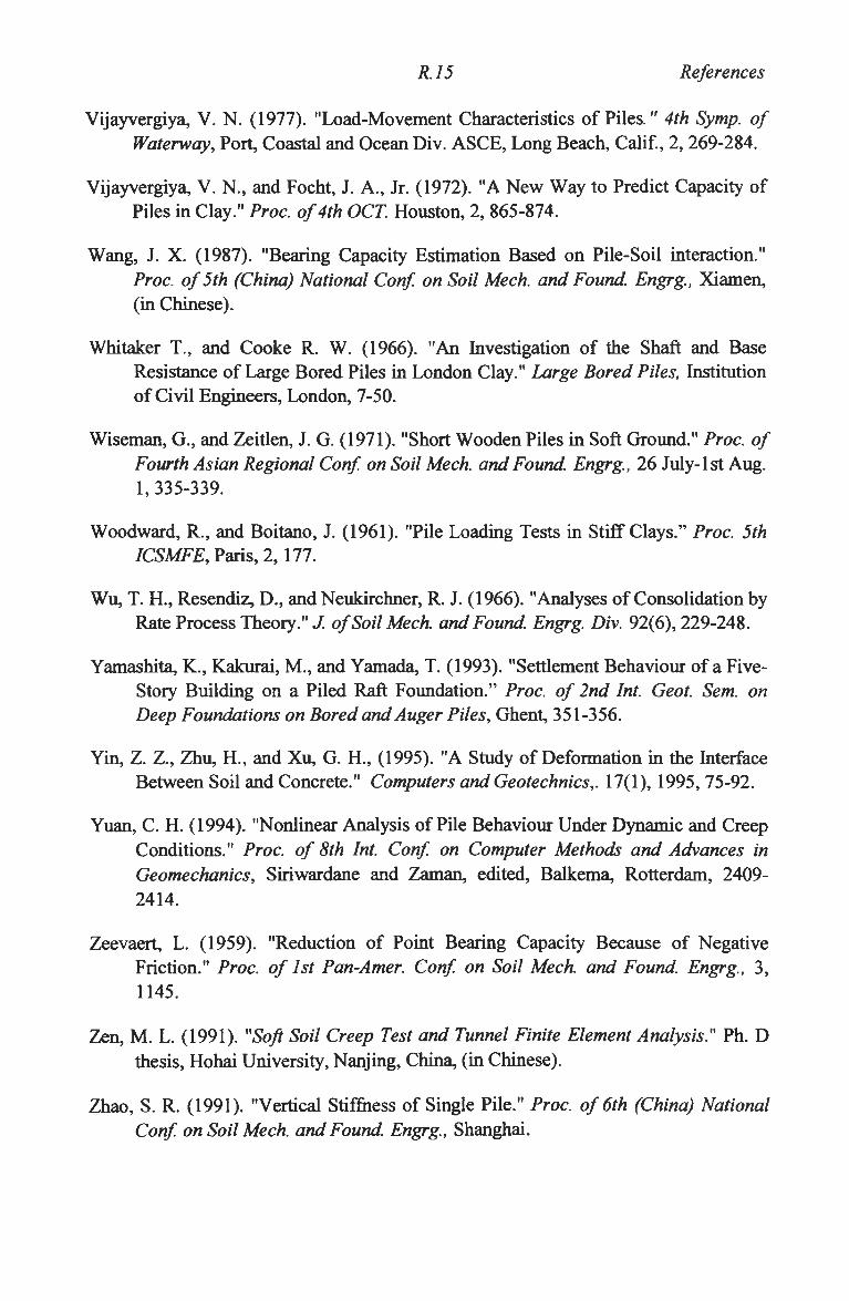
R.15 References
Vijayvergiya, V. N. (1977). "Load-Movement Characteristics of Piles." 4th Symp. of
Waterway, Port, Coastal and Ocean Div. ASCE, Long Beach, Calif, 2,269-284.
Vijayvergiya, V. N., and Focht, J. A., Jr. (1972). "A New Way to Predict Capacity of
Piles in Clay." Proc. of 4th OCT. Houston, 2, 865-874.
Wang, J. X. (1987). "Bearing Capacity Estimation Based on Pile-Soil interaction."
Proc. of 5th (China) National Conf. on Soil Meek and Found. Engrg., Xiamen,
(in Chinese).
Whitaker T., and Cooke R. W. (1966). "An Investigation of the Shaft and Base
Resistance of Large Bored Piles in London Clay." Large Bored Piles, Institution
of Civil Engineers, London, 7-50.
Wiseman, G., and Zeitlen, J. G. (1971). "Short Wooden Piles in Soft Ground." Proc. of
Fourth Asian Regional Conf. on Soil Meek and Found. Engrg., 26 July-1st Aug.
1, 335-339.
Woodward, R., and Boitano, J. (1961). "Pile Loading Tests in Stiff Clays." Proc. 5th
ICSMFE, Paris, 2,177.
Wu, T. H., Resendiz, D., and Neukirchner, R. J. (1966). "Analyses of Consolidation by
Rate Process Theory." J. ofSoilMech. and Found. Engrg. Div. 92(6), 229-248.
Yamashita, K., Kakurai, M., and Yamada, T. (1993). "Settlement Behaviour of a Five-
Story Building on a Piled Raft Foundation." Proc. of 2nd Int. Geot. Sem. on
Deep Foundations on Bored and Auger Piles, Ghent, 351-356.
Yin, Z. Z., Zhu, H., and Xu, G. H., (1995). "A Study of Deformation in the Interface
Between Soil and Concrete." Computers and Geotechnics,. 17(1), 1995, 75-92.
Yuan, C. H. (1994). "Nonlinear Analysis of Pile Behaviour Under Dynamic and Creep
Conditions." Proc. of 8th Int. Conf on Computer Methods and Advances in
Geomechanics, Siriwardane and Zaman, edited, Balkema, Rotterdam, 2409-
2414.
Zeevaert, L. (1959). "Reduction of Point Bearing Capacity Because of Negative
Friction." Proc. of 1st Pan-Amer. Conf. on Soil Meek and Found. Engrg., 3,
1145.
Zen, M. L. (1991). "Soft Soil Creep Test and Tunnel Finite Element Analysis." Ph. D
thesis, Hohai University, Nanjing, China, (in Chinese).
Zhao, S. R. (1991). "Vertical Stiffness of Single Pile." Proc. of 6th (China) National
Conf. on Soil Meek and Found. Engrg., Shanghai.
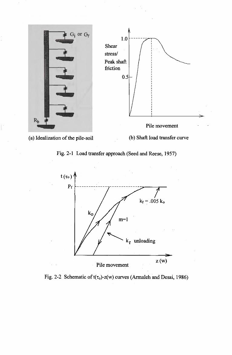
(a) Idealization of the pile-soil
Pile movement
(b) Shaft load transfer curve
Fig. 2-1 Load transfer approach (Seed and Reese, 1957)
Pile movement z(w)
Fig. 2-2 Schematic of t(x0)-z(w) curves (Armaleh and Desai, 1986)
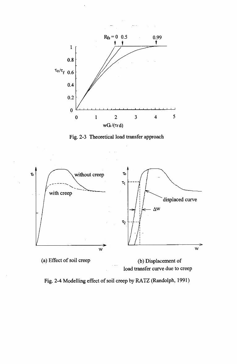
Wt f 0.6
Fig. 2-3 Theoretical load transfer approach
without creep
(a) Effect of soil creep (b) Displacement of
load transfer curve due to creep
Fig. 2-4 Modelling effect of soil creep by R A T Z (Randolph, 1991)
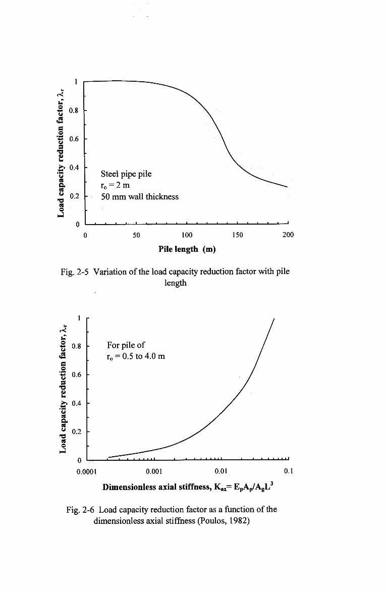
L.
<<
O (J *** a ,©
9 -a u u £> es
a es
1
0.8
0.6
0.4
0.2
Steel pipe pile r0 =
- 50 = 2m m m wall thickness
es o „L
50 100
Pile length (m)
150 200
Fig. 2-5 Variation of the load capacity reduction factor with pile length
l r
0.8 -u o
a | 0.6
9
£» 0.4 -
*3 es
a es -a es o
0.2
0
0.0001
For pile of r0 = 0.5 to 4.0 m
• i — i — i i 1 1 1 1 • *
0.001 0.01 0.1
Dimensionless axial stiffness, K a x = E pAp/A gL
Fig. 2-6 Load capacity reduction factor as a function of the dimensionless axial stiffness (Poulos, 1982)
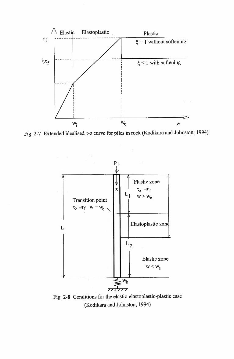
Elastoplastic Plastic
w :
£ = 1 without softening
t, < 1 with softening
w P w
Fig. 2-7 Extended idealised x-z curve for piles in rock (Kodikara and Johnston, 1994)
p
A
\
2
Transition point
XQ ==if w = we
L
t
1 1 f
L
/
L
Plastic zone
1 w > we
\
Elastoplastic zont
2
Elastic zone
w < we
i
w b
Fig. 2-8 Conditions for the elastic-elastoplastic-plastic case
(Kodikara and Johnston, 1994)
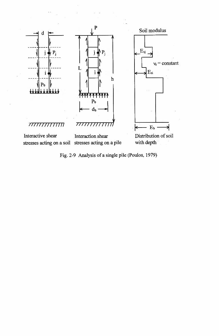
\
\
\
\
\
WW
d
j«
i <
Pb
ill
\
h t \
Lu
1
i'fa
T T T T T T r T T T
//////////llll T7T7TT77TTTTT]
Interactive shear Interaction shear
stresses acting on a soil stresses acting on a pile
Soil modulus
vs = constant
< — > Esi
Eb H Distribution of soil with depth
Fig. 2-9 Analysis of a single pile (Poulos, 1979)
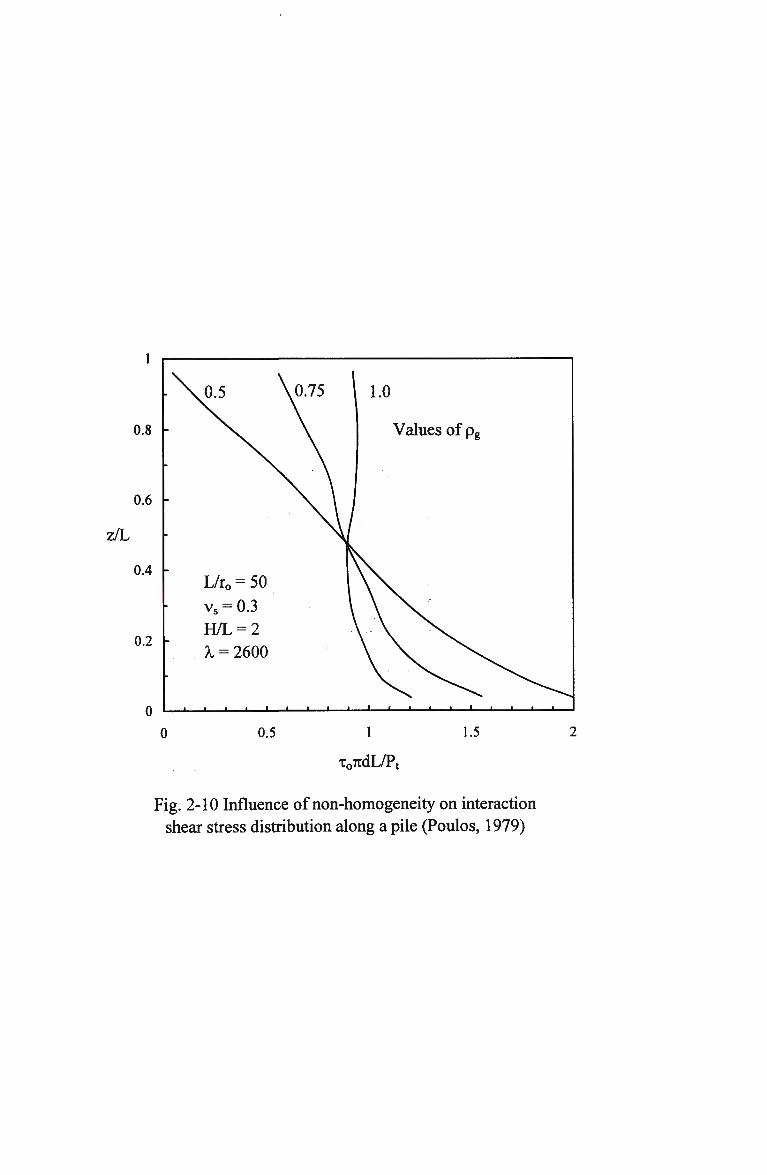
0 0.5 1 1.5 2
x07cdL/Pt
Fig. 2-10 Influence of non-homogeneity on interaction shear stress distribution along a pile (Poulos, 1979)
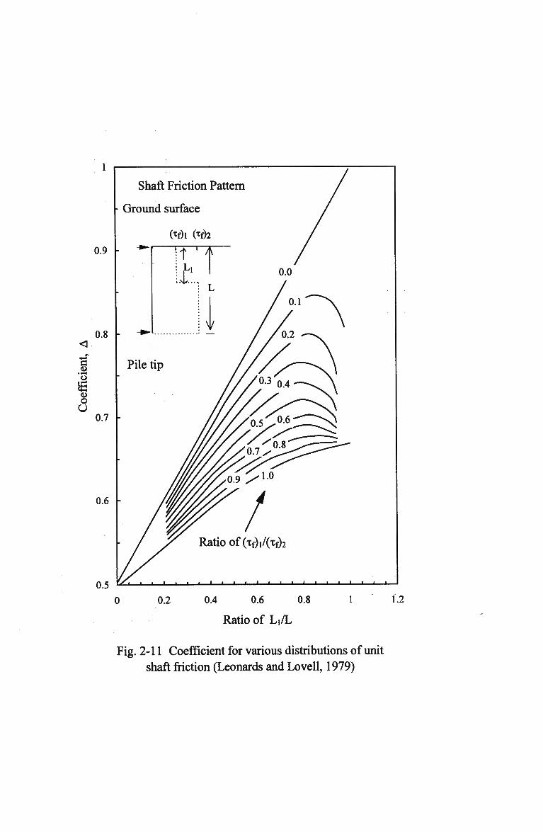
Shaft Friction Pattern
Ground surface
(*f)l (Tf)2
0.9
0.8 i \
L
/
S3
o U 0.7
0.6
0.5 0.2 0.4 0.6 0.8
Ratio of Li/L
1.2
Fig. 2-11 Coefficient for various distributions of unit shaft friction (Leonards and Lovell, 1979)
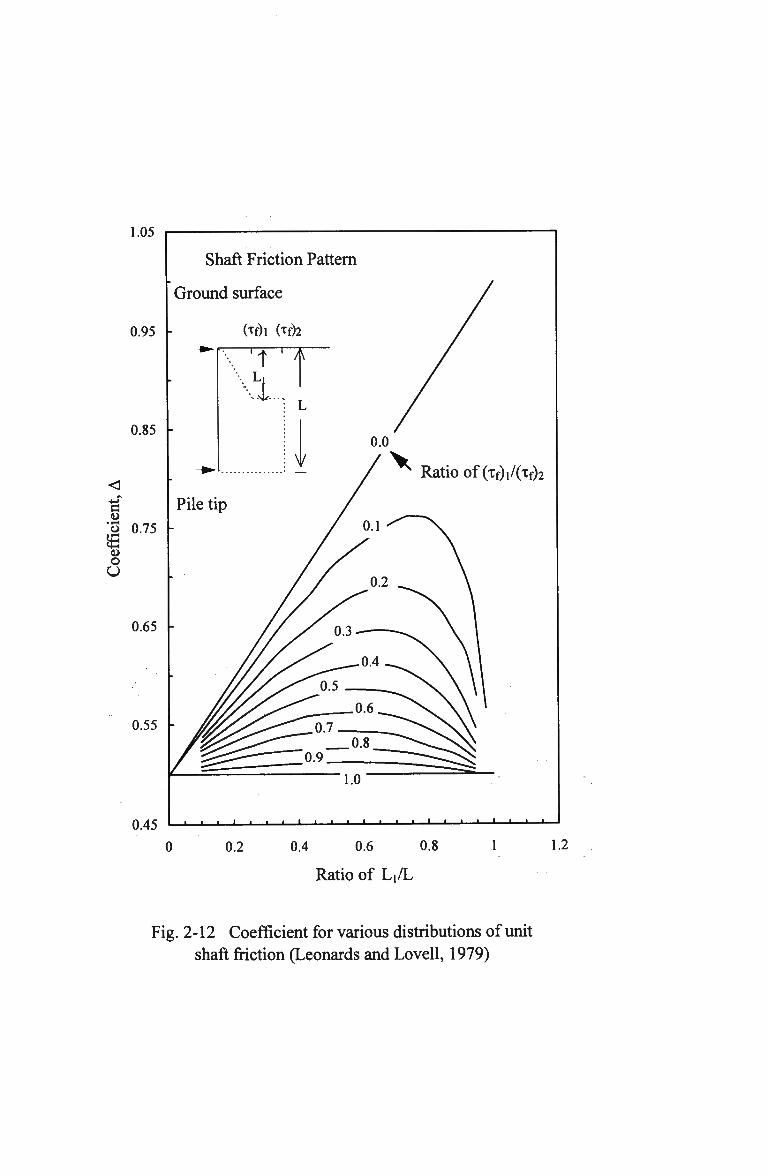
1.05
0.95
0.85
0.75
Shaft Friction Pattern
Ground surface
(Tf)l (tf)2
Pile tip
0.65 -
0.55
Ratio of (xf)i/(Xf)2
0 4 5 I L _ I • • • i i i — i — i — i — i — i — i — i — i — i — i — i — i — " — ' — > -
0 . 2 0 . 4 0 . 6 0 . 8
Ratio of Li/L
1.2
Fig. 2-12 Coefficient for various distributions of unit shaft friction (Leonards and Lovell, 1979)
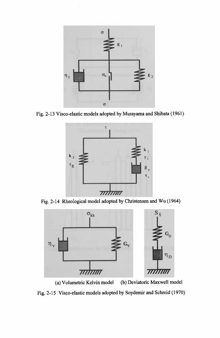
Fig. 2-13 Visco-elastic models adopted by Murayama and Shibata (1961)
/////////
Fig. 2-14 Rheological model adopted by Christensen and W u (1964)
S
/////////
(a) Volumetric Kelvin model (b) Deviatoric Maxwell model
Fig. 2-15 Visco-elastic models adopted by Soydemir and Schmid (1970)
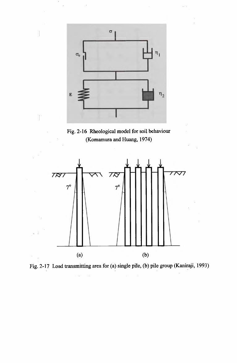
Fig. 2-16 Rheological model for soil behaviour
(Komamura and Huang, 1974)
(a) (b)
Fig. 2-17 Load transmitting area for (a) single pile, (b) pile group (Kaniraji, 1993)
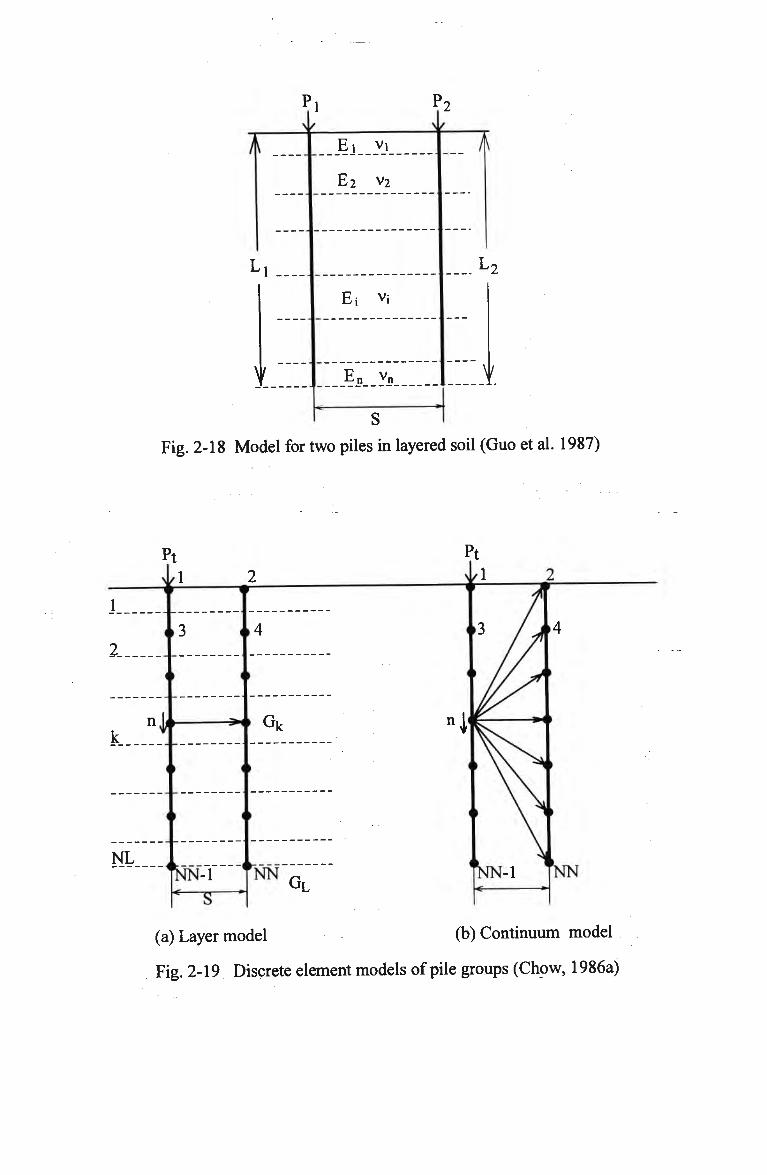
1
L
\
P
i
'1
(
1 ? >
E i vi
E2 v2
Et Vi
£l<n V n
S
2
/\
L-
V
Fig. 2-18 Model for two piles in layered soil (Guo et al. 1987)
Pt
u 1
1
2
i
n 1,
k "*
I
(
NL i
i <
»3 «
> <
• (
» <
NN-1 c S '
2 »
• 4
»
• G k
»
»
NN r GL
P \ i
•
1
1
1
t
NN-1 < >
2
.4
\
VlN
(a) Layer model (b) Continuum model
Fig. 2-19 Discrete element models of pile groups (Chow, 1986a)
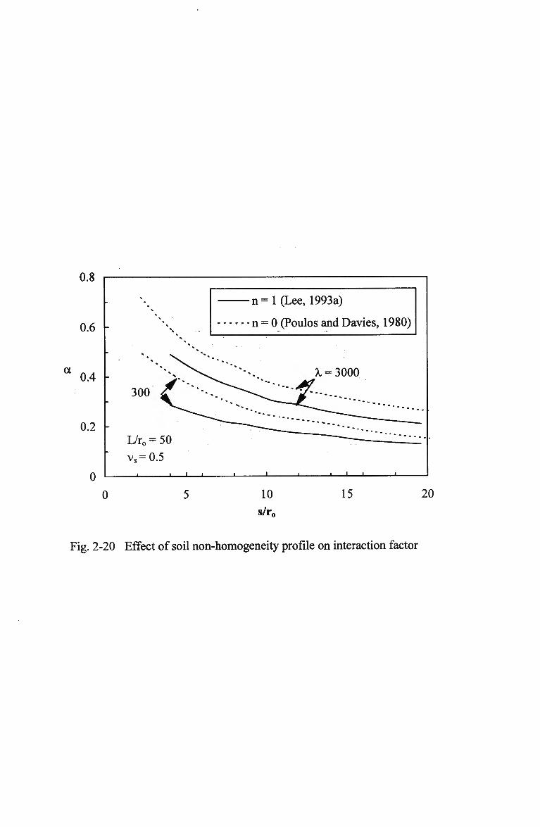
a
0.8
0.6 -
0.4
0.2
0
0
300
L/r0 =
vs=0.5 -i i i
n = l (Lee, 1993a)
n = 0 (Poulos and Davies, 1980)
J i i_
10
s/r0
15 20
Fig. 2-20 Effect of soil non-homogeneity profile on interaction factor
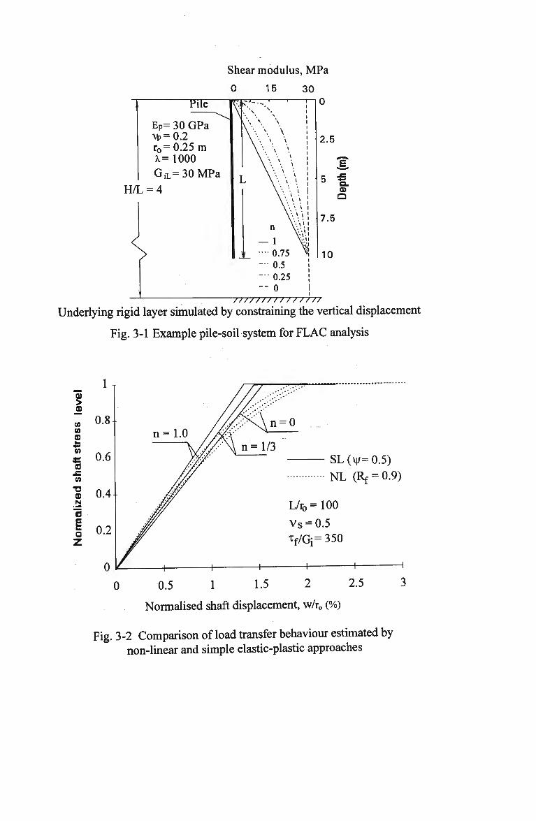
Shear modulus, M P a
0 15 30
Pile—
EP= 30 GPa M>=0.2 ro=0.25 m x= 1000 G i L = 3 0 M P a
H/L = 4
Underlying rigid layer simulated by constraining the vertical displacement
Fig. 3-1 Example pile-soil system for F L A C analysis
03 > M
CO CO 03 i-
CO
I CO •o
cu N
"5 E t_
o
0
SL(\|/=0.5)
N L (Rf = 0.9)
L/ib=100
v s = 0.5
xf/Gi= 350
0.5 1 1-5 2
Normalised shaft displacement, w/r0
2.5
Fig. 3-2 Comparison of load transfer behaviour estimated by non-linear and simple elastic-plastic approaches
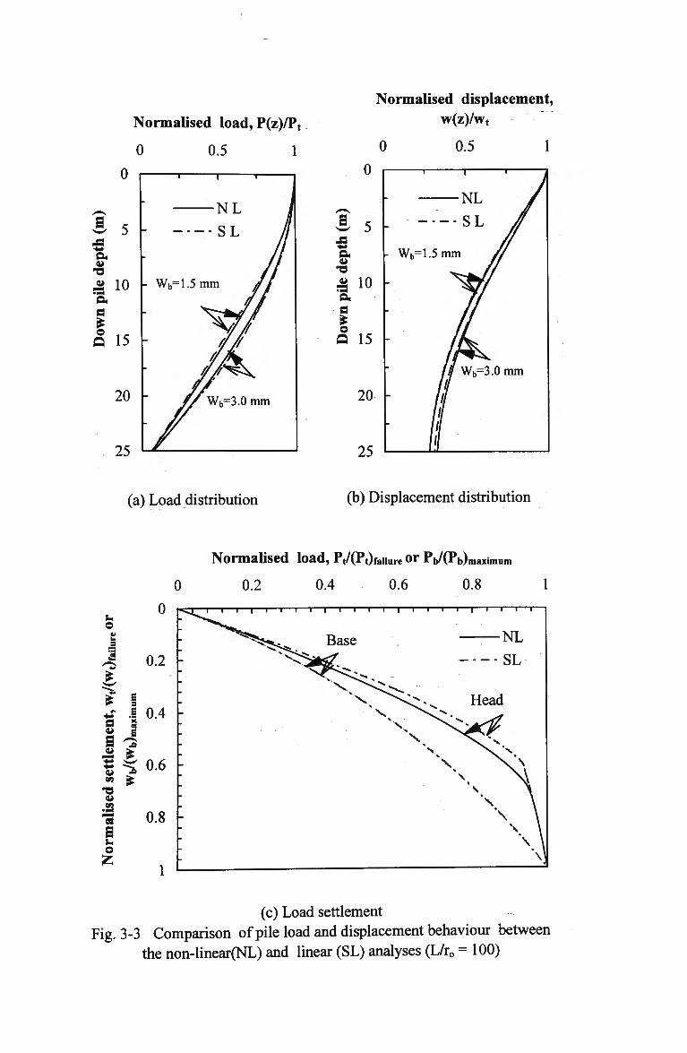
Normalised load, P(z)/Pt
0 0.5 1
0 i . , .
S
a -a a. a 2 15
- Wb=1.5 m m
20 -
25
b=3.0 m m
Normalised displacement,
w(z)/wt
0 0.5 1
a
o
5 -
a -a £ 10 a
I Q 15
20 -
25
.
-
- wb=
-
-NL
•SL
=1.5 mm /,
// III
III 1
Wb=3.0 mm
(a) Load distribution (b) Displacement distribution
0
Normalised load, Pt/(Pt)failure Or Pb/(Pb)maximum
0.2 0.4 0.6 0.8 1
(c) Load settlement Fig. 3-3 Comparison of pile load and displacement behaviour between
the non-linear(NL) and linear (SL) analyses (L/r0 = 100)
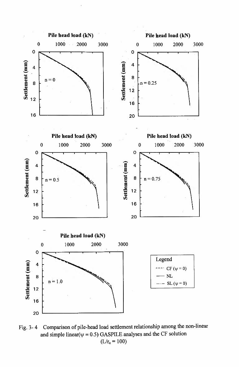
Pile head load (kN)
0 1000 2000 3000
0 i^-. r
Pile head load (kN)
0 1000 2000 3000
Pile head load (kN)
0 1000 2000 3000
a a a
a
CG
Pile head load (kN)
0 1000 2000 3000
0 isr—. r
a a a
a
in
8 •
12
16 -
20
Pile head load (kN)
1000 2000 3000
Legend
-- CF(\|/ = 0)
NL
SL(y = 0)
Fig. 3- 4 Comparison of pile-head load settlement relationship among the non-linear
and simple linear(i|/ = 0.5) GASPILE analyses and the CF solution
(L/ro=100)
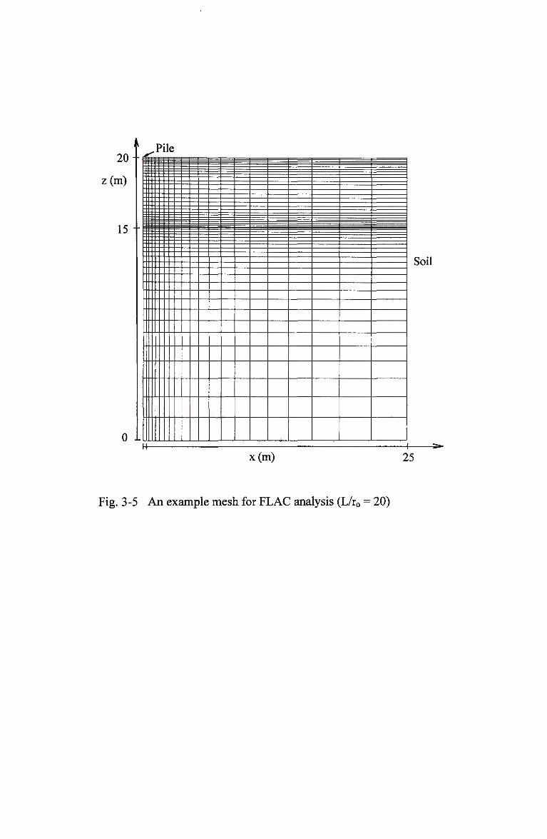
20
z(m)
15 ••
0 1
.Pile
H
Soil
| —r-
x(m) 25
Fig. 3-5 An example mesh for FLAC analysis (L/r0 = 20)
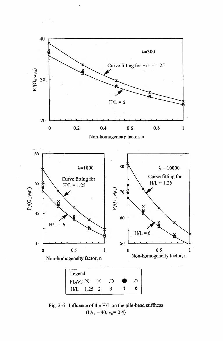
20
X,=300
Curve fitting for H/L = 1.25
H/L = 6
-I I I — _ l I I l _ _ i I I I I I I I I I I I I I 1 1 L .
0 0.2 0.4 0.6 0.8
Non-homogeneity factor, n
65
A.=1000
Curve fitting for H/L =1.25
0 0.5 1
Non-homogeneity factor, n
50
X= 10000
Curve fitting for H/L =1.25
H/L = 6
0 0.5 1 Non-homogeneity factor, n
Legend
FLAC X X H/L 1.25 2
O 3
•
4
A
6
Fig. 3-6 Influence of the H/L on the pile-head stiffness
(L/ro = 40,vs=0.4)
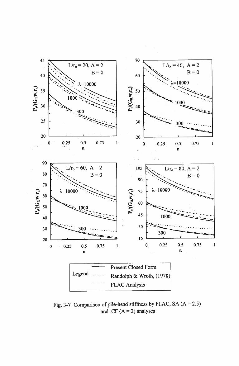
20 0.25 0.5
n 0.75
70
60 -
h. 50
O ^ 40
30 -
20
«
"
-N^ •
-
*-"
^
' ^ * „
* v.
*^^*NJ
L/r0 =
**.. x "* «
-.. w_
i
= 40, A :
B =
=10000
*- S<. "V, ****
*•
1000 " ^ s
300 •-•
i
= 2 = 0
,*w """••i , .
" • ^ r * ^ - . » .
• ^ ^ s - - ^
"*"~"
0.25 0.5 n
0.75
0.25 0.5
n
0.75
105
90
2 75
tj 60
OH
45
30
15
V L/r0
. ^=10000 '
5is**s<
300
= 80,
1
A =
B =
(NO
/ /'
II II
/ /.
LC^.
i
*
^ LC=.
-=-=
0.25 0.5 n
0.75
Legend Present Closed Form
Randolph & Wroth, (1978)
FLAC Analysis
Fig. 3-7 Comparison of pile-head stiffness by FLAC, SA (A = 2.5) and CF (A = 2) analyses
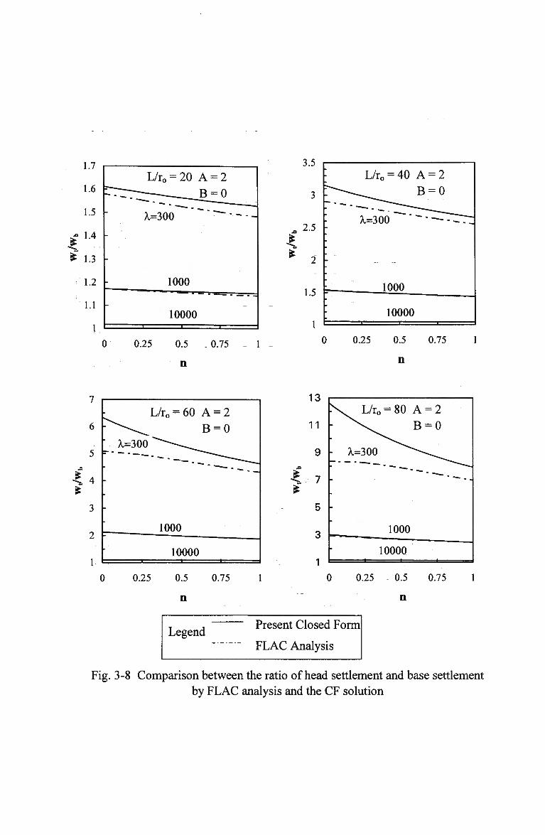
1.7
1.6
1.5
£ 1.4
£ 1.3
1.2
1.1 -
-
"
-
L/ro = 20 A = 2
X=300
1000
10000
0.25 0.5
n
0.75
3.5
3
2.5
£ £ 2 -
1.5
L/ro = 40 A
^ — ^ B
^=300 "~" ~""
: 1000
10000 r 1 1
= 2 = 0
^
0 0.25 0.5 0.75 1
n
/
6
5
4
3
2
i
L/ro = 60 A = 2
^ \ ^ B = 0 " A.=300 ""^-^^
^ ^""^:::^r:
1000
10000 1 1 1-
0.25 0.5 0.75
n
L/ro = 80 A = 2
B = 0
9 - X=300
7 -
5
3
1
1000
10000 < - • —
0 0.25 0.5 0.75
n
Legend Present Closed Form
FLAC Analysis
Fig. 3-8 Comparison between the ratio of head settlement and base settlement by FLAC analysis and the CF solution
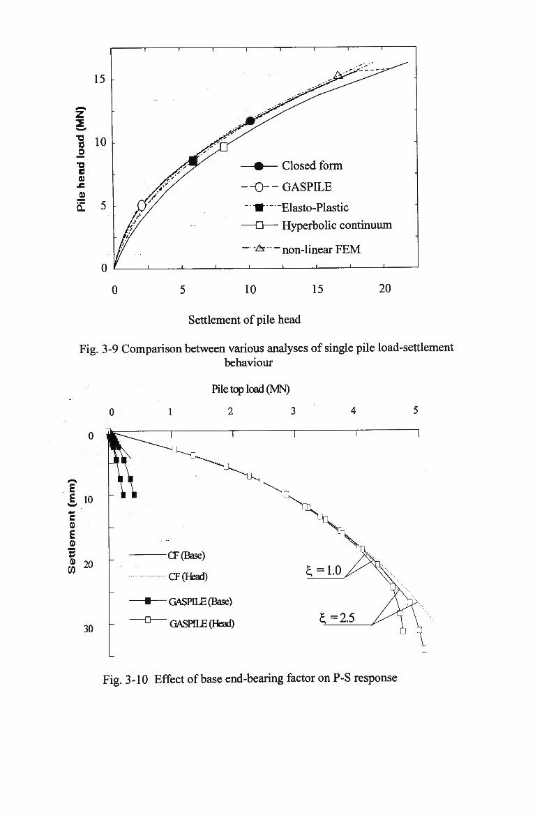
0 10 15 20
Settlement of pile head
Fig. 3-9 Comparison between various analyses of single pile load-settlement behaviour
E
e 0)
E cu CJ 20
30
Pile top load (MN)
1 2 3
CF(Base)
CF(Head)
-GASPILE (Base)
GASPILE (Head)
a,=i.o
£=2.5
Fig. 3-10 Effect of base end-bearing factor on P-S response
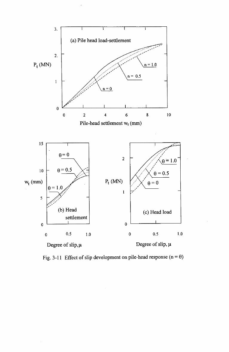
Pt(MN)
(a) Pile head load-settlement
n=1.0
n= 0.5
2 4 6 8
Pile-head settlement wt (mm)
10
15
10
wt (mm)
5 ~
0
-
e =
:'''
1
e=o
9=0.5 V -
• * r
(b) Head
settlement i
Pt(MN)
0
(c) Head load
0 0.5 l.o 0 0.5 1.0
Degree of slip, p Degree of slip, p
Fig. 3-11 Effect of slip development on pile-head response (n = 0)
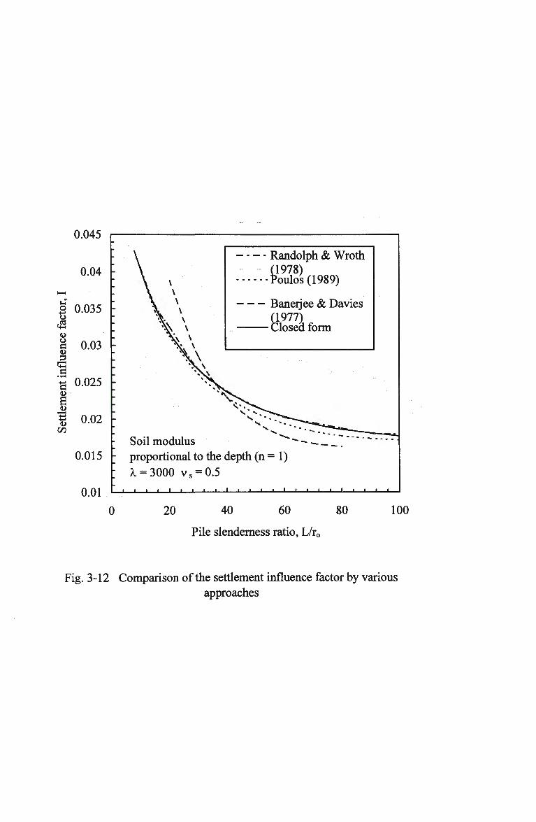
0.045
0.04
i—i
2 0.035
I 0.03 =3
^ 0.025
I I 0.02
0.015
0.01
- Randolph & Wroth 1978) >oulos (1989)
- - Banerjee & Davies 1977) "losed form
Soil modulus ** ~~ ~ " proportional to the depth (n = 1)
X = 3000 vs = 0.5 i I_I i i i i • I__I I__I I__I i_
0 20 40 60 80
Pile slenderness ratio, L/r0
100
Fig. 3-12 Comparison of the settlement influence factor by various approaches
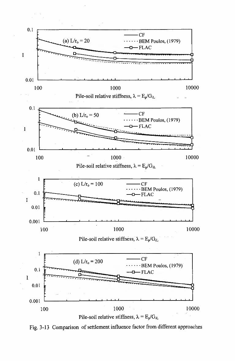
0.1
0.01
100
0.1
0.01
100
1
0.1
0.01 =
0.001
100
1000
Pile-soil relative stiffness, X = Ep/GjL
10000
1000
Pile-soil relative stiffness, X = Ep/GiL
10000
(c)L/ro=100 CF B E M Poulos, (1979) FLAC
• ' I I I l—L -l I I u
1000
Pile-soil relative stiffness, X = Ep/GjL
10000
0.1 ?
0.01 :
0.001
100
(d)L/ro = 200 CF
B E M Poulos, (1979)
FLAC
• • l l I—L. _l I I I L_l 1_1_
10000 1000
Pile-soil relative stiffness, X = Ep/GiL
Fig. 3-13 Comparison of settlement influence factor from different approaches
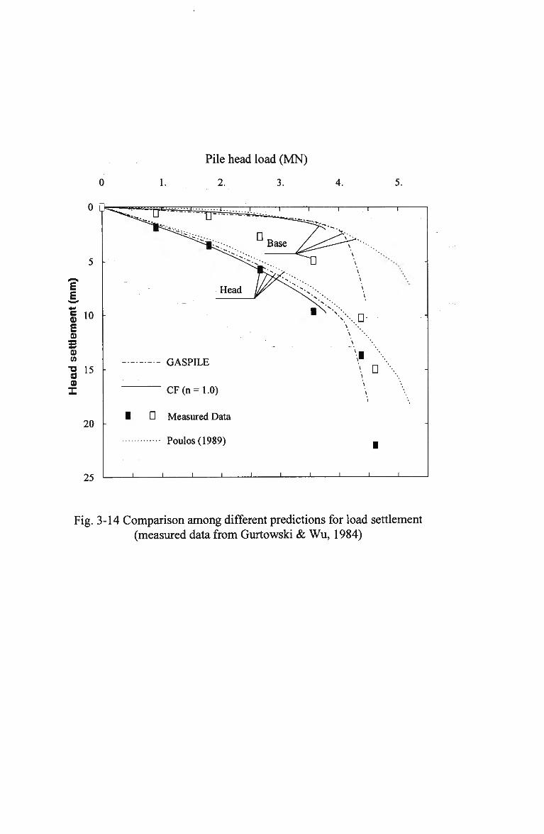
Pile head load (MN)
1. 2. 3. 4.
GASPILE
CF(n=1.0)
• • Measured Data
Poulos (1989)
\ D
i
J L
Fig. 3-14 Comparison among different predictions for load settlement (measured data from Gurtowski & W u , 1984)
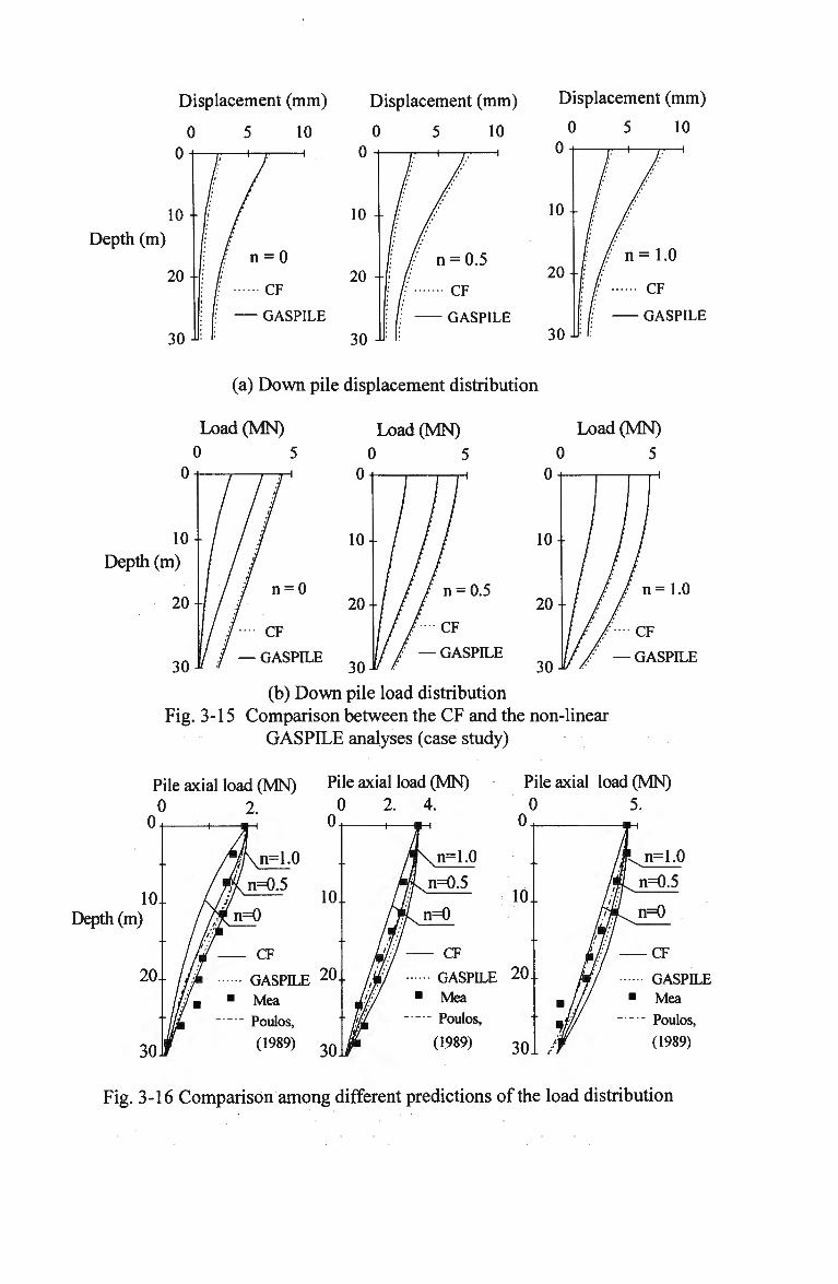
Displacement (mm) Displacement (mm) Displacement (mm)
Depth (m)
(a) Down pile displacement distribution
Load(MN)
0 5 Oi , r-rH
10-
Depth (m)
Load(MN) 0 5
OH , r—H
(b) Down pile load distribution Fig. 3-15 Comparison between the CF and the non-linear
GASPILE analyses (case study)
Pile axial load (MN) Pile axial load (MN)
0
n=1.0
Depth (m)
CF
GASPILE 2 0
Mea
Poulos,
(1989) 3 Q
Pile axial load(MN)
0 5. OH ^
CF
GASPILE 20.. Mea
Poulos,
(1989) 3 0
Fig. 3-16 Comparison among different predictions of the load distribution
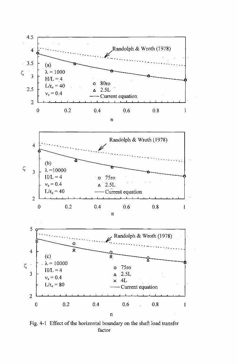
4.5
4 -
3.5
3
2.5
2
(a)
X =1000
H/L = 4
L/r0 = 40
vs = 0.4
i i i • '
Randolph & Wroth (1978)
o 80ro A 2.5L
Current equation ' ' l _ _ l I I 1 _ _ J I I I I I l _ l L.
0 0.2 0.4 0.6
n
0.8
3 -
(b)
X=10000
H/L = 4
vs = 0.4
L/r0 = 40
X Randolph & Wroth (1978)
o 75ro
A 2.5L
— Current equation -i I _ J i i i i i i i i i ' • • • •
0.2 0.4 0.6
n 0.8
(c)
?i= 10000
H/L = 4
vs = 0.4
L/r0 = 80
_i i i i i_
Randolph & Wroth (1978)
o 75ro
A 2.5L
x 4L
Current equation
-i i i i i i — i — i — i i i i
0 0.2 0.4 0.6
n
0.8
Fig. 4-1 Effect of the horizontal boundary on the shaft load transfer
factor
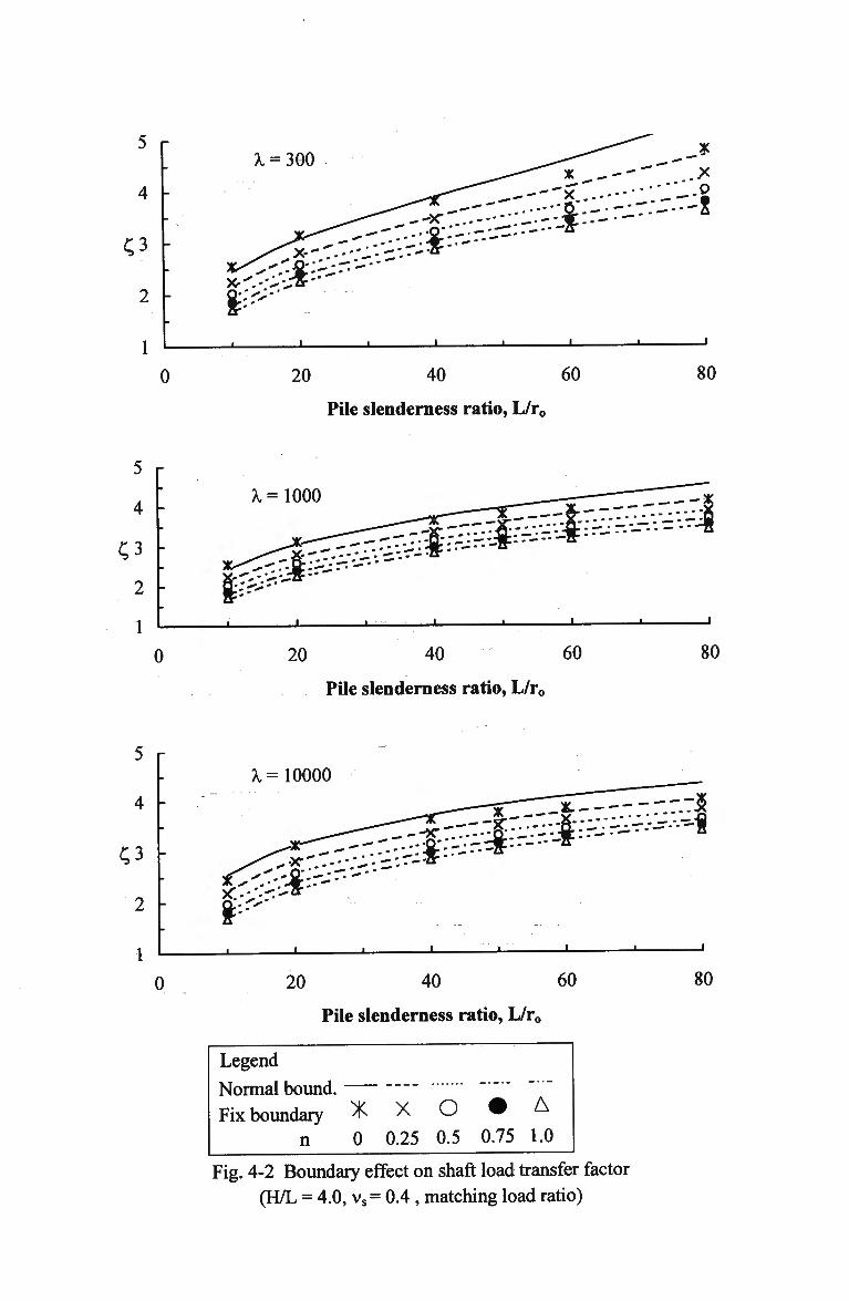
4
2
1
^ = 300
X ^ ** jQ- • ' . — V • '
- f:-''-i I •
IV4::
i
^ x _--- - " x -•
1
yx. .*
••••".o
i
0 20 40 60
Pile slenderness ratio, L/r0
80
5
4
G3
2
1
0 20 40 60
Pile slenderness ratio, L/r0
80
5 r
4 -
C3
2
1
0
A, = 10000
sd--$--;
xV--'>.-*"
.. x- ..-• • •;.- ~:'--Zr
20 40 60
Pile slenderness ratio, L/r0
Legend
Normal bound. Fix boundary >K X O • A
n 0 0.25 0.5 0.75 1.0
Fig. 4-2 Boundary effect on shaft load transfer factor
(H/L = 4.0, vs= 0.4 , matching load ratio)
_ _ i
80
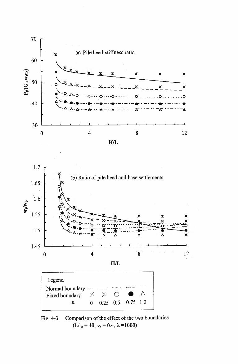
1.7
1.65
1.6
1.55
1.5
1.45
0
(b) Ratio of pile head and base settlements
' • I L.
12
H/L
Legend
Normal boundary Fixed boundary % X O • ^
n 0 0.25 0.5 0.75 1.0
Fig. 4-3 Comparison of the effect of the two boundaries
(L/ro = 40,vs = 0.4,A,=1000)
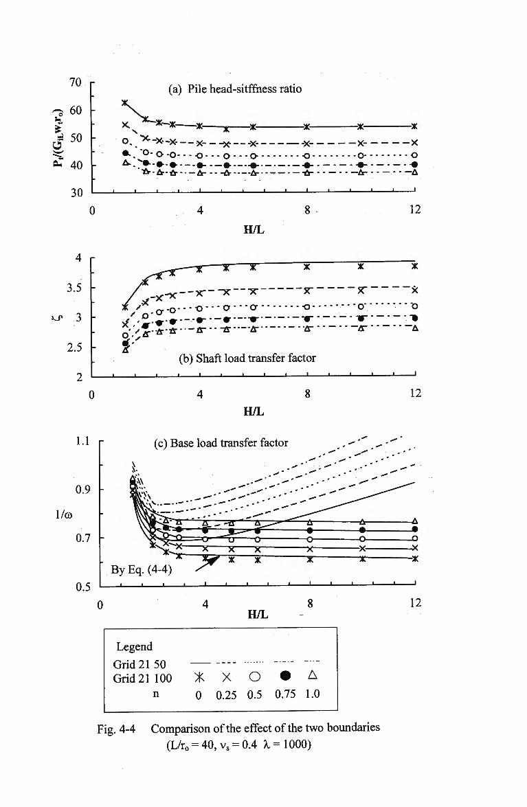
70 r
60 o
| 50
fc 40
30
0
4 r
3.5
^ 3
2.5
2
0
., <K—M
(a) Pile head-sitffhess ratio
-x- -x- -x- x * N "~*-* * ac o. --x-X- x- - -X— -X- -x- X- X ••. "°- o -o- - - -o- - - o -- -o o o o A.. **••-#.. #•--.# •-- — -•- ••- -• -•
""A--A--A- A fr...-.fr. -fr fr fr
H/L
(b) Shaft load transfer factor
12
12
H/L
1.1 r
0.9 -
1/co
0.7 -
0.5
(c) Base load transfer factor
By Eq. (4-4) j i_
0 H/L
Legend
Grid 21 50 Grid 21 100
n X 0
X o 0.25 0.5
• A
0.75 1.0
Fig. 4-4 Comparison of the effect of the two boundaries
(L/ro = 40,vs = 0.4 A. = 1000)
12
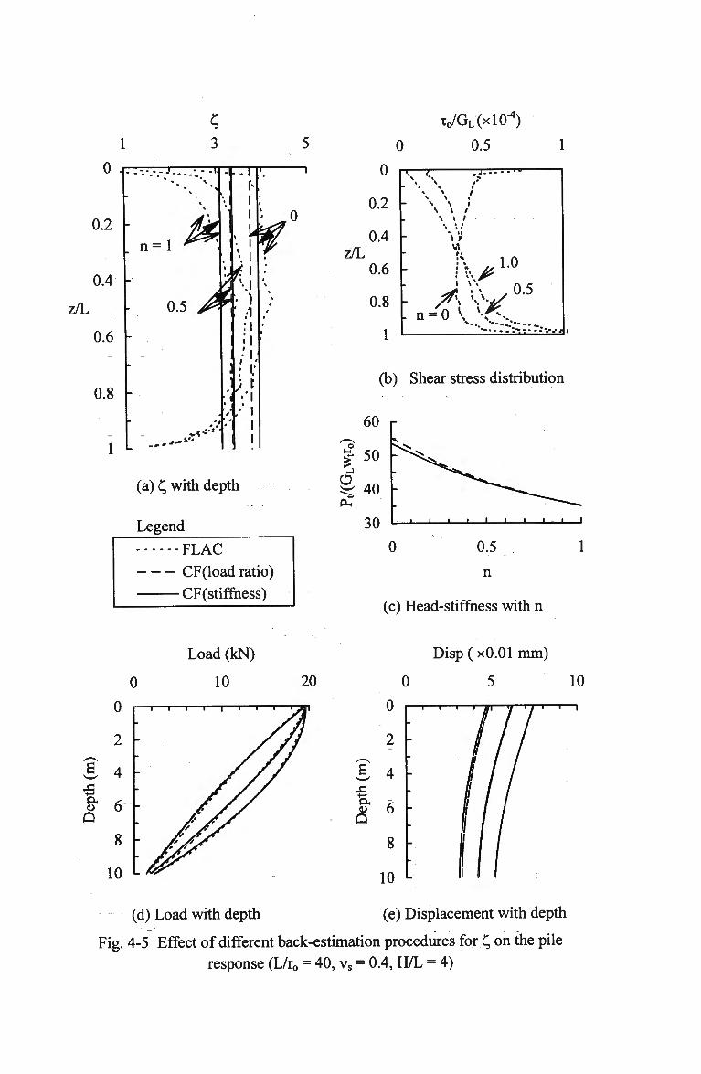
0
0.2
0.4 -
z/L
0.6
0.8
.. J..—=-rn: .
* •
n = 1 ^ i
u
0.5 A^
-
4 *
.4"
1
• I
i | i .
i i i
1 a 1
r 1
0
1
§
I
1
(a) C, with depth
Legend
F L A C
CF(load ratio)
CF(stiffhess)
0
x0/GL(xlO"4)
0.5
(b) Shear stress distribution
60 r
0 0.5
n
(c) Head-stiffness with n
0
Load (kN)
10
10 L
20
Disp (xO.01 mm)
0 5 10
0
& 4
<u 6 Q
8
10
- i — i — r — m — r i—i—l
(d) Load with depth (e) Displacement with depth
Fig. 4-5 Effect of different back-estimation procedures for C, on the pile
response (L/r0 = 40, vs = 0.4, H/L = 4)
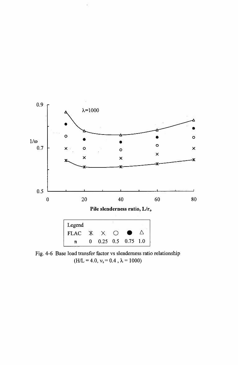
0.9 r
1/co 0.7
0.5
0
A=1000
o
X
-X-
o X
-X-
o
X
-x-
20 40 60
Pile slenderness ratio, L/r0
Legend
FLAC X X. O
n 0 0.25 0.5
• A
0.75 1.0
X
-X
80
Fig. 4-6 Base load transfer factor vs slenderness ratio relationship
(H/L = 4.0, vs= 0.4, X =1000)
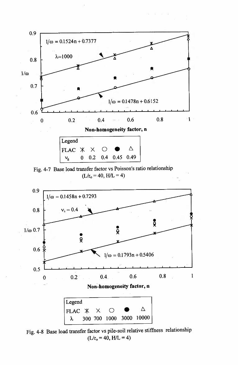
0.9
0.8
1/co = 0.1524n + 0.7377
X,=1000
1/co
0.7 -
1/co = 0.1478n +0.6152
) £ T | I I 1 1 1 1 1 1 1 1 1 1 1 1 1 " "-
0 0.2 0.4 0.6 0.8
Non-homogeneity factor, n
Legend
FLAC
vs
X 0
X
0.2 o 0.4
•
0.45
A
0.49
Fig. 4-7 Base load transfer factor vs Poisson's ratio relationship (L/ro = 40,H/L = 4)
1/co = 0.1458n +0.7293
vs = 0.4
0
1/co = 0.1793n +0.5406
J — i — i — i — i — i — " — • — ' — ' — ' — • -
0.2 0.4 0.6 0.8
Non-homogeneity factor, n
Legend
FLAC X X O X 300 700 1000
• A
3000 10000
Fig. 4-8 Base load transfer factor vs pile-soil relative stiffness relationship (L/ro = 40,H/L = 4)
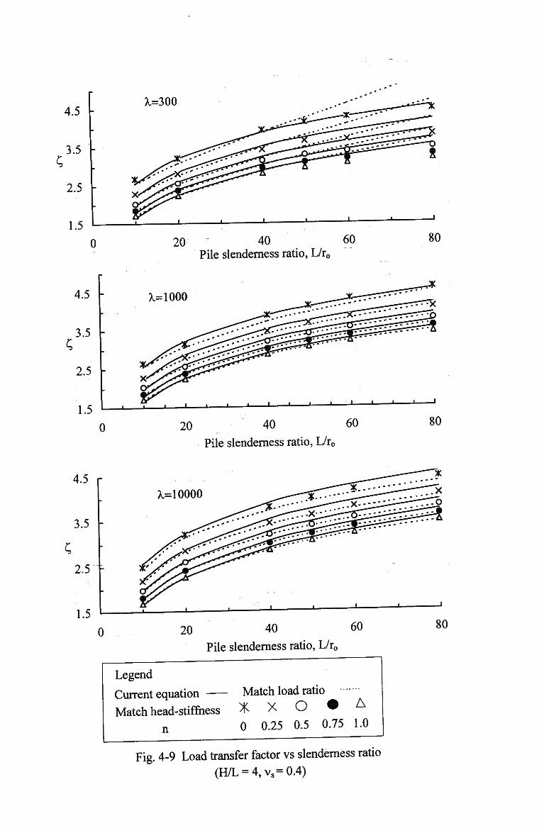
4.5 -
3.5 -
2.5
1.5
A.=300
0
0
20 40 60 Pile slenderness ratio, L/r0
20 40 60
Pile slenderness ratio, L/r0
80
4.5 r
3.5 -
2.5 -
1.5
0 20 40 60
Pile slenderness ratio, L/r0
Legend
Current equation —
Match head-stiffness
n
Match load ratio
X X O • A 0 0.25 0.5 0.75 1.0
Fig. 4-9 Load transfer factor vs slenderness ratio (H/L = 4,vs=0.4)
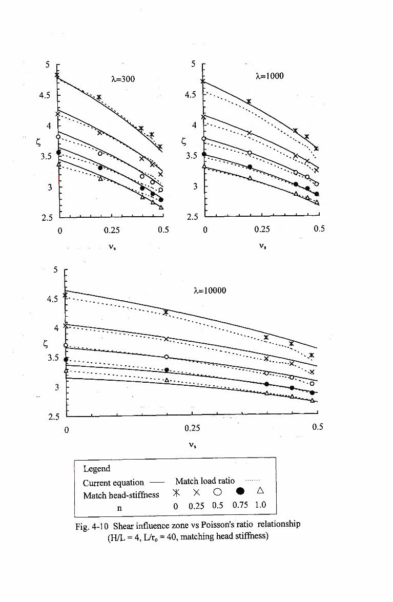
k=300
0
A.=1000
0.25
vs
0.5
A,=10000
Legend
Current equation —
Match head-stiffness
n
Match load ratio
X X O • A 0 0.25 0.5 0.75 1.0
Fig. 4-10 Shear influence zone vs Poisson's ratio relationship (H/L = 4, L/r0 = 40, matching head stiffness)
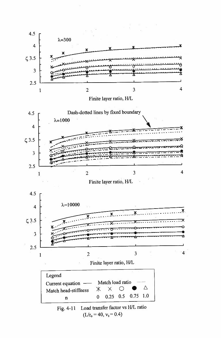
.5
4
£3.5
3
2.5
1
?i=300
- - - -T ^
2 3
Finite layer ratio, H/L
Dash-dotted lines by fixed boundary
\
- ^..—"JS.—~~-~-'*"w"-"'—^*~-—•---•-'* p & i i a ^ f T P T W z-=*Q
r n • • •"' r.'.T/i i A I I U _ I M I I " A .• ;.'_
2 3
Finite layer ratio, H/L
2 3
Finite layer ratio, H/L
Match load ratio
Legend
Current equation —
Match head-stiffness X X •
n 0 0.25 0.5 0.75 1.0
Fig. 4-11 Load transfer factor vs H/L ratio (L/ro = 40,vs=0.4)
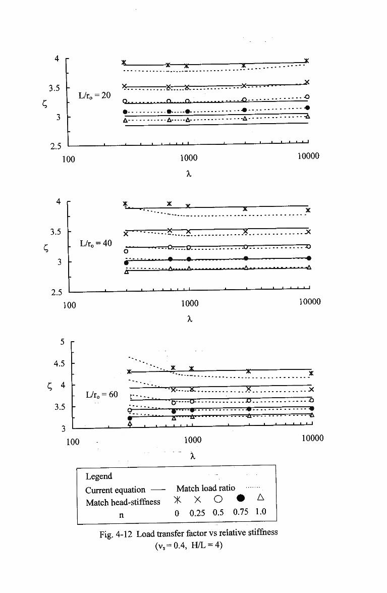
4 r -x-
3.5 L/r0 = 20
x-
D . . . .- .• Ci O- - - • . xy.
-A-
_o
^A
2.5
100
• • • L _ J _
1000
X
J L. I • • • I I
10000
4 r
3.5
L/r0 = 40
2.5
100
5 r
4.5
^ 4
3.5
3
x
X-
L/ro = 60 r-.
cr •r
-X-
-x~
100
l ^ u
I I
1000
X
• * x
i—*W •XT
A ,
» » • •
•a A-" - i i — i — i -
1000
X
Legend
Current equation —
Match head-stiffness
n
• * —
X
.u
• I 1 L.
X
10000
-x-
7T
x
o
' • • •
10000
Match load ratio X X O • A
0 0.25 0.5 0.75 1.0
Fig. 4-12 Load transfer factor vs relative stiffness
(vs=0.4, H/L = 4)
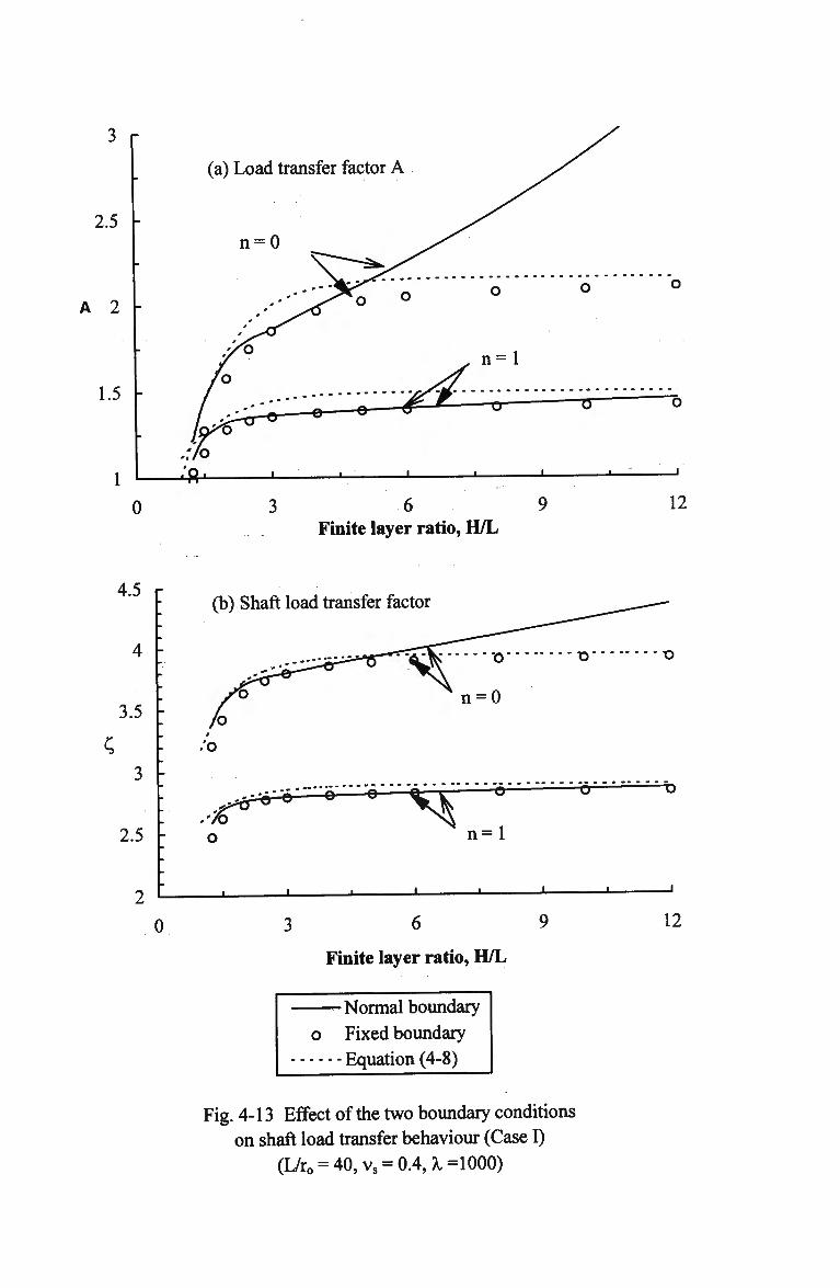
3 r
2.5 -
A 2 -
1.5 -
0 6 9 Finite layer ratio, H/L
12
4.5 r
3.5
(b) Shaft load transfer factor
2.5 vo o
-e e- X$ n=l
-o-
0 3 6 9
Finite layer ratio, H/L
— - N o r m a l boundary
o Fixed boundary
Equation (4-8)
Fig. 4-13 Effect of the two boundary conditions on shaft load transfer behaviour (Case I)
(L/r0 = 40, vs = 0.4,^=1000)
12
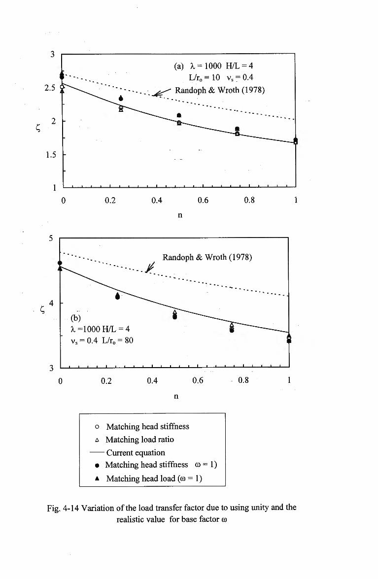
2.5
;
1.5
0
_ i i _
0.2
(a) A, = 1000 H/L = 4
L/ro=10 vs = 0.4
^ - - Randoph & Wroth (1978)
0.4 0.6
n
0.8
_ i i i i i i i i i i i — i — i — i — i — i — i -
- - - /
Randoph & Wroth (1978)
(b) A. =1000 H/L = 4
vs = 0.4 L/ro = 80
• • L
ft
• • • • ' • I I-
0 0.2 0.4 0.6
n
0.8
o
A
•
A
Matching head stiffness
Matching load ratio
Current equation
Matching head stiffness
Matching head load (co =
co =
D 1)
Fig. 4-14 Variation of the load transfer factor due to using unity and the
realistic value for base factor co
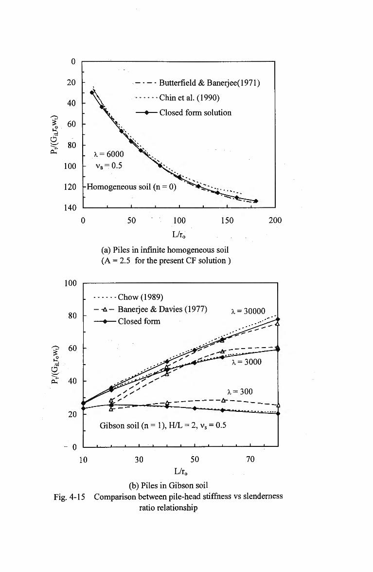
0
20
120
140
^ 3t o u* J
O
yu
40
60
80
100
JM
" -
-- 1 =
- vs
X*
\fc-> ^ k »
Tk."
^ ^ s
^^> 6000 * V = 0.5 "^
- - Butterfield & Banerjee(1971)
Chin etal. (1990)
Closed form solution
-Homogeneous soil (n = 0)
0 50 100
L/r0
150
(a) Piles in infinite homogeneous soil (A = 2.5 for the present CF solution)
200
100
80
*> 60
5 o §" 40
20
Chow (1989)
- - A - Banerjee & Davies (1977)
• Closed form k= 30000
Gibson soil (n = 1), H/L = 2, vs = 0.5
n i i i i i 1 1 1 1 —
10 30 50 70
L/r0
(b) Piles in Gibson soil Fig. 4-15 Comparison between pile-head stiffness vs slenderness
ratio relationship
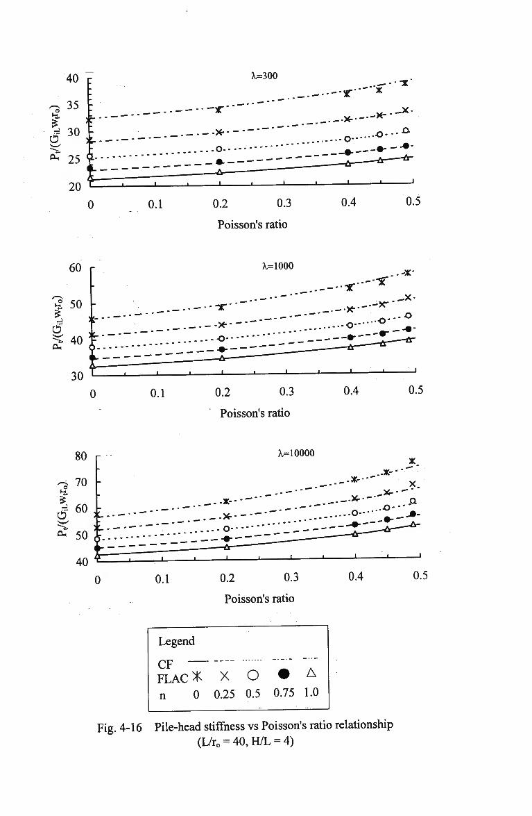
X=300
0 0.1 0.2 0.3
Poisson's ratio
0.4 0.5
60 r k=1000
0 0.1 0.2 0.3
Poisson's ratio
0.4
80 r \=10000
0 0.1 0.2 0.3
Poisson's ratio
0.4
Legend
CF FLACX X O • A n 0 0.25 0.5 0.75 1.0
Fig. 4-16 Pile-head stiffness vs Poisson's ratio relationship (L/ro = 40,H/L = 4)
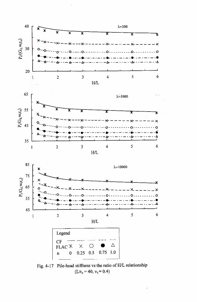
40
30
20
k=300
T
x-_ X--
- o. •o-
A-*.
•o-
•fr-.
X-
• o-
•X-
o-
X-
o.
-L,
4 H/L
65 r
55
45
35
^=1000
X---v-
'••o-.
•x-
o- •o-
x-o-
X
o
X
o
• A . A- ^ ^ .£ fr fr fr
H/L
85
75
65
55
45
x *.=10000
-X- W 1
X-
H/L
Legend
CF "•"•" """ FLACX X O • A n 0 0.25 0.5 0.75 1.0
• H ^
_ i i 1 J 1 ' ' >
Fig. 4-17 Pile-head stiffness vs the ratio of H/L relationship (L/ro = 40,vs=0.4)
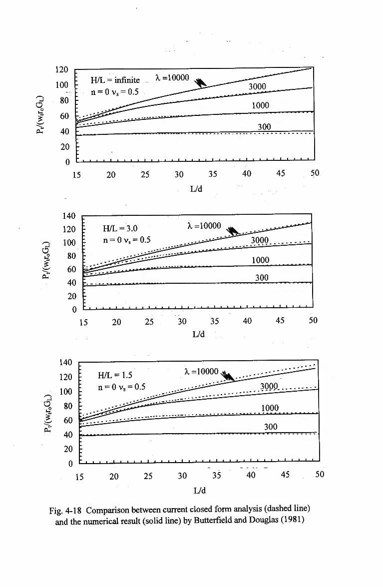
o
I OH
120
100
80
60
40
20
0
H/L = infinite ^ =10000
300 W I I I M I I I
' I ' I I I I 1 1 1 1 1 1 1 1 • 1 • < -
15 20 25 30 35 40 45
L/d
50
O
L/d
140
120 | H/L =1.5 n = 0 vs = 0.5
O 80
>t 60 +-»
PU
40 20
0
15
X=10000
' — I I I
20 25 30 35
L/d
40 45 50
Fig. 4-18 Comparison between current closed form analysis (dashed line) and the numerical result (solid line) by Butterfield and Douglas (1981)
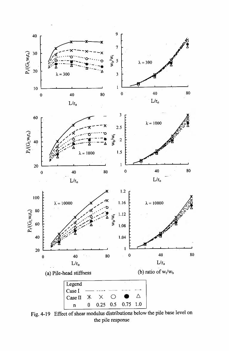
40
r o 2 20 10
//.'Q. -..„ w
k = 300
O -• A
40
L/r0
80
40
L/r0
80
40
L/r„
80
(a) Pile-head stiffness
40
L/r0
(b) ratio of wt/wb
Legend
Case I Casell X X O • A
n 0 0.25 0.5 0.75 1.0
Fig. 4-19 Effect of shear modulus distributions below the pile base level on the pile response
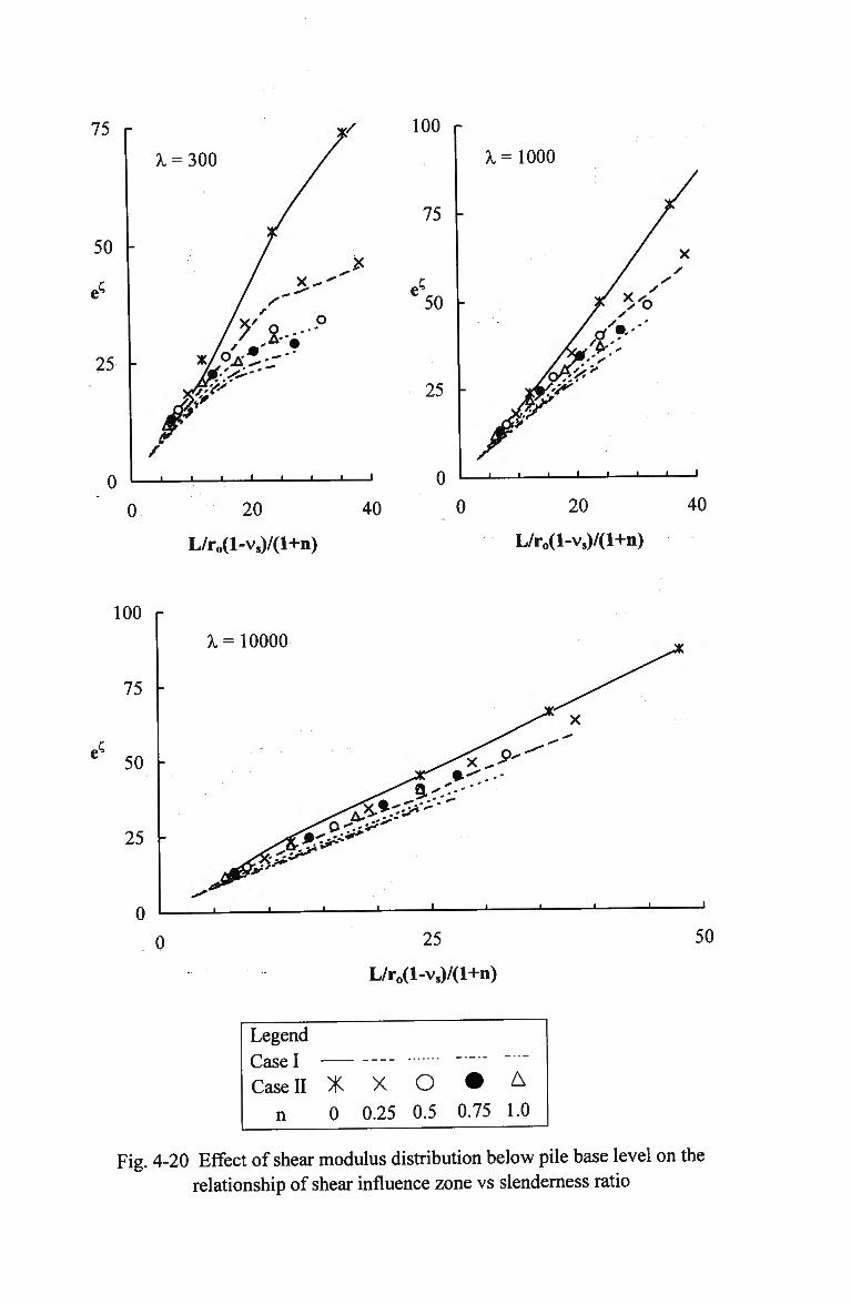
75 r
A. = 300
50
e
25
0
100 r
J L
0 20 40
L/r„(l-vs)/(l+n)
0 20 40
L/r„(l-vs)/(l+n)
100 r
75
50
25
0
A, = 10000
0
.t '"" v:^.*
*^**
-I L- J L. 1
25
L/r0(l-vs)/(l+n)
Legend
Case I
Case II
n
X 0
X o 0.25 0.5
• A
0.75 1.0
50
Fig. 4-20 Effect of shear modulus distribution below pile base level on the relationship of shear influence zone vs slenderness ratio
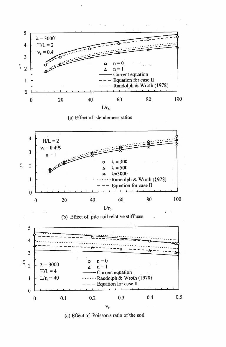
Current equation Equation for case II Randolph & Wroth (1978)
Q I • • • • i • • i i I i i i — i — I — i — i — i — i — I — i — ' '—
0 20 40 60
L/r0
(a) Effect of slenderness ratios
80 100
4
3
2
1
0
H/L = 2
vs = 0.499
n = l
o A, = 300 A A, = 500 x A.=3000
Randolph & Wroth (1978) Equation for case II
i i i — i — i — i — i — i — " — i — i — i — " — < -
0 20 40 60
L/r0
(b) Effect of pile-soil relative stiffness
80
4 -
2
1
0
- A. = 3000 H/L = 4 L/r0 = 40
o n = 0 A n = 1
Current equation • - - - Randolph & Wroth (1978)
Equation for case II i i i — i — i — i — i — i — i -
0 0.1 0.2 0.3
vs
(c) Effect of Poisson's ratio of the soil
0.4
100
0.5
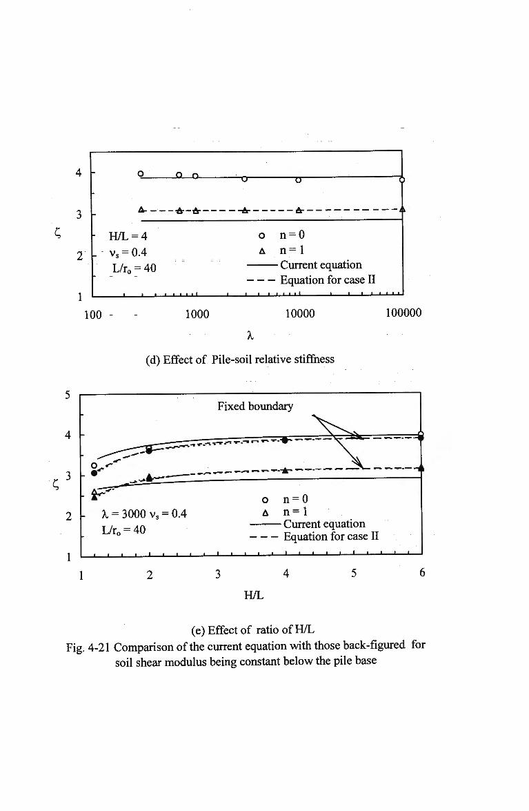
Q 0 o
•A—A--
H/L = 4
vs = 0.4
L/r0 = 40
o n = 0 A n = 1
Current equation Equation for case II
• • • i i — i — i i 1 1 1
100 1000 10000 100000
(d) Effect of Pile-soil relative stiffness
C
Fixed boundary
^ ti
X = 3000 vs = 0.4
r° Equation for case II
i i i — i — i — i — i — i — i — " — " — ' — > -
o n = 0 A n = 1
Current equation
3 4
H/L
(e) Effect of ratio of H/L
Fig. 4-21 Comparison of the current equation with those back-figured for soil shear modulus being constant below the pile base
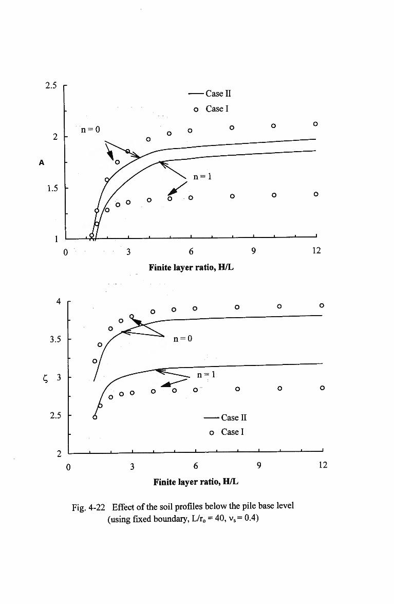
— Case II
o Case I
0
I I I I I 1 1 L.
3 6 9
Finite layer ratio, H/L
12
Case II
o Case I
j i i 1 1 1 — i i i i
12 0 3 6 9
Finite layer ratio, H/L
Fig. 4-22 Effect of the soil profiles below the pile base level
(using fixed boundary, L/r0 = 40, vs= 0.4)
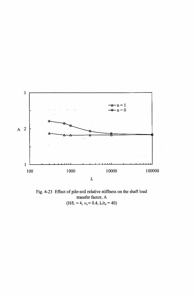
A 2 -
"
-
A—
i i • i i • i
-A &
i i l l
-A-n=l -e-n = 0
• • i — i i i 1 1
100 1000 10000 100000
Fig. 4-23 Effect of pile-soil relative stiffness on the shaft load transfer factor, A
(H/L = 4,vs=0.4,L/ro = 40)
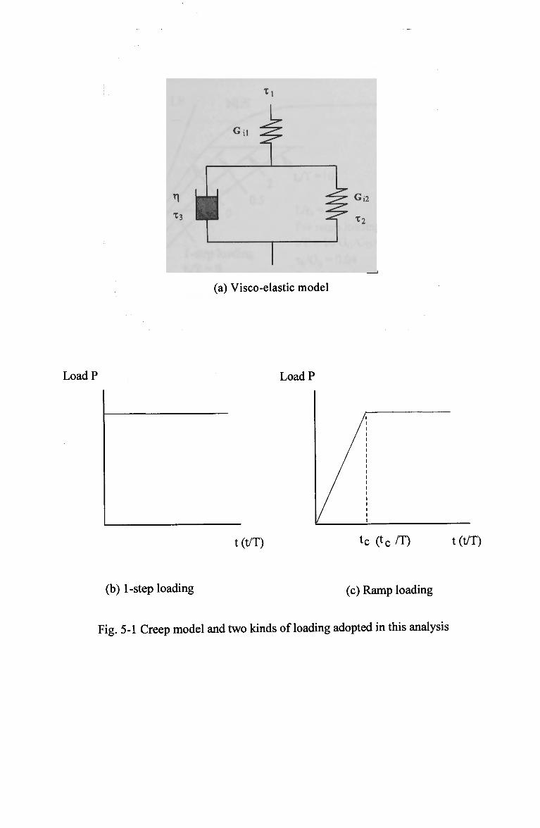
tl
r\ L x3 |
Gn ^
--*" <^i2
X2
(a) Visco-elastic model
LoadP LoadP
t(t/T) tc(tc/T) t(t/T)
(b) 1-step loading (c) Ramp loading
Fig. 5-1 Creep model and two kinds of loading adopted in this analysis
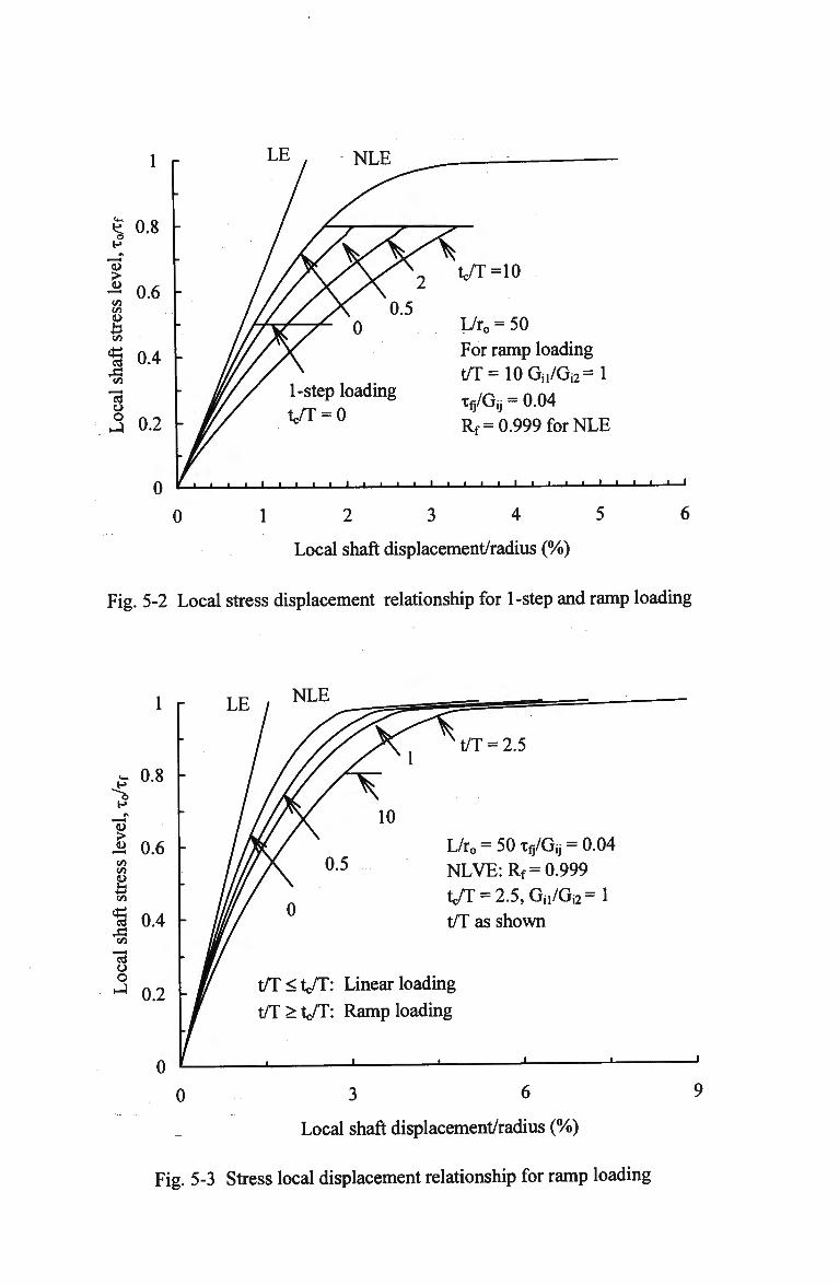
1 r
tf o p
^^ 0> > JJ on on u £ on
« XI on . ra o O
0.8
0.6
0.4
0.2
0
0
1-step loading
tc/T = 0
tc/T=10
L/r0 = 50
For ramp loading
t/T=10Gn/Gi2=l
Tf/Gjj = 0.04
R f = 0.999 for N L E
_ i _ i i i i i i • • i i i i i • — i — i — i — i — i — i — • — i
1 2 3 4 5
Local shaft displacement/radius (%)
Fig. 5-2 Local stress displacement relationship for 1-step and ramp loading
1 r NLE
^
0.8
JB 0.6 on on fi on
% 0.4 -on
"ra
o o 0.2
0
0
L/r0 = 50 Tf/Gij = 0.04
N L V E : R f = 0.999
tc/T = 2.5,Gil/Gi2=l
t/T as shown
t/T<tc/T: Linear loading
t/T > t/T: Ramp loading
3 6
Local shaft displacement/radius (%
Fig. 5-3 Stress local displacement relationship for ramp loading
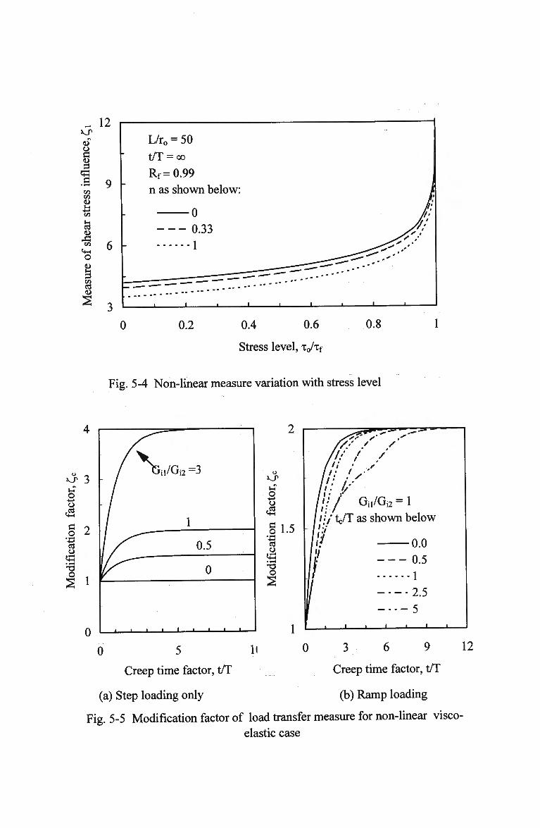
- 12 u1
u u
•S 9 on on U
J3
on
o
1 on ra
s
L/r0 = 50
t/T = oo
Rf=0.99
n as shown below
0 0.2 0.4 0.6
Stress level, xjxf
0.8
Fig. 5-4 Non-linear measure variation with stress level
0
0 5
Creep time factor, t/T
(a) Step loading only
H
v_r
*1.5 o
• i-H
O
Gi,/Gi2 = 1
ij/tc/T as shown below
• /
0.0
0.5
1
2.5
5
_J I L
0 3 6 9
Creep time factor, t/T
(b) Ramp loading
12
Fig. 5-5 Modification factor of load transfer measure for non-linear visco
elastic case
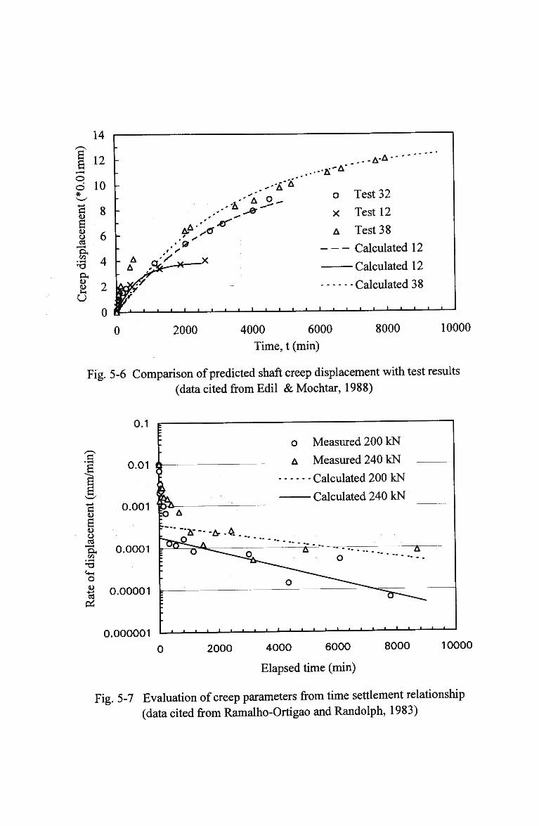
14
12
b * — *->
B o ra
a .1—1
T3 ft OJ
u I-U
10
8
6
4
2
0
.-•'A
*.AV«'
1 — 1 I I L.
0 2000
...-A-A-"'" -A"A'
o Test 32
x Test 12
A Test 38
Calculated 12
Calculated 12
Calculated 38
_i i i-
4000 6000
Time, t (min)
8000 10000
Fig. 5-6 Comparison of predicted shaft creep displacement with test results
(data cited from Edil & Mochtar, 1988)
0.1 P
a 6 CD
M "el on
o PH
0.01
0.001
0.0001 :
§ 0.00001 r
0.000001
o Measured 200 kN
A Measured 240 kN
-- --Calculated200kN
Calculated 240 kN
0 2000 4000 6000 8000 10000
Elapsed time (min)
Fig. 5-7 Evaluation of creep parameters from time settlement relationship
(data cited from Ramalho-Ortigao and Randolph, 1983)
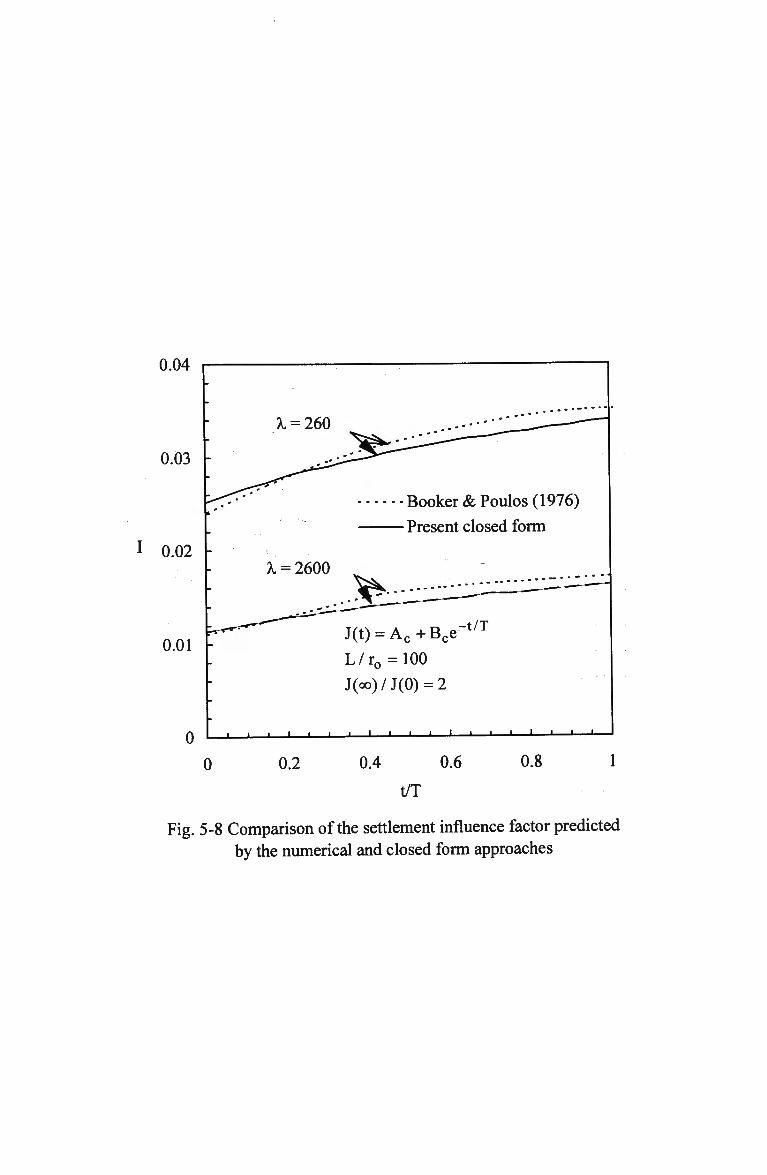
.04
.03
0.02
0.01
A. = 260
Booker & Poulos (1976)
Present closed form
A, = 2600
J(t) = A c + B c e "
L/r o=100
J(oo)/J(0) = 2
0 • ' I I L. • I I I 1 1 1 1-
0 0.2 0.4 0.6
t/T
0.8
Fig. 5-8 Comparison of the settlement influence factor predicted by the numerical and closed form approaches
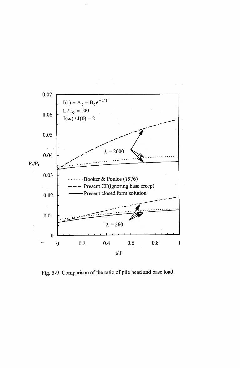
0.07
0.06
0.05
0.04
0.03 -
0.02
0.01
0
J(t) = A c + B c e
L/r0 = 100
J(oo)/J(0) = 2
-t/T
Booker & Poulos (1976) Present CF(ignoring base creep)
Present closed form solution
0 0.2 0.4 0.6 0.8
t/T
Fig. 5-9 Comparison of the ratio of pile head and base load
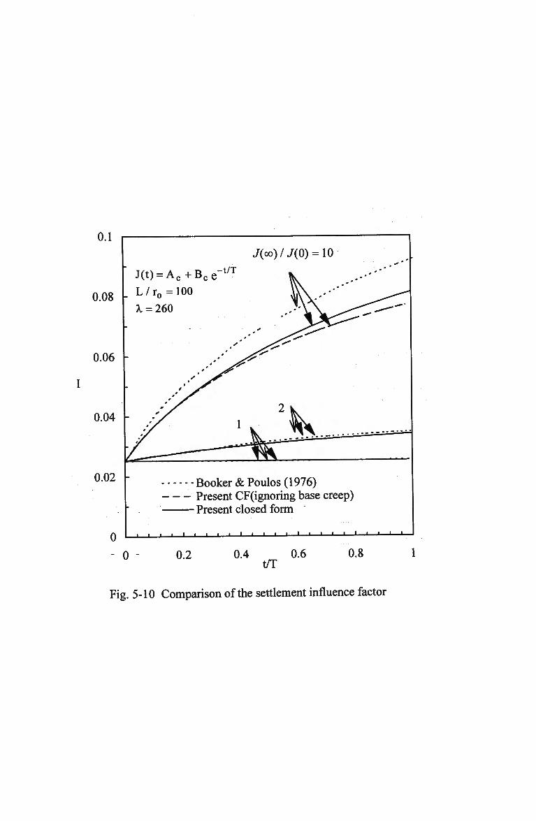
0.1
0.08
0.06
0.04
J(oo)lJ(0) = \0
J(t) = A c + B -t/T
0.02
0
Booker & Poulos (1976) Present CF(ignoring base creep) Present closed form
...III! | | | 1 1 1 1 1 1_
0 0.2 0.4 0.6 t/T
0.8
Fig. 5-10 Comparison of the settlement influence factor
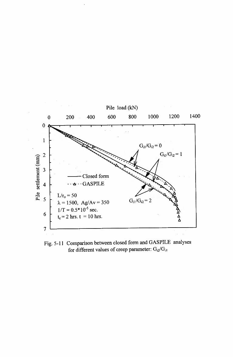
Pile load(kN)
0 200 400 600 800 1000 1200 1400
Fig. 5-11 Comparison between closed form and GASPILE analyses for different values of creep parameter: Gi2/Gii
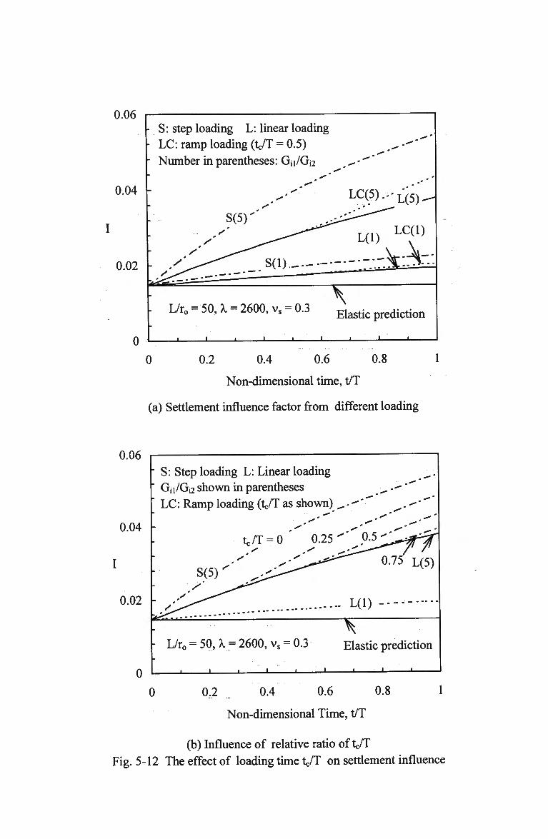
0.06
0.04
0.02
S: step loading L: linear loading LC: ramp loading (t/T = 0.5)
Number in parentheses: Gn/Gj2
LC(5).-L(5)
0
L/r0 - S U - 2600, vs = 0.3 Elastic prediction
J I I L J I L
0 0.2 0.4 0.6 0.8
Non-dimensional time, t/T
(a) Settlement influence factor from different loading
0.06
0.04
0.02
0
S: Step loading L: Linear loading Gji/Gj2 shown in parentheses LC: Ramp loading (t/T as shown)
tc/T = 0 ' 0.25"' .0.5
- L/r0 = 50, A. = 2600, vs = 0.3 Elastic prediction
j i i_
0 0.2 0.4 0.6 0.8
Non-dimensional Time, t/T
(b) Influence of relative ratio of t/T
Fig. 5-12 The effect of loading time t/T on settlement influence
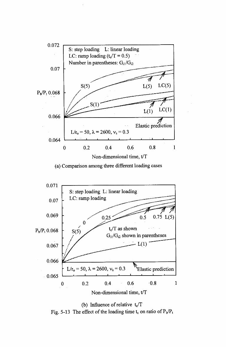
0.072
0.07
Pb/Pt 0.068
0.066
0.064
S: step loading L: linear loading LC: ramp loading (t/T = 0.5)
Number in parentheses: Gn/Gj2
- . i " " ^ 1
S(5)
y^*L—
U.5) LC(5)
L(l) LC(1)
yr~ Elastic prediction
L/r0 = 50, A. = 2600, vs = 0.3 • i i i i i 1 1 i
0 0.2 0.4 0.6 0.8
Non-dimensional time, t/T
(a) Comparison among three different loading cases
1
0.071
0.07
0.069
Pb/Pt 0.068
0.067
0.066
0.065
S: step loading L: linear loading LC: ramp loading
.> - • • •
0.25 C**^' 0.5 0.75 L(5)
t/T as shown
Gn/Gi2 shown in parentheses
_.----'" L(1)
L/r0 = 50, A. = 2600, vs = 0.3 Elastic prediction _l L J I L.
0 0.2 0.4 0.6 0.8
Non-dimensional time, t/T
(b) Influence of relative t/T
Fig. 5-13 The effect of the loading time on ratio of Pb/Pt
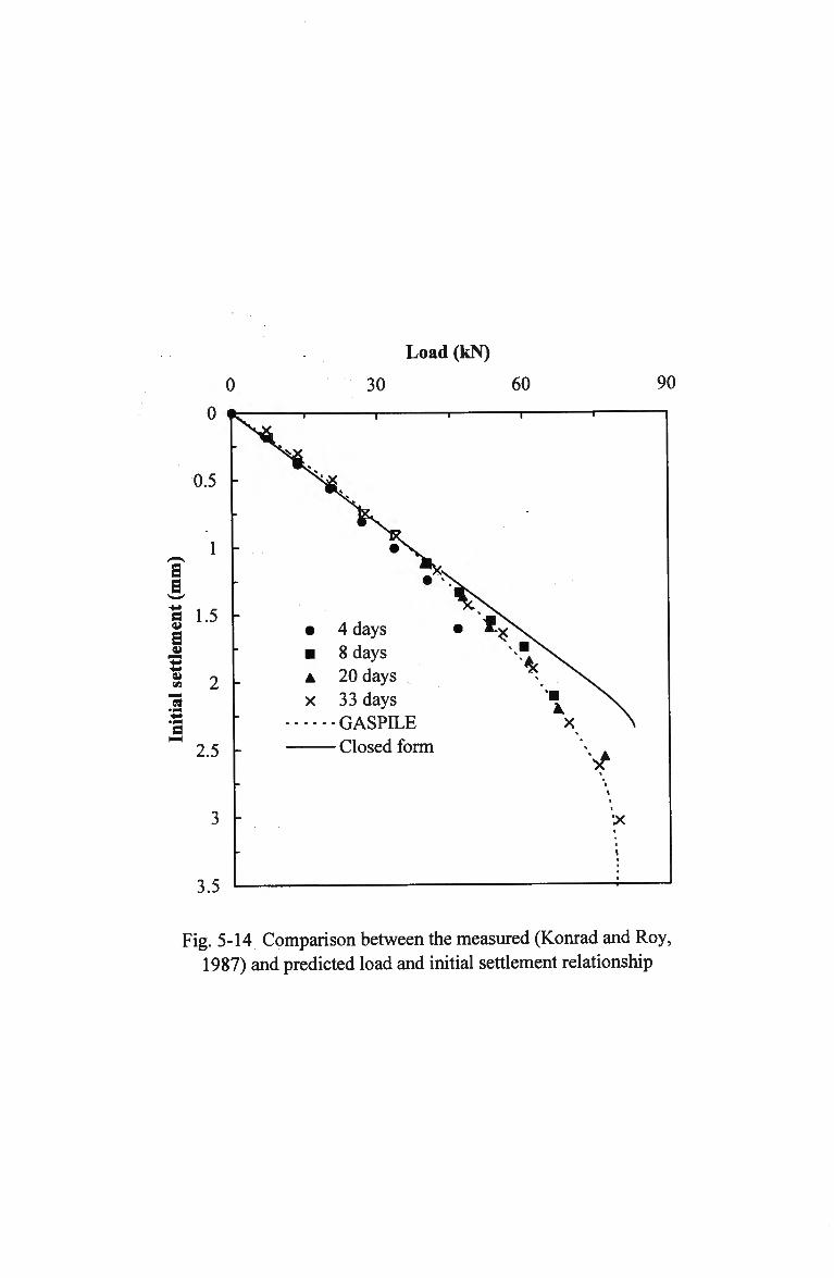
0
Load (kN)
30 60
x
4 days 8 days 20 days 33 days GASPILE • Closed form
90
^
x
Fig. 5-14 Comparison between the measured (Konrad and Roy, 1987) and predicted load and initial settlement relationship
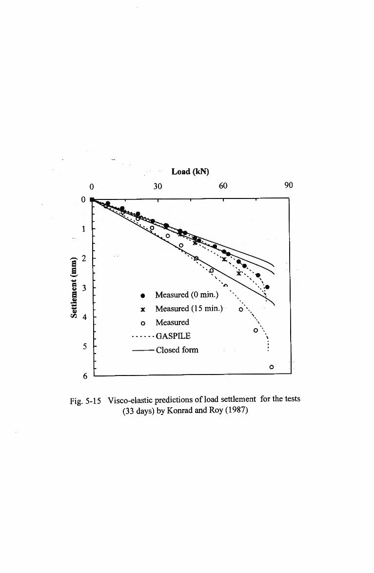
0
Load (kN)
30 60 90
"x.
• Measured (0 min.)
x Measured (15 min.)
o Measured
----GASPILE
Closed form
o \
Fig. 5-15 Visco-elastic predictions of load settlement for the tests (33 days) by Konrad and Roy (1987)
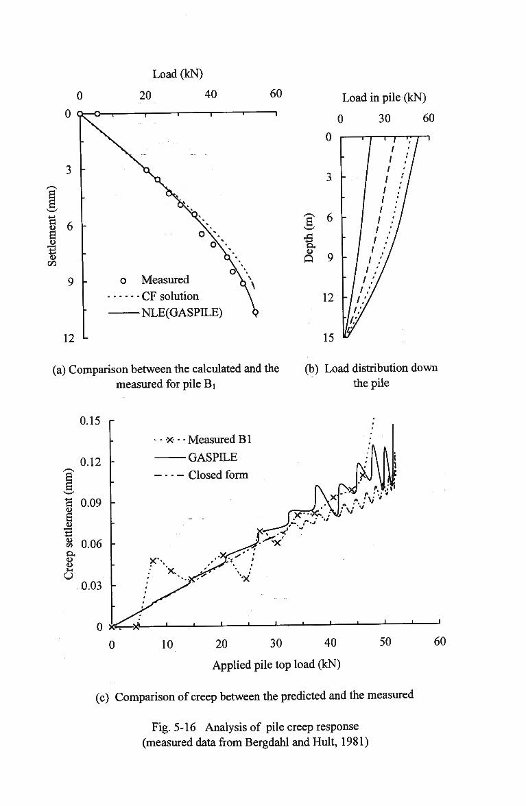
0 0
U o
s C/3
12
Load (kN)
20 40
o Measured
CF solution
NLE(GASPILE)
60 Load in pile (kN)
0 30 60
0 I r-j n—f~J—I
3 -
f Q
9 -
12 -
15
(a) Comparison between the calculated and the (b) Load distribution down measured for pile Bi the pile
0.15 r
0.12
3 0.09 i>
S u Sn 0.06 CH
o (U (-1
u 0.03 -
0
0
x --Measured BI
GASPILE
Closed form
10 20 30 40
Applied pile top load (kN)
50 60
(c) Comparison of creep between the predicted and the measured
Fig. 5-16 Analysis of pile creep response (measured data from Bergdahl and Hult, 1981)
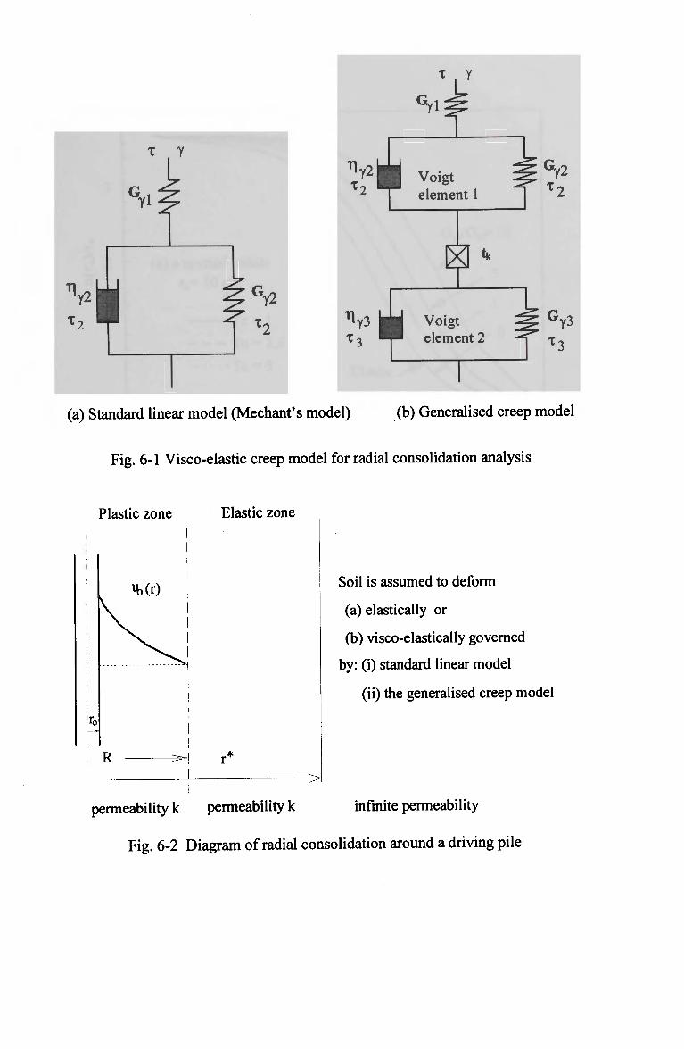
T y
Tl Y2
Tl Y3
Si
Voigt element 1
Kh Voigt element 2
(a) Standard linear model (Mediant's model) (b) Generalised creep model
Fig. 6-1 Visco-elastic creep model for radial consolidation analysis
Plastic zone Elastic zone
%
4>(r)
R ^>
Soil is assumed to deform
(a) elastically or
(b) visco-elastically governed
by: (i) standard linear model
(ii) the generalised creep model
permeability k permeability k infinite permeability
Fig. 6-2 Diagram of radial consolidation around a driving pile
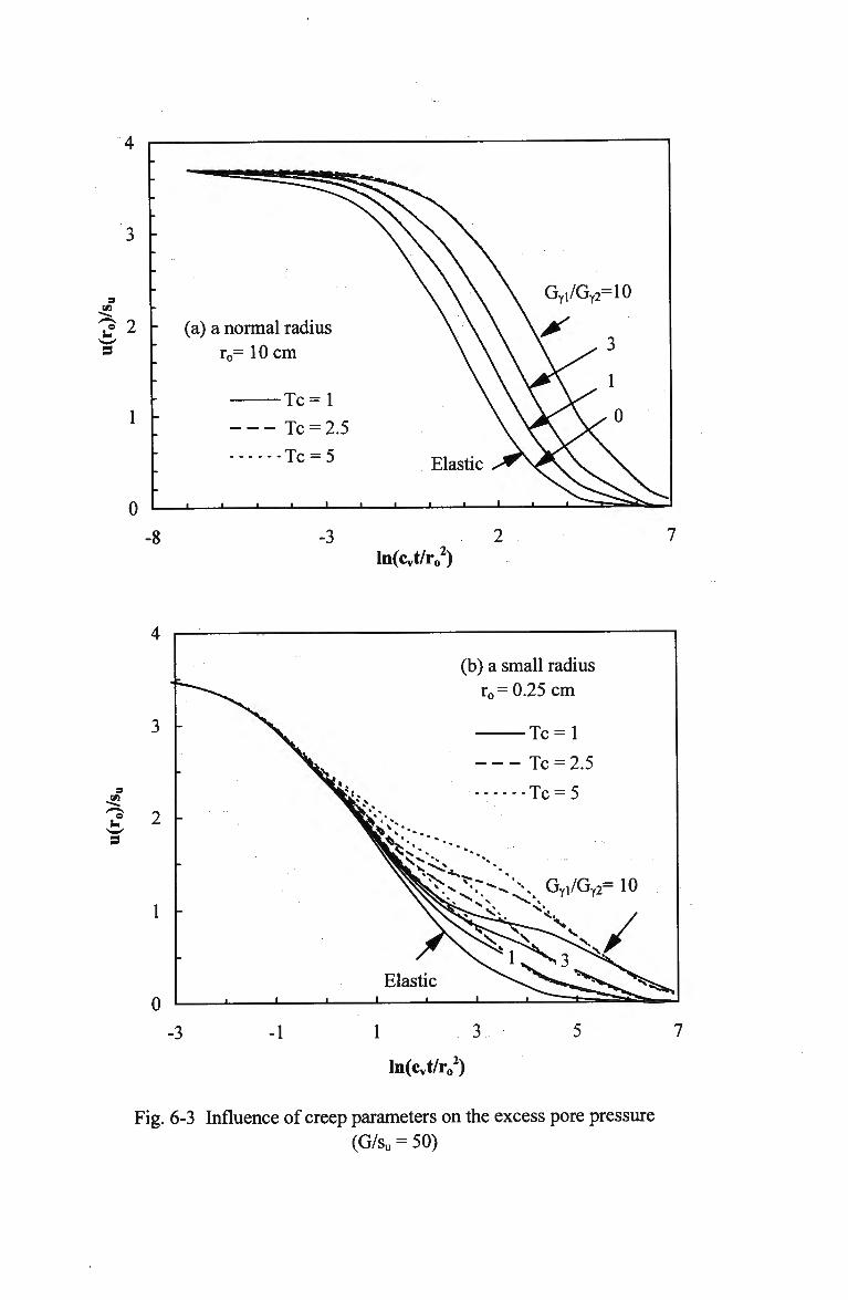
3 -
2 -
1 -
0
: — * ^
-
(a) a normal radius
r0= 10 cm
T c = l
Tc = 2.5
Tc = 5
• __• 1 1 1 1 —
Elastic s&
J i i i
V Gyl/Gy2—10
V.3 \A\ I
V V A ^ O
0
-3 2 ln(cvt/r0
2)
(b) a small radius
r0 = 0.25 cm
Tc = 2.5
» GYi/GY2- 10
1 3
ln(cvt/r02)
Fig. 6-3 Influence of creep parameters on the excess pore pressure
(G/su = 50)
0.01 0.1 1 10
In CD 100 1000
Fig. 6-4 Variation of times for 50 and 9 0 % degree of consolidation with the ratio Uo(r0)/su
Pile top load (kN)
0 100 200 300 400 500 600 700 800
0
s a, 110 a S
15
20
i — r — i — i — i — i i i — | - 1 — i — r - i — | — r — i — r — i — | — ' — • — i — i — I — • — i — • — i — r ~ i — i - " — " — I
•NLVE2.5hr
NLVE 1 Month
NLE
Pb
— A — M e a
(a) Test 2 (24m)
0
25 L
200
Pile top load (kN)
400 600 800 1000
(b) Test 2 (30m) Fig. 6-5 Comparisons between the calculated and the measured
by Trenter and Burt (1981) for pile 2
Pile top load (kN)
0 500 1000
Pile top load (kN)
0 800 1600
a a a
a
tt
(a) 1.7 days (b) 10.5 days
0
Pile top load (kN)
600 1200 1800
Pb
NLVE LE —A—Mea
0
Pile top load (kN)
600 1200 1800
N L V E LE
--Pb — A — M e a
(c) 20.5 days (d) 32.5 days
Fig. 6-6 Comparisons between the calculated and the measured
by Trenter and Burt (1981) for pile 4
0
Pile top load (kN)
600 1200 1800
0
5
10
15
20
25
30 -
35 L
Fig.
Pile top load (kN)
600 1200 1800
Pile top load (kN)
600 1200
(d) 4.2 days
1800
•NLVE LE
Pb — A — M e a
6-7 Comparisons between the calculated and the measured
by Trenter and Burt (1981) for pile 3
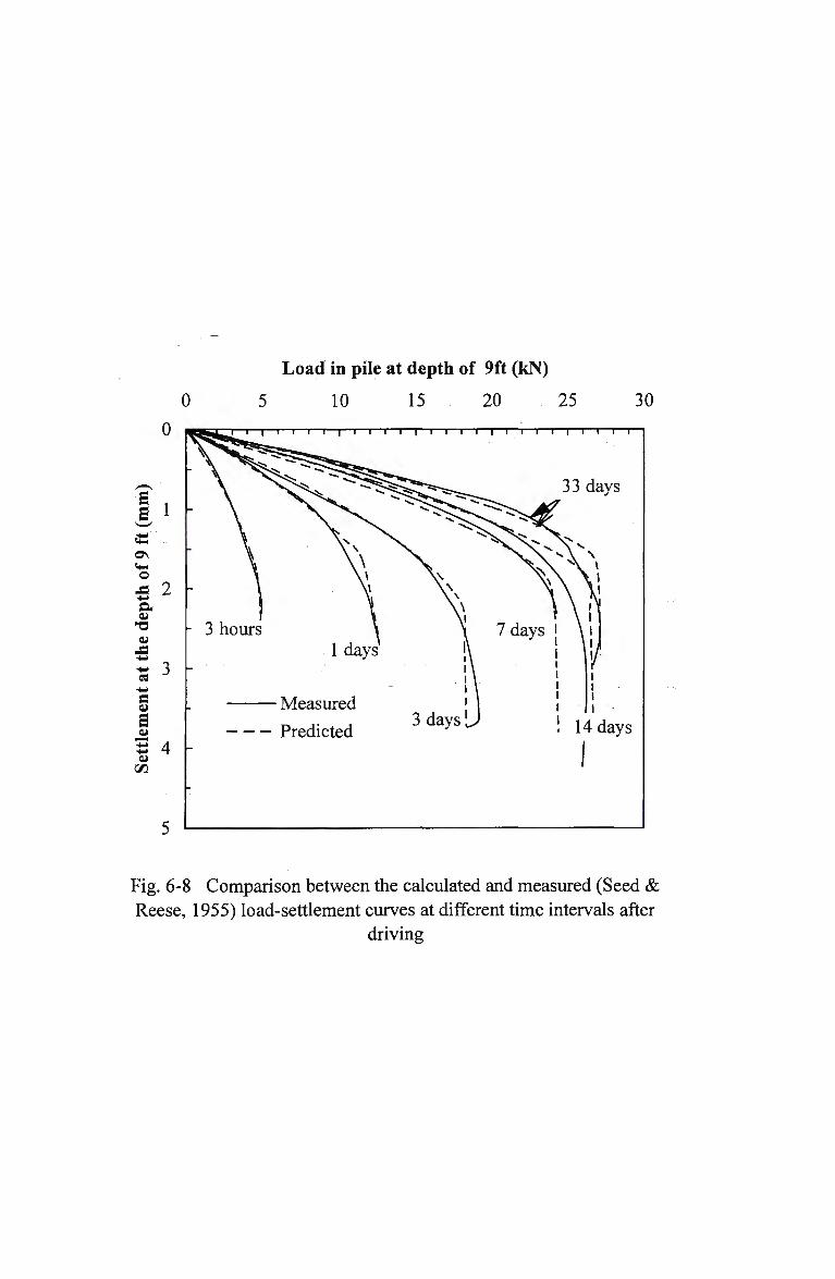
0
Load in pile at depth of 9ft (kN)
5 10 15 20 25 30
0
a i
O
JS 2 a <u
-a -M
-M
c «
E
5 4 cu
TT^LL* ' ' ' ' ' ' ' ' '
» ^ C ^ —•^•—^J^"*^
\ V \ V
\ \v - 3 hours \
1 days
Measured
Predicted
— i — i i i i
\l
1
3 days
— i — | — i — i — i — r
7 days
- i — T " ' i — I —
33 days
\ s
\ V
! 1-
I
i
1 days
Fig. 6-8 Comparison between the calculated and measured (Seed &
Reese, 1955) load-settlement curves at different time intervals after
driving
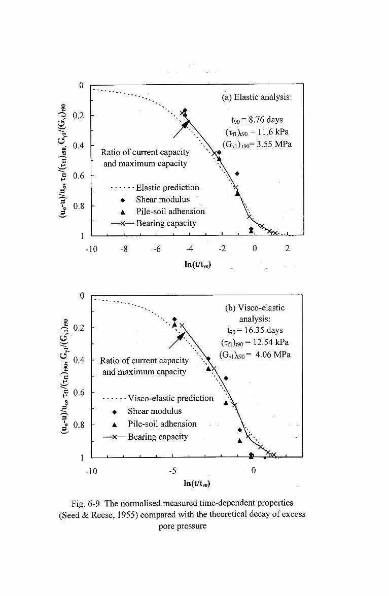
0
o
c
o
•
o 3
0.4
0.6
0.8
Ratio of current capacity
and m a x i m u m capacity
•10
Elastic prediction
• Shear modulus
A Pile-soil adhension
— x — Bearing capacity
(a) Elastic analysis:
t90= 8.76 days
(tfi)t9o= 11.6kPa
(GYl)t9o= 3.55 M P a
-8 -4 -2
ln(t/t90)
0
0
-•? 0.2 O
o 0.4 -
c
1= 0.6 o
.3
| 0.8
" * - fc
^Ax
A - Ratio of current capacity -X
and m a x i m u m capacity ^
Visco-elastic prediction
• Shear modulus
A Pile-soil adhension
— x — Bearing capacity
• • i i 1 1 1 —
(b) Visco-elastic
analysis:
t9o= 16.35 days
(Tn)t9o= 12.54 kPa
(GYi)t9o= 4.06 M P a
\ *
A*V
A X^
—' " tl A^X... '
•10 In(t/t90)
Fig. 6-9 The normalised measured time-dependent properties
(Seed & Reese, 1955) compared with the theoretical decay of excess
pore pressure
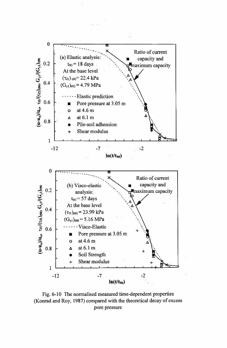
0
0.2
o
o : 0.4 -
c
£ 0.6 9
.3
| 0.8
"™ n
(a) Elastic analysis: " * *. >v t9o=18days
At the base level (Tfl)t90=22.4kPa
(Gyl)t9(
•
o A
•
+
,= 4.79 M P a
- Elastic prediction Pore pressure at 3.05 at 4.6 m at 6.1 m Pile-soil adhension Shear modulus
• • • • I
•
%« A \
%
m
_ i
Ratio of current capacity and
naximum capacity
» \
V \
\ \ 1 \
\ \
A\
i I i B i" *•-..-;
•12 -7 ln(t/t90)
-2
0
^ 0 . 2 ?-
O
o ; 0.4 -
c
£ 0.6 e
s
s 0.8 -
" * *. X
(b) Visco-elastic N. K \ analysis:
t90=57days At the base level (Tfi)t90= 23.99 kPa
• (GYi)t90= 5.16 M P a
Visco-Elastic • Pore pressure at 3.05 o at 4.6 m A at 6.1 m • Soil Strength + Shear modulus
i i i i . i . — i 1 —
•
\ A^ \A
m
•
Ratio of current capacity and
tnaximum capacity
V \ \
\ \
» »
A\
H *
, i t+ T*rr-
•12 -7 ln(t/t90)
-2
Fig. 6-10 The normalised measured time-dependent properties (Konrad and Roy, 1987) compared with the theoretical decay of excess pore pressure
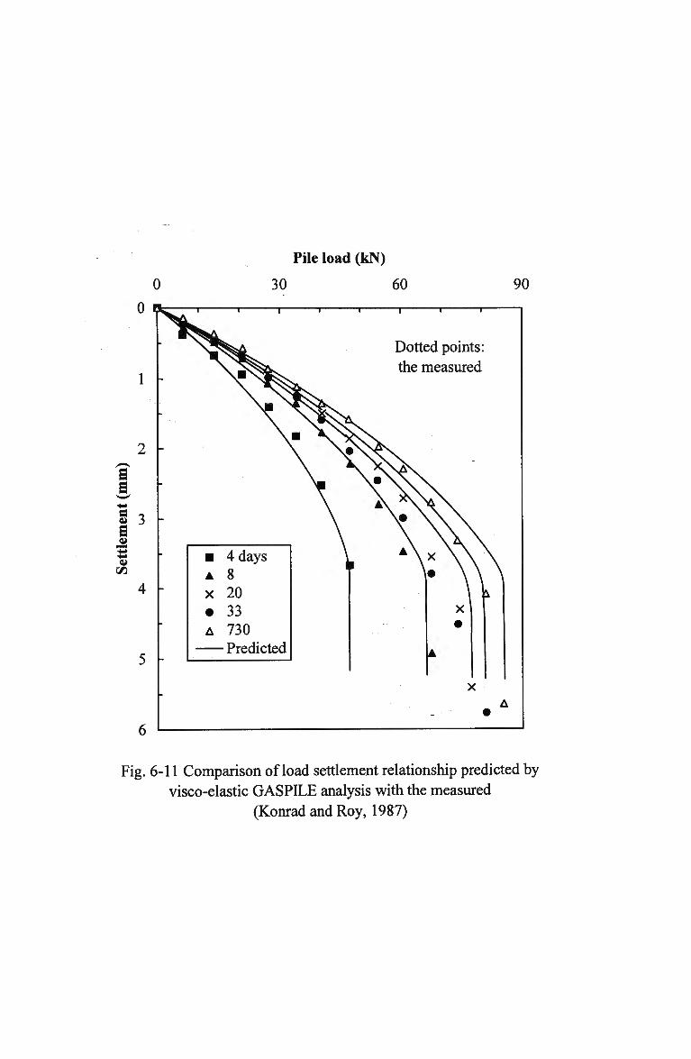
0 0
a a i3
<u
2 tt
Pile load (kN)
30 60
i 1 1 1 1 1 1 r
•
A
X
•
A
4 days 8 20 33 730 - Predicted
Dotted points: the measured
90
Fig. 6-11 Comparison of load settlement relationship predicted by visco-elastic GASPILE analysis with the measured
(Konrad and Roy, 1987)

0
Total load (kN)
30 60 90
-i r
5 -
Visco-elastic
• Elastic
4 days 8 20 33 730
Fig. 6-12 Comparison of elastic and visco-elastic load settlement relationship predicted by GASPILE
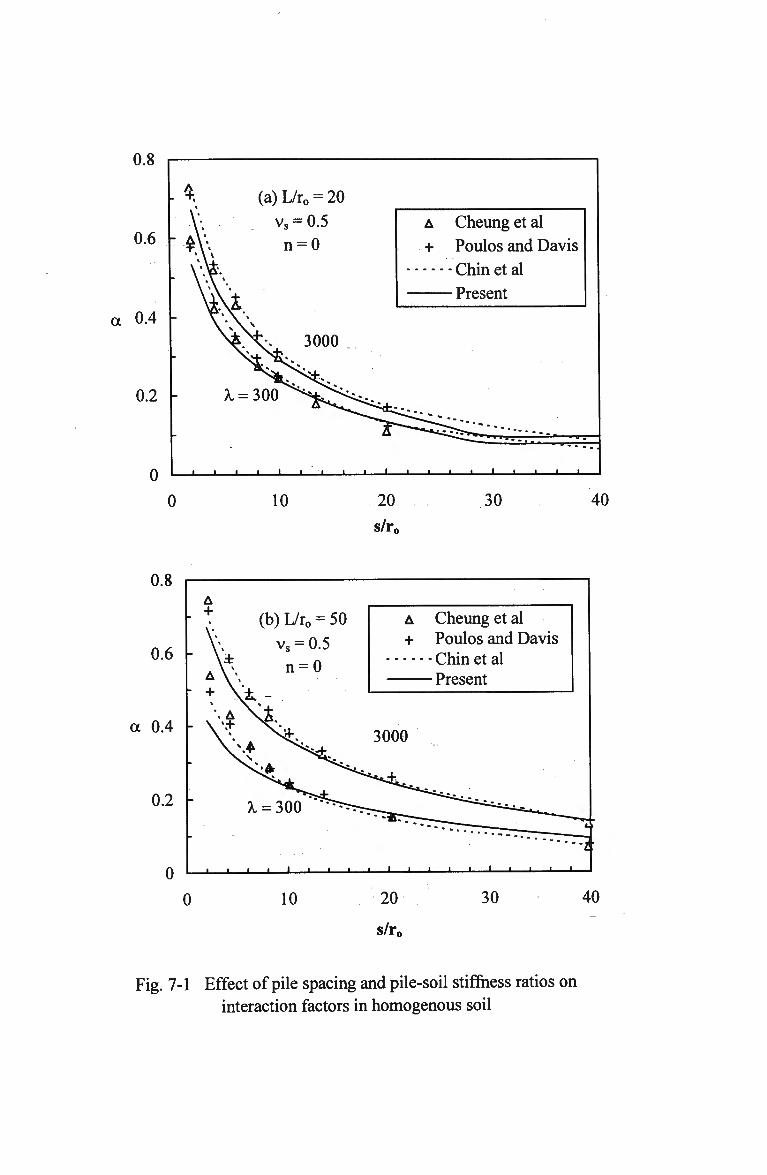
a
0.8
0.6
0.4
.*. (a) L/r0 = 20
vs = 0.5
$\\ n = 0
0.2 - A, = 300
0
A Cheung et al
+ Poulos and Davis
Chin et al
Present
•* i i . .'
• • • • i i i i i i i i i i i — i — • -
0 10 20
s/r0
30 40
0.8
0.6
a 0.4
0.2
0
A + (b) L/r0 = 50
vs = 0.5
n = 0
A Cheung et al + Poulos and Davis
Chin et al Present
A. = 300
i • . i • i i i i i i i — 1 _
0 10 20
s/r0
30 40
Fig. 7-1 Effect of pile spacing and pile-soil stiffness ratios on interaction factors in homogenous soil
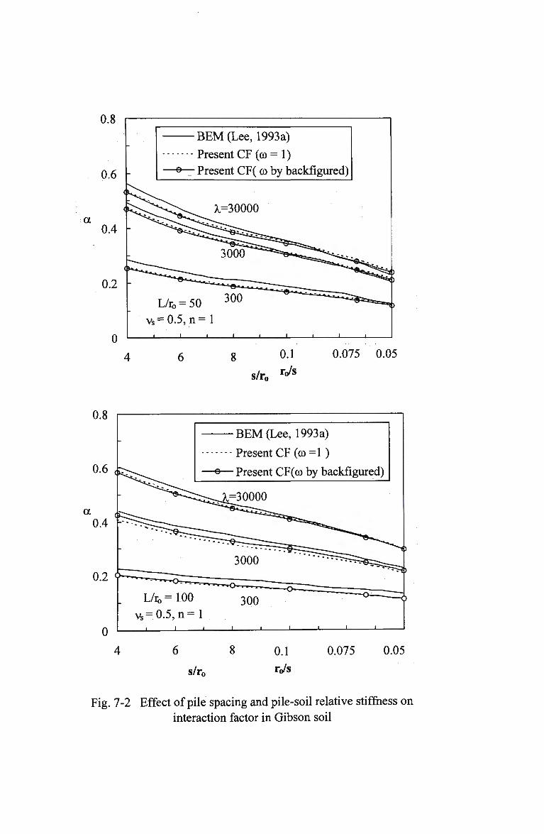
a
0.8
0.6 -
0.4 -
0.2 -
0
-
-
^ ^
B E M (Lee, 1993a)
Present CF(co=l)
° Present CF( co by backfigured)
^ ^ ^ X=30000
L/ro = S C i ^ ^ ^ ^ ^ ^ ^
vs=0.5, n = 1 • i i i • • i i i
8 0.1
s/r„ ^s
0.075 0.05
0.8
0.6
a 0.4
B E M (Lee, 1993a)
Present CF (co =1)
-©— Present CF(co by backfigured)
^=30000
3000
s/r0
0.1
rjs
0.075 0.05
Fig. 7-2 Effect of pile spacing and pile-soil relative stiffness on
interaction factor in Gibson soil
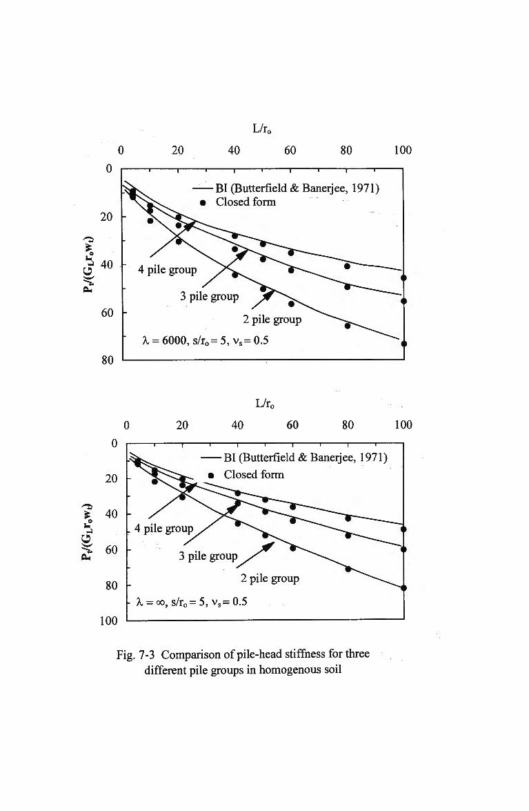
0 20
L/r0
40 60 80 100
0
20
i?
PM
60
80
i ' r T 1 1 r
BI (Butterfield & Banerjee, 1971) Closed form
4 pile group
3 pile group
2 pile group
A, = 6000, s/r0=5, vs=0.5
0 20
L/r0
40 60
0
20
? 40 o M -J
> 60
80
100
-i 1 r
80 100
— i 1 1 1 1 1 —
BI (Butterfield & Banerjee, 1971)
Closed form
4 pile group
3 pile group
2 pile group
A. = oo, s/r0= 5, vs= 0.5
Fig. 7-3 Comparison of pile-head stiffness for three different pile groups in homogenous soil
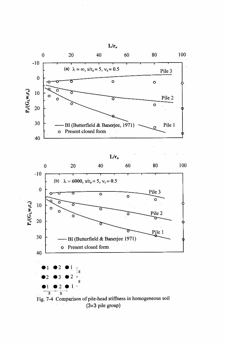
0 20
L/r0
40 60
•10
0
10
20
30
40
1 1 1 1 r
(a) A, = oo, s/r0 = 5, vs = 0.5
80 100
-i r
— BI (Butterfield & Banerjee, 1971) o Present closed form
Pile 3
Pilel
0
-10
0
10
20
30
40
20
L/r0
40 60
— i 1 1 1 1 i
(b) A, = 6000,s/ro=5,vs=0.5
80 100
BI (Butterfield & Banerjee 1971)
o Present closed form
2 +
Fig. 7-4 Comparison of pile-head stiffness in homogeneous soil
(3x3 pile group)
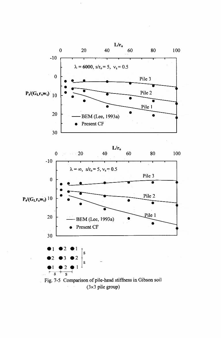
0 20 L/r0
40 60 80
•10
0 -
P,/(GLr0wt) 1Q
20 -
30
100
A,=
• •
• • 9
•
-
•
— 1 " 1 r-
= 6000, s/r0=5, vs=
• •
• " - —
- B E M (Lee, 1993a)
Present CF
1 —
0.5
•
•
— i 1 "
Pile 3
Pile 2
"""•"" — .
__Pilel
• ;.
L/r0 0 20 40 60
•10
0 -
Pt/(GLr0wt) 10 -
20 -
30
80 100
1 1 r -|— i—-
X = 00, s/r0= 5, vs=0.5
• • 1 *-• • 9 _
•*""""""-^«.
B E M (Lee, 1993a)
• Present CF
— i —
•
•
— i 1 1
Pile 3 •
Pile 2
^^Pilel
(
• i #2 m\
•2 #3 #2
• 1 # 2 • 1
s s Fig. 7-5 Comparison of pile-head stiffness in Gibson soil
(3x3 pile group)
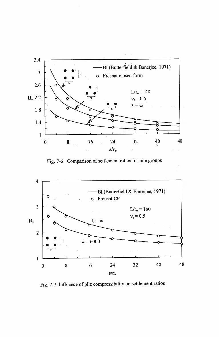
3.4
3
2.6
2.2
1.8
1.4
0
BI (Butterfield & Banerjee, 1971)
o Present closed form
8 16 24
s/r„
L/r0 = 4 0
vs=0.5
A, = oo
32 40
Fig. 7-6 Comparison of settlement ratios for pile groups
48
Rs
0
BI (Butterfield & Banerjee, 1971)
o Present CF
L/ro=160
v,= 0.5
j L. < i 1 1 1 •-
16 24
s/r0
32 40 48
Fig. 7-7 Influence of pile compressibility on settlement ratios
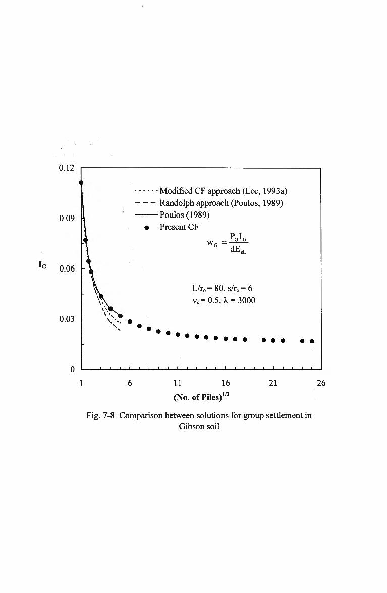
0.12
0.09
IG 0.06
0.03
Modified CF approach (Lee, 1993 a)
Randolph approach (Poulos, 1989)
Poulos (1989)
Present CF
W G = dEsL
L/ro=80, s/r0=6
vs=0.5, A. = 3000
0 f l i i i i l i i i i l i i i i I i i i i
21 26
(No. of Piles)1 16 .1/2
Fig. 7-8 Comparison between solutions for group settlement in Gibson soil
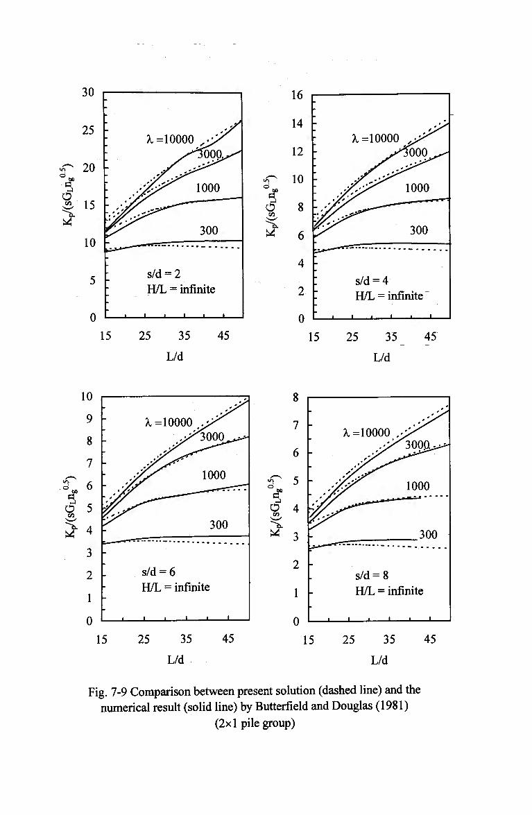
o
o on
30
25 -
20 -
15 -
10 -
5
0
15
-
; X =10000 yyS /^3000^^
a £*^r
--:yr^
'• s/d =
; H/L
• i i
1000
300 -
2 = infinite
i • i
25 35
L/d
45
O on
16
14 -
12
10
4
2
0
?i =10000
s/d = 4 H/L = infinite
15 25 35 45
L/d
10
9
8
7 -
O on
5
6
5
4
3
2
1
0
-
_
--
a m a J a ^j
-
-
-
-
a _^r
a^f
x =10000 yy' ^^3000^**
*f^ -rf"***^
y^y^ ry£s 1000
0 f*f 1-
300
s/d = 6 H/L = infinite
15 25 35
L/d
45
7
6
r 5 9 4 2^ 3
2 -
1 -
0
-
-
•
•
a A
it/
-
-
-
-
A. =10000 a ^T
a T
Y-y^ * X* f X* f
9^j^
s/d = 8
a
a f^
a ^^^
^ 0 0 0 ^ ^jj**00*"^
1000
300
H/L = infinite
i 1 1 L. • •
15 25 35
L/d
45
Fig. 7-9 Comparison between present solution (dashed line) and the numerical result (solid line) by Butterfield and Douglas (1981)
(2x1 pile group)
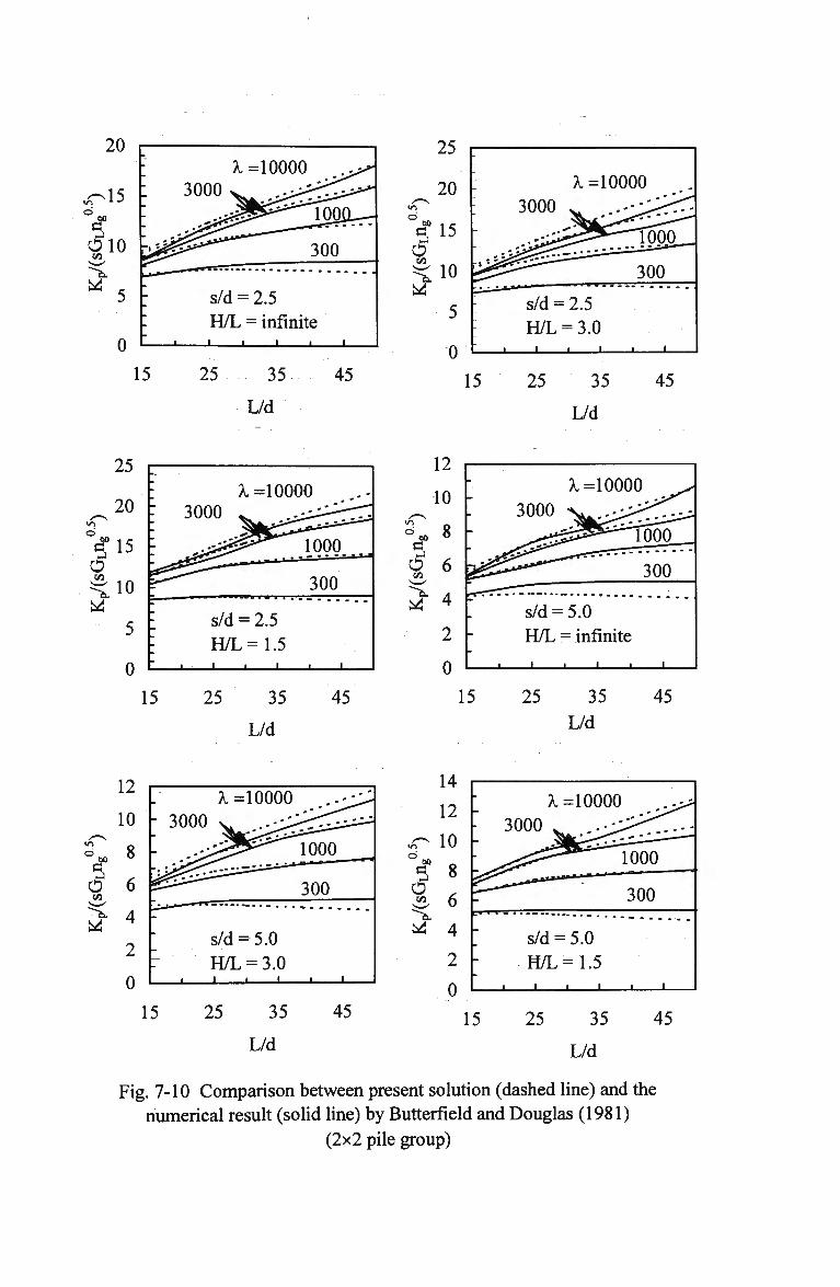
20
0
15
A. =10000
s/d = 2.5 H/L = infinite
25 35
L/d
45
25
20
> 15 o on
5
0
-
X =10000
3000 ^ .-
s/d = 2.5 H/L = 3.0
• • • •
rrrjoooL 300
• i
15 25 35
L/d
45
O on
5
12
10
8
6
4
2
0
15
" 3000 A. =10000 ^
>^y^<^^ ^3^^Tooo_
300 ^
s/d = H/L i
5.0 = infinite
• • i
25 35
L/d
45
A. =10000
15
s/d = 5.0 H/L = 3.0
25 35
L/d
45
IT)
o so CJ
o on > tf
14
12
10
8
6
4
2
0
A. 3000 .
- j j ^ ^ * *
: s/d= - H/L
=10000 ,.^>
,, •"
- " « " " "
5.0 = 1.5 i i
..-v;
1000
300
'
15 25 35
L/d
45
Fig. 7-10 Comparison between present solution (dashed line) and the numerical result (solid line) by Butterfield and Douglas (1981)
(2x2 pile group)
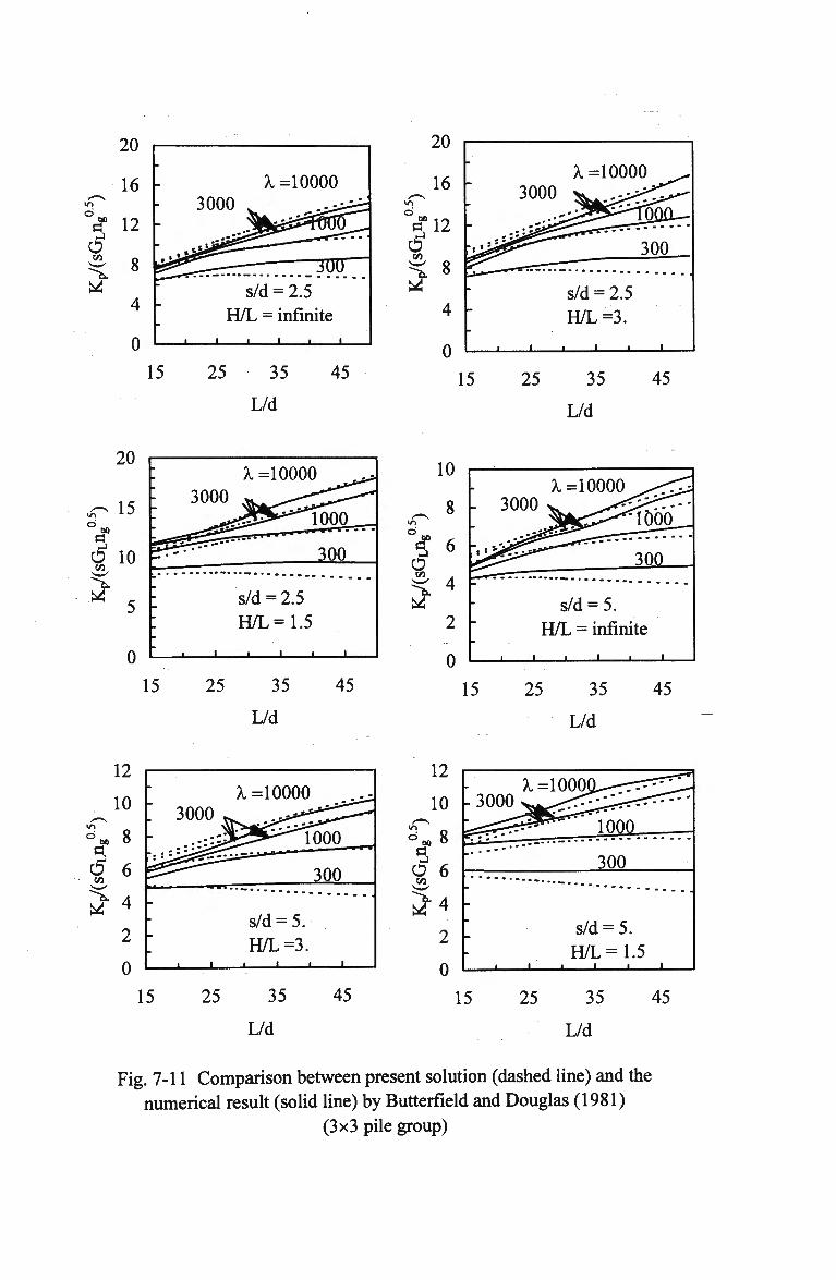
4
0
15
s/d = 2.5 H/L = infinite
J I I I L
25 35
L/d
45
20
15
A. =10000
s/d = 2.5 H/L =3.
I I I u
25 35
L/d
45
o 00 Si O on """*. Nd
20
15
10
5
0
15
A. =10000
s/d = 2.5 H/L=1.5
25 35
L/d
45
15 25 35
L/d
45
2
0
15
s/d = 5. H/L=1.5
25 35
L/d
45
Fig. 7-11 Comparison between present solution (dashed line) and the numerical result (solid line) by Butterfield and Douglas (1981)
(3x3 pile group)
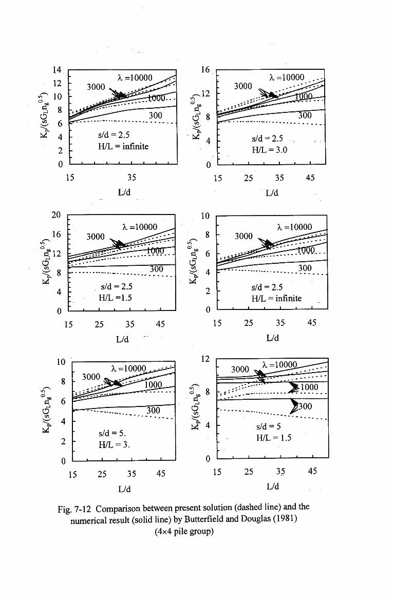
o on
2
14
12
10
8
6
4
2
0
15
s/d = 2.5 H/L = infinite
i i • ' • i i _
35
L/d
15
s/d = 2.5 H/L = infinite
25 35
L/d
45 15 25 35
L/d
45
12
V o on
^ 4
.:::--::'; '^1000
0
A, =10000.
J 300 s/d = 5 H/L =1.5
15 25 35
L/d
45
Fig. 7-12 Comparison between present solution (dashed line) and the numerical result (solid line) by Butterfield and Douglas (1981)
(4x4 pile group)
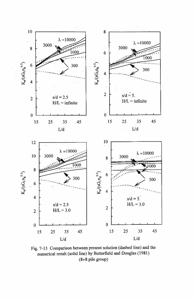
10
0
s/d = 2.5 H/L = infinite
J I L
15 25 35
L/d
45
6 -
d 4 on ^> tf
0
-
X =10000 ^ 3000 ^ . ^ ^ ^
.-r^^^TOOO^
"""' > 300
s/d = 5. H/L = infinite
1
15 25 35
L/d
45
c O on
tf
Yl
10
8
6
4
2
0
A. =10000
s/d = 2.5 H/L = 3.0
J i_
10
15 25 35 45
L/d
2 6 «;
o on tf 4
0
3000 A. =10000
^ ^ >>1000
- • y *
^ 300
s/d = 5. H/L = 3.0
_l L
15 25 35 45
L/d
Fig. 7-13 Comparison between present solution (dashed line) and the numerical result (solid line) by Butterfield and Douglas (1981)
(8x8 pile group)
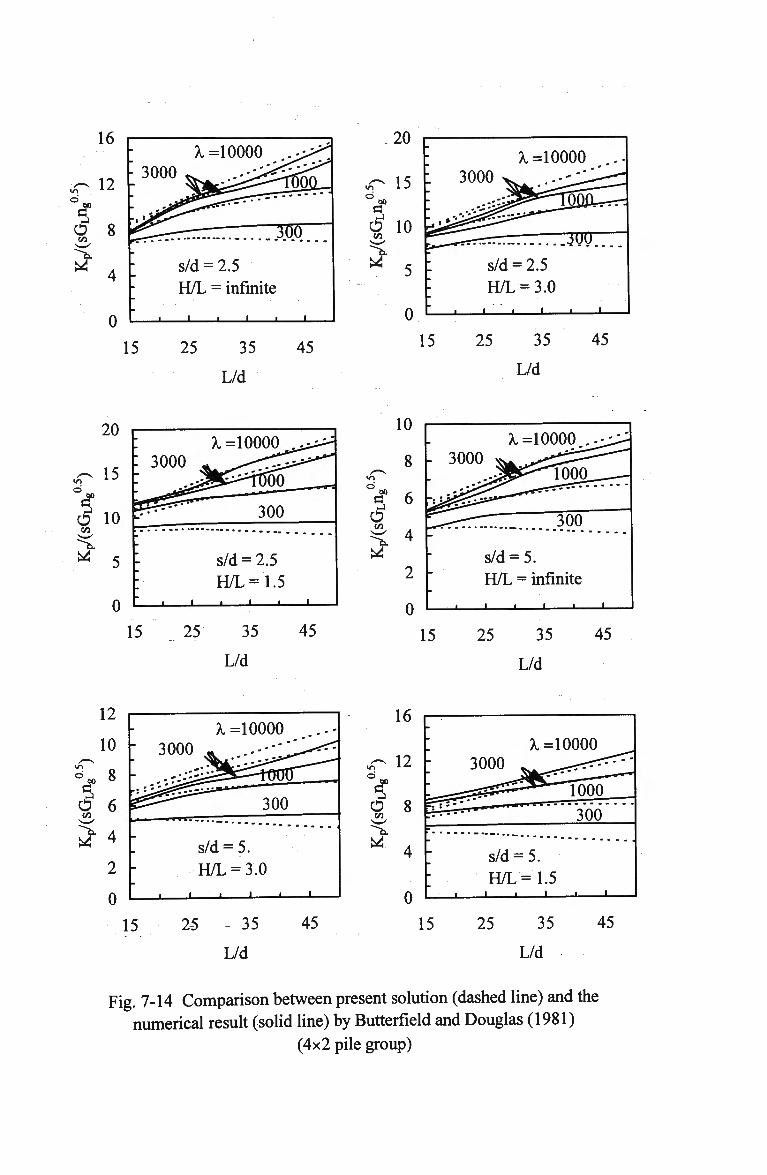
0
15
s/d = 2.5 H/L = infinite
25 35
L/d
45
20
15
O 10 on
J* 5
0
-
: 3000 >.
: s/d = H/L
• i i
A. =10000
= 2.5 = 3.0
•
m •»• * ^^^^^
SSu^ JOU
•
15 25 35
L/d
45
zo
^ 15
o io on
n
: 3000
• 1
A. = 1 0 0 0 0 ^ ^
300
s/d = 2.5 H/L=1.5
i i — i
15 25 35
L/d
45
O on
10
8
6
4
2
0
A. =10000
15
s/d = 5. H/L = infinite
• • < i _
25 35
L/d
45
1Z
10
2" 8 60 °
O 6 on
2
P.
A. =10000 ....
3000 A ..---r^^**^
-'_•'"— 7 nmw
: ^ ^ 300
s/d = 5. H/L = 3.0
i i 1 1 1 1
15 25 35
L/d
45
4
0
15
s/d = 5.
H/L =1.5
25 35
L/d
45
Fig. 7-14 Comparison between present solution (dashed line) and the numerical result (solid line) by Butterfield and Douglas (1981)
(4x2 pile group)
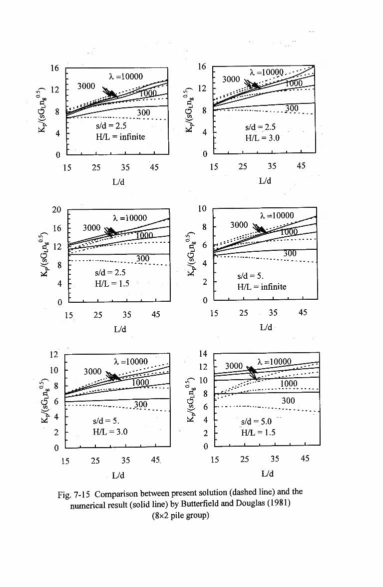
16
JT 12
O 8 on
£ 4 -0
15
: A. : 3000 v ^
- -*li*2i
s/d = : H/L =
J... 1 L.
=10000 ^
300
2.5 = infinite
i • i
25 35
L/d
45
^ 4
0
15
s/d = 2.5 H/L = 3.0
25 35
L/d
45
20
16
V 12 o
5 8 tf
0
j 3 0 0 0 ^
— i i "* IL t 1 ~~
% • •
s/d =
: H/L
1 1
A, = 1 0 0 0 0 ^ .
= 2.5 = 1.5
j i_
300
15 25 35
L/d
45
10
8 -
50 6 •3.
o on
5 2 0
A. =10000
15
s/d = 5. H/L = infinite
_ i i i 1 1
25 35
L/d
45
12
10
V O 6 Vi 2
0
15
A, =10000 ...
" • ^ ^ ^
s/d = 5. H/L = 3.0
__i 1 1 1 1 1
25 35
L/d
45
14
°co
•3.
o on
5
rt-
12 - 3000
10
8
6
4
2
0
A, =10000
15
1000
300
s/d = 5.0 H/L =1.5
25 35
L/d
45
Fig. 7-15 Comparison between present solution (dashed line) and the numerical result (solid line) by Butterfield and Douglas (1981)
(8x2 pile group)
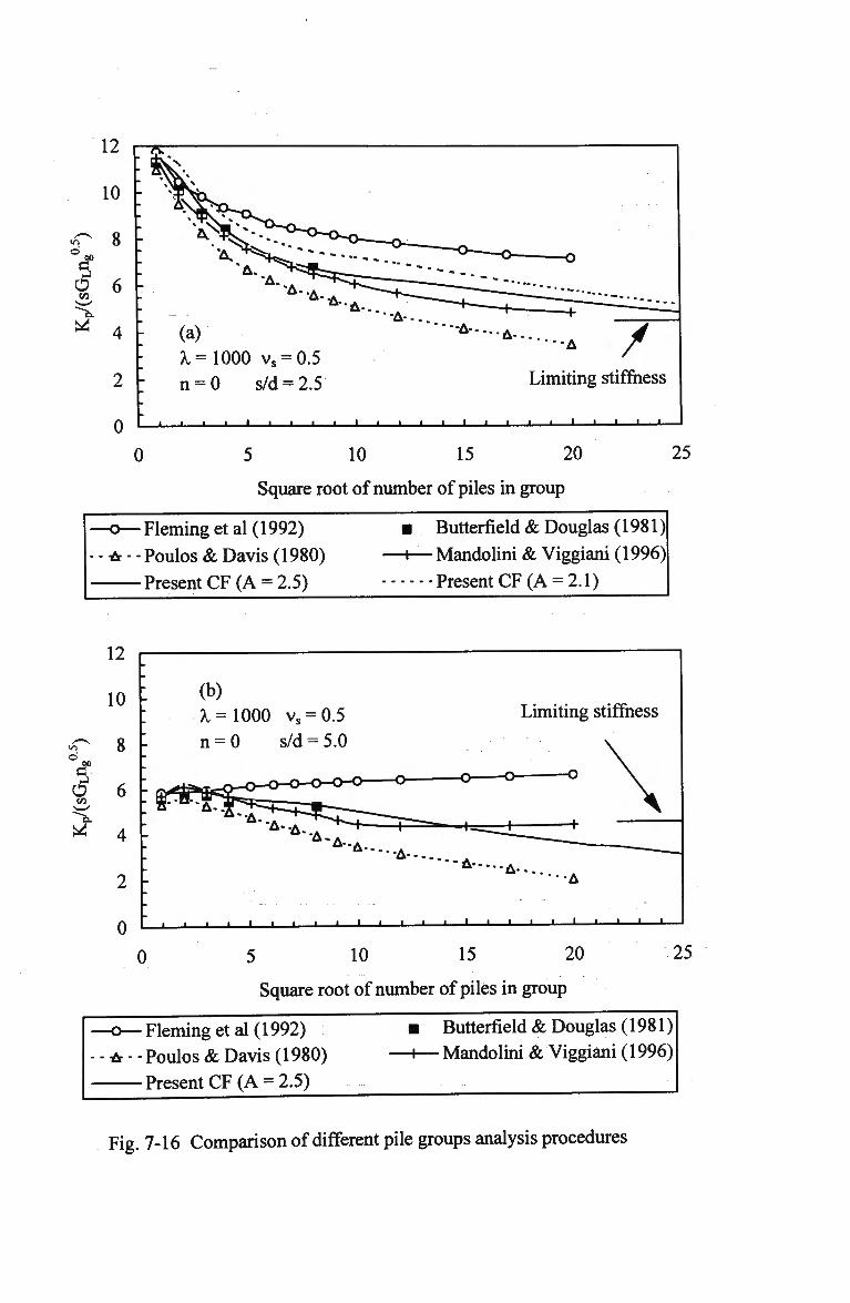
12
10
on
>
2 -
0
(a) A. = 1000 vs = 0.5
n = 0 s/d = 2.5
A-..
Limiting stiffness
• • • • ' • • • • • • i i i i i i — - J — i — i — i — • — • — i -
0 5 10 15 20
Square root of number of piles in group
25
-o—Fleming etal (1992)
A- - - Poulos & Davis (1980)
Present CF (A = 2.5)
• Butterfield & Douglas (1981)
-i—Mandolini & Viggiani (1996)
----PresentCF (A = 2.1)
12
10 -
d 6 on
tf 4
0
(b) A, = 1000 vs = 0.5
n = 0 s/d = 5.0
Limiting stiffness
A . . •A
• • I I I I 1 L. I l l I I I
0 5 10 15 20
Square root of number of piles in group
25
-o—Fleming etal (1992)
A- -- Poulos & Davis (1980) Present CF (A = 2.5)
• Butterfield & Douglas (1981)
H — Mandolini & Viggiani (1996)
Fig. 7-16 Comparison of different pile groups analysis procedures
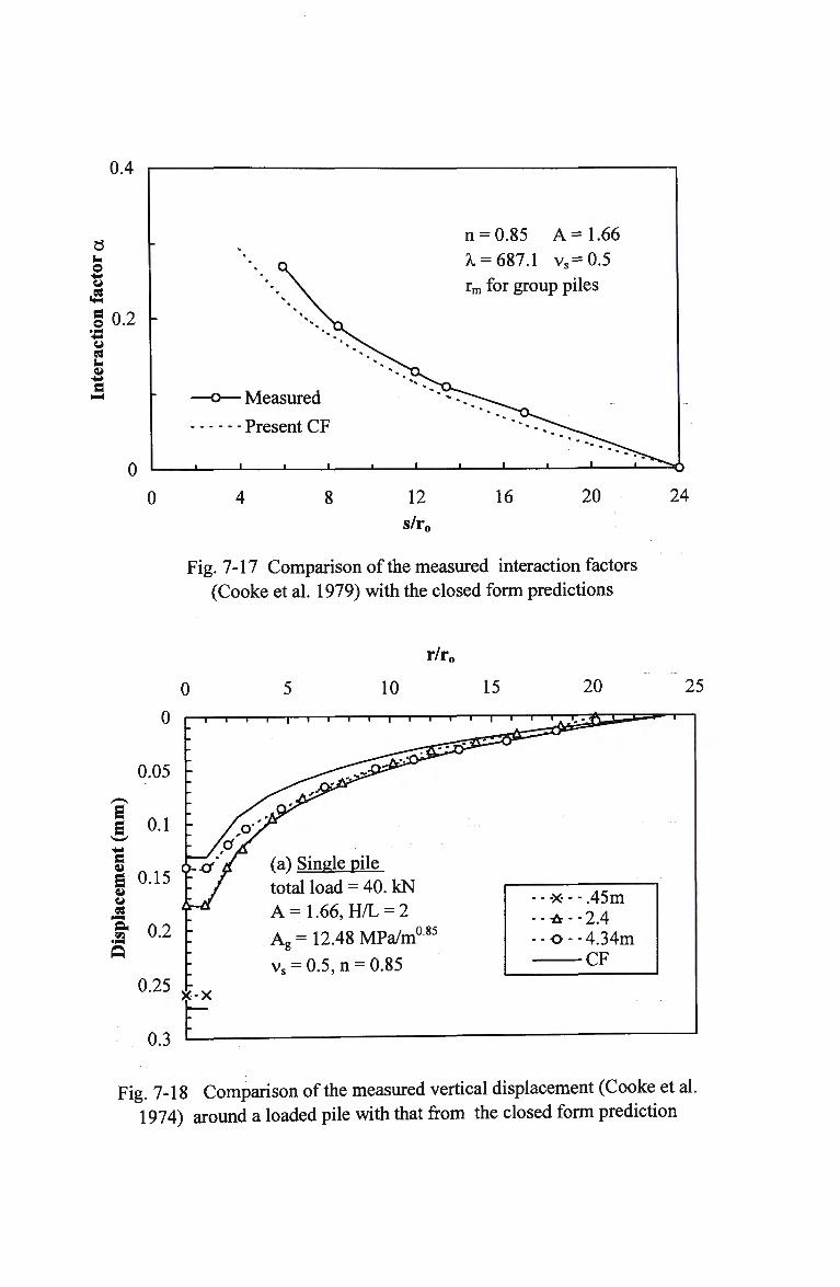
0.4
O u
S 0.2
u I-
0
0
Measured
Present CF
n = 0.85 A =1.66
A, = 687.1 vs=0.5
rm for group piles
12
s/r0
16 20
Fig. 7-17 Comparison of the measured interaction factors (Cooke et al. 1979) with the closed form predictions
24
r/r0
0 10 15 20
* 0.2 h «5
(a) Single pile total load = 40. kN A =1.66, H/L = 2
A g = 12.48 MPa/m1
vs = 0.5, n = 0.85
0.85
0.25 J;
0.3
x-x
- - x - - .45m --A---2.4 --o--4.34m
CF
25
Fig. 7-18 Comparison of the measured vertical displacement (Cooke et al. 1974) around a loaded pile with that from the closed form prediction
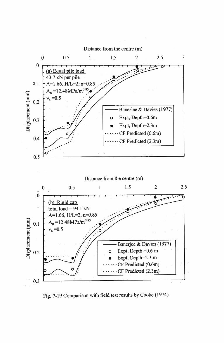
0 0.5
Distance from the centre (m)
1 1.5 2 2.5
0
0.1
0.2 -
0.3 -
0.4
0.5
— i — i — i — i — r ~ i — i — i — i — I — r — i —
! (a) Equal pile load ; 43.7 kN per pile -A=1.66,H/L=2,n=0.85 ,.-
- Ag=12.48MPa/m085
<«'^/
-vs=0.5 •' 7 /
* fi / * / * AT
1 / 1 /
* / * / '/ ' / •-/ '/
y^ o/:
o''
1 1 1 1—1 1 1—(TT 1 1 ,lr*\QI—I" ' '
LJancrjCC OC UttVlCa \Y J 1 1)
o Expt, Depth=0.6m
• Expt, Depth=2.3m
CF Predicted (0.6m)
CF Predicted (2.3m)
0
0
Distance from the centre (m)
0.5 1 1.5
0.1 . Ag=12.48MPa/m'
vs=0.5
0.2
0.3
- i — i — i — i — i — i — i — i — i — i — i — i — i — i — i — i — i — " — i g ~
fb) Rigid cap ..^^o total load = 94.1 k N A=1.66,H/L=2,n=0.85
0.85
2.5
^ ^ a
Banerjee & Davies (1977)
o Expt, Depth =0.6 m
• Expt, Depth=2.3 m
CF Predicted (0.6m) CF Predicted (2.3m)
Fig. 7-19 Comparison with field test results by Cooke (1974)
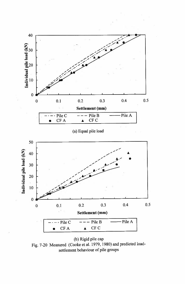
0 0.1 0.2 0.3
Settlement (mm)
- - - Pile C • CFA
Pile B A CFC
(a) Equal pile load
0.4 0.5
Pile A
0 0.1 0.2 0.3
Settlement (mm)
- - - Pile C
• CFA
Pile B A CFC
0.4 0.5
Pile A
(b) Rigid pile cap Fig. 7-20 Measured (Cooke et al. 1979,1980) and predicted load-
settlement behaviour of pile groups
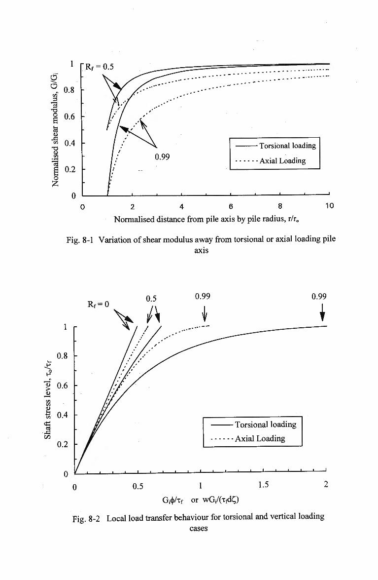
o o on
I S3
.3 on
-a u on
la o
1
0.8
0.6
0.4
0.2
0
Rf = 0.5
Torsional loading
Axial Loading
2 4 6 8
Normalised distance from pile axis by pile radius, r/r0
10
Fig. 8-1 Variation of shear modulus away from torsional or axial loading pile
axis
0.99 R f = 0
1 r
0.8
o
g 0.6
on
£ 0.4
% tt
0.2
0
0
Torsional loading
Axial Loading
i — i — i i — i -
0.5 1 1.5
Gi^/tf or wGj/(TfdQ
0.99
Fig. 8-2 Local load transfer behaviour for torsional and vertical loading
cases
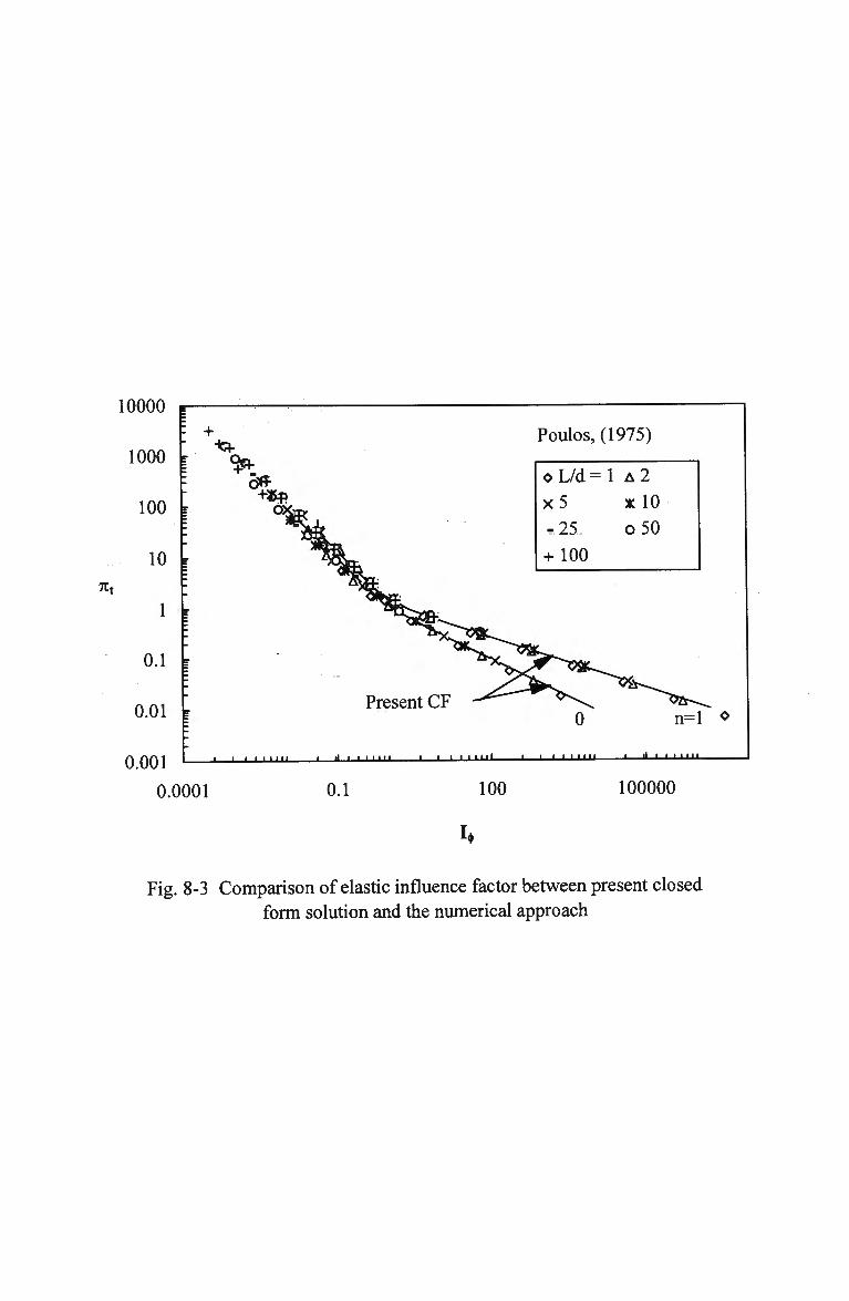
10000
1000
100
10
7lt
0.1 !
0.01
0.001
e z
r
"
r
B
r
+
c» OXm^
I • 1 1 1 1 1 1 1 1
Present CF -*^
•< •• • i i 1 1 1 u i i
Poulos,
oL/d =
x5 -25 + 100
0
1 1 1 1 Ull
(1975)
= 1 A2 xlO o50
n=l o
• ii 11 IJJJJ
0.0001 0.1 100 100000
Fig. 8-3 Comparison of elastic influence factor between present closed form solution and the numerical approach
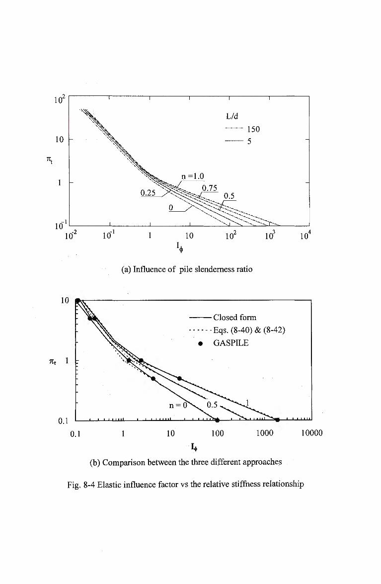
(a) Influence of pile slenderness ratio
10
7tt 1 :
0.1
^ V ^ A .
\
:
• l l l i i ill l J _ l _
n:
• i • ui
= 0 •
l -lOSCU IOH11
C n c SQ AC\\ fr (Q A0\ nqs. yo-^yj) a. yo-Hz.)
• GASPILE
i i 1 7 V ^ i I*-... • i 11 • ! " • * > < • i i i i 111
0.1 10 100 1000 10000
(b) Comparison between the three different approaches
Fig. 8-4 Elastic influence factor vs the relative stiffness relationship
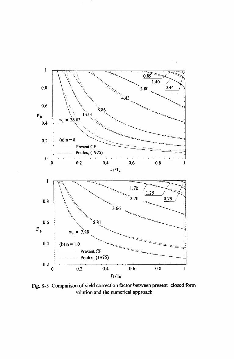
0.8
0.6
F* 0.4
0.2 (a) n = 0
Present CF Poulos, (1975)
0.2 0.4 0.6 Tt/Tu
0.8
0.8
0.6
0.4
0.2
7ct = 7.89
: (b)n=1.0
Present CF
Poulos, (1975)
0 0.2 0.4 0.6 0.8
Tt/Tu
Fig. 8-5 Comparison of yield correction factor between present closed form
solution and the numerical approach
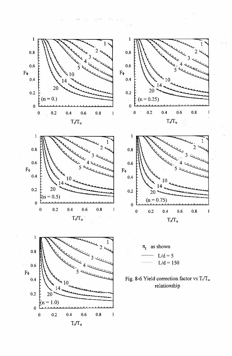
0.8 -
F*
0 0.2 0.4 0.6 0.8
Tt/Tu
0.6
0.4
0.2
0 • i •
0 0.2 0.4 0.6 0.8 1
Tt/Tu
0.8
0.6
F* 0.4 -
0.2 -
0 0.2 0.4 0.6 0.8 1
Tt/Tu
7^ as shown
L/d = 5
L/d = 1 5 0
Fig. 8-6 Yield correction factor vs Tt/Tu relationship
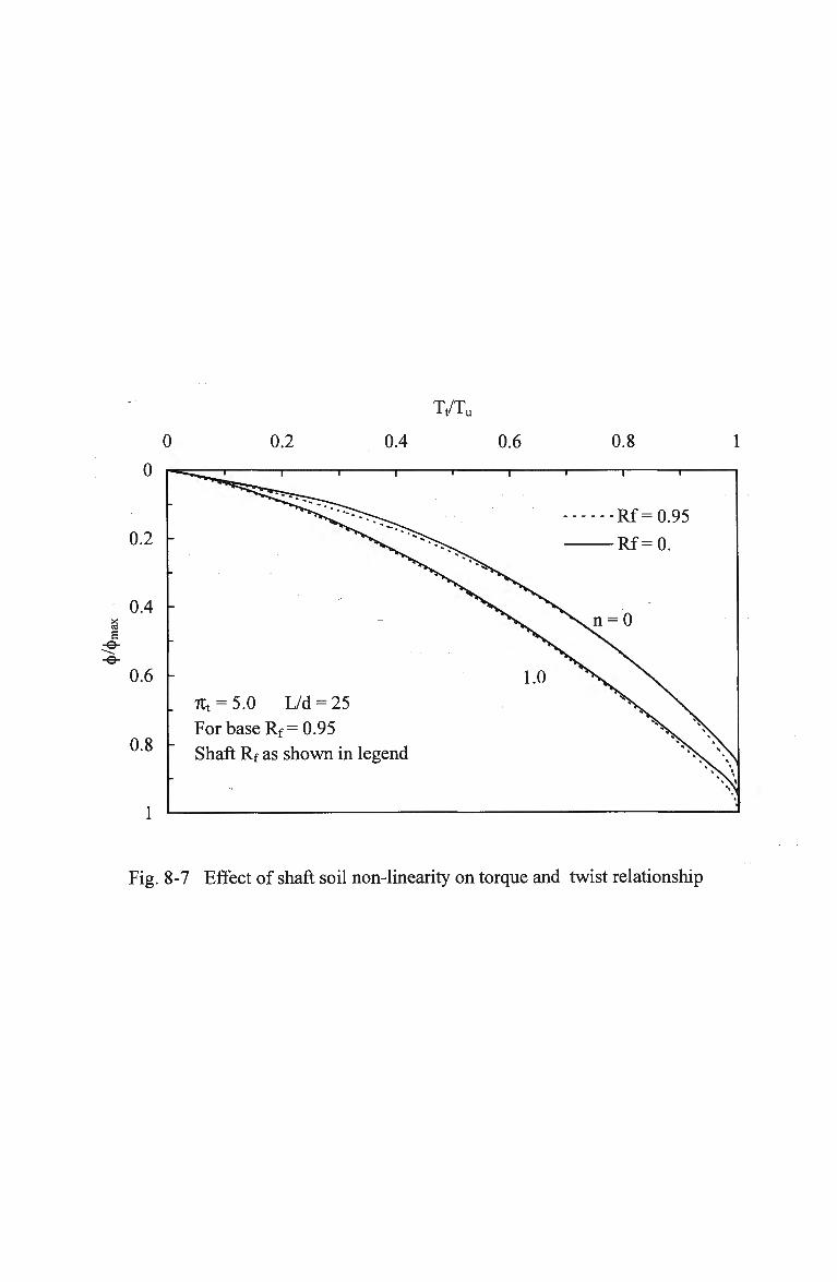
Tt/Tu
0 0.2 0.4 0.6 0.8 1
Fig. 8-7 Effect of shaft soil non-linearity on torque and twist relationship
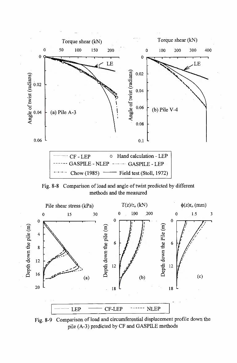
Torque shear (kN) Torque shear (kN)
0 100 200 300 400
0.06
CF - LEP o Hand calculation - LEP
GASPILE-NLEP GASPILE-LEP
Chow (1985) Field test (Stoll, 1972)
Fig. 8-8 Comparison of load and angle of twist predicted by different methods and the measured
Pile shear stress (kPa)
0 15 30
T(z)/r0(kN)
0 100 200
<|>(z)r0 (mm)
0 1.5 3
B
• i — <
P H
<U
a o
•B OH
Q
6 -
12
18 L
LEP CF-LEP NLEP
Fig. 8-9 Comparison of load and circumferential displacement profile down the pile (A-3) predicted by CF and GASPILE methods
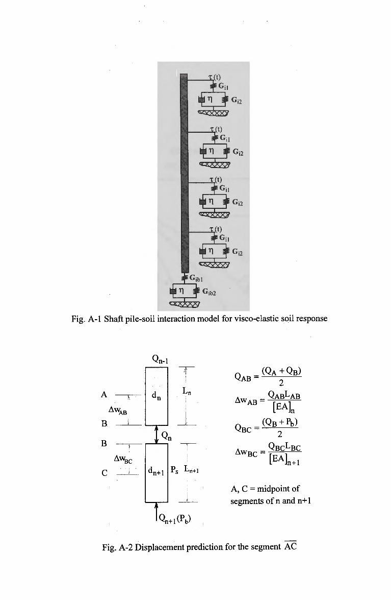
Qn-
B
B
K
AwAB
i
d„ n
i
\ >
AWBC
dn+l
/
I
n
Ps 1
\
-Tl
t j i
-n+1
i
Qn+l(Pb>
QAB =
AwAB
QBC =
Aw B C =
(QA+QB)
2 QABLAB
' [EAln (QB + Pb)
2
QBCLBC
[EA]n + 1
A, C = midpoint of
segments of n and n+1
Fig. A-2 Displacement prediction for the segment AC
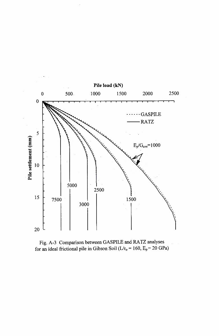
Pile load (kN)
0 500 1000 1500 2000 2500
Fig. A-3 Comparison between GASPILE and R A T Z analyses for an ideal frictional pile in Gibson Soil (L/r0 = 160, Ep= 20 GPa)
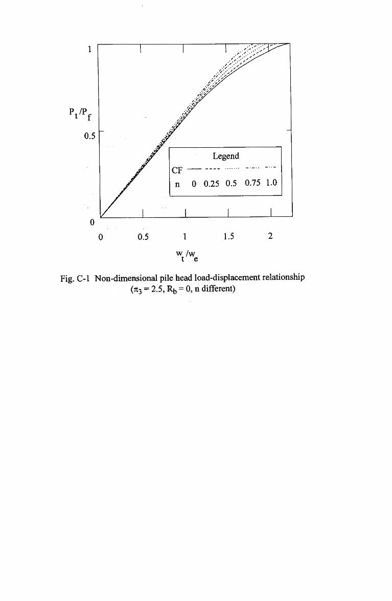
p /p
0.5
0
0
Legend
n 0 0.25 0.5 0.75 1.0
0.5 1.5
w / w t e
Fig. C-l Non-dimensional pile head load-displacement relationship (TI3 = 2.5, Rb = 0, n different)
0 10 20 30 40 50 60
7l3
Legend CF -n 0 0.25 0.5 0.75 1.0
Fig. C-2 Non-dimensional load ratio Pt /Pf versus 7r3 relationship (£ = 1, Rb = 0)
nn
0.2
0
Legend CF n 0 0.5 1.0
• • I L ' I I I I 1 1 1 U
0
Fig. C-3 nmax versus TI3 relationship
(£, as shown and Rb = 0)
7
6
5
o U s 3
2
1
0
n = 0
A normal radius
r0= 10 cm, and
G/su = 250
_i i i
-2 ln(Cvt/r„2)
Fig. E-l Influence of radial non-homogeneity on dissipation of
excess pore pressure (elastic analysis)
Related Documents


