Analytic wave model of Stark deceleration dynamics

Analytic wave model of Stark deceleration dynamics

Koos Gubbels, Gerard Meijer, and Bretislav FriedrichFritz-Haber-Institut der Max-Planck-Gesellschaft, Faradayweg 4-6, D-14195 Berlin, Germany

�Received 2 February 2006; published 12 June 2006�

Stark deceleration relies on time-dependent inhomogeneous electric fields which repetitively exert a decel-erating force on polar molecules. Fourier analysis reveals that such fields, generated by an array of field stages,consist of a superposition of partial waves with well-defined phase velocities. Molecules whose velocities comeclose to the phase velocity of a given wave get a ride from that wave. For a square-wave temporal dependenceof the Stark field, the phase velocities of the waves are found to be odd-fraction multiples of a fundamentalphase velocity � /�, with � and � the spatial and temporal periods of the field. Here we study explicitly thedynamics due to any of the waves as well as due to their mutual perturbations. We first solve the equations ofmotion for the case of single-wave interactions and exploit their isomorphism with those for the biasedpendulum. Next we analyze the perturbations of the single-wave dynamics by other waves and find that thesehave no net effect on the phase stability of the acceleration or deceleration process. Finally, we find that apacket of molecules can also ride a wave which results from an interference of adjacent waves. In this case,small phase stability areas form around phase velocities that are even-fraction multiples of the fundamentalvelocity. A detailed comparison with classical trajectory simulations and with experiment demonstrates that theanalytic “wave model” encompasses all the longitudinal physics encountered in a Stark decelerator.

DOI: 10.1103/PhysRevA.73.063406 PACS number�s�: 32.60.�i, 32.80.Pj, 45.50.�j

I. INTRODUCTION

Achieving an ever better control over both the internaland external degrees of freedom of gas-phase molecules hasbeen a prominent goal of molecular physics over the lastdecades. Molecular beams, both continuous and pulsed, havebeen widely used to produce large densities of molecules inselected quantum states. In these beams, the longitudinaltemperature of the molecules is typically 1 K, and the meanvelocity of the beam can be varied between about 300 and3000 m/s by adjusting the temperature of the source or byusing different carrier gases. Control over the spatial orien-tation or alignment of molecules in a beam has beenachieved by actively manipulating the rotation of the mol-ecules using electrostatic or magnetic multipole fields as wellas with the help of laser radiation. The application of inho-mogeneous fields has enabled control over the transversemotion of the oriented or aligned molecules, and thus theirstate selection �1–3�.

The control over the longitudinal motion of molecules ina molecular beam has been greatly enhanced as well. In1999, it was first demonstrated that an array of time-varying,inhomogeneous electric fields can slow down a beam of po-lar molecules �4�. This so-called Stark decelerator for neutralpolar molecules is the equivalent of a linear accelerator�LINAC� for charged particles. In a Stark decelerator, thequantum-state specific force that acts on a polar moleculesubject to an electric field is exploited. This force is ratherweak, typically some eight to ten orders of magnitudeweaker than the force that would act on the molecular ion inthe same electric field. This force nevertheless suffices toprovide complete control over the motion of polar molecules,using techniques akin to those used for the control of chargedparticles. This has been explicitly demonstrated by the con-struction of two different types of linear decelerators �4,5�, abuncher �6�, a mirror �7�, two different types of traps �8,9�

and a storage ring �10� for neutral polar molecules.A crucial feature of the Stark decelerator is its phase sta-

bility. Phase stability, which is at the core of synchrotron-likecharged-particle accelerators as well �11�, enables to holdtogether a packet of neutral molecules throughout the Stark-deceleration process. Phase-stable operation of a Stark decel-erator, viewed as trapping of neutral molecules in a travelingpotential well, was first explicitly demonstrated in experi-ments on metastable CO �12�. In that work, as well as in laterpublications on the deceleration of various isotopomers ofammonia, the one-dimensional �1D� equation of motion formolecules that undergo phase-stable transport was stated�12–14�. In order to obtain the longitudinal equation of mo-tion, the Stark energy �potential energy� of the moleculeswas expressed as a function of position along the longitudi-nal decelerator axis, and the change in Stark energy per de-celeration stage was evaluated. As this treatment did notyield a priori an expression for the force on the molecules asa function of time, assumptions about the time dependenceof the force were made in order to arrive, in an intuitive way,at the equation of motion. The validity of these assumptionswas checked against trajectory calculations, and it had beenconcluded that this equation of motion indeed describes cor-rectly the physics of the phase-stable motion in a Stark de-celerator �12–14�. Nevertheless, a mathematically rigorousderivation of the equation of motion and an in-depth analysisof the complex dynamics in a Stark decelerator was stillwanting.

A description of the �longitudinal� force acting on themolecules as a function of both their position in the decel-erator and as a function of time could be obtained by ex-pressing the spatial and temporal dependence of the electricfields in the decelerator in terms of a Fourier series �15�. Thisdescription, in which the force has been expressed as aninfinite sum of stationary and counter-propagating waves,contained all the correct physics, but it was not directly evi-dent how to connect this description to the trajectory calcu-

PHYSICAL REVIEW A 73, 063406 �2006�

1050-2947/2006/73�6�/063406�20� ©2006 The American Physical Society063406-1

http://dx.doi.org/10.1103/PhysRevA.73.063406

lations or to the actual experiments. In particular, it was notclear why, in discussing phase stability, it is allowed to onlyconsider the interaction of the molecules with one of theinfinitely many waves. It was not clear either where the ex-perimentally observed first- and second-order resonances inthe decelerator—which have a straightforward interpretationin the intuitive model �16�—come from the Fourier-seriesdescription.

In this paper, we give a detailed description of the longi-tudinal motion of molecules in a Stark decelerator �or accel-erator�. This description is based on the Fourier analysis ofthe force that acts on the molecules as a function of positionand time �15�. The motion of the molecules in phasespace due to any of the interacting waves, as well as due totheir mutual perturbations, is analyzed. A detailed compari-son with trajectory calculations and experiment has shownthat the “wave model” presented here holds up to all thescrutiny applied, and provides a complete and accurate de-scription of the longitudinal dynamics of polar molecules ina Stark decelerator.

Thus our treatment here is restricted to the motion alongthe molecular beam axis. In more recent work, the couplingbetween the transverse and the longitudinal motion was in-cluded, and the transverse stability in a Stark decelerator wasdiscussed as well �17�.

II. FOURIER REPRESENTATION OF THE ELECTRICFIELD IN A STARK ACCELERATOR OR DECELERATOR

Figure 1 shows a prototypical switchable field array suit-able for accelerating or decelerating polar molecules. Theelectric fields are generated by field stages �rod-electrodepairs, cylindrical electrodes, or other� longitudinally sepa-rated by a distance � /2. In the array, every other field stageis energized and every other grounded. Which field stagesare energized and which are grounded determines one of twopossible field configurations of the array. Figure 1�a� shows,for the case of four field stages, the electric fields that aregenerated by the two field configurations. The magnitudes ofthe electric fields that pertain to the upper and lower fieldconfiguration are shown by the red and blue curves and willbe referred to as the red, �r, and blue, �b, field, respectively.Also shown is the longitudinal coordinate z. A given fieldstage is energized or grounded during a time � /2, after whichthe fields are switched, i.e., the field stages that were ener-gized become grounded and the field stages that weregrounded become energized. Figure 1�b� shows the alterna-tion between the red and blue fields as a function of time, t.An energized field stage becomes grounded or vice versaduring a transient time, ��. For ��, the temporal alterna-tion between the red and blue fields is square-wave like.

We will now represent the spatial and temporal depen-dence of the net field, which results from the switching be-tween the static red and blue fields, by a Fourier series.

We will begin by Fourier expanding the spatial depen-dence of the red field, which is produced by field stages atpositions z= � 1

4 +m��, with m=0,1 ,2 ,3. . ., see Fig. 1�a�. Thestrength of the red field is given by

�r�z� =1

2�0 + �

m=1

�

�m cos�m� , �1�

where �m are the spatial Fourier coefficients and

� 2z/� − /2. �2�

The blue field is produced by field stages at positionsz= � 3

4 +m��, see Fig. 1�a�, and so is obtained from the redfield by shifting it by � /2, i.e.

�b�z� = �r�z −�

2� =

1

2�0 + �

m=1

�

�− 1�m�m cos�m� . �3�

Taking ��=0, the net field, ��z , t�, is given by

FIG. 1. �Color online� A prototypical switchable field array thatgenerates fields suited for accelerating or decelerating polar mol-ecules. The field stages are longitudinally separated by a distance� /2. Every other field stage is energized and every other grounded.There are two possible field configurations. �a� Electric fields gen-erated by the two field configurations �for the case of four fieldstages�. The electric fields that pertain to the upper and lower fieldconfigurations are shown by the red and blue curves and are re-ferred to here as the red, �r, and blue, �b, fields, respectively. Alsoshown is the longitudinal coordinate z; �b� Alternation between thered and blue fields as a function of time, t. A given field stage isenergized or grounded during a time � /2, after which the fields areswitched, i.e., the field stages that were energized become groundedand vice versa. An energized field stage becomes grounded or viceversa during a transient time, ��. The figure pertains to the case ofguiding, for which the period � is constant. The case of a varyingperiod is shown in Fig. 2.

GUBBELS, MEIJER, AND FRIEDRICH PHYSICAL REVIEW A 73, 063406 �2006�

063406-2

��z,t� = �b�z� for 0 � t � �/2,

��z,t� = �r�z� for �/2 � t � � , �4�

see Fig. 1�b�.In order to derive the Fourier representation of the net

field, we will expand Eq. �4� in terms of a temporal Fourierseries. By invoking the “well-known” result for a temporalsquare wave �18�, the net field can be written as

��z,t� =1

2��b�z� + �r�z�� +

1

2��b�z� − �r�z��

� �� odd

�4

�sin�� , �5�

where is the temporal phase such that

�t� = ��t� =2

��t��6�

with � the angular frequency. While Fig. 1�b� shows a timedependence of the field with a constant period � �which cor-responds to the so-called guiding, see below�, Fig. 2 shows atime sequence with a varying period �=��t� �one which cor-responds to deceleration�. In either case, the square waverises and falls when the temporal phase becomes equal to aninteger multiple of .

Substitution into Eq. �5� from Eqs. �1�–�3� yields

��z,t� =1

2�0 + �

p even

�

�− 1�1/2p�p cos�pkz�

+ �n odd

�

�� odd

�4

��− 1�1/2�n+1��n sin�nkz�sin��

=1

2�0 + �

p even

�

�− 1�1/2p�p cos�pkz�

+ �n odd

�

�� odd

�2

n��− 1�1/2�n+1�

��n�cos �+,n,� − cos �−,n,�� , �7�

where we made use of the identity sin � sin �= 12 �cos��

−��−cos��+��, defined the spatial frequency �wave vec-tor�

k � 2/� �8�

and introduced the phase

�±,n,� � nkz � � . �9�

Note that p ,n ,� are all positive integers.Equation �7� reveals that the net field consists of a super-

position of stationary and of pair-wise counter-propagatingpartial waves. The propagating waves move with well-defined phase velocities

V±,n,� � −��±,n,�/�t�z

��±,n,�/�z�t= ±

�

n

�t�k

= ±�

n

��t�k

= ±�

n

�

��t�

� ±�

nV�t� �10�

from left to right �� sign� and from right to left �� sign�.The second line of Eq. �10� defines the fundamental phasevelocity, V�t�, which is determined solely by the spatial andtemporal periods � and ��t�.

The path taken here in deriving Eq. �7� is a shortcut of theroute used to derive the same equation in our previous work�15�. The time dependence of the temporal period or fre-quency is here emphasized right from the outset.

Note that the spatial Fourier coefficients �m along with thesquare-wave time dependence fully characterize the net field.While the temporal Fourier coefficients fall only as �−1, thespatial ones fall off roughly exponentially with m, i.e.

�m � exp�− �m� , �11�

where � is a decay parameter which depends on the geometryof the field array. Hence we can expect waves with small nand larger � to dominate; as we will see in Sec. V, waveswith n�5 and ��21 account for all the dynamics observedso far.

III. POTENTIAL AND FORCE

A molecule with a space-fixed electric dipole moment�= �� subject to field �7� has a Stark energy

FIG. 2. The time dependence of the field pertaining to the caseof deceleration, for which the period � is a function of time,�=��t�. The case of a constant period is shown in Fig. 1. The timingsequence, generated by Eq. �33�, is suitable for decelerating OHradicals on the �+,1 ,1� wave with �s=53° from an initial velocityof 370 m/s to a final velocity of 25 m/s in the decelerator pre-sented in Refs. �17,16�. The upper panel shows the correspondingdependence of the switching half period, ��t� /2. The points markthe time difference between two subsequent switching times. SeeSec. IV C.

ANALYTIC WAVE MODEL OF STARK DECELERATION¼ PHYSICAL REVIEW A 73, 063406 �2006�

063406-3

W�z,t� = − ��z,t� . �12�

In what follows, we will consider molecular states whosespace-fixed electric dipole moment is independent of theelectric field strength; this is the case when the field-molecule interaction is governed by the first-order Stark ef-fect. Molecular states whose space-fixed electric dipole mo-ment � is parallel ��0� or antiparallel ��0� to theelectric field strength are referred to as high or low-field seek-ing states, respectively. Whereas the eigenenergy of high-field seekers decreases with increasing field strength, it in-creases for the low-field seekers. As a result, in aninhomogeneous electric field, such as ��z , t�, high-field seek-ers seek regions of maximum, and low-field seekers seekregions of minimum field strength where their eigenenergy isminimal. In the net field �7�, the Stark energy becomes

W�z,t� =1

2W0 + �

p even

�

�− 1�1/2pWp cos�pkz�

+ �n odd

�

�� odd

�2

��− 1�1/2�n+1�Wn�cos �+,n,�

− cos �−,n,�� 13�

with

Wi = − ��i i = 1,2,3, . . . �14�

We note that in the case of nonlinear Stark effect �19�, Eq.�13� can still be used to represent the Stark energy, althoughEq. �14� is no longer valid. In order to obtain the correctFourier coefficients Wi, we need to first numerically calculatethe Stark energy of a molecule in the two electric-field con-figurations �r�z� and �b�z�. Subsequently, we can Fourier ex-pand the Stark energy, just as we expanded the electric field,and extract the Wi coefficients, which leaves Eq. �13� intact�20�.

Since the Stark energy plays the role of a potential for themotion of the molecules, the force, F�z , t�, that the field ex-erts on a molecule of mass M is given by

F�z,t� = −dW�z,t�

dz= �

p evenMAp sin�pkz�

+ �n odd

�� odd

MAn,��sin �+,n,� − sin �−,n,�� , �15�

where

Ap � �− 1�1/2p pk

MWp,

An,� � �− 1�1/2�n+1� 2nk

�MWn. �16�

Thus we see that a molecule subject to force �15� is actedupon by an infinite multitude of stationary as well as propa-gating and counter-propagating waves. However, as we willsee in Sec. IV, only a single wave governs the molecule-fieldinteraction. Which wave it is is determined by the differencebetween the wave’s phase velocity and the velocity of the

molecule: only a wave whose initial phase velocity comesclose to the initial velocity of the molecule can become para-mount. In order to find out how close this needs to be, wemust do the dynamics.

IV. DYNAMICS OF THE INTERACTION OF MOLECULESWITH A SINGLE WAVE

In this section we will examine the dynamics of the inter-action of a bunch of molecules with a single wave. Afterdeveloping a formalism for describing such an interactionand discussing its dynamics, we will be able to show why, toan excellent approximation, the effect of all the other wavescan be neglected. In Sec. V we will consider the full-fledgeddynamics and evaluate explicitly the perturbing effects dueto other waves. We will also tackle the �marginal� effects dueto interfering waves which interact jointly with a bunch ofmolecules.

A. Force exerted by an arbitrary wave

As we can glean from Eqs. �7�, �13�, and �15�, an arbitrarypropagating wave can be labeled by a pair of odd integers, nand �, and by its propagation direction �� for left to right or� for right to left�, i.e., by �±,n ,��. Since the moleculesmove from left to right by convention, in what follows wewill consider waves moving from left to right. Thus such anotherwise arbitrary wave travels from left to right with aphase velocity

Vn,� � V+,n,� =�

n

k, �17�

cf. Eq. �10�, and exerts a force on a molecule given by

Fn,��z,t� = MAn,� sin �n,� �18�

with the phase

�n,� � �+,n,� = nkz − � . �19�

The corresponding acceleration then becomes

an,� � zn,� =Fn,��z,t�

M= An,� sin �n,�. �20�

B. Synchronous molecule and its velocity

A key concept in tackling the molecule-wave interactionis that of a synchronous molecule. This is defined as themolecule which maintains a constant (synchronous) phase

�s � ��n,��s = nkzs − � = const. �21�

with respect to a given wave �n ,�� throughout the accelera-tion or deceleration process—no matter what, see Fig. 3.

It should be noted that the definition of the synchronousphase given here is slightly different from the definition thathas been used in earlier descriptions of phase stability in aStark decelerator �12–14,16�. In these earlier studies the syn-chronous phase was defined in terms of the position of thesynchronous molecule relative to the electrodes, and this po-


063406-4

sition was required to be the same every time the electricfields were switched from one configuration to the other.Although this definition takes the full spatial dependence ofthe Stark interaction into account, it only specifies the syn-chronous phase at the moment when the fields are switched.In the case when the spatial and temporal dependence of theStark interaction is governed by a single wave �n ,��, thedefinitions are equivalent.

From Eq. �18� it immediately follows that the synchro-nous molecule is acted upon by a constant force

�Fn,��s = MAn,� sin �s �22�

and thus has a constant acceleration

�an,��s = An,� sin �s � as. �23�

From Eq. �23� we see that the acceleration/deceleration ratecan be controlled by tuning the synchronous phase. As fol-lows from Eq. �21�, at t=0, when the fields are switched forthe first time, the synchronous phase is simply

�s�zs,t = 0� = nkzs. �24�

Therefore, the synchronous phase can be tuned by launchingthe switching sequence �or burst� when the synchronousmolecule has the desirable longitudinal coordinate zs. Thesubsequent switching times between the two field configura-tions can always be chosen such that the synchronous mol-ecule will keep the same phase.

With a tunable acceleration or deceleration, the initial ve-locity of the synchronous molecule can be increased or de-creased to any value

vs�t� = vs�t = 0� + ast . �25�

C. Phase velocity, temporal phase, and switchingsequence

In order to keep the phase of the synchronous moleculeconstant during acceleration or deceleration, the phase veloc-

ity of the wave that interacts with the molecule needs to bevaried. This is done by applying a variable switching se-quence to the field array as the molecule progresses throughit. In other words, the temporal frequency or period of theapplied field is made time dependent, �=��t� or �=��t�. Asa result, the phase velocity becomes also time dependent, cf.Eq. �10�. In this paragraph we will show that the phase ve-locity of the wave is always equal to the synchronous veloc-ity of the molecule, as one would expect. Furthermore, wewill evaluate the temporal phase and hence the timing se-quence needed to keep a molecule synchronous.

From the definition of the synchronous phase, Eq. �21�,we obtain

�s = 0 = nkzs − � �26�

from which it follows that

zs � vs =�

n

k. �27�

By comparing this result with Eq. �17�, we see that, indeed,the phase velocity is equal to the synchronous velocity

vs = Vn,�. �28�

In what follows we will use the following notation for theinitial phase and synchronous velocities

vs�0� = Vn,��0� =�

n

��t = 0�k

=�

n

�

��t = 0��

�

nV0. �29�

In order to derive an expression for the temporal phaseconsistent with the condition of a constant synchronousphase, we invoke Eq. �21�

=nkzs

�−

�s

��30�

and substitute for zs from the first integral of Eq. �25�

zs =1

2ast

2 + vs�0�t + z0 =1

2ast

2 +�

nV0t +

�s

nk, �31�

where the initial position, z0, was obtained from Eq. �24�.This yields a temporal phase

=nkzs

�−

�s

�=

1

2

n

�kast

2 + kV0t , �32�

which pertains to a square wave that falls or rises only whenthe following periodic condition is fulfilled:

�t� =1

2

n

�kast

2 + kV0t = q q = 0,1,2, . . . �33�

Equation �33� defines exactly that switching sequence whichis required in order to keep the phase of the synchronousmolecule constant and hence for achieving a constant accel-eration or deceleration. The corresponding switching timesare given by solving Eq. �33� for t�q�, with the result

FIG. 3. �Color online� A synchronous and a nonsynchronousmolecule subjected to the field ��z , t� of a�+,n ,�� wave moving at a phase velocity Vn,� �all motion is fromleft to right�. The change of the velocity, vs, of a synchronous mol-ecule is such that its phase �s with respect to the traveling fieldremains constant. This is the case when vs=Vn,�. The velocity, v, ofa nonsynchronous molecule and its phase, �, change with time.Also shown are the spatial coordinates of the synchronous and non-synchronous molecule, zs and z, respectively.


063406-5

t�q� =�

n

V0

as��2qnas

k�V02 + 1�1/2

− 1� , �34�

which is identical with a result obtained earlier �21�. We notethat since we determine �t�, via Eq. �33�, before computing��t� or ��t�, a need to evaluate the integration constant of Eq.�6� never arises.

Figure 2 shows a switching sequence, generated by Eq.�33�, which is suitable for decelerating OH radicals.

D. Equation of motion

The equation of motion of a nonsynchronous moleculesubjected to wave �n ,�� is

z =Fn,�

M= An,� sin �n,�, �35�

where we made use of Eq. �18�. For the synchronous mol-ecule we have

zs =Fn,�

M= An,� sin �s. �36�

A combination of Eqs. �35� and �36� yields

z − zs = An,��sin �n,� − sin �s� . �37�

The left-hand side of Eq. �37� can be recast in terms of thenonsynchronous and synchronous phase. We have, with thehelp of Eq. �19�

�n,��t� − �s�t� � ��n,��t� = nkz�t� − � �t� − �nkzs�t� − � �t��

= nk�z�t� − zs�t�� nk�z�t� , �38�

where �z�z−zs is the longitudinal distance between thenonsynchronous and synchronous molecule, see also Fig. 3.Equation �38� implies the following equations for the timederivatives:

�n,��t� − �s�t� � ��n,��t� = nk�z − zs� � nk�z �39�

and

�n,��t� − �s�t� � ��n,��t� = nk�z − zs� � nk�z . �40�

However,

��n,��t� = �n,��t� �41�

and

��n,��t� = �n,��t� �42�

since, by definition, �s�t�= �s�t�=0.Substituting Eqs. �40� and �42� into Eq. �37� finally yields

�n,� = �n,��sin �n,� − sin �s� �43�

with

�n,� � nkAn,� = �− 1�1/2�n+1�2n2k2

�MWn. �44�

E. Solving the equation of motion

Relating the motion of all molecules to a molecule whichmaintains a constant �synchronous� phase with respect to agiven wave not only greatly simplifies the equation of mo-tion but reduces it to a form which is isomorphic with theequation of motion of a biased pendulum, see Fig. 4. Sincethe biased pendulum problem can be well understood—bothmathematically and intuitively—it offers invaluable lessonsabout the Stark accelerator/decelerator dynamics �15�.

Both the biased-pendulum problem and the Starkaccelerator/decelerator have the following Lagrangian:

L��,�� =1

2��2 − ��n,��cos � + � sin �s� , �45�

where � and �n,� are constants different for the two prob-lems. The application of Lagrange’s equation

�L��

=d

dt

�L

��46�

immediately yields the correct equation of motion, namelyEq. �43�.

The first term of the Lagrangian �45� is the kinetic energy,the second term is the potential

V�� = ��n,��cos � + � sin �s�

= �− 1�1/2�n+1�2Wn

��cos � + � sin �s�

� VP�� + VB�� . �47�

In writing down the potential we split it into the pendulumpart, VP��, and the bias part, VB��. These are plotted for

FIG. 4. �Color online� Realizations of a plane biased pendulum:a bob of mass m is fixed to a rigid suspension of length r which isattached to an axle of diameter R; wound around the axle is a stringthat carries a bias of mass M. A plane biased pendulum is a one-dimensional system, whose only coordinate is the angle � betweenthe vertical axis z and the bob suspension r. The stable and unstableequilibrium points are located symmetrically with respect to a planeperpendicular to the direction of the z axis at angles �s and −�s,respectively. The stable-equilibrium angle �s of the biased pendu-lum corresponds to the synchronous phase of the Starkaccelerator/decelerator.


063406-6

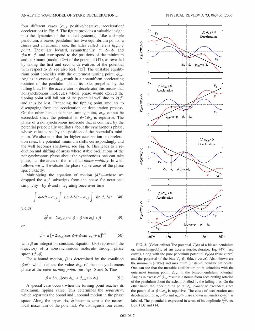
four different cases ��n,� positive/negative, acceleration/deceleration� in Fig. 5. The figure provides a valuable insightinto the dynamics of the studied system�s�. Like a simplependulum, a biased pendulum has two equilibrium points, astable and an unstable one, the latter called here a tippingpoint. These are located, symmetrically, at �=�s and�=−�s and correspond to the positions of the minimumand maximum �modulo 2� of the potential �47�, as revealedby taking the first and second derivatives of the potentialwith respect to �, see also Ref. �15�. The unstable equilib-rium point coincides with the outermost turning point, �out.Angles in excess of �out result in a nonuniform acceleratingrotation of the pendulum about its axle, propelled by thefalling bias. For the accelerator or decelerator this means thatnonsynchronous molecules whose phase would exceed thetipping point will fall out of the potential well due to V��and thus be lost. Exceeding the tipping point amounts todisengaging from the acceleration or deceleration process.On the other hand, the inner turning point, �in, cannot beexceeded, since the potential at ��in is repulsive. Thephase of a nonsynchronous molecule that is confined by thepotential periodically oscillates about the synchronous phase,whose value is set by the position of the potential’s mini-mum. We also note that for higher acceleration or decelera-tion rates, the potential minimum shifts correspondingly andthe well becomes shallower, see Fig. 6. This leads to a re-duction and shifting of areas where stable oscillations of thenonsynchronous phase about the synchronous one can takeplace, i.e., the areas of the so-called phase stability. In whatfollows we will evaluate the phase-stable areas of the phasespace exactly.

Multiplying the equation of motion �43�—where wedropped the n ,� subscripts from the phase for notationalsimplicity—by � and integrating once over time

��dt = �n,� sin ��dt − �n,� sin �s�dt �48�

yields

�2 = − 2�n,��cos � + � sin �s� + � �49�

or

� = ± �− 2�n,��cos � + � sin �s� + ��1/2 �50�

with � an integration constant. Equation �50� represents thetrajectory of a nonsynchronous molecule through phasespace �� ,��.

For a bound motion, � is determined by the condition�=0, which defines the value �out of the nonsynchronousphase at the outer turning point, see Figs. 5 and 6. Thus

� = 2�n,��cos �out + �out sin �s� . �51�

A special case occurs when the turning point reaches itsmaximum, tipping value. This determines the separatrix,which separates the bound and unbound motion in the phasespace. Along the separatrix, � becomes zero at the nearestlocal maximum of the potential. We distinguish four cases,

FIG. 5. �Color online� The potential V�� of a biased pendulumor, interchangeably, of an accelerator/decelerator, Eq. �47� �redcurve�, along with the pure pendulum potential VP�� blue curve�and the potential of the bias VB�� black curve�. Also shown arethe minimum �stable� and maximum �unstable� equilibrium points.One can see that the unstable equilibrium point coincides with theoutermost turning point, �out, in the biased-pendulum potential.Angles in excess of �out result in a nonuniform accelerating rotationof the pendulum about the axle, propelled by the falling bias. On theother hand, the inner turning point, �in, cannot be exceeded, sincethe potential at ��in is repulsive. The cases of acceleration anddeceleration for �n,��0 and �n,��0 are shown in panels �a�–�d�, as

labeled. The potential is expressed in terms of its amplitude2Wn

� , seeEqs. �13� and �14�.


063406-7

corresponding to the four different types of potentials shownin Figs. 5 and 6.

Case 1: �n,��0, 0��s�2 and −��, pertaining to

deceleration.

Along the separatrix, � becomes zero at �out=−�s, seealso Fig. 5�a�. Using Eq. �51� we obtain for the correspond-ing �

� = − 2�n,��cos �s − � − �s�sin �s� . �52�

Inserting this into Eq. �50� gives the expression for the sepa-ratrix

� = ± �− 2�n,��cos � + cos �s + �� − + �s�sin �s��1/2,

�53�

which is plotted for various values of �s in Fig. 7�a�. For theother cases we can follow exactly the same procedure.

Case 2: �n,��0, − 2 ��s�0 and −��, pertaining

to acceleration.Along the separatrix, � becomes zero at �out=−−�s;

see also Fig. 5�b�. Here

� = − 2�n,��cos �s + � + �s�sin �s� �54�

and the separatrix is given by

� = ± �− 2�n,��cos � + cos �s + �� + + �s�sin �s��1/2,

�55�

which is plotted for various values of �s in Fig. 7�b�.Case 3: �n,��0, −��s�−

2 and −2��0, pertain-ing to deceleration.

Along the separatrix, � becomes zero at �out=−−�s;see also Fig. 5�c�. Here

� = 2�n,��− cos �s − � + �s�sin �s� �56�

and so the separatrix is given by

� = ± �2�n,��− cos � − cos �s − �� + + �s�sin �s��1/2

�57�

which is plotted for various values of �s in Fig. 7�c�.Case 4: �n,��0,

2 ��s� and 0��2, pertaining toacceleration.

Along the separatrix, � becomes zero at �out=−�s; seealso Fig. 5�d�. Here

� = 2�n,��− cos �s + � − �s�sin �s� �58�

and the separatrix is given by

� = ± �2�n,��− cos � − cos �s + � − � − �s�sin �s��1/2,

�59�

which is plotted for various values of �s in Fig. 7�d�.For all other combinations of �n,� and �s there is no

phase stability, as also illustrated by Fig. 6. We note that�s��n,��0�→�s��n,��0�− for deceleration �cases 1 and3� and �s��n,��0�→�s��n,��0�+ for acceleration �cases2 and 4�.

F. Small-angle dynamics

Equation �43� can be solved analytically for small phaseoscillations, i.e., for ��1. In that case

FIG. 6. �Color online� Biased pendulum or, interchangeably,Stark accelerator/decelerator potential V�� for a range of values ofthe stable equilibrium point or, interchangeably, of the synchronousphase, �s. For �s= ± /2, the stable and unstable equilibrium pointscoincide and the potential cannot support any bound states. The

potential is expressed in terms of its amplitude2Wn

� , see Eqs. �13�and �14�.


063406-8

sin � = sin�� + �s� = sin �s cos �� + cos �s sin ��

� sin �s + �� cos �s �60�

and so Eq. �43� becomes

�� n,�� cos �s, �61�

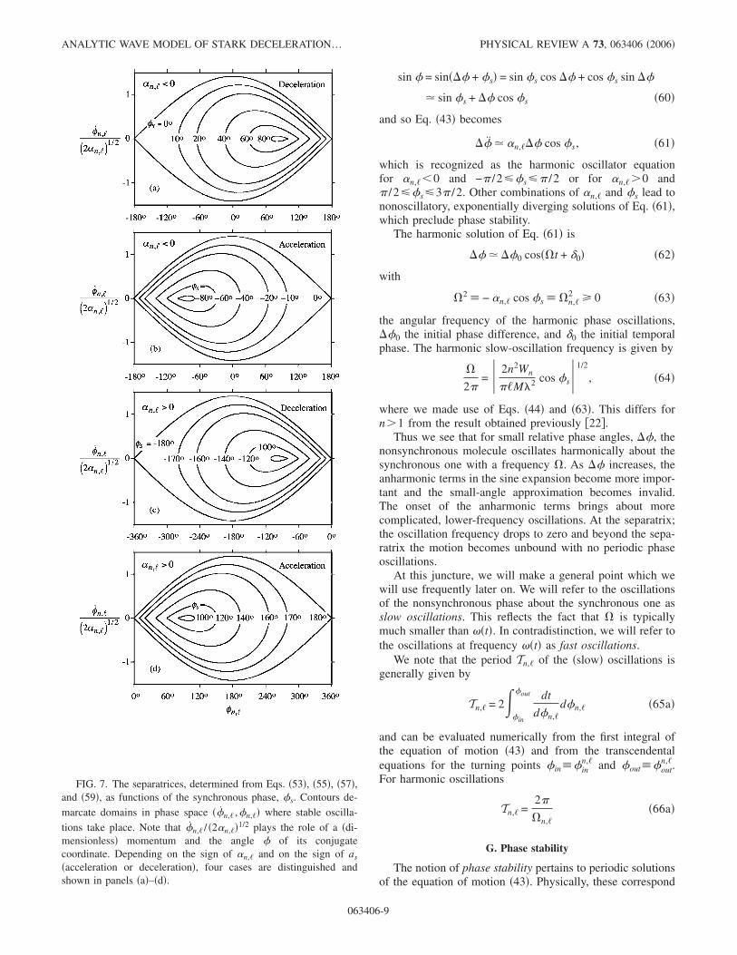
which is recognized as the harmonic oscillator equationfor �n,��0 and − /2��s� /2 or for �n,��0 and /2��s�3 /2. Other combinations of �n,� and �s lead tononoscillatory, exponentially diverging solutions of Eq. �61�,which preclude phase stability.

The harmonic solution of Eq. �61� is

�� 0 cos��t + �0� �62�

with

�2 � − �n,� cos �s � �n,�2 � 0 �63�

the angular frequency of the harmonic phase oscillations,��0 the initial phase difference, and �0 the initial temporalphase. The harmonic slow-oscillation frequency is given by

�

2= � 2n2Wn

�M�2 cos �s�1/2

, �64�

where we made use of Eqs. �44� and �63�. This differs forn�1 from the result obtained previously �22�.

Thus we see that for small relative phase angles, ��, thenonsynchronous molecule oscillates harmonically about thesynchronous one with a frequency �. As �� increases, theanharmonic terms in the sine expansion become more impor-tant and the small-angle approximation becomes invalid.The onset of the anharmonic terms brings about morecomplicated, lower-frequency oscillations. At the separatrix;the oscillation frequency drops to zero and beyond the sepa-ratrix the motion becomes unbound with no periodic phaseoscillations.

At this juncture, we will make a general point which wewill use frequently later on. We will refer to the oscillationsof the nonsynchronous phase about the synchronous one asslow oscillations. This reflects the fact that � is typicallymuch smaller than ��t�. In contradistinction, we will refer tothe oscillations at frequency ��t� as fast oscillations.

We note that the period Tn,� of the �slow� oscillations isgenerally given by

Tn,� = 2 �in

�out dt

d�n,�d�n,� �65a�

and can be evaluated numerically from the first integral ofthe equation of motion �43� and from the transcendentalequations for the turning points �in��in

n,� and �out��outn,�.

For harmonic oscillations

Tn,� =2

�n,��66a�

G. Phase stability

The notion of phase stability pertains to periodic solutionsof the equation of motion �43�. Physically, these correspond

FIG. 7. The separatrices, determined from Eqs. �53�, �55�, �57�,and �59�, as functions of the synchronous phase, �s. Contours de-marcate domains in phase space ��n,� ,�n,�� where stable oscilla-tions take place. Note that �n,� / �2�n,��1/2 plays the role of a �di-mensionless� momentum and the angle � of its conjugatecoordinate. Depending on the sign of �n,� and on the sign of as

�acceleration or deceleration�, four cases are distinguished andshown in panels �a�–�d�.


063406-9

to stable oscillations of the nonsynchronous molecule aboutthe synchronous one. The solutions of the equation of mo-tion, given by Eqs. �53�, �55�, �57�, and �59�, determine aboundary for the momentum of the nonsynchronous mol-ecule, �n,�, as a function of its phase, �n,�, that pertains tophase-stable motion. That is to say, together, ��n,� ,�n,�� de-limit an area of phase stability in the phase space for mol-ecules interacting with a given wave �n ,��.

Phase stability is a key property of a Stark accelerator ordecelerator, which enables handling other molecules thanjust the synchronous one. This is what makes the device apractical one, since bunches of molecules, with a distributionof positions and velocities, can then be accelerated or decel-erated. Without phase stability, only a single molecule couldbe handled, namely the synchronous one �23,24�.

The explicit evaluation of the phase-stable areas, Eqs.�53�, �55�, �57�, and �59�, clarifies several issues:

�a� The choice of the synchronous molecule. The dis-tribution of positions and velocities of molecules in a bunch�typically Gaussian, for a pulsed supersonic beam, Ref. �25��occupies a certain region of phase space. In order for theaccelerator or decelerator to act on most of the molecules inthe bunch, an overlap between the phase space occupied bythe bunch and the separatrices for phase-stable accelerationor deceleration needs to be sought. As the calculations of theseparatrices attest, the synchronous molecule is always at thecenter of the phase-stable area, cf. Fig. 7. Hence a maximumphase-space overlap is achieved when the position and ve-locity of the synchronous molecule coincides with the mostprobable position and velocity of the molecular-beam pulse,see Fig. 8. Thus in an acceleration or deceleration experi-ment, the synchronous molecule is generally defined by themost probable position and velocity of the molecular-beampulse.

�b� The size of the phase-stable areas depends on �swhich, in turn, determines the acceleration or deceleration

rate. At higher deceleration rates, only smaller bunches ofmolecules can be handled. The largest bunches of moleculescan be handled at zero deceleration, when a bunch is justtransported �i.e., guided� through the field array.

�c� The dominant wave. Since �1 is the largest spatialFourier coefficient, cf. Eq. �11�, we see that �11 supports thelargest phase-stable area and affords the highest accelerationor deceleration rate. The corresponding wave, ��, 1, 1�, re-ferred to as the first-harmonic wave, gives the best yieldaccording to this 1D treatment. Higher overtones are nor-mally not used in experiments, but the effects of many havebeen observed �16�. In Sec. V we will examine in more detailthe relative sizes of the phase-stable areas due to differentovertones.

H. Why does a single wave do nearly the whole job ?

So far we limited our considerations to the single-wavedynamics, i.e., to the equation of motion and its solutionsthat pertain to a single wave �±,n ,�� interacting with abunch of molecules. Here we will show that it is indeed justa single wave that gives a ride to molecules, with the infi-nitely many other waves, Eq. �15�, playing no role or a mar-ginal one �see Sec. V C on interferences�.

In order to see why this is the case, we will look at theeffect an arbitrary perturbing wave �+,r ,s� has on the phase-stable motion of molecules due to a �+,n ,�� wave, whosedynamics we outlined in Sec. IV.

Before delving into that, however, let us consider first therelationship between the velocities of the nonsynchronousand synchronous molecules for an arbitrary single wave.Since the averages of the nonsynchronous phase and its timederivatives over the oscillation period Tn,� are identicallyequal to zero

�n,� �1

Tn,� �n,�dt = 0 �67�

and since, from Eq. �39�,

�z = z − zs = v − vs = nk��n,� = nk�n,�, �68�

we see that

v − vs =1

Tn,� �v − vs�dt =

1

Tn,� vdt −

1

Tn,� vsdt

= v − vs = nk�n,� = 0, �69�

i.e., the nonsynchronous velocity averaged over a phase os-cillation is equal to the average synchronous velocity. This inturn shows that the synchronous velocity �pertaining to agiven wave� acts as a pilot for the nonsynchronous velocity�pertaining to that same wave� as long as phase stability ismaintained. Therefore, molecules which periodically oscil-late about a molecule synchronous with an arbitrary wavewill get a ride from that wave! In what follows we will call awave that gives a ride to a given bunch of molecules a reso-nant wave.

Let us now approach the problem from the other side andlook at the effect of a perturbing wave on the motion driven

FIG. 8. Phase-space distribution of a molecular beam as it entersa Stark accelerator/decelerator. The best overlap between a phasestable area �black fishes� and the molecular beam pulse �swarm ofdots� is obtained when the synchronous molecule matches the meanposition and velocity of the beam molecules. Cf. Fig. 2.


063406-10

by a resonant wave. We will look at the case of zero accel-eration, i.e., the case when the switching frequency � is con-stant and the Stark accelerator/decelerator serves as a guide.This will make our calculations simpler, although the samearguments would apply to the general case of nonzero accel-eration. Also, we will make our notation more accurate and,invoking Eqs. �17� and �19�, write the molecule’s coordinateas

zn,� =�n,�

nk+

�

nV0t . �70�

The acceleration of a molecule whose motion is resonantwith the �+,n ,�� wave is given by

zn,� =Fn,�

M= An,� sin �n,� = An,� sin�nkzn,� − ��t� , �71�

where we made use of Eqs. �19�, �35�, and �70�. For smalloscillations, the unperturbed coordinate of a molecule ridingthe �+,n ,�� wave is

zn,��t� =��0

nkcos��n,�t + �0� +

�

nV0t +

�s

nk�72�

as follows from Eqs. �38�, �62�, and �70�; its velocity, ob-tained by taking the time derivative of Eq. �72�, is

vn,��t� =�

nV0 −

��0�n,�

nksin��n,�t + �0� . �73�

The harmonic slow-oscillation frequency �n,� is given byEq. �63�.

We will consider now the perturbing effect of the�+,r ,s� wave on the motion of a molecule which is riding the�+,n ,�� wave. The �+,r ,s� wave perturbs the ride of themolecule by acting on its coordinate zn,� as determined bythe �+,n ,�� wave. Thus the acceleration imparted to a mol-ecule by the perturbing �+,r ,s� wave is

zn,�r,s =

Fn,�r,s �t�M

= Ar,s sin�rkzn,��t� − s�t� = Ar,s sin� r

n�n,� − �n,�

r,s t� ,

�74�

where we made use of Eq. �70� and introduced the frequency

�n,�r,s �

ns − �r

n� �

2

�n,�r,s , �75�

which is a fast-oscillation frequency, since it is on the orderof �. Clearly, the time average of the perturbing force Fn,�

r,s

over the perturbation period �n,�r,s vanishes

Fn,�r,s �

1

�n,�r,s Fn,�

r,s dt = 0 �76�

as follows by substitution of Eq. �74� into Eq. �76� and inte-gration, under the assumption that the slowly oscillatingphase �n,� remains constant over the period �n,�

r,s . Hence theperturbing force is seen to average out fast, as a result of

which the perturbing wave has no net effect on the phase-stable motion of the molecule.

The velocity, vn,�r,s , and the displacement, zn,�

r,s , imparted bythe perturbing wave can be obtained by integrating Eq. �74�.Integrating once �under the assumption of �n,� constant�yields the instantaneous velocity due to the perturbing wave

vn,�r,s �t� =

1

�m,�r,s Ar,s cos� r

n�n,� − �n,�

r,s t� . �77�

Integrating once more gives the displacement caused by theperturbing force

zn,�r,s = −

1

��n,�r,s �2Ar,s sin� r

n�n,� − �n,�

r,s t� . �78�

Thus the effect of the perturbing wave on the velocity and onthe displacement of the resonant wave is suppressed by �n,�

r,s

and ��n,�r,s �2, respectively. We see that the net effect of the

perturbing wave vanishes because the perturbing wave failsto displace the molecule. This is indeed the reason why, to anexcellent approximation, we are allowed to single out theresonant wave and handle it separately from the perturbingone�s�. It is also the reason why a perturbing wave has noinfluence on phase stability.

The motion of a molecule resonant with the �+,n ,�� waveand perturbed by the �+,r ,s� wave can now be easily evalu-ated �for the case of small oscillations� by simply addingEqs. �72� and �78� or �73� and �77�, respectively. This ana-lytic result can be compared with the result of a numericalintegration of the differential equation for a nonsynchronousmolecule interacting with the �+,n ,�� and �+,r ,s� waves.For example, for the ��,1,1� and ��,3,5� waves, the equationis

z = A11 sin�kz − �t� + A35 sin�3kz − 5�t� �79�

and Fig. 9 shows the result of the corresponding numericalintegration. The initial conditions are chosen such that themolecule interacts resonantly with the ��,3,5� wave, whichmeans that the ��,1,1� wave acts as a nonresonant, perturb-ing wave. Since the ��,1,1� wave dominates the right-moving waves and since its phase velocity is close to ��,3,5�wave, the perturbing effect of the ��,1,1� wave is muchlarger than the effect of all the other waves in the Fourierexpansion, Eq. �15�. And yet, this perturbing effect is seen tobe strongly suppressed because of the fast oscillations withrespect to the ��,3,5� wave. While the perturbation of thevelocity is still noticeable on a short time scale, see Fig. 9�a�,the perturbation of the coordinate amounts to just a ripple,see Fig. 9�b�. We note that the frequency and amplitude ofthe fast oscillations are correctly predicted by Eqs. �77� and�78�, which reconfirms the validity of the assumptions usedin the analysis of the perturbations.

In the case of acceleration or deceleration, the switchingfrequency is not constant, but increases or decreases linearlywith time throughout the acceleration or deceleration pro-cess. Nevertheless, the treatment of the perturbations for thecase of guiding, as given above in this paragraph, remains in


063406-11

place for this case as well, since ��t� essentially does notchange during a fast-oscillation period �typically by less than1%� and so can be treated as a constant.

The above treatment only breaks down in the limit��t�=kV�t�→0, where the used assumption ��t�� nolonger holds. In practice, such a situation does not occur,since even if the molecules are decelerated to velocities con-ducive to trapping, see Ref. �9�, ��t� still considerably ex-ceeds �, and so the treatment remains in place.

I. Two (or more) waves traveling with the same phase velocity

When the resonant and perturbing waves travel at thesame phase velocity �i.e., for � /n=s /r=�� /�n, with � anodd integer�, the perturbing force, Eq. �74�, does not averageout. In this case one cannot speak of resonant and nonreso-nant waves, because all the waves which travel at this samevelocity are equally resonant and will jointly create phase

stability. Since, obviously, any �+,n ,�� wave has suchfellow-traveler waves �+,�n ,��, this is actually the usualsituation. Figure 10�a� shows typical relative sizes of twowaves with successive n, traveling at the same velocity. Wesee that the resulting shape of the well is dominated by oneof the two waves, namely the one with the smaller n, cf. Eq.�11�. Hence in order to draw conclusions about phase stabil-ity �which is determined by the shape and depth of the well�,we can rely solely on the properties of the dominant wave.

However, when calculating switching sequences accu-rately, the influence of the nondominant wave�s� cannot befully dismissed, because of the effect it has on the accelera-tion as �typically, a deviation of a few percent with respect toa single-wave treatment can accumulate over 100acceleration/deceleration stages�. Thus when evaluating theacceleration on a dominant �+,n ,�� wave, one should re-place Eq. �23� with the sum

FIG. 9. �Color online� Dynamics of a nonsynchronous moleculeriding the �3, 5� wave and perturbed by the �1, 1� wave. The dy-namics was determined by numerically integrating the differentialequation of the molecule interacting with the two waves, for initialconditions that make the �3, 5� wave resonant and the �1, 1� waveperturbing. Both the longitudinal velocity, v�t�, panel �a�, and thelongitudinal position, z�t�−vst, relative to the synchronous moleculemoving at a velocity vs, panel �b�, exhibit slow oscillations super-posed by fast oscillations. The slow oscillations arise from thesingle-wave interaction of the molecule with the resonant �3, 5�wave and are described by Eqs. �72� and �73�. The fast oscillationsare due to the perturbing �1, 1� wave and are described by Eqs. �77�and �78�. While the influence of the nonresonant wave on the ve-locity is significant, its effect on the position z�t� is strongly sup-pressed. The time scale is given in terms of the slow-oscillationperiod Tn,�

FIG. 10. �Color online� �a� Relative magnitude of the electricfields due to the �1, 1� wave and the �3, 3� wave �black dottedcurves�, which are traveling at the same velocity. These relativemagnitudes are typical for two waves with successive n and thesame velocity. We see that the net field �red curve� is determinedpredominantly by the �1, 1� wave, i.e., the one with the smallervalue of n. The conclusions about phase stability can be reached byconsidering solely this wave. �b� Typical relative magnitudes of theforce due to the �1, 1�, �3, 3�, and �5, 5� waves �black dottedcurves�, which are all traveling at the same velocity. Since a smalldeviation in the force can accumulate when calculating a switchingsequence comprising many stages, one should rely on the net force�red curve� rather than on the dominant term, cf. Eq. �80�.


063406-12

as = �� odd

�

A�n,�� sin��s� . �80�

Note that this sum converges very fast, cf. Eqs. �14� and�16�. Figure 10�b� shows, for the case of the ��,1,1� domi-nant wave, the modification of the force due to the presenceof the resonant nondominant waves. We note that in order toachieve an accurate correspondence between as and �s, sev-eral terms in Eq. �80� may have to be taken into account.

V. FULL-FLEDGED DYNAMICS

In Sec. IV H, we discussed the dynamics due to a singleresonant wave perturbed by a single nonresonant wave.However, the exact �longitudinal� force that is acting on themolecules, Eq. �15�, is due to infinitely many partial waves,out of which all but one are nonresonant �notwithstandingthe discussion of Sec. IV I�. In order to fully assess the roleof the resonant wave vis à vis the nonresonant waves, weevaluated the combined effect due to a large number ofwaves and compared it with a single-wave effect. The single-wave dynamics, the full-fledged dynamics and the correctionthat needs to be applied to the single-wave dynamics in orderto reproduce the full-fledged dynamics can be best visualizedin a phase-space diagram. Such a diagram, or phase portrait,exemplified in Fig. 11, shows the average velocities of themolecules as a function of their initial velocity and initialspatial phase. The link between the average velocity andphase stability is given by Eq. �69�. Note that in the phase

FIG. 11. �Color online� Global phase portrait showing the phasestable areas due to the various waves �case of guiding�. The con-tours pertain to average velocities of OH molecules plotted as afunction of their initial velocity v and initial spatial phase kz; thelink between the average velocity and phase stability is given byEq. �69�. The contour plot is obtained by numerically integratingthe full equation of motion �81� for 80 waves with a temporal phaseand switching sequence given, respectively, by Eqs. �32� and �33�corresponding to guiding �sin �s=0� at V0=150 m/s. The phaseportrait is in perfect agreement with Monte Carlo trajectory simu-lations which, in turn, are in perfect agreement with experiment.

FIG. 12. �Color online� Detailed view of the phase stable areasof Fig. 11 around �a� V0 and �b� 5

3V0 �the case of guiding�. Thecontours pertain to average velocities of OH molecules plotted as afunction of their initial velocity v and initial spatial phase kz. Zoom-ing in at the global phase portrait allows for an accurate comparisonof the full-fledged numerical result with the analytic treatment ofthe dynamics. The white curves show the separatrices calculatedfrom Eqs. �86� and �87� for a resonant, single-wave interaction. Thegreen curves are obtained from Eq. �89� and comprise the perturba-tions due to all the other, nonresonant waves. The yellow curvescombine the two and are seen to render a perfect agreement with thefull-fledged calculation.


063406-13

space regions corresponding to phase stability all the mol-ecules have the same average velocity. The velocities that thecontours correspond to can be read off from the velocityscale on the right.

The cases of guiding and of acceleration or decelerationdue to a single wave will be described separately in Secs.V A and V B. Single-wave dynamics gives rise to featureswhich occur at odd-fraction multiples, � /n, of the fundamen-tal velocity V0. In Sec. V C we will deal with features whichoccur at even-fraction multiples of the fundamental velocityV0. These features arise from the interference of �typically�two adjacent waves.

A. Guiding

The phase portrait shown in Fig. 11 was obtained from anumerical integration of the full equation of motion

z�t� =F�z,t�

M�81�

with F�z , t� given by Eq. �15� and the temporal phase of thewaves given by Eq. �32� with sin �s=0 corresponding toguiding. We found that increasing the number of waves in-cluded in the computation beyond 80 �n�5,��25� did notlead to any changes of the phase portraits in the range of theinitial velocities and positions shown. Moreover, we foundthat the phase portrait of Fig. 11 agrees perfectly well withthe one obtained from trajectory simulations which, in turn,perfectly reproduces experiment �16�. Therefore, for all in-tents and purposes, the phase portrait of Fig. 11 can be con-sidered to be exact. The phase portrait captures all the com-plexity of the dynamics in question and makes it possible tosee at a glance the phase-stable areas due to various waves.We remind ourselves of the fact that while the spatial Fouriercomponents of F�z , t� decrease exponentially with increasingn, the temporal Fourier components decrease only as �−1.Therefore, phase-stable areas corresponding to waves withn�3 can hardly be discerned but those with ��7 can stillbe easily observed in the phase-space area depicted.

Figure 12 shows in panels �a� and �b� detailed views ofthe phase-stable areas due to the first harmonic wave ��, 1,1� and due to the ��, 3, 5� wave �note that �11�0 and�3��0 for the example of low-field seeking states consid-ered here�. The main features can be understood, for the caseof guiding, from Eqs. �53� and �57�, respectively. Before weapply these, we realize that, generally, the phase �n,�, Eq.�19�, yields a molecular velocity

vn,� =�n,�

nk+

�

nV0 �82�

and an initial position of the molecule

zn,� =�n,�

nkat t = 0. �83�

Equation �53� and �57�, simplified for the case of guiding,become

�n,� = ± �− 2�n��cos �n,� + 1��1/2 �n� � 0 �84�

and

�n,� = ± �2�n��− cos �n,� + 1��1/2 �n� � 0. �85�

Their combinations with Eq. �82� give the separatrices

vn,� = ±�− 2�n��1 + cos �n,��1/2

nk+

�

nV0 �86�

and

FIG. 13. �Color online� Detailed view of the phase stable areasaround �a� V0 and �b� 5

3V0 for the case of deceleration. The contourspertain to average velocities of OH molecules plotted as a functionof their initial velocity v and initial spatial phase kz. The contourswere obtained by numerically integrating the equation of motion�81� for 80 waves, with a temporal phase and switching sequencegiven, respectively, by Eqs. �32� and �33� corresponding to decel-eration �An,� sin �s�0�. Panel �a� shows the full-fledged numericalcalculation for deceleration on the first-harmonic �1, 1� wave with�s=20°. Panel �b� shows the full-fledged numerical calculation fordeceleration on the �+,3 ,5� wave with �s=−170°. The white curvespertain to the separatrices obtained for a resonant, single-wave in-teraction, as given by Eqs. �53� and �57�. The green curves areobtained from Eq. �89� and comprise the perturbations due to all theother, nonresonant waves. The yellow curves combine the two andare seen to be in perfect agreement with the full-fledged calculation.


063406-14

vn,� = ±�2�n��1 − cos �n,��1/2

nk+

�

nV0 �87�

for the cases represented by waves ��, 1, 1� and ��, 3, 5�,respectively. The separatrices obtained from Eqs. �86� and�87� are shown in Fig. 12 by the white curves. The equationscapture all the qualitative features of the respective phase-stable areas seen in Figs. 11 and 12: �1� the phase-stableareas occur at velocities �

nV0; �2� the velocity �i.e., vertical�width of a phase-stable area for a given n is proportional to�−1/2, because ��n��−1, Eq. �44�; �3� the velocity width of aphase-stable area for a given � is proportional to exp�− 1

2�n�,cf. Eqs. �11� and �44�; �4� when the spatial phase, kzn,�, var-ies between − and , then the initial phase �n,��t=0�=nkzn,� varies between −n and n; as a result, the phase-stable area corresponding to an �±,n ,�� wave consists of n“fishes” when the �horizontal� initial kzn,�=�n,��t=0� /nspans the interval of − to ; �5� for �n��0, the nodesoccur at kzn,�= ± , ±�

2n , ±�

4n , . . .; for �n��0, the

nodes occur at kzn,�=0, ± 2n , ± 4

n , . . .A closer inspection of Fig. 12 reveals that the agreement

between the separatrix obtained from either Eq. �86� or Eq.�87� with the exact phase portrait is not perfect. The agree-ment can be improved to the point of perfection by correct-ing for the effect of the nonresonant waves. This we do byapplying the approach developed for a single perturbingwave in Sec. IV H to all the perturbing waves, starting withEq. �15�. As a result

vn,��z,t� � �r odd

�s odd

vn,�r,s �t� = �

r odd�

s odd

n

��ns − �r�Ar,s

�cos� r

n�n,� −

��ns − �r�n

t�+ �

r odd�

s odd

n

��ns + �r�Ar,s

�cos� r

n�n,� +

��ns + �r�n

t� − �p even

n

p��Ap

�cos� p

n��n,� + ��t�� , �88�

where vn,� is the velocity change of the molecules riding theresonant �+,n ,�� wave due to the effect of all the nonreso-nant waves �so the summation is over all r ,s=1,3 , . . . forwhich ns−�r�0�. Truncating the summation at r=1 andp=2, we obtain for t=0

vn,��z,t = 0� � �s odd

n

�ns − ��A1s cos�kz�

+ �s odd

n

�ns + ��A1s cos�kz� −

n

2��A2 cos�2kz� .

�89�

This is shown by the green line in Fig. 12 for s�21. Theyellow line shows the velocity vn,��z , t=0�+ vn,��z , t=0�, andis seen to be in full agreement with the phase-stable area

obtained from the full-fledged calculation. No correction wasneeded for the position zn,�, as the effect of the nonresonantwaves is diminished by a factor proportional to �2, see Eq.�78� and Fig. 9�b�, and so does not show on the scale of thefigure.

B. Acceleration or deceleration

The phase portraits obtained for guiding can be easilygeneralized to the case of acceleration or deceleration, byincorporating in the numerical calculations a temporal phase,Eq. �32�, corresponding to an accelerating or deceleratingwave. Figure 13 attests to this being the case: panels �a� and�b� show the same parts of the phase space as panels �a� and�b� in Fig. 12, but for �s=20° and �s=−170°, respectively,and both for deceleration. The white curves show the sepa-ratrices

vn,��t�

= ±�− 2�n��cos �n,� + cos �s + ��n,� − + �s�sin �n,��1/2

nk

+�

nV�t� �90�

and

vn,��t�

= ±�2�n��− cos �n,� − cos �s − ��n,� + + �s�sin �n,��1/2

nk

+�

nV�t� �91�

obtained from the general formulas �53� and �57�, thegreen lines the correction due to the nonresonant waves,Eq. �89�, and the yellow lines the corrected separatrices.Again, the agreement with the exact phase portraits isexcellent.

C. Interference effects

1. Derivation

A close look at Fig. 11 reveals small regions of phasestability centered at “strange” velocities, such as 3

2V0 or 2V0.These phase-stable areas cannot arise from single-wave in-teractions, since, as we saw above, single waves travel atphase velocities �

nV0 with � and n odd. Here we will showthat the phase-stable areas occurring at even-fraction mul-tiples of V0 actually arise from the interference of two waveswith n and � odd.

We reach this conclusion in four steps, outlined below forthe case of guiding. First, we transform the equation of mo-tion of a molecule at a position z subject to two arbitrarywaves �+,n ,�� and �+,r ,s�

z = An,� sin�nkz − ��t� + Ar,s sin�rkz − s�t� �92�

cf. Eq. �35�, to a frame moving with velocity


063406-15

Vg =� + s

n + rV0, �93�

where the two waves act on the molecule with the samefrequency

�g =ns − �r

n + r� . �94�

Note that �g is a fast oscillation. The molecule’s position insuch a frame is

zg = z − Vgt . �95�

The transformed equation of motion thus becomes

zg = An,� sin�nkzg + �gt� + Ar,s sin�rkzg − �gt� , �96�

where we made use of the equality z= zg.Second, we integrate Eq. �96� under the condition that

the spatial phase kzg remain constant with respect to thetemporal phase �gt; this is consistent with our aim to findstable, slowly oscillating solutions. For the constant spatialphase we take the value nkzg�t�� the spatial phase acquires atan arbitrary time, t�. Thus we obtain

zg�t� = −An,�

�gcos�nkzg�t�� + �gt� +

Ar,s

�gcos�rkzg�t�� − �gt�

+ C1, �97�

where C1 is an integration constant, which can be evaluatedby integrating both sides of Eq. �97� over a fast oscillationperiod, �g� 2

�g. This yields

1

�g

t�−�g/2

t�+�g/2

zg�t�dt � zg�t�� = zg�t�� = C1. �98�

Now integrating Eq. �97� for nkzg�t�� constant yields

zg�t� = −An,�

�g2 sin�nkzg�t�� + �gt� −

Ar,s

�g2 sin�rkzg�t�� − �g�t��

+ zg�t��t − t�� + C2, �99�

where we made use of Eq. �98�. Here C2 is another integra-tion constant, which can be evaluated by integrating Eq. �99�over a fast-oscillation period �g

1

�g

t�−�g/2

t�+�g/2

zg�t�dt � zg�t�� = C2. �100�

Note that Eqs. �97� and �99� are valid at time t� t�. In par-ticular, for t= t� Eq. �99� yields

zg�t�� = −An,�

�g2 sin�nkzg�t�� + �gt�� −

Ar,s

�g2 sin�rkzg�t�� − �gt��

+ zg�t�� . �101�

Since the time t� was chosen arbitrarily, Eq. �101�holds at all times, which makes t� into a time variable;we will denote it by t again �t�→ t�. Furthermore, wewill solve Eq. �101� iteratively. The inequalities An,� /�g

2�1

and Ar,s /�g2�1 �cf. Sec. IV H� along with Eq. �101� imply

that

zg�t� � zg�t� �102�

from which it follows that already the first iteration (i.e.,zg�t�→ zg�t�, on the right-hand side) generates an accuratesolution

zg�t� = −An,�

�g2 sin�nkzg�t� + �gt� −

Ar,s

�g2 sin�rkzg�t� − �gt�

+ zg�t� = a + b + zg, �103�

where the quantities a and b are shorthands for the first andsecond term, respectively.

Third, we insert Eq. �103� into the equation ofmotion �96� and invoke the following trigonometricapproximations:

sin�nk�a + b�� nk�a + b� sin�rk�a + b�� rk�a + b�

cos�nk�a + b�� 1 cos�rk�a + b�� 1. �104�

As a result, we obtain the equation of motion in the form

zg � nkAn,��a + b�cos�nkzg + �gt� + rkAr,s�a + b�cos�rkzg

− �gt� + An,� sin�nkzg + �gt� + Ar,s sin�rkzg − �gt�

= �1 − �g−2�nkAn,� cos�nkzg + �gt� + rkAr,s cos�rkzg

− �gt�� An,� sin�nkzg + �gt� + Ar,s sin�rkzg − �gt�� .

�105�

Taking an average of Eq. �105� over the fast-oscillation pe-riod �g yields

1

�g

t−�g/2

t+�g/2

zg�t�dt� � zg�t� = zg�t�

= −1

2�g2An,�Ar,s�n + r�k sin��n + r�kzg� .

�106�

Equation �106� is a second-order differential equation for zgwhich reveals that a molecule that has a coordinate zg� zgwith respect to a synchronous molecule traveling at a veloc-ity Vg is subject to a sine-shaped restoring force which leadsto slow stabilizing oscillations. This comes about in exactlythe same manner as in the case of a single-wave interaction.

Fourth, we realize that the waves �+,n ,�� and �+,r ,s� actjointly as a single wave �+,n+r ,�+s�. As this wave movesat the phase velocity Vg= �+s

n+rV0, cf. Eq. �93�, we can ascribeit a phase

�n+r,�+s � �n + r�kz − �� + s��t . �107�

Plugging Eqs. �93� and �95� into Eq. �107� then gives

�n+r,�+s = �n + r�kzg � �n + r�kzg, �108�

which implies


063406-16

�n+r,�+s � �n + r�kzg. �109�

Substitution from Eqs. �108� and �109� into Eq. �106� yieldsthe final result

�n+r,�+s = −1

2�g2An,�Ar,s�n + r�2k2 sin �n+r,�+s

= An+r,�+s�n + r�k sin �n+r,�+s

= �n+r,�+s sin �n+r,�+s, �110�

where we set

An+r,�+s � −1

2�g2An,�Ar,s�n + r�k �111�

and

�n+r,�+s � An+r,�+s�n + r�k . �112�

Equation �110� is of the same form as Eq. �43� for asingle-wave interaction �in the case of guiding, with sin�s=0�. Therefore, all the results �for guiding� obtained fromEq. �43� are equally valid for the interference dynamics.

Figure 14 illustrates the interference dynamics of a mol-ecule interacting with the �1, 1� and �1, 3� waves whichpropagate at phase velocities V0 and 3V0, respectively. Thedynamics was obtained by numerical integration of Eq. �92�,with the initial condition set such that v�0�= �+s

n+rV0=2V0.Note the similarity between Figs. 9 and 14. The former per-tains to a nonsynchronous molecule interacting resonantlywith the �3, 5� wave and nonresonantly with the �1, 1� wave.As a result, the molecule’s velocity slowly oscillates about53V0, with superposed fast oscillation due to the perturbationby the �1, 1� perturbing wave. Figure 14 shows a similardynamics, but now the slow, stable velocity oscillation iscentered around 1+3

1+1V0. Hence the �1, 1� and �1, 3� waves actindividually as perturbing waves, but act jointly as a singlestabilizing �2, 4� wave propagating at 2V0.

We note that the frequency and amplitude of the fast os-cillations are correctly predicted by Eqs. �97� and �103�.

2. Comparison with the exact phase portraits

Equipped with Eq. �110�, we can now return to Fig. 11and check whether the strange features occurring at even-fraction multiples of the fundamental velocity can indeed beexplained by our analytic model of the Stark accelerator/decelerator.

First, we observe that the phase-stable areas are found atthe velocities 2

4V0, 64V0, and 4

2V0. Zooming in would revealmany more phase-stable areas, e.g., at 10

4 V0 or 86V0. The sta-

bility at all these velocities follows directly from Eqs. �93�and �110�. Table I lists pairs of waves that give rise to a givenphase-stable area due to interferences. Thus we see that, forinstance, the stability at 4

2V0 results from the interference ofthe �1, 1� and �1, 3� waves, and at 2

4V0 from the interferenceof the �1, 1� and �3, 1� waves. Next, we observe that thephase-stable area at 4

2V0 exhibits two fishes, whereas phasestability at 2

4V0 exhibits four. Also this is in full agreement

FIG. 14. Interference dynamics of a nonsynchronous moleculeinteracting with the �1, 1� wave and the �1, 3� wave which jointlycreate phase stability at 2V0. The dynamics was obtained by nu-merically integrating the equation of motion �92� for a moleculeinteracting with the two waves, with the initial condition v�0�=2V0. Both the longitudinal velocity, v�t�, panel �a�, and the relativeposition, �z=z�t�−2V0t, panel �b�, exhibit slow oscillations super-posed by fast oscillations. The two interfering waves �1, 1� and �1,3� act jointly as a single �2, 4� wave, giving rise to slow oscillationsof period T2,4. Note the similarity with Fig. 9.

TABLE I. A list of the properties of typical two-wave interference effects.

Interfering waves �1,1�,�1,3� �1,1�,�3,1� �1,1�,�5,7� �3,7�,�1,3�

Vg 4

2V0=2V0

2

4V0=

1

2V0

8

6V0=

4

3V0

10

4V0=

5

2V0

n+r 2 4 6 4

�g � � /2 � /3 � /2

An+r,�+s−

4k3W12

32M2�2

96k3W1W3

2M2�2 −540k3W1W5

72M2�2

64W1W3

72M2�2


063406-17

with our treatment, and follows immediately from the�n+r� factor in the argument of the sine in Eq. �110�. Thesign of the prefactor �n+r,�+s explains correctly whether theinterference effect exhibits a node or an antinode at z=0.Last but not least, we can evaluate the slow-oscillation fre-quency in the harmonic limit, cf. Eq. �63�, from

� = ��n+r,�+s�1/2 = �r + n�k�An,�Ar,s

2�g2 �1/2

� �n+r,�+s,

�113�

where the absolute value accommodates the cases of nega-tive An,�, Ar,s, or �g.

Let us zoom in Fig. 11 on the phase-stable area occurringat 2V0, and use it as a testing ground for the accuracy of ourtreatment of the interference effects. A magnification of thisphase-stable area is displayed in Fig. 15�a�. The white curveshows the separatrix obtained from Eqs. �86� and �107� forthe resonant �+,n+r ,�+s�= �+,2 ,4� wave. We see that itcorrectly renders the size of the separatrix but not quite itsshape. As in the case of single-wave dynamics, in order toobtain a full agreement between our theory and the exactresult we have to take into account the influence of the per-turbing waves. This influence can be taken into account inexactly the same way as before, i.e., by means of Eq. �89�.We have to substitute into it n+r=2 for n and �+s=4 for �,which gives

v2,4�z,t = 0� � �p odd

2

�2p − 4��A1,p cos�kz�

+ �p odd

2

�2p + 4��A1,p cos�kz� −

2

8�A2 cos�2kz�

= �p odd

� 1

�p − 2�p+

1

�p + 2�p�A1,1

�cos�kz�

−A2

4�cos�2kz� = −

A2

4�cos�2kz� . �114�

We see that in this particular case, the sum over p vanishesand so the correction given by Eq. �114� takes quite a simpleform. The correction is shown by the green curve in Fig.15�a�. The yellow curve is a sum of the white and greencurves, and is seen to agree perfectly with the exact separa-trix. We thus arrive at the conclusion that our analytic modelaccounts perfectly well for the observed phase stability ateven-fraction multiples of the fundamental velocity, in termsof interferences of waves with n ,� odd.

Above, we treated the dynamics due to two interferingwaves. In particular, we showed that the ��, 1, 1� and the��, 1, 3� waves jointly create phase stability at 2V0. Butthese are not the only waves that create stability at this ve-locity! An interference wave, just as a single wave, is alwaysaccompanied by fellow-traveler waves. For example, the ��,1, 1� and ��, 1, 5� waves also create phase stability at 2V0, asdo the ��, 1, 3� and the ��, 1, 7� waves, etc.

Taking into account all combinations of the �±,1 ,��waves that generate phase stability at 2V0, we obtain for thetotal �2,4 coefficient

�2,4 = −8k4W1

2

2M2�2�1

3− �

i=3,5,. . .

�1

i2�i − 2��i + 2�� = −k4W1

2

4M2�2 ,

�115�

where we note that Eq. �115� is in complete agreement withEq. 24 of Ref. �16�. The combined effect of the fellow-traveler waves is small. In total, they give rise to a correctionof about 8% to the value of �2,4 obtained by considering the��, 1, 1� and ��, 1, 3� waves only. This results in a correc-tion of 4% for the corresponding separatrix. Therefore, inevaluating the phase-stable areas around 2V0, we could relysolely on the interference wave arising from the combinationof the ��, 1, 1� and ��, 1, 3� waves.

FIG. 15. �Color online� Detailed view of the phase stable areaaround 2V0 for the case of guiding �with �s=0°�, panel �a�, and ofdeceleration �with �s=20°�, panel �b�. The contours pertain to av-erage velocities of OH molecules plotted as a function of theirinitial velocity v and initial spatial phase kz. The full-fledged nu-merical calculations are compared with the analytic result for thecase of the interference of the �1, 1� wave with the �1, 3� wave,which give jointly rise to a �2, 4� wave. The white curves show theseparatrices �at t=0� obtained from Eq. �53� for n→n+r and �→�+s, and with �n+r,�+s and �n+r,�+s as given by Eqs. �107� and�112�. The green curves were obtained from Eq. �114� and comprisethe perturbations due to all nonresonant waves. The yellow curvescombine the two and are seen to be in excellent agreement with thefull-fledged numerical calculation. The temporal phase and switch-ing sequence used for deceleration, panel �b�, is given, respectively,by Eqs. �121� and �122�. We note that the A2 coefficient is negativefor the case of low-field seekers, considered in this calculation.


063406-18

The same discussion can be applied to phase stability at12V0, which is not due just to the ��, 1, 1� and ��, 3, 1�waves, but also to the ��, 1, 3� and ��, 3, 1� waves, the��, 1, 1� and ��, 3, 3� waves, etc. Taking into accountall combinations of the �±,1 ,�� and �±,3 ,�� waves thatgenerate phase stability at 1

2V0, we obtain for the total �4,2coefficient

�4,2 =96k4W1W3

2M2�2 �4 − �i=1,3,. . .

� � 1

�i + 1/2�2i�i + 2�

+1

�i + 3/2�2i�i + 2�� =16k4W1W3

M2�2 �4 −16

3� ,

�116�

which is in full agreement with Eq. 26 of Ref. �16�.Again, the correction due to the fellow-traveler waves hasno significant effect on the size of the separatrix as evaluatedfrom the combination of the ��, 1, 1� and ��, 3, 1� wavesalone.

3. Accelerating or decelerating on an interference

Accelerating or decelerating on an interference wave issomewhat trickier than it is on a single wave. The mainreason is that the An+r,�+s coefficient, Eq. �111�, which de-pends on �, becomes itself time dependent through the timedependence of �=��t�. This needs to be taken into accountwhen re-deriving expressions for vs�t� and ��t� from the con-dition of a constant synchronous phase with respect to the�n+r ,�+s� wave.

First we realize that the acceleration imparted to thesynchronous molecule by the interference wave is givenby

as�t� = An+r,�+s�t�sin �s = −�n + r�3

2�ns − �r�2�2�t�kAn,�Ar,s sin �s

�Ad

�2�t�, �117�

where we made use of Eqs. �23�, �94�, and �111� and so isseen to depend on time. This time dependence does notaffect the derivation of the interference dynamics �Sec. V C�since ��t� does not change appreciably during a fast-oscillation period. Equation �117� can be integrated toyield the synchronous velocity, which must equal the phasevelocity

vs�t� =� + s

n + rV0 +

0

t

as�t��dt� =� + s

n + rV0 +

0

t Ad

�2�t��dt�

= Vn+r,�+s�t� �� + s

n + r

��t�k

. �118�

The time derivative of Eq. �118� can be recast into a differ-ential equation for ��t�

��t� =n + r

� + s

kAd

�2�t�, �119�

which can be easily solved by direct integration. With theinitial condition ��0�=�0 we obtain

��t� = �3�n + r�kAd

� + st + �0

3�1/3

. �120�

From Eq. �120�, the temporal phase becomes

�t� = 0

t

��t��dt� =� + s

4�n + r�kAd�3�n + r�kAd

� + st + �0

3�4/3

−�� + s��0

4

4�n + r�kAd, �121�

which generates the switching sequence required for accel-erating or decelerating on an interference wave

�t� = q q = 0,1,2, . . . �122�

The switching sequence obtained from Eq. �121� was used ina full-fledged calculation for the case of deceleration �at �s=20°� to generate the phase portrait shown in Fig. 15�b�.Also shown is the separatrix �white curve� obtained by sub-stituting �n+r,�+s�t=0� into Eq. �53�. We note that the value of�n+r,�+s�t� at t=0 is minimal, and so determines the depth ofthe potential well that captures the molecules which, in turn,determines the area of phase stability �note that any increaseof the well depth during deceleration is of no avail�. Alsoshown are the perturbations by all the other waves �greencurve� and the net separatrix �yellow curve�. Again, an ex-cellent agreement between the latter and the full-fledged cal-culation is found. Deceleration on an interference is of littlepractical interest, since the corresponding deceleration ratesand phase-stable areas are puny.

4. Multiple interferences

Furthermore, it is quite easy to generalize the treatment ofthe interference effect to more than two waves. This can bedone by treating the interference wave on the same footing asa single wave and letting it interfere with another singlewave, in exactly the same way as the two single waves thatgave rise to the interference. This results in tiny, so far un-observed effects.

VI. CONCLUSIONS

Stark acceleration or deceleration is a phase-stable pro-cess that enables full control of the translational motion ofquantum-state-selected polar molecules. The acceleration ordeceleration process abounds in rich dynamics, which hasbeen accurately captured by an analytic model presented inthis paper. The model is based on a Fourier analysis of thetime-varying inhomogeneous electric field produced by aStark accelerator/decelerator, which reveals that the fieldconsists of an infinite multitude of stationary and counter-propagating waves with well defined phase velocities. Theensuing physical picture set forth by the “wave model” is


063406-19

that molecules injected into the accelerator/decelerator ridethe waves.

In this paper, we tackled explicitly the interaction of theinjected molecules with an arbitrary wave in the Fourier ex-pansion, and obtained an analytic description of the accelera-tion or deceleration dynamics which is both intuitive andexact. We found that the dynamics is dominated by the in-teraction of the molecules with a single wave. This wave isdistinguished from all the other waves by its phase velocity,which is such as to come close to the velocity of the mol-ecules �resonant wave�. We studied explicitly the effect ofthe nonresonant, perturbing waves on the resonant-wave dy-namics and showed that it is heavily suppressed, with littleconsequence for phase stability. We also showed that two �ormore� waves can interfere with one another and act jointly asa single wave that gives rise to a phase-stable motion of themolecules.

We compared the dynamics derived from the wave modelwith Monte Carlo trajectory simulations of the accelerationor deceleration dynamics, which in previous work had beenfound to be in perfect agreement with experiment. This com-parison showed that every tiny detail of the observed rich

phase-space structures could be accounted for by invokingeither single-wave dynamics, or perturbations by nonreso-nant waves, or interference dynamics.

The link between various regions of phase stability andexperimental observations was studied earlier �16�. However,the wave model led us to reinterpret the first- and second-order resonances, identified in the previous work, in terms ofsingle-wave and interference dynamics. We were able to ex-tend the previous study and show that arbitrary overtonewaves can be used for deceleration. This was subsequentlycorroborated by experiment �26�.

Thus we conclude that the analytic wave model encom-passes all the longitudinal dynamics that arises in a Starkaccelerator/decelerator.

ACKNOWLEDGMENTS

We thank our colleagues at the Fritz-Haber-Institut forhelpful discussions, in particular Dr. Rick Bethlem �now alsoat the Vrije Universiteit Amsterdam�, Joop Gilliamse, Dr.Bas van de Meerakker, and Dr. Nicolas Vanhaecke �now atLaboratoire Aime Cotton�.

�1� C. H. Townes and A. L. Schawlow, Microwave Spectroscopy�Dover, New York, 1975�.

�2� G. Scoles, Atomic and Molecular Beam Methods �Oxford Uni-versity Press, New York, 1988�.

�3� H. Pauly, Atom, Molecule, and Cluster Beams �Springer, Ber-lin, 2000�.

�4� H. L. Bethlem, G. Berden, and G. Meijer, Phys. Rev. Lett. 83,1558 �1999�.

�5� H. L. Bethlem, A. J. A. van Roij, R. T. Jongma, and G. Meijer,Phys. Rev. Lett. 88, 133003 �2002�.

�6� F. M. H. Crompvoets, R. T. Jongma, H. L. Bethlem, A. J. A.van Roij, and G. Meijer, Phys. Rev. Lett. 89, 093004 �2002�.

�7� S. A. Schulz, H. L. Bethlem, J. van Veldhoven, J. Küpper, H.Conrad, and G. Meijer, Phys. Rev. Lett. 93, 020406 �2004�.

�8� H. L. Bethlem, G. Berden, F. M. H. Crompvoets, R. T.Jongma, A. J. A. van Roij, and G. Meijer, Nature �London�406, 491 �2000�.

�9� J. van Veldhoven, H. L. Bethlem, and G. Meijer, Phys. Rev.Lett. 94, 083001 �2005�.

�10� F. M. H. Crompvoets, H. L. Bethlem, R. T. Jongma, and G.Meijer, Nature �London� 411, 174 �2001�.

�11� S. Humphries, Principles of Charged Particle Acceleration�Wiley, New York, 1986�.

�12� H. L. Bethlem, G. Berden, A. J. A. van Roij, F. M. H.Crompvoets, and G. Meijer, Phys. Rev. Lett. 84, 5744 �2000�.

�13� H. L. Bethlem, F. M. H. Crompvoets, R. T. Jongma, S. Y. T.van de Meerakker, and G. Meijer, Phys. Rev. A 65, 053416�2002�.

�14� H. L. Bethlem and G. Meijer, Int. Rev. Phys. Chem. 22, 73�2003�.

�15� B. Friedrich, Eur. Phys. J. D 31, 313 �2004�.�16� S. Y. T. van de Meerakker, N. Vanhaecke, H. L. Bethlem, and

G. Meijer, Phys. Rev. A 71, 053409 �2005�.�17� S. Y. T. van de Meerakker, N. Vanhaecke, H. L. Bethlem, and

G. Meijer, Phys. Rev. A 73, 023401 �2006�.�18� G. B. Arfken and H. J. Weber, Mathematical Methods for

Physicists �Academic Press, New York, 1995�.�19� B. Friedrich and D. R. Herschbach, Comments At. Mol. Phys.

32, 47 �1995�.�20� The Stark-energy Fourier coefficients Wi of Eq. �14� coincide

with the Stark-energy Fourier coefficients ai introduced in pre-vious work, Ref. �14�, i.e., Wi=ai.

�21� Formula �34� is identical with Eq. �15� of Ref. �14� for n=�=1 where, in the notation used in that reference, it takes the

form t�q�= mL2a1 sin �0

�v�z=0�−�v2�z=0�−4qa1

m sin �0�. The oldnotation translates into the new one in the following way: a1

→W1; �0→�s; L→ �

2 , so that k= 2� =

L ; m→M; v�z=0�→V0.

�22� Formula �64� differs from Eq. �10� of Ref. �16� which, in the

old notation, cf. end note �21�, reads �an cos�n�0�

2msL2 , and so is seento lack a factor of n1/2 in the numerator.

�23� V. Veksler, J. Phys. �USSR� 9, 153 �1944�.�24� E. M. McMillan, Phys. Rev. 68, 143 �1945�.�25� R. Campargue, editor, Atomic and Molecular Beams �Springer,

Berlin, 2001�.�26� K. Gubbels, Master’s thesis, University of Nijmegen, 2006.


063406-20

Analytic wave model of Stark deceleration dynamics

Documents