Analytic results for the planar double box integral relevant to ...

Page 1

arX

iv:1

806.

0498

1v2

[he

p-ph

] 2

6 O

ct 2

018

MITP/18-045

Analytic results for the planar double box integral relevant to

top-pair production with a closed top loop

Luise Adams, Ekta Chaubey and Stefan Weinzierl

PRISMA Cluster of Excellence, Institut für Physik,

Johannes Gutenberg-Universität Mainz,

D - 55099 Mainz, Germany

Abstract

In this article we give the details on the analytic calculation of the master integrals forthe planar double box integral relevant to top-pair production with a closed top loop. Weshow that these integrals can be computed systematically to all order in the dimensionalregularisation parameter ε. This is done by transforming the system of differential equationsinto a form linear in ε, where the ε0-part is a strictly lower triangular matrix. Explicit resultsin terms of iterated integrals are presented for the terms relevant to NNLO calculations.

Page 2

1 Introduction

Precision particle physics relies on our ability to compute the relevant quantum corrections. Weare now entering an era of precision physics, where two-loop corrections to processes with mas-sive particles are required. It is well known that starting from two loops not all Feynman integralsmay be expressed in terms of multiple polylogarithms. The simplest Feynman integral whichcannot be expressed in terms of multiple polylogarithms is given by the two-loop equal-masssunrise integral [1–20]. This integral is related to an elliptic curve and can be expressed to allorders in the dimensional regularisation parameter ε in terms of iterated integrals of modularforms [21]. Integrals, which do not evaluate to multiple polylogarithms are now an active field ofresearch in particle physics [21–40] and string theory [41–46]. The equal mass sunrise integralis an integral which depends on a single scale p2/m2.

In realistic scattering processes we face in general Feynman integrals, which depend on mul-tiple scales. A prominent example is given by the planar double box integral for tt-productionwith a closed top loop. This integral enters the next-to-next-to-leading order (NNLO) contri-bution for the process pp → tt. Until quite recently, it has not been known analytically. Theexisting NNLO calculation for the process pp → tt treats this integral numerically [47–51]. Thisintegral is clearly a cornerstone and should be understood for further progress on the analyticalside. In a recent letter we reported how this integral can be treated analytically [52]. With thislonger article we would like to give all the technical details.

Our starting point is the method of differential equations [53–63] for the master integrals. Inthe modern incarnation of this method one tries to find a basis of master integrals ~J, such that thesystem of differential equations is in ε-form [59]:

d~J = εA~J, (1)

where A does not depend on ε. If such a form is achieved, a solution in terms of iterated integralsis immediate, supplemented by appropriate boundary conditions. This strategy has successfullybeen applied to many Feynman integrals evaluating to multiple polylogarithms. The difficulty ofFeynman integral calculations is therefore reduced to finding the right basis of master integrals.In the case of multiple polylogarithms the transformation from a Laporta basis~I to the basis ~J isalgebraic in the kinematic variables. If the transformation is rational in the kinematic variables,several algorithms exist to find such a transformation [62, 64–72]. Less is known in the genuinealgebraic case (i.e. involving roots) [71]. In ref. [26] we showed that an ε-form can even beachieved for the equal-mass sunrise / kite system, essential steps leading to an ε-form have beendiscussed in [17, 23]. This is made possible by enlarging the set of transformations from the La-porta basis I to the basis J from algebraic functions in the kinematic variables towards algebraicfunctions in the kinematic variables, the periods of the elliptic curve and their derivatives.

We may slightly relax the form of the differential equation and consider

d~J =(

A(0)+ εA(1))~J, (2)

where A(0) is strictly lower-triangular and A(0) and A(1) are independent of ε. This does notspoil the property, that the system of differential equations is easily solved in terms of iterated

2

Page 3

integrals. Since A(0) is strictly lower triangular, one can easily transform the system to an ε-form by introducing primitives for the terms occurring in the ε0-part. In this paper we givefor the system of the double box integral a transformation matrix, which transforms the systemfrom a pre-canonical form to a form linear in ε, as in eq. (2). The transformation is rational inthe kinematic variables, the periods of the elliptic curves and their derivatives. A subsequenttransformation, which brings the system into ε-form is possible, however this would introduceadditional transcendental functions.

We choose the basis of master integrals ~J such that A(0) vanishes if either t = m2 or s = ∞.In the former case the solution reduces to multiple polylogarithms, in the latter case the solutionreduces to iterated integrals of modular forms already encountered in the sunrise / kite system.

The attentive reader might have noticed that we put “elliptic curves” into the plural. The sys-tem of differential equations for the double box integral is not governed by a single elliptic curve.We find that there are three elliptic curves involved, originating from different sub-topologies.We show how the elliptic curves can be extracted from the maximal cuts. This fact has conse-quences: Elliptic multiple polylogarithms are defined as iterated integrals on a punctured ellipticcurve [14–17, 22, 24, 35–38, 73–78]. Inherent to this definition is the notion of a single ellipticcurve. Since in our problem there are three distinct elliptic curves involved, we do not expectour results to be expressible in terms of elliptic multiple polylogarithms (which by definition aretied to one specific elliptic curve). We express our results as iterated integrals of the integrationkernels appearing in eq. (2). Let us however also stress the other side of the medal: Our analysisalso shows that nothing worse than elliptic curves appears in the calculation.

This paper is organised as follows: In section 2 we introduce our notation and review a fewbasic facts about Feynman integrals. In section 3 we discuss iterated integrals. There are twospecial cases of iterated integrals, which we briefly review: multiple polylogarithms and iteratedintegrals of modular forms. In section 4 we discuss in detail the kinematic variables related tothe subset of Feynman integrals, which evaluate to multiple polylogarithms. Section 5 is devotedto elliptic curves. After a discussion of the generic quartic case, we show how to extract theelliptic curves from the maximal cuts. We discuss the three occurring elliptic curves in detail. Insection 6 we define the basis of master integrals ~J. The system of differential equations for thisset of master integrals is given in section 7. In section 8 we show how the boundary values areobtained. The results for the master integrals up to order ε4 are given in section 9. Finally, ourconclusions are given in section 10. The article is supplemented by an appendix. In appendix Awe show Feynman graphs for all master topologies. In appendix B we give an extra relation,which reduces the number of master integrals in the sector 93 from five to four. In appendix Cwe collected useful information on the modular forms occurring in the s → ∞ limit. Appendix Dlists the full set of bondary constants. Appendix E describes the supplementary electronic fileattached to this article, which gives the definition of the master integrals, the differential equationand the results in electronic form.

2 Notation, definitions and review of basics facts

We consider the planar double box integral shown in fig. (1). This integral is relevant to the

3

Page 4

p1

p2 p3

p4

1

2

3

4

5

6

7

Figure 1: The planar double box. Solid lines correspond to massive propagators of mass m,dashed lines correspond to massless propagators. All external momenta are out-going and on-shell: p2

1 = p22 = 0 and p2

3 = p24 = m2.

p1

p2 p3

p4

1

2

3 8

4

5

9 6

7

−p13 −p24

Figure 2: The auxiliary topology with nine propagators.

NNLO corrections for tt-production at the LHC. In fig. (1) the solid lines correspond to propaga-tors with a mass m, while dashed lines correspond to massless propagators. All external momentaare out-going and on-shell. Thus we have

p1 + p2 + p3 + p4 = 0, p21 = p2

2 = 0, p23 = p2

4 = m2. (3)

We further set

s = (p1 + p2)2 , t = (p2 + p3)

2 . (4)

Since there are two independent loop momenta and three independent external momenta wehave nine independent scalar products involving the loop momenta. We therefore consider anauxiliary topology with nine propagators, shown in fig. (2). In D-dimensional Minkowski space

4

Page 5

the integral family for this auxiliary topology is given by

Iν1ν2ν3ν4ν5ν6ν7ν8ν9

(D,s, t,m2,µ2

)= e2γE ε

(µ2)ν−D

∫dDk1

iπD2

dDk2

iπD2

9

∏j=1

1

Pν j

j

, (5)

where γE denotes the Euler-Mascheroni constant, µ is an arbitrary scale introduced to render theFeynman integral dimensionless, the quantity ν is given by

ν =9

∑j=1

ν j (6)

and

P1 =−(k1 + p2)2 +m2, P2 =−k2

1 +m2, P3 =−(k1 + p1 + p2)2 +m2,

P4 =−(k1 + k2)2 +m2, P5 =−k2

2, P6 =−(k2 + p3 + p4)2 ,

P7 =−(k2 + p3)2 +m2, P8 =−(k1 + p2 − p3)

2 +m2, P9 =−(k2 − p2 + p3)2 . (7)

The original double box integral corresponds to ν8 = ν9 = 0. It will be convenient to introducea short-hand notation: If ν8 = ν9 = 0, we may suppress these indices. Furthermore we will notalways write explicitly the dependency on the variables s, t, m2 and µ2. Thus

Iν1ν2ν3ν4ν5ν6ν7 (D) = Iν1ν2ν3ν4ν5ν6ν700(D,s, t,m2,µ2) . (8)

We are interested in the Laurent expansion of these integrals in ε, where ε = (4−D)/2 denotesthe dimensional regularisation parameter. Thus we write

Iν1ν2ν3ν4ν5ν6ν7 (4−2ε) =∞

∑j= jmin

ε j I( j)ν1ν2ν3ν4ν5ν6ν7

. (9)

A sector (or topology) is defined by the set of propagators with positive exponents. We define asector id (or topology id) by

id =9

∑j=1

2 j−1Θ(ν j). (10)

Most parts of our paper are valid for arbitrary values of s and t. In detail, there are no restrictionson s and t in section 2 to section 8. In particular, the system of differential equations is valid forall values of s and t. The results in sections 9.1-9.4 are given in terms of iterated integrals. Theseare valid for all values of s and t, if a proper analytic continuation around branch cuts accordingto Feynman’s iε-prescription is understood. In a neighbourhood of the boundary point (which wetake as s = ∞ and t = m2) no analytic continuation is needed. For the analytic continuation wehave to choose the integration path such that it avoids the singularities of the integration kernelsaccording to Feynman’s iε-prescription. At the same time we have to ensure that the integrationkernels are continuous along the integration path. The integration kernels will involve the periods

5

Page 6

of the elliptic curves. We have to ensure that the periods vary continuously along the integrationpath. We express the periods in a neighbourhood of the boundary point in terms of completeelliptic integrals. The complete elliptic integral K(k), when viewed as a function of k2 has abranch cut along [1,∞[. It may happen that the image of the integration path in k2-space crossesthis cut. If this happens, we have to compensate for the discontinuity of K(k) by taking themonodromy around k2 = 1 into account. This has been discussed in [25]. In section 9.5 weperform a numerical check. We expand all integrands in power series and integrate term by term.This is limited to the region of convergence of the power series expansions.

2.1 Chains and cycles

It will be useful to group the internal propagators Pj into chains [79]. Two propagators belongto the same chain, if their momenta differ only by a linear combination of the external momenta.Obviously, each internal line can only belong to one chain. In fig. (2) we have three chains:

C(1) = {P8,P3,P1,P2} , C(2) = {P9,P6,P7,P5} , C(3) = {P4} . (11)

We define a cycle to be a closed circuit in the diagram. We can denote a cycle by specifying thechains which belong to the cycle. In the two-loop diagram of fig. (2) there are three differentcycles, given by

C(13), C(23), C(12). (12)

Here we used the notation that C(i j) denotes the cycle consisting of the chains C(i) and C( j).A cycle corresponds to a one-loop sub-graph. The discussion carries over to sub-topologies ofeq. (5) by deleting the appropriate propagators from the chains C(1), C(2) and C(3). If a chainis empty, the two-loop integral factorises into two one-loop integrals. For non-empty chainsC(1), C(2) and C(3) we are interested in a cycle with a minimum number of propagators. Acycle with a minimum number of propagators simplifies the calculation of the maximal cut ofa Feynman integral within the loop-by-loop approach. The choice of such a cycle may not beunique, for example for the sunrise topology all three cycles have two propagators. For theauxiliary topology shown in fig. (2) and all non-trivial sub-topologies (i.e. sub-topologies whichare not products of one-loop integrals) it is always possible to choose either

C1 = C(13) or C2 = C(23) (13)

as a cycle with a minimal number of propagators. This is due to the fact that the chain C(3)

contains already the minimal number of propagators for a non-trivial chain.

2.2 The Feynman parameter representation

It is useful to discuss the Feynman integral representation for the double box integral. TheFeynman parameter integral for ν8 = ν9 = 0 reads

Iν1ν2ν3ν4ν5ν6ν7 (D) = e2γE ε Γ(ν−D)7∏j=1

Γ(ν j)

∫

σ

(7

∏j=1

xν j−1j

)Uν− 3

2 D

F ν−Dω, (14)

6

Page 7

where the integration is over

σ ={[x1 : ... : x7] ∈ RP6|xi ≥ 0

}. (15)

The differential form ω is given by

ω =7

∑j=1

(−1) j−1 x j dx1 ∧ ...∧ dx j ∧ ...∧dx7, (16)

where the hat indicates that the corresponding term is omitted. The graph polynomials are givenby

U = (x1 + x2 + x3)(x5 + x6 + x7)+ x4 (x1 + x2 + x3 + x5 + x6 + x7) ,

F = [x2x3 (x4 + x5 + x6 + x7)+ x5x6 (x1 + x2 + x3 + x4)+ x2x4x6 + x3x4x5]

(−s

µ2

)

+x1x4x7

(−t

µ2

)+ x7 [(x2 + x3)x4 +(x5 + x6)(x1 + x2 + x3 + x4)]

(−m2

µ2

)

+(x1 + x2 + x3 + x4 + x7)Um2

µ2. (17)

The graph polynomial U reads in expanded form

U = x1x5 + x1x6 + x1x7 + x2x5 + x2x6 + x2x7 + x3x5 + x3x6 + x3x7

+x1x4 + x2x4 + x3x4 + x4x5 + x4x6 + x4x7. (18)

Let us further define the derivatives of the graph polynomial F with respect to s and t by

F ′s = −µ2 d

dsF = x2x3 (x4 + x5 + x6 + x7)+ x5x6 (x1 + x2 + x3 + x4)+ x2x4x6 + x3x4x5,

F ′t = −µ2 d

dtF = x1x4x7. (19)

The graph polynomials for sub-topologies are obtained from U and F by setting the Feynmanparameters to zero which correspond to propagators not present in the sub-topology.

2.3 Dimensional shift relations and differential equations

Let us introduce an operator i+, which raises the power of the propagator i by one, e.g.

1+Iν1ν2ν3ν4ν5ν6ν7(D) = I(ν1+1)ν2ν3ν4ν5ν6ν7(D). (20)

In addition we define two operators D±, which shift the dimension of space-time by two through

D±Iν1ν2ν3ν4ν5ν6ν7 (D) = Iν1ν2ν3ν4ν5ν6ν7 (D±2) . (21)

7

Page 8

The dimensional shift relations for ν1, ...,ν7 ≥ 0 read [80, 81]

D−Iν1ν2ν3ν4ν5ν6ν7 (D) = U(ν11+,ν22+,ν33+,ν44+,ν55+,ν66+,ν77+

)Iν1ν2ν3ν4ν5ν6ν7 (D) .

(22)

The dimensional shift relations for integrals with irreducible numerators (i.e. ν8 < 0 or ν9 < 0)can be obtained as follows: One first converts to a basis of master integrals with ν8 = ν9 = 0 (andraised propagators), applies the dimensional shift relations to the latter and converts back to theoriginal basis.

The differential equations for ν1, ...,ν7 ≥ 0 can be obtained from

µ2 d

dsIν1ν2ν3ν4ν5ν6ν7 (D) = D+F ′

s

(ν11+, ...,ν77+

)Iν1ν2ν3ν4ν5ν6ν7 (D) ,

µ2 d

dtIν1ν2ν3ν4ν5ν6ν7 (D) = D+F ′

t

(ν11+, ...,ν77+

)Iν1ν2ν3ν4ν5ν6ν7 (D) . (23)

The right-hand side is given by integrals in (D+2) dimensions with three propagators raised byan additional unit. Reducing these integrals to the basis in D dimensions gives the differentialequation. Let us mention that eq. (23) allows us to write the differential equations in a compactway. However, from a computational point of view it is not the most advantageous representation,since it requires reduction of integrals with large ν.

We use the programs Reduze [82], Kira [83], Fire [84] and LiteRed [85, 86] to reduce theintegrals to master integrals. These programs are based on integration-by-parts identities [87,88]and implement the Laporta algorithm [89]. There are 44 master integrals. We may choose a basisof master integrals for which the auxiliary propagators P8 and P9 are not present, at the expenseof having higher powers of the propagators for the propagators P1 - P7. It is therefore possibleto label these master integrals by Iν1ν2ν3ν4ν5ν6ν7 . In some sectors we have more than one masterintegral. The list of master integrals is shown in table 1. The master topologies are shown inappendix A.

We may change the basis of master integrals. Let us denote by ~I the vector of the pre-canonical master integrals. The differential equation for~I reads for µ = m

d~I = A~I, A = Asds

m2+At

dt

m2. (24)

The matrix-valued one-form A satisfies the integrability condition

dA−A∧A = 0. (25)

Under a change of basis [59]

~J = U~I, (26)

one obtains

d~J = A′~J, (27)

8

Page 9

number of block sector master integrals master integrals kinematicpropagators basis~I basis ~J dependence

2 1 9 I1001000 J1 −3 2 14 I0111000 J2 s

3 28 I0011100, I0021100 J3,J4 s

4 49 I1000110 J5 s

5 73 I1001001, I2001001 J6,J7 t

6 74 I0101001 J8 −4 7 15 I1111000 J9 s

8 29 I1011100 J10 s

9 54 I0110110 J11 s

10 57 I1001110, I2001110 J12,J13 s

11 75 I1101001 J14 t

12 78 I0111001, I0211001 J15,J16 s

13 89 I1001101 J17 t

14 92 I0011101, I0021101 J18,J19 s

15 113 I1000111 J20 s

5 16 55 I1110110 J21 s

17 59 I1101110 J22 s

18 62 I0111110 J23 s

19 79 I1111001, I2111001, I1211001 J24,J25,J26 s, t20 93 I1011101, I2011101, I1021101, J27,J28,J29, s, t

I1012101 J30

21 118 I0110111 J32 s

22 121 I1001111, I2001111, I1001112 J33,J34,J35 s, t

6 23 63 I1111110 J36 s

24 119 I1110111 J37 s

25 123 I1101111, I1101211 J38,J39 s, t26 126 I0111111 J40 s

7 27 127 I1111111, I2111111, I1211111, J41,J42,J43, s, tI1111112, I3111111 J44,J45

Table 1: Overview of the set of master integrals. The first column denotes the number of propa-gators, the second column labels consecutively the sectors or topologies, the third column givesthe sector id (defined in eq. (10)), the fourth column lists the master integrals in the basis ~I,the fifth column the corresponding ones in the basis ~J. The last column denotes the kinematicdependence.

9

Page 10

where the matrix A′ is related to A by

A′ = UAU−1−UdU−1. (28)

A comment is in order: The statement that there are 44 master integrals (and not 45) is alreadya non-trivial statement. We first run Reduze, Kira and Fire (the latter in combination withLiteRed [85,86] and without). Taking trivial symmetry relations into account, all programs givewith standard settings 45 master integrals. However, the reductions disagree for the three mostcomplicated topologies and at first sight the results of two of the three programs seem to violatethe integrability condition eq. (25). All these symptoms are resolved once an additional relationsis taken into account. The relation is given in appendix B. This relation reduces the number ofmaster integrals in sector 93 from 5 to 4 (and in turn the total number of master integrals from 45to 44). Imposing this relation, the results from Reduze, Kira and Fire agree and the integrabilitycondition is satisfied. We have found this relation by comparing the output of the three programsabove. All differences are proportional to a single equation. In addition, we verified numericallythe first few terms in the ε-expansion of this relation. This extra relation comes from a highersector (i.e. sector 123). We would like to mention that Reduze is able to find the relation andcan be forced to use this relation with the command distribute_external1. We also wouldlike to mention that the new version 1.1 of Kira gives 44 master integrals2. Let us also mentionthat MINT [90] and AZURITE [91] are programs, which can be used to count the number of masterintegrals. MINT analyses critical points, AZURITE is based on syzygy relations. Applied to ourproblem, MINT reports 4 master integrals for sector 93, AZURITE gives 5.

3 Iterated integrals

Let us first review Chen’s definition of iterated integrals [92]: Let M be a n-dimensional manifoldand

γ : [0,1]→ M (29)

a path with start point xi = γ(0) and end point x f = γ(1). Suppose further that ω1, ..., ωk aredifferential 1-forms on M. Let us write

f j (λ)dλ = γ∗ω j (30)

for the pull-backs to the interval [0,1]. For λ ∈ [0,1] the k-fold iterated integral of ω1, ..., ωk

along the path γ is defined by

Iγ (ω1, ...,ωk;λ) =

λ∫

0

dλ1 f1 (λ1)

λ1∫

0

dλ2 f2 (λ2) ...

λk−1∫

0

dλk fk (λk) . (31)

1We thank L. Tancredi for pointing this out.2We thank P. Maierhoefer and J. Usovitsch.

10

Page 11

We define the 0-fold iterated integral to be

Iγ (;λ) = 1. (32)

We have

d

dλIγ (ω1,ω2, ...,ωk;λ) = f1 (λ) Iγ (ω2, ...,ωk;λ) . (33)

Let us now specialise to our case of interest: Without loss of generality we may set µ = m in

eq. (5). Then the Feynman integrals I( j)ν1ν2ν3ν4ν5ν6ν7

appearing in the Laurent expansion of eq. (9)depend only on two dimensionless ratios, which may be taken as

s

m2,

t

m2. (34)

In other words, we may view the integrals I( j)ν1ν2ν3ν4ν5ν6ν7

as functions on M = P2(C), where

[s : t : m2] (35)

denote the homogeneous coordinates. We will express I( j)ν1ν2ν3ν4ν5ν6ν7

as iterated integrals onP2(C).

Note that we are free to choose any convenient coordinates on M. One possibility is given byeq. (34). We will refer to this choice as (s, t)-coordinates.

A second possibility is given by the set (x,y), where x and y are related to s and t by

s

m2 = −(1− x)2

x,

t

m2 = y. (36)

We will refer to this choice as (x,y)-coordinates.The (s, t)-coordinates and the (x,y)-coordinates will be our main coordinate systems, al-

though not the only ones. The (s, t)-coordinates are closest to physics, however in these coor-dinates we encounter square roots already in very simple sub-topologies. The (x,y)-coordinatesrationalise the most prominent square root

√−s(4m2 − s). However, this is not the only occur-

ring square root. For example, we also encounter the square root√

−s(−4m2 − s). In order tosimultaneously rationalise both square roots we use the coordinates (x,y), where x is defined by

s

m2= −

(1+ x2

)2

x(1− x2). (37)

However, there is a price to pay: Rationalising square roots will increase the degree of the poly-nomials in intermediate stages of the calculation. For this reason we work bottom-up and treateach sub-topology in a coordinate system adapted to this sub-topology.

On top of this there are several elliptic topologies. Here we use the modular parameter τ ofthe associated elliptic curve as one variable.

11

Page 12

3.1 Multiple polylogarithms

Multiple polylogarithms are a special case of iterated integrals. For zk 6= 0 they are definedby [93–96]

G(z1, ...,zk;y) =

y∫

0

dy1

y1 − z1

y1∫

0

dy2

y2 − z2...

yk−1∫

0

dyk

yk − zk

. (38)

The number k is referred to as the depth of the integral representation or the weight of the multiplepolylogarithm. Let us introduce the short-hand notation

Gm1,...,mk(z1, ...,zk;y) = G(0, ...,0︸ ︷︷ ︸

m1−1

,z1, ...,zk−1,0...,0︸ ︷︷ ︸mk−1

,zk;y), (39)

where all z j for j = 1, ...,k are assumed to be non-zero. This allows us to relate the integralrepresentation of the multiple polylogarithms to the sum representation of the multiple polylog-arithms. The sum representation is defined by

Lim1,...,mk(x1, ...,xk) =

∞

∑n1>n2>...>nk>0

xn11

n1m1

. . .x

nk

k

nkmk. (40)

The number k is referred to as the depth of the sum representation of the multiple polylogarithm,the weight is now given by m1 +m2 + ...mk. The relations between the two representations aregiven by

Lim1,...,mk(x1, ...,xk) = (−1)kGm1,...,mk

(1

x1,

1

x1x2, ...,

1

x1...xk

;1

),

Gm1,...,mk(z1, ...,zk;y) = (−1)k Lim1,...,mk

(y

z1,z1

z2, ...,

zk−1

zk

). (41)

Note that in the integral representation one variable is redundant due to the following scalingrelation (recall zk 6= 0):

G(z1, ...,zk;y) = G(xz1, ...,xzk;xy). (42)

If one further sets g(z;y) = 1/(y− z), then one has

d

dyG(z1, ...,zk;y) = g(z1;y)G(z2, ...,zk;y) (43)

and

G(z1,z2, ...,zk;y) =

y∫

0

dy1 g(z1;y1)G(z2, ...,zk;y1). (44)

12

Page 13

One can slightly enlarge the set of multiple polylogarithms and define G(0, ...,0;y) with k zerosfor z1 to zk to be

G(0, ...,0;y) =1

k!(lny)k . (45)

This permits us to allow trailing zeros in the sequence (z1, ...,zk) by defining the function G withtrailing zeros via eq. (44) and eq. (45). Please note that the scaling relation eq. (42) does not holdfor multiple polylogarithms with trailing zeros. Using the shuffle product it is possible to removetrailing zeros and to express any multiple polylogarithms as a linear combination of terms whichinvolve multiple polylogarithms without trailing zeros and powers of lny.

It will be convenient to introduce the following notation: For differential one-forms

ω j =r j

∑r=1

c j,rdy

y− z j,r(46)

we define G(ω1, ...,ωk;y) recursively through

G(ω1,ω2, ...,ωk;y) =r1

∑r=1

c1,r

y∫

0

dy1 g(z1,r,y1) G(ω2, ...,ωk;y1) . (47)

Methods for the numerical evaluation of multiple polylogarithms can be found in [97].

3.2 Iterated integrals of modular forms

A second special case of iterated integrals are iterated integrals of modular forms. Let f1(τ),f2(τ), ..., fk(τ) be modular forms of a congruence subgroup.

The (full) modular group SL2(Z) is the group of (2×2)-matrices over the integers with unitdeterminant:

SL2(Z) =

{(a b

c d

)∣∣∣∣ a,b,c,d ∈ Z, ad −bc = 1

}. (48)

The standard congruence subgroups of the modular group SL2(Z) are defined by

Γ0(N) =

{(a b

c d

)∈ SL2(Z) : c ≡ 0 mod N

},

Γ1(N) =

{(a b

c d

)∈ SL2(Z) : a,d ≡ 1 mod N, c ≡ 0 mod N

},

Γ(N) =

{(a b

c d

)∈ SL2(Z) : a,d ≡ 1 mod N, b,c ≡ 0 mod N

}. (49)

The most prominent example in our application will be the congruence subgroup Γ1(6). Let usfurther assume that fk(τ) vanishes at the cusp τ = i∞. We define the k-fold iterated integral by

F ( f1, f2, ..., fk;q) = (2πi)k

τ∫

i∞

dτ1 f1 (τ1)

τ1∫

i∞

dτ2 f2 (τ2) ...

τk−1∫

i∞

dτk fk (τk) , q = e2πiτ. (50)

13

Page 14

The case where fk(τ) does not vanishes at the cusp τ= i∞ is discussed in [21,98] and is similar totrailing zeros in the case of multiple polylogarithms. This is easily seen by changing the variablefrom τ to q:

2πi

τ∫

i∞

dτ1 f (τ1) =

q∫

0

dq1

q1f (τ1 (q1)) , τ1 (q1) =

1

2πilnq1 (51)

Modular forms have a Fourier expansion around the cusp τ = i∞:

f j (τ) =∞

∑n=0

a j,nqn. (52)

f j(τ) vanishes at τ = i∞ if a j,0 = 0. Using the Fourier expansion and integrating term-by-termone obtains the q-series of the iterated integral of modular forms corresponding to eq. (50):

F ( f1, f2, ..., fk;q) =∞

∑n1=0

...∞

∑nk=0

a1,n1

n1 + ...+nk

...ak−1,nk−1

nk−1 +nk

ak,nk

nk

qn1+...+nk . (53)

4 The kinematic variables for the multiple polylogarithms

A large fraction of the integrals under consideration will only depend on the kinematic variables, but not on t. These integrals are expressible in terms of multiple polylogarithms. Furthermoreone finds that all integrals under consideration are expressible in terms of multiple polylogarithmsin the special kinematic configuration t = m2. Let us now introduce several variables related tothe multiple polylogarithms. They all replace the kinematic variable s and rationalise one orseveral square roots. The difference lies in the square roots they rationalise.

Let us start with the simplest case relevant to integrals with a singular point at s = 4m2. Thevariable x replaces s and is defined by [99–102]

s

m2= −(1− x)2

x, x =

1

2

(−s

m2+2−

√−s

m2

√4− s

m2

). (54)

The interval s ∈]−∞,0] is mapped to x ∈ [0,1], with the point s = −∞ being mapped to x = 0and the point s = 0 being mapped to x = 1. This change of variables rationalises the square root√

−s(4m2 − s). In more detail we have

ds

s=

2dx

x−1− dx

x,

ds

s−4m2 =2dx

x+1− dx

x,

ds√−s(4m2 − s)

=dx

x. (55)

We will encounter sub-topologies, which have a singular point at s = −4m2. The simplest ex-ample is given by sector 57. For these integrals we change from the variable s to a variable x′

defined through

s

m2= −(1+ x′)2

x′, x′ =

1

2

(−s

m2−2−

√− s

m2

√−4− s

m2

). (56)

14

Page 15

The interval s ∈]−∞,−4m2] is mapped to x′ ∈ [0,1]. The point s = −∞ is mapped to x′ = 0,the point s = 0 is mapped to x′ = −1. This change of variables rationalises the square root√

−s(−4m2 − s), but not the square root√−s(4m2 − s). We have

ds

s=

2dx′

x′+1− dx′

x′,

ds

s+4m2 =2dx′

x′−1− dx′

x′,

ds√−s(−4m2 − s)

=dx′

x′. (57)

We further have

x′ = −1+(1− x)2

2x− 1− x

2x

√x2 −6x+1,

x = 1+(1+ x′)2

2x′− 1+ x′

2x′√

x′2 +6x′+1. (58)

In order to rationalise simultaneously the two square roots√−s(4m2 − s) and

√−s(−4m2 − s)

we introduce a variable x through

x = x(1− x)

(1+ x), x =

1

2

(1− x−

√x2 −6x+1

). (59)

Expressing x′ in terms of x yields

x′ = x(1+ x)

(1− x). (60)

We have

ω0 =ds

s=

2(2x)dx

x2 +1− dx

x−1− dx

x+1− dx

x,

ω4 =ds

s−4m2 =2(2x−2)dx

x2 −2x−1− dx

x−1− dx

x+1− dx

x,

ω−4 =ds

s+4m2=

2(2x+2)dx

x2 +2x−1− dx

x−1− dx

x+1− dx

x,

ω0,4 =ds√

−s(4m2 − s)=

dx

x−1− dx

x+1+

dx

x,

ω−4,0 =ds√

−s(−4m2 − s)= − dx

x−1+

dx

x+1+

dx

x. (61)

In eq. (61) we defined for later convenience the differential forms ω0, ω4, ω−4, ω0,4 and ω−4,0.Note that

2xdx

x2 +1=

dx

x− i+

dx

x+ i,

(2x−2)dx

x2 −2x−1=

dx

x−(

1+√

2) +

dx

x−(

1−√

2) ,

15

Page 16

(2x+2)dx

x2 +2x−1=

dx

x−(−1+

√2) +

dx

x−(−1−

√2) . (62)

From eq. (55), eq. (57) and eq. (61) we may read off the alphabets A , A ′ and A for the variablesx, x′ and x, respectively. We have

A = {−1,0,1} ,A ′ = {−1,0,1} ,A =

{−1,0,1, i,−i,1+

√2,1−

√2,−1+

√2,−1−

√2}. (63)

Thus, iterated integrals in the variable x involving the differential forms of eq. (55) may beexpressed in terms of the smaller class of harmonic polylogarithms [103, 104]. The same holdstrue for iterated integrals in the variable x′ involving the differential forms of eq. (57). On theother hand, iterated integrals in the variable x involving the differential forms of eq. (61) have alarger alphabet and are expressed in terms of multiple polylogarithms [93–96].

In practice, the results for the more complicated integrals are most compactly expressedby introducing the notation of eq. (47). All sub-topologies, which depend only on s, can beexpressed as iterated integrals with integration kernels given by the five differential one-forms

{ω0,ω4,ω−4,ω0,4,ω−4,0} . (64)

In addition, for t = m2 (or equivalently y = 1) all master integrals can be expressed as iteratedintegrals with these integration kernels. From eq. (61) and eq. (62) it is clear that all iteratedintegrals in these integration kernels are expressible in terms of multiple polylogarithms.

5 Elliptic curves

In this section we discuss elliptic curves. We start with a review of the general quartic case insection 5.1. The relevant elliptic curves are extracted from the maximal cuts. This is done insection 5.2. We find three different elliptic curves, which we label E(a), E(b) and E(c). Thesecurves are discussed individually in sections 5.3 - 5.5.

5.1 The general quartic case

Let us consider the elliptic curve

E : w2 − (z− z1)(z− z2)(z− z3)(z− z4) = 0, (65)

where the roots z j may depend on variables x = (x1, ...,xn):

z j = z j (x) , j ∈ {1,2,3,4}. (66)

16

Page 17

We use the notation

d f (x) =n

∑i=1

(∂ f

∂xi

)dxi. (67)

We set

Z1 = (z2 − z1)(z4 − z3) , Z2 = (z3 − z2)(z4 − z1) , Z3 = (z3 − z1)(z4 − z2) . (68)

Note that we have

Z1 +Z2 = Z3. (69)

We define the modulus and the complementary modulus of the elliptic curve E by

k2 =Z1

Z3, k2 = 1− k2 =

Z2

Z3. (70)

Note that there are six possibilities of defining k2. Our standard choice for the periods and quasi-periods is

ψ1 =4K (k)

Z123

, ψ2 =4iK

(k)

Z123

,

φ1 =4 [K (k)−E (k)]

Z123

, φ2 =4iE(k)

Z123

. (71)

These periods satisfy the first-order system of differential equations

d

(ψi

φi

)=

(−1

2d lnZ212d ln Z2

Z1

−12d ln Z2

Z3

12d ln Z2

Z23

)(ψi

φi

), i ∈ {1,2}, (72)

and the Legendre relation

ψ1φ2 −ψ2φ1 =8πi

Z3. (73)

The parameter τ and the nome squared q are defined by

τ =ψ2

ψ1, q = e2iπτ. (74)

We have

2πi dτ = d lnq =2πi

ψ21

4πi

Z3d ln

Z2

Z1. (75)

17

Page 18

Let us now consider a path γ : [0,1]→Cn such that xi = xi(λ), where the variable λ parametrisesthe path. A specific example is the path γα : [0,1]→ Cn, indexed by α = [α1 : ... : αn] ∈ CPn−1

and given explicitly by

xi (λ) = xi(0)+αiλ, 1 ≤ i ≤ n. (76)

For a path γ we may view the periods ψ1 and ψ2 as functions of the variable λ. We then have

[d2

dλ2 + p1,γd

dλ+ p0,γ

]ψi = 0, i ∈ {1,2}, (77)

where

p1,γ =d

dλlnZ3 −

d

dλln

(d

dλln

Z2

Z1

), (78)

p0,γ =1

2

(d

dλlnZ1

)(d

dλlnZ2

)− 1

2

(d

dλZ1)(

d2

dλ2 Z2

)−(

d2

dλ2 Z1

)(d

dλZ2)

Z1(

ddλZ2

)−Z2

(d

dλZ1)

+1

4Z3

[1

Z1

(d

dλZ1

)2

+1

Z2

(d

dλZ2

)2].

This defines the Picard-Fuchs operator along the path γ:

Lγ =d2

dλ2+ p1,γ

d

dλ+ p0,γ. (79)

The Wronskian is defined by

Wγ = ψ1d

dλψ2 −ψ2

d

dλψ1 =

4πi

Z3

d

dλln

Z2

Z1. (80)

We have

d

dλWγ = −p1,γWγ,

2πidτ =2πi Wγ

ψ21

dλ. (81)

Let us now specify to the case, where the base space is given by the two variables (x,y). Eq. (78)and eq. (80) allows us to obtain the Picard-Fuchs operator and the Wronskian from the roots z1,z2, z3 and z4 for the variation of the elliptic curve along the paths

γα : [0,1]→ C2,

x(λ) = x+α1λ, y(λ) = y+α2λ. (82)

18

Page 19

We define the Wronskians Wx and Wy at the point (x,y) as the derivatives in the directions x andy, respectively. Thus

Wx = ψ1d

dxψ2 −ψ2

d

dxψ1, Wy = ψ1

d

dyψ2 −ψ2

d

dyψ1. (83)

We have

Wγα = α1Wx +α2Wy,

2πidτ =2πiWγα

ψ21

dλ =2πi

ψ21

(Wxdx+Wydy) . (84)

We may use the Picard-Fuchs operator to eliminate second derivatives:

d2

dx2 ψ1 = −p1,xd

dxψ1 − p0,xψ1, (85)

d2

dy2 ψ1 = −p1,yd

dyψ1 − p0,yψ1,

2d2

dxdyψ1 = −(p1,x+y − p1,x)

d

dxψ1 − (p1,x+y − p1,y)

d

dyψ1 − (p0,x+y − p0,x − p0,y)ψ1,

where the subscript x+ y refers to the path with (α1,α2) = (1,1). This leaves us with

ψ1,d

dxψ1,

d

dyψ1. (86)

There is a further relation, since we may exchange any derivative of ψ1 in favour of φ1:

12

(ddx

lnZ2)

ψ1 +ddx

ψ1

12

ddx

ln Z2Z1

= φ1 =

12

(ddy

lnZ2

)ψ1 +

ddy

ψ1

12

ddy

ln Z2Z1

. (87)

This yields

1

2

(d

dyln

Z2

Z1

)d

dxψ1 −

1

2

(d

dxln

Z2

Z1

)d

dyψ1 =

1

4

[(d

dxlnZ2

)(d

dylnZ1

)−(

d

dylnZ2

)(d

dxlnZ1

)]ψ1. (88)

Using eq. (88) we may eliminate one derivative, say ddx

ψ1. This leaves us with

ψ1,d

dyψ1, (89)

as expected, since the first cohomology group of an elliptic curve is two dimensional.

19

Page 20

5.2 Maximal cuts

In order to identify the elliptic curves associated to a Feynman integrals we use maximal cutsin the Baikov representation [105–111]. For the maximal cut of an integral we use the loop-by-loop approach [109]. Let us first assume that all propagators occur to the power one, although weallow irreducible numerators. We first consider a one-loop sub-graph with a minimal number ofpropagators. This is equivalent to the statement that the dimension of the sub-space spanned bythe external momenta for this sub-graph is minimal. Let us assume that this sub-graph contains(e+ 1) propagators P1, ..., Pe+1, therefore the sub-space spanned by the external momenta forthis sub-graph has dimension e. We change the integration variables for this sub-graph accordingto

dDk

iπD2

= u2−eπ− e

2

Γ(

D−e2

)G(p1, ..., pe)1+e−D

2 G(k, p1, ..., pe)D−e−2

2

e+1

∏j=1

dPj, (90)

where the momenta p1, ..., pe denote the linearly independent external momenta for this sub-graph, the Gram determinant (in Minkowski space) is defined by

G(p1, ..., pe) = det(−pi · p j

)1≤i, j≤e

, (91)

and u denotes an (irrelevant) phase (|u|= 1). The maximal cuts are solutions of the homogeneousdifferential equations [112]. Any such solution remains a solution upon multiplication with anon-zero constant. Therefore the phase u is not relevant.

We then repeat this procedure for the second loop, replacing p1, ..., pe by the set of indepen-dent external momenta for the full graph. For an integral of the form

I = e2γE ε(µ2)n−D

∫dDk1

iπD2

dDk2

iπD2

N (k1,k2)n

∏j=1

1

Pj, (92)

where N(k1,k2) is a polynomial in k1 and k2, a maximal cut is given by

MaxCutC I = e2γE ε(µ2)n−D

∫

C

dDk1

iπD2

dDk2

iπD2

N (k1,k2)n

∏j=1

δ(Pj

), (93)

where the integration measure is re-written according to eq. (90) and the integration is over a(yet to be) specified contour in the variables Pj not eliminated by the delta distributions. Theexact definition of the integration contour is not relevant for the extraction of the elliptic curvefrom the maximal cut. We aim for a one-dimensional integral representation for the maximal cutwith a constant in the numerator and a square root of a quartic polynomial in the denominator.This defines the elliptic curve. The possible choices for the integration contour are then givenby an integration between any pair of roots of the quartic polynomial. This integration gives aperiod of the elliptic curve. The result for any choice of integration contour may be expressed asa linear combination of two independent periods. In practice we label/order the roots and definethe periods by eq. (71).

20

Page 21

For integrals with ν j > 1 we may compute a maximal cut by first converting to a basis withν j = 1 and possibly irreducible numerators and then computing the maximal cut in this basis.Alternatively, we may interpret the delta distribution δ(Pj) as a contour integration along a smallcircle around Pj = 0. We may therefore compute the maximal cut from residues.

Let us look at a few examples. We start with the equal mass sunrise integral (sector 73) intwo space-time dimensions. Starting with the sub-loop C1 first we obtain

MaxCutC I1001001 (2−2ε) = (94)

uµ2

π2

∫

C

dP′

(P′− t +2m2)12 (P′− t +6m2)

12 (P′2 +6m2P′−4m2t +9m4)

12

+O (ε) .

For the sunrise integral we could equally well start with the sub-loop C2. Doing so we find

MaxCutC I1001001 (2−2ε) = (95)

uµ2

π2

∫

C

dP

(P− t)12 (P− t +4m2)

12 (P2 +2m2P−4m2t +m4)

12

+O (ε) .

The two representations are related by P′ = P−2m2.Let us now look at the maximal cut of the double box integral (sector 127), this time in four

space-time dimensions. We have

MaxCutC I1111111 (4−2ε) = (96)

uµ6

4π4s2

∫

C

dP

(P− t)12 (P− t +4m2)

12

(P2 +2m2P−4m2t +m4 − 4m2(m2−t)

2

s

) 12

+O (ε) .

One recognises in eq. (94), eq. (95) and eq. (96) the typical period integrals of an elliptic curve.We note that the integrand of eq. (96) differs from the one of eq. (95). The difference is given bythe additional term

−4m2(m2 − t

)2

s. (97)

This term vanishes in the limit s → ∞.Let us now look at the maximal cut in the sector 79. We find with P = P8

MaxCutC I1112001 (4−2ε) = (98)

uµ4

4π3s

∫

C

dP

(P− t)12 (P− t +4m2)

12

(P2 +2m2P−4m2t +m4 − 4m2(m2−t)

2

s

) 12

+O (ε) .

Up to the prefactor, this is the same maximal cut integral as in eq. (96). Therefore the sectors 79and 127 are associated to the same elliptic curve.

21

Page 22

Our next example is the maximal cut in the sector 121. Here we find with P = P9 +2m2

MaxCutC I2001111 (4−2ε) =uµ4

4π3 (−s)12 (4m2 − s)

12

(99)

×∫

C

dP

(P− t)12 (P− t +4m2)

12

(P2 +2m2 (s+4t)

(s−4m2)P+m2 (m2 −4t) s

s−4m2 − 4m2t2

s−4m2

) 12

+O (ε) .

This corresponds to an elliptic curve different from the one found in sectors 79 and 127. In thelimit s → ∞ the maximal cut integral reduces again up to a prefactor to the one of eq. (95).

The most complicated example is the maximal cut in sector 93. For this sector we find firstwithin the loop-by-loop approach a two-fold integral representation in P2 and P8 for the maximalcut. The integrand has a single pole at P2 = 0. Choosing as a contour for the P2-integration asmall circle around this pole leads (with P = P8) to

1

εMaxCutC I1012101 (4−2ε) = (100)

uµ4

π2s

∫

C

dP

(P− t)12 (P− t +4m2)

12

(P2 +2m2P−4m2t +m4 − 4m2(m2−t)

2

s

) 12

+O (ε) .

We recognise again the elliptic curve of sector 79 and 127.Our last example is the maximal cut in the sector 123. Here we find with P = P9 +2m2

MaxCutC I1101111 (4−2ε) =uµ4

4π3 (−s)12 (4m2 − s)

12

(101)

×∫

C

dP

(P− t)

(P2 +2m2 (s+4t)

(s−4m2)P+m2 (m2 −4t) s

s−4m2 − 4m2t2

s−4m2

) 12

+O (ε) .

The denominator may be viewed as a square root of a quartic polynomial, where two rootscoincide. This does not involve an elliptic curve and corresponds to genus zero.

5.3 The elliptic curve associated to sector 73

From eq. (95) we may read off the elliptic curve for the sunrise integral:

E(a) : w2 −(

z− t

µ2

)(z− t −4m2

µ2

)(z2 +

2m2

µ2 z+m4 −4m2t

µ4

)= 0. (102)

The roots of the quartic polynomial are

z(a)1 =

t −4m2

µ2, z

(a)2 =

−m2 −2m√

t

µ2, z

(a)3 =

−m2 +2m√

t

µ2, z

(a)4 =

t

µ2. (103)

22

Page 23

This curve has the j-invariant

j(

E(a))

=

(3m2 + t

)3 (3m6 +75m4t −15m2t2+ t3

)3

m6t (m2 − t)6(9m2 − t)

2. (104)

Two elliptic curves over C are isomorphic, if and only if they have the same j-invariant. Let usnow consider a path γβ in (s, t)-space parametrised by

s = s0 +β1λµ2, t = t0+β2λµ2. (105)

For the Wronskian and the Picard-Fuchs operator ddλ2 + p

(a)1,γβ

ddλ

+ p(a)0,γβ

we find

W(a)γβ

= 2πiµ6 3β2

t (t −m2)(t −9m2),

p(a)1,γβ

= −µ2

(β1

d

ds+β2

d

dt

)lnW

(a)γβ

,

p(a)0,γβ

= µ10 2πi

W(a)γβ

3β32

(t −3m2

)

t2 (t −m2)2(t −9m2)

2 . (106)

Eq. (88) reduces to the trivial equation

0 = 0. (107)

We have

16η(

τ(a)

2

)24η(

2τ(a))24

η(τ(a))48 =

(k(a)k(a)

)2= 16

m3√

t(m−

√t)3 (

3m+√

t)

(m+

√t)6 (

3m−√

t)2

. (108)

Dedekind’s eta function is defined by

η(τ) = eiπτ12

∞

∏n=1

(1− e2πinτ) = q1

24

∞

∏n=1

(1−qn), q = e2πiτ. (109)

For a path γα in (x,y)-space

x = α1λ, y = 1+α2λ (110)

we may use eq. (108) to express λ as a power series in q(a) and vice versa. The point (x,y)= (0,1)corresponds to τ(a) = i∞.

For y = 1 we have

ψ(a)1

∣∣∣y=1

=π

2,

d

dyψ(a)1

∣∣∣∣y=1

= −π

8. (111)

23

Page 24

5.4 The elliptic curve associated to sector 79, sector 93 and sector 127

From eq. (96) we obtain the elliptic curve associated to the double box integral:

E(b) : w2 −(

z− t

µ2

)(z− t −4m2

µ2

)(z2 +

2m2

µ2 z+m4 −4m2t

µ4 − 4m2(m2 − t

)2

µ4s

)= 0.

(112)

The roots of the quartic polynomial are now

z(b)1 =

t −4m2

µ2, z

(b)2 =

−m2 −2m

√t +

(m2−t)2

s

µ2, z

(b)3 =

−m2 +2m

√t +

(m2−t)2

s

µ2,

z(b)4 =

t

µ2. (113)

The j-invariant is given by

j(

E(b))= (114)

{s(3m2 + t

)[s(3m6 +75m4t −15m2t + t3

)+8m2

(m2 − t

)2 (9m2 − t

)]+16m4

(m2 − t

)4}3

sm6 (s−4m2)2[st +(m2 − t)

2](m2 − t)

6[s(9m2 − t)−4m2 (m2 − t)]

2.

For the Wronskian and the Picard-Fuchs operator ddλ2 + p

(b)1,γβ

ddλ + p

(b)0,γβ

we find for the path γβ

defined in eq. (105)

W(b)γβ

= 2πiµ6 β1(m2 − t

)[s(t +3m2

)−4m2

(m2 − t

)]+β2s

(s−4m2

)(2m2 −3s−2t

)

(s−4m2)(t −m2)[st +(m2 − t)

2][s(9m2 − t)−4m2 (m2 − t)]

,

p(b)1,γβ

= −µ2

(β1

d

ds+β2

d

dt

)lnW

(b)γβ

, (115)

p(b)0,γβ

= µ10 2πi

W(b)γβ

N(b)

s2 (s−4m2)2(t −m2)

2[st +(m2 − t)

2]2[s(9m2 − t)−4m2 (m2 − t)]

2,

with

N(b) = 2β31

(m2 − t

)4m2(

8m8 −10m6s−16m6t +9m4s2 +4m4st +8m4t2 +8m2s2t

+6m2st2− s2t2)

+β21β2s

(m2 − t

)2 (96m12 −248m10s−288m10t +276m8s2 +504m8st +288m8t2

−63m6s3 −360m6s2t −264m6st2−96m6t3+119m4s3t +84m4s2t2+8m4st3

−18m2s4t −25m2s3t2+2s4t2+ s3t3)

24

Page 25

+2β1β22s2(4m2 − s

)(m2 − t

)2(

24m8 −78m6s−48m6t +88m4s2 +84m4st

+24m4t2 −18m2s3 −24m2s2t −6m2st2+ s3t)

+β32s3 (4m2 − s

)2(

8m8 −30m6s−24m6t +36m4s2 +62m4st +24m4t2−9m2s3

−42m2s2t −34m2st2−8m2t3 +3s3t +6s2t2+2st3) . (116)

Eq. (88) yields

ψ(b)1 =

(s−4m2

)(3s+2t −2m2

)

t −m2

d

dsψ(b)1 − s

(t +3m2

)−4m2

(m2 − t

)

s

d

dtψ(b)1 . (117)

In (x,y)-space this translates to

ψ(b)1 = −(x+1)

(3x2 −2xy−4x+3

)

(x−1)(y−1)

d

dxψ(b)1 − x2y+3x2 −6xy−2x+ y+3

(x−1)2

d

dyψ(b)1 . (118)

We have with

χ(b) =

√

t +(m2 − t)

2

s(119)

the relation

16η(

τ(b)

2

)24η(

2τ(b))24

η(τ(b))48 =

(k(b)k(b)

)2(120)

= 16m3χ(b)

(m2 + t −2mχ(b)

)(3m2 − t −2mχ(b)

)

(m2 + t +2mχ(b)

)2 (3m2 − t +2mχ(b)

)2 .

For a path γα in (x,y)-space

x = α1λ, y = 1+α2λ (121)

we may use eq. (120) to express λ as a power series in q(b) and vice versa. The point (x,y)= (0,1)corresponds to τ(b) = i∞.

For y = 1 we have

ψ(b)1

∣∣∣y=1

=π

2,

d

dyψ(b)1

∣∣∣∣y=1

= −π

8. (122)

5.5 The elliptic curve associated to sector 121

From eq. (99) we obtain the elliptic curve associated to sector 121:

E(c) : w2 −(

z− t

µ2

)(z− t −4m2

µ2

)(z2 +

2m2 (s+4t)

µ2 (s−4m2)z+

sm2(m2 −4t

)−4m2t2

µ4 (s−4m2)

)= 0.

25

Page 26

(123)

The roots of the quartic polynomial are now

z(c)1 =

t −4m2

µ2 ,

z(c)2 =

1

µ2

(−m2 (s+4t)

(s−4m2)− 2

4m2 − s

√sm2

(st +(m2 − t)

2))

,

z(c)3 =

1

µ2

(−m2 (s+4t)

(s−4m2)+

2

4m2 − s

√sm2

(st +(m2 − t)

2))

,

z(c)4 =

t

µ2 . (124)

The j-invariant is given by

j(

E(c))

=

{s(3m2 + t

)(3m6 +75m4t −15m2t + t3

)+192m6

(m2 − t

)2}3

m6[st +(m2 − t)

2](m2 − t)

4[s(m2 − t)(9m2 − t)−64m6]

2.

For the Wronskian and the Picard-Fuchs operator ddλ2 + p

(c)1,γβ

ddλ

+ p(c)0,γβ

we find for the path γβ

defined in eq. (105)

W(c)γβ

= 2πiµ6

(s−4m2

){β1(t −m2

)(t2 −6m2t −3m4

)+β2s

(3s(t −m2

)+2(t −m2

)2+16m4

)}

s(t −m2)[st +(m2 − t)

2][s(m2 − t)(9m2 − t)−64m6]

,

p(c)1,γβ

=−µ2

(β1

d

ds+β2

d

dt

)lnW

(c)γβ

, (125)

p(c)0,γβ

= µ10 2πi

W(c)γβ

N(c)

s3 (s−4m2)(t −m2)2[st +(m2 − t)

2]2

[s(m2 − t)(9m2 − t)−64m6]2,

with

N(c) =

−2β31m2

(m2 − t

)2 (3m4 +6m2t − t2

)(32m12 −62m10s−64m10t +3m8s2 −24m8st

+32m8t2 −26m6s2t −20m6st2−36m4s2t2−24m4st3−6m2s2t3+2m2st4 + s2t4)

−β21β2s

(m2 − t

)(9600m18 −8232m16s−17920m16t +1656m14s2 +18736m14st

+7424m14t2 −81m12s3 −8724m12s2t −7512m12st2+512m12t3+1356m10s3t

26

Page 27

+2972m10s2t2−416m10st3+384m10t4−54m8s4t −1045m8s3t2+632m8s2t3+1896m8st4

+96m6s4t2−256m6s3t3 −720m6s2t4 −400m6st5−28m4s4t3 +37m4s3t4 +92m4s2t5

+24m4st6 −16m2s4t4−12m2s3t5−4m2s2t6+2s4t5+ s3t6)

−2β1β22s2(4m2 − s

)(544m16 −518m14s−768m14t +84m12s2 +1252m12st −192m12t2

−420m10s2t −58m10st2+512m10t3+39m8s3t +416m8s2t2+536m8st3−96m8t4

−76m6s3t2−176m6s2t3 −250m6st4+34m4s3t3+108m4s2t4 +68m4st5+4m2s3t4

−12m2s2t5−6m2st6− s3t5)

+β32s3(4m2 − s

)2(

736m12 −542m10s−672m10t +120m8s2 +562m8st −96m8t2−9m6s3

−206m6s2t −340m6st2+32m6t3+21m4s3t +122m4s2t2+76m4st3−15m2s3t2

−42m2s2t3−14m2st4+3s3t3+6s2t4 +2st5). (126)

Eq. (88) yields

ψ(c)1 =

s(s−4m2

)[3s(t −m2

)+2(t −m2

)2+16m4

]

(t +3m2) [s(t −m2)+8m4]

d

dsψ(c)1

−(s−4m2

)(t −m2

)(t2−6m2t −3m4

)

(t +3m2) [s(t −m2)+8m4]

d

dtψ(c)1 . (127)

In (x,y)-space this translates to

ψ(c)1 = −(x+1)(x−1)

(3x2y−2xy2 −3x2 −2xy−12x+3y−3

)

(y+3)(x2y− x2 −2xy−6x+ y−1)

d

dxψ(c)1

− (x+1)2 (y−1)(y2 −6y−3

)

(y+3)(x2y− x2 −2xy−6x+ y−1)

d

dyψ(c)1 . (128)

We have with

χ(c) =

√sm2

(st +(m2 − t)

2)

(129)

the relation

16η(

τ(c)

2

)24η(

2τ(c))24

η(τ(c))48 =

(k(c)k(c)

)2(130)

= 16m2(4m2 − s

)χ(c)

(sm2 + st +2χ(c)

)(3sm2 − st −16m4 +2χ(c)

)

(sm2 + st −2χ(c)

)2 (3sm2 − st −16m4 −2χ(c)

)2 .

For a path γα in (x,y)-space

x = α1λ, y = 1+α2λ (131)

27

Page 28

we may use eq. (130) to express λ as a power series in q(c) and vice versa. The point (x,y)= (0,1)corresponds to τ(c) = i∞.

For y = 1 we have

ψ(c)1

∣∣∣y=1

=π

2

(1+ x)

(1− x),

d

dyψ(c)1

∣∣∣∣y=1

= −π

8

(1+ x)

(1− x). (132)

5.6 Modular forms

The integrals which only depend on t, but not on s, are all related to the elliptic curve E(a).Associated to the curve E(a) are modular forms of Γ1(6). The differential one-forms relevant tothe integrals dependent on t but not on s are of the form

f (2πi)dτ(a)6 , (133)

where

τ(a)6 =

1

6

ψ(a)2

ψ(a)1

, (134)

which we substitute for y (or t). Furthermore, f is a modular form of Γ1(6) from the set

{1, f2, f3, f4,g2,1} . (135)

The modular weights are given by 0, 2, 3, 4 and 2, respectively. The non-trivial modular formsare given by

f2 = −1

4

(3y2 −10y−9

)(

ψ(a)1

π

)2

,

f3 = −3

2y(y−1)(y−9)

(ψ(a)1

π

)3

,

f4 =1

16(y+3)4

(ψ(a)1

π

)4

,

g2,1 = −1

2y(y−9)

(ψ(a)1

π

)2

. (136)

In appendix C we collected useful information on the occurring modular forms of Γ1(6) and givealternative representations.

28

Page 29

5.7 The high-energy limit

In the high-energy limit s→∞ (or equivalently x = 0) the elliptic curves E(b) and E(c) degenerateto the elliptic curve E(a). In this limit we therefore have only one elliptic curve E(a). In this limitwe may express all master integrals in terms of iterated integrals of modular forms. The resultingset of modular forms is slightly larger than eq. (135). In order to present this set, we first set

gn,r = −1

2

y(y−1)(y−9)

y− r

(ψ(a)1

π

)n

,

hn,s = −1

2y(y−1)1+s (y−9)

(ψ(a)1

π

)n

. (137)

Relevant to the high-energy limit is the set

{1,g2,0,g2,1,g2,9,g3,1,h3,0,g4,0,g4,1,g4,9,h4,0,h4,1} . (138)

These are again modular forms of Γ1(6) in the variable τ(a)6 . Additional details are given in

appendix C. All integration kernels reduce in the high-energy limit to Q-linear combinations of

elements of this set (times (2πi)dτ(a)6 ).

6 Master integrals

In this section we define the 44 master integrals in the basis ~J. They are labelled J1 − J30 andJ32 − J45. An integral J31 is missing due to the extra relation given in eq. (202). In the followingwe set µ = m and D = 4−2ε.

The basis ~J is constructed as follows: The master integrals, which only depend on s do notpose any problems and can in principal be constructed with the algorithms of [66–71]. Themaster integrals, which only depend on t are similar to the kite / sunrise system and can beconstructed along the lines of [21, 26]. This leaves the master integrals, which depend on s andt. Here we first analyse the diagonal blocks. Combining the information from the maximal cutswith the technique based on the factorisation properties of Picard-Fuchs operators [62] we firstobtain an intermediate basis with the desired properties up to sub-topologies. We then use aslightly modified version of the algorithm of Meyer [69, 70] for the non-diagonal blocks and fixthe sub-topologies.

Sector 9: J1 = ε2 D−I1001000,

Sector 14: J2 = ε2 (1− x)(1+ x)

2xD−I0111000,

Sector 28: J3 = ε2

(1− x2

)

x

[I0021200 +

1

2I0022100

],

J4 = ε2 (1− x)2

xI0022100,

29

Page 30

Sector 49: J5 = − (1− x)2

2xε2 D−I1000110,

Sector 73: J6 = ε2 π

ψ(a)1

D−I1001001,

J7 =6

ε

(ψ(a)1

)2

2πiW(a)y

d

dyJ6 −

1

4

(3y2 −10y−9

)(

ψ(a)1

π

)2

J6,

Sector 74: J8 = 4ε2 D−I0101001,

Sector 15: J9 = − ε3 (1− ε)(1− x)2

xI1111000,

Sector 29: J10= − ε3 (1− x)2

xI1012100,

Sector 54: J11= − ε2 (1+ x) (1− x)3

4x2D−I0110110,

Sector 57: J12= ε2

(1− x′2

)

x′

[−(1+ x′)2

x′I2001210 −

ε

2(1+2ε)I2002000

],

J13= − ε3 (1+ x′)2

x′I2001110,

Sector 75: J14= ε3 (1− y) I1102001,

Sector 78: J15= ε2

(1− x2

)2

x2I0212001 −

3ε2 (1− x)2

2xI0202001,

J16= ε3

(1− x2

)

xI0112001,

Sector 89: J17= ε3 (1− y) I2001101,

Sector 92: J18= ε2 (1+ x)2

xI0021102 − ε2 (1+ x)

x

(I0021200 +

1

2I0022100

),

J19= ε3

(1− x2

)

xI0021101,

Sector 113: J20= ε3 (1− ε)

(1− x2

)

xI1000111,

Sector 55: J21= ε3 (1−2ε)(1− x)2

xI1110110,

Sector 59: J22= ε4 (1− x)2

xI1101110,

Sector 62: J23= ε3 (1−2ε)(1− x)2

xI0111110,

30

Page 31

Sector 79: J24= ε3 (1− x)2

x

π

ψ(b)1

I1112001,

J25= ε3 (1−2ε)(1− x)2

xI1111001 −

1

3(y−9)

ψ(b)1

πJ24,

J26=6

ε

(ψ(b)1

)2

2πiW(b)y

d

dyJ24 −

1

4

(3y2 −10y−9

)(

ψ(b)1

π

)2

J24

− 1

24

(y2 −30y−27

) ψ(b)1

π

ψ(a)1

πJ6,

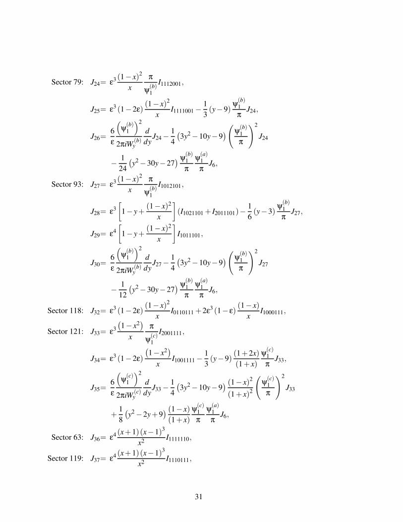
Sector 93: J27= ε3 (1− x)2

x

π

ψ(b)1

I1012101,

J28= ε3

[1− y+

(1− x)2

x

](I1021101 + I2011101)−

1

6(y−3)

ψ(b)1

πJ27,

J29= ε4

[1− y+

(1− x)2

x

]I1011101,

J30=6

ε

(ψ(b)1

)2

2πiW(b)y

d

dyJ27 −

1

4

(3y2 −10y−9

)(

ψ(b)1

π

)2

J27

− 1

12

(y2 −30y−27

) ψ(b)1

π

ψ(a)1

πJ6,

Sector 118: J32= ε3 (1−2ε)(1− x)2

xI0110111 +2ε3 (1− ε)

(1− x)

xI1000111,

Sector 121: J33= ε3

(1− x2

)

x

π

ψ(c)1

I2001111,

J34= ε3 (1−2ε)

(1− x2

)

xI1001111 −

1

3(y−9)

(1+2x)

(1+ x)

ψ(c)1

πJ33,

J35=6

ε

(ψ(c)1

)2

2πiW(c)y

d

dyJ33 −

1

4

(3y2 −10y−9

) (1− x)2

(1+ x)2

(ψ(c)1

π

)2

J33

+1

8

(y2 −2y+9

) (1− x)

(1+ x)

ψ(c)1

π

ψ(a)1

πJ6,

Sector 63: J36= ε4 (x+1)(x−1)3

x2 I1111110,

Sector 119: J37= ε4 (x+1)(x−1)3

x2 I1110111,

31

Page 32

Sector 123: J38= 2ε4

(x2 −1

)

x

[I11011110(−1)− (y−2) I1101111

]− 4

x−1J22,

J39= ε4 (1− y)(1− x)2

xI1101111,

Sector 126: J40= ε4 (x+1)(x−1)3

x2I0111111,

Sector 127: J41= ε4 (1− x)4

x2

π

ψ(b)1

I1111111,

J42= 8ε4 (1− x)2

xI1111111(−1)(−1)−8ε4 (y−2)(1− x)2

xI1111111(−1)0

−8ε4 y(1− x)2

xI11111110(−1)−

8x

(1− x)2

ψ(b)1

πJ41

−4(x−1)

(x2 −2xy+1

)

(x+1)3 J40 −4x2 −2xy+1

(x−1)(x+1)J37

−4x2 −2xy−4x+1

(x−1)(x+1)J36 −

4

3(y+3)

ψ(b)1

πJ27 +

8

3(y+3)

ψ(b)1

πJ24

−(

4+32ε

(1−2ε)

(x4 − yx3 − xy+1

)

(x−1)2 (x+1)2

)J23 −16

(y−1)x

(x−1)2 J22

−8(x−1)

(x2 − xy+ x+1

)

(x+1)3 J19 +4(x−1)2

(y−1)xJ17

+16(x−1)

(x2 − xy+ x+1

)

(x+1)3 J16 −4

3

(6x2 −5xy−7x+6

)

(y−1)xJ14,

J43=6

ε

(ψ(b)1

)2

2πiW(b)y

d

dyJ41 −

1

4

(3y2 −10y−9

)(

ψ(b)1

π

)2

J41 +4y(1− x)

(1+ x)

ψ(b)1

π

ψ(c)1

πJ33

+2

3y(y−9)

(ψ(b)1

π

)2

J27 +2

3y(y−3)

(ψ(b)1

π

)2

J24,

J44= ε4 (1− x)4

x2I1111111(−1)0 −

1

3(2y−3)

ψ(b)1

πJ41 − ε4 (1− x)4

x2I0111111

+ ε4 (1− x)2 (x2 −2xy+1

)

x2I1101111,

J45= ε4 (x−1)2 (x+1)2

x2I11111110(−1)−

(2x2y−9x2 +8xy−6x+2y−9

)

3(x−1)2

ψ(b)1

πJ41

− 2

x−1J36 +

1

2

(1

x+ x− 2

3y

)ψ(b)1

πJ27 −

(1

x+ x− 2

3y

)ψ(b)1

πJ24. (139)

32

Page 33

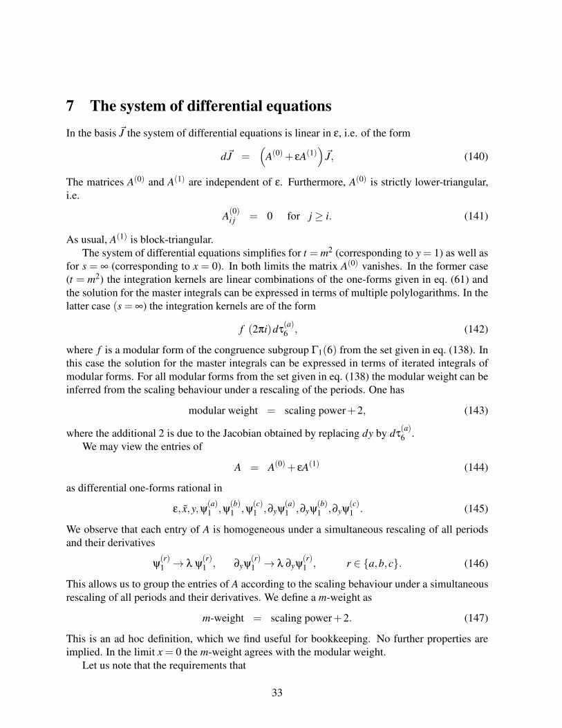
7 The system of differential equations

In the basis ~J the system of differential equations is linear in ε, i.e. of the form

d~J =(

A(0)+ εA(1))~J, (140)

The matrices A(0) and A(1) are independent of ε. Furthermore, A(0) is strictly lower-triangular,i.e.

A(0)i j = 0 for j ≥ i. (141)

As usual, A(1) is block-triangular.The system of differential equations simplifies for t = m2 (corresponding to y = 1) as well as

for s = ∞ (corresponding to x = 0). In both limits the matrix A(0) vanishes. In the former case(t = m2) the integration kernels are linear combinations of the one-forms given in eq. (61) andthe solution for the master integrals can be expressed in terms of multiple polylogarithms. In thelatter case (s = ∞) the integration kernels are of the form

f (2πi)dτ(a)6 , (142)

where f is a modular form of the congruence subgroup Γ1(6) from the set given in eq. (138). Inthis case the solution for the master integrals can be expressed in terms of iterated integrals ofmodular forms. For all modular forms from the set given in eq. (138) the modular weight can beinferred from the scaling behaviour under a rescaling of the periods. One has

modular weight = scaling power+2, (143)

where the additional 2 is due to the Jacobian obtained by replacing dy by dτ(a)6 .

We may view the entries of

A = A(0)+ εA(1) (144)

as differential one-forms rational in

ε, x,y,ψ(a)1 ,ψ

(b)1 ,ψ

(c)1 ,∂yψ

(a)1 ,∂yψ

(b)1 ,∂yψ

(c)1 . (145)

We observe that each entry of A is homogeneous under a simultaneous rescaling of all periodsand their derivatives

ψ(r)1 → λ ψ

(r)1 , ∂yψ

(r)1 → λ ∂yψ

(r)1 , r ∈ {a,b,c}. (146)

This allows us to group the entries of A according to the scaling behaviour under a simultaneousrescaling of all periods and their derivatives. We define a m-weight as

m-weight = scaling power+2. (147)

This is an ad hoc definition, which we find useful for bookkeeping. No further properties areimplied. In the limit x = 0 the m-weight agrees with the modular weight.

Let us note that the requirements that

33

Page 34

- A is linear in ε,

- A(0) is strictly lower-triangular,

- A(0) vanishes for x = 0 or y = 1,

- A(1) reduces to integration kernels for multiple polylogarithms for y = 1,

- A(1) reduces to modular forms for x = 0,

do not fix uniquely the set of master integrals ~J and the matrix A. There is still a “gauge freedom”of transformations left, leaving these conditions intact.

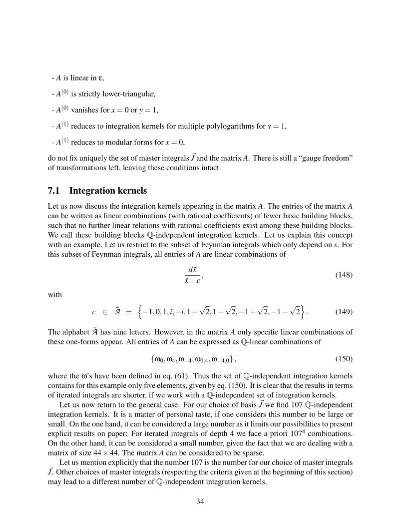
7.1 Integration kernels

Let us now discuss the integration kernels appearing in the matrix A. The entries of the matrix A

can be written as linear combinations (with rational coefficients) of fewer basic building blocks,such that no further linear relations with rational coefficients exist among these building blocks.We call these building blocks Q-independent integration kernels. Let us explain this conceptwith an example. Let us restrict to the subset of Feynman integrals which only depend on s. Forthis subset of Feynman integrals, all entries of A are linear combinations of

dx

x− c, (148)

with

c ∈ A ={−1,0,1, i,−i,1+

√2,1−

√2,−1+

√2,−1−

√2}. (149)

The alphabet A has nine letters. However, in the matrix A only specific linear combinations ofthese one-forms appear. All entries of A can be expressed as Q-linear combinations of

{ω0,ω4,ω−4,ω0,4,ω−4,0} , (150)

where the ω’s have been defined in eq. (61). Thus the set of Q-independent integration kernelscontains for this example only five elements, given by eq. (150). It is clear that the results in termsof iterated integrals are shorter, if we work with a Q-independent set of integration kernels.

Let us now return to the general case. For our choice of basis ~J we find 107 Q-independentintegration kernels. It is a matter of personal taste, if one considers this number to be large orsmall. On the one hand, it can be considered a large number as it limits our possibilities to presentexplicit results on paper: For iterated integrals of depth 4 we face a priori 1074 combinations.On the other hand, it can be considered a small number, given the fact that we are dealing with amatrix of size 44×44. The matrix A can be considered to be sparse.

Let us mention explicitly that the number 107 is the number for our choice of master integrals~J. Other choices of master integrals (respecting the criteria given at the beginning of this section)may lead to a different number of Q-independent integration kernels.

34

Page 35

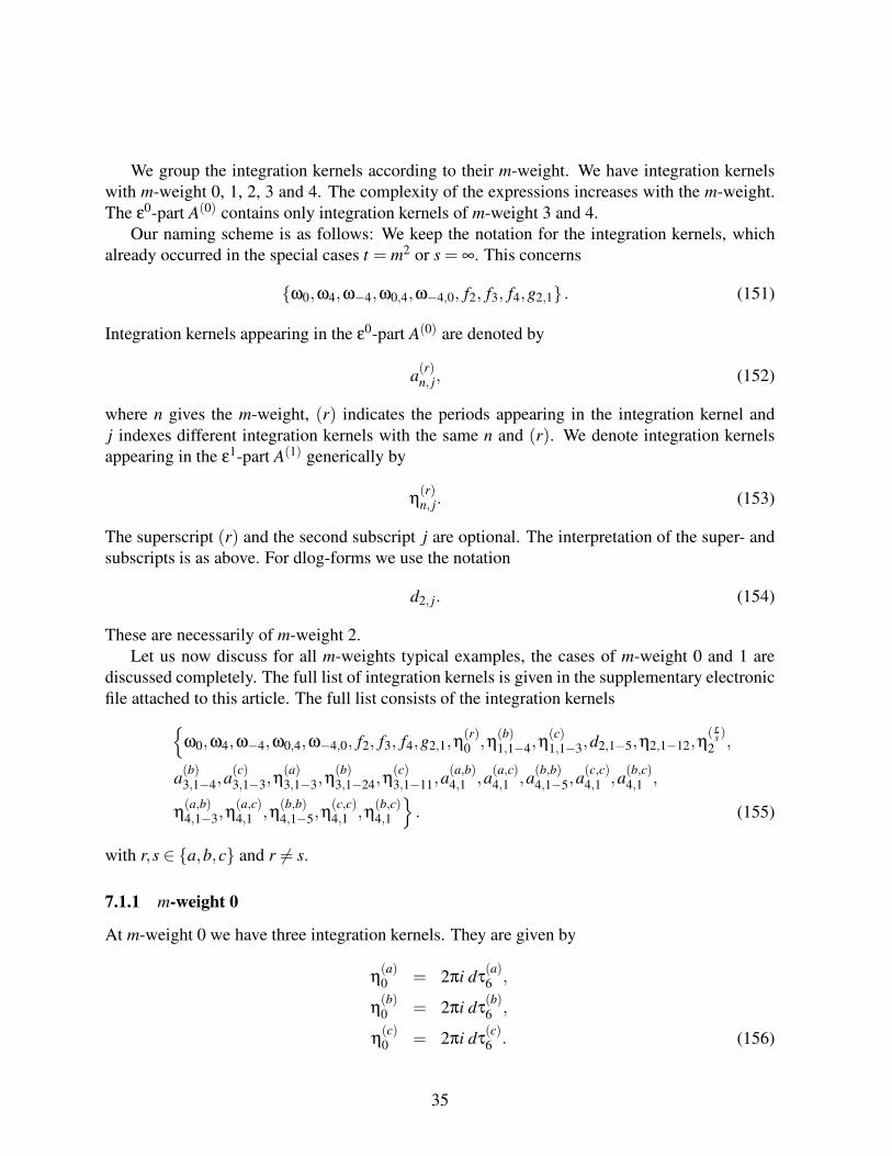
We group the integration kernels according to their m-weight. We have integration kernelswith m-weight 0, 1, 2, 3 and 4. The complexity of the expressions increases with the m-weight.The ε0-part A(0) contains only integration kernels of m-weight 3 and 4.

Our naming scheme is as follows: We keep the notation for the integration kernels, whichalready occurred in the special cases t = m2 or s = ∞. This concerns

{ω0,ω4,ω−4,ω0,4,ω−4,0, f2, f3, f4,g2,1} . (151)

Integration kernels appearing in the ε0-part A(0) are denoted by

a(r)n, j, (152)

where n gives the m-weight, (r) indicates the periods appearing in the integration kernel andj indexes different integration kernels with the same n and (r). We denote integration kernelsappearing in the ε1-part A(1) generically by

η(r)n, j. (153)

The superscript (r) and the second subscript j are optional. The interpretation of the super- andsubscripts is as above. For dlog-forms we use the notation

d2, j. (154)

These are necessarily of m-weight 2.Let us now discuss for all m-weights typical examples, the cases of m-weight 0 and 1 are

discussed completely. The full list of integration kernels is given in the supplementary electronicfile attached to this article. The full list consists of the integration kernels

{ω0,ω4,ω−4,ω0,4,ω−4,0, f2, f3, f4,g2,1,η

(r)0 ,η

(b)1,1−4,η

(c)1,1−3,d2,1−5,η2,1−12,η

( rs)

2 ,

a(b)3,1−4,a

(c)3,1−3,η

(a)3,1−3,η

(b)3,1−24,η

(c)3,1−11,a

(a,b)4,1 ,a

(a,c)4,1 ,a

(b,b)4,1−5,a

(c,c)4,1 ,a

(b,c)4,1 ,

η(a,b)4,1−3,η

(a,c)4,1 ,η

(b,b)4,1−5,η

(c,c)4,1 ,η

(b,c)4,1

}. (155)

with r,s ∈ {a,b,c} and r 6= s.

7.1.1 m-weight 0

At m-weight 0 we have three integration kernels. They are given by

η(a)0 = 2πi dτ

(a)6 ,

η(b)0 = 2πi dτ

(b)6 ,

η(c)0 = 2πi dτ

(c)6 . (156)

35

Page 36

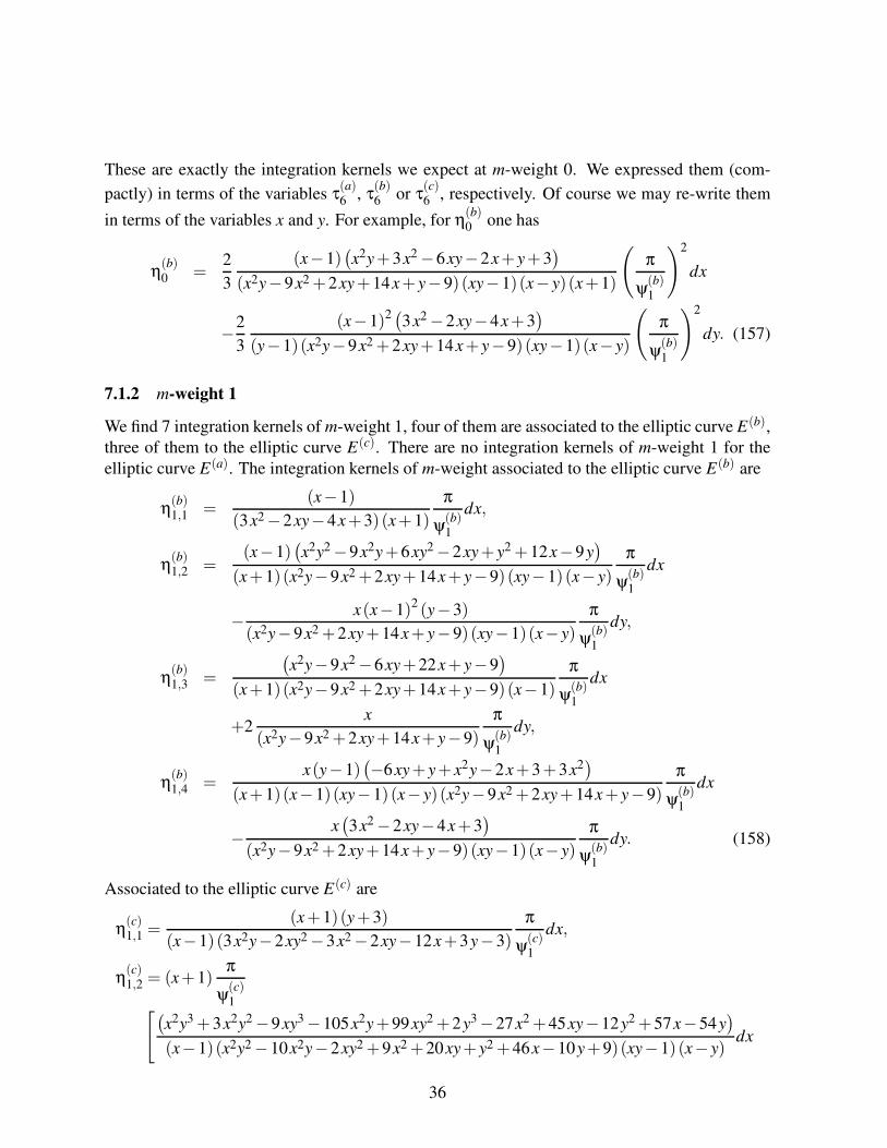
These are exactly the integration kernels we expect at m-weight 0. We expressed them (com-

pactly) in terms of the variables τ(a)6 , τ

(b)6 or τ

(c)6 , respectively. Of course we may re-write them

in terms of the variables x and y. For example, for η(b)0 one has

η(b)0 =

2

3

(x−1)(x2y+3x2 −6xy−2x+ y+3

)

(x2y−9x2 +2xy+14x+ y−9) (xy−1)(x− y)(x+1)

(π

ψ(b)1

)2

dx

−2

3

(x−1)2 (3x2 −2xy−4x+3)

(y−1)(x2y−9x2 +2xy+14x+ y−9) (xy−1)(x− y)

(π

ψ(b)1

)2

dy. (157)

7.1.2 m-weight 1

We find 7 integration kernels of m-weight 1, four of them are associated to the elliptic curve E(b),three of them to the elliptic curve E(c). There are no integration kernels of m-weight 1 for theelliptic curve E(a). The integration kernels of m-weight associated to the elliptic curve E(b) are

η(b)1,1 =

(x−1)

(3x2 −2xy−4x+3) (x+1)

π

ψ(b)1

dx,

η(b)1,2 =

(x−1)(x2y2 −9x2y+6xy2 −2xy+ y2 +12x−9y

)

(x+1)(x2y−9x2 +2xy+14x+ y−9) (xy−1) (x− y)

π

ψ(b)1

dx

− x(x−1)2 (y−3)

(x2y−9x2 +2xy+14x+ y−9) (xy−1)(x− y)

π

ψ(b)1

dy,

η(b)1,3 =

(x2y−9x2 −6xy+22x+ y−9

)

(x+1)(x2y−9x2 +2xy+14x+ y−9) (x−1)

π

ψ(b)1

dx

+2x

(x2y−9x2 +2xy+14x+ y−9)

π

ψ(b)1

dy,

η(b)1,4 =

x(y−1)(−6xy+ y+ x2y−2x+3+3x2

)

(x+1)(x−1)(xy−1) (x− y) (x2y−9x2 +2xy+14x+ y−9)

π

ψ(b)1

dx

− x(3x2 −2xy−4x+3

)

(x2y−9x2 +2xy+14x+ y−9) (xy−1)(x− y)

π

ψ(b)1

dy. (158)

Associated to the elliptic curve E(c) are

η(c)1,1 =

(x+1)(y+3)

(x−1) (3x2y−2xy2 −3x2 −2xy−12x+3y−3)

π

ψ(c)1

dx,

η(c)1,2 = (x+1)

π

ψ(c)1[(

x2y3 +3x2y2 −9xy3 −105x2y+99xy2 +2y3 −27x2 +45xy−12y2 +57x−54y)

(x−1)(x2y2 −10x2y−2xy2 +9x2 +20xy+ y2 +46x−10y+9)(xy−1) (x− y)dx

36

Page 37

+x(3x2y2 −4xy3 −30x2y+38xy2 −2y3 +27x2 −48xy+25y2 +78x−84y−3

)

(y−1)(x2y2 −10x2y−2xy2 +9x2 +20xy+ y2 +46x−10y+9)(x− y) (xy−1)dy

],

η(c)1,3 =

(x+1)2 (y−3)

(x−1) (3x2y−2xy2 −3x2 −2xy−12x+3y−3)√

x2 −6x+1

π

ψ(c)1

dx. (159)

Note that in the last expression the square root is rationalised by using the variable x. An alter-

native form for η(c)1,3 is

η(c)1,3 =− π

ψ(c)1

dx (160)

(y−3)(x2 −2 x−1

)2

(x2 +1)(3 x4y+2 x3y2 −3 x4 −4 x3y+18 x3 +6 x2y−2 x y2 −6 x2 +4 x y−18 x+3y−3),

which is manifestly rational in x, y and ψ(c)1 .

7.1.3 m-weight 2

The integration kernels of m-weight 2 are numerous and we only list a few typical cases. Theintegration kernels for the multiple polylogarithms

ω0, ω4, ω−4, ω0,4, ω−4,0, (161)

defined in eq. (61) belong to this class. Furthermore, the modular forms of modular weight 2clearly belong to this class:

f2 (2πi)dτ(a)6 =

dy

y−1+

dy

y−9− dy

2y,

g2,1 (2πi)dτ(a)6 =

dy

y−1. (162)

The differential one-forms in eq. (161) and eq. (162) are all dlog-forms, depending either on x (oralternatively on x) or y, but not both. There are further dlog-forms, depending on both variablesx and y. These are

d2,1 = d ln(x− y)+d ln(xy−1) ,

d2,2 = d ln(xy−1) ,

d2,3 = d ln(x2 − xy− x+1

),

d2,4 = d ln(3x2 −2xy−4x+3

),

d2,5 = d ln(x2y−9x2 +2xy+14x+ y−9

). (163)

There are six differential one-forms involving ratios of periods, one for each ratio. For example

η( b

a )2 =

1

2

(x+1)

x (x−1)

ψ(b)1

ψ(a)1

dx (164)

37

Page 38

− 1

12

(3x2y2 +2xy3 −90x2y+52xy2 −81x2 +138xy+3y2 +144x−90y−81

)

y (y−1)(y−9)(3x2 −2xy−4x+3)

ψ(b)1

ψ(a)1

dy.

In addition there are 12 differential one-forms of m-weight 2, which do not belong to any classdiscussed up to now. An example is given by

η2,1 =(x−1)

(x+1)(3x2 −2xy−4x+3)dx. (165)

For our choice of master integrals ~J we observe that in the integration kernels of m-weight 2polynomials in denominator occur only as a single power, i.e. there are no higher poles in m-weight 2.

7.1.4 m-weight 3

At m-weight 3 we have first of all the modular form of weight 3 from the sunrise sector

f3 (2πi)dτ(a)6 = 3

ψ(a)1

πdy. (166)

At m-weight 3 we have integration kernels appearing in the ε0-part A(0), an example is given by

a(b)3,1 =

(x2y−3x2 +4xy+ y−3

)(y−1)

(x−1)(3x2 −2xy−4x+3) (x+1)

ψ(b)1

πdx

+

(x2y2 −9x2y+6xy2 −2xy+ y2 +12x−9y

)(y−1)

(x−1)(3x2 −2xy−4x+3) (x+1)

(∂yψ

(b)1

π

)dx

− x(y−1)

(3x2 −2xy−4x+3)

ψ(b)1

πdy− (y−3)x(y−1)

(3x2 −2xy−4x+3)

(∂yψ

(b)1

π

)dy. (167)

In addition, there are integration kernels of m-weight 3 in the ε1-part A(1), an example is givenby

η(b)3,1 = 4

(y−1)

(3x2 −2xy−4x+3)

ψ(b)1

πdx− (x−1)(x+1)

(3x2 −2xy−4x+3)

ψ(b)1

πdy. (168)

7.1.5 m-weight 4

At m-weight 4 we have one modular form of weight 4 from the sunrise sector

f4 (2πi)dτ(a)6 = − (y+3)4

8y(y−1)(y−9)

(ψ(a)1

π

)2

dy. (169)

38

Page 39

In addition, we encounter integration kernels appearing in the ε0-part A(0). An example is givenby

a(b,b)4,3 = −2

3

(y−3)(y−1)N(b,b)4,3,1

(x−1)(x+1)(3x2 −2xy−4x+3)2

(ψ(b)1

π

)2

dx

+4

3

x(y−3)(y−1)2N(b,b)4,3,2

(x−1)(x+1)(3x2 −2xy−4x+3)2

(ψ(b)1

π

)(∂yψ

(b)1

π

)dx

+2

3

xN(b,b)4,3,3

(3x2 −2xy−4x+3)2

(ψ(b)1

π

)2

dy

+4

3

x(y−3)(y−1)N(b,b)4,3,4

(3x2 −2xy−4x+3)2

(ψ(b)1

π

)(∂yψ

(b)1

π

)dy, (170)

with

N(b,b)4,3,1 = 3x4y−2x3y2 +9x4 +20x3y−20x2y2 −18x3 +2x2y−2xy2 −6x2 +20xy−18x

+3y+9,

N(b,b)4,3,2 = x2y2 −24x2y+18xy2 −9x2 +16xy+ y2 +30x−24y−9,

N(b,b)4,3,3 = 9x2y2 −8xy3 −6x2y+10xy2 −27x2 −20xy+9y2 +66x−6y−27,

N(b,b)4,3,4 = 3x2y−4xy2 +9x2 −2xy−18x+3y+9. (171)

Finally, there are integration kernels of m-weight 4 appearing in the ε1-part A(1). An example isgiven by

η(b,b)4,3 =

1

9

1

(xy−1)(x− y) (3x2 −2xy−4x+3)2(x2y−9x2 +2xy+14x+ y−9)

(y−1)P(b,b)4,3,1

(x−1)(x+1)dx−

(x−1)2P(b,b)4,3,2

(y−1)dy

(

ψ(b)1

π

)2

, (172)

with

P(b,b)4,3,1 = 27x8y4 −75x7y5 +48x6y6 −243x8y3 +909x7y4 −946x6y5 +288x5y6 +2673x8y2

−7182x7y3 +5914x6y4 −1237x5y5 −288x4y6 −729x8y−6966x7y2 +17592x6y3

−11277x5y4 +1828x4y5 +288x3y6 −3159x7y+22392x6y2 −36146x5y3

+15766x4y4 −1237x3y5 +48x2y6 +729x7 +13770x6y−41898x5y2 +43510x4y3

−11277x3y4 −946x2y5 +1134x6 −25929x5y+52590x4y2 −36146x3y3

+5914x2y4 −75xy5 −9369x5 +30942x4y−41898x3y2 +17592x2y3 +909xy4

+15012x4 −25929x3y+22392x2y2 −7182xy3 +27y4 −9369x3 +13770x2y

39

Page 40

−6966xy2 −243y3 +1134x2 −3159xy+2673y2 +729x−729y,

P(b,b)4,3,2 = 27x6y4 −45x5y5 −30x4y6 +48x3y7 +243x6y3 −603x5y4 +828x4y5 −460x3y6

+729x6y2 −2592x5y3 +1899x4y4 −126x3y5 −30x2y6 +729x6y−4212x5y2

+8085x4y3 −4686x3y4 +828x2y5 −2187x5y+6741x4y2 −8864x3y3 +1899x2y4

−45xy5 −729x5 +7587x4y−9708x3y2 +8085x2y3 −603xy4 +810x4 −9954x3y

+6741x2y2 −2592xy3 +27y4 −810x3 +7587x2y−4212xy2 +243y3 +810x2

−2187xy+729y2 −729x+729y. (173)

7.2 Singularities

As already mentioned, the integration kernels are rational in

ε, x,y,ψ(a)1 ,ψ

(b)1 ,ψ

(c)1 ,∂yψ

(a)1 ,∂yψ

(b)1 ,∂yψ

(c)1 . (174)

In the next section we will choose as boundary point the point (x,y) = (0,1) (or equivalently(s, t) = (∞,m2)). This motivates the introduction of the variable

y = 1− y. (175)

Our boundary point is then (x, y) = (0,0).Of particular interest are the polynomials in x and y appearing in the denominator of the

integration kernels. There aren’t too many. Polynomials, which only depend on x are (comparewith eq. (61))

Q1 = x,

Q2 = x−1,

Q3 = x+1,

Q4 = x2 +1,

Q5 = x2 −2x−1,

Q6 = x2 +2x−1. (176)

Polynomials, which only depend on y are

Q7 = y,

Q8 = y−1,

Q9 = y+8. (177)

Polynomials, which depend on x and y are

Q10 = x2 − x y− y+1,

Q11 = −x2y+ x2 + x y+1,

40

Page 41

Q12 = x4 − x3y+2 x2 + x y+1,

Q13 = 3 x4 −2 x3y+6 x2 +2 x y+3,

Q14 = x4y+8 x4 −4 x3y+2 x2y+16 x2 +4 x y+ y+8,

Q15 = 3 x4y−2 x3y2 −16 x3 +6 x2y+2 x y2 +16 x+3 y,

Q16 = x2y−8 x+ y+8,

Q17 = x2y+8 x2 +8 x+ y. (178)

It is helpful to have corresponding expressions in (s, t)-space: The polynomials Q10 and Q11

appear when the expression st +(m2 − t)2 is expressed in the variables x and y:

st +(m2 − t

)2=

Q10Q11

x (x−1)(x+1). (179)

The polynomial Q12 is related to

m2 − t − s = − Q12

x (x−1)(x+1). (180)

The polynomials Q13 and Q14 are related to the elliptic curve E(b). We have

3s+2t −2m2 =Q13

x (x−1)(x+1),

s(t −9m2)+4m2 (m2 − t

)= − Q14

x (x−1)(x+1), (181)

The polynomial Q13 enters through eq. (117) or eq. (118), the polynomial Q14 appears in the

Picard-Fuchs operator for ψ(b)1 in eq. (115).

The polynomials Q15, Q16 and Q17 are related to the elliptic curve E(c). We have

3s(t −m2

)+2(t −m2

)2+16m4 = − Q15

x (x−1)(x+1),

s(t −9m2

)(t −m2

)−64m6 =

Q16Q17

x(x−1)(x+1). (182)

The polynomial Q15 enters through eq. (127) or eq. (128), the polynomials Q16 and Q17 appears

in the Picard-Fuchs operator for ψ(c)1 in eq. (125).

Note that the polynomials Q1, Q7, Q15 and Q17 vanish for (x, y) = (0,0).

8 Boundary conditions and boundary constants

We integrate the system of differential equations starting from the point (x,y) = (0,1) (corre-sponding to s = ∞ and t = m2). In order to do so, we need the boundary constants at this point.

41

Page 42

The boundary constants may be expressed as a linear combination of transcendental constants.A basis of these transcendental constants up to weight four is given by [113]

w = 1 : ln(2),

w = 2 : ζ2, ln2(2),

w = 3 : ζ3, ζ2 ln(2), ln3(2),

w = 4 : ζ4, Li4

(1

2

), ζ3 ln(2), ζ2 ln2(2), ln4(2). (183)

The boundary constants for the master integrals, which are products of one-loop integrals areeasily computed. For example, the master integral J1 is a product of two tadpole integrals. Thetadpole integral is given by

Tν

(D,m2,µ2

)= eγE ε

(µ2)ν−D

2

∫dDk

iπD2

1

(−k2 +m2)ν = eγE ε Γ

(ν− D

2

)

Γ(ν)

(m2

µ2

)D2 −ν

. (184)

For D = 2−2ε, µ = m and ν = 1 we have

T1 (2−2ε) = eγE εΓ(ε) =1

ε

[1+

1

2ζ2ε2 − 1

3ζ3ε3 +

9

16ζ4ε4 +O

(ε5)]

. (185)

In addition we need to calculate explicitly the boundary constants for the integrals, which neitherdepend on s nor on t. There are two such integrals: J1 (which is also a product of tadpoles) andJ8 (the sunrise integral at the pseudo-threshold). For the latter we proceed as follows: We startfrom the Feynman parameter integral. We have

J8 = 6ε2e2γE εΓ(1+2ε)

1∫

0

dx2

1∫

0

dx4

[1

x2 −1− 1

x2 +1

][1

x4 +1− 1

x4 + x2

]

×(x2 +1)ε (x4 +1)−2ε (x4 + x2)−2ε

(x4 +

x2

x2 +1

)ε

. (186)

At each order in ε, the x4-integration is easily performed, resulting in multiple polylogarithmsG(z1, ...,zk;x2), where the remaining variable x2 appears in the argument list z1, ..., zk. With themethods of [97, 114] we convert all polylogarithms to a form, where the parameters z1, ..., zk donot depend on x2, the simplest example is given by

G(−x2;1) = G(−1;x2)−G(0;x2) . (187)

We may then perform the integration over the variable x2. The resulting expressions may besimplified with the help of the PSLQ-algorithm [115].

For all other master integrals we obtain the boundary constants from the behaviour at a spe-cific point, where the master integral vanishes or reduces to simpler integrals. The specificpoints which we consider are (x,y) = (0,1), (x,y) = (1,1) and (x,y) = (−1,1). For the points(x,y) = (1,1) or (x,y) = (−1,1) we integrate the system along y = 1 from x = 0 to x =±1. Fory = 1 we only obtain multiple polylogarithms. We evaluate the multiple polylogarithms to highprecision [97] and use the PSLQ-algorithm to extract the transcendental constants.

The complete list of boundary constants is given in appendix D.

42

Page 43

9 Results

For all basis integrals we write

Jk =∞

∑j=0

ε jJ( j)k . (188)

Obviously, the basis of master integrals involves also rather simple sub-topologies, where resultsfor these integrals are known in the literature [116–118].

9.1 Integrals, which do not depend on s nor t

The integrals J1 and J8 are independent of s and t (or equivalently independent of x and y). Theintegrals J1 and J8 are given by

J1 = 1+ζ2ε2 − 2

3ζ3ε3 +

7

4ζ4ε4 +O

(ε5),

J8 = 6ζ2ε2 + ε3 (21ζ3 −36ζ2 ln2)+ ε4

(144Li4

(1

2

)−78ζ4 +72ζ2 ln2 (2)+6ln4 (2)

)

+O

(ε5). (189)

9.2 Integrals, which only depend on s

The integrals J2 − J5, J9 − J13, J15 − J16, J18 − J23, J32, J36 − J37 and J40 depend only on thevariable s. We may group them into three categories. The first category contains most of theseintegrals. More concretely, the integrals in the first category are given by J2 − J5, J9 − J11,J15−J16, J18−J21, J23, J32, J37 and J40. These integrals are most naturally expressed in terms ofharmonic polylogarithms in the variable x.

The integrals J12 and J13 belong to the second category. These integrals have a singular pointat s = −4m2 but not at s = 4m2. These two integrals are most naturally expressed in terms ofharmonic polylogarithms in the variable x′.

The integrals J22 and J36 belong to the third category. These integrals have a singular point ats =−4m2 and at s = 4m2. These two integrals are expressed in terms of multiple polylogarithmsin the variable x.

9.2.1 Integrals, which are expressed in the variable x

The integrals J2 − J5, J9 − J11, J15 − J16, J18 − J21, J23, J32, J37 and J40 are most naturally ex-pressed in terms of harmonic polylogarithms in the variable x.

J(0)2 = 0,

J(1)2 = −G(0;x) ,

J(2)2 = 2G(−1,0;x)−G(0,0;x)+ζ2,

43

Page 44

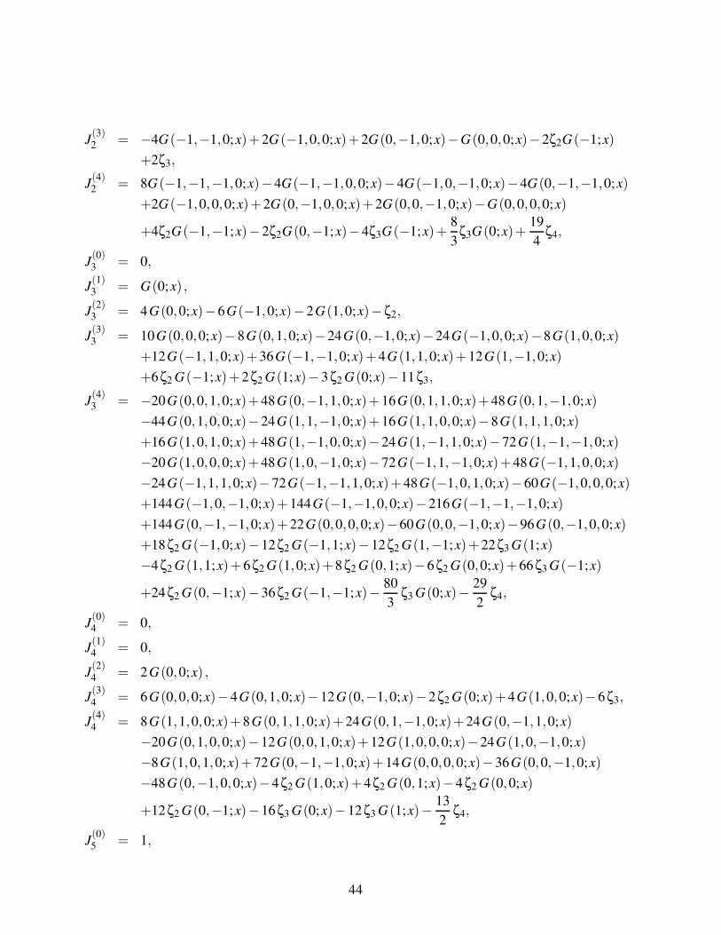
J(3)2 = −4G(−1,−1,0;x)+2G(−1,0,0;x)+2G(0,−1,0;x)−G(0,0,0;x)−2ζ2G(−1;x)

+2ζ3,

J(4)2 = 8G(−1,−1,−1,0;x)−4G(−1,−1,0,0;x)−4G(−1,0,−1,0;x)−4G(0,−1,−1,0;x)

+2G(−1,0,0,0;x)+2G(0,−1,0,0;x)+2G(0,0,−1,0;x)−G(0,0,0,0;x)

+4ζ2G(−1,−1;x)−2ζ2G(0,−1;x)−4ζ3G(−1;x)+8

3ζ3G(0;x)+

19

4ζ4,

J(0)3 = 0,

J(1)3 = G(0;x) ,

J(2)3 = 4G(0,0;x)−6G(−1,0;x)−2G(1,0;x)−ζ2,

J(3)3 = 10G(0,0,0;x)−8G(0,1,0;x)−24G(0,−1,0;x)−24G(−1,0,0;x)−8G(1,0,0;x)

+12G(−1,1,0;x)+36G(−1,−1,0;x)+4G(1,1,0;x)+12G(1,−1,0;x)

+6ζ2 G(−1;x)+2ζ2 G(1;x)−3ζ2 G(0;x)−11ζ3,

J(4)3 = −20G(0,0,1,0;x)+48G(0,−1,1,0;x)+16G(0,1,1,0;x)+48G(0,1,−1,0;x)

−44G(0,1,0,0;x)−24G(1,1,−1,0;x)+16G(1,1,0,0;x)−8G(1,1,1,0;x)

+16G(1,0,1,0;x)+48G(1,−1,0,0;x)−24G(1,−1,1,0;x)−72G(1,−1,−1,0;x)

−20G(1,0,0,0;x)+48G(1,0,−1,0;x)−72G(−1,1,−1,0;x)+48G(−1,1,0,0;x)

−24G(−1,1,1,0;x)−72G(−1,−1,1,0;x)+48G(−1,0,1,0;x)−60G(−1,0,0,0;x)

+144G(−1,0,−1,0;x)+144G(−1,−1,0,0;x)−216G(−1,−1,−1,0;x)

+144G(0,−1,−1,0;x)+22G(0,0,0,0;x)−60G(0,0,−1,0;x)−96G(0,−1,0,0;x)

+18ζ2 G(−1,0;x)−12ζ2 G(−1,1;x)−12ζ2 G(1,−1;x)+22ζ3 G(1;x)

−4ζ2 G(1,1;x)+6ζ2 G(1,0;x)+8ζ2 G(0,1;x)−6ζ2 G(0,0;x)+66ζ3 G(−1;x)

+24ζ2 G(0,−1;x)−36ζ2 G(−1,−1;x)− 80

3ζ3 G(0;x)− 29

2ζ4,

J(0)4 = 0,

J(1)4 = 0,

J(2)4 = 2G(0,0;x) ,

J(3)4 = 6G(0,0,0;x)−4G(0,1,0;x)−12G(0,−1,0;x)−2ζ2 G(0;x)+4G(1,0,0;x)−6ζ3,

J(4)4 = 8G(1,1,0,0;x)+8G(0,1,1,0;x)+24G(0,1,−1,0;x)+24G(0,−1,1,0;x)

−20G(0,1,0,0;x)−12G(0,0,1,0;x)+12G(1,0,0,0;x)−24G(1,0,−1,0;x)

−8G(1,0,1,0;x)+72G(0,−1,−1,0;x)+14G(0,0,0,0;x)−36G(0,0,−1,0;x)

−48G(0,−1,0,0;x)−4ζ2 G(1,0;x)+4ζ2 G(0,1;x)−4ζ2 G(0,0;x)

+12ζ2 G(0,−1;x)−16ζ3 G(0;x)−12ζ3 G(1;x)− 13

2ζ4,

J(0)5 = 1,

44

Page 45

J(1)5 = −2G(1;x)+G(0;x) ,

J(2)5 = 4G(1,1;x)−2G(1;x)G(0;x)+G(0,0;x) ,

J(3)5 = −8G(1,1,1;x)+4G(1,1;x)G(0;x)−2G(1;x)G(0,0;x)+G(0,0,0;x)− 8

3ζ3,

J(4)5 = 16G(1,1,1,1;x)−8G(1,1,1;x)G(0;x)+4G(1,1;x)G(0,0;x)−2G(1;x)G(0,0,0;x)

+G(0,0,0,0;x)+16

3ζ3G(1,x)− 8

3ζ3G(0;x)−3ζ4,

J(0)9 = 0,

J(1)9 = 0,

J(2)9 = G(0,0;x) ,

J(3)9 = G(0,0,0;x)−2G(0,−1,0;x)−ζ2 G(0;x)−3ζ3,

J(4)9 = G(0,0,0,0;x)−2G(0,0,−1,0;x)−2G(0,−1,0,0;x)+4G(0,−1,−1,0;x)

+2ζ2 G(0,−1;x)−2ζ3 G(0;x)− 5

4ζ4,

J(0)10 = 0,

J(1)10 = 0,

J(2)10 = 0,

J(3)10 = 2G(0,0,0;x)−4G(1,0,0;x)−4ζ3,

J(4)10 = 4G(0,1,0,0;x)−4G(0,0,1,0;x)+6G(0,0,0,0;x)−12G(0,0,−1,0;x)

−12G(1,0,0,0;x)+24G(1,0,−1,0;x)+8G(1,0,1,0;x)−8G(1,1,0,0;x)

−2ζ2 G(0,0;x)+4ζ2 G(1,0;x)+12ζ3 G(1;x)−6ζ3 G(0;x)+4ζ4,

J(0)11 = 0,

J(1)11 = −G(0;x) ,

J(2)11 = 2G(−1,0;x)−3G(0,0;x)+2G(1;x)G(0;x)+ζ2,

J(3)11 = 6G(−1,0,0;x)−4G(−1,−1,0;x)+4G(0,−1,0;x)−7G(0,0,0;x)

+6G(1;x)G(0,0;x)−4G(0;x)G(1,1;x)−4G(−1,0;x)G(1;x)+2ζ2G(0;x)

−2ζ2G(−1;x)−2ζ2G(1;x)+2ζ3,

J(4)11 = 12G(0,−1,0,0;x)−15G(0,0,0,0;x)+8G(0,0,−1,0;x)−8G(0,−1,−1,0;x)

+14G(−1,0,0,0;x)−8G(−1,0,−1,0;x)−12G(−1,−1,0,0;x)

+8G(−1,−1,−1,0;x)+8G(0;x)G(1,1,1;x)−12G(1,1;x)G(0,0;x)

+14G(1;x)G(0,0,0;x)−8G(0,−1,0;x)G(1;x)−12G(−1,0,0;x)G(1;x)

+8G(−1,−1,0;x)G(1;x)+8G(1,1;x)G(−1,0;x)+4ζ2G(1,1;x)+4ζ2G(0,0;x)

+4ζ2G(−1,−1;x)+4ζ2G(−1;x)G(1;x)−4ζ2G(−1;x)G(0;x)−4ζ2G(1;x)G(0;x)

45

Page 46

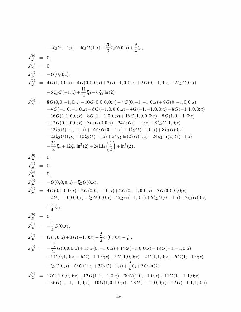
−4ζ3G(−1;x)−4ζ3G(1;x)+20

3ζ3G(0;x)+

9

4ζ4,

J(0)15 = 0,

J(1)15 = 0,

J(2)15 = −G(0,0;x) ,

J(3)15 = 4G(1,0,0;x)−4G(0,0,0;x)+2G(−1,0,0;x)+2G(0,−1,0;x)−2ζ2 G(0;x)

+6ζ2 G(−1;x)+11

2ζ3 −6ζ2 ln(2) ,

J(4)15 = 8G(0,0,−1,0;x)−10G(0,0,0,0;x)−4G(0,−1,−1,0;x)+8G(0,−1,0,0;x)

−4G(−1,0,−1,0;x)+8G(−1,0,0,0;x)−4G(−1,−1,0,0;x)−8G(−1,1,0,0;x)

−16G(1,1,0,0;x)−8G(1,−1,0,0;x)+16G(1,0,0,0;x)−8G(1,0,−1,0;x)

+12G(0,1,0,0;x)−3ζ2 G(0,0;x)−24ζ2 G(1,−1;x)+8ζ2 G(1,0;x)

−12ζ2 G(−1,−1;x)+16ζ2 G(0,−1;x)+4ζ2 G(−1,0;x)+8ζ3 G(0;x)

−22ζ3 G(1;x)+10ζ3 G(−1;x)+24ζ2 ln(2) G(1;x)−24ζ2 ln(2) G(−1;x)

−23

2ζ4 +12ζ2 ln2 (2)+24Li4

(1

2

)+ ln4 (2) ,

J(0)16 = 0,

J(1)16 = 0,

J(2)16 = 0,

J(3)16 = −G(0,0,0;x)−ζ2 G(0;x) ,

J(4)16 = 4G(0,1,0,0;x)+2G(0,0,−1,0;x)+2G(0,−1,0,0;x)−3G(0,0,0,0;x)

−2G(−1,0,0,0;x)−ζ2 G(0,0;x)−2ζ2 G(−1,0;x)+6ζ2 G(0,−1;x)+2ζ3 G(0;x)

+1

4ζ4,

J(0)18 = 0,

J(1)18 = −1

2G(0;x) ,

J(2)18 = G(1,0;x)+3G(−1,0;x)− 5

2G(0,0;x)−ζ2,

J(3)18 = −17

2G(0,0,0;x)+15G(0,−1,0;x)+14G(−1,0,0;x)−18G(−1,−1,0;x)

+5G(0,1,0;x)−6G(−1,1,0;x)+5G(1,0,0;x)−2G(1,1,0;x)−6G(1,−1,0;x)

−ζ2 G(0;x)−ζ2 G(1;x)+3ζ2 G(−1;x)+9

4ζ3 +3ζ2 ln(2) ,

J(4)18 = 17G(1,0,0,0;x)+12G(1,1,−1,0;x)−30G(1,0,−1,0;x)+12G(1,−1,1,0;x)

+36G(1,−1,−1,0;x)−10G(1,0,1,0;x)−28G(−1,1,0,0;x)+12G(−1,1,1,0;x)

46

Page 47

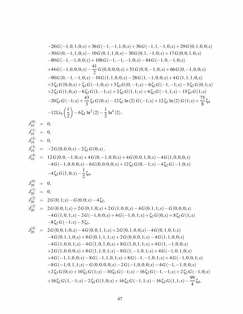
−28G(−1,0,1,0;x)+36G(−1,−1,1,0;x)+36G(−1,1,−1,0;x)+29G(0,1,0,0;x)

−30G(0,−1,1,0;x)−10G(0,1,1,0;x)−30G(0,1,−1,0;x)+17G(0,0,1,0;x)

−80G(−1,−1,0,0;x)+108G(−1,−1,−1,0;x)−84G(−1,0,−1,0;x)

+44G(−1,0,0,0;x)− 41

2G(0,0,0,0;x)+51G(0,0,−1,0;x)+66G(0,−1,0,0;x)

−90G(0,−1,−1,0;x)−10G(1,1,0,0;x)−28G(1,−1,0,0;x)+4G(1,1,1,0;x)

+3ζ2 G(0,0;x)+ζ2 G(−1,0;x)+3ζ2 G(0,−1;x)−6ζ2 G(−1,−1;x)−5ζ2 G(0,1;x)

+2ζ2 G(1,0;x)−6ζ2 G(1,−1;x)+2ζ2 G(1,1;x)+6ζ2 G(−1,1;x)−15ζ3 G(1;x)

−20ζ3 G(−1;x)+43

3ζ3 G(0;x)−12ζ2 ln(2) G(−1;x)+12ζ2 ln(2) G(1;x)+

75

8ζ4

−12Li4

(1

2

)−6ζ2 ln2 (2)− 1

2ln4 (2) ,

J(0)19 = 0,

J(1)19 = 0,

J(2)19 = 0,

J(3)19 = −2G(0,0,0;x)−2ζ2 G(0;x) ,

J(4)19 = 12G(0,0,−1,0;x)+4G(0,−1,0,0;x)+4G(0,0,1,0;x)−4G(1,0,0,0;x)

−4G(−1,0,0,0;x)−6G(0,0,0,0;x)+12ζ2 G(0,−1;x)−4ζ2 G(−1,0;x)

−4ζ2 G(1,0;x)− 1

2ζ4,

J(0)20 = 0,

J(1)20 = 0,

J(2)20 = 2G(0,1;x)−G(0,0;x)−4ζ2,

J(3)20 = 2G(0,0,1;x)+2G(0,1,0;x)+2G(1,0,0;x)−4G(0,1,1;x)−G(0,0,0;x)

−4G(1,0,1;x)−2G(−1,0,0;x)+4G(−1,0,1;x)+ζ2 G(0;x)+8ζ2 G(1;x)

−8ζ2 G(−1;x)−5ζ3,

J(4)20 = 2G(0,0,1,0;x)−4G(0,0,1,1;x)+2G(0,1,0,0;x)−4G(0,1,0,1;x)

−4G(0,1,1,0;x)+8G(0,1,1,1;x)+2G(0,0,0,1;x)−4G(1,1,0,0;x)

−4G(1,0,0,1;x)−4G(1,0,1,0;x)+8G(1,0,1,1;x)+4G(1,−1,0,0;x)

+2G(1,0,0,0;x)+8G(1,1,0,1;x)−8G(1,−1,0,1;x)+4G(−1,0,1,0;x)

+4G(−1,1,0,0;x)−8G(−1,1,0,1;x)+8G(−1,−1,0,1;x)+4G(−1,0,0,1;x)

−8G(−1,0,1,1;x)−G(0,0,0,0;x)−2G(−1,0,0,0;x)−4G(−1,−1,0,0;x)

+2ζ3 G(0;x)+10ζ3 G(1;x)−10ζ3 G(−1;x)−16ζ2 G(−1,−1;x)+2ζ2 G(−1,0;x)

+16ζ2 G(1,−1;x)−2ζ2 G(1,0;x)+16ζ2 G(−1,1;x)−16ζ2 G(1,1;x)− 99

4ζ4,

47

Page 48

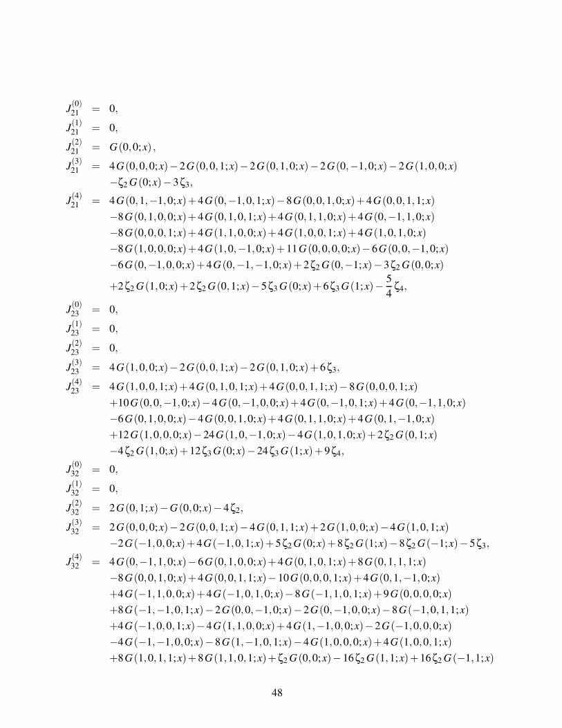
J(0)21 = 0,

J(1)21 = 0,

J(2)21 = G(0,0;x) ,

J(3)21 = 4G(0,0,0;x)−2G(0,0,1;x)−2G(0,1,0;x)−2G(0,−1,0;x)−2G(1,0,0;x)

−ζ2 G(0;x)−3ζ3,

J(4)21 = 4G(0,1,−1,0;x)+4G(0,−1,0,1;x)−8G(0,0,1,0;x)+4G(0,0,1,1;x)

−8G(0,1,0,0;x)+4G(0,1,0,1;x)+4G(0,1,1,0;x)+4G(0,−1,1,0;x)

−8G(0,0,0,1;x)+4G(1,1,0,0;x)+4G(1,0,0,1;x)+4G(1,0,1,0;x)

−8G(1,0,0,0;x)+4G(1,0,−1,0;x)+11G(0,0,0,0;x)−6G(0,0,−1,0;x)

−6G(0,−1,0,0;x)+4G(0,−1,−1,0;x)+2ζ2 G(0,−1;x)−3ζ2 G(0,0;x)

+2ζ2 G(1,0;x)+2ζ2 G(0,1;x)−5ζ3 G(0;x)+6ζ3 G(1;x)− 5

4ζ4,

J(0)23 = 0,

J(1)23 = 0,

J(2)23 = 0,

J(3)23 = 4G(1,0,0;x)−2G(0,0,1;x)−2G(0,1,0;x)+6ζ3,

J(4)23 = 4G(1,0,0,1;x)+4G(0,1,0,1;x)+4G(0,0,1,1;x)−8G(0,0,0,1;x)

+10G(0,0,−1,0;x)−4G(0,−1,0,0;x)+4G(0,−1,0,1;x)+4G(0,−1,1,0;x)

−6G(0,1,0,0;x)−4G(0,0,1,0;x)+4G(0,1,1,0;x)+4G(0,1,−1,0;x)

+12G(1,0,0,0;x)−24G(1,0,−1,0;x)−4G(1,0,1,0;x)+2ζ2 G(0,1;x)

−4ζ2 G(1,0;x)+12ζ3 G(0;x)−24ζ3 G(1;x)+9ζ4,

J(0)32 = 0,

J(1)32 = 0,

J(2)32 = 2G(0,1;x)−G(0,0;x)−4ζ2,

J(3)32 = 2G(0,0,0;x)−2G(0,0,1;x)−4G(0,1,1;x)+2G(1,0,0;x)−4G(1,0,1;x)

−2G(−1,0,0;x)+4G(−1,0,1;x)+5ζ2 G(0;x)+8ζ2 G(1;x)−8ζ2 G(−1;x)−5ζ3,

J(4)32 = 4G(0,−1,1,0;x)−6G(0,1,0,0;x)+4G(0,1,0,1;x)+8G(0,1,1,1;x)

−8G(0,0,1,0;x)+4G(0,0,1,1;x)−10G(0,0,0,1;x)+4G(0,1,−1,0;x)

+4G(−1,1,0,0;x)+4G(−1,0,1,0;x)−8G(−1,1,0,1;x)+9G(0,0,0,0;x)

+8G(−1,−1,0,1;x)−2G(0,0,−1,0;x)−2G(0,−1,0,0;x)−8G(−1,0,1,1;x)

+4G(−1,0,0,1;x)−4G(1,1,0,0;x)+4G(1,−1,0,0;x)−2G(−1,0,0,0;x)

−4G(−1,−1,0,0;x)−8G(1,−1,0,1;x)−4G(1,0,0,0;x)+4G(1,0,0,1;x)

+8G(1,0,1,1;x)+8G(1,1,0,1;x)+ζ2 G(0,0;x)−16ζ2 G(1,1;x)+16ζ2 G(−1,1;x)

48

Page 49

−6ζ2 G(0,1;x)−10ζ2 G(1,0;x)+16ζ2 G(1,−1;x)−16ζ2 G(−1,−1;x)

+8ζ2 G(0,−1;x)+2ζ2 G(−1,0;x)−10ζ3 G(−1;x)+7ζ3 G(0;x)+10ζ3 G(1;x)

−139

4ζ4,

J(0)37 = 0,

J(1)37 = 0,

J(2)37 = 0,

J(3)37 = 0,

J(4)37 = −6G(0,0,0,0;x)+6G(0,0,0,1;x)+4G(0,0,1,0;x)+2G(0,1,0,0;x)

−4ζ2 G(0,0;x) ,

J(0)40 = 0,

J(1)40 = 0,

J(2)40 = 0,

J(3)40 = 0,

J(4)40 = −G(0,0,0,0;x)−8G(0,0,−1,0;x)+6G(0,0,0,1;x)+4G(0,1,0,0;x)

−4ζ2 G(0,0;x)−2ζ3 G(0;x)−3ζ4. (190)

9.2.2 Integrals, which are expressed in the variable x′

The integrals J12 − J13 are most naturally expressed in terms of harmonic polylogarithms in thevariable x′.

J(0)12 = 0,

J(1)12 = 0,

J(2)12 = G

(0,0;x′

)−2G

(0,−1;x′

)+ζ2,

J(3)12 = 4G

(0,0,0;x′

)−8G

(0,0,−1;x′

)−2G

(0,−1,0;x′

)+4G

(0,−1,−1;x′

)

−4G(1,0,0;x′

)+8G

(1,0,−1;x′

)+4G

(−1,0,−1;x′

)−2G

(−1,0,0;x′

)

+2ζ2 G(0;x′)−4ζ2 G

(1;x′)−2ζ2 G

(−1;x′

)−4ζ3,

J(4)12 = 10G

(0,0,0,0;x′

)−20G

(0,0,0,−1;x′

)−8G

(0,0,−1,0;x′

)+16G

(0,0,−1,−1;x′

)

−32G(1,1,0,−1;x′

)+4G

(−1,−1,0,0;x′

)−16G

(1,0,−1,−1;x′

)

−8G(−1,−1,0,−1;x′

)+16G

(0,−1,0,−1;x′

)−8G

(0,−1,−1,−1;x′

)

−8G(0,−1,0,0;x′

)+4G

(0,−1,−1,0;x′

)−12G

(0,1,0,0;x′

)−16G

(1,0,0,0;x′

)

−8G(−1,0,0,0;x′

)+32G

(1,0,0,−1;x′

)+8G

(1,0,−1,0;x′

)+8G

(1,−1,0,0;x′

)

−16G(1,−1,0,−1;x′

)+24G

(0,1,0,−1;x′

)+8G

(−1,1,0,0;x′

)

−16G(−1,1,0,−1;x′

)+16G

(1,1,0,0;x′

)+16G

(−1,0,0,−1;x′

)

49

Page 50

+4G(−1,0,−1,0;x′

)−8G

(−1,0,−1,−1;x′

)−6ζ2 G

(0,−1;x′

)+3ζ2 G

(0,0;x′

)

−12ζ2 G(0,1;x′

)+16ζ2 G

(1,1;x′

)+8ζ2 G

(1,−1;x′

)−8ζ2 G

(1,0;x′

)

−4ζ2 G(−1,0;x′

)+8ζ2 G

(−1,1;x′

)+4ζ2 G

(−1,−1;x′

)+16ζ3 G

(1;x′

)

+8ζ3 G(−1;x′

)−8ζ3 G

(0;x′

),

J(0)13 = 0,

J(1)13 = 0,

J(2)13 = 0,

J(3)13 = G

(0,0,0;x′

)−2G

(0,0,−1;x′

)+ζ2 G

(0;x′

)−2ζ3,

J(4)13 = 3G

(0,0,0,0;x′

)+8G

(0,1,0,−1;x′

)−2G

(0,0,−1,0;x′

)+4G

(0,−1,0,−1;x′

)

−4G(0,1,0,0;x′

)+4G

(0,0,−1,−1;x′

)−2G

(0,−1,0,0;x′

)−6G

(0,0,0,−1;x′

)

+2G(−1,0,0,0;x′

)−4G

(−1,0,0,−1;x′

)+ζ2 G

(0,0;x′

)−4ζ2 G

(0,1;x′

)

−2ζ2 G(0,−1;x′

)+2ζ2 G

(−1,0;x′

)−2ζ3 G

(0;x′

)−4ζ3 G

(−1;x′

)+

5

4ζ4. (191)

9.2.3 Integrals, which are expressed in the variable x

The integrals J22 and J36 are expressed in terms of multiple polylogarithms in the variable x. Weuse the notation of eq. (47). The differential one-forms ω0,ω0,4 and ω−4,0 are defined in eq. (61).

J(0)22 = 0,

J(1)22 = 0,

J(2)22 = 0,

J(3)22 = 0,

J(4)22 = G(ω0,ω−4,0,ω−4,0,ω0; x)−G(ω0,ω0,ω0,4,ω0,4; x)−ζ2 G(ω0,ω−4,0; x)+

7

4ζ4,

J(0)36 = 0,

J(1)36 = 0,

J(2)36 = 0,

J(3)36 = 0,

J(4)36 =−7G(ω0,4,ω0,ω0,4,ω0,4; x)+2G(ω0,4,ω0,4,ω0,ω0,4; x)+2G(ω0,4,ω0,4,ω0,4,ω0; x)

+4G(ω0,4,ω−4,0,ω−4,0,ω0; x)−4ζ2 G(ω0,4,ω−4,0; x)−10ζ3 G(ω0,4; x)− 39

2ζ4. (192)

9.3 Integrals, which only depend on t

The integrals J6 − J7, J14 and J17 depend only on the variable t (or equivalently only on thevariable y). They are expressed as iterated integrals of modular forms {1, f2, f3, f4,g2,1}. The

50

Page 51

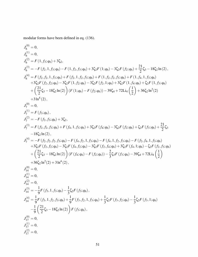
modular forms have been defined in eq. (136).

J(0)6 = 0,

J(1)6 = 0,

J(2)6 = F (1, f3;q6)+3ζ2,

J(3)6 =−F ( f2,1, f3;q6)−F (1, f2, f3;q6)+3ζ2F (1;q6)−3ζ2F ( f2;q6)+

21

2ζ3 −18ζ2 ln(2) ,

J(4)6 = F ( f2, f2,1, f3;q6)+F ( f2,1, f2, f3;q6)+F (1, f2, f2, f3;q6)+F (1, f4,1, f3;q6)

+3ζ2F ( f2, f2;q6)−3ζ2F (1, f2;q6)−3ζ2F ( f2,1;q6)+3ζ2F (1, f4;q6)+ζ2F (1, f3;q6)

+

(21

2ζ3 −18ζ2 ln(2)

)(F (1;q6)−F ( f2;q6))−39ζ4 +72Li4

(1

2

)+36ζ2 ln2(2)

+3ln4 (2) ,

J(0)7 = 0,

J(1)7 = F ( f3;q6) ,

J(2)7 =−F ( f2, f3;q6)+3ζ2,

J(3)7 = F ( f2, f2, f3;q6)+F ( f4,1, f3;q6)+3ζ2F ( f4;q6)−3ζ2F ( f2;q6)+ζ2F ( f3;q6)+

21

2ζ3

−18ζ2 ln(2) ,

J(4)7 =−F ( f2, f2, f2, f3;q6)−F ( f4, f2,1, f3;q6)−F ( f4,1, f2, f3;q6)−F ( f2, f4,1, f3;q6)

+3ζ2F ( f2, f2;q6)−3ζ2F ( f4, f2;q6)−3ζ2F ( f2, f4;q6)+3ζ2F ( f4,1;q6)−ζ2F ( f2, f3;q6)

+

(21

2ζ3 −18ζ2 ln(2)

)(F ( f4;q6)−F ( f2;q6))−

2

3ζ3F ( f3;q6)−39ζ4 +72Li4

(1

2

)

+36ζ2 ln2(2)+3ln4 (2) ,

J(0)14 = 0,

J(1)14 = 0,

J(2)14 = 0,

J(3)14 =−1

9F ( f3,1, f3;q6)−

1

3ζ2F ( f3;q6) ,

J(4)14 =

1

9F ( f3,1, f2, f3;q6)+

1

9F ( f3, f2,1, f3;q6)+

1

3ζ2F ( f3, f2;q6)−

1

3ζ2F ( f3,1;q6)

−1

9

(21

2ζ3 −18ζ2 ln(2)

)F ( f3;q6) ,

J(0)17 = 0,

J(1)17 = 0,

J(2)17 = 0,

51

Page 52

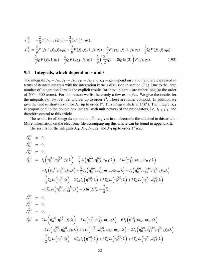
J(3)17 =−2

9F ( f3,1, f3;q6)−

2

3ζ2F ( f3;q6) ,

J(4)17 =

2

9F ( f3,1, f2, f3;q6)+

2

9F ( f3, f2,1, f3;q6)−

4

9F (g2,1, f3,1, f3;q6)+

2

3ζ2F ( f3, f2;q6)

−2

3ζ2F ( f3,1;q6)−

4

3ζ2F (g2,1, f3;q6)−

2

9

(21

2ζ3 −18ζ2 ln(2)

)F ( f3;q6) . (193)

9.4 Integrals, which depend on s and t

The integrals J24 − J30, J33 − J35, J38 − J39 and J41 − J45 depend on s and t and are expressed interms of iterated integrals with the integration kernels discussed in section (7.1). Due to the largenumber of integration kernels the explicit results for these integrals are rather long (at the orderof 200− 300 terms). For this reason we list here only a few examples. We give the results forthe integrals J24, J27, J33, J38 and J39 up to order ε3. These are rather compact. In addition wegive the (not so short) result for J41 up to order ε4. This integral starts at O(ε4). The integral J41

is proportional to the double box integral with unit powers of the propagators, i.e. I1111111, andtherefore central to this article.

The results for all integrals up to order ε4 are given in an electronic file attached to this article.More information on the electronic file accompanying this article can be found in appendix E.

The results for the integrals J24, J27, J33, J38 and J39 up to order ε3 read

J(0)24 = 0,

J(1)24 = 0,

J(2)24 = 0,

J(3)24 = Iγ

(η(b)0 ,η

( ba)

2 , f3;λ

)− 3

2Iγ

(η(b)0 ,η

(b)3,5,ω0,4;λ

)−3 Iγ

(η(b)1,1,ω0,4,ω0,4;λ

)

+Iγ

(η( a

b )2 ,η

(a)0 , f3;λ

)+

9

2Iγ

(η(b)0 ,a

(b)3,2,ω0,4,ω0,4;λ

)+ Iγ

(η(b)0 ,a

(a,b)4,1 ,η

(a)0 , f3;λ

)

+7

4ζ2 Iγ

(η(b)0 ;λ

)−2ζ2 Iγ

(η(b)1,1;λ

)+3ζ2 Iγ

(η( a

b)

2 ;λ)+3ζ2 Iγ

(η(b)0 ,a

(b)3,2;λ

)

+3ζ2 Iγ

(η(b)0 ,a

(a,b)4,1 ;λ

)−3 ln(2)ζ2 −

7

4ζ3,

J(0)27 = 0,

J(1)27 = 0,

J(2)27 = 0,

J(3)27 = 2 Iγ

(η(b)0 ,η

( ba)

2 , f3;λ

)−3 Iγ

(η(b)0 ,η

(b)3,5,ω0,4;λ

)−6 Iγ

(η(b)1,1,ω0,4,ω0,4;λ

)

+2 Iγ

(η( a

b)

2 ,η(a)0 , f3;λ

)+9 Iγ

(η(b)0 ,a

(b)3,2,ω0,4,ω0,4;λ

)+2 Iγ

(η(b)0 ,a

(a,b)4,1 ,η

(a)0 , f3;λ

)

+7

2ζ2 Iγ

(η(b)0 ;λ

)−4ζ2 Iγ

(η(b)1,1;λ

)+6ζ2 Iγ

(η( a

b)

2 ;λ)+6ζ2 Iγ

(η(b)0 ,a

(b)3,2;λ

)

52

Page 53

+6ζ2 Iγ

(η(b)0 ,a

(a,b)4,1 ;λ

)−6 ln(2)ζ2 −

7

2ζ3,

J(0)33 = 0,

J(1)33 = 0,

J(2)33 = 0,

J(3)33 = Iγ

(η(c)0 ,η

( ca )

2 , f3;λ)+

3

2Iγ

(η(c)0 ,η

(c)3,3,ω0;λ

)+ Iγ

(η(c)1,1,ω0,4,ω0;λ

)

+2 Iγ

(η(c)1,3,ω−4,0,ω0;λ

)+ Iγ

(η( a

c)

2 ,η(a)0 , f3;λ

)− 1

3Iγ

(η(c)0 ,a

(c)3,2,ω0,4,ω0;λ

)

−Iγ

(η(c)0 ,a

(c)3,3,ω−4,0,ω0;λ

)+ Iγ

(η(c)0 ,a

(a,c)4,1 ,η

(a)0 , f3;λ

)+

3

4ζ2 Iγ

(η(c)0 ;λ

)

−4ζ2 Iγ

(η(c)1,1;λ

)−2ζ2 Iγ

(η(c)1,3;λ

)+3ζ2 Iγ

(η( a

c)

2 ;λ)+

4

3ζ2 Iγ

(η(c)0 ,a

(c)3,2;λ

)

+ζ2 Iγ

(η(c)0 ,a

(c)3,3;λ

)+3ζ2 Iγ

(η(c)0 ,a

(a,c)4,1 ;λ

),

J(0)38 = 0,

J(1)38 = 0,

J(2)38 = 0,

J(3)38 = 0,

J(0)39 = 0,

J(1)39 = 0,

J(2)39 = 0,

J(3)39 = 0. (194)

Finally, let us give the result the result for the integral J41. We recall that this integral is propor-tional to the double box integral with unit powers of the propagators, e.g.

J41 = ε4 (1− x)4

x2

π

ψ(b)1

I1111111. (195)

This integral starts at O(ε4), hence

J(0)41 = 0, J

(1)41 = 0, J

(2)41 = 0, J

(3)41 = 0. (196)

Due to the differential equation we may write J(4)41 as an integral over ε3-terms J

(3)i . Starting the

integration path as usual at (x,y) = (0,1) we obtain

J(4)41 = −79

4ζ4 +8Li4

(1

2

)−8ζ2 (ln(2))

2 +1

3(ln(2))4 +

∫

γ

(1

9η2,9 −

1

3g2,1 −2ω0,4

)J(3)24

53

Page 54

+

∫

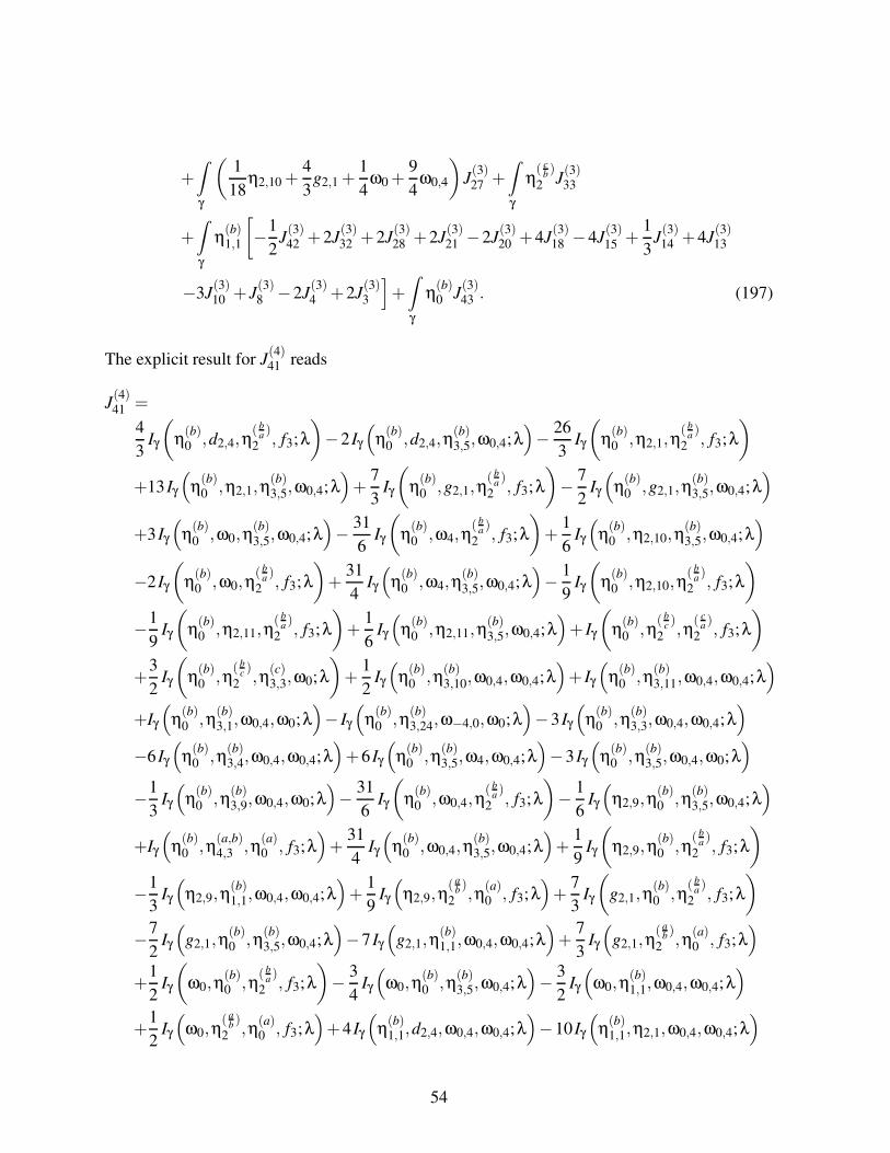
γ

(1

18η2,10 +

4

3g2,1 +

1

4ω0 +

9

4ω0,4

)J(3)27 +

∫

γ

η( c

b)

2 J(3)33

+∫

γ

η(b)1,1

[−1

2J(3)42 +2J

(3)32 +2J

(3)28 +2J

(3)21 −2J

(3)20 +4J

(3)18 −4J

(3)15 +

1

3J(3)14 +4J

(3)13

−3J(3)10 + J

(3)8 −2J

(3)4 +2J

(3)3

]+

∫

γ

η(b)0 J

(3)43 . (197)

The explicit result for J(4)41 reads

J(4)41 =

4

3Iγ

(η(b)0 ,d2,4,η

( ba)

2 , f3;λ

)−2 Iγ

(η(b)0 ,d2,4,η

(b)3,5,ω0,4;λ

)− 26

3Iγ

(η(b)0 ,η2,1,η

( ba)

2 , f3;λ

)

+13 Iγ

(η(b)0 ,η2,1,η

(b)3,5,ω0,4;λ

)+

7

3Iγ

(η(b)0 ,g2,1,η

( ba)

2 , f3;λ

)− 7

2Iγ

(η(b)0 ,g2,1,η

(b)3,5,ω0,4;λ

)

+3 Iγ

(η(b)0 ,ω0,η

(b)3,5,ω0,4;λ

)− 31

6Iγ

(η(b)0 ,ω4,η

( ba )

2 , f3;λ

)+

1

6Iγ

(η(b)0 ,η2,10,η

(b)3,5,ω0,4;λ

)

−2 Iγ

(η(b)0 ,ω0,η

( ba)

2 , f3;λ

)+

31

4Iγ

(η(b)0 ,ω4,η

(b)3,5,ω0,4;λ

)− 1

9Iγ

(η(b)0 ,η2,10,η

( ba)

2 , f3;λ

)

−1

9Iγ

(η(b)0 ,η2,11,η

( ba)

2 , f3;λ

)+

1

6Iγ

(η(b)0 ,η2,11,η

(b)3,5,ω0,4;λ

)+ Iγ

(η(b)0 ,η

( bc)

2 ,η( c

a)

2 , f3;λ

)

+3

2Iγ

(η(b)0 ,η

( bc)

2 ,η(c)3,3,ω0;λ

)+

1

2Iγ

(η(b)0 ,η

(b)3,10,ω0,4,ω0,4;λ

)+ Iγ

(η(b)0 ,η

(b)3,11,ω0,4,ω0,4;λ

)

+Iγ

(η(b)0 ,η

(b)3,1,ω0,4,ω0;λ

)− Iγ

(η(b)0 ,η

(b)3,24,ω−4,0,ω0;λ

)−3 Iγ

(η(b)0 ,η

(b)3,3,ω0,4,ω0,4;λ

)

−6 Iγ

(η(b)0 ,η

(b)3,4,ω0,4,ω0,4;λ

)+6 Iγ

(η(b)0 ,η

(b)3,5,ω4,ω0,4;λ

)−3 Iγ

(η(b)0 ,η

(b)3,5,ω0,4,ω0;λ

)

−1

3Iγ

(η(b)0 ,η

(b)3,9,ω0,4,ω0;λ

)− 31

6Iγ

(η(b)0 ,ω0,4,η

( ba)

2 , f3;λ

)− 1

6Iγ

(η2,9,η

(b)0 ,η

(b)3,5,ω0,4;λ

)

+Iγ

(η(b)0 ,η

(a,b)4,3 ,η

(a)0 , f3;λ

)+

31

4Iγ

(η(b)0 ,ω0,4,η

(b)3,5,ω0,4;λ

)+

1

9Iγ

(η2,9,η

(b)0 ,η

( ba)

2 , f3;λ

)

−1

3Iγ

(η2,9,η

(b)1,1,ω0,4,ω0,4;λ

)+

1

9Iγ

(η2,9,η

( ab )

2 ,η(a)0 , f3;λ

)+

7

3Iγ

(g2,1,η

(b)0 ,η

( ba )

2 , f3;λ

)

−7

2Iγ

(g2,1,η

(b)0 ,η

(b)3,5,ω0,4;λ

)−7 Iγ

(g2,1,η

(b)1,1,ω0,4,ω0,4;λ

)+

7

3Iγ

(g2,1,η

( ab )

2 ,η(a)0 , f3;λ

)

+1

2Iγ

(ω0,η

(b)0 ,η

( ba)

2 , f3;λ

)− 3

4Iγ

(ω0,η

(b)0 ,η

(b)3,5,ω0,4;λ

)− 3

2Iγ

(ω0,η

(b)1,1,ω0,4,ω0,4;λ

)

+1

2Iγ

(ω0,η

( ab)

2 ,η(a)0 , f3;λ

)+4 Iγ

(η(b)1,1,d2,4,ω0,4,ω0,4;λ

)−10 Iγ

(η(b)1,1,η2,1,ω0,4,ω0,4;λ

)

54

Page 55

−9

2Iγ

(η(b)1,1,ω0,ω0,4,ω0,4;λ

)+

1

2Iγ

(η(b)1,1,ω4,ω0,4,ω0,4;λ

)− 16

9Iγ

(η(b)1,1,η

(b)1,2,η

( ba)

2 , f3;λ

)

+8

3Iγ

(η(b)1,1,η

(b)1,2,η

(b)3,5,ω0,4;λ

)+

8

3Iγ

(η(b)1,1,η

(b)1,4,η

( ba)

2 , f3;λ

)−4 Iγ

(η(b)1,1,η

(b)1,4,η

(b)3,5,ω0,4;λ

)

− 2

27Iγ

(η(b)1,1,η

(a)3,1,η

(a)0 , f3;λ

)− 1

54Iγ

(η(b)1,1,η

(a)3,2,η

(a)0 , f3;λ

)+12 Iγ

(η(b)1,1,ω0,4,ω4,ω0,4;λ

)

−8 Iγ

(η(b)1,1,ω0,4,ω0,4,ω0;λ

)−4 Iγ

(η(b)1,1,ω0,4,ω0,4,ω0,4;λ

)−4 Iγ

(η(b)1,1,ω−4,0,ω−4,0,ω0;λ

)

+1

9Iγ

(η2,10,η

(b)0 ,η

( ba)

2 , f3;λ

)− 1

6Iγ

(η2,10,η

(b)0 ,η

(b)3,5,ω0,4;λ

)+

1

9Iγ

(η2,10,η

( ab)

2 ,η(a)0 , f3;λ

)

−1

3Iγ

(η2,10,η

(b)1,1,ω0,4,ω0,4;λ

)+ Iγ

(η( c

b)

2 ,η(c)0 ,η

( ca)

2 , f3;λ)+

3

2Iγ

(η( c

b)

2 ,η(c)0 ,η

(c)3,3,ω0;λ

)

+Iγ

(η( c

b)

2 ,η(c)1,1,ω0,4,ω0;λ

)+2 Iγ

(η( c

b)

2 ,η(c)1,3,ω−4,0,ω0;λ

)− 15

2Iγ

(ω0,4,η

(b)1,1,ω0,4,ω0,4;λ

)

+Iγ

(η( c

b)

2 ,η( a

c)

2 ,η(a)0 , f3;λ

)+

5

2Iγ

(ω0,4,η

(b)0 ,η

( ba)

2 , f3;λ

)− 15

4Iγ

(ω0,4,η

(b)0 ,η

(b)3,5,ω0,4;λ

)

+5

2Iγ

(ω0,4,η

( ab)

2 ,η(a)0 , f3;λ

)−6 Iγ

(η(b)0 ,a

(b)3,2,d2,4,ω0,4,ω0,4;λ

)

+15 Iγ

(η(b)0 ,a

(b)3,2,η2,1,ω0,4,ω0,4;λ

)+

27

4Iγ

(η(b)0 ,a

(b)3,2,ω0,ω0,4,ω0,4;λ

)

−3

4Iγ

(η(b)0 ,a

(b)3,2,ω4,ω0,4,ω0,4;λ

)+

8

3Iγ

(η(b)0 ,a

(b)3,2,η

(b)1,2,η

( ba )

2 , f3;λ

)

−4 Iγ

(η(b)0 ,a

(b)3,2,η

(b)1,2,η

(b)3,5,ω0,4;λ

)−4 Iγ

(η(b)0 ,a

(b)3,2,η

(b)1,4,η

( ba)

2 , f3;λ

)

+6 Iγ

(η(b)0 ,a

(b)3,2,η

(b)1,4,η

(b)3,5,ω0,4;λ

)+

1

9Iγ

(η(b)0 ,a

(b)3,2,η

(a)3,1,η

(a)0 , f3;λ

)

+1

36Iγ

(η(b)0 ,a

(b)3,2,η

(a)3,2,η

(a)0 , f3;λ

)−18 Iγ

(η(b)0 ,a

(b)3,2,ω0,4,ω4,ω0,4;λ

)

+12 Iγ

(η(b)0 ,a

(b)3,2,ω0,4,ω0,4,ω0;λ

)+6 Iγ

(η(b)0 ,a

(b)3,2,ω0,4,ω0,4,ω0,4;λ

)

+6 Iγ

(η(b)0 ,a

(b)3,2,ω−4,0,ω−4,0,ω0;λ

)+6 Iγ

(η(b)0 ,d2,4,a

(b)3,2,ω0,4,ω0,4;λ

)

+4

3Iγ

(η(b)0 ,d2,4,a

(a,b)4,1 ,η

(a)0 , f3;λ

)−39 Iγ

(η(b)0 ,η2,1,a

(b)3,2,ω0,4,ω0,4;λ

)

−26

3Iγ

(η(b)0 ,η2,1,a

(a,b)4,1 ,η

(a)0 , f3;λ

)+

21

2Iγ

(η(b)0 ,g2,1,a

(b)3,2,ω0,4,ω0,4;λ

)

+7

3Iγ

(η(b)0 ,g2,1,a

(a,b)4,1 ,η

(a)0 , f3;λ

)−9 Iγ

(η(b)0 ,ω0,a

(b)3,2,ω0,4,ω0,4;λ

)

−2 Iγ

(η(b)0 ,ω0,a

(a,b)4,1 ,η

(a)0 , f3;λ

)− 93

4Iγ

(η(b)0 ,ω4,a

(b)3,2,ω0,4,ω0,4;λ

)

−31

6Iγ

(η(b)0 ,ω4,a

(a,b)4,1 ,η

(a)0 , f3;λ

)+ Iγ

(η(b)0 ,a

(b,c)4,1 ,η

(c)0 ,η

( ca)

2 , f3;λ)

55

Page 56

+3

2Iγ

(η(b)0 ,a

(b,c)4,1 ,η

(c)0 ,η

(c)3,3,ω0;λ

)+ Iγ

(η(b)0 ,a

(b,c)4,1 ,η

(c)1,1,ω0,4,ω0;λ

)

+2 Iγ

(η(b)0 ,a

(b,c)4,1 ,η

(c)1,3,ω−4,0,ω0;λ

)+ Iγ

(η(b)0 ,a

(b,c)4,1 ,η

( ac)

2 ,η(a)0 , f3;λ

)

+Iγ

(η(b)0 ,a

(b,b)4,3 ,η

(b)0 ,η

( ba)

2 , f3;λ

)− 3

2Iγ

(η(b)0 ,a

(b,b)4,3 ,η

(b)0 ,η

(b)3,5,ω0,4;λ

)

−3 Iγ

(η(b)0 ,a

(b,b)4,3 ,η

(b)1,1,ω0,4,ω0,4;λ

)+ Iγ

(η(b)0 ,a

(b,b)4,3 ,η

( ab)

2 ,η(a)0 , f3;λ

)

+2 Iγ

(η(b)0 ,a

(b,b)4,4 ,η

(b)0 ,η

( ba )

2 , f3;λ

)−3 Iγ

(η(b)0 ,a

(b,b)4,4 ,η

(b)0 ,η

(b)3,5,ω0,4;λ

)

−6 Iγ

(η(b)0 ,a

(b,b)4,4 ,η

(b)1,1,ω0,4,ω0,4;λ

)+2 Iγ

(η(b)0 ,a

(b,b)4,4 ,η

( ab)

2 ,η(a)0 , f3;λ

)

−1

2Iγ

(η(b)0 ,η2,10,a

(b)3,2,ω0,4,ω0,4;λ

)− 1

9Iγ

(η(b)0 ,η2,10,a

(a,b)4,1 ,η

(a)0 , f3;λ

)

−1

2Iγ

(η(b)0 ,η2,11,a

(b)3,2,ω0,4,ω0,4;λ

)− 1

9Iγ

(η(b)0 ,η2,11,a

(a,b)4,1 ,η

(a)0 , f3;λ

)

−1

3Iγ

(η(b)0 ,η

( bc)

2 ,a(c)3,2,ω0,4,ω0;λ

)− Iγ

(η(b)0 ,η

( bc)

2 ,a(c)3,3,ω−4,0,ω0;λ

)

+Iγ

(η(b)0 ,η

( bc)

2 ,a(a,c)4,1 ,η

(a)0 , f3;λ

)− 93

4Iγ

(η(b)0 ,ω0,4,a

(b)3,2,ω0,4,ω0,4;λ

)

−31

6Iγ

(η(b)0 ,ω0,4,a

(a,b)4,1 ,η

(a)0 , f3;λ

)+

1

2Iγ

(η2,9,η

(b)0 ,a

(b)3,2,ω0,4,ω0,4;λ

)

+1

9Iγ

(η2,9,η

(b)0 ,a

(a,b)4,1 ,η

(a)0 , f3;λ

)+

21

2Iγ

(g2,1,η

(b)0 ,a

(b)3,2,ω0,4,ω0,4;λ

)

+7

3Iγ

(g2,1,η

(b)0 ,a

(a,b)4,1 ,η

(a)0 , f3;λ

)+

9

4Iγ

(ω0,η

(b)0 ,a

(b)3,2,ω0,4,ω0,4;λ

)

+1

2Iγ

(ω0,η

(b)0 ,a

(a,b)4,1 ,η

(a)0 , f3;λ

)+

8

3Iγ

(η(b)1,1,a

(b)3,1,η

(b)0 ,η

( ba )

2 , f3;λ

)

−4 Iγ

(η(b)1,1,a

(b)3,1,η

(b)0 ,η

(b)3,5,ω0,4;λ

)−8 Iγ

(η(b)1,1,a

(b)3,1,η

(b)1,1,ω0,4,ω0,4;λ

)

+8

3Iγ

(η(b)1,1,a

(b)3,1,η

( ab)

2 ,η(a)0 , f3;λ

)+4 Iγ

(η(b)1,1,a

(b)3,3,η

(b)0 ,η

( ba)

2 , f3;λ

)

−6 Iγ

(η(b)1,1,a

(b)3,3,η

(b)0 ,η

(b)3,5,ω0,4;λ

)−12 Iγ

(η(b)1,1,a

(b)3,3,η

(b)1,1,ω0,4,ω0,4;λ

)

+4 Iγ

(η(b)1,1,a

(b)3,3,η

( ab)

2 ,η(a)0 , f3;λ

)−8 Iγ

(η(b)1,1,η

(b)1,2,a

(b)3,2,ω0,4,ω0,4;λ

)

−16

9Iγ

(η(b)1,1,η

(b)1,2,a

(a,b)4,1 ,η

(a)0 , f3;λ

)+12 Iγ

(η(b)1,1,η

(b)1,4,a

(b)3,2,ω0,4,ω0,4;λ

)

+8

3Iγ

(η(b)1,1,η

(b)1,4,a

(a,b)4,1 ,η

(a)0 , f3;λ

)+

1

2Iγ

(η2,10,η

(b)0 ,a

(b)3,2,ω0,4,ω0,4;λ

)

+1

9Iγ

(η2,10,η

(b)0 ,a

(a,b)4,1 ,η

(a)0 , f3;λ

)− 1

3Iγ

(η( c

b)

2 ,η(c)0 ,a

(c)3,2,ω0,4,ω0;λ

)

56

Page 57

−Iγ

(η( c

b)

2 ,η(c)0 ,a

(c)3,3,ω−4,0,ω0;λ

)+ Iγ

(η( c

b)

2 ,η(c)0 ,a

(a,c)4,1 ,η

(a)0 , f3;λ

)

+45

4Iγ

(ω0,4,η

(b)0 ,a

(b)3,2,ω0,4,ω0,4;λ

)+

5

2Iγ

(ω0,4,η

(b)0 ,a

(a,b)4,1 ,η

(a)0 , f3;λ

)

+12 Iγ

(η(b)0 ,a

(b)3,2,η

(b)1,2,a

(b)3,2,ω0,4,ω0,4;λ

)+

8

3Iγ

(η(b)0 ,a

(b)3,2,η

(b)1,2,a

(a,b)4,1 ,η

(a)0 , f3;λ

)

−18 Iγ

(η(b)0 ,a

(b)3,2,η

(b)1,4,a

(b)3,2,ω0,4,ω0,4;λ

)−4 Iγ

(η(b)0 ,a

(b)3,2,η

(b)1,4,a

(a,b)4,1 ,η

(a)0 , f3;λ

)

−1

3Iγ

(η(b)0 ,a

(b,c)4,1 ,η

(c)0 ,a

(c)3,2,ω0,4,ω0;λ

)− Iγ

(η(b)0 ,a

(b,c)4,1 ,η

(c)0 ,a

(c)3,3,ω−4,0,ω0;λ

)

+Iγ

(η(b)0 ,a

(b,c)4,1 ,η

(c)0 ,a

(a,c)4,1 ,η

(a)0 , f3;λ

)+

9

2Iγ

(η(b)0 ,a

(b,b)4,3 ,η

(b)0 ,a

(b)3,2,ω0,4,ω0,4;λ

)

+Iγ

(η(b)0 ,a

(b,b)4,3 ,η

(b)0 ,a

(a,b)4,1 ,η

(a)0 , f3;λ

)+9 Iγ

(η(b)0 ,a

(b,b)4,4 ,η

(b)0 ,a

(b)3,2,ω0,4,ω0,4;λ

)

+2 Iγ

(η(b)0 ,a

(b,b)4,4 ,η

(b)0 ,a

(a,b)4,1 ,η

(a)0 , f3;λ

)+12 Iγ

(η(b)1,1,a

(b)3,1,η

(b)0 ,a

(b)3,2,ω0,4,ω0,4;λ

)

+8

3Iγ

(η(b)1,1,a

(b)3,1,η

(b)0 ,a

(a,b)4,1 ,η

(a)0 , f3;λ

)+18 Iγ

(η(b)1,1,a

(b)3,3,η

(b)0 ,a

(b)3,2,ω0,4,ω0,4;λ

)

+4 Iγ

(η(b)1,1,a

(b)3,3,η

(b)0 ,a

(a,b)4,1 ,η

(a)0 , f3;λ

)−6 Iγ

(η(b)0 ,a

(b)3,2,a

(b)3,3,η

(b)0 ,η

( ba)

2 , f3;λ

)

+18 Iγ

(η(b)0 ,a

(b)3,2,a

(b)3,3,η

(b)1,1,ω0,4,ω0,4;λ

)−6 Iγ

(η(b)0 ,a

(b)3,2,a

(b)3,3,η

( ab)

2 ,η(a)0 , f3;λ

)

+9 Iγ

(η(b)0 ,a

(b)3,2,a

(b)3,3,η

(b)0 ,η

(b)3,5,ω0,4;λ

)−27 Iγ

(η(b)0 ,a

(b)3,2,a

(b)3,3,η

(b)0 ,a

(b)3,2,ω0,4,ω0,4;λ

)

−6 Iγ

(η(b)0 ,a

(b)3,2,a

(b)3,3,η

(b)0 ,a

(a,b)4,1 ,η

(a)0 , f3;λ

)+6 Iγ

(η(b)0 ,a

(b)3,2,a

(b)3,1,η

(b)0 ,η

(b)3,5,ω0,4;λ

)

+12 Iγ

(η(b)0 ,a

(b)3,2,a

(b)3,1,η

(b)1,1,ω0,4,ω0,4;λ

)−4 Iγ

(η(b)0 ,a

(b)3,2,a

(b)3,1,η

( ab )

2 ,η(a)0 , f3;λ

)

−4 Iγ

(η(b)0 ,a

(b)3,2,a

(b)3,1,η

(b)0 ,η

( ba)

2 , f3;λ

)−18 Iγ

(η(b)0 ,a

(b)3,2,a

(b)3,1,η

(b)0 ,a

(b)3,2,ω0,4,ω0,4;λ

)

−4 Iγ

(η(b)0 ,a

(b)3,2,a

(b)3,1,η

(b)0 ,a

(a,b)4,1 ,η

(a)0 , f3;λ

)

+

[7

3Iγ

(η(b)0 ,d2,4;λ

)− 91

6Iγ

(η(b)0 ,η2,1;λ

)+

49

12Iγ

(η(b)0 ,g2,1;λ

)− 7

2Iγ

(η(b)0 ,ω0;λ

)

−217

24Iγ

(η(b)0 ,ω4;λ

)− 7

36Iγ

(η(b)0 ,η2,10;λ

)− 7

36Iγ

(η(b)0 ,η2,11;λ

)+

3

4Iγ

(η(b)0 ,η

( bc)

2 ;λ

)

+1

3Iγ

(η(b)0 ,η

(b)3,10;λ

)+

2

3Iγ

(η(b)0 ,η

(b)3,11;λ

)−4 Iγ

(η(b)0 ,η

(b)3,1;λ

)+ Iγ

(η(b)0 ,η

(b)3,24;λ

)

+4

3Iγ

(η(b)0 ,η

(b)3,9;λ

)+3 Iγ

(η(b)0 ,η

(a,b)4,3 ;λ

)− 217

24Iγ

(η(b)0 ,ω0,4;λ

)+

7

36Iγ

(η2,9,η

(b)0 ;λ

)

−2

9Iγ

(η2,9,η

(b)1,1;λ

)+

1

3Iγ

(η2,9,η

( ab)

2 ;λ)+

49

12Iγ

(g2,1,η

(b)0 ;λ

)− 14

3Iγ

(g2,1,η

(b)1,1;λ

)

+7 Iγ

(g2,1,η

( ab)

2 ;λ)+

7

8Iγ

(ω0,η

(b)0 ;λ

)− Iγ

(ω0,η

(b)1,1;λ

)+

3

2Iγ

(ω0,η

( ab)

2 ;λ)

57

Page 58

+8

3Iγ

(η(b)1,1,d2,4;λ

)− 20

3Iγ

(η(b)1,1,η2,1;λ

)− 8

3Iγ

(η(b)1,1,g2,1;λ

)+ Iγ

(η(b)1,1,ω0;λ

)

+1

3Iγ

(η(b)1,1,ω4;λ

)− 28

9Iγ

(η(b)1,1,η

(b)1,2;λ

)+

14

3Iγ

(η(b)1,1,η

(b)1,4;λ

)− 2

9Iγ

(η(b)1,1,η

(a)3,1;λ

)

− 1

18Iγ

(η(b)1,1,η

(a)3,2;λ

)+

16

3Iγ

(η(b)1,1,ω0,4;λ

)+4 Iγ

(η(b)1,1,ω−4,0;λ

)+

7

36Iγ

(η2,10,η

(b)0 ;λ

)

−2

9Iγ

(η2,10,η

(b)1,1;λ

)+

1

3Iγ

(η2,10,η

( ab )

2 ;λ)+

3

4Iγ

(η( c

b )2 ,η

(c)0 ;λ

)−4 Iγ

(η( c

b )2 ,η

(c)1,1;λ

)

−2 Iγ

(η( c

b)

2 ,η(c)1,3;λ

)+3 Iγ

(η( c

b)

2 ,η( a

c)

2 ;λ)+

35

8Iγ

(ω0,4,η

(b)0 ;λ

)−5 Iγ

(ω0,4,η

(b)1,1;λ

)

+15

2Iγ

(ω0,4,η

( ab)

2 ;λ)−4 Iγ

(η(b)0 ,a

(b)3,2,d2,4;λ

)+10 Iγ

(η(b)0 ,a

(b)3,2,η2,1;λ

)

+4 Iγ

(η(b)0 ,a

(b)3,2,g2,1;λ

)− 3

2Iγ

(η(b)0 ,a

(b)3,2,ω0;λ

)− 1

2Iγ

(η(b)0 ,a

(b)3,2,ω4;λ

)

+14

3Iγ

(η(b)0 ,a

(b)3,2,η

(b)1,2;λ

)−7 Iγ

(η(b)0 ,a

(b)3,2,η

(b)1,4;λ

)+

1

3Iγ

(η(b)0 ,a

(b)3,2,η

(a)3,1;λ

)

+1

12Iγ

(η(b)0 ,a

(b)3,2,η

(a)3,2;λ

)−8 Iγ

(η(b)0 ,a

(b)3,2,ω0,4;λ

)−6 Iγ

(η(b)0 ,a

(b)3,2,ω−4,0;λ

)

+4 Iγ

(η(b)0 ,d2,4,a

(b)3,2;λ

)+4 Iγ

(η(b)0 ,d2,4,a

(a,b)4,1 ;λ

)−26 Iγ

(η(b)0 ,η2,1,a

(b)3,2;λ

)

−26 Iγ

(η(b)0 ,η2,1,a

(a,b)4,1 ;λ

)+7 Iγ

(η(b)0 ,g2,1,a

(b)3,2;λ

)+7 Iγ

(η(b)0 ,g2,1,a

(a,b)4,1 ;λ

)

−6 Iγ

(η(b)0 ,ω0,a

(b)3,2;λ

)−6 Iγ

(η(b)0 ,ω0,a

(a,b)4,1 ;λ

)− 31

2Iγ

(η(b)0 ,ω4,a

(b)3,2;λ

)

−31

2Iγ

(η(b)0 ,ω4,a

(a,b)4,1 ;λ

)+

3

4Iγ

(η(b)0 ,a

(b,c)4,1 ,η

(c)0 ;λ

)−4 Iγ

(η(b)0 ,a

(b,c)4,1 ,η

(c)1,1;λ

)

−2 Iγ

(η(b)0 ,a

(b,c)4,1 ,η

(c)1,3;λ

)+3 Iγ

(η(b)0 ,a

(b,c)4,1 ,η

( ac )

2 ;λ)+

7

4Iγ

(η(b)0 ,a

(b,b)4,3 ,η

(b)0 ;λ

)

−2 Iγ

(η(b)0 ,a

(b,b)4,3 ,η

(b)1,1;λ

)+3 Iγ

(η(b)0 ,a

(b,b)4,3 ,η

( ab)

2 ;λ)+

7

2Iγ

(η(b)0 ,a

(b,b)4,4 ,η

(b)0 ;λ

)

−4 Iγ

(η(b)0 ,a

(b,b)4,4 ,η

(b)1,1;λ

)+6 Iγ

(η(b)0 ,a

(b,b)4,4 ,η

( ab)

2 ;λ)− 1

3Iγ

(η(b)0 ,η2,10,a

(b)3,2;λ

)

−1

3Iγ

(η(b)0 ,η2,10,a

(a,b)4,1 ;λ

)− 1

3Iγ

(η(b)0 ,η2,11,a

(b)3,2;λ

)− 1

3Iγ

(η(b)0 ,η2,11,a

(a,b)4,1 ;λ

)

+4

3Iγ

(η(b)0 ,η

( bc )

2 ,a(c)3,2;λ

)+ Iγ

(η(b)0 ,η

( bc )

2 ,a(c)3,3;λ

)+3 Iγ

(η(b)0 ,η

( bc )

2 ,a(a,c)4,1 ;λ

)

−31

2Iγ

(η(b)0 ,ω0,4,a

(b)3,2;λ

)− 31

2Iγ

(η(b)0 ,ω0,4,a

(a,b)4,1 ;λ

)+

1

3Iγ

(η2,9,η

(b)0 ,a

(b)3,2;λ

)

+1

3Iγ

(η2,9,η

(b)0 ,a

(a,b)4,1 ;λ

)+7 Iγ

(g2,1,η

(b)0 ,a

(b)3,2;λ

)+7 Iγ

(g2,1,η

(b)0 ,a

(a,b)4,1 ;λ

)

+3

2Iγ

(ω0,η

(b)0 ,a

(b)3,2;λ

)+

3

2Iγ

(ω0,η

(b)0 ,a

(a,b)4,1 ;λ

)+

14

3Iγ

(η(b)1,1,a

(b)3,1,η

(b)0 ;λ

)

−16

3Iγ

(η(b)1,1,a

(b)3,1,η

(b)1,1;λ

)+8 Iγ

(η(b)1,1,a

(b)3,1,η

( ab )

2 ;λ)+7 Iγ

(η(b)1,1,a

(b)3,3,η

(b)0 ;λ

)

58

Page 59

−8 Iγ

(η(b)1,1,a

(b)3,3,η

(b)1,1;λ

)+12 Iγ

(η(b)1,1,a

(b)3,3,η

( ab)

2 ;λ)− 16

3Iγ

(η(b)1,1,η

(b)1,2,a

(b)3,2;λ

)

−16

3Iγ

(η(b)1,1,η

(b)1,2,a

(a,b)4,1 ;λ

)+8 Iγ

(η(b)1,1,η

(b)1,4,a

(b)3,2;λ

)+8 Iγ

(η(b)1,1,η

(b)1,4,a

(a,b)4,1 ;λ

)

+1

3Iγ

(η2,10,η

(b)0 ,a

(b)3,2;λ

)+

1

3Iγ

(η2,10,η

(b)0 ,a

(a,b)4,1 ;λ

)+

4

3Iγ

(η( c

b)

2 ,η(c)0 ,a

(c)3,2;λ

)

+Iγ

(η( c

b )2 ,η

(c)0 ,a

(c)3,3;λ

)+3 Iγ

(η( c

b )2 ,η

(c)0 ,a

(a,c)4,1 ;λ

)+

15

2Iγ

(ω0,4,η

(b)0 ,a

(b)3,2;λ

)

+15

2Iγ

(ω0,4,η

(b)0 ,a

(a,b)4,1 ;λ

)+8 Iγ

(η(b)0 ,a

(b)3,2,η

(b)1,2,a

(b)3,2;λ

)+8 Iγ

(η(b)0 ,a

(b)3,2,η

(b)1,2,a

(a,b)4,1 ;λ

)

−12 Iγ

(η(b)0 ,a

(b)3,2,η

(b)1,4,a

(b)3,2;λ

)−12 Iγ

(η(b)0 ,a

(b)3,2,η

(b)1,4,a

(a,b)4,1 ;λ

)

+4

3Iγ

(η(b)0 ,a

(b,c)4,1 ,η

(c)0 ,a

(c)3,2;λ

)+ Iγ

(η(b)0 ,a

(b,c)4,1 ,η

(c)0 ,a

(c)3,3;λ

)

+3 Iγ

(η(b)0 ,a

(b,c)4,1 ,η

(c)0 ,a

(a,c)4,1 ;λ

)+3 Iγ

(η(b)0 ,a

(b,b)4,3 ,η

(b)0 ,a

(b)3,2;λ

)

+3 Iγ

(η(b)0 ,a

(b,b)4,3 ,η

(b)0 ,a

(a,b)4,1 ;λ

)+6 Iγ

(η(b)0 ,a

(b,b)4,4 ,η

(b)0 ,a

(b)3,2;λ

)

+6 Iγ

(η(b)0 ,a

(b,b)4,4 ,η

(b)0 ,a

(a,b)4,1 ;λ

)+8 Iγ

(η(b)1,1,a

(b)3,1,η

(b)0 ,a

(b)3,2;λ

)

+8 Iγ

(η(b)1,1,a

(b)3,1,η

(b)0 ,a

(a,b)4,1 ;λ

)+12 Iγ

(η(b)1,1,a

(b)3,3,η

(b)0 ,a

(b)3,2;λ

)

+12 Iγ

(η(b)1,1,a

(b)3,3,η

(b)0 ,a

(a,b)4,1 ;λ

)−12 Iγ

(η(b)0 ,a

(b)3,2,a

(b)3,1,η

( ab)

2 ;λ)

−18 Iγ

(η(b)0 ,a

(b)3,2,a

(b)3,3,η

( ab)

2 ;λ)−18 Iγ

(η(b)0 ,a

(b)3,2,a

(b)3,3,η

(b)0 ,a

(a,b)4,1 ;λ

)

−18 Iγ

(η(b)0 ,a

(b)3,2,a

(b)3,3,η

(b)0 ,a

(b)3,2;λ

)− 21

2Iγ

(η(b)0 ,a

(b)3,2,a

(b)3,3,η

(b)0 ;λ

)

+12 Iγ

(η(b)0 ,a

(b)3,2,a

(b)3,3,η

(b)1,1;λ

)−12 Iγ

(η(b)0 ,a

(b)3,2,a

(b)3,1,η

(b)0 ,a

(a,b)4,1 ;λ

)

−12 Iγ

(η(b)0 ,a

(b)3,2,a

(b)3,1,η

(b)0 ,a

(b)3,2;λ

)−7 Iγ

(η(b)0 ,a

(b)3,2,a

(b)3,1,η

(b)0 ;λ

)

+8 Iγ

(η(b)0 ,a

(b)3,2,a

(b)3,1,η

(b)1,1;λ

)]ζ2

+

[49

12Iγ

(η(b)0 ;λ

)− 7

36Iγ (η2,9;λ)− 49

12Iγ (g2,1;λ)− 7

8Iγ (ω0;λ)+

22

3Iγ

(η(b)1,1;λ

)

− 7

36Iγ (η2,10;λ)− 35

8Iγ (ω0,4;λ)−11 Iγ

(η(b)0 ,a

(b)3,2;λ

)− 7

4Iγ

(η(b)0 ,a

(b,b)4,3 ;λ

)

−7

2Iγ

(η(b)0 ,a

(b,b)4,4 ;λ

)− 14

3Iγ

(η(b)1,1,a

(b)3,1;λ

)−7 Iγ

(η(b)1,1,a

(b)3,3;λ

)+7 Iγ

(η(b)0 ,a

(b)3,2,a

(b)3,1;λ

)

+21

2Iγ

(η(b)0 ,a

(b)3,2,a

(b)3,3;λ

)]ζ3

+

[7 Iγ

(η(b)0 ;λ

)− 1

3Iγ (η2,9;λ)−7 Iγ (g2,1;λ)− 3

2Iγ (ω0;λ)−8 Iγ

(η(b)1,1;λ

)− 1

3Iγ (η2,10;λ)

59

Page 60

−15

2Iγ (ω0,4;λ)+12 Iγ

(η(b)0 ,a

(b)3,2;λ

)−3 Iγ

(η(b)0 ,a

(b,b)4,3 ;λ

)−6 Iγ

(η(b)0 ,a

(b,b)4,4 ;λ

)

−8 Iγ

(η(b)1,1,a

(b)3,1;λ

)−12 Iγ

(η(b)1,1,a

(b)3,3;λ

)+18 Iγ

(η(b)0 ,a

(b)3,2,a

(b)3,3;λ

)

+12 Iγ

(η(b)0 ,a

(b)3,2,a

(b)3,1;λ

)]ζ2 ln(2)− 79

4ζ4 +8Li4

(1

2

)−8ζ2 (ln(2))

2 +1

3(ln(2))4 . (198)

The large number of terms for J(4)41 can be traced back to the already large number of terms of

J(3)42 and J

(3)43 , which are according to eq. (197) integrated further with η

(b)1,1 and η

(b)0 , respectively.

The expression in eq. (198) involves 47 of the 107 integration kernels.

9.5 Numerical checks

All results have been verified numerically with the help of the program sector_decomposition

[119]. The program sector_decomposition allows (as SecDec [120–123] or FIESTA [124,125]) the numerical evaluation of multi-loop integrals. On the one hand we evaluated all masterintegrals of the basis~I at a few kinematic points numerically with the program sector_decom-

position. On the other hand, we evaluated our results in the basis ~J at the same kinematicpoints, converted to the basis~I and compared the two results. We find good agreement.

The evaluation of the iterated integrals appearing in our results is done as follows: We splitthe integration path into two pieces: First we integrate in (x, y)-space from (0,0) to (x,0), thenfrom (x,0) to (x, y). The integration along the first part gives only multiple polylogarithms, whichcan be evaluated to high precision [97]. We use these results as new boundary constants for theintegration along the second part. Assuming that y is small, we may expand for the integrationalong the second part all integration kernels in y.

As a reference we give numerical results for the master integrals in the basis ~J at the kinematicpoint

s = −12769

840m2, t =

10

11m2. (199)

This point corresponds to

x =7

120, y =

10

11, (200)

or equivalently

x =1

15, y =

1

11. (201)

The numerical results for the first five terms of ε-expansion are given in tables 2 and 3.

60

Page 61

ε0 ε1 ε2 ε3 ε4

J1 1 0 1.6449341 −0.80137127 1.8940657J2 0 2.8415816 −2.8295758 6.4116869 −7.7009279J3 0 −2.8415816 15.355894 −39.817554 97.903278J4 0 0 8.074586 −20.479468 55.140667J5 1 −2.7213737 3.7029375 −6.5645107 7.7616443J6 0 0 4.7951687 −7.7339091 23.583241J7 0 −0.13797489 5.0760627 −8.5195954 25.27333J8 0 0 9.8696044 −15.803336 48.383357J9 0 0 4.037293 −2.1975902 7.5750011J10 0 0 0 −10.577768 19.861743J11 0 2.8415816 −10.562581 19.960005 −34.628948J12 0 0 4.8094349 −23.163298 56.79741J13 0 0 0 −9.6340372 18.255071J14 0 0 0 0.074587202 −0.1198646J15 0 0 −4.037293 23.437914 −62.690651J16 0 0 0 8.4983135 −20.922966J17 0 0 0 0.1491744 0.058984085J18 0 1.4207908 −12.163995 44.930917 −88.809767J19 0 0 0 16.996627 −15.625817J20 0 0 −10.735443 −9.8004674 −37.795989J21 0 0 4.037293 −13.184573 21.864228J22 0 0 0 0 8.4599162J23 0 0 0 4.8796692 −25.793413J24 0 0 0 2.6138189 −0.23796592J25 0 0 4.037293 −9.2635254 25.950914J26 0 0 2.7276656 −1.848663 13.397014J27 0 0 0 5.2276379 8.7055971J28 0 0 0 8.9388561 12.795847J29 0 0 0 0 18.80581J30 0 0 5.4553312 −3.9355497 35.856907J32 0 0 −10.735443 −40.306104 −35.268067J33 0 0 0 7.3822471 10.116064J34 0 0 10.735443 −3.4643927 53.616756J35 0 0 0.97741243 5.1104476 15.424638

Table 2: Numerical results for the first five terms of the ε-expansion of the master integralsJ1-J35 at the kinematic point s =−12769

840 m2, t = 1011m2.

61

Page 62

ε0 ε1 ε2 ε3 ε4

J36 0 0 0 0 −13.214347J37 0 0 0 0 −43.342128J38 0 0 0 0 44.194787J39 0 0 0 0 0.28609557J40 0 0 0 0 −26.330837J41 0 0 0 0 11.147258J42 0 0 0 −19.021429 −320.23817J43 0 0 0 0.89070327 9.183764J44 0 0 0 0 21.040337J45 0 0 0 0 −1.4008206

Table 3: Numerical results for the first five terms of the ε-expansion of the master integralsJ36-J45 at the kinematic point s =−12769

840 m2, t = 1011m2.

10 Conclusions

In this article we gave a detailed account on the analytic calculation of the master integrals forthe planar double box integral relevant to top-pair production with a closed top loop. The planardouble box integral depends on two scales and involves several elliptic sub-sectors. We showedthat the associated elliptic curves can be extracted from the maximal cuts. We demonstratedthat the system involves three inequivalent elliptic curves. To the best of our knowledge, thisis the first time an integral involving more than one elliptic curve has been calculated. Ellipticpolylogarithms are by definition iterated integrals on a single elliptic curve. Since the systemdiscussed in this article involves three elliptic curves, we do not expect that our results are nat-urally expressible in terms of elliptic polylogarithms. We showed that the system of differentialequations can be transformed to a form linear in ε, where the ε0-term is strictly lower-triangular.This system of differential equations is easily solved to any desired order in ε. We expressed ourresults in terms of iterated integrals and discussed the occurring integration kernels. We believethat the techniques used in this paper are applicable to a wider class of Feynman integrals.

Acknowledgements

We would like to thank Andreas von Manteuffel for advice on Reduze. L.A. and E.C. are gratefulfor financial support from the research training group GRK 1581. S.W. would like to thankthe Hausdorff Research Institute for Mathematics in Bonn for hospitality, where part of thiswork was carried out. The Feynman diagrams in this article have been made with the programaxodraw [126].

62

Page 63

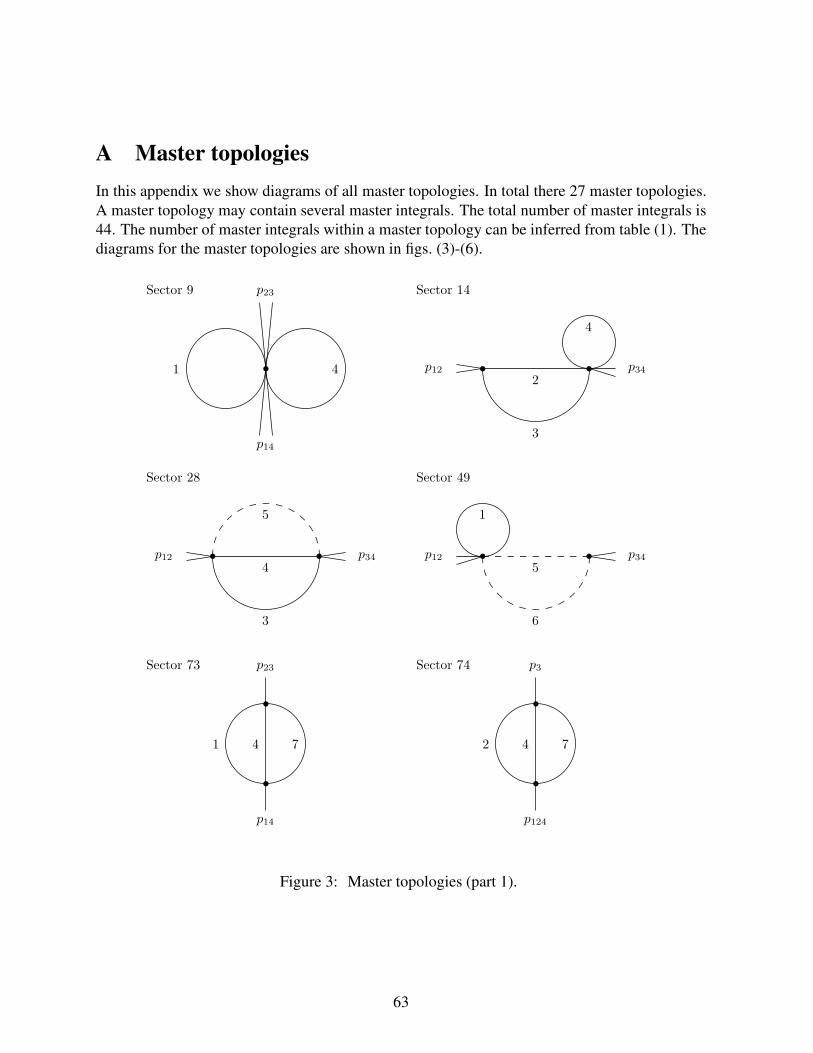
A Master topologies

In this appendix we show diagrams of all master topologies. In total there 27 master topologies.A master topology may contain several master integrals. The total number of master integrals is44. The number of master integrals within a master topology can be inferred from table (1). Thediagrams for the master topologies are shown in figs. (3)-(6).

p14

p23

1 4

Sector 9

p12 p34

3

2

4

Sector 14

p12 p34

3

4

5

Sector 28

p12 p34

6

5

1

Sector 49

p14

p23

1 4 7

Sector 73

p124

p3

2 4 7

Sector 74

Figure 3: Master topologies (part 1).

63

Page 64

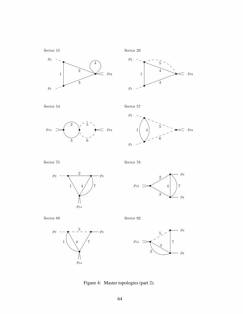
p1

p2

p341

3

2

4

Sector 15

p1

p2

p341

3

4

5

Sector 29

p12 p34

2

3

5

6

Sector 54

p1

p2

p341 45

6

Sector 57

p14

p2 p32

1 4 7

Sector 75

p12

p3

p4

2

3

4 7

Sector 78

p14

p2 p35

1 4 7

Sector 89

p12

p3

p4

5

74

3

Sector 92

Figure 4: Master topologies (part 2).

64

Page 65

p4

p3

p12 7

6

5

1

Sector 113

p1

p2

p341

2

3

5

6

Sector 55

p1

p2

p34

1 5

6

4

2

Sector 59

p12 p34

2

3

5

6

4

Sector 62

p1

p2

p4

p3

1 4 7

3

2

Sector 79

p1

p2

p4

p3

1 4 7

3

5

Sector 93

p12

p3

p4

2

3

5

6

7

Sector 118

p1

p2

p4

p3

1 4 7

6

5

Sector 121

Figure 5: Master topologies (part 3).

65

Page 66

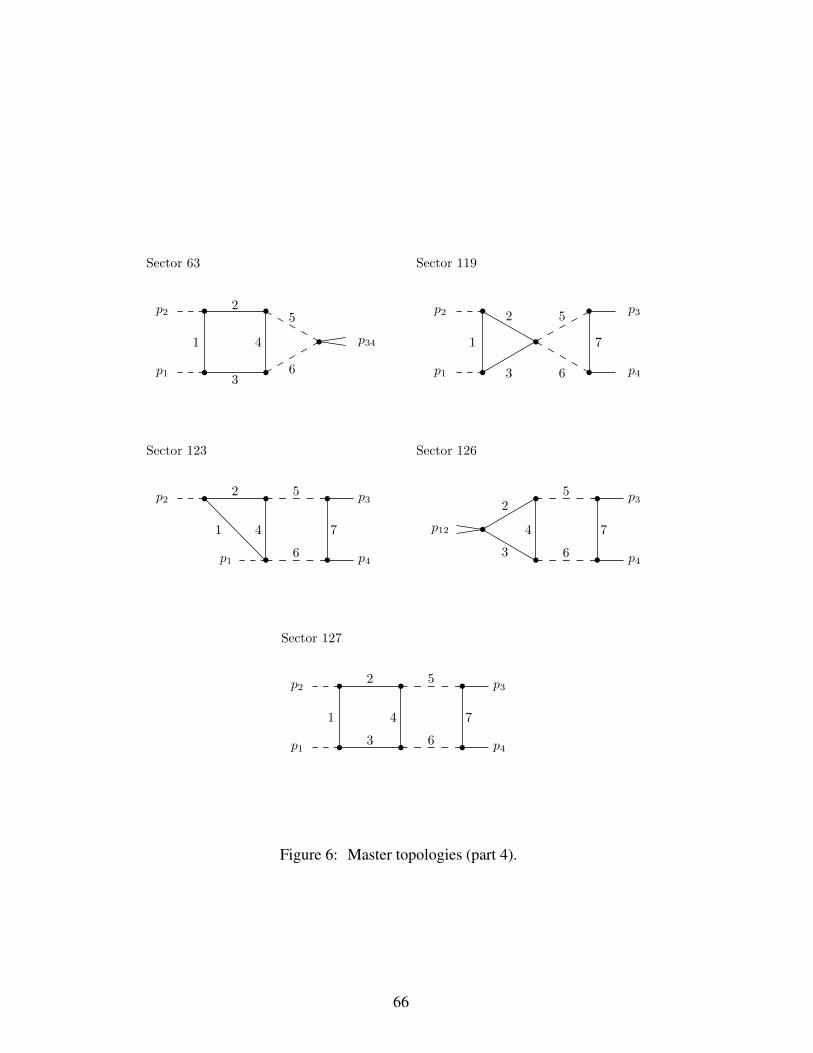
p1

p2

p341

2

3

4

5

6

Sector 63

p1

p2 p3

p4

1

2

3

5

6

7

Sector 119

p1

p2 p3

p4

1

2

4

5

6

7

Sector 123

p12

p3

p4

2

3

4

5

6

7

Sector 126

p1

p2 p3

p4

1

2

3

4

5

6

7

Sector 127

Figure 6: Master topologies (part 4).

66

Page 67

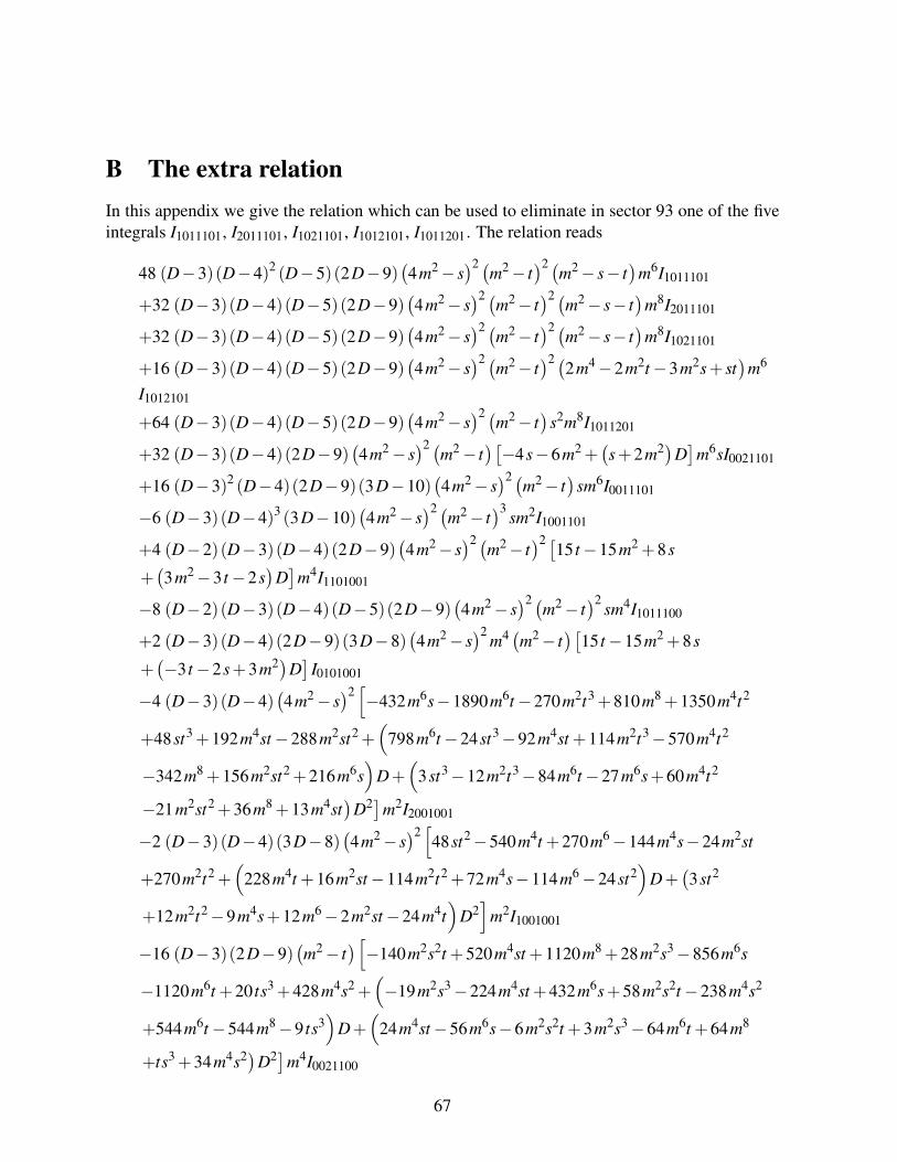
B The extra relation

In this appendix we give the relation which can be used to eliminate in sector 93 one of the fiveintegrals I1011101, I2011101, I1021101, I1012101, I1011201. The relation reads

48 (D−3)(D−4)2 (D−5)(2D−9)(4m2 − s

)2 (m2 − t

)2 (m2 − s− t

)m6I1011101

+32 (D−3)(D−4)(D−5)(2D−9)(4m2 − s

)2 (m2 − t

)2 (m2 − s− t

)m8I2011101

+32 (D−3)(D−4)(D−5)(2D−9)(4m2 − s

)2 (m2 − t

)2 (m2 − s− t

)m8I1021101

+16 (D−3)(D−4)(D−5)(2D−9)(4m2 − s

)2 (m2 − t

)2 (2m4 −2m2t −3m2s+ st

)m6

I1012101

+64 (D−3)(D−4)(D−5)(2D−9)(4m2 − s

)2 (m2 − t

)s2m8I1011201

+32 (D−3)(D−4)(2D−9)(4m2 − s

)2 (m2 − t

)[−4s−6m2 +

(s+2m2

)D]

m6sI0021101

+16 (D−3)2 (D−4)(2D−9)(3D−10)(4m2 − s

)2 (m2 − t

)sm6I0011101

−6 (D−3)(D−4)3 (3D−10)(4m2 − s

)2 (m2 − t

)3sm2I1001101

+4 (D−2)(D−3)(D−4)(2D−9)(4m2 − s

)2 (m2 − t

)2 [15 t −15m2 +8s

+(3m2 −3 t −2s

)D]

m4I1101001

−8 (D−2)(D−3)(D−4)(D−5)(2D−9)(4m2 − s

)2 (m2 − t

)2sm4I1011100

+2 (D−3)(D−4)(2D−9)(3D−8)(4m2 − s

)2m4 (m2 − t

)[15 t −15m2 +8s

+(−3 t −2s+3m2)D

]I0101001

−4 (D−3)(D−4)(4m2 − s

)2[−432m6s−1890m6t −270m2t3+810m8 +1350m4t2

+48st3+192m4st −288m2st2+(

798m6t −24st3−92m4st +114m2t3−570m4t2

−342m8 +156m2st2+216m6s)

D+(

3st3−12m2t3−84m6t −27m6s+60m4t2

−21m2st2+36m8 +13m4st)

D2]

m2I2001001

−2 (D−3)(D−4)(3D−8)(4m2 − s

)2[48st2−540m4t +270m6 −144m4s−24m2st

+270m2t2 +(

228m4t +16m2st −114m2t2 +72m4s−114m6 −24st2)

D+(3st2

+12m2t2−9m4s+12m6 −2m2st −24m4t)

D2]

m2I1001001

−16 (D−3)(2D−9)(m2 − t

)[−140m2s2t +520m4st +1120m8+28m2s3 −856m6s

−1120m6t +20 ts3+428m4s2 +(−19m2s3 −224m4st +432m6s+58m2s2t −238m4s2

+544m6t −544m8 −9 ts3)

D+(

24m4st −56m6s−6m2s2t +3m2s3 −64m6t +64m8

+ts3+34m4s2)

D2]

m4I0021100

67

Page 68

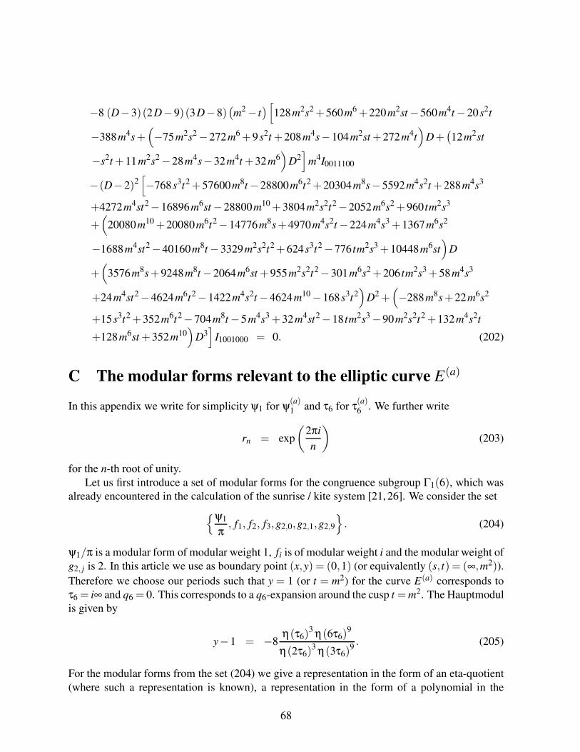
−8 (D−3)(2D−9)(3D−8)(m2 − t

)[128m2s2 +560m6 +220m2st −560m4t −20s2t

−388m4s+(−75m2s2 −272m6 +9s2t +208m4s−104m2st +272m4t

)D+

(12m2st

−s2t +11m2s2 −28m4s−32m4t +32m6)

D2]

m4I0011100

−(D−2)2[−768s3t2 +57600m8t −28800m6t2 +20304m8s−5592m4s2t +288m4s3

+4272m4st2−16896m6st −28800m10 +3804m2s2t2−2052m6s2 +960 tm2s3

+(

20080m10 +20080m6t2−14776m8s+4970m4s2t −224m4s3 +1367m6s2

−1688m4st2−40160m8t −3329m2s2t2+624s3t2 −776 tm2s3 +10448m6st)

D

+(

3576m8s+9248m8t −2064m6st +955m2s2t2 −301m6s2 +206 tm2s3 +58m4s3

+24m4st2−4624m6t2−1422m4s2t −4624m10 −168s3t2)

D2 +(−288m8s+22m6s2

+15s3t2 +352m6t2−704m8t −5m4s3 +32m4st2−18 tm2s3 −90m2s2t2 +132m4s2t

+128m6st +352m10)

D3]

I1001000 = 0. (202)

C The modular forms relevant to the elliptic curve E(a)

In this appendix we write for simplicity ψ1 for ψ(a)1 and τ6 for τ

(a)6 . We further write

rn = exp

(2πi

n

)(203)

for the n-th root of unity.Let us first introduce a set of modular forms for the congruence subgroup Γ1(6), which was

already encountered in the calculation of the sunrise / kite system [21, 26]. We consider the set

{ψ1

π, f1, f2, f3,g2,0,g2,1,g2,9

}. (204)

ψ1/π is a modular form of modular weight 1, fi is of modular weight i and the modular weight ofg2, j is 2. In this article we use as boundary point (x,y) = (0,1) (or equivalently (s, t) = (∞,m2)).Therefore we choose our periods such that y = 1 (or t = m2) for the curve E(a) corresponds toτ6 = i∞ and q6 = 0. This corresponds to a q6-expansion around the cusp t =m2. The Hauptmodulis given by

y−1 = −8η(τ6)

3 η(6τ6)9

η(2τ6)3 η(3τ6)

9 . (205)

For the modular forms from the set (204) we give a representation in the form of an eta-quotient(where such a representation is known), a representation in the form of a polynomial in the

68

Page 69

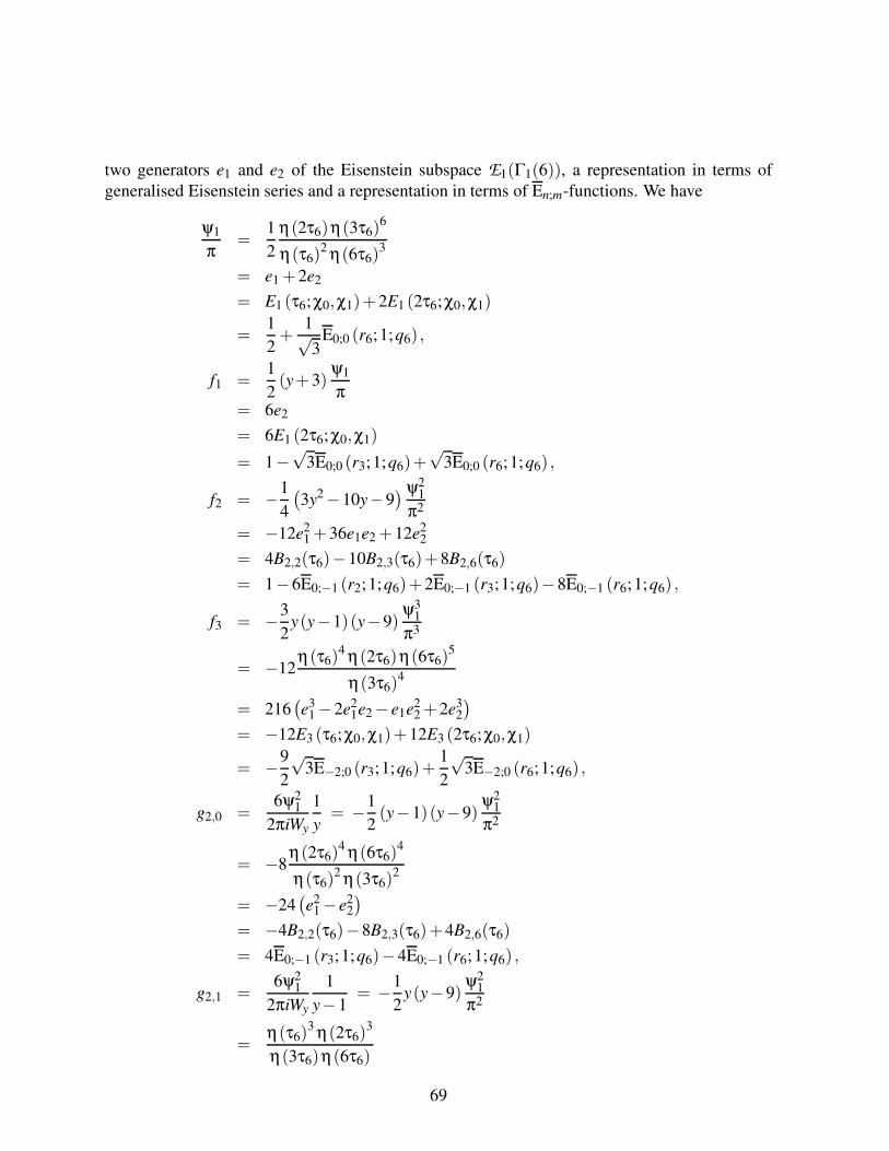
two generators e1 and e2 of the Eisenstein subspace E1(Γ1(6)), a representation in terms ofgeneralised Eisenstein series and a representation in terms of En;m-functions. We have

ψ1

π=

1

2

η(2τ6)η(3τ6)6

η(τ6)2 η(6τ6)

3

= e1 +2e2

= E1 (τ6;χ0,χ1)+2E1 (2τ6;χ0,χ1)

=1

2+

1√3

E0;0 (r6;1;q6) ,

f1 =1

2(y+3)

ψ1

π= 6e2

= 6E1 (2τ6;χ0,χ1)

= 1−√

3E0;0 (r3;1;q6)+√

3E0;0 (r6;1;q6) ,

f2 = −1

4

(3y2 −10y−9

) ψ21

π2

= −12e21 +36e1e2 +12e2

2

= 4B2,2(τ6)−10B2,3(τ6)+8B2,6(τ6)

= 1−6E0;−1 (r2;1;q6)+2E0;−1 (r3;1;q6)−8E0;−1 (r6;1;q6) ,

f3 = −3

2y(y−1)(y−9)

ψ31

π3

= −12η(τ6)

4 η(2τ6)η(6τ6)5

η(3τ6)4

= 216(e3

1 −2e21e2 − e1e2

2 +2e32

)

= −12E3 (τ6;χ0,χ1)+12E3 (2τ6;χ0,χ1)

= −9

2

√3E−2;0 (r3;1;q6)+

1

2

√3E−2;0 (r6;1;q6) ,

g2,0 =6ψ2

1

2πiWy

1

y= −1

2(y−1)(y−9)

ψ21

π2

= −8η(2τ6)

4 η(6τ6)4

η(τ6)2 η(3τ6)

2

= −24(e2

1 − e22

)

= −4B2,2(τ6)−8B2,3(τ6)+4B2,6(τ6)

= 4E0;−1 (r3;1;q6)−4E0;−1 (r6;1;q6) ,

g2,1 =6ψ2

1

2πiWy

1

y−1= −1

2y(y−9)

ψ21

π2

=η(τ6)

3 η(2τ6)3

η(3τ6)η(6τ6)

69

Page 70

= −18e21 +18e1e2 +36e2

2

= −3B2,2(τ6)−9B2,3(τ6)+9B2,6(τ6)

= 1−3E0;−1 (r2;1;q6)−9E0;−1 (r6;1;q6) ,

g2,9 =6ψ2

1

2πiWy

1

y−9= −1

2y(y−1)

ψ21

π2

=η(τ6)

7 η(6τ6)7

η(2τ6)5 η(3τ6)

5

= −6e21 +18e1e2 −12e2

2

= 5B2,2(τ6)−5B2,3(τ6)+B2,6(τ6)

= −3E0;−1 (r2;1;q6)+4E0;−1 (r3;1;q6)−E0;−1 (r6;1;q6) , (206)

Here we used the notation B2,N(τ) = E2(τ)−NE2(Nτ) and

e1 = E1 (τ6;χ0,χ1) , e2 = E1 (2τ6;χ0,χ1) , (207)

where χ0 and χ1 denote primitive Dirichlet characters with conductors 1 and 3, respectively.They are given in terms of the Kronecker symbol by

χ0 =

(1

n

), χ1 =

(−3

n

). (208)

The definition of the generalised Eisenstein series is as in [21, 127]. The two Eisenstein series{e1,e2} give a basis for the modular forms of modular weight 1 for the Eisenstein subspaceE1(Γ1(6)).

The En;m-functions are defined by [17, 24]

En;m (x;y;q) =

1i

[ELin;m (x;y;q)−ELin;m

(x−1;y−1;q

)], n+m even,

ELin;m (x;y;q)+ELin;m(x−1;y−1;q

), n+m odd.

(209)

and

ELin;m (x;y;q) =∞

∑j=1

∞

∑k=1

x j

jn

yk

kmq jk. (210)

Products of modular forms are again modular forms. In particular

f4 = f 41 (211)

and

g3,1 = g2,1ψ1

π,

g4, j = g2, j

(ψ1

π

)2, j ∈ {0,1,9},

70

Page 71

h3,0 =1

3f3,

h4,0 =1

3f3

ψ1

π,

h4,1 =2

3f1 f3 −

4

3f3

ψ1

π. (212)

This shows that all elements of the set in eq. (138) are modular forms.

D Boundary constants

In this appendix we list the boundary constants at the point (x, y) = (0,0) (or equivalently (s, t)=(∞,m2) or (x,y) = (0,1)). The boundary constants are given by

J1|(x,y)=(0,0) = 1+ζ2ε2 − 2

3ζ3ε3 +

7

4ζ4ε4 +O

(ε5),

J2|(x,y)=(0,0) = ζ2ε2 +2ζ3ε3 +19

4ζ4ε4 +O

(ε5),

J3|(x,y)=(0,0) = −ζ2ε2 −11ζ3ε3 − 29

2ζ4ε4 +O

(ε5),

J4|(x,y)=(0,0) = −6ζ3ε3 − 13

2ζ4ε4 +O

(ε5),

J5|(x,y)=(0,0) = 1− 8

3ζ3ε3 −3ζ4ε4 +O

(ε5),

J6|(x,y)=(0,0) = 3ζ2ε2 +

[21

2ζ3 −18ζ2 ln(2)

]ε3 +

[72Li4

(1

2

)−39ζ4 +36ζ2 ln2 (2)

+3 ln4 (2)]

ε4 +O

(ε5),

J7|(x,y)=(0,0) = 3ζ2ε2 +

[21

2ζ3 −18ζ2 ln(2)

]ε3 +

[72Li4

(1

2

)−39ζ4 +36ζ2 ln2 (2)

+3 ln4 (2)]

ε4 +O

(ε5),

J8|(x,y)=(0,0) = 6ζ2ε2 +[21ζ3 −36ζ2 ln2]ε3 +

[144Li4

(1

2

)−78ζ4 +72ζ2 ln2 (2)

+6ln4 (2)]

ε4 +O

(ε5),

J9|(x,y)=(0,0) = −3ζ3ε3 − 5

4ζ4ε4 +O

(ε5),

J10|(x,y)=(0,0) = −4ζ3ε3 +4ζ4ε4 +O

(ε5),

J11|(x,y)=(0,0) = ζ2ε2 +2ζ3ε3 +9

4ζ4ε4 +O

(ε5),

J12|(x,y)=(0,0) = ζ2ε2 −4ζ3ε3 +O

(ε5),

71

Page 72

J13|(x,y)=(0,0) = −2ζ3ε3 +5

4ζ4ε4 +O

(ε5),

J14|(x,y)=(0,0) = O

(ε5),

J15|(x,y)=(0,0) =

[11

2ζ3 −6ζ2 ln(2)

]ε3 +

[24Li4

(1

2

)− 23

2ζ4 +12ζ2 ln2 (2)+ ln4 (2)

]ε4

+O

(ε5),

J16|(x,y)=(0,0) =1

4ζ4ε4 +O

(ε5),

J17|(x,y)=(0,0) = O

(ε5),

J18|(x,y)=(0,0) = −ζ2ε2 +

[9

4ζ3 +3ζ2 ln(2)

]ε3 +

[−12Li4

(1

2

)+

75

8ζ4 −6ζ2 ln2 (2)

−1

2ln4 (2)

]ε4 +O

(ε5),

J19|(x,y)=(0,0) = −1

2ζ4ε4 +O

(ε5),

J20|(x,y)=(0,0) = −4ζ2ε2 −5ζ3ε3 − 99

4ζ4ε4 +O

(ε5),

J21|(x,y)=(0,0) = −3ζ3ε3 − 5

4ζ4ε4 +O

(ε5),

J22|(x,y)=(0,0) =7

4ζ4ε4 +O

(ε5),

J23|(x,y)=(0,0) = 6ζ3ε3 +9ζ4ε4 +O

(ε5),

J24|(x,y)=(0,0) =

[−7

4ζ3 −3ζ2 ln(2)

]ε3 +

[15

4ζ4 +18ζ2 ln2 (2)

]ε4 +O

(ε5),

J25|(x,y)=(0,0) =

[−23

6ζ3 +2ζ2 ln(2)

]ε3 +

[−8Li4

(1

2

)+3ζ4 −4ζ2 ln2 (2)− 1

3ln4 (2)

]ε4

+O

(ε5),

J26|(x,y)=(0,0) =7

4ζ2ε2 +

[35

8ζ3 −

27

2ζ2 ln(2)

]ε3 +

[42Li4

(1

2

)−19ζ4 +39ζ2 ln2 (2)

+7

4ln4 (2)

])ε4 +O

(ε5),

J27|(x,y)=(0,0) =

[−7

2ζ3 −6ζ2 ln(2)

]ε3 +

[105

4ζ4 +36ζ2 ln2 (2)

]ε4 +O

(ε5),

J28|(x,y)=(0,0) =

[−1

3ζ3 −4ζ2 ln(2)

]ε3 +

[16Li4

(1

2

)−12ζ4 +8ζ2 ln2 (2)+

2

3ln4 (2)

]ε4

+O

(ε5),

72

Page 73

J29|(x,y)=(0,0) = O

(ε5),

J30|(x,y)=(0,0) =7

2ζ2ε2 +

[35

4ζ3 −27ζ2 ln(2)

]ε3 +

[84Li4

(1

2

)− 77

4ζ4 +78ζ2 ln2 (2)

+7

2ln4 (2)

]ε4 +O

(ε5),

J32|(x,y)=(0,0) = −4ζ2ε2 −5ζ3ε3 − 139

4ζ4ε4 +O

(ε5),

J33|(x,y)=(0,0) =105

4ζ4ε4 +O

(ε5),

J34|(x,y)=(0,0) = 4ζ2ε2 +

[11

2ζ3 −6ζ2 ln(2)

]ε3 +

[24Li4

(1

2

)+

7

2ζ4 +12ζ2 ln2 (2)

+ ln4 (2)]

ε4 +O

(ε5),

J35|(x,y)=(0,0) =3

4ζ2ε2 +

[21

8ζ3 −

9

2ζ2 ln(2)

]ε3 +

[18Li4

(1

2

)+

33

2ζ4 +9ζ2 ln2 (2)

+3

4ln4 (2)

]ε4 +O

(ε5),

J36|(x,y)=(0,0) = −39

2ζ4ε4 +O

(ε5),

J37|(x,y)=(0,0) = O

(ε5),

J38|(x,y)=(0,0) =17

2ε4ζ4 +O

(ε5),

J39|(x,y)=(0,0) = O

(ε5),

J40|(x,y)=(0,0) = −3ζ4ε4 +O

(ε5),

J41|(x,y)=(0,0) =

[8Li4

(1

2

)− 79

4ζ4 −8ζ2 ln2 (2)+

1

3ln4 (2)

]ε4 +O

(ε5),

J42|(x,y)=(0,0) = −24ζ3ε3 −102ζ4ε4 +O

(ε5),

J43|(x,y)=(0,0) =

[49

12ζ3 +7ζ2 ln(2)

]ε3 +

[8Li4

(1

2

)− 109

4ζ4 −50ζ2 ln2 (2)

+1

3ln4 (2)

]ε4 +O

(ε5),

J44|(x,y)=(0,0) =

[16

3Li4

(1

2

)+

31

12ζ4 −

16

3ζ2 ln2 (2)+

2

9ln4 (2)

]ε4 +O

(ε5),

J45|(x,y)=(0,0) =

[−56

3Li4

(1

2

)− 11

12ζ4 +

56

3ζ2 ln2 (2)− 7

9ln4 (2)

]ε4 +O

(ε5). (213)

73

Page 74

E Supplementary material

Attached to this article is an electronic file in ASCII format with Maple syntax, defining thequantities

I_basis, U, Uinv, A, integration_kernels, J.

I_basis is a vector defining the basis ~I as listed in the fourth column of table 1, U gives thetransformation matrix to the basis ~J, i.e.

~J = U~I, (214)

Uinv denotes the matrix inverse of U . The quantity A defines the matrix

A = A(0)+ εA(1) (215)

appearing in the differential equation

d~J = A~J. (216)

The entries of A are linear combinations of integration kernels (with symbolic names), whoseexplicit expressions are defined in integration_kernels. Finally, J contains the results for themaster integrals up to order ε4 in terms of iterated integrals, including the boundary constants forthe boundary point (x,y) = (0,1).

References

[1] D. J. Broadhurst, J. Fleischer, and O. Tarasov, Z.Phys. C60, 287 (1993), arXiv:hep-ph/9304303.

[2] F. A. Berends, M. Buza, M. Böhm, and R. Scharf, Z.Phys. C63, 227 (1994).

[3] S. Bauberger, M. Böhm, G. Weiglein, F. A. Berends, and M. Buza, Nucl.Phys.Proc.Suppl. 37B, 95 (1994),arXiv:hep-ph/9406404.

[4] S. Bauberger, F. A. Berends, M. Böhm, and M. Buza, Nucl.Phys. B434, 383 (1995), arXiv:hep-ph/9409388.

[5] S. Bauberger and M. Böhm, Nucl.Phys. B445, 25 (1995), arXiv:hep-ph/9501201.

[6] M. Caffo, H. Czyz, S. Laporta, and E. Remiddi, Nuovo Cim. A111, 365 (1998), arXiv:hep-th/9805118.

[7] S. Laporta and E. Remiddi, Nucl. Phys. B704, 349 (2005), hep-ph/0406160.

[8] B. A. Kniehl, A. V. Kotikov, A. Onishchenko, and O. Veretin, Nucl. Phys. B738, 306 (2006), arXiv:hep-ph/0510235.

[9] S. Groote, J. G. Körner, and A. A. Pivovarov, Annals Phys. 322, 2374 (2007), arXiv:hep-ph/0506286.

[10] S. Groote, J. Körner, and A. Pivovarov, Eur.Phys.J. C72, 2085 (2012), arXiv:1204.0694.

[11] D. H. Bailey, J. M. Borwein, D. Broadhurst, and M. L. Glasser, J. Phys. A41, 205203 (2008),arXiv:0801.0891.

[12] S. Müller-Stach, S. Weinzierl, and R. Zayadeh, Commun. Num. Theor. Phys. 6, 203 (2012), arXiv:1112.4360.

[13] L. Adams, C. Bogner, and S. Weinzierl, J. Math. Phys. 54, 052303 (2013), arXiv:1302.7004.

74

Page 75

[14] S. Bloch and P. Vanhove, J. Numb. Theor. 148, 328 (2015), arXiv:1309.5865.

[15] L. Adams, C. Bogner, and S. Weinzierl, J. Math. Phys. 55, 102301 (2014), arXiv:1405.5640.

[16] L. Adams, C. Bogner, and S. Weinzierl, J. Math. Phys. 56, 072303 (2015), arXiv:1504.03255.

[17] L. Adams, C. Bogner, and S. Weinzierl, J. Math. Phys. 57, 032304 (2016), arXiv:1512.05630.

[18] E. Remiddi and L. Tancredi, Nucl.Phys. B880, 343 (2014), arXiv:1311.3342.

[19] S. Bloch, M. Kerr, and P. Vanhove, Adv. Theor. Math. Phys. 21, 1373 (2017), arXiv:1601.08181.

[20] S. Groote and J. G. Körner, (2018), arXiv:1804.10570.

[21] L. Adams and S. Weinzierl, Commun. Num. Theor. Phys. 12, 193 (2018), arXiv:1704.08895.

[22] S. Bloch, M. Kerr, and P. Vanhove, Compos. Math. 151, 2329 (2015), arXiv:1406.2664.

[23] E. Remiddi and L. Tancredi, Nucl. Phys. B907, 400 (2016), arXiv:1602.01481.

[24] L. Adams, C. Bogner, A. Schweitzer, and S. Weinzierl, J. Math. Phys. 57, 122302 (2016), arXiv:1607.01571.

[25] C. Bogner, A. Schweitzer, and S. Weinzierl, Nucl. Phys. B922, 528 (2017), arXiv:1705.08952.

[26] L. Adams and S. Weinzierl, Phys. Lett. B781, 270 (2018), arXiv:1802.05020.

[27] M. Søgaard and Y. Zhang, Phys. Rev. D91, 081701 (2015), arXiv:1412.5577.

[28] R. Bonciani et al., JHEP 12, 096 (2016), arXiv:1609.06685.

[29] A. von Manteuffel and L. Tancredi, JHEP 06, 127 (2017), arXiv:1701.05905.

[30] A. Primo and L. Tancredi, Nucl. Phys. B921, 316 (2017), arXiv:1704.05465.

[31] J. Ablinger et al., J. Math. Phys. 59, 062305 (2018), arXiv:1706.01299.

[32] J. L. Bourjaily, A. J. McLeod, M. Spradlin, M. von Hippel, and M. Wilhelm, Phys. Rev. Lett. 120, 121603(2018), arXiv:1712.02785.

[33] M. Hidding and F. Moriello, (2017), arXiv:1712.04441.

[34] G. Passarino, European Physical Journal C 77, 77 (2017), arXiv:1610.06207.

[35] E. Remiddi and L. Tancredi, Nucl. Phys. B925, 212 (2017), arXiv:1709.03622.

[36] J. Broedel, C. Duhr, F. Dulat, and L. Tancredi, JHEP 05, 093 (2018), arXiv:1712.07089.

[37] J. Broedel, C. Duhr, F. Dulat, and L. Tancredi, Phys. Rev. D97, 116009 (2018), arXiv:1712.07095.

[38] J. Broedel, C. Duhr, F. Dulat, B. Penante, and L. Tancredi, (2018), arXiv:1803.10256.

[39] R. N. Lee, A. V. Smirnov, and V. A. Smirnov, JHEP 03, 008 (2018), arXiv:1709.07525.

[40] R. N. Lee, A. V. Smirnov, and V. A. Smirnov, (2018), arXiv:1805.00227.

[41] J. Broedel, C. R. Mafra, N. Matthes, and O. Schlotterer, JHEP 07, 112 (2015), arXiv:1412.5535.

[42] J. Broedel, N. Matthes, and O. Schlotterer, J. Phys. A49, 155203 (2016), arXiv:1507.02254.

[43] J. Broedel, N. Matthes, G. Richter, and O. Schlotterer, J. Phys. A51, 285401 (2018), arXiv:1704.03449.

[44] E. D’Hoker, M. B. Green, Ö. Gürdogan, and P. Vanhove, Commun. Num. Theor. Phys. 11, 165 (2017),arXiv:1512.06779.

[45] S. Hohenegger and S. Stieberger, Nucl. Phys. B925, 63 (2017), arXiv:1702.04963.

[46] J. Broedel, O. Schlotterer, and F. Zerbini, (2018), arXiv:1803.00527.

[47] M. Czakon, P. Fiedler, and A. Mitov, Phys.Rev.Lett. 110, 252004 (2013), arXiv:1303.6254.

75

Page 76

[48] P. Bärnreuther, M. Czakon, and P. Fiedler, JHEP 02, 078 (2014), arXiv:1312.6279.

[49] M. Czakon, Phys. Lett. B664, 307 (2008), arXiv:0803.1400.

[50] M. Czakon, A. Mitov, and S. Moch, Nucl. Phys. B798, 210 (2008), arXiv:0707.4139.

[51] M. Czakon, Comput. Phys. Commun. 175, 559 (2006), hep-ph/0511200.

[52] L. Adams, E. Chaubey, and S. Weinzierl, Phys. Rev. Lett. 121, 142001 (2018), arXiv:1804.11144.

[53] A. V. Kotikov, Phys. Lett. B254, 158 (1991).

[54] A. V. Kotikov, Phys. Lett. B267, 123 (1991).

[55] E. Remiddi, Nuovo Cim. A110, 1435 (1997), hep-th/9711188.

[56] T. Gehrmann and E. Remiddi, Nucl. Phys. B580, 485 (2000), hep-ph/9912329.

[57] M. Argeri and P. Mastrolia, Int. J. Mod. Phys. A22, 4375 (2007), arXiv:0707.4037.

[58] S. Müller-Stach, S. Weinzierl, and R. Zayadeh, Commun.Math.Phys. 326, 237 (2014), arXiv:1212.4389.

[59] J. M. Henn, Phys. Rev. Lett. 110, 251601 (2013), arXiv:1304.1806.

[60] J. M. Henn, J. Phys. A48, 153001 (2015), arXiv:1412.2296.

[61] J. Ablinger et al., Comput. Phys. Commun. 202, 33 (2016), arXiv:1509.08324.

[62] L. Adams, E. Chaubey, and S. Weinzierl, Phys. Rev. Lett. 118, 141602 (2017), arXiv:1702.04279.

[63] J. Bosma, K. J. Larsen, and Y. Zhang, Phys. Rev. D97, 105014 (2018), arXiv:1712.03760.

[64] T. Gehrmann, A. von Manteuffel, L. Tancredi, and E. Weihs, JHEP 06, 032 (2014), arXiv:1404.4853.

[65] M. Argeri et al., JHEP 03, 082 (2014), arXiv:1401.2979.

[66] R. N. Lee, JHEP 04, 108 (2015), arXiv:1411.0911.

[67] M. Prausa, Comput. Phys. Commun. 219, 361 (2017), arXiv:1701.00725.

[68] O. Gituliar and V. Magerya, Comput. Phys. Commun. 219, 329 (2017), arXiv:1701.04269.

[69] C. Meyer, JHEP 04, 006 (2017), arXiv:1611.01087.

[70] C. Meyer, Comput. Phys. Commun. 222, 295 (2018), arXiv:1705.06252.

[71] R. N. Lee and A. A. Pomeransky, (2017), arXiv:1707.07856.

[72] M. Becchetti and R. Bonciani, JHEP 01, 048 (2018), arXiv:1712.02537.

[73] A. Beilinson and A. Levin, in Motives, ed. U. Jannsen, S. Kleiman, J.-P. Serre, Proc. of Symp. in PureMathematics 55, Part 2, AMS, 1994, 123-190.

[74] A. Levin, Comp. Math. 106, 267 (1997).

[75] A. Levin and G. Racinet, (2007), arXiv:math/0703237.

[76] B. Enriquez, Selecta Math. 20, 491 (2014), arXiv:1003.1012.

[77] F. Brown and A. Levin, (2011), arXiv:1110.6917.

[78] J. Wildeshaus, Lect. Notes Math. 1650, Springer, (1997).

[79] T. Kinoshita, J. Math. Phys. 3, 650 (1962).

[80] O. V. Tarasov, Phys. Rev. D54, 6479 (1996), hep-th/9606018.

[81] O. V. Tarasov, Nucl. Phys. B502, 455 (1997), hep-ph/9703319.

76

Page 77

[82] A. von Manteuffel and C. Studerus, (2012), arXiv:1201.4330.

[83] P. Maierhöfer, J. Usovitsch, and P. Uwer, Comput. Phys. Commun. 230, 99 (2018), arXiv:1705.05610.

[84] A. V. Smirnov, Comput. Phys. Commun. 189, 182 (2015), arXiv:1408.2372.

[85] R. N. Lee, (2012), arXiv:1212.2685.

[86] R. N. Lee, J. Phys. Conf. Ser. 523, 012059 (2014), arXiv:1310.1145.

[87] F. V. Tkachov, Phys. Lett. B100, 65 (1981).

[88] K. G. Chetyrkin and F. V. Tkachov, Nucl. Phys. B192, 159 (1981).

[89] S. Laporta, Int. J. Mod. Phys. A15, 5087 (2000), hep-ph/0102033.

[90] R. N. Lee and A. A. Pomeransky, JHEP 11, 165 (2013), arXiv:1308.6676.

[91] A. Georgoudis, K. J. Larsen, and Y. Zhang, Comput. Phys. Commun. 221, 203 (2017), arXiv:1612.04252.

[92] K.-T. Chen, Bull. Amer. Math. Soc. 83, 831 (1977).

[93] A. B. Goncharov, Math. Res. Lett. 5, 497 (1998).

[94] A. B. Goncharov, (2001), math.AG/0103059.

[95] J. M. Borwein, D. M. Bradley, D. J. Broadhurst, and P. Lisonek, Trans. Amer. Math. Soc. 353:3, 907 (2001),math.CA/9910045.

[96] S. Moch, P. Uwer, and S. Weinzierl, J. Math. Phys. 43, 3363 (2002), hep-ph/0110083.

[97] J. Vollinga and S. Weinzierl, Comput. Phys. Commun. 167, 177 (2005), hep-ph/0410259.

[98] F. Brown, (2014), arXiv:1407.5167.

[99] J. Fleischer, A. V. Kotikov, and O. L. Veretin, Nucl. Phys. B547, 343 (1999), hep-ph/9808242.

[100] A. Kotikov, J. H. Kuhn, and O. Veretin, Nucl. Phys. B788, 47 (2008), arXiv:hep-ph/0703013.

[101] R. Bonciani, G. Degrassi, and A. Vicini, Comput. Phys. Commun. 182, 1253 (2011), arXiv:1007.1891.

[102] J. M. Henn and V. A. Smirnov, JHEP 11, 041 (2013), arXiv:1307.4083.

[103] J. A. M. Vermaseren, Int. J. Mod. Phys. A14, 2037 (1999), hep-ph/9806280.

[104] E. Remiddi and J. A. M. Vermaseren, Int. J. Mod. Phys. A15, 725 (2000), hep-ph/9905237.

[105] P. A. Baikov, Nucl. Instrum. Meth. A389, 347 (1997), arXiv:hep-ph/9611449.

[106] R. N. Lee, Nucl. Phys. B830, 474 (2010), arXiv:0911.0252.

[107] D. A. Kosower and K. J. Larsen, Phys. Rev. D85, 045017 (2012), arXiv:1108.1180.

[108] S. Caron-Huot and K. J. Larsen, JHEP 1210, 026 (2012), arXiv:1205.0801.

[109] H. Frellesvig and C. G. Papadopoulos, JHEP 04, 083 (2017), arXiv:1701.07356.

[110] J. Bosma, M. Sogaard, and Y. Zhang, JHEP 08, 051 (2017), arXiv:1704.04255.

[111] M. Harley, F. Moriello, and R. M. Schabinger, JHEP 06, 049 (2017), arXiv:1705.03478.

[112] A. Primo and L. Tancredi, Nucl. Phys. B916, 94 (2017), arXiv:1610.08397.

[113] J. Blümlein, D. J. Broadhurst, and J. A. M. Vermaseren, Comput. Phys. Commun. 181, 582 (2010),arXiv:0907.2557.

[114] J. Broedel, O. Schlotterer, and S. Stieberger, Fortsch. Phys. 61, 812 (2013), arXiv:1304.7267.

[115] H. R. P. Ferguson and D. H. Bailey, (1992), RNR Technical Report RNR-91-032.

77

Page 78

[116] A. I. Davydychev and M. Y. Kalmykov, Nucl. Phys. B605, 266 (2001), hep-th/0012189.

[117] A. I. Davydychev and M. Y. Kalmykov, Nucl. Phys. B699, 3 (2004), hep-th/0303162.

[118] V. V. Bytev, M. Yu. Kalmykov, and B. A. Kniehl, Nucl. Phys. B836, 129 (2010), arXiv:0904.0214.

[119] C. Bogner and S. Weinzierl, Comput. Phys. Commun. 178, 596 (2008), arXiv:0709.4092.

[120] J. Carter and G. Heinrich, Comput. Phys. Commun. 182, 1566 (2011), arXiv:1011.5493.

[121] S. Borowka, J. Carter, and G. Heinrich, Comput. Phys. Commun. 184, 396 (2013), arXiv:1204.4152.

[122] S. Borowka et al., Comput. Phys. Commun. 196, 470 (2015), arXiv:1502.06595.

[123] S. Borowka et al., Comput. Phys. Commun. 222, 313 (2018), arXiv:1703.09692.

[124] A. V. Smirnov and M. N. Tentyukov, Comput. Phys. Commun. 180, 735 (2009), arXiv:0807.4129.

[125] A. V. Smirnov, V. A. Smirnov, and M. Tentyukov, Comput. Phys. Commun. 182, 790 (2011),arXiv:0912.0158.

[126] J. A. M. Vermaseren, Comput. Phys. Commun. 83, 45 (1994).

[127] W. A. Stein, Modular Forms, a Computational Approach (American Mathematical Society, 2007).

78