Analytic Expressions and Visual- ization of Minimum Energy ... · 3.2 The Underwood Equations for Minimum Energy Underwood’s methods for multicomponent mixtures (Underwood 1945,

Chapter 3

Analytic Expressions and Visual-ization of Minimum Energy

Consumption in MulticomponentDistillation:

A Revisit of the UnderwoodEquations.

Ivar J. Halvorsen and Sigurd Skogestad

The classical Underwood equations are used to com-pute the operational characteristics of a two-product distillation column with a multicomponentfeed. The Vmin-diagram is introduced to effec-tively visualize how the energy consumption isrelated to the feed component distribution for allpossible operating points of the column. This dia-gram becomes very useful when we later shall useit for assessment of Petlyuk arrangements.

A preliminary version was presented at AIChEAnnual Meeting in Dallas, Texas, November 1999

NTNU Dr. ing. Thesis 2001:43 Ivar J. Halvorsen

64

sfully0),m-

umbeenergpo-well

tlyukThis

ol-odel

and

3.1 Introduction

3.1.1 Background

The equations of Underwood (1945,1946ab,1948) have been applied succesby many authors for analysis of multicomponent distillation, e.g. Shiras (195King (1971), Franklin and Forsyth (1953), Wachter et. al. (1988) and in a coprehensive review of minimum energy calculations by Koehler (1995). Minimenergy expressions for Petlyuk arrangements with three components havepresented by Fidkowski and Krolikowski (1986) and Carlberg and Westerb(1989ab). However, minimum energy requirements for the general multicomnent case is the topic of this chapter, and this issue has so far not beenunderstood.

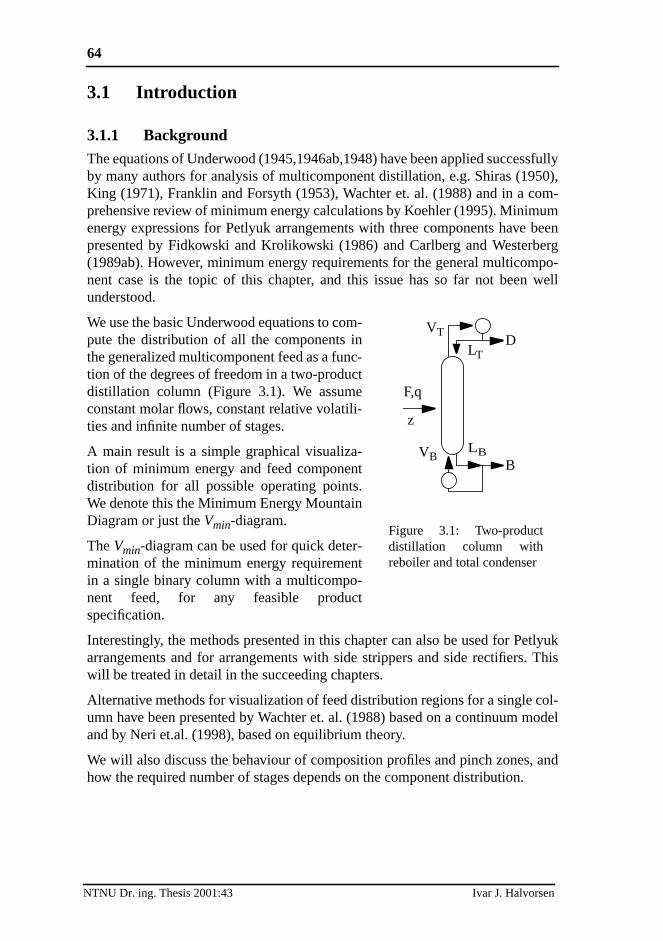
We use the basic Underwood equations to com-pute the distribution of all the components inthe generalized multicomponent feed as a func-tion of the degrees of freedom in a two-productdistillation column (Figure 3.1). We assumeconstant molar flows, constant relative volatili-ties and infinite number of stages.

A main result is a simple graphical visualiza-tion of minimum energy and feed componentdistribution for all possible operating points.We denote this the Minimum Energy MountainDiagram or just theVmin-diagram.

TheVmin-diagram can be used for quick deter-mination of the minimum energy requirementin a single binary column with a multicompo-nent feed, for any feasible productspecification.

Interestingly, the methods presented in this chapter can also be used for Pearrangements and for arrangements with side strippers and side rectifiers.will be treated in detail in the succeeding chapters.

Alternative methods for visualization of feed distribution regions for a single cumn have been presented by Wachter et. al. (1988) based on a continuum mand by Neri et.al. (1998), based on equilibrium theory.

We will also discuss the behaviour of composition profiles and pinch zones,how the required number of stages depends on the component distribution.

Figure 3.1: Two-productdistillation column withreboiler and total condenser

LT

VT

LBVB

F,q

z

D

B


3.2 The Underwood Equations for Minimum Energy 65

esuctelythem-lumne thatimited

by

y

riestage.

ted.

ab,por-

onbe

at a

gve as

3.1.2 Problem Definition - Degrees of Freedom

With a given feed, a two-product distillation column normally has two degrefreedom of operation. For a binary feed, this is sufficient to specify any proddistribution. In the case of a multicomponent feed, however, we cannot frespecify the compositions in both products. In practice, one usually specifiesdistribution of two key components, and then the distribution of the non-key coponents is then completely determined for a given feed. In some cases, the copressure could be considered as a third degree of freedom, but we will assumthe pressure is constant throughout this chapter since the pressure has a limpact on the product distribution.

For every possible operating point we want to find the distribution, here giventhe set of recoveries , the normalized vapour flow rate (V/F) and the overall product split(D/F or B/F). This can be expressed qualitativelfor the top section as:

(3.1)

It is sufficient to consider only one of the top or bottom sections as the recoveand flows in the other section can be found by a material balance at the feed sThe feed properties are given by the composition vectorz, flow rateF, liquid frac-tion q and relative volatilities . A recovery ( ) is the amount of componenitransported in a stream or through a section divided by the amount in the fe

3.2 The Underwood Equations for Minimum Energy

Underwood’s methods for multicomponent mixtures (Underwood 1945, 19461948) play a major role in our analysis, and here we summarize the most imtant equations for minimum energy calculations. The analysis is basedconsidering a two-product column with a single feed, but the usage canextended to all kinds of column section interconnections.

3.2.1 Some Basic Definitions

The starting point for Underwood’s methods is the material balance equationcross-section in the column. The net material transport (wi) of componentiupwards through a stagen is the difference between the amount travellinupwards from a stage as vapour and the amount entering a stage from aboliquid:

(3.2)

R r1 r2 … r Nc, , ,[ ]=

VT

F------- D

F---- RT, , f Spec1 Spec2 Feed properties, ,( )=

α r i

wi Vnyi n, Ln 1+ xi n 1+,–=


66

l-

thetheneed

ef-

of:

s of:

tage:

Note that at steady state,wi is constant through each column section. In the folowing we assume constant molar flows (L=Ln=Ln-1 and V=Vn=Vn+1) andconstant relative volatility ( ).

In the top section the net product flow and:

(3.3)

In the bottom section, , and the net material flow is:

(3.4)

The positive direction of the net component flows is defined upwards, but inbottom the components normally travel downwards from the feed stage andwe have . With a single feed stream the net component flow in the fis given as:

. (3.5)

A recovery can then be regarded as a normalized component flow:

(3.6)

At the feed stage, is defined positive into the column. Note that with our dinition in (3.6) the recovery is also a signed variable.

3.2.2 Definition of Underwood Roots

The Underwood roots ( ) in the top section are defined as the solutions

(3.7)

In the bottom there is another set of Underwood roots given by the solution

(3.8)

Note that these equations are related via the material balance at the feed s

αi

D Vn Ln 1+–=

wi T, xi D, D r i D, ziF= =

B Ln 1+ Vn–=

wi B, x– i B, B ri B, ziF= =

wi B, 0≤

wi F, ziF=

r i wi wi F,⁄ wi ziF( )⁄= =

wi F,

φ Nc

VT

αiwi T,αi φ–----------------

i 1=

Nc

∑=

ψ

VB

αiwi B,αi ψ–----------------

i 1=

Nc

∑=



o-r of-in

rod-allthe,

hilein-re

eis

to

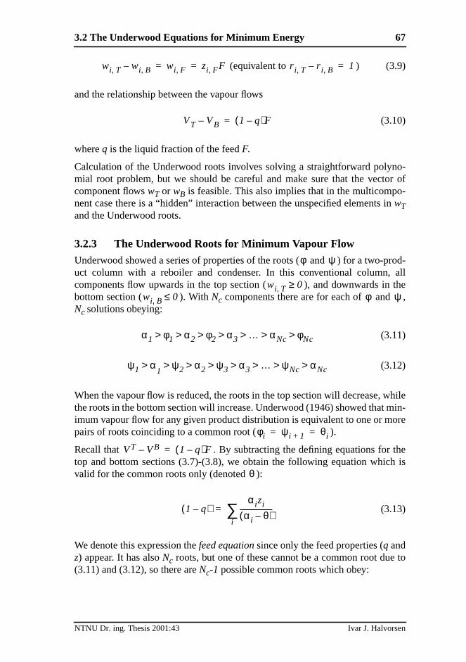
(equivalent to ) (3.9)

and the relationship between the vapour flows

(3.10)

whereq is the liquid fraction of the feedF.

Calculation of the Underwood roots involves solving a straightforward polynmial root problem, but we should be careful and make sure that the vectocomponent flowswT or wB is feasible. This also implies that in the multicomponent case there is a “hidden” interaction between the unspecified elementswTand the Underwood roots.

3.2.3 The Underwood Roots for Minimum Vapour Flow

Underwood showed a series of properties of the roots ( and ) for a two-puct column with a reboiler and condenser. In this conventional column,components flow upwards in the top section ( ), and downwards inbottom section ( ). WithNc components there are for each of andNc solutions obeying:

(3.11)

(3.12)

When the vapour flow is reduced, the roots in the top section will decrease, wthe roots in the bottom section will increase. Underwood (1946) showed that mimum vapour flow for any given product distribution is equivalent to one or mopairs of roots coinciding to a common root ( ).

Recall that . By subtracting the defining equations for thtop and bottom sections (3.7)-(3.8), we obtain the following equation whichvalid for the common roots only (denoted ):

(3.13)

We denote this expression thefeed equationsince only the feed properties (q andz) appear. It has alsoNc roots, but one of these cannot be a common root due(3.11) and (3.12), so there areNc-1 possible common roots which obey:

wi T, wi B,– wi F, zi F, F= = r i T, r i B,– 1=

VT VB– 1 q–( )F=

φ ψ

wi T, 0≥wi B, 0≤ φ ψ

α1 φ1 α2 φ2 α3 … αNc φNc> > >> > > >

ψ1 α>1

ψ2 α2 ψ3 α3 … ψNc αNc> > >> > > >

φi ψi 1+ θi= =

VT VB– 1 q–( )F=

θ

1 q–( )αi zi

αi θ–( )-------------------

i∑=


68

ith-cts.

in-

,ents

as

urply

thors,

theal

e-tsof

olu-geis

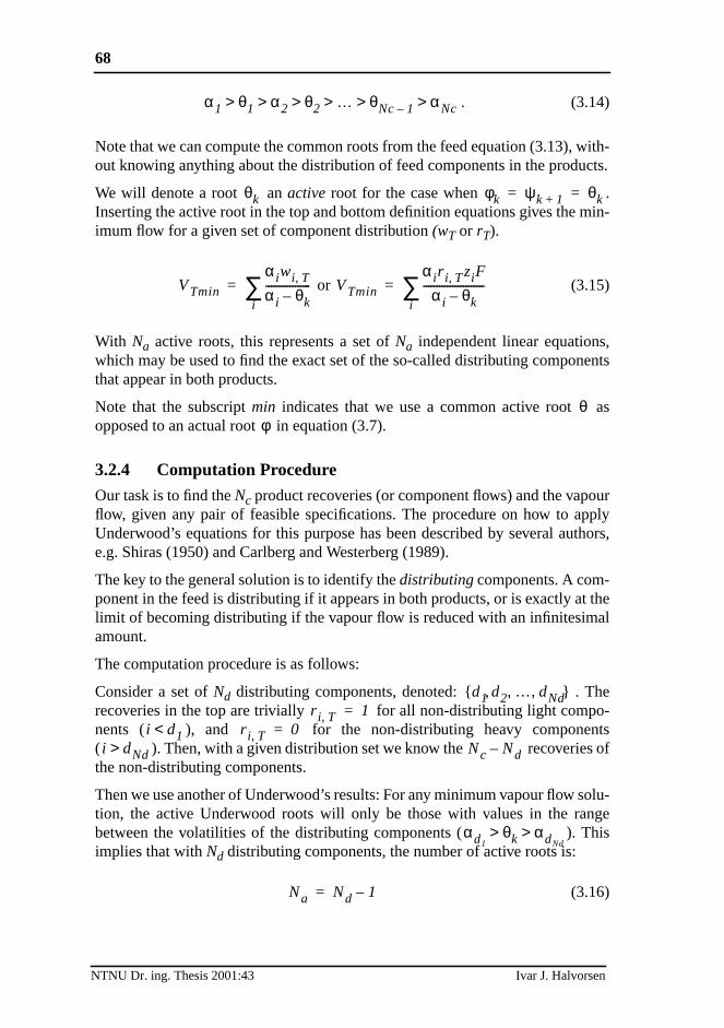
. (3.14)

Note that we can compute the common roots from the feed equation (3.13), wout knowing anything about the distribution of feed components in the produ

We will denote a root anactive root for the case when .Inserting the active root in the top and bottom definition equations gives the mimum flow for a given set of component distribution(wT or rT).

or (3.15)

With Na active roots, this represents a set ofNa independent linear equationswhich may be used to find the exact set of the so-called distributing componthat appear in both products.

Note that the subscriptmin indicates that we use a common active rootopposed to an actual root in equation (3.7).

3.2.4 Computation Procedure

Our task is to find theNc product recoveries (or component flows) and the vapoflow, given any pair of feasible specifications. The procedure on how to apUnderwood’s equations for this purpose has been described by several aue.g. Shiras (1950) and Carlberg and Westerberg (1989).

The key to the general solution is to identify thedistributingcomponents. A com-ponent in the feed is distributing if it appears in both products, or is exactly atlimit of becoming distributing if the vapour flow is reduced with an infinitesimamount.

The computation procedure is as follows:

Consider a set ofNd distributing components, denoted: . Threcoveries in the top are trivially for all non-distributing light components ( ), and for the non-distributing heavy componen( ). Then, with a given distribution set we know the recoveriesthe non-distributing components.

Then we use another of Underwood’s results: For any minimum vapour flow stion, the active Underwood roots will only be those with values in the ranbetween the volatilities of the distributing components ( ). Thimplies that withNd distributing components, the number of active roots is:

(3.16)

α1 θ1 α2 θ2 … θNc 1– αNc> >> > > >

θk φk ψk 1+ θk= =

VTmin

αiwi T,αi θk–-----------------

i∑= VTmin

αi r i T, ziF

αi θk–-----------------------

i∑=

θφ

d1 d2 …, dNd,{ , }r i T, 1=

i d1< r i T, 0=i dNd> Nc Nd–

αd1θk αdNd

> >

Na Nd 1–=



thets.

nts

ten as

Thus, as illustrated in Table 3.1, we have enough information to determinesolution in equation (3.1) completely, given the set of distributing componen

Define a vector X containing the recoveries of the distributing componeand the normalized vapour flow in the top section:

(3.17)

(superscript T denotes transposed). The equation set (3.15) can then be writ

a linear equation set on matrix form:

(3.18)

With the detailed elements in the matrices expanded, this is the same as:

Table 3.1: Number of unknown variables and equations

Total number of variables (VT,RT) Nc+1

- Specified degrees of freedom 2

= Initially unknown variables Nc-1

- Number of non-distributing components Nc-Nd

= Remaining unknown variables Nd-1

- Number of equations=number of active rootsNa = Nd-1

= Required extra equations 0

Nd

X rd1 T, rd2 T, … rdNd T,VT

F-------, , , ,

T=

M X⋅ Z=

M

αd1zd1

αd1θd1

–---------------------

αd2zd2

αd2θd1

–--------------------- …

αdNdzdNd

αd1θd1

–--------------------- 1–

αd1zd1

αd1θd2

–---------------------

αd2zd2

αd2θd2

–--------------------- …

αdNdzdNd

αd1θd2

–--------------------- 1–

… … … … 1–

αd1zd1

αd1θdNd 1–

–-----------------------------

αd2zd2

αd2θdNd 1–

–----------------------------- …

αdNdzdNd

αd1θdNd 1–

–----------------------------- 1–

X

rd1 T,

r d2 T,

…r dNd T,

VT F⁄

•

Z

αi zi

αi θd1–

------------------i 1=

d1 1–

∑–

αi zi

αi θd2–

------------------i 1=

d1 1–

∑–

…

αi zi

αi θdNd 1––

--------------------------i 1=

d1 1–

∑–

=


70

thes theryzero

ofr

uce

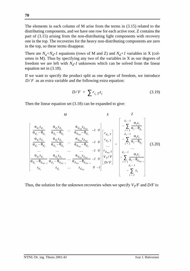
The elements in each column of M arise from the terms in (3.15) related todistributing components, and we have one row for each active root. Z containpart of (3.15) arising from the non-distributing light components with recoveone in the top. The recoveries for the heavy non-distributing components arein the top, so these terms disappear.

There areNa=Nd-1 equations (rows of M and Z) andNd+1 variables in X (col-umns in M). Thus by specifying any two of the variables in X as our degreesfreedom we are left withNd-1 unknowns which can be solved from the lineaequation set in (3.18).

If we want to specify the product split as one degree of freedom, we introd as an extra variable and the following extra equation:

(3.19)

Then the linear equation set (3.18) can be expanded to give:

(3.20)

Thus, the solution for the unknown recoveries when we specifyVT/F andD/F is:

D F⁄

D F⁄ r i T, zi∑=

M

αd1zd1

αd1θd1

–---------------------

αd2zd2

αd2θd1

–--------------------- …

αdNdzdNd

αdNdθd1

–------------------------ 1– 0

αd1zd1

αd1θd2

–---------------------

αd2zd2

αd2θd2

–--------------------- …

αdNdzdNd

αdNdθd2

–------------------------ 1– 0

… … … … 1– 0

αd1zd1

αd1θdNd 1–

–-----------------------------

αd2zd2

αd2θdNd 1–

–----------------------------- …

αdNdzdNd

αdNdθdNd 1–

–-------------------------------- 1– 0

zd1zd2

… zdNd0 1–

X

rd1 T,

r d2 T,

…r dNd T,

VT F⁄

D F⁄

Z

αi zi

αi θd1–

------------------i 1=

d1 1–

∑–

αi zi

αi θd2–

------------------i 1=

d1 1–

∑–

…

αi zi

αi θdNd 1––

--------------------------i 1=

d1 1–

∑–

zii 1=

d1 1–

∑–

=



ting

ithn:

oes

pec-ivesdK)ow

s ofa-

eav-e tothe

thatries

hen

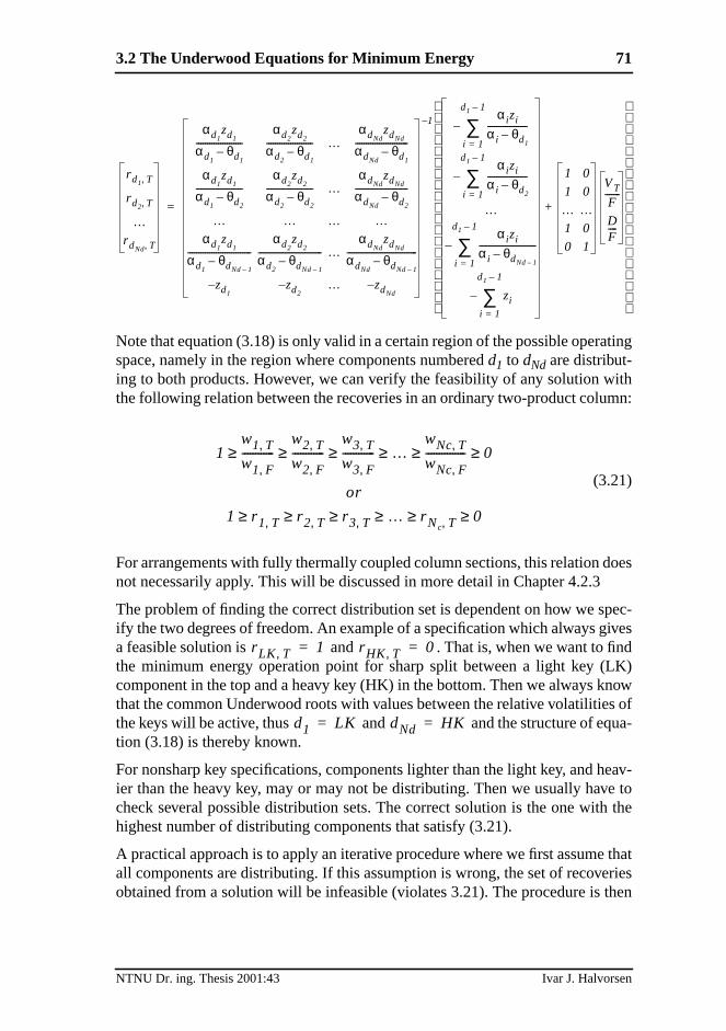
Note that equation (3.18) is only valid in a certain region of the possible operaspace, namely in the region where components numberedd1 to dNd are distribut-ing to both products. However, we can verify the feasibility of any solution wthe following relation between the recoveries in an ordinary two-product colum

(3.21)

For arrangements with fully thermally coupled column sections, this relation dnot necessarily apply. This will be discussed in more detail in Chapter 4.2.3

The problem of finding the correct distribution set is dependent on how we sify the two degrees of freedom. An example of a specification which always ga feasible solution is and . That is, when we want to finthe minimum energy operation point for sharp split between a light key (Lcomponent in the top and a heavy key (HK) in the bottom. Then we always knthat the common Underwood roots with values between the relative volatilitiethe keys will be active, thus and and the structure of eqution (3.18) is thereby known.

For nonsharp key specifications, components lighter than the light key, and hier than the heavy key, may or may not be distributing. Then we usually havcheck several possible distribution sets. The correct solution is the one withhighest number of distributing components that satisfy (3.21).

A practical approach is to apply an iterative procedure where we first assumeall components are distributing. If this assumption is wrong, the set of recoveobtained from a solution will be infeasible (violates 3.21). The procedure is t

r d1 T,

r d2 T,

…r dNd T,

αd1zd1

αd1θd1

–---------------------

αd2zd2

αd2θd1

–--------------------- …

αdNdzdNd

αdNdθd1

–------------------------

αd1zd1

αd1θd2

–---------------------

αd2zd2

αd2θd2

–--------------------- …

αdNdzdNd

αdNdθd2

–------------------------

… … … …αd1

zd1

αd1θdNd 1–

–-----------------------------

αd2zd2

αd2θdNd 1–

–----------------------------- …

αdNdzdNd

αdNdθdNd 1–

–--------------------------------

z– d1z– d2

… z– dNd

1– αi zi

αi θd1–

------------------i 1=

d1 1–

∑–

αi zi

αi θd2–

------------------i 1=

d1 1–

∑–

…

αi zi

αi θdNd 1––

--------------------------i 1=

d1 1–

∑–

zii 1=

d1 1–

∑–

1 0

1 0

… …1 0

0 1

VT

F-------

DF----

+

=

1w1 T,w1 F,------------≥

w2 T,w2 F,------------

w3 T,w3 F,------------ …

wNc T,wNc F,--------------- 0≥ ≥ ≥ ≥ ≥

or

1 r≥ 1 T, r2 T, r3 T, … r Nc T, 0≥ ≥ ≥ ≥ ≥

r LK T, 1= rHK T, 0=

d1 LK= dNd HK=


72

ibleber:

mayneingn.

oodnde-

nce, andhichthesetree-et isAny-ble

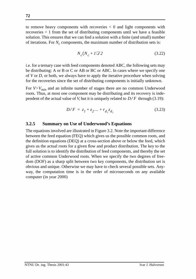
to remove heavy components with recoveries < 0 and light components withrecoveries > 1 from the set of distributing components until we have a feassolution. This ensures that we can find a solution with a finite (and small) numof iterations. ForNc components, the maximum number of distribution sets is

(3.22)

i.e. for a ternary case with feed components denoted ABC, the following setsbe distributing: A or B or C or AB or BC or ABC. In cases where we specify oof V or D, or both, we always have to apply the iterative procedure when solvfor the recoveries since the set of distributing components is initially unknow

For V>Vmin and an infinite number of stages there are no common Underwroots. Thus, at most one component may be distributing and its recovery is ipendent of the actual value ofV, but it is uniquely related to through (3.19):

(3.23)

3.2.5 Summary on Use of Underwood’s Equations

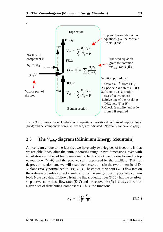
The equations involved are illustrated in Figure 3.2. Note the important differebetween the feed equation (FEQ) which gives us the possible common rootsthe definition equations (DEQ) at a cross-section above or below the feed, wgives us the actual roots for a given flow and product distribution. The key tofull solution is to identify the distribution of feed components, and thereby theof active common Underwood roots. When we specify the two degrees of fdom (DOF) as a sharp split between two key components, the distribution sobvious and unique. Otherwise we may have to check several possible sets.way, the computation time is in the order of microseconds on any availacomputer (in year 2000)

Nc Nc 1+( ) 2⁄

D F⁄

D F⁄ z1 z2… rd1zd1

+ +=


3.3 The Vmin-diagram (Minimum Energy Mountain) 73

thatwithtop

l D-

umnion-

ws

.

3.3 TheVmin-diagram (Minimum Energy Mountain)

A nice feature, due to the fact that we have only two degrees of freedom, iswe are able to visualize the entire operating range in two dimensions, evenan arbitrary number of feed components. In this work we choose to use thevapour flow(VT/F) and the product split, expressed by the distillate (D/F), asdegrees of freedom and we will visualize the solutions in the two-dimensionaV plane (really normalized toD/F, V/F). The choice of vapour (V/F) flow rate onthe ordinate provides a direct visualization of the energy consumption and colload. Note also that it follows from the linear equation set (3.20) that the relatship between the these flow rates (D,V) and the recoveries (R) is always linear fora given set of distributing components. Thus, the function:

(3.24)

VT

αiwi T,αi φ–----------------

i∑=

VB

αiwi B,αi ψ–----------------

i∑=

1 q–( )αi zi

αi θ–--------------

i∑=

The feed equationgives the common“Vmin”-roots ( ):θ

Top section

Bottom section

Top and bottom definitionequations give the “actual”- roots andφ ψ

Solution procedure:

1. Obtain all from FEQ.2. Specify 2 variables (DOF)3. Assume a distribution

(set of active roots)4. Solve one of the resulting

DEQ sets (T or B)5. Check feasibility and redo

from 3 if required

θ

wi,T

wi,F=Fzi,F

wi,B

(1-q)F

Vapour part ofthe feed

Figure 3.2: Illustration of Underwood’s equations. Positive directions of vapour flo(solid) and net component flows (wi, dashed) are indicated. (Normally we havewi,B<0).

Net flow of

DEQT:

FEQ:component i:

DEQB:

RT fDF----

VT

F-------,

=


74

anyingthe

,

-e

ucet

t ofAB,

umn,der-es. If, weance

ive

-

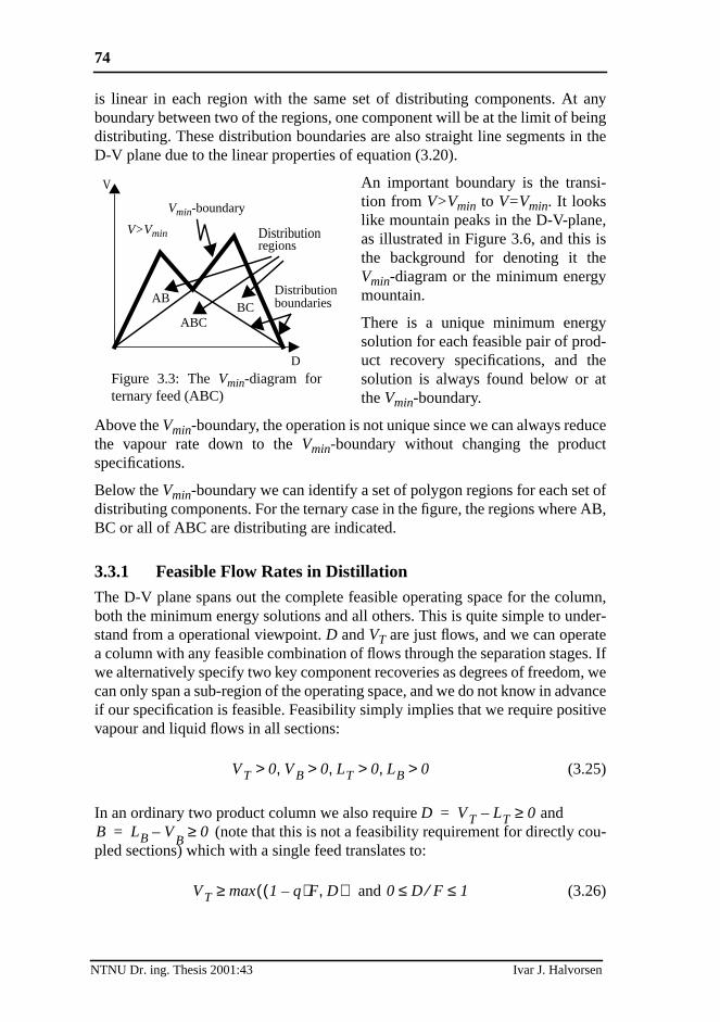
is linear in each region with the same set of distributing components. Atboundary between two of the regions, one component will be at the limit of bedistributing. These distribution boundaries are also straight line segments inD-V plane due to the linear properties of equation (3.20).

An important boundary is the transi-tion from V>Vmin to V=Vmin. It lookslike mountain peaks in the D-V-planeas illustrated in Figure 3.6, and this isthe background for denoting it theVmin-diagram or the minimum energymountain.

There is a unique minimum energysolution for each feasible pair of product recovery specifications, and thsolution is always found below or attheVmin-boundary.

Above theVmin-boundary, the operation is not unique since we can always redthe vapour rate down to theVmin-boundary without changing the producspecifications.

Below theVmin-boundary we can identify a set of polygon regions for each sedistributing components. For the ternary case in the figure, the regions whereBC or all of ABC are distributing are indicated.

3.3.1 Feasible Flow Rates in Distillation

The D-V plane spans out the complete feasible operating space for the colboth the minimum energy solutions and all others. This is quite simple to unstand from a operational viewpoint.D andVT are just flows, and we can operata column with any feasible combination of flows through the separation stagewe alternatively specify two key component recoveries as degrees of freedomcan only span a sub-region of the operating space, and we do not know in advif our specification is feasible. Feasibility simply implies that we require positvapour and liquid flows in all sections:

(3.25)

In an ordinary two product column we also require and(note that this is not a feasibility requirement for directly cou

pled sections) which with a single feed translates to:

and (3.26)

Vmin-boundary

Distributionregions

AB

ABCBC

V

DFigure 3.3: TheVmin-diagram forternary feed (ABC)

V>Vmin

Distributionboundaries

VT 0 VB 0 LT 0 LB 0>,>,>,>

D VT LT– 0≥=B LB V–

B0≥=

VT max 1 q–( )F D,( )≥ 0 D F⁄ 1≤ ≤



e

lit-

ein

ost

p

ase.tive

gley

3.3.2 Computation Procedure for the Multicomponent Case

The procedure for computing the required points to draw theVmin-mountain-dia-gram for a general multicomponent case (Nc components) is as follows:

1. Find all possible common Underwood roots [ ] from thfeed equation (3.13).

2. Use equation (3.20) (or 3.18+3.19) to find the full solutions for sharp spbetween every possible pair of light (LK) and heavy key (HK) specifications. Each solution gives the component recoveries (R), minimum vapourflow (Vmin/F) and product split (D/F). These are the peaks and knots in thdiagram, and there are such key combinations, describedmore detail below:

- Nc-1 cases with no intermediates (e.g. AB, BC, CD,....)These points are the peaks in theVmin-diagram

- Nc-2 cases with one intermediate (e.g. AC, BD, CE,....)These are the knots between the peaks, and the line segmentsbetween the peaks and these knots forms theVmin-boundary

- e.t.c.

- 2 cases withNc-3 intermediates (Nc-1 components distribute)

- 1 case withNc-2 intermediates (all components distribute)

This last case is the “preferred split” solution where the keys are the mlight and heavy components, and all intermediates distribute.

3. Finally we will find the asymptotic points where all recoveries in the toare zero and one, respectively. These are trivially found asVTmin=0 forD=0 and VTmin=(1-q)F for D=F (Note that this is the same asVBmin=0 forB=0).

3.3.3 Binary Case

Before we explore the multicomponent cases, let us look closer at a binary cConsider a feed with light component A and heavy component B with relavolatilities , feed composition , feed flow rateF=1 andliquid fraction q. In this case we obtain from the feed equation (3.13) a sincommon root obeying . The minimum vapour flow is found bapplying this root in the definition equation (3.15):

(3.27)

θ1 θ2 … θNc 1–, , ,

Nc Nc 1–( ) 2⁄

αA αB,[ ] z zA zB,[ ]=

θA αA θA αB> >

VTmin

F---------------

αAr A T, zA

αA θA–-------------------------

αBrB T, zB

αB θA–------------------------+=


76

thereng

aightn

We also have from (3.19):

(3.28)

The procedure in section 3.3.2 becomes very simple in the binary case sinceis only one possible pair of key components (A,B). We obtain the followiresults which we plot in the in theD-V-plane of theVmin diagram in Figure 3.4.First we find the operating point which gives sharp A/B-split:

PAB: =>

and then the asymptotic points:

P0 : =>

P1 : =>

These three points make up a triangle as shown in Figure 3.4. Along the strline P0-PAB we haveV=Vmin for a pure top product ( ), and the line cabe expressed by:

DF---- r A T, z

ArB T, zB+=

r A T, rB T,,[ ] 1 0,[ ]= D VTmin,[ ] zA

αAzA

αA θA–-------------------, F=

r A T, rB T,,[ ] 0 0,[ ]= D VTmin,[ ] 0 0,[ ]=

r A T, rB T,,[ ] 1 1,[ ]= D VTmin,[ ] 1 1 q–( ),[ ]F=

0 FD

only B is distributing

A+B are distributing

Figure 3.4: TheVmin-diagram, or minimum energy mountain.Visualization of the regions of distributing components for a binary feed case.

(1-q)F

PAB: VTmin

VT

V>VminV=Vmin(rA,rB)

V>Vmin

P0

P1

only A is distributing

r B,T

=0

rA

,T =1

Infeasible region: (V<D or V<(1-q)F

A at the boundary ofbecoming distributing

B at the boundary ofbecoming distributing

θA active

Region (B) where

Region (A) where

Region (AB) where both

=> no active roots

A/B

Vmin forsharp A/B-split

zAF

(no B in distillate).

(no A in bottoms).

rB T, 0=



ameboth

trib-re

erean be.

il-rate(P

nentnd

ul-

where (3.29)

Similarly, along the straight line PAB-P1, we haveV=Vmin for a pure bottom prod-uct ( ), and the line can be expressed by:

where (3.30)

Inside the triangle, we may specify any pair of variables among(VT,D,rA,rB) anduse the equation set (3.27-3.28) to solve for the others. This is exactly the sequation set as given in (3.20) for the general multicomponent case whencomponents are distributing.

Above the triangle (Vmin-mountain),V>Vmin, and we have no active Underwoodroots, so (3.27) no longer applies. However, since only one component is disuting, we have either or . This implies that the recoveries adirectly related toD, and we have:

for or for (3.31)

which is equivalent to (3.23) in the general multicomponent case. Anywhabove the triangle we obviously waste energy since the same separation cobtained by reducing the vapour flow until we hit the boundary to region AB

VT>D andVT>(1-q)F for feasible operation of a conventional two-product distlation column. The shaded area represents an infeasible region where a flowsomewhere in the column would be negative. Note that the asymptotic points0and P1) are infeasible in this case.

We may also visualise the non-sharp split solutions with specified comporecoveries. This is illustrated in Figure 3.5 for the example a

(dashed lines). The unique solution with both specifications f

filled is at the intersection inside region AB. Note that forV>Vmin these becomevertical lines.

We also indicate the alternative coordinate system (dashed) ifVB andB are usedas degrees of freedom. The relation toVT andD is trivial

VT

F-------

αAr A T, zA

αA θA–-------------------------= D r A T, zAF=

r A T, 1=

VT

F-------

αAzA

αA θA–-------------------

αBrB T, zB

αB θA–------------------------+= D

F---- zA rB T, zB+=

r A T, 1= rB T, 0=

DF---- r A T, z

A=

DF---- zA≤ D

F---- zA rB T, zB+=

DF---- zA≥

VT rA 0.85= D( )

VT rB 0.25= D( )


78

in

.

3.3.4 Ternary Case

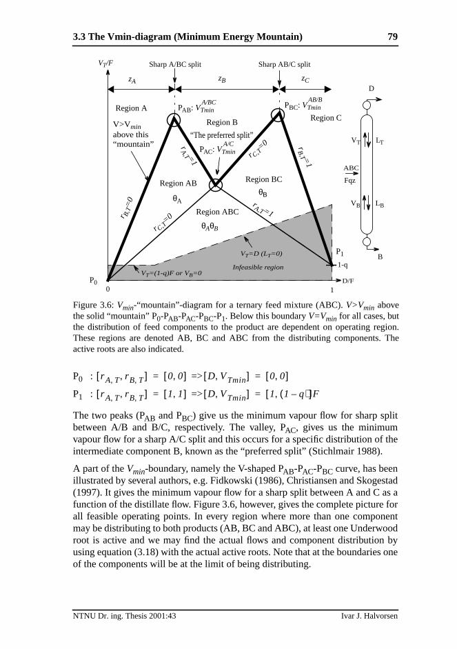
Figure 3.6 shows an example of theVmin-diagram, or “minimum energy moun-tain” for a ternary feed (ABC). To plot this diagram we apply the procedureSection 3.3.2 and identify the following five points:

The peaks, which giveVmin for sharp splits A/B and B/C (no distributingcomponents):

PAB: =>

PBC: =>

The preferred split, which givesVmin for sharp A/C-split (B is distributing):

PAC: =>

where is the recovery of B:

and the trivial asymptotic points:

0 F D

Figure 3.5: Solution for a given pair of recoveryspecifications visualized in theVmin-diagram

(1-q)F

PAB

VT rA,T=0.85

P0

P1

rB,T=0.25 VB

B

Solution

r A T, rB T,,[ ] 1 0,[ ]= D VTmin,[ ] zA

αAzA

αA θA–-------------------, F=

rB T, rC T,,[ ] 1 0,[ ]= D VTmin,[ ] zA zB+αAzA

αA θB–-------------------

αBzB

αB θB–-------------------+, F=

r A T, rC T,,[ ] 1 0,[ ]= D VTmin,[ ] zA βzB+αAzA

αA θB–-------------------

αBβzB

αB θB–-------------------+, F=

β β rB T,A C/

αAzA

αBzB-------------–

αB θA–( ) αB θB–( )αA θA–( ) αA θB–( )

-------------------------------------------------= =



t

the

stads afornentodbyone

gion.The

P0 : =>

P1 : =>

The two peaks (PAB and PBC) give us the minimum vapour flow for sharp splibetween A/B and B/C, respectively. The valley, PAC, gives us the minimumvapour flow for a sharp A/C split and this occurs for a specific distribution ofintermediate component B, known as the “preferred split” (Stichlmair 1988).

A part of theVmin-boundary, namely the V-shaped PAB-PAC-PBC curve, has beenillustrated by several authors, e.g. Fidkowski (1986), Christiansen and Skoge(1997). It gives the minimum vapour flow for a sharp split between A and C afunction of the distillate flow. Figure 3.6, however, gives the complete pictureall feasible operating points. In every region where more than one compomay be distributing to both products (AB, BC and ABC), at least one Underworoot is active and we may find the actual flows and component distributionusing equation (3.18) with the actual active roots. Note that at the boundariesof the components will be at the limit of being distributing.

r A T, rB T,,[ ] 0 0,[ ]= D VTmin,[ ] 0 0,[ ]=

r A T, rB T,,[ ] 1 1,[ ]= D VTmin,[ ] 1 1 q–( ),[ ]F=

0 1

VT/F

D/F

1-q

ABC

D

VT LT

VT=D (LT=0)

“The preferred split”

Sharp A/BC split Sharp AB/C split

Infeasible regionVT=(1-q)F or VB=0

Fqz

Region A

zA

Region B Region C

Region ABC

Region AB Region BC

θA

θAθB

θΒ

P0

P1

V>Vminabove this“mountain”

VB LB

B

zB zC

r C,T=0

r C,T=0

rA,T=1

rA,T =1

r B,T

=0

rB

,T =1

Figure 3.6:Vmin-“mountain”-diagram for a ternary feed mixture (ABC).V>Vmin abovethe solid “mountain” P0-PAB-PAC-PBC-P1. Below this boundaryV=Vmin for all cases, butthe distribution of feed components to the product are dependent on operating reThese regions are denoted AB, BC and ABC from the distributing components.active roots are also indicated.

PBC: VTminAB/B

PAB: VTminA/BC

PAC: VTminA/C


80

d

ry

e isgion

ow

t:

ve

P

At boundaries B/AB and ABC/BC:rA,T=1 (rA,B=0)At boundary A/AB:rB,T=0 (rB,B=1)At boundary C/CB:rB,T=1 (rB,B=0)At boundaries B/BC and AB/ABC:rC,T=0 (orrC,B=1)

Comment: King’s minimum reflux formula (ref. Chapter 2) can be deducefrom the exact Underwood solution at PAC for a saturated liquid feed (q=1):

(3.32)

However, King’s formula cannot be applied for sharp A/B or B/C split. If we tthis for example at PAB, we clearly have:

(3.33)

The underlying reason is that in the deduction of King’s formula, a pinch zonassumed to exist across the feed stage. However, this is only true in the rewhere all components distribute, which is only in the triangle region ABC belthe preferred split, denoted Class 1 separations (Shiras 1950).

Example: For and equimolar, saturated liquid feed, we ge

and

Note that King’s formula predicts minimum reflux to be significantly abothe real minimum which is obtained by Underwood’s expression.

However, for the preferred split (PAC) we obtain:

Here we must apply the more complex Underwood expression for pointACgiven at page 78.

LTmin

F--------------

VTmin D–

F------------------------- 1

αLK αHK⁄ 1–----------------------------------- 1

αA αC⁄ 1–---------------------------= = =

Kings Lmin

1αA αB⁄ 1–---------------------------

Underwoods Lmin

θAzA

αA θA–-------------------

≠

α 4 2 1, ,[ ]=

Kings Lmin

1αA αB⁄ 1–--------------------------- 1

4 2⁄ 1–------------------- 1= =

Underwoods Lmin

θAzA

αA θA–------------------- 2.76 1 3⁄( )

4 2.76–------------------------- 0.74= =

Kings Lmin

1αA αC⁄ 1–---------------------------

Underwoods Lmin

13---

= }



tourthe

qual

point

entsng,

here,

3.3.5 Five Component Example

A 5-component example is shown in Figure 3.7. Here we also plot the conlines for constant values of the recoveries in the top for each component inrange 0.1 to 0.9.

Note that the boundary lines (solid bold) are contour lines for top recoveries eto zero or one and that any contour line is vertical forV>Vmin. This diagramclearly shows how each component recovery depends on the operating(D,V).

Since we assume constant relative volatility only adjacent groups of componcan be distributing. In the example with five components ABCDE, the followidistributing groups exist: A, B, C, D, E, AB, BC, CD, DE, ABC, BCD, CDEABCD, BCDE, ABCDE. To draw theVmin-diagram forNc components, we mustidentify the points (Pij ) given in the procedure in Section 3.3.2.

Number of points (peaks and knots) Pij : (3.34)

This is simply the sum of the arithmetic series{1+2+...+(Nc-1)} (one point withno intermediates + two points with one intermediate+...+(Nc-1) points with nointermediates). This number is equal to the number of distribution regions wV=Vmin (10 for the 5-component example: AB, BC, CD, DE, ABC, BCD, CDEABCD, BCDE, ABCDE). Note thatV>Vmin only in the regions where just onecomponent distributes.

0 0.1 0.2 0.3 0.4 0.5 0.6 0.7 0.8 0.9 10

0.5

1

1.5V

T

D

Vmin

−diagram

rA,T

0.1

0.2

0.3

0.4

0.5

0.6

0.7

0.8

0.9

rB,T

0.1

0.2

0.3

0.4

0.5

0.6

0.7

0.8

0.9

rC,T

0.1

0.2

0.3

0.4

0.5

0.6

0.7

0.8

0.9

rD,T

0.1

0.2

0.3

0.4

0.5

0.6

0.7

0.8

0.9

rE,T

0.1

0.2

0.3

0.4

0.5

0.6

0.7

0.8

0.9

PAB

AB

PAC

ABCP

AD

ABCDP

AE

ABCDE

PBC

BC

PBD

BCDP

BE

BCDE

PCD

CD

PCE

CDE

PDE

DE

1−q

Infeasible region

Case:α=[9 6 3.5 2 1]z=[0.2 0.2 0.2 0.2 0.2]q=0.8

Figure 3.7: TheVmin-diagram for a 5-component feed (F=1).Contour lines for constant top product recoveries are included.

Nc Nc 1–( ) 2⁄


82

canf

i-e

mpo-rlyrt of):

by:

of ali-

thescribeharp

Figure 3.7 also illustrates that some combinations of recovery specificationsbe infeasible, e.g.rA,T=0.9 andrC,T=0.6. Observe that combined specification oD and an intermediate recovery may have multiple solutions, e.g.D=0.2 andrB,T=0.3. The specification ofV and a recovery will be unique, as will the specfication of D andV. The specification of two (feasible) recoveries will also bunique, and the solution will always be a minimum energy solution (V=Vmin).

3.3.6 Simple Expression for the Regions Under the Peaks

In the Vmin-diagram, the peaks represent sharp splits between adjacent conents (j andj+1). In the region just under the peaks, the vapour flow is particulasimple to compute since there is only one active root, (this is in fact the stastep 2 of the general procedure in Section 3.3.2). We find directly from (3.15

(3.35)

(3.36)

Recall and observe that the slopes under the peaks are given

and (3.37)

The contour lines under the peaks PAB, PBC, PCD and PDE in Figure 3.7 are exam-ples of lines where the slopes are given by equation (3.37). In the casecompletely sharp split, , , the expression in (3.35) simpfies to:

and (3.38)

Equation (3.38) gives us the peaks and (3.35) describes the behaviour inregion under the peaks. Thus we can use these simple linear equations to dethe local behaviour for a 2-product column where we specify a reasonable ssplit between two groups of components.

VTmin r j T, r j 1+ T,,( )αi zi

αi θ j–----------------

i 1=

j 1–

∑α j zj

α j θ j–-----------------r j T,

α j 1+ zj 1+

α j 1+ θ j–--------------------------r j 1+ T,+ +=

k0 kj r j T, kj 1+ r j 1+ T,+ +=

D zii 1=

j 1–

∑

zj r j T, zj 1+ r j 1+ T,+ +=

α j θ j α j 1+> >

kj

α j zj

α j θ j–----------------- 0>= kj 1+

α j 1+ zj 1+

α j 1+ θ j–--------------------------= 0<

r j T, 1= r j 1+ T, 0=

VTminj/j+1 αi zi

αi θ j–----------------

i 1=

j

∑= D zii 1=

j

∑=


3.4 Discussion 83

thanlin-

eby

we

pledof a

osi-

n ascom-

very.

er-that

-w

two

om-

monmon

onand

3.4 Discussion

3.4.1 Specification of Recovery vs. Composition

We have chosen to use component recovery (or net component flow), rathercomposition, which is used by many authors. One important reason is to get aear equation set inV, D andR inside each distribution region. If we choose to uscomposition in (3.18), the equation set may again become linear if we divideD and compute the ratio V/D. But then we do not have the vapour flow (whichuse as energy indicator) directly available.

Another important reason is that when we apply the equations for directly coucolumns, there is no single product stream since the product is the differencecounter flowing vapour and liquid stream. Then there is not any unique comption related to a certain specification ofV and D as degrees of freedom.

Nevertheless, for the final products, it is more common to use compositiospecification. But we choose to compute the corresponding recovery (or netponent flow) and use those variables in Underwood’s equations.

The relation between recovery and net component flow is simply that the recocan be regarded as a normalized component flow: =In the following we switch between usingr or w depending on which one is themost convenient in a certain expression.

3.4.2 Behaviour of the Underwood Roots

TheVmin-diagram is also very well suited to illustrate the behaviour of the Undwood roots in each section ( ) as we change the vapour flow. RecallUnderwood showed that as the vapour flow (V) is reduced, a certain pair of rootswill coincide, and we getV=Vmin. But how do we find which pair, and what happen to the other roots? Also, recall thatVmin is not a constant, but depends on howe select the two degrees of freedom in the column.

We illustrate the behaviour with a ternary example in Figure 3.8. We havecommon roots ( ). In each of the three casesi-iii , D is kept constant andVis reduced from a large value in the region whereV>Vmin until we are in regionABC where all feed components distribute. The behaviour of the roots is cputed from the defining equations (3.7) and (3.8). Observe how the pairapproaches the common root and how approaches the other comroot as we cross a distribution boundary to the region where each comroot becomes active.

Note also that in caseii , where we pass through the preferred split, both commroots become active at the same time. Observe that one root ( ) in the topone ( ) in the bottom, never coincide with any other root.

r i wi wi F,⁄= wi ziF( )⁄

φ ψ,

θA θB,

φA ψB,θA φB ψC,

θB

φCψA


84

theinere

m

Figure 3.9a shows how the important root in the top, behaves outsideregions AB or ABC where it is constant . A similar result is shownFigure 3.9b) for the root in the bottom, outside the regions ABC or BC wh

. Note that these contours are linear in each distribution region.

0 0.5 10

0.5

1

1.5

Vmin

diagram

i) ii) iii)

AB BCABC

α=[4 2 1]z=[1 1 1]/3q=1F=1

V

D

> ii> iii

> iii

0 1 2 3 4 50

0.5

1

1.5Case i: D=0.33

V

Underwood roots

θA

θB

αA

αB

αC

φC

φB

φA

ψC

ψB

ψA

0 1 2 3 4 50

0.5

1

1.5Case ii: D=0.44

V

Underwood roots

θA

θB

αA

αB

αC

φC

φB

φA

ψC

ψB

ψA

0 1 2 3 4 50

0.5

1

1.5Case iii: D=0.50

V

Underwood roots

θA

θB

αA

αB

αC

φC

φB

φA

ψC

ψB

ψA

Figure 3.8: Observe how a pair of Underwood roots coincide as vapour flow (V) is reducedand the operation cross a distribution boundary in theVmin-diagram.

φAφA θA=

ψCψC θB=

0.2 0.4 0.6 0.8

0.6

0.8

1

1.2

1.4

1.6

Infeasible region

D

V

φA=θ

A=2.76

φA=θ

A

a) Contours of constant φA

2.812.91

3.01

3.11

3.21

0.2 0.4 0.6 0.8

0.6

0.8

1

1.2

1.4

1.6

Infeasible region

D

V

ψC

=θB=1.244

ψC

=θB

b) Contours of constant ψC

1.231.

21

1.19

1.17

1.15

Figure 3.9: Contour plot of the most important roots a) in the top- and b) in the bottosections outside the region when these roots are active. Same feed as in Figure 3.8


3.4 Discussion 85

ione tocen-

rgyosi-ition

withsed

omtenosi-

ativem-by

) wey Cinchhewerom

om-on2),

3.4.3 Composition Profiles and Pinch Zones

At minimum energy operation with infinite number of stages, the compositprofile will have certain pinch-zones where there are no changes from stagstage. Shiras (1950) denoted these as points of infinitude. The pinch zone is atral issue in the deduction of Underwood’s equations for minimum enecalculations. In this section we will present expressions for pinch zone comptions and discuss important characteristics of the pinch zones and composprofiles.

3.4.4 Constant Pinch-zone Compositions (Ternary Case)

Underwood showed how to compute the pinch zone compositions for casesinfinite number of stages. In Underwood (1945) the following expression is uto find a pinch zone composition in the top section for componenti, related toUnderwood rootk:

(3.39)

In the bottom section, we simply apply the roots for the bottom ( ) and bottcomponent flows (wi,B) to get the corresponding pinch zone compositions (nothat each elementwi,B is normally negative since we define the positive directioupwards). Underwood (1945) also showed that we may get infeasible comptions from this equation. We also see that as the roots approach a relvolatility, the denominator term in (3.39) will approach zero, and so will the coponent flow in the nominator. We can get around this numerical problemalways assuming a very small component flow when computing the roots.

Let us use a ternary example with feed components A, B and C. From (3.39find three compositions for each section. In region AB we remove the heavfrom the top product. Thus, somewhere in the top section there will be a pzone where only A and B appear. In this region, will be an active root. Tactual pinch composition can be found by applying in (3.39). Note thatcompute the actual roots ( ) from (3.7) after we have computed and f(3.18).

, (3.40)

We may use an alternative approach to find this pinch zone composition. We cbine the assumption about a pinch ( ) in the top sectiwhere component C is fully removed ( ) with the material balance (3.

xi PT,φk

xi D, D

LT---------------

φk

αi φk–( )---------------------

wi T,LT

-----------φk

αi φk–( )---------------------= =

ψ

θAφB

φ wT LT

xA PT,wA T,LT

-------------φB

αA φB–( )------------------------= xB PT,

wB T,LT

------------φB

αB φB–( )------------------------ 1 xA PT,–= =

xi n, xi n 1+, xi PT,= =xC n, 0=


86

theor

nde-otri-

theonerupte top,ved

them-

m-

dice isdatapo-first

the equilibrium expression, and the definition equation (3.15) where we applyroot (which we know is the only active root in region AB). When we solve fthe pinch, we obtain:

, (3.41)

Surprisingly, from (3.41), which is valid for any operating point within regioAB, we observe that the pinch-zone composition in the top section will be inpendent of the operating point (V,D) since is a constant. This issue was npointed out by Underwood, and it is not at all obvious from (3.40) since all vaables in (3.40), except , are varying in region AB.

In the bottom section, all components will be present in the product, and herepinch zone will be determined by (again not a common root). This pinch zwill actually appear from the feed stage and downwards, but we will see an abcomposition change in the stages above the feed stage. Unlike the pinch in ththe pinch composition in the bottom will change as the operating point is moaround in region AB.

When the column is operated in region BC, the roles will be exchanged andpinch zone composition on the bottom will be invariant, but the pinch zone coposition in the top will vary withD,V.

Finally in region ABC where both common roots are active, both pinch zone copositions will be constant and independent onD,V.

Example.We will illustrate this by a numerical ternary example whereF=1,z=[0.33 0.33 0.33], =[4 2 1], q=1.The composition profile has been computeusing a stage-by-stage model with 50 stages in each section, which in practan infinite number of stages for this example. In Table 3.2 we have given thefor four operating points, which are all in the AB region. The pinch zone comsitions are computed by (3.39) and the actual root applied is indicated in thecolumn.

θA

xA PT,αB αA θA–( )θA αA αB–( )--------------------------------= xB PT,

αA θA αB–( )θA αA αB–( )-------------------------------- 1 xA PT,–= =

θA

α

ψA

α


3.4 Discussion 87

s int thed 4),sere,po-

por-t thetheand

C,eedn as

sec-

e

0

0

0

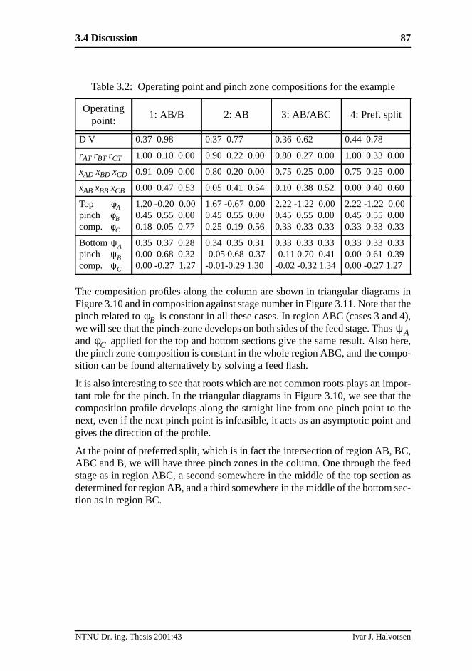
The composition profiles along the column are shown in triangular diagramFigure 3.10 and in composition against stage number in Figure 3.11. Note thapinch related to is constant in all these cases. In region ABC (cases 3 anwe will see that the pinch-zone develops on both sides of the feed stage. Thuand applied for the top and bottom sections give the same result. Also hthe pinch zone composition is constant in the whole region ABC, and the comsition can be found alternatively by solving a feed flash.

It is also interesting to see that roots which are not common roots plays an imtant role for the pinch. In the triangular diagrams in Figure 3.10, we see thacomposition profile develops along the straight line from one pinch point tonext, even if the next pinch point is infeasible, it acts as an asymptotic pointgives the direction of the profile.

At the point of preferred split, which is in fact the intersection of region AB, BABC and B, we will have three pinch zones in the column. One through the fstage as in region ABC, a second somewhere in the middle of the top sectiodetermined for region AB, and a third somewhere in the middle of the bottomtion as in region BC.

Table 3.2: Operating point and pinch zone compositions for the exampl

Operatingpoint:

1: AB/B 2: AB 3: AB/ABC 4: Pref. split

D V 0.37 0.98 0.37 0.77 0.36 0.62 0.44 0.78

rAT rBT rCT 1.00 0.10 0.00 0.90 0.22 0.00 0.80 0.27 0.00 1.00 0.33 0.0

xAD xBD xCD 0.91 0.09 0.00 0.80 0.20 0.00 0.75 0.25 0.00 0.75 0.25 0.0

xAB xBB xCB 0.00 0.47 0.53 0.05 0.41 0.54 0.10 0.38 0.52 0.00 0.40 0.6

Toppinchcomp.

1.20 -0.20 0.000.45 0.55 0.000.18 0.05 0.77

1.67 -0.67 0.000.45 0.55 0.000.25 0.19 0.56

2.22 -1.22 0.000.45 0.55 0.000.33 0.33 0.33

2.22 -1.22 0.000.45 0.55 0.000.33 0.33 0.33

Bottompinchcomp.

0.35 0.37 0.280.00 0.68 0.320.00 -0.27 1.27

0.34 0.35 0.31-0.05 0.68 0.37-0.01-0.29 1.30

0.33 0.33 0.33-0.11 0.70 0.41-0.02 -0.32 1.34

0.33 0.33 0.330.00 0.61 0.390.00 -0.27 1.27

φAφBφC

ψAψBψC

φBψA

φC


88

.

3.2.

Case 1: Region AB/A

A

B

C

z

xd

xb

xT,Pinch

xB,Pinch

xn (stages)

z,xd,x

b

Case 2: Inside region AB

A

B

C

z

xd

xb

Invariant pinch

Case 3: Region AB/ABC

A

B

C

zx

d

xb

Case 4: Preferred split

A

B

C

zx

d

xb

Figure 3.10: The composition profiles attempt to reach the theoretical pinch pointsPlot shows composition profiles in for the four cases given in Table 3.2.

Top Feed Bottom0

0.2

0.4

0.6

0.8

1 Case 1: Region AB/A

Top Feed Bottom0

0.2

0.4

0.6

0.8

1Case 2: Inside region AB

ABC

Top Feed Bottom0

0.2

0.4

0.6

0.8

1 Case 3: Region AB/ABC

Top Feed Bottom0

0.2

0.4

0.6

0.8

1Case 4: Preferred split

Figure 3.11: Composition profiles by stage number for the four cases given in tableNote the constant pinch zone in the top section


3.4 Discussion 89

po-riantthele forpear

od-

es

e

e

woe willes in

lleds thetheurflowrosst of

they ton is

3.4.5 Invariant Multicomponent Pinch-zone Compositions

In the general case we will find that in every region where one or more comnents are completely removed from one of the products, we will have an invapinch zone composition. More precisely, this occurs in the regions belowboundary for sharp split between the most extreme components. For exampthe 5-component case in Figure 3.7, the invariant pinch zone compositions apin regions AB, ABC, ABCD, ABCDE, BCDE, CDE and DE.

To select the proper root to be used in (3.39) the following rules apply:

• When there are heavy components not distributed to the top pruct, the root applied in (3.39) will give us the invariant pinchzone composition in the top for the whole distribution region. This appliin each of the regions to the left of the preferred split (e.g. below PAB-PAC-PAD-PAE in Figure 3.7). In the bottom will give the pinch below thefeed stage.

• Similarly, when there are light components, not distributed to thbottom (but all are distributed to the top product), the rootapplied in (3.39) will give us the invariant pinch zone composition in thbottom (e.g. for the regions below PAE-PBE-PCE-PDE in Figure 3.7). In thetop will give the pinch above the feed stage.

At the boundaries, where a component is at the limit of being distributing, tpinch zones may appear in each section. Note that at the preferred split, therbe a pinch zone through the feed stage, and we observe the invariant pinchthe neighbouring regions in both column ends.

The behaviour of the pinch zones plays an important role in directly (or so-cafully thermally) coupled columns. In the ternary case, the top pinch representmaximum composition of the light (A) component which can be obtained infirst column when the reflux into the column is in equilibrium with the vapoleaving the column. When the columns are connected, the minimum vapourin the succeeding column will have its minimum when there is a pinch zone acthe feed region. And this minimum will be as low as possible when the amounlight component is as high as possible.

Furthermore, in the Petlyuk column, we know that the energy requirement insucceeding column is constant in a certain operation region. This is easexplain from the fact that when the feed pinch composition in a binary columconstant, the energy requirement will also be constant.

NHNdφNc NHNd–

ψ1

NLNdψ1 NLNd+

φNc


90

use

ureame

ol-

entmerstheets.

split.s inumnken

ever,sec-

The

B/

3.4.6 Pinch Zones forV>Vmin

We have above discussed the pinch-zones for the case whenV=Vmin. Above theVmin-mountain, in region B, we may still use equation (3.41), but we have tothe actual root in the top section , instead of :

, , (3.42)

When we combine this expression with the behaviour of as shown in Fig3.9a we know that the pinch-zone composition will be constant along the sstraight contour lines where is constant.

A similar relation is found for and the pinch zone in the bottom when the cumn is operated in region B. This is also illustrated in Figure 3.9b.

, , (3.43)

3.4.7 Finite Number of Stages

Considering a ternary feed (A,B, and C) we will now look at the stage requiremfor a split close to sharp A/C split, with a specified impurity in the top and bottofor a column with finite number of stages. Minimum energy for infinite numbof stages is easily found from theVmin-diagram as the V-shaped boundariebetween the regions AB/B and B/BC. However, with finite number of stagesreal minimum vapour flow (VRmin) has to be slightly higher. We want to keep thratio VRmin/Vmin below a certain limit, and this gives us the stage requiremenFigure 3.12 shows the result forVRmin/Vmin=1.05 for a given feed and impurityconstraints. The total number of stages (N=NT+NB) is minimized for each oper-ating point.

Observe that the largest number of stages is required close to the preferredWhen we move away from the preferred split, the number of required stageone of the sections is reduced. The lesson learned from this is that if the colis designed for operation on one side of the preferred split, this can be taadvantage of by reducing number of stages in the appropriate section. Howif the column is to be operated at, or on both sides of the preferred split, bothtions have to be designed with its maximum number of stages (N dashed).

The top section stage requirement is reduced to the left of the preferred split.reason is that the real minimum vapour flowVRmin(dotted) is determined by therequirement of removing A from the bottom which is given by the boundary AB. At the same time the required “Vmin” for removing C from the top is given by

φA θA

xA PT,αB αA φA–( )φA αA αB–( )--------------------------------= xB PT, 1 xA PT,–= xC PT, 0=

φA

φA

ψC

xA PB, 0= xB PB,αC αB ψC–( )ψC αB αC–( )---------------------------------= xB PB, 1 xB PB,–=


3.4 Discussion 91

gesve C.

ion

bot-rity

n

ints

the boundary between regions AB/ABC. This implies that we may take out stain the top because we have a much larger vapour flow than required to remoThus we really haveV>>”V min” and the requiredNT will then approach a lowerlimit, NTmin, which can be approximated by the wellknown Fenske equatwhich can be applied between any two keys (L,H) and any two stages (here top(T) and feed (F)) and infinite reflux (L=V):

(3.44)

In the top section we have to consider separation between B and C, and in thetom, separation between A and B. Note that in this equation, the impucomposition (e.g.xC,T in the top andxA,B in the bottom) will normally dominatethe expression, soNmin will neither depend much on the feed pinch compositionor on the intermediate (B) in the end.

5

10

15

20

25

N=NT+N

B

NT

NB

N=max(NT)+max(N

B)

Sta

ges

23

21

12

10

0.3 0.35 0.4 0.45 0.5 0.55 0.6 0.65 0.70.5

1

1.5

D

VT

AB

ABC

BC

B Vα = [ 4 2 1]

z = [ 0.33 0.33 0.33]

q = [ 1.00]

Vmin

Figure 3.12: Required number of stages in top and bottom section forV/Vmin=1.05 andseparation between A and C with less than 1% impurity. The actual operating poconsidered are shown (dotted) in theVmin-diagram.

Nmin

log SLH TF,( )log αL αH⁄( )-------------------------------= where SLH TF,

xL T, xH T,⁄xL F, xH F,⁄---------------------------=


92

formplesim-

for

vedh aom-give

rom

ben acts

ABC,ofasesse tothethe

ingting

dingThender-

alln forand

shall

ctly

At the preferred split, the Fenske equation gives andthe feed data and purity requirement as in Figure 3.12. We may then for exause the very simple rule (see Chapter 2) as a first approach in aple design procedure for each section. This rule would in fact be quite goodthe example above.

3.4.8 Impurity Composition with Finite Number of Stages

Note that in all distribution regions in aVmin-diagram, except in the triangle belowthe preferred split, one or more feed components will be completely remofrom one of the products with infinite number of stages. However, even witfinite number of stages we will in practice remove these components almost cpletely. Consider now that we have designed the number of stages tosatisfactory performance in a range on both sides of the preferred split (e.gNT=11andNB=12 in the previous example). Then, as we move the operation away fthe preferred split, we have both “N>>Nmin” and “V>>Vmin” in one of the sec-tions, and the impurity of the component to be removed in that section willmuch smaller than the required specification. Thus, in these cases the columas a true rectifier for the component to be removed. This means that in regionof the ternary example, when we move a bit away from the boundary AB/ABthe mole fraction of C in the top will become very small also for finite numberstages. This can be observed in the composition profiles in Figure 3.11 for c1 and 2 where we observe that the C-composition approaches zero quite clothe feed stage, and the top is in practice “over-purified”. A rough estimate ofremaining impurity can be obtained by the Fenske equation (3.44) by usingreal number of stages and solve for the appropriate impurity.

3.5 Summary

TheVmin-diagram gives a simple graphical interpretation of the whole operatspace for a 2 product distillation column. A key issue is that the feasible operaspace is only dependent of two degrees of freedom and that theD-V plane spansthis space completely. The distribution of feed components and corresponminimum energy requirement is easily found by just a glance at the diagram.characteristic peaks and knots are easily computed by the equations of Uwood and represent minimum energy operation for sharp split betweenpossible pairs of key components. The diagram represents the exact solutiothe case of infinite number of stages, and the computations are simpleaccurate.

Although the theory has been deduced for a single conventional column, wesee in the next chapter that the simpleVmin-diagram for a two-product columncontains all the information needed for optimal operation of a complex dire(fully thermally) coupled arrangement, for example the Petlyuk column.

NTmin 5≈ NBmin 6≈

N 2Nmin=


3.6 References 93

thatcom-ve toto

e wessible

fork

fornd

Pet-dr

ated

a-

n-

Cal-

In this work we have only considered simple ideal systems. But it is clearsuch diagrams can be computed for non-ideal systems too. The key is to useponent property data in the pinch zones. The material balance equations habe fulfilled in the same way for non-ideal systems. It is also straightforwardcompute the knots and peaks from a commercial simulator e.g. Hysys, wheruse a large number of stages and specify close to sharp split between each popair of key components.

3.6 References

Carlberg, N.A. and Westerberg, A.W. (1989a). Temperature-Heat DiagramsComplex. Columns. 3. Underwood’s Method for the PetlyuConfiguration.Ind. Eng. Chem. Res.Vol. 28, p 1386-1397, 1989.

Carlberg, N.A. and Westerberg, A.W. (1989b). Temperature-Heat DiagramsComplex. Columns. 2. Underwood’s Method for Side-strippers aEnrichers.Ind. Eng. Chem. Res.Vol. 28, p 1379-1386, 1989.

Christiansen, A.C. and Skogestad S. (1997). Energy Savings in Integratedlyuk Distillation Arrangements. Importance of Using the PreferreSeparation,AIChE Annual meeting,Los Angeles, November 1997. Pape199d, updated version as found in as found in Christiansen (1997).

Christiansen, A.C. (1997). “Studies on optimal design and operation of integrdistillation arrangements.Ph.D thesis ,1997:149, Norwegian Universityof Science and Technology (NTNU).

Z. Fidkowski and L. Krolikowski (1986). Thermally Coupled System of Distilltion Columns: Optimization Procedure,AIChE Journal,Vol. 32, No. 4,1986.

Franklin, N.L. Forsyth, J.S. (1953), The interpretation of Minimum Reflux Coditions in Multi-Component Distillation.Trans. IChemE,Vol. 31, 1953.(Reprinted in Jubilee Supplement -Trans. IChemE,Vol. 75, 1997).

King, C.J. (1980), Separation Processes.McGraw-Hill, Chemical EngineeringSeries,New York.

Koehler, J. and Poellmann, P. and Blass, E. A Review on Minimum Energyculations for Ideal and Nonideal Distillations.Ind. Eng. Chem. Res,Vol.34, no 4, p 1003-1020, 1995

Neri, B. Mazzotti, M. Storti, G. Morbidelli, M. Multicomponent DistillationDesign Through Equilibrium Theory.Ind. Eng. Chem. Res.Vol. 37, p2250-2270, 1998


94

flux

s.

s.

-

t

av-

Shiras, R.N., Hansson, D.N. and Gibson, C.H. Calculation of Minimum Rein Distillation Columns.Industrial and Engineering Chemistry,Vol. 42,no 18, p 871-876, 1950

Stichlmair, J. (1988). Distillation and Rectification,Ullmann’s Encyclopedia ofIndustrial Chemistry,B3, 4-1 -4-94, 1988, VCH

Stichlmair, J. James R. F. (1998), Distillation: Principles and Practice.Wiley.

Underwood, A.J.V. et. al. (1945), Fractional Distillation of Ternary MixturePart I.J. Inst. Petroleum,31, 111-118, 1945

Underwood, A.J.V. et. al. (1946a), Fractional Distillation of Ternary MixturePart II.J. Inst. Petroleum,32, 598-613, 1946

Underwood, A.J.V. (1946b), Fractional Distillation of Multi-Component Mixtures - Calculation of Minimum reflux Ratio.Inst. Petroleum,32, 614-626, 1946

Underwood, A.J.V. (1948), Fractional Distillation of Multi-ComponenMixtures.Chemical Engineering Progress,Vol. 44, no. 8, 1948

Wachter, J.A. and Ko, T.K.T. and Andres, R.P., (1988) Minimum Reflux Behiour of Complex Distillation Columns.AIChE J.Vol. 34, no 7, 1164-84,1988


Analytic Expressions and Visual- ization of Minimum Energy ... · 3.2 The Underwood Equations for Minimum Energy Underwood’s methods for multicomponent mixtures (Underwood 1945,

Documents