Analytic combinatory calculi and the elimination of transitivity

Archive for Mathematical Logic manuscript No.(will be inserted by the editor)

Pierluigi Minari

Analytic Combinatory Calculi and the Elimination ofTransitivity

Received: date / Revised version: date –c© Springer-Verlag 2003

Abstract. We introduce, in a general setting, an “analytic” version of standard equationalcalculi of combinatory logic. Analyticity lies on the one side in the fact that these calculiare characterized by the presence of combinatory introduction rules in place of combinatoryaxioms, and on the other side in that the transitivity rule proves to be eliminable. Apart fromconsistency, which follows immediately, we discuss other almost direct consequences ofanalyticity and the main transitivity elimination theorem; in particular theChurch-Rosserand theleftmost reductiontheorems for the associated notions of reduction.The last two sections deal with analytic combinatory calculi with the extensionality ruleadded. Here, as far as the elimination of transitivity is concerned, we have only partialresults, which unfortunately do not cover, at present, fullCL+Ext . Yet, they are sufficientto prove the decidability of weaker combinatory calculi with extensionality, including e.g.BCK + Ext .

1. Introduction

Equational calculiare very simple in structure and easy to describe. We havean equational languageLE, containing countably many individual variables, theequality relation= and, depending onE, a certain number of individual constantsand of functors of given arity.LE-termst, s, . . . are generated from individualvariables and constants by means of functor-application;LE-formulas areequa-tions between terms. Next, we have certain specific axioms, consisting in a setAX (E) of equations, closed under substitutions. Finally, there is the logical appa-ratus, which is restricted to thereflexivityaxiom schema (t = t) and the inferencerules ofsymmetryandtransitivityof equality, plusf -congruencefor every functorf (or equivalent variants thereof):

ti = si

fn(t1, . . . , tn) = fn(t1, . . . , ti−1, si, ti+1, . . . , tn)(1 ≤ i ≤ n).

And, by Birkhoff’s Completeness Theorem: `E t = s iff AX (E) |= t = s.

Pierluigi Minari: Dept. of Philosophy, University of Florence, Via Bolognese 52, I-50139Firenze, Italy; e-mail:[email protected]

Key words or phrases:Combinatory logic – Extensionality – Equational logic – Eliminationof transitivity

Mathematics Subject Classification (2000):03B40, 03F03, 03F07

2 Pierluigi Minari

Suppose now we do not have a natural,non trivial model of a givenE ready athand: we may then try to get one by establishing theconsistencyof E by syntac-tical methods. In general, however, this proves to be a difficult task to be carriedout. Essentially, the problem is that due to the presence of thetransitivity rule,equational calculi aresyntheticin nature, and do not lend themselves directly toproof-theoretical analysis. It goes without saying that, without the transitivity rule,one could immediately conclude thatx = y, with x distinct fromy, is unprovable(unless it is an axiom !); on the other side, it is obvious that such rule cannot bedispensed with, except that in trivial cases.

Is it possible to turn synthetic equational calculi into equivalentanalyticequa-tional calculi, in which the transitivity rule iseliminable? We will address thisquestion relatively to a specific class of equational calculi, strictly related to, andincluding, combinatory logicCL (or the calculus of weak equality; see e.g. [1],[2], [3], [4], [8]), which is perhaps the simplest undecidable theory.

The language ofCL comprises the individual constantsK andS, and the bi-nary functorap (application); as usual,ts is short forap(t, s), tsr for (ts)r, etc.AX (CL) consists of the instances of the two schemas:

Kts = t and Stsr = tr(sr) .

Historically, the first known models ofCL were theproof-theoreticallyobtainedterm models(so-called “mathematical” models appeared much later, by the end ofthe Sixties on). Exploiting the intuitive left/right asymmetry of the axioms onKandS, a relation ofreductionbetween terms is introduced, whose analysis (hingingon the fundamentalChurch-Rosser theorem) provides a satisfactory interpretationof provable equality, one under which it is easily seen (by theuniqueness of normalforms) thatCL is consistent. Yet the reduction calculus is no more an equationalcalculus in the strict sense; perhaps, instead of speaking of aproof-theoryof CL , itwould be more appropriate to speak of anoperational semanticsfor CL (see e.g.[5]).

Our proposal here is to give a different account of the mentioned left/rightasymmetry in theK andS axioms. We stick to equality but, aiming to make tran-sitivity dispensable, we turn the axioms into corresponding (left and right)intro-duction rules. The natural candidates

t = s

Ktr = s,

t = s

t = Ksr;

tq(rq) = s

Strq = s,

t = sq(rq)t = Ssrq

are trivially to reject, on the basis that e.g. one could not proveKKKxy = xwithout transitivity. But if we allow (possibly empty) “contexts”:

tp1 . . . pn = s

Ktrp1 . . . pn = sKl

t = sp1 . . . pn

t = Ksrp1 . . . pnKr (n ≥ 0),

tq(rq)p1 . . . pn = s

Strqp1 . . . pn = sSl

t = sq(rq)p1 . . . pn

t = Ssrqp1 . . . pnSr (n ≥ 0),

and also remove the symmetry rule, then we can prove that the resulting “analytic”calculusG[C] is equivalent toCL , and admits theelimination of transitivity. Animmediate consequence is theconsistencyof G[C], and so also ofCL .

Analytic Combinatory Calculi and the Elimination of Transitivity 3

Actually, it turns out that the possibility of replacing axioms with introductionrules, as well as the proof of the elimination theorem, do not depend but on verygeneral constraints on the combinatory axioms. We will therefore introduce “com-binatory systems”X and the associated synthetic and analytic calculiC[X ] andG[X ] (sect. 2), and will prove a general transitivity elimination theorem for thelatter (sect. 3 ).

Apparently, there is some sort of analogy betweencut-eliminationin analytic,sequent-style logical calculi, andtransitivity eliminationin analytic combinatorycalculi. Cut-free calculi enjoy thesubformula property(in more or less restrictedforms), whose many interesting direct applications are well known. Transitivity-free derivations too, on their part, enjoy some kind of “subterm property” (cf.Lemma 4) which can be naturally exploited towards the analysis of combinatoryreductions.In sect. 4 we will consider two such applications: an almost immedi-ate derivation of theChurch-Rosser Theorem, and a rather smooth proof of theLeftmost reduction Theorem, both for general combinatory systems.

Analytic combinatory calculi endowed with theextensionalityrule are intro-duced and investigated in sect. 5. The main result consists in a strengthening ofthe elimination theorem of sect. 3, which covers combinatory systems with exten-sionality in which every combinator is, like e.g.K,B, C and unlike e.g.S andW,“non-duplicating” (linear, as we will say). Then, as an application of this theorem,we show by proof-theoretic methods that every recursive, linear and pure com-binatory calculus with extensionality isdecidable(without extensionality, this isimmediate; cf. Corollary 1).

Theopenquestion concerning the provability ofτ -elimination for the analyticversion ofCL+ext is briefly discussed in the last section of the paper, togetherwith some related issues and other open problems.

Acknowledgements.I would like to thank an anonymous referee for his valuable sugges-tions and detailed comments to the first version of this paper, as well as for correcting somemistakes in the previous statements and proofs of Proposition 2, Remark 2, Lemma 9 andLemma 12 (iv).

2. Analytic combinatory calculi

Combinatory languages

Given a non-empty, possibly infinite setX of individual constants (combinators),we denote byLX theequationallanguage consisting of:

– predicate constants:= (binary:equality);– function symbols:ap (binary:application);– the individual constants inX ;– the countable setV = {v1, v2, v3, . . .} of individual variables.

As usual,LX-terms are inductively generated from variables and combinators inX by means ofap. LX-formulas are equations between terms.We denote byTX the set of allLX-terms; moreover, we let:

– x, y, z, . . . vary overV ;

4 Pierluigi Minari

– F, G,H, . . . vary overX ;– t, s, r, . . . (occasionallyΦ, Ψ, . . .) vary overTX.

The standard conventions for writing application terms are adopted throughout:

– ts is an abbreviation ofap(t, s);– outermost parentheses are omitted, and missing ones are restored by associat-

ing to theleft.

Further notational conventions include:

– V (t) := the set of all variables occurring int;– T n

X := the set of all termst such thatV (t) ⊆ {v1, . . . , vn} (the set of all closedterms, ifn = 0);

– t[x1/s1, . . . xn/sn] := the term resulting fromt by simultaneous substitutionof si for xi (1 ≤ i ≤ n);

– for Φ ∈ T nX , Φ[s1, . . . , sn] := Φ[v1/s1, . . . vn/sn];

– the symbol≡ denotes syntactic equality between terms.

Finally, ‖t‖ denotes thelengthof t, i.e. the number of occurrences of individualvariables and individual constants int.

Combinatory calculi

Standard combinatory calculi (e.g. the systemCL in its usual presentation) areequational calculi determined by a certain number ofaxiom schemasin equationalform (like Kts = t andStsr = tr(sr) in CL) and the followinginference rulesfor equality:

• reflexivity:t = t

[%]

• symmetry:t = s

s = t[σ]

• transitivity:t = s s = r

t = r[τ ]

• ap-congruence:t = s

rt = rs[µ] and

t = s

tr = sr[ν]

Recall that:

(i) [%], which we conveniently treat as a0-premises inference rule, can be re-stricted to atomic terms (t = t for arbitraryt is then provable by means of[µ],or [ν]);

(ii) in presence of[τ ], the two rules[µ] and[ν] may be equivalently replaced bythe singleparallel applicationrule:

t1 = s1 t2 = s2

t1t2 = s1s2[App].

In order to definestandardandanalyticcombinatory calculi in full generality, weneed the following notions.


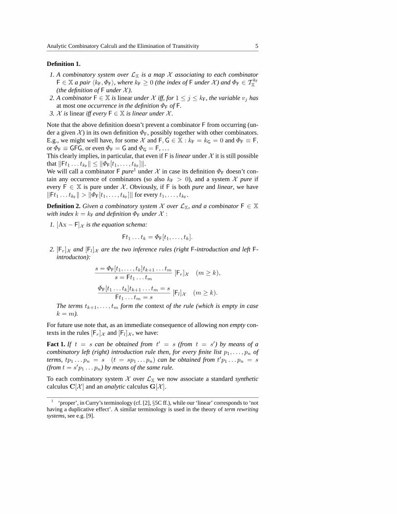
Definition 1.

1. A combinatory system overLX is a mapX associating to each combinatorF ∈ X a pair 〈kF, ΦF〉, wherekF ≥ 0 (the index ofF underX ) andΦF ∈ T kF

X(the definition ofF underX ).

2. A combinatorF ∈ X is linearunderX iff, for 1 ≤ j ≤ kF, the variablevj hasat most oneoccurrence in the definitionΦF of F.

3. X is linear iff everyF ∈ X is linear underX .

Note that the above definition doesn’t prevent a combinatorF from occurring (un-der a givenX ) in its own definitionΦF, possibly together with other combinators.E.g., we might well have, for someX andF, G ∈ X : kF = kG = 0 andΦF ≡ F,or ΦF ≡ GFG, or evenΦF = G andΦG = F, . . .This clearly implies, in particular, that even ifF is linear underX it is still possiblethat‖Ft1 . . . tkF

‖ ≤ ‖ΦF[t1, . . . , tkF]‖.

We will call a combinatorF pure1 underX in case its definitionΦF doesn’t con-tain any occurrence of combinators (so alsokF > 0), and a systemX pure ifeveryF ∈ X is pure underX . Obviously, if F is bothpure and linear, we have‖Ft1 . . . tkF

‖ > ‖ΦF[t1, . . . , tkF]‖ for everyt1, . . . , tkF

.

Definition 2. Given a combinatory systemX overLX, and a combinatorF ∈ Xwith indexk = kF and definitionΦF underX :

1. [Ax− F]X is the equation schema:

Ft1 . . . tk = ΦF[t1, . . . , tk].

2. [Fr]X and [Fl]X are the two inference rules (rightF-introduction and leftF-introducton):

s = ΦF[t1, . . . , tk]tk+1 . . . tms = Ft1 . . . tm

[Fr]X (m ≥ k),

ΦF[t1 . . . tk]tk+1 . . . tm = s

Ft1 . . . tm = s[Fl]X (m ≥ k).

The termstk+1, . . . , tm form thecontextof the rule (which is empty in casek = m).

For future use note that, as an immediate consequence of allowingnon emptycon-texts in the rules[Fr]X and[Fl]X , we have:

Fact 1. If t = s can be obtained fromt′ = s (from t = s′) by means of acombinatory left (right) introduction rule then, for every finite listp1, . . . , pn ofterms,tp1 . . . pn = s (t = sp1 . . . pn) can be obtained fromt′p1 . . . pn = s(from t = s′p1 . . . pn) by means of the same rule.

To each combinatory systemX overLX we now associate a standardsyntheticcalculusC[X ] and ananalyticcalculusG[X ].

1 ‘proper’, in Curry’s terminology (cf. [2],§5C ff.), while our ‘linear’ corresponds to ‘nothaving a duplicative effect’. A similar terminology is used in the theory ofterm rewritingsystems, see e.g. [9].

6 Pierluigi Minari

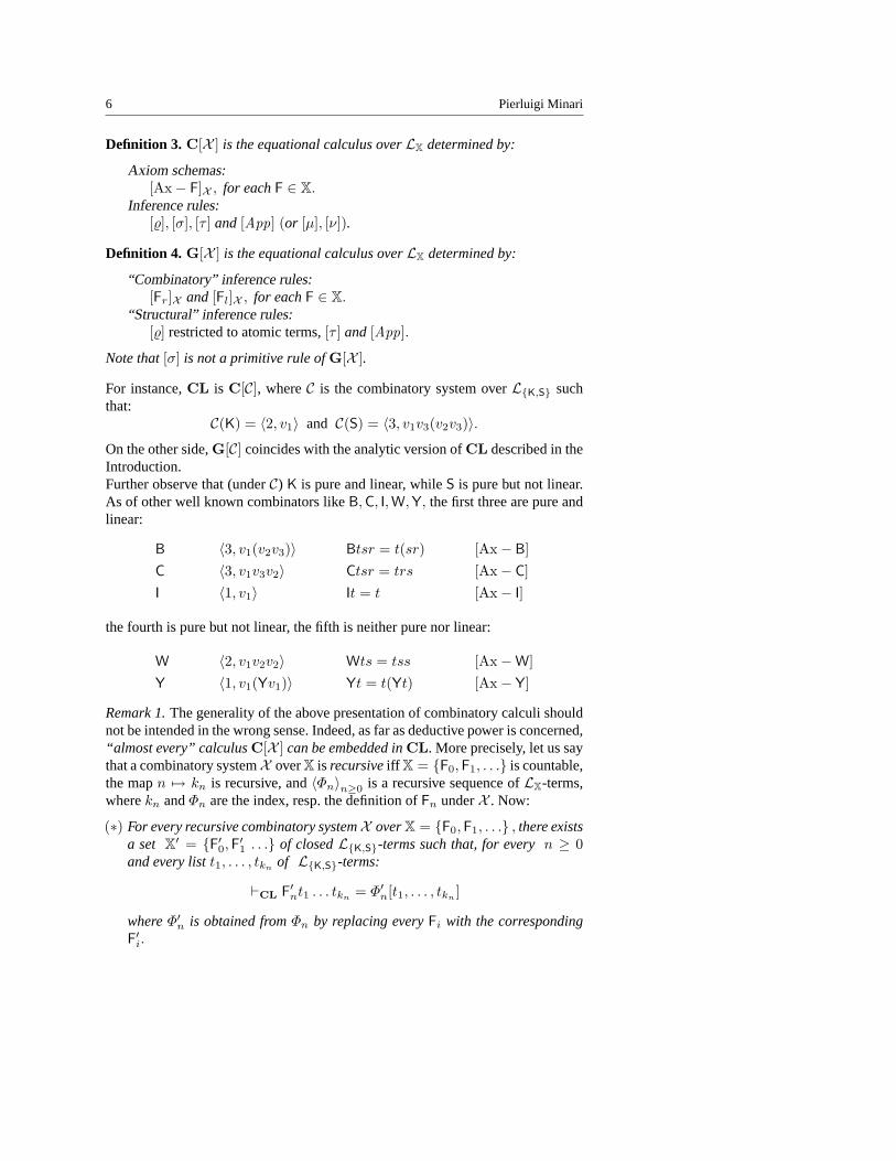
Definition 3. C[X ] is the equational calculus overLX determined by:

Axiom schemas:[Ax− F]X , for eachF ∈ X.

Inference rules:[%], [σ], [τ ] and[App] (or [µ], [ν]).

Definition 4. G[X ] is the equational calculus overLX determined by:

“Combinatory” inference rules:[Fr]X and[Fl]X , for eachF ∈ X.

“Structural” inference rules:[%] restricted to atomic terms, [τ ] and[App].

Note that[σ] is not a primitive rule ofG[X ].

For instance,CL is C[C], whereC is the combinatory system overL{K,S} suchthat:

C(K) = 〈2, v1〉 and C(S) = 〈3, v1v3(v2v3)〉.On the other side,G[C] coincides with the analytic version ofCL described in theIntroduction.Further observe that (underC) K is pure and linear, whileS is pure but not linear.As of other well known combinators likeB,C, I, W, Y, the first three are pure andlinear:

B 〈3, v1(v2v3)〉 Btsr = t(sr) [Ax− B]C 〈3, v1v3v2〉 Ctsr = trs [Ax− C]I 〈1, v1〉 It = t [Ax− I]

the fourth is pure but not linear, the fifth is neither pure nor linear:

W 〈2, v1v2v2〉 Wts = tss [Ax−W]Y 〈1, v1(Yv1)〉 Yt = t(Yt) [Ax− Y]

Remark 1.The generality of the above presentation of combinatory calculi shouldnot be intended in the wrong sense. Indeed, as far as deductive power is concerned,“almost every” calculusC[X ] can be embedded inCL. More precisely, let us saythat a combinatory systemX overX is recursiveiff X = {F0, F1, . . .} is countable,the mapn 7→ kn is recursive, and〈Φn〉n≥0 is a recursive sequence ofLX-terms,wherekn andΦn are the index, resp. the definition ofFn underX . Now:

(∗) For every recursive combinatory systemX overX = {F0,F1, . . .} , there existsa set X′ = {F′0, F′1 . . .} of closedL{K,S}-terms such that, for everyn ≥ 0and every listt1, . . . , tkn of L{K,S}-terms:

`CL F′nt1 . . . tkn = Φ′n[t1, . . . , tkn ]

whereΦ′n is obtained fromΦn by replacing everyFi with the correspondingF′i.


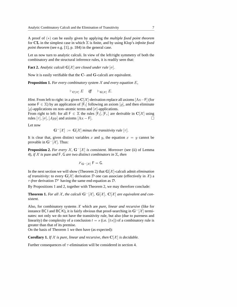
A proof of (∗) can be easily given by applying themultiple fixed point theoremfor CL in the simplest case in whichX is finite, and by using Klop’sinfinite fixedpoint theorem(see e.g. [1], p. 184) in the general case.

Let us now turn to analytic calculi. In view of the left/right symmetry of both thecombinatory and the structural inference rules, it is readily seen that:

Fact 2. Analytic calculiG[X ] are closed under rule[σ].

Now it is easily verifiable that theC- andG-calculi are equivalent.

Proposition 1. For every combinatory systemX and every equationE,

`C[X ] E iff `G[X ] E.

Hint. From left to right: in a givenC[X ]-derivation replace all axioms[Ax−F] (forsomeF ∈ X) by an application of[Fl] following an axiom[%], and then eliminate[%]-applications on non–atomic terms and[σ]-applications.From right to left: for allF ∈ X the rules[Fl], [Fr] are derivable inC[X ] usingrules[τ ], [σ], [App] and axioms[Ax− F]. ¤Let now

G−[X ] := G[X ] minus the transitivity rule[τ ].

It is clear that, given distinct variablesx andy, the equationx = y cannot beprovable inG−[X ]. Thus:

Proposition 2. For everyX , G−[X ] is consistent. Moreover(see (ii) of Lemma4), if X is pureandF, G are two distinct combinators inX, then

0G−[X ] F = G.

In the next section we will show (Theorem 2) thatG[X ]-calculi admiteliminationof transitivity: to everyG[X ] derivationD one can associate (effectively inX ) aτ -freederivationD∗ having the same end-equation asD.

By Propositions 1 and 2, together with Theorem 2, we may therefore conclude:

Theorem 1.For all X , the calculiG−[X ], G[X ], C[X ] are equivalent and con-sistent.

Also, for combinatory systemsX which arepure, linear and recursive(like forinstanceBC I andBC K), it is fairly obvious that proof-searching inG−[X ] termi-nates: not only we do not have the transitivity rule, but also (due to pureness andlinearity) the complexity of a conclusiont = s (i.e.‖ts‖) of a combinatory rule isgreater than that of its premise.On the basis of Theorem 1 we then have (as expected):

Corollary 1. If X is pure, linear and recursive, thenC[X ] is decidable.

Further consequences ofτ -elimination will be considered in section 4.

8 Pierluigi Minari

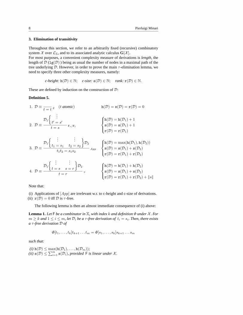
3. Elimination of transitivity

Throughout this section, we refer to an arbitrarily fixed (recursive) combinatorysystemX overLX, and to its associated analytic calculusG[X ].For most purposes, a convenient complexity measure of derivations islength,thelength ofD (lg(D) ) being as usual the number of nodes in a maximal path of thetree underlyingD. However, in order to prove the mainτ -elimination lemma, weneed to specify three other complexity measures, namely:

c-height:h(D) ∈ N; c-size:s(D) ∈ N; rank: r(D) ∈ N.

These are defined by induction on the construction ofD:

Definition 5.

1. D ≡t = t

% (t atomic) h(D) = s(D) = r(D) = 0

2. D ≡D1

{ ...t′ = s′

t = sFr/Fl

h(D) = h(D1) + 1s(D) = s(D1) + 1r(D) = r(D1)

3. D ≡D1

{ ...t1 = s1

...t2 = s2

}D2

t1t2 = s1s2App

h(D) = max(h(D1), h(D2))s(D) = s(D1) + s(D2)r(D) = r(D1) + r(D2)

4. D ≡D1

{ ...t = s

...s = r

}D2

t = rτ

h(D) = h(D1) + h(D2)s(D) = s(D1) + s(D2)r(D) = r(D1) + r(D2) + ‖s‖

Note that:

(i) Applications of[App] are irrelevant w.r. to c-height and c-size of derivations.(ii) r(D) = 0 iff D is τ -free.

The following lemma is then an almost immediate consequence of (i) above:

Lemma 1. LetF be a combinator inX, with indexk and definitionΦ underX . Form ≥ k and1 ≤ i ≤ m, letDi be aτ -free derivation ofti = si. Then, there existsa τ -free derivationD of

Φ[t1, . . . , tk]tk+1 . . . tm = Φ[s1, . . . , sk]sk+1 . . . sm

such that:

(i) h(D) ≤ max(h(D1), . . . , h(Dm));(ii) s(D) ≤ ∑m

i=1 s(Di), providedF is linear underX .


The reason for the proviso onF in point (ii) above lies in the fact that, beingD obtained by means of[%] and [App] inferences from theDi

′s, someDi mustbe used more than once ifF is not linear. And, in this case, we may well haves(D) >

∑mi=1 s(Di).

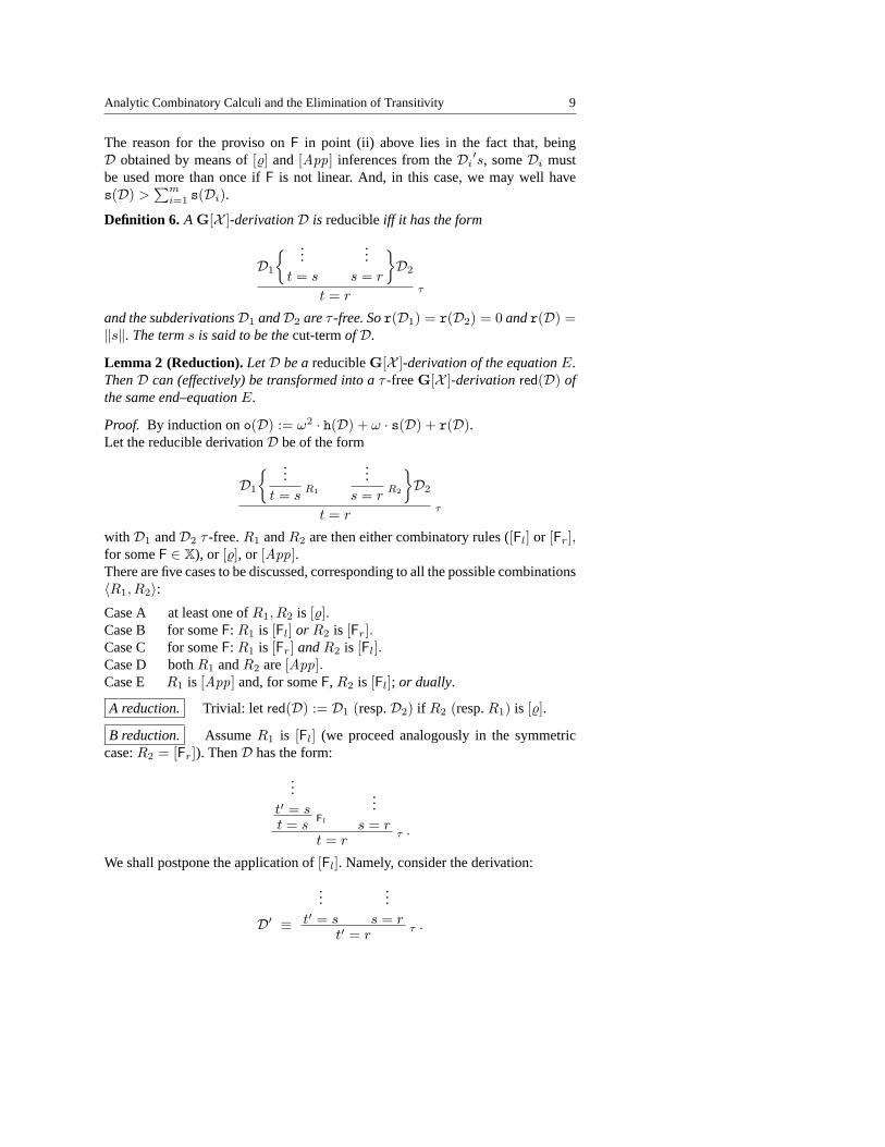
Definition 6. A G[X ]-derivationD is reducibleiff it has the form

D1

{ ...t = s

...s = r

}D2

t = rτ

and the subderivationsD1 andD2 areτ -free. Sor(D1) = r(D2) = 0 andr(D) =‖s‖. The terms is said to be thecut-termofD.

Lemma 2 (Reduction).LetD be areducibleG[X ]-derivation of the equationE.ThenD can (effectively) be transformed into aτ -freeG[X ]-derivationred(D) ofthe same end–equationE.

Proof. By induction ono(D) := ω2 · h(D) + ω · s(D) + r(D).Let the reducible derivationD be of the form

D1

{ ...t = s

R1

...s = r

R2

}D2

t = rτ

with D1 andD2 τ -free.R1 andR2 are then either combinatory rules ([Fl] or [Fr],for someF ∈ X), or [%], or [App].There are five cases to be discussed, corresponding to all the possible combinations〈R1, R2〉:Case A at least one ofR1, R2 is [%].Case B for someF: R1 is [Fl] or R2 is [Fr].Case C for someF: R1 is [Fr] andR2 is [Fl].Case D bothR1 andR2 are[App].Case E R1 is [App] and, for someF, R2 is [Fl]; or dually.

A reduction. Trivial: let red(D) := D1 (resp.D2) if R2 (resp.R1) is [%].

B reduction. AssumeR1 is [Fl] (we proceed analogously in the symmetriccase:R2 = [Fr]). ThenD has the form:

...t′ = st = s

Fl

...s = r

t = rτ .

We shall postpone the application of[Fl]. Namely, consider the derivation:

D′ ≡

...t′ = s

...s = r

t′ = rτ .

10 Pierluigi Minari

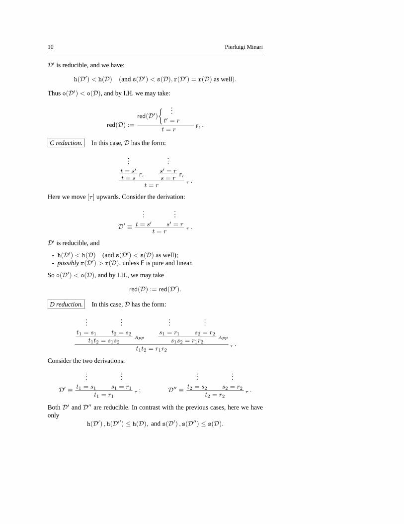
D′ is reducible, and we have:

h(D′) < h(D) (ands(D′) < s(D), r(D′) = r(D) as well).

Thuso(D′) < o(D), and by I.H. we may take:

red(D) :=red(D′)

{ ...t′ = r

t = rFl

.

C reduction. In this case,D has the form:

...t = s′t = s

Fr

...s′ = rs = r

Fl

t = rτ .

Here we move[τ ] upwards. Consider the derivation:

D′ ≡

...t = s′

...s′ = r

t = rτ .

D′ is reducible, and

- h(D′) < h(D) (ands(D′) < s(D) as well);- possiblyr(D′) > r(D), unlessF is pure and linear.

Soo(D′) < o(D), and by I.H., we may take

red(D) := red(D′).

D reduction. In this case,D has the form:

...t1 = s1

...t2 = s2

t1t2 = s1s2App

...s1 = r1

...s2 = r2

s1s2 = r1r2App

t1t2 = r1r2τ .

Consider the two derivations:

D′ ≡

...t1 = s1

...s1 = r1

t1 = r1τ ; D′′ ≡

...t2 = s2

...s2 = r2

t2 = r2τ .

BothD′ andD′′ are reducible. In contrast with the previous cases, here we haveonly

h(D′) , h(D′′) ≤ h(D), ands(D′) , s(D′′) ≤ s(D).


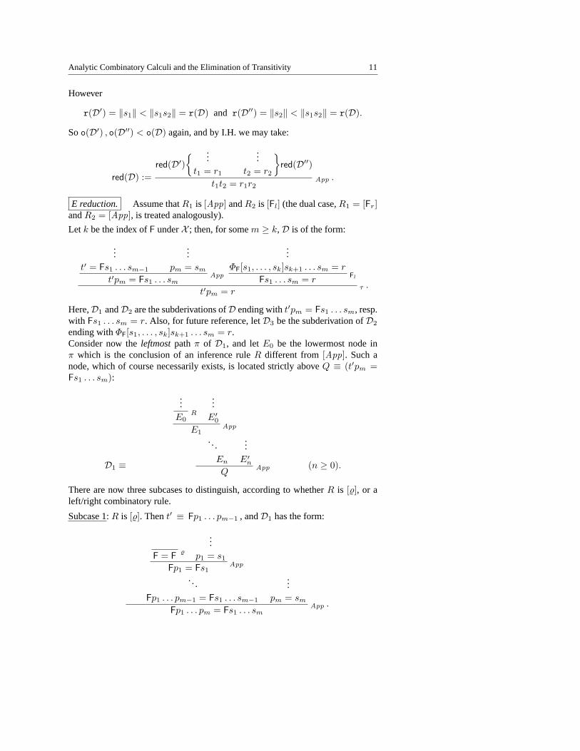
However

r(D′) = ‖s1‖ < ‖s1s2‖ = r(D) and r(D′′) = ‖s2‖ < ‖s1s2‖ = r(D).

Soo(D′) , o(D′′) < o(D) again, and by I.H. we may take:

red(D) :=red(D′)

{ ...t1 = r1

...t2 = r2

}red(D′′)

t1t2 = r1r2App .

E reduction. Assume thatR1 is [App] andR2 is [Fl] (the dual case,R1 = [Fr]andR2 = [App], is treated analogously).

Let k be the index ofF underX ; then, for somem ≥ k,D is of the form:

...t′ = Fs1 . . . sm−1

...pm = sm

t′pm = Fs1 . . . smApp

...ΦF[s1, . . . , sk]sk+1 . . . sm = r

Fs1 . . . sm = rFl

t′pm = rτ .

Here,D1 andD2 are the subderivations ofD ending witht′pm = Fs1 . . . sm, resp.with Fs1 . . . sm = r. Also, for future reference, letD3 be the subderivation ofD2

ending withΦF[s1, . . . , sk]sk+1 . . . sm = r.Consider now theleftmostpathπ of D1, and letE0 be the lowermost node inπ which is the conclusion of an inference ruleR different from [App]. Such anode, which of course necessarily exists, is located strictly aboveQ ≡ (t′pm =Fs1 . . . sm):

D1 ≡

...E0

R

...E′

0

E1App

. ..

En

...E′

n

QApp (n ≥ 0).

There are now three subcases to distinguish, according to whetherR is [%], or aleft/right combinatory rule.

Subcase 1: R is [%]. Thent′ ≡ Fp1 . . . pm−1 , andD1 has the form:

F = F%

...p1 = s1

Fp1 = Fs1App

.. .

Fp1 . . . pm−1 = Fs1 . . . sm−1

...pm = sm

Fp1 . . . pm = Fs1 . . . smApp .

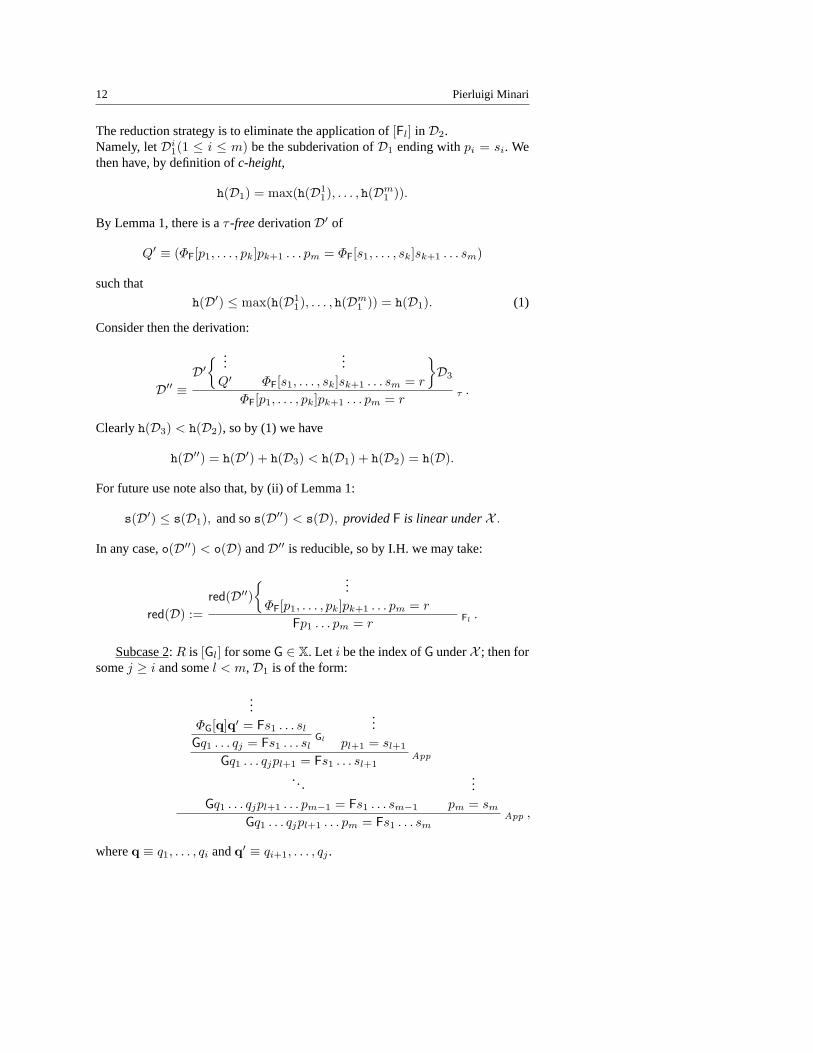
12 Pierluigi Minari

The reduction strategy is to eliminate the application of[Fl] in D2.Namely, letDi

1(1 ≤ i ≤ m) be the subderivation ofD1 ending withpi = si. Wethen have, by definition ofc-height,

h(D1) = max(h(D11), . . . , h(Dm

1 )).

By Lemma 1, there is aτ -freederivationD′ of

Q′ ≡ (ΦF[p1, . . . , pk]pk+1 . . . pm = ΦF[s1, . . . , sk]sk+1 . . . sm)

such that

h(D′) ≤ max(h(D11), . . . , h(Dm

1 )) = h(D1). (1)

Consider then the derivation:

D′′ ≡D′

{ ...Q′

...ΦF[s1, . . . , sk]sk+1 . . . sm = r

}D3

ΦF[p1, . . . , pk]pk+1 . . . pm = rτ .

Clearlyh(D3) < h(D2), so by (1) we have

h(D′′) = h(D′) + h(D3) < h(D1) + h(D2) = h(D).

For future use note also that, by (ii) of Lemma 1:

s(D′) ≤ s(D1), and sos(D′′) < s(D), providedF is linear underX .

In any case,o(D′′) < o(D) andD′′ is reducible, so by I.H. we may take:

red(D) :=red(D′′)

{ ...ΦF[p1, . . . , pk]pk+1 . . . pm = r

Fp1 . . . pm = rFl

.

Subcase 2: R is [Gl] for someG ∈ X. Let i be the index ofG underX ; then forsomej ≥ i and somel < m,D1 is of the form:

...ΦG[q]q′ = Fs1 . . . sl

Gq1 . . . qj = Fs1 . . . slGl

...pl+1 = sl+1

Gq1 . . . qjpl+1 = Fs1 . . . sl+1App

.. .

Gq1 . . . qjpl+1 . . . pm−1 = Fs1 . . . sm−1

...pm = sm

Gq1 . . . qjpl+1 . . . pm = Fs1 . . . smApp ,

whereq ≡ q1, . . . , qi andq′ ≡ qi+1, . . . , qj .


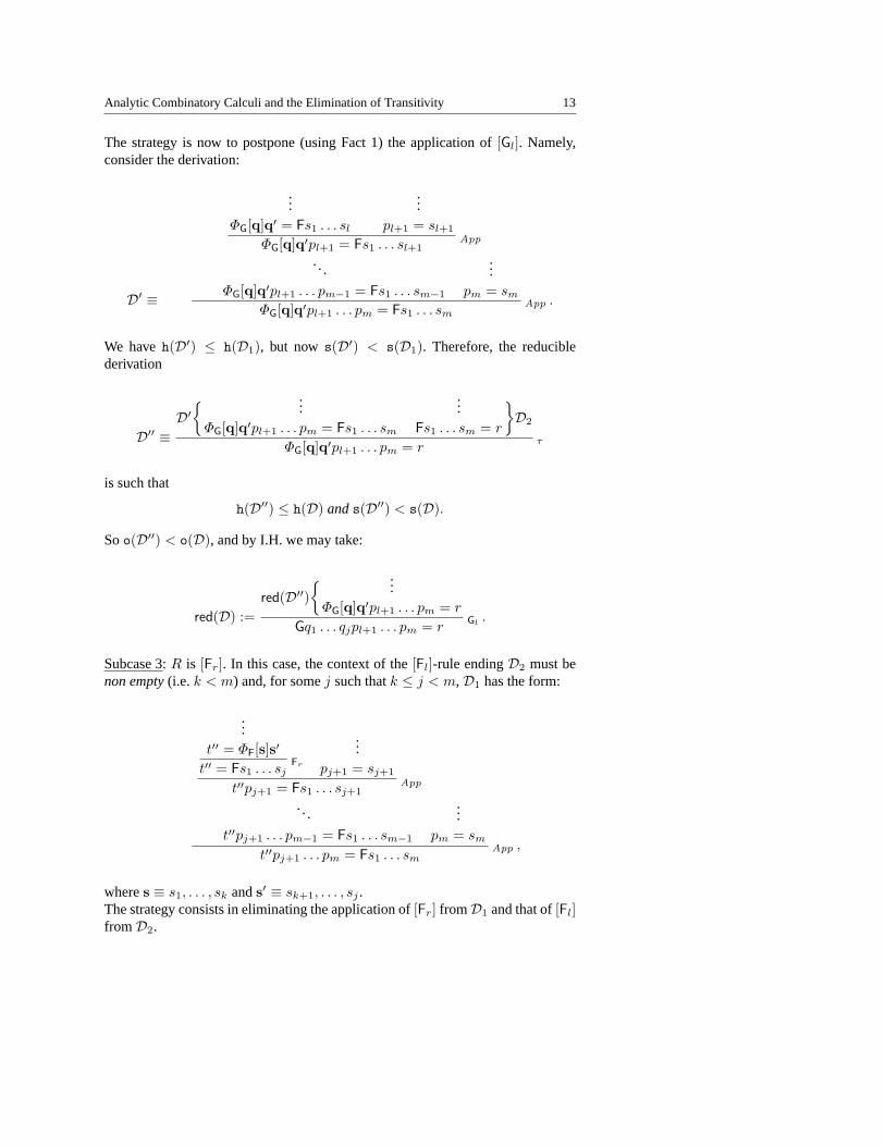
The strategy is now to postpone (using Fact 1) the application of[Gl]. Namely,consider the derivation:

D′ ≡

...ΦG[q]q′ = Fs1 . . . sl

...pl+1 = sl+1

ΦG[q]q′pl+1 = Fs1 . . . sl+1App

.. .

ΦG[q]q′pl+1 . . . pm−1 = Fs1 . . . sm−1

...pm = sm

ΦG[q]q′pl+1 . . . pm = Fs1 . . . smApp .

We haveh(D′) ≤ h(D1), but nows(D′) < s(D1). Therefore, the reduciblederivation

D′′ ≡D′

{ ...ΦG[q]q′pl+1 . . . pm = Fs1 . . . sm

...Fs1 . . . sm = r

}D2

ΦG[q]q′pl+1 . . . pm = rτ

is such that

h(D′′) ≤ h(D) ands(D′′) < s(D).

Soo(D′′) < o(D), and by I.H. we may take:


{ ...ΦG[q]q′pl+1 . . . pm = r

Gq1 . . . qjpl+1 . . . pm = rGl

.

Subcase 3: R is [Fr]. In this case, the context of the[Fl]-rule endingD2 must benon empty(i.e.k < m) and, for somej such thatk ≤ j < m,D1 has the form:

...t′′ = ΦF[s]s′

t′′ = Fs1 . . . sjFr

...pj+1 = sj+1

t′′pj+1 = Fs1 . . . sj+1App

. . .

t′′pj+1 . . . pm−1 = Fs1 . . . sm−1

...pm = sm

t′′pj+1 . . . pm = Fs1 . . . smApp ,

wheres ≡ s1, . . . , sk ands′ ≡ sk+1, . . . , sj .The strategy consists in eliminating the application of[Fr] fromD1 and that of[Fl]fromD2.

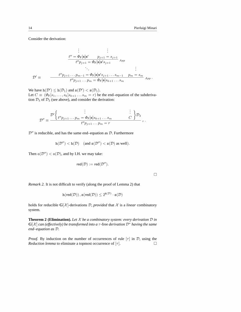
14 Pierluigi Minari

Consider the derivation:

D′ ≡

...t′′ = ΦF[s]s′

...pj+1 = sj+1

t′′pj+1 = ΦF[s]s′sj+1App

.. .

t′′pj+1 . . . pm−1 = ΦF[s]s′sj+1 . . . sm−1

...pm = sm

t′′pj+1 . . . pm = ΦF[s]sk+1 . . . smApp .

We haveh(D′) ≤ h(D1) ands(D′) < s(D1).Let C ≡ (ΦF[s1, . . . , sk]sk+1 . . . sm = r) be the end–equation of the subderiva-tionD3 of D2 (see above), and consider the derivation:

D′′ ≡D′

{ ...t′′pj+1 . . . pm = ΦF[s]sk+1 . . . sm

...C

}D3

t′′pj+1 . . . pm = rτ .

D′′ is reducible, and has the same end–equation asD. Furthermore

h(D′′) < h(D) (ands(D′′) < s(D) as well).

Theno(D′′) < o(D), and by I.H. we may take:

red(D) := red(D′′).

¤

Remark 2.It is not difficult to verify (along the proof of Lemma 2) that

h(red(D)) , s(red(D)) ≤ 2h(D) · s(D)

holds for reducibleG[X ]-derivationsD, providedthatX is a linear combinatorysystem.

Theorem 2(Elimination). LetX be a combinatory system: every derivationD inG[X ] can (effectively) be transformed into aτ -freederivationD∗ having the sameend–equation asD.

Proof. By induction on the number of occurrences of rule[τ ] in D, using theReduction lemmato eliminate a topmost occurrence of[τ ]. ¤


4. Applications of τ -elimination

Given a combinatory systemX , let us now consider the (straightforward) rela-tivization toX of the standard notions ofredexandcontractum, one step reduction,(weak) reduction, (weak) normal formetc. fromCL.

Definition 7.1. t is aX -redex, andt′ is theX -contractumof t, iff there exists someF ∈ X such

thatt ≡ Fs1 . . . sk and t′ ≡ ΦF[s1, . . . , sk],

wherek andΦF are the index, resp. the definition ofF underX .2. t →X s iff s is obtained fromt by replacing exactly one occurrence of aX -

redex int by the correspondingX -contractum.3. ³X := the reflexive and transitive closure of→X .4. t is a X -normal form (t ∈ NFX ) iff t doesn’t contain occurrences ofX -

redexes.5. t hasaX -normal formiff t ³X s for somes ∈ NFX .6. X is Church-Rosser,CR(X ), iff ³X is confluent, i.e. for everyt, s1, s2 :

( s1 ´X t ³X s2 ) ⇒ ∃r( s1 ³X r ´X s2 ).

Below, we will drop the subscriptX in →X and³X whenever possible.

Remark 3.In contrast to what we observed in Remark 1 about provableX -equality,note thatX -reduction cannot, in general, be faithfully simulated by means of stan-dardCL w(eak)-reduction. Indeed, denoting by′ the embedding ofG[X ] into CLobtained as in 1, one may well have, for someX and someLX-termst, s: t →X sand nott′ →w s′. E.g., ifX (F) = 〈0,F〉, one hasF →X F, while it is easy to seethatF′ →w F′ is impossible.

X -reducibility andG[X ]-derivability are related as expected:

Lemma 3. If t ³X s then `G[X ] t = s.

In view of the peculiar form of combinatory inference rules inG-calculi, τ -freederivations enjoy the following simple yet usefulweak subterm property.

Lemma 4. LetD be aτ -free derivation oft = s in G[X ].(i) If D containsat least oneoccurrence of aleft (right) combinatory introduction

rule, then the termt (resp.:s) containsat least oneoccurrence of aX -redex.(ii) If both t ands areX -normal forms, thent ≡ s.

Proof. (i): by induction on the length ofD. Under the assumptions, we have thatthe final inferenceR of D is either[Fl]/[Fr], or [App]. In the first case the con-clusion follows at once. In the second case, at least one of the two immediatesubderivations ofD must satisfy the assumptions, so we get the conclusion by ap-plying the I.H.(ii): Under the assumptions, it follows by (i) that the only inference rules occurringinD are[%] and[App], and clearly the end–equation of every such derivation mustbe of the formr = r. ¤We will now exploitτ -elimination (Theorem 2), and present two interesting appli-cations.

16 Pierluigi Minari

Church-Rosser

First of all, it turns out that we may getCR(X ) almost for free.

Lemma 5. If `G−[X ] t = s then t ³ r ´ s for somer.

Proof. By straightforward induction on the length of theτ -free derivationD oft = s in G[X ]. ¤

Theorem 3(CR). Every combinatory systemX is Church-Rosser.

Proof. Supposes1 ´ t ³ s2. By Lemma 3 botht = s1 andt = s2 are derivablein G[X ] and so also, by symmetry (which is admissible by Fact 2) and transitivity:

`G[X ] s1 = s2 .

Then, by the Elimination Theorem 2,

`G−[X ] s1 = s2 ,

whence the conclusion immediately follows by Lemma 5. ¤

Remark 4.As usual, CR(X ) impliesuniqueness ofX -normal forms:

( t ³ r, t ³ s, r, s ∈ NFX ) ⇒ r ≡ s.

In the present context, note also the following short alternative proof, which doesnot pass through CR.

Proof. Assumet ³ r andt ³ s, with r, s ∈ NFX . Then, as above, there exists aderivationD in G−[X ] of r = s. The conclusion now follows by (ii) of Lemma 4.

¤

Note also that ifX is pure and linearwe trivially have (i)strong normalizationfor X (for every termt, theX -reduction graph oft is finite) and so, directly andwithout using CR, (ii) everyLX termt hasexactly oneX -normal form.

Leftmost reduction

A second consequence ofτ -elimination consists in a relatively simple proof of (ageneralized form of) theleftmost(or: normal) reduction Theoremfor CL, sayingthat the leftmost reduction strategy, consisting in reducing step by step always theleftmostredex occurrence, is normalizing, i.e.: whenever applied to a termt havinga normal form, it terminates in the normal form oft. Usually, this theorem followsas an immediate corollary to the strongerStandardization Theorem(see e.g. [1]and [8]).

Definition 8.

1. t →l X s iff s is obtained fromt by replacing theleftmostX -redex occurrencein t by the correspondingX -contractum.

2. ³l

X := the reflexive and transitive closure of→l X .


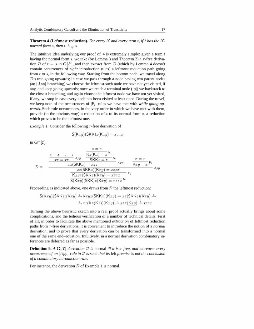
Theorem 4(Leftmost reduction). For everyX and every termt, if t has theX -normal forms, thent ³l

X s.

The intuitive idea underlying our proof of 4 is extremely simple: given a termthaving the normal forms, we take (by Lemma 3 and Theorem 2) aτ -free deriva-tion D of t = s in G[X ], and thenextract from D (which by Lemma 4 doesn’tcontain occurrences ofright introduction rules) a leftmost reduction path goingfrom t to s, in the following way. Starting from the bottom node, we travel alongD’s tree going upwards; in case we pass through a node having two parent nodes(an[App]-branching) we choose the leftmost such node we have not yet visited, ifany, and keep going upwards; once we reach a terminal node ([%]) we backtrack tothe closest branching, and again choose the leftmost node we have not yet visited,if any; we stop in case every node has been visited at least once. During the travel,we keep note of the occurrences of[Fl] rules we have met withwhile going up-wards. Such rule occurrences, in the very order in which we have met with them,provide (in the obvious way) a reduction oft to its normal forms, a reductionwhich proves to be the leftmost one.

Example 1.Consider the followingτ -free derivation of

S(Kxy)(SKK)z(Kxy) = xzzx

in G−[C]:

D ≡

x = x z = z

xz = xzApp

z = z

Kz(Kz) = zKl

SKKz = zSl

xz(SKKz) = xzzApp

x = x

Kxy = xKl

xz(SKKz)(Kxy) = xzzx

Kxyz(SKKz)(Kxy) = xzzx

S(Kxy)(SKK)z(Kxy) = xzzxSl

Kl

App

Proceeding as indicated above, one draws fromD the leftmost reduction:

S(Kxy)(SKK)z(Kxy) →l Kxyz(SKKz)(Kxy) →l xz(SKKz)(Kxy) →l→l xz(Kz(Kz))(Kxy) →l xzz(Kxy) →l xzzx.

Turning the above heuristic sketch into a real proof actually brings about somecomplications, and the tedious verification of a number of technical details. Firstof all, in order to facilitate the above mentionedextractionof leftmost reductionpaths fromτ -free derivations, it is convenient to introduce the notion of anormalderivation, and to prove that every derivation can be transformed into a normalone of the same end–equation. Intuitively, in a normal derivation combinatory in-ferences are deferred as far as possible.

Definition 9. A G[X ]-derivationD is normal iff it is τ -free, and moreover everyoccurrence of an[App]-rule inD is such that itsleft premiseis notthe conclusionof a combinatory introduction rule.

For instance, the derivationD of Example 1 is normal.

18 Pierluigi Minari

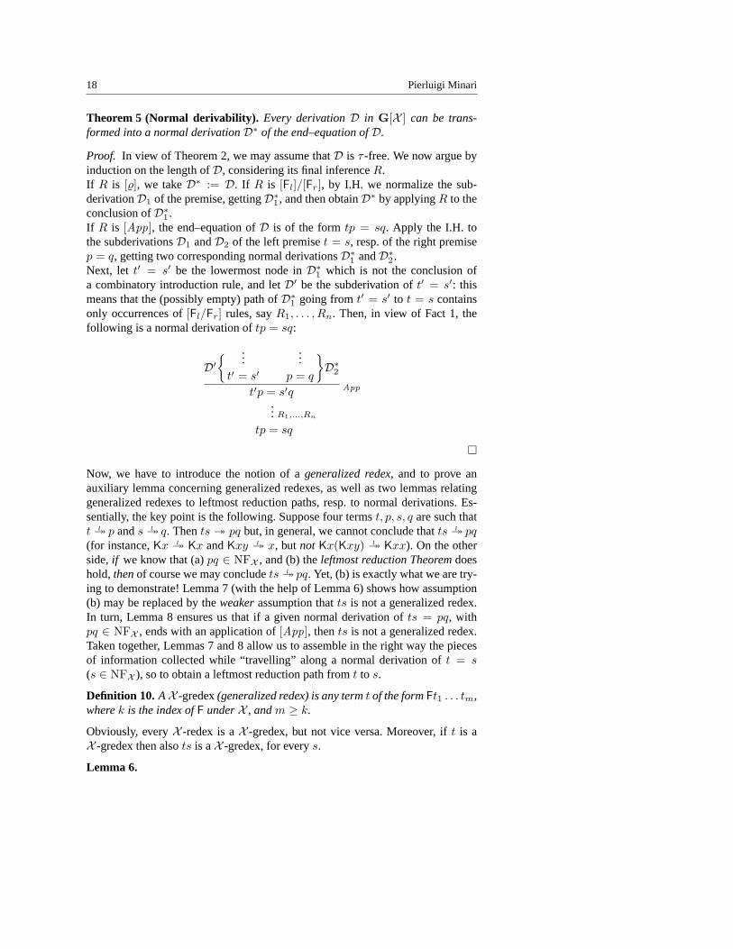
Theorem 5(Normal derivability). Every derivationD in G[X ] can be trans-formed into a normal derivationD∗ of the end–equation ofD.

Proof. In view of Theorem 2, we may assume thatD is τ -free. We now argue byinduction on the length ofD, considering its final inferenceR.If R is [%], we takeD∗ := D. If R is [Fl]/[Fr], by I.H. we normalize the sub-derivationD1 of the premise, gettingD∗1 , and then obtainD∗ by applyingR to theconclusion ofD∗1 .If R is [App], the end–equation ofD is of the formtp = sq. Apply the I.H. tothe subderivationsD1 andD2 of the left premiset = s, resp. of the right premisep = q, getting two corresponding normal derivationsD∗1 andD∗2 .Next, let t′ = s′ be the lowermost node inD∗1 which is not the conclusion ofa combinatory introduction rule, and letD′ be the subderivation oft′ = s′: thismeans that the (possibly empty) path ofD∗1 going fromt′ = s′ to t = s containsonly occurrences of[Fl/Fr] rules, sayR1, . . . , Rn. Then, in view of Fact 1, thefollowing is a normal derivation oftp = sq:

D′{ ...

t′ = s′

...p = q

}D∗2

t′p = s′q App

... R1,...,Rn

tp = sq

¤

Now, we have to introduce the notion of ageneralized redex, and to prove anauxiliary lemma concerning generalized redexes, as well as two lemmas relatinggeneralized redexes to leftmost reduction paths, resp. to normal derivations. Es-sentially, the key point is the following. Suppose four termst, p, s, q are such thatt ³l p ands ³l q. Thents ³ pq but, in general, we cannot conclude thatts ³l pq(for instance,Kx ³l Kx andKxy ³l x, but not Kx(Kxy) ³l Kxx). On the otherside,if we know that (a)pq ∈ NFX , and (b) theleftmost reduction Theoremdoeshold, thenof course we may concludets ³l pq. Yet, (b) is exactly what we are try-ing to demonstrate! Lemma 7 (with the help of Lemma 6) shows how assumption(b) may be replaced by theweakerassumption thatts is not a generalized redex.In turn, Lemma 8 ensures us that if a given normal derivation ofts = pq, withpq ∈ NFX , ends with an application of[App], thents is not a generalized redex.Taken together, Lemmas 7 and 8 allow us to assemble in the right way the piecesof information collected while “travelling” along a normal derivation oft = s(s ∈ NFX ), so to obtain a leftmost reduction path fromt to s.

Definition 10. AX -gredex(generalized redex) is any termt of the formFt1 . . . tm,wherek is the index ofF underX , andm ≥ k.

Obviously, everyX -redex is aX -gredex, but not vice versa. Moreover, ift is aX -gredex then alsots is aX -gredex, for everys.

Lemma 6.


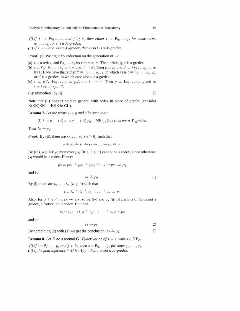
(i) If t → Fs1 . . . sj and j ≥ 0, then eithert ≡ Fq1 . . . qj for some termsq1, . . . , qj , or t is aX -gredex.

(ii) If t → s ands is aX -gredex, then alsot is aX -gredex.

Proof. (i): We argue by induction on the generation of→:

(a) t is a redex, andFs1 . . . sj its contractum. Then, trivially,t is a gredex.(b) t ≡ t′p, Fs1 . . . sj ≡ s′p, andt′ → s′. Thenp ≡ sj ands′ ≡ Fs1 . . . sj−1, so

by I.H. we have that eithert′ ≡ Fq1 . . . qj−1, in which caset ≡ Fq1 . . . qj−1p,or t′ is a gredex, in which case alsot is a gredex.

(c) t ≡ p t′, Fs1 . . . sj ≡ ps′, and t′ → s′. Thenp ≡ Fs1 . . . sj−1, and sot ≡ Fs1 . . . sj−1 t′.

(ii): immediate, by (i). ¤

Note that (ii) doesn’t hold in general withredex in place of gredex(considerK(KK)KK → KKK in CL ).

Lemma 7. Let the termst, s, p andq be such that:

(i) t ³l p , (ii) s ³l q , (iii) pq ∈ NFX , (iv) ts is not aX -gredex.

Then ts ³l pq.

Proof. By (ii), there ares0, . . . , sn (n ≥ 0) such that

s ≡ s0 →l s1 →l s2 →l . . . →l sn ≡ q .

By (iii), p ∈ NFX ; moreoverpsi (0 ≤ i ≤ n) cannot be a redex, since otherwisepq would be a redex. Hence:

ps ≡ ps0 →l ps1 →l ps2 →l . . . →l psn ≡ pq

and sops ³l pq . (1)

By (i), there aret0, . . . , tn (n ≥ 0) such that

t ≡ t0 →l t1 →l t2 →l . . . →l tn ≡ p .

Also, for 0 ≤ i ≤ n: ts ³ tis; so by (iv) and by (ii) of Lemma 6,tis is not agredex, a fortiori not a redex. But then

ts ≡ t0s →l t1s →l t2s →l . . . →l tns ≡ ps

and sots ³l ps . (2)

By combining (2) with (1) we get the conclusion:ts ³l pq. ¤

Lemma 8. LetD be anormalG[X ]-derivation of t = s, with s ∈ NFX .

(i) If t ≡ Fp1 . . . pj andj < kF, thens ≡ Fq1 . . . qj for someq1, . . . , qj .(ii) If the final inference inD is [App], thent is notaX -gredex.

20 Pierluigi Minari

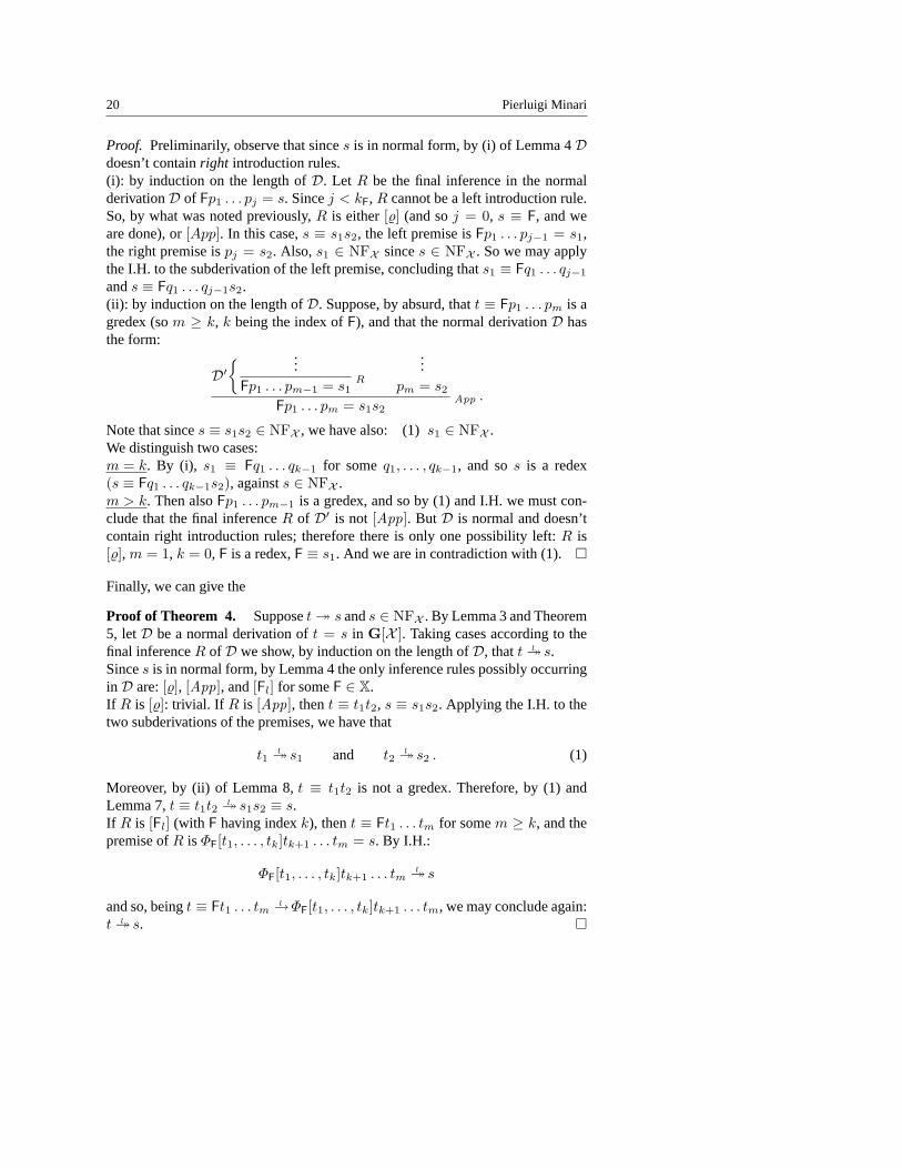
Proof. Preliminarily, observe that sinces is in normal form, by (i) of Lemma 4Ddoesn’t containright introduction rules.(i): by induction on the length ofD. Let R be the final inference in the normalderivationD of Fp1 . . . pj = s. Sincej < kF, R cannot be a left introduction rule.So, by what was noted previously,R is either[%] (and soj = 0, s ≡ F, and weare done), or[App]. In this case,s ≡ s1s2, the left premise isFp1 . . . pj−1 = s1,the right premise ispj = s2. Also, s1 ∈ NFX sinces ∈ NFX . So we may applythe I.H. to the subderivation of the left premise, concluding thats1 ≡ Fq1 . . . qj−1

ands ≡ Fq1 . . . qj−1s2.(ii): by induction on the length ofD. Suppose, by absurd, thatt ≡ Fp1 . . . pm is agredex (som ≥ k, k being the index ofF), and that the normal derivationD hasthe form:

D′{ ...

Fp1 . . . pm−1 = s1R

...pm = s2

Fp1 . . . pm = s1s2App .

Note that sinces ≡ s1s2 ∈ NFX , we have also: (1)s1 ∈ NFX .We distinguish two cases:m = k. By (i), s1 ≡ Fq1 . . . qk−1 for someq1, . . . , qk−1, and sos is a redex(s ≡ Fq1 . . . qk−1s2), againsts ∈ NFX .m > k. Then alsoFp1 . . . pm−1 is a gredex, and so by (1) and I.H. we must con-clude that the final inferenceR of D′ is not [App]. ButD is normal and doesn’tcontain right introduction rules; therefore there is only one possibility left:R is[%], m = 1, k = 0, F is a redex,F ≡ s1. And we are in contradiction with (1).¤

Finally, we can give the

Proof of Theorem 4. Supposet ³ s ands ∈ NFX . By Lemma 3 and Theorem5, letD be a normal derivation oft = s in G[X ]. Taking cases according to thefinal inferenceR of D we show, by induction on the length ofD, thatt ³l s.Sinces is in normal form, by Lemma 4 the only inference rules possibly occurringin D are:[%], [App], and[Fl] for someF ∈ X.If R is [%]: trivial. If R is [App], thent ≡ t1t2, s ≡ s1s2. Applying the I.H. to thetwo subderivations of the premises, we have that

t1 ³l s1 and t2 ³l s2 . (1)

Moreover, by (ii) of Lemma 8,t ≡ t1t2 is not a gredex. Therefore, by (1) andLemma 7,t ≡ t1t2 ³l s1s2 ≡ s.If R is [Fl] (with F having indexk), thent ≡ Ft1 . . . tm for somem ≥ k, and thepremise ofR is ΦF[t1, . . . , tk]tk+1 . . . tm = s. By I.H.:

ΦF[t1, . . . , tk]tk+1 . . . tm ³l s

and so, beingt ≡ Ft1 . . . tm →l ΦF[t1, . . . , tk]tk+1 . . . tm, we may conclude again:t ³l s. ¤


5. Adding extensionality

In this section, we consider the extension ofC- andG- calculi by means of theextensionalityrule

[Ext ] :tx = sx

t = s(x /∈ V (ts)).

We recall that, as far as standard combinatory logicCL is concerned, it holds(see e.g. [8]) thatCL+[Ext ] is equivalentto CL+[ξ∗], where[ξ∗] is the rule

t = s

λ∗x.t = λ∗x.s.

Here, for everyCL -term t and every individual variablex, λ∗x.t is theCL -termwhich is defined inductively as follows:

1. λ∗x.x := SKK,2. λ∗x.s := Ks, if x /∈ V (s),3. λ∗x.sx := s, if x /∈ V (s),4. λ∗x.sr := S(λ∗x.s)(λ∗x.r), if (2) and (3) do not apply tosr.

It holds that:

(i) V (λ∗x.t) = V (t) \ {x} ,(ii) `CL (λ∗x.t)s = t[x/s] , for every terms.

The extensionality rule[Ext ] has been chosen here for investigation, since theextensionality rule[ξ∗], whose formulation depends on the definability of (someform of) λ-abstraction, can obviously not be immediately generalized to arbitrarycombinatory systems.

Given a combinatory systemX , byCext[X ] andGext[X ] we shall denote thecalculusC[X ], resp.G[X ], plus the new inference rule[Ext ]; by G−

ext[X ] thecalculusGext[X ] minus the transitivity rule.It can be easily verified thatCext[X ] andGext[X ] areequivalentfor everyX , inthe sense of Proposition 1.

Lemma 9. LetD be aτ -free derivation oft = s in Gext[X ].

(i) If a left (right) combinatory introduction rule occurs inD, then t (resp.s)contains at least one occurrence of a combinator.

(ii) If both t ands do not contain occurrences of combinators, thent ≡ s.(iii) If X is apurecombinatory system, and aleft (right) F-introduction rule occurs

in D, thent (resp.s) contains at least one occurrence of the combinatorF.

Proof. (i): by straightforward induction on the length ofD.(ii): immediate by (i), after observing that ifD is aGext[X ]-derivation in whichcombinatory introduction rules are not applied at all, then every equation occurringin D has the formp = p for some termp.

22 Pierluigi Minari

(iii): by induction on the length ofD. We will discuss only the case in which thefinal inference ofD is [Gl], for some combinatorG ∈ X. So let

D ≡D′

{ ...ΦG[t1, . . . , tk] tk+1 . . . tm = s

Gt1, . . . , tm = sGl

wherek is the index ofG andm ≥ k.SinceX is pureby assumption, it holds that no combinator occurs inΦG; thereforeevery combinatorH which either occurs inΦG[t1, . . . , tk]tk+1 . . . tm or is identicalwith G must occur also inGt1, . . . , tm. The conclusion now follows by applyingthe I.H. to the subderivationD′. ¤

Note that Lemma 9 (i) is a weaker form of Lemma 4 (i) which, as it stands, is nolonger true forGext[X ]: indeed, a redex created by an introduction rule may bedestroyed by a successive application of an[Ext ]-rule.

Now, it is an immediate consequence of Lemma 9 (ii) that

0G−ext[X ] x = y

wheneverx andy are distinct variables. Therefore:

Proposition 3. For every combinatory systemX , G−ext[X ] is consistent.

Unfortunately, as anticipated in the Introduction, we are able to proveτ -elimina-tion only for a (very) restricted class of combinatory systems:

Theorem 6(Restricted elimination). LetX be alinearcombinatory system: ev-ery derivationD in Gext[X ] can (effectively) be transformed into aτ -freederiva-tionD∗ having the same end–equation asD.

As a consequence, we cannot derive any longer – but for linear combinatory sys-tems – the consistency ofC- andG- calculi with extensionality merely on the basisof τ -elimination and of Proposition 3, as we previously did for calculi without ex-tensionality (Theorem 1). As a matter of fact,Cext[X ] is consistentfor everyX ,but to prove this we have to embedCext[X ] into CLext (see Remark 1) and toappeal to the known consistency of the latter.

Remark 5.It is not a surprising fact that, for someX , Gext[X ] is equivalenttoG[X ], i.e. that [Ext ] is admissible inG[X ]. A nice example thereof isK, thesystem overX = {K} defining the standard combinatorK. A simple proof of thisfact can be given using Theorem 2 (hint: first, show that if`G−[K] tx = s andx /∈ V (ts), then`G[K] t = Ks).On the other side, to be sure, there are plenty ofpure and linear combinatorysystemsX such thatGext[X ] is strongerthanG[X ]. For example, letX be thesystem over{B, K} (over{B, I}) giving B andK (B andI) the standard definitions.It is easily verified (using Theorem 2) thatBBK = BKK (BI = I) is derivable inGext[X ] and is not derivable inG[X ].


We shall now prove Theorem 6. First of all, given a derivationD in Gext[X ], wedefineh(D) (ce-heightof D), s(D) (ce-sizeof D), r(D) as in sect. 3, except thatnow also an application of[Ext ] increases ce-height and ce-size by 1 (actually,ce-height will not be used here). Next, we need the following lemma concerningsubstitution:

Lemma 10.LetD be a (τ -free) derivation oft = s in Gext[X ]. Then, for everyx ∈ V and every termr, there exists a (τ -free) derivationD′ of t[x/r] = s[x/r]such that:

h(D′) ≤ h(D) ands(D′) ≤ s(D).

Proof. By straightforward induction on the length ofD, considering its final infer-enceR. E.g., ifR = [Ext ] we have

D ≡D1

{ ...tu = su

t = sExt

with u /∈ V (ts). So if u coincides withx we havet[x/r] ≡ t ands[x/r] ≡ s, andwe may takeD′ := D. If u is distinct fromx, apply first of all the I.H. to obtainfrom D1 a derivationD′1 of tw = sw, wherew /∈ V (tsr). Next, apply the I.H.to get fromD′1 a derivationD′′1 of t[x/r]w = s[x/r]w, s.t.h(D′′1 ) ≤ h(D1) ands(D′′1 ) ≤ s(D1). A final application of[Ext ] yields the conclusion. ¤

Finally we prove aReduction Lemma,which is the analogue of Lemma 2except forthe restriction to linear systems,yielding Theorem 6 as an immediate consequence.Note how we have to keep thece-sizeof the reduced derivation under control.

Lemma 11.LetX be alinearcombinatory system, andD be areducibleGext[X ]-derivation of the equationE. ThenD can (effectively) be transformed into aGext[X ]-derivationred(D) of E, such that:

(i) red(D) is τ -free;(ii) s(red(D)) ≤ s(D).

Proof. By main induction ons(D) and secondary induction onr(D), i.e. by in-duction onor(D) := ω · s(D) + r(D).Let the reducible derivationD be of the form

D1

{ ...t = s

R1

...s = r

R2

}D2

t = rτ

with D1 andD2 τ -free. R1 andR2 are then either combinatory rules, or[%], or[App], or [Ext ].According to all the possible combinations〈R1, R2〉, there are nowsixcases to bediscussed, namely the five cases (A – E) considered in the proof of Lemma 2, plusthe new one:

24 Pierluigi Minari

Case F at least one ofR1, R2 is [Ext ].

A, B, C, D reductions. We obtainred(D) exactly as in the corresponding casesin the proof of Lemma 2, using themainI.H. in cases B and C, and thesecondaryI.H. in case D.It is immediately verified that also condition (ii) is satisfied in each case.

E reduction. As in the corresponding case in the proof of Lemma 2 we con-sider, within the leftmost path ofD1, the lowermost nodeE0 which is the conclu-sion of an inferenceR different from[App].The subcases to be considered are now the followingfour.Subcase 1: R is [%]. We proceed exactly as in 2, except that here, the combinatorysystemX beinglinear by assumption, it is

s(D′′) = s(D′) + s(D3) < s(D)

by (ii) of Lemma 1, and we may conclude by applying the main I.H. once-size.Furthermore, by I.H.

s(red(D′′)) ≤ s(D′′),and so (ii) does hold:

s(red(D)) = s(red(D′′)) + 1 ≤ s(D′′) + 1 ≤ s(D).

Subcases 2 and 3: R is [Gl] / R is [Fr]. Both reductions are the same as in 2: I.H.once-sizeis sufficient. Also, it is easily seen that (ii) is satisfied.Subcase 4: R is [Ext ]. In this case, there exists aj (0 ≤ j < m) such thatD1 hasthe form:

Da

{ ...t′′x = Fs1 . . . sjx

t′′ = Fs1 . . . sjExt

...pj+1 = sj+1

}Db

t′′pj+1 = Fs1 . . . sj+1App

. . .

t′′pj+1 . . . pm−1 = Fs1 . . . sm−1

...pm = sm

t′′pj+1 . . . pm = Fs1 . . . smApp

wherex /∈ V (t′′Fs1 . . . sj).The strategy consists in avoiding the application of[Ext ] in favor of two suitablyeliminable applications of[τ ].Look at the subderivationsDa,Db of D1 indicated above, and letDc be the sub-derivation ofD1 ending witht′′pj+1 = Fs1 . . . sj+1. Note that:

s(Dc) = s(Da) + 1 + s(Db). (1)

By Lemma 10 applied toDa, letD∗a be aτ -free derivation of

t′′pj+1 = Fs1 . . . sjpj+1


satisfying: s(D∗a) ≤ s(Da).Also, let

D∗b ≡

...Fs1 . . . sj = Fs1 . . . sj

...pj+1 = sj+1

}Db

Fs1 . . . sjpj+1 = Fs1 . . . sj+1App .

Obviouslys(D∗b ) = s(Db) sinceFs1 . . . sj = Fs1 . . . sj is derivable using[%] and[App] only.Consider now the derivation

D′c ≡D∗a

{ ...t′′pj+1 = Fs1 . . . sjpj+1

...Fs1 . . . sjpj+1 = Fs1 . . . sj+1

}D∗b

t′′pj+1 = Fs1 . . . sj+1τ .

D′c is reducible, and by (1):

s(D′c) = s(D∗a) + s(D∗b ) ≤ s(Da) + s(Db) < s(Dc). (2)

Also,s(Dc) ≤ s(D1) ≤ s(D1) + s(D2) = s(D), (3)

so by (2) and (3):

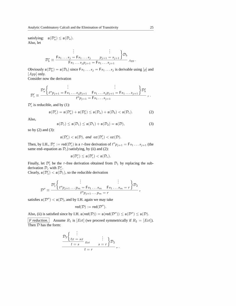
s(D′c) < s(D), and or(D′c) < or(D).

Then, by I.H.,D∗c := red(D′c) is aτ -free derivation oft′′pj+1 = Fs1 . . . sj+1 (thesame end–equation asDc) satisfying, by (ii) and (2):

s(D∗c ) ≤ s(D′c) < s(Dc).

Finally, letD′1 be theτ -free derivation obtained fromD1 by replacing the sub-derivationDc with D∗c .Clearly,s(D′1) < s(D1), so the reducible derivation

D′′ ≡D′1

{ ...t′′pj+1 . . . pm = Fs1 . . . sm

...Fs1 . . . sm = r

}D2

t′′pj+1 . . . pm = rτ

satisfiess(D′′) < s(D), and by I.H. again we may take

red(D) := red(D′′).Also, (ii) is satisfied since by I.H.s(red(D)) = s(red(D′′)) ≤ s(D′′) ≤ s(D).

F reduction. AssumeR1 is [Ext ] (we proceed symmetrically ifR2 = [Ext ]).ThenD has the form:

D3

{ ...tx = sx

t = sExt

...s = r

}D2

t = rτ .

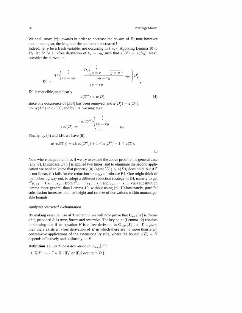
26 Pierluigi Minari

We shall move[τ ] upwards in order to decrease thece-sizeof D; note howeverthat, in doing so, the length of the cut term is increased !Indeed, lety be a fresh variable, not occurring int, s, r. Applying Lemma 10 toD3, let D′ be aτ -free derivation ofty = sy, such thats(D′) ≤ s(D3). Next,consider the derivation:

D′′ ≡D′

{ ...ty = sy

D2

{ ...s = r y = y

%

sy = ryApp

}D′2

ty = ryτ .

D′′ is reducible, and clearlys(D′′) < s(D), (4)

since one occurrence of[Ext ] has been removed, ands(D′2) = s(D2).Soor(D′′) < or(D), and by I.H. we may take:


{ ...ty = ry

t = rExt

Finally, by (4) and I.H. we have (ii):

s(red(D)) = s(red(D′′)) + 1 ≤ s(D′′) + 1 ≤ s(D).

¤

Note where the problem lies if we try to extend the above proof to the general case(anyX ). In subcase E4[τ ] is applied two times, and to eliminate the second appli-cation we need to know that property (ii) (s(red(D)) ≤ s(D)) does hold; but ifFis not linear, (ii) fails for the reduction strategy of subcase E1. One might think ofthe following way out: to adopt a different reduction strategy in E4, namely to gett′′pj+1 = Fs1 . . . sj+1 from t′′x = Fs1 . . . sjx andpj+1 = sj+1 via a substitutionlemma more general than Lemma 10, without using[τ ]. Unfortunately,parallelsubstitution increases both ce-height and ce-size of derivations within unmanage-able bounds.

Applying restrictedτ -elimination.

By making essential use of Theorem 6, we will now prove thatCext[X ] is decid-able, providedX is pure, linear andrecursive. The key point (Lemma 12) consistsin showing that if an equationE is τ -free derivable inGext[X ] andX is pure,then there exists aτ -free derivation ofE in which there are no more thani(E)consecutiveapplications of the extensionality rule, where the boundi(E) ∈ Ndepends effectively and uniformly onE.

Definition 11. LetD be a derivation inGext[X ]:

1.X[D] := {F ∈ X | [Fl] or [Fr] occurs inD };


2. d(D) := max{kF | F ∈ X[D] };3.D is detour-freeiff no application of[App] in D is immediately followed by an

application of[Ext ].

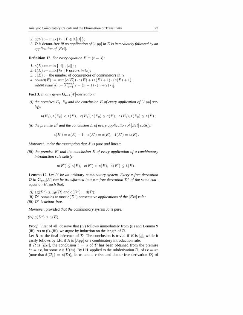
Definition 12. For every equationE ≡ (t = s):

1. a(E) := min {‖t‖ , ‖s‖} ;2. i(E) := max{kF | F occurs ints};3. c(E) := the number of occurrences ofcombinatorsin ts.4. bound(E) := sum(c(E)) · i(E) + (a(E) + 1) · (c(E) + 1),

wheresum(n) :=∑n+1

i=1 i = (n + 1) · (n + 2) · 12 .

Fact 3. In any givenGext[X ]-derivation:

(i) the premisesE1, E2 and the conclusionE of every application of[App] sat-isfy:

a(E1), a(E2) < a(E), c(E1), c(E2) ≤ c(E), i(E1), i(E2) ≤ i(E) ;

(ii) the premiseE′ and the conclusionE of every application of[Ext ] satisfy:

a(E′) = a(E) + 1, c(E′) = c(E), i(E′) = i(E) .

Moreover, under the assumption thatX is pureand linear:

(iii) the premiseE′ and the conclusionE of every application of a combinatoryintroduction rule satisfy:

a(E′) ≤ a(E), c(E′) < c(E), i(E′) ≤ i(E) .

Lemma 12.Let X be anarbitrary combinatory system. Everyτ -free derivationD in Gext[X ] can be transformed into aτ -free derivationD∗ of the same end–equationE, such that:

(i) lg(D∗) ≤ lg(D) andd(D∗) = d(D);(ii) D∗ containsat mostd(D∗) consecutiveapplications of the[Ext ] rule;

(iii) D∗ is detour-free.

Moreover,providedthat the combinatory systemX is pure:

(iv) d(D∗) ≤ i(E).

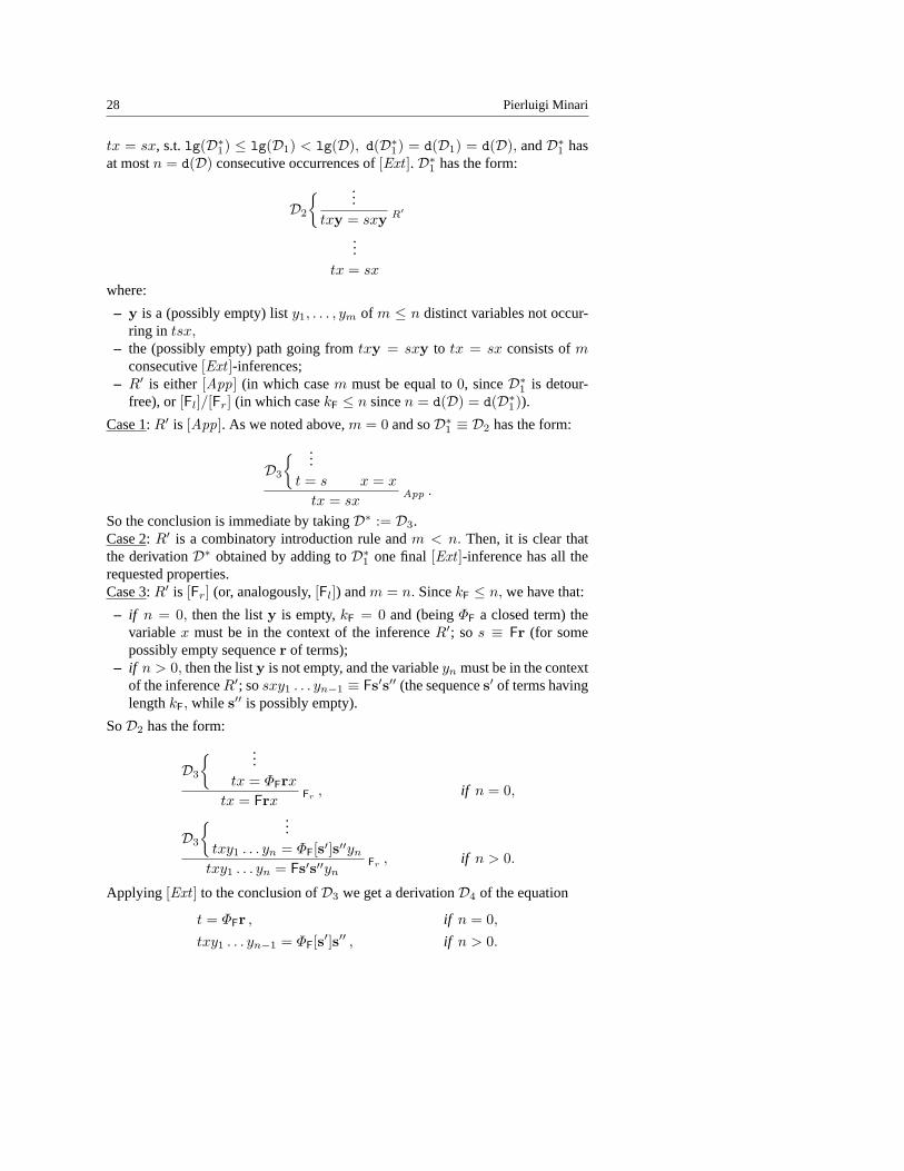
Proof. First of all, observe that (iv) follows immediately from (ii) and Lemma 9(iii). As to (i)–(iii), we argue by induction on the length ofD.Let R be the final inference ofD. The conclusion is trivial ifR is [%], while iteasily follows by I.H. ifR is [App] or a combinatory introduction rule.If R is [Ext ], the conclusiont = s of D has been obtained from the premisetx = sx, for somex /∈ V (ts). By I.H. applied to the subderivationD1 of tx = sx(note thatd(D1) = d(D)), let us take aτ -free and detour-free derivationD∗1 of

28 Pierluigi Minari

tx = sx, s.t.lg(D∗1) ≤ lg(D1) < lg(D), d(D∗1) = d(D1) = d(D), andD∗1 hasat mostn = d(D) consecutive occurrences of[Ext ].D∗1 has the form:

D2

{ ...txy = sxy R′

...tx = sx

where:

– y is a (possibly empty) listy1, . . . , ym of m ≤ n distinct variables not occur-ring in tsx,

– the (possibly empty) path going fromtxy = sxy to tx = sx consists ofmconsecutive[Ext ]-inferences;

– R′ is either[App] (in which casem must be equal to0, sinceD∗1 is detour-free), or[Fl]/[Fr] (in which casekF ≤ n sincen = d(D) = d(D∗1)).

Case 1: R′ is [App]. As we noted above,m = 0 and soD∗1 ≡ D2 has the form:

D3

{ ...t = s x = x

tx = sxApp .

So the conclusion is immediate by takingD∗ := D3.Case 2: R′ is a combinatory introduction rule andm < n. Then, it is clear thatthe derivationD∗ obtained by adding toD∗1 one final[Ext ]-inference has all therequested properties.Case 3: R′ is [Fr] (or, analogously,[Fl]) andm = n. SincekF ≤ n, we have that:

– if n = 0, then the listy is empty,kF = 0 and (beingΦF a closed term) thevariablex must be in the context of the inferenceR′; so s ≡ Fr (for somepossibly empty sequencer of terms);

– if n > 0, then the listy is not empty, and the variableyn must be in the contextof the inferenceR′; sosxy1 . . . yn−1 ≡ Fs′s′′ (the sequences′ of terms havinglengthkF, while s′′ is possibly empty).

SoD2 has the form:

D3

{ ...tx = ΦFrx

tx = Frx Fr , if n = 0,

D3

{ ...txy1 . . . yn = ΦF[s′]s′′yn

txy1 . . . yn = Fs′s′′ynFr , if n > 0.

Applying [Ext ] to the conclusion ofD3 we get a derivationD4 of the equation

t = ΦFr , if n = 0,

txy1 . . . yn−1 = ΦF[s′]s′′ , if n > 0.


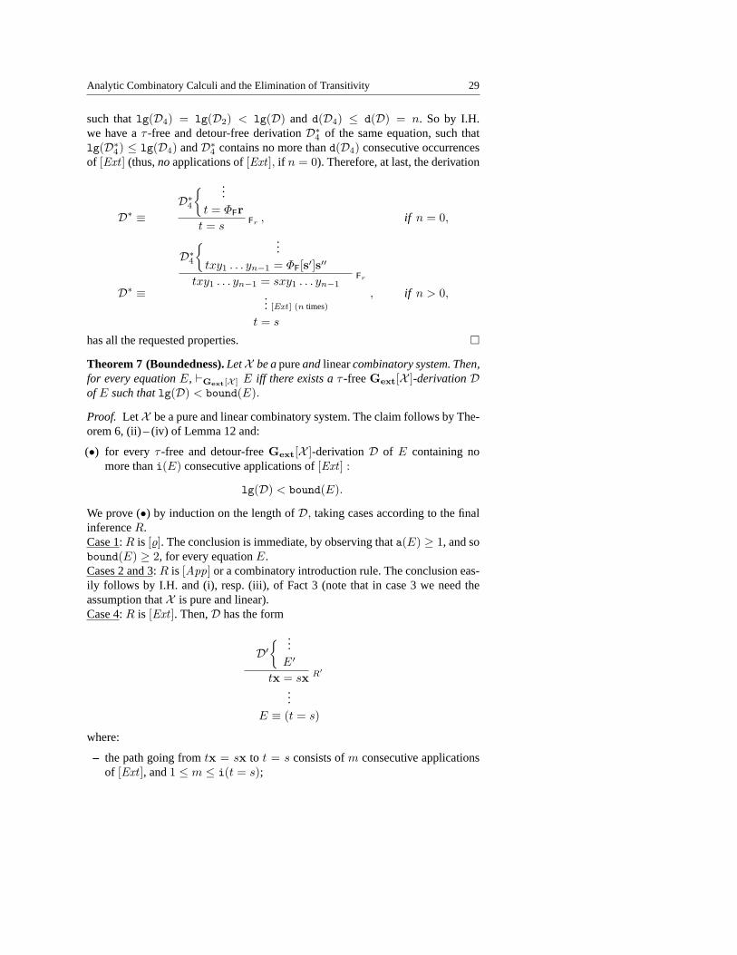
such thatlg(D4) = lg(D2) < lg(D) and d(D4) ≤ d(D) = n. So by I.H.we have aτ -free and detour-free derivationD∗4 of the same equation, such thatlg(D∗4) ≤ lg(D4) andD∗4 contains no more thand(D4) consecutive occurrencesof [Ext ] (thus,noapplications of[Ext ], if n = 0). Therefore, at last, the derivation

D∗ ≡D∗4

{ ...t = ΦFr

t = sFr , if n = 0,

D∗ ≡

D∗4{ ...

txy1 . . . yn−1 = ΦF[s′]s′′

txy1 . . . yn−1 = sxy1 . . . yn−1Fr

... [Ext] (n times)

t = s

, if n > 0,

has all the requested properties. ¤

Theorem 7(Boundedness).LetX be apureandlinearcombinatory system. Then,for every equationE, `Gext[X ] E iff there exists aτ -freeGext[X ]-derivationDof E such thatlg(D) < bound(E).

Proof. LetX be a pure and linear combinatory system. The claim follows by The-orem 6, (ii) – (iv) of Lemma 12 and:

(•) for every τ -free and detour-freeGext[X ]-derivationD of E containing nomore thani(E) consecutive applications of[Ext ] :

lg(D) < bound(E).

We prove (•) by induction on the length ofD, taking cases according to the finalinferenceR.Case 1: R is [%]. The conclusion is immediate, by observing thata(E) ≥ 1, and sobound(E) ≥ 2, for every equationE.Cases 2 and 3: R is [App] or a combinatory introduction rule. The conclusion eas-ily follows by I.H. and (i), resp. (iii), of Fact 3 (note that in case 3 we need theassumption thatX is pure and linear).Case 4: R is [Ext ]. Then,D has the form

D′{ ...

E′

tx = sx R′

...E ≡ (t = s)

where:

– the path going fromtx = sx to t = s consists ofm consecutive applicationsof [Ext ], and1 ≤ m ≤ i(t = s);

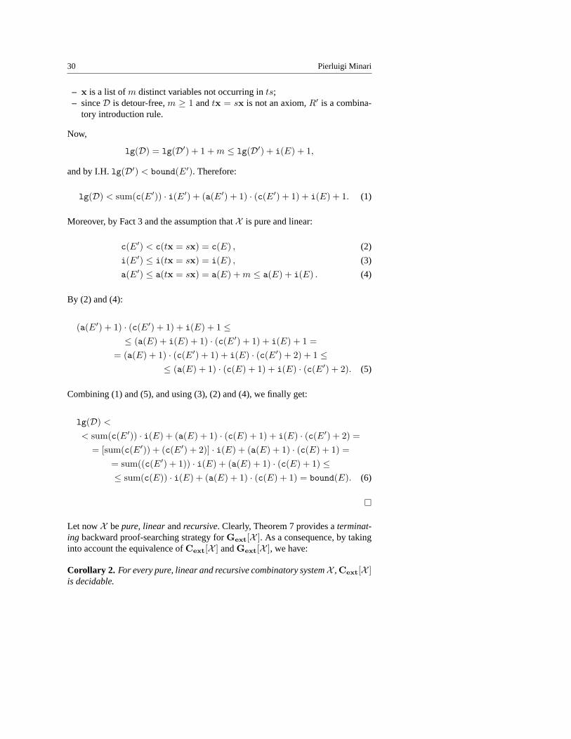
30 Pierluigi Minari

– x is a list ofm distinct variables not occurring ints;– sinceD is detour-free,m ≥ 1 andtx = sx is not an axiom,R′ is a combina-

tory introduction rule.

Now,

lg(D) = lg(D′) + 1 + m ≤ lg(D′) + i(E) + 1,

and by I.H.lg(D′) < bound(E′). Therefore:

lg(D) < sum(c(E′)) · i(E′) + (a(E′) + 1) · (c(E′) + 1) + i(E) + 1. (1)

Moreover, by Fact 3 and the assumption thatX is pure and linear:

c(E′) < c(tx = sx) = c(E) , (2)

i(E′) ≤ i(tx = sx) = i(E) , (3)

a(E′) ≤ a(tx = sx) = a(E) + m ≤ a(E) + i(E) . (4)

By (2) and (4):

(a(E′) + 1) · (c(E′) + 1) + i(E) + 1 ≤≤ (a(E) + i(E) + 1) · (c(E′) + 1) + i(E) + 1 =

= (a(E) + 1) · (c(E′) + 1) + i(E) · (c(E′) + 2) + 1 ≤≤ (a(E) + 1) · (c(E) + 1) + i(E) · (c(E′) + 2). (5)

Combining (1) and (5), and using (3), (2) and (4), we finally get:

lg(D) <

< sum(c(E′)) · i(E) + (a(E) + 1) · (c(E) + 1) + i(E) · (c(E′) + 2) == [sum(c(E′)) + (c(E′) + 2)] · i(E) + (a(E) + 1) · (c(E) + 1) =

= sum((c(E′) + 1)) · i(E) + (a(E) + 1) · (c(E) + 1) ≤≤ sum(c(E)) · i(E) + (a(E) + 1) · (c(E) + 1) = bound(E). (6)

¤

Let nowX bepure, linear andrecursive. Clearly, Theorem 7 provides aterminat-ing backward proof-searching strategy forGext[X ]. As a consequence, by takinginto account the equivalence ofCext[X ] andGext[X ], we have:

Corollary 2. For every pure, linear and recursive combinatory systemX ,Cext[X ]is decidable.


6. Open problems and further work

The general question whether Theorem 6 can be proved without restrictions atall, i.e. whetherGext[X ] admits transitivity-eliminationfor everycombinatorysystemX , is presentlyopen. In particular, for standardcombinatory logicwithextensionalitythe following questions areopen:

Problem 1. Is Gext[C], the analytic version ofCL+ ext, equivalent toG−ext[C] ?

Problem 2. Is G[C] + ξ∗ equivalent toG−[C] + ξ∗ ?

Problem 3. Is G−ext[C] equivalent toG−[C] + ξ∗ ?

([ξ∗] is the rule mentioned at the beginning of sect. 5).

To start with, observe that:

Fact 4. For every equationE betweenCL-terms:

(i) if G−ext[C] ` E thenG−[C] + ξ∗ ` E;

(ii) Gext[C] ` E iff G[C] + ξ∗ ` E.

Proof. [Ext ] is derivable inG−[C]+ξ∗: applying[ξ∗] to tx = sx we getλ∗x.tx =λ∗x.sx, i.e. t = s if x /∈ V (ts) (by the definition ofλ∗). On the other side,[ξ∗] is derivable inGext[C]: assumingt = s, we get(λ∗x.t)x = (λ∗x.s)x from(λ∗x.t)x = t and (λ∗x.s)x = s by means of[τ ], and thenλ∗x.t = λ∗x.s by[Ext ], sincex /∈ V ((λ∗x.t)(λ∗x.s)). ¤

On the basis of Fact 4, it is easily verified that Problem 1 is equivalent to theconjunctionof Problems 2 and 3, i.e. that a positive solution to 1 entails a positivesolution toboth2 and 3, and conversely.

A positiveanswer to Problem 2 – thus,a fortiori, a positive answer to Problem1 – would have an interesting consequence, as we are going to show.

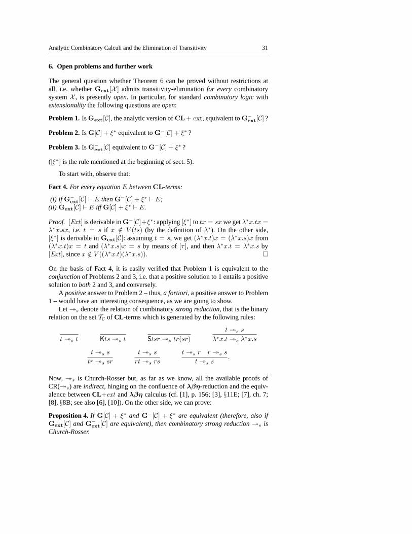
Let ³s denote the relation of combinatorystrong reduction, that is the binaryrelation on the setTC of CL -terms which is generated by the following rules:

t ³s t Kts ³s t Stsr ³s tr(sr)t ³s s

λ∗x.t ³s λ∗x.s

t ³s s

tr ³s sr

t ³s s

rt ³s rs

t ³s r r ³s s

t ³s s.

Now, ³s is Church-Rosser but, as far as we know, all the available proofs ofCR(³s) areindirect, hinging on the confluence ofλβη-reduction and the equiv-alence betweenCL+ext andλβη calculus (cf. [1], p. 156; [3],§11E; [7], ch. 7;[8], §8B; see also [6], [10]). On the other side, we can prove:

Proposition 4. If G[C] + ξ∗ and G−[C] + ξ∗ are equivalent (therefore, also ifGext[C] andG−

ext[C] are equivalent), then combinatory strong reduction³s isChurch-Rosser.

32 Pierluigi Minari

This result merely indicates how a (more)direct proof of CR(³s) could possiblybe obtained; namely, by providing a positive solution (for example via aτ -elimina-tion proof) to our Problem 1 or to (thepossiblyweaker) Problem 2.

Proposition 4 is an immediate consequence of the following Lemma, whoseproof can in turn be easily obtained similarly to the proof of Lemmas 3 and 5:

Lemma 13.For all CL-terms t, s :

(i) if t ³s s then `G[C]+ξ∗ t = s;(ii) if `G−[C]+ξ∗ t = s then t ³s r ´s s for someCL-termr.

Finally, we think it would be interesting to try and extend the “analytic” ap-proach, which has been developed here for combinatory logic, to equational proofsystems forλβ- andλβη-reduction. Unfortunately, our first attempts in this di-rection have failed so far.

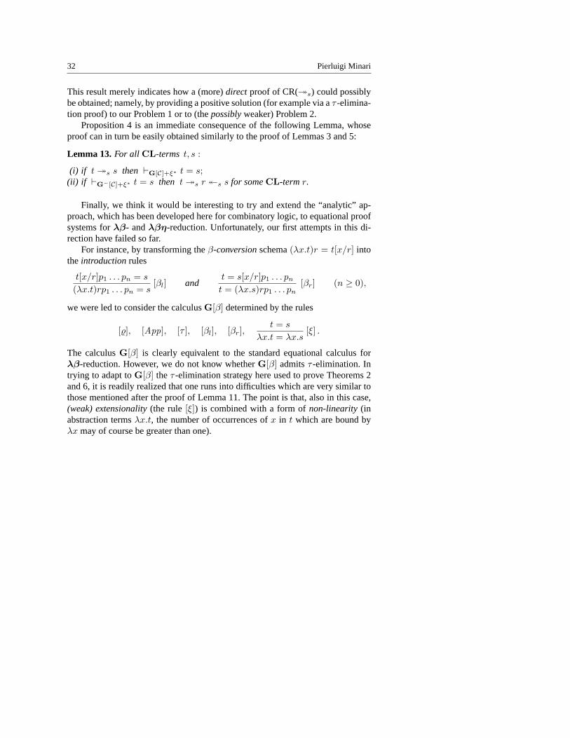
For instance, by transforming theβ-conversionschema(λx.t)r = t[x/r] intothe introductionrules

t[x/r]p1 . . . pn = s

(λx.t)rp1 . . . pn = s[βl] and

t = s[x/r]p1 . . . pn

t = (λx.s)rp1 . . . pn[βr] (n ≥ 0),

we were led to consider the calculusG[β] determined by the rules

[%], [App], [τ ], [βl], [βr],t = s

λx.t = λx.s[ξ] .

The calculusG[β] is clearly equivalent to the standard equational calculus forλβ-reduction. However, we do not know whetherG[β] admitsτ -elimination. Intrying to adapt toG[β] theτ -elimination strategy here used to prove Theorems 2and 6, it is readily realized that one runs into difficulties which are very similar tothose mentioned after the proof of Lemma 11. The point is that, also in this case,(weak) extensionality(the rule[ξ]) is combined with a form ofnon-linearity (inabstraction termsλx.t, the number of occurrences ofx in t which are bound byλx may of course be greater than one).


Added in Proof. We can prove that Problem 6.3 has a positive solution, and thatthe analytic calculusG[β] (mentioned below Lemma 6.1) admitsτ -elimination(although presently we do not have a purely proof-theoretic demonstration of thisfact).

34 P. Minari: Analytic Combinatory Calculi

References

1. H.P. Barendregt,The Lambda Calculus, its Syntax and Semantics,revised edition,North Holland, Amsterdam 1984.

2. H.B. Curry, R. Feys,Combinatory Logic, Vol. I,North Holland, Amsterdam 1958.3. H.B. Curry, J.R. Hindley, J.P. Seldin,Combinatory Logic, Vol. II,North Holland, Am-

sterdam 1972.4. E. Engeler,Foundations of Mathematics: Questions of Analysis, Geometry & Algorith-

mics(engl. transl.), Springer, Berlin 1983.5. J-Y Girard, P. Taylor, Y. Lafont,Proofs and Types,revised edition, Cambridge Univer-

sity Press, Cambridge 1990.6. J.R. Hindley,Axioms for strong reduction in combinatory logic,The Journal of Sym-

bolic Logic 32 (1967), pp. 224–236.7. J.R. Hindley, B. Lercher, J.P. Seldin,Introduction to Combinatory Logic,Cambridge

University Press, London 1972.8. J.R. Hindley, J.P. Seldin,Introduction to Combinators andλ–Calculus,Cambridge

University Press, London 1986.9. J.W. Klop,Term Rewriting Systems,in: S. Abramsky, Dov M. Gabbay, T.S.E. Maibaum,

Handbook of Logic in Computer Science, Vol. 2,Clarendon Press, Oxford 1992.10. B. Lercher,The decidability of Hindley’s axioms for strong reduction,The Journal of

Symbolic Logic 32 (1967), pp. 237–239.

Analytic combinatory calculi and the elimination of transitivity

Documents