1 Analyst Recommendations and International Stock Market Returns Henk Berkman * , Wanyi Yang ** , First Draft: July 2016 This Draft: November 2016 Abstract This paper documents that analyst recommendations aggregated at the country level predict international stock market returns. A trading strategy based on past country-level recommendations yields an abnormal return of around one percent per month. Aggregate analyst recommendations also help to predict changes in gross domestic product after accounting for survey-based forecasts. Overall, our results suggest that analyst recommendations aggregated at the country level provide useful information to guide international asset allocation. Keywords: analyst recommendation, international asset allocation, aggregate information, stock return prediction, GDP prediction * Department of Accounting and Finance, University of Auckland Business School, Auckland, New Zealand; Email: [email protected]. ** Department of Accounting and Finance, University of Auckland Business School, Auckland, New Zealand; Email: [email protected].

Welcome message from author
This document is posted to help you gain knowledge. Please leave a comment to let me know what you think about it! Share it to your friends and learn new things together.
Transcript

1
Analyst Recommendations and International Stock Market Returns
Henk Berkman*, Wanyi Yang**,
First Draft: July 2016
This Draft: November 2016
Abstract
This paper documents that analyst recommendations aggregated at the country level predict
international stock market returns. A trading strategy based on past country-level
recommendations yields an abnormal return of around one percent per month. Aggregate
analyst recommendations also help to predict changes in gross domestic product after
accounting for survey-based forecasts. Overall, our results suggest that analyst
recommendations aggregated at the country level provide useful information to guide
international asset allocation.
Keywords: analyst recommendation, international asset allocation, aggregate information,
stock return prediction, GDP prediction
* Department of Accounting and Finance, University of Auckland Business School, Auckland, New Zealand;
Email: [email protected]. ** Department of Accounting and Finance, University of Auckland Business School, Auckland, New Zealand;
Email: [email protected].
2
1. Introduction
This paper examines whether analyst recommendations aggregated at the country level
have predictive value. We define the aggregate recommendation for a country as the value-
weighted average of all outstanding recommendations for shares listed in the domestic stock
market. By averaging across firms, we eliminate firm-specific information contained in analyst
recommendations and obtain a measure that potentially contains unique information about the
aggregate company outlook for each of the 33 countries in our sample. This country-level
recommendation is used in our main trading strategy which consists of buying the MSCI
market index (in USD) of countries in the quintile with the highest average recommendations
and selling the MSCI market index of countries in the quintile with the lowest average
recommendations. Depending on the international asset pricing model and portfolio formation
window used, this strategy yields an abnormal return that ranges from 0.6 to 1.0 percent per
month.
Prior studies show that analyst recommendations provide valuable information at the
firm level. For example, Barber, Lehavy, McNichols, and Trueman (2001) find that buying
stocks with the most favourable consensus analyst recommendations and short selling stocks
with the least favourable consensus recommendations, yields annual abnormal returns of more
than four percent. Jegadeesh, Kim, Krische, and Lee (2004) show that changes in consensus
recommendations over the previous quarter also predict future returns of individual firms.1 A
small number of studies take an international perspective. For example, Jegadeesh and Kim
(2006) evaluate the value of analyst recommendations in the G7 countries. They show that
1 See also Davies and Canes (1978), Beneish (1991), Stickel (1995), Green (2006) and Irvine, Lipson, and Puckett
(2007).

3
calendar time trading strategies that buy upgraded stocks and sell downgraded stocks are
profitable in six of the seven countries.2
This study extends the literature on analyst recommendations by examining the
information content of analyst recommendations at the country level. Our research is related to
Howe, Unlu, and Yan (2009) and Boni and Womack (2006). Howe et al. (2009) show that
changes in aggregate analyst recommendations for US stocks forecast future excess returns for
the US stock market. However, their evidence with regard to the ability of industry-aggregated
analyst recommendations to predict industry returns is substantially weaker. Examining the
same issue, Boni and Womack (2006) conclude there is no predictive value in industry-
aggregated analyst recommendations.
We use IBES analyst recommendations for stocks from 33 different countries for the
period from January 1994 to June 2015, to construct monthly average country-specific
recommendations. In our base case, we focus on the value-weighted average consensus forecast
using three-month outstanding recommendations and one-month-ahead stock market returns.
Buying the market index of the quintile of countries with the highest average recommendations
and selling the market index of the quintile of countries with the lowest average
recommendations yields a monthly abnormal return of 0.935% (t-statistic is 3.12) based on the
international asset pricing model in Brusa, Ramadorai, and Verdelhan (2014), and a monthly
abnormal return of 0.802% (t-statistic is 2.46) based on the international five factor asset
pricing model in Fama and French (2015b). Similar results are obtained in a panel setting that
allows for time-variation in risk exposures of international stock markets. Additional tests show
these results are robust to changes in research design and also hold in the more recent period
2 See also Moshirian, Ng, and Wu (2009).
4
after the regulatory changes affecting the brokerage industry around the world in 2002 and
2003.
We build on the result that international stock market returns are predictable and test
the conjecture that one of the reasons our trading strategy is successful is that country level
recommendations contain useful information about future macroeconomic conditions. Brown,
Call, Clement and Sharp (2015) report that private communication with management is the
most important input to analysts’ earnings forecasts and stock recommendations. Aggregating
stock recommendations across analysts might, therefore, provide a unique insight into the
aggregate outlook for the corporate sector of different countries and be useful in predicting
future macroeconomic conditions in these countries. To test this conjecture, we examine
whether country-level recommendations predict future growth in gross domestic product (GDP)
for the countries in our sample. We find a highly significant relation between country-level
analyst recommendations and next quarter’s GDP growth in a model that includes country fixed
effects, quarter fixed effects, and last quarter’s GDP growth. Country-level recommendations
still have predictive power for GDP growth two-quarters later, but do not after that. Consistent
with our claim that country-level recommendations provide an additional and unique insight
into the outlook for the corporate sector for the different countries, we find that our results do
not change when we include the average score from the World Economic Survey (WES) for
each country-quarter pair regarding the state of the economy over the next 6 months.
Our results should be of interest to practitioners. For example, Busse, Goyal and Wahal
(2014) find little evidence of superior performance by actively managed global equity funds.
Similarly, Gallagher, Harman, Schmidt and Warren (2016) report that country selection does
not contribute significantly to excess returns of global equity managers. The simple trading
strategy proposed in our study has the potential to contribute to the performance of global
equity funds considerably. Our finding that country-level recommendations help to predict
5
future GDP growth for a broad cross-section of countries should be of interest to several
economic actors given the importance of macroeconomic predictions for policy decisions at a
national and international level.
We contribute to the literature by showing that aggregate analyst recommendations for
individual countries contain information about the cross-section of future international stock
market returns and the cross-section of future GDP-growth. We thus contribute to an emerging
literature that focuses on the information content of firm-specific variables that are aggregated
at the market level (see for example, Anilowski, Feng, and Skinner (2007) for earnings
guidance; Kothari et al. (2006) for aggregate earnings surprises; and Hirshleifer, Hou, and Teoh
(2009) for aggregate accruals and aggregate cash flows). In line with these studies, we show
that aggregating firm-level information provides useful information that is not yet reflected in
expectations and prices.
2. Data, Variable definitions, and Descriptive Statistics
In this section, we first discuss data sources and sample selection. Next, we discuss the
construction of our aggregate analyst recommendation measure. Finally, we present descriptive
statistics.
2.1 Data sources and sample selection
We obtain analyst recommendations from the I/B/E/S Recommendation Detail files for
US stocks and the I/B/E/S Recommendation Detail files for International stocks for the period
from January 1994 to June 2015.3 We include the 33 countries that have more than 10,000
recommendations in I/B/E/S for stocks listed on their domestic stock exchanges and for which
3 For 31 of the 33 countries in our sample, calendar year 1994 is the first full year with recommendations in the
IBES database. The coverage for Russia and Poland starts in July, 1997 and June, 1995 respectively.

6
data are available in Compustat.4 Analysts may have individual recommendation scales, but
I/B/E/S standardizes recommendations as 1 (strong buy), 2 (buy), 3 (hold), 4 (sell) and 5 (strong
sell). Following previous studies, we reverse the ordering of the recommendation labels so that
large (small) numbers represent positive (negative) recommendations. Recommendations can
be upgrades, downgrades, reiterations or initial recommendations. Since we focus on the
information content of aggregate recommendations across all firms in a country, the sample
consists of all types of recommendations.
The final sample of recommendations is constructed using the following criteria5:
(1) The recommended stock must have a CUSIP or SEDOL identifier;
(2) The recommendation must be from an analyst with a non-missing analyst code;
(3) The recommendation must range from 1 to 5;
(4) The announcement date should not be later than the activation date6;
(5) The country domicile code for the firm is available7;
We merge the recommendation data with Compustat and require that the GVKEY,
Issue ID, stock prices, the number of shares outstanding, incorporation country code and
exchange country code are available in Compustat.8 For each firm, we only retain share issues
with the same exchange country code and incorporation country code, so that we exclude
recommendations for cross-listed issues from our sample.9
4 On average, these 33 countries represent around 80% observations in the IBES Recommendation database with
110 countries’ recommendations available in total. 5 Based on Jegadeesh and Kim (2006) and Howe et al. (2009). 6 The Activation Date is the date that the recommendation was recorded by Thomson Reuters. 7 For each company we obtain the country domicile code from the I/B/E/S Summary History-Company
Identification- file and match it with the corresponding country name using the IBES “Summary History Manual. 8 For observations with the same GVKEY and same Issue id, we only keep the observations with largest market
capitalization in U.S. dollars. 9 Because of this requirement, the country-level recommendation is more likely to be based on recommendations
from local analysts. For a sample of 32 countries, Bae, Stulz, and Tan (2008) find that local analysts typically

7
We obtain monthly value-weighted gross total return indices for each of the individual
countries and the world market from the MSCI Index Performance Website.10 We use country
returns based on the MSCI index expressed in US dollars in our main tests. For country i and
month t, this return is indicated as 𝑀𝑆𝐶𝐼_𝑅𝑒𝑡_𝑈𝑆𝐷𝑖,𝑡. One particularly attractive feature of
MSCI country indices is that there are ETFs denominated in U.S. dollars on these indices so
that our starategies can easily be replicated in practice. 11 We also present the results of
robustness tests based on a value-weighted market return (expressed in US dollars) that is
strictly based on the stocks used in the calculation of the corresponding aggregate
recommendation for that country-month.
We use the one-month US Treasury bill rate as the risk-free rate and obtain global factor
returns from Kenneth French’s website.12 Finally, we get the monthly currency risk factors -
the carry factor and the dollar factor - from Adrien Verdelhan’s website.13
2.2 Country-level of aggregate analyst recommendations
The country-specific measure of aggregate analyst recommendations used in our main
test is the value-weighted average of all outstanding recommendations in that country. More
specifically, for each firm j, we first calculate the consensus recommendation at the end of each
calendar month t, 𝑅𝑒𝑐𝑗,𝑡, based on all outstanding recommendations issued a minimum of two
days and a maximum of 3 months prior to the end of calendar month t. 14 𝑅𝑒𝑐𝑗,𝑡 , therefore, is
have a significant information advantage over foreign analysts. When we include recommendations for cross-
listed stocks our results are marginally weaker but our conclusions do not change. 10 https://www.msci.com/end-of-day-data-search 11 After the introduction of an ETF on MSCI China A in June 2016, all of the countries in our sample have ETFs
on their market’s MSCI index in the form of ishares offered by BlackRock. Based on BlackRock’s website, the
average expense ratio for MSCI country index ETF’s is 0.48% per annum. 12 http://mba.tuck.dartmouth.edu/pages/faculty/ken.french/data_library.html. The global factors are expressed in
U.S. dollar values and are based on 23 developed markets. 13 http://web.mit.edu/adrienv/www/Data.html. Specifically, we download our data from the “The Monthly
Currency Excess Returns” file, where the “RX” variable is the dollar factor and the “HML” variable is the carry
factor (for details, see Lustig, Roussanov, and Verdelhan, 2011). 14 We use a similar method as Jegadeesh et al. (2004) when constructing the consensus recommendation. An
alternative method is to only use the most recent recommendation. Results based on this method are discussed in
the robustness tests.

8
an average across all analysts with an outstanding recommendation for stock j, where for each
analyst we only use the most recent recommendation. Specifically, a recommendation is
outstanding if it has not been stopped by the broker (Loh and Stulz, 2011).15 Next, for each
country i, we weigh the consensus recommendation for each stock j based on the previous
month’s market capitalization, 𝑀𝑘𝑡_𝐶𝑎𝑝𝑗,𝑡−1. This value-weighted average recommendation
across all n stocks in country i is defined as follows:
𝑉𝑎𝑙𝑢𝑒_𝑅𝑒𝑐𝑖,𝑡 = ∑ 𝑅𝑒𝑐𝑗,𝑡
𝑛
𝑗=1∗
𝑀𝑘𝑡_𝐶𝑎𝑝𝑗,𝑡−1
∑ 𝑀𝑘𝑡_𝐶𝑎𝑝𝑗,𝑡−1𝑛𝑗=1
(1)
By calculating the average recommendation across all stocks in each country,
idiosyncratic firm-specific information contained in these recommendations is averaged out.
To ensure a reasonable amount of diversification, we follow Bae et al. (2008) and only include
country-months if there are at least 50 firms with outstanding recommendations.
2.3 Descriptive statistics
After imposing the criteria discussed previously, we obtain a sample of 1,881,953
analyst recommendations from 33 countries for the period January 1994 to June 2015.
Following Howe et al. (2009), we separate these recommendations into “initial
recommendations” and “revised recommendations.” An initial recommendation is a
recommendation by an analyst without a recommendation for the same stock in the past 12
months. A revised recommendation is a recommendation by an analyst on a stock for which
(s)he issued at least one recommendation in the previous 12 months.
Using this definition, we get 896,706 initial recommendations and 985,247 revised
recommendations. Table 1 presents the distribution of all recommendations across the five tiers
of the revised I/B/E/S rating scale, where Panel A provides the distribution of initial
15 This information is available in the IBES Recommendations-Stop Recommendations File.

9
recommendations, and Panel B provides the distribution for revised recommendations. Table
1, Panel B also gives information about the direction of revised recommendation changes, with
each cell showing the number of recommendations changes from the rating of the row index to
the score of the column index.
From Table 1, we see that more than 80 percent of all recommendations are neutral or
favorable regardless of whether they are initial or revised recommendations. Panel B shows
that analysts are more likely to make no changes or small changes in their recommendations.
About 23 percent of the recommendations updates are unchanged, and 47 percent of the
changes are one step up or one step down (e.g. from buy to strong buy or hold).
[Table 1]
Table 2 shows the descriptive statistics of all recommendations in the sample for each year
between 1994 and 2015. The sample coverage in column (2) in Table 2 indicates that the
recommendations for the stocks listed in the 33 countries in the sample represent approximately
79% of all available recommendations in IBES through time. From column (3), we see that the
number of firms covered more than doubles during the period from 1994 to 2015, and column
(4) shows that the number of analysts who issue recommendations almost triples in this period.
As shown in column (5) in the last row of Table 2, the mean number of analysts per firm is
7.01 and column (7) in the last row shows that the average number of companies covered per
analyst is 8.31. These statistics are similar to Howe et.al (2009) for the U.S. The last column
of Table 2 shows that for each year in the sample period the average recommendation is
somewhere between buy and hold (greater than 3), which is also consistent with the findings
of previous studies.
[Table 2]

10
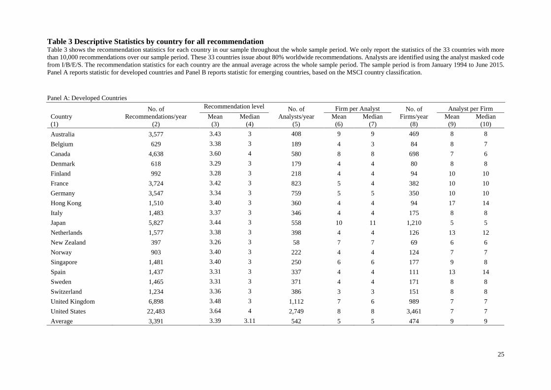
Table 3 shows descriptive statistics for the recommendations for domestic stocks for
each country in our sample. Table 3, Panel A reports the descriptive statistics for developed
countries and Table 3, Panel B reports the descriptive statistics for emerging countries.16 The
average number of recommendations for developed countries is more than twice as large as the
average number of recommendations for emerging countries. Similar observations can be made
for the number of analysts and the number of firms covered. Generally, analyst coverage on
IBES is most extensive for the U.S. Column 3 and 4 report the average and median
recommendation scores for each of the countries. The highest average recommendation is for
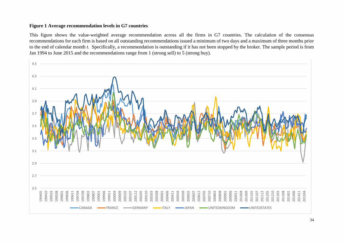
China (4.06) and the lowest average recommendation is for New Zealand (3.26). To illustrate
the evolution of the country-level recommendations over time, Figure 1 plots the average
recommendation level for G7 countries for each month during the sample period. The average
number of firms per analyst in developed countries equals five, which is lower than the average
number of firms per analyst in emerging countries, which equals seven. At the same time, the
average number of analysts per firm in developed countries at nine is higher than it in emerging
countries at seven.
[Table 3]
[Figure 1]
Table 4 Panel A (B) presents descriptive statistics for the monthly stock market returns
in US dollars for each of the developed (emerging) countries in our sample. The highest average
return across all countries is for Russia at 1.99%, and the lowest average return is for Japan at
0.27%. The results also show that emerging markets have higher average monthly returns and
are more volatile (the mean return is 1.02% per month with a standard deviation of 10.32% per
16 Countries are classified based on the MSCI classification, see https://www.msci.com/market-classification.
11
month) compared to developed markets (the average return is 0.86% per month with a standard
deviation of 6.33% per month).
[Table 4]
3. The informativeness of aggregate analyst recommendations
In this paper, we test if the information content of the average recommendation across
analysts in a country is fully incorporated in the stock market index of that country. Our tests
involve a simple strategy that buys ‘winner’ countries (countries with a relatively high average
recommendation) and sells ‘loser’ countries (countries with a relatively low average
recommendation). We first present results based on calendar-time portfolio strategies. These
strategies are easy to replicate as the country returns used in our tests are based on value-
weighted gross total return MSCI indices (expressed in US dollars), which are exactly
replicated by tradable ETFs. These ETFs trade on a continuous basis and can be sold short.
In our second set of tests, we examine the question whether country-level
recommendations predict future stock market returns in a panel setting that allows for time-
varying risk exposure for the individual countries and also controls for country-specific
momentum, year fixed effects and country fixed effects.
3.1 Calendar time portfolio strategy
Each month t, we split all countries in our sample into quintile portfolios based on the
relative position of the average country recommendation observed at the end of month t-1. For
each portfolio, we then calculate the return for month t as the equally-weighted average market
return across all countries in that portfolio.17 Our main test is based on a zero-cost hedge
portfolio that takes a long position in the quintile of countries with the most favorable
17 Using market capitalization data from the World Development Indicator, we also form value-weighted
portfolios, where we weigh each country’s return by its market capitalization at the beginning of each calendar
year. Results of this test and several other robustness tests are presented in section 5.

12
recommendations and a short position in the quintile of countries with the least favorable
recommendations.
We use four different international asset pricing models to examine the profitability of
our trading strategy. First, we use a simple world-CAPM, which incorporates the global market
return (in US dollars) but does not account for currency risk (see, Sharpe, 1964; Lintner, 1965).
Second, we use the International CAPM Redux model presented in Brusa et al. (2014), which
in addition to the global market return denominated in local currencies includes a carry factor
and a dollar factor to capture the exchange rate risk faced by US-based investors.18 Third, we
use the international five-factor asset pricing model presented in Fama and French (2015b).
Finally, we present the results for an extended Fama and French (2015b) model that also
includes the carry factor and the dollar factor.19
More specifically, we estimate the following four time-series models for PRi,t , the
return (in US dollar) in month t on each quintile portfolio i. The first model, given in equation
(2), is the world-CAPM:
𝑃𝑅𝑖,𝑡 − 𝑅𝐹𝑡 = 𝛼 + 𝛽1 ∗ 𝑊𝑀𝐾𝑇𝑡 + 𝜀𝑡 (2)
where 𝑅𝐹𝑡 is the 30 days U.S. T-bill rate in month t, and 𝑊𝑀𝐾𝑇𝑡 is the excess return on the
world market portfolio in month t, denominated in US dollar.
The second model, in equation (3), is the International CAPM Redux:
𝑃𝑅𝑖,𝑡 − 𝑅𝐹𝑡 = 𝛼 + 𝛽1 ∗ 𝐿𝑊𝑀𝐾𝑇𝑡 + 𝛽2 ∗ 𝐷𝑜𝑙𝑙𝑎𝑟𝑡 + 𝛽3 ∗ 𝐶𝑎𝑟𝑟𝑦𝑡 + 𝜀𝑡 (3)
18 See also Lustig et al. (2011) and Verdelhan (2015). 19 Brusa et al. (2015) compare the performance of several international asset pricing models and find that
International CAPM Redux model outperforms the World CAPM and the Fama-French three factor model. While
they do not examine the Fama French five factor model, evidence in Fama and French (2015b) suggests that the
five factor model displays the same limited ability to explain variation in international stock market returns as the
international Fama-French three factor model.
13
where 𝐿𝑊𝑀𝐾𝑇𝑡 is the month t excess return on the world market portfolio denominated in
local currencies. The dollar factor is defined as the average change in the exchange rate between
the U.S. dollar and all other currencies, and the carry factor is defined as the difference in
exchange rates between baskets of high and low-interest rate currencies (see, Lustig et al., 2011)
The third model is the five-factor international asset pricing model proposed in Fama
and French (2015b):
𝑃𝑅𝑖,𝑡 − 𝑅𝐹𝑡 = 𝛼 + 𝛽1 ∗ 𝑊𝑀𝐾𝑇𝑡 + 𝛽2 ∗ 𝑆𝑀𝐵𝑡 + 𝛽3 ∗ 𝐻𝑀𝐿𝑡 + 𝛽4 ∗ 𝑅𝑀𝑊𝑡 + 𝛽5 ∗ 𝐶𝑀𝐴𝑡 +
𝜀𝑡 (4)
where 𝑆𝑀𝐵𝑡 is the return on a value-weighted portfolio that is long small-cap stocks and short
large-cap stocks; 𝐻𝑀𝐿𝑡 is the return on a value-weighted portfolio that is long value stocks and
short growth stocks; RMWt (Robust Minus Weak) is the return on a value-weighted portfolio
that is long robust operating profitability stocks and short weak operating profitability stocks;
CMAt (Conservative Minus Aggressive) is the average return on a value-weighted portfolio
that is long conservative investment stocks and short aggressive investment stocks.
The final model, equation (5), is an extension of the Fama-French five-factor model
and also includes the dollar factor and the carry factor.
𝑃𝑅𝑖,𝑡 − 𝑅𝐹𝑡 = 𝛼 + 𝛽1 ∗ 𝑊𝑀𝐾𝑇𝑡 + 𝛽2 ∗ 𝑆𝑀𝐵𝑡 + 𝛽3 ∗ 𝐻𝑀𝐿𝑡 + 𝛽4 ∗ 𝑅𝑀𝑊𝑡 + 𝛽5 ∗ 𝐶𝑀𝐴𝑡 + 𝛽6 ∗
𝐷𝑜𝑙𝑙𝑎𝑟𝑡 + 𝛽7 ∗ 𝐶𝑎𝑟𝑟𝑦𝑡 + 𝜀𝑡 (5)
Table 5 reports the monthly abnormal returns (alphas) for the various portfolios, for
each of the four international asset pricing models. Group one represents the quintile of
countries with the least favorable recommendations, and group five represents the quintile of
countries with the most favorable recommendations. The self-financing hedge portfolio is long
quintile five countries and short quintile one countries.

14
[Table 5]
For each pricing model, we find that countries with more favorable recommendations
have higher average abnormal returns than countries with less favorable recommendations. For
example, for the International CAPM Redux, the alphas increase monotonically from a
significant negative alpha of -0.65% per month for group 1 to an insignificant positive alpha
of 0.285% per month for group 5. The zero-cost hedge portfolio based on the CAPM Redux
has an alpha of 0.935% per month (t-statistic is 3.12).
The results based on the World CAPM, the global Fama-French five-factor model, and
the extended Fama-French five-factor model all show that the gross returns on our proposed
trading strategy of buying winner countries and selling loser countries cannot be explained by
global factors and currency risk factors. Hence, analyst recommendations aggregated at the
country level provide valuable information regarding the future cross-section of international
stock market returns. In section 5 we present a battery of robustness tests that show that this
conclusion is not sensitive to alternative ways of defining country-level recommendations or
stock market returns. We also show that the results hold for the most recent subperiod,
following the regulation changes that affected the brokerage industry in 2002 and 2003.
3.2. Panel Regressions results and time-varying risk exposure
Brusa et al. (2014) show that there are significant differences across international stock
markets in both the magnitude of risk exposure and the degree to which these risk exposures
vary over time (see also Dumas & Solnik, 1995). To account for this time-variation in risk
exposures in our empirical tests, we use the following procedure to calculate the abnormal
return of the stock market of each country i in month t. First, for each country i and each month
t, we use the previous 60-months and run a time-series regression to estimate the relevant factor
15
loadings for each of the four international asset pricing models discussed before.20 For each of
these four models, we then multiply the relevant factor loadings with the corresponding factor
realization in month t to obtain, 𝐸𝑥𝑝𝑒𝑐𝑡_𝑅𝑒𝑡𝑖,𝑡, the predicted stock market return for country i
in month t. Finally, we subtract this predicted return from the realized return and obtain the
unexpected market return for country i in month t. This unexpected market return,
𝑈𝑛𝑒𝑥𝑝𝑒𝑐𝑡_𝑅𝑒𝑡𝑖,𝑡, is the dependent variable in the following panel regression,
𝑈𝑛𝑒𝑥𝑝𝑒𝑐𝑡_𝑅𝑒𝑡𝑖,𝑡 = 𝛼 + 𝛽1 ∗ 𝑅𝑎𝑛𝑘_𝑉𝑎𝑙𝑢𝑒_𝑅𝑒𝑐𝑖,𝑡−1 + 𝛽2 ∗ 𝑀𝑜𝑚𝑒𝑛𝑡𝑢𝑚𝑖,𝑡−1,𝑡−6 + 𝐶𝑖 + 𝑀𝑡 +
𝜀𝑖,𝑡 (6)
where 𝑅𝑎𝑛𝑘_𝑉𝑎𝑙𝑢𝑒_𝑅𝑒𝑐𝑖,𝑡−1 indicates the relative position of the country-level recommendation
each month. To obtain this rank value, we sort all aggregate recommendations into ten groups
and allocate a value that ranges from -0.5 for the smallest decile to +0.5 for the largest decile.21
𝑀𝑜𝑚𝑒𝑛𝑡𝑢𝑚𝑖,𝑡−1,𝑡−6 measures the abnormal return for country i over the previous 6 months (t-
1, t-6). The variables 𝐶𝑖 indicates country fixed effects and 𝑀𝑡 indicates month fixed effects.
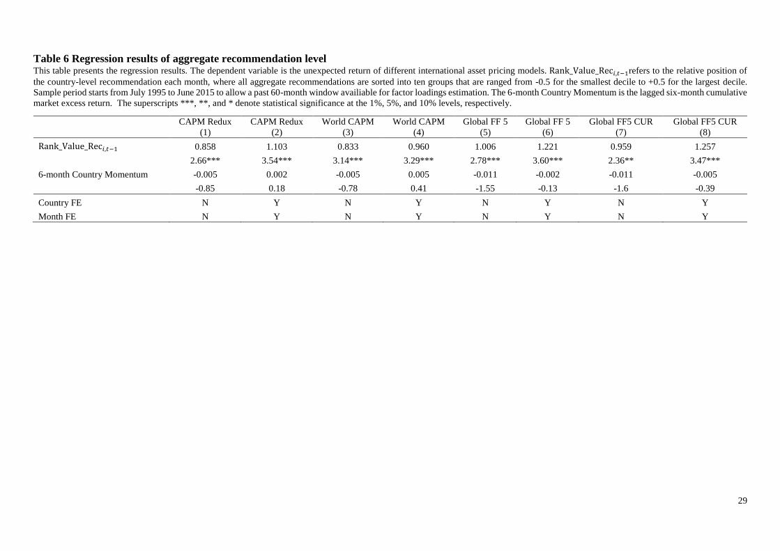
Table 6 presents the results for equation (6) based on each of the four international asset
pricing models with and without the fixed effects. The t-statistics reported in Table 6 are based
on standard errors clustered by country. For all four asset pricing models, the results show
aggregate analyst recommendations at the country level significantly predict next month’s
stock market returns. The coefficient on 𝑅𝑎𝑛𝑘_𝑉𝑎𝑙𝑢𝑒_𝑅𝑒𝑐𝑖,𝑡−1 is consistent with the results in
Table 5. For example, based on the International CAPM Redux, a portfolio that buys the decile
10 country indices and sells decile 1 country indices, yields an abnormal return 0.858 percent
per month. When we include country fixed effects and month fixed effects this coefficient
20 Because the Fama French Five factors are available from July 1990, the first observations used in the panel
regressions in this section are for July 1995, allowing for a 60-month period to estimate the factor loadings. 21 We use ranks instead of the actual average recommendations to mitigate the impact of possible structural
changes in the level of average recommendations through time. For example, there is evidence that after the
regulation changes around 2002, analysts, on average, issue less optimistic recommendations than before (see
Barber et al., 2006; Kadan, Madureira, Wang, and Zach, 2009). The conclusions do not change when we base our
measure on the unadjusted value of the country-level recommendations.

16
decreases from 0.858 to 1.103, which indicates that our findings are not the result of the
exceptional or persistent outperformance of only some of the countries in our sample.22
[Table 6]
Overall, we conclude that country-level recommendations predict one-month-ahead
international stock market returns.
4. Do country level recommendations contain information about the macroeconomy?
In this section, we test the conjecture that one of the reasons our trading strategy is
successful partly because average country level recommendations contain useful information
about future macroeconomic conditions. To test our conjecture, we examine whether country-
level recommendations predict future growth in gross domestic product (GDP) for the countries
in our sample.
We obtain the quarterly GDP growth from the OECD database.23 GDP growth is
defined as the percentage change in GDP relative to the same quarter in the previous year
(seasonally-differenced). To examine whether aggregate analyst recommendations can predict
future GDP changes, we estimate the following panel regressions:
∆𝐺𝐷𝑃𝑖,𝑞 = 𝛼0 + 𝛼1𝑅𝑒𝑐𝑖,𝑞−1 + 𝛼2∆𝐺𝐷𝑃𝑖,𝑞−1 + 𝛼3𝑊𝐸𝑆𝑖,𝑞−1 + 𝐶𝑖 + 𝑄𝑅𝑇𝑞 + 𝜀𝑖,𝑞 (7)
Where ∆𝐺𝐷𝑃𝑖,𝑞 is the percentage change in GDP for country i (from quarter q-4 to quarter q).
𝑅𝑒𝑐𝑖,𝑞−1 is the average analyst recommendation for country i at the end of the previous quarter
q-1. 𝑊𝐸𝑆𝑖,𝑞−1 is the average score from the World Economic Survey on the country i's expected
22 When we run Fama McBeth-type regressions for each of the countries and for each of the months, we find that
the strategy is effective for both the cross-section of countries and for each of the countries separately (time series).
For each of the countries, we first regress excess returns (according to the International CAPM Redux) on the
lagged recommendation decile. The average of these coefficients across the 33 countries is 1.079 (t-statistic is
2.57). When repeat this process for each of the months separately and regress excess country returns (according
to the International CAPM Redux) on the lagged recommendation decile, then the average of the coefficients
across the 235 months is 0.944 (t-statistic is 2.41). 23 https://data.oecd.org/ Quarterly GDP data is available for 27 countries. The database does not include GDP data
for Hong Kong, Malaysia, Philippines, Singapore, Thailand and Taiwan.
17
situation regarding the overall economy at the end of the next 6 months as measured in the first
month on the previous quarter q-1. 24(Appendix II provides background information on the
World Economic Survey). Since growth in GDP is highly auto-correlated, we also include
lagged GDP growth in the model. Finally, to allow for systematic differences in growth rates
across countries and years, we include country fixed effects, Ci and quarter fixed effects QRTq
(a unique dummy for each of the 82 quarters in the sample).
The first column in Table 7 report the results for panel regressions 7 without country
fixed effects. The results in the second column are based on the panel regression including
country fixed effects. In both cases, the results show that the average country level analyst
recommendation is a significant predictor of next quarter’s growth in GDP. In column 3, we
present the results from the Anderson-Hsiao estimator of equation 7. We include these results
to deal with the well-known problem that using fixed effects in a model that includes lagged
values of the dependent variable results in biased estimates (Anderson and Hsiao, 1982). The
use of the Anderson-Hsiao estimator involves differencing equation 7 to remove the country
and quarter fixed effects, and replacing (𝐺𝐷𝑃𝑐,𝑞−1 − 𝐺𝐷𝑃𝑐,𝑞−2) by 𝐺𝐷𝑃𝑐,𝑞−2 as an instrument.
The coefficient estimate based on the Anderson Hsiao estimator is similar to the previous
results and again shows that aggregate analyst recommendations predict next-quarter GDP
growth.
In the final three columns, we test whether the average country recommendation helps
to predict economic growth in next two, three or four quarters, based on the Anderson-Hsiao
estimator. The results in columns 4-6 show that the average country recommendation predicts
GDP growth two-quarters ahead but has no predictive ability for the next two quarters.
24 We collect the World Survey data from Datastream for all countries that in our sample. Specifically, we use
the expected economic situation in next 6-month to measure growth expectations.

18
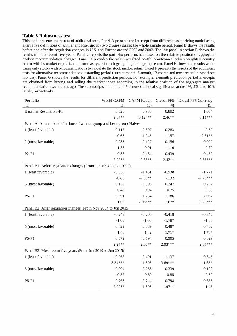
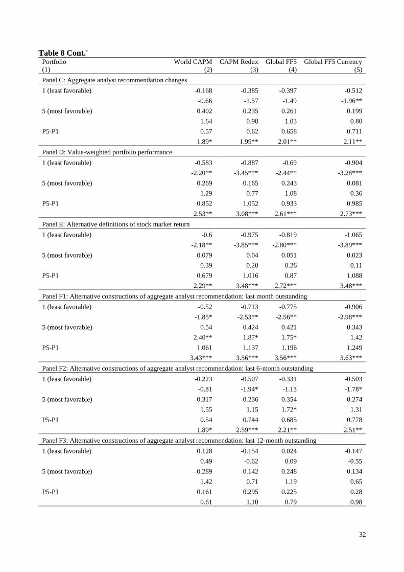
5. Robustness tests
This section presents a battery of robustness tests where we focus on the hedge portfolio
results in Table 5. We show that the results in Table 5 are robust to changes in the definition
of winner and loser groups, the definition of country level recommendations, the measurement
of international stock market returns and sample period. The results of these tests are presented
in Table 8 and focus on the results for the portfolio of countries in the lowest and highest
recommendation quintiles and the hedge portfolio that is short the former and long the latter.
The first row in Table 8, presents the base case results for each international asset pricing model,
which are the same as the results in Table 5.
Alternative definition of winner group and loser group
In order to increase diversification of the long and short portfolio across countries, we
split the sample into two halves and go long the countries above the median in terms of their
country recommendation and short the countries below the median. The benefit of this strategy
is increased diversification of the long and short portfolios across the sample countries.
However, in line with the idea that portfolios with less extreme values for country
recommendations result in smaller abnormal returns, we find that average abnormal returns
decrease. For example, based on the CAPM Redux, the average monthly return decreases from
0.935 percent (t-statistic is 3.12) for the base case to 0.434% per month (t-statistic is 2.53) for
this alternative strategy that has more than twice the number of countries in the long and short
portfolios.
Regulation changes in the brokerage industry
The brokerage industry was confronted with significant regulatory changes in 2002 in
the US and 2003 in Europe. We expect that after the regulatory changes, recommendations are
more comparable across countries, potentially enhancing the returns of the trading strategy.
19
However, the regulatory changes also resulted in a decline in informativeness of
recommendations in the US (see Kadan et al., 2009), and possibly other countries.
In panel B1 in Table 8, we present the results of the base case trading strategy for the
period Jan 1994-Dec 2001, i.e. before the regulation changes. Panel B2, in Table 8 shows the
results for the period Jan 2004- Jun 2015, after the regulation changes. Focusing on the CAPM
Redux, we see a very high abnormal return of 1.887 percent per month in the pre-regulation
period. In the post-regulation, the abnormal return drops to 0.491 percent per month but is still
economically and statistically significant.25
Informativeness of aggregate analyst recommendation changes
Many studies on the information content of analyst recommendations focus on
recommendation changes rather that recommendation levels. Panel C in Table 8 presents the
results for a strategy that buys the MSCI market index (in USD) of countries in the quintile
with the largest positive changes in country level recommendations and sells the MSCI market
index of the quintile of countries with the largest negative changes in country level
recommendations, where the country level recommendation change is measured from the end
of the prior calendar month to the end of the current calendar month.
The results for this strategy indicate that analyst recommendation changes also provide
valuable information to investors, but the abnormal returns are not as high as the strategy based
on recommendation levels. For example, for the International CAPM Redux, the average
monthly abnormal return is 0.62 percent (t-statistic is 1.99). This finding that returns for the
strategy based on recommendation changes results in lower abnormal returns than the strategy
based on recommendation levels is contrary to studies of analyst recommendations at the firm
25 The trading strategy performs poorly in the 24 month period between 2002 and 2003, with an insignificant and
slightly negative abnormal return of -0.284 percent per month (t-statistic is -0.26).
20
level that tend to find that analyst recommendation revisions provide more useful information
to investors.26
Value-weighted portfolio performance
The base case results are based on portfolios where each country has an equal weight.
In Panel D of Table 8, we present the result of an alternative strategy where the weight of each
country in the long and short portfolio is based on the total market capitalization of that country
at the start of the calendar year, based on data from the World Development Indicator.27 The
mean abnormal return based on the International CAPM Redux is 1.052% (t-statistic is 3.08),
which is economically and statistically significant. These results again confirm our previous
findings that country-level analyst recommendations are useful for international asset
allocation.
Alternative definition of the stock market index
In this test we replace the MCSI index returns used in our main tests with a value-
weighted market return for each country that only includes the stocks with recommendations,
resulting in a closer match between the return measures and the country-level recommendations.
To calculate the monthly value-weighted stock market return of all the companies with
recommendations in country i in month t, we weigh the return of each stock
j, 𝑀𝑜𝑛𝑡ℎ_ 𝑅𝑒𝑡𝑢𝑟𝑛𝑗,𝑡, by its market capitalisation in month t-1, 𝑀𝑘𝑡_𝐶𝑎𝑝𝑗,𝑡−1:
𝑉𝑎𝑙𝑢𝑒_𝑅𝑒𝑡𝑖,𝑡 = ∑ 𝑀𝑜𝑛𝑡ℎ_ 𝑅𝑒𝑡𝑢𝑟𝑛𝑗,𝑡
𝑛
𝑗=1∗
𝑀𝑘𝑡_𝐶𝑎𝑝𝑗,𝑡−1
∑ 𝑀𝑘𝑡_𝐶𝑎𝑝𝑗,𝑡−1𝑛𝑗=1
(8)
Table 8, Panel E shows that, with a closer match between a country’s market return and
the aggregate analyst recommendation, the abnormal return of the trading strategy is slightly
26 See, for example, Womack (1996) and Jegadeesh et al. (2004). 27 Market capitalization data is based on listed domestic companies. Investment funds, unit trusts, and companies
whose only business is to hold shares of other listed companies are excluded. Data are end of year values,
converted to U.S. dollars using corresponding year-end foreign exchange rates. Market capitalization data is
available from 1993 to 2012, and is available for all countries in our sample apart from Taiwan.
21
larger and more significant. For example, based on the International CAPM Redux the average
abnormal return equals 1.016% (t-statistic is 3.48) per month.
Alternative constructions of aggregate analyst recommendation
The base case results are based on the average consensus forecast using outstanding
recommendations that were announced within the last quarter. Table 8, Panel F presents the
results when we only consider outstanding recommendations within the last month, last half
year and last year. For all four asset pricing models, we find that the results are stronger if
country-level recommendations are based on more recent forecasts. For the International
CAPM Redux, the abnormal return is 1.137%% (t-statistic is 3.56) when the consensus
recommendation is based on last month’s recommendations only, whereas the average
abnormal return is 0.295% (t-statistic is 1.1) if the consensus recommendation is based on all
recommendations in the last year.28
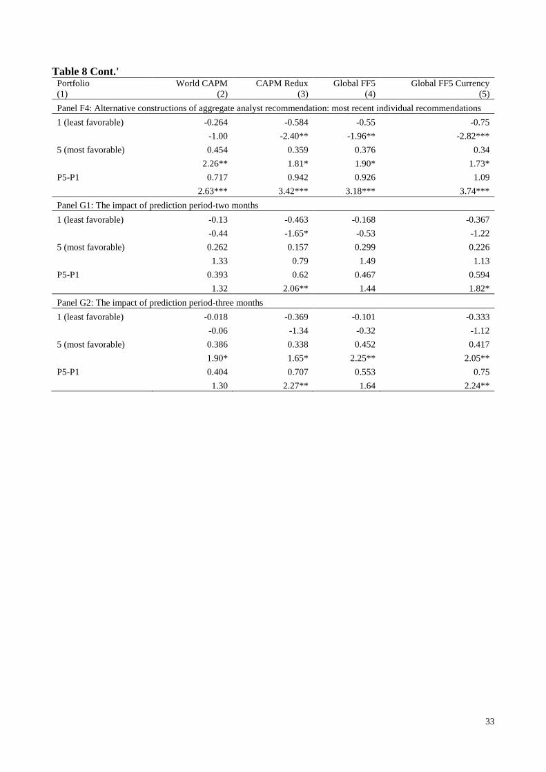
The last panel in Table 8, Panel F presents the results if the country-level
recommendation is based on the most recent recommendation across analysts for each stock.
That is, for each stock at the end of each month, we only use the most recent recommendation
in past 3-months to calculate the average country-level recommendation. The average
abnormal returns based on this measure are higher than the base case results and lower than the
results based on outstanding recommendations within the last month.
The impact of prediction period
Panel G of Table 8 shows that country level recommendations have some predictive ability
about international stock market returns two months and three months ahead. The return of
28 Note that the consensus forecasts only use the most recent recommendation for each analyst for each stock. By
extending the window back to 12 months, there are approximately 65% more recommendations in the sample
compared to the 3 month window (i.e. covering more stocks, but also potentially including more stale forecasts).
Using the 12 month window, 35% of the outstanding recommendations were announced within the last 3 months,
28% were announced within the last 4 to 6 months, and 37% of the recommendations are more than 6 months old.
22
buying the most favorable group of countries and selling the least favorable group of countries
based on the country-level recommendation at the end of month t-2 yields a significant
abnormal return of 0.62 percent (t-statistic is 2.06). The strategy still yields a significant
abnormal return of 0.707 percent (t-statistic 2.27) three month after portfolio formation.
However, four months after portfolio formation the strategy is no longer profitable (unreported).
5. Conclusion
This study shows that analyst information aggregated at the country level can predict one-
month–ahead stock market returns across countries. The portfolio performance of a self-
financing hedge portfolio that buys the stock market indices of the countries with the most
favorable recommendations and sells the stock market indices of the countries with the least
favorable recommendations yields a return of around one percent per month. Results are robust
to different international asset pricing models, portfolio construction rules and measurement
windows. We also show that country-level analyst recommendations predict next quarter’s
growth in GDP even when we control for survey-based forecasts by a panel of economists.

23
Table 1 Descriptive Statistics for Analyst Recommendations from I/B/E/S This table presents the distribution of all recommendations across five tiers of I/B/E/S rating scale. The sample
consists of all international markets with at least 10,000 individual recommendations from January 1994 to June
2015. To comply with previous studies, we reverse the ordering of analyst recommendation, where 1 represents
strong sell, and 5 represents strong buy. Specifically, these data are presented in two panels. Panel A provides the
distribution of initial recommendation, and Panel B provides the distribution of revised recommendation. It also
provides information about the direction of revised recommendation changes. Each cell in Panel B shows the
number of recommendations changes from the rating of row index to the score of column index.
Panel A: Distribution of Initial Recommendation
Recommendation level 1 2 3 4 5 total
% of initial recommendation
38,948
4.34
63,796
7.11
312,259
34.82
267,350
29.81
214,353
23.90
896,706
-
Panel B: Transition Matrix of Analyst Recommendation
To Recommendation
From recommendation 1 2 3 4 5 total
1 7,585 6,098 28,371 3,765 9,538 55,357
2 6,876 18,589 47,161 18,623 5,146 96,395
3 28,851 50,363 90,109 116,958 78,194 364,475
4 3,912 19,707 129,419 69,520 50,911 273,469
5 9,734 5,735 84,200 51,232 44,650 195,551
Subtotal 56,958 100,492 379,260 260,098 188,439 985,247
% of subtotal 5.78 10.20 38.49 26.40 19.13 -
Total 95,906 164,288 691,519 527,448 402,792 1,881,953
% of total 5.10 8.73 36.74 28.03 21.40 100.00

24
Table 2 Descriptive Statistics of all recommendations by year Column 2 is the number of firms with at least one valid recommendation in our sample, by year. Column 3 shows the
number of analysts that can be identified by the analyst masked code. The mean and median number of analysts issuing
recommendations for each covered firm is shown by year. This is followed by the average number of firms each analyst
covered. The number of average recommendation simply takes the arithmetic mean of all the available recommendation
across all countries in our sample.
Year
(1)
No. of
Firms
(2)
No. of
Analysts
(3)
Analyst per Firm Firm per Analyst Average
Recommendation
(8)
Mean
(4)
Median
(5)
Mean
(6)
Median
(7)
1994 6,030 3,620 6.30 3 10.49 4 3.45
1995 6,156 4,666 5.99 3 7.90 4 3.33
1996 8,033 6,588 6.46 3 7.87 4 3.42
1997 10,288 8,147 6.22 3 7.86 5 3.51
1998 12,249 9,276 6.41 3 8.47 6 3.56
1999 12,065 10,007 6.91 4 8.33 5 3.69
2000 11,848 10,388 6.35 3 7.24 5 3.73
2001 11,203 10,719 7.29 4 7.62 5 3.56
2002 11,106 10,850 9.89 5 10.12 7 3.48
2003 11,127 10,408 8.92 5 9.53 7 3.37
2004 12,442 10,272 7.47 4 9.05 7 3.46
2005 13,497 10,559 6.96 4 8.90 6 3.45
2006 14,242 11,367 6.89 4 8.63 6 3.49
2007 15,169 12,187 7.03 4 8.74 6 3.55
2008 14,106 12,129 7.90 4 9.19 6 3.41
2009 13,290 12,074 8.56 4 9.42 7 3.45
2010 13,934 12,830 7.35 4 7.98 6 3.61
2011 14,456 13,714 7.49 4 7.90 5 3.62
2012 14,340 13,239 7.30 4 7.90 5 3.53
2013 14,189 12,275 6.62 4 7.65 5 3.53
2014 15,027 12,242 5.94 3 7.29 5 3.58
2015 12,052 10,256 3.97 2 4.66 3 3.50
Average 12,130 10,355 7.01 3.68 8.31 5.41 3.51
25
Table 3 Descriptive Statistics by country for all recommendation Table 3 shows the recommendation statistics for each country in our sample throughout the whole sample period. We only report the statistics of the 33 countries with more
than 10,000 recommendations over our sample period. These 33 countries issue about 80% worldwide recommendations. Analysts are identified using the analyst masked code
from I/B/E/S. The recommendation statistics for each country are the annual average across the whole sample period. The sample period is from January 1994 to June 2015.
Panel A reports statistic for developed countries and Panel B reports statistic for emerging countries, based on the MSCI country classification.
Panel A: Developed Countries
Country
(1)
No. of
Recommendations/year
(2)
Recommendation level No. of
Analysts/year
(5)
Firm per Analyst No. of
Firms/year
(8)
Analyst per Firm
Mean
(3)
Median
(4)
Mean
(6)
Median
(7)
Mean
(9)
Median
(10)
Australia 3,577 3.43 3 408 9 9 469 8 8
Belgium 629 3.38 3 189 4 3 84 8 7
Canada 4,638 3.60 4 580 8 8 698 7 6
Denmark 618 3.29 3 179 4 4 80 8 8
Finland 992 3.28 3 218 4 4 94 10 10
France 3,724 3.42 3 823 5 4 382 10 10
Germany 3,547 3.34 3 759 5 5 350 10 10
Hong Kong 1,510 3.40 3 360 4 4 94 17 14
Italy 1,483 3.37 3 346 4 4 175 8 8
Japan 5,827 3.44 3 558 10 11 1,210 5 5
Netherlands 1,577 3.38 3 398 4 4 126 13 12
New Zealand 397 3.26 3 58 7 7 69 6 6
Norway 903 3.40 3 222 4 4 124 7 7
Singapore 1,481 3.40 3 250 6 6 177 9 8
Spain 1,437 3.31 3 337 4 4 111 13 14
Sweden 1,465 3.31 3 371 4 4 171 8 8
Switzerland 1,234 3.36 3 386 3 3 151 8 8
United Kingdom 6,898 3.48 3 1,112 7 6 989 7 7
United States 22,483 3.64 4 2,749 8 8 3,461 7 7
Average 3,391 3.39 3.11 542 5 5 474 9 9
26
Table 3 Cont’
Panel B: Emerging countries
Country
(1)
No. of
Recommendations/year
(2)
Recommendation level No. of
Analysts/year
(5)
Firm per Analyst No. of
Firm/year
(8)
Analyst per Firm
Mean
(3)
Median
(4)
Mean
(6)
Median
(7)
Mean
(9)
Median
(10)
Brazil 1,313 3.47 3 195 7 7 147 9 9
China 2,690 4.06 4 412 5 6 651 4 4
India 3,091 3.60 4 425 7 7 395 7 6
Indonesia 857 3.38 3 135 7 6 108 8 8
Korea 3,166 3.73 4 528 6 6 396 7 8
Malaysia 1,956 3.36 3 248 8 8 251 8 7
Mexico 506 3.54 3 118 4 4 67 8 8
Philippines 453 3.47 3 75 6 6 64 7 6
Poland 502 3.31 3 92 6 6 84 6 5
Russia 556 3.46 3 106 5 5 103 5 5
South Africa 1,327 3.40 3 149 9 7 183 7 7
Taiwan 2,272 3.52 3 292 8 8 348 7 7
Thailand 1,711 3.33 3 188 9 9 217 8 9
Turkey 820 3.45 3 110 8 7 123 7 6
Average 1,516 3.51 3.21 219 7 7 224 7 7

27
Table 4 Descriptive Statistics for Stock Market Return Table 4 presents descriptive statistics for the monthly MSCI stock market returns in U.S. dollar. We use the MSCI Gross
index obtained from the MSCI website. The sample period is from January 1994 to June 2015. All the numbers in the
table are in the percentage format. Panel A reports statistic for developed countries and Panel B reports statistic for
emerging countries, based on the MSCI country classification.
Panel A: Developed Countries
Country
(1)
Mean
(2)
Median
(3)
Max
(4)
Min
(5)
Std.
(6)
Num. of Obs
(7)
Australia 0.92 1.19 17.79 -25.51 6.05 258
Belgium 0.82 1.45 18.19 -36.56 6.05 258
Canada 0.94 1.51 21.26 -26.94 5.85 258
Denmark 1.20 1.80 18.34 -25.67 5.75 258
Finland 1.37 1.16 33.26 -31.76 9.38 258
France 0.75 1.13 15.74 -22.41 5.90 258
Germany 0.84 1.26 23.69 -24.35 6.61 258
Hong Kong 0.76 0.85 33.23 -28.86 7.22 258
Italy 0.68 0.56 19.67 -23.60 6.99 258
Japan 0.27 0.22 16.79 -14.78 5.25 258
Netherlands 0.85 1.39 14.39 -25.11 5.84 258
New Zealand 0.71 1.29 18.04 -22.44 6.29 258
Norway 1.00 1.34 21.47 -33.36 7.66 258
Singapore 0.67 0.80 25.84 -28.99 7.25 258
Spain 1.02 1.29 22.09 -25.27 6.99 258
Sweden 1.22 0.88 25.49 -26.66 7.44 258
Switzerland 0.91 1.30 14.56 -15.63 4.79 258
United Kingdom 0.65 0.70 13.87 -18.96 4.59 258
United States 0.84 1.32 10.99 -17.10 4.32 258
Average 0.86 1.13 20.25 -24.95 6.33 -
Panel B: Emerging Countries
Country
(1)
Mean
(2)
Median
(3)
Max
(4)
Min
(5)
Std.
(6)
Num. of Obs
(7)
Brazil 1.45 1.88 36.78 -37.63 11.05 258
China 1.18 0.99 28.59 -25.08 8.56 174
India 1.02 1.17 36.68 -28.48 8.66 258
Indonesia 1.05 1.19 55.58 -40.54 12.57 258
Korea 1.07 0.25 70.60 -31.25 10.98 258
Malaysia 0.51 0.82 50.04 -30.20 8.23 258
Mexico 0.95 1.77 19.14 -34.25 8.28 258
Philippines 0.50 0.59 43.39 -29.22 8.54 258
Poland 0.76 0.92 40.21 -34.82 10.96 258
Russia 1.99 2.05 61.13 -60.57 15.16 246
South Africa 1.02 1.17 19.45 -30.51 7.67 258
Taiwan 0.58 0.73 29.24 -21.73 8.00 258
Thailand 0.65 0.70 43.24 -34.01 10.87 258
Turkey 1.56 1.59 72.30 -41.24 14.89 258
Average 1.02 1.13 43.31 -34.25 10.32 -

28
Table 5 Monthly returns for long-short recommendation portfolios This table presents monthly percentage returns earned by portfolios formed according to the rank of aggregate analyst
recommendation. We require at least 50 firms that have an outstanding recommendation for each month-country when
calculating aggregate recommendations. The World CAPM intercept is the estimated intercept from a time-series
regression of the portfolio return (RP-RF) on the global market excess return denominated in the U.S. dollar (WMKT).
The intercept for the International CAPM Redux is the estimated intercept from a time-series regression of the portfolio
return on the world market excess return denominated in local currencies (LWMKT) and two currency risk factors, Dollar
and Carry. The Global FF5 intercept is the estimated intercept from a time-series regression of the portfolio return on the
WMKT, a zero-investment size portfolio (SMB), a zero-cost book-to-market portfolio (HML), and two additional factors,
RMW (Robust Minus Weak), CMA (Conservative Minus Aggressive) variables. The Global FF5 Currency risk intercept
is estimated by adding two additional currency risk factors, Dollar and Carry.The sample period ranges from January
1994 to June 2015. It also presents the alphas for each group. The table provides the equal-weighted portfolio outcomes,
which take the mean of return of all countries in each group to get the group return. The t-statistics for returns are clustered
by country and month. The superscripts ***, **, and * denote statistical significance at the 1%, 5%, and 10% levels,
respectively.
Portfolio
(1)
World CAPM
(2)
CAPM Redux
(3)
Global FF5
(4)
Global FF5 Currency
(5)
1 (least favorable) -0.278 -0.65 -0.471 -0.724
-0.99 -2.49** -1.55 -2.54**
2 -0.129 -0.228 -0.314 -0.35
-0.67 -1.19 -1.53 -1.72*
3 0.21 0.148 0.082 0.061
1.15 0.83 0.45 0.33
4 0.241 0.111 0.151 0.109
1.29 0.64 0.79 0.60
5 (most favorable) 0.347 0.285 0.331 0.28
1.73* 1.42 1.63 1.36
P5-P1 0.625 0.935 0.802 1.004
2.07** 3.12*** 2.46** 3.11***
29
Table 6 Regression results of aggregate recommendation level This table presents the regression results. The dependent variable is the unexpected return of different international asset pricing models. Rank_Value_Rec𝑖,𝑡−1refers to the relative position of
the country-level recommendation each month, where all aggregate recommendations are sorted into ten groups that are ranged from -0.5 for the smallest decile to +0.5 for the largest decile.
Sample period starts from July 1995 to June 2015 to allow a past 60-month window availiable for factor loadings estimation. The 6-month Country Momentum is the lagged six-month cumulative
market excess return. The superscripts ***, **, and * denote statistical significance at the 1%, 5%, and 10% levels, respectively.
CAPM Redux
(1)
CAPM Redux
(2)
World CAPM
(3)
World CAPM
(4)
Global FF 5
(5)
Global FF 5
(6)
Global FF5 CUR
(7)
Global FF5 CUR
(8)
Rank_Value_Rec𝑖,𝑡−1 0.858 1.103 0.833 0.960 1.006 1.221 0.959 1.257
2.66*** 3.54*** 3.14*** 3.29*** 2.78*** 3.60*** 2.36** 3.47***
6-month Country Momentum -0.005 0.002 -0.005 0.005 -0.011 -0.002 -0.011 -0.005
-0.85 0.18 -0.78 0.41 -1.55 -0.13 -1.6 -0.39
Country FE N Y N Y N Y N Y
Month FE N Y N Y N Y N Y

30
Table 7 Regressions of One-Quarter-Ahead GDP on Aggregate Analyst Recommendations This table shows the regression results of one-quarter-ahead GDP on aggregate analyst recommendations. The sample
period is from 1995Q1 to 2015Q4. All variables are quarterly. We include 27 countries in GDP analysis due to data
availability. The lagged one-quarter aggregate analyst recommendation is the aggregate analyst recommendation at the
previous quarter-end month. We also require at least 50 firms that have an outstanding recommendation for that quarter-
end-month in each country. 𝑊𝐸𝑆𝑖,𝑞−1 is the average score from the World Economic Survey on the country i's expected
situation regarding the overall economy at the end of the next 6 months as measured in the first month on the previous
quarter q-1. The first column in Table 7 reports the results for panel regressions 7 without country fixed effects. The
results in the second column are based on the panel regression including country fixed effects. In column 3, we present
the results from the Anderson-Hsiao estimator of equation 7. Column 4-6 shows whether the average country
recommendation helps to predict economic growth in next two, three or four quarters, based on the Anderson-Hsiao
estimator. All the t-statistics are clustered by country. The superscripts ***, **, and * denote statistical significance at the
1%, 5%, and 10% levels, respectively.
∆𝐺𝐷𝑃𝑖,𝑞
(1)
∆𝐺𝐷𝑃𝑖,𝑞
(2)
∆𝐺𝐷𝑃𝑖,𝑞
Anderson-Hsiao (3)
∆𝐺𝐷𝑃𝑖,𝑞+1
Anderson-Hsiao (4)
∆𝐺𝐷𝑃𝑖,𝑞+2
Anderson-Hsiao (5)
∆𝐺𝐷𝑃𝑖,𝑞+3
Anderson-Hsiao (6)
𝑅𝑒𝑐𝑖,𝑞−1 0.452 0.546 0.61 0.624 0.100 -0.209
2.6*** 2.05** 3.88*** 3.95*** 0.62 -1.26
𝑊𝐸𝑆𝑖,𝑞−1 0.037 0.049 0.025 0.027 0.034 0.031
3.00*** 3.78*** 2.1** 2.29** 2.87*** 2.55**
Quarter FE Y Y N N N N
Country FE N Y N N N N
31
Table 8 Robustness test This table presents the results of additional tests. Panel A presents the intercept from different asset pricing model using
alternative definitions of winner and loser group (two groups) during the whole sample period. Panel B shows the results
before and after the regulation changes in U.S. and Europe around 2002 and 2003. The last panel in section B shows the
results in most recent five years. Panel C reports the portfolio performance based on the relative position of aggregate
analyst recommendation changes. Panel D provides the value-weighted portfolio outcomes, which weighted country
return with its market capitalization from last year in each group to get the group return. Panel E shows the results when
using only stocks with recommendations to calculate the stock market return. Panel F presents the results of the additional
tests for alternative recommendation outstanding period (current month, 6-month, 12-month and most recent in past three
months). Panel G shows the results for different prediction periods. For example, 2-month prediction period intercepts
are obtained from buying and selling the market index according to the relative position of the aggregate analyst
recommendation two months ago. The superscripts ***, **, and * denote statistical significance at the 1%, 5%, and 10%
levels, respectively.
Portfolio
(1)
World CAPM
(2)
CAPM Redux
(3)
Global FF5
(4)
Global FF5 Currency
(5)
Baseline Results: P5-P1 0.625 0.935 0.802 1.004
2.07** 3.12*** 2.46** 3.11***
Panel A: Alternative definitions of winner group and loser group-Halves
1 (least favorable) -0.117 -0.307 -0.283 -0.39
-0.68 -1.94* -1.57 -2.31**
2 (most favorable) 0.233 0.127 0.156 0.099
1.58 0.91 1.10 0.72
P2-P1 0.35 0.434 0.439 0.489
2.09** 2.53** 2.42** 2.66***
Panel B1: Before regulation changes (From Jan 1994 to Oct 2002)
1 (least favorable) -0.539 -1.431 -0.938 -1.771
-0.86 -2.50** -1.32 -2.73***
5 (most favorable) 0.152 0.303 0.247 0.297
0.49 0.94 0.75 0.85
P5-P1 0.691 1.734 1.186 2.067
1.09 2.96*** 1.67* 3.20***
Panel B2: After regulation changes (From Nov 2004 to Jun 2015)
1 (least favorable) -0.243 -0.205 -0.418 -0.347
-1.05 -1.00 -1.78* -1.63
5 (most favorable) 0.429 0.389 0.487 0.482
1.46 1.42 1.71* 1.78*
P5-P1 0.672 0.594 0.905 0.829
2.27** 2.00** 2.93*** 2.67***
Panel B3: Most recent five years (From Jun 2010 to Jun 2015)
1 (least favorable) -0.967 -0.491 -1.137 -0.546
-3.34*** -1.89* -3.69*** -1.83*
5 (most favorable) -0.204 0.253 -0.339 0.122
-0.52 0.69 -0.85 0.30
P5-P1 0.763 0.744 0.798 0.668
2.00** 1.80* 1.97** 1.46
32
Table 8 Cont.' Portfolio
(1)
World CAPM
(2)
CAPM Redux
(3)
Global FF5
(4)
Global FF5 Currency
(5)
Panel C: Aggregate analyst recommendation changes
1 (least favorable) -0.168 -0.385 -0.397 -0.512
-0.66 -1.57 -1.49 -1.96**
5 (most favorable) 0.402 0.235 0.261 0.199
1.64 0.98 1.03 0.80
P5-P1 0.57 0.62 0.658 0.711
1.89* 1.99** 2.01** 2.11**
Panel D: Value-weighted portfolio performance
1 (least favorable) -0.583 -0.887 -0.69 -0.904
-2.20** -3.45*** -2.44** -3.28***
5 (most favorable) 0.269 0.165 0.243 0.081
1.29 0.77 1.08 0.36
P5-P1 0.852 1.052 0.933 0.985
2.53** 3.08*** 2.61*** 2.73***
Panel E: Alternative definitions of stock market return
1 (least favorable) -0.6 -0.975 -0.819 -1.065
-2.18** -3.85*** -2.80*** -3.89***
5 (most favorable) 0.079 0.04 0.051 0.023
0.39 0.20 0.26 0.11
P5-P1 0.679 1.016 0.87 1.088
2.29** 3.48*** 2.72*** 3.48***
Panel F1: Alternative constructions of aggregate analyst recommendation: last month outstanding
1 (least favorable) -0.52 -0.713 -0.775 -0.906
-1.85* -2.53** -2.56** -2.98***
5 (most favorable) 0.54 0.424 0.421 0.343
2.40** 1.87* 1.75* 1.42
P5-P1 1.061 1.137 1.196 1.249
3.43*** 3.56*** 3.56*** 3.63***
Panel F2: Alternative constructions of aggregate analyst recommendation: last 6-month outstanding
1 (least favorable) -0.223 -0.507 -0.331 -0.503
-0.81 -1.94* -1.13 -1.78*
5 (most favorable) 0.317 0.236 0.354 0.274
1.55 1.15 1.72* 1.31
P5-P1 0.54 0.744 0.685 0.778
1.89* 2.59*** 2.21** 2.51**
Panel F3: Alternative constructions of aggregate analyst recommendation: last 12-month outstanding
1 (least favorable) 0.128 -0.154 0.024 -0.147
0.49 -0.62 0.09 -0.55
5 (most favorable) 0.289 0.142 0.248 0.134
1.42 0.71 1.19 0.65
P5-P1 0.161 0.295 0.225 0.28
0.61 1.10 0.79 0.98
33
Table 8 Cont.' Portfolio
(1)
World CAPM
(2)
CAPM Redux
(3)
Global FF5
(4)
Global FF5 Currency
(5)
Panel F4: Alternative constructions of aggregate analyst recommendation: most recent individual recommendations
1 (least favorable) -0.264 -0.584 -0.55 -0.75
-1.00 -2.40** -1.96** -2.82***
5 (most favorable) 0.454 0.359 0.376 0.34
2.26** 1.81* 1.90* 1.73*
P5-P1 0.717 0.942 0.926 1.09
2.63*** 3.42*** 3.18*** 3.74***
Panel G1: The impact of prediction period-two months
1 (least favorable) -0.13 -0.463 -0.168 -0.367
-0.44 -1.65* -0.53 -1.22
5 (most favorable) 0.262 0.157 0.299 0.226
1.33 0.79 1.49 1.13
P5-P1 0.393 0.62 0.467 0.594
1.32 2.06** 1.44 1.82*
Panel G2: The impact of prediction period-three months
1 (least favorable) -0.018 -0.369 -0.101 -0.333
-0.06 -1.34 -0.32 -1.12
5 (most favorable) 0.386 0.338 0.452 0.417
1.90* 1.65* 2.25** 2.05**
P5-P1 0.404 0.707 0.553 0.75
1.30 2.27** 1.64 2.24**
34
Figure 1 Average recommendation levels in G7 countries
This figure shows the value-weighted average recommendation across all the firms in G7 countries. The calculation of the consensus
recommendations for each firm is based on all outstanding recommendations issued a minimum of two days and a maximum of three months prior
to the end of calendar month t. Specifically, a recommendation is outstanding if it has not been stopped by the broker. The sample period is from
Jan 1994 to June 2015 and the recommendations range from 1 (strong sell) to 5 (strong buy).
2.5
2.7
2.9
3.1
3.3
3.5
3.7
3.9
4.1
4.3
4.5
19
94
05
19
94
10
19
95
03
19
95
08
19
96
01
19
96
06
19
96
11
19
97
04
19
97
09
19
98
02
19
98
07
19
99
01
19
99
06
19
99
11
20
00
04
20
00
09
20
01
02
20
01
07
20
01
12
20
02
05
20
02
10
20
03
03
20
03
08
20
04
01
20
04
06
20
04
11
20
05
04
20
05
09
20
06
02
20
06
07
20
06
12
20
07
05
20
07
10
20
08
03
20
08
08
20
09
01
20
09
06
20
09
11
20
10
04
20
10
09
20
11
02
20
11
07
20
11
12
20
12
05
20
12
10
20
13
03
20
13
08
20
14
01
20
14
06
20
14
11
20
15
04
CANADA FRANCE GERMANY ITALY JAPAN UNITEDKINGDOM UNITEDSTATES
35
Reference
Anderson, T. W., & Hsiao, C. (1982). Formulation and estimation of dynamic models using panel
data. Journal of Econometrics, 18(1), 47-82.
Anilowski, C., Feng, M., & Skinner, D. J. (2007). Does earnings guidance affect market returns? The
nature and information content of aggregate earnings guidance. Journal of Accounting and
Economics, 44(1), 36-63.
Bae, K., Stulz, R. M., & Tan, H. (2008). Do local analysts know more? A cross-country study of the
performance of local analysts and foreign analysts. Journal of Financial Economics, 88(3), 581-
606.
Barber, B., Lehavy, R., McNichols, M., & Trueman, B. (2001). Can investors profit from the
prophets? Security analyst recommendations and stock returns. The Journal of Finance, 56(2),
531-563.
Barber, B. M., Lehavy, R., McNichols, M., & Trueman, B. (2006). Buys, holds, and sells: The
distribution of investment banks’ stock ratings and the implications for the profitability of
analysts’ recommendations. Journal of Accounting and Economics, 41(1), 87-117.
Beneish, M. D. (1991). Stock prices and the dissemination of analysts' recommendation. Journal of
Business, 393-416.
Boni, L., & Womack, K. L. (2006). Analysts, industries, and price momentum. Journal of Financial
and Quantitative Analysis, 41(01), 85-109.
Brown, L. D., Call, A. C., Clement, M. B., & Sharp, N. Y. (2015). Inside the “Black Box” of Sell‐
Side Financial Analysts. Journal of Accounting Research, 53(1), 1-47.

36
Brusa, F., Ramadorai, T., & Verdelhan, A. (2014). The international CAPM redux. Available at SSRN
2462843.
Busse, J. A., Goyal, A., & Wahal, S. (2014). Investing in a global world. Review of Finance, 18(2),
561-590.
Davies, P. L., & Canes, M. (1978). Stock prices and the publication of second-hand information.
Journal of Business, 43-56.
Dumas, B., & Solnik, B. (1995). The World Price of Foreign Exchange Risk. Journal of Finance,
445-479.
Fama, E. F., & MacBeth, J. D. (1973). Risk, return, and equilibrium: Empirical tests. Journal of
Political Economy, , 607-636.
Fama, E. F., & French, K. R. (2015a). A five-factor asset pricing model. Journal of Financial
Economics, 116(1), 1-22.
Fama, E. F., & French, K. R. (2015b). International tests of a five-factor asset pricing model. Fama-
Miller Working Paper.
Gallagher, D. R., Harman, G., Schmidt, C., & Warren, G. (2016). Global Equity Fund Performance:
An Attribution Approach. Available at SSRN 2568483.
Green, T. C. (2006). The value of client access to analyst recommendations. Journal of Financial and
Quantitative Analysis, 41(01), 1-24.
Hirshleifer, D., Hou, K., & Teoh, S. H. (2009). Accruals, cash flows, and aggregate stock returns.
Journal of Financial Economics, 91(3), 389-406.
37
Howe, J. S., Unlu, E., & Yan, X. S. (2009). The predictive content of aggregate analyst
recommendations. Journal of Accounting Research, 47(3), 799-821.
Irvine, P., Lipson, M., & Puckett, A. (2007). Tipping. Review of Financial Studies, 20(3), 741-768.
Jegadeesh, N., Kim, J., Krische, S. D., & Lee, C. (2004). Analyzing the analysts: When do
recommendations add value? The Journal of Finance, 59(3), 1083-1124.
Jegadeesh, N., & Kim, W. (2006). Value of analyst recommendations: International evidence. Journal
of Financial Markets, 9(3), 274-309.
Kadan, O., Madureira, L., Wang, R., & Zach, T. (2009). Conflicts of interest and stock
recommendations: The effects of the global settlement and related regulations. Review of
Financial Studies, 22(10), 4189-4217.
Koijen, R. S., Schmeling, M., & Vrugt, E. B. (2015). Survey expectations of returns and asset pricing
puzzles. Available at SSRN 2513701.
Kothari, S., Lewellen, J., & Warner, J. B. (2006). Stock returns, aggregate earnings surprises, and
behavioral finance. Journal of Financial Economics, 79(3), 537-568.
Lintner, J. (1965). The valuation of risk assets and the selection of risky investments in stock
portfolios and capital budgets. The Review of Economics and Statistics, 47 (1), 13-37.
Loh, R. K., & Stulz, R. M. (2011). When are analyst recommendation changes influential? Review of
Financial Studies, 24(2), 593-627.
Lustig, H., Roussanov, N., & Verdelhan, A. (2011). Common risk factors in currency markets. Review
of Financial Studies, , hhr068.
38
Moshirian, F., Ng, D., & Wu, E. (2009). The value of stock analysts' recommendations: Evidence
from emerging markets. International Review of Financial Analysis, 18(1), 74-83.
Sharpe, W. F. (1964). Capital asset prices: A theory of market equilibrium under conditions of risk.
The Journal of Finance, 19(3), 425-442.
Stangl, A. (2007). European Data Watch. Schmollers Jahrbuch, 127(487), 496.
Stickel, S. E. (1995). The Anatomy of the Performance of Buy and Sell Recommendations. Financial
Analysts Journal, 51(5), 25-39.
Verdelhan, Adrien, The Share of Systematic Variation in Bilateral Exchange Rates (July 1, 2015).
Journal of Finance, Forthcoming. Available at SSRN: http://ssrn.com/abstract=1930516 or
http://dx.doi.org/10.2139/ssrn.1930516.
Womack, K. L. (1996). Do Brokerage Analysts' Recommendations Have Investment Value? Journal
of Finance, 51(1),
39
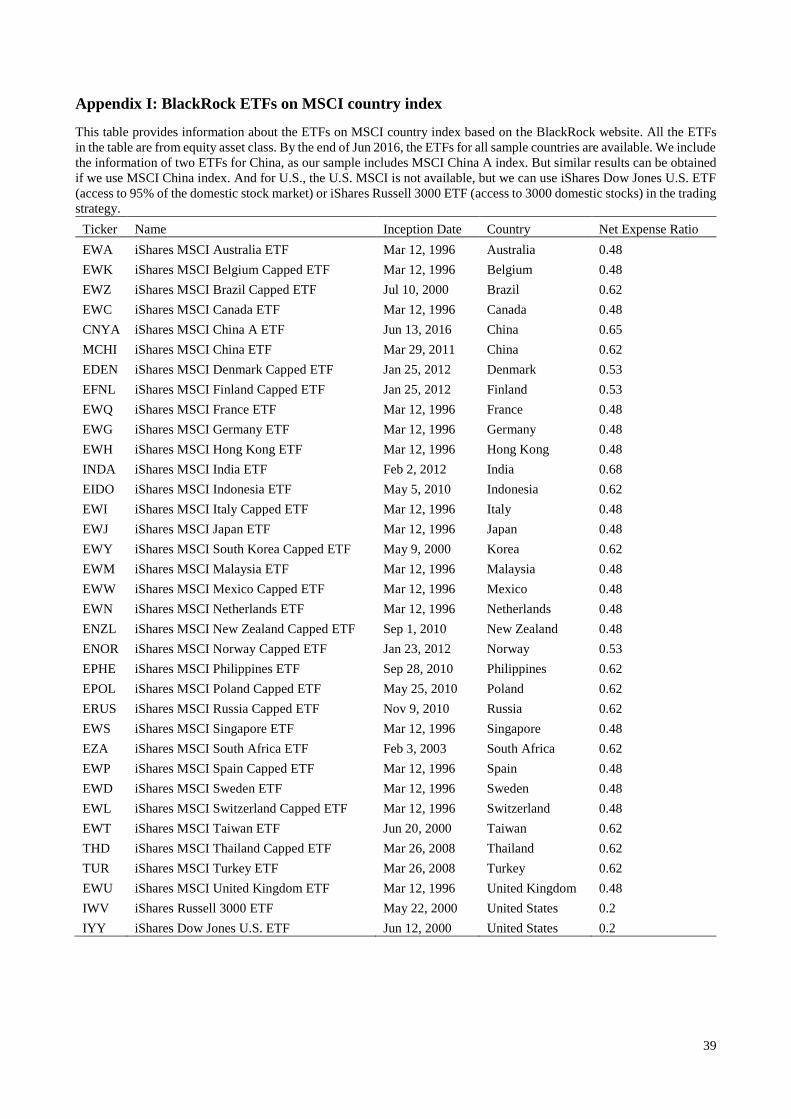
Appendix I: BlackRock ETFs on MSCI country index
This table provides information about the ETFs on MSCI country index based on the BlackRock website. All the ETFs
in the table are from equity asset class. By the end of Jun 2016, the ETFs for all sample countries are available. We include
the information of two ETFs for China, as our sample includes MSCI China A index. But similar results can be obtained
if we use MSCI China index. And for U.S., the U.S. MSCI is not available, but we can use iShares Dow Jones U.S. ETF
(access to 95% of the domestic stock market) or iShares Russell 3000 ETF (access to 3000 domestic stocks) in the trading
strategy.
Ticker Name Inception Date Country Net Expense Ratio
EWA iShares MSCI Australia ETF Mar 12, 1996 Australia 0.48
EWK iShares MSCI Belgium Capped ETF Mar 12, 1996 Belgium 0.48
EWZ iShares MSCI Brazil Capped ETF Jul 10, 2000 Brazil 0.62
EWC iShares MSCI Canada ETF Mar 12, 1996 Canada 0.48
CNYA iShares MSCI China A ETF Jun 13, 2016 China 0.65
MCHI iShares MSCI China ETF Mar 29, 2011 China 0.62
EDEN iShares MSCI Denmark Capped ETF Jan 25, 2012 Denmark 0.53
EFNL iShares MSCI Finland Capped ETF Jan 25, 2012 Finland 0.53
EWQ iShares MSCI France ETF Mar 12, 1996 France 0.48
EWG iShares MSCI Germany ETF Mar 12, 1996 Germany 0.48
EWH iShares MSCI Hong Kong ETF Mar 12, 1996 Hong Kong 0.48
INDA iShares MSCI India ETF Feb 2, 2012 India 0.68
EIDO iShares MSCI Indonesia ETF May 5, 2010 Indonesia 0.62
EWI iShares MSCI Italy Capped ETF Mar 12, 1996 Italy 0.48
EWJ iShares MSCI Japan ETF Mar 12, 1996 Japan 0.48
EWY iShares MSCI South Korea Capped ETF May 9, 2000 Korea 0.62
EWM iShares MSCI Malaysia ETF Mar 12, 1996 Malaysia 0.48
EWW iShares MSCI Mexico Capped ETF Mar 12, 1996 Mexico 0.48
EWN iShares MSCI Netherlands ETF Mar 12, 1996 Netherlands 0.48
ENZL iShares MSCI New Zealand Capped ETF Sep 1, 2010 New Zealand 0.48
ENOR iShares MSCI Norway Capped ETF Jan 23, 2012 Norway 0.53
EPHE iShares MSCI Philippines ETF Sep 28, 2010 Philippines 0.62
EPOL iShares MSCI Poland Capped ETF May 25, 2010 Poland 0.62
ERUS iShares MSCI Russia Capped ETF Nov 9, 2010 Russia 0.62
EWS iShares MSCI Singapore ETF Mar 12, 1996 Singapore 0.48
EZA iShares MSCI South Africa ETF Feb 3, 2003 South Africa 0.62
EWP iShares MSCI Spain Capped ETF Mar 12, 1996 Spain 0.48
EWD iShares MSCI Sweden ETF Mar 12, 1996 Sweden 0.48
EWL iShares MSCI Switzerland Capped ETF Mar 12, 1996 Switzerland 0.48
EWT iShares MSCI Taiwan ETF Jun 20, 2000 Taiwan 0.62
THD iShares MSCI Thailand Capped ETF Mar 26, 2008 Thailand 0.62
TUR iShares MSCI Turkey ETF Mar 26, 2008 Turkey 0.62
EWU iShares MSCI United Kingdom ETF Mar 12, 1996 United Kingdom 0.48
IWV iShares Russell 3000 ETF May 22, 2000 United States 0.2
IYY iShares Dow Jones U.S. ETF Jun 12, 2000 United States 0.2
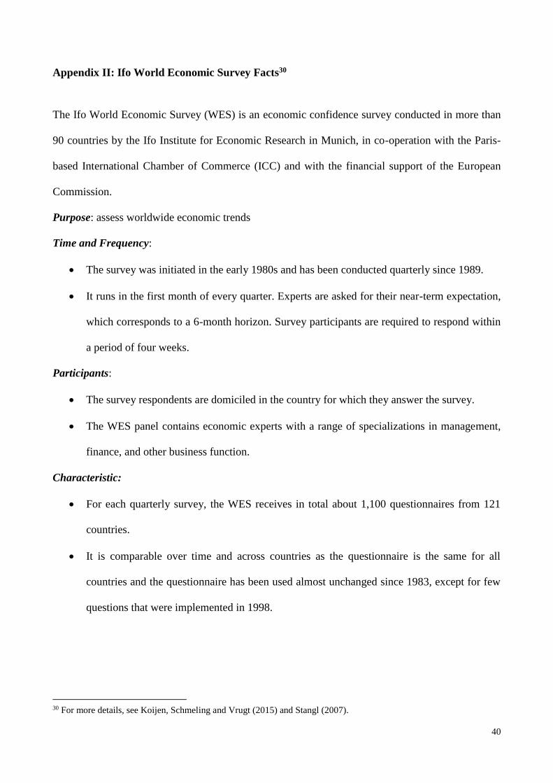
40
Appendix II: Ifo World Economic Survey Facts30
The Ifo World Economic Survey (WES) is an economic confidence survey conducted in more than
90 countries by the Ifo Institute for Economic Research in Munich, in co-operation with the Paris-
based International Chamber of Commerce (ICC) and with the financial support of the European
Commission.
Purpose: assess worldwide economic trends
Time and Frequency:
The survey was initiated in the early 1980s and has been conducted quarterly since 1989.
It runs in the first month of every quarter. Experts are asked for their near-term expectation,
which corresponds to a 6-month horizon. Survey participants are required to respond within
a period of four weeks.
Participants:
The survey respondents are domiciled in the country for which they answer the survey.
The WES panel contains economic experts with a range of specializations in management,
finance, and other business function.
Characteristic:
For each quarterly survey, the WES receives in total about 1,100 questionnaires from 121
countries.
It is comparable over time and across countries as the questionnaire is the same for all
countries and the questionnaire has been used almost unchanged since 1983, except for few
questions that were implemented in 1998.
30 For more details, see Koijen, Schmeling and Vrugt (2015) and Stangl (2007).

41
The survey is qualitative in nature and respondents can answer either “higher”, “about the
same” or “lower”. There are eight standard questions, regularly recurring additional questions
and one-time questions on current issues in the world economy.
Related Documents