ANALYSIS OF THE FIELDS IN THREE DIMENSIONAL CASSEGRAIN SYSTEM

Progress In Electromagnetics Research, PIER 71, 227–241, 2007

ANALYSIS OF THE FIELDS IN TWO DIMENSIONALCASSEGRAIN SYSTEM

A. Aziz and Q. A. Naqvi

Department of ElectronicsQuaid-i-Azam UniversityIslamabad, Pakistan

K. Hongo

3-34-24, Nakashizu, Sakura city, Chiba, Japan

Abstract—High frequency field expressions are derived around feedpoint of a two dimensional cassegrain system using the Maslov’smethod. Maslov’s method is a systematic procedure for predictingthe field in the caustic region combining the simplicity of ray theoryand generality of the transform method. Numerical computations aremade for the analysis of field pattern around the caustic of a cassegrainsystem.

1. INTRODUCTION

Asymptotic ray theory (ART) or the geometrical optics approximationis widely used to study various kinds of problems in the areas ofelectromagnetics, acoustics waves, seismic waves, etc. [1–5]. It isalso well known that the geometrical optics fails in the vicinity ofcaustic. So, in order to study the field behavior near caustic [6–9],other approach is required. Maslov proposed a method to predict thefield in the caustic region [10]. Maslov method combines the simplicityof asymptotic ray theory and the generality of the Fourier transformmethod. This is achieved by representing the geometrical opticsfields in terms of mixed coordinates consisting of space coordinatesand wave vector coordinates. That is by representing the field interms of six coordinates. It may be noted that information of raytrajectories is included in both space coordinates R = (x, y, z) andwave vector coordinates P = (px, py, pz). In this way, conventionalray expression may be considered as projection into space coordinates.

228 Aziz, Naqvi, and Hong

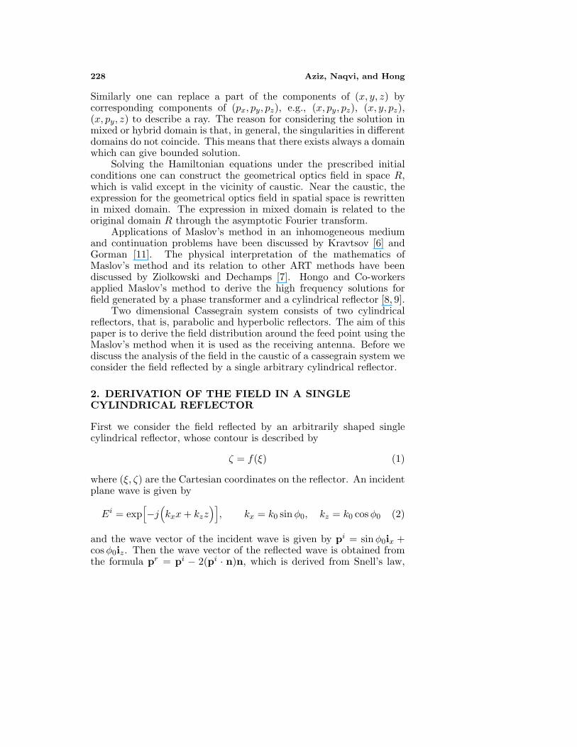
Similarly one can replace a part of the components of (x, y, z) bycorresponding components of (px, py, pz), e.g., (x, py, pz), (x, y, pz),(x, py, z) to describe a ray. The reason for considering the solution inmixed or hybrid domain is that, in general, the singularities in differentdomains do not coincide. This means that there exists always a domainwhich can give bounded solution.

Solving the Hamiltonian equations under the prescribed initialconditions one can construct the geometrical optics field in space R,which is valid except in the vicinity of caustic. Near the caustic, theexpression for the geometrical optics field in spatial space is rewrittenin mixed domain. The expression in mixed domain is related to theoriginal domain R through the asymptotic Fourier transform.

Applications of Maslov’s method in an inhomogeneous mediumand continuation problems have been discussed by Kravtsov [6] andGorman [11]. The physical interpretation of the mathematics ofMaslov’s method and its relation to other ART methods have beendiscussed by Ziolkowski and Dechamps [7]. Hongo and Co-workersapplied Maslov’s method to derive the high frequency solutions forfield generated by a phase transformer and a cylindrical reflector [8, 9].

Two dimensional Cassegrain system consists of two cylindricalreflectors, that is, parabolic and hyperbolic reflectors. The aim of thispaper is to derive the field distribution around the feed point using theMaslov’s method when it is used as the receiving antenna. Before wediscuss the analysis of the field in the caustic of a cassegrain system weconsider the field reflected by a single arbitrary cylindrical reflector.

2. DERIVATION OF THE FIELD IN A SINGLECYLINDRICAL REFLECTOR

First we consider the field reflected by an arbitrarily shaped singlecylindrical reflector, whose contour is described by

ζ = f(ξ) (1)

where (ξ, ζ) are the Cartesian coordinates on the reflector. An incidentplane wave is given by

Ei = exp[−j

(kxx+ kzz

)], kx = k0 sinφ0, kz = k0 cosφ0 (2)

and the wave vector of the incident wave is given by pi = sinφ0ix +cosφ0iz. Then the wave vector of the reflected wave is obtained fromthe formula pr = pi − 2(pi · n)n, which is derived from Snell’s law,

Progress In Electromagnetics Research, PIER 71, 2007 229

where n is the unit normal of the surface given by

n = sin θix+cos θiz, sin θ =−f ′(ξ)√

1 + [f ′(ξ)]2, cos θ =

1√1 + [f ′(ξ)]2

(3)where f ′(ξ) is the derivative of the function with respect to ξ. By usingthese relations we derive pr as

Pr =[sinφ0 − 2 sin θ cos(θ − φ0)

]ix +

[cosφ0 − 2 cos θ cos(θ − φ0)

]iz

= − sin(2θ − φ0)ix − cos(2θ − φ0)iz = prxix + prziz (4)

The coordinates of the point on the reflected ray is given by [11]

x = ξ + prxt, z = f(ξ) + przt (5)

and the geometrical optics expression of field associated with the rayis given by [12]

U(r) = A0(ξ, ζ)[D(t)D(0)

]− 12

exp{−jk

[ξ sinφ0 + f(ξ) cosφ0 + t

]}(6)

where A0(ξ, ζ) is the amplitude of the incident wave at the reflectedpoint (ξ, ζ), and t represents the distance along the ray from a certainreference point. The value ξ sinφ0 +f(ξ) cosφ0 represents the initialvalue of the phase function. D(t) is the Jacobian of the transformationfrom the Cartesian to the ray coordinates, and it is given by

D(t) =∂(x, z)∂(ξ, t)

= − cos(2θ − φ0) + f ′(ξ) sin(2θ − φ0) + 2∂θ

∂ξt

= −cos(θ − φ0)cos θ

− 2 cos2 θf ′′(ξ)t (7a)

J(t) =D(t)D(0)

= 1 +2 cos3 θ

cos(θ − φ0)f ′′(ξ)t (7b)

The caustic of this ray is given by the point satisfying D(t) = 0 and(5), more explicitly,

xc = ξ+sin(2θ − φ0) cos(θ − φ0)

2 cos3 θf ′′(ξ), zc = f(ξ)+

cos(2θ − φ0) cos(θ − φ0)2 cos3 θf ′′(ξ)

(8)It is seen that the ray reflected from the singular point f ′′(ξ) = 0can not form the caustics. At the point satisfying (8), the ray becomes

230 Aziz, Naqvi, and Hong

infinity. According to the Maslov’s method, the ray expression coveringthe caustics can be derived from the formula

U(r) =

√k

j2π

∫ ∞

−∞A0(ξ)

[D(t)D(0)

∂pz∂z

]− 12

× exp{−jk

[S0 + t− z(x, pz)pz + pzz

]}dpz (9)

where S0 = ξ sinφ0 + f(ξ) cosφ0 is the initial phase. In (9) z(x, pz)means that the coordinate z should be expressed in terms of mixedcoordinates (x, pz) by using the solution. The same is true for t and itis given by t = x−ξ

px. The phase function S(pz) is given by

S(pz) = ξ sinφ0 + f(ξ) cosφ0 +x− ξpx

− f(ξ)pz − (pz)2x− ξpx

+ pzz

= ξ[sinφ0+sin(2θ−φ0)

]+f(ξ)

[cosφ0+cos(2θ−φ0)

]+pxx+pzz

= 2[ξ sin θ + f(ξ) cos θ

]cos(θ − φ0) − ρ cos(2θ − φ− φ0) (10)

and the amplitude of the integrand is evaluated in Appendix A. In theabove equation, we introduce the polar coordinates

x = ρ sinφ, z = ρ cosφ (11)

Substituting these results in (9), we have the field expression valid incaustic region as

U(r) =√π exp

(−j π

4

) ∫ Θ

−ΘA0(ξ)

[cos(θ − φ0)cos3 θf ′′(ξ)

] 12

× exp{−j2k

[ξ sin θ + f(ξ) cos θ

]cos(θ − φ0)

}× exp

[jkρ cos(2θ − φ− φ0)

]dθ (12)

where Θ is the half angle of θ at the edge of the reflector and we havechanged the integration variable from pz to θ.

In a region far from the caustics, (12) can be evaluated approx-imately by applying the stationary phase method of integration [11]and the result should agree with the GO expression derived in (6) with(7b). This serves as an important check of the validity of the expression(12). The stationary point is determined from

S′(θs) = 2[ξ cos(2θ − φ0) − f(ξ) sin(2θ − φ0)

]× cos(θ − φ0) + 2ρ sin(2θ − φ− φ0)

= 0 (13)

Progress In Electromagnetics Research, PIER 71, 2007 231

The second derivative of the phase function is

S′′(θs) = −4[ξ sin(2θ − φ0) + f(ξ) cos(2θ − φ0)

]+2

[cos(2θ − φ0) − f(ξ) sin(2θ − φ0)

]dξdθ

+4ρ cos(2θ−φ−φ0)

−2cos(θ − φ0)cos3 f ′′(ξ)

[1 + 2

cos3 θcos(θ − φ0)

f ′′(ξ)t

]

= −2cos(θ − φ0)cos3 f ′′(ξ)

J(t) (14)

and

S(θs) = 2[ξ sin θ + f(ξ) cos θ

]cos(θ − φ0) − ρ cos(2θ − φ− φ0)

= ξ[sin(2θ − φ0) + sinφ0

]+ f(ξ)

[cos(2θ − φ0) + cosφ0

]−x sin(2θ − φ0) − z cos(2θ − φ0)

= ξ sinφ0 + f(ξ) cosφ0 + t (15)

We substitute (14) and (15) into (12) and carry out the integration,then we reproduce (6).

3. RECEIVING CHARACTERISTIC OF CYLINDRICALCASSEGRAIN REFLECTOR

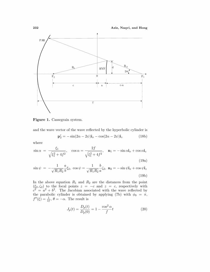
Cassegrain reflector consists of two reflectors, one is parabolic mainreflector and another is hyperbolic subreflector. This system hasmany advantages over a single parabolic reflector. We consider herea receiving characteristic of this system by applying Maslov’s method.The equation of each surface is given by [see Fig. 1]

ζ1 =ξ214f

− f + c, ζ2 = a

[ξ22b2

+ 1

] 12

, c2 = a2 + b2 (16)

where (ξ1, ζ1) and (ξ2, ζ2) are the Cartesian coordinates of the pointon the parabolic and hyperbolic reflectors, respectively. Incident waveis given by

Ei = exp(jkz) (17)

The wave vector of the wave reflected by the parabolic cylinder is givenby

pr1 = − sin 2αix + cos 2αiz (18a)

232 Aziz, Naqvi, and Hong

a c-ac

f

0

R1

F1F2

R2

2dHYF

PAR

α

Figure 1. Cassegrain system.

and the wave vector of the wave reflected by the hyperbolic cylinder is

pr2 = − sin(2α− 2ψ)ix − cos(2α− 2ψ)iz (18b)

where

sinα =ξ1√

ξ21 + 4f2, cosα =

2f√ξ21 + 4f2

, n1 = − sinαix + cosαiz

(19a)

sinψ = − 1√R1R2

a

bξ2, cosψ =

1√R1R2

b

aζ2, n2 = − sinψix + cosψiz

(19b)

In the above equation R1 and R2 are the distances from the point(ξ2, ζ2) to the focal points z = −c and z = c, respectively withc2 = a2 + b2. The Jacobian associated with the wave reflected bythe parabolic cylinder is obtained by applying (7b) with φ0 = π,f ′′(ξ) = 1

2f , θ = −α. The result is

Jp(t) =Dp(t)Dp(0)

= 1 − cos2 αf

t (20)

Progress In Electromagnetics Research, PIER 71, 2007 233

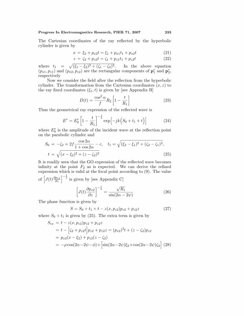
The Cartesian coordinates of the ray reflected by the hyperboliccylinder is given by

x = ξ2 + px2t = ξ1 + px1t1 + px2t (21)z = ζ2 + pz2t = ζ1 + pz1t1 + pz2t (22)

where t1 =√

(ξ1 − ξ2)2 + (ζ1 − ζ2)2. In the above equation(px1, pz1) and (px2, pz2) are the rectangular components of pr

1 and pr2,

respectivelyNow we consider the field after the reflection from the hyperbolic

cylinder. The transformation from the Cartesian coordinates (x, z) tothe ray fixed coordinates (ξ1, t) is given by [see Appendix B]

D(t) =cos2 αf

R2

[1 − t

R1

](23)

Thus the geometrical ray expression of the reflected wave is

Er = Er0

[1 − t

R1

]− 12

exp[−jk

(S0 + t1 + t

)](24)

where Er0 is the amplitude of the incident wave at the reflection point

on the parabolic cylinder and

S0 = −ζ2 = 2fcos 2α

1 + cos 2α− c, t1 =

√(ξ2 − ξ1)2 + (ζ2 − ζ1)2,

t =√

(x− ξ2)2 + (z − ζ2)2 (25)

It is readily seen that the GO expression of the reflected wave becomesinfinity at the point F2 as is expected. We can derive the refinedexpression which is valid at the focal point according to (9). The value

of[J(t)∂pz2

∂z

]− 12 is given by [see Appendix C]

[J(t)

∂pz2

∂z

]− 12

=√R1

sin(2α− 2ψ)(26)

The phase function is given by

S = S0 + t1 + t− z(x, pz2)pz2 + pz2z (27)

where S0 + t1 is given by (25). The extra term is given by

Sex = t− z(x, pz2)pz2 + pz2z

= t−[ζ2 + pz2t

]pz2 + pz2z = (px2)2t+ (z − ζ2)pz2

= px2(x− ξ2) + pz2(z − ζ2)= −ρ cos(2α−2ψ−φ)+

[sin(2α−2ψ)ξ2+cos(2α−2ψ)ζ2

](28)

234 Aziz, Naqvi, and Hong

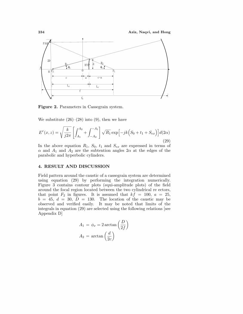
Figure 2. Parameters in Cassegrain system.

We substitute (26)–(28) into (9), then we have

Er(x, z) =

√k

j2π

[∫ A2

A1

+∫ −A1

−A2

] √R1 exp

[−jk

(S0 + t1 + Sex

)]d(2α)

(29)In the above equation R1, S0, t1 and Sex are expressed in terms ofα and A1 and A2 are the subtention angles 2α at the edges of theparabolic and hyperbolic cylinders.

4. RESULT AND DISCUSSION

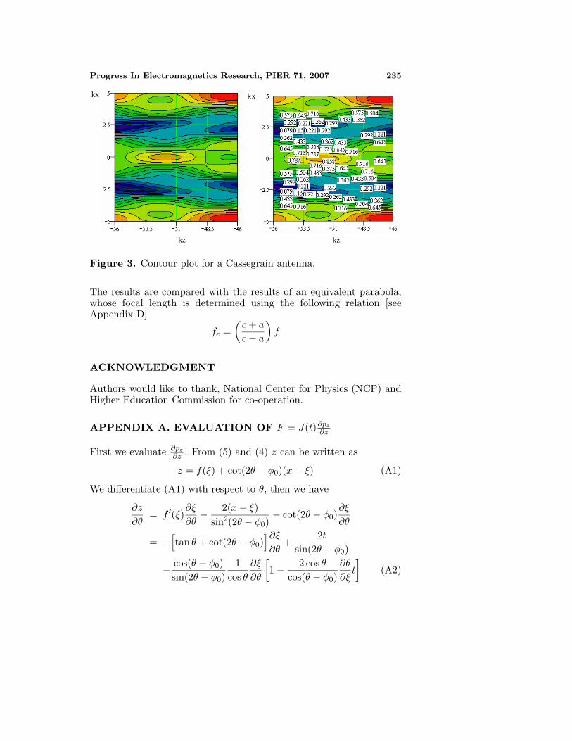
Field pattern around the caustic of a cassegrain system are determinedusing equation (29) by performing the integration numerically.Figure 3 contains contour plots (equi-amplitude plots) of the fieldaround the focal region located between the two cylindrical re ectors,that point F2 in figures. It is assumed that kf = 100, a = 25,b = 45, d = 30, D = 130. The location of the caustic may beobserved and verified easily. It may be noted that limits of theintegrals in equation (29) are selected using the following relations [seeAppendix D]

A1 = φν = 2 arctan(D

2f

)

A2 = arctan(d

2c

)

Progress In Electromagnetics Research, PIER 71, 2007 235

kx

kz

kx

kz

Figure 3. Contour plot for a Cassegrain antenna.

The results are compared with the results of an equivalent parabola,whose focal length is determined using the following relation [seeAppendix D]

fe =(c+ ac− a

)f

ACKNOWLEDGMENT

Authors would like to thank, National Center for Physics (NCP) andHigher Education Commission for co-operation.

APPENDIX A. EVALUATION OF F = J(t)∂pz

∂z

First we evaluate ∂pz

∂z . From (5) and (4) z can be written as

z = f(ξ) + cot(2θ − φ0)(x− ξ) (A1)

We differentiate (A1) with respect to θ, then we have

∂z

∂θ= f ′(ξ)

∂ξ

∂θ− 2(x− ξ)

sin2(2θ − φ0)− cot(2θ − φ0)

∂ξ

∂θ

= −[tan θ + cot(2θ − φ0)

]∂ξ∂θ

+2t

sin(2θ − φ0)

− cos(θ − φ0)sin(2θ − φ0)

1cos θ

∂ξ

∂θ

[1 − 2 cos θ

cos(θ − φ0)∂θ

∂ξt

](A2)

236 Aziz, Naqvi, and Hong

Hence the derivative ∂z∂pz

can be derived as follows.

∂z

∂pz=∂z

∂θ

∂θ

∂pz=

12 sin(2θ − φ0)

∂z

∂θ

= − cos(θ − φ0)2 sin2(2θ − φ0) cos θ

∂ξ

∂θ

[1 +

2f ′′(ξ) cos3 θcos(θ − φ0)

t

](A3)

Using (A3) and (7b) yields the final result

F = J(t)∂pz∂z

=

[1 +

2f ′′(ξ) cos3 θcos(θ − φ0)

t

] [2 cos3 θ sin2(2θ − φ0)

cos(θ − φ0)f ′′(ξ)

]

×[1 +

2f ′′(ξ) cos3 θcos(θ − φ0)

t

]−12 cos3 θ sin2(2θ − φ0)

cos(θ − φ0)f ′′(ξ) (A4)

APPENDIX B. DERIVATION OF THE JACOBIAN

We evaluate the Jacobian of coordinate transformation (x, z) to (ξ1, t)with (x, z) given by (21).

D(t) =∂(x, z)∂(ξ1, t)

=

∣∣∣∣∣∂ξ2∂ξ1

+∂px2

∂ξ1t

∂ζ2∂ξ1

+∂pz2

∂ξ1t

px2 pz2

∣∣∣∣∣= 2

∂(α− ψ)∂ξ1

t− cos(2α− ψ)cosψ

∂ξ2∂ξ1

(B1)

where we have used the relation ∂ζ2∂ξ1

= ∂ζ2∂ξ2

∂ξ2∂ξ1

= tanψ ∂ξ2∂ξ1

. The relationbetween (ξ1, ζ1) and (ξ2, ζ2) is given by

ξ2 − ξ1 = − tan 2α(ζ2 − ζ1) (B2)

and we differentiate the both sides with respect to ξ1. Then we have

∂ξ2∂ξ1

=cosψ

cos(2α− ψ)

[1 − ζ2 − ζ1

f

cos2 αcos 2α

]

=cosψ

cos(2α− ψ)R2 cos2 α

f(B3)

Furthermore we have

∂α

∂ξ1=

12f

cos2 α,∂ψ

∂ξ1=∂ψ

∂ξ2

∂ξ2∂ξ1

= cos2 ψa4

b21ζ32

∂ξ2∂ξ1

(B4)

Progress In Electromagnetics Research, PIER 71, 2007 237

Substituting (B3) and (B4) in (B1) yields

D(t) = 2t

{cos2 α

2f− cos3 ψ

cos(2α− ψ)a4

b2ζ32

[1 − ζ2 − ζ1

f

cos2 αcos 2α

]}

−[1 − ζ2 − ζ1

f

cos2 αcos 2α

](B5)

From Fig. 1 and simple calculation we readily find that the followingrelations hold

ζ2 = c−R2 cos 2α, ζ1 =ξ214f

− f + c = −f cos 2αcos2 α

+ c;

1 − ζ2 − ζ1f

cos2 αcos 2α

=R2

fcos2 α (B6)

Hence D(t) can be written as

D(t) =cos2 αf

{[1 − 2 cos3 ψ

cos(2α− ψ)a4

b2ζ32R2

]t−R2

}(B7)

By using the relations

cos 2α =c− ζ2R2

, sin 2α =ξ2R2

(B8)

cos(2α− ψ) in (B7) can be expressed by

cos(2α− ψ) =c− ζ2R2

cosψ +ξ2R2

sinψ

=1

R2

√R1R2

[b

aζ2(c− ζ2) +

a

bξ22

]

1R2

√R1R2

[b

acζ2 − ab

(ζ22a2

− ξ22

b2

)]

=1

R2

√R1R2

b

a(cζ2 − a2) =

b√R1R2

(B9)

where we have used the relation R2 =√

(c− ζ2)2 + ξ22 = cζ2−a2

a . Thenthe coefficient of t in (B7) is simplified to

U = 1 − 2 cos3 ψcos(2α− ψ)

a4

b2ζ32R2 = 1 − 2abR2

(R1R2)32

aR2

√R1R2

b(cζ2 − a2)

= 1 − 2aR1

=R2

R1(B10)

238 Aziz, Naqvi, and Hong

Hence D(t) in (B7) becomes

D(t) =cos2 αf

R2

[1 − t

R1

](B11)

This shows that the ray is focused at point F2.

APPENDIX C. EVALUATION OF F = J(t)∂pz2

∂z

We now evaluate the integrand of (9) to derive the expression which isvalid at the focal point F . From the relation

z = ζ2 +pz2

px2(x− ξ2) = ζ2 + cot(2α− 2ψ)(x− ξ2) (C1)

we have

∂z

∂ξ2=∂ζ2∂ξ2

− 2(x− ξ2)sin2(2α− 2ψ)

∂(α− ψ)∂ξ2

− cot(2α− 2ψ)

= − cos(2α− ψ)cosψ sin(2α− 2ψ)

+2t

sin(2α− 2ψ)∂(α− ψ)∂ξ2

1sin(2α− 2ψ)

∂ξ1∂ξ2

[2t∂(α− ψ)∂ξ1

− cos(2α− ψ)cosψ

∂ξ2∂ξ1

](C2)

By using the relations

∂z

∂pz2=∂z

∂ξ2

∂ξ2∂pz2

,∂pz2

∂z=∂ξ2∂z

∂pz2

∂ξ2;

∂pz2

∂ξ2= 2 sin(2α− 2ψ)

∂(α− ψ)∂ξ2

= 2 sin(2α− 2ψ)∂ξ1∂ξ2

∂(α− ψ)∂ξ1

(C3)

we have

∂pz2

∂z=∂ξ2∂z

∂pz2

∂ξ2

= 2 sin(2α− 2ψ)∂ξ1∂ξ2

∂(α− ψ)∂ξ1

sin(2α− 2ψ)∂ξ2∂ξ1

×[2t∂(α− ψ)∂ξ1

− cos(2α− ψ)cosψ

∂ξ2∂ξ1

]−1

(C4)

Progress In Electromagnetics Research, PIER 71, 2007 239

There we have

D(t)D(0)

∂pz2

∂z=

[2t∂(α− ψ)∂ξ1

− cos(2α− ψ)cosψ

∂ξ2∂ξ1

][cosψ

cos(2α−ψ)∂ξ2∂ξ2

]∂pz2

∂z

= 2 sin2(2α− 2ψ)∂(α− ψ)∂ξ1

cosψcos(2α− ψ)

∂ξ1∂ξ2

(C5)

From the results of Appendix B we have

D(t)D(0)

∂pz2

∂z= 2 sin2(2α−2ψ)

cos2 α2f

R2

R1

cosψcos(2α−ψ)

cos(2α−ψ)cosψ

f

R2 cos2α

=sin2(2α− 2ψ)

R1(C6)

where

R1 =cζ2 + a2

a= a

c cosψ +√a2 cos2 ψ − b2 sin2 ψ√

a2 cos2 ψ − b2 sin2 ψ,

cosψ =c+ a cos 2α√

a2 + c2 + 2ac cos 2α, sinψ =

a sin 2α√a2 + c2 + 2ac cos 2α

,

ξ1 = 2f tanα, ζ1 = c− 2f cos 2α1 + cos 2α

ξ2 =b2 sinψ√

a2 cos2 ψ − b2 sin2 ψ, ζ2 =

a2 cosψ√a2 cos2 ψ − b2 sin2 ψ

(C7)

APPENDIX D. PARAMETERS OF CASSEGRAINANTENNA

D.1. tan φv

2 = D2f and tan φr

2 = D2fe

The equation of the parabolic cylinder is given by (16). Hence we have

OA = −f + c, AH =D2

4f, FH = f − D

2

4f(D1)

and

tanφv =D

f − D2

4f

=2 · D

2f

1 −(D

2f

)2 =2 tan

φv

2

1 − tan2 φv

2

(D2)

240 Aziz, Naqvi, and Hong

From (D2) we have tan φv

2 = D2f . It may be noted that D is height of

the edge of the parabolic cylinder from horizontal axis.Similarly we have

tanφr

2=D

2fe(D3)

where fe is the focal length of the equivalent parabola.

D.2. e = sin 12(φv+φr)

sin 12(φv−φr)

From the similarities of the triangles we have

fef

=Lr

Lv=c+ ac− a =

e+ 1e− 1

=tan

12φv

tan12φr

(D4)

The last term is obtained from the results in (D1). From the aboveequation e is obtained as

e =tan

12φv + tan

12φr

tan12φv − tan

12φr

=sin

12(φv + φr)

sin12(φv − φr)

=Lr + Lv

Lr − Lv(D5)

and

1 − 1e

=2Lv

Lr + Lv= 1 −

sin12(φv + φr)

sin12(φv − φr)

(D6)

REFERENCES

1. Dechamps, G. A., “Ray techniques in electromagnetics,” Proc.IEEE, Vol. 60, 1022–1035, 1972.

2. Felson, L. B., Hybrid Formulation of wave Propagation andScattering, Nato ASI Series, Martinus Nijhoff, Dordrecht, TheNetherland, 1984.

3. Chapman, C. H. and R. Drummond, “Body wave seismogramsin inhomogeneous media using Maslov asymptotic theory,” Bull.Seismol., Soc. Am., Vol. 72, 277–317, 1982.

4. Fuks, I. M., “Asymptotic solutions for backscattering by smooth2D surfaces,” Progress In Electromagnetics Research, PIER 53,189–226, 2005.

Progress In Electromagnetics Research, PIER 71, 2007 241

5. Martinez, D., F. Las-Heras, and R. G. Ayestaran, “Fast methodsfor evaluating the electric field level in 2D-indoor enviroments,”Progress In Electromagnetics Research, PIER 69, 247–255, 2007.

6. Kravtsov, V. A., “Two new methods in the theory of wavepropagation in inhomogeneous media (review),” Sov. Phys.Acoust., Vol. 14, No. 1, 1–17, 1968.

7. Ziolkowski, R. W. and G. A. Deschamps, “Asymptotic evaluationof high frequency field near a caustic: An introduction to Maslov’smethod,” Radio Sci., Vol. 19, 1001–1025, 1984.

8. Hongo, K. and Yu Ji. and E. Nakajimi, “High-frequency expressionfor the field in the caustic region of a reflector using Maslov’smethod,” Radio Sci., Vol. 21, No. 6, 911–919, 1986.

9. Hongo, K. and Yu Ji, “High-frequency expression for the fieldin the caustic region of a cylindrical reflector using Maslov’smethod,” Radio Sci., Vol. 22, No. 3, 357–366, 1987.

10. Maslov, V. P., Perturbation Theory and Asymptotic Method,Moskov., Gos. Univ., Moscow, 1965 (in Russian). (Translated intoJapanese by Ouchi et al., Iwanami, Tokyo, 1976.)

11. Gorman, A. D., “Vector field near caustics,” J. Math. Phys.,Vol. 26, 1404–1407, 1985.

12. Felson, L. B. and N. Marcuvitz, Radiation and Scattering ofWaves, Prentice-Hall, Englewood Cliffs, N. J., 1973.