analysis of the dynamic and causal relationship

T.C.

SAKARYA UNIVERSITY SOCIAL SCIENCES INSTITUTE

ANALYSIS OF THE DYNAMIC AND CAUSAL RELATIONSHIP BETWEEN EXCHANGE RATE AND SELECTED

MACROECONOMIC VARIABLES IN SOMALIA: ARDL AND TODA-YAMAMOTO METHODOLOGIES

MASTER’S THESIS

ABDIKANI ABDULLAHI SHEIKDON

Department: Economics

Thesis Advisor: Prof. Dr. Ali Kabasakal

June 2021

T.C.

SAKARYA UNIVERSITY SOCIAL SCIENCES INSTITUTE

ANALYSIS OF THE DYNAMIC AND CAUSAL RELATIONSHIP BETWEEN EXCHANGE RATE AND SELECTED

MACROECONOMIC VARIABLES IN SOMALIA: ARDL AND TODA-YAMAMOTO METHODOLOGIES

MASTER’S THESIS

ABDIKANI ABDULLAHI SHEIKDON

Department: Economics

“The examination was held online on /29/06 /2021 and approved unanimously By the following committee members.”

COMMITTEE MEMBERS ASSESSMENT Prof.Dr. Ali KABASAKAL SUCCESSFUL Prof.Dr. Seyit KÖSE SUCCESSFUL

Prof.Dr. Şakir GÖRMÜŞ SUCCESSFUL

ACKNOWLEDGMENTS

To begin with, thanks be to almighty Allah who made it possible for me to witness such

achievement. Secondly, I feel it necessary to use this opportunity to pay my earnest

gratitude to my supervisor Dr. Ali Kabasakal, who gave me unwavering support

throughout the preparation of my thesis as his insightful comments and guidance has

greatly enhanced the value of my thesis and surely this great work would not have been

possible without his support. In addition, I would like to offer my sincere gratitude to my

family, who have always stood by me to give moral support and encouraged me to achieve

many memorable milestones. Finally, special thanks are due to my treasured sister Hibo

who has always been my side and supported me unconditionally throughout my student

life.

Abdikani Abdullahi Sheikdon

29.06.2021

i

İÇİNDEKİLER

LIST OF ABBREVIATIONS ....................................................................................... iii

LIST OF TABLES ......................................................................................................... iv

LIST OF FIGURES ........................................................................................................ v

ABSTRACT ................................................................................................................... vi

ÖZET ............................................................................................................................. vii

INTRODUCTION .......................................................................................................... 1

CHAPTER ONE: DEFINITIONS, THEORETICAL AND CONCEPTUAL

FRAMEWORK .............................................................................................................. 4

1.1. Exchange Rate Definition .......................................................................................... 4

1.1.1. Direct Quoting of the Exchange Rate .............................................................. 4

1.1.2. Indirect Quoting of the Exchange Rate ........................................................... 5

1.2. Conceptual Frame Work ............................................................................................ 5

1.2.1. Spot Exchange Rates ....................................................................................... 6

1.2.2. Forward Exchange Rates ................................................................................. 6

1.2.3. Types of the Exchange Rates .......................................................................... 6

1.2.4. Nominal Exchange Rate .................................................................................. 7

1.2.5. Real Exchange Rate ......................................................................................... 7

1.2.6. Purchasing Power Parity (PPP) ....................................................................... 7

1.2.7. Absolute Purchasing Power Parity (APPP) ..................................................... 8

1.2.8. Relative Purchasing Power Parity (RPPP) ...................................................... 8

1.3. Exchange Rate Regimes ............................................................................................ 9

1.3.1. Pegged Exchange Rate Regime ....................................................................... 9

1.3.2. Floating Exchange Rate Regime ................................................................... 10

1.3.3. Mixed Exchange Rate Regime ...................................................................... 11

1.3.4. The Impossible Trinity .................................................................................. 12

1.4. Dollarization in Somalia .......................................................................................... 13

1.5. Exchange Rate Regime in Somalia ......................................................................... 14

CHAPTER TW0: RELATED LITERATURE REVIEW ....................................... 16

ii

2.1. Exchange Rate and Inflation ................................................................................... 16

2.2. Exchange Rate and Trade Openness ....................................................................... 19

2.3. Exchange Rate and Investment ............................................................................... 23

2.4. Exchange Rate and Government Spending ............................................................. 26

2.5. Exchange Rate and Economic Growth .................................................................... 30

CHAPTER THREE: ANALYSIS AND RESULTS SECTION .............................. 35

3.1. Dataset and Variables .............................................................................................. 35

3.2. Unit Root Tests ........................................................................................................ 35

3.2.1. Augmented Dickey-Fuller (ADF) Unit Root Test......................................... 36

3.2.2. Philips-Peron (PP) Unit Root Test ................................................................ 37

3.3. ARDL Model ........................................................................................................... 37

3.4. Bounds Test ............................................................................................................. 38

3.5. Toda-Yamamoto Causality Test .............................................................................. 39

3.6. Findings ................................................................................................................... 40

3.7. Unit Root Tests ........................................................................................................ 40

3.8. Diagnostics Tests ..................................................................................................... 44

3.8.1. Serial Correlation........................................................................................... 45

3.8.2. Heteroskedasticity Test ................................................................................. 45

3.8.3. Normality check ............................................................................................ 46

3.8.4. Model Stability .............................................................................................. 46

3.9. Toda-Yamamoto Causality Test Findings ............................................................... 47

DISCUSSIONS AND RECOMMENDATIONS ........................................................ 50

REFERENCES ............................................................................................................. 54

APPENDIX ................................................................................................................... 62

CURRICULUM VITAE .............................................................................................. 63

iii

LIST OF ABBREVIATIONS

ADF : Augmented Dickey-Fuller

ARCH : Autoregressive Conditional Heteroskedasticity

ARDL : Autoregressive Distributed Lag

APPP : Absolute Purchasing Power Parity

CBS : Central Bank of Somalia

CPI : Consumer Price Index

ECT : Error Correction Term

GARCH : Generalized Autoregressive Conditional Heteroskedasticity

GBP : Great Britain Pound

IMF : International Monetary Fund

PP : Philips-Perron

PPP : Purchasing Power Parity

RPPP : Relative Purchasing Power Parity

SHSO : Shilling Somali

UNSD : United Nations Division of Statistics

USD : United States Dollar

VAR : Vector Auto Regression

VEC : Vector Error Correction

iv

LIST OF TABLES

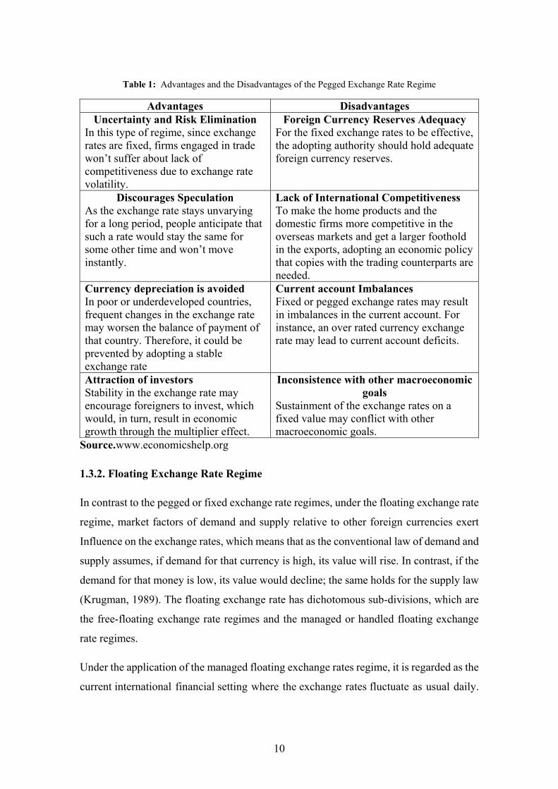
Table 1: Advantages and the Disadvantages of the Pegged Exchange Rate Regime ... 10

Table 2: Benefits and the Drawbacks of the Floating Exchange Rate Regimes .......... 11

Table 3: Results of the ADF and PP unit root tests ....................................................... 40

Table 4: Bounds test results ........................................................................................... 41

Table 5: Short-run results .............................................................................................. 43

Table 6: Serial Correlation Test Results ........................................................................ 45

Table 7: Breusch-Pagan-Godfrey Heteroskedasticity Results ....................................... 45

Table 8: Lag length determination according to the lag selection criteria .................... 48

Table 9: Toda-Yamamoto Causality Test Findings ....................................................... 48

v

LIST OF FIGURES

Figure 1: A Comprehensive Framework of the exchange rates ...................................... 6

Figure 2: The Impossible Trinity. N. Gregory Mankiw, Macroeconomics textbook .... 12

Figure 3: The 20 best models according to the Akaike information criterion ............... 44

Figure 4: Normality check histogram ............................................................................ 46

Figure 5: CUSUM Test ................................................................................................. 46

Figure 6: CUSUM Square Test ..................................................................................... 47

Figure 7: Examining the Graph of Residuals ................................................................ 47

vi

Sakarya University Institute of Social Sciences Abstract of Thesis

Master Degree Ph.D

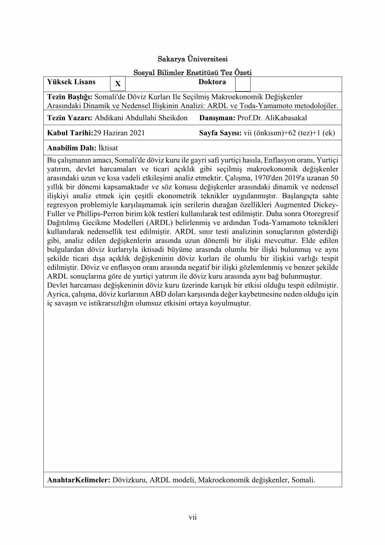
Title of Thesis: Analysis of the dynamic and causal relationship between Exchange rate and selected macroeconomic variables in Somalia. ARDL and Toda-Yamamoto methodologies Author of Thesis: Abdikani Abdullahi Sheikdon Supervisor: Prof.Dr. Ali Kabasakal

Accepted Date: 29 June 2021 Number of Pages: vii (pre text) +62 (main body) + 1 (app)

Department: Economics The main target of this study is to analyze the long and short-run interaction between the exchange rate and the selected macroeconomic indicators like the gross domestic product, inflation rates, domestic investment, government spending, and the trade openness in Somalia. The study covers 50 years ranging from 1970 to 2019 and applied various econometric techniques to estimate the dynamic and the causal relationship between the said variables. At the outset, to avoid being encountered the problem of spurious regression, it has been tested the presence of a unit root in the series using augmented Dickey-Fuller and the Phillips-Perron unit root tests. Afterwards, it has been specified the autoregressive distributed lag models (ARDL) and then followed by testing the causality using Toda-Yamamoto techniques. As the ARDL bound test findings depict, there’s a long-run relationship among the analyzed series. The findings found a positive relationship between exchange rate and economic growth. Likewise, the trade openness variable has been ascertained that it has a positive relationship with exchange rates. A negative relationship has been observed between the exchange and inflation rate. Similarly, according to the results of the ARDL, the same nexus is found between domestic investment and the exchange rate. The government expenditure variable was found to have a mixed impact on the exchange rate. Notably, the study revealed the negative impact of the civil war, as it's likely to cause the exchange rates to depreciate against the US dollar. ABSTRACT

Keywords: Exchange rate, ARDL model, Macroeconomic variables, Somalia.

X

vii

Sakarya Üniversitesi

Sosyal Bilimler Enstitüsü Tez Özeti Yüksek Lisans Doktora

Tezin Başlığı: Somali'de Döviz Kurları Ile Seçilmiş Makroekonomik Değişkenler Arasındaki Dinamik ve Nedensel Ilişkinin Analizi: ARDL ve Toda-Yamamoto metodolojiler. Tezin Yazarı: Abdikani Abdullahi Sheikdon Danışman: Prof.Dr. AliKabasakal

Kabul Tarihi:29 Haziran 2021 Sayfa Sayısı: vii (önkısım)+62 (tez)+1 (ek)

Anabilim Dalı: İktisat Bu çalışmanın amacı, Somali'de döviz kuru ile gayri safi yurtiçi hasıla, Enflasyon oranı, Yurtiçi yatırım, devlet harcamaları ve ticari açıklık gibi seçilmiş makroekonomik değişkenler arasındaki uzun ve kısa vadeli etkileşimi analiz etmektir. Çalışma, 1970'den 2019'a uzanan 50 yıllık bir dönemi kapsamaktadır ve söz konusu değişkenler arasındaki dinamik ve nedensel ilişkiyi analiz etmek için çeşitli ekonometrik teknikler uygulanmıştır. Başlangıçta sahte regresyon problemiyle karşılaşmamak için serilerin durağan özellikleri Augmented Dickey-Fuller ve Phillips-Perron birim kök testleri kullanılarak test edilmiştir. Daha sonra Otoregresif Dağıtılmış Gecikme Modelleri (ARDL) belirlenmiş ve ardından Toda-Yamamoto teknikleri kullanılarak nedensellik test edilmiştir. ARDL sınır testi analizinin sonuçlarının gösterdiği gibi, analiz edilen değişkenlerin arasında uzun dönemli bir ilişki mevcuttur. Elde edilen bulgulardan döviz kurlarıyla iktisadi büyüme arasında olumlu bir ilişki bulunmuş ve aynı şekilde ticari dışa açıklık değişkeninin döviz kurları ile olumlu bir ilişkisi varlığı tespit edilmiştir. Döviz ve enflasyon oranı arasında negatif bir ilişki gözlemlenmiş ve benzer şekilde ARDL sonuçlarına göre de yurtiçi yatırım ile döviz kuru arasında aynı bağ bulunmuştur. Devlet harcaması değişkeninin döviz kuru üzerinde karışık bir etkisi olduğu tespit edilmiştir. Ayrica, çalışma, döviz kurlarının ABD doları karşısında değer kaybetmesine neden olduğu için iç savaşın ve istikrarsızlığın olumsuz etkisini ortaya koyulmuştur. ÖZET

AnahtarKelimeler: Dövizkuru, ARDL modeli, Makroekonomik değişkenler, Somali.

X

1

INTRODUCTION

Economists have known for ages that imperfectly administered exchange rates can have

devastating implications on economic growth. As globalization deepens, the interaction

between the countries gets stronger, and the world countries' economies become more

intertwined and affect each other. Thus, the trades between countries become more fragile

to the economic events or even the structural and regime changes implemented in a

country other than the executing nation. As countries start being open and trade with the

world, irrefutable exchange rate considerably influences the behaviors of the key

macroeconomic indicators.

There’s a rising consensus that persistent exchange rate instability typically leads to

serious macroeconomic disequilibrium. As a result, recent discussions emphasize the

undeniable effect of the real exchange rate on the economy at large. When narrowed the

overall perspective to Africa, the interaction and the nexus between the real exchange rate

and the would-be used macroeconomic indicators such as trade openness, public

expenditure, and the inflation rate must have different impact levels compared to the

developing or the advanced countries. In the context of Somalia, though in the last decade

dollarization has become a factor, yet Somali shilling remains and serves as the sole

means of exchange and the unit of account in the transactions of the undersized businesses

(Nor et al. 2020).

However, to dive deeply into the concepts related to exchange rates, the structure that the

study follows is that, in its first section, the description the exchange rates, the various

sorts of exchange rates, the exchange rate regimes of pegged exchange rate system,

floating exchange rate system, and mixed exchange rate systems, as well as some

background of Somalia’s exchange rate regime and the recent dollarization phenomenon,

are discussed. The second part has reviewed the recent empirical research that discusses

the relationship among exchange rates, trade openness, inflation, investment, public

expenditure, and economic progress. While in the third part, the analysis and the results

section were given the space to examine the causal relationship between exchange rates

and the indicated macroeconomic variables in Somalia. At the outset, to avoid being

encountered in spurious regression or, in other words avoiding the use of none stationary

series in the regression, augmented Dickey-Fuller (ADF) unit root and some theoretical

2

explanations were made regarding the autoregressive distributed lag (ARDL) models and

the Toda-Yamamoto causality techniques. In the concluding part, the findings obtained

from the applied econometric analysis are interpreted, while it has been finalized with

some comments and discussion.

Research Topic

The research topic discusses the “dynamic and the causal relationship between the real

exchange rate and the selected macroeconomic variables in Somalia between 1970 and

2018”.

Problem Statement

The interaction of the exchange rate with other macroeconomic indicators of any

economy is all inclusively given an exceptional consideration due to its unfavorable cost

on the economy. In recent discussions, it has kept being a focal point issue in the

promising economies. Ideally, the presence of an effective central bank authority or

monitory board could help initiate and set useful policies that regulate the amount of

money in circulation. However, given the lack of strong public financial institutions and

functioning central bank in Somalia from the decline of the military regime in 1991, the

circulation of banknotes throughout the country was determined by actors other than the

state’s central bank (Luther, 2015). The disappearance of the central bank led the country

to face a cash shortage as the only notes in circulation were those that the late government

had printed before it toppled in 1991. To cover that need for banknotes, both private

business owners and some federal member states have commenced printing banknotes

abroad on their discretion and later importing them into the country to replace the old

damaged banknotes that were already in circulation and consequently the lack of the

central bank authority. The monitoring board has resulted in the Somali shilling being

over printed, which eventually led the Somali shilling to depreciate against the dollar.

However, the depreciation of the Somali shilling, its recurrent fluctuations, and most

notably, its vulnerability to being forged have resulted in people losing faith in the local

currency and have shifted to have greater confidence in the US dollar (USD) and use it

as a store of value. Even in the last decade, businesses' use of the USD as the price tags

of goods & services have shown a substantial increase. Therefore, since no enough study

3

has been made on the dynamic and causal link between the exchange rates and the

selected macroeconomic indicators in Somalia, the study seeks to fill up the gap as well

as suggest recommendations to the policymakers.

Significance of the Study

Needless to say that foreign currency exchange has an undeniable impact on the economic

activities in every country, and it interacts with other macroeconomic indicators through

various transmission channels consequently; in this study, it has been discussed the long

and the short-run nexus between the real exchange rate and the selected predictors of,

trade openness, inflation rate, investment, government expenditure, and the economic

progress, and what's more the study attempts to determine the causality behavior among

the variables. Therefore, now that the study incorporates all these variables in one setting,

it calls attention to its importance. Moreover, the study seeks to contribute to the existing

literature on the link between exchange rates and these accumulated bunches of other

predictors.

Purpose of the Study

The study's main intention is first to review the theoretical framework of the variables

used in the study and afterward, using the econometric models to explore the long and

short-run linkages between the real exchange rate and the macroeconomic variables and

investigate their causal relationship.

Research Methodology

For determining the stage at which the series is stationary, the study used various

stationarity tests such as the ADF and the Philips-Perron (PP) unit root test.

Henceforward, autoregressive distributed lag models were used to explore the dynamic

behavior of the variables in both the long and short-run, and finally, the Toda-Yamamoto

causality approach was applied.

4

CHAPTER ONE: DEFINITIONS, THEORETICAL AND

CONCEPTUAL FRAMEWORK

1.1. Exchange Rate Definition

The price of one country’s currency in terms of another’s currency is known as the

exchange rate (Mankiw, 2007. 135). For instance, how many Somali shillings does one

need to get 1 USD? Or, in other currency’s elucidation, how much Turkish Lira does it

cost to buy 1 USD? As can be extracted from both the definition of the exchange rate and

the followed guiding questions, it entails that one should consider the exchange rate

before any economic transaction such as investment decision, trade, and Et cetera.

Because the exchange rates involve an essential position in the economy, it has been given

much attention to discussing its impact and relationship with the other macroeconomic

indicators.

In understanding the exchange rates, there many entailing and relevant concepts that help

understand how the exchange rate works, such as the exchange rate’s quoting methods,

the different exchange rate types, the PPP (purchasing power parity), and the various

exchange rate regimes. There are two approaches or styles to quoting exchange rates in

the financial markets, that is to say, direct quoting and indirect quoting.

1.1.1. Direct Quoting of the Exchange Rate

A direct quote is a kind of quotation that expresses the home or the domestic currency

prices in terms of a foreign currency (Investopedia, 2021). To put it another way, in the

direct quotation system, it’s asked the literal load of domestic currency that is desired to

acquire a unit of the foreign currency. In the direct or straight quotation system, the

foreign currency serves as the base currency, whilst the domestic currency is the quoted

one.

For example, let’s consider the following rates.

8.68 TL/USD

This rate demonstrates the amount of Turkish Lira that one needs to purchase one US

dollar.

5

1.1.2. Indirect Quoting of the Exchange Rate

Indirect quoting states the variable quantity of a foreign currency one needs to buy and

trade a unit of the home currency, and this kind of quotation system is called the “Quantity

Quotation” as it says the literal quantity or the literal amount of the foreign currency

desired to purchase a single unit of the home currency. In other words, in the indirect

quote, home currency serves as the base currency.

For example, 8.69 TL: 1 USD

This rate shows the quantity of USD that can be purchased for the stated amount of the

Turkish Lira.

In the same way, another imperative distinction that should be brought to the target

audiences’ attention when discussing exchange rates is the differentiation between spot

and forward exchange rates.

1.2. Conceptual Frame Work

Regarding the understanding of the laymen or those unfamiliar with the main concepts of

economics, it’s often confusing for them to comprehend the exchange rate and the related

concepts. Furthermore, there are various ways to be applied to gauging the different kinds

of exchange rates. This section concentrates on giving the basic definitions for the key

terminological terms of the exchange rates and the multiple alternatives in measuring the

exchange rate. In figure 1.1, it is shown a very comprehensive conceptual framework that

outlines the diverse measurements of the exchange rate that are common and practiced in

the foreign exchange markets.

6

Figure 1: A Comprehensive Framework of the exchange rates

Source: (Takaendesa, 2006)

1.2.1. Spot Exchange Rates

The spot exchange rate refers to the price whereupon a foreign currency is sold and

acquired instantly on the spot without any delay (Hassan & Mano, 2019). The spot

exchange rates could additionally be divided into nominal and real exchange rates.

1.2.2. Forward Exchange Rates

The forward exchange rates also refer to exchange rates whereupon foreign currencies

are purchased and sold. Nevertheless, the deliverance of the currency crops up for a

moment in the future, not instantaneously (Hassan & Mano, 2019).

1.2.3. Types of the Exchange Rates

Different classifications are made regarding the different types of exchange rates. In this

sub-section, the intent is to illustrate the various exchange rate sorts: The real exchange

Nominal Effective

Forward

Nominal Real

Bilateral Multilateral Bilateral Multilateral

Nominal Bilateral

Spot

Real Bilateral

Real Effective

Exchange Rate

7

rates, the nominal exchange rates, the bilateral exchange rates, and the multilateral

exchange rates.

1.2.4. Nominal Exchange Rate

The nominal exchange rates could be exemplified like those rates, more precisely real

rates, usually being given in the markets of the foreign exchanges (Catão, 2007). These

aforesaid exchange rates, of course, state the literal quantity of local currency which is

desired so as to be exchanged smoothly for foreign currency. To make a distinction, the

key property that nominal exchange rates have is that being the unaltered weighted or

accumulated aggregate value of a local currency compared to alternative relative foreign

currency aggregated together in a single index (Catão, 2007).

1.2.5. Real Exchange Rate

The real exchange rates could be defined as the kind of exchange rates that demonstrate

the price discrepancies among two commodities exchanged or traded (Catão,2007).The

rates are gauged using the price indices, which subsequently reflect the comparative price

discrepancies from a specified base period. The real exchange rate could be precisely said

as the nominal exchange rate accounted for inflation (Catão,2007).

1.2.6. Purchasing Power Parity (PPP)

The term purchasing power parity (PPP) was initially introduced by the prominent

economist from Sweden, Karl Gustav Cassel (1866-1945). The PPP assumption or the

law of one price assumes that the purchasing power of the currencies of two comparable

countries’ when purchasing a certain package of goods and services. To say it differently,

the theory is anchored in the postulation that the two identical commodities ought to be

sold at an identical price once the currencies have been changed into a common currency

(Chen& Hu, 2018). The theory is anchored in avoiding the arbitrage opportunity; for

example, let’s assume that a loaf of bread costs 2US dollars in the United States and its

corresponding amount in Turkish Lira 17.38 TL, while a loaf of bread in Turkey costs

only 3 TL that corresponds to 0.34 USD cents. Therefore, this extreme cheapness

motivates what is called arbitrage opportunity, which are the Turkish people to start

trading the bread and ship it to the United States to make higher profits.

8

1.2.7. Absolute Purchasing Power Parity (APPP)

The APPP theory could be enlightened through the following equation.

𝐸𝐸 =𝑃𝑃 ∗𝑃𝑃

P= indicates the foreign-price

P*= represents the domestic price

E = is the sports exchange rate.

Consequently, the APPP indicates that the real exchange rate equals 1.

This assumption could be considered relevant in the long-run; conversely, for the short-

run, this could not be sensibly regarded as a viable theory (Maepa, 2015). In the case that

the rate of the exchange is above the value of the purchasing power parity of one, the

currency under consideration is said to be overvalued. On the other hand, vice versa is

considered an undervalued currency (Maepa, 2015).

Except for the stated critics of the absolute purchasing power parity theory that this

assumption isn’t realistic in the short-run, the theory doesn’t consider the existence of

other inevitable costs, for example, the transportation costs, trade duties such as the tariffs,

and so on.

1.2.8. Relative Purchasing Power Parity (RPPP)

Following the drawbacks of the APPP, the RPPP was afterward proposed. The relative

purchasing power parity theory predicts a link between the price rises of two countries in

a certain period and the exchange rate changes between currencies of the two countries

during the matching time (Rogoff, 1996). It is a dynamic sort of absolute purchasing

power parity theory.

This theory could further be illustrated in the following equation.

∆𝐸𝐸 = 𝜋𝜋 − 𝜋𝜋 ∗

Where ∆𝐸𝐸 represent changes in the exchange rates.

𝜋𝜋Indicates the inflation rate for the domestic country while 𝜋𝜋 ∗ denotes the inflation rate

for the foreign country.

9

1.3. Exchange Rate Regimes

The preference of exchange rate regime and its impact on the other macroeconomic

indicators’ performance is considered among the unsettled arguments and divisive issues

in the economic policy, and its determination could be an exclusive authority for the

governments or the monetary authorities to decide or, one that is directed by the market

forces of the demand and supply. In the recent literature discussions, choosing the optimal

exchange rate regime that stimulates growth became an unsettled debate in developing

and emerging economies. Generally, exchange rate regimes can be broadly categorized

into pegged exchange rate regimes and flexible exchange rates regimes.

1.3.1. Pegged Exchange Rate Regime

The Pegged exchange rate system happens to be a regime typically implemented by the

monetary authorities of a country, in search of tackling the adverse impact of the exchange

rates or higher currency instability, as well as to attain a goal for the nominal exchange

rate where money authorities get involved the market place in achieving this objective

(Marí del Cristo, 2014).The pegged exchange rate, which is otherwise known as the fixed

exchange rate, is considered to be useful in certain aspects, such as eliminating exchange

rate uncertainty which distresses or imposes an unfavorable impact on the perception of

the potential investors that would invest in the country, as well as retaining the existing

investments.

10

Table 1: Advantages and the Disadvantages of the Pegged Exchange Rate Regime

Advantages Disadvantages Uncertainty and Risk Elimination

In this type of regime, since exchange rates are fixed, firms engaged in trade won’t suffer about lack of competitiveness due to exchange rate volatility.

Foreign Currency Reserves Adequacy For the fixed exchange rates to be effective, the adopting authority should hold adequate foreign currency reserves.

Discourages Speculation As the exchange rate stays unvarying for a long period, people anticipate that such a rate would stay the same for some other time and won’t move instantly.

Lack of International Competitiveness To make the home products and the domestic firms more competitive in the overseas markets and get a larger foothold in the exports, adopting an economic policy that copies with the trading counterparts are needed.

Currency depreciation is avoided In poor or underdeveloped countries, frequent changes in the exchange rate may worsen the balance of payment of that country. Therefore, it could be prevented by adopting a stable exchange rate

Current account Imbalances Fixed or pegged exchange rates may result in imbalances in the current account. For instance, an over rated currency exchange rate may lead to current account deficits.

Attraction of investors Stability in the exchange rate may encourage foreigners to invest, which would, in turn, result in economic growth through the multiplier effect.

Inconsistence with other macroeconomic goals

Sustainment of the exchange rates on a fixed value may conflict with other macroeconomic goals.

Source.www.economicshelp.org

1.3.2. Floating Exchange Rate Regime

In contrast to the pegged or fixed exchange rate regimes, under the floating exchange rate

regime, market factors of demand and supply relative to other foreign currencies exert

Influence on the exchange rates, which means that as the conventional law of demand and

supply assumes, if demand for that currency is high, its value will rise. In contrast, if the

demand for that money is low, its value would decline; the same holds for the supply law

(Krugman, 1989). The floating exchange rate has dichotomous sub-divisions, which are

the free-floating exchange rate regimes and the managed or handled floating exchange

rate regimes.

Under the application of the managed floating exchange rates regime, it is regarded as the

current international financial setting where the exchange rates fluctuate as usual daily.

11

Still, the monetary authorities or the central banks try to manipulate their countries’

exchange rates through purchasing and selling currencies to preserve a definite range

(IMF, 2008).

Table 2: Benefits and the Drawbacks of the Floating Exchange Rate Regimes

Advantages Disadvantages Automatic Stabilization Any disequilibrium that is experienced at the balance of the payment, floating exchange rate regime would help fix automatically

Increased uncertainty Frequent exchange rate change may increase uncertainty.

Freeing domestic Policy For the floating exchange rates system, the regime may follow the interior policy goals, such as expansion in an economic wise and job creation in the nonexistence of the inflation arising from excess demand.

Reduction in Investment Uncertainties experienced in the floating regime may dishearten the multinational companies' invest.

Lower Reserves Contrasting to the fixed-rate regime, the floating system doesn’t necessitate having large or adequate reserves.

Increased Speculation The frequent fluctuation under the floating system may incentivize speculative movements of the hot money, thereby resulting in extra fluctuations.

Flexibility The floating system can easily cope with the changes in the government policies or the trading counterpart.

Lack of Discipline Due to the repetitive fluctuations, there will be a lack of financial pattern or discipline that will also result in instability in interest rates.

Source.www.economicsdiscussion.net

1.3.3. Mixed Exchange Rate Regime

Under the appliance of the mixed exchange rate regimes, the currency is fixed around a

certain value. At the same time, it’s allowed to fluctuate usually within a certain interval

when necessary. In that sense, the market determiners of demand and supply are effective

and settle on the currency behavior; however, when necessary, the monetary authority

intervenes in the foreign exchange rate market and makes the optimal decision. Usually,

the central bank or the monetary authorities do the exchange rate market intervention to

prevent or control the extreme fluctuations and stabilize the exchange rate (Dornbush&

Fisher, 1990).

12

1.3.4. The Impossible Trinity

When it comes to thrashing out about a country’s preference for one of the exchange rate

systems, it’s noteworthy to discuss the theory of the impossible trinity.

Figure 2: The Impossible Trinity. N. Gregory Mankiw, Macroeconomics textbook

As the above figure implies, the analysis of the exchange rate regimes incites a single

conclusion that no authority can have the entire three regimes simultaneously. In

economics, this concept is called the impossible trinity, also known as the

Macroeconomic Trilemma. The impossible trinity concept argues that it’s unfeasible for

a nation to have the three regimes at the same time, to put in another way, it’s not viable

for a country to practice free movement of capitals, a pegged exchange rate, and also to

have an independent monetary policy. Therefore, a country ought to prefer a single edge

of the demonstrated triangle while foregoing the opposing corner (Mankiw, 2013). The

first preference allows free movement of capital and adopts an independent monetary

policy as the US did, but in this condition, it’s unfeasible to have a pegged regime; instead,

the exchange rate should fluctuate to balance the foreign currency market exchange rate.

As Hong Kong did, the subsequent preference aims to accept free capital movement and

peg the exchange rate. In that case, the country loses or would be unable to exercise an

independent monetary policy. The third option is as China adopted recently, is to limit

the international movement of capital. In this respect, interest rates are determined by

domestic forces, and it will previously exert influence by world interest rates, much like

a closed economy. In that case, it’s feasible to both peg the exchange rate and adopts an

independent or autonomous monetary policy.

13

1.4. Dollarization in Somalia

Bogetic (2000) describes the dollarization as a portfolio shift where the domestic country

shifts from the use of its currency to the use of the USD in fulfilling all the functional

purposes of the money, which is to use as the store of value, medium of exchange and the

unit of account. A heightened domestic risk resulted from the uncertain exchange rates

and high volatilities typically induce the preference of the dollar to avoid the

unanticipated loss of value of the local currency. Banks giving loans in dollars, customers

depositing in dollars, price tags of the goods and services using USD, and exchanging in

dollars are considered the noticeable signs of basically dollarizing the economy (Musoke,

2017).

When the military regime in Somalia is toppled in 1991, the country descended into a

chaotic situation, a period of prolonged statelessness, where the main public institutions

became idle and non-functional. Consequently, among the major public institutions

whose role was missed include the Central Bank of Somalia (CBS). This sole authority

had the right to set rules for the other commercial banks, monitor them, and intervene in

the market. Luther (2015), the absence of an effective central bank since 1991 has resulted

in Somalia not have new currency printed to cover the cash shortage in the country and

replace the old banknotes.

However, the central bank’s missed role was attempted to be filled by businessmen who

were printing banknotes at their discretion and some federal member states (FMS) in

various times who were taking advantage of the lack of effective central government.

Zhang et al. (2016) argue that printing banknotes, to an extreme extent, yield domestic

currency holders to convert their money into USD, which eventually leads to local

currency depreciation. The Somali shilling (SHSO) began to depreciate and lose its value

against the US dollar. The wealthy private businessmen overprinted and installed an

uncountable number of Somali shillings into the market. The excess supply of the Somali

shilling that has been printed domestically and imported from abroad resulted in recurrent

currency fluctuation and uncertainty, which eventually led Somali people to lose their

faith in it (Luther, 2015). Unofficially people gradually started dollarizing every business

transaction until it has reached a level where minor business deals and the informal sector

businesses even operate and conduct their transactions in dollars. In the present day, given

14

the fact that almost all price tags of the goods and services appear in USD, in the same

way, those businesses pay their tax levies to the government in dollars. The government

workers are paid in USD; families pay their house rents in dollars; school fees are also

paid in dollars, making the overall conclusion that dollarization is a real phenomenon in

Somalia.

1.5. Exchange Rate Regime in Somalia

Considering the different economic and financial structures of the governments, it has

been well documented that de facto exchange rate arrangements, monetary policy as well

as the flow of capital customarily depart from genuine practices(Calvo et al., 2002)

indicate that for many countries that made self-declaration in their choice to describe their

foreign exchange market and the exchange rate regimes as floaters, were nearly

impossible to differentiate from those countries that openly operate under the fixed

exchange rate regime. Reinhart & Rogoff (2004) pointed out that measuring the accurate

magnitude of the exchange rate flexibility necessitates slotting in the parallel exchange

rate market during the Bretton Woods period to classify the exchange rate arrangements

in some of the exchange rate arrangements developing and the developed countries.

Leeson, (2007) historically, since Somali was colonized by Italy; it had officially adopted

a pegged exchange rate regime in 1976, where the Somali shilling was pegged with Italian

lira, and at that moment 1 Italian lira was pegged to 8 Somali shillings. Before the central

government of Somalia was toppled in 1991 when the center of Somalia had the full

authority and ability to make an intervention into the exchange market and set the policies

for financial markets.

According to the International Monetary Fund’s (IMF)currency rate arraignments and

exchange restrictions report (2019), pertaining to the aspect of Somalia, given the fact

that the Somali shilling is the official currency, the de facto currency in extensive use in

Somalia is the USD. All government transactions are carried out and denominated in

USD; most financial transactions are conducted in dollars. When it comes to the smaller

payments between private and small-scale businesses, the Somali shillings catalyze

transactions. Such banknotes are utilized sub-denominations to USD, and the currencies

of the bordering countries are conducted transactions along with border areas. Of course,

15

this extensive use of the dollar in all transactions in Somalia doesn’t mean that giving up

the Somali shilling and use the USD as an alternate currency is chosen as the ultimate and

the everlasting option, but rather the CBS is being brought to life on a gradual basis. The

central bank is putting into operation a comprehensive and extensive financial and

currency reform to restore the lost confidence in the national currency and combat the

existing counterfeiting banknotes.

The effectiveness of Somalia’s central bank resulted in the bank not to have a

considerable role in exchange markets, and the rate is freely market established rate since

the Somali exchange market is made up of private money traders. Depending on the

domestic liquidity and demand-supply conditions, exchange rates may differ even among

the regions within Somalia.

However, given that Somalia’s central bank had an inoperative status in the last three

decades and the absence of its role to control the exchange market, the de jure exchange

rate arrangement is yet irresolute and undetermined. Nevertheless, the de facto exchange

rate arrangement or the one in practice is considered a free-floating arrangement, and the

market-clearing rate freely determines the rate.

16

CHAPTER TW0: RELATED LITERATURE REVIEW

Exchange rate arrangements have numerous impacts on an assortment of variables and

economic activities in the mission of any country to reach both sustained growths in

economic wise and development. Accordingly, plenty of empirical studies have been

made regarding the exchange rate on various scopes and study areas; therefore, this

chapter discusses the literature review about the exchange rate and the variables selected

in this research study.

2.1. Exchange Rate and Inflation

Numerous studies that have been conducted through various scales and different study

areas evaluating the nexus between exchange rate and inflation and their joint impact on

the other key macroeconomic variables have been conducted. Kataranova (2010) applied

the Granger causality test and distributed lag model technique in investigating the

connection between the exchange rate and inflation in Russia. Using monthly dataset

2000 to 2008, the author discovered that the exchange rate exerted negative effects on

inflation in the country. A unidirectional causality flowing from exchange rate to inflation

was identified. In addition to that, their study found out that as a result of the pass-through,

consumer prices respond to depreciation instantly than the national currency’s

appreciation, and that’s firmly true in the case of food prices. In recommending to the

policymakers, they’ve suggested that regular decrease in general prices or inflation can

be solely attained by combining macroeconomic kind policies of controlled fiscal and

monitory policy.

Ahmad & Ali (1999) did similar research by taking Pakistan as their case study; they

investigated the cause & effect relation between inflation and the exchange rate in

Pakistan. The authors applied the Granger causality technique on quarterly data from

1982 to 1996 to assess the causal connection between the aforementioned variables. They

confirmed a bidirectional relation between both variables in the short and long-runs, i.e.,

inflations Granger causes exchange rates and exchange rates Granger causes inflations.

They also pointed out that the speed at which the prices adjust and exchange rate responds

to local or even exterior impulses were slow; the policies that are intended to fight the

17

inflation or the anti-inflationary policies would not be noticed their impact instantly, but

rather on a gradual basis.

Asari et al. (2011) employed a set of econometric techniques (vector error correction

model, co-integration tests, testing causality via Granger, as well as impulse response

functions) to study the link between exchange rate and other selected variables (inflation

rate inclusive) in Malaysia in the period 1999-2009.They concluded that exchange rate

shock exerts an adverse long-run impact on the Malaysian inflation rate.

Odusola et al. (2001) adopted the vector autoregression (VAR) and impulse response

function technique while utilizing quarterly data series spanning from 1970.1 to 1995.4

from Nigeria to explore the nexus between naira depreciation by the official exchange

rate, output, and inflation. Their results revealed a long-run relation (co-integration)

between the variables under study. In other words, the impulse response functions that

gauge the effects of the shocks and the variance decomposition brought to bear that an

expansionary impact on exchange rate downgrading in the output throughout both

medium and long-terms. While in the short-run the opposite case has been observed,

indicating that there was a contractionary impact.

Madesha et al. (2013) applied the Johansen Cointegration technique and Granger

causality approach on time series data between 1980 and 2007 to examine the empirical

nexus between inflation and exchange. Their study found a long-run association among

the variables, as well as bi-directional causation. Immole & Enoma (2011), using a dataset

from Nigeria that ranges from 1986 to 2008, employed the ARDL model technique to

ascertain the long-run and short-run interactions among the money supply, depreciation

of exchange rates, and gross domestic product. Their study results revealed that the loss

of naira value exerted positive impacts on inflation in Nigeria.

Udoh & Egwaikhide (2008) conducted a study using a yearly data set from 1970 to 2005

to evaluate the impact of exchange rate shocks on inflation and foreign direct investment.

According to their findings, currency rate volatility and inflation uncertainty have a

considerable detrimental impact on foreign direct investment.

Adetiloye (2010) used the causality approach to ascertain the causal nexus consumer price

index and official and parallel exchange rates in Nigeria. They reported that a cord of

18

causal relationships exists. The parallel exchange rate influenced the official exchange

rate, subsequently resulting in a pull on the rates, while both the parallel and the official

rates impact the consumer price index.

Abdurehman & Hacilar (2016) tried to evaluate the nexus among exchange rates regarded

by Great Britain’s Pound and the Turkish Lira and inflation in Turkey. The researchers

applied the OLS technique and GARCH model to assess the connection between inflation

and exchange rate. The OLS method results revealed that purchasing power parity (PPP)

does not hold for Turkey. However, ARCH and GARCH effects were proven to be

present, implying that divergences from the PPT are not random or accidental and goes

after a certain pattern (Bayraktutan & Arslan, 2003) employed co-integration and

causality tests to examine the link between exchange rate and other selected variables

(inflation inclusive) in Turkey from 1980 to 2000.Their findings showed a long-run

connection between the variables; however, no causal link was discovered in either

direction.

Gül & Ekinci (2006) examined the relationship between inflation and the nominal

exchange rate in Turkey using monthly series from 1984.1 to 2003.12. Their findings

demonstrated the presence of a co-integration connection between inflation and the

exchange rate, as well as unidirectional causation flowing from the exchange rate to

inflation. Albuquerque and Portugal (2005) used more sophisticated generalized auto-

regressive conditional models GARCH to evaluate the link between exchange rate and

inflation uncertainties. The researchers concluded that the relationship between inflation

shocks and exchange rates was semi concave.

Bailliu & Fujii (2005) examine whether it follows a shift to an environment with lower

inflation, stimulated by a change in financial stance, brings in a noticeable decline in the

pass-through level of the exchange rate movements to the end-user prices. To differ from

the existing literature, the researchers used a panel data approach that consists of 11

industrialized countries that cover from the period 1977 to 2007, and their result holds

the assumption that the exchange rates pass-through takes a rain check through a change

to a lower-inflation environment passed through a change in the monetary policy regime.

Consequently, the results also put forward that pass-through to the producer, the imports,

19

and consumer prices decreased following the strategies designated to stabilize the

inflation in many industrialized countries at the beginning of the early 1990s.

Asad et al. (2012) investigated the nexus between the exchange rates and many other

macroeconomic factors such as real income, money supply, inflations, swiftness of

income circulation, and the real effective exchange rates in Pakistan. The researcher’s

time interval of dataset covered 1970-2007, and the results concluded that the

consequence of exchange rate on the inflation in Pakistan was insignificant; in other

words, from the inference of the correlation matrix, it has been discovered a strong

positive association between the exchange rates and inflation.

Stone et al. (2009) study on the IMF’s occasional papers has explored the policy and

operational position of the exchange rate within the wider inflation targeting monetary

framework in the developing economies. Their analyses were about case studies and

comprehensive documentations of exchange rate performance in different countries while

utilizing a small model tailored to inflation targeting economies. The mentionable

outcomes include. The model-based analyses offer precise support for an open but some

degree of role for the exchange rate. Secondly, the gains of a more explicit policy position

for the exchange rate rely on how that economy has been structured. The shocks to which

is encountered are taken into account in the policy rule.

Telatar & Kazdagli (1998) attempting to investigate the long-run purchasing power parity

hypothesis; the researchers used the major trading partners of Turkey as their case study

& utilized a dataset from 1980 to 1993. They’ve considered France, Germany, the United

Kingdom and, the United States as the key counterparts in trading partnerships to examine

the long-run PPP hypothesis. From the inference of their analyses, the PPP hypotheses

did not hold, and there were no long-run bilateral exchange rates and price nexus among

Turkey and its major trading partners.

2.2. Exchange Rate and Trade Openness

A stable real exchange rate could be assumed to be a key and most essential element in

determining a country’s economic openness and interaction with other economies. A

body of literature has focused on investigating how trade openness indicator affects other

macroeconomic indicators and what kind of relationship it has with other variables.

20

Zakaria & Ghauri (2011) studied the effects of trade openness on Pakistan’s exchange

rate. The researchers utilized quarterly data that spans from 1972Q1 to 2010Q2, and the

researchers have applied the Generalized Method of Moments (GMM) in making the

estimations. The findings point out a substantial positive link between trade openness and

Pakistan's exchange rate.

Aizenman & Riera-Crichton (2008), in their study, researchers weighted up the impact of

the terms of trade shocks TOT, international reserves, and capital movements on the

exchange rates. Using a panel dataset that composes developing and developed countries,

their study observed that global reserves mitigate the adverse footprint of the trade shocks

on the exchange rates and that this impact is more crucial for the emerging economies

than for industrialized countries. Their study also revealed that contingent upon the

countries' economic progress, the real exchange rate appears designated more responsive

and sensitive to shifts in reserve assets. At the same time, industrialized economies show

a significant connection between real exchange rates and hot money.

Aizenman & Jinjarak (2011) conducted a cross-country study that attempts to estimate

the variation in the fiscal incentive with the exchange rate change proliferated through

the global crises that the world economies experienced during the year 2008-9. The results

of their study exposed that higher openness in trade had been linked with minor fiscal

stimulus, and in addition to that, greater exchange rate depreciation is associated.

Obiechina et al. (2013), using different econometric techniques, they’ve examined the

dynamic and causal nexus between economic progress, the flow of capitals, the Naira &

USD exchange rate, and trade openness in Nigeria for the period between 1970-2010.

The researchers tested the co-integration by employing the Engle-Granger two-step

technique. They found out that the variables under consideration have a long-run

connection, specifically that the exchange rates and trade openness share a common trend.

Chowdhury et al. (2016) re-examined the nexus among the exchange rate system choices

and the fiscal regulation targeting the trade openness and wanted to test the conventional

view of fixed or pegged exchange rate regime yields bounteous fiscal disciplines. In

contrast, the contemporary view stresses flexible or floating exchange rate regimes are

more fiscal disciplines. The researchers used a panel dataset that comprises copious of

21

developed and developing nations; on top of that, they’ve also used pooled panel ordinary

least square (OLS)to include instrumental variable estimation techniques. They

documented that a pegged exchange rate regime is punitive at a minor intensity of

openness in trade. In contrast, an inelastic exchange rate system yields a bigger fiscal

discipline higher than a limited amount of trade openness, and this identified relationship

only to the industrialized nations.

Wilson (2001) has studied the relationship between Singapore's real exchange rates and

real trade balance and a group of bilateral commercial partners such as Malaysia, Korea,

the United States, and Japan from 1970 to 1996 on a quarterly basis. The researcher found

out that, regarding the case of Korean trade with the USA, there’s no evidence that the

real exchange rates affect the real trade balance.

Gantman & Dabós (2018),in using an innovative econometric method that could handle

and take into account the heterogeneity problem and the potential cross-sectional

dependence, the researcher used the datasets of 101 countries throughout 1960-

2011.Their research looked at the connection between real effective exchange rates REER

and several predictor factors such as trade openness, terms of trade, trade balance, factor

productivity, productivity of factor production, and exchange rate system. The findings

of their investigations got enough evidence to shore up the hypothesis that a boost

experienced in trade openness yields depreciation in the real effective exchange rates.

Brada et al. (1997) have performed research to estimate the linkage between exchange

rates and trade balance in Turkey and its responsiveness of trade balance to currency

devaluation. They’ve used high-frequency data of quarterly series from 1969.1 to 1993.1.

Their results revealed that the predictors that have been selected to include in analyses

are all co-integrated and have long-term relationships and after modeling the short

dynamic relationship. Their findings indicated that after the 1980s, liberalized trade

regime allowed both world and domestic incomes to influence the trade balance in the

long term.

Bleaney & Tian (2014), in assessing the responsiveness of trade sense of balance against

exchange rate fluctuations across copious countries, the researchers used annual panel

data of 87 countries for 1994 to 2010. They grouped the chosen countries in the sample

into three categories. Developing, industrial, and emerging markets to draw a multi-

22

country empirical inference. Their findings point out that trade balance progresses

considerably after experiencing real depreciation and to a comparable extent in the long-

run for the whole countries in the specified sample. Still, in the case of industrialized

countries, the adjustment is notably slower. For instance, Boyd et al. (2001) took quarterly

data for eight countries to look into the effect of the exchange rates on the balance of

trade. The quarterly data interval used in the analyses had been on different years such as

France (1975Q1–1996Q4), Germany (1978Q3–1996Q4), Canada (1975Q1–1996Q4),

Japan (1975Q1–1994Q4), Italy (1975Q1–1996Q4), the Netherlands (1977Q1–1994Q4),

USA (1975Q1–1994Q4), and the UK (1975Q1–1994Q4).In their paper, they used three

econometric methods; in the first stage, they’ve used a co-integrating VAR that accounts

for the whole variables in the analyses as endogenous, and after that method, they also

utilized a sophisticated technique of vector error correction model VECM moreover; the

ultimate model was the ARDL models. The researchers concluded and found out that; for

the countries Germany, Canada. And the USA demonstrated that exchanges have a

statistically considerable effect on the balance of trade.

Yusoff & Febrina (2014) used the Johansen methodology of testing co-integration and

the Granger causality techniquefrom1970 to 2009. The researchers observed the nexus

between exchange rate and trade openness with other predictors such as domestic

investment and economic progress in Indonesia. The empirical findings discovered the

occurrence of a common trend or long-run relationships among the variables under

consideration.

Omojimite & Akpokodje (2010), by utilizing the Generalized Method of Moments and

OLS as their analysis method, with a dataset that covers the period between 1986-2007,

the researchers attempted to look into the collision of the exchange rate reforms on trade

performance in Nigeria. The researchers found out that contingent upon Nigeria, the

reforms in the exchange rates have accounted for notable progress in terms of the trade

balance. However, their study couldn’t find enough evidence that supports the view that

exchange rate reform policies discourage or disheartens the imports of consumable goods,

and opposite to that view, the study implied that during the implementation of the reforms,

the importations of the raw materials for manufacturing usage and the capital goods,

exceeded the pre-reform period.

23

Bahmani-Oskooee (2001), with the purpose to explore the influence of the nominal and

real effective exchange on trade performance of up to 11 Middle Eastern economies and

whether the real currency downgrading improves the trade performance of the countries

in the analyses, therefore the researchers used a high frequency and a repetitive quarterly

data that covers the period of 1971.1-1994.4. By employing Engle-Granger and

Johansen's co-integration testing techniques, the researchers found out that the real

currency downgrading has a favorable long-term upshot on the trade performance in most

Middle Eastern countries that are non-oil exporters.

Aftab (2002), on the other hand, used a quarterly dataset to determine the short and long-

run impact of the exchange rate depreciation on Pakistan’s trade effectiveness and

whether the Marshall-Lerner ML conditions are satisfied or hold for Pakistan. The

researchers’ findings reaffirmed that in the distant future Marshall-Lerner condition holds

for Pakistan. Furthermore, the researchers stressed that in the light of the findings, the

authentic depreciation of the Pak rupee could be a crucial element that could be exercised

as a policy means to develop the trading effectiveness of Pakistan.

Longe et al. (2019), using secondary data ranging from 19880 through 2016, analyzed the

short-run and long-run links between the official exchange rates and openness in Nigeria.

The researchers investigated the relationship using non-linear ARDL models. They

discovered that trade openness has an adverse influence on the official exchange rate of

the Naira against the dollar in Nigeria in both the short and long term. Moreover, the

researchers came to the conclusion that is guiding trade policies in Nigeria aren’t in the

positive direction of the exchange rates of Naira.

2.3. Exchange Rate and Investment

Fluctuations in the currency rates have an irrefutable effect on the economies of our

intertwined and highly interdependent world. Macroeconomic actors such as the inflation

rates, GDP, unemployment, the exports & the imports, and the different components of

the investment of whether it would be private domestic investment, foreign direct

investment, or the government domestic investment and other macroeconomic indicators

instantly react and are vastly responsive and reactive to the shifts in the exchange rates.

From the theoretical aspect, currency devaluation is usually anticipated to boost domestic

24

investment due to increasing global and domestic demand as exports turn out to be

comparatively cheaper, eventually leading to a well-performing economy, increasing

domestic investment. However, such an economic assumption might appear contradictory

as the available pieces of literature have given mixed findings. Panda & Nanda (2019),

by drawing an extended sample of 1222 firms representing the Indian manufacturing

industry for the period 2000-2016, researchers studied the nonlinear connection between

the exchange rates and the investment in six pivotal Indian manufacturing sectors

considered under various conditions of financial elasticity while utilizing the two-step

Generalized Method of Moments estimator 2SGMM. Their study revealed concave bonds

involving the real exchange rates and the durable investment, specifically machinery,

construction, chemical, and textile sectors. Moreover, the study discovered that

investment in these sectors experienced an incremental increase with the value decline in

the real exchange rate.

Harchaoui et al. (2005) have investigated the nexus between the exchange rates and

investment at the industry level for a panel of 22 Canadian manufacturing industries from

1981-97. According to their empirical outcomes, the exchange rate has a statistically

negligible impact on investment. Moreover, their results revealed that various investment

portfolios respond to exchange rate shifts via three routes. The number one route is that

through changes that are experienced in total output demands when the exchange rate

volatility is stumpy, currency downgrading could have a favorable impact on the overall

asset investment. The second channel is through the movements in equipment and

machinery changes other than investments in technology. Thirdly, investments made

through the industries with lower markup ratios are probably affected by the shifts in the

exchange rate.

Contrary to those arguments, Bahmani‐Oskooee et al. (2018) considered the case of 6

emerging economies in Latin America, Asia, and South Africa, and utilizing quarterly

dataset for the period 1980 to 2014; the researchers examined the asymmetric reactions

of local investment to the actions in the real exchange rate. In general, the researchers

found out that, in the short-run, in almost all countries, there’s the asymmetric effect of

the exchange rate changes on domestic investment. Furthermore, using the non-linear co-

integration has been established a considerable long-run asymmetric effect in the case of

25

three countries to be precise, Hungary, Mexico, and Malaysia and following the outcomes

of the non-linear co-integration model, it’s been revealed that in the case of Mexico and

Hungary, real currency appreciation has a considerable unfavorable effect on domestic

investment while real depreciation doesn’t. However, in the case of Malaysia, the

opposite holds.

Nucci et al. (2001) proposed a comprehensive and simple theoretical model to elucidate

the association between exchange rate instability and decisions made regarding the

investment, based on a panel sample of manufacturing firms in Italy. According to their

findings, their results supported the hypothesis that currency depreciation is associated

with a favorable effect on investment in the course of generating revenue; then again,

depreciation had an adverse effect through the costs channel. Landon &Smith (2009)

carried out research attempting to shed light on the nexus between the investment and the

exchange rate in both the short and the long-run in a panel sample of 17 countries covering

an annual period of 1971 to 2003. Using the ARDL models and the Error correction

methods, the researchers estimated the aggregate and sector-based investment. They

discovered that the real currency downgrading is linked to a decline in overall investment

and the investment in all sectors that have been included in the analysis in the short and

the long-run. They also found out that a decrease in investment is relatively unrelenting

in service-providing sectors.

Campa & Goldberg (1999) assessed the investment pass-through and the exchange rates

based on a cross-country comparison to provide evidence on the potential effect that the

exchange rate fluctuations could have on different investment activities made by the

manufacturing industries in the US, the UK, Japan, and Canada. In both theoretical

manner and empirical, the researchers demonstrated that the extent to which investment

responds to exchange rates differs in due course. They discovered that it responds

positively concerning the sectoral dependence on the share in exports and negatively with

the inputs imported in production.

Swift (2006) similarly presents a comprehensive quantitative gauge of the magnitude and

the directions of the exchange rate movements on investment of Australia’s

manufacturing industries over 1998 and 2001. Their empirical findings confirmed that for

Australian manufacturing, a 10% percent real currency gain of the Australian dollar tends

26

to yield an average 8% decline in the overall investment via the export share medium and

similarly an average 3.8% percent boost via the imported input share channel.

Soleymani & Akbari (2011), using a panel dataset from selected fifteen Sub-Saharan

African countries, researchers examined the nexus between the exchange rate uncertainty

and the home investment. The researchers employed GARCH (1, 1) model to obtain the

indicator representing the uncertainty of the exchange rate. They used the fixed-effects

model to capture the heterogeneity between the countries under consideration. However,

their results revealed an unfavorable relationship between the exchange rate uncertainty

and investment. Moreover, their findings demonstrated that investments made into the

countries under study are very responsive to the exchange rate uncertainty.

For example, Byrne & Davis (2005) worked on quarterly panel data from G7 member

countries and investigated the short-run and the long-run impact of the exchange rate

uncertainty on investment. The researchers used Generalized Auto-regressive

Conditional Heteroskedasticity GARCH to derive the uncertainty component from the

main exchange rate indicator. They found out that for the pooled subsample of the

European countries, that by no means, the permanent component of the volatility that

affects negatively the investment, but rather it’s the transitory component. Furthermore,

they’ve exposed that the short-term exchange rate uncertainty GARCH model typifies

considerable higher frequency shocks created by unstable short-run capital flows.

Bhandari & Upadhyaya (2010) used an annual panel time-series dataset that spans from

1972 to 2001. Researchers looked into the impact of the real exchange rate insecurity on

the non-public investment in the South-East Asian economies, to be precise, Malaysia,

Indonesia, Thailand, and the Philippines. The researchers employed both random and

fixed effects estimators, and their findings suggest that real exchange rates had an

unfavorable effect on private investment in the stated countries.

2.4. Exchange Rate and Government Spending

In essence, the argument that government expenditure is considered among the core fiscal

policy tools that trace a multiplier effect through a sequence of channels could be broadly

comprehended by referring back to the underlying economic theories. In the recent

27

discussions, the nexus between government expenditure and the real exchange rates have

been a subject of great debate showing its essentiality and keenness of the researchers to

reach a conclusive inference but, given the so far available pieces of literature, the debate

seems to inconclusive. To this end, the main theoretical arguments for the previously

discussed literature could be summarized into these three findings that got a large

consensus in the literature; the first issue relates to the temporary impact of the

government expenditure on real exchange rates, and the literature predominantly predicts

the real exchange rates experience appreciation in the transitory period in return to an

increment in government spending, while contrastingly in the long-run real exchange rate

stays unaffected. By contrast, some other empirical studies have argued that government

spending creates a real depreciation of the exchange rate in the short-run. Second,

significant works of literature have also recorded the recurrence of real exchange rate

volatility, indicating an incredibly extended period of adjustment aftershocks. On the

contrary, some other substantial literature argues that; the estimated divergences of the

real exchange rate from its mean stated in the theoretical model are very transitory.

Thirdly, an arguable policy subject in the contemporary literature concerns the connection

between government expenditure and private or non-state consumption in the transitory

period. The hypothetical models anticipate a negative correlation in the transitory due to

the private sector’s decision to withdraw its resources. Government spending increases

the marginal utility of the wealth, which causes the firms to raise their labor supply and

cut the consumption of goods in the short-run. On the contrary, considerable literature

has also recorded a positive and favorable correlation between private consumption and

public spending in the short-run. Given this contrasting literature, the research revisits the

most recent empirical findings discussing the effect and the nexus between government

spending and the exchange rate.

Monacelli & Perotti (2010), employing the VAR methodologies, the researchers

evaluated the impact of government spending on the real exchange rate by taking three

OECD countries and the US as their case study. Their empirical findings delivered two

conclusions; the first is that increases in government expenditure tend to stimulate a real

exchange rate appreciation and a trade balance deficit that has a noticeable effect in the

other OECD countries but less effective in the US. The second findings the researchers

28

explored is that; in all the countries that have been included in the study, private

consumption experiences an increase in reaction to the government spending shock,

consequently co-moves in the same direction with the real exchange rate.

Miyamoto et al. (2019), with the use of panel datasets that incorporate a copious sample

representing up to 125 countries, researchers intended to investigate the effect of the

government spending, specifically the Military spending component, on the real exchange

rate in both advanced and emerging economies for the period1989-2013. In presenting

their empirical findings, the researchers documented that an increment in government

expenditure would lead the real exchange rates to appreciate and raises the consumption

considerably in the emerging economies. In contrast, on the other aspect in the case of

the developed countries, government spending is linked with real exchange rate

depreciation plus a decline in consumption.

Ravn et al. (2007), for instance, used a quarterly dataset from four industrialized

economies, Australia, Canada, the US, and the UK, and analyzed the effect of the

government expenditure alarming on the balance of trade, overall productivity, and the

real exchange rates by using a panel structural vector autoregression (SVAR) technique.

To summarize the researchers’ findings, they found that a favorable increment in

government spending tends to cause a sequence of effects such as the output to expand,

consumption to increase, depreciation in the real exchange rates, and a decline in the trade

balance.

Bajo-Rubio et al. (2020), attempting to study the factors that determine Spain's exchange

rates, demonstrated fresh evidence from it by using a dataset that spans from 1995 and

covers up to 2016. The researchers incorporated in their study the real effective exchange

rates in respect of the eurozone along with other predictors such as the relative

government spending of Spain, the real GDP, the relative public investment, and the

balance of trade in Spain. Anchored in their empirical findings from evaluating the

connection between fiscal policy and the real exchange rates, the researchers observed

that a reduction in government expenditure relative to the eurozone would generate a

depreciation of the real exchange rates. In contrast, a reduction in government investment

would appreciate the consumer price index-based real exchange rates and depreciation of

the real exchange rates derived from export prices.

29

For instance, Lane &Perotti (2003) study the effects of the fiscal policies in the

macroeconomic aspect of an open economy by employing a panel dataset for OECD

countries from 1964-1993; the researchers emphasized the cost and the real exchange rate

channels as the two transmission channels. The researchers documented that an increment

in government wages increases the real product wage and discourages the potential

productivity in the sectors traded, which implies a considerable cost transmission channel

of the fiscal policy. Furthermore, their findings suggest that the favorable impact of the

product and the unfavorable impact of the potential profitability are considerably greater

in the aspect of the flexible exchange rate system, which additionally indicates the

existence of the exchange rate channel.

Galstyan & Lane (2009), intending to shed light on the argument that the composition of

government expenditure has a substantial effect on the long-run dynamics of the exchange

rate, the researchers investigated the empirical effect of the fiscal policy on the real

exchange rate on a panel set of 19 developed economies and reporting their empirical

results the researchers argued that; considering the accounted panel, growth in

government expenditure is associated with appreciation in the real exchange rate and also

leads to an increment in the relative prices of the non-tradable goods.

Di Giorgio et al. (2018),in the two-country model, the researchers revised the reaction of

the real exchange rates to the government spending shock. Consistent with the previous

consensus of the literature, the empirical evidence of the researchers confirmed that the

real exchange rate experiences depreciation after an increment in domestic government

spending, and the depreciation happens on both impact and the transition. Gidey & Nuru

(2021) analyzes the effect of the government expenditure shocks on the real exchange

rate in the East African country of Ethiopia by collecting quarterly data that ranges from

quarter one 2000 up to quarter one 2016. Using the VAR model, the researchers modeled

the effect of the public expenditure shocks in the company with its components such as

the government investment and the government consumption upon the exchange rate.

However, their conclusions are consistent with the Neo-Keynesian school of thought,

which argues that a boost in government expenses likely drives the real exchange rate to

appreciate. While in contrast, insignificant exchange rate depreciation is experienced

following the shock in government investment; moreover, in the case of Ethiopia, the

30

researchers found out that government consumption shock results in the exchange rate

appreciating.

Chen & Liu (2018) similarly revisited the nexus between government expenditure shocks

and the real exchange rate of China quarterly for the period between 1995Q1 and 2015Q2

by employing an SVAR technique. The researchers concluded that; both expansionary

government shocks and expansionary government investment shocks result in

appreciation in the real exchange rates of China, which contradicts the empirical literature

consensus for some advanced economies. However, their findings are in line with the

conventional hypothesis of the Mundell-Fleming model. Furthermore, they revealed that

positive and favorable public expenditure plus investment shocks tend to decline the

balance of trade and greater public budget shortage, which eventually generates twin

deficits.

2.5. Exchange Rate and Economic Growth

The relation involving exchange rates and economic progress has been an unsettled issue

of great controversy in the literature. The discussions and findings in the eminent papers

include that of Razin & Collins (1997), Eichengreen (2007), Rodrik (2008),which all

discussed the theoretical and the empirical nexus between the exchange rates and the

economic expansion in various scales and study areas. However, a significant piece of

literature seems to have gotten systematic and almost similar inferences from their

empirical findings.

Rodrik (2007), making use of panel datasets that comprises 184 countries from the period

of 1950-54 through 2000-04, the researcher provided evidence that sustained

undervaluation, or in other words, a maintained high real exchange rate boosts the relative

profitability to invest in tradable goods which eventually triggers economic progress. This

conclusion holds for the developing countries. Rapetti et al. (2012) showed that D

Rodrik’s findings are insightful and used an empirical approach to investigate potential

asymmetries among the groups of the countries under consideration. The researchers

confirmed that undervaluation or higher exchange rate on economic progress is larger in

emerging economies. Furthermore, the researcher stresses that the nexus between

31

currency undervaluation and economic growth doesn’t solely confine to the developed

countries. The relationship holds in the richest and the least developed countries.

Missio et al. (2015) evaluated the link between the real exchange rate and economic

growth in their empirical study. The researchers categorized their sample into two groups

and used unbalanced panel data to estimate the different techniques of the panel data

analysis, such as the fixed and random effects and the panel co-integration technique.

Their findings suggest a quite tentative illustration that the link doesn’t exist or holds for

the developed economies. Concerning the policy implications, the researchers suggested

that sustaining a competitive real exchange rate for the emerging economies could

generate crucial effects on the production pattern of these countries as it results to change

their specialization model, lightens up the balance of payments, and hence eventually

allowing for a privileged long-term economic growth.

Razzaque et al. (2017), aiming to look into the impact of the exchange rate movements

on the economic progress in Bangladesh, the researchers used the co-integration

technique and to drive the specification of the empirical model. Their results revealed the

factors under consideration have a common trend and are co-integrated. However, their

findings put forward that, in the long-run, a real exchange rate depreciation of ten percent

is expected to generate an average of 3.2%incrementsin the overall output. Furthermore,

the researchers found out that unlike the long-run response of the exchange rate against

the economic expansion, in the short a contractionary effect is detected, and the same

extent of the real currency depreciation is expected to generate a half percent decrease in

the gross domestic product.

Ahmad et al. (2013) looked into the effect of the exchange rate along with other predictors

such as the inflation rate, foreign direct investment, the capital stock on the economic

progress of Pakistan. They have used a time series dataset covering the period ranging

from 1975 to 2011 and have employed a simple OLS model. To spotlight the coefficient

estimators that concern our literature, the researchers found out that the exchange rate has

an unfavorable effect on the economic growth of Pakistan. As a policy implication, the

researchers suggested the government of Pakistan take crucial steps that encourage the

country's export to increase, which would result in a smoother balance of trade in the

long-run.

32

MacDonald (2000), for instance, examines the exchange rates' role in boosting the

economic progress in the euro-zone, and the researcher emphasized the floating exchange

rates system since the flexible exchange rate systems are professed to be exceedingly

volatile. Its fluctuations may affect the economic progress via investment and trade

channels. The researchers also investigated the connection between the aggregate and the

growth of the various economic sectors by applying the Balassa-Samuelson hypotheses.

However, the researcher concluded that the contemporary exchange rate systems for the

eurozone economies are likely to drive and incentivize economic progress. Moreover,

according to the findings, the researcher argued that there’s enough evidence which

suggests that Balassa-Samuelson kind of effects are statistically meaningful and

important for the economies in the Euro-zone area. It would necessarily have potential

implications for the external and internal exchange rate performance between the member

states.

Habib et al. (2017) attempted to study the impact of the actual exchange rate shifts on the

growth in the economy using a panel dataset of 150 countries. The researchers used

country-specific instruments to deal with the heterogeneity problem. They considered

capital flow between individual countries or financial openness, and the growth rate in

the official reserves of each country, as their country-specific instruments. The

researchers explored that a real appreciation is linked with a significant decline in the real

gross domestic product. In contrast, contrastingly, a real depreciation is linked with a

substantial increment in the real GDP.

Tang (2015) conducts a study on the long-run linkages between the real exchange rate

and China's economic growth by using a co-integration VAR model for the period

January 1994 to December 2012. The researchers specified a broad econometric model

that incorporates real exchange rate RER indicator and real GDP along with several other

explanatory variables such as the inflation rate, exports, imports, foreign currency

reserves, and foreign direct investment. However, the researcher finds that contingent

upon China, exchange rate and economic progress are not co-integrated; in other words,

a long-run association has not identified, and consistent with the empirical findings, the

researcher stresses that the Chinese economy is stirred and motivated by the growth in

exports and foreign capital inflows.

33

Uddin et al. (2014) studied the causal link between the exchange rates and economic

progress in Bangladesh by using a time-series dataset that covers 41 years ranging from

1973 to 2013. The researchers used Johansen co-integration technique to confirm the

occurrence of a long-run connection. Afterward, they used the Granger causality

methodology to ascertain the direction of the causation if it exists. Their findings suggest

a long-run association between the variables under investigation. In addition to that, they

found out the existence of a bidirectional or two-way causal link between the exchange

rates and economic expansion. Uğurlu (2006), using the quarterly dataset of Turkey that

covers the period between 1989.1 and 2005.2, the researcher assessed the nexus between

real exchange rate and economic growth. From the empirical results of the Johansen co-

integration test, the researcher finds evidence that there is a least one co-integrating

equation; in other words, the variables under consideration share a common trend, and

subsequently, the researcher proceeded to model the short-run dynamics by estimating

additional econometric techniques. Moreover, the impulse response functions and the

variance decomposition analysis put forward that a positive real exchange rate shock

boosts economic progress.

Wong (2013) investigated the real exchange rate misalignment and the economic progress

in Malaysia by using the ARDL models’ approach. In addition, the researchers also

employed the generalized forecast error variance decomposition. Their empirical findings

suggest that an increment in the real exchange rate misalignment will decline economic

growth. Moreover, their findings were consistent with the previous pieces of literature in

the case that devaluation will boost the economic progress while alternatively,

appreciation leads the economic progress to shrink.

For example, Lee & Yue 2017) evaluated the impact of the USD exchange rate on

economic growth along with several other predictors by applying the SVAR technique

and the Johansen co-integration test quarterly during the period between 1989 and 2015.

The researchers concluded that the USD exchange rate significantly affects the economy

and increases growth.

Ali et al. (2015), focusing on the Naira exchange rate misalignments on the economic

progress in Nigeria, the researchers utilized quarterly time series data that ranges from

2000-2014, and they used the Gregory-Hansen co-integration test since it takes into

34

consideration the possible structural breaks the series may have during the specified

period. Their findings suggest strong support that there’s an unfavorable effect of real

exchange rate misalignment on the economic progress of Nigeria. As a final point, the

researchers recommended using a market-based exchange rate system to make sure that

the Naira real exchange rate tracks its course of sustainable balance.

Munthali et al. (2010) found a result that contradicts the literature by analyzing the real

exchange rate and the economic growth of Malawi. The researchers assessed the influence

of the Malawian currency's real exchange rate on growth. Their findings show that real

effective exchange rate volatility has a negative influence on Malawi's economic

performance. Furthermore, the researchers found that Malawian currency’s real exchange

rate appreciation is considerably and favorably linked with better performance economic-

wise. In contrast, the real exchange rate volatility is associated with a decline in economic

growth, reflecting the potential investor’s preference for a steady and non-fluctuating

exchange rate. Conversely, the researchers couldn’t find enough evidence that

devaluation of the real exchange rate stimulates economic growth.

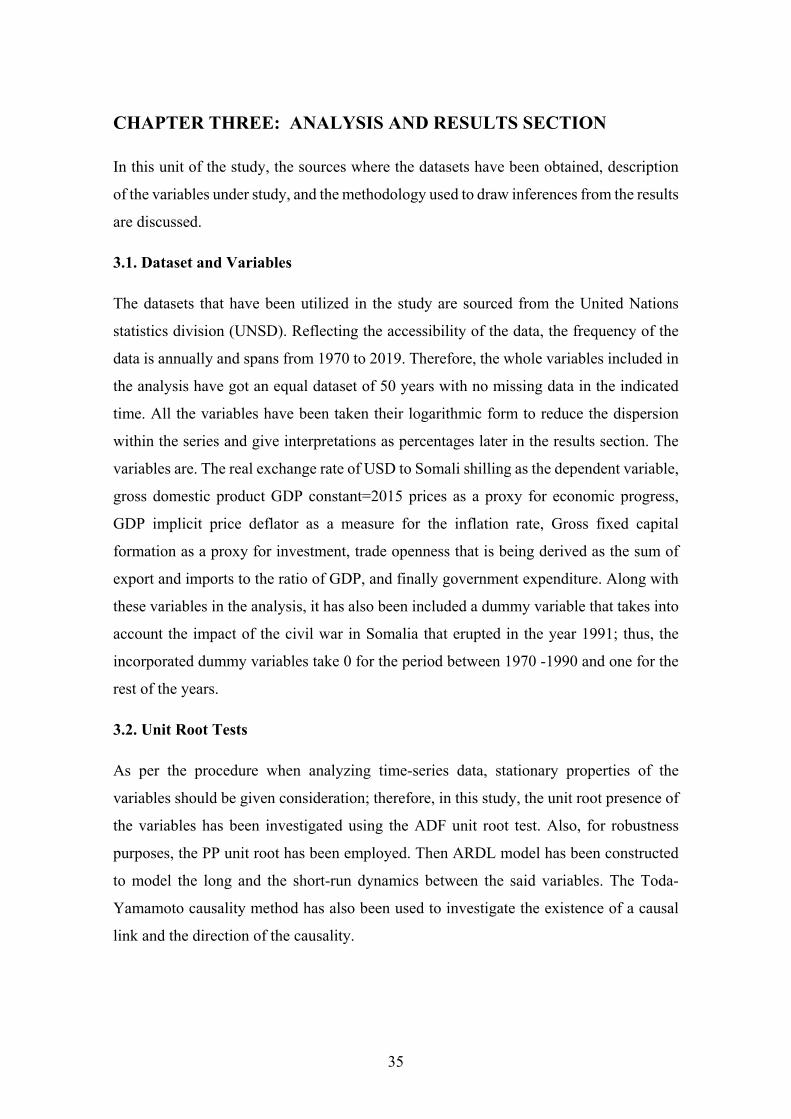
35

CHAPTER THREE: ANALYSIS AND RESULTS SECTION

In this unit of the study, the sources where the datasets have been obtained, description

of the variables under study, and the methodology used to draw inferences from the results

are discussed.

3.1. Dataset and Variables

The datasets that have been utilized in the study are sourced from the United Nations

statistics division (UNSD). Reflecting the accessibility of the data, the frequency of the

data is annually and spans from 1970 to 2019. Therefore, the whole variables included in

the analysis have got an equal dataset of 50 years with no missing data in the indicated

time. All the variables have been taken their logarithmic form to reduce the dispersion

within the series and give interpretations as percentages later in the results section. The

variables are. The real exchange rate of USD to Somali shilling as the dependent variable,

gross domestic product GDP constant=2015 prices as a proxy for economic progress,

GDP implicit price deflator as a measure for the inflation rate, Gross fixed capital

formation as a proxy for investment, trade openness that is being derived as the sum of

export and imports to the ratio of GDP, and finally government expenditure. Along with

these variables in the analysis, it has also been included a dummy variable that takes into

account the impact of the civil war in Somalia that erupted in the year 1991; thus, the

incorporated dummy variables take 0 for the period between 1970 -1990 and one for the

rest of the years.

3.2. Unit Root Tests

As per the procedure when analyzing time-series data, stationary properties of the

variables should be given consideration; therefore, in this study, the unit root presence of

the variables has been investigated using the ADF unit root test. Also, for robustness

purposes, the PP unit root has been employed. Then ARDL model has been constructed

to model the long and the short-run dynamics between the said variables. The Toda-

Yamamoto causality method has also been used to investigate the existence of a causal

link and the direction of the causality.

36

3.2.1. Augmented Dickey-Fuller (ADF) Unit Root Test

Macroeconomic series often are not stationary at the level, and if used when I (0), it would

lead to a spurious regression (Granger & Newbold, 1974). Therefore, the stationary

properties of the series are investigated with unit root tests. Stationary time-series datasets

have a stable mean and variance that do not change overtime. Trending in time,

seasonality, and cyclical fluctuations cause the series to lose stability, and thus it is said

to be non-stationary series (Gujarati & Porter, 1999).

Unlike the Dickey-Fuller unit root test, the augmented Dicey-Fuller is used to overcome

the autocorrelation problem in the series, and the lagged version of the dependent variable

is added to the DF equation (Dickey &Fuller, 1979).

The equation for the ADF unit root test could be specified as follows.

∆𝑌𝑌𝑡𝑡 = 𝛿𝛿𝑌𝑌𝑡𝑡−1 + ∑ 𝛼𝛼∆𝑌𝑌𝑡𝑡−𝑖𝑖 + 𝜀𝜀𝑡𝑡 𝑚𝑚𝑖𝑖=1 (1)

∆𝑌𝑌𝑡𝑡 = 𝛽𝛽1 + 𝛿𝛿𝑌𝑌𝑡𝑡−1 + ∑ 𝛼𝛼∆𝑌𝑌𝑡𝑡−𝑖𝑖 + 𝜀𝜀𝑡𝑡 𝑚𝑚𝑖𝑖=1 (2)

∆𝑌𝑌𝑡𝑡 = 𝛽𝛽1 + 𝛽𝛽2𝑡𝑡 + 𝛿𝛿𝑌𝑌𝑡𝑡−1 + ∑ 𝛼𝛼∆𝑌𝑌𝑡𝑡−𝑖𝑖 + 𝜀𝜀𝑡𝑡 𝑚𝑚𝑖𝑖=1 (3)

Here, three equations are presented; the first one ∆Y series, is explained by its lagged

value and its differenced form to eliminate the autocorrelation problem. The first equation

is built on a random process as it doesn’t carry any deterministic part, both constant and

trend. Unlike the first one drift term, the second equation is included, while the last

equation composes of both deterministic terms of constant and the trend.

The following two hypotheses are tested in the ADF unit root tests.

𝐻𝐻0. 𝛿𝛿 = 0: Has a unit root.

𝐻𝐻𝑎𝑎. 𝛿𝛿 < 0: Does not have a unit root.

According to 𝐻𝐻0 hypothesis, the series is not stationary since the series contains a unit

root. While the alternate hypothesis 𝐻𝐻𝑎𝑎says the series is stationary since it doesn’t contain

a unit root (Dickey & Fuller, 1979).

37

3.2.2. Philips-Peron (PP) Unit Root Test

Phillips and Perron (1988) have put forward a nonparametric test that takes into account

the autocorrelation between the error terms by modifying the conventional Dickey-Fuller

method. Philips & Perron unit root testing is a renovation of the ADF test, and this

transformation removes the parameter dependency asymptotically. The conversion is

made to the test statistics, not the regression equation in the procedure (Phillips and

Perron, 1988).

For the Philips-Perron unit root test, the following equation should be considered.

𝑌𝑌𝑡𝑡 = 𝛼𝛼0∗ + 𝑎𝑎1∗𝑦𝑦𝑡𝑡−1 + 𝜀𝜀𝑡𝑡 (4)

𝑌𝑌𝑡𝑡 = 𝑎𝑎0~ + 𝑎𝑎1~𝑦𝑦𝑡𝑡−1 + 𝑎𝑎2~ �𝑡𝑡 −12𝑇𝑇� + 𝜀𝜀𝑡𝑡 (5)

In the equation, T depicts the number of observations, and 𝜀𝜀 represents the pure error

process.

The method is based on the postulation that the expected error terms (E= (𝜀𝜀t) = 0).

However, with the basic assumption of the PP data generating process, 𝑦𝑦𝑡𝑡 = 𝑦𝑦𝑡𝑡−1 + 𝜀𝜀𝑡𝑡

the coefficients of the 𝑎𝑎0∗ , and 𝑎𝑎1∗ is tested through the test statistics (Phillips-Perron,

1988).

3.3. ARDL Model

There are various methods that are used for testing the existence of long-term

relationships between the variables, among the most familiar approaches that are

employed in the econometric analysis include the methodology proposed by Johansen

(1988) and Johansen & Juselius (1990) test of co-integration, Engle &Granger (1987) co-

integration test, as well as the co-integration test technique developed by Pesaran et al.

(2001).

In doing co-integration analysis, variables with different integration orders could be

observed their co-integration feature by employing the model developed by Pesaran &

Shin (1995). The method is known as ARDL that is used to expose the co-integration

existence between the variables in the analysis, while the model incorporates a mixture

of both variables that are I (0) and I(1) integrated. The main motive why the study

38

implements this methodology could be summarized in these three points. First, the model

is appropriate in the case of undersized sample datasets (Pesaran et al., 2001). Secondly,

the ARDL model is able to capture both the long and short-run links between the

variables, and finally, the model is a better estimator when variables under consideration

are a combination of both I (0) and (1).

In the case of this study, the ARDL (𝑝𝑝, 𝑞𝑞1, 𝑞𝑞2, 𝑞𝑞3, 𝑞𝑞4, 𝑞𝑞5) model could be specified as

follows. (6)

∆𝐿𝐿𝐿𝐿𝐸𝐸𝐿𝐿𝐶𝐶𝑡𝑡 = 𝛼𝛼 + �∅∆𝐿𝐿𝐿𝐿𝐸𝐸𝐿𝐿𝐶𝐶𝑡𝑡−1 +𝑝𝑝

𝑖𝑖=𝑗𝑗

�𝛽𝛽∆𝐿𝐿𝐿𝐿𝐿𝐿𝐿𝐿𝑃𝑃𝑡𝑡−1

𝑞𝑞1

𝑖𝑖=𝑗𝑗

+ �𝜗𝜗∆𝐿𝐿𝐿𝐿𝐿𝐿𝐿𝐿𝐹𝐹𝑡𝑡−1 + �𝛾𝛾∆𝐿𝐿𝐿𝐿𝐿𝐿𝐸𝐸𝐿𝐿𝑡𝑡−1 +𝑞𝑞3

𝑖𝑖=𝑗𝑗

𝑞𝑞2

𝑖𝑖=𝑗𝑗

�𝛿𝛿∆𝐿𝐿𝐿𝐿𝐿𝐿𝐿𝐿𝑉𝑉𝑡𝑡−1 +𝑞𝑞4

𝑖𝑖=𝑗𝑗

�𝜑𝜑∆𝐿𝐿𝐿𝐿𝐿𝐿𝑃𝑃𝐿𝐿𝑡𝑡−1 +𝑞𝑞5

𝑖𝑖=𝑗𝑗

𝜆𝜆𝐿𝐿𝐿𝐿𝐸𝐸𝐿𝐿𝐶𝐶𝑡𝑡−1

+ 𝜆𝜆𝐿𝐿𝐿𝐿𝐿𝐿𝐿𝐿𝑃𝑃𝑡𝑡−1 + 𝜆𝜆𝐿𝐿𝐿𝐿𝐿𝐿𝐿𝐿𝐹𝐹𝑡𝑡−1 + 𝜆𝜆𝐿𝐿𝐿𝐿𝐿𝐿𝐸𝐸𝐿𝐿𝑡𝑡−1 + 𝜆𝜆𝐿𝐿𝐿𝐿𝐿𝐿𝐿𝐿𝑉𝑉𝑡𝑡−1 + 𝛽𝛽𝛽𝛽𝛽𝛽𝛽𝛽 + 𝜆𝜆𝐿𝐿𝐿𝐿𝐿𝐿𝑃𝑃𝐿𝐿𝑡𝑡−1 + 𝜀𝜀𝑡𝑡

Where LN is the natural log sign, ∆ indicates the difference operator, 𝛼𝛼represents the

constant term and∅, 𝛽𝛽,𝜗𝜗, 𝛾𝛾, 𝛿𝛿,𝜑𝜑, are the coefficient parameters of the short-run

estimations while 𝜆𝜆is the long-run estimator of the model, and 𝜀𝜀is the error term. It’s

noteworthy and irrefutable the impact that the civil war had on the financial system and

the economic progress in Somalia. Therefore; to avoid ignoring that impact, the model

has been included a dummy variable that counts the outbreak of the civil war in Somalia.

In this regard, the created dummy variable takes zero before the eruption of the civil war

and one from 1991, which was the time Somalia descended into chaos.

3.4. Bounds Test

To look into the presence of a cointegration link, the Bound test is applied, and the overall

significance of the coefficients is tested. The Bounds test sets upper and lower limits;

therefore, if the computed F-statistics is a value that is below the lower limit of the critical

value, the 𝐻𝐻0of no-integration is accepted. Similarly, contingent upon the computed F-

statistics is a value that exceeds the upper limit of the critical value, thenthe𝐻𝐻0is rejected,

and it said that the variables under consideration are co-integrated, Pesaran et al. (2001).

Once the co-integration relationship is assured, the error correction model specification

could be stepped on as the next step. The short-run dynamics model is constructed as

follows. (7)

39

∆𝐿𝐿𝐿𝐿𝐸𝐸𝐿𝐿𝐶𝐶𝑡𝑡 = 𝛼𝛼 + �∅∆𝐿𝐿𝐿𝐿𝐸𝐸𝐿𝐿𝐶𝐶𝑡𝑡−1 +𝑝𝑝

𝑖𝑖=𝑗𝑗

�𝛽𝛽∆𝐿𝐿𝐿𝐿𝐿𝐿𝐿𝐿𝑃𝑃𝑡𝑡−1

𝑞𝑞1

𝑖𝑖=𝑗𝑗

+ �𝜗𝜗∆𝐿𝐿𝐿𝐿𝐿𝐿𝐿𝐿𝐹𝐹𝑡𝑡−1 + �𝛾𝛾∆𝐿𝐿𝐿𝐿𝐿𝐿𝐸𝐸𝐿𝐿𝑡𝑡−1 +𝑞𝑞3

𝑖𝑖=𝑗𝑗

𝑞𝑞2

𝑖𝑖=𝑗𝑗

�𝛿𝛿∆𝐿𝐿𝐿𝐿𝐿𝐿𝐿𝐿𝑉𝑉𝑡𝑡−1 +𝑞𝑞4

𝑖𝑖=𝑗𝑗

�𝜑𝜑∆𝐿𝐿𝐿𝐿𝐿𝐿𝑃𝑃𝐿𝐿𝑡𝑡−1 +𝑞𝑞5

𝑖𝑖=𝑗𝑗

𝛽𝛽𝛽𝛽𝛽𝛽𝛽𝛽

+ 𝜆𝜆𝐸𝐸𝐶𝐶𝑀𝑀𝑡𝑡−1 +𝜇𝜇𝑡𝑡

In the above model, theα represents the constant term and ∅, 𝛽𝛽,𝜗𝜗, 𝛾𝛾, 𝛿𝛿,𝜑𝜑, are the

coefficient parameters of the short-run estimations. In this case,𝜆𝜆 term placed before the

error correction term depicts the long-run disequilibrium adjustment in the system. The

coefficient of the ECM term should be negative and significant to be interpretable

estimation (Engel & Granger, 1987).

3.5. Toda-Yamamoto Causality Test

For analysis on the causal relation, the study employs the Toda–Yamamoto causality test.

According to Toda-Yamamoto (1995), this approach has dominance over the frequently

practiced conventional Granger causality procedure as the maximum lag length is

thoroughly decided based on the VAR system, which does not change, consequently

yields consistent and reliable inferences. This method of the Toda & Yamamoto causality

test involves applying a modified Wald statistic (MWALD) from the non‐causality

hypothesis of the traditional Granger (1969). After establishing the VAR model, the

causality link among the variables is investigated using the Toda-Yamamoto causality

technique.

Toda-Yamamoto’s (1995) causality analysis was developed based on the corrected VAR

model to investigate Granger causality. In the Toda-Yamamoto test, the length of the lags

included (k) and the maximum integration order (𝑑𝑑𝑚𝑚𝑎𝑎𝑚𝑚) are important to determine. After

determining these two values 𝑘𝑘 + 𝑑𝑑𝑚𝑚𝑎𝑎𝑚𝑚 the VAR model is estimated, and causality could

also be tested.

To perform the Toda Yamamoto causality test, the VAR 𝑘𝑘 + 𝑑𝑑𝑚𝑚𝑎𝑎𝑚𝑚 the model could be

specified as follows.

𝑌𝑌𝑡𝑡 = 𝛾𝛾0 + ∑ 𝛼𝛼1𝑖𝑖𝑦𝑦𝑡𝑡−1 +𝑘𝑘+𝑑𝑑𝑚𝑚𝑚𝑚𝑚𝑚𝑖𝑖=1 ∑ 𝛽𝛽2𝑖𝑖𝑥𝑥𝑡𝑡−1 +𝑘𝑘+𝑑𝑑𝑚𝑚𝑚𝑚𝑚𝑚

𝑖𝑖=1 𝜀𝜀1𝑡𝑡 (8)

𝐿𝐿𝑡𝑡 = 𝛾𝛾0 + ∑ 𝛼𝛼2𝑖𝑖𝑦𝑦𝑡𝑡−1 +𝑘𝑘+𝑑𝑑𝑚𝑚𝑚𝑚𝑚𝑚𝑖𝑖=1 ∑ 𝛽𝛽2𝑖𝑖𝑥𝑥𝑡𝑡−1 +𝑘𝑘+𝑑𝑑𝑚𝑚𝑚𝑚𝑚𝑚

𝑖𝑖=1 𝜀𝜀2𝑡𝑡 (9)

40

The null hypothesis of the model equation 4 says that variable X doesn’t Granger cause

variable Y; in other words, there’s no direct causality from X to Y. The null

hypothesis 𝐻𝐻0.𝛽𝛽1𝑖𝑖 = 0. While the alternative hypothesis is established as X Granger

causes Y, which indicates that there’s causality running from X to Y. The alternative

hypothesis𝐻𝐻1.𝛽𝛽1𝑖𝑖 ≠ 0.

3.6. Findings

This study employed the ARDL models and the Toda-Yamamoto causality techniques to

investigate the dynamic and causal link between exchange rate and the selected

macroeconomic variables. At the outset of every analysis with time series structure, the

presence of unit root in the series is tested, therefore using the ADF and PP unit root tests,

the stationarity properties of the series were investigated.

3.7. Unit Root Tests

Stationarity properties of the real exchange rates and the other selected variables were

tested by employing the ADF unit root. The outcomes of the ADF and PP unit root test

were interpreted by considering the probability value. Consequently, if the absolute value

of the ADF is less than the critical value, the𝐻𝐻0 hypothesis won’t be rejected, and since

it is found a unit root in the series, it is said that the series isn’t stationary. In the unit root

outcome, if the ADF absolute value is higher than the given critical value, then the

alternative hypothesis𝐻𝐻1which states that the series contains a unit root is accepted. To

put it another way, it indicates that the series is stationary (Dickey & Fuller, 1979). For

robustness purposes, it has also been employed PP unit test for cross-checking the result

of the ADF test.

Table 3: Results of the ADF and PP unit root tests

Level First difference Variables ADF PP ADF PP LOGEXC -1.23910 -0.993846 -3.259349 *** -3.237164*** LOGINF -2.35914 -1.954650 -5.837778*** -5.954975***

41

LOGGEX -4.314783*** -4.313781*** -1.728509 -7.073519*** LOGINV -2.149790 -2.095707 -8.397852*** -8.390040*** LOGTOP -1.424415 -1.600809 -8.814509*** -11.09343*** LOGGDP -1.072030 -1.235569 -7.353065*** -7.356879***

Note. *** denotes significance at %5 level

When the figures in Table 3 are examined, the findings of the ADF and PP unit root tests

have been presented. The left side of the table demonstrates the level value of the

variables for both the ADF and PP unit root tests. The exchange rate variable, which is

the main variable of the study, is abbreviated as LOGEXC. Similarly, the predictors

LOGINF, LOGGEX, LOGINV, LOGTOP, and LOGGDP also respectively express

inflation rate, government expenditure, investment, trade openness, and gross domestic

product that are usually used as a proxy variable or indicator for economic growth.

The results of both ADF and PP stationarity tests have proved that the entire variables

under consideration integrated of order one (1) except the government expenditure

variable, which is stationary at the level, and the rest of the variables turn out to be

stationary after when their first differences are taken. At the first difference, the P-value

of all the series is less than 0.05, which indicates that the null hypothesis of the series is

non-stationary or has a unit root should be rejected and accepted the alternative

hypothesis. Since the orders of the integration of the whole variables are determined, the

subsequent step that is being carried out is to run the already specified ARDL model. The

following are the results of the ARDL Bounds-test

Table 4: Bounds test results

Null Hypothesis. No long-run relationships exist Test Statistic Value K F-statistic 11.16138 6

Critical Value Bounds Significance I0 Bound I1 Bound 10% 1.99 2.94 5% 2.27 3.28 2.5% 2.55 3.61 1% 2.88 3.99 According to the above results, the following hypothesis is tested.𝐻𝐻0. 𝜆𝜆 = 𝜆𝜆 = 𝜆𝜆 = 𝜆𝜆 =

𝜆𝜆 = 𝜆𝜆 = 0The null hypothesis states that the coefficients of long-run parameters are all

zero, which means no long-run association exists, against the alternative hypothesis that

there is a cointegrating relationship.

42

𝐻𝐻1. 𝜆𝜆 ≠ 𝜆𝜆 ≠ 𝜆𝜆 ≠ 𝜆𝜆 ≠ 𝜆𝜆 ≠ 𝜆𝜆 ≠ 0

As the result shows, the Bounds test computed F-statistics has a value above all the upper

critical limit values, which concludes that the null hypothesis of no long-run association

is rejected. The alternative hypothesis states that the study variables are co-integrated and

have a long-run connection is accepted. Once the existence of the co-integration is

assured, the dynamics of the short-run model could be specified.

The following is the output estimation of the ARDL based ECM.

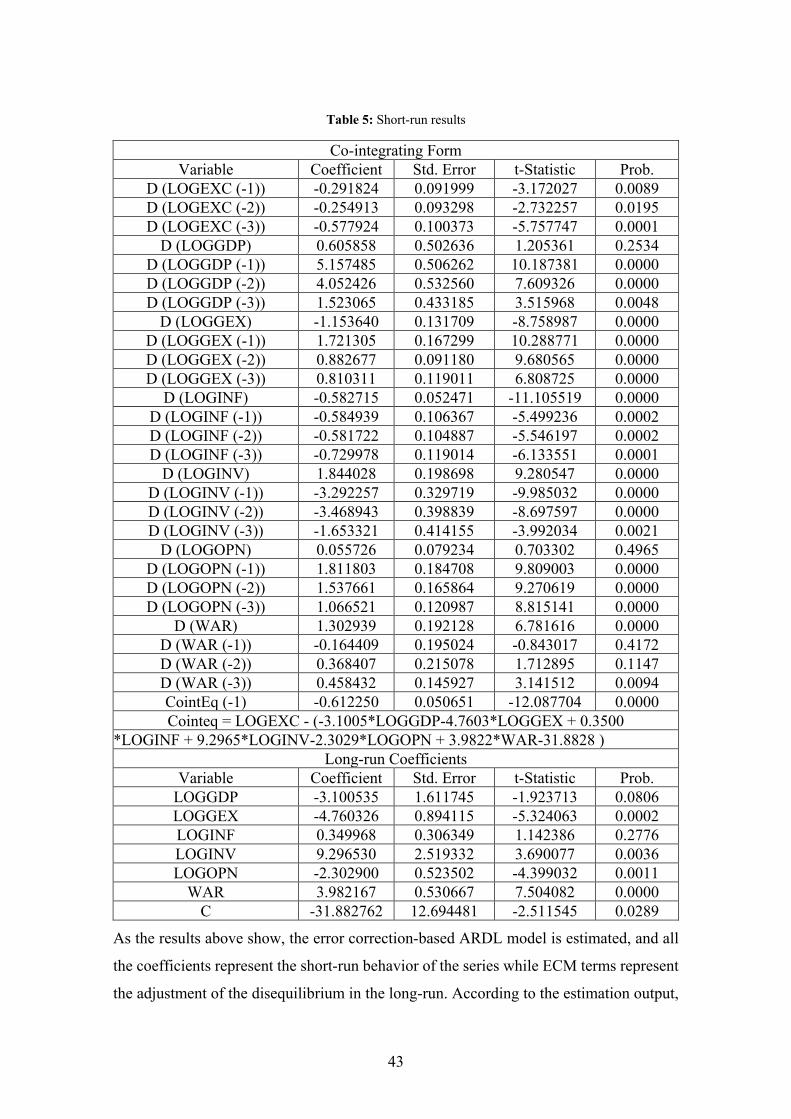
43

Table 5: Short-run results

Co-integrating Form Variable Coefficient Std. Error t-Statistic Prob.

D (LOGEXC (-1)) -0.291824 0.091999 -3.172027 0.0089 D (LOGEXC (-2)) -0.254913 0.093298 -2.732257 0.0195 D (LOGEXC (-3)) -0.577924 0.100373 -5.757747 0.0001

D (LOGGDP) 0.605858 0.502636 1.205361 0.2534 D (LOGGDP (-1)) 5.157485 0.506262 10.187381 0.0000 D (LOGGDP (-2)) 4.052426 0.532560 7.609326 0.0000 D (LOGGDP (-3)) 1.523065 0.433185 3.515968 0.0048

D (LOGGEX) -1.153640 0.131709 -8.758987 0.0000 D (LOGGEX (-1)) 1.721305 0.167299 10.288771 0.0000 D (LOGGEX (-2)) 0.882677 0.091180 9.680565 0.0000 D (LOGGEX (-3)) 0.810311 0.119011 6.808725 0.0000

D (LOGINF) -0.582715 0.052471 -11.105519 0.0000 D (LOGINF (-1)) -0.584939 0.106367 -5.499236 0.0002 D (LOGINF (-2)) -0.581722 0.104887 -5.546197 0.0002 D (LOGINF (-3)) -0.729978 0.119014 -6.133551 0.0001

D (LOGINV) 1.844028 0.198698 9.280547 0.0000 D (LOGINV (-1)) -3.292257 0.329719 -9.985032 0.0000 D (LOGINV (-2)) -3.468943 0.398839 -8.697597 0.0000 D (LOGINV (-3)) -1.653321 0.414155 -3.992034 0.0021

D (LOGOPN) 0.055726 0.079234 0.703302 0.4965 D (LOGOPN (-1)) 1.811803 0.184708 9.809003 0.0000 D (LOGOPN (-2)) 1.537661 0.165864 9.270619 0.0000 D (LOGOPN (-3)) 1.066521 0.120987 8.815141 0.0000

D (WAR) 1.302939 0.192128 6.781616 0.0000 D (WAR (-1)) -0.164409 0.195024 -0.843017 0.4172 D (WAR (-2)) 0.368407 0.215078 1.712895 0.1147 D (WAR (-3)) 0.458432 0.145927 3.141512 0.0094 CointEq (-1) -0.612250 0.050651 -12.087704 0.0000 Cointeq = LOGEXC - (-3.1005*LOGGDP-4.7603*LOGGEX + 0.3500

*LOGINF + 9.2965*LOGINV-2.3029*LOGOPN + 3.9822*WAR-31.8828 ) Long-run Coefficients

Variable Coefficient Std. Error t-Statistic Prob. LOGGDP -3.100535 1.611745 -1.923713 0.0806 LOGGEX -4.760326 0.894115 -5.324063 0.0002 LOGINF 0.349968 0.306349 1.142386 0.2776 LOGINV 9.296530 2.519332 3.690077 0.0036 LOGOPN -2.302900 0.523502 -4.399032 0.0011

WAR 3.982167 0.530667 7.504082 0.0000 C -31.882762 12.694481 -2.511545 0.0289

As the results above show, the error correction-based ARDL model is estimated, and all

the coefficients represent the short-run behavior of the series while ECM terms represent

the adjustment of the disequilibrium in the long-run. According to the estimation output,

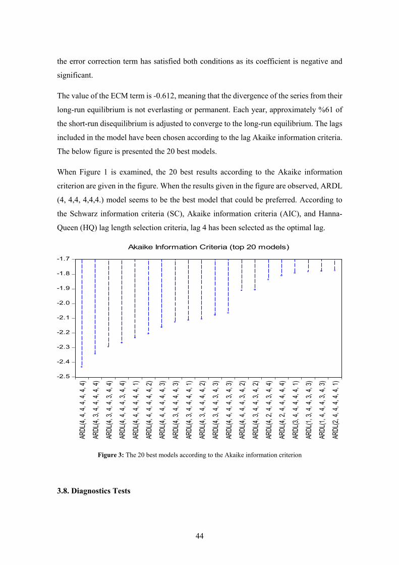
44

the error correction term has satisfied both conditions as its coefficient is negative and

significant.

The value of the ECM term is -0.612, meaning that the divergence of the series from their

long-run equilibrium is not everlasting or permanent. Each year, approximately %61 of

the short-run disequilibrium is adjusted to converge to the long-run equilibrium. The lags

included in the model have been chosen according to the lag Akaike information criteria.

The below figure is presented the 20 best models.

When Figure 1 is examined, the 20 best results according to the Akaike information

criterion are given in the figure. When the results given in the figure are observed, ARDL

(4, 4,4, 4,4,4.) model seems to be the best model that could be preferred. According to

the Schwarz information criteria (SC), Akaike information criteria (AIC), and Hanna-

Queen (HQ) lag length selection criteria, lag 4 has been selected as the optimal lag.

-2.5

-2.4

-2.3

-2.2

-2.1

-2.0

-1.9

-1.8

-1.7

ARDL

(4, 4,

4, 4,

4, 4,

4)

ARDL

(4, 3,

4, 4,

4, 4,

4)

ARDL

(4, 3,

4, 4,

3, 4,

4)

ARDL

(4, 4,

4, 4,

3, 4,

4)

ARDL

(4, 4,

4, 4,

4, 4,

1)

ARDL

(4, 4,

4, 4,

4, 4,

2)

ARDL

(4, 4,

4, 4,

4, 4,

3)

ARDL

(4, 3,

4, 4,

4, 4,

3)

ARDL

(4, 3,

4, 4,

4, 4,

1)

ARDL

(4, 3,

4, 4,

4, 4,

2)

ARDL

(4, 3,

4, 4,

3, 4,

3)

ARDL

(4, 4,

4, 4,

3, 4,

3)

ARDL

(4, 4,

4, 4,

3, 4,

2)

ARDL

(4, 3,

4, 4,

3, 4,

2)

ARDL

(4, 2,

4, 4,

3, 4,

4)

ARDL

(4, 2,

4, 4,

4, 4,

4)

ARDL

(3, 4,

4, 4,

4, 4,

1)

ARDL

(1, 3,

4, 4,

3, 4,

3)

ARDL

(1, 4,

4, 4,

3, 4,

3)

ARDL

(2, 4,

4, 4,

4, 4,

1)

Akaike Information Criteria (top 20 models)

Figure 3: The 20 best models according to the Akaike information criterion

3.8. Diagnostics Tests

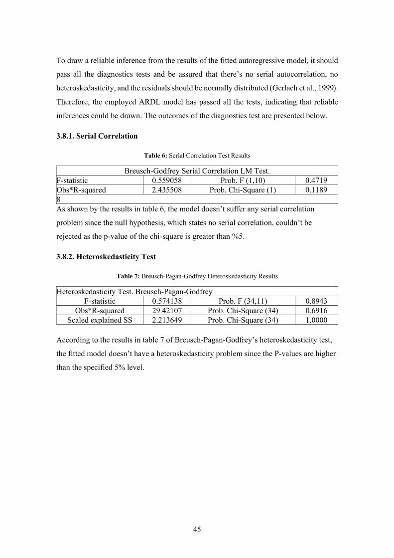
45

To draw a reliable inference from the results of the fitted autoregressive model, it should

pass all the diagnostics tests and be assured that there’s no serial autocorrelation, no

heteroskedasticity, and the residuals should be normally distributed (Gerlach et al., 1999).

Therefore, the employed ARDL model has passed all the tests, indicating that reliable

inferences could be drawn. The outcomes of the diagnostics test are presented below.

3.8.1. Serial Correlation

Table 6: Serial Correlation Test Results

Breusch-Godfrey Serial Correlation LM Test. F-statistic 0.559058 Prob. F (1,10) 0.4719 Obs*R-squared 2.435508 Prob. Chi-Square (1) 0.1189 8 As shown by the results in table 6, the model doesn’t suffer any serial correlation

problem since the null hypothesis, which states no serial correlation, couldn’t be

rejected as the p-value of the chi-square is greater than %5.

3.8.2. Heteroskedasticity Test

Table 7: Breusch-Pagan-Godfrey Heteroskedasticity Results

Heteroskedasticity Test. Breusch-Pagan-Godfrey F-statistic 0.574138 Prob. F (34,11) 0.8943

Obs*R-squared 29.42107 Prob. Chi-Square (34) 0.6916 Scaled explained SS 2.213649 Prob. Chi-Square (34) 1.0000

According to the results in table 7 of Breusch-Pagan-Godfrey’s heteroskedasticity test,

the fitted model doesn’t have a heteroskedasticity problem since the P-values are higher

than the specified 5% level.

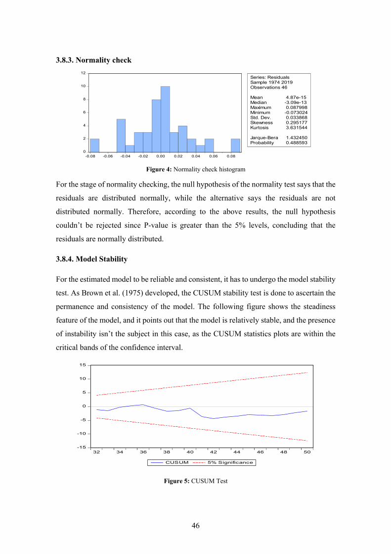
46

3.8.3. Normality check

0

2

4

6

8

10

12

-0.08 -0.06 -0.04 -0.02 0.00 0.02 0.04 0.06 0.08

Series: ResidualsSample 1974 2019Observations 46

Mean 4.87e-15Median -3.09e-13Maximum 0.087998Minimum -0.073024Std. Dev. 0.033868Skewness 0.295177Kurtosis 3.631544

Jarque-Bera 1.432450Probability 0.488593

Figure 4: Normality check histogram

For the stage of normality checking, the null hypothesis of the normality test says that the

residuals are distributed normally, while the alternative says the residuals are not

distributed normally. Therefore, according to the above results, the null hypothesis

couldn’t be rejected since P-value is greater than the 5% levels, concluding that the

residuals are normally distributed.

3.8.4. Model Stability

For the estimated model to be reliable and consistent, it has to undergo the model stability

test. As Brown et al. (1975) developed, the CUSUM stability test is done to ascertain the

permanence and consistency of the model. The following figure shows the steadiness

feature of the model, and it points out that the model is relatively stable, and the presence

of instability isn’t the subject in this case, as the CUSUM statistics plots are within the

critical bands of the confidence interval.

-15

-10

-5

0

5

10

15

32 34 36 38 40 42 44 46 48 50

CUSUM 5% Significance

Figure 5: CUSUM Test

47

-0.4

0.0

0.4

0.8

1.2

1.6

09 10 11 12 13 14 15 16 17 18 19

CUSUM of Squares 5% Significance

Figure 6: CUSUM Square Test

-.08

-.04

.00

.04

.08

.12

0

2

4

6

8

10

12

1975 1980 1985 1990 1995 2000 2005 2010 2015

Residual Actual Fitted

Figure 7: Examining the Graph of Residuals

Looking at the graph of the residuals, the lines of the observed values and estimated

values overlap closely on one another till they became indistinguishable, thus pointing

out that the model estimation was successful, and it can be said that the model gives good

results.

3.9. Toda-Yamamoto Causality Test Findings

Unlike other causality tests, the one introduced by Toda-Yamamoto (1995) has the

exclusive lead of allowing the variables to be tested their causal relationship regardless

of their level of the order of integration since co-integration is ignored in this test. Once

assured of the integration order of the series, the subsequent move is to estimate the VAR

48

model; therefore, how many lags to include in the model should be decided. The below

table has presented the lags to be chosen.

Table 8: Lag length determination according to the lag selection criteria

Note. *depicts lag orders selected by the lag selection criterions

According to the lag result of the lag selection criteria, there’s uniformity in the chosen

lag order as all the criterions marked the 4th lag as the optimal lag to be included in the

analysis of the Toda-Yamamoto causality test.

The following table demonstrates the output of the Toda-Yamamoto causality.

Table 9: Toda-Yamamoto Causality Test Findings

Null hypothesis Chi-square P-value Granger causality GDP doesn’t granger cause EXC 5.258498 0.3852 Accept EXC doesn’t granger cause GDP 52.26370 0.0000 Reject INF doesn’t granger cause EXC 10.39830 0.0325 Reject EXC doesn’t granger cause INF 4.753046 0.4468 Accept INV doesn’t granger cause EXC 2.407219 0.7904 Accept EXC doesn’t granger cause INV 21.51971 0.0006 Reject OPN doesn’t granger cause EXC 6.772849 0.2381 Accept EXC doesn’t granger cause OPN 26.31030 0.0001 Reject GEX doesn’t granger cause EXC 5.891468 0.3169 Accept EXC doesn’t granger cause GEX 36.23222 0.0000 Reject

Source. Author’s computations

The result in Table 9 demonstrates the Toda & Yamamoto causality analysis outcome

between the exchange rate and the other predictors such as the gross domestic product,

inflation rate, investment and government expenditure, and trade openness.

According to the test result, there’s no causality from gross domestic product to the

exchange rate since the P-values are greater than 0.05. In other words, causality running

from exchange rate to gross domestic product has been observed as the P-values are less

than 0.05 concluding to the rejection of the 𝐻𝐻0and accepting the𝐻𝐻1hypothesis. Following

Lag LogL LR FPE AIC SC HQ 0 -30.77660 NA 1.99e-07 1.598983 1.837501 1.688333 1 202.9337 396.2915 3.74e-11 -6.997119 -5.327490* -6.371666 2 245.6449 61.28120 3.03e-11 -7.288908 -4.188168 -6.127352 3 315.4198 81.90974 8.68e-12 -8.757385 -4.225534 -7.059726 4 392.8277 70.67672* 2.30e-12* -10.55773* -4.594764 -8.323964*

49

the test results, a causal relationship running from inflation rate to exchange rate has been

detected as the P-values of the result is less than 5%. In comparison, the opposite of the

exchange rate to inflation hasn’t been true since the P-values are greater than 5%.

Regarding the test result, there’s no causality from investment to the exchange rate as the

P-value associated with the result is greater than 5%. In contrast, the opposite direction

shows a causal link, meaning that there’s a causality running from exchange rates to the

investment since the P-value associated with it is less than 5%. Consistent with the Toda

& Yamamoto causality test results, the established null hypothesis of trade openness

doesn’t Granger cause exchange rate couldn’t be rejected since the P-value is greater than

5%. Meanwhile, the exchange rate to trade openness has been confirmed as the P-value

is less than 5%.

50

DISCUSSIONS AND RECOMMENDATIONS

This research has been revisited the recent empirical studies on the exchange rate’s

interaction with other key macroeconomic variables in various countries and different

periods. In our case, the study discussed the dynamic and the causal link between

exchange rate and some selected predictors over the period between 1970 and 2019. The

dataset used in the study has been sourced from the United Nations Statistics Division.

The variables indicators were the real exchange rate that has been used as the dependent

variable, the gross fixed capital formation that has been used as a proxy variable to

represent domestic investment, the inflation rate, the government expenditure, and the

trade openness. Because Somalia is recovering from prolonged insecurity and civil war

of almost three decades, the study incorporates a dummy variable to count for the impact

of the civil war on the currency and the exchange rate changes. The dummy variable has

been fitted in between the most chaotic and stateless eras. It has been designated to take

0 for the time between 1970 and 1990 and 1 from 1991, which was the year Somalia

descended into the civil war.

The study used an assortment of econometric techniques with the help of the E-views 9

software package and using the ADF unit root test to examine the integration order of the

series. For robustness and consistency purposes, the PP test unit root test has been

employed. Afterward, it has been specified ARDL to capture the long-run, and the short-

run dynamics of said variables. After that, the Toda-Yamamoto causality test has been

utilized to ascertain a causal link and the direction of the causality. Subsequently, to have

healthy estimations, the fitted model has gone under several diagnostics tests such as the

serial correlation test to make certain that the model doesn’t suffer from auto-correlation

problems and heteroskedasticity test normality check CUSUM and CUSUM square tests.

As expected, the findings of the dynamic model have been consistent with some of the

previous empirical works of literature. From the reported results in Table 5, it can be

drawn the inference of the short-run coefficients. According to the findings presented in

Table 5, the coefficient of the GDP, which was representing economic growth, is lag

sensitive. The associated coefficients are all positive and statistically significant at all

lags, stating that being held everything else constant, a one percent change in the gross

domestic product brings a depreciation in the exchange rates, and this outcome is in line

51

with the empirical research findings of Habib et al. (2017) from a panel analysis.

However, the impact was not the same both in the short and long-run as the coefficient of

the log run had a negative sign but statically insignificant, as also revealed by Tang (2015)

in their study on China. In consistence with the results in Table 5, the coefficients of

government expenditure are all statistically significant but had mixed signs. However, in

the short-run, the coefficient of the government expenditure is negative, indicating that

assuming everything else constant, a one percent rise in government expenditure will

result in appreciation of the exchange rate by 1.1%. The findings are consistent with those

of Galstyan& Lane (2009), Monacelli & Perotti (2010), Miyamoto et al. (2019), and

contrary with those of Ravn et al. (2007) and Bajo-Rubio et al. (2020).

Similarly, the coefficients of the inflation rates are all negative and statistically

significant. According to the results in Table 5, keeping everything else the same, a rise

in inflation rates is expected to appreciate the exchange rates by %0.5. On the other hand,

it had a contrary impact in the long-run but statistically negligible. Correspondingly, the

coefficient representing investment had a statistically negative coefficient, and economic

wise in it could be interpreted as, assuming everything else remains constant, a one

percent rise in domestic investment is projected to generate the exchange rate to

appreciate by %1.8 in the short-run, while in the long-run investment had a different

impact on the exchange as it is estimated that a change in domestic investment leads the

exchange rates to depreciate by %9.

Trade openness coefficients also had mixed effects in the long-run and the short-run

terms. According to Table 5, the coefficient of trade openness is negligible in the short-

run. In contrast, the coefficient associated with trade openness is negative and statistically

considerable in the long-run, implying that assuming everything else stays the same, a

one percent change in trade openness the exchange rate is expected to appreciate by %2.3

in the long-run. Another key indicator was in the model to capture the impact of the civil

war on the exchange rate dynamics, and it had consistent results in both the long-run and

the short-run. Its coefficients figures were negative and statistically significant.

According to the output in Table 5, for each year of civil war, the exchange rate is

anticipated to depreciate in both the short-run and the long-run by %1.3 and 3.9,

respectively. The error correction term has met the conditions as it’s statistically

52

significant and has a negative value, which indicates that the disequilibrium in the process

isn’t long-lasting and permanent. It is anticipated that the imbalances will self-adjust with

an adjustment speed of % 61 each year.

From the Toda-Yamamoto causality analysis results in Table 9, the null hypothesis of

exchange rate doesn’t Granger cause GDP has been firmly rejected with strong P-value,

indicating that there’s a unidirectional causal relationship. According to the causality

results in Table 9, the inflation rate Granger causes the exchange rate as its null hypothesis

of no causality has been rejected. Correspondingly, the findings of the causality analysis

imply that the exchange rates Granger cause the domestic investment. Similarly, the null

hypothesis of no causality between the trade openness and exchange rates has been

rejected, and according to the results in Table 9, the exchange rate Granger causes

openness. Therefore, there’s a one-way causal relationship. To end with, as its P-value is

very small, the exchange rate Granger causes government spending; consequently, there’s

a unidirectional relationship between the said variables.

On a final note, it has been found that the variables selected for the study had different

links with the exchange rate, and their impacts had also been mixed in both favorable and

unfavorable effects. This research work adds fresh findings to the previous literature on

determining the relationship and impact of variables under consideration with the

exchange rate. The findings have been confirmed with some of the previous literature,

while others had a contrary conclusion. In recommendation, the study suggests to the

policymakers or the authorities of the central bank to be observant of their policies related

to the fiscal and monetary policies as they might have both adverse and favorable effects

depending on the period and the rationale behind its application, as well as the

government, to consider policies that incentivize trade openness as it has favorable effect

with the exchange rate contingent upon Somalia. It is also imperative to note the

devastating effects of the civil war and the instability on the country's economy in general

as the insecurity induces the large businesses to dissolve and stagnate, the key revenue-

generating public sources to fade away, which eventually leads to a shortage of

government revenue that harms the economic progress of the country. Consequently, to

avoid economic hardship or even worse impact, elevated priority should be given to the

stability and the general security of the country.

53

The study also recommends that future researchers consider including some other

relevant variables into the model. There might be better predictors that could’ve been

included in the study and would explain the exchange rate better but didn’t happen due

to constraints such as limited data availability. Moreover, the study suggests the future

potential researchers reexamine the connection of the exchange rates with these variables

in terms of industrial separation to gauge the impact and see whether it would lead to a

different conclusion.

54

REFERENCES

Abdurehman, A. A., &Hacilar, S. (2016). The relationship between exchange rate and inflation. An empirical study of Turkey. International Journal of Economics and Financial Issues, 6 (4), 1454–1459.

Adetiloye, K. A. (2010). Exchange rates and the consumer price index in Nigeria. A causality approach. Journal of emerging trends in economics and management sciences, 1 (2), 114-120.

Aftab, Z. (2002). The long-run and short-run impact of exchange rate devaluation on Pakistan's trade performance. The Pakistan Development Review, 277-286.

Ahmad, A., Ahmad, N., & Ali, S. (2013). Exchange rate and economic growth in Pakistan (1975-2011). Ahmad, Arslan, Najid Ahmad, and Sharafat Ali." Exchange Rate and Economic Growth in Pakistan (1975-2011)." (2013), 740-746.

Ahmad, E., & Ali, S. A. (1999). Relationship between exchange rate and inflation. Pakistan Economic and Social Review, 139-154.

Ahmad, E., & Ali, S. A. (2019). Pakistan Institute of Development Economics, Islamabad Exchange Rate, and Inflation Dynamics Author( s ). Eatzaz Ahmad and Saima Ahmed Ali Source . The Pakistan Development Review, Vol . 38, No. 3( Autumn 1999 ), pp. 235-251 Published by . Pakistan,38 (3), 235–251.

Aizenman, J., &Jinjarak, Y. (2011). The Fiscal Stimulus of 2009–2010. Trade Openness, Fiscal Space, and Exchange Rate Adjustment. NBER International Seminar on Macroeconomics (Vol. 8). https.//doi.org/10.1086/663626

Aizenman, J., &Riera-Crichton, D. (2008). Real exchange rate and international reserves in an era of growing financial and trade integration. Review of Economics and Statistics, 90 (4), 812–815. https.//doi.org/10.1162/rest.90.4.812

Albuquerque, C. R., & Portugal, M. S. (2005). Exchange rate and inflation. a case of sulkiness of volatility. UFRGS, Departamento de Economia, texto para discussão, (1).

Ali, A. I., Ajibola, I. O., Omotosho, B. S., Adetoba, O. O., &Adeleke, A. O. (2015). Real exchange rate misalignment and economic growth in Nigeria. CBN Journal of Applied Statistics, 6 (2), 103-131.

Arrangements, E., & Restrictions, E. (2019). Exchange Arrangements and Exchange Restrictions.

Asad, I., Ahmad, N., & Hussain, Z. (2012). Impact of real effective exchange rate on inflation in Pakistan. Asian Economic and Financial Review, 2 (8), 983.

Asari, F. F. A. H., Baharuddin, N. S., Jusoh, N., Mohamad, Z., Shamsudin, N., &Jusoff, K. (2011). A vector error correction model (VECM) approach in explaining the

55

relationship between interest rate and inflation towards exchange rate volatility in Malaysia. World Applied Sciences Journal, 12 (3), 49-56.

Bahmani-Oskooee, M. (2001). Nominal and real effective exchange rates of Middle Eastern countries and their trade performance. Applied Economics, 33 (1), 103-111.

Bahmani‐Oskooee, M., Halicioglu, F., & Neumann, R. (2018). Domestic investment responses to changes in the real exchange rate. Asymmetries of appreciation versus depreciation. International Journal of Finance & Economics, 23 (4), 362-375.

Bailliu, J., &Fujii, E. (2011). Exchange Rate Pass-Through and the Inflation Environment in Industrialized Countries. An Empirical Investigation. SSRN Electronic Journal. https.//doi.org/10.2139/ssrn.560762

Bajo-Rubio, O., Berke, B., &Esteve, V. (2020). Fiscal policy and the real exchange rate. some evidence from Spain. Empirica, 47 (2), 267-280.

Bayraktutan, Y., &Arslan, İ. (2003). Exchange rate in Turkey, imports and inflation relationship. econometric analysis (1980-2000). AfyonKocatepe University, Journal of II BF , 5 (2), 89-104.

Bhandari, R., &Upadhyaya, K. P. (2010). Panel data evidence of the impact of exchange rate uncertainty on private investment in South-east Asia. Applied Economics, 42 (1), 57-61.

Bleaney, M., &Tian, M. (2014). Exchange rates and trade balance adjustment. a multi-country empirical analysis. Open Economies Review, 25 (4), 655-675.

Bogetic, Z. (2000). Official dollarization. Current experiences and issues. Cato J., 20, 179.

Boyd, D., Caporale, G. M., & Smith, R. (2001). Real exchange rate effects on the balance of trade. cointegration and the Marshall–Lerner condition. International Journal of Finance & Economics, 6 (3), 187-200.

Brada, J. C., Kutan, A. M., & Zhou, S. (1997). The exchange rate and the balance of trade. the Turkish experience. The Journal of Development Studies, 33 (5), 675-692.

Brown, R. L., Durbin, J., & Evans, J. M. (1975). Techniques for testing the constancy of regression relationships over time. Journal of the Royal Statistical Society. Series B (Methodological), 37 (2), 149-163.

Byrne, J. P., & Philip Davis, E. (2005). The impact of short‐and long‐run exchange rate uncertainty on investment. A panel study of industrial countries. Oxford Bulletin of Economics and Statistics, 67 (3), 307-329.

Calvo, G. A., & Reinhart, C. M. (2002). Fear of floating. The Quarterly journal of economics, 117 (2), 379-408.

56

Calvo, G. A., & Reinhart, C. M. (2002). Fear of floating. The Quarterly journal of economics, 117 (2), 379-408.

Campa, J. M., & Goldberg, L. S. (1999). Investment, pass‐through, and exchange rates. a cross‐country comparison. International Economic Review, 40 (2), 287-314.

Cassel, G. (1918). Abnormal deviations in international exchanges. The Economic Journal, 28 (112), 413-415.

Catão, L. A. (2007). Why real exchange rates?. Finance & Development, 44 (003).

Chen, M., & Hu, X. (2018). Linkage between consumer price index and purchasing power parity. Theoretic and empirical study. The Journal of International Trade & Economic Development, 27 (7), 729-760.

Chen, Y., & Liu, D. (2018). Government spending shocks and the real exchange rate in China. Evidence from a sign-restricted VAR model. Economic Modelling, 68, 543-554.

Chowdhury, M. T. H., Bhattacharya, P. S., Mallick, D., &Ulubaşoğlu, M. A. (2016). Exchange rate regimes and fiscal discipline. The role of trade openness. International Review of Economics and Finance, 45, 106–128. https.//doi.org/10.1016/j.iref.2016.04.013

De Facto Classification of Exchange Rate Regimes and Monetary Policy Frameworks, April 31, 2008https.//www.imf.org/external/np/mfd/er/2008/eng/0408.htm Date accessed May 2021.

Di Giorgio, G., Nisticò, S., &Traficante, G. (2018). Government spending and the exchange rate. International Review of Economics & Finance, 54, 55-73.

Dickey, D. A., & Fuller, W. A. (1979). Distribution of the estimators for autoregressive time series with a unit root. Journal of the American statistical association, 74 (366a), 427-431.

Dornbush, R., & Fisher, A. (1990). Macroeconomics, New York, McGraw-Hill, Coll. Economics series.

Eichengreen, B. (2007). The real exchange rate and economic growth. Social and Economic Studies, 7-20.

Engle, R. F., & Granger, C. W. (1987). Co-integration and error correction. representation, estimation, and testing. Econometrica.Journal of the Econometric Society, 251-276.

Galstyan, V., & Lane, P. R. (2009). The composition of government spending and the real exchange rate. Journal of Money, Credit and Banking, 41 (6), 1233-1249.

Gantman, E. R., &Dabós, M. P. (2018). Does trade openness influence the real effective exchange rate? New evidence from panel time-series. SERIEs, 9 (1), 91-113.

57

Gerlach, R., Carter, C., & Kohn, R. (1999). Diagnostics for time series analysis. Journal of Time Series Analysis, 20 (3), 309-330.

Gidey, H. T., &Nuru, N. Y. (2021). The effects of government spending shocks on real exchange rate in Ethiopia. Journal of Economic and Administrative Sciences.

Granger, C. W., Newbold, P., &Econom, J. (1974). Spurious regressions in econometrics. Baltagi, Badi H. A Companion of Theoretical Econometrics, 557-61.

Gujarati, D. N., & Porter, D. C. (1999). Essentials of econometrics (Vol. 2). Singapore. Irwin/McGraw-Hill.

Gül, E., &Ekinci, A. (2006). Türkiye’deenflasyonvedövizkuruarasındakinedensellikilişkisi. 1984-2003.

Habib, M. M., Mileva, E., &Stracca, L. (2017). The real exchange rate and economic growth. Revisiting the case using external instruments. Journal of International Money and Finance, 73, 386-398.

Harchaoui, T., Tarkhani, F., & Yuen, T. (2005). The effects of the exchange rate on investment. Evidence from Canadian manufacturing industries (No. 2005-22). Bank of Canada.

Hassan, T. A., & Mano, R. C. (2019). Forward and spot exchange rates in a multi-currency world. The Quarterly Journal of Economics, 134 (1), 397-450.

Imimole, B., &Enoma, A. (2011). Exchange rate depreciation and inflation in Nigeria (1986–2008). Business and Economics Journal, 28, 1-11.

ImranaAsad, Ahmad, N., & Hussain, Z. (2012). Impact of Real Effective Exchange Rate on Inflation in Pakistan. Asian Economic and Financial Review, 2 (8), 983–990.

Johansen, S. (1988). Statistical analysis of cointegration vectors. Journal of economic dynamics and control, 12 (2-3), 231-254.

Johansen, S., &Juselius, K. (1990). Maximum likelihood estimation and inference on cointegration—with applications to the demand for money. Oxford Bulletin of Economics and Statistics, 52 (2), 169-210.

Kataranova, M. (2010). The Relationship Between the Exchange Rate and Inflation in Russia. Problems of Economic Transition, 53 (3), 45–68. https.//doi.org/10.2753/PET1061-1991530303

Krugman, P. (1989). The case for stabilizing exchange rates. Oxford Review of Economic Policy, 5 (3), 61-72.

Landon, S., & Smith, C. E. (2009). Investment and the exchange rate.Short-run and long-run aggregate and sector-level estimates. Journal of International Money and Finance, 28 (5), 813-835.

58

Lane, P. R., &Perotti, R. (2003). The importance of composition of fiscal policy. evidence from different exchange rate regimes. Journal of Public Economics, 87 (9-10), 2253-2279.

Lee, J., & Yue, C. (2017). Impacts of the US dollar (USD) exchange rate on economic growth and the environment in the United States. Energy Economics, 64, 170-176.

Leeson, P. T. (2007). Better off stateless. Somalia before and after government collapse. Journal of comparative economics, 35 (4), 689-710.

Longe, A. E., Muhammad, S., Ajayi, P. I., &Omitogun, O. (2019). Oil price, trade openness, current account balances and the official exchange rate in Nigeria. OPEC Energy Review, 43 (4), 446-469.

Luther, W. J. (2015). The monetary mechanism of stateless Somalia. Public Choice, 165 (1), 45-58.

MacDonald, R. (2000). The role of the exchange rate in economic growth. a euro-zone perspective. National Bank of Belgium working paper, (9).

Madesha, W., Chidoko, C., &Zivanomoyo, J. (2013). Empirical Test of the Relationship Between Exchange Rate and Inflation in Zimbabwe, 4 (1), 52–59.

Maepa, M. M. (2015). The effects of exchange rate volatility on South African investments (Doctoral dissertation).

Management, B., Mara, U. T., Asari, F. F. A. H., Baharuddin, N. S., Jusoh, N., Mohamad, Z., … Jusoff, K. (2011). A Vector Error Correction Model( VECM ) Approach in Explaining the Relationship Between Interest Rate and Inflation Towards Exchange Rate Volatility in Malaysia. World Applied Sciences Journal, 12, 49–56.

Mankiw, N. Gregory (2013). Macroeconomics, 8th edition, Worth, New York, NY

Marí del Cristo, M. L. (2014). Essays on the optimal choice of exchange rate regime in emerging countries (Doctoral dissertation, Universitat de Barcelona).

Missio, F. J., Jayme Jr, F. G., Britto, G., & Luis Oreiro, J. (2015). Real exchange rate and economic growth. new empirical evidence. Metroeconomica, 66 (4), 686-714.

Miyamoto, W., Nguyen, T. L., &Sheremirov, V. (2019). The effects of government spending on real exchange rates. Evidence from military spending panel data. Journal of International Economics, 116, 144-157.

Monacelli, T., &Perotti, R. (2010). Fiscal policy, the real exchange rate and traded goods. The Economic Journal, 120 (544), 437-461.

Munthali, T., Simwaka, K., &Mwale, M. (2010). The real exchange rate and growth in Malawi. Exploring the transmission route. Journal of Development and Agricultural Economics, 2 (9), 303-315.

59

Musoke, Z. (2017). An empirical investigation on dollarization and currency devaluation. A case study of Tanzania (No. 2017-8). Economics Discussion Papers.

Nipun Shttps.//www.economicsdiscussion.net/international-trade/finance/floating-exchange-rates-advantages-and-disadvantages-currencies/26267 Date accessed 11/05/2021

Nor, M. I., Masron, T. A., &Alabdullah, T. T. Y. (2020). Macroeconomic fundamentals and the exchange rate volatility. empirical evidence from Somalia. SAGE Open, 10 (1), 2158244019898841.

Nucci, F., &Pozzolo, A. F. (2001). Investment and the exchange rate. An analysis with firm-level panel data. European Economic Review, 45 (2), 259-283.

Obiechina, M. E., &Uzodinmaukeje, E. (2013). Economic Growth, Capital Flows, Foreign Exchange Rate, Export and Trade Openness in Nigeria. International Journal of Economics and Management Sciences, 2 (9), 1–13.

Odusola, A. F., &Akinlo, A. E. (2001). Output, inflation, and exchange rate in developing countries. An application to Nigeria. Developing Economies, 39 (2), 199–222. https.//doi.org/10.1111/j.1746-1049.2001.tb00900.x

Omojimite, B. U., &Akpokodje, G. (2010). The impact of exchange rate reforms on trade performance in Nigeria. Journal of social sciences, 23 (1), 53-62.

Panda, A. K., & Nanda, S. (2019). The nexus between exchange rate and long-term investment in Indian manufacturing industry. Management Research Review.

Pesaran, M. H., & Shin, Y. (1995). An autoregressive distributed lag modelling approach to cointegration analysis.

Pesaran, M. H., Shin, Y., & Smith, R. J. (2001). Bounds testing approaches to the analysis of level relationships. Journal of applied econometrics, 16 (3), 289-326.

Phillips, P. C., & Perron, P. (1988). Testing for a unit root in time series regression. Biometrika, 75(2), 335-346.

Rapetti, M., Skott, P., &Razmi, A. (2012). The real exchange rate and economic growth. are developing countries different?. International Review of Applied Economics, 26 (6), 735-753.

Ravn, M. O., Schmitt-Grohé, S., & Uribe, M. (2007). Explaining the effects of government spending shocks on consumption and the real exchange rate (No. w13328). National Bureau of Economic Research.

Razzaque, M. A., Bidisha, S. H., &Khondker, B. H. (2017). Exchange rate and economic growth. An empirical assessment for Bangladesh. Journal of South Asian Development, 12 (1), 42-64.

60

Reinhart, C. M., &Rogoff, K. S. (2004). The modern history of exchange rate arrangements. a reinterpretation. the Quarterly Journal of economics, 119 (1), 1-48.

Rodrik, D. (2007). The real exchange rate and economic growth. theory and evidence.

Rogoff, K. (1996). The purchasing power parity puzzle. Journal of Economic Literature, 34 (2),647-668.

Shrutihttps.//www.economicsdiscussion.net/fixed-exchange-rate/fixed-exchange-rate-system-advantages-and-disadvantages/11964 Date accessed 11/05/2021

Soleymani, M., &Akbari, A. (2011). The relationship between exchange rate uncertainty and investment in some of Sub-Saharan African Countries. International Journal of Business and Public Management, 1 (1), 51-57.

Stone, M., Roger, S., Shimizu, S., Nordstrom, A., Kişnbay, T., &Restrepo, J. (2009). The role of the exchange rate in inflation-targeting emerging economies. IMF Occasional Papers.

Swift, R. (2006). Measuring the effects of exchange rate changes on investment in Australian manufacturing industry. Economic record, 82, S19-S25.

Takaendesa, P. (2006). The behaviour and fundamental determinants of the real exchange rate in South Africa (Doctoral dissertation, Rhodes University).

Tang, B. (2015). Real exchange rate and economic growth in China. A cointegrated VAR approach. China Economic Review, 34, 293-310.

Telatar, E., &Kazdagli, H. (1998). Re-examine the long-run purchasing power parity hypothesis for a high inflation country. the case of Turkey 1980–93. Applied Economics Letters, 5 (1), 51-53.

Toda, H. Y., & Yamamoto, T. (1995). Statistical inference in vector autoregressions with possibly integrated processes. Journal of econometrics, 66 (1-2), 225-250.

Uddin, K. M. K., Rahman, M. M., &Quaosar, G. A. A. (2014). Causality between exchange rate and economic growth in Bangladesh. European Scientific Journal, 10 (31).

Udoh, E., &Egwaikhide, F. (2010). Exchange Rate Volatility, Inflation Uncertainty and Foreign Direct Investment in Nigeria. Botswana Journal of Economics, 5 (7). https.//doi.org/10.4314/boje.v5i7.60304

Ugurlu, E. (2006). Real exchange rate and economic growth. Turkey.

Wilson, P. (2001). Exchange rates and the trade balance for dynamic Asian economies—does the J-curve exist for Singapore, Malaysia, and Korea?. Open economies review, 12 (4), 389-413.

61

Wong, H. T. (2013). Real exchange rate misalignment and economic growth in Malaysia. Journal of Economic Studies.

Yusoff, M. B., &Febrina, I. (2014). Trade openness, real exchange rate, gross domestic investment and growth in Indonesia. Margin. The Journal of Applied Economic Research, 8 (1), 1-13.

Zakaria, M. G. A. B., (2011). Trade Openness and Real Exchange Rate. Some Evidence from Pakistan. Romanian Economic Journal, (39), 201–229.

Zhang, G., Marsh, I., & MacDonald, R. (2016). A hybrid approach to exchange rates. How do macro news and order flow affect exchange rate volatility?. Studies in Economics and Finance.

62

APPENDIX

The graphical visualization of the variables used in the analysis.

0

2

4

6

8

10

12

70 75 80 85 90 95 00 05 10 15

LOGEXC

20.4

20.6

20.8

21.0

21.2

21.4

70 75 80 85 90 95 00 05 10 15

LOGGDP

17.50

17.75

18.00

18.25

18.50

18.75

19.00

70 75 80 85 90 95 00 05 10 15

LOGGEX

3.6

4.0

4.4

4.8

5.2

5.6

70 75 80 85 90 95 00 05 10 15

LOGINF

18.8

19.0

19.2

19.4

19.6

19.8

20.0

70 75 80 85 90 95 00 05 10 15

LOGINV

-4.5

-4.0

-3.5

-3.0

-2.5

-2.0

70 75 80 85 90 95 00 05 10 15

LOGOPN

63

CURRICULUM VITAE

Abdikani Abdullahi Sheikdon received his undergraduate degree in economics from the

University of Somalia in 2017. To pursue his education, in 2019, Mr. Sheikdon joined the

Department of Economics at Sakarya University in Turkey. Mr. Sheikdon is an ingenious

enough, result-oriented with strong sense of motivation driven by desire to achieve goals

and objectives. Mr. Sheikdon has excellent records and technical practices throughout his

student life. İn addition to that he has published some of his works on international

journals.