Analysis of the Cahn-Hilliard Equation with Relaxation ...mawang/research/CahnHillardn-ARMA.pdf · of the solution. We also study the sharp interface limit of the system. The ...

Archive for Rational Mechanics and Analysis manuscript No.(will be inserted by the editor)

Xinfu Chen · Xiaoping Wang · XianminXu

Analysis of the Cahn-Hilliard Equationwith Relaxation Boundary ConditionModeling the Contact Angle Dynamics

Abstract We analyze the Cahn-Hilliard equation with relaxation boundarycondition modeling the evolution of interface in contact with solid boundary.An L∞ estimate is established which enables us to prove the global existenceof the solution. We also study the sharp interface limit of the system. Thedynamic of the contact point and the contact angle are derived and the resultsare compared with the numerical simulations.

1 Introduction

Wetting and spreading are of critical importance for many applications suchas microfludics, inkjet printing, surface engineering and oil recovery [4] [14].The subject has attracted much interest in physics and applied mathematics

This work is supported in part by the Hong Kong RGC grants GRF-HKUST605513, 605311 and NNSF of China grant 91230102. Xinfu Chen would like tothank the Hong Kong University of Science and Technology where most of thiswork was carry out while he was visiting; he also thanks the financial support fromNational Science Foundation DMS-1008905. Xianmin Xu would also like to thankthe financial support from NSFC 11001260. The authors also thank Professor D.Kinderlehrer and the anonymous referee for their valuable suggestions to make thepaper more readable.

X. ChenDepartment of Mathematics,University of Pittsburgh, PA, 15260, USA. E-mail:[email protected]

X. WangDepartment of Mathematics, The Hong Kong University of Science and Technology,Clear Water Bay, Kowloon, Hong Kong, China, E-mail: [email protected]

X. XuInstitute of Computational Mathematics and Scientific/Engineering Computing,Chinese Academy of Sciences, Beijing 100080, China. E-mail: [email protected]

2 Xinfu Chen et al.

communities. The phenomena of wetting and spreading are governed by thesurface and interfacial interactions, acting usually at small scale. The fun-damental concept that characterizes wetting property of the solid surface isthe static contact angle, which is defined as the measurable angle that a liq-uid makes with a solid. The contact angle of liquid with a flat, homogenoussurface is given by the Young’s equation [26]

cos θ =νSV − νSL

ν, (1)

where νSV , νSL and ν are the surface tension of the solid-vapor interface, thesolid-liquid interface and the liquid-vapor interface respectively (see Fig. 1).Mathematically, the wetting phenomena and the equilibrium state of the

Fig. 1 Contact angle formed by the liquid air interface with the solid boundary

two phase fluid on solid surface can be described by the phenomenologicalCahn-Landau theory [4] [6] which uses the interfacial free energy in a squared-gradient approximation, with the addition of a surface energy term in orderto account for the interaction with the solid wall (see also [18])

F =

∫Ω

1

2ε|ϕ|2 + 1

εF (ϕ)dr +

∫∂Ω

ν(ϕ, x)dS, (2)

where ε is a small parameter, ϕ is the composition field, F (ϕ) is the doublewell potential for the bulk free energy density in Ω. The simplest double wellpotential is given by F (ϕ) = (1 − ϕ2)2. ν(ϕ, x) is the free energy densityat the solid boundary ∂Ω which interpolates between νSL and νSV and itis locally x dependent for rough surfaces [23, 24]. The equilibrium interfacestructure is obtained by minimizing the total free energy F , which results in

Analysis of the Cahn-Hilliard equation with relaxation BC 3

the following Cahn-Landau equation

−ε∆ϕ+1

εF ′(ϕ) = 0, in Ω (3)

ε∂ϕ

∂n+∂ν

∂ϕ= 0 on ∂Ω (4)

Young’s equation (1) can be derived from the boundary condition (4) in thesharp interface limit (see e.g. [23]). A special case of (4) ∂nϕ = 0 correspondsto the 90o contact angle when ν is a constant function.

The dynamics of a two phase system on a solid surface can be modeledby the Cahn-Hilliard equation

ϕt = ∆v, v = −ε∆ϕ+ 1εF

′(ϕ) in Ω × (0,∞),

ϕt + α(ε∂nϕ+ ν′(ϕ, x)

)= 0 on ∂Ω × (0,∞),

∂nv = 0 on ∂Ω × (0,∞),

ϕ(·, t) = ϕ0(·) on Ω × 0

(5)

where ′ = ∂/∂ϕ, ∂n = n · ∇, and n is the unit exterior normal to the bound-ary ∂Ω of a smooth bounded domain Ω, v is the chemical potential in thebulk. The above system is a special case of a more general diffusive interfacemodel for the two phase flow consisting of a coupled Cahn-Hilliard-Navier-Stokes system with the Generalized Navier Boundary Conditions (GNBC)introduced in [20–22] to model the moving contact line problem. In the slowdynamics, one can neglect the effect of the flow and the system is reduced tothe Cahn-Hilliard equation with a relaxation boundary condition (5) whichenables us to study the evolution of the interface along the solid boundaryand the dynamic contact angle.

The system is a gradient flow of an energy functional (2) (see section 2).We note that the Cahn-Hilliard equation with the standard boundary cond-tions ∂nv = 0 and ∂nϕ = 0 has been well-studied, see [3, 8, 10, 11, 19] andthe references therein. However, there seems to be no standard theory in theliterature that can be applied to obtain the well-posedness of the problem(5).

This paper consists of two objectives: a rigorous mathematical analysis forthe well-posedness of the problem (5), and a formal derivation for dynamicsof contact angle in the ε 0 limit. The former part shows that (5) is amathematically sound formulation and the latter part shows its potentialapplication, thereby supporting the conclusion that (5) is a reasonable modelfor the underline physics.

We shall establish the global-in-time existence of classical solution of (5).We first propose a new regularization scheme for the system (5) and prove thelocal-in-time existence of the solution by a standard fix-point approach forsemi-linear problems. Clearly, the key for the global existence of a classicalsolution is the L∞ estimate. For this, we utilize a technique that is quitedifferent from that of Caffarelli-Muller [8]. In [8], the non-linear function fis assumed to be of linear growth, so potential theory for the linear partand Sobolev imbedding for the non-linear part cooperates in harmony. In

4 Xinfu Chen et al.

general for semi-linear problems, even for gradient flow such as Navier-Stokesequations, one can only establish global existence of classical solution for lowspace dimensions. Nevertheless, bearing in mind that (5) is a gradient flowwith a unique structure here we imposed a condition that is opposite from [8].We assume that f has a physically meaningful super-linear growth:

uf(u) > u3 if |u| > 2. (6)

Such kind of conditions work very well for second order parabolic equations(such as the Allen-Chan equation [1]), due to the celebrated tool of themaximum principle. Here we introduce a novel yet quite simple technique(§3.2, 4.4) that enables us to use the idea of the maximum principle to showthat the non-linear term is indeed a good term that forbids the solution fromblow-up, thus in agreement with modeling of the physics. As far as we known,our method of utilizing the non-linearity (6) to show the L∞ bound for thefourth order Cahn-Hilliard equation and the phase field model is new in theliterature. In essence, our technique can be classified as an invariant regionmethod.

The Cahn-Hilliard equation is a phase field model used to describe interfa-cial dynamics. Clearly we would like to know what and how the macroscopicphenomena, i.e. law of motion of sharp interface (ε 0 limit of the zerolevel set of ϕ) that the Cahn-Hilliard equation enforces. In this direction, theleading work is that by Pego [19] who derived the law of motion of interface.Rigorous verification of Pego’s derivation is carried out in [2, 11]. However,Pego’s work did not touch the important issue of how the interface interactswith the boundary. Here we carry out, only in a formal level, a multi-scaleexpansion for the system. We demonstrate, in the case of a droplet spreadingalong a flat surface, that the Cahn-Hilliard system (5) models at the tip ofinterface the following dynamic contact angle law:

d

dsβ(s) =

α√A

(β − sinβ cosβ)3/2[cosβ − σ(p(s))]

sinβ[sinβ − β cosβ].

Here s = εt, A is the volume of the phase domain, p(s) and β(s) are respec-tively the contact point and contact angle of interface with the boundary ∂Ω(in the limit as ε→ 0 of zero level set of ϕ).

The paper is organized as follows. Sections 2-4 are rigorous mathematicalanalysis whereas Sections 5-6 are only in a formal level. In section 2, weshow some basic properties of the Cahn-Hilliard equation (5), mainly itsgradient flow structure of a energy functional with a boundary energy term.In section 3, we construct a regularized system for the equation and study itswell-posedness. In section 4, the well-posedness of (5) is studied. We provethe existence, uniqueness and regularity of the solution of the equation. InSection 5, we briefly go over Pego’s conclusion [19] regarding the law ofmotion of interface. In the last section, we study the fast time behavior for(5) by asymptotic analysis, to derive the dynamics of contact angle. In theregular time scale, the contact angle is seen as a constant, the equilibriumangle of Young’s equation.


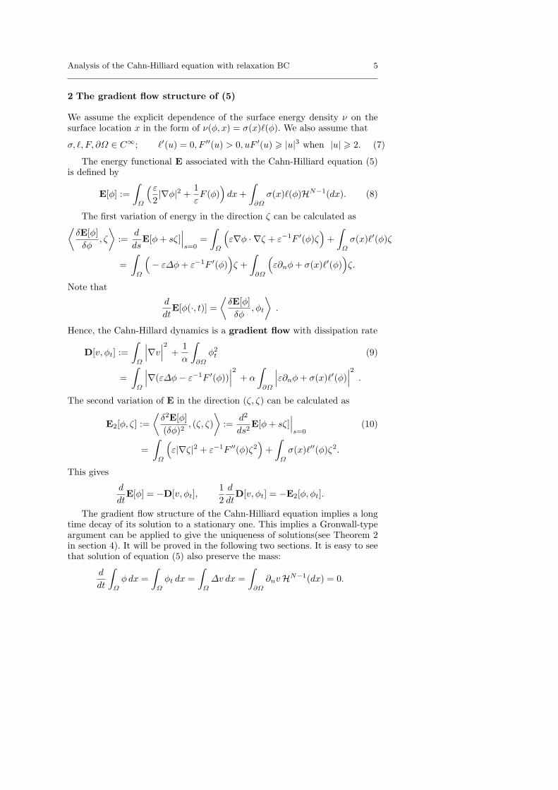
2 The gradient flow structure of (5)

We assume the explicit dependence of the surface energy density ν on thesurface location x in the form of ν(ϕ, x) = σ(x)ℓ(ϕ). We also assume that

σ, ℓ, F, ∂Ω ∈ C∞; ℓ′(u) = 0, F ′′(u) > 0, uF ′(u) > |u|3 when |u| > 2. (7)

The energy functional E associated with the Cahn-Hilliard equation (5)is defined by

E[ϕ] :=

∫Ω

(ε2|∇ϕ|2 + 1

εF (ϕ)

)dx+

∫∂Ω

σ(x)ℓ(ϕ)HN−1(dx). (8)

The first variation of energy in the direction ζ can be calculated as⟨δE[ϕ]

δϕ, ζ

⟩:=

d

dsE[ϕ+ sζ]

∣∣∣s=0

=

∫Ω

(ε∇ϕ · ∇ζ + ε−1F ′(ϕ)ζ

)+

∫Ω

σ(x)ℓ′(ϕ)ζ

=

∫Ω

(− ε∆ϕ+ ε−1F ′(ϕ)

)ζ +

∫∂Ω

(ε∂nϕ+ σ(x)ℓ′(ϕ)

)ζ.

Note that

d

dtE[ϕ(·, t)] =

⟨δE[ϕ]

δϕ, ϕt

⟩.

Hence, the Cahn-Hillard dynamics is a gradient flow with dissipation rate

D[v, ϕt] :=

∫Ω

∣∣∣∇v∣∣∣2 +1

α

∫∂Ω

ϕ2t (9)

=

∫Ω

∣∣∣∇(ε∆ϕ− ε−1F ′(ϕ))∣∣∣2 + α

∫∂Ω

∣∣∣ε∂nϕ+ σ(x)ℓ′(ϕ)∣∣∣2 .

The second variation of E in the direction (ζ, ζ) can be calculated as

E2[ϕ, ζ] :=

⟨δ2E[ϕ]

(δϕ)2, (ζ, ζ)

⟩:=

d2

ds2E[ϕ+ sζ]

∣∣∣s=0

(10)

=

∫Ω

(ε|∇ζ|2 + ε−1F ′′(ϕ)ζ2

)+

∫Ω

σ(x)ℓ′′(ϕ)ζ2.

This gives

d

dtE[ϕ] = −D[v, ϕt],

1

2

d

dtD[v, ϕt] = −E2[ϕ, ϕt].

The gradient flow structure of the Cahn-Hilliard equation implies a longtime decay of its solution to a stationary one. This implies a Gronwall-typeargument can be applied to give the uniqueness of solutions(see Theorem 2in section 4). It will be proved in the following two sections. It is easy to seethat solution of equation (5) also preserve the mass:

d

dt

∫Ω

ϕdx =

∫Ω

ϕt dx =

∫Ω

∆v dx =

∫∂Ω

∂nvHN−1(dx) = 0.

6 Xinfu Chen et al.

3 Well-Posedness of A Regularized Problem

To establish the existence of a solution of (5), we start with the followingregularizationδϕt − ε∆ϕ+ ε−1F ′(ϕ) = v, δvt −∆v = −ϕt in Ω × (0,∞),

ϕt − δ∆∂Ωϕ = −α(∂nϕ+ σℓ′(ϕ)), ∂nv = 0 on ∂Ω × (0,∞),

ϕ(·, 0) = ϕ0, v(·, 0) = v0 on Ω × 0

(11)

where δ ∈ (0, 1] is a parameter and ∆∂Ω is the surface Laplacian of themanifold ∂Ω. Note that except the boundary condition, this is the well-studied phase field model [7] in which ϕ is a phase order parameter and v isthe temperature.

The main result in this section is the following theorem.

Theorem 1 Assume (7) and (ϕ0, v0) ∈ C2(Ω)×C1(Ω). Then problem (11)admits a unique solution and the solution is smooth on Ω × (0,∞).

The proof is given in two steps (see in Section 3.1 and 3.2, respectively).In the first step, we prove a local in time existence. In the second step, weestablish an L∞ bound so the local solution can be extended step by step toΩ × [0,∞).

3.1 Local in Time Existence

First we establish the existence of a solution on ΩT := Ω × [0, T ] where T isa small positive constant. In the sequel, η ∈ (0, 1) is a fixed Holder exponentand C is a generic constant that depends only on η, ε, α, δ,Ω, σ(·), ℓ(·), andF (·), but not on T . We denote

c0 :=1

|Ω|

∫Ω

(δv0 + ϕ0

)dx, M0 := max

1, ∥v0∥C1(Ω), ∥ϕ0∥C2(Ω)

.

We shall prove the local existence via the fixed point of a certain operator inthe function space

XM,T :=ϕ ∈ C1,1/2(ΩT ) | ∥ϕ∥C1,1/2(ΩT ) 6M, ϕ(·, 0) = ϕ0

where M > M0 is a positive constant to be chosen later. Here the index(1, 1/2) in C1,1/2 are corresponding to x and t respectively.

1. Fix an arbitrary ϕ ∈ XM,T . Let V be the solution of the linear parabolicequation

δVt −∆V = c0 − ϕ in ΩT , ∂nV = 0 on ∂ΩT , V (·, 0) = V0 (12)

where V0 ∈ C2(Ω) is defined by

−∆V0 = c0 − δv0 − ϕ0 in Ω, ∂nV0 = 0 on ∂Ω,∫ΩV0 = 0.


By the classical elliptic estimate [13,16],

∥V0∥C2+η(Ω) 6 C∥δv0 + ϕ0∥C1(Ω) 6 CM0.

Comparing V with a linear function of t, we find that

∥V ∥L∞(ΩT ) 6 ∥V0∥L∞(Ω) + δ−1∥c0 − ϕ∥L∞(ΩT )T.

Hence, applying Schauder regularity theory [17] for the parabolic equation(12) we have

∥V ∥C2+η,1+η/2(ΩT ) 6 C∥V ∥L∞(ΩT ) + ∥V0∥C2+η(Ω) + ∥c0 − ϕ∥C1,1/2(ΩT )6 CM1 + T. (13)

Setting v = Vt we see that v is the unique solution (in distribution sense) of

δvt −∆v = −ϕt in ΩT , ∂nv = 0 on ∂ΩT , v = v0 on Ω × 0.

2. Next, we define the boundary value ϕ as the solution of

ϕt − δ∆∂Ωϕ = −α(∂nϕ+ σℓ′(ϕ)) in ∂ΩT , ϕ = ϕ0 on ∂Ω × 0. (14)

Then by parabolic estimate [17],

∥ϕ∥C1+η,(1+η)/2(∂ΩT ) 6 C∥ϕ0∥C2(∂Ω) + (1 + T )∥∂nϕ+ σℓ′(ϕ)∥C(∂ΩT )

6 CM1 + T. (15)

Finally, we define ψ as the solution of

δψt − ε∆ψ + ε−1F ′(ψ) = Vt in ΩT , ψ = ϕ on ∂ΩT , ψ = ϕ0 on Ω × 0.(16)

Note that ε−1F ′(ψ) 6 Vt at any interior point of local maximum of ψ andε−1F ′(ψ) > Vt at any interior point of local minimum. Hence, we can use (7)to derive that

∥ψ∥L∞(ΩT ) 6 max∥ϕ∥C(ΩT ), ∥ϕ0∥C(Ω), 2,

√ε∥Vt∥L∞(ΩT )

6 CM1 + T.

It then follows by parabolic estimate [17] that

∥ψ∥C1+η,(1+η)/2(ΩT )

6 C∥ϕ0∥C2(Ω) + ∥ϕ∥C1+η,(1+η)/2(∂ΩT ) + ∥ε−1F ′(ψ)− Vt∥L∞(ΩT )(1 + T )

6 C

M + |F ′(CM [1 + T ])|+ |F ′(−CM [1 + T ])|

(1 + T ).

Finally, by the definition of Holder norm, we can derive that

∥ψ − ϕ0∥C1,1/2(ΩT ) 6 ∥ψ∥C1+η,(1+η)/2(ΩT )Tη/2.

3. Fix M = 2M0. One can check that if T > 0 is sufficiently small, themap ϕ → ψ maps XM,T to itself and is a contraction, and therefore admitsa unique fixed point. The unique fixed point provides a unique solution of(11) on ΩT . In addition, by a bootstrap argument and standard parabolicregularity theory [17], (ϕ, v) is smooth in Ω × (0, T ]. We omit the details.

8 Xinfu Chen et al.

3.2 Global Existence

Let (ϕ, v) be a solution of (11) in Ω × [0, T ). Suppose we can show that∥ϕ∥L∞(ΩT ) is bounded. Then from the equation for V in (12) and parabolicLp estimate, v = Vt is bounded in Lp(ΩT ) for any p > 1. Consequently, fromthe equation for ϕ, we see that ϕ is bounded inW 2,1

p (ΩT ) for any p > 1, which

implies that ϕ is bounded in C1+η,(1+η)/2(ΩT ); see the derivation from (19)(with L∞(ΩT ) replaced by Lp(ΩT ) for p ≫ 1) to (20) below. A bootstrapargument then shows that (ϕ, v) ∈ C∞(Ω × (0, T ]). Hence, the solution canbe extended beyond T . Therefore, to establish the global in time existence,we need only establish an L∞ bound of ϕ. For this, assume that (ϕ, v) is asolution in Ω × [0, T ] and define

M1 = maxΩT

|ϕ|, M2 = maxΩT

|v| = maxΩT

|Vt|.

As we are establishing the upper bound of M1, we need only consider thecase M1 > 2M0.

Let (x∗, t∗) ∈ ΩT be a point such that M1 = |ϕ(x∗, t∗)|. Without loss ofgenerality, we assume that ϕ(x∗, t∗) > 0. As M1 > 2M0, we have t∗ > 0.If x∗ ∈ ∂Ω, then ∂nϕ(x

∗, t∗) > 0, ∂tϕ(x∗, t∗) > 0, and ∆∂Ωϕ(x

∗, t∗) 6 0,so the boundary condition for ϕ implies that σ(x∗)ℓ′(ϕ(x∗, t∗)) < 0. By (7),this implies that ϕ(x∗, t∗) 6 2, contradicting the assumption ϕ(x∗, t∗) =M1 > 2M0 > 2. Hence, x∗ ∈ Ω and t∗ > 0. Consequently, ∆ϕ(x∗, t∗) 60, ϕt(x

∗, t∗) > 0, so ε−1F ′(ϕ(x∗, t∗)) 6 v(x∗, t∗). This implies that, by (7),

(M1)2 6 F ′(ϕ(x∗, t∗)) 6 εv(x∗, t∗) 6 εM2. (17)

Similarly, if ϕ(x∗, t∗) is a global minimum of ϕ then either ϕ(x∗, t∗) > −2M0

or F ′(ϕ(x∗, t∗)) > −εM2. Without loss of generality, we can assume thatM2 > 1. Then,

∥F ′(ϕ)∥C(ΩT ) 6 max

maxu∈[−2,2]

|F ′(u)|, |F ′(ϕ(x∗, t∗))|, |F ′(ϕ(x∗, t∗))|

6 CM2. (18)

Applying the parabolic estimates first for ϕ and then for ϕ we derive that

∥ϕ∥C1+η,(1+η)/2(ΩT ) 6 C1+TM0+∥ε−1F ′(ϕ)−v∥L∞(ΩT )+∥∂nϕ∥C(∂ΩT )+1.(19)

The quantity ∥∂nϕ∥C(∂ΩT ) on the right-hand side can be control by the left-hand side via the interpolation: there exists a positive constant C = C(Ω, η)

such that for any δ ∈ (0, 1],

∥∇ϕ∥C(ΩT ) 6 Cδ−1/η∥ϕ∥C(ΩT ) + δ∥ϕ∥C1+η,(1+η)/2(ΩT ).

Setting δ = 1/[2C(1 + T )] we then derive from (19) and (18) that

∥ϕ∥C1+η,(1+η)/2(ΩT ) 6 C1 + T1/η+1M1 + ∥ε−1F ′ − v∥L∞(ΩT )

6 C1 + T1/η+1M2. (20)


Now we use the parabolic estimate for (12) to obtain

∥V ∥L∞(ΩT ) 6 C∥V0∥L∞(Ω) + ∥c0 − ϕ∥L∞(ΩT )T 6 C[1 + T ]M1,

∥V ∥C2+η,1+η/2(ΩT ) 6 C∥V0∥C2+η(Ω) + ∥c0 − ϕ∥C1,1/2(ΩT )(1 + T )

6 C[1 + T ]1/η+2M2

by (20). Finally, using v = Vt and the interpolation with θ = η/(1 + η) weobtain

M2 6 ∥V ∥C2,1(ΩT ) 6 2∥V ∥θL∞(ΩT )∥V ∥1−θC2+η,1+η/2(ΩT )

6 C[1 + T ]1/η+1Mθ1M

1−θ2 .

Upon using M1 6√εM2 we derive that

M2 6 C(1 + T )1/η+1Mθ/22 M1−θ

2

so that

M2 6 C[1 + T ]2(1/η+1)/θ, M1 6 C[1 + T ](1/η+1)/θ.

This completes the proof of Theorem 1. ⊓⊔

3.3 Energy Estimates

The a priori estimates in the preceding subsection depend on δ. In order topass to the limit δ 0, we need estimates that do not depend on δ. For this,we employ energy estimates.

1. For each t > 0, integrating δvt − ∆v + ϕt = 0 multiplied by v =δϕt−ε∆ϕ+ε−1F ′(ϕ) over Ω, using integrating by parts with the substitution∂nv = 0 and −ε∂nϕ = [ϕt − δ∆∂Ωϕ+ ασℓ′(ϕ)]/α on ∂Ω we obtain

0 =

∫Ω

v(δvt −∆v + ϕt) =

∫Ω

(δvvt − v∆v + [δϕt − ε∆ϕ+ ε−1F ′(ϕ)]ϕt

)=

∫Ω

(δvvt + |∇v|2 + δϕ2t + ε∇ϕ · ∇ϕt +

F ′(ϕ)ϕtε

)+

∫∂Ω

ϕt − δ∆∂Ωϕ+ ασℓ′(ϕ)]

αϕt

=d

dt

∫Ω

(δv22

+ε|∇ϕ|2

2+F (ϕ)

ε

)+

∫∂Ω

(δ|∇∂Ωϕ|2

2α+ σℓ(ϕ)

)+

∫Ω

(|∇v|2 + δϕ2t

)+

∫∂Ω

ϕ2tα.

Similarly, using −ε∂nϕt = −(ε∂nϕ)t = [ϕtt − δ∆∂Ωϕt + σℓ′′(ϕ)ϕt]/α on ∂Ω,we derive that

0 =

∫Ω

vt

(δvt −∆v + ϕt

)=

∫Ω

(δv2t − vt∆v + [δϕtt − ε∆ϕt + ε−1F ′′(ϕ)ϕt]ϕt

)=

d

dt

∫Ω

( |∇v|22

+δϕ2t2

)+

∫∂Ω

ϕ2t2α

+

∫Ω

(δv2t + ε|∇ϕt|2 +

F ′′(ϕ)ϕ2tε

)+

∫∂Ω

(δ|∇∂Ωϕt|2

α+ σℓ′′(ϕ)ϕ2t

).

10 Xinfu Chen et al.

Since both F ′′ and ℓ′′ have lower bounds, these two energy estimates willprovide norm bounds that do not depend on the non-linearity of F .

2. Non-linearity may mess up the usefulness of higher order energy esti-mates. We write two of them:

0 =

∫Ω

vt

(δvt −∆v + ϕt

)t

=

∫Ω

(δvtvtt − vt∆vt + [δϕtt − ε∆ϕt + ε−1F ′′(ϕ)ϕt]ϕtt

)=

d

dt

∫Ω

(δv2t2

+ε|∇ϕt|2

2+F ′′(ϕ)ϕ2t

2ε

)+

∫∂Ω

δ|∇∂Ωϕt|2

2α

+

∫Ω

(|∇vt|2 + δϕ2tt −

F ′′′(ϕ)ϕ3t2ε

)+

∫∂Ω

(ϕ2ttα

+σℓ′′′(ϕ)ϕtϕtt

2

),

0 =

∫Ω

vtt

(δvt −∆v + ϕt

)t

=

∫Ω

(δv2tt − vtt∆vt + [δϕttt − ε∆ϕtt + ε−1F ′′(ϕ)ϕtt + ε−1F ′′′(ϕ)ϕ2t ]ϕtt

=d

dt

∫Ω

( |∇vt|22

+δϕ2tt2

)+

∫∂Ω

ϕ2tt2α

+

∫∂Ω

(δ|∇∂Ωϕtt|2

α+ σℓ′′(ϕ)ϕ2tt + σℓ′′′(ϕ)ϕ2tϕtt

)+

∫Ω

(δv2tt + ε|∇ϕtt|2 +

F ′′(ϕ)ϕ2tt + F ′′′(ϕ)ϕ2tϕttε

).

We summarize the estimates as follows. Introduce

E[ϕ] =

∫Ω

(ε|∇ϕ|22

+F (ϕ)

ε

)+

∫∂Ω

σℓ(ϕ),

D[v, ζ] =

∫Ω

|∇v|2 +∫∂Ω

ζ2

α,

E2[ϕ, ζ] =

∫Ω

(ε|∇ζ|2 + F ′′(ϕ)ζ2

ε

)+

∫∂Ω

σℓ′′(ϕ)ζ2.

Then we have the fundamental energy identities

0 =d

dt

(E[ϕ] +

δ

2

[∥v∥2L2(Ω) + α−1∥∇∂Ωϕ∥2L2(∂Ω)

])+D[v, ϕt] + δ∥ϕt∥2L2(Ω),

0 =1

2

d

dt

(D[v, ϕt] + δ∥ϕt∥2L2(Ω)

)+E2[ϕ, ϕt] + δ[∥vt∥2L2(Ω) + α−1∥∇∂Ωϕt∥2L2(∂Ω)].

Higher order energy identities can be derived by direct differentiation: forany positive integer k,

1

2

d

dtEδ

2[ϕ, ∂kt ϕ, ∂

kt v] +Dδ[∂kt v, ∂

k+1t ϕ] = N2k+1,

1

2

d

dtDδ[∂kt v, ∂

k+1t ϕ] +Eδ[ϕ, ∂k+1

t ϕ, ∂k+1v] = N2k+2


where ∂kt = ∂k

∂tkand

Eδ2[ϕ, ∂

kt ϕ, ∂

kt v] :=

∫Ω

(ε|∇∂kt ϕ|2 +

F ′′(ϕ)|∂kt ϕ|2

ε+ δ|∂kt v|2

)+

∫∂Ω

δ|∇∂Ω∂kt ϕ|

2

α,

Dδ[∂kt v, ∂k+1t ϕ] := ∥∇∂kt v∥2L2(Ω) + α−1∥∂k+1

t ϕ∥2L2(∂Ω) + δ∥∂k+1t ϕ∥2L2(Ω),

N2k+1 :=1

ε

∫Ω

(∂k+1t ϕ

[∂kt F

′(ϕ)− F ′′(ϕ)∂kt ϕ]− F ′′′(ϕ)ϕt(∂

kt ϕ)

2

2

)+

∫∂Ω

σ∂k+1t ϕ∂kt ℓ

′(ϕ),

N2k+2 :=1

ε

∫Ω

∂k+1t ϕ

[∂k+1t F ′(ϕ)− F ′′(ϕ)∂k+1

t ϕ]+

∫∂Ω

σ∂k+1t ϕ∂k+1

t ℓ′(ϕ).

3. Using cut-off functions, one can establish estimate for arbitrary higherorder derivatives. For interior estimates, suppose ζ = ζ(x) is smooth andζ = 0 on ∂Ω. Then for any integer index β = (β1, · · · , βN+1), denoting

∂β = ∂|β|

∂xβ11 ···∂xβN

N ∂tβN+1we have

0 =

∫Ω

ζ∂βv∂β [δvt −∆v + ϕt]

=

∫Ω

ζδ∂βv∂βvt − ∂βv∆∂βv + ∂β [δϕt − ε∆ϕ+ F ′(ϕ)]∂βϕt

=

1

2

d

dt

∫Ω

(δ|∂βv|2 + ε|∇∂βϕ|2 + F ′′(ϕ)

ε|∂βϕ|2

)ζ

+

∫Ω

(|∇∂βv|2 + δ|∂βϕt|2

)ζ + · · ·

where · · · are lower order terms.Near boundary, one can begin with estimating tangential derivatives,

∇∂Ω := ∇− n(n · ∇) where n is a smooth vector function in Ω such that nis the unit exterior normal to ∂Ω. For example, suppose p ∈ ∂Ω and ζ is asmooth function in RN vanishing outside of a small neighborhood of p. Then

0 =

∫Ω

ζ∇∂Ωv · ∇∂Ω [δvt −∆v + ϕt]

=

∫Ω

ζδ∇∂Ωv · ∇∂Ωvt −∇∂Ωv · ∇∂Ω∆v +∇∂Ω [δϕt − ε∆ϕ+ F ′(ϕ)] · ∇∂Ωϕt

)=

1

2

d

dt

(∫Ω

(δ|∇∂Ωv|2 + ε|∇∇∂Ωϕ|2 +

F ′′(ϕ)

ε|∇∂Ωϕ|2

)ζ +

∫∂Ω

δ|∇2∂Ωϕ|2

2αζ

)+

∫Ω

(|∇∇∂Ωv|2 + δ|∇∂Ωϕt|2)ζ +

∫∂Ω

δ|∇∂Ωϕt|2

αζ + · · ·

Here we use the fact that the boundary condition equations ∂nv = 0 and∂tϕ + α(ε∂n + σℓ′(ϕ)) = 0 can be differentiated in t and in any tangentialdirections.


Finally, any other derivatives involving differentiation in the normal di-rection can be estimated by using the differential equation and the boundarycondition equation. We omit the details.

4 Well-posedness of (5)

In this section, we establish the well-posedness of (5). We show the uniquenessof the weak solution of (5) in Theorem 2 and existence and regularity of thesolution in Theorem 3. The proof of Theorem 3 is based on a L∞ estimatewhich is shown in section 4.4. In the last subsection, we derive formally thesharp-interface limit of the Cahn-Hilliard equation.

4.1 Weak Solution and Uniqueness

For completeness, we begin with the definition of a weak solution and itsuniqueness.

Definition 1 A pair (ϕ, v) is called a weak solution of (5) if for every T > 0,

ϕ,∇ϕ, v,∇v ∈ L2(ΩT ), ϕF ′(ϕ) ∈ L1(ΩT ), ϕt, σℓ′(ϕ) ∈ L2(∂ΩT )

and for every smooth ζ, η with compact support in Ω × [0,∞),∫ ∞

0

∫Ω

vζ dxdt =

∫ ∞

0

∫Ω

(ε∇ϕ · ∇ζ + F ′(ϕ)ζ

ε

)+

∫ ∞

0

∫∂Ω

(ϕtζα

+ σℓ′(ϕ)ζ),∫ ∞

0

∫Ω

∇v · ∇η dxdt =∫ ∞

0

∫Ω

ϕηt +

∫Ω

ϕ0(·)η(·, 0).

Theorem 2 Assume that F, σ, ℓ are smooth and F ′′ > −m and |ℓ′′| 6 m forsome m ∈ (0,∞). Then for every ϕ0 ∈ L2(Ω), there exists at most one weaksolution of (5).

Proof. Let (ϕ1, v1) and (ϕ2, v2) be two weak solutions. Fix T > 0. Set

ζ = ϕ1 − ϕ2 and η(·, t) =∫ t

T(v1(·, τ) − v2(·, τ))dτ for t ∈ [0, T ] and set

ζ = 0, η = 0 for t > T . Since F (u) + mu2/2 is a convex function we canderive that for every u1, u2 ∈ R,

max|u2F ′(u1)|, |u1F ′(u2)| 6 max|u1F ′(u1)|, |u2F ′(u2)|+m[|u1|2 + |u2|2] .

This implies that both ϕ1F′(ϕ2) and ϕ2F

′(ϕ1) are in L1(ΩT ). Thus, by anapproximation process, both ζ and η can be used as test functions. Takingthe difference of the definition equations for (ϕ1, v1) and (ϕ2, v2) and usingηt = v1 − v2 we obtain∫ T

0

∫Ω

∇(v1 − v2) · ∇η =

∫ T

0

∫Ω

(ϕ1 − ϕ2)ηt =

∫ ∞

0

∫Ω

(v1 − v2)ζ

=

∫ T

0

∫Ω

(ε|∇ζ|2 + (F ′(ϕ1)− F ′(ϕ2))ζ

ε

)+

∫ T

0

∫∂Ω

(ζtζα

+ σ[ℓ′(ϕ1)− ℓ′(ϕ2)]ζ).


As v1 − v2 = ηt the left-hand side equals∫ T

0

∫Ω

∇(v1 − v2) · ∇η =

∫ T

0

∫Ω

∇ηt · ∇η = −1

2

∫Ω

|∇η(·, 0)|2.

Also, using F ′′ > −m and |ℓ′′| 6 m we have

(F ′(ϕ1)− F ′(ϕ2))ζ > −mζ2, σ[ℓ′(ϕ1)− ℓ′(ϕ2)]ζ > −m∥σ∥L∞ζ2.

By Sobolev imbedding there exists a constant A = A(ε,m, ∥σ∥L∞ , Ω) suchthat

m

ε

∫Ω

ζ2 +m∥σ∥L∞

∫∂Ω

ζ2 6 ε

2

∫Ω

|∇ζ|2+A∫∂Ω

ζ2. (21)

Thus we obtain

−1

2

∫Ω

|∇η(·, 0)|2 >∫ T

0

∫Ω

(ε|∇ζ|2 − mζ2

ε) +

∫Ω

ζ(·, T )2

2α−m∥σ∥L∞

∫ T

0

∫∂Ω

ζ2

> ε

2

∫Ω

|∇ζ|2 + 1

2α

∫∂Ω

ζ(·, T )2 −A

∫ T

0

∫∂Ω

ζ2.

In particular, set w(t) =∫∂Ω

[ϕ1(·, t)−ϕ2(·, t)]2 we find that w(T ) 6 2αA∫ T

0w(t)dt.

As w(0) = 0 and T > 0 is arbitrary, the Gronwall’s inequality then impliesthat w ≡ 0, from which we derive that ϕ1 ≡ ϕ2 and v1 ≡ v2. This completesthe proof. ⊓⊔

4.2 Existence of A Strong Solution

A weak solution is called a strong solution if it has more regularity than itis needed in the definition. It is called a classical solution if all derivativesappeared in (5) exist in a classical sense and the equations are satisfied point-wisely. We can now pass to the limit δ 0 from the solution of (11) to obtaina strong solution of (5).

Theorem 3 Assume (7). Let ϕ0 ∈ C∞(ΩT ) be given. Set v0 = ε−1F ′(ϕ0)−ε∆ϕ0, ϕ0t = ∆v0 and assume that the compatibility condition ϕ0t+α(∂nϕ0+σℓ′(ϕ0)) = 0 on ∂Ω holds. Then problem (5) admits a unique weak solution.The solution satisfies the following estimates:

d

dt

∫Ω

ϕdx = 0,d

dtE[ϕ] = −D[v, ϕt],

D[v, ϕt] + 2

∫ t

0

E2[ϕ, ϕt]dτ 6 D[v0, ϕ0t].

In addition, if the space dimension N 6 3, then the solution is smooth inΩ × (0,∞).


Proof. Denote

m = max

−min

u∈RF ′′(u),max

u∈R|ℓ′′(u)|

.

We derive from (21) that

E2[ϕ, ζ] >ε

2

∫Ω

(|∇ζ|2 + ζ2)−A

∫∂Ω

ζ2 > ε

2∥ζ∥2H1(Ω) −Aα D[v, ζ]. (22)

Hence, for the solution of (11), integrating the first two energy identitieswe obtain

supt>0

(E[ϕ] + δ∥v∥2L2(Ω) +

δ∥∇∂Ωϕ∥2L2(∂Ω)

α

)

+

∫ ∞

0

(D[v, ϕt] + δ∥ϕt∥2L2(Ω)

)dt 6 C0,

supt>0

(D[v, ϕt] + δ∥ϕt∥2L2(Ω)

)+

∫ ∞

0

(ε∥ϕt∥2H1(Ω) + δ∥vt∥2L2(Ω) +

δ∥∇∂Ωϕt∥2L2(∂Ω)

α

)6 C0

where C0 is a constant that does not depend on δ ∈ (0, 1].It then follows from a standard procedure that along a sequence of δ 0,

the solution of (11) approaches a limit which is a strong solution of (5). Asweak solutions are unique, the whole sequence of solutions of (11) convergesto the weak solution of (5), as δ 0.

Suppose N 6 3 and we can show that solution of (5) is bounded,

then we can used higher order energy identities to estimate E2[ϕ,∂kϕ∂tk

] and

D[∂kv

∂tk, ∂

k+1ϕ∂tk+1 ] for k = 2, 3, · · · . Also one establish energy estimates for spatial

derivatives to derive that (ϕ, v) is smooth and is a classical solution.Hence, to show that we have a classical solution thereby completing the

proof of Theorem 3, we need only establish an L∞ estimate for the solution.This will be done in the next two subsections.

Suppose we can show that ∥ϕ∥L∞(ΩT ) 6 K(T ) for a classical solution.For weak solutions, we argue as follows: first we modify F ′ by zero in(−∞,−K(T )−1]∪ [K(T )+1,∞) to obtain a classical solution. This classicalsolution will be bounded by K(T ) so it is the weak solution of the originalproblem. Hence, we need only work on classical solutions.

4.3 The Principal Eigenvalue

We denote

λε(t) := inf∫Ω

ζ=0

∫Ω[ε|∇ζ|2 + ε−1F ′′(ϕ)ζ2] +

∫∂Ω

σ(x)ℓ′′(ϕ)ζ2

1α

∫∂Ω

ζ2 +∫Ω|∇∆−1

N ζ|2,

Λε := min

inft∈[0,∞)

λε(t) , 0


where ∆−1N is the inverse of the Laplace operator under the Neumann bound-

ary condition, i.e., ζ = ∆−1N ζ is defined as the solution of

∆ζ = ζ − 1

|Ω|

∫Ω

ζ in Ω, ∂nζ = 0 on ∂Ω,

∫Ω

ζ dx = 0.

Note that Λε > −Aα where A is defined in (22). If the interface is well-developed, the eigenvalue is investigated in [12] with the conclusion that Λε

is bounded from below by a constant that does not depend on ε. Here weallow Λε to depend on ε.

The energy identity implies that

1

2

d

dtD[v, ϕt] = −E2[ϕ, ϕt] 6 −λε(t)D[v, ϕt] 6 Λε

d

dtE[ϕ].

Set D(t) = D[v(·, t), ϕt(·, t)] and E(t) := E[ϕ(·, t)]. Integrating the aboveinequality in [0, t] we obtain

D(t) 6 D(0)− 2Λε[E(0)− E(t)] 6 D(0) + 2AαE(0) =: C

Thus, we have

supt>0

(∫Ω

|∇v|2 + 1

α

∫∂Ω

ϕ2t

)6 C.

Using [11, Lemma 3.4] we have

∥v∥H1(Ω) := ∥∇v∥L2(Ω) + ∥v∥L2(Ω) 6 C(Ω,m)(E[ϕ] + ∥∇v∥L2(Ω)

)6 C1

Hence, by Sobolev’s imbedding

∥v∥Lp(Ω) 6 C(p,Ω)∥v∥H1(Ω) 6 CC1, p =2N

N − 2

(if N 6 2, p > 1 is arbitrary

).

4.4 The L∞ Estimate

Assume N 6 3. Then p := 2N/(N − 2) > N .Let aε be a constant defined in (23) below. We set

k = α(5aε + ∥σℓ′∥L∞(Ω×R)

)+ 1.

Let (x∗, t∗) ∈ Ω × [0, T ] be a point such that

ϕ(x∗, t∗)− kt∗ = maxΩ×[0,T ]

(ϕ(x, t)− kt).

Then maxΩTϕ 6 ϕ(x∗, t∗) + kT. We now estimate ϕ(x∗, t∗).

(i) If t∗ = 0, we have ϕ(x∗, t∗) = ϕ0(x∗) 6M0.

(ii) Suppose t∗ > 0. Denote Φ(y, t) = ϕ(x∗+εy, t), B = y | |y| < 1, x∗+εy ∈ Ω. Then

εv = −∆yΦ+ F ′(Φ) in B.


Let Ψ(·, t) be a solution of

−∆Ψ = v(y) := εv(x∗ + εy, t) in B, Ψ = 0 on ∂B.

Then, since p > N ,

∥∇yΨ(·, t)∥L∞(B) + ∥Ψ(·, t)∥L∞(B) 6 C∥v∥Lp(B) 6 Cε1−N/p∥v∥Lp(Ω)

6 Cε2−N/2∥v∥L∞(0,∞;Lp(Ω)) =: aε. (23)

Denote Ψ = Ψ − 2aε(1− |y|2) and Φ = Φ− Ψ . Then Φ = Φ+ Ψ and

−∆yΦ = −F ′(Φ+ Ψ) + 4Naε in B.

Let (y, t) ∈ B × [0, T ] be a point of maximum of Φ− kt in B × [0, T ].

(1) The case |y| = 1 is impossible, since we would have Ψ(y, t) = 0 so

Φ(y, t)− kt = Φ(y, t)− kt 6 ϕ(x∗, t∗)− kt∗ = Φ(0, t∗) + Ψ(0, t∗)− kt∗

6 Φ(0, t∗)− kt∗ − aε,

which contradicts the definition of (y, t).

(2) The case x := x∗ + εy ∈ ∂Ω is also impossible, since at (x, t), we

would have ϕt = Φt(y, t) > k (here we observe that Ψt = 0 on ∂B × [0, T ])

and ε∂nϕ > −∥∇Ψ∥L∞ > −5aε, contradicts the boundary condition ϕt +α(ε∂nϕ+ σℓ′(ϕ)) = 0 and the definition of k.

(3) Hence, y must be an interior point of B. Then −∆yΦ(y, t) > 0, so we

have F ′(Φ + Ψ) 6 4Naε. This implies that Φ(y, t) + Ψ(y, t) 6 2 +√4Naε.

Hence,

ϕ(x∗, t∗) = Φ(0, t∗) + Ψ(0, t∗) 6 Φ(y, t) + k(t∗ − t) + Ψ(0, t∗)

6 2 +√

4Naε − Ψ(y, t) + k(t∗ − t) + Ψ(0, t∗)

6 2 +√

4Naε + kT + 3aε.

Similarly, we can establish a lower bound of ϕ. Hence, we have

K(T ) := maxΩ×[0,T ]

|ϕ| 6M0 + 2kT + 3aε +√

4Naε.

This completes the proof of Theorem 3.


5 Formal Asymptotic Limit as ε 0

Assume that F is a double equal-well potential: F (u) > F (±1) = 0 for allu = ±1. Also assume that the initial data ϕ0 = ϕε0 depends on ε and satisfies

1

|Ω|

∫Ω

ϕε0(x)dx = m, E[ϕε0] 6 e0

where m ∈ (−1, 1) and e0 are positive constant that does not depend onε. Denote the solution of (5) by (ϕε, vε). Then one can show that along asequence ε 0, (ϕε, vε) approaches a limit (ϕ∗, v∗) having the property|ϕ∗| = 1 a.e.; see, for example [11]. Also, denote

Ω±t =

x ∈ Ω

∣∣∣ limr0

limε0

miny∈Ω,|y−x|6r

±ϕε(y, t) > 1

,

Γt = ∂Ω+t ∩ ∂Ω−

t , Γ = ∪t>0Γt × t.It is formally derived by Pego [19] and then rigorously verified by Alikakos,Bates and Chen [2, 11] for the classical Cahn-Hilliard system that v∗ solves

∆v∗ = 0 in Ω \ Γt, v∗ = σ0(N − 1)κΓt , [[nΓt · ∇v∗]]∣∣∣Γt

= 2VΓt on Γt.

where σ0 =∫ 1

−1

√F (s)/2ds, [[ · ]]|Γt is the jump across Γt, nΓt is the normal

of ∂Ω+t at Γt, κΓt and Vt are the mean curvature and advancing speed of

the front Γt of Ω+t . Together with the boundary condition ∂nv

∗ = 0 on ∂Ω,the limit free boundary problem for (v∗, Γ ) is well-posed provided we knowthe dynamics of the intersection Γt ∩ ∂Ω.

Here we provide a formal argument showing that the intersection of in-terface Γt with ∂Ω does not change in time:

Γτ ∩ ∂Ω ⊂ Γt ∩ ∂Ω ∀ 0 6 τ < t .

For this assume N = 2 and [−1, 1]× 0 is part of the boundary of ∂Ω.Assume that one of the intersection points is (xε(t), 0), and that from t = 0to t = T , the intersection point moves from xε(0) = 0 to xε(T ) = b > 0. Foreach x1 ∈ (0, b), denote by t±ε (x1) the time at which ϕε(x1, 0, t

±ε (x1)) = ±1/2.

Then

b = limε0

∫ b

0

[ϕε(x1, 0, t+ε (x1))− ϕ(x1, 0, t

−ε (x1))]dx1

= limε0

∫ b

0

∫ t+ε (x1)

t−ε (x1)

ϕε,t(x1, 0, t)dtdx1

6 limε0

√∫ ∞

0

∫∂Ω

ϕ2ε,t√

|Dε| 6 C0 limε0

√|Dε|

where |Dε| is the area of the region Dε := (x, t) | x ∈ ∂Ω, 0 6 t 6T, |ϕε(x, t)| 6 1/2. Formally, Dε has thickness O(ε) so limε0 |Dε| = 0.Thus b = 0. Hence, formally, in the limit ε 0, intersection points of Γt

with ∂Ω do not move.


6 Fast Time Motion

Assume that N = 2 and Γt has only one component. When 1 ≪ t≪ 1/ε, theinterface is almost circular whereas its intersection with ∂Ω does not shownoticeable motion. Hence we assume that initially the interface is circularand use fast time s = εt. Note that s ∈ [0, 1] is equivalent to t ∈ [0, 1/ε].

To derive the dynamic laws for the interface, contact angle and the con-tact points under the fast time s, we use the techniques of the matchedasymptotic expansions. We shall first perform the standard matched asymp-totic expansion away from the solid boundary which follows the steps givenin [19]. For simplicity, we only summarize the results from the outer and innerexpansions. We then focus our attention on the near contact point expansionto derive the dynamics of the contact angle and the intersection points.

The initial-boundary value problem of the Cahn-Hilliard equation be-comes

F ′(ϕ)− ε2∆ϕ = εv, ∆v = εϕs in Ω × (0,∞),

εϕs = −α[ε∂nϕ+ σ(x)ℓ′(ϕ)], ∂nv = 0, on ∂Ω × (0,∞)ϕ = ϕ0 on Ω × 0.

(24)

The energy identity implies that∫ ∞

0

(∫Ω

|∇v|2 + α

∫∂Ω

[ε∂nϕ+ σ(x)ℓ′(ϕ)]2)

6 εE[ϕ0].

Hence as ε 0, v(·, s) approaches a constant, which indicates that theinterface is circular.

We consider a simple case (see Figure 2) where Ω = (−1, 1)× (0, 1) andthe initial interface is a circular arc:

Γ0 = ⟨0,−h(0)⟩+R(0)⟨sin θ, cos θ⟩ | |θ| 6 β(0),Ω−

0 = (x1, x2) | x2 > 0, x21 + (x2 + h(0))2 < R(0)2

where h(0) = R(0) cosβ(0) and β(0) ∈ (0, π) and R(0) > 0. The area of theregion Ω−

0 is

A = |Ω−0 | = R(0)2

(β(0)− sinβ(0) cosβ(0)

).

6.1 The Outer Expansion

Away from the interface in the phase regionΩ±s , we have the outer expansions

v ∼ v± ∼ v±0 +∑

i>1 εiv±i , ∆v± = εϕ±s ,

ϕ ∼ ϕ± ∼ ϕ±0 +∑

i>1 εiϕ±i , F ′(ϕ±) = εv± + ε2∆ϕ±.

It is easy to show that the leading order solutions are ϕ±0 = ±1 and v±0 satisfy

∆v±0 = 0


Ω−

Ω+

Rβ

x1

x2

Fig. 2 Region Ω,Ω+, Ω−

with boundary condition

∂nv±0 = 0 on ∂Ω ∩ ∂Ω±

s . (25)

Since the outer expansion equations for ϕ±j do not allow the imposing of anyboundary conditions, boundary layers are expected.

6.2 The Inner Expansion

For s > 0, we expect the limit interface (ε→ 0) be a circular arc centered at(0,−h(s)) with radius R(s):

Γs =⟨0,−h(s)⟩+R(s)⟨sin θ, cos θ⟩

∣∣ |θ| 6 β(s), h(s) = R(s) cosβ(s).

We assume that the zero level set, Γ εs of ϕ can be written as

Γ εs = ⟨0,−h(s)⟩+Rε(θ, t)⟨sin θ, cos θ⟩

∣∣ |θ| 6 βε(s).

We use the expansion

Rε(θ, s) ∼ R(s) +∑i>1

εiRi(θ, s) = R(s) + εRε(θ, s), R ∼∑i>1

εi−1Ri.

It is convinient to use the polar coordinates (r, θ) centered at (0,−h(s)):

x = ⟨0,−h(s)⟩+ r⟨sin θ, cos θ⟩, r := |x− ⟨0,−h(t)⟩|, θ = Arctanx1

x2 + h(s).


We now consider the change of variable (x, s) → (z, θ, s) where z, a specialversion of the stretched variable1, is defined by

z =r −Rε(θ, s)

ε=

|x− ⟨0,−h(s)⟩| −R(s)− εRε(θ, s)

ε.

Near the interface, we use the expansion

ϕ(x, s) ∼∑i>0

εiϕi(z, θ, s), v(x, t) ∼∑i>0

εivi(z, θ, s). (26)

Denote

X(θ, s) := ⟨0,−h(s)⟩+R(s)N(θ), N(θ) = ⟨sin θ, cos θ⟩.

One can derive the following matching conditions, as z → ±∞:

v0(z, θ, s) ∼ v±0 (X(θ, s), s),

v1(z, θ, s) ∼ v±1 (X(θ, s), s) + (R1(θ, s) + z)v0,r(X(θ, s), s),

· · · · · · · · ·

Similarly, we can also derive matching conditions for ϕ.Substitute the expansions (26) into the Cahn-Hilliard equations (24), we

can easily derive the leading order solution ϕ0(z, θ, s),

ϕ0(z, θ, s) = Q(z)

where Q is the unique solution of

Qzz − F ′(Q) = 0 on R, Q(±∞) = ±1, Q(0) = 0. (27)

This implies that

Qz(z) =√

2F (Q(z)),

∫ Q(z)

0

du√2F (u)

= z ∀ z ∈ R.

For the leading order v0, we have

v0(z, θ, s) = − σ0R(s)

,

where

σ0 :=1

2

∫RQ2

z(z)dz =1√2

∫ 1

−1

√F (u)du (28)

The solvability condition for the higher order solutions then shows that theinterface dynamics preserve the area of Ω−

s , i.e.

|Ω−s | = R2[β − sinβ cosβ] = |Ω−

0 | = A.

1 Typically the stretched variable is defined as z = d(x, Γ εs )/ε where d(x, Γ ε

s ) isthe signed distance from x to Γ ε

s


6.3 Expansion Near Contact Point

Assume for simplicity that the solution is symmetric with respect to the x2-axis. Near the right intersection pε = ⟨Rε(θ, s) sin θ, 0⟩|θ=βε(s), we use thethe stretched variable (y, z) defined by

y =x2ε, z =

r −Rε(θ, s)

ε

(r =

√x21 + (x2 + h(s))2, θ = Arctan

x1x2 + h(s)

).

Expand ϕ ∼∑

i>0 εiΦi(z, y, s), v ∼

∑i>0 ε

iV i(z, y, s), and βε(s) ∼ β(s) +∑i>0 ε

iβi(s). The leading order expansion becomes

Φ0zz + 2 cosβ Φ0

yz + Φ0yy − F (Φ0) = 0 ∀ z ∈ R, y > 0, s > 0,

Φ0(z,∞, s) = Q(z), ∀ z ∈ R, s > 0,

(hs cosβ−Rs−α cosβ)Φ0z = α[Φ0

y − σ(R sinβ, 0)ℓ′(Φ0)] ∀z ∈ R, y = 0, s > 0.(29)

In general it is very hard to find an explicit solution for this problem. Nev-ertheless, we can assume, for simplicity that

ℓ′(u) =√

2F (u)

so that we have

ℓ′(Q) = Qz.

This choice of ℓ(u) is in fact preferred as argued in [23]. Then, we have anexplicit solution Φ0(z, y, s) = Q(z), subject to the compatibility condition

hs cosβ −Rs = α(cosβ − σ(R sinβ, 0)

).

Using the relations

R =

√A√

β − sinβ cosβ, h = R cosβ =

√A cosβ√

β − sinβ cosβ(30)

we then derive the dynamics

d

dsβ(s) =

α√A

(β − sinβ cosβ)3/2[cosβ − σ(√A sin β√

β−sin β cos β, 0)]

sinβ[sinβ − β cosβ]. (31)

Once the contact angle β(s) is solved from (31), the evolution of the dropradius R(s) and the position of the contact point x(s) = R(s) sin(β(s)) canthen determined by using (30).


6.4 A Traveling Wave Problem

For general ℓ, the dynamics can be obtained as follows. First we solve a non-linear eigenvalue problem: for p ∈ ∂Ω and θ ∈ (0, π), find λ = λ(p, θ) andΦ(·) = Φ(p, θ; ·) on R× [0,∞) such thatΦzz + 2 cos θΦyz + Φyy − F ′(Φ) = 0 on R× (0,∞),

Φ(·,∞) = Q(·), on R× ∞,Φy = σ(p)ℓ′(Φ)− λΦz on R× 0.

(32)

Then the dynamics becomes

hs cosβ −Rs = α[cosβ − λ(p, β)], h = R cosβ, p = ⟨R sinβ, 0⟩.

Note that from a solution of (32), we have a traveling wave of the formu(z, y, s) = Φ(z − λs, y) where u solves

uzz + 2 cos θuzy + uyy = F ′(u) on R× (0,∞)× R,us = uy − σ(p)ℓ′(u) on R× 0 × R.

It is still open to show that the non-linear eigenvalue problem (32) admits aunique solution for general monotonic ℓ(·) satisfying ℓ′(±1) = 0.

To have a basic estimate of λ, note that

∂

∂z

(12Φ2z −

1

2Φ2y − F (Φ)

)+

∂

∂y

(ΦyΦz + cos θΦ2

z

)= 0.

Integrating over z ∈ R we then derive that

d

dy

∫R

(ΦzΦy + cos θΦ2

z

)dz = 0 ∀ y > 0.

This implies that∫RΦy(z, 0)Φz(z, 0)dz = cos θ

∫R[Q2

z(z)− Φ2z(z, 0)]dz.

Thus, integrating Φy(z, 0) = σ(p)ℓ′(Φ)−λΦz multiplied by Φz over z ∈ R wederive that

λ = σ(p)ℓ(1)− ℓ(−1)∫R Φ

2z(z, 0) dz

+ cos θ

∫R[Φ

2z(z, 0)−Q2

z(z)] dz∫R Φ

2z(z, 0) dz

;

Here, of course, Φ depends on p and θ.


0 5 10 15 20 25 30 35 400.3

0.32

0.34

0.36

0.38

0.4

0.42

0.44

0.46

0.48

0.5

s

β/π

ODEε=0.05ε=0.1

Fig. 3 Contact Angel Dynamics—the function β = βε(s). Top curve is the so-lution of (31); middle and bottom curves correspond to the solution of the Cahn-Hillard equation with ε = 0.05 and ε = 0.1, respectively. The dotted line corre-sponds to the equilibrium contact angle π/3.

6.5 Numerical Verification of the Contact Angle Evolution Law (31).

Here we numerically verify (31) by (i) numerically solving the Cahn-Hilliard equation (24) with small ϵ, (ii) finding the evolution of the contactangle from the resulting numerical solution, and (iii) comparing the dynamicsof the contact angle with the solution of (31).

We set σ(·) ≡ cos(π/3) = 1/2 and α = 1 and choose Ω = (−1, 1)× (0, 1)

and initial drop as a half disk with radius Rε(0)=√

0.8/π ≈0.5046, contactangle βε(0) = π/2, and volume A = πRε(0)2/2 = 0.4.

The solution β = β(t) of the equation (31) is plotted in Figure 3. Itis clear that when t → ∞, β(t) approaches the equilibrium contact angleβ(∞) = arccosσ = π/3.

Numerically solving the Cahn-Hilliad equation with small ε is very diffi-cult. We use a numerical scheme recently developed by Gao and Wang in [25].From the numerical solution, we computer the dynamics of the point and an-gle of contact by following the evolution of the intersection of the zero contourline of ϕϵ(x, t) with the boundary. The evolutions of the computed contactangles, for ϵ = 0.1 and ϵ = 0.05, are shown in Figure 3. The results not onlyillustrate a good convergence to the dynamic law (31) as ϵ → 0, but alsodemonstrate the excellent performance of the numerical scheme developedin [25].


References

1. S. Allen and J. W. Cahn, A microscopic theory for antiphase boundary motionand its application to antiphase domain coarsening, Acta. Metall. 27 (1979),1084-1095.

2. N.D. Alikakos, P.W. Bates, & Xinfu Chen, Convergence of the Cahn-Hilliardequation to the Hele-Shaw model, Arch. Rational Mech. Anal. 128 (1994), 165-205.

3. P.W. Bates & P. C. Fife, Nucleation Dynamics in the Cahn-Hilliard Equation,SIAM J. Appl. Math. 53 (1993), 990-1008.

4. D. Bonn and D. Ross, Wetting transitions, Rep. Prog. Phys. 64 (2001) p-p. 1085-1163.

5. G. Caginalp, An analysis of a phase field model of a free boundary, Arch.Rational Mech. Anal., 92 (1986) 205-245.

6. J. Cahn, Critical point wetting, J. Chem. Phys., 66 (1977), 3667-3672.7. G. Caginalp, An analysis of a phase field model of a free boundary, Arch.

Rational Mech. Anal., 92 (1986) 205-245.8. L. A. Caffarelli & N. E. Muller, An L∞ bound for solutions of the Cahn-Hilliard

equation, Arch. Rational Mech. Anal. 133 (1995), 129–144.9. J.W. Cahn and J.E. Hilliard. Free energy of a non-uniform system i. interfacial

free energy. J. Chem. Phys., 28 (1958), 258-26710. J. Cahn, C.M. Elliott and A. Novick-Cohen, The Cahn-Hilliard equation with

a concentration dependent mobility: motion by minus the Laplacian of the meancurvature. Euro. J. Appl. Math. 7 (1996), 287-301.

11. Xinfu Chen, Global asymptotic limit of solutions of the Cahn-Hilliard equation,J. Differential Geometry, 44 (1996), 262-311.

12. Xinfu Chen, Spectrum for the Allen-Cahn, Cahn-Hilliard, and phase-field e-quations for generic interfaces. Comm. Partial Differential Equations 19 (1994),no. 7-8, 1371-1395.

13. Ya-Zhe Chen & Lan-Cheng Wu, Second Order Elliptic Equations and EllipticSystems, Translation of the mathematical monographs, 174, Amer. Math. Soc.1998.

14. D. Bonn, J. Eggers, J. Indekeu, J. Meunier, E. Rolley. Wetting and spreading, Rev. Mod. Phys. 81 , 739 (2009)

15. C. M. Elliott & S. Zheng, On the Cahn-Hilliard Equation, Arch. RationalMech. Anal. 96, (1986) 339-357.

16. D. Gilbarg & N. Tradinger, Elliptic partial differential equations of secondorder, Springer, 1998

17. O.A. Ladyzhenskaja, V.A. Solonnikov, & N. N. Ural’ceva, Linear and quasi-linear equations of parabolic type, Translations of Mathematical Monographs,23, Providence, RI, 1968.

18. L. Modica, Gradient theory of phase transitions with boundary energy, Ann.Inst. Henri Poincare, 4 (1987) 487-512.

19. R. Pego, Front Migration in the Nonlinear Cahn-Hilliard Equation, Proc. R.Soc. Lond., A, 422(1989), 261-278.

20. T. Qian, X.P. Wang, P. Sheng, Molecular scale contact line hydrodynamics ofimmiscible flows, Phys. Rev. E 68 (2003), 016306.

21. T. Z. Qian, X. P. Wang, P. Sheng, Power-law slip profile of the moving contactline in two-phase immiscible flows, Phys. Rev. Lett. 93 (2004) 094501.

22. X.-P. Wang, T. Qian and P. Sheng, Moving contact line on chemically pat-terned surfaces, J. of Fluid Mechanics, 605 (2008), 59-78.

23. Xianmin Xu and X.P. Wang, Derivation of Wenzel’s and Cassie’s equationsfroma phase fieeld model for two phase flow on rough surface, SIAM J. Appl.Math, 70 (2010), 2929-2941.

24. Xianmin Xu and Xiaoping Wang, Analysis of wetting and contact angle hys-teresis on chemically patterned surfaces, SIAM J. Applied Math, 71 (2011) ,pp. 1753-1779

25. M. Gao and X.P. Wang, A Gradient Stable Scheme for a Phase Field Model forthe Moving Contact Line Problem, J. Computational Physics, 231 2012, Pages1372-1386

26. T. Young, An essay on the cohesion of fluids, Philos. Trans. R. Soc. London(1805), 95, pp. 6587.

Analysis of the Cahn-Hilliard Equation with Relaxation ...mawang/research/CahnHillardn-ARMA.pdf · of the solution. We also study the sharp interface limit of the system. The ...

Documents