analysis of surface water quality and ground water flow

ANALYSIS OF SURFACE WATER QUALITY AND GROUND WATER FLOW IN THE CARMANS RIVER WATERSHED, LONG ISLAND, NEW YORK

by

Tracey McGregor O’Malley

A thesis submitted in partial fulfillment

of the requirements for the Master of Science Degree

State University of New York

College of Environmental Science and Forestry Syracuse, New York

April 2008

Approved: Department of Forest and Natural Resources Management Area of Study: Forest Hydrology and Watershed Management _____________________________ Dr. Lee Herrington, Major Professor

_________________________________ Dr. Raymond C. Francis, Chair, Examining Committee

_____________________________ Dr. David Newman, Department Chair

__________________________________ Dr. Dudley J. Raynal, Dean, Instruction and Graduate Studies

2

Acknowledgements

The completion of this thesis would not have been possible without the

tremendous support and guidance from several individuals. First and foremost, I would

like to thank my major advisor, Dr. Lee Herrington, for his support, sense of humor, and

sense of adventure.

Secondly, I would like to thank my committee members, Dr. Laura Lautz, Dr.

Russell Briggs and Dr. John Stella for their support and feedback. I am deeply indebted

to Dr. Laura Lautz for her tremendous guidance with both the chemistry and modeling

analyses, and for allowing me to use the ion chromatograph.

I would also like to thank the “Hydro Group”, specifically Rosemary Fanelli, Ginny

Collins and Jamie Ong for their friendship and support. My research would not have

been possible without Rosemary. Rosemary assisted me in the field and was a master

at using the GPS. She was willing to camp out on Long Island, and retrieve storm water

samples at all hours of the night.

I would also like to thank my family for their encouragement, and especially my

mother Deborah McGregor.

And last but certainly not least, I would like to thank my husband, Brian O’Malley.

I could not have done this without his support and patience. He always provided a

listening ear, an eye for editing, and hands in the field. His positive attitude always kept

me grounded, and reminded me of what was important in life.

3

TABLE OF CONTENTS Acknowledgements……………………………………………………………………………..2

Table of Contents……………………………………………………………………………….3

List of Tables…………………………………………………………………………………….6

List of Figures…………………………………………………………………………………...7

Abstract…………………………………………………………………………………………11

CHAPTER I: INTRODUCTION ..................................................................................... 12

CHAPTER II: LITERATURE REVIEW .......................................................................... 15

2.1 Soil Characteristics .............................................................................................. 16

2.2 Agriculture ........................................................................................................... 16

2.3 Previous Investigations on Long Island Regarding Nitrate Levels ....................... 17

2.4 Ground Water Modeling....................................................................................... 21

2.5 Long Island Ground Water Modeling ................................................................... 23

2.6 Precipitation and Recharge ................................................................................. 26

CHAPTER III: MATERIALS AND METHODS .............................................................. 27

3.1 Study Area........................................................................................................... 27

3.1.1 Carmans River Watershed............................................................................ 27

3.1.2 Soils .............................................................................................................. 30

3.1.3 Land Use....................................................................................................... 30

3.2 Field Methods ...................................................................................................... 31

3.3 Laboratory Analysis ............................................................................................. 34

4

3.4 Modeling Methods ............................................................................................... 34

3.4.1 Available Data ............................................................................................... 35

3.4.2 Conceptual Model ......................................................................................... 39

3.4.3 Model Inputs.................................................................................................. 41

3.4.4 River Boundary ............................................................................................. 42

3.4.5 Model Calibration .......................................................................................... 43

3.4.6 Zone Budget.................................................................................................. 44

3.4.7 Sensitivity Analysis........................................................................................ 45

3.4.8 Particle Tracking and MODPATH Simulations .............................................. 45

CHAPTER IV: RESULTS.............................................................................................. 47

4.1 Modeling Results ................................................................................................. 47

4.1.1 Calibration Results ........................................................................................ 47

4.1.2 Zone Budget and River Cell Flux .................................................................. 51

4.1.3 River Cell Flux Sensitivity Analysis ............................................................... 55

4.1.4 Ground Water Contributing Area................................................................... 59

4.2 MODPATH Simulations ....................................................................................... 60

4.2.1 Residence Times and Sourcesheds.............................................................. 60

4.3 Chemistry Results................................................................................................ 65

4.3.1 Basic Water Quality Parameters ................................................................... 65

4.3.2 Major Ions ..................................................................................................... 67

4.3.3 Nitrate ........................................................................................................... 74

4.3.4 Sodium Chloride............................................................................................ 75

4.3.5 Road Density................................................................................................. 79

5

CHAPTER V: DISCUSSION ......................................................................................... 82

5.1 Ground Water Flow.............................................................................................. 83

5.1.1 Sourcesheds ................................................................................................. 83

5.1.2 Residence Times .......................................................................................... 85

5.1.3 Assumptions and Limitations of Modeling ..................................................... 86

5.2 Changes in Chemistry with Distance Downstream .............................................. 89

5.2.1 Temperature and pH ..................................................................................... 89

5.2.2 Major Ions ..................................................................................................... 91

5.2.3 Nitrate ........................................................................................................... 94

5.3 Implications.......................................................................................................... 94

CHAPTER VI: CONCLUSIONS .................................................................................... 96

REFERENCES.............................................................................................................. 98

Appendix A: Soil Types ............................................................................................. 103

Appendix B: Hydrographs for Synoptic Sampling Events .......................................... 112

Appendix C: % Error .................................................................................................. 115

Appendix D: Water Quality Parameters ..................................................................... 117

Appendix E: Major Cations ........................................................................................ 119

Appendix F: Major Anions.......................................................................................... 121

VITA………………………………………………………………………………………… 123

6

LIST OF TABLES

Table Page

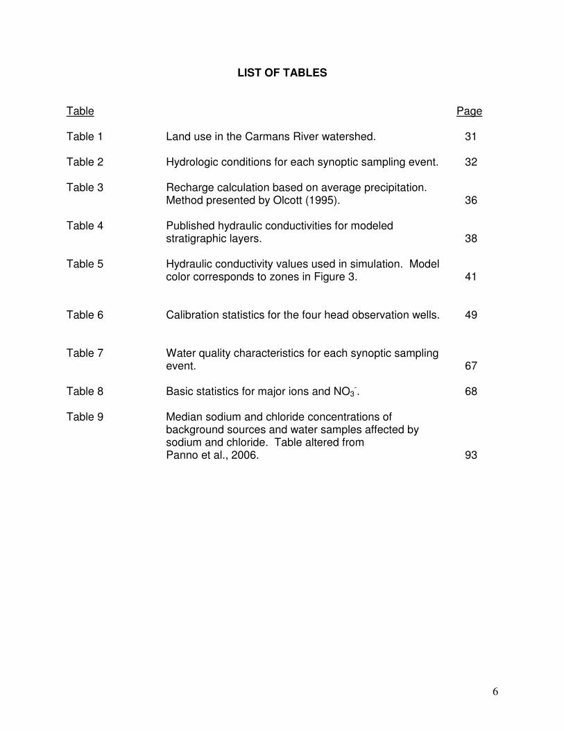
Table 1 Land use in the Carmans River watershed. 31

Table 2 Hydrologic conditions for each synoptic sampling event. 32 Table 3 Recharge calculation based on average precipitation. Method presented by Olcott (1995). 36 Table 4 Published hydraulic conductivities for modeled stratigraphic layers. 38 Table 5 Hydraulic conductivity values used in simulation. Model color corresponds to zones in Figure 3. 41 Table 6 Calibration statistics for the four head observation wells. 49 Table 7 Water quality characteristics for each synoptic sampling

event. 67 Table 8 Basic statistics for major ions and NO3

-. 68 Table 9 Median sodium and chloride concentrations of

background sources and water samples affected by sodium and chloride. Table altered from Panno et al., 2006. 93

7

LIST OF FIGURES

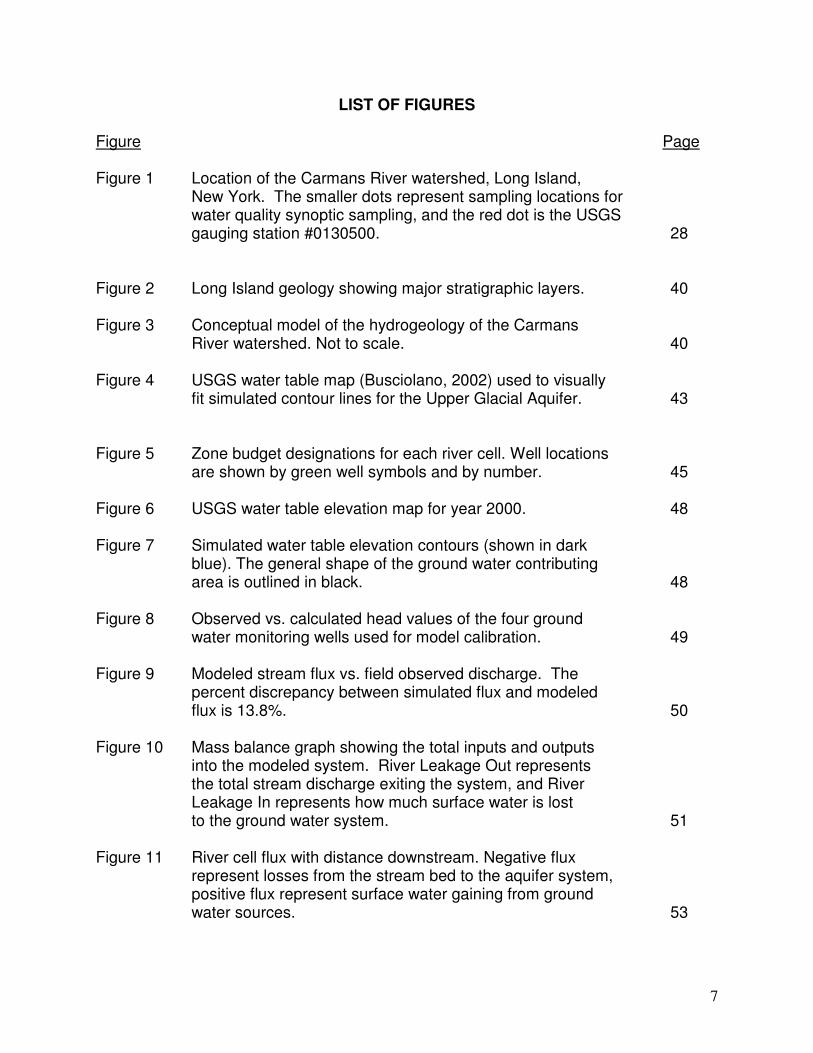
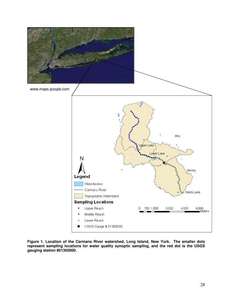
Figure Page Figure 1 Location of the Carmans River watershed, Long Island,

New York. The smaller dots represent sampling locations for water quality synoptic sampling, and the red dot is the USGS gauging station #0130500. 28

Figure 2 Long Island geology showing major stratigraphic layers. 40 Figure 3 Conceptual model of the hydrogeology of the Carmans River watershed. Not to scale. 40 Figure 4 USGS water table map (Busciolano, 2002) used to visually

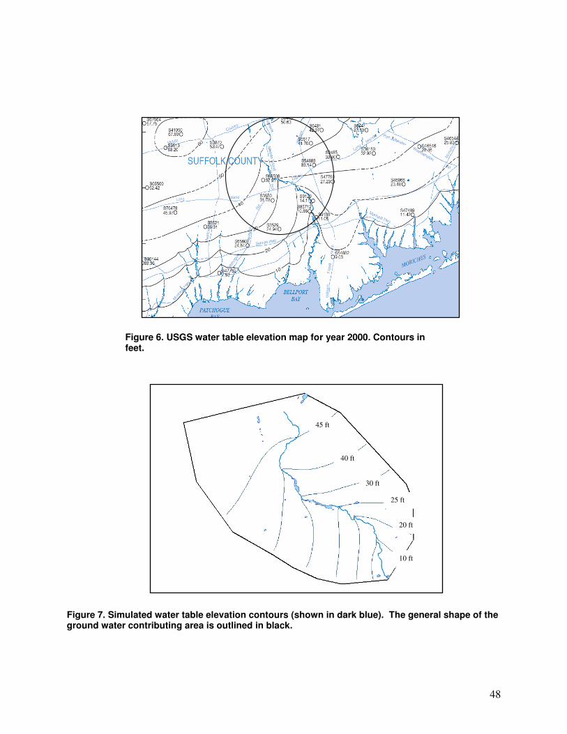
fit simulated contour lines for the Upper Glacial Aquifer. 43 Figure 5 Zone budget designations for each river cell. Well locations are shown by green well symbols and by number. 45 Figure 6 USGS water table elevation map for year 2000. 48 Figure 7 Simulated water table elevation contours (shown in dark blue). The general shape of the ground water contributing

area is outlined in black. 48 Figure 8 Observed vs. calculated head values of the four ground water monitoring wells used for model calibration. 49 Figure 9 Modeled stream flux vs. field observed discharge. The percent discrepancy between simulated flux and modeled flux is 13.8%. 50 Figure 10 Mass balance graph showing the total inputs and outputs into the modeled system. River Leakage Out represents the total stream discharge exiting the system, and River Leakage In represents how much surface water is lost to the ground water system. 51 Figure 11 River cell flux with distance downstream. Negative flux represent losses from the stream bed to the aquifer system, positive flux represent surface water gaining from ground

water sources. 53

8

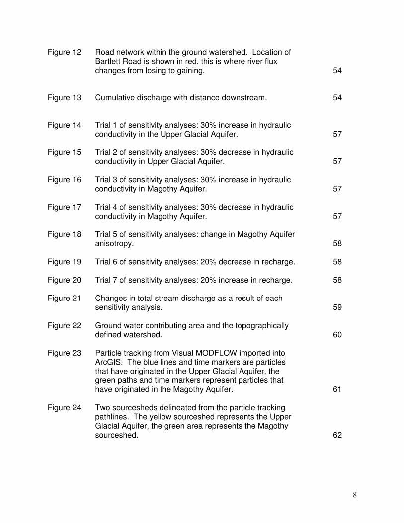
Figure 12 Road network within the ground watershed. Location of Bartlett Road is shown in red, this is where river flux changes from losing to gaining. 54

Figure 13 Cumulative discharge with distance downstream. 54 Figure 14 Trial 1 of sensitivity analyses: 30% increase in hydraulic conductivity in the Upper Glacial Aquifer. 57 Figure 15 Trial 2 of sensitivity analyses: 30% decrease in hydraulic conductivity in Upper Glacial Aquifer. 57 Figure 16 Trial 3 of sensitivity analyses: 30% increase in hydraulic conductivity in Magothy Aquifer. 57 Figure 17 Trial 4 of sensitivity analyses: 30% decrease in hydraulic conductivity in Magothy Aquifer. 57 Figure 18 Trial 5 of sensitivity analyses: change in Magothy Aquifer anisotropy. 58 Figure 19 Trial 6 of sensitivity analyses: 20% decrease in recharge. 58 Figure 20 Trial 7 of sensitivity analyses: 20% increase in recharge. 58 Figure 21 Changes in total stream discharge as a result of each

sensitivity analysis. 59 Figure 22 Ground water contributing area and the topographically defined watershed. 60 Figure 23 Particle tracking from Visual MODFLOW imported into ArcGIS. The blue lines and time markers are particles that have originated in the Upper Glacial Aquifer, the

green paths and time markers represent particles that have originated in the Magothy Aquifer. 61

Figure 24 Two sourcesheds delineated from the particle tracking pathlines. The yellow sourceshed represents the Upper Glacial Aquifer, the green area represents the Magothy sourceshed. 62

9

Figure 25 3-D view of particle tracking in Visual MODFLOW. Downstream flow is from right to left. Pathlines show that the majority of flow is in the Upper Glacial Aquifer, and fewer pathlines flow through the Magothy Aquifer. 62

Figure 26 Diagram showing direction of flow paths through the Upper Glacial and Magothy Aquifers. The majority of flow passes through the Upper Glacial Aquifer, but some flow from

farther distances passes through the Magothy before discharging into the Carmans River. Arrows indicate direction of flow. 63

Figure 27 Upper Clacial Aquifer residence times. Each line represents 5 years. 63 Figure 28 Magothy Aquifer residence time contours in 100 year intervals. Ground water entering the system at the top

of the watershed can be up to 500 years old. Note this image attempts to represent 3D conditions, that is why the 100 year contour is missing from the image. 64

Figure 29 Delineated sourcesheds for the headwaters and each lake. 64 Figure 30 pH with distance downstream. 66 Figure 31 Temperature with distance downstream. 66 Figure 32 Trilinear diagram representing all three sampling events. 69 Figure 33 Relative composition of cations in stream water for July 2005 sampling event. 71 Figure 34 Relative composition of anions in stream water for July 2005 sampling event. 71 Figure 35 Relative composition of cations in stream water for October 2005 sampling event. Note this was a partial sampling event due to a storm. 72 Figure 36 Relative composition of anions in stream water for October 2005 sampling event. 72 Figure 37 Relative composition of cations in stream water for July 2006 sampling event. 73

10

Figure 38 Relative composition of anions in stream water for July 2006 sampling event. 73 Figure 39 Nitrate concentration with distance downstream for the July and October 2005 and July 2006 sampling events. 74 Figure 40 Sodium and chloride concentrations with distance downstream for the October 2005 sampling event. 76 Figure 41 Sodium and chloride concentrations with distance downstream for the July 2005 sampling event. 76 Figure 42 Sodium and chloride concentrations with distance downstream for the July 2006 sampling event. 77 Figure 43 Sodium versus chloride for the July 2005 synoptic event. 77 Figure 44 Sodium versus chloride for the October 2005 synoptic event. 78

Figure 45 Sodium versus chloride for the July 2006 synoptic event. 78 Figure 46 Road density of the ground water shed. Density is in km/km2. 80 Figure 47 Road density by subwatershed. The upper subwatershed is

15.9 km2 and has a road density of 3.42 km/km2, the middle subwatershed is 13.6 km2 and has a road density of 1.99 km/km2, and the lower subwatershed is 43.4 km2 and has a road density of 3.5 km/km2. 81

Figure 48 Median sodium and chloride concentrations by subwatershed.

The pattern follows road density, the middle subwatershed has the lowest road density and has the lowest median concentrations, whereas the lower subwatershed has the highest road density,

and the highest median concentrations. 81

11

Abstract

O’Malley, Tracey, L.M. Analysis of surface water quality and ground water flow in the Carmans River Watershed, Long Island, New York. Word-processed and bound thesis 123 pages, 9 tables, 48 figures, 2008.

Agriculture and urban development on Long Island, New York have caused many of its rivers and streams to become eutrophic, and have led to poor water quality in the Great South Bay. The Carmans River provides the largest discharge into the Great South Bay, and therefore may be a primary contributor of nitrate and other constituents. In this investigation, ground water flow was simulated using a calibrated, steady state model, and a synoptic sampling of base flow was conducted and analyzed for major anions and cations. The dominant cations are sodium and calcium, the dominant anions are chloride and bicarbonate, and the average nitrate [NO3

-] concentration is 5.5 mg L-1. Modeling results suggest that there are two aquifer sources that feed the river, but the majority of streamflow is derived from the Upper Glacial Aquifer, which has a residence time of less than 20 years. Keywords: Base flow, MODFLOW, major ions, residence time, particle tracking. Authors name in full Tracey Lynn McGregor O’Malley Candidate for the degree of Master of Science Date May 2008 Major Professor Dr. Lee Herrington Department Forest and Natural Resources Management

State University of New York College of Environmental Science and Forestry, Syracuse, New York

Signature of Major Professor _____________________________________

Dr. Lee Herrington

12

CHAPTER I

INTRODUCTION

Land use activities such as urbanization and agriculture can severely alter water

quality and aquatic habitats of rivers, streams, lakes and estuaries. The two primary

factors affecting water quality and aquatic life throughout Long Island, New York, are

agricultural land use practices and urban development (Ayers et al., 2000).

Consequently, these two factors have led to the poor water quality of the Great South

Bay, the largest shallow estuarine bay in New York. Diminishing water quality has

affected living resources through habitat degradation, thus reducing estuarine

productivity and eliminating feeding and nursery habitat for finfish, shellfish, shorebirds

and colonial waterbirds. Hard clam harvests have fallen to record lows; a decrease by

more than 93% in 25 years. (Long Island South Shore Estuary Reserve Comprehensive

Management Plan, 2001).

Excessive levels of nitrogen pose one of the greatest threats to the South Shore

Estuary Reserve (SSER) (Long Island South Shore Estuary Reserve Comprehensive

Management Plan, 2001). Although nitrogen is an essential nutrient for plant growth

excessive concentrations promote algal blooms which can lead to hypoxic conditions in

coastal waters (Long Island Sound Study, 1998; Monti and Scorca, 2003). Algal blooms

decrease dissolved oxygen through the decomposition process, and when the oxygen

supply is depleted, fish and invertebrates die. Primary sources contributing to these

excessive nitrogen levels include lawn and agricultural fertilizers, manure application,

waterfowl and animal waste, and failed private septic systems.

13

The Carmans River, located in Suffolk County, Long Island, New York, is one of

the larger rivers feeding the Great South Bay (Figure 1). At approximately 16 km long, it

is the second largest river in Long Island, and is considered the region’s most pristine

river (Long Island South Shore Estuary Reserve Council, date unknown). Estimates

made by Monti and Scorca (2003) indicate that the Carmans River provides the greatest

discharge to the South Shore Estuary Reserve.

Nitrate levels are elevated throughout the island’s ground water system due to

past land use activities including extensive agriculture and duck farming, in combination

with the well drained and aerated soils (Ayers et al., 2000).

The effects of urbanization and agricultural practices can have detrimental

impacts on the quality and quantity of potable ground water systems. Watershed

monitoring programs and water quality models are widely used to investigate the effects

of urbanization and land use practices. MODFLOW, a block centered, finite difference,

ground water flow model, developed by McDonald and Harbaugh (1988) was used to

simulate ground water flow within the Carmans River watershed. This modeling

approach, combined with synoptic surface water quality monitoring, allowed for an

extensive investigation of water quality and ground water flow.

14

There were several objectives of this investigation:

Objective 1: Use synoptic sampling methods to investigate water chemistry during

base flow conditions.

Hypothesis 1: Higher nitrate concentrations will be found downstream of the farm located on Bartlett Road. Hypothesis 2: Sodium chloride concentrations will be higher in areas with higher road densities.

Hypothesis 3: The three impoundments along the river will increase surface water temperature and pH.

Objective 2: Determine the extent of the ground water sourceshed.

Hypothesis 4: The ground water contributing area is much larger than the topographically defined watershed.

Objective 3: Determine the areal extent and residence time for the Upper Glacial and Magothy Aquifer sources.

15

CHAPTER II

LITERATURE REVIEW

This literature review encompasses relevant topics that pertain to this thesis,

including soil characteristics found on Long Island, previous nitrate investigations that

have been conducted on Long Island, and ground water modeling literature including

island-wide models that were created to simulate ground water patterns for all of Long

Island. Soil characteristics are important because they influence soil aeration and

leaching which impact soil amendment applications in agricultural areas. Long Island

was once heavily used for agriculture but only one farm exists in the Carmans River

watershed today. Nitrogen concentrations throughout the Long Island ground water

system have been extensively investigated. This review encompasses only a handful of

relevant literature, including works from 1897 to present.

Ground water modeling was used in this investigation to simulate the Carmans

River watershed. This review incorporates a brief description of how Visual MODFLOW

operates, and the specific inputs used in the model. Two ground water models have

been developed for Long Island and are summarized for comparison.

16

2.1 Soil Characteristics

Soil can be defined as a dynamic medium composed of liquid, gases, living

organisms, inorganic solids, and organic solids such as plant matter. Soil is influenced

by climate and living organisms. There are five factors involved in soil formation: (1)

parent material, (2) climate, (3) topography, (4) living mater (biota), and (5) time. Long

Island soils are considered young. These mineral soils were deposited as a result of

glaciation during the Wisconsinian age, where the last glacier retreated approximately

11,000 years ago (Long Island Natural Environment Online, Date Unknown). The

majority of materials deposited were glacial outwash and till, and glaciolacustrine and

marine clays (McClymonds and Franke, 1972). The bedrock on Long Island is primarily

glacial age quartz-feldspar sands.

2.2 Agriculture

Agriculture is a long term land use practice in which nitrogen-enriched fertilizers

are repeatedly applied to the soil. Nitrogen is mobile in aquifer systems and becomes

widely distributed from ground water flow (Modica et al., 1998). From the time Long

Island was settled over 300 years ago, agriculture has been a major land use. Today,

Long Island agriculture includes over 20 km2 in vegetables, 24-28 km2 of nurseries, 16

km2 in sod production, 12 km2 in grapes for wine production, 1.4 km2 in floriculture and

six operating duck farms (Long Island Farm Bureau, 2007). Within the Carmans River

watershed one plant nursery and one vegetable farm are located in the headwaters

immediately adjacent to the river. Modica et al., (1997) showed that conservative

17

contaminants (non-reactive, such as chloride) that flow through the ground water

system can take several years to pass through the system, depending on their proximity

to the surface water body.

2.3 Previous Investigations on Long Island Regarding Nitrate Levels

There has been considerable research conducted on Long Island regarding the

high nitrate levels found in the ground water. A number of land use activities can

contribute to high nitrate concentrations in ground water. Sources of nitrate include

agricultural fertilizers, turf grass fertilizers (Perlmutter and Koch, 1972; Soren, 1977;

Kreitler et al., 1978; Bleifuss et al., 2005), failing septic systems or sewer lines

(Perlmutter and Koch, 1972;), animal wastes (Kreitler et al., 1978) and atmospheric

deposition (Mayer et al., 2002). The following studies show that nitrate concentrations

are influenced by local conditions, however natural levels can range between 0 -1.2 mg

L-1.

As early as 1897 research documented high nitrate concentrations for sparsely

populated areas of both Nassau and Suffolk Counties. From 1897 to 1902 Burr et al.

(1904) investigated nitrate concentrations at five well fields in a sparsely populated

region of Nassau County. They found nitrate concentrations ranging between 0.0 and

2.5 mg L-1, with an average of 0.7 mg L-1, in ground water wells 7.3 to 33.5 meters

deep.

Ground water from observation wells in Suffolk County near Brookhaven National

Laboratory, collected between 1948 and 1953 exhibited nitrate concentrations from 0.0

to 2.8 mg L-1, with an average concentration of 0.265mg L-1 (deLaguna, 1964, Table 6).

18

In an observation well near Shirley, a developed area located south of Brookhaven and

near the South Shore Estuary, nitrate concentrations ranged from 0.1 to 10 mg L-1, with

an average concentration of 2.6 mg L-1 (deLaguna, 1964, Table 6). Ground water

collected from a well at the sewage treatment plant had concentrations ranging from 5-

15 mg L-1, and ground water collected from a well thought to be contaminated by

cesspool effluent exhibited concentrations of 0 to 100 mg L-1 (deLaguna, 1964, Table 6).

Samples thought to be impacted by fertilizers showed nitrate concentrations ranging

between 38-47 mg L-1.

The majority of nitrate research, however, has focused on the more urbanized

areas of Nassau County. Perlmutter and Koch (1972) investigated aquifer and stream

water quality in a 499 km2 area in Southern Nassau County from 1966 to 1970. The

study area included hydrologically similar adjoining sewered and unsewered areas.

Natural levels of nitrate [NO3-] in ground water were estimated to be less than or equal

to 0.20 mg L-1, and concentrations greater than 1 mg L-1 may have been caused by

anthropogenic activities. In the sewered and unsewered areas, the average nitrate

concentrations of ground water were between 28 and 36 mg L-1, respectively. However,

there were seven places where nitrate levels equaled or exceeded 100 mg L-1. Nitrate

concentrations in streams whose discharge is dominated by ground water had average

concentrations of 11 and 25 mg L-1 in the sewered and unsewered areas, respectively.

In 1976, Suffolk County ranked first in New York State in total agricultural sales.

Over 243 km2 of the county were in agricultural production. Potatoes accounted for

approximately 101 km2 of the total 243 (Baier and Rykbost, 1976). Other agricultural

19

activities included duck farming, sod production, nursery products, and other fruits and

vegetables (Suffolk County CES, 1973, as cited by Baier and Rykbost, 1976).

Baier and Rykbost (1976) evaluated alternative N fertilization schemes which

would reduce nitrate leaching losses while maintaining potato yields and turfgrass

quality. Rykbost (unpublished data, as cited by Baier and Rykbost, 1976) conducted a

fertilization survey which indicated that application rates for potato fertilization ranged

from 0.23 to 0.56kg-N/km2. Turfgrass application rates had a larger range, from zero to

about 0.65 kg-N/km2 a year. Baier and Rykbost (1976) concluded that a loss of 0.09

kg-N/km2 via leaching, along with the average amount of recharge (58.4 cm per year),

would maintain a ground water nitrate [NO3-] concentration of 44 mg L-1. Baier and

Rykbost (1976) concluded that fertilizer nitrogen was the source of nitrate in the ground

water system beneath agricultural areas.

Kreitler et al. (1978) used isotopic tracers to determine the source of nitrate in

the Upper Glacial Aquifer by comparing Long Island ground water samples to other

known source signatures. They found that the average δN15 value was +5.3‰, similar

to signatures observed for unfertilized cultivated land, and was higher than signatures

typical of nitrate when it is derived solely from nitrogen fertilizer. Although the average

signature for Suffolk County was heavier than known signatures for fertilized land, it is

lighter than the other three counties in Long Island. The researchers therefore

concluded that the samples from Suffolk County represent fertilized or unfertilized

cultivated lands, whereas the other more residential counties were more influenced by

animal waste sources.

20

Flipse et al. (1984) investigated nitrogen concentrations in ground water and

precipitation post construction of a new housing development on forested land. The

study site was located in a housing development east of the Carmans River called

Twelve Pines. Surface water from the Carmans River was evaluated prior to

development from 1966 to 1970, and concentrations of [NO3-] ranged from 0.88 to 3.96

mg L-1 (U.S. Geological Survey, 1966-70 as cited by Flipse et al. 1984). A public survey

was conducted to determine the application rate and composition of lawn fertilizers used

in the Twelve Pines area, and monthly water meters on homes were read to

approximate the rate of irrigation.

Fourteen test wells and one control were installed after development from 1972

to 1979. Flipse et al. (1984) found a general increase in nitrate concentrations of 0.97

mg L-1 yr-1. This increase was attributed to nitrate from fertilizers in Twelve Pines where

the average application rate of fertilizer nitrogen was 107.5 kg ha-1 yr-1 (Porter et al.,

1978, as cited by Flipse et al., 1984), contributing approximately 2,300 kg of nitrogen

per year to ground water. Contributions of animal wastes to ground water were

considered to be approximately 4.5 kg ha-1 yr-1. Nitrogen isotopes were used to

distinguish among animal wastes, human wastes, and other sources of nitrate. The

results of the study indicated that the source of nitrate was non-animal sources, and

therefore supported the conclusion that fertilizer was the primary source of nitrate in the

Twelve Pines region.

In 1998, the U.S. Geological Survey in cooperation with New York State

Department of State (NYSDOS) began investigating nitrogen loading (mass per year) to

the South Shore Estuary Reserve (SSER). Within the Carmans River watershed

21

stream discharge was measured at the Hards Lake Dam, which is approximately 4 km

downstream from the USGS continuous-recording gauging-station (number 01305040).

Discharge measurements indicate that Carmans River provides the largest discharge of

all streams to the SSER (1.78 m3/s for water years 1972-98). Discharge measurements

taken at Hards Lake Dam indicate that flow is 2.6 times greater than the discharge at

the continuous-recording station (Monti and Scorca, 2003). Average annual nitrogen

loads were calculated for selected streams with sufficient data. The Carmans River had

a calculated load of 30,000 kg/year. This load was determined using the gauged flow

data. Since the discharge downstream becomes appreciably larger, depending on

nitrogen concentration downstream, it is possible that nitrogen loads from the Carmans

River could be larger than what was previously calculated.

The combination of soil properties and the wide use of fertilizers and septic

systems throughout Long Island have caused widespread nitrate contamination in the

ground water system. Documentation of nitrate concentrations began in 1897 and

investigations continue today. The Carmans River is fed primarily by ground water.

Land use activities impact ground water quality and subsequently surface water quality

of the Carmans River. Ground water modeling is necessary to determine how and what

land use activities in the ground water watershed are impacting the Carmans River.

2.4 Ground Water Modeling

There are three types of ground water models: predictive, interpretive and

generic (Anderson and Woessner, 1992). In the field of hydrogeology, models are

relied upon to investigate two general questions: (1) why a flow system is behaving the

way it is; and (2) how a flow system will behave in the future (Fetter, 2001).

22

Models are simple depictions of natural systems, and therefore rely on several

assumptions for simplification. The first step of creating a successful ground water flow

model is to develop a conceptual model that best describes the system. Data required

to transform a conceptual model into a mathematical model include (1) physical

characteristics such as the location, areal extent, and thickness of the aquifers and

confining hydrostratigraphic units; (2) hydraulic properties such as hydraulic

conductivities of the units, specific storage or specific yields for confined and unconfined

aquifers, respectively; (3) recharge through precipitation or other sources such as

recharge basins, wells or return flow from irrigation; (4) stream flow discharges; and (5)

natural boundary conditions such as geologic formations, salt water intrusion locations

and natural water bodies (Fetter, 2001).

MODFLOW is a block-centered, finite-difference, numerical, ground water flow

model originally developed by the United States Geological Survey (McDonald and

Harbaugh, 1988) for the study of ground water systems. Anderson and Woessner

(1992) state that “Numerical mathematical models simulate ground water flow indirectly

by means of a governing equation thought to represent the physical processes that

occur in the system, together with equations that describe heads or flows along the

boundaries of the model”. MODPATH (Pollock, 1988, 1989) is a three-dimensional

tracking extension that can be used in conjunction with MODFLOW. MODPATH uses

the head distributions in the flow model to calculate flow velocities and directions of

imaginary particles. This particle tracking extension only simulates advection but is

nonetheless a widely used program for determining residence times and flow patterns of

ground water.

23

2.5 Long Island Ground Water Modeling

Two island-wide models have been created to investigate the ground water

system and how it responds to developmental stresses. Researchers from the USGS

developed a predictive model using a finite-difference ground water flow model

(McDonald and Harbaugh, 1988) to investigate (1) predevelopment conditions; (2)

present conditions associated with developmental stressed conditions; and (3) drought

conditions that plagued Long Island in the 1960’s. This model was applied to observe

proposed water-supply development strategies for the year 2020 (Buxton and

Smolensky, 1999).

This USGS model represents the main body of Long Island (excluding the North

and South Forks, and Shelter Island). Stratigraphic layers represent the aquifers and

confining units, and the grid has 46 rows and 118 columns, where each cell is 1220 m

by 1220 m (Buxton et al., 1991). The first layer is the Upper Glacial aquifer, the

second and third layers are the upper and lower zones of the Magothy aquifer, and the

fourth layer is the Lloyd aquifer. Major confining units consist of Gardiners Clay and

Raritan confining unit.

Hydraulic conductivities used in the USGS model were based on field

measurements. Estimates made for previous numerical models were adjusted through

model calibration to represent “a best estimate at the island-wide analysis”. The Upper

Glacial Aquifer has two zones, the moraine and outwash, their hydraulic conductivity

was estimated as 15 m/d and 73 m/d, respectively, with anisotropy (horizontal versus

vertical hydraulic conductivity) of 10 to 1. The upper part of the Magothy Aquifer has an

24

estimated conductivity of 15 m/d, and the basal part has an estimated conductivity of 23

m/d, with anisotropy of 100 to 1.

The particle tracking method (Pollock, 1988, 1989) was applied to this model to

determine aquifer recharge areas in the regional ground water system (Buxton et al.,

1991). Recharge areas were simulated for the three hydrologic conditions stated

above. Water budget calculations from the Finite-Difference Model (Buxton and

Smolensky, 1999) were compared to water budget calculations derived from the

Particle-Tracking Algorithm (Pollack, 1988). For all three simulations, recharge is

derived solely from the Upper Glacial Aquifer and discharges to the stream and

shoreline (Buxton et al., 1991).

In 2003, Suffolk County Department of Health Services (SCDHS) hired Camp,

Dresser & McKee (CDM) to develop a ground water flow model for the purposes of

understanding and managing the ground water resources (Camp, Dresser & McKee,

2003). CDM developed a calibrated model of the main body of Suffolk County using the

DYNSYSTEM set of simulation algorithms developed at CDM. The model allows users

to evaluate island-wide conditions, and to assess more in-depth conditions within the

Southwest Sewer District (SWSD) and Brookhaven National Laboratory in Upton, NY.

The intention of Suffolk County Department of Health Services was that this model

would serve as a tool to be installed on County computers, for use by trained County

staff.

The model grid is comprised of nodes spaced between 914 and 1220 m apart. In

areas of special interest, such as Brookhaven National Laboratory, nodal spacing was

reduced to approximately 100 m. Stratigraphy was based on USGS preliminary

25

framework and from site-specific investigations by SCDHS, SCWA and NYSDEC. The

model stratigraphy was represented by eight model layers of variable thickness and

properties. The bottom of the model was the Lloyd Aquifer, and the top of the model

was the ground water surface. Layer 1 represents Lloyd Aquifer and Layer 2 represents

the Raritan clay layer. Layer 3 represents the coarsest zone of the Magothy Aquifer,

termed “Basal Magothy”. Basal Magothy materials have been estimated to have a

conductivity of 15 m/d by the USGS and anisotropy (vertical flow) of 0.15 m/d. CDM

estimates for the BNL area are 23 m/d and 0.23 m/d. In the model, horizontal

conductivity for the basal Magothy layer was 38 m/d, and vertical conductivity was 0.38

m/d. Layer 4 represents the middle Magothy Aquifer with a horizontal hydraulic

conductivity of 20 m/d, and a vertical conductivity of 0.20 m/d. Layer 5 represents the

Magothy Aquifer, and for the Carmans River area the middle Magothy conductivity is

the same as layer 4, but the BNL area has localized zones of lower conductivity. Layer

6 includes the Gardiners clay unit that is found in the Carmans watershed. The Upper

Glacial aquifer is also found in this layer, with a horizontal conductivity of 76 m/d, and a

vertical conductivity of 0.76 m/d. Layer 7 represents the Upper Glacial Aquifer with the

same conductivity as layer 6, and a zone of coarser grained sediments are included

underlying the Carmans River with a horizontal conductivity of 84 m/d, and a vertical of

0.84 m/d. Layer eight, the ground surface is the Upper Glacial Aquifer, and in the

Carmans watershed has a horizontal conductivity of 76 and 84 m/d on the left and right

side of the river, respectively.

26

2.6 Precipitation and Recharge

Precipitation and recharge vary with season. In the growing season (warm

season: from April through September) precipitation events are characterized as short

and intense. These short intense storms produce large amounts of runoff, and

therefore little recharge (Busciolano, 2002). Recharge that does enter the unsaturated

zone is quickly absorbed by vegetation and lost through evapotranspiration. In the non-

growing season (cool season: October through March), precipitation events tend to be

long and steady and in the form of rain, snow or ice. The aquifers of Long Island are

recharged from these events not only because of the duration of the event, but also

because vegetation is dormant during this period.

Average annual precipitation for central Long Island is from 107 to 127 cm

(Busciolano, 2000). The Long Island hydrologic cycle has been broken down by Olcott

(1995) in “Ground Water Atlas of the United States; Connecticut, Maine,

Massachusetts, New Hampshire, New York, Rhode Island, Vermont” (original source:

Franke and McClymonds, 1972). Based on the average amount of precipitation that

falls on Long Island per day, 1.3% is runoff. Of the remaining water, 50.3% is lost

through evapotranspiration, and approximately 49.7% is infiltrated. From the volume of

water that infiltrates the soil, approximately 2% is returned to the atmosphere as ground

water evapotranspiration.

27

CHAPTER III

MATERIALS AND METHODS

3.1 Study Area

Long Island, NY extends approximately 193 km east-northeast into the Atlantic

Ocean from the southeast tip of New York (Olcott, 1995). Long Island is a part of the

Coastal Plain Province, which is characterized by low topographic relief and temperate

climates. Most areas of Long Island exhibit elevations of less than 30 m above sea

level, but elevations range from sea level to almost 122 m above sea level (Dowhan et

al., Date Unknown). Long Island is dominated by two parallel ridges that run the length

of the island. These terminal moraines are the Harbor Hill Terminal Moraine and the

Ronkonkoma Terminal Moraine, both of which were deposited during the Wisconsinian

glacial episode (Olcott, 1995). The moraine material is a mix of sand, outwash and

gravel.

Long Island consists of four counties that encompass a total area of

approximately 3756 km2. The counties are Kings, Queens, Nassau and Suffolk

(Busciolano, 2002). Nassau and Suffolk Counties make up the majority of the island,

with a population over 2.8 million (U.S. Bureau of the Census, 2000). The Carmans

River is located in Suffolk County.

3.1.1 Carmans River Watershed

The Carmans River watershed (Figure 1) was selected for modeling because it is

the subject of an on-going study of nonpoint pollution impacts on river water quality and

the Great South Bay. The river extends from near the center of the island and flows

28

Figure 1. Location of the Carmans River watershed, Long Island, New York. The smaller dots represent sampling locations for water quality synoptic sampling, and the red dot is the USGS gauging station #01305000.

www.maps.google.com

29

south for approximately 18 km to the Great South Bay. The headwaters of the Carmans

River originate in the parking lot of Longwood Library, in Middle Island, New York.

Surface water inputs feeding the headwaters gather in a detention basin in the parking

lot of the library, flow through a culvert under a dirt road, and then out into a small

stream channel. The majority (95%) of stream flow is derived from ground water

(Pluhowski and Kantrowitz, 1964).

There are three impoundments that have subsequently created three reservoirs

along the Carmans River: Upper Lake, Lower Lake, and Hards Lake, which have areas

of approximately 7.4 ha, 4.7 ha, and 12.8 ha, respectively (Figure 1). The

impoundments have contributed to elevated temperatures within these reservoirs.

Hards Lake Dam is a tidal dam that separates freshwater from brackish water, and is

the largest lake in the system. One United States Geological Survey (USGS) gauging

station, #01305000, is centrally located along the river (Figure 1). The station does not

have real time capabilities, but stage data are available via USGS personnel in the

Coram NY office, or through published data for a particular water year.

30

3.1.2 Soils

Long Island soils were formed from glaciations during the Wisconsinian age, and

are mostly composed of glacial outwash and till, with small fractions of clay and silt.

The Riverhead-Plymouth-Carver Soil Association is found in the watershed (Appendix

A). “This association consists of deep, nearly level to gently sloping, well drained and

excessively drained, moderately coarse textured and coarse textured soils on the

southern outwash plain” (Warner et al., 1975). Riverhead soils dominate approximately

45 percent of this association, Plymouth soils make up approximately 30 percent of the

association, and Carver and Plymouth sands make up 10 percent. The remaining 15

percent is a mixture of various soil types, such as Atsion, which buffer the stream banks

and underlying streambed.

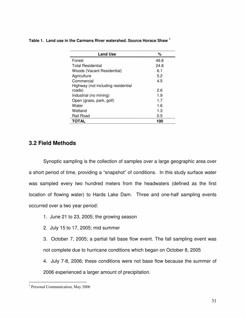
3.1.3 Land Use

Land use within the Carmans River Watershed is broken up into several uses

(Table 1). The two dominant uses are “forest” and “total residential”. The “total

residential” category encompasses all residential parcels with lot sizes from 0.1012 ha

to 1.012 ha.

31

Table 1. Land use in the Carmans River watershed. Source Horace Shaw 1

Land Use %

Forest 49.8

Total Residential 24.8

Woods (Vacant Residential) 6.1

Agriculture 5.2

Commercial 4.5 Highway (not including residential roads) 2.6

Industrial (no mining) 1.9

Open (grass, park, golf) 1.7

Water 1.6

Wetland 1.3

Rail Road 0.5

TOTAL 100

3.2 Field Methods

Synoptic sampling is the collection of samples over a large geographic area over

a short period of time, providing a “snapshot” of conditions. In this study surface water

was sampled every two hundred meters from the headwaters (defined as the first

location of flowing water) to Hards Lake Dam. Three and one-half sampling events

occurred over a two year period:

1. June 21 to 23, 2005; the growing season

2. July 15 to 17, 2005; mid summer

3. October 7, 2005; a partial fall base flow event. The fall sampling event was

not complete due to hurricane conditions which began on October 8, 2005

4. July 7-8, 2006; these conditions were not base flow because the summer of

2006 experienced a larger amount of precipitation.

1 Personal Communication, May 2006

32

Drought conditions were present for the summer of 2005 (Table 2). Precipitation

records were obtained from Shirley, NY, located in the lower eastern portion of the

watershed (Figure 1) from the Weather Underground2 site. This website provides a

searchable database with month-to-month precipitation and provides actual and

average precipitation received. The hydrologic conditions prior to the first, second and

third sampling events were below average. However, the night of the third sampling

event provided intense precipitation which continued through the following week due to

hurricane conditions. The fourth sampling event took place in the summer of 2006,

when the hydrologic conditions (precipitation and stream discharge) were well above

average.

Table 2. Hydrologic conditions for each synoptic sampling event.

Synoptic Sampling Total

Precipitation Previous 5 Days

(cm)

Total Precipitation Previous 14

Days (cm)

Monthly Total (cm)

Average Monthly

Total (cm)

#1 - June 21-23, 2005 0.05 0.76 3.53 9.32

#2 - July 15-17, 2005 0.76 5.13 5.31 7.14

#3 - October 7, 2005 0.00 1.47 35.74 9.19

#4 - July 7-8, 2006 6.27 11.7 13.87 7.44

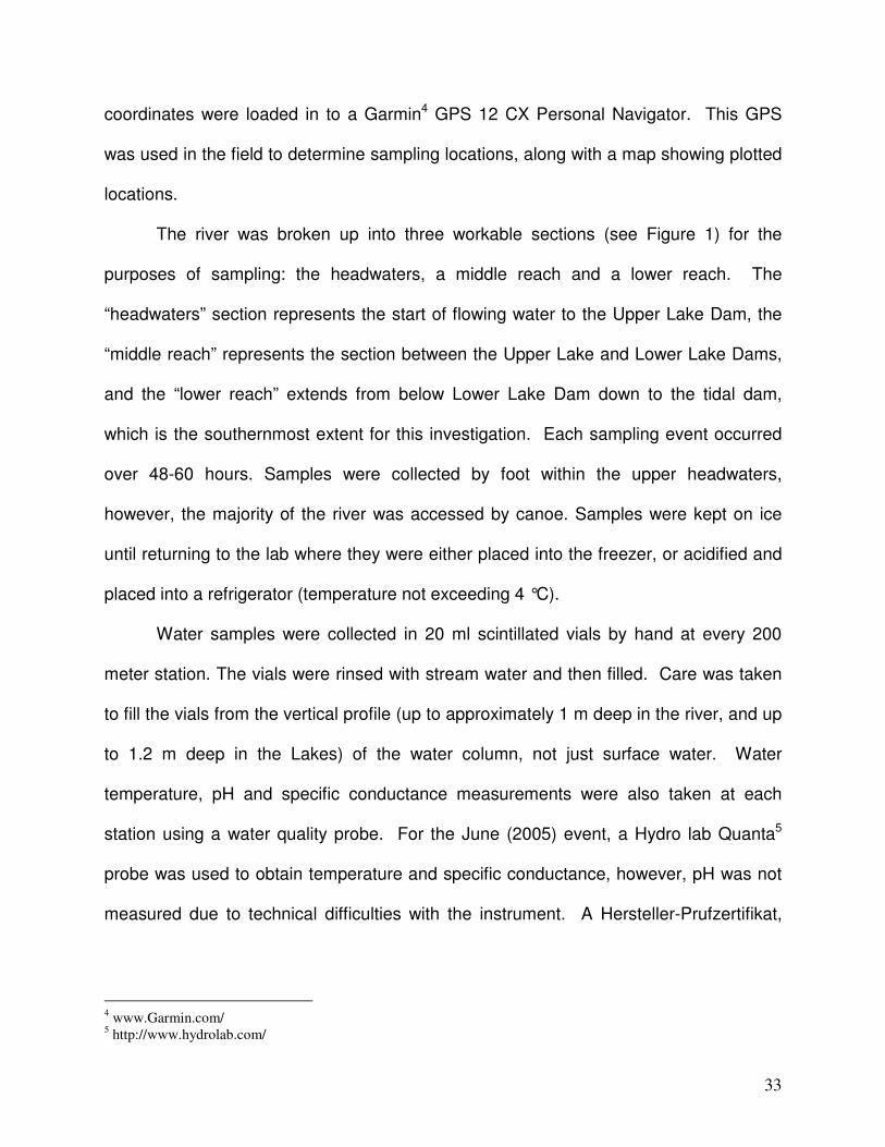
Prior to conducting the synoptic sampling events, sampling sites were

determined using ArcGIS©3 to plot sampling locations every 200 m along the river.

After obtaining longitude and latitude coordinates for each sampling location the

2 www.weatherunderground.com

3 www.esri.com/

33

coordinates were loaded in to a Garmin4 GPS 12 CX Personal Navigator. This GPS

was used in the field to determine sampling locations, along with a map showing plotted

locations.

The river was broken up into three workable sections (see Figure 1) for the

purposes of sampling: the headwaters, a middle reach and a lower reach. The

“headwaters” section represents the start of flowing water to the Upper Lake Dam, the

“middle reach” represents the section between the Upper Lake and Lower Lake Dams,

and the “lower reach” extends from below Lower Lake Dam down to the tidal dam,

which is the southernmost extent for this investigation. Each sampling event occurred

over 48-60 hours. Samples were collected by foot within the upper headwaters,

however, the majority of the river was accessed by canoe. Samples were kept on ice

until returning to the lab where they were either placed into the freezer, or acidified and

placed into a refrigerator (temperature not exceeding 4 °C).

Water samples were collected in 20 ml scintillated vials by hand at every 200

meter station. The vials were rinsed with stream water and then filled. Care was taken

to fill the vials from the vertical profile (up to approximately 1 m deep in the river, and up

to 1.2 m deep in the Lakes) of the water column, not just surface water. Water

temperature, pH and specific conductance measurements were also taken at each

station using a water quality probe. For the June (2005) event, a Hydro lab Quanta5

probe was used to obtain temperature and specific conductance, however, pH was not

measured due to technical difficulties with the instrument. A Hersteller-Prufzertifikat,

4 www.Garmin.com/

5 http://www.hydrolab.com/

34

Multi-Parameter (multi 340i) was used to measure temperature, pH and specific

conductance for all other sampling events.

3.3 Laboratory Analysis

Upon returning to Syracuse, samples that were to be analyzed for calcium,

magnesium, sodium and potassium (Ca2+, Mg2+, Na+ and K+) were preserved with 1%

nitric acid (HNO3; trace metal grade by Fisher), and stored in the refrigerator until

analysis on an Inductively Coupled Plasma-Optical Emission Spectrometer (Perkin-

Elmer OPTIMA 3300DV ICP-OES). Samples that would be analyzed for nitrate,

chloride and sulfate (NO3-, Cl- and SO4

2-) were placed in the freezer until analysis.

Samples were then thawed immediately before analysis on a Dionex Reagent Free Ion

Chromatography System, ICS-2000. Bicarbonate was calculated by difference between

the sum of cations and the sum of anions in meq L-1.

3.4 Modeling Methods

The modeling software used to simulate the subsurface conditions in the

Carmans River Watershed was Visual MODFLOW6 (Visual MODFLOW Pro 4.1,

Waterloo Hydrogeologic Inc.) The following paragraphs describe the available data for

importation, the conceptual model, model boundaries, model calibration and sensitivity

analyses and simulations.

6 http://www.flowpath.com/software/visual_modflow_pro/visual_modflow_pro_ov.htm

35

3.4.1 Available Data

Several data sources were utilized to develop a representative model of the

Carmans River ground water system. Surface topography was imported into

MODFLOW using 10 m digital elevation models (DEM) for the area surrounding the

Carmans River watershed. DEM’s were obtained from the Cornell University

Geospatial Information Repository (CUGIR7). The DEM format obtained from CUGIR

did not permit direct importation into Visual MODFLOW, therefore several conversions

were necessary using ArcGIS. Due to the size of the watershed, it was necessary to

resize each DEM from 10 x 10 m grid spacing to 100 x 100 m grid spacing. Each DEM

was converted to a raster file, which was then converted to a point file. Point files allow

integers to be associated with each grid cell in the model in order to obtain the elevation

values. In order to pair X and Y coordinates with elevation values, X and Y fields were

added to the ArcGIS attribute tables. X and Y coordinates were calculated by a visual

basic code. X, Y and Z values were then exported into Microsoft Excel for importation

into Visual MODFLOW.

Orthophoto imagery was downloaded from the New York State Geographical

Information System Clearinghouse8 and was used to estimate the width of the river

channel and the size of the lakes through the use of the measure tool in ArcGIS.

General aquifer characteristics such as aquifer thickness have been estimated by

Olcott (1995) and Doriski (1986). Recharge and evapotranspiration rates were

estimated based on methodology from Olcott (1995) (altered from Franke and

7 http://cugir.mannlib.cornell.edu/

8 http://www.nysgis.state.ny.us/

36

McClymonds, 1972). Precipitation records from two sources were utilized: (1)

www.weatherunderground.com (precipitation records for Shirley, NY, which is located

near the southern end of the watershed), and (2) Brookhaven National Laboratory9

(BNL) (Figure 1). The period of record at BNL is 57 years. The BNL source provided

useful information for determining the recharge boundary in MODFLOW and the

Weather Underground website provided daily precipitation records useful for base flow

sampling.

Based on Brookhaven National Laboratory precipitation records, average

precipitation over the 57 years of record is 123.5 cm yr-1. Olcott (1995) presents a

breakdown of the hydrologic cycle for all of Long Island (Table 3). Based on the

methodology Olcott (1995) proposed for Long Island, using average precipitation over

the past 57 years, recharge entering the ground water aquifer systems is 59.4 cm yr-1.

Table 3. Recharge calculation based on average precipitation. Method presented by Olcott (1995)

Precipitation Breakdown cm yr-1

Total Precipitation 123.5

1.3% runoff directly to streams 1.6

Of Remaining Water 121.9

50.3% Evapotranspiration 61.4

49.7% Recharge 60.6

Ground water Evaporation

2% Returned to the atmosphere 1.2

TOTAL RECHARGE 59.4

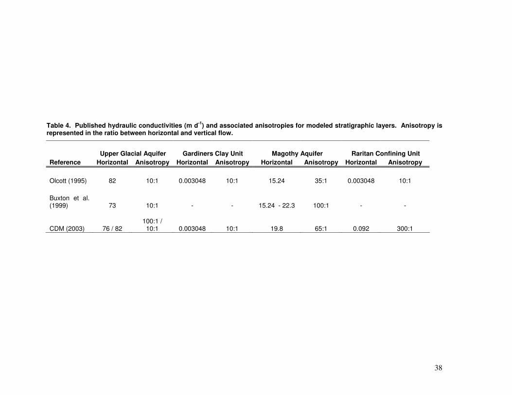
Layer properties such as hydraulic conductivity were obtained from three primary

sources (Table 4). The first source was from Olcott, (1995): Ground Water Atlas of the

United States; Connecticut, Maine, Massachusetts, New Hampshire, New York, Rhode

9 http://www.bnl.gov/weather/4cast/precip.html

37

Island, Vermont; USGS publication #HA 730-M. This publication gives general physical

characteristics of Long Island surficial and aquifer systems, including hydrogeology,

ground water flow, and ground water quality. The second source is Buxton et al.

(1998). This study reports the findings of a ground water flow model representing the

entire island. The third resource is Camp, Dresser and McKee (2003).

For calibration purposes, a water table and potentiometric surface map

developed by the USGS (Busciolano, 2002) for 2000 were used to simulate the water

table. Ground water levels in 2000 characterize average conditions according to R.

Busciolano (USGS office in Coram, NY personal communications, May, 2006). Four

United States Geologic Survey (USGS) monitoring wells were imported into the model

as ground water level monitoring wells. Information regarding past water levels was

accessed from the “USGS Ground-water levels for New York” website10.

10

http://nwis.waterdata.usgs.gov/nwis/gw

38

Table 4. Published hydraulic conductivities (m d-1

) and associated anisotropies for modeled stratigraphic layers. Anisotropy is represented in the ratio between horizontal and vertical flow.

Upper Glacial Aquifer Gardiners Clay Unit Magothy Aquifer Raritan Confining Unit

Reference Horizontal Anisotropy Horizontal Anisotropy Horizontal Anisotropy Horizontal Anisotropy

Olcott (1995) 82 10:1 0.003048 10:1 15.24 35:1 0.003048 10:1

Buxton et al. (1999) 73 10:1 - - 15.24 - 22.3 100:1 - -

CDM (2003) 76 / 82 100:1 / 10:1 0.003048 10:1 19.8 65:1 0.092 300:1

39

3.4.2 Conceptual Model

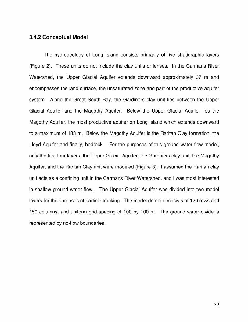
The hydrogeology of Long Island consists primarily of five stratigraphic layers

(Figure 2). These units do not include the clay units or lenses. In the Carmans River

Watershed, the Upper Glacial Aquifer extends downward approximately 37 m and

encompasses the land surface, the unsaturated zone and part of the productive aquifer

system. Along the Great South Bay, the Gardiners clay unit lies between the Upper

Glacial Aquifer and the Magothy Aquifer. Below the Upper Glacial Aquifer lies the

Magothy Aquifer, the most productive aquifer on Long Island which extends downward

to a maximum of 183 m. Below the Magothy Aquifer is the Raritan Clay formation, the

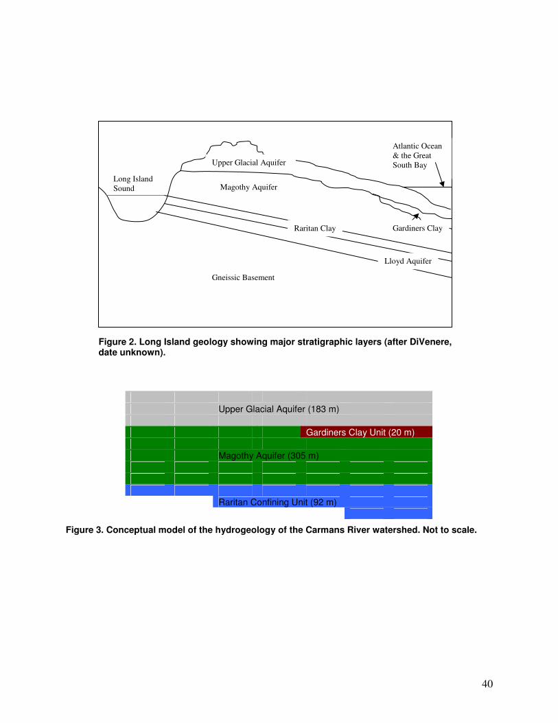
Lloyd Aquifer and finally, bedrock. For the purposes of this ground water flow model,

only the first four layers: the Upper Glacial Aquifer, the Gardniers clay unit, the Magothy

Aquifer, and the Raritan Clay unit were modeled (Figure 3). I assumed the Raritan clay

unit acts as a confining unit in the Carmans River Watershed, and I was most interested

in shallow ground water flow. The Upper Glacial Aquifer was divided into two model

layers for the purposes of particle tracking. The model domain consists of 120 rows and

150 columns, and uniform grid spacing of 100 by 100 m. The ground water divide is

represented by no-flow boundaries.

40

Upper Glacial Aquifer (183 m)

Gardiners Clay Unit (20 m)

Magothy Aquifer (305 m)

Raritan Confining Unit (92 m)

Figure 3. Conceptual model of the hydrogeology of the Carmans River watershed. Not to scale.

Gneissic Basement

Lloyd Aquifer

Raritan Clay

Magothy Aquifer

Gardiners Clay

Upper Glacial Aquifer

Long Island

Sound

Atlantic Ocean

& the Great

South Bay

Figure 2. Long Island geology showing major stratigraphic layers (after DiVenere, date unknown).

41

3.4.3 Model Inputs

Hydraulic conductivities for each model layer are shown in Table 5. Conductivity

values used in the Carmans River simulation were close to published values stated

above in Table 4. Recharge was applied over the entire model domain, and was

assumed to be uniform. The recharge value calculated using methodology from Olcott

(1995) was 59.4 cm yr-1, however, during the calibration process it was determined that

63.5 cm yr-1 provided a better fit for the model (see section 3.5.4).

Table 5. Hydraulic conductivity values used in simulation. Model color corresponds to zones in Figure 3.

Hydraulic Conductivities (m/d)

Stratiographic Layer x y z Model Color


Left side of Carmans River 76 76 7.6

Right side of Carmans River 83 83 8.3

Gardiner Clay Unit 0.3 0.3 0.003

Magothy Aquifer 15.24 15.24 1

Raritan Confining Unit 0.003048 0.003048 0.0001

42

3.4.4 River Boundary

The River Boundary was used to model how surface water bodies influence

ground water flow (Waterloo Hydrogeologic Inc., 2005 (p.223). The River Boundary

allows the user to assign a river stage, a river bed conductance, and the rivers width to

a set of cells that represent the river.

The River Boundary was applied to all cells in which the river flowed, and the two

lakes in the upper watershed: Spring Ponds and Artist Lake. The hydraulic gradient

between the surface water body and the ground water system determines whether the

surface water bodies contribute flow to the ground water system or function as

discharge zones for the ground water system. The River Boundary package determines

the interaction between the surface water body and the ground water system by a

seepage layer which separates the two systems (Waterloo Hydrologic, 2005) (p.223).

The River Boundary requires values for river stage, riverbed bottom (the elevation of the

river bed), and conductance. The conductance value represents the resistance to flow

caused by the seepage layer. The conductance value is calculated within the River

Boundary package using the following equation:

C = K x L x W / M

Where:

K = the vertical hydraulic conductivity of the riverbed material

L = the length of the reach

W = the width of the river within the cell

M = the thickness of the riverbed

43

This equation is used in river simulations where the river boundary can be

applied to each cell individually or can be applied as a linear gradient. When the River

Boundary package is used to create lakes, a polygon can be drawn to represent the

lake, and the length and width terms of the conductance value are calculated using the

X-Y dimensions. In the Carmans River simulation the vertical hydraulic conductivity for

the riverbed was assumed to be uniform with a value of 1 m d-1, and the riverbed

thickness was 0.3 m (~1ft).

3.4.5 Model Calibration

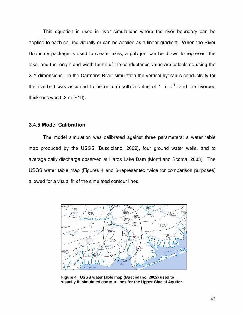
The model simulation was calibrated against three parameters: a water table

map produced by the USGS (Busciolano, 2002), four ground water wells, and to

average daily discharge observed at Hards Lake Dam (Monti and Scorca, 2003). The

USGS water table map (Figures 4 and 6-represented twice for comparison purposes)

allowed for a visual fit of the simulated contour lines.

Figure 4. USGS water table map (Busciolano, 2002) used to visually fit simulated contour lines for the Upper Glacial Aquifer.

44

The four wells scattered throughout the model domain were used to calibrate the

water table. The head values used for calibration were obtained from the 2000 water

table map (Busciolano, 2002). All four wells are within the Upper Glacial Aquifer with

two wells in layer one and two wells in layer two.

In addition to head calibration, the River boundary flux allowed for calibration

against total discharge at Hards Lake Dam. This metric was used for determining the

ground contributing area. In terms of model input uncertainties, such as aquifer

properties, recharge rates and model domain area, the size of the model domain has

the greatest uncertainty. Therefore, river leakage was calibrated to ground watershed

size.

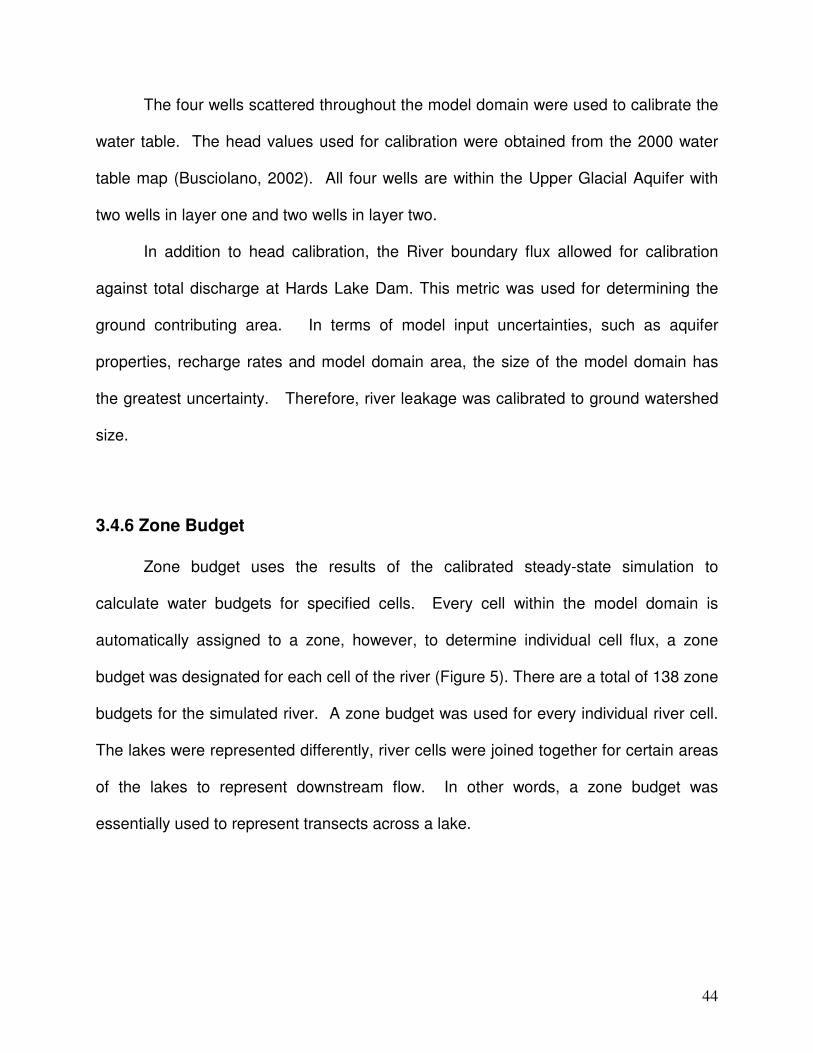
3.4.6 Zone Budget

Zone budget uses the results of the calibrated steady-state simulation to

calculate water budgets for specified cells. Every cell within the model domain is

automatically assigned to a zone, however, to determine individual cell flux, a zone

budget was designated for each cell of the river (Figure 5). There are a total of 138 zone

budgets for the simulated river. A zone budget was used for every individual river cell.

The lakes were represented differently, river cells were joined together for certain areas

of the lakes to represent downstream flow. In other words, a zone budget was

essentially used to represent transects across a lake.

45

Figure 5. Zone budget designations for each river cell. Well locations are shown by green well symbols and by number.

3.4.7 Sensitivity Analysis

To determine how sensitive the river cell flux was to model parameters,

sensitivity analyses were performed by altering hydraulic conductivities and recharge.

Hydraulic conductivities within the Upper Glacial Aquifer and the Magothy Aquifer were

altered independently from one another and were increased and decreased by 30%.

Anisotropy within the Magothy Aquifer was also investigated due to the different values

stated in the literature.

3.4.8 Particle Tracking and MODPATH Simulations

Particle tracking was used to examine the areal extent of the ground water

sourceshed aquifers and to estimate ground water residence times (Modica et al.,

46

1998). Particles were placed under the stream bed and tracked backwards to their

point of origin (Brawley et al., 2000; Pint et al., 2003; Wayland et al., 2002). Time

markers for 5 and 100 year intervals, for the Upper Glacial and Magothy Aquifers

respectively, allowed for manual delineation of sourcesheds and residence time

contours. Path lines and time markers were then imported into ArcGIS for delineation.

The two aquifer sourcesheds could be distinguished from one another based on their

path line length, and the time markers on each path line. Shapefiles were created to

manually delineate the two aquifer sourcesheds, and also to draw contours. Travel time

contours for the Upper Glacial aquifer were clipped with the aquifer sourceshed

boundary.

47

CHAPTER IV

RESULTS

This section is divided into two parts: modeling and chemistry. The modeling

section presents modeling results beginning with calibration and sensitivity and

concluding with the areal extent of the aquifer sourcesheds and residence times. The

chemistry section presents the chemistry results generated from the synoptic water

chemistry surveys.

4.1 Modeling Results

4.1.1 Calibration Results

The steady-state model was calibrated to average ground water conditions as

stated on the 2000 water table map (Busciolano, 2002) (Figure 6). Simulated water

table elevation contours (Figure 7) closely follow the pattern found on the USGS

produced map for 2000. Simulated contours show that the middle and lower portions of

the watershed are gaining from the ground water system, and portions of the upper

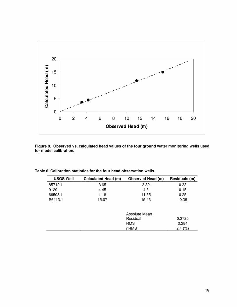
watershed are primarily losing. The four wells used to calibrate head in the Upper

Glacial Aquifer produced a normalized root mean square error of 2.4% (Figure 8, Table

6).

48

Figure 7. Simulated water table elevation contours (shown in dark blue). The general shape of the ground water contributing area is outlined in black.

Figure 6. USGS water table elevation map for year 2000. Contours in feet.

45 ft

40 ft

30 ft

25 ft

20 ft

10 ft

49

0

5

10

15

20

0 2 4 6 8 10 12 14 16 18 20

Observed Head (m)

Calc

ula

ted

Head

(m

)

Figure 8. Observed vs. calculated head values of the four ground water monitoring wells used for model calibration.

Table 6. Calibration statistics for the four head observation wells.

USGS Well Calculated Head (m) Observed Head (m) Residuals (m)

85712.1 3.65 3.32 0.33

9129 4.45 4.3 0.15

66508.1 11.8 11.55 0.25

S6413.1 15.07 15.43 -0.36

Absolute Mean Residual 0.2725

RMS 0.284

nRMS 2.4 (%)

50

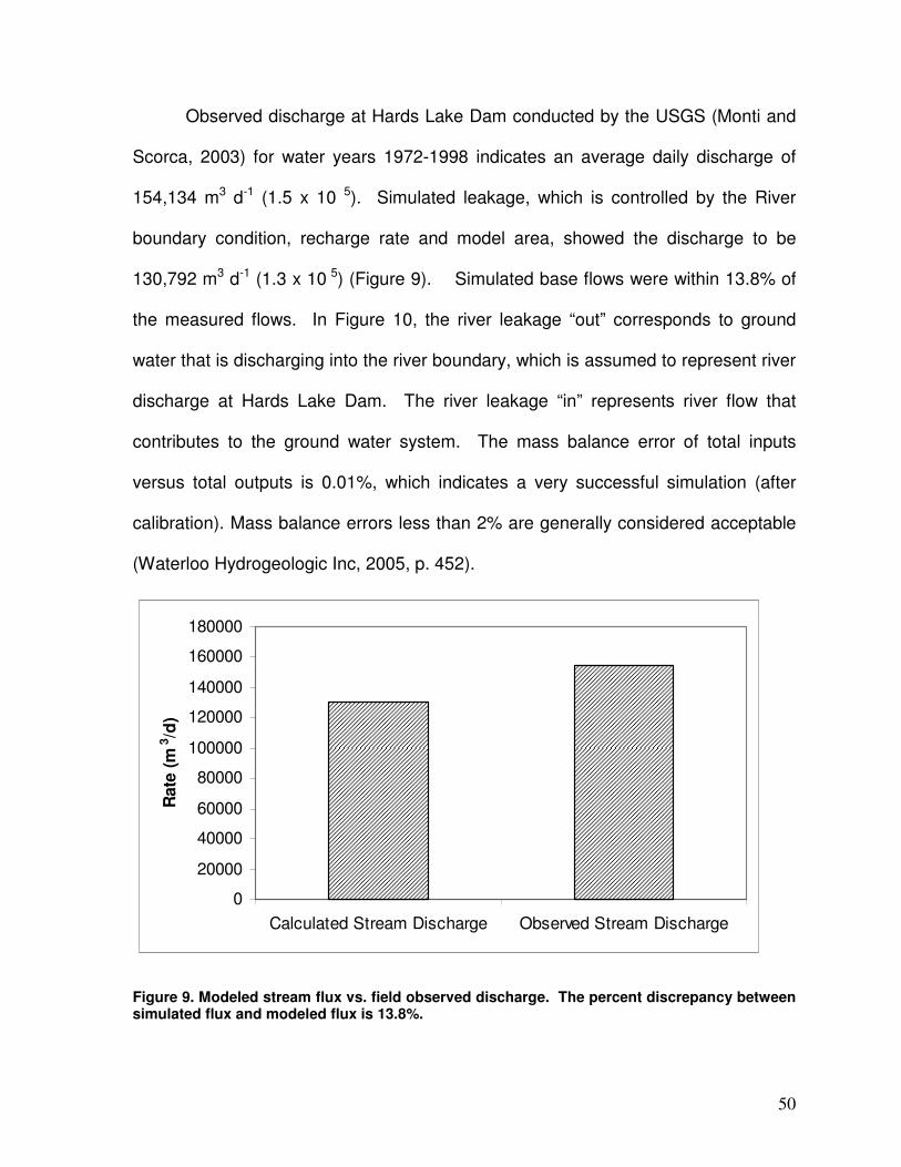
Observed discharge at Hards Lake Dam conducted by the USGS (Monti and

Scorca, 2003) for water years 1972-1998 indicates an average daily discharge of

154,134 m3 d-1 (1.5 x 10 5). Simulated leakage, which is controlled by the River

boundary condition, recharge rate and model area, showed the discharge to be

130,792 m3 d-1 (1.3 x 10 5) (Figure 9). Simulated base flows were within 13.8% of

the measured flows. In Figure 10, the river leakage “out” corresponds to ground

water that is discharging into the river boundary, which is assumed to represent river

discharge at Hards Lake Dam. The river leakage “in” represents river flow that

contributes to the ground water system. The mass balance error of total inputs

versus total outputs is 0.01%, which indicates a very successful simulation (after

calibration). Mass balance errors less than 2% are generally considered acceptable

(Waterloo Hydrogeologic Inc, 2005, p. 452).

0

20000

40000

60000

80000

100000

120000

140000

160000

180000

Calculated Stream Discharge Observed Stream Discharge

Rate

(m

3/d

)

Figure 9. Modeled stream flux vs. field observed discharge. The percent discrepancy between simulated flux and modeled flux is 13.8%.

51

0

20000

40000

60000

80000

100000

120000

140000

160000

River Leakage

In

River Leakage

Out

Total In Total Out

Dis

ch

arg

e R

ate

s (

m3/d

)

Figure 10. Mass balance graph showing the total inputs and outputs into the modeled system. River Leakage Out represents the total stream discharge exiting the system, and River Leakage In represents how much surface water is lost to the ground water system.

4.1.2 Zone Budget and River Cell Flux

Flow budgets for each River boundary cell show that the majority of cells in

the upper watershed lose surface water inputs to the ground water system (Figure

11). Positive flux corresponds to ground water loss to surface waters (stream flow

gains), and negative flux corresponds to ground water gains (or stream flow losses).

Simulated flux ranges between 1653 m3 d-1 to -4617 m3 d-1. The river consistently

becomes a gaining stream (gaining from the ground water system) after it passes

under Bartlett Road (Figure 12). From this point downstream, there are only a few

locations within the river system in which the river bed loses to the ground water

system. The two dams are causing a negative flux to occur slightly upstream from

52

the dam locations because of the difference in river stage. A negative flux (ground

water is gaining) occurs immediately before the dam. Immediately downstream of

the dam the river begins to again gain ground water. Figure 13 shows the

cumulative discharge with distance downstream.

53

-2000

-1000

0

1000

2000

3000

4000

5000

Flu

x R

ate

(m

3/d

)

Bartlett road; the beginning

of the agricultural

farm.

Upper Lake Begins

Upper Lake Dam Lower Lake Dam

Hards Lake Begins

Figure 11. River cell flux with distance downstream. Negative flux represent losses from the stream bed to the aquifer system; positive flux represent surface water gaining from ground water sources.

54

Cumulative Discharge

-20000

0

20000

40000

60000

80000

100000

120000

140000

160000

Distance Downstream

Dis

ch

arg

e (

m3/d

)

Cumulative Discharge

Figure 13. Cumulative discharge with distance downstream.

Figure 12. Road network within the ground watershed. Location of Bartlett Road is shown in red, this is where river flux changes from losing to gaining.

55

4.1.3 River Cell Flux Sensitivity Analysis

A sensitivity analysis was performed to observe how the simulated river flux

changes with alterations in model parameters. Figure 11 shows flux for each river

boundary cell (river cells were combined to form transects across the Lakes). For each

trial the difference in flux between the calibrated model and sensitivity trial were plotted

with distance downstream, showing either a positive gain or loss in stream discharge

from the ground water system. Figures 14 through 20 show how each cell is impacted

due to changes in either hydraulic conductivity or recharge. Overall percent difference

was calculated based on the discrepancy in flux between the calibrated zone budgets

for each cell, and those for each trial. Overall, the average difference between the

increasing and decreasing parameter trials are not that different, however, Figures 14

through 20 show that the simulated trials impact different cells (or reaches) of the river.

Trials 1 and 2 (Figures 14 and 15) show how changes in hydraulic conductivity in

the Upper Glacial Aquifer impact each individual cell. In trial 1, hydraulic conductivity is

increased by 30%. Increasing conductivity results in more ground water available to the

headwater system and less relative ground water to the lower reaches. Trial 1 resulted

in an absolute difference of 42%. In trial 2, hydraulic conductivity is decreased by 30%.

As a result, the headwaters lose even more to the ground water system, and the lower

reaches gain more from the ground water system. This simulation resulted in an

average difference of 40%.

Hydraulic conductivity changes in the Magothy Aquifer produce similar patterns

with distance downstream (Figures 16 and 17). Overall average differences between

the calibrated simulation and a 30% increase and decrease in hydraulic conductivity is

56

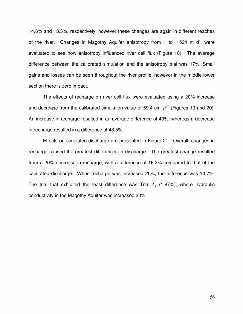
14.6% and 13.5%, respectively, however these changes are again in different reaches

of the river. Changes in Magothy Aquifer anisotropy from 1 to .1524 m d-1 were

evaluated to see how anisotropy influenced river cell flux (Figure 18). The average

difference between the calibrated simulation and the anisotropy trial was 17%. Small

gains and losses can be seen throughout the river profile, however in the middle-lower

section there is zero impact.

The effects of recharge on river cell flux were evaluated using a 20% increase

and decrease from the calibrated simulation value of 59.4 cm yr-1 (Figures 19 and 20).

An increase in recharge resulted in an average difference of 40%, whereas a decrease

in recharge resulted in a difference of 43.5%.

Effects on simulated discharge are presented in Figure 21. Overall, changes in

recharge caused the greatest differences in discharge. The greatest change resulted

from a 20% decrease in recharge, with a difference of 16.3% compared to that of the

calibrated discharge. When recharge was increased 20%, the difference was 10.7%.

The trial that exhibited the least difference was Trial 4, (1.87%), where hydraulic

conductivity in the Magothy Aquifer was increased 30%.

57

-8000

-6000

-4000

-2000

0

2000

Distance Downstream

Ch

an

ge

in

Sim

ula

ted

Dis

ch

arg

e

(m3/d

)

-8000

-6000

-4000

-2000

0

2000

Distance Downstream

Ch

an

ge in

Sim

ula

ted

Dis

ch

arg

e

(m3/d

)

-8000

-6000

-4000

-2000

0

2000

Distance Downstream

Ch

an

ge i

n S

imu

late

d D

isch

arg

e

(m3/d

)

-8000

-6000

-4000

-2000

0

2000

Distance Downstream

Ch

an

ge in

Sim

ula

ted

Dis

ch

arg

e

(m3/d

)

Figure 14. Trial 1 of sensitivity analyses: 30% increase in hydraulic conductivity in the Upper Glacial Aquifer.

Figure 15. Trial 2 of sensitivity analyses: 30% decrease in hydraulic conductivity in Upper Glacial Aquifer.

Figure 16. Trial 3 of sensitivity analyses: 30% increase in hydraulic conductivity in the Magothy Aquifer.

Figure 17. Trial 4 of sensitivity analyses: 30% decrease in hydraulic conductivity in the Magothy Aquifer.

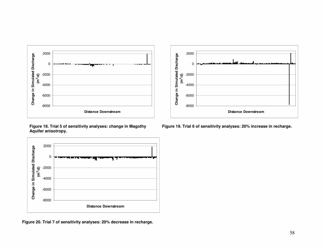
58

-8000

-6000

-4000

-2000

0

2000

Distance Downstream

Ch

an

ge i

n S

imu

late

d D

isch

arg

e

(m3/d

)

-8000

-6000

-4000

-2000

0

2000

Distance Downstream

Ch

an

ge i

n S

imu

late

d D

isch

arg

e

(m3/d

)

-8000

-6000

-4000

-2000

0

2000

Distance Downstream

Ch

an

ge i

n S

imu

late

d D

isch

arg

e

(m3/d

)

Figure 18. Trial 5 of sensitivity analyses: change in Magothy Aquifer anisotropy.

Figure 19. Trial 6 of sensitivity analyses: 20% increase in recharge.

Figure 20. Trial 7 of sensitivity analyses: 20% decrease in recharge.

59

0

20000

40000

60000

80000

100000

120000

140000

160000

180000

Obs

erve

d

Calib

rate

d

Trial 1

Trial 2

Trial 3

Trial 4

Trial 5

Trial 6

Trial 7

Trial Number

Dis

ch

arg

e (

m3/d

)

Discharge

4.1.4 Ground Water Contributing Area

The general ground water boundaries were delineated using the 2000 water

table map (Busciolano, 2002). The boundary was then calibrated to the other known

parameters in the system such as hydraulic conductivity, recharge and river discharge.

Since the ground water contributing area has the greatest uncertainty out of the other

modeled parameters, the no flow boundary was manipulated until a fit was found that

represented the USGS water table maps. The simulated ground water contributing area

is much larger than the topographically defined watershed (Figure 22).

Figure 21. Changes in total stream discharge as a result of each sensitivity analysis.

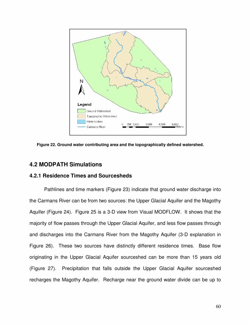
60

4.2 MODPATH Simulations

4.2.1 Residence Times and Sourcesheds

Pathlines and time markers (Figure 23) indicate that ground water discharge into

the Carmans River can be from two sources: the Upper Glacial Aquifer and the Magothy

Aquifer (Figure 24). Figure 25 is a 3-D view from Visual MODFLOW. It shows that the

majority of flow passes through the Upper Glacial Aquifer, and less flow passes through

and discharges into the Carmans River from the Magothy Aquifer (3-D explanation in

Figure 26). These two sources have distinctly different residence times. Base flow

originating in the Upper Glacial Aquifer sourceshed can be more than 15 years old

(Figure 27). Precipitation that falls outside the Upper Glacial Aquifer sourceshed

recharges the Magothy Aquifer. Recharge near the ground water divide can be up to

Figure 22. Ground water contributing area and the topographically defined watershed.

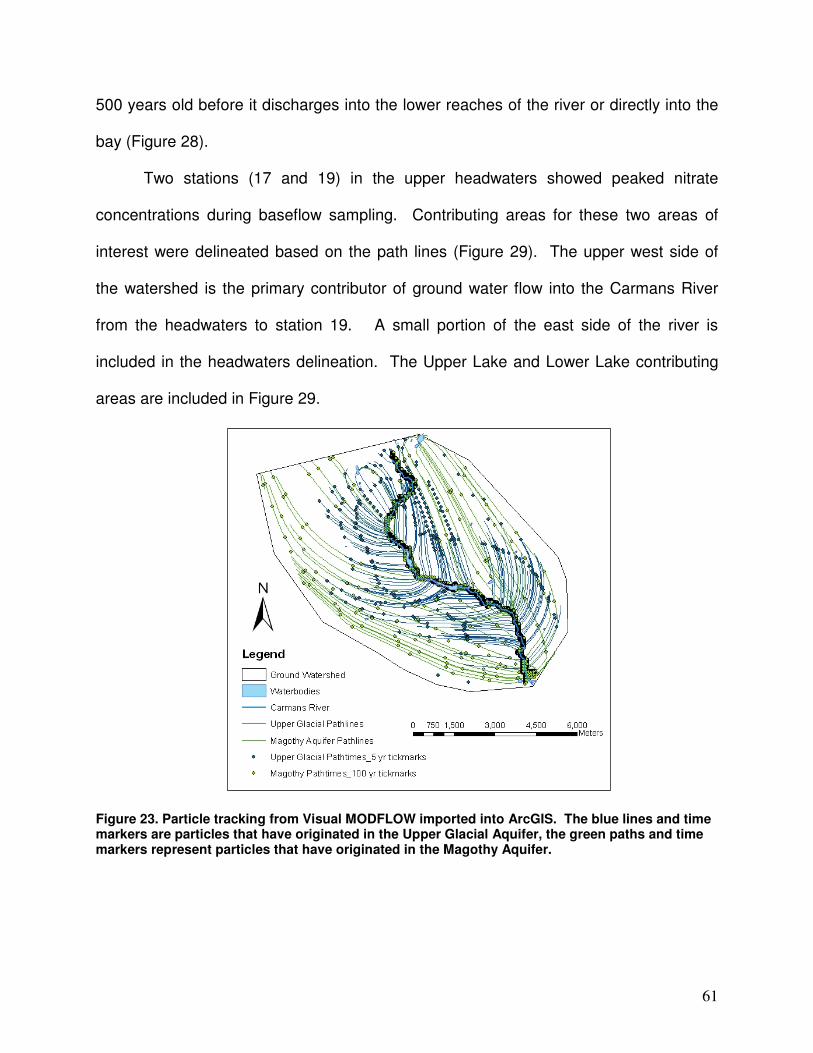
61

500 years old before it discharges into the lower reaches of the river or directly into the

bay (Figure 28).

Two stations (17 and 19) in the upper headwaters showed peaked nitrate

concentrations during baseflow sampling. Contributing areas for these two areas of

interest were delineated based on the path lines (Figure 29). The upper west side of

the watershed is the primary contributor of ground water flow into the Carmans River

from the headwaters to station 19. A small portion of the east side of the river is

included in the headwaters delineation. The Upper Lake and Lower Lake contributing

areas are included in Figure 29.

Figure 23. Particle tracking from Visual MODFLOW imported into ArcGIS. The blue lines and time markers are particles that have originated in the Upper Glacial Aquifer, the green paths and time markers represent particles that have originated in the Magothy Aquifer.

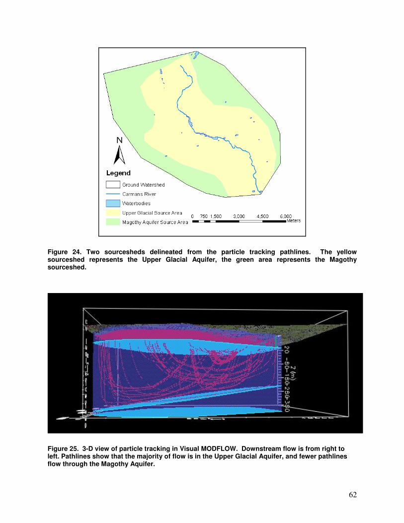
62

Figure 24. Two sourcesheds delineated from the particle tracking pathlines. The yellow sourceshed represents the Upper Glacial Aquifer, the green area represents the Magothy sourceshed.

Figure 25. 3-D view of particle tracking in Visual MODFLOW. Downstream flow is from right to left. Pathlines show that the majority of flow is in the Upper Glacial Aquifer, and fewer pathlines flow through the Magothy Aquifer.

63


Magothy Aquifer

Figure 27. Upper Glacial Aquifer residence times. Each line represents 5 years.

5 10 15

Figure 26. Diagram showing direction of flow paths through the Upper Glacial and Magothy Aquifers. The majority of flow passes through the Upper Glacial Aquifer, but some flow from farther distances passes through the Magothy before discharging into the Carmans River. Arrows indicate direction of flow.

5 10 15

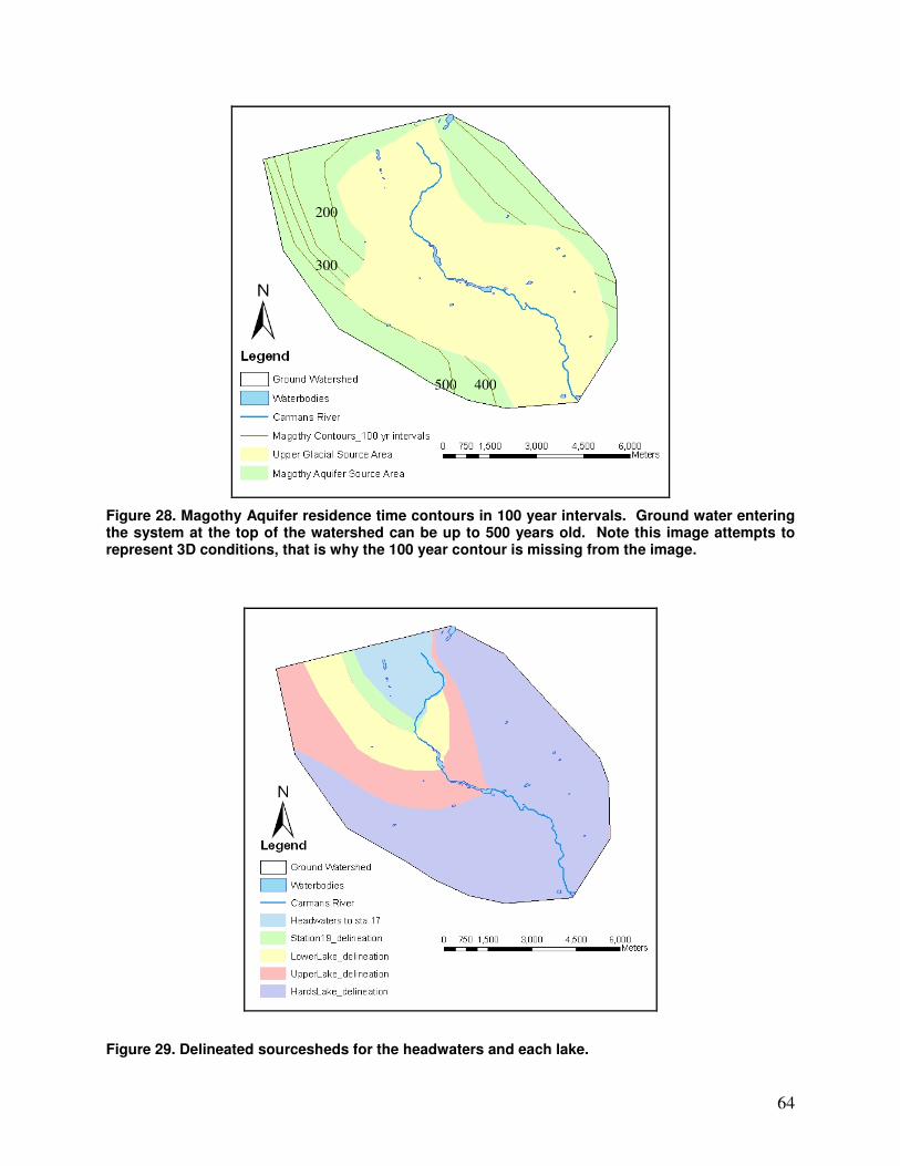
64

Figure 28. Magothy Aquifer residence time contours in 100 year intervals. Ground water entering the system at the top of the watershed can be up to 500 years old. Note this image attempts to represent 3D conditions, that is why the 100 year contour is missing from the image.

Figure 29. Delineated sourcesheds for the headwaters and each lake.

200

300

400 500

65

4.3 Chemistry Results

4.3.1 Basic Water Quality Parameters

Water chemistry was analyzed from the four sampling events. Although I tried to

sample during base flow conditions, the July 2005 and July 2006 sampling events

received 5.13 cm and 11.7 cm of precipitation, respectively, in the two weeks prior to

sampling (Table 2). Hydrographs for each sampling event are located in Appendix B.

Basic water chemistry parameters such as pH and specific conductivity, along

with temperature, were analyzed at each sampling point (Appendix D). The highest pH

observed was 9.36, which was observed during the July 2005 sampling event just

upstream from the Lower Lake dam (Figure 30). The lowest pH observed was 5.8 in

the headwater reaches during the high flow sampling event in July 2006 (Table 7). The

lowest temperature observed was in October 2005, and was 13.9 °C, and the highest

temperature was observed in July 2005, and was 30.8 °C (Table 7). This high

temperature of 30.8 °C was observed just upstream from the Lower Lake dam, at the

same location that had the highest pH reading (Figure 31). The specific conductivity

dataset is only complete for the July 2005 event. The maximum value was 261 µs cm-1,

and the minimum value was 98 µs cm-1. The highest value was observed in the upper

headwaters, and the lowest value of 98 µs cm-1 was observed in the outfall of Weeks

Pond.

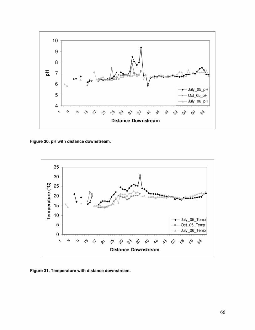
66

4

5

6

7

8

9

10

1 5 9 13 17 21 25 29 33 37 40 44 48 52 56 60 64

Distance Downstream

pH

July_05_pH

Oct_05_pH

July_06_pH

Figure 30. pH with distance downstream.

0

5

10

15

20

25

30

35

1 5 9 13 17 21 25 29 33 37 40 44 48 52 56 60 64

Distance Downstream

Tem

pera

ture

(°C

)

July_05_Temp

Oct_05_Temp

July_06_Temp

Figure 31. Temperature with distance downstream.

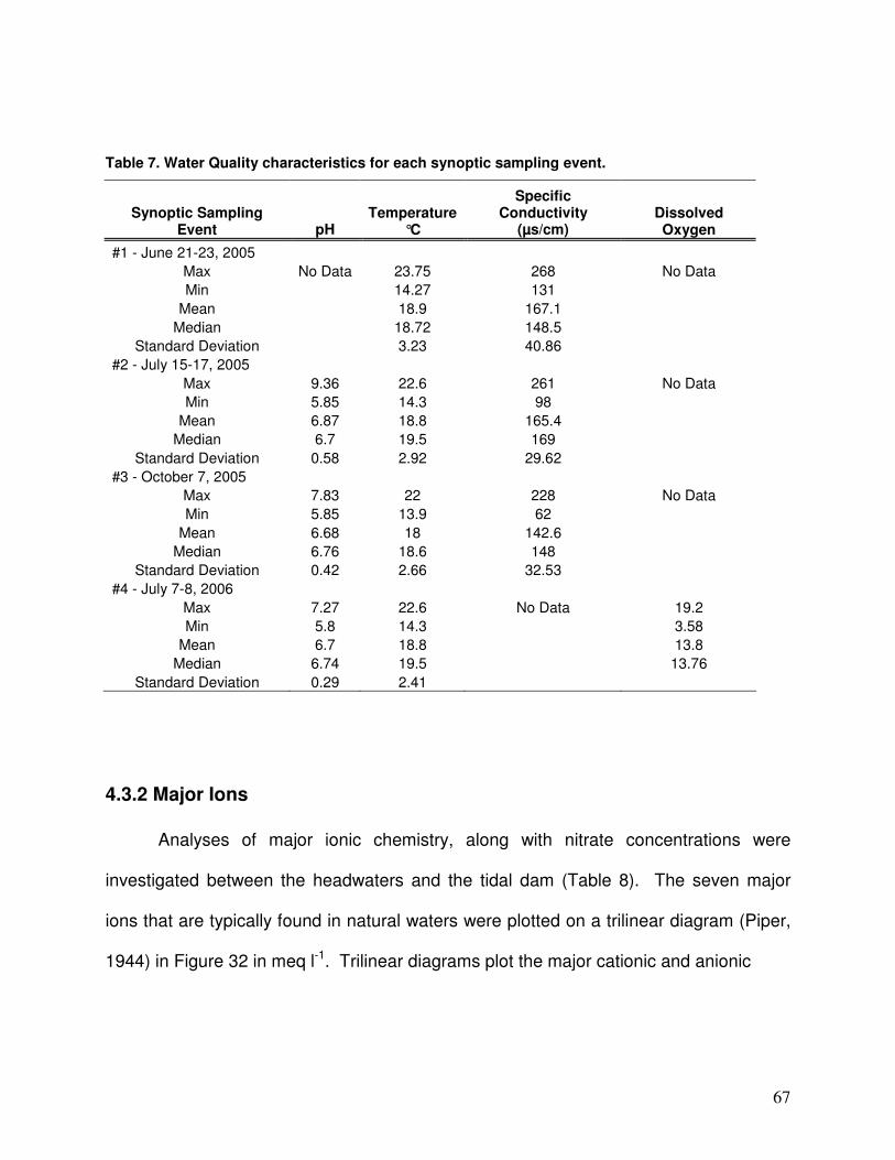
67

Table 7. Water Quality characteristics for each synoptic sampling event.

Synoptic Sampling Event pH

Temperature °C

Specific Conductivity

(µs/cm) Dissolved Oxygen

#1 - June 21-23, 2005

Max No Data 23.75 268 No Data

Min 14.27 131

Mean 18.9 167.1

Median 18.72 148.5

Standard Deviation 3.23 40.86

#2 - July 15-17, 2005

Max 9.36 22.6 261 No Data

Min 5.85 14.3 98

Mean 6.87 18.8 165.4

Median 6.7 19.5 169

Standard Deviation 0.58 2.92 29.62

#3 - October 7, 2005

Max 7.83 22 228 No Data

Min 5.85 13.9 62

Mean 6.68 18 142.6

Median 6.76 18.6 148

Standard Deviation 0.42 2.66 32.53

#4 - July 7-8, 2006

Max 7.27 22.6 No Data 19.2

Min 5.8 14.3 3.58

Mean 6.7 18.8 13.8

Median 6.74 19.5 13.76

Standard Deviation 0.29 2.41

4.3.2 Major Ions

Analyses of major ionic chemistry, along with nitrate concentrations were

investigated between the headwaters and the tidal dam (Table 8). The seven major

ions that are typically found in natural waters were plotted on a trilinear diagram (Piper,

1944) in Figure 32 in meq l-1. Trilinear diagrams plot the major cationic and anionic

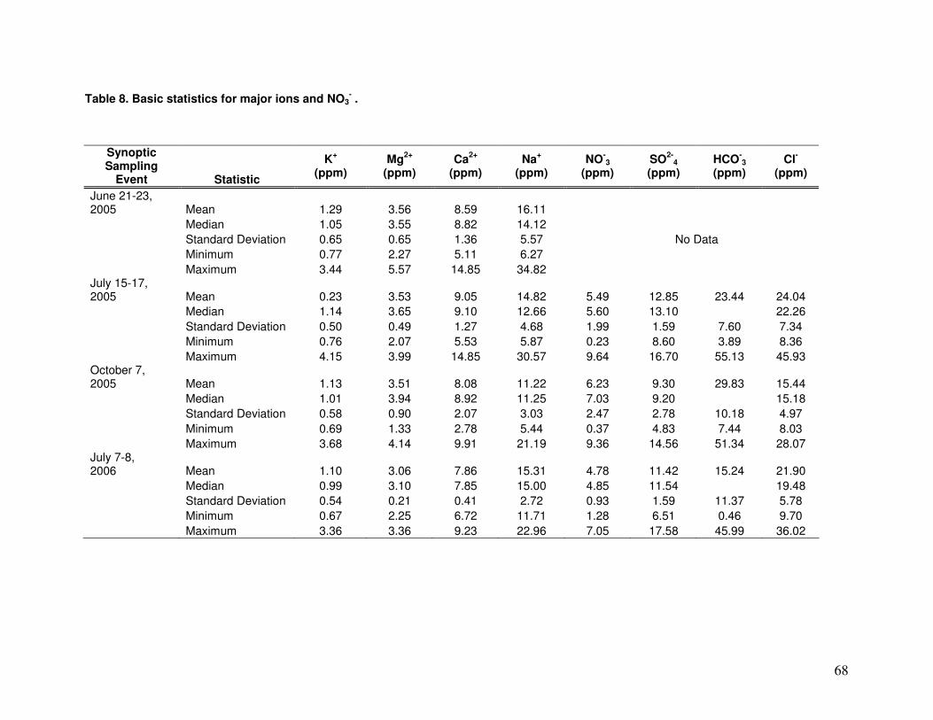
68

Table 8. Basic statistics for major ions and NO3- .

Synoptic Sampling

Event Statistic

K+

(ppm) Mg

2+

(ppm) Ca

2+

(ppm) Na

+

(ppm) NO

-3

(ppm) SO

2-4

(ppm) HCO

-3

(ppm) Cl

-

(ppm)

June 21-23, 2005 Mean 1.29 3.56 8.59 16.11

Median 1.05 3.55 8.82 14.12

Standard Deviation 0.65 0.65 1.36 5.57 No Data

Minimum 0.77 2.27 5.11 6.27

Maximum 3.44 5.57 14.85 34.82 July 15-17, 2005 Mean 0.23 3.53 9.05 14.82 5.49 12.85 23.44 24.04

Median 1.14 3.65 9.10 12.66 5.60 13.10 22.26

Standard Deviation 0.50 0.49 1.27 4.68 1.99 1.59 7.60 7.34

Minimum 0.76 2.07 5.53 5.87 0.23 8.60 3.89 8.36

Maximum 4.15 3.99 14.85 30.57 9.64 16.70 55.13 45.93 October 7, 2005 Mean 1.13 3.51 8.08 11.22 6.23 9.30 29.83 15.44

Median 1.01 3.94 8.92 11.25 7.03 9.20 15.18


Minimum 0.69 1.33 2.78 5.44 0.37 4.83 7.44 8.03

Maximum 3.68 4.14 9.91 21.19 9.36 14.56 51.34 28.07 July 7-8, 2006 Mean 1.10 3.06 7.86 15.31 4.78 11.42 15.24 21.90

Median 0.99 3.10 7.85 15.00 4.85 11.54 19.48


Minimum 0.67 2.25 6.72 11.71 1.28 6.51 0.46 9.70

Maximum 3.36 3.36 9.23 22.96 7.05 17.58 45.99 36.02

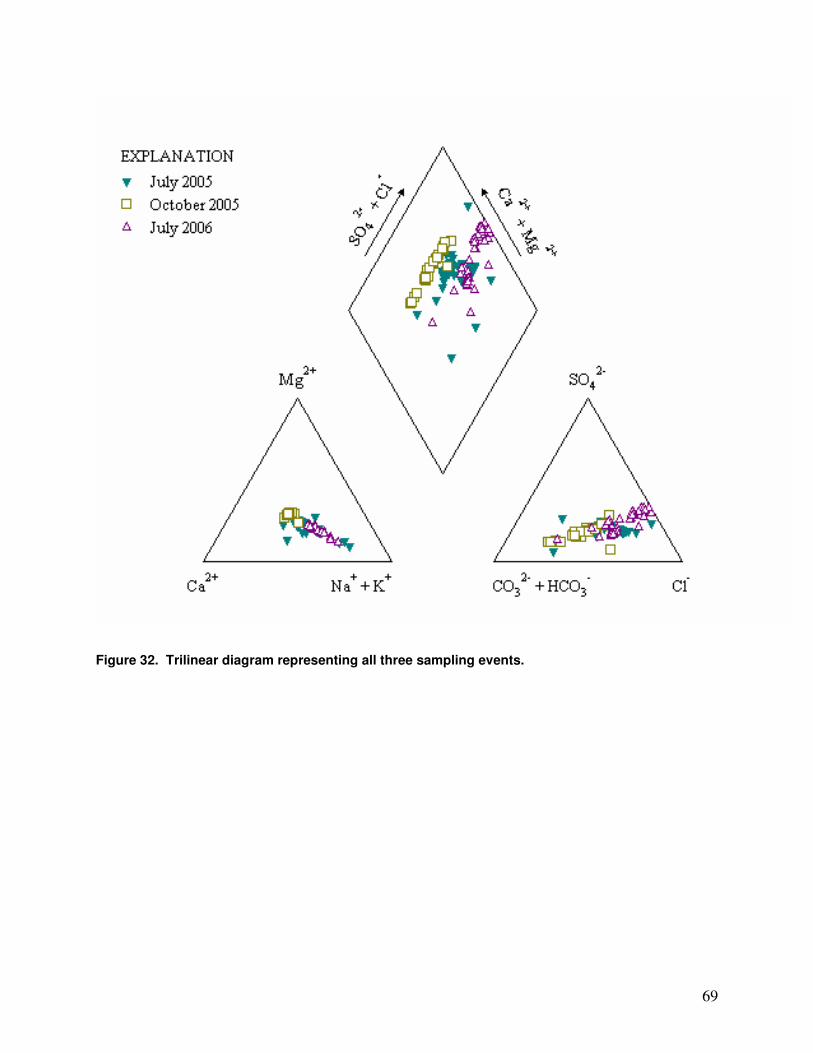
69

Figure 32. Trilinear diagram representing all three sampling events.

70

species as a percentage of the respective total for each sample onto two separate

trilinear plots. Cation and anion relative percentages are then plotted onto a central

diamond shaped plot which is used to determine the water type or hydrochemical

facies. Bar charts were also used to investigate relative concentrations of ions (Figures

33 – 38).

The trilinear plot shows two patterns, a horizontal shift towards the Na-Cl facies,

and a vertical shift from the Ca2+-HCO3- water type towards the Ca2+-SO4

2- water type.

The horizontal migration towards the Na-Cl water type is influenced by the hydrologic

condition (Table 2). The October event had experienced the least amount of rain prior

to sampling and represents only the upper and middle subwatersheds. The July 2006

event experienced the greatest amount of rain prior to sampling and river stage was

much higher in 2006 than in 2005. Although the results of the trilinear diagram indicate

that there is no dominant water type in base flow conditions in the Carmans River,

results from the trilinear plot would suggest that in wetter conditions the water type shifts

towards a Na-Cl water type.

Figures 33 thru 38 illustrate the relative concentrations of cations and anions

from the headwaters to the tidal dam, respectively. These bar graphs show how the

relative composition of stream water changes from upstream to downstream. It is

evident that the headwater system has the most variable water chemistry for each

sampled hydrologic regime. In addition, these charts suggest that the dominant cations

are sodium and calcium and the dominant anion is chloride, and then bicarbonate.

71

0%

20%

40%

60%

80%

100%

Nur

sery

Pon

d 9 14 18 21 24 27 30 33 36

wea

ks p

ond 41 44 48 51 54 57 60 63

Distance Downstream

Rela

tive C

om

po

sit

ion

(%

)

Sodium %Potassium %Magnesium %Calcium %

Figure 33. Relative composition of cations in stream water for July 2005 sampling event.

0%

20%

40%

60%

80%

100%

Nur

sery

Pon

d 9 14 19 22 25 28 31 34 37 39 42 46 49 52 55 58 61 64

Distance Downstream

Rela

tive C

om

po

sit

ion

s (

%)

Bicarbonate %Sulfate %Nitrate %Chloride %

Figure 34. Relative composition of anions in stream water for July 2005 sampling event.

72

0%

20%

40%

60%

80%

100%

1 3a

Nur

sery

Pon

d 7 12 14 17 19 21 23 25 27 29 31 33 35

Distance Downstream

Rela

tive C

om

po

sit

ion

(%

)

Sodium %

Potassium %

Magnesium %

Calcium %

Figure 35. Relative composition of cations in stream water for October 2005 sampling event. Note this was a partial sampling event due to a storm.

0%

20%

40%

60%

80%

100%

1 3a

Nur

sery

Pon

d 7 12 14 17 19 21 23 25 27 29 31 33 35

Distance Downstream

Rela

tive C

om

po

sit

ion

(%

)

Bicarbonate %

Sulfate %

Nitrate %

Chloride %

Figure 36. Relative composition of anions in stream water for October 2005 sampling event

73

0%

20%

40%

60%

80%

100%

1 4 7 13 17 20 23 26 29 32 35 38 40 43 48 51 54 57 60 63

Distance Downstream

Rela

tive C

om

po

sit

ion

(%

)

Sodium %

Potassium %

Magnesium %

Calcium %

Figure 37. Relative composition of cations in stream water for July 2006 sampling event.

0%

20%

40%

60%

80%

100%

1 4 7 16 19 22 25 28 31 34 37 39 42 47 50 53 56 59 62 65

Distance Downstream

Rela

tive C

om

po

sit

ion

s (

%)

Bicarbonate %Sulfate %Nitrate %Chloride %

Figure 38. Relative composition of anions in stream water for July 2006 sampling event.

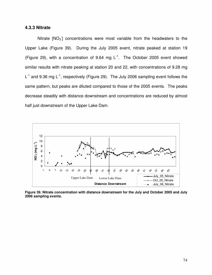
74

4.3.3 Nitrate

Nitrate [NO3-] concentrations were most variable from the headwaters to the

Upper Lake (Figure 39). During the July 2005 event, nitrate peaked at station 19

(Figure 29), with a concentration of 9.64 mg L-1. The October 2005 event showed

similar results with nitrate peaking at station 20 and 22, with concentrations of 9.28 mg

L-1 and 9.36 mg L-1, respectively (Figure 29). The July 2006 sampling event follows the

same pattern, but peaks are diluted compared to those of the 2005 events. The peaks

decrease steadily with distance downstream and concentrations are reduced by almost

half just downstream of the Upper Lake Dam.

0

2

4

6

8

10

12

1 4 7 10 13 16 19 22 25 28 31 34 37 39 42 45 48 51 54 57 60 63

Distance Downstream

NO

- 3 (

mg

L-1

)

July_05_Nitrate

Oct_05_Nitrate

July_06_Nitrate

Figure 39. Nitrate concentration with distance downstream for the July and October 2005 and July 2006 sampling events.

Upper Lake Dam Lower Lake Dam

75

4.3.4 Sodium Chloride

Sodium and chloride are two of the dominating ions in the Carmans River. The

progression of sodium and chloride concentration with distance downstream is

illustrated in Figures 40 through 42. There are few samples in the upper headwaters,

however, these concentrations are higher than any others found throughout the river.

Concentrations progressively increase again in the lower reaches.

Figures 43 through 45 are scatter plots showing the relationship between sodium

and chloride along the 1:1 line in meq L-1 for July 2005, October 2005 and July 2006,

respectively. Stations were grouped together according to location, where stations 1-25

are considered the headwater reaches down to the Upper Lake Dam. Stations 26-36

are considered the middle reaches; from Upper Lake Dam to Lower Lake Dam, and

stations 37-65 are considered the lower reaches; from below the Lower Lake Dam to

Hards Lake Dam.

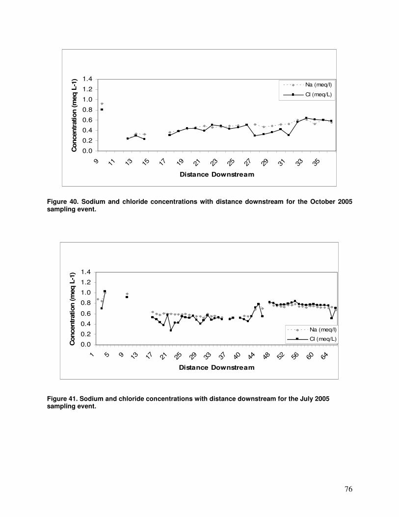
76

0.0

0.2

0.4

0.6

0.8

1.0

1.2

1.4

9 11 13 15 17 19 21 23 25 27 29 31 33 35

Distance Downstream

Concentr

ation (m

eq L

-1)

Na (meq/l)

Cl (meq/L)

Figure 40. Sodium and chloride concentrations with distance downstream for the October 2005 sampling event.

0.0

0.2

0.4

0.6

0.8

1.0

1.2

1.4

1 5 9 13 17 21 25 29 33 37 40 44 48 52 56 60 64

Distance Downstream

Concentr

ation (m

eq L

-1)

Na (meq/l)

Cl (meq/L)

Figure 41. Sodium and chloride concentrations with distance downstream for the July 2005 sampling event.

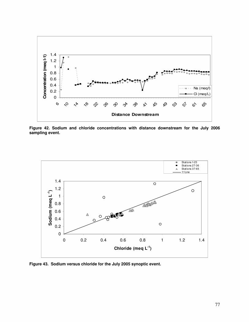
77

0

0.2

0.4

0.6

0.8

1

1.2

1.4

6 10 14 18 22 26 30 34 38 41 45 49 53 57 61 65

Distance Downstream

Concentr

ation (m

eq l-1

)

Na (meq/l)

Cl (meq/L)

Figure 42. Sodium and chloride concentrations with distance downstream for the July 2006 sampling event.

0

0.2

0.4

0.6

0.8

1

1.2

1.4

0 0.2 0.4 0.6 0.8 1 1.2 1.4

Chloride (meq L-1)

So

diu

m (

meq

L-1

)

Stat ions 1-25

Stat ions 27-36

Stat ions 37-65

1:1 Line

Figure 43. Sodium versus chloride for the July 2005 synoptic event.

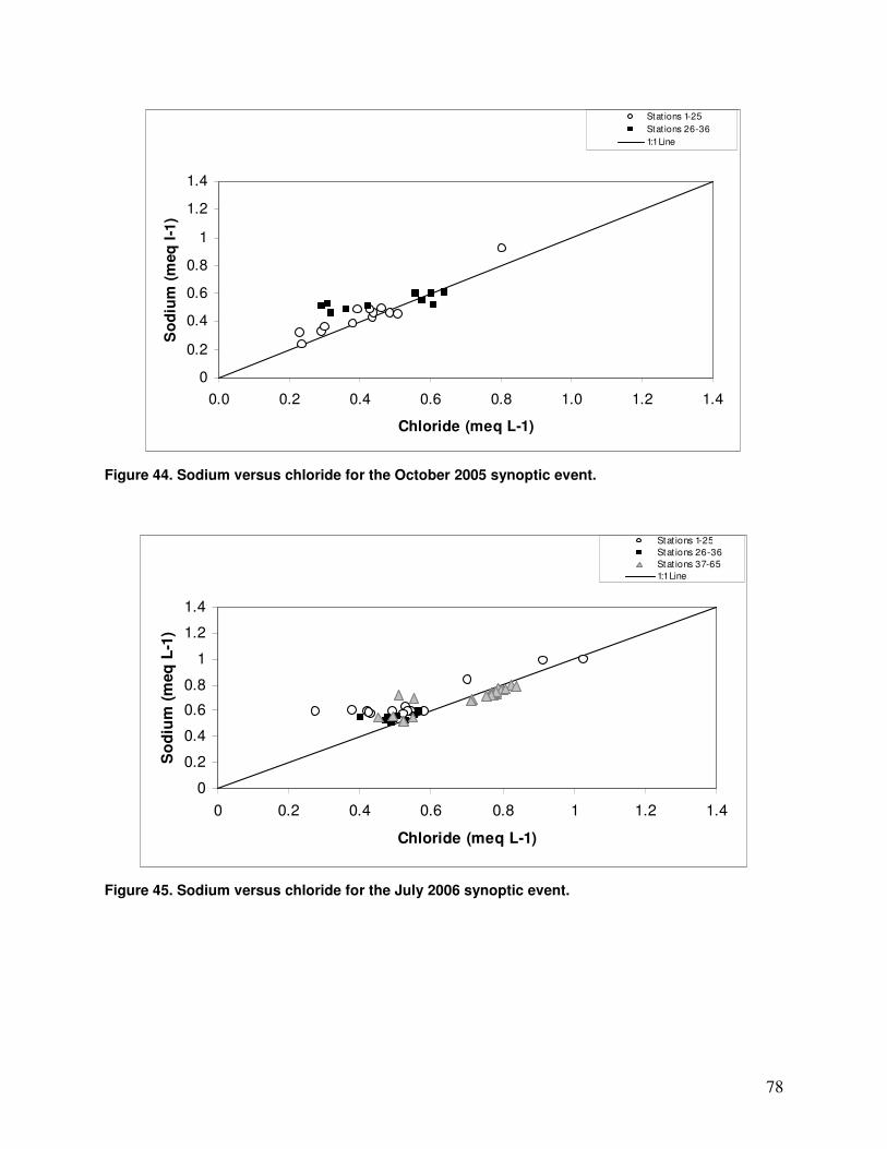
78

0

0.2

0.4

0.6

0.8

1

1.2

1.4

0.0 0.2 0.4 0.6 0.8 1.0 1.2 1.4

Chloride (meq L-1)

So

diu

m (

meq

l-1

)

Stat ions 1-25

Stat ions 26-36

1:1 Line

Figure 44. Sodium versus chloride for the October 2005 synoptic event.

0

0.2

0.4

0.6

0.8

1

1.2

1.4

0 0.2 0.4 0.6 0.8 1 1.2 1.4

Chloride (meq L-1)

So

diu

m (

meq

L-1

)

Stat ions 1-25

Stat ions 26-36

Stat ions 37-65

1:1 Line

Figure 45. Sodium versus chloride for the July 2006 synoptic event.

79

4.3.5 Road Density

Figure 46 shows the distribution of road density throughout the watershed in

km/km2. Average road density by subwatershed was calculated using a weighted

average according to subwatershed size (Figure 47). The upper and lower

subwatersheds have similar road densities, whereas the middle subwatershed has the

lowest density of roads. Figure 48 shows median sodium and chloride concentrations,

respectively by subwatershed. Both sodium and chloride follow the road density

pattern, where sodium and chloride concentrations are the highest where road density

is the greatest.

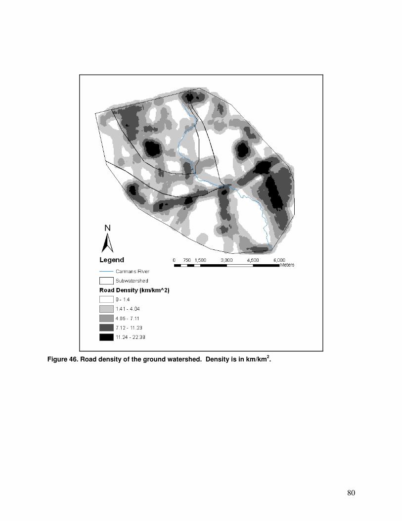
80

Figure 46. Road density of the ground watershed. Density is in km/km2.

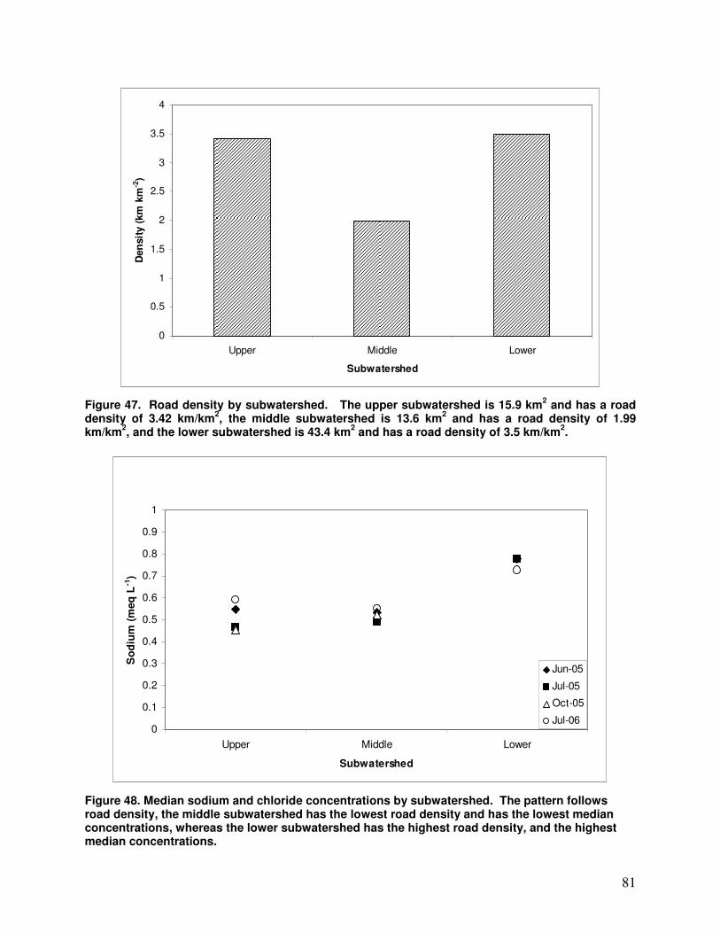
81

0

0.5

1

1.5

2

2.5

3

3.5

4

Upper Middle Lower

Subwatershed

Den

sit

y (

km

km

-2)

Figure 47. Road density by subwatershed. The upper subwatershed is 15.9 km2 and has a road

density of 3.42 km/km2, the middle subwatershed is 13.6 km

2 and has a road density of 1.99

km/km2, and the lower subwatershed is 43.4 km

2 and has a road density of 3.5 km/km

2.

0

0.1

0.2

0.3

0.4

0.5

0.6

0.7

0.8

0.9

1

Upper Middle Lower

Subwatershed

So

diu

m (

meq

L-1

)

Jun-05

Jul-05

Oct-05

Jul-06

Figure 48. Median sodium and chloride concentrations by subwatershed. The pattern follows road density, the middle subwatershed has the lowest road density and has the lowest median concentrations, whereas the lower subwatershed has the highest road density, and the highest median concentrations.

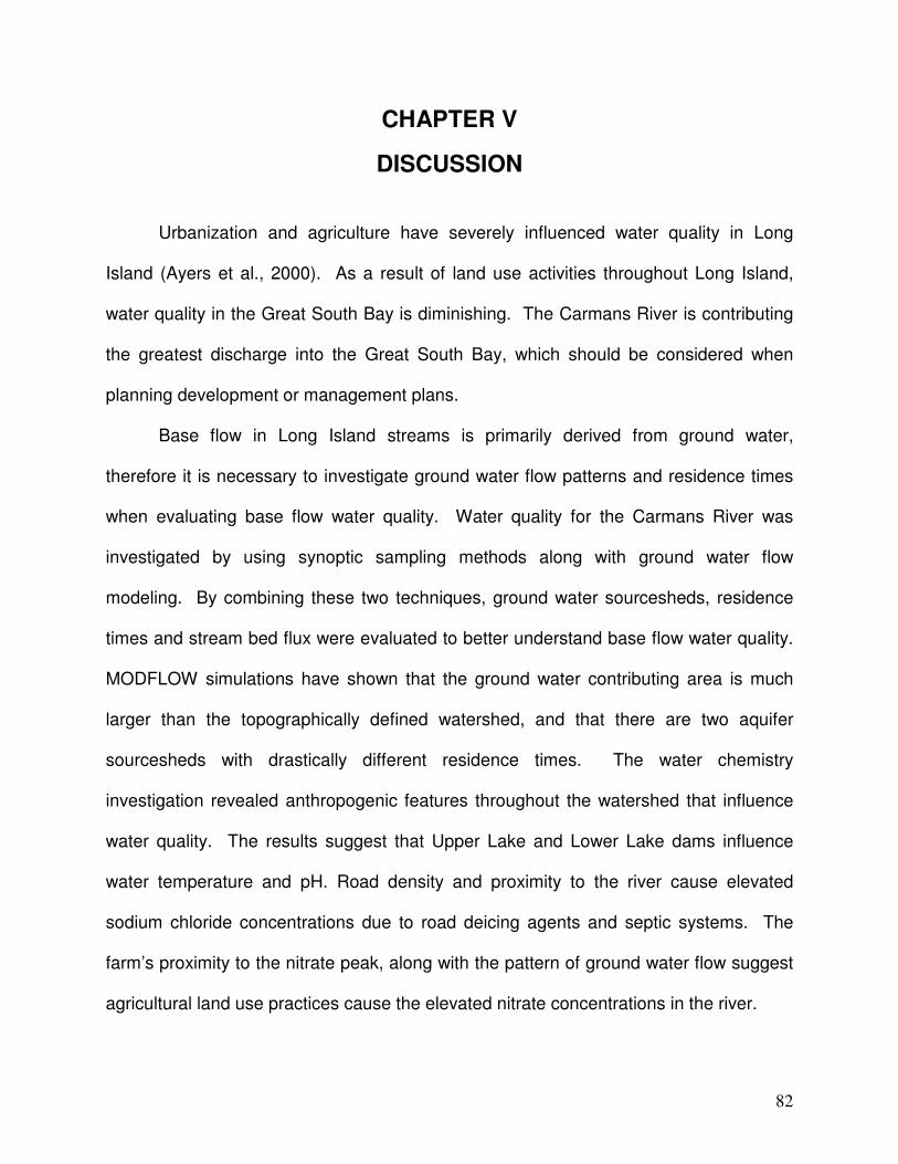
82

CHAPTER V

DISCUSSION

Urbanization and agriculture have severely influenced water quality in Long

Island (Ayers et al., 2000). As a result of land use activities throughout Long Island,

water quality in the Great South Bay is diminishing. The Carmans River is contributing

the greatest discharge into the Great South Bay, which should be considered when

planning development or management plans.

Base flow in Long Island streams is primarily derived from ground water,

therefore it is necessary to investigate ground water flow patterns and residence times

when evaluating base flow water quality. Water quality for the Carmans River was

investigated by using synoptic sampling methods along with ground water flow

modeling. By combining these two techniques, ground water sourcesheds, residence

times and stream bed flux were evaluated to better understand base flow water quality.

MODFLOW simulations have shown that the ground water contributing area is much

larger than the topographically defined watershed, and that there are two aquifer

sourcesheds with drastically different residence times. The water chemistry

investigation revealed anthropogenic features throughout the watershed that influence

water quality. The results suggest that Upper Lake and Lower Lake dams influence

water temperature and pH. Road density and proximity to the river cause elevated

sodium chloride concentrations due to road deicing agents and septic systems. The

farm’s proximity to the nitrate peak, along with the pattern of ground water flow suggest

agricultural land use practices cause the elevated nitrate concentrations in the river.

83

5.1 Ground Water Flow

5.1.1 Sourcesheds

The average ground water contributing area was determined using the USGS

water table map (Busciolio, 2002) and was calibrated using river flux. The ground water

contributing area is considerably larger than the topographically defined watershed.

Simulated path lines suggest however that the Upper Glacial Aquifer sourceshed

closely mimics the topographically defined watershed. MODFLOW simulations viewed

in 3-D show that the majority of subsurface flow is generated from the Upper Glacial

Aquifer. All precipitation that falls outside of the topographically defined watershed

recharges the Magothy Aquifer before discharging into the Carmans River or the Great

South Bay. Recharge that enters the upper portions of the watershed near the regional

divide does recharge the Magothy Aquifer before returning to the river. The flow paths

that abruptly reach the model boundary and then flow vertically up to the Carmans River

are strictly a function of the boundary condition. In reality, these flow paths would

continue flowing through the Magothy Aquifer and enter the Carmans River farther

downstream.

Buxton et al. (1991) determined recharge areas for the island using a three

dimensional finite difference model and the particle tracking code (Pollock, 1988).

Minimum and maximum recharge areas were estimated for present conditions. This

simulation found that for both minimum and maximum hydrologic conditions, the

recharge area is predominantly along the island-wide regional ground water divide, and

extends east to west along the length of Long Island. The recharge area curves around

the Carmans River watershed, showing that all precipitation that falls within the

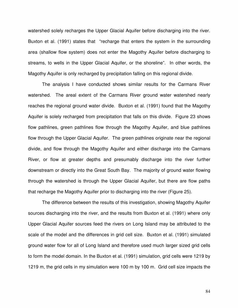
84

watershed solely recharges the Upper Glacial Aquifer before discharging into the river.

Buxton et al. (1991) states that “recharge that enters the system in the surrounding

area (shallow flow system) does not enter the Magothy Aquifer before discharging to

streams, to wells in the Upper Glacial Aquifer, or the shoreline”. In other words, the

Magothy Aquifer is only recharged by precipitation falling on this regional divide.

The analysis I have conducted shows similar results for the Carmans River

watershed. The areal extent of the Carmans River ground water watershed nearly

reaches the regional ground water divide. Buxton et al. (1991) found that the Magothy

Aquifer is solely recharged from precipitation that falls on this divide. Figure 23 shows

flow pathlines, green pathlines flow through the Magothy Aquifer, and blue pathlines

flow through the Upper Glacial Aquifer. The green pathlines originate near the regional

divide, and flow through the Magothy Aquifer and either discharge into the Carmans

River, or flow at greater depths and presumably discharge into the river further

downstream or directly into the Great South Bay. The majority of ground water flowing

through the watershed is through the Upper Glacial Aquifer, but there are flow paths

that recharge the Magothy Aquifer prior to discharging into the river (Figure 25).

The difference between the results of this investigation, showing Magothy Aquifer

sources discharging into the river, and the results from Buxton et al. (1991) where only

Upper Glacial Aquifer sources feed the rivers on Long Island may be attributed to the

scale of the model and the differences in grid cell size. Buxton et al. (1991) simulated

ground water flow for all of Long Island and therefore used much larger sized grid cells

to form the model domain. In the Buxton et al. (1991) simulation, grid cells were 1219 by

1219 m, the grid cells in my simulation were 100 m by 100 m. Grid cell size impacts the

85

accuracy of discretization since the ground water flow equation used in MODFLOW is

solved in the center of every cell. The larger the cell, the more homogeneous head

calculations become because localized heterogeneities in hydraulic conductivity and

transmissivity are generalized from the kriging process.

5.1.2 Residence Times

The results found in this simulation suggest that in steady state conditions,

Magothy Aquifer sources can discharge into the Carmans River. Discharge from the

Magothy Aquifer is much older than discharge from the Upper Glacial Aquifer. Ground

water residence times are shortest for recharge that enters the ground water system

closest to the point of discharge. These flow paths move laterally through the shallow

aquifer. Recharge that enters the system farther away from the stream has longer flow

paths, and with greater distances can move deeper into the aquifer system before

discharging into the stream. Ground water sources that discharge into the stream are

therefore a mixture of Magothy and Upper Glacial Aquifer sources.

Modica et al. (1997) simulated ground water flow for a generic coastal plain

aquifer system, such that is found in Long Island and New Jersey, to determine the

shape of the stream subsystems and their relations to deeper ground water flow

(Modica et al., 1997). They found that ground water flow that discharges to stream

systems can originate from anywhere within the source area, and the longer the flow

path the higher the residence time. Lower river reaches receive increasingly older

ground water than headwater reaches. The combination of shallow and deep flow

results in a mixture of ground water age within the stream. Ground water residence

86

times for these three simulated rivers ranged from 0 to over 250 years within the

immediate sourceshed.

Modica et al. (1998) investigated source areas and residence times within the

Cohansey River Basin in New Jersey. This coastal plain system is similar to the

hydrogeology of Long Island, with high hydraulic conductivities, but has a much

shallower system compared to Long Island’s deep aquifer systems. Five selected

model cells within the Cohansey River Basin simulation had residence times from 0 to

over 100 years.

In this study, I found that ground water residence times are dramatically different

between the Upper Glacial and Magothy Aquifer sources (Figures 27 and 28). Ground

water flowing through the Upper Glacial Aquifer can be between 0 and over 15 years

old before it discharges into the Carmans River, and ground water traveling through the

Magothy Aquifer that originated near the regional ground water divide in the upper

headwaters can be over 500 years in age.

5.1.3 Assumptions and Limitations of Modeling

The results found in this investigation, including the size of ground water

sourcesheds and ground water residence times are based on modeled simulations. It is

important to remember that this simulation is an attempt to approximate the ground

water flow system and that in reality the ground water flow system is more complex.

Assumptions were used to simplify the modeling process, which are discussed below.

The calibration process in model development is conducted to ensure that the

model can reproduce observed head and discharge measurements. During the

87

calibration process it was determined that a recharge rate of 63.5 cm yr-1, instead of

59.4 cm yr-1 (the rate calculated using Olcott (1995) methodology) allowed the

simulated discharge and head measurements to “fit” more closely to observed

conditions. The method presented by Olcott (1995) suggests a total ground water

recharge of approximately 48% of total precipitation, the percent recharge used in this

simulation was approximately 51.4% of the total precipitation. This percentage more

closely matches the recharge rate (52%) used by Buxton and Smolensky (1998).

Discrepancies between the recharge rate presented by Olcott (1995), and

simulated rates can be attributed to a number of factors. The breakdown presented by

Olcott (1995) (original source Franke and McClymonds (1972)) is based on a water

budget calculated for the main body of Long Island. This method represents an island-

wide average, and does not take into account local conditions due to varying

precipitation, soil permeability, surface gradients and impervious surfaces.

In the case of the Carmans River simulation, the recharge rate was based on

average annual precipitation from the past 57 years. This estimate was based on one

gauge located at Brookhaven National Laboratory (BNL), located east of the Carmans

River watershed. This was the only source of precipitation data, and therefore area-

weighted averages could not be calculated for the watershed. An assumption in this

method is that precipitation was uniform throughout the watershed, and that it equaled

the gauge data.

In addition to the assumption that there was uniform precipitation throughout the

watershed, steady state conditions were also used in simulation. Steady state

conditions assume uniform recharge throughout the model domain and assume

88

average conditions over time. In reality the system is constantly changing due to

variations in the amount and areal extent of precipitation.

In addition to an accurate portrayal of a system, the precision of these results are

contingent upon grid resolution and the number of particles tracked in the simulation

(Modica et al., 1998). The grid size in this simulation is 100m x 100m. This was the

finest resolution possible due to the width of the river. The boundary condition used in

this simulation only permits the river to pass through one cell, and this cell has to be

wide enough for the width of the river. In other words, you cannot use two cells next to

each other to represent a wide section of the river.

The number of particles used in this simulation could also impact the outcome.

Fewer particle pathlines could have changed the size and shape of the aquifer

sourceshed. Particles were placed under the stream bed, and aligned every outer edge

of the stream. The more particles used, the more accurate the simulation will be

because the entire modeled area will be represented.

Lastly, an assumption was made regarding substrate and the confining unit. It

was assumed that there were no heterogeneities throughout the aquifer system.

However, clay lenses are dispersed throughout Long Island and consequently not

represented in the model. The Raritan clay unit was used to represent the “bottom” of

the model. In actuality, bedrock underlies the entire system.

The sensitivity analyses showed how the River Boundary reacted to changes in

hydraulic conductivity and recharge. Since simulated discharge is calculated using the

principles of conservation of mass, where recharge into the model must equal simulated

discharge, inaccurate estimates of the ground water contributing area could impact

89

results. However, model parameters and the size of the ground water contributing area

were kept consistent with estimates cited in the literature and the USGS water table

map. If, however, these estimates are incorrect, modeled results such as the watershed

size and residence times could be impacted.

In conclusion, the assumptions and limitations just outlined concern: 1) steady

state conditions; 2) precipitation rate equal to BNL and uniform over watershed; 3) grid

resolution; 4) number of tracking particles; and 5) no heterogeneities in the watershed

can impact the outcome of this investigation. The soureshed boundaries would change

over time depending on fluctuating precipitation and recharge in a transient simulation.

Particle tracking is influenced by the head values calculated in each cell and the

hydraulic conductivity, therefore grid resolution and heterogeneities would impact how

particles travel. A finer grid resolution would capture small changes in head values, and

heterogeneities would influence velocity due to changes in hydraulic conductivity.

5.2 Changes in Chemistry with Distance Downstream

5.2.1 Temperature and pH

Surface water temperature is greatly affected by the Upper and Lower Lake

Dams. There are several factors that may be causing temperatures to rise in these two

lakes. Surface water temperatures are determined by several factors, including

topographically induced shade, upland vegetation, precipitation, air temperature, wind

speed, solar angle, cloud cover, relative humidity, phreatic ground water temperature

and discharge and tributary temperature and flow (Poole and Berman, 2001). However,

90

the impoundments along the river have altered the natural flow regime which

subsequently has impacted temperature. In the Carmans River surface water

temperatures increase at the impoundment locations. The lack of shade, along with

river aggregation and stagnation are most likely causing these temperature increases.

Since most of the river is heavily buffered with riparian forests and wetlands, surface

waters are not greatly affected by solar radiation. However, the Upper and Lower Lakes

are the only two areas of the river that are not shaded.

The Carmans River system on a whole is a shallow system. The impoundments

are exacerbating sedimentation and aggregation. While canoeing in the lakes, we

estimated the depth to be less than 1.5 meters. Visually, sedimentation seems to be a

big problem for the two lakes. I was able to stick my paddle quite deeply into the

sediment and organic matter along the lake bottom.

Air temperature and the time of day, coupled with the time of year are causing

the differences in temperature among the three sampling events. The highest

temperatures were observed during the July 2005 event, from Upper Lake to Lower

Lake. The time of day these highs were observed ranged from 2:00 to 5:00 pm. The

October event exhibited the lowest temperatures, and these samples were taken

between 9:00 am and 1:00 pm, earlier in the day compared to the other sampling

events. The time of sample collection for the July 2006 event was between 2:00 pm and

4:00 pm. This pattern would suggest that air temperature associated with the time of

year, along with the time of day sampling occurred, impacts the temperatures observed

for each sampling event.

91

The impoundments are also affecting pH. pH was elevated upstream of the

Lower Lake Dam in the July 2005 sampling event. Upper and Lower Lakes have

elevated temperatures and prolific algae growth. CO2 removal from photosynthesis

reduces acidity and therefore increases pH.

5.2.2 Major Ions

The Piper Plot in Figure 32 illustrates two distinct spatial and temporal patterns.

The spatial changes can be seen by the progression of samples migrating from the

bottom left corner of the plot, which represents a more Ca2+-Mg2+-HCO3- water type, to

the upper right corner of the plot, representing Ca2+-SO42- water type. However, when

comparing this progression with Figures 33-38, results suggest that this progression is

not necessarily in an upstream-downstream linear pattern. Overall, calcium and

magnesium tend to be higher in the upper reaches for all three sampling events.

Sulfate tends to be fairly uniform for the July and October 2005 events and more

variable with higher percentages in the upper reaches during the July 2006 event.

Bicarbonate tends to be higher in the upper and middle reaches, but Figures 35 and 36

show that the station with the highest percentage of HCO3- is station 27, which is

directly downstream of Upper Lake Dam, and in the middle of the river.

The temporal pattern is distinct between each sampling event. There is a shift

towards the Na+Cl- water type with an increase in precipitation. There are many

sources, both natural and anthropogenic, that can contribute to sodium and chloride

concentrations. Natural sources of sodium and chloride can include atmospheric

deposition, interactions between soil or rock and water, and salt water intrusion.

92

Anthropogenic sources can include effluent from septic systems, agricultural chemicals,

municipal landfills and deicing agents. Given the pattern of Na+Cl- with distance

downstream, and the parallel pattern with road density, anthropogenic sources such as

deicing agents and septic systems are the likely source.

An analysis of road density weighted by subwatershed area indicates that the

lowermost subwatershed has the greatest road density, albeit nearly equal to the

uppermost watershed, and the middle subwatershed exhibits the least amount of roads.

This pattern of road density is parallel with that of median sodium chloride

concentrations for each subwatershed.

Sodium chloride (rock salt) is commonly used for roadway deicing. However,

calcium chloride is also a popular deicing agent. The Town of Brookhaven highway

department could not answer the question as to what deicing materials are used.

Apparently deicing materials change year to year according to awarded contracts.

Median calcium chloride concentrations were plotted by subwatershed (not shown),

however the pattern did not coincide with road density as does sodium chloride in

Figure 42.

Road density and Na+Cl- concentrations follow the same pattern, suggesting that

the Na+Cl- concentrations may be from rock salt, however, road density can also be an

indication of population density and septic systems. Nevertheless, median

concentrations of sodium and chloride are very low (Table 3) compared to other

systems tested by Panno et al., 2006. Panno et al., 2006 reference sodium and

chloride concentrations for different systems, both affected and not affected by

anthropogenic sources, throughout the Midwest (Table 9). The magnitude of sodium

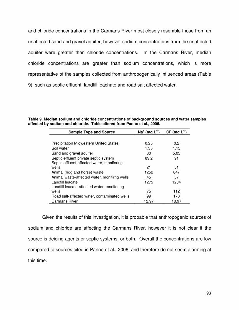
93

and chloride concentrations in the Carmans River most closely resemble those from an

unaffected sand and gravel aquifer, however sodium concentrations from the unaffected

aquifer were greater than chloride concentrations. In the Carmans River, median

chloride concentrations are greater than sodium concentrations, which is more

representative of the samples collected from anthropogenically influenced areas (Table

9), such as septic effluent, landfill leachate and road salt affected water.

Table 9. Median sodium and chloride concentrations of background sources and water samples affected by sodium and chloride. Table altered from Panno et al., 2006.

Sample Type and Source Na+ (mg L

-1) Cl

- (mg L

-1)

Precipitation Midwestern United States 0.25 0.2

Soil water 1.35 1.15

Sand and gravel aquifer 30 5.05

Septic effluent private septic system 89.2 91 Septic effluent-affected water, moniforing wells 21 51

Animal (hog and horse) waste 1252 847

Animal waste-affected water, monitirng wells 45 57

Landfill leacate 1275 1284 Landfill leacate-affected water, monitoring wells 75 112

Road salt-affected water, contaminated wells 99 170

Carmans River 12.97 18.97

Given the results of this investigation, it is probable that anthropogenic sources of

sodium and chloride are affecting the Carmans River, however it is not clear if the

source is deicing agents or septic systems, or both. Overall the concentrations are low

compared to sources cited in Panno et al., 2006, and therefore do not seem alarming at

this time.

94

5.2.3 Nitrate

With each synoptic event, nitrate concentrations have a comparable pattern with

increasing distance downstream. Base flow conditions from July and October 2005

show a remarkable similarity in the upper headwaters. With increased precipitation

from the July 2006 event, nitrate follows the same pattern but concentrations are lower,

almost certainly due to dilution. The contributing areas that were delineated based on

the spike in headwater nitrate concentrations show that most of the source areas are

found on the upper west side of the river. However, there is a small fraction of land on

the east side of the river that is within the source area. It is at this location that the one

farm is located.

In addition to the presence of the farm, simulated riverbed flux shows that this is

the approximate location of where the stream system becomes a consistently gaining

stream. Simulated flux shows that the headwaters are losing to the ground water

system but then progressively become a gaining stream. Gaining conditions are

sustained and become constant at the location marked “Bartlett Road”. Bartlett Road

(Figure 12) is the location of the farm where the corner of the farm is situated at the

intersection of the river and Bartlett Road. Therefore, it seems as though the spike in

nitrate could be due to two factors: the farm or a major influx of ground water.

5.3 Implications

This modeling approach combined with a synoptic water quality analysis, shows

how a linkage can be made between sources of ground water and the location in which

it discharges into the river, and in turn, how this may impact water quality (Modica et al.,

95

1998). This method can aid watershed managers, policy makers and planners in

decisions regarding where to focus watershed management strategies or where to plan

for development.

The results of this study suggest that there are two aquifer sources that feed into

the Carmans River. However, residence times greatly differ between these two sources.

Since the areal extent of the Upper Glacial Aquifer closely mimics the topographically

defined watershed, and since the residence time of this aquifer is less than 20 years,

watershed managers, policy makers and planners should focus on activities within this

contributing area in order to make a more immediate difference in water quality.

The farm is most likely causing the elevated nitrate concentrations in the

headwaters. Best management practices including strategic timing of fertilizers, and a

wider riparian buffer may improve water quality. Since the farm is immediately adjacent

to the river, these two practices could have immediate effects on water quality.

However, any changes made farther away from the river, but within the Upper Glacial

Aquifer sourceshed could take up to 20 years to improve conditions.

96

CHAPTER VI

CONCLUSIONS

An analysis of surface water quality and ground water flow for the Carmans River

watershed suggest the following conclusions:

(1) The peak in nitrate could be due to two factors: the farm, or the influx of

ground water.

(2) Water quality during base flow conditions is dominated by sodium and

calcium, and chloride and bicarbonate. Sodium and chloride concentrations

increase in areas of the watershed that have higher road densities,

suggesting the sodium chloride is due to anthropogenic sources such as road

salt or septic systems.

(3) The temperature within the stream is altered by the Upper and Lower Lake

Dams.

(4) Modeled simulations suggest that the ground water contributing area is larger

than the topographically defined watershed.

(5) Both aquifer systems, the Upper Glacial Aquifer and the Magothy Aquifer, can

discharge into the Carmans River, however ground water discharge is

dominated by the Upper Glacial Aquifer.

97

(6) The Upper Glacial Aquifer has a residence time of less than 20 years.

(7) Magothy Aquifer sources originating from the regional ground water divide

can have residence times up to 500 years before discharging into the

Carmans River.

98

REFERENCES

Anderson, M.P. and W.W. Woessner. 1992. Applied Groundwater Modeling; Simulation of

Flow and Advective Transport. Academic Press, San Diego, California, 381p. Ayers, M.A., J.G., Kennen, and P.E. Stakelberg. 2000. Water quality in the Long Island-New

Jersey coastal drainages, New York and New Jersey, 1996-98. US Geological Survey Circular 1201.

Baier, J.H. and K.A. Rykbost. 1976. The contribution of fertilizer to the ground water of Long

Island. Ground Water 14: 439-448. Bleifuss, P.S., G.N. Hanson, and M.A.A. Schoonen. 2005. Tracing sources of nitrate in the

Long Island aquifer system. Access from the World Wide Web on May 2006 from http://www.geo.sunysb.edu/reports/bleifuss/.

Brady, N.C., and R.R. Weil. 2002. The Nature and Properties of Soils, 13th ed. Prentice

Hall Press, New Jersey Brawley, J.W., G. Collins, J.N. Kremer and C.H. Sham. 2000. A time-dependent model

of nitrogen loading to estuaries from coastal watershed. Journal of Environmental Quality 29: 1448-1461.

Brookhaven National Laboratory. January 2, 2007. Monthly Precipitation Records.

Accessed from the World Wide Web on July 20, 2007 from http://www.bnl.gov/weather/4cast/precip.html.

Burr, W.H., R., Hering, and J.R. Freeman. 1904. Report of the commission on additional

water supply for the city of New York: New York, Martin B. Brown Co., 980 p. Busciolano, R. 2002. Water-Table and potentiometric-surface altitudes of the upper

glacial, magothy, and lloyd aquifers on Long Island, New York, in March-April 2000, with a summary of hydrogeologic conditions: U.S. Geological Survey Water-Resources Investigations Report 01-4165, 17 p., 6 plates.

Busciolano, R. Personal Communications May 2006. Buxton, H.T., T.E. Reilly, D.W. Pollock, and D.A. Smolensky. 1991. Particle tracking

analysis of recharge areas on Long Island, New York. Ground Water 29: 63-71. Buxton, H.T., and D.A. Smolensky. 1998. Simulation of the effects of development of

the ground-water flow System of Long Island, New York. Water-Resources Investigations Report 98-4069.

99

Camp, Dresser & McKee. October 2003. Suffolk county groundwater model; final report. Suffolk County Department of Health Services.

Cornell University Geospatial Information Repository. 2006-2007. Elevation Data.

Accessed from the World Wide Web on June 6 2006 from http://cugir.mannlib.cornell.edu/.

deLaguna, W. 1964. Chemical quality of water, Brookhaven National Laboratory and

vicinity, Suffolk County, New York, U.S. Geological Survey Bulletin 1156-D. Divenere,V. Date Unknown. Groundwater Geology of Long Island. Accessed from the

World Wide Web on March 16, 2008 from http://myweb.cwpost.liu.edu/vdivener/notes/LIgroundwater.htm

Doriski, T.P.1986. Potentiometric-surface altitude of major aquifers on Long Island, New

York, in 1983. U.S. Geological Survey Water-Resources Investigations Report 85-4321, 4 pls., scale 1:125,000.

Dowhan, J., T. Halavik, A. Milliken, A. MacLachlan, M. Laplis, K. Lima, and A. Zimba.

Date Unknown. Significant habitats and habitat complexes of the New York Bight watershed. Geomorphic provinces and section of the New York Bight Watershed. Accessed from the World Wide Web on October 19, 2006 from http://training.fws.gov/library/pubs5/web_link/text/geolsect.htm.

Fetter, C.W. 2001. Applied Hydrogeology, 4th ed. Prentice Hall Press, New Jersey. Flipse, W. J., B.G. Katz, J.B. Lindner and R. Markel. 1984. Sources of nitrate in ground water

in a sewered housing development, central Long Island, New York. Ground Water 22: 418-426.

Geomorphic Provinces and Sections of the New York Bight Watershed. Date Unknown.

Retrieved April 27, 2006. Accessed from the World Wide Web at http://training .fws.gov/library/pubs5/web_link/text/geolsect.htm.

Hem. J. D. 1985. Study and Interpretation of the Chemical Characteristics of Natural

Water. U. S. Geological Survey Water-Supply Paper 2254. Kreitler, C.W., S.E. Ragone and B.G. Katz. 1978. N15/N14 Ratios of ground-water nitrate, Long

Island, New York. Ground Water 16: 404-409. Long Island Farm Bureau. 2004-2007. About Long Island agriculture. Accessed from

the World Wide Web on July 20, 2007 from http://www.lifb.com/.

100

Long Island Natural Environment Online. Date Unknown. Nature of soils. Accessed from the World Wide Web on July 20, 2007 from http://www.chipr.sunysb.edu/eserc/longis/

Long Island South Shore Estuary Reserve Council. Date Unknown. Wertheim National Wildlife Refuge. Accessed from the World Wide Web on January 5, 2007 from http://www.estuary.cog.ny.us/access_guide/site58.html

Long Island South Shore Estuary Reserve. April 12, 2001. Comprehensive

management plan. Long Island Sound Study. 1998. Phase III actions for hypoxia management: EPA 902-

R-98-002, 25 p. Mayer et al., (fix later) 2002. Sources of nitrate in rivers draining sixteen watershed in

the northeastern U.S.: Isotopic constraints. Biogeochemistry 57/58: 171-197. McDonald, M.G., and A.W. Harbaugh, 1988.A modular three-dimensional finite-

difference ground-water flow model. Techniques of Water-Resources Investigations 06-A1, USGS, 576 p.

Modica, E. T.E. Reilly, and D.W. Pollock. 1997. Patterns and age distribution of ground-

water flow to streams. Ground Water 35: 523-537. Modica, E. and H.T. Buxton. 1998. Evaluating the source and residence times of

groundwater seepage to streams, New Jersey Coastal Plain. Water Resources Research 34: 2797-2810.

Monti, J. and M.P. Scorca. 2003. Trends in nitrogen concentration and nitrogen loads entering

the South Shore Estuary Reserve from streams and ground-water discharge in Nassau and Suffolk counties, Long Island, New York, 1952-97.Water Resources Investigations Report 02-4255.

New York State Geographic Information Clearinghouse. Accessed from the World Wide

Web on July 1, 2006, from http://www.nysgis.state.ny.us/ Olcott, P.J. 1995. Ground water atlas of the United States; Connecticut, Maine,

Massachusetts, New Hampshire, New York, Rhode Island, Vermont. HA 730-M. Access from the World Wide Web on March 22, 2006 from http://capp.water.usgs.gov/gwa/ch_m/M-text3.html.

Panno, S.V., K.C. Hackley, H.H. Hwang, S.E. Greenberg, I.G. Krapac, S. Landsberger,

and D.J. O’Kelly. 2006. Characterization and Identification of Na-Cl Sources in Ground Water. Ground Water 44: 176-187.

101

Perlmutter, N.M. and E. Koch. 1972. Preliminary hydrogeologic appraisal of nitrate in ground water and streams, Southern Nassau County, Long Island, New York, U.S. Geol. Surv. Prof. Pap. 800-B, pp.225-235.

Piper, A.M. 1944. A graphical procedure in the geochemical interpretation of water

analyses. Transactions, American Geophysical Union 25:914-923. Pint, C.D., R.J. Hunt, and M.P. Anderson. 2003. Flowpath delineation and ground water

age, Allequash Basin, Wisconsin. Ground Water 41: 895-902. Pluhowski, E.J. and I.H. Kantrowitz, 1964. Hydrology of the Babylon-Islip Area, Suffolk

County, Long Island, New York. USGS Water Supply Paper 1768, 116pp (p. 35). Pollock, D.W. 1988. Semianalytical computation of path lines for finite-difference models.

Ground Water 26:743-750. Pollock, D.W. 1989. Documentation of computer programs to complete and display pathlines

using results from the U.S. Geological Survey modular three-dimensional finite-difference ground-water model. USGS, Open File Report 89-381, 81p.

Poole, G.C. and C.H. Berman. 2001. An ecological perspective on in-stream

temperature: natural heat dynamics and mechanisms of human-caused thermal degradation. Environmental Management 27: 787-802.

Porter, K.S., D.R. Boulkin, C.A. Shoemakes, L.B. Baskin, D.H. Zaeh, S. Pacenka, and D.H.

Fricke. 1978. Nitrogen on Long Island: sources and fate. Cornell University Cooperative Extension, Ithaca, N.Y. 186 pp.

Soren, J.,1977. Ground-water quality near the water table in Suffolk County, Long

Island, New York. Long Island Water Resources Bulletin LIWR-8. Suffolk County Cooperative Extension Service. 1973. Comparative importance of Suffolk

County, New York agriculture. Unpublished mimeo. Suffolk County Cooperative Extension Service.

The Weather Underground, Inc. 2007. Shirley, New York. Accessed from the World

Wide Web on July 20, 2007 from http://www.weatherunderground.com/US/NY/Shirley.html.

United States Environmental Protection Agency. 2006. Drinking water contaminants.

Office of Ground Water and Drinking Water. Accessed from the World Wide Web on August 1, 2007, from http://www.epa.gov/safewater/contaminants/index.html#sec.

102

United States Geological Survey. 1966-1970. Water resources data for New York, Part 2-Long Island, water quality records. U.S. Geological Survey Open-File Report (released annually, 1961-74).

United States Census Bureau. 2000. August 11, 2005. Census 2000 data for the state of New

York. Accessed from the World Wide Web on January 3, 2007 from http://www.census.gov/census2000/states/ny.html.

Warner J.W., W.E. Hanna, R.J. Landry, J.P. Wulforst, J.A. Neeley, R.L. Holmes and C.E. Rice.

1975. Soil Survey of Suffolk County, New York. USDA Soil Conservation Service. Waterloo Hydrogeologic Inc. 2005. Visual MODFLOW v. 4. 1. Professional Edition,

Users Manual, Ontario, Canada, 2005. Wayland, K.G., D.W. Hyndman, D. Boutt, B.C. Pijanowski, and D.T. Long. 2002.

Modelling the impact of historical land uses on surface-water quality using groundwater flow and solute-transport models. Lakes & Reservoirs: Research and management 7:189-199.

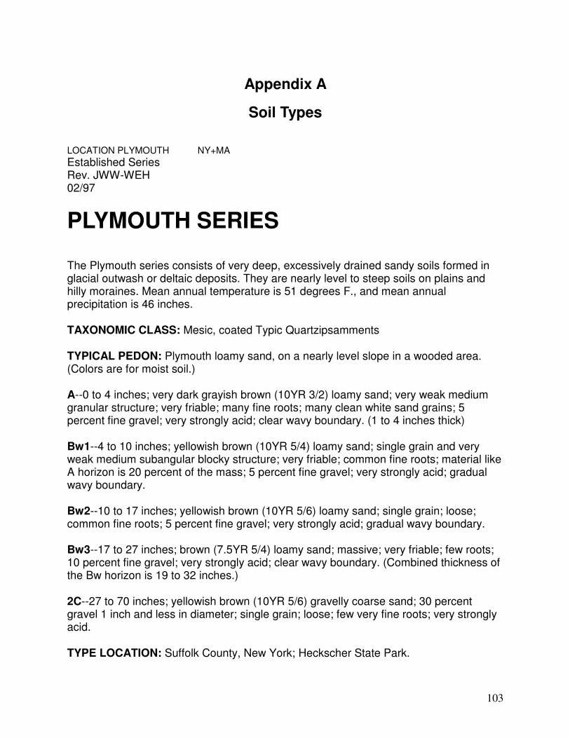
103

Appendix A

Soil Types LOCATION PLYMOUTH NY+MA

Established Series Rev. JWW-WEH 02/97

PLYMOUTH SERIES

The Plymouth series consists of very deep, excessively drained sandy soils formed in glacial outwash or deltaic deposits. They are nearly level to steep soils on plains and hilly moraines. Mean annual temperature is 51 degrees F., and mean annual precipitation is 46 inches.

TAXONOMIC CLASS: Mesic, coated Typic Quartzipsamments

TYPICAL PEDON: Plymouth loamy sand, on a nearly level slope in a wooded area. (Colors are for moist soil.)

A--0 to 4 inches; very dark grayish brown (10YR 3/2) loamy sand; very weak medium granular structure; very friable; many fine roots; many clean white sand grains; 5 percent fine gravel; very strongly acid; clear wavy boundary. (1 to 4 inches thick)

Bw1--4 to 10 inches; yellowish brown (10YR 5/4) loamy sand; single grain and very weak medium subangular blocky structure; very friable; common fine roots; material like A horizon is 20 percent of the mass; 5 percent fine gravel; very strongly acid; gradual wavy boundary.

Bw2--10 to 17 inches; yellowish brown (10YR 5/6) loamy sand; single grain; loose; common fine roots; 5 percent fine gravel; very strongly acid; gradual wavy boundary.

Bw3--17 to 27 inches; brown (7.5YR 5/4) loamy sand; massive; very friable; few roots; 10 percent fine gravel; very strongly acid; clear wavy boundary. (Combined thickness of the Bw horizon is 19 to 32 inches.)

2C--27 to 70 inches; yellowish brown (10YR 5/6) gravelly coarse sand; 30 percent gravel 1 inch and less in diameter; single grain; loose; few very fine roots; very strongly acid.

TYPE LOCATION: Suffolk County, New York; Heckscher State Park.

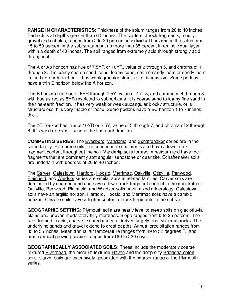
104

RANGE IN CHARACTERISTICS: Thickness of the solum ranges from 20 to 40 inches. Bedrock is at depths greater than 60 inches. The content of rock fragments, mostly gravel and cobbles, ranges from 2 to 30 percent in individual horizons of the solum and 15 to 50 percent in the sub stratum but no more than 35 percent in an individual layer within a depth of 40 inches. The soil ranges from extremely acid through strongly acid throughout.

The A or Ap horizon has hue of 7.5YR or 10YR, value of 2 through 5, and chroma of 1 through 3. It is loamy coarse sand, sand, loamy sand, coarse sandy loam or sandy loam in the fine-earth fraction. It has weak granular structure, or is massive. Some pedons have a thin E horizon below the A horizon.

The B horizon has hue of 5YR through 2.5Y, value of 4 or 5, and chroma of 4 through 8, with hue as red as 5YR restricted to subhorizons. It is coarse sand to loamy fine sand in the fine-earth fraction. It has very weak or weak subangular blocky structure, or is structureless. It is very friable or loose. Some pedons have a BC horizon 1 to 7 inches thick.

The 2C horizon has hue of 10YR or 2.5Y, value of 5 through 7, and chroma of 2 through 6. It is sand or coarse sand in the fine-earth fraction.

COMPETING SERIES: The Evesboro, Vanderlip, and Schaffenaker series are in the same family. Evesboro soils formed in marine sediments and have a lower rock fragment content throughout the soil. Vanderlip soils formed in residum and have rock fragments that are dominantly soft angular sandstone or quartzite. Schaffenaker soils are underlain with bedrock at 20 to 40 inches.

The Carver, Galestown, Hartford, Hoosic, Merrimac, Oakville, Otisville, Penwood, Plainfield, and Windsor series are similar soils in related families. Carver soils are dominated by coarser sand and have a lower rock fragment content in the substratum. Oakville, Penwood, Plainfield, and Windsor soils have mixed mineralogy. Galestown soils have an argillic horizon. Hartford, Hoosic, and Merrimac soils have a cambic horizon. Otisville soils have a higher content of rock fragments in the subsoil.

GEOGRAPHIC SETTING: Plymouth soils are nearly level to steep soils on glaciofluvial plains and uneven moderately hilly moraines. Slope ranges from 0 to 35 percent. The soils formed in acid, coarse textured material derived largely from siliceous rocks. The underlying sands and gravel extend to great depths. Annual precipitation ranges from 35 to 56 inches. Mean annual air temperature ranges from 49 to 52 degrees F., and mean annual growing season ranges from 180 to 220 days.

GEOGRAPHICALLY ASSOCIATED SOILS: These include the moderately coarse textured Riverhead, the medium textured Haven and the deep silty Bridgehampton soils. Carver soils are extensively associated with the coarser range of the Plymouth series.

105

DRAINAGE AND PERMEABILITY: Excessively drained. Runoff is slow to moderate. Permeability is rapid in the solum and very rapid in the underlying substratum.

USE AND VEGETATION: Small areas are used for cropland. Most areas are in woodland, or are used for urban and suburban development. Principal trees are white and black oak, pitch pine, and scrub oak.

DISTRIBUTION AND EXTENT: Long Island, New York, Massachusetts, and northern New Jersey. The soils are of moderate extent.

MLRA OFFICE RESPONSIBLE: Amherst, Massachusetts

SERIES ESTABLISHED: Plymouth County, Massachusetts, 1911.

REMARKS: The series was inactivated in 1961, and was reactivated in 1969. The soil was previously classified as siliceous mesic Typic Udipsamments. Data from New York and Massachusetts show less than 10 percent weatherable minerals.

Diagnostic horizons and other features recognized in this pedon are: 1. Ochric epipedon - the zone from the surface of the soil to a depth of 4 inches (A horizon). 2. Quartzipsamments great group - the determinant fraction (0.02 to 2 mm) is more than 90 percent resistant minerals.

National Cooperative Soil Survey U.S.A. LOCATION RIVERHEAD NY MA NJ PA

Established Series Rev. JDV-WEH-STS 03/2003

RIVERHEAD SERIES

The Riverhead series consists of very deep, well drained soils formed in glacial outwash deposits derived primarily from granitic materials. They are on outwash plains, valley trains, beaches, and water-sorted moraines. Slope ranges from 0 to 50 percent slopes. Mean annual temperature is 51 degrees F. and mean annual precipitation is 47 inches.

TAXONOMIC CLASS: Coarse-loamy, mixed, active, mesic Typic Dystrudepts

TYPICAL PEDON: Riverhead sandy loam, on a 2 percent slope in an area used for recreation. (Colors are for moist broken soil).

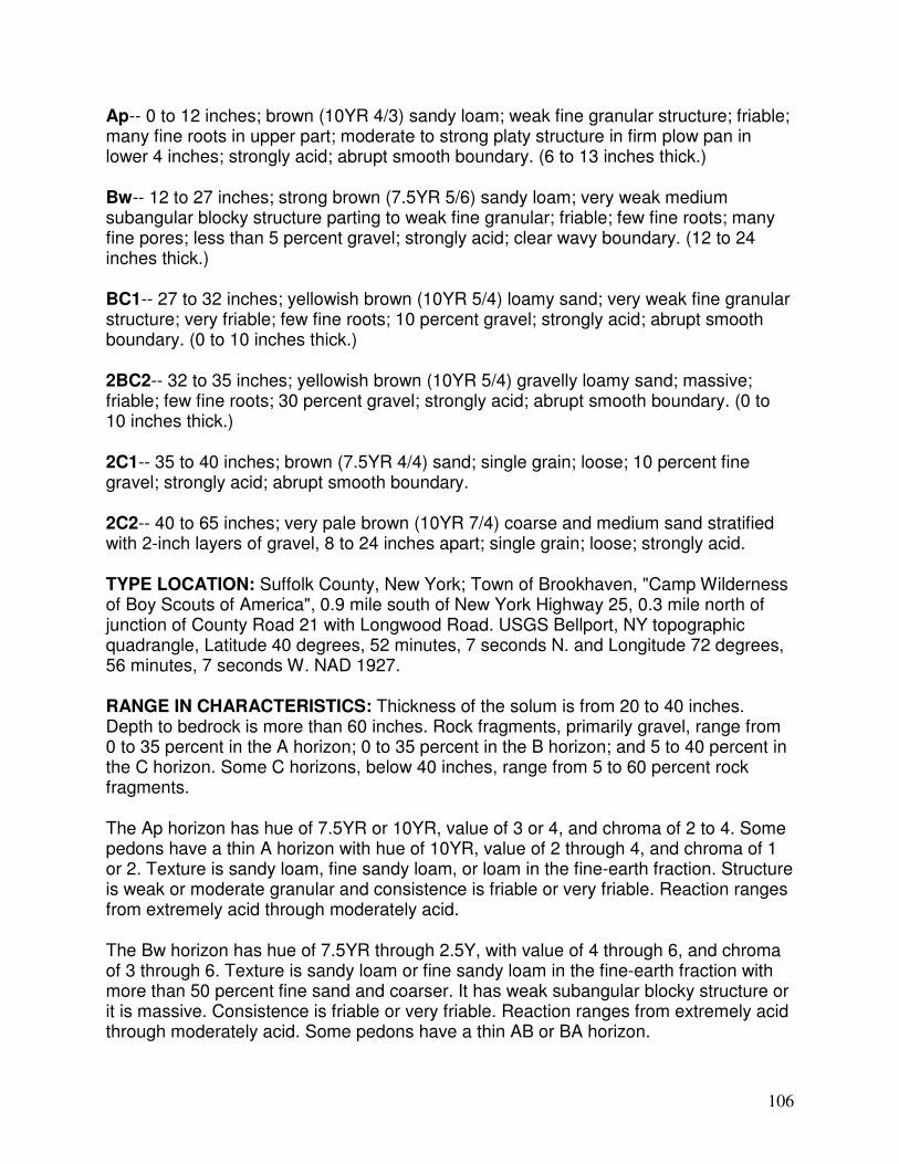
106

Ap-- 0 to 12 inches; brown (10YR 4/3) sandy loam; weak fine granular structure; friable; many fine roots in upper part; moderate to strong platy structure in firm plow pan in lower 4 inches; strongly acid; abrupt smooth boundary. (6 to 13 inches thick.)

Bw-- 12 to 27 inches; strong brown (7.5YR 5/6) sandy loam; very weak medium subangular blocky structure parting to weak fine granular; friable; few fine roots; many fine pores; less than 5 percent gravel; strongly acid; clear wavy boundary. (12 to 24 inches thick.)

BC1-- 27 to 32 inches; yellowish brown (10YR 5/4) loamy sand; very weak fine granular structure; very friable; few fine roots; 10 percent gravel; strongly acid; abrupt smooth boundary. (0 to 10 inches thick.)

2BC2-- 32 to 35 inches; yellowish brown (10YR 5/4) gravelly loamy sand; massive; friable; few fine roots; 30 percent gravel; strongly acid; abrupt smooth boundary. (0 to 10 inches thick.)

2C1-- 35 to 40 inches; brown (7.5YR 4/4) sand; single grain; loose; 10 percent fine gravel; strongly acid; abrupt smooth boundary.

2C2-- 40 to 65 inches; very pale brown (10YR 7/4) coarse and medium sand stratified with 2-inch layers of gravel, 8 to 24 inches apart; single grain; loose; strongly acid.

TYPE LOCATION: Suffolk County, New York; Town of Brookhaven, "Camp Wilderness of Boy Scouts of America", 0.9 mile south of New York Highway 25, 0.3 mile north of junction of County Road 21 with Longwood Road. USGS Bellport, NY topographic quadrangle, Latitude 40 degrees, 52 minutes, 7 seconds N. and Longitude 72 degrees, 56 minutes, 7 seconds W. NAD 1927.

RANGE IN CHARACTERISTICS: Thickness of the solum is from 20 to 40 inches. Depth to bedrock is more than 60 inches. Rock fragments, primarily gravel, range from 0 to 35 percent in the A horizon; 0 to 35 percent in the B horizon; and 5 to 40 percent in the C horizon. Some C horizons, below 40 inches, range from 5 to 60 percent rock fragments.

The Ap horizon has hue of 7.5YR or 10YR, value of 3 or 4, and chroma of 2 to 4. Some pedons have a thin A horizon with hue of 10YR, value of 2 through 4, and chroma of 1 or 2. Texture is sandy loam, fine sandy loam, or loam in the fine-earth fraction. Structure is weak or moderate granular and consistence is friable or very friable. Reaction ranges from extremely acid through moderately acid.

The Bw horizon has hue of 7.5YR through 2.5Y, with value of 4 through 6, and chroma of 3 through 6. Texture is sandy loam or fine sandy loam in the fine-earth fraction with more than 50 percent fine sand and coarser. It has weak subangular blocky structure or it is massive. Consistence is friable or very friable. Reaction ranges from extremely acid through moderately acid. Some pedons have a thin AB or BA horizon.

107

The BC and 2BC horizons have hue of 7.5YR through 2.5Y, value of 4 through 6, and chroma of 3 through 6. Textures are loamy sand, fine sandy loam, or sandy loam in the fine-earth fraction with coarser texture restricted to the 2BC horizon. They have weak granular or subangular blocky structure or they are massive. Consistence is friable or very friable. Reaction ranges from very strongly acid through moderately acid.

The C or 2C horizon has hue of 7.5YR through 2.5Y, value of 3 through 7, and chroma of 3 through 6. Texture is coarse sand, sand, or loamy sand in the fine-earth fraction or it is stratified sand and gravel. Layers of loamy fine sand are present in some pedons. Some pedons also have a loamy 3C horizon below 40 inches with fine-earth textures of sandy loam or fine sandy loam. Reaction ranges from very strongly acid through neutral. Neutral reactions are restricted to depths greater than 30 inches.

COMPETING SERIES: The Ashe, Brookfield, Buladean, Cardigan, Charlton, Chestnut, Delaware, Dutchess, Edneyville, Flatbush (T), Foresthills (T), Gallimore, Greenbelt (T), Hazel, Lordstown, Newport, Soco, St. Albans, Stecoah, Steinsburg, and Yalesville series are in the same family. Ashe, Cardigan, Hazel, Sharpcrest (T), Soco, Steinsburg, and Yalesville soils are 20 to 40 inches deep to bedrock. Brookfield, Charlton, Dutchess, and St. Albans soils formed in deep glacial till and do not have stratified sand and gravel C horizons. Buladean and Stecoah soils have paralithic contacts at 40 to 60 inches. Chestnut soils have a paralithic contact at 20 to 40 inches. Delaware soils have less than 50 percent fine sand and coarser in the B horizon. Edneyville soils are underlain by saprolite derived from granite and gneiss and do not have stratified sand and gravel C horizons. Flatbush (T) soils are anthropogenic soils formed in fly ash. Foresthills(T) and Greenbelt(T) soils are anthropogenic soils with surface layers of loamy fill. Gallimore soils are deeper than 50 inches to the bottom of the cambic horizon. Lordstown soils are moderately deep. Newport soils have very dense substrata. Sharpcrest (T) soils do not have an OSD on file to compete.

GEOGRAPHIC SETTING: Riverhead soils are nearly level to steep soils on outwash plains, valley trains, beaches, and water-sorted moraines. Slope ranges from 0 to 50 percent. The soils developed in 20 to 40 inches of water-sorted sandy loam or fine sandy loam relatively low in gravel content over stratified gravel and sand. Mean annual temperature ranges from 48 to 55 degrees F., mean annual precipitation ranges from 38 to 55 inches, and mean annual frost-free days ranges from 135 to 220 days. Elevation ranges from 50 to 1350 feet above sea level.

GEOGRAPHICALLY ASSOCIATED SOILS: These are the Bridgehampton, Carver, Chenango, Enfield, Haven, Hempstead, Hoosic, Mineola, Montauk, Plymouth, and Sudbury soils. Bridgehampton, Enfield, Haven, and Hempstead soils contain more silt in the layers above the stratified sand and gravel and, in addition, Hempstead soils have thicker dark surface layers. Chenango and Hoosic soils are loamy- skeletal and sandy skeletal, respectively. Mineola soils have thicker dark surfaces and more sand in the subsoil. Montauk soils are closely associated on morainic landforms but have firm till substrata. Plymouth and Carver soils are sandy throughout. Sudbury soils are moderately well drained.

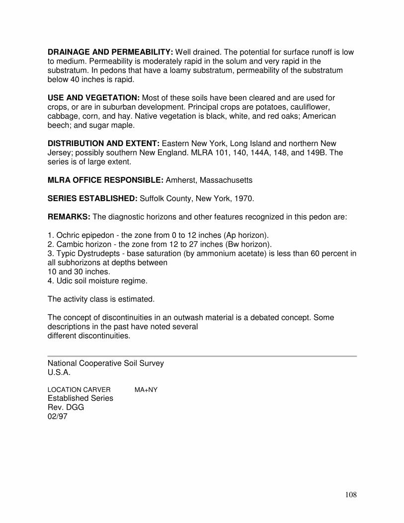
108

DRAINAGE AND PERMEABILITY: Well drained. The potential for surface runoff is low to medium. Permeability is moderately rapid in the solum and very rapid in the substratum. In pedons that have a loamy substratum, permeability of the substratum below 40 inches is rapid.

USE AND VEGETATION: Most of these soils have been cleared and are used for crops, or are in suburban development. Principal crops are potatoes, cauliflower, cabbage, corn, and hay. Native vegetation is black, white, and red oaks; American beech; and sugar maple.

DISTRIBUTION AND EXTENT: Eastern New York, Long Island and northern New Jersey; possibly southern New England. MLRA 101, 140, 144A, 148, and 149B. The series is of large extent.


SERIES ESTABLISHED: Suffolk County, New York, 1970.

REMARKS: The diagnostic horizons and other features recognized in this pedon are:

1. Ochric epipedon - the zone from 0 to 12 inches (Ap horizon). 2. Cambic horizon - the zone from 12 to 27 inches (Bw horizon). 3. Typic Dystrudepts - base saturation (by ammonium acetate) is less than 60 percent in all subhorizons at depths between 10 and 30 inches. 4. Udic soil moisture regime.

The activity class is estimated.

The concept of discontinuities in an outwash material is a debated concept. Some descriptions in the past have noted several different discontinuities.

National Cooperative Soil Survey U.S.A. LOCATION CARVER MA+NY

Established Series Rev. DGG 02/97

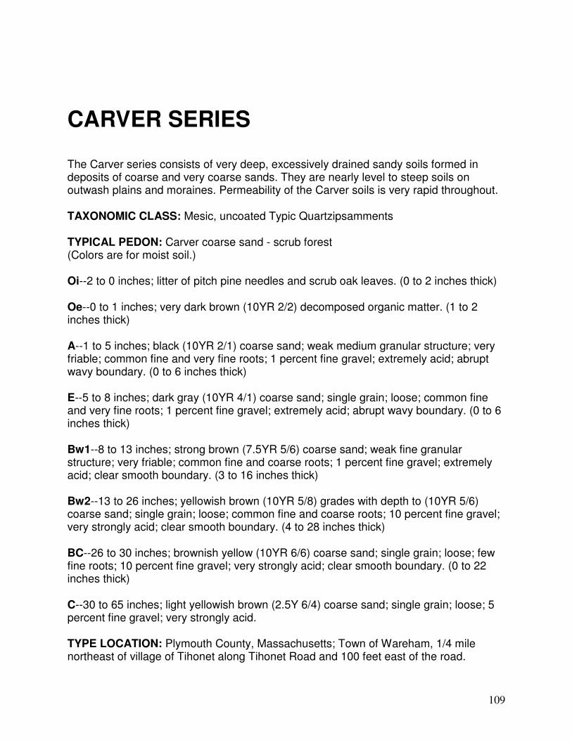
109

CARVER SERIES

The Carver series consists of very deep, excessively drained sandy soils formed in deposits of coarse and very coarse sands. They are nearly level to steep soils on outwash plains and moraines. Permeability of the Carver soils is very rapid throughout.

TAXONOMIC CLASS: Mesic, uncoated Typic Quartzipsamments

TYPICAL PEDON: Carver coarse sand - scrub forest (Colors are for moist soil.)

Oi--2 to 0 inches; litter of pitch pine needles and scrub oak leaves. (0 to 2 inches thick)

Oe--0 to 1 inches; very dark brown (10YR 2/2) decomposed organic matter. (1 to 2 inches thick)

A--1 to 5 inches; black (10YR 2/1) coarse sand; weak medium granular structure; very friable; common fine and very fine roots; 1 percent fine gravel; extremely acid; abrupt wavy boundary. (0 to 6 inches thick)

E--5 to 8 inches; dark gray (10YR 4/1) coarse sand; single grain; loose; common fine and very fine roots; 1 percent fine gravel; extremely acid; abrupt wavy boundary. (0 to 6 inches thick)

Bw1--8 to 13 inches; strong brown (7.5YR 5/6) coarse sand; weak fine granular structure; very friable; common fine and coarse roots; 1 percent fine gravel; extremely acid; clear smooth boundary. (3 to 16 inches thick)

Bw2--13 to 26 inches; yellowish brown (10YR 5/8) grades with depth to (10YR 5/6) coarse sand; single grain; loose; common fine and coarse roots; 10 percent fine gravel; very strongly acid; clear smooth boundary. (4 to 28 inches thick)

BC--26 to 30 inches; brownish yellow (10YR 6/6) coarse sand; single grain; loose; few fine roots; 10 percent fine gravel; very strongly acid; clear smooth boundary. (0 to 22 inches thick)

C--30 to 65 inches; light yellowish brown (2.5Y 6/4) coarse sand; single grain; loose; 5 percent fine gravel; very strongly acid.

TYPE LOCATION: Plymouth County, Massachusetts; Town of Wareham, 1/4 mile northeast of village of Tihonet along Tihonet Road and 100 feet east of the road.

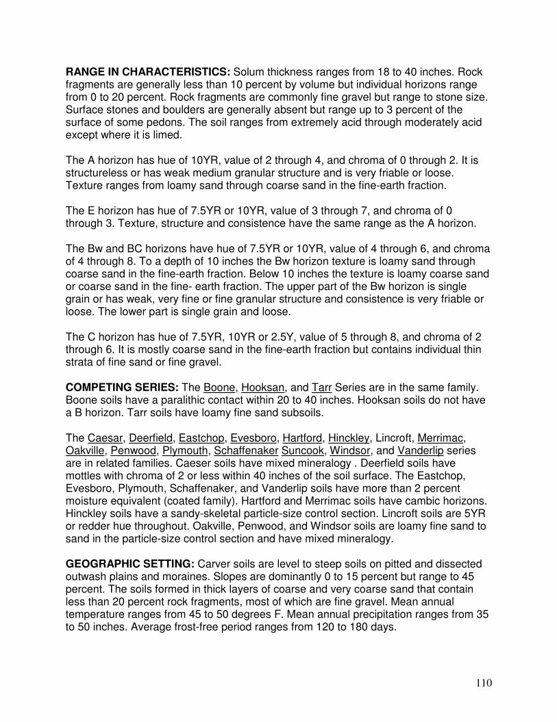
110

RANGE IN CHARACTERISTICS: Solum thickness ranges from 18 to 40 inches. Rock fragments are generally less than 10 percent by volume but individual horizons range from 0 to 20 percent. Rock fragments are commonly fine gravel but range to stone size. Surface stones and boulders are generally absent but range up to 3 percent of the surface of some pedons. The soil ranges from extremely acid through moderately acid except where it is limed.

The A horizon has hue of 10YR, value of 2 through 4, and chroma of 0 through 2. It is structureless or has weak medium granular structure and is very friable or loose. Texture ranges from loamy sand through coarse sand in the fine-earth fraction.

The E horizon has hue of 7.5YR or 10YR, value of 3 through 7, and chroma of 0 through 3. Texture, structure and consistence have the same range as the A horizon.

The Bw and BC horizons have hue of 7.5YR or 10YR, value of 4 through 6, and chroma of 4 through 8. To a depth of 10 inches the Bw horizon texture is loamy sand through coarse sand in the fine-earth fraction. Below 10 inches the texture is loamy coarse sand or coarse sand in the fine- earth fraction. The upper part of the Bw horizon is single grain or has weak, very fine or fine granular structure and consistence is very friable or loose. The lower part is single grain and loose.

The C horizon has hue of 7.5YR, 10YR or 2.5Y, value of 5 through 8, and chroma of 2 through 6. It is mostly coarse sand in the fine-earth fraction but contains individual thin strata of fine sand or fine gravel.

COMPETING SERIES: The Boone, Hooksan, and Tarr Series are in the same family. Boone soils have a paralithic contact within 20 to 40 inches. Hooksan soils do not have a B horizon. Tarr soils have loamy fine sand subsoils.

The Caesar, Deerfield, Eastchop, Evesboro, Hartford, Hinckley, Lincroft, Merrimac, Oakville, Penwood, Plymouth, Schaffenaker Suncook, Windsor, and Vanderlip series are in related families. Caeser soils have mixed mineralogy . Deerfield soils have mottles with chroma of 2 or less within 40 inches of the soil surface. The Eastchop, Evesboro, Plymouth, Schaffenaker, and Vanderlip soils have more than 2 percent moisture equivalent (coated family). Hartford and Merrimac soils have cambic horizons. Hinckley soils have a sandy-skeletal particle-size control section. Lincroft soils are 5YR or redder hue throughout. Oakville, Penwood, and Windsor soils are loamy fine sand to sand in the particle-size control section and have mixed mineralogy.

GEOGRAPHIC SETTING: Carver soils are level to steep soils on pitted and dissected outwash plains and moraines. Slopes are dominantly 0 to 15 percent but range to 45 percent. The soils formed in thick layers of coarse and very coarse sand that contain less than 20 percent rock fragments, most of which are fine gravel. Mean annual temperature ranges from 45 to 50 degrees F. Mean annual precipitation ranges from 35 to 50 inches. Average frost-free period ranges from 120 to 180 days.

111

GEOGRAPHICALLY ASSOCIATED SOILS: The competing Deerfield, Eastchop, Plymouth and Windsor soils often are on adjacent landscapes. The organic Freetown and Swansea soils and the very poorly drained Scarboro soils are in the kettleholes of the pitted outwash plains and the Gloucester and Montauk soils are intermingled on moraines. The Merrimac and Haven soils, which contain more silt, and the loamy Riverhead soils are on plains adjacent to the moraines. Carver is the excessively drained member of a drainage sequence which includes the moderately well drained Deerfield, somewhat poorly drained Saugatuck and Pipestone soils, and the very poorly drained Berryland soils.

DRAINAGE AND PERMEABILITY: Excessively drained. Runoff is very slow. Permeability is very rapid.

USE AND VEGETATION: Mostly forested to scrub oak, pitch pine and white pine. A small part is cleared and cropped.

DISTRIBUTION AND EXTENT: Massachusetts, New York, and New Jersey. The soil is extensive, estimated 110,000 acres.


SERIES ESTABLISHED: Plymouth County, Massachusetts, 1911.

REMARKS: 1. This soil was previously classified as siliceous, mesic Typic Udisamments. Lab data indicates by far the majority of Carver soils have more than 90 percent minerals resistant to weathering. The classification is thus changed to reflect this condition.

2. Diagnostic horizons and features recognized in this pedon are:

a. Ochric epipedon - the zone from the surface of the soil to a depth of 8 inches (A and E horizons).

b. Sandy feature - the zone from 10 to 40 inches averages about 85 percent sand.

National Cooperative Soil Survey U.S.A.

112

Appendix B

Hydrographs for Synoptic Sampling Events

113

114

http://waterdata.usgs.gov/nwis/dv/?site_no=01305000&referred_module=sw Accessed on

May 03, 2007

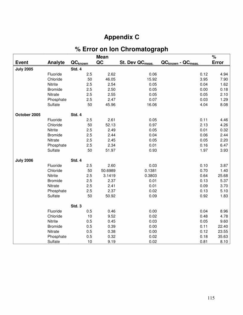
115

Appendix C

% Error on Ion Chromatograph

Event Analyte QCknown Mean QC St. Dev QCmeas. QCknown - QCmeas.

% Error

July 2005 Std. 4

Fluoride 2.5 2.62 0.06 0.12 4.94

Chloride 50 46.05 15.92 3.95 7.90

Nitrite 2.5 2.54 0.05 0.04 1.62

Bromide 2.5 2.50 0.05 0.00 0.18

Nitrate 2.5 2.55 0.05 0.05 2.10

Phosphate 2.5 2.47 0.07 0.03 1.29

Sulfate 50 45.96 16.06 4.04 8.08

October 2005 Std. 4

Fluoride 2.5 2.61 0.05 0.11 4.46

Chloride 50 52.13 0.97 2.13 4.26

Nitrite 2.5 2.49 0.05 0.01 0.32

Bromide 2.5 2.44 0.04 0.06 2.44

Nitrate 2.5 2.45 0.05 0.05 2.20

Phosphate 2.5 2.34 0.01 0.16 6.47

Sulfate 50 51.97 0.93 1.97 3.93

July 2006 Std. 4

Fluoride 2.5 2.60 0.03 0.10 3.87

Chloride 50 50.6989 0.1381 0.70 1.40

Nitrite 2.5 3.1419 0.3803 0.64 25.68

Bromide 2.5 2.37 0.01 0.13 5.37

Nitrate 2.5 2.41 0.01 0.09 3.70

Phosphate 2.5 2.37 0.02 0.13 5.10

Sulfate 50 50.92 0.09 0.92 1.83

Std. 3

Fluoride 0.5 0.46 0.00 0.04 8.96

Chloride 10 9.52 0.02 0.48 4.78

Nitrite 0.5 0.45 0.03 0.05 9.60

Bromide 0.5 0.39 0.00 0.11 22.40

Nitrate 0.5 0.38 0.00 0.12 23.55

Phosphate 0.5 0.32 0.02 0.18 35.63

Sulfate 10 9.19 0.02 0.81 8.10

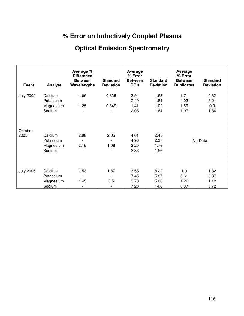
116

% Error on Inductively Coupled Plasma

Optical Emission Spectrometry

Event Analyte

Average % Difference Between

Wavelengths Standard Deviation

Average % Error Between

QC's Standard Deviation

Average % Error Between

Duplicates Standard Deviation

July 2005 Calcium 1.06 0.839 3.94 1.62 1.71 0.82

Potassium - - 2.49 1.84 4.03 3.21

Magnesium 1.25 0.849 1.41 1.02 1.59 0.9

Sodium - - 2.03 1.64 1.97 1.34

October 2005 Calcium 2.98 2.05 4.61 2.45

Potassium - - 4.96 2.37

Magnesium 2.15 1.06 3.29 1.76

Sodium - - 2.86 1.56

No Data

July 2006 Calcium 1.53 1.87 3.58 8.22 1.3 1.32

Potassium - - 7.45 5.87 5.61 3.37

Magnesium 1.45 0.5 3.73 5.08 1.22 1.12

Sodium - - 7.23 14.8 0.87 0.72

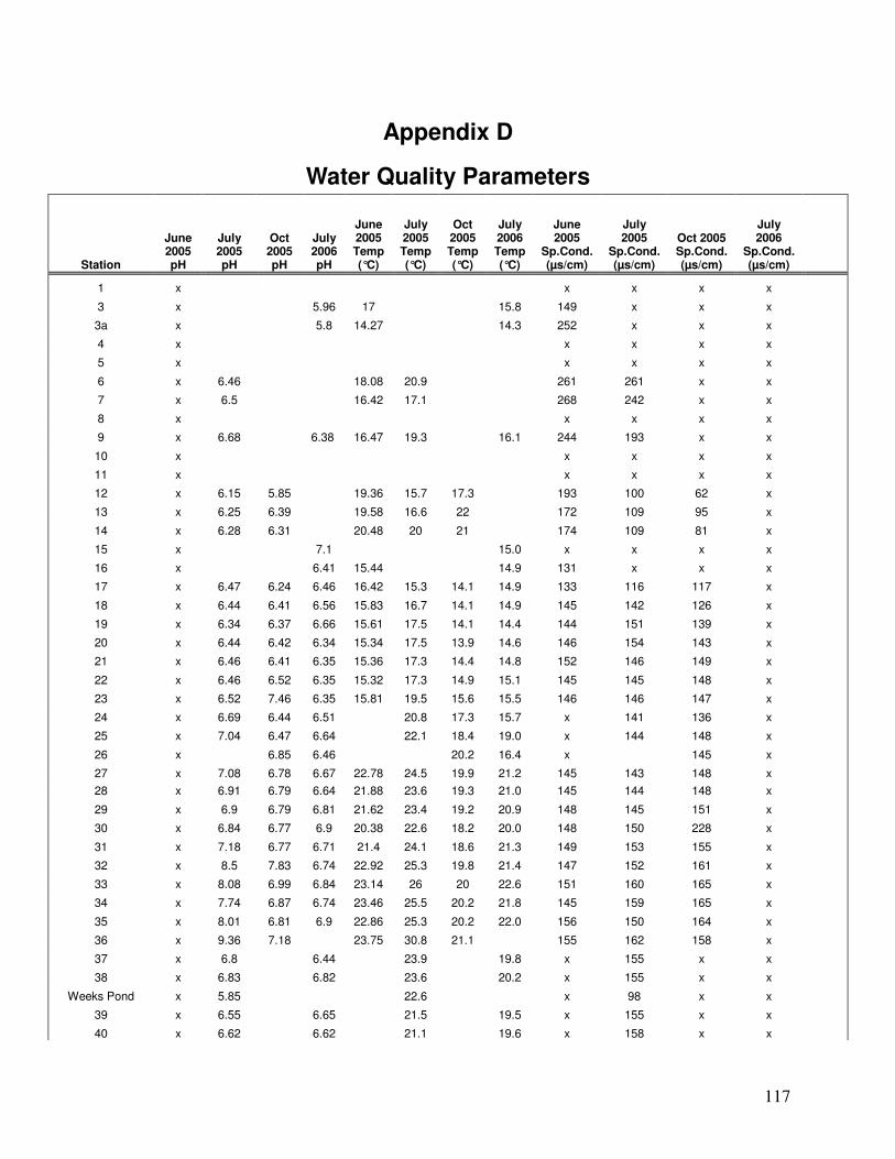
117

Appendix D

Water Quality Parameters

Station

June 2005 pH

July 2005 pH

Oct 2005 pH

July 2006 pH

June 2005 Temp (°C)

July 2005 Temp (°C)

Oct 2005 Temp (°C)

July 2006 Temp (°C)

June 2005

Sp.Cond. (µs/cm)

July 2005

Sp.Cond. (µs/cm)

Oct 2005 Sp.Cond. (µs/cm)

July 2006

Sp.Cond. (µs/cm)

1 x x x x x

3 x 5.96 17 15.8 149 x x x

3a x 5.8 14.27 14.3 252 x x x

4 x x x x x

5 x x x x x

6 x 6.46 18.08 20.9 261 261 x x

7 x 6.5 16.42 17.1 268 242 x x

8 x x x x x

9 x 6.68 6.38 16.47 19.3 16.1 244 193 x x

10 x x x x x

11 x x x x x

12 x 6.15 5.85 19.36 15.7 17.3 193 100 62 x

13 x 6.25 6.39 19.58 16.6 22 172 109 95 x

14 x 6.28 6.31 20.48 20 21 174 109 81 x

15 x 7.1 15.0 x x x x

16 x 6.41 15.44 14.9 131 x x x

17 x 6.47 6.24 6.46 16.42 15.3 14.1 14.9 133 116 117 x

18 x 6.44 6.41 6.56 15.83 16.7 14.1 14.9 145 142 126 x

19 x 6.34 6.37 6.66 15.61 17.5 14.1 14.4 144 151 139 x

20 x 6.44 6.42 6.34 15.34 17.5 13.9 14.6 146 154 143 x

21 x 6.46 6.41 6.35 15.36 17.3 14.4 14.8 152 146 149 x

22 x 6.46 6.52 6.35 15.32 17.3 14.9 15.1 145 145 148 x

23 x 6.52 7.46 6.35 15.81 19.5 15.6 15.5 146 146 147 x

24 x 6.69 6.44 6.51 20.8 17.3 15.7 x 141 136 x

25 x 7.04 6.47 6.64 22.1 18.4 19.0 x 144 148 x

26 x 6.85 6.46 20.2 16.4 x 145 x

27 x 7.08 6.78 6.67 22.78 24.5 19.9 21.2 145 143 148 x

28 x 6.91 6.79 6.64 21.88 23.6 19.3 21.0 145 144 148 x

29 x 6.9 6.79 6.81 21.62 23.4 19.2 20.9 148 145 151 x

30 x 6.84 6.77 6.9 20.38 22.6 18.2 20.0 148 150 228 x

31 x 7.18 6.77 6.71 21.4 24.1 18.6 21.3 149 153 155 x

32 x 8.5 7.83 6.74 22.92 25.3 19.8 21.4 147 152 161 x

33 x 8.08 6.99 6.84 23.14 26 20 22.6 151 160 165 x

34 x 7.74 6.87 6.74 23.46 25.5 20.2 21.8 145 159 165 x

35 x 8.01 6.81 6.9 22.86 25.3 20.2 22.0 156 150 164 x

36 x 9.36 7.18 23.75 30.8 21.1 155 162 158 x

37 x 6.8 6.44 23.9 19.8 x 155 x x

38 x 6.83 6.82 23.6 20.2 x 155 x x

Weeks Pond x 5.85 22.6 x 98 x x

39 x 6.55 6.65 21.5 19.5 x 155 x x

40 x 6.62 6.62 21.1 19.6 x 158 x x

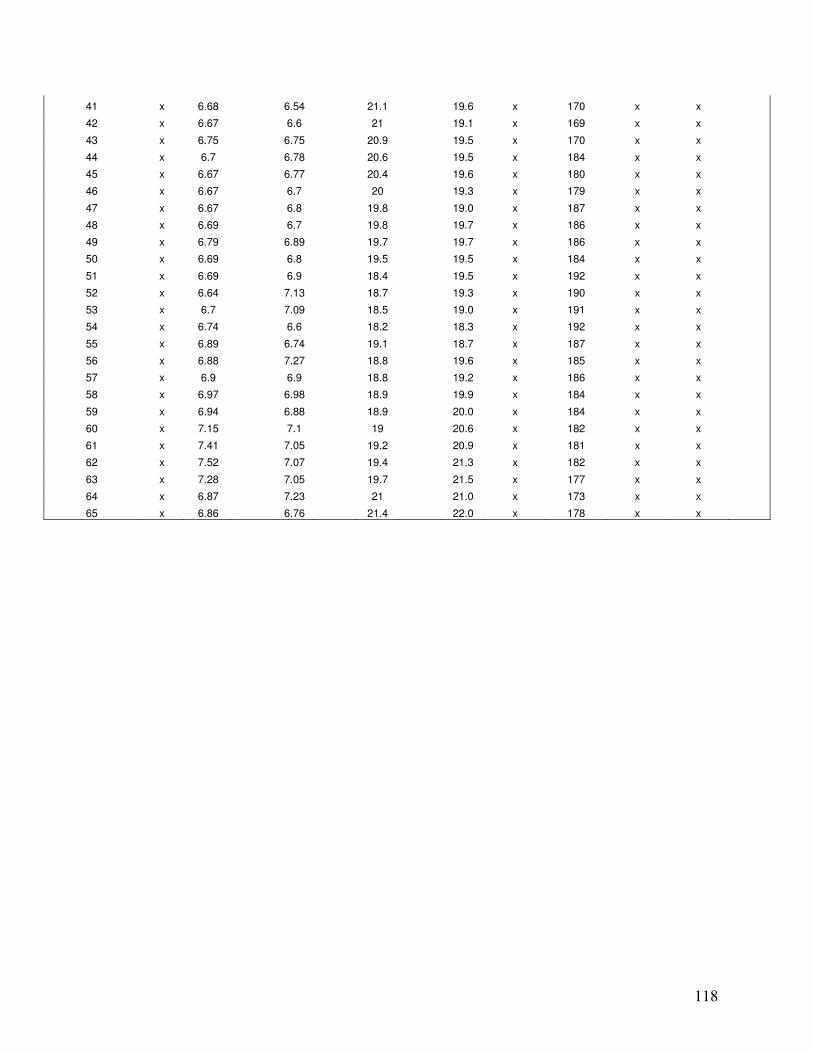
118

41 x 6.68 6.54 21.1 19.6 x 170 x x

42 x 6.67 6.6 21 19.1 x 169 x x

43 x 6.75 6.75 20.9 19.5 x 170 x x

44 x 6.7 6.78 20.6 19.5 x 184 x x

45 x 6.67 6.77 20.4 19.6 x 180 x x

46 x 6.67 6.7 20 19.3 x 179 x x

47 x 6.67 6.8 19.8 19.0 x 187 x x

48 x 6.69 6.7 19.8 19.7 x 186 x x

49 x 6.79 6.89 19.7 19.7 x 186 x x

50 x 6.69 6.8 19.5 19.5 x 184 x x

51 x 6.69 6.9 18.4 19.5 x 192 x x

52 x 6.64 7.13 18.7 19.3 x 190 x x

53 x 6.7 7.09 18.5 19.0 x 191 x x

54 x 6.74 6.6 18.2 18.3 x 192 x x

55 x 6.89 6.74 19.1 18.7 x 187 x x

56 x 6.88 7.27 18.8 19.6 x 185 x x

57 x 6.9 6.9 18.8 19.2 x 186 x x

58 x 6.97 6.98 18.9 19.9 x 184 x x

59 x 6.94 6.88 18.9 20.0 x 184 x x

60 x 7.15 7.1 19 20.6 x 182 x x

61 x 7.41 7.05 19.2 20.9 x 181 x x

62 x 7.52 7.07 19.4 21.3 x 182 x x

63 x 7.28 7.05 19.7 21.5 x 177 x x

64 x 6.87 7.23 21 21.0 x 173 x x

65 x 6.86 6.76 21.4 22.0 x 178 x x

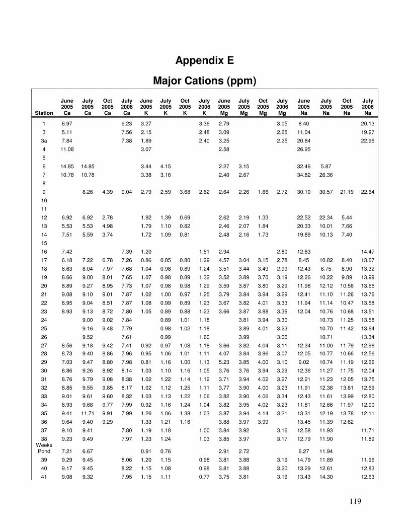
119

Appendix E

Major Cations (ppm)

Station

June 2005 Ca

July 2005 Ca

Oct 2005 Ca

July 2006 Ca

June 2005

K

July 2005

K

Oct 2005

K

July 2006

K

June 2005 Mg

July 2005 Mg

Oct 2005 Mg

July 2006 Mg

June 2005 Na

July 2005 Na

Oct 2005 Na

July 2006 Na

1 6.97 9.23 3.27 3.36 2.79 3.05 8.40 20.13

3 5.11 7.56 2.15 2.48 3.09 2.65 11.04 19.27

3a 7.84 7.38 1.89 2.40 3.25 2.25 20.84 22.96

4 11.08 3.07 2.58 26.95

5

6 14.85 14.85 3.44 4.15 2.27 3.15 32.46 5.87

7 10.78 10.78 3.38 3.16 2.40 2.67 34.82 26.36

8

9 8.26 4.39 9.04 2.79 2.59 3.68 2.62 2.64 2.26 1.66 2.72 30.10 30.57 21.19 22.64

10

11

12 6.92 6.92 2.78 1.92 1.39 0.69 2.62 2.19 1.33 22.52 22.34 5.44

13 5.53 5.53 4.98 1.79 1.10 0.82 2.46 2.07 1.84 20.33 10.01 7.66

14 7.51 5.59 3.74 1.72 1.09 0.81 2.48 2.16 1.73 19.89 10.13 7.40

15

16 7.42 7.39 1.20 1.51 2.94 2.80 12.83 14.47

17 6.18 7.22 6.78 7.26 0.86 0.85 0.80 1.29 4.57 3.04 3.15 2.78 8.45 10.82 8.40 13.67

18 8.63 8.04 7.97 7.68 1.04 0.98 0.89 1.24 3.51 3.44 3.49 2.99 12.43 8.75 8.90 13.32

19 8.66 9.00 8.01 7.65 1.07 0.98 0.89 1.32 3.52 3.89 3.70 3.19 12.26 10.22 9.89 13.99

20 8.89 9.27 8.95 7.73 1.07 0.98 0.98 1.29 3.59 3.87 3.80 3.29 11.96 12.12 10.56 13.66

21 9.08 9.10 9.01 7.87 1.02 1.00 0.97 1.25 3.79 3.84 3.94 3.29 12.41 11.10 11.26 13.76

22 8.95 9.04 8.51 7.87 1.08 0.99 0.89 1.23 3.67 3.82 4.01 3.33 11.94 11.14 10.47 13.58

23 8.93 9.13 8.72 7.80 1.05 0.89 0.88 1.23 3.66 3.87 3.88 3.36 12.04 10.76 10.68 13.51

24 9.00 9.02 7.84 0.89 1.01 1.18 3.81 3.94 3.30 10.73 11.25 13.58

25 9.16 9.48 7.79 0.98 1.02 1.18 3.89 4.01 3.23 10.70 11.42 13.64

26 9.52 7.61 0.99 1.60 3.99 3.06 10.71 13.34

27 8.56 9.18 9.42 7.41 0.92 0.97 1.08 1.18 3.66 3.82 4.04 3.11 12.34 11.00 11.79 12.96

28 8.73 9.40 8.86 7.96 0.95 1.06 1.01 1.11 4.07 3.84 3.96 3.07 12.05 10.77 10.66 12.56

29 7.03 9.47 8.80 7.98 0.81 1.16 1.00 1.13 5.23 3.85 4.00 3.10 9.02 10.74 11.19 12.66

30 8.86 9.26 8.92 8.14 1.03 1.10 1.16 1.05 3.76 3.76 3.94 3.29 12.36 11.27 11.75 12.04

31 8.76 9.79 9.08 8.38 1.02 1.22 1.14 1.12 3.71 3.94 4.02 3.27 12.21 11.23 12.05 13.75

32 8.85 9.55 9.85 8.17 1.02 1.12 1.25 1.11 3.77 3.90 4.00 3.23 11.91 12.38 13.81 12.69

33 9.01 9.61 9.60 8.32 1.03 1.13 1.22 1.06 3.82 3.90 4.06 3.34 12.43 11.61 13.99 12.80

34 8.93 9.68 9.77 7.99 0.92 1.16 1.24 1.04 3.82 3.95 4.02 3.23 11.81 12.66 11.97 12.00

35 9.41 11.71 9.91 7.99 1.26 1.06 1.38 1.03 3.87 3.94 4.14 3.21 13.31 12.19 13.78 12.11

36 9.64 9.40 9.29 1.33 1.21 1.16 3.88 3.97 3.99 13.45 11.39 12.62

37 9.10 9.41 7.80 1.19 1.18 1.00 3.84 3.92 3.16 12.58 11.93 11.71

38 9.23 9.49 7.97 1.23 1.24 1.03 3.85 3.97 3.17 12.79 11.90 11.89 Weeks Pond 7.21 6.67 0.91 0.76 2.91 2.72 6.27 11.94

39 9.29 9.45 8.06 1.20 1.15 0.98 3.81 3.88 3.19 14.79 11.89 11.96

40 9.17 9.45 8.22 1.15 1.08 0.98 3.81 3.88 3.20 13.29 12.61 12.83

41 9.08 9.32 7.95 1.15 1.11 0.77 3.75 3.81 3.19 13.43 14.30 12.63

120

42 7.06 9.43 8.02 0.99 1.11 0.78 5.57 3.84 3.19 10.21 14.34 12.73

43 8.32 9.25 8.08 1.12 1.07 0.77 3.98 3.80 3.17 13.11 14.69 15.74

44 9.20 9.61 8.23 1.18 1.12 0.84 3.73 3.90 3.17 17.67 17.72 17.97

45 9.01 8.16 1.16 0.82 3.65 3.17 17.31 16.03

46 9.07 8.86 0.96 1.08 3.65 3.56 17.64 17.25

47 9.11 9.20 8.20 0.96 1.11 0.83 3.61 3.65 3.10 18.70 18.17 18.40

48 9.03 9.29 8.07 0.97 1.14 0.78 3.57 3.66 3.11 18.63 18.38 17.44

49 8.92 9.33 8.01 0.94 1.18 0.80 3.54 3.65 3.07 18.33 18.44 17.15

50 7.07 9.10 7.94 0.77 1.14 0.72 5.10 3.56 3.08 13.20 18.25 17.05

51 8.83 9.04 7.72 0.96 1.15 0.74 3.48 3.57 3.04 19.62 19.49 16.65

52 8.90 9.07 7.86 1.01 1.23 0.76 3.47 3.53 3.06 19.93 19.37 17.55

53 8.87 9.04 7.84 0.97 1.20 0.74 3.46 3.54 3.00 19.16 19.44 17.68

54 8.82 9.07 7.99 0.99 1.22 0.80 3.45 3.53 3.11 19.00 19.38 18.15

55 8.73 9.08 7.46 0.96 1.27 0.76 3.43 3.55 2.85 18.54 18.98 16.87

56 8.88 8.92 7.70 1.08 1.19 0.72 3.42 3.50 2.96 18.98 18.41 17.01

57 8.74 8.63 7.36 1.08 1.16 0.75 3.38 3.32 2.86 18.76 17.89 16.54

58 8.66 8.83 7.73 1.04 1.19 0.73 3.36 3.38 2.95 18.60 18.15 17.14

59 8.62 8.84 7.77 1.07 1.17 0.72 3.35 3.39 2.99 18.47 18.13 17.17

60 8.42 8.71 7.52 1.05 1.16 0.77 3.33 3.39 2.89 18.16 17.89 16.85

61 8.54 9.02 7.49 1.05 1.16 0.72 3.38 3.43 2.88 18.25 18.46 16.63

62 8.41 8.73 7.44 1.02 1.16 0.69 3.30 3.47 2.90 17.77 17.67 16.58

63 6.80 8.48 7.44 0.85 1.18 0.71 5.02 3.32 2.89 12.75 17.38 16.42

64 8.76 8.61 7.66 0.98 1.26 0.67 3.44 3.36 2.95 17.88 17.73 16.66

65 8.60 8.51 6.72 1.02 1.19 0.72 3.36 3.31 2.66 17.86 17.36 15.53

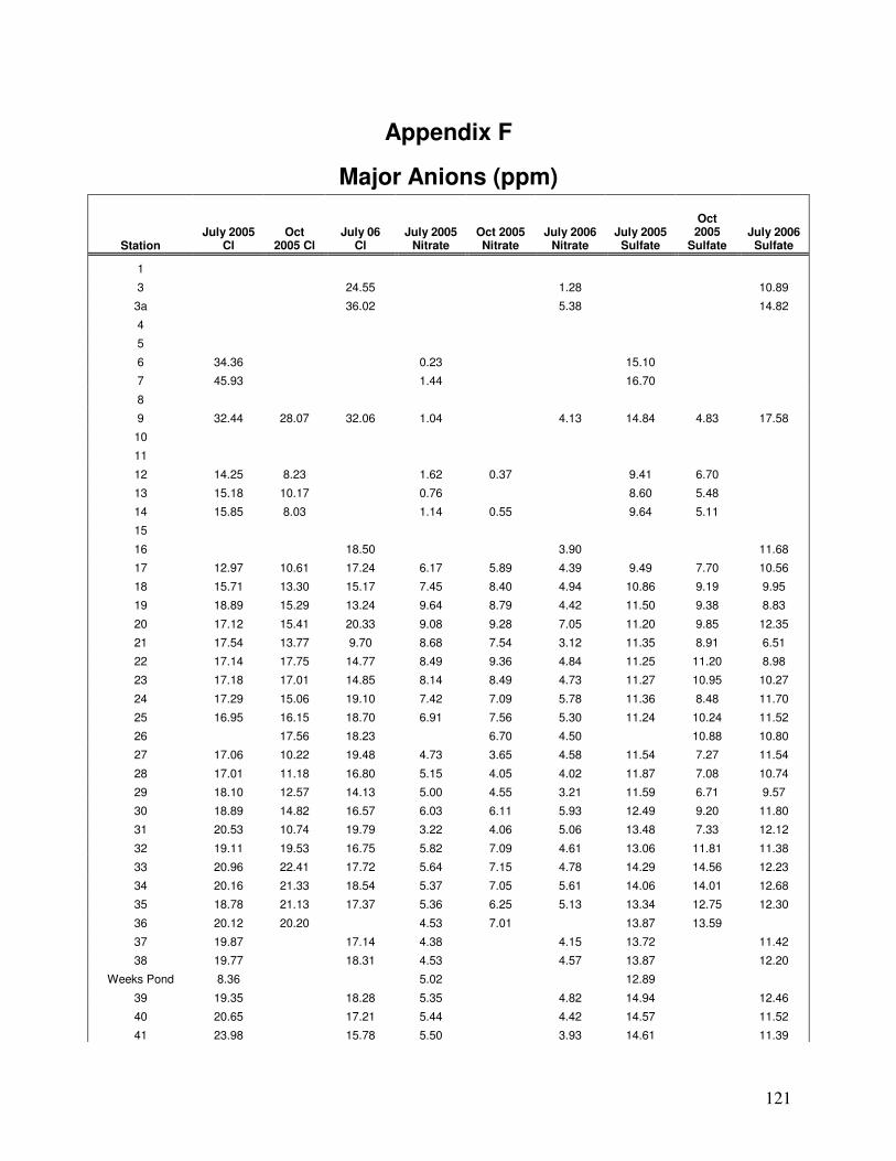
121

Appendix F

Major Anions (ppm)

Station July 2005

Cl Oct

2005 Cl July 06

Cl July 2005

Nitrate Oct 2005 Nitrate

July 2006 Nitrate

July 2005 Sulfate

Oct 2005

Sulfate July 2006

Sulfate

1

3 24.55 1.28 10.89

3a 36.02 5.38 14.82

4

5

6 34.36 0.23 15.10

7 45.93 1.44 16.70

8

9 32.44 28.07 32.06 1.04 4.13 14.84 4.83 17.58

10

11

12 14.25 8.23 1.62 0.37 9.41 6.70

13 15.18 10.17 0.76 8.60 5.48

14 15.85 8.03 1.14 0.55 9.64 5.11

15

16 18.50 3.90 11.68

17 12.97 10.61 17.24 6.17 5.89 4.39 9.49 7.70 10.56

18 15.71 13.30 15.17 7.45 8.40 4.94 10.86 9.19 9.95

19 18.89 15.29 13.24 9.64 8.79 4.42 11.50 9.38 8.83

20 17.12 15.41 20.33 9.08 9.28 7.05 11.20 9.85 12.35

21 17.54 13.77 9.70 8.68 7.54 3.12 11.35 8.91 6.51

22 17.14 17.75 14.77 8.49 9.36 4.84 11.25 11.20 8.98

23 17.18 17.01 14.85 8.14 8.49 4.73 11.27 10.95 10.27

24 17.29 15.06 19.10 7.42 7.09 5.78 11.36 8.48 11.70

25 16.95 16.15 18.70 6.91 7.56 5.30 11.24 10.24 11.52

26 17.56 18.23 6.70 4.50 10.88 10.80

27 17.06 10.22 19.48 4.73 3.65 4.58 11.54 7.27 11.54

28 17.01 11.18 16.80 5.15 4.05 4.02 11.87 7.08 10.74

29 18.10 12.57 14.13 5.00 4.55 3.21 11.59 6.71 9.57

30 18.89 14.82 16.57 6.03 6.11 5.93 12.49 9.20 11.80

31 20.53 10.74 19.79 3.22 4.06 5.06 13.48 7.33 12.12

32 19.11 19.53 16.75 5.82 7.09 4.61 13.06 11.81 11.38

33 20.96 22.41 17.72 5.64 7.15 4.78 14.29 14.56 12.23

34 20.16 21.33 18.54 5.37 7.05 5.61 14.06 14.01 12.68

35 18.78 21.13 17.37 5.36 6.25 5.13 13.34 12.75 12.30

36 20.12 20.20 4.53 7.01 13.87 13.59

37 19.87 17.14 4.38 4.15 13.72 11.42

38 19.77 18.31 4.53 4.57 13.87 12.20

Weeks Pond 8.36 5.02 12.89

39 19.35 18.28 5.35 4.82 14.94 12.46

40 20.65 17.21 5.44 4.42 14.57 11.52

41 23.98 15.78 5.50 3.93 14.61 11.39

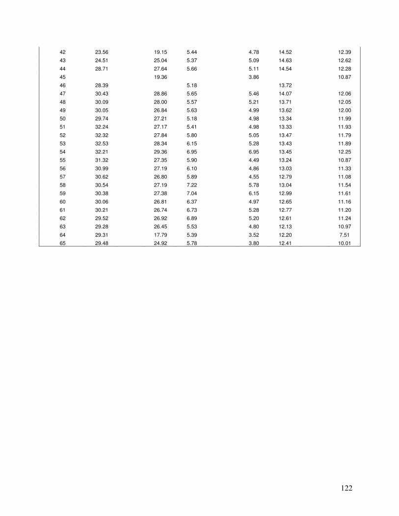
122

42 23.56 19.15 5.44 4.78 14.52 12.39

43 24.51 25.04 5.37 5.09 14.63 12.62

44 28.71 27.64 5.66 5.11 14.54 12.28

45 19.36 3.86 10.87

46 28.39 5.18 13.72

47 30.43 28.86 5.65 5.46 14.07 12.06

48 30.09 28.00 5.57 5.21 13.71 12.05

49 30.05 26.84 5.63 4.99 13.62 12.00

50 29.74 27.21 5.18 4.98 13.34 11.99

51 32.24 27.17 5.41 4.98 13.33 11.93

52 32.32 27.84 5.80 5.05 13.47 11.79

53 32.53 28.34 6.15 5.28 13.43 11.89

54 32.21 29.36 6.95 6.95 13.45 12.25

55 31.32 27.35 5.90 4.49 13.24 10.87

56 30.99 27.19 6.10 4.86 13.03 11.33

57 30.62 26.80 5.89 4.55 12.79 11.08

58 30.54 27.19 7.22 5.78 13.04 11.54

59 30.38 27.38 7.04 6.15 12.99 11.61

60 30.06 26.81 6.37 4.97 12.65 11.16

61 30.21 26.74 6.73 5.28 12.77 11.20

62 29.52 26.92 6.89 5.20 12.61 11.24

63 29.28 26.45 5.53 4.80 12.13 10.97

64 29.31 17.79 5.39 3.52 12.20 7.51

65 29.48 24.92 5.78 3.80 12.41 10.01

123

VITA Name Tracey L.M. O’Malley

Date and Place of Birth December 1, 1977 Niskayuna, New York

Education Name and Location Dates Degree High School Scotia-Glenville High School 1992-1996 Diploma College Plattsburgh State University 1996-2000 B.S. (Env. Sci.)

Of New York

Employment Position Dates Labat-Anderson Incorporated Environmental Analyst 2000-2001 New York City Department of Stream Restoration Technician- 2001-2002 Environmental Protection Americorps Member The Nature Conservancy Conservation Assistant 2003-2005

analysis of surface water quality and ground water flow

Documents