Analysis of Repeated Measures and Time Series: An ...

W O R K I N G P A P E R

Analysis of Repeated Measuresand Time Series: An Introductionwith Forestry ExamplesBiometrics Information Handbook No.6

⁄

Province of British ColumbiaMinistry of Forests Research Program

Analysis of Repeated Measuresand Time Series: An Introductionwith Forestry ExamplesBiometrics Information Handbook No.6

Amanda F. Linnell Nemec

Province of British ColumbiaMinistry of Forests Research Program

The use of trade, firm, or corporation names in this publication is for theinformation and convenience of the reader. Such use does not constitute anofficial endorsement or approval by the Government of British Columbia ofany product or service to the exclusion of any others that may also besuitable. Contents of this report are presented for discussion purposes only.

Citation:Nemec, Amanda F. Linnell. 1996. Analysis of repeated measures and time series: anintroduction with forestry examples. Biom. Inf. Handb. 6. Res. Br., B.C. Min. For.,Victoria, B.C. Work. Pap. 15/1996.

Prepared byAmanda F. Linnell NemecInternational Statistics and Research CorporationP.O. Box 496Brentwood Bay, BC V8M 1R3forB.C. Ministry of ForestsResearch Branch31 Bastion SquareVictoria, BC V8W 3E7

Copies of this report may be obtained, depending upon supply, from:B.C. Ministry of ForestsForestry Division Services Branch1205 Broad StreetVictoria, BC V8W 3E7

Province of British Columbia

The contents of this report may not be cited in whole or in part without theapproval of the Director of Research, B.C. Ministry of Forests, Victoria, B.C.

iii

ABSTRACT

Repeated measures and time-series data are common in forestry. Becausesuch data tend to be serially correlated—that is, current measurements arecorrelated with past measurements—they require special methods of anal-ysis. This handbook is an introduction to two broad classes of methodsdeveloped for this purpose: repeated-measures analysis of variance andtime-series analysis. Both types of analyses are described briefly and areillustrated with forestry examples. Several procedures for the analysis ofrepeated measures and time series are available in the SAS/STAT andSAS/ETS libraries. Application of the REPEATED statement in PROC GLM(and PROC ANOVA) and the time-series procedures PROC AUTOREG,PROC ARIMA, and PROC FORECAST are discussed.

iv

ACKNOWLEDGEMENTS

The author thanks all individuals who responded to the request forrepeated-measures and time-series data. Their contributions were essentialin the development of this handbook. Many constructive criticisms, sug-gestions, and references were received from the 12 reviewers of the firstand second drafts. Discussions with Vera Sit, Wendy Bergerud, IanCameron, and Dave Spittlehouse of the Research Branch were particularlyhelpful and contributed much to the final content of the handbook.Financial support was provided by the B.C. Ministry of Forests and Inter-national Statistics and Research Corporation.

v

CONTENTS

Abstract . . . . . . . . . . . . . . . . . . . . . . . . . . . . . . . . . . . . . . . . . . . . . . . . . . . . . . . . . . . . . . . . . . . . . . . . . . . . . . . . . . . . . . . . iii

Acknowledgements . . . . . . . . . . . . . . . . . . . . . . . . . . . . . . . . . . . . . . . . . . . . . . . . . . . . . . . . . . . . . . . . . . . . . . . . . iv

1 Introduction . . . . . . . . . . . . . . . . . . . . . . . . . . . . . . . . . . . . . . . . . . . . . . . . . . . . . . . . . . . . . . . . . . . . . . . . . . . . 11.1 Examples . . . . . . . . . . . . . . . . . . . . . . . . . . . . . . . . . . . . . . . . . . . . . . . . . . . . . . . . . . . . . . . . . . . . . . . . . . . . 1

1.1.1 Repeated measurement of seedling height . . . . . . . . . . . . . . . . . . . . . 21.1.2 Missing tree rings . . . . . . . . . . . . . . . . . . . . . . . . . . . . . . . . . . . . . . . . . . . . . . . . . . . . . . . 31.1.3 Correlation between ring index and rainfall . . . . . . . . . . . . . . . . . . 3

1.2 Definitions . . . . . . . . . . . . . . . . . . . . . . . . . . . . . . . . . . . . . . . . . . . . . . . . . . . . . . . . . . . . . . . . . . . . . . . . . 41.2.1 Trend, cyclic variation, and irregular variation . . . . . . . . . . . . . . 61.2.2 Stationarity . . . . . . . . . . . . . . . . . . . . . . . . . . . . . . . . . . . . . . . . . . . . . . . . . . . . . . . . . . . . . . . . 71.2.3 Autocorrelation and cross-correlation . . . . . . . . . . . . . . . . . . . . . . . . . . . 8

2 Repeated-measures Analysis . . . . . . . . . . . . . . . . . . . . . . . . . . . . . . . . . . . . . . . . . . . . . . . . . . . . . 92.1 Objectives . . . . . . . . . . . . . . . . . . . . . . . . . . . . . . . . . . . . . . . . . . . . . . . . . . . . . . . . . . . . . . . . . . . . . . . . . . 92.2 Univariate Analysis of Repeated Measures . . . . . . . . . . . . . . . . . . . . . . . . . . . . . 112.3 Multivariate Analysis of Repeated Measures . . . . . . . . . . . . . . . . . . . . . . . . . . . 13

3 Time-series Analysis . . . . . . . . . . . . . . . . . . . . . . . . . . . . . . . . . . . . . . . . . . . . . . . . . . . . . . . . . . . . . . . . 143.1 Objectives . . . . . . . . . . . . . . . . . . . . . . . . . . . . . . . . . . . . . . . . . . . . . . . . . . . . . . . . . . . . . . . . . . . . . . . . . . 143.2 Descriptive Methods . . . . . . . . . . . . . . . . . . . . . . . . . . . . . . . . . . . . . . . . . . . . . . . . . . . . . . . . . . . . 14

3.2.1 Time plot . . . . . . . . . . . . . . . . . . . . . . . . . . . . . . . . . . . . . . . . . . . . . . . . . . . . . . . . . . . . . . . . . . 153.2.2 Correlogram and cross-correlogram . . . . . . . . . . . . . . . . . . . . . . . . . . . . . 153.2.3 Tests of randomness . . . . . . . . . . . . . . . . . . . . . . . . . . . . . . . . . . . . . . . . . . . . . . . . . . . 20

3.3 Trend . . . . . . . . . . . . . . . . . . . . . . . . . . . . . . . . . . . . . . . . . . . . . . . . . . . . . . . . . . . . . . . . . . . . . . . . . . . . . . . . . 213.4 Seasonal and Cyclic Components . . . . . . . . . . . . . . . . . . . . . . . . . . . . . . . . . . . . . . . . . 223.5 Time-Series Models . . . . . . . . . . . . . . . . . . . . . . . . . . . . . . . . . . . . . . . . . . . . . . . . . . . . . . . . . . . . . 23

3.5.1 Autoregressions and moving averages . . . . . . . . . . . . . . . . . . . . . . . . . . . 243.5.2 Advanced topics . . . . . . . . . . . . . . . . . . . . . . . . . . . . . . . . . . . . . . . . . . . . . . . . . . . . . . . . . 25

3.6 Forecasting . . . . . . . . . . . . . . . . . . . . . . . . . . . . . . . . . . . . . . . . . . . . . . . . . . . . . . . . . . . . . . . . . . . . . . . . . 27

4 Repeated-measures and Time-series Analysis with SAS . . . . . . . . . . . . . . 284.1 Repeated-measures Analysis . . . . . . . . . . . . . . . . . . . . . . . . . . . . . . . . . . . . . . . . . . . . . . . . . 28

4.1.1 Repeated-measures data sets . . . . . . . . . . . . . . . . . . . . . . . . . . . . . . . . . . . . . . . . 284.1.2 Univariate analysis . . . . . . . . . . . . . . . . . . . . . . . . . . . . . . . . . . . . . . . . . . . . . . . . . . . . . . 304.1.3 Multivariate analysis . . . . . . . . . . . . . . . . . . . . . . . . . . . . . . . . . . . . . . . . . . . . . . . . . . . 38

4.2 Time-series Analysis . . . . . . . . . . . . . . . . . . . . . . . . . . . . . . . . . . . . . . . . . . . . . . . . . . . . . . . . . . . . 404.2.1 Time-series data sets . . . . . . . . . . . . . . . . . . . . . . . . . . . . . . . . . . . . . . . . . . . . . . . . . . . 404.2.2 PROC ARIMA . . . . . . . . . . . . . . . . . . . . . . . . . . . . . . . . . . . . . . . . . . . . . . . . . . . . . . . . . . . . . 434.2.3 PROC AUTOREG . . . . . . . . . . . . . . . . . . . . . . . . . . . . . . . . . . . . . . . . . . . . . . . . . . . . . . . . . 574.2.4 PROC FORECAST . . . . . . . . . . . . . . . . . . . . . . . . . . . . . . . . . . . . . . . . . . . . . . . . . . . . . . . 58

5 SAS Examples . . . . . . . . . . . . . . . . . . . . . . . . . . . . . . . . . . . . . . . . . . . . . . . . . . . . . . . . . . . . . . . . . . . . . . . . . . 625.1 Repeated-measures Analysis of Seedling Height Growth . . . . . . . . . . 625.2 Cross-correlation Analysis of Missing Tree Rings . . . . . . . . . . . . . . . . . . . 70

6 Conclusions . . . . . . . . . . . . . . . . . . . . . . . . . . . . . . . . . . . . . . . . . . . . . . . . . . . . . . . . . . . . . . . . . . . . . . . . . . . . . 78

vi

1 Average height of seedlings . . . . . . . . . . . . . . . . . . . . . . . . . . . . . . . . . . . . . . . . . 79

2 Ring widths . . . . . . . . . . . . . . . . . . . . . . . . . . . . . . . . . . . . . . . . . . . . . . . . . . . . . . . . . . . . . . . 80

3 Ring index and rainfall . . . . . . . . . . . . . . . . . . . . . . . . . . . . . . . . . . . . . . . . . . . . . . . 81

References . . . . . . . . . . . . . . . . . . . . . . . . . . . . . . . . . . . . . . . . . . . . . . . . . . . . . . . . . . . . . . . . . . . . . . . . . . . . . . . . . . . . . 82

1 Split-plot ANOVA model for seedling experiment . . . . . . . . . . . . . . . . . . . . . . . . 122 Analysis of annual height increments: summary of p-values . . . . . . . . 70

1 Average height of seedlings . . . . . . . . . . . . . . . . . . . . . . . . . . . . . . . . . . . . . . . . . . . . . . . . . . . . . . 22 Missing tree rings . . . . . . . . . . . . . . . . . . . . . . . . . . . . . . . . . . . . . . . . . . . . . . . . . . . . . . . . . . . . . . . . . . . . 43 Comparison of ring index with annual spring rainfall . . . . . . . . . . . . . . . . 54 Temporal variation . . . . . . . . . . . . . . . . . . . . . . . . . . . . . . . . . . . . . . . . . . . . . . . . . . . . . . . . . . . . . . . . . . 65 Daily photosynthetically active radiation . . . . . . . . . . . . . . . . . . . . . . . . . . . . . . . . . . . . 86 Null hypotheses for repeated-measures analysis . . . . . . . . . . . . . . . . . . . . . . . . . . 107 Time plots of annual snowfall for Victoria, B.C. . . . . . . . . . . . . . . . . . . . . . . . . 168 White noise . . . . . . . . . . . . . . . . . . . . . . . . . . . . . . . . . . . . . . . . . . . . . . . . . . . . . . . . . . . . . . . . . . . . . . . . . . . . 179 Soil temperatures . . . . . . . . . . . . . . . . . . . . . . . . . . . . . . . . . . . . . . . . . . . . . . . . . . . . . . . . . . . . . . . . . . . . 18

10 Correlograms for ring-index and rainfall series . . . . . . . . . . . . . . . . . . . . . . . . . . 1911 Cross-correlogram for prewhitened ring-index and

rainfall series . . . . . . . . . . . . . . . . . . . . . . . . . . . . . . . . . . . . . . . . . . . . . . . . . . . . . . . . . . . . . . . . . . . . . . . . . . 2012 Smoothed daily soil temperatures . . . . . . . . . . . . . . . . . . . . . . . . . . . . . . . . . . . . . . . . . . . . . 2313 Time series generated by AR, MA, ARMA, and ARIMA models . . . 2614 Univariate repeated-measures analysis of seedling data:

univariate data set . . . . . . . . . . . . . . . . . . . . . . . . . . . . . . . . . . . . . . . . . . . . . . . . . . . . . . . . . . . . . . . . . . . 3115 Univariate repeated-measures analysis of seedling data:

multivariate data set . . . . . . . . . . . . . . . . . . . . . . . . . . . . . . . . . . . . . . . . . . . . . . . . . . . . . . . . . . . . . . . . 3416 Multivariate repeated-measures analysis of seedling data . . . . . . . . . . . . . 3917 Time plot of weekly soil temperatures created with PROC

TIMEPLOT . . . . . . . . . . . . . . . . . . . . . . . . . . . . . . . . . . . . . . . . . . . . . . . . . . . . . . . . . . . . . . . . . . . . . . . . . . . . . 4318 Time-series analysis of ring-index series: model identification . . . . . 4519 Cross-correlation of prewhitened ring-index and rainfall series . . . 4820 Time-series analysis of ring-index series: model estimation . . . . . . . . . 5121 Time-series analysis of ring-index series: PROC AUTOREG . . . . . . . . . . . 5922 Ring-index forecasts generated with PROC FORECAST . . . . . . . . . . . . . . . . 6223 Repeated-measures analysis of the growth of Douglas-fir and

lodgepole pine seedlings . . . . . . . . . . . . . . . . . . . . . . . . . . . . . . . . . . . . . . . . . . . . . . . . . . . . . . . . . . . 6424 Cross-correlation analysis of missing tree rings . . . . . . . . . . . . . . . . . . . . . . . . . . 73

1

1 INTRODUCTION

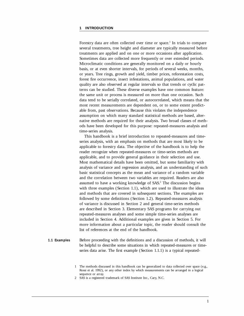
Forestry data are often collected over time or space.1 In trials to compareseveral treatments, tree height and diameter are typically measured beforetreatments are applied and on one or more occasions after application.Sometimes data are collected more frequently or over extended periods.Microclimatic conditions are generally monitored on a daily or hourlybasis, or at even shorter intervals, for periods of several weeks, months,or years. Tree rings, growth and yield, timber prices, reforestation costs,forest fire occurrence, insect infestations, animal populations, and waterquality are also observed at regular intervals so that trends or cyclic pat-terns can be studied. These diverse examples have one common feature:the same unit or process is measured on more than one occasion. Suchdata tend to be serially correlated, or autocorrelated, which means that themost recent measurements are dependent on, or to some extent predict-able from, past observations. Because this violates the independenceassumption on which many standard statistical methods are based, alter-native methods are required for their analysis. Two broad classes of meth-ods have been developed for this purpose: repeated-measures analysis andtime-series analysis.

This handbook is a brief introduction to repeated-measures and time-series analysis, with an emphasis on methods that are most likely to beapplicable to forestry data. The objective of the handbook is to help thereader recognize when repeated-measures or time-series methods areapplicable, and to provide general guidance in their selection and use.Most mathematical details have been omitted, but some familiarity withanalysis of variance and regression analysis, and an understanding of suchbasic statistical concepts as the mean and variance of a random variableand the correlation between two variables are required. Readers are alsoassumed to have a working knowledge of SAS.2 The discussion beginswith three examples (Section 1.1), which are used to illustrate the ideasand methods that are covered in subsequent sections. The examples arefollowed by some definitions (Section 1.2). Repeated-measures analysisof variance is discussed in Section 2 and general time-series methodsare described in Section 3. Elementary SAS programs for carrying outrepeated-measures analyses and some simple time-series analyses areincluded in Section 4. Additional examples are given in Section 5. Formore information about a particular topic, the reader should consult thelist of references at the end of the handbook.

1.1 Examples Before proceeding with the definitions and a discussion of methods, it willbe helpful to describe some situations in which repeated-measures or time-series data arise. The first example (Section 1.1.1) is a typical repeated-

1 The methods discussed in this handbook can be generalized to data collected over space (e.g.,Rossi et al. 1992), or any other index by which measurements can be arranged in a logicalsequence or array.

2 SAS is a registered trademark of SAS Institute Inc., Cary, N.C.

2

measures experiment. Repeated-measures designs are often used to assesstreatment effects on trees or vegetation, and to monitor growth and yield inpermanent sample plots. The second and third examples involve tree rings,which is an important area of application of time-series methods in for-estry. Section 1.1.2 illustrates how several tree-ring series from a single treecan be used to reconstruct the growth history of a tree. In Section 1.1.3, thecorrespondence between ring width and rainfall is examined.

1.1.1 Repeated measurement of seedling height To assess the effectsof three site-preparation treatments, four blocks comprising 12 rows of25 seedlings were established at a single trial site in the Sub-Boreal Spruce(SBS) dry warm subzone in the Cariboo Forest Region. Three site-prepa-ration treatments (V = v-plow, S = 30 × 30 cm hand screef, and U = anuntreated control), two seedling species (FD = Douglas-fir andPL = lodgepole pine), and two types of stock (B = bareroot and P = plug)were randomly assigned to the rows, with one row for each of the 12combinations. Seedling height, diameter, condition, and survival weremeasured at the time of planting (1983) and annually for the next sixyears (1984–1989). Figure 1 shows the average height of the seedlings that

V–plow

Hand screef

Control

1982 1984 1986 1988 1990

Hei

ght

(cm

)H

eigh

t (c

m)

a) Douglas-fir (bareroot)

1982 1984 1986 1988 1990

b) Douglas-fir (plug)

01982 1984 1986 1988 1990

Year

c) Lodgepole pine (bareroot)

0

20

40

60

80

0

20

40

60

80

40

80

120

160

200

0

40

80

120

160

200

1982 1984 1986 1988 1990Year

d) Lodgepole pine (plug)

1 Average height of seedlings: (a) Douglas-fir grown from bareroot stock, (b) Douglas-fir grown from plugs,(c) lodgepole pine grown from bareroot stock, and (d) lodgepole pine grown from plugs.

3

survived to 1989 (i.e., the average over seedlings in all rows and blocks)plotted against year, for each of the three site-preparation treatments (thedata are in Appendix 1). The objective of the experiment is to determinewhether treatment or stock type affects the growth of either species ofseedling.

1.1.2 Missing tree rings Tree rings are a valuable source of information.When cross-sectional disks are cut at several heights, the growth history ofa tree can be reconstructed by determining the year that the tree firstreached the height of each disk (i.e., the year when the innermost ring ofthe disk was formed). For disks that have a complete complement ofrings, this is a simple matter of counting backwards from the outermostring (which is assumed to correspond to the year in which the tree wascut) to the year of the innermost ring. Dating rings is more complicatedif, during the course of its growth, a tree experiences adverse growingconditions and in response fails to produce a uniform sheath of xylemeach year. If this happens, one or more rings will be missing in at leastsome disks (e.g., the sheath might not fully encircle a disk or it might notextend down as far as the disk).

Figure 2 shows two tree-ring series from a paper birch tree (the dataare in Appendix 2). Figure 2a is for a disk cut at a height of 1.3 m; Fig-ure 2b shows the corresponding series for a disk taken at 2.0 m. Elevenadditional disks were sampled at heights ranging from 0.3 m to 20 m. InFigure 2c, the height of each disk is plotted against the year of the inner-most ring, with no adjustment for missing rings. Until it was felled in1993, the tree in Figure 2 was growing in a mixed birch and coniferstand. In the early stages of development of the stand, the birch trees weretaller than the conifers, but during the forty years before cutting theywere overtopped by the conifers. Because paper birch is a shade-intolerantspecies, the trees were subject to increasing stress and therefore some ofthe outermost rings are expected to be missing, especially in disks cutnear the base of the tree.

One method of adjusting for missing rings (Cameron 1993) is to alignthe tree-ring series by comparing patterns of growth. If there are no miss-ing rings, then the best match should be achieved by aligning the outer-most ring of each series. Otherwise, each series is shifted by an amountequal to the estimated number of missing rings and the growth curve isadjusted accordingly (Figure 2d). The same approach is used to date treesexcept that an undated ring series from one tree is aligned with a datedseries from a second tree, or with a standard chronology. For more infor-mation about the time-series analysis of tree rings, refer to Monserud(1986).

1.1.3 Correlation between ring index and rainfall The width of a treering depends on the age of the tree. Typically, ring width increases rapidlywhen the tree is young, decreases as the tree matures, and eventually levelsout. Ring width is also affected by climate and environmental conditions.To reveal the less obvious effects of rainfall, air temperature, or pollution,the dominant growth trend is removed from the ring-width series by a

4

0.00

0.05

0.10

0.15

0.20

0.25

0.30

0.35

1880 1900 1920 1940 1960 1980 2000

Rin

g w

idth

(cm

)

Year (uncorrected)

a) Disk height = 1.3 m

1880 1900 1920 1940 1960 1980 2000

Year (uncorrected)

b) Disk height = 2.0 m

0

5

10

15

20

25

1860 1870 1880 1890 1900 1910 1920 1930 1940 1950

Hei

gh

t of

dis

k (m

)

Year of innermost ring (uncorrected)

c)

1860 1870 1880 1890 1900 1910 1920 1930 1940 1950

Year of innermost ring (corrected)

d)

2 Missing tree rings: (a) ring widths for disk at 1.3 m, (b) ring width for disk at 2.0 m, (c) disk height versusyear (no correction for missing rings), and (d) disk height versus year (corrected for missing rings).

process called detrending or ‘‘standardization’’ 3 (refer to Section 3.3). Thedetrended ring width is called a ring index. Figure 3a shows a ring-indexseries for a Douglas-fir tree on the Saanich Peninsula, while Figure 3bgives the total rainfall during March, April, and May of the same years, asrecorded at the Dominion Astrophysical Observatory (corrected, adjusted,and extended by comparison with stations at Gonzales Observatory andVictoria Airport). Data for the two series are given in Appendix 3. In thisexample, the investigator wants to determine whether annual spring rain-fall has any effect on ring width.

1.2 Definitions Let y1 , y2 , . . . , yn be a sequence of measurements (average height of arow of seedlings, ring width, annual rainfall, etc.) made at n distincttimes. Such data are called repeated measures, if the measurements are

3 A set of computer programs for standardizing tree-ring chronologies is available from theInternational Tree-Ring Data Bank (1993).

5

0.00

0.40

0.80

1.20

1.60

2.00

1880 1900 1920 1940 1960 1980 2000

Inde

x

Year

a) Ring index

0

100

200

300

400

1880 1900 1920 1940 1960 1980 2000

(mm

)

Year

b) Spring rainfall

3 Comparison of ring index with annual spring rainfall: (a) ring index versus year and (b) total rainfall duringMarch, April, and May versus year.

made on relatively few occasions (e.g., n ≤ 10), or a time series, if thenumber of observations is large (e.g., n ≥ 25). Thus the seedling measure-ments (Figure 1) would normally be considered repeated measures, whilethe tree-ring data and rainfall measurements (Figures 2a, 2b, 3a, and 3b)are time series. Figures 1–3 illustrate another common distinction bet-ween repeated measures and time series. Repeated-measures designs gener-ally include experimental units (e.g., rows of trees) from two or morestudy groups (e.g., site-preparation, species, and stock-type combina-tions)—notice that each curve in Figure 1 represents a separate group ofseedlings. In contrast, time series often originate from a single populationor experimental unit (e.g., a single tree or weather station). This division,which is based on the number of observation times and presence orabsence of experimental groups, is more or less arbitrary, but should helpthe reader recognize when a repeated-measures analysis is warranted andwhen the methods that are generally referred to as time-series analysis areapplicable.

Repeated-measures analysis is a type of analysis of variance (ANOVA),in which variation between experimental units (often called ‘‘between-sub-jects’’ variation) and variation within units (called ‘‘within-subjects’’ varia-tion) are examined. Between-units variation can be attributed to thefactors that differ across the study groups (e.g., treatment, species, andstock type). Within-units variation is any change, such as an increase inheight, that is observed in an individual experimental unit. In Figure 1,the between-units variation accounts for the separation of the curves,while the within-units variation determines the shape of the curves (ifthere were no within-units variation then the curves would be flat). Theobjectives of a repeated-measures analysis are twofold: (1) to determinehow the experimental units change over time and (2) to compare thechanges across study groups.

Time-series analysis encompasses a much wider collection of methodsthan repeated-measures analysis. It includes descriptive methods, model-fitting techniques, forecasting and regression-type methods, and spectral

6

analysis. Time-series analysis is concerned with short- and long-termchanges, and the correlation or dependence between past and presentmeasurements.

1.2.1 Trend, cyclic variation, and irregular variation Forestryresearchers are frequently interested in temporal variation. If repeated-measures or time-series data are plotted against time, one or more ofthree distinct types of variation will be evident (Figure 4). The simplesttype of variation is a trend (Figure 4a), which is a relatively slow shift inthe level of the data. Trends can be linear (Figure 4a) or nonlinear (Fig-ures 2a and 2b), and can correspond to an increase or decrease in themean, or both. The growth in height of a tree or row of seedlings (e.g.,Figure 1) is a familiar example of a trend.

Some data oscillate at more or less regular intervals as illustrated inFigure 4b. This type of variation is called cyclic variation. Insect and ani-mal populations sometimes display cyclic variation in their numbers. Sea-sonal variation is cyclic variation that is controlled by seasonal factors

a) b)

c) d)

4 Temporal variation: (a) linear trend (and irregular variation), (b) seasonal (and irregular) variation,(c) irregular variation, and (d) trend, seasonal, and irregular variation.

7

and therefore completes exactly one cycle per year. Air temperatures typ-ically exhibit a seasonal increase in the spring and summer, and a corre-sponding decrease in the fall and winter. The distinction between trendand cyclic variation can depend on the length of the observation periodand on the frequency of the measurements. If only part of a cycle is com-pleted during the period of observation, then cyclic variation becomesindistinguishable from trend. Identification of a cyclic component is alsoimpossible if sampling is too infrequent to cover the full range of vari-ability (e.g., if the observation times happen to coincide with the maxi-mum of each cycle, the data will show no apparent periodicity).

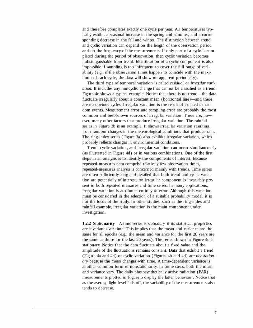
The third type of temporal variation is called residual or irregular vari-ation. It includes any noncyclic change that cannot be classified as a trend.Figure 4c shows a typical example. Notice that there is no trend—the datafluctuate irregularly about a constant mean (horizontal line)—and thereare no obvious cycles. Irregular variation is the result of isolated or ran-dom events. Measurement error and sampling error are probably the mostcommon and best-known sources of irregular variation. There are, how-ever, many other factors that produce irregular variation. The rainfallseries in Figure 3b is an example. It shows irregular variation resultingfrom random changes in the meteorological conditions that produce rain.The ring-index series (Figure 3a) also exhibits irregular variation, whichprobably reflects changes in environmental conditions.

Trend, cyclic variation, and irregular variation can occur simultaneously(as illustrated in Figure 4d) or in various combinations. One of the firststeps in an analysis is to identify the components of interest. Becauserepeated-measures data comprise relatively few observation times,repeated-measures analysis is concerned mainly with trends. Time seriesare often sufficiently long and detailed that both trend and cyclic varia-tion are potentially of interest. An irregular component is invariably pre-sent in both repeated measures and time series. In many applications,irregular variation is attributed entirely to error. Although this variationmust be considered in the selection of a suitable probability model, it isnot the focus of the study. In other studies, such as the ring-index andrainfall example, irregular variation is the main component underinvestigation.

1.2.2 Stationarity A time series is stationary if its statistical propertiesare invariant over time. This implies that the mean and variance are thesame for all epochs (e.g., the mean and variance for the first 20 years arethe same as those for the last 20 years). The series shown in Figure 4c isstationary. Notice that the data fluctuate about a fixed value and theamplitude of the fluctuations remains constant. Data that exhibit a trend(Figure 4a and 4d) or cyclic variation (Figures 4b and 4d) are nonstation-ary because the mean changes with time. A time-dependent variance isanother common form of nonstationarity. In some cases, both the meanand variance vary. The daily photosynthetically active radiation (PAR)measurements plotted in Figure 5 display the latter behaviour. Notice thatas the average light level falls off, the variability of the measurements alsotends to decrease.

8

0

10

20

30

40

50

60

70

0 28 56 84 112 140 168 196 224 252

PAR

Day(Source: D. Spittlehouse, B.C. Ministry of Forests; Research Branch)

May December

5 Daily photosynthetically active radiation (PAR).

Stationarity is a simplifying assumption that underlies many time-seriesmethods. If a series is nonstationary, then the nonstationary components(e.g., trend) must be removed or the series transformed (e.g., to stabilizea nonstationary variance) before the methods can be applied. Nonstation-arity must also be considered when computing summary statistics. Forinstance, the sample mean is not particularly informative if the data areseasonal, and should be replaced with a more descriptive set of statistics,such as monthly averages.

1.2.3 Autocorrelation and cross-correlation Repeated measures andtime series usually exhibit some degree of autocorrelation. Autocorrelation,also known as serial correlation, is the correlation between any two mea-surements ys and yt in a sequence of measurements y1 , y2 , . . . , yn (i.e.,correlation between a series and itself, hence the prefix ‘‘auto’’). Seedlingheights and tree-ring widths are expected to be serially correlated becauseunusually vigorous or poor growth in one year tends to carry over to thenext year. Serially correlated data violate the assumption of independenceon which many ANOVA and regression methods are based. Therefore,the underlying models must be revised before they can be applied tosuch data.

The autocorrelation between ys and yt can be positive or negative, andthe magnitude of the correlation can be constant, or decrease more or lessquickly, as the time interval between the observations increases. The auto-correlation function (ACF) is a convenient way of summarizing the depen-dence between observations in a stationary time series. If the observationsy1 , y2 , . . . , yn are made at n equally spaced times and yt is the observa-tion at time t, let yt +1 be the next observation (i.e., the measurementmade one step ahead), let yt +2 be the measurement made two steps

9

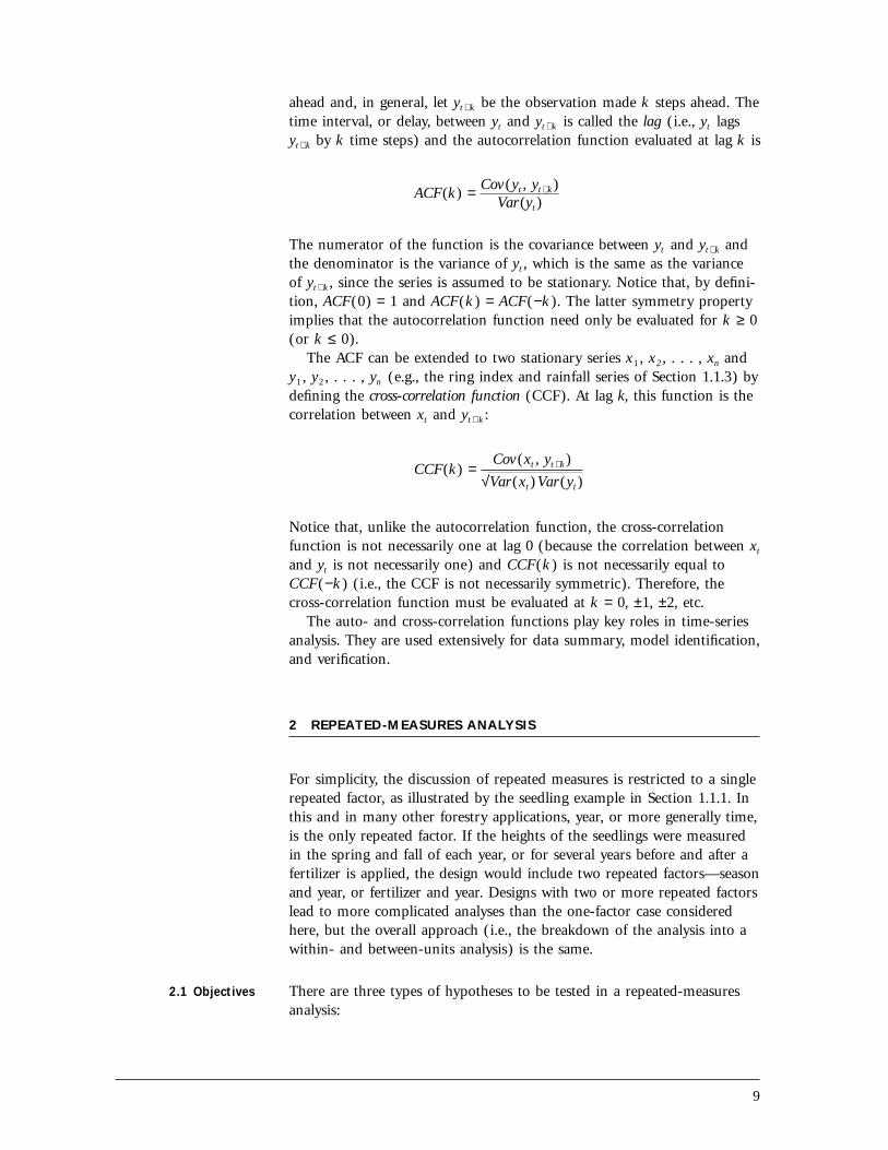
ahead and, in general, let yt +k be the observation made k steps ahead. Thetime interval, or delay, between yt and yt +k is called the lag (i.e., yt lagsyt +k by k time steps) and the autocorrelation function evaluated at lag k is

ACF(k) = Cov(yt , yt +k )Var(yt )

The numerator of the function is the covariance between yt and yt +k andthe denominator is the variance of yt , which is the same as the varianceof yt +k , since the series is assumed to be stationary. Notice that, by defini-tion, ACF(0) = 1 and ACF(k ) = ACF(−k ). The latter symmetry propertyimplies that the autocorrelation function need only be evaluated for k ≥ 0(or k ≤ 0).

The ACF can be extended to two stationary series x1 , x2 , . . . , xn andy1 , y2 , . . . , yn (e.g., the ring index and rainfall series of Section 1.1.3) bydefining the cross-correlation function (CCF). At lag k, this function is thecorrelation between xt and yt + k :

CCF(k) =Cov(xt , yt +k )

√Var(xt )Var(yt )

Notice that, unlike the autocorrelation function, the cross-correlationfunction is not necessarily one at lag 0 (because the correlation between xt

and yt is not necessarily one) and CCF(k ) is not necessarily equal toCCF(−k ) (i.e., the CCF is not necessarily symmetric). Therefore, thecross-correlation function must be evaluated at k = 0, ±1, ±2, etc.

The auto- and cross-correlation functions play key roles in time-seriesanalysis. They are used extensively for data summary, model identification,and verification.

2 REPEATED-MEASURES ANALYSIS

For simplicity, the discussion of repeated measures is restricted to a singlerepeated factor, as illustrated by the seedling example in Section 1.1.1. Inthis and in many other forestry applications, year, or more generally time,is the only repeated factor. If the heights of the seedlings were measuredin the spring and fall of each year, or for several years before and after afertilizer is applied, the design would include two repeated factors—seasonand year, or fertilizer and year. Designs with two or more repeated factorslead to more complicated analyses than the one-factor case consideredhere, but the overall approach (i.e., the breakdown of the analysis into awithin- and between-units analysis) is the same.

2.1 Objectives There are three types of hypotheses to be tested in a repeated-measuresanalysis:

10

H01: the growth curves or trends are parallel for all groups (i.e., there are nointeractions involving time),

H02: there are no trends (i.e., there are no time effects), andH03: there are no overall differences between groups (i.e., the between-units

factors have no effect).The three hypotheses are illustrated in Figure 6 with the simple case of

one between-units factor. This figure shows the expected average height ofa row of lodgepole pine seedlings (Section 1.1.1), grown from plugs, plot-ted against year. Each curve corresponds to a different site-preparationtreatment, which is the between-units factor. Hypotheses H01 and H02 con-cern changes over time, which are examined as part of the within-unitsanalysis. Hypothesis H01 (Figure 6a) implies that site-preparation treat-ment has no effect on the rate of growth of the seedlings. If this hypoth-esis is retained, it is often appropriate to test whether the growth curvesare flat (H02, Figure 6b). Acceptance of H02 implies that there is nochange over time. In this example, H02 is not very interesting because theseedlings are expected to show some growth over the seven-year period ofthe study. The last hypothesis concerns the separation of the three growthcurves and is tested as part of the between-units analysis. If the groupsshow parallel trends (i.e., H01 is true) then, H03 implies that growth pat-terns are identical for the three groups (Figure 6c). Otherwise, H03 implies

0

40

80

120

160

200

240

Hei

gh

t (c

m)

Hei

gh

t (c

m)

a) b)

0

40

80

120

160

200

240

1982 1984 1986 1988 1990

Year

c)

1982 1984 1986 1988 1990

1982 1984 1986 1988 1990 1982 1984 1986 1988 1990

Year

d)

6 Null hypotheses for repeated-measures analysis: (a) parallel trends, (b) no trends, (c) no difference betweengroups, and (d) differences between groups cancel over time.

11

that there is no difference between the groups when the effects of the site-preparation treatments are averaged over time. Relative gains and lossesare cancelled over time, as illustrated in Figure 6d.

Rejection of H01 implies that the trends are not parallel for at least twogroups. When this occurs, additional hypotheses can be tested to deter-mine the nature of the divergence (just as multiple comparisons are usedto pinpoint group differences in a factorial ANOVA). One approach is tocompare the groups at each time, as suggested by Looney and Stanley(1989). Alternatively, one of the following can be tested:

H04: the expected difference between two consecutive values, yt − yt − 1, is thesame for all groups,

H05: the expected difference between an observation at time t and its initialvalue, yt − y1, is the same for all groups, or

H06: the expected value of the k th-order polynomial contrasta 1k y1 + a 2k y2 + . . . + ank yn is the same for all groups.

Each hypothesis comprises a series of n − 1 hypotheses about the within-row effects. In the first two cases (H04 and H05), the n − 1 incrementsy2 − y1, y3 − y2 , . . . , yn − yn − 1 , or cumulative incrementsy2 − y1 , y3 − y1 , . . . , yn − y1 , are tested for significant group differences bycarrying n − 1 separate analyses of variance. If the trends are expected tobe parallel for at least part of the observation period, then H04 is often ofinterest. Alternatively, the trends might be expected to diverge initially andthen converge, in which case H05 might be more relevant. The last hypoth-esis (H06) is of interest when the trends are adequately described by a poly-nomial of order k (i.e., β0 + β1t + . . . + βkt

k ). In this case, a set ofcoefficients a1k , a2k , . . . , ank (see Bergerud 1988 for details) can be chosenso that the expected value of linear combination a1k y1 + a2k y2 + . . . + ank yn

depends only on βk . Thus an ANOVA of the transformed valuesa1k y1 + a2k y2 + . . . + ank yn is equivalent to assessing the effects of the bet-ween-units factors on βk . If the order of the polynomial is unknown,ANOVA tests can be performed sequentially, starting with polynomials oforder n − 1 (which is the highest-order polynomial that can be tested whenthere are n observation times) and ending with a comparison of linearcomponents. Refer to Littell (1989), Bergerud (1991), Meredith and Steh-man (1991), Sit (1992a), and Gumpertz and Brownie (1993) for a discus-sion of the comparison of polynomial and other nonlinear trends.

2.2 Univariate Analysisof Repeated Measures

Univariate repeated-measures analysis is based on a split-plot ANOVAmodel in which time is the split-plot factor (refer to Keppel 1973; Moseret al. 1990; or Milliken and Johnson 1992 for details). As an illustration,consider the average row heights for the seedling data (Section 1.1.1).The split-plot ANOVA (with an additive block effect) is summarized inTable 1. The top part of the table summarizes the between-rows analysis.It is equivalent to an ANOVA of the time-averaged responses(y1 + y2 + . . . + yn )/n and has the same sources of variation, degrees offreedom, sums of squares, expected mean squares, and F-tests as a facto-rial (SPP × STK × TRT) randomized block design with no repeated fac-tors. The bottom part of the table summarizes the within-rows analysis.

12

1 Split-plot ANOVA model for seedling experiment (Section 1.1.1)

Source of Degrees of Error term forvariation freedom testing effect

Between rowsBlock, BLK 3Species, SPP 1 Error – rowStock type, STK 1 Error – rowSite-preparation treatment, TRT 2 Error – rowSPP × STK 1 Error – rowSPP × TRT 2 Error – rowSTK × TRT 2 Error – rowSPP × STK × TRT 2 Error – rowError – row 33

Within rowsTime, YEAR 6 YEAR × BLKYEAR × BLK 18YEAR × SPP 6 Error – row × yearYEAR × STK 6 Error – row × yearYEAR × TRT 12 Error – row × yearYEAR × SPP × STK 6 Error – row × yearYEAR × SPP × TRT 12 Error – row × yearYEAR × STK × TRT 12 Error – row × yearYEAR × SPP × STK × TRT 12 Error – row × yearError – row × year 198

Total 335

It includes the main effect of time (YEAR) and all other time-relatedsources of variation (YEAR × SPP, YEAR × STK, YEAR × TRT, etc.),which are readily identified by forming time interactions with the factorslisted in the top part of the table. If all the interactions involving time aresignificant, each of the 12 groups (2 species × 2 stock types × 3 site-prep-aration treatments) will have had a different pattern of growth. Theabsence of one or more interactions can simplify the comparison ofgrowth curves. For example, if there are no interactions involving treat-ment and year (i.e., the terms YEAR × TRT, YEAR × SPP × TRT,YEAR × STK × TRT, and YEAR × SPP × STK × TRT are absent from themodel), then the three growth curves corresponding to the three site-preparation treatments are parallel for each species and stock type.

The univariate model allows for correlation between repeated meas-urements of the same experimental unit (e.g., successive height measure-ments of the same row of seedlings). This correlation is assumed to be thesame for all times and all experimental units.4 The univariate model, likeany randomized block design, also allows for within-block correlation—thatis, correlation between measurements made on different experimental unitsin the same block (e.g., the heights of two rows of seedlings in the same

4 This condition can be replaced with the less restrictive ‘‘Huynh-Feldt condition,’’ which isdescribed in Chapter 26 of Milliken and Johnson (1992).

13

block). In the repeated-measures model, inclusion of a year-by-block inter-action (YEAR × BLK) implies that the within-block correlation depends onwhether measurements are made on different experimental units in thesame block (e.g., the heights of two rows of seedlings in the same block).Measurements made in the same year (and in the same block) are assumedto be more strongly correlated than those made in different years. However,in both cases, the correlation is assumed to be the same for all blocks andexperimental units. All other measurements (e.g., the heights of two rows indifferent blocks) are assumed to be independent. In addition, all measure-ments are assumed to have the same variance.

2.3 MultivariateAnalysis of Repeated

Measures

In a univariate analysis, repeated measurements are treated as separateobservations and time is included as a factor in the ANOVA model. In themultivariate approach, repeated measurements are considered elements ofa single multivariate observation and the univariate within-units ANOVAis replaced with a multivariate ANOVA, or MANOVA. The main advan-tage of the multivariate analysis is a less restrictive set of assumptions.Unlike the univariate ANOVA model, the MANOVA model does notrequire the variance of the repeated measures, or the correlation betweenpairs of repeated measures, to remain constant over time (e.g., the vari-ance of the average height of a row of seedlings might increase with time,and the correlation between two measurements of the same row mightdecrease as the time interval between the measurements increases). Bothmodels do, however, require the variances and correlations to be homoge-neous across units (e.g., for any given year, the variance of the averageheight of a row of seedlings is the same for all rows, as are the inter-yearcorrelations of row heights). The greater applicability of the multivariatemodel is not without cost. Because the model is more general than theunivariate model, more parameters (i.e., more variances and correlations)need to be estimated and therefore there are fewer degrees of freedom fora fixed sample size. Thus, for reliable results, multivariate analyses typ-ically require larger sample sizes than univariate analyses.

The multivariate analysis of the between-units variation is equivalent tothe corresponding univariate analysis. However, differences in the under-lying models lead to different within-units analyses. Several multivariatetest statistics can be used to test H01 and H02 in a multivariate repeated-measures analysis: Wilks’ Lambda, Pillai’s trace, Hotelling-Lawley trace,and Roy’s greatest root. To assess the statistical significance of an effect,each statistic is referred to an F-distribution with the appropriate degreesof freedom. If the effect has one degree of freedom, then the tests basedon the four statistics are equivalent. Otherwise the tests differ, although inmany cases they lead to similar conclusions. In some situations, the testslead to substantially different conclusions so the analyst must considerother factors, such as the relative power of the tests (i.e., the probabilitythat departures from the null hypothesis will be detected), before arrivingat a conclusion. For a more detailed discussion of multivariate repeated-measures analysis, refer to Morrison (1976), Hand and Taylor (1987), andTabachnick and Fidell (1989), who discuss the pros and cons of the fourMANOVA test statistics; Moser et al. (1990), who compare the multi-

14

variate and univariate approaches to the analysis of repeated measures;and Gumpertz and Brownie (1993), who provide a clear and detailedexposition of the multivariate analysis of repeated measures in randomizedblock and split-plot experiments.

3 TIME-SERIES ANALYSIS

Time series can be considered from two perspectives: the time domainand the frequency domain. Analysis in the time domain relies on the auto-correlation and cross-correlation functions (defined in Section 1.2.3) todescribe and explain the variability in a time series. In the frequencydomain, temporal variation is represented as a sum of sinusoidal compo-nents, and the ACF and CCF are replaced by the corresponding Fouriertransforms, which are known as the spectral and cross-spectral densityfunctions. Analysis in the frequency domain, or spectral analysis as it ismore commonly called, is useful for detecting hidden periodicities (e.g.,cycles in animal populations), but is generally inappropriate for analyzingtrends and other nonstationary behaviour. Because the results of a spectralanalysis tend to be more difficult to interpret than those of a time-domainanalysis, the following discussion is limited to the time domain. For acomprehensive introduction to time-series analysis in both the time andfrequency domains, the reader should refer to Kendall and Ord (1990);Diggle (1991), who includes a discussion (Section 4.10, Chapter 4) of thestrengths and weaknesses of spectral analysis; or Chatfield (1992). Formore information about spectral analysis, the reader should consultJenkins and Watts (1968) or Bloomfield (1976).

3.1 Objectives The objectives of a time-series analysis range from simple description tomodel development. In some applications, the trend or cyclic componentsof a series are of special interest, and in others, the irregular component ismore important. In either case, the objectives usually include one or moreof the following:• data summary and description• detection, description, or removal of trend and cyclic components• model development and parameter estimation• prediction of a future value (i.e., forecasting)

Many time-series methods assume that the data are equally spaced intime. Therefore, the following discussion is limited to equally spacedseries (i.e., the measurements y1 , y2 , . . . , yn are made at times t0 + d,t0 + 2d , . . . , t0 + nd where d is the fixed interval between observations).This is usually not a serious restriction because in many applications,observations occur naturally at regular intervals (e.g., annual tree rings)or they can be made at equally spaced times by design.

3.2 DescriptiveMethods

Describing a time series is similar to describing any other data set. Stan-dard devices include graphs and, if the series is stationary, such familiarsummary statistics as the sample mean and variance. The correlogram andcross-correlogram, which are plots of the sample auto- and cross-

15

correlation functions, are powerful tools. They are unique to time-seriesanalysis and offer a simple way of displaying the correlation within orbetween time series.

3.2.1 Time plot All time series should be plotted before attempting ananalysis. A time plot—that is, a plot of the response variable yt versustime t—is the easiest and most obvious way to describe a time series.Trends (Figure 4a), cyclic behaviour (Figure 4b), nonstationarity (Figures2a, 2b, 5), outliers, and other prominent features of the data are oftenmost readily detected with a time plot. Because the appearance of a timeplot is affected by the choice of symbols and scales, it is always advisableto experiment with different types of plots. Figure 7 illustrates how thelook of a series (Figure 7a) changes when the connecting lines are omit-ted (Figure 7b) and when the data are plotted on a logarithmic scale(Figure 7c). Notice that the asymmetric (peaks in one direction) appear-ance of the series (Figures 7a and 7b) is eliminated by a log transforma-tion (Figure 7c). If the number of points is very large, time plots aresometimes enhanced by decimating (i.e., retaining one out of every tenpoints) or aggregating the data (e.g., replacing the points in an intervalwith their sum or average).

3.2.2 Correlogram and cross-correlogram The correlogram, or sampleautocorrelation function, is obtained by replacing Cov(yt , yt − k ) andVar(yt ) in the true autocorrelation function (Section 1.2.3) with the cor-responding sample covariance and variance:

ACF (k) =∧

∑(yt − y-) (yt +k − y-)n −k

t =1 = rk

∑ (yt − y-)2

n

t =1

and plotting autocorrelation coefficient rk against k. For reliable estimates,the sample size n should be large relative to k (e.g., n > 4k and n > 50)and, because the autocorrelation coefficients are sensitive to extremepoints, the data should be free of outliers.

The correlogram contains a lot of information. The sample ACF for apurely random or ‘‘white noise’’ series (i.e., a series of independent, iden-tically distributed observations) is expected to be approximately zero forall non-zero lags (Figure 8). If a time series has a trend, then the ACFfalls off slowly (e.g., linearly) with increasing lags. This behaviour is illus-trated in Figure 9b, which shows the correlogram for the nonstationaryseries of average daily soil temperatures displayed in Figure 9a. If a timeseries contains a seasonal or cyclic component, the correlogram alsoexhibits oscillatory behaviour. The correlogram for a seasonal series withmonthly intervals (e.g., total monthly rainfall) might, for example, havelarge negative values at lags 6, 18, etc. (because measurements made inthe summer and winter are negatively correlated) and large positive valuesat lags 12, 24, etc. (because measurements made in the same season arepositively correlated).

16

0

1

2

3

4

5

6

1890 1910 1930 1950 1970 1990Year

c)

0

50

100

150

200

250

1890 1910 1930 1950 1970 1990

b)

0

50

100

150

200

250

1890 1910 1930 1950 1970 1990To

tal a

ccum

ulat

ion

(cm

)To

tal a

ccum

ulat

ion

(cm

)To

tal a

ccum

ulat

ion

(log

cm

)

a)

7 Time plots of annual snowfall for Victoria, B.C.: (a) with connecting lines,(b) without connecting lines, and (c) natural logarithmic scale.

Since the theoretical ACF is defined for stationary time series, furtherinterpretation of the correlogram is possible only after trend and seasonalcomponents are eliminated. Trend can often be removed by calculatingthe first difference between successive observations (i.e., yt − yt −1). Figure9c shows the first difference of the soil temperature series and Figure 9d is

17

0

1

2

3

-1

-2

-30 20 40 60 80 100

y(t)

Time (t)

a)

0

0.5

1

-0.5

-10 5 10 15 20 25

Sam

ple

AC

F(k)

Lag (k)

b)

8 White noise: (a) time plot and (b) correlogram.

the corresponding correlogram. Notice that the trend that was evident inthe original series (Figures 9a and 9b) is absent in the transformed series.The first difference is usually sufficient to remove simple (e.g., linear)trends. If more complicated (e.g., polynomial) trends are present, the dif-ference operator can be applied repeatedly—that is, the second difference[(yt − yt −1) − (yt −1 − yt −2) = yt − 2yt −1 + yt −2], etc. can be applied to theseries. Seasonal components can be eliminated by calculating an appropri-ate seasonal difference (e.g., yt − yt −12 for a monthly series or yt − yt −4 fora quarterly series).

18

0

2

4

6

8

10

12

14

16

0 28 56 84 112 140 168 196

Tem

per

atur

e (o C

)

a) Average daily soil temperature (oC)

May 1, 1988 October 31, 1988

May 1, 1988 October 31, 1988

0

0.5

1

-0.5

-10 5 10 15 20 25

AC

F(k)

b) Sample ACF(k) for soil temperatures

c) Change in soil temperature d) Sample ACF(k) for first differences

0

1

2

3

-1

-2

-30 28 56 84 112 140 168 196

Tem

per

atur

e (o C

)

Day

0

0.5

1

-0.5

-10 5 10 15 20 25

AC

F(k)

Lag (k)

Day Lag (k)

9 Soil temperatures: (a) daily soil temperatures, (b) correlogram for daily soil temperatures, (c) first difference ofdaily soil temperatures, and (d) correlogram for first differences.

Correlograms of stationary time series approach zero more quicklythan processes with a nonstationary mean. The correlograms for the ring-index (Figure 3a) and rainfall (Figure 3b) series, both of which appear tobe stationary, are shown in Figure 10. For some series, the ACF tails off(i.e., falls off exponentially, or consists of a mixture of damped exponen-tials and damped sine waves) and for others, it cuts off abruptly. The for-mer behaviour is characteristic of autoregressions and mixed autoregressive-moving average processes, while the latter is typical of a moving average(refer to Section 3.5 for more information about these processes).

The cross-correlogram, or sample CCF of two series x1 , x2 , . . . , xn andy1 , y2 , . . . , yn , is:

CCF (k) =∧

∑ (xt − x-) (yt +k − y-)n −k

t =1

√ ∑ (xt − x-)2 ∑ (yt − y-)2

n n

t =1 t =1

19

0

0.5

1

-0.5

-10 5 10 15 20 25

AC

F(k)

a) Sample ACF(k) for ring-index series

0

0.5

1

-0.5

-10 5 10 15 20 25

AC

F(k)

Lag (k)

Lag (k)

b) Sample ACF(k) for rainfall series

10 Correlograms for ring-index and rainfall series: (a) correlogram for ring-index series shown in Figure 3a and (b) correlogram for rainfall seriesshown in Figure 3b.

A cross-correlogram can be more difficult to interpret than a correlogrambecause its statistical properties depend on the autocorrelation of the indi-vidual series, as well as on the cross-correlation between the series. Across-correlogram might, for example, suggest that two series are cross-correlated when they are not, simply because one or both series is auto-correlated. Trends can also affect interpretation of the cross-correlogrambecause they dominate the cross-correlogram in much the same way as

20

they dominate the correlogram. To overcome these problems, time seriesare usually detrended and prewhitened prior to computing the sampleCCF. Detrending is the removal of trend from a time series, which can beachieved by the methods described in Section 3.3. Prewhitening is theelimination of autocorrelation (and cyclic components). Time series areprewhitened by fitting a suitable model that describes the autocorrelation(e.g., one of the models described in Section 3.5.1) and then subtractingthe fitted values. The resultant series of residuals is said to be prewhitenedbecause it is relatively free of autocorrelation and therefore resembleswhite noise. More information about the cross-correlogram, and detrend-ing and prewhitening can be obtained in Chapter 8 of Diggle (1991) orChapter 8 of Chatfield (1992).

Figure 11 shows the cross-correlogram for the ring-index and rainfallseries of Section 1.1.3 (Figure 3). Both series have been prewhitened(refer to Section 4.2.2 for details) to reduce the autocorrelation that isevident from the correlograms (Figure 10). Detrending is not requiredbecause the trend has already been removed from the ring index and therainfall series shows no obvious trend. Notice that the cross-correlogramhas an irregular pattern with one small but statistically significant spike atlag zero. There is no significant cross-correlation at any of the other lags.This suggests that ring width is weakly correlated with the amount ofrainfall in the spring of the same year, but the effect does not carry overto subsequent years.

Sam

ple

CC

F(k)

0

0.2

0.4

-0.2

-0.4

0 5 10 15-5-10-15Lag (k)

11 Cross-correlogram for prewhitened ring-index and rainfall series.

3.2.3 Tests of randomness Autocorrelation can often be detected byinspecting the time plot or correlogram of a series. However, some seriesare not easily distinguished from white noise. In such cases, it is useful tohave a formal test of randomness.

21

There are several ways to test the null hypothesis that a stationary timeseries is random. If the mean of the series is zero, then the Durbin-Watsontest can be used to test the null hypothesis that there is no first-orderautocorrelation (i.e., ACF(1) = 0). The Durbin-Watson statistic is

D − W =∑(yt + 1 − yt)2

n −1

t =1

∑ y t2

n

t =1

which is expected to be approximately equal to two, if the series {yt } israndom. Otherwise it will tend to be near zero if the series is positivelycorrelated, or near four if the series is negatively correlated. To calculate ap-value, D − W must be referred to a special table, such as that given inDurbin and Watson (1951).

Other tests of randomness use one or more of the autocorrelation coef-ficients rk . If a time series is random, then rk is expected to be zero for allk ≠ 0. This assumption can be verified by determining the standard errorof rk under the null hypothesis (assuming the observations have the samenormal distribution) and carrying out an appropriate test of significance.Alternatively, a ‘‘portmanteau’’ chi-squared test can be derived to test thehypothesis that autocorrelations for the first k lags are simultaneously zero(refer to Chapter 48 of Kendall et al. [1983], and Chapters 2 and 8 ofBox and Jenkins [1976] for details). For information on additional testsof randomness, refer to Chapter 45 of Kendall et al. (1983).

3.3 Trend There are two main ways to estimate trend: (1) by fitting a function oftime (e.g., a polynomial or logistic growth curve) or (2) by smoothingthe series to eliminate cyclic and irregular variation. The first method isapplicable when the trend can be described by a fixed or deterministicfunction of time (i.e., a function that depends only on the initial condi-tions, such as the linear trend shown in Figure 4a). Once the function hasbeen identified, the associated parameters (e.g., polynomial coefficients)can be estimated by standard regression methods, such as least squares ormaximum likelihood estimation.

The second method requires no specific knowledge of the trend and isuseful for describing stochastic trends (i.e., trends that vary randomly overtime, such as the trend in soil temperatures shown in Figure 9a). Smooth-ing can be accomplished in a number of ways. An obvious method is todraw a curve by eye. A more objective estimate is obtained by calculatinga weighted average of the observations surrounding each point, as well asthe point itself; that is,

mt = ∑ wk yt + k

p

k = −q

22

where mt is the smoothed value at time t and {wk } are weights. The sim-plest example is an ordinary moving average 5

∑ yt + k

p

k = −q

1 + p + q

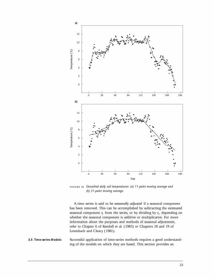
which is the arithmetic average of the points yt −q , . . . , yt −1 , yt ,yt +1 , . . . , yt +p . This smooths the data to a greater or lesser degree as thenumber of points included in the average is increased or decreased. Thisis illustrated in Figure 12, which compares the results of applying a 11-point (Figure 12a) and 21-point (Figure 12b) moving average to the dailysoil temperatures in Figure 9a.

Moving averages attach equal weight to each of the p + q + 1 pointsyt −q , . . . , yt −1 , yt , yt +1 , . . . ,yt +p . Better estimates of trend are sometimesobtained when less weight is given to the observations that are farthestfrom yt. Exponential smoothing uses weights that fall off exponentially.Many other methods of smoothing are available, including methods thatare less sensitive to extreme points than moving averages (e.g., movingmedians or trimmed means).

After the trend has been estimated, it can be removed by subtraction ifthe trend is additive, or by division if it is multiplicative. The process ofremoving a trend is called detrending and the resultant series is called adetrended series. Detrended series typically contain cyclic and irregularcomponents, which more or less reflect the corresponding components ofthe original series. However, detrended series should be interpreted withcaution because some methods of detrending can introduce spurious peri-odicity or otherwise alter the statistical properties of a time series (refer toSection 46.14 of Kendall et al. [1983] for details).

3.4 Seasonal andCyclic Components

After a series has been detrended, seasonal or cyclic components (withknown periods) can be estimated by regression methods or by calculatinga weighted average. The first approach is applicable if the component isadequately represented by a periodic (e.g., sinusoidal) function. The sec-ond approach is similar to the methods described in the previous sectionexcept that the averaging must take into account the periodic nature ofthe data. For a monthly series, a simple way to estimate a seasonal com-ponent is to average values in the same month; that is,

st =∑ yt + 12k

q

k = −p

1 + p + q

where the {yt +12k } are detrended values and st is the estimated seasonalcomponent.

5 This moving average should not be confused with the moving average model defined inSection 3.5. The former is a function that operates on a time series and the latter is amodel that describes the statistical properties of a time series.

23

0

2

4

6

8

10

12

10

12

0 28 56 84 112 140 168 196

a)

0

2

4

6

8

0 28 56 84 112 140 168 196

Tem

per

atur

e (°

C)

Tem

per

atur

e (°

C)

Day

b)

12 Smoothed daily soil temperatures: (a) 11-point moving average and(b) 21-point moving average.

A time series is said to be seasonally adjusted if a seasonal componenthas been removed. This can be accomplished by subtracting the estimatedseasonal component st from the series, or by dividing by st , depending onwhether the seasonal component is additive or multiplicative. For moreinformation about the purposes and methods of seasonal adjustment,refer to Chapter 6 of Kendall et al. (1983) or Chapters 18 and 19 ofLevenbach and Cleary (1981).

3.5 Time-series Models Successful application of time-series methods requires a good understand-ing of the models on which they are based. This section provides an

24

overview of some models that are fundamental to the description andanalysis of a single time series (Section 3.5.1). More complicated modelsfor the analysis of two or more series are mentioned in Section 3.5.2.

3.5.1 Autoregressions and moving averages One of the simplest modelsfor autocorrelated data is the autoregression. An autoregression has thesame general form as a linear regression model:

yt = ν +∑ φ i yt − i + ε t

p

i = 1

except in this case the response variables y1 , y2 , . . . , yn are correlatedbecause they appear on both sides of the equation (hence the name‘‘auto’’ regression). The maximum lag (p ) of the variables on the rightside of the equation is called the order of the autoregression, ν is a con-stant, and the {φi } are unknown autoregressive parameters. Like otherregression models, the errors {εt }, are assumed to be independent andidentically (usually normally) distributed. Autoregressions are often deno-ted AR or AR(p).

Another simple model for autocorrelated data is the moving average :

yt = ν + εt − ∑ θ i ε t − i

q

i = 1

Here the observed value yt is a moving average of an unobserved series ofindependent and identically (normally) distributed random variables {εt }.The maximum lag q is the order of the moving average and the {θi } areunknown coefficients. Because there is overlap of the moving averages onthe right side of the equation, the corresponding response variables arecorrelated. Moving average models are often denoted MA or MA(q ).

The autoregressive and moving average models can be combined toproduce a third type of model known as mixed autoregressive-movingaverage :

yt = ν + ∑ φi yt − i + εt − ∑ θj ε t − j

p q

i = 1 j = 1

which is usually abbreviated as ARMA or ARMA(p,q ). A related class ofnonstationary models is obtained by substituting the first differenceyt = yt − yt −1 or the second difference yt = yt − 2yt −1 + yt −2 etc., for yt inthe preceding ARMA model. The resultant model

yt = ν + ∑ φi yt − i + ε t − ∑ θk εt − i

p q

i = 1 i = 1

is called an autoregressive-integrated-moving average and is abbreviated asARIMA, or ARIMA(p,d,q ), where d is the order of the difference (i.e.,

25

d = 1 if yt is a first difference, d = 2 if yt is a second difference, etc.).The ARMA model can be extended to include seasonal time series by sub-stituting a seasonal difference for yt .

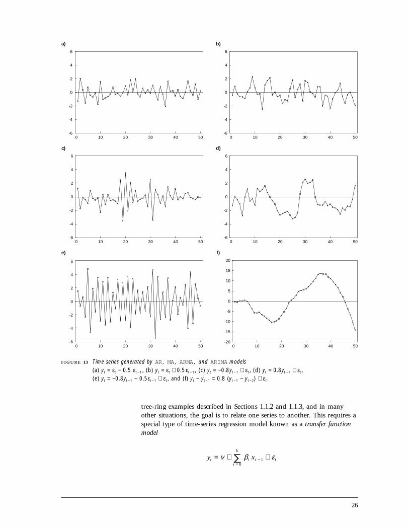
The class of AR, MA, ARMA, and ARIMA models embodies a widevariety of stationary and nonstationary time series (Figure 13), whichhave many practical applications. All MA processes are stationary (Figures13a, b). In contrast, all time series generated by ARIMA models are non-stationary (Figure 13f). Pure AR models and mixed ARMA models areeither stationary or nonstationary (depending on the particular combina-tion of autoregressive parameters {φi }, although attention is generallyrestricted to the stationary case (Figures 13c, d, e). More informationabout AR, MA, ARMA, and ARIMA models is available in Chapter 3 ofChatfield (1992).

Box and Jenkins (1976) developed a general scheme for fitting AR,MA, ARMA, and ARIMA models, which has become known as Box-Jenkins modelling. The procedure has three main steps: (1) model identi-fication (i.e., selection of p, d, and q ), (2) model estimation (i.e., estima-tion of the parameters φ1 , φ2 , . . . , φp and θ1 , θ2 , . . . , θq ), and (3)model verification. Because the models have characteristic patterns ofautocorrelation that depend on the values of p, d, and q, the correlogramis an important tool for model identification. The autocorrelation func-tion is generally used in conjunction with the partial autocorrelation func-tion (PACF), which measures the amount of autocorrelation that remainsunaccounted for after fitting autoregressions of orders k = 1, 2, etc. (i.e.,PACF(k ) is the amount of autocorrelation that cannot be explained by anautoregression of order k ). These two functions provide complementaryinformation about the underlying model: for an AR(p ) process, the ACFtails off and the PACF cuts off after lag p (i.e., the PACF is zero if theorder of the fitted autoregression is greater than or equal to true value p );for an MA(q ) process, the ACF cuts off after lag q and the PACF tails off.Refer to Table 6.1 of Kendall and Ord (1990) or Figure 6.2 of Diggle(1991) for a handy guide to model identification using the ACF andPACF. Other tools for model identification include the inverse autocorrela-tion function (IACF) of an autoregressive moving average process, whichis the ACF of the ‘‘inverse’’ process obtained by interchanging the parame-ters φ1 , φ2 , . . . , φp and θ1 , θ2 , . . . , θq (see Chatfield 1979 for details),and various automatic model-selection procedures, which are described inSection 11.4 of Chatfield (1992) and in Sections 7.26–31 of Kendall andOrd (1990).

After the model has been identified, the model parameters are esti-mated (e.g., by maximum likelihood estimation) and the adequacy of thefitted model is assessed by analyzing the residuals. For a detailed exposi-tion of the Box-Jenkins procedure, the reader should consult Box andJenkins (1976), which is the standard reference; McCleary and Hay(1980); or Chapters 3 and 4 of Chatfield (1992), for a less mathematicalintroduction to the subject.

3.5.2 Advanced topics The AR, MA, ARMA, and ARIMA models areuseful for describing and analyzing individual time series. However, in the

26

0

2

4

6

-2

-4

-60 10 20 30 40 50

e)

0

5

10

15

20

-5

-10

-15

-200 10 20 30 40 50

f)

0

2

4

6

-2

-4

-60 10 20 30 40 50

c)

0

2

4

6

-2

-4

-60 10 20 30 40 50

d)

0

2

4

6

-2

-4

-60 10 20 30 40 50

a)

0

2

4

6

-2

-4

-60 10 20 30 40 50

b)

13 Time series generated by AR, MA, ARMA, and ARIMA models(a) yt = εt − 0.5 εt − 1 , (b) yt = εt + 0.5εt − 1 , (c) yt = −0.8yt − 1 + εt , (d) yt = 0.8yt − 1 + εt ,(e) yt = −0.8yt − 1 − 0.5εt − 1 + εt , and (f) yt − yt − 1 = 0.8 (yt − 1 − yt − 2) + εt .

tree-ring examples described in Sections 1.1.2 and 1.1.3, and in manyother situations, the goal is to relate one series to another. This requires aspecial type of time-series regression model known as a transfer functionmodel

yt = ν + ∑ β i xt − 1 + εt

k

i = 0

27

in which the response variables {yt } and explanatory variables {xt } areboth cross-correlated and autocorrelated. Readers who are interested inthe identification, estimation, and interpretation of transfer functionmodels should consult Chapters 11 and 12 of Kendall and Ord (1990) formore information.

Time series often arise as a collection of two or more time series. Forinstance, in the missing tree-ring problem (Section 1.1.2), each disk hasan associated series of ring widths. In such situations, it seems natural toattempt to analyze the time series simultaneously by fitting a multivariatemodel. Multivariate AR, MA, ARMA, and ARIMA models have beendeveloped for this purpose. They are, however, considerably more com-plex than their univariate counterparts. The reader should refer to Section11.9 of Chatfield (1992) for an outline of difficulties and to Chapter 14 ofKendall and Ord (1990) for a description of the methods that can beused to identify and estimate multivariate models.

Other time-series models include state-space models, which are equiva-lent to multivariate ARIMA models and are useful for representingdependencies among one or more time series (see Chapter 9 of Kendalland Ord [1990] or Chapter 10 of Chatfield [1992]), and interventionmodels, useful for describing sudden changes in a time series, such as adisruption in growth caused by an unexpected drought, fire, or insectinfestation (see Chapter 13 of Kendall and Ord [1990]). The readershould consult the appropriate reference for more information aboutthese and other topics that are well beyond the introduction that thishandbook is intended to provide.

3.6 Forecasting Forecasting is the prediction of a future value yn +k from a series of n pre-vious values y1 , y2 , . . . , yn . There are three general strategies for produc-ing a forecast: (1) extrapolation of a deterministic trend, (2) exponentialsmoothing, and (3) the Box-Jenkins method. The preferred methoddepends on the properties of the time series (e.g., the presence or absenceof a trend or seasonal component), the sample size n, the lead time k(i.e., the number of steps into the future for which the forecast isneeded), and the required level of precision. If a time series is dominatedby a deterministic trend, then the first method might be appropriate. Onthe other hand, this method sometimes produces unrealistic forecasts, inpart, because it gives equal weight to current and past observations, eventhough the latter are generally less useful for predicting the future thanthe former. Exponential smoothing can be used to extrapolate short-termstochastic trends, as well as seasonal components. It is simple to use andautomatically discounts remote observations. The Box-Jenkins methodgenerates forecasts by fitting an ARIMA or seasonal ARIMA model to thedata. It has considerable versatility, but is more difficult to apply than theother two methods because a suitable model must be identified and fitted.

All three methods have a subjective element, either in the selection of amodel or in determination of the appropriate amount of smoothing. Var-ious automatic forecasting methods have been developed in an attempt toeliminate this subjectivity (e.g., stepwise autoregression is a type of auto-matic Box-Jenkins procedure). More information about forecasting

28

can be found in McCleary and Hay (1980), Levenbach and Cleary (1981),Kendall et al. (1983), or Chatfield (1992).

4 REPEATED-MEASURES AND TIME-SERIES ANALYSIS WITH SAS

The SAS package is equipped to carry out both repeated-measures andtime-series analyses. Repeated-measures analysis is available in the statisticsmodule SAS/STAT (SAS Institute 1989). Procedures for time-series analysisare collected together in the econometric and time-series module SAS/ETS(SAS Institute 1991a).

4.1 Repeated-measuresAnalysis

A repeated-measures analysis is a special type of ANOVA, which isrequested with a REPEATED statement in the general linear model pro-cedure, PROC GLM, of SAS/STAT (SAS Institute 1989). The REPEATEDstatement performs a univariate or multivariate analysis, or both. If thedesign is balanced (i.e., the sample sizes are equal for all groups) and theresiduals are not required, the same analyses can also be performed withPROC ANOVA.

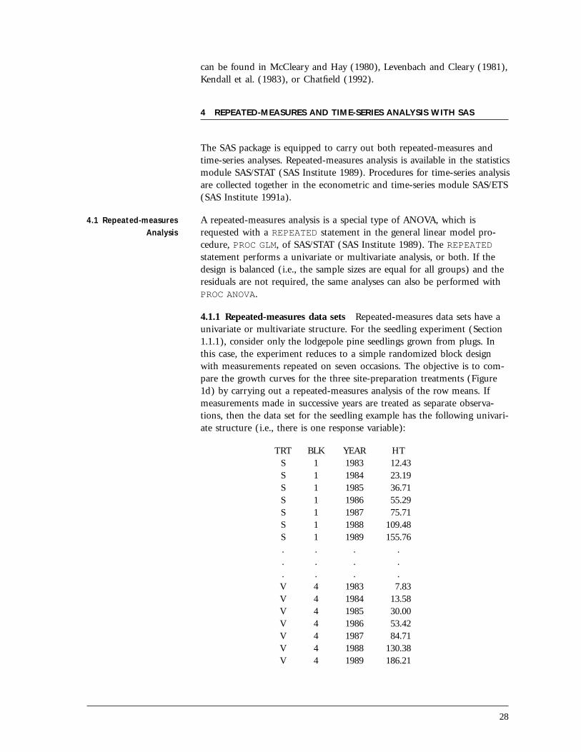
4.1.1 Repeated-measures data sets Repeated-measures data sets have aunivariate or multivariate structure. For the seedling experiment (Section1.1.1), consider only the lodgepole pine seedlings grown from plugs. Inthis case, the experiment reduces to a simple randomized block designwith measurements repeated on seven occasions. The objective is to com-pare the growth curves for the three site-preparation treatments (Figure1d) by carrying out a repeated-measures analysis of the row means. Ifmeasurements made in successive years are treated as separate observa-tions, then the data set for the seedling example has the following univari-ate structure (i.e., there is one response variable):

TRT BLK YEAR HTS 1 1983 12.43S 1 1984 23.19S 1 1985 36.71S 1 1986 55.29S 1 1987 75.71S 1 1988 109.48S 1 1989 155.76. . . .. . . .. . . .V 4 1983 7.83V 4 1984 13.58V 4 1985 30.00V 4 1986 53.42V 4 1987 84.71V 4 1988 130.38V 4 1989 186.21

29

This data set has a total of 84 observations (3 treatments × 4 blocks ×7 years) with one response variable (HT = average height of seedlings) foreach observation (row and year).

Alternatively, the same data can be converted to a multivariate data setwith 12 observations (rows of seedlings) and seven response variables(average planting height, [PHT], and the average heights for 1984–89,[HT84, HT85 . . . , HT89) for each row:

TRT BLK PHT HT84 HT85 HT86 HT87 HT88 HT89S 1 12.43 23.19 36.71 55.29 75.71 109.48 155.76S 2 10.23 18.59 33.91 53.59 74.09 108.27 150.64S 3 9.59 17.82 32.05 49.86 69.50 97.59 133.55S 4 13.48 21.70 34.26 48.22 73.39 103.83 141.48U 1 12.00 22.86 34.38 49.00 71.10 105.05 148.71U 2 9.43 17.14 30.10 43.33 60.95 87.24 125.67U 3 8.15 15.95 28.60 39.65 58.75 89.00 129.40U 4 8.75 15.70 27.45 42.55 58.45 85.55 123.85V 1 12.28 19.52 33.12 55.12 89.24 136.16 193.56V 2 9.57 17.13 28.74 46.65 74.00 114.22 163.13V 3 10.25 17.83 29.38 48.00 78.88 116.29 161.50V 4 7.83 13.58 30.00 53.42 84.71 130.38 186.21

With SAS, the univariate data set (UVDATA) can be readily transformedto the multivariate form (MVDATA), as illustrated below:

PROC SORT DATA=UVDATA;BY TRT BLK;

DATA MVDATA(KEEP=TRT BLK PHT HT84-HT89);ARRAY H(7) PHT HT84-HT89;DO YEAR=1983 TO 1989;

SET UVDATA;BY TRT BLK;H(YEAR-1982)=HT;IF LAST.BLK THEN RETURN;

END;RUN;

The reverse transformation can be achieved with the followingstatements:

DATA UVDATA(KEEP=TRT BLK YEAR HT);ARRAY H(7) PHT HT84-HT89;SET MVDATA;DO YEAR=1983 TO 1989;

HT=H(YEAR-1982);OUTPUT;

END;RUN;

30

4.1.2 Univariate analysis A univariate repeated-measures ANOVA is requestedin PROC GLM (or PROC ANOVA) by supplying the necessary MODEL andTEST statements, if the input data set has a univariate structure, or byreplacing the TEST statement with a REPEATED statement, if the data set ismultivariate. The two methods are illustrated below for the seedling data.

For the univariate data set, the SAS statements are:

PROC GLM DATA=UVDATA;TITLE1 ‘Univariate Repeated-Measures Analysis’;TITLE2 ‘Method 1: univariate data set analyzed with TEST statement’;CLASS BLK TRT YEAR;MODEL HT=BLK TRT BLK*TRT YEAR YEAR*TRT YEAR*BLK;TEST H=TRT E=BLK*TRT;TEST H=YEAR E=BLK*YEAR;

RUN;

Here the repeated-measures analysis is performed by specifying the bet-ween- and within-units factors with the MODEL statement. The correcterror terms for testing the between-row effect of treatment and thewithin-row effect of year are selected with the TEST statement. Alter-natively, the two TEST statements can be replaced with a single RANDOMstatement with the TEST option:

RANDOM BLK BLK*TRT YEAR*BLK/TEST;

This calculates expected mean squares and automatically selects the correcterror term for each effect, which is particularly useful if the investigator isuncertain about which error term to use. Application of the RANDOMstatement is described in more detail in the SAS/STAT manual (SAS Insti-tute 1989) and in Sit (1992b).

The results of the analysis of the univariate data set are displayed in Fig-ure 14. Notice that the TRT*YEAR interaction is highly significant (A), soit is reasonable to conclude that the growth curves for the three treatments(Figure 1d) are not parallel. The tests of H02—no growth over the seven-year study period—and H03—no overall difference between treatments(after averaging over the seven years)—are labelled B and C, respectively.Both are highly significant, although the first is not particularly interestingin this example because the seedlings have obviously grown in height.

Results from a more informative univariate analysis, including an inves-tigation of polynomial trends, are readily obtained from an analysis of themultivariate data set. The required SAS statements are:

PROC GLM DATA=MVDATA;TITLE1 ‘Univariate Repeated-Measures Analysis’;TITLE2 ‘Method 2: multivariate data set analyzed with REPEATED statement’;CLASS BLK TRT;MODEL PHT HT84-HT89=BLK TRT;REPEATED YEAR 7 (1983 1984 1985 1986 1987 1988 1989) POLYNOMIAL/SUMMARYPRINTM NOM;

RUN;

31

Univariate Repeated-Measures AnalysisMethod 1: univariate data set analyzed with TEST statement

General Linear Models Procedure

Dependent Variable: HTSum of Mean

Source DF Squares Square F Value Pr > F

Model 47 198236.399 4217.796 290.70 0.0001

Error 36 522.326 14.509

Corrected Total 83 198758.725

R-Square C.V. Root MSE HT Mean

0.997372 6.067216 3.80908 62.7813

Source DF Type III SS Mean Square F Value Pr > F

BLK 3 1206.093 402.031 27.71 0.0001TRT 2 3032.285 1516.143 104.50 0.0001BLK*TRT 6 340.388 56.731 3.91 0.0041YEAR 6 188835.114 31472.519 2169.16 0.0001TRT*YEAR 12 4206.553 350.546 24.16 0.0001 (A)BLK*YEAR 18 615.966 34.220 2.36 0.0140

Tests of Hypotheses using the Type III MS for BLK*TRT as an error term

Source DF Type III SS Mean Square F Value Pr > F

TRT 2 3032.28507 1516.14254 26.72 0.0010 (B)

Tests of Hypotheses using the Type III MS for BLK*YEAR as an error term

Source DF Type III SS Mean Square F Value Pr > F

YEAR 6 188835.114 31472.519 919.70 0.0001 (C)

14 Univariate repeated-measures analysis of seedling data: univariate data set.

When the multivariate data set is used, the repeated factor (YEAR) andits levels (1983, 1984, . . . , 1989) are specified in the REPEATEDstatement and the respective response variables (PHT HT84-HT89) areidentified in the MODEL statement. The REPEATED statement carries outboth univariate and multivariate analyses, unless one or the other is sup-pressed with the NOU (no univariate analysis) or NOM (no multivariateanalysis) option. In this example, NOM is chosen because only univariateanalyses are required (the multivariate analysis is discussed in the nextsection). The POLYNOMIAL transformation and SUMMARY option are also

32

selected. The POLYNOMIAL transformation generates all possible (in thiscase, six) polynomial combinations of the repeated measures and theSUMMARY option produces an ANOVA of each (which are used to testhypothesis H06 of Section 2.1). The same results can be obtained, withoutthe REPEATED statement, by first creating and then analyzing the trans-formed variables (POLY1, POLY2, . . . , POLY6) as follows:

DATA POLY;SET MVDATA;POLY1=-3*PHT-2*HT84 -HT85 +0*HT86 +HT87+2*HT88+3*HT89;POLY2= 5*PHT+0*HT84 -3*HT85 -4*HT86 -3*HT87+0*HT88+5*HT89;POLY3=-1*PHT+1*HT84 +1*HT85 +0*HT86 -1*HT87-1*HT88+1*HT89;POLY4= 3*PHT-7*HT84 +1*HT85 +6*HT86 +1*HT87-7*HT88+3*HT89;POLY5=-1*PHT+4*HT84 -5*HT85 +0*HT86 +5*HT87-4*HT88+1*HT89;POLY6= 1*PHT-6*HT84+15*HT85-20*HT86+15*HT87-6*HT88+1*HT89;

PROC GLM DATA=POLY;CLASS BLK TRT;MODEL POLY1-POLY6=BLK TRT/SS3;

RUN;

Notice that the coefficients (-3, -2, -1, 0, 1, 2, 3) are the same as thoseused to define polynomial contrasts in an ANOVA, and can be found insuch textbooks as Keppel (1973). Other linear combinations can beselected by making the appropriate substitution for POLYNOMIAL in theREPEATED statement: PROFILE for successive differences (refer to H04 ofSection 2.1) and CONTRAST 6 for cumulative differences (refer to H05 ofSection 2.1). The PRINTM option can be added to the REPEATED state-ment to verify that the correct transformation has been selected. Thiscauses the contrast coefficients to be printed.

When the REPEATED statement is applied to a randomized blockdesign, or any other design with random effects (e.g., designs with sub-sampling), a complication arises. Because the REPEATED statementassumes that all effects are fixed, the residual mean square is used as theerror term for all within-units tests. Consequently, the F-ratio for testingthe main effect of time (YEAR) is incorrect. In the seedling example, thecorrect F-ratio can be calculated by dividing the mean square for time(YEAR) by the proper error term, which is the mean square for the timeby block interaction (YEAR*BLK). The same problem occurs in theANOVA of the transformed data (i.e., POLY1, POLY2, etc.), where theF-ratio for testing the statistical significance of the overall mean of eachvariable (labelled MEAN in the ANOVA tables produced by the REPEATEDstatement) is incorrect. In the seedling example, the correct F-tests for thepolynomial contrasts can be obtained by inserting the following MANOVAstatement after the REPEATED statement:

6 The CONTRAST transformation of the REPEATED statement is not to be confused with theCONTRAST statement of PROC GLM.

33

MANOVA H=INTERCEPT E=BLK M=(-3 -2 -1 0 1 2 3, 5 0 -3 -4 -3 0 5,-1 1 1 0 -1 -1 1, 3 -7 1 6 1 -7 3,-1 4 -5 0 5 -4 1, 1 -6 15 -20 15 -6 1)

MNAMES=POLY1 POLY2 POLY3 POLY4 POLY5 POLY6/ORTH SUMMARY;

A MANOVA statement is a multivariate analog of the TEST statement.It is used whenever a test involves the elements of a multivariate array (inthis case, the repeated measures). The H=INTERCEPT option requests atest of the intercept or overall mean; the E=BLK option identifies BLK asthe correct error matrix (this is a matrix of sums of squares and cross-products and is the multivariate equivalent of the univariate YEAR*BLKsum of squares); M=(-3 -2 -1 0 1 2 3, etc.) defines the transformedvariables to be analyzed (in this case polynomial contrasts); andMNAMES=POLY1, etc., names the transformed variables. Proper use of theMANOVA statement requires a good understanding of multivariate modelsand multivariate hypothesis testing. Refer to Gumpertz and Brownie(1993) for a complete description of the analysis of randomized blockdesigns with repeated measures and the use of MANOVA statements toobtain the correct analysis in SAS.

An edited version of the output from the second univariate analysis ofthe seedling data is shown in Figure 15. It has five main parts:• an ANOVA for each year;• a repeated-measures ANOVA of the between-rows (‘‘Between Subjects’’)

variation;• a repeated-measures ANOVA of the within-rows (‘‘Within Subjects’’)

variation;• an ANOVA of each of the six polynomial contrasts among years; and • the correct F-tests for the overall means of the polynomial contrasts,which are labelled A, B, C, D, and E, respectively.

The first part of the output (A) gives the ANOVA results for each year.For brevity, only the results for 1989 are shown in Figure 15. Notice thatthere was a significant difference (A.1) between the three treatmentgroups in that year. The results for the other years (not shown) suggestthat there were no significant differences between groups from the time ofplanting up to the end of the first year, but by 1985 and in subsequentyears, there were significant differences between the groups.

The test for an overall treatment effect in the between-rows analysis(B) is the same as the TRT test (C) in Figure 14. Likewise, the test for atreatment effect in the within-rows analysis (C.3) is the same as theTRT*YEAR test (A) in Figure 14. However, notice that the within-rowstest of year (C.1), which uses the incorrect error term, is not the same asthe corresponding test (B) in Figure 14. The correct F-statistic for theyear effect (F = 919.70) can be calculated by dividing the mean square forYEAR, which is 31472.5190 (C.1), by the mean square for YEAR*BLK,which is 34.2203 (C.2).

At the end of the within-units analysis there are two numbers labelled‘‘Greenhouse-Geisser Epsilon’’ and ‘‘Huynh-Feldt Epsilon’’ (C.4). If thevariances and correlations of the repeated measures are constant over time(as required by the univariate repeated-measures analysis), then these two

34

Univariate Repeated-Measures AnalysisMethod 2: multivariate data set analyzed with REPEATED statement

General Linear Models Procedure

Dependent Variable: HT89 (A)Sum of Mean

Source DF Squares Square F Value Pr > F

Model 5 5115.06413 1023.01283 13.29 0.0034

Error 6 461.95544 76.99257

Corrected Total 11 5577.01957

R-Square C.V. Root MSE HT89 Mean

0.917168 5.806303 8.77454 151.121

Source DF Type III SS Mean Square F Value Pr > F

BLK 3 1009.76203 336.58734 4.37 0.0591TRT 2 4105.30210 2052.65105 26.66 0.0010 (A.1)

Tests of Hypotheses for Between Subjects Effects

Source DF Type III SS Mean Square F Value Pr > F

BLK 3 1206.0928 402.0309 7.09 0.0213TRT 2 3032.2851 1516.1425 26.72 0.0010 (B)

Error 6 340.3883 56.7314

Univariate Tests of Hypotheses for Within Subject Effects (C)

Source: YEARAdj Pr > F

DF Type III SS Mean Square F Value Pr > F G - G H - F6 188835.113904 31472.518984 2169.16 0.0001 0.0001 0.0001 (C.1)

Source: YEAR*BLKAdj Pr > F

DF Type III SS Mean Square F Value Pr > F G - G H - F18 615.966173 34.220343 2.36 0.0140 0.1482 0.0673 (C.2)

Source: YEAR*TRTAdj Pr > F

DF Type III SS Mean Square F Value Pr > F G - G H - F12 4206.552681 350.546057 24.16 0.0001 0.0004 0.0001 (C.3)

15 Univariate repeated-measures analysis of seedling data: multivariate data set.

35

Source: Error(YEAR)

DF Type III SS Mean Square36 522.326420 14.509067

Greenhouse-Geisser Epsilon = 0.2065 (C.4)Huynh-Feldt Epsilon = 0.4505

Analysis of Variance of Contrast Variables (D)

YEAR.N represents the nth degree polynomial contrast for YEAR

Contrast Variable: YEAR.1

Source DF Type III SS Mean Square F Value Pr > F

MEAN 1 175659.5789 175659.5789 2455.33 0.0001 (D.1)BLK 3 517.2866 172.4289 2.41 0.1654TRT 2 3578.8219 1789.4110 25.01 0.0012

Error 6 429.2521 71.5420

Contrast Variable: YEAR.2

Source DF Type III SS Mean Square F Value Pr > F

MEAN 1 12900.59010 12900.59010 1532.32 0.0001BLK 3 83.10595 27.70198 3.29 0.0999TRT 2 587.24391 293.62195 34.88 0.0005

Error 6 50.51387 8.41898

Contrast Variable: YEAR.3

Source DF Type III SS Mean Square F Value Pr > F

MEAN 1 262.0476732 262.0476732 143.48 0.0001BLK 3 10.5190901 3.5063634 1.92 0.2276TRT 2 27.1102199 13.5551099 7.42 0.0239

Error 6 10.9585841 1.8264307Contrast Variable: YEAR.4

Source DF Type III SS Mean Square F Value Pr > F

MEAN 1 0.84138232 0.84138232 0.28 0.6149BLK 3 2.76045704 0.92015235 0.31 0.8195TRT 2 11.52322226 5.76161113 1.93 0.2258

Error 6 17.94389412 2.99064902

15 (continued)

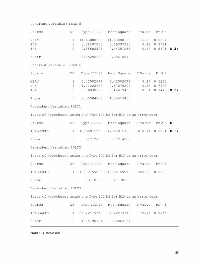
36

Contrast Variable: YEAR.5

Source DF Type III SS Mean Square F Value Pr > F

MEAN 1 11.63080680 11.63080680 16.80 0.0064BLK 3 0.58185855 0.19395285 0.28 0.8381TRT 2 0.88502506 0.44251253 0.64 0.5601 (D.2)

Error 6 4.15295236 0.69215873

Contrast Variable: YEAR.6

Source DF Type III SS Mean Square F Value Pr > F

MEAN 1 0.42502079 0.42502079 0.27 0.6230BLK 3 1.71225628 0.57075209 0.36 0.7843TRT 2 0.96838905 0.48419453 0.31 0.7475 (D.3)

Error 6 9.50504759 1.58417460

Dependent Variable: POLY1

Tests of Hypotheses using the Type III MS for BLK as an error term

Source DF Type III SS Mean Square F Value Pr > F (E)

INTERCEPT 1 175659.5789 175659.5789 1018.74 0.0001 (E.1)

Error 3 517.2866 172.4289

Dependent Variable: POLY2

Tests of Hypotheses using the Type III MS for BLK as an error term

Source DF Type III SS Mean Square F Value Pr > F

INTERCEPT 1 12900.59010 12900.59010 465.69 0.0002

Error 3 83.10595 27.70198

Dependent Variable: POLY3

Tests of Hypotheses using the Type III MS for BLK as an error term

Source DF Type III SS Mean Square F Value Pr > F

INTERCEPT 1 262.0476732 262.0476732 74.73 0.0033

Error 3 10.5190901 3.5063634

15 (continued)

37

Dependent Variable: POLY4

Tests of Hypotheses using the Type III MS for BLK as an error term

Source DF Type III SS Mean Square F Value Pr > F

INTERCEPT 1 0.84138232 0.84138232 0.91 0.4095

Error 3 2.76045704 0.92015235

Dependent Variable: POLY5

Tests of Hypotheses using the Type III MS for BLK as an error term

Source DF Type III SS Mean Square F Value Pr > F

INTERCEPT 1 11.63080680 11.63080680 59.97 0.0045 (E.2)

Error 3 0.58185855 0.19395285

Dependent Variable: POLY6

Tests of Hypotheses using the Type III MS for BLK as an error term

Source DF Type III SS Mean Square F Value Pr > F

INTERCEPT 1 0.42502079 0.42502079 0.74 0.4516 (E.3)

Error 3 1.71225628 0.57075209

15 (concluded).

numbers should be approximately equal to one. When this assumption isviolated, the numbers will be substantially less than one and the F-testsfor the within-units analysis will be incorrect. To compensate for thisproblem, SAS uses the Greenhouse-Geisser epsilon and the Huynh-Feldtepsilon to make two separate adjustments to the p-value for each F-test.The adjusted p-values (‘‘Adj Pr>F’’) are labelled ‘‘G - G’’ (Greenhouse-Geisser correction) and ‘‘H - F’’ (Huynh-Feldt correction) in the output.More information about these adjustments can be found in Chapter 27 ofMilliken and Johnson (1992).

The ANOVA tables for the six polynomial contrasts (D) are labelledYEAR.1 (linear trend), YEAR.2 (quadratic trend), etc., in Figure 15. Asdiscussed previously, the test for a MEAN effect is incorrect in these tablesand should be replaced with the corresponding MANOVA test (i.e., theINTERCEPT test for POLY1=YEAR.1, POLY2=YEAR.2, etc., which isgiven in E). For example, the correct F-ratio for testing the overall meanof the linear transformation (YEAR.1 in D and POLY1 in E) is 1018.74(E.1), not 2455.33 (D.1). Notice that treatment has no significant effect

38

on the sixth-order polynomial contrasts (i.e., there is no significant differ-ence between β6 for the three site-preparation treatments in D.3). More-over, the average of these three coefficients is not significantly differentfrom zero (E.3). This suggests that the growth curves for the three treat-ment groups are adequately described by polynomials of order no greaterthan five (i.e., β6 = 0). Examining the results for the fifth-order poly-nomial transformation (YEAR.5 and POLY5) reveals that there is a fifth-order term in the trends (E.2), but it is not significantly different for thethree treatment groups (D.2). The same conclusion holds for the fourth-order term. Site-preparation does, however, have a significant effect on thecubic and lower-order terms. Thus the evidence suggests that the growthcurves can be described by fifth-order polynomials with the effects of site-preparation treatment limited to the cubic and lower-order terms.

4.1.3 Multivariate analysis The REPEATED statement automatically per-forms a multivariate repeated-measures analysis (unless the NOM option isused). The SAS statements for carrying out a multivariate repeated-measures analysis of the seedling data set are:

PROC GLM DATA=MVDATA;TITLE ‘Multivariate Repeated-Measures Analysis’;CLASS BLK TRT;MODEL PHT HT84-HT89=BLK TRT/SS3;REPEATED YEAR 7 (1983 1984 1985 1986 1987 1988 1989)/NOU;

RUN;

In this case, the NOU (no univariate analysis) option is used to suppressthe univariate tests of the within-units effects. These are replaced by mul-tivariate tests, the results of which are displayed in Figure 16. Recall thatSAS does not recognize that block is a random effect. Therefore, the mul-tivariate test of the main effect of year (labelled A in Figure 16), like thecorresponding univariate test, is incorrect. If there were seven or moreblocks, then the following MANOVA statement would produce the correcttest:

MANOVA H=INTERCEPT E=BLK M=( 1 -1 0 0 0 0 0, 0 1 -1 0 0 0 0,0 0 1 -1 0 0 0, 0 0 0 1 -1 0 0,0 0 0 0 1 -1 0, 0 0 0 0 0 1 -1);

However, for this particular design, which has fewer blocks than years,there are too few degrees of freedom to carry out the test. Fortunately, thetest for no time effect is not very important in this example.

The results of the multivariate test for parallel growth curves (B in Fig-ure 16) should be compared with the corresponding results of the uni-variate tests (A in Figure 14 and C.1 in Figure 15). Notice that theunivariate tests suggest that the growth curves are not parallel for thethree groups (i.e., the YEAR*TRT effect is significant), but that two of thethree multivariate tests (the sample sizes are too small to compute the

39

Multivariate Repeated-Measures Analysis

Manova Test Criteria and Exact F Statistics forthe Hypothesis of no YEAR Effect

(A)

H = Type III SS&CP Matrix for YEAR E = Error SS&CP Matrix

S=1 M=2 N=-0.5

Statistic Value F Num DF Den DF Pr F

Wilks’ Lambda 0.00025957 641.9264 6 1 0.0302Pillai’s Trace 0.99974043 641.9264 6 1 0.0302Hotelling-Lawley Trace 3851.5581633 641.9264 6 1 0.0302Roy’s Greatest Root 3851.5581633 641.9264 6 1 0.0302

Manova Test Criteria and F Approximations forthe Hypothesis of no YEAR*BLK Effect

H = Type III SS&CP Matrix for YEAR*BLK E = Error SS&CP Matrix

S=3 M=1 N=-0.5

Statistic Value F Num DF Den DF Pr > F

Wilks’ Lambda 0.01032163 0.7433 18 3.313708 0.7084Pillai’s Trace 1.65054752 0.6116 18 9 0.8210Hotelling-Lawley Trace 40.36355908 . 18 -1 .Roy’s Greatest Root 39.16883650 19.5844 6 3 0.0167

NOTE: F Statistic for Roy’s Greatest Root is an upper bound.

Manova Test Criteria and F Approximations forthe Hypothesis of no YEAR*TRT Effect (B)

H = Type III SS&CP Matrix for YEAR*TRT E = Error SS&CP Matrix

S=2 M=1.5 N=-0.5

Statistic Value F Num DF Den DF Pr > F

Wilks’ Lambda 0.00172637 3.8446 12 2 0.2248Pillai’s Trace 1.73572577 2.1893 12 4 0.2340Hotelling-Lawley Trace 151.08093445 . 12 0 .Roy’s Greatest Root 148.19852119 49.3995 6 2 0.0200

NOTE: F Statistic for Roy’s Greatest Root is an upper bound.NOTE: F Statistic for Wilks’ Lambda is exact.

16 Multivariate repeated measures analysis of seedling data.

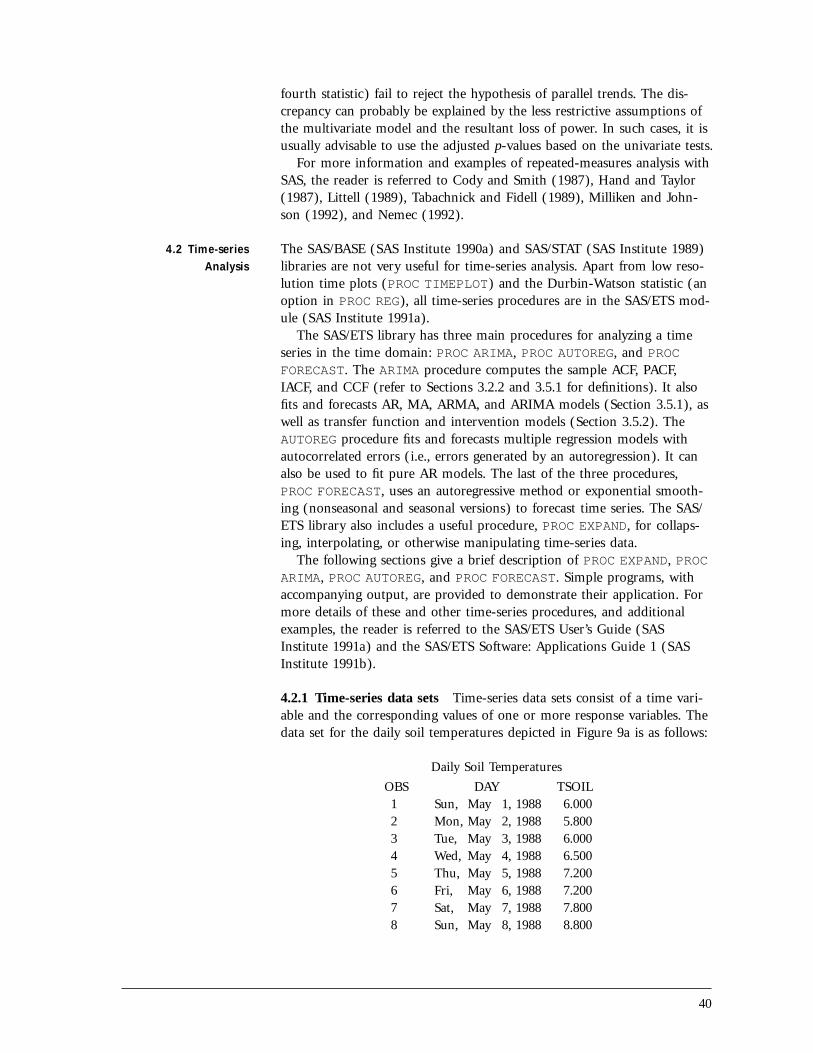
40

fourth statistic) fail to reject the hypothesis of parallel trends. The dis-crepancy can probably be explained by the less restrictive assumptions ofthe multivariate model and the resultant loss of power. In such cases, it isusually advisable to use the adjusted p-values based on the univariate tests.

For more information and examples of repeated-measures analysis withSAS, the reader is referred to Cody and Smith (1987), Hand and Taylor(1987), Littell (1989), Tabachnick and Fidell (1989), Milliken and John-son (1992), and Nemec (1992).

4.2 Time-seriesAnalysis

The SAS/BASE (SAS Institute 1990a) and SAS/STAT (SAS Institute 1989)libraries are not very useful for time-series analysis. Apart from low reso-lution time plots (PROC TIMEPLOT) and the Durbin-Watson statistic (anoption in PROC REG), all time-series procedures are in the SAS/ETS mod-ule (SAS Institute 1991a).

The SAS/ETS library has three main procedures for analyzing a timeseries in the time domain: PROC ARIMA, PROC AUTOREG, and PROCFORECAST. The ARIMA procedure computes the sample ACF, PACF,IACF, and CCF (refer to Sections 3.2.2 and 3.5.1 for definitions). It alsofits and forecasts AR, MA, ARMA, and ARIMA models (Section 3.5.1), aswell as transfer function and intervention models (Section 3.5.2). TheAUTOREG procedure fits and forecasts multiple regression models withautocorrelated errors (i.e., errors generated by an autoregression). It canalso be used to fit pure AR models. The last of the three procedures,PROC FORECAST, uses an autoregressive method or exponential smooth-ing (nonseasonal and seasonal versions) to forecast time series. The SAS/ETS library also includes a useful procedure, PROC EXPAND, for collaps-ing, interpolating, or otherwise manipulating time-series data.

The following sections give a brief description of PROC EXPAND, PROCARIMA, PROC AUTOREG, and PROC FORECAST. Simple programs, withaccompanying output, are provided to demonstrate their application. Formore details of these and other time-series procedures, and additionalexamples, the reader is referred to the SAS/ETS User’s Guide (SASInstitute 1991a) and the SAS/ETS Software: Applications Guide 1 (SASInstitute 1991b).

4.2.1 Time-series data sets Time-series data sets consist of a time vari-able and the corresponding values of one or more response variables. Thedata set for the daily soil temperatures depicted in Figure 9a is as follows:

Daily Soil Temperatures

OBS DAY TSOIL1 Sun, May 1, 1988 6.0002 Mon, May 2, 1988 5.8003 Tue, May 3, 1988 6.0004 Wed, May 4, 1988 6.5005 Thu, May 5, 1988 7.2006 Fri, May 6, 1988 7.2007 Sat, May 7, 1988 7.8008 Sun, May 8, 1988 8.800

41

9 Mon, May 9, 1988 9.50010 Tue, May 10, 1988 10.50011 Wed, May 11, 1988 10.90012 Thu, May 12, 1988 11.500. . .. . .. . .

(more data)

In this case, the time index, DAY, is an SAS date variable (printed inWEEKDATE17. format) and the response variable, TSOIL, is the soil tem-perature in degrees Celsius. Indexing a time series with an SAS date vari-able facilitates data verification and manipulation with SAS/ETSprocedures but is not essential (e.g., the variable DAY could be omittedfrom the previous data set).

For PROC ARIMA, PROC AUTOREG, and PROC FORECAST, the inputdata set must be sorted in order of ascending time and the series must beequally spaced in time. If the data are not equally spaced, then PROCEXPAND can be used to convert the series, by interpolation, to equal timeintervals. The same procedure can also be used to collapse or expand thesampling interval (e.g., by summing or averaging data points), to replacemissing values with interpolated values, or to perform other operations onthe series. As a simple illustration, consider the soil temperature series. Toconvert the daily series to weekly averages, PROC EXPAND can be used asfollows:

PROC EXPAND DATA=DAILY OUT=WEEKLY FROM=DAY TO=WEEK;CONVERT TSOIL/METHOD=AGGREGATE OBSERVED=AVERAGE;ID DATE;

PROC PRINT DATA=WEEKLY;TITLE ‘Weekly Averages’;

RUN;

The input series (DAILY), part of which was listed at the beginning ofthis section, and the output series (WEEKLY) are specified by the DATAand OUT options in the PROC EXPAND line. The change of intervals fromdaily to weekly is defined with the FROM and TO options, and the type ofconversion is selected with the METHOD and OBSERVED options of theCONVERT statement (i.e., METHOD=AGGREGATE specifies that the outputseries is an aggregation of the input series and OBSERVED=AVERAGE spe-cifies that the aggregation is by averaging). The resultant weekly series islisted below.

Weekly Averages

OBS DATE TSOIL1 Sun, 1 May 88 6.64292 Sun, 8 May 88 10.21433 Sun, 15 May 88 9.00004 Sun, 22 May 88 9.5286

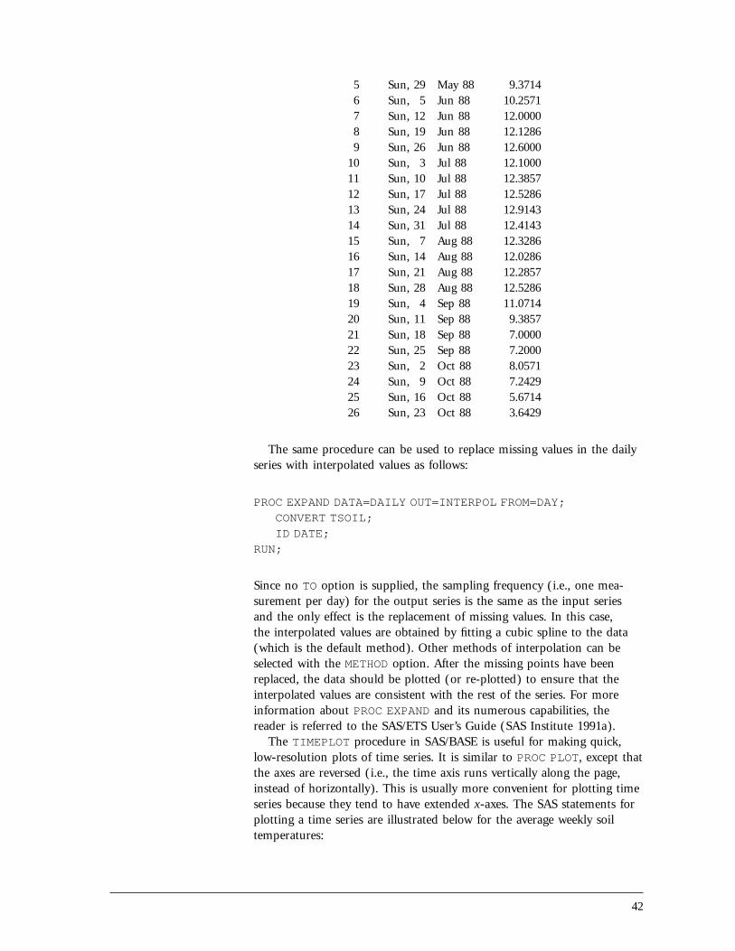
42

5 Sun, 29 May 88 9.37146 Sun, 5 Jun 88 10.25717 Sun, 12 Jun 88 12.00008 Sun, 19 Jun 88 12.12869 Sun, 26 Jun 88 12.6000

10 Sun, 3 Jul 88 12.100011 Sun, 10 Jul 88 12.385712 Sun, 17 Jul 88 12.528613 Sun, 24 Jul 88 12.914314 Sun, 31 Jul 88 12.414315 Sun, 7 Aug 88 12.328616 Sun, 14 Aug 88 12.028617 Sun, 21 Aug 88 12.285718 Sun, 28 Aug 88 12.528619 Sun, 4 Sep 88 11.071420 Sun, 11 Sep 88 9.385721 Sun, 18 Sep 88 7.000022 Sun, 25 Sep 88 7.200023 Sun, 2 Oct 88 8.057124 Sun, 9 Oct 88 7.242925 Sun, 16 Oct 88 5.671426 Sun, 23 Oct 88 3.6429

The same procedure can be used to replace missing values in the dailyseries with interpolated values as follows:

PROC EXPAND DATA=DAILY OUT=INTERPOL FROM=DAY;CONVERT TSOIL;ID DATE;

RUN;

Since no TO option is supplied, the sampling frequency (i.e., one mea-surement per day) for the output series is the same as the input seriesand the only effect is the replacement of missing values. In this case,the interpolated values are obtained by fitting a cubic spline to the data(which is the default method). Other methods of interpolation can beselected with the METHOD option. After the missing points have beenreplaced, the data should be plotted (or re-plotted) to ensure that theinterpolated values are consistent with the rest of the series. For moreinformation about PROC EXPAND and its numerous capabilities, thereader is referred to the SAS/ETS User’s Guide (SAS Institute 1991a).

The TIMEPLOT procedure in SAS/BASE is useful for making quick,low-resolution plots of time series. It is similar to PROC PLOT, except thatthe axes are reversed (i.e., the time axis runs vertically along the page,instead of horizontally). This is usually more convenient for plotting timeseries because they tend to have extended x-axes. The SAS statements forplotting a time series are illustrated below for the average weekly soiltemperatures:

43

PROC TIMEPLOT DATA=WEEKLY;TITLE ‘Average Weekly Soil Temperatures’;PLOT TSOIL=’*’;ID YEAR;

RUN;

The output is shown in Figure 17.

4.2.2 PROC ARIMA The ARIMA procedure has three main statements:IDENTIFY, ESTIMATE, and FORECAST. The IDENTIFY statementappears first. It defines the time series to be analyzed and calculates sum-mary statistics that are useful for model identification, including the sam-ple ACF, IACF, and PACF, and if applicable, the sample CCF (refer toSections 3.2.2 and 3.5.1 for definitions). Once a model has been identi-fied, it can be fitted to the series by including an ESTIMATE statement

Average Weekly Soil Temperature

DATE TSOIL

Sun, 1 May 88 6.64Sun, 8 May 88 10.21Sun, 15 May 88 9.00Sun, 22 May 88 9.53Sun, 29 May 88 9.37Sun, 5 Jun 88 10.26Sun, 12 Jun 88 12.00Sun, 19 Jun 88 12.13Sun, 26 Jun 88 12.60Sun, 3 Jul 88 12.10Sun, 10 Jul 88 12.39Sun, 17 Jul 88 12.53Sun, 24 Jul 88 12.91Sun, 31 Jul 88 12.41Sun, 7 Aug 88 12.33Sun, 14 Aug 88 12.03Sun, 21 Aug 88 12.29Sun, 28 Aug 88 12.53Sun, 4 Sep 88 11.07Sun, 11 Sep 88 9.39Sun, 18 Sep 88 7.00Sun, 25 Sep 88 7.20Sun, 2 Oct 88 8.06Sun, 9 Oct 88 7.24Sun, 16 Oct 88 5.67Sun, 23 Oct 88 3.64

min max3.6428571423 12.914285712

*––––––––––––––––––––––––––––––––––––––––––*

*––––––––––––––––––––––––––––––––––––––––––*

**

***

***

**********

**

**

**

**

17 Time plot of weekly soil temperatures created with PROC TIMEPLOT.

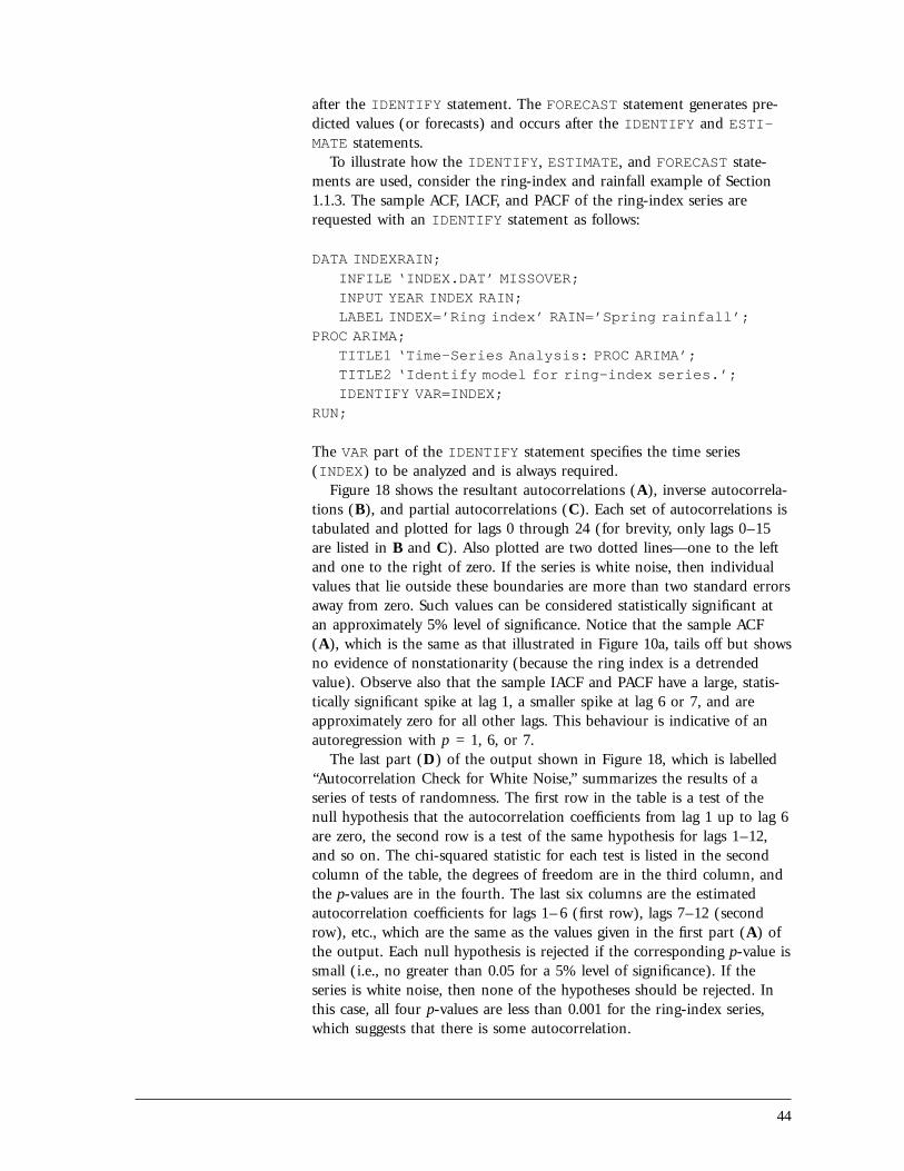
44

after the IDENTIFY statement. The FORECAST statement generates pre-dicted values (or forecasts) and occurs after the IDENTIFY and ESTI-MATE statements.

To illustrate how the IDENTIFY, ESTIMATE, and FORECAST state-ments are used, consider the ring-index and rainfall example of Section1.1.3. The sample ACF, IACF, and PACF of the ring-index series arerequested with an IDENTIFY statement as follows:

DATA INDEXRAIN;INFILE ‘INDEX.DAT’ MISSOVER;INPUT YEAR INDEX RAIN;LABEL INDEX=’Ring index’ RAIN=’Spring rainfall’;

PROC ARIMA;TITLE1 ‘Time-Series Analysis: PROC ARIMA’;TITLE2 ‘Identify model for ring-index series.’;IDENTIFY VAR=INDEX;

RUN;

The VAR part of the IDENTIFY statement specifies the time series(INDEX) to be analyzed and is always required.

Figure 18 shows the resultant autocorrelations (A), inverse autocorrela-tions (B), and partial autocorrelations (C). Each set of autocorrelations istabulated and plotted for lags 0 through 24 (for brevity, only lags 0–15are listed in B and C). Also plotted are two dotted lines—one to the leftand one to the right of zero. If the series is white noise, then individualvalues that lie outside these boundaries are more than two standard errorsaway from zero. Such values can be considered statistically significant atan approximately 5% level of significance. Notice that the sample ACF(A), which is the same as that illustrated in Figure 10a, tails off but showsno evidence of nonstationarity (because the ring index is a detrendedvalue). Observe also that the sample IACF and PACF have a large, statis-tically significant spike at lag 1, a smaller spike at lag 6 or 7, and areapproximately zero for all other lags. This behaviour is indicative of anautoregression with p = 1, 6, or 7.

The last part (D) of the output shown in Figure 18, which is labelled‘‘Autocorrelation Check for White Noise,’’ summarizes the results of aseries of tests of randomness. The first row in the table is a test of thenull hypothesis that the autocorrelation coefficients from lag 1 up to lag 6are zero, the second row is a test of the same hypothesis for lags 1–12,and so on. The chi-squared statistic for each test is listed in the secondcolumn of the table, the degrees of freedom are in the third column, andthe p-values are in the fourth. The last six columns are the estimatedautocorrelation coefficients for lags 1– 6 (first row), lags 7–12 (secondrow), etc., which are the same as the values given in the first part (A) ofthe output. Each null hypothesis is rejected if the corresponding p-value issmall (i.e., no greater than 0.05 for a 5% level of significance). If theseries is white noise, then none of the hypotheses should be rejected. Inthis case, all four p-values are less than 0.001 for the ring-index series,which suggests that there is some autocorrelation.

45

Time-Series Analysis: PROC ARIMAIdentify model for ring-index series.

ARIMA Procedure

Name of variable = INDEX.

Mean of working series = 0.99646Standard deviation = 0.191788Number of observations = 463

Autocorrelations (A)

Lag Covariance Correlation -1 9 8 7 6 5 4 3 2 1 0 1 2 3 4 5 6 7 8 9 10 0.036782 1.00000 ********************1 0.026179 0.71173 . **************2 0.020030 0.54455 . ***********3 0.015960 0.43391 . *********4 0.011755 0.31958 . ******5 0.009626 0.26170 . *****6 0.0092158 0.25055 . *****7 0.0057674 0.15680 . ***8 0.0033671 0.09154 . **.9 0.0024593 0.06686 . * .10 0.0012791 0.03477 . * .11 0.0014994 0.04076 . * .12 0.0017450 0.04744 . * .13 -0.000112 -0.00304 . .14 -0.0014171 -0.03853 . * .15 -0.0026482 -0.07200 . * .16 -0.0047892 -0.13020 .*** .17 -0.0066828 -0.18168 **** .18 -0.0076178 -0.20710 **** .19 -0.0081882 -0.22261 **** .20 -0.0079820 -0.21700 **** .21 -0.0079143 -0.21516 **** .22 -0.0089012 -0.24200 ***** .23 -0.0084721 -0.23033 ***** .24 -0.0093843 -0.25513 ***** .

‘‘.’’ marks two standard errors

18 Time-series analysis of ring-index series: model identification.

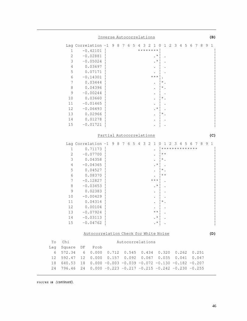
46

Inverse Autocorrelations (B)

Lag Correlation -1 9 8 7 6 5 4 3 2 1 0 1 2 3 4 5 6 7 8 9 11 -0.42101 ********2 -0.02881 .* .3 -0.05024 .* .4 0.03697 . .5 0.07171 . .6 -0.14301 *** .7 0.03444 . *.8 0.04396 . *.9 -0.00244 . .10 0.03660 . *.11 -0.01465 . .12 -0.06493 .* .13 0.02966 . *.14 0.01278 . .15 -0.01721 . .

Partial Autocorrelations (C)

Lag Correlation -1 9 8 7 6 5 4 3 2 1 0 1 2 3 4 5 6 7 8 9 11 0.71173 . **************2 -0.07700 . **3 0.04358 . *.4 -0.04365 .* .5 0.04527 . *.6 0.08370 . **7 -0.12827 *** .8 -0.03453 .* .9 0.02383 . .10 -0.00429 . .11 0.04314 . *.12 0.00104 . .13 -0.07924 ** .14 -0.03113 .* .15 -0.04762 .* .

Autocorrelation Check for White Noise (D)

To Chi AutocorrelationsLag Square DF Prob6 572.34 6 0.000 0.712 0.545 0.434 0.320 0.262 0.25112 592.47 12 0.000 0.157 0.092 0.067 0.035 0.041 0.04718 640.53 18 0.000 -0.003 -0.039 -0.072 -0.130 -0.182 -0.20724 796.46 24 0.000 -0.223 -0.217 -0.215 -0.242 -0.230 -0.255

18 (continued).

47

The IDENTIFY statement generates summary statistics for differencedseries, as well as untransformed series. To analyze a differenced series(yt − yt −k), the interval k is enclosed in parentheses after the variablename. If the series is differenced more than once (e.g., [yt − yt −1] −[yt −1 − yt −2], then the corresponding intervals must be separated bycommas as illustrated below:

PROC ARIMA DATA=INDXRAIN;IDENTIFY VAR=INDEX(1); /* First difference of INDEX series */IDENTIFY VAR=INDEX(1,1); /* Second difference of INDEX series */

RUN;

Alternatively, the same results can be achieved by creating, with the LAGfunction (SAS Institute 1990b), the differenced series in a DATA step:

DATA DIFFS;INFILE ‘INDEX.DAT’ MISSOVER;INPUT YEAR INDEX RAIN;DIFF1=INDEX-LAG1(INDEX);DIFF2=INDEX-2*LAG1(INDEX)+LAG2(INDEX);

PROC ARIMA DATA=DIFFS;IDENTIFY VAR=DIFF1; /* First difference of INDEX series */IDENTIFY VAR=DIFF2; /* Second difference of INDEX series */

RUN;

The IDENTIFY statement has various options. The CROSSCOR optionrequests a cross-correlation analysis of the main series (i.e., the seriesdefined by VAR) and one or more other series. The latter are identified byvariable names enclosed in parentheses after CROSSCOR, with differencedseries specified in the same manner as described above for the mainseries. The CROSSCOR option is demonstrated in the following example:

PROC ARIMA DATA=PWSERIES;IDENTIFY VAR=PWINDEX CROSSCOR(PWRAIN) NLAG=15OUTCOV=STATS;

RUN;

Here a prewhitened ring-index series (PWINDEX) is cross-correlated witha prewhitened rainfall series (PWRAIN). (Details of the computation ofthe prewhitened series are deferred until the discussion of FORECAST.)The NLAG and OUTCOV options are also illustrated. The NLAG optiondefines the maximum lag for which the ACF, IACF, PACF, and CCF are tobe calculated (a warning message is printed if NLAG exceeds 25% of theseries length); and the OUTCOV option creates a data set (STATS) con-taining the summary statistics generated by the IDENTIFY statement.

Output from the last example includes the sample ACF, IACF, and PACFof the prewhitened index series for lags 0 through 15, and a check for whitenoise. These results have the same interpretation as Figure 18 and will notbe discussed further. The rest of the output is displayed in Figure 19. Itshows the cross-correlogram for lags −15 through 15, which was also plotted

48

in Figure 11. If a cross-correlation value lies outside the pair of dotted linesit can be considered statistically significant at an approximately 5% level ofsignificance (i.e., the null hypothesis that the cross-correlation is zero canbe rejected at the 5% level of significance). Notice that in this case, onlyone significant spike occurs at lag 0, suggesting that the ring index is(weakly) correlated with the rainfall during the spring of the same year, butis uncorrelated with the rainfall in previous years.

Correlation of PWINDEX and PWRAINVariance of input = 2965.586Number of observations = 102

Crosscorrelations

Lag Covariance Correlation -1 9 8 7 6 5 4 3 2 1 0 1 2 3 4 5 6 7 8 9 1-15 -0.290235 -0.03318 . * .-14 0.871138 0.09958 . ** .-13 0.084201 0.00962 . .-12 0.287734 0.03289 . * .-11 0.297993 0.03406 . * .-10 -0.120706 -0.01380 . .-9 -0.145245 -0.01660 . .-8 -0.432502 -0.04944 . * .-7 0.987679 0.11290 . ** .-6 0.578575 0.06614 . * .-5 -1.566862 -0.17910 **** .-4 0.755446 0.08635 . ** .-3 0.945793 0.10811 . ** .-2 -0.388612 -0.04442 . * .-1 0.579211 0.06621 . * .0 2.351343 0.26878 . *****1 -0.567222 -0.06484 . * .2 -0.204336 -0.02336 . .3 1.412760 0.16149 . ***.4 -1.019255 -0.11651 . ** .5 -0.302926 -0.03463 . * .6 -0.160564 -0.01835 . .7 0.089897 0.01028 . .8 -0.746720 -0.08536 . ** .9 -0.686667 -0.07849 . ** .10 0.392745 0.04489 . * .11 -0.900352 -0.10292 . ** .12 1.354699 0.15485 . ***.13 -1.016035 -0.11614 . ** .14 0.709422 0.08109 . ** .15 -0.040492 -0.00463 . .

‘‘.’’ marks two standard errors

19 Cross-correlation of prewhitened ring-index and rainfall series.

49

The sample ACF, IACF, and PACF (Figure 18) suggest that an ARmodel (refer to Section 3.5.1) might be appropriate for the ring-indexseries. Since the order of the autoregression is uncertain, three candidatemodels are fitted as follows:

PROC ARIMA DATA=INDXRAIN;TITLE1 ‘Time-Series Analysis: PROC ARIMA’;TITLE2 ‘Fit models to ring-index series.’;IDENTIFY VAR=INDEX NOPRINT NLAG=10;ESTIMATE P=1 METHOD=ML;ESTIMATE P=7 METHOD=ML;ESTIMATE P=(1 6 7) METHOD=ML PLOT;

RUN;

Each model is defined by a separate ESTIMATE statement and is fittedto the series specified in the preceding IDENTIFY statement. Since allthree models are fitted to the same series (INDEX), only one IDENTIFYstatement is needed. The NOPRINT option of IDENTIFY suppresses theprinting of the sample ACF, IACF, and PACF (Figure 18), which were use-ful for model identification but are not required here. The P option of theESTIMATE statements defines the autoregressive terms that are to beincluded in the fitted models. The option P=k includes all terms up to lagk. Thus the first two ESTIMATE statements fit the models

yt = ν + φ 1 yt − 1 + εt

and

yt = ν + φ 1 yt − 1 + φ 2 yt − 2 + . . . + φ 7 yt − 7 + εt

respectively. To limit the model to a specific set of autoregressive terms,the corresponding lags must be enclosed in parentheses as illustrated bythe last ESTIMATE statement, which fits the model

yt = ν + φ 1 yt − 1 + φ 6 yt − 6 + φ 7 yt − 7 + εt

Moving-average models are defined in a similar manner with the Qoption: for instance,

PROC ARIMA;IDENTIFY VAR=INDEX;ESTIMATE Q=(1 3);

RUN;

fits the model yt = ν + εt − φ 1 εt − 1 − φ 3 εt − 3 . Mixed models require that Pand Q be specified: thus,

PROC ARIMA;IDENTIFY VAR=INDEX;ESTIMATE P=2 Q=(1 3);

RUN;

50

fits the ARMA model yt = ν + φ 1 yt − 1 + φ 2 yt − 2 + εt − φ 1 εt − 1 − φ 3 εt − 3 .To fit an ARIMA model, the appropriate differenced series is specifiedin the IDENTIFY statement (or created in a previous data step). The cor-responding ARMA model is selected with the P and Q options of ESTI-MATE. The following example demonstrates how PROC ARIMA can beused to fit an ARIMA(1, 1, 1) model:

PROC ARIMA;IDENTIFY VAR=INDEX(1);ESTIMATE P=1 Q=1;

RUN;

The results of fitting the three AR models are displayed in A, B, and Cof Figure 20. For each model, the parameter estimates, approximate stan-dard errors, T-statistics (with degrees of freedom equal to the number ofobservations minus the number of free parameters in the model), and asso-ciated lags are summarized in a table labelled ‘‘Maximum Likelihood Esti-mation.’’ The title reflects the method of estimation, which is selected withthe METHOD option of ESTIMATE. In this case, maximum likelihood esti-mation (METHOD=ML) was used. Other methods are available, but maxi-mum likelihood estimation is usually preferred because the resultantestimates have desirable statistical properties (see Chapter 6 of Diggle 1991).

Each set of parameter estimates includes an estimate of the mean of theresponse variable (MU ), estimates of any autoregressive parameters {φi }(which have labels with the prefix ‘‘AR’’), and estimates of any moving-average parameters {θi } (prefix ‘‘MA’’). The estimate of the constant ν islabelled ‘‘Constant Estimate’’ and the estimated variance (standard devia-tion) of εt is labelled ‘‘Variance Estimate’’ (‘‘Std Error Estimate’’). All ARand MA estimates are numbered consecutively, with the associated lags lis-ted in the last column. For example, reading the relevant parameter esti-mates (C.1) from Figure 20 yields the third and final fitted model:

yt = 0.26800 + 0.70855 yt − 1 + 0.16708 yt − 6 − 0.14479 yt − 7 + εt

Similarly, the estimates for the first and second models can be read fromA.1 and B.1 of the output.

The constant and variance estimates are followed by two numberslabelled ‘‘AIC’’ and ‘‘SBC,’’ which stand for ‘‘Akaike’s information crite-rion’’ and ‘‘Schwartz’s Bayesian criterion.’’ Models are sometimes comparedon the basis of these criteria, which take into account both the quality ofthe fit and the number of estimated parameters. Models with smallervalues are judged to be ‘‘better’’ (i.e., provide a better fit without substan-tially increasing number parameters) than models with larger values.Comparison of AIC and SBC for the three AR models (refer to A.2, B.2,and C.2 in Figure 20) suggests that the last model is best. The other twomodels are rejected because the first does not provide a good fit (seebelow) and the second has too many terms (notice that the AR parame-ters for lags 2–5 are not statistically significant according to theirT-statistics).

51

Time-Series Analysis: PROC ARIMAFit models to ring-index series.

ARIMA Procedure

Maximum Likelihood Estimation (A)

Approx.Parameter Estimate Std Error T Ratio LagMU 0.99608 0.02187 45.55 0AR1,1 0.71594 0.03252 22.02 1 (A.1)

Constant Estimate = 0.28294583

Variance Estimate = 0.01807707 (A.2)Std Error Estimate = 0.134451AIC = -541.41897SBC = -533.14351Number of Residuals= 463

Correlations of the Estimates

Parameter MU AR1,1

MU 1.000 0.009AR1,1 0.009 1.000

Autocorrelation Check of Residuals (A.3)

To Chi AutocorrelationsLag Square DF Prob6 17.48 5 0.004 -0.055 0.007 0.077 -0.029 -0.026 0.16312 24.26 11 0.012 -0.019 -0.047 0.024 -0.046 0.001 0.09518 28.50 17 0.039 -0.016 -0.013 0.022 -0.031 -0.064 -0.05324 39.04 23 0.020 -0.066 -0.036 0.010 -0.094 0.013 -0.08330 53.72 29 0.003 -0.088 0.034 -0.092 0.041 -0.055 -0.08836 62.06 35 0.003 -0.051 -0.063 -0.041 0.015 -0.036 -0.08342 68.37 41 0.005 0.036 -0.007 -0.090 0.009 0.054 -0.010

Model for variable INDEX

Estimated Mean = 0.99608307

Autoregressive FactorsFactor 1: 1 - 0.71594 B**(1)

20 Time-series analysis of ring-index series: model estimation.

52

Time-Series Analysis: PROC ARIMAFit models to ring-index series.

ARIMA Procedure

Maximum Likelihood Estimation (B)

Approx.Parameter Estimate Std Error T RatioLagMU 0.99591 0.02334 42.68 0AR1,1 0.67213 0.04653 14.45 1 (B.1)AR1,2 0.04622 0.05572 0.83 2AR1,3 0.05693 0.05564 1.02 3AR1,4 -0.06529 0.05577 -1.17 4AR1,5 -0.00958 0.05587 -0.17 5AR1,6 0.17429 0.05574 3.13 6AR1,7 -0.13755 0.04665 -2.95 7

Constant Estimate = 0.26176758

Variance Estimate = 0.01765436 (B.2)Std Error Estimate = 0.1328697AIC = -546.23093SBC = -513.12911Number of Residuals= 463

Correlations of the Estimates

Parameter MU AR1,1 AR1,2 AR1,3 AR1,4 AR1,5

MU 1.000 0.004 0.002 0.002 -0.001 0.000AR1,1 0.004 1.000 -0.554 -0.037 -0.060 0.060AR1,2 0.002 -0.554 1.000 -0.439 -0.000 -0.085AR1,3 0.002 -0.037 -0.439 1.000 -0.433 0.000AR1,4 -0.001 -0.060 -0.000 -0.433 1.000 -0.438AR1,5 0.000 0.060 -0.085 0.000 -0.438 1.000AR1,6 -0.000 0.017 0.042 -0.091 0.006 -0.439AR1,7 0.001 -0.084 0.014 0.065 -0.062 -0.041

Parameter AR1,6 AR1,7

MU -0.000 0.001AR1,1 0.017 -0.084AR1,2 0.042 0.014AR1,3 -0.091 0.065AR1,4 0.006 -0.062AR1,5 -0.439 -0.041AR1,6 1.000 -0.552AR1,7 -0.552 1.000

20 (continued)

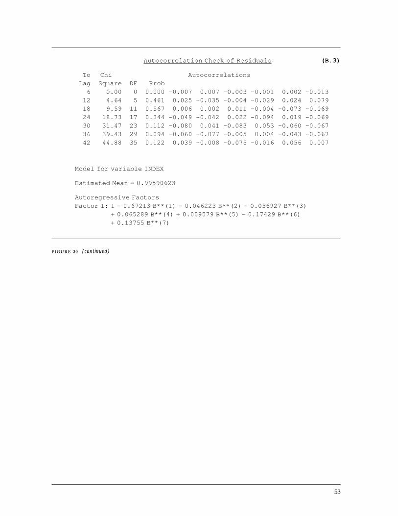
53

Autocorrelation Check of Residuals (B.3)

To Chi AutocorrelationsLag Square DF Prob6 0.00 0 0.000 -0.007 0.007 -0.003 -0.001 0.002 -0.01312 4.64 5 0.461 0.025 -0.035 -0.004 -0.029 0.024 0.07918 9.59 11 0.567 0.006 0.002 0.011 -0.004 -0.073 -0.06924 18.73 17 0.344 -0.049 -0.042 0.022 -0.094 0.019 -0.06930 31.47 23 0.112 -0.080 0.041 -0.083 0.053 -0.060 -0.06736 39.43 29 0.094 -0.060 -0.077 -0.005 0.004 -0.043 -0.06742 44.88 35 0.122 0.039 -0.008 -0.075 -0.016 0.056 0.007

Model for variable INDEX

Estimated Mean = 0.99590623

Autoregressive FactorsFactor 1: 1 - 0.67213 B**(1) - 0.046223 B**(2) - 0.056927 B**(3)

+ 0.065289 B**(4) + 0.009579 B**(5) - 0.17429 B**(6)+ 0.13755 B**(7)

20 (continued)

54

Time-Series Analysis: PROC ARIMAFit models to ring-index series.

ARIMA Procedure

Maximum Likelihood Estimation (C)

Approx.Parameter Estimate Std Error T Ratio LagMU 0.99568 0.02278 43.71 0AR1,1 0.70855 0.03339 21.22 1 (C.1)AR1,2 0.16708 0.04655 3.59 6AR1,3 -0.14479 0.04637 -3.12 7

Constant Estimate = 0.26799846

Variance Estimate = 0.01763278 (C.2)Std Error Estimate = 0.13278848AIC = -550.7613SBC = -534.21039Number of Residuals= 463

Correlations of the Estimates

Parameter MU AR1,1 AR1,2 AR1,3

MU 1.000 0.007 0.000 0.001AR1,1 0.007 1.000 -0.125 -0.092AR1,2 0.000 -0.125 1.000 -0.698AR1,3 0.001 -0.092 -0.698 1.000

Autocorrelation Check of Residuals (C.3)

To Chi AutocorrelationsLag Square DF Prob6 3.54 3 0.316 -0.043 0.024 0.066 -0.019 -0.014 -0.01412 8.09 9 0.525 0.017 -0.033 0.016 -0.033 0.017 0.08118 12.70 15 0.625 0.002 0.002 0.014 -0.009 -0.074 -0.06224 23.26 21 0.330 -0.053 -0.044 0.019 -0.104 0.026 -0.07030 37.40 27 0.088 -0.080 0.047 -0.096 0.050 -0.060 -0.06936 45.46 33 0.073 -0.050 -0.080 -0.015 0.004 -0.041 -0.07242 50.90 39 0.096 0.040 -0.007 -0.076 -0.011 0.056 -0.006

20 (continued)

55

Autocorrelation Plot of Residuals (C.4)

Lag Covariance Correlation -1 9 8 7 6 5 4 3 2 1 0 1 2 3 4 5 6 7 8 9 10 0.017633 1.00000 ********************1 -0.0007632 -0.04328 .* .2 0.00042402 0.02405 . .3 0.0011637 0.06600 . *.4 -0.0003339 -0.01894 . .5 -0.0002492 -0.01414 . .6 -0.0002487 -0.01410 . .7 0.00029504 0.01673 . .8 -0.0005798 -0.03288 .* .9 0.00028309 0.01605 . .10 -0.0005744 -0.03257 .* .

‘‘.’’ marks two standard errors

Inverse Autocorrelations

Lag Correlation -1 9 8 7 6 5 4 3 2 1 0 1 2 3 4 5 6 7 8 9 11 0.03989 . *.2 -0.02780 .* .3 -0.07089 .* .4 0.01846 . .5 0.01828 . .6 0.01898 . .7 -0.01985 . .8 0.02563 . *.9 -0.01135 . .10 0.03281 . *.

Partial Autocorrelations

Lag Correlation -1 9 8 7 6 5 4 3 2 1 0 1 2 3 4 5 6 7 8 9 11 -0.04328 .* .2 0.02222 . .3 0.06814 . *.4 -0.01380 . .5 -0.01898 . .6 -0.01931 . .7 0.01852 . .8 -0.02874 .* .9 0.01426 . .10 -0.03316 .* .

Model for variable INDEX

Estimated Mean = 0.995679

Autoregressive FactorsFactor 1: 1 - 0 0.70855 B**(1) - 0.16708 B**(6) = 0.14479 B**(7)

20 (concluded).

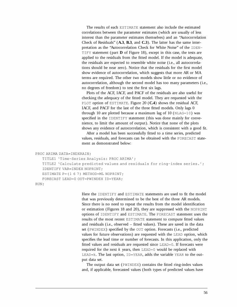
56

The results of each ESTIMATE statement also include the estimatedcorrelations between the parameter estimates (which are usually of lessinterest than the parameter estimates themselves) and an ‘‘AutocorrelationCheck of Residuals’’ (A.3, B.3, and C.3). The latter has the same inter-pretation as the ‘‘Autocorrelation Check for White Noise’’ of the IDEN-TIFY statement (part D of Figure 18), except in this case, the tests areapplied to the residuals from the fitted model. If the model is adequate,the residuals are expected to resemble white noise (i.e., all autocorrela-tions should be near zero). Notice that the residuals for the first modelshow evidence of autocorrelation, which suggests that more AR or MAterms are required. The other two models show little or no evidence ofautocorrelation, although the second model has too many parameters (i.e.,no degrees of freedom) to test the first six lags.

Plots of the ACF, IACF, and PACF of the residuals are also useful forchecking the adequacy of the fitted model. They are requested with thePLOT option of ESTIMATE. Figure 20 (C.4) shows the residual ACF,IACF, and PACF for the last of the three fitted models. Only lags 0through 10 are plotted because a maximum lag of 10 (NLAG=10) wasspecified in the IDENTIFY statement (this was done mainly for conve-nience, to limit the amount of output). Notice that none of the plotsshows any evidence of autocorrelation, which is consistent with a good fit.

After a model has been successfully fitted to a time series, predictedvalues, residuals, and forecasts can be obtained with the FORECAST state-ment as demonstrated below:

PROC ARIMA DATA=INDXRAIN;TITLE1 ‘Time-Series Analysis: PROC ARIMA’;TITLE2 ‘Calculate predicted values and residuals for ring-index series.’;IDENTIFY VAR=INDEX NOPRINT;ESTIMATE P=(1 6 7) METHOD=ML NOPRINT;FORECAST LEAD=0 OUT=PWINDEX ID=YEAR;

RUN;

Here the IDENTIFY and ESTIMATE statements are used to fit the modelthat was previously determined to be the best of the three AR models.Since there is no need to repeat the results from the model identificationor estimation (Figures 18 and 20), they are suppressed with the NOPRINToptions of IDENTIFY and ESTIMATE. The FORECAST statement uses theresults of the most recent ESTIMATE statement to compute fitted valuesand residuals (i.e., observed – fitted values). These are saved in the dataset (PWINDEX) specified by the OUT option. Forecasts (i.e., predictedvalues for future observations) are requested with the LEAD option, whichspecifies the lead time or number of forecasts. In this application, only thefitted values and residuals are requested since LEAD=0. If forecasts wererequired for the next k years, then LEAD=0 would be replaced withLEAD=k. The last option, ID=YEAR, adds the variable YEAR to the out-put data set.

The output data set (PWINDEX) contains the fitted ring-index valuesand, if applicable, forecasted values (both types of predicted values have

57

the variable name FORECAST), the corresponding estimated standarderrors (STD), upper (U95) and lower (L95) 95% confidence limits, theresiduals (RESIDUAL), and the identification variable YEAR. The residualsare the prewhitened values that were used to calculate the cross-correlo-gram shown in Figure 19. The rainfall series was prewhitened in the samemanner, by fitting a suitable time-series model and computing theresiduals.

The ARIMA procedure is extremely versatile. It can be used for explor-atory analyses (i.e., computation of the ACF, CCF, etc.), time-series mod-elling (including transfer function models and intervention models, aswell as ARIMA models), and forecasting. For more information about theIDENTIFY, ESTIMATE, and FORECAST statements of PROC ARIMA, andtheir various other options, the reader should consult the SAS/ETS User’sGuide (SAS Institute 1991a).

4.2.3 PROC AUTOREG The model on which PROC REG is based—theordinary least-squares regression model—assumes that the data are inde-pendent; that is,

yt = β 0 + β 1 x 1t + β 2 x 2t + . . . + βm xmt + εt

where the errors {εt } are independent and identically distributed normalrandom variables. When observations are made over time, the indepen-dence assumption may not be realistic. To allow for this possibility, PROCAUTOREG assumes that the errors are generated by an autoregression;that is,

εt = δt − α 1 εt − 1 − α 2 εt − 2 − . . . − αp εt − p

where {δt } are independent and identically distributed normal randomvariables. Notice that when there are no independent variables (i.e.,yt = β 0 + εt ), the model reduces to a simple autoregression:

yt = α 0 − α 1 yt − 1 − α 2 yt − 2 − . . . − αp yt − p + δt

with α 0 = β 0

To illustrate PROC AUTOREG, consider the final AR model that was fit-ted to ring-index series with PROC ARIMA. The same analysis can be per-formed with PROC AUTOREG as follows:

PROC AUTOREG DATA=INDXRAIN;TITLE1 ‘Time-Series Analysis: PROC AUTOREG’;TITLE2 ‘Fit model to ring-index series.’;MODEL INDEX=/NLAG=7 METHOD=ML;LAGLIST 1 6 7;OUTPUT OUT=RESID R=PWINDEX;

RUN;

58

The MODEL statement identifies the dependent response variable(INDEX) and the regressors x 1t , x 2t , . . . , xmt . In this example there areno regressors, but if there were they would be listed after the equals sign(e.g., MODEL INDEX=X1 X2;). The options NLAG and METHOD specify theorder of the autoregression for the error process and the method of esti-mation (ML = maximum likelihood estimation). A LAGLIST statement isalso required since the number of autoregressive parameters is less thanthe value specified by NLAG. It identifies the lagged terms that are to beincluded in the autoregression (if LAGLIST is omitted, all lags up to andincluding NLAG are selected). The OUTPUT statement identifies the outputdata set (RESID) and names the residuals (PWINDEX).

The output from PROC AUTOREG is presented in Figure 21. The firstpart (A) gives the ordinary least-squares estimates of the parameters(which are the same as the values that would be obtained with PROCREG) and the results of a diagnostic analysis of the residuals, includingthe Durbin-Watson statistic and sample ACF up to the lag specified byNLAG. Notice that the Durbin-Watson statistic (0.5685) is considerablyless than 2, which is the expected value under the null hypothesis of inde-pendent errors. This confirms the need for a model with autocorrelatederrors.

The second part (B) of the output lists preliminary estimates of themean square error and autoregressive parameters for the correlated-errorsmodel. These so-called ‘‘Yule-Walker’’ estimates are the starting values forthe iterative scheme that is used to obtain the maximum likelihood esti-mates, given in the last part of the output (C). The Yule-Walker estimatesare easier to calculate and are usually good first approximations to themaximum likelihood estimates. Notice that the standard error (0.02280)for the maximum likelihood estimate (C.1) is considerably larger than thecorresponding standard error (0.008923) for the ordinary least-squaresestimate of the intercept (A.1), even though the estimated intercepts areapproximately equal. Here, and in general, failure to account for autocor-relation among the observations causes the standard errors of the regres-sion coefficients to be underestimated. Notice also that the maximumlikelihood estimates of AR parameters and associated summary statistics(AIC, SBC, etc.) are the same as the values obtained with PROC ARIMA,apart from the sign reversal of the AR estimates, which reflects the differ-ent parameters used by the two procedures. The Durbin-Watson statisticprovides an additional check of the residuals, which is not available inPROC ARIMA. After fitting the AR model, the residuals no longer showevidence of autocorrelation (i.e., the Durbin-Watson statistic is close to 2).

4.2.4 PROC FORECAST The emphasis of PROC ARIMA and PROCAUTOREG is model development and hypothesis testing. In contrast, theprimary objective of PROC FORECAST is forecasting, without necessarilyunderstanding details of the process by which the data are generated.There are three methods for generating forecasts with PROC FORECAST: astepwise autoregressive method (STEPAR), exponential smoothing(EXPO), and the Holt-Winters method (WINTERS). The choice of methoddepends on the characteristics of the series—that is, the type of trend, if

59

Time-Series Analysis: PROC AUTOREGFit model to ring-index series.

Autoreg Procedure

Dependent Variable = INDEX Tree ring index

Ordinary Least Squares Estimates (A)

SSE 17.0303 DFE 462MSE 0.036862 Root MSE 0.191995SBC -209.091 AIC -213.228Reg Rsq 0.0000 Total Rsq 0.0000Durbin-Watson 0.5685

Variable DF B Value Std Error t Ratio Approx Prob

Intercept 1 0.996460043 0.008923 111.676 0.0001 (A.1)

Estimates of Autocorrelations

Lag Covariance Correlation -1 9 8 7 6 5 4 3 2 1 0 1 2 3 4 5 6 7 8 9 1

0 0.036782 1.000000 ********************1 0.026179 0.711727 **************2 0.02003 0.544552 ***********3 0.01596 0.433909 *********4 0.011755 0.319577 ******5 0.009626 0.261701 *****6 0.009216 0.250548 *****7 0.005767 0.156796 ***

Preliminary MSE = 0.017658

Estimates of the Autoregressive Parameters (B)

Lag Coefficient Std Error t Ratio1 -0.70299696 0.03365984 -20.8853346 -0.16280822 0.04638895 -3.5096337 0.13521321 0.04624735 2.923696

Expected Autocorrelations

Lag Autocorr0 1.00001 0.71152 0.51433 0.38324 0.30135 0.25816 0.24817 0.1550

21 Time-series analysis of ring-index series: PROC AUTOREG.

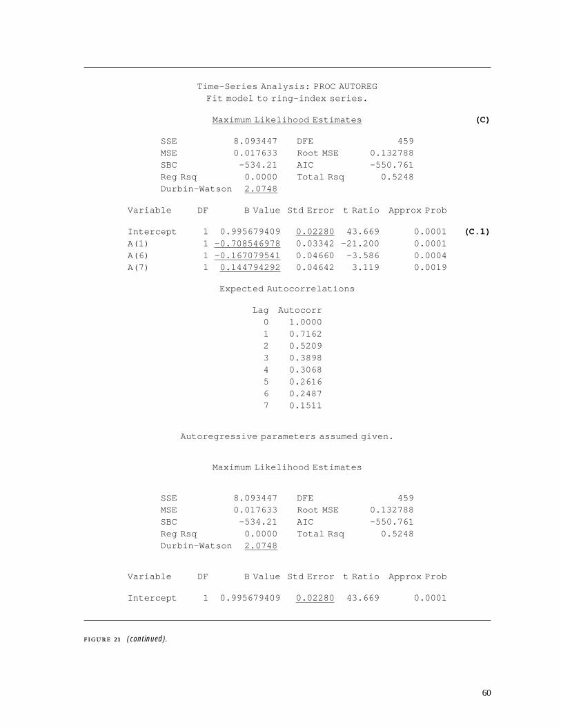
60

Time-Series Analysis: PROC AUTOREGFit model to ring-index series.

Maximum Likelihood Estimates (C)

SSE 8.093447 DFE 459MSE 0.017633 Root MSE 0.132788SBC -534.21 AIC -550.761Reg Rsq 0.0000 Total Rsq 0.5248Durbin-Watson 2.0748

Variable DF B Value Std Error t Ratio Approx Prob

Intercept 1 0.995679409 0.02280 43.669 0.0001 (C.1)A(1) 1 -0.708546978 0.03342 -21.200 0.0001A(6) 1 -0.167079541 0.04660 -3.586 0.0004A(7) 1 0.144794292 0.04642 3.119 0.0019

Expected Autocorrelations

Lag Autocorr0 1.00001 0.71622 0.52093 0.38984 0.30685 0.26166 0.24877 0.1511

Autoregressive parameters assumed given.

Maximum Likelihood Estimates

SSE 8.093447 DFE 459MSE 0.017633 Root MSE 0.132788SBC -534.21 AIC -550.761Reg Rsq 0.0000 Total Rsq 0.5248Durbin-Watson 2.0748

Variable DF B Value Std Error t Ratio Approx Prob

Intercept 1 0.995679409 0.02280 43.669 0.0001

21 (continued).

61

there is one, and the presence or absence of a seasonal component. Thestepwise AR method is applicable when there is no seasonal componentand the trend is adequately approximated by a deterministic linear orquadratic function (e.g., Figure 4a). If the series exhibits a stochastictrend (e.g., Figure 9a), exponential smoothing or the Holt-Wintersmethod can be used. The former is applicable when no seasonal compo-nent is present. When a seasonal component is present, the latter (whichis a seasonal version of exponential smoothing) should be used.

Forecasts for the ring-index series can be generated with PROC FORE-CAST, as follows:

PROC FORECAST DATA=INDXRAIN METHOD=STEPAR AR=7 TREND=1LEAD=5 OUT=FORECAST OUTLIMIT OUTEST=PARMS;

VAR INDEX;ID YEAR;

PROC PRINT DATA=PARMS;TITLE1 ‘Forecast ring-index series with PROC FORECAST.’;TITLE2 ‘Parameter estimates.’;

PROC PRINT DATA=FORECAST;TITLE ‘Forecast ring-index series with PROC FORECAST’;TITLE2 ‘Forecasts for 1993-1997.’;

RUN;

The PROC FORECAST line sets the options for generating forecasts andcontrols the output (refer to SAS/ETS User’s Guide [SAS Institute 1991a],for a complete list of options). In this case, the stepwise AR method is cho-sen (METHOD=STEPAR). The AR (or NLAGS) option selects the maximumorder for the fitted autoregression. Based on the previous analyses, AR=7 ischosen. If no estimate of the order is available, a large value should beassigned (the default is AR=13) and the order of the fitted autoregressiondetermined automatically. The order selection process is controlled by theoptions SLENTRY (significance level for entering a term) and SLSTAY (sig-nificance level for removing a term), as well as AR. In this case, SLSTAYand SLENTRY are omitted so the default values of 0.05 and 0.2 are used.The TREND option describes the type of the trend (1 = constant, 2 = linear,3 = quadratic) and LEAD specifies the number of time steps into the futureto be forecasted. Here LEAD=5 requests forecasts for the five years followingthe last observation (i.e., forecasts for the years 1993–1997). The three‘‘OUT’’ options control the output: OUT names the output data set for theforecasts, OUTLIMIT requests confidence limits for the forecasts, and OUT-EST names the data set for the parameter estimates.

The output from the preceding program is displayed in Figure 22. Thefirst part (A) lists the parameter estimates. Notice that an autoregressionwith lags 1, 6, and 7 is fitted (the missing values for lags 2–5 imply thatthose terms were dropped) and that estimated parameters are the same asthe preliminary Yule-Walker estimates calculated by PROC AUTOREG (partB of Figure 21). The forecasts for the years 1993 through 1997 (B), andthe corresponding 95% confidence limits, are printed after the parameterestimates.

62

Forecast ring-index series with PROC FORECAST. (A)Parameter estimates.

OBS TYPE YEAR INDEX1 N 1992 4632 SIGMA 1992 0.13346153 CONSTANT 1992 0.996464 AR1 1992 0.7029975 AR2 1992 .6 AR3 1992 .7 AR4 1992 .8 AR5 1992 .9 AR6 1992 0.162808210 AR7 1992 -0.135213

Forecast ring-index series with PROCFORECAST (B)

Forecasts for 1993-1997.

OBS YEAR TYPE LEAD INDEX

1 1993 FORECAST 1 1.150132 1993 L95 1 0.887693 1993 U95 1 1.412584 1994 FORECAST 2 1.098275 1994 L95 2 0.777826 1994 U95 2 1.418737 1995 FORECAST 3 1.043078 1995 L95 3 0.697539 1995 U95 3 1.3886210 1996 FORECAST 4 1.0503911 1996 L95 4 0.6930912 1996 U95 4 1.4076913 1997 FORECAST 5 1.0456514 1997 L95 5 0.6826915 1997 U95 5 1.40862

22 Ring-index forecasts generated with PROC FORECAST (METHOD=STEPAR).

5 SAS EXAMPLES

5.1 Repeated-measuresAnalysis of Seedling

Height Growth

The first example is an expanded analysis of the seedling data (Section1.1.1). In the previous analysis (Section 4.1), only seedlings grown fromlodgepole pine plugs were considered. The following SAS program carriesout both univariate and multivariate repeated-measures analyses of the

63

complete data set, and the corresponding analyses for each of the two spe-cies: Douglas-fir (FD) and lodgepole pine (PL). The analysis of the indi-vidual species includes an ANOVA of successive height increments (i.e.,the change in height from 1983 to 1984, 1984 to 1985, etc.). This is easilygenerated with the PROFILE transformation and SUMMARY option of theREPEATED statement. A MANOVA statement is added to test the statisticalsignificance of the overall mean of each increment. Part of the output isshown in Figure 23.

DATA SEEDLING; /* Read data in multivariate form. */INFILE ‘SURVIV.DAT’;INPUT SPP STK TRT BLK ROW TRENO PHT HT84-HT89;

PROC SORT DATA=SEEDLING; /* Sort data set and calculate row */BY SPP STK TRT BLK ROW; /* averages. */

PROC SUMMARY DATA=SEEDLING;BY SPP STK TRT BLK ROW;VAR PHT HT84-HT89;OUTPUT OUT=ROWMEANS MEAN=;

/* Repeated measures analysis of row *//* means - both species. */

PROC GLM DATA=ROWMEANS;TITLE ‘Repeated-Measures Analysis of Seedling Growth (Section 1.1.1)’;CLASS BLK TRT SPP STK;MODEL PHT HT84-HT89=BLK TRT SPP STK/SS3;REPEATED YEAR 7 (1983 1984 1985 1986 1987 1988 1989);

/* Repeated measures analysis of row *//* means - by species. */

PROC GLM DATA=ROWMEANS;TITLE1 ‘Repeated-Measures Analysis of Seedling Growth - by species’;BY SPP;CLASS BLK TRT STK;MODEL PHT HT84-HT89=BLK TRT STK/SS3;REPEATED YEAR 7 (1983 1984 1985 1986 1987 1988 1989) PROFILE/SUMMARY;MANOVA H=INTERCEPT E=BLK M=( 1 -1 0 0 0 0 0, 0 1 -1 0 0 0 0,

0 0 1 -1 0 0 0, 0 0 0 1 -1 0 0,0 0 0 0 1 -1 0, 0 0 0 0 0 1 -1)

MNAMES=INC1 INC2 INC3 INC4 INC5 INC6/SUMMARY;RUN;

The results of the analysis of the complete data set (not shown inFigure 23) suggest that site-preparation treatment, species, and stocktype have a nonadditive effect on the growth of seedlings (i.e., theYEAR*TRT*SPP*STK interaction is significant, which implies that theeffect of one factor depends on the other two). Analyzing each speciesseparately provides insight into the various effects.

The results of the multivariate within-rows analyses (Parts A and Cof Figure 23) suggest that treatment and stock type have a significant

64

Repeated-Measures Analysis of Seedling Growth - by species

--------------------------------- SPP=FD ---------------------------------

Manova Test Criteria and F Approximations for (A)the Hypothesis of no YEAR*BRT Effect

H = Type III SS&CP Matrix for YEAR*BRT E = Error SS&CP Matrix

S=3 M=1 N=4

Statistic Value F Num DF Den DF Pr > F

Wilks’ Lambda 0.35327581 0.7107 18 28.76955 0.7734Pillai’s Trace 0.78357175 0.7071 18 36 0.7816Hotelling-Lawley Trace 1.45319704 0.6997 18 26 0.7814Roy’s Greatest Root 1.13784264 2.2757 6 12 0.1062

NOTE: F Statistic for Roy’s Greatest Root is an upper bound.

Manova Test Criteria and F Approximations forthe Hypothesis of no YEAR*TRT Effect

H = Type III SS&CP Matrix for YEAR*TRT E = Error SS&CP Matrix

S=2 M=1.5 N=4

Statistic Value F Num DF Den DF Pr > F

Wilks’ Lambda 0.08931022 3.9103 12 20 0.0035Pillai’s Trace 1.39068228 4.1843 12 22 0.0018Hotelling-Lawley Trace 4.82248581 3.6169 12 18 0.0070Roy’s Greatest Root 3.07430517 5.6362 6 11 0.0068

NOTE: F Statistic for Roy’s Greatest Root is an upper bound.NOTE: F Statistic for Wilks’ Lambda is exact.

Manova Test Criteria and Exact F Statistics forthe Hypothesis of no YEAR*STK Effect

H = Type III SS&CP Matrix for YEAR*STK E = Error SS&CP Matrix

S=1 M=2 N=4

Statistic Value F Num DF Den DF Pr > F

Wilks’ Lambda 0.09360369 16.1389 6 10 0.0001Pillai’s Trace 0.90639631 16.1389 6 10 0.0001Hotelling-Lawley Trace 9.68333917 16.1389 6 10 0.0001Roy’s Greatest Root 9.68333917 16.1389 6 10 0.0001

23 Repeated-measures analysis of the growth of Douglas-fir (FD) and lodgepole pine (PL) seedlings.

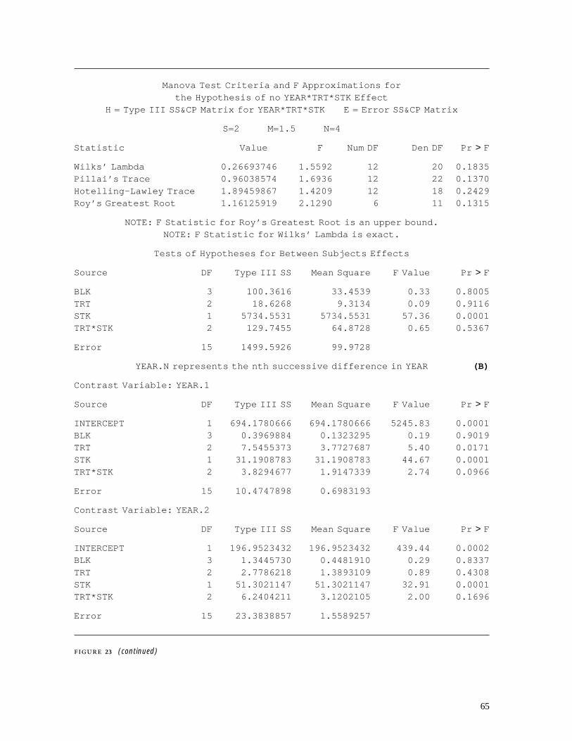
65

Manova Test Criteria and F Approximations forthe Hypothesis of no YEAR*TRT*STK Effect

H = Type III SS&CP Matrix for YEAR*TRT*STK E = Error SS&CP Matrix

S=2 M=1.5 N=4

Statistic Value F Num DF Den DF Pr > F

Wilks’ Lambda 0.26693746 1.5592 12 20 0.1835Pillai’s Trace 0.96038574 1.6936 12 22 0.1370Hotelling-Lawley Trace 1.89459867 1.4209 12 18 0.2429Roy’s Greatest Root 1.16125919 2.1290 6 11 0.1315

NOTE: F Statistic for Roy’s Greatest Root is an upper bound.NOTE: F Statistic for Wilks’ Lambda is exact.

Tests of Hypotheses for Between Subjects Effects

Source DF Type III SS Mean Square F Value Pr > F

BLK 3 100.3616 33.4539 0.33 0.8005TRT 2 18.6268 9.3134 0.09 0.9116STK 1 5734.5531 5734.5531 57.36 0.0001TRT*STK 2 129.7455 64.8728 0.65 0.5367

Error 15 1499.5926 99.9728

YEAR.N represents the nth successive difference in YEAR (B)

Contrast Variable: YEAR.1

Source DF Type III SS Mean Square F Value Pr > F

INTERCEPT 1 694.1780666 694.1780666 5245.83 0.0001BLK 3 0.3969884 0.1323295 0.19 0.9019TRT 2 7.5455373 3.7727687 5.40 0.0171STK 1 31.1908783 31.1908783 44.67 0.0001TRT*STK 2 3.8294677 1.9147339 2.74 0.0966

Error 15 10.4747898 0.6983193

Contrast Variable: YEAR.2

Source DF Type III SS Mean Square F Value Pr > F

INTERCEPT 1 196.9523432 196.9523432 439.44 0.0002BLK 3 1.3445730 0.4481910 0.29 0.8337TRT 2 2.7786218 1.3893109 0.89 0.4308STK 1 51.3021147 51.3021147 32.91 0.0001TRT*STK 2 6.2404211 3.1202105 2.00 0.1696

Error 15 23.3838857 1.5589257

23 (continued)

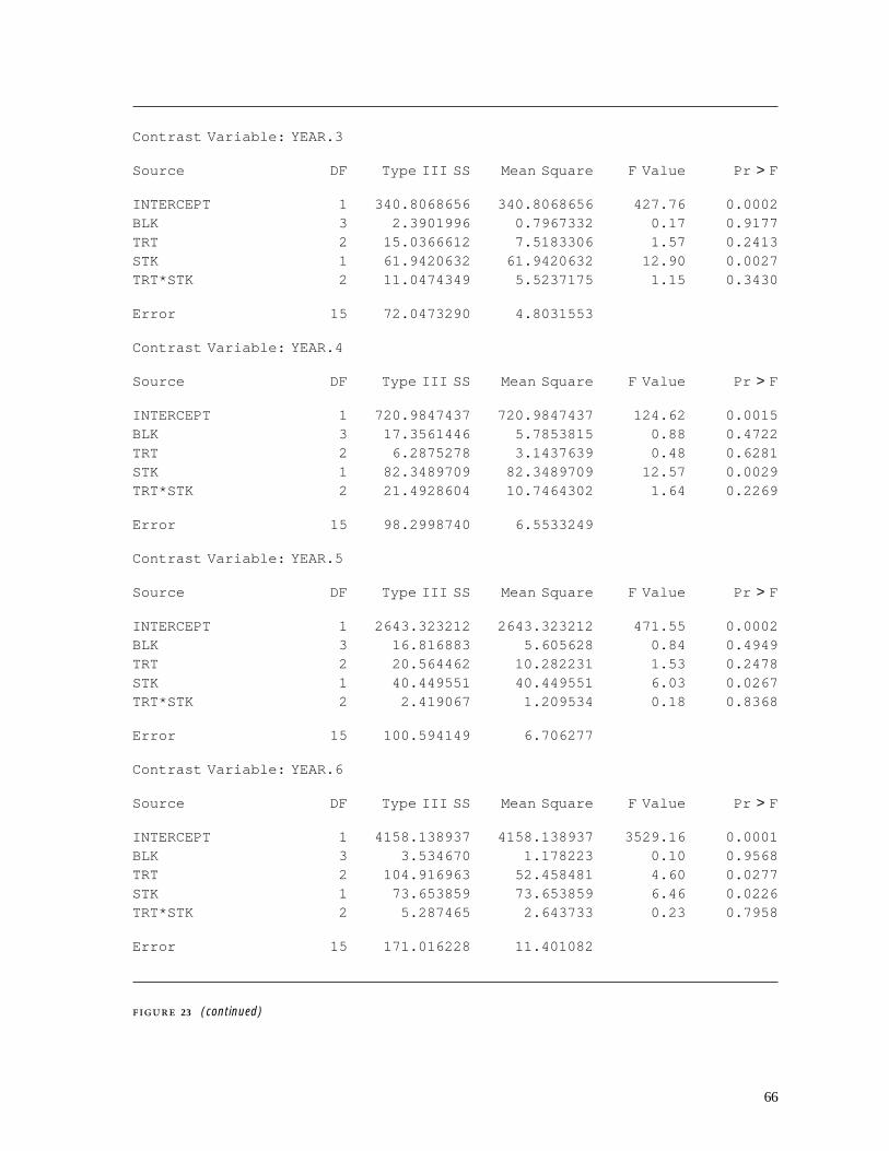
66

Contrast Variable: YEAR.3

Source DF Type III SS Mean Square F Value Pr > F

INTERCEPT 1 340.8068656 340.8068656 427.76 0.0002BLK 3 2.3901996 0.7967332 0.17 0.9177TRT 2 15.0366612 7.5183306 1.57 0.2413STK 1 61.9420632 61.9420632 12.90 0.0027TRT*STK 2 11.0474349 5.5237175 1.15 0.3430

Error 15 72.0473290 4.8031553

Contrast Variable: YEAR.4

Source DF Type III SS Mean Square F Value Pr > F

INTERCEPT 1 720.9847437 720.9847437 124.62 0.0015BLK 3 17.3561446 5.7853815 0.88 0.4722TRT 2 6.2875278 3.1437639 0.48 0.6281STK 1 82.3489709 82.3489709 12.57 0.0029TRT*STK 2 21.4928604 10.7464302 1.64 0.2269

Error 15 98.2998740 6.5533249

Contrast Variable: YEAR.5

Source DF Type III SS Mean Square F Value Pr > F

INTERCEPT 1 2643.323212 2643.323212 471.55 0.0002BLK 3 16.816883 5.605628 0.84 0.4949TRT 2 20.564462 10.282231 1.53 0.2478STK 1 40.449551 40.449551 6.03 0.0267TRT*STK 2 2.419067 1.209534 0.18 0.8368

Error 15 100.594149 6.706277

Contrast Variable: YEAR.6

Source DF Type III SS Mean Square F Value Pr > F

INTERCEPT 1 4158.138937 4158.138937 3529.16 0.0001BLK 3 3.534670 1.178223 0.10 0.9568TRT 2 104.916963 52.458481 4.60 0.0277STK 1 73.653859 73.653859 6.46 0.0226TRT*STK 2 5.287465 2.643733 0.23 0.7958

Error 15 171.016228 11.401082

23 (continued)

67

Repeated-Measures Analysis of Seedling Growth - by species

--------------------------------- SPP=PL ---------------------------------

Manova Test Criteria and F Approximations for (C)the Hypothesis of no YEAR*BLK Effect

H = Type III SS&CP Matrix for YEAR*BLK E = Error SS&CP Matrix

S=3 M=1 N=4

Statistic Value F Num DF Den DF Pr > F

Wilks’ Lambda 0.19910807 1.2296 18 28.76955 0.3025Pillai’s Trace 1.16471225 1.2692 18 36 0.2640Hotelling-Lawley Trace 2.40797089 1.1594 18 26 0.3576Roy’s Greatest Root 1.62683040 3.2537 6 12 0.0389

NOTE: F Statistic for Roy’s Greatest Root is an upper bound.

Manova Test Criteria and F Approximations forthe Hypothesis of no YEAR*TRT Effect

H = Type III SS&CP Matrix for YEAR*TRT E = Error SS&CP Matrix

S=2 M=1.5 N=4

Statistic Value F Num DF Den DF Pr > F

Wilks’ Lambda 0.03787338 6.8974 12 20 0.0001Pillai’s Trace 1.55376510 6.3836 12 22 0.0001Hotelling-Lawley Trace 9.78228222 7.3367 12 18 0.0001Roy’s Greatest Root 7.77242156 14.2494 6 11 0.0001

NOTE: F Statistic for Roy’s Greatest Root is an upper bound.NOTE: F Statistic for Wilks’ Lambda is exact.

Manova Test Criteria and Exact F Statistics forthe Hypothesis of no YEAR*STK Effect

H = Type III SS&CP Matrix for YEAR*STK E = Error SS&CP Matrix

S=1 M=2 N=4

Statistic Value F Num DF Den DF Pr > F

Wilks’ Lambda 0.18244512 7.4685 6 10 0.0031Pillai’s Trace 0.81755488 7.4685 6 10 0.0031Hotelling-Lawley Trace 4.48110016 7.4685 6 10 0.0031Roy’s Greatest Root 4.48110016 7.4685 6 10 0.0031

23 (continued)

68

Manova Test Criteria and F Approximations forthe Hypothesis of no YEAR*TRT*STK Effect

H = Type III SS&CP Matrix for YEAR*TRT*STK E = Error SS&CP Matrix

S=2 M=1.5 N=4

Statistic Value F Num DF Den DF Pr > F

Wilks’ Lambda 0.40010042 0.9682 12 20 0.5072Pillai’s Trace 0.68713772 0.9595 12 22 0.5119Hotelling-Lawley Trace 1.28133196 0.9610 12 18 0.5154Roy’s Greatest Root 1.07931424 1.9787 6 11 0.1547

NOTE: F Statistic for Roy’s Greatest Root is an upper bound.NOTE: F Statistic for Wilks’ Lambda is exact.

Tests of Hypotheses for Between Subjects Effects

Source DF Type III SS Mean Square F Value Pr > F

BLK 3 310.8867 103.6289 0.80 0.5144TRT 2 5176.6388 2588.3194 19.91 0.0001STK 1 2069.3402 2069.3402 15.92 0.0012TRT*STK 2 35.1474 17.5737 0.14 0.8746

Error 15 1949.8385 129.9892

YEAR.N represents the nth successive difference in YEAR (D)

Contrast Variable: YEAR.1

Source DF Type III SS Mean Square F Value Pr > F

INTERCEPT 1 1148.722693 1148.722693 278.69 0.0005BLK 3 12.365716 4.121905 3.61 0.0384TRT 2 12.682957 6.341478 5.55 0.0157STK 1 32.713768 32.713768 28.65 0.0001TRT*STK 2 2.137003 1.068502 0.94 0.4140

Error 15 17.128055 1.141870

Contrast Variable: YEAR.2

Source DF Type III SS Mean Square F Value Pr > F

INTERCEPT 1 3306.602159 3306.602159 1882.02 0.0001BLK 3 5.270843 1.756948 0.73 0.5488TRT 2 28.463329 14.231665 5.93 0.0127STK 1 47.177524 47.177524 19.66 0.0005TRT*STK 2 4.344947 2.172474 0.91 0.4254

Error 15 35.996519 2.399768

23 (continued)

69

Contrast Variable: YEAR.3

Source DF Type III SS Mean Square F Value Pr > F

INTERCEPT 1 6335.366338 6335.366338 9195.68 0.0001BLK 3 2.066852 0.688951 0.11 0.9544TRT 2 81.064714 40.532357 6.33 0.0102STK 1 20.249735 20.249735 3.16 0.0957TRT*STK 2 25.405195 12.702598 1.98 0.1722

Error 15 96.094158 6.406277

Contrast Variable: YEAR.4

Source DF Type III SS Mean Square F Value Pr > F

INTERCEPT 1 10941.23603 10941.23603 12593.09 0.0001BLK 3 2.60649 0.86883 0.06 0.9817TRT 2 716.78647 358.39323 23.27 0.0001STK 1 129.45717 129.45717 8.40 0.0110TRT*STK 2 1.71725 0.85863 0.06 0.9460

Error 15 231.04136 15.40276

Contrast Variable: YEAR.5

Source DF Type III SS Mean Square F Value Pr > F

INTERCEPT 1 23787.47161 23787.47161 1770.44 0.0001BLK 3 40.30773 13.43591 1.11 0.3754TRT 2 740.50850 370.25425 30.63 0.0001STK 1 221.90586 221.90586 18.36 0.0007TRT*STK 2 3.33963 1.66982 0.14 0.8721

Error 15 181.31448 12.08763

Contrast Variable: YEAR.6

Source DF Type III SS Mean Square F Value Pr > F

INTERCEPT 1 39922.99305 39922.99305 1577.06 0.0001BLK 3 75.94464 25.31488 2.26 0.1233TRT 2 794.08672 397.04336 35.46 0.0001STK 1 279.89157 279.89157 25.00 0.0002TRT*STK 2 9.53943 4.76972 0.43 0.6608

Error 15 167.96039 11.19736

23 (concluded).

70

additive effect on the growth of both species (i.e., the YEAR*STK andYEAR*TRT interactions are significant for both species but theYEAR*TRT*STK interaction is not). The analysis of the annual incre-ments (B and D), which are labelled YEAR.1 (1983 height–1984 height),YEAR.2 (1984 height–1985 height), etc., are even more informative. Toreduce the amount of output, the ANOVA tables for the increments havebeen modified by replacing the default test for the MEAN (i.e., the testproduced by the REPEATED statement, which is incorrect for a ran-domized block design) with the correct MANOVA test (labelled INTER-CEPT). For convenience, the p-values for the corrected analyses have beenextracted from the output and are summarized in Table 2. Notice thatstock type appears to have a more significant and persistent effect on theDouglas-fir seedlings than the method of site preparation. However, bothfactors have an important and apparently prolonged effect on the growthof lodgepole pine seedlings.

2 Analysis of annual height increments: summary of p-values (p-values lessthan 0.05 are underlined)

Source 1983–84 1984–85 1985–86 1986–87 1987–88 1988–89

Douglas-firINTERCEPT 0.0001 0.0002 0.0002 0.0015 0.0002 0.0001BLK 0.9019 0.8337 0.9177 0.4722 0.4949 0.9568TRT 0.0171 0.4308 0.2413 0.6281 0.2478 0.0277STK 0.0001 0.0001 0.0027 0.0029 0.0267 0.0226TRT*STK 0.0966 0.1696 0.3430 0.2269 0.8368 0.7958

Lodgepole pineINTERCEPT 0.0005 0.0001 0.0001 0.0001 0.0001 0.0001BLK 0.0384 0.5488 0.9544 0.9817 0.3754 0.1233TRT 0.0157 0.0127 0.0102 0.0001 0.0001 0.0001STK 0.0001 0.0005 0.0957 0.0110 0.0007 0.0002TRT*STK 0.4140 0.4254 0.1722 0.9460 0.8721 0.6608

5.2 Cross-correlationAnalysis of Missing

Tree Rings

The second example is a cross-correlation analysis of the tree-ring seriesshown in Figure 2a and 2b. The objective is to find the number of yearsby which the lower series must be shifted relative to the upper series toachieve the best alignment, or maximum cross-correlation, of the growthpatterns. Before calculating the cross-correlation function, the confound-ing effects of trend and autocorrelation must be eliminated.

An SAS program for carrying out the preliminary detrending and pre-whitening of the individual series and the final cross-correlation analysis islisted below. First, a log transformation is applied to each series to convertthe exponential trend into a linear trend. This has the added effect of sta-bilizing the variance. Next a trend line is fitted to each series with PROCREG (PROC AUTOREG could also be used). Subtraction of the trend pro-duces a detrended ring index or, in this case, the log of the ring index.Prewhitening is accomplished by fitting a first-order autoregression toeach ring-index series. (A preliminary model identification step suggestedthat both ring-index series are adequately described by a first-order auto-

71

regression.) The prewhitened series are calculated by including a FORE-CAST statement in the PROC ARIMA step (refer to Section 4.2.2). Thissaves the residuals from the fitted autoregressions, which are the requiredprewhitened values. Finally, the two prewhitened series are cross-correlatedin a third application of PROC ARIMA.

/* Read data from input file and *//* apply log transformation. */

DATA TREE94;TITLE ‘Example 1.1.2: Cross-Correlation Analysis of Missing Tree Rings’;INFILE ‘TREE94.DAT’ MISSOVER;INPUT DISKHT 21-25 YEAR 29-32 RINGNO 34-36 RNGWIDTH 39-43;LOGRW=LOG(RNGWIDTH);

/* Fit trend line to each series. */PROC SORT DATA=TREE94;

BY DISKHT;PROC REG NOPRINT;

BY DISKHT;MODEL LOGRW=RINGNO;

OUTPUT OUT=TREND P=RNGTREND;/* Subtract trend from each series*//* and convert data to multi- *//* variate form. */

PROC SORT DATA=TREND;BY YEAR DISKHT;

PROC SORT DATA=TREE94;BY YEAR DISKHT;

DATA RINGS94 (KEEP=YEAR RW1-RW13 LR1-LR13 RI1-RI13 RT1-RT13);MERGE TREE94 TREND;BY YEAR DISKHT;RETAIN;ARRAY DISK HT1-HT13 (20 18 16 14 12 10 8 5.9 4 2 1.3 0.7 0.3);ARRAY RING RW1-RW13;ARRAY LOGRING LR1-LR13;ARRAY TREND RT1-RT13;ARRAY RNGINDX RI1-RI13;IF FIRST.YEAR THEN DO I=1 TO 13;

RING(I)=.;LOGRING(I)=.;RNGINDX(I)=.;TREND(I)=.;

END;DO I=1 TO 13;

IF DISKHT=DISK(I) THEN DO;RING(I)=RNGWIDTH;LOGRING(I)=LOGRW;TREND(I)=RNGTREND;RNGINDX(I)=LOGRING(I)-TREND(I);

END;

72

END;IF LAST.YEAR THEN OUTPUT;

/* Prewhiten detrended series for *//* disks at 2.0 and 1.3 meters. */

PROC SORT DATA=RINGS94;BY YEAR;

PROC ARIMA DATA=RINGS94;TITLE ‘Prewhiten first series (disk at 2.0m)’;IDENTIFY VAR=RI10 NOPRINT;ESTIMATE P=1 NOPRINT;FORECAST LEAD=0 BACK=0 OUT=RES10 ID=YEAR;

PROC ARIMA DATA=RINGS94;TITLE ‘Prewhiten second series (disk at 1.3m)’;IDENTIFY VAR=RI11 NOPRINT;ESTIMATE P=1 NOPRINT;FORECAST LEAD=0 BACK=0 OUT=RES11 ID=YEAR;

/* Merge residual data sets. */DATA PWINDX94;

MERGE RES10(RENAME=(RESIDUAL=PW10)) RES11(RENAME=(RESIDUAL=PW11));BY YEAR;

/* Cross-correlate detrended, *//* prewhitened series. */

PROC ARIMA DATA=PWINDX94;TITLE ‘Cross-correlation analysis of prewhitened ring-index series’;IDENTIFY VAR=PW11 CROSSCOR=PW10;

RUN;

The results of the preceding analysis are displayed in Figure 24. The fit-ted first-order autoregressions that were used to prewhiten the two ring-index series are given in the first two sections (A and B). Output fromthe cross-correlation analysis (third PROC ARIMA statement) is given next(C). This includes the ACF, IACF, and PACF (C.1–C.3) of the pre-whitened ring-index series for the disk at 1.3 m (i.e., the variable namedin the VAR option of the IDENTIFY statement) and the correspondingautocorrelation test for randomness (C.4). Notice that all of these checksare consistent with a white noise or a purely random series. This confirmsthe effectiveness of the detrending and prewhitening procedure. The samechecks can be applied to the other series by including another IDENTIFYstatement with VAR=PW10.

The key part of the output is the cross-correlation function for the twoseries (C.5). Inspection of the cross-correlation function reveals a clearspike at a lag of −5 years. This suggests that the best alignment of the twoseries occurs when the series for the lower disk (PW11) is shifted to theleft by 5 years. In other words, the five outer rings of the upper disk aremissing in the lower disk and the year of the innermost ring of that diskmust be adjusted accordingly. The same analysis can be applied to allpairs of disks and the results used to obtain a corrected estimate of theyear of the innermost ring of each disk. The effect of these corrections isillustrated in Figures 2c and 2d.

73

Prewhiten first series (disk at 1.3m)

ARIMA Procedure

Model for variable RI10 (A)

Estimated Mean = -0.0957115

Autoregressive FactorsFactor 1: 1 0.68642 B**(1)

Prewhiten second series (disk at 2.0m)

ARIMA Procedure

Model for variable RI11 (B)

Estimated Mean = -0.1387615

Autoregressive FactorsFactor 1: 1 - 0.75888 B**(1)

24 Cross-correlation analysis of missing tree rings.

74

Cross-correlation analysis of prewhitened ring-index series (C)

ARIMA Procedure

Name of variable = PW11.

Mean of working series = 0.02743Standard deviation = 0.372727Number of observations = 106

Autocorrelations (C.1)

Lag Covariance Correlation -1 9 8 7 6 5 4 3 2 1 0 1 2 3 4 5 6 7 8 9 10 0.138925 1.00000 ********************1 -0.0072260 -0.05201 . * .2 -0.0027024 -0.01945 . .3 0.019128 0.13769 . ***.4 -0.0009828 -0.00707 . .5 -0.0019721 -0.01420 . .6 -0.0062541 -0.04502 . * .7 -0.0014004 -0.01008 . .8 -0.016739 -0.12049 . ** .9 0.0010574 0.00761 . .10 0.0029933 0.02155 . .11 -0.029235 -0.21043 **** .12 -0.0062555 -0.04503 . * .13 0.0050624 0.03644 . * .14 -0.0076410 -0.05500 . * .15 0.0040052 0.02883 . * .16 -0.015233 -0.10965 . ** .17 0.017330 0.12474 . ** .18 0.009667 0.06958 . * .19 -0.0025763 -0.01854 . .20 -0.0060426 -0.04350 . * .21 -0.012409 -0.08932 . ** .22 0.011612 0.08358 . ** .23 -0.015190 -0.10934 . ** .24 -0.0064761 -0.04662 . * .

‘‘.’’ marks two standard errors

24 (continued)

75

Inverse Autocorrelations (C.2)

Lag Correlation -1 9 8 7 6 5 4 3 2 1 0 1 2 3 4 5 6 7 8 9 11 0.06895 . * .2 0.00465 . .3 -0.08517 . ** .4 0.04779 . * .5 0.04779 . * .6 -0.00019 . .7 0.02669 . * .8 0.12002 . ** .9 0.00915 . .10 0.02568 . * .11 0.16505 . ***.12 0.11763 . ** .13 -0.00310 . .14 0.04324 . * .15 0.02690 . * .16 0.11930 . ** .17 -0.10980 . ** .18 -0.06740 . * .19 0.04166 . * .20 0.06931 . * .21 0.08527 . ** .22 -0.01543 . .23 0.09676 . ** .24 0.04462 . * .

24 (continued)

76

Partial Autocorrelations (C.3)

Lag Correlation -1 9 8 7 6 5 4 3 2 1 0 1 2 3 4 5 6 7 8 9 11 -0.05201 . * .2 -0.02222 . .3 0.13593 . ***.4 0.00676 . .5 -0.00971 . .6 -0.06641 . * .7 -0.01644 . .8 -0.12308 . ** .9 0.01049 . .10 0.02302 . .11 -0.18193 **** .12 -0.07550 . ** .13 0.01537 . .14 -0.01694 . .15 0.04037 . * .16 -0.13835 .*** .17 0.10932 . ** .18 0.06625 . * .19 -0.02336 . .20 -0.09580 . ** .21 -0.11291 . ** .22 0.03130 . * .23 -0.10579 . ** .24 -0.05140 . * .

Autocorrelation Check for White Noise (C.4)

To Chi AutocorrelationsLag Square DF Prob6 2.70 6 0.845 -0.052 -0.019 0.138 -0.007 -0.014 -0.04512 10.06 12 0.611 -0.010 -0.120 0.008 0.022 -0.210 -0.04518 14.86 18 0.671 0.036 -0.055 0.029 -0.110 0.125 0.07024 19.14 24 0.745 -0.019 -0.043 -0.089 0.084 -0.109 -0.047

24 (continued)

77

Correlation of PW11 and PW10 (C.5)Variance of input = 0.112964Number of observations = 99

Crosscorrelations

Lag Covariance Correlation -1 9 8 7 6 5 4 3 2 1 0 1 2 3 4 5 6 7 8 9 1-21 -0.014955 -0.12510 .*** .-20 0.0034147 0.02856 . * .-19 -0.0016700 -0.01397 . .-18 -0.0021975 -0.01838 . .-17 -0.019465 -0.16283 .*** .-16 -0.018676 -0.15623 .*** .-15 0.017216 0.14401 . ***.-14 -0.014613 -0.12224 . ** .-13 -0.010219 -0.08549 . ** .-12 0.0020309 0.01699 . .-11 -0.012335 -0.10319 . ** .-10 0.0018776 0.01571 . .-9 0.0066333 0.05549 . * .-8 0.0031654 0.02648 . * .-7 0.0068038 0.05692 . * .-6 0.0064057 0.05359 . * .-5 0.060589 0.50684 . **********-4 -0.0094345 -0.07892 . ** .-3 0.020050 0.16772 . ***.-2 0.022023 0.18423 . ****-1 0.00031661 0.00265 . .0 -0.0004457 -0.00373 . .1 0.0049424 0.04134 . * .2 0.0018182 0.01521 . .3 -0.012707 -0.10630 . ** .4 -0.0063191 -0.05286 . * .5 0.0056615 0.04736 . * .6 -0.029310 -0.24519 ***** .7 0.020149 0.16855 . ***.8 -0.026690 -0.22327 **** .9 0.0019742 0.01651 . .10 -0.0020306 -0.01699 . .11 -0.012346 -0.10327 . ** .12 0.0063665 0.05326 . * .13 0.011237 0.09400 . ** .14 -0.0013013 -0.01089 . .15 -0.010942 -0.09153 . ** .16 -0.0004128 -0.00345 . .17 -0.0037202 -0.03112 . * .18 -0.022580 -0.18889 **** .19 -0.00034 -0.00284 . .20 0.0064959 0.05434 . * .21 -0.013566 -0.11348 . ** .

‘‘.’’ marks two standard errors

24 (concluded).

78

6 CONCLUSIONS

Repeated measurements of the same experimental unit or process areoften correlated and require special methods of analysis. If the number ofobservation times is relatively small and the objective is to compare trendsfor several treatment groups, then repeated-measures ANOVA is applica-ble. There are two types of repeated-measures ANOVA—one is based on asplit-plot univariate model and the other on a multivariate model. Themultivariate model is less restrictive than the univariate model, but theassociated statistical tests may lack power because there are more param-eters to estimate and therefore fewer degrees of freedom. When the datado not satisfy the correlation assumptions of the univariate model,another alternative is to apply the Greenhouse-Geisser or Huynh-Feldtcorrection to the univariate tests. Both univariate and multivariaterepeated-measures analyses are available in PROC GLM and PROC ANOVAof the SAS system. They are requested with the REPEATED statement,which also provides a range of options for comparing polynomial trendsand other contrasts over time.

Time series have various properties that are of interest to researchers,including the presence or absence of trend, seasonality, and other types ofnonstationarity, and for stationary time series, the presence or absence ofshort-term autocorrelation. Many statistical methods are available for theanalysis of univariate time series. The time plot, correlogram, and samplePACF and IACF are useful for describing a time series, and are valuabletools for outlier detection, model identification, and verification. Trendand cyclic components can be described or removed by regression meth-ods, or by smoothing the series. If the objective is model development orforecasting, then the Box-Jenkins procedure can be used to fit and predictstationary and nonstationary ARIMA processes. Alternative forecastingmethods include stepwise autoregression, exponential smoothing, and theHolt-Winters method. The SAS/ETS library provides a full range of time-series analyses. There are three main procedures for analyzing time seriesin the time domain: PROC ARIMA, PROC AUTOREG, and PROC FORE-CAST, and a fourth procedure, PROC EXPAND, can be used to aggregate,interpolate, or otherwise manipulate a time series in preparation foranalysis.

79

APPENDIX 1 Average height of seedlings

Average height (cm)a

Spp. Stk. Trt. Blk. Row Initial 1984 1985 1986 1987 1988 1989

FD B S 1 12 18.78 22.89 22.44 22.89 22.44 27.56 33.56FD B S 2 10 15.92 20.08 21.50 24.75 28.42 39.67 53.67FD B S 3 10 20.80 26.60 28.20 27.90 36.90 48.30 59.80FD B S 4 4 18.60 22.60 21.40 23.00 22.20 30.60 39.80FD B U 1 1 14.10 18.40 20.80 24.70 29.00 40.80 57.70FD B U 2 12 17.00 21.00 22.00 18.00 20.00 22.00 25.00FD B U 3 9 18.00 22.22 25.22 27.56 29.33 38.67 49.67FD B U 4 9 18.14 23.29 25.36 28.36 30.07 38.00 48.50FD B V 1 10 16.14 19.81 22.10 25.95 33.43 45.76 59.19FD B V 2 2 14.89 19.28 21.11 25.78 30.28 39.89 53.83FD B V 3 5 15.08 18.08 19.77 23.08 27.08 37.38 52.08FD B V 4 8 19.00 23.06 24.24 28.12 34.47 45.35 58.12FD P S 1 5 18.94 26.71 31.06 33.24 42.00 54.12 65.94FD P S 2 8 22.82 28.91 34.05 39.91 47.32 59.50 75.64FD P S 3 3 22.90 28.15 32.95 39.05 49.20 62.60 74.85FD P S 4 5 20.59 25.65 30.12 33.35 39.53 49.29 61.65FD P U 1 8 21.56 29.22 31.17 38.00 43.83 54.72 66.78FD P U 2 5 20.47 27.11 33.16 39.95 46.74 57.37 70.79FD P U 3 6 19.05 27.52 31.33 37.95 46.62 56.95 68.52FD P U 4 3 16.29 24.71 31.05 35.76 43.48 55.62 70.86FD P V 1 6 18.08 23.63 28.54 37.08 47.83 64.75 86.75FD P V 2 6 20.88 26.58 30.50 35.88 42.83 53.71 70.58FD P V 3 2 20.19 25.94 28.38 32.38 37.06 48.63 67.63FD P V 4 11 20.40 26.25 30.00 34.25 38.35 49.05 65.30PL B S 1 11 12.44 20.28 34.67 49.83 65.78 90.83 125.17PL B S 2 7 16.33 22.00 32.00 47.33 58.33 81.73 113.07PL B S 3 4 11.32 20.05 32.45 47.45 66.77 96.32 132.55PL B S 4 7 11.11 16.37 28.74 44.11 65.79 94.05 130.74PL B U 1 7 12.40 17.40 26.50 36.80 49.60 75.80 109.90PL B U 2 11 13.44 18.44 24.75 41.00 54.31 80.00 111.56PL B U 3 1 14.19 19.44 29.63 48.38 62.25 86.69 120.31PL B U 4 10 15.22 20.61 29.61 41.83 55.06 70.72 97.78PL B V 1 4 12.31 17.08 26.38 41.46 64.08 100.38 147.62PL B V 2 4 13.94 19.00 28.41 46.41 81.94 118.41 166.18PL B V 3 8 11.53 18.58 29.68 45.47 70.89 105.47 150.32PL B V 4 2 12.63 16.63 27.06 43.75 67.38 103.06 146.75PL P S 1 3 12.43 23.19 36.71 55.29 75.71 109.48 155.76PL P S 2 9 10.23 18.59 33.91 53.59 74.09 108.27 150.64PL P S 3 12 9.59 17.82 32.05 49.86 69.50 97.59 133.55PL P S 4 1 13.48 21.70 34.26 48.22 73.39 103.83 141.48PL P U 1 2 12.00 22.86 34.38 49.00 71.10 105.05 148.71PL P U 2 3 9.43 17.14 30.10 43.33 60.95 87.24 125.67PL P U 3 7 8.15 15.95 28.60 39.65 58.75 89.00 129.40PL P U 4 12 8.75 15.70 27.45 42.55 58.45 85.55 123.85PL P V 1 9 12.28 19.52 33.12 55.12 89.24 136.16 193.56PL P V 2 1 9.57 17.13 28.74 46.65 74.00 114.22 163.13PL P V 3 11 10.25 17.83 29.38 48.00 78.88 116.29 161.50PL P V 4 6 7.83 13.58 30.00 53.42 84.71 130.38 186.21

a Data provided by T. Newsome and N. Daintith, B.C. Ministry of Forests, Cariboo Forest Region.

80

APPENDIX 2 Ring widths

Ring width (cm)a

Year Disk at 2.0 m Disk at 1.3 m

1888 . 0.0901889 . 0.0491890 . 0.1321891 . 0.1371892 . 0.1751893 . 0.1351894 . 0.1141895 0.090 0.1481896 0.153 0.2431897 0.096 0.2111898 0.157 0.2151899 0.168 0.2221900 0.270 0.2111901 0.264 0.1731902 0.209 0.1411903 0.243 0.2031904 0.261 0.1961905 0.196 0.2811906 0.186 0.2681907 0.260 0.2791908 0.304 0.2461909 0.323 0.1641910 0.305 0.2401911 0.265 0.1481912 0.330 0.1271913 0.225 0.2221914 0.219 0.2071915 0.223 0.1271916 0.163 0.1381917 0.211 0.1361918 0.166 0.1341919 0.143 0.1081920 0.132 0.0931921 0.145 0.1081922 0.159 0.1101923 0.136 0.1211924 0.065 0.1021925 0.094 0.1031926 0.098 0.0891927 0.093 0.1021928 0.073 0.0721929 0.097 0.0671930 0.070 0.0991931 0.047 0.1091932 0.073 0.0851933 0.068 0.1011934 0.067 0.1051935 0.080 0.1181936 0.092 0.0831937 0.088 0.0511938 0.103 0.0781939 0.083 0.0621940 0.138 0.089

Ring width (cm)

Year Disk at 2.0 m Disk at 1.3 m

1941 0.110 0.0671942 0.063 0.0671943 0.075 0.0461944 0.063 0.0421945 0.072 0.0621946 0.079 0.0241947 0.067 0.0321948 0.059 0.0911949 0.051 0.1011950 0.066 0.1001951 0.039 0.1261952 0.029 0.1251953 0.080 0.1081954 0.076 0.1011955 0.059 0.0931956 0.068 0.0361957 0.045 0.0331958 0.059 0.0531959 0.062 0.0201960 0.082 0.0251961 0.023 0.0231962 0.027 0.0191963 0.032 0.0151964 0.024 0.0091965 0.016 0.0191966 0.014 0.0311967 0.013 0.0671968 0.024 0.0361969 0.017 0.0851970 0.032 0.0681971 0.025 0.0621972 0.062 0.0611973 0.042 0.0591974 0.048 0.0511975 0.051 0.0381976 0.072 0.0321977 0.037 0.0451978 0.032 0.0191979 0.040 0.0291980 0.035 0.0231981 0.029 0.0161982 0.044 0.0261983 0.022 0.0291984 0.022 0.0261985 0.026 0.0221986 0.023 0.0211987 0.015 0.0091988 0.009 0.0061989 0.012 0.0051990 0.011 0.0041991 0.013 0.0071992 0.008 0.0121993 0.005 0.006

a Data provided by I. Cameron, B.C. Ministry of Forests, Research Branch.

81

APPENDIX 3 Ring index and rainfall

Spring rainfallYear Ring indexa (mm)

1891 1.153 209.21892 1.296 232.11893 1.428 343.41894 1.432 356.01895 1.019 156.31896 0.976 137.51897 0.893 191.61898 1.032 96.01899 1.133 264.11900 1.286 219.81901 1.201 187.41902 1.139 164.31903 1.228 192.21904 1.114 194.31905 1.084 150.71906 1.014 99.71907 0.825 106.91908 0.785 237.61909 0.700 71.41910 0.718 164.91911 0.655 147.01912 0.681 145.91913 0.759 116.31914 0.912 111.41915 0.743 114.41916 0.895 251.21917 0.836 280.61918 0.616 189.81919 0.771 158.01920 0.873 166.31921 0.847 129.41922 0.837 102.31923 0.739 131.31924 0.769 63.71925 0.715 100.31926 0.617 108.81927 0.678 123.21928 0.816 160.21929 0.888 185.01930 0.861 153.21931 1.100 159.41932 1.203 194.61933 1.241 92.31934 1.373 212.81935 1.021 139.11936 1.208 110.81937 1.427 139.41938 1.144 114.71939 1.264 116.21940 1.326 162.61941 0.991 116.9

Spring rainfallYear Ring indexa (mm)

1942 1.299 67.71943 1.168 244.91944 1.228 108.71945 1.020 175.11946 1.316 201.21947 1.112 133.61948 1.425 221.51949 1.229 96.51950 1.077 212.11951 0.912 112.81952 0.975 104.91953 0.885 80.71954 0.842 81.21955 1.079 160.21956 0.697 111.31957 0.977 152.61958 1.111 119.61959 0.748 183.11960 0.927 180.31961 0.891 138.71962 0.831 137.91963 1.086 88.11964 0.916 116.71965 0.859 105.21966 0.803 98.31967 0.968 149.61968 0.745 203.21969 0.881 185.21970 0.836 210.61971 1.043 164.61972 1.122 64.01973 0.802 60.21974 0.945 149.21975 0.755 76.61976 1.043 57.31977 1.083 168.21978 0.937 157.41979 0.820 93.71980 1.209 163.01981 1.387 172.01982 1.035 89.71983 1.240 164.21984 1.451 239.91985 1.152 140.71986 0.969 162.21987 0.948 177.91988 0.918 241.91989 0.778 190.81990 0.945 177.61991 1.023 199.21992 1.221 105.2

a Data provided by D. Spittlehouse, Research Branch.

82

REFERENCES

Bergerud, W. 1988. Determining polynomial contrast coefficients. B.C.Min. For., Res. Branch, Victoria, B.C. Biom. Inf. Pam. No. 12.

. 1991. Analysing a split-plot in time with the proper repeated mea-sures ANOVA. B.C. Min. For., Res. Branch, Victoria, B.C. Biom. Inf.Pam. No. 32.

Bloomfield, P. 1976. Fourier analysis of time series: an introduction.Wiley, New York, N.Y.

Box, G.P. and G.M. Jenkins. 1976. Time series analysis: forecasting andcontrol. Revised ed. Holden-Day, Oakland, Calif.

Cameron, I.R. 1993. Correcting ring counts for missing rings in paperbirch. Ecology and Management of B.C. Hardwoods Workshop, Dec.1–2, Richmond, B.C. Poster pap.

Chatfield, C. 1979. Inverse autocorrelations. J. R. Stat. Soc. A. 142:363–77.

. 1992. The analysis of time series. 4th ed. Chapman and Hall,London.

Cody, R.P. and J.K. Smith. 1987. Applied statistics and the SAS program-ming language. 2nd ed. North-Holland, New York, N.Y.

Diggle, P.J. 1991. Time series: A biostatistical introduction. Oxford Univer-sity Press, New York, N.Y.

Durbin, J. and G.S. Watson. 1951. Testing for serial correlation in leastsquares regression: II. Biometrika 38:159–77.

Gumpertz, M.L. and C. Brownie. 1993. Repeated measures in randomizedblock and split-plot experiments. Can. J. For. Res. 23:625–39.

Hand, D.J. and C.C. Taylor. 1987. Multivariate analysis of variance andrepeated measures. Chapman and Hall, London.

International Tree-Ring Data Bank. 1993. International tree-ring data bank(ITRDB) programs. Lab. Tree-Ring Res., Univ. Ariz., Tucson, Ariz.(Dr. Harold C. Fritts, Chairman of the ITRDB).

Jenkins, G.M. and D.G. Watts. 1968. Spectral analysis and its applications.Holden-Day, Oakland, Calif.

Kendall, M. and J.K. Ord. 1990. Time series. 3rd ed. Oxford UniversityPress, New York, N.Y.

Kendall, M., A. Stuart, and J.K. Ord. 1983. The advanced theory of statis-tics. 4th ed. Griffin & Co., London. Vol. 3.

Keppel, G. 1973. Design and analysis: a researcher’s handbook. Prentice-Hall, Englewood Cliffs, N.J.

Levenbach, H. and J.P. Cleary. 1981. The beginning forecaster: the fore-casting process through data analysis. Lifetime Learning Publ., Bel-mont, Calif.

Littell, R.C. 1989. Statistical analysis of experiments with repeated mea-sures. HortScience 24:37–40.

83

Looney, S.W. and W.B. Stanley. 1989. Exploratory repeated measures anal-ysis for two or more groups. Am. Stat. 43:220–25.

McCleary, R. and R.A. Hay, Jr. 1980. Applied time series analysis for thesocial sciences. Sage Publ., London.

Meredith, M.P. and S.V. Stehman. 1991. Repeated measures experiments inforestry: focus on analysis of response curves. Can. J. For. Res.21:957–65.

Milliken, G.A. and D.E. Johnson. 1992. Analysis of messy data. Vol. I:Designed experiments. Chapman and Hall, New York, N.Y.

Monserud, R.A. 1986. Time-series analysis of tree-ring chronologies. For.Sci. 32:349–72.

Morrison, D.F. 1976. Multivariate statistical methods. 2nd ed. Macmillan(Griffin), New York, N.Y.

Moser, E.B., A.M. Saxton, and S.R. Pezeshki. 1990. Repeated measuresanalysis of variance: application to tree research. Can. J. For. Res.20:524–35.

Nemec, A.F.L. 1992. Guidelines for the statistical analysis of forest vegeta-tion management data. B.C. Min. For., Res. Br., Victoria, B.C., Biom.Inf. Handb. No. 3.

Rossi, R.E., D.J. Mulla, A.G. Journel, and E.H. Franz. 1992. Geostatisticaltools for modelling and interpreting ecological spatial dependence.Ecol. Monogr. 62:277–314.

SAS Institute Inc. 1989. SAS/STAT user’s guide, Version 6, 4th ed., Vols. 1and 2, SAS Institute Inc., Cary, N.C.

. 1990a. SAS procedures guide, Version 6. 3rd ed. SAS Institute Inc.,Cary, N.C.

. 1990b. SAS language: reference, Version 6. 1st ed. SAS InstituteInc., Cary, N.C.

. 1991a. SAS/ETS user’s guide, Version 6. 1st ed. SAS Institute Inc.,Cary, N.C.

. 1991b. SAS/ETS software: applications guide 1—time series mod-elling and forecasting, financial reporting, and loan analysis, Version6. 1st ed. SAS Institute Inc., Cary, N.C.

Sit, V. 1992a. A repeated measures example. B.C. Min. For., Res. Branch,Victoria, B.C., Biom. Inf. Pam. No. 39.

. 1992b. Finding the expected mean squares and the proper errorterms with SAS. B.C. Min. For., Res. Branch, Victoria, B.C., Biom.Inf. Pam. No. 40.

Tabachnick, B.G. and L.S. Fidell. 1989. Using multivariate statistics. 2nded. Harper Collins, New York, N.Y.