Analysis of Longitudinal Data in Stata, Splus and SAS

Analysis of Longitudinal Data inStata, Splus and SAS

Rino Bellocco, Sc.D.Department of Medical Epidemiology

Karolinska InstitutetStockholm, Sweden

[email protected]

March 12, 2001

NASUGS, 2001

OUTLINE

• Longitudinal data

• Review

• Sample data set

• STATA (XTGEE, XTREG, GLLAMM6)

• SAS (Proc Mixed (Repetead, Random), ProcGlinmix,Proc Genmod)

• Splus (LME, YAGS)

• References

NASUGS, 2001 1

Longitudinal Data

• Longitudinal Studies: studies in which theoutcome variable is measured repeatedly overtime. We do not necessarily require the samenumber of observations on each subject or thatmeasurements be taken at the same times.

yij = value of jth observation on the ith subject

measures at time tij.

• Repeated measures: Older term used for aspecial set of longitudinal designs withmeasurements at a common set of occasions,usually in an experimental design.

• Models for the analysis of longitudinal data canbe considered a special case of generalized linearmodels, with the peculiar feature that theresiduals terms are correlated, as theobservations at different time points in alongitudinal study are taken on the same subject.Any of the model being proposed must take thisdependence into account.

NASUGS, 2001 2

Potential Advantages of LongitudinalStudies

• Allow investigation of events that occur in time;essential to the study of normal growth andageing.

• Essential to the study of temporal patterns ofresponse to treatments.

• Permit more complete ascertainment of exposurehistories in epidemiological studies.

• Reduce unexplained variability in the response byusing subject as his or her own control.

NASUGS, 2001 3

Normally Distributed Data - MarginalModels

With longitudinal data, we can consider models ofthe form

Yij = β0 + β1X1ij + β2X2ij + . . . + βQXQij + εij

where the εij are correlated within individuals (i.e.Cov(εij, εik) 6= 0) and the covariates(X1ij, ..., XQij) include time, tij (or indicators oftime trends), treatment/exposure indicators andtheir interactions.

Recall that the “compound symmetry” assumptionis unrealistic for longitudinal studies, instead weneed to consider alternative models forCov(εij, εik).

NASUGS, 2001 4

Models for the Covariance

:

Note that with p repeated measures, there arep(p+1)

2 parameters in the covariance matrix.

In selecting a model for the covariance matrix, abalance must be struck:

• With too little structure (e.g., unstructured).there may be too many parameters to beestimated with a limited amount of data(information) available =⇒ weaker inferencesconcerning β

• With too much structure (e.g., compoundsymmetry), there is more information availablefor estimating β but the potential risk of modelmisspecification =⇒ apparently stronger, butpotentially biased, inferences concerning β

NASUGS, 2001 5

Other models

A number of additional models for the covariancethat may be suitable for longitudinal data are

1. Autoregressive: The first-order autoregressivemodel, AR(1), has covariances of the form,Cov(Yij, Yik) = σ2ρ|j−k|,i.e., homogeneous variances and correlations thatdecline over time.

occasion1 2 3 4

occasion

1234

1 ρ ρ2 ρ3

ρ 1 ρ ρ2

ρ2 ρ 1 ρρ3 ρ2 ρ 1

Autoregressive models are appropriate forequally-spaced measurement.

2. Exponential correlation models can handleunequally-spaced measurements.

Suppose that measurements are made at timestj, then the covariances are of the form,

Cov(Yij, Yik) = σ2ρ|tj−tk|.

NASUGS, 2001 6

STATA

xtgee fits generalized linear models of Yij, withcovariates Xij. Main components of a model:

1. family - assumed distribution of the responsevariables

2. link - link between response and its linearpredictor

3. corr - structure of the working correlation

NASUGS, 2001 7

Stata-xtgee

************************************************ Sample program for NASUG 2001* Data set: depress.dat from Hasbekt & Everitt* Rino Bellocco*********************************************infile subj group pre dep1 dep2 dep3 dep4 dep5 dep6using c:\rino\nasug\depress.dat, clear(61 observations read)

subj group pre dep1 dep2 dep3 dep4 dep5 dep61 0 18 17 18 15 17 14 152 0 27 26 23 18 17 12 10

Observations are correlated!

| pre dep1 dep2 dep3 dep4 dep5 dep6-----+---------------------------------------------------------pre | 1.0000dep1 | 0.2027 1.0000dep2 | 0.2292 0.1937 1.0000dep3 | 0.1683 0.0700 0.5645 1.0000dep4 | 0.0561 0.0594 0.5125 0.9015 1.0000dep5 | 0.1160 0.0654 0.5256 0.9160 0.9606 1.0000dep6 | 0.1037 0.0184 0.5045 0.9035 0.9499 0.9743 1.0000

NASUGS, 2001 8

Stata-xtgee

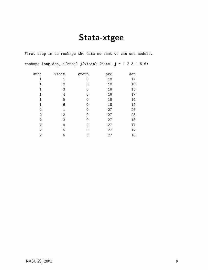
First step is to reshape the data so that we can use models.

reshape long dep, i(subj) j(visit) (note: j = 1 2 3 4 5 6)

subj visit group pre dep1 1 0 18 171 2 0 18 181 3 0 18 151 4 0 18 171 5 0 18 141 6 0 18 152 1 0 27 262 2 0 27 232 3 0 27 182 4 0 27 172 5 0 27 122 6 0 27 10

NASUGS, 2001 9

Stata-xtgee

First, I run a model with independence structure

xtgee dep group pre visit, i(subj) t(visit) corr(indep) link(iden) fam(normal) nmp

GEE population-averaged model Number of obs = 295Group variable: subj Number of groups = 61Link: identity Obs per group: min = 1Family: Gaussian avg = 4.8Correlation: independent max = 6

Wald chi2(3) = 144.15Scale parameter: 25.80052 Prob > chi2 = 0.0000

Pearson chi2(291): 7507.95 Deviance = 7507.95Dispersion (Pearson): 25.80052 Dispersion = 25.80052

------------------------------------------------------------------------------dep | Coef. Std. Err. z P>|z| [95% Conf. Interval]

-------------+----------------------------------------------------------------group | -4.290664 .6072954 -7.07 0.000 -5.480941 -3.100387

pre | .4769071 .0798565 5.97 0.000 .3203913 .633423visit | -1.307841 .169842 -7.70 0.000 -1.640725 -.9749569_cons | 8.233577 1.803945 4.56 0.000 4.697909 11.76924

------------------------------------------------------------------------------

NASUGS, 2001 10

Stata-xtgee

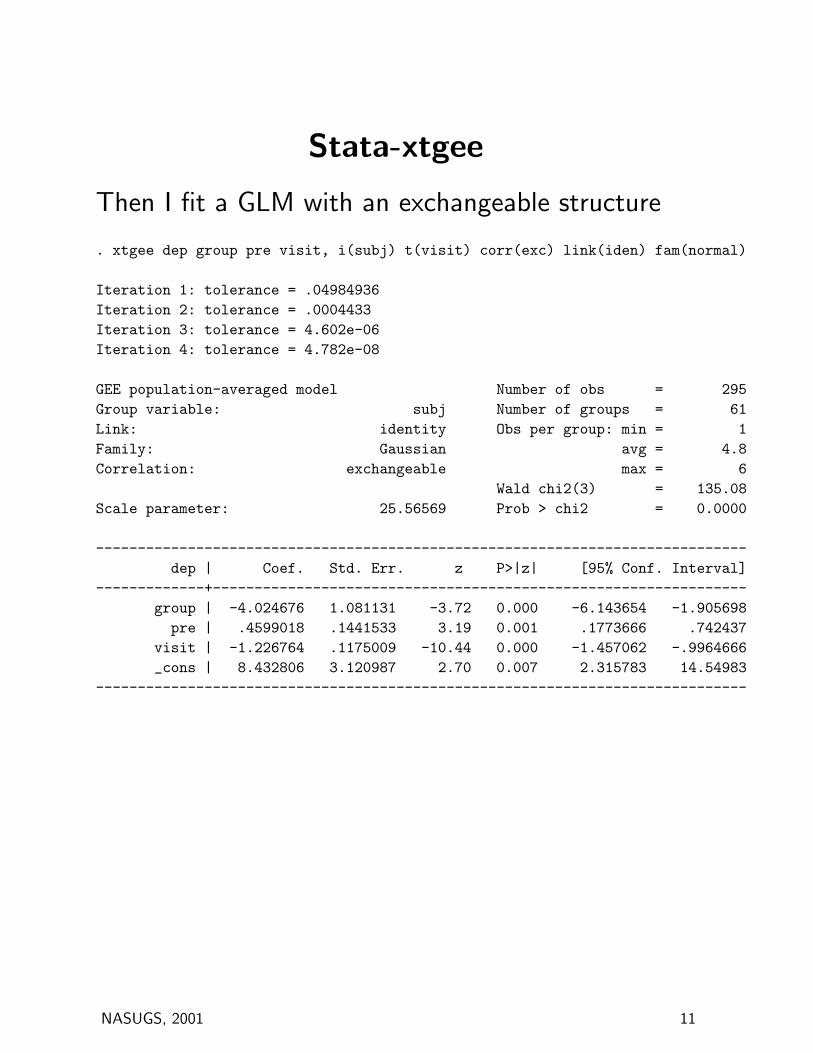
Then I fit a GLM with an exchangeable structure

. xtgee dep group pre visit, i(subj) t(visit) corr(exc) link(iden) fam(normal)

Iteration 1: tolerance = .04984936Iteration 2: tolerance = .0004433Iteration 3: tolerance = 4.602e-06Iteration 4: tolerance = 4.782e-08

GEE population-averaged model Number of obs = 295Group variable: subj Number of groups = 61Link: identity Obs per group: min = 1Family: Gaussian avg = 4.8Correlation: exchangeable max = 6



-------------+----------------------------------------------------------------group | -4.024676 1.081131 -3.72 0.000 -6.143654 -1.905698

pre | .4599018 .1441533 3.19 0.001 .1773666 .742437visit | -1.226764 .1175009 -10.44 0.000 -1.457062 -.9964666_cons | 8.432806 3.120987 2.70 0.007 2.315783 14.54983

------------------------------------------------------------------------------

NASUGS, 2001 11

Stata-xtgee

Then I fit a model with unstructured correlation

xtgee dep group pre visit, i(subj) t(visit) corr(uns) link(iden) fam(normal)

GEE population-averaged model Number of obs = 295Group and time vars: subj visit Number of groups = 61Link: identity Obs per group: min = 1Family: Gaussian avg = 4.8Correlation: unstructured max = 6



-------------+----------------------------------------------------------------group | -4.134413 .9986306 -4.14 0.000 -6.091693 -2.177133

pre | .3399185 .1326684 2.56 0.010 .0798932 .5999437visit | -1.228327 .1492831 -8.23 0.000 -1.520916 -.9357372_cons | 11.13045 2.892903 3.85 0.000 5.460464 16.80044

------------------------------------------------------------------------------

NASUGS, 2001 12

Stata-xtgee

And finally a model with AR1 structure

xtgee dep group pre visit, i(subj) t(visit) corr(ar1) link(iden) fam(normal)note: some groups have fewer than 2 observations

not possible to estimate correlations for those groups8 groups omitted from estimation

Iteration 1: tolerance = .10070858Iteration 2: tolerance = .00136623Iteration 3: tolerance = .00002736Iteration 4: tolerance = 5.508e-07

GEE population-averaged model Number of obs = 287Group and time vars: subj visit Number of groups = 53Link: identity Obs per group: min = 2Family: Gaussian avg = 5.4Correlation: AR(1) max = 6



-------------+----------------------------------------------------------------group | -4.218194 1.053504 -4.00 0.000 -6.283023 -2.153364

pre | .4268002 .1376156 3.10 0.002 .1570785 .6965219visit | -1.181975 .1907298 -6.20 0.000 -1.555799 -.8081517_cons | 9.037864 3.036076 2.98 0.003 3.087264 14.98846

------------------------------------------------------------------------------

NASUGS, 2001 13

SAS-GLM

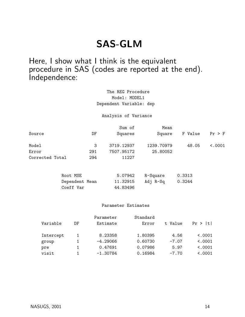
Here, I show what I think is the equivalentprocedure in SAS (codes are reported at the end).Independence:

The REG ProcedureModel: MODEL1

Dependent Variable: dep

Analysis of Variance

Sum of MeanSource DF Squares Square F Value Pr > F

Model 3 3719.12937 1239.70979 48.05 <.0001Error 291 7507.95172 25.80052Corrected Total 294 11227

Root MSE 5.07942 R-Square 0.3313Dependent Mean 11.32915 Adj R-Sq 0.3244Coeff Var 44.83496

Parameter Estimates

Parameter StandardVariable DF Estimate Error t Value Pr > |t|

Intercept 1 8.23358 1.80395 4.56 <.0001group 1 -4.29066 0.60730 -7.07 <.0001pre 1 0.47691 0.07986 5.97 <.0001visit 1 -1.30784 0.16984 -7.70 <.0001

NASUGS, 2001 14

SAS-GLM

Unrestricted Covariance structureStandard

Effect group Estimate Error DF t Value Pr > |t|

Intercept 6.2422 2.8737 58 2.17 0.0339group 0 4.1207 0.9739 58 4.23 <.0001group 1 0 . . . .pre 0.3641 0.1292 58 2.82 0.0066visit -1.1091 0.1426 58 -7.78 <.0001Compound structure

StandardEffect group Estimate Error DF t Value Pr > |t|

Intercept 4.4124 3.1901 58 1.38 0.1719group 0 4.0216 1.0887 58 3.69 0.0005group 1 0 . . . .pre 0.4598 0.1452 58 3.17 0.0025visit -1.2259 0.1167 233 -10.50 <.0001

AR1 structureEffect group Estimate Error DF t Value Pr > |t|


NASUGS, 2001 15

SAS-GLM

libname rino ’c:\rino\nasug’;data rino;infile ’c:\rino\nasug\depress.dat’;input subj group pre dep1 dep2 dep3 dep4 dep5 dep6;

if dep1=-9 then dep1=. ;if dep2=-9 then dep2=. ;if dep3=-9 then dep3=. ;if dep4=-9 then dep4=. ;if dep5=-9 then dep5=. ;if dep6=-9 then dep6=. ;run;proc means;var dep1 dep2 dep3 dep4 dep5 dep6 group pre;run;

data rino1;set rino;

visit=1; dep=dep1;t=1;output;visit=2; dep=dep2;t=2;output;visit=3; dep=dep3;t=3;output;visit=4; dep=dep4;t=4;output;visit=5; dep=dep5;t=5;output;visit=6; dep=dep6;t=6;output;run;proc means;var dep time pre group;run;

/* proc print data=rino1;run;

*/proc reg data=rino1;model dep=group pre visit ;run;

proc mixed data=rino1 noclprint method=ml ;class subj group t;

NASUGS, 2001 16

model dep = group pre visit /s;repeated t /type=un subject=subj r;title ’unrest.cov. structure, linear trend, ML’;run;

proc mixed data=rino1 noclprint method=ml;class subj group t;model dep = group pre visit /s;repeated t /type=cs subject=subj r;title ’compound structure, linear trend, ML’;run;

proc mixed data=rino1 noclprint method=ml;class subj group t;model dep = group pre visit /s;repeated t /type=ar(1) subject=subj r;title ’ar1 structure, linear trend, ML’;run;

proc mixed data=rino1 noclprint method=ml;class subj group t;model dep = group pre visit /s;random intercept /type =un sub=subj s;title ’random intercept, linear trend, ML’;run;

proc mixed data=rino1 noclprint method=ml;class subj group t;model dep = group pre visit /s;random intercept visit /type =un sub=subj s;title ’random intercept, linear trend, ML’;run;

NASUGS, 2001 17

Stata SAS- comparison

Similar results are observed, however not the sameestimates are produced. Testing and comparison ofmodels with different covariance structures will bereported in a future paper (most likely an STBbullettin).

NASUGS, 2001 18

Normally Distributed DataRandom Effect Models

This approach assumes that the correlation arisesamong repeated measures as the regressioncoefficients vary across individuals.

That is, each subject is assumed to have an(unobserved) underlying level of response whichpersists across the p measurements.

This subject effect is treated as random and themodel becomes

Yij = β0+β1X1ij+β2X2ij+. . .+βp−1Xp−1,ij+bi+eij

or

Yij = (β0+bi)+β1X1ij+β2X2ij+. . .+βp−1Xp−1,ij+eij

(also known as “random intercepts model”).

NASUGS, 2001 19

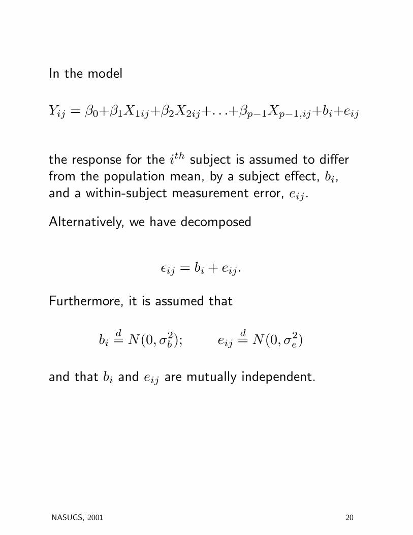
In the model

Yij = β0+β1X1ij+β2X2ij+. . .+βp−1Xp−1,ij+bi+eij

the response for the ith subject is assumed to differfrom the population mean, by a subject effect, bi,and a within-subject measurement error, eij.

Alternatively, we have decomposed

εij = bi + eij.

Furthermore, it is assumed that

bid= N(0, σ2

b); eijd= N(0, σ2

e)

and that bi and eij are mutually independent.

NASUGS, 2001 20

The introduction of a random subject effect inducescorrelation among the repeated measures.

It can be shown that the following correlationstructure results:

Var(Yij) = σ2b + σ2

e

Cov(Yij, Yik) = σ2b

=⇒ Corr(Yij, Ylj) =σ2

b

σ2b + σ2

e

= correlation of observations on the same individual

Stata can fit this model using the XTREGprocedure.

NASUGS, 2001 21

XTREG/Stata

. xtreg dep group pre visit, i(subj) mle

Random-effects ML regression Number of obs = 295Group variable (i) : subj Number of groups = 61

Random effects u_i ~ Gaussian Obs per group: min = 1avg = 4.8max = 6

LR chi2(3) = 111.62Log likelihood = -832.36607 Prob > chi2 = 0.0000------------------------------------------------------------------------------

dep | Coef. Std. Err. z P>|z| [95% Conf. Interval]-------------+----------------------------------------------------------------

group | -4.021599 1.08894 -3.69 0.000 -6.155882 -1.887316pre | .4597672 .1451952 3.17 0.002 .1751898 .7443446

visit | -1.225857 .1168668 -10.49 0.000 -1.454912 -.9968024_cons | 8.434001 3.142894 2.68 0.007 2.274042 14.59396

-------------+----------------------------------------------------------------/sigma_u | 3.805795 .4160801 9.15 0.000 2.990293 4.621297/sigma_e | 3.346938 .15434 21.69 0.000 3.044438 3.649439

-------------+----------------------------------------------------------------rho | .5638883 .0600327 .4451442 .6771015

------------------------------------------------------------------------------Likelihood ratio test of sigma_u=0: chibar2(01)= 127.28Prob>=chibar2 = 0.000

NASUGS, 2001 22

SAS

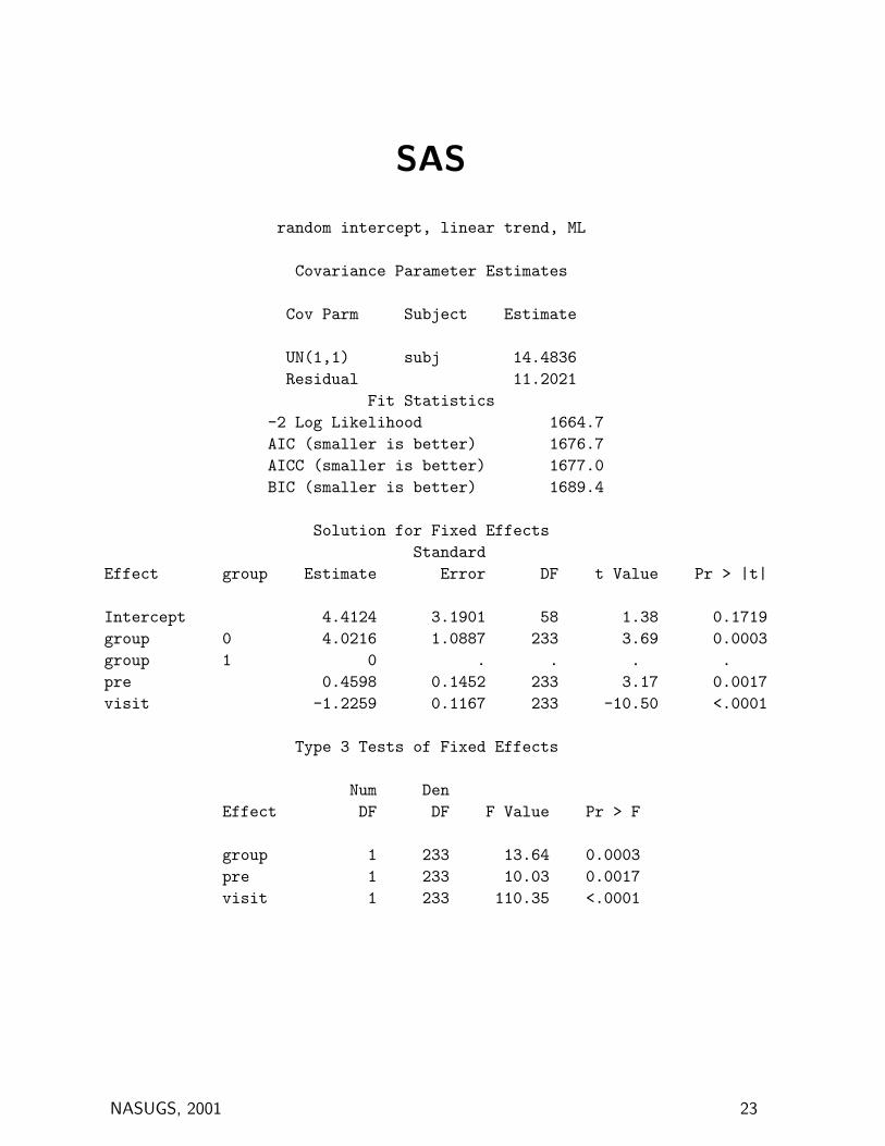
random intercept, linear trend, ML

Covariance Parameter Estimates

Cov Parm Subject Estimate

UN(1,1) subj 14.4836Residual 11.2021

Fit Statistics-2 Log Likelihood 1664.7AIC (smaller is better) 1676.7AICC (smaller is better) 1677.0BIC (smaller is better) 1689.4

Solution for Fixed EffectsStandard

Effect group Estimate Error DF t Value Pr > |t|


Type 3 Tests of Fixed Effects

Num DenEffect DF DF F Value Pr > F

group 1 233 13.64 0.0003pre 1 233 10.03 0.0017visit 1 233 110.35 <.0001

NASUGS, 2001 23

Splus

> summary(rem0)Linear mixed-effects model fit by REMLData: rino

AIC BIC logLik1678.536 1700.576 -833.2679

Random effects:Formula: visit ~ 1 | subj

(Intercept) ResidualStdDev: 3.923239 3.353891

Fixed effects: dep ~ visit + pre + groupValue Std.Error DF t-value p-value

(Intercept) 8.435886 3.224813 233 2.61593 0.0095visit -1.224393 0.117018 233 -10.46327 <.0001

pre 0.459552 0.149022 58 3.08379 0.0031group -4.016623 1.117115 58 -3.59553 0.0007

Correlation:(Intr) visit pre

visit -0.107pre -0.960 0.005

group -0.130 -0.040 -0.066

Standardized Within-Group Residuals:Min Q1 Med Q3 Max

-3.840718 -0.5559042 -0.03438542 0.4645086 3.912141

Number of Observations: 295 Number of Groups: 61

NASUGS, 2001 24

Random Intercepts and Slopes Models

A natural extension of the random intercepts model.The introduction of random intercepts and slopesinduces a covariance matrix that depends on time(tij).Consider the following model with intercepts andslopes that vary randomly among subjects

Yij = β0 + β1tij + bi0 + bi1tij + eij

Assume that bi0 and bi1 have mean zero and letV ar(eij) = σ2

e, V ar(bi0) = σ200, V ar(bi1) = σ2

11,and Cov(bi0, bi1) = σ01.Then, it can be shown that

V ar(Yij) = σ200 + 2tijσ01 + σ2

11t2ij + σ2

e

and

Cov(Yij, Yik) = σ200 + (tij + tik)σ01 + σ2

11tijtik

That is, the covariance matrix is a function of time.Stata has limited resources for modelinglongitudinal data (GLLAMM6 is a routine provided

NASUGS, 2001 25

by Rabe-Hesketh which allows to fits this model,but it is not part of regular Stata and as, Sophiahas told me, GLLAMM6 is intended for non-normaldata where no exact method exists; instead we canuse PROC MIXED in SAS and LME in Splus.

NASUGS, 2001 26

STATA

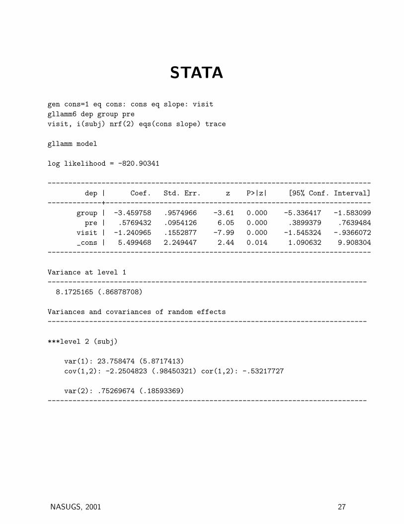
gen cons=1 eq cons: cons eq slope: visitgllamm6 dep group previsit, i(subj) nrf(2) eqs(cons slope) trace

gllamm model

log likelihood = -820.90341


-------------+----------------------------------------------------------------group | -3.459758 .9574966 -3.61 0.000 -5.336417 -1.583099

pre | .5769432 .0954126 6.05 0.000 .3899379 .7639484visit | -1.240965 .1552877 -7.99 0.000 -1.545324 -.9366072_cons | 5.499468 2.249447 2.44 0.014 1.090632 9.908304

------------------------------------------------------------------------------

Variance at level 1-----------------------------------------------------------------------------

8.1725165 (.86878708)

Variances and covariances of random effects-----------------------------------------------------------------------------

***level 2 (subj)

var(1): 23.758474 (5.8717413)cov(1,2): -2.2504823 (.98450321) cor(1,2): -.53217727

var(2): .75269674 (.18593369)-----------------------------------------------------------------------------

NASUGS, 2001 27

SAS

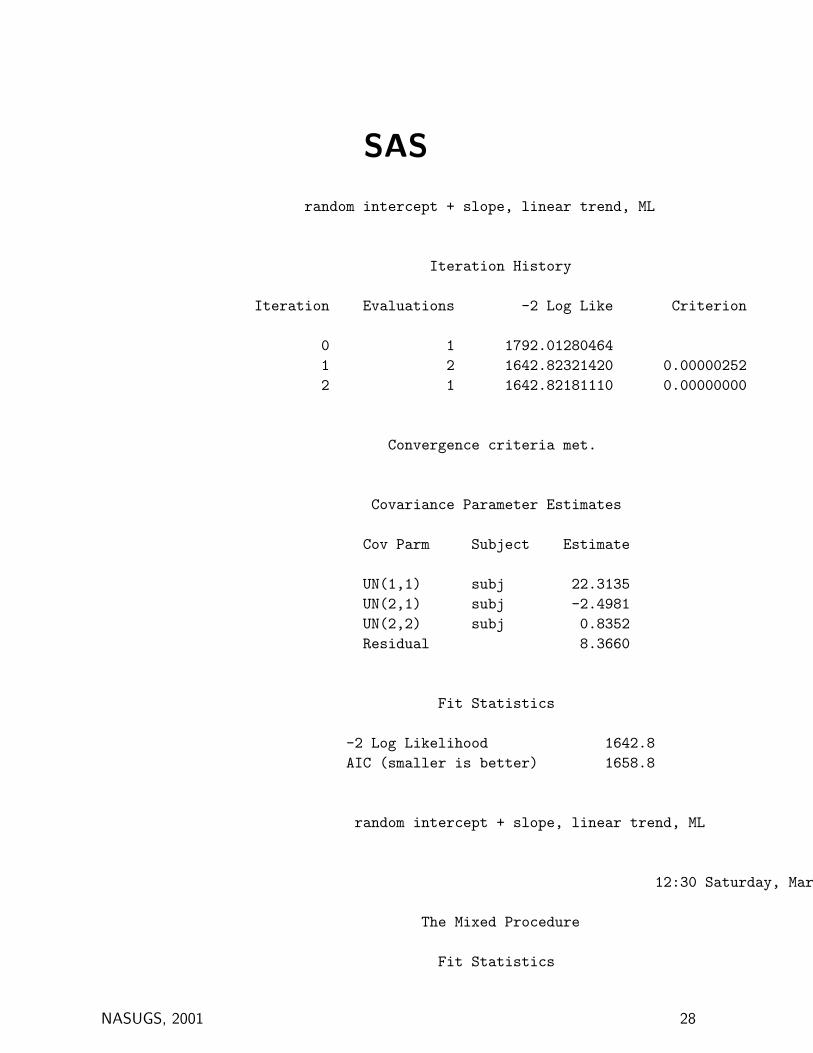
random intercept + slope, linear trend, ML

Iteration History

Iteration Evaluations -2 Log Like Criterion

0 1 1792.012804641 2 1642.82321420 0.000002522 1 1642.82181110 0.00000000

Convergence criteria met.

Covariance Parameter Estimates

Cov Parm Subject Estimate

UN(1,1) subj 22.3135UN(2,1) subj -2.4981UN(2,2) subj 0.8352Residual 8.3660

Fit Statistics

-2 Log Likelihood 1642.8AIC (smaller is better) 1658.8

random intercept + slope, linear trend, ML 14

12:30 Saturday, March 10, 2001

The Mixed Procedure

Fit Statistics

NASUGS, 2001 28

AICC (smaller is better) 1659.3BIC (smaller is better) 1675.7

Null Model Likelihood Ratio Test

DF Chi-Square Pr > ChiSq

3 149.19 <.0001

Solution for Fixed Effects

StandardEffect group Estimate Error DF t Value Pr > |t|


NASUGS, 2001 29

Splus

> summary(rem1)Linear mixed-effects model fit by REMLData: rino

AIC BIC logLik1659.905 1689.292 -821.9527

Random effects:Formula: ~ visit | subjStructure: General positive-definite

StdDev Corr(Intercept) 4.8414891 (Inter

visit 0.9303804 -0.572Residual 2.8915377

Fixed effects: dep ~ visit + pre + groupValue Std.Error DF t-value p-value

(Intercept) 8.243741 3.247253 233 2.538682 0.0118visit -1.206358 0.167118 233 -7.218614 <.0001

pre 0.468243 0.149474 58 3.132615 0.0027group -4.034921 1.121173 58 -3.598840 0.0007

Correlation:(Intr) visit pre

visit -0.139pre -0.956 0.005

group -0.126 -0.047 -0.067

Standardized Within-Group Residuals:Min Q1 Med Q3 Max

-3.315408 -0.5357005 -0.09072777 0.4617966 3.058502

Number of Observations: 295 Number of Groups: 61

NASUGS, 2001 30

Non Normal Data

In this case, we cannot always specify a likelihoodwith an arbitrary structure. We can define randomeffect models by introducing a random interceptand slope into the linear predictor (generalizedlinear mixed models). These models can be difficultto estimate (GLLAMM6).In the GEE approach, we can specify any covariancestructure and link function without specifying thejoint distribution of the the repeated observations.

REM and GEE lead to different interpretations ofbetween subject effects. In the first case, a betweensubject effect stands for the difference betweensubjects conditional on the same random effect,while the parameters of GEE represent the averagedifference between subject.

NASUGS, 2001 31

References

• Laird,Ware paper on REM, (Biometrics 1982)

• Zeger, Liang, Albert, on GEE (Biometrics, 1988)

• Horton, Lipsitz, on GEE software, (The AmericanStatistician, 1998)

NASUGS, 2001 32

Analysis of Longitudinal Data in Stata, Splus and SAS

Documents