Analysis of Interconnected Arrivals on Queueing-Inventory ...

electronics

Article

Analysis of Interconnected Arrivals on Queueing-InventorySystem with Two Multi-Server Service Channels and OneRetrial Facility

K. Jeganathan 1 , T. Harikrishnan 2 , S. Selvakumar 1 , N. Anbazhagan 3 , S. Amutha 4 , Srijana Acharya 5,∗ ,Rajendra Dhakal 6,∗ and Gyanendra Prasad Joshi 6

�����������������

Citation: Jeganathan, K.;

Harikrishnan, T.; Selvakumar, S.;

Anbazhagan, A.; Amutha, S.;

Acharya, S.; Dhakal, R.; Joshi, G.P.

Analysis of Interconnected Arrivals

on Queueing-Inventory System with

Two Multi-Server Service Channels

and One Retrial Facility. Electronics

2021, 10, 576. https://doi.org/

10.3390/electronics10050576

Academic Editor: Dimitra I.

Kaklamani

Received: 1 February 2021

Accepted: 23 February 2021

Published: 1 March 2021

Publisher’s Note: MDPI stays neutral

with regard to jurisdictional claims in

published maps and institutional affil-

iations.

Copyright: © 2021 by the authors.

Licensee MDPI, Basel, Switzerland.

This article is an open access article

distributed under the terms and

conditions of the Creative Commons

Attribution (CC BY) license (https://

creativecommons.org/licenses/by/

4.0/).

1 Ramanujan Institute for Advanced Study in Mathematics, University of Madras, Chennai 600005, India;[email protected] (K.J.); [email protected] (S.S.)

2 Guru Nanak College (Autonomous), University of Madras, Chennai 600042, India;[email protected]

3 Department of Mathematics, Alagappa University, Karaikudi 630004, India;[email protected]

4 Ramanujan Center for Higher Mathematics, Alagappa University, Karaikudi 630004, India;[email protected]

5 Department of Digital Convergence Business, Yeungnam University, 280 Daehak-Ro, Gyeongsan,Gyeongbuk 38541, Korea

6 Department of Computer Science and Engineering, Sejong University, Seoul 05006, Korea; [email protected]* Correspondence: [email protected] (S.A.); [email protected] (R.D.)

Abstract: Present-day queuing inventory systems (QIS) do not utilize two multi-server servicechannels. We proposed two multi-server service channels referred to as T1S (Type 1 n-identicalmulti-server) and T2S (Type 2 m-identical multi-server). It includes an optional interconnectedservice connection between T1S and T2S, which has a finite queue of size N. An arriving customereither uses the inventory (basic service or main service) for their demand, whom we call T1, or simplyuses the service only, whom we call T2. Customer T1 will utilize the server T1S, while customer T2will utilize the server T2S, and T1 can also get the second optional service after completing theirmain service. If there is a free server with a positive inventory, there is a chance that T1 customersmay go to an infinite orbit whenever they find that either all the servers are busy or no sufficientstock. The orbital customer can request for T1S service under the classical retrial policy. Q(= S− s)items are replaced into the inventory whenever it falls into the reorder level s such that the inequalityalways holds n < s. We use the standard (s, Q) ordering policy to replace items into the inventory. Byvarying S and s, we investigate to find the optimal cost value using stationary probability vector φ. Weused the Neuts Matrix geometric approach to derive the stability condition and steady-state analysiswith R-matrix to find φ. Then, we perform the waiting time analysis for both T1 and T2 customersusing Laplace transform technique. Further, we computed the necessary system characteristics andpresented sufficient numerical results.

Keywords: interconnected optional arrival; two multi-server service channels; classical retrial policy;waiting time; retrial facility

1. Introduction

As we see in real-life scenarios, many motorcycle service centers operate multi-servicechannels for motorcycle servicing and motorcycle sales. Generally, these services areprovided on different floors in the same buildings. Customers, generally, came only forservice or buying a bike. However, because the business provides an additional service, thecustomers who came for motorcycle servicing may go for additional services. In fact, thisis not a compulsory service, and it depends on their choice. This situation was impressiveand motivated us to make mathematical modeling in a stochastic queuing inventory sector.

Electronics 2021, 10, 576. https://doi.org/10.3390/electronics10050576 https://www.mdpi.com/journal/electronics

Electronics 2021, 10, 576 2 of 35

In a supply chain’s business operations, the enterprise must update itself in variousdimensions to meet its customers’ current requirements and expectations. One of the di-mensions of the businesses to keep on updating is through its alternative technologies. Thealternative technologies help improving goals that will serve as standards and benchmarksto technically and operationally evaluate its performance. Businesses need to allocatean exceptional value to satisfy the demand for implementing strategic goals. The firm’sfocus should aim at a better-spelled strategy to provide efficient and systematic serviceplatforms in their marketing society. Planning well-standard innovative ideas ensures anamalgamation of the demands and retailers more consistently. An ideology of a businessrequires concentration on making and providing opportunities at every stage.

Most of the firms concentrate on providing an excellent service to their customersby framing new strategies because the overall service-related problems can eventuallylead to their name’s demise. When we provide good customer service, they will be moreinterested in remaining loyal to our business, and this loyalty ensures that they will likelystick around. Looking into the queuing inventory system (QIS), a service facility is essentialfor all the mechanisms. At the initial time, many researchers discussed the QIS withoutservice facility. When we compare such models to real life, the chances are significantly lessto accept the models without a service facility. For example, in modern society, customersare not well aware of the handling procedures and utilizing skills when they wish topurchase their new items. Every customer needs a demonstration while purchasing it. Forinstance, if a customer wants to buy an induction cooktop, washing machine, refrigerator,etc., they need to know its operating procedure. The system requires the service facility toprovide excellent service to their customer. Many authors come forward to attack the QISwith the service facility concerning this. By the way, Melikov and Sigman [1,2] introducedservice facilities in their corresponding work, namely the transportation storage systemand heuristic queue, respectively.

Berman [3] discussed a deterministic approximation for their inventory system withservice facility and found the total cost, which depends upon the average inventory, acustomer in the queue, and reorder rates. After some years, Berman [4] studied thesame inventory system in which they found an inventory policy that minimizes the totalexpected customer waiting, ordering, and holding costs over a finite queue and deducesthe results to an infinite queue. They also analyzed an optimal order quantity with asimple heuristic method. Berman [5] developed the inventory system with an arbitraryservice time for a finite queue. In recent years, Paul Manuel et al. [6] examined a singleserver inventory system where an arrival follows the Markovian Arrival Process (MAP).Amirthakodi [7] considered an inventory system with a single server service facility andfinite retrial feedback customer. For more details about a single server queuing-inventorysystem, one can refer to Reference [8–12].

In this emerging society, the single-server system is not convenient for providinga good service. When a new customer enters the waiting hall during the peak hoursand sees a long queue in front of them, they get irritated and become impatient, whichleads a customer to lose. On behalf of this, Kuo-Hsiung and Keng yuan Tai [13] studiedthe additional servers that came into the service due to the queue size, which exceedsthe threshold level. Jongho Bae [14] introduced an optional service rate named as a two-stage service policy, which means that the server starts work with regular service rate (µ1)till the system reaches N customer; after N customer, it turns into a faster service rateµ2(µ2 ≥ µ1), including the customer at the moment. Jeganathan et al. [15] investigateda single server system by varying the speed of service rate under the threshold policy toreduce a customer’s impatience.

However, increasing the server’s speed or providing a faster service rate if the queuelength exceeds a fixed limit is not enough to rectify an arriving customer’s impatience,whose expectation is different from this type of service. Jeganathan et al. [16] presented thecomparison of homogeneous versus heterogeneous servers in their two-server Markovianinventory system in which they showed an efficiency of a heterogeneous system.

Electronics 2021, 10, 576 3 of 35

The Markovian inventory scheme with two parallel queues is considered byJeganathan et al. [17], in which an arriving customer will enter the shortest queue. Mean-while, we can see in real life that there are two kinds of customers who can approach thesystem for either service or inventory only. Jeganathan et al. [10] analyze the perishableinventory model of a single server (s, Q) that consists of two priority clients, such as type 1and type 2. The customer arrival flows are independent Poisson processes, and type 1and type 2 customer service times are exponential distribution. Pandelis [18] introducedthe concept of interconnected queues under different service rates. Apart from the twodedicated servers, they introduced a flexible trained server for working in both stages. Thesame work has been modeled in a perishable inventory system with two dedicated serversfor each service station by Jeganathan et al. [19]. They also assumed a flexible servicethat can provide the service at any station with a new service rate. Jeganathan and AbdulReiyas [20] recently researched a modified and delayed working vacation with two priorityclients.

Every day-to-day lifestyle requirement changes depending upon time, satisfaction onan item, a fair service process, and so on. Many firms introduced a multi-service channelto reduce customer loss and wait time to satisfy such requirements. According to theinconveniences of a single server queuing model, Krishnamoorthy et al. [21] attempteda parallel server inventory system that consists of a homogeneous service rate. On theother hand, Rajkumar et al. [22] studied an identical server in their inventory system.Arivarignan et al. [23] discussed a multi-server channel in QIS with MAP arrival. Yadav-elli et al. [24] gave the extension of work of Arivarignan by introducing negative customers.Nair et al. [25] discussed the multi-server QIS in which a customer leaves the system andthe server removed from the system after the service completion. For more details about amulti-server queuing inventory system, refer to Reference [26–31].

The majority of the inventory framework has examined a single type of multi-serverwith different assumptions from the above discussion. No research has been carried out tothe best of our knowledge on combining two multi-server forms in the inventory market.Interestingly, a two multi-server service system in the queuing system is investigated byCheng-Yuan Ku and Scott Jordan [32]. On doing such keen observation from the literaturereview, we found and enlisted some research gaps as follows:

1. No two multi-server service channels involving QIS.2. Interconnected arrivals between the two multi-server service channels.3. Two different two multi-server service channels providing their service for two differ-

ent streams of arrival.

Upon a keen survey through the above-mentioned research gaps and motivations,the first time in the QIS, we introduce the interconnected two types of multi-server servicechannels for providing a satisfactory service of two different arrival streams with which thesystem allows an optional interconnected arrival between the two multi-service channel.

Customers know that queues are inevitable in many cases. Therefore, the proposedmodel can satisfy the customer, both in inventory sales and service. This paper preservesthe optimum total cost for the interconnected arrival between two multi-server servicechannel inventory systems. Besides, the probability r (which causes the interconnectedarrival between two multi-server service channels) increases, and we achieve a decrementin both customers lost. Further, the waiting time of both retrial and T2 customers’ is derivedanalytically by Laplace-Stieltjes transform. The numerical analysis results show that it hassignificant applications in real-life economics.

The rest of the paper is organized as follows. Section 2 describes the proposed model.The analysis of the proposed model is given in Section 3. The waiting time analysis is inSection 4, and system performance measures are detailed in Section 5. The cost analysisand numerical illustration are presented in Section 6, and the conclusion is in Section 7.

Electronics 2021, 10, 576 4 of 35

2. Model Description

In this section, we describe the proposed model. The notations used in this article aredefined in the notation section at the end of the article.

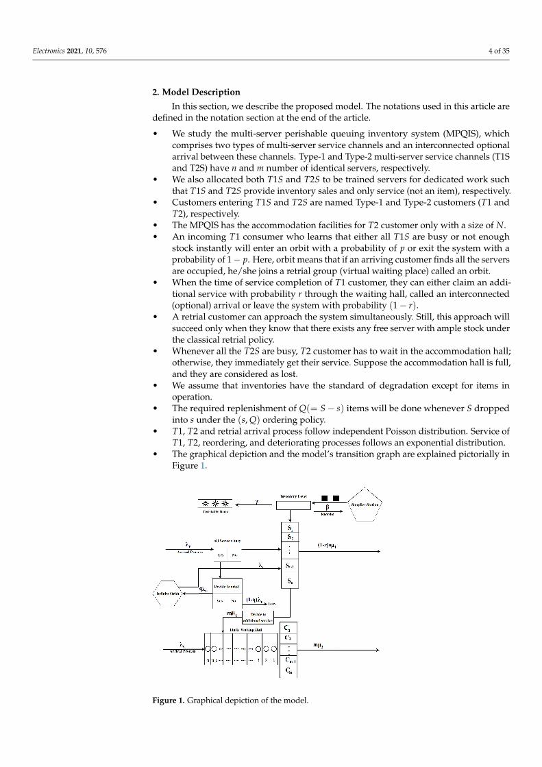
• We study the multi-server perishable queuing inventory system (MPQIS), whichcomprises two types of multi-server service channels and an interconnected optionalarrival between these channels. Type-1 and Type-2 multi-server service channels (T1Sand T2S) have n and m number of identical servers, respectively.

• We also allocated both T1S and T2S to be trained servers for dedicated work suchthat T1S and T2S provide inventory sales and only service (not an item), respectively.

• Customers entering T1S and T2S are named Type-1 and Type-2 customers (T1 andT2), respectively.

• The MPQIS has the accommodation facilities for T2 customer only with a size of N.• An incoming T1 consumer who learns that either all T1S are busy or not enough

stock instantly will enter an orbit with a probability of p or exit the system with aprobability of 1− p. Here, orbit means that if an arriving customer finds all the serversare occupied, he/she joins a retrial group (virtual waiting place) called an orbit.

• When the time of service completion of T1 customer, they can either claim an addi-tional service with probability r through the waiting hall, called an interconnected(optional) arrival or leave the system with probability (1− r).

• A retrial customer can approach the system simultaneously. Still, this approach willsucceed only when they know that there exists any free server with ample stock underthe classical retrial policy.

• Whenever all the T2S are busy, T2 customer has to wait in the accommodation hall;otherwise, they immediately get their service. Suppose the accommodation hall is full,and they are considered as lost.

• We assume that inventories have the standard of degradation except for items inoperation.

• The required replenishment of Q(= S− s) items will be done whenever S droppedinto s under the (s, Q) ordering policy.

• T1, T2 and retrial arrival process follow independent Poisson distribution. Service ofT1, T2, reordering, and deteriorating processes follows an exponential distribution.

• The graphical depiction and the model’s transition graph are explained pictorially inFigure 1.

Figure 1. Graphical depiction of the model.

Electronics 2021, 10, 576 5 of 35

3. Analysis of the Model

The process X(t) = {(X1(t), X2(t), X3(t), X4(t), X5(t)), t ≥ 0} is a continuous-time

Markov chain (CTMC) having the state space E given by E =4⋃

i=1Ei.

Define the following ordered sets:

〈〈〈〈u1, u2, u3, u4〉〉〉〉 ={

(u1, u2, u3, u4, u4), u4 ∈ V0m−1,

(u1, u2, u3, u4, m), u2 ∈ VS \Vm−1,〈〈〈u1, u2, u3〉〉〉 = (〈〈〈〈u1, u2, u3, 0〉〉〉〉, 〈〈〈〈u1, u2, u3, 1〉〉〉〉, · · · , 〈〈〈〈u1, u2, u3, N〉〉〉〉)

〈〈u1, u2〉〉 ={〈〈〈u1, u2, 0〉〉〉, 〈〈〈u1, u2, 1〉〉〉, · · · , 〈〈〈u1, u2, u2〉〉〉, u2 ∈ V0

n−1,〈〈〈u1, u2, 0〉, 〈〈〈u1, u2, 1〉, · · · , 〈〈〈u1, u2, n〉, u2 ∈ VS \Vn−1,

〈u1〉 = (〈〈u1, 0〉〉, 〈〈u1, 1〉〉, · · · , 〈〈u1, S〉〉).

Then, the state space can be ordered as (〈0〉, 〈1〉, · · · ).

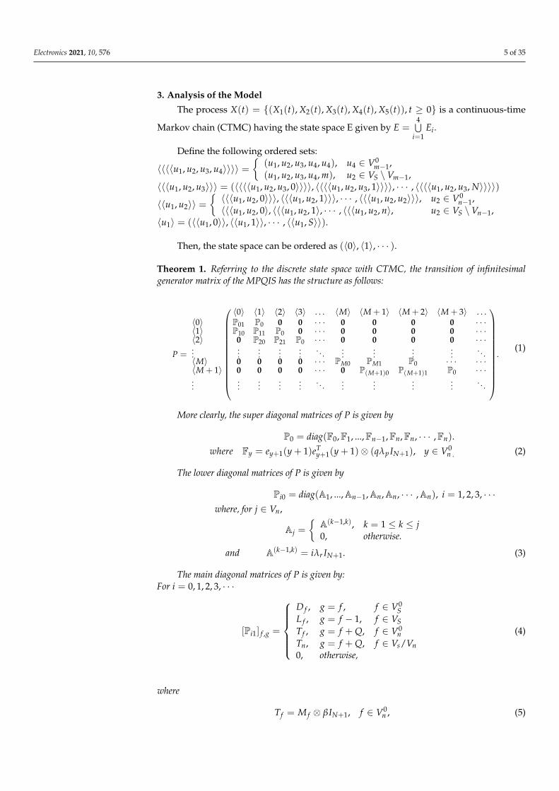
Theorem 1. Referring to the discrete state space with CTMC, the transition of infinitesimalgenerator matrix of the MPQIS has the structure as follows:

P =

〈0〉 〈1〉 〈2〉 〈3〉 . . . 〈M〉 〈M + 1〉 〈M + 2〉 〈M + 3〉 . . .〈0〉 P01 P0 0 0 · · · 0 0 0 0 · · ·〈1〉 P10 P11 P0 0 · · · 0 0 0 0 · · ·〈2〉 0 P20 P21 P0 · · · 0 0 0 0 · · ·...

......

......

. . ....

......

.... . .

〈M〉 0 0 0 0 · · · PM0 PM1 P0 · · · · · ·〈M + 1〉 0 0 0 0 · · · 0 P(M+1)0 P(M+1)1 P0 · · ·...

......

......

. . ....

......

.... . .

.

(1)

More clearly, the super diagonal matrices of P is given by

P0 = diag(F0,F1, ...,Fn−1,Fn,Fn, · · · ,Fn).

where Fy = ey+1(y + 1)eTy+1(y + 1)⊗ (qλp IN+1), y ∈ V0

n . (2)

The lower diagonal matrices of P is given by

Pi0 = diag(A1, ...,An−1,An,An, · · · ,An), i = 1, 2, 3, · · ·where, for j ∈ Vn,

Aj =

{A(k−1,k), k = 1 ≤ k ≤ j0, otherwise.

and A(k−1,k) = iλr IN+1. (3)

The main diagonal matrices of P is given by:For i = 0, 1, 2, 3, · · ·

[Pi1] f ,g =

D f , g = f , f ∈ V0

SL f , g = f − 1, f ∈ VSTf , g = f + Q, f ∈ V0

nTn, g = f + Q, f ∈ Vs/Vn0, otherwise,

(4)

where

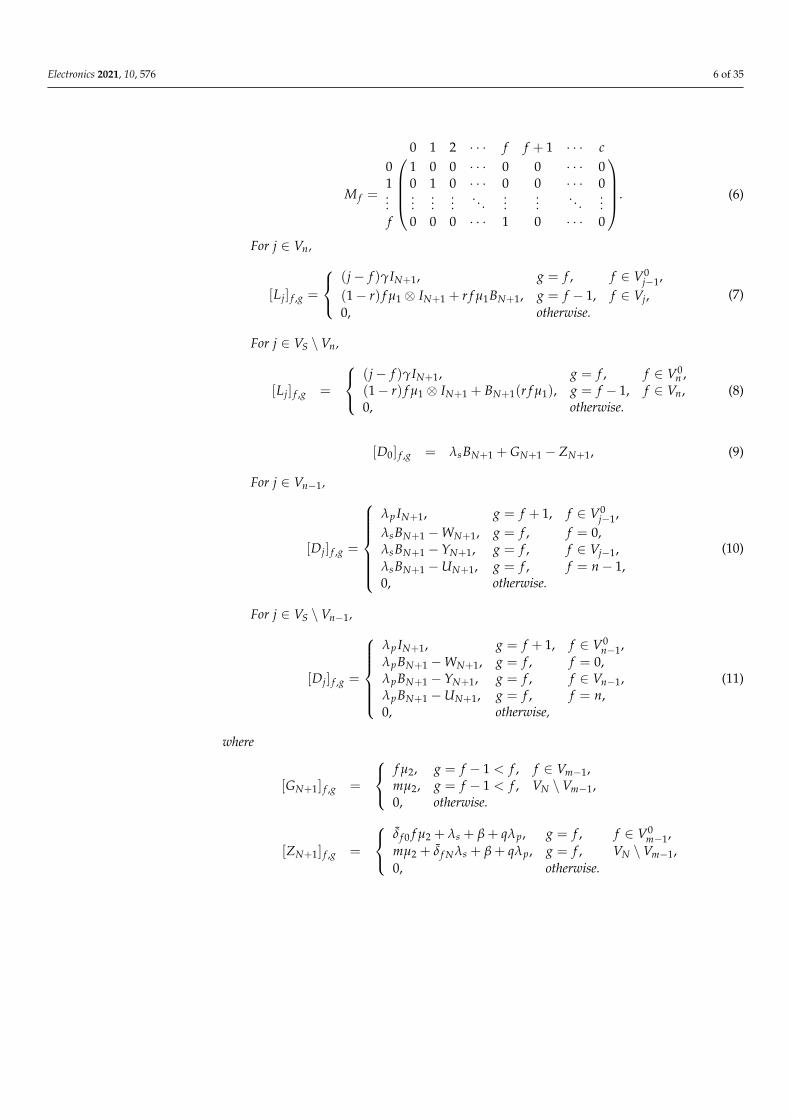
Tf = M f ⊗ βIN+1, f ∈ V0n , (5)

Electronics 2021, 10, 576 6 of 35

M f =

0 1 2 · · · f f + 1 · · · c

0 1 0 0 · · · 0 0 · · · 01 0 1 0 · · · 0 0 · · · 0...

......

.... . .

......

. . ....

f 0 0 0 · · · 1 0 · · · 0

. (6)

For j ∈ Vn,

[Lj] f ,g =

(j− f )γIN+1, g = f , f ∈ V0

j−1,(1− r) f µ1 ⊗ IN+1 + r f µ1BN+1, g = f − 1, f ∈ Vj,0, otherwise.

(7)

For j ∈ VS \Vn,

[Lj] f ,g =

(j− f )γIN+1, g = f , f ∈ V0

n ,(1− r) f µ1 ⊗ IN+1 + BN+1(r f µ1), g = f − 1, f ∈ Vn,0, otherwise.

(8)

[D0] f ,g = λsBN+1 + GN+1 − ZN+1, (9)

For j ∈ Vn−1,

[Dj] f ,g =

λp IN+1, g = f + 1, f ∈ V0j−1,

λsBN+1 −WN+1, g = f , f = 0,λsBN+1 −YN+1, g = f , f ∈ Vj−1,λsBN+1 −UN+1, g = f , f = n− 1,0, otherwise.

(10)

For j ∈ VS \Vn−1,

[Dj] f ,g =

λp IN+1, g = f + 1, f ∈ V0

n−1,λpBN+1 −WN+1, g = f , f = 0,λpBN+1 −YN+1, g = f , f ∈ Vn−1,λpBN+1 −UN+1, g = f , f = n,0, otherwise,

(11)

where

[GN+1] f ,g =

f µ2, g = f − 1 < f , f ∈ Vm−1,mµ2, g = f − 1 < f , VN \Vm−1,0, otherwise.

[ZN+1] f ,g =

δ̄ f 0 f µ2 + λs + β + qλp, g = f , f ∈ V0

m−1,mµ2 + δ̄ f Nλs + β + qλp, g = f , VN \Vm−1,0, otherwise.

Electronics 2021, 10, 576 7 of 35

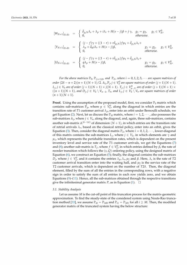
[WN+1]g1,g2 =

{δ̄g1 Nλs + λp + iλr + H(s− j)β + j γ, g1 = g2, g1 ∈ V0

N ,0, otherwise.

[YN+1]g1,g2 =

(j− f )γ + ((1− r) + rδ̄g1 N) f µ1 + δ̄g1 Nλs+λp + δ̄0iiλr + H(s− j)β, g1 = g2, g1 ∈ V0

N ,0, otherwise.

[UN+1]g1,g2 =

(j− f )γ + ((1− r) + rδ̄g1 N) f µ1 + δ̄g1 Nλs+qλp + H(s− j)β, g1 = g2, g1 ∈ V0

N ,0, otherwise.

For the above matrices P0, P(i+1)0, and Pi1, where i = 0, 1, 2, 3, · · · are square matrices oforder (2S− n + 2)(n + 1)(N + 1)/2. Aj,Fj, j ∈ V0

n are square matrices of order (j + 1)(N + 1).Lj, j ∈ Vn are of order (j + 1)(N + 1)× j(N + 1). Tj, j ∈ V0

n−1, are of order (j + 1)(N + 1)×((n + 1)(N + 1), and Dj, j ∈ VS \ Vn−1, Tn, and Lj, j ∈ VS \ Vn are square matrices of order(n + 1)(N + 1).

Proof. Using the assumption of the proposed model, first, we consider P0 matrix whichcontains sub-matrices Fy, where y ∈ V0

n , along the diagonal in which entries are thetransition rate of T1 customer arrival λp, enter into an orbit under Bernoulli schedule, weget Equation (2). Next, let us discuss the Pi0 matrix, where i = 1, 2, · · · , also possesses thesub-matrices Aj, where j ∈ Vn, along the diagonal, and, again, these sub-matrices, containsanother sub-matrix A(k−1,k) of dimension (N + 1), in which entries are the transition rateof retrial arrivals λr, based on the classical retrial policy, enter into an orbit, gives theEquation (3). Then, consider the diagonal matrix Pii, where i = 0, 1, 2, · · · , lower-diagonalof this matrix contains the sub-matrices Lj, where j ∈ VS, in which elements are γ andµ1, which represents the perishable transition rates, which is dependent on the presentinventory level and service rate of the T1 customer arrivals, we get the Equations (7)and (8); another sub-matrix is Tf , where f ∈ V0

n , in which entries defined by β, the rate ofreorder transition which follows the (s, Q) ordering policy, using the designed matrix ofEquation (6), we construct an Equation (5); finally, the diagonal contains the sub-matricesDj, where j ∈ V0

S , and it contains the entries λp, λs, µ2 and β. Here, λs is the rate of T2customer arrival transition enter into the waiting hall, and µ2 is the service rate of theT2 customer arrivals, which is dependent on the number of T2S. Then, the diagonalelement, filled by the sum of all the entries in the corresponding rows, with a negativesign in order to satisfy the sum of all entries in each row yields zero, and we obtainEquations (9)–(11). Hence, all the sub-matrices obtained through the respective transitionsgive the infinitesimal generator matrix P, as in Equation (1).

3.1. Stability Analysis

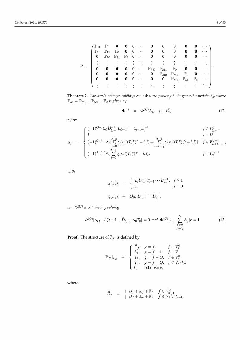
Let us assume M is the cut-off point of this truncation process for the matrix-geometricapproximation. To find the steady-state of the considered system using Neuts-Rao trunca-tion method [33], we assume Pi0 = PM0 and Pi1 = PM1 for all i ≥ M. Then, the modifiedgenerator matrix of the truncated system having the below structure:

Electronics 2021, 10, 576 8 of 35

P̂ =

P01 P0 0 0 0 · · · 0 0 0 0 0 · · ·P10 P11 P0 0 0 · · · 0 0 0 0 0 · · ·0 P20 P21 P0 0 · · · 0 0 0 0 0 · · ·...

......

......

. . ....

......

......

. . .0 0 0 0 0 · · · PM0 PM1 P0 0 0 · · ·0 0 0 0 0 · · · 0 PM0 PM1 P0 0 · · ·0 0 0 0 0 · · · 0 0 PM0 PM1 P0 · · ·...

......

......

.... . .

......

......

. . .

.

Theorem 2. The steady-state probability vector Φ corresponding to the generator matrix PM wherePM = PM0 + PM1 + P0 is given by

Φ(j) = Φ(Q)∆j, j ∈ V0S , (12)

where

∆j =

(−1)Q−jLQD̂−1Q−1LQ−1 · · · Lj+1D̂−1

j j ∈ V0Q−1,

I, j = Q

(−1)S−j+1∆s[s−n∑

i=0χ(s, i)Tnζ(S− i, j) +

n−1∑

i=j−Qχ(s, i)Tiζ(Q + i, j)], j ∈ VQ+1

Q+n−1

(−1)S−j+1∆sS−j∑

i=0χ(s, i)Tnζ(S− i, j), j ∈ VQ+n

S

,

with

χ(i, j) =

{LiD̂−1

i−1Ti−1 · · · D̂−1i−j, j ≥ 1

I, j = 0

ζ(i, j) = D̂iLiD̂−1i−1 · · · D̂

−1j ,

and Φ(Q) is obtained by solving

Φ(Q)[∆Q+1LQ + 1 + D̂Q + ∆0T0] = 0 and Φ(Q)[I +S

∑f 6=0f 6=Q

∆ f ]e = 1. (13)

Proof. The structure of PM is defined by

[PM] f ,g =

D̂ f , g = f , f ∈ V0

SL f , g = f − 1, f ∈ VSTf , g = f + Q, f ∈ V0

nTn, g = f + Q, f ∈ Vs/Vn0, otherwise,

where

D̂ f =

{D f +A f + F f , f ∈ V0

n−1D f +An + Fn, f ∈ VS \Vn−1,

Electronics 2021, 10, 576 9 of 35

and the matrices L f , Tf , Tn are defined in Equation (4). Let Φ be the steady state probabilityvector of PM, and the normalizing condition gives

ΦPM = 0 and Φe = 1. (14)

Then, vector Φ can be represented by Φ = (Φ(0), Φ(1), · · · , Φ(S)). Using the equationof ΦPM = 0, we get the following set of equations:

Φj+1Lj+1 + ΦjD̂j = 0, j = 0, 1, · · · , Q− 1Φj+1Lj+1 + ΦjD̂j + Φj−QT = 0, j = Q, Q + 1, · · · , S− 1ΦjD̂j + Φj−QT = 0, j = S

. (15)

Solving the system of Equations (15) recursively and using (13), we get (12).

Theorem 3. The stability condition of the system at the truncation point M is given by

c1qλp < c2λr, (16)

where

c1 =n−1

∑j=0

j

∑f=0

m−1

∑g=0

Φ(j, f ,g,g) +S

∑j=n

n

∑f=0

m−1

∑g=0

Φ(j, f ,g,g)

+n−1

∑j=0

j

∑f=0

N

∑g=m

Φ(j, f ,g,m) +n

∑j=S

n

∑f=0

N

∑g=m

Φ(j, f ,g,m),

and

c2 =

{n−1

∑j=1

j

∑f=0

m−1

∑g=0

Φ(j, f ,g,g) +S

∑j=n

n

∑f=0

m−1

∑g=0

Φ(j, f ,g,g)

+n−1

∑j=1

j

∑f=0

N

∑g=m

Φ(j, f ,g,m) +n

∑j=S

n

∑f=0

N

∑g=m

Φ(j, f ,g,m)

}M.

Proof. From the notable result after effect of Neuts [33] on the positive recurrence of PM,the condition,

ΦP0e < ΦPM0e,

provides the result as in (16).

3.2. Steady State Analysis

It can be seen from the structure of the rate matrix P, and from Theorem 3, that theMarkov process X(t) with the state space E is regular. Hence, the limiting probabilitydistribution,

φ(i,j, f ,g,g1) = limt→∞

Pr[X1(t) = i, X2(t) = j, X3(t) = f , X4(t) = g, X5(t) = g1, |X1(0), X2(0), X3(0), X4(0), X5(0)],

exists and is independent of the initial state. Let φ =(

φ(0), φ(1), . . . ,)

be the stationaryprobability vector satisfying

φP = 0, φe = 1.

3.3. Computation of R-Matrix

Due to the specific structure of P, using the vector φ and R can be determined by

Electronics 2021, 10, 576 10 of 35

R2PM0 + RPM1 + P0 = 0, (17)

where R is the minimal non-negative solution of above matrix quadratic equation, and it isdefined by

R =

R(0,0) R(0,1) · · · R(0,S)

R(1,0) R(1,1) · · · R(1,S)

R(2,0) R(2,1) · · · R(2,S)

......

. . ....

R(S,0) R(S,1) · · · R(S,S)

.

This R has only (S + 1)(N + 1) non-zero rows of dimension (2S− n + 2)(n + 1)(N +1)/2. Now, due to the specified structure of P0, the structure of the block matrix R(i,j) is ofthe form:

R(0,j) =( 0 1 · · · j

0 R(0,l)(0) R(0,l)

(j) · · · R(0,l)(l)

), j ∈ V0

n−1

R(0,j) =( 0 1 · · · n

0 R(0,l)(0) R(0,l)

(1) · · · R(0,l)(n)

), j ∈ Vn

S

R(j,j) =

0 1 · · · j

0 0 0 · · · 01 0 0 · · · 0...

......

. . ....

j R(j,j)(0) R(j,j)

(1) · · · R(j,j)(j)

, j ∈ Vn−1

R(j,j) =

0 1 · · · n

0 0 0 · · · 01 0 0 · · · 0...

......

. . ....

n R(j,j)(0) R(j,j)

(1) · · · R(j,j)(n)

, j ∈ VnS

R( f ,j) =

0 1 · · · j

0 0 0 · · · 01 0 0 · · · 0...

......

. . ....

f R( f ,j)(0) R( f ,j)

(1) · · · R( f ,j)(j)

, f ∈ Vn−1, j ∈ V f+1n

Electronics 2021, 10, 576 11 of 35

R( f ,j) =

0 1 · · · n

0 0 0 · · · 01 0 0 · · · 0...

......

. . ....

f R( f ,j)(0) R( f ,j)

(1) · · · R( f ,j)(n)

, f ∈ Vn−1, j ∈ V f+1S

R( f ,j) =

0 1 · · · j

0 0 0 · · · 01 0 0 · · · 0...

......

. . ....

f R( f ,j)(0) R( f ,j)

(1) · · · R( f ,j)(j)

, f ∈ Vn−1, j ∈ V0f−1

R( f ,j) =

0 1 · · · j

0 0 0 · · · 01 0 0 · · · 0...

......

. . ....

n R( f ,j)(0) R( f ,j)

(1) · · · R( f ,j)(j)

, f ∈ VnS , j ∈ V0

n−1

R( f ,j) =

0 1 · · · n

0 0 0 · · · 01 0 0 · · · 0...

......

. . ....

n R( f ,j)(0) R( f ,j)

(1) · · · R( f ,j)(n)

, f ∈ VnS , j ∈ Vn

S ,

where R(a,b)(c) defined as

R(a,b)(c) =

v00 v01 · · · v0Nv10 v11 · · · v1Nv20 v21 · · · v21

......

. . ....

vN1 vN1 · · · vNN

N+1

.

Theorem 4. The stationary probability vector φ of the CTMC can be determined by

φ(i+M−1) = φ(M−1)Ri; i ≥ 0, (18)

where R is a solution of Equation (17) and the vector φ(i), i ≥ 0

φ(i) =

σY(0)M∏j=i

Pj0(−P′j−1), 0 ≤ i ≤ M− 1

σY(0)R(i−M), i ≥ M,(19)

where

σ = [1 + Y(0)M−1

∑i=0

M

∏j=i

Pj0(−P′j−1)e]−1, (20)

and Y(0) can be computed by using the normalizing condition

Y(0)(I − R)−1e = 1.

Electronics 2021, 10, 576 12 of 35

Proof. The sub-vector (φ(0), φ(1), . . . , φ(M−1)) and the block partitioned matrix of P̂ givesthe set of equations:

φ(0)P01 + φ(1)P10 = 0

φ(i−1)P0 + φ(i)Pi1 + φ(i+1)P(i+1)0 = 0; 1 ≤ i ≤ M− 1 (21)

φ(M−2)P0 + φ(M−1)(P(M−1)1 + RPM0) = 0;

using Equation (21),φ(0) = φ(1)P10(−P01)

−1,

again, using (21),φ(1) = φ(2)P20(−P′1)−1,

where P′1 = (P11 + P10(−P′0)−1P′0),P′0 = P01.

Next,φ(2) = φ(3)P30(−P′2)−1,

where P′2 = (P21 + P20(−P′1)−1P′0)

On continuing this procedure up to M− 1 times, we get:

φ(i) = φ(i+1)P(i+1)0(−P′i)−1, 0 ≤ i ≤ M− 1, (22)

where

P′i ={

Pi0, i = 0(Pi1 − Pi0(−P′i−1)

−1P′0), 1 ≤ i ≤ M.

To find the vectors (φ(M), φ(M+1), φ(M+2) . . .), we apply block Gaussian eliminationmethod. The sub-vector (φ(M), φ(M+1), φ(M+2) . . .), corresponding to non-boundary states,satisfies the following relation:

(φ(M), φ(M+1), φ(M+2) . . .)

P′M P0 0 0 0 · · ·PM0 PM1 P0 0 0 · · ·

0 PM0 PM1 P0 0 · · ·...

......

......

. . .

= 0. (23)

Assume:

σ =∞∑

i=Mφ(i)e

Y(i) = σ−1φ(M+i), i ≥ 0.

From (23), we get

φ(M)PM + φ(M+1)PM0 = 0

φ(M+i) = φ(M+i−1)R, i ≥ 1.

This can be written as

Y(0)PM + Y(1)PM0 = 0 (24)

Y(i) = Y(i−1)R, i ≥ 1,

Electronics 2021, 10, 576 13 of 35

and (24) becomes

Y(0)[PM + RPM0] = 0. (25)

Since∞∑

i=0Y(i)e=1, then,

Y(0)(I − R)−1e = 1. (26)

Therefore, Y(0) is the unique solution of the Equations (25) and (26).

Hence,

φ(i) = σY(0)R(i−M), i ≥ M. (27)

Again, by (22) and (27), we get (19). Since∞∑

i=0φ(i)e=1, and using (19),

σY(0)M−1

∑i=0

M

∏j=i

Pj0(−P′j−1)e + σY(0)∞

∑M

R(i−M)e = 1,

which gives σ as in (20).

4. Waiting Time Analysis

The customer wait time (WT) is defined as interim time between an epoch of arrivalof a demand enters into the waiting hall or orbit and the instant at which they enter intothe service. We examine the WT of demand in the queue and orbit separately using theLaplace-Stieltjes transform (LST). Naturally, we limit the orbit size to finite for finding thewaiting time of an orbital demand. We represent Wq and Wo as the continuous-time randomvariables to denote the WT of demand in queue and an orbit. Due to such restriction, themodified state-space of a CTMC is E∗, which is obtained by improving the co-ordinatefrom u1 ∈W to u1 ∈ V0

L in each Ei, i = 1, 2, 3, 4.

WT of a Demand in Queue and Orbital Demand

Theorem 5. The probability of a demand that does not wait into the queue is considered as

P{Wq = 0} = 1− ηew, (28)

where

ηew =L

∑i=0

n

∑k=0

m

∑j=1

φ(i,k,k,j,j) +L

∑i=0

n

∑k=0

N−1

∑j=m+1

φ(i,k,k,j,m) +L

∑i=0

S

∑k=n+1

m

∑j=1

φ(i,k,n,j,j)

+L

∑i=0

S

∑k=n+1

N−1

∑j=m+1

φ(i,k,n,j,m). (29)

Proof. Since the sum of probability of zero and positive waiting time is 1, we have

P{Wq = 0}+ P{Wq > 0} = 1. (30)

Clearly, the probability of positive waiting time of demand in the queue can bedetermined as

P{Wq > 0} = ηew. (31)

Electronics 2021, 10, 576 14 of 35

As we obtained the stationary probability vector φ by Theorem (4) in Section 3, andsubstituting the φ’s in Equation (29), we get Equation (31). From (30) and (31), we obtainthe stated result as desired.

To enable WT distribution of Wq, we shall define some complementary variables.Suppose that the MPQIS is at state (i, k, l, j, g), j > 0 at an arbitrary time t:

1. Wq(i, k, l, j, g) is the time until chosen demand become satisfied.2. LST of Wq(i, k, l, j, g) is ∗Wq(i, k, l, j, g)(y), and we denote Wq by ∗Wq(y).3. ∗Wq(y) = E[eyWq ] LST of unconditional waiting time (UWT).4. ∗Wq(i, k, l, j, g)(y) = E[eyWq(i,k,l,j,g)] LST of conditional waiting time (CWT).

Theorem 6. The LS transforms {∗Wq(i, k, l, j, g)(y), (i, k, l, j, g) ∈ D∗, where D∗ = D ∪ {∗}}satisfy the following system:

Zq(y)∗Wq(y) = −gµ2e(i, k, l, j, g), (i, k, l, j, g) ∈ D. (32)

Zq(y) = (J− yI), and the matrix J is derived from P by removing the following states (i, k, l, 0, 0) :{0 ≤ i ≤ L, 0 ≤ k ≤ n, 0 ≤ l ≤ k} ∪ {0 ≤ i ≤ L, n + 1 ≤ k ≤ S, 0 ≤ l ≤ n} and {∗} is theabsorbing state, and the absorption occurs if the T2 customer demands to enter into the service.

Proof. To obtain the CWT, we apply first step analysis as follows:For 0 ≤ i ≤ L, 1 ≤ j ≤ m− 1,

∗Wq(i, 0, 0, j, j)(y) =δ̄iLqλp

a1

∗Wq(i + 1, 0, 0, j, j)(y) +λs

a1

∗Wq(i, 0, 0, j + 1, j + 1)(y)

+β

a1

∗Wq(i, Q, 0, j, j)(y) +(j− 1)µ2

a1

∗Wq(i, 0, 0, j− 1, j− 1)(y) +µ2

a1. (33)

For 0 ≤ i ≤ L, m ≤ j ≤ N,

∗Wq(i, 0, 0, j, m)(y) =δ̄iLqλp

a1

∗Wq(i + 1, 0, 0, j, m)(y)

+δ̄jNλs

a1

∗Wq(i, 0, 0, j + 1, m)(y) +β

a1

∗Wq(i, Q, 0, j, m)(y) (34)

+δjm(j− 1)µ2

a1

∗Wq(i, 0, 0, j− 1, m− 1)(y)

+H(j− (m + 1))(m− 1)µ2

a1

∗Wq(i, 0, 0, j− 1, m)(y) +µ2

a1,

where a1 = y + δ̄iLqλp + δ̄jNλs + β + H((m− 1)− j)jµ2 + H(j− (m− 1))mµ2.

Electronics 2021, 10, 576 15 of 35

For 0 ≤ i ≤ L, 1 ≤ k ≤ n, 0 ≤ l ≤ k, 1 ≤ j ≤ m− 1,

∗Wq(i, k, l, j, j)(y) =δ̄lkiλr

a2

∗Wq(i− 1, k, l + 1, j, j)(y)

+(1− r)nµ1

a2

∗Wq(i, k− 1, l − 1, j, j)(y) +(k− l)γ

a2

∗Wq(i, k− 1, l, j, j)(y)

+δ̄lkλp

a2

∗Wq(i, k, l + 1, j, j)(y) +β

a2

∗Wq(i, Q + k, l, j, j)(y) (35)

+λs

a2

∗Wq(i, k, l, j + 1, j + 1)(y) +δlk δ̄iLqλp

a2

∗Wq(i + 1, k, l, j, j)(y)

+rnµ1

a2

∗Wq(i, k− 1, l − 1, j + 1, j + 1)(y) +(j− 1)µ2

a2

∗Wq(i, k, l, j− 1, j− 1)(y)

+µ2

a1.

For 0 ≤ i ≤ L, 1 ≤ k ≤ n, 0 ≤ l ≤ k, m ≤ j ≤ N,

∗Wq(i, k, l, j, m)(y) =δ̄lkiλr

a2

∗Wq(i− 1, k, l + 1, j, m)(y)

+(1− r)nµ1

a2

∗Wq(i, k− 1, l − 1, j, m)(y) +(k− l)γ

a2

∗Wq(i, k− 1, l, j, m)(y)

+δ̄lkλp

a2

∗Wq(i, k, l + 1, j, m)(y) +β

a2

∗Wq(i, Q + k, l, j, m)(y)

+δ̄jNλs

a2

∗Wq(i, k, l, j + 1, m)(y) +δlk δ̄iLqλp

a2

∗Wq(i + 1, k, l, j, m)(y) + (36)

δ̄jNrnµ1

a2

∗Wq(i, k− 1, l − 1, j + 1, m)(y) +δjm(j− 1)µ2

a2

∗Wq(i, k, l, j− 1, m− 1)(y)

+H(j− (m + 1))(m− 1)µ2

a2

∗Wq(i, k, l, j− 1, m)(y) +µ2

a2,

where a2 = y + δ̄lkiλr + (1− r)nµ1 + (k− l)γ + δ̄lkλp + β + δ̄jNλs + δlk δ̄iLqλp+ δ̄jNrnµ1 + H((m− 1)− j)jµ2 + H(j− (m− 1))mµ2.

For 0 ≤ i ≤ L, n + 1 ≤ k ≤ S, 0 ≤ l ≤ n, 1 ≤ j ≤ m− 1,

∗Wq(i, k, l, j, j)(y) =δ̄lniλr

a3

∗Wq(i− 1, k, l + 1, j, j)(y)

+(1− r)nµ1

a3

∗Wq(i, k− 1, l − 1, j, j)(y) +(k− l)γ

a3

∗Wq(i, k− 1, l, j, j)(y)

+δ̄lnλp

a3

∗Wq(i, k, l + 1, j, j)(y) + H(s− k)β

a3

∗Wq(i, Q + k, l, j, j)(y) (37)

+λs

a3

∗Wq(i, k, l, j + 1, j + 1)(y) +δln δ̄iLqλp

a3

∗Wq(i + 1, k, l, j, j)(y)

+rnµ1

a3

∗Wq(i, k− 1, l − 1, j + 1, j + 1)(y) +(j− 1)µ2

a3

∗Wq(i, k, l, j− 1, j− 1)(y)

+µ2

a3.

For 0 ≤ i ≤ L, n + 1 ≤ k ≤ S, 0 ≤ l ≤ n, m ≤ j ≤ N,

Electronics 2021, 10, 576 16 of 35

∗Wq(i, k, l, j, m)(y) =δ̄lniλr

a3

∗Wq(i− 1, k, l + 1, j, m)(y)

+(1− r)nµ1

a3

∗Wq(i, k− 1, l − 1, j, m)(y) +(k− l)γ

a3

∗Wq(i, k− 1, l, j, m)(y)

+δ̄lnλp

a3

∗Wq(i, k, l + 1, j, m)(y) +H(s− k)β

a3

∗Wq(i, Q + k, l, j, m)(y) (38)

+δ̄jNλs

a3

∗Wq(i, k, l, j + 1, m)(y) +δln δ̄iLqλp

a3

∗Wq(i + 1, k, l, j, m)(y) +

δ̄jNrnµ1

a3

∗Wq(i, k− 1, l − 1, j + 1, m)(y) +δjm(j− 1)µ2

a3

∗Wq(i, k, l, j− 1, m− 1)(y)

+H(j− (m + 1))(m− 1)µ2

a3

∗Wq(i, k, l, j− 1, m)(y) +µ2

a3,

where a3 = y + δ̄lniλr + (1− r)nµ1 + (k− l)γ + δ̄lnλp + H(s− k)β +δ̄jNλs + δln δ̄iLqλp + δ̄jNrnµ1 + H((m− 1)− j)jµ2 + H(j− (m− 1))mµ2.

From the linear system of Equations (33)–(38), we obtain a coefficient matrix of theunknowns as a block tridiagonal yields a stated result.

Theorem 7. The nth moments of CWT is given by

Zq(y)dn+1

dyn+1∗Wq(y)− (n + 1)

dn+1

dyn+1∗Wq(y) = 0, (39)

and

dn+1

dyn+1∗Wq(y)|y=0 = E[Wn+1

q (i, k, l, j, g)(y)], (i, k, l, j, g) ∈ D∗. (40)

Proof. On exploring the set of equations which are acquired in Theorem (6), we get arecursive algorithm to find a conditional and unconditional waiting times.Now, we differentiate the Equations (33)–(38) for (n + 1) times and computing at y = 0,and we have:

For 0 ≤ i ≤ L, 1 ≤ j ≤ m− 1,

E[Wn+1

q (i, 0, 0, j, j)]=

δ̄iLqλp

b1E[Wn+1

q (i + 1, 0, 0, j, j)]

+λs

b1E[Wn+1

q (i, 0, 0, j + 1, j + 1)]+

β

b1E[Wn+1

q (i, Q, 0, j, j)]

(41)

+(j− 1)µ2

b1E[Wn+1

q (i, 0, 0, j− 1, j− 1)]+

(n + 1)b1

E[Wn

q (i, 0, 0, j, j)].

Electronics 2021, 10, 576 17 of 35

For 0 ≤ i ≤ L, m ≤ j ≤ N,

E[Wn+1

q (i, 0, 0, j, m)]=

δ̄iLqλp

b1E[Wn+1

q (i + 1, 0, 0, j, m)]

+δ̄jNλs

b1E[Wn+1

q (i, 0, 0, j + 1, m)]+

β

b1E[Wn+1

q (i, Q, 0, j, m)]

+δjm(j− 1)µ2

b1E[Wn+1

q (i, 0, 0, j− 1, m− 1)]+ (42)

H(j− (m + 1))(m− 1)µ2

b1E[Wn+1

q (i, 0, 0, j− 1, m)]

+(n + 1)

b1E[Wn

q (i, 0, 0, j, m)],

where b1 = y + δ̄iLqλp + δ̄jNλs + β + H((m− 1)− j)jµ2 + H(j− (m− 1))mµ2.

For 0 ≤ i ≤ L, 1 ≤ k ≤ n, 0 ≤ l ≤ k, 1 ≤ j ≤ m− 1,

E[Wn+1

q (i, k, l, j, j)]=

δ̄lkiλr

b2E[Wn+1

q (i− 1, k, l + 1, j, j)]

+(1− r)nµ1

b2E[Wn+1

q (i, k− 1, l − 1, j, j)]+

(k− l)γb2

E[Wn+1

q (i, k− 1, l, j, j)]

+δ̄lkλp

b2E[Wn+1

q (i, k, l + 1, j, j)]+

β

b2E[Wn+1

q (i, Q + k, l, j, j)]

(43)

+λs

b2E[Wn+1

q (i, k, l, j + 1, j + 1)]+

δlk δ̄iLqλp

b2E[Wn+1

q (i + 1, k, l, j, j)]

+rnµ1

b2E[Wn+1

q (i, k− 1, l − 1, j + 1, j + 1)]

+(j− 1)µ2

b2E[Wn+1

q (i, k, l, j− 1, j− 1)]+

(n + 1)b2

E[Wn

q (i, k, l, j, j)].

For 0 ≤ i ≤ L, 1 ≤ k ≤ n, 0 ≤ l ≤ k, m ≤ j ≤ N,

E[Wn+1

q (i, k, l, j, m)]=

δ̄lkiλr

b2E[Wn+1

q (i− 1, k, l + 1, j, m)]

+(1− r)nµ1

b2E[Wn+1

q (i, k− 1, l − 1, j, m)]+

β

b2E[Wn+1

q (i, Q + k, l, j, m)]

+(k− l)γ

b2E[Wn+1

q (i, k− 1, l, j, m)]+

δ̄lkλp

b2E[Wn+1

q (i, k, l + 1, j, m)]

+δlk δ̄iLqλp

b2E[Wn+1

q (i + 1, k, l, j, m)]+

δ̄jNλs

b2E[Wn+1

q (i, k, l, j + 1, m)]

(44)

+δ̄jNrnµ1

b2E[Wn+1

q (i, k− 1, l − 1, j + 1, m)]

+H(j− (m + 1))(m− 1)µ2

b2E[Wn+1

q (i, k, l, j− 1, m)]

+δjm(j− 1)µ2

b2E[Wn+1

q (i, k, l, j− 1, m− 1)]+

(n + 1)b2

E[Wn

q (i, k, l, j, m)],

where b2 = y + δ̄lkiλr + (1− r)nµ1 + (k− l)γ + δ̄lkλp + β + δ̄jNλs + δlk δ̄iLqλp+ δ̄jNrnµ1 + H((m− 1)− j)jµ2 + H(j− (m− 1))mµ2.

Electronics 2021, 10, 576 18 of 35

For 0 ≤ i ≤ L, n + 1 ≤ k ≤ S, 0 ≤ l ≤ n, 1 ≤ j ≤ m− 1,

E[Wn+1

q (i, k, l, j, j)]=

δ̄lniλr

b3E[Wn+1

q (i− 1, k, l + 1, j, j)]

+(1− r)nµ1

b3E[Wn+1

q (i, k− 1, l − 1, j, j)]+

(k− l)γb3

E[Wn+1

q (i, k− 1, l, j, j)]

+δ̄lnλp

b3E[Wn+1

q (i, k, l + 1, j, j)]+

H(s− k)β

b3E[Wn+1

q (i, Q + k, l, j, j)]

(45)

+λs

b3E[Wn+1

q (i, k, l, j + 1, j + 1)]+

δln δ̄iLqλp

b3E[Wn+1

q (i + 1, k, l, j, j)]+

rnµ1

b3E[Wn+1

q (i, k− 1, l − 1, j + 1, j + 1)]+

(j− 1)µ2

b3E[Wn+1

q (i, k, l, j− 1, j− 1)]

+(n + 1)

b3E[Wn

q (i, k, l, j, j)].

For 0 ≤ i ≤ L, n + 1 ≤ k ≤ S, 0 ≤ l ≤ n, m ≤ j ≤ N,

E[Wn+1

q (i, k, l, j, m)]=

δ̄lniλr

b3E[Wn+1

q (i− 1, k, l + 1, j, m)]

+(1− r)nµ1

b3E[Wn+1

q (i, k− 1, l − 1, j, m)]+

(k− l)γb3

E[Wn+1

q (i, k− 1, l, j, m)]

+δ̄lnλp

a3E[Wn+1

q (i, k, l + 1, j, m)]+

H(s− k)β

b3E[Wn+1

q (i, Q + k, l, j, m)]

(46)

+δ̄jNλs

b3E[Wn+1

q (i, k, l, j + 1, m)]+

δln δ̄iLqλp

b3E[Wn+1

q (i + 1, k, l, j, m)]+

δ̄jNrnµ1

b3E[Wn+1

q (i, k− 1, l − 1, j + 1, m)]+

δjm(j− 1)µ2

b3E[Wn+1

q (i, k, l, j− 1, m− 1)]

+H(j− (m + 1))(m− 1)µ2

b3E[Wn+1

q (i, k, l, j− 1, m)]+

(n + 1)b3

E[Wn

q (i, k, l, j, 0)],

where b3 = y + δ̄lniλr + (1− r)nµ1 + (k− l)γ + δ̄lnλp + H(s− k)β + δ̄jNλs + δln δ̄iLqλp +δ̄jNrnµ1 + H((m− 1)− j)jµ2 + H(j− (m− 1))mµ2.

With reference to Equations (41)–(46), one can examine the unknownsE[Wn+1

q (i, k, l, j, g)] in terms of moments having one order less. On setting n = 0, weattain the desired moments of particular order in an algorithmic way.

Theorem 8. The LST of UWT of a demand in the queue is given by

∗Wq(y) = 1− ηew +L

∑i=0

n

∑k=0

m−1

∑j=1

φ(i,k,k,j,j) ∗Wq(i, k, k, j + 1, j + 1)

+L

∑i=0

n

∑k=0

N−1

∑j=m

φ(i,k,k,j,m) ∗Wq(i, k, k, j + 1, m) + (47)

L

∑i=0

S

∑k=n+1

m−1

∑j=1

φ(i,k,n,j,j) ∗Wq(i, k, n, j + 1, j + 1)

+L

∑i=0

S

∑k=n+1

N−1

∑j=m

φ(i,k,n,j,m) ∗Wq(i, k, n, j + 1, m).

Electronics 2021, 10, 576 19 of 35

Proof. Using PASTA (Poisson arrival see time averages) property, one can obtain the LSTof Wq as follows:

∗Wq(y) = φ(i) ∗Wq(i, k, l, j, g)(y), (i, k, l, j, g) ∈ D,

and, using the expression (48), we get the stated result. By referring Euler and Post-Widderalgorithms in Abatt and Whitt [34] for the numerical inversion of (47), we obtain Wq.

Theorem 9. 1. The nth moments of UWT, using the above theorem, is given by

E[Wnq ] = δ0n + (1− δ0n)

{L

∑i=0

n

∑k=0

m−1

∑j=1

φ(i,k,k,j,j)E[Wn

q (i, k, k, j + 1, j + 1)]

+L

∑i=0

n

∑k=0

N−1

∑j=m

φ(i,k,k,j,m)E[Wn

q (i, k, k, j + 1, m)]

(48)

+L

∑i=0

S

∑k=n+1

m−1

∑j=1

φ(i,k,n,j,j)E[Wn

q (i, k, n, j + 1, j + 1)]

+L

∑i=0

S

∑k=n+1

N−1

∑j=m

φ(i,k,n,j,m)E[Wn

q (i, k, n, j + 1, m)]}

.

Proof. To evaluate the moments of Wq, we differentiate Theorem (8), n times, and evaluateat y = 0, and we get the desired result, which gives the nth moments of UWT in terms ofthe CWT of same order.

Theorem 10. The expected waiting time of a demand in the queue is defined by

E[Wq] =L

∑i=0

n

∑k=0

m−1

∑j=1

φ(i,k,k,j,j)E[Wq(i, k, k, j + 1, j + 1)

]+

L

∑i=0

n

∑k=0

N−1

∑j=m

φ(i,k,k,j,m)E[Wq(i, k, k, j + 1, m)

](49)

+L

∑i=0

S

∑k=n+1

m−1

∑j=1

φ(i,k,n,j,j)E[Wn

q (i, k, n, j + 1, j + 1)]

+L

∑i=0

S

∑k=n+1

N−1

∑j=m

φ(i,k,n,j,m)E[Wq(i, k, n, j + 1, m)

].

Proof. Using equation (48) in Theorem (9), and substituting n = 1, we get the desiredresult as in (49).

Theorem 11. The expected waiting time of an orbital demand is defined by

E[Wo] =L−1

∑i=0

n

∑k=0

m

∑j=0

φ(i+1,k,k,j,j)E[Wo(i + 1, k, k, j, j)]

+L−1

∑i=0

n

∑k=0

N

∑j=m+1

φ(i,k,k,j,m)E[Wo(i + 1, k, k, j, m)]

+L−1

∑i=0

S

∑k=n+1

m

∑j=0

φ(i,k,n,j,j)E[Wno (i + 1, k, n, j, j)] (50)

+L−1

∑i=0

S

∑k=n+1

N

∑j=m+1

φ(i,k,n,j,m)E[Wo(i + 1, k, n, j, m)].

Electronics 2021, 10, 576 20 of 35

Proof. The considered CTMC has the modified state space C for finding waiting time ofan orbital demand. With the help of Theorems (6)–(8), we can derive the nth moment of anunconditional waiting time for the orbital demand as:

E[Wno ] = δ0n + (1− δ0n)

{L−1

∑i=0

n

∑k=0

m

∑j=0

φ(i,k,k,j,j)E[Wno (i + 1, k, k, j, j)]

+L−1

∑i=0

n

∑k=0

N

∑j=m+1

φ(i,k,k,j,m)E[Wno (i + 1, k, k, j, m)] (51)

+L−1

∑i=0

S

∑k=n+1

m

∑j=0

φ(i,k,n,j,j)E[Wno (i + 1, k, n, j, j)]

+L−1

∑i=0

S

∑k=n+1

N

∑j=m+1

φ(i,k,n,j,m)E[Wno (i + 1, k, n, j, m)]

}.

Now, to find E[Wo], put n = 1 in Equation (51), and we get (50).

5. System Performance Measures

In this section, we establish some system performance measures in the steadystate situations which can be used to estimate the total expected cost rate.

(i) Mean Inventory Level [Λ1] :

Λ1 =∞

∑i=0

S

∑k=1

kφ(i,k)e.

(ii) Mean Reorder Rate [Λ2] :

Λ2 =∞

∑i=0

n

∑l=1

m

∑j=0

lµ1

[φ(i,s+1,l,j,j)

]+

∞

∑i=0

n

∑l=1

N

∑j=m+1

lµ1

[φ(i,s+1,l,j,m)

]+

∞

∑i=0

n

∑l=0

m

∑j=0

((s + 1)− l)γ

[φ(i,s+1,l,j,j)

]+

∞

∑i=0

n

∑l=0

N

∑j=m+1

((s + 1)− l)γ

[φ(i,s+1,l,j,m)

].

(iii) Mean Perishable Rate [Λ3] :

Λ3 =∞

∑i=0

n

∑k=1

k−1

∑l=0

m

∑j=0

(k− l)γ

[φ(i,k,l,j,j)

]+

∞

∑i=0

n

∑k=1

k−1

∑l=0

N

∑j=m+1

(k− l)γ

[φ(i,k,l,j,m)

]

+∞

∑i=0

S

∑k=n+1

n

∑l=0

m

∑j=0

(k− l)γ

[φ(i,k,l,j,j)

]+

∞

∑i=0

S

∑k=n+1

n

∑l=0

N

∑j=m+1

(k− l)γ

[φ(i,k,l,j,m)

].

(iv) Overall rate of retrials [Λ5] :

Λ5 =∞

∑i=1

iλrφ(i)e.

Electronics 2021, 10, 576 21 of 35

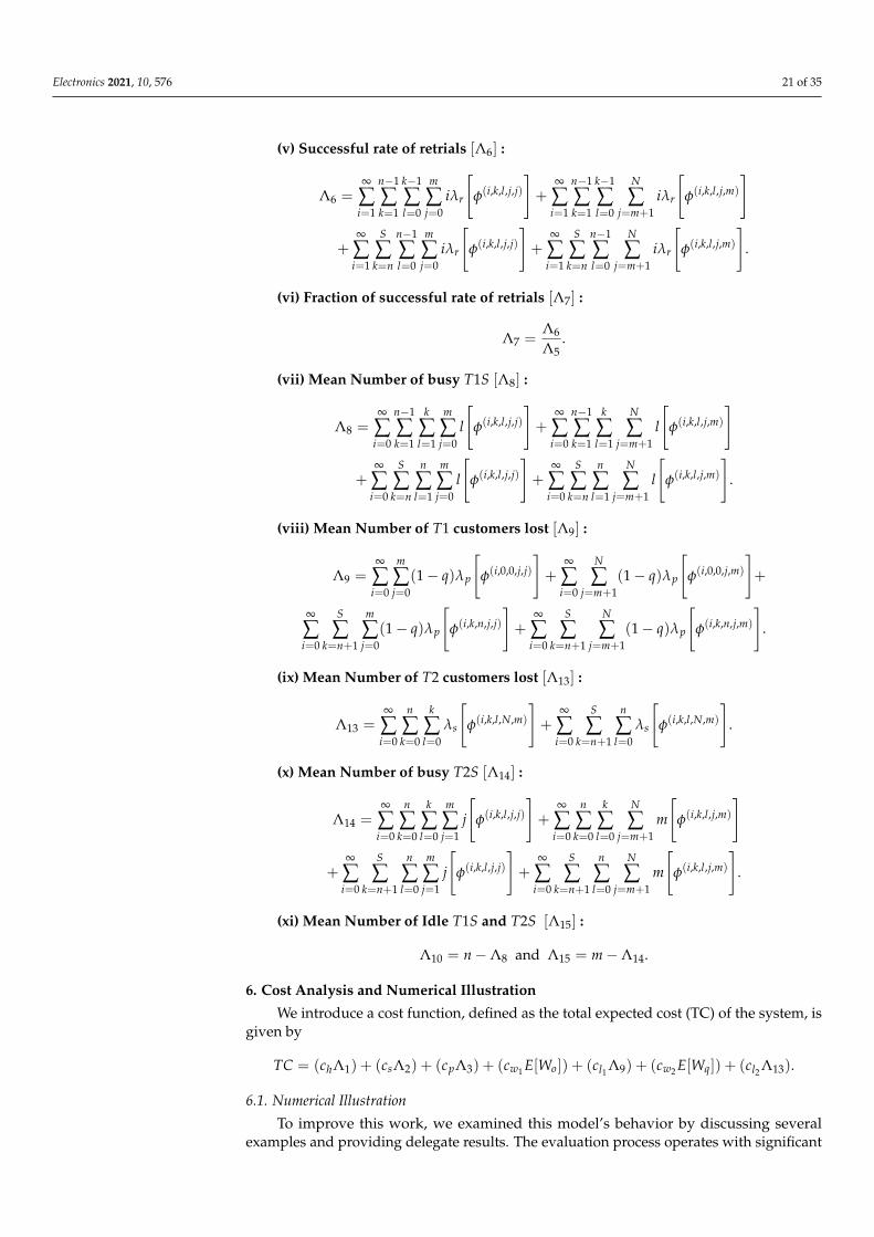
(v) Successful rate of retrials [Λ6] :

Λ6 =∞

∑i=1

n−1

∑k=1

k−1

∑l=0

m

∑j=0

iλr

[φ(i,k,l,j,j)

]+

∞

∑i=1

n−1

∑k=1

k−1

∑l=0

N

∑j=m+1

iλr

[φ(i,k,l,j,m)

]

+∞

∑i=1

S

∑k=n

n−1

∑l=0

m

∑j=0

iλr

[φ(i,k,l,j,j)

]+

∞

∑i=1

S

∑k=n

n−1

∑l=0

N

∑j=m+1

iλr

[φ(i,k,l,j,m)

].

(vi) Fraction of successful rate of retrials [Λ7] :

Λ7 =Λ6

Λ5.

(vii) Mean Number of busy T1S [Λ8] :

Λ8 =∞

∑i=0

n−1

∑k=1

k

∑l=1

m

∑j=0

l

[φ(i,k,l,j,j)

]+

∞

∑i=0

n−1

∑k=1

k

∑l=1

N

∑j=m+1

l

[φ(i,k,l,j,m)

]

+∞

∑i=0

S

∑k=n

n

∑l=1

m

∑j=0

l

[φ(i,k,l,j,j)

]+

∞

∑i=0

S

∑k=n

n

∑l=1

N

∑j=m+1

l

[φ(i,k,l,j,m)

].

(viii) Mean Number of T1 customers lost [Λ9] :

Λ9 =∞

∑i=0

m

∑j=0

(1− q)λp

[φ(i,0,0,j,j)

]+

∞

∑i=0

N

∑j=m+1

(1− q)λp

[φ(i,0,0,j,m)

]+

∞

∑i=0

S

∑k=n+1

m

∑j=0

(1− q)λp

[φ(i,k,n,j,j)

]+

∞

∑i=0

S

∑k=n+1

N

∑j=m+1

(1− q)λp

[φ(i,k,n,j,m)

].

(ix) Mean Number of T2 customers lost [Λ13] :

Λ13 =∞

∑i=0

n

∑k=0

k

∑l=0

λs

[φ(i,k,l,N,m)

]+

∞

∑i=0

S

∑k=n+1

n

∑l=0

λs

[φ(i,k,l,N,m)

].

(x) Mean Number of busy T2S [Λ14] :

Λ14 =∞

∑i=0

n

∑k=0

k

∑l=0

m

∑j=1

j

[φ(i,k,l,j,j)

]+

∞

∑i=0

n

∑k=0

k

∑l=0

N

∑j=m+1

m

[φ(i,k,l,j,m)

]

+∞

∑i=0

S

∑k=n+1

n

∑l=0

m

∑j=1

j

[φ(i,k,l,j,j)

]+

∞

∑i=0

S

∑k=n+1

n

∑l=0

N

∑j=m+1

m

[φ(i,k,l,j,m)

].

(xi) Mean Number of Idle T1S and T2S [Λ15] :

Λ10 = n−Λ8 and Λ15 = m−Λ14.

6. Cost Analysis and Numerical Illustration

We introduce a cost function, defined as the total expected cost (TC) of the system, isgiven by

TC = (chΛ1) + (csΛ2) + (cpΛ3) + (cw1 E[Wo]) + (cl1 Λ9) + (cw2 E[Wq]) + (cl2 Λ13).

6.1. Numerical Illustration

To improve this work, we examined this model’s behavior by discussing severalexamples and providing delegate results. The evaluation process operates with significant

Electronics 2021, 10, 576 22 of 35

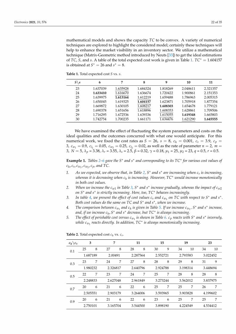
mathematical models and shows the capacity TC to be convex. A variety of numericaltechniques are explored to highlight the considered model; certainly these techniques willhelp to enhance the market visibility in an inventory sector. We utilize a mathematicaltechnique (Matrix-Geometric method introduced by Neuts [33]) to get the ideal estimationsof TC, S, and s. A table of the total expected cost work is given in Table 1. TC∗ = 1.604157is obtained at S∗ = 26 and s∗ = 8.

Table 1. Total expected cost S vs. s.

S\s 6 7 8 9 10 11

23 1.637039 1.635928 1.684324 1.818269 2.048611 2.32135724 1.633410 1.616670 1.636674 1.720422 1.900861 2.15135325 1.639975 1.613164 1.612219 1.659488 1.786963 2.00531526 1.650045 1.619325 1.604157 1.623871 1.705918 1.87735427 1.669872 1.630105 1.608217 1.608303 1.654678 1.77912128 1.690378 1.651656 1.618896 1.608353 1.628861 1.70950629 1.716295 1.672536 1.639336 1.615055 1.619348 1.66580330 1.742754 1.700235 1.661171 1.634476 1.621290 1.645555

We have examined the effect of fluctuating the system parameters and costs on theideal qualities and the outcomes concurred with what one would anticipate. For thisnumerical work, we fixed the cost rates as S = 26, s = 8, ch = 0.001, cs = 3.9, cp =3, cw1 = 0.9, cl1 = 0.05, cw2 = 0.25, cl2 = 0.02, as well as the rate of parameter n = 2, m =3, N = 5, λp = 3.38, λr = 3.55, λs = 2.5, β = 0.32, γ = 0.18, µ1 = 25, µ2 = 23, q = 0.5, r = 0.5.

Example 1. Tables 2–6 gave the S∗ and s∗ and corresponding to its TC∗ for various cost values ofch, cs, cw1 , cw2 , cp, and TC.

1. As we expected, we observe that, in Table 2, S∗ and s∗ are increasing when cs is increasing,whereas it is decreasing when ch is increasing. However, TC∗ would increase monotonicallyin both cost values.

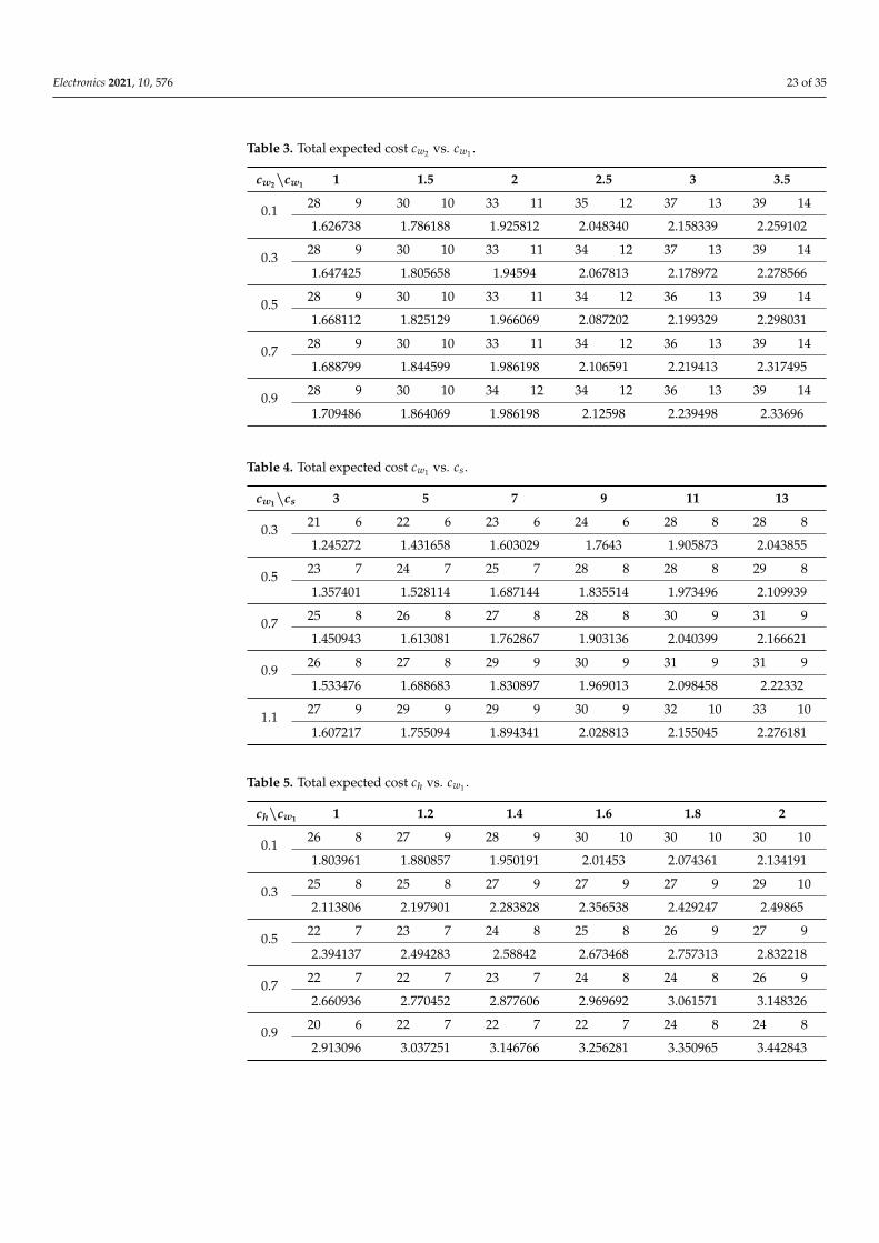
2. When we increase the cw1 in Table 3, S∗ and s∗ increase gradually, whereas the impact of cw2on S∗ and s∗ is strictly increasing. Here, too, TC∗ behaves increasingly.

3. In table 4, we present the effect of cost values cs and cw1 on TC with respect to S∗ and s∗.Both cost values do the same on TC and S∗ and s∗, when we increase.

4. The comparison between cw1 and ch is given in Table 5. If we increase cw1 , S∗ and s∗ increase,and, if we increase ch, S∗ and s∗ decrease, but TC∗ is always increasing.

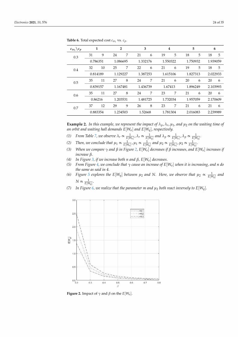
5. The effect of perishable cost versus cw1 is shown in Table 6. cp reacts with S∗ and s∗ inversely,while cw1 reacts directly. In addition, TC∗ is always monotonically increasing.

Table 2. Total expected cost ch vs. cs.

ch\cs 3 7 11 15 19 23

0.1 25 8 27 8 28 8 30 9 34 10 34 10

1.687189 2.00491 2.287564 2.552721 2.793583 3.022452

0.3 23 7 24 7 27 8 28 8 29 8 31 9

1.980232 2.326817 2.640796 2.924788 3.198314 3.448694

0.5 22 7 23 7 24 7 25 7 28 8 28 8

2.248833 2.627048 2.961849 3.273244 3.562012 3.837975

0.7 20 6 21 6 22 6 25 7 25 7 26 7

2.505551 2.903179 3.264006 3.593965 3.903828 4.199602

0.9 20 6 21 6 22 6 23 6 25 7 25 7

2.750101 3.165704 3.544500 3.898190 4.224549 4.534412

Electronics 2021, 10, 576 23 of 35

Table 3. Total expected cost cw2 vs. cw1 .

cw2\cw1 1 1.5 2 2.5 3 3.5

0.1 28 9 30 10 33 11 35 12 37 13 39 14

1.626738 1.786188 1.925812 2.048340 2.158339 2.259102

0.3 28 9 30 10 33 11 34 12 37 13 39 14

1.647425 1.805658 1.94594 2.067813 2.178972 2.278566

0.5 28 9 30 10 33 11 34 12 36 13 39 14

1.668112 1.825129 1.966069 2.087202 2.199329 2.298031

0.7 28 9 30 10 33 11 34 12 36 13 39 14

1.688799 1.844599 1.986198 2.106591 2.219413 2.317495

0.9 28 9 30 10 34 12 34 12 36 13 39 14

1.709486 1.864069 1.986198 2.12598 2.239498 2.33696

Table 4. Total expected cost cw1 vs. cs.

cw1\cs 3 5 7 9 11 13

0.3 21 6 22 6 23 6 24 6 28 8 28 8

1.245272 1.431658 1.603029 1.7643 1.905873 2.043855

0.5 23 7 24 7 25 7 28 8 28 8 29 8

1.357401 1.528114 1.687144 1.835514 1.973496 2.109939

0.7 25 8 26 8 27 8 28 8 30 9 31 9

1.450943 1.613081 1.762867 1.903136 2.040399 2.166621

0.9 26 8 27 8 29 9 30 9 31 9 31 9

1.533476 1.688683 1.830897 1.969013 2.098458 2.22332

1.1 27 9 29 9 29 9 30 9 32 10 33 10

1.607217 1.755094 1.894341 2.028813 2.155045 2.276181

Table 5. Total expected cost ch vs. cw1 .

ch\cw1 1 1.2 1.4 1.6 1.8 2

0.1 26 8 27 9 28 9 30 10 30 10 30 10

1.803961 1.880857 1.950191 2.01453 2.074361 2.134191

0.3 25 8 25 8 27 9 27 9 27 9 29 10

2.113806 2.197901 2.283828 2.356538 2.429247 2.49865

0.5 22 7 23 7 24 8 25 8 26 9 27 9

2.394137 2.494283 2.58842 2.673468 2.757313 2.832218

0.7 22 7 22 7 23 7 24 8 24 8 26 9

2.660936 2.770452 2.877606 2.969692 3.061571 3.148326

0.9 20 6 22 7 22 7 22 7 24 8 24 8

2.913096 3.037251 3.146766 3.256281 3.350965 3.442843

Electronics 2021, 10, 576 24 of 35

Table 6. Total expected cost cw1 vs. cp.

cw1\cp 1 2 3 4 5 6

0.3 31 9 24 7 21 6 19 5 18 5 18 5

0.786351 1.086695 1.332176 1.550322 1.750932 1.939059

0.4 32 10 25 7 22 6 21 6 19 5 18 5

0.814189 1.129227 1.387253 1.615106 1.827313 2.022933

0.5 35 11 27 8 24 7 21 6 20 6 20 6

0.839157 1.167481 1.436739 1.67413 1.896249 2.103993

0.6 35 11 27 8 24 7 23 7 21 6 20 6

0.86216 1.203531 1.481725 1.732034 1.957059 2.170609

0.7 37 12 29 9 26 8 23 7 21 6 21 6

0.883354 1.234503 1.52668 1.781304 2.016083 2.239989

Example 2. In this example, we represent the impact of λp, λr, µ1, and µ2 on the waiting time ofan orbit and waiting hall demands E[Wo] and E[Wq], respectively.

(1) From Table 7, we observe λr ∝ 1E[Wo ]

, λr ∝ 1E[Wq ]

and λp ∝ 1E[Wo ]

, λp ∝ 1E[Wq ]

.

(2) Then, we conclude that µ1 ∝ 1E[Wo ]

, µ1 ∝ 1E[Wq ]

and µ2 ∝ 1E[Wo ]

, µ2 ∝ 1E[Wq ]

.

(3) When we compare γ and β in Figure 2, E[Wo] decreases if β increases, and E[Wo] increases ifincrease β.

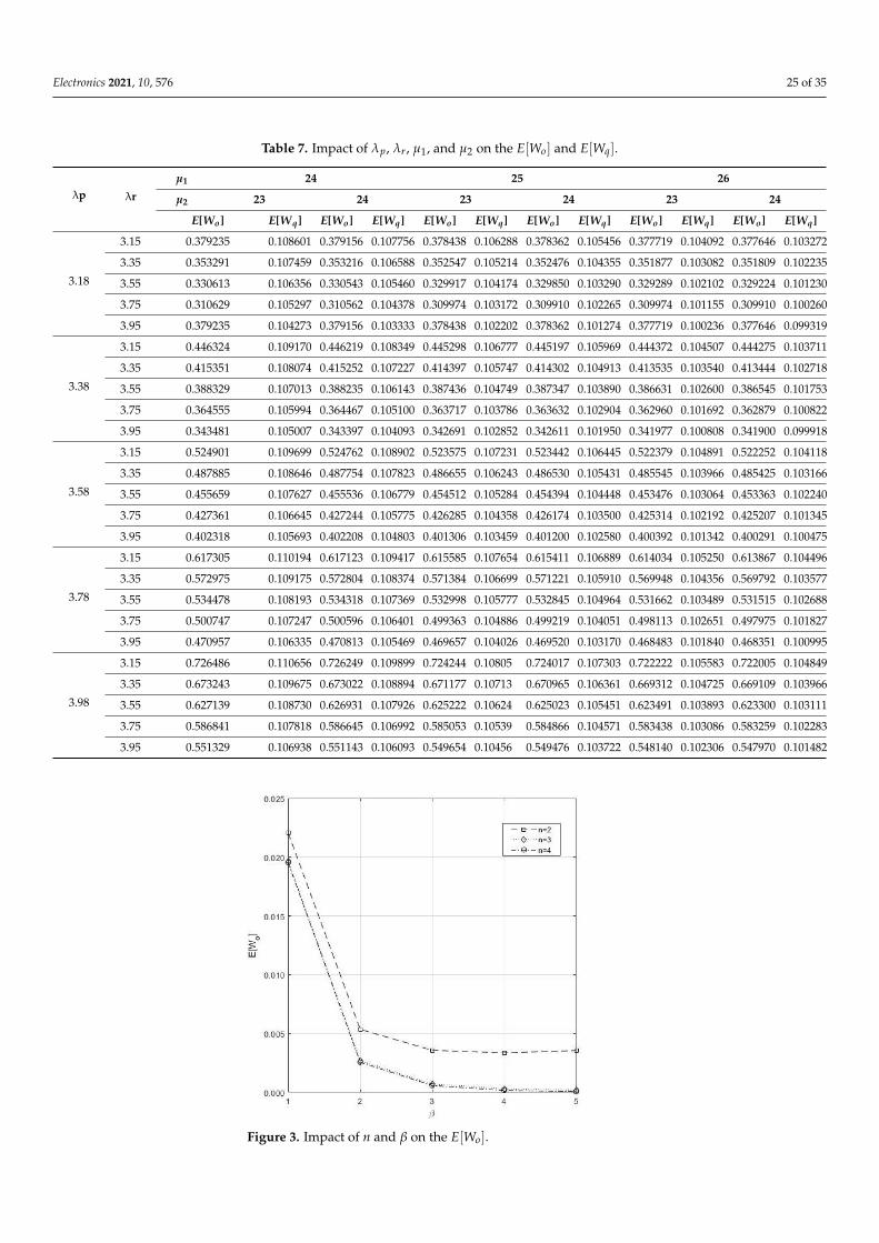
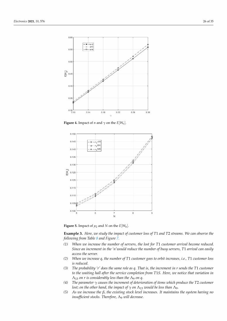
(4) In Figure 3, if we increase both n and β, E[Wo] decreases.(5) From Figure 4, we conclude that γ cause an increase of E[Wo] when it is increasing, and n do

the same as said in 4.(6) Figure 5 explores the E[Wq] between µ2 and N. Here, we observe that µ2 ∝ 1

E[Wq ]and

N ∝ 1E[Wq ]

.

(7) In Figure 6, we realize that the parameter m and µ2 both react inversely to E[Wq].

Figure 2. Impact of γ and β on the E[Wo].

Electronics 2021, 10, 576 25 of 35

Table 7. Impact of λp, λr, µ1, and µ2 on the E[Wo] and E[Wq].

λp λr

µ1 24 25 26

µ2 23 24 23 24 23 24

E[Wo] E[Wq] E[Wo] E[Wq] E[Wo] E[Wq] E[Wo] E[Wq] E[Wo] E[Wq] E[Wo] E[Wq]

3.18

3.15 0.379235 0.108601 0.379156 0.107756 0.378438 0.106288 0.378362 0.105456 0.377719 0.104092 0.377646 0.103272

3.35 0.353291 0.107459 0.353216 0.106588 0.352547 0.105214 0.352476 0.104355 0.351877 0.103082 0.351809 0.102235

3.55 0.330613 0.106356 0.330543 0.105460 0.329917 0.104174 0.329850 0.103290 0.329289 0.102102 0.329224 0.101230

3.75 0.310629 0.105297 0.310562 0.104378 0.309974 0.103172 0.309910 0.102265 0.309974 0.101155 0.309910 0.100260

3.95 0.379235 0.104273 0.379156 0.103333 0.378438 0.102202 0.378362 0.101274 0.377719 0.100236 0.377646 0.099319

3.38

3.15 0.446324 0.109170 0.446219 0.108349 0.445298 0.106777 0.445197 0.105969 0.444372 0.104507 0.444275 0.103711

3.35 0.415351 0.108074 0.415252 0.107227 0.414397 0.105747 0.414302 0.104913 0.413535 0.103540 0.413444 0.102718

3.55 0.388329 0.107013 0.388235 0.106143 0.387436 0.104749 0.387347 0.103890 0.386631 0.102600 0.386545 0.101753

3.75 0.364555 0.105994 0.364467 0.105100 0.363717 0.103786 0.363632 0.102904 0.362960 0.101692 0.362879 0.100822

3.95 0.343481 0.105007 0.343397 0.104093 0.342691 0.102852 0.342611 0.101950 0.341977 0.100808 0.341900 0.099918

3.58

3.15 0.524901 0.109699 0.524762 0.108902 0.523575 0.107231 0.523442 0.106445 0.522379 0.104891 0.522252 0.104118

3.35 0.487885 0.108646 0.487754 0.107823 0.486655 0.106243 0.486530 0.105431 0.485545 0.103966 0.485425 0.103166

3.55 0.455659 0.107627 0.455536 0.106779 0.454512 0.105284 0.454394 0.104448 0.453476 0.103064 0.453363 0.102240

3.75 0.427361 0.106645 0.427244 0.105775 0.426285 0.104358 0.426174 0.103500 0.425314 0.102192 0.425207 0.101345

3.95 0.402318 0.105693 0.402208 0.104803 0.401306 0.103459 0.401200 0.102580 0.400392 0.101342 0.400291 0.100475

3.78

3.15 0.617305 0.110194 0.617123 0.109417 0.615585 0.107654 0.615411 0.106889 0.614034 0.105250 0.613867 0.104496

3.35 0.572975 0.109175 0.572804 0.108374 0.571384 0.106699 0.571221 0.105910 0.569948 0.104356 0.569792 0.103577

3.55 0.534478 0.108193 0.534318 0.107369 0.532998 0.105777 0.532845 0.104964 0.531662 0.103489 0.531515 0.102688

3.75 0.500747 0.107247 0.500596 0.106401 0.499363 0.104886 0.499219 0.104051 0.498113 0.102651 0.497975 0.101827

3.95 0.470957 0.106335 0.470813 0.105469 0.469657 0.104026 0.469520 0.103170 0.468483 0.101840 0.468351 0.100995

3.98

3.15 0.726486 0.110656 0.726249 0.109899 0.724244 0.10805 0.724017 0.107303 0.722222 0.105583 0.722005 0.104849

3.35 0.673243 0.109675 0.673022 0.108894 0.671177 0.10713 0.670965 0.106361 0.669312 0.104725 0.669109 0.103966

3.55 0.627139 0.108730 0.626931 0.107926 0.625222 0.10624 0.625023 0.105451 0.623491 0.103893 0.623300 0.103111

3.75 0.586841 0.107818 0.586645 0.106992 0.585053 0.10539 0.584866 0.104571 0.583438 0.103086 0.583259 0.102283

3.95 0.551329 0.106938 0.551143 0.106093 0.549654 0.10456 0.549476 0.103722 0.548140 0.102306 0.547970 0.101482

Figure 3. Impact of n and β on the E[Wo].

Electronics 2021, 10, 576 26 of 35

Figure 4. Impact of n and γ on the E[Wo].

Figure 5. Impact of µ2 and N on the E[Wh].

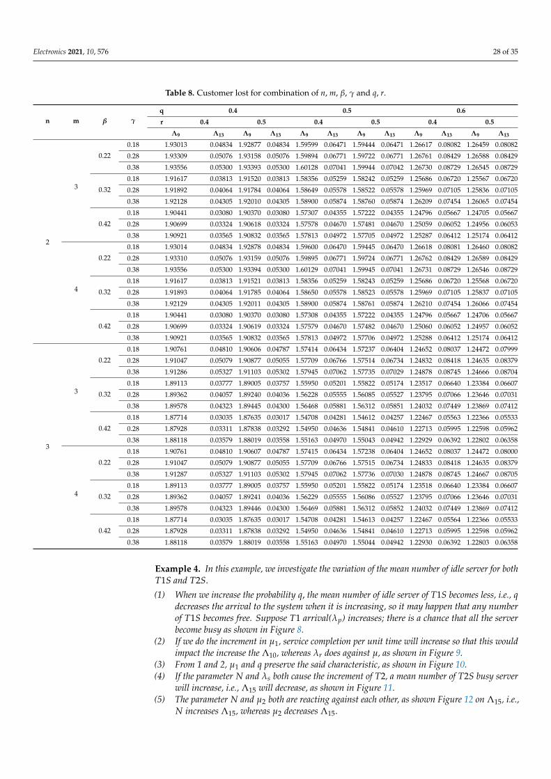
Example 3. Here, we study the impact of customer loss of T1 and T2 streams. We can observe thefollowing from Table 8 and Figure 7.

(1) When we increase the number of servers, the lost for T1 customer arrival become reduced.Since an increment in the ‘n’would reduce the number of busy servers, T1 arrival can easilyaccess the server.

(2) When we increase q, the number of T1 customer goes to orbit increases, i.e., T1 customer lossis reduced.

(3) The probability ‘r’ does the same role as q. That is, the increment in r sends the T1 customerto the waiting hall after the service completion from T1S. Here, we notice that variation inΛ13 on r is considerably less than the Λ9 on q.

(4) The parameter γ causes the increment of deterioration of items which produce the T2 customerlost; on the other hand, the impact of γ on Λ13 would be less than Λ9.

(5) As we increase the β, the existing stock level increases. It maintains the system having noinsufficient stocks. Therefore, Λ9 will decrease.

Electronics 2021, 10, 576 27 of 35

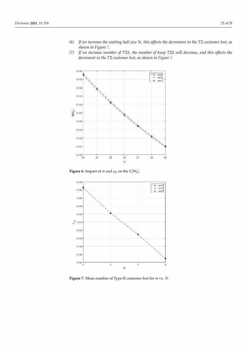
(6) If we increase the waiting hall size N, this affects the decrement in the T2 customer lost, asshown in Figure 7.

(7) If we increase number of T2S, the number of busy T2S will decrease, and this affects thedecrement in the T2 customer lost, as shown in Figure 7.

Figure 6. Impact of m and µ2 on the E[Wh].

Figure 7. Mean number of Type-II customer lost for m vs. N.

Electronics 2021, 10, 576 28 of 35

Table 8. Customer lost for combination of n, m, β, γ and q, r.

n m β γ

q 0.4 0.5 0.6

r 0.4 0.5 0.4 0.5 0.4 0.5

Λ9 Λ13 Λ9 Λ13 Λ9 Λ13 Λ9 Λ13 Λ9 Λ13 Λ9 Λ13

2

3

0.22

0.18 1.93013 0.04834 1.92877 0.04834 1.59599 0.06471 1.59444 0.06471 1.26617 0.08082 1.26459 0.08082

0.28 1.93309 0.05076 1.93158 0.05076 1.59894 0.06771 1.59722 0.06771 1.26761 0.08429 1.26588 0.08429

0.38 1.93556 0.05300 1.93393 0.05300 1.60128 0.07041 1.59944 0.07042 1.26730 0.08729 1.26545 0.08729

0.32

0.18 1.91617 0.03813 1.91520 0.03813 1.58356 0.05259 1.58242 0.05259 1.25686 0.06720 1.25567 0.06720

0.28 1.91892 0.04064 1.91784 0.04064 1.58649 0.05578 1.58522 0.05578 1.25969 0.07105 1.25836 0.07105

0.38 1.92128 0.04305 1.92010 0.04305 1.58900 0.05874 1.58760 0.05874 1.26209 0.07454 1.26065 0.07454

0.42

0.18 1.90441 0.03080 1.90370 0.03080 1.57307 0.04355 1.57222 0.04355 1.24796 0.05667 1.24705 0.05667

0.28 1.90699 0.03324 1.90618 0.03324 1.57578 0.04670 1.57481 0.04670 1.25059 0.06052 1.24956 0.06053

0.38 1.90921 0.03565 1.90832 0.03565 1.57813 0.04972 1.57705 0.04972 1.25287 0.06412 1.25174 0.06412

4

0.22

0.18 1.93014 0.04834 1.92878 0.04834 1.59600 0.06470 1.59445 0.06470 1.26618 0.08081 1.26460 0.08082

0.28 1.93310 0.05076 1.93159 0.05076 1.59895 0.06771 1.59724 0.06771 1.26762 0.08429 1.26589 0.08429

0.38 1.93556 0.05300 1.93394 0.05300 1.60129 0.07041 1.59945 0.07041 1.26731 0.08729 1.26546 0.08729

0.32

0.18 1.91617 0.03813 1.91521 0.03813 1.58356 0.05259 1.58243 0.05259 1.25686 0.06720 1.25568 0.06720

0.28 1.91893 0.04064 1.91785 0.04064 1.58650 0.05578 1.58523 0.05578 1.25969 0.07105 1.25837 0.07105

0.38 1.92129 0.04305 1.92011 0.04305 1.58900 0.05874 1.58761 0.05874 1.26210 0.07454 1.26066 0.07454

0.42

0.18 1.90441 0.03080 1.90370 0.03080 1.57308 0.04355 1.57222 0.04355 1.24796 0.05667 1.24706 0.05667

0.28 1.90699 0.03324 1.90619 0.03324 1.57579 0.04670 1.57482 0.04670 1.25060 0.06052 1.24957 0.06052

0.38 1.90921 0.03565 1.90832 0.03565 1.57813 0.04972 1.57706 0.04972 1.25288 0.06412 1.25174 0.06412

3

3

0.22

0.18 1.90761 0.04810 1.90606 0.04787 1.57414 0.06434 1.57237 0.06404 1.24652 0.08037 1.24472 0.07999

0.28 1.91047 0.05079 1.90877 0.05055 1.57709 0.06766 1.57514 0.06734 1.24832 0.08418 1.24635 0.08379

0.38 1.91286 0.05327 1.91103 0.05302 1.57945 0.07062 1.57735 0.07029 1.24878 0.08745 1.24666 0.08704

0.32

0.18 1.89113 0.03777 1.89005 0.03757 1.55950 0.05201 1.55822 0.05174 1.23517 0.06640 1.23384 0.06607

0.28 1.89362 0.04057 1.89240 0.04036 1.56228 0.05555 1.56085 0.05527 1.23795 0.07066 1.23646 0.07031

0.38 1.89578 0.04323 1.89445 0.04300 1.56468 0.05881 1.56312 0.05851 1.24032 0.07449 1.23869 0.07412

0.42

0.18 1.87714 0.03035 1.87635 0.03017 1.54708 0.04281 1.54612 0.04257 1.22467 0.05563 1.22366 0.05533

0.28 1.87928 0.03311 1.87838 0.03292 1.54950 0.04636 1.54841 0.04610 1.22713 0.05995 1.22598 0.05962

0.38 1.88118 0.03579 1.88019 0.03558 1.55163 0.04970 1.55043 0.04942 1.22929 0.06392 1.22802 0.06358

4

0.22

0.18 1.90761 0.04810 1.90607 0.04787 1.57415 0.06434 1.57238 0.06404 1.24652 0.08037 1.24472 0.08000

0.28 1.91047 0.05079 1.90877 0.05055 1.57709 0.06766 1.57515 0.06734 1.24833 0.08418 1.24635 0.08379

0.38 1.91287 0.05327 1.91103 0.05302 1.57945 0.07062 1.57736 0.07030 1.24878 0.08745 1.24667 0.08705

0.32

0.18 1.89113 0.03777 1.89005 0.03757 1.55950 0.05201 1.55822 0.05174 1.23518 0.06640 1.23384 0.06607

0.28 1.89362 0.04057 1.89241 0.04036 1.56229 0.05555 1.56086 0.05527 1.23795 0.07066 1.23646 0.07031

0.38 1.89578 0.04323 1.89446 0.04300 1.56469 0.05881 1.56312 0.05852 1.24032 0.07449 1.23869 0.07412

0.42

0.18 1.87714 0.03035 1.87635 0.03017 1.54708 0.04281 1.54613 0.04257 1.22467 0.05564 1.22366 0.05533

0.28 1.87928 0.03311 1.87838 0.03292 1.54950 0.04636 1.54841 0.04610 1.22713 0.05995 1.22598 0.05962

0.38 1.88118 0.03579 1.88019 0.03558 1.55163 0.04970 1.55044 0.04942 1.22930 0.06392 1.22803 0.06358

Example 4. In this example, we investigate the variation of the mean number of idle server for bothT1S and T2S.

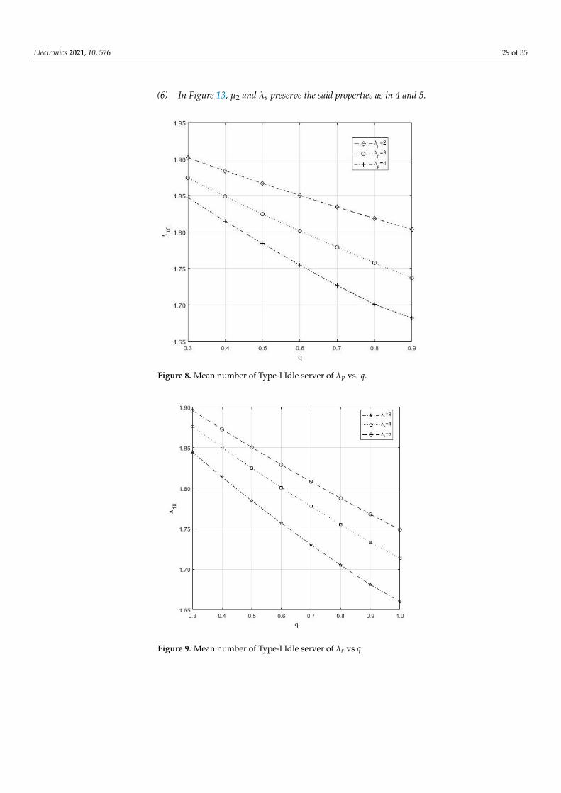
(1) When we increase the probability q, the mean number of idle server of T1S becomes less, i.e., qdecreases the arrival to the system when it is increasing, so it may happen that any numberof T1S becomes free. Suppose T1 arrival(λp) increases; there is a chance that all the serverbecome busy as shown in Figure 8.

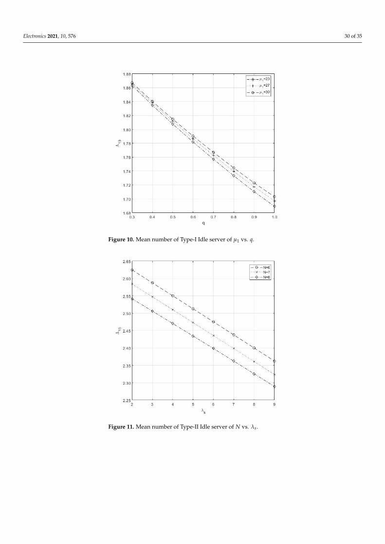
(2) If we do the increment in µ1, service completion per unit time will increase so that this wouldimpact the increase the Λ10, whereas λr does against µ, as shown in Figure 9.

(3) From 1 and 2, µ1 and q preserve the said characteristic, as shown in Figure 10.(4) If the parameter N and λs both cause the increment of T2, a mean number of T2S busy server

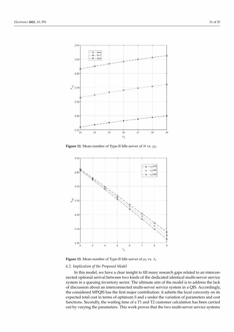
will increase, i.e., Λ15 will decrease, as shown in Figure 11.(5) The parameter N and µ2 both are reacting against each other, as shown Figure 12 on Λ15, i.e.,

N increases Λ15, whereas µ2 decreases Λ15.

Electronics 2021, 10, 576 29 of 35

(6) In Figure 13, µ2 and λs preserve the said properties as in 4 and 5.

Figure 8. Mean number of Type-I Idle server of λp vs. q.

Figure 9. Mean number of Type-I Idle server of λr vs q.

Electronics 2021, 10, 576 30 of 35

Figure 10. Mean number of Type-I Idle server of µ1 vs. q.

Figure 11. Mean number of Type-II Idle server of N vs. λs.

Electronics 2021, 10, 576 31 of 35

Figure 12. Mean number of Type-II Idle server of N vs. µ2.

Figure 13. Mean number of Type-II Idle server of µ2 vs. λs

6.2. Implication of the Proposed Model

In this model, we have a clear insight to fill many research gaps related to an intercon-nected optional arrival between two kinds of the dedicated identical multi-server servicesystem in a queuing inventory sector. The ultimate aim of the model is to address the lackof discussion about an interconnected multi-server service system in a QIS. Accordingly,the considered MPQIS has the first major contribution: it admits the local convexity on itsexpected total cost in terms of optimum S and s under the variation of parameters and costfunctions. Secondly, the waiting time of a T1 and T2 customer calculation has been carriedout by varying the parameters. This work proves that the two multi-server service systems

Electronics 2021, 10, 576 32 of 35

significantly reduce the waiting time of both T1 and T2. Further, the discussion of customerloss of both T1 and T2 and the number of idle servers of both T1S and T2S suggests howthe findings are much needed to make an acceptable policy. Hence, we believe that ourresearch findings of this MPQIS could constitute a critical source of intelligence because ithas some risk of fixing the convexity, comparing the other (single multi-server) systems.

7. Conclusions

In the interconnected performance of two different multi-server service channels inthe MPQIS, we discussed a Matrix geometric technique for two types of arrival streams.The wait time distribution for both streams is derived analytically by LST method. Subse-quently, to fill the necessity of the proposed model in inventory management, we exploredits functions numerically in all examples. In nature, the environment is relatively unstable.Firms are ready to make a significant change by creating opportunities for their demands.All the firms must study the factors that are very useful to redefine their value poten-tially at regular intervals, and this can assist and generate a new strategy to manage theemerging problems around the industry when approaching a generic model in stochasticqueuing modeling, as well as would deliver a well-build and predicted results successfully.Moreover, this technique provides a positive variance which can expose a business, as towhether it is on the right track. In such a way that, the approached model would benefit theinventory industrialists and managements. The proposed model can also be an applicableon computational intelligence consisting electronic-based sensor technologies in the fieldof smart inventory management. In the future, we are planning to develop this model in aMarkovian arrival process with the Phase-type distribution environment.

Author Contributions: Conceptualization, K.J. and N.A.; Data curation, K.J. and S.S.; Formal analysis,K.J. and T.H.; Funding acquisition, R.D. and G.P.J.; Investigation, S.A. (S. Amutha) and S.A. (SrijanaAcharya); Methodology, T.H., S.A. (S. Amutha) and S.A. (Srijana Acharya); Project administration,R.D. and G.P.J.; Software, T.H.; Supervision, G.P.J.; Validation, S.S. and S.A. (Srijana Acharya);Visualization, S.A. (S. Amutha); Writing—original draft, N.A.; Writing—review & editing, G.P.J. Allauthors have read and agreed to the published version of the manuscript.

Funding: Anbazhagan and Amutha would like to thank RUSA Phase 2.0(F 24-51/2014-U), DST-FIST(SR/FIST/MS-I/2018/17), DST-PURSE 2nd Phase programme (SR/PURSE Phase 2/38) andUGC-SAP(DRS-I)(F.510/8/DRS-I/2016(SAP-I)), Govt. of India.

Data Availability Statement: The data presented in this study are available on request from thecorresponding authors.

Conflicts of Interest: The authors declare no conflict of interest.

Notations

0 zero matrixe A column vector of covenient size having one in each co-ordinatesem(n) A column vector of dimension m with 1 in the n-th positionIn An identity matrix of order nW Whole numbersM Cut-off point of the truncation process in the matrix geometric

approximationA(a,b) entry at (a, b)th position of a matrix AjZ1 ⊗ Z2 Kronecker product of matrices Z1 and Z2X1(t) Number of customers in the orbit at time tX2(t) Number of items in the inventory at time tX3(t) Number of busy T1S at time t

.

Electronics 2021, 10, 576 33 of 35

X4(t) Number of T2 customers (waiting and being served)in the waiting hall at time t

X5(t) Number of busy T2S at time tS Maximum inventory levels Reorder pointS∗ Optimum inventory levels∗ Optimum reorder pointλp Intensity rate of T1 arrivalλs Intensity rate of T2 arrivalλr Intensity rate of retrial arrivalµ1 Intensity rate of T1 serviceµ2 Intensity of T1 arrivalβ Intensity rate of reordering itemγ Intensity rate of deteriorating itemch Inventory carrying costs per unit timecs Setup cost per unit timecp Perishable cost per unit timecw1 T1 customers’ waiting cost per unit timecl1 T1 customers’ lost cost per unit timecl2 T2 customers’ lost cost per unit timecw2 T2 customers’ waiting cost per unit timeTC Total expected costTC∗ optimum expected total cost

δij

{1, if j = i,0, if j 6= i

H(x){

1, if x ≥ 0,0, if x < 0

N Size of the waiting hall

[BN+1]i,j

{1, if i < j = i + 1,0, otherwise

δ̄ij 1− δijVk {1, 2, ..., k}Va

k {a, a + 1, ..., k}, 0 ≤ a ≤ kE1 {(u1, u2, u3, u4, u5) : u1 ∈W, u2 ∈ V0

n−1, u3 ∈ V0u2

, u4 ∈ V0m−1, u5 = u4}

E2 {(u1, u2, u3, u4, u5) : u1 ∈W, u2 ∈ V0n−1, u3 ∈ V0

u2, u4 ∈ VN \Vm−1, u5 = m}

E3 {(u1, u2, u3, u4, u5) : u1 ∈W, u2 ∈ VS \Vn−1, u3 ∈ V0n , u4 ∈ V0

m−1, u5 = u4}E4 {(u1, u2, u3, u4, u5) : u1 ∈W, u2 ∈ VS \Vn−1, u3 ∈ V0

n , u4 ∈ VN \Vm−1, u5 = m}D {(i, k, l, j, g) : i ∈ V0

L , k ∈ V0n , l ∈ V0

k , j ∈ Vm, g = j}∪{(i, k, l, j, g) : i ∈ V0

L , k ∈ V0n , l ∈ V0

k , j ∈ Vm+1N , g = j}∪

{(i, k, l, j, g) : i ∈ V0L , k ∈ Vn+1

S , l ∈ V0n , j ∈ Vm, g = j}∪

{(i, k, l, j, g) : i ∈ V0L , k ∈ Vn+1

S , l ∈ V0n , j ∈ Vm+1

N , g = j}C {(i, k, l, j, g) : i ∈ V1

L , k ∈ V0n , l ∈ V0

k , j ∈ V0m, g = j}∪

{(i, k, l, j, g) : i ∈ V1L , k ∈ V0

n , l ∈ V0k , j ∈ Vm+1

N , g = j}∪{(i, k, l, j, g) : i ∈ V1

L , k ∈ Vn+1S , l ∈ V0

n , j ∈ V0m, g = j}∪

{(i, k, l, j, g) : i ∈ V1L , k ∈ Vn+1

S , l ∈ V0n , j ∈ Vm+1

N , g = j}

.

References1. Melikov, A.Z.; Molchanov, A.A. Stock Optimization in Transport/Storage. Cybern. Syst. Anal. 1992, 28, 484–487. [CrossRef]2. Sigman, K.; Simchi-Levi, D. Light traffic heuristic for an M/G/1 queue with limited inventory. Ann. Oper. Res. 1992, 40, 371–380.

[CrossRef]3. Berman, O.; Kaplan, E.H.; Shimshak, D.G. Deterministic Approximations for Inventory Management at Service Facilities. IIE

Trans. 1993, 25, 98–104. [CrossRef]

Electronics 2021, 10, 576 34 of 35

4. Berman, O.; Kim, E. Stochastic Inventory Policies for Inventory Management at Service Facilities. Stoch. Models 1999, 15, 695–718.[CrossRef]

5. Berman, O.; Sapna, K.P. Inventory Management at Service Facilities for Systems with Arbitrarily Distributed Service Times. Stoch.Models 2000, 16, 343–360. [CrossRef]

6. Paul Manual,; Sivakumar, B.; Arivarignan, G. A Perishable inventory system with service facilities and retrial customers. Comput.Ind. Eng. 2008, 54, 484–501. [CrossRef]

7. Amirthakodi, M.; Sivakumar, B. An inventory system with service facility and finite orbit size for feedback customers. OPSEARCH2014, 52, 225-–255. [CrossRef]

8. Amirthakodi, M.; Radhamani, V.; Sivakumar, B. A perishable inventory system with service facility and feedback customers. Ann.Oper. Res. 2015, 233, 25—55. [CrossRef]

9. Jeganathan, K.; Anbazhagan, N.; Kathiresan, J. A Retrial Inventory System with Non-Preemptive Priority Service. Int. J. Inf.Manag. Sci. 2013, 24, 57–77.

10. Jeganathan, K.; Kathiresan, J.; Anbazhagan, N. A retrial inventory system with priority customers and second optional service.OPSEARCH 2016, 53, 808–834. [CrossRef]

11. Melikov, A.Z.; Shahmaliyev, M.O. Queueing System M/M/1/∞ with Perishable Inventory and Repeated Customers. Autom.Remote Control. 2019, 80, 53–65. [CrossRef]

12. Reshmi, P.S.; Jose, K.P. A MAP/PH/1 Perishable Inventory System with Dependent Retrial Loss. Int. J. Appl. Comput. Math.2020, 6, 1–11. [CrossRef]

13. Kuo-Hsiung, W.; Keng-Yuan, T. A queueing system with queue dependent servers and finite capacity. Appl. Math. Model. 2000,24, 807–814.

14. Bae, J.; Kim, J.; Lees, E.Y. An optimal service rate in a Poisson arrival with two-stage queue service policy. Math. Methods Oper.Res. 2003, 58, 477–482. [CrossRef]

15. Jeganathan, K.; Reiyas, M.A.; Padmasekaran, S.; Lakshmanan, K. An M/EK/1/N Queueing-Inventory System with Two ServiceRates Based on Queue Lengths. Int. J. Appl. Comput. Math. 2017, 3, 357–386. [CrossRef]

16. Jeganathan, K.; Reiyas, M.A.; Prasanna Lakshmi, K.; Saravanan, S. Two server Markovian inventory systems with serverinterruptions:Heterogeneous vs. homogeneous servers. Math. Comput. Simul. 2019, 155, 177–200. [CrossRef]

17. Jeganathan, K.; Sumathi, J.; Mahalakshmi, G. Markovian Inventory Model With Two Parallel Queues, Jockeying And ImpatientCustomers. Yugosl. J. Oper. Res. 2016, 26, 467–506. [CrossRef]

18. Pandelis, D.G. Optimal stochastic scheduling of two interconnected queues with varying service rates. Oper. Res. Lett. 2008, 36,492–495. [CrossRef]

19. Jeganathan, K.; Melikov, A.Z.; Padmasekaran, S.; Jehoashan Kingsly, S.; Prasanna Lakshmi, K. A Stochastic Inventory Model withTwo Queues and a Flexible Server. Int. J. Appl. Comput. Math. 2019, 5, 1–27. [CrossRef]

20. Jeganathan, K.; Reiyas, M.A. Two parallel heterogeneous servers Markovian inventory system with modified and delayedworking vacations. Math. Comput. Simul. 2020, 172, 273–304. [CrossRef]

21. Krishnamoorthy, A.; Manikandan, R.; Shajin, D. Analysis of a Multiserver Queueing-Inventory System. Adv. Oper. Res. 2015,2015, 1–16. [CrossRef]

22. Rajkumar, M.; Sivakumar, B.; Arivarignan, G. An infinite waiting hall at a multi-server inventory system. Int. J. Inventory Res.2014, 2, 189–221. [CrossRef]

23. Arivarignan, G.; Yadavalli, V.S.S.; Sivakumar, B. A perishable inventory system with multi-server service facility and retrialcustomers. Manag. Sci. Pract. 2008, 3–27.

24. Yadavalli, V.S.S.; Sivakumar, B.; Arivarignan, G.; Olufemi, A. A Multi-Server Perishable Inventory System With negative customer.Comput. Ind. Eng. 2011, 61, 254–273. [CrossRef]

25. Nair, A.N.; Jacob, M.J.; Krishnamoorthy, A. The multi server M/M/(s,S) queueing inventory system. Ann. Oper. Res. 2013,233, 321–333. [CrossRef]

26. Wang, F.; Bhagat, A.; Chang, T. Analysis of priority multi-server retrial queueing inventory systems with MAP arrivals andexponential services. OPSEARCH 2017, 54, 44—66. [CrossRef]

27. Paul, M.; Sivakumar, B.; Arivarignan, G. A Multi-Server Perishable Inventory System With Service Facility. Pac. J. Appl. Math.2009, 2, 69–82.

28. Suganya, C.; Sivakumar, B.; Arivarignan G. Numerical investigation on MAP/PH(1), PH(2)/2 inventory system with multipleserver vacations. Int. J. Oper. Res. 2017, 29, 1–32. [CrossRef]

29. Suganya, C.; Sivakumar, B. MAP/PH(1), PH(2)/2 finite retrial inventory system with service facility, multiple vacations forservers. Int. J. Math. Oper. Res. 2019, 15, 265–295. [CrossRef]

30. Yadavalli, V.S.S.; Sivakumar, B.; Arivarignan G.; Olufemi, A. A finite source multi-server inventory system with service facility.Comput. Ind. Eng. 2012, 63, 739-–753. [CrossRef]

31. Gabi, H.; Tal, A.; Tatyana, C.; Uri, Y. A multi-server system with inventory of preliminary services and stock-dependent demand.Int. J. Prod. Res. 2020, 1–19.

32. Cheng-Yuan, K.; Scott, J. Access Control to Two Multiserver Loss Queues in Series. IEEE Trans. Autom. Control. 1997, 42,1017—1023. [CrossRef]

Electronics 2021, 10, 576 35 of 35

33. Neuts, M.F. Matrix-Geometric Solutions in Stochastic Models—An Algorithmic Approach; Dover Publication Inc.: New York, NY,USA, 1981.

34. Abate, J.; Ehitt, W. Numerical inversion of laplace transformation of probability distributions. ORSA J. Comput. 1995, 7, 36–43.[CrossRef]