Master of Science in Electric Power Engineering June 2011 Kjetil Uhlen, ELKRAFT Submission date: Supervisor: Norwegian University of Science and Technology Department of Electric Power Engineering Analysis of IEEE Power System Stabilizer Models Anders Hammer

Welcome message from author
This document is posted to help you gain knowledge. Please leave a comment to let me know what you think about it! Share it to your friends and learn new things together.
Transcript
Master of Science in Electric Power EngineeringJune 2011Kjetil Uhlen, ELKRAFT
Submission date:Supervisor:
Norwegian University of Science and TechnologyDepartment of Electric Power Engineering
Analysis of IEEE Power SystemStabilizer Models
Anders Hammer

Analysis of IEEE Power System Stabilizer Models NTNU
Anders Hammer, Spring 2011 II
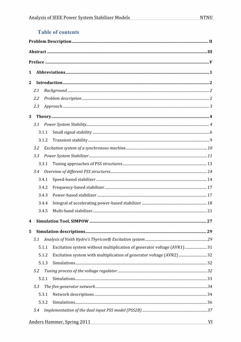
Problem Description In 2005 IEEE (The Institute of Electrical and Electronic Engineers) introduced a new standard
model for Power System Stabilizers, the PSS4B. This is an advanced multi-band stabilizer
that may give a better performance than the regular PSSs often used today. The new stabilizer
has three parallel control blocks, each aiming at damping different oscillatory modes or
different frequency bands of the low frequency oscillations in the power system. So far the
PSS4B is not very known in the market, but in the future it will probably become a standard
requirement for key power plants in the power system. This master thesis is a continuation of
a project performed in the autumn 2010, where the power system model and the framework
for analysis were established. The power system will during this master thesis be upgraded to
contain an additional smaller generator and also two different multiple-input stabilizer
models, the PSS2B and the PSS4B. These stabilizer models will be implemented and tuned
for the small hydro generator in the network. Comparisons between the different network
configurations will be performed where the focus will be at the inter-area and local oscillation
modes. This master thesis will seek to find an answer on following questions:
• How should the PSS4B be tuned to give the best damping of the local and inter-area
oscillation mode?
• Will an implementation of PSS4B give a better result compared to PSS2B?
• What are the pros and cons of PSS2B and PSS4B?
Assignment given: 10. January 2011
Supervisor: Kjetil Uhlen

Analysis of IEEE Power System Stabilizer Models NTNU
Anders Hammer, Spring 2011 III
Abstract Student: Anders Hammer Supervisor: Kjetil Uhlen Contact: Daniel Mota Collaboration with: Voith Hydro
Problem description
IEEE (Institute of Electrical and Electronics Engineers) presented in 2005 a new PSS
structure named IEEE PSS4B (Figure 0-‐1). Voith Hydro wants to analyse the pros and cons
of using this new type compared to older structures. The PSS4B is a multi-band stabilizer that
has three separate bands and is specially designed to handle different oscillation frequencies
in a wide range. Until now, Voith Hydro has used the common PSS2B in their installations,
but in the future they will probably start to implement the new PSS4B. This master thesis will
seek to find an answer on following questions:
• How should the PSS4B be tuned to give the best damping of the local and inter-area
oscillation mode?
• Will an implementation of PSS4B give a better result compared to PSS2B?
• What are the pros and cons of PSS2B and PSS4B?
Figure 0-1: The multi-band stabilizer, IEEE PSS4B [1].
Method
In order to test and compare different PSS models, a simple two-area network model is
created in a computer simulation programme (SIMPOW). One of the generating units is a

Analysis of IEEE Power System Stabilizer Models NTNU
Anders Hammer, Spring 2011 IV
hydro generator, which has a model of a static excitation system made by Voith Hydro. This
network is characterised by a poorly damped inter-area oscillation mode, and in addition some
local oscillation modes related to each machine. Different PSS structures (PSS2B and PSS4B)
are then tuned and installed in the excitation system of the hydro generator, in order to
improve the stability of the network. Different tuning methods of the PSS4B are designed,
tested and later compared with the more common stabilizer the PSS2B. Simplifications are
made where parts of the stabilizer is disconnected in order to adapt the control structure to the
applied network and its oscillations. Totally 5 different tuning methods are presented, and all
these methods are based on a pole placement approach and tuning of lead/lag-filters.
Results
Initial eigenvalues of the different setups are
analysed and several disturbances are studied
in time domain analysis, in order to describe
the robustness of the system. Figure 2
illustrates the rotor speed of the generator,
where the different PSS’s are implemented.
PSS4B is clearly resulting in increased
damping of all speed oscillations in this
network. The same results can also be seen in
an eigenvalue analysis.
Conclusion
The best overall damping obtained in this master thesis occurs when the high frequency band
of the PSS4B is tuned first, and in order to maximize the damping of the local oscillation
mode in the network. The intermediate frequency band is then tuned as a second step,
according to the inter-area oscillation mode. Results of this tuning technique show a better
performance of the overall damping in the network, compared to PSS2B. The improvement of
the damping of the inter-area oscillation mode is not outstanding, and the reason is that the
applied machine is relative small compared to the other generating units in the network. The
oscillation modes in the network (local and inter-area) have a relative small frequency
deviation. A network containing a wider range of oscillation frequencies will probably obtain
a greater advantage of implementing a multi-band stabilizer.
!"##$%
!"###%
&"!!!%
&"!!&%
&"!!'%
&"!!(%
&"!!)%
!"!!% &"!!% '"!!% ("!!% )"!!% *"!!% +"!!% ,"!!% $"!!%
!"##$%&"'()%
*+,#%&-)%
-.//0%12%3--% -.//0%3--'4% -.//0"%3--)4%567/%&%
Figure 2: Time domain analysis of rotor speed after a small disturbance in the network.

Analysis of IEEE Power System Stabilizer Models NTNU
Anders Hammer, Spring 2011 V
Preface
This master thesis presents the results of my master thesis, which is the final course in the
Master of Science-degree at the Norwegian University of Science and Technology (NTNU).
In front of this master thesis a pre-project is performed, where some of the basics of a simple
single-input power system stabilizer (PSS1A) are explained. More advanced PSS structures
(PSS2B and PSS4B) are further analysed and compared during this master thesis. Voith
Hydro gives this topic, and in addition SINTEF Energy Research has been a major support
during the whole period.
A special thank goes to my supervisor, professor Kjetil Uhlen, for support and motivation
during my master thesis. I would also like to thank Voith Hydro for giving me this task, and
specially Daniel Mota for the introduction of Thyricon® Excitation System and for interesting
points of view during the whole work.
Trondheim 14. June 2011
Anders Hammer
Analysis of IEEE Power System Stabilizer Models NTNU
Anders Hammer, Spring 2011 VI
Table of contents Problem Description .................................................................................................................................... II
Abstract ........................................................................................................................................................... III
Preface ............................................................................................................................................................... V
1 Abbreviations ........................................................................................................................................... 1
2 Introduction .............................................................................................................................................. 2 2.1 Background ................................................................................................................................................................ 2 2.2 Problem description ............................................................................................................................................... 2 2.3 Approach ..................................................................................................................................................................... 3
3 Theory ......................................................................................................................................................... 4 3.1 Power System Stability .......................................................................................................................................... 4 3.1.1 Small signal stability ................................................................................................................................ 6 3.1.2 Transient stability ..................................................................................................................................... 9
3.2 Excitation system of a synchronous machine ............................................................................................ 10 3.3 Power System Stabilizer ..................................................................................................................................... 11 3.3.1 Tuning approaches of PSS structures ............................................................................................ 13
3.4 Overview of different PSS structures ............................................................................................................. 14 3.4.1 Speed-‐based stabilizer ......................................................................................................................... 14 3.4.2 Frequency-‐based stabilizer ................................................................................................................ 17 3.4.3 Power-‐based stabilizer ........................................................................................................................ 17 3.4.4 Integral of accelerating power-‐based stabilizer ....................................................................... 18 3.4.5 Multi-‐band stabilizer ............................................................................................................................. 21
4 Simulation Tool, SIMPOW ................................................................................................................. 27
5 Simulation descriptions ..................................................................................................................... 29 5.1 Analysis of Voith Hydro’s Thyricon® Excitation system ...................................................................... 29 5.1.1 Excitation system without multiplication of generator voltage (AVR1) ........................ 31 5.1.2 Excitation system with multiplication of generator voltage (AVR2) ............................... 32 5.1.3 Simulations ................................................................................................................................................ 32
5.2 Tuning process of the voltage regulator ..................................................................................................... 32 5.2.1 Simulations ................................................................................................................................................ 33
5.3 The five-‐generator network .............................................................................................................................. 34 5.3.1 Network descriptions ........................................................................................................................... 34 5.3.2 Simulations ................................................................................................................................................ 36
5.4 Implementation of the dual input PSS model (PSS2B) ......................................................................... 37
Analysis of IEEE Power System Stabilizer Models NTNU
Anders Hammer, Spring 2011 VII
5.4.1 Simulations ................................................................................................................................................ 38 5.5 Implementation of the multi-‐band PSS model (PSS4B) ........................................................................ 38 5.5.1 Loading the PSS4B structure with sample data given by IEEE .......................................... 39 5.5.2 Tuning of the PSS structure based on the actual network oscillations ........................... 40 5.5.3 Final choice of tuning the PSS4B ...................................................................................................... 42
5.6 PSS2B vs. PSS4B ..................................................................................................................................................... 42
6 Results ..................................................................................................................................................... 43 6.1 Analysis of Voith Hydro’s Thyricon® Excitation System ...................................................................... 43 6.1.1 Without multiplication of generator voltage at exciter output, AVR1 ............................ 43 6.1.2 With multiplication of generator voltage at exciter output, AVR2 ................................... 45
6.2 Tuning of the PID regulator of Thyricon® Excitation System .......................................................... 46 6.3 Analysis of the five-‐generator network ........................................................................................................ 47 6.4 Implementing a dual input stabilizer (PSS2B) ......................................................................................... 50 6.4.1 Analysis of the input transducers .................................................................................................... 50 6.4.2 PSS2B lead/lag-‐filter and gain .......................................................................................................... 50 Time domain analysis ..................................................................................................................................... 54 6.4.3 .............................................................................................................................................................................. 54
6.5 Implementing a multi-‐band stabilizer (PSS4B) ....................................................................................... 55 6.5.1 Loading the PSS4B structure with sample data given by IEEE .......................................... 55 6.5.2 Tuning of the PSS4B structure based on the actual network oscillations ..................... 56 6.5.3 Final choice of tuning of the PSS4B ................................................................................................ 68
6.6 PSS2B vs. PSS4B ..................................................................................................................................................... 70
7 Discussion ............................................................................................................................................... 73 7.1 The contribution of generator voltage in the excitation system ...................................................... 73 7.2 Analysis of the five-‐generator network ........................................................................................................ 73 7.3 Tuning of the PSS2B ............................................................................................................................................. 74 7.4 The different tuning procedures of PSS4B .................................................................................................. 75 7.5 PSS4B vs. PSS2B ..................................................................................................................................................... 76
8 Conclusions ............................................................................................................................................ 78
9 Further work ......................................................................................................................................... 79
References ..................................................................................................................................................... 80
10 Appendix .............................................................................................................................................. 82
Analysis of IEEE Power System Stabilizer Models NTNU
Anders Hammer, Spring 2011 1
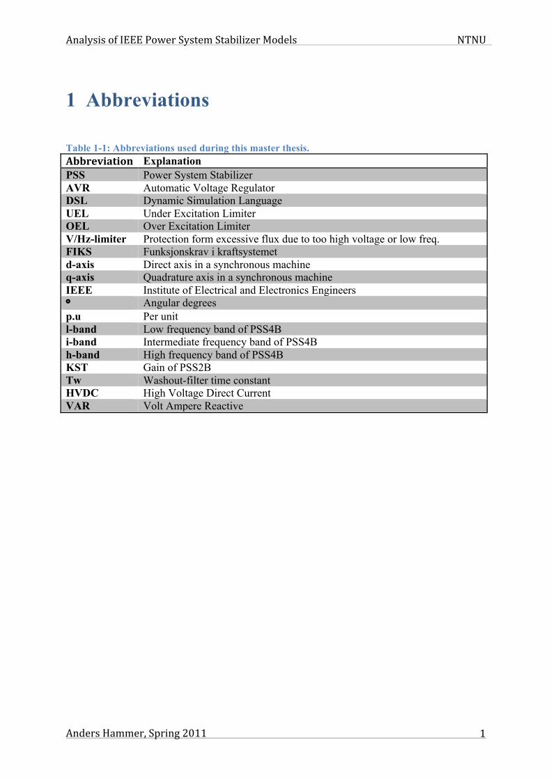
1 Abbreviations
Table 1-1: Abbreviations used during this master thesis. Abbreviation Explanation PSS Power System Stabilizer AVR Automatic Voltage Regulator DSL Dynamic Simulation Language UEL Under Excitation Limiter OEL Over Excitation Limiter V/Hz-limiter Protection form excessive flux due to too high voltage or low freq. FIKS Funksjonskrav i kraftsystemet d-axis Direct axis in a synchronous machine q-axis Quadrature axis in a synchronous machine IEEE Institute of Electrical and Electronics Engineers ° Angular degrees p.u Per unit l-band Low frequency band of PSS4B i-band Intermediate frequency band of PSS4B h-band High frequency band of PSS4B KST Gain of PSS2B Tw Washout-filter time constant HVDC High Voltage Direct Current VAR Volt Ampere Reactive

Analysis of IEEE Power System Stabilizer Models NTNU
Anders Hammer, Spring 2011 2
2 Introduction
2.1 Background Electrical power systems are often operated in critical situations that may lead to stability
problems in the power grid, and in worst-case blackouts. Large interruptions have historically
occurred in many of power systems around the world and this may lead to panic and state of
emergency in the society [6]. Because of todays climate change the European Union have
decided that at least 20 % of the energy production must come from renewable energy sources
by 2020 (Known as one of the 20-20-20 targets) [7]. To reach this goal, an increasing amount
of renewable energy sources such as wind farms and smaller hydro plants are implemented in
the power grids. The results of this may increase the network stability problems and the grid
cannot be loaded close to the limit of maximum transfer capacity. This can in some cases
reduce the needs of new power lines and thereby valuable space in the community [8].
The generator control equipment is able to improve the damping of oscillations in an
electrical network and thereby prevent instability in the grid. One of the solutions to improve
a troublesome grid may be to coordinate and tune this control equipment correctly [9]. In
larger key power plants the share of keeping the system stability is high. These plants must be
equipped with additional regulator loops, which will increase the damping of the power
oscillations. To prevent instability in the Norwegian power grid these Power System
Stabilizers (PSSs) are required as a part of the control equipment for generators above 25
MVA [10]. There exist several different types of PSS’s in the market. IEEE (The Institute of
Electrical and Electronics Engineers) has defined some standards, these are mainly based on
different input signals and processing of signals [1].
2.2 Problem description In 2005 IEEE (The Institute of Electrical and Electronic Engineers) introduced a new standard
model for Power System Stabilizers, the PSS4B. This is an advanced multi-band stabilizer
that may give a better performance than the regular PSS’s often used today. The new
stabilizer has three separate control structures, handling different frequency bands of the low
frequency oscillations at the power system. So far the PSS4B is not very known in the market,
but in the future it will probably become a standard requirement for key power plants in the

Analysis of IEEE Power System Stabilizer Models NTNU
Anders Hammer, Spring 2011 3
power system. This master thesis will be a continuation of a project performed in the autumn
2010, where the power system model and the framework for analysis were established. The
power system will during this master thesis be upgraded to contain an additional smaller
generator and also two different multiple-input stabilizer models, the PSS2B and the PSS4B.
These stabilizer models will be implemented and tuned in the small generator and the
different configurations will be compared. The focus during the simulation work will be at the
inter-area and local oscillation modes.
2.3 Approach A pre-project of this master thesis was performed during the autumn of 2010, where a basic
single-input PSS (PSS1A) was introduced in a two-area network with four equal rated
machines. The goal of the project was to uncover the basics of implementing and tuning a
PSS, and thereby improve the stability of the heavy loaded network. To visualize some
stability problems of an electrical network a classical two-area network was used as a base.
This network model was copied from the book named “Power System Stability and Control”
written by P. Kundur [11].
During this master thesis several changes of the classical two-area network are performed in
order to better fulfil Voith Hydro’s subject: planning and commissioning of hydropower
plants. The original network consists of four equal rated synchronous machines with round
rotors, and now a new synchronous machine is installed in parallel with one of the existing
machines. This new machine is a typical hydro generator with salient poles and the rating is
much smaller compared to the other generating units. Additionally a more advanced
excitation system is implemented, tuned and tested. This excitation system is a simplified
version of the Thyricon® Static Excitation System, developed by Voith Hydro. Next two
different PSS models are implemented and tuned in the hydro generator of the five-generator
network. First a dual-input stabilizer (PSS2B) is implemented and then a multi-band stabilizer
(PSS4B). The goal is to tune these PSS’s to maximize the damping of both local and inter-
area oscillation modes, and also verify robustness in the system. At the end of the simulation
work pros and cons of these two different stabilizer models are discussed.
The applied simulation computer programme in this master thesis is SIMPOW, developed by
the Swedish company Stri AB, and MatLab is used in order to create frequency response plots
and generally as a mathematical tool.

Analysis of IEEE Power System Stabilizer Models NTNU
Anders Hammer, Spring 2011 4
3 Theory
3.1 Power System Stability Power system stability is the ability to maintain a stationary state in an electrical system after
a disturbance has occurred. This disturbance can for instance be loss of generation, change in
power demand or faults on the line. The system’s ability to return to a steady state condition
depends on the initial loading of the system and type of disturbance. Power system stability
can be divided into four different phenomena’s: wave, electromagnetic, electromechanical
and thermodynamic (listed in ascending order of time response). This master thesis is only
focusing at the electromechanical phenomenon, which takes place in the windings of a
synchronous machine. A disturbance in the electrical network will create power fluctuations
between the generating units and the electrical network. In addition the electromechanical
phenomenon will also disturb the stability of the rotating parts in the power system [6].
The stability of a power system can further be divided, according to Figure 3-‐1, into different
categories, based on which part of the system that is affected.
Figure 3-1: Classification of power system stability (based on CIGRE Report No. 325) [6].
Frequency stability and voltage stability are related to the relation between the generated
power and consumed power in the system. A change in the reactive power flow will cause a
change in the system voltage, and similar a change in the active power flow will lead to a
change in the system frequency. The frequency stability enhancement is less significant in a
stiff network and this is not further analysed during this master thesis [6].
Rotor angle stability describes the ability for the synchronous machines to stay synchronised
after a disturbance has occurred. This criterion can be uncovered by study of the oscillation in

Analysis of IEEE Power System Stabilizer Models NTNU
Anders Hammer, Spring 2011 5
the power system. The rotor angle category can be further divided into small disturbance
stability and transient stability. See the following chapter 3.1.1 and 3.1.2 for discussion of
these two different stability behaviours.
In order to explain the rotor oscillation in a synchronous machine the swing equation is
developed. This equation is presented in equation 3.1 and describes the relation between the
mechanical parts in the machine and the accelerating torque.
(Equation 3.1)
Where = Total moment of inertia, = Rotational speed (mechanical), = Damping
coefficient, = Turbine torque, = Electrical torque and = accelerating torque.
The damping coefficient is a result from friction and the effect of electrical damping in the
machine. In steady state condition the rotor speed deviation (acceleration) is zero, and the
turbine torque is equal to the electrical torque multiplied by the damping torque ( ). A
disturbance in the electrical system will cause an approximate instantaneous change in the
electromagnetic torque of the generator. The turbine applies the mechanical torque and this
can initially be considered as constant. A result of this is a change in the rotor speed followed
by an accelerating or decelerating rotor torque [6]. The rotational speed of the rotor (ωm) can
be written as:
(Equation 3.2)
Where = mechanical rotor angle and = synchronous speed of the machine.
The swing equation can be rewritten, to contain rotor angle and power by using the relation
T=P/ω, and inserting equation 3.2 into 3.1 and multiply by .
(Equation 3.3)
Where , =Mm=angular moment, Pm=Mechanical power and Pe=Electrical
power.
The inertia is often normalized in order to be able to compare different machines in a
network. The total amount of inertia (J) is therefore replaced with a normalized H, which is:
J ! d"m
dt+ Dd !"m = # t $ # e = # acc
J !m Dd
! t ! e ! acc
Dd !"m
!m =! sm +d"m
dt
!m ! sm
! sm
J! smd 2"m
dt 2= Pm # Pe # Dm
d"m
dt
Dm =! smDd J! sm
Analysis of IEEE Power System Stabilizer Models NTNU
Anders Hammer, Spring 2011 6
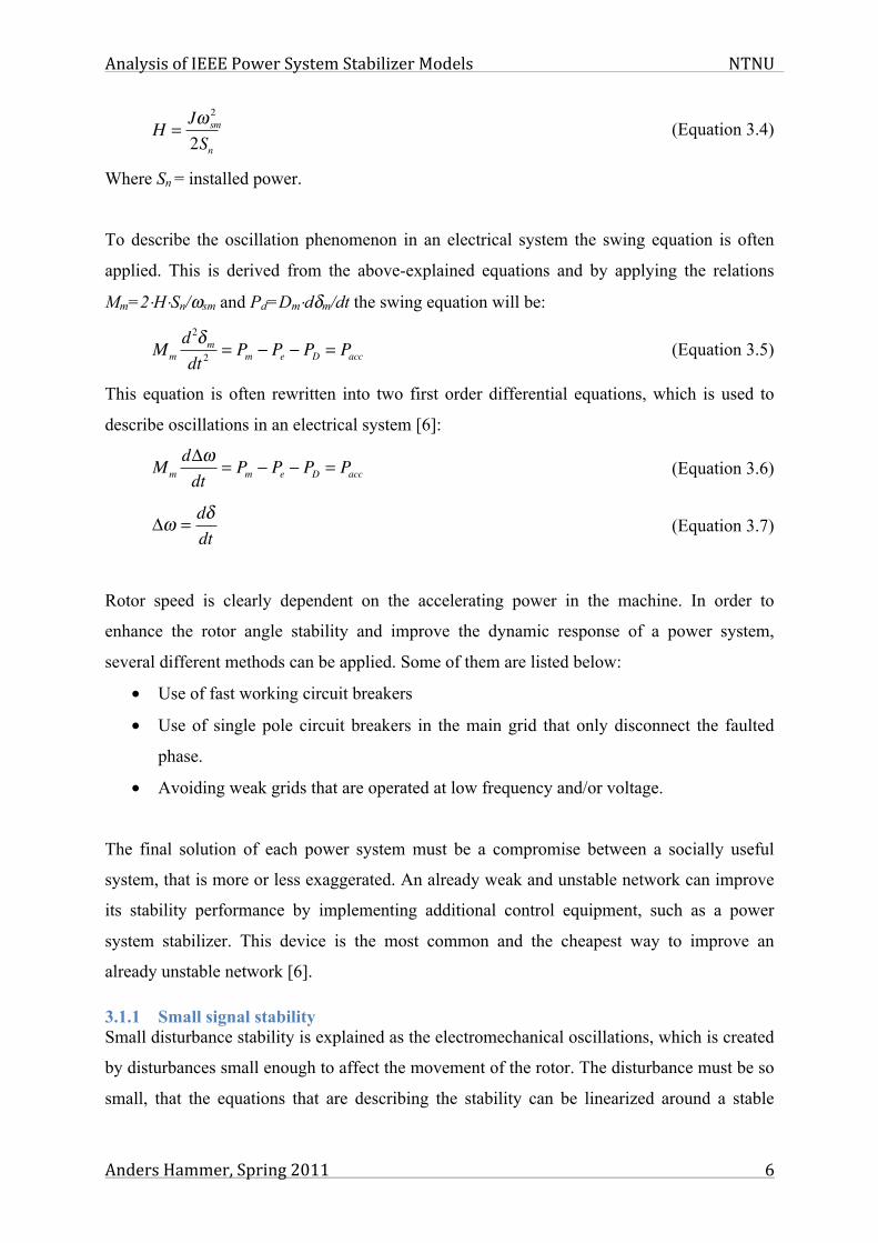
(Equation 3.4)
Where Sn = installed power.
To describe the oscillation phenomenon in an electrical system the swing equation is often
applied. This is derived from the above-explained equations and by applying the relations
Mm=2⋅H⋅Sn/ωsm and Pd=Dm⋅dδm/dt the swing equation will be:
(Equation 3.5)
This equation is often rewritten into two first order differential equations, which is used to
describe oscillations in an electrical system [6]:
(Equation 3.6)
(Equation 3.7)
Rotor speed is clearly dependent on the accelerating power in the machine. In order to
enhance the rotor angle stability and improve the dynamic response of a power system,
several different methods can be applied. Some of them are listed below:
• Use of fast working circuit breakers
• Use of single pole circuit breakers in the main grid that only disconnect the faulted
phase.
• Avoiding weak grids that are operated at low frequency and/or voltage.
The final solution of each power system must be a compromise between a socially useful
system, that is more or less exaggerated. An already weak and unstable network can improve
its stability performance by implementing additional control equipment, such as a power
system stabilizer. This device is the most common and the cheapest way to improve an
already unstable network [6].
3.1.1 Small signal stability Small disturbance stability is explained as the electromechanical oscillations, which is created
by disturbances small enough to affect the movement of the rotor. The disturbance must be so
small, that the equations that are describing the stability can be linearized around a stable
H =J! sm
2
2Sn
Mmd 2!m
dt 2= Pm " Pe " PD = Pacc
Mmd!"dt
= Pm # Pe # PD = Pacc
!" =d#dt
Analysis of IEEE Power System Stabilizer Models NTNU
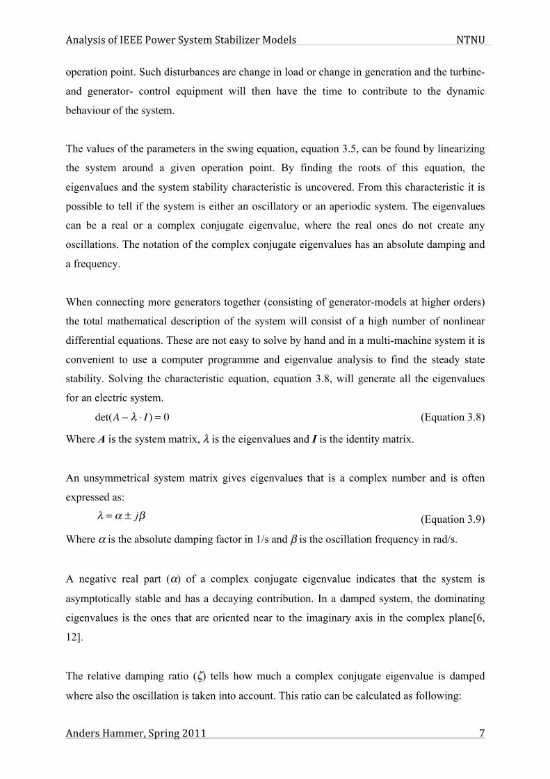
Anders Hammer, Spring 2011 7
operation point. Such disturbances are change in load or change in generation and the turbine-
and generator- control equipment will then have the time to contribute to the dynamic
behaviour of the system.
The values of the parameters in the swing equation, equation 3.5, can be found by linearizing
the system around a given operation point. By finding the roots of this equation, the
eigenvalues and the system stability characteristic is uncovered. From this characteristic it is
possible to tell if the system is either an oscillatory or an aperiodic system. The eigenvalues
can be a real or a complex conjugate eigenvalue, where the real ones do not create any
oscillations. The notation of the complex conjugate eigenvalues has an absolute damping and
a frequency.
When connecting more generators together (consisting of generator-models at higher orders)
the total mathematical description of the system will consist of a high number of nonlinear
differential equations. These are not easy to solve by hand and in a multi-machine system it is
convenient to use a computer programme and eigenvalue analysis to find the steady state
stability. Solving the characteristic equation, equation 3.8, will generate all the eigenvalues
for an electric system.
(Equation 3.8)
Where A is the system matrix, λ is the eigenvalues and I is the identity matrix.
An unsymmetrical system matrix gives eigenvalues that is a complex number and is often
expressed as:
(Equation 3.9)
Where α is the absolute damping factor in 1/s and β is the oscillation frequency in rad/s.
A negative real part (α) of a complex conjugate eigenvalue indicates that the system is
asymptotically stable and has a decaying contribution. In a damped system, the dominating
eigenvalues is the ones that are oriented near to the imaginary axis in the complex plane[6,
12].
The relative damping ratio (ζ) tells how much a complex conjugate eigenvalue is damped
where also the oscillation is taken into account. This ratio can be calculated as following:
det(A ! " # I ) = 0
! = " ± j#
Analysis of IEEE Power System Stabilizer Models NTNU
Anders Hammer, Spring 2011 8
(Equation 3.10)
The most interesting pair of eigenvalues is the one with the lowest relative damping ratio.
These are the ones that give most oscillations in the system. A negative relative damping ratio
will create an increase of the oscillation, rather than a damping. Such eigenvalues can not
occur in order to have a stable system [6, 12]. Many utility companies require a minimum
relative damping ratio of 0.05. For low frequency modes, such as the inter-area mode, the
requirement could be set even higher and often greater than 0.1. This limit is then set to
secure a safer damping of the oscillations in the network [4].
The oscillations around the stable operation point are divided in several different groups. The
American association IEEE has standardized the different oscillation modes that take place
when synchronous machines are connected to a power system. By standardizing these modes
there are easier for network operators to communicate and cooperate when handling stability
problems [13]. The different oscillation modes, described in the literature, are listed below:
Torsional/lateral mode: Torsional mode will act on the generator-turbine shaft and create
twisting oscillations in a frequency above 4 Hz and is most distinctive in turbo machines with
long shafts. These oscillations are usually difficult to detect with the generator models used to
detect oscillations with lower frequencies. If the excitation system is powerful enough the
torsional oscillation may add up to such a level that the turbine shaft may be damaged [13].
Lateral modes are related to horizontal mounted rotors that may slightly move from side to
side during operation. These oscillations have the same characteristic as the torsional modes
[14].
Inter-unit mode: Inter-unit mode will act between different generators in the same power
plant or between plants that are located near each other. This oscillation mode occurs in a
frequency range from 1.5 to 3 Hz, and by implementing a power system stabilizer when
having an inter-unit mode the oscillation may become unstable. This is because the PSS is
often tuned at a lower frequency than the inter-unit mode, and the PSS settings are therefore
critical. A complete eigenvalue analysis must be executed in order to ensure that the damping
of a potential inter-unit mode not becomes troublesome [13].
! ="#
# 2 + $ 2

Analysis of IEEE Power System Stabilizer Models NTNU
Anders Hammer, Spring 2011 9
Control/exciter modes: The control/exciter mode is directly related to the control equipment
of the generator and is a version of the local oscillation mode. These oscillations could be a
result of poorly coordinated regulators in the system such as excitation systems, HVDC
converters, and static VAR compensators. As a result of these oscillations the generator shaft
may be affected and the torsional mode will then be more noticeable [11].
Local machine modes: In this mode of oscillation typically one or more generators swing
against the rest of the power system in a frequency range from 0.7 Hz to 2 Hz. This oscillation
may occur and become a problem if the generator is highly loaded and connected to a weak
grid. In an excitation system containing a high transient gain and no PSS, these local machine
oscillations may increase. A correctly tuned PSS in such a system may decrease the local
machine oscillations [13].
Inter-area modes: The inter-area oscillation mode can be seen in a large part of a network
where one part of the system oscillates against other parts at a frequency below 0.5 Hz. Since
there is a large amount of generating units involved in these oscillations, the network
operators must cooperate, tune and implement applications that will damp this mode of
oscillations. A PSS is often a good application to provide positive damping of the inter-area
modes [13]. Also a higher frequency inter-area oscillation can appear (from 0.4 to 0.7 Hz)
when side groups of generating units oscillate against each other [11].
Global modes: This mode of oscillations is caused by a large amount of generating units in
one area that is oscillating against a large group in another area. The oscillating frequency is
typically in the range from 0.1 to 0.3 Hz and the mode is closely related to the inter-area mode
[11].
Small signal stability means that the above-mentioned modes are dampened within a
reasonable level.
3.1.2 Transient stability Transient stability occurs in the rotor angle stability category when a large disturbance is
introduced in the network. This large disturbance may be a three-phase fault over a longer
time period, or a disconnection of a line, and such a disturbance gives a new state of

Analysis of IEEE Power System Stabilizer Models NTNU
Anders Hammer, Spring 2011 10
operation. This will result in a change of the system matrix and a linear analysis is no longer
adequate. Under this new state of operation the rotor angle tries to find a new point of steady
state position [6].
In this project the disturbance in the network will be considered as a small signal disturbance
and the transient stability of the network will not be studied.
3.2 Excitation system of a synchronous machine The main type of generator in the world is a synchronous machine. This is because of its good
controlling capabilities, high ratings and a low inrush current. In order to produce electrical
power at the stator, the rotor of the machine has to be fed with direct current. This can be
executed in several different ways and examples are for instance from cascaded DC
generators, rotating rectifiers without slip rings, or from a controlled rectifier made of power
electronics. This appliance is named exciter, and the exciter used in this master thesis is a
controlled rectifier. Other mentioned systems are not further explained here.
Figure 3-2: (a): Block diagram of the excitation system of one generator connected to the grid. (b): Phasor diagram of the signals in the excitation system [6].
To control the performance of the synchronous machine, the DC rotor current has to be
controlled. This is done by an automatic voltage regulator (AVR), which controls the gate
opening of the thyristors in the controlled rectifier. The whole system that is controlling and
producing the excitation voltage is called excitation system and a typical excitation system
block diagram is illustrated in Figure 3-‐2. This illustrates that the generator voltage is

Analysis of IEEE Power System Stabilizer Models NTNU
Anders Hammer, Spring 2011 11
measured and compared with a reference voltage, in order to calculate a voltage error signal,
ΔV. This signal is then regulated to give the wanted DC output voltage of the exciter (Ef),
which gives the correct AC generator terminal voltage [6].
The excitation system is capable to make an influence on the oscillations in the connected
network. These excitation systems are acting fast and maximize the synchronous torque of the
generating unit. This leads to a rotor movement that becomes stable, and goes back to its
steady state position after a transient fault has occurred. A fast excitation system can also
contribute to a high terminal voltage that leads to a high current during a fault. It is favourable
to maintain a high current in order to improve the tripping ability of protective relays. The fast
response of the voltage regulator may create an unstable situation if the machine is connected
to a weak transmission system. Such problems can be solved by implementation of a power
system stabilizer (PSS) in the excitation system, which is introducing an additional voltage
control signal (VPSS in Figure 3-‐2) [15].
3.3 Power System Stabilizer The main reason for implementing a power system stabilizer (PSS) in the voltage regulator is
to improve the small signal stability properties of the system. Back in the 1940 and 50s the
generators were produced with a large steady state synchronous reactance. This led to
reduction in field flux and to a droop in synchronising torque. The result was a machine with
poor transient stability, especially when it was connected to a weak grid. To solve this
transient stability problem, a fast thyristor controlled static excitation system was later
introduced. This installation eliminated the effect of the high armature reaction, but it also
created another problem. When the generator was operated at a high load and connected to a
weak external grid, the voltage regulator created a negative damping torque and gave rise to
oscillations and instability. An external stabilizing signal was therefore introduced as an input
to the voltage regulator. This signal improved the damping of the rotor oscillations and the
device was called power system stabilizer (PSS). The PSS introduces a signal that optimally
results in a damping electrical torque at the rotor. This torque acts opposite of the rotor speed
fluctuations [4].
Other solutions on the oscillation problem exist, but these are not covered in this master
thesis. It is the introduction of a PSS that is the easiest and most economical solution in most
cases. A single machine connected to an external grid is often used to explain the dynamics of

Analysis of IEEE Power System Stabilizer Models NTNU
Anders Hammer, Spring 2011 12
an electrical network. In 1952 Heffron and Phillips developed a model for this setup, and this
model contained an electromechanical model of a synchronous generator with an excitation
system. De Mello and Concordia
(1969) picked up the Heffron &
Phillips model, and developed an
understanding of electrical oscillations
and damping torque in an electrical
system. These understandings can also
be transferred to a larger system with
several generation units and more
complex grids. The Heffron & Phillips
model is illustrated in Figure 3-‐3,
where GEP(s) is the transfer function
of electric torque and reference voltage
input. An additional stabilizing signal
should optimally correct the phase
shift of this transfer function. Assuming that the single machine is connected to an infinite bus
the GEP(s) transfer function can be uncovered by performing a field test of the generator.
When the electrical system obtain a new operation condition, the GEP(s) transfer function
changes, and the PSS transfer function must optimally follow this deviation. This is
practically impossible and the solution is to provide a phase lead/lag structure that acts in a
wide range of frequencies [4].
The excitation system can, with an external damping signal, produce a repressive rotor torque
in phase with the rotor speed deviation. Since the generator and the exciter produce a small
phase shift, the damping signal from a PSS has to contain a phase angle correction, in addition
to the gain. The phase angle correction is realized by adding a phase-lead/lag-filter in the PSS
structure, and it is important that the phase-lead generated by the PSS compensates for the lag
between the exciter input and the generator air gap torque. Without any phase shift in the
system, the phase-angle between the PSS output signal and the electrical torque is directly
180 degrees [4, 6, 11].
Figure 3-3: Heffron & Phillip's single-machine infinite-bus model [4, 5].
Analysis of IEEE Power System Stabilizer Models NTNU
Anders Hammer, Spring 2011 13
3.3.1 Tuning approaches of PSS structures
Basically the tuning of a PSS structure can be performed in three different approaches. These
are a damping torque approach (based on Heffron & Phillips model), a frequency response
approach and an eigenvalue/state-space approach [4]. When increasing the gain of a well-
tuned PSS, the eigenvalues should move exactly horizontally and to the left in the complex
plane. Theoretically it is around 180 degrees between the machine rotor speed and the
electrical torque variations, and the PSS should contribute with a pure negative signal. The
PSS structure contains a negative multiplication that will provide a 180-degree phase shift. In
practise the straight horizontal movement of eigenvalues may not happen because of the
electrical phase shift in the system. Implementing and correct tuning of lead-lag filters (block
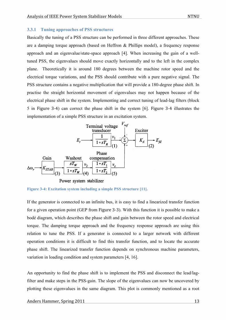
5 in Figure 3-‐4) can correct the phase shift in the system [6]. Figure 3-‐4 illustrates the
implementation of a simple PSS structure in an excitation system.
Figure 3-4: Excitation system including a simple PSS structure [11].
If the generator is connected to an infinite bus, it is easy to find a linearized transfer function
for a given operation point (GEP from Figure 3-‐3). With this function it is possible to make a
bodé diagram, which describes the phase shift and gain between the rotor speed and electrical
torque. The damping torque approach and the frequency response approach are using this
relation to tune the PSS. If a generator is connected to a larger network with different
operation conditions it is difficult to find this transfer function, and to locate the accurate
phase shift. The linearized transfer function depends on synchronous machine parameters,
variation in loading condition and system parameters [4, 16].
An opportunity to find the phase shift is to implement the PSS and disconnect the lead/lag-
filter and make steps in the PSS-gain. The slope of the eigenvalues can now be uncovered by
plotting these eigenvalues in the same diagram. This plot is commonly mentioned as a root

Analysis of IEEE Power System Stabilizer Models NTNU
Anders Hammer, Spring 2011 14
locus plot. Angle between the horizontal real axis in the complex plane and the root locus plot
will be the phase angle for that specific eigenvalue. This tuning method is the eigenvalue
approach based on pole placement [4].
Another method to locate the total phase angle between the rotor speed and the electrical
torque is to plot these two variables in a time domain analysis and thereby find the phase shift.
The preferred method, which is utilized in this master thesis, is the eigenvalue approach
where the base is analysis of pole placement and root locus plots. This method is
preferred since the computer simulation tool used in this master thesis can easily
compute eigenvalues of the whole system, while it cannot create transfer functions and
nice frequency responses of the multi machine network.
3.4 Overview of different PSS structures In order to provide a damping torque signal, the PSS could use the rotor speed deviation from
the actual rotor speed from the synchronous speed (Δωr) as an input. Other parameters, which
are easily available and measurable, could also be used to provide the damping torque. These
signals could be electrical frequency, electrical power or the synthesized integral of electrical
power signal. In the measurements of input signals, different types of signal noise could be
present. The stabilizer has to filter out this noise in order to feed the AVR with a steady
signal, which could damp the actual rotor oscillation [6]. An explanation of different PSS’s is
given in the following sub chapters.
3.4.1 Speed-based stabilizer
The simplest method to provide a damping torque in the synchronous machine is to measure
the rotor speed and use it directly as an input signal in the stabilizer structure. This method is
illustrated in Figure 3-‐4, where block number 4 is a washout filter and will only pass
through the transient variations in the speed input signal. Ordinary variations in speed,
frequency and power must not generally enter the PSS structure and thereby affect the field
voltage [4]. The washout constant should be chosen according to these criteria [13]: “
1. It should be long enough so that its phase shift does not interfere significantly with the
signal conditioning at the desired frequencies of stabilization.

Analysis of IEEE Power System Stabilizer Models NTNU
Anders Hammer, Spring 2011 15
2. It should be short enough that the terminal voltage will not be affected by regular
system speed variations, considering system-islanding conditions, where applicable.”
Operating a network containing really low frequency inter-area modes, the washout time
constant (Tw) has to be set as high as 10 or 20 second. The reason is that the washout-filter
has to cover these low frequency oscillation modes. If not having this low inter-area
oscillation mode, the Tw could be set to a lower value [4].
After finding the angle of the selected eigenvalue, in the eigenvalue approach, a lead/lag-filter
must be implemented in order to correct the angle of the specific eigenvalue. This filter can be
a filter of n’th order, similar to the transfer function in Equation 3.11.
Lead / lag ! filter = 1+T1 " s1+T2 " s#$%
&'(
n
Equation 3.11
n is the order of the filter, s is the Laplace operator and T1&T2 is the time constants.
Tuning of the time constants in this filter can be performed based on the phase shift (ϕ1) and
the frequency (ω1) of the selected eigenvalue, according to Equation 3.12 and 3.13 [17].
T1 =1!1
! tan 45° + "12n
"#$
%&'
Equation 3.12
T2 =1!1
! 1
tan 45° + "12n
"#$
%&'
Equation 3.13
ω1 is the frequency of the eigenvalue in rad/s, ϕ1 is the phase shift in degrees and n is the
order of the filter.
As an example a first order filter and a second order filter should correct an eigenvalue at 1
rad/sec and with a phase shift of 30 degrees.
First order filter:
T1 =1
1rad / sec! tan 45° + 30°
2 !1"#$
%&' =1.7321
Analysis of IEEE Power System Stabilizer Models NTNU
Anders Hammer, Spring 2011 16
T2 =1
1rad / sec! 1
tan 45° + 30°2 !1
"#$
%&'= 0.5774
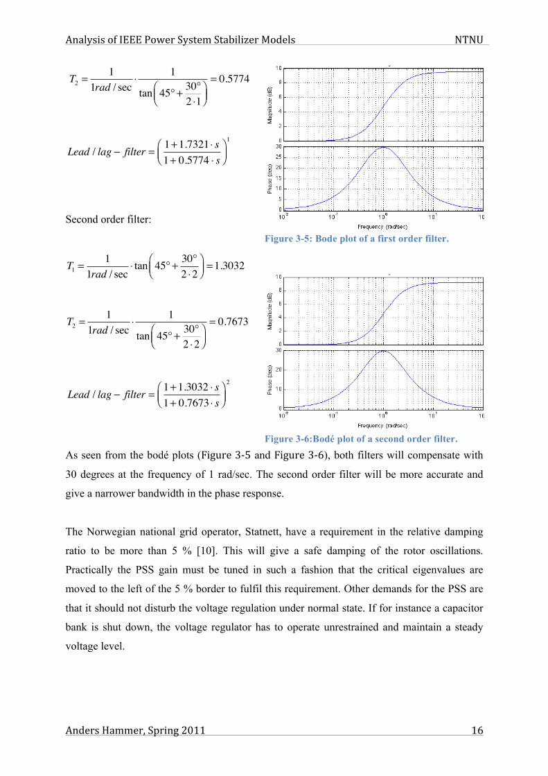
Second order filter:
T1 =1
1rad / sec! tan 45° + 30°
2 !2"#$
%&' =1.3032
T2 =1
1rad / sec! 1
tan 45° + 30°2 !2
"#$
%&'= 0.7673
As seen from the bodé plots (Figure 3-‐5 and Figure 3-‐6), both filters will compensate with
30 degrees at the frequency of 1 rad/sec. The second order filter will be more accurate and
give a narrower bandwidth in the phase response.
The Norwegian national grid operator, Statnett, have a requirement in the relative damping
ratio to be more than 5 % [10]. This will give a safe damping of the rotor oscillations.
Practically the PSS gain must be tuned in such a fashion that the critical eigenvalues are
moved to the left of the 5 % border to fulfil this requirement. Other demands for the PSS are
that it should not disturb the voltage regulation under normal state. If for instance a capacitor
bank is shut down, the voltage regulator has to operate unrestrained and maintain a steady
voltage level.
Lead / lag ! filter = 1+1.7321 " s1+ 0.5774 " s
#$%
&'(1
Lead / lag ! filter = 1+1.3032 " s1+ 0.7673 " s
#$%
&'(2
Figure 3-5: Bode plot of a first order filter.
Figure 3-6:Bodé plot of a second order filter.

Analysis of IEEE Power System Stabilizer Models NTNU
Anders Hammer, Spring 2011 17
The main disadvantage of using the rotor speed deviation as an input signal is that this signal
can contain a relatively large amount of disturbance. Rotor speed is directly measured by use
of sensors mounted on the rotating shaft. During a disturbance the rotor could create lateral
movement in a vertical mounted machine. For large horizontally mounted turbo generators
(1800 or 3000 rpm) the rotor shaft can twist and create torsional oscillations. Turbo
generators have a long rotor shaft and a short diameter to limit the centripetal force that is
created at these rotational speeds. To limit these interactions, several speed sensors could be
mounted along the rotor shaft. A disadvantage of doing this is increased costs and
maintenance. In addition a special electrical filter can be installed to filter out unwanted signal
noise. The disadvantage of this torsional filter is that it would also introduce a phase lag at
lower frequencies, and it can create a destabilizing effect at the exciter oscillation mode as the
gain of the stabilizer is increased. The maximum gain from the PSS is then limited and the
system oscillations could then not be as damped as wanted. This torsional filter must also be
custom designed in order to fit the generating unit. To get rid of these limitations a new PSS
structure was created, the PSS2b, which is an integral of accelerating power-based stabilizer
[4, 14]. This type is further described later in this chapter.
3.4.2 Frequency-based stabilizer
This type of stabilizer has the same structure as used in the speed-based stabilizer mentioned
above. By using the system frequency as an input signal the low frequency inter-area
oscillations are better captured. These oscillations are thereby better damped in a frequency-
based stabilizer, compared to the speed-based stabilizer. Oscillations between machines close
to each other are not well captured by the frequency-based stabilizer, and the damping of the
local oscillations is then not highly improved. The frequency signal may also vary with the
network loading and operation. An arc furnace nearby could for instance create large
unwanted transients in the measurement signal, and the PSS might produce a unwanted
behaviour of the generator [14].
3.4.3 Power-based stabilizer
Power and speed of the rotor are in a direct correlation, according to the swing equation
described below:
Equation 3.14
Where the damping coefficient is set to zero.
2 !H !Sn! sm
! d"!dt
= Pm # Pe $d"!dt
= 12 !H
Pm # Pe( )
Analysis of IEEE Power System Stabilizer Models NTNU
Anders Hammer, Spring 2011 18
The electrical power is easy to measure and also use as an input signal. Mechanical power is a
more problematic value to measure. In most power-based stabilizers this mechanical power is
threated as a constant value and the rotor speed variations are then proportional with electrical
power. Change in the mechanical loading will then be registered by the PSS and it will create
an unwanted output signal. A strict PSS output limiter must in those cases be established to
prevent the PSS to contribute under a change in generator loading. This will reduce the
overall PSS performance and the power system oscillations will not get as damped as wanted.
Electrical power as an input signal will only improve the damping of one oscillation mode.
Several oscillating frequencies in the network require a compromise solution of the lead/lag-
filter [14].
3.4.4 Integral of accelerating power-based stabilizer
As mentioned as a drawback of the speed-based stabilizer, a filter has to be implemented in
the main stabilizing path to reduce the contribution of lateral and torsional movements. This
filter must also be applied in the pure frequency- and power-based single input stabilizers.
The Integral of accelerating power-based stabilizer was developed to solve the filtering
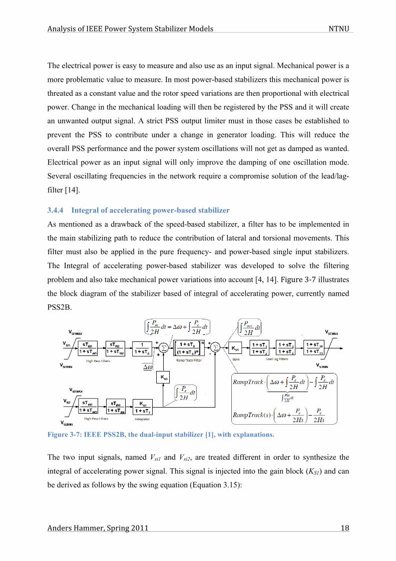
problem and also take mechanical power variations into account [4, 14]. Figure 3-‐7 illustrates
the block diagram of the stabilizer based of integral of accelerating power, currently named
PSS2B.
Figure 3-7: IEEE PSS2B, the dual-input stabilizer [1], with explanations.
The two input signals, named Vsi1 and Vsi2, are treated different in order to synthesize the
integral of accelerating power signal. This signal is injected into the gain block (KS1) and can
be derived as follows by the swing equation (Equation 3.15):
Analysis of IEEE Power System Stabilizer Models NTNU
Anders Hammer, Spring 2011 19
Equation 3.15
Change of speed is clearly dependent on power and the integral of mechanical power can now
be expressed by change in rotor speed and integral of electrical power:
Equation 3.16
Vsi1 input signal is a speed- or frequency signal and Vsi2 is a power signal. Vsi1 can be used
directly and the time constant T6 is then set to zero. Vsi2, the power signal, must pass an
integral block and also be divided by 2H, which is performed by the gain constant KS2.
Equation 3.15 indicates that the derived integral of accelerating power can represent the speed
change in the machine.
The torsional filter is commonly mentioned as a ramp-track filter, and by introducing this
filter the torsional and lateral oscillations will be reduced in the integral of mechanical power
branch. The electrical power signal does not usually contain any amount of torsional modes,
and the torsional filter can be skipped in the integral of electrical power branch. An advantage
of doing this is that the exciter oscillation mode will not become destabilized [4, 14]. At the
end of the transducer block the electrical signal is subtracted from the mechanical signal, and
the integral of accelerating power signal is then synthesized. This can be explained by
combining equation 3.15 and 3.16 in such a fashion that only electrical power and speed
remains as an input parameter, seen in equation 3.17. By doing this signal processing it
becomes unnecessarily to measure the tricky mechanical power in the machine.
Equation 3.17
Taking the Laplace transformation of equation 3.17 gives equation 3.18, which is the base for
the block diagram in Figure 3-‐7.
Equation 3.18
The final integral of accelerating power signal should exactly follow the rotor speed
variations, and the rest of the PSS2B can then be tuned as a common single-input PSS with a
gain and a lead/lag-filter [4].
!! = 12H
(Pm " Pe )dt# $ 12H
Pacc. dt# Equation 1
Pm2H
dt! = "! + Pe2H
dt! Equation 2
Pacc.2H
dt! " RampTrack # $! + Pe2H
dt!%&'
()*
Pm2H
dt!! "## $##
+ Pe2H
dt! Equation 3
Pacc.2H
dt! " RampTrack(s) # $! + Pe2Hs
%&'
()* +
Pe2Hs
Equation 4

Analysis of IEEE Power System Stabilizer Models NTNU
Anders Hammer, Spring 2011 20
PSS2B stabilizer uses, as mentioned, to different signals as input parameters: speed/frequency
and active electric power of the machine. In order to create a theoretical frequency response
(bodé plot) of the whole PSS2B it is possible to synthesize the electric power signal (used as
input Vsi2) from the speed signal.
Thereby a transfer function with one
input- and one output-parameter can be
created and also a frequency response.
The method for synthesising the power
input signal could be derived from the
swing equation that explains the relationship between change in speed and change in power.
Figure 3-‐8 is a conceptual drawing of the method of finding the complete transfer function of
a dual-input stabilizer [3].
Voith Hydro has given an example of typical transducer parameters presented in Table 3-‐1.
These parameters, except form KS2, are not normally changed in a regular tuning procedure. Table 3-1: PSS2B transducer parameters, given by Voith Hydro [2].
TF TP Tw1 – 4 T6 T7 KS2=T7/2H KS3 T8 M N T9 0.02 0.02 3 0 3 0.5137* 1 0.4 4 1 0.1
* 100 MVA generator with inertia (H) equal to 2.92.
The two parameters TF and TP, from Table 3-‐1, are related to measurement equipment and is
a fixed value. These parameters explain the time constants of the frequency- and power
transducers. First order filters are therefore implemented in the front of the PSS2B, and these
represents each input transducer. Tw parameters are washout-time constants and acts like high
pass filters. Only oscillations above a certain frequency pass these filters. The power-branch
needs an integrator block in order to produce the wanted stabilizer signal. T7 will define this
function, and the bodé plot of the integrator block is presented in Figure 3-‐9.
Figure 3-8: Principal model to find the frequency response of a dual input stabilizer [3].

Analysis of IEEE Power System Stabilizer Models NTNU
Anders Hammer, Spring 2011 21
Figure 3-9: Left: Bode plot of PSS2B-integrator block and a pure integrator block. Right: Bode plot of ramp-track filter, where a contribution from frequency and power branch is present.
Time constant T7 states that frequencies above 0.053 Hz will be affected by the integrator
block (1/T7=0.33rad/s à 0.053Hz), this is also illustrated in the left bodé plot of Figure 3-‐9.
The bodé plot oriented to the right in Figure 3-‐9 illustrates the ramp-track filter performance,
where the frequency branch of PSS2B handles the frequencies below approximately 1 Hz and
the power branch handles frequencies above approximately 1 Hz. Parameters presented in
Table 3-‐1 gives the frequency response of the whole transducer-part of PSS2B, illustrated in
Figure 3-‐10. The plot indicates that the -3 db cut-off frequency is oriented at 0.08 Hz and 8.5
Hz. This is the boundary where the signals are
starting to reduce rather than increase after
passing the transducer blocks [12]. In the
frequency range of 0.08 ∼ 8.5 Hz, the phase
response varies of approximately 315 degrees.
To achieve a good signal quality, which acts
in the direct opposite direction (-180 degrees)
of speed variations, the filtering process may
get troublesome, especially if the network
struggles with several oscillations modes in a
wide frequency range.
3.4.5 Multi-band stabilizer
The motivation for developing a new type of stabilizer was that the lead/lag compensating
filters in the older structures could not give an accurate compensation over a wide range of
60
40
20
0
20
40
60M
agni
tude
(dB)
10 3 10 2 10 1 100 101 10290
45
0
Phas
e (d
eg)
Bode Diagram
Frequency (Hz)
pureintegratoractpowint
100
50
0
50
Mag
nitu
de (d
B)
10 2 10 1 100 101 102270
180
90
0
Phas
e (d
eg)
Bode Diagram
Frequency (Hz)
frequencypower
10 2 10 1 100 101270
180
90
0
90
180
Phas
e (d
eg)
Bode Diagram
Frequency (Hz)
20
15
10
5
0
5
10
System: PSS2BtransFrequency (Hz): 0.0797Magnitude (db): 3
System: PSS2BtransFrequency (Hz): 8.47Magnitude (db): 3.02
Mag
nitu
de (d
b)
PSS2Btrans
Figure 3-10: Bodé-plot of the transducer-part of PSS2B.

Analysis of IEEE Power System Stabilizer Models NTNU
Anders Hammer, Spring 2011 22
oscillation frequencies. If the network suffers from low- and high frequency oscillations, the
tuning procedure of the single-band stabilizers have to compromise and will not achieve
optimal damping in any of the oscillations. The multi-band stabilizer has three separate signal
bands, which can be tuned individually to handle different oscillation frequencies. This
stabilizer is presented in Figure 3-‐11 and this structure has a relative large amount of tuning
flexibility.
Figure 3-11: Multi-band stabilizer, IEEE PSS4B [1].
At first glance this stabilizer structure seems that it would require a tedious tuning procedure.
An IEEE report [1] presents a simple tuning procedure where a selection of three centre
frequencies and associated gains are used as base of the parameter settings. One frequency for
the low frequent oscillations, one for the intermediate and one for the highest oscillation
frequency that occurs at the stator terminals. Totally four equations is used to calculate the
time constants for each band. The equations for the intermediate frequency band are
presented, as an example, in equation 3.19 – 3.22. R is a constant set equal to 1.2 and Fi is the
centre frequency of the intermediate band [1]:
Equation 3.19 Ti2 = Ti7 = 1
2 !! !Fi ! R Equation 1
Analysis of IEEE Power System Stabilizer Models NTNU
Anders Hammer, Spring 2011 23
Equation 3.20
Equation 3.21
Equation 3.22
The associated gains (Ki, Kl and Kh) are set to a value that gives a reasonable contribution of
the amplitude in each band. All other parameters not mentioned here are set to a value that
cancels the respective blocks.
By choosing the IEEE tuning method for all the three bands, the frequency response of the
total PSS will give a more accurate compensation and in a wider frequency range than for a
typical lead/lag-filter structure. As seen in the structure of the PSS4B (Figure 3-‐11), different
input parameters are used in this model (ΔωH and ΔωL-I). This is similar to the dual-input
stabilizer, presented in the previous subchapter, which is also using two input signals. The
two upper bands of PSS4B (Figure 3-‐11) are designed to handle low- and intermediate
oscillation frequencies, while the high frequency oscillations only enters the lower band. To
create these different input signals two different input transducers are used. These are
presented in Figure 3-‐12, where rotor speed (Δω) is used directly as an input signal to the
upper transducer. The low and intermediate part of the oscillations is passing this transducer
block, and the signal is later injected as an input to the low and intermediate part of the
PSS4B. To create a signal that represents the high frequent oscillations, the electrical power
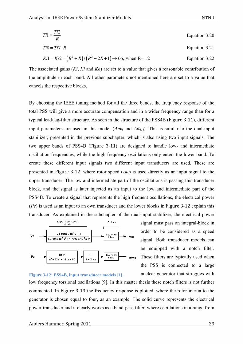
(Pe) is used as an input to an own transducer and the lower blocks in Figure 3-‐12 explain this
transducer. As explained in the subchapter of the dual-input stabilizer, the electrical power
signal must pass an integral-block in
order to be considered as a speed
signal. Both transducer models can
be equipped with a notch filter.
These filters are typically used when
the PSS is connected to a large
nuclear generator that struggles with
low frequency torsional oscillations [9]. In this master thesis these notch filters is not further
commented. In Figure 3-‐13 the frequency response is plotted, where the rotor inertia to the
generator is chosen equal to four, as an example. The solid curve represents the electrical
power-transducer and it clearly works as a band-pass filter, where oscillations in a range from
Ti1= Ti2R
Equation 2
Ti8 = Ti7 !R Equation 3
Ki1= Ki2 = R2 + R( ) / R2 ! 2R +1( )" 66, when R=1.2 Equation 4
Figure 3-12: PSS4B, input transducer models [1].

Analysis of IEEE Power System Stabilizer Models NTNU
Anders Hammer, Spring 2011 24
0.25 ∼ 12.7 Hz is passing. The oscillations at a
lower frequency are then taken care of by the
bands connected to the speed-transducer. This
has only one -3db cut-off frequency and this is
located at approximately 12.7 Hz. Oscillations
above 12.7 Hz will then not enter the low and
intermediate part of the stabilizer structure.
Breaking down the structure into smaller
parts, makes it possible to easier analyse the
behaviour of this multi-band structure. By only looking at two of the blocks in one of the
three bands will make the mathematics easier. A block diagram of this simplification is
illustrated in Figure 3-‐14.
Zeros: Poles:
The time constants decides whatever this structure is a high pass or a band pass filter. One
special situation, which is utilized in the IEEE Std. 421.5 document [1], is when and
. The transfer function will then be reduced as following:
H = OutIn
= 1+T1s1+T2s
! 1+T31+T4
H = (1+T1s)(1+T4s)(1+T2s)(1+T4s)
! (1+T3s)(1+T2s)(1+T2s)(1+T4s)
H = 1+ (T1 +T4 )s +T1T4s2 !1! (T3 +T2 )s !T3T2s
2
(1+T1s)(1+T4s)
H = (T1 +T4 !T3 !T2 )s + (T1T4 !T3T2 )s2
(1+T1s)(1+T4s)=(T1 +T4 !T3 !T2 )s + 1+ T1T4 !T3T2
T1 +T4 !T2 !T3s
"#$
%&'
(1+T1s)(1+T4s)
s = ! T1T4 !T3T2T1 +T4 !T2 !T3
s = ! 1T2
s = ! 1T4
T3 = T2
T1 = (T2T3) /T4 = (T2 )2 /T4
Hred. =
T2( )2T4
+T4 ! 2T2"
#$
%
&' s ( 1+
T2( )2T4
T4 ! T2( )2
T2( )2T4
+T4 ! T2( )2s
"
#
$$$$
%
&
''''
(1+T2s)(1+T4s)=
T2( )2T4
+T4 ! 2T2"
#$
%
&' s
(1+T2s)(1+T4s)
Figure 3-14: A simple differential filter.
10 2 10 1 100 101180
90
0
90
180
270
Phas
e (d
eg)
Bode Diagram
Frequency (Hz)
20
15
10
5
0
5
System: PSS4bwHFrequency (Hz): 0.251Magnitude (db): 3
System: PSS4bwHFrequency (Hz): 12.7Magnitude (db): 3.03
Mag
nitu
de (d
b)
PSS4bwLIPSS4bwH
Figure 3-13: Bodé plot of PSS4B input transducers.
Analysis of IEEE Power System Stabilizer Models NTNU
Anders Hammer, Spring 2011 25
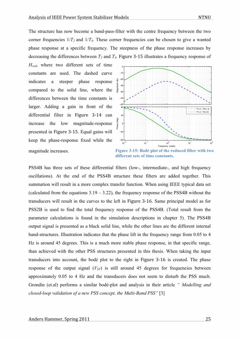
The structure has now become a band-pass-filter with the centre frequency between the two
corner frequencies 1/T2 and 1/T4. These corner frequencies can be chosen to give a wanted
phase response at a specific frequency. The steepness of the phase response increases by
decreasing the differences between T2 and T4. Figure 3-‐15 illustrates a frequency response of
Hred, where two different sets of time
constants are used. The dashed curve
indicates a steeper phase response
compared to the solid line, where the
differences between the time constants is
larger. Adding a gain in front of the
differential filter in Figure 3-‐14 can
increase the low magnitude-response
presented in Figure 3-‐15. Equal gains will
keep the phase-response fixed while the
magnitude increases.
PSS4B has three sets of these differential filters (low-, intermediate-, and high frequency
oscillations). At the end of the PSS4B structure these filters are added together. This
summation will result in a more complex transfer function. When using IEEE typical data set
(calculated from the equations 3.19 – 3.22), the frequency response of the PSS4B without the
transducers will result in the curves to the left in Figure 3-‐16. Same principal model as for
PSS2B is used to find the total frequency response of the PSS4B. (Total result from the
parameter calculations is found in the simulation descriptions in chapter 5). The PSS4B
output signal is presented as a black solid line, while the other lines are the different internal
band-structures. Illustration indicates that the phase lift in the frequency range from 0.05 to 4
Hz is around 45 degrees. This is a much more stable phase response, in that specific range,
than achieved with the other PSS structures presented in this thesis. When taking the input
transducers into account, the bodé plot to the right in Figure 3-‐16 is created. The phase
response of the output signal (VST) is still around 45 degrees for frequencies between
approximately 0.05 to 4 Hz and the transducers does not seem to disturb the PSS much.
Grondin (et.al) performs a similar bodé-plot and analysis in their article “ Modelling and
closed-loop validation of a new PSS concept, the Multi-Band PSS” [3]
Figure 3-15: Bodé plot of the reduced filter with two different sets of time constants.
60
50
40
30
20
10
0
Mag
nitu
de (d
b)
10 2 10 1 100 101 10290
45
0
45
90
Phas
e (d
eg)
Bode Diagram
Frequency (rad/s)
T1=1, T4=1.5T1=1, T4=10

Analysis of IEEE Power System Stabilizer Models NTNU
Anders Hammer, Spring 2011 26
Figure 3-16: Bodé-plot of PSS4B. Left diagram: Without transducers. Right diagram: With transducers.
Another approach to tune the multi-band stabilizer is to disconnect the lower branch of each
band, and use the upper branch as a regular lead/lag-filter in addition to a gain. Each of the
different bands can be tuned separately according to the actual network oscillations. This is a
much simpler tuning procedure where the tuning of the lead/lag-filters can be done similar to
the procedure used in the dual-input PSS (PSS2B). First step is to find the critical oscillation
modes in the network. Then one of the three bands in the PSS4B can be assigned to each of
the oscillation modes where the damping will be improved. Disconnecting two of the three
bands makes it possible to tune the third band to give a maximized damping of the selected
oscillation mode. The goal is to move the selected eigenvalue straight to the left in the
complex plane. Next step is to tune one of the other bands according to another oscillating
eigenvalue.
20
10
0
10
20
30
40
50M
agni
tude
(db)
Frequency (Hz)10
210
110
010
110
290
45
0
45
90
Phas
e (d
eg)
80
60
40
20
0
20
40
60
Mag
nitu
de (d
b)
10 2 10 1 100 101 10290
45
0
45
90
Phas
e (d
eg)
Frequency (Hz)
LOWINTERHIGHVST
Analysis of IEEE Power System Stabilizer Models NTNU
Anders Hammer, Spring 2011 27
4 Simulation Tool, SIMPOW The stability analysis of a power network is a difficult procedure when calculating by hand. A
computer programme called SIMPOW, developed and operated by the Swedish company
STRI AB, performs therefore the stability simulations in this project. Since the system matrix
of a large power system can become very large, it is more convenient to perform the stability
analysis by using the computer programme. The simulation programme linearizes the system
around an arbitrary state, in order to perform a linear analysis. Out of this it is possible to
generate eigenvalues, perform modal analysis and make a frequency scan or a data scan.
SIMPOW using the quick-response-method (QR-method) to uncover the eigenvalues, and the
eigenvalues could be improved by using the inversed iteration method to get a more accurate
solution. The modal analysis is a tool that detects which parts of the network that is oscillating
against each other. This information is obtained from the eigenvectors in the electrical system.
In a frequency scan the system is excited by a sinusoidal source with varying frequency and
the system response can be studied. The data scan indicates the movement of the eigenvalues
when ramping one of the system parameters [18].
SIMPOW has also an ability to perform a time domain analysis of the system, where variation
of different system parameters can be plotted over a time period. This analysis can in many
cases strengthen the results found in the linear analysis and different fault scenario can be
implemented [18].
It is often a benefit to have the ability to implement different regulator structures in the
simulation programme. SIMPOW uses a coding language named Dynamic Simulation
Language - code (DSL-code). A DSL-code can be generated automatically by drawing the
block diagram of the regulator structure in a code-generating programme. This coding
programme is called HYDRAW and makes the programming work a lot easier. In some cases
the programmer must be able to understand and read the code in order to make corrections. A
generated programme code can be compiled in a library, which can contain different regulator
models. By doing this different DSL-codes can be used together during the simulations.
When working with simulation tools it is important to determine the base values used in the
p.u. system. SIMPOW uses p.u. base-values, according to the descriptions in the user manual:
[18] “

Analysis of IEEE Power System Stabilizer Models NTNU
Anders Hammer, Spring 2011 28
• One p.u. field current is the field current which would theoretically be required to
produce one p.u. stator voltage, i.e. rated voltage, on the air-gap line at open-circuit
rated speed steady-state conditions.
• One p.u. field voltage is the corresponding field voltage at the field winding
temperature to consider (usually 75 or 100 degrees centigrade). ”
This means that when the machine is running at no load, the current in the field windings
produce a certain terminal voltage. This voltage has no saturation and is mentioned as the air-
gap voltage. The value of the field current that is producing nominal terminal voltage at no-
load is set as the base value in SIMPOW.

Analysis of IEEE Power System Stabilizer Models NTNU
Anders Hammer, Spring 2011 29
5 Simulation descriptions The simulation work is divided into different tasks, and a short intro is here presented:
• Analysis of the Voith Hydro’s Thyricon® Excitation System.
o Uncover the effect of generator voltage in the Thyricon® Excitation System.
o Tuning of the Thyricon® Excitation System parameters according to a 100
MVA hydro machine.
• Build a five-generator two-area network model containing one hydro power plant at
100 MVA in addition to four 900 MVA turbo generators.
o Analyse different oscillation modes when Thyricon® Excitation System
(without a PSS) is installed in the 100 MVA machine.
• Implementation of the dual input PSS model (PSS2B) in the excitation system of the
100 MVA machine.
o Tuning of the PSS’s lead/lag-parameters and gain, according to the two-area
network model.
o Analyse the contribution of this PSS at overall damping in the system.
• Implementation of the multi-band PSS model (PSS4B) in the excitation system of the
100 MVA machine.
o Loading the PSS4B with IEEE sample data and analyse the overall damping in
the system.
o Tuning of the PSS4B parameters according to the actual oscillations in the
two-area network model, and analyse the overall damping in the system.
• Comparing the performance of PSS2B and PSS4B, and detect pros and cons of each
stabilizer structure.
5.1 Analysis of Voith Hydro’s Thyricon® Excitation system In the pre-project of this master thesis a four-generator two-area network was analysed, and
one of the generating units was simulating a hydro power plant at 900 MVA. This generator

Analysis of IEEE Power System Stabilizer Models NTNU
Anders Hammer, Spring 2011 30
was equipped with a very simplified version of the Thyricon® Excitation System, delivered
by Voith Hydro. This system is a static excitation system where thyristors are used to produce
a DC excitation voltage. The applied excitation system was basically modelled as a PID-
regulator, where the D-part was disconnected. Additionally a simple gain and a time constant
were representing the thyristor rectifier. Further explanation about the four-generator network
can be found in the pre-project of this thesis. A PID controller will generally give a good and
fast regulation of the voltage after a disturbance. The Norwegian grid operator, Statnett, has a
PID-regulator as a requirement in every voltage regulators above 1 MVA [10].
In this master thesis the Thyricon® Excitation System is further analysed and the model is
upgraded. Thyricon is a static excitation system where the generator stator voltage is rectified
by a thyristor bridge. This DC excitation voltage is injected to the rotor windings through slip
rings, and the rotor becomes excited. As the excited rotor rotates inside the stator, an AC
voltage is generated at the stator terminals. Deviations in the stator voltage will directly affect
the excitation voltage, and by skipping this contribution in the model may give a result that is
incorrect. Different versions of the Thyricon® Excitation System is therefore modelled and
compared, in order to study the contribution of a deviation in the stator voltage. One model
with and one model without a multiplication of the generator voltage and exciter output are
studied. The goal is to locate the effect of implementing this multiplication in the excitation
system. A full description of the Thyricon® Excitation System, with all its limiters and
stabilizers, is placed in the appendix. Figure 5-‐1 shows the exciter main structure, which is
the base for the exciter modelled in the simulation programme of this master thesis. The
different exciter models, applied in this master thesis, are recreated in a DSL-code
programme, named HIDRAW, and these block diagrams are illustrated later in this chapter.
Figure 5-1: Thyricon® Excitation System, main structure [2].
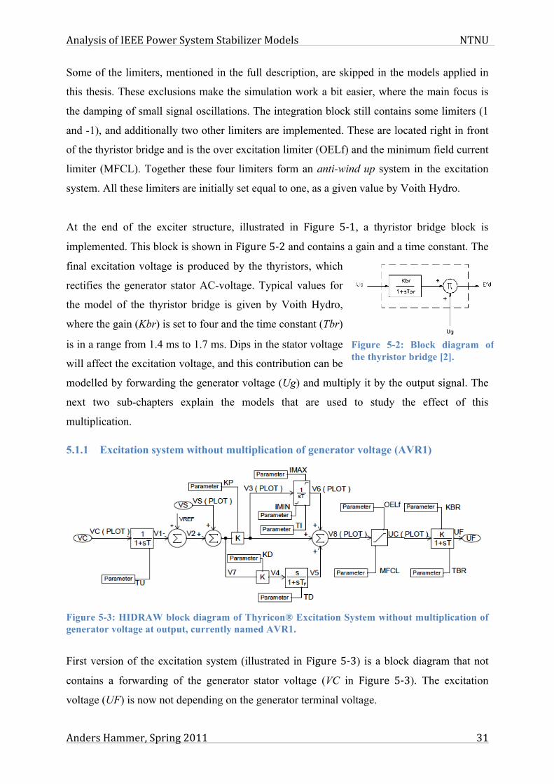
Analysis of IEEE Power System Stabilizer Models NTNU
Anders Hammer, Spring 2011 31
Some of the limiters, mentioned in the full description, are skipped in the models applied in
this thesis. These exclusions make the simulation work a bit easier, where the main focus is
the damping of small signal oscillations. The integration block still contains some limiters (1
and -1), and additionally two other limiters are implemented. These are located right in front
of the thyristor bridge and is the over excitation limiter (OELf) and the minimum field current
limiter (MFCL). Together these four limiters form an anti-wind up system in the excitation
system. All these limiters are initially set equal to one, as a given value by Voith Hydro.
At the end of the exciter structure, illustrated in Figure 5-‐1, a thyristor bridge block is
implemented. This block is shown in Figure 5-‐2 and contains a gain and a time constant. The
final excitation voltage is produced by the thyristors, which
rectifies the generator stator AC-voltage. Typical values for
the model of the thyristor bridge is given by Voith Hydro,
where the gain (Kbr) is set to four and the time constant (Tbr)
is in a range from 1.4 ms to 1.7 ms. Dips in the stator voltage
will affect the excitation voltage, and this contribution can be
modelled by forwarding the generator voltage (Ug) and multiply it by the output signal. The
next two sub-chapters explain the models that are used to study the effect of this
multiplication.
5.1.1 Excitation system without multiplication of generator voltage (AVR1)
Figure 5-3: HIDRAW block diagram of Thyricon® Excitation System without multiplication of generator voltage at output, currently named AVR1.
First version of the excitation system (illustrated in Figure 5-‐3) is a block diagram that not
contains a forwarding of the generator stator voltage (VC in Figure 5-‐3). The excitation
voltage (UF) is now not depending on the generator terminal voltage.
Figure 5-2: Block diagram of the thyristor bridge [2].
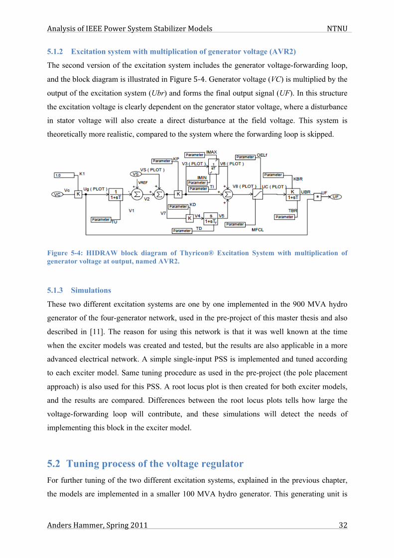
Analysis of IEEE Power System Stabilizer Models NTNU
Anders Hammer, Spring 2011 32
5.1.2 Excitation system with multiplication of generator voltage (AVR2)
The second version of the excitation system includes the generator voltage-forwarding loop,
and the block diagram is illustrated in Figure 5-‐4. Generator voltage (VC) is multiplied by the
output of the excitation system (Ubr) and forms the final output signal (UF). In this structure
the excitation voltage is clearly dependent on the generator stator voltage, where a disturbance
in stator voltage will also create a direct disturbance at the field voltage. This system is
theoretically more realistic, compared to the system where the forwarding loop is skipped.
Figure 5-4: HIDRAW block diagram of Thyricon® Excitation System with multiplication of generator voltage at output, named AVR2.
5.1.3 Simulations
These two different excitation systems are one by one implemented in the 900 MVA hydro
generator of the four-generator network, used in the pre-project of this master thesis and also
described in [11]. The reason for using this network is that it was well known at the time
when the exciter models was created and tested, but the results are also applicable in a more
advanced electrical network. A simple single-input PSS is implemented and tuned according
to each exciter model. Same tuning procedure as used in the pre-project (the pole placement
approach) is also used for this PSS. A root locus plot is then created for both exciter models,
and the results are compared. Differences between the root locus plots tells how large the
voltage-forwarding loop will contribute, and these simulations will detect the needs of
implementing this block in the exciter model.
5.2 Tuning process of the voltage regulator For further tuning of the two different excitation systems, explained in the previous chapter,
the models are implemented in a smaller 100 MVA hydro generator. This generating unit is
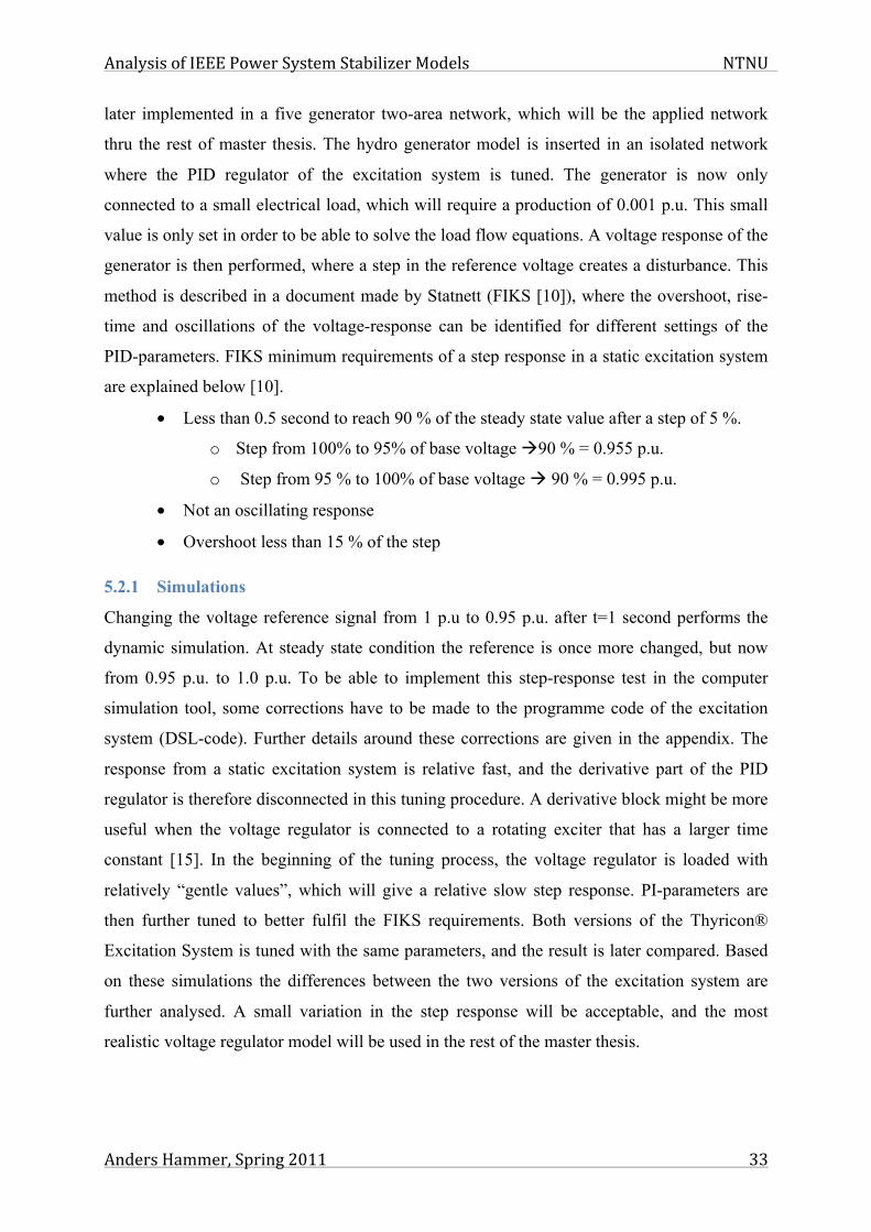
Analysis of IEEE Power System Stabilizer Models NTNU
Anders Hammer, Spring 2011 33
later implemented in a five generator two-area network, which will be the applied network
thru the rest of master thesis. The hydro generator model is inserted in an isolated network
where the PID regulator of the excitation system is tuned. The generator is now only
connected to a small electrical load, which will require a production of 0.001 p.u. This small
value is only set in order to be able to solve the load flow equations. A voltage response of the
generator is then performed, where a step in the reference voltage creates a disturbance. This
method is described in a document made by Statnett (FIKS [10]), where the overshoot, rise-
time and oscillations of the voltage-response can be identified for different settings of the
PID-parameters. FIKS minimum requirements of a step response in a static excitation system
are explained below [10].
• Less than 0.5 second to reach 90 % of the steady state value after a step of 5 %.
o Step from 100% to 95% of base voltage à90 % = 0.955 p.u.
o Step from 95 % to 100% of base voltage à 90 % = 0.995 p.u.
• Not an oscillating response
• Overshoot less than 15 % of the step
5.2.1 Simulations
Changing the voltage reference signal from 1 p.u to 0.95 p.u. after t=1 second performs the
dynamic simulation. At steady state condition the reference is once more changed, but now
from 0.95 p.u. to 1.0 p.u. To be able to implement this step-response test in the computer
simulation tool, some corrections have to be made to the programme code of the excitation
system (DSL-code). Further details around these corrections are given in the appendix. The
response from a static excitation system is relative fast, and the derivative part of the PID
regulator is therefore disconnected in this tuning procedure. A derivative block might be more
useful when the voltage regulator is connected to a rotating exciter that has a larger time
constant [15]. In the beginning of the tuning process, the voltage regulator is loaded with
relatively “gentle values”, which will give a relative slow step response. PI-parameters are
then further tuned to better fulfil the FIKS requirements. Both versions of the Thyricon®
Excitation System is tuned with the same parameters, and the result is later compared. Based
on these simulations the differences between the two versions of the excitation system are
further analysed. A small variation in the step response will be acceptable, and the most
realistic voltage regulator model will be used in the rest of the master thesis.
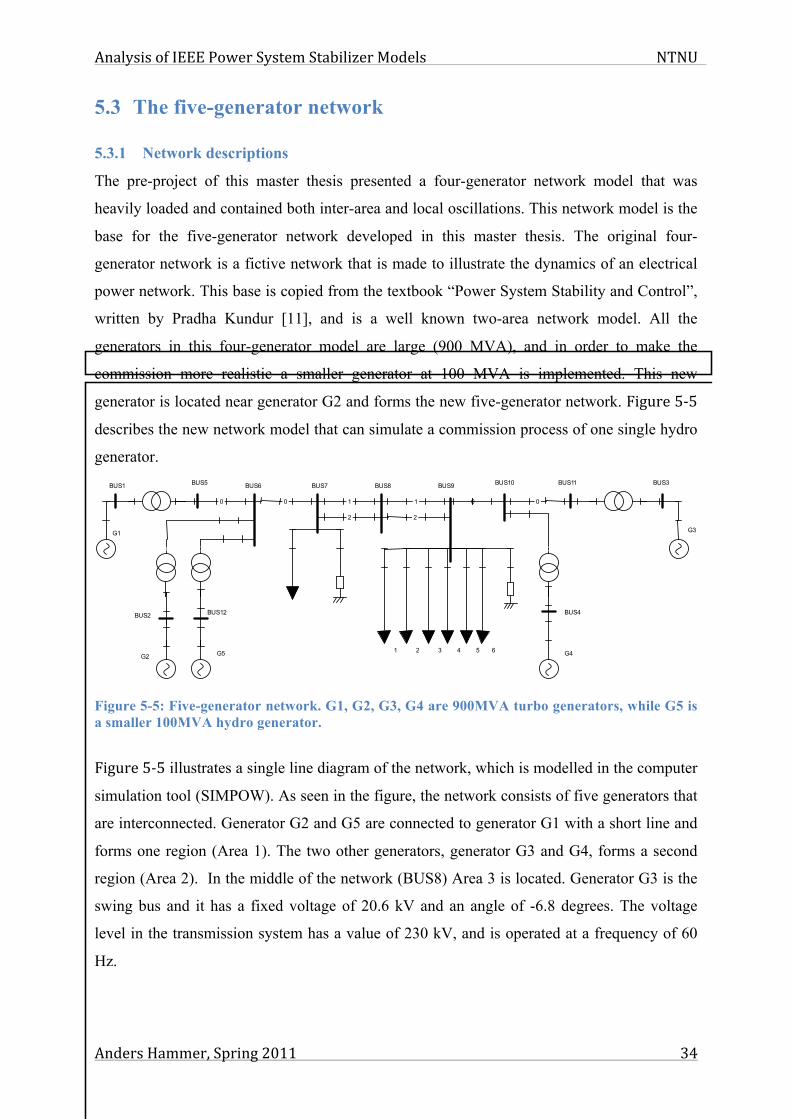
Analysis of IEEE Power System Stabilizer Models NTNU
Anders Hammer, Spring 2011 34
5.3 The five-generator network
5.3.1 Network descriptions
The pre-project of this master thesis presented a four-generator network model that was
heavily loaded and contained both inter-area and local oscillations. This network model is the
base for the five-generator network developed in this master thesis. The original four-
generator network is a fictive network that is made to illustrate the dynamics of an electrical
power network. This base is copied from the textbook “Power System Stability and Control”,
written by Pradha Kundur [11], and is a well known two-area network model. All the
generators in this four-generator model are large (900 MVA), and in order to make the
commission more realistic a smaller generator at 100 MVA is implemented. This new
generator is located near generator G2 and forms the new five-generator network. Figure 5-‐5
describes the new network model that can simulate a commission process of one single hydro
generator.
Figure 5-5: Five-generator network. G1, G2, G3, G4 are 900MVA turbo generators, while G5 is a smaller 100MVA hydro generator.
Figure 5-‐5 illustrates a single line diagram of the network, which is modelled in the computer
simulation tool (SIMPOW). As seen in the figure, the network consists of five generators that
are interconnected. Generator G2 and G5 are connected to generator G1 with a short line and
forms one region (Area 1). The two other generators, generator G3 and G4, forms a second
region (Area 2). In the middle of the network (BUS8) Area 3 is located. Generator G3 is the
swing bus and it has a fixed voltage of 20.6 kV and an angle of -6.8 degrees. The voltage
level in the transmission system has a value of 230 kV, and is operated at a frequency of 60
Hz.
Simpow 11.0.009 JOB=kundur DATE 11 MAY 2011 TIME 12:00:40 Page 1 / 2 [1 : 1]
2
1
2
10 00 0
BUS9
0
0
BUS1
G1
BUS4
G4
BUS2
G2
BUS50 BUS10
0
BUS6
0
BUS3
G3
BUS11
0
BUS7
0
0
BUS8
BUS12
0
G5 1 2 3 4 5 6
Analysis of IEEE Power System Stabilizer Models NTNU
Anders Hammer, Spring 2011 35
The appendix contains a complete load flow analysis, and this indicates that area 1 exports
and area 2 imports active power under normal state of operation. An active power flow of
approximately 400 MW is transmitted from left to the right thru the tie line in the model. The
long distance between the two areas generates a voltage in BUS8 that is below the limit, and
the network is now heavily loaded. A disturbance may, under these conditions, lead to
oscillations and system instability. There are clearly two areas in the network that is
connected together by a weak tie grid, and this will easily lead to network stability problems.
To provoke instability there is a possibility to make a three-phase short circuit at area 3, or by
switching off some of the loads connected to BUS7 or BUS9. The active load at BUS9 is
divided into smaller parts, for the reason to be able to trip a small load, and then analyse the
network oscillations. A full overview of the loads is found in the appendix of this master
thesis.
Four of the generators in the system have an equal rating of 900 MVA and 20 kV, but there
are some differences in the inertia. The fifth generator is a smaller unit at 100 MVA. An own
table in the simulation code describes the saturation in the machines, and this describes the
terminal voltage as the field current rises. All the large generators in the network (900 MVA)
are modelled as turbo generators with a round rotor. Voith Hydro is only working with hydro
generators and most of them have a salient pole rotor. Generator G5 is therefore modelled as a
salient pole generator, where a non-uniform reluctance between the rotor and stator appears.
The resulting reactance’s in the salient pole generator is therefore different from the ones in
the round rotor machines [6]. All the large synchronous generators are modelled as Type 1 in
the computer simulation tool. This means that they have one field winding, one damper
winding in d-axis and two damper windings in q-axis. The salient pole generator is modelled
as Type 2, which means a generator with one field winding, one damper winding in d-axis and
one damper winding in q-axis [18]. The appendix contains tables of the parameters for the
generators, lines, transformers and the loads used in this five-generator network.
The different generating units in the network are connected to different turbine/governor
models. An approximate model of a steam turbine with a single reheat (ST1) is connected to
the turbo generators, and a general speed-governing model (SG1) regulates the speed of these
turbines. A classical penstock hydro turbine model (HT1) generates the torque at the hydro
generator, and the governor named DSLS/HYGOV regulates the speed. All these models are
already implemented in the simulation software, and the parameters is chosen as typical
Analysis of IEEE Power System Stabilizer Models NTNU
Anders Hammer, Spring 2011 36
values. One important difference between a steam turbine and a hydro turbine is that the
hydro turbine has two different droop parameters. A step in the water gate position of a hydro
turbine will not give an instant increase in the power output of the turbine, but rather a small
drop. The water flow in the penstock cannot increase instantaneously, so the velocity of the
flow in the turbine will initially decrease after a gate opening. After a short delay the water
flow in the penstock has the time to accelerate, and the power output of the turbine can
increase. To handle this phenomenon the hydro governing model has two different droop
parameters. This compensates for the water flow to catch up after a step in the gate position.
One droop parameter reducing the gain after fast changes (called transient- or temporary-
droop) and one droop parameter for slower changes in the gate opening (called permanent
droop) [6]. The different models and parameters for turbine and governor are further
described in the appendix. SINTEF Energy Research has given the parameter values as
typical values for a turbine governing system.
5.3.2 Simulations
Under commissioning of generators it is usually difficult to tune the PSS at the inter-area
oscillation mode, and only the local oscillation mode is often taken into consideration [19].
The simulation work in this document will identify the inter-area oscillations in addition to
the local oscillations. Both modes are taken into consideration, and the goal is to increase the
damping of the local as well as the inter-area oscillation mode in this five-generator network.
Initially the network is not containing any power system stabilizers, and at this stage the
different network oscillations modes is analysed. The computer simulation programme
includes a modal analysis tool and by using this, at the most critical eigenvalues, the different
oscillation modes will be uncovered. These modes can then further be treated individually, in
order to increase the damping. All eigenvalue analysis is, during this master thesis, performed
at the initially state.
The different network oscillations are also described by performing a time domain analysis.
To start the oscillations in this heavy loaded network, a 3-phase short circuit connection is
introduced in BUS7. This fault is only present in 0.05 seconds and then it is totally removed.
No other change is made in the electrical system, and the fault can be considered as an
automatic re-connection. 0.05 seconds is a really short duration, and the fault represents a
small disturbance of the system.

Analysis of IEEE Power System Stabilizer Models NTNU
Anders Hammer, Spring 2011 37
The next step in the step in this master thesis is to start improving the system stability by
implementing different power system stabilizer´s in the network.
5.4 Implementation of the dual input PSS model (PSS2B) In order to increase the damping of the system oscillations, the dual input stabilizer (PSS2B)
is implemented in the hydro generator of the five-generator network. This generator is much
smaller than the other generators in the network, and the lack of thrust will only result in
smaller performance of damping of inter-area oscillations. In spite, it is always favourable to
increase rather than decrease the damping of these oscillations after installing a PSS.
PSS2B is implemented in the computer simulation programme as a DSL-code, and the block
diagram of this code is presented in Figure 5-‐6. System frequency and electrical power of the
machine is the input parameters of this stabilizer structure.
Figure 5-6: HIDRAW block diagram of PSS2B stabilizer structure.
SIGNAL1, located in the middle of the block diagram, is the synthesised integral of
accelerating power signal, and the blocks in front of this signal is mentioned as the PSS2B
transducer. This transducer has parameters that will not change from situation to situation,
except from the gain KS2, which is dependent on the generator inertia. Table 5-‐1 describes
the chosen parameters in the transducer part of the PSS2B.
ABB POWER SYSTEMS ABRev Ind Revision Appd Year Week
Drawn by
Drawing checked by
Design checked by
Iss by Dept Year Month Day
Rev Ind
Rev Ind
Sheet
Sheet
Cont
FUNCTIONAL DIAGRAMName: PSS2B
Proc.type:
Type: TASK Anders Hammer
DSL Code Generator 1000
1002
00
VSK 1+sTB
C
1+sT1+sT
B
C
1+sT1+sT
B
C
1+sT
Parameter Parameter Parameter Parameter
Parameter Parameter Parameter
Parameter
Parameter
VREF+
--1.
11+sT
11+sT
K1+sT
sF
K1+sT
sF
Parameter
Parameter Parameter
Parameter
11+sT
K1+sT
sF
K1+sT
sF
Parameter Parameter
Parameter Parameter
+
+
K
1+sTB
C
1+sT
Parameter
Parameter
Parameter
PEG K1+sT
Parameter
+
-
FIFI 11+sT
11+sT
11+sT
KS1 T1
T2
T3 T10
T11T4
PSSMAX
PSSMIN
VS
SIGNAL1 ( PLOT )
SIGNAL2 ( PLOT )
TW1 TW2
TFT6
TW3 TW4
TPT7
P2 ( PLOT )
F1 ( PLOT )
T9
T8
F2 ( PLOT )
KS3
KS2
P1 ( PLOT )
F3 ( PLOT )
Ramp track filter
Integral of acc. power
Lead/lag filters
Gain
PSS Limiter
SIMPOW requirements
Washout filter
WashoutfilterFrequencytransducer
Electric powertransducer
Integrator

Analysis of IEEE Power System Stabilizer Models NTNU
Anders Hammer, Spring 2011 38
Table 5-1: PSS2B transducer parameters given by Voith Hydro. TF TP Tw1=Tw2=Tw3=Tw4 T6 T7 KS2=T7/2H KS3 T8 T9 0.02 0.02 3 0 3 0.5137* 1 0.4 0.1 *100MVA generator, inertia: H=2.92.
5.4.1 Simulations
To verify that the PSS2B-transducer acts in a proper way, the integral of accelerating power
signal is compared with the actual rotor speed of the machine. A well-adjusted transducer has
an integral of accelerating power signal that follows the speed variations accurately. This test
is performed in the beginning of the simulation work, and the following task is to tune the
lead/lag-filters and gain so the overall damping is maximized. This procedure is based on a
pole placement approach and tuning of lead/lag-filters, the same procedure as for a single
input stabilizer. Theory part of this master thesis explains this in more detail and it is
additionally explained in the previous chapter of this master thesis.
The next simulation is a time domain analysis where the three-phase short circuit connection
is implemented at the tie line connection. This fault starts some oscillations in the generator
speed and the implementation of a well-tuned PSS2B will optimally reduce these oscillations.
The PSS output signal is additionally plotted in order to illustrate the overall behaviour of the
PSS. Another time domain analysis is also performed, where a load of 500 MW at BUS9 is
disconnected. This small disturbance produces a shift in the load flow, and the power
generated by generator G5 will start to oscillate. The goal of this test is to detect the
contribution of PSS2B in the hydro generator during regular operation of the network.
Optimally the PSS must not disturb this regular operation, in any great concern.
5.5 Implementation of the multi-band PSS model (PSS4B) A multi-band stabilizer (PSS4B) is, during this part of the simulation work, implemented in
the hydro generator of the five-generator network. HIDRAW, the DSL-coding programme, is
also used to implement this stabilizer, and the PSS4B block diagram is presented in Figure
5-‐7. The input signals in the upper two bands are the rotor speed, while the lower band uses
the generator power as an input signal. These signals are passing through transducer models,
which is similar to the models presented in the theory of this master thesis.

Analysis of IEEE Power System Stabilizer Models NTNU
Anders Hammer, Spring 2011 39
5.5.1 Loading the PSS4B structure with sample data given by IEEE
First step in the simulations, performed with this stabilizer structure, is to implement and load
it with IEEE data, described in IEEE Std. 421.5. This data set is additionally described in the
theory part of this master thesis, and a complete table of the chosen parameters is listed in
Table 5-‐2. PSS4B is commonly used to achieve damping of oscillations in a wide frequency
range and the IEEE data will approximately give a phase shift of 45 degrees from 0,1 Hz to 4
Hz. A simple time domain analysis of generator speed and stabilizing signal indicates the
outcome of this PSS data set. The goal of this test is to see if the stabilizer gives an acceptable
damping only by simply load it with the sample data.
Figure 5-7: HIDRAW block diagram of PSS4B stabilizer structure.
+
-
VS
VREF+
--1.
Parameter
Parameter
++
+
Parameter
Parameter
K
Parameter
1+sTB
C
1+sT
Parameter
Parameter
1+sTB
C
1+sTA+sBC+sD
Parameter
Parameter
Parameter
Parameter
Parameter
K
1+sTB
C
1+sT
Parameter
Parameter
1+sTB
C
1+sTA+sBC+sD
Parameter
Parameter
Parameter
Parameter
Parameter
K
Parameter
Parameter
1.0
1.0
+
-
Parameter
Parameter
K
Parameter
1+sTB
C
1+sT
Parameter
Parameter
1+sTB
C
1+sTA+sBC+sD
Parameter
Parameter
Parameter
Parameter
Parameter
K
1+sTB
C
1+sT
Parameter
Parameter
1+sTB
C
1+sTA+sBC+sD
Parameter
Parameter
Parameter
Parameter
Parameter
K
Parameter
Parameter
1.0
1.0
+
-
Parameter
Parameter
K
Parameter
1+sTB
C
1+sT
Parameter
Parameter
1+sTB
C
1+sTA+sBC+sD
Parameter
Parameter
Parameter
Parameter
Parameter
K
1+sTB
C
1+sT
Parameter
Parameter
1+sTB
C
1+sTA+sBC+sD
Parameter
Parameter
Parameter
Parameter
Parameter
K
Parameter
Parameter
1.0
1.0
11+sT
Parameter
W k=0
j=0
skk
sjj
1
2
b
a
k=0
j=0
skk
sjj
2
3
d
c
PEG
K
Parameter
L4 ( PLOT )
VSTmax
VSTmin
VLmax
VLmin
KL
VL ( PLOT )
TL6
TL5
L3
TL3
TL4TL2
KL11TL1
L2L1
TL12
TL11
L7
TL9
TL10TL8
KL17
TL7
L6L5
KL1
KL2
L8 ( PLOT )
I4 ( PLOT )
VImax
VImin
KI
TI6
TI5
I3
TI3
TI4TI2
KI11TI1
I2I1
TI12
TI11
I7
TI9
TI10TI8
KI17
TI7
I6I5
KI1
KI2
I8 ( PLOT )
H4 ( PLOT )
VHmax
VHmin
KH
TH6
TH5
H3
TH3
TH4TH2
KH11TH1
H2H1
TH12
TH11
H7
TH9
TH10TH8
KH17
TH7
H6H5
KH1
KH2
H8 ( PLOT )
VI ( PLOT )
VH ( PLOT )
PE3 ( PLOT )
TWOH
PE2 ( PLOT )
PE1 ( PLOT )
W1W2 ( PLOT )
KST
VST2 ( PLOT )
VST1
Electric powertransducer model
Speed transducer model

Analysis of IEEE Power System Stabilizer Models NTNU
Anders Hammer, Spring 2011 40
Table 5-2: List of parameters of PSS4B, according to IEEE sample data. (Parameters not mentioned in this table are set equal to 1)
l-band i-band h-band KL=7.5 FL=0.07 Hz KI=30 FI=0.7 Hz KH=120 FH=8 Hz
VLmax=0.075 VLmin=-0.075 VImax=0.6 VImin=-0.6 VHmax=0.6 VHmin=-0.6 TL1=1.73 TL7=2.075 TI1=0.173 TI7=0.2075 TH1=0.01513 TH7=0.01816 TL2=2.075 TL8=2.491 TI2=0.2075 TI8=0.2491 TH2=0.01816 TH8=0.02179
KL1=KL2=KI1=KI2=KH1=KH2=66, VSTmax=0.15, VSTmin=-0.15
5.5.2 Tuning of the PSS structure based on the actual network oscillations
The next step is to tune the stabilizer more accurately, based on the actual oscillation modes
in the electrical network. A more exact tuning procedure is here performed in five different
cases. All cases are based on pole placement and root locus plots of eigenvalues. Setting the
internal branch-gains KL2, KI2 and KH2 in Figure 5-‐7 to zero disconnects the lower branch
of the three bands in PSS4B. Only the top branch is now used in the tuning processes, and
initially only a simple washout block in the top branch is implemented. All the band-gains
(KL, KI, KH in Figure 5-‐7) are initially set to zero and the other filters are initially set to not
give any phase shift. By increasing one of the band-gains, the contribution from that specific
branch is found and the need of a lead/lag-filter is identified based on a pole placement
approach. The tuning process is now simplified, where the lead/lag-filters and gains for each
band are tuned separately, and in different orders.
At the end of each case, a complete eigenvalue analysis is performed in order to assure that all
eigenvalues in the system has acceptable values. Each case contains also time domain
analysis, where a 3-phase short circuit, with duration of 0.05 seconds, is introduced in BUS8.
The speed of generator G5 is analysed and additionally the PSS output signal. The time
domain analyses of each case are plotted together with the situation where no PSS is
implemented in the system. By comparing these graphs the improvement of the damping of
speed oscillations is highly visible. Limiter values of the PSS4B are set equal to the limiter
values used for the PSS2B. The reason is that this makes it possible to later compare the
results of the respective time domain analysis, and the overall performance of each stabilizer
structure. An overview of the different cases is now listed in Table 5-‐3 and a more detailed
description is presented below.

Analysis of IEEE Power System Stabilizer Models NTNU
Anders Hammer, Spring 2011 41
Table 5-3: Overview of PSS4B tuning procedures. Tuning procedure Step 1 Step 2
Case 1 h-band is tuned according to the local oscillation mode
i-band is tuned according to the inter-area oscillation mode
Case 2 h-band is tuned according to the inter-area oscillation mode
i-band is tuned according to the local oscillation mode
Case 3 i-band is tuned according to the inter-area oscillation mode
h-band is tuned according to the local oscillation mode
Case 4 i-band is tuned according to the local oscillation mode
h-band is tuned according to the inter-area oscillation mode
Case 5 Same as case 4, but different gain Same as case 4
Case 1
First step of case 1 is to tune the high frequency band (h-band) according to the local
oscillation mode, and secondary tune the intermediate frequency band (i-band) to maximize
the damping in the inter-area mode. The transducer of the h-band is specially designed to
handle the highest oscillation frequencies, and the i-band is designed to handle the lowest
frequencies. Tuning approach of case 1 utilize this natural allocation of frequencies according
to each band.
This tuning procedure is starting with increasing the gain of the high frequency band (Kh),
and thereby a root locus analysis of the most critical eigenvalues is performed. By using the
same method of tuning and implementing lead/lag-filters as described for the PSS2B, the h-
band is tuned to correct the initial angle of the movement of the local oscillation mode. The
gain is then set to a reasonable value that increases the absolute damping of this mode,
without highly disturbing the oscillating frequency. Next step is to adjust the inter-area
oscillation mode by tuning the intermediate frequency band (i-band). By increasing the gain
of the i-band (Ki), the initial angle of the movement of the inter-area mode is uncovered. This
angle is the base of the tuning of the lead/lag-filters in the i-band.
Case 2
The tuning-order of case 2 is similar to case 1 where the h-band is tuned as the first step.
Only difference from case 1 is that the h-band is here tuned according to the inter-area
oscillation mode, and the i-band is then tuned to maximize the damping of the local
oscillation mode. This approach is a more unnatural choice, but the result can uncover the
importance of allocating the right frequencies to each band.

Analysis of IEEE Power System Stabilizer Models NTNU
Anders Hammer, Spring 2011 42
Case 3
The tuning order of case 3 are directly shifted compared to case 1, where the i-band is tuned
first according to the inter-area oscillation mode, and the h-band is tuned according to the
local oscillation mode. This approach will illustrate the differences of initially focusing on the
inter-area mode, compared to start with the local mode.
Case 4
Case 4 is similar to case 3, where the i-band is tuned before the h-band. The difference is that
the i-band is tuned according to the local oscillation mode. Next step is to tune the h-band
according to the inter-area oscillation mode.
Case 5
Case 5 has the same tuning procedure like case 3, besides from choosing different gains of the
i-band. The point of this test is to uncover the result of choosing a higher gain, in order to
maximize the damping of the local oscillation mode. As a final step is the h-band tuned to
improve the damping of the inter-area oscillation mode.
5.5.3 Final choice of tuning the PSS4B
In order to find the best solution of tuning the PSS4B, the results from the different cases are
compared. First the improvements of the eigenvalues are examined, and the cases which gives
acceptable results is further compared in time domain analysis. A load of 500 MW is then
disconnected at BUS9, and the time response of the active and reactive power is analysed for
each case.
5.6 PSS2B vs. PSS4B The parameters that gave the best results of the two different stabilizer structures, PSS2B and
PSS4B, are in this chapter compared in an eigenvalue analysis and also in different time
domain analysis. The same disturbances as used in the previous chapters are also used to
compare the performance of each stabilizer structure.
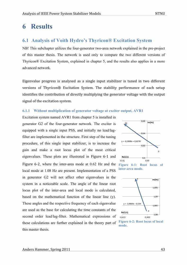
Analysis of IEEE Power System Stabilizer Models NTNU
Anders Hammer, Spring 2011 43
6 Results
6.1 Analysis of Voith Hydro’s Thyricon® Excitation System NB! This subchapter utilizes the four-generator two-area network explained in the pre-project
of this master thesis. The network is used only to compare the two different versions of
Thyricon® Excitation System, explained in chapter 5, and the results also applies in a more
advanced network.
Eigenvalue progress is analysed as a single input stabilizer is tuned in two different
versions of Thyricon® Excitation System. The stability performance of each setup
identifies the contribution of directly multiplying the generator voltage with the output
signal of the excitation system.
6.1.1 Without multiplication of generator voltage at exciter output, AVR1
Excitation system named AVR1 from chapter 5 is installed in
generator G2 of the four-generator network. The exciter is
equipped with a single input PSS, and initially no lead/lag-
filter are implemented in the structure. First step of the tuning
procedure, of this single input stabilizer, is to increase the
gain and make a root locus plot of the most critical
eigenvalues. These plots are illustrated in Figure 6-‐1 and
Figure 6-‐2, where the inter-area mode at 0.62 Hz and the
local mode at 1.08 Hz are present. Implementation of a PSS
in generator G2 will not affect other eigenvalues in the
system in a noticeable scale. The angle of the linear root
locus plot of the inter-area and local mode is calculated,
based on the mathematical function of the linear line (y).
These angles and the respective frequency of each eigenvalue
are used as the base for calculating the time constants of the
second order lead/lag-filter. Mathematical expressions of
these calculations are further explained in the theory part of
this master thesis.
!"
#!"
$"%"&!'()*)+","!'-(.)"
!'-"
!'-("
!'-/"
!'--"
&!'0!" !'!!"
!"#$%&'
()#*+,&'
12345"6546" 782495":12345"6546;"Figure 6-1: Root locus of inter-area mode.
!"
#"
$"%"&'()*+#,"&"!(-'#"
.(!*"
.(!*-"
.(!)"
.(!)-"
.(."
&!(#.-" &!(#!-"
!"#$%&'
()#*+,&'
/0123" /45678"9/0123:"Figure 6-2: Root locus of local mode.
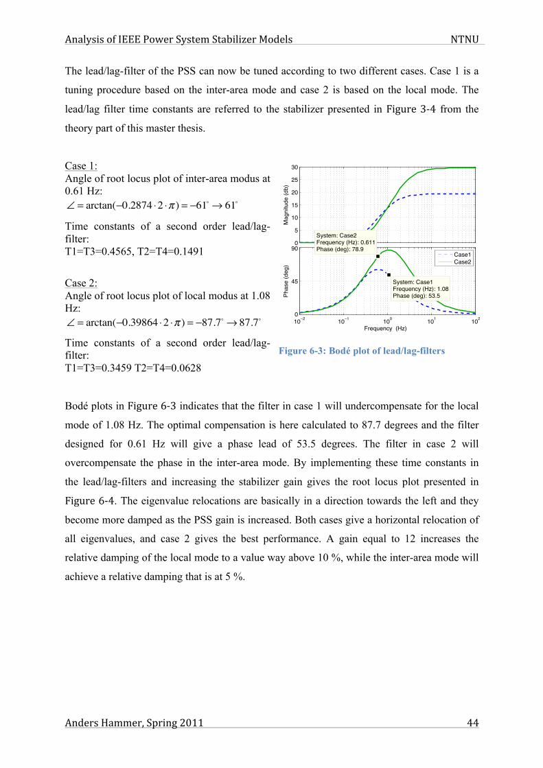
Analysis of IEEE Power System Stabilizer Models NTNU
Anders Hammer, Spring 2011 44
The lead/lag-filter of the PSS can now be tuned according to two different cases. Case 1 is a
tuning procedure based on the inter-area mode and case 2 is based on the local mode. The
lead/lag filter time constants are referred to the stabilizer presented in Figure 3-‐4 from the
theory part of this master thesis.
Case 1: Angle of root locus plot of inter-area modus at 0.61 Hz:
Time constants of a second order lead/lag-filter: T1=T3=0.4565, T2=T4=0.1491
Case 2: Angle of root locus plot of local modus at 1.08 Hz:
Time constants of a second order lead/lag-filter: T1=T3=0.3459 T2=T4=0.0628
Bodé plots in Figure 6-‐3 indicates that the filter in case 1 will undercompensate for the local
mode of 1.08 Hz. The optimal compensation is here calculated to 87.7 degrees and the filter
designed for 0.61 Hz will give a phase lead of 53.5 degrees. The filter in case 2 will
overcompensate the phase in the inter-area mode. By implementing these time constants in
the lead/lag-filters and increasing the stabilizer gain gives the root locus plot presented in
Figure 6-‐4. The eigenvalue relocations are basically in a direction towards the left and they
become more damped as the PSS gain is increased. Both cases give a horizontal relocation of
all eigenvalues, and case 2 gives the best performance. A gain equal to 12 increases the
relative damping of the local mode to a value way above 10 %, while the inter-area mode will
achieve a relative damping that is at 5 %.
! = arctan("0.2874 #2 #! ) = "61!$ 61!
! = arctan("0.39864 #2 #! ) = "87.7!$ 87.7!
0
5
10
15
20
25
30
Mag
nitu
de (d
b)
Bode Diagram
Frequency (Hz)10 2 10 1 100 101 1020
45
90
System: Case1Frequency (Hz): 1.08Phase (deg): 53.5
System: Case2Frequency (Hz): 0.611Phase (deg): 78.9
Phas
e (d
eg)
Case1Case2
Figure 6-3: Bodé plot of lead/lag-filters

Analysis of IEEE Power System Stabilizer Models NTNU
Anders Hammer, Spring 2011 45
Figure 6-4: Root locus plot of the most critical eigenvalues in the system. PSS1A is installed in AVR1 in generator G2 and is tuned according to the cases. Right graph is a zoom up at the inter-area mode.
6.1.2 With multiplication of generator voltage at exciter output, AVR2
This exciter is first loaded with the same PSS parameters used for AVR1 (case 1 and case 2),
and next the PSS is tuned specific according to AVR2. Calculations and bode-plot of these
cases (Case 3 and Case 4) are left in the appendix. A result of the integration of these filters is
presented in the root locus plot in Figure 6-‐5, where the gain of the single input PSS is
increased. The graphs indicate that the multiplication of generator voltage has great influence
at the pole placements.
Figure 6-5: Root locus plot of the most critical eigenvalues in the system. PSS1A is installed in AVR2 in generator G2 and is tuned according to the cases. Right graph is a zoom up at the inter-area mode.
When the lead/lag-filter is tuned according to the inter-area mode (case 1 & case 3) the
eigenvalues is initially moving to the right in the complex plane. At around a gain of 15 they
bend off and rapidly starting to move towards the right part of the complex plane. The
!"#
$%#
$%#
$%#
&#!'#!"#
$%#
$%#$%#''#
$%#
%#
%($#
!#
!($#
'#
'($#
)*(%# )'(&# )'(+# )'("# )'('# )'(%# )!(&# )!(+# )!("# )!('# )!(%# )%(&# )%(+# )%("# )%('# %(%#
!"#$%&#'()*+,-)
./#0)*123-)
$#,##-./0#1234567# !%#,#-./0#1234567# 89#/.21:/27# ;2<.#!# ;2<.#'#
!"#
$#%&#%'#
!"#
"(!!#
"()#
"()!#
"(*#
"(*!#
+"($# +"()# +"('# +"(&# "("#
!"#$%&'
()*+'#,-.&'
!"#$%#
!"#
$"#
!"#
"#$%#!"#
"#
$%#!"#
"#
"&!#
$#
$&!#
%#
'(&%# ')&*# ')&%# '%&*# '%&%# '$&*# '$&%# '"&*# '"&%# "&)# "&+# $&)# $&+# %&)#
!"#$%&#'()*+,-)
./#0)*123-)
!#,##-./0#1234567# $"#,#-./0#1234567# 89#/.21:/27# #;2<.#$##;2<.#%# ;2<.#)# #;2<.#(#
!"#
$"#
!"#
$%#
"&!!#
"&'#
"&'!#
"&(#
"&(!#
)"&*# )"&'# )"&+# )"&%# "&"#
!"#$%&'#
()*+#$,-.'#

Analysis of IEEE Power System Stabilizer Models NTNU
Anders Hammer, Spring 2011 46
maximum damping obtained in this case is lower compared to the result from AVR1 in the
previous subchapter. When the lead/lag filter is tuned according to the local oscillation mode
(case 2 & case 4) the eigenvalues is moving in a more favourable direction, and the damping
gets higher for both local and inter-area mode. Overall the tuning of AVR2 is more
troublesome compared to AVR1, since the eigenvalues tends to easily move towards the left
part of the complex plane.
6.2 Tuning of the PID regulator of Thyricon® Excitation System The PID-part of the excitation systems is here further tuned, according to a step in reference
voltage. To handle this voltage step the DSL-code must be modified, and further explanation
of these DSL-file corrections is placed in the appendix. Excitation system named AVR1 and
AVR2, explained in the simulation description, is loaded with two sets of PID-parameters.
One set has parameters that have relative gentle values, while the other set has a set of more
“aggressive” values. The exact parameter values are found in Table 6-‐1.
By initially loading the excitation
system named AVR1 with so-called
“gentle” parameters the voltage
overshoot, illustrated as a blue dashed
line in Figure 6-‐6, is measured to:
.
The response is not oscillating and it
takes about 0.8 second to reach 90 %
of the step. This is a voltage response
that is too slow compared to the given
restrictions. The parameters are then
adjusted to give a result that practically gives no overshoot and to take about 0.4 seconds to
reach 90 % of the step. This “adjusted” settings gives a voltage response that is within the
requirements. When the variation of generator voltage is directly taken into account, by
multiplication of stator voltage at AVR output, the step response gives a higher voltage
overshoot, but not a higher rise-time. The result of the step responses, presented in Figure
6-‐6, shows clearly that AVR1 gives less overshoot compared to AVR2. The complete results
1.004 !1.00.05
= 0.08" 8%
!"#$%!"#$&%!"#&%!"#&&%!"#'%!"#'&%!"#(%!"#(&%!"#)%!"#)&%!"##%!"##&%
*%*"!!&%*"!*%
!% *% +% ,% $% &% '% (% )% #% *!% **% *+% *,% *$%
!"#$%&'()*+,-((((
./0'()1-(
-./*%012&%342+%
-./*%012*!%352(%
-./+%012&%352+%
-./+%012*!%35(%
#!%6%78%9:;<%
Figure 6-6: Voltage step response of AVR1 and AVR2.

Analysis of IEEE Power System Stabilizer Models NTNU
Anders Hammer, Spring 2011 47
of the step response test are also presented in Table 6-‐1, and the overall difference between
the excitation systems is not enormous. Table 6-1: Step-response performance of the different excitation systems with two sets of parameters Excitation sys. AVR1 AVR2
PI-parameters “Gentle” Kp=5, Ti=2
Adjusted Kp=10, Ti=7
“Gentle” Kp=5, Ti=2
Adjusted Kp=10, Ti=7
Overshoot (max 15 %) ∼0 % 8 % 2 % 12 % Rise time (max 0.5 s) 0.8 s 0.4 s 0.8 s 0.4 s Oscillations - - - -
AVR2 is the most correct representation of Voith Hydro’s Thyricon® Excitation system, and
it is used in the following simulations. It is loaded with the adjusted parameters presented in
Table 6-‐1 in the following simulations.
6.3 Analysis of the five-generator network The excitation system that includes the multiplication of the generator voltage (AVR2) is
installed in the hydro generator of the five-generator
network. A PSS is not initially implemented in the
network, but it will be implemented in the small
generator in the following chapters of this master
thesis. Eigenvalue diagram, presented in Figure 6-‐7,
explains the system oscillation when no PSS is
installed. The eigenvalue at ∼0.62 Hz is the worst
damped eigenvalue, and it is located considerable
close to the imaginary axis. At around 1.1 Hz two
other eigenvalues is located, and at approximately 1.6
Hz the last critical eigenvalue is found. These four eigenvalues will highly contribute to
oscillations in the network.
One solid line and one dashed line are drawn in the diagram to indicate the relative damping
of 5 % and 10 %, respectively. A higher oscillating frequency (imaginary axis) requires more
absolute damping (real axis), in order to be considered as well damped [6]. The modal
analysis of the five-generator network (Figure 6-‐8) indicates that the network is struggling
with four oscillation modes.
!"
!#$"
%"
%#$"
&"
'(" '$" ')" '%"
!"#$%&'(#
)*#$+,(#
*+",--" $"."/012"3456789"%!"."/012"3456789"
Figure 6-7: Most critical eigenvalues in the network.
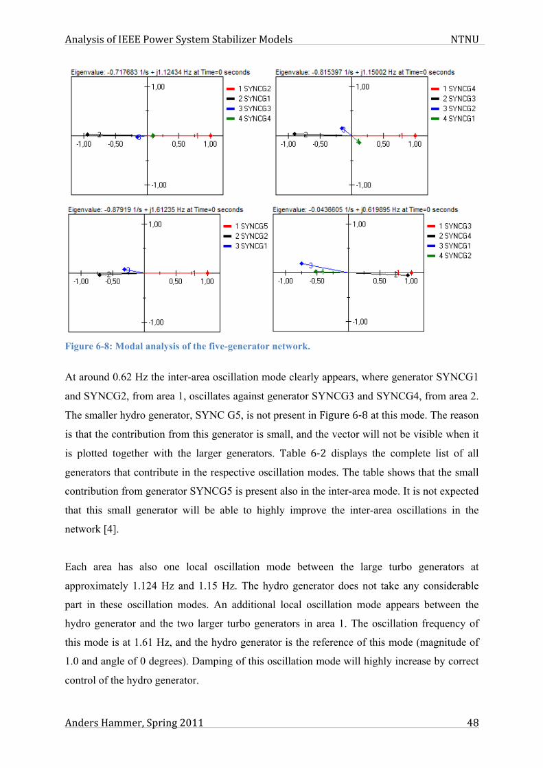
Analysis of IEEE Power System Stabilizer Models NTNU
Anders Hammer, Spring 2011 48
Figure 6-8: Modal analysis of the five-generator network.
At around 0.62 Hz the inter-area oscillation mode clearly appears, where generator SYNCG1
and SYNCG2, from area 1, oscillates against generator SYNCG3 and SYNCG4, from area 2.
The smaller hydro generator, SYNC G5, is not present in Figure 6-‐8 at this mode. The reason
is that the contribution from this generator is small, and the vector will not be visible when it
is plotted together with the larger generators. Table 6-‐2 displays the complete list of all
generators that contribute in the respective oscillation modes. The table shows that the small
contribution from generator SYNCG5 is present also in the inter-area mode. It is not expected
that this small generator will be able to highly improve the inter-area oscillations in the
network [4].
Each area has also one local oscillation mode between the large turbo generators at
approximately 1.124 Hz and 1.15 Hz. The hydro generator does not take any considerable
part in these oscillation modes. An additional local oscillation mode appears between the
hydro generator and the two larger turbo generators in area 1. The oscillation frequency of
this mode is at 1.61 Hz, and the hydro generator is the reference of this mode (magnitude of
1.0 and angle of 0 degrees). Damping of this oscillation mode will highly increase by correct
control of the hydro generator.

Analysis of IEEE Power System Stabilizer Models NTNU
Anders Hammer, Spring 2011 49
Table 6-2: Vectors (magnitude and angle) of kinetic energy represented in the eigenvalues.
Eigenvalue ([1/s], [Hz]): -0.71771, 1.1243 Eigenvalue ([1/s], [Hz]): -0.81539, 1.15 Generator Area Magnitude Angle [°] Generator Area Magnitude Angle [°] SYNC G1 1 0.94582 178.22 SYNC G1 1 0.18938 -49.855 SYNC G2 1 1.0000 0.0000 SYNC G2 1 0.21498 135.66 SYNC G3 2 0.15743 -169.43 SYNC G3 2 0.90916 177.74 SYNC G4 2 0.094176 -0.85834 SYNC G4 2 1.000 0.000 SYNC G5 1 0.013682 47.095 SYNC G5 1 0.0056527 -178.06 Eigenvalue ([1/s], [Hz]): -0.04358, 0.61987 Eigenvalue ([1/s], [Hz]): -0.8796, 1.6125 Generator Area Magnitude Angle [°] Generator Area Magnitude Angle [°] SYNC G1 1 0.11173 165.48 SYNC G1 1 0.32915 -165.73 SYNC G2 1 0.51883 177.39 SYNC G2 1 0.70653 -177.28 SYNC G3 2 1.000 0.00 SYNC G3 2 0.023592 142.64 SYNC G4 2 0.94625 -2.782 SYNC G4 2 0.05005 -175.93 SYNC G5 1 0.035099 171.38 SYNC G5 1 1.000 0.000
Table 6-‐3 displays two of the most critical eigenvalues in the system, which can be improved
by the hydro generator. Additionally the relative damping of these are calculated according to
equation 3.10 from the theory part of this master thesis. Generator G5 is later used to improve
the damping of these two eigenvalues. Table 6-3: Critical eigenvalues that can be improved by generator G5.
Stabilizer Oscillation mode Eigenvalue [1/s], [Hz] Relative damping [ζ]
No PSS Local (-0.8796, 1.6125) 8.65 % Inter-area (-0.0436, 0.6198) 1.12 %
The oscillations mentioned above can also be shown in a time domain analysis, illustrated in
Figure 6-‐9, where a 3-phase short circuit
at BUS8 is present for 0.05 seconds.
Suddenly in the aftermath of the
disturbance the more high frequent local
oscillations is present. These oscillations
are damped, and thereby replaced by an
oscillation with a lower frequency. After
approximately 5 seconds only the inter-
area oscillations remains, where generator
G1, G2 and G5 (Area 1) clearly oscillates
against generator G3 and G4 (Area 2).
!"##$%&
!"###&
!"###%&
'&
'"!!!%&
'"!!'&
'"!!'%&
'"!!(&
'"!!(%&
'"!!)&
!& '& (& )& *& %& +& ,&
!"##$%&"'()%
*+,#%&-)%
-'& -(& -)& -*& -%"&./&011&
Figure 6-9: Time response of the generator speeds after a 3-phase short circuit fault at BUS8.

Analysis of IEEE Power System Stabilizer Models NTNU
Anders Hammer, Spring 2011 50
This oscillation is considerable poorly damped. The blue dashed line in Figure 6-‐9 indicates
that G5 struggles with the toughest oscillations in the network. An installation of a PSS at this
unit seems to be a good choice.
6.4 Implementing a dual input stabilizer (PSS2B)
6.4.1 Analysis of the input transducers
PSS2B stabilizer is implemented in
generator G5 of the five-generator
network and a 3-phase short circuit, with
duration of 0.05 second, starts the
oscillations presented in Figure 6-‐10.
The integral of accelerating power signal
is compared to the actual rotor speed in
Figure 6-‐10, and this is slightly leading a
bit in the first oscillations. After
approximately five seconds the integral
of accelerating power signal is directly following the generator speed signal. The overall
variation between the two signals is considerable low, and the integral of accelerating power
can be used as an input-signal to the lead/lag-filter and gain part of the stabilizer. The integral
of accelerating power signal can now be considered as an equivalent speed signal, as
described in the theory of this PSS [4].
6.4.2 PSS2B lead/lag-filter and gain
By increasing the gain of the stabilizer in the range 0<KST<2, and with a step of 0.5, the
eigenvalues are relocated according to Figure 6-‐11. The linear part of this movement
indicates the needs of phase compensation. Three different cases of tuning the lead/lag-blocks
are now performed. All these cases are based on the respective eigenvalue frequency and the
initial angle of the root locus plot in Figure 6-‐11. The lead/lag-filter in case 1 is tuned at the
inter-area mode, the filter in case 2 are tuned at the local mode, and the filter in case 3 are
tuned as a compromise between those two modes.
!"##$%
!"##&%
!"###%
'%
'"!!'%
'"!!(%
'"!!)%
'"!!*%
!% '% (% )% *% +% ,% $% &%
!"#$%&&&&
'()*&!+%&
-./.01230%45..6%7/2.8019%3:%;<<=%>3?.0%
Figure 6-10: Time domain analysis of actual generator speed and PSS2B synthesised speed.
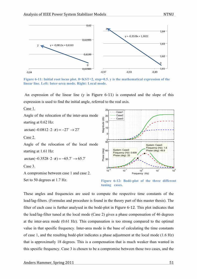
Analysis of IEEE Power System Stabilizer Models NTNU
Anders Hammer, Spring 2011 51
Figure 6-11: Initial root locus plot. 0<KST<2, step=0.5. y is the mathematical expression of the linear line. Left: Inter-area mode. Right: Local mode.
An expression of the linear line (y in Figure 6-‐11) is computed and the slope of this
expression is used to find the initial angle, referred to the real axis.
Case 1.
Angle of the relocation of the inter-area mode
starting at 0.62 Hz:
Case 2.
Angle of the relocation of the local mode
starting at 1.61 Hz:
Case 3.
A compromise between case 1 and case 2.
Set to 50 degrees at 1.7 Hz.
These angles and frequencies are used to compute the respective time constants of the
lead/lag-filters. (Formulas and procedure is found in the theory part of this master thesis). The
filter of each case is further analysed in the bodé-plot in Figure 6-‐12. This plot indicates that
the lead/lag-filter tuned at the local mode (Case 2) gives a phase compensation of 46 degrees
at the inter-area mode (0.61 Hz). This compansation is too strong compared to the optimal
value in that spesific frequency. Inter-area mode is the base of calculating the time constants
of case 1, and the resulting bodé-plot indicates a phase adjustment at the local mode (1.6 Hz)
that is approximatly 18 degrees. This is a compensation that is much weaker than wanted in
this spesific frequency. Case 3 is chosen to be a compromise between those two cases, and the
!"
#" $"%"&!'!()#*"+"!',),-"
!',).(/"
!',).."
!',)../"
!',#"
&!'!0"
!',#12'"34"5678957:" ;<=6>?"@!',#12'"34"5678957:A"
!"
#"
$"%"&!'()#*+","-'(!##"
-'.-"
-'.#"
-'.("
-'./"
&!'01" &!'0(" &!'*0"-'.-"23'"45"6789:68;"" <=>7?@"A-'.-"23'"45"6789:68;"B"
arctan(!0.0812 "2 "! ) = !27!# 27!
arctan(!0.3528 "2 "! ) = !65.7!# 65.7!
0
5
10
15
20
25
Mag
nitu
de (d
b)
Frequency (Hz)10 2 10 1 100 101 1020
30
60
90System: Case3Frequency (Hz): 1.6Phase (deg): 49.9
System: Case3Frequency (Hz): 0.609Phase (deg): 33
Phas
e (d
eg)
Case1Case2Case3
Figure 6-12: Bodé-plot of the three different tuning cases.
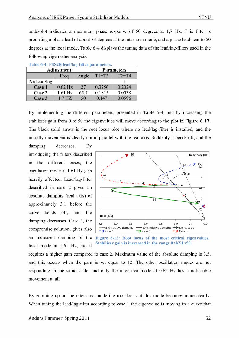
Analysis of IEEE Power System Stabilizer Models NTNU
Anders Hammer, Spring 2011 52
bodé-plot indicates a maximum phase response of 50 degrees at 1,7 Hz. This filter is
produsing a phase lead of about 33 degrees at the inter-area mode, and a phase lead near to 50
degrees at the local mode. Table 6-‐4 displays the tuning data of the lead/lag-filters used in the
following eigenvalue analysis. Table 6-4: PSS2B lead/lag-filter parameters.
Adjustment Parameters Freq. Angle T1=T3 T2=T4
No lead/lag - - 1 1 Case 1 0.62 Hz 27 0.3256 0.2024 Case 2 1.61 Hz 65.7 0.1815 0.0538 Case 3 1.7 HZ 50 0.147 0.0596
By implementing the different parameters, presented in Table 6-‐4, and by increasing the
stabilizer gain from 0 to 50 the eigenvalues will move according to the plot in Figure 6-‐13.
The black solid arrow is the root locus plot where no lead/lag-filter is installed, and the
initially movement is clearly not in parallel with the real axis. Suddenly it bends off, and the
damping decreases. By
introducing the filters described
in the different cases, the
oscillation mode at 1.61 Hz gets
heavily affected. Lead/lag-filter
described in case 2 gives an
absolute damping (real axis) of
approximately 3.1 before the
curve bends off, and the
damping decreases. Case 3, the
compromise solution, gives also
an increased damping of the
local mode at 1,61 Hz, but it
requires a higher gain compared to case 2. Maximum value of the absolute damping is 3.5,
and this occurs when the gain is set equal to 12. The other oscillation modes are not
responding in the same scale, and only the inter-area mode at 0.62 Hz has a noticeable
movement at all.
By zooming up on the inter-area mode the root locus of this mode becomes more clearly.
When tuning the lead/lag-filter according to case 1 the eigenvalue is moving in a curve that
!"#
$#%&#%'#
('# !"#
"#$#&#
%$#('#
!"#
&#'#
%$#
!"#
"#
")!#
%#
%)!#
$#
$)!#
(#
*()!# *()"# *$)!# *$)"# *%)!# *%)"# *")!# ")"#
!"#$%&#'()*+,-)
./#0)*123-)
!#+##,-./01-#2/34567# %"#+#,-./01-#2/34567# 89#.-/2:./7#;/<-#%# ;/<-#$# ;/<-#(#
Figure 6-13: Root locus of the most critical eigenvalues. Stabilizer gain is increased in the range 0<KS1<50.

Analysis of IEEE Power System Stabilizer Models NTNU
Anders Hammer, Spring 2011 53
has an initially horizontal direction, as
expected from the calculations. The damping
increases in the whole range and stops at
approximately 0.14, where the gain is 50. This
gain is too high when the local oscillation
mode (Figure 6-‐13) is taken into
consideration. The result of implementing the
lead/lag filter presented in case 2 gives a
relocation of the inter-area mode that is pointing downwards in the complex plane. The
compromise solution (case 3) achieves a better result compared to case 2, where the
oscillatory frequency is more or less unchanged.
By choosing a PSS gain equal to 12 and a lead/lag-filter according to case 3, the local mode
(starting at 1.61Hz) has moved to its point of
maximum damping. Here is the absolute damping
approximately 3.5 and the frequency is 2.1 Hz. The
inter-area oscillating frequency has decreased, while
the absolute damping of this eigenvalue has
increased. Figure 6-‐15 displays the most critical
eigenvalues in the system, the ones closest to the
imaginary axis, where the green dots is the result
without a PSS, and the blue dots is the result where
PSS2B is implemented. The eigenvalue starting at 1.6
Hz is moving rapidly to the left by implementing PSS2B and the damping of this local mode
has increased. An other eigenvalue has appeared close to 1 Hz as an adverse effect of
implementing PSS2B. The eigenvalue related to the inter-area mode is not improved
considerable, but the relative damping is calculated to 1.3 % (Table 6-‐5). This is a small
improvement compared to the relative damping of 1.12 % obtained in the situation where no
PSS was installed. Table 6-5: Resulting eigenvalues of case 3 and a gain of 12.
Stabilizer Oscillation mode Eigenvalue [1/s], [Hz] Relative damping [ζ]
No PSS Local (-0.8796, 1.6125) 8.65 % Inter-area (-0.0436, 0.6198) 1.12 %
PSS2B, Case 3 Local (-3.4664, 2.1099) 25.3 % Inter-area (-0.0506, 0.61976) 1.30 %
!"#
$%#&'#
!"#
"#$(#
&%#
!"#
!"#
")%$'#
")%$%#
")%$*#
")%(#
")%((#
")%('#
+")$'# +")$(# +")$"# +")"*# +")"%# +")"'# +")"(# ")""#
!"#$%&'#
()#$*+,'#
,-#./012.03# 405/#$# 405/#(# 405/#&#
Figure 6-14: Zoom up at the inter-area mode.
!"
!#$"
%"
%#$"
&"
&#$"
'(" ')" '*" '&" !"
!"#$%&'(#
)*#$+,(#
+,"-.." -..&/"$"0"1234"56789:;" %!"0"1234"56789:;"
Figure 6-15: Most critical eigenvalues in the system with and without PSS2B.
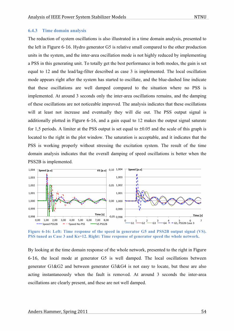
Analysis of IEEE Power System Stabilizer Models NTNU
Anders Hammer, Spring 2011 54
6.4.3 Time domain analysis
The reduction of system oscillations is also illustrated in a time domain analysis, presented to
the left in Figure 6-‐16. Hydro generator G5 is relative small compared to the other production
units in the system, and the inter-area oscillation mode is not highly reduced by implementing
a PSS in this generating unit. To totally get the best performance in both modes, the gain is set
equal to 12 and the lead/lag-filter described as case 3 is implemented. The local oscillation
mode appears right after the system has started to oscillate, and the blue-dashed line indicate
that these oscillations are well damped compared to the situation where no PSS is
implemented. At around 3 seconds only the inter-area oscillations remains, and the damping
of these oscillations are not noticeable improved. The analysis indicates that these oscillations
will at least not increase and eventually they will die out. The PSS output signal is
additionally plotted in Figure 6-‐16, and a gain equal to 12 makes the output signal saturate
for 1,5 periods. A limiter at the PSS output is set equal to ±0.05 and the scale of this graph is
located to the right in the plot window. The saturation is acceptable, and it indicates that the
PSS is working properly without stressing the excitation system. The result of the time
domain analysis indicates that the overall damping of speed oscillations is better when the
PSS2B is implemented.
Figure 6-16: Left: Time response of the speed in generator G5 and PSS2B output signal (VS). PSS tuned as Case 3 and Ks=12. Right: Time response of generator speed the whole network.
By looking at the time domain response of the whole network, presented to the right in Figure
6-‐16, the local mode at generator G5 is well damped. The local oscillations between
generator G1&G2 and between generator G3&G4 is not easy to locate, but these are also
acting instantaneously when the fault is removed. At around 3 seconds the inter-area
oscillations are clearly present, and these are not well damped.
!"#"$%
"#""%
"#"$%
"#&"%
"#''(%
"#'''%
&#"""%
&#""&%
&#"")%
&#""*%
&#""+%
"#""% &#""% )#""% *#""% +#""% $#""% ,#""% -#""% (#""%
!"#$%&'(#"%))*#$%&'(#
+,-)#$.(#
./001%2..)3% ./001%45%2..% 6.%2..)3%
!"##$%
!"###%
&"!!!%
&"!!&%
&"!!'%
&"!!(%
&"!!)%
!% &% '% (% )% *% +% ,%
!"##$%&"'()%
*+,#%&-)%
-&% -'% -(% -)% -*"%.//'0%1234%(%

Analysis of IEEE Power System Stabilizer Models NTNU
Anders Hammer, Spring 2011 55
Another time domain analysis is performed where a load of 500 MW is disconnected at
BUS9. Figure 6-‐17 illustrates that active power, delivered by generator G5, starts to oscillate
against a lower value, and the implementation of PSS2B has only marginally effect on the
damping of this oscillation. PSS2B gives a response of the reactive power that is more
fluctuating compared to the situation where PSS2B is disconnected. The peak value is near to
0.5 p.u, and this aggravation of reactive power response is a prise to pay for the increased
damping of the system oscillations.
Figure 6-17: Time domain analysis, where 500 MW at BUS9 is disconnected. PSS2B is installed in generator G5 and tuned according to case 3.
6.5 Implementing a multi-band stabilizer (PSS4B)
6.5.1 Loading the PSS4B structure with sample data given by IEEE
Power system stabilizer PSS4B is here tuned and installed in the hydro generator (G5) of the
five-generator network, according to the sample data given by IEEE (Table 5-‐2). This
implementation will give eigenvalues according to the left plot in Figure 6-‐18, and this
indicates that two of them have less relative damping than 5 %. Based on this analysis, the
electrical system is worse damped and a fault in this state of operation will give stronger
oscillations compared to a system without a PSS.
The result of a time domain analysis (right graph in Figure 6-‐18) shows that the damping of
the speed oscillations (blue-dashed line) is reduced when the PSS4B is implemented and
loaded with the sample data, given in IEEE Std. 421.5 [1]. The speed of generator G5 will
also oscillate with a higher frequency compared to the situation where the PSS is turned off
(red dash-dotted line). Signal VS (the green solid line) is the output signal from the PSS, and
the figure indicates that the PSS is clearly stressed. The stabilizer will not act as wanted and
!"#$
!"#%$
!"#&$
!"#'$
!"#($
!"($
!"(%$
!"(&$
!$ )$ *!$ *)$ %!$
!"#$%&'"
()*+"#,'"
+"$,-$+..$ +"$+..%/$0123$4$
!"#$%
!"#&%
"%
"#&%
"#$%
"#'%
"#(%
"#)%
"% )% &"% &)% $"%
!"#$%&'"
()*+"#,'"
*#%+,%-..% *#%-..$/%

Analysis of IEEE Power System Stabilizer Models NTNU
Anders Hammer, Spring 2011 56
thereby increase the damping. The stressed PSS results in a stressed excitation system and the
speed of the generator is highly disturbed. PSS output limiter is set according to IEEE
example data equal to 0.15. This value gives a time domain result that is difficult to compare
with the result from PSS2B, which has a limiter value of 0.05. There is a need of extra tuning
of this multi-band PSS, in order to improve the damping of the system oscillations and also
make it comparable with the dual-input PSS.
Figure 6-18: PSS4B with IEEE example parameters is installed in generator G5. Left: Critical eigenvalues in the network. Right: Time response of rotor speed and PSS output signal (VS) after a 3-phase short circuit has occurred in the network.
6.5.2 Tuning of the PSS4B structure based on the actual network oscillations
Complete lists of PSS4B parameter values and eigenvalues of each case are found in the
appendix of this master thesis.
Case 1
Parameter Kh of PSS4B is increased with steps of 0.5, in order to find the initial angle of the
root locus plot of the local and inter-area eigenvalue. Figure 6-‐19 displays the initially
eigenvalue relocations, and a mathematical expression of the linear line. The angles of these
lines are calculated blow:
Angle of the relocation of the local mode, starting at 1.6125 Hz:
arctan(2π⋅-1.049)=81.37° (lead)
Angle of the relocation of the inter-area mode, starting at 0.61987 Hz:
arctan(2π⋅0.0667)=22.74° (lag)
!"
!#$"
%"
%#$"
&"
&#$"
'"
'#$"
()" ($" ('" (%"
!"#$%&'(#
)*#$+,(#
*+",--" ,--./"0111"$"2"3456"789:;<=" %!"2"3456"789:;<="
!"#$"%
!"#&'%
!"#&"%
!"#"'%
"#""%
"#"'%
"#&"%
"#&'%
"#(('%
"#(()%
"#((*%
"#((+%
"#(((%
&#"""%
&#""&%
&#""$%
&#"",%
&#""-%
"#""% &#""% $#""% ,#""% -#""% '#""% )#""% *#""% +#""%
!"#$%&'(#"%))*#$%&'(#
+,-)#$.(#
./001%2333% ./001%45%6..% 7.%2333%
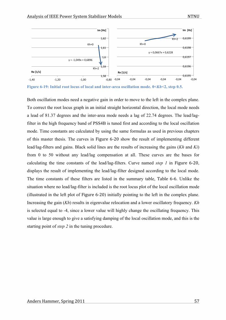
Analysis of IEEE Power System Stabilizer Models NTNU
Anders Hammer, Spring 2011 57
Figure 6-19: Initial root locus of local and inter-area oscillation mode. 0<Kh<2, step 0.5.
Both oscillation modes need a negative gain in order to move to the left in the complex plane.
To correct the root locus graph in an initial straight horizontal direction, the local mode needs
a lead of 81.37 degrees and the inter-area mode needs a lag of 22.74 degrees. The lead/lag-
filter in the high frequency band of PSS4B is tuned first and according to the local oscillation
mode. Time constants are calculated by using the same formulas as used in previous chapters
of this master thesis. The curves in Figure 6-‐20 show the result of implementing different
lead/lag-filters and gains. Black solid lines are the results of increasing the gains (Kh and Ki)
from 0 to 50 without any lead/lag compensation at all. These curves are the bases for
calculating the time constants of the lead/lag-filters. Curve named step 1 in Figure 6-‐20,
displays the result of implementing the lead/lag-filter designed according to the local mode.
The time constants of these filters are listed in the summary table, Table 6-‐6. Unlike the
situation where no lead/lag-filter is included is the root locus plot of the local oscillation mode
(illustrated in the left plot of Figure 6-‐20) initially pointing to the left in the complex plane.
Increasing the gain (Kh) results in eigenvalue relocation and a lower oscillatory frequency. Kh
is selected equal to -4, since a lower value will highly change the oscillating frequency. This
value is large enough to give a satisfying damping of the local oscillation mode, and this is the
starting point of step 2 in the tuning procedure.
!"#$%
!"#&%
'%#%()*$+,-%.%$*/0,/%
)*10%
)*1,%
)*/%
)*/)%
)*/&%
)*/2%
()*+$% ()*&$% ()*$$% ($*0$%
!"#$%&'#
()#$*+,'#
34%56789%
!"#$%
!"#&%
'%#%$($))*+%,%$()&&-%
$()./0%
$()./)%
$()./*%
$()./-%
$().//%
$()&%
1$($2% 1$($2% 1$($2% 1$($2% 1$($2% 1$($2%
!"##$%&'#
()#$*+,'#
34%56789%

Analysis of IEEE Power System Stabilizer Models NTNU
Anders Hammer, Spring 2011 58
Figure 6-20: Root locus plots of local mode and inter-area mode, performed in case 1.
Right plot in Figure 6-‐20 is a zoom up at the inter-area oscillation mode and this graph is also
pointing to the left, but initially not as straight as the local mode. This movement is corrected
in step 2 by implementing the i-band of PSS4B. Step 2 is performed after the gain and
lead/lag-filter, found in step 1, is implemented, and the i-band is now tuned to give a
favourable eigenvalue relocation of the inter-area oscillation mode. This mode needs an
initially lead of 60°, and this angle is found by the same procedure as used in step 1. The
result of implementing the lead/lag-filter time constants of step 2 is shown as green solid lines
in Figure 6-‐20. As the figure indicates will the inter-area eigenvalue now initially move
straight to the left, while the local eigenvalue will move with an angle upwards in the
complex plane. In order to try to totally get a better result, a compromise of tuning the
lead/lag-filter at the local and inter-area oscillation mode is made. Frequency responses of
these three different lead/lag-filters are
presented in Figure 6-‐21. One of the filters in
the frequency response is tuned at the local
mode, one is tuned at the inter-area mode, and
the last filter is tuned as a compromise
between those two oscillation modes. This
compromise, illustrated as the red, dash-dotted
line, compensates with 52.5° at the inter-area
mode and 31.2° at the local mode. After
including this compromise filter in the i-band
of PSS4B, the root locus plot indicates a more
horizontal movement of both eigenvalues. In spite of this gives the compromise solution not a
!"#$%&!"#$'&
!"#$()&
!*#+%&
!*#()&
!*#,)&!*#,'&
!*#()&
!"#()&
!*#-&
!*#.'&!*#+'&!*#()&
$)/.&
)/%&
)/0&
./%&
./0&
+/%&
$.'& $.-& $.%& $.+& $.)& $'& $-& $%& $+& )&
!"#$%&'#
()$*+,'#
12&34567358& 9:4;&.& 9:4;&+&<2=;>2=*?4& (&@&65=;*A8& .)&@&65=;*A8&
!"#$%
!"#&'%
!"#&($%
!)#($%!)#*$%
!"#($%
!)#+%!)#,-%!)#.-%
!)#($%
$/+,%
$/+,(%
$/+.%
$/+.(%
$/+*%
&$/$0% &$/$-% &$/$1% &$/$+% &$/$(% &$/$'% &$/$*% &$/$.% &$/$,%
!"#$%&'
()#*+,&'
23%45678469% :;5<%,% :;5<%.% =3><?3>)@5%
0
5
10
15
20
Mag
nitu
de (d
b)
Bode Diagram
Frequency (Hz)10 2 10 1 100 101 1020
30
60
System: CompromiseFrequency (Hz): 0.616Phase (deg): 52.5
System: CompromiseFrequency (Hz): 1.55Phase (deg): 31.2
Phas
e (d
eg)
InterAreaLocalCompromise
Figure 6-21: Bodé plot of the lead/lag filters used in Step 2.

Analysis of IEEE Power System Stabilizer Models NTNU
Anders Hammer, Spring 2011 59
better damping, compared to the situation where no lead/lag-filter is implemented. The final
choice of step 2 is to not implement a lead/lag filter in the i-band at all, since this solution
gives the best damping. By choosing a gain of the i-band equal to 28, and without
implementing a lead lag filer in the i-band, a grate damping of both modes is obtained without
considerable stressing the PSS. The final selection of case 1 is a lead/lag-filter in the h-band
tuned at the local mode, and no lead/lag filter in the i-band. A summary of this tuning
procedure is presented in Table 6-‐6.
Table 6-6: Summary of the tuning process presented in case 1. Step 1 Step 2
Tuning order h-band is tuned according to the local oscillation mode
i-band is tuned according to the inter-area oscillation mode
Wanted compensation
1.6125 Hz (local mode): 81.37° lead
0.6193 Hz (inter-area mode): 47.83° lead
Compromise - 0.8 Hz, 50° lead Chosen
compensation 1.6125 Hz (local mode):
81.37° lead No lead/lag
Lead/lag-filter time constants
Th3=Th5=0.215 Th4=Th6=0.0453
Ti3=Ti5=1 Ti4=Ti6=1
Gain Kh=-4 Ki=28 Resulting
eigenvalues Local mode ([1/s], [Hz]): (-16.415, 0.00) à ζ=100%
Inter-area mode ([1/s], [Hz]): (-0.0878, 0.61978) à ζ=2.25 %
A time domain analyses of the PSS output signal (VS) and generator speed are illustrated to
the right in Figure 6-‐22, and to the left a plot of the initially eigenvalues is presented.
Figure 6-22: PSS4B is installed in generator G5 and tuned according to case 1. Left: Most critical eigenvalues in the network, with and without PSS4B. Right: Time domain analysis where a 3-phase short circuit with duration of 0.05 seconds is present at BUS8 in the network.
After one second a 3-phase short circuit is introduced at BUS8, and the duration is 0.05
seconds. This fault starts the oscillations in the electrical network, and the output signal of the
PSS reaches suddenly the respective limiter value (±0.05) for 3 times. The speed plot
!"
!#$"
%"
%#$"
&"
'(" ')" '*" '&" !"!"#$%&'(#
)*#$+,(#
+,"-.." -..*/#"0123"%"$"4"5367"819:;<=" %!"4"5367819:;<="
!"#"$%
"#""%
"#"$%
"#&"%
"#''(%
"#'''%
&#"""%
&#""&%
&#"")%
&#""*%
&#""+%
"#""% &#""% )#""% *#""% +#""% $#""% ,#""% -#""% (#""%
!"#$%&'(#"%))*#$%&'(#
+,-)#$.(#
./001%2340%&% ./001%56%7..% 8.%2340%&%

Analysis of IEEE Power System Stabilizer Models NTNU
Anders Hammer, Spring 2011 60
indicates that the implementation of PSS4B, tuned according to Case 1 (blue dashed line),
gives increased damping of the oscillation, compared to the situation where no PSS is present
(red dash-dotted line). The high frequency oscillations are removed and only the inter-area
oscillation remains. The damping of these oscillations is also increased compared to the
situation where no PSS is installed.
Case 2
First step in case 2 is to tune the lead/lag-filter in the h-band, according to the initial angle of
the movement of the inter-area oscillation mode. Increasing the Kh will relocate the
eigenvalue, related to the inter-area mode, to the right in the complex plane. The damping of
this mode is then decreasing (See Figure 6-‐23). This movement is corrected in the opposite
direction by choosing a gain that rather decreases from 0 to -50. In order to correct the
relocation of the eigenvalues related to the inter-area mode, the lead/lag filter must cause a
phase lag of 22.74° at 0.62 Hz (See Figure 6-‐19). This angle is calculated in the previous
case. The eigenvalue of the local oscillation mode is moving towards the imaginary axis, and
a compromise is made in order to totally get a better response. The compromise uses only a
negative gain with no lead/lag-filter in the high-frequency branch. This gives a better result in
both local and inter-area oscillation modes, and the gain (Kh) is selected equal to -50, in order
to maximize the damping of the inter-area mode. Absolute damping of the inter-area mode is
now increased to approximately 0.06 1/s. The eigenvalue related to the local mode has moved
upwards in the complex plane with a final value of approximately 2 Hz, and it has no
improvement of the damping. This is the starting point of step 2 in the tuning procedure of
case 2.
Figure 6-23: Root locus plots of inter-area mode and local mode, performed in case 2.
!"#$%&
!"#%&!"#'$%&
!"#'$%&
!(#)*&
!(#$%&
%+,)&
%+,)$&
%+,*&
%+,*$&
%+,-&
'%+%.& '%+%/& '%+%0& '%+%,& '%+%$& '%+%1& '%+%-& '%+%*& '%+%)&
!"#$%&'
()#*+,&'
23&45678469& :;5<&)& :;5<&*& =3><?3>(@5&
!"#$%&
!"#'$%&!"#'$%&!(#)&
!(#*+&
!(#*,&
!(#+,&
!(#$%&
!(#,&
!(#$%&
!(#,&
%&
*&
+&
-&
.&
$&
)&
/&
'*-& '**& '0& '/& '$& '-& '*& *&
!"#$%&'#
()$*+,'#
12&34567358& 9:4;&*& 9:4;&+&<2=;>2=(?4& $&@&65=;(A8& *%&@&65=;(A8&

Analysis of IEEE Power System Stabilizer Models NTNU
Anders Hammer, Spring 2011 61
Step 2 in this case utilizing the i-band of PSS4B to increase the damping of the local
oscillation mode. The h-band is now held to the fixed values explained in step 1. An increased
Ki gives a root locus plot that pointing in a favourable direction, but with a leading angle of
17.77°. Introducing a phase-leading filter at this value corrects the angle, and the result of this
implementation is illustrated as the green solid line in Figure 6-‐23. The implementation
causes only a smaller difference in the inter-area mode, compared to the situation where no
lead/lag-filter is present in the i-band. A compromise solution is illustrated as the red dash-
dotted line in Figure 6-‐23, where a lower angle of 9° gives increased damping of the local
mode. The relocation of the local mode bends off and starts to decrease at around an absolute
damping of 8 1/s. This filter and gain is the final solution of step 2. Table 6-‐7 is a summary of
the tuning process of case 2 and contains the chosen parameters.
Table 6-7: Summary of the tuning process presented in case 2. Step 1 Step 2
Tuning order h-band is tuned according to the inter-area mode
i-band is tuned according to the local mode
Wanted compensation
0.61987 Hz (inter-area mode): 22.74 ° lag in neg. dir.
1.62 Hz (local mode): 17.77° lead
Compromise 0.61987 Hz (inter-area mode): 0° and a neg.dir.
1.62 Hz (local mode): 9° lead
Chosen compensation 0.61987 Hz (inter-area mode): 0° and a neg.dir.
1.62 Hz (local mode): 9° lead
Lead/lag-filter time constants
Th3=Th5=1 Th4=Th6=1
Ti3=Ti5=0.0836 Ti4=Ti6=0.0714
Gain Kh=-50 Ki=8
Resulting eigenvalue Local mode ([1/s], [Hz]): (-8.6772, 1,5177) à ζ=67.3 % Inter-area mode ([1/s], [Hz]): (-0.0709, 0.6196) à ζ=1.82 %
The result of the time domain analysis, where a 3-phase fault is introduced, indicates that this
tuning procedure will also give an acceptable result. The instantaneously high frequent
oscillations are removed, and the inter-area oscillation has an increased damping. PSS output
signal reach the limiter value for three times and does not stress the excitation system.
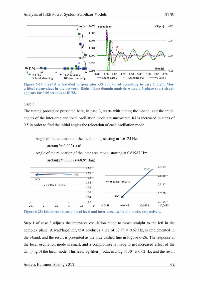
Analysis of IEEE Power System Stabilizer Models NTNU
Anders Hammer, Spring 2011 62
Figure 6-24: PSS4B is installed in generator G5 and tuned according to case 2. Left: Most critical eigenvalues in the network. Right: Time domain analysis where a 3-phase short circuit appears for 0.05 seconds at BUS8.
Case 3
The tuning procedure presented here, in case 3, starts with tuning the i-band, and the initial
angles of the inter-area and local oscillation mode are uncovered. Ki is increased in steps of
0.5 in order to find the initial angles the relocation of each oscillation mode.
Angle of the relocation of the local mode, starting at 1.6125 Hz:
arctan(2π⋅0.002) ≈ 0°
Angle of the relocation of the inter area mode, starting at 0.61987 Hz:
arctan(2π⋅0.0667)=68.9° (lag)
Figure 6-25: Initial root locus plots of local and inter-area oscillation mode, respectively.
Step 1 of case 3 adjusts the inter-area oscillation mode to move straight to the left in the
complex plane. A lead/lag-filter, that produces a lag of 68.9° at 0.62 Hz, is implemented in
the i-band, and the result is presented as the blue dashed line in Figure 6-‐26. The response at
the local oscillation mode is small, and a compromise is made to get increased effect of the
damping of the local mode. This lead/lag-filter produces a lag of 30° at 0.62 Hz, and the result
!"
!#$"
%"
%#$"
&"
'(" ')" '*" '&" !"!"#$%&'(#
)*#$+,(#
+,"-.." -..*/#"0123"&"$"4"5367"819:;<=" %!"4"5367"819:;<="
!"#"$%
"#""%
"#"$%
"#&"%
"#''(%
"#'''%
&#"""%
&#""&%
&#"")%
&#""*%
&#""+%
"#""% &#""% )#""% *#""% +#""% $#""% ,#""% -#""% (#""%
!"#$%&'(#"%))*#$%&'(#
+,-)#$.(#
./001%2340%)% ./001%56%7..% 8.%2340%)%
!"#$%!"#&%
'%#%$($$&)%*%+(,+-.%
+(-%
+(-&%
+(-/%
+(-,%
+(-0%
+(,%
+(,&%
+(,/%
1&(-% 1&% 1+(-% 1+% 1$(-% $%23456%7389(%:3%6958;65<%=6>9?%
!"#$%
!"#&%
'%#%$()&*+,%-%$(./01%
$(.&1+%
$(.&1.%
$(.&10%
$(.&12%
$(.&11%
3$($))2% 3$($))/% 3$($)/2% 3$($)//%4567839879%:;<7(%5;%=79<>=9?3@=678%
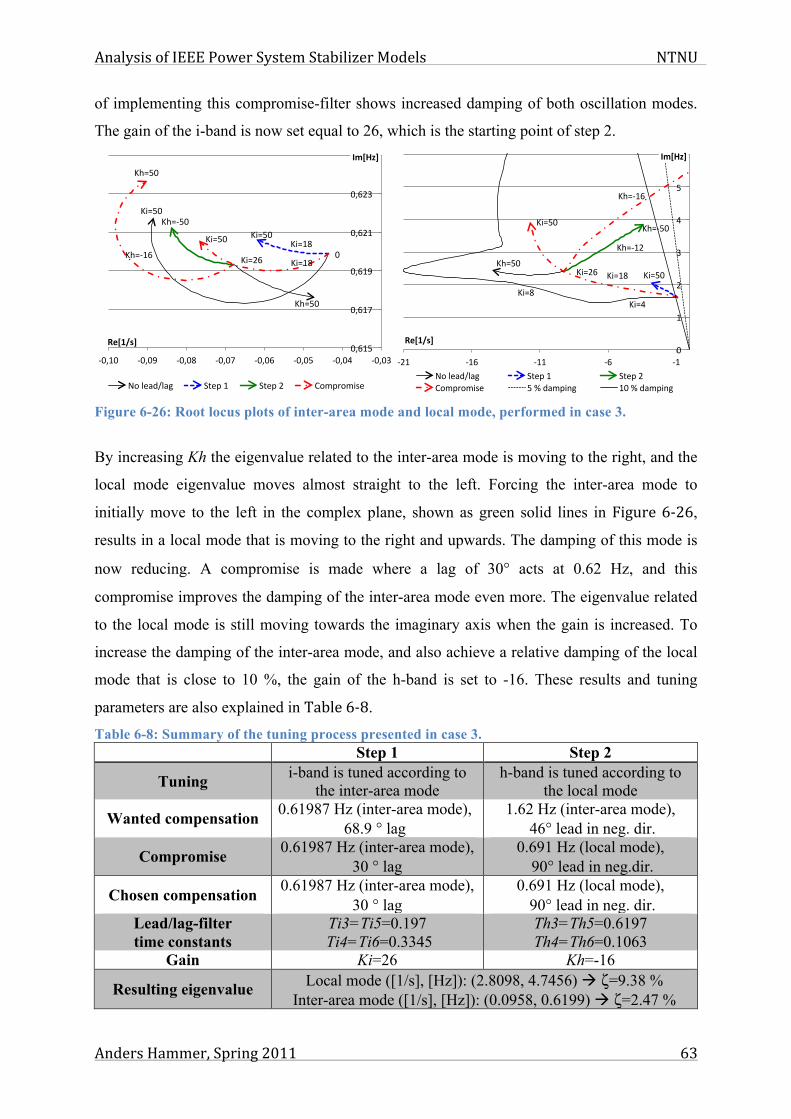
Analysis of IEEE Power System Stabilizer Models NTNU
Anders Hammer, Spring 2011 63
of implementing this compromise-filter shows increased damping of both oscillation modes.
The gain of the i-band is now set equal to 26, which is the starting point of step 2.
Figure 6-26: Root locus plots of inter-area mode and local mode, performed in case 3.
By increasing Kh the eigenvalue related to the inter-area mode is moving to the right, and the
local mode eigenvalue moves almost straight to the left. Forcing the inter-area mode to
initially move to the left in the complex plane, shown as green solid lines in Figure 6-‐26,
results in a local mode that is moving to the right and upwards. The damping of this mode is
now reducing. A compromise is made where a lag of 30° acts at 0.62 Hz, and this
compromise improves the damping of the inter-area mode even more. The eigenvalue related
to the local mode is still moving towards the imaginary axis when the gain is increased. To
increase the damping of the inter-area mode, and also achieve a relative damping of the local
mode that is close to 10 %, the gain of the h-band is set to -16. These results and tuning
parameters are also explained in Table 6-‐8.
Table 6-8: Summary of the tuning process presented in case 3. Step 1 Step 2
Tuning i-band is tuned according to the inter-area mode
h-band is tuned according to the local mode
Wanted compensation 0.61987 Hz (inter-area mode), 68.9 ° lag
1.62 Hz (inter-area mode), 46° lead in neg. dir.
Compromise 0.61987 Hz (inter-area mode), 30 ° lag
0.691 Hz (local mode), 90° lead in neg.dir.
Chosen compensation 0.61987 Hz (inter-area mode), 30 ° lag
0.691 Hz (local mode), 90° lead in neg. dir.
Lead/lag-filter time constants
Ti3=Ti5=0.197 Ti4=Ti6=0.3345
Th3=Th5=0.6197 Th4=Th6=0.1063
Gain Ki=26 Kh=-16
Resulting eigenvalue Local mode ([1/s], [Hz]): (2.8098, 4.7456) à ζ=9.38 % Inter-area mode ([1/s], [Hz]): (0.0958, 0.6199) à ζ=2.47 %
!"#$%&
%&!"#'(&
!"#$%&!)#*$%&
!"#'(&!"#+,&
!"#$%&
!)#$%&
!)#*',&
!)#$%&
%-,'$&
%-,'.&
%-,'/&
%-,+'&
%-,+0&
%-,+$&
*%-'%& *%-%/& *%-%(& *%-%.& *%-%,& *%-%$& *%-%1& *%-%0&
!"#$%&'
()#*+,&'
23&45678469& :;5<&'& :;5<&+& =3><?3>"@5&
!"#$%!"#&%
!"#'(%
!)#*+,%
!)#*'(%
!"#+&%!"#,-%
!"#'(%
!)#'(%
!)#*+-%
(%
+%
,%
.%
$%
'%
-%
*,+% *+-% *++% *-% *+%
!"#$%&'
()#*+,&'
/0%12345136% 7829%+% 7829%,%:0;9<0;"=2% '%>%43;9"?6% +(%>%43;9"?6%

Analysis of IEEE Power System Stabilizer Models NTNU
Anders Hammer, Spring 2011 64
A time domain analysis of generator speed and PSS output signal (right graph in Figure 6-‐27)
indicates that the output signal reaches the limiter value four times and the PSS is more
stressed compared to the other cases until now. The overall damping of speed oscillations is
acceptable, where the inter-area oscillation is clearly decreasing and the local mode is only
visible in the first seconds after the disturbance has occurred. The inter-area mode is visible
from 3 seconds, and these are better damped when PSS4B is installed and tuned according to
case 3. The eigenvalue analysis, oriented to the left in Figure 6-‐27, shows that one high
frequency eigenvalue has appeared near to 5 Hz. This has a relative damping that is below 10
%.
Figure 6-27: PSS4B is installed in generator G5 and tuned according to case 3. Left: Most critical eigenvalues in the network. Right: Time domain analysis where a 3-phase short circuit appears for 0.05 seconds at BUS8.
Case 4
The tuning presented in case 4 take advantage of the already good relocation of the
eigenvalue related to the local oscillation mode when no lead/lag-filter is installed, and the
gain of the i-band is increased. The first step in this case is to set this Ki equal to 4, and then
tune the inter-area mode as a second step by using the h-band for the PSS4B. The black solid
line in Figure 6-‐28 indicates that both eigenvalues moves to the right when Kh is increased,
and the damping of these modes decreases. By rather decreasing the gain, the initial relocation
of the inter-area eigenvalue points in a straight horizontal direction away from the imaginary
axis. The movement of the local mode is initially pointing upwards and turning against the
imaginary axis. There is a large difference between the responses of the respective oscillating
modes, and a compromise is made where a lead/lag-filter is designed to produce a lead of 45°
!"
#"
$"
%"
&"
'"
()" (*" (&" ($" !"!"#$%&'(#
)*#$+,(#
+,"-.." -..&/0"1234"%"'"5"6478"92:;<=>" #!"5"6478"92:;<=>"
!"#"$%
"#""%
"#"$%
"#&"%
"#''(%
"#'''%
&#"""%
&#""&%
&#"")%
&#""*%
&#""+%
"#""% &#""% )#""% *#""% +#""% $#""% ,#""% -#""% (#""%
!"#$%&'(#"%))*#$%&'(#
+,-)#$.(#
./001%2340%*% ./001%56%7..% 8.%2340%*%

Analysis of IEEE Power System Stabilizer Models NTNU
Anders Hammer, Spring 2011 65
at 0,62 Hz. This compromise filter is implemented in the h-band, and by setting the gain at -8
gives the best result of this case.
Figure 6-28: Root locus plots of local mode and inter-area mode, performed in case 4.
Table 6-‐9 is listing a summary of the tuning process of case 4, and this presents the chosen
parameters. Table 6-9: Summary of the tuning process presented in case 4.
Step 1 Step 2
Tuning i-band is tuned according to the local mode
h-band is tuned according to the inter area mode
Wanted compensation 1.6125 Hz (local mode): 0 °
0.619 Hz (inter-area mode): 180°
Compromise - 0.619 Hz (inter-area mode): 45° lead
Chosen compensation 1.6125 Hz (local mode): 0 °
0.619 Hz (inter-area mode): 45° lead
Lead/lag-filter time constants
Ti3=Ti5=1 Ti4=Ti6=1
Th3=Th5=0.3851 Th4=Th6=0.1719
Gain Ki=4 Kh=-8
Resulting eigenvalue Local mode ([1/s], [Hz]): (-4.9100, 2.1395) à ζ=34.30 % Inter-area mode ([1/s], [Hz]): (-0.0573, 0.6178) à ζ=1.48 %
The result of the time domain analysis, presented in to the left in Figure 6-‐29, shows an
output signal that hits the limiter value (0.05) twice, and the PSS is not in a stressed operation.
Damping of inter-area oscillations is practically the same with and without the PSS, but the
local oscillations is effectively decreased. This analysis supports the results of the eigenvalue
analysis, where the local mode has obtained an increased damping, while the inter-area mode
has only a smaller improvement.
!"#$%!"#&%
!"#'%!"#()%
!"#*)%
!+#*)%
!+#,*)%!+#,'%
!+#,*)%
)%
(%
-%
.%
$%
*%
&%
/%
,--%,-(%,-)%,(0%,('%,(/%,(&%,(*%,($%,(.%,(-%,((%,()%,0% ,'% ,/% ,&% ,*% ,$% ,.% ,-% ,(% )%
!"#$%&'
()#*+,&'
12%34567358% 9:4;%-% <2=;>2="?4%*%@%65=;"A8% ()%@%65=;"A8%
!"#$%
!"#&%
!"#'$%
!(#'$%
!(#)'$%
!(#)*%
!(#)'$%
$+,-'%
$+,-.%
$+,-/%
$+,0-%
$+,01%
$+,0'%
)$+-$% )$+$*% )$+$,% )$+$&% )$+$0%
!"#$%&'
()#*+,&'
23%45678469% :;5<%0% =3><?3>"@5%

Analysis of IEEE Power System Stabilizer Models NTNU
Anders Hammer, Spring 2011 66
Figure 6-29: PSS4B is installed in generator G5 and tuned according to case 4. Left: Most critical eigenvalues in the network. Right: Time domain analysis where a 3-phase short circuit appears for 0.05 seconds at BUS8.
Case 5
Case 5 uses the same i-band setup as case 4, besides of a gain equal to 10. At this point the
root locus movement is shifting from moving to the right to start pointing to the left in the
complex plane, and the absolute damping is maximized. At this point the two oscillation
modes will start moving in different directions by increasing the gain of the h-band. The
damping of the local mode increases slightly, while the damping of the inter-area mode
decreases rapidly, in relation to the respective scales of the graphs.
Figure 6-30: Root locus plots of a zoom up of the local mode and the inter-area mode preformed in case 5.
Kh is now rather decreased towards -50, in order to force the inter-area mode in a rightwards
direction. Additionally a lead of 37.5° at 0.6174 Hz is implemented, and the result is an
initially straight movement of the inter-area mode. The local mode is now moving to the left,
but not in a considerable scale. In order to get a better response of the inter-area mode, a lead
!"
!#$"
%"
%#$"
&"
&#$"
'"
()" (*" (+" (&" !"!"#$%&'(#
)*#$+,(#
,-".//" .//+0#"1234"+"$"5"6478"92:;<=>" %!"5"6478"92:;<=>"
!"#"$%
"#""%
"#"$%
"#&"%
"#''(%
"#'''%
&#"""%
&#""&%
&#"")%
&#""*%
&#""+%
"#""% &#""% )#""% *#""% +#""% $#""% ,#""% -#""% (#""%
!"#$%&'(#"%))*#$%&'(#
+,-)#$.(#
./001%2340%+% ./001%56%7..% 8.%2340%+%
!"#$%&
!'#(%&
!'#)(%&
!'#)$*&!'#)(%&
+,-&
+,-(&
+,.&
+,.(&
+,(&
+,((&
+,/&
)+$,.& )+$,+& )+$& )+%,*& )+%,/& )+%,.& )+%,+&
!"#$%&'
()#*+,&'
01&23456& 7458&+& 91:861:";5&
!"#$%&
!'#%&
!'#(&
!'#)%&
!'#$%&
!"#*$%&
!"#*)+&
!"#*$%&
%,-)$&
%,-)+&
%,-.)&
%,-.(&
*%,)%& *%,%+& *%,%-& *%,%(& *%,%.& %,%%&
!"#$%&'
()#*+,&'
/0&12345136& 7829&.& :0;9<0;'=2&

Analysis of IEEE Power System Stabilizer Models NTNU
Anders Hammer, Spring 2011 67
of 60° at 0.6174 Hz is tested as a compromise. This filter gives an increased damping in the
inter-area mode, compared to the filter that gives an initially straight relocation of the
eigenvalue. The compromise filter is the final choice, and Kh is set equal to -18. This
maximizes the absolute damping of the inter-area mode, without highly disturbing the
oscillating frequency. These results are also presented in Table 6-‐10, as a summary of case 5.
Table 6-10: Summary of the tuning process in presented in case 5. Step 1 Step 2
Tuning i-band is tuned according to the local mode
h-band is tuned according to the inter-area mode
Wanted compensation 1.6125 Hz (local mode), 0 °
0.6174 Hz (inter-area mode), 37,5° in neg. dir.
Compromise - 0.6174 Hz (inter-area mode), 60 ° lead
Chosen compensation 1.6125 Hz (local mode), 0 °
0.6174 Hz (inter-area mode), 60° lead
Lead/lag-filter time constants
Ti3=Ti5=1 Ti4=Ti6=1
Ti3=Ti5=0.4465 Ti4=Ti6=0.1488
Gain Ki=10 Kh=-18
Resulting eigenvalues Local mode ([1/s], [Hz]): (-20.365, 2.4540) à ζ=79.72 % Inter-area mode ([1/s], [Hz]): (-0.0868, 0.6184) à ζ=2.23 %
The resulting eigenvalue analysis (right plot in Figure 6-‐31) shows that no new eigenvalues
has obtained a poor damping. A time domain analysis of the solution presented in case 5 is
plotted to the right in Figure 6-‐31 and this shows an PSS output signal that reaches the limiter
value four times. The local oscillation mode that has obtained an increased damping, while
the damping of the inter-area mode is not highly improved.
Figure 6-31: PSS4B is installed in generator G5 and tuned according to case 5. Left: Most critical eigenvalues in the system. Right: Time domain analysis where a 3-phase short circuit appears for 0.05 seconds at BUS8.
!"
!#$"
%"
%#$"
&"
&#$"
'"
'#$"
("
)*" )+" )(" )&" !"!"#$%&'(#
)*#$+,(#
,-".//" .//(0#"1234"$"%!"5"6478"92:;<=>" %!"5"6478"92:;<=>"
!"#"$%
"#""%
"#"$%
"#&"%
"#''(%
"#'''%
&#"""%
&#""&%
&#"")%
&#""*%
&#""+%
"#""% &#""% )#""% *#""% +#""% $#""% ,#""% -#""% (#""%
!"#$%&'(#"%))*#$%&'(#
+,-)#$.(#
./001%2340%$% ./001%56%7..% 8.%2340%$%

Analysis of IEEE Power System Stabilizer Models NTNU
Anders Hammer, Spring 2011 68
6.5.3 Final choice of tuning of the PSS4B
The eigenvalues of the respective cases in the previous chapter is compared in order to find
the case that obtains the initially best eigenvalue performance. According to Table 6-‐11 gives
case 1 the best eigenvalue performance, where the local mode is completely removed and the
eigenvalue related to the inter-area mode obtains a relative damping of 2.25 %. Only case 3
obtains a relative damping of the local mode that is below 10 %, and this is basically not a
preferred tuning method of the PSS4b. All remaining cases are basically methods that can be
used to tune the PSS4B. These cases (case 1, 2, 4 and 5) are further compared in order to
pinpoint the best method of tuning the PSS4B. Table 6-11: Resulting eigenvalues of the local and inter-area oscillation mode of each tuning method. Tuning Oscillation mode Eigenvalue ([1/s], [Hz]) Relative damping ζ
Case 1 Local Inter-area
(-16.415, 0.0000) (-0.0878, 0.6198)
100 % 2.25 %
Case 2 Local Inter-area
(-8.6772, 1,5177) (-0.0709, 0.6196)
67.3 % 1.82 %
Case 3 Local Inter-area
(2.8098, 4.7456) (0.0958, 0.6199)
9.38 % 2.47 %
Case 4 Local Inter-area
(-4.9100, 2.1395) (-0.0573, 0.6178)
34.30 % 1.48 %
Case 5 Local Inter-area
(-20.365, 2.4540) (-0.0868, 0.6184)
79.72 % 2.23 %
A new time domain analysis is now performed where a load of 500 MW at BUS9 is
disconnected. The power response where PSS4B is installed and tuned according to the
respective cases is presented in Figure 6-‐32 and Figure 6-‐33. Green solid lines in the figures
are the response of no PSS installed in the excitation system, and the blue dashed lines are the
response where PSS4B is installed. Generally, after implementing the PSS4B, the oscillations
of the active power are clearly unbalanced in the first seconds after the disturbance has
occurred. As the time goes, the damping of the active power oscillations is increasing, and the
oscillations are finally dying out. Case 1 and case 5 obtains the initially most disturbed power
response, but after approximately 5 seconds they are well damped. Out of the four cases
tested in this analysis is case 1 the case that best damps the oscillations of active power, while
case 4 has no considerable improvement of the damping of the active power oscillations.
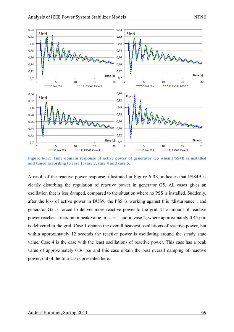
Analysis of IEEE Power System Stabilizer Models NTNU
Anders Hammer, Spring 2011 69
Figure 6-32: Time domain response of active power of generator G5 when PSS4B is installed and tuned according to case 1, case 2, case 4 and case 5.
A result of the reactive power response, illustrated in Figure 6-‐33, indicates that PSS4B is
clearly disturbing the regulation of reactive power in generator G5. All cases gives an
oscillation that is less damped, compared to the situation where no PSS is installed. Suddenly,
after the loss of active power in BUS9, the PSS is working against this “disturbance”, and
generator G5 is forced to deliver more reactive power to the grid. The amount of reactive
power reaches a maximum peak value in case 1 and in case 2, where approximately 0.45 p.u.
is delivered to the grid. Case 1 obtains the overall heaviest oscillations of reactive power, but
within approximately 12 seconds the reactive power is oscillating around the steady state
value. Case 4 is the case with the least oscillations of reactive power. This case has a peak
value of approximately 0.36 p.u and this case obtain the best overall damping of reactive
power, out of the four cases presented here.
!"#$
!"#%$
!"#&$
!"#'$
!"#($
!"($
!"(%$
!"(&$
!$ )$ *!$ *)$ %!$
!"#$%&'"
()*+"#,'"
+"$,-$+..$ +"$+..&/$0123$*$
!"#$
!"#%$
!"#&$
!"#'$
!"#($
!"($
!"(%$
!"(&$
!$ )$ *!$ *)$ %!$
!"#$%&'"
()*+"#,'"
+"$,-$+..$ +"$+..&/$0123$%$
!"#$
!"#%$
!"#&$
!"#'$
!"#($
!"($
!"(%$
!"(&$
!$ )$ *!$ *)$ %!$
!"#$%&'"
()*+"#,'"
+"$,-$+..$ +"$+..&/$0123$&$
!"#$
!"#%$
!"#&$
!"#'$
!"#($
!"($
!"(%$
!"(&$
!$ )$ *!$ *)$ %!$
!"#$%&'"
()*+"#,'"
+"$,-$+..$ +"$+..&/$0123$)$

Analysis of IEEE Power System Stabilizer Models NTNU
Anders Hammer, Spring 2011 70
Figure 6-33: Time domain response of reactive power of generator G5 when PSS4B is installed and tuned according to case 1, case 2, case 4 and case 5.
6.6 PSS2B vs. PSS4B PSS4B tuned according to case 1 obtained the best overall result in the previous chapter, and
it is here compared to the performance PSS2B. First the rotor speed response is compared,
where the same 3-phase short circuit as
used in the previous chapters is
introduced. As Figure 6-‐34 illustrates
will a tuning of PSS4B according to
case 1, give a better damping of both
high and low frequency rotor
oscillations, compared to the results
from PSS2B. The red dash-dotted
curve illustrates the situation where no
PSS is installed, and initially after the
disturbance a high frequency oscillation appears. This oscillation is well damped by the
PSS2B, while the PSS4B setup completely removes this oscillation. Also the low frequency
!"#$%
!"#&%
"%
"#&%
"#$%
"#'%
"#(%
"#)%
"% )% &"% &)% $"%
!"#$%&'"
()*+"#,'"
*#%+,%-..% *#-..(/%%0123%&%
!"#$%
!"#&%
"%
"#&%
"#$%
"#'%
"#(%
"#)%
"% )% &"% &)% $"%
!"#$%&'"
()*+"#,'"
*#%+,%-..% *#%-..(/%0123%$%
!"#$%
!"#&%
"%
"#&%
"#$%
"#'%
"#(%
"#)%
"% )% &"% &)% $"%
!"#$%&'"
()*+"#,'"
*#%+,%-..% *#-..(/%%0123%(%
!"#$%
!"#&%
"%
"#&%
"#$%
"#'%
"#(%
"#)%
"% )% &"% &)% $"%
!"#$%&'"
()*+"#,'"
*#%+,%-..% *#%-..(/%0123%)%
!"##$%
!"###%
&"!!!%
&"!!&%
&"!!'%
&"!!(%
&"!!)%
!"!!% &"!!% '"!!% ("!!% )"!!% *"!!% +"!!% ,"!!% $"!!%
!"##$%&"'()%
*+,#%&-)%
-.//0%12%3--% -.//0%3--'4% -.//0"%3--)4%567/%&%
Figure 6-34: Time response of rotor speed where a small signal disturbance is introduced.
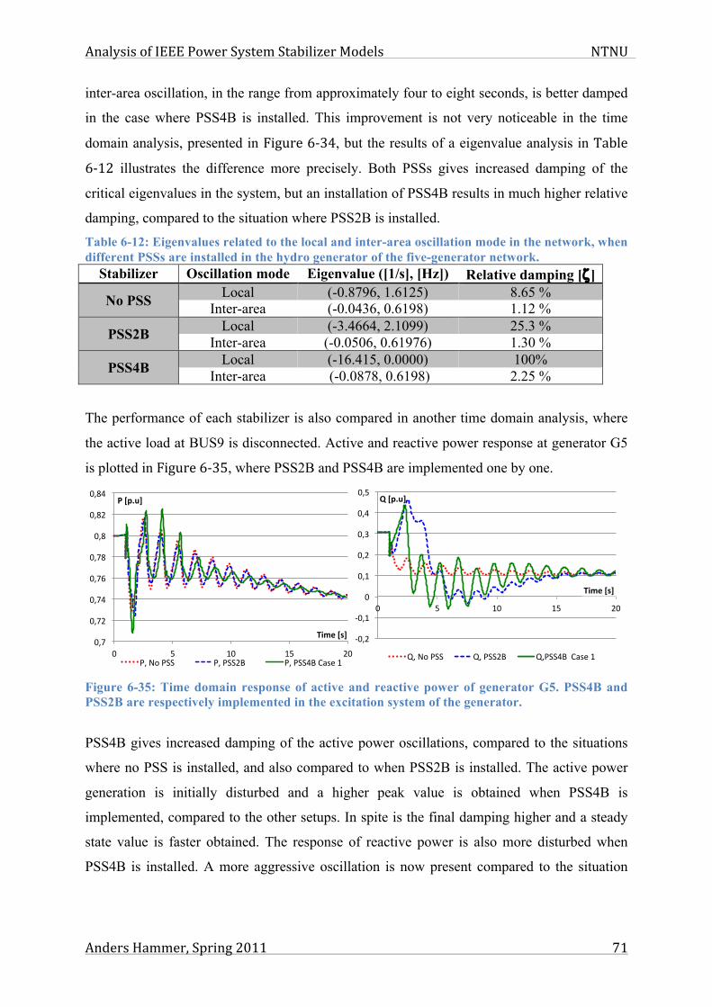
Analysis of IEEE Power System Stabilizer Models NTNU
Anders Hammer, Spring 2011 71
inter-area oscillation, in the range from approximately four to eight seconds, is better damped
in the case where PSS4B is installed. This improvement is not very noticeable in the time
domain analysis, presented in Figure 6-‐34, but the results of a eigenvalue analysis in Table
6-‐12 illustrates the difference more precisely. Both PSSs gives increased damping of the
critical eigenvalues in the system, but an installation of PSS4B results in much higher relative
damping, compared to the situation where PSS2B is installed. Table 6-12: Eigenvalues related to the local and inter-area oscillation mode in the network, when different PSSs are installed in the hydro generator of the five-generator network.
Stabilizer Oscillation mode Eigenvalue ([1/s], [Hz]) Relative damping [ζ]
No PSS Local (-0.8796, 1.6125) 8.65 % Inter-area (-0.0436, 0.6198) 1.12 %
PSS2B Local (-3.4664, 2.1099) 25.3 % Inter-area (-0.0506, 0.61976) 1.30 %
PSS4B Local (-16.415, 0.0000) 100% Inter-area (-0.0878, 0.6198) 2.25 %
The performance of each stabilizer is also compared in another time domain analysis, where
the active load at BUS9 is disconnected. Active and reactive power response at generator G5
is plotted in Figure 6-‐35, where PSS2B and PSS4B are implemented one by one.
Figure 6-35: Time domain response of active and reactive power of generator G5. PSS4B and PSS2B are respectively implemented in the excitation system of the generator.
PSS4B gives increased damping of the active power oscillations, compared to the situations
where no PSS is installed, and also compared to when PSS2B is installed. The active power
generation is initially disturbed and a higher peak value is obtained when PSS4B is
implemented, compared to the other setups. In spite is the final damping higher and a steady
state value is faster obtained. The response of reactive power is also more disturbed when
PSS4B is installed. A more aggressive oscillation is now present compared to the situation
!"#$
!"#%$
!"#&$
!"#'$
!"#($
!"($
!"(%$
!"(&$
!$ )$ *!$ *)$ %!$
!"#$%&'"
()*+"#,'"
+"$,-$+..$ +"$+..%/$ +"$+..&/$0123$*$
!"#$%
!"#&%
"%
"#&%
"#$%
"#'%
"#(%
"#)%
"% )% &"% &)% $"%
!"#$%&'"
()*+"#,'"
*#%+,%-..% *#%-..$/% *#-..(/%%0123%&%

Analysis of IEEE Power System Stabilizer Models NTNU
Anders Hammer, Spring 2011 72
where no PSS and PSS2B are installed. This oscillation starts to oscillate around the steady
state value, and it is finally damped out.
The variation of reactive power is directly related to variation in generator voltage, and the
same pattern of the reactive power
(Figure 6-‐35) can be seen in Figure
6-‐36. This figure illustrates the
variation of generator voltage after the
disconnection of the 500 MW load in
BUS9. Both PSS2B and PSS4B give
peak values below 1.06 p.u. and
above 0.98 p.u. PSS4B gives a more
oscillatory response compared to
PSS2B, and it gives also a shorter
period of voltage overshoot.
!"#$%
!"##%
&%
&"!&%
&"!'%
&"!(%
&"!)%
&"!*%
&"!+%
&"!,%
!% *% &!% &*% '!%
!"#$%&'"
()*+"#,'"
-"%./%011% -"%011'2% -"%011)2%3456%&%Figure 6-36: Time response of generator voltage after a reduction of loading.

Analysis of IEEE Power System Stabilizer Models NTNU
Anders Hammer, Spring 2011 73
7 Discussion
7.1 The contribution of generator voltage in the excitation system The pre-project of this master thesis was using a simplified model of Thyricon® Excitation
System, where the multiplication of generator voltage and exciter output signal was not
implemented (AVR1). During this master thesis, a study of the contribution from a varying
generator voltage is performed, and the simplified model of Thyricon® Excitation System is
upgraded to contain a multiplication block at the output of the exciter (AVR2). The difference
of the performance between the exciter models (with and without multiplication of generator
voltage at exciter output) is distinctive. The simple excitation system (AVR1) gives an
eigenvalue response that is more stable compared to the excitation system that contains the
contribution from a varying stator voltage. A root locus plot of a varying PSS gain is created,
and the main deviation between AVR1 and AVR2 is that the eigenvalues of AVR2 is tending
to be more destabilized. Tuning of the PSS in AVR2 is more brittle, where a small change in
the lead/lag-filter time constants gives a considerable change in the eigenvalue relocations.
The test, performed in this master thesis, shows the importance of including the contribution
of a varying generator voltage in the exciter model. A disturbance of the generator stator
voltage will also affect the DC field voltage, delivered by the thyristors in the excitation
system. It is important to include this contribution in the excitation system, in order to
simulate the most realistic situation. The upgraded version of the excitation system (AVR2) is
therefore used in the rest of the master thesis, where more advanced PSS’s are installed and
tuned.
For even more detailed simulations, where for instance transient stability is investigated, the
models of the excitation system has to be upgraded even more. All the protection circuits and
limiter structures, presented in the original model description [2], must then be implemented
in order to give a representative result.
7.2 Analysis of the five-generator network In this master thesis a five-generator two-area network is established, based on the well-
known four-generator network “Kundur’s Two Area System” [11, 20]. A smaller hydro
Analysis of IEEE Power System Stabilizer Models NTNU
Anders Hammer, Spring 2011 74
generator is installed, and this obtains a heavier oscillation compared to the larger turbo
machines. This is because the rotor inertia of this machine is smaller compared to the other
inertias in the system. The swing equation explains this phenomenon. A modal analysis of this
five-generator network is performed, and it indicates that hydro generator take a considerable
part of one of the local oscillation modes. Correct control of this unit will highly improve the
damping of this oscillation mode. The hydro generator is not highly represented in the modal
analysis of the inter-area oscillation mode, and correct control of this unit will not effectively
improve the damping of this mode. One essential factor is that the improved damping of the
local oscillation mode must not destabilize the inter-area oscillation mode, but rather improve
the damping as much as possible.
7.3 Tuning of the PSS2B The dual-input stabilizer is quick and easy to tune, where it has only one lead/lag-structure
and a one associated gain. Frequency and electrical power is measured and used as input
signals in an advanced transducer structure, where the integral of accelerating power is
computed. This synthesized signal has, in this mater thesis, a time response that is more or
less in phase with the rotor speed, and this signal is used as an input to the lead/lag-structure.
The advantage of this stabilizer is that it would not introduce a phase lag at lower frequencies,
and it does not destabilize the exciter oscillation mode as the gain is increased [4, 14]. This
advantage is not further illustrated in this master thesis, and the reason is that the network
does not contain any torsional oscillations.
Theoretically a higher limiter value could be set, in order to achieve an increased damping of
the rotor oscillations. Kundur explains in [11] that a maximum PSS output limit of 0.1 to 0.2
is acceptable if the generator terminal voltage is limited to its maximum allowable value,
usually 1.12 to 1.15 p.u. Voith Hydro gives the PSS limiter values used in this thesis and
these are relative strict values [2]. These limiters prevent the PSS of highly disturbing the
voltage regulation under normal operation conditions.
In order to give a satisfying result of both oscillating modes, a compromise solution of the
lead/lag-filter time constants has to be made. A disadvantage of this compromise is that it
gives not an optimal improvement of the oscillation modes. This drawback is more present in
networks containing a wide spectre of oscillation modes, since the lead/lag filter cannot cover

Analysis of IEEE Power System Stabilizer Models NTNU
Anders Hammer, Spring 2011 75
a wide range of frequencies. To increase the damping of the inter-area mode the stabilizer
gain can be increased, but a major side effect of this is that the local oscillation mode becomes
less damped. This is clearly illustrated in the root locus plot, where the eigenvalues of each
oscillation mode moves in opposite directions as the stabilizer gain is increased above the
chosen value. The need of this compromise lead/lag compensation is the drawback of the
dual-input stabilizer, where none of the oscillation modes gets an optimal damping.
7.4 The different tuning procedures of PSS4B A PSS4B stabilizer is a complicated structure, and it can be tuned in many ways. The first
tuning method, performed in this master thesis, is to implement the whole structure and tune it
according to the sample data presented in the IEEE standard [1]. The procedure focusing at
centre frequencies and associated gain values, and the phase response of the PSS is not further
commented. It seems that this procedure is more convenient in a network containing a wider
spectre of oscillation modes. Results from loading the PSS4B with IEEE sample data
indicates that it must be tuned more specifically in order to act appropriate in this network.
PSS4B consists of 3 separate bands that are designed to handle 3 different oscillation modes.
One of the branches of each band is here disconnected, and the reason is that the structure is
now much simpler. Each band is tuned one by one as a well-known lead/lag structure. Tuning
of lead/lag-filters is successfully performed in the previous chapter, where the PSS2B is
implemented. The following tuning procedure is divided into 5 different cases. Each of the 5
cases has different order of which band, and of which oscillation mode that is tuned first. This
is done in order to find an effective tuning technique. In case 1 the h-band of the stabilizer is
tuned first, so the damping of the local oscillation mode is improved. Secondary the i-band is
tuned to give an improvement of the lower frequency inter-area mode. This tuning technique
gives the best damping of the local oscillation mode, where the eigenvalue analysis gives a
non-oscillating eigenvalue. The damping of the inter-area mode is additionally improved,
where the relative damping is at the second best value ever achieved in this master thesis. The
other tuning techniques are generally more troublesome, and in some cases will the
eigenvalue relocations go in opposite directions as the band gains are increased.
The results from the eigenvalue analysis are also presented in time domain analysis of
generator speed. At case 1 is practically only the inter-area oscillation is present and this test
Analysis of IEEE Power System Stabilizer Models NTNU
Anders Hammer, Spring 2011 76
shows that it is a correlation between the eigenvalue analysis and the time domain analysis.
To further test the robustness of the network a disconnection of an active load is performed.
Results indicate an increased damping of the active power oscillations after implementing the
PSS4B, which is tuned according to case 1. The reactive power delivered by generator G5 is
more fluctuating, but the oscillations decreases and the steady state value is finally found. A
price to pay of increased damping of rotor oscillations is increased variations of reactive
power in the machine. The peak values of reactive power are not higher, but the damping of
these oscillations is reduced. An explanation of this can be that the control of the generating
unit is more active, in order to damp the rotor oscillation, and therefore will also the reactive
power in the machine fluctuate.
Case 4 is the case that gives the lowest disturbance in reactive power, after the disconnection
of the active load. Damping of oscillations in active power is then not increased considerable
and so is the oscillation of the rotor speed. This is similar to the damping of the inter-area
mode, found in the eigenvalue analysis.
7.5 PSS4B vs. PSS2B The tuning of the multi-band stabilizer that achieves the overall best performance is case 1,
and this stabilizer is now compared to the tuned dual-input stabilizer. In the dual-input
stabilizer, the lead/lag-filter must be tuned as a compromise between the actual oscillation
modes present in the network. This solution gives not an optimal result. The result of
comparing the time domain analysis of the rotor oscillations indicates that the multi-band
stabilizer will give an overall best damping of the oscillation modes.
The inter-area oscillation mode is though not highly improved, neither by installation of
PSS2B or by PSS4B. This phenomena is also described in [11] where an effective alternative
solution could be an installation of a static VAR compensation and/or by control of HVDC
converters (if present). Generator G5 is a small generating unit, and its ability to improve the
inter-area mode is limited. By installing a PSS in one of the other (larger) generating units, the
inter-area oscillation mode may probably be better damped. The pre-project of this master
thesis presents such a solution with great results.

Analysis of IEEE Power System Stabilizer Models NTNU
Anders Hammer, Spring 2011 77
An instantaneously decrease of the generator loading is performed, and both stabilizers give a
disturbed regulation of reactive power (and voltage), compared to the situation where no PSS
is installed. An increased damping of rotor oscillations results in a higher level of reactive
power oscillations. PSS4B is clearly more active in the aftermath of a disturbance of the
network operation condition. This can also be seen in the time plot of the PSS output signal.
Variations of the reactive power are also seen in the response of generator voltage, which
shows a voltage overshoot of 1.06 p.u. This overshoot is within the given regulations of 110
% (EN 50160) and cannot be considered as a voltage swell [21]. The voltage level can be
considered as stable when it stays inside a limit of ±0.5 % of system voltage, and both
stabilizers are reaching this value at approximately the same time [21]. This oscillatory
generator voltage is the price to pay for increased rotor stability in the network.
Table 7-‐1 and Table 7-‐2 describes some advantages and disadvantages about the respective
PSS’s. Table 7-1: Pros and cons of PSS2B.
+ - Well known in the market. Single lead/lag-filter must be tuned as a
compromise between all oscillatory modes in the system.
Simple tuning procedure. Often only tuned at the local oscillation mode for one specific machine [19].
Handles a higher gain compared to a single input stabilizer, without destabilizing the exciter oscillation mode.
Cannot cover a large variation of oscillation frequencies in the network.
Table 7-2: Pros and cons of PSS4B.
+ - Gives increased damping of both oscillation modes presented in this master thesis.
New in the market, and few really good papers are describing it.
Great tuning flexibility. The complicated structure needs more tuning compared to older and simpler PSS structures.
Will theoretically be very useful in a system with a wide spectre of oscillation modes.
Have to be further benchmarked in the real world to ensure the theoretically good performance.

Analysis of IEEE Power System Stabilizer Models NTNU
Anders Hammer, Spring 2011 78
8 Conclusions The best overall damping, obtained in this master thesis, occurs when the high frequency band
(h-band) of the PSS4B is tuned first, and in order to improve the damping of the local
oscillation mode. The intermediate frequency band (i-band) is then tuned as a second step,
according to the inter-area oscillation mode. PSS4B has a complicated structure and the
tuning process can, in the first glance, look troublesome. IEEE has proposed a method of
tuning each band of the multi-band stabilizer, where a selection of three centre frequencies
and associated gains are used as a base of the parameter settings. This method does not tune
the phase shift directly, and the IEEE sample parameters gives not a good result in this master
thesis. In a commission process, where the stabilizer has to deliver an exact phase response,
the stabilizer has to be fine tuned in order to give an optimal result. Several simplifications of
the PSS4B structure are here made, where parts of the stabilizer are disconnected. The lower
branch of each band is disconnected, and the top branch is tuned as a regular lead/lag-filter.
An input transducer of the h-band is specially designed to handle the high frequencies in the
applied network, and the remaining bands have an input transducer that is optimized for the
lower frequencies in the network. Results from the different tuning techniques, presented in
this master thesis, indicate that it is an advantage that this design is exploited. The tuning
order can be mixed, and the result indicates an improved damping. A drawback of these
procedures is that they gives root locus plots and time domain analysis that are more
troublesome. The oscillation modes in the network of this master thesis (local and inter-area)
has a relative small frequency deviation, and a network containing a wider spectre of
oscillation frequencies will probably obtain a greater advantage of implementing the PSS4B.
PSS4B gives higher tuning flexibility and better performance compared to PSS2B. The
absolute damping of the inter-area oscillation mode obtains a value of 0.0506 1/s when using
PSS2B, and the PSS4B gives a value of 0.0878 1/s. This oscillation mode is still poorly
damped, and the reason is that the applied generator has a small participation of this mode.
When the oscillatory frequency is taken into consideration the relative damping is computed,
and PSS4B gives a value of 2.25 %, while PSS2B gives a relative damping of 1.3 %. This
result indicates that PSS4B gives almost twice as good relative damping of the inter-area
mode! PSS4B gives also a much better damping of the local oscillation mode, where the
relative damping is 100 %, and the oscillation mode is completely damped. By way of
comparison obtains PSS2B only a relative damping of 25 % for the local oscillation mode.

Analysis of IEEE Power System Stabilizer Models NTNU
Anders Hammer, Spring 2011 79
9 Further work As a further work of this master thesis the multi-band stabilizer can be implemented in a
network containing oscillations in a wider spectre. The multi-band stabilizer (PSS4B) is
designed to handle oscillation modes in three different bands, and the network analysed in this
master thesis contains only two modes of concern. These modes have a small variation of
frequency (~ 1 Hz) and are local- and inter-area oscillation modes. It will usually be difficult
to obtain an increased damping of all torsional-, local-, inter-area-, and global oscillation
modåes in a network by implementing the traditional PSS’s. These are oscillations with large
frequency deviation (0.05 - 4 Hz) and the advanced structure of PSS4B can be tuned specific
to cover this wide spectre. Utilizing the h-band of the PSS4B can reduce torsional oscillation
modes in a generator, or reduce some of the local oscillation modes in the network. The l-
band can reduce low frequency global oscillations in a network, and the i-band can be tuned
to reduce the inter-area oscillation mode at around 0.5 Hz.
The stabilizers could additionally be tuned according to the other tuning approaches,
explained in the theory part of this master thesis. These techniques are the damping torque
approach and the frequency response approach. The complete network can then be
implemented in another computer simulation programme, which can compute mathematical
transfer functions, and the frequency response of the system can be detected.
The excitation system could be upgraded to contain all the protective circuits and limiters,
described in the complete Thyricon® Excitation System model description [2], and a transient
stability analysis of the network could be performed. This analysis would identify the
performance of each PSS during large faults in the network.
In order to analyse the performance of PSS4B more deeply, the model could be implemented
in a real world excitation system, and several commissioning tests could be performed.

Analysis of IEEE Power System Stabilizer Models NTNU
Anders Hammer, Spring 2011 80
References [1] IEEE, "IEEE Recommended Practice for Excitation System Models for Power System
Stability Studies," in IEEE Std 421.5-2005 (Revision of IEEE Std 421.5-1992), ed: IEEE, 2006, pp. 1-85.
[2] D. Mota, "Models for Power System Stability Studies, Thyricon(R) Excitation System," Trondheim Patent, 2010.
[3] R. Grondin, I. Kamwa, G. Trudel, L. Gerin-Lajoie, and J. Taborda, "Modeling and closed-loop validation of a new PSS concept, the multi-band PSS," Power Engineering Society General Meeting, 2003, IEEE, vol. 3, p. 1809, 13-17 July 2003 2003.
[4] B. Pal and B. Chaudhuri, Robust Control in Power Systems. Boston, MA: Springer Science+Business Media, Inc., 2005.
[5] W. G. Heffron and R. A. Phillips, "Effect of a Modern Amplidyne Voltage Regulator on Underexcited Operation of Large Turbine Generators," Power Apparatus and Systems, Part III. Transactions of the American Institute of Electrical Engineers, vol. 71, pp. 692-697, 1952.
[6] J. Machowski, J. W. Bialek, and J. R. Bumby, Power system dynamics: stability and control. Chichester: Wiley, 2008.
[7] E. C. C. C.-E. f. a. C. W. EU. (2008). EU action against climate change. Available: http://ec.europa.eu/climateaction/eu_action/index_en.htm
[8] J. F. Manwell, J. G. McGowan, and A. L. Rogers, Wind Power Explained - Theory, Designe and Application, 1. edition ed.: John Wiley & Sons, 2002.
[9] I. Kamwa, R. Grondin, and G. Trudel, "IEEE PSS2B versus PSS4B: the limits of performance of modern power system stabilizers," Power Systems, IEEE Transactions on, vol. 20, pp. 903-915, 2005.
[10] Statnett. (2008). Funksjonskrav i kraftsystemet. Available: http://www.statnett.no/default.aspx?ChannelID=1416
[11] P. Kundur, N. J. Balu, and M. G. Lauby, Power system stability and control. New York: McGraw-Hill, 1994.
[12] K. Bjørvik and P. Hveem, Reguleringsteknikk. Trondheim: Høgskolen i Sør Trøndelag, Avd. for teknologi, Program for elektro- og datateknikk, 2007.
[13] IEEE, "IEEE Guide for Identification, Testing, and Evaluation of the Dynamic Performance of Excitation Control Systems," in IEEE Std 421.2-1990, ed, 1990, p. 45.
[14] G. R. Bérubé and L. M. Hajagos, "Accelerating-Power Based Power System Stabilizers," p. 10, Year not known.
[15] K. Kiyong and R. C. Schaefer, "Tuning a PID controller for a digital excitation control system," Industry Applications, IEEE Transactions on, vol. 41, pp. 485-492, 2005.
[16] A. Murdoch, S. Venkataraman, R. A. Lawson, and W. R. Pearson, "Integral of accelerating power type PSS. I. Theory, design, and tuning methodology," Energy Conversion, IEEE Transactions on, vol. 14, pp. 1658-1663, 1999.
[17] N. Martins and L. T. G. Lima, "Eigenvalue and Frequency Domain Analysis of Small Signal Electromechanical Stability Problems," 1989.
[18] STRI, "SIMPOW, Power System Simulation Software, USER MANUAL (Beta release)," vol. 10.2, ed, 2004.
[19] D. Mota, "Project meeting in this master thesis," A. Hammer, Ed., ed. Trondheim, 2011.
[20] J. Person and STRI, "Kundur's Two Area System," vol. 10.1, 1996.

Analysis of IEEE Power System Stabilizer Models NTNU
Anders Hammer, Spring 2011 81
[21] Norges-vassdrags-og-energidirektorat. (2004). Forskrift om leveringskvalitet i kraftsystemet. Available: http://www.lovdata.no/cgi-‐wift/ldles?doc=/sf/sf/sf-‐20041130-‐1557.html
Analysis of IEEE Power System Stabilizer Models NTNU
Anders Hammer, Spring 2011 82
10 Appendix 1 Tuning of AVR2 in the four-‐generator network. .......................................................................... 1
2 Parameters for the network components ...................................................................................... 2
3 Parameters for the different cases of PSS4B, referred to the SIMPOW model. .................. 4
4 Thyricon® Excitation System, main structure. ............................................................................. 5
5 Load flow analysis of the five-‐generator network: ...................................................................... 7
6 Corrections of the DSL-‐file to implement a voltage step response in the AVR. .................. 8
7 Complete list of eigenvalues No PSS: ............................................................................................. 11
8 Complete list of eigenvalues PSS2B, case 3: ................................................................................ 11
9 Complete list of eigenvalues PSS4B, IEEE parameters: ........................................................... 13
10 Complete list of eigenvalues PSS4B, case 1: ............................................................................. 14
11 Complete list of eigenvalues PSS4B, case 2: ............................................................................. 15
12 Complete list of eigenvalues PSS4B, case 3: ............................................................................. 17
13 Complete list of eigenvalues PSS4B, case 4: ............................................................................. 18
14 Complete list of eigenvalues PSS4B, case 5: ............................................................................. 19

Analysis of IEEE Power System Stabilizer Models NTNU
Anders Hammer, Spring 2011 1
1 Tuning of AVR2 in the four-‐generator network.
Figure 10-1: Determination of angles of root locus plot with AVR2 containing single input PSS.
Case 3: Initial angle of inter-area modus at 0.61 Hz:
Time constant of a second order lead/lag filter:
T1=T3=0.3981, T2=T4=0.1676
Case 4: Initial angle of local modus at 1.08 Hz: Time constant of a second order lead/lag filter:
T1=T3=0.3558, T2=T4=0.061
!"
#$%"
&"'"(!$#)*%+","!$*--)"
!$*#."
!$*#/"
!$*#%"
!$*#*"
!$*#)"
!$*#0"
!$!." !$!/" !$!/" !$!%"
12345"6546" 782495":12345"6546;"
!"
#"
$"%"&'#()*"+",'-,(."
#'!/,"
#'!/&"
#'!/."
#'!//"
#'!)"
0!'1)." 0!'1)&" 0!'1),"
"23452" 6789:;"<"23452="
! = arctan(2! " #0.1765) = #47.95!$ 48!
! = arctan(2! " #4.159) = 87.8!$ 90!
0
10
20
30
40
Mag
nitu
de (d
B)Bode Diagram
Frequency (Hz)10 2 10 1 100 101 1020
45
90
System: Case4Frequency (Hz): 0.612Phase (deg): 81.2
System: Case3Frequency (Hz): 1.08Phase (deg): 41.8
Phas
e (d
eg)
Case3Case4

Analysis of IEEE Power System Stabilizer Models NTNU
Anders Hammer, Spring 2011 2
2 Parameters for the network components Table 10-1: Generator data.
Parameters Type 1 Round
Type 2 Sailient
Reactances
Direct-axis synchronous reactance (Xd) 1.8 1.1 Quadrature-axis synchronous reactance (Xq) 1.7 0.8
Direct-axis transient reactance (Xd’) 0.3 0.25 Quadrature-axis transient reactance (Xq’) 0.55 - Direct-axis subtransient reactance (Xd’’) 0.25 0.16
Quadrature-axis subtransient reactance (Xq’’) 0.25 0.25 Leakage reactance in stator (Xa) 0.1
Time constants
Direct-axis transient open circuit time constant (Td0’) 8.0 s 7.8 s Quadrature-axis transient open circuit time constant
(Tq0’) 0.4 s -
Direct-axis subtransient open circuit time constant (Td0’’) 0.03 s 0.03 s
Quadrature-axis subtransient open circuit time constant (Tq0’’) 0.05 s 0.05 s
Others
Damping torque coefficient KD (mechanical damping) 0 0 Asat (Saturation const. to define the saturation table) 0.015 0.015 Bsat (Saturation const. to define the saturation table) 9.6 9.6
Armature resistance (Ra) 0.0025 0.0018 Inertia of G1 & G2 (H) = 6.5
Inertia of G3 & G4 (H) = 6.175 Inertia of G5 (H) = 2.92
Table 10-2: Line data. Nominal base voltage 230 kV Nominal base power 100 MVA
Resistance (r) 0.0001 P.U/km Reactance (xL) 0.001 P.U/km Susceptance (bC) 0.00175 P.U/km
Table 10-3: Line lengths. Line Bus 5-‐6 Bus 6-‐7 Bus 7-‐8 Bus 8-‐9 Bus 9-‐10 Bus10-‐11
Lengths 25 km 10 km 110 km 110 km 10 km 25 km
Table 10-4: Transformer data. Uprim Usec Reactance Sn Off-‐nominal ratio 20 kV 230 kV 0.15 p.u 900 MVA 1.0

Analysis of IEEE Power System Stabilizer Models NTNU
Anders Hammer, Spring 2011 3
Table 10-5: Loads modelled as constant power for each area.
Area 1 (Bus 7) Active load (PL) 967 MW
Capacitive load (Xc) 200 MVAr Inductive load (XL) 100 MVAr
Area 2 (Bus 9)
Active load (PL-‐1) 767 MW Active load (PL-‐2) 500 MW Active load (PL-‐3) 250 MW Active load (PL-‐4) 125 MW Active load (PL-‐5) 50 MW Active load (PL-‐6) 25 MW Capacitive load (Xc) 350 MWAr Inductive load (XL) 100 MVAr
Figure 10-2: Left: penstock turbine model, HT1. Right: hydro governor, DSLS/HYGOV.
Table 10-6: Turbine and governor model description.
*Parameters given by SINTEF as typical values
Turbine model Governor model Shortening Description Value Shortening Description Value
Y Gate opening -‐ Y Gate opening -‐ Y0 Initial gate opening -‐ TG Servo time const. 0.2 Tw Water start time 1 s TF Filter time const. 0.05 Tm Mech. torque -‐ TR Gov. time const. 5 KD Turb. Damp. Const. 1 Nm/P.U ΔW Change in speed -‐ W Speed of machine -‐ W Speed of machine -‐ W0 Nominal speed -‐ R Permanent droop 0.04 r Temporary droop 0.4 VELM Gate velocity limit 0.1 GMAX Max gate limit 1 GMIN Min. gate limit 0

Analysis of IEEE Power System Stabilizer Models NTNU
Anders Hammer, Spring 2011 4
3 Parameters for the different cases of PSS4B, referred to the SIMPOW model. Table 10-7: PSS4B Case 1. (Parameter not mentioned is set equal to 1).
KL11=KI11=KH11=KL1=KL2=KI2=KH2=0, VSTmax=0.05, VSTmin=-0.05 TL1=TL2=TI1=TI2=TH1=TH2=3 (washout filters)
VLmax=0.075 VLmin=-0.075 VImax=0.6 VImin=-0.6 VHmax=0.6 VHmin=-0.6 TL3=1 TL7=1 TI3=1 TI5=1 TH3=0.21535 TH5=0.21536 TL4=1 TL8=1 TI4=1 TI6=1 TH4=0.04538 TH6=0.04538
KL=0 (L-band disconnected) KI=28 KH=-4 Table 10-8: PSS4B Case 2. (Parameter not mentioned is set equal to 1).
KL11=KI11=KH11=KL1=KL2=KI2=KH2=0, VSTmax=0.05, VSTmin=-0.05 TL1=TL2=TI1=TI2=TH1=TH2=3 (washout filters)
VLmax=0.075 VLmin=-0.075 VImax=0.6 VImin=-0.6 VHmax=0.6 VHmin=-0.6 TL3=1 TL7=1 TI3=0.0836 TI5=0.0836 TH3=1 TH5=1 TL4=1 TL8=1 TI4=0.0714 TI6=0.0714 TH4=1 TH6=1
KL=0 (L-band disconnected) KI=8 KH=-50 Table 10-9: PSS4B Case 3. (Parameter not mentioned is set equal to 1).
KL11=KI11=KH11=KL1=KL2=KI2=KH2=0, VSTmax=0.05, VSTmin=-0.05 TL1=TL2=TI1=TI2=TH1=TH2=3 (washout filters)
VLmax=0.075 VLmin=-0.075 VImax=0.6 VImin=-0.6 VHmax=0.6 VHmin=-0.6 TL3=1 TL7=1 TI3=0.197 TI5=0.197 TH3=0.6197 TH5=0.6197 TL4=1 TL8=1 TI4=0.3345 TI6=0.3345 TH4=0.1063 TH6=0.1063
KL=0 (L-band disconnected) KI=26 KH=-16 Table 10-10: PSS4B Case 4. (Parameter not mentioned is set equal to 1).
KL11=KI11=KH11=KL1=KL2=KI2=KH2=0, VSTmax=0.05, VSTmin=-0.05 TL1=TL2=TI1=TI2=TH1=TH2=3 (washout filters)
VLmax=0.075 VLmin=-0.075 VImax=0.6 VImin=-0.6 VHmax=0.6 VHmin=-0.6 TL3=1 TL7=1 TI3=1 TI5=1 TH3=0.3851 TH5=0.3851 TL4=1 TL8=1 TI4=1 TI6=1 TH4=0.1719 TH6=0.1719
KL=0 (L-band disconnected) KI=4 KH=-8 Table 10-11: PSS4B Case 5. (Parameter not mentioned is set equal to 1).
KL11=KI11=KH11=KL1=KL2=KI2=KH2=0, VSTmax=0.05, VSTmin=-0.05 TL1=TL2=TI1=TI2=TH1=TH2=3 (washout filters)
VLmax=0.075 VLmin=-0.075 VImax=0.6 VImin=-0.6 VHmax=0.6 VHmin=-0.6 TL3=1 TL7=1 TI3=1 TI5=1 TH3=0.4465 TH5=0.4465 TL4=1 TL8=1 TI4=1 TI6=1 TH4=0.1488 TH6=0.1488
KL=0 (L-band disconnected) KI=10 KH=-18

Analysis of IEEE Power System Stabilizer Models NTNU
Anders Hammer, Spring 2011 5
4 Thyricon® Excitation System, main structure.

Analysis of IEEE Power System Stabilizer Models NTNU
Anders Hammer, Spring 2011 6

Analysis of IEEE Power System Stabilizer Models NTNU
Anders Hammer, Spring 2011 7
5 Load flow analysis of the five-‐generator network:
Show Powerflow Result Jobid:KUN Optpow
1
2
3
4
5
6
7
8
9
10
11
12
13
14
15
16
17
18
19
20
21
22
23
24
25
26
27
28
29
30
31
32
33
34
35
36
37
38
39
40
41
42
43
44
45
46
47
48
49
50
51
52
Name Region Area U p.u. Remark U kV FI(u) Deg. P1 MW Q1 Mvar P2 MW Q2 Mvar P3 MW Q3 Mvar
BUS1 1 1 1.03 20.6 29.4477
TR2 BUS1 BUS5 0 -700 -201.121 700 117.787 0 0
PROD G1 700 201.121 0 0 0 0
BUS2 1 1 1.01 20.2 19.6424
TR2 BUS2 BUS6 0 -700 -273.355 700 181.089 0 0
PROD G2 700 273.355 0 0 0 0
BUS5 1 1 1.00387 230.889 22.9691
LINE BUS5 BUS6 0 -700 -117.787 687.491 -3.0494 0 0
TR2 BUS1 BUS5 0 -700 -201.121 700 117.787 0 0
BUS6 1 1 0.971782 223.51 12.8158
LINE BUS5 BUS6 0 -700 -117.787 687.491 -3.0494 0 0
LINE BUS6 BUS7 0 -1467.49 -197.89 1444.27 -32.713 0 0
TR2 BUS2 BUS6 0 -700 -273.355 700 181.089 0 0
TR2 BUS12 BUS6 0 -80 -30.6426 80 19.8511 0 0
BUS7 1 1 0.948008 ** Low ** 218.042 3.77542
SHUN BUS7 0 1.90951E-007 179.744 0 0 0 0
LINE BUS6 BUS7 0 -1467.49 -197.89 1444.27 -32.713 0 0
LINE BUS7 BUS8 1 -238.634 -23.5155 231.585 -30.3007 0 0
LINE BUS7 BUS8 2 -238.634 -23.5155 231.585 -30.3007 0 0
LOAD BUS7 0 -967 -100 0 0 0 0
BUS12 1 1 1.01 20.2 19.8385
TR2 BUS12 BUS6 0 -80 -30.6426 80 19.8511 0 0
PROD G5 80 30.6426 0 0 0 0
BUS3 1 2 1.03 20.6 -6.8
TR2 BUS3 BUS11 0 -646.927 -166.424 646.927 96.3243 0 0
PROD G3 646.927 166.424 0 0 0 0
BUS4 1 2 1.01 20.2 -15.2582
TR2 BUS4 BUS10 0 -700 -217.985 700 130.164 0 0
PROD G4 700 217.985 0 0 0 0
BUS9 1 2 0.963835 221.682 -30.0704
SHUN BUS9 0 -3.86036E-006 325.142 0 0 0 0
LINE BUS9 BUS10 0 1317.67 -60.0575 -1336.4 -125.582 0 0
LINE BUS8 BUS9 1 -231.585 30.3007 224.663 -82.5425 0 0
LINE BUS8 BUS9 2 -231.585 30.3007 224.663 -82.5425 0 0
LOAD BUS9 1 -767 -100 0 0 0 0
LOAD BUS9 2 -500 -2.219E-006 0 0 0 0
LOAD BUS9 3 -250 -1.1095E-006 0 0 0 0
LOAD BUS9 4 -125 -5.54751E-007 0 0 0 0
LOAD BUS9 5 -75 6.09059E-007 0 0 0 0
LOAD BUS9 6 -50 1.3577E-008 0 0 0 0
BUS10 1 2 0.980854 225.596 -22.0214
LINE BUS10 BUS11 0 636.405 -4.58258 -646.927 -96.3243 0 0
LINE BUS9 BUS10 0 1317.67 -60.0575 -1336.4 -125.582 0 0
TR2 BUS4 BUS10 0 -700 -217.985 700 130.164 0 0
BUS11 1 2 1.00852 231.959 -12.7578
LINE BUS10 BUS11 0 636.405 -4.58258 -646.927 -96.3243 0 0
TR2 BUS3 BUS11 0 -646.927 -166.424 646.927 96.3243 0 0
BUS8 1 3 0.924299 ** Low ** 212.589 -13.3529
LINE BUS7 BUS8 1 -238.634 -23.5155 231.585 -30.3007 0 0
LINE BUS7 BUS8 2 -238.634 -23.5155 231.585 -30.3007 0 0
LINE BUS8 BUS9 1 -231.585 30.3007 224.663 -82.5425 0 0
LINE BUS8 BUS9 2 -231.585 30.3007 224.663 -82.5425 0 0
Page 1 of 1 12:29 11 May 2011

Analysis of IEEE Power System Stabilizer Models NTNU
Anders Hammer, Spring 2011 8
6 Corrections of the DSL-‐file to implement a voltage step response in the AVR.
Excitation system is called THYRAVR6_PSS in the simulation file. !! *-------- DSL Code Generator, Simpow ---------------------- !! * !! * Name : THYRAVR6_PSS !! * Explanation: Thyricon AVR, reconstructed. !! * !! * DSL Code Generator, release 1.3, 2005-02-10. !! * Copyright STRI AB, Sweden. !! *-------------------------------------------------------------- !! Department : !! Designed by: !! Checked by : !! Approved by: !! Date : !! *-------------------------------------------------------------- PROCESS THYRAVR6_PSS(KP,VC,KBR,TBR, & OELf,MFCL,VS,IMIN, & IMAX,TD,TI,KD, & TU,UF,UF0, REFTAB) EXTERNAL KP,VC,KBR,TBR EXTERNAL OELf,MFCL,VS,IMIN EXTERNAL IMAX,TD,TI,KD EXTERNAL TU,UF0 EXTERNAL REFTAB !AH revisjon !! End of external declarations. REAL KP,K1/*/,VC,KBR REAL TBR,OELf,MFCL,VS REAL IMIN,IMAX,TD,TI REAL KD,TU,Ug,V1 REAL REF/*/,V2,UF0,V7 REAL V4,V5,INTER_1 REAL INTER_2,V3,V6,V8 REAL UC,UBR,UF INTEGER CHECK_OF_LIMITS REAL REFX !AH revisjon INTEGER IREFTAB !AH revisjon !! End of real and integer declarations. STATE IREFTAB/1/ !AH revisjon ARRAY REFTAB(*,2) !AH revisjon PLOT VS,Ug,V3,V6 PLOT V8,UC STATE V1,INTER_2,V6,UBR STATE CHECK_OF_LIMITS/0/ !! End of state declarations. IF (START) THEN K1=1.0 ENDIF !!Here starts the reftab IF(TIME.GE/0/.0.)THEN IF (NROW(REFTAB) .EQ.1 .AND. !AH revisjon REFTAB SEKVENS & REFTAB(1,1).EQ.-99999.AND.REFTAB(1,2).EQ.-99999.) THEN REFX=1. ELSE IF (IREFTAB.LT. NROW(REFTAB))THEN IF (TIME .GE/0/. REFTAB(IREFTAB+1,1))THEN IREFTAB=IREFTAB+1 PRINT "DISCONTINUITY IN REFTAB"

Analysis of IEEE Power System Stabilizer Models NTNU
Anders Hammer, Spring 2011 9
ENDIF ENDIF IF (IREFTAB.EQ. NROW(REFTAB)) THEN REFX = REFTAB(NROW(REFTAB),2) ELSE IF (REFTAB(IREFTAB+1,1)-REFTAB(IREFTAB,1) .NE/0/. 0.)THEN REFX = (REFTAB(IREFTAB,2)+(TIME-REFTAB(IREFTAB,1))* & (REFTAB(IREFTAB+1,2)-REFTAB(IREFTAB,2))/ & (REFTAB(IREFTAB+1,1)-REFTAB(IREFTAB,1))) ELSE REFX= REFTAB(IREFTAB,2) ENDIF ENDIF ENDIF ELSE REFX=1. ENDIF !!! End of reftab !! End of parameter setting and initiations of THYRAVR6_PSS. !! Here starts the dynamic part of process THYRAVR6_PSS. !! Multiplication of two signals. Ug=K1*Vc !! First-order filter with filter constant TU. IF (START00) THEN V1=Ug ELSE V1: V1=Ug-TU*.D/DT.V1 ENDIF !! A signal subtracted to the reference, Reference. V2=REF*REFX-V1 !AH revisjon. *REFX !! Summation of two signals. V7=VS+V2 !! Multiplication of two signals. V4=KD*V7 !! Filtered deriving function s/(1+sTD). INTER_1=V4/TD INTER_2: INTER_2=INTER_1-TD*.D/DT.INTER_2 V5=INTER_1-INTER_2 !! Multiplication of two signals. V3=KP*V7 !! An integrator of non-wind-up type with integral time TI. IF (V6.GE.IMAX.AND. & V3.GE.0.AND..NOT.START) THEN V6=IMAX PRINT-I'V6 is at maximum limit.' ELSEIF (V6.LE.IMIN.AND. & V3.LT.0.AND..NOT.START) THEN V6=IMIN PRINT-I'V6 is at minimum limit.' ELSE V6: TI*.D/DT.V6=V3 PRINT'V6 is within limits.' ENDIF !! Summation of three signals. V8=V6+V3+V5 !! Limiter, MFCL <= UC <= OELf. !! Checking the limits of the Limit function. IF (OELf.LT.MFCL) THEN STOP'The upper limit is lower than the lower limit.' ENDIF

Analysis of IEEE Power System Stabilizer Models NTNU
Anders Hammer, Spring 2011 10
IF (V8.GE.OELf.AND..NOT.START) THEN UC=OELf PRINT-I'UC is at maximum limit.' ELSEIF (V8.LE.MFCL.AND..NOT.START) THEN UC=MFCL PRINT-I'UC is at minimum limit.' ELSE UC=V8 PRINT'UC is within limits.' ENDIF !! First-order filter with filter constant TBR !! and the constant KBR in the numerator. IF (START00) THEN UBR=KBR*UC ELSE UBR: UBR=KBR*UC-TBR*.D/DT.UBR ENDIF !! Multiplication of two signals. UF=UBR*Ug !! Initial control of some of the block diagrams. IF (START) THEN !! Checks start conditions by setting REF. REF: UF=UF0 !! A check of the filtered deriving function s/(1+sTD). IF (TD.LE.0) THEN STOP'Time constant TD in block s/(1+sTF) less or equal zero!' ENDIF ENDIF !! End of initial control of some of the block diagrams. !! Control of block diagram outputs within given limits. IF (.NOT.START.AND.CHECK_OF_LIMITS.EQ.0) THEN !! An integrator of non-wind-up type with integral time TI. !! This is a start-up check. IF (V6.GE.IMAX.AND. & V3.GT.0.OR. & V6.GT.IMAX) THEN STOP'V6 is at maximum limit.' ELSEIF (V6.LE.IMIN.AND. & V3.LT.0.OR. & V6.LT.IMIN) THEN STOP'V6 is at minimum limit.' ENDIF IF (V8.GE.OELf) THEN PRINT-I'UC is at maximum limit.' ELSEIF (V8.LE.MFCL) THEN PRINT-I'UC is at minimum limit.' ENDIF CHECK_OF_LIMITS=1 ENDIF !! End of control of block diagram outputs within given limits. END !! End of THYRAVR6_PSS. :-)
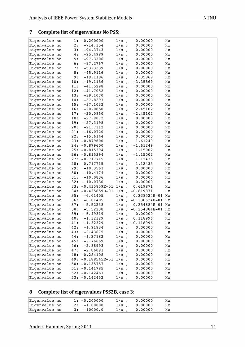
Analysis of IEEE Power System Stabilizer Models NTNU
Anders Hammer, Spring 2011 11
7 Complete list of eigenvalues No PSS: Eigenvalue no 1: -0.200000 1/s , 0.00000 Hz Eigenvalue no 2: -714.354 1/s , 0.00000 Hz Eigenvalue no 3: -94.3743 1/s , 0.00000 Hz Eigenvalue no 4: -95.4989 1/s , 0.00000 Hz Eigenvalue no 5: -97.3306 1/s , 0.00000 Hz Eigenvalue no 6: -97.2767 1/s , 0.00000 Hz Eigenvalue no 7: -53.3239 1/s , 0.00000 Hz Eigenvalue no 8: -45.9116 1/s , 0.00000 Hz Eigenvalue no 9: -19.1186 1/s , 3.35869 Hz Eigenvalue no 10: -19.1186 1/s , -3.35869 Hz Eigenvalue no 11: -41.5298 1/s , 0.00000 Hz Eigenvalue no 12: -41.7052 1/s , 0.00000 Hz Eigenvalue no 13: -39.1070 1/s , 0.00000 Hz Eigenvalue no 14: -37.8297 1/s , 0.00000 Hz Eigenvalue no 15: -37.1032 1/s , 0.00000 Hz Eigenvalue no 16: -20.0850 1/s , 2.45102 Hz Eigenvalue no 17: -20.0850 1/s , -2.45102 Hz Eigenvalue no 18: -27.9072 1/s , 0.00000 Hz Eigenvalue no 19: -27.3198 1/s , 0.00000 Hz Eigenvalue no 20: -21.7312 1/s , 0.00000 Hz Eigenvalue no 21: -16.0720 1/s , 0.00000 Hz Eigenvalue no 22: -15.6144 1/s , 0.00000 Hz Eigenvalue no 23: -0.879600 1/s , 1.61249 Hz Eigenvalue no 24: -0.879600 1/s , -1.61249 Hz Eigenvalue no 25: -0.815394 1/s , 1.15002 Hz Eigenvalue no 26: -0.815394 1/s , -1.15002 Hz Eigenvalue no 27: -0.717715 1/s , 1.12435 Hz Eigenvalue no 28: -0.717715 1/s , -1.12435 Hz Eigenvalue no 29: -10.3563 1/s , 0.00000 Hz Eigenvalue no 30: -10.4174 1/s , 0.00000 Hz Eigenvalue no 31: -10.0836 1/s , 0.00000 Hz Eigenvalue no 32: -10.0730 1/s , 0.00000 Hz Eigenvalue no 33: -0.435859E-01 1/s , 0.619871 Hz Eigenvalue no 34: -0.435859E-01 1/s , -0.619871 Hz Eigenvalue no 35: -6.01405 1/s , 0.238524E-01 Hz Eigenvalue no 36: -6.01405 1/s , -0.238524E-01 Hz Eigenvalue no 37: -5.52238 1/s , 0.254884E-01 Hz Eigenvalue no 38: -5.52238 1/s , -0.254884E-01 Hz Eigenvalue no 39: -5.49319 1/s , 0.00000 Hz Eigenvalue no 40: -1.32329 1/s , 0.118996 Hz Eigenvalue no 41: -1.32329 1/s , -0.118996 Hz Eigenvalue no 42: -1.91834 1/s , 0.00000 Hz Eigenvalue no 43: -2.43675 1/s , 0.00000 Hz Eigenvalue no 44: -1.27182 1/s , 0.00000 Hz Eigenvalue no 45: -2.76669 1/s , 0.00000 Hz Eigenvalue no 46: -2.88993 1/s , 0.00000 Hz Eigenvalue no 47: -2.86091 1/s , 0.00000 Hz Eigenvalue no 48: -0.284108 1/s , 0.00000 Hz Eigenvalue no 49: -0.188545E-01 1/s , 0.00000 Hz Eigenvalue no 50: -0.135757 1/s , 0.00000 Hz Eigenvalue no 51: -0.141785 1/s , 0.00000 Hz Eigenvalue no 52: -0.142467 1/s , 0.00000 Hz Eigenvalue no 53: -0.142452 1/s , 0.00000 Hz
8 Complete list of eigenvalues PSS2B, case 3: Eigenvalue no 1: -0.200000 1/s , 0.00000 Hz Eigenvalue no 2: -1.00000 1/s , 0.00000 Hz Eigenvalue no 3: -10000.0 1/s , 0.00000 Hz
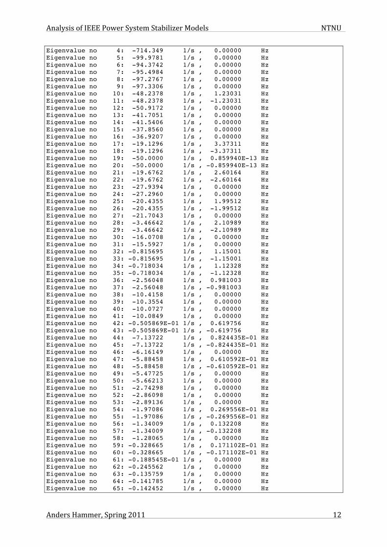
Analysis of IEEE Power System Stabilizer Models NTNU
Anders Hammer, Spring 2011 12
Eigenvalue no 4: -714.349 1/s , 0.00000 Hz Eigenvalue no 5: -99.9781 1/s , 0.00000 Hz Eigenvalue no 6: -94.3742 1/s , 0.00000 Hz Eigenvalue no 7: -95.4984 1/s , 0.00000 Hz Eigenvalue no 8: -97.2767 1/s , 0.00000 Hz Eigenvalue no 9: -97.3306 1/s , 0.00000 Hz Eigenvalue no 10: -48.2378 1/s , 1.23031 Hz Eigenvalue no 11: -48.2378 1/s , -1.23031 Hz Eigenvalue no 12: -50.9172 1/s , 0.00000 Hz Eigenvalue no 13: -41.7051 1/s , 0.00000 Hz Eigenvalue no 14: -41.5406 1/s , 0.00000 Hz Eigenvalue no 15: -37.8560 1/s , 0.00000 Hz Eigenvalue no 16: -36.9207 1/s , 0.00000 Hz Eigenvalue no 17: -19.1296 1/s , 3.37311 Hz Eigenvalue no 18: -19.1296 1/s , -3.37311 Hz Eigenvalue no 19: -50.0000 1/s , 0.859940E-13 Hz Eigenvalue no 20: -50.0000 1/s , -0.859940E-13 Hz Eigenvalue no 21: -19.6762 1/s , 2.60164 Hz Eigenvalue no 22: -19.6762 1/s , -2.60164 Hz Eigenvalue no 23: -27.9394 1/s , 0.00000 Hz Eigenvalue no 24: -27.2960 1/s , 0.00000 Hz Eigenvalue no 25: -20.4355 1/s , 1.99512 Hz Eigenvalue no 26: -20.4355 1/s , -1.99512 Hz Eigenvalue no 27: -21.7043 1/s , 0.00000 Hz Eigenvalue no 28: -3.46642 1/s , 2.10989 Hz Eigenvalue no 29: -3.46642 1/s , -2.10989 Hz Eigenvalue no 30: -16.0708 1/s , 0.00000 Hz Eigenvalue no 31: -15.5927 1/s , 0.00000 Hz Eigenvalue no 32: -0.815695 1/s , 1.15001 Hz Eigenvalue no 33: -0.815695 1/s , -1.15001 Hz Eigenvalue no 34: -0.718034 1/s , 1.12328 Hz Eigenvalue no 35: -0.718034 1/s , -1.12328 Hz Eigenvalue no 36: -2.56048 1/s , 0.981003 Hz Eigenvalue no 37: -2.56048 1/s , -0.981003 Hz Eigenvalue no 38: -10.4158 1/s , 0.00000 Hz Eigenvalue no 39: -10.3554 1/s , 0.00000 Hz Eigenvalue no 40: -10.0727 1/s , 0.00000 Hz Eigenvalue no 41: -10.0849 1/s , 0.00000 Hz Eigenvalue no 42: -0.505869E-01 1/s , 0.619756 Hz Eigenvalue no 43: -0.505869E-01 1/s , -0.619756 Hz Eigenvalue no 44: -7.13722 1/s , 0.824435E-01 Hz Eigenvalue no 45: -7.13722 1/s , -0.824435E-01 Hz Eigenvalue no 46: -6.16149 1/s , 0.00000 Hz Eigenvalue no 47: -5.88458 1/s , 0.610592E-01 Hz Eigenvalue no 48: -5.88458 1/s , -0.610592E-01 Hz Eigenvalue no 49: -5.47725 1/s , 0.00000 Hz Eigenvalue no 50: -5.66213 1/s , 0.00000 Hz Eigenvalue no 51: -2.74298 1/s , 0.00000 Hz Eigenvalue no 52: -2.86098 1/s , 0.00000 Hz Eigenvalue no 53: -2.89136 1/s , 0.00000 Hz Eigenvalue no 54: -1.97086 1/s , 0.269556E-01 Hz Eigenvalue no 55: -1.97086 1/s , -0.269556E-01 Hz Eigenvalue no 56: -1.34009 1/s , 0.132208 Hz Eigenvalue no 57: -1.34009 1/s , -0.132208 Hz Eigenvalue no 58: -1.28065 1/s , 0.00000 Hz Eigenvalue no 59: -0.328665 1/s , 0.171102E-01 Hz Eigenvalue no 60: -0.328665 1/s , -0.171102E-01 Hz Eigenvalue no 61: -0.188545E-01 1/s , 0.00000 Hz Eigenvalue no 62: -0.245562 1/s , 0.00000 Hz Eigenvalue no 63: -0.135759 1/s , 0.00000 Hz Eigenvalue no 64: -0.141785 1/s , 0.00000 Hz Eigenvalue no 65: -0.142452 1/s , 0.00000 Hz

Analysis of IEEE Power System Stabilizer Models NTNU
Anders Hammer, Spring 2011 13
Eigenvalue no 66: -0.142467 1/s , 0.00000 Hz Eigenvalue no 67: -0.332994 1/s , 0.00000 Hz Eigenvalue no 68: -0.333344 1/s , 0.00000 Hz Eigenvalue no 69: -0.333323 1/s , 0.00000 Hz
9 Complete list of eigenvalues PSS4B, IEEE parameters: Eigenvalue no 1: -0.200000 1/s , 0.00000 Hz Eigenvalue no 2: -1.00000 1/s , 0.00000 Hz Eigenvalue no 3: -1.00000 1/s , 0.00000 Hz Eigenvalue no 4: -1.00000 1/s , 0.00000 Hz Eigenvalue no 5: -1.00000 1/s , 0.00000 Hz Eigenvalue no 6: -1.00000 1/s , 0.00000 Hz Eigenvalue no 7: -1.00000 1/s , 0.00000 Hz Eigenvalue no 8: -1.00000 1/s , 0.00000 Hz Eigenvalue no 9: -1.00000 1/s , 0.00000 Hz Eigenvalue no 10: -1.00000 1/s , 0.00000 Hz Eigenvalue no 11: -1.00000 1/s , 0.00000 Hz Eigenvalue no 12: -1.00000 1/s , 0.00000 Hz Eigenvalue no 13: -1.00000 1/s , 0.00000 Hz Eigenvalue no 14: -1340.48 1/s , 0.00000 Hz Eigenvalue no 15: -714.509 1/s , 0.00000 Hz Eigenvalue no 16: -94.3783 1/s , 0.00000 Hz Eigenvalue no 17: -95.5075 1/s , 0.00000 Hz Eigenvalue no 18: -97.3308 1/s , 0.00000 Hz Eigenvalue no 19: -97.2766 1/s , 0.00000 Hz Eigenvalue no 20: -78.6428 1/s , 0.00000 Hz Eigenvalue no 21: -71.1943 1/s , 0.00000 Hz Eigenvalue no 22: -58.7861 1/s , 0.00000 Hz Eigenvalue no 23: -39.5240 1/s , 3.30501 Hz Eigenvalue no 24: -39.5240 1/s , -3.30501 Hz Eigenvalue no 25: -50.1924 1/s , 0.00000 Hz Eigenvalue no 26: -48.9260 1/s , 0.00000 Hz Eigenvalue no 27: -41.7051 1/s , 0.00000 Hz Eigenvalue no 28: -41.5370 1/s , 0.00000 Hz Eigenvalue no 29: -37.8520 1/s , 0.00000 Hz Eigenvalue no 30: -37.0401 1/s , 0.00000 Hz Eigenvalue no 31: -19.1619 1/s , 3.36531 Hz Eigenvalue no 32: -19.1619 1/s , -3.36531 Hz Eigenvalue no 33: -20.1701 1/s , 2.47551 Hz Eigenvalue no 34: -20.1701 1/s , -2.47551 Hz Eigenvalue no 35: -27.9395 1/s , 0.00000 Hz Eigenvalue no 36: -27.3450 1/s , 0.00000 Hz Eigenvalue no 37: -0.235963 1/s , 2.92876 Hz Eigenvalue no 38: -0.235963 1/s , -2.92876 Hz Eigenvalue no 39: -21.8407 1/s , 0.00000 Hz Eigenvalue no 40: -16.0568 1/s , 0.00000 Hz Eigenvalue no 41: -15.6052 1/s , 0.00000 Hz Eigenvalue no 42: -10.4187 1/s , 0.00000 Hz Eigenvalue no 43: -10.3570 1/s , 0.00000 Hz Eigenvalue no 44: -10.0831 1/s , 0.00000 Hz Eigenvalue no 45: -10.0732 1/s , 0.00000 Hz Eigenvalue no 46: -0.815882 1/s , 1.15005 Hz Eigenvalue no 47: -0.815882 1/s , -1.15005 Hz Eigenvalue no 48: -0.724437 1/s , 1.12312 Hz Eigenvalue no 49: -0.724437 1/s , -1.12312 Hz Eigenvalue no 50: -6.10337 1/s , 0.452343E-01 Hz Eigenvalue no 51: -6.10337 1/s , -0.452343E-01 Hz Eigenvalue no 52: -5.00316 1/s , 0.00000 Hz Eigenvalue no 53: -5.62163 1/s , 0.00000 Hz Eigenvalue no 54: -5.47431 1/s , 0.00000 Hz

Analysis of IEEE Power System Stabilizer Models NTNU
Anders Hammer, Spring 2011 14
Eigenvalue no 55: -0.850148E-01 1/s , 0.619555 Hz Eigenvalue no 56: -0.850148E-01 1/s , -0.619555 Hz Eigenvalue no 57: -0.843710 1/s , 0.392731 Hz Eigenvalue no 58: -0.843710 1/s , -0.392731 Hz Eigenvalue no 59: -2.35870 1/s , 0.00000 Hz Eigenvalue no 60: -2.73620 1/s , 0.00000 Hz Eigenvalue no 61: -2.89188 1/s , 0.00000 Hz Eigenvalue no 62: -2.86100 1/s , 0.00000 Hz Eigenvalue no 63: -1.24715 1/s , 0.114567 Hz Eigenvalue no 64: -1.24715 1/s , -0.114567 Hz Eigenvalue no 65: -1.33708 1/s , 0.468503E-01 Hz Eigenvalue no 66: -1.33708 1/s , -0.468503E-01 Hz Eigenvalue no 67: -1.04041 1/s , 0.00000 Hz Eigenvalue no 68: -0.932842 1/s , 0.00000 Hz Eigenvalue no 69: -0.438746 1/s , 0.128696E-01 Hz Eigenvalue no 70: -0.438746 1/s , -0.128696E-01 Hz Eigenvalue no 71: -0.272549 1/s , 0.00000 Hz Eigenvalue no 72: -0.188545E-01 1/s , 0.00000 Hz Eigenvalue no 73: -0.171226 1/s , 0.00000 Hz Eigenvalue no 74: -0.135746 1/s , 0.00000 Hz Eigenvalue no 75: -0.141785 1/s , 0.00000 Hz Eigenvalue no 76: -0.142452 1/s , 0.00000 Hz Eigenvalue no 77: -0.142467 1/s , 0.00000 Hz
10 Complete list of eigenvalues PSS4B, case 1: Eigenvalue no 1: -0.200000 1/s , 0.00000 Hz Eigenvalue no 2: -1.00000 1/s , 0.00000 Hz Eigenvalue no 3: -1.00000 1/s , 0.00000 Hz Eigenvalue no 4: -1.00000 1/s , 0.00000 Hz Eigenvalue no 5: -1.00000 1/s , 0.00000 Hz Eigenvalue no 6: -1.00000 1/s , 0.00000 Hz Eigenvalue no 7: -1.00000 1/s , 0.00000 Hz Eigenvalue no 8: -1.00000 1/s , 0.00000 Hz Eigenvalue no 9: -1.00000 1/s , 0.00000 Hz Eigenvalue no 10: -1339.67 1/s , 0.00000 Hz Eigenvalue no 11: -717.375 1/s , 0.00000 Hz Eigenvalue no 12: -94.3704 1/s , 0.00000 Hz Eigenvalue no 13: -95.4899 1/s , 0.00000 Hz Eigenvalue no 14: -97.3304 1/s , 0.00000 Hz Eigenvalue no 15: -97.2767 1/s , 0.00000 Hz Eigenvalue no 16: -79.8757 1/s , 0.00000 Hz Eigenvalue no 17: -68.5509 1/s , 0.00000 Hz Eigenvalue no 18: -12.7133 1/s , 5.55589 Hz Eigenvalue no 19: -12.7133 1/s , -5.55589 Hz Eigenvalue no 20: -50.8848 1/s , 0.00000 Hz Eigenvalue no 21: -48.2374 1/s , 0.00000 Hz Eigenvalue no 22: -41.5367 1/s , 0.00000 Hz Eigenvalue no 23: -41.7051 1/s , 0.00000 Hz Eigenvalue no 24: -19.3333 1/s , 3.38036 Hz Eigenvalue no 25: -19.3333 1/s , -3.38036 Hz Eigenvalue no 26: -37.8526 1/s , 0.00000 Hz Eigenvalue no 27: -37.0366 1/s , 0.00000 Hz Eigenvalue no 28: -20.3249 1/s , 2.50144 Hz Eigenvalue no 29: -20.3249 1/s , -2.50144 Hz Eigenvalue no 30: -30.1825 1/s , 0.00000 Hz Eigenvalue no 31: -27.9358 1/s , 0.00000 Hz Eigenvalue no 32: -27.3443 1/s , 0.00000 Hz Eigenvalue no 33: -21.7090 1/s , 0.00000 Hz Eigenvalue no 34: -16.4154 1/s , 0.00000 Hz Eigenvalue no 35: -16.0209 1/s , 0.00000 Hz

Analysis of IEEE Power System Stabilizer Models NTNU
Anders Hammer, Spring 2011 15
Eigenvalue no 36: -15.5917 1/s , 0.00000 Hz Eigenvalue no 37: -10.4194 1/s , 0.00000 Hz Eigenvalue no 38: -10.3573 1/s , 0.00000 Hz Eigenvalue no 39: -10.0829 1/s , 0.00000 Hz Eigenvalue no 40: -10.0732 1/s , 0.00000 Hz Eigenvalue no 41: -0.815949 1/s , 1.15005 Hz Eigenvalue no 42: -0.815949 1/s , -1.15005 Hz Eigenvalue no 43: -0.725084 1/s , 1.12293 Hz Eigenvalue no 44: -0.725084 1/s , -1.12293 Hz Eigenvalue no 45: -6.12400 1/s , 0.490444E-01 Hz Eigenvalue no 46: -6.12400 1/s , -0.490444E-01 Hz Eigenvalue no 47: -5.63056 1/s , 0.00000 Hz Eigenvalue no 48: -5.47573 1/s , 0.00000 Hz Eigenvalue no 49: -4.82793 1/s , 0.00000 Hz Eigenvalue no 50: -0.878199E-01 1/s , 0.619711 Hz Eigenvalue no 51: -0.878199E-01 1/s , -0.619711 Hz Eigenvalue no 52: -1.16948 1/s , 0.321128 Hz Eigenvalue no 53: -1.16948 1/s , -0.321128 Hz Eigenvalue no 54: -2.63094 1/s , 0.00000 Hz Eigenvalue no 55: -2.70181 1/s , 0.00000 Hz Eigenvalue no 56: -2.89290 1/s , 0.00000 Hz Eigenvalue no 57: -2.86103 1/s , 0.00000 Hz Eigenvalue no 58: -1.39552 1/s , 0.00000 Hz Eigenvalue no 59: -1.21829 1/s , 0.848072E-01 Hz Eigenvalue no 60: -1.21829 1/s , -0.848072E-01 Hz Eigenvalue no 61: -1.03868 1/s , 0.00000 Hz Eigenvalue no 62: -0.929053 1/s , 0.00000 Hz Eigenvalue no 63: -0.371486 1/s , 0.00000 Hz Eigenvalue no 64: -0.188546E-01 1/s , 0.00000 Hz Eigenvalue no 65: -0.267319 1/s , 0.00000 Hz Eigenvalue no 66: -0.333333 1/s , 0.00000 Hz Eigenvalue no 67: -0.171265 1/s , 0.00000 Hz Eigenvalue no 68: -0.135747 1/s , 0.00000 Hz Eigenvalue no 69: -0.141785 1/s , 0.00000 Hz Eigenvalue no 70: -0.142452 1/s , 0.00000 Hz Eigenvalue no 71: -0.142467 1/s , 0.00000 Hz Eigenvalue no 72: -1.00000 1/s , 0.00000 Hz Eigenvalue no 73: -1.00000 1/s , 0.00000 Hz Eigenvalue no 74: -1.00000 1/s , 0.00000 Hz Eigenvalue no 75: -1.00000 1/s , 0.00000 Hz Eigenvalue no 76: -1.00000 1/s , 0.00000 Hz Eigenvalue no 77: -1.00000 1/s , 0.00000 Hz
11 Complete list of eigenvalues PSS4B, case 2: Eigenvalue no 1: -0.200000 1/s , 0.00000 Hz Eigenvalue no 2: -1.00000 1/s , 0.00000 Hz Eigenvalue no 3: -1.00000 1/s , 0.00000 Hz Eigenvalue no 4: -1.00000 1/s , 0.00000 Hz Eigenvalue no 5: -1.00000 1/s , 0.00000 Hz Eigenvalue no 6: -1.00000 1/s , 0.00000 Hz Eigenvalue no 7: -1.00000 1/s , 0.00000 Hz Eigenvalue no 8: -1.00000 1/s , 0.00000 Hz Eigenvalue no 9: -1.00000 1/s , 0.00000 Hz Eigenvalue no 10: -1.00000 1/s , 0.00000 Hz Eigenvalue no 11: -1.00000 1/s , 0.00000 Hz Eigenvalue no 12: -1340.16 1/s , 0.00000 Hz Eigenvalue no 13: -715.651 1/s , 0.00000 Hz Eigenvalue no 14: -94.3726 1/s , 0.00000 Hz Eigenvalue no 15: -95.4948 1/s , 0.00000 Hz Eigenvalue no 16: -97.3305 1/s , 0.00000 Hz
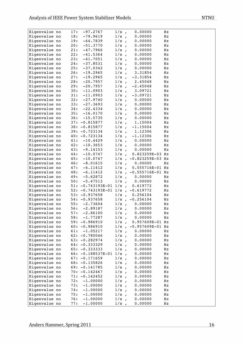
Analysis of IEEE Power System Stabilizer Models NTNU
Anders Hammer, Spring 2011 16
Eigenvalue no 17: -97.2767 1/s , 0.00000 Hz Eigenvalue no 18: -79.9619 1/s , 0.00000 Hz Eigenvalue no 19: -64.7839 1/s , 0.00000 Hz Eigenvalue no 20: -51.3770 1/s , 0.00000 Hz Eigenvalue no 21: -47.7966 1/s , 0.00000 Hz Eigenvalue no 22: -41.5364 1/s , 0.00000 Hz Eigenvalue no 23: -41.7051 1/s , 0.00000 Hz Eigenvalue no 24: -37.8531 1/s , 0.00000 Hz Eigenvalue no 25: -37.0342 1/s , 0.00000 Hz Eigenvalue no 26: -19.2965 1/s , 3.31854 Hz Eigenvalue no 27: -19.2965 1/s , -3.31854 Hz Eigenvalue no 28: -20.7957 1/s , 2.45048 Hz Eigenvalue no 29: -20.7957 1/s , -2.45048 Hz Eigenvalue no 30: -11.0903 1/s , 3.09721 Hz Eigenvalue no 31: -11.0903 1/s , -3.09721 Hz Eigenvalue no 32: -27.9740 1/s , 0.00000 Hz Eigenvalue no 33: -27.3693 1/s , 0.00000 Hz Eigenvalue no 34: -22.4334 1/s , 0.00000 Hz Eigenvalue no 35: -16.0170 1/s , 0.00000 Hz Eigenvalue no 36: -15.5735 1/s , 0.00000 Hz Eigenvalue no 37: -0.815877 1/s , 1.15004 Hz Eigenvalue no 38: -0.815877 1/s , -1.15004 Hz Eigenvalue no 39: -0.723134 1/s , 1.12306 Hz Eigenvalue no 40: -0.723134 1/s , -1.12306 Hz Eigenvalue no 41: -10.4429 1/s , 0.00000 Hz Eigenvalue no 42: -10.3653 1/s , 0.00000 Hz Eigenvalue no 43: -9.14153 1/s , 0.00000 Hz Eigenvalue no 44: -10.0747 1/s , 0.823259E-03 Hz Eigenvalue no 45: -10.0747 1/s , -0.823259E-03 Hz Eigenvalue no 46: -8.01615 1/s , 0.00000 Hz Eigenvalue no 47: -6.11412 1/s , 0.555716E-01 Hz Eigenvalue no 48: -6.11412 1/s , -0.555716E-01 Hz Eigenvalue no 49: -5.62872 1/s , 0.00000 Hz Eigenvalue no 50: -5.47513 1/s , 0.00000 Hz Eigenvalue no 51: -0.743193E-01 1/s , 0.619772 Hz Eigenvalue no 52: -0.743193E-01 1/s , -0.619772 Hz Eigenvalue no 53: -0.937658 1/s , 0.256104 Hz Eigenvalue no 54: -0.937658 1/s , -0.256104 Hz Eigenvalue no 55: -2.73604 1/s , 0.00000 Hz Eigenvalue no 56: -2.89187 1/s , 0.00000 Hz Eigenvalue no 57: -2.86100 1/s , 0.00000 Hz Eigenvalue no 58: -1.77287 1/s , 0.00000 Hz Eigenvalue no 59: -0.986910 1/s , 0.957609E-01 Hz Eigenvalue no 60: -0.986910 1/s , -0.957609E-01 Hz Eigenvalue no 61: -1.05217 1/s , 0.00000 Hz Eigenvalue no 62: -0.780046 1/s , 0.00000 Hz Eigenvalue no 63: -0.282974 1/s , 0.00000 Hz Eigenvalue no 64: -0.333329 1/s , 0.00000 Hz Eigenvalue no 65: -0.333333 1/s , 0.00000 Hz Eigenvalue no 66: -0.188537E-01 1/s , 0.00000 Hz Eigenvalue no 67: -0.171659 1/s , 0.00000 Hz Eigenvalue no 68: -0.135826 1/s , 0.00000 Hz Eigenvalue no 69: -0.141785 1/s , 0.00000 Hz Eigenvalue no 70: -0.142467 1/s , 0.00000 Hz Eigenvalue no 71: -0.142452 1/s , 0.00000 Hz Eigenvalue no 72: -1.00000 1/s , 0.00000 Hz Eigenvalue no 73: -1.00000 1/s , 0.00000 Hz Eigenvalue no 74: -1.00000 1/s , 0.00000 Hz Eigenvalue no 75: -1.00000 1/s , 0.00000 Hz Eigenvalue no 76: -1.00000 1/s , 0.00000 Hz Eigenvalue no 77: -1.00000 1/s , 0.00000 Hz

Analysis of IEEE Power System Stabilizer Models NTNU
Anders Hammer, Spring 2011 17
12 Complete list of eigenvalues PSS4B, case 3: Eigenvalue no 1: -0.200000 1/s , 0.00000 Hz Eigenvalue no 2: -1.00000 1/s , 0.00000 Hz Eigenvalue no 3: -1.00000 1/s , 0.00000 Hz Eigenvalue no 4: -1.00000 1/s , 0.00000 Hz Eigenvalue no 5: -1.00000 1/s , 0.00000 Hz Eigenvalue no 6: -1.00000 1/s , 0.00000 Hz Eigenvalue no 7: -1.00000 1/s , 0.00000 Hz Eigenvalue no 8: -1340.26 1/s , 0.00000 Hz Eigenvalue no 9: -715.271 1/s , 0.00000 Hz Eigenvalue no 10: -94.3768 1/s , 0.00000 Hz Eigenvalue no 11: -95.5040 1/s , 0.00000 Hz Eigenvalue no 12: -97.3307 1/s , 0.00000 Hz Eigenvalue no 13: -97.2766 1/s , 0.00000 Hz Eigenvalue no 14: -79.3839 1/s , 0.00000 Hz Eigenvalue no 15: -65.6081 1/s , 0.00000 Hz Eigenvalue no 16: -52.1650 1/s , 0.00000 Hz Eigenvalue no 17: -2.80981 1/s , 4.74457 Hz Eigenvalue no 18: -2.80981 1/s , -4.74457 Hz Eigenvalue no 19: -45.4991 1/s , 0.177821 Hz Eigenvalue no 20: -45.4991 1/s , -0.177821 Hz Eigenvalue no 21: -41.5386 1/s , 0.00000 Hz Eigenvalue no 22: -41.7051 1/s , 0.00000 Hz Eigenvalue no 23: -37.0444 1/s , 0.00000 Hz Eigenvalue no 24: -37.8509 1/s , 0.00000 Hz Eigenvalue no 25: -19.2500 1/s , 3.36660 Hz Eigenvalue no 26: -19.2500 1/s , -3.36660 Hz Eigenvalue no 27: -20.2703 1/s , 2.48166 Hz Eigenvalue no 28: -20.2703 1/s , -2.48166 Hz Eigenvalue no 29: -27.9387 1/s , 0.00000 Hz Eigenvalue no 30: -27.3447 1/s , 0.00000 Hz Eigenvalue no 31: -21.6794 1/s , 0.00000 Hz Eigenvalue no 32: -15.6040 1/s , 0.00000 Hz Eigenvalue no 33: -16.0550 1/s , 0.00000 Hz Eigenvalue no 34: -10.4188 1/s , 0.00000 Hz Eigenvalue no 35: -10.3571 1/s , 0.00000 Hz Eigenvalue no 36: -10.0831 1/s , 0.00000 Hz Eigenvalue no 37: -10.0732 1/s , 0.00000 Hz Eigenvalue no 38: -0.815939 1/s , 1.15005 Hz Eigenvalue no 39: -0.815939 1/s , -1.15005 Hz Eigenvalue no 40: -0.725635 1/s , 1.12299 Hz Eigenvalue no 41: -0.725635 1/s , -1.12299 Hz Eigenvalue no 42: -0.957974E-01 1/s , 0.619892 Hz Eigenvalue no 43: -0.957974E-01 1/s , -0.619892 Hz Eigenvalue no 44: -6.44465 1/s , 0.00000 Hz Eigenvalue no 45: -6.10372 1/s , 0.463091E-01 Hz Eigenvalue no 46: -6.10372 1/s , -0.463091E-01 Hz Eigenvalue no 47: -5.62263 1/s , 0.00000 Hz Eigenvalue no 48: -5.47443 1/s , 0.00000 Hz Eigenvalue no 49: -1.11105 1/s , 0.426365 Hz Eigenvalue no 50: -1.11105 1/s , -0.426365 Hz Eigenvalue no 51: -3.41806 1/s , 0.00000 Hz Eigenvalue no 52: -1.73096 1/s , 0.195718 Hz Eigenvalue no 53: -1.73096 1/s , -0.195718 Hz Eigenvalue no 54: -2.56432 1/s , 0.00000 Hz Eigenvalue no 55: -2.73490 1/s , 0.00000 Hz Eigenvalue no 56: -2.89193 1/s , 0.00000 Hz Eigenvalue no 57: -2.86100 1/s , 0.00000 Hz Eigenvalue no 58: -1.24654 1/s , 0.870476E-01 Hz Eigenvalue no 59: -1.24654 1/s , -0.870476E-01 Hz Eigenvalue no 60: -1.30657 1/s , 0.00000 Hz

Analysis of IEEE Power System Stabilizer Models NTNU
Anders Hammer, Spring 2011 18
Eigenvalue no 61: -1.03847 1/s , 0.00000 Hz Eigenvalue no 62: -0.918116 1/s , 0.00000 Hz Eigenvalue no 63: -0.370737 1/s , 0.00000 Hz Eigenvalue no 64: -0.188542E-01 1/s , 0.00000 Hz Eigenvalue no 65: -0.267961 1/s , 0.00000 Hz Eigenvalue no 66: -0.171346 1/s , 0.00000 Hz Eigenvalue no 67: -0.333333 1/s , 0.00000 Hz Eigenvalue no 68: -0.135763 1/s , 0.00000 Hz Eigenvalue no 69: -0.141785 1/s , 0.00000 Hz Eigenvalue no 70: -0.142467 1/s , 0.00000 Hz Eigenvalue no 71: -0.142452 1/s , 0.00000 Hz Eigenvalue no 72: -1.00000 1/s , 0.00000 Hz Eigenvalue no 73: -1.00000 1/s , 0.00000 Hz Eigenvalue no 74: -1.00000 1/s , 0.00000 Hz Eigenvalue no 75: -1.00000 1/s , 0.00000 Hz Eigenvalue no 76: -1.00000 1/s , 0.00000 Hz Eigenvalue no 77: -1.00000 1/s , 0.00000 Hz
13 Complete list of eigenvalues PSS4B, case 4: Eigenvalue no 1: -0.200000 1/s , 0.00000 Hz Eigenvalue no 2: -1.00000 1/s , 0.00000 Hz Eigenvalue no 3: -1.00000 1/s , 0.00000 Hz Eigenvalue no 4: -1.00000 1/s , 0.00000 Hz Eigenvalue no 5: -1.00000 1/s , 0.00000 Hz Eigenvalue no 6: -1.00000 1/s , 0.00000 Hz Eigenvalue no 7: -1.00000 1/s , 0.00000 Hz Eigenvalue no 8: -1.00000 1/s , 0.00000 Hz Eigenvalue no 9: -1.00000 1/s , 0.00000 Hz Eigenvalue no 10: -1340.41 1/s , 0.00000 Hz Eigenvalue no 11: -714.784 1/s , 0.00000 Hz Eigenvalue no 12: -94.3739 1/s , 0.00000 Hz Eigenvalue no 13: -95.4978 1/s , 0.00000 Hz Eigenvalue no 14: -97.3306 1/s , 0.00000 Hz Eigenvalue no 15: -97.2767 1/s , 0.00000 Hz Eigenvalue no 16: -79.9673 1/s , 0.00000 Hz Eigenvalue no 17: -61.5976 1/s , 0.00000 Hz Eigenvalue no 18: -52.1621 1/s , 0.00000 Hz Eigenvalue no 19: -47.0516 1/s , 0.00000 Hz Eigenvalue no 20: -41.5355 1/s , 0.00000 Hz Eigenvalue no 21: -41.7051 1/s , 0.00000 Hz Eigenvalue no 22: -37.8560 1/s , 0.00000 Hz Eigenvalue no 23: -37.0157 1/s , 0.00000 Hz Eigenvalue no 24: -19.1271 1/s , 3.35018 Hz Eigenvalue no 25: -19.1271 1/s , -3.35018 Hz Eigenvalue no 26: -32.5235 1/s , 0.00000 Hz Eigenvalue no 27: -20.1600 1/s , 2.43248 Hz Eigenvalue no 28: -20.1600 1/s , -2.43248 Hz Eigenvalue no 29: -27.8712 1/s , 0.00000 Hz Eigenvalue no 30: -27.2898 1/s , 0.00000 Hz Eigenvalue no 31: -21.4864 1/s , 0.00000 Hz Eigenvalue no 32: -4.91338 1/s , 2.13954 Hz Eigenvalue no 33: -4.91338 1/s , -2.13954 Hz Eigenvalue no 34: -16.0720 1/s , 0.00000 Hz Eigenvalue no 35: -15.6140 1/s , 0.00000 Hz Eigenvalue no 36: -10.4181 1/s , 0.00000 Hz Eigenvalue no 37: -10.3567 1/s , 0.00000 Hz Eigenvalue no 38: -10.0833 1/s , 0.00000 Hz Eigenvalue no 39: -10.0731 1/s , 0.00000 Hz Eigenvalue no 40: -0.815832 1/s , 1.15002 Hz Eigenvalue no 41: -0.815832 1/s , -1.15002 Hz
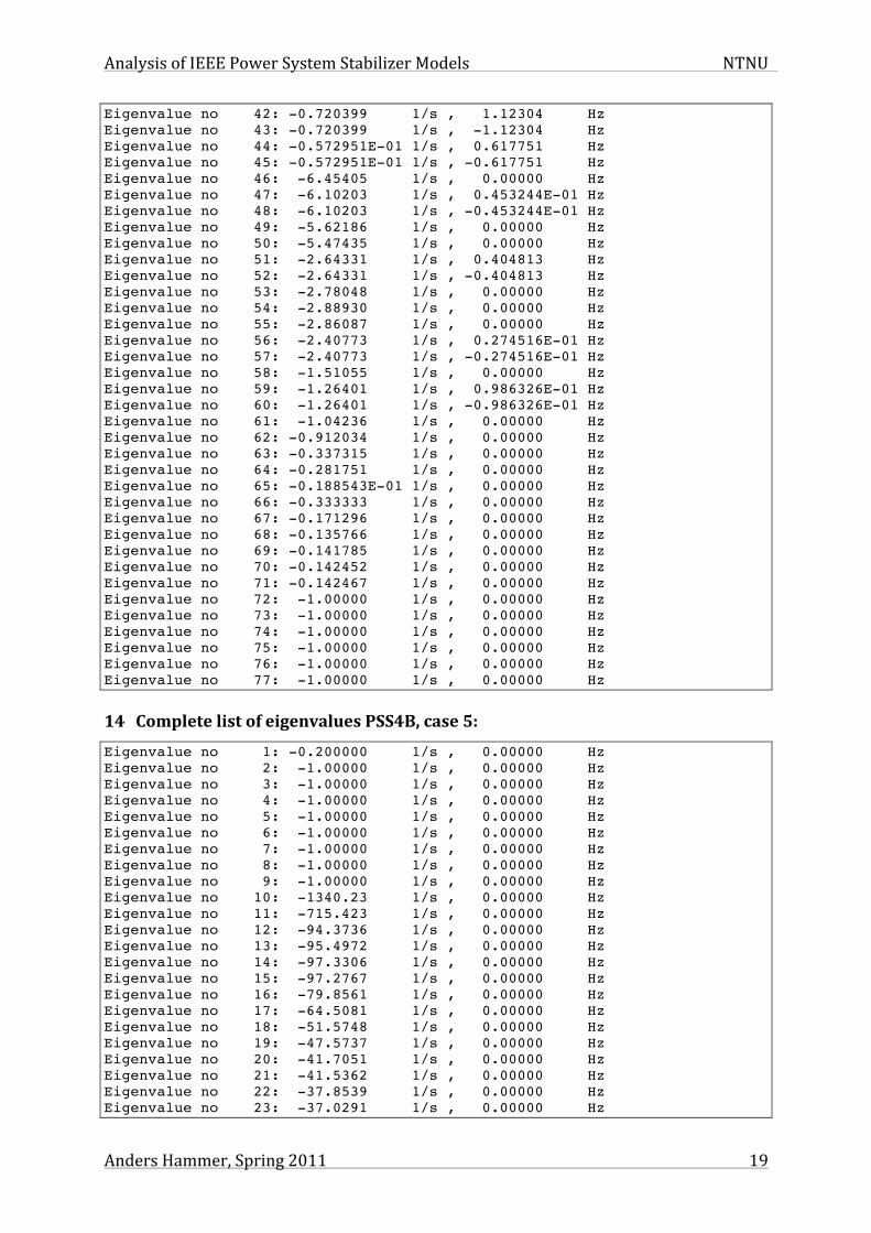
Analysis of IEEE Power System Stabilizer Models NTNU
Anders Hammer, Spring 2011 19
Eigenvalue no 42: -0.720399 1/s , 1.12304 Hz Eigenvalue no 43: -0.720399 1/s , -1.12304 Hz Eigenvalue no 44: -0.572951E-01 1/s , 0.617751 Hz Eigenvalue no 45: -0.572951E-01 1/s , -0.617751 Hz Eigenvalue no 46: -6.45405 1/s , 0.00000 Hz Eigenvalue no 47: -6.10203 1/s , 0.453244E-01 Hz Eigenvalue no 48: -6.10203 1/s , -0.453244E-01 Hz Eigenvalue no 49: -5.62186 1/s , 0.00000 Hz Eigenvalue no 50: -5.47435 1/s , 0.00000 Hz Eigenvalue no 51: -2.64331 1/s , 0.404813 Hz Eigenvalue no 52: -2.64331 1/s , -0.404813 Hz Eigenvalue no 53: -2.78048 1/s , 0.00000 Hz Eigenvalue no 54: -2.88930 1/s , 0.00000 Hz Eigenvalue no 55: -2.86087 1/s , 0.00000 Hz Eigenvalue no 56: -2.40773 1/s , 0.274516E-01 Hz Eigenvalue no 57: -2.40773 1/s , -0.274516E-01 Hz Eigenvalue no 58: -1.51055 1/s , 0.00000 Hz Eigenvalue no 59: -1.26401 1/s , 0.986326E-01 Hz Eigenvalue no 60: -1.26401 1/s , -0.986326E-01 Hz Eigenvalue no 61: -1.04236 1/s , 0.00000 Hz Eigenvalue no 62: -0.912034 1/s , 0.00000 Hz Eigenvalue no 63: -0.337315 1/s , 0.00000 Hz Eigenvalue no 64: -0.281751 1/s , 0.00000 Hz Eigenvalue no 65: -0.188543E-01 1/s , 0.00000 Hz Eigenvalue no 66: -0.333333 1/s , 0.00000 Hz Eigenvalue no 67: -0.171296 1/s , 0.00000 Hz Eigenvalue no 68: -0.135766 1/s , 0.00000 Hz Eigenvalue no 69: -0.141785 1/s , 0.00000 Hz Eigenvalue no 70: -0.142452 1/s , 0.00000 Hz Eigenvalue no 71: -0.142467 1/s , 0.00000 Hz Eigenvalue no 72: -1.00000 1/s , 0.00000 Hz Eigenvalue no 73: -1.00000 1/s , 0.00000 Hz Eigenvalue no 74: -1.00000 1/s , 0.00000 Hz Eigenvalue no 75: -1.00000 1/s , 0.00000 Hz Eigenvalue no 76: -1.00000 1/s , 0.00000 Hz Eigenvalue no 77: -1.00000 1/s , 0.00000 Hz
14 Complete list of eigenvalues PSS4B, case 5: Eigenvalue no 1: -0.200000 1/s , 0.00000 Hz Eigenvalue no 2: -1.00000 1/s , 0.00000 Hz Eigenvalue no 3: -1.00000 1/s , 0.00000 Hz Eigenvalue no 4: -1.00000 1/s , 0.00000 Hz Eigenvalue no 5: -1.00000 1/s , 0.00000 Hz Eigenvalue no 6: -1.00000 1/s , 0.00000 Hz Eigenvalue no 7: -1.00000 1/s , 0.00000 Hz Eigenvalue no 8: -1.00000 1/s , 0.00000 Hz Eigenvalue no 9: -1.00000 1/s , 0.00000 Hz Eigenvalue no 10: -1340.23 1/s , 0.00000 Hz Eigenvalue no 11: -715.423 1/s , 0.00000 Hz Eigenvalue no 12: -94.3736 1/s , 0.00000 Hz Eigenvalue no 13: -95.4972 1/s , 0.00000 Hz Eigenvalue no 14: -97.3306 1/s , 0.00000 Hz Eigenvalue no 15: -97.2767 1/s , 0.00000 Hz Eigenvalue no 16: -79.8561 1/s , 0.00000 Hz Eigenvalue no 17: -64.5081 1/s , 0.00000 Hz Eigenvalue no 18: -51.5748 1/s , 0.00000 Hz Eigenvalue no 19: -47.5737 1/s , 0.00000 Hz Eigenvalue no 20: -41.7051 1/s , 0.00000 Hz Eigenvalue no 21: -41.5362 1/s , 0.00000 Hz Eigenvalue no 22: -37.8539 1/s , 0.00000 Hz Eigenvalue no 23: -37.0291 1/s , 0.00000 Hz

Analysis of IEEE Power System Stabilizer Models NTNU
Anders Hammer, Spring 2011 20
Eigenvalue no 24: -19.2459 1/s , 3.34729 Hz Eigenvalue no 25: -19.2459 1/s , -3.34729 Hz Eigenvalue no 26: -6.69575 1/s , 3.55422 Hz Eigenvalue no 27: -6.69575 1/s , -3.55422 Hz Eigenvalue no 28: -20.3652 1/s , 2.45400 Hz Eigenvalue no 29: -20.3652 1/s , -2.45400 Hz Eigenvalue no 30: -30.2458 1/s , 0.00000 Hz Eigenvalue no 31: -27.8644 1/s , 0.00000 Hz Eigenvalue no 32: -27.2913 1/s , 0.00000 Hz Eigenvalue no 33: -21.3703 1/s , 0.00000 Hz Eigenvalue no 34: -16.0608 1/s , 0.00000 Hz Eigenvalue no 35: -15.6074 1/s , 0.00000 Hz Eigenvalue no 36: -10.4187 1/s , 0.00000 Hz Eigenvalue no 37: -10.3570 1/s , 0.00000 Hz Eigenvalue no 38: -10.0831 1/s , 0.00000 Hz Eigenvalue no 39: -10.0732 1/s , 0.00000 Hz Eigenvalue no 40: -0.815925 1/s , 1.15004 Hz Eigenvalue no 41: -0.815925 1/s , -1.15004 Hz Eigenvalue no 42: -0.724453 1/s , 1.12296 Hz Eigenvalue no 43: -0.724453 1/s , -1.12296 Hz Eigenvalue no 44: -6.46283 1/s , 0.00000 Hz Eigenvalue no 45: -6.10461 1/s , 0.454980E-01 Hz Eigenvalue no 46: -6.10461 1/s , -0.454980E-01 Hz Eigenvalue no 47: -5.62213 1/s , 0.00000 Hz Eigenvalue no 48: -5.47438 1/s , 0.00000 Hz Eigenvalue no 49: -0.867562E-01 1/s , 0.618383 Hz Eigenvalue no 50: -0.867562E-01 1/s , -0.618383 Hz Eigenvalue no 51: -1.13669 1/s , 0.409687 Hz Eigenvalue no 52: -1.13669 1/s , -0.409687 Hz Eigenvalue no 53: -2.74969 1/s , 0.00000 Hz Eigenvalue no 54: -2.89124 1/s , 0.00000 Hz Eigenvalue no 55: -2.86097 1/s , 0.00000 Hz Eigenvalue no 56: -2.37737 1/s , 0.312728E-01 Hz Eigenvalue no 57: -2.37737 1/s , -0.312728E-01 Hz Eigenvalue no 58: -1.51012 1/s , 0.00000 Hz Eigenvalue no 59: -1.19050 1/s , 0.984668E-01 Hz Eigenvalue no 60: -1.19050 1/s , -0.984668E-01 Hz Eigenvalue no 61: -1.04602 1/s , 0.00000 Hz Eigenvalue no 62: -0.883359 1/s , 0.00000 Hz Eigenvalue no 63: -0.343789 1/s , 0.00000 Hz Eigenvalue no 64: -0.188542E-01 1/s , 0.00000 Hz Eigenvalue no 65: -0.278317 1/s , 0.00000 Hz Eigenvalue no 66: -0.333333 1/s , 0.00000 Hz Eigenvalue no 67: -0.171370 1/s , 0.00000 Hz Eigenvalue no 68: -0.135776 1/s , 0.00000 Hz Eigenvalue no 69: -0.141785 1/s , 0.00000 Hz Eigenvalue no 70: -0.142452 1/s , 0.00000 Hz Eigenvalue no 71: -0.142467 1/s , 0.00000 Hz Eigenvalue no 72: -1.00000 1/s , 0.00000 Hz Eigenvalue no 73: -1.00000 1/s , 0.00000 Hz Eigenvalue no 74: -1.00000 1/s , 0.00000 Hz Eigenvalue no 75: -1.00000 1/s , 0.00000 Hz Eigenvalue no 76: -1.00000 1/s , 0.00000 Hz Eigenvalue no 77: -1.00000 1/s , 0.00000 Hz
Related Documents