ANALYSIS OF DIPMETER LOGS - Crain's Petrophysical … · ANALYSIS OF DIPMETER LOGS PART 2 - COMPUTER DISPLAYS OF DIPMETERS . E. R. (Ross) Crain, P.Eng. Spectrum 2000 Mindware Ltd

ANALYSIS OF DIPMETER LOGS PART 2 - COMPUTER DISPLAYS OF DIPMETERS

E. R. (Ross) Crain, P.Eng.

Spectrum 2000 Mindware Ltd Calgary AB

403 – 845 – 2527 [email protected]

Written in 1992. this part was never published. A version of this paper forms Chapter 27 of Crain’s Petrophysical Handbook. Author’s Note: All of the material in this paper is still current, although the resolution and borehole coverage of some tools has improved. ERC Jan 2005.. ABSTRACT Part 1 of this two part article covered the evolution of dipmeter tools and data processing techniques. This part reviews the modern dipmeter displays generated by computer and provides a brief outline of the uses for each type of display.

FORMATION IMAGING FROM DIPMETER DATA An extension of the SHDT processing provides a core-like image of the borehole, using the LOC dip correlations and the measured resistivity curves. The program is called STRATIM (Schlumberger trademark). FIGURE 1: STRATIM image created from SHDT data

An example is given in Figure 1. The program produces a 360 degree image of the borehole wall by interpolating between the eight resistivity measurements from the eight electrodes on the SHDT pads. Images can be coded in gray scale or colour. Dark gray or dark colour usually represents conductive, often tight shale, beds and light colour resistive, often porous sand, beds. If shales are more resistive than sands (or carbonates), the colour scheme can be reversed to keep shales looking dark.

The dipmeter curves are rotated to their true azimuth but are not adjusted to true dip. The dips seen on the image are as they would appear on the surface of a conventional core. The trace of a plane dipping bed forms a sinusoidal curve when the image of the borehole wall is unwrapped and laid flat, as they are in these images. Bed boundaries, dipping beds, slump features, and fractures are easily seen, if present. Images can be

enhanced as in Formation Microscanner processing, but processing is cheaper because much less data is manipulated.

A similar program, called DIPVUE is available from Western Atlas, illustrated in Figure 2. In addition, most core service companies can provide core photographs and dip logs from core data for comparison with log derived borehole images.

FIGURE 2: DIPVUE image created from dipmeter data

X-ray tomography images can also be used to compare with dipmeter images. Resolution on core tomography is in the order of a few millimeters, similar to that for the formation microscanner and finer than STRATIM. Examples of both horizontal and vertical tomograph slices are found in Figure 3.

FIGURE 3: X-ray tomography image can be compared to dipmeter data

RESISTIVITY MICROSCANNER IMAGE LOGS The Formation Microscanner is a further extension of the capabilities of the dipmeter tool. Instead of creating images by interpolation of dip correlations from 8 resistivity curves as in the STRATIM program, it records 50 to 200 finely spaced micro resistivity curves and maps the values into a spatial image of the well bore face. See Formation Imaging with Microelectrical Scanning Arrays, M.P. Ekstrome et al, SPEJ, May 1987 for tool details. To obtain image information from this tool, a considerable amount of data processing is involved. During acquisition, the vertically staggered array is sampled at constant cable depth increments as measured uphole, effectively a constant temporal sampling rate, and the signals obtained must be shifted vertically to bring the linear arrays into vertical depth synchronization. Under ideal conditions of constant tool velocity, this involves a static shift of an integral number of vertical inter-row spacings. Under typical conditions of non-constant or intermittent tool motion arising from sonde mass, cable elasticity, and pad friction, the shift to be applied is variable and depends on the instantaneous tool velocity. This correction is made by estimating the tool speed

using a recursive linear least squares estimation algorithm, called a Kalman filter, to process measurements from a three axis accelerometer incorporated into the tool. The microresistivity data provided by this tool are of very high resolution, in the order of a millimeter. Thus, a substantially large data array must be handled, and it is an obvious challenge to process and display this information in a way which facilitates its interpretation. This is resolved through a point to point mapping of the resistivity traces into a spatial image, each pixel in the image display having a gray scale value associated with a particular current level. Subsequent interpretation benefits from the close relationship between this image and core photography. Samples of six different uses of the images are shown as Figure 4 and 5.

FIGURE 4: Formation microscanner images in various environments

FIGURE 5: Formation microscanner images in various environments

With the data in the form of a digital image, several image processing operations can be used to improve the overall quality of the imagery. For example, systematic variations between electrode responses are normalized, and dynamic or user controlled gray scale compensation is used to enhance local image contrast and improve the fine image detail. An example is shown in the next Section. Stretching, squeezing, or clipping of the gray scale spectrum, or mapping of the gray scale to colours, are common processing functions. Edge enhancement or directional filters can also be applied to sharpen various features seen on the images. The FMS Image Examiner is an interactive computer program for image enhancement and dip calculation using data from the formation microscanner. The program provides the analyst with the tools to manipulate the image in many ways, one of which is to calculate dip angle and direction. A simple example will illustrate the technique. Figure 6 shows the colour image from two passes of the microscanner. Dark colours represent shale and light colours are sandstone. Notice the detailed depth scale (shown in meters). The white area is very high resistivity, probably a limestone stringer.

FIGURE 6: Image Examiner showing tight streak (white) in sand shale sequence on formation

microscanner images

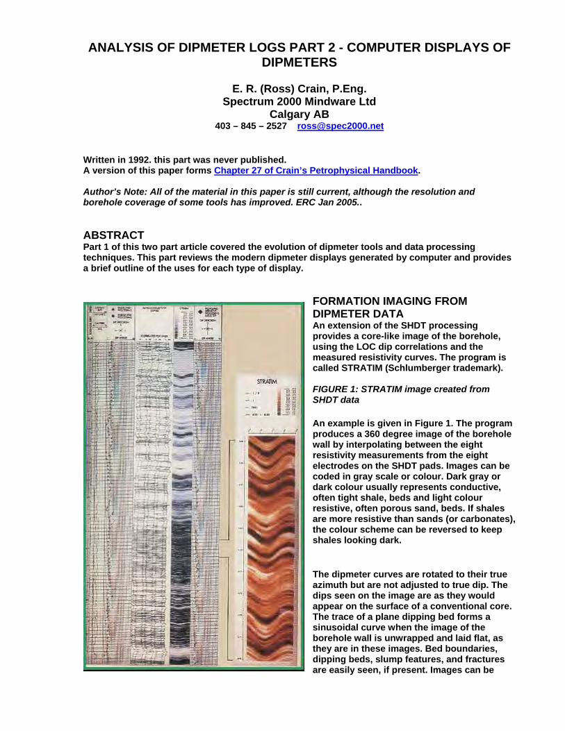
By using a mouse to digitize bedding planes such as the thin shale laminations and the boundaries of the limestone layer, the program fits a sine wave to the points. The sine wave represents a plane slicing through the borehole, and its dip and direction can be calculated. These are displayed on the right edge of the screen. It is obvious that the sine waves shown within the white (limestone) layer could not have been digitized from this image. In fact, the image scale was enlarged (Figure 7), then the colour scale was shifted (Figure 8) to provide greater resolution in the high resistivity band, turning previously bright colours into black, and white into distinguishable colours. Now the bedding planes can be digitized and dips computed.

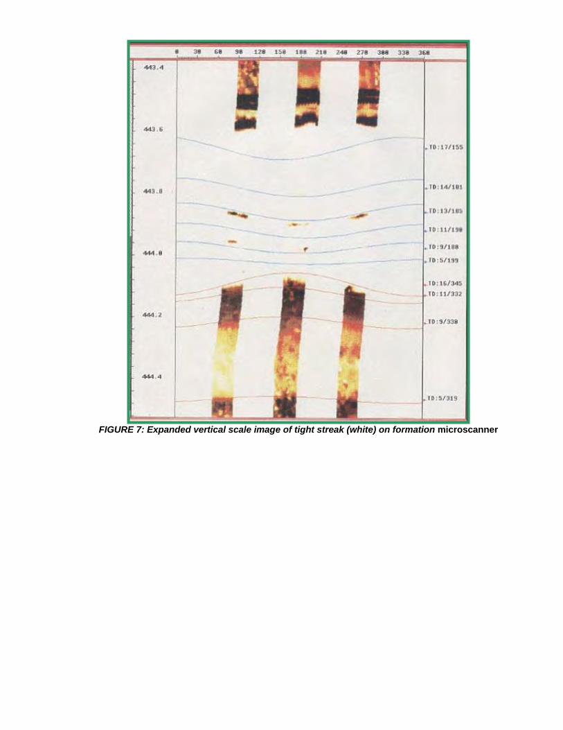
FIGURE 7: Expanded vertical scale image of tight streak (white) on formation microscanner

FIGURE 8: Expanded colour scale image of tight streak (light brown) on formation microscanner

Dips can also be computed automatically by the same methods as used for the stratigraphic high resolution dipmeter. MSD, CSB, LOC, FMS, and handpicked dips over the same interval are demonstrated in Figures 9 through 12. Each plot has entirely different dip results, emphasizing the need to understand the different dip calculation methods. In particular, the MSD dips in a strongly cross bedded formation suffer badly from the averaging calculation. Compare Figure 9 (MSD) with 10 (CSB). It is clear that MSD dips do not follow the bed boundaries very well and underestimate dip angle at the sand top and base by 7 to 10 degrees.

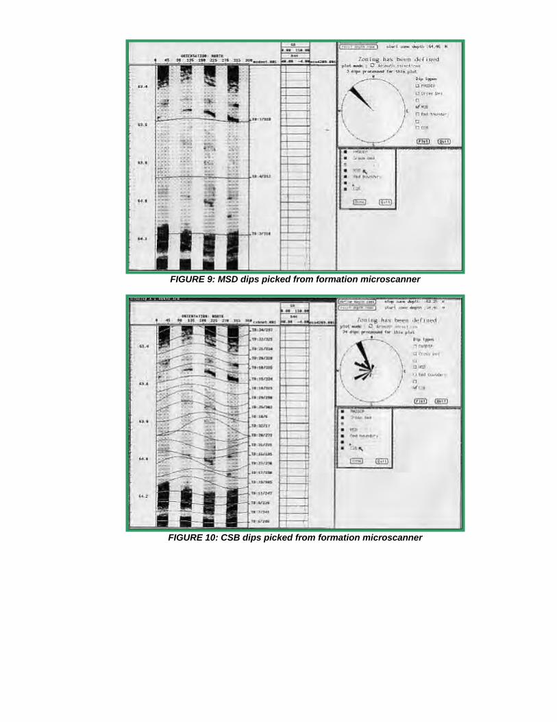
FIGURE 9: MSD dips picked from formation microscanner

FIGURE 10: CSB dips picked from formation microscanner

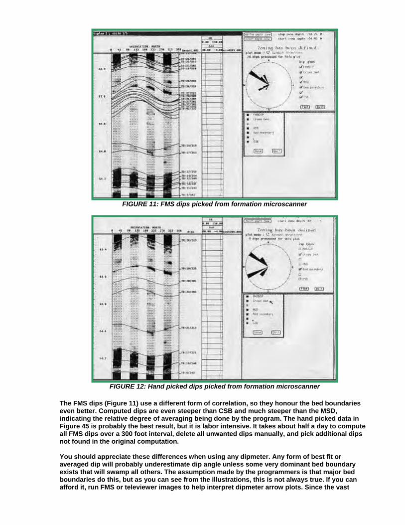
FIGURE 11: FMS dips picked from formation microscanner

FIGURE 12: Hand picked dips picked from formation microscanner

The FMS dips (Figure 11) use a different form of correlation, so they honour the bed boundaries even better. Computed dips are even steeper than CSB and much steeper than the MSD, indicating the relative degree of averaging being done by the program. The hand picked data in Figure 45 is probably the best result, but it is labor intensive. It takes about half a day to compute all FMS dips over a 300 foot interval, delete all unwanted dips manually, and pick additional dips not found in the original computation. You should appreciate these differences when using any dipmeter. Any form of best fit or averaged dip will probably underestimate dip angle unless some very dominant bed boundary exists that will swamp all others. The assumption made by the programmers is that major bed boundaries do this, but as you can see from the illustrations, this is not always true. If you can afford it, run FMS or televiewer images to help interpret dipmeter arrow plots. Since the vast

majority of existing dipmeters cannot be augmented by FMS, BEWARE of averaged results. The borehole televiewer, an ultrasonic borehole imaging tool, has much resolution than the dipmeter based imaging tools. As a result, only the largest dip and bedding features can be seen. It is used mostly for fracture identification and is discussed more fully in Chapter Twenty-Eight.

DIPMETER ADVISOR - AN EXPERT SYSTEM Schlumberger's DIPMETER ADVISOR system attempts to emulate human expert performance in dipmeter interpretation. It utilizes dipmeter patterns together with local geological knowledge and measurements from other logs. It is a typical example of the class of programs that deal with what has come to be known as signal to symbol transformation. The best description of the program appears in “The Dipmeter Advisor System”, IJCAI, 1983, by Reid Smith and James Baker. The system is made up of four central components: - a number of production rules partitioned into several distinct sets according to function (eg., structural rules vs stratigraphic rules). - an inference engine that applies rules in a forward-chained manner, resolving conflicts by rule order. - a set of feature detection algorithms that examines both dipmeter and open hole data (eg., to detect tadpole patterns and identify lithological zones). - a menu-driven graphical user interface that provides smooth scrolling of log data. There are 90 rules and the rule language uses approximately 30 predicates and functions. A sample is shown below, similar to an actual interpretation rule, but simplified somewhat for presentation: IF there exists a delta dominated, continental shelf marine zone AND there exists a sand zone intersecting the marine zone AND there exists a blue pattern within the intersection THEN assert a distributary fan zone WITH top = top of blue pattern WITH bottom = bottom blue pattern WITH flow = azimuth of blue pattern The system divides the task of dipmeter interpretation into 11 successive phases as shown below. After the system completes its analysis for a phase, it engages the human interpreter in an interactive dialogue. He can examine, delete, or modify conclusions reached by the system. He can also add his own conclusions. In addition, he can revert to earlier phases of the analysis to refer to the conclusions, or to rerun the computation. 1. initial examination: The human interpreter can view the available data and select logs for display. 2. validity check: The system compares log data with user defined criteria to find evidence of tool malfunction or incorrect processing. 3. green pattern detection: The system identifies zones in which the tadpoles have similar magnitude and azimuth. 4. structural dip analysis: The system merges and filters green patterns to determine zones of constant structural dip. *5. preliminary structural analysis: The system applies a set of rules to identify structural features (eg., faults). 6. structural pattern detection: The system examines the dipmeter data for red and blue patterns in the vicinity of structural features. *7. final structural analysis: The system applies a set of rules that combines information from previous phases to refine its conclusions about structural features (eg., strike of faults). 8. lithology analysis: The system examines the open hole data (eg., gamma ray) to determine zones of constant lithology (eg., sand and shale). *9. depositional environment analysis: The system applies a set of rules that draws conclusions about the depositional environment. For example, if told by the

human interpreter that the depositional environment is marine, the system attempts to infer the water depth at the time of deposition. 10. stratigraphic pattern detection: The system examines the dipmeter data for red, blue, and green patterns in zones of known depositional environment. *11. stratigraphic analysis: The system applies a set of rules that uses information from previous phases to draw conclusions about stratigraphic features (eg., channels, fans, bars). An asterisk indicates that the phase uses production rules written on the basis of interactions with an expert interpreter. The remaining phases do use rules, but these must be specified entirely by the user. A sample screen is shown in Figure 13.

FIGURE 13: A messy montage of Dipmeter Advisor screens

During the creation of these components, Schlumberger has developed a number of proprietary software tools for constructing expert systems. These include STROBE for definition of data representation, rule definition and rule integrity checking; IMPULSE for data entry to STROBE; XPLAIN for justifying and explaining rules and deductions; CRYSTAL for interactive display of data, graphics, window management on the screen, as well as task definition; and a relational data base manager. The tools are written in Interlisp-D on Xerox equipment, or Commonlisp and C on DEC VAX equipment. Some processing is done by a host computer which communicates with the Xerox workstation. The Dipmeter Advisor is in use within Schlumberger as a test-bed for further development and for some consulting/interpretation jobs. AUXILIARY DIPMETER PRESENTATIONS Dipmeter computation data are displayed graphically and in tabular form in many different formats, to facilitate interpretation. The standard output consists of a raw data plot, arrow plot, and numerical listings, many of which have been shown earlier in the discussion of tool and program theory. The balance are optional at extra cost. They are usually run only after evaluation of the standard output. 1. Stick Diagrams The cross section plot or stick diagram, is a two dimensional cross section representing the

dipping bedding planes at a pre-selected azimuth, as in Figure 14. It shows the apparent dip of each bedding plane as it would cross the borehole at the specified cross section azimuth. A common use is to establish the dip expected between a well with computed dipmeter information and a projected well close to the original well, or between two wells.

FIGURE 14: Stick diagram in steep regional dip - gamma ray (not shown) was used to aid

correlation

This allows the person using the plot to estimate the depth to particular horizons in the new well. Another use is in correlating formations from one well to another when both have dipmeter data. The ability to compute a stick diagram with apparent dip along any defined azimuth makes it easy to project formation tops from one well to another. The direction of the stick plot can also be presented parallel and/or perpendicular to a seismic line and the apparent dips compared with the dips observed on the seismic line. FIGURE 15: Cylindrical plot in complex cross bedding 2. Cylindrical Plots The cylindrical plot is a two-dimensional presentation that has the appearance of the borehole split along the south axis. When placed in a transparent cylinder, shown in Figure 15, the bedding planes appear as they would in an oriented core. The cylindrical plot is especially useful for locating the position of faults or major unconformities where these are reflected by a change in dip direction or magnitude. The STRATIM and DIPVUE images described earlier offer the same advantages.

3. Schmidt Plots The modified Schmidt diagram is used to determine structural dip when it is hard to find from the arrow plot. The paper is polar with North at the top. Dip magnitudes are represented by concentric circles. The plot is divided into cells at 1 degree magnitude and 10 degree azimuth; the dots are plotted for all dips computed. In some cells there may be no dots; in others, one dot; in still others, two or more dots. The plot can be generated by hand or by c The dots will fall into distinctive groupings or patterns, which be outlined by contour lines. Structural dip is an elongated pattern hugging the outer rim of the plot, possibly extending owide range of azimuths. The remaining dips (slope and cpatterns) will plot in rough triangles with their apexes pointing toward the center of thplot. A sam

omputer.

can

ver a

urrent

e ple is plotted in the

Figure 16.

FIGURE 16: Schmidt plot separates regional from stratigraphic dips

4. Azimuth Frequency Plots Azimuth frequency plots, often called rose diagrams, are plotted on polar coordinate paper with north at the top and 10 degree azimuth increments. The length of each 10 degree segment is proportional to the number of dips in the interval having that azimuth range, with zero frequency at the center. The result will be little fans originating at the center which may be composed of structural dip and current patterns, often at right angles to each other. There is no information in the azimuth frequency plot concerning the magnitude of dip. This information must come from other plots. Azimuth frequency diagrams are excellent tools for delineating bars, reefs, channels, and troughs. An illustrative example is shown in Figure 17, along with a schematic diagram of the channel represented by the frequency plots.

FIGURE 17: Azimuth frequency plots (rose diagrams) show preferential sedimentation directions

Figure 17 is, in fact, called a pattern azimuth frequency plot, because dips belonging to red and blue patterns (to be described later) are preserved and plotted separately. Blue patterns show direction of transport and red patterns show direction to the thicker sand. If plotted in black and white, as is the normal case, the lobes of the diagram are often still identifiable, as in Figure 18 (right hand side).

FIGURE 18: Rose diagrams on FMS Image Examiner

The arrow plot presented to the customer contains azimuth frequency plots generated for each 100 ft. interval or other regular interval as designated by the analyst. These plots are used for general information concerning the direction of dip for each interval of the computed analysis. Additional computer generated azimuth frequency plots can be run over specific zones which have a particular geologic significance. These zones can be the upper and lower boundaries of a formation, the zone between two faults, the zone between a fault and an unconformity or any other breakdown which is indicated by knowledge of the local geology or interpretation of the dipmeter data itself. With the advent of interactive computer programs, decisions on what to plot can be made as processing and analysis take place. An example is shown in Figure 51, using the FMS Image Examiner program. 5. Regional Dip Removal Plots If structural dip is greater than three or four degrees, it should be vectorally subtracted from the dips by the computer, leaving the absolute current and slope pattern dips. This provides better definition of stratigraphic dips, as plotted in Figure 19. The effect can be quite dramatic, and some events may appear after dip subtraction that were not noticed before.

FIGURE 19: Regional dip removal changes the dip patterns, making sedimentary interpretation

easier

All the above plots are available in a hands-on mode when using Schlumberger's Dipmeter Advisor, and most are available on the Atlas Wireline DIPVUE program.

SYNTHETIC DIPMETER CURVES One of the problems associated with high resolution and stratigraphic dipmeter results is the sheer volume of data. It is difficult to review, let alone use, all the answers provided. Therefore a systematic analysis procedure is as necessary here as it is for other open hole logs. A computer program to facilitate this procedure is available from Schlumberger, called SYNDIP. It is presented here as an illustration of what can be done. You could invent your own presentation to summarize your data set. The description below was extracted from “Uses of Dipmeter Synthetic Curves” by Eric Standen, Trans CWLS, 1985.

SYNDIP was developed to quantify and display synthetic curves calculated from the dipmeter resistivity and computed dip data. This program calculates up to seventeen variables, some of which are displayed to present are In most cases, the Local Dip (pattern recognition) computation is used for the necessary input dip data. If a Local Dip answer file is not available, the Syndip program will still run; howevth The program attempts to identify units of different bedding characteristics and therefore different depositional environments. It also tries to describe the overall sequence trends which would help in the interpretation of the dipmeter. It does this by looking at things that a human would look such as correlation curve activity, resistivity trends, dip planar(both magnitude and direction), and similar visually apparent anomalies. These results are plotted as continuous curves or as individual coded symbols. To

geologic description of the formations in terms of bedding and lative grain size information.

er, some of e synthetic curves will be missing since they are computed from Local Dip results.

at, ity, dip parallelism, dip scatter

visualize the following description, refer to Figure 20 (in colour) and Figure 21 (in black and white).

FIGURE 20: Output plot for pattern recognition dip program SYNDIP

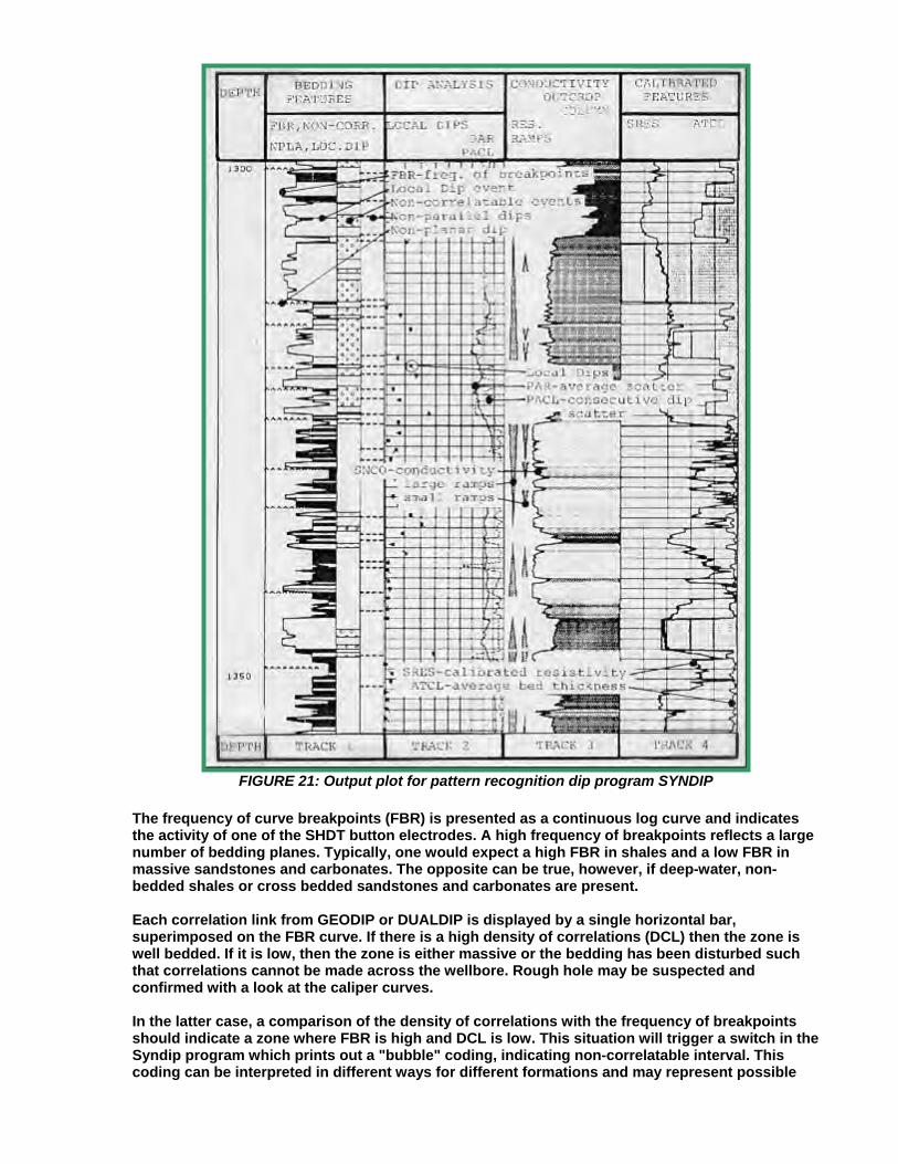
FIGURE 21: Output plot for pattern recognition dip program SYNDIP

The frequency of curve breakpoints (FBR) is presented as a continuous log curve and indicates the activity of one of the SHDT button electrodes. A high frequency of breakpoints reflects a large number of bedding planes. Typically, one would expect a high FBR in shales and a low FBR in massive sandstones and carbonates. The opposite can be true, however, if deep-water, non-bedded shales or cross bedded sandstones and carbonates are present. Each correlation link from GEODIP or DUALDIP is displayed by a single horizontal bar, superimposed on the FBR curve. If there is a high density of correlations (DCL) then the zone is well bedded. If it is low, then the zone is either massive or the bedding has been disturbed such that correlations cannot be made across the wellbore. Rough hole may be suspected and confirmed with a look at the caliper curves. In the latter case, a comparison of the density of correlations with the frequency of breakpoints should indicate a zone where FBR is high and DCL is low. This situation will trigger a switch in the Syndip program which prints out a "bubble" coding, indicating non-correlatable interval. This coding can be interpreted in different ways for different formations and may represent possible

bioturbation, brecciation, or distortion of bedding in the zone. The non-planarity flag is triggered when the Local Dip computation falls below a preset planarity criterion. In general this reflects curved bedding surfaces in the well bore which may indicate erosional events or scour surfaces. The tolerance on this flag is set fairly high so that only significant breaks are detected. Non-planarity is shown as a jiggly line superimposed on the NBR curve. The non-parallelism flag is an indication that consecutive beds are different in dip magnitude by ten degrees or more. The implication is that there is some depositional or structural break, often caused by cross bedding sequences. It is plotted as a short dashed line beside the non-correlated interval bubbles. All of this information is plotted in the left hand track of the log. Local dips are plotted in the next track along with two other parameters, the average dip scatter (PAR) and consecutive dip scatter (PACL). The average dip scatter (PAR) is actually the dip spherical standard deviation on a polar plot of the dip data. Within a window of length (usually five meters) an average dip magnitude variation is computed and displayed on a reverse scale to the dip plot. High dip scatter suggests a high energy of deposition as opposed to a low dip magnitude scatter in low energy zones. The dip angle between consecutive correlation links (PACL) will track with PAR but will usually show more variation since it is looking at consecutive correlation links and not an average. PACL will also reflect energy of deposition which can be analyzed for any structural tilting of the formations. In track three, a normalized micro-conductivity curve (SNCO) forms the outline for the outcrop-like column and is derived from the button electrodes. The program takes the resistivity values and scales them from 0 (high resistivity) to 100 (low resistivity) taking into account the automatic voltage changes that were applied to the tool during logging. The program can also function and display the curve as an SHDT fast channel conductivity, linear conductivity, or logarithmic resistivity. The colour or gray scale which is used to shade the curve area uses light colours for high resistivity and dark colours for low resistivity. These can be tuned to create a realistic image of the formation layers. By inference, the presentation defines shales as being low resistivity zones and clean sandstone and carbonate as high resistivity. Should the opposite be the case, a switch in the program will allow a reversal of the presentation. In addition to the outcrop presentation, fining upward and coarsening upward trends are inferred from the resistivity curve values. These are shown as large or small scale ramps beside the outcrop curve. These cycles are derived from the SNCO curve and are simply gradients on the curve which fall within certain parameters of slope, maximum resistivity change, and minimum length. As with the SNCO curve, the ramps can be reversed in the case of low resistivity (relative to shale), coarse grained formations. The same logic is used for short ramps as for the large ramps except that the parameters are selected to limit the size of the small ramps. Resistivity ramps are used to estimate grain size variations. When the grain size of the rock decreases, the volume of water (both irreducible and bound to the clays) increases, with a corresponding decrease in resistivity. The large ramps are designed to reflect large scale features and should terminate at major depositional boundaries. Within these large scale ramps several small ramps may be present which may or may not agree with the major trend. This is a function of the depositional environment. Likewise, the ramp trends of Syndip may disagree with other information or log data such as gamma ray logs. This situation does not indicate an error in the program or any log; it is probably just a unique character of that formation, for example a radioactive sand or variations in amount of cementing or overgrowth. In track four is a calibrated, reconstructed resistivity curve (SRES) and the average bed thickness curve (ATCL). SRES is calibrated to an open hole spherically focused log or a shallow laterolog. This curve has much finer resolution than the curve to which it is calibrated.

The apparent thickness between consecutive correlation links (ATCL) is displayed on the log and is used as an indication of well bedded versus poorly bedded zones. The curve can also be used to quantify the thickness of the individual beds. If a zone is known to contain thin beds, procedures should be adopted to increase the sample rate of certain logging tools or modify the interpretation program for better thin bed resolution. For reservoir development, knowledge that a zone contains thin laminations may allow completion closer to a water leg since more vertical permeability barriers exist. Conversely, a massive zone would suggest higher vertical permeability. The analysis aids provided by the SYNDIP concept make it easier for the analyst to figure out the structure and stratigraphy in a well. The analyst is still stuck with the problem of choosing which interpretation is most reasonable based on the available data. A program which helps do this, the Dipmeter Advisor, is discussed later in this Chapter.

DIPMETER CALCULATIONS Although it is seldom done anymore, manual dipmeter calculations with a scientific calculator is quite practical and instructive. The technique given below was presented by R. Bateman and C. Konen in "The Log Analyst and the Programmable Calculator" in The Log Analyst, Jan 1978. The method is based on hand measurements of curve offsets from the raw dipmeter curves and readings from the hole direction data. These equations are for the four arm dipmeter and ignore closure and planarity errors. The position of the angles in space is shown in Figure 22.

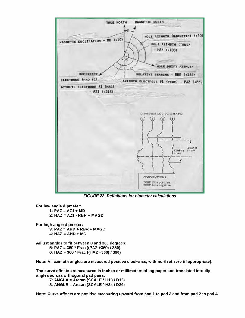
FIGURE 22: Definitions for dipmeter calculations

For low angle dipmeter: 1: PAZ = AZ1 + MD 2: HAZ = AZ1 - RBR + MAGD For high angle dipmeter: 3: PAZ = AHD + RBR + MAGD 4: HAZ = AHD + MD Adjust angles to fit between 0 and 360 degrees: 5: PAZ = 360 * Frac ((PAZ +360) / 360) 6: HAZ = 360 * Frac ((HAZ +360) / 360) Note: All azimuth angles are measured positive clockwise, with north at zero (if appropriate). The curve offsets are measured in inches or millimeters of log paper and translated into dip angles across orthogonal pad pairs: 7: ANGLA = Arctan (SCALE * H13 / D13) 8: ANGLB = Arctan (SCALE * H24 / D24) Note: Curve offsets are positive measuring upward from pad 1 to pad 3 and from pad 2 to pad 4.

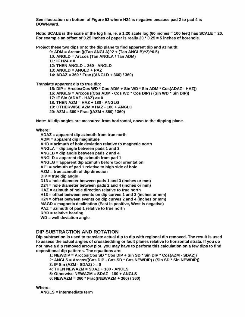
See illustration on bottom of Figure 53 where H24 is negative because pad 2 to pad 4 is DOWNward. Note: SCALE is the scale of the log film, ie. a 1:20 scale log (60 inches = 100 feet) has SCALE = 20. For example an offset of 0.25 inches of paper is really 20 * 0.25 = 5 inches of borehole. Project these two dips onto the dip plane to find apparent dip and azimuth: 9: ADM = Arctan (((Tan ANGLA)^2 + (Tan ANGLB)^2)^0.5) 10: ANGLD = Arccos (Tan ANGLA / Tan ADM) 11: IF H24 < 0 12: THEN ANGLD = 360 - ANGLD 13: ANGLD = ANGLD + PAZ 14: ADAZ = 360 * Frac ((ANGLD + 360) / 360) Translate apparent dip to true dip: 15: DIP = Arccos(Cos WD * Cos ADM + Sin WD * Sin ADM * Cos(ADAZ - HAZ)) 16: ANGLG = Arccos ((Cos ADM - Cos WD * Cos DIP) / (Sin WD * Sin DIP)) 17: IF Sin (ADAZ - HAZ) >= 0 18: THEN AZM = HAZ + 180 - ANGLG 19: OTHERWISE AZM = HAZ - 180 + ANGLG 20: AZM = 360 * Frac ((AZM + 360) / 360) Note: All dip angles are measured from horizontal, down to the dipping plane. Where: ADAZ = apparent dip azimuth from true north ADM = apparent dip magnitude AHD = azimuth of hole deviation relative to magnetic north ANGLA = dip angle between pads 1 and 3 ANGLB = dip angle between pads 2 and 4 ANGLD = apparent dip azimuth from pad 1 ANGLG = apparent dip azimuth before tool orientation AZ1 = azimuth of pad 1 relative to high side of hole AZM = true azimuth of dip direction DIP = true dip angle D13 = hole diameter between pads 1 and 3 (inches or mm) D24 = hole diameter between pads 2 and 4 (inches or mm) HAZ = azimuth of hole direction relative to true north H13 = offset between events on dip curves 1 and 3 (inches or mm) H24 = offset between events on dip curves 2 and 4 (inches or mm) MAGD = magnetic declination (East is positive, West is negative) PAZ = azimuth of pad 1 relative to true north RBR = relative bearing WD = well deviation angle DIP SUBTRACTION AND ROTATION Dip subtraction is used to translate actual dip to dip with regional dip removed. The result is used to assess the actual angles of crossbedding or fault planes relative to horizontal strata. If you do not have a dip removed arrow plot, you may have to perform this calculation on a few dips to find depositional dip patterns. The equations are: 1: NEWDIP = Arccos(Cos SD * Cos DIP + Sin SD * Sin DIP * Cos(AZM - SDAZ)) 2: ANGLS = Arccos((Cos DIP - Cos SD * Cos NEWDIP) / (Sin SD * Sin NEWDIP)) 3: IF Sin (AZM - SDAZ) >= 0 4: THEN NEWAZM = SDAZ + 180 - ANGLS 5: Otherwise NEWAZM = SDAZ - 180 + ANGLS 6: NEWAZM = 360 * Frac((NEWAZM + 360) / 360) Where: ANGLS = intermediate term

AZM = true dip azimuth before structural dip removal DIP = true dip angle before structural dip removal NEWDIP = dip after structural dip removal NEWAZM = azimuth after structural dip removal SD = structural (regional) dip to remove SDAZ = azimuth of structural dip It is sometimes necessary or desirable to project the actual dip onto a new azimuth. This is sometimes called dip rotation. This is used to prepare dips for presentation on a stick diagram at arbitrary cross section orientations, such as the line of section between two wells or along the section of a seismic line. The equation is: 1: PROJDIP = Arctan (Tan DIP * Cos (PROJAZM - AZM)) Where: AZM = true dip azimuth before rotation DIP = true dip angle before rotation PROJDIP = projected dip PROJAZM = projected azimuth TRUE STRATIGRAPHIC AND TRUE VERTICAL THICKNESS True stratigraphic and true vertical thickness are important in dipping beds and in deviated holes, since reservoir volume depends on these properties and not the measured thickness. The formulas are documented in "The Log Analyst and the Programmable Calculator" by R. Bateman and C. Konen in The Log Analyst, Mar 1979. Definitions of the terms are illustrated in Figure 23.

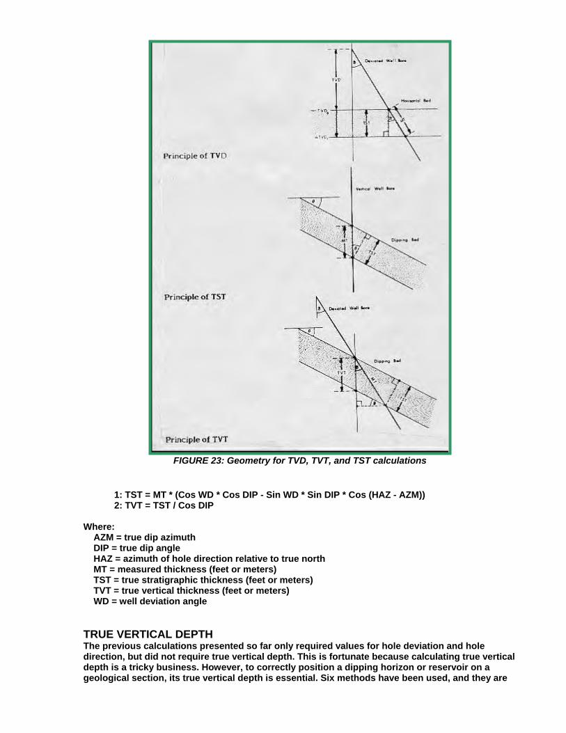
FIGURE 23: Geometry for TVD, TVT, and TST calculations

1: TST = MT * (Cos WD * Cos DIP - Sin WD * Sin DIP * Cos (HAZ - AZM)) 2: TVT = TST / Cos DIP Where: AZM = true dip azimuth DIP = true dip angle HAZ = azimuth of hole direction relative to true north MT = measured thickness (feet or meters) TST = true stratigraphic thickness (feet or meters) TVT = true vertical thickness (feet or meters) WD = well deviation angle TRUE VERTICAL DEPTH The previous calculations presented so far only required values for hole deviation and hole direction, but did not require true vertical depth. This is fortunate because calculating true vertical depth is a tricky business. However, to correctly position a dipping horizon or reservoir on a geological section, its true vertical depth is essential. Six methods have been used, and they are

presented below in ascending order of preference and also complexity. This material was presented in Petroleum Engineer, March 1976, by J.T. Craig and B.V. Randall in "Directional Survey Calculations". 1. Tangential Method The tangential method uses only the inclination and direction angles measured at the lower end of the survey course length. The well bore path is assumed to be a straight line throughout the course. This method has probably been used more than any other and is the least accurate. It makes the well appear too shallow and the lateral displacement too large. In a typical deviated well, the true vertical depth can be wrong by more than 50 feet. It has been used and perpetuated because of its inherent simplicity of hand calculation. Calculating the survey by the tangential method, however, is no longer justifiable because programmable calculators and field portable computers make the better methods just as easy as this one. This method is not recommended any time in any well. However, many such surveys are in the well files and many true vertical depths have been used, and may still be accepted, based on this erroneous data. All that is needed for a re-computation using better methods is the raw inclination and direction data, and this is usually available. Re-computation is strongly recommended. If surveys were taken at approximately 1 ft. intervals, the error would be tolerable, but this frequency cannot be economically justified with typical single shot surveys. However, this frequency of measurement is achieved with continuous directional surveys run with the dipmeter. If computations are made at short intervals, then the tangential method works fine. Most station by station surveys are taken at much larger intervals, such as a few to several hundred feet apart, and therefore the results are inaccurate. If the dipmeter program calculates vertical depth at similar intervals, it is also inadequate. The formula are: 1: North = SUM ((MD2 - MD1) * Sin WD2 * Cos HAZ2) 2: East = SUM ((MD2 - MD1) * Sin WD2 * Sin HAZ2) 3: TVD = SUM ((MD2 - MD1) * Cos WD2) NOTE: This is the high tangential method. If WD1 and HAZ1 replace WD2 and HAZ2, it is the low tangential method. Where: East = easterly displacement (feet or meters) - negative = West HAZ1 = hole azimuth at top of course (degrees) HAZ2 = hole azimuth at bottom of course (degrees) MD1 = measured depth at top of course (feet or meters) MD2 = measured depth at bottom of course (feet or meters) North = northerly displacement (feet or meters) - negative = South TVD = true vertical depth (feet or meters) WD1 = well deviation at top of course (degrees) WD2 = well deviation at bottom of course (degrees) 2. Average Tangential Method The angle averaging method uses the angles measured at both the top and bottom of the course length in such a fashion that the simple average of the two sets of measured angles is assumed to be the inclination and the direction. The wellbore then is calculated tangentially using these two average angles over the course length. This method is a very simple, and more accurate, means of calculating a wellbore survey. 1: North = SUM ((MD2 - MD1) * Sin ((WD2 + WD1) / 2) * Cos ((HAZ2 + HAZ1) / 2)) 2: East = SUM ((MD2 - MD1) * Sin ((WD2 + WD1) / 2) * Sin ((HAZ2 + HAZ1) / 2)) 3: TVD = SUM ((MD2 - MD1) * Cos ((WD2 + WD1) / 2)) 3. Balanced Tangential Method The balanced tangential method uses the inclination and direction angles at the top and bottom of

the course length to tangentially balance the two sets of measured angles. This method combines the trigonometric functions to provide the average inclination and direction angles which are used in standard computational procedures. The values of the inclination at WD2 and WD1 are combined in the proper sine-cosine functions and averaged. This method did not lend itself to hand calculations in the early days, but modern programmable scientific calculators make the job easy. This technique provides a smoother curve which should more closely approximate the actual wellbore between surveys. The longer the distance between survey stations, the greater the possibility of error. The formula are: 1: North = SUM (MD2 - MD1) * ((Sin WD1 * Cos HAZ1 + Sin WD2 * Cos HAZ2) / 2) 2: East = SUM (MD2 - MD1) * ((Sin WD1 * Sin HAZ1 + Sin WD2 * Sin HAZ2) / 2) 3: TVD = SUM ((MD2 - MD1) * (Cos WD2 + Cos WD1) / 2) 4. Mercury Method The mercury method is a combination of the tangential and the balanced tangential method that treats that portion of the measured course defined by the length of the measuring tool in a straight line (tangentially) and the remainder of the measured course in a balanced tangential manner. The name of the mercury method originated from its common usage at the Mercury, Nevada test site by the US Government. 1: North = SUM ((MD2 - MD1 - STL)*((Sin WD1 * Cos HAZ1 + Sin WD2 * Cos HAZ2)/2) + STL * Sin WD2 * Cos HAZ2) 2: East = SUM ((MD2 - MD1 - STL) * ((Sin WD1 * Sin HAZ1 + Sin WD2 * Sin HAZ2) / 2) + STL * Sin WD2 * Sin HAZ2) 3: TVD = SUM (((MD2 - MD1 - STL) * (Cos WD2 + Cos WD1) / 2) + STL * Cos HAZ2) Where: STL is the length of the survey tool 5. Radius of Curvature Method The radius of curvature method uses sets of angles measured at the top and bottom of the course length to generate a space curve (representing the wellbore path) that has the shape of a spherical arc passing through the measured angles at both the upper and lower ends of the measured course. This method is one of the more accurate means of determining the position of a wellbore when survey spacing is sparse. The assumption that the wellbore is a smooth curve between surveys makes this method less sensitive to placement and distances between the survey points than other methods. CAUTION: It is a terrible method when data is closely spaced, as the subtractions in the equation create either "divide by zero errors" or an incorrect TVD when the borehole is a straight line but deviated. 1: North = SUM (MD2 - MD1) * (Cos WD1 - Cos WD2) * (Sin HAZ2 - Sin HAZ1) / ((WD2 - WD1) * (HAZ2 - HAZ1)) 2: East = SUM (MD2 - MD1) * (Cos WD1 - Cos WD2) * (Cos HAZ1 - Cos HAZ2) / ((WD2 - WD1) * (HAZ2 - HAZ1)} 3: TVD = SUM (MD2 - MD1) * (Sin WD2 - Sin WD1) / (WD2 - WD1) 6. Minimum Curvature Method The minimum curvature method, like the radius of curvature method, takes the space vectors defined by inclination and direction measurements and smoothes these onto the wellbore curve by the use of a ratio factor which is defined by the curvature (dog-leg) of the wellbore section. The method produces a circular arc as does the radius of the curvature. This is not, however, an assumption of the method, but a result of minimizing the total curvature within the physical constraints on a section of wellbore. 1: DL = Arccos (Cos (WD2 - WD1) - Sin WD1 * Sin WD2 * (1 - Cos (HAZ2 - HAZ1))) 2: CF = 2 / DL * (Tan (DL / 2)) 3: North = SUM ((MD2 - MD1)*((Sin WD1 * Cos HAZ1 + Sin WD2 * Cos HAZ2) / 2) * CF) 4: East = SUM ((MD2 - MD1) * ((Sin WD1 * Sin HAZ1 + Sin WD2 * Sin HAZ2) / 2) * CF) 5: TVD = SUM (((MD2 - MD1) * (Cos WD2 * Cos WD1) / 2) * CF)

Where: DL = dog leg severity (degrees) CF = curvature factor CONCLUSIONS The evolution of the dipmeter over the last 60 years has created a wealth of variety in the data acquisition methods, presentation styles, and computation methods. The uses have remained constant: to define structural and stratigraphic features of sedimentary rocks. Numerous techniques to aid the analyst have been presented; each individual must choose the one best suited to the problem to be solved. Although dipmeter analysis can be ambiguous, sufficient geological constraints, local knowledge, and experience serve to improve skills and speed analysis. Modern computer processing, in particular dip removed arrow plots and stick plots, are essential ingredients. Image processing techniques, while relatively new, have proven useful because of their visual impact. However, the analysis of structure and stratigraphy from dipmeter data still depends on the basics: dip angle, dip direction, and a plausible model that fits the data. BIBLIOGRAPHY Dipmeter Processing 1: Automatic computation of dipmeter logs digitally recorded of magnetic tapes; Moran,J.H., Coufleau,M.A., Miller,G.K., Timmons,J.P.; 36th Annual Technical Meeting Society of Petroleum Engineers American Institute of Mining Metallurgical Engineers, 19 p., 1961 2: Supplementary computer programs for dipmeter analysis; Matthews,R.R., Mooney,T.D., Haynie,R.B., Albright,J.C.; Society of Professional Well Log Analysts, 19 p., 1965 3: An accurate method of low angle dip calculation; Schoonover,L.G.; Society of Professional Well Log Analysts 14th Annual Logging Symposium, 15 p., 1973 4: Computer recognition of diplog patterns a tool for stratigraphic analysis; Schoonover,L.G.; Society of Professional Well Log Analysts 15th Annual Logging Symposium, 12 p., 1974 5: Cluster: a method for selecting the most probable dip results from dipmeter surveys; Hepp,V., Dumestre,A.C.; 50th Annual Technical Meeting of Society of Petroleum Engineers of American Institute of Mining Metallurgical Engineers, SPE 5543, 1975 6: Geodip: an approach to detailed dip determination using correlation by pattern recognition; Vincent,Ph., Gartner,J.E., Attali,G.; 52nd Annual Technical Meeting of Society of Petroleum Engineers of American Institute of Mining Metallurgical Engineers, SPE 6823, 1977 7: True vertical depth, true vertical thickness and true stratigraphic thickness logs; Holt,O.R., Schoonover,L.G., Wichmann,P.A.; Society of Professional Well Log Analysts 18th Annual Logging Symposium, 19 p., 1977 8: The log analyst and the programmable pocket calculator; Bateman,R.M., Konen,C.E.; Society of Professional Well Log Analysts: The Log Analyst, p. 3-9, 1978 9: A simplified true vertical thickness (TVT) calculation using a programmable pocket calculator; Smith,S.W., Keen,D.; Society of Professional Well Log Analysts: The Log Analyst, p. 28-32, 1979 10: Formation dip determination - an artificial intelligence approach; Kerzner,M.G.; Society of Professional Well Log Analysts: The Log Analyst, p. 10-22, 1983 11: SHIVA processing: the integration of fundamental geological principles with dipmeter

computations; Enderlin,M.B., Epps,D.S., Yuratich,M.A.; Society of Professional Well Log Analysts: The Log Analyst, 22 p., 1985 12: Effect of tool rotation on the computation of dip; Waid,C.C.; Society of Professional Well Log Analysts 28th Annual Logging Symposium, 22 p., 1987 13: A rule based approach to dipmeter processing; Kerzner,M.G.; 63rd Annual Technical Conference of Society of Petroleum Engineers, p. 239-251, 1988 14: Dipvue analysis package; Atlas Wireline; Brochure, 1 p, 1988 15: The effects of noise on interval correlation methods; part 1: accuracy and precision; Waid,C.C., Faraguna,J.K., Easton,S.B.; 63rd Annual Technical Conference of Society of Petroleum Engineers, p. 227-238, 1988 Directional Surveys 1: Radius of curvature method for computing directional surveys; Wilson,G.J.; Society of Professional Well Log Analysts 9th Annual Logging Symposium, p. 1-11, 1968 2: Surwel gyroscopic directional surveys; Sperry Sun; Catalogue, 20 p., 1970 3: Computing accurate directional surveys; Blythe,E.J.,Jr.; World Oil, p. 25-28, 1975 4: Model gives accurate wellbore displacement; Guillory,C. Jr.; The Oil and Gas Journal, p. 138-141, 1975 5: Gyro technics; Slusarchuk,L.M.; Schlumberger, 53 p, 1976 6: Directional survey calculation; Craig,J.T.,Jr., Randall,B.V.; Petroleum Engineer, p. 38-54, 1976 7: Surface recording gyroscope system saves rig time; Guillory,C.,Jr.; The Oil and Gas Journal, p. 186-192, 1978 8: On site computer helps speed directional survey analysis; Kipcheff,J.T.,Honeybourne,J.W.G., Penny,S.J.; The Oil and Gas Journal, p. 79-86, 1978 9: Survey procedures prepared for Panarctic Oils Ltd; Sperry Sun, 13 p., 1979 10: Directional survey calculation methods compared and programmed; Callas,N.P., Novak,P.C., Henderson,J.R.; The Oil and Gas Journal, p. 53-58, 1979 11: Programs enhance directional drilling; VanDusen,M.D., Stephens,H.D.; World Oil, p. 103-106, 1979 12: Graphs give thickness in deviated wells; Travis,R.B.; The Oil and Gas Journal, p. 87-94, 1979 13: How to avoid gyro misruns; Plite,J., Bount,S.; The Oil and Gas Journal, p.109-117, 1980 14: Directional drilling technology strives for speed and accuracy; Enenback,J.H.; Petroleum Engineer International, p. 124-132, 1980 15: Directional drilling information is refined by computer at SDI facilities; Ibbotson,G.; The Journal of Canadian Petroleum Technology, p. 35-36, 1981 16: Randomly simulated borehole tests accuracy of directional survey methods; Fitchard,E.E.; The Oil and Gas Journal, p. 140-150, 1981 17: Use of magnetic ranging logging tool to direct Amoco et al Steep A7-28-66-7W26M drilling; Duguid,A.T.; 33rd Annual Technical Meeting of Petroleum Society of Canadian Institute of Mining, 13 p., 1982

18: Use well logs to find proximity of relief wells to blowouts; Baldwin,W.F.; World Oil, p. 67-69, 1983

ABOUT THE AUTHOR

Mr Crain is a Professional Engineer with over 35 years of experience in reservoir description, petrophysical analysis, and management. He has been a specialist in the integration of well log analysis and petrophysics with geophysical, geological, engineering, and simulation phases of oil and gas exploration and exploitation, with widespread Canadian and Overseas experience. He has an Engineering degree from McGill University in Montral and is a registered engineer in Alberta. He wrote “The Log Analysis Handbook”, published by Pennwell, and offers seminars, mentoring, or petrophysical consulting to oil companies, government agencies, and consulting service companies around the world. Ross is credited with the invention of the first desktop log analysis system (LOG/MATE) in 1976, 5 years before IBM invented the PC. He continues to advise and train people on softwadesign, implementation, and training. For his

consulting practice, he uses his own proprietary software (META/LOG), and is familiar with most commercia

re

l systems. He has won Best Paper Awards from CWLS and CSEG and has authored more than 30 technical papers. He is currently building an Interactive Learning Center for petrophysics on the World Wide Web. Mr Crain was installed as an Honourary Member of the Canadian Well Logging Society for his contributions to the science of well log analysis.