Analysis of Design Alternatives of Sörredskorsningen A road intersection in Gothenburg Master of Science Thesis in the Master’s Programme Geo and Water Engineering SAAD NUSRULLAH MIRZA SYED DANIAL ALI Department of Civil and Environmental Engineering Division of GeoEngineering Road and Traffic Research Group CHALMERS UNIVERSITY OF TECHNOLOGY Göteborg, Sweden 2012 Master‟s Thesis 2012:10

Welcome message from author
This document is posted to help you gain knowledge. Please leave a comment to let me know what you think about it! Share it to your friends and learn new things together.
Transcript

Analysis of Design Alternatives of
Sörredskorsningen
A road intersection in Gothenburg
Master of Science Thesis in the Master’s Programme Geo and Water Engineering
SAAD NUSRULLAH MIRZA
SYED DANIAL ALI
Department of Civil and Environmental Engineering
Division of GeoEngineering
Road and Traffic Research Group
CHALMERS UNIVERSITY OF TECHNOLOGY
Göteborg, Sweden 2012
Master‟s Thesis 2012:10


MASTER‟S THESIS 2012:10
Analysis of Design Alternatives of
Sörredskorsningen
A road intersection in Gothenburg
Master of Science Thesis in the Master’s Programme Geo and Water Engineering
SAAD NUSRULLAH MIRZA
SYED DANIAL ALI
Department of Civil and Environmental Engineering
Division of GeoEngineering
Road and Traffic Research Group
CHALMERS UNIVERSITY OF TECHNOLOGY
Göteborg, Sweden 2012

Analysis of Design Alternatives of Sörredskorsningen
A road intersection in Gothenburg
Master of Science Thesis in the Master’s Programme Geo and Water Engineering
SAAD NUSRULLAH MIRZA
SYED DANIAL ALI
© SAAD NUSRULLAH MIRZA & SYED DANIAL ALI, 2012
Examensarbete / Institutionen för bygg- och miljöteknik,
Chalmers tekniska högskola 2012:10
Department of Civil and Environmental Engineering
Division of GeoEngineering
Road and Traffic Research Group
Chalmers University of Technology
SE-412 96 Göteborg
Sweden
Telephone: + 46 (0)31-772 1000
Chalmers Reproservice / Department of Civil and Environmental Engineering
Göteborg, Sweden 2012
I
Analysis of Design Alternatives of Sörredskorsningen
A road intersection in Gothenburg
Master of Science Thesis in the Master’s Programme Geo and Water Engineering
SAAD NUSRULLAH MIRZA
SYED DANIAL ALI Department of Civil and Environmental Engineering
Division of GeoEngineering
Road and Traffic Research Group
Chalmers University of Technology
ABSTRACT
The growth of versatile traffic on a yearly basis in the city of Göteborg requires
proper planning and measurements to avoid accidents and congestions at the
intersections in the future. Hence, the traffic authorities are working on projects like
K2020 aiming to develop the public transport and Vision Zero project targeting no
serious injuries in the traffic environment in Gothenburg.
The topic of this thesis is to evaluate and predict traffic congestion situation at Sörreds
intersection located in the vicinity of the Volvo area. Moreover, this work is aimed to
predict the congestion situation at Sörreds intersection. Two alternatives were
proposed by SWECO with the possibility of building a ring road either at
Sörredsvägen or at Road-155 i.e. Torslandavägen, as there is a forecast of 200%
increase in traffic at the junction by 2035. In this thesis, a discussion is made in order
to select the more feasible alternative out of them.
The case study has been performed using German traffic simulation software,
VISSIM. VISSIM has been used to represent the actual situation of the traffic for the
Sörreds intersection by considering the present scenario as well as future scenario of
the intersection. For the purpose, different microscopic simulation models were
created to resolve the congestion issue at Sörreds intersection, including simulation
models for the actual situation supported by VISSIM. Also simulation of the same
model with future vehicular input has been checked to justify whether a ring-
road/flyover is needed or not.
Finally, the comparisons of alternatives made by SWECO has discussed in the last
part. The results gained by both comparisons are debated to give a good decision.
Further studies are recommended because of certain limitations of this study in terms
of limited data availability for the particular junction.
Key words: VISSIM, VisVAP, LHROVA technique, traffic volumes, simulation
model, signalized intersection, signal control, performance measure.

II

CHALMERS Civil and Environmental Engineering, Master‟s Thesis 2012:10 III
Contents
ABSTRACT I
CONTENTS III
PREFACE VII
GLOSSARY VIII
DEFINITION VIII
1 INTRODUCTION 1
1.1 Background 1
1.2 Aim of the study 4
1.3 Method of the study 4
1.4 Limitations of the study 5
2 LITERATURE REVIEW 6
2.1 Intersection design and capacity 6
2.2 Volume studies and characteristics 9 2.2.1 Volume calculation periods 9
2.2.2 Techniques for volume studies 11
2.3 Signal control at the intersection 12
2.3.1 Signal phase design 13 2.3.2 Actuated signal control 14 2.3.3 Detectors 15
2.3.4 Dilemma zone 17
2.3.5 LHOVRA technique 19
2.4 Performance measures 23 2.4.1 Travel time and delays 24 2.4.2 Queue counters 24
3 METHODOLOGY 25
3.1 Site description 25
3.2 Data collection methods 26 3.2.1 Manual and video counting 26 3.2.2 Site drawings provided by SWECO 27
3.3 Use of VISSIM 27
3.4 Model construction 28
3.5. Data input 28 3.5.1 Car following model 28 3.5.2 Technical specification of vehicles 29 3.5.3 Pedestrian data input 31
3.6 Signal timing parameters 31

CHALMERS, Civil and Environmental Engineering, Master‟s Thesis 2012:10 IV
3.6.1 Minimum green time 32
3.6.2 Maximum green time 33 3.6.3 Amber and amber/red time 33 3.6.4 Allowable gap 33
3.7 Vehicle actuated programming 33
3.8 Signal groups and signal control 34
3.9 Simulation of models 34
3.10 Models representing different scenarios 35 3.10.1 Model – Current scenario 35
3.10.2 Model - Alternative 2 36 3.10.3 Model - Alternative 3A 36
4 ANALYSIS OF RESULTS 37
4.1 Present situation 37 4.1.1 Delays 37 4.1.2 Travel times 40
4.1.3 Queue record 43
4.2 Present situation with future traffic inputs 43
4.3 Alternative 2 45
4.3.1 Delays 45 4.3.2 Travel times 50
4.3.3 Queue record 56
4.4 Alternative 3A 57 4.4.1 Delays 57
4.4.2 Travel times 62
4.4.3 Queue record 67
4.5 Comparative analysis 68 4.5.1 Delay time comparison 68
4.5.2 Travel time comparison 69 4.5.3 Queue lengths comparison 70
4.6 Comparative analysis by SWECO 70 4.6.1 Environment and safety 70 4.6.2 Road safety 71
4.6.3 Travel time 72 4.6.4 Comparison against established targets 74
5 DISCUSSION AND CONCLUSION 75
6 RECOMMENDATIONS 76
7 REFERENCES 77
APPENDIX 1A (OVERVIEW OF ALTERNATIVE 2 DESIGN) 79

CHALMERS Civil and Environmental Engineering, Master‟s Thesis 2012:10 V
APPENDIX 1B (OVERVIEW OF ALTERNATIVE-3A DESIGN) 80
APPENDIX 1C (OVERVIEW OF ALTERNATIVE-3 DESIGN) 81
APPENDIX 2A (RECORDED MOTORIZED AND NON-MOTORIZED TRAFFIC
FLOW) 82
APPENDIX 2B (VEHICLE AMOUNTS FOR PRESENT SCENARIO) 83
APPENDIX 2C (VEHICLE AMOUNTS FOR ALTERNATIVES) 84
APPENDIX 3 85 (*.pua and *.vap files for Present scenario model)
APPENDIX 4A 92 (*.pua and *.vap files for Alternative-2 Sörreds North intersection)
APPENDIX 4B 98 (*.pua and *.vap files for Alternative-2 Sörreds South intersection)
APPENDIX 5 103
(*.pua and *.vap files for Alternative-3A)

CHALMERS, Civil and Environmental Engineering, Master‟s Thesis 2012:10 VI

CHALMERS Civil and Environmental Engineering, Master‟s Thesis 2012:10 VII
Preface
All praise to Allah Almighty with whose
abundance and unlimited blessing we were able to
complete our Master‟s thesis.
Deepest gratitude to our supervisor and examiner Gunnar Lannér
whose reliable and trustworthy knowledge become a source of
enlightened path for us to proceed in the research area. Without his
sincere and genuine contribution it was hard to endure our
achievements.
We would like to pay thanks to Bertil Hallman at Traffic Authority, to
give support and guidance about the work. We can‟t forget the
cooperation of Stefan Andersson and Berglund Charlotte from SWECO,
to provide us valuable information and necessary data for the project.
A heartiest gratitude to Edwards Santana, instructor for VISSIM, who
guided us a lot during the whole period. Very warm thanks to Tong
Wo, our classmate in the master program, who assisted us in the
VisVAP programming.
Finally, we dedicate our work to our parents who always
encouraged us to forward ahead in the race of life and
excavate positives effects in our lives.
Gothenburg, January 2012
Saad Nusrullah Mirza
Syed Danial Ali

CHALMERS, Civil and Environmental Engineering, Master‟s Thesis 2012:10 VIII
Glossary
English to Swedish
Gothenburg Göteborg
Swedish Transport Administration Trafikverket
Sörreds intersection Sörredskorsningen
Sörreds road Sörredsvägen
Torslanda road Torslandavägen
Swedish to English
Västtrafik Public Transport Company
Göteborg Gothenburg
Trafikverket Swedish Transport Administration
Sörredskorsningen Sörreds intersection
Sörredsvägen Sörreds road
Torslandavägen Torslanda road
Definition
Öckerö An island in the west of Gothenburg
K2020 A Public Transport development
program for Gothenburg
AADT Annual average daily traffic

CHALMERS, Civil and Environmental Engineering, Master‟s Thesis 2012:10 1
1 Introduction
In this chapter the aim, method, background and limitation of the study will be
discussed. The report describes the study of the Sörreds crossing, the intersection of
Sörredsvägen and Torslandavägen in Gothenburg as shown in Figure 1.1.
Figure1.1 Aerial view of Sörredskorsningen along with Torslandavägen.
(Source: Google Earth 6.0)
1.1 Background
Among 150 countries of the world, Sweden is ranked number four due to its quality
and efficient logistic operations (Arvis et.al, 2010). Gothenburg is the second largest
city of Sweden and fifth largest in Scandinavia. One reason of the importance of
Gothenburg is because of the presence of the largest seaport of Nordic countries. It
can be named as logistic hub of Scandinavia.
Consequently, the need of import and export of goods and materials within the
country and with other countries demands an efficient and effective road network
within the city of Gothenburg. Owing to the fact that the Swedish Transport
Administration of Gothenburg region is keen, in the reformation of road networks and
adding new roads which will be required in the near future. In this respect, altering
Sörreds intersection is one of the main projects under consideration at the moment.
The Sörreds intersection is at the outskirt of the city Gothenburg, connected with the
industrial area of the city, i.e. Volvo Headquarter and other industries. It also connects
the Torslanda and Öckerö with the centre of the city. Continuous flow of raw
CHALMERS, Civil and Environmental Engineering, Master‟s Thesis 2012:10 2
material, goods and limited private vehicles are the important aspects that need to be
fulfilled. Thus, for the purpose, the road network within the location of Sörreds
intersection needs to be highly fluent and efficient.
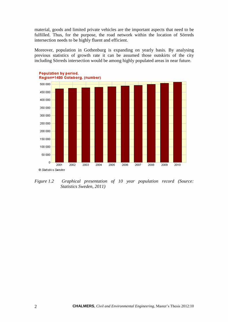
Moreover, population in Gothenburg is expanding on yearly basis. By analysing
previous statistics of growth rate it can be assumed those outskirts of the city
including Sörreds intersection would be among highly populated areas in near future.
Figure 1.2 Graphical presentation of 10 year population record (Source:
Statistics Sweden, 2011)

CHALMERS, Civil and Environmental Engineering, Master‟s Thesis 2012:10 3
Figure 1.3 Graphical presentation of 10 year population growth (Source:
Statistics Sweden, 2011)
In addition to this, certain projects including K2020 are also under consideration by
Swedish Transport Administration, Trafikverket. These approaches reflect that
planners are thinking to make Gothenburg a more sustainable area in terms of
mobility, accessibility and traffic safety. Moreover, Trafikverket is willing to study
the Sörreds- junction to enhance its capacity to fulfil the future need. A plan for the
future is to study the possibility of new road or addition of a flyover at the
intersection, i.e. if it is required and study for best possible design of Sörreds crossing
for an actual scenario.
Figure 1.4 Above chart represents the traffic statistics of Gothenburg (Data
source: Statistics Sweden, 2011)

CHALMERS, Civil and Environmental Engineering, Master‟s Thesis 2012:10 4
In order to avoid the gridlock and accidents at a particular junction, it is essential to
study and analyze it. Therefore, the intersection has already been studied by SWECO,
a civil engineering consultant company. According to the SWECO‟s proposal,
„‟purpose of commissioning SWECO is to investigate an alternate solution that can be
accommodated within the framework of the allocated budget’’ (translated from
SWECO, 2011).
Two alternatives named as Alternative-2 and Alternative-3A, have been proposed by
SWECO which are based on to build a flyover and a ring road. The alternative-3A is
an advanced or modified form of alternative-3, which is somehow different with the
alternative-3A. SWECO‟s study is based on the comparison analysis of alternative-2
and alternative-3. Alternative-3A is a new design and it is now consider in place of
alternative-3.
Alternative-2, as shown in Appendix 1A, will consist of a flyover on Sörredsvägen
which crosses the Torslandavägen or Road-155. Volvo track will remain on ground
level and thus would not be affected by Sörredsvägen. Alternative-3A is in
consideration of a flyover on Torslandavägen. Sörredsvägen and Volvo track will
remain on ground level. Appendix 1C showing the drawing of alternative-3, which is
not considering in this debate.
In both alternatives, Raffinaderivägen, Kärrlyckegatan and Arendalsvägen will closed
for direct entrance to the Road-155. However these roads will merge as Sörreds south
as shown in Appendices 1A and 1B. (SWECO, 2011)
SWECO has examined both alternatives by using “CAPCAL” traffic capacity analysis
software. History of the intersection, volume characteristics of the intersection,
comparison analysis by considering different parameters has been studied by
SWECO. (SWECO, 2011)
1.2 Aim of the study
The aim of this assignment is to study the current scenario of Sörreds intersection in
terms of accessibility, traffic safety and to discuss the future perspective of the
intersection by considering the increasing amount of traffic. The two design
alternatives for the intersection will be a major task to study and to make their
comparison. A more suitable alternative would be recommended after the comparison
analysis. The proposal would also provide an assistive document for the public
transport to make a traffic plan for the implication of K2020.
1.3 Method of the study
Initially, a comprehensive literature study was performed including different books,
papers, previous thesis of traffic engineering and traffic planning. A traffic simulation
computer program VISSIM version 5.3 was used to analyse the intersection and also
for its alternatives. MS Excel and AutoCAD 2011 used as major assistive tools. Field
survey and data collection of one hour traffic flow from 16:00 – 17:00 in a weekday
was done by the researchers.
The collected data and other related information which was gained during survey,
utilized in VISSIM. Firstly, a model having current situation of the intersection is
CHALMERS, Civil and Environmental Engineering, Master‟s Thesis 2012:10 5
developed and initialize in VISSIM. Secondly,same model having future amount of
traffic is developed just to realize the importance of the new design plan. Finally,
models of both alternatives were developed on VISSIM platform and then simulated.
The outcomes which were gained through simulation process were then examined and
used in the results.
1.4 Limitations of the study
During the development of the study, certain limitations were considered and are
mentioned below:
The study has been made, by comparing the study of only one intersection i.e.
Sörredskorsningen, in Gothenburg.
Only two alternatives i.e., 2 and 3A, as SWECO proposed were considered to
examine.
Manual counting and video counting has been made only during the hours16:00 –
17:00 by considering it as peak hour of a week day. This data was used to
compare with the SWECO‟s data.
The traffic flow data from the report of SWECO used as input data in VISSIM.
This is because the purpose of this project is to compare the results obtained with
CAPCAL to the results with VISSIM.
Drawings of the current scenario and both alternatives provided by SWECO, was
then imported in VISSIM to draw the links and connectors of roads and
flyovers.There might be a limited possibility to differ somehow with actual
situation in terms of elevation and size.
Model representing the present scenario of the intersection don‟t includes the rail
road traffic.
The models for the alternative designs are only considers the selected motorized
traffic excluding rail road, pedestrian and bicyclists.
The conversion from Swedish to English version for the SWECO report while
using Google translate might have changed some of the terminologies or criteria,
being originally used in the study by SWECO.

CHALMERS, Civil and Environmental Engineering, Master‟s Thesis 2012:10 6
2 Literature Review
This chapter gives an overview about the basics of intersection design, methodology
of traffic volume studies, signal control design and other related functions i.e. vehicle
actuated controllers, traffic detectors and Swedish signal control technique-
LHOVRA.
2.1 Intersection design and capacity
“Intersections, where two or more roads meet, or point of potential vehicle conflict”.
A signalized intersection can be defined as “The signal controlled intersection is a
location in the road network where road users of different types are focused to share
a common road surface”. It is also stated that engineers should plan and design any
intersection in a way that it becomes safer, efficient for road users. (O‟Flaherty, 1997)
Intersections design varies not only from cities to cities but also from countries to
countries. An example is presented to clarify above statement. In designing
intersection in China, an important thing to consider while designing is the large
number of pedal-driven vehicles and pedestrians alongside buses, trucks, taxis and
growing number of cars. On other hand, in Europe the problem is associated to the
design of an intersection, considering large number of cars alongside buses and
trams.(O‟Flaherty, 1997)
Moreover, any intersection consists of three or more approaches, each of which
contains one or more lanes. When there are more lanes these are separated by a
broken white line painted on the surface of the road, each lane being 3m to 5m wide.
At the intersection , each lane ends at a stop line, a thicker unbroken white line across
the end of the lane indicating the point beyond which the car at the front of the queue
should not be proceed when the signal is red. Where the lane is reserved for one or
more movements, this is indicated by one of two-headed arrows, painted in the white
in the centre of the lane on the approach of the stop line. These arrows should be
located sufficiently far from the stop line to avoid being obscured by the queue.
(O‟Flaherty, 1997)
In addition to this, intersections are resigned in a way that they provide adequate
spaces for queues. Also at signal heads there must have clearly visible locations.
Suggested space requirement for queues is 1.2 multiplied by the mean arrival rate
over the cycle, multiplied by 6 m per vehicle. Concerning the visibility, a distance of
70 m is recommended for signal location besides if the maximum allowed speed is 50
km/h or a distance of 125 m if the maximum allowed speed is 70 km/h. (O‟Flaherty,
1997)
In UK and European countries, three lamps i.e. green, yellow and red, are vertically
arranged having red at the top for long distance visibility, following yellow and then
green at bottom. There is a black board behind the lamp to make the signals clearly
visible from larger distances. The height of the signal lamp should be 2m from
ground. The arrangement of signal in Japan is a bit different, as they are arranged
horizontally above the road.(O‟Flaherty, 1997)
The principles of intersections design are illustrated below in Figure 2.1,

CHALMERS, Civil and Environmental Engineering, Master‟s Thesis 2012:10 7
Figure 2.1 Simple four-arm intersection (O’Flaherty, 1997)
In Figure 2.1,it can be visualized that lanes are about 4 to 5m wide and vehicle stop
position is also indicated with stop line. In Germany primary signal head is about 2.5
to 3.5 m downstream of the line making it clearly visible for vehicles in first queue.
Also pedestrian lines are shown that are supposed to be 1m downstream of stop line
having 3 to 12 m width (O‟Flaherty, 1997)
Signals can be further divided in uncontrolled, priority controlled Stop; give way,
space sharing i.e. roundabouts, time sharing i.e. traffic signal controlled, or grade
separated including interchanges. (O‟Flaherty, 1997).
Some basic intersections forms are illustrated below:

CHALMERS, Civil and Environmental Engineering, Master‟s Thesis 2012:10 8
Figure 2.2 Illustration of some basic forms of intersections (O’Flaherty, 1997).
In early stage, data collection is made for site as well as for traffic condition in “at-
grade design process”. After that, the preliminary design is prepared from which the
layout has been selected. The last step is the development of the final design using
appropriate design standards. (O‟Flaherty, 1997)
It is explained that traffic data collection for design purposes normally include peak
period traffic volumes, turning movements and composition for the design year,
vehicle operating speeds on intersecting roads, movement of pedestrians and cyclists,
public transport requirements, accident experience, parking practices and special
needs of oversize vehicles. (O‟Flaherty, 1997)
For the site data it should be included topography, land usage, and drainage and
related physical features, public and private utility services, horizontal and vertical
alignments of intersecting roads, and adjacent necessary accesses (O‟Flaherty, 1997).
More recently, O‟Flaherty (1997) has issued guidelines for intersection design stated
below:
Minimizing the carriageway area where conflicts can occur
Reduce points of conflicts
Traffic streams should merge/diverge at flat angles and cross at right angles
Encourage low vehicle speeds on the approaches to right-angle intersections
Decelerating or stopping vehicles should be removed from the through traffic
stream
Favor high-priority traffic movements
Discourage undesirable traffic movements
Provide refuges for vulnerable road users
Provide reference markers for road users

CHALMERS, Civil and Environmental Engineering, Master‟s Thesis 2012:10 9
Control access in the vicinity of an intersection
Provide good safe locations for the installation of traffic control devices
Provide advance warning of change
Illuminate intersections where possible
2.2 Volume studies and characteristics
According to Roess et al (2004), a traffic engineer must have in mind for designing
purposes, what are the reasons for designing a road or an intersection i.e. either the
road will be used for public or for industrial use. It is quite necessary to understand
the traveller‟s demand of using any road or intersection.
Moreover, important things while designing intersection are volume studies, speed
studies, travel-time studies, delay studies, accident studies, density studies and
calibration studies. Under the heading of volume studies more focus has been given to
volume characteristics. Roess et.al (2004) found in their research that important things
under volume characteristics are volume, rate of flow, demand and capacity.
2.2.1 Volume calculation periods
Any intersection should be designed considering peak hour conditions. During
weekdays peak hours usually are from 7am to 10am in the morning. In the evening,
the range is usually between 4pm to 7pm. (Roesset.al, 2004)
Figure 2.3 illustrates the percentage of daily traffic on different rural routes in
different days of a week.
Figure 2.3 Variation for rural typical routes has been shown during different days
of a week (Roess et.al, 2004).

CHALMERS, Civil and Environmental Engineering, Master‟s Thesis 2012:10 10
From figure 2.3, gradual rise can be observed during hours 7am until 3pm for all three
days shown (i.e. Wednesday, Saturday and Sunday). After attaining peak position at
hour 6pm for curve representing Saturday graph started plunging down. This indicates
maximum activities on Saturday are around 6pm.Curves shown in graph represents
that intercity routes are being used at their peaks during hours 12pm to 6pm during
three different days representing maximum activities having some fluctuation during
the week days. In the hour ending graph peak hours for routine days show that
maximum traffic at local route is at 9am in morning and 6pm in evening.
Similarly, daily variation in traffic in various hours can be seen below in Figure 2.4.
Figure2.4 Variation in traffic during different hours in a day (Roess et.al, 2004)
From figure 2.4, it can be observed that peak hours during the week days are from
7am to 9 am in the morning and in the evening, the peak hours are from 4pm to 7pm.
The reason could be people going to offices and schools in the morning and in the
evening returning to their homes. In addition, it is also explained that geographical
conditions, weather conditions are also important factors responsible for traffic
variation in volumes. (Roess et al, 2004). It can be seen in Figure 2.5.

CHALMERS, Civil and Environmental Engineering, Master‟s Thesis 2012:10 11
Figure 2.5 Illustration of monthly variation in traffic as percent of AADT (Roess
et al., 2004)
The curve shown above for AADT maximum plateau can be observed for the month
of August. So, indicating peak trend in traffic during a year in month of August. So,
AADT it can be concluded that any intersection or road can be designed considering
months of July and August, with maximum activities going on.
2.2.2 Techniques for volume studies
Further research in the continuation of above explains many techniques for volume
studies in the field. There are three different ways of counting traffic volumes
mentioned below. (Roess et al., 2004)
Manually counted techniques
Portable count techniques
Permanent counts
For manual counters the simplest one is mechanical hand counter. The disadvantage
of manual counts is that the data is manually recorded periodically in the field(Roess
et al., 2004). Moreover, it requires man hours and continuous attention of observer.
Also there is high probability of human error during counting and distraction in traffic
could be among another disadvantage if counting person is not quite well aware of
procedure and rules.
In the case of portable techniques, the mostly used one is the pneumatic tube that is
fastened across the pavements. Whenever any vehicle passes above it, a pulse is
generated and can be sensed by counters attached to it. Figure 2.6a displays the
installation of pneumatic portable counters and their working (Roess et al., 2004).

CHALMERS, Civil and Environmental Engineering, Master‟s Thesis 2012:10 12
Figure 2.6a Installation pattern of pneumatic tube (Roess et.al, 2004).
Figure 2.6b Illustration of Pneumatic tubes counting and detection for a vehicle
(Roess et al., 2004).
Later research demonstrated that permanent counters are installed at different
locations to count the data for 24 hours a day and 365 days. The purpose is to use the
data for real time monitoring (Roess et al., 2004).
2.3 Signal control at the intersection
Traffic signals are used to regulate and control the clash between opposing directed
traffic and pedestrian as well. Traffic signals are helpful to improve the junction
capacity and also improve the road safety (Slinn, Matthews and Guest, 2005). On the
other hand, the disadvantages of the traffic signals are longer stopped delays and
complex consideration requires while making the design. Despite the fact that, the

CHALMERS, Civil and Environmental Engineering, Master‟s Thesis 2012:10 13
overall delay may be lesser, but a user is more concerned about the stopped
delay.(IIT-Bombay, 200?)
Some common and useful terminologies related to traffic signals are; (IIT-Bombay,
200?)
Cycle It is one complete rotation with respect to the all provided
indications.
Cycle length It is the time in seconds in which a signal control complete one
cycle of indications.
Interval It is the change from one stage to another stage. It consists of
two types – change interval and clearance interval. Change
interval is the interval between green and red signal indications,
also called yellow time indication. Clearance interval is the
interval after each yellow interval indicating a period in which
all signals showing red, used to for the clearing-off the vehicles
at the intersection.
Green interval The actual turned on duration of green light.
Red interval The actual turned on duration of red light.
Phase It is the green interval plus the following clearance and change
interval.
Lost time It is the time during which an intersection is not effectively
utilized for the movement of vehicles.
2.3.1 Signal phase design
The development of an appropriate signal phase plan is the most critical aspect of
signal design. If this is done, many other steps of related to signal timing can be
treated analytically in a deterministic way. (Roess et al., 2004)
The purpose of the phase design is to divide the conflicting movements in an
intersection into different phases. There would be large number of phases required if
all the conflicting movements need to be separate. (IIT-Bombay, 200?)
A signal design mainly consists of six major steps. (IIT-Bombay, 200?)
1) Phase design
2) Determination of amber time
3) Determination of cycle length
4) Green time allocation
5) Pedestrian crossing requirement
6) Performance evaluation of the design

CHALMERS, Civil and Environmental Engineering, Master‟s Thesis 2012:10 14
The design methodology of the phases can be guided by the geometry of the
intersection, traffic flow pattern especially the turning movements, the relative
magnitude of flow. As there is no precise methodology for designing the phases, a
trial and error method by choosing these parameters often adopted. (IIT-Bombay,
200?)
2.3.2 Actuated signal control
Pre-timed signal controllers have uniform phase sequence, cycle length and all
interval timings and remain constant from cycle to cycle. In this situation, each signal
cycle is exact replica of the other signal cycle. On the other hand, actuated signal
control utilizes the current information of traffic flow, received from the detectors
within the intersection, and each signal cycle may be different from the other. It is
assisted to fulfil the current demand of traffic signal. The actuated traffic controllers
can range from semi-actuated, to full actuated and to volume-density control. (Roess
et al., 2004)
Al-Mudhaffar (2006) states that in Sweden, some form of vehicle actuated control is
applied at virtually all isolated intersection because of its flexibility to short term
traffic variations. However, vehicle actuated control requires to proper installation of
detectors in all the way/approaches for the purpose of detection of vehicle presence.
Actuated signal controllers may be design by selecting; (Roess et al., 2004)
Variable phase sequences
Variable green times for each phase
Variable cycle length
Figure 2.7 Variation in arrival demand of a signalized intersection (Roess et
al.,2004)

CHALMERS, Civil and Environmental Engineering, Master‟s Thesis 2012:10 15
There are five consecutive cycles shown in Figure 2.7, it is important to note that the
signal has the discharging capacity of 50 vehicles and the total demand during the five
cycles is also 50 vehicles. As a result of this, over the five cycles as shown, total
demand equals to the total capacity. (Roess et al., 2004)
2.3.3 Detectors
Traffic detectors are primary instrument for actuated signal controllers as they
transmit the data in to the local intersection controller in order to achieve the
motorized and non-motorized traffic demand. The traffic controller is then display the
appropriate signal indications according to the data which is received by detectors.
There are various types of detectors usually selected according to the operational
requirements and physical layout of the area to be detectorized. (Kell and Fullerton,
1998)
The operating mode refers to the principles on behalf of detectors‟ noticing the
motorized and non-motorized traffic. The mode affects the duration of the actuation
submitted to the controller by the detection unit. There are two modes commonly
applied as discussed below; (FHWA, 2008)
Pulse mode
By the selection of this mode, the detector will detects the passage of a vehicle by
motion only (point detection). A short “on” pulse of 0.1-0.15 seconds duration sent to
the controller. Actuation will start with the arrival of vehicle in the detection zone and
finish with end of pulse duration. (FHWA, 2008)
Presence mode
This mode is used to measure the occupancy. Actuation starts with the arrival of the
vehicle to the detection zone and ends with the vehicle leaves the detection zone.
Duration of the time in the presence mode depends on the detection zone length,
vehicle length, and vehicle speed. This mode measures the time that a vehicle is
within the detection zone and will require shorter extension or gap timing with its use.
Typically, it is used with long-loop detection located at the stop-line. (FHWA, 2008)

CHALMERS, Civil and Environmental Engineering, Master‟s Thesis 2012:10 16
Figure 2.8 Maximum allowable headway for presence and pulse detector modes.
(Bonneson and McCoy, 2005)
Location of Detectors
There are many standards have established by several agencies and department related
to the effective placement of longitudinal location (setback) of detectors relative to the
stop line. It should be ideal condition for detector placement that speed, type, and
volume of approaching vehicles as well as the type of controller unit are considered.
The detector requirements for low-speed arrivals differ from the requirements related
with high-speed arrivals. (Kell and Fullerton, 1998)
An example of possible detector setbacks is expressed in Table 2.1.

CHALMERS, Civil and Environmental Engineering, Master‟s Thesis 2012:10 17
Table 2.1 Safe stopping distance and detector setback (modified from Kell
andFullerton, 1998)
2.3.4 Dilemma zone
Dilemma zone is an area close to stop line, where there is a high potential of accident
at a high speed signalized intersection. Figure 2.9 explains clear concept of dilemma
zone at any signalized intersection. This is defined as ´´an area in the approach to the
stop-line where a driver on seeing amber may not be able to stop in advance of the
stop line with an acceptable deceleration rate, or to clear the intersection during the
change interval´´. (Al-Mudhaffar, 2006)

CHALMERS, Civil and Environmental Engineering, Master‟s Thesis 2012:10 18
Figure 2.9 Illustration showing systematic scheme of a dilemma zone (Al-
Mudhaffar, 2006).
However, in continuation with the study, the limits of the dilemma zone have been
defined (Al-Mudhaffar, 2006).
; for the maximum distance of a passing car (2.1)
; for minimum stopping distance (2.2)
Where:
v0 = Approaching speed in m/s
x = Approaching distance in m.
δ2 = Reaction time for braking + time to start braking
r = Required retardation
τ = Time length of the amber light
It has been stated that dilemma zone problems can be reduced by advance signals with
or without flashers and also by amber interval timings.
Moreover, it is also stated that the ranges of dilemma zone for vehicles approaching
with speed of 70km/h are between 97 and 53 meters upstream of a stop line. In this
case driver can proceed without red light infringement from a distance of 97m
upstream of a stop line. Also he can take a decision whether to stop or not from a
CHALMERS, Civil and Environmental Engineering, Master‟s Thesis 2012:10 19
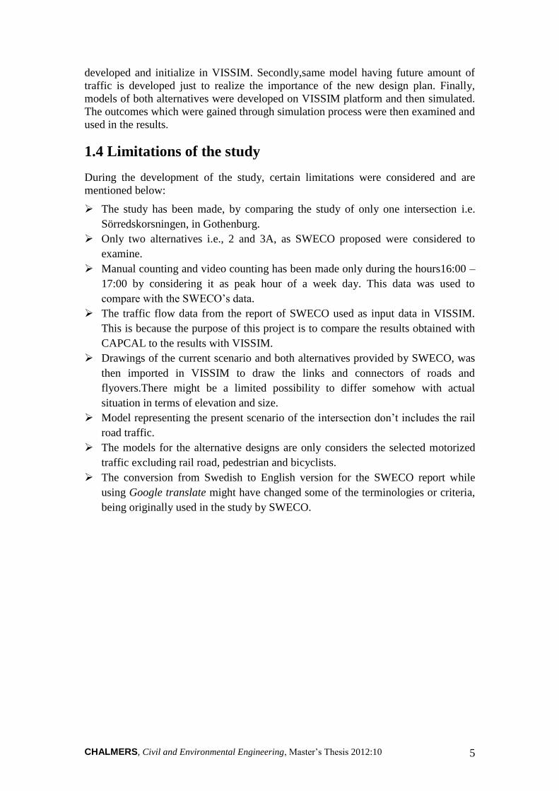
distance of 53m upstream of a stop line. Zone ranging from 97 to 53 meter is known
as dilemma zone. (Al-Mudhaffar, 2006)
Stop distance can be thus calculated by the formula below,(Al-Mudhaffar, 2006)
Stop distance = reaction distance + deceleration distance
Figure 2.10 illustrates the concept of stop distance and dilemma zone at any
intersection with vehicles approaching with a speed of 70km/h.
Figure 2.10 Illustration of a dilemma zone with vehicles approaching having speed
of 70km/h. (Al-Mudhaffar, 2006)
2.3.5 LHOVRA technique
LHOVRA is predominant techniques used to increase safety and reduce lost time in
Sweden. In the initial stage LHOVRA was implemented, during trial period accidents
rate has been reduced from 0.7 accidents per million vehicle incoming to 0.5. After
this successful implementation, LHOVRA technique has been widely implemented in
Sweden as well as in other Scandinavian countries; first with speed limit of 70km/h in
rural areas and then also with lower speed limit of 50 km/h. (Al-Mudhaffar, 2006)
According to Al-Mudhaffar (2006) word “LHOVRA “is described below in Table 2.2,

CHALMERS, Civil and Environmental Engineering, Master‟s Thesis 2012:10 20
Table 2.2 Illustration of LHOVRA acronym description (Al-Mudhaffar, 2006)
Implementation of LHOVRA signals and their locations at any intersection are shown
in Figure 2.11.
Figure 2.11 Illustration of detectors for LHOVRA functions and specific locations
for their implementation. (Al-Mudhaffar, 2006)
LHOVRA functions are described below,
Acronym English English Translation
with Swedish meaning
L Truck, bus priority
(Lastbilprioritering)
H Main road priority
(Huvudvägprioritering)
O Incident reduction
(Olycka function)
V Variable amber time
(Variabelgul)
R Red driving control,
variable red time
(Rödkörning control)
A All red turning
(Allrödvänding)

CHALMERS, Civil and Environmental Engineering, Master‟s Thesis 2012:10 21
L function
L-function is used where truck priority is required on any primary road. One of the
disadvantages is far away installation of detectors which makes it much
costly/expensive (Al-Mudhaffar, 2006).
H function
H-Function is used on major as well as on primary roads that requires any priority. It
takes primary roads as priority ones. In this function disadvantage is not consideration
of safety aspects. (Al-Mudhaffar, 2006)
O function
O-function is normally used function. Difficult aspect of O function is the
determination of practical dilemma zone. Determination of practical dilemma zone is
important, as it should allow the last extending vehicle to pass through before lights
turn red. (Al-Mudhaffar, 2006)
V function
V-functions are used at sub roads/links having maximum speed limit of 50km/h. In V
function detectors are installed at 80 m distance. (Al-Mudhaffar, 2006)
R function
Using R function alone is quite risky, so R function is used combined with O function.
This function allows some of vehicles to pass through red signal with minimum
chances of collision (Al-Mudhaffar, 2006).
Figure 2.12 illustrates the working of R function along with O function at a signal.

CHALMERS, Civil and Environmental Engineering, Master‟s Thesis 2012:10 22
Figure 2.12 Illustration of R function along with O function on a signal (Al-
Mudhaffar, 2006).
In Figure 2.12, a variable red extension is about 2.5s. It means that a car driving 2s
after maximum extension is considered not dangerous and minimum possibility of
collision exists in this scenario/region.
A function
Al-Mudhaffar (2006), defines A-function as,
”This function aims to reduce as far as possible the number of instantaneous green-
amber–red-green cycles and to ensure that the approaching vehicle is far enough
away if they occur”.
The purpose of A-function is to detect following vehicles in system and avoid
unnecessary changes also reduce stress on the drivers mainly before red signals
occurrence (Al-Mudhaffar, 2006).
The research has also defined that the data required for the implementation of
LHOVRA techniques in VISSIM simulation are summarized as: (Al-Mudhaffar,
2006)
Car following model parameters,
Stop distance at the stop line,
Acceleration and retardation,
Probability to drive or stop at change from green to amber,

CHALMERS, Civil and Environmental Engineering, Master‟s Thesis 2012:10 23
Arriving traffic generation (time gap),
Flow and turning flows through the time,
Traffic composition,
Queue length,
Lane distribution,
Saturation Flow
2.4 Performance measures
Performance measures in traffic engineering planning and design generally termed as
the parameters which are used to evaluate the effectiveness of design. There are many
parameters involved in this evaluation but most common parameters are delay,
queuing and stops. (IIT-Bombay, 200?)
In general, performance measures are used to evaluate the different alternative
effectiveness on the basis of program objective. These measures are mostly applied to
quantifying an objective; however they can be measured in less quantitative way.
Public feedback and responder observation have been used as qualitative performance
measures by measures. (Kutz, 2003)
Delay is generally focused to extra or additional travel time which is experienced by
driver, or pedestrian. It is the time which is consumed during the traversing of
intersection. Figure 2.13 explained this phenomena by consider one vehicle. (IIT-
Bombay, 200?)
Figure 2.13 Illustration of delay measures (IIT-Bombay, 200?).
Queue is another parameter used the performance measures in traffic planning and
design. It is a line of motorized or non-motorized traffic waiting to be served by a
phase in which flow rate from front of the queue determines the average speed within
the queue. However a faster-moving queue usually referred as platoon or moving
queue. (FHWA, 2008)
CHALMERS, Civil and Environmental Engineering, Master‟s Thesis 2012:10 24
Stop is however the third parameter used to measure the performance in traffic
planning and design. There are two main reasons to show its importance, as discussed
below (FHWA, 2008);
Stops have greater impact on emission than Delay does because an accelerating
vehicle emits more pollutants and utilizes more fuel than an idle vehicle.
Motorists are usually frustrated when they have to face several stops. As Stops are
referred as the measures of the quality of progression along an arterial. As a
reason of this, some signal timing softwares are able to give relative importance of
stops and delays through the use of weighting factors. By assigning high level of
importance to stops, effectiveness on arterials will improve although the result
may be as overall delay. Vehicular Stops can recurrently play a bigger role than
Delay in the perception of effectiveness of signal timing plan of a network.
All the parameters can be measured by VISSIM. The software generates files having
different formats when these parameters are selected before starting the simulation.
The software describes these parameters a below.
2.4.1 Travel time and delays
Travel time sections comprises of start and destination cross section. These section
counts the time when a vehicle travel between them. It is necessary for the
measurement that the vehicles pass both cross sections. (PTV, 2011)
Delay time segments are based on one or more travel time sections. The vehicles
types that are selected in delay time calculation are captured by the segments when
they pass these travel time sections. (PTV, 2011)
2.4.2 Queue counters
Queue counter in VISSIM used to count the following parameters,
Average queue length
Maximum queue length
Number of vehicle stops within the queue
Queue length show in the unit of not in number of vehicles. The most suitable places
for queue counters are the stop lines of a signalized intersection. The counter
measures the queue length of vehicles that are coming from upstream side. If there is
more incoming way towards the counter, then the counter counts for each way and
report the longest as the maximum queue length. Number of stops within the queue
represents the number of events when a vehicle enters in the queue. (PTV, 2011)
CHALMERS, Civil and Environmental Engineering, Master‟s Thesis 2012:10 25
3 Methodology
Literature chapter has revealed some of important parameters used in research for
Sörreds intersection study. The VISSIM input parameters, signal control strategy and
other model building functions will be discussed in this chapter.
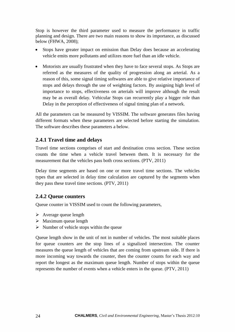
3.1 Site description
The case study has been performed in area of Sörreds intersection. Intersection is
located in industrial zone close to the vicinity of Volvo area. There is continuous flow
of heavy traffic with considerable number of private and public transport. Below
shown Figure 3.1 provides close view of intersection characterizing present scenario
of Sörreds intersection along with number of PT stops located at site of study.
Figure 3.1 Overview of present scenario at Sörreds intersection along with PT
stops (SWECO, 2011).

CHALMERS, Civil and Environmental Engineering, Master‟s Thesis 2012:10 26
Figure 3.2 Traffic flow directions around the intersection.
Overview of Figure 3.1, illustrates that four PT-stops are located close to intersection.
However, model representing the present scenario has been made considering three
PT-stops namely Läg A, Läg B andLäg C. Existence of Läg D is not debated due to its
minor influence to the intersection traffic. Roads linked to intersection are named as
Torslandavägen or V-155, Sörredsvägen and Monteringsvägen.
3.2 Data collection methods
Site has been visited for several times during study period for data collection.
Methods for collecting data are discussed below briefly;
3.2.1 Manual and video counting
Manual counting has been performed for measuring vehicle inputs at the intersection
during different peak hours more specifically ranging from hours 1600 to 1900.
Manual data was cross verified by means of video capturing in similar time interval. It
covered various directions also the type of vehicles was individually spotted. Video
counting also helped in characterizing driver behaviour. Further it can be used for
later reference and other extraction of other useful data.
Attached Appendix 2A gives number of counted vehicles proceeding in different
directions at the intersection. In construction of simulation model, data used for
vehicle input is taken from SWECO report shown in Appendix 2B and 2C. The reason
for collecting the data is just to compare the vehicle quantities given by SWECO.

CHALMERS, Civil and Environmental Engineering, Master‟s Thesis 2012:10 27
3.2.2 Site drawings provided by SWECO
Site data has been extracted from AutoCAD files provided by SWECO. Some of the
irrelevant data e.g. presence of vicinity constructions including buildings, was
neglected. The purpose behind was to make file process-able for VISSIM as heavy
files effect by slowing down the simulation process. Appendix 1A and 1B are drawing
on AutoCAD used as source files for alternatives and altered accordingly for
importing into VISSIM.
3.3 Use of VISSIM
Traffic simulation is a model building and analysis technique widely useful in
planning, design and also assists in decision making for professionals. Traffic
simulation is also becoming a major instrument in the Intelligent Transport Systems
(ITS), its design and evaluation. The reason behind this is its dealing with time
dependencies of traffic phenomena especially when real-time management operations
are a critical feature of the system. These simulation models are also suitable tools for
properly dealing with the variable traffic over time. For researchers, it is a helpful tool
to get understanding of traffic phenomena and to conduct experiments in their virtual
laboratories. (Barceló, 2010)
Due to modernization in Traffic studies, Traffic simulation is becoming an essential
tool for traffic engineers and traffic planners. VISSIM is a microscopic, behaviour-
based multi-purpose traffic simulation tool widely used to analyze and optimize traffic
flows. It offers a broad range of its applications in urban and highway planning,
analyzing and also for the public and private transportation as well as for pedestrian
movement. Different kind of complex traffic conditions can be visualized with high
level of detail supported by realistic traffic models. (Barceló, 2010).
For study purpose VISSIM version 5.30 is utilized. VISSIM is a step and behaviour
based software used for modelling urban (including public and local transport
operations) as well as pedestrian flows (PTV, 2011).
Visualization of VISSIM desktop window can be seen in Figure 3.3 illustrating
different tools being used for development of Model.

CHALMERS, Civil and Environmental Engineering, Master‟s Thesis 2012:10 28
Figure 3.3 Overview of VISSIM desktop window and tools used for construction of
model (PTV, 2011)
3.4 Model construction
The altered AutoCAD files were imported in VISSIM 5.30, scaled according to the
software interface and used as background to draw road networks. Models
representing intersections for present scenario and two alternatives provided by
SWECO had been drawn using VISSIM.
All roads and pedestrian way networks which were on ground supposed to be at zero
level for the interface by neglecting the elevation difference. The reason behind this is
to show the clearer picture of networks and to distinguishing the roads with fly over.
However, gradient tool is used to change the acceleration of vehicles in the low/high
regions.
3.5. Data input
3.5.1 Car following model
Car Model used in constructing VISSIM is based on WIDEMANN (1974) Theory
(PTV, 2011). WIDEMANN (1974) theory is based on idea, that a vehicle with high
acceleration starts decelerating as they reach in their individual perception threshold
of vehicle with slow speed. After reaching another perception threshold, vehicle starts
to slightly accelerate again. Since, this is iterative process of continuous acceleration
and deceleration (PTV, 2011). Later on WIDEMANN (1999) approach has also been
added in VISSIM latest versions. Approach adopted in WIDEMANN (1999) is the
Modelling of RTI-Elements on multi-lane roads (PTV, 2011).
CHALMERS, Civil and Environmental Engineering, Master‟s Thesis 2012:10 29
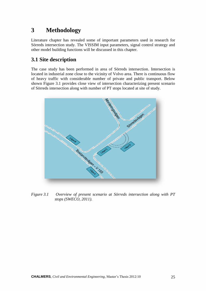
Example of WIDEMANN (1999) approach and different parameters and their
properties are stated in Table 3.1.
Table 3.1 Different properties used in WIDEMANN (99) approach in different
scenarios (PTV, 2011).
* As defined in the VISSIM defaults
** Lane 2 closed to all HGV (PTV, 2011)
From Table 3.1, it is quite clear that right hand rule is being utilized while using
default settings. Speed limits are ranging from 80 to 120 mph maximum for cars. Also
for HGV maximum speed limit is defined as 85 mph.
3.5.2 Technical specification of vehicles
Technical specifications of vehicles required for VISSIM model construction purpose
is mentioned below. (PTV, 2011)
Length
Maximum speed
Potential acceleration
Actual position in the network
Actual speed and acceleration
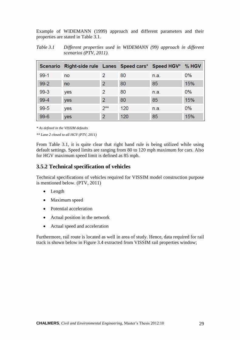
Furthermore, rail route is located as well in area of study. Hence, data required for rail
track is shown below in Figure 3.4 extracted from VISSIM rail properties window;
CHALMERS, Civil and Environmental Engineering, Master‟s Thesis 2012:10 30
Figure 3.4 Overview of technical specifications required for rail road parameters
used in VISSIM model construction (PTV, 2011).
All the parameters used for construction of rail road track for site of Sörreds
intersection are standard with default values of widths and heights (i.e. gauge and rail
height properties).
As there are separates lines for PT are considered in both of the alternatives, the PT-
stops are created accordingly as illustrate in the alternatives drawing. There are 4 PT-
stops are supposed in the alternatives around the intersection.
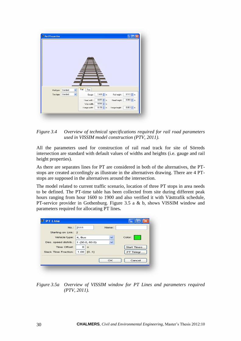
The model related to current traffic scenario, location of three PT stops in area needs
to be defined. The PT-time table has been collected from site during different peak
hours ranging from hour 1600 to 1900 and also verified it with Västtrafik schedule,
PT-service provider in Gothenburg. Figure 3.5 a & b, shows VISSIM window and
parameters required for allocating PT lines.
Figure 3.5a Overview of VISSIM window for PT Lines and parameters required
(PTV, 2011).

CHALMERS, Civil and Environmental Engineering, Master‟s Thesis 2012:10 31
Figure 3.5b Overview of VISSIM window for PT Lines and parameters required
(PTV, 2011).
3.5.3 Pedestrian data input
As the intersection also deals with pedestrian and cyclists, the routes for pedestrian
and cyclists is however been created for the present scenario model. The pedestrian
routes is somehow differ with the other routes (motorists) as it need a random and
non-uniform movement of pedestrian, and it is also connected to the PT-stops.
Pedestrian mode of the software is therefore used to build this route.
3.6 Signal timing parameters
Signal timing parameters needs to be defined while preparing the controller settings.
Following parameters are important to consider in this stage. Figure 3.6 illustrates
some of the parameters, which will discuss below;

CHALMERS, Civil and Environmental Engineering, Master‟s Thesis 2012:10 32
Figure 3.6 An actuated signal phase Intervals definition. (Bonneson, Sunkari&
Pratt, 2009)
3.6.1 Minimum green time
Minimum green time must be considered for each signal phase while adopting
actuated control signal control. It is usually based on type and the location of the
detectors. (Roess et al., 2004)
Point or passage detector usually located to a distance d meters from the STOP line. If
the vehicles occupies the area between the STOP line and the detector location, the
minimum green time should be a long enough to clear these vehicle queue. (Roess et
al., 2004)
Following expression can be used to estimate the minimum green time. (Roess et al.,
2004)
(3.1)
Where Gmin = Minimum green time in seconds
l1 = Startup lost time in seconds
d = distance between the detectors and the STOP line in meters
6.1 = Assumed head-to-head spacing between vehicles in queue, in
meters.
The startup lost time ranges 2-4 seconds are often used. (Roess et al., 2004)
If the pedestrians are also present in the case, the minimum green time should be long
enough for crossing time of pedestrian.

CHALMERS, Civil and Environmental Engineering, Master‟s Thesis 2012:10 33
The expression is useful in this case. (HCM, 2000)
(3.2)
(3.3)
Where
Gp = Minimum pedestrian green time in seconds
3.2 = Pedestrian startup time in seconds
L = Crosswalk length in meters
Sp = Walking speed of pedestrian crossing during an interval
WE = Effective crosswalk width in meters
3.6.2 Maximum green time
It is the maximum green time allowed for a green phase. A phase will adopt this time
when it has sufficient demand. (Kutz, 2003)
It is a user defined parameter, local practices usually considered an important factor to
determine this parameter (HCM, 2000). However a typical range is selected to define
in the each signal phase of the model by considering the influence of traffic. The
range is about 10-50 seconds. Site visits was also helpful to select this range.
3.6.3 Amber and amber/red time
Amber time is the time interval in which driver alerts because the signal light is going
to change from green to red. In Sweden, according to the V-function of LHOVRA
technique, a variable amber time is used within the limits of 3-5 seconds. The
amber/red time is however set as 1 second according to the Swedish standards. (Li M.
&Wo T., 2011)
3.6.4 Allowable gap
It is the time elapsed between the departure of a vehicle and arrival of the next
vehicle, observed by detector. In Sweden, it is practicing that this time should be less
than 5.6 seconds, according to the O-function of the LHOVRA technique. (Li M.
&Wo T., 2011)
3.7 Vehicle actuated programming
VisVAP program is used to define the signal control logics by using the VAP
programming language (vehicle actuated programming). It is comfortable tool to
assign the signal control logics by considering the VAP language. The control logic
i.e. *.pua file, is assigned first in a text file also called inter-stages file. The main logic
file *.vap file is then created by using VisVAP interface.

CHALMERS, Civil and Environmental Engineering, Master‟s Thesis 2012:10 34
3.8 Signal groups and signal control
The signal control is assigned to each signalized intersection in the models. Similarly,
signal groups as assigned in *.pua file, are then added in VISSIM signal control, and
assign it to each individual signal head as shown in drawings provided by SWECO.
The *.pua and *.vap files are then imported in the signal control menu to execute the
signals during simulation.
The signal control window can be seen in Figure 3.8.
Figure 3.8 Signal control window showing signal groups.
3.9 Simulation of models
Next step is to run the simulation. In VISSIM one step or continuous simulation can
be made. Also option of toggling from single step to continuous step is available.
VISSIM simulation window is illustrated in Figure 3.9.

CHALMERS, Civil and Environmental Engineering, Master‟s Thesis 2012:10 35
Figure 3.9 Overview of VISSIM simulation window and parameters need to be
filled (PTV, 2011)
It can be seen in figure 3.9, that times used for running simulation is about 3600
seconds. Simulation speed is 1.0 sim.sec./s. in addition right hand side traffic is being
utilized i.e. as practiced in Sweden.
3.10 Models representing different scenarios
Three different models are drawn discussing three different scenarios.
3.10.1 Model – Current scenario
First model discusses present scenario of Sörreds intersection. Figure 3.10 gives
present scenario of Sörreds intersection.
Figure 3.10 Simulation model for the current traffic scenario.

CHALMERS, Civil and Environmental Engineering, Master‟s Thesis 2012:10 36
3.10.2 Model - Alternative 2
Model for alternative-2 has been created as shown in Figure 3.11. Torslandavägen
proceeds under the flyover with no interruption from Sörreds link.
In the model, the roads which are on ground are located at 0m elevation while flyover
maximum height is 6m regardless of elevations related to sea level. Figure 3.11
illustrates the model of alternative-2 having flyover at Sörredsvägen.
Figure 3.11 Simulation model for the Alternative-2, Sörredsvägen over the
Torslandavägen.
3.10.3 Model - Alternative 3A
As discussed earlier, alternative-3A consists the flyover on Torslandavägen.
Sörredsvägen is therefore will be on ground level. Elevations used in developing the
model are same as used in model of alternative-2. Illustration of model of alternative-
3A is presented in Figure 3.12.
Figure 3.12 Simulation model for the Alternative-3A, Torslandavägen over the
Sörredsvägen.

CHALMERS, Civil and Environmental Engineering, Master‟s Thesis 2012:10 37
4 Analysis of results
The chapter includes the results based on the performance measure parameters as
discussed in the previous chapter. Simulations were made for all the models
representing the current scenario of intersection with present and future amount of
traffic and traffic flow situation in the alternatives. The results were then generated in
tabular forms as a result of one hour simulation.
It has been discussed earlier that the traffic amounts for the present situation and for
the alternatives were used as provided in SWECO‟s report. However on the other
hand, the amount of public transport is set as doubled to the present amount.
4.1 Present situation
The results for the selected parameters concerned to the traffic flow are then plotted in
graphical format. Results for each traffic route are shown in a separate illustration.
4.1.1 Delays
Delay in traffic flow for each traffic route as recorded by VISSIM are plotted as
illustrate below. A red horizontal line in every illustration shows the average of all
delays.
46.39
0
20
40
60
80
100
120
1
69
13
7
20
5
27
3
34
1
40
9
47
7
54
5
61
3
68
1
74
9
81
7
88
5
95
3
10
21
10
89
11
57
12
25
12
93
13
61
14
29
De
lay
tim
e
No. of vehicles
Current Scenario
Centrum-Torslanda Average
Figure 4.1 Delay times of vehicles and their average are plotted for Centrum to
Torslanda route.

CHALMERS, Civil and Environmental Engineering, Master‟s Thesis 2012:10 38
41.69
0
20
40
60
80
1001
10
19
28
37
46
55
64
73
82
91
10
0
10
9
11
8
12
7
13
6
14
5
15
4
16
3
17
2
De
lay
tim
e
No. of vehicles
Current Scenario
Sörredsvägen-Torslanda Average
Figure 4.2 Delay times of vehicles and their average are plotted for Sörredsvägen
to Torslanda route.
21.34
0
20
40
60
80
100
1
16
31
46
61
76
91
10
6
12
1
13
6
15
1
16
6
18
1
19
6
21
1
22
6
24
1
25
6
27
1
28
6
30
1
De
lay
tim
e
No. of vehicles
Current Scenario
Centrum-Sörredsvägen Average
Figure 4.3 Delay times of vehicles and their average are plotted for Centrum to
Sörredsvägen route.

CHALMERS, Civil and Environmental Engineering, Master‟s Thesis 2012:10 39
53.19
0
50
100
150
200
2501
27
53
79
10
5
13
1
15
7
18
3
20
9
23
5
26
1
28
7
31
3
33
9
36
5
39
1
41
7
44
3
46
9
49
5
52
1
54
7
De
lay
tim
e
No. of vehicles
Current Scenario
Sörredsvägen-Centrum Average
Figure 4.4 Delay times of vehicles and their average are plotted for Sörredsvägen
to Centrum route.
40.32
0
50
100
150
1
38
75
11
2
14
9
18
6
22
3
26
0
29
7
33
4
37
1
40
8
44
5
48
2
51
9
55
6
59
3
63
0
66
7
70
4
74
1
77
8
De
lay
tim
e
No. of vehicles
Current Scenario
Torslanda-Centrum Average
Figure 4.5 Delay times of vehicles and their average are plotted for Torslanda to
Centrum route.

CHALMERS, Civil and Environmental Engineering, Master‟s Thesis 2012:10 40
46.61
0
20
40
60
80
100
1201
18
35
52
69
86
10
3
12
0
13
7
15
4
17
1
18
8
20
5
22
2
23
9
25
6
27
3
29
0
30
7
32
4
34
1
35
8
De
lay
tim
e
No. of vehicles
Current Scenario
Torslanda-Söredsvägen Average
Figure 4.6 Delay times of vehicles and their average are plotted for Torslanda to
Sörredsvägen route.
4.1.2 Travel times
Travel times for each traffic route as recorded by VISSIM are plotted as illustrate
below. A red horizontal line in each illustration showing the average of all travel
times.
103
0
50
100
150
200
250
1
69
13
7
20
5
27
3
34
1
40
9
47
7
54
5
61
3
68
1
74
9
81
7
88
5
95
3
10
21
10
89
11
57
12
25
12
93
13
61
14
29
Trav
el t
ime
No. of vehicles
Current Scenario
Centrum-Torslanda Average
Figure 4.7 Travel times of vehicles and their average are plotted for Centrum to
Torslanda route.

CHALMERS, Civil and Environmental Engineering, Master‟s Thesis 2012:10 41
80.89
0
50
100
150
2001
10
19
28
37
46
55
64
73
82
91
10
0
10
9
11
8
12
7
13
6
14
5
15
4
16
3
17
2
Trav
el t
ime
No. of vehicles
Current Scenario
Sörredsvägen-Torslanda Average
Figure 4.8 Travel times of vehicles and their average are plotted for Sörredsvägen
to Torslanda route.
53.08
0
50
100
150
1
16
31
46
61
76
91
10
6
12
1
13
6
15
1
16
6
18
1
19
6
21
1
22
6
24
1
25
6
27
1
28
6
30
1
Trav
el t
ime
No. of vehicles
Current Scenario
Centrum-Sörredsvägen Average
Figure 4.9 Travel times of vehicles and their average are plotted for Centrum to
Sörredsvägen route.

CHALMERS, Civil and Environmental Engineering, Master‟s Thesis 2012:10 42
93.59
0
50
100
150
200
250
3001
27
53
79
10
5
13
1
15
7
18
3
20
9
23
5
26
1
28
7
31
3
33
9
36
5
39
1
41
7
44
3
46
9
49
5
52
1
54
7
Trav
el t
ime
No. Of Vehicles
Current Scenario
Sörredsvägen-Centrum Average
Figure 4.10 Travel times of vehicles and their average are plotted for Sörredsvägen
to Centrum route.
97.89
0
50
100
150
200
250
1
38
75
11
2
14
9
18
6
22
3
26
0
29
7
33
4
37
1
40
8
44
5
48
2
51
9
55
6
59
3
63
0
66
7
70
4
74
1
77
8
Trav
el t
ime
No. Of vehicles
Current Scenario
Torslanda-Centrum Average
Figure 4.11 Travel times of vehicles and their average are plotted for Torslanda to
Centrum route.

CHALMERS, Civil and Environmental Engineering, Master‟s Thesis 2012:10 43
83.93
0
50
100
150
200
1
17
33
49
65
81
97
11
3
12
9
14
5
16
1
17
7
19
3
20
9
22
5
24
1
25
7
27
3
28
9
30
5
32
1
33
7
35
3
36
9
Current Scenario
Torslanda-Söredsvägen Average
Figure 4.12 Travel times of vehicles and their average are plotted for Torslanda to
Sörredsvägen route.
4.1.3 Queue record
The average and maximum values of the queue generated around the intersection and
the number of stops are presented below.
0
200
400
600
800
1000
1200
1400
Ce
ntr
um
-To
rsla
nd
a
Sörr
ed
sväg
en-T
ors
lan
da
Ce
ntr
um
-Sö
rred
sväg
en
Sörr
ed
sväg
en-C
en
tru
m
Tors
lan
da-
Cen
tru
m
Tors
lan
da-
Sörr
edsv
äge
n
Current Scenario
Average Maximum Stop
Figure 4.13 Traffic queue values with their respective junction.
4.2 Present situation with future traffic inputs
Developed model of Sörreds Intersection was checked for future vehicular input for
year 2035 shown in Appendix 2C. As a result of this, a grid lock situation werecreated

CHALMERS, Civil and Environmental Engineering, Master‟s Thesis 2012:10 44
in the model and more than 2000 vehicles could not enter in the model due to the long
queues and stops of vehicles.
However a comparison is made to represent this situation with the current flow of
traffic.
0
50
100
150
200
Ce
ntr
um
-To
rsla
nd
a
Ce
ntr
um
-Sö
rre
dsv
ägen
Sörr
ed
väge
n-
Tors
lan
da
Sörr
ed
sväg
en-
Ce
ntr
um
Tors
lan
da-
Sörr
ed
sväg
en
Tors
lan
da-
Ce
ntr
um
De
lay
tim
e
Delay Time
Average (Future traffic) Average (Present Traffic)
Figure 4.14 Comparison in Delay timing considering the present and future amount
of traffic.
0
50
100
150
200
250
Ce
ntr
um
-To
rsla
nd
a
Ce
ntr
um
-Sö
rre
dsv
ägen
Sörr
ed
väge
n-
Tors
lan
da
Sörr
ed
sväg
en-
Ce
ntr
um
Tors
lan
da-
Sörr
ed
sväg
en
Tors
lan
da-
Ce
ntr
um
Trav
el t
ime
Travel Time
Average (Future traffic) Average (Present Traffic)
Figure 4.15 Comparison in Travel timing considering the present and future amount
of traffic.

CHALMERS, Civil and Environmental Engineering, Master‟s Thesis 2012:10 45
050
100150200250300350
Ce
ntr
um
-To
rsla
nd
a
Ce
ntr
um
-Sö
rre
dsv
ägen
Sörr
ed
sväg
en-
Ce
ntr
um
Sörr
ed
sväg
en-
Tors
lan
da
Tors
lan
da-
Sörr
ed
sväg
en
Tors
lan
da-
Ce
ntr
um
Qu
eu
e le
ngt
h
Queue Length
Average (Future traffic) Average (Present Traffic)
Figure 4.16 Average queue length comparisons by considering the present and
future amount of traffic.
4.3 Alternative 2
Alternative-2 model was simulated in VISSIM and to get following results for
analysis.
4.3.1 Delays
Delay in traffic flow for each traffic route that recorded by VISSIM are plotted as
illustrated below. A red horizontal line in each illustration showing the average of all
delay times
19.41
0
20
40
60
80
13
05
98
81
17
14
61
75
20
42
33
26
22
91
32
03
49
37
84
07
43
64
65
49
45
23
55
25
81
61
06
39
De
lay
tim
e
No. Of vehicles
Alternative 2
Centrum-Sörreds North Average
Figure 4.17 Delay times of vehicles and their average are plotted for Centrum to
Sörreds North route.

CHALMERS, Civil and Environmental Engineering, Master‟s Thesis 2012:10 46
9.390
10
20
30
40
50
601
11
62
31
34
64
61
57
66
91
80
69
21
10
36
11
51
12
66
13
81
14
96
16
11
17
26
18
41
19
56
20
71
21
86
23
01
24
16
25
31
De
lay
tim
e
No. Of vehicles
Alternative 2
Centrum-Torslanda Average
Figure 4.18 Delay times of vehicles and their average are plotted for Centrum to
Torslanda route.
118.07
0
100
200
300
400
1 3 5 7 9 11 13 15 17 19 21 23 25 27 29 31 33 35 37 39 41 43 45 47
De
lay
tim
e
No. Of vehicles
Alternative 2
Centrum-Sörreds South Average
Figure 4.19 Delay times of vehicles and their average are plotted for Centrum to
Sörreds South route.

CHALMERS, Civil and Environmental Engineering, Master‟s Thesis 2012:10 47
67.4
0
50
100
150
200
2501
63
12
5
18
7
24
9
31
1
37
3
43
5
49
7
55
9
62
1
68
3
74
5
80
7
86
9
93
1
99
3
10
55
11
17
11
79
12
41
13
03
De
lay
tim
e
No. Of vehicles
Alternative 2
Sörreds North-Centrum Average
Figure 4.20 Delay times of vehicles and their average are plotted for Sörreds North
to Centrum route.
40.98
0
20
40
60
80
100
120
1 5 9 13 17 21 25 29 33 37 41 45 49 53 57 61 65 69 73 77 81 85 89
De
lay
tim
e
No. Of vehicles
Alternative 2
Sörreds South-Sörreds North Average
Figure 4.21 Delay times of vehicles and their average are plotted for Sörreds South
to Sörreds North route.

CHALMERS, Civil and Environmental Engineering, Master‟s Thesis 2012:10 48
65.84
0
50
100
150
200
250
1 5 9 13 17 21 25 29 33 37 41 45 49 53 57 61 65 69 73 77 81 85 89 93
De
lay
tim
e
No. Of vehicles
Alternative 2
Sörreds South-Centrum Average
Figure 4.22 Delay times of vehicles and their average are plotted for Sörreds South
to Centrum route.
45.45
0
20
40
60
80
100
120
1
27
53
79
10
5
13
1
15
7
18
3
20
9
23
5
26
1
28
7
31
3
33
9
36
5
39
1
41
7
44
3
46
9
49
5
52
1
54
7
De
lay
tim
e
No. Of vehicles
Alternative 2
Sörreds South-Torslanda Average
Figure 4.23 Delay times of vehicles and their average are plotted for Sörreds South
to Torslanda route.

CHALMERS, Civil and Environmental Engineering, Master‟s Thesis 2012:10 49
18.91
0
20
40
60
801
39
77
11
5
15
3
19
1
22
9
26
7
30
5
34
3
38
1
41
9
45
7
49
5
53
3
57
1
60
9
64
7
68
5
72
3
76
1
79
9
83
7
De
lay
tim
e
No. Of vehicles
Alternative 2
Sörreds North - Torslanda Average
Figure 4.24 Delay times of vehicles and their average are plotted for Sörreds North
to Torslanda route.
51.45
0
50
100
150
1
37
73
10
9
14
5
18
1
21
7
25
3
28
9
32
5
36
1
39
7
43
3
46
9
50
5
54
1
57
7
61
3
64
9
68
5
72
1
75
7
De
lay
tim
e
No. Of vehicles
Alternative 2
Torslanda-Sörreds North Average
Figure 4.25 Delay times of vehicles and their average are plotted for Torslanda to
Sörreds North route.
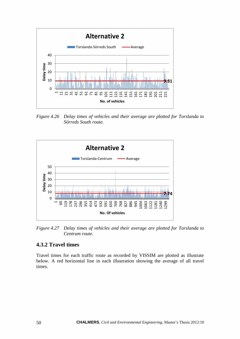
CHALMERS, Civil and Environmental Engineering, Master‟s Thesis 2012:10 50
9.31
0
10
20
30
401
11
21
31
41
51
61
71
81
91
10
11
11
12
11
31
14
11
51
16
11
71
18
11
91
20
12
11
22
1
De
lay
tim
e
No. of vehicles
Alternative 2
Torslanda-Sörreds South Average
Figure 4.26 Delay times of vehicles and their average are plotted for Torslanda to
Sörreds South route.
7.740
10
20
30
40
50
16
01
19
17
82
37
29
63
55
41
44
73
53
25
91
65
07
09
76
88
27
88
69
45
10
04
10
63
11
22
11
81
12
40
12
99
De
lay
tim
e
No. Of vehicles
Alternative 2
Torslanda-Centrum Average
Figure 4.27 Delay times of vehicles and their average are plotted for Torslanda to
Centrum route.
4.3.2 Travel times
Travel times for each traffic route as recorded by VISSIM are plotted as illustrate
below. A red horizontal line in each illustration showing the average of all travel
times.

CHALMERS, Civil and Environmental Engineering, Master‟s Thesis 2012:10 51
72.57
0
50
100
1501
32
63
94
12
5
15
6
18
7
21
8
24
9
28
0
31
1
34
2
37
3
40
4
43
5
46
6
49
7
52
8
55
9
59
0
62
1
65
2
Trav
el t
ime
No. of vehicles
Alternative 2
Centrum-Sörreds North Average
Figure 4.28 Travel times of vehicles and their average are plotted for Centrum to
Sörreds North route.
132.47
0
50
100
150
200
250
1
12
2
24
3
36
4
48
5
60
6
72
7
84
8
96
9
10
90
12
11
13
32
14
53
15
74
16
95
18
16
19
37
20
58
21
79
23
00
24
21
25
42
Trav
el t
ime
No. Of vehicles
Alternative 2
Centrum-Torslanda Average
Figure 4.29 Travel times of vehicles and their average are plotted for Centrum to
Torslanda route.

CHALMERS, Civil and Environmental Engineering, Master‟s Thesis 2012:10 52
176.48
0
100
200
300
400
500
1 3 5 7 9 11 13 15 17 19 21 23 25 27 29 31 33 35 37 39 41 43 45 47
Trav
el t
ime
No. Of vehicles
Alternative 2
Centrum-Sörreds South Average
Figure 4.30 Travel times of vehicles and their average are plotted for Centrum to
Sörreds South route.
148.85
0
100
200
300
400
1
63
12
5
18
7
24
9
31
1
37
3
43
5
49
7
55
9
62
1
68
3
74
5
80
7
86
9
93
1
99
3
10
55
11
17
11
79
12
41
13
03
Trav
el t
ime
No. Of vehicles
Alternative 2
Sörreds North-Centrum Average
Figure 4.31 Travel times of vehicles and their average are plotted for Sörreds North
to Centrum route.

CHALMERS, Civil and Environmental Engineering, Master‟s Thesis 2012:10 53
72.31
0
50
100
150
1 5 9 13 17 21 25 29 33 37 41 45 49 53 57 61 65 69 73 77 81 85 89
Trav
el t
ime
No. Of vehicles
Alternative 2
Sörreds South-Sörreds North Average
Figure 4.32 Travel times of vehicles and their average are plotted for Sörreds South
to Sörreds North route.
128.15
0
50
100
150
200
250
300
1 5 9 13 17 21 25 29 33 37 41 45 49 53 57 61 65 69 73 77 81 85 89 93
Trav
el t
ime
No.of vehicles
Alternative 2
Sörreds South-Centrum Average
Figure 4.33 Travel times of vehicles and their average are plotted for Sörreds South
to Centrum route.

CHALMERS, Civil and Environmental Engineering, Master‟s Thesis 2012:10 54
146.38
0
50
100
150
200
2501
27
53
79
10
5
13
1
15
7
18
3
20
9
23
5
26
1
28
7
31
3
33
9
36
5
39
1
41
7
44
3
46
9
49
5
52
1
54
7
Trav
el t
ime
No. Of vehicles
Alternative 2
Sörreds South-Torslanda Average
Figure 4.34 Travel times of vehicles and their average are plotted for Sörreds South
to Torslanda route.
113.83
0
50
100
150
200
1
40
79
11
8
15
7
19
6
23
5
27
4
31
3
35
2
39
1
43
0
46
9
50
8
54
7
58
6
62
5
66
4
70
3
74
2
78
1
82
0
Trav
el t
ime
No. Of vehicles
Alternative 2
Sörreds North - Torslanda Average
Figure 4.35 Travel times of vehicles and their average are plotted for Sörreds North
to Torslanda route.

CHALMERS, Civil and Environmental Engineering, Master‟s Thesis 2012:10 55
162.16
0
50
100
150
200
2501
37
73
10
9
14
5
18
1
21
7
25
3
28
9
32
5
36
1
39
7
43
3
46
9
50
5
54
1
57
7
61
3
64
9
68
5
72
1
75
7
Trav
el t
ime
No. Of vehicles
Alternative 2
Torslanda-Sörreds North Average
Figure 4.36 Travel times of vehicles and their average are plotted for Torslanda to
Sörreds North route.
101.97
0
50
100
150
1
12
23
34
45
56
67
78
89
10
0
11
1
12
2
13
3
14
4
15
5
16
6
17
7
18
8
19
9
21
0
22
1
Trav
el t
ime
No. Of vehicles
Alternative 2
Torslanda-Sörreds South Average
Figure 4.37 Travel times of vehicles and their average are plotted for Torslanda to
Sörreds South route.

CHALMERS, Civil and Environmental Engineering, Master‟s Thesis 2012:10 56
130.51
0
50
100
150
200
2501
62
12
3
18
4
24
5
30
6
36
7
42
8
48
9
55
0
61
1
67
2
73
3
79
4
85
5
91
6
97
7
10
38
10
99
11
60
12
21
12
82
Trav
el t
ime
No. Of vehicles
Alternative 2
Torslanda-Centrum Average
Figure 4.38 Travel times of vehicles and their average are plotted for Torslanda to
Centrum route.
4.3.3 Queue record
Average and maximum queue lengths and number of stops against each route of
alternative-2 are summarized in Figure 4.39.
0
200
400
600
800
1000
1200
Ce
ntr
um
-Sö
rred
s So
uth
Ce
ntr
um
-Sö
rred
s N
ort
h
Sörr
ed
s N
ort
h-S
örr
ed
sSo
uth
& C
entr
um
Sörr
ed
sväg
en-C
en
tru
m
Tors
lan
da-
Sörr
eds
No
rth
Sörr
ed
s So
uth
-Sö
rred
sN
ort
h &
To
rsla
nd
a
Alternative 2
Average Maximum Stop
Figure 4.39 Traffic queue values with their respective junction.

CHALMERS, Civil and Environmental Engineering, Master‟s Thesis 2012:10 57
4.4 Alternative 3A
Alternative-3A model, having flyover at Torslandavägen was simulated in VISSIM
and following parameters for evaluation of results were analyzed.
4.4.1 Delays
Delay in traffic flow for each traffic route that recorded by VISSIM are plotted as
illustrate below. A red horizontal line in each illustration showing the average of all
delay times
17.48
0
10
20
30
40
50
1 2 3 4 5 6 7 8 9 10 11 12 13 14 15 16 17 18 19 20 21
De
lay
tim
e
No. Of vehicles
Alternative 3A
Centrum-Torslanda Average
Figure 4.40 Delay times of vehicles and their average are plotted for Centrum to
Torslanda route.
49.34
0
50
100
150
1
30
59
88
11
7
14
6
17
5
20
4
23
3
26
2
29
1
32
0
34
9
37
8
40
7
43
6
46
5
49
4
52
3
55
2
58
1
61
0
De
lay
tim
e
No. Of vehicles
Alternative 3A
Centrum-Sörreds North Average
Figure 4.41 Delay times of vehicles and their average are plotted for Centrum to
Sörreds North route.

CHALMERS, Civil and Environmental Engineering, Master‟s Thesis 2012:10 58
93.01
0
50
100
150
200
1 3 5 7 9 1113151719212325272931333537394143454749515355
De
lay
tim
e
No. Of vehicles
Alternative 3A
Centrum-Sörreds South Average
Figure 4.42 Delay times of vehicles and their average are plotted for Centrum to
Sörreds South route.
181.36
0
50
100
150
200
250
1 6
11
16
21
26
31
36
41
46
51
56
61
66
71
76
81
86
91
96
10
1
De
lay
tim
e
No. Of vehicles
Alternative 3A
Sörreds South-Sörreds North Average
Figure 4.43 Delay times of vehicles and their average are plotted for Sörreds South
to Sörreds North route.

CHALMERS, Civil and Environmental Engineering, Master‟s Thesis 2012:10 59
112.15
0
50
100
150
200
2501 6
11
16
21
26
31
36
41
46
51
56
61
66
71
76
81
86
91
96
10
1
De
lay
tim
e
No. Of vehicles
Alternative 3A
Sörreds South-Centrum Average
Figure 4.44 Delay times of vehicles and their average are plotted for Sörreds South
to Centrum route.
202.03
0
50
100
150
200
250
300
1
25
49
73
97
12
1
14
5
16
9
19
3
21
7
24
1
26
5
28
9
31
3
33
7
36
1
38
5
40
9
43
3
45
7
48
1
50
5
De
lay
tim
e
No. Of vehicles
Alternative 3A
Sörreds South-Torslanda Average
Figure 4.45 Delay times of vehicles and their average are plotted for Sörreds South
to Torslanda route.

CHALMERS, Civil and Environmental Engineering, Master‟s Thesis 2012:10 60
11.880
50
100
150
2001
64
12
7
19
0
25
3
31
6
37
9
44
2
50
5
56
8
63
1
69
4
75
7
82
0
88
3
94
6
10
09
10
72
11
35
11
98
12
61
13
24
De
lay
tim
e
No. Of vehicles
Alternative 3A
Torslanda-Centrum Average
Figure 4.46 Delay times of vehicles and their average are plotted for Torslanda to
Centrum route.
96.29
0
50
100
150
200
250
1
36
71
10
6
14
1
17
6
21
1
24
6
28
1
31
6
35
1
38
6
42
1
45
6
49
1
52
6
56
1
59
6
63
1
66
6
70
1
73
6
De
lay
tim
e
No. Of vehicles
Alternative 3A
Torslanda-Sörreds North Average
Figure 4.47 Delay times of vehicles and their average are plotted for Torslanda to
Sörreds North route.
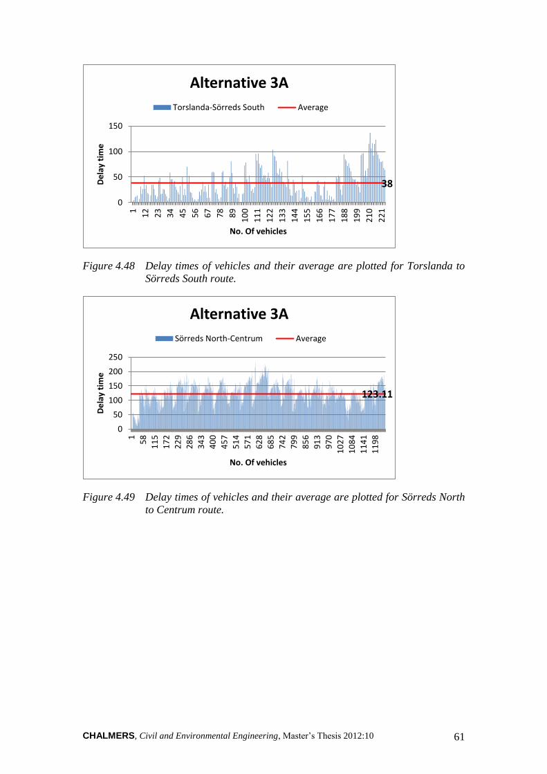
CHALMERS, Civil and Environmental Engineering, Master‟s Thesis 2012:10 61
38
0
50
100
1501
12
23
34
45
56
67
78
89
10
0
11
1
12
2
13
3
14
4
15
5
16
6
17
7
18
8
19
9
21
0
22
1
De
lay
tim
e
No. Of vehicles
Alternative 3A
Torslanda-Sörreds South Average
Figure 4.48 Delay times of vehicles and their average are plotted for Torslanda to
Sörreds South route.
123.11
0
50
100
150
200
250
1
58
11
5
17
2
22
9
28
6
34
3
40
0
45
7
51
4
57
1
62
8
68
5
74
2
79
9
85
6
91
3
97
0
10
27
10
84
11
41
11
98
De
lay
tim
e
No. Of vehicles
Alternative 3A
Sörreds North-Centrum Average
Figure 4.49 Delay times of vehicles and their average are plotted for Sörreds North
to Centrum route.

CHALMERS, Civil and Environmental Engineering, Master‟s Thesis 2012:10 62
28.43
0
20
40
60
80
100
1201
27
53
79
10
5
13
1
15
7
18
3
20
9
23
5
26
1
28
7
31
3
33
9
36
5
39
1
41
7
44
3
46
9
49
5
52
1
54
7
De
lay
tim
e
No. Of vehicles
Alternative 3A
Sörreds North-Torslanda Average
Figure 4.50 Delay times of vehicles and their average are plotted for Sörreds North
to Torslanda route.
4.4.2 Travel times
Travel times for each traffic route as recorded by VISSIM are plotted as illustrate
below. A red horizontal line in each illustration showing the average of all travel
times.
144.68
0
100
200
300
400
1
11
8
23
5
35
2
46
9
58
6
70
3
82
0
93
7
10
54
11
71
12
88
14
05
15
22
16
39
17
56
18
73
19
90
21
07
22
24
23
41
24
58
Trav
el t
ime
No. Of vehicles
Alternative 3A
Centrum-Torslanda Average
Figure 4.51 Travel times of vehicles and their average are plotted for Centrum to
Torslanda route.

CHALMERS, Civil and Environmental Engineering, Master‟s Thesis 2012:10 63
98.87
0
50
100
150
200
2501
30
59
88
11
7
14
6
17
5
20
4
23
3
26
2
29
1
32
0
34
9
37
8
40
7
43
6
46
5
49
4
52
3
55
2
58
1
61
0
Trav
el t
ime
No. Of vehicles
Alternative 3A
Centrum-Sörreds North Average
Figure 4.52 Travel times of vehicles and their average are plotted for Centrum to
Sörreds North route.
156
0
50
100
150
200
250
300
1 3 5 7 9 1113151719212325272931333537394143454749515355
Trav
el t
ime
No. Of Vehicles
Alternative 3A
Centrum-Sörreds South Average
Figure 4.53 Travel times of vehicles and their average are plotted for Centrum to
Sörreds South route.

CHALMERS, Civil and Environmental Engineering, Master‟s Thesis 2012:10 64
213.27
0
50
100
150
200
250
3001 6
11
16
21
26
31
36
41
46
51
56
61
66
71
76
81
86
91
96
10
1
Trav
el t
ime
No. Of vehicles
Alternative 3A
Sörreds South-Sörreds North Average
Figure 4.54 Travel times of vehicles and their average are plotted for Sörreds South
to Sörreds North route.
184.37
0
50
100
150
200
250
300
1 6
11
16
21
26
31
36
41
46
51
56
61
66
71
76
81
86
91
96
10
1
Trav
el t
ime
No. Of vehicles
Alternative 3A
Sörreds South-Centrum Average
Figure 4.55 Travel times of vehicles and their average are plotted for Sörreds South
to Centrum route.

CHALMERS, Civil and Environmental Engineering, Master‟s Thesis 2012:10 65
308
0
100
200
300
400
5001
25
49
73
97
12
1
14
5
16
9
19
3
21
7
24
1
26
5
28
9
31
3
33
7
36
1
38
5
40
9
43
3
45
7
48
1
50
5
Trav
el t
ime
No. Of vehicles
Alternative 3A
Sörreds South-Torslanda Average
Figure 4.56 Travel times of vehicles and their average are plotted for Sörreds South
to Torslanda route.
140
0
100
200
300
400
1
64
12
7
19
0
25
3
31
6
37
9
44
2
50
5
56
8
63
1
69
4
75
7
82
0
88
3
94
6
10
09
10
72
11
35
11
98
12
61
13
24
Trav
el t
ime
No. Of vehicles
Alternative 3A
Torslanda-Centrum Average
Figure 4.57 Travel times of vehicles and their average are plotted for Torslanda to
Centrum route.

CHALMERS, Civil and Environmental Engineering, Master‟s Thesis 2012:10 66
205.5
0
100
200
300
4001
36
71
10
6
14
1
17
6
21
1
24
6
28
1
31
6
35
1
38
6
42
1
45
6
49
1
52
6
56
1
59
6
63
1
66
6
70
1
73
6
Trav
el t
ime
No. Of vehicles
Alternative 3A
Torslanda-Sörreds North Average
Figure 4.58 Travel times of vehicles and their average are plotted for Torslanda to
Sörreds North route.
137.36
0
50
100
150
200
250
300
1
12
23
34
45
56
67
78
89
10
0
11
1
12
2
13
3
14
4
15
5
16
6
17
7
18
8
19
9
21
0
22
1
Trav
el t
ime
No. Of vehicles
Alternative 3A
Torslanda-Sörreds South Average
Figure 4.59 Travel times of vehicles and their average are plotted for Torslanda to
Sörreds South route.

CHALMERS, Civil and Environmental Engineering, Master‟s Thesis 2012:10 67
201.7
0
100
200
300
4001
59
11
7
17
5
23
3
29
1
34
9
40
7
46
5
52
3
58
1
63
9
69
7
75
5
81
3
87
1
92
9
98
7
10
45
11
03
11
61
12
19
Trav
el t
ime
No. Of Vehicles
Alternative 3A
Sörreds North-Centrum Average
Figure 4.60 Travel times of vehicles and their average are plotted for Sörreds South
to Centrum route.
121.36
0
50
100
150
200
250
1
28
55
82
10
9
13
6
16
3
19
0
21
7
24
4
27
1
29
8
32
5
35
2
37
9
40
6
43
3
46
0
48
7
51
4
54
1
56
8
Trav
el t
ime
No. Of vehicles
Alternative 3A
Sörreds North-Torslanda Average
Figure 4.61 Travel times of vehicles and their average are plotted for Sörreds North
to Torslanda route.
4.4.3 Queue record
Average and maximum queue lengths and number of stops against each route of
alternative-3a are summarized in Figure 4.62.

CHALMERS, Civil and Environmental Engineering, Master‟s Thesis 2012:10 68
0
200
400
600
800
1000
1200
1400
Ce
ntr
um
-Sö
rred
s N
ort
h
Tors
lan
da-
Sörr
eds
No
rth
Sörr
ed
sväg
en-C
en
tru
m
Tors
lan
da-
Cen
tru
m (
PT
line
)
Sörr
ed
s N
ort
h-S
örr
ed
sSo
uth
& C
entr
um
Sörr
ed
s So
uth
-Sö
rred
sN
ort
h &
To
rsla
nd
a
Ce
ntr
um
-To
rsla
nd
a (P
Tlin
e)
Ce
ntr
um
-Sö
rred
s So
uth
Alternative 3A
Average Maximum Stop
Figure 4.62 Traffic queue values with their respective route.
4.5 Comparative analysis
The results as plotted above can be given a good idea about the better alternative that
fulfils the demand in more efficient way. However, in the continuation of results a
comparison is made by considering average values of results. The comparisons
include both alternatives as well as the present scenario of the intersection with the
same amount of traffic as in the alternatives. The purpose to include the present
scenario model is to show the necessity of flyover to fulfil the future demand of traffic
flow.
4.5.1 Delay time comparison
The comparison as given in Figure 4.63 clearly shows the highest delay time in the
present scenario case. However alternative-2 standing with lowest value almost in all
routing comparison.

CHALMERS, Civil and Environmental Engineering, Master‟s Thesis 2012:10 69
0
50
100
150
200
250Sö
rre
ds
No
rth
-To
rsla
nd
a
Sörr
ed
s N
ort
h-
Ce
ntr
um
Tors
lan
da-
Sörr
eds
Sou
th
Tors
lan
da-
Sörr
eds
No
rth
Tors
lan
da-
Cen
tru
m
Sörr
ed
s So
uth
-To
rsla
nd
a
Sörr
ed
s So
uth
-C
en
tru
m
Sörr
ed
s So
uth
-Sö
rred
sN
ort
h
Ce
ntr
um
-Sö
rre
ds
Sou
th
Ce
ntr
um
-Sö
rre
ds
No
rth
Ce
ntr
um
-To
rsla
nd
a
De
lay
tim
e
Delay Time Comparison
Alternative-2 (Average) Alternative-3a (Average)
Current Scenario with Future traffic (Average)
Figure 4.63 Average delay time comparisons between alternatives and present
scenario having same amount of traffic.
4.5.2 Travel time comparison
Travel timings for the selected routes are plotted in the same way as did in delay time
comparison. The results as illustrates in the Figure 4.64 shows that the lowest travel
times belongs to alternative-2 almost in all routing decisions.
0
50
100
150
200
250
300
350
Sörr
ed
s N
ort
h-
Tors
lan
da
Sörr
ed
s N
ort
h-
Ce
ntr
um
Tors
lan
da-
Sörr
eds
Sou
th
Tors
lan
da-
Sörr
eds
No
rth
Tors
lan
da-
Cen
tru
m
Sörr
ed
s So
uth
-To
rsla
nd
a
Sörr
ed
s So
uth
-C
en
tru
m
Sörr
ed
s So
uth
-Sö
rred
sN
ort
h
Ce
ntr
um
-Sö
rred
sSo
uth
Ce
ntr
um
-Sö
rred
sN
ort
h
Ce
ntr
um
-To
rsla
nd
a
Trav
el T
ime
Travel Times Comparison
Alternative-2 (Average) Alternative-3a (Average)
Current Scenario with Future traffic (Average)
Figure 4.64 Average travel time comparisons between alternatives and present
scenario having same amount of traffic.
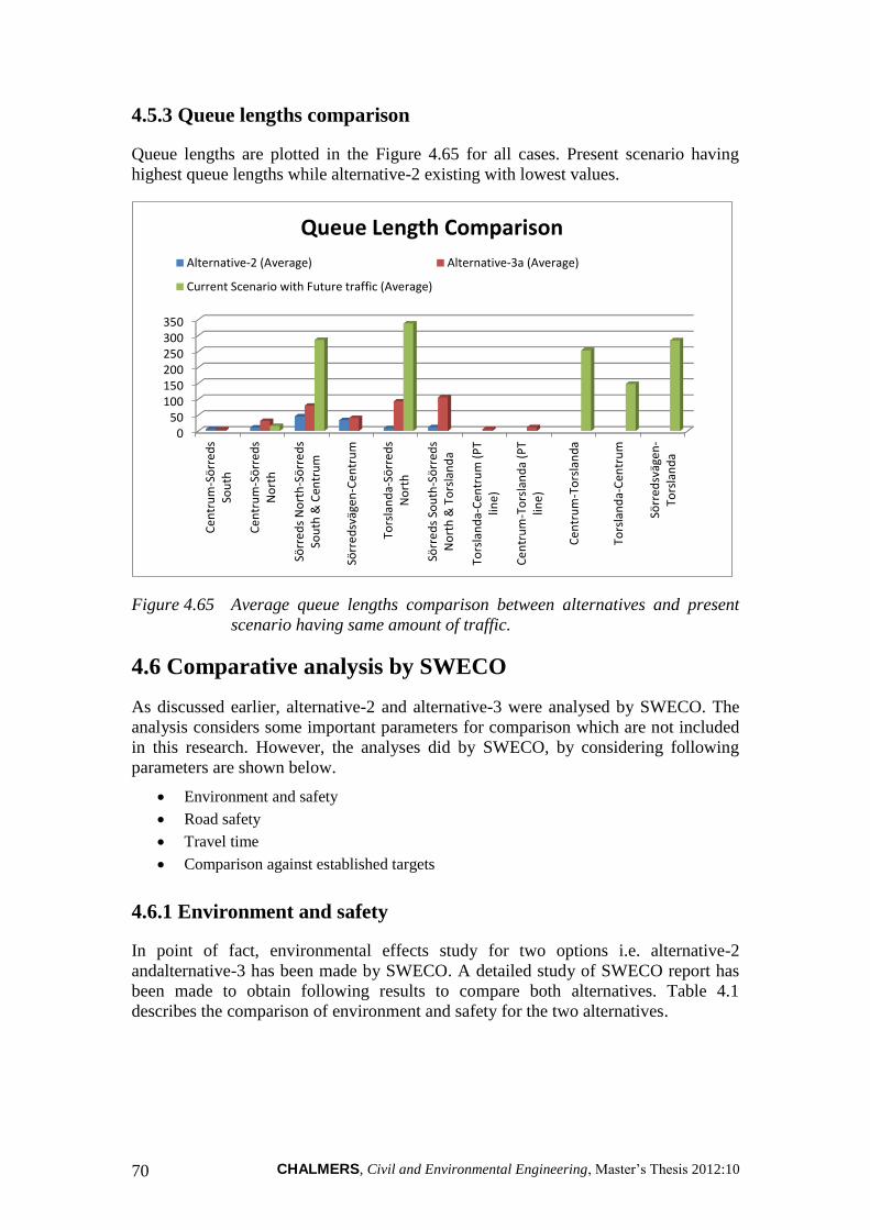
CHALMERS, Civil and Environmental Engineering, Master‟s Thesis 2012:10 70
4.5.3 Queue lengths comparison
Queue lengths are plotted in the Figure 4.65 for all cases. Present scenario having
highest queue lengths while alternative-2 existing with lowest values.
050
100150200250300350
Ce
ntr
um
-Sö
rred
sSo
uth
Ce
ntr
um
-Sö
rred
sN
ort
h
Sörr
ed
s N
ort
h-S
örr
ed
sSo
uth
& C
entr
um
Sörr
ed
sväg
en-C
en
tru
m
Tors
lan
da-
Sörr
eds
No
rth
Sörr
ed
s So
uth
-Sö
rred
sN
ort
h &
To
rsla
nd
a
Tors
lan
da-
Cen
tru
m (
PT
line
)
Ce
ntr
um
-To
rsla
nd
a (P
Tlin
e)
Ce
ntr
um
-To
rsla
nd
a
Tors
lan
da-
Cen
tru
m
Sörr
ed
sväg
en-
Tors
lan
da
Queue Length Comparison
Alternative-2 (Average) Alternative-3a (Average)
Current Scenario with Future traffic (Average)
Figure 4.65 Average queue lengths comparison between alternatives and present
scenario having same amount of traffic.
4.6 Comparative analysis by SWECO
As discussed earlier, alternative-2 and alternative-3 were analysed by SWECO. The
analysis considers some important parameters for comparison which are not included
in this research. However, the analyses did by SWECO, by considering following
parameters are shown below.
Environment and safety
Road safety
Travel time
Comparison against established targets
4.6.1 Environment and safety
In point of fact, environmental effects study for two options i.e. alternative-2
andalternative-3 has been made by SWECO. A detailed study of SWECO report has
been made to obtain following results to compare both alternatives. Table 4.1
describes the comparison of environment and safety for the two alternatives.

CHALMERS, Civil and Environmental Engineering, Master‟s Thesis 2012:10 71
Table 4.1 Environmental safety comparison for both alternatives, i.e. 2 and 3,
presented by SWECO (SWECO, 2011 translated version)
Alt. 2 Comments Alt. 3 Comments
Environment
-Exhaust + Fewer vehicles affected by
the signal. The ramp to the
center gives the road
extension and increased
transport.
- More vehicles affected by
the signal.
-Airborne
particles
- Higher and more irregular
rate gives more airborne + Lower speeds means less
airborne
-CO2 + Fewer vehicles affected by
the signal. The ramp to the
center gives the road
extension and increased
transport.
- More vehicles affected by
the signal.
-Noise 0 Equivalent 0 Equivalent
Safety
-Pedestrian - HPL during/under the
bridge. Precarious. + HPL along walkways.
Open and bright. More
secure.
-Bicycle - Cycle path south of the
row 155 for passage of the
ramps are in the trough.
Insecure!
+ Bicycle Trail open and in
the plane. More secure!
Environmental comparison for two alternatives shown above in Table 4.1 states that
fewer vehicles are affected by signals in alternative-2 as compared to alternative-3
Hence, consequences are more vehicle delays producing more emissions in
alternative-3. It means that alternative-2 is more environmental friendly as compared
to alternative-3.
4.6.2 Road safety
Table 4.2 gives road safety comparison for both alternatives.
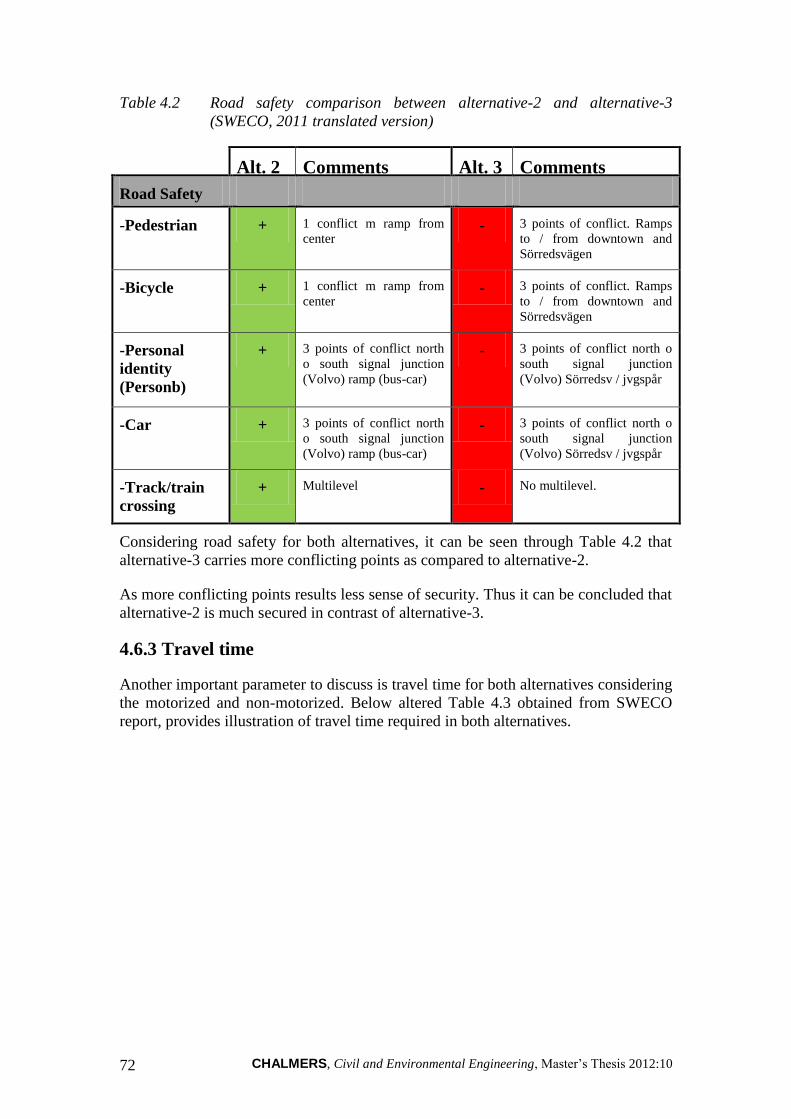
CHALMERS, Civil and Environmental Engineering, Master‟s Thesis 2012:10 72
Table 4.2 Road safety comparison between alternative-2 and alternative-3
(SWECO, 2011 translated version)
Alt. 2 Comments Alt. 3 Comments
Road Safety
-Pedestrian + 1 conflict m ramp from
center - 3 points of conflict. Ramps
to / from downtown and
Sörredsvägen
-Bicycle + 1 conflict m ramp from
center - 3 points of conflict. Ramps
to / from downtown and
Sörredsvägen
-Personal
identity
(Personb)
+ 3 points of conflict north
o south signal junction
(Volvo) ramp (bus-car)
- 3 points of conflict north o
south signal junction
(Volvo) Sörredsv / jvgspår
-Car + 3 points of conflict north
o south signal junction
(Volvo) ramp (bus-car)
- 3 points of conflict north o
south signal junction
(Volvo) Sörredsv / jvgspår
-Track/train
crossing
+ Multilevel - No multilevel.
Considering road safety for both alternatives, it can be seen through Table 4.2 that
alternative-3 carries more conflicting points as compared to alternative-2.
As more conflicting points results less sense of security. Thus it can be concluded that
alternative-2 is much secured in contrast of alternative-3.
4.6.3 Travel time
Another important parameter to discuss is travel time for both alternatives considering
the motorized and non-motorized. Below altered Table 4.3 obtained from SWECO
report, provides illustration of travel time required in both alternatives.

CHALMERS, Civil and Environmental Engineering, Master‟s Thesis 2012:10 73
Table 4.3 Travel time comparison in both alternative-2 and alternative-3
(SWECO, 2011 translated version)
Alt. 2 Comments Alt. 3 Comments
Travel Time
-Pedestrian - Longer paths. Larger
differences in height.
Fewer conflict points of
delay.
+ Short paths. Small
differences in height. More
points of conflict that gives
a delay.
-Bicycle - Longer paths. Larger
differences in height.
Fewer conflict points of
delay.
+ Short paths. Small
differences in height. More
points of conflict that gives
a delay.
-Bus travelers,
consistently
+ -
-Bus
Passengers,
exchange +
goals / start
journeys
- +
- Bus
passengers,
weighted
+ - More consistently travelers!
-Car + Fewer vehicles affected by
the signal. The ramp to the
center gives the road
extension and increased
transport
- More vehicles affected by
the signal. More conflicts
and bus priority reduces
capacity.
-Truck + Fewer vehicles affected by
the signal. The ramp to the
center gives the road
extension and increased
transport
- More vehicles affected by
the signal.
For pedestrians, alternative-3 is more suitable considering fact of small height and
short paths. Apparently conflicting areas are more in numbers causing delay for
pedestrians. Despite of this fact, alternative-3 can be more feasible and convenient for
pedestrians to walk through as compared to alternative-2, especially considering fact
of long winter and rainy season in Sweden.
On the contrary, from Table 4.3, alternative-2 can be regarded as best option for cars
and other heavy traffic by means of less conflicting areas.

CHALMERS, Civil and Environmental Engineering, Master‟s Thesis 2012:10 74
4.6.4 Comparison against established targets
Results obtained by SWECO report has been altered and analysed in detail for
comparing against established targets stated below in Table 4.4.
Table 4.4 Comparison between alternative-2 andalternative-3 against established
targets (SWECO, 2011 translated version)
Alt.2 Comments Alt. 3 Comments
-Multilevel rail
crossing
Yes Multilevel - No multilevel
-Enhance safety
and accessibility
on the Road 155
Yes Fair
-Attractive cycle
path
Fair
Poor alignment but plan
separately Fair Good alignment but the
level crossing
-Attractive public
transport services
to Torslanda
Yes Bus Lane - Bus lanes but too poor
accessibility standard
with stops on the ramps
- Attractive
exchange item
Fair
It will be better than
today. Does not the
requirements for
"Attractive exchange
point" according to VT
Fair It will be better than
today. Does not the
requirements for
"Attractive exchange
point" according to VT
-Coordination
with the ongoing
expansion work
Fair equivalent Fair equivalent
-Keeping given
budget
- +
Overall assessment for both alternatives has been presented in Table 4.4. It is quite
clear that alternative-3 is not fulfilling project development purposes in terms of
following basic objectives:
One of the purposes to build flyover was to make multilevel rail crossing. In
scenario 3 and 3A, there are no multilevel crossing for rail road thus resulting
conflicts between road traffic and rail.
Less safer especially for non-motorized traffic. More chances to conflict with rail
road and other traffic.
Less attractive public transport facility to Torslandavägen with stops located on
ramps.

CHALMERS, Civil and Environmental Engineering, Master‟s Thesis 2012:10 75
5 Discussion and conclusion
In this thesis, a microscopic simulation software program namely VISSIM has been
utilized to study Sörreds Intersection. First use of VISSIM was to display the present
working of Sörreds intersection has been made. Later on studies continued on the
basis of future increased assumed traffic. It was observed that double volumes in year
2035 will exceed capacity of lanes during peak hours. Thus, two different alternatives
proposed by SWECO were analysed by utilizing VISSIM and display of future
working of junction has been shown. More congestion situations were experienced in
case of implementing alternative 3A more specifically at the start point of Sörreds
north entry link. Also, increased green time period for particular link adversely affects
other links by increasing queue lengths and delay periods. Furthermore, alternative 3A
carries insufficient capacity and will not be able to dismantle the design traffic flows.
Referring from SWECO report, it is clear that growth of traffic is more for Road-155
i.e. Torslandavägen. However the main objective of making flyover was to make
traffic more fluent and safer for Sörreds intersection rather than only making
Torslandavägen link more fluent. Moreover, another benefit for existence of flyover at
Sörreds intersection is provision of multilevel crossing for rail and road users.

CHALMERS, Civil and Environmental Engineering, Master‟s Thesis 2012:10 76
6 Recommendations
Overall discussion reflects that the alternative-2 is a better choice while considering
the traffic flow and other parameters rather than economic parameter. However it is
not an ending document for the research. The real world is full of complexities and
the created models can‟t fully demonstrate that what will happen in future? To get
closer picture, continues research should keep in process. There are several aspects
and parameters which have been avoided until now, can be helpful to get more
accurate findings. Some possible aspects which can consider for the further research
are mentioned below.
Rail road, pedestrians and bicyclists inclusion in both alternatives‟ model.
Several kinds of survey from frequent users, public transport drivers and industrial
personnel can be helpful to make a good judgment.
Study of other similar projects that can give assistive information for decision.
It is observed during both simulation models, that there was a traffic congestion
situation occurred at the ring road, when the vehicles going towards centrum from
Sörreds north and Sörreds south. The reason is that the ring road which meets
Sörredsvägen with Torslandavägen is a combination of a two lane road converting
into one lane road. The design can be reviewed by keeping two lanes until it meets
Torslandavägen and then can be analyze through simulation.

CHALMERS, Civil and Environmental Engineering, Master‟s Thesis 2012:10 77
7 References
Al-Mudhaffar, A., 2006.Impacts of Traffic Signal Control Strategies. Ph.D. Thesis.
Traffic and transport planning, infrastructure and planning. Royal Institute of
Technology, Stockholm, Sweden
Arvis J-F., et al., 2010. Connecting to Compete- Trade Logistics in the Global
Economy [Online] The World Bank. Available at:
<http://siteresources.worldbank.org/INTTLF/Resources/LPI2010_for_web.pdf >
[Accessed on: 2011-10-30]
Bonneson J.A., McCoy P.T., 2005. Manual of Traffic detector design-Chapter 4 [pdf]
Institute of Transportation Engineers (ITE). Available at:
http://www.webs1.uidaho.edu/ce572s07/resources/other/manual%20of%20traffic
%20detector%20design.pdf [Accessed on: 2011-11-25]
Bonneson J., Sunkari S., & Pratt M., 2009. TRAFFIC SIGNAL OPERATIONS
HANDBOOK, TEXAS TRANSPORTATION INSTITUTE
Barceló, J., 2010. Fundamentals of Traffic Simulation. New York: Springer
Science+Business Media, LLC.
Federal Highway Administration (FHWA), 2008. Traffic Signal Timing Manual [pdf]
US-Department of Transportation. Available at:
http://ops.fhwa.dot.gov/publications/fhwahop08024/fhwa_hop_08_024.pdf
[Accessed on: 2011-11-25]
Google Earth 6.0. 2008. Sörredsvägen, Gothenburg, Västra Götalands Läan, Sweden
57°42'43.30"N, 11°50'28.92"E, Elevation 31 ft.
Available through: <http://www.google.com/earth/index.html> [Accessed
through: 25 September 2011].
Highway Capacity Manual (HCM), 2000.(Fourth edition).TRB, National Research
Council, Washington, D.C., 2000.
IIT-Bombay, 200?Transportation engineering. [Online] Available at:
http://www.cdeep.iitb.ac.in/nptel/Civil%20Engineering/Transportation%20Engg%
20I/72-homes/01-home.html [Accessed on: 2011-11-23]
Kell J.H., Fullerton I.J., 1998. Manual of traffic signal design - Chapter 7. [pdf]
Institute of Transportation Engineers. Available at:
http://www.webs1.uidaho.edu/ce572s07/resources/other/manual%20of%20traffic
%20signal%20design%20-%20ch%207.pdf [Accessed on: 2011-11-25]
Kutz M., 2003. Handbook of Transportation Engineering. [e-book] New York:
McGraw-Hill. Available through: Chalmers University Library website
<http://www.lib.chalmers.se>[Accessed on: 2011-11-28]
Li M., Wo T., 2011. Prediction and evaluation of traffic quality by static and dynamic
simulation; Impact of new bus terminal at Myggenäs intersection, MSc Thesis,

CHALMERS, Civil and Environmental Engineering, Master‟s Thesis 2012:10 78
Road and Traffic Group, Department of Civil and Environmental Engineering,
Chalmers University of Technology, Sweden.
PTV, 2011. VISSIM User Manual – Version 5.30-05, PTV Planung Transport
Verkehr AG, Karlsruhe, Germany
Roess R.P., et al., 2004. Traffic Engineering.Third Edition. Upper Saddle River, NJ:
Pearson Prentice Hall.
Slinn, M., Matthews, P., Guest, P., 2005. Traffic engineering design: principles and
practice (second edition). Oxford, UK: Elsevier.
Statistics Sweden, 2011.Population by period. Year 2001-2010 [Online] (Updated on:
2011-02-18 09:40) Available at:
http://www.ssd.scb.se/databaser/igraph/MakeGraph.asp?onpx=y&pxfile=tmp2011
103117412836BE0101N1.px&PLanguage=2&menu=y&gr_type=1[Accessed on:
2011-10-30]
Statistics Sweden, 2011.Population growth by period. Year 2001-2010 [Online]
(Updated on: 2011-02-18 09:40) Available at:
http://www.ssd.scb.se/databaser/igraph/MakeGraph.asp?onpx=y&pxfile=tmp2011
10311743090BE0101N2.px&PLanguage=2&menu=y&gr_type=1[Accessed on:
2011-10-30]
Statistics Sweden, 2011. Fordon enligt bilregistret efter fordonsslag och bestånd.
Månad 1975M01-2011M09 [Online] (Updated on: 2011-10-03 09:30) Available at:
http://www.ssd.scb.se/databaser/makro/SaveShow.asp [Accessed on: 2011-10-30]
SWECO AB, 2011. Sörredskorsningen-Utformning av trafikplats – jämförande analys
av två alternativ, Trafikverket, Gothenburg, Sweden, 2011

CHALMERS, Civil and Environmental Engineering, Master‟s Thesis 2012:10 79
Appendix 1A (Overview of Alternative 2 Design)

CHALMERS, Civil and Environmental Engineering, Master‟s Thesis 2012:10 80
Appendix 1B (Overview of Alternative-3A design)
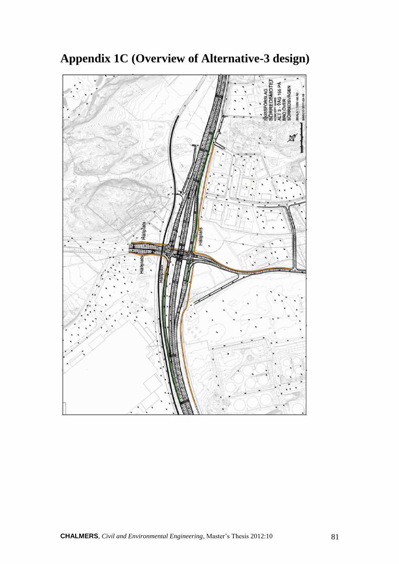
CHALMERS, Civil and Environmental Engineering, Master‟s Thesis 2012:10 81
Appendix 1C (Overview of Alternative-3 design)

CHALMERS, Civil and Environmental Engineering, Master‟s Thesis 2012:10 82
Appendix 2A (Recorded motorized and non-
motorized traffic flow)

CHALMERS, Civil and Environmental Engineering, Master‟s Thesis 2012:10 83
Appendix 2B (Vehicle amounts for present scenario)

CHALMERS, Civil and Environmental Engineering, Master‟s Thesis 2012:10 84
Appendix 2C (Vehicle amounts for alternatives)

CHALMERS, Civil and Environmental Engineering, Master‟s Thesis 2012:10 85
Appendix 3
(*.pua and *.vap files for Present scenario model)
$SIGNAL_GROUPS
VAP VISSIM
$
S1 1
S2 2
S3 3
S4 4
S5 5
S6 6
P1 7
P2 8
P3 9
P4 10
$STAGES
VAP VISSIM
1 Stage_1
2 Stage_2
3 Stage_3
4 Stage_4
$
STAGE_1 S1 S2 P1
STAGE_2 S3 S4 P2

CHALMERS, Civil and Environmental Engineering, Master‟s Thesis 2012:10 86
STAGE_3 S5 S6 P3 P4
$STARTING_STAGE
$
STAGE_1
$INTERSTAGE1
LENGTH [s] : 15
FROM STAGE : 1
TO STAGE : 2
$
S1 -127 14
S2 -127 0
S3 7 127
S4 7 127
P1 -127 0
P2 4 127
$INTERSTAGE2
LENGTH [s] : 35
FROM STAGE : 1
TO STAGE : 3
$
S1 -127 2
S2 -127 0

CHALMERS, Civil and Environmental Engineering, Master‟s Thesis 2012:10 87
S5 0 127
S6 8 127
P1 -127 0
P3 2 127
P4 10 127
$INTERSTAGE3
LENGTH [s] : 35
FROM STAGE : 2
TO STAGE : 3
$
S3 -127 0
S4 -127 10
S5 6 127
S6 6 127
P2 -127 0
P3 7 127
P4 14 127
$INTERSTAGE4
LENGTH [s] : 15
FROM STAGE : 2
TO STAGE : 1
$
S1 3 127
S2 4 127
S3 -127 0

CHALMERS, Civil and Environmental Engineering, Master‟s Thesis 2012:10 88
S4 -127 0
P1 4 127
P2 -127 0
$INTERSTAGE5
LENGTH [s] : 18
FROM STAGE : 3
TO STAGE : 1
$
S 7 127
S2 7 127
S5 -127 10
S6 -127 0
P1 5 127
P3 -127 0
P4 -127 0
$INTERSTAGE6
LENGTH [s] : 15
FROM STAGE : 3
TO STAGE : 2
$
S3 8 127
S4 7 127
S5 -127 2

CHALMERS, Civil and Environmental Engineering, Master‟s Thesis 2012:10 89
S6 -127 0
P2 6 127
P3 -127 0
P4 -127 2
$END

CHALMERS, Civil and Environmental Engineering, Master‟s Thesis 2012:10 90

CHALMERS, Civil and Environmental Engineering, Master‟s Thesis 2012:10 91
PARAMETERS Gen Comment
MAX_GAP 5 Max. gap time
MAX_STG1 15 Max. duration of stage 1
MAX_STG2 25 Max. duration of stage 2
MAX_STG3 25 Max. duration of stage 3
EXPRESSIONS Contents
Extend_Stg1
(Headway( 1 ) <= MAX_GAP) OR (Headway( 2 ) <=
MAX_GAP)
Extend_Stg2
(Headway( 3 ) <= MAX_GAP) OR (Headway( 4 ) <=
MAX_GAP)
Extend_Stg3
(Headway( 5 ) <= MAX_GAP) OR (Headway( 6 ) <=
MAX_GAP)
O1 Occupancy( 1 ) > 4
O2 Occupancy( 2 ) > 6
O3 Occupancy( 3 ) > 2
O4 Occupancy( 4 ) > 2
O5 Occupancy( 5 ) > 4
O6 Occupancy( 6 ) > 8

CHALMERS, Civil and Environmental Engineering, Master‟s Thesis 2012:10 92
Appendix 4A
(*.pua and *.vap files for Alternative-2 Sörreds North intersection)
$SIGNAL_GROUPS
VAP VISSIM
$
S1 1
S2 2
S3 3
S4 4
S5 5
$STAGES
VAP VISSIM
1 Stage_1
2 Stage_2
3 Stage_3
$
STAGE_1 S1 S5
STAGE_2 S2 S3
STAGE_3 S4
$STARTING_STAGE
$
STAGE_1

CHALMERS, Civil and Environmental Engineering, Master‟s Thesis 2012:10 93
$INTERSTAGE1
LENGTH [s] : 10
FROM STAGE : 1
TO STAGE : 2
$
S1 -127 0
S5 -127 5
S2 3 127
S3 8 127
$INTERSTAGE2
LENGTH [s] : 7
FROM STAGE : 1
TO STAGE : 3
$
S1 -127 0
S5 -127 10
S4 2 27
$INTERSTAGE3
LENGTH [s] : 7
FROM STAGE : 2
TO STAGE : 3
$
S2 -127 0

CHALMERS, Civil and Environmental Engineering, Master‟s Thesis 2012:10 94
S3 -127 0
S4 3 127
$INTERSTAGE4
LENGTH [s] : 12
FROM STAGE : 2
TO STAGE : 1
$
S1 3 127
S5 5 127
S2 -127 0
S3 -127 0
$INTERSTAGE5
LENGTH [s] : 12
FROM STAGE : 3
TO STAGE : 1
$
S1 5 127
S5 0 127
S4 -127 0
$INTERSTAGE6
LENGTH [s] : 15
FROM STAGE : 3
TO STAGE : 2
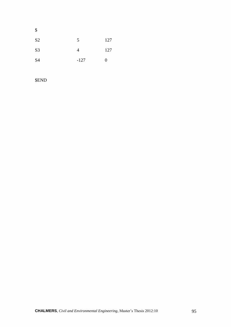
CHALMERS, Civil and Environmental Engineering, Master‟s Thesis 2012:10 95
$
S2 5 127
S3 4 127
S4 -127 0
$END

CHALMERS, Civil and Environmental Engineering, Master‟s Thesis 2012:10 96

CHALMERS, Civil and Environmental Engineering, Master‟s Thesis 2012:10 97
PARAMETERS Gen Comment
MAX_GAP 5 Max. gap time
MAX_STG1 30 Max. duration of stage 1
MAX_STG2 40 Max. duration of stage 2
MAX_STG3 8 Max. duration of stage 3
EXPRESSIONS Contents
Extend_Stg1 (Headway( 1 ) <= MAX_GAP) OR (Headway( 5 ) <= MAX_GAP)
Extend_Stg2 (Headway( 2 ) <= MAX_GAP) OR (Headway( 3 ) <= MAX_GAP)
Extend_Stg3 (Headway( 4 ) <= MAX_GAP)
O1 Occupancy( 1 ) > 4
O2 Occupancy( 2 ) > 6
O3 Occupancy( 3 ) > 8
O4 Occupancy( 4 ) > 0
O5 Occupancy( 5 ) > 4

CHALMERS, Civil and Environmental Engineering, Master‟s Thesis 2012:10 98
Appendix 4B
(*.pua and *.vap files for Alternative-2 Sörreds South intersection)
$SIGNAL_GROUPS
VAP VISSIM
$
S1 1
S2 2
S3 3
S4 4
$STAGES
VAP VISSIM
1 Stage_1
2 Stage_2
3 Stage_3
$
STAGE_1 S1
STAGE_2 S2
STAGE_3 S3 S4
$STARTING_STAGE
$
STAGE_1
$INTERSTAGE1

CHALMERS, Civil and Environmental Engineering, Master‟s Thesis 2012:10 99
LENGTH [s] : 18
FROM STAGE : 1
TO STAGE : 2
$
S1 -127 0
S2 3 127
$INTERSTAGE2
LENGTH [s] : 20
FROM STAGE : 1
TO STAGE : 3
$
S1 -127 0
S3 5 127
S4 2 127
$INTERSTAGE3
LENGTH [s] : 20
FROM STAGE : 2
TO STAGE : 3
$
S2 -127 0
S3 4 127
S4 5 127
$INTERSTAGE4

CHALMERS, Civil and Environmental Engineering, Master‟s Thesis 2012:10 100
LENGTH [s] : 10
FROM STAGE : 2
TO STAGE : 1
$
S1 3 127
S2 -127 0
$INTERSTAGE5
LENGTH [s] : 10
FROM STAGE : 3
TO STAGE : 1
$
S1 5 127
S3 -127 0
S4 -127 8
$INTERSTAGE6
LENGTH [s] : 20
FROM STAGE : 3
TO STAGE : 2
$
S2 4 127
S3 -127 0
S4 -127 0
$END

CHALMERS, Civil and Environmental Engineering, Master‟s Thesis 2012:10 101

CHALMERS, Civil and Environmental Engineering, Master‟s Thesis 2012:10 102
PARAMETERS Gen Comment
Max_Gap 5 Max. gap time
MAX_STG1 10 Max. duration of stage 1
MAX_STG2 20 Max. duration of stage 2
MAX_STG3 20 Max. duration of stage 3
EXPRESSIONS Contents
Extend_Stg1 (Headway( 1 ) <= MAX_GAP) OR (Headway( 5 ) <= MAX_GAP)
Extend_Stg2 (Headway( 2 ) <= MAX_GAP) OR (Headway( 3 ) <= MAX_GAP)
Extend_Stg3 (Headway( 4 ) <= MAX_GAP)
O1# Occupancy( 1 ) > 2
O2# Occupancy( 2 ) > 6
O3# Occupancy( 3 ) > 8
O4# Occupancy( 4 ) > 8

CHALMERS, Civil and Environmental Engineering, Master‟s Thesis 2012:10 103
Appendix 5
(*.pua and *.vap files for Alternative-3A)
$SIGNAL_GROUPS
VAP VISSIM
$
S1 1
S2 2
S3 3
S4 4
S5 5
S6 6
S7 7
S8 8
S9 9
S10 10
S11 11
S12 12
$STAGES
VAP VISSIM
1 Stage_1
2 Stage_2
3 Stage_3
$
STAGE_1 S1 S2 S9 S11

CHALMERS, Civil and Environmental Engineering, Master‟s Thesis 2012:10 104
STAGE_2 S4 S5 S6 S10
STAGE_3 S3 S8 S7 S12
$STARTING_STAGE
$
STAGE_1
$INTERSTAGE1
LENGTH [s]: 27
FROM STAGE : 1
TO STAGE : 2
$
S1 -127 0
S2 -127 4
S9 -127 0
S11 -127 0
S4 1 127
S5 6 127
S6 5 127
S10 5 127
$INTERSTAGE2
LENGTH [s] : 18
FROM STAGE : 1
TO STAGE : 3

CHALMERS, Civil and Environmental Engineering, Master‟s Thesis 2012:10 105
$
S1 -127 0
S2 -127 0
S9 -127 12
S11 -127 0
S3 5 127
S8 6 127
S7 6 127
S12 4 127
$INTERSTAGE3
LENGTH [s] : 18
FROM STAGE : 2
TO STAGE : 3
$
S4 -127 0
S5 -127 3
S6 -127 3
S10 -127 0
S3 5 127
S8 8 127
S7 8 127
S12 5 127
$INTERSTAGE4
LENGTH [s] : 26

CHALMERS, Civil and Environmental Engineering, Master‟s Thesis 2012:10 106
FROM STAGE : 2
TO STAGE : 1
$
S4 -127 3
S5 -127 0
S6 -127 2
S10 -127 3
S1 6 127
S2 0 127
S9 7 127
S11 8 127
$INTERSTAGE5
LENGTH [s] : 27
FROM STAGE : 3
TO STAGE : 2
$
S3 -127 0
S8 -127 0
S7 -127 0
S12 -127 0
S4 2 127
S5 6 127
S6 5 127
S10 5 127
$INTERSTAGE6
LENGTH [s] : 26
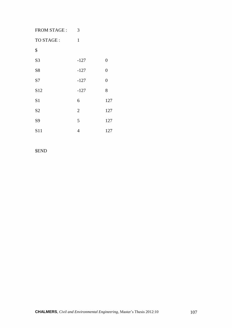
CHALMERS, Civil and Environmental Engineering, Master‟s Thesis 2012:10 107
FROM STAGE : 3
TO STAGE : 1
$
S3 -127 0
S8 -127 0
S7 -127 0
S12 -127 8
S1 6 127
S2 2 127
S9 5 127
S11 4 127
$END
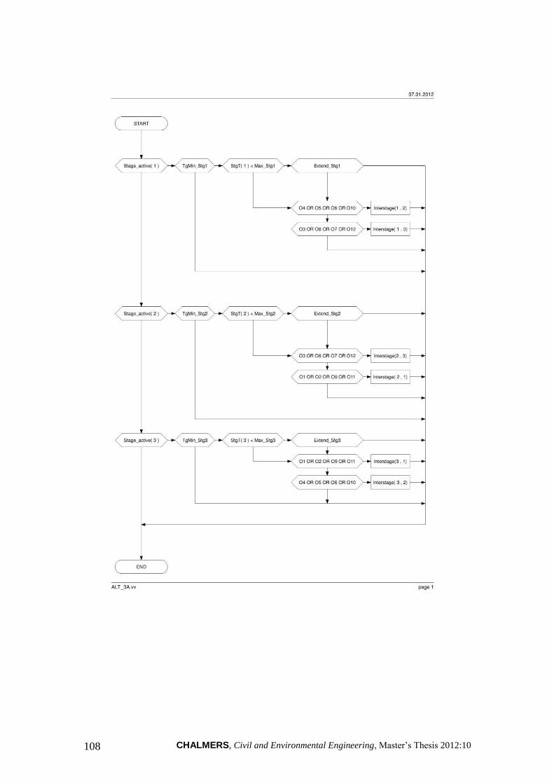
CHALMERS, Civil and Environmental Engineering, Master‟s Thesis 2012:10 108

CHALMERS, Civil and Environmental Engineering, Master‟s Thesis 2012:10 109
PARAMETERS Gen Comment
Max_Gap 5 Max. gap time
MAX_STG1 35 Max. duration of stage 1
MAX_STG2 40 Max. duration of stage 2
MAX_STG3 30 Max. duration of stage 3
EXPRESSIONS Contents
TgMin_Stg1
(Tg( S1 ) >= Tgmin( S1 )) & (Tg( S2 ) >= Tgmin( S2 )) &
(Tg( S9 ) >= Tgmin( S9 )) & (Tg( S11) >= Tgmin( S11))
Extend_Stg1
(Headway ( 1 ) <= Max_Gap) OR (Headway ( 2 ) <= Max_Gap)
OR (Headway ( 9 ) <= Max_Gap) OR (Headway ( 11 ) <= Max_Gap)
TgMin_Stg2
(Tg( S4 ) >= Tgmin( S4 )) & (Tg( S5 ) >= Tgmin( S5 )) & (Tg( S6 )
>= Tgmin( S6 )) & (Tg( S10) >= Tgmin( S10))
Extend_Stg2
(Headway (4) <= Max_Gap) OR (Headway (5) <= Max_Gap)
OR (Headway (6) <= Max_Gap) OR (Headway ( 10 ) <= Max_Gap)
Extend_Stg3
(Headway (3) <= Max_Gap) OR (Headway ( 8) <= Max_Gap)
OR (Headway ( 7 ) <= Max_Gap) OR (Headway ( 12 ) <= Max_Gap)
TgMin_Stg3
(Tg( S3 ) >= Tgmin( S3 )) & (Tg( S8 ) >= Tgmin( S8 )) & (Tg( S7 )
>= Tgmin( S7 )) & (Tg( S12) >= Tgmin( S12))
O1 Occupancy( 1 ) > 10
O2 Occupancy( 2 ) > 6
O3 Occupancy( 3 ) > 1
O4 Occupancy( 4 ) > 8
O5 Occupancy( 5 ) > 4
O6 Occupancy( 6 ) > 4
O7 Occupancy( 7 ) > 3
O8 Occupancy( 8 ) > 1
O9 Occupancy( 9 ) > 4
O10 Occupancy( 10 ) > 8
O11 Occupancy( 11 ) > 2
O12 Occupancy( 12 ) > 8
Related Documents