Analysis of Biological Networks: Networks in Disease

Analysis of Biological Networks:Networks in Disease

Lecturer: Roded SharanScribe: Yaniv Bar and Naama Hazan

Lecture 11. June 03, 2009

1 Disease and drug-related networks

The idea of using networks to understand drugs and diseases was established in two innovative papers ofAlbert Laszlo Barabasi.

1.1 The human disease network

In the first paper of Barabasi et al.[2], a global view, named ’Diseasome’, of the combined set of all knowndisorder/disease gene associations was presented.

The ’Diseasome’ construction is a bipartite network containing a set of diseases/phenotypes and a set ofgenes, where each gene is connected to a disease if it causes it. Such a network offers a platform to explorein a single graph theoretic framework all known phenotype and disease gene associations, indicating thecommon genetic origin of many diseases.

The work examined the two projections of the Diseasome: The projection on diseases, called HDN(Human Disease Network), and the projection on genes, called DGN (Disease Gene Network).

The networks were constructed according to the database called OMIM, a catalogue of genetic diseasesin human. The catalogue currently contains 2300 diseases whose genetic cause is known and 3500 diseaseswhose genetic origin is unknown. For 1000 of the diseases with unknown cause, there is a known geneticsite with a linkage to them.

Figure 1 depicts the construction of the diseasome bipartite network: (Center) A small subset of OMIM-based disorder disease gene associations, where circles and rectangles correspond to disorders and diseasegenes, respectively. A link is placed between a disorder and a disease gene if mutations in that gene leadto the specific disorder. The size of a circle is proportional to the number of genes participating in thecorresponding disorder, and the color corresponds to the disorder class to which the disease belongs. (Left)The HDN projection of the diseasome bipartite graph, in which two disorders are connected if there is a genethat is implicated in both. The width of a link is proportional to the number of genes that are implicated in

1

both diseases. For example, three genes are implicated in both breast cancer and prostate cancer, resultingin a link of weight three between them. (Right) The DGN projection where two genes are connected if theyare involved in the same disorder. The width of a link is proportional to the number of diseases with whichthe two genes are commonly associated.

Figure 1: Construction of the diseasome bipartite network [2].

1.1.1 Properties of the HDN

If each human disorder tends to have a distinct and unique genetic origin, then the HDN would be discon-nected into many single nodes corresponding to specific disorders or grouped into small clusters of a fewclosely related disorders. In contrast, the obtained HDN displays many connections between both individualdisorders and disorder classes

Of 1284 diseases in the graph, 867 diseases are of degree higher that zero. 867 diseases share the causewith at least one other disease. In addition 516 diseases form a giant component (the greatest connectedcomponent in the network). This number is half of the size of the network. This is much lower numberthan the expected number in a random network and therefore the network is more clustered, suggesting thatthe genetic origins of most diseases, to some extent, are shared with other diseases. The major hubs in thisnetwork are of high interest in the research frontier these days.

1.1.2 Properties of the DGN

In the DGN, two disease genes are connected if they are associated with the same disorder, providinga complementary, gene-centered view of the diseasome. Given that the links signify related phenotypic

2

associations between two genes, they represent a measure of their phenotypic relatedness, which could beused in future studies.

In the DGN, 1,377 of 1,777 disease genes are connected to other disease genes, and 903 genes belongto a giant component. Like in the HDN, the connected component in this network is smaller than expected.Several disease genes are involved in as many as 10 disease, representing major hubs in the network. Themajor hub is P53, one of the most well known tumor suppressors.

1.1.3 Characterizing the disease modules

The DGN and HGN networks have a relatively high correlation with other databases.

If genes linked by disorder associations encode proteins that interact in functionally distinguishablemodules, then the proteins within such disease modules should more likely interact with one another thanwith other proteins. To test this, the DGN network was overlaid on a network of PPI derived from high-quality systematic interactome mapping and literature. It was found that 290 interactions overlap betweenthe two networks, a 10-fold increase relative to random expectation. This fact is not surprising, as knockoutof two proteins that function in the same complex or in the same metabolic pathway are likely to cause thesame disease. This is shown in figure 2a.

Genes associated with the same disorder share common cellular and functional characteristics, as anno-tated in the Gene Ontology (GO). If the HDN shows modular organization, then a group of genes associatedwith the same common disorder should share similar cellular and functional characteristics, as annotated inGO. It was found that 68% of disorders exhibited almost perfect tissue-homogeneity, namely most of thedisease associated genes share the same tissue expression profile. This is shown in figure 2b.

Finally, genes in the DGN network that participate in a common functional module should also showhigh expression profiling correlation. This is shown in the figure 2c and 2d.

3

Figure 2: Characterizing of the disease modules. Note that in all subfigures the control group is obtainedfrom corresponding randomized networks: (2a) Number of observed physical interactions between the prod-ucts of genes within the same disorder (red arrow) and the distribution of the expected number of interac-tions for the random control (blue). (2b) Distribution of the tissue-homogeneity of a disorder (red). Randomcontrol (blue) with the same number of genes chosen randomly is shown for comparison. (2c), (2d) Thedistribution of the expression profiles/average expression profiles of each disease gene pair that belongs tothe same disorder (red) and the control (blue), representing the distribution between all gene pairs. [2].

1.2 Drug-Target network

From the other side of the spectrum, the second paper of Barabasi et al.[1], covers a drug-target networkcontaining a set of drugs/disease genes, which is obtained from the drug bank database.

DrugBank is a database that contains all FDA approved drugs and drugs in a the stage of clinical exper-iments. There are 4800 drugs in the database that target 2500 genes. Most drugs target only one gene, butthere are many drugs that target many genes. Similarly, most genes are targeted by no more than one drug,and yet, some genes are targeted by almost all marketed drugs.

4

In the drug-target network of [1] there are 890 drugs and 394 targets. Each drug and each gene arerepresented by a vertex. A drug is connected by edges to all genes that it targets. 788 drugs have an edgeand 476 drugs form the giant component. Its greatest connected component is also small suggesting thatthe network is clustered by the therapeutic departments/classes of the diseases (e.g, drugs related to heartdiseases, to breath defects, blood diseases etc.).

Figure 3: Drugtarget network (DT network). The DT network is generated by using the known associationsbetween FDA-approved drugs and their target proteins. Circles and rectangles correspond to drugs and targetproteins, respectively. A link is placed between a drug node and a target node if the protein is a known targetof that drug. The area of the drug (protein) node is proportional to the number of targets that the drug has (thenumber of drugs targeting the protein). Color codes are given in the legend. Drug nodes (circles) are coloredaccording to their Anatomical Therapeutic Chemical Classification, and the target proteins (rectangularboxes) are colored according to their cellular component obtained from the Gene Ontology database.[1].

305 targets in the network have an edge and 122 targets form the giant component. Interestingly, 62%of the targets are membrane proteins. This can be explained by the difficulty of producing a drug that is ableto cross the membrane.

5

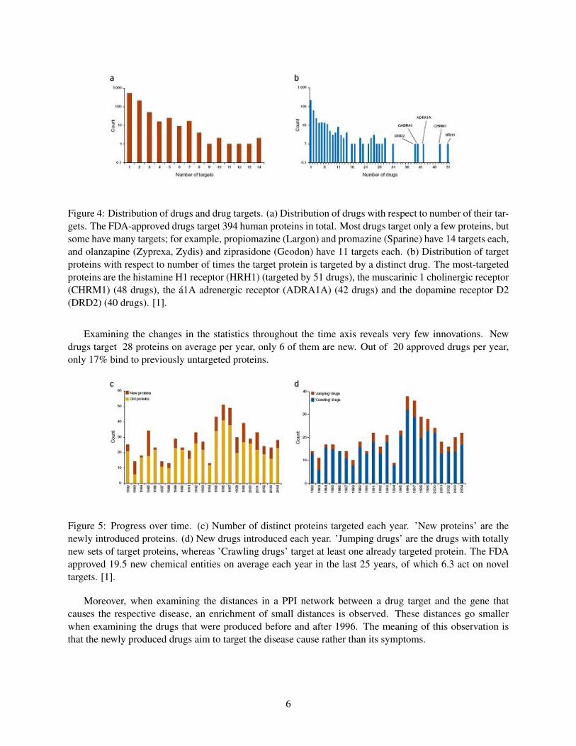
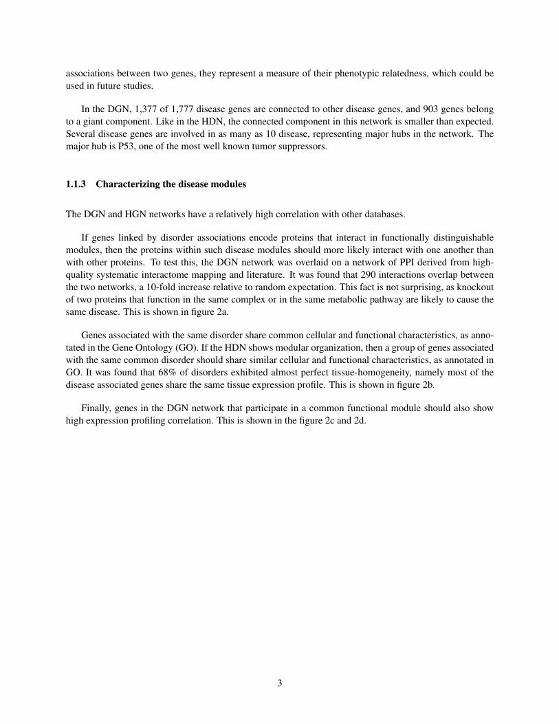
Figure 4: Distribution of drugs and drug targets. (a) Distribution of drugs with respect to number of their tar-gets. The FDA-approved drugs target 394 human proteins in total. Most drugs target only a few proteins, butsome have many targets; for example, propiomazine (Largon) and promazine (Sparine) have 14 targets each,and olanzapine (Zyprexa, Zydis) and ziprasidone (Geodon) have 11 targets each. (b) Distribution of targetproteins with respect to number of times the target protein is targeted by a distinct drug. The most-targetedproteins are the histamine H1 receptor (HRH1) (targeted by 51 drugs), the muscarinic 1 cholinergic receptor(CHRM1) (48 drugs), the a1A adrenergic receptor (ADRA1A) (42 drugs) and the dopamine receptor D2(DRD2) (40 drugs). [1].

Examining the changes in the statistics throughout the time axis reveals very few innovations. Newdrugs target 28 proteins on average per year, only 6 of them are new. Out of 20 approved drugs per year,only 17% bind to previously untargeted proteins.

Figure 5: Progress over time. (c) Number of distinct proteins targeted each year. ’New proteins’ are thenewly introduced proteins. (d) New drugs introduced each year. ’Jumping drugs’ are the drugs with totallynew sets of target proteins, whereas ’Crawling drugs’ target at least one already targeted protein. The FDAapproved 19.5 new chemical entities on average each year in the last 25 years, of which 6.3 act on noveltargets. [1].

Moreover, when examining the distances in a PPI network between a drug target and the gene thatcauses the respective disease, an enrichment of small distances is observed. These distances go smallerwhen examining the drugs that were produced before and after 1996. The meaning of this observation isthat the newly produced drugs aim to target the disease cause rather than its symptoms.

6

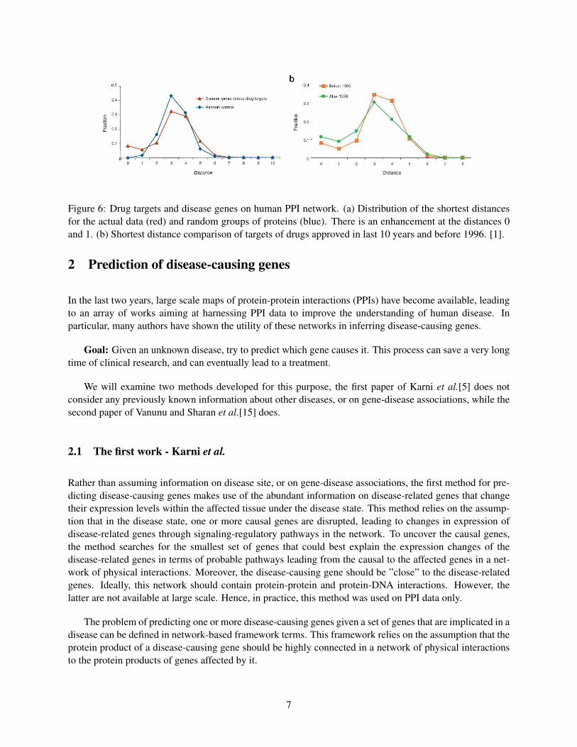
Figure 6: Drug targets and disease genes on human PPI network. (a) Distribution of the shortest distancesfor the actual data (red) and random groups of proteins (blue). There is an enhancement at the distances 0and 1. (b) Shortest distance comparison of targets of drugs approved in last 10 years and before 1996. [1].

2 Prediction of disease-causing genes

In the last two years, large scale maps of protein-protein interactions (PPIs) have become available, leadingto an array of works aiming at harnessing PPI data to improve the understanding of human disease. Inparticular, many authors have shown the utility of these networks in inferring disease-causing genes.

Goal: Given an unknown disease, try to predict which gene causes it. This process can save a very longtime of clinical research, and can eventually lead to a treatment.

We will examine two methods developed for this purpose, the first paper of Karni et al.[5] does notconsider any previously known information about other diseases, or on gene-disease associations, while thesecond paper of Vanunu and Sharan et al.[15] does.

2.1 The first work - Karni et al.

Rather than assuming information on disease site, or on gene-disease associations, the first method for pre-dicting disease-causing genes makes use of the abundant information on disease-related genes that changetheir expression levels within the affected tissue under the disease state. This method relies on the assump-tion that in the disease state, one or more causal genes are disrupted, leading to changes in expression ofdisease-related genes through signaling-regulatory pathways in the network. To uncover the causal genes,the method searches for the smallest set of genes that could best explain the expression changes of thedisease-related genes in terms of probable pathways leading from the causal to the affected genes in a net-work of physical interactions. Moreover, the disease-causing gene should be ”close” to the disease-relatedgenes. Ideally, this network should contain protein-protein and protein-DNA interactions. However, thelatter are not available at large scale. Hence, in practice, this method was used on PPI data only.

The problem of predicting one or more disease-causing genes given a set of genes that are implicated in adisease can be defined in network-based framework terms. This framework relies on the assumption that theprotein product of a disease-causing gene should be highly connected in a network of physical interactionsto the protein products of genes affected by it.

7

Formally, the basic problem we consider is defined as follows:Definition (Gene-Cover (GC)): Given a graph G=(V,E) a subset U ⊆ V , a distance threshold l, and aparameter k, find a subset of vertices, D of size at most k such that for a maximal number of vertices u ∈ Uthere exists a vertex in D of distance at most l from u.

It is easy to see that this problem is NP-complete and is polynomially equivalent to the Set Coverproblem.

This is shown in the next following theorem:Theorem: The decision versions of GC and Set Cover are polynomially equivalent.

Definition (Gene-Cover (GC) decision problem): Given a graph G=(V,E) a subset U ⊆ V , a distancethreshold l, and a parameter k, decide whether there exist a subset of vertices, D of size at most k such thatfor all vertices u ∈ U there exists a vertex in D of distance at most l from u.

Definition (Set-Cover (SC) decision problem): Given a set of elements, S, a collection of subsets ofS, C, and a parameter k, decide whether there exists a subcollection of C , {c1, c2, ...ck} of size at most k,s.t. for every s ∈ S there exists an i, s.t. s ∈ ci.

Proof: In one direction, let (S,C,k) be an instance of Set Cover where S is the set of elements, C isa collection of subsets of S and k is a parameter. Without lose of generality, we assume that C covers S.We can easily transform this instance into an instance (G,S,1,k) of the decision version of GC as follows:we construct a bipartite graph G=(S,C,E) with vertices on one side representing elements and vertices onthe other side representing subsets. For every T ∈ C and s ∈ T we add an edge (s,T) to E. It is trivial toobserve that the Set Cover instance admits a solution iff the GC instance admits a solution. Note that theonly problematic case is when a GC solution contains an element from S, but such an element can alwaysbe substituted by a subset containing it.

In the other direction, suppose we are given an instance (G,U,l,k) of GC. We transform it into an instance(U,C,k) of Set Cover, where C is defined as follows: for each vertex v ∈ G we create a subset T ⊆ Ucomposed of all vertices that are of distance at most l from v (including v if it is part of U). If T 6= � weadd it to C. Again there is a solution to the GC instance iff there is a solution to the Set Cover instance.

As stated above, the SC problem is known to be NP-hard, however, it can be efficiently approximatedto within a logarithmic factor. Using a greedy algorithm for solving the set cover problem (in each stepchoose the set that covers the maximal number of vertices, remove it and all vertices covered by it) we get alogarithmic approximation ofO(log(|U |)). As the reduction from Gene Cover to Set Cover is approximationpreserving, it also implies O(log(|U |)).

The formulation presented above treats all edges of the protein network being analyzed in a uniformmanner. Since protein-protein interactions vary greatly in their associated confidence scores, it is desirableto take edge reliabilities into account.

A natural extension to the distance-based formulation above is to quantify the relatedness of a proteinto a set U by the expected number of proteins in U that can be reached from it by paths of length at most l.Denote this expectation by El(u, V ) we can consider the following (biologically motivated) formulation ofthe gene coverage problem:

8

Definition (Maximum-expectation Gene Cover (MGC)): Given a graph G=(V,E) a subset U ⊆ V , adistance threshold l, and a parameter k, find a subset of vertices, D of size at most k such that∑v∈D

El(v, U) =∑v∈D

∑u∈U

Pl(v, u) is maximal.

Pl(a, b) is the probability of having a path of length at most l between a and b. For two vertices a andb, let Πl(a, b) = {Π1, ..,Πm} denote the set of paths of length at most l between a and b. Let πi be a

random variable indicating whether the path Πi exists. Then: Pl(a, b) = Prob(m⋃i=1

)πi. This probability can

be computed using the inclusion-exclusion formula in time that is exponential in m.

To save on running time, one can partition the set of paths into subsets that are edge-disjoint. This isdone by constructing a new graph whose vertices represent paths and whose edges connect edge-intersectingpaths. The connected components of this graph yield the desired partition. Let ∆1, ..,∆t denote the resulting

subsets of paths, and consider a pair of vertices a,b. Then: Pl(a, b) = 1−t∏i=1

(1− Prob(⋃

π∈∆i

π)).

Each term can be computed by an inclusion-exclusion formula:

Prob(⋃

π∈∆i

π) =|∆i|∑k=1

(−1)k−1|∆i|∑

∆⊆∆i,|∆|=kProb(

⋂π∈∆

π) where the probability of an intersection of paths is

simply the product of the probabilities of the edges in the intersection.Note that this computation is practical for up to 25 paths.

As we shall see next, it is possible to approximate MGC to within a factor O(log(|U |)) by adapting thegreedy-based approximation algorithm for Weighted Set Cover.

2.1.1 The MGC algorithm

We focus on the biologically motivated MGC.Given a protein network G and a subset of disease-related proteins U, we apply an iterative algorithm toinfer the disease-causing genes. Intuitively, at each iteration the protein, whose ”coverage” expectation withrespect to the current subset U is maximal, is chosen and the diseased proteins that it ”covers” are removedfrom U. However, the expectation computation gives an advantage to high degree proteins. To circumventthis problem, we compare the original expectation to that obtained w.r.t. 100 random disease-related subsetsof the same size as U.

The results of the random runs are used to derive a z-score for each vertex, and the highest scoringvertex is chosen at each iteration. The algorithm terminates when the highest score attained is below apredefined threshold (1.65, corresponding to a p-value of 0.05), or when all the disease-related genes havebeen ”covered”.

Due to the randomized nature of the algorithm (in computing the z-score), the results may changeslightly between runs. Hence, each experiment (described below) is repeated 50 times, and the genes areranked based on their average ranks in these 50 runs.

In many cases, additional information is available that can help us to limit the search. Specifically,association studies may provide information on genomic regions which are associated with the investigateddisease, reducing the initial search space from thousands of proteins to a few hundred. Similarly, copy

9

number variation data can pinpoint areas of the genome whose copy number is modified in the disease state;these areas are then good candidates for causal gene searches.

The algorithm was evaluated both on simulated data and real data.To simulate partial knowledge on real data concerning the location of the causal gene, information on thechromosomal segment in which the gene is located was obtained from the OMIM database. A subnetworkcontaining only genes in the relevant chromosomal segment was used as the input to MGC algorithm.

2.1.2 Determining the search depth

Real data was used to optimize the maximal search depth parameter l. Search depth size of l = 3 wasselected as the optimal search depth, and subsequently used in all the runs against both simulated and realdata. This is shown below.

In order to choose an optimal maximal depth with which to run the algorithm, it was applied withmaximal depth of 1-5 to three real data sets (ATM knockout, NFκB knockout, and MLL gene expressiondata), where the disease causing gene is known. For each data set, different locus sizes that contain theknown causing gene were selected. For each such scenario (locus size and depth), running the algorithmrecovers the disease causing genes through a calculation of the average rank.

For depths 1 and 2, correct results were found only when considerably narrowing the search site (to afew dozens of genes, data not shown). The results for depths 3 to 5 are shown in the Figure 7. Note thatselecting a larger depth level increases the sensitivity of the algorithm in the expense of noise exposure.Considering the interaction between sensitivity and noise the best results were attained at maximal depthof 3. Moreover, from a computational aspect, a smaller depth level is more efficient. This is evident fromfigure 7 where the best results (except for the ATM knockout data) were attained at maximal depth of 3.

Figure 7: Performance with different maximal search depths (1 to 5) and different sized sites for three realdata sets: ATM and NFκB knockouts and MLL gene expression data. For each disease and depth, theaverage rank (by the 3 different loci sizes) of the disease causing gene is shown in the plot[5]

In the case of NFκB knockout, when knocking out the transcription factor NFκB, 48 genes changedtheir expression levels. This gene is located in chromosomal segment 4q24, which contains 31 genes, 15 ofwhich appear in the PPI network. For all tested scenarios NFκB disease causing gene was ranked first. As

10

an example, NFκB was ranked with an average degree of 7 for a site of size 206 and a distance of size 3.

When knocking out the signaling protein ATM, 47 genes changed their expression levels. ATM lieswithin segment 11q22, which contains 75 genes, 31 of which appear in the PPI network. Overall, ATMranked third, with an average rank of 3.12.

In the last case the data on acute lymphoblastic leukemia (ALL) was used, consisting of expressionprofiles for a subset of acute leukemias involving chromosomal translocation of the mixed leukemia gene(MLL). Overall, 67 genes were found to be differentially expressed and appeared in our network. The MLLgene is located at segment 11q23, which contains 168 genes, 61 of which are in the PPI network. Whenapplying the algorithm to this data, MLL scored best with an average rank of 1.5. The second highestranking gene, with an average rank of 2.86, was matrix metallopeptidase 7 (MMP-7), a member of thematrix metalloproteinase family. This gene has been linked before to leukemia, and many other forms ofcancer. Three additional proteins that ranked among the top 10 are involved in phosphorylation signalingcascades known to be involved in the leukemic processes.

2.1.3 Performance on simulated data

To evaluate the performance of the algorithm, it was applied to simulated data. In each simulation, one”disease-causing” protein was taken at random from the network, and artificial site (based on the neigh-borhood in the network, rather than chromosomal segments), consisting of 50 to 200 genes each, wereconstructed around the gene it encode. To construct a ”disease-related” subset of a certain size (between 30and 180), proteins were chosen at random from the set of proteins of distance at most 3 from the ”disease-causing” ones. For each site size and ”disease-related” subset, 50 random tests were conducted (in each testfinding the rank of the disease causing gene using the MGC algorithm).

This simulation setting ensures that the random instances follow the assumptions on the disease-causinggenes. Thus, the simulations mainly serve to test under what conditions can one recover these genes.

The results obtained in simulations of a single causal gene are summarized in Figure 8. Note that whenlimiting the search to a certain site, the algorithm almost always ranks the simulated causal gene first. Theaccuracy is lower when searching the entire network: the average rank of the causal gene ranges between3.8 and 5.8, and it is ranked first 22% to 52% of the time, depending on the site size.

The performance on simulated results were compared against a naive approach that ranks proteins ac-cording to their sum of distances to the input disease-related genes. As can be seen in figure 9, the algorithmis considerably more accurate when searching the entire network, achieving performance gains of more than70%. In restricted search sites an improvement is also shown, but it is much less evident.

To test the robustness of the algorithm to noise in the input list of disease-related genes, simulationswere carried out in which the size of the disease-related set was fixed at 100, and up to 25% of the proteinsin the set were replaced by random proteins. Genes whose ”coverage” expectation was equal to that of thesimulated causal gene were removed (as they are indistinguishable from it).

The results are depicted in the figure 10. It can be seen that the algorithm’s results are robust even athigh noise levels.

11

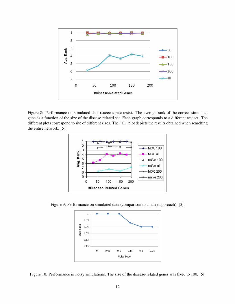
Figure 8: Performance on simulated data (success rate tests). The average rank of the correct simulatedgene as a function of the size of the disease-related set. Each graph corresponds to a different test set. Thedifferent plots correspond to site of different sizes. The ”all” plot depicts the results obtained when searchingthe entire network. [5].

Figure 9: Performance on simulated data (comparison to a naive approach). [5].

Figure 10: Performance in noisy simulations. The size of the disease-related genes was fixed to 100. [5].

12

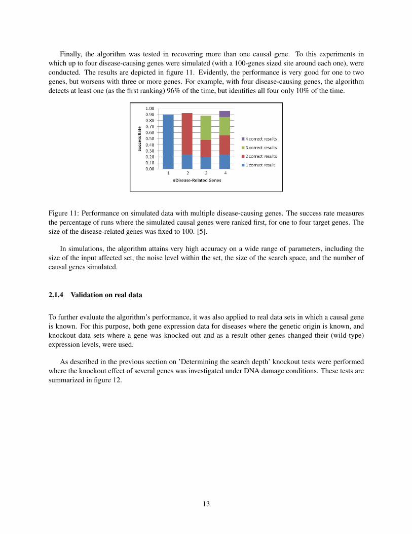
Finally, the algorithm was tested in recovering more than one causal gene. To this experiments inwhich up to four disease-causing genes were simulated (with a 100-genes sized site around each one), wereconducted. The results are depicted in figure 11. Evidently, the performance is very good for one to twogenes, but worsens with three or more genes. For example, with four disease-causing genes, the algorithmdetects at least one (as the first ranking) 96% of the time, but identifies all four only 10% of the time.

Figure 11: Performance on simulated data with multiple disease-causing genes. The success rate measuresthe percentage of runs where the simulated causal genes were ranked first, for one to four target genes. Thesize of the disease-related genes was fixed to 100. [5].

In simulations, the algorithm attains very high accuracy on a wide range of parameters, including thesize of the input affected set, the noise level within the set, the size of the search space, and the number ofcausal genes simulated.

2.1.4 Validation on real data

To further evaluate the algorithm’s performance, it was also applied to real data sets in which a causal geneis known. For this purpose, both gene expression data for diseases where the genetic origin is known, andknockout data sets where a gene was knocked out and as a result other genes changed their (wild-type)expression levels, were used.

As described in the previous section on ’Determining the search depth’ knockout tests were performedwhere the knockout effect of several genes was investigated under DNA damage conditions. These tests aresummarized in figure 12.

13

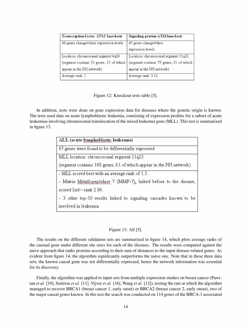
Figure 12: Knockout tests table [5].

In addition, tests were done on gene expression data for diseases where the genetic origin is known.The tests used data on acute lymphoblastic leukemia, consisting of expression profiles for a subset of acuteleukemias involving chromosomal translocation of the mixed leukemia gene (MLL). This test is summarizedin figure 13.

Figure 13: All [5].

The results on the different validation sets are summarized in figure 14, which plots average ranks ofthe causual gene under different site sizes for each of the diseases. The results were compared against thenaive approach that ranks proteins according to their sum of distances to the input disease-related genes. Asevident from figure 14, the algorithm significantly outperforms the naive one. Note that in these three datasets, the known causal gene was not differentially expressed, hence the network information was essentialfor its discovery.

Finally, the algorithm was applied to input sets from multiple expression studies on breast cancer (Pawi-tan et al. [10], Sotiriou et al. [11], Vijver et al. [16], Wang et al. [12]), testing the rate at which the algorithmmanaged to recover BRCA1 (breast cancer 1, early onset) or BRCA2 (breast cancer 2, early onset), two ofthe major causal genes known. In this test the search was conducted on 114 genes of the BRCA-1 associated

14

Figure 14: Performance a maximal search depth of 3 for three real data sets: ATM and NFkB knockouts andMLL gene expression data. In addition, the performance is compared to the naive approach (on the samedata sets). [5].

segment (chromosomal segment 17q21) and the 32 genes of the BRCA2 associated segment (chromosomalsegment 13q12). The results, summarized in figure 15, show that at least one of BRCA1 or BRCA2 wasrecovered in each of the data sets.

Figure 15: Average ranks of BRCA1 and BRCA2 on breast cancer data from different studies. [5].

In validation on real expression data from knockout experiments, the algorithm manages to pinpoint thedisrupted gene with high accuracy. Further validations on expression data from different types of cancershow high accuracy in pinpointing known oncogenes. Importantly, it is shown that the algorithm outper-forms a naive algorithm that ranks disease-associated genes according to their distances in the network tothe directly affected genes.

2.2 The second work - Vanunu et al.

This work uses a different approach in which prior information is used based on the disease network. Insteadof searching the entire PPI network, the method identifies the genes that cause similar diseases and scores theproteins according to their neighborhood in the PPI network and to their relevance to the disease. Previousworks used a combination of PPI networks and disease similarity metrics based on medical terms.

15

For example:

1. A local scoring method that scores proteins according to the relevance of the neighbors in the PPInetwork to the disease [Lage et al. [8]].

2. Random walk from causal proteins of similar diseases. A protein is scored by the frequency of reach-ing it by the walks [Kohler et al. [6]].

3. CIPHER - Correlate a disease similarity profile with protein proximity profile [Wu et al. [13]]. Theassumption behind this method is that proteins that cause similar diseases should be close in thenetwork to the protein that causes the disease

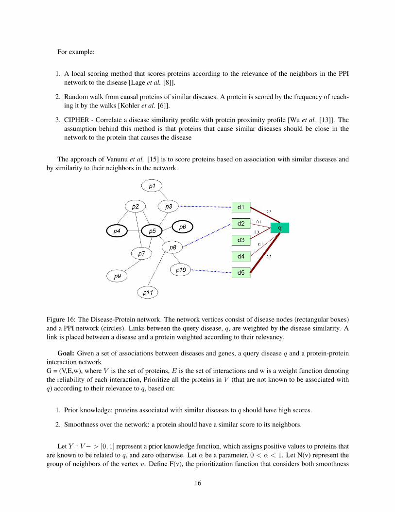
The approach of Vanunu et al. [15] is to score proteins based on association with similar diseases andby similarity to their neighbors in the network.

Figure 16: The Disease-Protein network. The network vertices consist of disease nodes (rectangular boxes)and a PPI network (circles). Links between the query disease, q, are weighted by the disease similarity. Alink is placed between a disease and a protein weighted according to their relevancy.

Goal: Given a set of associations between diseases and genes, a query disease q and a protein-proteininteraction networkG = (V,E,w), where V is the set of proteins, E is the set of interactions and w is a weight function denotingthe reliability of each interaction, Prioritize all the proteins in V (that are not known to be associated withq) according to their relevance to q, based on:

1. Prior knowledge: proteins associated with similar diseases to q should have high scores.

2. Smoothness over the network: a protein should have a similar score to its neighbors.

Let Y : V− > [0, 1] represent a prior knowledge function, which assigns positive values to proteins thatare known to be related to q, and zero otherwise. Let α be a parameter, 0 < α < 1. Let N(v) represent thegroup of neighbors of the vertex v. Define F(v), the prioritization function that considers both smoothness

16

and prior knowledge: F (v) = α[∑

u∈N(v)

F (u)w′(u, v)] + (1 − α)Y (u) where w′ is a normalized form of

w, such that∑

u∈N(v)

w′(v, u) ≤ 1 for every node v ∈ V . Here, the first term expresses the smoothness

condition, while the second term expresses the prior information constraint. The parameter α ∈ (0, 1)weighs the relative importance of these constraints with respect to one another.

2.2.1 Computing the prioritization function

The requirements on F can be expressed in linear form as follows:F = αW ′F + (1− α)Y ⇔ F = (1− αW ′)−1(1− α)Y where W ′ is a |V | X |V | matrix whose values aregiven by w′, and F and Y are viewed here as vectors of size |V |. Since W ′ is normalized, its eigenvaluesare in [0, 1]. Since α ∈ (0, 1), the eigenvalues of (I − αW ′) are in (0, 1]; in particular, all its eigenvaluesare positive and, hence, (I − αW ′)−1 exists. While the above linear system can be solved exactly, forlarge networks an iterative propagation based algorithm works faster and is guaranteed to converge to thesystem’s solution. Specifically, Vanunu et al. [15] use the algorithm of Zhou et al. [14] which at iteration tcomputes F t := αW ′F t−1 + (1− α)Y where F 0 := 0. This iterative algorithm can be best understood assimulating a process where nodes for which prior information exists pump information to their neighbors.In addition, every node propagates the information received in the previous iteration to its neighbors. Inpractice, as a final iteration the propagation step is applied with α = 1 to smooth the obtained prioritizationfunction F . The weight of an edge is normalized by the degrees of its end-points, since the latter relateto the probability of observing an edge between the same end-points in a random network with the samenode degrees. Formally, define a diagonal matrix D such that D(i, i) is the sum of row i of W . W ′ is setW ′ = D−1/2WD−1/2 which yields a symmetric matrix with row sums at most 1, whereW ′i,j = Wi,j/

√D(i, i)D(j, j). This normalization improves the results of the algorithm.

2.2.2 Validation and Parameter tuning

Cross validation and precision-recall plots were done to test the parameters on the performance of the algo-rithm, as follows:

• Choose one association < d, p > and leave it out.

• Construct an artificial interval of size 100 around p

• Apply the algorithm for disease d

• Rank proteins in interval using obtained F

• Refer to proteins ranked in the top k% as predicted associations to d

• Observe precision vs. recall for different k’s:

• Precision - % predicted associations that are correct

• Recall - % true associations that are successfully predicted

17

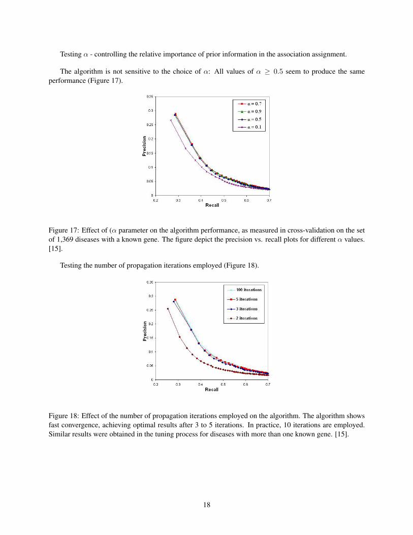
Testing α - controlling the relative importance of prior information in the association assignment.

The algorithm is not sensitive to the choice of α: All values of α ≥ 0.5 seem to produce the sameperformance (Figure 17).

Figure 17: Effect of (α parameter on the algorithm performance, as measured in cross-validation on the setof 1,369 diseases with a known gene. The figure depict the precision vs. recall plots for different α values.[15].

Testing the number of propagation iterations employed (Figure 18).

Figure 18: Effect of the number of propagation iterations employed on the algorithm. The algorithm showsfast convergence, achieving optimal results after 3 to 5 iterations. In practice, 10 iterations are employed.Similar results were obtained in the tuning process for diseases with more than one known gene. [15].

18

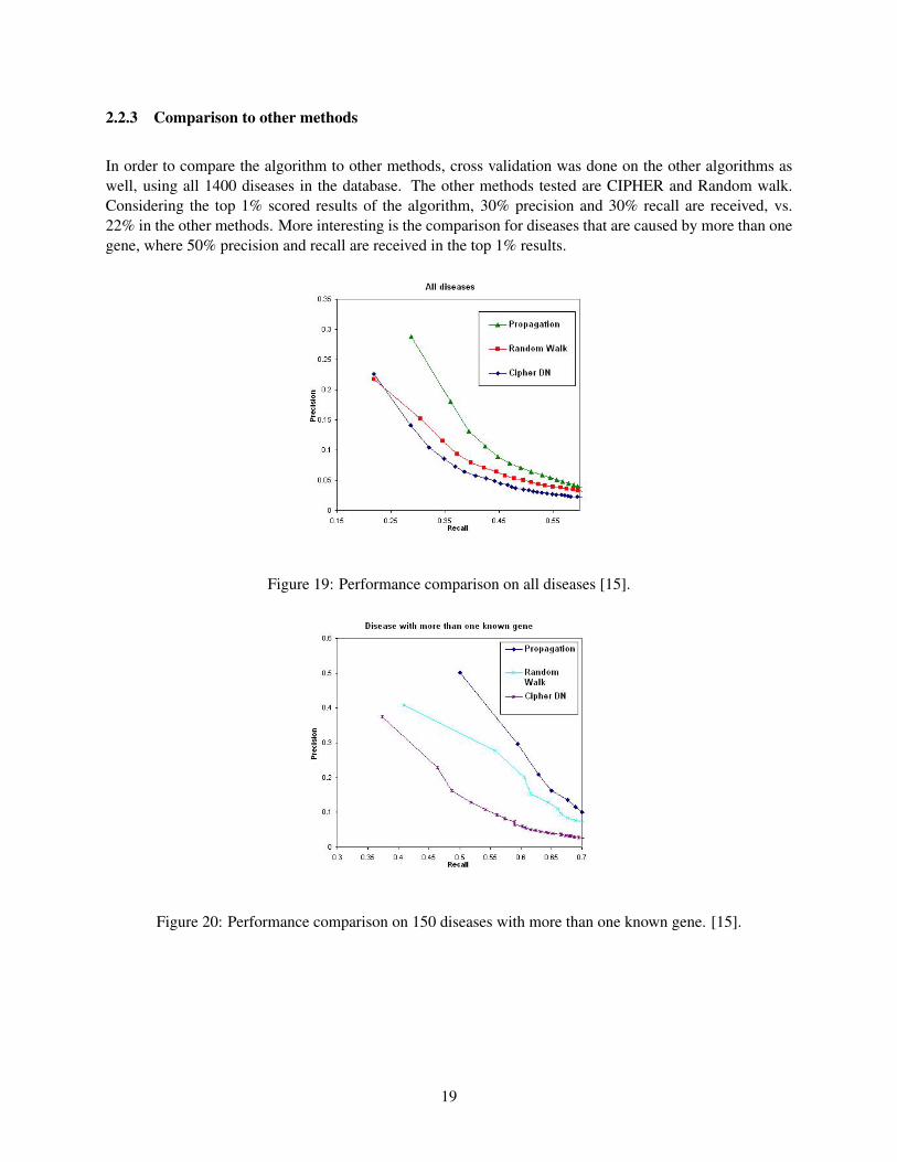
2.2.3 Comparison to other methods

In order to compare the algorithm to other methods, cross validation was done on the other algorithms aswell, using all 1400 diseases in the database. The other methods tested are CIPHER and Random walk.Considering the top 1% scored results of the algorithm, 30% precision and 30% recall are received, vs.22% in the other methods. More interesting is the comparison for diseases that are caused by more than onegene, where 50% precision and recall are received in the top 1% results.

Figure 19: Performance comparison on all diseases [15].

Figure 20: Performance comparison on 150 diseases with more than one known gene. [15].

19

3 Prediction of drug targets

A different goal in this field is, given a drug to predict its targets.

3.1 Campillos et al.

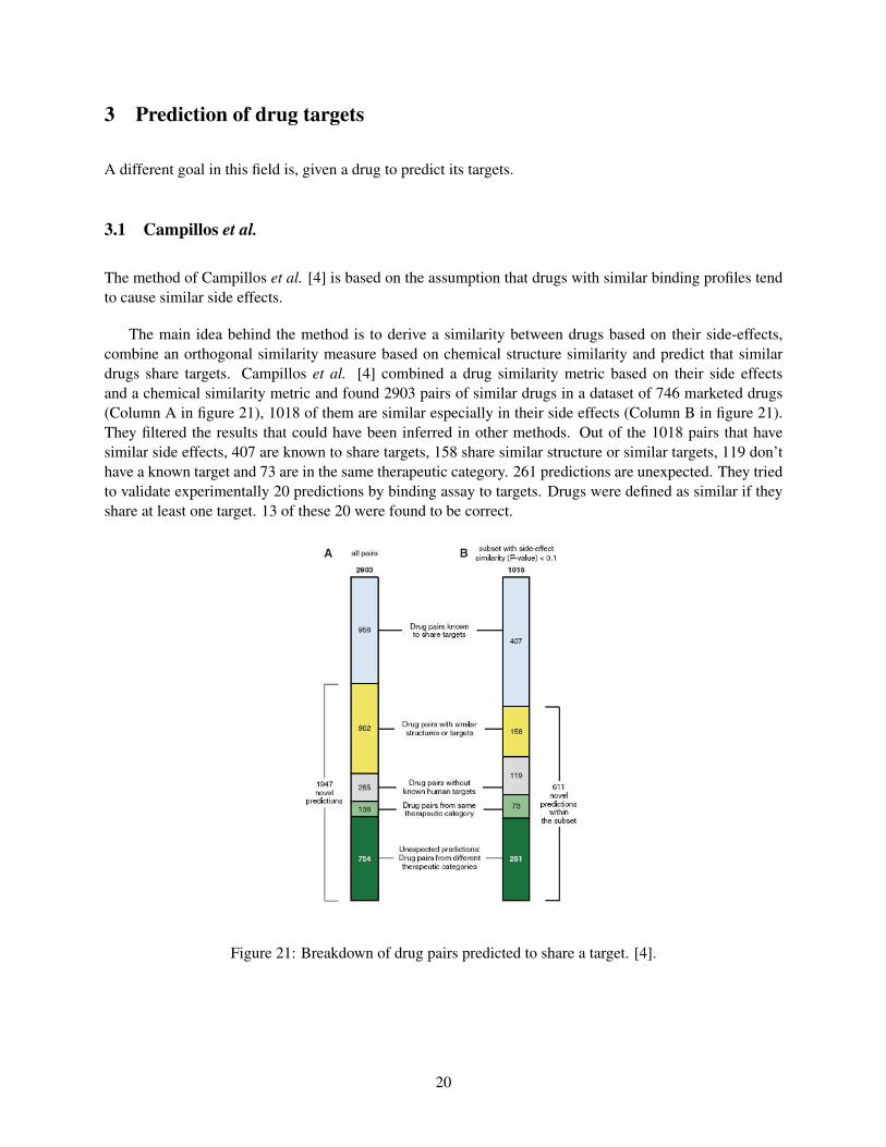
The method of Campillos et al. [4] is based on the assumption that drugs with similar binding profiles tendto cause similar side effects.

The main idea behind the method is to derive a similarity between drugs based on their side-effects,combine an orthogonal similarity measure based on chemical structure similarity and predict that similardrugs share targets. Campillos et al. [4] combined a drug similarity metric based on their side effectsand a chemical similarity metric and found 2903 pairs of similar drugs in a dataset of 746 marketed drugs(Column A in figure 21), 1018 of them are similar especially in their side effects (Column B in figure 21).They filtered the results that could have been inferred in other methods. Out of the 1018 pairs that havesimilar side effects, 407 are known to share targets, 158 share similar structure or similar targets, 119 don’thave a known target and 73 are in the same therapeutic category. 261 predictions are unexpected. They triedto validate experimentally 20 predictions by binding assay to targets. Drugs were defined as similar if theyshare at least one target. 13 of these 20 were found to be correct.

Figure 21: Breakdown of drug pairs predicted to share a target. [4].

20

3.2 Kutalik et al.

A different method for drug-target discovery was introduced by Kutalik et al. [7].The main idea is based on integrating gene expression data and drug sensitivity data to infer drug-geneinteractions and transcriptional response to drugs.

Although many methods have been suggested for extracting global properties from massive data, mostalgorithms only infer information on the structure of one data set at a time. However, with the advent ofhigh-throughput data covering different aspects of gene regulation, as well as other properties of the samples,there is an increasing need for combined analysis of multiple noisy data sets. A particularly challengingapplication pertains to data sets where the same cell samples have been studied using assays that probedifferent aspects of their phenotypes.

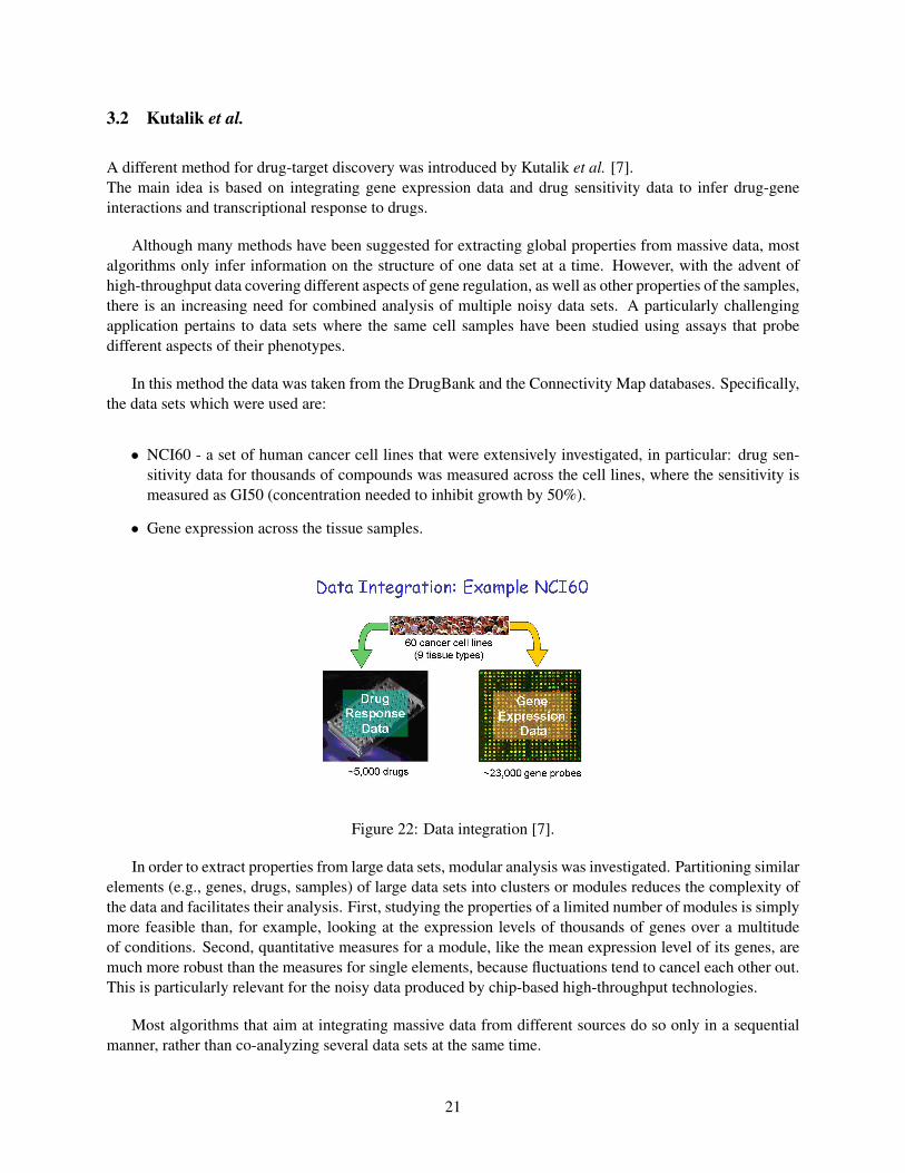
In this method the data was taken from the DrugBank and the Connectivity Map databases. Specifically,the data sets which were used are:

• NCI60 - a set of human cancer cell lines that were extensively investigated, in particular: drug sen-sitivity data for thousands of compounds was measured across the cell lines, where the sensitivity ismeasured as GI50 (concentration needed to inhibit growth by 50%).

• Gene expression across the tissue samples.

Figure 22: Data integration [7].

In order to extract properties from large data sets, modular analysis was investigated. Partitioning similarelements (e.g., genes, drugs, samples) of large data sets into clusters or modules reduces the complexity ofthe data and facilitates their analysis. First, studying the properties of a limited number of modules is simplymore feasible than, for example, looking at the expression levels of thousands of genes over a multitudeof conditions. Second, quantitative measures for a module, like the mean expression level of its genes, aremuch more robust than the measures for single elements, because fluctuations tend to cancel each other out.This is particularly relevant for the noisy data produced by chip-based high-throughput technologies.

Most algorithms that aim at integrating massive data from different sources do so only in a sequentialmanner, rather than co-analyzing several data sets at the same time.

21

In this method the modular analysis approach is extended from one to two large-scale data sets that shareone common dimension. The goal is to break down the massive sets of data into smaller building blocksthat exhibit similar patterns across certain genes and drugs in some of the cell lines.

For such a building block generated from two data sets the term co-module is used. A co-module isessentially a (weighted) ensemble of certain genes, drugs and cell lines such that its genes are expressedacross its cell lines and its drugs induce similar response profiles across the same cell lines. Representingcoherent features across both data sets in terms of such co-modules reduces the complexity of the data. Thismodular reduction makes it generally easier to study the underlying biology and allows prediction of morerobust drug-gene associations.

For identifying co-modules, three modular approaches that follow different strategies were suggested:The ISA, the ISA(E)ISA(R), and the Ping-Pong algorithm (PPA).

The Iterative Signature Algorithm (ISA) which was introduced by Bergmann et al. [3] is one of thestate-of-the art methods for modular analysis of large-scale data (typically tens of thousands of gene probestested over hundreds of conditions) according to various criteria19 and has been used for numerous biologi-cal studies. Briefly, the ISA identifies from a set of expression data a compendium of transcription modulesconsisting of co-expressed genes as well as the experimental conditions for which this coherent expressionis the most pronounced18. Here, the ISA approach is applied directly to the matrix of pair-wise correla-tions between gene-expression data and drug response profiles across all cell lines The second approach,ISA(E)ISA(R), first performs independent modular analyses of each data set (giving transcription modulesand drug-response modules) and then matches these modules according to the sets of cell lines they contain.Finally, the third method, termed Ping-Pong Algorithm (PPA), iteratively refines coherent patterns acrossboth data sets by alternating between them until convergence to co-modules is reached.

The main distinction between the three different modular approaches lies in whether the modularizationof the data sets is applied after (ISA), before (ISA(E)ISA(R)) or simultaneously with the data integration(PPA).

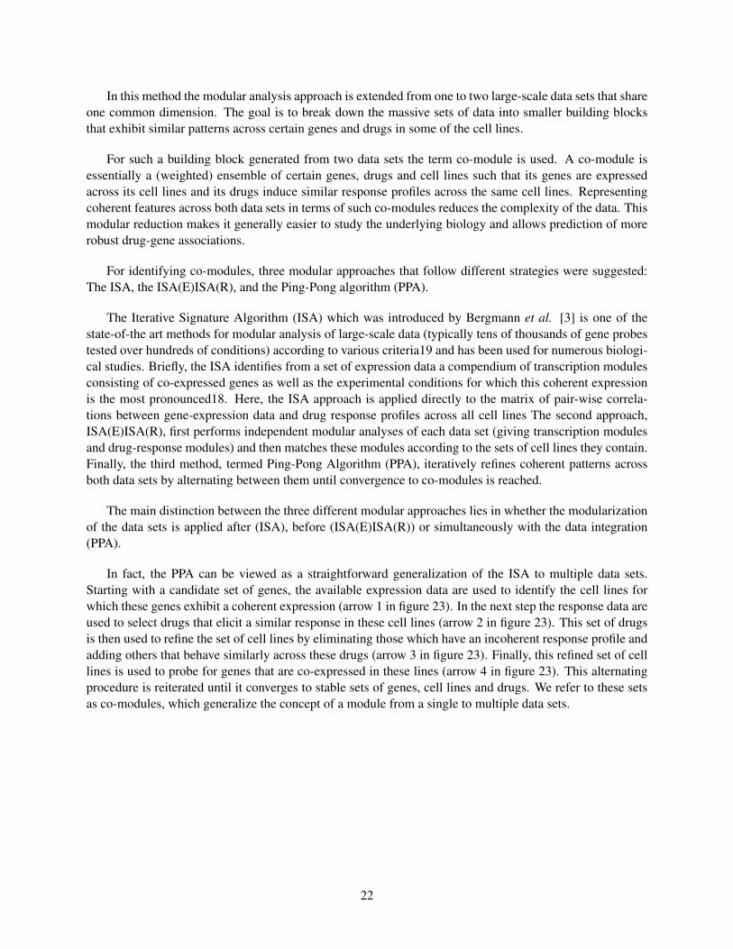
In fact, the PPA can be viewed as a straightforward generalization of the ISA to multiple data sets.Starting with a candidate set of genes, the available expression data are used to identify the cell lines forwhich these genes exhibit a coherent expression (arrow 1 in figure 23). In the next step the response data areused to select drugs that elicit a similar response in these cell lines (arrow 2 in figure 23). This set of drugsis then used to refine the set of cell lines by eliminating those which have an incoherent response profile andadding others that behave similarly across these drugs (arrow 3 in figure 23). Finally, this refined set of celllines is used to probe for genes that are co-expressed in these lines (arrow 4 in figure 23). This alternatingprocedure is reiterated until it converges to stable sets of genes, cell lines and drugs. We refer to these setsas co-modules, which generalize the concept of a module from a single to multiple data sets.

22

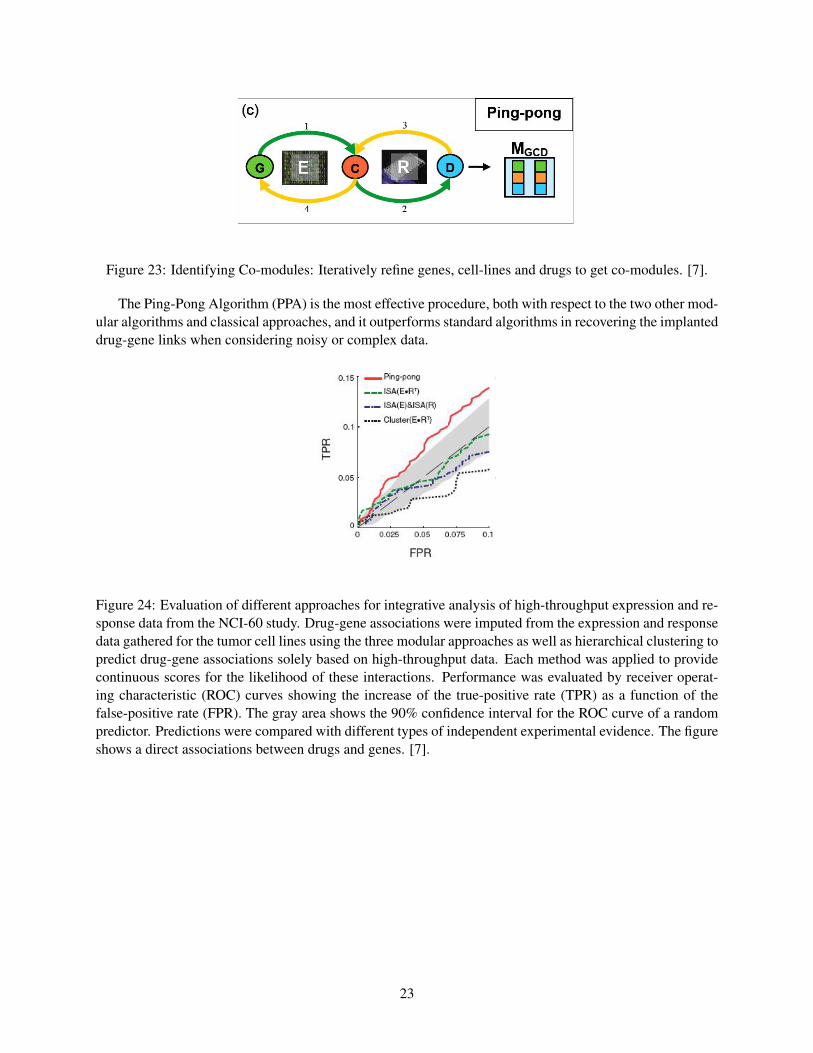
Figure 23: Identifying Co-modules: Iteratively refine genes, cell-lines and drugs to get co-modules. [7].

The Ping-Pong Algorithm (PPA) is the most effective procedure, both with respect to the two other mod-ular algorithms and classical approaches, and it outperforms standard algorithms in recovering the implanteddrug-gene links when considering noisy or complex data.

Figure 24: Evaluation of different approaches for integrative analysis of high-throughput expression and re-sponse data from the NCI-60 study. Drug-gene associations were imputed from the expression and responsedata gathered for the tumor cell lines using the three modular approaches as well as hierarchical clustering topredict drug-gene associations solely based on high-throughput data. Each method was applied to providecontinuous scores for the likelihood of these interactions. Performance was evaluated by receiver operat-ing characteristic (ROC) curves showing the increase of the true-positive rate (TPR) as a function of thefalse-positive rate (FPR). The gray area shows the 90% confidence interval for the ROC curve of a randompredictor. Predictions were compared with different types of independent experimental evidence. The figureshows a direct associations between drugs and genes. [7].

23

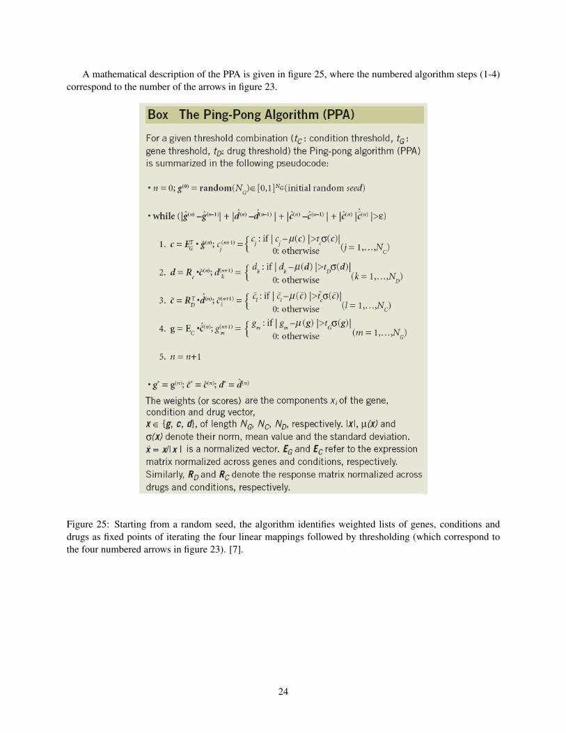
A mathematical description of the PPA is given in figure 25, where the numbered algorithm steps (1-4)correspond to the number of the arrows in figure 23.

Figure 25: Starting from a random seed, the algorithm identifies weighted lists of genes, conditions anddrugs as fixed points of iterating the four linear mappings followed by thresholding (which correspond tothe four numbered arrows in figure 23). [7].

24

3.3 Lamb et al.

Finally, the most ambitious effort for drug-target discovery was introduced by Lamb et al. [9]. This method,based on the generation of a connectivity map, a computational tool that connects gene expression signaturesvia expressed genes to chemical compounds that might influence these genes, is the most comprehensiveeffort yet for using genomics in a drug-discovery framework.

Several papers demonstrate the connectivity map’s ability to accurately predict the molecular actions ofnovel therapeutic compounds and to suggest ways that existing drugs can be newly applied to treat diseasessuch as cancer.

To build the Connectivity Map, the different effects of drugs and diseases are first described using thecommon language of ”genomic signatures” - the full complement of genes that are turned on and off by aparticular drug or disease. Then, the genomic signatures of approximately 450 drugs and other biologicallyactive compounds, are compiled, forming a database of biological ”barcodes” that denote cells’ responses tothe different drugs. Next, algorithms for finding matches (correlation), or reverse matches (anti-correlation),between the barcodes based on the patterns shared among them are developed. Together, these featuresenable the generation of the first connectivity map to directly compare the biological effects of differentdrugs with each other, and also with those seen in diseases. One of the Connectivity Map’s unique featuresis that it allows researchers to screen compounds against genome wide disease signatures, rather than a pre-selected set of target genes. Drugs are paired with diseases using sophisticated pattern-matching methodswith a high level of resolution and specificity.

We will cover two examples which can lead to the development of new drugs. In the first example,given independent disease signatures form two Alzheimer patients. Querying the connection map DB withtwo independent Alzheimer signatures (denoted A and B in figure 26) identifies DAPH. DAPH is known toreverse the formation of fibrils. The DAPH was solely (no other compound was consistently discovered)identified with a low rank (425 and 442 in A, 428 and 438 in B), suggesting an anti-correlation to the diseasesignatures which means that DAPH can possibly serve as a drug to the disease.

Figure 26: DAPH is anti-correlated with Alzheimer. [9].

25

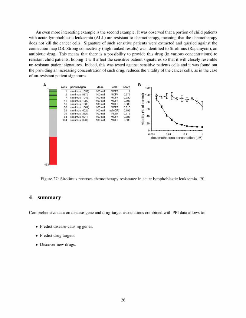
An even more interesting example is the second example. It was observed that a portion of child patientswith acute lymphoblastic leukaemia (ALL) are resistant to chemotherapy, meaning that the chemotherapydoes not kill the cancer cells. Signature of such sensitive patients were extracted and queried against theconnection map DB. Strong connectivity (high ranked results) was identified to Sirolimus (Rapamycin), anantibiotic drug. This means that there is a possibility to provide this drug (in various concentrations) toresistant child patients, hoping it will affect the sensitive patient signatures so that it will closely resembleun-resistant patient signatures. Indeed, this was tested against sensitive patients cells and it was found outthe providing an increasing concentration of such drug, reduces the vitality of the cancer cells, as in the caseof un-resistant patient signatures.

Figure 27: Sirolimus reverses chemotherapy resistance in acute lymphoblastic leukaemia. [9].

4 summary

Comprehensive data on disease-gene and drug-target associations combined with PPI data allows to:

• Predict disease-causing genes.

• Predict drug targets.

• Discover new drugs.

26

References

[1] Albert Laszlo Barabasi et al. Drugtarget network. Nature Biotechnology, page 11191126, 2007.

[2] Albert Laszlo Barabasi et al. The human disease network. PNAS, 104(21):86858690, 2007.

[3] Bergmann et al. Iterative signature algorithm for the analysis of large-scale gene expression data. Phys,67, 2003.

[4] Campillos et al. Drug target identification using side-effect similarity. Science, 321(5886):263–266,2008.

[5] Karni et al. A network-based method for predicting disease-causing genes. JOURNAL OF COMPU-TATIONAL BIOLOGY, 16(2):181–189, 2009.

[6] Kohler et al. Walking the interactome for prioritization of candidate disease genes. American journalof human genetics, 82(4):949958, 2008.

[7] Kutalik et al. A modular approach for integrative analysis of large scale gene-expression and drug-response data. NPG, 26(5):531–539, 2008.

[8] Lage et al. A human phenome-interactome network of protein complexes implicated in genetic disor-ders. Nat Biotech, 25(3):309316, 2007.

[9] Lamb et al. The connectivity map: Using gene-expression signatures to connect small molecules,genes, and disease. Science, 313(5795):1929–1935, 2006.

[10] Pawitan et al. Gene expression profiling spares early breast cancer patients from adjuvant therapy:derived and validated in two population-based cohorts. Breast Cancer Res, page 953964, 2005.

[11] Sotiriou et al. Breast cancer classification and prognosis based on gene expression profiles from apopulation-based study. Proc. Natl. Acad. Sci. USA, pages 10393–10398, 2003.

[12] Wang et al. Gene-expression profiles to predict distant metastasis of lymph-nodenegative primarybreast cancer. Lancet 365, pages 671–679, 2005.

[13] Wu et al. Network-based global inference of human disease genes. Mol Syst Biol, 2008.

[14] Zhou et al. Learning with local and global consistency. In 18th Annual Conf.on Neural InformationProcessing Systems, 2003.

[15] Roded Sharan Oron Vanunu. A propagation-based algorithm for inferring gene-disease assocations.German Conference on Bioinformatics, 2008.

[16] van de Vijver et al. A gene-expression signature as a predictor of survival in breast cancer. N. Engl. J.Med., pages 1999–2009, 2002.

27