ANALYSIS ANDDESIGN OFACANCOMBUSTOR

ANALYSIS AND DESIGN OF A CAN COMBUSTOR

A THESIS FOR

MASTER OF SCIENCE IN CHEMICAL ENGINEERING

BySanjoy Kumer BhattachariaStudent No: 04020201 IF

DEPARTMENT OF CHEMICAL ENGINEERINGBANGLADESH UNIVERSITY OF ENGINEERING AND TECHNOLOGY

DHAKA, BANGLADESH ,

ANALYSIS AND DESIGN OF A CAN COMBUSTOR

BySanjoy Kumer BhattachariaStudent No: 04020201 IF

A thesis submitted to the Department of Chemical Engineering, Bangladesh University ofEngineering and Technology, Dhaka, in partial fulfillment of the requirement for the

degree of Master of Science in Chemical Engineering.

~~ ••rq~

t ~iC ~'r.; \510 .'\' , ~

~~,:6Y

DEPARTMENT OF CHEMICAL ENGINEERINGBANGLADESH UNIVERSITY OF ENGINEERING AND TECHNOLOGY

DHAKA, BANGLADESH

June 2006

BANGLADESH UNIVERSITY OF ENGINEERIN.G AND TECHNOLOGYDEPARTMENT OF CHEMICAL ENGINEERING

•CERTIFICA nON OF THESIS WORK

We, the undersigned, certify that Sanjoy Kumer Bhattacharia, candidate for thedegree of Master of Science in Engineering (Chemical), has presented his thesis onthe subject "Analysis and Design of A Can Combustor" that the thesis is acceptablein form and content, and that the student demonstrated a satisfactory knowledge of thefield covered by this thesis in the oral examination held on the June 7, 2006.

-JJnAD~ ~~Du4~;~n-dr~- Nath MondalAssociate ProfessorDepartment of Chem ical EngineeringSUET, Dhaka

~v::sDr Ijaz Hossain.ProfessorDepartment of Chemical EngineeringBUET, Dhaka

En"r. Rashed Maksud KhChairmanBengal Fine Ceramics td52/1 New Eskaton, 0 aka-IOOO.

Chairman

Member

Member

Member (External)

".

DECLARATION

I do hereby declare that this thesis or any part of it has not been submitted elsewhere forthe award of any degree or diploma.

Sanjoy Kumer BhattaehariaStudent No.: 040202011(F)

/

."

Fig 3.1

Fig 3.2(a)

Fig 3.2(b)

Fig4.1(a)

Fig 4.1(b)

Fig 4.1(c)

Fig4.1(d)

Fig 4.2(a)

Fig 4.2(b)

Fig 4.2(c)

Fig 4.2(d)

Fig 4.3(a)

Fig 4.3(a)

Fig 4.3(c)

Fig 4.3(d)

Fig 4.4(a)

Fig 4.4(b)

Fig 4.4(c)

Fig 4.4(d)

LIST OF FIGURES AND TABLES

Page No

Model of the Can combustor. 29

Discretised Model. 29

Discretised Model. 29

Velocity vector colored by velocity magnitude at y=0 for the 30angle of rotation ono'.

Velocity vector colored by velocity magnitude at y=0 for the 30angle of rotation of 45'.

Velocity vector colored by velocity magnitude at y=0 for the 31angle of rotation of 60'.

Velocity vector colored by velocity magnitude at y=0 for the 31angle of rotation of 90'.

Contour of static temperature at the plane y=o for the angle of 32rotation 30'.

Contour of static temperature at the plane y=o for the angle of 32rotation 45'.

Contour of static temperature at the plane Y=O for the angle of 32rotation 60'.

Contour of static temperature at the plane y=o for the angle of 32rotation 90'.

Contour of the concentration of methane at the plane Y~O for the 34angle of rotation 30'.

Contour of the concentration of methane at the plane y=o for the 34angle of rotation 45'.

Contour of the concentration of methane at the plane y=o for the 34angle of rotation 60'.

Contour of the concentration of methane at the plane y=o for the 34angle of rotation 90'.

Contour ofthe concentration of NO x at the plane Y=O for the 35angle of rotation 30'.

Contour ofthe concentration of NO x at the plane Y=O for the 35angle of rotation 45'.

Contour of the concentration of NO x at the plane y=o for the 36angle of rotation 60'.

Contour of the concentration of NOx at the plane y=o for the 36angle of rotation 90'.

Fig 4.5(a) Contour of the concentration of CO2 at the plane y=o for the 37angle of rotation 30°.

Fig 4.5(b) Contour of the concentration of CO2 at the plane y=o for the 37angle of rotation 45°.

Fig 4.5(c) Contour of the concentration of CO2 at the plane y=o for the 37angle of rotation 60°.

Fig 4.5(d) Contour of the concentration of CO2 at the plane Y=O for the 37angle of rotation 90°.

Fig 4.6(a) Contours of Static Temperature at the plane y=0 when 50% 39Excess air is used in the primary air inlet.

Fig 4.6(b) Contours of Static Temperature at the plane y=0 when 75% 39Excess air is used in the primary air inlet.

Fig 4.6(c) Contours of Static Temperature at the plane y=0 when 100% 39Excess air is used in the primary air inlet.

Fig 4.6(d) Contours of Static Temperature at the plane y=0 when 125% 39Excess air is used in the primary air inlet.

Fig 4.7(a) Contour of the concentration of methane at the plane y=0 when 4050% Excess air is used in the primary air inlet.

Fig 4.7(b) Contour of the concentration of methane at the plane y=0 when 4075% Excess air is used in the primary air inlet.

Fig 4.7(c) Contour ofthe concentration of methane at the plane y=0 when 41100% Excess air is used in the primary air inlet.

Fig 4.7(d) Contour of the concentration of methane at the plane y=0 when 41125% Excess air is used in the primary air inlet.

Fig 4.8(a) Contour of the mass fraction of NOx at the plane y=0 when 50% 42Excess air is used in the primary air inlet.

Fig 4.8(b) Contour of the mass fraction of NOx at the plane y=0 when 75% 42Excess air is used in the primary air inlet.

Fig 4.8(c) Contour of the mass fraction of NOx at the plane y=0 when 100% 42Excess air is used in the primary air inlet.

Fig 4.8(d) Contour of the mass fraction of NOx at the plane y=0 when.125% 42Excess air is used in the primary air inlet.

Fig 4.9(a) Contour of mass fraction of CO, for 50% excess air. 43

Fig 4.9(b) Contour of mass fraction of CO, for 75% excess air. 43

Fig4.9(c) Contour of mass fraction of CO, for 100% excess air. 44

Fig 4.9(d) Contour of mass fraction of CO2 for 125% excess air. 44

. Fig 4.1O(a) Velocity vector colored by velocity magnitude at x=O, when 45secondary air is Off.

II

Fig 4.1O(b) Velocity vector colored by velocity magnitude at x=O, when 45secondary air is off

Fig 4.11(a) Contours of Static Temperature at the plane y=0, when secondary 46air is off.

Fig 4.11(b) Contours of Static Temperature at the plane y=0 with secondary 46Air.

Fig 4.12(a) Velocity vector colored by Static Temperature at the plane y=0, 46when secondary air is off.

Fig4.12(b) Velocity vector colored by Static Temperature at the plane y=0 46with secondary air.

Fig 4.13(a) Contours of mass fraction of methane at the plane y=0, when 47secondary air is off.

Fig 4.13(b) Contours of Contours of mass fraction of methane at the plane 47y=0 with secondary air.

Fig 4.14(a) Contours of mass fraction of CO, at the plane y=0, when 48secondary air is off.

Fig 4.14(b) Contours of Contours of mass fraction of CO, at the plane y=0 48with secondary air

Fig 4.15(a) Contours of mass fraction of NOx at the plane y=0, when 49secondary air is off.

Fig 4.15(b) Contours of Contours of mass fraction of NO x at the plane y=0 49with secondary air.

Fig 4.16(a) Velocity vector for the secondary air at point 2. 50

Fig 4.16(b) Velocity vector for the secondary at point I. 50

Fig4.17(a) Contour of static temperature at the plane y=0 for secondary air at 51point 2.

Fig 4.17(b) Contour of static temperature at the plane x=O for secondary air at 51point 2.

Fig 4.18(a) Contour of static temperature at the plane y=0 for secondary air at 51point I.

Fig 4.18(b) Contour of static temperature at the plane x=O for secondary air at 51point 1

Fig4.19 Contour of mass fraction of Methane at y=0 for secondary air at 52point 2.

Fig 4.20(a) Contour ofthe mass fraction of NOx at the plane y=0 for 53secondary air at point 2.

Fig 4.20(b) Contour of the mass fraction of NOx at the plane y=0 for 53secondary air at point I.

III

Fig 4.21 Secondary air is introduced at three different position at the plane 53x=O.

Fig 4.22(a) Contour of secondary air at the plane y=0 for three secondary air 54inlet.

Fig 4.22(b) Contour of secondary air at the plane x=O for three secondary air 54inlet.

Fig 4.23 Contour of mass fraction of methane for three secondary air inlet. 55

Fig 4.24 Contour of mass fraction of NOx at the plane x=O for secondary 56air inlet.

Fig 4.25 Contour of static temperature at the plane x=O for secondary air 57inlet point 3 at x=O

Fig 4.26 Contour of static temperature at the plane x=O for secondary air 57inlet point 3 at x=O

Fig 4.27(a) Contours of Static Temperature at the plane y=0 for Radiation Off 58

Fig 4.27(b) Contours of Static Temperature at the plane y=0 for Radiation On 58

Fig 4.28(a) Contour of mass fraction of NOx for Radiation Off 58

Fig 4.28(b) Contour of mass fraction of NOx for Radiation Off 58

Fig 4.29(a) Contour of static temperature at the plane y=0 for two step 60reaction.

Fig 4.29(b) Contour of static temperature at the plane y=0 for single step 60reaction.

Fig 4.30(a) Contour of mass fraction of methane at the plane y=0 for two step 60reaction.

Fig 4.30(b) . Contour of mass fraction of methane at the plane y=0 for single 60step reaction.

Fig 4.31 (a) Contour of static temperature at the plane y=0 for constant Cpo 61

Fig4.31(b) Contour of static temperature at the plane y=0 for Cp (piece wise 61polynomial).

Fig 4.32(a) Contour of mass fraction of NOx for at the plane y=0 for constant 62Cpo

Fig 4.32(b) Contour of mass fraction of NOx for at the plane y=o for Cp 62(piecewise polynomial).

Fig 4.33(a) Contour of mass fraction of CO, for at the plane y=O for constant 62Cpo

Fig 4.33(b) Contour of mass fraction of CO, for at the plane y=0 for Cp 62(piecewise polynomial).

Fig C.I Iteration Curve 88

IV

Table A.I Wall Temperature for Different Rotation of Primary Air Inlet 69

Table A.2 Wall Temperature for the variation % Excess Air 69

Table A.3 Effect of Secondary Air on Wall Temperature- I69

Table AA Effect of Secondary Air on Wall Temperature- 1169

Table A.5 Effect of Secondary Air on Wall Temperature- III 70

Table A.6 Effect of Radiation heat transfer on wall temperature 70

v

NOMENCLATURE

Cp -Heat capacity at constant pressure, (J/kg-K, Btullbm-F)Gk -Generation of turbulence. kinetic energy due to the mean velocity

gradientsCh, -Generation of turbulence kinetic energy due to buoyancyN -Total number of fluid phase chemical species present in the systemu -Velocity magnitude (mis, fils)v -Velocity vectorT -Temperature (OCor"K)k -Turbulence kinetic energy (J/kg, Btullbm)%, -Material derivativeR; -Net rate of production of specie 'i' by chemical reactionS; -Rate of creation by addition from the dispersed phase.Sk -User defined source termsS, -User defined source termsYM -Contribution of fluctuating dilation in compressible turbulence to the

overall dissipation ratee -Turbulence dissipation rateT -Momentum stress tensorp -Density (kg/m3, Ibm/ft3)(1k -Turbulent Prandtle numbers for k(1, -Turbulent Prandtle numbers for EP, -Turbu lent viscosity

VI

ACKNOWLEDGEMENTS

The author acknowledges with thanks and gratitude the encouraging advice and helpful

co-operation he received from Dr. Harendra Nath Modal, Associate Professor,

Department of Chemical Engineering, Bangladesh University of Engineering and

Technology (BUET), under whose supervision the research work was carried out. The

author acknowledges his gratitude to the Head, Department of Chemical Engineering,

BUET for providing required facilities. The author also extends his thanks to Mr.

Satyajit Roy, graduate student of Department of Chemical Engineering, BUET, for his

extensive help in the work.

VII

ABSTRACT

A Can combustor is a feature of gas turbine engine. Prediction of the performance of

combustor becomes an integral part for the development of efficient combustor. Primary

design objectives are to bum the fuel efficiently, keep the wall temperature as low as

possible and minimize emissions such as NOx, Unburnt Hydrocarbon, etc. Some of the

parameters that controls the performances of a combustor are fuel/air ratio, degree of

turbulence, geometry of the primary air, flow rate of secondary air, etc. Efficient burning

depends on how well the fuel and air are mixed before ignition which in tum depends on

the degree of turbulence. To keep the wall temperature as low as possible, excess air with

higher volume plays an important role, which affects the burning and the process becomes

further complicated. To enhance the turbulence, different air injection patterns of primary

air inlet are studied and the effect of secondary air injection is investigated. Some

theoretical aspects are investigated using different reaction steps and ways of heat transfer.

Fluent, a CFD software, is used for the simulation of the combustor applying k-c model for

turbulence computation and eddy-dissipation model for studying reaction dynamics.

Investigation revealed some important features of the performance of a Can combustor.

Investigation revealed that increasing the angle of rotation of primary air inlet and

percentage of excess air could reduce wall temperature as well as increase NOx production.

It is found that injection of secondary air inlet reduces the wall temperature significantly.

Applying the secondary air inlet in different position together reduces wall temperature

more effectively along with efficient burning of methane in the combustor. It is also found

that wall temperature was drastically reduced when radiation heat transfer is off and

variation of reaction steps makes a very little effect on the performance.

vm

CONTENTS

List of Figures and Tables

Nomenclature VI

Acknowledgements VII

Abstract VIII

CHAPTER 1. Introduction 1-2

1.1 Motivation I

1.2 Objectives 2

CHAPTER 2. Literature Review 3-252.1 General 4

2.1.1 The process of Combustion 52.1.2 Stationary films 62.1.3 Combustion Fundamentals 62.1.4 Mechanism of Combustion 72.1.5 Elementary Carbon 82.1.6 Combustion of Methane 82.1.7 Flame Propagation 92.1.8 Fonnation of NOx 102.1.9 Thennal NOx 10

2.2 Computational Fluid Dynamics II2.2.1 Benefits of CFD II2.2.2 Methods of Prediction 122.2.3 Choice of Prediction method 142.2.4 Nature of Numerical Methods 14

2.3 Review of Previous work on modeling of Combustor 16

CHAPTER 3. Description of the Modeling Procedure 26-293.1 Methodology 26

3.1.1 Assumptions 263.2 Model Calculation 273.2.1 The Standard k-E Model 27 •3.2.2 Eddy dissipation Model 28

3.3 Description of the Unit 283.4 Description of the software 29

CHAPTER 4. Results and Discussion 30-624.1 Variation of Geometry of Primary air inlet 304.1.1 Effect of Rotation of Primary air inlet on the wall 31

temperature4.1.2 Concentration of Methane in the combustor 334.1.3 NOx concentration in the combustor 354.1.4 CO, concentration in the combustor 36

CHAPTER

APPENDIXAPPENDIXAPPENDIX

4.24.2.14.2.24.2.34.2.4

4.34.3.14.3.24.3.34.3.4

4.44.4.14.4.24.4.3

4.54.5.14.5.2

4.64.7

5.

ABC

Influence of Excess Air on can CombustorEffect of Excess Air on the Wall TemperatureConcentration of Methane in the combustorProduction of NOxCO, Concentration in the combustor

Effect of Secondary AirEffect of Secondary Air

Concentration of Methane in the CombustorProduction of CO, in combustorNOx Production

Secondary Air Inlet at different PositionSecondary Air Inlet below the reference pointSecondary Air inlet at three placesSecondary Air Inlet at Two different position

Radiation Off and OnWall TemperatureNOx Production

Reaction StepsHeat CapacityConclusion and RecommendationREFERENCESAPPENDICESWall Temperature for different mode of operationModel specification and Material PropertiesCalculation using the Software

3838404143444547474849495356575759596163-6465-6869-88697177

Chapter 1

1. Introduction

1.1 MotivationThis study is related to the main component of a gas turbine engines, and more particularly

to a compact annular Can combustor, which provides enhanced performance in gas turbine

engines having gaseous oxidant delivered to the gas turbine engine via a conduit or duct

from a pressurized source. It is well known that, in order to maximize fuel efficiency and

power output from such a gas turbine engine, the engine should be operated with a

combustion temperature and a turbine inlet temperature, which are as high as possible. As a

practical malter, however, the maximum temperatures which may be utilized are determined

by the ability of materials used in fabricating components of the engine, such as the

combustor, turbine wheel, nozzle, and shroud, to withstand extended exposure to elevated

temperatures. While it is not possible to overcome the limitations on combustion and turbine

inlet temperatures which are imposed by the materials, it is well known in the art that an

acceptable balance between power output, reliability, and life of the engine may be achieved

by utilizing a relatively high combustion temperature and providing means within the engine

for utilizing a portion of the compressed oxidant either as a diluent injected just upstream of

the nozzle for reducing the temperature of the hot gases, or for convectively cooling engine

components exposed to the hot gases.

In technical process, combustion nearly always takes place in the turbulent rather than a

laminar flow field. The reason is two fold: First, turbulence increases the mixing process and

thereby enhances combustion. Combustion releases heat and thereby generates flow

instability by buoyancy and gas expansion, which then enhance transition to turbulence.

Some of the parameters playa major in a combustion reactor. Air fuel ratio, primary air

inlet, secondary air inlet, fuel inlet, turbulence and wall temperature are the important

variable which should be optimized to get maximum efficiency from combustion reactor.

Control over the production of pollutants like NOx, SOz, CO2, CO, Soot and unbumt

Hydrocarbon (HC) is another concern of a combustion process. Researchers used different

computational model to study the effect of various parameter for the enhancement of the

performance of different combustor where they have shown that prior modeling is one of the

most effective ways to predict the performance of a combustor. But no work was reported

about the optimization of the performance of a Can combustor studying its controlling

parameter. In this study, performance of a Can combustor will be evaluated using a

Computational Fluid Dynamics tool.

1.2 ObjectivesPrimary design objectives are to bum the fuel efficiently, keep the wall temperature as low

as possible and minimize emissions. Efficient burning depends on how well the fuel and air

are mixed before combustion which in tum depends on the degree of turbulence. To enhance

the turbulence, different fuel and air injection patterns will be studied. To maintain the wall

temperature and minimize emissions, different fuel to air ratios will be investigated, and

different geometric arrangements for primary and secondary air will also be studied. Hence

simulation will be carried out to study the following parameter to enhance combustion and

reduce emission:

~ Effect of degree of swirl of the primary air

~ Variation percentage of excess air

~ Effect of secondary air on the performance and finding out the optimal

location for injection of secondary air.

}> Effect of Radiation heat transfer on wall temperature

}> Effect of reaction steps of the conversion of methane.

}> Effect of heat capacity on the wall temperature.

2

Chapter 2

2. Literature Review

2.1 General

Man has been fascinated by fire from earliest existence on earth, but a quantitative

understanding of the combustion process was not achieved until about the year 1880. Prior

to that date, one can trace the development of many hypotheses concerning the nature and

properties of fire, including some that were expressed in supernatural terms of fear and

awe. However, even the existence of the now discredited phlogiston theory of combustion

did not prevent enterprising engineers from designing and constructing boilers to generate

steam for the earliest steam engines.

Phlogiston was a hypothetical mysterious substance which sometimes was presumed to

have the property of negative weight and which combined with a body to render it com-

bustible. First proposed by G. E. Stahl in 1697, the phlogiston theory dominated the

chemical thought of the 18th century. Even such a perceptive observer as Joseph Priestly,

who in 1774 discovered the unique power of oxygen for supporting combustion, accepted

the phlogiston theory. In the years between 1775 and 1781, Antoine L. Lavoisier

substituted for it the theory of oxygenation and provided experimental evidence that

combustion was the union of the substance burned with the oxygen of the atmosphere.

In 1755 Joseph Black discovered carbon dioxide, and in 1781 Henry Cavendish demon-

strated the compound nature of water. At about this same time Lavoisier made the precise

measurements and formulated the volume and weight relationships that underlie the

modem theory of combustion. Beyond this, in 1811 Amedeo Avogadro established that the

number of molecules in a unit volume under standard conditions is the same for all gases.

During this same period John Dalton articulated the law of partial pressures, and in 1803

3

his study of the physical properties of gases led to formulation of the atomic theory,

including the law of combining weights. A related observation was made by Gay-Lussac in

1808 that gases always combine in volumes that bear simple ratios to each other. Volume

under standard conditions is the same for all gases. During this same period John Dalton

enunciated the law of partial pressures, and in 1803 his study of the physical properties of

gases led to formulation of the atomic theory, including the law of combining weights. A

related observation was made by Gay-Lussac in 1808 that gases always combine in

volumes that bear simple ratios to each other.

2.1.1 The Process of CombustionAt one time, it was thought there were only four elements, which composed all nature: fire,

water, air, and earth. In fact, fire has been regarded with fear by men throughout history, for

the useful effects it could perform as well as for the terrible destruction it might cause.

Researchers have spent hundreds of many years studying the effects of the numerous

variables on burning. Nevertheless, many aspects of combustion are still only partly

understood [Beer & Chigar, 1972].

Combustion is the rapid, high-temperature oxidation of fuels. Since most fuels used at

present consist almost entirely of carbon and hydrogen, burning involves the rapid

oxidation of carbon to carbon dioxide, or carbon monoxide, and of hydrogen to water

vapor. The combustion reaction takes place in the gaseous phase, except for the burning of

the fixed carbon in solid fuels. Even in the latter case, the oxygen and the combustion

products exist as gases, and only the fixed carbon itself is present as a solid. Flame may be

defined as gas rendered luminous by the liberation of chemical energy.

The flame front is the surface or area between the luminous region and the dark region of

unburned gas, which exists in all combustion reactions in the gaseous phase. Since the

gases may not become luminous instantly, it is expedient to visualize the burning zone as

consisting of a luminous zone and a reaction zone [Toong, 1983].

Ignition and most of the oxidation occur in the latter zone, while completion of burning and

emission of light take place in the luminous zone. Generally, the locally available supply of

oxygen is consumed in the reaction zone. It is difficult to make a clear distinction between

these regions because the total thickness of the burning zone may vary from a few

4

thousandths of an inch to an indefinite thickness, depending upon the turbulence and the

homogeneity of the gases.

These definitions provide for the persistence of flame until it remains luminous and ceases

radiation, even after the chemical reaction has proceeded to equilibrium. The continuance

of luminosity, called after burning, is evident in various types of combustion, especially in

spark ignition engines. A fast-burning mixture has a very thin reaction zone, and ignition,

combustion, and luminescence occur almost simultaneously.

2.1.2 Stationary Flames

A stationary flame is one in which the flame front is more or less stationary in space; the

unburned gases flow toward the reaction zone at the propel speed to maintain the position;

of the flame. This type of flame may be further classified as combustion in which the fuel is

premixed with air or in which the fuel and air enter the combustion area separately. The

latter is called a diffusion flame as it becomes necessary for the oxygen to be diffused into

the reaction zone and mixed with the fuel before burning can occur.

Stationary flames are utilized at atmospheric pressure or at other pressures, higher or lower.

Gas burners, pulverized-coal burners employ this type of flame. The flow of mixture to

these flames may be either laminar or turbulent. If there is a great deal of turbulence, the

reaction zone and resulting flame front may be irregular and rather unsteady. Such

turbulence may create what appears to be a solid cone of flame in the vicinity of the

combustion. Some oil and gas burners operate with a diffusion flame. In these cases

considerable turbulence of the air and fuel in the combustion chamber is employed to

ensure fairly rapid mixing. A true diffusion flame creates a much longer zone of reaction,

and there are comparatively few applications where diffusion of the gases alone is relied

upon to provide mixing of the fuel and oxygen.

2.1.3 Combustion Fundamentals

To the engineer concerned with boiler design and performance, combustion may be

considered as the chemical union of the combustible of a fuel and the oxygen of the air,

controlled at such a rate as to produce useful heat energy. The principal combustible con-

stituents are elemental carbon, hydrogen, and their compounds. In the combustion process,

the compounds and elements are burned to carbon dioxide and water vapor. Small quan-

5

tities of sulfur are present in most fuels. Although sulfur is a combustible and contributes

slightly to the heating value of the fuel, its presence is generally detrimental because of the

corrosive nature of its compounds.

Air, the usual source of oxygen for combustion in boilers, is a mixture of oxygen, nitrogen

and small amounts of water vapor, carbon dioxide, argon and other elements. In an ideal

situation, the combustion process would occur with the exact proportions of oxygen and a

combustible that are called for in theory as the stoichiometric quantities. But it is

impractical to operate a boiler at the theoretical level of zero percent excess oxygen. In

practice, this condition is approached by providing an excess of air varies with fuel, boiler

load and type firing equipment.

2.1.4 Mechanism of CombustionThe term mechanism of combustion refers to the reactions by which fuel is transformed

chemically to combustion products. A self-sustaining chemical process which consists of a

series of different reactions in which intermediate products are formed in one step and

destroyed in a succeeding step is known as a chain reaction. The intermediate products

formed are known as chain carriers since they help to carry the reaction to completion.

Chain carriers may be free atoms of diatomic gases such as Hydrogen (H) and Oxygen (0),

free radicals (like OH, CHO, CH, etc.), or some organic compound (such as formaldehyde,

HCHO). A free radical is a group of atoms, which carries one unpaired electron. In other

words, a free radical has a free valence bond. The hydroxyl free radical like OH unites with

a free hydrogen atom to form a water molecule, H20, or it may enter into many other

reactions. A chain carrier may exist only a minute fraction of a second. Billions of chain

carriers are formed and instantly destroyed during the course of a chain reaction.

Any chain reaction consists of an initiation phase, a propagation phase, .and a termination

phase. In the first phase the chain carriers are formed which promote the propagation phase.

Combustion may be terminated by a chain breaking reaction in which some of the chain.

carriers are taken out of play by another substance, which reacts with or adsorbs the chain

carriers. A cold combustion chamber wall in an oil burner, for instance, apparently adsorbs

enough of the chain carriers to stop the combustion of fuel oil near the surface. As a result

there is a strong tendency to deposit partially burned fuel, or soot, on combustion chamber

6

walls when they are cold. Some intermediate reactions occur in such a manner that several

chain carriers are formed with each step. Such a reaction is known as a chain branching

reaction. Each of these new chain carriers may then branch out and start a new series of

reactions of its own.

2.1.5 Elementary CarbonThe combustion mechanism for elementary carbon in the solid state, as it appears in the

fixed carbon in coal, coke, or charcoal, not thoroughly understood, and various

investigators have arrived at different conclusion as to the predominant reactions. The basic

mechanism involve the diffusion of gaseous oxygen to the surface of the solid carbon

where the oxygen molecules react to form a primary product, which may be either carbon

monoxide or carbon dioxide. This gaseous product must then diffuse from the surface to

allow more oxygen to contact the surface molecules of carbon. It is thought that two

distinctly different types of reaction are involved, the one mechanism prevailing at

temperatures over 1800 F and the other at lower temperatures. In either case, the speed of

the actual chemical reaction is so great, when compared to the rate of diffusion of gases to

and from the carbon surface, that diffusion control the rate of burning almost entirely.

Temperatures between about 1650 and 2000 F the reaction rate increases with temperature,

and above 2000 F it appears to remain fairly constant. Some C02 may be detected as a

primary product at the surface, but the concentration of the C02 is low as compared with

the CO at all times. Evidently the oxidation reaction at the surface proceeds only to the

formation of CO, and the gaseous CO oxidized at some point beyond the carbon surface.

2.1.6 Combustion of MethaneThe combustion of methane whereby methane and air can unite, but that only a branched-

chain mechanism produces active combustion, as follows

Oz + CH3 -+ CH300 .

CH4+ CH300' -+ CH3' + CH300HCH300H -+ CO + 2Hz + 0 .CH4+ O' -+ CH3' + ORThe net effect of the above series of reactions may be represented by the following

equation, which sums up the action of the primary chain:

7

CH4 + O2 -+CO + 4H2

The primary products CO and H2 are then oxidized to CO2 and H20 by the secondary

mechanisms:

CO+OH -+ H'+C02

02 + CO + H -+ OR + C02

H2 + OH -+ H' + H20O2+ H2 + H -+ OH' + H20The CH)OOH (methylhydroperoxide) is termed a propagating center, which serves as a

carrier to promote the chain, It normally breaks up into two primary products and an

oxygen atom, thus branching the chain. To ignite a mixture of methane and air, it seems

necessary to produce a few CH)OOH molecules to act as propagating centers. This may be

accomplished by heating the mixture to the ignition temperature or by some auxiliary

means. However, it appears quite certain that the critical factor in ignition is the production

of propagating centers by inducing reactions and not the temperature of the mixture.

2.1. 7 Flame PropagationIn burner flames, the flame is propagating against the flow of the reagents of the reagents

and its position is stationary. Variation in input condition such as fuel flow rate, air/fuel

ratio or preheat can cause these flame to become non stationary or unstable. A flame is

considered to be stable over a range of an input parameter if variation of such a parameter

within this range does not cause the flame to blow off or to flashback into the burner tube.

One of the basic concept in flame theory is that of flame propagation. This refers to the

propagation of the zone of burning or of the combustion wave through a combustible

mixture. It is generally appreciated that the ignition source is a source of heat. It also

produces atoms and free radicals, which may act as chain carrier in the chemical reaction.

Once the heat flow and the diffusion of these active species have initiated chemical reaction

in the adjacent layer of the combustible medium, this layer becomes the source of heat and

'of chain carriers and is capable of initiating reaction in the next layer. A quantitative theory

of flame propagation is based on the transfer of heat and mass from the reaction zone to the

unburned mixture,

8

2.1.8 Formation of NOxNitrogen monoxide (NO) and nitrogen dioxide (N02) are byproducts of the combustion

process of virtually all fossil fuels. The quantity of these inorganic compounds in the

products of combustion was not sufficient to affect boiler performance, and their presence

was largely ignored. In recent years, oxides of nitrogen have been shown to be. key

constituents in the complex photochemical oxidant reaction with sunlight to form smog.

Today, the presence of N02 and NO (collectively referred to as NOx) is regulated by the

authorities and has become an important consideration in design of fuel firing equipment.

2.1.9 Thermal NOxThe formation of NOx in the combustion process is often explained in terms of the source

of nitrogen required for the reaction. The N2 can originate from the atmospheric air, in

which case the product is referred to as thermal NOx or from the organically bound

nitrogen components found in all coals and fuel oils that are termed fuel NOx. 11 is;

important to note that even though NOx consists usually of 9S percent NO and only S

percent N02, the normal practice is to calculate concentrations of NOx as 100 percent N02.

The mechanisms involving thermal NOx were first described by Zeldovich and later

modified to what is referred to as the extended Zeldovich mechanism.

~O-+NO+N

N+02 -+ NO+O

N +OH -+NO+H

As the equilibrium values predicted by this mechanism are higher than those actually

measured, it is generally assumed that first reaction is rate determining due to its high

activation energy of 317 kllmo!.

Although the kinetics involved in the conversion of organically bound nitrogen compounds

found in fossil fuels are not yet well understood, numerous investigators have shown fuel

NOx to be an important mechanism in NOx formation from fuel oil, and the dominant

mechanism in NOx generated from the combustion of coa!. A most significant property of

fuel nitrogen conversion that affects the design of fuel-firing equipment relates to the

availability of oxygen to react with the fuel-nitrogen compounds in their gaseous state.

Simply stated, the compounds that evolve from a coal particle such as NCH and NH), are

9

relatively unstable and will reduce to harmless N2 under fuel-rich conditions, or to NO

under air-rich conditions.

2.2 Computational Fluid Dynamics (CFD)A Working Definition of CFD: computation Fluid Dynamics - the dynamics of things that

flow. CFD - a computational technology that enables to study the dynamics of things that

flow. It is mathematical prediction method. Using CFD, a computational model can be built

that represents a system or device. Then the fluid flow physics can be applied to this virtual

prototype, and the software will give a prediction of the fluid dynamics. CFD is a

sophisticated analysis technique. It not only predicts fluid flow behavior, but also the

transfer of heat, mass, phase change, chemical reaction such as combustion, mechanical

movement such as an impeller turning, and stress or deformation of related solid structures

such as a mast bending in the wind.

2.2.1 Benefits of CFDBasically, the compelling reasons to use CFD are these three:

Insight: There are many devices and systems that are very difficult to prototype. Often,

CFD analysis shows the parts of the system or phenomena happening within the system that

would not otherwise be visible through any other means. CFD gives a means of visualizing

and enhanced understanding of the designs.

Foresight: Because CFD is a tool for predicting what will happen under a given set of

circumstances, it can answer many 'what if?' questions very quickly. Effects of the

variation of different variables could be found out easily. As a result, performance

prediction of a design can be carried out in a short time. All these prediction can be made

before the physical proto typing, which helps to design better and faster.

Efficiency: Better and faster design or analysis leads to shorter design cycles. Time and

money are saved. Products get to market faster. Equipment improvements are built and

installed with minimal downtime. CFD is a tool for compressing the design and

development cycle.

10

2.2.2 Methods of PredictionPrediction of heat transfer and fluid-flow processes can be obtained by two main methods:

experimental investigation and theoretical calculation. A comparison between the methods

is discussed in the following.

2.2.2.1 Experimental InvestigationThe most reliable information about a physical process is often gIven by actual

measurement. An experimental investigation involving full-scale equipment can be used to

predict how identical copies of the equipment would perform under the same conditions.

Such full-scale tests are in mosCcases, prohibitively expensive and often impossible. The

alternative then is to perform experiments on small-scale models. The resulting

information, however, must be extrapolated to full scale, and general rules for doing this

are often unavailable. Further, the small-scale models do not always simulate all the

features of the full-scale equipment; frequently, important features such as combustion or

boiling are omitted from the model tests. This further reduces the usefulness of the test

results. Finally, it must be remembered that there are serious difficulties of measurement in

many situations, and that the measuring instruments are not free from errors.

2.2.2.2 Theoretical CalculationA theoretical prediction works out the consequences of a mathematical model, rather than

those of an actual physical model. For the physical processes of interest here, the

mathematical model mainly consists of a set of differential equations. If the methods of

classical mathematics were to be used for solving these equations, there would be little

hope of predicting many phenomena of practical interest. A look at a classical text on heat

conduction or fluid mechanics leads to the conclusion that only a tiny fraction of the range

of practical problems can be solved in closed form. Further, these solutions often contain

infinite series, special functions, transcendental equations for Eigen values, etc., so that

their numerical evaluation may present a formidable task. Development of numerical

methods and the availability of large digital computers hold the promise that the

. implications of a mathematical model can be worked out for almost any practical problem.

11

2.2.2.3 Advantages of a Theoretical CalculationA theoretical calculation offers following advantages over a corresponding experimental

investigation

Low cost: The most important advantage of a computational prediction is its low' cost. In

most applications, the cost of a computer run is many orders of magnitude lower .than the

cost of a corresponding experimental investigation. This factor assumes increasing

importance as the physical situation to he studied becomes larger and more complicated.

Whereas the prices of most items are increasing, computing costs are likely to be even

lower in the future.

Speed: A computational investigation can.be perfomled with remarkable speed: A designer

can study the implications of hundreds of different configurations in less than a day and

choose the optimum design. On the other hand, a corresponding experimental investigation,

it is easy to imagine, would take a very long time.

Complete ill/ormatioll: A computer solution of a problem gIves detailed and complete

information. It can provide the values of all the relevant variables (such as velocity,

pressure, temperature, concentration, turbulence intensity) throughout the domain of

interest. Unlike the situation in an experiment, there are few inaccessible locations in a

computation, and there is no counterpart to the flow disturbance caused by the probes.

Obviously, no experimental study can be expected to measure the distributions of all

variables over the entire domain. For this reason, even when an experiment is performed,

there is great value in obtaining a companion computer solution to supplement the

experimental information.

Ability to simulate realistic cOllditiolls: In a theoretical calculation, realistic conditions can

be easily simulated. There is no need to resort to small-scale or cold-flow models. For a

computer program, there is little difficulty in having very large or very small dimensions, in

treating very low or very high temperatures, in handling toxic or flammable substances, or

in following very fast or very slow processes.

Ability to simulate ideal conditions: A prediction method is sornetimes used to study a

basic phenomenon, rather than a complex engineering application. In the study of a

phenomenon, one wants to focus attention on a few essential parameters and eliminate all

irrelevant features. Thus, many idealizations are desirable-for example, two-dimensionality,

12

constant density, an adiabatic surface, or infinite reaction rate. In a computation, such

conditions can be easily and exactly set up. On the other hand, even a very careful

experiment can barely approximate the idealization.

2.2.3 Choice of Prediction MethodAn appreciation of the strengths and weaknesses of both approaches is essential to the

proper choice of the appropriate technique. There is no doubt that experiment is the only

method for investigating a new basic phenomenon. In this sense, experiment leads and

computation follows. It is in the synthesis of a number of interacting known phenomena

that the computation performs more efficiently. Even then, sufficient validation of the

computed results by comparison with experimental data is required. On the other hand, for

the design of experimental apparatus, preliminary computations are often helpful, and the

amount of experimentation can usually be significantly reduced if the investigation is

supplemented by computation [Patankar 1980]. An optimal prediction effort should thus be

a judicious combination of computation and experiment. The proportions of the two

ingredients would depend on the nature of the problem, on the objectives of the prediction,

and on the economic and other constraints of the situation.

2.2.4 Nature of Numerical MethodsA numerical solution of a differential equation consists of a set of numbers from which the

distribution of the dependent variable <Dcan be constructed. In this sense, a numerical

method is akin to a laboratory experiment, in which a set of instrument readings enables us

to establish the distribution of the measured quantity in the domain under investigation. The

numerical analyst and the laboratory experimenter both must remain content with only a

finite number of numerical values as the outcome, although this number can, at least in

principle, be made large enough for practical purposes.

<P can be represented by a polynomial in x like following:~ 23m'fI = Go + a,x + G]X + a4x + + amx

and employ a numerical method to find the finite number of coefficients au,al,a, am•

This will enable to evaluate <P at any location x by substituting the value of x and the values

13

of a's into equation. This procedure is, however, somewhat inconvenient if our ultimate

interest is to obtain the values of <P at various locations. The values of a's are not

particularly meaningful, and the substitution operation must be carried out to arrive at the

required values of <P. Numerical method treats as its basic unknowns the values of the

dependent variable at a finite number of locations, which are call~d the grid points, in the

calculation domain. The method includes the tasks of providing a set of algebraic equations

for these unknowns and of prescribing an algorithm for solving the equations.

2.2.4.1 DiscretizetionA discretization equation is an algebraic relation connecting the values of <P for a group of

grid points. Such an equation is derived from the differential equation governing <P and

thus expresses the same physical information as the differential equation. That only a few

grid points participate in a given discretization equation is a consequence of the piecewise

nature of the profiles chosen. The value of <P at a grid point thereby influences the

distribution of <P only in its immediate neighborhood. As the number of grid points

. becomes very large, the solution of the discretization equations is expected to approach the

exact solution of the corresponding differential equation. This follows from the

consideration that, as the grid points get closer together, the change in <P between

neighboring grid points becomes small, and then the actual details of the profile assumption

become unimportant. For a given differential equation, the possible discretization equations

are by no means unique, although all types of discretization equations are, in the limit of a

very large number of grid points, expected to give the same solution. The different types

arise from the differences in the profile assumptions and in the methods of derivation.

2.2.4.2 Control volume FormulationThe discretization equation obtained in this manner expresses the conservation principle for

<Dfor the finite control volume, just as the differential equation expresses it for an

infinitesimal control volume. The most attractive feature of the control-volume formulation

is that the resulting solution would imply that the integral conservation of quantities such as

mass, momentum, and energy is exactly satisfied over any group of control volumes and, of

course, over the whole calculation domain. This characteristic exists for any number of grid

points-not just in a limiting sense when the number of grid points becomes large. Thus,

14

even the coarse-grid solution exhibits exact integral balances. When the discretization

equations are solved to obtain the grid-point values of the dependent variable, the result can

be viewed in two different ways. In the finite-element method and in most weighted-

residual methods, the assumed variation of <Dconsisting of the grid-point values and the

interpolation functions between the grid points is taken as the approximate solution. In the

finite-difference method, however, only the grid-point values of <Dare considered to

constitute the solution, without any explicit reference as to how <Dvaries between the grid

points. This is similar to a laboratory experiment where the distribution of a quantity is

obtained in terms of the measured values at some discrete locations without any statement

about the variation between these locations.

2.3 Review of Previous works on modeling of Combustor

Combustion is a mass energy conversion process during which chemical bond energy is

converted into thermal energy. Combustion is the dominant technology in energy sector.

Combustion and its control are very essential and it has been said that approximately 80

percent of the energy in the world came from combustion sources. Fossil fuel, still, remains

the main source of energy for domestic heating, power generation and transportation.

Combustion of fossil fuels continues to provide most of the energy required for

transportation and for stationary power generation. Combustion of fossil fuel, being

humanity's oldest technology, remains a key technology today and for the foreseeable

future. Industrial processes rely heavily on combustion. Iron, steel, aluminum, and other

metal refining industries employ furnaces for producing the raw products, while heat

treating and annealing furnaces or ovens are used down-stream to add value to the raw

material as it is converted into a finished product. Other industrial combustion devices

include boilers, refinery and chemical fluid heaters, glass melters, solid dryers, orgamc

fume incinerators etc. can be cited to give just a few examples. The cement manufacturing

industry is a heavy user of heat energy delivered by combustion. So it can be generalized

that great energy savings could be made by improving combusting devices. Combustion

requires that fuel and oxidizer to be mixed at the molecular level. Molecular mixing of fuel

and oxidizer, as a prerequisite of combustion, therefore takes place at the interface between

15

small eddies. Chemical reaction consumes the fuel and oxidizer at the interface and will

thereby steepen gradients even further. The downside issue associated with combustion is

directly associated with environmental pollution. It is well known that combustion, not only

generates heat, but also produces pollutants like NOx, SOz, COz, CO, Soot and unbumt

Hydrocarbon.

The recent development in computer hardware and numerical methods raises the possibility

to use more complex combustion models in three-dimensional predictions of combustor. In

most three-dimensional simulation codes of combustion for practical systems, suitable

assumption reaction chemistry is used to model the gas phase combustion. Chemical

kinetics, however, have a major influence on pollutant formation, especially in combustion

systems equipped with air or fuel staging. Although the use of a detailed description of

turbulent combustion would be extremely time and memory consuming, it paves the way of

better prediction of the performance. The primary objectives in the design of the next

generation gas turbine engines are to enhance combustion efficiency, reduce pollutant

emissions and maintain stable combustion in the lean limit. Techniques such as the lean

premixed pre-vaporized combustion process are being explored to achieve low emission

combustion. A side effect of lean combustion is that the combustion process can go unstable

leading to large-amplitude, low frequency pressure oscillation that can result in system

failure. Active and passive control methods are being studied to suppress this type of

instability. However, it is difficult to isolate and differentiate between the various system

parameters that control the combustion dynamics. Numerical simulation of combustion

instability is even more difficult since the process is highly time-dependent and unsteady

and is a result of coupling between unsteady. heat release and acoustic modes in the

combustor. Proper resolution in space and time of the pressure oscillation and heat release is

required to predict the instability process accurately. Fortunately, the instability is due to the

low frequency, long wavelength disturbance that can be resolved in a simulation approach

such as large-eddy simulation (LES). In LES modeling of the momentum transport scales

larger than the grid size are computed using a time and space accurate scheme, while the

effect of the unresolved smaller scales (assumed to be mostly isotropic) on the resolved

motion is modeled using an eddy viscosity based subgrid model. This approach is acceptable

16

for momentum transport since all the energy containing scales are resolved and all the

unresolved scales that primarily provide for dissipation of the energy transferred in large

scales can be modeled by using an eddy dissipation sub grid model. However, these

arguments cannot be extended to reacting flows since, for combustion to occur, fuel and

oxidizer species must first mix at the molecular level. Since, this process is dominated by the

mixing process in the small-scales, ad hoc eddy diffusivity concepts cannot be used except

under very specialized conditions. To deal with these distinctly different modeling

requirements, a new sub grid mixing and combustion model has been developed that allows

for proper resolution of the small scale scalar mixing and combustion effects within the

framework of a conventional LES approach. The earlier studies [Kim & Menon 1999; Kim,

Menon & Mongia 1999] have established the ability of the LES model in premixed

combustion and in fuel-air mixing. To reduce the computational cost, the past calculations

employed flame let models for premixed combustion or simulated fuel-air mixing without

detailed chemical kinetics. However, for realistic simulations for the reacting flow,

especially to predict pollutant emission, detailed finite-rate kinetics must be included. The

computational effort involved when using detailed kinetics is so large as to make LES of

even a simple configuration computationally infeasible. Typically, global kinetics is

employed to reduce the computational cost. However, such kinetics is not able to deal with

ignition and extinction processes and is also unable to predict the pollutants (NOx, CO and

UHC) formation accurately. Recent development of skeletal mechanisms has provided an

opportunity to address these issues. Skeletal mechanisms are derived from the full

mechanisms using sensitivity analysis and have been shown to be reasonably accurate over a

wide range of equivalence ratio. Although typical skeletal mechanism is much smaller than

a full mechanism, the computational cost is still exorbitant for LES application. Menon et al

carried out a study on the development of the simulation methodology and investigates

issues related to the integration of detailed finite-rate kinetics into the LES solver [Menon

& Stone 1999]. The use of in-situ adaptive tabulation to calculate multi-species finite-rate

kinetics is demonstrated Application of global kinetics to study fuel-air mixing and

combustion in a Trapped Vortex Combustor is also discussed and analyzed. It was shown

that a LES methodology could be used to simulate complex reacting flows in gas turbine

17

engines. Prediction of utility boiler performance becomes an important tool for the

development of new combustion methods [Bray 1978; Gorres, Schnell & Hein 1994;

Howard Williams & Fine 1994]. But advanced combustion modifications require more

detailed modeling of turbulent combustion when the formation and destruction processes of

carbon monoxide are to be predicted in order to reduce harmful concentrations near the

furnace walls. Recent development in computer hardware and numerical methods raises the

possibility to use more complex combustion models in three-dimensional predictions of

utility boilers. In most three-dimensional simulation codes of pulverized coal combustion

for practical systems the infinite-fast-chemistry assumption is used to model the gas phase

combustion [Libby & Williams 1980]. Chemical kinetics, however, have a major influence

on pollutant formation, especially in combustion systems equipped with air or fuel staging.

The use of a detailed description of turbulent combustion, even if available, would be

extremely time and memory consuming and therefore not be applicable to practical three-

dimensional calculations. Thus simplifications in the description of the turbulence behavior

and the chemical reaction mechanisms are necessary [Magel el al 1995].

Numerical simulation of utility boilers was reported [Magnussen & Hjertager 1976]. This

study presented calculations of a pulverized coal flame and a coal-fired utility boiler with

advanced combustion technologies. A combustion model based on an extended Eddy

Dissipation Concept combined with finite rate chemistry was described. A domain

decomposition method was used to introduce locally refined grids. Validation and

comparison of both combustion models were made by comparison with measurement data

of a swirled flame with air staging in a semi-industrial pulverized coal combustion facility.

The application of three-dimensional combustion systems was demonstrated by the

simulation of an industrial coal-fired boiler. It was shown that the inclusion of chemical

kinetics in the combustion model could achieve significant improvement in comparison to a

combustion model that assumes infinite fast chemistry. The EDC combined with finite rate

chemistry is a promising concept to calculate the near burner field of swirled flames.

Reacting computational fluid dynamics (CFD) models have been shown to be useful in

evaluating and optimizing performance of these new technologies and operating conditions

[Adams & Smith 1993]. These CFD models have traditionally used equilibrium chemistry

18

models to predict specie concentrations throughout the combustor, however equilibrium

assumptions for CO oxidation at lower temperatures is inaccurate. Performance of

industrial and utility combustion systems is becoming increasingly affected by limits on

pollutant emissions such as NOx and CO [O'Connor, Himes & Facchiano 1999]. CO

emissions impact design and operation of combustion systems, particularly when coupled

with NOx reduction technologies that involve lower temperature operation or staged firing.

Lower combustion temperatures or delayed mixing of fuel and air helps minimize NOx

formation, but can increase CO concentrations and minimize CO oxidation rates [Miller &

Bowman 1989]. CO oxidizes rapidly at high temperatures in the presence of oxygen, but

does not oxidize as well at the cooler temperatures or less mixed conditions common with

some in-furnace NOx control technologies. Reacting Computational Fluid Dynamics (CFD)

tools can be used to evaluate NOx reduction technologies and their impact on CO

emissions, provided the chemistry in the combustion model is sufficiently accurate to

represent the actual system behavior. CFD models for chemically reacting flows commonly

use an equilibrium chemistry approach to compute the chemical reactions in the

combustion or reaction process [Adams & Smith 1995]. This is based on the fact that in

diffusion flames, the fuel and oxidizer are initially separated in different streams, which

must be intimately contacted on a molecular level before reaction can occur. The

assumption is made that this micro-mixing process is what controls the rate at which

chemical reactions proceed. This allows the chemistry to be computed from equilibrium

considerations. Only one differential equation is required to describe the degree of

mixedness between fuel and oxidant at a point, a great simplification compared to the

immense system of equations required for a detailed chemical kinetic scheme. This

improves computational times without compromising accuracy and allows chemistry

calculations to be coupled with fluid flow, heat transfer and particle phase calculations.

Alternative techniques that focus on detailed chemistry require tracking of multiple species

and significantly greater computational effort, making it difficult to couple with full fluid

flow and heat transfer calculations for complex geometries typical of actual combustion

systems. Adams et al studied the development of a non-equilibrium CO model and

integration with a reacting CFD model [Adams, Cremer & Wang 2000]. The use of the

19

resulting model is illustrated on two combustion systems - a waste gas incinerator and a

cyclone-fired utility boiler. Results showed that low temperature CO oxidation can be

accurately predicted with the use of the nonequilibrium CO model. Modeling of various

aspects of methane-air combustion were reported [Chen 1988]. A general procedure for

constructing QSSA based reduced mechanisms through automatic matrix operation by a

computer was developed to study the methane air combustion. An interactive code (CARM:

Computer Assisted Reduction Mechanism) for automatic generation of reduced chemistry

was also developed for the same purpose [Chang 1996]. This code produces FORTRAN

source codes needed for computing the chemical sources, which can be linked to Chemkin

[Kee, Rupley & Miller 1989]. Homma and Chen proposed new mechanism for methane-air

combustion [Homma & Chen 1999]. Two new 14-step and 16-step reduced mechanisms for

methane-air combustion were developed with the emphasis on their capabilities to predict

N02 formation with the help of CARM code. The systematic reduction was carried out by

assuming the quasi-steady state for 26-28 species in the starting mechanism with the help of

a automatic mechanism reduction code. The two reduced mechanisms reproduce N02

formation behaviors obtained with the starting mechanism both in post flame region and in

opposed diffusion flames. The promotion of N02 formation by hydrocarbon additive was

also successfully predicted by the reduced chemistry. In addition, the reduced chemistry is

accurate in predicting the diffusion flame structure and the ignition delay time.

Ravary and Johnsen developed a 2D modeling of the combustion in a furnace. They carried

a preliminary numerical study of the combustion of CO/Si02 gas and NOx formation in a

Silicon furnace [Ravary & Johansen 1999]. A preliminary numerical study of the

combustion of CO/Si02 gas and NOx formation, in a Ferro Silicon furnace was conducted.

Two compositions of the process gas have been considered: only CO and a mixture of CO

and Si02. Inputs to this model are either physical data or, parameters that are deduced from

former measurements and observations in a Ferro Silicon plant. The calculated distributions

of velocity, temperature and species seem physically correct. In the case of the upper intake

of air, the jet of air results in a peculiar flow field with gas sucked towards the air inlet. It

was shown that NOx formation depends mainly on the temperature distribution in the

20

furnace, which in tum depends on its geometry and in particular the design of air intakes. It

was also found that when Si02 is introduced, NOx formation is increased. This is due to the

higher heat of reaction for Si02 combustion. The comparison with measurements of NOx

concentration and off gas temperature showed a fair agreement.

Kidiguchi et at investigated the reduction mechanism of NOx in diesel combustion using a

mathematical model [Kiduguchi, Miwas & Mohamrnadi 2001]. Rich and high turbulence

combustion was formed experimentally using a rapid compression machine with changed

swirl velocity and equivalence ratio, and transient concentrations of NO and lower

hydrocarbons were measured at each stage of combustion by a total gas-sampling method.

High-speed photography and CFD computation were also employed for the analysis of the

flame behavior and NO formation. Results show that the heat release rate is proportional to

the concentration of light hydrocarbons produced by the thermal cracking of fuel. NO

concentration gradually increase at the initial combustion stage and, at the end of diffusion

combustion, the concentration keeps maximum level. However, on the rich and high swirl

condition, NO concentration decreases during the diffusion combustion. Analysis of the

flame behavior shows that, under the rich and high swirl condition, a ring flame is formed

inside the periphery of the chamber and the flame keeps the ring structure until the end of

the combustion. In the ring flame region, rich and high temperature mixture is formed. A

large amount of thermally cracked hydrocarbons is confined in the flame and NO formation

rate decreases. It was shown that, in the local rich and high turbulence region, NOx emission

should be reduced by a chemically reduction mechanism. The mechanism is caused by some

chemical species formed through the fuel decomposition. Reduction of NOx emission from

direct-injection diesel engines is of urgent necessity from a standpoint of preserving the

environment. NOx emission from a direct-injection diesel engine mainly comes from

thermal NO that is described by Zeldovich mechanism. The previous works for NOx

reduction have been conducted mainly to control the formation of Zeldovich NO, namely,

reducing initial combustion by reducing combustion temperature and oxygen concentration.

Injection timing retard, two stage combustion and EGR have been employed to reduce NOx

emission during combustion process [Konno, Chikahisa & Murayama 1993; Baert,

Beckman & Verbeek 1996; Kidoguchi, Yang & Miwa 1999]. However, it is necessary to

2\

find restoration mechanism for the further NOx reduction. In regard of NOx restoration,

after treatment is employed [Myerson 1975; Chandker et at 2000]. While, Myerson has

reported NO reduction mechanism caused by hydrocarbons, and the authors reported that

NO could be reduced by thermal cracked hydrocarbons using a flow reactor [Ikeda, Nakami,

Kidoguchi & Miwa 1998]. It is suggested that NO may be restored during diesel

combustion.

An investigation of in-furnace DeNOx technologies usmg a mathematical model was

reported [Magel et at 1996]. Two 'global' NO models were used to calculate the fuel

nitrogen conversion in pulverized coal combustion with DeNOx technologies. The

investigated models showed good agreement of predicted effluent NO emissions with

measured trends for the change of unstaged to fuel-staged combustion. Further investigation

was carried out including detailed reaction mechanism based on eddy dissipation concept to

describe the interaction between chemistry and turbulence. Preliminary results show that

this approach accounts for all major trends that are observed in the experiments. It was

shown that turbulence has a major effect on NO chemistry. Magel et at showed a

combustion model that is able to explain finite rate chemistry in turbulent combustion

[Magel et at 1995]. Predictions of pulverized coal combustion systems with air staging were

presented. It was shown that the inclusion of chemical kinetics in the combustion model can

achieve significant improvement in comparison to a combustion model which assumes

infinite fast chemistry.A series of investigations were reported on combustion in a diesel engme. A newly

developed "conceptual diesel model" proposed by Dec [Dec 1997] represents the status in

which the overall diesel process is described as a cold fuel spray entraining hot ambient air

and supplying hydrocarbon fragments to a lifted diffusion combustion flame. Contrary to

classical spray models, in which soot is assumed to be formed along the stoichiometric

surface on the rich side of a Burke-Schumann diffusion flame, Dec's conceptual model

locates the soot cloud formation downstream of the fuel jet, prior to the main combustion

zone. The difference between the earlier theoretical predictions and Dec's experimental

observation reveals a weak point of classical diesel combustion models, although many

22

authors declared that the overall thermodynamic performance of their models is in good

agreement with experimental measurements. The inaccurate predictions of the diesel flame

structure can often be traced to the fact that many numerical approaches use Magnussen

and Hjertager' eddy-dissipation concept [Magnussen & Hjertager 1989], in which the

complexity of chemical reactions is eliminated by replacing it with the fast chemistry limit.

As in the diesel combustion process there exists a full spectrum of chemical and turbulence

time scales from slow, distributed chemistry limit to turbulent mixing-controlled fast

chemistry limit, both mixing and chemical time scales are crucial to the diesel modeling. A

few attempts to improve the numerical predictions have been made. The flame-let model

[Peters 1984] suggests that reactions occur in wrinkled turbulent flames, which can be

considered as a collection of laminar flame-lets and, thus, the chemical reactions and

molecular transport are approximated by means of a laminar flame structure. However, the

use of flame1et models requires the separation between chemistry and turbulence time

scales in the inertial sub-range. This limitation restricts the applicability of flame-let models

particularly when the auto-ignition, extinction and stabilization of diesel sprays are

concemed. Another modification suggested by Abraham and Bracco [Abraham & Bracco

1993] is to replace the controlling time scale in the Magnussen and Hjertager's model by

the slowest one of the mixing time and the chemical time. However, this modification

improves the eddy dissipation concept model only to a minor extent because it just includes

the time scales from the limiting ends of the diesel combustion time scale spectrum. In a

series of recent publications [Chomiak & Karlsson 1996; Golovitchev, Tao & Chomiak

1999; Tao, Golovitchev & Chomiak 2000; Golovitchev, Nordin, Jarnicki & Chomiak 2000]

different types modeling of chemical reaction rates were proposed to study the turbulence-

chemistry interaction. Tao et al studied numerically the detailed flame zone structure of

diesel sprays using the KIVA-3 code [Tao, Golovitchev & Chomiak 2001]. A subgrid

partially stirred reactor model was applied to handle turbulence-chemistry interaction.

Diesel fuel was assumed to be single-component and its oxidation chemistry was

represented by the n-heptane kinetics. The chemical mechanism, reduced to a size of 65

species and 273 elementary reactions, retains the important lowlintermediate temperature

ignition reactions for n-heptane, the low hydrocarbon oxidation chemistry, the formation

23

reactions of polycyclic aromatic hydrocarbons and the NOx formation kinetics. The

numerical prediction showed that this model was capable of capturing the essential features

of the diesel process such as auto-ignition and liftoff phenomena. The simulation illustrated

that the lifted flame was stabilized as triple flame. The simulated spatial soot and NO

distributions were similar to those described in Dec's conceptual diesel model. Analysis of

the flame zone shows the molecular precursors of soot produced during the rich burning of

the sprays contributing to soot formation, whereas NO was formed closer to the oxygen

diffusion layer on the lean side of the flame.

Luecke et al developed a three-dimensional model of the combustion chamber in order to

describe the influence of mixing [Luecke, Hartge & Werther 2004]. It was shown that the

model was validated against data from measurements in the large-scale combustor. The

models also revealed that insufficient fuel mixing generated mal-distributions of locally

released volatiles, which were the basis for the uneven reactants distribution at steady-state.

In the case of two-stage operation, the injected secondary air did not reach immediately the

reactor's center but was slowly mixed with the main gas flow. The concentration gradients

hardly vanish before the exit of the combustion chamber. Researcher of General Electronic

carried out numerical simulations of late lean ignition processes in an axially-staged test

cell combustor using a network reactor model, a modified eddy dissipation model, a non

adiabatic variant of PPDF model and a laminar flamelet model [Tangirala, Haynes, Correa

& Seiser 2002]. They showed that Dry low NOx combustion systems have made it possible

to reduce NOx emissions from gas turbine combustors to below 25 ppm. Giezendanner et

al carried out an investigation of periodic combustion instabilities in a gas Turbine Model

[Giezendanner et al 2005]. It was shown that the driving mechanism of pulsation in gas

turbine combustors depends on a complex interaction between flow field, chemistry, heat

release, and acoustics. The phase-resolved measurements revealed significant variations of

all measured quantities in the vicinity of the nozzle exit, which trailed off quickly with

increasing distance. A strong correlation of the heat release rate and axial velocity at the

nozzle was observed, while the mean mixture fraction as well as the temperature in the

periphery of the flame is phase shifted with respect to axial velocity oscillations. A

qualitative interpretation of the experimental observations was also given, which explained

24

the interaction between flow field, mixing, heat release and temperature in pulsating

reacting flows. I1iuta et el developed a mathematical models for in-line low-NO x combustor

(lliuta, & [liuta 2003]. The analysis showed that the mixing rate of oxygen into the main

flow determined oxidation rates in the oxidizing zone that in tum affect the level of NO

emISSIOn.

25

Chapter 33.Description of the Modeling Procedure

3.1 Methodology

Conservation equations relevant to mass, momentum and energy will be solved along with

species transport model for turbulent condition. Theses are as follow:

Mass conservation Equation

ap +\7.(pV)=OatMomentum conservation Equation

Energy Conservation Equation

a( ) ( _) ( ) ( _) [alnV]DP DC"- pC T =-\7. pC Tv - \7.q - r:v + -- --+pT--at P P alnT Dt Dt

In above equations, p is the density, v represents velocity vector, T is the temperature, T is

the momentum stress tensor and %, is the material derivative.

3.1.1 Assumptions• 3D system.

• Only steady state solutions are considered.

• Pressure operation was taken as I atm (101.3 kPa).

• Turbulence is handled by using the classical k-£ turbulence model.

• Radiation was modeled by using the PI radiation model.

• Infinitely fast chemistry is assumed.

• Species, CH4 O2 CO2 H20 N2 are considered in order to describe the flame chemistry.

• Thickness of the wall is considered as 0 (Zero).

• Cp is considered as function of temperature.

• Non-premixed combustion, fuel and oxidizer enter the reaction zone In distinct

streams.

26

3.2 Model of Calculation

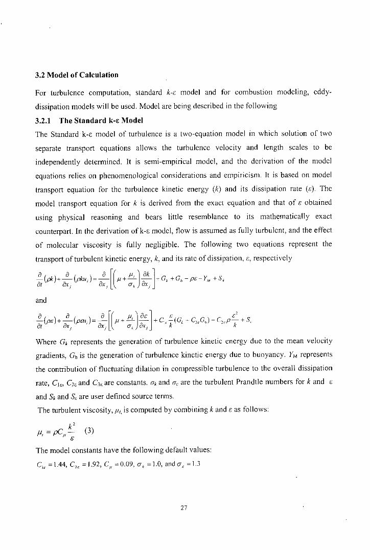
For turbulence computation, standard k-E: model and for combustion modeling, eddy-

dissipation models will be used. Model are being described in the following

3.2.1 The Standard k-l:Model

The Standard k-l: model of turbulence is a two-equation model in which solution of two

separate transport equations allows the turbulence velocity and length scales to be

independently determined. It is semi-empirical model, and the derivation of the model

equations relies on phenomenological considerations and empiricism, It is based on model

transport equation for the turbulence kinetic energy (k) and its dissipation rate (c). The

model transport equation for k is derived from the exact equation and that of E: obtained

using physical reasoning and bears little resemblance to its mathematically exact

counterpart. In the derivation ofk-E model, flow is assumed as fully turbulent, and the effect

of molecular viscosity is fully negligible. The following two equations represent the

transport of turbulent kinetic energy, k, and its rate of dissipation, E, respectively

~(pk)+~(pku, )~~[( Ii +~J 8k ]+G, +Gh - p£- YM +s,at aXj ax; l Uk ax)

and

Where Gk represents the generation of turbulence kinetic energy due to the mean velocity

gradients, Gb is the generation of turbulence kinetic energy due to buoyancy. YM represents

the contribution of fluctuating dilation in compressible turbulence to the overall dissipation

rate, Cleo C2e and C3c are constants. (Ik and (Ie are the turbulent Prandtle numbers for k and E

and Sk and S" are user defined source terms.

The turbulent viscosity, j.l,. is computed by combining k and c as follows:

k'fl, = pC" - (3)

[;

The model constants have the following default values:

C/, = 1.44, C" = 1.92, C'I = 0.09, (Yk = 1.0, and (Y" = 1.3

27

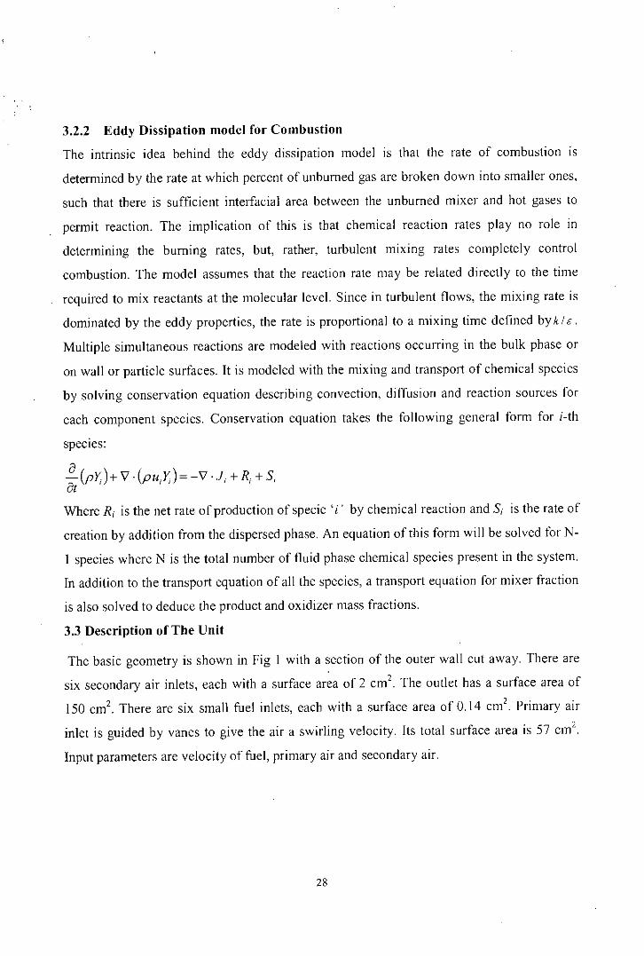
3.2.2 Eddy Dissipation model for Combustion

The intrinsic idea behind the eddy dissipation model is that the rate of combustion is

determined by the rate at which percent of unburned gas are broken down into smaller ones,

such that there is sufficient interfacial area between the unburned mixer and hot gases to

permit reaction. The implication of this is that chemical reaction rates play no role in

determining the burning rates, but, rather, turbulent mixing rates completely control

combustion. The model assumes that the reaction rate may be related directly to the time

required to mix reactants at the molecular level. Since in turbulent flows, the mixing rate is

dominated by the eddy properties, the rate is proportional to a mixing time defined by k IE.

Multiple simultaneous reactions are modeled with reactions occurring in the bulk phase or

on wall or particle surfaces. It is modeled with the mixing and transport of chemical species

by solving conservation equation describing convection, diffusion and reaction sources for

each component species. Conservation equation takes the following general form for i-th

species:

Where R; is the net rate of production of specie; i' by chemical reaction and S; is the rate of

creation by addition from the dispersed phase. An equation of this form will be solved for N-

I species where N is the total number of fluid phase chemical species present in the system.

In addition to the transport equation of all the species, a transport equation for mixer fraction

is also solved to deduce the product and oxidizer mass fractions.

3.3 Description of The Unit

The basic geometry is shown in Fig I with a section of the outer wall cut away. There are

six secondary air inlets, each with a surface area of 2 cm2 The outlet has a surface area of

ISO cm'. There are six small fuel inlets, each with a surface area of 0.14 cm2 Primary air

inlet is guided by vanes to give the air a swirling velocity. Its total surface area is 57 cm'.

Input parameters are velocity of fuel, primary air and secondary air.

28

)

I"r20 em

+10cm.!.

Ol"dletSurhilce are:a:150 cJ

<Eo-- CombustorRadius=11 .5 em

+-- Secondary Air Inlets (6)Surface area =2.0 crJ (each)

___ PrimM.,. Air Inlets (6)Tolal suface area=57 err(

Fig 1 : Model of the Can Combustor

3.4 Description ofthe Software

FLUENT version 6.122 has been used for modeling. It has been configured to run in

parallel network of personal computers, having Intel Pentium 4 (2.6 GHz) processors

running Windows 2000 server. The free Message Passing Interface (MPI) software called

MPICH from www-unix.mcs.anl.gov/mpilmpich will be used for cluster configuration. The

model of the Can Combustor has been built on the software Gambit 2.1.6.

Fig 3 .2(a) Discretised Model

29

Fig 3.2(b) Discretised Model

Chapter 4

4. Results and Discussion

4.1 Variation in Geometry of primary air inlet

Different parameters are varied to study the performances of the combustor. Effect of the

geometry of the primary air inlet on the performance of the Can combustor has been

investigated. Variation of geometry for primary air inlet produces different swirling pattern

in the combustor. Effects of swirl velocity on combustion process are investigated by

varying the pattern of rotation of the primary air inlet. Investigation has revealed significant

changes of the distribution of static temperature, NOx production. Angles of rotation that

has been used for the investigation are 30°, 45°, 60° and 90°. Fuel flow rate, flow rate of

primary air and secondary air for this investigation are 40 mis, 20 mls and 6 mlsrespectively. Predicted flow fields in the combustor are shown on figure 4.1(a), 4.1(b),

4.I(c) and 4.1 (d) for 30°, 45°, 60° and 90° respectively.

Velocity Vectors Col!Jred B.J'Velocitr Magnitude Im/SJep 06. 2004FLUENT 6, [3d. s"9reg3ted. speS, s~eJ

Fig 4.1(a) Velocity vector colored byvelocity magnitude at y=O for theangle of rotation of 30°

30

VelOl::ity Vectors Colored By Veloctty Magnitude Imfsgep DB, 2004~LUENT 6.1 (3d. segregated, spe5, skll'J

Fig 4.1(b) Velocity vector colored byvelocity magnitude at y=O for theangle of rotation of 45°

"j"'I'4. e. Iill:: tI.1"1'. 4e4 (

: 1:: I

I."'1'. C. I. " I.I'i: I:Ii::! I!:! ::iII. "1'I. e. 1

1:1 g; 1I: :: II: ::!s:! :;~i1:1~:H~" "I"l:4 e. at--xLIII:'- I

Velor;ity Veclors Colored By Yelodty Mognitude lm/sgep 06, 200.FLUENT 15.1 13Cl, segregated. spIt5,.ske

Fig 4.I(c) Velocity vector colored byvelocity magnitude at y=O for theangle of rotation of 60°

VelocIty Vectors Colored By velocltr N<lgn1tudeo tm/sgep 06. 2004FLUENT 6. [3d, segregate-c!. spe5. ske)

Fig 4.1 (d) Velocity vector colored byvelocity magnitude at y=0 for theangle of rotation of 90°

4.1.1 Effect of rotation of primary air inlet on the wall temperatnre

Figure 4.2(a), 4.2(b), 4.2(c) and 4.2(d) illustrate the contour of static temperature at y=O

plane for the rotation of primary air inlet of 30°, 45°, 60° and 90° respectively. Figures

show that wall temperature of the combustor decreases with the increase of the rotation of

the primary air inlet. Size and temperature of the flame in the combustor was also

influenced with the rotation of the primary air inlet. Flame size decreased with the increase

of angle of rotation. Heat transfer from the flame to the wall decreased as the flame size

decreased. So increasing the turbulence by increasing the angle of rotation decreases the

wall temperature. Table Al (in Appendix A) shows the variation of temperature of wall

with the variation of geometry of primary air inlet. The degree of turbulence generated by

the air swirling depends on the swirling angle and on the number of the air swirler. Because

these two factors directly affect the airflow pressure drop after the swirler and velocity

distribution.

31

Fig 4.2(a) Contour of statictemperature at the plane y=0 for theangle of rotation 30°

Fig 4.2(b) Contour of statictemperature at the plane y=O for theangle of rotation 45°

i, ,',I,

'j\\B G

'~

\ ":":,' 'I' I'( • I

Fig 4.2( c) Contour of statictemperature at the plane y=O for theangle of rotation 60°

Fig 4.2(d) Contour of statictemperature at the plane y=0 for theangle of rotation 90°

32

With high swirl, rapid mixing between fuel and air is achieved. It increases the rate of

firing. At higher swirl above 30° the flame length decreases, so does heat transfer to tube

wall. At 30° and 45°, the flame length is found to be wider compare to the flame produced

at 600and 90°. The reason is that mixing of air and fuel is not complete for 30° and 45°, and

unfavorable regions of high fuel ratio exist where unreacted combustible mixture formed.

Figure 4.I(a), 4.1(b), 4.1(c) and 4.1(d) illustrate that swirl creates a recirculation zone

specially at high swirl intensities, which acts as a mixing zone between the two streams. Fig

4.1(d) shows that rapid mixing between fuel and air is achieved at high swirl. It increases

the rate of firing. Increasing the swirl results better burning due to the speeded reaction

process. At 60° and 90°, rapid mixing leads to short and efficient flame and higher

combustion efficiencies. So investigation showed that increasing the turbulence of the

primary air inlet, wall temperature could be reduced with higher combustion efficiency.

4.1.2 Concentration of Methane in the combustor

Contour of the concentration of methane is shown on Fig 4.3(a), 4.3(b), 4.3(c) and 4.3(d)

for the rotation of primary air inlet of 30°, 45°, 60° and 90° respectively. Methane burnt

completely in after entering in the combustor for the rotation of 60° and 90°. Fig 4.3(c) and

4.3(d) show that there is a rapid mixing between air and fuel, which facilitated better

burning for the rotation of 60° and 90°. Fig 4.3(a) and 4.3(b) show that methane burnt

comparatively upper part of the combustor because of relatively poor mixing between air

methane. So, at high flow rate of fuel, unburnt methane could go out the exhaust gas, which

would pollute the air. So, high intensity of turbulence by increasing the angle of rotation for

primary air inlet.

33

Contours or Mass fraction of cM Sep Ofi. 2004FLUENT6.1 l3d. segregated, spe5. skeJ

Fig 4.3 (a) Contour of the massfraction of methane at the plane Y=Ofor the angle of rotation 30°

CQf1tours of Mass fraction of ch<4 S"'p 06. 2004FLUENT 6.1 (3d, segregated. speS. eke]

Fig 4.3(b) Contour of the massfraction of methane at the plane Y=Ofor the angle of rotation 45°

j:nm:1 ::~ I

I-I'-i1': g:H-1'-i1J r:~1!:jl 1=1!

I'::::. c- I- ,- I- ,-~1~~ll:mmt-x

UIGe~IO

1-11'- I. e- I. c- I

~- 1

:1 ~:~I:11::81-1!::H

IJim,5.i e~ I'-j ,- ,4. c- I4. e-l:m: I

!:1m I'-'1'- I'-j ,- ,I:! :: I1:!I:: !Ui:J.t-,U.UUe~~'o

Contours of Mass fraction of cM Sep 06. 200<4FLUENT 6.1 !'3d. lill'grll'>lOlt",d .• p"'5. "kll'J

iFig 4.3 (c) Contour of the massfraction of methane at the plane Y=Ofur the angle of rotation 60°

Contours of Mass fraction of eM Sep 06. 2004FLUENT 6.1 (3d, segregated, spe5. ske)

Fig 4.3(d) Contour of the massfraction of methane at the plane Y=Ofur the angle of rotation 90°

34

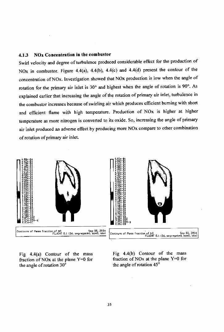
4.1.3 NOx Concentration in the combustorSwirl velocity and degree of turbulence produced considerable effect for the production of

NOx in combustor. Figure 4.4(a), 4.4(b), 4.4(c) and 4.4(d) present the contour of the

concentration ofNOx. Investigation showed that NOx production is low when the angle of

rotation for the primary air inlet is 30° and highest when the angle of rotation is 90°. As

explained earlier that increasing the angle of the rotation of primary air inlet, turbulence in

the combustor increases because of swirling air which produces efficient burning with short

and efficient flame with high temperature. Production of NOx is higher at higher

temperature as more nitrogen is converted to its oxide. So, increasing the angle of primary

air inlet produced an adverse effect by producing more NOx compare to other combination

of rotation of primary air inlet.

Contours of Mass fraction of NO Sep 06, 2004FLUENT 6.1 [3d. segregated. speS. skeJ

Fig 4.4(a) Contour of the massfraction of NOx at the plane Y=O forthe angle of rotation 30°

Contours of Mass fraction of NO Sep 06. 2004FLUENT6.1 [3d, segregated, spe5, skeJ

Fig 4.4(b) Contour of the massfraction of NOx at the plane Y=O forthe angle of rotation 45°

35

~.5Ge 04I.II'-i'I:~:ol. le-04."'-1'7 e- ~,:,1.- ,

:U!i~lil-1"-04t~5e-04d!~:il'.59.-04i:.30e-04Hl~:ill:1l;:ilHl~:ill.lj~:U1.72'-1'L43e- 4

U!~:ll:il~:isl-xo. Oe~OO

L07e 03

l:!l~:U!:!i~:il

I l:i\~:U

[lm!j!:!irll5.76.- ,5.He- "5.12.-04•. BOe-O.U8'-I'•• L6e- "l:!i~-1HI!:ilH••-I,i:!ti~:ll!:ll~:l!:li~:ll-xO.OOe .• OO

Contours of Mass fraction of NO 5ep ~6, 200FLUENT6.1 (3d, segregated, spe5. skI

Fig 4.4(c) Contour of the massfraction ofNOx at the plane y=o forthe angle of rotation 60°

Contours of Mass fraction of NO 5ep 06, 200-4FLUENT 6.1 [3d. segregated, spe5. skeJ

Fig 4.4(d) Contour of the massfraction of NOx at the plane Y=O forthe angle of rotation 90°

4.1.4 C02 Concentration in the combustorFigure 4.5(a), 4.5(b), 4.5(c) and 4.5(d) show the contour of mass fraction of CO2 at y=0

plane. These figures show that production of C02 in the combustor follows almost the

identical pattern as the flame size, which means that efficient burning occurs in a

comparatively short film size.

36

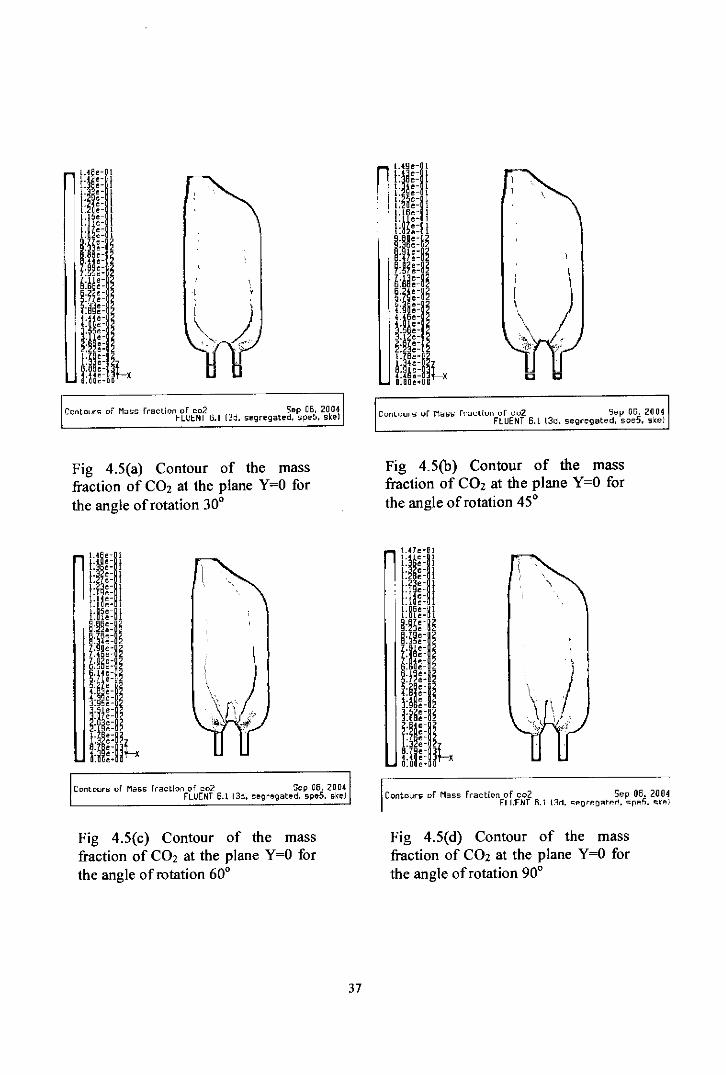
Contours of Mass fraction of co2 Sap 06, 2004I-LUI;NI 0.1 [::ld. segregated. speto. skel

Fig 4.5(a) Contour of the massfraction of C02 at the plane y=o forthe angle of rotation 30°

CIJlllvul'\;. vf -Ni::l\:>\:> fl-i::lo.:l!Ull I,)f 0.:1,)2 51:f' 00, 2004FLUENT6. L l3d. segregated, spe5. skel

Fig 4.5(b) Contour of the massfraction of C02 at the plane Y=O forthe angle of rotation 45°

Contours of Mass fraclion of co2 Sep OB, 2004FLUENT 6.1 (3d. segregated. spe5. skeJ

Fig 4.5(c) Contour of the massfraction of C02 at the plane Y=O forthe angle of rotation 60°

37

Contours of Mass fraction of co2 Sep 06. 2004FIIIFNT R.l l:lrl. c;f!orf!o~tf'!r1. <::pf'!li. <::Kf'!)

Fig 4.5(d) Contour of the massfraction of C02 at the plane Y=O forthe angle of rotation 90°

4.2 Influence of excess air on can combustor

Excess air in the combustor affects the wall temperature and the performance of the

combustor considerably. Excess air in the combustor also influences the efficiency of

burning in combustor. To study the effect of excess air, 50%, 75%,100% and 125% excess

air were used to monitor the performance.

4.2.1 Effect of excess air on the wall temperature

Figure 4.6(a), 4.6(b), 4.6(c) and 4.6(d) represent the contour of static temperature at y=o

plane for 50%, 75%, 100% and 125% of excess air respectively which show the influence

of excess air in the Can combustor. Fuel flow rate used for this investigation is 40 m/s.

Figures reveal that temperature distribution and flame size in the combustion zone have

been changed with the increase of volume of excess air. Distribution of heat changes with

the increase of volume of excess air. At higher volume of air, flame size decreases due to

the presence of higher volume of excess air with high velocity. This played a significant

ro Ie to reduce the wall temperature as figures showed that wall temperature decreases with

the increase of excess air. Heat transfer by radiation from the flame to the wall depends on

the flame size. So higher volume of excess air reduces heat transfer from the flame to the

wall. Concentration of gas near the wall was higher at higher volume of excess air, which

in tum produces lower wall temperature. Table A2 (in Appendix A) shows the wall

temperature for each investigation. Investigation shows that range of wall temperature was

777 - 1217 °c for 50% excess air and the same for 100% and 125% excess air were 646-

1137 °c and 576-757 °c respectively. So increase of excess air improves the burning of gas

in combustor as well as reduces the wall temperature significantly, which is an important

improvement for designing a combustor.

38

r",I

"

tOl1tOu'"'; of ~t;Hic Te-llpet~h..•"e It I 'Sep DB.. 20D(FlLEflT fI.1 l3d, "~'9r~;;;t(-d..;,pe-5. g;~J

Fig 4.6(a): Contours of Static Temperatureat the plane y=0 when 50% Excess air isused

tontol,:,-Ii of 9:~ticTl!'I1P't"';;lIlufl! u:' Sep Oil 2Dil,(rLUI:iJ.lT 11.1 I~l!.ce!)"'~9.:r.[<,j. o;.r~£ic c•.•..,

Fig 4.6(b): Contours of Static Temperatureat the plane y=O when 75% Excess air is used

Ui;:I''1.1 , •. "• ~ I t::i

"~'.'II. e'I, ,.I:~;;IL. eoL. ,.l. (!.I. f:.

f:~'E.nL ;:11L '.1./' ,.n ljli1'1" !I, r 1:1!..

I, R.' (:. ~I S. I!!:'! t. t& .•

't ,dk-r.URt.l;! .

l:ontC1.lflr of St;lllo Te-npel";,tufl!' U.:I 5~p06. 21]011FwWT 6.1 l2d. ,;~re9;'Ie-d. ;pf!5, .•~oe~

Fig 4.6(c): Contours of Static Temperature atthe plane y=0 when 100% Excess air is used

39

CO:!"llO"'.H~ of St:atl~ T~l1per •• t..".elie), Sep 0&. 2DGcFLu:Etl~ B.'I l,::id. Soegrt:gated. "F'es.~ 5ikeJ

Fig 4.6(d): Contours of Static Temperatureat the plane y=O when 125% Excess air isused

4.2.2 Concentration Methane in the combustor

Figure 4.7(a), 4.7(b), 4.7(c) and 4.7(d) show the contour of methane for 50%, 75%,100%

and 125% excess air in the combustor respectively. Fig 4.7(a) shows presence of methane

up to the outlet, which depicted the comparatively inefficient burning. So unburnt

hydrocarbon comes out with the exhaust if flow rate of fuel is increased. It reveals that

burning of methane is not completed at 50% excess air. But for 125% excess air, methane

was burnt completely in the flame. So higher volume of excess air ensures both the low

wall temperature and complete burning ..

I.DO~'OO:II::!i1:11::11.4 e- I•t c- I

!:Ii;: Ij:!i::il:li;:I'I:!!::1.4 c- I

':1'1;:114. e- Ii. e- IJ. e- I

umi1.!1'-I'I. e- I. ,-I!o!!~il~x

Clmtours of Mass' fraction of ch4 S"P 05. 2004FI lJFNT6. j f3d. "egregRted spe5. j;kel

Fig 4.7(a) Contour of the mass fractionof methane at the plane y=0 when 50%Excess air is used

40

Contours I;lf Mass fraction of ch4 , Sep 06, 2004FLUENT 6.1 [3d. score-gated. spe5. skel

Fig 4.7(b) Contour of the mass fractionof methane at the plane y=0 when 75%Excess air is used

Contours' of Mass fraction of ctl4 Sep 06, 2004FLUENT6.1 (3d, segrlt9ated, speS, ske)

Fig 4.7(c) Contour of the mass fractionof methane at the plane y=O when100% Excess air is used

Contours of Mass fraction of ctl4 Sep 06, 2004FLUENT6.1 (3d, segregated. speS, skel

Fig 4.7(d) Contour of the mass fractionof methane at the plane y=O when 125%Excess air is used

4.2.3 Production of NOx

Contour of NOx in combustor for the variation of excess air is shown on figure 4.8(a),

4.8(b), 4.8(c) and 4.8(d). Investigation showed that the production of NOx is influenced by

the volume of excess air significantly. Figure 4.8(a) showed that NOx production was

higher at 50% excess air and it was dispersed near the wall. The reason may be attributed to

the inefficient burning. NOx production is comparatively low for 75% and 100% excess air.

But increased again for 125% excess air. So increasing the excess air after a certain level,

NOx production increased. Figure 4.8(a), 4.8(b), 4.8(c) and 4.8(d) showed that changes in

pattern ofthe production of NOx and concentrated in the center of the downstream. So this

investigation revealed that controlling of the production of NOx is dependent on the

volume of excess air.

41

Contours of Mass fraction of NO Sop 06. 2004FLUENT 6.1 (3d. segregated. spe5. skel

Fig 4.8(a) Contour of the mass fractionof NOx at the plane y=0 when 50%Excess air is used

Contours of Mass fraetlon of NO Sep 06. 2004FLUENT6.1 (3d. segregated. speS. skeJ

Fig 4.8(b) Contour of the mass fractionof NOx at the plane y=0 when 75%Excess air is used

t.2Sc-03L.2n.-OJL.l6e-03i:!l;:iJLI"-iJ!:II1:~:8:!~:~l!:m:11U'd'7.LOe-O~

1:ll1:81f l'-~'4:~~:!l4.4 ~- 44.lie- 4

Hlri1j:!l::!:,:ll::lld e- 4t.1 e- 4~

!:I!::lll-,O.OOe~OO

Contours of Mass fraction of NO Sep 06. 2004FLUENT 6.1 13d. segregated. speS. skeJ

Fig 4.8(c) Contour of the mass fraction ofNOx at the plane y=O when 100% Excess airis used

42

Contours of Mass fraction of NO Sep 06. 2004FLUENT6.1 (3d. segregated. spe5. skeJ

Fig 4.8(d) Contour of the mass fractionof NOx at the plane y=0 when 125%Excess air is used

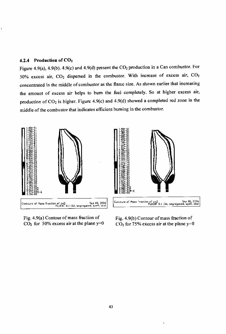
4.2.4 Production of C02Figure 4.9(a), 4.9(b). 4.9(c) and 4.9(d) present the C02 production in a Can combustor. For

50% excess air, C02 dispersed in the combustor. With increase of excess air, C02

concentrated in the middle of combustor as the flame size. As shown earlier that increasing

the amount of excess air helps to bum the fuel completely. So at higher excess air,

production of C02 is higher. Figure 4.9(c) and 4.9(d) showed a completed red zone in the

middle ofthe combustor that indicates efficient burning in the combustor.

Contours of Mass fraction of co2 Sep 06, 2004FLUENT 6.1 [3d ••••.• 9f""901t •.•d. IOp",5 ••• 1<:•.•)

Fig. 4.9(a) Contourofrnass fraction ofC02 for 50% excess air at the plane y=0

43

Contours of Mass fraction of co2 Sep 06. 2004FLUENT6.1 ~3d, segregated. spe5, skel

Fig. 4.9(b) Contour of mass fraction ofC02 for 75% excess air at the plane y=0

l.41e- t1:'),: I

Ll!'- L1. c~ l1. e- I1.1 e- l

1:1 ;: I1. c- L. 1'-. ,-. ,-:l}':li~:i,,-:}I":

i:1 !~1:!11~ l-x

Contours of Mass Fraction of co2 Sep 06, 2004FLUENT B.t (3d, segregated, spe5. skeJ

Fig.4.9(c) Contour of mass fractionof C02 for 100% excess air

COrltcufS of Mass fractIon of co2 Sep 06. 2004FLUENT6.1 l3d. segregated, spe5. skeJ

Fig. 4.9(d) Contour of mass fractionof C02 for 125% excess air

4.3 Effect of Secondary AirThe problem of wall heating of the gas turbine combustion chamber is of special

importance since the flame tube measured in thousand of hours. Maximum life of the

combustor cannot be expected unless the design material temperature is limited to a

maximum value. The wall heating depends on some factors like total heat transfer from

flame to the wall, construction of the flame tube and flow of air in the combustor. In this

case, a secondary air inlet in the wall of combustor will be used with view to reduce the

wall temperature. A part of the total air will be flown thorough this path. Figure 4.10(a)

presents the flow field in the Can Combustor without secondary air inlet and 4.10(b)

presents same with secondary air inlet.

44

o!~!~I. e' t

!l!l iq~:l!o! ,. ,I. e' I

i I';: i1. e' IU f' IL3 e' Ilit!'d,.!t"l!:l L-,l.~e- I

Fig 4.10(a) Velocity vector colored byvelocity magnitude at x=O, whensecondary air is off

Fig 4.10(b) Velocity vector colored byvelocity magnitude at x=O withsecondary air.

4.3.1 Effect ofsecondary air on wall temperature

Figure 4.11 (a) shows contour of static temperature at y=0 plane in the combustor when

secondary air is not used and 4.11 (b) presents the contour of static temperature when

secondary air is used. Both the investigation was carried out for 100% excess air with 60°

rotation in the primary air inlet. Figure 4.11 (a) illustrates the combustor as a red zone,

which reveals rate of heat transfer from flame to the wall is very high as wall temperature

attains very high values. Figure 4.11 (b) shows that heat transfer from the flame to the wall

is reduced gradually. It is found from figure 4.11(a) and 4.II(b) that the absence of

secondary air increased the wall temperature drastically. Temperature of the combustor

wall is changed to a great extent compare to the case with the presence of secondary air.

Table A3 [in appendix A] shows the ranges of wall temperature for both the absence and

presence of air. Wall temperature varies from 1057 °c to 1787°C when there is no

secondary air. On the other hand, range of wall temperature was found to be 646°C -113 7°C

when secondary air is used. This is happened because secondary air reduces flame size.

Figure 4.12(a) and 4.12(b) shows that secondary air impedes the flame to be dispersed

outward thereby impede heat to spread toward the wall as it flows thorough near the wall.

45

Secondary air also facilitates the unbumt hydrocarbon to bum completely. So this

investigation showed that secondary air is an important consideration for designing a Can

combustor as introduction of secondary air in combustor through the wall of combustor

reduces wall temperature significantly.

CotItOU't of 'i18tiC Tellpetllrl.tt III

Fig 4.1 I (a) Contours of StaticTemperature at the plane y=O, whensecondary air is off

Fig 4. 11(b) Contours of StaticTemperature at the plane y=O withsecondary Air

Fig 4.12(a) Velocity vector colored byStatic Temperature at the plane y=O,when secondary air is off

46

Velocity Vectors Colored B3 Static Temperature (kJ 5ep 06, 2004FLUENT6.1 13d. segregated. speS. ske)

Fig 4.l2(b) Velocity vector colored byStatic Temperature at the plane y=O withsecondary Air

4.3.2 Methane in the combustorFig 4.13(a) and 4.13(b) present the contour of the mass fraction ofCH4 Fig 4.1 3(a) showed

that very small fraction of CH4 goes out with exhaust. Though this volume is rather

insignificant. But at high scale, this could be higher which is a source of pollution. The,

velocity of fuel is high as a result a small fraction of fuel may not react with the oxygen of

primary air. But introduction of secondary air through the wall [in fig 4.13(b)] ensures

relatively complete burning of unreacted methane.

COI\10U'9 of naS! 1rsolion of eM Contours of Mass fraotlon of eM Sep (16,2004FLUENT 6.1 (3d, segregated. sp"S. s\;eJ

Fig 4.13(a) Contours of mass fraction ofmethane at the plane y=O, whensecondary air is off

Fig 4.13(b) Contours of Contours ofmass fraction of methane at the planey=Owith secondary Air

4.3.3 Production of C02

Figure 4.14(a) shows the contour of C02 at y=O when secondary air is off and 4.14(b)

presents it when secondary air is used. As absence of secondary air produces inefficient

burning, it should produce less carbon dioxide compare to the presence of secondary air

because ofits role to bum fuel more efficiently.

47

1~1l:Il-lli:I~t:-1

111~11.':I. 1::!,-

11~11jj:1!!:I1l:ll

~pL1:lP..llIeo 13., 2114. r.'ont(luro; 1)( NOlI,,'!: fr ••ctlon "r 0:-,,2 5!!>p 06. 2004

fU(NT 6.1I3d.l~eg~ta.~. ael FLUENT6.1 [3d. segregated. speS. steJ

Fig 4.14(a) Contours of mass fraction ofCO2 at the plane y=O, when secondaryair is off

Fig 4.l4(b) Contours of Contours ofmass fraction of C02 at the plane y=Owith secondary Air

4.3.4 NOx ProductionFig 4.1 5(a) and 4.l5(b) presents contour of NOx in the combustor. Figure 4.15(a) shows

that absence of secondary produces more NOx compare to the presence of secondary air.

Absence of secondary air produced more NOx near the wall according to the fig 4.15(a)

and 4.l5(b) because of higher Temperature near the wall and inefficient burning. Usually

nitrogen is converted to its oxide to a great extent at higher temperature. Fig 4.15(b)

showed the evidence of less production of NOx in the combustor because secondary air in

the combustor facilitates efficient burning and reduces the temperature near wall drastically

as stated earlier.

48

B.laKlS...,..,.••••••••••••••5.1tt"GS•••••••••••••••••

! i.drill

'~i..,..,.ai3MI3!LIHS••••••••••••••2.45rQ9.-0'••••••••LJlriS1.41t-113

••••••••."....,.•...•.•.•••.••l1.45ti1t h•..•..•,

Ic.,,,.,,, •. ""'" ,•••••• ofOJ

""0-11UiTg:I. c-d i:l,9.51'. ,9./ ,. ,

'hml1:I!g:~1:~~:~t:i~.ill:lSg:il"1°0-1'4. 3c- "Big: Il:!!g:ilH\~:il

. , Umilt-.,o.ooe+~~

FUbTB.i.Il'id.IIII"'~"~ Contours of Mass fraction or NO Sep 06, 20114~ FLUENT 6.1 (3d, SCl,lrCQaled. speS, 5tel

Fig 4.15(a) Contours of mass fraction ofNOx at the plane y=O, when secondaryair is off

Fig 4.15(b) Contours of Contours ofmass fraction of NOx at the plane y=0with secondary Air

4.4 Secondary air inlet at different position

Injection of secondary air at different position of the wall produces variation in

performance of a Can combustor in terms of wall temperature, burning of fuel and NOx

production. That is why; secondary air is introduced in different position to investigate its

effect. Position of secondary air inlet in fig 3.1 is considered as the reference (point I) in

which its position is located 30cm above the bottom of the combustor. Positions of

secondary air are varied by shifting the position of secondary air inlet upward or downward

from the reference. Investigations were carried out for 100% excess air with 60° rotation in

the primary air inlet.

4.4.1 Secondary air inlet below the reference pointSecondary air inlet is introduced at 20 em above the,bottom of the combustor (point 2) of

secondary air. Fig 4.16(a) and 4.16(b) shows the contour velocity vector with secondary air

inlet for two different points. Following effects were investigated:

49

Fig 4.16(a) Velocity vector for thesecondary air at point 2

"'!"I'"j ,. ,1. ",. c~ 1

j:gg!;li'1'" ,: 4~:I'11"11. ,.. C. 1. e. I~.4 c. 1

Plgil,I." I1.71" ,1.5 C. J

U g: I

1':11111

1:!iI11ILrVeioclty Vectors Colored B-1VelocIty MagnItude Im/iJep" 06. 2004

~LlIENT B.I {3d .. segregated. spe5. sloe}

Fig 4.l6(b) Velocity vector for thesecondary at point I

4.4.1.1 Wall temperatureFig 4.l7(a) and 4.l7(b) show contour of static temperature at y=O and x=O respectively for

the injection of secondary air at point 2. 4.18(a) and 4.18(b) show the same for secondary

air at reference point (point I). The fig 4.17(a) and 4.17(b) depict that flame in the

combustor gradually dispersed towards the wall and wall temperature is higher compare to

the fig 4.18(a) and fig 4.18(b). Table AA [in Appendix A] presents the comparison of wall

temperature in the combustor for the variation of the position of secondary air inlet. The

range of wall temperature is found to be 646-1137 °c when secondary air is applied at point

I. The wall temperature is found as 827-1237 °c when secondary is applied at point 2.

These results show the difference in wall temperature of wall temperature for the changes

in the position of secondary air inlet. Fig 4.16(a) shows that fuel and secondary air

interacts better compare to other cases. So for this case, flow rate needs to be increased for

the reduction of wall temperature.

50

Cfl/ltOtR of 5llJUO Terprifllf'e nJ

"!

i ::

! I j'\ !

\ i>?, oj

LI ,:. :I ,:I ~:I •.I. .:...I' .:

,, I

Fig 4.17(a) Contour of static temperatureat the plane y=O for secondary air atpoint 2

Fig 4.l7(b) Contour of static temperatureat the plane x=O for secondary air atpoint 2

'f"'1 !:!l!~li'.n!:I 1:

If II "If III. e~I' 0"

,I "1Iii

. ,.i l. ~. . ,.: f: ~: 1. e~

1. e~1 '"hlg;I. "1u~:

J I:r J'rl( e' l. e" I "U ,: l. e.•l. ,H

1J'~:1 r;~g

~i: \\. ,.

. "Ii F\1 1: I v!~5. ~. 0L e' -:\:~,: .1-, ~. C" L,oJ I ,.l.Ut-oil! •• : ~~:

Fig 4. I8(a) Contour of static temperatureat the plane y=O for secondary air atpoint I

51

ContDurs or !ltlltic: T"mpcrllturc UJ !lcp oa. 2001:FLU£NT 6.1 (3d. segregated, 5Pc5. ~keJ

Fig 4.18(b) Contour of static temperatureat the plane x=O for secondary air atpoint 1

4.4.1.2 Concentration of MethaneFig 4.19 shows the contour of the concentration of methane when secondary air is

introduced at point 2. Figure shows that methane is burnt well as almost no methane go out

with exhaust. It proves that methane mixes well with air at this position of secondary air.

HI1:=I'-I,-'"::i'-I"I:' I. := 1,-,-".\J Ifllil~lh

Fig 4.19 Contour of mass fraction ofMethane at y=0 for secondary air at point 2.

4.4.1.3 NOx productionFig 4.20(a) and fig 4.20(b) present the contour of NOx for secondary air below the

reference position and secondary at the reference position. Fig 4.20(a) shows that NOx

production is higher at upper part of the combustor for secondary air below the reference

position. As shown earlier that secondary air at this position produces higher temperature in

the upper part of the combustor as a result production of NOx is higher.

52

Fig 4.20(a) Contour of the mass fractionof NOx at the plane y=0 for secondaryair at point 2.

Contours of Mass fraotlon of NO Sep DB. 2004FI UFNT fl. 1 f::ld. !':egregRted. !':pe5. l'll:"el

Fig 4.20(b) Contour of the mass fractionof NOx at the plane y=O for secondaryair at point I.

4.4.2 Secondary air at three places

Secondary air is used in three different places to investigate the effect. Figure 4.21 shows

the position of three secondary air inlets. Three places are (i) 20 cm above the bottom of the

combustor (ii) 30 cm above the bottom of the combustor and (iii) 40 cm above the bottom

of the combustor. Investigation was carried out to monitor the changes of wall temperature,

burning of methane, NOx production. Investigation was carried out for 100% excess air

with 60° rotation in the primary air inlet.

Secotldety AirInlot

Fig 4.21 secondary air is introduced at threedifferent position at the plane x=O.

53

4.4.2.1 Wall temperatureFigure 4.22(a) and 4.22(b) present the contour of static temperature at the plane y=0 and

x=O respectively. Figures show that flame size become less wide and temperature near wall

decreased. Specially, temperature near the wall in the bottom half of the combustor

decreased significantly. In this region, temperature varies from 60 1°C_I077°C (shown in

Table A5 in Appendix I) and this distribution is found in more than half of the area of the

wall. Compare to the other combinations of secondary air inlet, this produces a significant

improvement. But at upper part of the combustor, temperature near the wall is higher. This

could also be improved by increasing the flow rate of air through the upper most secondary

air inlet. It also ensures the better burning as flame temperature is found to be 1937°C. So

introduction of secondary air in three different positions yield better temperature

distribution near the wall because flame size is made less wide by secondary air with

efficient burning. That is why transfer of heat towards the wall is less.

'UH~"to'2.l'~e.•1!3€.f.z~.•c"u.i))& .•[I), ~.5]e;ll]

) i.TJa"03

Ik~e.£l3

, M1i!HIJ, iAo!ie.f1~.":'»c"CJa.26eTD'._'•••••.n~i.lTe .•D39S1e.D2&.n •.•Dl".ra.~.f12:6.&JfJ."ozU1& .•Q2"-91e<'n~U15e.ll~h3.Ue .•Dl

2.2t •• 13l-l zc..t1J2.1~.[I]t.9~nlI""~O'~-l.T:Je. [I]" 1.8•.~D3J t.5i:'Co .• t.JlAfe' tlt,;]:wr:!1,260.Uh~Qlf(l]1.170'"['3M!Jt."('2o..rte.(l21.7e..-D2M3t"~2~re.D2t.9le--f;?,Mk"~zl:- .:Llle.cP

Fig 4.22(a): Contour of secondary air atthe plane y=O for three secondary airinlet

54

Fig 4.22(b): Contour of secondary air atthe plane x=O for three secondary airinlet

4.4.2.2 Concentration of Methane in the combustorFig 4.23 shows the concentration of Methane in the combustor. Figure show that all the

methane is burnt in the combustor and no methane goes out with exhaust. Secondary air in

three different positions ensures the mixing of the entire unburnt hydrocarbon with air that

leads to the complete burning of methane in the combustor. So introduction of secondary

air in different position together improves the burning ofthe fuel.

1.000 •.00!lbDc-Ul!lOla-III&.5lc-1i&.Dlc.-II7.5lrllT.Uh':'OlI3.5De-U13.010-01"5.608-11SoUDe':"14.500-114.DIa-1l3.5lc-ll

"1/ 3.BDc-ll2.6!edi2.0na-1I1.<60&-11~.BlIo-U!1,5.Dlc-I~XD.DDc •.aO .

Fig 4.23 Contour of mass fraction of methane for threesecondary air inlets.

4.4.2.3 Production of NOxFig 4.24 presents the production of NOx in the combustor. Figure shows that production

pattern of NOx is reasonably good. Introduction of secondary air at three different places

controls the temperature in the combustor very well which in turn produces NOx

reasonably because production of NOx is dependent on the temperature in the combustor.

Low temperature near the wall along with the better burning of fuel ensures the efficient

performance of the combustor.

55

5.Z0tr03".!Mo-OJ-".6&&-oi'.'2c-0]

.'~16e-033.90e-033.13-4'&-033.36&-033.12~032.86e-032.600-032.:Mo-OJ2.08&-031.&20-031.58~031.300-031.140-031.&00-0'

6.20&""04;h. .2.S0a-041.390-2

C"0Il10U"IJof MR. frsollon of NO _ -'SI:P_D~,.20 05. .' FLuENT 6.1 (3a., ~e=oatecl. IJpcQ. sal

Fig 4.24 Contour of mass fraction of NO X at the plane

x=O for three secondary air inlets.

4.4.3 Secondary air in two more positionSecondary air is applied in two different positions separately to investigate the effect.

Positions of the two secondary air inlets are 40 em and 45 em above the bottom of the

combustor. Figure 4.25 and 426 illustrate the contour of the static temperature for both. It

is found from the figure the temperature near the wall is higher for both cases compare to

the other combination of secondary air inlet. Temperature near the wall in the bottom half

of the combustor is lot higher. This investigation shows secondary air inlet at in this region

does not contribute to improve the efficiency of the combustor by reducing the wall

temperature.

56

2.21e"13

Fig 4.25 Contour of static temperature at theplane x=O for secondary air inlet point 3 atx=O

ContOU'1lor lJtalto Teftpet3tuf'e (k) ,'3ep 24. 2D15I'LUI:NT ".1 (3a •.segreg:lJ1ea, Ilpeo. !like)

Fig 4.26 Contour of static temperature at theplane x=O for secondary air inlet point 4 atx=O

4.5 Radiation off and onThis study was carried to observe the effect of radiation heat transfer on wall temperature.

The total heat transfer from the flame to the combustion zone wall consists of two parts,

one is heat transfer by radiation and other is heat transfer by convection. Absence of

radiation heat transfer will ensure that heat will transfer toward the wall by only

convection. Investigation was conducted for 100% excess air and 60° rotation of primary

air inlet.

4.5.1 Wall TemperatureFig 4.27(a) and 4.27(b) present the contour of static temperature for radiation Off and On

respectively. Fig 4.27(a) shows that wall temperature of the combustor decreased

drastically when radiation is off. Table A6 [in Appendix A] shows the wall temperature for

both ,"ondition of radiation Off and On, which reveals the wide difference of wall

temperature. This shows that bulk of the heat transfers from the flame to the wall by

radiation. When the radiation is offheat is transferred to the wall by the internal convection

and turbulent dissipation.

57

Contour~ of St~tic Tompcrllturc (k) Scp 06. 2004FLUENT 6.1 (3d. segregated. spe5. skeJ

Fig 4.27(a) Contours of Static Temperatureat the plane y=O for Radiation Off

Fig 4.27(b) Contours of StaticTemperature at the plane y=O forRadiation On

Contours of Mass fraction of NO Sep 06, 2004FLUENT 6.1 (3d. segregated. spe5. sl:el

Fig 4.28(a) Contour of mass fraction ofNOx for Radiation Off

58

Contours of Mass fraction Qf NO Sep 06. 2004FLUENT B.L (3d. segregated. spe5. skeJ

Fig 4.28(b) Contour of mass fraction ofNOx for Radiation On

4.5.2 NOx productionFig 4.28(a) and 4.28(b) show contour of NOx for radiation off and radiation on

respectively. The production of NOx showed almost identical pattern. NOx concentration is

bit higher when radiation is on. This happens because of higher temperature through out the

combustor, as energy dissipation is higher for radiation to be on. The rate of conversion of

nitrogen to its oxide is higher at high temperature.

4.6 Reaction stepsThis investigation was carried out by altering the reaction steps. Fluent provides two ways

for modeling a combustor. They are (i) Two steps (ii) Single steps. Performance of the

combustor was monitor for both type of reaction. All the investigations were carried on

using secondary air and 100%excess air. Fig 4.29(a) and 4.29(b) represent the contour of

static temperature for two steps and single step reaction respectively. Two steps reaction

produced highest flame temperature of2087° C while single step reaction produced highest

flame temperature of2057 °c. But single step reaction produced almost a uniform flame in

the combustor while, for two steps reaction, temperature varied from 1887° C to 2087° C.

Wall temperature for two steps reaction varied from 645°C to 1207 °C. Single step

produced wall temperature between 636°C to 1187 °C. But average temperature near the

wall is lower for single step reaction compare to two steps reaction.

Fig 4.30(a) and 4.30(b) showed the contour of NOx and showed the comparison between

the two steps and single step reaction. Single step reaction produced more NOx in the

combustor compare to two steps reaction.

59

f.,'I

I.ilII III

ContOl"lrs of Statlc Temperature (kJ Sep DB. 2004FLUENT6.1 (3d, segregated, speS. ske)

Fig 4.29(a) Contour of static temperatureat the plane y=O for two step reaction.

Contours of StaUc Temperature lkl Sep 06. 2004FlUENT 6. [ (3d. segregated. spe5. ste!

.Fig 4.29(b) Contour of static temperatureat the plane y=O for single step reaction.

L.22'-~l1:1l~:ujI:!i~:ilI:iig:~l.:liBl:l~l1

':1' g: 1. e-.. e- i,- ,: ~:il

l:!ll~I"i ,- ·t. ,-.. ,- 1: ~: 4,- .d g: l

nil~l~xContours of Mass fraction of NO Sep DB, 21104

FLUENT 6.1 (3d. segrE!gated. speS, sl::eJ

Fig 4.30(a) Contour of mass fraction ofNOx at the plane y=O for two stepsreaction.

60

Contours of Mess fraction of NO Sep DB, 2004FLUENT6.1 (3d. segregated. speS. ste)

Fig 4.30(b) Contour of mass fraction ofNOx at the plane y=O for single stepreaction.

4.7 Heat CapacityEffect of heat capacity was investigated by using constant Cp of the element and Cp as the

function of temperature (piecewise polynomial) using following equation

cp(T) = AI + A2T + A3T3 + ...

Fig 4.31 (a) and 4.31 (b) shows the contour of static temperature for constant Cp and Cp as

function of temperature (piecewise polynomial). Figures illustrate that constant Cp doesn't

produce better figure, which is necessary for analysis. Cp as the function of temperature

produces the better smooth curve. As the temperature in a combustor is very high and is

varied in different point from the flame to wall. Analysis based on temperature is more

reliable. Fig 4.32(a) and 4.32(b) show the contour of NOx for constant Cp and Cp as the

function of temperature and 4.33(a) and 4.33(b) present the same for C02. For both cases,

figures produced for Cp as function of temperature produced better and smooth figures.

That is why other investigations were carried out using Cp as the piecewise polynomial

function of temperature.

2.7ge~03 2.7ge+03

!:m:il l:!l::il:11,:i U":Hl:ll!:ll l:ll!:il!:I!d! l:!!!:11I:!I,:H 1:11::11i:ll::11 l:ll::11l: ~~: 1: ,~: \ ,

U!::ll U!::81Um!! I'! !~!! ~,'

I:ll!lll I:! !:, ,.:::h

l:l!::i !t.-x 50 H~~: 503.00e"02 3.COe"02

Contours of Static Temperature ~kJ Sep DEl,2004FLUENT6.1 (3d. segregated. spe5. !ike)

Contours of Static Temperature lkJ Sep 06, 2004FLUD.jf S.l [3d. segregated, spe5. !ike)

Fig 4.31 (a) Contour of static temperatureat the plane y=O for constant Cp

Fig 4.31 (b) Contour of static temperatureat the plane y=O for Cp (piece wisepolynomial)

61

Contours of M8!1!1fr8ctl0l'\ of NO Sep 06. 200~FLUENT6.1 (3d. segregated, spe5. skel

Fig 4.32(a) Contour of mass fraction ofNOx for at the plane y=O for constantCp

I;ontcurs ct Mass tractlcn Qt NU Sep Ul::i.,UU4:FLUENT6.1 13d. ~gregated. spe5. ekeJ

Fig 4.32(b) Contour of mass fmction ofNOx for at the plane y=O for Cp(piecewise polynomial)

C""luur,; ur M"",,,, rrCl,-,UUJl"r '-'u2 s •••.•00. 20 D.FLUENT6.t {3d, segregated. spe5. skel

Fig 4.33(a) Contour of mass fraction ofC02 for at the plane y=O for constantCp

Contours of Mas'S fractltm of co2 _ Sep 06. 200~rUA:NI 0.1 IJd. s"'9regated. spe~. skil'l

Fig 4.33(b) Contour of mass fmction ofC02 for at the plane y=O for Cp(piecewise polynomial)

62

Chapter 5

5. Conclusions and Recommendations

This study was conducted with a vIew to predicting the performance of Can type

combustor using the CFD software. This study revealed some important features, which

can be considered for better design of a Can combustor. It provided a general view of the

performance of the combustor with a specific combination of performance parameter.

Although some of the investigation like consideration of heat transfer without radiation,

is completely theoretical, but this provided an interesting aspect of the performance of

the combustor. Performance of the combustor was monitored by varying swirling pattern

of the primary air inlet, Primary air for combustion, secondary air, location of the

secondary air, radiation heat transfer, steps ofreaction and constant heat capacity. Based

on the investigation, following inference could be drawn

1. It showed that higher swirl velocity by increasing the degree of rotation of the

primary air inlet reduced the wall temperature, but produced more NOx.

2. The wall temperature is reduced by higher volume of excess air. But NOx

production is higher at higher percentage of excess air

3. It also clearly revealed that the injection of secondary air helped to maintain wall

temperature lower and the absence of secondary air increased the wall

temperature drastically, and reduced overall efficiency of the combustor.

4. Secondary air at three different position (according to the investigation) produced

better performance in terms of reduction of wall temperature, burning of

methane, production ofNOx.

5. Wall temperature was drastically reduced when radiation heat transfer was off.

6. Variation of Reaction steps didn't produce any significant change in the

performance.

63

Considering the results of the investigations in terms of the temperature near the wall,

burning of methane and NOx production, 90° rotation of primary air inlet, 125% excess

air and injection secondary air at three different positions together would produce

optimum performance of a Can combustor. As mentioned earlier that this work is a

prediction of the performance of a Can type combustor, an experimental investigation

would ensure how the designed combustor work in specific combination of variables. So

future work must be focused on the experimental investigation with full-scale equipment

to monitor the performance an identical unit. Continuation of this present work should

be leading to develop an experimental model for investigating how it performs in

identical conditions as the mathematical model. Moreover, more theoretical works

should be carried out by changing the scale of the combustor, fuel flow rate and flow

rate of primary and secondary air.

64

REFERENCES

Adams, B. R and Smith, P. J.,"Three-dimensional discrete-Ordinates modeling ofradiative transfer in a geometrically complex furnace," Combustion Science andTechnology, 88, 293, (1993).

Adams, B. R and Smith, P.1., "Modeling effects of soot and turbulence-radiationcoupling on Radiative transfer in turbulent gaseous combustion," Combustion Scienceand Technology, 109,121, (1995).

Adams B. R, Cremer M. A. Wang D H, "Modeling non-equilibrium co oxidation incombustion systems" International Mechanical Engineering Congress & Exposition,Orlando, Florida, November 5-10, (2000).

Abraham, J. and Bracco, F.V., SAE paper 932656, (1993).

Bray, K.N.C "The Interaction between Turbulence and Combustion" 17th Symp. (Int.)on Combustion, The Combustion Institute, p. 233, (1978).

Baert R S. G., Beckman, D. E. and Verbeek, R. P., SAE Paper 960848, (1996).

Beer, J.M., Chigar N. A., Combustion Aerodynamics" Applied Science Publisher Ltd,London, First Edition (1972).

Chang, W.e., "Modeling of NOx formation in turbulent flames development of reducedmechanisms and mixing models" Ph.D. Thesis, University of California at Berkeley(1996).

Chen, I.Y., "A General procedure for constructing reduced reaction mechanisms withgiven independent relations" Combustion Science and Technology, 57, pp.89-94 (1988).

Chandker, G.R, Cooper, B.1., Harris, J.P., Thoss, J.E., Uusimaki, A. Walker, A.P. andWarren, J.P., SAE Paper 2000-01-0188, (2000).

Chomiak, J. and Karlsson, A., 26th International Symposium on Combustion, Thecombustion Institute, pp.2557-2564 (1996).

Dec, I.E., SAE paper 970873 (1997).

Gorres J., Schnell U. and Hein K RG., "Trajectories of burning coal particles in highlyswirling reactive flows, Int. Symp. on Turbulence, Heat and Mass Transfer", (1994).

Golovitchev, V.I., Nordin, N., Jarnicki, R. and Chomiak, J., SAE paper 2000-01-1891(2000).

65

Golovitchev, V.I., Tao, F. and Chomiak, J., SAE paperOI-3552 (1999).

Giezendanner R, Weigand P, Duan X.R, Meier W, MeierU, Aigner M and Lehmann B"Laser-Based Investigations of Periodic Combustion Instabilities in a Gas Turbine modelCombustor" Journal of Engineering for Gas Turbines and Power, Volume 127, Issue 3,pp. 492-496 (2005).

Howard J. B., Williams G. C. and Fine D.H., "Kinetics of Carbon Monoxide Oxidationin Postflame" Gases, 14th Symp. (Int.) on Combustion, The Combustion Institute, p.975, (1972).

Homma R. and Chen J.Y., "Reduced mechanisms for prediction of NO, formation inmethane-air combustion" ASPACC (1999).

Kim, W.W. and Menon, S. "A new incompressible solver for large-eddy simulations"International Journal of Numerical Fluid Mechanics 31, 983-1017 (1999).

Kim, W.W., Menon, S. and Mongia, H. C. "Large-eddy simulation of a gas turbinecombustor flow" Combustion Science and Technology 143, 25(62) (1999).

Kee, R. J., Rupley, F. M., and Miller, J. A., "Chemkin-II: A FORTRAN ChemicalKinetics Package for the Analysis of Gas-Phase Chemical Kinetics." Sandia NationalLaboratories Report No. SAND 89-8009, (1989).

Ikeda, A., Nakami, T., Kidoguchi, Y. and Miwa, K., Proc. of JSME, NO.984-1, pp.2.31-2.32 (1998).

Iliuta, I. and Iliuta, M, "NOx Emission in In-Line Low-NOx Calciner -- A theoreticalstudy", International Journal of Chemical Reactor Engg. Vol. 1Article A28 (2003).

Luecke K, Hartge E U, and Werther J "A 3D Model of Combustion in Large-ScaleCirculating Fluidized Bed Boilers," International Journal of Chemical ReactorEngineering, Vol. 2: All (2004).

Kiduguchi, Y; Miwas, K and Mohammadi, A, "Reduction mechanism of NOx in richand high turbulence diesel engine", Fifth international symposium on diagnostic andmodeling of combustion in internal combustion engine, Nagoya, Japan July 14 (200 I).

Konno, M., Chikahisa, T. and Murayama, T., SAE Paper 932797, (1993).

Kidoguchi, Y., Yang, C. and Miwa, K., SAE Paper 1999-01-1502, (1999).

Libby P.A. and Williams F.A., "Turbulent Reacting Flows", Springer Verlag Berlin,(1980).

Magnussen B. F. and Hjertager B.H., "On mathematical modeling of turbulentcombustion", 17th Symposium (lnt.) on Combustion, The Combustion Institute, p. 719-729, (1976).

66

Magel H. C., Schneider R., Risio B., Schnell u., Hein K.R.G. "Numerical simulation ofutility boilers with advanced combustion technologies" Eighth International Symposiumon Transport Phenomena in Combustion, San Francisco, (1995).

Miller J.A, and Bowman C. T, "Mechanism and modeling of nitrogen chemistry incombustion," Prog. Energy Combust. Sci., Vol. 15, pp. 287-338 (1989).

Myerson, A.L., Combust. 15th Symp. (Int.) on Combust., Combust. Inst., pp.1 085-1092(1975).

Magel H.C., Greul u., Schnell U., SpliethoffH. and Hein K.R.G. "NOx- reduction withstaged combustion - comparison of experimental and modeling results" Joint Meeting ofthe Portuguese, British, Spanish and Swedish Section of the Combustion Institute,Madeira (1996).

Magnussen, B.F. and Hjertager, B.H., 16th Symposium(International) on Combustion,The Combustion Institute, pp.719-729 (1989).

O'Connor, D., Himes R. and Facchiano A., "The State of the Art in Cyclone Boiler NOxReduction," EPRI-DOE-EPA Combined Utility Air Pollution Symposium: The MegaSymposium, Vol. 2: NOx and Multi-Pollutant Controls, August 1999, pp. 11-109 - 11-118 (1999).

Peters, N., Progress in Energy and Combustion and Science, 10:319-339 (1984).

Patankar S. V. "Numerical Heat Transfer and Fluid Flow" Hemisphere PubkishingCorporation, USA, First edition (1980).

Ravary, B and Johansen, S.T, "2D Modeling of the Combustion and NOx Formation infurnaces Producing Fesi", Second International Conference on CFD in the Minerals andProcess Industries, CSIRO, Melbourne, Australia, 6-8 December (1999).

Tao, F., Golovitchev, V.1. and Chomiak, J., SAE paper2001-01-2931 (2000).

Tao F, Golovitchev V.I and Chomiak J "Application of complex chemistry toinvestigate the combustion zone structure of di diesel sprays underengine-likeconditions" The Fifth International Symposium on Diagnostics and Modeling ofcombustion in Internal Combustion Engines (COMODIA 2001), Nagoya July 1-4,(2001 ).

Tangirala V, Haynes J., Correa S. M. and Seiser R., "Numerical simulation oflate-Ieanignition processes" Technical Information Series, 200 ICRD21 0, Article published inConference Proceedings: ISABE 15th International Symposium January (2002).

Toong, T. Y " Combustion Dynamic: The Dynamics of Chemically Reacting Fluid"McGraw Hill Book Company, First edition (1983)

67

APPENDIX A

Wall Temperature for different mode of operation

Table A 1: Wall Temperature for Different Rotation of Primary Air Inlet

Degree of Wall temperature caC)Rotation30° 827-125745° 767-113760° 690-99790° 557-927

Table A 2 Wall Temperature for the variation % Excess Air

Excess Air Wall temperature (OC)50% 777-121775% 767-1197100% 646-1137125% 576-757

Table A 3 Effect of Secondary Air on Wall Temperature- I

Mode of operation Wall temperature (0C)Without secondary air 1057-1787

With secondary air 646-1137

Table A 4 Effect of Secondary Air on Wall Temperature- II

Mode of operation Wall temperature(DC)

Secondary air at Point I (30 cm above the 646-1137bottom of the CombustorSecondary air at Point 2 (20 cm above the 827-1237bottom of the Combustor

69

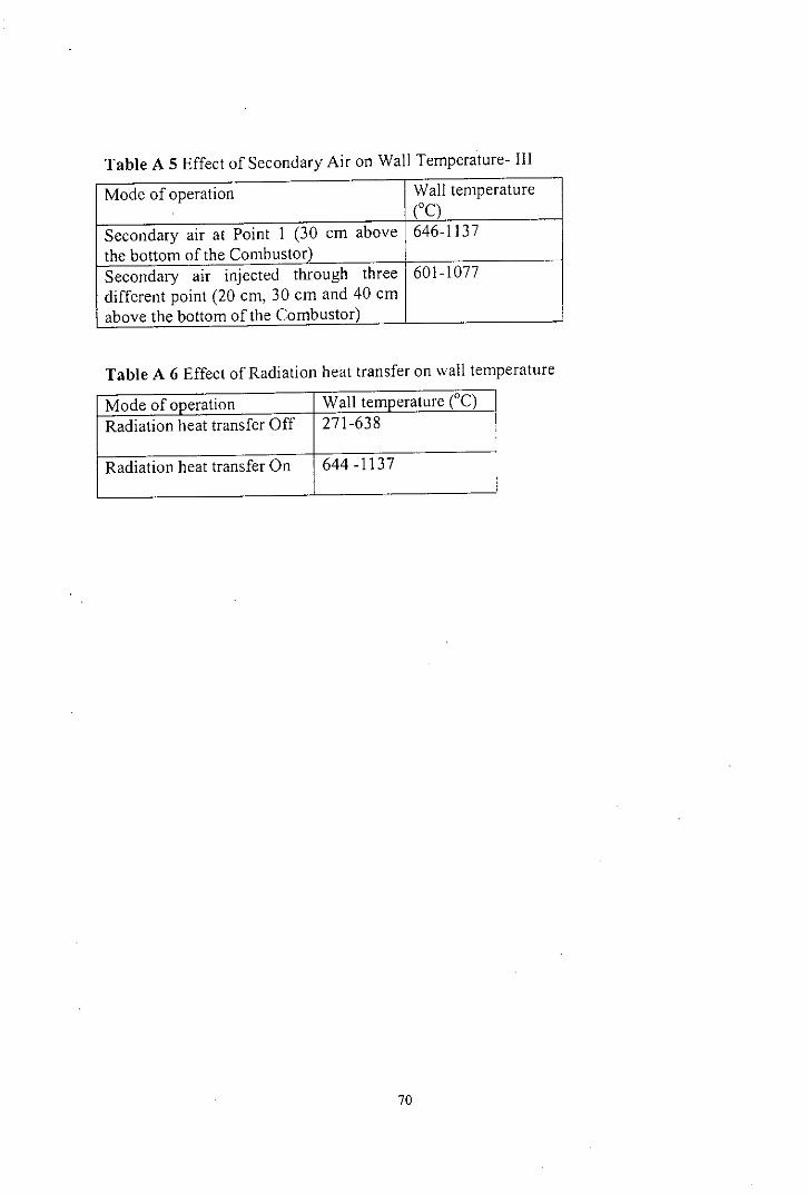
Table A 5 Effect of Secondary Air on Wall Temperature- III

Mode of operation Wall temperature(0C)

Secondary air at Point I (30 cm above 646-1137the bottom of the Combustor)Secondary air injected through three 601-1077different point (20 cm, 30 cm and 40 cmabove the bottom of the Combustor)

Table A 6 Effect of Radiation heat transfer on wall temperature

Mode of operation Wall temperature (0C)Radiation heat transfer Off 271-638

Radiation heat transfer On 644 -1137

70

APPENDIXBModel specification and Material Properties

Name of the Software: FLUENTRelease: 6.1.22Model: 3d, Segregated.

Models

Model Settings------~-------------------------------------------------~-------SpaceTimeViscousWall TreatmentHeal TransferSolidlficationand MeltingRadiationSpecies TransportCoupled DispersedPhaseSoot

Solver Controls

Equations

Equation Solved

Flow yesTurbulence yesCH, yesO2 yesCO, yesH,O yesEnergy yesPI yes

Numerics

Numeric

3DSteadyStandard k-epsilon turbulence modelStandard Wall FunctionsEnabled

DisabledPI ModelReacting (5 species)

DisabledDisabled

Enabled.---------------------------- .---------------.----Absolute Velocity Formulation yes

71

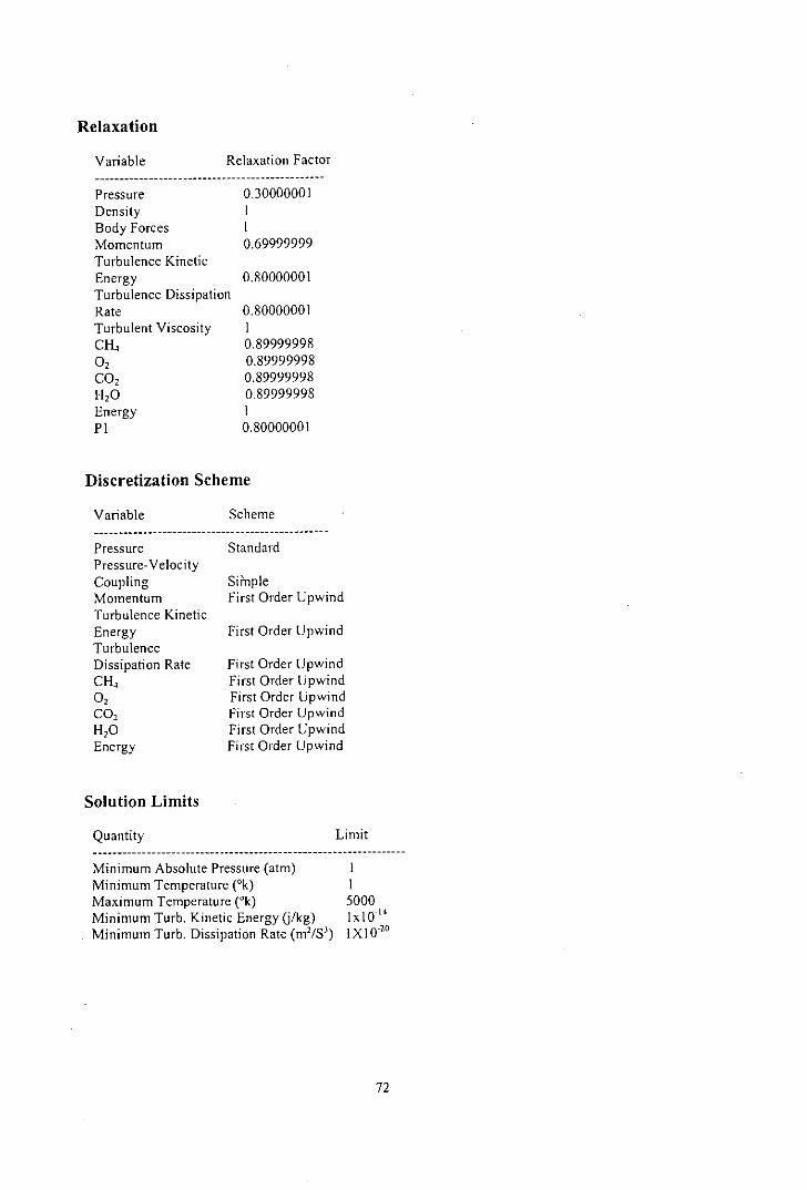
Relaxation

Variable Relaxation Factor

PressureDensityBody ForcesMomentumTurbulence KineticEnergyTurbulence DissipationRateTurbulent ViscosityCH,a,co2

H20EnergyPI

0.30000001II0.69999999

0.80000001

0.80000001I0.899999980.899999980.899999980.89999998I0.80000001

Discretization Scheme

Variable

PressurePressure- VelocityCouplingMomentumTurbulence KineticEnergyTurbulenceDissipation RateCH,O2CO,H20Energy

Solution Limits

Quantity

Scheme

Standard

SimpleFirst Order Upwind

First Order Upwind

First Order UpwindFirst Order UpwindFirst Order UpwindFirst Order UpwindFirst Order UpwindFirst Order Upwind

Limit

Mlnimum Absolute Pressure (atm)Minimum Temperature (Ok)Maximum Temperature ek)Minimum Turb. Kinetic Energy (j/kg)Minimum Turb. Dissipation Rate (m2/SJ)

II5000Ix 10.14

IXIO'20

72

Material Properties

Material: Methane-Air (mixture)

Property Units Method

Mixture SpeciesReaction Eddy-dissipationDensity kg/mJ lncompressible-

Ideal-gasCp (Specific Heat) j/kg-k Mixing-lawThermal Conductivity w/m-k ConstantViscosity kg/m-s ConstantMass Diffusivity m2/s ConstantAbsorption Coefficient 11m ConstantScattering Coefficient 11m ConstantScattering Phase Function IsotropicThermal ExpansionCoefficient Ilk Constant

Value

CH" 0" CO" H20, N,

0.04540000 I1.72 xl0052.88 x I0.05

aa

a

Nitrogen

Property Units Method Value---.--------------------------------------------------------------------------Density kg/mJ Constant 1.138Thermal Conductivity w/m-k Constant 0.0242Viscosity kg/m-s Constant 1.663x I0.05Molecular Weight kg/kg-mol Constant 28.0 134Standard StateEnthalpy j/kgmol Constant aStandard State Entropy j/kgmol-k Constant 191494.78Reference Temperature k Constant 298.15L-J Characteristic Length Angstrom Constant 3.621L-J Energy Parameter k Constant 97.53Absorption Coefficient 11m Constant aScattering Coefficient 11m Constant aScattering Phase Function IsotropicThermal ExpansionCoefficient Ilk Constant 0Degrees of Freedom Constant a

73

Water-vapor

Property Units Method Value(s)-------------_.-----------------------_.---------------------------------------

Density kg/mJ Constant 0.5542Thennal Conductivity w/m-k Constant 0.0261Viscosity kg/m-s Constant 1.34X I00;Molecular Weight kg/kg-mol Constant 18.01534Standard StateEnthalpy j/kg-mol Constant -2.418379XI08

Standard State Entropy j/kg-mol-k Constant 188696.44Reference Temperature k Constant 298.15L-J Characteristic Length Angstrom Constant 2.605L-J Energy Parameter k Constant 572.4Absorption Coefficient lim Constant 0.54Scattering Coefficient 11m Constant 0Scattering Phase Function IsotropicThermal ExpansionCoefficient Ilk Constant 0Degrees of Freedom Constant 0

Carbon Dioxide

Property Units Method Value--------------------P-----.---.----------------------- ________________

Density kg/m' Constant 1.7878Thennal Conductivity w/m-k Constant 0.0145Viscosity kg/m-s Constant 1.37X I0.0;Molecular Weight kg/kg-mol Constant 44.00995Standard StateEnthalpy j/kg-mol Constant -3.9353235X I0'Standard State Entropy j/kg-mol-k Constant 213715.88Reference Temperature k Constant 29815L-J CharacteristicLength Angstrom Constant 3.941L-J Energy Parameter k Constant 1952Absorption Coefficient 11m Constant 0.43Scattering Coefficient 11m Constant 0Scattering Phase Function IsotropicThermal ExpansionCoefficient Ilk Constant 0Degrees of Freedom Constant 0

74

Oxygen

Property Units Method Value

Constant 0Constant 0

DensityThermal ConductivityViscosityMolecular WeightStandard State EnthalpyStandard State EntropyReference TemperatureL-] Characteristic LengthL-] Energy ParameterAbsorption CoefficientScattering CoefficientScattering Phase FunctionThermal ExpansionCoefficientDegrees of Freedom

Methane

kg/m'w/m-kkg/m-skg/kg-molj/kg-molj/kg-mol-kkAngstromk11m11m

I/k

ConstantConstantConstantConstantConstantConstantConstantConstantConstantConstantConstantIsotropic

1.29990.02461.919XI005

31.9988o20502686298.1534581074oo

Property Units Method Value

Ilk Constant 0Constant 0

DensityCp (Specific Heat)Thermal ConductivityViscosityMolecular WeightStandard State EnthalpyStandard State EntropyReference TemperatureL-] Characteristic LengthL-] Energy ParameterAbsorption CoefficientScattering CoefficientScattering Phase FunctionThermal ExpansionCoefficientDegrees of Freedom

kg/m' Constantj/kg-k Constantw/m-k Constantkg/m-s Constantkg/kg-mol Constantj/kg-mol Constantj/kg-mol-k Constantk ConstantAngstrom Constantk Constant11m Constant11m Constant

Isotropic

0.667922220.03321.087X I0.05

16.04303-74895176186040.09298153.758148.60.62o

75

Air

Property Units Method Value----------------------------------------------------------------_.---------.-----DensityThermal ConductivityViscosityMolecular WeightStandard State EnthalpyStandard State EntropyReference TemperatureL-J Characteristic LengthL-J Energy ParameterAbsorption CoefficientScattering CoefficientScattering Phase FunctionThermal ExpansionCoefficientDegrees of Freedom

kgimJ

w/m-kkglm-skg/kg-moljlkg-molj/kg-mol-kkAngstromk11m11m

Ilk

ConstantConstantConstantConstantConstantConstantConstantConstantConstantConstantConstantIsotropic

ConstantConstant

76

1.2250.0242I. 789400 I X I0.0528.966oo298.149993.71178.6oo

oo

APPENDIX C

Screen Output for a typical run (For 100% Excess Air and 60° rotation in Primary Air Inlet:

Iter no continuity. x-velocity. y-velocity. z-velocity. energy k Epsilon CH4 0, co, H,O P I time/iter

1 1.0000e+00 8.7508e-02 9.2578e-01 5.1787e+00 1.I81ge+00 5.2695e-01 1.2907e+013.5646e-01 1.0006e-01 1.7765e+00 1.7878e+00 2.0098e-02 3:19:48 9992 8.7488e-01 1.6855e-01 1.6817e-01 2.3705e-01 9.499ge-03 8.1780e-01 2.6582e+00 1.1495e-01 1.5550e-02 2.8972e-02 2.2624e-02 1.964ge-02 3:19:36 998temperature limited to 5.000000e+03 in 2594 cells on zone 2 in domain I3 1.0000e+00 1.2697e-0 I 1.1466e-01 2.1233e-0 I 1.1428e-02 1.4340e+00 1.0974e+0 I 1.5943e-0 I 1.0161 e-02 1.70 IOe-02 1.1946e-02 9.0283e-03 3: 19:24 9974 3.547ge-01 8.0260e-02 7.822ge-02 1.0211e-01 6.2766e-03 1.4026e-01 2.5172e-01 8.2326e-02 6.9490e-03 1.273ge-02 9.583ge-03 5.5815e-03 3:19:12 9965 3.584Ie-01 2.5724e-02 2.464Ie-02 4.5971 e-02 5.6518e-03 7.4683c-02 1.242ge-0 I 6.6740e-02 5.3563e-03 1.0520e-02 8.41 83e-03 4.9313e-03 3: 15:41 9956 9.5602e-01 7.4817e-02 7.293ge-02 1.1283e-01 6.2036e-03 8.5554c-02 1.140ge-01 4.4603e-02 4.9892e-03 1.0450e-02 8.6748e-03 3.2376e-03 3:16:09 9947 8.1617e-0 I 3.5776e-02 3.1735e-02 8.3 I44e-02 6.3270e-03 7.02 1ge-02 9.9033c-02 3.5071 e-02 4.6273e-03 9.9233e-03 8.2982e-03 2.3807e-03 3: 13: I 0 9938 6.365ge-01 3.182Ie-02 2.8883e-02 6.4610e-02 4.3834e-03 6.6650e-02 8.9138e-02 3.1446e-02 4.2753e-03 9.3858e-03 7.9525e-03 1.8961e-03 3:14:04 99294.8341 e-Ol 2.5863e-02 2.4542e-02 4.2871 e-02 3.5432e-03 6.1381 e-02 7.9625e-02 2.944ge-02 3.8743e-03 8.7244e-03 7.4928e-03 1.5564e-03 3: II :26 99110 3.8262e-0 I 2.0135e-02 1.9303e-02 2.9135e-02 3.28 I4e-03 5.4958e-02 7.3245e-02 2.7827e-02 3.5546e-03 8. I48ge-03 7.0762e-03 1.3238e-03 3: 12:35 990II 3.128Ie-01 1.5601e-02 1.5117e-02 2. I397e-02 3. I996e-03 4.8932c-02 6.7588e-02 2.5807e-02 3.3283e-03 7.6898e-03 6.7725e-03 1.1535e-03 3:10:11 98912 2.5724e-01 1.2055e-02 1.1770e-02 1.6971 e-02 3.2388e-03 4.4672e-02 6.3327e-02 2.3982e-02 3. I824e-03 7.398ge-03 6.6531 e-03 1.0223e-03 3: II :31 98813 2.3435e-01 1.103ge-02 1.0936e-02 1.638ge-02 3.1 060e-03 4.1414e-02 6.0047e-02 2.2391 e-02 3.0496e-03 7.0248e-03 6.4973e-03 9.1606e-04 3:09: 15 98714 2.0261 e-OI 9.5782e-03 9.5571 e-03 1.5 I24e-02 2.8740e-03 3.9146e-02 5.7552c-02 2.1244e-02 2.9652e-03 6.5180e-03 6. 1978e-03 8.2865e-04 3: I0:41 98615 1.8214e-01 9.124Ie-03 9.0837e-03 1.4671e-02 2.602Ie-03 3.708ge-02 5.5385e-02 2.0340e-02 2.9419c-03 5.985ge-03 5.8458e-03 7.5507e-04 3:08:3098516 1.6638e-0 I 8.6878e-03 8.5582e-03 1.4094e-02 2.3538e-03 3.5196e-02 5.348ge-02 1.9800e-02 29620e-03 5.6784e-03 5.5768e-03 6.91 94e-04 3: I0:0 I 98417 1.5314e-0 I 8.2356e-03 8.0397e-03 1.3408e-02 2.1780e-03 3.3428c-02 5. I832e-02 1.9546e-02 2.9883e-03 5.5071 e-03 5.3976e-03 6.3784e-04 3:07:54 98318 1.4093e-0 I 7.7990e-03 7.5740e-03 1.2484e-02 2.0778e-03 3. I726e-02 5.0385c-02 1.9763e-02 3.0281 e-03 5.3935e-03 5.2835e-03 5.891ge-04 3:09:27 98219 1.3235e-0 I 7.4568e-03 7.2305e-03 1.1654c-02 2.0816e-03 3.0030e-02 4.9164c-02 2.0437e-02 3. I240e-03 5.3070e-03 5.2166e-03 5.4694e-04 3:07:22 98120 1.2435e-0 I 7.1052c-03 6.896ge-03 1.10 15c-02 2.1 086e-03 2.8281 c-02 4.791 Oe-02 2.1161 e-02 3.267ge-03 5. I882e-03 5.1 I65e-03 5.096ge-04 3:08:57 98021 1.1786e-0 I 6.81 75e-03 6.645ge-03 1.0502e-02 2. I660e-03 2.6592c-02 4.651 Oe-02 2.1 787e-02 3.4367e-03 5.0547e-03 4.986ge-03 4.7649c-04 3:06:54 97922 1.1272e-0 I 6.555ge-03 6.4261 e-03 1.0007e-02 2.21 00e-03 2.50 16e-02 4.4906e-02 2.2125e-02 3.6267e-03 4.9311 e-03 4.8456e-03 4.4693e-04 3:08:29 97823 1.084ge-0 I 6.3255e-03 6.2 I9ge-03 9.6\51 e-03 2.240 Ie-03 2.3586e-02 43243e-02 2.2223e-02 3.8157e-03 4.8223e-03 4.70 1ge-03 4.2000e-04 3:06:27 97724 1.0514e-0 1 6.1421 e-03 6.0325e-03 9.3888e-03 2.2283e-03 2.2421 e-02 4.1411 e-02 2.21 02e-02 3.9814e-03 4.7211 e-03 4.5515e-03 3.9564e-04 3:04:48 97625 1.0343e-0 I 5.9834e-03 5.875Ie-03 9.1986e-03 2. I778c-03 2.1443e-02 3.9530e-02 2.181 Oe-02 4.1 I47e-03 4.689ge-03 4.4456e-03 3.7395e-04 3 :06:41 97526 1.0232e-0 I 5.8488e-03 5.7714e-03 8.913Ie-03 2.1380e-03 2.0543e-02 3.7573e-02 2.125\ e-02 4.1496e-03 4.6323e-03 4.314 7e-03 3.5443e-04 3:04:55 97427 1.0 121e-01 5.7690e-03 5.7565e-03 8.5211 e-03 2.0407e-03 1.973ge-02 3.5728e-02 2.0574e-02 4.0655e-03 4.5676e-03 4.1926c-03 3.3697e-04 3:03:27 97328 9.9837e-02 5.6580e-03 5.6876e-03 8.1906e-03 1.9493e-03 1.8892e-02 3.3752e-02 1.9841 e-02 3.9 I96e-03 4.5204e-03 4.1371 c-03 3.2168e-04 3:05:30 972

77

299.81490-025.50730-035.56020-037.92810-03 1.89260-03 1.80660-023.18690-021.89800-023.72510-03 4.45870-03 4.14390-033.08560-04 3:03:51 971309.67040-025.42300-035.41670-037.85860-03 1.87290-03 1.72410-023.01090-02 1.80570-023.47230-03 4.33080-03 4.13040-03 2.97480-04 3:05:43 970319.55350-025.44520-03 5.31050-03 7.97470-031.81860-031.63950-022.84900-02 1.71830-023.20060-03 4.20600-03 4.13620-032.87850-04 3:03:57 969329.35540-025.45300-035.22310-038.16620-03 1.75320-03 1.55460-022.70270-021.62000-022.92360-03 4.07600-03 4.13790-03 2.78870-04 3:02:30 96833 9.11700-02 5.37530-03 5.07770-03 8.24610-03 1.66270-03 1.46600-02 2.56130-02 1.52420-02 2.66020-03 3.97520-03 4.15720-03 2.70470-04 3:04:32 967

iter continuity x-velocity y-velocity z-velocity energy k epsilon ch4 02 co2 h20 pI time/iter348.75770-025.28290-034.93570-038.22400-03 1.56610-03 1.38200-022.43660-021.41500-022.43480-03 3.92350-03 4.18820-03 2.62330-04 3:02:54 966358.33160-025.13580-034.74120-038.02670-03 1.45880-03 1.29910-022.31550-021.29520-022.25680-03 3.91890-03 4.21880-03 2.54450-04 3:04:46 965367.88870-024.93420-034.53210-037.55480-03 1.35580-03 1.21890-022.17480-021.17740-022.12600-03 3.93410-03 4.21370-032.46860-04 3:03:00 964377.47880-024.71300-03 4.33190-03 6.99470-03 1.26500-03 1.14420-022.04500-02 1.07930-02 2.03450-03 3.92540-03 4.16660-03 2.39770-04 3:01 :34 963387.05240-024.51530-034.13400-036.60300-03 1.18290-03 1.08130-02 1.92490-029.97010-03 1.97610-033.87690-034.08580-032.32950-04 3:03:35 96239 6.65860-024.33490-03 3.97610-03 6.25690-03 1.11630-03 1.02960-02 1.82780-02 9.24880-03 1.91060-03 3.77090-03 3.95530-03 2.26190-04 3:01 :57 961406.29270-024.13380-03 3.83830-03 5.87010-031.04380-039.83250-031.73430-02 8.62850-031.82990-033.63700-033.80180-03 2.19590-04 3:03:48 96041 5.97360-02 3.91830-03 3.71680-03 5.46310-03 9.92800-04 9.37980-03 1.61920-02 8.04500-03 1.72520-03 3.47440-03 3.62420-03 2.13180-04 3:02:03 959425.69630-023.71460-033.57870-035.13320-03 9.43300-04 8.97530-031.53650-027.50580-031.61590-03 3.30900-03 3.44540-03 2.07000-04 3:03:49 958435.46390-023.52800-033.46060-034.85550-03 9.05210-04 8.64560-031.44610-027.04130-031.50810-03 3.13810-03 3.26240-03 2.01110-04 3:05:11 957445.25120-023.36660-033.35070-03 4.61040-03 8.72230-04 8.36260-031.37890-026.69780-031.40290-03 2.96780-03 3.08140-031.95550-04 3:06:14 956455.07200-023.23260-033.25500-034.41470-03 8.41700-04 8.14800-031.32010-026.48200-031.30360-032.80780-03 2.91210-031.90270-04 3:07:02 955464.91250-023.12230-033.16900-034.26530-03 8.18920-04 7.99080-031.28520-026.36780-031.21700-03 2.66480-03 2.76060-031.85100-04 3:07:37 954474.78440-02 3.02740-03 3.08860-03 4.11880-03 8.0210e-04 7.8765e-03 1.25730-02 6.30610-03 1.14380-03 2.54630-03 2.63360-03 1.79990-04 3: 11: 14 953484.66970-022.93500-033.00740-033.97690-03 7.9568e-04 7.79710-03 1.2357e-02 6.25060-03 1.08470-032.44090-03 2.5206e-03 1.74990-04 3:10:55 952494.57320-022.84770-03 2.92770-03 3.85810-03 7.90190-047.75620-031.23030-026.22740-03 1.0376e-03 2.36420-03 2.43670-031.70100-04 3:10:36 951504.48200-022.76880-032.86190-033.75600-03 7.88160-04 7.74330-031.20880-026.19940-031.00230-03 2.30670-03 2.37200-031.65350-04 3:13:30 950514.38900-022.69600-032.79850-033.66950-03 7.79870-04 7.73610-03 1.1937e-02 6.16190-03 9.73910-04 2.2640e-03 2.32290-03 1.60780-04 3:12:35 949524.29560-022.63230-03 2.7380e-03 357980-03 7.72350-04 7.72860-031.18930-026.13030-039.52210-04 2.23150-03 2.28310-031.56360-04 3:14:59 948534.20360-022.57450-032.68630-033.49880-03 7.68190-04 7.71230-031.16870-026.09430-03 9.33460-04 2.20730-03 2.25240-031.52110-04 3:13:42 947544.11030-022.51410-03 2.63160-03 3.42850-03 7.63580-04 7.68520-03 1.14310-02 6.03390-03 9.15280-04 2.18220-03 2.22240-03 1.48030-04 3: 12:39 946554.01180-022.45640-03 2.57370-03 3.36810-03 7.55300-04 7.63140-031.11240-025.95160-03 8.9874c-04 2.1595e-03 2.1952e-03 1.4412e-04 3:14:54 94556 3.9102e-02 2.3978e-03 2.5154e-03 3.3071e-03 7.4838e-04 7.5517e-03 1.0820e-02 5.8564e-03 8.81420-04 2.13230-03 2.1657e-03 1.4036e-04 3:13:31 94457 3.80510-022.34210-03 2.4632e-03 3.2430e-03 7.4215e-04 7.45180-03 1.0426e-02 5.7601c-03 8.6297e-04 2.1 070e-03 2.137ge-03 1.3674e-04 3: 12:22 94358 3.7014e-02 2.2921e-03 2.4112e-03 3.183ge-03 7.361 Oe-04 7.3290e-03 9.9567e-03 5.6537e-03 8.4335e-04 2.081ge-03 2.1103e-03 1.3331e-04 3: 11:25 94259 3.5955e-02 2.2385e-03 2.3571e-03 3.123Ie-03 7.2730e-04 7.1761e-03 9.501ge-03 5.5330e-03 8.2542e-04 2.055ge-03 2.0832e-03 1.2990e-04 3:10:36 94160 3.4974e-02 2.1985e-03 2.30760-03 3.08390-03 7.269Ie-04 7.03310-03 9.1813e-03 5.4187c-03 8.09410-04 2.03530-03 2.0603e-03 1.2662e-04 3:06:47 940613.40420-02 2. 1652e-03 2.26490-03 3.0422e-03 7.24850-04 6.8755e-03 8.7441e-03 5.32030-03 7.95940-04 2.016Ie-03 2.0395e-03 1.23440-04 3:06:50 939623.31590-02 2.13260-03 2.23160-03 3.0088e-03 7.25890-04 6.72370-03 8.28140-03 5.23350-03 7.81980-04 1.99810-03 2.01960-03 1.20350-04 3:06:50 938633.22400-022.09950-032.19020-03 2.97760-03 7.2 160e-04 6.57610-03 7.87390-03 5.14660-03 7.70670-04 1.98480-032.00420-031.17390-04 3:06:47 937643.13450-022.06500-03 2.14370-03 2.93950-03 7.19820-04 6.43270-03 7.55820-03 5.04720-03 7.60530-041.97340-031.98960-031.14580-04 3:06:42 93665 3.04370-02 2.02190-03 2.09620-03 2.88210-03 711590-04 6.29310-03 7.17640-03 4.94790-03 7.50160-04 1.96100-03 1.97620-03 1.11870-04 3:03:29 935

78

66 2.9570e-02 1.980ge-03 2.045ge-03 2.8364e-03 7.0365e-04 6.1881e-03 6.8162e-03 4.8502e-03 7.4202e-04 1.9582e-03 1.9716e-03 1.0926e-04 3:04:00 93467 2.8736e-02 1.940ge-03 1.9975e-03 2.7917e-03 6.9670e-04 6.102ge-03 6.5195e-03 4.7531e-03 7.3636e-04 1.962ge-03 1.9744e-03 1.0672e-04 3:04:21 93368 2.7926e-02 1.9048e-03 1.9476e-03 2.7550e-03 6.9247e-04 6.0431e-03 6.3345e-03 4.6582e-03 7.3386e-04 1.9750e-03 1.9861e-03 1.0427e-04 3:01:30 93269 2.7194e-02 1.8657e-03 1.9031e-03 2.7241e-03 6.8952e-04 6.0051e-03 6.128ge-03 4.5596e-03 7.3258e-04 1.9858e-03 1.9970e-03 1.018ge-04 3:11:36 93170 2.6520e-02 1.8282e-03 1.8636e-03 2.6856e-03 6.8624e-04 5.9804e-03 5.8295e-03 4.475ge-03 7.3222e-04 1.9990e-03 2.0102e-03 9.9594e-05 3:19:37 930712.5931e-02 1.7954e-03 1.8287e-03 2.638ge-03 6.827ge-04 5.9752e-03 5.6592e-03 4.3865e-03 7.3135e-04 2.0115e-03 2.0230e-03 9.7374e-05 3:19:46 92972 2.5312e-02 1.759ge-03 1.7882e-03 2.5945e-03 6.7921e-04 5.9734e-03 5.4410e-03 4.3001e-03 7.3041e-04 2.0215e-03 2.0320e-03 9.5238e-05 3:16:46 92873 2.4692e-02 1.7267e-03 1.7478e-03 2.5505e-03 6.6993e-04 5.970ge-03 5.2244e-03 4.2081e-03 7.2672e-04 2.026ge-03 2.0388e-03 9.3167e-05 3:14:19 92774 2.4064e-02 1.6886e-03 1.7071e-03 2.5098e-03 6.6118e-04 5.9684e-03 5.1158e-03 4.1123e-03 7.2226e-04 2.0342e-03 2.046ge-03 9.1 175e-05 3: 12:20 92675 2.3430e-02 1.6512e-03 1.6658e-03 2.4820e-03 6.5022e-04 5.9662e-03 4.9310e-03 4.0033e-03 7.1685e-04 2.0368e-03 2.0506e-03 8.9231e-05 3:10:42 92576 2.2778e-02 1.6124e-03 1.6190e-03 2.4640e-03 6.4222e-04 5.9612e-03 4.7433e-03 3.8942e-03 7.096ge-04 2.0321e-03 2.0472e-03 8.7367e-05 3:09:21 92477 2.2133e-02 1.5707e-03 1.576ge-03 2.4335e-03 6.3443e-04 5.9545e-03 4.6380e-03 3.8047e-03 7.0156e-04 2.0281e-03 2.0441e-03 8.5555e-05 3:08:14 92378 2.157ge-02 1.5333e-03 1.5397e-03 2.387ge-03 6.2566e-04 5.942ge-03 4.4475e-03 3.7257e-03 6.9315e-04 2.0217e-03 2.038ge-03 8.3797e-05 3:07:19 92279 2.1052e-02 1.4953e-03 1.5032e-03 2.3435e-03 6.181 Oe-04 5.9248e-03 4.2831e-03 3.6597e-03 6.8441e-04 2.0 145e-03 2.0328e-03 8.2081 e-05 3:06:31 92180 2.0535e-02 1.4586e-03 1.4687e-03 2.2963e-03 6.0846e-04 5.9000e-03 4.1134e-03 3.5861e-03 6.7553e-04 2.0114e-03 2.0308e-03 8.0413e-05 3:05:51 92081 1.9997e-02 1.4194e-03 1.4317e-03 2.2586e-03 6.0280e-04 5.8687e-03 3.9535e-03 3.5022e-03 6.6677e-04 2.0012e-03 2.0213e-03 7.8784e-05 3:05:17 91982 1.9511e-02 1.3835e-03 1.3955e-03 2.2254e-03 5.9301e-04 5.8297e-03 3.7907e-03 3.4246e-03 6.5658e-04 1.9873e-03 2.0083e-03 7.7203e-05 3:04:47 91883 1.9044e-02 1.3483e-03 1.3602e-03 2.1962e-03 5.8468e-04 5.7848e-03 3.643Ie-03 3.3508e-03 6.4644e-04 1.9778e-03 1.9996e-03 7.5655e-05 3:04:21 91784 1.8582e-02 1.3 11ge-03 1.3215e-03 2.1638e-03 5.7826e-04 5.7292e-03 3.4808e-03 3.2772e-03 6.3764e-04 1.9672e-03 1.9891 e-03 7.414ge-05 3:00:54 91685 1.8136e-02 1.275ge-03 1.2850e-03 2.1261 e-03 5.7052e-04 5.6658e-03 3.3327e-03 3.2067e-03 6.2862e-04 1.9581e-03 1.9805e-03 7.2691e-05 3:01: 10 91586 1.7714e-02 1.2430e-03 1.249ge-03 2.0832e-03 5.6434e-04 5.597Ie-03 3. 1804e-03 3.1404e-03 6.1957e-04 1.949Ie-03 1.9710e-03 7.1277e-05 3:01:20 91487 1.7314e-02 1.211Oe-03 1.2165e-03 2.0381e-03 5.5778e-04 5.521ge-03 3.044ge-03 3.0743e-03 6.1355e-04 1.9476e-03 1.9696e-03 6.9893e-05 3:01:26 91388 1.6960e-02 1.1798e-03 1.1843e-03 1.9968e-03 5.5585e-04 5.4425e-03 2.8973e-03 2.999ge-03 6.0754e-04 1.9430e-03 1.9650e-03 6.8564e-05 3:04:30 91289 1.6616e-02 1.1480e-03 1.1530e-03 1.9610e-03 5.4887e-04 5.3608e-03 27696e-03 2.9258e-03 6.002ge-04 1.931ge-03 1.9531e-03 6.727ge-05 3:06:55 91190 1.6277e-02 1.1165e-03 1.1240e-03 1.9276e-03 5.3967e-04 5.2794e-03 2.6386e-03 2.8593e-03 5.9250e-04 1.917ge-03 1.9383e-03 6.6041e-05 3:05:46 91091 1.5932e-02 1.0876e-03 1.0968e-03 1.896le-03 5.2905e-04 5.1956e-03 2.5283e-03 2.7941e-03 5.8388e-04 1.9030e-03 1.9224e-03 6.484ge-05 3:04:49 90992 1.558ge-02 1.0580e-03 1.0681e-03 1.8688e-03 5.1866e-04 5.1106e-03 2.4148e-03 2.7256e-03 5.7527e-04 1.8861e-03 1.9052e-03 6.3685e-05 3:04:0090893 1.5217e-02 1.0257e-03 1.0357e-03 1.8432e-03 5.0993e-04 5.0255e-03 2.3166e-03 2.6580e-03 5.6687e-04 1.8703e-03 1.8890e-03 6.2592e-05 3:00:18 90794 1.4891e-02 9.969ge-04 1.006ge-03 1.8 172e-03 5.0528e-04 4.9347e-03 2.21 18e-03 2.5940e-03 5.5850e-04 1.8544e-03 1.8725e-03 6.1556e-05 3:00:19 90695 1.4554e-02 9.6948e-04 9.8275e-04 1.7853e-03 4.9777e-04 4.8395e-03 2. 1278e-03 2.5287e-03 5.51 03e-04 1.8405e-03 1.8580e-03 6.0526e-05 3:00: 18 90596 1.4217e-02 9.3943e-04 9.5674e-04 1.748ge-03 4.9102e-04 4. 7443e-03 2.0374e-03 2.4566e-03 5.4231 e-04 1.8207e-03 1.8376e-03 5.952ge-05 3:00: 14 90497 1.388ge-02 9.0826e-04 9.306ge-04 1.7188e-03 4.7874e-04 4.6568e-03 1.9631 e-03 23841e-03 5.2902e-04 1.783ge-03 1.8004e-03 5.8587e-05 3:00:09 90398 1.3583e-02 8.7946e-04 9.0568e-04 1.6981 e-03 4.5886e-04 4.5746e-03 1.8857e-03 2.3632e-03 5.171ge-04 1.7520e-03 1.767ge-03 5.7706e-05 3:00:03 90299 1.3250e-02 8.5165e-04 8.793ge-04 1.6736e-03 4.481 Oe-04 4.4963e-03 1.823ge-03 2.3262e-03 5.0598e-04 1.7235e-03 1.7384e-03 5.6844e-05 2:59:55 901100 1.2924e-02 8.247ge-04 8.5337e-04 1.6433e-03 4.3867e-04 4.4266e-03 1.7588e-03 2.2803e-03 4.9528e-04 1.6961e-03 1.7100e-03 5.6024e-05 3:05:46 900101 1.2618e-02 8.0054e-04 8.3013e-04 1.6115e-03 4.2843e-04 4.361ge-03 1.7087e-03 2.2314e-03 4.847ge-04 1.6670e-03 1.6801e-03 5.5250e-05 3: 16:24 899102 1.2331e-02 7.7744e-04 8.094ge-04 1.581ge-03 4.2026e-04 4.2936e-03 1.6558e-03 2.1817e-03 4.7330e-04 1.63 18e-03 1.6441e-03 5.4500e-05 3:24:50 898103 1.2063e-02 7.5412e-04 7.9025e-04 1.5502e-03 4.1 01ge-04 4.2084e-03 1.6146e-03 2. 1335e-03 4.6116e-04 1.5951 e-03 1.6064e-03 5.3812e-05 3:31 :32 897

79

1041.1802e-02 7.3265e-04 7.7357e-04 1.5 I67e-03 4.0012e-04 4.1016e-03 1.5642e-03 2.0782e-03 4.4757e-04 1.551ge-03 1.5624e-03 5.3162e-05 3:36:49 896105 1.1542e-02 7.1052e-04 7.5720e-04 1.4868e-03 3.8926e-04 3.9732e-03 1.5201e-03 2.0122e-03 4.3292e-04 1.5043e-03 1.5134e-03 5.2530e-05 3:41:00 8951061.1273e-02 6.8881e-04 7.3887e-04 1.4531e-03 3.7792e-04 3.8254e-03 1.4683e-03 1.944ge-03 4.1742e-04 1.4496e-03 1.4577e-03 5.1920e-05 3:41:18 894107 1.1026e-02 6.6952e-04 7.2230e-04 1.4197e-03 3.6554e-04 3.6538e-03 1.4244e-03 1.8891e-03 4.0122e-04 1.3947e-03 1.4016e-03 5. I346e-05 3:44:28 893108 1.0788e-02 6.5103e-04 7.0742e-04 1.3852e-03 3.5520e-04 3.4573e-03 1.336ge-03 1.8427e-03 3.8541e-04 1.3411e-03 1.3472e-03 5.0811e-05 3:35:03 892109 1.054ge-02 6.3306e-04 6.9351e-04 1.3482e-03 3.4674e-04 3.2483e-03 1.3464e-03 1.7994e-03 3.7062e-04 1.2905e-03 1.2955e-03 5.0312e-05 3:27:29 891110 1.0324e-02 6.1533e-04 6.7958e-04 1.310 le-03 3.3870e-04 3.031ge-03 1.284ge-03 1.7553e-03 3.5658e-04 1.2408e-03 1.244ge-034.9837e-05 3:21 :24 890111 1.0107e-02 5.9758e-04 6.6610e-04 1.2715e-03 3.3028e-04 2.818Ie-03 1.236ge-03 1.711Oe-03 3.430ge-04 1.1924e-03 1.1957e-03 4.9382e-05 3:16:30 889112 9.8946e-03 5.808Ie-04 6.5341e-04 1.2342e-03 3.215Ie-04 2.6136e-03 1.2076e-03 1.6664e-03 3.2970e-04 1.1440e-03 1.1463e-03 4.8950e-05 3:12:33 888113 9.6811e-03 5.6427e-04 6.4062e-04 1.1990e-03 3.1 I92e-04 2.4272e-03 1.1308e-03 1.6225e-03 3.1675e:04 1.0972e-03 1.0990e-034.8534e-05 3:09:21 887114 9.457ge-03 5.4792e-04 6.2663e-04 1.1643e-03 3.0200e-04 2.2633e-03 1.1544e-03 1.5740e-03 3.0420e-04 1.0502e-03 1.0513e-03 4.8133e-05 3:06:45 886115 9.223ge-03 5.3032e-04 6.1141e-04 1.1286e-03 2.9216e-04 2.1190e-03 1.1078e-03 1.5283e-03 2.9203e-04 1.0053e-03 1.005ge-03 4.7746e-05 3:0 I :41 885116 8.9924e-03 5.1323e-04 5.9654e-04 1.0931 e-03 2.8292e-04 1.994ge-03 1.0380e-03 1.4862e-03 2.8063e-04 9.6351e-04 9.6356e-04 4.7368e-05 3:00:32 884117 8.7667e-03 4.9662e-04 5.8133e-04 1.0571e-03 2.7328e-04 1.8920e-03 1.0743e-03 1.4467e-03 2.6997e-04 9.2345e-04 9.2316e-04 4.6995e-05 2:59:35 883118 8.5520e-03 4.8038e-04 5.6573e-04 1.0204e-03 2.6246e-04 1.8020e-03 1.0413e-03 1.4088e-03 2.5933e-04 8.8413e-04 8.8367e-04 4.6622e-05 2:58:47 882119 8.324ge-03 4.6423e-04 5.4892e-04 9.8408e-04 2.553ge-04 1.7244e-03 9.7826e-04 1.3695e-03 2.4947e-04 8.4694e-04 8.4628e-04 4.6243e-05 2:58:06 8811208.1 043e-03 4.4763e-04 5.3125e-04 9.4904e-04 2.4572e-04 1.6613e-03 1.0178e-03 1.3315e-03 2.3983e-04 8.1 070e-04 8.0976e-04 4.5866e-05 2:57:31 880121 7.8913e-03 4.3168e-04 5. 1404e-04 9. 1574e-04 2.3757e-04 1.607ge-03 9.8830e-04 1.2956e-03 2.3083e-04 7.7691e-04 7.7580e-04 4.547ge-05 2:57:01 879122 7.6780e-03 4.1560e-04 4.9717e-04 8.8376e-04 2.3012e-04 1.5611e-03 9.2865e-04 1.2602e-03 2.2270e-04 7.4613e-04 7.4482e-04 4.5088e-05 2:56:34 878123 7.469Ie-03 4.0042e-04 4.799ge-04 8.5282e-04 2.2312e-04 1.523ge-03 9.7126e-04 1.2262e-03 2.1505e-04 7. I757e-04 7.1617e-04 4.4691 e-05 2:56: 11 877124 7.2614e-03 3.8600e-04 4.626Ie-04 8.2347e-04 2. I778e-04 1.4908e-03 9.4401e-04 1.194Ie-03 2.077le-04 6.9065e-04 6.8908e-04 4.4293e-05 2:55:49 876125 7.0748e-03 3.7213e-04 4.4536e-04 7.9482e-04 2.099Ie-04 1.4591e-03 8.8626e-04 1.1616e-03 2.006ge-04 6.6455e-04 6.6292e-04 4.3898e-05 2:55:30 875126 6.9003e-03 3.5900e-04 42854e-04 7.6658e-04 2.0344e-04 1.4331e-03 9.3038e-04 1.1300e-03 1.9420e-04 6.404ge-04 6.389ge-04 4.3506e-05 2:55:12 874127 6.7285e-03 3.4591e-04 4.121ge-04 7.384ge-04 1.9696e-04 1.4071e-03 9.031Ie-04 1.0993e-03 1.8837e-04 6.1872e-04 6.1712e-04 4.3115e-05 2:54:55 873128 6.5527e-03 3.3326e-04 3.9622e-04 7.1126e-04 1.9143e-04 1.3803e-03 8.4455e-04 1.0678e-03 1.8293e-04 5.9748e-04 5.9585e-04 4.2724e-05 2:54:39 872129 6.3702e-03 3.2093e-04 3.8045e-04 6.8564e-04 1.866ge-04 1.3576e-03 8.870ge-04 1.0381 c-03 1.7765e-04 5.7725e-04 5.7564e-04 4.2334e-05 3:00: 13 871130 6.2005e-03 3.087ge-04 3.6514e-04 6.6114e-04 1.8038e-04 1.3330e-03 8.5966e-04 1.011Oe-03 1.7258e-04 5.582ge-04 5.5668e-04 4.1942e-05 3:04:36 870131 6.0333e-03 2.9721 e-04 3.5026e-04 6.3774e-04 17470e-04 1.3084e-03 8.0268e-04 9.8482e-04 1.6806e-04 5.4145e-04 5.3981e-04 4.155ge-05 3:02: 16 869132 5.8623e-03 2.8605e-04 3.357ge-04 6.160ge-04 1.698ge-04 1.286ge-03 8.4705e-04 9.5921e-04 1.6395e-04 5.2598e-04 5.2433e-04 4.1175e-05 3:00:22 868133 5.6906e-03 2.7506e-04 3.2178e-04 5.9546e-04 1.6507e-04 1.2628e-03 8.207ge-04 9.3422e-04 1.6027e-04 5.1 I66e-04 5.1 003e-04 4.0798e-05 2:58:49 867134 5.520Ie-03 2.6468e-04 3.0822e-04 5.759ge-04 1.6023e-04 1.236ge-03 7.6431 e-04 9.0976e-04 1.5688e-04 4.986ge-04 4.9705e-04 4.0428e-05 2:54:38 866135 5.3430e-03 2.5454e-04 2.9515e-04 5.5726e-04 1.5684e-04 1.2141e-03 8.0787e-04 8.8476e-04 1.5388e-04 4.868ge-04 4.8520e-04 4.0067e-05 2:54:09 865136 5. I 747e-03 2.4490e-04 2.8265c-04 5.3978e-04 1.5150e-04 1.1884e-03 7.8050e-04 8.6010e-04 1.510ge-04 4.7558e-04 4.7384e-04 3.9711 e-05 2:53:43 864137 5.0074e-03 2.3621e-04 2.7092e-04 5.2344e-04 1.4685e-04 1.1607e-03 7.2254e-04 8.3580e-04 1.4837e-04 4.6454e-04 4.6285e-04 3.9364e-05 2:50:27 863138 4.84 I8e-03 2.2788e-04 2.5993e-04 5.0774e-04 1.4222e-04 1.1355e-03 7.653ge-04 8. I228e-04 1.4562e-04 4.5325e-04 4.5156e-04 3.9026e-05 2:50:41 862139 4.6750e-03 2.2001e-04 2.4948e-04 4.9325e-04 1.3748e-04 1.1080e-03 7.3741 e-04 7.9081e-04 1.4277e-04 4.4225e-04 4.4053e-04 3.8696e-05 2:50:50 861140 4.5078e-03 2. 1280e-04 2.3964e-04 4.7942e-04 1.3278e-04 1.0786e-03 6.8035e-04 7.71 04e-04 1.3984e-04 4.3142e-04 4.296ge-04 3.8374e-05 2:48:02 860141 4.3456e-03 2.0605e-04 2.3053e-04 4.6464e-04 1.281ge-04 1.0516e-03 7.2385e-04 7.5225e-04 1.3712e-04 4.2 I50e-04 4. 197ge-04 3.8060e-05 2:48:38 859

80

142 4.1891e-03 1.9951e-04 2.2180e-04 4.4938e-04 1.2408e-04 1.0221e-03 6.9651e-04 7.3326e-04 1.3451e-04 4.1193e-04 4.102ge-04 3.7755e-05 2:49:04 858143 4.0348e-03 1.929ge-04 2. 135ge-04 4.3457e-04 1.2034e-04 9.9123e-04 6.3876e-04 7. 1374e-04 1.317ge-04 4.0197e-04 4.0034e-04 3.7458e-05 2:49:23 857144 3.882ge-03 1.8677e-04 2.0575e-04 4.2202e-04 1.1655e-04 9.6344e-04 6.8094e-04 6.9406e-04 1.2891e-04 3.9147e-04 3.8988e-04 3.7171e-05 2:46:44 856145 3.7394e-03 1.8143e-04 1.9880e-04 4.1 167e-04 1.1278e-04 9.3421e-04 6.5314e-04 6.7558e-04 1.2581e-04 3.808ge-04 3.7937e-04 3.689Ie-05 2:47:26 855146 3.604ge-03 1.7670e-04 1.9254e-044.0248e-04 1.091ge-04 9.0400e-04 5.9627e-04 6.5834e-04 1.2263e-04 3.7051e-04 3.6907e-04 3.6620e-05 2:47:57 854147 3.4757e-03 1.7216e-04 1.8675e-04 3.9358e-04 1.0596e-04 8.7738e-04 6.3997e-04 6.4136e-04 1.1956e-04 3.5988e-04 3.5850e-04 3.6358e-05 2:45:29 853148 3.3533e-03 1.6762e-04 1.8134e-04 3.8401 e-04 1.023ge-04 8.4971 e-04 6.1393e-04 6.2474e-04 1.1635e-04 3.4930e-04 3.4797e-04 3.61 05e-05 2:46: 18 852149 3.2376e-03 1.6324e-04 1.7654e-04 3.7378e-04 9.9230e-05 8.2165e-04 5.5861e-04 6.0801e-04 1.1323e-04 3.389ge-04 3.3767e-04 3.5860e-05 2:46:56 851150 3.1270e-03 1.590ge-04 1.7205e-04 3.637ge-04 9.6005e-05 7.9786e-04 6.0342e-04 5.9145e-04 1.1027e-04 3.2901e-04 3.2770e-04 3.5625e-05 2:47:23 850151 3.020ge-03 1.5482e-04 1.6765e-04 3.5351e-04 9.2996e-05 7.7357e-04 5.786ge-04 5.7441e-04 1.0728e-04 3.1865e-04 3.1741e-04 3.5396e-05 2:44:53 849152 2.9186e-03 1.5076e-04 1.6331e-04 3.4387e-04 8.9976e-05 7.4867e-04 5.2446e-04 5.5740e-04 1.041ge-04 3.083ge-04 3.0722e-04 3.5176e-05 2:45:40 848153 2.8203e-03 1.4682e-04 1.5896e-04 3.3478e-04 8.699ge-05 7.2824e-04 5.700ge-04 5.4112e-04 1.0122e-04 2.9833e-04 2.971ge-04 3.4963e-05 2:46: 16 847154 2.7257e-03 1.4283e-04 1.5461e-04 3.2564e-04 8.4128e-05 7.0740e-04 5.4617e-04 5.2614e-04 9.830ge-05 2.8880e-04 2.8764e-04 3.4757e-05 2:43:52 846155 2.6347e-03 1.3888e-04 1.5032e-04 3.1627e-04 8.1467e-05 6.866ge-04 4.9303e-04 5.1146e-04 9.5585e-05 2.7980e-04 2.786ge-04 3.4556e-05 2:44:44 8451562.5486e-03 1.3480e-04 1.4607e-04 3.0674e-04 7.9005e-05 6.7025e-04 5.3986e-04 4.9723e-04 9.2988e-05 2.7095e-04 2.6986e-04 3.4364e-05 2:45:24 8441572.4657e-03 1.3078e-04 1.4195e-04 2.9744e-04 7.664Ie-05 6.5351e-04 5. I745e-04 4.8373e-04 9.0378e-05 2.6235e-04 2.6130e-04 3.4177e-05 2:45:53 8431582.3873e-03 1.2715e-04 1.3790e-04 2.887ge-04 7.430ge-05 6.3654e-04 4.6601e-04 4.7008e-04 8.7803e-05 2.5428e-04 2.5322e-04 3.3997e-05 2:43:25 842159 2.3125e-03 1.2374e-04 1.3391e-04 2.8063e-04 7.2040e-05 6.2374e-04 5.1382e-04 4.564ge-04 8.5335e-05 2.4633e-04 2.4532e-04 3.3823e-05 2:44:13 841160 2.2412e-03 1.2021e-04 1.2980e-04 2.7228e-04 6.9834e-05 6.0984e-04 4.9237e-04 4.4356e-04 8.2921e-05 2.3875e-04 2.3778e-04 3.3654e-05 2:44:49 840161 2.1733e-03 1.1668e-04 1.2578e-04 2.6393e-04 6.7757e-05 5.9510e-04 4.4201e-04 4.31 15e-04 8.058ge-05 2.3135e-04 2.3042e-04 3.3491e-05 2:42:28 839162 2.1 085e-03 1.1324e-04 1.2182e-04 2.5565e-04 6.5703e-05 5.8365e-04 4.8996e-04 4.1914e-04 7.8360e-05 2.2434e-04 2.2341e-04 3.3333e-05 2:43:20 838163 2.0454e-03 1.0990e-04 1.1795e-04 2.4747e-04 6.3865e-05 5.707ge-04 4.6907e-04 4.0763e-04 7.6234e-05 2.1768e-04 2. I677e-04 3.3 I80e-05 2:44:00 837164 1.9836e-03 1.0666e-04 1.1415e-04 2.3997e-04 6.2098e-05 5.5654e-04 4. 1884e-04 3.9613e-04 7.4171e-05 2.1140e-04 2.1055e-04 3.3034e-05 2:41:41 836165 1.9252e-03 1.0360e-04 1.1044e-04 2.3294e-04 6.0351e-05 5.4533e-04 4.6692e-04 3.8488e-04 7.2207e-05 2.051ge-04 2.0432e-04 3.2894e-05 2:42:36 835166 1.8692e-03 1.0064e-04 1.0685e-04 2.261ge-04 5.8518e-05 5.3248e-04 4.4646e-04 3.742ge-04 7.0282e-05 1.9911 e-04 1.9827e-04 3.2761 e-05 2:43: 17 834167 1.8146e-03 9.7813e-05 1.034ge-04 2.1997e-04 5.6871e-05 5.1853e-04 3.9698e-04 3.6416e-04 6.8360e-05 1.9331e-04 1.924ge-04 3.2633e-05 2:43:47 833168 1.7622e-03 9.5120e-05 1.0018e-04 2.1413e-04 5.5315e-05 50770e-04 4.4540e-04 3.540ge-04 6.6577e-05 1.8784e-04 1.8706e-04 3.250ge-05 2:41 :23 832169 1.7120e-03 9.2324e-05 9.6864e-05 2.0807e-04 5.383ge-05 4.9514e-04 4.2557e-04 3.4448e-04 6.4853e-05 1.8252e-04 1.8175e-04 3.2387e-05 2:42:11 831170 1.6636e-03 8.9657e-05 9.3740e-05 2.0206e-04 5.2350e-05 48146e-04 3.7661e-04 3.3515c-04 6.3166e-05 1.7726e-04 1.7652e-04 3.2267e-05 2:42:48 830171 1.6168e-03 8.7156e-05 9.0731 e-05 1.9636e-04 5.0805e-05 4.7092e-04 4.251 Oe-04 3.2617e-04 6.1492e-05 1.7228e-04 1.7156e-04 3.2152e-05 2:40:29 829172 1.5714e-03 8.4736e-05 8.7826e-05 1.9088e-04 4.9354e-05 4.5868e-04 4.0574e-04 3. 176ge-04 5.9882e-05 1.6752e-04 1.6682e-04 3.203ge-05 2:41:21 828173 1.527ge-03 8.2406e-05 8.5017e-05 1.8537e-04 4.7926e-05 4.4530e-04 3.5738e-04 3.0935e-04 5.8342c-05 1.6275e-04 1.6206e-04 3.1930e-05 2:42:00 827174 1.4855e-03 8.0002e-05 8.2256e-05 1.7985e-04 4.6500e-05 4.3290e-04 3.3653e-04 3.0131 e-04 5.6754e-05 1.5822e-04 1.575ge-04 3.1824e-05 2:42:29 826175 1.4443e-03 7.768Ie-05 7.9580e-05 1.7452e-04 4.5244e-05 4.2320e-04 4.0193e-04 2.9367e-04 5.5248e-05 1.5381e-04 1.531ge-04 3.172le-05 2:40:05 825176 1.4042e-03 7.5350e-05 7.697ge-05 1.6944e-04 4.3960e-05 4.1 156e-04 3.8226e-04 2.8635e-04 5.3793e-05 1.4944e-04 1.4885e-04 3.1621 e-05 2:40:52 824177 1.3658e-03 7.312Ie-05 7.4521 e-05 1.6435e-04 4.2672e-05 3.9844e-04 3.331ge-04 2.790ge-04 5.2328e-05 1.4523e-04 1.4465e-04 3.1526e-05 2:41 :28 823178 1.3285e-03 7.1008e-05 7.2194e-05 1.5954e-04 4.1448e-05 3.8656e-04 3.1144e-04 2.7212e-04 5.0954c-05 1.4122e-04 1.4065e-04 3.1432e-05 2:41:53 822179 1.2921e-03 6.9031e-05 6.9995e-05 1.549ge-04 4.031ge-05 3.772ge-04 3.7645e-04 2.655ge-04 4.9653e-05 1.3742e-04 I 3688e-04 31342e-05 2:39:27 821

81

180 1.2567e-03 6.709ge-05 6.789ge-05 1.506ge-04 3.9255e-05 3.6623e-04 3.5773e-04 2.5917e-04 4.8395e-05 1.3370e-04 1.331ge-04 3.1254e-05 2:40: 13 820181 1.2222e-03 6.5273e-05 6.5848e-05 1.4666e-04 3.8205e-05 3.5400e-04 3.096ge-04 2.5264e-04 4.7181e-05 1.3008e-04 1.2956e-04 3.1171e-05 2:40:46 819182 1.I887e-03 6.3525e-05 6.3911e-05 1.4308e-04 3.716ge-05 3.429ge-04 2.8888e-04 2.4640e-04 4.5995e-05 1.2660e-04 1.2611e-04 3.1 091e-05 2:41: 11 818183 1.I562e-03 6.1871e-05 6.2060e-05 1.3973e-04 3.6223e-05 3.3467e-04 3.541ge-04 2.4052e-04 4.4837e-05 1.2313e-04 1.2264e-04 3.1013e-05 2:38:45 817184 1.I247e-03 6.0216e-05 6.0234e-05 1.3636e-04 3.5227e-05 3.2454e-04 3.3606e-04 2.3488e-04 4.3671 e-05 1.I976e-04 1.1932e-04 3.0938e-05 2:39:29 816185 1.0947e-03 5.8535e-05 5.8417e-05 1.3278e-04 3.4324e-05 3.1316e-04 2.8895e-04 2.2924e-04 4.2558e-05 1.I658e-04 1.I614e-04 3.0866e-05 2:40:02 815186 1.0650e-03 5.6885e-05 5.6667e-05 1.2904e-04 3.3352e-05 3.0306e-04 2.6896e-04 2.2368e-04 4.1508e-05 1.I348e-04 1.I304e-04 3.0795e-05 2:37:43 814187 1.0373e-03 5.5318e-05 5.5026e-05 1.249ge-04 3.2450e-05 2.9568e-04 3.3470e-04 2.1848e-04 4.0463e-05 1.1044e-04 1.1002e-04 3.0726e-05 2:38:32 813188 1.0086e-03 5.3713e-05 5.3374e-05 1.2132e-04 3.1620e-05 2.8677e-04 3.1726e-04 2.1347e-04 3.9454e-05 1.0754e-04 1.0712e-04 3.065ge-05 2:39:09 812189 9.8098e-04 5.220ge-05 5.1795e-05 1.1797e-04 3.080ge-05 2.7672e-04 2.7066e-04 2.0831e-04 3.8456e-05 1.0467e-04 1.0427e-04 3.0594e-05 2:39:36 811190 9.5385e-04 5.0751e-05 5.0252e-05 1.I491e-04 3.0017e-05 2.679ge-04 2.509ge-04 2.0338e-04 3.7487e-05 1.0191e-04 1.0153e-04 3.0531e-05 2:37:14 810191 9.2765e-04 4.937ge-05 4.8784e-05 1.1 198e-04 2.9283e-05 2.6195e-04 3.1652e-04 1.9886e-04 3.655Ie-05 9.9253e-05 9.8885e-05 3.0470e-05 2:37:59 809192 9.022ge-04 4.8072e-05 4.7397e-05 1.0912e-04 2.8570e-05 2.5418e-04 2.9932e-04 1.944ge-04 3.564ge-05 9.6721e-05 9.636ge-05 3.040ge-05 2:38:33 808193 8.7793e-04 4.6816e-05 4.6088e-05 1.0634e-04 2.7868e-05 2.4538e-04 2.5336e-04 1.8995e-04 3.4762e-05 9.4175e-05 9.3834e-05 3.034ge-05 2:38:58 807194 8.5390e-04 4.557ge-05 4.4848e-05 1.0366e-04 2.7167e-05 2.3785e-04 2.3445e-04 1.8564e-04 3.3870e-05 9.1634e-05 9.1306e-05 3.0291e-05 2:36:34 806195 8.3131e-04 4.4446e-05 4.3736e-05 1.0111e-04 2.6454e-05 2.329ge-04 3.0026e-04 1.8180e-04 3.3004e-05 8.9232e-05 8.891ge-05 3.0234e-05 2:37: 18 805196 8.0925e-04 4.330ge-05 4.2668e-05 9.8560e-05 2.5801e-05 2.2636e-04 2.8354e-04 1.7810e-04 3.2175e-05 8.6943e-05 8.6640e-05 3.0177e-05 2:37:51 804197 7.8818e-04 4.2186e-05 4.1667e-05 9.6015e-05 2.5184e-05 2.1850e-04 2.3793e-04 1.74 I5e-04 3.1384e-05 8.4748e-05 8.4453e-05 3.0121e-05 2:38:14 803198 7.6765e-04 4.105ge-05 4.0732e-05 9.350ge-05 2.4594e-05 2.1191e-04 2.1914e-04 1.7026e-04 3.0628e-05 8.2611e-05 8.2327e-05 3.0066e-05 2:35:50 802199 7.4802e-04 4.0052e-05 3.9844e-05 9.1167e-05 2.4020e-05 2.0797e-04 2.847ge-04 1.6667e-04 2.9878e-05 8.0528e-05 8.0256e-05 3.0012e-05 2:36:33 801200 7.2892e-04 3.9092e-05 3.897ge-05 8.8947e-05 2.3464e-05 2.0233e-04 2.682 1e-04 1.6317e-04 2.9146e-05 7.8491e-05 7.8227e-05 2.995ge-05 2:37:05 800201 7.1030e-04 3.8146e-05 3.8147e-05 8.6733e-05 2.2914e-05 1.9545e-04 2.230ge-04 1.5955e-04 2.8431e-05 7.649ge-05 7.6244e-05 2.9907e-05 2:37:28 799202 6.9232e-04 3.7217e-05 3.7354e-05 8.451ge-05 2.2366e-05 1.8976e-04 2.0482e-04 1.5602e-04 2.7727e-05 7.4534e-05 7.4288e-05 2.9855e-05 2:35:05 798203 6.749ge-04 3.6306e-05 3.6578e-05 8.2327e-05 2.1828e-05 1.8666e-04 2.7052e-04 1.5285e-04 2.7048e-05 7.2652e-05 7.2413e-05 2.9803e-05 2:35:47 797204 6.5802e-04 3.5408e-05 3.5818e-05 8.0 130e-05 2.1323e-05 1.8184e-04 2.5438e-04 1.4977e-04 2.6383e-05 7.0786e-05 7.0562e-05 2.9752e-05 2:36:19 796205 6.4171e-04 3.4557e-05 3.508ge-05 78014e-05 2.0831e-05 1.7581e-04 2.0972e-04 1.4652e-04 2.5717e-05 6.8944e-05 6.871ge-05 2.9702e-05 2:36:42 795206 6.2500e-04 3.3708e-05 3.4343e-05 7.6013e-05 2.0315e-05 1.7088e-04 1.9185e-04 1.4335e-04 2.5061 e-05 6.7133e-05 6.6911 e-05 2.9653e-05 2:34: 19 794207 6.0930e-04 3.2883e-05 3.3614e-05 7.4011e-05 1.9826e-05 1.6636e-04 1.8371e-04 1.4037e-04 2.4427e-05 6.5403e-05 6.5192e-05 2.9604e-05 2:35:01 793208 5.937ge-04 3.2100e-05 3.2913e-05 7.2018e-05 1.9376e-05 1.6420e-04 2.5473c-04 1.3765e-04 23805c-05 6.3696e-05 6.3494e-05 2.9555e-05 2:35:32 792209 5.7860e-04 3. 1318e-05 3.2186e-05 7.0097c-05 1.8909c-05 1.602ge-04 24088e-04 13498c-04 2.3196e-05 6.2046c-05 6.1850e-05 29507e-05 2:33: 16 791210 5.6376e-04 3.0534c-05 3.1459c-05 6.8187e-05 1.8442e-05 1.5484e-04 1.9582c-04 1.3208e-04 2.2751 c-05 6.0906e-05 6.0711 e-05 2.9460e-05 2:44:36 790211 5.4957e-04 2.9813c-05 3.0743c-05 6.6376e-05 1.8353e-05 1.5062e-04 1.7727c-04 1.2733e-04 2.2247e-05 5.9505e-05 5.9316c-05 2.9413e-05 2:50:58789212 5.3701e-04 2.91 0ge-05 3.0034e-05 64596c-05 1.7888e-05 I 4684e-04 1.6925e-04 1.2360c-04 2.1714e-05 5.8056e-05 5.7872c-05 2.936ge-05 2:50:45 788213 5.237ge-04 2.8573e-05 2.9412e-05 6.3250e-05 1.7445e-05 1.4553e-04 2403ge-04 1.2043e-04 2.1 186e-05 5.6604e-05 5.6424e-05 2.9325e-05 2:47:54 787214 5.1081e-04 2.8005e-05 2.8752c-05 6.1952e-05 1.7006c-05 1.4226e-04 2.2670e-04 1.175ge-04 2.0655e-05 5.5157e-05 5.497ge-05 2.9282e-05 2:45:35 786215 4.9824e-04 2.7366e-05 2.8072c-05 6.050ge-05 1.6567e-05 1.3745e-04 1.8211e-04 1.1473e-04 2.0124c-05 5.3700e-05 5.3527e-05 2.9238c-05 2:43:42 7852164.8591e-04 2.6674e-05 2.7398e-05 5.8900e-05 1.612ge-05 1.3384e-041.6412e-04 1.1207e-04 1.9606c-05 5.2305e-05 5.2137e-05 29195e-05 2:42:09 784217 4.7373e-04 2.5993e-05 2.6761e-05 5.7141 e-05 1.570ge-05 1.3057e-04 1.5666e-04 1.0964c-04 1.9104e-05 5.0942e-05 5.0774e-05 2.9152e-05 2:40:53 783

82

218 4.6218e-04 2.5327e-05 2.6153e-05 5.5253e-05 1.5315e-05 1.2946e-04 2.2793e-04 1.073ge-04 1.8604e-05 4.9582e-05 4.9421e-05 2.910ge-05 2:39:49 7822194.5014<:-04 2.4623e-05 2.5485e-05 5.3482e-05 1.4943e-05 1.2657e-04 2.1452e-04 1.0515e-04 1.8114e-05 4.8265e-05 4.8108e-05 2.9067e-05 2:38:56 781220 4.3821e-04 2.3957e-05 2.4815e-05 5.1890e-05 1.4574e-05 1.221ge-04 1.7020e-04 1.0262e-04 1.7637e-05 4.6957e-05 4.6803e-05 2.9025e-05 2:38:11 780221 4.2657e-04 2.3334e-05 2.4152e-05 5.0403e-05 1.4217e-05 1.1896e-04 1.5214e-04 1.0017e-04 1.7168e-05 4.5671e-05 4.5521e-05 2.8983e-05 2:37:33 779222 4. 1524e-04 2.2750e-05 2.3530e-05 4.9072e-05 1.3880e-05 1.1610e-04 1.4446e-049.7946e-05 1.6714e-05 4.4426e-05 4.4283e-05 2.8942e-05 2:37:00 778223 4.0436e-04 2.221ge-05 2.2957e-05 4.7846e-05 1.3568e-05 1.1547e-04 2.1557e-04 9.598ge-05 1.6273e-05 4.3231e-05 4.308ge-05 2.8901e-05 2:36:31 777224 3.9400e-04 2.1688e-05 2.239ge-05 4.666ge-05 1.325ge-05 1.1307e-04 2.0237e-04 9.4156e-05 1.5838e-05 4.2042e-05 4. 190ge-05 2.8860e-05 2:36:05 776225 3.8390e-04 2.1I56e-05 2.1846e-05 4.5475e-05 1.2951e-05 1.0912e-04 1.584ge-04 9.2134e-05 1.5408e-05 4.0890e-05 4.0760e-05 2.8820e-05 2:38: 18 775226 3.7436e-04 2.0631e-05 2.1306e-05 4.4272e-05 1.2638e-05 1.062ge-04 1.4086e-04 9.0136e-05 1.4997e-05 3.9772e-05 3.9646e-05 2.8780e-05 2:40:01 774227 3.6517e-04 2.0126e-05 2.0790e-05 4.3070e-05 1.2341e-05 1.0382e-04 1.3361e-04 8.8275e-05 1.4597e-05 3.8690e-05 3.8566e-05 2.8741e-05 2:38:46 773228 3.5612e-04 1.964ge-05 2.0288e-05 4.1891e-05 1.2052e-05 1.0358e-04 2.0491e-04 8.660ge-05 1.4215e-05 3.7656e-05 3.7538e-05 2.8702e-05 2:37:44 772229 3.4707e-04 1.9155e-05 1.9778e-054.0723e-05 1.1773e-05 1.0151e-04 1.9193e-04 8.4985e-05 1.3838e-05 3.6661e-05 3.6547e-05 2.8663e-05 2:36:51 771230 3.3817e-04 1.8667e-05 1.9280e-05 3.9603e-05 1.149ge-05 9.7863e-05 1.4827e-04 8.3127e-05 1.3483e-05 3.572ge-05 3.5618e-05 2.8624e-05 2:36:07 770231 3.2951e-04 1.8193e-05 1.8784e-05 3.8523e-05 1.123ge-05 9.5351e-05 1.3082e-04 8.1274e-05 1.3145e-05 3.4825e-05 3.4717e-05 2.8586e-05 2:35:30 769232 3.2125e-04 1.7742e-05 1.8324e-05 3.7495e-05 1.0990e-05 9.3231e-05 1.2382e-04 7.9598e-05 1.2820e-05 3.3962e-05 3.3858e-05 2.854ge-05 2:34:57 768233 3.1312e-04 1.7297e-05 1.7870e-05 3.6496e-05 1.0748e-05 9.119ge-05 1.1960e-04 7.7987e-05 1.2508e-05 3.3131 e-05 3.3033e-05 2.8511 e-05 2:37:02 767234 3.0551e-04 1.6905e-05 1.7457e-05 3.5578e-05 1.0516e-05 9.1300e-05 1.9121e-04 7.6613e-05 1.2207e-05 3.2326e-05 3.2232e-05 2.8475e-05 2:33:33 766235 2.9806e-04 1.6506e-05 1.7034e-05 3.4702e-05 1.0290e-05 8.9714e-05 1.8167e-04 7.5213e-05 1.1910e-05 3.1543e-05 3.1453e-05 2.843ge-05 2:35:50 765236 2.9090e-04 1.6127e-05 1.6638e-05 3.3866e-05 1.0064e-05 8.6466e-05 1.3814e-04 7.358ge-05 1.1614e-05 3.0738e-05 3.064ge-05 2.8403e-05 2:32:31 764237 2.8388e-04 1.5745e-05 1.624ge-05 3.3028e-05 9.8215e-06 8.4316e-05 1.2070e-04 7.2027e-05 1.1328e-05 2.9986e-05 2.9901e-05 2.8367e-05 2:40:00 763238 2.7702e-04 1.5362e-05 1.5864e-05 3.2178e-05 9.6078e-06 8.2460e-05 1.1364e-04 7.0581e-05 1.1054e-05 2.9246e-05 2.9167e-05 2.8332e-05 2:51 :01 762239 2.7040e-04 1.498ge-05 1.5497e-05 3. 1327e-05 9.3938e-06 8.0702e-05 1.0962e-04 6.9168e-05 1.0783e-05 2.851ge-05 2.8444e-05 2.8297e-05 2:57: 13 761240 2.6453e-04 1.4630e-05 1.5167e-05 3.0507e-05 9.1856e-06 7.9030e-05 1.0535e-04 6.7826e-05 1.051ge-05 2.7816e-05 2.7743e-05 2.8262e-05 3:02:07 760241 2.5795e-04 1.4274e-05 1.4824e-05 2.9700e-05 8.9803e-06 7.7415e-05 1.0180e-04 6.6457e-05 1.0261 e-05 2.7133e-05 2.7061e-05 2.8228e-05 3:05:59 759242 2.5218e-04 1.3946e-05 1.4496e-05 2.894ge-05 8.7908e-06 7.7936e-05 1.7607e-04 6.5287e-05 1.0013e-05 2.6475e-05 2.6406e-05 2.8194e-05 3:09:01 758243 2.4620e-04 1.361Oe-05 1.4171e-05 2.8217e-05 8.6044e-06 7.680ge-05 1.6924e-04 6.4124e-05 9.770ge-06 2.5835e-05 2.5770e-05 2.8160e-05 3:13:55 757244 2.4046e-04 1.3277e-05 1.384ge-05 2.7490e-05 8.419ge-06 7.3880e-05 1.2613e-04 6.2757e-05 9.5320e-06 2.5211 e-05 2.5146e-05 2.8127e-05 3: 10: 12 756245 2.3477e-04 1.2948e-05 1.3524e-05 2.678ge-05 8.2333e-06 7.2068e-05 1.0888e-04 6.1432e-05 93046e-06 2.4611e-05 2.454ge-05 2.8094e-05 3:02:10 755246 2.2912e-04 1.2635e-05 1.3213e-05 2.6116e-05 8.0523e-06 7.0520e-05 1.0195e-04 6.0225e-05 9.0823e-06 2.401ge-05 2.3958e-05 2.8062e-05 2:58: 13 754247 2.2378e-04 1.2338e-05 1.2922e-05 2.5465e-05 7.8764e-06 6.9092e-05 9.819ge-05 5.9043e-05 8.8650e-06 2.3435e-05 2.3376e-05 2.802ge-05 2:52:30 753248 2.1850e-04 1.2043e-05 1.2637e-05 2.4825e-05 7.7040e-06 6.7694e-05 9.4067e-05 5.7926e-05 8.6527e-06 2.288 Ie-05 2.2824e-05 2.7997e-05 2:47:54 752249 2.1334e-04 1.1754e-05 1.235ge-05 2.4193e-05 7.5464e-06 6.6331e-05 9.0754e-05 5.6800e-05 8.4470e-06 2.2340e-05 2.2286e-05 2.7965e-05 2:44:11 751250 2.0842e-04 1.1474e-05 1.208ge-05 2.3587e-05 7.3917e-06 6.5008e-05 8.8494e-05 5.5695e-05 8.2485e-06 2.18170-05 2. 1764e-05 2.7934e-05 2:41: 10 750251 2.0361e-04 1.1201e-05 1.1825e-05 2.2992e-05 7.2346e-06 6.3733e-05 8.6713e-05 5.4611 e-05 80570e-06 2.130ge-05 2.1258e-05 2.7903e-05 2:38:43 749252 1.9906e-04 1.0943e-05 1.1570e-05 2.2418e-05 7.0847e-06 6.2550e-05 8.5173e-05 5.3585e-05 7.8717e-06 2.0814e-05 2.0765e-05 2.7873e-05 2:36:44 748253 1.9468e-04 1.0697e-05 1.1326e-05 2.185ge-05 6.939ge-06 6.1388e-05 8.3874e-05 5.260ge-05 7.6906e-06 2.0341e-05 2.0292e-05 2.7842e-05 2:35:06 747254 1.9041e-04 1.0467e-05 1.1098e-05 2.1332e-05 6.8020e-06 6.231ge-05 1.5967e-04 5.1817e-05 7.5191 e-06 1.9885e-05 1.9838e-05 2.7812e-05 2:33:45 746255 1.8617e-04 1.0224e-05 1.0858e-05 2.0808e-05 6.6720e-06 6.1588e-05 1.5351e-04 5.101 Oe-05 7.3506e-06 1.9437e-05 1.9391e-05 2.7782e-05 2:32:38 745

83

256 1.8200e-04 9.9783e-06 1.0628e-05 2.0283e-05 6.536ge-06 5.9024e-05 1.1114e-04 4.9970e-05 7.1836e-06 1.8992e-05 1.8948e-05 2.7752e-05 2:31 :42 744257 1.7779,,-04 9.7410e-06 1.0401e-05 1.9785e-05 6.3992e-06 5.7547e-05 9.4173e-05 4.8942e-05 7.0203e-06 1.8553e-05 1.8511e-05 2.7723e-05 2:30:55 743258 1.7374e-04 9.5131e-06 1.0176e-05 1.9305e-05 6.2615e-06 5.6333e-05 8.7417e-05 4.8037e-05 6.8613e-06 1.812ge-05 1.8088e-05 2.7695e-05 2:30:15 742259 1.6980e-04 9.2992e-06 9.9587e-06 1.8837e-05 6. 1334e-06 5.5203e-05 8.4014e-05 4.7130e-05 6.7058e-06 1.7724e-05 1.7683e-05 2.7666e-05 2:29:41 741260 1.6600e-04 9.0906e-06 9.7514e-06 1.8383e-05 6.075ge-06 5.4074e-05 8.0163e-05 4.626ge-05 6.5560e-06 1.7328e-05 1.728ge-052.7638e-05 2:29:11 740261 1.6254e-04 8.8930e-06 9.5568e-06 1.7942e-05 5.9573e-06 5.3021e-05 7.7190e-05 4.5400e-05 6.4110e-06 1.6945e-05 1.6907e-05 2.7610e-05 2:31: 13 739262 1.5886e-04 8.6885e-06 9.3585e-06 1.7504e-05 5.8384e-06 5.1987e-05 7.5263e-05 4.4548e-05 6.2701e-06 1.6570e-05 1.6534e-05 2.7582e-05 2:30:19 738263 1.5555e-04 8.4877e-06 9. 1647e-06 1.7070e-05 5.7247e-06 5.0973e-05 7.3722e-05 4.3722e-05 6. 1320e-06 1.6201e-05 1.6166e-05 2.7555e-05 2:29:35 737264 1.5200e-04 8.2921e-06 8.9714e-06 1.6643e-05 5.6095e-06 5.0025e-05 7.2424e-05 4.2947e-05 5.9960e-06 1.5845e-05 1.5811e-05 2.7528e-05 2:28:56 736265 1.4866e-04 8.1057e-06 8.7842e-06 1.6231e-05 5.5036e-06 4.9117e-05 7.1433e-05 4.221 Oe-05 5.8657e-06 1.5498e-05 1.5465e-05 2.7501 e-05 2:28:23 735266 1.4541e-04 7.9313e-06 8.6046e-06 1.583ge-05 5.3966e-06 4.8288e-05 7.0635e-05 4.1503e-05 5.7382e-06 1.5165e-05 1.5134e-05 2.7475e-05 2:35: 15 734267 1.4224e-04 7.7617e-06 8.4307e'06 1.5467e-05 5.2972e-06 4.7485e-05 6.987ge-05 4.0806e-05 5.6156e-06 1.4844e-05 1.4815e-05 2.744ge-05 2:35:48 733268 1.3901e-04 7.5905e-06 8.2592e-06 1.5106e-05 5.1945e-06 4.6643e-05 6.9046e-05 4.0103e-05 5.4974e-06 1.4531 e-05 1.4503e-05 2.7423e-05 2:36: II 732269 1.3594e-04 7.4246e-06 8.0933e-06 1.4760e-05 5.0976e-06 4.5823e-05 6.8232e-05 3.9402e-05 5.3826e-06 1.4228e-05 1.4201e-05 2.7398e-05 2:34:01 731270 1.330ge-04 7.2684e-06 7.9346e-06 1.4427e-05 4.9987e-06 4.501ge-05 6.7417e-05 3.8710e-05 5.2713e-06 1.3932e-05 1.3907e-05 2.7372e-05 2:29:49 730271 1.302ge-04 7.1191e-06 7.7824e-06 1.4096e-05 4.9071e-06 4.424ge-05 6.6631 e-05 3.8044e-05 5.1632e-06 1.3644e-05 1.3620e-05 2.7347e-05 2:28:51 729272 1.2741e-04 6.9658e-06 7.6300e-06 1.3767e-05 4.8125e-06 4.3457e-05 6.5793e-05 3.7397e-05 5.0575e-06 1.3363e-05 1.3340e-05 2.7322e-05 2:28:02 728273 1.2478e-04 6.8141e-06 7.4811e-06 1.3436e-05 4.7262e-06 4.2646e-05 6.5021e-05 3.6772e-05 4.9547e-06 1.3088e-05 1.3066e-05 2.7298e-05 2:27:21 727274 1.2208e-04 6.6728e-06 7.3368e-06 1.3121e-05 4.6363e-06 4. I878e-05 6.4287e-05 3.6163e-05 4.8544e-06 1.2820e-05 1.279ge-05 2.7274e-05 2:26:45 726275 1.1943e-04 6.533ge-06 7.191ge-06 1.2818e-05 4.5522e-06 4.1121 e-OS 6.3521 e-05 3.556ge-05 4.7557e-06 1.2563e-05 1.2543e-05 2.7250e-05 2:23:49 725276 1.1724e-04 6.4180e-06 7.063ge-06 1.2536e-05 4.4657e-06 4.0433e-05 6.2842e-05 3.4981e-05 4.6615e-06 1.2313e-05 1.2293e-05 2.7226e-05 2:23:52 724277 1.1455e-04 6.2851e-06 6.9244e-06 1.224ge-05 4.3842e-06 3.9728e-05 6.211ge-05 3.4401e-05 4.5683e-06 1.2066e-05 1.2048e-05 2.7203e-05 2:23:51 723278 1.1205e-04 6.1447e-06 6.7830e-06 1.1960e-05 4.3013e-06 3.8998e-05 6.1378e-05 3.3835e-05 4.4776e-06 1.182ge-05 1.1811e-05 2.7180e-05 2:23:48 722279 1.096ge-04 6.0183e-06 6.651ge-06 1.1687e-05 4.2263e-06 3.8318e-05 6.0684e-05 3.3286e-05 4.3887e-06 1.1572e-05 1.1555e-05 2.7157e-05 2:23:43 721280 1.0726e-04 5.8950e-06 6.5244e-06 1.1424e-05 4.115ge-06 3.7651e-05 5.9991 e-05 3.2707e-05 4.3573e-06 1.133ge-05 1.1322e-05 2.7135e-05 2:21: 13 720281 1.050ge-04 5.782ge-06 6.4063e-06 1.116ge-05 4.0427e-06 3.7014e-05 5.9364e-05 3.2178e-05 4.3105e-06 l.ll 08e-05 l.l 091 e-05 2.7112e-05 2:21 :35 719282 1.0297e-04 5.6773e-06 6.2925e-06 1.0935e-05 3.9688e-06 3.6421e-05 5.8736e-05 3.1680e-05 4.2583e-06 1.0887e-05 1.0871 e-05 2.7090e-05 2:21 :49 718283 1.006ge-04 5.5694e-06 6.1750e-06 1.0700e-05 3.902ge-06 3.5790e-05 5.8072e-05 3.1204e-05 4.2014e-06 1.0670e-05 1.0655e-05 2.706ge-05 2:21:59 717284 9.8571e-05 5.4637e-06 6.0621 e-06 1.0468e-05 3.8344e-06 3.5171 e-05 5.7397e-05 3.0741 e-05 4.1426e-06 1.0460e-05 1.0446e-05 2.7048e-05 2: 19:41 716285 9.6697e-05 5.3663e-06 5.9561e-06 1.0247e-05 3.7727e-06 3.4590e-05 5.6745e-05 3.0286e-05 4.0805e-06 1.0254e-05 1.0241e-05 2.7027e-05 2:20:11 715286 9.4748e-05 5.2734e-06 5.8544e-06 1.0030e-05 3.7042e-06 3.4042e-05 56132e-05 2.9842e-05 4.0182e-06 1.005ge-05 1.0046e-05 2.7006e-05 2:20:33 714287 9.2735e-05 5.1734e-06 5.7476e-06 9.8128e-06 3.6430e-06 3.3464e-05 5.545ge-05 2.9397e-05 3954ge-06 9.8692e-06 9.8572e-06 2.6986e-05 2:20:48 713288 9.1 017e-05 5.0734e-06 5.6436e-06 9.5887e-06 3.5777e-06 32870e-05 5.4768e-05 2.8952e-05 3.8928e-06 9.6842e-06 9.6731 e-06 2.6965e-05 2: 18:36 712289 8.9423e-05 4.9891e-06 5.550ge-06 9.3835e-06 3.5195e-06 3.2306e-05 5.4083e-05 2.8504e-05 3.8298e-06 9.4998e-06 9.4892e-06 2.6945e-05 2:19:10 7112908. 7441e-05 4.8950e-06 5.452Ie-06 9.1837e-06 3.4537e-06 3.1751e-05 5.3397e-05 2.8072e-05 3.7652e-06 9.3226e-06 9.3121 e-06 2.6926e-05 2: 19:34 710291 8.5707e-05 4.8007e-06 5.3502e-06 8.9843e-06 3.3960e-06 3.1212e-05 52736e-05 2.7651 e-05 3.7016e-06 9.1454e-06 9. 1357e-06 2.6906e-05 2: 17:30 709292 8.4037e-05 4.7164e-06 5.2583e-06 8.7913e-06 3.3338e-06 3.0702e-05 5.2101e-05 2.7244e-05 3.6382e-06 8.9727e-06 8.963ge-06 2.6887e-05 2:18:10 708293 8.2188e-05 4.6256e-06 5.1615e-06 8.5983e-06 3.280 le-06 3.0 178e-05 5.1404e-05 2.6843e-05 3.5771 e-06 8.8080e-06 8.8003e-06 26868e-05 2: 18:39 707

84

294 8.0864e-05 4.5467e-06 5.0758e-06 8.4203e-06 3.2244e-06 2.9648e-05 5.0714e-05 2.6446e-05 3.5164e-06 8.6462e-06 8.6394e-06 2.6850e-05 2:19:00 706295 7.8982e-05 4.4654e-06 4.9838e-06 8.2437e-06 3.1737e-06 2.9143e-05 5.0056e-05 2.6065e-05 3.457ge-06 8.4875e-06 8.4813e-06 2.6832e-05 2:16:54 705296 7.7342e-05 4.381 Oe-06 4.8908e-06 8.0697e-06 3.1193e-06 2.8644e-05 4.9406e-05 2.5693e-05 3.4001e-06 8.333ge-06 8.3281 e-06 2.6814e-05 2: 17:31 704297 7.5863e-05 4.3087e-06 4.8085e-06 7.9093e-06 3.0691e-06 2.8171e-05 4.8792e-05 2.5333e-05 3.3433e-06 8.1847e-06 8. 1794e-06 2.6796e-05 2: 17:59 703298 7.4698e-05 4.2502e-06 4.7391e-06 7.7603e-06 3.0166e-06 2.7736e-05 4.8247e-05 2.4977e-05 3.2867e-06 8.037ge-06 8.0331 e-06 2.6778e-05 2: 15:58 702299 7.3034e-05 4.1776e-06 4.6587e-06 7.6026e-06 2.9695e-06 2.7276e-05 4.7633e-05 2.4628e-05 3.2316e-06 7.8953e-06 7.8913e-06 2.6761e-05 2:16:40 701300 7. 1705e-05 4.0990e-06 4.5735e-06 7.441ge-06 2.9175e-06 2.6802e-05 4.7015e-05 2.4287e-05 3.1762e-06 7.7550e-06 7.751Oe-06 2.6744e-05 2: 17: 10 700301 7.0282e-05 4.0294e-06 4.4955e-06 7.2885e-06 2.8704e-06 2.6346e-05 4.641 Oe-05 2.3956e-05 3.1216e-06 7.6178e-06 7.6141e-06 2.6727e-05 2: 17:32 699302 6.9167e-05 3.9701e-06 4.4295e-06 7.1470e-06 2.8230e-06 2.5902e-05 4.5796e-05 2.3636e-05 3.067ge-06 7.4861e-06 7.4835e-06 2.671Ie-05 2:15:28 698303 6.7825e-05 3.9072e-06 4.3565e-06 7.0066e-06 2.7800e-06 2.5481e-05 4.5201e-05 2.3320e-05 3.0155e-06 7.3586e-06 7.3564e-06 2.6694e-05 2:16:06 697304 6.6464e-05 3.836ge-06 4.2775e-06 6.8634e-06 2.732ge-06 2.5056e-05 4.4603e-05 2.3003e-05 2.9638e-06 7.2324e-06 7.2302e-06 2.6678e-05 2: 16:34 696305 6.5193e-05 3.7714e-06 4.2045e-06 6.7282e-06 2.6904e-06 2.4631e-05 4.4004e-05 2.2694e-05 2.912ge-06 7.11 04e-06 7.1 087e-06 2.6662e-05 2: 16:54 695306 6.4565e-05 3.7293e-06 4.1503e-06 6.6098e-06 2.6463e-06 2.4232e-05 4.3436e-05 2.2386e-05 2.8622e-06 6.9877e-06 6.9861e-06 2.6647e-05 2:14:48 694307 6.3080e-05 3.6716e-06 4.0856e-06 6.4835e-06 2.6045e-06 2.3835e-05 4.2871 e-05 2.2087e-05 2.8120e-06 6.8705e-06 6.8692e-06 2.6632e-05 2: 15:24 693308 6.188ge-05 3.5992e-06 4.0094e-06 6.3492e-06 2.560ge-06 2.3433e-05 4.2296e-05 2.1788e-05 2.7630e-06 6.7542e-06 6.7532e-06 2.6617e-05 2: 15:51 692309 6.1202e-05 3.5572e-06 3.955ge-06 6.238ge-06 2.5226e-06 2.3055e-05 4. I73ge-05 2.1491e-05 2.7153e-06 6.6388e-06 6.637ge-06 2.6602e-05 2:16:10 691310 5.991ge-05 3.5021e-06 3.8945e-06 6.121ge-06 2.4811e-06 2.2677e-05 4.1144e-05 2.119ge-05 2.6682e-06 6.5282e-06 6.5276e-06 2.6588e-05 2: 14:04 690311 5.9240e-05 3.4451e-06 3.8433e-06 6.0100e-06 2.4467e-06 2.230ge-05 4.0571e-05 2.0913e-05 2.6233e-06 6.4204e-06 6.4204e-06 2.6574e-05 2:14:40 689312 5.8393e-05 3.4037e-06 3.7911e-06 5.907ge-06 2.4062e-06 2.1950e-05 4.00 12e-05 2.0634e-05 2.5784e-06 6.3144e-06 6.313ge-06 2.6560e-05 2: 15:06 688313 5.728ge-05 3.3527e-06 3.7288e-06 5.797ge-06 2.3727e-06 2.1595e-05 3.9467e-05 2.035ge-05 2.5343e-06 6.2071e-06 6.2067e-06 2.6547e-05 2:15:24 687314 5.6196e-05 3.2913e-06 3.660ge-06 5.6860e-06 2.3335e-06 2.122ge-05 3.8911e-05 2.0086e-05 2.4915e-06 6.1041e-06 6.1040e-06 2.6533e-05 2:13:19 686315 5.5466e-05 3.2501e-06 3.608ge-06 5.5890e-06 2.3000e-06 2.0888e-05 3.8372e-05 1.9818e-05 2.4494e-06 6.0006e-06 6.0004e-06 2.6520e-05 2:13:54 685316 5.4387e-05 3.2003e-06 3.551ge-06 5.4884e-06 2.2636e-06 2.0552e-05 3.7833e-05 1.955ge-05 2.4070e-06 5.9001 e-06 5.8998e-06 2.6508e-05 2: 14: 19 684317 5.3515e-05 3.1508e-06 3.4923e-06 5.3888e-06 2.2318e-06 2.0211e-05 3.7283e-05 1.9300e-05 2.3662e-06 5.801 Oe-06 5.80 14e-06 2.6495e-05 2: 12:21 683318 5.2797e-05 3.1077e-06 3.4465e-06 5.297ge-06 2. I966e-06 1.9888e-05 3.6754e-05 1.9050e-05 23250e-06 5.7051e-06 5.7044e-06 2.6483e-05 2:13:00 682319 5.1752e-05 3.0602e-06 3.3914e-06 5.2051e-06 2.1652e-06 1.9562e-05 3.621ge-05 1.8791e-05 2.2853e-06 5.6093e-06 5.6085e-06 2.6471e-05 2:13:29 681320 5.0863e-05 3.0082e-06 3.3323e-06 5.1 080e-06 2.1318e-06 1.9226e-05 35694e-05 1.8541e-05 2.2468e-06 5.5187e-06 5.5184e-06 2645ge-05 2: 13:50 680321 5.0256e-05 2.9672e-06 3.2880e-06 5.0232e-06 2.1 03ge-06 1.8917e-05 3.5232e-05 1.8291e-05 2.21 06e-06 5.4285e-06 5.4281 e-06 2.6448e-05 2: 11 :48 679322 4.9258e-05 2.9184e-06 3.2332e-06 4.9354e-06 2.0722e-06 1.8610e-05 3.4753e-05 1.8046e-05 2.1747e-06 5.3416e-06 5.3411e-06 2.6437e-05 2:12:24 678323 4.8468e-05 2.868ge-06 3. 1780e-06 4.8476e-06 2.0464e-06 1.8298e-05 3.4255e-05 1.7804e-05 2. 1392e-06 5.2554e-06 5.2547e-06 2.6426e-05 2:12:51 677324 4.8134e-05 2.8363e-06 3.1503e-06 4. 7793e-06 2.015ge-06 1.8011e-05 3.3738e-05 1.7566e-05 2.1 046e-06 5.1708e-06 5.1701 e-06 2.6416e-05 2: 10:55 676325 4.7212e-05 2.7976e-06 3.0978e-06 4.6980e-06 1.9888e-06 1.7718e-05 3.3280e-05 1.7328e-05 20705e-06 5.0857e-06 5.0850e-06 2.6405e-05 2: II :34 675326 4.6375e-05 2.7486e-06 3.039ge-06 4.6091e-06 1.9564e-06 1.7415e-05 3.2787e-05 1.7098e-05 2.0363e-06 5.0017e-06 5.000ge-06 2.6395e-05 2: 12:04 674327 4.575ge-05 2.7152e-06 2.9998e-06 4.5334e-06 1.9302e-06 1.7128e-05 3.2313e-05 1.6866e-05 2.0028e-06 4.917ge-06 4.916ge-06 2.6386e-05 2: 10: 10 673328 4.4835e-05 2.6706e-06 2.9508e-06 4.4527e-06 1.8984e-06 1.6843e-05 3.1858e-05 1.663ge-05 1.968ge-06 48356e-06 4.8348e-06 2.6376e-05 2: 10:52 672329 4.410ge-05 2.6265e-06 2.898ge-06 4.3705e-06 1.871ge-06 1.6560e-05 3.141ge-05 1.6414e-05 1.9357e-06 4.7523e-06 4.7516e-06 2.6367e-05 2: 11:22 671330 4.3521e-05 2.5935e-06 2.8620e-06 4.3020e-06 1.8420e-06 1.6284e-05 3.0955e-05 1.6191 e-05 1.9025e-06 4.6727e-06 4.6714e-06 2.6358e-05 2:09:31 670331 4.2725e-05 2.5530e-06 2.8162e-06 4.2302e-06 1.8176e-06 1.6011e-05 3.0498e-05 1.5970e-05 1.8712e-06 4.5927e-06 4.5918e-06 2.634ge-05 2: 10: 13 669

85

332 4.2098e-05 2.5125e-06 2.7695e-06 4.1580e-06 1.7887e-06 1.5772e-05 3.0126e-05 1.5755e-05 1.8394e-06 4.5178e-06 4.516ge-06 2.6341e-05 2: 10:44 6683334.1448<:-05 2.4795e-06 2.7324e-06 4.0945e-06 1.7651e-06 1.5512e-05 2.9677e-05 1.5537e-05 1.8094e-06 4.440ge-06 4.4401e-06 2.6333e-05 2: 11 :07 667334 4.0734e-05 2.437ge-06 2.6884e-06 4.0254e-06 1.7378e-06 1.5238e-05 2.9224e-05 1.5328e-05 1.7785e-06 4.3681e-06 4.3673e-06 2.6325e-05 2:09:09 666335 3.9954e-05 2.3937e-06 2.6400e-06 3.9528e-06 1.7143e-06 1.4976e-05 2.8800e-05 1.5124e-05 1.7496e-06 4.2950e-06 4.2938e-06 2.6318e-05 2:09:46 665336 3.9475e-05 2.3623e-06 2.6067e-06 3.8902e-06 1.686ge-06 1.471ge-05 2.8383e-05 1.4921e-05 1.7203e-06 4.2248e-06 4.2236e-06 2.631 Oe-05 2: 10: 13 664337 3.8716e-05 2.3220e-06 2.5635e-06 3.8222e-06 1.6660e-06 1.4474e-05 2.798Ie-05 1.4721e-05 1.6926e-06 4.1153e-06 4.1146e-06 2.6303e-05 2:08:20 663338 3.8130e-05 2.2835e-06 2.521ge-06 3.7525e-06 1.5892e-06 1.4256e-05 2.7646e-05 1.4430e-05 1.749ge-06 4.0882e-06 4.0872e-06 2.6296e-05 2:08:59 662339 3.7708e-05 2.2583e-06 2.4911e-06 3.6940e-06 1.6306e-06 1.4027e-05 2.7277e-05 1.4302e-05 1.6912e-06 3.9812e-06 3.9804e-06 2.6290e-05 2:09:28 661340 3.6947e-05 2.218ge-06 2.4536e-06 3.6328e-06 1.5506e-06 1.3786e-05 2.6862e-05 1.4041e-05 1.7386e-06 3.9578e-06 3.9567e-06 2.6284e-05 2:07:37 660341 3.6364e-05 2. 1776e-06 2.4092e-06 3.5607e-06 1.5921e-06 1.3541e-05 2.6492e-05 1.3935e-05 1.6734e-06 3.8525e-06 3.8517e-06 2.627ge-05 2:08: 18 659342 3.5926e-05 2.1514e-06 2.3814e-06 3.5040e-06 1.5132e-06 1.3321e-05 2.6098e-05 1.3683e-05 1.7150e-06 3.8331e-06 3.8325e-06 2.6273e-05 2:08:48 658343 3.539ge-05 2. 1224e-06 2.3465e-06 3.4385e-06 1.554ge-06 1.3120e-05 2.5794e-05 1.3583e-05 1.6467e-06 3.7302e-06 3.7292e-06 2.6268e-05 2:06:59 657344 3.4805e-05 2.0857e-06 2.3083e-06 3.3805e-06 1.4760e-06 1.2928e-05 2.541ge-05 1.333ge-05 1.6844e-06 3.7308e-06 3.731 Oe-06 2.6263e-05 2:07:40 656345 3.4391e-05 2.0586e-06 2.276ge-06 3.3228e-06 1.4657e-06 1.2677e-05 2.5036e-05 1.313ge-05 1.7006e-06 3.6970e-06 3.6956e-06 2.625ge-05 2:06:00 655346 3.3820e-05 2.0247e-06 2.2425e-06 3.2720e-06 1.4995e-06 1.246ge-05 2.4674e-05 1.3050e-05 1.6224e-06 3.6496e-06 3.6492e-06 2.6254e-05 2: 15:31 654347 3.3238e-05 1.9885e-06 2.2047e-06 3.220ge-06 1.4260e-06 1.2273e-05 2.432Ie-05 1.2815e-05 1.6504e-06 3.6307e-06 3.6305e-06 2.6250e-05 2:18:44 653348 3.3035e-05 1.9726e-06 2.1813e-06 3.1680e-06 1.411Ie-06 1.2087e-05 2.4036e-05 1.2623e-05 1.6604e-06 3.6073e-06 3.6068e-06 2.6247e-05 2: 16:53 652349 3.2367e-05 1.9408e-06 2.1474e-06 3.1195e-06 1.3973e-06 I. 1905e-05 2.3696e-05 1.2445e-05 1.6644e-06 3.5790e-06 3.5788e-06 2.6243e-05 2:15:23 651350 3.1843e-05 1.9018e-06 2.107ge-06 3.0654e-06 1.3784e-06 1.1694e-05 2.3348e-05 1.2280e-05 1.6634e-06 3.5801e-06 3.5797e-06 2.623ge-05 2:14:08 650351 3.1522e-05 1.881ge-06 2.0834e-06 3.0 193e-06 1.4163e-06 1.1498e-05 2.30 11e-05 1.2215e-05 1.574ge-06 3.5063e-06 3.5067e-06 2.6236e-05 2: 10:57 649352 3.0968e-05 1.853ge-06 2.0512e-06 2.9676e-06 1.3433e-06 1.1321e-05 2.2678e-05 1.2002e-05 1.591ge-06 3.4704e-06 3.4706e-06 2.6232e-05 2:10:31 648353 3.0585e-05 1.8272e-06 2.016ge-06 2.9160e-06 1.3320e-06 1.1166e-05 2.2443e-05 1.1827e-05 1.5942e-06 3.4341e-06 3.4341e-06 2.622ge-05 2:07:58 647354 3.0227e-05 1.8086e-06 1.9928e-06 2.8745e-06 1.311 Oe-06 1.0994e-05 2.2128e-05 1.1662e-05 1.5923e-06 3.3947e-06 3.394ge-06 2.6226e-05 2:08:04 646355 2.9687e-05 1.776ge-06 1.9602e-06 2.8296e-06 1.2993e-061.0808e-05 2.1811e-05 1.1506e-05 1.5861e-06 3.3533e-06 3.3540e-06 2.6222e-05 2:08:05 645356 2.9213e-05 1.7441e-06 1.9246e-06 2.7826e-06 1.2808e-06 1.0637e-05 2.1517e-05 1.1356e-05 1.5773e-06 3.3133e-06 3.3137e-06 2.621ge-05 2:08:04 644357 2.8943e-05 1.725ge-06 1.9022e-06 2.7440e-06 1.2697e-06 1.0472e-05 2.1226e-05 1.120ge-05 1.5674e-06 3.2722e-06 3.2730e-06 2.6216e-05 2:05:53 643358 2.8552e-05 1.7045e-06 1.8750e-06 2.7011 e-06 1.2516e-06 1.0350e-05 2.10 14e-05 1.106ge-05 1.5560e-06 3.2316e-06 3.2325e-06 2.6213e-05 2:06: 13 642359 2.8034e-05 1.6751e-06 1.8394e-06 2.6534e-06 1.2403e-06 1.0206e-05 2.073ge-05 1.0933e-05 1.544ge-06 3.1913e-06 3.1921 e-06 2.621 Oe-05 2:04:20 6413602.785ge-05 1.6582e-06 1.8187e-06 2.6168e-06 1.2233e-06 1.0043e-05 2.0448e-05 1.0797e-05 1.5317e-06 3.1512e-06 3.1521e-06 2.6207e-05 2:04:54 640361 2.732ge-05 1.6326e-06 1.7884e-06 2.575ge-06 1.211ge-06 98970e-06 2.0171e-05 1.0665e-05 1.5182e-06 3.1112e-06 3.1122e-06 2.6204e-05 2:05:20 639362 2.6933e-05 1.6042e-06 1.7547e-06 2.5317e-06 1.1947e-06 9.753ge-06 1.9910e-05 1.0534e-05 1.5038e-06 3.0720e-06 3.0732e-06 2.6201e-05 2:07:45 638363 2.6816e-05 1.5952e-06 1.7391e-06 2.50 14e-06 I. 1846e-06 9.6470e-06 1.9714e-05 1.0405e-05 1.4890e-06 3.0330e-06 3.0342e-06 2.6198e-05 2:07:31 637364 2.6302e-05 1.5710e-06 1.7107e-06 2.463ge-06 I. 166ge-06 9.5285e-06 1.9454e-05 1.0280e-05 1.4734e-06 2.9937e-06 2.9950e-06 2.6195e-05 2:07: 18 636365 2.5873e-05 1.5388e-06 1.6745e-06 2.4202e-06 1.1557e-06 9.3654e-06 1.9165e-05 1.0153e-05 1.4578e-06 2.9561e-06 2.9573e-06 2.6191e-05 2:04:58 6353662.5667e-05 1.5240e-06 1.6548e-06 2.3892e-06 1.1392e-06 9.2286e-06 1.889ge-05 1.002ge-05 1.4423e-06 2.9190e-06 2.9206e-06 2.6188e-05 2:05: 10 634367 2.5215e-05 1.5024e-06 1.6266e-06 2.3548e-06 1.1291e-06 9.1 057e-06 1.8668e-05 9.907ge-06 1.4264e-06 2.8825e-06 2.8843e-06 2.6185e-05 2:03: 11 633368 2.492le-05 1.4828e-06 1.5994e-06 2.3194e-06 1.1133e-06 9.0184e-06 1.8520e-05 9.787ge-06 1.4102e-06 2.8502e-06 2.8517e-06 2.6182e-05 2:03:41 632369 2.4673e-05 1.4701e-06 1.5812e-06 2.2936e-06 1.1036e-06 8.9094e-06 1.8293e-05 9.6693e-06 1.3947e-06 2.814ge-06 2.8 I67e-06 2.6178e-05 2:01:55 631

86

370 2.4231e-05 1.4451e-06 1.5534e-06 2.2595e-06 1.0884e-06 8.7758e-06 1.8106e-05 9.5285e-06 1.3827e-06 2.7857e-06 2.7881e-06 2.6175e-05 2:02:35 6303712.3965<:-05 1.4248e-06 1.5275e-06 2.227ge-06 1.0722e-06 8.5346e-06 1.7542e-05 9.3787e-06 1.3658e-06 2.7434e-06 2.7451e-06 2.6172e-05 2:03:04 629372 2.3637e-05 1.404ge-06 1.5064e-06 2.1925e-061.0560e-06 8.3831e-06 1.7208e-05 9.2672e-06 1.3481e-06 2.7068e-06 2.7085e-06 2.616ge-05 2:01:20 628373 2.3368e-05 1.3850e-06 1.4852e-06 2.1577e-06 1.0488e-06 8.3267e-06 1.7034e-05 9.1645e-06 1.3307e-06 2.6741e-06 2.6760e-06 2.6166e-05 2:01 :59 627374 2.3116e-05 1.3680e-06 1.4660e-06 2.1250e-06 1.0355e-06 8.2546e-06 1.6840e-05 9.0671e-06 1.3137e-06 2.6445e-06 2.6463e-06 2.6163e-05 2:06:39 626375 2.2696e-05 1.3456e-06 1.4367e-06 2.0838e-06 1.027ge-06 8.1690e-06 1.6643e-05 8.9700e-06 1.2980e-06 2.6 I62e-06 2.6180e-06 2.6160e-05 2:12:24 625376 2.2438e-05 1.3360e-06 1.4145e-06 2.0557e-06 1.0135e-06 8.109ge-06 1.6486e-05 8.8725e-06 1.282ge-06 2.5892e-06 2.5912e-06 2.6157e-05 2: 19:02 624377 2.2126e-05 1.3275e-06 1.3941e-06 2.0395e-06 1.0053e-06 8.061ge-06 1.6343e-05 8.773ge-06 1.2680e-06 2.5658e-06 2.5681e-06 2.6153e-05 2:22:12 623378 2.1912e-05 1.3144e-06 1.3706e-06 2.0246e-06 9.9336e-07 8.0490e-06 1.6271e-05 8.6771e-06 1.2543e-06 2.5406e-06 2.542ge-06 2.6150e-05 2:26:45 622379 2.1701e-05 1.3045e-06 1.3550e-06 2.013ge-06 9.8391e-07 8.0154e-06 1.6132e-05 8.5814e-06 1.240ge-06 2.5188e-06 2.5212e-06 2.6147e-05 2:30:20 621380 2.1325e-05 1.2817e-06 1.3301e-06 1.9917e-06 9.7028e-07 7.9531e-06 1.5966e-05 8.4865e-06 1.2282e-06 2.4935e-06 2.4960e-06 2.6144e-05 2:31 :04 620

-- - 381 2.1087e-05 1.2638e-06 1.3091e-06 1.9670e-06 9.6395e-07 7.9044e-06 1.5825e-05 8.3973e-06 1.2154e-06 2.469ge-06 2.4725e-06 2.6140e-05 2:33:41 619P"~"\",'~382 2.0797e-05 1.2468e-06 1.2905e-06 1.9386e-06 9.5028e-07 7.8606e-06 1.5697e-05 8.31 08e-06 1.2031e-06 2.4455e-06 2.447ge-06 2.6137e-05 2:25:24 618.'... \. 383 2.0592e-05 1.2304e-06 1.2708e-06 1.9051e-06 9.4830e-07 7.8521e-06 1.5636e-05 8.2283e-06 1.1906e-06 2.4218e-06 2.4242e-06 2.6133e-05 2:20:49 617. "

{,.. , .. ,: \~84 2.0401e-05 1.2180e-06 1.2598e-06 1.8787e-06 9.3552e-07 7.816ge-06 1.5511e-05 8.1474e-06 1.1782e-06 2.3982e-06 2.4007e-06 2.6130e-05 2: 17:06 61G; I :. :., \ "<i85 2.008ge-05 1.1951e-06 1.2373e-06 1.8446e-06 9.2807e-07 7.7542e-06 1.535ge-05 8.0695e-06 1.16GOe-06 2.3732e-06 2.3757e-06 2.6127e-05 2:12:04 GI5

;~:I (: .~386 1.9878e-05 1.1835e-06 1.2205e-06 1.8126e-06 9. 1775e-07 7.697ge-06'1.5233e-05 7.9927e-06 1.1537e-OG 2.3480e-06 2.3505e-06 2.6124e-05 2:10:02 614~ j :: ' ~'817 1.9622e-05 1.1666e-06 1.2037e-06 1.7851e-06 9.1426e-07 7.649Ie-06 1.5113e-05 7.9192e-06 1.1422e-06 2.3245e-06 2.326ge-06 2.G 121e-05 2:06:20 613'I!J\ :. ·_38~ 1.9555e-05 1.1564e-06 1.1902e-OG 1.7647e-06 9.0422e-07 7.6380e-06 1.5062e-05 7.8441e-06 I. 1315e-06 2.3012e-06 2.3037e-06 2.61 17e-05 2:05:23 612

:: " ~~8'9 1.9243e-05 1.1428e-06 1.174ge-06 1.7466e-06 8.995Ge-07 7.5960e-06 1.4948e-05 7.7705e-06 1.1200e-06 22793e-06 2.2818e-06 2.6114e-05 2:04:35 Gil, '\ : : / . 390 1.9033e-05 1.127Ie-06 1.156ge-06 1.7277e-06 8.8852e-07 7.5236e-06 1.4804e-05 7.6982e-OG 1.1084e-06 2.2567e-OG 2.259Ie-06 2.6111e-05 2:01:52 G10'\ •...\: : . ~91 1.8798e-05 1.1147e-06 1.1417e-06 1.7147e-OG 8.8320e-07 7.4681e-06 1.4685e-05 7.6243e-06 1.0974e-OG 2.2337e-06 2.2360e-06 2.GI08e-05 2:0 1:42 G09

"<i","'-- 392 1.8597e-05 1.l021e-06 1.1266e-06 1.7004e-06 8.72G6e-07 7.4171e-06 1.4572e-05 7.5527e-06 1.0871e-06 2.209ge-06 2.2122e-06 2.6105e-05 1:59:29 608, '..,. ../ 393 1.8508e-05 1.095Ge-06 1.1157e-OG I.G887e-06 8.6855e-07 7.3973e-06 1.4518e-05 7.4828e-OG 1.0762e-06 2.1887e-06 2.1912e-06 2.610 Ie-05 1:59:43 607" '.--/ 394 1.823ge-05 1.0834e-06 1.l018e-06 1.6728e-06 8.5798e-07 7.3550e-06 1.4408e-05 7.4113e-06 1.0G53e-06 2.1675e-06 2.1697e-06 2.G098e-05 1:59:51 G06

395 1.8037e-05 1.0662e-06 1.0854e-06 1.6548e-06 8.5384e-07 7.2808e-06 1.4261e-05 7.3431 e-06 1.0552e-OG 2.1447e-06 2.1471e-06 2.6095e-05 1:57:55 605396 1.7835e-05 1.0542e-06 1.0716e-06 1.6355e-06 8.4205e-07 7.2228e-06 1.413ge-05 7.277ge-06 1.0447e-06 2.1215e-OG 2. 123ge-06 2.G092e-05 1:58:20 604397 1.7637e-05 1.0421e-06 1.0586e-06 1.6163e-06 8.3708e-07 7.1688e-06 1.4026e-05 7.2128e-OG 1.0342e-06 2.0992e-OG 2.1 015e-OG 2.G08ge-05 1:5G:37 G03398 1,7572e-05 1.0363e-OG 1.0507e-06 1.5990e-OG 8.2723e-07 7.14G7e-06 1.3974e-05 7.1476e-06 1.0233e-06 2.0774e-06 2.0795e-06 2.6085e-05 1:57: 13 602399 1.7323e-05 1.0242e-06 1.038ge-06 1.5811 e-06 8.23G7e-07 7.1 064e-06 1.38G8e-05 7.0876e-OG 1.0130e-06 2.055Ge-OG 2.057ge-OG 2.6082e-05 3: 14:43 1000400 1.7134e-05 1.0097e-06 1.0247e-06 1.5614e-06 8. 137ge-07 7.0288e-OG 1.3726e-05 7.0254c-06 1.002Ge-OG 2.0340e-OG 2.03G2e-OG 2.G07ge-05 3: 12: 15 999401 1.6956e-05 9.9764e-07 1.0123e-06 1.5453e-06 8.1008e-07 G.9718e-OG 1.3608e-05 6.96G4e-06 9.9275e-07 2.0125c-OG 2.0144e-06 2.607Ge-05 3:10:14 998402 I.G780e-05 9.8730e-07 1.00Ile-OG 1.5307e-06 8.005Ge-07 6.9186e-06 1.350 le-05 G.9078c-06 9.8171 e-07 1.9922e-06 1.9942e-06 2.6072e-05 3: II :55 997403 1.6742e-05 9.8260e-07 9,9445e-07 1.5194e-06 7.9748e-07 6.8976e-OG 1.3450e-05 6.8497e-06 9.7202e-07 1.972Ge-06 1.9748e-06 2.G06ge-05 3:09:54 996404 1.6515e-05 9.73IOe-07 9.8437e-07 1.5075e-06 7.8921e-07 6.8544e-06 1.3348e-05 G.7920e-06 9.6235e-07 1.9525e-06 1.9543e-OG 2.G066e-05 3:08:15 995

Done.

87

_____ '~, ,

Residuals-continui-x-ve!oc-y-vE!cic-z-vE!ocenergy

-k. epsilon

-ch4I 02-co2-h20

01

1 e+ 0 2

1e+ 0 1

1e+ 0 0

1 e- 0 1

1e- 0 2

1e- 0 3

1 e- 0 4

1e- 0 5

1 e- 0 6

Ii

Fig.G.l Iteration Curve

May 09.2006FLUENT 6.1 [3d. segregated. spe5. skeJ

1e- 0 7o

Scaled Residuals

50 100 150 200 250 300 350 400 450Iterat ions

88