Analysis and Interpretation of Findings Using Multiple Regression Techniques

http://rcb.sagepub.com

Rehabilitation Counseling Bulletin

DOI: 10.1177/00343552060490040401 2006; 49; 223 Rehabil Couns Bull

William T. Hoyt, Stephen Leierer and Michael J. Millington Analysis and Interpretation of Findings Using Multiple Regression Techniques

http://rcb.sagepub.com/cgi/content/abstract/49/4/223 The online version of this article can be found at:

Published by: Hammill Institute on Disabilities

and

http://www.sagepublications.com

can be found at:Rehabilitation Counseling Bulletin Additional services and information for

http://rcb.sagepub.com/cgi/alerts Email Alerts:

http://rcb.sagepub.com/subscriptions Subscriptions:

http://www.sagepub.com/journalsReprints.navReprints:

http://www.sagepub.com/journalsPermissions.navPermissions:

at CONCORDIA UNIV LIBRARY on June 23, 2010 http://rcb.sagepub.comDownloaded from

RCB 49:4 pp. 223–233 (2006) 223

Analysis and Interpretation of FindingsUsing Multiple Regression Techniques

Multiple regression and correlation (MRC) methods form a flexible family of statisticaltechniques that can address a wide variety of different types of research questions ofinterest to rehabilitation professionals. In this article, we review basic concepts andterms, with an emphasis on interpretation of findings relevant to research questions ofinterest to rehabilitation researchers. To assist readers in using MRC effectively, we re-view common analytical models (e.g., mediator and moderator tests) and recent think-ing on topics such as interpretation of effect sizes and power analysis.

William T. HoytUniversity of Wisconsin–MadisonStephen LeiererUniversity of MemphisMichael J. MillingtonAbita Springs, LA

In the nearly 40 years since the publication of JacobCohen’s (1968) seminal article heralding multiple re-gression as a “general data-analytic system,” multiple

regression and correlation (MRC) techniques have be-come increasingly popular in both basic and appliedresearch journals. This is also true of the journal Rehabili-tation Counseling Bulletin: In our survey of five completevolumes (2000 through 2004), we found 29 articles inwhich some form of MRC analysis (e.g., simultaneousmultiple regression, hierarchical regression, stepwise re-gression, logistic regression, or simple correlation) wasused to test the research hypothesis. This represents 34%of the 83 articles published in these five volumes thatreported some form of statistical analysis. A similar fre-quency was observed in a survey of recent issues of Reha-bilitation Psychology. Clearly, researchers in rehabilitationcounseling and rehabilitation psychology regard MRCtechniques as an important research tool.

The purpose of this article is to review best practicesfor researchers using MRC. We assume that readers havesome familiarity with MRC techniques. So, although wereview basic terminology and procedures, we refer thoseinterested in a more detailed treatment of fundamentals

to other sources (e.g., Cohen, Cohen, West, & Aiken,2003; Wampold & Freund, 1987). We focus on applica-tion of MRC techniques for testing hypotheses relevant torehabilitation psychology and on conceptual and inter-pretational issues that have the potential to confound re-searchers making use of these techniques.

REGRESSION MODELS

A major reason that MRC techniques are so attractive toresearchers is their flexibility: MRC may be used to testhypotheses of linear or curvilinear associations amongvariables, to examine associations among pairs of variablescontrolling for potential confounds, and to test complexassociations among multiple variables (such as mediatorand moderator hypotheses). Predictor variables in multi-ple regression analyses may be correlated with one an-other, and they may be continuous, categorical, or acombination of the two. In fact, ANOVA and ANCOVAcan be regarded as special cases of MRC in which cate-gorical predictor variables are of primary interest, althoughcontinuous covariates may also be included (Cohen,

at CONCORDIA UNIV LIBRARY on June 23, 2010 http://rcb.sagepub.comDownloaded from

224 Rehabilitation Counseling Bulletin

1968). Although bivariate (i.e., single-predictor) regres-sion and correlation are frequently useful for assessing as-sociations among pairs of variables, the analytical powerof regression analyses is greatly enhanced when multiplepredictor variables are studied. In this section, we describethree common models for multiple regression analyses.These models are distinguished by how predictors areentered into the regression equation: simultaneously, hier-archically (in an order predetermined by the investiga-tor), or empirically (with the order of entry determined bywhich variables contribute most or least to prediction at agiven step in the regression equation).

Simultaneous Regression

The basic application of multiple regression involves si-multaneous use of a set of predictor variables to make themost accurate prediction possible of scores on the crite-rion variable (DV). This analysis provides informationabout variance in the DV accounted for by the predictorsas a set and also the unique association of each predictorwith the DV when all of the other predictors in the re-gression analysis are statistically controlled.

Example 1: Two Predictors of Worker Satis-factoriness. Millington, Leierer, and Abadie (2000) ex-amined role-play employers’ attitudes toward writtendescriptions of job applicants on the Employment Expec-tations Questionnaire (revised; EEQ-B) as predictors ofthese same employers’ expectations about applicant jobperformance. For simplicity, we initially consider the first two EEQ-B dimensions as predictor variables (X1 = JobKnowledge and Skill; X2 = Socialization and Emotional

Coping Skills), with the employers’ predictions of the ap-plicants’ job satisfactoriness (Y) as the dependent vari-able. In this example, X1 and X2 are factor scores with atheoretical range of −5.0 to 5.0; in the present sample, M = 1.74 and −0.35; SD = 1.64 and 1.92, respectively.The Worker Satisfactoriness Scale (WSS) in this studyhad a range of 0 to 100, in 10-point intervals (0, 10, 20,etc.), with M = 49.85 and SD = 19.55 in the presentsample.

To address the question of how well these two EEQ-Bdimensions predict WSS scores, we can use a statisticalapplication, such as SPSS, to regress the criterion variable(Y) onto the two predictor variables (X1 and X2). Using aleast squares algorithm, which minimizes the sum of thesquared errors of prediction (called residuals) across allcases in the sample, the software application outputs theoptimal regression equation for predicting Y scores fromscores on X1 and X2 for this sample. This equation takesthe form

Y = B1X1 + B2X2 + B0

and can be used to compute a predicted score Y on the cri-terion variable for any person from the population whosescores on X1 and X2 are known. The regression coefficientsB1 and B2 are the multipliers for X1 and X2, respectively,to be used in computing the predicted score. The third re-gression coefficient (B0) is called the constant or the inter-cept; it denotes the predicted value of Y for a person withscores X1 = X2 = 0.

When X1 and X2 are theorized to be causally prior toY (as here), coefficients B1 and B2 are interpreted in termsof the causal impact of the predictor on the criterion (seeNote 1), or the predicted change in Y for a one-unitchange in X1 or X2. When multiple predictors are included,B1 and B2 are partial regression coefficients, each indicat-ing the causal effect of one predictor on Y, with the otherpredictor partialed out (i.e., statistically controlled). Theinterpretation of partial regression coefficients is discussedbelow, in the section on Effect Sizes in Multiple Regression.

In our example (see Table 1), we obtained the re-gression equation

Y = (3.98)X1 + (2.86)X2 + 43.91

This tells us that a 1-point increase in perceived JobKnowledge (X1) is expected to produce an increase of 3.98points in employee satisfactoriness (Y) when perceivedSocialization (X2) is statistically controlled (i.e., heldconstant). By comparison, when Job Knowledge is heldconstant, a 1-point increase in Socialization (X2) yields apredicted 2.86-point increase in satisfactoriness. The in-tercept in this equation (B0 = 43.91) is the predicted Y score for a person scoring 0 on both X1 and X2.

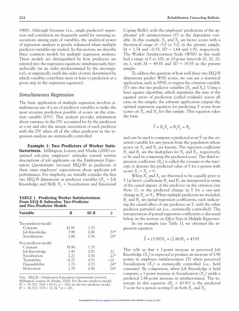
TABLE 1. Predicting Worker Satisfactoriness From EEQ-B Subscales: Two-Predictor and Five-Predictor Models

Variable B SE B β

Two-predictor modelConstant 43.91 1.57Job Knowledge 3.98 0.66 .33*Socialization 2.86 0.56 .28*

Five-predictor modelConstant 39.96 1.75Job Knowledge 1.43 0.87 .12Socialization 2.21 0.56 .22*Trainability −0.27 0.71 −.02Dependability 2.73 0.73 .24*Motivation 1.79 0.80 .16*

Note. EEQ-B = Employment Expectations Questionnaire (revised;Millington, Leierer, & Abadie, 2000). For the two-predictor model, R2 = .29, F(2, 316) = 63.11, p < .001; for the five-predictor model, R2 = .34, F(5, 313) = 32.24, * p < .001.

at CONCORDIA UNIV LIBRARY on June 23, 2010 http://rcb.sagepub.comDownloaded from

Volume 49, No. 4 (Summer 2006) 225

SPSS also outputs a standard error, t statistic, and p value for each regression coefficient. If the p value is lessthan the designated alpha level for the study (e.g., p <.05), the regression coefficient differs significantly fromzero, indicating a significant association between the des-ignated predictor and the criterion variable, controllingfor the remaining predictors. In this rather large sample(N = 319), both X1 and X2 are significant predictors of Y(both p < .001).

A final item of interest (especially when the goal ofthe study is to predict as much variance as possible in thecriterion) is the multiple correlation (R = .53), represent-ing the correlation between the predicted scores Y and theactual scores (Y) on the criterion variable; its square, R2 =.29, F(2, 316) = 63.11, p < .001, is interpreted as the pro-portion of variance in Y that is accounted for by the pre-dictor variables as a set. The significance test for R2 is anF test (which is identically also a significance test for R);when the associated p value is less than the designatedcritical value (e.g., p < .05), the multiple correlation coef-ficient differs significantly from zero, indicating a signifi-cant association between the predictors as a set and Y.

Example 2: Five Predictors of Worker Satis-factoriness. In point of fact, the EEQ-B has five sub-scales denoting aspects of employability. (In addition toX1 and X2, described above, these are X3 = Trainability/Flexibility; X4 = Dependability; and X5 = Motivation.)Table 1 (bottom section) shows how the regression of Y onto all five predictors compares with the simpler two-predictor model just discussed.

First, from the note to Table 1, we see that the threeadditional predictors increase the proportion of Y vari-ance explained: R2 = .29 for the two-predictor model, ascompared with .34 for the five-predictor model. Second,notice that in the five-predictor model (unlike the sim-pler model), not all of the X variables contribute uniquelyto prediction of scores on the WSS. In the five-predictormodel, only Socialization, Dependability, and Motivationemerge as significant predictors of satisfactoriness.

This finding illustrates an important consideration ininterpreting results of MRC analyses, namely that the as-sociation between a predictor and a given DV depends onthe other predictors included in the regression equation.The Job Knowledge subscale (X1) is a significant univari-ate predictor of Worker Satisfactoriness ratings (rY1 = .48,p < .05), and it is also significant in the two-predictormodel, controlling for X2 (βY1.2 = .33, p < .05). In thefive-predictor model, however, X1 does not contribute sig-nificantly to predicting Y when the other four EEQ-B sub-scales are statistically controlled (βY1.2345 = .12, p > .05).This reduction in the standardized regression coefficient β(which corresponds to similar decreases in the unstan-dardized coefficient B) as additional predictor scales areadded to the model reflects the intercorrelations among

EEQ-B subscales, or, to put it another way, the redundancyof the information provided by X1 ratings with that pro-vided by ratings on the other four subscales. When all fiveEEQ-B dimensions are included, the unique (nonredun-dant) information provided by X1 does not contribute sig-nificantly to our ability to predict WSS scores.

Summary. Simultaneous regression yields informa-tion about the joint association of a set of predictor vari-ables with Y (multiple R2 and associated significance test)and about the unique association of each predictor Xi withY, when all other predictor variables are statistically con-trolled (Bi or βi and the associated significance test). Be-cause correlations among predictor variables are the rulein nonexperimental research, the interpretation of theregression coefficient (B or β) is relative to the otherpredictors included in the regression equation; variablesthat are significant predictors of the DV in one analysismay become nonsignificant in subsequent analyses if ad-ditional, overlapping predictor variables are added.

Hierarchical Regression

In hierarchical regression analysis (HRA), predictor vari-ables are entered sequentially in two or more sets, withthe groupings and order of entry predetermined by theinvestigator. Nielsen (2003) used HRA to determinewhether social support added significantly to the predic-tion of posttraumatic stress disorder (PTSD) among 168adults with spinal cord injury, over and above the vari-ance predicted by demographic and injury-related vari-ables (gender, age, education, marital status, time sinceinjury, loss of consciousness as a result of injury, and neu-rological level).

Nielsen (2003) entered the demographic and injury-related variables to be statistically controlled as the firstblock in the HRA. The results for this first block are iden-tical to those for a simultaneous regression of PTSD scoresonto these seven predictor variables. As a set, these vari-ables were significantly related to PTSD symptoms: R2 =.10, F(7, 160) = 2.6, p < .05. Regression coefficients fortwo of the predictors in this set differed significantly fromzero: marital status (married persons were less likely to re-port PTSD symptoms) and neurological level (higherneurological functioning predicted fewer PTSD symp-toms).

Nielsen (2003) incorporated two social supportscales, one measuring total quantity of support and one as-sessing satisfaction with support. She entered these twovariables as a second block in the HRA. At this secondstep, the new predictors are added, and all of the originalpredictors remain in the predictor set. Thus, PTSD scoresare simultaneously regressed onto demographic variables,injury-related variables, and the two social support scores;

at CONCORDIA UNIV LIBRARY on June 23, 2010 http://rcb.sagepub.comDownloaded from

226 Rehabilitation Counseling Bulletin

however, R2 for these nine variables as a set is not thefocus of interpretation. Instead, Nielsen examined thechange in R2 (∆R2) from Block 1 to Block 2. In this case,the additional variance explained when the Block 2 vari-ables were added to the predictor set was both substantialand statistically significant: ∆R2 = .19, F(2, 158) = 21.0, p < .001. This significant increment to the variance ac-counted for by the prediction model affirms that the socialsupport measures, as a set, contribute significantly to theprediction of PTSD scores, over and above the demo-graphic and injury-related predictor variables.

In addition, it is appropriate to examine the regres-sion coefficients for the two social support scales to seetheir relative contributions to predicting PTSD. Nielsenfound that the total support score was a significant uniquepredictor, but overall satisfaction was not significantly re-lated to PTSD, controlling for the other eight predictorsin the equation at Block 2.

Summary. In the social sciences, variables of inter-est are not always capable of experimental manipulation,for either ethical or practical reasons. As noted in the pre-vious section, a central problem for disentangling causalrelations among measured (as opposed to experimentallymanipulated) variables is the issue of correlated predictors.When predictor variables are not statistically indepen-dent of one another, they will account for overlapping(common) variance as well as unique variance in the cri-terion variable. HRA allows the investigator to enter in-dividual predictors or sets of predictors in a specified order(in accordance with causal or conceptual priority). InHRA, the initial predictor set gets credit for all of the cri-terion variance it can account for; the second predictorset gets credit for only the additional criterion variance ituniquely accounts for (beyond that accounted for inBlock 1: i.e., ∆R2). If there is a third predictor set, it getscredit for unique variance accounted for over and abovethat predicted by Blocks 1 and 2 combined, and so on.Thus, investigators can use HRA to examine the criterionvariance uniquely accounted for by a predictor variable(or set) of theoretical interest (such as social support, forNielsen, 2003), after controlling for potential confound-ing variables that have a causally prior association withthe criterion variable. Other applications of HRA (someof which we discuss in more detail below) include analy-sis of nominal (i.e., categorical) variables using MRC,testing moderator relations (i.e., statistical interactionsamong two or more predictors), and assessment of incre-mental predictive validity from the addition of a new pre-dictor variable to an existing predictor set.

EMPIRICAL (STEPWISE) REGRESSION

Another option for establishing an order of entry for vari-ables in a hierarchical analysis is to use empirical rather

than theoretical criteria. In a stepwise regression analysis,the bivariate association of each predictor variable withthe criterion variable is examined, and the variable with the greatest predictive power is entered first. Thenthe remaining predictors are assessed for their incremen-tal predictive validity, and the one that explains the mostadditional criterion variance (i.e., the one that results inthe largest ∆R2) is added second. This procedure is re-peated until no further predictors would result in a signif-icant ∆R2, at which point the final predictor set (whichnormally contains only a subset of the possible predictorvariables) is regarded as definitive. Most statistical soft-ware packages include several variants on this procedure(e.g., step-up, step-down), which automate the process ofselecting variables for inclusion in the regression equa-tion.

Empirical regression methods may be appealing be-cause they relieve the researcher of having to maketheory-based decisions about the order of entry of predic-tor variables (Cohen et al., 2003). Indeed, although onlyone study published in Rehabilitation Counseling Bulletin inthe 5-year period we surveyed used stepwise regressionanalyses, this technique was much more common in Re-habilitation Psychology: In our survey of four consecutive is-sues (1 year) of this journal, we found that 5 of the 16articles using MRC used empirical regression methods.

The consensus in the methodological community isthat stepwise regression should be used very rarely (seeCohen et al., 2003, p. 162) or not at all (Thompson,1995) in psychological research. The main critique ofstepwise methods is that they yield a so-called optimalpredictor set that is very unlikely to generalize to futuresamples. We recommend that rehabilitation researchersfamiliarize themselves with the weaknesses of stepwisemethods and avoid using these procedures, substitutingeither simultaneous regression or HRA.

EFFECT SIZE IN MRC

Following a decade of increasingly strident criticism ofpsychology’s reliance on p values as summaries of studyfindings (see Kline, 2004, pp. 6–17, for a brief historicaloverview), the American Psychological Association con-vened a Task Force on Statistical Inference and charged itwith making recommendations about research design andinterpretation for the new century. Among many helpfulrecommendations in the report of this task force (Wilkin-son & the Task Force on Statistical Inference, 1999) is theexhortation to “always present effect sizes for primary out-comes” (p. 599).

An effect size quantifies the magnitude of associationbetween two (or more) variables. Effect sizes tell readersmore than simply that “X is significantly related to Y”;they indicate both the strength and the direction of the

at CONCORDIA UNIV LIBRARY on June 23, 2010 http://rcb.sagepub.comDownloaded from

Volume 49, No. 4 (Summer 2006) 227

relationship. Users of MRC are fortunate to have avail-able a variety of effect size indices among which tochoose. In this section, we highlight the most commonlypresented effect size indices and discuss how each is inter-preted.

Effect Sizes in Bivariate RegressionBy definition, bivariate regression analysis involves onepredictor variable and one criterion variable. There aretwo possible effect sizes that can be reported from such ananalysis: unstandardized and standardized.

Unstandardized Regression Coefficient. Thebrief summary of MRC given previously focused on whatis properly called the unstandardized regression coefficient,or B1. When Y is regressed onto a single predictor variable(X1), B1 tells the predicted change in Y (or, equivalently,the change in Y for a one-unit change in X1. Geometri-cally, it represents the slope of the Y-on-X1 regression line,when X1 and Y are scaled in their original (raw score)units. In causal terms, we can think of B1 as reflecting thecausal impact (or effect) on Y of a one-unit increase in X1.

Consider the Millington et al. (2000) study describedin Examples 1 and 2 in the Regression Models section. IfWorker Satisfactoriness (Y) is regressed onto Job Knowl-edge (X1) as the sole predictor variable, we obtain aregression coefficient of BY1 = 5.69. This represents a pre-dicted increase of 5.69 satisfactoriness points for every 1point gained in ratings of Job Knowledge. So, if a trainingprogram were created to enhance job-specific knowledgeand skills, and that program led to average gains of 2 points in X1 scores, we would expect an indirect effecton WSS ratings of 2(5.69), or about 11 points.

Standardized Effect Sizes. Note that in this ex-ample, if readers are unfamiliar with either or both mea-sures (EEQ-B or WSS), the unstandardized regressioncoefficient BY1 may not be very meaningful. It is difficultat a glance to tell whether a 5.69-unit increase on Y foreach unit increase on X1 is a large or important effect.When the units of measurement on one or both variablesare not readily interpretable, Wilkinson and the TaskForce on Statistical Inference (1999) recommend report-ing standardized coefficients. A standardized regression coef-ficient is the regression coefficient that would be obtainedif we first transformed Y and X1 into their respective z scores (zY and z1; see Note 2) and then regressed zY ontoz1. We can convert the unstandardized regression coeffi-cient BY1 into the equivalent standardized regression coef-ficient (denoted as βY1) by multiplying it by the ratiosd1/sdY. Thus,

Standardized regression coefficients are scaled identicallyto the Pearson r (i.e., –1 ≤ βY1 ≤ 1), with large positive (orlarge negative) coefficients indicative of a strong relationbetween X1 and Y. In fact, for bivariate regression, βY1 isidentical to the Pearson product-moment correlation(rY1), and each can be interpreted as the predicted changein Y, in standard deviation (SD) units, for a 1-SD changein X1. That is, if two people differ by 1 SD (1.64 points)in their Job Knowledge scores, we expect a difference ofabout 0.48 SDs (or about 9.4 points) in their satisfactori-ness ratings. Because the coefficient is positive, we expectthat the person scoring higher on the EEQ-B will be ratedhigher on the WSS.

A second use of the Pearson r as an aid to interpret-ing magnitude of association is to square the correlationcoefficient and interpret it as an index of variance ac-counted for. In this example, r2 = (.48)2 = .23. Thus, jobknowledge ratings account for 23% of the variance inWSS scores.

When the units of measurement are meaningful on apractical level (e.g., number of cigarettes smoked per day),it is usually preferable to report an unstandardized measure(regression coefficient or mean difference) rather than astandardized measure (r or d; Wilkinson & the Task Forceon Statistical Inference, 1999). When reporting an effectsize, it is also helpful to add brief comments (e.g., com-parisons with effect sizes obtained in related investi-gations) to assist readers in gauging the practical andtheoretical importance of this association.

Effect Sizes in Multiple RegressionMultiple regression is often used to examine the (presumedcausal) effects of correlated predictors on a DV. When twoor more predictors are examined simultaneously, the co-efficients in the regression equation are termed partialregression coefficients, to reflect the fact that in deter-mining the predicted effect of each variable on the DV,the effect of each of the other predictor variables is heldconstant, or partialed out.

Meaning of Partial Coefficients. To illustrate,consider Example 1 in the Regression Models section, inwhich we simultaneously regressed WSS scores onto X1and a second EEQ-B subscale (X2 = Socialization andEmotional Coping Skills). In this example, we are inter-ested in the joint effects of Job Knowledge (X1) and So-cialization (X2) on Worker Satisfactoriness (Y). BecauseX1 and X2 are correlated (r12 = .50), the squared bivariatecorrelation of each of these predictors with satisfactori-ness (i.e., r2

Y1or r2Y2) reflects a combination of unique

variance shared with Y and common variance shared withboth the other predictor and Y. To assess the uniquecontribution of each variable to predicting Y, we usedmultiple regression, constructing a least squares regression

βY1 = BY1 = 5.69 = .48sd1

sdY

1.6419.55( )

at CONCORDIA UNIV LIBRARY on June 23, 2010 http://rcb.sagepub.comDownloaded from

228 Rehabilitation Counseling Bulletin

equation for predicting Y from scores on both X1 and X2(see Table 1).

Because X1 and X2 are correlated, the partial regres-sion coefficient in Equation 1 is not equal to the bivariateregression coefficient described in the preceding section.This difference is reflected by a change in the notation ofthe regression coefficient: The bivariate coefficient is de-noted as BY1, whereas the partial coefficient is denoted asBY1⋅2 (i.e., the regression of Y on X1 from which X2 hasbeen partialed). In general, it is expected that BY1⋅2will besmaller in absolute value (i.e., closer to zero) than BY1 (seeNote 3).

The partial regression coefficient BY1⋅2 is the pre-dicted change in Y for a given change in X1, when X2scores are statistically controlled (i.e., held constant). Inreality, if a person’s Job Knowledge score (X1) increases,we expect a corresponding (although somewhat smaller)increase in Socialization (X2) (because r12 > 0), with bothchanges (in X1 and X2) producing corresponding changesin Y. To examine the unique effect of X1 on Y, indepen-dent of the common variance shared with X2, we need tohold the value of X2 constant and see what happens to Ywith a given change in X1. Although this is not possiblein reality, we can accomplish this feat mathematically;this is what is meant when we say that BY1⋅2 is the (par-tial) regression coefficient for Y on X1, statistically control-ling for X2.

The partial regression coefficient BY1⋅2 can also bethought of as the slope of the partial regression line when Yis regressed onto X1 for a sample of individuals who sharethe same score on X2. This formulation reminds us of animportant assumption underlying this discussion of partialcoefficients: These interpretations hold as long as theslope of the partial regression of Y on X1 is identical for allvalues of X2. This assumption can be tested by examiningthe significance of the X1-by-X2 interaction. When thereis no significant interaction between X1 and X2 in pre-dicting Y, the partial regression of Y on X1 is independentof X2, or, equivalently, the slope of the partial regressionline when Y is regressed onto X1 does not depend on thevalue of X2. When the X1-by-X2 interaction is significant,however, the effect of X1 on Y differs at different levels ofX2, which is to say that different Y-on-X1 partial regres-sion lines (i.e., regression lines for different constant val-ues of X2) have different slopes (see Note 4).

Unstandardized Partial Coefficients. As justnoted, the unstandardized partial regression coefficientBY1⋅2 reflects the predicted change in Y for a one-unitchange in X1 when X2 is held constant. This quantifiesthe unique (presumed causal) effect of X1 on Y, fromwhich its joint effect with X2 has been partialed. FromTable 1, the partial regression coefficient BY1⋅2= 3.98,about 30% smaller than the corresponding bivariate coef-ficient (BY1 = 5.69) given earlier. Thus, almost one third

of the bivariate association between X1 and Y is attribut-able to the overlap between X1 and X2. The interpretationof this discrepancy between bivariate and partial coeffi-cients (and the interpretation of partial coefficients moregenerally) depends on the hypothesized causal model forassociations among these variables (see Cohen et al.,2003, pp. 75–79).

Standardized Partial Coefficients. As in thecase of bivariate regression, when the units of predictor orcriterion variables are not intuitively meaningful, it is usu-ally preferable to report standardized effect sizes. Twostandardized effect size measures, β and sr2, are commonlyused to reflect the unique contribution of a single predic-tor variable in standardized units; a third measure, R2, re-flects the variance accounted for by a set of predictors inMRC.

Standardized partial regression coefficient (β). As inthe bivariate case, βY12 can be computed from BY12 bymultiplying the latter by the ratio sd1/sdY. Thus,

Thus, when Socialization scores are statistically controlled,a 1-SD (i.e., 1.64-point) increase in Job Knowledge is pre-dicted to result in a corresponding increase in Y of 0.33SD units (or about 6.5 points). Note that when the SDs ofthe predictor variables differ, their unstandardized regres-sion coefficients are not comparable. The two betaweights, however, are both standardized and directly re-flect the relative strength of association. For this example,βY2⋅1 = .28, which is somewhat smaller than βY1⋅2 = .33.This implies that socialization ratings have a slightlysmaller unique association with predicted satisfactorinessthan job knowledge ratings; however, a statistical signifi-cance test (e.g., Azen & Budescu, 2003) should be con-ducted before strong inferences are made about therelative importance of predictors in MRC.

Squared semipartial correlation (sr2). When MRC isused for predictive purposes, rather than for analysis ofpresumed causal associations, investigators may wish toreport on the proportion of variance in Y uniquely ac-counted for by one predictor variable. The semipartialcorrelation (which some statistical packages refer to bythe older name part correlation), when squared, is the rele-vant effect size. Because these are standardized effect sizes,comparison of the squared semipartials gives an indicationof the relative unique contributions of different predictors(although again, strong conclusions about differences inpredictive validity should be based on significance testsrather than on numerical differences alone). For Example1, sr1

2 = .08 and sr22 = .06, again reflecting the slightly

larger unique contribution of Job Knowledge, relative toSocialization, in predicting Worker Satisfactoriness.

βY1.2 = BY3.2 = 3.98 . = .33sd1

sdY

1.6419.55

at CONCORDIA UNIV LIBRARY on June 23, 2010 http://rcb.sagepub.comDownloaded from

Volume 49, No. 4 (Summer 2006) 229

It is helpful to recall that significance tests for B, β,and sr2 are identical—if one is statistically significant, theothers will be as well. The choice of which effect size toreport is based on the nature of the research question (i.e.,causal analysis vs. predictive validity) and on whether theunits of measurement are inherently meaningful.

Squared Multiple Correlation (R2). A final ef-fect size commonly reported in multiple regression analy-ses reflects the proportion of variance in Y accounted forby all of the predictors together, as a set. The multiple cor-relation coefficient (R) is the correlation between the pre-dicted Y scores (computed for each participant in thestudy using Equation 1) and the actual measured Y scores.For our example study, R2 = .29, which indicates that jobknowledge and socialization jointly account for 29% ofthe variance in Worker Satisfactoriness ratings.

SPECIALIZED APPLICATIONS

OF MRC

The shift from a simultaneous approach to multiple re-gression (in which the dependent variable is regressedonto all predictors simultaneously) to a hierarchical ap-proach (in which sets of predictors are entered sequen-tially in an order predetermined by the investigator)greatly enhances the flexibility of MRC analyses to ad-dress a variety of research hypotheses of interest to re-searchers in the social sciences. We have already notedone important application of HRA, in which the first pre-dictor set serves as a statistical control of potential con-founding variables, and the predictors of theoreticalimport are entered as a second block. The ∆R2 for Block 2represents the unique (and hence unconfounded) associa-tion of this second predictor set with the criterion vari-able. In the next sections, we consider applications ofMRC to research questions involving categorical ratherthan continuous measures, to mediator hypotheses, toanalysis of change, and to moderator hypotheses (i.e., sta-tistical interactions).

CATEGORICAL VARIABLES

AND MRC

Categorical Variables as Predictors

Coding Dichotomous Variables. Regressionand correlation methods were developed to quantify rela-tions among continuous variables. However, categorical(nominal) variables may also be analyzed using MRC.This process is straightforward for dichotomous variables(i.e., nominal variables with exactly two categories). Forexample, Nielsen (2003) included gender and marital sta-

tus among her control variables. Each of these was adichotomous variable, which could be included in theanalysis by assigning a numerical code to each of the cat-egories (e.g., 0 = male; 1 = female). Although any two dif-ferent numerical values will work, the zero–one coding(called dummy coding) is a good approach, as it makes theregression coefficient for this coded variable easy to inter-pret. Specifically, if gender (coded 0 or 1, as above) is theonly predictor (X1), then the intercept (B0) represents thepredicted Y score for males (best estimate of the criterionwhen X1 = 0). By extension, B1 represents the differencebetween means for females and males (i.e., B1 = Mf − Mm).This follows from the definition of the regression coeffi-cient: the predicted change in Y for a one-unit change inX1 (i.e., the change in means from the group coded as 0 tothe group coded as 1).

Interpretation of the (partial) regression coefficientfor gender when multiple predictors are included in theregression analysis follows this same principle, except thatin this case B0 and B1 will be functions of adjusted means(controlling for the other predictor variables in the equa-tion; see Cohen et al., 2003, pp. 342–350). Becauseregression coefficients for dichotomous variables are in-terpretable only if the numerical codes for the categoriesare known, it is crucial that investigators state how thesevariables were coded, either in the methods section or inthe results section (and also in the table note, when re-gression results are tabulated).

Coding Polychotomous Variables. When anominal variable has more than two categories (groups),the information from that variable cannot be completelyrepresented by a single code variable. In general, if a nom-inal variable encompasses g groups, a set of (g − 1) codevariables will be needed to represent membership in thesegroups as a predictor in MRC. These code variables canthen be entered as a set in HRA to assess the associationbetween the categorical predictor variable and the con-tinuous dependent variable. More details on creatingdummy coded variables, on other coding schemes, and oninterpreting regression output involving sets of variablescoded to represent nominal scales can be found in mostgraduate level textbooks on MRC (e.g., Cohen et al.,2003, chap. 8; Pedhazur, 1982, chap. 9). Using these cod-ing strategies, and entering coded variables as sets inHRA, allows researchers to combine categorical and con-tinuous predictors within the MRC framework.

Categorical Variable as CriterionRehabilitation researchers are often interested in outcomevariables that are dichotomous rather than continuous.For example, Taylor et al. (2003) followed children for 4 years following a traumatic brain injury (TBI) to iden-tify predictors of long-term education outcomes. The de-

at CONCORDIA UNIV LIBRARY on June 23, 2010 http://rcb.sagepub.comDownloaded from

230 Rehabilitation Counseling Bulletin

pendent variable for this study was placement in specialeducation (vs. no special education). When the depen-dent variable is naturally categorical, as here, traditionalMRC techniques cannot be used. However, a related an-alytic technique called logistic regression is designed forcategorical and continuous predictors of categorical crite-rion variables. Logistic regression can be conducted witheither simultaneous or sequential (hierarchical) entry ofpredictors, and it provides estimates of both the uniquecontribution of individual predictors and the joint contri-bution of sets of predictors to the prediction of outcomestatus (Cohen et al., 2003, chap. 13). Thus, categoricaldependent variables, like categorical predictor variables,can be accommodated within the broad family of MRCtechniques.

TESTS OF MEDIATOR AND MODERATOR

HYPOTHESES IN MRC

When previous research has demonstrated an associationbetween a predictor variable (designated as the indepen-dent variable, or IV, to reflect its presumed causal priority)and a dependent variable (DV), investigators may wish toexamine proposed mediators or moderators of this associ-ation. Although the terms mediator and moderator aresometimes used interchangeably, they have distinct mean-ings in the context of hypothesis formulation and dataanalysis (Baron & Kenny, 1986). A mediator is an inter-vening variable that is caused by the IV, and that in turncauses the DV, so that at least part of the causal effect ofthe IV on the DV is explained by its indirect effect via themediator. A moderator is a third variable that affects the strength or the direction of the association betweenthe IV and the DV.

Baron and Kenny (1986) provided an informativediscussion of these terms, with details about how to testeach of these types of hypotheses using MRC. Anothervery helpful resource for testing moderator hypothesesusing MRC is Aiken and West (1991, especially chap. 2).More recently, Frazier, Tix, and Barron (2004) published auseful, step-by-step guide to testing mediator and modera-tor hypotheses and reporting findings. The astute readerwill note that all of these sources recommend MRC as theoptimal analysis for testing mediator and moderator hy-potheses involving naturally continuous variables. In par-ticular, researchers should avoid the common practice ofdichotomizing continuous predictor variables (using a“median split,” for example) so that ANOVA may be usedto test moderator hypotheses (statistical interactions). Asdemonstrated by MacCallum, Zhang, Preacher, andRucker (2002), dichotomization of continuous variablesfor any type of analysis (not just moderator analyses) com-promises statistical power and can yield misleading results.Any of the references just cited can assist readers in ana-

lyzing and interpreting interactions between continuouspredictors using MRC.

ANALYSIS OF CHANGE IN MRC

When data are collected at two or more time points, in-vestigators may test hypotheses involving prediction ofchange in the dependent variable over time. Such analy-ses always (either explicitly or implicitly) involve compu-tation of change scores reflecting the change in status foreach individual on the dependent variable between thetwo time points of interest. Appropriate analysis of hy-potheses involving change is the subject of a rich litera-ture (see the classic paper by Cronbach & Furby, 1970, for a thorough introduction); here we mention only onesmall controversy, which relates to the use of MRC.

The most natural, and perhaps the most commonmethod of testing hypotheses of change between two timepoints uses difference scores, which are derived by subtract-ing each person’s score at Time 1 from his or her score atthe later Time 2, as an index of change. Difference scoresare an intuitive means to quantify change over time, andare used implicitly in such common analyses as the t testfor dependent samples and the group × time (repeatedmeasures) ANOVA for assessing treatment effects (Huck& MacLean, 1975). Difference scores have been criticizedas an index of change, however, because they are neces-sarily (negatively) correlated with Time 1 scores (Cohenet al., 2003, pp. 59–60). When investigators wish to cre-ate change scores that are statistically independent of ini-tial status, they should use residualized change scores (alsocalled partialed change scores; Cohen et al., 2003, pp. 570–571), regressing Time 2 scores (DV) onto Time 1 scores(predictor) and saving the residuals as an index of change.By definition, these residuals are independent of (i.e., un-correlated with) Time 1 status. Residualized change scoresare implicitly analyzed when ANCOVA is used to test for group differences with initial scores on the DV as acovariate (Kenny, 1979, chap. 11). Likewise, in any re-gression analysis with Time 2 scores as the dependentvariable, where Time 1 scores on this DV are entered asone of the predictor variables, the partial regression coef-ficients for the remaining predictor variables reflect theirassociation with change on the DV (i.e., with participants’residualized change scores on this variable, describedabove).

MISCELLANEOUS TOPICS

Power Analysis in MRC

An important question for the design of research studiesusing MRC concerns the sample size necessary to have ad-

at CONCORDIA UNIV LIBRARY on June 23, 2010 http://rcb.sagepub.comDownloaded from

Volume 49, No. 4 (Summer 2006) 231

equate statistical power. Methodologists commonly rec-ommend that researchers aim for power of at least .80,which corresponds to a Type II error rate of 20%. Proce-dures for estimating statistical power differ for two types of hypothesis testing common to studies using MRC: (a) tests that determine whether the multiple correlation(R) between a set of predictors and the criterion variableis different from zero and (b) tests to determine whetherthe association of a single predictor variable (or a set ofvariables, when HRA is used) with the DV is nonzero,when other predictors are also in the regression equation(and therefore are statistically controlled)—that is, testsof the significance of B, β, or sr2. A challenge for poweranalysis for each of these analyses, but especially for thesecond type of research question, is the determination ofthe expected effect size. Because of space limitations (andbecause excellent resources on power analysis are readilyavailable), we provide only a brief introduction to poweranalysis in MRC.

Although several rules of thumb have been proposedfor determining sample size in MRC (e.g., N = 10k, wherek is the number of predictor variables), none of these isabove reproach, and most bear little or no relation to theactual (complex) relation between power and sample size(Maxwell, 2000). An important reason for this failure isthat these rules of thumb completely ignore the most im-portant determinant of power other than sample size,which is the effect size. The best approach is to conduct apower analysis using a predicted effect size to determinethe sample size (N) necessary to attain a specified powerlevel (Cohen, 1988). See Cohen et al. (2003) for conciseinstructions on conducting a power analysis for testing thehypothesis that R2 = 0 (p. 92) or for instructions on test-ing that incremental variance explained by a new set ofvariables (denoted as Set B; variance explained uniquelyby this set of predictors is denoted sR2

B) is zero (pp. 176–177). The latter test works for sets containing a singlevariable (i.e., kB = 1) or multiple variables (i.e., kB > 1).When kB = 1, the significance test for sR2

B is identical tothat for B or β (even if all predictors are entered simulta-neously rather than using HRA).

In summary, rules of thumb for determining samplesize based only on the number of predictor variables aremisleading, and they bear little relation to actual statisti-cal power. Power calculations should be based on the ex-pected effect size (either R2 or sR2

B).

FACTORS AFFECTING EFFECT

SIZE ESTIMATES

We noted that a convenience of MRC is the plethora ofeffect size measures available from regression analyses.This boon is mitigated somewhat by the caveat that, for avariety of reasons, observed correlation and regression co-

efficients typically distort the true magnitude of asso-ciation between constructs in the population under study.Fortunately, the direction of bias in the effect size esti-mates is predictable and can (and should) be taken intoaccount in interpreting study findings.

Measurement Error and AttenuationA factor that universally affects research using measured(rather than experimentally manipulated) variables is mea-surement error. Scores on psychological assessments arealways less than perfectly reliable, so that variance in scoresreflects a composite of error variance and true score vari-ance. Because the error components of two sets of scoresare, by definition, uncorrelated, correlations between mea-sured variables are always attenuated (i.e., reduced) rela-tive to the correlations between their respective truescores. As score reliability decreases, the degree of attenu-ation of the bivariate correlation increases (Schmidt &Hunter, 1999). In other words, the poorer the reliabilityof its measures, the greater the degree to which a study’s

observed correlation is expected to underestimate the true (population) correlation between the constructs ofinterest.

Distribution, Range Restriction, and DichotomizationOther factors can attenuate effect sizes in correlational re-search (see Cohen et al., 2003, pp. 51–62). When scoreson one variable are significantly skewed, correlations withother measures will be attenuated. When the range ofscores in the sample is restricted relative to the range inthe population, correlations with scores on another vari-able will be attenuated. When researchers convert con-tinuous measures to dichotomous measures (usually so thatthey can use ANOVA rather than MRC), they discardvalid variance and further attenuate correlations betweenthis variable and others in their study. In bivariate analy-ses, all of these factors act to attenuate the observed effectsize, producing observed effect sizes (r or B) that under-estimate the corresponding population effect size.

SummaryResearchers studying measured (rather than experimen-tally manipulated) variables should be aware that ob-served effect sizes are generally attenuated relative to thecorresponding population effect size and that the degreeof attenuation can be minimized by (a) using reliablemeasures of the constructs of interest; (b) transforminghighly skewed variables prior to analysis; (c) samplingbroadly to reduce the risk of range restriction; and (d) us-ing MRC methods to analyze continuous variables (ratherthan dichotomizing these scores to analyze them using

at CONCORDIA UNIV LIBRARY on June 23, 2010 http://rcb.sagepub.comDownloaded from

232 Rehabilitation Counseling Bulletin

ANOVA). When multiple predictor variables are ana-lyzed, the effects of measurement error, deviations fromnormality, and range restriction on partial coefficients aremore complex. For example, low reliability in a variablethat is statistically controlled in a given analysis can havethe effect of inflating, rather than attenuating, the partialregression coefficient between another predictor and thecriterion (Cohen et al., 2003, pp. 122–124). Also, the sta-tistical power of moderator analyses is particularly stronglyreduced by unreliability of measurement, because the reli-ability of the product term (which carries the interactionvariance) is primarily a function of the product of the re-liabilities of the IV and the moderator variable (Aiken &West, 1991, pp. 144–145), especially when the IV andmoderator are only weakly correlated with one another.

CONCLUSION

MRC techniques give researchers the flexibility to addressa wide variety of research questions of interest to rehabil-itation professionals. Good data analysis begins with care-ful conceptualization (selecting constructs of interest andcreating theory-derived hypotheses about the relationsamong them) and thoughtful choice of measures. Poweranalysis, relying on estimates from past research or esti-mates about the likely magnitude of hypothesis-relevanteffect sizes, is an essential component of good research de-sign. It is critical that the analysis chosen conform to thehypothesis to be tested, and that observed effect sizes, aswell as significance tests, be presented and interpreted assubstantive findings concerning the magnitude of hypothe-sized associations.

NOTES

1. Although we follow the linguistic conventions thattreat the predictor variable as the putative cause of thecriterion variable, it is important to remember that re-gression is a correlational analysis and does not by itselfprovide empirical evidence of a cause-and-effect rela-tion between two variables.

2. The z score is a deviation score that is expressed in SDunits:

where zi is the z score for person i, Xi is the raw score forthat person, MX is the mean of all the X scores in thesample, and SDX is their standard deviation. If zi = 1.0,this means person i scored 1 SD above the samplemean.

3. The exception to this general rule, in which the partialcoefficient BY1⋅2 is larger in absolute value than the cor-

responding bivariate coefficient BY1 (or, equivalently,the standardized partial coefficient βY1⋅2 is larger thanthe bivariate correlation rY1), is known as suppression.Although bona fide cases of suppression appear to befairly rare in the social science literature, they do exist,and this pattern of relations can have theoretical sig-nificance. For a detailed discussion of suppression, withsubstantive examples, see Tzelgov and Henik (1991).

4. By symmetry, everything said in the last three para-graphs about BY1⋅2 also applies to BY2⋅1, if X1 and X2 areinterchanged.

REFERENCES

Aiken, L. S., & West, S. G. (1991). Multiple regression: Testing and in-terpreting interactions. Newbury Park, CA: Sage.

Azen, R., & Budescu, D. V. (2003). The dominance analysis approachfor comparing predictors in multiple regression. Psychological Meth-ods, 8, 129–148.

Baron, R. M., & Kenny, D. A. (1986). The moderator-mediator vari-able distinction in social psychological research: Conceptual, strate-gic, and statistical considerations. Journal of Personality and SocialPsychology, 51, 1173–1182.

Cohen, J. (1968). Multiple regression as a general data-analytic strategy.Psychological Bulletin, 70, 426–443.

Cohen, J. (1988). Statistical power analysis for the behavioral sciences (2nded.). Hillsdale, NJ: Erlbaum.

Cohen, J., Cohen, P., West, S. G., & Aiken, L. S. (2003). Applied mul-tiple regression/ correlation analysis for the behavioral sciences (3rd ed.).Mahwah, NJ: Erlbaum.

Cronbach, L. J., & Furby, L. (1970). How should we measure“change”—or should we? Psychological Bulletin, 74, 68–80.

Frazier, P. A., Tix, A. P., & Barron, K. E. (2004). Testing moderator andmediator effects in counseling psychology research. Journal of Coun-seling Psychology, 51, 115–134.

Huck, S. W., & MacLean, R. A. (1975). Using a repeated measuresANOVA to analyze the data from a pretest–posttest design: A po-tentially confusing task. Psychological Bulletin, 82, 511–518.

Kenny, D. A. (1979). Correlation and causality. New York: Wiley. Kline, R. B. (2004). Beyond significance testing: Reforming data analysis in

behavioral research. Washington, DC: American Psychological Asso-ciation.

MacCallum, R. C., Zhang, S., Preacher, K. J., & Rucker, D. D. (2002).On the practice of dichotomization of quantitative variables. Psy-chological Methods, 7, 19–40.

Maxwell, S. E. (2000). Sample size and multiple regression analysis.Psychological Methods, 5, 434–458.

Millington, M. J., Leierer, S. J., & Abadie, M. (2000). Validity and theEmployment Expectation Questionnaire–beta version: Do attitudesmediate outcomes? Rehabilitation Counseling Bulletin, 44, 39–47.

Nielsen, M. S. (2003). Prevalence of posttraumatic stress disorder inpersons with spinal cord injuries: The mediating effect of social sup-port. Rehabilitation Psychology, 48, 289–295.

Pedhazur, E. J. (1982). Multiple regression in behavioral research: Explana-tion and prediction (2nd ed.). Fort Worth, TX: Harcourt Brace.

Schmidt, F. L., & Hunter, J. E. (1999). Theory testing and measurementerror. Intelligence, 27, 183–198.

Taylor, H. G., Wade, S. L., Stancin, T., Yeates, K. O., Drotar, D., &Montpetite, M. (2003). Long-term educational interventions aftertraumatic brain injury in children. Rehabilitation Psychology, 48,227–236.

zi = Xi – MX

sdX

at CONCORDIA UNIV LIBRARY on June 23, 2010 http://rcb.sagepub.comDownloaded from

Volume 49, No. 4 (Summer 2006) 233

Thompson, B. (1995). Stepwise regression and stepwise discriminantanalysis need not apply here: A guidelines editorial. Educational andPsychological Measurement, 55, 525–534.

Tzelgov, J., & Henik, A. (1991). Suppression situations in psychologi-cal research: Definitions, implications, and applications. Psychologi-cal Bulletin, 109, 524–536.

Wampold, B. E., & Freund, R. D. (1987). Use of multiple regression incounseling psychology research: A flexible data-analytic strategy.Journal of Counseling Psychology, 34, 372–382.

Wilkinson, L., & Task Force on Statistical Inference. (1999). Statisticalmethods in psychology journals: Guidelines and explanations. TheAmerican Psychologist, 54, 594–604.

at CONCORDIA UNIV LIBRARY on June 23, 2010 http://rcb.sagepub.comDownloaded from