Analysing the Performance of a Compressor Impeller for a Micro Gas Turbine by Marco Bindeman April 2019 Thesis presented in partial fulfilment of the requirements for the degree of Master of Engineering (Mechanical) in the Faculty of Engineering at Stellenbosch University Supervisor: Prof. S.J. van der Spuy Co-supervisor: Prof. T.W. von Backström

Welcome message from author
This document is posted to help you gain knowledge. Please leave a comment to let me know what you think about it! Share it to your friends and learn new things together.
Transcript
Analysing the Performance of a Compressor
Impeller for a Micro Gas Turbine
by
Marco Bindeman
April 2019
Thesis presented in partial fulfilment of the requirements for the degree
of Master of Engineering (Mechanical) in the Faculty of Engineering at
Stellenbosch University
Supervisor: Prof. S.J. van der Spuy
Co-supervisor: Prof. T.W. von Backström

Declaration
By submitting this thesis electronically, I declare that the entirety of the workcontained therein is my own, original work, that I am the sole author thereof(save to the extent explicitly otherwise stated), that reproduction and publicationthereof by Stellenbosch University will not infringe any third party rights andthat I have not previously in its entirety or in part submitted it for obtaining anyqualication.
April 2019Date: . . . . . . . . . . . . . . . . . . . . . . . . . . . . . . . . .
Copyright © 2019 Stellenbosch UniversityAll rights reserved.
ii
Stellenbosch University https://scholar.sun.ac.za
Plagiarism Declaration
1. Plagiarism is the use of ideas, material and other intellectual property ofanother's work and to present it as my own.
2. I agree that plagiarism is a punishable oence because it constitutes theft.
3. I also understand that direct translations are plagiarism.
4. Accordingly all quotations and contributions from any source whatsoever(including the internet) have been cited fully. I understand that the repro-duction of text without quotation marks (even when the source is cited) isplagiarism.
5. I declare that the work contained in this assignment, except where otherwisestated, is my original work and that I have not previously (in its entiretyor in part) submitted it for grading in this module/assignment or anothermodule/assignment.
Student number Signature
Initials and surname Date
iii
M. Bindeman 21/02/2019
Stellenbosch University https://scholar.sun.ac.za
Abstract
Analysing the Performance of a Compressor Impeller for a
Micro Gas Turbine
M. Bindeman
Department of Mechanical and Mechatronic Engineering,
University of Stellenbosch,
Private Bag X1, Matieland 7602, South Africa.
Thesis: MEng (Mech)
April 2019
This project sets out to numerically evaluate the performance of micro gas turbine(MGT) compressor impellers and to improve the 1-Dimensional (1-D) mean-linecode developed for the in-house analysis of these impellers. The objective for theimprovement of the code is to accurately predict the performance of both radialow and mixed-ow impellers. The possible applications for MGTs are numer-ous. They nd specic application for the propulsion of unmanned aerial vehicles(UAVs). Mixed-ow compressors oer the opportunity to reduce the frontal areaof a MGT engine while maintaining a high pressure ratio and ensuring a highthrust-to-weight ratio. The use of mixed-ow impellers in MGTs are thus at-tractive. Although detailed aerodynamic design is normally based on two- andthree-dimensional viscous ow analysis, 1-D analysis with empirical work inputand loss models is the basis for most aerodynamic performance analyses. Using1-D mean-line ow analyses also allows the researcher to analyse multiple geome-tries in a short time span, while only analysing the best performing geometrieswith 3-D Computational Fluid Dynamics (CFD). Two areas of the mean-line codewere identied for improvement. A new slip factor formulation taking both radialand axial ow components into account was implemented. Secondly, an alterna-tive location for the inter-blade throat area was proposed, considering the areabetween a main blade and splitter blade, as opposed to the area close to the in-ducer section which is eectively between the main blades. The code was adaptedto calculate the throat parameters for the alternative location and two iterations
iv
Stellenbosch University https://scholar.sun.ac.za
ABSTRACT v
of the code were subsequently created. The rst employing the new slip factor andthe second employing both the new slip factor and an alternative throat location.Three dierent impellers, of which one impeller is a mixed-ow impeller, wereanalysed using the adapted mean-line code and the results were validated with 3-dimensional CFD. The newly adapted 1-D mean-line code was found to predict theperformance of the mixed-ow impeller reasonably well. The mean-line code overpredicted both the pressure ratio and isentropic eciency (total-to-total) by 1.6%and 2.8% respectively, while also predicting a larger operating range. The pressureratio of the centrifugal impellers was under predicted on average by 15%, whilethe the isentropic eciency was predicted within 3%. It was however found that ablade outlet angle of 90 adversely aected the performance prediction of the code.
Keywords: micro gas turbine, mixed-ow compressor, one dimensional mean-linecode.
Stellenbosch University https://scholar.sun.ac.za
Uittreksel
Analise van die Werksverigting van n Kompressor Rotor vir
n Mikro-gasturbine
(Analysing the Performance of a Compressor Impeller for a Micro Gas Turbine)
M. Bindeman
Departement Meganiese en Megatroniese Ingenieurswese,
Universiteit van Stellenbosch,
Privaatsak X1, Matieland 7602, Suid Afrika.
Tesis: MIng (Meg)
April 2019
Hierdie projek beoog om numeries die prestasie van mikro-gasturbine kompressorsrotor te evalueer, asook die 1-dimensionele (1-D) werkverrigting-berekeningskodewat ontwikkel is vir 'n interne analise van die rotors. Die mikpunt van die verbe-terde kode is om die prestasie van die radiale vloei en die gemengde-vloei rotorsakkuraat te voorspel. Daar is vele moontlike toepassings vir mikro-gasturbines.Mikro-gasturbines kan spesiek gebruik word vir die aandrywing van onbemandevliegtuie. Gemengde-vloei kompressors bied die geleentheid om die voorste areavan 'n mikro-gasturbine-enjin te verklein, terwyl dit 'n hoë drukverhouding en'n dryfkrag-tot-gewig verhouding behou. Die gebruik van gemengde-vloei ro-tors in mikro-gasturbines is dus aanloklik. Al is gedetailleerde aërodinamieseontwerpe gewoonlik gebaseer op 2- of 3-dimensionele viskeuse vloei-analise, is 1-dimensionele analises met empiriese werksinsette en werksuitsette se modelle diebasis vir die meeste aërodinamiese prestasie-analises. Deur die 1-D werkverrigting-berekeningvloei analise te gebruik, kan die navorser ook meervoudige geometrieëanaliseer in 'n kort tydperk, deur slegs die hoogs presterende geometrieë te ana-liseer met 3-D berekenings vloeidinamika. Twee areas van die werkverrigting-berekeningskode is geïdentiseer om te verbeter. 'n Nuwe glipfaktor formulering,wat beide die radiale en die aksiale vloei komponente in ag neem, is geïmplemen-teer. Tweedens is 'n alternatiewe posisie vir die inter-lem keëlarea voorgestel, watdie area tussen die hooem en die sekondêre lem in ag neem, eerder as die area
vi
Stellenbosch University https://scholar.sun.ac.za
UITTREKSEL vii
naby die inlaat wat eektief tussen die hooemme is. Die kode is aangepas omdie keëlparameters te bereken vir die alternatiewe posisie en twee iterasies vandie kode is vervolgens geskep. Die eerste een is die toepassing van die nuwe glip-faktor en tweede, die toepassing van beide die nuwe glipfaktor en 'n alternatiewekeëlposisie. Drie verskillende rotors, waarvan een 'n gemengde-vloei rotor was, isgeanaliseer deur die aangepaste werkverrigting-berekeningskode te gebruik en dieresultate is gevalideer met 3-dimensionele berekenings vloeidinamika. Die nuutaangepaste 1-D werkverrigting-berekeningskode het bevind dat die voorspellingvan die gemengde-vloei rotors se prestasie, redelik goed is. Die werkverrigting-berekeningskode het beide die drukverhouding en die isentropiese doeltreendheid(totaal-tot-totale) met 1,6% en 2,8% afsonderlik oorskat, terwyl dit ook 'n groterwerksbestek voorspel het. Die drukverhouding van die sentrifugale rotors was on-derskat met 'n gemiddelde 15%, terwyl die isentropiese doeltreendheid voorspelwas binne 3%. Dit is wel bevind, dat die lem se uitlaathoek van 90 'n nadeligeeek op die prestasievoorspelling van die kode het.
Sleutelwoorde: mikro gasturbine, gemengde-vloei kompressors, een-dimensionelewerkverrigting-berekeningskode.
Stellenbosch University https://scholar.sun.ac.za
Acknowledgements
My acknowledgements go to the following individuals and institutions to whomI wish to express my sincere appreciation and gratitude for accompanying me onmy MEng journey:
First and foremost I want to thank God for His faithfulness and immeasurablegrace. He strengthed me and provided me with hope beyond that which theworld can oer. I thank Him for saving me and giving me life, and providingme with the opportunity to complete this thesis. "For from Him and throughHim and to Him are all things. To Him be glory forever. Amen."
My dad, Franco Bindeman and my grandparents, Rob and Mavis Guthrie.They supported me nancially, emotionally and most important in prayer.Thank you for always believing in me and calling out the best in me. Ilearned from you to never give up, but instead to see a challenge as a chanceto grow in character.
My two supervisors, Prof. S. J. van der Spuy and Prof. T. W. von Backström,for their guidance, patience, and invaluable wisdom regarding turbomachin-ery. Also to Prof. van der Spuy, for his support in nding and providingfunding for this project. I learned from you to work hard and to do so withexcellence. I also learned to keep on searching and to dig deeper until areason or solution can be provided.
To Holger Dietrich for his never ending and timely help with Numeca.
To my girlfriend, Karla Brand, for her support and help throughout the twoyears. I learned from you that it is okay to sometimes take a time out andto return to a problem with a fresh perspective.
CSIR, CONVERGE as well as ARMSCOR for the funding of this project.
To the sta in charge of the high performance cluster at Stellenbosch Uni-versity.
viii
Stellenbosch University https://scholar.sun.ac.za

Dedications
To my Mom...
ix
Stellenbosch University https://scholar.sun.ac.za
Contents
Declaration ii
Abstract iv
Uittreksel vi
Acknowledgements viii
Dedications ix
Contents x
List of Figures xiii
List of Tables xv
Nomenclature xvi
1 Introduction 1
1.1 Background . . . . . . . . . . . . . . . . . . . . . . . . . . . . . . . 11.2 Motivation . . . . . . . . . . . . . . . . . . . . . . . . . . . . . . . . 21.3 Objectives . . . . . . . . . . . . . . . . . . . . . . . . . . . . . . . . 31.4 Thesis Outline . . . . . . . . . . . . . . . . . . . . . . . . . . . . . . 41.5 Previous Research . . . . . . . . . . . . . . . . . . . . . . . . . . . . 4
2 Literature Study 7
2.1 Micro Gas Turbine . . . . . . . . . . . . . . . . . . . . . . . . . . . 72.2 Mixed-Flow Compressors . . . . . . . . . . . . . . . . . . . . . . . . 82.3 Basic Compressor Theory . . . . . . . . . . . . . . . . . . . . . . . 112.4 Impeller Performance . . . . . . . . . . . . . . . . . . . . . . . . . . 132.5 Slip . . . . . . . . . . . . . . . . . . . . . . . . . . . . . . . . . . . . 152.6 Splitter Blades . . . . . . . . . . . . . . . . . . . . . . . . . . . . . 17
x
Stellenbosch University https://scholar.sun.ac.za
CONTENTS xi
2.7 Compressor Instabilities . . . . . . . . . . . . . . . . . . . . . . . . 18
3 Mean-Line Code 20
3.1 Introduction . . . . . . . . . . . . . . . . . . . . . . . . . . . . . . . 203.2 Code Structure . . . . . . . . . . . . . . . . . . . . . . . . . . . . . 213.3 Code Inputs . . . . . . . . . . . . . . . . . . . . . . . . . . . . . . . 213.4 Impeller Geometry . . . . . . . . . . . . . . . . . . . . . . . . . . . 22
3.4.1 Endwalls . . . . . . . . . . . . . . . . . . . . . . . . . . . . . 233.4.2 Blades . . . . . . . . . . . . . . . . . . . . . . . . . . . . . . 24
3.5 Impeller Performance . . . . . . . . . . . . . . . . . . . . . . . . . . 273.6 Code Output . . . . . . . . . . . . . . . . . . . . . . . . . . . . . . 283.7 Adjustment of the In-House Code . . . . . . . . . . . . . . . . . . . 28
3.7.1 Slip Formulation . . . . . . . . . . . . . . . . . . . . . . . . 283.7.2 Throat Area . . . . . . . . . . . . . . . . . . . . . . . . . . . 36
3.8 Summary . . . . . . . . . . . . . . . . . . . . . . . . . . . . . . . . 40
4 Computational Fluid Dynamics 41
4.1 Introduction . . . . . . . . . . . . . . . . . . . . . . . . . . . . . . . 414.2 Impeller Geometry . . . . . . . . . . . . . . . . . . . . . . . . . . . 41
4.2.1 Geometry File Format . . . . . . . . . . . . . . . . . . . . . 424.2.2 Geometric Scans . . . . . . . . . . . . . . . . . . . . . . . . 43
4.3 Computational Domain . . . . . . . . . . . . . . . . . . . . . . . . . 444.4 Mesh Generation . . . . . . . . . . . . . . . . . . . . . . . . . . . . 454.5 Fluid and Flow Model . . . . . . . . . . . . . . . . . . . . . . . . . 504.6 Boundary Conditions . . . . . . . . . . . . . . . . . . . . . . . . . . 514.7 Settings . . . . . . . . . . . . . . . . . . . . . . . . . . . . . . . . . 534.8 Post-processing . . . . . . . . . . . . . . . . . . . . . . . . . . . . . 564.9 Summary . . . . . . . . . . . . . . . . . . . . . . . . . . . . . . . . 56
5 Results and Discussion 57
5.1 Mean-Line Code Results . . . . . . . . . . . . . . . . . . . . . . . . 575.2 k27 Impeller . . . . . . . . . . . . . . . . . . . . . . . . . . . . . . . 595.3 Van der Merwe Impeller . . . . . . . . . . . . . . . . . . . . . . . . 625.4 Diener Impeller . . . . . . . . . . . . . . . . . . . . . . . . . . . . . 665.5 Summary . . . . . . . . . . . . . . . . . . . . . . . . . . . . . . . . 68
6 Conclusions and Recommendations 69
6.1 Conclusions . . . . . . . . . . . . . . . . . . . . . . . . . . . . . . . 696.2 Recommendations . . . . . . . . . . . . . . . . . . . . . . . . . . . . 71
List of References 72
Stellenbosch University https://scholar.sun.ac.za

CONTENTS xii
Appendix A: Impeller Geometry Parameters 76
Appendix B: Mean-Line Code Flow Charts 79
Appendix C: geomTurbo File Format 83
Appendix D: Compressor Maps 85
Appendix E: CFD Grid Dependency 90
Stellenbosch University https://scholar.sun.ac.za
List of Figures
1.1 KKK k27 Centrifugal Compressor Impeller (Van der Merwe, 2012) . . . 51.2 Van der Merwe Optimised Centrifugal Impeller (Van der Merwe, 2012) 61.3 Diener Impeller . . . . . . . . . . . . . . . . . . . . . . . . . . . . . . . 6
2.1 Components of a typical MGT. Adapted from Wehrly (2014) . . . . . . 82.2 Mixed-Flow Compressor Components in the Meridional Plane (Diener,
2016) . . . . . . . . . . . . . . . . . . . . . . . . . . . . . . . . . . . . . 102.3 Mixed-Flow Compressor Impeller Velocity Triangles (Diener, 2016) . . 112.4 Mollier Chart for a Compressor . . . . . . . . . . . . . . . . . . . . . . 122.5 Overall Characteristic of a Compressor (Dixon, 1998) . . . . . . . . . . 152.6 Velocity Triangle at the Outlet of a Backswept Impeller (Ji et al., 2010) 152.7 Coriolis Circulation in a Centrifugal Impeller . . . . . . . . . . . . . . . 172.8 Rotating Stall in a Centrifugal Compressor Inducer (Boyce, 1993) . . . 18
3.1 Meridional View of Endwall Contours and Bézier Control Points . . . . 243.2 Denition of the Blade Camber Line by β angle (Verstraete et al., 2010) 253.3 Blade Thickness Distribution Normal to the Camber Line (not to scale)
(Verstraete et al., 2010) . . . . . . . . . . . . . . . . . . . . . . . . . . 263.4 Various Slip Factors for Eckardt's Rotor 'A' . . . . . . . . . . . . . . . 303.5 Dierent Slip Factors (Peiderer's denition) for the Eckardt Rotor A . 353.6 Dierent Slip Factors for the k27 Rotor . . . . . . . . . . . . . . . . . . 353.7 Quasi-Normal Geometry . . . . . . . . . . . . . . . . . . . . . . . . . . 363.8 Throat in Transformed Plane . . . . . . . . . . . . . . . . . . . . . . . 38
4.1 Curves and Surfaces Dening k27 Impeller Geometry . . . . . . . . . . 424.2 k27 Computational Domain . . . . . . . . . . . . . . . . . . . . . . . . 444.3 Diener Impeller Computational Domain . . . . . . . . . . . . . . . . . 454.4 y+ Values of the k27 Impeller at Design Point. mdesign=0.277 kg/s . . . 474.5 k27 Impeller H&I Topology for Main and Splitter Blades . . . . . . . . 484.6 Final Mesh for the k27 Impeller . . . . . . . . . . . . . . . . . . . . . . 504.7 Periodic Boundary Connections . . . . . . . . . . . . . . . . . . . . . . 52
xiii
Stellenbosch University https://scholar.sun.ac.za
LIST OF FIGURES xiv
4.8 Global Convergence History . . . . . . . . . . . . . . . . . . . . . . . . 554.9 Mass Flow Convergence History . . . . . . . . . . . . . . . . . . . . . . 55
5.1 Results Comparison for the k27 Rotor at 121 krpm . . . . . . . . . . . 605.2 Dierent Computational Domains for the k27 Impeller . . . . . . . . . 615.3 Relative Mach Number at 90% Span for the k27 Impeller . . . . . . . . 625.4 1-D Mean-line comparison of Van der Merwe mean-line rotor at 121
krpm. mdesign = 0.325 kg/s . . . . . . . . . . . . . . . . . . . . . . . . 635.5 1-D Mean-line comparison of Van der Merwe optimised rotor at 121
krpm. mdesign = 0.325 kg/s . . . . . . . . . . . . . . . . . . . . . . . . 645.6 Results Comparison for the Optimised Van der Merwe Impeller at 121
krpm. mdesign = 0.325 kg/s . . . . . . . . . . . . . . . . . . . . . . . . 665.7 Results Comparison for the Final Diener Impeller at 95 krpm. mdesign =
0.85 kg/s . . . . . . . . . . . . . . . . . . . . . . . . . . . . . . . . . . 675.8 Relative Mach Number at 90% Span for the Optimised Diener Impeller 68
B.1 Flow Diagram of the in-house Design Code (Van der Merwe, 2012) . . 80B.2 Flow Diagram for the getPerformance Matlab Script . . . . . . . . . . 81B.3 Flow Diagram for the displayChart Matlab Script . . . . . . . . . . . . 82
D.1 k27 Impeller Compressor Map . . . . . . . . . . . . . . . . . . . . . . . 86D.2 Van der Merwe mean-line Impeller Compressor Map . . . . . . . . . . . 87D.3 Van der Merwe Optimised Impeller Compressor Map . . . . . . . . . . 88D.4 Diener Optimised Impeller Compressor Map . . . . . . . . . . . . . . . 89
Stellenbosch University https://scholar.sun.ac.za
List of Tables
1.1 CFD Results for Impeller Comparison (Van der Merwe, 2012) . . . . . 5
3.1 Free Parameters of Van der Merwe (2012) Rotor . . . . . . . . . . . . . 223.2 K27 Main Parameters . . . . . . . . . . . . . . . . . . . . . . . . . . . 233.3 Thickness Distribution Parameters for the k27 Impeller . . . . . . . . . 263.4 Target Values for Respective Impellers . . . . . . . . . . . . . . . . . . 283.5 Main Geometrical Parameters for the Eckardt Rotor 'A' . . . . . . . . 303.6 Ji et al. Slip Factor Results. Adapted from Ji et al. (2010) . . . . . . . 323.7 SRE Slip Factors Compared to Predictions by other Authors, for RR=0.5
and β = 50. . . . . . . . . . . . . . . . . . . . . . . . . . . . . . . . . 33
4.1 k27 Mesh Quality . . . . . . . . . . . . . . . . . . . . . . . . . . . . . . 494.2 Van der Merwe optimised impeller Mesh Quality . . . . . . . . . . . . . 494.3 Diener impeller Mesh Quality . . . . . . . . . . . . . . . . . . . . . . . 494.4 Inlet Boundary Imposed Quantities . . . . . . . . . . . . . . . . . . . . 52
5.1 Summary of Performance Results for the Dierent Code Iterations forDierent Rotors . . . . . . . . . . . . . . . . . . . . . . . . . . . . . . 58
A.1 Main Geometrical Parameters for the k27 Impeller . . . . . . . . . . . 76A.2 Main Geometrical Parameters for the Van der Merwe m-l Impeller . . . 77A.3 Main Geometrical Parameters for the Van der Merwe optimised Impeller 77A.4 Main Geometrical Parameters for the Diener optimised Impeller . . . . 78
E.1 Mesh Dependency Study for the k27 Impeller . . . . . . . . . . . . . . 90E.2 Mesh Dependency Study for the Van der Merwe Impeller . . . . . . . . 91E.3 Mesh Dependency Study for the Diener Impeller . . . . . . . . . . . . . 91
xv
Stellenbosch University https://scholar.sun.ac.za
Nomenclature
Abbreviations
ANN Articial neural network
CAD Computer aided design
CFD Computational uid dynamics
CFL Courant-Friedrich-Levy
CL Clearance Gap
GUI Graphical User Interface
IGES Three-dimensional computer model format
KKK Kuhnle, Kopp & Kausch
LE Leading edge
MEP Maximum eciency point
MGT Micro gas turbine
m-l Mean-Line
NACA National Advisory Committee for Aeronautics
RR Radius Ratio
SRE Single Relative Eddy
stl Stereolithography
TE Trailing edge
UAV Unmanned aerial vehicle
1-D One-dimensional
3-D Three-dimensional
Symbols
A Area . . . . . . . . . . . . . . . . . . . . . . . . . . . . . . . [m2 ]
AR Passage area ratio . . . . . . . . . . . . . . . . . . . . . . [− ]
At Blade passage throat area ratio . . . . . . . . . . . . . . [− ]
xvi
Stellenbosch University https://scholar.sun.ac.za
NOMENCLATURE xvii
b Blade height . . . . . . . . . . . . . . . . . . . . . . . . . . [m ]
C Absolute uid velocity . . . . . . . . . . . . . . . . . . . . [m/s ]
c Blade length . . . . . . . . . . . . . . . . . . . . . . . . . . [m ]
Deq Equivalent diusion factor . . . . . . . . . . . . . . . . . [− ]
d Diameter . . . . . . . . . . . . . . . . . . . . . . . . . . . . [m ]
dm Meridional length along meridional co-ordinate m . . . [− ]
F Shape factor, solidity inuence coecient . . . . . . . . [−,− ]
fstartsplit Splitter fraction of main blade length . . . . . . . . . . . [− ]
h Specic enthalpy, hub control point . . . . . . . . . . . . [ J/kg,− ]
ht Throat width . . . . . . . . . . . . . . . . . . . . . . . . . [m ]
I Rothalpy, Work input coecient . . . . . . . . . . . . . [ J/kg,− ]
K Diuser camber line constant . . . . . . . . . . . . . . . [− ]
L Length . . . . . . . . . . . . . . . . . . . . . . . . . . . . . [m ]
m Mass, meridional length, meridional co-ordinate . . . . [ kg,m,− ]
N Rotational speed . . . . . . . . . . . . . . . . . . . . . . . [ rpm ]
n station or state, distance along a quasi-normal . . . . . [−,−,m ]
P Penalty term value . . . . . . . . . . . . . . . . . . . . . . [− ]
p pressure, parameter . . . . . . . . . . . . . . . . . . . . . [Pa,− ]
r Radius, radial co-ordinate . . . . . . . . . . . . . . . . . . [m,− ]
s Entropy, shroud control point, blade pitch . . . . . . . . [ kJ/kg K,−,m ]
T Temperature . . . . . . . . . . . . . . . . . . . . . . . . . . [K ]
t Blade thickness, clearance gap . . . . . . . . . . . . . . . [m ]
U Blade velocity . . . . . . . . . . . . . . . . . . . . . . . . . [m/s ]
u Non-dimensionalised length . . . . . . . . . . . . . . . . . [− ]
V Velocity . . . . . . . . . . . . . . . . . . . . . . . . . . . . . [m/s ]
W Relative uid velocity, specic work done . . . . . . . . [m/s, J/kg ]
x− y − z Cartesian co-ordinates . . . . . . . . . . . . . . . . . . . . [− ]
y Distance . . . . . . . . . . . . . . . . . . . . . . . . . . . . [m ]
Z, z Number of blades, axial co-ordinate . . . . . . . . . . . . [−,− ]
∂ Partial derivative . . . . . . . . . . . . . . . . . . . . . . . [− ]
∈ Is a member of . . . . . . . . . . . . . . . . . . . . . . . . [− ]
Stellenbosch University https://scholar.sun.ac.za
NOMENCLATURE xviii
Greek symbols
αC Streamline slope angle with the axial co-ordinate . . . [ ]
β Blade camber angle . . . . . . . . . . . . . . . . . . . . . [ rad ]
γ Specic heat ratio . . . . . . . . . . . . . . . . . . . . . . [− ]
∆ Dierence . . . . . . . . . . . . . . . . . . . . . . . . . . . [− ]
ε Deviation of a quasi-normal from a true normal . . . . [ ]
η Isentropic eciency . . . . . . . . . . . . . . . . . . . . . [− ]
θ End wall contour angle, blade camber circumferential position, tan-gential co-ordinate . . . . . . . . . . . . . . . . . . . . . . [ rad, rad, ]
λ Impeller tip distortion factor . . . . . . . . . . . . . . . . [− ]
µ Mutation rate . . . . . . . . . . . . . . . . . . . . . . . . . [− ]
ν Kinematic viscosity . . . . . . . . . . . . . . . . . . . . . . [m2/s ]
u Pressure ratio . . . . . . . . . . . . . . . . . . . . . . . . . [− ]
ρ Density . . . . . . . . . . . . . . . . . . . . . . . . . . . . . [ kg/m3 ]
σ Slip factor . . . . . . . . . . . . . . . . . . . . . . . . . . . [− ]
φ2 Tip ow coecient . . . . . . . . . . . . . . . . . . . . . . [− ]
Ω Rotor angular velocity . . . . . . . . . . . . . . . . . . . . [− ]
ω Rotational speed, vorticity . . . . . . . . . . . . . . . . . [ rad/s,− ]
ωcr Supercritical Mach number loss coecient . . . . . . . . [− ]
ωmix Mixing loss coecient . . . . . . . . . . . . . . . . . . . . [− ]
Subscripts
0 Compressor inlet
0n Total condition, stagnation condition
1 Impeller inlet
2 Impeller tip
3 Diuser outlet
B, b Bézier control point, blade parameter
CL Camber line quantity
design Specied design condition
e Exit of impeller
H, h Hub quantity
hub Hub quantity
imp Impeller
Stellenbosch University https://scholar.sun.ac.za
NOMENCLATURE xix
lim Limiting
m Meridional component
main Main blade quantity
max Maximum quantity
n Compressor section
QN Parameter on a quasi-normal
r, θ, z Cylindrical co-ordinate components
ref Reference quantity
S, s Shroud, isentropic process, stall condition, slip
shroud Shroud quantity
slip Slip condition
split splitter blade quantity
t− t Total-to-total quantity
t Total condition
th Quantity at throat
U Tangential velocity component
wall Condition at the wall
x, y, z Cartesian co-ordinate components
Superscripts
˙ Time rate of change+ Dimensionless wall distance indicator′ Innite number of blades
Stellenbosch University https://scholar.sun.ac.za
Chapter 1
Introduction
This thesis aims to adapt an already existing 1-D mean-line code for compres-sors to include mixed-ow impellers and compare the results to CFD analysis.The two impellers under consideration were developed by Van der Merwe (2012)(centrifugal) and Diener (2016) (mixed-ow).
1.1 Background
The possible applications for MGTs are numerous and include portable powergeneration, residential and small commercial backup power or cogeneration andmarine power generation (Krige, 2013; Shukla, 2013; Vick et al., 2010). Aircraftpropulsion, such as in unmanned aerial vehicles (UAVs), completes the list of pos-sible applications and is the focus for the impeller designed by Diener (2016).
This study specically considers the compressor stage of an MGT with the focuson the impeller section of the stage. Both axial and centrifugal compressors areused in the aerospace industry. Centrifugal compressors are preferred above axialcompressors for MGTs, because only one stage is usually required, compared tomultiple compressors stages in an axial compressor, to achieve a specic pressureratio. Centrifugal compressors do however have a drawback in that they require alarger diameter to produce the required pressure ratio in one stage. For aerospaceapplication, this is important, as the drag of a MGT is proportional to its frontalarea. Mixed-ow compressor impellers potentially allow the radius of the rotor tobe reduced, leading to a reduction in frontal area and lower drag for the engine.Mixed-ow compressors also have a relatively high mass ow rate compared tocentrifugal compressors and together with the possibility of achieving a high pres-sure ratio in one stage sets the mixed-ow compressor apart to be implemented ina certain range of MGTs used for UAVs.
1
Stellenbosch University https://scholar.sun.ac.za
CHAPTER 1. INTRODUCTION 2
Pressure ratio and eciency versus mass ow rate are the main parameters usedwhen analysing the performance of a compressor impeller (Diener, 2016). The mostcommon way to analyse these parameters is to do a three-dimensional (3-D) Com-putational Fluid Dynamics (CFD) analysis; however, this can be computationallyexpensive and time consuming. A one-dimensional (1-D) analysis is inexpensiveand allows the user to analyse multiple geometries in a short time span.
This document addresses the amendment of the in-house, one-dimensional code,written in Matlab® by De Wet (2011) and updated by successive master's stu-dents, in order to successfully predict the performance of both centrifugal andmixed-ow impellers. A 3-D analysis is performed on various rotors to evaluatethe results of the 1-D analyses.
1.2 Motivation
Since the 1990s advanced UAVs were developed, and the successful integrationof MGTs into these aircraft required high performance and lower cross-sectionalarea engines (Cevik, 2009). These requirements eventually facilitated the intro-duction of mixed-ow compressors as a strategic alternative for use in a specicsize of MGT. The increased interest from military and civil sectors in the appli-cation of MGTs makes the development of such an engine and its components aviable project (Marcellan, 2015). To analyse the feasibility of using these typesof compressors for aero engines, several capabilities must be put in place in or-der to ensure that the design is eective as well as reliable. Although detailedaerodynamic design is normally based on two- and three-dimensional inviscid orviscous ow analysis, one-dimensional analysis with empirical work input and lossmodels is the basis for most aerodynamic performance analysis (Aungier, 2000). Itis therefore important to have a 1-D code that is able to predict the performanceof both centrifugal and mixed-ow impellers.
Diener (2016) has proved that a mixed-ow compressor for application in an MGTis viable, but stated that further research and development is necessary concerningthe meridional exit angle. Rajakumar et al. (2015) states that it is well known thatthe interaction between a mixed-ow impeller and diuser substantially inuencesthe ow elds and performance of the entire compressor. Rajakumar et al. (2015)comments that it is, therefore, necessary to study and understand the complexow eld inside the ow channel of mixed-ow compressors. A cross-over diuserfor a mixed-ow impeller has been developed by Kock (2017) and testing of the
Stellenbosch University https://scholar.sun.ac.za
CHAPTER 1. INTRODUCTION 3
mixed-ow compressor has since been completed by Swanepoel (2018), although,at the time of writing, the results are not yet published.
The in-house 1-D mean-line code as developed by De Wet (2011) was modied byDiener (2016) to accommodate the meridional outlet angle, αc2. This was done inorder to analyse a mixed-ow impeller instead of only a radial ow impeller. Dienerrecorded a 22% dierence between the mean-line and CFD pressure ratio and wasforced to use a commercial one-dimensional layout tool, namely CFTurbo®. Thein-house mean-line code therefore still requires further adaptation to work for bothcentrifugal and mixed-ow compressor congurations.
1.3 Objectives
The objective of this thesis is to evaluate the performance of both centrifugal andmixed-ow compressor impellers for MGT application. The KKK k27 impellerwill be used as a benchmark rotor. Both the mean-line and optimised Van derMerwe (2012) impellers will also be analysed as well as the Diener impeller. Abrief point-wise discussion of the methodology used to achieve the thesis objectiveare listed below:
Complete a literature study on the design of mixed-ow compressors.
Review the existing 1-D mean-line code and determine specic areas to beimproved in order to analyse a mixed-ow impeller.
Adapt the areas identied for improvement in the in-house 1-D mean-linecode.
Model the k27 impeller in a Computer Aided Design (CAD) package. Autodesk®
Inventor® Professional 2018 is the CAD package used.
Analyse the k27, mean-line and optimised Van der Merwe and Diener im-pellers in the 1-D mean-line code. The in-house code, developed by De Wet(2011) and based on centrifugal compressor theory by Aungier (2000) is usedfor the mean-line analysis.
Export each impeller geometry into a 3-D Computational Fluid Dynamicsoftware package to model and analyse the impellers. The Numeca suite ofCFD software packages was used for the CFD analyses.
Evaluate and compare the numerical results from the 1-D mean-line code tothat of the 3-D CFD results.
Stellenbosch University https://scholar.sun.ac.za
CHAPTER 1. INTRODUCTION 4
Draw conclusions from the evaluation of the dierent compressor impellersanalysed and provide recommendations for future work.
1.4 Thesis Outline
The project objectives and motivation have been discussed in this chapter, alongwith background information on MGTs. Chapter 2 details the information gath-ered during the literature study and also covers the rst objective.
Chapter 3 discusses the details regarding the set-up of the in-house mean-line codeand the adjustments made to the code in order to reach the 2nd objective. Chap-ter 4 contains all the information on the setup of the 3-D computational uiddynamics analysis.
All the results, of both the in-house mean-line code impeller performance and theadjustments made to the code, and the computational uid dynamics analyses arediscussed in Chapter 5. Finally, the project conclusion is presented in Chapter 6along with recommendations to be considered in future studies.
1.5 Previous Research
Several projects regarding the development and optimisation of compressor im-pellers for micro gas turbine application have been conducted at Stellenbosch Uni-versity. De Wet (2011) developed an in-house 1-D code to analyse compressorimpellers. Van der Merwe (2012) focussed on the development of a new radialow impeller for application in a 200 N thrust MGT. Krige (2013) then conducteda study on the development of a new radial diuser for the BMT 120 KS MGT.De Villiers (2014) focussed on the simultaneous optimisation of the compressorimpeller and diuser. A diuser section was added to the in-house mean-line codeby De Villiers (2014) as part of his project. Burger (2016) went one step furtherby developing a single vaned crossover diuser for the 200 N thrust engine. Thefocus then shifted to mixed-ow impellers for MGT application and Diener (2016)conducted the rst study on mixed-ow impellers with the objective to develop amixed-ow impeller for a 600 N MGT application. Kock (2017) designed a cross-over diuser for the Diener impeller.
The 1-D code developed by De Wet (2011) was used for many of the above-mentioned projects to create a mean-line geometry for further CFD analysis. Vander Merwe (2012) used the KKK k27 impeller to complete a benchmark analysis.
Stellenbosch University https://scholar.sun.ac.za
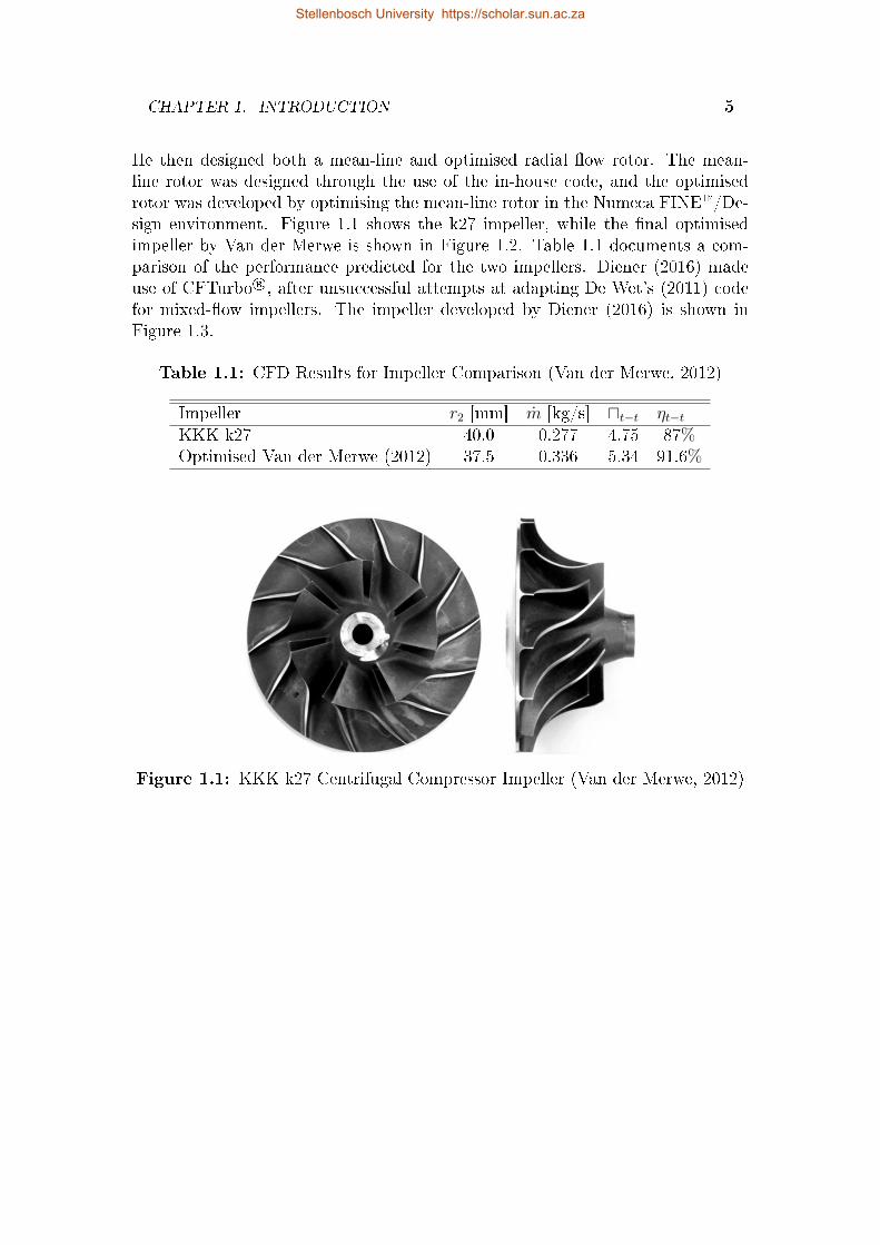
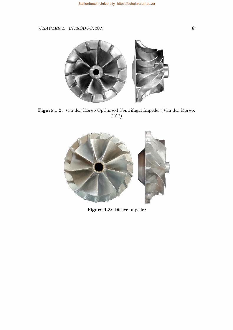
CHAPTER 1. INTRODUCTION 5
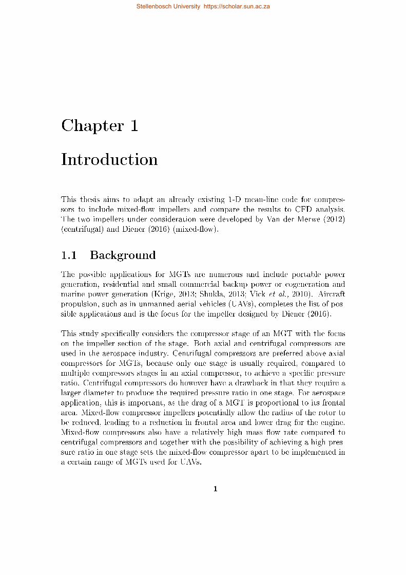
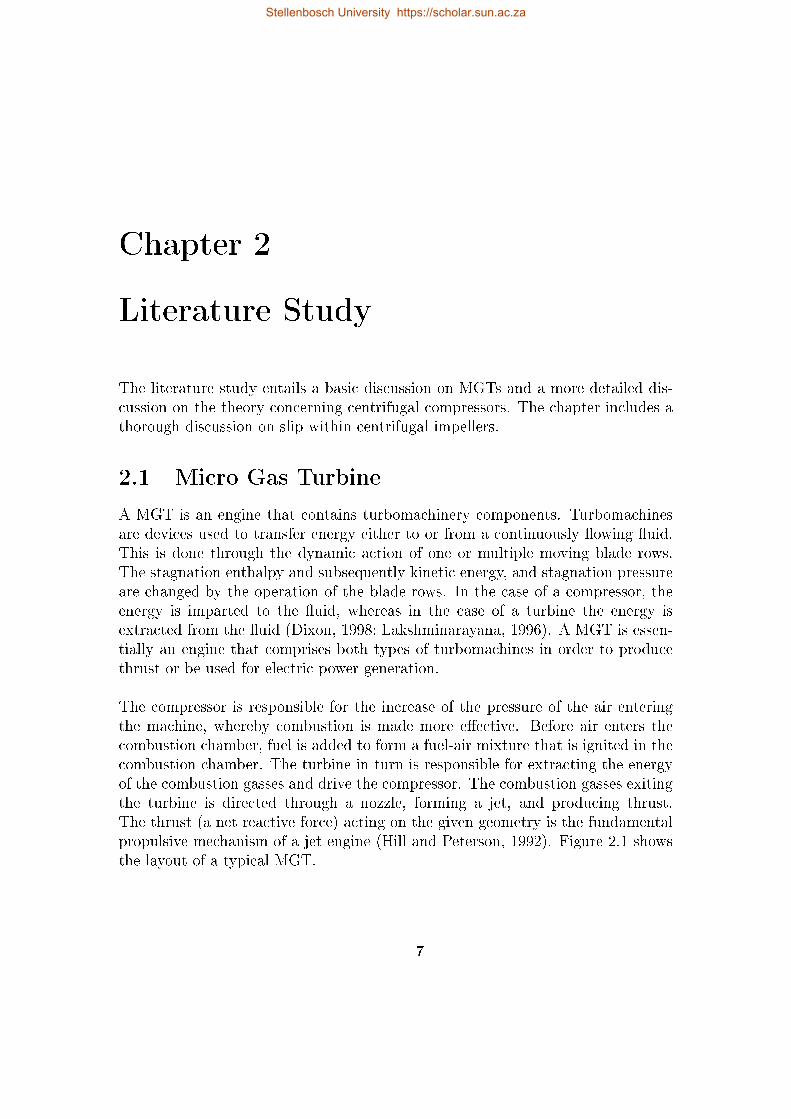
He then designed both a mean-line and optimised radial ow rotor. The mean-line rotor was designed through the use of the in-house code, and the optimisedrotor was developed by optimising the mean-line rotor in the Numeca FINE/De-sign environment. Figure 1.1 shows the k27 impeller, while the nal optimisedimpeller by Van der Merwe is shown in Figure 1.2. Table 1.1 documents a com-parison of the performance predicted for the two impellers. Diener (2016) madeuse of CFTurbo®, after unsuccessful attempts at adapting De Wet's (2011) codefor mixed-ow impellers. The impeller developed by Diener (2016) is shown inFigure 1.3.
Table 1.1: CFD Results for Impeller Comparison (Van der Merwe, 2012)
Impeller r2 [mm] m [kg/s] ut−t ηt−t
KKK k27 40.0 0.277 4.75 87%Optimised Van der Merwe (2012) 37.5 0.336 5.34 91.6%
Figure 1.1: KKK k27 Centrifugal Compressor Impeller (Van der Merwe, 2012)
Stellenbosch University https://scholar.sun.ac.za
CHAPTER 1. INTRODUCTION 6
Figure 1.2: Van der Merwe Optimised Centrifugal Impeller (Van der Merwe,2012)
Figure 1.3: Diener Impeller
Stellenbosch University https://scholar.sun.ac.za
Chapter 2
Literature Study
The literature study entails a basic discussion on MGTs and a more detailed dis-cussion on the theory concerning centrifugal compressors. The chapter includes athorough discussion on slip within centrifugal impellers.
2.1 Micro Gas Turbine
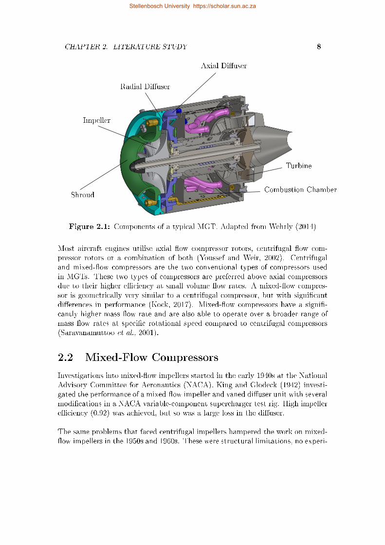
A MGT is an engine that contains turbomachinery components. Turbomachinesare devices used to transfer energy either to or from a continuously owing uid.This is done through the dynamic action of one or multiple moving blade rows.The stagnation enthalpy and subsequently kinetic energy, and stagnation pressureare changed by the operation of the blade rows. In the case of a compressor, theenergy is imparted to the uid, whereas in the case of a turbine the energy isextracted from the uid (Dixon, 1998; Lakshminarayana, 1996). A MGT is essen-tially an engine that comprises both types of turbomachines in order to producethrust or be used for electric power generation.
The compressor is responsible for the increase of the pressure of the air enteringthe machine, whereby combustion is made more eective. Before air enters thecombustion chamber, fuel is added to form a fuel-air mixture that is ignited in thecombustion chamber. The turbine in turn is responsible for extracting the energyof the combustion gasses and drive the compressor. The combustion gasses exitingthe turbine is directed through a nozzle, forming a jet, and producing thrust.The thrust (a net reactive force) acting on the given geometry is the fundamentalpropulsive mechanism of a jet engine (Hill and Peterson, 1992). Figure 2.1 showsthe layout of a typical MGT.
7
Stellenbosch University https://scholar.sun.ac.za
CHAPTER 2. LITERATURE STUDY 8
Radial Diuser
Axial Diuser
Turbine
Combustion Chamber
Impeller
Shroud
Figure 2.1: Components of a typical MGT. Adapted from Wehrly (2014)
Most aircraft engines utilise axial ow compressor rotors, centrifugal ow com-pressor rotors or a combination of both (Youssef and Weir, 2002). Centrifugaland mixed-ow compressors are the two conventional types of compressors usedin MGTs. These two types of compressors are preferred above axial compressorsdue to their higher eciency at small volume ow rates. A mixed-ow compres-sor is geometrically very similar to a centrifugal compressor, but with signicantdierences in performance (Kock, 2017). Mixed-ow compressors have a signi-cantly higher mass ow rate and are also able to operate over a broader range ofmass ow rates at specic rotational speed compared to centrifugal compressors(Saravanamuttoo et al., 2001).
2.2 Mixed-Flow Compressors
Investigations into mixed-ow impellers started in the early 1940s at the NationalAdvisory Committee for Aeronautics (NACA). King and Glodeck (1942) investi-gated the performance of a mixed-ow impeller and vaned diuser unit with severalmodications in a NACA variable-component supercharger test rig. High impellereciency (0.92) was achieved, but so was a large loss in the diuser.
The same problems that faced centrifugal impellers hampered the work on mixed-ow impellers in the 1950s and 1960s. These were structural limitations, no experi-
Stellenbosch University https://scholar.sun.ac.za
CHAPTER 2. LITERATURE STUDY 9
mental data-base, limited computational ability, and severe problems with diuserdesign (Musgrave and Plehn, 1987). In the early 1980s, Whiteld and Roberts(1981) presented a paper on the overall performance of a turbocharger compressoremploying three mixed-ow impellers, reviving the interest in mixed-ow impellers.They found that ow stability was improved by the application of a mixed-owimpeller with a horizontal cut o at the vane tips. Hoping that the results of theirstudy would stimulate further investigation into mixed-ow impellers, Musgraveand Plehn (1987) designed and tested a mixed-ow compressor stage with a pres-sure ratio of 3:1.
Noting that high power-to-weight ratio is a predominant requirement for smalljet-engines and that the demands on the compressor can either be fullled by aconventional two-stage unit or by an extremely loaded single stage, Monig et al.(1987) discussed the possible application of a mixed-ow compressor to meet thecompressor demands. Mönig et al. (1993) then went on to design and test a su-personic mixed-ow compressor with a pressure ratio of 5:1. Eisenlohr and Benfer(1994) designed and experimentally tested a single stage mixed-ow impeller. Theimpeller pressure ratio at design speed and design corrected mass ow rate met thedesign value of 7.5, while isentropic impeller eciencies above 91% were recorded.
Focussing on subsonic ow Youssef and Weir (2002) developed and patented amixed-ow/centrifugal compressor combination for a turbojet engine. Hamiltonand Sundstrand have successfully developed MGTs that employ mixed-ow com-pressors for thrusts between 200 and 450 N (Harris et al., 2003). Cevik (2009)generated a mixed-ow impeller using the individual design methodology he de-veloped for a centrifugal impeller. The impeller has a pressure ratio of 4.34 at arotational speed of 120000 rpm. Diener (2016) developed a mixed-ow impellerwith a simulated pressure ratio of 5.25 and isentropic eciency of 86%. Dienermade use of coupled aero-mechanical optimisation, using FINE/Design3D v. 9-1.3, to obtain his nal impeller design.
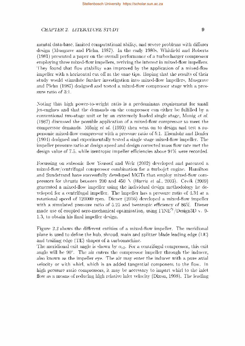
Figure 2.2 shows the dierent entities of a mixed-ow impeller. The meridionalplane is used to dene the hub, shroud, main and splitter blade leading edge (LE)and trailing edge (TE) shapes of a turbomachine.The meridional exit angle is shown by αc2. For a centrifugal compressor, this exitangle will be 90. The air enters the compressor impeller through the inducer,also known as the impeller eye. The air may enter the inducer with a pure axialvelocity or with whirl, which is an added tangential component to the ow. Inhigh pressure ratio compressors, it may be necessary to impart whirl to the inletow as a means of reducing high relative inlet velocity (Dixon, 1998). The leading
Stellenbosch University https://scholar.sun.ac.za
CHAPTER 2. LITERATURE STUDY 10
Figure 2.2: Mixed-Flow Compressor Components in the Meridional Plane(Diener, 2016)
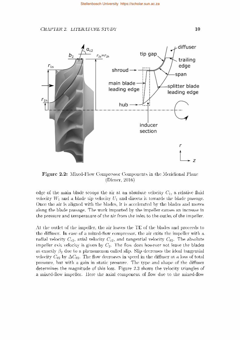
edge of the main blade scoops the air at an absolute velocity C1, a relative uidvelocity W1 and a blade tip velocity U1 and directs it towards the blade passage.Once the air is aligned with the blades, it is accelerated by the blades and movesalong the blade passage. The work imparted by the impeller causes an increase inthe pressure and temperature of the air from the inlet to the outlet of the impeller.
At the outlet of the impeller, the air leaves the TE of the blades and proceeds tothe diuser. In case of a mixed-ow compressor, the air exits the impeller with aradial velocity Cr2, axial velocity Cz2, and tangential velocity Cθ2. The absoluteimpeller exit velocity is given by C2. The ow does however not leave the bladesat exactly β2 due to a phenomenon called slip. Slip decreases the ideal tangentialvelocity Cθ2 by ∆Cθ2. The ow decreases in speed in the diuser at a loss of totalpressure, but with a gain in static pressure. The type and shape of the diuserdetermines the magnitude of this loss. Figure 2.3 shows the velocity triangles ofa mixed-ow impeller. Here the axial component of ow due to the mixed-ow
Stellenbosch University https://scholar.sun.ac.za
CHAPTER 2. LITERATURE STUDY 11
impeller, as opposed to a centrifugal impeller can be visualised from the impellerexit velocity triangles. Decreasing the meridional exit angle (< 90) will cause theaxial velocity component to increase.
Figure 2.3: Mixed-Flow Compressor Impeller Velocity Triangles (Diener, 2016)
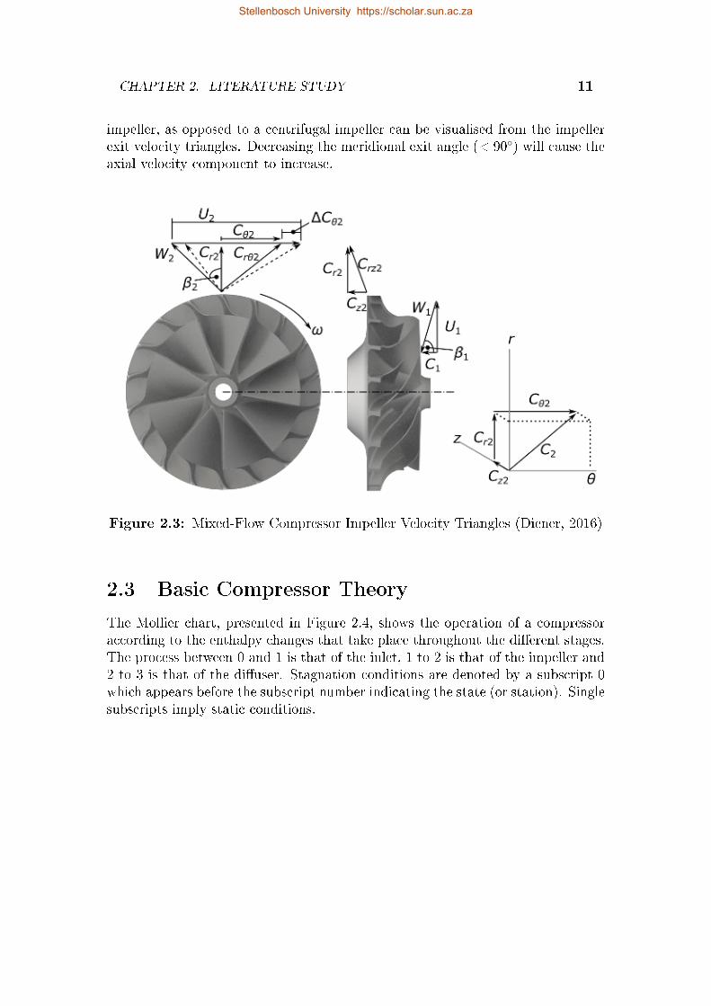
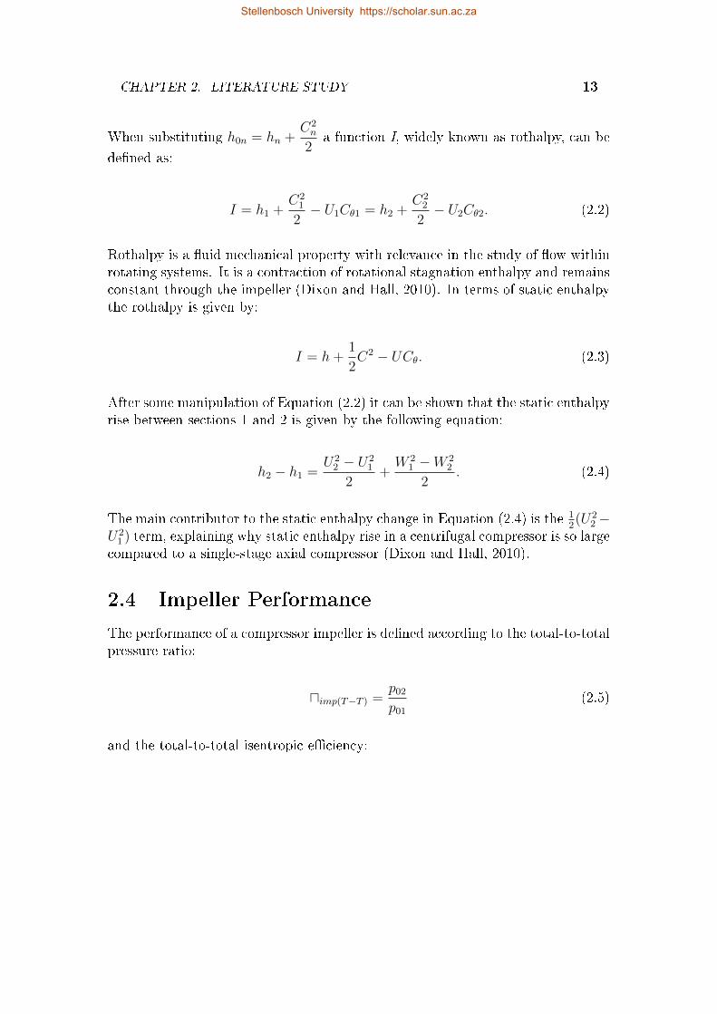
2.3 Basic Compressor Theory
The Mollier chart, presented in Figure 2.4, shows the operation of a compressoraccording to the enthalpy changes that take place throughout the dierent stages.The process between 0 and 1 is that of the inlet, 1 to 2 is that of the impeller and2 to 3 is that of the diuser. Stagnation conditions are denoted by a subscript 0which appears before the subscript number indicating the state (or station). Singlesubscripts imply static conditions.
Stellenbosch University https://scholar.sun.ac.za
CHAPTER 2. LITERATURE STUDY 12
P3P03
P02
02
03s
03ss
02s
2
P2
P01
P1
h00 = h01
h02 = h03
0100
0
1
C222
C232
Enthalpy,h
Entropy, s
C212
3
Figure 2.4: Mollier Chart for a Compressor
Work is done on the uid between sections 1 and 2, thereby raising the totalenthalpy. The rise in enthalpy is equal to the amount of work done by the impelleron the ow, W :
∆W = U2Cθ2 − U1Cθ1 = h02 − h01. (2.1)
Stellenbosch University https://scholar.sun.ac.za
CHAPTER 2. LITERATURE STUDY 13
When substituting h0n = hn +C2
n
2a function I, widely known as rothalpy, can be
dened as:
I = h1 +C2
1
2− U1Cθ1 = h2 +
C22
2− U2Cθ2. (2.2)
Rothalpy is a uid mechanical property with relevance in the study of ow withinrotating systems. It is a contraction of rotational stagnation enthalpy and remainsconstant through the impeller (Dixon and Hall, 2010). In terms of static enthalpythe rothalpy is given by:
I = h+1
2C2 − UCθ. (2.3)
After some manipulation of Equation (2.2) it can be shown that the static enthalpyrise between sections 1 and 2 is given by the following equation:
h2 − h1 =U22 − U2
1
2+
W 21 −W 2
2
2. (2.4)
The main contributor to the static enthalpy change in Equation (2.4) is the 12(U2
2 −U21 ) term, explaining why static enthalpy rise in a centrifugal compressor is so large
compared to a single-stage axial compressor (Dixon and Hall, 2010).
2.4 Impeller Performance
The performance of a compressor impeller is dened according to the total-to-totalpressure ratio:
uimp(T−T ) =p02p01
(2.5)
and the total-to-total isentropic eciency:
Stellenbosch University https://scholar.sun.ac.za
CHAPTER 2. LITERATURE STUDY 14
ηimp(T−T ) =h02s − h01s
h02 − h01
=(p02p01
)γ−1γ − 1
(T02
T01)− 1
. (2.6)
Total-to-static values are often used if the exit kinetic energy is lost (Dixon andHall, 2010). The impeller tip speed, U2, has a signicant eect on the pressure ra-tio that an impeller can achieve. Material properties, however, limit the tip speedthat can be attained, because the material stresses increase proportionally to thetip speed squared (Sandberg, 2016).
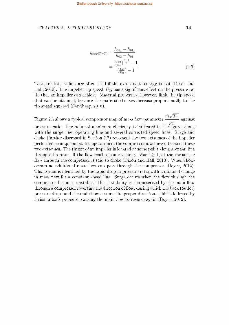
Figure 2.5 shows a typical compressor map of mass ow parameterm√T01
p01against
pressure ratio. The point of maximum eciency is indicated in the gure, alongwith the surge line, operating line and several corrected speed lines. Surge andchoke (further discussed in Section 2.7) represent the two extremes of the impellerperformance map, and stable operation of the compressor is achieved between thesetwo extremes. The throat of an impeller is located at some point along a streamlinethrough the rotor. If the ow reaches sonic velocity, Mach ≥ 1, at the throat theow through the compressor is said to choke (Dixon and Hall, 2010). When chokeoccurs no additional mass ow can pass through the compressor (Boyce, 2012).This region is identied by the rapid drop in pressure ratio with a minimal changein mass ow for a constant speed line. Surge occurs when the ow through thecompressor becomes unstable. This instability is characterised by the main owthrough a compressor reversing the direction of ow, during which the back (outlet)pressure drops and the main ow assumes its proper direction. This is followed bya rise in back pressure, causing the main ow to reverse again (Boyce, 2012).
Stellenbosch University https://scholar.sun.ac.za
CHAPTER 2. LITERATURE STUDY 15
Figure 2.5: Overall Characteristic of a Compressor (Dixon, 1998)
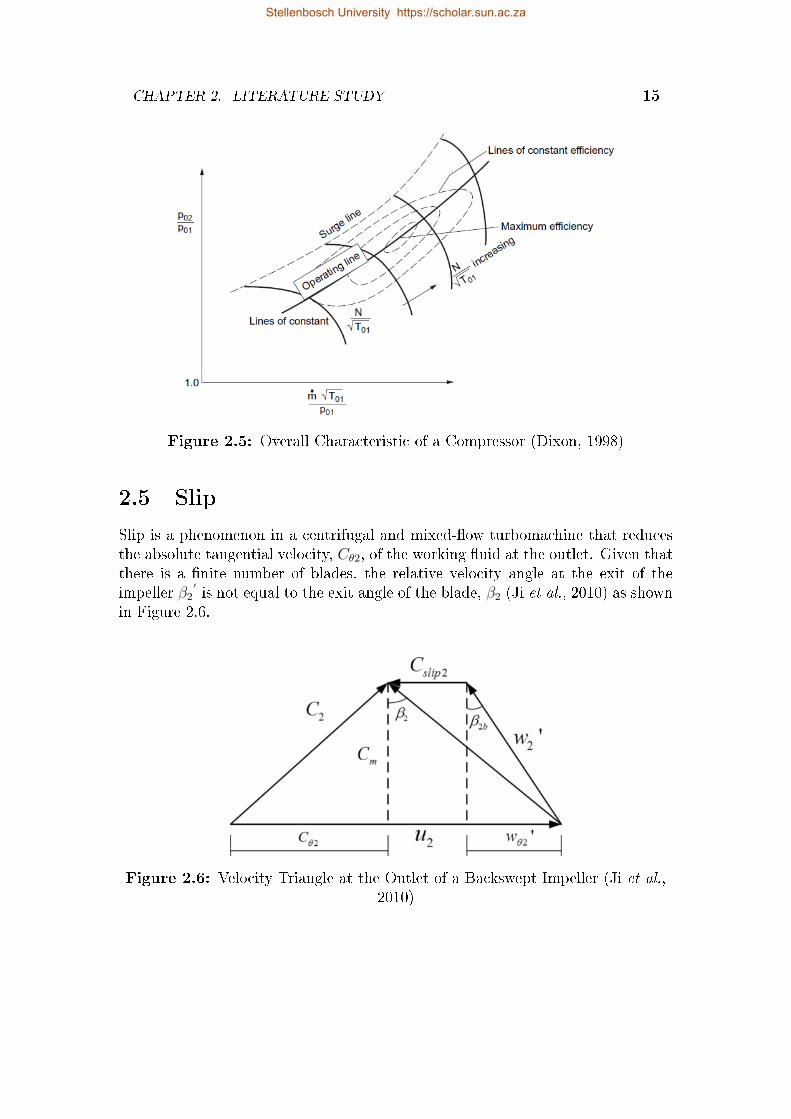
2.5 Slip
Slip is a phenomenon in a centrifugal and mixed-ow turbomachine that reducesthe absolute tangential velocity, Cθ2, of the working uid at the outlet. Given thatthere is a nite number of blades, the relative velocity angle at the exit of theimpeller β2
′is not equal to the exit angle of the blade, β2 (Ji et al., 2010) as shown
in Figure 2.6.
Figure 2.6: Velocity Triangle at the Outlet of a Backswept Impeller (Ji et al.,2010)
Stellenbosch University https://scholar.sun.ac.za
CHAPTER 2. LITERATURE STUDY 16
Boyce (1993) mentions that the cause of the slip phenomenon within an impelleris not known exactly, but there are however general reasons that contribute to thechange in the ow, namely:
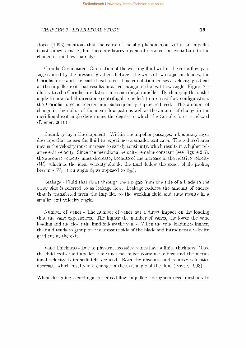
Coriolis Circulation - Circulation of the working uid within the rotor ow pas-sage caused by the pressure gradient between the walls of two adjacent blades, theCoriolis force and the centrifugal force. This circulation causes a velocity gradientat the impeller exit that results in a net change in the exit ow angle. Figure 2.7illustrates the Coriolis circulation in a centrifugal impeller. By changing the outletangle from a radial direction (centrifugal impeller) to a mixed-ow conguration,the Coriolis force is relaxed and subsequently slip is reduced. The amount ofchange in the radius of the mean ow path as well as the amount of change in themeridional exit angle determines the degree to which the Coriolis force is relaxed(Diener, 2016).
Boundary layer Development - Within the impeller passages, a boundary layerdevelops that causes the uid to experience a smaller exit area. The reduced areameans the velocity must increase to satisfy continuity, which results in a higher rel-ative exit velocity. Since the meridional velocity remains constant (see Figure 2.6),the absolute velocity must decrease, because of the increase in the relative velocity(W
′2, which is the ideal velocity should the uid follow the exact blade prole,
becomes W2 at an angle β2 as opposed to β2b).
Leakage - Fluid that ows through the tip gap from one side of a blade to theother side is referred to as leakage ow. Leakage reduces the amount of energythat is transferred from the impeller to the working uid and thus results in asmaller exit velocity angle.
Number of Vanes - The number of vanes has a direct impact on the loadingthat the vane experiences. The higher the number of vanes, the lower the vaneloading and the closer the uid follows the vanes. When the vane loading is higher,the uid tends to group on the pressure side of the blade and introduces a velocitygradient at the exit.
Vane Thickness - Due to physical necessity, vanes have a nite thickness. Oncethe uid exits the impeller, the vanes no longer contain the ow and the merid-ional velocity is immediately reduced. Both the absolute and relative velocitiesdecrease, which results in a change in the exit angle of the uid (Boyce, 1993).
When designing centrifugal or mixed-ow impellers, designers need methods to
Stellenbosch University https://scholar.sun.ac.za

CHAPTER 2. LITERATURE STUDY 17
Figure 2.7: Coriolis Circulation in a Centrifugal Impeller
accurately predict impeller drive shaft torque and the energy input into the ow.Ji et al. (2010) states that "predicting slip factor for centrifugal impellers is at thecore of turbomachinery meanline modeling." The slip factor inuences the velocitytriangle at the exit, the work input, and pressure rise. Slip factor is usually deter-mined by the vorticity of the internal ow relative to the rotating impeller. Theslip factor formulation by Stodola (1945) is one of the most common formulationsused in textbooks, while there are many other authors with approximate slip factorpredictions. Qiu et al. (2011) found that slip factor predictions by authors such asStodola (1945), Wiesner (1967), and Eck (1973) typically work well for one seriesof impellers, while they performed worse or even failed (unrealistic results and/orunable to produce a result) for other types of impellers. Furthermore, tests haveshown that the slip factor varies from design to o-design conditions (Qiu et al.,2011). The implementation of slip factor in the 1-D mean-line code is furtherdiscussed in Section 3.7.1.
2.6 Splitter Blades
Cumpsty (1989) states that there must be an adequate number of blades at theexit of an impeller if the blade loading is to be kept within reasonable bounds.The problem with a larger number of blades is that the blockage at the inducersection of the impeller may impose a constraint on the mass ow in high pressuremachines (Cumpsty, 1989). The expedient adopted is the use of splitter blades.They reduce the blade loading and potentially increase the mass ow capabilityat the throat of the inducer (Aungier, 2000; Cumpsty, 1989; Japikse, 1996). Thesplitter blade starts some length downstream of the inlet of the impeller and con-tinues up until the exit of the impeller.
It is customary to design these splitter blades to be identical to the full blades,
Stellenbosch University https://scholar.sun.ac.za
CHAPTER 2. LITERATURE STUDY 18
but cut back. The impeller is manufactured with a full set of blades, with everyother blade being cut back, forming the splitter blades. Cumpsty (1989) howevernotes that this is not the right procedure as the leading edge of the splitter bladeswill not align with the ow approaching it in the middle of the passage. Shroudpressure contours measured by Senoo et al (1979) show that the ow in the twopassages divided by a splitter behave quite dierently. Cumpsty further mentionsthat there are many potential outcomes with both axial and radial variation in theleading edge of a splitter blade.
2.7 Compressor Instabilities
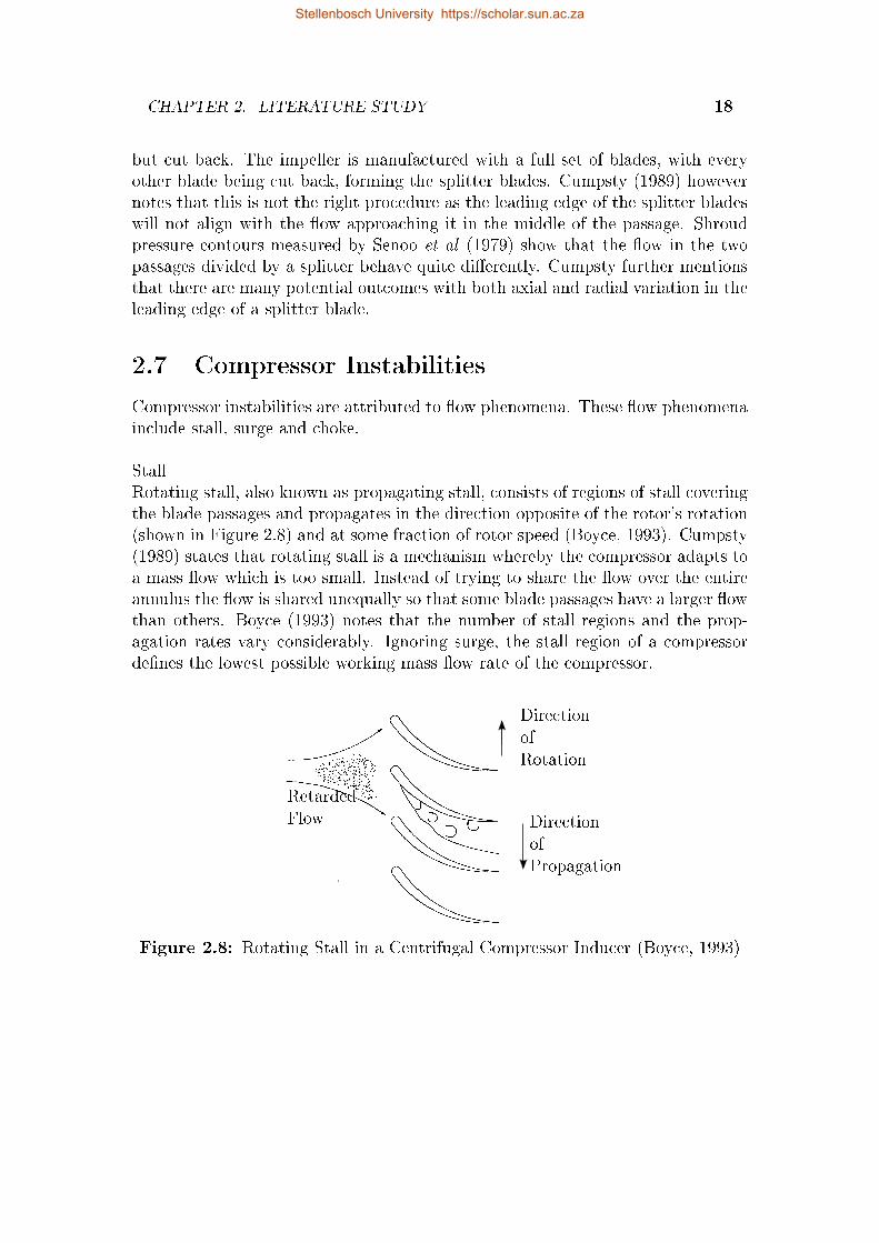
Compressor instabilities are attributed to ow phenomena. These ow phenomenainclude stall, surge and choke.
StallRotating stall, also known as propagating stall, consists of regions of stall coveringthe blade passages and propagates in the direction opposite of the rotor's rotation(shown in Figure 2.8) and at some fraction of rotor speed (Boyce, 1993). Cumpsty(1989) states that rotating stall is a mechanism whereby the compressor adapts toa mass ow which is too small. Instead of trying to share the ow over the entireannulus the ow is shared unequally so that some blade passages have a larger owthan others. Boyce (1993) notes that the number of stall regions and the prop-agation rates vary considerably. Ignoring surge, the stall region of a compressordenes the lowest possible working mass ow rate of the compressor.
DirectionofRotation
DirectionofPropagation
RetardedFlow
Figure 2.8: Rotating Stall in a Centrifugal Compressor Inducer (Boyce, 1993)
Stellenbosch University https://scholar.sun.ac.za
CHAPTER 2. LITERATURE STUDY 19
SurgeSurge is an unstable condition that results in the reversal of ow and pressureuctuations in the system (Boyce, 1993). Boyce also states that an excessive in-crease in the resistance of a system while operating at a specic speed will resultin surge. The result of the added resistance is an instability in the ow. Surgecan also take place when the resistance remains unchanged, but the speed is re-duced considerably. Surge thus depends on the type of system and the shape ofthe resistance curve (Boyce, 1993). The resistance curve is a line representing theprocess resistance of the compressor and the steady state operating point of thecompressor is usually found where the resistance curve intersects the line of con-stant speed (Mirsky et al., 2013). The shape of the resistance curve thus dependson the process resistance of the system.
ChokeThe throat areas of a compressor stage are the regions in the compressor where theinternal ow area is a minimum along a streamline. If the Mach number reachesunity at the throat area, the mass ow is at a maximum, and the ow is said tobe choked (Diener, 2016). In comparison to the stall region, the choke region of acompressor denes the highest possible working mass ow rate that the compressorcan attain.
Stellenbosch University https://scholar.sun.ac.za
Chapter 3
Mean-Line Code
This chapter details the 1-D mean-line code developed by De Wet (2011) in orderto give the reader an understanding of how the code works. The proposed changesto be made to the code to allow the performance analysis of both centrifugal andmixed-ow impellers are also discussed in this chapter.
3.1 Introduction
The one-dimensional mean-line code is an in-house code, written in Matlab®, thatwas rst developed by De Wet (2011), based on the procedure as developed byAungier (2000). Aungier allows for the denition of component sizing, geometrydenition and performance of the compressor. The design process consists of: 1)the meridional passage design, 2) detailed blade design, 3) component sizing, 4)and performance analysis. The user denes the total thermodynamic conditionsand angular momentum for the inlet conditions.
Later versions of the code allow for optimisation and therefore the design of animpeller according to user-dened design parameters. The code can also be appliedfor analysis of a single geometry by specifying the design parameters as non-varyingparameters. By doing this the "optimisation" of a geometry within specic designboundaries is eliminated, and instead, a single geometry is created according to theuser-dened geometry specications. Although the mean-line code was used foranalysis only (of existing impellers) in this thesis, both the structure and functionsof the code are described in this chapter for continuity.
20
Stellenbosch University https://scholar.sun.ac.za
CHAPTER 3. MEAN-LINE CODE 21
3.2 Code Structure
The mean-line code was initially developed to predict the performance of centrifu-gal compressors. Subsequent authors of follow up research projects added to theoriginal code to enable it to analyse diusers as well. This research project aimedto adapt the code to allow for the analysis of a mixed-ow impeller in addition to aradial ow impeller. The mean-line code generates a geomTurbo output le (con-taining the three-dimensional impeller geometry) which can be uploaded directlyinto Numeca AutoGrid5 to start the CFD validation and optimisation process.
The mean-line code is executed from one main function. The main function, op-timise, makes use of a genetic algorithm (Van der Merwe, 2012) to create thebest performing impeller according to the performance criteria and geometricalconstraints. The optimisation process is executed for a user-dened number of op-timisation steps. It should be noted that the number of optimisation steps shouldbe increased as the number of free parameters is increased. The development ofthe impeller geometry and performance analysis are executed within a loop, ac-cording to the number of chromosomes specied by the user. This loop is repeatedfor each optimisation step.
The rst step is to create an impeller geometry and calculate a blade throat areaaccording to the specic geometry. Once the geometry is created and the throatarea is known, the performance of the impeller can be determined. When the opti-misation steps are nished, the best possible impeller for the specied geometricallimits is created, upon which the performance of the compressor is determined atdierent rotational speeds. Van der Merwe (2012) added the creation of a per-formance map for the compressor at dierent operational speeds. A ow diagramshowing the logic for the mean-line code structure is shown in Figure B.1.
3.3 Code Inputs
The code, in its intended format, consists of several functions that are used to de-termine the performance of the impeller and then create a geometry based on theparameters that deliver the best performance. The main geometric and operatingproperties of the compressor are specied in the main function called optimise.These parameters can vary and are subsequently given a range of possible values.The free geometric parameters for the Van der Merwe (2012) mean-line rotor, withtheir bounds are given in Table 3.1.
The main function generates a compressor geometry based on the main parameters
Stellenbosch University https://scholar.sun.ac.za
CHAPTER 3. MEAN-LINE CODE 22
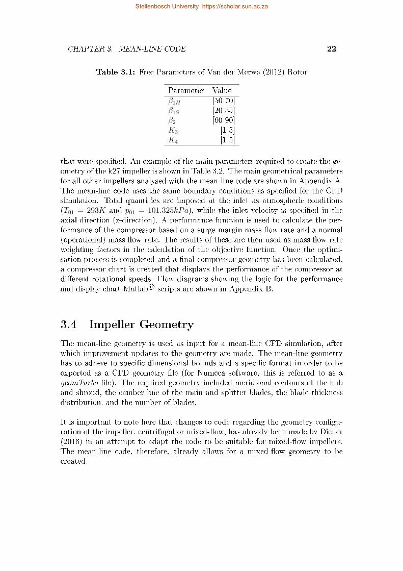
Table 3.1: Free Parameters of Van der Merwe (2012) Rotor
Parameter Valueβ1H [50 70]β1S [20 35]β2 [60 90]K3 [1 5]K4 [1 5]
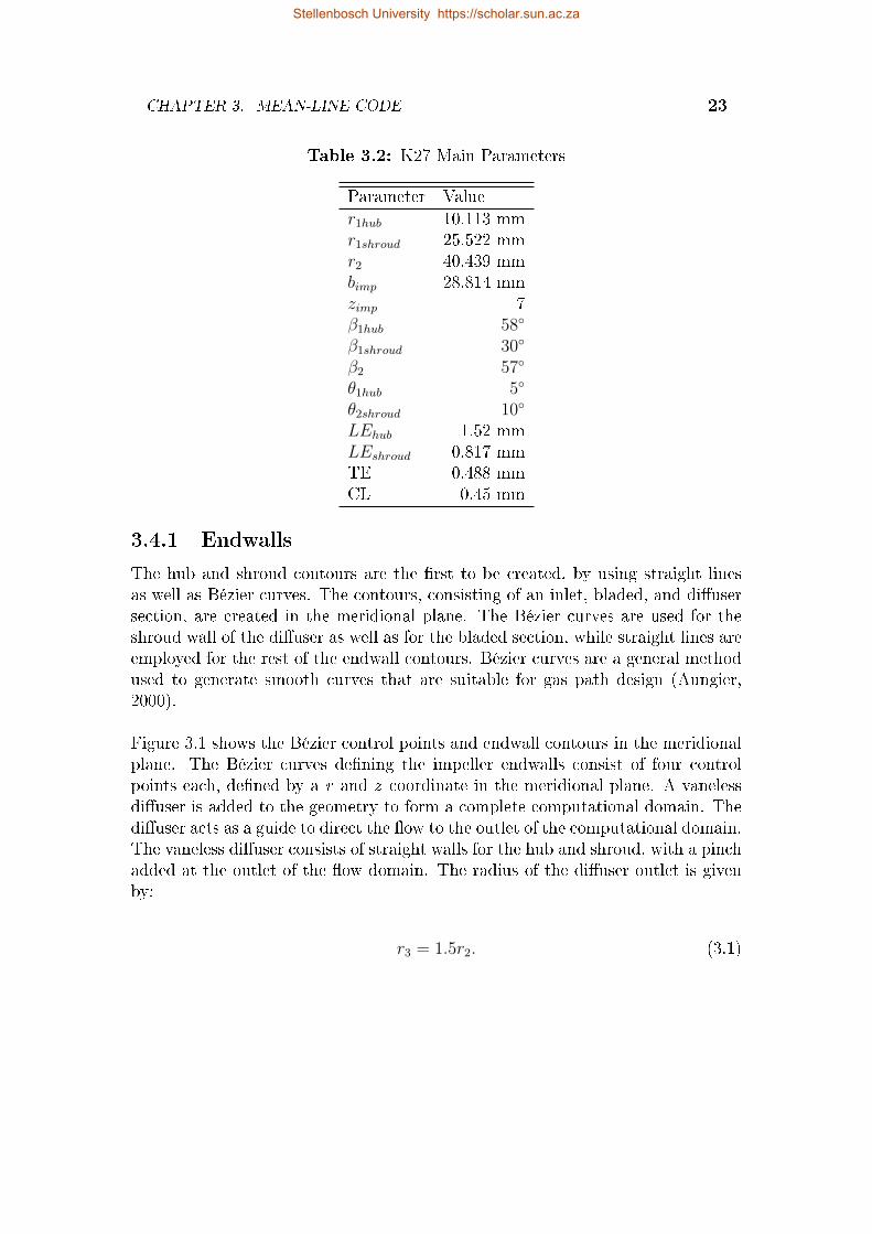
that were specied. An example of the main parameters required to create the ge-ometry of the k27 impeller is shown in Table 3.2. The main geometrical parametersfor all other impellers analysed with the mean-line code are shown in Appendix A.The mean-line code uses the same boundary conditions as specied for the CFDsimulation. Total quantities are imposed at the inlet as atmospheric conditions(T01 = 293K and p01 = 101.325kPa), while the inlet velocity is specied in theaxial direction (z-direction). A performance function is used to calculate the per-formance of the compressor based on a surge margin mass ow rate and a normal(operational) mass ow rate. The results of these are then used as mass ow rateweighting factors in the calculation of the objective function. Once the optimi-sation process is completed and a nal compressor geometry has been calculated,a compressor chart is created that displays the performance of the compressor atdierent rotational speeds. Flow diagrams showing the logic for the performanceand display chart Matlab® scripts are shown in Appendix B.
3.4 Impeller Geometry
The mean-line geometry is used as input for a mean-line CFD simulation, afterwhich improvement updates to the geometry are made. The mean-line geometryhas to adhere to specic dimensional bounds and a specic format in order to beexported as a CFD geometry le (for Numeca software, this is referred to as ageomTurbo le). The required geometry included meridional contours of the huband shroud, the camber line of the main and splitter blades, the blade thicknessdistribution, and the number of blades.
It is important to note here that changes to code regarding the geometry congu-ration of the impeller, centrifugal or mixed-ow, has already been made by Diener(2016) in an attempt to adapt the code to be suitable for mixed-ow impellers.The mean-line code, therefore, already allows for a mixed-ow geometry to becreated.
Stellenbosch University https://scholar.sun.ac.za
CHAPTER 3. MEAN-LINE CODE 23
Table 3.2: K27 Main Parameters
Parameter Value
r1hub 10.113 mmr1shroud 25.522 mmr2 40.439 mmbimp 28.814 mmzimp 7β1hub 58
β1shroud 30
β2 57
θ1hub 5
θ2shroud 10
LEhub 1.52 mmLEshroud 0.817 mmTE 0.488 mmCL 0.45 mm
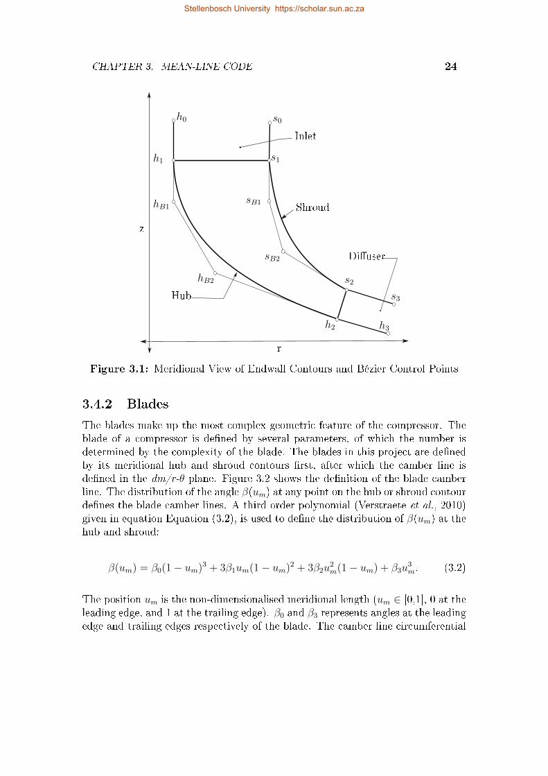
3.4.1 Endwalls
The hub and shroud contours are the rst to be created, by using straight linesas well as Bézier curves. The contours, consisting of an inlet, bladed, and diusersection, are created in the meridional plane. The Bézier curves are used for theshroud wall of the diuser as well as for the bladed section, while straight lines areemployed for the rest of the endwall contours. Bézier curves are a general methodused to generate smooth curves that are suitable for gas path design (Aungier,2000).
Figure 3.1 shows the Bézier control points and endwall contours in the meridionalplane. The Bézier curves dening the impeller endwalls consist of four controlpoints each, dened by a r and z coordinate in the meridional plane. A vanelessdiuser is added to the geometry to form a complete computational domain. Thediuser acts as a guide to direct the ow to the outlet of the computational domain.The vaneless diuser consists of straight walls for the hub and shroud, with a pinchadded at the outlet of the ow domain. The radius of the diuser outlet is givenby:
r3 = 1.5r2. (3.1)
Stellenbosch University https://scholar.sun.ac.za
CHAPTER 3. MEAN-LINE CODE 24
Shroud
Hub
Diuser
Inlet
r
z
h0
h1
hB1
hB2
h2 h3
s3
s2
sB2
sB1
s1
s0
Figure 3.1: Meridional View of Endwall Contours and Bézier Control Points
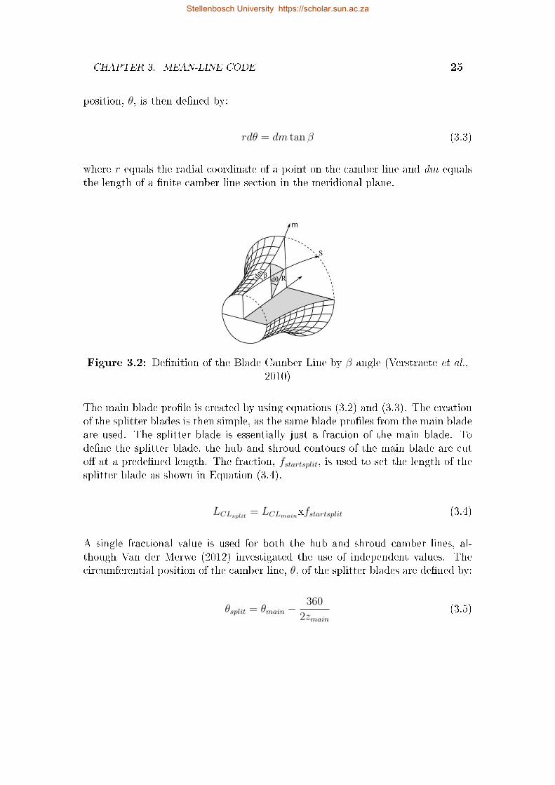
3.4.2 Blades
The blades make up the most complex geometric feature of the compressor. Theblade of a compressor is dened by several parameters, of which the number isdetermined by the complexity of the blade. The blades in this project are denedby its meridional hub and shroud contours rst, after which the camber line isdened in the dm/r-θ plane. Figure 3.2 shows the denition of the blade camberline. The distribution of the angle β(um) at any point on the hub or shroud contourdenes the blade camber lines. A third order polynomial (Verstraete et al., 2010)given in equation Equation (3.2), is used to dene the distribution of β(um) at thehub and shroud:
β(um) = β0(1− um)3 + 3β1um(1− um)
2 + 3β2u2m(1− um) + β3u
3m. (3.2)
The position um is the non-dimensionalised meridional length (um ∈ [0,1], 0 at theleading edge, and 1 at the trailing edge). β0 and β3 represents angles at the leadingedge and trailing edges respectively of the blade. The camber line circumferential
Stellenbosch University https://scholar.sun.ac.za
CHAPTER 3. MEAN-LINE CODE 25
position, θ, is then dened by:
rdθ = dm tan β (3.3)
where r equals the radial coordinate of a point on the camber line and dm equalsthe length of a nite camber line section in the meridional plane.
Figure 3.2: Denition of the Blade Camber Line by β angle (Verstraete et al.,2010)
The main blade prole is created by using equations (3.2) and (3.3). The creationof the splitter blades is then simple, as the same blade proles from the main bladeare used. The splitter blade is essentially just a fraction of the main blade. Todene the splitter blade, the hub and shroud contours of the main blade are cuto at a predened length. The fraction, fstartsplit, is used to set the length of thesplitter blade as shown in Equation (3.4).
LCLsplit= LCLmain
xfstartsplit (3.4)
A single fractional value is used for both the hub and shroud camber lines, al-though Van der Merwe (2012) investigated the use of independent values. Thecircumferential position of the camber line, θ, of the splitter blades are dened by:
θsplit = θmain −360
2zmain
(3.5)
Stellenbosch University https://scholar.sun.ac.za
CHAPTER 3. MEAN-LINE CODE 26
where θ is given in degrees and zmain refers to the number of main blades on theimpeller.
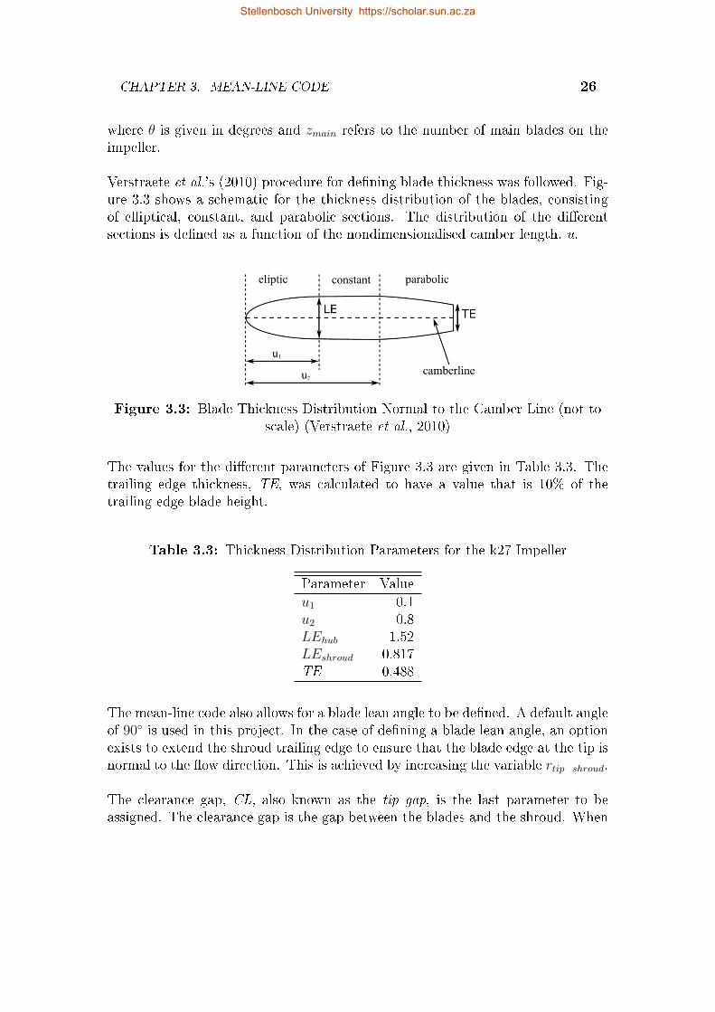
Verstraete et al.'s (2010) procedure for dening blade thickness was followed. Fig-ure 3.3 shows a schematic for the thickness distribution of the blades, consistingof elliptical, constant, and parabolic sections. The distribution of the dierentsections is dened as a function of the nondimensionalised camber length, u.
Figure 3.3: Blade Thickness Distribution Normal to the Camber Line (not toscale) (Verstraete et al., 2010)
The values for the dierent parameters of Figure 3.3 are given in Table 3.3. Thetrailing edge thickness, TE, was calculated to have a value that is 10% of thetrailing edge blade height.
Table 3.3: Thickness Distribution Parameters for the k27 Impeller
Parameter Value
u1 0.1u2 0.8LEhub 1.52LEshroud 0.817TE 0.488
The mean-line code also allows for a blade lean angle to be dened. A default angleof 90 is used in this project. In the case of dening a blade lean angle, an optionexists to extend the shroud trailing edge to ensure that the blade edge at the tip isnormal to the ow direction. This is achieved by increasing the variable rtip_shroud.
The clearance gap, CL, also known as the tip gap, is the last parameter to beassigned. The clearance gap is the gap between the blades and the shroud. When
Stellenbosch University https://scholar.sun.ac.za
CHAPTER 3. MEAN-LINE CODE 27
assigning the clearance gap size, it is important to consider the operation of theimpeller at full speed. Centrifugal- and heat-expansion forces are signicant con-tributors to the blades expanding and require sucient space to maintain a gapfor safe operation. A clearance gap, constant along the length of the blade, wascalculated using the following relation from Zemp et al. (2010):
CL
b2= 4.5%. (3.6)
3.5 Impeller Performance
As mentioned in Section 3.3, the performance of the impeller is evaluated accordingto pressure ratio and isentropic eciency at the outlet of the impeller. An objec-tive function is used to weigh the pressure ratios and eciencies for the dierentgeometries throughout the optimisation process. This then allows the performanceof the impeller to be evaluated as a single value, given by:
P =ut−t
5+
ηt−t
0.8. (3.7)
The target values for pressure ratio and eciency for the respective impellers areused as weighting factors in Equation (3.7). Table 3.4 shows the target values forthe respective impellers. The objective function target value is therefore 2. A valuehigher than two would indicate better performance than the target performance,and a value below two would indicate weaker performance. The performance ofeach iteration geometry within the optimisation process is evaluated through afunction calculating the pressure ratio and eciency according to the speciedgeometry. The performance of each iteration is then compared to the previousone, where the impeller with the best performance is then saved as the "best"performing impeller. This process continues until all the possible geometries areevaluated (Van der Merwe, 2012)
Stellenbosch University https://scholar.sun.ac.za
CHAPTER 3. MEAN-LINE CODE 28
Table 3.4: Target Values for Respective Impellers
Impeller Target Valuesu η
k27 4.5 0.85Van der Merwe 5 0.9Diener 5 0.85
3.6 Code Output
The code generates several gures, showing the hub and shroud Bézier endwalls,along with a 3-D gure showing the hub and shroud curves with the blades. Thecomplete geometry created by the code is written to a CFD geometry le format,while all the contours are written to separate text les. Finally, a compressorperformance map is created, showing the pressure ratio and eciency curves forthe impeller at dierent operating speeds. Included in the performance maps isa surge line based on the surge condition specied by the user. The compressormaps for each impeller analysed in the mean-line code are shown in Appendix D.
3.7 Adjustment of the In-House Code
This section outlines the steps followed in order to successfully modify the in-housemean-line code to analyse mixed-ow impellers.
3.7.1 Slip Formulation
The pressure rise in a compressor is supplied by the useful work input of the im-peller blades. Impeller work input is essentially the total enthalpy rise imparted tothe uid by the impeller. When the uid entering an impeller is considered to beirrotational, a relative eddy rotating in the opposite direction of the rotor direc-tion is required to maintain the irrotational ow in the absolute frame of reference.This is the main contributor to slip that exists at the impeller outlet (Dixon, 1998;Ji et al., 2010; Qiu et al., 2011).
Slip reduces the eective work of an impeller on the working uid passing througha compressor. Predicting the amount of slip that occurs for a given impeller istherefore important to correctly determine the performance of an impeller. Overthe years many authors have proposed dierent correlations for slip factor in order
Stellenbosch University https://scholar.sun.ac.za
CHAPTER 3. MEAN-LINE CODE 29
to quantify the eective/real ow as opposed to the ideal ow at impeller outlet.It should be mentioned though that most slip factor correlations are derived forcentrifugal impellers only or blades with no sweep.
Busemann (1928) was one of the rst researchers to publish a method by whichthe slip in radial ow impellers could be predicted. Busemann (1928) derived hismethod by analysis of the ow eld between logarithmic spiral blades. Most stud-ies, however, prefer to use the curves published by Wislicenus (1965), due to theextensive mathematical treatment required to use the Busemann method. Wies-ner (1967) also derived an equation for the prediction of slip, but he based hisequation on the analysis of a large number of empirical results. Stodola (1945)presented a simplied derivation of slip that is followed by many textbooks. Theformulation by Stodola makes use of the relative eddy mechanism, often consideredas the most important mechanism for slip. Stodola describes the relative eddy asa circle, inserted between the blade passages near the outer radius of the rotor.The circle, with a vorticity of ω, touches the suction side trailing edge of one bladeand is tangent to the pressure side of the neighbouring blade. The slip velocity isthen given by ∆w = πΩre(cosβ)/Z.
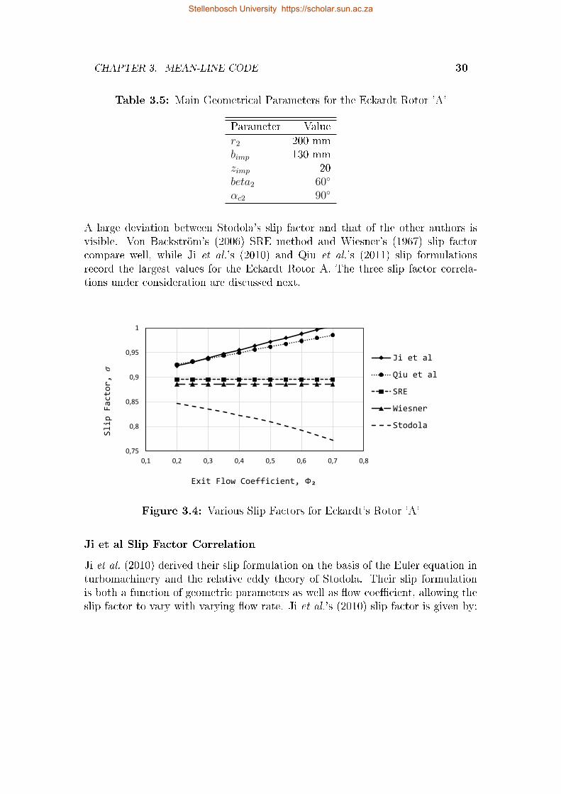
Many more researchers like Stanitz (1952), Eck (1973), Pampreen and Musgrave(1978), Peiderer (1961), Visser et al. (1994), and Paeng and Chung (2001) pro-posed their own estimations for slip. This thesis specically considers slip formu-lations by the following authors: Ji et al. (2010), Von Backström (2006), and Qiuet al. (2011). These authors developed formulations for slip factor which are validfor both centrifugal and mixed-ow compressor impellers. Diener (2016) employedthe Wiesner (1967) slip formulation in the 1-D mean-line code, but the code did notsuciently predict the performance of a mixed-ow impeller. It should be notedthat the slip formulation according to Wiesner (1967) does not take the meridionaloutlet angle into account. It, therefore, does not cater for the axial ow elementin the working uid leaving the impeller. Ji et al. (2010) and Qiu et al. (2011)accommodates mixed-ow impellers by incorporating the meridional exit angle,αc2, in their formulation of the slip factor. Table 3.5 shows the main geometricalparameters for the Eckardt Rotor 'A', while Figure 3.4 shows the dierences inslip factor according to dierent authors for the Eckardt Rotor 'A' impeller.
Stellenbosch University https://scholar.sun.ac.za
CHAPTER 3. MEAN-LINE CODE 30
Table 3.5: Main Geometrical Parameters for the Eckardt Rotor 'A'
Parameter Value
r2 200 mmbimp 130 mmzimp 20beta2 60
αc2 90
A large deviation between Stodola's slip factor and that of the other authors isvisible. Von Backström's (2006) SRE method and Wiesner's (1967) slip factorcompare well, while Ji et al.'s (2010) and Qiu et al.'s (2011) slip formulationsrecord the largest values for the Eckardt Rotor A. The three slip factor correla-tions under consideration are discussed next.
0,75
0,8
0,85
0,9
0,95
1
0,1 0,2 0,3 0,4 0,5 0,6 0,7 0,8
Slip Factor, 𝜎
Exit Flow Coefficient, Ф₂
Ji et al
Qiu et al
SRE
Wiesner
Stodola
Figure 3.4: Various Slip Factors for Eckardt's Rotor 'A'
Ji et al Slip Factor Correlation
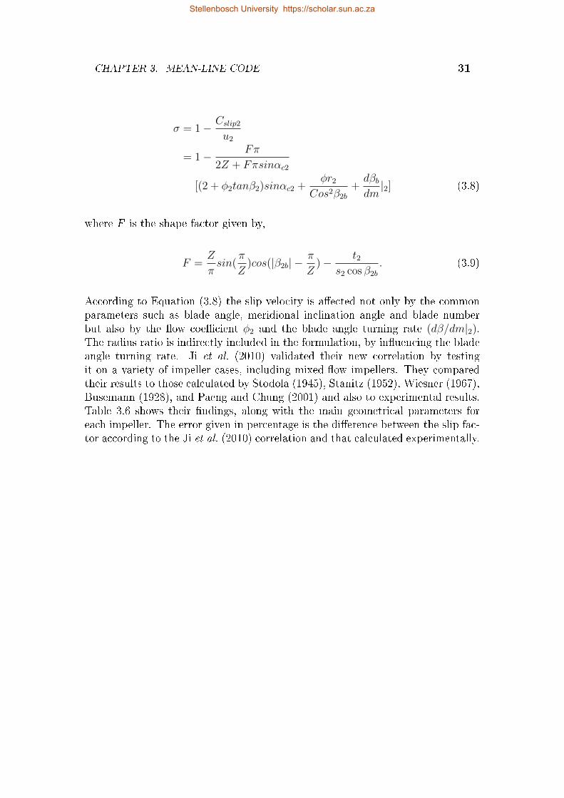
Ji et al. (2010) derived their slip formulation on the basis of the Euler equation inturbomachinery and the relative eddy theory of Stodola. Their slip formulationis both a function of geometric parameters as well as ow coecient, allowing theslip factor to vary with varying ow rate. Ji et al.'s (2010) slip factor is given by:
Stellenbosch University https://scholar.sun.ac.za
CHAPTER 3. MEAN-LINE CODE 31
σ = 1− Cslip2
u2
= 1− Fπ
2Z + Fπsinαc2
[(2 + φ2tanβ2)sinαc2 +φr2
Cos2β2b
+dβb
dm|2] (3.8)
where F is the shape factor given by,
F =Z
πsin(
π
Z)cos(|β2b| −
π
Z)− t2
s2 cos β2b
. (3.9)
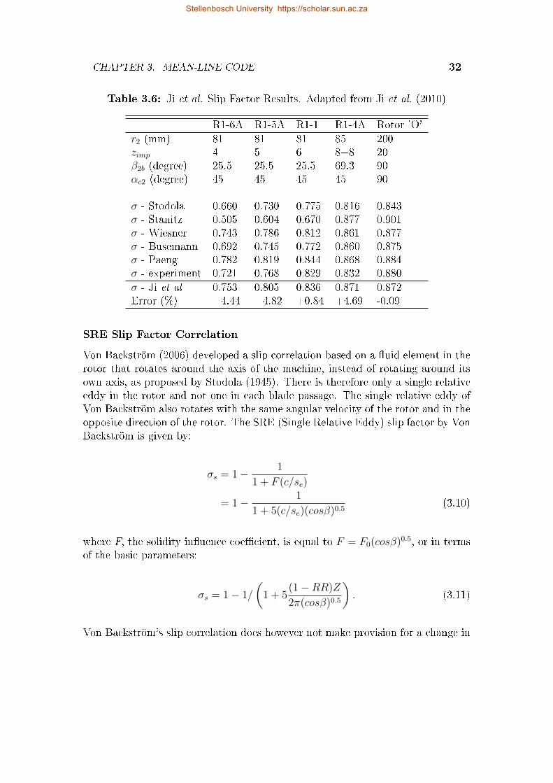
According to Equation (3.8) the slip velocity is aected not only by the commonparameters such as blade angle, meridional inclination angle and blade numberbut also by the ow coecient φ2 and the blade angle turning rate (dβ/dm|2).The radius ratio is indirectly included in the formulation, by inuencing the bladeangle turning rate. Ji et al. (2010) validated their new correlation by testingit on a variety of impeller cases, including mixed-ow impellers. They comparedtheir results to those calculated by Stodola (1945), Stanitz (1952), Wiesner (1967),Busemann (1928), and Paeng and Chung (2001) and also to experimental results.Table 3.6 shows their ndings, along with the main geometrical parameters foreach impeller. The error given in percentage is the dierence between the slip fac-tor according to the Ji et al. (2010) correlation and that calculated experimentally.
Stellenbosch University https://scholar.sun.ac.za
CHAPTER 3. MEAN-LINE CODE 32
Table 3.6: Ji et al. Slip Factor Results. Adapted from Ji et al. (2010)
R1-6A R1-5A R1-1 R1-4A Rotor 'O'
r2 (mm) 81 81 81 85 200zimp 4 5 6 8+8 20β2b (degree) 25.5 25.5 25.5 69.3 90αc2 (degree) 45 45 45 45 90
σ - Stodola 0.660 0.730 0.775 0.816 0.843σ - Stanitz 0.505 0.604 0.670 0.877 0.901σ - Wiesner 0.743 0.786 0.812 0.861 0.877σ - Busemann 0.692 0.745 0.772 0.860 0.875σ - Paeng 0.782 0.819 0.844 0.868 0.884σ - experiment 0.721 0.768 0.829 0.832 0.880
σ - Ji et al 0.753 0.805 0.836 0.871 0.872Error (%) +4.44 +4.82 +0.84 +4.69 -0.09
SRE Slip Factor Correlation
Von Backström (2006) developed a slip correlation based on a uid element in therotor that rotates around the axis of the machine, instead of rotating around itsown axis, as proposed by Stodola (1945). There is therefore only a single relativeeddy in the rotor and not one in each blade passage. The single relative eddy ofVon Backström also rotates with the same angular velocity of the rotor and in theopposite direction of the rotor. The SRE (Single Relative Eddy) slip factor by VonBackström is given by:
σs = 1− 1
1 + F (c/se)
= 1− 1
1 + 5(c/se)(cosβ)0.5(3.10)
where F, the solidity inuence coecient, is equal to F = F0(cosβ)0.5, or in terms
of the basic parameters:
σs = 1− 1/
(1 + 5
(1−RR)Z
2π(cosβ)0.5
). (3.11)
Von Backström's slip correlation does however not make provision for a change in
Stellenbosch University https://scholar.sun.ac.za
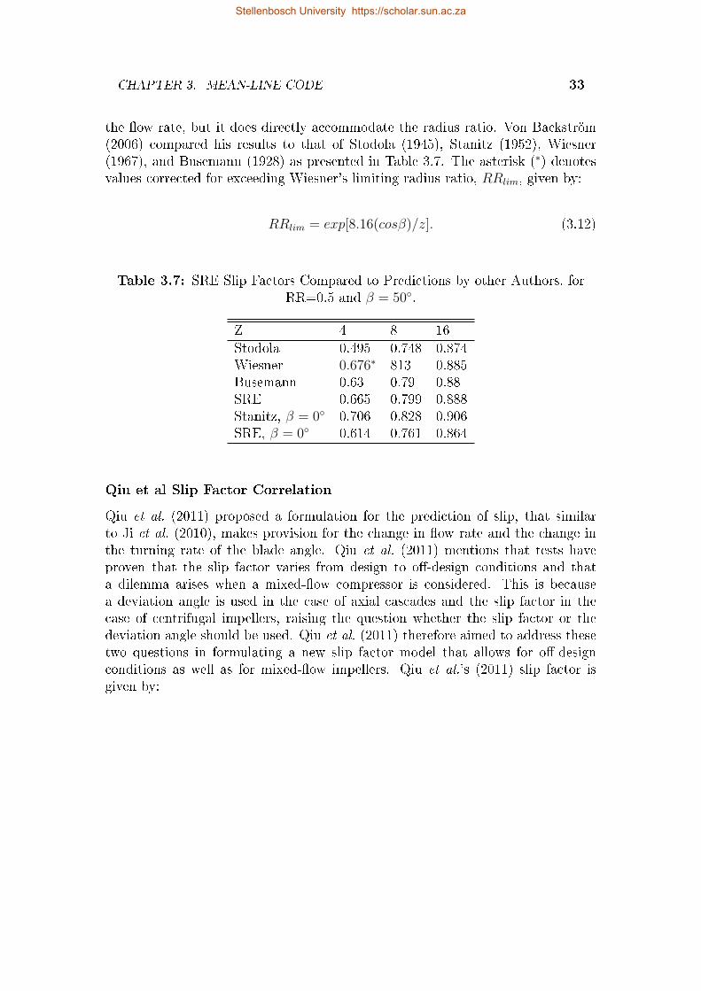
CHAPTER 3. MEAN-LINE CODE 33
the ow rate, but it does directly accommodate the radius ratio. Von Backström(2006) compared his results to that of Stodola (1945), Stanitz (1952), Wiesner(1967), and Busemann (1928) as presented in Table 3.7. The asterisk (∗) denotesvalues corrected for exceeding Wiesner's limiting radius ratio, RRlim, given by:
RRlim = exp[8.16(cosβ)/z]. (3.12)
Table 3.7: SRE Slip Factors Compared to Predictions by other Authors, forRR=0.5 and β = 50.
Z 4 8 16
Stodola 0.495 0.748 0.874Wiesner 0.676∗ 813 0.885Busemann 0.63 0.79 0.88SRE 0.665 0.799 0.888Stanitz, β = 0 0.706 0.828 0.906SRE, β = 0 0.614 0.761 0.864
Qiu et al Slip Factor Correlation
Qiu et al. (2011) proposed a formulation for the prediction of slip, that similarto Ji et al. (2010), makes provision for the change in ow rate and the change inthe turning rate of the blade angle. Qiu et al. (2011) mentions that tests haveproven that the slip factor varies from design to o-design conditions and thata dilemma arises when a mixed-ow compressor is considered. This is becausea deviation angle is used in the case of axial cascades and the slip factor in thecase of centrifugal impellers, raising the question whether the slip factor or thedeviation angle should be used. Qiu et al. (2011) therefore aimed to address thesetwo questions in formulating a new slip factor model that allows for o-designconditions as well as for mixed-ow impellers. Qiu et al.'s (2011) slip factor isgiven by:
Stellenbosch University https://scholar.sun.ac.za
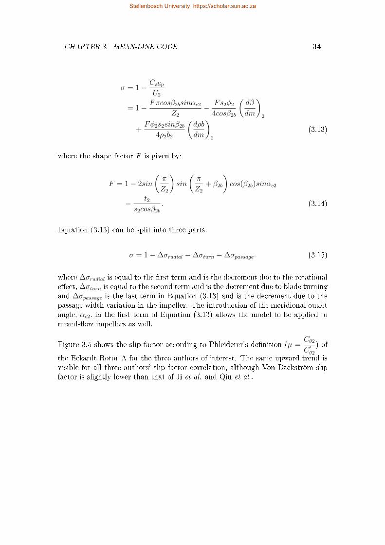
CHAPTER 3. MEAN-LINE CODE 34
σ = 1− Cslip
U2
= 1− Fπcosβ2bsinαc2
Z2
− Fs2φ2
4cosβ2b
(dβ
dm
)2
+Fφ2s2sinβ2b
4ρ2b2
(dρb
dm
)2
(3.13)
where the shape factor F is given by:
F = 1− 2sin
(π
Z2
)sin
(π
Z2
+ β2b
)cos(β2b)sinαc2
− t2s2cosβ2b
. (3.14)
Equation (3.13) can be split into three parts:
σ = 1−∆σradial −∆σturn −∆σpassage. (3.15)
where ∆σradial is equal to the rst term and is the decrement due to the rotationaleect, ∆σturn is equal to the second term and is the decrement due to blade turningand ∆σpassage is the last term in Equation (3.13) and is the decrement due to thepassage width variation in the impeller. The introduction of the meridional outletangle, αc2, in the rst term of Equation (3.13) allows the model to be applied tomixed-ow impellers as well.
Figure 3.5 shows the slip factor according to Phleiderer's denition (µ =Cθ2
C′θ2
) of
the Eckardt Rotor A for the three authors of interest. The same upward trend isvisible for all three authors' slip factor correlation, although Von Backström slipfactor is slightly lower than that of Ji et al. and Qiu et al..
Stellenbosch University https://scholar.sun.ac.za
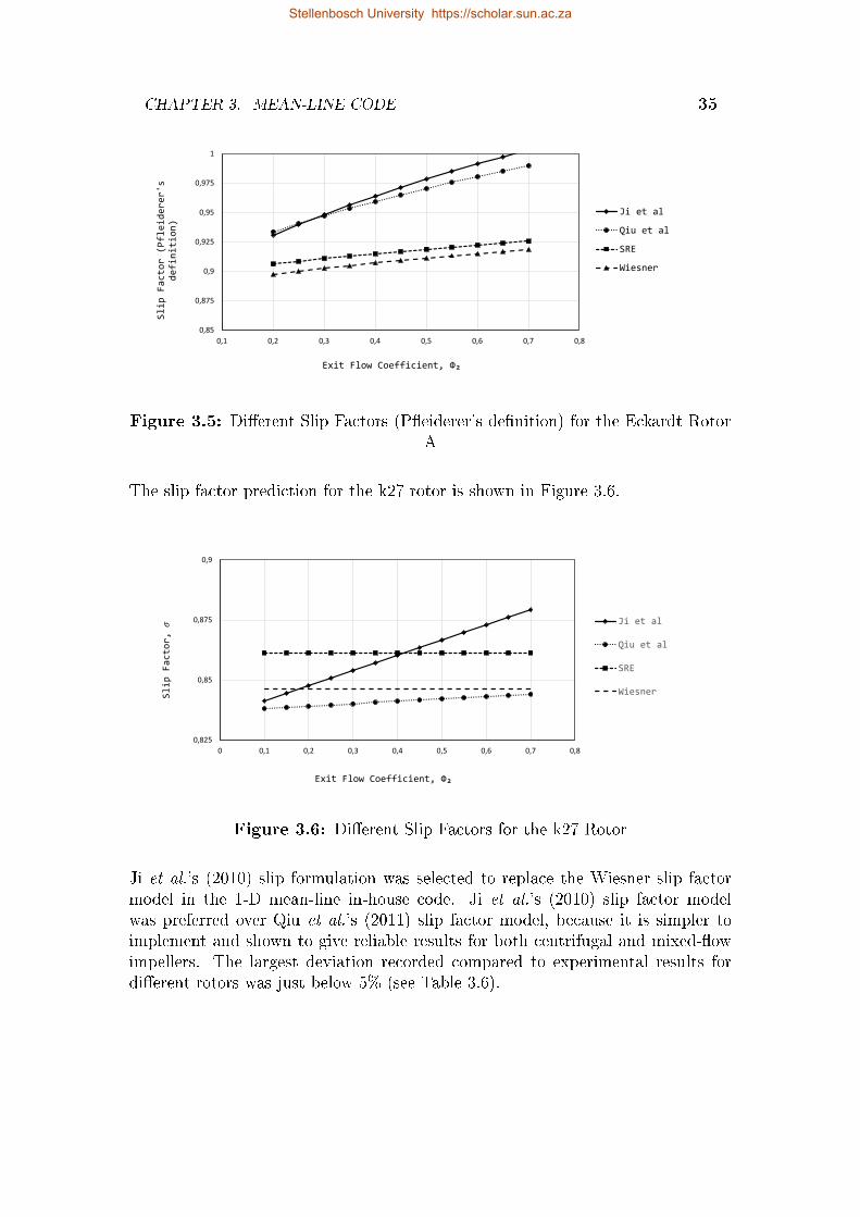
CHAPTER 3. MEAN-LINE CODE 35
0,85
0,875
0,9
0,925
0,95
0,975
1
0,1 0,2 0,3 0,4 0,5 0,6 0,7 0,8
Slip Factor (Pfleiderer's
definition)
Exit Flow Coefficient, Ф₂
Ji et al
Qiu et al
SRE
Wiesner
Figure 3.5: Dierent Slip Factors (Peiderer's denition) for the Eckardt RotorA
The slip factor prediction for the k27 rotor is shown in Figure 3.6.
0,825
0,85
0,875
0,9
0 0,1 0,2 0,3 0,4 0,5 0,6 0,7 0,8
Slip Factor, 𝜎
Exit Flow Coefficient, Ф₂
Ji et al
Qiu et al
SRE
Wiesner
Figure 3.6: Dierent Slip Factors for the k27 Rotor
Ji et al.'s (2010) slip formulation was selected to replace the Wiesner slip factormodel in the 1-D mean-line in-house code. Ji et al.'s (2010) slip factor modelwas preferred over Qiu et al.'s (2011) slip factor model, because it is simpler toimplement and shown to give reliable results for both centrifugal and mixed-owimpellers. The largest deviation recorded compared to experimental results fordierent rotors was just below 5% (see Table 3.6).
Stellenbosch University https://scholar.sun.ac.za
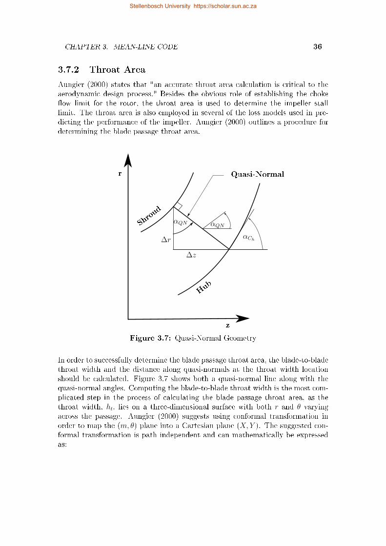
CHAPTER 3. MEAN-LINE CODE 36
3.7.2 Throat Area
Aungier (2000) states that "an accurate throat area calculation is critical to theaerodynamic design process." Besides the obvious role of establishing the chokeow limit for the rotor, the throat area is used to determine the impeller stalllimit. The throat area is also employed in several of the loss models used in pre-dicting the performance of the impeller. Aungier (2000) outlines a procedure fordetermining the blade passage throat area.
z
r Quasi-Normal
Hub
Shroud
αQNαQN
αCh
∆z
∆r
Figure 3.7: Quasi-Normal Geometry
In order to successfully determine the blade passage throat area, the blade-to-bladethroat width and the distance along quasi-normals at the throat width locationshould be calculated. Figure 3.7 shows both a quasi-normal line along with thequasi-normal angles. Computing the blade-to-blade throat width is the most com-plicated step in the process of calculating the blade passage throat area, as thethroat width, ht, lies on a three-dimensional surface with both r and θ varyingacross the passage. Aungier (2000) suggests using conformal transformation inorder to map the (m, θ) plane into a Cartesian plane (X,Y ). The suggested con-formal transformation is path independent and can mathematically be expressedas:
Stellenbosch University https://scholar.sun.ac.za
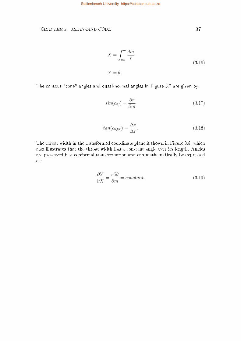
CHAPTER 3. MEAN-LINE CODE 37
X =
∫ m
m1
dm
r
Y = θ.
(3.16)
The contour "cone" angles and quasi-normal angles in Figure 3.7 are given by:
sin(αC) =∂r
∂m(3.17)
tan(αQN) =∆z
∆r. (3.18)
The throat width in the transformed coordinate plane is shown in Figure 3.8, whichalso illustrates that the throat width has a constant angle over its length. Anglesare preserved in a conformal transformation and can mathematically be expressedas:
∂Y
∂X=
r∂θ
∂m= constant. (3.19)
Stellenbosch University https://scholar.sun.ac.za
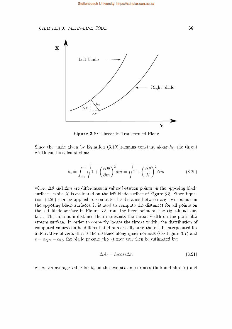
CHAPTER 3. MEAN-LINE CODE 38
Y
X
ht
∆Y
∆X
Left blade
Right blade
Figure 3.8: Throat in Transformed Plane
Since the angle given by Equation (3.19) remains constant along ht, the throatwidth can be calculated as:
ht =
∫ m
m1
√1 +
(r∂θ
∂m
)2
dm =
√1 +
(∆θ
X
)2
∆m (3.20)
where ∆θ and ∆m are dierences in values between points on the opposing bladesurfaces, while X is evaluated on the left blade surface of Figure 3.8. Since Equa-tion (3.20) can be applied to compute the distance between any two points onthe opposing blade surfaces, it is used to compute the distances for all points onthe left blade surface in Figure 3.8 from the xed point on the right-hand sur-face. The minimum distance then represents the throat width on the particularstream surface. In order to correctly locate the throat width, the distribution ofcomputed values can be dierentiated numerically, and the result interpolated fora derivative of zero. If n is the distance along quasi-normals (see Figure 3.7) andε = αQN − αC , the blade passage throat area can then be estimated by:
∆At = htcosε∆n (3.21)
where an average value for ht on the two stream surfaces (hub and shroud) and
Stellenbosch University https://scholar.sun.ac.za
CHAPTER 3. MEAN-LINE CODE 39
an average of ∆ncos(ε) on the opposing blade surfaces are used. To account forthe fact that the quasi-normal may not be normal to the stream surfaces, cos(ε)is used in Equation (3.21).
The original version of the mean-line code assumes that the throat of the impeller(where choke occurs) is located between the main blades of the impeller. It washowever found that choke may take place between the main blade and splitterblade of the k27 impeller, raising the question whether the throat area of an im-peller might be further downstream of the inlet. This led to the adaptation of themean-line code throat area in order to calculate the throat parameters for the caseof the throat being located between a main blade and splitter blade.
The change in the passage ow area, due to a change in the prediction of the throatarea, necessitates a change in the amount of uid ow through the throat area.This was achieved by the introduction of a new parameter that adapts the amountof ow by a factor equal to the newly predicted throat area over the originallypredicted throat area. For the mean-line script that determines the design pointof the impeller, this parameter is only used once in the throat conditions for-loop.In the script that determines the performance of the impeller for several impellerrotational speeds, this parameter is both employed in the throat conditions for-loop and in the for-loop determining the overall performance of the impeller. Flowdiagrams for the main-, performance-, and display scripts are given in Appendix B.
The passage area ratio, AR, is another variable that is inuenced by the changein the throat area (Equation (3.22)). AR is eectively the ratio of the impeller tipow area to the throat area. It is formulated in such a manner that it permitsanalysts to make adjustments to the throat area in order to match performancepredictions to an experimentally observed impeller choke limit without having anundesired eect on the work input prediction (Aungier, 2000). With the changein the throat area prediction, the minimum throat area may move down from theinlet of the impeller to the start of the splitter blade. To maintain the correctratio of impeller tip ow area to throat area, A1 should be replaced by Ath and A2
should be halved in Equation (3.22):
AR =A2sinβ2
A1sinβth
. (3.22)
Stellenbosch University https://scholar.sun.ac.za
CHAPTER 3. MEAN-LINE CODE 40
3.8 Summary
The mean-line code, as initially developed for centrifugal impeller design and anal-ysis was adapted, after which dierent impellers were analysed. The two areas ofadaptation were the slip formulation employed in the code, and the location andcalculation of the throat area. Three dierent iterations of the code, original, rst,and second were developed and each impeller was analysed using each iteration ofthe code. The results of the mean-line analyses are discussed in Chapter 5.
Stellenbosch University https://scholar.sun.ac.za
Chapter 4
Computational Fluid Dynamics
This chapter is concerned with the 3-D analyses of the impellers under consider-ation in this study. The process that was followed to set up the 3-D analyses isdiscussed and mesh details for each impeller is given.
4.1 Introduction
The analysis of an impeller through the use of a mean-line code, followed by aComputational Fluid Dynamics simulation forms part of this project. The mean-line code is used to get a rst approximation for the pressure ratio and eciency ofthe impeller. A CFD analysis is completed once the mean-line results are knownand is then compared to the mean-line results. The k27 impeller was used to com-plete the benchmark analysis, which is the same impeller that was numericallyanalysed by Van der Merwe (2012). The k27 impeller was originally designed fora turbocharger in the trucking industry, but turned out to be popular as a perfor-mance component in the aftermarket modication of street cars (Van der Merwe,2012).
This chapter contains details concerning the meshing of the k27, Van der Merwe,and Diener impeller geometries and the set-up of the CFD analyses. Numeca soft-ware was chosen to perform the CFD analyses. AutoGrid5 and FINE/Turboare dedicated software for generating meshes and setting up a ow analyses re-spectively for turbomachinery.
4.2 Impeller Geometry
The impeller geometry is required in order to create a computational mesh for theCFD analysis. Several le formats can be imported into Numeca AutoGrid5 in
41
Stellenbosch University https://scholar.sun.ac.za
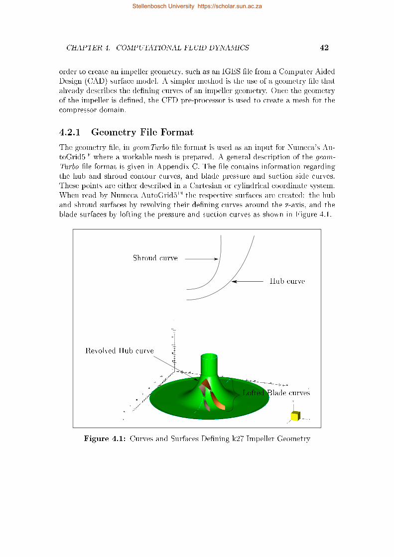
CHAPTER 4. COMPUTATIONAL FLUID DYNAMICS 42
order to create an impeller geometry, such as an IGES le from a Computer AidedDesign (CAD) surface model. A simpler method is the use of a geometry le thatalready describes the dening curves of an impeller geometry. Once the geometryof the impeller is dened, the CFD pre-processor is used to create a mesh for thecompressor domain.
4.2.1 Geometry File Format
The geometry le, in geomTurbo le format is used as an input for Numeca's Au-toGrid5 where a workable mesh is prepared. A general description of the geom-Turbo le format is given in Appendix C. The le contains information regardingthe hub and shroud contour curves, and blade pressure and suction side curves.These points are either described in a Cartesian or cylindrical coordinate system.When read by Numeca AutoGrid5 the respective surfaces are created: the huband shroud surfaces by revolving their dening curves around the z-axis, and theblade surfaces by lofting the pressure and suction curves as shown in Figure 4.1.
Hub curve
Shroud curve
Lofted Blade curves
Revolved Hub curve
Figure 4.1: Curves and Surfaces Dening k27 Impeller Geometry
Stellenbosch University https://scholar.sun.ac.za
CHAPTER 4. COMPUTATIONAL FLUID DYNAMICS 43
A new geometry le can be generated in three dierent ways:
Numeca Autoblade/ Autogrid can be used to create a geometry fromscratch with sketching tools.
A custom code with impeller parameters as input that creates the neces-sary curves based on the input parameters and then writes a geometry lecontaining the generated curves can be used.
A custom code and geometric measurements and/or scans can be used tocreate a surface model and the necessary curves from the surface model canthen be imported into either Autoblade, Autogrid or IGG.
For all three of the k27, Van der Merwe, and Diener rotors the impeller parametersare known. The exact impeller geometry was however required in order to performa benchmark analysis. It was not necessary to generate a geometry le for theVan der Merwe optimised impeller and Diener impeller as geometry les for theseimpellers are available. For the k27 impeller, however, a geometry le had to becreated as one was not available. An impeller CAD model of the k27 impellerthat was created through geometric scans was used to generate the geometry lethrough importing the impeller curves of the CAD model into Autogrid. Theprocess of the scans are discussed in Section 4.2.2.
4.2.2 Geometric Scans
Since the k27 impeller is an existing impeller, it was possible to create an accurateCAD surface model through geometric scans of the existing k27 impeller. Van derMerwe (2012) performed geometric scans on the k27 impeller through an opticalscanner, creating a point cloud of the geometry. This was done multiple times withdierent orientations of the impeller in order to scan all the important geometricfeatures of the impeller. The multiple scans were then superimposed using xedcoordinate stickers on the model.
The resulting point cloud was then exported in stl format to be processed by CADsoftware (Van der Merwe, 2012). The author thus used the already existing stl leof the k27 impeller created by Van der Merwe (2012) to create a surface model ofthe geometry using Autodesk® Inventor® Professional 2018. The CAD surfacemodel was exported in IGES le format and imported into AutoGrid5 .
Stellenbosch University https://scholar.sun.ac.za
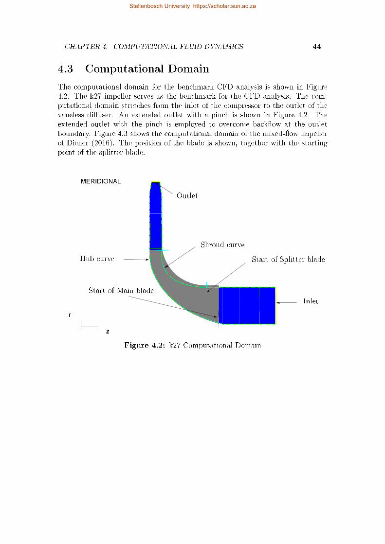
CHAPTER 4. COMPUTATIONAL FLUID DYNAMICS 44
4.3 Computational Domain
The computational domain for the benchmark CFD analysis is shown in Figure4.2. The k27 impeller serves as the benchmark for the CFD analysis. The com-putational domain stretches from the inlet of the compressor to the outlet of thevaneless diuser. An extended outlet with a pinch is shown in Figure 4.2. Theextended outlet with the pinch is employed to overcome backow at the outletboundary. Figure 4.3 shows the computational domain of the mixed-ow impellerof Diener (2016). The position of the blade is shown, together with the startingpoint of the splitter blade.
Outlet
Shroud curve
Start of Main blade
Inlet
Start of Splitter bladeHub curve
Figure 4.2: k27 Computational Domain
Stellenbosch University https://scholar.sun.ac.za
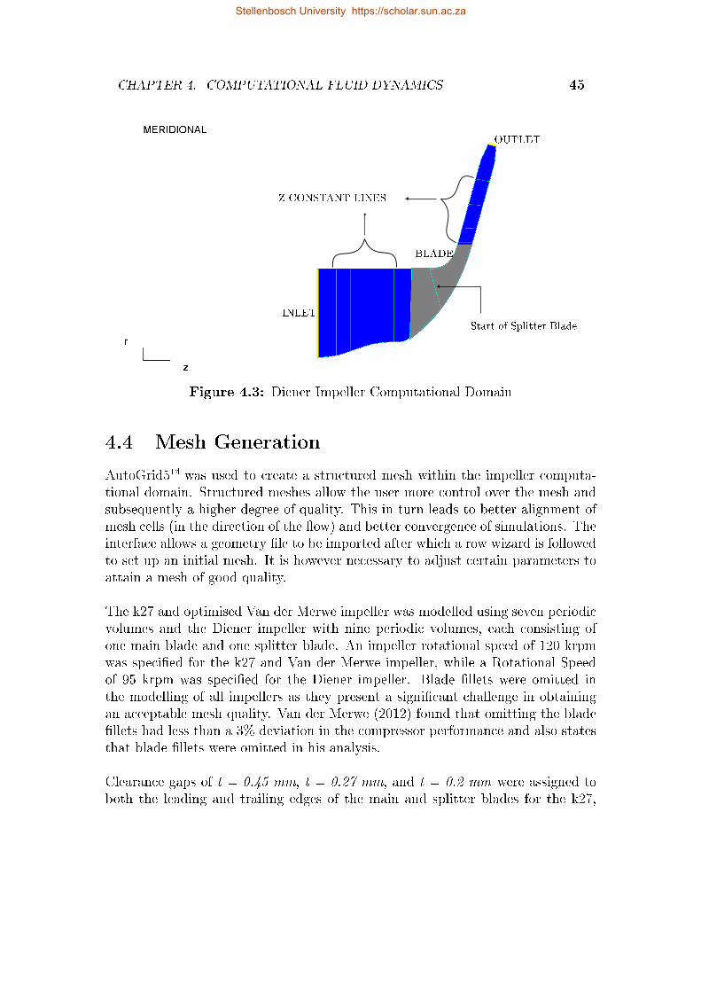
CHAPTER 4. COMPUTATIONAL FLUID DYNAMICS 45
Z CONSTANT LINES
OUTLET
INLET
BLADE
Start of Splitter Blade
Figure 4.3: Diener Impeller Computational Domain
4.4 Mesh Generation
AutoGrid5 was used to create a structured mesh within the impeller computa-tional domain. Structured meshes allow the user more control over the mesh andsubsequently a higher degree of quality. This in turn leads to better alignment ofmesh cells (in the direction of the ow) and better convergence of simulations. Theinterface allows a geometry le to be imported after which a row wizard is followedto set up an initial mesh. It is however necessary to adjust certain parameters toattain a mesh of good quality.
The k27 and optimised Van der Merwe impeller was modelled using seven periodicvolumes and the Diener impeller with nine periodic volumes, each consisting ofone main blade and one splitter blade. An impeller rotational speed of 120 krpmwas specied for the k27 and Van der Merwe impeller, while a Rotational Speedof 95 krpm was specied for the Diener impeller. Blade llets were omitted inthe modelling of all impellers as they present a signicant challenge in obtainingan acceptable mesh quality. Van der Merwe (2012) found that omitting the bladellets had less than a 3% deviation in the compressor performance and also statesthat blade llets were omitted in his analysis.
Clearance gaps of t = 0.45 mm, t = 0.27 mm, and t = 0.2 mm were assigned toboth the leading and trailing edges of the main and splitter blades for the k27,
Stellenbosch University https://scholar.sun.ac.za
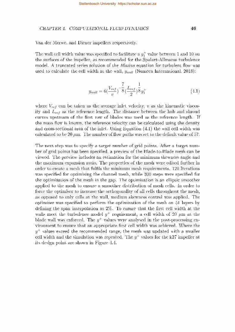
CHAPTER 4. COMPUTATIONAL FLUID DYNAMICS 46
Van der Merwe, and Diener impellers respectively.
The wall cell width value was specied to facilitate a y+1 value between 1 and 10 onthe surfaces of the impeller, as recommended for the Spalart-Allmaras turbulencemodel. A truncated series solution of the Blasius equation for turbulent ow wasused to calculate the cell width at the wall, ywall (Numeca International, 2018):
ywall = 6(Vref
v)−7
8 (Lref
2)
1
8y+1 (4.1)
where Vref can be taken as the average inlet velocity, v as the kinematic viscos-ity and Lref as the reference length. The distance between the hub and shroudcurves upstream of the rst row of blades was used as the reference length. Ifthe mass ow is known, the reference velocity can be calculated using the densityand cross-sectional area of the inlet. Using Equation (4.1) the wall cell width wascalculated to be 20 µm. The number of ow paths was set to the default value of 57.
The next step was to specify a target number of grid points. After a target num-ber of grid points has been specied, a preview of the Blade-to-Blade mesh can beviewed. The preview includes an estimation for the minimum skewness angle andthe maximum expansion ratio. The properties of the mesh were edited further inorder to create a mesh that fulls the minimum mesh requirements. 120 Iterationswas specied for optimising the channel mesh, while 300 steps were specied forthe optimisation of the mesh in the gap. The optimisation is an elliptic smootherapplied to the mesh to ensure a smoother distribution of mesh cells. In order toforce the optimiser to increase the orthogonality of all cells throughout the mesh,as opposed to only cells at the wall, medium skewness control was applied. Theoptimiser was specied to perform the optimisation of the mesh on 51 layers bydening the span interpolation as 2%. To ensure that the rst cell width at thewalls meet the turbulence model y+ requirement, a cell width of 20 µm at theblade wall was enforced. The y+ values were analysed in the post-processing en-vironment to ensure that an appropriate rst cell width was achieved. Where they+ values exceed the recommended range, the mesh was updated with a smallercell width and the simulation was repeated. The y+ values for the k27 impeller atits design point are shown in Figure 4.4.
Stellenbosch University https://scholar.sun.ac.za
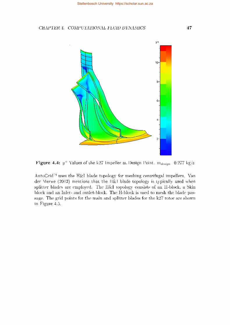
CHAPTER 4. COMPUTATIONAL FLUID DYNAMICS 47
Figure 4.4: y+ Values of the k27 Impeller at Design Point. mdesign=0.277 kg/s
AutoGrid uses the H&I blade topology for meshing centrifugal impellers. Vander Merwe (2012) mentions that the H&I blade topology is typically used whensplitter blades are employed. The H&I topology consists of an H-block, a Skinblock and an Inlet- and outlet-block. The H-block is used to mesh the blade pas-sage. The grid points for the main and splitter blades for the k27 rotor are shownin Figure 4.5.
Stellenbosch University https://scholar.sun.ac.za
CHAPTER 4. COMPUTATIONAL FLUID DYNAMICS 48
Main
Splitter
Figure 4.5: k27 Impeller H&I Topology for Main and Splitter Blades
Once the mesh properties have been adjusted and set, the Topology and GridPoint Distribution is initialized for the impeller. The ow paths through thecomputational domain are generated and the Blade-to-Blade mesh can be seen.The nal step is to generate the 3-Dimensional mesh. Once the 3-Dimensionalmesh has been generated, the mesh quality is evaluated. The quality of the gridis evaluated to ensure solver stability and convergence of the solution. There arefour major quality criteria that need to be adhered to, in order to ensure that themesh is of suitable quality. These criteria are dened as follows:
Orthogonality is the minimum angle between the edges of a cell (measuredin a 2-dimensional plane) and has a value between 0 and 90.
Aspect ratio is given as the length of a cell divided by its width, with a valueranging between 1 and 50,000.
Expansion ratio is the size variation between two adjacent cell surfaces in aspecic direction, ranging between 1 and 100.
Angular deviation is the deviation in angle between two adjacent cell surfacesmeasured in all directions, with a range between 0 and 180.
Stellenbosch University https://scholar.sun.ac.za
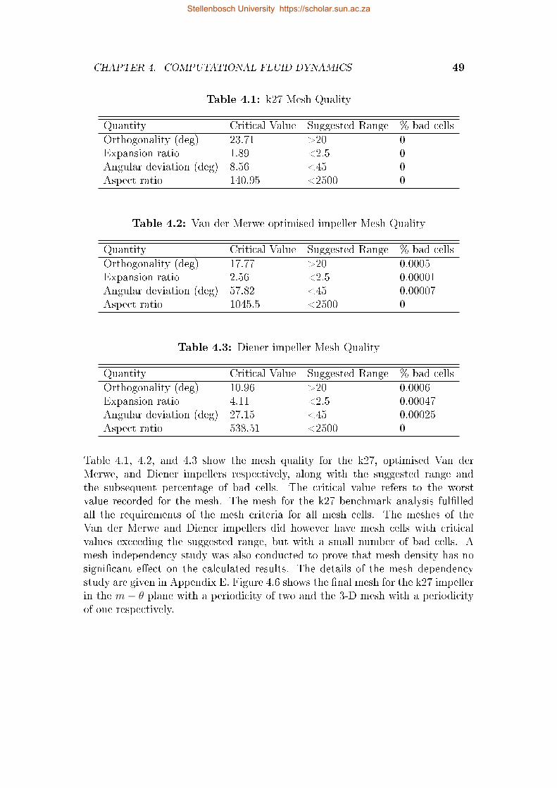
CHAPTER 4. COMPUTATIONAL FLUID DYNAMICS 49
Table 4.1: k27 Mesh Quality
Quantity Critical Value Suggested Range % bad cells
Orthogonality (deg) 23.71 >20 0Expansion ratio 1.89 <2.5 0Angular deviation (deg) 8.56 <45 0Aspect ratio 140.95 <2500 0
Table 4.2: Van der Merwe optimised impeller Mesh Quality
Quantity Critical Value Suggested Range % bad cells
Orthogonality (deg) 17.77 >20 0.0005Expansion ratio 2.56 <2.5 0.00001Angular deviation (deg) 57.82 <45 0.00007Aspect ratio 1045.5 <2500 0
Table 4.3: Diener impeller Mesh Quality
Quantity Critical Value Suggested Range % bad cells
Orthogonality (deg) 10.96 >20 0.0006Expansion ratio 4.11 <2.5 0.00047Angular deviation (deg) 27.15 <45 0.00025Aspect ratio 538.51 <2500 0
Table 4.1, 4.2, and 4.3 show the mesh quality for the k27, optimised Van derMerwe, and Diener impellers respectively, along with the suggested range andthe subsequent percentage of bad cells. The critical value refers to the worstvalue recorded for the mesh. The mesh for the k27 benchmark analysis fullledall the requirements of the mesh criteria for all mesh cells. The meshes of theVan der Merwe and Diener impellers did however have mesh cells with criticalvalues exceeding the suggested range, but with a small number of bad cells. Amesh independency study was also conducted to prove that mesh density has nosignicant eect on the calculated results. The details of the mesh dependencystudy are given in Appendix E. Figure 4.6 shows the nal mesh for the k27 impellerin the m− θ plane with a periodicity of two and the 3-D mesh with a periodicityof one respectively.
Stellenbosch University https://scholar.sun.ac.za
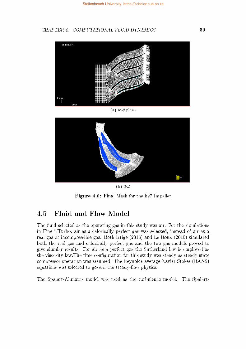
CHAPTER 4. COMPUTATIONAL FLUID DYNAMICS 50
(a) m-θ plane
(b) 3-D
Figure 4.6: Final Mesh for the k27 Impeller
4.5 Fluid and Flow Model
The uid selected as the operating gas in this study was air. For the simulationsin Fine/Turbo, air as a calorically perfect gas was selected, instead of air as areal gas or incompressible gas. Both Krige (2013) and Le Roux (2010) simulatedboth the real gas and calorically perfect gas and the two gas models proved togive simular results. For air as a perfect gas the Sutherland law is employed asthe viscosity law.The time conguration for this study was steady as steady statecompressor operation was assumed. The Reynolds-average Navier-Stokes (RANS)equations was selected to govern the steady-ow physics.
The Spalart-Allmaras model was used as the turbulence model. The Spalart-
Stellenbosch University https://scholar.sun.ac.za
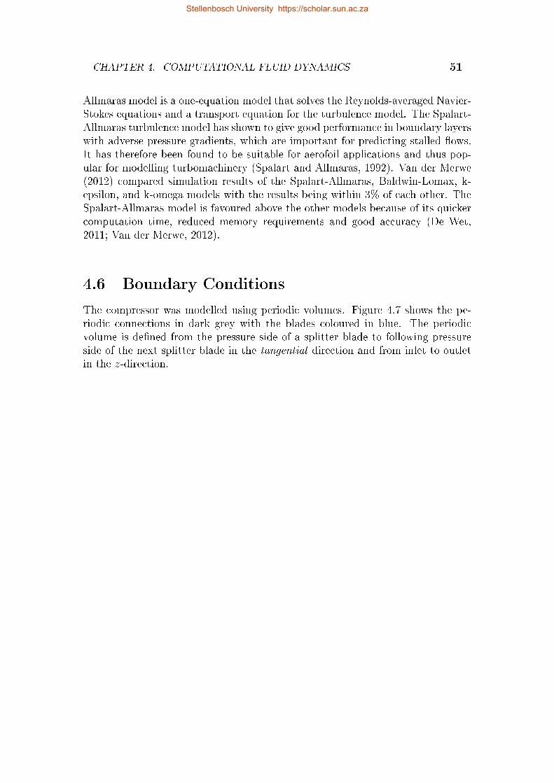
CHAPTER 4. COMPUTATIONAL FLUID DYNAMICS 51
Allmaras model is a one-equation model that solves the Reynolds-averaged Navier-Stokes equations and a transport equation for the turbulence model. The Spalart-Allmaras turbulence model has shown to give good performance in boundary layerswith adverse pressure gradients, which are important for predicting stalled ows.It has therefore been found to be suitable for aerofoil applications and thus pop-ular for modelling turbomachinery (Spalart and Allmaras, 1992). Van der Merwe(2012) compared simulation results of the Spalart-Allmaras, Baldwin-Lomax, k-epsilon, and k-omega models with the results being within 3% of each other. TheSpalart-Allmaras model is favoured above the other models because of its quickercomputation time, reduced memory requirements and good accuracy (De Wet,2011; Van der Merwe, 2012).
4.6 Boundary Conditions
The compressor was modelled using periodic volumes. Figure 4.7 shows the pe-riodic connections in dark grey with the blades coloured in blue. The periodicvolume is dened from the pressure side of a splitter blade to following pressureside of the next splitter blade in the tangential direction and from inlet to outletin the z-direction.
Stellenbosch University https://scholar.sun.ac.za
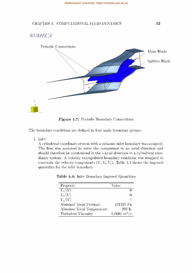
CHAPTER 4. COMPUTATIONAL FLUID DYNAMICS 52
Periodic Connections
Main Blade
Splitter Blade
Figure 4.7: Periodic Boundary Connections
The boundary conditions are dened in four main boundary groups:
1. InletA cylindrical coordinate system with a subsonic inlet boundary was assigned.The ow was assumed to enter the compressor in an axial direction andshould therefore be constrained in the z-axial direction in a cylindrical coor-dinate system. A velocity extrapolated boundary condition was assigned toconstrain the velocity components (Vr, Vt, Vz). Table 4.4 shows the imposedquantities for the inlet boundary.
Table 4.4: Inlet Boundary Imposed Quantities
Property Value
Vr/|V | 0Vt/|V | 0Vz/|V | 1Absolute Total Pressure 101325 PaAbsolute Total Temperature 293 KTurbulent Viscosity 0.0001 m2/s
Stellenbosch University https://scholar.sun.ac.za
CHAPTER 4. COMPUTATIONAL FLUID DYNAMICS 53
2. OutletAn averaged static pressure boundary condition was imposed for the outlet,since the approximation of a uniform static pressure at the outlet is notaccurate. This boundary condition extrapolates a pressure prole from theinterior eld (Numeca International, 2018). Backow Control was enabled asthe outlet was of a radial diuser type. This option controls the temperaturedistribution along the exit section. This ensures that in the case of owpartially re-entering, the reverse ow temperature is adjusted to have thesame averaged value as that of the exiting ow.
3. Periodic boundariesOne important feature of the AutoGrid5 mesh generator concerns the au-tomatic establishment of all connecting and periodic boundary conditions.When importing the mesh le created in AutoGrid5 to FINE/Turbo, theproperties of the periodic boundaries are transferred to the FINE/Turbointerface, with the advantage that the user does not need to specify any inputconcerning these boundary conditions.
4. Wall boundariesThe wall boundaries include the impeller hub, shroud and blades. The huband blade surfaces rotate at the same speed relative to the stationary shroudwall, modelled as rotating walls, while the shroud surface remains static.The rotational speed of the rotating surfaces was set to the same speed asthe required impeller speed. Smooth surfaces and no heat transfer (adiabaticow) was assumed for all wall boundaries. The boundaries were dened inthe cylindrical coordinate frame for the rotating blocks and no rotor-statorinterface was selected as only the impeller was modelled.
4.7 Settings
NUMECA's solver for FINE/Turbo, EURANUS, allows for a multigrid strategyto eciently solve ow equations. This multigrid strategy makes use of coarse gridinitialisation, which uses the coarser grid level solutions as an initial solution forthe ner grid levels. AutoGrid5 creates meshes with three grid levels, namely000, 111 and 222, where 000 is the nest grid level and 222 is the coarsest gridlevel. It indicates for each of the i, j, and k directions, the currently selectedgrid level. The current grid level was set to be the nest and the number of gridlevels employed for the coarse grid initialisation was 3. Under the Expert Param-eters, linear progression was selected as the Scheme denition used for the sweepson each grid level. By selecting linear progression for the solver, the number ofsweeps performed on each grid level equals the level number, e.g. 2 sweeps on
Stellenbosch University https://scholar.sun.ac.za
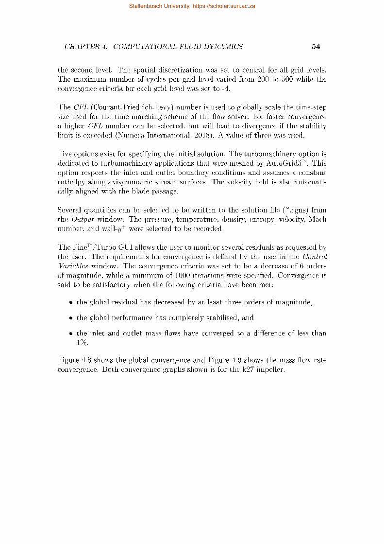
CHAPTER 4. COMPUTATIONAL FLUID DYNAMICS 54
the second level. The spatial discretization was set to central for all grid levels.The maximum number of cycles per grid level varied from 200 to 500 while theconvergence criteria for each grid level was set to -4.
The CFL (Courant-Friedrich-Levy) number is used to globally scale the time-stepsize used for the time marching scheme of the ow solver. For faster convergencea higher CFL number can be selected, but will lead to divergence if the stabilitylimit is exceeded (Numeca International, 2018). A value of three was used.
Five options exist for specifying the initial solution. The turbomachinery option isdedicated to turbomachinery applications that were meshed by AutoGrid5. Thisoption respects the inlet and outlet boundary conditions and assumes a constantrothalpy along axisymmetric stream surfaces. The velocity eld is also automati-cally aligned with the blade passage.
Several quantities can be selected to be written to the solution le (*.cgns) fromthe Output window. The pressure, temperature, density, entropy, velocity, Machnumber, and wall-y+ were selected to be recorded.
The Fine/Turbo GUI allows the user to monitor several residuals as requested bythe user. The requirements for convergence is dened by the user in the ControlVariables window. The convergence criteria was set to be a decrease of 6 ordersof magnitude, while a minimum of 1000 iterations were specied. Convergence issaid to be satisfactory when the following criteria have been met:
the global residual has decreased by at least three orders of magnitude,
the global performance has completely stabilised, and
the inlet and outlet mass ows have converged to a dierence of less than1%.
Figure 4.8 shows the global convergence and Figure 4.9 shows the mass ow rateconvergence. Both convergence graphs shown is for the k27 impeller.
Stellenbosch University https://scholar.sun.ac.za
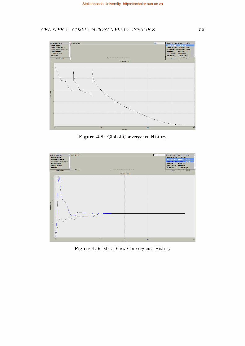
CHAPTER 4. COMPUTATIONAL FLUID DYNAMICS 55
Figure 4.8: Global Convergence History
Figure 4.9: Mass Flow Convergence History
Stellenbosch University https://scholar.sun.ac.za
CHAPTER 4. COMPUTATIONAL FLUID DYNAMICS 56
4.8 Post-processing
CFView is a parallelised scientic visualisation software system that was usedfor the post-processing. In order to evaluate the performance of the impeller only,a post-processing macro was created that enables the required properties such astotal pressure and total temperature to be evaluated at a user-dened constantradius plane. Together with CFView the NUMECA result le (*.mf) was used.The relevant performance parameters, as well as the mass ow at inlet and outletof the ow domain, are listed in the result le.
4.9 Summary
The computational domain and mesh set-up for the k27, optimised Van der Merwe,and Diener impellers are discussed in this chapter. The mesh quality for eachimpeller is shown, and the ow solver set-up is discussed. The results of the 3-DCFD analyses are presented in Chapter 5.
Stellenbosch University https://scholar.sun.ac.za
Chapter 5
Results and Discussion
In the presented study, several numerical simulations, comprising of both 1-D and3-D analyses, have been performed in order to assess the performance of severalcompressor impellers. The in-house 1-D Matlab® code was also adapted to ac-commodate mixed-ow impellers. The following section details the results of theinvestigation.
5.1 Mean-Line Code Results
In adapting the in-house 1-D mean-line code, several iterations of the code wasdeveloped. Each iteration represents a dierent amendment of the code. The orig-inal designation represents the original code as developed by De Wet in 2011 andadapted by Van der Merwe. The original code serves as the baseline for all otheriterations. The rst iteration designation refers to the code implementing the newJi et al. (2010) slip factor formulation as discussed in Section 3.7.1. The seconditeration represents the adaptation of the throat area prediction of the impeller asdiscussed in Section 3.7.2, while the new slip factor is also employed.
The rst and second iterations of the mean-line code allows insight into the eectof the slip factor and the throat area on the performance prediction for dierentconguration rotors. Each impeller was analysed using both iterations of the codeas well as the original version of the mean-line code in order to quantify the eectof each adaptation on each rotor.
57
Stellenbosch University https://scholar.sun.ac.za
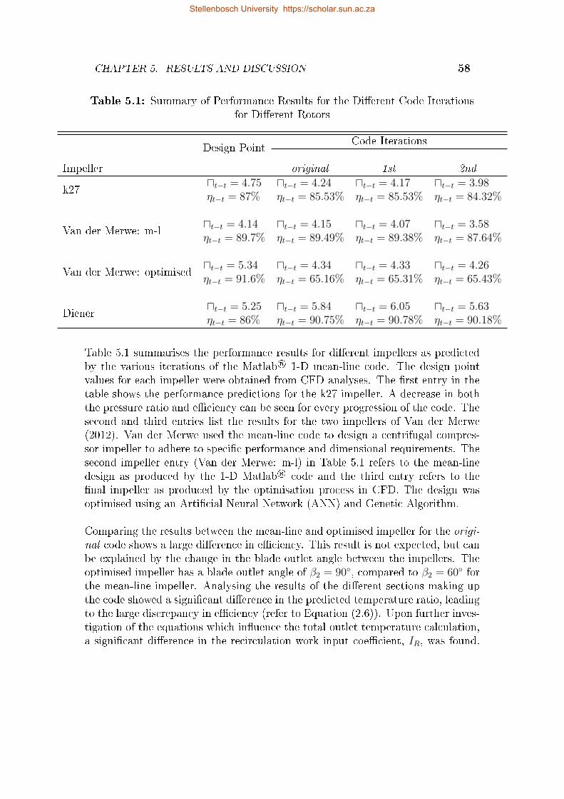
CHAPTER 5. RESULTS AND DISCUSSION 58
Table 5.1: Summary of Performance Results for the Dierent Code Iterationsfor Dierent Rotors
Design PointCode Iterations
Impeller original 1st 2nd
k27ut−t = 4.75ηt−t = 87%
ut−t = 4.24ηt−t = 85.53%
ut−t = 4.17ηt−t = 85.53%
ut−t = 3.98ηt−t = 84.32%
Van der Merwe: m-lut−t = 4.14ηt−t = 89.7%
ut−t = 4.15ηt−t = 89.49%
ut−t = 4.07ηt−t = 89.38%
ut−t = 3.58ηt−t = 87.64%
Van der Merwe: optimisedut−t = 5.34ηt−t = 91.6%
ut−t = 4.34ηt−t = 65.16%
ut−t = 4.33ηt−t = 65.31%
ut−t = 4.26ηt−t = 65.43%
Dienerut−t = 5.25ηt−t = 86%
ut−t = 5.84ηt−t = 90.75%
ut−t = 6.05ηt−t = 90.78%
ut−t = 5.63ηt−t = 90.18%
Table 5.1 summarises the performance results for dierent impellers as predictedby the various iterations of the Matlab® 1-D mean-line code. The design pointvalues for each impeller were obtained from CFD analyses. The rst entry in thetable shows the performance predictions for the k27 impeller. A decrease in boththe pressure ratio and eciency can be seen for every progression of the code. Thesecond and third entries list the results for the two impellers of Van der Merwe(2012). Van der Merwe used the mean-line code to design a centrifugal compres-sor impeller to adhere to specic performance and dimensional requirements. Thesecond impeller entry (Van der Merwe: m-l) in Table 5.1 refers to the mean-linedesign as produced by the 1-D Matlab® code and the third entry refers to thenal impeller as produced by the optimisation process in CFD. The design wasoptimised using an Articial Neural Network (ANN) and Genetic Algorithm.
Comparing the results between the mean-line and optimised impeller for the origi-nal code shows a large dierence in eciency. This result is not expected, but canbe explained by the change in the blade outlet angle between the impellers. Theoptimised impeller has a blade outlet angle of β2 = 90, compared to β2 = 60 forthe mean-line impeller. Analysing the results of the dierent sections making upthe code showed a signicant dierence in the predicted temperature ratio, leadingto the large discrepancy in eciency (refer to Equation (2.6)). Upon further inves-tigation of the equations which inuence the total outlet temperature calculation,a signicant dierence in the recirculation work input coecient, IR, was found.
Stellenbosch University https://scholar.sun.ac.za
CHAPTER 5. RESULTS AND DISCUSSION 59
The change in outlet angle resulted in the recirculation coecient IR changingfrom 0.0244 to 0.287, with the larger outlet angle resulting in more recirculationwork. This can be explained by considering the equation for the recirculationcoecient, Equation (5.1):
IR = (Deq
2− 1)[
WU2
Cm2
− 2cot(β2)]. (5.1)
The eect of the blade outlet angle on the recirculation coecient is contained inthe last term of Equation (5.1). When the blade outlet angle nears 90 the lastterm eectively falls away and IR increases. The blade outlet angle is however notthe only value that has a signicant impact on the recirculation coecient, withthe relative tangential velocity and absolute meridional velocity also aecting IR.This is important to note as the eciency recorded for the Eckardt "O" rotor by DeWet (2011), which also has a blade outlet angle of 90, as predicted by the originalmean-line code correlates well with experimental and CFD results, predicting aneciency between 80% and 85%. This result is not expected (on the basis of theVan der Merwe optimised rotor results) as the blade outlet angle is also 90, butthe blade tip speed is 1.6 times smaller than that of the optimised Van der Merwerotor and thus the relative tangential velocity, WU2, is much smaller, leading to asmall recirculation coecient and subsequently to a higher eciency.
5.2 k27 Impeller
Figure 5.1 shows the results for the k27 impeller, comparing both the 1-D mean-line and CFD results from this study to that obtained by Van der Merwe (2012).There is a discrepancy in the results for the mean-line as well as for the CFDresults between this study and that of Van der Merwe. The discrepancy in theCFD results is attributed to both the dierent computational domains (as theexact computational domain used by Van der Merwe is not available) as well asthe location of the evaluation plane. It should also be noted that the step gapmodelled by Van der Merwe was not modelled in this study.
Stellenbosch University https://scholar.sun.ac.za
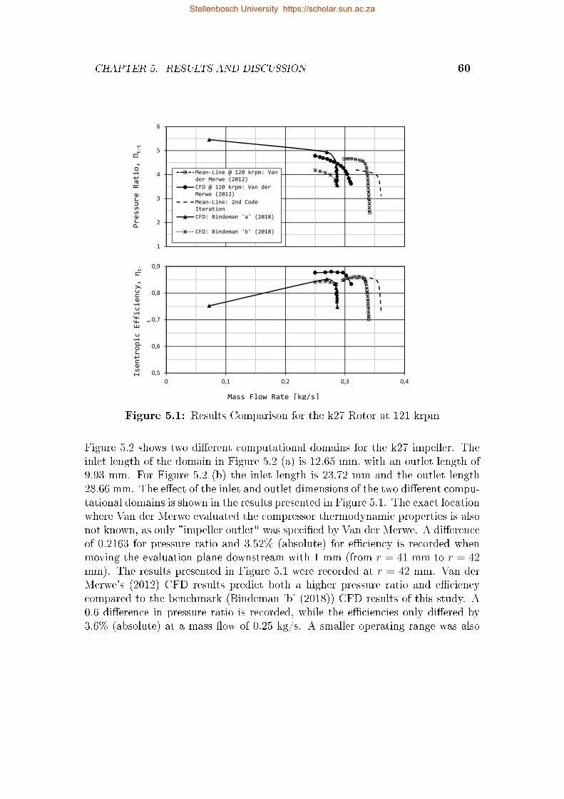
CHAPTER 5. RESULTS AND DISCUSSION 60
1
2
3
4
5
6Pr
essu
re R
atio
, Π t
-t
Mean-Line @ 120 krpm: Vander Merwe (2012)CFD @ 120 krpm: Van derMerwe (2012)Mean-Line: 2nd CodeIterationCFD: Bindeman 'a' (2018)
CFD: Bindeman 'b' (2018)
0,5
0,6
0,7
0,8
0,9
0 0,1 0,2 0,3 0,4
Isen
trop
ic E
ffic
ienc
y, η
t-
t
Mass Flow Rate [kg/s]
Figure 5.1: Results Comparison for the k27 Rotor at 121 krpm
Figure 5.2 shows two dierent computational domains for the k27 impeller. Theinlet length of the domain in Figure 5.2 (a) is 12.65 mm, with an outlet length of9.93 mm. For Figure 5.2 (b) the inlet length is 23.72 mm and the outlet length28.66 mm. The eect of the inlet and outlet dimensions of the two dierent compu-tational domains is shown in the results presented in Figure 5.1. The exact locationwhere Van der Merwe evaluated the compressor thermodynamic properties is alsonot known, as only "impeller outlet" was specied by Van der Merwe. A dierenceof 0.2163 for pressure ratio and 3.52% (absolute) for eciency is recorded whenmoving the evaluation plane downstream with 1 mm (from r = 41 mm to r = 42mm). The results presented in Figure 5.1 were recorded at r = 42 mm. Van derMerwe's (2012) CFD results predict both a higher pressure ratio and eciencycompared to the benchmark (Bindeman 'b' (2018)) CFD results of this study. A0.6 dierence in pressure ratio is recorded, while the eciencies only diered by3.6% (absolute) at a mass ow of 0.25 kg/s. A smaller operating range was also
Stellenbosch University https://scholar.sun.ac.za
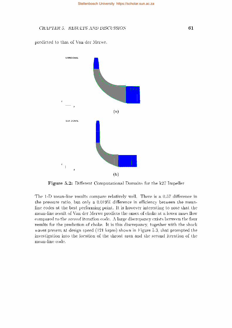
CHAPTER 5. RESULTS AND DISCUSSION 61
predicted to that of Van der Merwe.
(a)
(b)
Figure 5.2: Dierent Computational Domains for the k27 Impeller
The 1-D mean-line results compare relatively well. There is a 0.57 dierence inthe pressure ratio, but only a 0.019% dierence in eciency between the mean-line codes at the best performing point. It is however interesting to note that themean-line result of Van der Merwe predicts the onset of choke at a lower mass owcompared to the second iteration code. A large discrepancy exists between the fourresults for the prediction of choke. It is this discrepancy, together with the shockwaves present at design speed (121 krpm) shown in Figure 5.3, that prompted theinvestigation into the location of the throat area and the second iteration of themean-line code.
Stellenbosch University https://scholar.sun.ac.za
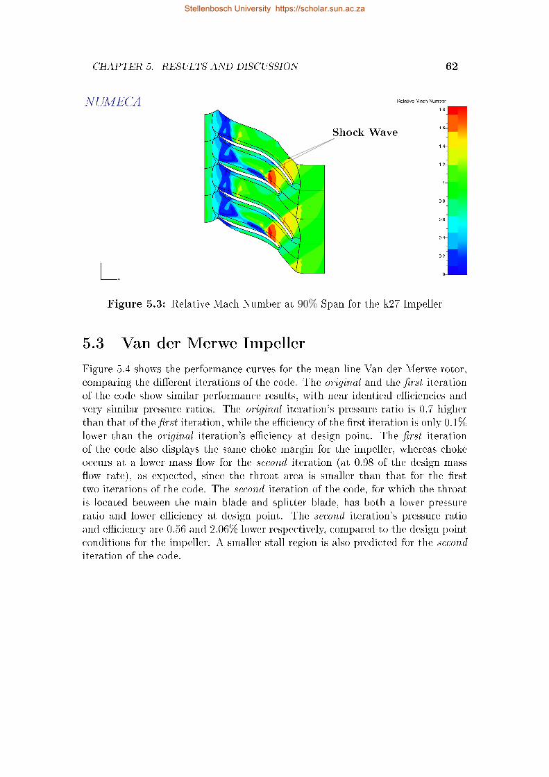
CHAPTER 5. RESULTS AND DISCUSSION 62
Shock Wave
Figure 5.3: Relative Mach Number at 90% Span for the k27 Impeller
5.3 Van der Merwe Impeller
Figure 5.4 shows the performance curves for the mean-line Van der Merwe rotor,comparing the dierent iterations of the code. The original and the rst iterationof the code show similar performance results, with near identical eciencies andvery similar pressure ratios. The original iteration's pressure ratio is 0.7 higherthan that of the rst iteration, while the eciency of the rst iteration is only 0.1%lower than the original iteration's eciency at design point. The rst iterationof the code also displays the same choke margin for the impeller, whereas chokeoccurs at a lower mass ow for the second iteration (at 0.98 of the design massow rate), as expected, since the throat area is smaller than that for the rsttwo iterations of the code. The second iteration of the code, for which the throatis located between the main blade and splitter blade, has both a lower pressureratio and lower eciency at design point. The second iteration's pressure ratioand eciency are 0.56 and 2.06% lower respectively, compared to the design pointconditions for the impeller. A smaller stall region is also predicted for the seconditeration of the code.
Stellenbosch University https://scholar.sun.ac.za
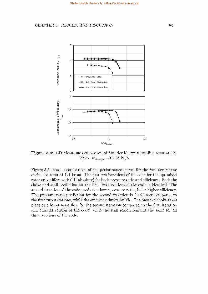
CHAPTER 5. RESULTS AND DISCUSSION 63
2
3
4
5
Pres
sure
rat
io,
Π 𝑡− 𝑡
Original Code
1st Code Iteration
2nd Code iteration
0,7
0,8
0,9
1
0,9 1 1,1
Isen
trop
ic E
ffic
ienc
y,
η 𝑡−𝑡
m/mdesign
Figure 5.4: 1-D Mean-line comparison of Van der Merwe mean-line rotor at 121krpm. mdesign = 0.325 kg/s
Figure 5.5 shows a comparison of the performance curves for the Van der Merweoptimised rotor at 121 krpm. The rst two iterations of the code for the optimisedrotor only diers with 0.1 (absolute) for both pressure ratio and eciency. Both thechoke and stall prediction for the rst two iterations of the code is identical. Thesecond iteration of the code predicts a lower pressure ratio, but a higher eciency.The pressure ratio prediction for the second iteration is 0.15 lower compared tothe rst two iterations, while the eciency diers by 1%. The onset of choke takesplace at a lower mass ow for the second iteration compared to the rst iterationand original version of the code, while the stall region remains the same for allthree versions of the code.
Stellenbosch University https://scholar.sun.ac.za
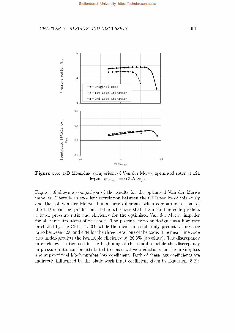
CHAPTER 5. RESULTS AND DISCUSSION 64
3
4
5
Pres
sure
rat
io,
Π 𝑡− 𝑡
Original code
1st Code Iteration
2nd Code iteration
0,5
0,6
0,7
0,8
0,9 1 1,1Isen
trop
ic E
ffic
ienc
y,
η 𝑡−𝑡
m/mdesign
Figure 5.5: 1-D Mean-line comparison of Van der Merwe optimised rotor at 121krpm. mdesign = 0.325 kg/s
Figure 5.6 shows a comparison of the results for the optimised Van der Merweimpeller. There is an excellent correlation between the CFD results of this studyand that of Van der Merwe, but a large dierence when comparing to that ofthe 1-D mean-line prediction. Table 5.1 shows that the mean-line code predictsa lower pressure ratio and eciency for the optimised Van der Merwe impellerfor all three iterations of the code. The pressure ratio at design mass ow ratepredicted by the CFD is 5.34, while the mean-line code only predicts a pressureratio between 4.26 and 4.34 for the three iterations of the code. The mean-line codealso under-predicts the isentropic eciency by 26.3% (absolute). The discrepancyin eciency is discussed in the beginning of this chapter, while the discrepancyin pressure ratio can be attributed to conservative predictions for the mixing lossand supercritical Mach number loss coecient. Both of these loss coecients areindirectly inuenced by the blade work input coecient given by Equation (5.2):
Stellenbosch University https://scholar.sun.ac.za
CHAPTER 5. RESULTS AND DISCUSSION 65
IB = σ(1− λφ2cotβ2)− U1CU1/U22 . (5.2)
The blade work input coecient aects the average blade velocity dierence, ∆W ,which then aects the maximum relative velocity, Wmax. Subsequently, the super-critical Mach number loss coecient, ωcr, is inuenced. Similarly to the super-critical Mach number loss, the wake mixing loss coecient, ωmix, is aected bythe maximum relative velocity which then aects the equivalent diusion factor,Deq, which has an inuence on determining the separation velocity that is usedin the calculation of the wake mixing loss coecient. The loss models indirectlyinuence the eciency as they are only used in the prediction of the outlet pressure.
Similar to Equation (5.1), Equation (5.2) is also inuenced by the blade outletangle, β2. When the blade has a pure radial outlet (no back-sweep) it has anadverse aect on the blade work input coecient and subsequently leads to a tooconservative prediction for both the mixing loss and supercritical Mach numberloss coecients. The greater these coecients, the smaller the predicted outletpressure. Apart from the discrepancy in pressure ratio and eciency, a smalleroperating range is predicted according to the 1-D mean-line analysis, versus theCFD analysis.
Stellenbosch University https://scholar.sun.ac.za
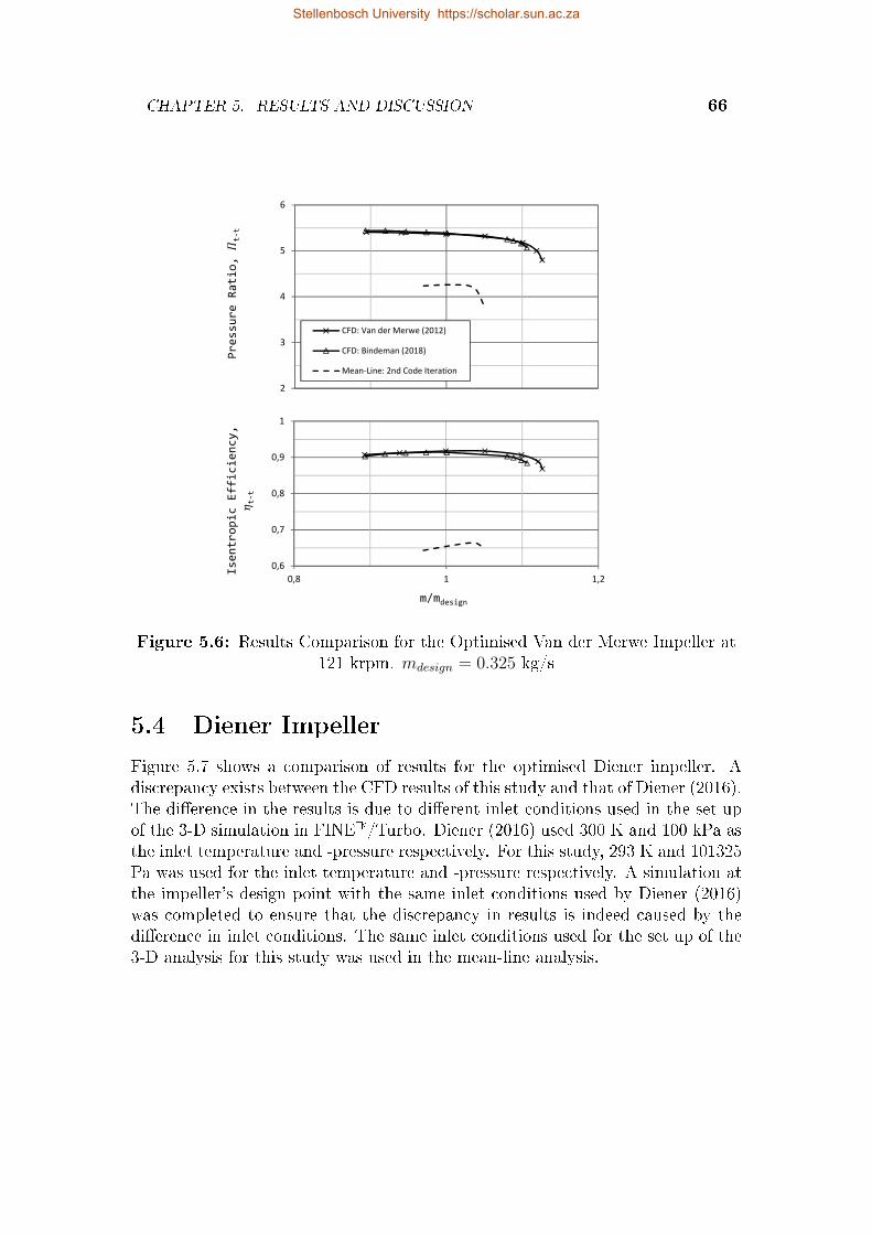
CHAPTER 5. RESULTS AND DISCUSSION 66
2
3
4
5
6
Pres
sure
Rat
io, 𝛱t-
t
CFD: Van der Merwe (2012)
CFD: Bindeman (2018)
Mean-Line: 2nd Code Iteration
0,6
0,7
0,8
0,9
1
0,8 1 1,2
Isen
trop
ic E
ffic
ienc
y,
𝜂t-
t
m/mdesign
Figure 5.6: Results Comparison for the Optimised Van der Merwe Impeller at121 krpm. mdesign = 0.325 kg/s
5.4 Diener Impeller
Figure 5.7 shows a comparison of results for the optimised Diener impeller. Adiscrepancy exists between the CFD results of this study and that of Diener (2016).The dierence in the results is due to dierent inlet conditions used in the set upof the 3-D simulation in FINE/Turbo. Diener (2016) used 300 K and 100 kPa asthe inlet temperature and -pressure respectively. For this study, 293 K and 101325Pa was used for the inlet temperature and -pressure respectively. A simulation atthe impeller's design point with the same inlet conditions used by Diener (2016)was completed to ensure that the discrepancy in results is indeed caused by thedierence in inlet conditions. The same inlet conditions used for the set up of the3-D analysis for this study was used in the mean-line analysis.
Stellenbosch University https://scholar.sun.ac.za
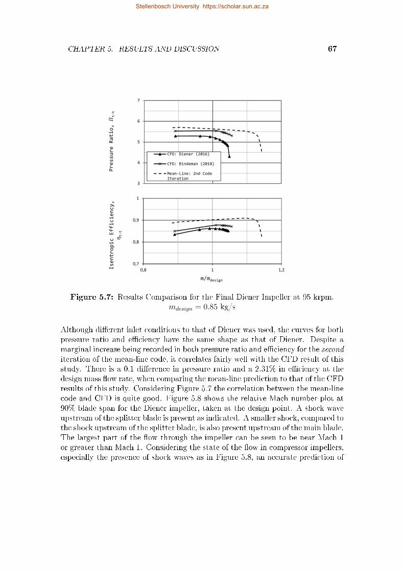
CHAPTER 5. RESULTS AND DISCUSSION 67
3
4
5
6
7
Pres
sure
Rat
io, 𝛱t-
t
CFD: Diener (2016)
CFD: Bindeman (2018)
Mean-Line: 2nd CodeIteration
0,7
0,8
0,9
1
0,8 1 1,2Isen
trop
ic E
ffic
ienc
y,
𝜂t-
t
m/mdesign
Figure 5.7: Results Comparison for the Final Diener Impeller at 95 krpm.mdesign = 0.85 kg/s
Although dierent inlet conditions to that of Diener was used, the curves for bothpressure ratio and eciency have the same shape as that of Diener. Despite amarginal increase being recorded in both pressure ratio and eciency for the seconditeration of the mean-line code, it correlates fairly well with the CFD result of thisstudy. There is a 0.1 dierence in pressure ratio and a 2.31% in eciency at thedesign mass ow rate, when comparing the mean-line prediction to that of the CFDresults of this study. Considering Figure 5.7 the correlation between the mean-linecode and CFD is quite good. Figure 5.8 shows the relative Mach number plot at90% blade span for the Diener impeller, taken at the design point. A shock waveupstream of the splitter blade is present as indicated. A smaller shock, compared tothe shock upstream of the splitter blade, is also present upstream of the main blade.The largest part of the ow through the impeller can be seen to be near Mach 1or greater than Mach 1. Considering the state of the ow in compressor impellers,especially the presence of shock waves as in Figure 5.8, an accurate prediction of
Stellenbosch University https://scholar.sun.ac.za
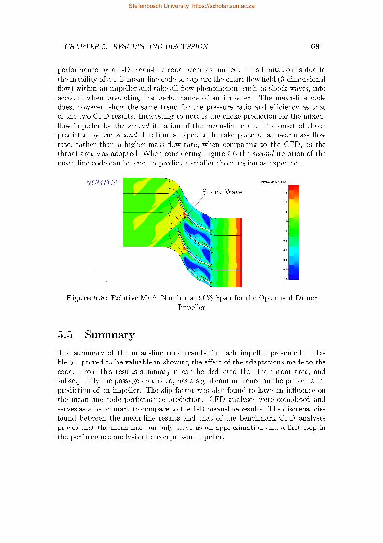
CHAPTER 5. RESULTS AND DISCUSSION 68
performance by a 1-D mean-line code becomes limited. This limitation is due tothe inability of a 1-D mean-line code to capture the entire ow eld (3-dimensionalow) within an impeller and take all ow phenomenon, such as shock waves, intoaccount when predicting the performance of an impeller. The mean-line codedoes, however, show the same trend for the pressure ratio and eciency as thatof the two CFD results. Interesting to note is the choke prediction for the mixed-ow impeller by the second iteration of the mean-line code. The onset of chokepredicted by the second iteration is expected to take place at a lower mass owrate, rather than a higher mass ow rate, when comparing to the CFD, as thethroat area was adapted. When considering Figure 5.6 the second iteration of themean-line code can be seen to predict a smaller choke region as expected.
Shock Wave
Figure 5.8: Relative Mach Number at 90% Span for the Optimised DienerImpeller
5.5 Summary
The summary of the mean-line code results for each impeller presented in Ta-ble 5.1 proved to be valuable in showing the eect of the adaptations made to thecode. From this results summary it can be deducted that the throat area, andsubsequently the passage area ratio, has a signicant inuence on the performanceprediction of an impeller. The slip factor was also found to have an inuence onthe mean-line code performance prediction. CFD analyses were completed andserves as a benchmark to compare to the 1-D mean-line results. The discrepanciesfound between the mean-line results and that of the benchmark CFD analysesproves that the mean-line can only serve as an approximation and a rst step inthe performance analysis of a compressor impeller.
Stellenbosch University https://scholar.sun.ac.za
Chapter 6
Conclusions and Recommendations
The possible applications where MGTs can be used are numerous, while thereis an increased interest in the application of MGTs for the propulsion of UAVs.This interest makes the development of a mixed-ow impeller for a specic size-range engine feasible. The use of both 1-D mean-line and 3-D CFD analysis is ofimportance for a detailed aerodynamic design and performance analysis of such animpeller. Relevant theory concerning mixed-ow impellers and how they functionwas explained. Literature concerning compressors as well as the 1-D and 3-Danalysis of several impellers were detailed.
6.1 Conclusions
Three dierent compressor impellers were analysed using a 1-D mean-line codedeveloped by De Wet (2011) which is based on the work of Aungier (2000). Twocentrifugal impellers, the k27 and Van der Merwe impeller, and the mixed-owimpeller of Diener (2016) were analysed and compared to the results of 3-D CFDanalyses. The objective of the thesis was to successfully adapt the in-house mean-line code for application with both centrifugal and mixed-ow impellers. Twospecic areas in the code were identied to be adapted; the slip formulation andthe throat area. The Wiesner (1967) slip formulation, employed by the originalcode was replaced with the Ji et al. (2010) slip formulation in order to account forthe axial ow component in a mixed-ow impeller. An alternative location for thethroat area was proposed, calculating the area between a main blade and splitterblade, instead of the area near the inducer section. The results of the adaptationsmade to the code are presented in Table 5.1, comparing three iterations of thecode for each impeller.
The second iteration of the mean-line code under-predicts both pressure ratio and
69
Stellenbosch University https://scholar.sun.ac.za
CHAPTER 6. CONCLUSIONS AND RECOMMENDATIONS 70
eciency for the centrifugal congurations, while it over-predicts eciency for themixed-ow conguration (all quantities taken as total-to-total as only the impelleris considered). The pressure ratio is under-predicted by 16.2% and the isentropiceciency by 3.1% for the k27 impeller. For the mean-line impeller of Van derMerwe the pressure ratio diers by 13.5% and the isentropic eciency by 2.3%.The optimised Van der Merwe impeller sees the largest dierence in the predictionof performance by the mean-line code with a 20.2% and 28.6% decit in pressureratio and isentropic eciency respectively. The performance of the mixed-owimpeller of Diener is, however, predicted more accurately, with a 7.2% and 4.9%over-prediction in pressure ratio and isentropic eciency respectively by the mean-line code.
At the maximum eciency point (MEP) of the CFD results for the k27 impeller,there is a 6.15% and 2.95% dierence in pressure ratio and isentropic eciencyrespectively between the CFD results of this study and that of Van der Merwe(2012). A higher pressure ratio, but lower eciency is predicted compared to theresults of Van der Merwe (2012). The discrepancy in results is due to a dierentcomputational domain used. For the optimised impeller of Van der Merwe thereis excellent agreement between the CFD results. There is only a 0.35% and 0.41%dierence in pressure ratio and eciency respectively, while Van der Merwe's max-imum choke mass ow rate is 1.79% larger.
The mean-line prediction for pressure ratio for the Diener impeller is close to thatof the CFD, with a 1.6% increase for pressure ratio and a 2.8% increase for theeciency. The mean-line code therefore correlates well with the 3-D analysis. Itshould be noted however that the stall criterion employed in the 1-D analysis hadto be changed from 1.75 to 2.5 (user-dened) in order for the compressor curve tobe plotted at the design speed of 95 krpm.
It is therefore concluded that the objective of adapting the in-house 1-D mean-linecode in order to analyse both centrifugal and mixed-ow impellers was successful.The results of the mean-line analysis for both centrifugal and mixed-ow impellerswere compared to 3-D CFD analysis results. It was found that a blade with apure radial outlet angle (β2b = 90) has an adverse eect on the prediction of the1-D mean-line performance of such an impeller. Furthermore, the throat area wasfound to have a signicant impact on the 1-D mean-line performance prediction.The discrepancies recorded between mean-line and CFD results suggest that a1-D mean-line analysis is only good enough to serve as an approximation of theexpected performance and that a 3-D CFD analysis is still required for an accurateprediction of the performance of an impeller.
Stellenbosch University https://scholar.sun.ac.za
CHAPTER 6. CONCLUSIONS AND RECOMMENDATIONS 71
6.2 Recommendations
Future work can be done on the adaptation of the 1-D mean-line code. The Jiet al. (2010) slip factor chosen in this thesis is only one of many slip factor formu-lations to choose from. A recommendation is to test more slip factors developedfor both mixed-ow and centrifugal impellers or only for mixed-ow impellers anddetermine if there is one that proves to give reliable results when compared to abenchmark analysis.
The importance of using an accurate throat area for performance prediction is ev-ident and therefore further investigation into the prediction of the throat area andcorresponding throat parameters is advised. Both the location and the calculationof the area for the throat can be revised and rened. Critical ratio's, such as the
passage area ratio (A2sinβ2
Athsinβth
) and relative velocity ratio (Wthshroud
Wth
), that has an
inuence on both pressure ratio and choke margin are aected by the calculationof the throat area and its location. Special attention should therefore be given tothe improvement of all throat parameters. Furthermore, the large discrepancy inperformance results for the optimised Van der Merwe impeller suggest that thereis merit in investigating the loss models (wake mixing loss and supercritical Machnumber loss) and work input coecients (IB and IR) proposed by Aungier (2000).Aungier himself states the "quality of results obtained directly depends on the va-lidity of the empirical models employed" and mentions that the success of a basicanalysis system depends on continual validation.
It is also recommended to compare the current in-house mean-line code to com-mercial software, such as Concepts NREC. Comparing the mean-line code to com-mercial software will give a better indication of the accuracy of the code. Lastly,the analysis of several mixed-ow geometries available in literature and the docu-mentation of the performance results of each geometry would be of great value todetermine the robustness of the code in predicting the performance of a mixed-owimpeller.
Stellenbosch University https://scholar.sun.ac.za
List of References
Aungier, R. (2000). Centrifugal Compressors. ASME Press, New York.
Boyce, M. (1993). Principles of operation and performance estimation of centrifugalcompressors. Proceedings of Turbomachinery Symposium, vol. 22.
Boyce, M.P. (2012). Compressor and Turbine Performance Characteristics. 4th edn.Elsevier Inc., Oxford. ISBN 9780123838421.
Burger, C.J. (2016). Design Procedure of a Compact Aerodynamic Crossover Diuser for
Micro Gas Turbine Application. Masters, University of Stellelbosch.
Busemann, A. (1928). Das Förderhöhenverhältnis radialer Kreiselpumpen mitlogarithmisch-spiraligen Schaufeln. ZAMM - Zeitschrift für Angewandte Mathematik
und Mechanik, vol. 8, no. 5, pp. 372384. ISSN 00442267.
Cevik, M. (2009). Design And Optimization Of A Mixed Flow Compressor Impeller Using
Robust Design Methods. Masters, Middle East Technical University.
Cumpsty, N.A. (1989). Compressor Aerodynamics. Longman Scientic & Technical.ISBN 9780582013643.
De Villiers, L. (2014). Design of a Centrifugal Compressor for Application in Micro Gas
Turbines. Masters, Stellenbosch.
De Wet, A.L. (2011). Performance Investigation of a Turbocharger Compressor. Masters,Stellenbosch University.
Diener, O. (2016). Development of a Mixed-Flow Compressor Impeller for Micro Gas
Turbine Application. Masters, Stellenbosch University.
Dixon, S. and Hall, C. (2010). Fluid Mechanics and Thermodynamics of Turbomachinery.6th edn. Elsevier Inc., Oxford.
Dixon, S.L. (1998). Fluid Mechanics , Thermodynamics of Turbomachinery. Fourth ediedn. Butterworth-Heinemann, Oxford.
Eck, B.F. (1973). Fans: design and operation of centrifugal, axial- ow, and cross-ow
fans. Oxford University Press, NewYork.
72
Stellenbosch University https://scholar.sun.ac.za
LIST OF REFERENCES 73
Eisenlohr, G. and Benfer, F.W. (1994). Aerodynamic Design and Investigation of a MixedFlow Compressor Stage. October, vol. 537, no. October 1993, pp. 20.1 20.7.
Harris, M., Jones, A. and Alexander, E. (2003). Miniature Turbojet Development atHamilton Sundstrand: The TJ-50, TJ-120 and TJ-30 Turbojets. In: 2nd AIAA "Un-
manned Unlimited" Conf. and Workshop & Exhibit, Infotech@Aerospace Conferences.American Institute of Aeronautics and Astronautics.Available at: https://doi.org/10.2514/6.2003-6568
Hill, P.G. and Peterson, C.R. (1992). MECHANICS AND THERMODYNAMICS. 2ndedn. Pearson.
Japikse, D. (1996). Centrifugal compressor design and performance. Concepts ETI,Wilder, Vt. ISBN 0933283032.
Ji, C., Zou, J., Ruan, X.D., Dario, P. and Fu, X. (2010). A new correlation for slip factorin radial and mixed-ow impellers. Power and Energy, vol. 225, pp. 114119.
King, J.A. and Glodeck, E. (1942). Performance Characteristics of Mixed ow impellerand vaned diuser with several modications. Tech. Rep., National Advisory Com-mittee for Aeronautics, Cleveland, Ohio.
Kock, M.P. (2017). Design of a Cross-over Diuser for a Mixed Flow Compressor Im-
peller. Masters, Stellenbosch.
Krige, D.S. (2013). Performance Evaluation of a Micro Gas Turbine Centrifugal Com-
pressor Diuser. Masters, Stellenbosch.
Lakshminarayana, B. (1996). Fluid Dynamics and Heat Transfer of Turbomachinery.John Wiley & Sons, New York, N.Y.
Le Roux, F.N. (2010). The CFD simulation of an axial ow fan. Masters, StellenboschUniversity.
Marcellan, A. (2015). An exploration into the potential of microturbine based propulsion
systems for civil Unmanned Aerial Vehicles. Masters, Delf University of Technology.
Mirsky, S., Jacobson, W., Tiscornia, D., McWhirter, J. and Zaghloul, M. (2013). DE-VELOPMENT AND DESIGN OF ANTISURGE AND PERFORMANCE CONTROLSYSTEMS.
Monig, R., Broichhausen, K. and Gallus, H. (1987). Application of Highly Loaded Single-Stage Mixed-Flow Compressors in Small Jet-Engines. In: AGARD Conference Pro-
ceedings No.421 Advanced Technology for Aero Gas Turbine Components.
Mönig, R., Elmendorf, W. and Callus, H.E. (1993). Design and Rotor Performance of aCompressor. Journal of Turbomachinery, vol. 1, no. July 1993.
Stellenbosch University https://scholar.sun.ac.za
LIST OF REFERENCES 74
Musgrave, D.S. and Plehn, N.J. (1987). Mixed-Flow Compressor Stage Design and TestResults With a Pressure Ratio of 3 : 1. Journal of Turbomachinery, vol. 109, no.October 1987, pp. 513519. ISSN 15288900.
Numeca International (2018). Fine/Turbo 11.2 User Manual.
Paeng, K.S. and Chung, M.K. (2001). A new slip factor for centrifugal impellers. Pro-ceedings of the Institution of Mechanical Engineers, Part A: Journal of Power and
Energy, vol. 215, no. 5, pp. 645649. ISSN 09576509.
Pampreen, R.C. and Musgrave, D.S. (1978). A Method of Calculating the Slip Factorof Centrifugal Compressors From Deviation Angle. Journal of Engineering for Power,vol. 100, no. 1, pp. 121128. ISSN 0742-4795.
Peiderer, C. (1961). Die Kreiselpumpen für Flüssigkeiten und Gase. 5th edn. Springer,Berlin.
Qiu, X., Japikse, D., Zhao, J. and Anderson, M.R. (2011). Analysis and Validation ofa Unied Slip Factor Model for Impellers at Design and. Jounal of Turbomachinery,vol. 133, no. October, pp. 19.
Rajakumar, D.R., Ramamurthy, S. and Govardhan, M. (2015). Experimental investiga-tions on eects of tip clearance in mixed-ow compressor performance. Proceedings
of the Institution of Mechanical Engineers, Part G: Journal of Aerospace Engineering,vol. 229, no. 5, pp. 933946. ISSN 20413025.
Sandberg, M.R. (2016). Centrifugal Compressor Conguration, Selection and Arrange-ment: A User's Perspective. Proceedings of the Forty-Fifth Turbomachinery Sympo-
sium.
Saravanamuttoo, H.I.H., Rogers, G.F.C. and Cohen, H. (2001). Gas Turbine Theory. 50years. Prentice Hall. ISBN 9780130158475.
Shukla, T. (2013). Micro Gas Turbine-A Review. International Journal on Theoretical
and Applied Research in Mechanical Engineering, vol. 2, no. 3, pp. 23193182.
Spalart, P. and Allmaras, S. (1992). A one-equation turbulence model for recirculatingows. AIAA Paper 92-0439. ISSN 16747348. arXiv:1011.1669v3.
Stanitz, J.D. (1952). Some Theoretical Aerodynamic Investigations of Impellers inRadial- and Mixed-Flow Impellers. Trans. ASME, vol. 74, pp. 473476.
Stodola, A. (1945). Steam and gas turbines : with a supplement on the prospects of the
thermal prime mover... New York, N.Y. : Smith, New York, N.Y.
Van der Merwe, B.B. (2012). Design of a Centrifugal Compressor Impeller for Micro
Gas Turbine Application. Masters, Stellenbosch.
Stellenbosch University https://scholar.sun.ac.za
LIST OF REFERENCES 75
Verstraete, T., Alsalihi, Z. and Van den Braembussche, R.A. (2010). MultidisciplinaryOptimization of a Radial Compressor for Microgas Turbine Applications. Journal ofTurbomachinery, vol. 132, no. 3, p. 031004. ISSN 0889504X.
Vick, M.J., Heyes, A. and Pullen, K. (2010). Design Overview of a Three KilowattRecuperated Ceramic Turboshaft Engine. Journal of Engineering for Gas Turbines &Power, vol. 132, no. September 2010, pp. 092301.1092301.9. ISSN 07424795.
Visser, F.C., Brouwers, J.J. and Badie, R. (1994). Theoretical analysis of inertially irrota-tional and solenoidal ow in two-dimensional radial-ow pump and turbine impellerswith equiangular blades. Journal of Fluid Mechanics, vol. 269, no. June 1994, pp.107141. ISSN 14697645.
Von Backström, T.W. (2006). A Unied Correlation for Slip Factor in Centrifugal Im-pellers. Journal of Turbomachinery, vol. 128, no. January 2006.
Wehrly, D. (2014). WREN MW54 Gas Turbine Jet Engine.
Whiteld, A. and Roberts, D.V. (1981). The Eect of Impeller Tip Design on thePerformance of a Mixed Flow Turbocharger Compressor. In: ASME Gas Turbine
Conference and Products Show, vol. 1, pp. 410. Housten, Texas. ISBN 9780791879610.ISSN 04021215.
Wiesner, F.J. (1967). A Review of Slip Factors for Centrifugal Impellers. Journal of
Engineering for Power, vol. 89, no. 4, pp. 558566. ISSN 0742-4795.
Wislicenus, G.F. (1965). Fluid Mechanics of Turbomachinery. 2nd edn. Constable andCompany, New York.
Youssef, N. andWeir, G. (2002). Mixed Flow and Centrifugal Compressor for Gas TurbineEngine.
Zemp, A., Kammerer, A. and Abhari, R.S. (2010). Unsteady Computational Fluid Dy-namics Investigation on Inlet Distortion in a Centrifugal Compressor. Journal of
Turbomachinery, vol. 132, no. 3, p. 031015. ISSN 0889504X.
Stellenbosch University https://scholar.sun.ac.za
Appendix A: Impeller Geometry
Parameters
The main parameters dening the impeller geometry for each impeller analysedby the mean-line code is given in the following tables. All angles are with respectto the tangential direction. The main parameters for the k27 impeller is shown inTable A.1.
Table A.1: Main Geometrical Parameters for the k27 Impeller
Parameter Value
Blade number 7r_1_hub 10.113 [mm]r_1_shroud 25.522 [mm]r_2_shroud 40.439 [mm]Impeller height 28.814 [mm]β_1_hub 58 [deg]β_1_shroud 30 [deg]β_2 57 [deg]LE_hub 1.52 [mm]LE_shroud 0.817 [mm]TE 0.488 [mm]b_2 4 [mm]CL 0.45 [mm]α_c2 90 [deg]
The main parameters for the mean-line Van der Merwe impeller is shown in Ta-ble A.2.
76
Stellenbosch University https://scholar.sun.ac.za
APPENDIX A: IMPELLER GEOMETRY PARAMETERS 77
Table A.2: Main Geometrical Parameters for the Van der Merwe m-l Impeller
Parameter Value
Blade number 7r_1_hub 8.138 [mm]r_1_shroud 26.01 [mm]r_2_shroud 37.5 [mm]Impeller height 30 [mm]β_1_hub 52 [deg]β_1_shroud 24.6 [deg]β_2 60 [deg]LE_hub 2 [mm]LE_shroud 0.6 [mm]TE 0.6 [mm]b_2 6 [mm]CL 0.27 [mm]α_c2 90 [deg]
The main parameters for the optimised Van der Merwe impeller is shown in Ta-ble A.3.
Table A.3: Main Geometrical Parameters for the Van der Merwe optimisedImpeller
Parameter Value
Blade number 7r_1_hub 8.138 [mm]r_1_shroud 26.01 [mm]r_2_shroud 37.5 [mm]Impeller height 32.976 [mm]β_1_hub 55.017 [deg]β_1_shroud 24.488 [deg]β_2 90 [deg]LE_hub 2 [mm]LE_shroud 0.6 [mm]TE 0.6 [mm]b_2 6 [mm]CL 0.27 [mm]α_c2 90 [deg]
Stellenbosch University https://scholar.sun.ac.za
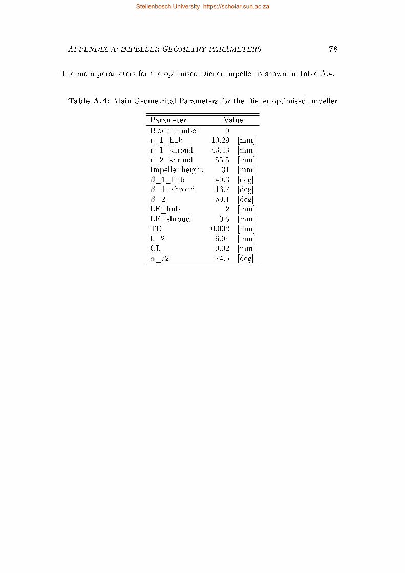
APPENDIX A: IMPELLER GEOMETRY PARAMETERS 78
The main parameters for the optimised Diener impeller is shown in Table A.4.
Table A.4: Main Geometrical Parameters for the Diener optimised Impeller
Parameter Value
Blade number 9r_1_hub 10.29 [mm]r_1_shroud 43.43 [mm]r_2_shroud 55.5 [mm]Impeller height 31 [mm]β_1_hub 49.3 [deg]β_1_shroud 16.7 [deg]β_2 59.1 [deg]LE_hub 2 [mm]LE_shroud 0.6 [mm]TE 0.002 [mm]b_2 6.94 [mm]CL 0.02 [mm]α_c2 74.5 [deg]
Stellenbosch University https://scholar.sun.ac.za
Appendix B: Mean-Line Code Flow
Charts
Three ow diagrams are presented in this appendix. Figure B.1 shows the owdiagram describing the logic of the mean-line code structure. Two of the functionsin Figure B.1, "getPerf" and "displayChart", is further expanded in separate owdiagrams in Figure B.2 and Figure B.3 respectively.
The function in Figure B.2 is used to predict the performance, pressure ratio andisentropic eciency, of an impeller at a specied mass ow rate. This function istherefore used to calculate the design point of the impeller under consideration.The function makes use of three for-loops to calculate the uid properties at threedierent locations in the impeller. The rst for-loop calculates the uid propertiesat the inlet of the impeller, the second for-loop calculates the uid properties atthe throat of the impeller, and the third for-loop calculates the uid propertiesat the exit of the impeller. The inlet conditions to each for-loop is taken as theoutlet conditions of the previous for-loop. For the rst for-loop, user-dened inletproperties are used.
The function in Figure B.3 is used to calculate the performance of the impeller atdierent operational speeds in order to plot a compressor performance map. ThedisplayChart function basically makes use of the getPerformance function. Incre-mentation of mass ow is added, together with a number of choke conditions, thatenables a curve of pressure ratio or eciency vs mass ow to be plotted.
79
Stellenbosch University https://scholar.sun.ac.za
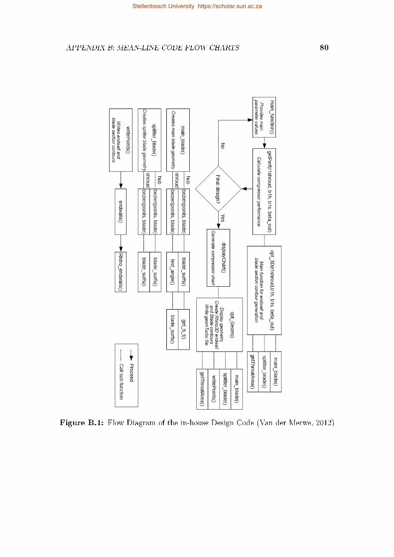
APPENDIX B: MEAN-LINE CODE FLOW CHARTS 80
Figure B.1: Flow Diagram of the in-house Design Code (Van der Merwe, 2012)
Stellenbosch University https://scholar.sun.ac.za
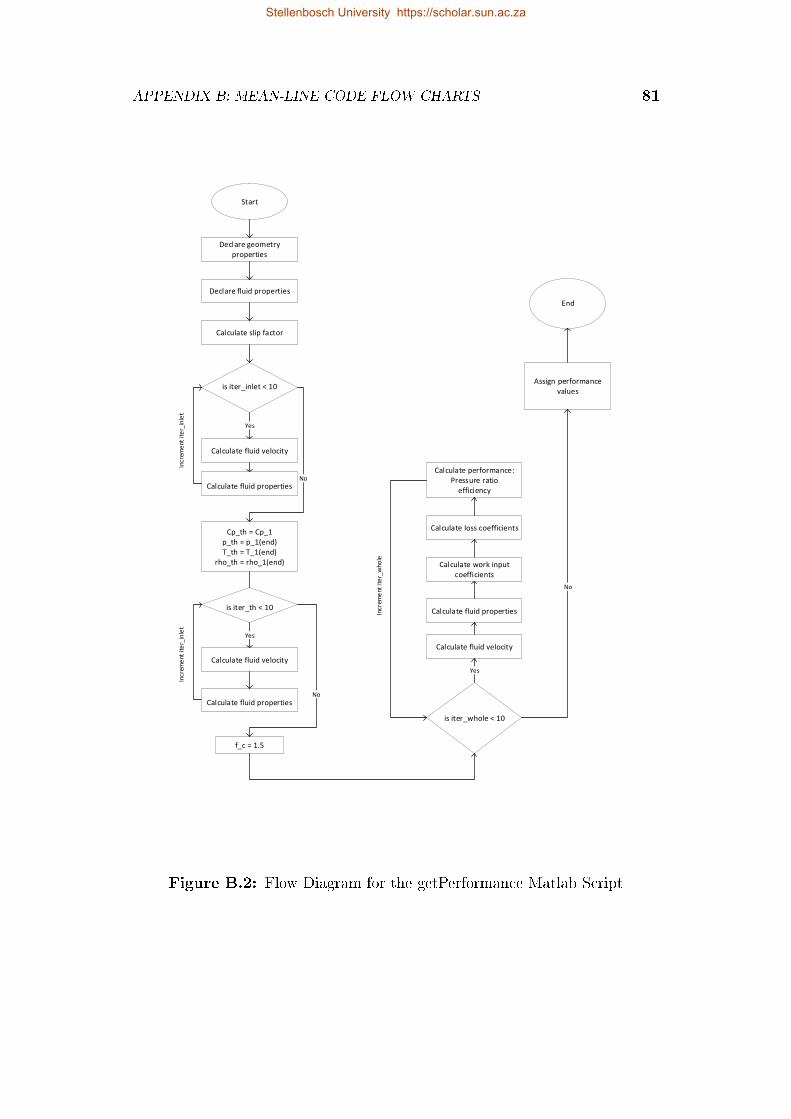
APPENDIX B: MEAN-LINE CODE FLOW CHARTS 81
Start
Declare geometry properties
Declare fluid properties
Calculate slip factor
is iter_inlet < 10
Calculate fluid velocity
Calculate fluid properties
Incr
eme
nt it
er_
inle
t
Cp_th = Cp_1p_th = p_1(end)T_th = T_1(end)
rho_th = rho_1(end)
No
is iter_th < 10
Yes
Calculate fluid velocity
Calculate fluid properties
Incr
eme
nt it
er_
inle
t
Yes
f_c = 1.5
No
is iter_whole < 10
Calculate fluid velocity
Calculate fluid properties
Yes
Assign performance values
End
No
Calculate work input coefficients
Calculate loss coefficients
Calculate performance:Pressure ratio
efficiency
Incr
eme
nt it
er_
who
le
Figure B.2: Flow Diagram for the getPerformance Matlab Script
Stellenbosch University https://scholar.sun.ac.za
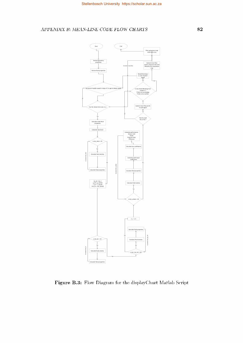
APPENDIX B: MEAN-LINE CODE FLOW CHARTS 82
Start
Declare geometry properties
Declare fluid properties
is iter_inlet < 10
Calculate fluid velocity
Calculate fluid properties
Incr
eme
nt it
er_
inle
t
Cp_th = Cp_1p_th = p_1(end)T_th = T_1(end)
rho_th = rho_1(end)
No
is iter_th < 10
Yes
Calculate fluid velocity
Calculate fluid properties
Incr
eme
nt it
er_
th
Yes
f_c = 1.5
No
is iter_whole < 10
Calculate fluid velocity
Calculate fluid properties
Yes
End
No
Calculate work input coefficients
Calculate loss coefficients
Calculate performance:Inducer stall
ChokePressure ratio
Efficiency
Incr
eme
nt it
er_
who
le
is iter_tip_init < 10
Calculate fluid velocity
Calculate fluid properties
Incr
eme
nt it
er_
tip
_in
it
Yes
No
Increment impeller speed in steps of 5 to get to design speed
Yes
Test for choke limit to be <1.1
Calculate initial fluid properties
Calculate slip factor
Test for stallYes or No ?
Capture mass flow points in stall region
Yes
Is any of the following true:Choke>1.1
Pratio not convergingPratio not a number
No
Break from loop to next impeller
speed
Yes
Capture mass flow points, pressure ratio and efficiency for compressor
map
Plot compressor map with stall curve
NoN
o
Increment mass flow
Figure B.3: Flow Diagram for the displayChart Matlab Script
Stellenbosch University https://scholar.sun.ac.za
Appendix C: geomTurbo File
Format
Every geomTurbo le starts with a header followed by the hub and shroud endwallcurves. The header contains the name of the curve to be dened as well as thecoordinate system used and the amount of entries for the specic curve followed byth coordinates dening the curve. The header section for the endwalls is denedas follows:
The coordinates for the main and splitter blades are also preceded by a header.This header states the number of of periodic bounds to be modelled in CFD,suction or pressure side, and the section. The coordinate system and number ofcoordinate entries once again precedes the coordinates dening the blade. Theheader for the blades is dened as follows:
83
Stellenbosch University https://scholar.sun.ac.za
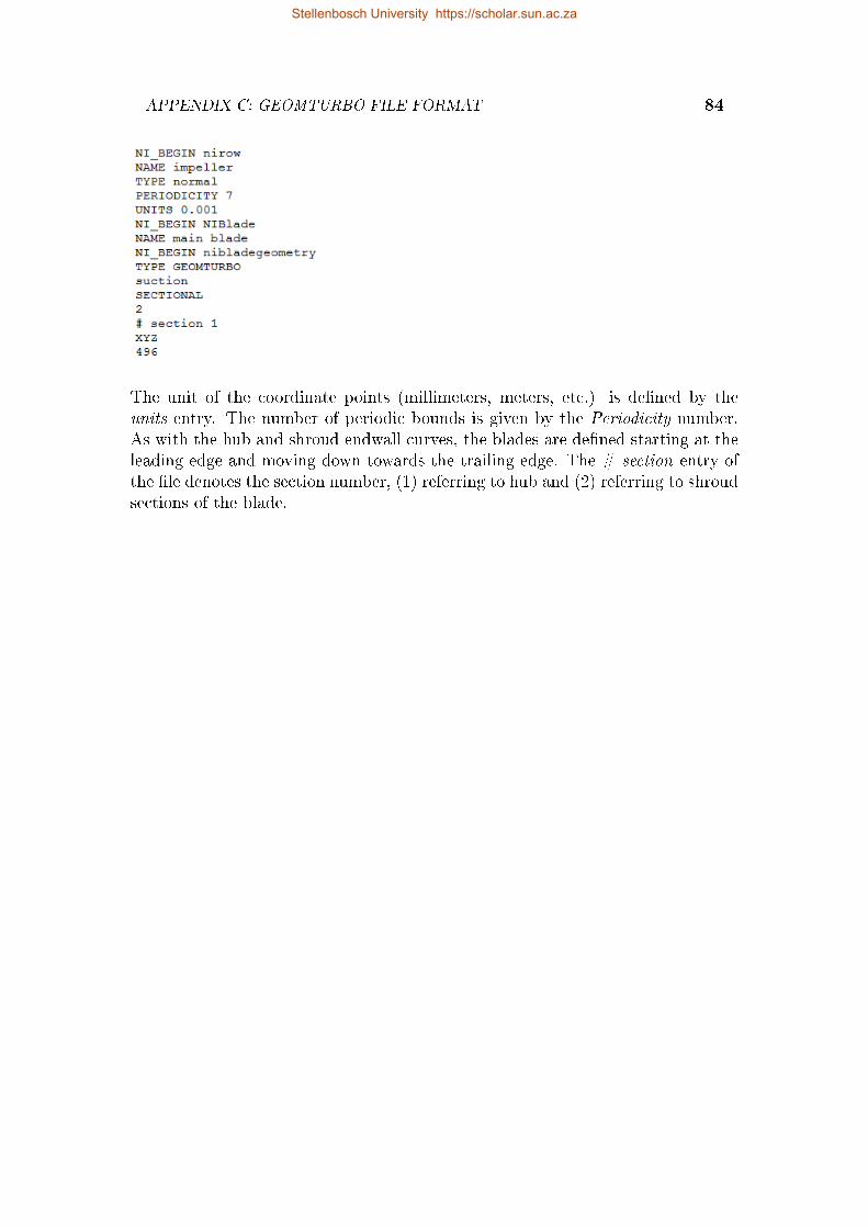
APPENDIX C: GEOMTURBO FILE FORMAT 84
The unit of the coordinate points (millimeters, meters, etc.) is dened by theunits entry. The number of periodic bounds is given by the Periodicity number.As with the hub and shroud endwall curves, the blades are dened starting at theleading edge and moving down towards the trailing edge. The # section entry ofthe le denotes the section number, (1) referring to hub and (2) referring to shroudsections of the blade.
Stellenbosch University https://scholar.sun.ac.za
Appendix D: Compressor Maps
The following compressor maps were generated through the in-house mean-linecode. The design point is determined by the getPerf Matlab® script based onthe user dened design mass ow rate. Once the design point for the compressorimpeller has been determined the displayChart script calculates and plot the pres-sure ratio and eciency curves for the impeller for ve dierent operating speeds.The operating speeds at which the compressor map is plotted depends on the mainoperating speed that was dened by the user.
The compressor map for the k27 impeller is shown in Figure D.1. The surge linealmost sits on the design point for the 120 krpm curve, with a small operatingrange predicted. The eciency for the impeller does not vary that much acrossthe dierent operating speeds as seen in Figure D.1, all being around 85%.
Figure D.2 shows the compressor map for the mean-line Van der Merwe rotor.Here the design point is closer to the choke region of the predicted operatingrange for the impeller. Figure D.3 shows the compressor map for the optimisedVan der Merwe rotor and Figure D.4 for the optimised Diener rotor. For theserotors the design point sits in the middle of the predicted performance curve. Forthe optimised Van der Merwe rotor the eciency decreases substantially for eachprogressive operation speed. The discrepancy in the eciency, compared to theother rotors, can be explained by the radial blade outlet angle.
85
Stellenbosch University https://scholar.sun.ac.za
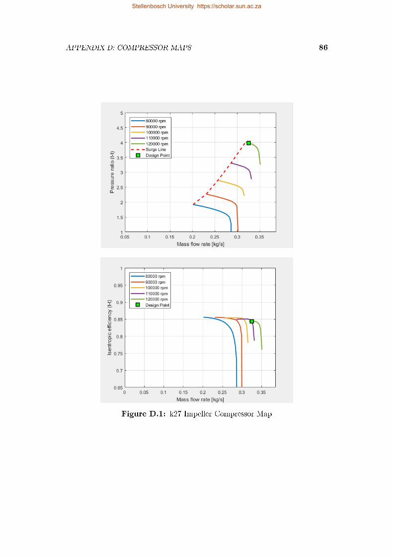
APPENDIX D: COMPRESSOR MAPS 86
Figure D.1: k27 Impeller Compressor Map
Stellenbosch University https://scholar.sun.ac.za
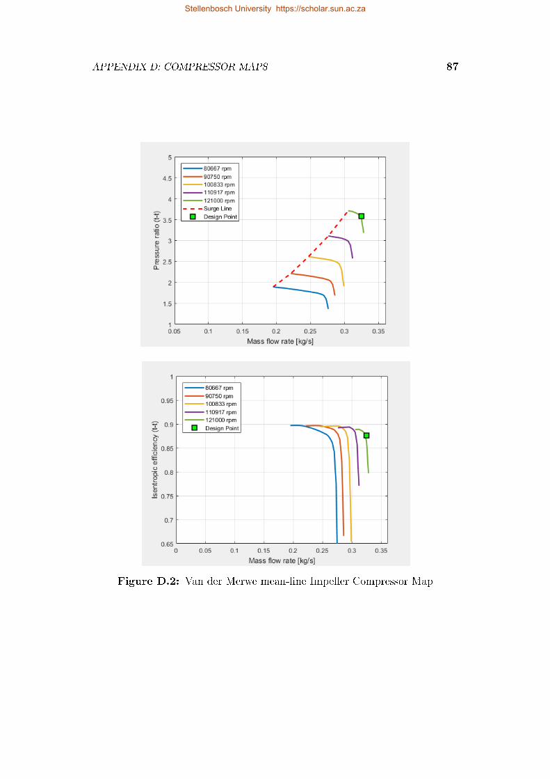
APPENDIX D: COMPRESSOR MAPS 87
Figure D.2: Van der Merwe mean-line Impeller Compressor Map
Stellenbosch University https://scholar.sun.ac.za
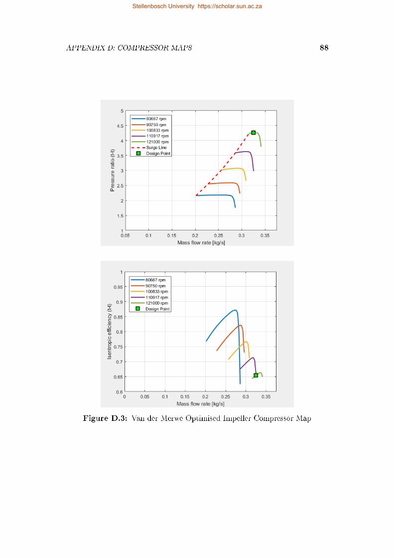
APPENDIX D: COMPRESSOR MAPS 88
Figure D.3: Van der Merwe Optimised Impeller Compressor Map
Stellenbosch University https://scholar.sun.ac.za
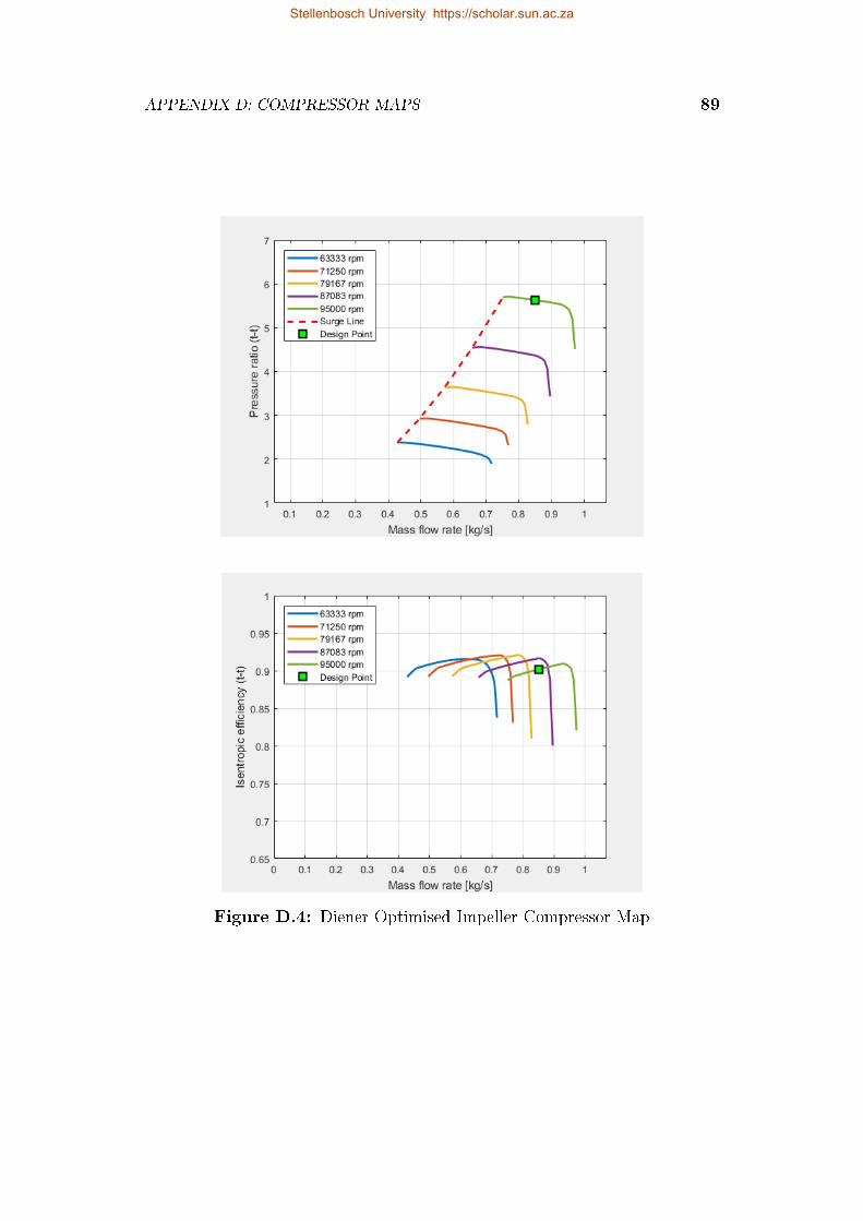
APPENDIX D: COMPRESSOR MAPS 89
Figure D.4: Diener Optimised Impeller Compressor Map
Stellenbosch University https://scholar.sun.ac.za
Appendix E: CFD Grid Dependency
This appendix contains details for the grid dependency study completed for eachof the impellers that were analysed in CFD. A table for each rotor is shown, con-taining the number of nodes, pressure ratio and eciency. The number of nodesgives an indication of how coarse or ne the mesh was. The grid dependency wascarried out for three dierent mesh groups, a coarse mesh, medium mesh, and nemesh. AutoGridallows one of three grid levels to be specied when creating amesh. The three mesh groups were therefore achieved by creating a mesh on therst grid level (coarse) and selecting the second and third grid levels respectivelyafter saving the previous grid level.
Table E.1 shows the results for the grid dependency study for the k27 impeller.The dierence in both pressure ratio and eciency is within 5% across the threedierent cell densities.
Table E.1: Mesh Dependency Study for the k27 Impeller
Mesh Property Coarse Medium Fine
Number of nodes 459,540 1,386,316 4,036,308Pressure ratio 3.704 3.778 3.86Eciency 82.027 83.385 84.093
Table E.2 shows the results for the grid dependency study for the optimised Vander Merwe impeller. The dierence in both pressure ratio and eciency is within5% across the three dierent cell densities. A higher pressure ratio is recorded forthe medium mesh compared to the coarse and ne mesh. This deviation may becaused by a poorer mesh quality compared to the other two meshes.
90
Stellenbosch University https://scholar.sun.ac.za
APPENDIX E: CFD GRID DEPENDENCY 91
Table E.2: Mesh Dependency Study for the Van der Merwe Impeller
Mesh Property Coarse Medium Fine
Number of nodes 557,172 1,700,076 4,997,380Pressure ratio 5.168 5.424 5.166Eciency 89.392 91.290 89.262
Table E.3 shows the results for the grid dependency study for the Diener impeller.The largest dierence in pressure ratio is 8.66% with the coarse mesh predicting amuch lower pressure ratio, while the eciencies are all within 2% of each other.
Table E.3: Mesh Dependency Study for the Diener Impeller
Mesh Property Coarse Medium Fine
Number of nodes 661,032 2,115,340 6,151,464Pressure ratio 5.08 5.54 5.51Eciency 88.92 87.735 87.471
Stellenbosch University https://scholar.sun.ac.za
Related Documents


