Analysing Monetary Policy with an Estimated DSGE Model

Analysing Monetary Policy with an Estimated DSGE Model∗

Niels Arne Dam and Jesper Gregers LinaaUniversity of Copenhagen and EPRU†

September 2004

Abstract

Keywords:

JEL Classifications:

very preliminary:please, do not quote without permission

edge JamboreeDublin, September 2004

∗We thank Henrik Jensen and Christopher Sims for valuable comments. Address for correspondence: Niels Arne Dam([email protected]) or Jesper Linaa ([email protected]), Institute of Economics, University of Copenhagen, Studiestræde6, 1455 Copenhagen K, Denmark

†The activities of EPRU (Economic Policy Research Unit) are financed by a grant from The Danish National ResearchFoundation.

1

1 IntroductionThe purpose of this paper is two-fold; first, we seek to establish a suitable framework for analysis of monetarypolicy in a small open economy which is firmly founded in economic theory as well as empirically relevant;secondly, we use the suggested framework to analyse the structural dynamics of a small open economywith microfounded nominal rigidities with particular emphasis on the monetary transaction mechanism. Inparticular, we apply our model to Danish data and consider the dynamics of this economy under a fixedexchange rate regime.We follow the current trend in this literature and consider the cashless limiting economy; that is, we

consider an economy where money-based transactions are sufficiently unimportant for the utility of realconsumption to be safely ignored. In this case, monetary policy is used to determine the short-term interestrate, which we consider to be the empirically relevant case. Woodford (2003) argues convincingly in favourof this approach.The particular model we use is based on the small open dsge economy constructed by Kollmann (2001,

2002). Thus, we have imperfect competition in the labour market as well as the market for intermediategoods. In both markets, suppliers update their prices infrequently and thus have to consider future marketconditions in order to set their prices optimally. While Kollmann calibrated his model, we perform a Bayesianestimation of the model by combining the likelihood function with prior distributions for the structuralparameters. Following Smets and Wouters (2003) we postulate that all stochastic volatility in the model isof structural nature. This necessitates that we extend the number of structural shocks from those includedin Kollmann’s model.This paper is strongly inspired by the work of Smets and Wouters (2003) who in turn draw heavily on

the model constructed by Christiano, Eichenbaum, and Evans (2001) (henceforth the cee model). Thereare three major differences between our analysis and that of Smets and Wouters. Firstly, we consider asmall open model instead of a closed economy. This expansion is of critical importance to us, since weseek a framework which can address the relative merits of a fixed exchange rate regime and an independentmonetary policy. Secondly, we have chosen to keep our theoretical model fairly close to that of Kollmann(2001, 2002), thus ignoring some of the frictions which were included in the cee model in order to capturethe empirically observed inertia in the data. Thirdly, whereas Smets and Wouters (2003) had to make thedubious assumption that monetary policy in the current euro area was properly described by a generalisedTaylor rule throughout the period 1980-1999, we can make the more appealing assumption that the Danishmonetary policy consisted of an imperfect peg on the euro (and the D-mark before 1999).

2 The ModelIn this section we build a fully micro-founded dsge model with staggered setting of wages and prices. Themodel is fairly rich in variables and parameters which we summarise in Appendix A.

2.1 Final Goods

Domestic final goods are produced from Dixit-Stiglitz aggregates of a continuum of tradable intermediategoods. These are produced domestically and abroad;

Qit =

∙Z 1

0

qi (s)1

1+ν ds

¸1+νt, i = d,m.

Zt is the production of final goods using the Cobb Douglas technology

Zt =

µQdt

αd

¶αd µQmt

αm

¶αm, αd + αm = 1. (2.1)

2

Domestic firms face the problem of minimizing the cost of producing Zt units of the final good;

minQdt ,Q

mt

P dt Q

dt + Pm

t Qmt (2.2)

s.t.µQdt

αd

¶αd µQmt

αm

¶αm= Zt, (2.3)

where individual intermediate-goods prices are pit (s) and appropriate ces price indices are given as

P it ≡

∙Z 1

0

pit (s)1−νt ds

¸1/(1−νt), i = d,m. (2.4)

The associated Lagrangian is

L = P dt Q

dt + Pm

t Qmt

−λt

⎡⎣µQdt

αd

¶αd ÃQft

1− αd

!1−αd− Zt

⎤⎦ ,and the first order condition with respect to Qi

t gives us

P it = λtα

i ZtQit

=⇒ Qit

αi= λt

ZtP it

(2.5)

Inserting equation (2.5) in the budget constraint (2.2) yields¡P dt

¢αd(Pm

t )1−αd

= λt. (2.6)

The appropriate aggregate price index Pt is the cost of producing one unit of the final good (Zt = 1). Thus,we use equation (2.5) again to obtain

µQdt

αd

¶αd ÃQEU,dt

1− αd

!1−αd= 1⇒

Pt ≡ P dt Q

dt + Pm

t Qmt

= λt¡αd + αm

¢= λt

=¡P dt

¢αd(Pm

t )αm (2.7)

Note that Pt is thus the marginal cost of the final-goods producing firm. With perfect competition inthe final-goods market, the price of one unit is thus Pt.Profit-maximizing demands are found by combining (2.5) with (2.7);

Qit = αiλt

ZtP it

= αiPtZtP it

, i = d,m. (2.8)

3

2.2 Intermediate Goods

Intermediate-goods producers have access to Cobb-Douglas technology

yt (s) = θtKt (s)ψLt (s)

1−ψ, 0 < ψ < 1,

and operate in a monopolistic competitive market, where each producer sets the price of her variety, takingother prices as given and supplying whatever amount is demanded at the price set. Cost minimizationimplies the following first-order conditions

(1− ψ) yt (s) /Lt (s) =Wt

ψyt (s) /Kt (s) = Rt,

¾⇒ Lt (s)

Kt (s)=1− ψ

ψ

Rt

Wt,

where Rt is the rental price of capital and Wt is the wage rate. Thus,

Lt (s) =1− ψ

ψ

Rt

WtKt (s)⇒ (2.9)

yt (s) = θtK (s)ψt

µ1− ψ

ψ

Rt

WtKt (s)

¶1−ψ= θtKt (s)

µ1− ψ

ψ

Rt

Wt

¶1−ψ⇒

Kt (s) =1

θt

µ1− ψ

ψ

Rt

Wt

¶−(1−ψ)yt (s) , (2.10)

Lt (s) =1

θt

µψ

1− ψ

Wt

Rt

¶−ψyt (s) .

Hence, the firm’s total and marginal costs are

TC (yt (s)) = WtLt +RtKt

=1

θt

"Wt

µψ

1− ψ

Wt

Rt

¶−ψ+Rt

µ1− ψ

ψ

Rt

Wt

¶−(1−ψ)#yt (s)

=1

θt

"W 1−ψ

t Rψt

µψ

1− ψ

¶−ψ+W 1−ψ

t Rψt

µψ

1− ψ

¶1−ψ#yt (s)

=1

θtW 1−ψ

t Rψt

"µψ

1− ψ

¶−ψ+

µψ

1− ψ

¶1−ψ#yt (s)

=1

θtW 1−ψ

t Rψt

"µψ

1− ψ

¶−ψ1

1− ψ

#yt (s)

=1

θtW 1−ψ

t Rψt ψ−ψ (1− ψ)−(1−ψ) yt (s)⇒

MCt =1

θtW 1−ψ

t Rψt ψ−ψ (1− ψ)

−(1−ψ). (2.11)

Following Calvo (1983), we assume that the firm only reoptimizes its prices in any given period withprobability 1 − d. Producers sell their good variety to both domestic and foreign final-goods producers;yt (s) = qdt (s) + qmt (s) and can price discriminate between the two markets. As is well-known from theDixit-Stiglitz models, final-good producers demand individiual varieties of intermediaries as follows

qit (s) =

µpit (s)

P it

¶− 1+νtνt

Qit, i = d,m.

4

Firm profits are thus

πdx¡pdt (s) , p

xt (s)

¢=

¡pdt (s)−MCt

¢qdt (s) + (etp

xt (s)−MCt) q

xt (s) (2.12)

=¡pdt (s)−MCt

¢µpdt (s)P dt

¶− 1+νtνt

Qdt

+(etpxt (s)−MCt)

µpxt (s)

Pxt

¶− 1+νtνt

Qxt

Here we assumed Dixit-Stiglitz demands from foreign final-goods producers;

qxt (s) =

µpxt (s)

P xt

¶− 1+νtνt

Qxt ,

Qxt =

µPxt

P ∗t

¶−ηY ∗t , η > 0, (2.13)

where the foreign aggregates P ∗t , Y∗t are exogenous.

Likewise, foreign exporters generate the following profits in the domestic market;

πm (pmt (s)) = (pmt (s)− etP

∗t )

µpmt (s)

Pmt

¶− 1+νtνt

Qmt

Hence, a domestic firm reoptimizing its domestic price faces the following problem:

pdt,t = argmaxω

∞Xτ=0

dτEt

£ρt,t+τπ

dx (ω, pxt (s))¤,

ρt,t+τ ≡ βτ (UC,t+τ/UC,t) (Pt/Pt+τ ) (2.14)

where ρt,t+τ appropriately discounts profits at time t+ τ , and dτ is the probability that the current pricingdecision is still in effect in period τ + τ . Substituting from the profit expression (2.12) yields

∞Xτ=0

dτEt

⎡⎢⎣ρt,t+τ ¡pdt,t −MCt+τ

¢Ã pdt,tP dt+τ

!− 1+νt+τνt+τ

Qdt+τ

⎤⎥⎦=

∞Xτ=0

dτEt

∙¡pdt,t −MCt+τ

¢ ¡pdt,t¢− 1+νt+τ

νt+τ ρt,t+τ¡P dt+τ

¢ 1+νt+τνt+τ Qd

t+τ

¸,

resulting in the following first-order condition;∞Xτ=0

dτEt

∙µ− 1

νt+τ

¡pdt,t¢− 1+νt+τ

νt+τ +1 + νt+τνt+τ

¡pdt,t¢− 1+2νt+τ

νt+τ MCt+τ

¶ρt,t+τ

¡P dt+τ

¢ 1+νt+τνt+τ Qd

t+τ

¸= 0⇒

∞Xτ=0

dτEt

⎡⎢⎣¡pdt,t − (1 + νt+τ )MCt+τ

¢ρt,t+τ

Ãpdt,tP dt+τ

!− 1+νt+τνt+τ Qd

t+τ

pdt,tνt+τ

⎤⎥⎦ = 0. (2.15)

Analogously, the optimal price for sales to foreign final-goods producers is determined from the followingcondition;

∞Xτ=0

dτEt

⎡⎣¡et+τpxt,t − (1 + νt+τ )MCt+τ

¢ρt,t+τ

µpxt,tP xt+τ

¶− 1+νt+τνt+τ Qx

t+τ

pxt,tνt+τ

⎤⎦ = 0. (2.16)

5

Import firms are owned by risk-neutral foreigners who discount future profits at the foreign nominalinterest rate Rt,t+τ ≡ Πt+τs=t (1 + i∗s)

−1. Thus, when they reoptimize, they set their prices in order to maximizediscounted future profits measured in foreign units;

pmt,t = argmaxω

∞Xτ=0

dτEt [Rt,t+τπm (ω) /et+τ ]

=∞Xτ=0

dτEt [Rt,t+τπm (ω) /et+τ ]

=∞Xτ=0

dτEt

⎡⎣Rt,t+τ

¡pmt,t − et+τP

∗t+τ

¢µ pmt,tPmt+τ

¶− 1+νt+τνt+τ

Qmt+τ/et+τ

⎤⎦=

∞Xτ=0

dτEt

∙Rt,t+τ

¡pmt,t/et+τ − P ∗t+τ

¢ ¡pmt,t¢− 1+νt+τ

νt+τ¡Pmt+τ

¢ 1+νt+τνt+τ Qm

t+τ

¸,

with first-order condition

∞Xτ=0

dτEt

∙µ− 1

νt+τpmt,t− 1+νt+τ

νt+τ /et+τ +1 + νt+τνt+τ

¡pmt,t¢− 1+2νt+τ

νt+τ P ∗t+τ

¶¡Pmt+τ


t+τ

¸= 0⇒

∞Xτ=0

dτEt

⎡⎣¡pmt,t (s) /et+τ − (1 + νt+τ )P∗t+τ

¢µ pmt,tPmt+τ

¶− 1+νt+τνt+τ Qm

t+τ

pmt,tνt+τ

⎤⎦ = 0. (2.17)

Considering aggregate Dixit-Stiglitz prices of the intermediate goods (equation (2.4)), we apply to thelaw of large numbers and the fact that the fraction d of firms that reoptimize is completely random to findthat ¡

P it

¢− 1νt =

Z 1

0

pit (s)− 1νt ds = d

Z 1

0

¡pit−1 (s)

¢− 1νt ds+ (1− d)

¡pit,t¢− 1

νt

= d¡P it−1¢− 1

νt + (1− d)¡pit,t¢− 1

νt , i = d,m, x. (2.18)

2.3 Households

A representative household is characterized by the following preferences with external habit formation inconsumption:

E0

" ∞Xt=0

βtU (C∗t , Lt)

#, U (C∗t , Lt) = [u (C

∗t )− v (Lt)] , (2.19)

where ζbt represents a shock to the discount rate and ζLt represents a shock to the labour supply. We define

C∗t = Ct − hCt−1 (2.20)

where Ct is the average consumption level, which is considered exogenous to the representative household.As in Kollmann (2001), we assume that the representative household supplies a continuum of labour

service varieties, i.e., lt (j) , j ∈ [0, 1].1 These labour services enter as a Dixit-Stiglitz aggregate in the

1This should mathematically be identical to the case where individual households each supply one variety of labor servicesand completely diversify individual income uncertainty in a security market.

6

intermediate-goods firm production; thus, letting lt (s, j) be the amount of labour service j utilized by firms we find that firm s uses the following amount of labour services;

Lt (s) =

∙Z 1

0

lt (s, j)1

1+γ dj

¸1+γt, γt > 1, (2.21)

and total labour is Lt =R 10Lt (s) ds.

In addition to consumption, the representative household can invest in domestic and foreign one-periodbonds as well as in domestic capital. Capital Kt earns rental rate Rt and accumulates as follows;

Kt+1 = Kt (1− δ) + It − φ (Kt+1,Kt) , 0 < δ < 1, (2.22)

where φ (Kt+1,Kt) is an adjustment cost. Domestic bonds At earns net interest it, while the interest ift

accruing to foreign bonds Bt held by domestic agents deviates from the foreign interest level i∗t as follows;³1 + ift

´= Ωjt (1 + i∗t ) , (2.23)

Ωt = υt exp

½−λetBt+1

PtΞ

¾, Ξ =

eP xQx

P(2.24)

where Ξ is the steady-state value of export in units of the domestic final good. Thus, the interest onforeign bonds is growing in the foreign debt level which ensures the existence of a unique equilibrium, cf.Schmitt-Grohe and Uribe (2003), while υt is a stochastic shock which can also be interpreted as a uip shock.The household owns domestic firms and thus earns profit from the intermediate-goods firms and rental

rates (Rt) on the capital in addition to wage income from its variety of labour services. The budget constraintis thus

At+1 + etBt+1 + Pt (Ct + It) = (2.25)

At (1 + it−1) + etBt

³1 + ift−1

´+RtKt +

Z 1

0

πdxt (s) ds+

Z 1

0

Z 1

0

wt (j) lt (s, j) djds.

Wage setting is staggered a la Calvo (1983). That is, in each period the household only optimize thewage of labour type j (styled wt (j)) with probability 1 − D. The household takes the average wage rate

Wt =hR 10wt (j)

− 11+γt dj

i−(1+γt)as given when it chooses the optimal wage wt,t, and will meet any demand

for the given type of labour;

lt (j) =

Z 1

0

l (s, j) ds. (2.26)

The household thus faces the following problem

maxCt,At+1,Bt+1,Kt+1wt,t∞t=0

E0

" ∞Xt=0

βtU (C∗t , Lt)

#(2.27)

s.t. (2.20)-(2.26).

7

Solving (2.25) with respect to Ct yields

Ct =1

Pt

©At (1 + it−1) + eEUt BEU

t

¡1 + iEUt−1

¢+ eROWt BROW

t

¡1 + iROWt−1

¢+RtKt −At+1 − etBt+1

−It +1

Pt

∙Z 1

0

πdxt (s) ds+

Z 1

0

Z 1

0

wt (j) lt (s, j) djds

¸⇐⇒

C∗t =1

Pt

hAt (1 + it−1) + etBt

³1 + ift−1

´+RtKt −At+1 − etBt+1

i− [Kt+1 −Kt (1− δ) + φ (Kt+1,Kt)]

+1

Pt

∙Z 1

0

πdxt (s) ds+

Z 1

0

Z 1

0

wt (j) lt (s, j) djds

¸− hCt−1,

Thus, an interior solution to the household’s problem (2.27) yields the following first-order conditions:Capital,

βtUC,t£−1− φ1,t

¤+ βt+1Et

∙UC,t+1

µRt+1

Pt+1+ (1− δ)− φ2,t+1

¶¸= 0⇐⇒

βt+1Et

∙UC,t+1

µRt+1

Pt+1+ (1− δ)− φ2,t+1

¶¸= βtUC∗,t

£1 + φ1,t

¤⇐⇒

βEt

hUC,t+1

³Rt+1Pt+1

+ (1− δ)− φ2,t+1

íUC,t

£1 + φ1,t

¤ = 1⇐⇒

Et

⎡⎣ρt,t+1Pt+1Pt

³Rt+1Pt+1

+ (1− δ)− φ2,t+1

´£1 + φ1,t

¤⎤⎦ = 1. (2.28)

Domestic bonds,

βtUC,t

∙− 1Pt

¸+ βt+1Et

∙UC,t+1

µ1 + itPt+1

¶¸= 0⇐⇒

(1 + it)βEt

∙UC,t+1UC,t

PtPt+1

¸= 1⇐⇒

(1 + it)Et

£ρt,t+1

¤= 1. (2.29)

8

Foreign bonds,

βtUC∗,t

µ− etPt

¶+ βt+1Et

⎡⎣UC∗,t+1⎛⎝et+1

³1 + ift

´Pt+1

⎞⎠⎤⎦ = 0⇐⇒

βEt

⎡⎣UC∗,t+1⎛⎝et+1

³1 + ift

´Pt+1

⎞⎠⎤⎦ = UC∗,tetPt⇐⇒

³1 + ift

´βEt

∙UC∗,t+1UC∗,t

et+1et

PtPt+1

¸= 1⇐⇒³

1 + ift

Ét

∙ρt,t+1

et+1et

¸= 1, (2.30)

where ρt,t+k is defined in equation (2.14) above.Since the household meets the demand for labour at its chosen wage level, we find the following relations;

lτ (s, j) =

µwt,t

Wτ

¶− 1+γtγt 1− ψ

ψ

Rτ

WτKτ (s)⇒

dlt (s, j)

dwt (j)= −1 + γt

γtw− 1+2γt

γtt,t

1− ψ

ψRtKt (s)W

1γtt ⇒Z

dlt (s, j)

dwt (j)ds = −1 + γt

γtw− 1+2γt

γtt,t χt,

andZ

d (lt (s)wt (j))

dwt (j)ds = − 1

γtw− 1+γt

γtt,t χt,

where χt ≡1− ψ

ψRt

ZKt (s) dsW

1γtt =

1− ψ

ψRtKtW

1γtt . (2.31)

Thus, we finally obtain the following first-order condition with respect to the wage rate;

∞Xτ=0

(βD)τ Et

"−UC,t+τ

Pt+τ

1

γt+τwt,t

− 1+γt+τγt+τ χt+τ + UL,t+τ

1 + γt+τγt+τ

w− 1+2γt+τ

γt+τ

t,t χt+τ

#= 0⇒

∞Xτ=0

(βD)τ χt+τγt+τ

w− 1+2γt+τ

γt+τ

t,t Et

∙UC,t+τPt+τ

wt,t −¡1 + γt+τ

¢UL,t+τ

¸= 0. (2.32)

Analogously to equation (2.18), the aggregate wage level is determined as

Wt =hD (Wt−1)

− 1γt + (1−D) (wt,t)

− 1γt

i−γt. (2.33)

9

2.4 Specifying Utility Functions and Capital Adjustment Costs

We now make particular assumptions for the functional forms for the felicity function, the disutility of labour,and the capital adjustment costs. Thus, utility is specified as follows;

u (C) =C1−σC

1− σC, v (L) =

L1+σL

1 + σL⇒

U (C∗t , Lt) = ζbt

"¡Ct − hCt−1

¢1−σCt

1− σC− ζLt

L1+σLt

1 + σL

#⇒

UC,t ≡∂U (C∗t , Lt)

∂Ct= ζbt

¡Ct − hCt−1

¢−σC= ζbt

¡Ct − hCt−1

¢−σC ,

and UL,t ≡∂U (C∗t , Lt)

∂Lt= ζbtζ

Lt L

σLt ,

where we have imposed the condition Ct = Ct.Capital costs are assumed to be quadratic;

φ (K0,K) =Φ

2

(K0 −K)2

K⇒

φ1,t ≡∂φ (Kt+1,Kt)

Kt+1= Φ

Kt+1 −Kt

Kt,

φ2,t ≡∂φ (Kt+1,Kt)

Kt+1=Φ

2

Ã1−

µKt+1

Kt

¶2!.

2.5 Market Clearing Conditions

All intermediaries are demanded from either domestic or foreign final goods producers

Yt = Qdt +Qx

d. (2.34)

In the final goods market equilibrium requires

Zt = Ct + It, (2.35)

and equilibria in the factor markets require

Lt =

ZLt (s) ds, Kt =

ZKt (s) ds.

2.6 The Household Budget Constraint and Net Foreign Assets

Manipulating the household budget constraint (2.25) and using the final-good market equilibrium (2.35)yields the following equation which simply states that the net foreign assets position (nfa) changes with

10

accruing interest and the net export.

etBt+1 + Pt (Ct + It) = etBt

³1 + ift−1

´+RtKt +WtLt

+P dt Q

dt + etP

xt Q

xt − (RtKt +WtLt)⇒

etBt+1 = etBt

³1 + ift−1

´− PtZt + P d

t Qdt + etP

xt Q

xt

= etBt

³1 + ift−1

´+ etP

xt Q

xt − Pm

t Qmt ⇒

Bt+1 = Bt

³1 + ift−1

´+ P x

t Qxt −

Pmt

etQmt

2.7 Monetary Policy

We postulate an imperfect peg against the euro as the monetary policy; in our model the interest rate is theinstrument, which is thus used to keep et constant up to an exogenous policy shock ξt with unity mean;

et = eξt. (2.36)

Log-linearizing equations (2.23) and (2.24) yields the following relation between the internal foreigninterest rate and that paid to domestic holders of foreign bonds;

ıft = ı∗t + υt − λBt.

Combining this relation with log-linearised versions of equations (2.29) and (2.30) yields

Et∆et+1 = ıt − ıft = ıt − ı∗t +³λBt − υt

´,

ıt ≡ log

µ1 + it1 + ı

¶, υt ≡ log (υt/υ) , Bt ≡ log

(Bt+1/P∗t )

Ξ,

which we can combine with (2.36) to obtain

ıt = ı∗t +³υt − λBt

´+Et∆ξt+1 (2.37)

that is, the interest rate responds (virtually) one-to-one with the foreign interest rate and the uip shock andis additionally skewed by the spread and the past policy shock.

3 Summarising and Solving the ModelRecapitulating the model, we have formed equations for two intermediary aggregates in the domestic market

Qdt = αd

PtZtP dt

, (3.1)

Qmt =

¡1− αd

¢ PtZtPmt

, (3.2)

one intermediary aggregate in the foreign market

Qxt =

µP xt

P ∗t

¶−ηY ∗t , (3.3)

11

and the aggregate price level

Pt =¡P dt

¢αd(Pm

t )1−αd . (3.4)

Cost minimization implies the aggregate L−K relationship

Lt =1− ψ

ψ

Rt

WtKt, (3.5)

and the aggregate K − Y relationship

Kt =1

θt

µ1− ψ

ψ

Rt

Wt

¶−(1−ψ)Yt, (3.6)

while the marginal cost of producing intermediate goods is

MCt =1

θtW 1−ψ

t Rψt ψ−ψ (1− ψ)

−(1−ψ). (3.7)

We define a utility-based pricing kernel

ρt,t+τ ≡ βτ (UC,t+τ/UC,t) (Pt/Pt+τ ) , (3.8)

and derive three optimal pricing equations for intermediate goods

∞Xτ=0

dτEt

⎡⎢⎣¡pdt,t − (1 + νt+τ )MCt+τ

¢ρt,t+τ

Ãpdt,tP dt+τ

!− 1+νt+τνt+τ Qd

t+τ

pdt,tνt+τ

⎤⎥⎦ = 0, (3.9)

∞Xτ=0

dτEt

⎡⎣¡et+τpxt,t − (1 + νt+τ )MCt+τ

¢ρt,t+τ

µpxt,tPxt+τ

¶− 1+νt+τνt+τ Qx

t+τ

pxt,tνt+τ

⎤⎦ = 0, (3.10)

∞Xτ=0

dτEt

∙Rt,t+τ

¡pmt,t/et+τ − P ∗t+τ

¢ ¡pmt,t¢− 1+νt+τ

νt+τ¡Pmt+τ


t+τ

¸= 0, (3.11)

where we use the foreign discount factor

Rt,t+τ ≡ Πt+τs=t (1 + i∗s)−1 , (3.12)

and three equations for the aggregate prices of intermediaries¡P dt

¢− 1νt = d

¡P dt−1¢− 1

νt + (1− d)¡pdt,t¢− 1

νt , (3.13)

(Pxt )− 1νt = d

¡P xt−1¢− 1

νt + (1− d)¡pxt,t¢− 1

νt , (3.14)

(Pmt )− 1νt = d

¡Pmt−1¢− 1

νt + (1− d)¡pmt,t¢− 1

νt . (3.15)

From the household decision problem we use a capital accumulation equation

Kt+1 = Kt (1− δ) + It −1

2

Φ (Kt+1 −Kt)2

Kt, 0 < δ < 1, (3.16)

a nfa accumulation equation

Bt+1 = Bt

³1 + ift−1

´+ P x

t Qxt −

Pmt

etQmt . (3.17)

12

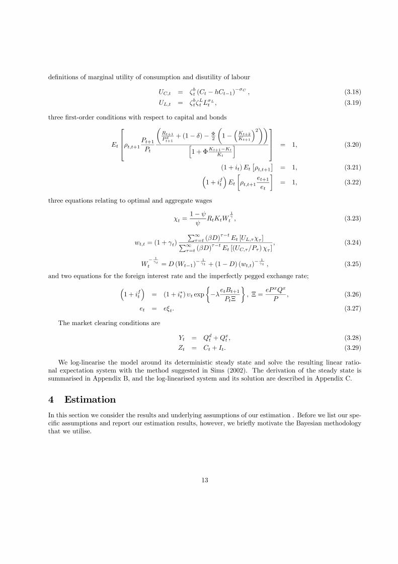
definitions of marginal utility of consumption and disutility of labour

UC,t = ζbt (Ct − hCt−1)−σC , (3.18)

UL,t = ζbtζLt L

σLt , (3.19)

three first-order conditions with respect to capital and bonds

Et

⎡⎢⎢⎣ρt,t+1Pt+1Pt

µRt+1Pdt+1

+ (1− δ)− Φ2µ1−

³Kt+2

Kt+1

´2¶¶h1 +ΦKt+1−Kt

Kt

i⎤⎥⎥⎦ = 1, (3.20)

(1 + it)Et

£ρt,t+1

¤= 1, (3.21)³

1 + ift

Ét

∙ρt,t+1

et+1et

¸= 1, (3.22)

three equations relating to optimal and aggregate wages

χt =1− ψ

ψRtKtW

1γ

t , (3.23)

wt,t = (1 + γt)

P∞τ=t (βD)

τ−tEt [UL,τχτ ]P∞

τ=t (βD)τ−tEt [(UC,τ/Pτ )χτ ]

, (3.24)

W− 1γt

t = D (Wt−1)− 1γt + (1−D) (wt,t)

− 1γt , (3.25)

and two equations for the foreign interest rate and the imperfectly pegged exchange rate;³1 + ift

´= (1 + i∗t )υt exp

½−λetBt+1

PtΞ

¾, Ξ =

eP xQx

P, (3.26)

et = eξt. (3.27)

The market clearing conditions are

Yt = Qdt +Qx

t , (3.28)

Zt = Ct + It. (3.29)

We log-linearise the model around its deterministic steady state and solve the resulting linear ratio-nal expectation system with the method suggested in Sims (2002). The derivation of the steady state issummarised in Appendix B, and the log-linearised system and its solution are described in Appendix C.

4 EstimationIn this section we consider the results and underlying assumptions of our estimation . Before we list our spe-cific assumptions and report our estimation results, however, we briefly motivate the Bayesian methodologythat we utilise.

13

4.1 Estimation Methodology

We seek suitable econometric tools to quantify and evaluate our postulated structural model of the Danisheconomy given our set of observed time series. Building on the seminal analysis in Smets and Wouters(2003), we follow what ? styled the strong econometric interpretation of our dsge model. This impliesthat we postulate a full probabilistic characterisation of our observed data which allows us to estimate thestructural parameters through classical maximum-likelihood methods; or alternatively—following Bayesianmethodology—through combining the likelihood function with prior distributions on the structural parametersand maximise the resulting posterior density.In this paper we follow the Bayesian approach which allows us to formalise the use of any prior knowledge

we may have on the structural parameters. On a more practical level it also helps stabilise the nonlinearminimization algorithm which we use for the estimation. Given the limited length of our sample, reasonableassumptions for the prior distributions (including restrictions on the support of certain parameters such as,e.g., standard deviations) are likely to be essential for obtaining plausible estimates. On the other hand, weutilise prior distributions we believe to be broad enough in order for the data to inform us on the structuralparameters of the theoretical model.We fix a subset of key parameters which are likely to be poorly determined in a model that only considers

deviations from the steady state. These parameters include β, δ, ψ, ν, αd, λ which are all assigned values whichshould be uncontroversial [to be added]. We also fix η at 1 which corresponds to a foreign technology equalto that assumed for the home country.Our model includes ten structural shocks and nine observed variables. Thus, we can proceed on the

assumption that there is no measurement error in the data set without facing the problem of stochasticsingularity. In other words, we attribute all stochastic volatility to identified structural shock processes.This approach was succesfully carried out in the Smets and Wouters (2003) analysis of a close variant ofthe cee closed-economy model. We should stress, however, that since our open-economy model does notinclude a number of the empirically motivated frictions of the cee model, we leave a larger amount of thedynamics to be explained by the exogenous processes; hence, we should be more cautious when we interpretthese processes as the true structural shocks.

4.2 Data

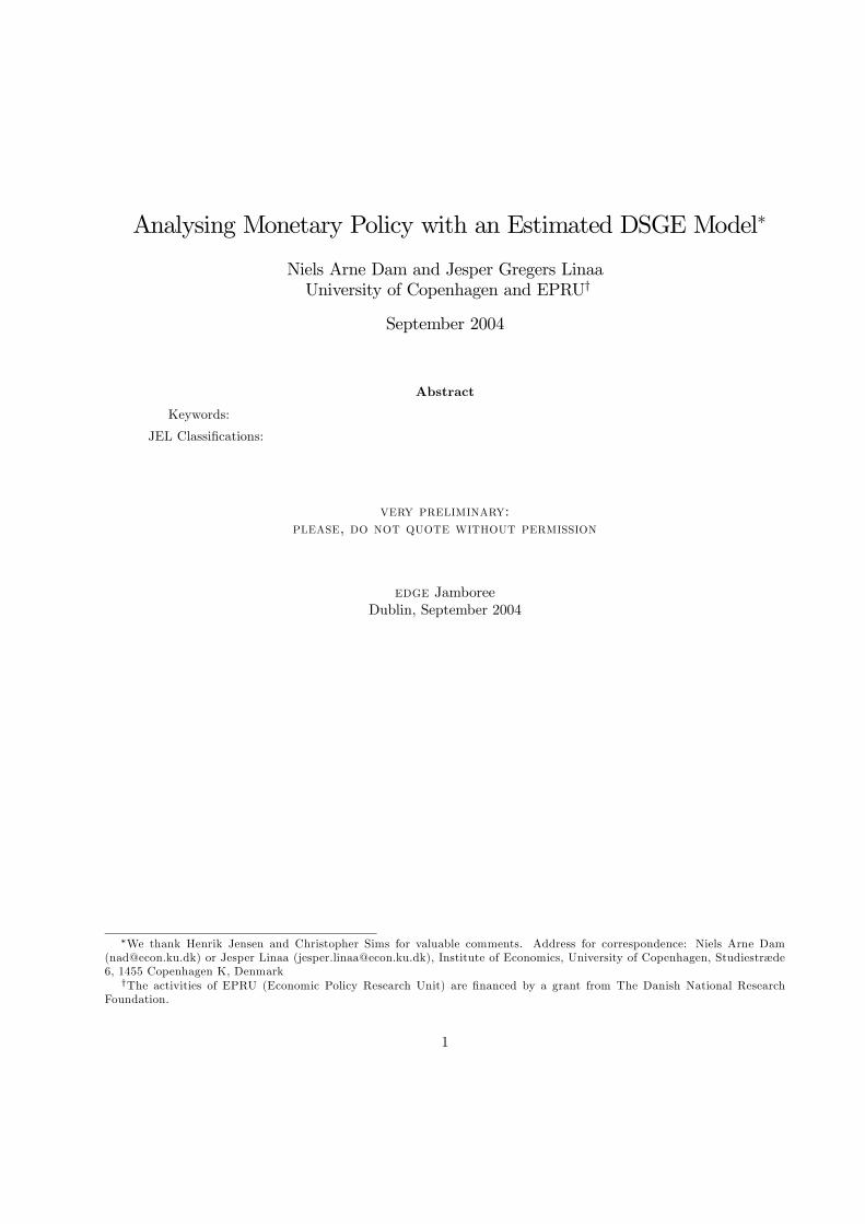
We treat Denmark as the home country and a weigthed average of a Germany, France and the Netherlandsas the foreign country. For Denmark we include observations of real gdp, total real consumption, the gdpdeflator, total employment adjusted for variations in hours worked, and a three-month money-market interestrate, corresponding to the theoretical variables Y,C, P, L and i.Since our model assumes that the home country is pegging the foreign country, and the Danish krone

was effectively pegged to the D-mark before the current peg on the euro, our foreign aggregate should at thesame time be broad enough to cover as much as possible of the Danish trade and narrow enough that we canplausibly claim that the relevant exchange rate for the foreign area was historically the D-mark. We settledon Germany, France and the Netherlands which constituted 28 percent of Danish exports in 2003. We usedtheir relative weights from the current effective exchange rate for the Danish krone as calculated by DanmarksNationalbank which are 69, 17 and 14 percent for Germany, France and the Netherlands, respectively. Forthis eu aggregate we include observations of geometric averages of real gdp and the gdp deflator, and of theD-mark/euro exchange rate vis-à-vis the Danish krone and a German three-month money-market interestrate, matching the theoretical variables Y ∗, P ∗, e and i∗.Since our log-linearized model describes stationary deviations from a steady state, we detrend the log of

our gdp, consumption and labour supply series. We further adjust the price series for a nominal trend ininflation and remove the same trend from the interest rates.

14

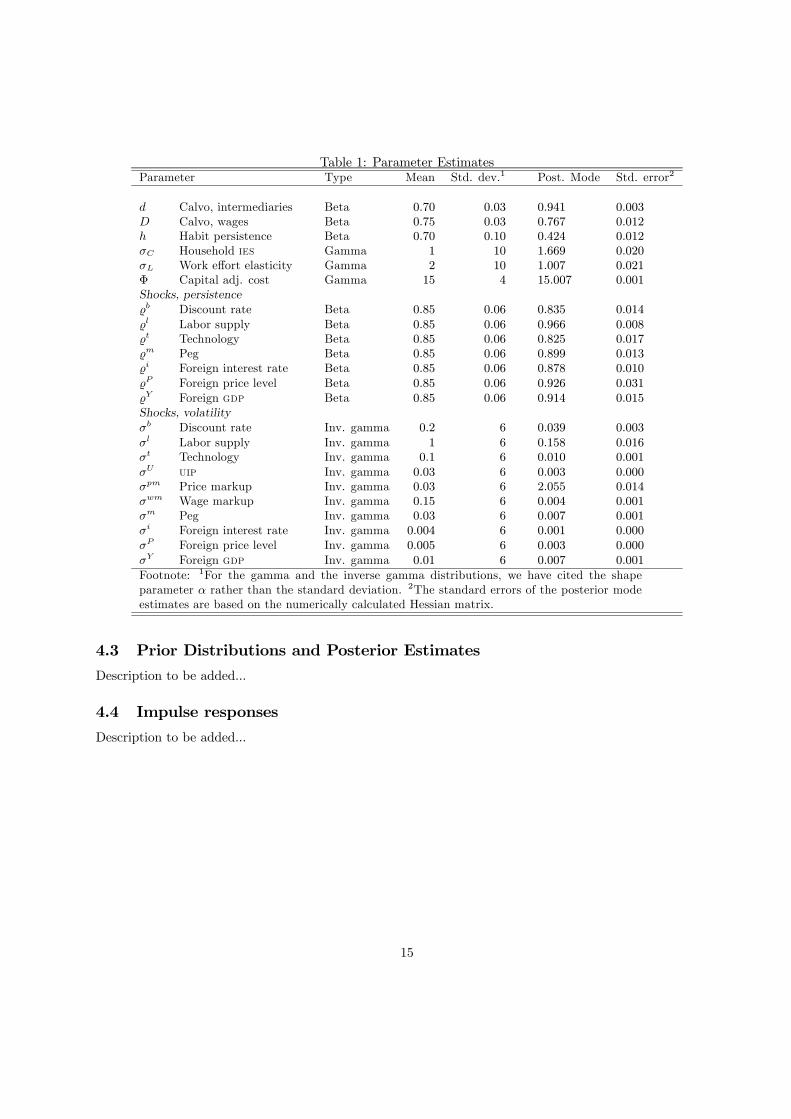
Table 1: Parameter EstimatesParameter Type Mean Std. dev.1 Post. Mode Std. error2

d Calvo, intermediaries Beta 0.70 0.03 0.941 0.003D Calvo, wages Beta 0.75 0.03 0.767 0.012h Habit persistence Beta 0.70 0.10 0.424 0.012σC Household ies Gamma 1 10 1.669 0.020σL Work effort elasticity Gamma 2 10 1.007 0.021Φ Capital adj. cost Gamma 15 4 15.007 0.001Shocks, persistenceb Discount rate Beta 0.85 0.06 0.835 0.014l Labor supply Beta 0.85 0.06 0.966 0.008t Technology Beta 0.85 0.06 0.825 0.017m Peg Beta 0.85 0.06 0.899 0.013i Foreign interest rate Beta 0.85 0.06 0.878 0.010P Foreign price level Beta 0.85 0.06 0.926 0.031Y Foreign gdp Beta 0.85 0.06 0.914 0.015Shocks, volatilityσb Discount rate Inv. gamma 0.2 6 0.039 0.003σl Labor supply Inv. gamma 1 6 0.158 0.016σt Technology Inv. gamma 0.1 6 0.010 0.001σU uip Inv. gamma 0.03 6 0.003 0.000σpm Price markup Inv. gamma 0.03 6 2.055 0.014σwm Wage markup Inv. gamma 0.15 6 0.004 0.001σm Peg Inv. gamma 0.03 6 0.007 0.001σi Foreign interest rate Inv. gamma 0.004 6 0.001 0.000σP Foreign price level Inv. gamma 0.005 6 0.003 0.000σY Foreign gdp Inv. gamma 0.01 6 0.007 0.001

Footnote: 1For the gamma and the inverse gamma distributions, we have cited the shapeparameter α rather than the standard deviation. 2The standard errors of the posterior modeestimates are based on the numerically calculated Hessian matrix.

4.3 Prior Distributions and Posterior Estimates

Description to be added...

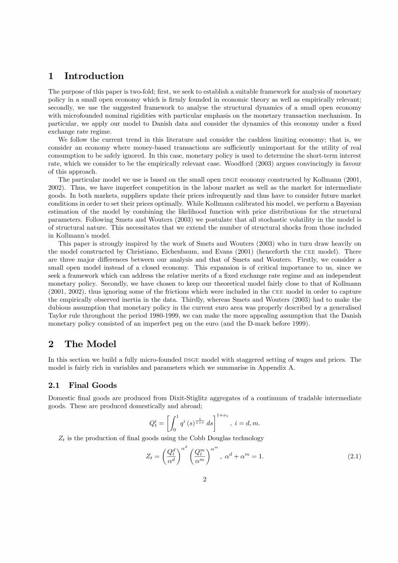
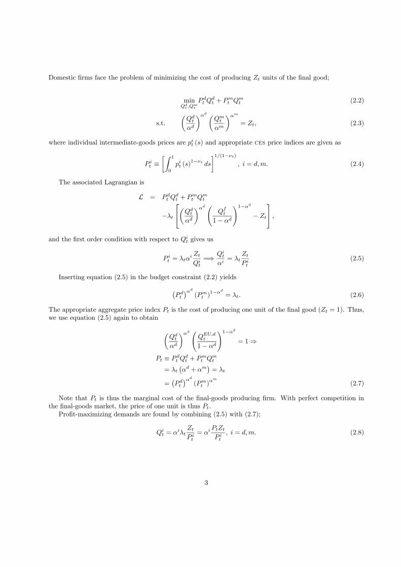
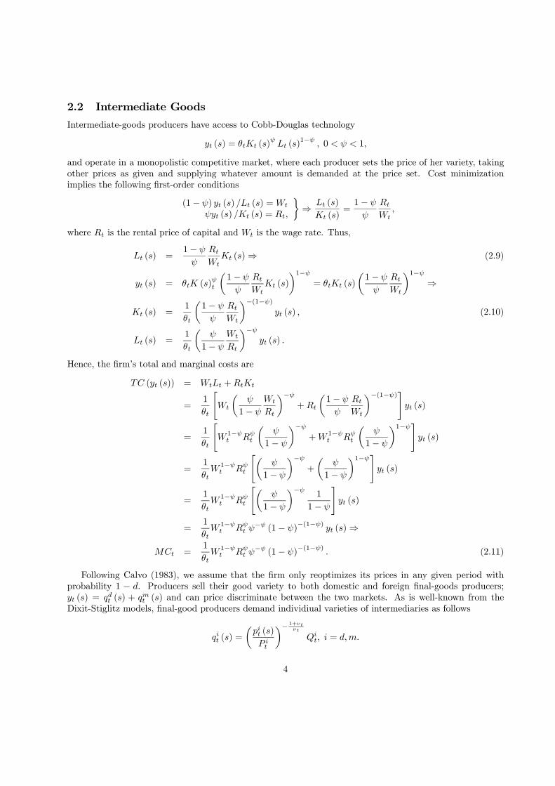
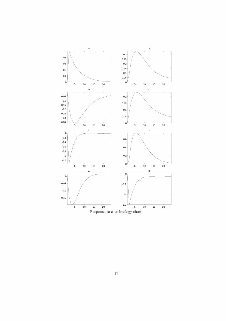
4.4 Impulse responses

Description to be added...

15

1985 1990 1995 2000 2005-0.1

-0.05

0

0.05

0.1Consumption

1985 1990 1995 2000 2005-0.02

0

0.02

0.04

0.06EU exchange rate

1985 1990 1995 2000 2005-0.01

0

0.01

0.02Interest rate

1985 1990 1995 2000 2005-0.1

-0.05

0

0.05

0.1Labor supply

1985 1990 1995 2000 2005-0.05

0

0.05Prices

1985 1990 1995 2000 2005-0.1

-0.05

0

0.05

0.1GDP

1985 1990 1995 2000 2005-0.01

-0.005

0

0.005

0.01EU interest rate

1985 1990 1995 2000 2005-0.04

-0.02

0

0.02

0.04EU Prices

1985 1990 1995 2000 2005-0.05

0

0.05

0.1

0.15EU GDP

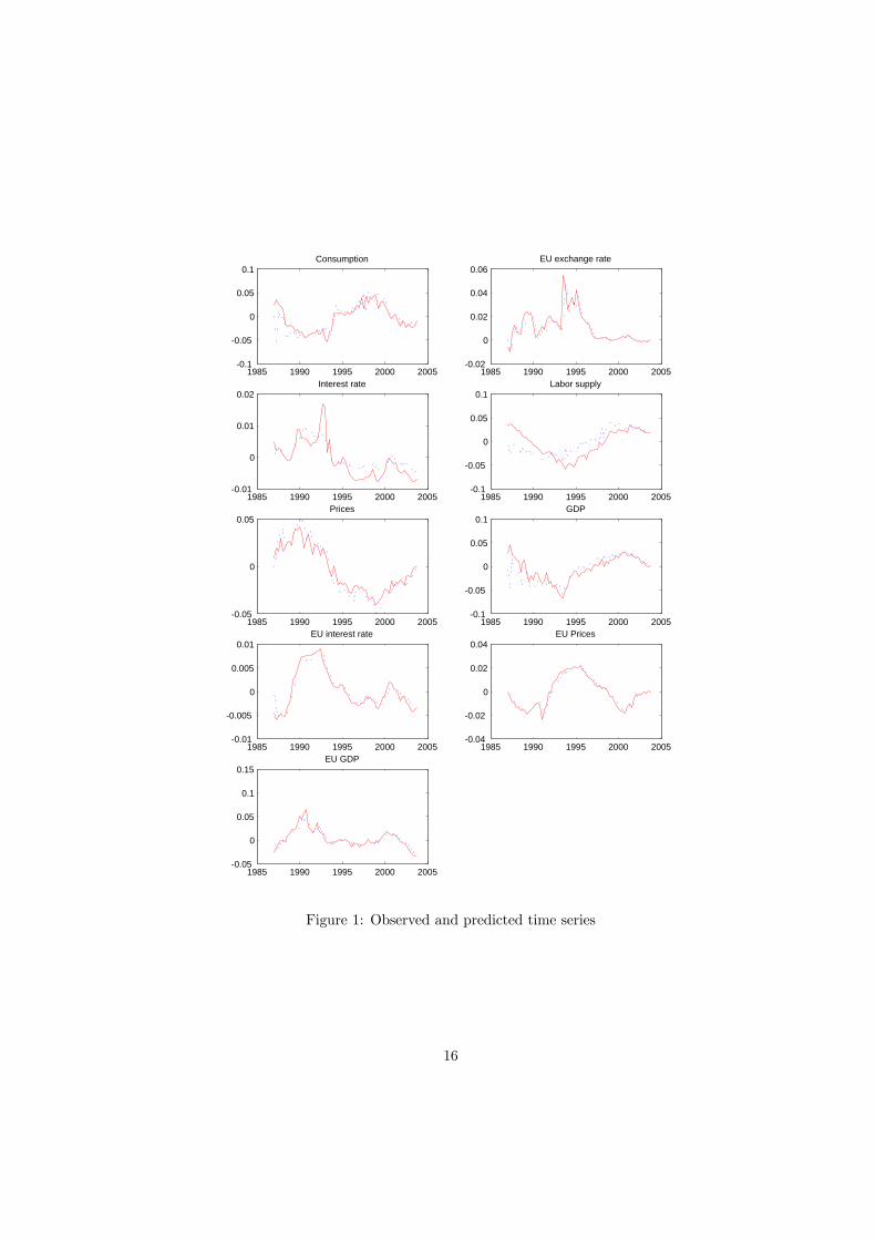
Figure 1: Observed and predicted time series

16

5 10 15 200

0.2

0.4

0.6

0.8

1θ

5 10 15 200

0.05

0.1

0.15

0.2

0.25

0.3

Y

5 10 15 20-0.35

-0.3

-0.25

-0.2

-0.15

-0.1

-0.05

P

5 10 15 200

0.05

0.1

0.15

0.2

C

5 10 15 20

-1.2

-1

-0.8

-0.6

-0.4

-0.2

0L

5 10 15 200

0.2

0.4

0.6

I

5 10 15 20

-0.15

-0.1

-0.05

0

W

5 10 15 20-1.5

-1

-0.5

0R

Response to a technology shock

17

5 10 15 200

0.2

0.4

0.6

0.8

e

5 10 15 20-0.1

-0.08

-0.06

-0.04

-0.02

0i

5 10 15 200

0.1

0.2

0.3

0.4

P

5 10 15 200

0.1

0.2

0.3

0.4

0.5

0.6

Y

5 10 15 200

0.05

0.1

0.15

0.2

0.25

0.3

C

5 10 15 200

0.2

0.4

0.6

0.8

L

5 10 15 200

0.5

1

1.5

2

I

5 10 15 200

0.2

0.4

0.6

0.8

1

1.2

R

Figure 2: Response to a monetary policy shock

18

5 10 15 200

0.2

0.4

0.6

0.8

Y*

5 10 15 200

0.05

0.1

0.15

0.2

0.25

Y

5 10 15 200

0.05

0.1

0.15

0.2

0.25P

5 10 15 200

0.02

0.04

0.06

0.08

0.1

0.12

C

5 10 15 200

0.1

0.2

0.3

L

5 10 15 200

0.2

0.4

0.6

0.8

I

5 10 15 200

0.1

0.2

0.3

0.4W

5 10 15 200

0.1

0.2

0.3

0.4

0.5

R

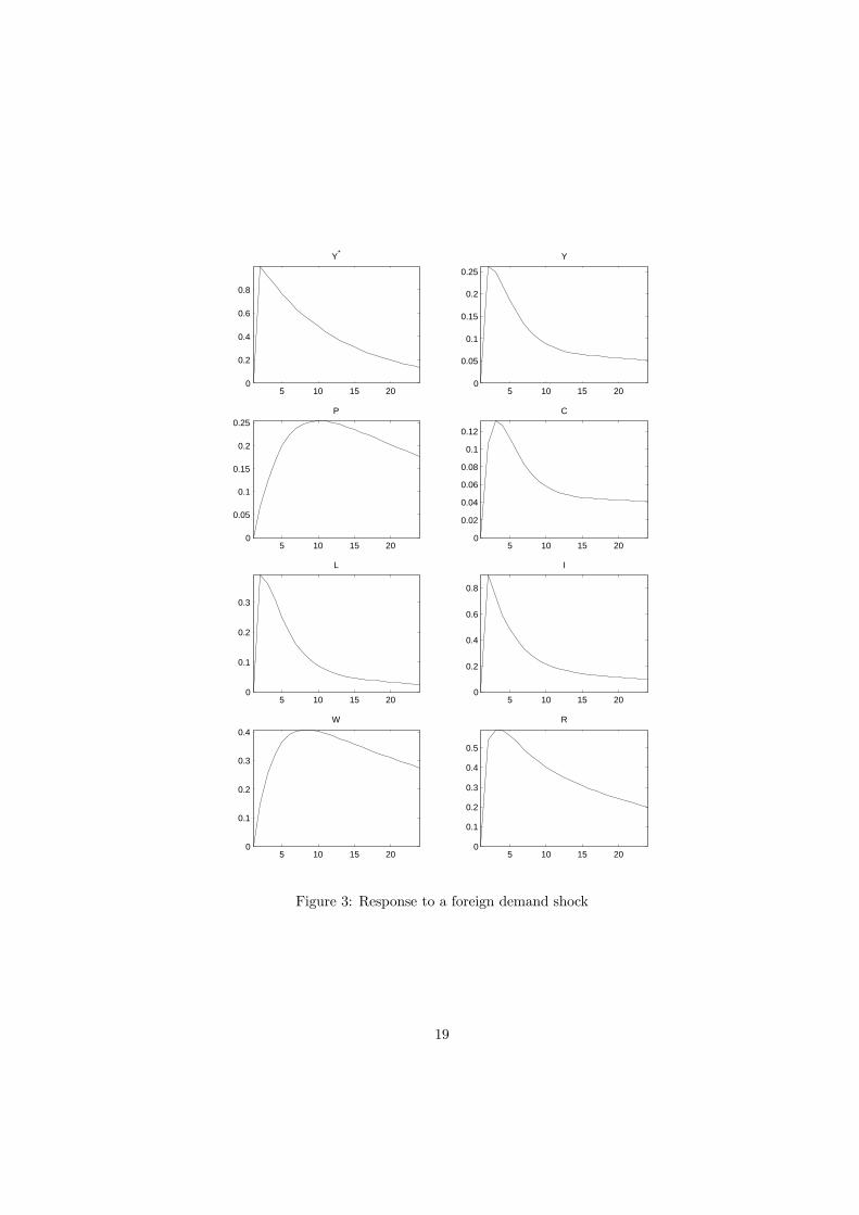
Figure 3: Response to a foreign demand shock

19

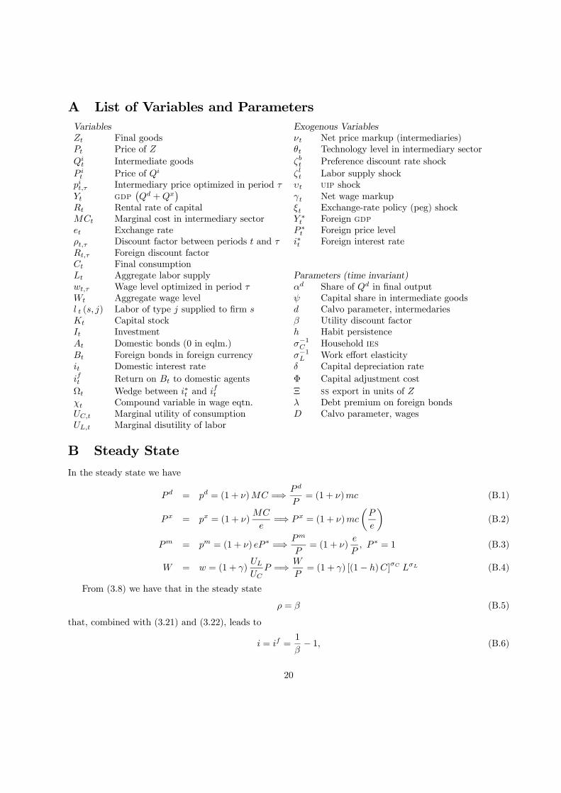
A List of Variables and ParametersVariables Exogenous VariablesZt Final goods νt Net price markup (intermediaries)Pt Price of Z θt Technology level in intermediary sectorQit Intermediate goods ζbt Preference discount rate shock

P it Price of Qi ζlt Labor supply shock

pit,τ Intermediary price optimized in period τ υt uip shockYt gdp

¡Qd +Qx

¢γt Net wage markup

Rt Rental rate of capital ξt Exchange-rate policy (peg) shockMCt Marginal cost in intermediary sector Y ∗t Foreign gdpet Exchange rate P ∗t Foreign price levelρt,τ Discount factor between periods t and τ i∗t Foreign interest rateRt,τ Foreign discount factorCt Final consumptionLt Aggregate labor supply Parameters (time invariant)wt,τ Wage level optimized in period τ αd Share of Qd in final outputWt Aggregate wage level ψ Capital share in intermediate goodsl t (s, j) Labor of type j supplied to firm s d Calvo parameter, intermedariesKt Capital stock β Utility discount factorIt Investment h Habit persistenceAt Domestic bonds (0 in eqlm.) σ−1C Household iesBt Foreign bonds in foreign currency σ−1L Work effort elasticityit Domestic interest rate δ Capital depreciation rateift Return on Bt to domestic agents Φ Capital adjustment costΩt Wedge between i∗t and ift Ξ ss export in units of Zχt Compound variable in wage eqtn. λ Debt premium on foreign bondsUC,t Marginal utility of consumption D Calvo parameter, wagesUL,t Marginal disutility of labor

B Steady StateIn the steady state we have

P d = pd = (1 + ν)MC =⇒ P d

P= (1 + ν)mc (B.1)

P x = px = (1 + ν)MC

e=⇒ P x = (1 + ν)mc

µP

e

¶(B.2)

Pm = pm = (1 + ν) eP ∗ =⇒ Pm

P= (1 + ν)

e

P, P ∗ = 1 (B.3)

W = w = (1 + γ)ULUC

P =⇒ W

P= (1 + γ) [(1− h)C]

σC LσL (B.4)

From (3.8) we have that in the steady state

ρ = β (B.5)

that, combined with (3.21) and (3.22), leads to

i = if =1

β− 1, (B.6)

20

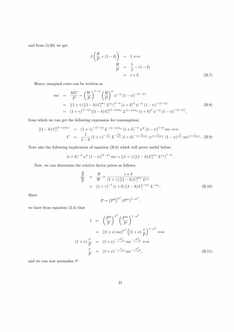
and from (3.20) we get

β

µR

P+ (1− δ)

¶= 1⇐⇒

R

P=

1

β− (1− δ)

= i+ δ. (B.7)

Hence, marginal costs can be written as

mc =MC

P=

µW

P

¶1−ψ µR

P

¶ψψ−ψ (1− ψ)−(1−ψ)

= [(1 + γ) [(1− h)C]σC LσL ]1−ψ

(i+ δ)ψ ψ−ψ (1− ψ)−(1−ψ) (B.8)

= (1 + γ)(1−ψ) [(1− h)C](1−ψ)σC L(1−ψ)σL (i+ δ)ψ ψ−ψ (1− ψ)−(1−ψ) ,

from which we can get the following expression for consumption;

[(1− h)C](1−ψ)σC = (1 + γ)

−(1−ψ)L−(1−ψ)σL (i+ δ)

−ψψψ (1− ψ)

1−ψmc⇐⇒

C =1

1− h(1 + γ)

− 1σC L

− σLσC (i+ δ)

− ψ(1−ψ)σC ψ

ψ(1−ψ)σC (1− ψ)

1σC mc

1(1−ψ)σC . (B.9)

Note also the following implication of equation (B.8) which will prove useful below;

(i+ δ)−ψ ψψ (1− ψ)(1−ψ)mc = [(1 + γ) [(1− h)C]σC LσL ]1−ψ

.

Now, we can determine the relative factor prices as follows;

RPWP

=R

W=

i+ δ

(1 + γ) [(1− h)C]σC LσL

= (1 + γ)−1 (i+ δ) [(1− h)C]−σC L−σL . (B.10)

SinceP =

¡P d¢αd

(Pm)1−αd

,

we have from equation (3.4) that

1 =

µP d

P

¶αd µPm

P

¶1−αd= [(1 + ν)mc]

αd³(1 + ν)

e

P

´1−αd⇐⇒

(1 + ν)e

P= (1 + ν)

− αd

1−αd mc− αd

1−αd ⇐⇒e

P= (1 + ν)

− 1

1−αd mc− αd

1−αd , (B.11)

and we can now normalize P .

21

Using this, (B.2) and (B.3) we then have

P x = (1 + ν)mc

µ(1 + ν)

− 1

1−αd mc− αd

1−αd

¶−1= (1 + ν)

2−αd1−αd mc

1

1−αd , (B.12)Pm

P= (1 + ν)

− αd

1−αd mc− αd

1−αd . (B.13)

In the steady state (3.17) looks like

PxQx =Pm

eQm,

and foreign demands is expressed, cf. (??), as

Qx =

µP x

P ∗

¶−ηY ∗

= (P x)−η ,

since in the steady state we assume that P ∗ = Y ∗ = 1, implying

Px (P x)−η =Pm

eQm ⇐⇒

Qm = (Px)1−η e

Pm=

1

1 + ν(Px)

1−η,

where we used that

e

Pm=

ePPm

P

=(1 + ν)

− 1

1−αd mc− αd

1−αd

(1 + ν)− αd

1−αd mc− αd

1−αd=

1

1 + ν.

Now use (B.12) to obtain

Qx = (1 + ν)−η 2−α

d

1−αd mc−η

1−αd , (B.14)

Qm =1

1 + ν(1 + ν)

(1−η)(2−αd)1−αd mc

1−η1−αd

= (1 + ν)(1−η)(2−αd)−1+αd

1−αd mc1−η1−αd

= (1 + ν)1−η(2−αd)

1−αd mc1−η1−αd (B.15)

= (1 + ν)1−η1−αd

−ηmc

1−η1−αd .

From (3.1) and (3.2) we obtain

Qd =αd

1− αd

µP d

P

¶−1µPm

P

¶Qm.

22

Now, substitute from (B.1) , (B.13) and (B.15) and re-arrange to get

Qd =αd

1− αd

µP d

P

¶−1µPm

P

¶Qm

=αd

1− αd[(1 + ν)mc]

−1∙(1 + ν)

− αd

1−αd mc− αd

1−αd

¸(1 + ν)

1−η(2−αd)1−αd mc

1−η1−αd

=αd

1− αd(1 + ν)

1−η(2−αd)1−αd

−1− αd


− αd

1−αd−1

=αd

1− αd(1 + ν)

1−η(2−αd)−(1−αd)−αd1−αd mc

1−η−αd−(1−αd)1−αd

=αd

1− αd(1 + ν)

−η 2−αd

1−αd mc−η

1−αd .

Furthermore,

Qm =¡1− αd

¢ PZPm⇐⇒

Z =1

1− αdPm

PQm

=1

1− αd(1 + ν)

− αd

1−αd mc− αd

1−αd (1 + ν)1−η(2−αd)


=1

1− αd(1 + ν)

1−η(2−αd)−αd1−αd mc

1−η−αd1−αd (B.16)

=1

1− αd(1 + ν)

1−η 2−αd

1−αd mc1− η

1−αd .

Given the various quantities of intermediaries we can obtain a steady-state expression for real gdp;

Y = Qd +Qx

=αd

1− αd(1 + ν)

−η 2−αd

1−αd mc−η

1−αd + (1 + ν)−η 2−α

d

1−αd mc−η

1−αd

= (1 + ν)−η 2−α

d

1−αd mc−η

1−αd

∙αd

1− αd+ 1

¸=

1

1− αd(1 + ν)

−η 2−αd

1−αd mc−η

1−αd . (B.17)

23

Turning to labour and capital, we have from (3.6) that

K = Y

µ1− ψ

ψ

R

W

¶−(1−ψ)=

1

1− αd(1 + ν)

−η 2−αd

1−αd mc−η

1−αd

∙1− ψ

ψ

i+ δ

(1 + γ) [(1− h)C]σC LσL

¸−(1−ψ)=

1

1− αd(1 + ν)

−η 2−αd

1−αd mc−η

1−αd

µψ

1− ψ

¶(1−ψ)(i+ δ)

−(1−ψ)[(1 + γ) [(1− h)C]

σC LσL ]1−ψ

=1

1− αd(1 + ν)

−η 2−αd1−αd mc

−η1−αd

µψ

1− ψ

¶(1−ψ)(i+ δ)

−(1−ψ)(i+ δ)

−ψψψ (1− ψ)

(1−ψ)mc

=ψ

(1− αd) (i+ δ)(1 + ν)

−η 2−αd

1−αd mc1− η

1−αd , (B.18)

where we made use of (B.8). Thus, using (2.9) we can solve for labour as follows;

L =1− ψ

ψ

R

WK

=1− ψ

ψ

i+ δ

(1 + γ) [(1− h)C]σC LσLψ

(1− αd) (i+ δ)(1 + ν)

−η 2−αd

1−αd mc1− η

1−αd

=1− ψ

1− αd(i+ δ)

h(i+ δ)

−ψ1−ψ ψ

ψ1−ψ (1− ψ)mc

11−ψ

i−1(1 + ν)

−η 2−αd

1−αd mc1− η

1−αd

=1

(1− αd)ψ−

ψ1−ψ (i+ δ)

ψ1−ψ (1 + ν)

−η 2−αd

1−αd mc1− η

1−αd− 11−ψ

=1

(1− αd)ψ−

ψ1−ψ (i+ δ)

ψ1−ψ (1 + ν)


1− η

1−αd− 11−ψ . (B.19)

Substituting (B.19) into (B.9) yields

C =1

1− h(1 + γ)

− 1σC L

− σLσC (i+ δ)

− ψ(1−ψ)σC ψ

ψ(1−ψ)σC (1− ψ)

1σC mc

1(1−ψ)σC

=1

1− h(1 + γ)

− 1σC

¡1− αd

¢ σLσC ψ

σLσC

ψ1−ψ+

ψ(1−ψ)σC (1− ψ)

1σC (i+ δ)

− σLσC

ψ1−ψ−

ψ(1−ψ)σC (1 + ν)

ησLσC

2−αd1−αd

×mc1

(1−ψ)σC− σLσC

³1− η

1−αd− 11−ψ

´

=(1 + γ)

− 1σC

1− h

¡1− αd

¢ σLσC

µψ

i+ δ

¶ (1+σL)σC

ψ1−ψ

(1− ψ)1σC (1 + ν)

ησLσC

2−αd1−αd

×mc1


³1− η

1−αd− 11−ψ

´,

so defining

ΛC ≡ (1 + γ)− 1σC

1− h

¡1− αd

¢ σLσC

µψ

i+ δ

¶ (1+σL)σC

ψ1−ψ

(1− ψ)1σC (1 + ν)

ησLσC

2−αd1−αd ,

we can write

C = ΛCmc1


³1− η

1−αd− 11−ψ

´. (B.20)

24

Now, combine equations (2.35) and (2.22) evaulated at the steady state in order to obtain

Z = C + I = C + δK ⇒

ΛZmc1− η

1−αd = ΛCmc1


³1− η

1−αd− 11−ψ

´+ δΛKmc

1− η

1−αd, (B.21)

where we have defined

ΛZ ≡ 1

1− αd(1 + ν)

1−η 2−αd

1−αd , ΛK ≡ ψ

(1− αd) (i+ δ)(1 + ν)

−η 2−αd

1−αd . (B.22)

Hence, we can now obtain a closed-form solution for the real marginal cost from (B.21);

¡ΛZ − δΛK

¢mc

1− η

1−αd = ΛCmc1


³1− η

1−αd− 11−ψ

´⇐⇒

mc1


³1− η

1−αd− 11−ψ

´−³1− η

1−αd

´=ΛZ − δΛK

ΛC⇐⇒

mc =

µΛZ − δΛK

ΛC

¶h 1(1−ψ)σC

− σLσC

³1− η

1−αd− 11−ψ

´−³1− η

1−αd

í−1

=

µΛZ − δΛK

ΛC

¶h 1+σL(1−ψ)σC

−σC+σLσC

1−αd−η1−αd

i−1.

We note that

ΛZ − δΛK

ΛC= ΛC

∙1

1− αd(1 + ν)

1−η 2−αd

1−αd − ψ

(1− αd) (i+ δ)(1 + ν)

−η 2−αd

1−αd

¸

= ΛC∙(1 + ν)− ψ

(i+ δ)

¸(1 + ν)

−η 2−αd

1−αd

1− αd.

B.1 Various steady-state ratios

Using the results above, we can derive the following steady-state ratios for use in the log-linearised systembelow;

Qd

Y=

αd

1−αd (1 + ν)−η 2−αd

1−αd mc−η

1−αd

11−αd (1 + ν)


−η1−αd

= αd,

Qx

Y= 1− αd,

Z = 11−αd (1 + ν)

1−η 2−αd1−αd mc

1− η

1−αd = ΛZmc1− η

1−αd

K = ψ(1−αd)(i+δ) (1 + ν)

−η 2−αd

1−αd mc1− η

1−αd = ΛKmc1− η

1−αd

⎫⎬⎭⇒K

Z=

ΛK

ΛZ=

ψ

(1− αd) (i+ δ)(1 + ν)

−η 2−αd

1−αd

∙1

1− αd(1 + ν)

1−η 2−αd

1−αd

¸−1=

ψ

(i+ δ) (1 + ν),

25

I

Z= δ

K

Z=

δψ

(i+ δ) (1 + ν),

C

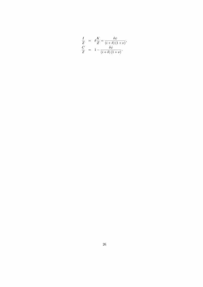
Z= 1− δψ

(i+ δ) (1 + ν).

26

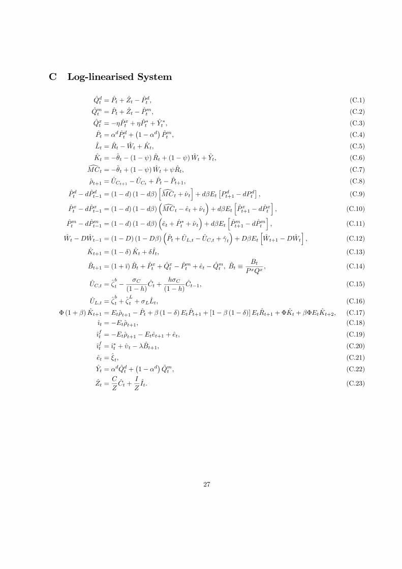
C Log-linearised System

Qdt = Pt + Zt − P d

t , (C.1)

Qmt = Pt + Zt − Pm

t , (C.2)

Qxt = −ηPx

t + ηP ∗t + Y ∗t , (C.3)

Pt = αdP dt +

¡1− αd

¢Pmt , (C.4)

Lt = Rt − Wt + Kt, (C.5)

Kt = −θt − (1− ψ) Rt + (1− ψ) Wt + Yt, (C.6)dMCt = −θt + (1− ψ) Wt + ψRt, (C.7)

ρt+1 = UCt+1 − UCt + Pt − Pt+1, (C.8)

P dt − dP d

t−1 = (1− d) (1− dβ)hdMCt + νt

i+ dβEt

£P dt+1 − dP d

t

¤, (C.9)

P xt − dPx

t−1 = (1− d) (1− dβ)³dMCt − et + νt

´+ dβEt

hPxt+1 − dP x

t

i, (C.10)

Pmt − dPm

t−1 = (1− d) (1− dβ)³et + P ∗t + νt

´+ dβEt

hPmt+1 − dPm

t

i, (C.11)

Wt −DWt−1 = (1−D) (1−Dβ)³Pt + UL,t − UC,t + γt

´+DβEt

hWt+1 −DWt

i, (C.12)

Kt+1 = (1− δ) Kt + δIt, (C.13)

Bt+1 = (1 + ı) Bt + P xt + Qx

t − Pmt + et − Qm

t , Bt ≡Bt

P xQx, (C.14)

UC,t = ζb

t −σC

(1− h)Ct +

hσC(1− h)

Ct−1, (C.15)

UL,t = ζb

t + ζL

t + σLLt, (C.16)

Φ (1 + β) Kt+1 = Etρt+1 − Pt + β (1− δ)EtPt+1 + [1− β (1− δ)]EtRt+1 +ΦKt + βΦEtKt+2, (C.17)

ıt = −Etρt+1, (C.18)

ıft = −Etρt+1 −Etet+1 + et, (C.19)

ıft = ı∗t + υt − λBt+1, (C.20)

et = ξt, (C.21)

Yt = αdQdt +

¡1− αd

¢Qmt , (C.22)

Zt =C

ZCt +

I

ZIt. (C.23)

27

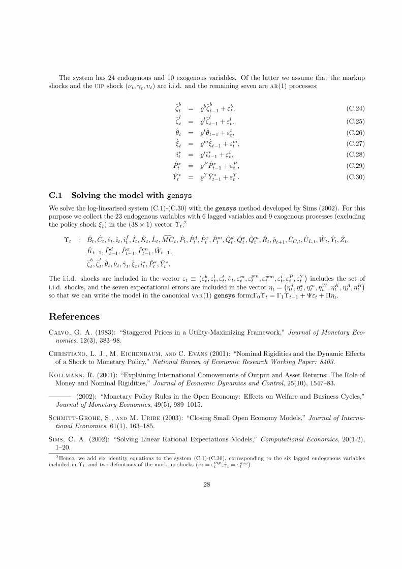
The system has 24 endogenous and 10 exogenous variables. Of the latter we assume that the markupshocks and the uip shock (νt, γt, υt) are i.i.d. and the remaining seven are ar(1) processes;

ζb

t = bζb

t−1 + εbt , (C.24)

ζl

t = lζl

t−1 + εlt, (C.25)

θt = tθt−1 + εtt, (C.26)

ξt = mξt−1 + εmt , (C.27)

ı∗t = iι∗t−1 + εit, (C.28)

P ∗t = P P ∗t−1 + εPt , (C.29)

Y ∗t = Y Y ∗t−1 + εYt . (C.30)

C.1 Solving the model with gensys

We solve the log-linearised system (C.1)-(C.30) with the gensys method developed by Sims (2002). For thispurpose we collect the 23 endogenous variables with 6 lagged variables and 9 exogenous processes (excludingthe policy shock ξt) in the (38× 1) vector Υt;2

Υt : Bt, Ct, et, ıt, ıft , It, Kt, Lt, dMCt, Pt, P

dt , P

xt , P

mt , Qd

t , Qxt , Q

mt , Rt, ρt+1, UC,t, UL,t, Wt, Yt, Zt,

Kt−1, Pdt−1, P

xt−1, P

mt−1, Wt−1,

ζb

t , ζl

t, θt, νt, γt, ξt, ı∗t , P

∗t , Y

∗t .

The i.i.d. shocks are included in the vector εt ≡¡εbt , ε

lt, ε

tt, υt, ε

mt , ε

pmt , εwmt , εit, ε

Pt , ε

Yt

¢includes the set of

i.i.d. shocks, and the seven expectational errors are included in the vector ηt =¡ηdt , η

xt , η

mt , η

Wt , ηKt , η

At , η

Bt

¢so that we can write the model in the canonical var(1) gensys form;Γ0Υt = Γ1Υt−1 +Ψεt +Πηt.

ReferencesCalvo, G. A. (1983): “Staggered Prices in a Utility-Maximizing Framework,” Journal of Monetary Eco-nomics, 12(3), 383—98.

Christiano, L. J., M. Eichenbaum, and C. Evans (2001): “Nominal Rigidities and the Dynamic Effectsof a Shock to Monetary Policy,” National Bureau of Economic Research Working Paper: 8403.

Kollmann, R. (2001): “Explaining International Comovements of Output and Asset Returns: The Role ofMoney and Nominal Rigidities,” Journal of Economic Dynamics and Control, 25(10), 1547—83.

(2002): “Monetary Policy Rules in the Open Economy: Effects on Welfare and Business Cycles,”Journal of Monetary Economics, 49(5), 989—1015.

Schmitt-Grohe, S., and M. Uribe (2003): “Closing Small Open Economy Models,” Journal of Interna-tional Economics, 61(1), 163—185.

Sims, C. A. (2002): “Solving Linear Rational Expectations Models,” Computational Economics, 20(1-2),1—20.2Hence, we add six identity equations to the system (C.1)-(C.30), corresponding to the six lagged endogenous variables

included in Υt, and two definitions of the mark-up shocks¡νt = εmp

t , γt = εmwt

¢.

28

Smets, F., and R. Wouters (2003): “An Estimated Dynamic Stochastic General Equilibrium Model ofthe Euro Area,” Journal of the European Economic Association, 1(5), 1123—1175.

Woodford, M. (2003): Interest & Prices. Princeton University Press, Princeton, New Jersey.

29

Analysing Monetary Policy with an Estimated DSGE Model

Documents