Analysing India's Exchange Rate Regime

WP-2021-022

Analysing India’s Exchange Rate Regime

Ila Patnaik and Rajeswari Sengupta

Indira Gandhi Institute of Development Research, MumbaiAugust 2021

Analysing India’s Exchange Rate Regime

Ila Patnaik and Rajeswari Sengupta

Email(corresponding author): [email protected]

AbstractWe analyse India's exchange rate regime through the prism of exchange market pressure. We estimate

the various regimes that India’s exchange rate has been through during the period from 2000 to 2020.

We find four specific regimes of the Indian rupee differentiated by the degree of flexibility. We document

the manner in which EMP in India has either been resisted through foreign exchange market

intervention, or relieved through exchange rate change, across these four exchange rate regimes. We

find that in only one of the four regimes the rupee-dollar exchange rate was relatively more flexible and

the share of exchange rate in EMP absorption was the highest. This regime corresponded with the

aftermath of the 2008 global crisis. In contrast, after 2013 the exchange rate was actively managed

using spot as well as forward market intervention. We also find that the RBI has been intervening in the

foreign exchange market in an asymmetric fashion to prevent the rupee from appreciating.

Keywords: Exchange rate regime, Forex intervention, Reserves, Exchange market pressure,Structural change

JEL Code: E58, F31, F41

Acknowledgements:

The views expressed are of the authors and not of their respective institutes. The authors are thankful to Josh Felman, Shekhar

Hari Kumar and the participants at the 2021 India Policy Forum Conference for useful discussions and to Madhur Mehta and

Surbhi Bhatia for assistance with the data.

Analysing India’s Exchange Rate Regime

Ila Patnaik Rajeswari [email protected] [email protected]

August, 2021

Forthcoming in the India Policy Forum, 2021-22

Abstract

We analyse India's exchange rate regime through the prism of exchange market pressure. Weestimate the various regimes that India’s exchange rate has been through during the periodfrom 2000 to 2020. We find four specific regimes of the Indian rupee differentiated by thedegree of flexibility. We document the manner in which EMP in India has either been resistedthrough foreign exchange market intervention, or relieved through exchange rate change,across these four exchange rate regimes. We find that in only one of the four regimes therupee-dollar exchange rate was relatively more flexible and the share of exchange rate in EMPabsorption was the highest. This regime corresponded with the aftermath of the 2008 globalcrisis. In contrast, after 2013 the exchange rate was actively managed using spot as well asforward market intervention. We also find that the RBI has been intervening in the foreignexchange market in an asymmetric fashion to prevent the rupee from appreciating.

Keywords: Exchange rate regime, Forex intervention, Reserves, Exchange marketpressure, Structural change

JEL codes: E58, F31, F41

Ila Patnaik is at the National Institute of Public Finance and Policy (NIPFP), New Delhi. Rajeswari Sengupta is at theIndira Gandhi Institute of Development and Research (IGIDR) Mumbai. The views expressed are of the authors andnot of their respective institutes. The authors are thankful to Josh Felman, Shekhar Hari Kumar and the participants atthe 2021 India Policy Forum Conference for useful discussions and to Madhur Mehta and Surbhi Bhatia for assistancewith the data.

Introduction

The exchange rate regime of a country depends on the manner in which the currency of the

country is managed with respect to other countries’ currencies. There are primarily three

different types of exchange rate regimes – freely floating, fixed and pegged or managed

floating. Most developed countries of the world have freely floating exchange rate regimes

wherein the central banks do not intervene in the foreign exchange markets to stabilise

currency fluctuations. On the other hand there are countries such as HongKong which has a

a fixed parity with the US dollar and the HongKong central bank uses its monetary policy to

maintain this peg. Majority of the emerging economies lie somewhere in between these two

extremes. They are mostly characterised by ‘managed floating’ exchange rate regimes or

some version of a ‘pegged’ regime, with their respective central banks intervening in the

foreign exchange market on a regular basis.

India falls in this category. In 1993 India officially moved towards a “market determined

exchange rate” from a fixed peg to the US dollar. This was part of the liberalisation and

deregulation reforms of the early 1990s. There has been a currency market since then, and at

the same time the Reserve Bank of India actively trades in this market.1 In this paper we

infer and document the evolution of India's exchange rate regime (henceforth, ERR) over a

long period of time, from 2000 to 2020. We introduce a novel angle of analysing the ERR,

by using an exchange market pressure index (henceforth, EMP). Specifically we ask how

was EMP managed across the different exchange rate regimes. The degree of foreign

exchange intervention and the degree of flexibility in the exchange rate are likely to differ

across the regimes based on the response of the central bank to the EMP.

The official de-jure classification of ERR of a country often diverges substantially from the

de-facto ERR that exists in practice (Reinhart and Rogoff, 2004). Full information about the

exchange rate regimes is often not disclosed by the central banks and hence the ERR needs

to be uncovered from historical data using statistical methods. Given the active foreign

exchange intervention by the RBI, it is difficult to decipher India’s ERR by simply looking

at the level of the exchange rate or the volatility. The actual rate that is observed is partly an

1 See Patnaik (2005) and Patnaik (2007) for more details.

outcome of the underlying macro-financial conditions or shocks faced by the economy and

partly of the intervention policy or currency policy of the central bank.

The IMF's AREAER report (till 2004) has classified India’s de-facto ERR as “managed

floating with no pre-determined path for the exchange rate”. Existing literature classifies

India’s ERR as a de-facto pegged exchange rate to the USD in the post-liberalisation period

(Patnaik, 2005, 2007; Zeileis et al, 2010 and Patnaik and Shah, 2009). Using data on

market-determined parallel exchange rates, Reinhart and Rogoff (2004) classifies India’s

de-facto ERR (in the post liberalisation period) as a “peg to US dollar” from August 1991 to

June 1995 and a “crawling peg to US dollar” from July 1995 to December 2001. Calvo and

Reinhart (2002) use a metric of currency flexibility that combines exchange rate volatility,

reserves volatility and interest rates volatility. They find that currency flexibility in India has

not changed in the 1979-1999 period despite the move to a ‘market-determined’ ERR in

1993.

The RBI intervenes in the forex market with the stated goal of “containing volatility”

(Patnaik, 2005) but there is evidence that the central bank intervenes in an asymmetric

manner, buying US dollars and selling rupees in order to prevent a currency appreciation

(Sen Gupta and Sengupta, 2013). This shows that India offers an interesting case-study for

deciphering the underlying ERR using a data-driven analytical framework.

EMP measures the pressure on the exchange rate, which is either resisted through foreign

exchange market intervention or relieved through an exchange rate change. In a floating

ERR, when macro-financial shocks hit the economy, this exerts pressure on the exchange

rate and the exchange rate freely fluctuates according to market forces. In a pegged or a

managed ERR, when shocks materialise, there is EMP and the exchange rate does not

change or changes much less. Instead, the central bank intervenes in the foreign exchange

market to absorb the EMP.

In the last decade, significant advances have been made in the literature in the context of

dating exchange rate regimes and also measuring exchange market pressure. New and

relatively more sophisticated statistical tools are being used in these fields which offer

greater conceptual clarity. In this paper we make use of these methodological innovations.

We estimate the exchange rate regimes in India using the methodology outlined in Zeileis et

al (2010). Their method is an improvement on a much-used linear regression framework

popularised by Frankel and Wei (1994). Once we find the ERR, we study the exchange

market pressure that prevailed during each of the regimes. For this, we use a new EMP

index proposed by Patnaik et al (2017). They measure EMP by analysing the amount of

adjustment needed in the exchange rate to remove any excess demand or excess supply of

the currency that may exist in the foreign exchange market in the absence of any currency

intervention.

We look at the evolution of this EMP index in India over the last two decades and document

the manner in which the RBI may have responded to changes in EMP across the different

exchange rate regimes. Specifically we ask whether the RBI attempted to manage the EMP

or let the exchange rate absorb the EMP. As mentioned above, an attempt to manage or

counter the EMP would lead to stabilisation of the exchange rate which has direct

implications for the underlying ERR. We also try to understand the transition from one

regime to the next. The Covid-19 pandemic has triggered unforeseen consequences for

economies all over the world. While on one hand the US government has announced a

massive fiscal stimulus which is already causing overheating of the economy, on the other

hand India continues to struggle with economic recovery amidst slow pace of vaccinations.

Towards the end of our paper we briefly discuss what this pandemic might imply for India’s

exchange rate dynamics going forward and what policy options might be available in this

context.

If the objective is to stabilise the exchange rate, this can be done using three instruments

from the central bank’s toolkit: (i) forex intervention, (ii) capital controls and (iii) monetary

policy. According to the Impossible Trilemma which is a key insight of modern day open

economy macroeconomics, a country cannot simultaneously have an open capital account, a

fixed exchange rate and monetary policy independence. This implies that if India has an

open capital account, and the RBI prefers to fix the exchange rate, monetary policy is driven

solely by the need to maintain the fixed exchange rate.

Alternatively, if the RBI wishes to retain monetary policy autonomy and at the same time

fix the exchange rate, it has to impose capital controls. In other words, if the decision is to

manage the exchange rate as opposed to letting the exchange rate float, then this objective

can be fulfilled in multiple ways. In this paper we primarily analyse how the RBI used forex

intervention to manage the exchange rate from time to time. In future research we plan to

delve deeper into the use of monetary policy and capital controls to stabilise the exchange

rate across ERR.

Our paper is closely related to the sizeable literature that exists by now on analysing

exchange rate regimes (see for example, Reinhart and Rogoff 2004; Levy-Yeyati and

Sturzenegger 2003; Bubula and Ötker-Robe 2002 among others). This literature mostly

developed in the 2000s when it became increasingly clear that a country’s de-jure ERR

(announced by the central bank) is not always the same as its de-facto ERR. Our study is

also related to existing work on dating structural breaks in India’s exchange rate (for

example, Patnaik and Shah, 2009).

The contribution of our work is to analyse ERR through the prism of the EMP, and also to

use the Zeileis et al (2010) methodology to study ERR in India for more than a 20-year

period. Most of the existing studies end in 2008. Extending the sample period gives us the

opportunity to throw light on the evolution of the de-facto ERR over a long period of time.

We find that during our sample period India witnessed four ERRs, roughly spanning the

periods from 2000 to 2004, 2004 to 2008, 2008 to 2013 and 2013 to December 2020. In 3

out of the 4 regimes, the pressure on the rupee was to appreciate. The RBI responded to this

appreciation pressure by intervening in the forex market and buying dollars which resulted

in a large accumulation of reserves. In only one regime, in the aftermath of the 2008 global

financial crisis, there was pressure on the rupee to depreciate. The RBI mostly allowed the

rupee to freely fluctuate in this time period. This is consistent with the additional evidence

we provide in the paper that confirms that the RBI intervenes in the forex market in an

asymmetric fashion, predominantly buying dollars when the rupee faces an appreciation

pressure. We find that in the fourth and last ERR ranging from 2013 to 2020, the rupee was

being actively managed through currency trading in both the spot and forward markets.

In the rest of the paper, we describe the methodology used to estimate ERR and discuss the

results we obtain for India in Section 2. In Section 3 we introduce the EMP measure and

analyse the exchange rate regimes using this EMP index. We discuss the transition periods

from one regime to the next in Section 4. In Section 5 we discuss the the ERR during the

period of the Covid-19 pandemic and touch upon the way forward. Finally, we end with our

concluding remarks in Section 6.

2. Exchange rate regimes

We estimate the exchange rate regimes prevalent in India from 2000 onwards using the

structural change dating methodology described in Zeileis et al (2010). They devise a data-

drive, inferential framework to study the evolution of ERR. Their method is based on the

standard, linear exchange rate regression model popularised by Frankel and Wei (1994)

which has been used in a number of studies to analyse a country’s de-facto ERR.2 The

model uses the returns on cross-currency exchange rates expressed in terms of a suitable

numeraire currency.

To apply this method, we use the New Zealand dollar (NZD) as the numeraire currency

given its stability over a long period of time.3 The underlying model that is estimated is as

follows:

yt = xTt β + ut (t = 1......n) (1)

where yt are the returns of the target currency, in our case Indian rupee (INR) in terms of

NZD and the xt are the vectors of returns of a basket of currencies at time t. For our purpose

2 See for example Kawai and Akiyama (2000), McKinnon (2000), Baig(2001), Ogawa (2002), Ogawa (2004), Bowman (2005), Patnaik et al (2005), B ́enassy-Qu ́er ́e et al (2006), Ogawa and Kudo (2007), Frankel and Wei (2007), Ogawa and Yang (2008), Shirono (2008), Patnaik and Shah (2009), Kawai and Pontines (2016) among others.

3 While Zeileis et al (2010) used the Swiss Franc as the numeraire currency, we use the NZD instead because in recent years the SWF has been actively managed with respect to the Euro. However as mentioned in Frankel and Wei (1994, 2007), for managed exchange rates the results of the regression analysis do not critically depend on the choice of the numeraire.

we use the US dollar, Japanese Yen, Euro, and British Pound all expressed in terms of the

NZD. These are the most important floating currencies in the world.4 We use the weekly

returns of these exchange rates in order to reduce the noise in the data and also ease the

computation burden of the regime-dating algorithm.5 This regression picks up the extent to

which the INR/NZD rate fluctuates in response to fluctuations in any of the currencies on

the right-hand side of the equation.

For example, if the INR is pegged to the USD, then the corresponding beta value will be

close to 1 and all the other beta values will be close to zero. If on the other hand the INR is

not pegged to any of these currencies, then all the beta values will be different from 0 and

will reflect the true trade and financial linkages of the economy with the rest of the world. If

the INR is instead pegged to a basket of currencies, then the beta values would reflect the

corresponding weights of the currencies in that basket. In the case of reduced exchange rate

flexibility, the R squared of this regression would also be very high, while lower values

would be obtained for floating currencies.

Using this linear regression model one can find out the relationship that exists between the

yt and xt currencies over a specific period of time. However one cannot infer whether this

relationship is stable within a given time period, whether it remains stable with future

incoming observations and in case of instabilities in the model parameters, when and how

did the estimated regime undergo a change. In other words, this regression model alone

cannot help to understand whether and when changes in ERR take place.

Exchange rate regimes can change due to changes in the policy interventions by the central

bank. However, the precise timing of these interventions is often not known which makes it

difficult to assess the time-window oveer which this model can be fitted. As a result of these

interventions, the underlying model parameters would change. In order to estimate the

changes in ERR, we need a methodology that takes into account the parameter instabilities

and dates the regime-changes based on these instabilities. This is the main premise of the

Zeileis et al (2010) method. They use statistical procedures for testing the stability of ERR

4 Since our sample period starts from 2000 we can safely use the Euro which was introduced as the official currency of the Euro zone from 1999 onwards.

5 We compute log-difference returns (in percentages) of all the currencies i.e. 100 (log pt– log pt-1), with pt being the price of a currency at time t expressed in terms of a numeraire currency.

based on past data, monitor the stability of the regimes as new data comes in and estimate

the break-points when the ERR changes using the structural change methodology of Bai and

Perron (2003).

The conventional method of estimating structural changes in exchange rates was based on

the algorithm devised by Bai and Perron (2003). One shortcoming of this method was that it

did not take into consideration changes in the error variance as a full model parameter. A

change in the underlying ERR necessarily involves a change in the error variance and hence

excluding this parameter would result in an incomplete picture. The error variance captures

the flexibility of the ERR. If for example the INR is pegged to the basket of five currencies

then the error variance will take a low value whereas if the INR is in a floating ERR, then

the error variance will be relatively high.

Zeileis et al (2010) extend the dating algorithm of Bai and Perron (2003) to maximum-

likelihood and quasi maximum-likelihood (ML and QML) models, include the error-

variance in the set of model parameters, over and above the estimated beta coefficients, and

assume that the error is normally distributed. In particular, they estimate a quasi-normal

model specified by the following density function:

f (y|x, β, σ2) = φ ((y – xT β)/σ)/σ (2)

where φ (.) is the standard normal density function with combined parameter ϴ = (βT, σ2)T

which has a length of k = c+2 (i.e. c currency coefficients or betas, intercept and error

variance). This way they are able to assess the parameter instability jointly for β and σ2.

They then devise a unified framework for testing and monitoring the stability of these

parameters and apply the dating algorithm of Bai and Perron (2003) to their maximum-

likelihood model.

They assume n observations of yt and xt such that the conditional distribution yt|xt follows

the quasi-likelihood function f (yt |xt , ϴt), with ϴt being a k-dimensional parameter, as

mentioned above. The hypothesis they test is that the parameter is stable over time i.e.

H0 : ϴt = ϴ0 (t = 1, 2, .....n) (3)

The alternative hypothesis is that ϴt changes over time (which is what we would expect in

the case of changes in ERR). If the parameters ϴt are stable over time, they can be estimated

by minimising the corresponding negative log-likelihood function (i.e. - log f (yt |xt , ϴt)).6

If the null hypothesis in Equation (3) is rejected i.e. there is evidence that the parameters do

change over time then dating algorithm can be applied to find out when these changes take

place. If the break-dates are known apriori, then estimation of the model parameters would

be relatively straightforward for each of the regimes or segments. Typically however the

break-points are not known. In that case, the optimal number of regimes (and hence break-

points, m) can be computed by using some information criteria (such as the BIC and a

modified BIC suggested by Liu et al, 1997).

Zeileis et al (2010) applied their methodology to India to uncover the de-factor ERR. They

found that during the period from April 1993 to April 2008, the optimal number of breaks

was m=3, implying four exchange rate regimes. Using their methodology we too find four

distinct exchange rate regimes in India during our sample period, 2000-2020, with the first

two regimes overlapping with the last two segments found by Zeileis et al (2010). We

report the dates of these regimes along with the corresponding, estimated coefficients of the

basket of currencies, the standard errors as well as the values of the error-variance and the R

squared in Table 1.

The first regime ranges from January, 2000 to March 2004, and can be categorised as

one where the rupee was closely pegged to the US dollar. The highly statistically

significant coefficient of the US dollar is close to 1 (0.95) while the coefficients of

the remaining 4 currencies are close to 0. The σ is the lowest in the sample period

and the R-squared value is the highest, further confirming a pegged ERR.

6 Further details on the tests and the monitoring mechanism can be seen from Zeileis et al (2010).

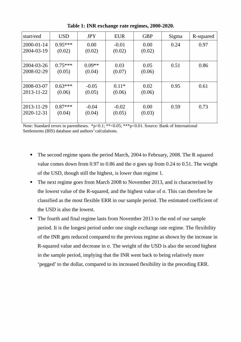
Table 1: INR exchange rate regimes, 2000-2020.

start/end USD JPY EUR GBP Sigma R-squared

2000-01-142004-03-19

0.95***(0.02)

0.00(0.02)

-0.01(0.02)

0.00(0.02)

0.24 0.97

2004-03-262008-02-29

0.75***(0.05)

0.09**(0.04)

0.03(0.07)

0.05(0.06)

0.51 0.86

2008-03-072013-11-22

0.63***(0.06)

-0.05(0.05)

0.11*(0.06)

0.02(0.06)

0.95 0.61

2013-11-292020-12-31

0.87***(0.04)

-0.04(0.04)

-0.02(0.05)

0.00(0.03)

0.59 0.73

Note: Standard errors in parentheses. *p<0.1; **<0.05; ***p<0.01. Source: Bank of International Settlements (BIS) database and authors’ calculations.

The second regime spans the period March, 2004 to February, 2008. The R squared

value comes down from 0.97 to 0.86 and the σ goes up from 0.24 to 0.51. The weight

of the USD, though still the highest, is lower than regime 1.

The next regime goes from March 2008 to November 2013, and is characterised by

the lowest value of the R-squared, and the highest value of σ. This can therefore be

classified as the most flexible ERR in our sample period. The estimated coefficient of

the USD is also the lowest.

The fourth and final regime lasts from November 2013 to the end of our sample

period. It is the longest period under one single exchange rate regime. The flexibility

of the INR gets reduced compared to the previous regime as shown by the increase in

R-squared value and decrease in σ. The weight of the USD is also the second highest

in the sample period, implying that the INR went back to being relatively more

‘pegged’ to the dollar, compared to its increased flexibility in the preceding ERR.

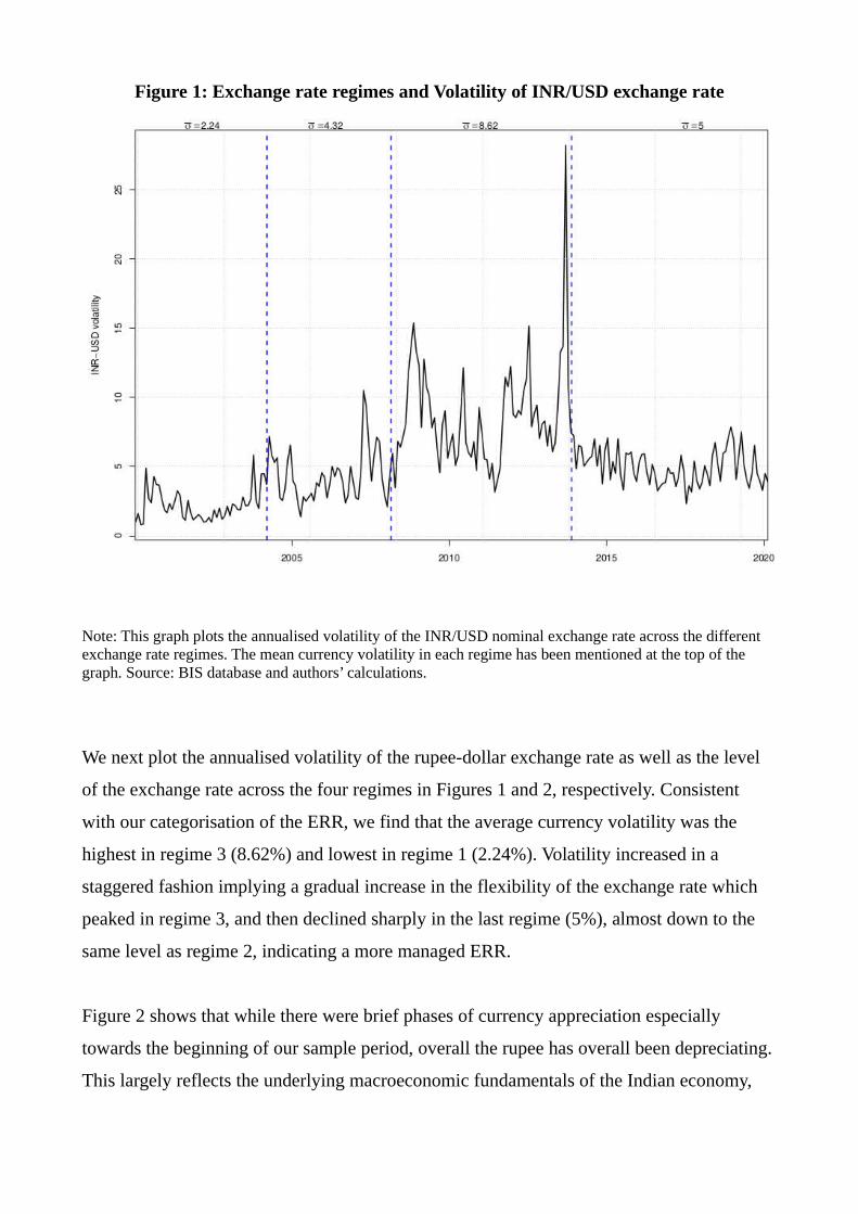
Figure 1: Exchange rate regimes and Volatility of INR/USD exchange rate

Note: This graph plots the annualised volatility of the INR/USD nominal exchange rate across the different exchange rate regimes. The mean currency volatility in each regime has been mentioned at the top of the graph. Source: BIS database and authors’ calculations.

We next plot the annualised volatility of the rupee-dollar exchange rate as well as the level

of the exchange rate across the four regimes in Figures 1 and 2, respectively. Consistent

with our categorisation of the ERR, we find that the average currency volatility was the

highest in regime 3 (8.62%) and lowest in regime 1 (2.24%). Volatility increased in a

staggered fashion implying a gradual increase in the flexibility of the exchange rate which

peaked in regime 3, and then declined sharply in the last regime (5%), almost down to the

same level as regime 2, indicating a more managed ERR.

Figure 2 shows that while there were brief phases of currency appreciation especially

towards the beginning of our sample period, overall the rupee has overall been depreciating.

This largely reflects the underlying macroeconomic fundamentals of the Indian economy,

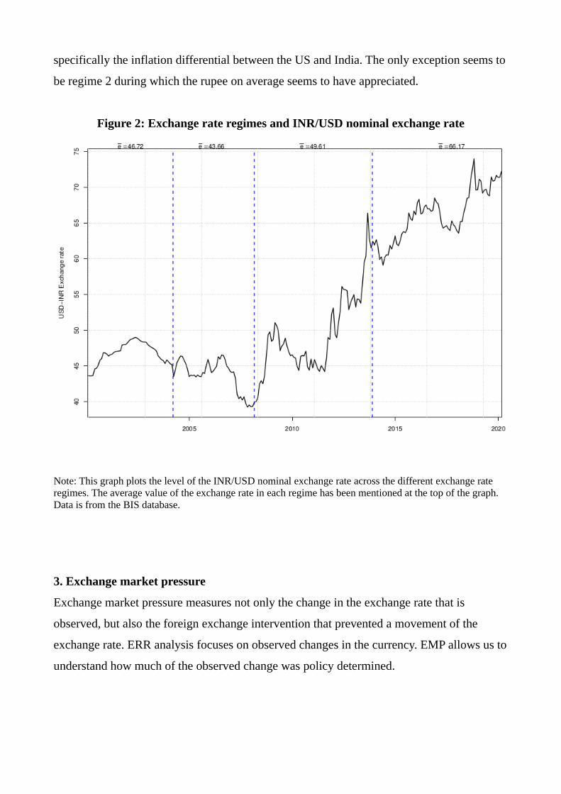
specifically the inflation differential between the US and India. The only exception seems to

be regime 2 during which the rupee on average seems to have appreciated.

Figure 2: Exchange rate regimes and INR/USD nominal exchange rate

Note: This graph plots the level of the INR/USD nominal exchange rate across the different exchange rate regimes. The average value of the exchange rate in each regime has been mentioned at the top of the graph. Data is from the BIS database.

3. Exchange market pressure

Exchange market pressure measures not only the change in the exchange rate that is

observed, but also the foreign exchange intervention that prevented a movement of the

exchange rate. ERR analysis focuses on observed changes in the currency. EMP allows us to

understand how much of the observed change was policy determined.

3.1. Measuring EMP

EMP is the total pressure on the exchange rate, resisted primarily through forex intervention

(thereby causing change in reserves) or relieved through exchange rate change. There exist

several measures of EMP in the literature that combine changes in the exchange rate and

reserves, but most of them suffer from problems of units. Some other measures tried to

resolve this problem by normalizing exchange rate and reserves and weighing them by the

inverse of their respective volatilities (or using alternative weights).7 However as pointed

out by Pontines and Siregar (2008) all these EMP indices are characterised by a common

problem of arbitrary choice of weights.

This in turn can result in misleading conclusions about EMP especially during ERR

changes. For example, having the inverse of the standard deviation of the exchange rate and

reserves as the weights imply that in a fixed ERR, the weight assigned to movements in

exchange rate by construction would be infinity (Patnaik et al, 2017). This means that if in a

country with a fixed ERR, small changes in the exchange rate are allowed, this will show up

as very high EMP values because of the large weight assigned to exchange rate movements

and small weight to reserve changes.

The EMP measure proposed by Patnaik et al. (2017) avoids these problems and also

measures the EMP in consistent units i.e. percentage change in exchange rate. They

calculate EMP as the actual change in the exchange rate that took place and the change that

would have occurred in the absence of any forex intervention. They estimate the following

equation to derive the EMP measure:

EMPt = Δ et + ρt It (4)

where, Δ et is the percentage change in nominal exchange rate, It is the actual intervention in

the forex market measured in billion dollars and ρt is the percentage change in exchange rate

associated with $1 billion forex intervention. They estimate the value of ρt which they call

the conversion factor. ρt It is therefore the exchange rate change that would have

7 See for example Eichengreen et al. (1996), Sachs et al. (1996), Kaminsky et al. (1998), Pentecost et al. (2001), Klaassen (2011) among others.

materialised had there been no forex intervention. This added to the actual change in the

exchange rate gives a comprehensive measure of the pressure faced by the exchange rate.

A negative EMP value denotes an appreciation pressure vis-a-vis the US dollar, whereas a

positive EMP value captures depreciation pressure. The EMP index is expressed in units of

percentage change in exchange rate over a one-month period.

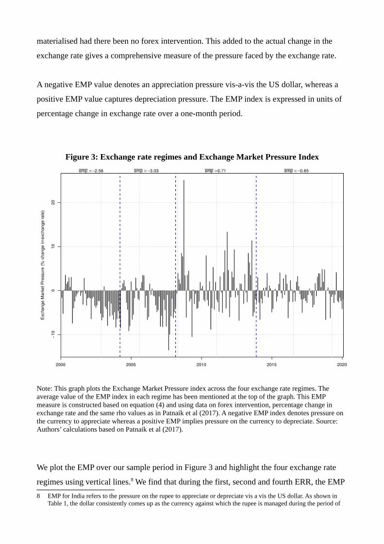
Figure 3: Exchange rate regimes and Exchange Market Pressure Index

Note: This graph plots the Exchange Market Pressure index across the four exchange rate regimes. The average value of the EMP index in each regime has been mentioned at the top of the graph. This EMP measure is constructed based on equation (4) and using data on forex intervention, percentage change in exchange rate and the same rho values as in Patnaik et al (2017). A negative EMP index denotes pressure on the currency to appreciate whereas a positive EMP implies pressure on the currency to depreciate. Source: Authors’ calculations based on Patnaik et al (2017).

We plot the EMP over our sample period in Figure 3 and highlight the four exchange rate

regimes using vertical lines.8 We find that during the first, second and fourth ERR, the EMP

8 EMP for India refers to the pressure on the rupee to appreciate or depreciate vis a vis the US dollar. As shown in Table 1, the dollar consistently comes up as the currency against which the rupee is managed during the period of

was mostly negative. This implies that the rupee experienced a pressure to appreciate for

majority of the sample period. The direction of EMP changed around the time of the 2008

global financial crisis. During the third ERR which ranges from 2008 to 2013, the rupee

primarily faced a pressure to depreciate.

When we look at Figure 2 and Figure 3 in conjunction, the implications are interesting.

During three of the four regimes, the EMP and the actual movement of the exchange rate

seem to have been in the same direction. In regimes 1 and 2, the EMP shows a pressure on

the rupee to appreciate and the exchange rate seems to have actually appreciated. In regime

3, the EMP shows a pressure on the rupee to depreciate and the currency seems to have

actually depreciated. However, this does not seem to be the case for regime 4. In the next

section, we explore this in greater detail and for this we look into the response of the RBI to

EMP across the four exchange rate regimes.

3.2. Managing EMP across exchange rate regimes

In this section we ask how was the EMP managed across the four exchange rate regimes?

Specifically we look into the proportion of EMP that was resisted through forex intervention

and the proportion that was relieved through exchange rate change, in each of the regimes.

Equation (5) below shows the share of EMP absorbed by the exchange rate change (Δ

et/EMPt) and the share of EMP absorbed by forex intervention (ρt It/EMPt). If the ERR is a

pegged (flexible) or actively (less actively) managed one, the share of forex intervention in

EMP absorption would be relatively higher (lower) and the corresponding share of exchange

rate would be lower (higher).

EMPt = Δ et + ρt It

1 = Δ et/EMPt + ρt It/EMPt (5)

our study. Also as shown by Ilzetzki et al (2017), US dollar continues to be the world’s dominant anchor currency. In the case of India, as of 2012, 86% of the exports and 80% of the imports were denominated in dollars.

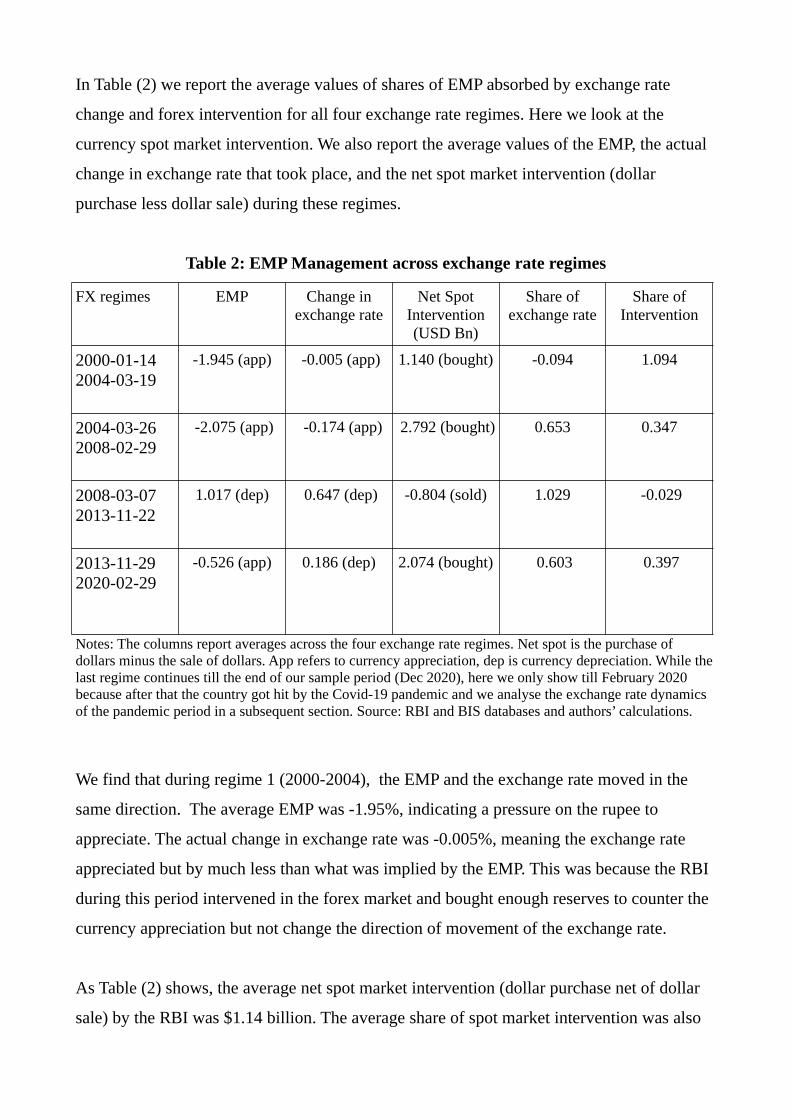
In Table (2) we report the average values of shares of EMP absorbed by exchange rate

change and forex intervention for all four exchange rate regimes. Here we look at the

currency spot market intervention. We also report the average values of the EMP, the actual

change in exchange rate that took place, and the net spot market intervention (dollar

purchase less dollar sale) during these regimes.

Table 2: EMP Management across exchange rate regimes

FX regimes EMP Change inexchange rate

Net SpotIntervention(USD Bn)

Share ofexchange rate

Share ofIntervention

2000-01-14 2004-03-19

-1.945 (app) -0.005 (app) 1.140 (bought) -0.094 1.094

2004-03-26 2008-02-29

-2.075 (app) -0.174 (app) 2.792 (bought) 0.653 0.347

2008-03-07 2013-11-22

1.017 (dep) 0.647 (dep) -0.804 (sold) 1.029 -0.029

2013-11-29 2020-02-29

-0.526 (app) 0.186 (dep) 2.074 (bought) 0.603 0.397

Notes: The columns report averages across the four exchange rate regimes. Net spot is the purchase of dollars minus the sale of dollars. App refers to currency appreciation, dep is currency depreciation. While thelast regime continues till the end of our sample period (Dec 2020), here we only show till February 2020 because after that the country got hit by the Covid-19 pandemic and we analyse the exchange rate dynamics of the pandemic period in a subsequent section. Source: RBI and BIS databases and authors’ calculations.

We find that during regime 1 (2000-2004), the EMP and the exchange rate moved in the

same direction. The average EMP was -1.95%, indicating a pressure on the rupee to

appreciate. The actual change in exchange rate was -0.005%, meaning the exchange rate

appreciated but by much less than what was implied by the EMP. This was because the RBI

during this period intervened in the forex market and bought enough reserves to counter the

currency appreciation but not change the direction of movement of the exchange rate.

As Table (2) shows, the average net spot market intervention (dollar purchase net of dollar

sale) by the RBI was $1.14 billion. The average share of spot market intervention was also

higher than the share of the exchange rate in EMP absorption; in fact it was the highest in

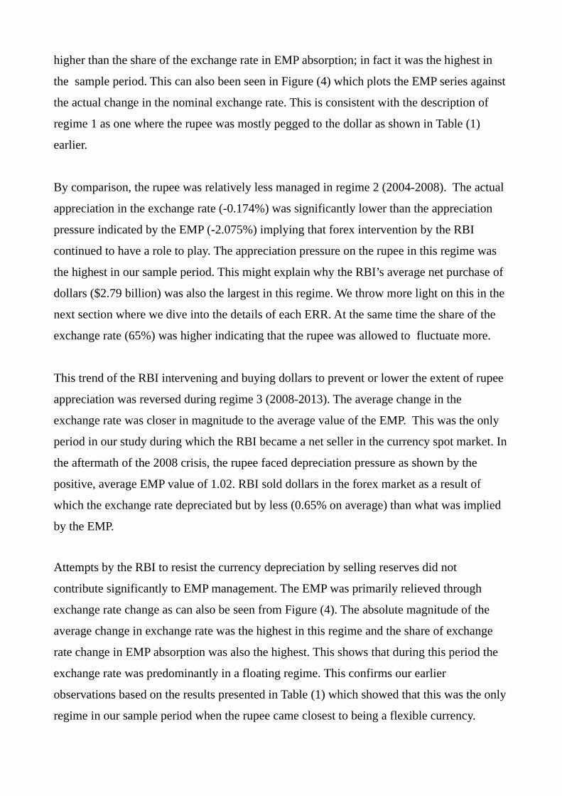
the sample period. This can also been seen in Figure (4) which plots the EMP series against

the actual change in the nominal exchange rate. This is consistent with the description of

regime 1 as one where the rupee was mostly pegged to the dollar as shown in Table (1)

earlier.

By comparison, the rupee was relatively less managed in regime 2 (2004-2008). The actual

appreciation in the exchange rate (-0.174%) was significantly lower than the appreciation

pressure indicated by the EMP (-2.075%) implying that forex intervention by the RBI

continued to have a role to play. The appreciation pressure on the rupee in this regime was

the highest in our sample period. This might explain why the RBI’s average net purchase of

dollars ($2.79 billion) was also the largest in this regime. We throw more light on this in the

next section where we dive into the details of each ERR. At the same time the share of the

exchange rate (65%) was higher indicating that the rupee was allowed to fluctuate more.

This trend of the RBI intervening and buying dollars to prevent or lower the extent of rupee

appreciation was reversed during regime 3 (2008-2013). The average change in the

exchange rate was closer in magnitude to the average value of the EMP. This was the only

period in our study during which the RBI became a net seller in the currency spot market. In

the aftermath of the 2008 crisis, the rupee faced depreciation pressure as shown by the

positive, average EMP value of 1.02. RBI sold dollars in the forex market as a result of

which the exchange rate depreciated but by less (0.65% on average) than what was implied

by the EMP.

Attempts by the RBI to resist the currency depreciation by selling reserves did not

contribute significantly to EMP management. The EMP was primarily relieved through

exchange rate change as can also be seen from Figure (4). The absolute magnitude of the

average change in exchange rate was the highest in this regime and the share of exchange

rate change in EMP absorption was also the highest. This shows that during this period the

exchange rate was predominantly in a floating regime. This confirms our earlier

observations based on the results presented in Table (1) which showed that this was the only

regime in our sample period when the rupee came closest to being a flexible currency.

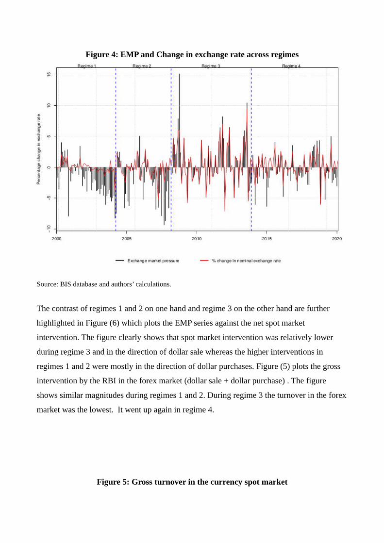
Figure 4: EMP and Change in exchange rate across regimes

Source: BIS database and authors’ calculations.

The contrast of regimes 1 and 2 on one hand and regime 3 on the other hand are further

highlighted in Figure (6) which plots the EMP series against the net spot market

intervention. The figure clearly shows that spot market intervention was relatively lower

during regime 3 and in the direction of dollar sale whereas the higher interventions in

regimes 1 and 2 were mostly in the direction of dollar purchases. Figure (5) plots the gross

intervention by the RBI in the forex market (dollar sale + dollar purchase) . The figure

shows similar magnitudes during regimes 1 and 2. During regime 3 the turnover in the forex

market was the lowest. It went up again in regime 4.

Figure 5: Gross turnover in the currency spot market

Note: This is a graph of the total dollar sale and purchase by the RBI expressed as a share of M0. The

average values are reported at the top of each regime. Data is obtained from RBI database.

During the last and most recent regime (2013-2020), the average EMP was -0.53% and the

actual change in exchange rate was 0.19%. This means that on average there was a pressure

on the exchange rate to appreciate but the exchange rate depreciated. The only way this

could have happened was if the RBI did ‘excessive intervention’ in the forex market to buy

dollars. If the RBI bought enough dollars to counter the currency appreciation or simply to

reduce the currency volatility then the exchange rate on average would still have appreciated

but the magnitude of appreciation would have been less than what was reflected in the EMP,

as was the case in regimes 1 and 2.

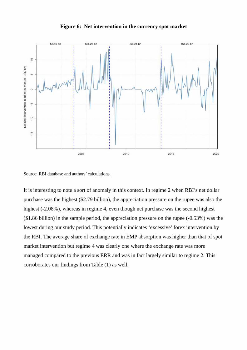
Figure 6: Net intervention in the currency spot market

Source: RBI database and authors’ calculations.

It is interesting to note a sort of anomaly in this context. In regime 2 when RBI’s net dollar

purchase was the highest ($2.79 billion), the appreciation pressure on the rupee was also the

highest (-2.08%), whereas in regime 4, even though net purchase was the second highest

($1.86 billion) in the sample period, the appreciation pressure on the rupee (-0.53%) was the

lowest during our study period. This potentially indicates ‘excessive’ forex intervention by

the RBI. The average share of exchange rate in EMP absorption was higher than that of spot

market intervention but regime 4 was clearly one where the exchange rate was more

managed compared to the previous ERR and was in fact largely similar to regime 2. This

corroborates our findings from Table (1) as well.

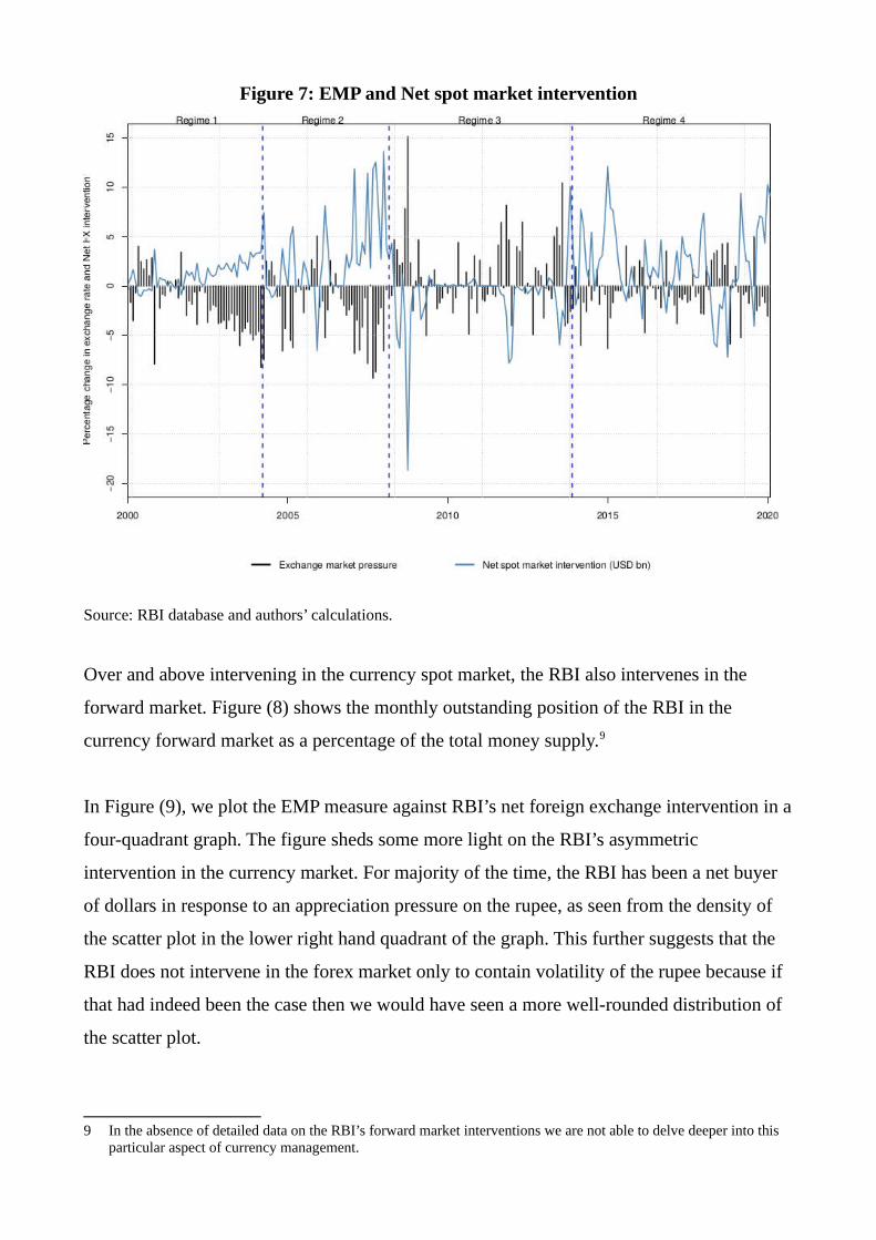
Figure 7: EMP and Net spot market intervention

Source: RBI database and authors’ calculations.

Over and above intervening in the currency spot market, the RBI also intervenes in the

forward market. Figure (8) shows the monthly outstanding position of the RBI in the

currency forward market as a percentage of the total money supply.9

In Figure (9), we plot the EMP measure against RBI’s net foreign exchange intervention in a

four-quadrant graph. The figure sheds some more light on the RBI’s asymmetric

intervention in the currency market. For majority of the time, the RBI has been a net buyer

of dollars in response to an appreciation pressure on the rupee, as seen from the density of

the scatter plot in the lower right hand quadrant of the graph. This further suggests that the

RBI does not intervene in the forex market only to contain volatility of the rupee because if

that had indeed been the case then we would have seen a more well-rounded distribution of

the scatter plot.

9 In the absence of detailed data on the RBI’s forward market interventions we are not able to delve deeper into this particular aspect of currency management.

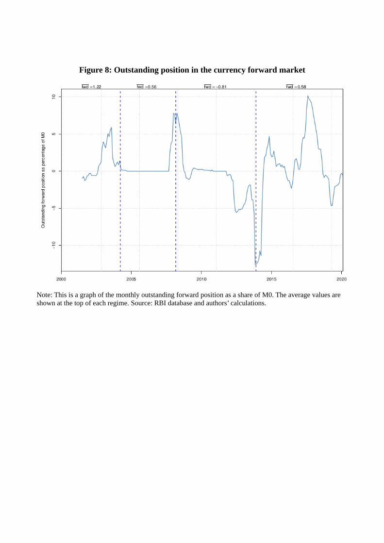
Figure 8: Outstanding position in the currency forward market

Note: This is a graph of the monthly outstanding forward position as a share of M0. The average values are shown at the top of each regime. Source: RBI database and authors’ calculations.

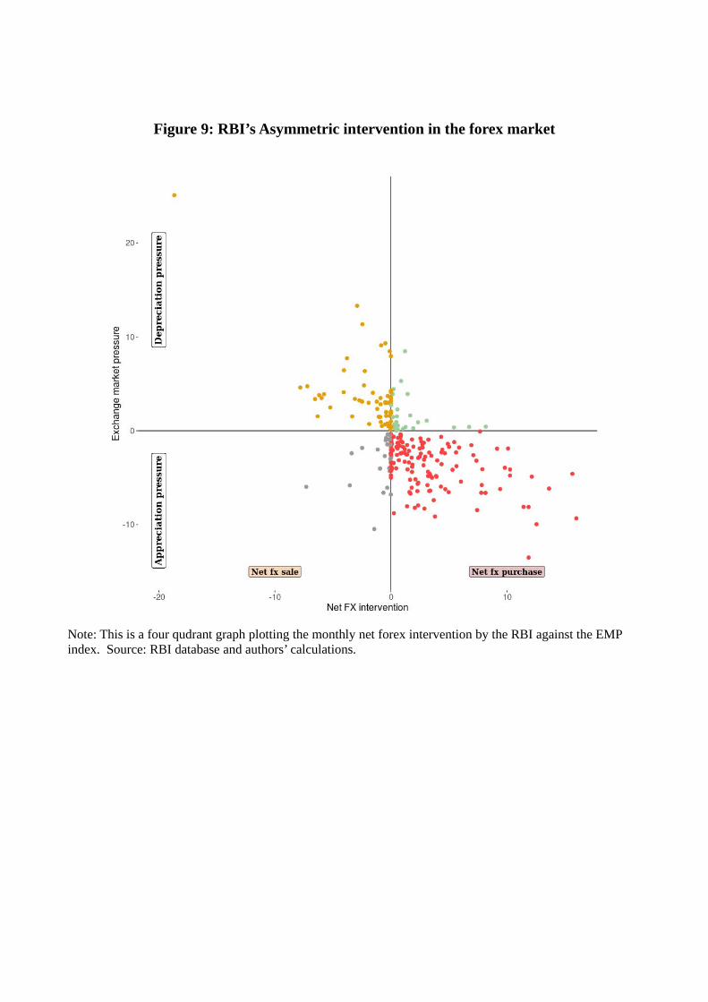
Figure 9: RBI’s Asymmetric intervention in the forex market

Note: This is a four qudrant graph plotting the monthly net forex intervention by the RBI against the EMP index. Source: RBI database and authors’ calculations.

4. Understanding the regime transitions

In this section we delve deeper into the transitions from one ERR to the another to throw

some light on the underlying macroeconomic conditions. While it is difficult to exactly

pinpoint the factors that cause regime changes, we provide a descriptive analysis of the

events leading up to a regime transition. The idea here is that the manner in which EMP was

managed in one regime vs. the other, might have been a function of the underlying

macroeconomic conditions or shocks faced by the economy during the transition periods.

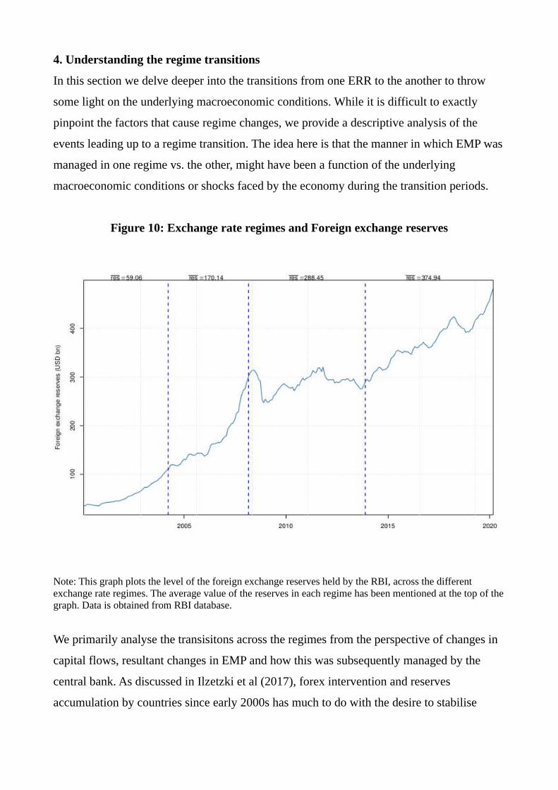
Figure 10: Exchange rate regimes and Foreign exchange reserves

Note: This graph plots the level of the foreign exchange reserves held by the RBI, across the different exchange rate regimes. The average value of the reserves in each regime has been mentioned at the top of thegraph. Data is obtained from RBI database.

We primarily analyse the transisitons across the regimes from the perspective of changes in

capital flows, resultant changes in EMP and how this was subsequently managed by the

central bank. As discussed in Ilzetzki et al (2017), forex intervention and reserves

accumulation by countries since early 2000s has much to do with the desire to stabilise

exchange rates in an environment of increased capital market integration.10 Figure (10)

shows the evolution during our sample period of the forex reserves holding of the RBI

across the four ERR.

4.1. Transition to regime 2 (March 2004)

The transition from regime 1 to regime 2 was shaped by the depletion of government bonds

on the RBI’s balance sheet towards the beginning of 2004, thereby hampering the process of

sterilisation of the RBI’s net dollar purchases in the forex market.

During the first exchange rate regime (Jan 2000 to March 2004), the Indian economy

received a total capital inflow of roughly $220 billion and witnessed an outflow of $175

billion. The net capital inflows led to appreciation pressure as reported in Table (2). This in

turn caused the RBI to intervene in the forex market and conduct an aggregate net purchase

of dollars of $58.2 billion. Reserves went up sharply from $34 billion in 2000 to $110

billion by early 2004 registering an average annual growth rate of around 33%, the highest

in our sample period. Most of this forex intervention by the central bank was sterilised as a

result of which inflation could be kept insulated from the consequences of RBI’s reserve

accumulation.

The purchase of dollars and full sterilisation by the RBI had led the market participants to

believe that once the stock of government bonds on the RBI’s balance sheet was exhausted,

RBI would stop buying dollars as it would not want to do unsterilised intervention lest it

fuels inflationary pressures. As a consequence, when that happened i.e. when the RBI

indeed ran out of government bonds, the rupee would appreciate. This further pushed up the

level of capital flows into India as foreign investors believed that the rupee was a one way

bet.

10 While we describe what the various regimes in India were during our period of study, we do not go into the potentialrationale behind the central bank’s actions, for example we are not trying to explain why the RBI let the rupee depreciate in 2008-2013 or why the RBI attempted to prevent an appreciation in the 2013-2020 period. This maybe taken up in future research.

As a result, the pressure on the currency to appreciate continued unabated and the RBI did

not stop buying dollars either. In 2004, a new arrangement for sterilisation of forex

intervention was put in place. Under this system, the RBI could continue to peg to the USD,

buy dollars and sell Market Stabilisation Scheme (MSS) bonds whose sole purpose was

sterilisation. This allowed the RBI to continue its purchase of dollars without worrying

about how to sterilise them.

4.2. Transition to regime 3 (March 2008)

In March 2008, Bear Sterns in the US had a liquidity crisis. These were the first signs of

trouble in the US financial system that eventually led up to the Global Financial Crisis

culminating in the collape of Lehman Brothers in September 2008. For emerging economies

like India this was the beginning of pressure on the currency to depreciate. Net capital

inflows fell sharply by 93%, from $106 billion in 2007-08 to a mere $7 billion in 2008-09.

The average EMP went from an appreciation pressure of -5.8% in 2007 to a depreciation

pressure of roughly 2.6% in 2008 in response to the massive capital outflows. The ERR

turned from one of a pegged rupee that was not being allowed to appreciate to one that was

much more volatile with RBI permitting it to depreciate.

4.3. Transition to regime 4 (November, 2013)

The exchange rate transitioned to the fourth and last regime in November 2013. The events

leading up to this date may help throw some light on the transition. In May 2013 the

erstwhile Federal Reserve Chair Ben Bernanke announced that the US Fed would soon

commence tightening of monetary policy and would taper the quantitative easing program

that had been initiated in the aftermath of the 2008 crisis. This episode was widely known as

the ‘taper tantrum’. In response to this announcement the US 10 year yield went up

drastically which in turn triggered massive capital outflows from emerging market

economies including India. India’s net capital inflows nearly halved from $89.3 billion in

2012-13 to $48.8 billion in 2013-14. This was the second biggest decline in net inflows in

our sample period, the largest being during the 2008 Global Financial Crisis. This resulted

in a sharp currency depreciation.

In April 2013, the EMP value for India was -2.58% indicating pressure on the currency to

apppreciate. This increased to 8.46% in May 2013, implying a strong pressure on the rupee

to depreciate. The average EMP for the period Jan-April 2013 was -0.55% while the average

EMP for the next four month period from May to August 2013 increased to 7.41%. In fact,

if we ignore the turbulent period of the 2008 Global Financial Crisis, August 2013 witnessed

the highest depreciation pressure on the rupee in our sample. Figure 1 shows the sharp

increase in currency volatility during this period. Volatility went up from 6.8% in May 2013

to 28.2% by September 2013, once again the highest in our sample period. This goes on to

show the kind of pressure and volatility experienced by the rupee-dollar exchange rate

towards the end of regime 3.

The RBI and the government responded to the sharp and rising depreciation pressure on the

Rupee, in the immediate aftermath of the tapering announcement, in multiple ways. These

involved restrictions on the currency derivatives markets, a series of steps by the RBI to

squeeze liquidity in the banking system and raise short-term interest rates, tariff hikes,

restrictions on gold and silver imports, tightening of capital controls to discourage capital

outflows by firms and households, increasing investment limits for foreign institutitonal

investors, liberalising external commercial borrowing by Indian firms and so on.

The 91-day Treasury Bill rate which is a reasonable proxy for the overall monetary policy

stance went up from roughly 7.5% in May 2013 to 12% in October 2013, a dramatic

increase of 440 basis points. At the same time however the RBI did not actively intervene in

the forex market to defend the rupee. Between May and October 2013, it sold a net amount

of only $10 billion in the spot market. In other words, the Rupee defense was carried out

mostly through monetary policy and capital controls.

It seems that after a prolonged period of minimal intervention to stabilise the currency

(2008-2013), the measures undertaken in the wake of the taper tantrum episode to reduce

liquidity in the system and defend the exchange rate may have triggered a change in the

ERR. As shown in Figure 1 earlier, from 2013 December onwards, the average volatility of

the currency came down from 8.6% to 5% indicating a more managed exchange rate.

5. Pandemic and beyond

During the period of the Covid-19 pandemic (March 2020 to March 2021), specifically in

the April-June and July-September quarters of 2020, India witnessed a current account

surplus after 17 years of deficit. Exports from India are expected to rise going forward as the

US economy and world trade recover from the shock imposed by the pandemic. In addition,

India remained an attractive investment destination with both foreign direct investment

(FDI) and foreign portfolio investment (FPI) flows coming into India.

Between March 2020 and February 2021, the average EMP was -1.95% implying that the

rupee faced an appreciation pressure, whereas on average the rupee appreciated only by

0.2%.11 RBI did an aggregate net purchase of $70 billion during this period, presumably to

reduce the extent of rupee appreciation. Foreign exchange reserves went up from roughly

$475 billion in March 2020 to close to $580 billion by March 2021. Our estimation of ERR

shows that the pandemic period was a part of regime 4 which started in November 2013. In

other words, the trend of the RBI intervening in the forex market to buy dollars and to

manage the EMP by reducing currency appreciation continued during the pandemic.

With the opening up of the trade and the capital accounts, the currency market has grown

very large.12 Old solutions, like buying a few billion dollars to prevent appreciation, or

selling a few billions from the central bank’s reserves to prevent a currency depreciation

may no longer work. Moreover the Indian economy is struggling to recover from the

adverse impact of the Covid-19 pandemic which has dealt a severe blow to economic

growth. If in the event of an external shock (such as the US Fed announcing a tightening of

11 The EMP index constructed in Patnaik et al (2017) extends from January 2000 to April 2021. 12The gross turnover in the currency spot market in January 2000 was roughly $2.34 billion (total dollar sale and purchase by the RBI). This had gone up to $47.92 billion by February 2021. This only captures trading by the central bank.

monetary policy, similar to the 2013 taper tantrum episode) and the consequent rupee

depreciation against the dollar, the RBI attempts to defend the currency either by tightening

liquidity in the domestic financial system or raising interest rates to discourage capital

outflows, this may hamper the growth recovery process. The RBI would need to weigh the

pros and cons of a currency defense strategy especially from a medium term perspective,

before embarking on a drive to prevent the rupee from depreciating.

6. Conclusion

The research on de-facto exchange rate regimes is an evolving field. In this paper we have

tried to understand India’s exchange rate regime using the techniques developed in the field

in recent years. The de-facto exchange rate regime literature is limited in that while it uses

observed data on exchange rates, it is unable to integrate this behaviour with the policy

intentions of the central bank. We therefore use the techniques developed in the Exchange

Market Pressure literature to understand how the pressure on the exchange rate is absorbed,

through forex interventions, or relieved through the movements of the exchange rate. This

brings into the analysis the exchange rate policy of the central bank.

We find 4 periods in India’s de-facto ERR. Among these, we find that there was one regime

(2008-2013) inwhich the rupee faced a pressure to depreciate and it was a period of

relatively high volatility of the rupee. The other 3 periods saw pressure on the rupee to

appreciate and relatively low volatility of the rupee. In these periods RBI accumulated

reserves. We also provide some evidence that the RBI has been intervening in the forex

market in an asymmetric fashion to prevent the rupee from appreciating.

In this paper we have not been able to measure the role of monetary policy (Goldberg and

Krogstrup, 2018) or of capital controls (Akram and Byrne, 2015). The techniques for

measuring these in absorbing exchange market pressure are still evolving. This is thus an

agenda for future research.

References

Akram, Gilal Muhammad & Byrne, Joseph P. (2015), “Foreign exchange market pressure and capital controls”, Journal of International Financial Markets, Institutions and Money, Elsevier, vol. 37(C), pages 42-53.

Bénassy-Quéré A, Coeuré B, Mignon V (2006), “On the Identification of De Facto CurrencyPegs”, Journal of the Japanese and International Economies, 20(1), 112–127.

Baig, T. (2001), “Characterizing Exchange Rate Regimes in Post-crisis East Asia”, IMF Working Paper 01/125.

Bai J, Perron P (2003), “Computation and Analysis of Multiple Structural Change Models.”Journal of Applied Econometrics, 18, 1–22.

Bowman, C. (2005), “Yen Bloc or Koala Bloc? Currency relationships after the East Asian crisis”, Japan and the World Economy, 17 (1), pp. 83-96

Bubula A, Ötker-Robe I (2002), “The Evolution of Exchange Rate Regimes Since 1990:Evidence from De Facto Policies”, Working Paper 02/155, International Monetary Fund.

Calvo, G A and C M Reinhart (2002), “Fear of Floating”, Quarterly Journal of Economics, Vol 117, No 2, pp 379-408.

Eichengreen, B., Rose, A., Wyplosz, C. (1996), “Contagious Currency Crises”, Technical Report. National Bureau of Economic Research.

Frankel JA, Wei SJ (2007), “Assessing China’s Exchange Rate Regime”, Economic Policy,22(51), 575–627.

Frankel J, Wei SJ (1994), “Yen Bloc or Dollar Bloc? Exchange Rate Policies of the EastAsian Countries”, In T Ito, A Krueger (eds.), Macroeconomic Linkage: Savings, ExchangeRates and Capital Flows. University of Chicago Press.

Goldberg, L S and Signe Krogstrup (2018), “International Capital Flow Pressures”, NBER Working Papers 24286, National Bureau of Economic Research, Inc.

Ilzetzki, Ethan, Carmen M. Reinhart and Kenneth S. Rogoff (2017), “Exchange Arrangements Entering the 21st Century: Which Anchor Will Hold?”, NBER Working Papers 23134, National Bureau of Economic Research, Inc.

Kaminsky, G., Lizondo, S., Reinhart, C. (1998), “Leading indicators of currency crises”, Staff Papers-Int. Monet. Fund, 1–48.

Klaassen, F. (2011), “Identifying the Weights in Exchange Market Pressure”, Tinbergen Institute Discussion Papers 11-030/2. Tinbergen Institute.

Kawai, Masahiro & Pontines, Victor (2016), “Is there really a renminbi bloc in Asia?: A modified Frankel–Wei approach”, Journal of International Money and Finance, Elsevier, vol. 62(C), pages 72-97.

Kawai, M., Akiyama, S. (2000), ‘Implications of the currency crisis for exchange rate arrangements in emerging East Asia”, Policy Research Working Paper Series 2502. World Bank, Washington, May.

Klaassen, F., Jager, H. (20110, “Definition-consistent measurement of exchange market pressure” Journal of International Money and Finance, 30, 74–95.

Levy-Yeyati E, Sturzenegger F (2003), “To Float or to Fix: Evidence on the Impact ofExchange Rate Regimes on Growth”, American Economic Review, 93(4), 1173–1193.

Liu J, Wu S, Zidek JV (1997),“On Segmented Multivariate Regression”, Statistica Sinica, 7,497–525.

McKinnon, R.I. (2001), “After the crisis, the East Asian dollar standard resurrected: an interpretation of high-frequency exchange rate pegging”, HKIMR Working Paper No.04/2001.

Ogawa, Eiji (2002), “Should East Asian countries return to a dollar peg again?” In P. Drysdale, K. Ishigaki (Eds.), East Asian Trade and Financial Integration: New Issues, Asia Pacific Press (2002), pp. 159-184

Ogawa, Eiji (2004), “Regional monetary cooperation in East Asia against asymmetric responses to the US dollar depreciation”, Journal of the Korean Economy, 5 (2) (2004), pp. 43-72

Ogawa, Eiji & Kudo, Takeshi (2007), “Asymmetric responses of East Asian currencies to the US dollar depreciation for reducing the US current account deficits”, Journal of Asian Economics, Elsevier, vol. 18(1), pages 175-194, February.

Ogawa, Eiji & Yang, Doo Yong (2008), ‘The dilemma of exchange rate arrangements in East Asia”, Japan and the World Economy, Elsevier, vol. 20(2), pages 217-235, March.

Pandey, Radhika, Rajeswari Sengupta, Aatmin Shah and Bhargavi Zaveri (2019), “Evolution of capital controls on foreign institutional investment in India”, Indira Gandhi Institute of Development Research, Mumbai Working Papers 2019-034, IGIDR.

Patnaik, I. (2005), “India’s experience with a pegged exchange rate”, In: Bery, S., Bosworth,B., Panagariya, A. (Eds.), The India Policy Forum 2004. Brookings Institution Press and NCAER, pp. 189–226.

Patnaik, I. (2007), “India’s currency regime and its consequences”, Economic and Political Weekly.

Patnaik, Ila and Ajay Shah (2009), “The difficulties of the Chinese and Indian exchange rateregimes”, European Journal of Comparative Economics, page 157--173, 6(1), June 2009.

Patnaik, Ila, Felman, Joshua and Shah, Ajay (2017), “An exchange market pressure measure for cross country analysis,” Journal of International Money and Finance, Elsevier, vol. 73(PA), pages 62-77.

Pentecost, E., Van Hooydonk, C., Van Poeck, A. (2001), “Measuring and estimating exchange market pressure in the EU”, Journal of International Money and Finance, 20, 401–418.

Pontines, V., Siregar, R. (2008), “Fundamental pitfalls of exchange market pressure-based approaches to identification of currency crises”, International Review of Economics and Finance, 17, 345–365.

Reinhart CM, Rogoff KS (2004). “The Modern History of Exchange Rate Arrangements: AReinterpretation”, The Quarterly Journal of Economics, 117, 1–48.

Sachs, J., Tornell, A., Velasco, A. (1996), “Financial Crises in Emerging Markets: The Lessons From 1995”, Technical Report. National Bureau of Economic Research.

Sen Gupta, Abhijit, and Rajeswari Sengupta (2013), “Management of Capital Flows in India”, South AsiaWorking Paper Series, Asian Development Bank, No. 17, March 2013.

Shah A, Zeileis A, Patnaik I (2005).,“What is the New Chinese Currency Regime?” Report 23, Department of Statistics and Mathematics, WU Wirtschaftsuniversität Wien, ResearchReport Series.

Shirono, Kazuko (2008), “Real effects of common currencies in East Asia”, Journal of Asian Economics, Elsevier, vol. 19(3), pages 199-212, June.

Zeileis, Z., Shah, A., Patnaik, I. (2010), “Testing, Monitoring, and Dating Structural Changes in Exchange Rate Regimes”, Computational Statistics & Data Analysis, 54(6), 1696–1706.

33