“Analysing Climatological Time Series of Temperature and Rainfall for Southern Districts of West Bengal over the period 1901-2011” Thesis submitted for the Degree of Doctor of Philosophy in Science (Geography) by DIPAK BISAI DEPARTMENT OF GEOGRAPHY AND ENVIRONMENT MANAGEMENT VIDYASAGAR UNIVERSITY MIDNAPORE, WEST BENGAL MARCH, 2016

Welcome message from author
This document is posted to help you gain knowledge. Please leave a comment to let me know what you think about it! Share it to your friends and learn new things together.
Transcript

“Analysing Climatological Time Series of Temperature and Rainfall for Southern Districts of West Bengal over
the period 1901-2011”
Thesis submitted for the Degree of Doctor of Philosophy
in Science (Geography)
by
DIPAK BISAI
DEPARTMENT OF GEOGRAPHY AND ENVIRONMENT MANAGEMENT
VIDYASAGAR UNIVERSITY MIDNAPORE, WEST BENGAL
MARCH, 2016


DECLARATION
This is declare that the thesis entitled “Analyzing Climatological
Time Series of Temperature and Rainfall for Southern Districts of West
Bengal over the period 1901-2011”, submitted for the degree of Ph.D. in
Geography of Vidyasager University is a record of my original work
done under the supervision of Dr. Soumendu Chatterjee, Department
of Geography, Presidency University. This is also to be stated that no
part of the thesis submitted herewith has been submitted previously
anywhere for any degree whatsoever either by me or anyone else.
(Dipak Bisai)

DEDICATION
I dedicate my Ph. D. work to my parents and my family. An
especial tribute to my loving wife Silpi Saha (Bisai) and my sweet kid
Writabrata Bisai whose inspiration all through the way has led my feet
towards success.
I also dedicate this work to my guide Dr. Soumendu Chatterjee
for his endless scientific supervision to meet my effort to a successful
end.

Acknowledgement
I would like to express the deepest appreciation to the Department of Geography and Environment Management of Vidyasagar University, Midnapore to give me a chance to do the Ph.D work.
I wish to offer my sincere gratitude to my respected guide and advisor Dr. Soumendu Chatterjee, H.O.D. Department of Geography, Presidency University, Kolkata for the continuous support of my Ph. D study and related research, for his patience, motivation and immense knowledge.
I would like to offer special thanks to the Director and office staff of the India Meteorological Department (IMD) for their support regarding Meteorological data.
I thank my fellow mates for the worthy discussion and contribution in this regard and also thanks to my colleagues for their mental support.
Last but not at the least; I would like to thank my family, my parents and my close friends for supporting me spiritually throughout last four years to complete this work.
Dipak Bisai

List of Table
Chapter-I
1. Observed pressure distribution over West Bengal in Monsoon Season
2. Principal special weather phenomenon.
Chapter-II
3. Considered observatories, coordinates, period of time series and nearest
distance of the station network.
4. Abbreviations of considered series.
5. Result of correlation for Mean Monthly Maximum Temperature (푇푀푎푥)
Series.
6. Result of correlation for Mean Monthly Minimum Temperature (푇푀푖푛)
Series
7. Result of correlation for Mean Monthly Rainfall Series.
8. Test statistic of SNHT-I for Mean Monthly Maximum Temperature (푇푀푎푥)
Series.
9. Test statistic of SNHT-I for Mean Monthly Minimum Temperature (푇푀푖푛)
Series.
10 (a). Test statistic of SNHT-I for Annual and Seasonal Mean Maximum
(퐴푇푀푎푥&푆푇푀푎푥) Temperature Series.
10 (b). Test Statistic of SNHT-I for Annual and Seasonal Mean Minimum
(퐴푇푀푖푛&푆푇푀푖푛) Temperature Series.
11(a). Result of SNHT-I (Break Point) for Annual Mean Maximum and Seasonal
Mean Maximum (퐴푇푀푎푥&푆푇푀푎푥) Series.
11(b). Result of SNHT-I (Break Point) for Annual Mean Minimum and Seasonal
Mean Minimum (퐴푇푀푎푥&푆푇푀푎푥) Series
12. Estimation of the Amount of Change by SNHT-I (푇푀푎푥 Series)
13. Estimation of the Amount of Change by SNHT-I (푇푀푖푛 Series)

Chapter-III 14. The 1% and 5% critical values for the 푄/√푛 statistic of Cumulative
Deviation Test as a Function of 푛 (Buishand Range Test).
15. The 1% and 5% critical values for the 푅/√푛 statistic of the Buishand Range
Test (BRT) as a Function of 푛 (Buishand, 1982).
16. The 1% and 5% Critical values for the Pettitt Test Statistic (Pettitt, 1979)
17. The 1% and 5% Critical values for 푛 of the Von-Neumann Ratio Test.
18. Result of the Cumulative Deviation Test of Mean Monthly Maximum (푇푀푎푥)
Temperature Series.
19. Result of the Cumulative Deviation Test of Seasonal Maximum (푆푇푀푎푥)
Temperature Series.
20. Result of the Cumulative Deviation Test of Mean Minimum (푇푀푖푛)
Temperature Series.
21. Result of the Cumulative Deviation Test of Annual Mean Minimum (퐴푇푀푖푛)
Temperature Series for 13 Observatories.
22. Result of the Cumulative Deviation Test of Mean Monthly Rainfall Series.
23. Result of the Cumulative Deviation Test of Annual rainfall Series for 13
Observatories.
24. Results of Buishand Range Test (BRT) of Mean Monthly Maximum (푇푀푎푥)
Temperature Series for 13 observatories.
25. Results of Buishand Range Test (BRT) of Mean Annual Maximum (퐴푇푀푎푥)
Temperature Series for 13 observatories.
26. Results of Buishand Range Test (BRT) of Seasonal Maximum Temperature
(푆푇푀푎푥) Series for 13 observatories.
27. Results of Buishand Range Test (BRT) of Mean Monthly Minimum (푇푀푖푛)
Temperature Series for 13 Observatories.
28. Results of Buishand Range Test (BRT) of Mean Annual Minimum (퐴푇푀푖푛)
Temperature Series for 13 Observatories.
29. Results of Buishand Range Test (BRT) of Seasonal Minimum (푆푇푀푖푛)
Temperature Series for 13 observatories.
30. Results of Buishand Range Test (BRT) of Mean Annual Rainfall Series for 13
Observatories.
31. Result of Pettitt Test of Mean Monthly Maximum (푇푀푎푥) Temperature Series
for 13 Observatories.

32. Result of Pettitt Test of Mean Annual Maximum (퐴푇푀푎푥) Temperature
Series for 13 observatories.
33. Probability Distribution Result after Pettitt Test for Mean Annual Maximum
(퐴푇푀푎푥) Temperature Series for 13 observatories.
34. Single Abrupt Change for Mean Seasonal Maximum (푆푇푀푎푥) Temperature
Series after Pettitt Test.
35. Single Abrupt Change for Mean Monthly Minimum (푇푀푖푛) Temperature
Series after Pettitt Test.
36. Single Abrupt Change for Mean Annual Minimum (퐴푇푀푖푛) Temperature
Series after Pettitt Test.
37. Single Abrupt Change for Mean Seasonal Minimum (푆푇푀푖푛) Temperature
Series after Pettitt Test.
38. Result of Von-Neumann Ratio Test for Mean Monthly Maximum (푇푀푎푥)
Temperature Series.
39. Results of Von-Neumann Ratio Test for Mean Annual Maximum (퐴푇푀푎푥)
and Mean Seasonal Maximum (푆푇푀푎푥) Temperature Series.
40. Results of Von-Neumann ratio Test (V.N.R.) of Mean Monthly Minimum
(푇푀푖푛) Temperature Series.
41. Results of Von-Neumann Ratio Test (V.N.R.) of Mean Annual Minimum
(퐴푇푀푖푛) Temperature Series.
Chapter-IV 42. Significant Change with different Level by CUSUM and Bootstrapping for
퐴푇푀푎푥 Series.
43. Result of Significant Change with different Level by CUSUM and
Bootstrapping analysis for 퐴푇푀푖푛 Series.
44. Result of Significant Change with different Level by CUSUM and
Bootstrapping analysis for 푆푇푀푎푥 Series (Winter).

List of Figure
Chapter-I
1. Organigram of Research Steps.
2. Geographical location of the study area.
Chapter-II
3. Components of Climatological time series.
4. Graphical presentation of Mean Monthly Maximum (푇푀푎푥) Temperature for
January of selected observatories.
5. Graphical presentation of Mean Monthly Maximum (푇푀푎푥 ) Temperature
Series for June of selected
observatories.
6. Graphical presentation of Mean Annual Maximum (퐴푇푀푎푥) Temperature
Series for selected observatories.
7. Graphical presentation of Mean Annual Minimum (퐴푇푀푖푛) Temperature
Series for Selected observatories.
8. Graphical presentation of the Amount of Change of Mean level for 푇푀푎푥
Series.
9. Graphical presentation of the Amount of Change of Mean level for
푇푀푖푛Series.
Chapter-III
10. The plots of Residual Mass values of Mean Annual (퐴푇푀푎푥) Maximum
Temperature for 13 observatories.
11. Graphical presentation of the Annual Maximum Temperature (퐴푇푀푎푥) Series
after BRT (Buishand Range Test).
12. Graphical presentation of the Annual Minimum Temperature (퐴푇푀푖푛) Series
after BRT (Buishand Range Test).
13. Shift of mean level of Mean Annual Maximum (퐴푇푀푎푥) Temperature Series
of 13 observatories by Pettitt Test.

Chapter-IV 14. CUSUM Chart for 퐴푇푀푎푥 Series of 13 observatories. Shaded meeting point
is refers to significant potential change point in each figure.
15. CUSUM Chart for 퐴푇푀푖푛 Series of 13 observatories. Shaded meeting point is
refers to significant potential change point in each figure.
16. CUSUM Chart for 푊푖푛푡푒푟 (푆푇푀푎푥) Temperature Series of 13 observatories.
Shaded meeting point is refers to significant potential change point in each
figure.
17. CUSUM chart for 푆푢푚푚푒푟 Temperature Series of 13 observatories. Shaded
meeting point is refers to significant potential change point in each figure.
18. CUSUM Chart for 푀표푛푠표표푛 (푆푇푀푎푥) Temperature Series of 13
observatories. Shaded meeting point is refers to significant potential change
point in each figure.
19. CUSUM Chart for 푃표푠푡푀표푛푠표표푛 Temperature Series of 13 observatories.
Shaded meeting point is refers to significant potential change point in each
figure.
20. CUSUM Chart for 퐴푛푛푢푎푙푅푎푖푛푓푎푙푙 Series of 13 observatories. Shaded
meeting point is refers to significant potential change point in each figure.
21. CUSUM Chart for 푀표푛푠표표푛푅푎푖푛푓푎푙푙 Series of 13 observatories.
Shadedmeeting point is refers to significant potential change point in each
figure.
Chapter-V 22. Significant increasing Slope tendency (푏 − 푣푎푙푢푒) of some Monthly 푇푀푎푥
Series for different observatories.
23. Significant increasing Slope tendency (푏 − 푣푎푙푢푒) of Annual Rainfall Series
of 13 observatories.
24. Potential changes in Annual Average Maximum Temperature (퐴푇푀푎푥)
Series as derived from Sequential Version of Mann-Kendall test statistic,
푢(푡푖) forward sequential statistic drawn red in colour and 푢′(푡푖) retrograde
sequential statistic drawn black in colour.

25. Potential changes in Annual Average Minimum Temperature (퐴푇푀푖푛) Series
as derived from Sequential Version of Mann-Kendall test statistic, 푢(푡푖)
forward sequential statistic drawn red in colour and 푢′(푡푖) retrograde
sequential statistic drawn black in colour.
Chapter-VI
26. Autocorrelation plots (푇푀푎푥) for Annual Average Maximum Temperature
Time Series.
27. Autocorrelation plots (푇푀푎푥) for Mean Annual Minimum Temperature Time
Series.

CONTENTS
Chapter-I (Introduction and Aspects of the Study) Page No 1.0 Introduction 1-2 1.1 Principal Objectives of this Thesis 3-4
1.2 General Aspect and Global Scale Background with Literature Review 5-13
1.3 Characteristics of Monsoon Type of Climate 14-20
1.3.1 Special Weather Phenomenon in West Bengal 20-23 1.4 Importance of Regional Analysis 23-24
1.5 Geographical Situation of the Study Area 25-27
1.6 References 28-36
Chapter-II (Quality Check and Quality Assurance) 2.0 Data Potential 37 2.1 General Description of the Data Network 37-38
2.2 Quality Check and Homogeneity of the Dataset 39-42
2.3 Statistical Treatment for Homogeneity and Change Point Detection 42-43
2.4 Result and Discussion. 44-66
2.5 References 67
Chapter-III (Variability Analysis) 3.0 Variability Analysis and Residual Mass Curve Fitting 68-70
3.1 Rank-Wise Sensitive Shift Detection and Adjusted
Partial Sums Estimation 70-71
3.2 Occurrence of Single Abrupt Change Detection 71-72
3.3 Detection of Randomness of Time Series 72-73
3.4 Result and Discussion 74-108
3.5 References 109

Chapter-IV (Monotonic and potential Change Point Detection) Page No 4.0 Potential Change Point Detection (CUSUM) and Bootstrapping 110-112
4.1 Result and Discussion 113-169
4.2 Series Classification and its Qualitative Interpretation 170-171
4.3 Conclusion 171
4.4 References 172
Chapter-V (Homogeneity Construction and Trend Detection) 5.0 Homogeneity Construction by MASH Application 173-176
5.1 Slope Analysis 176-177
5.2 Trend Detection by Mann-Kendall Test 177-179
5.3 Climatic Change Point Detection by Sequential Mann-Kendall Test 179-180
5.4 Magnitude of Change Estimation (Sen’s Slope Estimation) 180-181
5.5 Result and Discussion 182-215
5.6 References 216
Chapter-VI (Time Series Pattern and Major Findings and Conclusion) 6.0 Time Series Pattern Estimation 217-224
6.1 Major Findings and Conclusion 225-226
6.2 References 227
Appendix
Appendix-I 228-241
Appendix-II 242-263
Appendix-III 264-265
Appendix-IV 266-269
List of Publications. 270-271

Summary:
Climatology is an integrative interdisciplinary science that deals with
the relationship among Climatological parameters through temporal and
spatial scale. This science is very complex because several variables within the
Earth’s atmosphere, such as temperature, rainfall, barometric pressure,
humidity, wind velocity, clouds etc. are interacting with each other and
maintains a nonlinear structure for a particular geographical area. The
activeness and performance of these parameters has made often randomly
ordered outlier due to uneven correlation of climatic parameters through
frequency domain as well as time domain. Spatial inference of the climatic
parameters is also an influencing character for climatological analysis. This
study deals with the regional analysis of Climatological parameters like
ambient atmospheric temperature and rainfall series. The authenticated and
approved datasets are collected from India Meteorological Department (IMD,
Alipur, Kolkata) and Indian Water Portal Department
(www.indiawaterportal.org). The attribute of the implanted data series
combines Mean Monthly Maximum (푇푀푖푛 ) Temperature, Mean Monthly
Minimum (푇푀푖푛) Temperature and Average Monthly Rainfall series. Annual
average and seasonal series is also considered for this analysis and these series
has been confirmed from monthly average series. The considered temperature
data being the SI unit of ℃ and rainfall data unit is millimeter respectively.
Remarkably, the considered time series maintained consistency while used in
this study and the nearest distance covers 5 km and the far distance of the data
network has been covered 101 km from the farthest station. The temporal span
has confirmed 111 years (1901-2011) and there is no such temporal gap over
the considered time series.
The main objectives of this study are:
1. Quality Check and Change Point detection over the time series.
2. Variability analysis over the time series.
3. Potential Change Point detection over the time series.
4. Homogeneity construction of the time series.
5. Monotonic Trend detection.
6. Magnitude of Change and Pattern establishment.

The study area has been confirmed by 13 weather observatories location
spread over the southern part of West Bengal. Primarily, the data quality
control has been checked for proper analysis of the climatic system. Quality
assurance or quality control is a system of routine technical activity, to
measure and control the quality of the inventory while it is being developed.
So, the quality control system has been designed with a particular process
consisting continuous check to ensure the data integrity, correctness and
sequential completeness. Data quality depends primarily on the location of a
climatological station for data acquisition and its adjoining surroundings.
Often encountered inconveniences in terms of data homogeneity due to
changes in the immediate surroundings over temporal spell as well as changes
of the observatory location and exchanges of the data observational
techniques. Moreover, new techniques about the proper observation time,
changes or replacements of the high performance instruments, different active
observing practices, and formulae is used to calculate the mean of the series
which can cause artificial discontinuities from the prior time. In primary step
the data has been processed by correlation method. After that, some statistical
method has been adopted for the assessment of homogeneity nature of the
considered dataset. Both parametric and non-parametric statistical techniques
has been selected for this analysis like Cumulative Deviation (CD), Standard
Normal Homogeneity Test-I (SNHT-I), Pettitt Test, Buishand Range Test
(BRT), Von-Neuman Ratio Test and CUSUM and Bootstrapping. To complete
these inspections, different software has been used to find out the
inhomogeneity, abruptness, variability, randomness, outlier etc. over the
considered time series of 푇푀푎푥, 푇푀푖푛, 퐴푇푀푎푥, 퐴푇푀푖푛, 푆푇푀푎푥 , 푆푇푀푖푛,
monthly rainfall, annual rainfall and seasonal rainfall separately. The used
software’s are XLSTAT, Change Point Analyzer, AnClim , Regime Shift
Detection, TREND, MAKESENS_1_0 and SPSS_20.1. Moreover the
anthropogenic variability like data acquisition error, error made by the
observer and data transmission error has been detected by these strong
statistical methods. In accordance to these methods, the considered time series
has always assumed as normal distribution and primarily a Null Hypothesis
(퐻 ) has considered.

After that the Alternative Hypothesis (퐻 ) has been argued at 훼 = 0.05
level of significance. If the value statistic has defend at chosen level of
significance and if it is situated ≥ critical level as a function of, then the Null
Hypothesis has rejected and Alternative Hypothesis has accepted. Always 푛 is
considered as the number of observations. Adjusted Partial Sums (APS) and
Re-Scaled Adjusted Partial Sums (RAPS) have detected the variability and
break point in the middle of the considered period. Single abruptness over the
considered time series has been detected by Pettitt test. The ratio of mean
square successive difference (year to year) has identified the randomness over
the considered time series. One interesting statistical technique has implanted
here like CUSUM and Bootstrapping. This method confirms the level of
change at a particular point and bootstrapping has been confirmed by its
associated interval limit over the considered period. Ultimately,
inhomogeneity characters of the considered time series has established and
their effect (Number of Null Hypothesis rejection) has been categorized by
"푈푠푒푓푢푙" , "퐷표푢푏푡푓푢푙푙" and "푆푢푠푝푒푐푡푒푑" group.
Homogenization of climatic parameters like temperature and rainfall series
is a challenge to climate change researches, especially in cases where metadata
are not always available. So, the reference series building was a difficult
challenge in this concern. The quality check assessment has indicated that,
there is no one considered series which has been considered as homogeneous.
The result of the quality check has revealed uncertain frequency, outlier,
abnormality, variability as well as significant change point over the considered
period. Ultimately, Multiple Analysis of Series for Homogenization
(푀퐴푆퐻 푣 2.03) has been used to conduct the homogenization process for
considered time series. This process has been developed by the Hungarian
Meteorological Service. This procedure has been performed by "퐷푂푆" based
programme. This method is called relative homogeneity construction
procedures that do not assume any reference series as homogeneous. The
possible break points and change (Shift) on the time series can be detected and
adjusted through mutual comparisons (with replacement or without
replacement of sample shift value) of considered series within the same
climatic area.

The candidate series has been chosen from the available considered
series. In the mean time the remaining series has been considered as reference
series. The climatic variability has analyzed from two types of main frequency
domain such as temperature record as well as rainfall record. So, additive and
multiplicative model has been used comparatively. According to the basic
function of this method, additive model has considered for temperature series
and on the other hand, multiplicative model has considered for rainfall series.
According to "푏푎푠푒 − 2 푛푢푚푒푟푎푙" system, zero (0) amount of rainfall
converted to 1 numeric value consideration where needed. Serial number of
considered observatories with proper name, co-ordinates, nearest distance of
the considered series has been implanted carefully into the MASH method to
operate the process properly. Every series has been employed through
퐶푆푉 (퐶표푚푚푎 푆푒푝푎푟푎푡푒푑 푉푎푙푢푒푠) format. The candidate series has been
confirmed by manually inputs of series serial commend. The adjustment of
every frequency has noticed a particular weighted reference series and
displayed several difference series. The optimal weighted value is determined
by minimizing the variance of the difference series, in order to increase the
efficiency of the statistical test. After the relative homogenization process,
several statistical tests has been conducted for significant climatic break point
analysis (Sequential Mann-Kendall Test), trend analysis (Mann-Kendall Test),
magnitude of Change analysis (Sen’s Slope Estimator) and periodicity
estimation (ACFs & PACFs). The major findings of this study are:
1. The increasing trend of the 푇푀푎푥 series from the middle of the
considered series.
2. The positive increasing trend of the 푇푀푎푥 series from March to July for
every observatory.
3. The ling upward outlier whisker from the median for South 24 Pargana
observatory.
4. The cyclic pattern of 푇푀푎푥 and 푇푀푖푛 series by ACFs and PACFs.
5. Gentle positive trend for 퐴푇푀푎푥 time series after Mann-Kendall test.
6. The potential statistically significant change points in between two
temporal span, according to Sequential Mann-Kendall test. These two
spans are since 1954 to 1965 and 1982 to 1993.

7. The most uncommon seasonal noise signals and very low auto-correlation
between adjacent and near adjacent observation.
8. The increasing winter temperature over every decade.
9. “Spike” and “Step Jump” character for annual average temperature time
series.
10. The exception of “Phase Diffusion” structure for annual series.
11. Regular fluctuations of noise signal frequency domain after every twenty
years (with high positive auto-correlation function) and after every twenty
eight years (with high negative autocorrelation function).
12. The negative trend of rainfall series over the time period.
13. The cyclic pattern of annual rainfall series with inference noise
components.
14. The prediction of increasing temperature (ACFs & PACFs) for coming
twenty years.
15. 0.003 ℃ is the decadal growth of 퐴푇푀푎푥.

Analysing Climatological Time Series [Introduction and Aspects of the Study]
Dipak Bisai Ph.D Thesis 1
Chapter-I (Introduction and Aspects of the Study) 1.0 Introduction:
Climate is a dynamic system influenced not only by the immense external
environmental factors, such as solar radiation or the topographically diversified
surface of the solid Earth, but also by the apparently insignificant phenomena. The
dynamic system includes linearly unstable progresses and processes, such as
baroclinic instability, extreme weather events etc. in the lower atmospheric
subsection. Moreover, its dynamics are dissipative and transports energy from large
spatial scales to small spatial scales by hydrodynamic process, while emaciated
change or diffusion takes place at the smaller spatial scale. The thermodynamic
change of climatic system over a small scale may drag effective influences at larger
spatial scale. Transfer of internal energy of a dynamic climate system is generally
nonlinear whereas every factor can influence its change. After all, the nonlinearities
and the instabilities make the climate system unpredictable beyond certain
characteristic period. These characteristic time scales are different for the subsystems,
such as the ocean, mid-latitude troposphere, polar troposphere and tropical
troposphere. Therefore, in a strict sense, we have an idea about deterministic view for
our general climate system but we should use probabilistic ideas and statistics to
describe the climate system. The global climate analysis does not refer the regional
climatic pattern but regional analysis always refer the internal behave of the local
scale climatic variability. Estimation of mean maximum and mean minimum
temperature trend and magnitude, average rainfall trend and magnitude, humidity
concentration differentiation etc. are the gravity factors in regional scale. In this
circumstance, climate model building as second realization is more significant to the
simulated climate that is identical to the first or general simulation of dynamic
climate.

Analysing Climatological Time Series [Introduction and Aspects of the Study]
Dipak Bisai Ph.D Thesis 2
The Working Groups of the IPCC’s Fifth Assessment Report (AR5, 2015)
considers some important new evidences of climate change based on many
independent scientific analyses from observations of the climate system over the
world. Different paleo-climate archives, theoretical studies of climate processes and
simulations have been used to estimate the climate models. This report has raised the
common question against the prediction of climate change concerning future
behavior. The degree of uncertainty is the usual behavior of the present climate
structure in global scale as well as regional scale. While going through a variety of
empirical climate studies it has been observed that a detailed analysis of changes in
the trends of climate extremes has a vast application in the multivariable researches.
There seems to be a general agreement among the scientists that, the global
surface air temperature has increased over the past hundred years by 0.3 0.6C to C
on the basis of assumption of the enhanced Green House Effect or any other
anthropogenic activities. The global mean surface air temperature is the most useful
indicator of climate change and variability. Changes in the monthly mean maximum
and monthly mean minimum temperature has revealed intensive result after statistical
analysis. Because, increasing trends in the mean surface temperature can be changed
by either the maximum or the minimum temperature. Relative change can be
controlled by both of these temperature series. Sometimes, the series for mean
maximum and mean minimum temperature exhibit with more sensitive differences
and draw extreme variability of climate change. Diurnal temperature is also a very
useful indicator for such changes. Every climatic portion does have some different
components like seasonal component, cyclic component, trend component and
irregular component. Eventually, their effects are most crucial and complex over the
spatio-temporal extension. Over the last 50 years data evidence shows that the overall
temperature has increased significantly. In this context, many researches have been
conducted through scientific processes in different parts of the world. Their outcomes
directly indicate that, the atmosphere and surface section of oceans have become
warmer since the past half of the century.

Analysing Climatological Time Series [Introduction and Aspects of the Study]
Dipak Bisai Ph.D Thesis 3
1.1 Principal Objectives of this Thesis:
Various studies, discussing the topic of climatic changes, analysing present
day or paleo-climatic and paleo-ecologic climate records linked with environmental,
societal or economic systems, have already been carried out (IPCC reports 1996,
1996a, 1996b, 1998, 2001 and 2007).However, most of these studies using the Indian
climatological datasets are based on the time series of a limited number of
climatological stations, which are randomly selected over our country. These studies
smacks of knowledge of regional importance of climatic change in a particular region.
In this context we do not understand the influence of regional climatic change effect,
which is very contrasting factor itself. Consequently, a better analysis of regional
climate trend is essential to assess effect of climate change, natural hazards and the
resulting potential risk for considered area. The objectives of this study is to reveal
and quantify the decadal-scale variations and secular trends of mean maximum, mean
minimum temperatures and mean monthly rainfall in yearly and four separate seasons
during 1901 to 2011 for southern districts of West Bengal, India. Change point
detection for the considered time series, nature of trends for all stations during the
considered time period and magnitude of change have been analysed here. After all
the secular trends in mean maximum, mean minimum and average monthly rainfall,
The Southern part of West Bengal were analyzed and brought into relation between
related active climatic phenomenon and their simulating forecasts. Some focus will be
placed on variability and anomaly of mean maximum, mean minimum temperature
and monthly rainfall characteristics and seasonal variation in them. These outcomes
constitute an important basis for assessing the possible climatic influence for
concurrent variability of climatic disruption, natural hazards entire ecosystem
behaviour, hydrological changes, agricultural practices etc.

Analysing Climatological Time Series [Introduction and Aspects of the Study]
Dipak Bisai Ph.D Thesis 4
Figure-1 Organigram of Research Steps
To attain the objectives of this thesis, several working steps can be defined:
1. Quality Check and change point detection of the data series- Chapter-II
2. Variability Analysis of the time series- Chapter-III
3. Monotonic and Potential Change Point Detection- Chapter-IV.
4. Homogeneity Construction- Chapter-V
5. Magnitude of Change and Pattern establishment-Chapter-VI.

Analysing Climatological Time Series [Introduction and Aspects of the Study]
Dipak Bisai Ph.D Thesis 5
1.2 General Aspect and Global Scale Background with Literature Review:
Throughout the long geological time scale dates back 4.6 billion years, the
Earth’s climate has naturally changed numerously. Previously, some researchers has
established that, the climate change during the Cenozoic Era was very significant
which has been reconstructed by studying ocean sediments records (Bradley, R.S.,
1999). To make the proxy data, the researchers have adopted different modeling
techniques depending upon the evidences such as paleo corals, varved sediments,
cave deposits, ice cores etc. Paleoclimatologists strive to produce age information
from different sources to exclude age uncertainty and paleoclimatic interpretations
must take in to account uncertainties in time control. On the other hand, radiometric
dating, quality assessment of the secular variations in the radiocarbon clock over last
millions years have specified the climatic variations. Besides these evidences, the
chronological evolution of tree rings, lake planktons, insects and pollen etc. indicates
dynamical change of climate over different geological time scale. The statistical
models calibrated against such evidences and estimate the associated climate change
in respective climatological parameters. Such types of paleo-climatological analysis
highly depends on replication and cross-verification between paleo-climate records
from independent sources in order to construct confidence in inferences on past
climate variability and change.
According to the evidences of past record, the average temperature in late
Mesozoic Era was 3 5C to C cooler than the present age due to changes in
greenhouse gas forcing and ice sheet conditions. Evolution of life and human society
greatly perform on the temperature change as well as climate change over the world.
The average of the warmest times during the Middle Pliocene presents in a view of
the equilibrium state of a global warmer world, in which atmospheric 2CO
concentrations (estimated to be between 360 to 400 ppm) were likely upper than pre-
industrial average temperature values (Raymo and Rau, 1992; Raymo et al., 1996),
and in which geologic evidence and isotopes agree that sea level was at least 15 to 25
m above than the present levels (Dowsett and Cronin, 1990; Shackleton et al., 1995),
with correspondingly reduced ice sheets and lower continental aridity (Guo et al.,
2004).

Analysing Climatological Time Series [Introduction and Aspects of the Study]
Dipak Bisai Ph.D Thesis 6
In the both analysis in terrestrial and marine paleo-climatic proxies values
(Thompson, 1991; Dowsett et al., 1996; Thompson and Fleming, 1996) indicates that
high latitudes were significantly warmer than the other regions, but the tropical sea
surface temperatures and surface air temperatures were little different from the
present average temperature. As a result, the substantial decrease of lower
atmospheric temperature makes an argument against latitudinal temperature gradient
in different time scale. Global Climate Model (GCM) simulations driven by
reconstructed Sea Surface Temperature (SSTs) from the Paleo Research
Interpretations and Synoptic Mapping Group (Dowsett et al., 1996; Dowsett et al.,
2005) revealed winter surface air temperature warming of10 20C to C at high
northern latitudes with 5 10C to C increase over the northern north Atlantic ( 60 N ),
whereas there was no significant change of tropical surface air temperature (Chandler
et al., 1994; Sloan et al., 1996; Haywood et al., 2000, Jiang et al., 2005) in the same
considering time scale. The abruptness of the paleo-climate is a common feature
which has been established by different dimensional analysis. Alley et al., 1997; Alley
and Agustsdottri, 2005 have made a referential analytical research work where they
revealed that, an abrupt cooling of 2 6C to C was a common feature of Green Land
ice core at 8.2 ka. A similar record was documented in Europe and North America
where high resolution continental temperature proxy data were considered (Von
Grafenstein et al., 1998; Barber et al., 1999; Nesje et al., 2000; Rohling and Palike,
2005). In the end of the first half of the Holocene (5ka to 4ka) were established by
rapid changing events in climatological parameters at various latitudes, such as an
abrupt increase in North Hemisphere sea ice cover (Jennings et al., 2001), a
decreasing trend of atmospheric temperature in Greenland, reflecting a change in the
hydrological cycle (Masson-Delmotte et al.,2005b), abrupt cooling events in
European climate (Seppa and Birks, 2001; Lauritzen, 2003), widespread North
American drought for centuries (Booth et al., 2005) and changes in South American
climate (Marchant and Hooghiemstra, 2004).

Analysing Climatological Time Series [Introduction and Aspects of the Study]
Dipak Bisai Ph.D Thesis 7
Last 2000 years back, data record indicates more fluctuation and changing
trend in global atmospheric temperature. Mann et al., 1999 represents mean annual
temperature which is based on a range of proxy type data series. This research is
based on the data’s extracted from tree rings, ice cores and documentary sources and
number of instrumental records for both of temperature and precipitation from the 18th
century onwards. In last 900 years data series exhibits multi-decadal fluctuations with
amplitude up to 0.3 C superimposed in a negative trend of0.15 C , followed by a
abrupt warming about 0.4 C� matching the observed instrumental data during the
first half of the 20th century. Similar other two reconstructions one by Jones et al.,
1998 was based on a much smaller number of proxy data. On the other hand Briffa
et al., 2001 with the same number of proxy data which reveals continental fluctuation
of temperature has been observed since AD 1400. These analysis is emphasizing on
warm season rather than annual temperature with a geological focus on extra-tropical
land areas. These literatures suggest a greater range of variability on centennial time
scales prior to the 20th Century which also indicates slightly cooler atmospheric
condition during the17th Century in continental scale (Mann et al., 1998, 1999).
During the last few decades the issue of the influence of anthropogenic
activities on natural systems on earth has caused a lot of important climatic variability
as well as ‘climate change’ which is one of the central term used within this context.
Many researchers are working on the behavior of climate characteristics in various
parts of the world. These types of studies consists of wide range of observed climate
indicators and shows the changes that are consistent with the globally warming world.
Many international communities, non-government organizations and governments has
taken a great interest to climate scientists leading to several studies on climate trend
detection at global, hemispherical and regional scales (IPCC 2007, Joeri et al., 2011;
Spencer, R.W., 2008.) The global average surface temperature (the average of near
surface air temperature over land, and sea surface temperature) has increased since
1861. Over the 20th century, the increase of temperature has reached
0.6 0.2C to C (IPCC, 2001).

Analysing Climatological Time Series [Introduction and Aspects of the Study]
Dipak Bisai Ph.D Thesis 8
Temperature in the lower troposphere have been augmented by
0.13 0.22C to C per decade since 1979, according to the satellite temperature
measurements (Soon et al., 2000). Generally, there is contradiction among the
scientists that most of the observed increase in globally averaged temperatures since
the mid- 20th century is unequivocal and very likely due to the observed increase in
anthropogenic greenhouse gas concentrations. The ten (10) warmest years of the 20th
century falls among the last 15 years of the century and 1998 is the warmest one. To
some extent, other factors, such as variations in solar radiation (Brohan et al., 2006)
and land use at regional scale, are also considered to be the causes of the observed
global warming (Jones, P.D. and Moberg, A., 2003; Soon et al., 2000).Warming has
been observed to have concentrated in the most recent decades, from 2001 to
2010.The concentration of the warming trend in the Northern Hemisphere has
experienced prior to 2000. In particular, summer temperatures in the Northern
Hemisphere during recent decades are the warmest in and around North European
countries (Faidas et al., 2004). The average temperature near the surface of the Earth
in 1999 was the 5th highest so far recorded. The recorded temperature is 0.33 C more
than the average temperature of the recorded period since 1961-1990 (IPCC, 2001).
In spite of, ongoing researches on climate change conducted by various
International Agencies and Universities, the question, whether, rising global mean air
temperature is caused either by increasing emissions of Green House Gases to the
atmosphere or by the natural variability of climate has not yet been answered
satisfactorily (Faidas et al., 2004). In terms of analysis of satellite temperature data a
very slight warming trend since 1979 has been observed for the lower atmospheric
temperature, but not to the extent shown by surface observations (Faidas et al.,
2004).Major anomalies due to volcanic eruption and ocean current phenomena like
El-Nino, are detected but overall the trend is near zero. The warming of lower
atmospheric temperature has been recorded to be 0.04 C per decade through 23rd
year period, 1979-2001(Spencer, R., 1990). Climate diagnostics computation analysis
with gridded data by HadCRUT4 (Hadley Climate Research Unit) suggested that the
linear trends in temperature anomalies are approximately 0.07 C per decade from
1901 to 2010 and 0.17 C per decade from 1979 to 2010 globally (Colin et al., 2012).

Analysing Climatological Time Series [Introduction and Aspects of the Study]
Dipak Bisai Ph.D Thesis 9
Analysis of surface air temperature records around the Mediterranean basin
indicates pattern similar to the global and hemispheric scale. Besides this general
outcome, some extreme effect of temperature has drawn a cooling trend during the
period since 1955-1975 and a strong warming trend has been observed during the
1980s and the first half of the 1990s (Pierveitali et al., 1997). However, the east-west
Mediterranean difference in air and sea surface temperatures trend is distinct.
Most of the studies concerning air temperature around the Mediterranean area discern
a positive trend in the western part for the period 1950-1990, and a negative trend has
been observed around the eastern Mediterranean area for the same period (Parker et
al., 1994; Shasamanoglou H.S. and Makrogiannis T.J., 1992), which reinforces the
effect of Mediterranean oscillation between the western and eastern parts of this basin
(Kutiel H. and Maheras P., 1998). In rare cases the regional analysis of climate
variation does not match or follow the global climate variation but in most cases the
analysis in regional scale are very significant for future trend analysis. It is
established that, in middle latitude region, the local change in climatological variables
are mainly controlled by the atmospheric circulation (Parker et al., 1994; Hurrel
J.W., 1995 and Hurrel J.W. and Van Loon H., 1997).
Similar kinds of air temperature time series have been analyzed by the
European Environment Agency and published a report in 2008. They have evaluated
from the observed data for the years from 1950 to 2007, the warming trend of
temperature (mostly in spring and summer) for the entire European continent (EEA,
2008). In Romanian, it has already been established that during 1901-2007 the annual
mean temperature has increased by0.5 C , with a higher rate in the extra- Carpathians
region (Hobai R., 2009). Considering the regional temperature trends: Moldavia
(Sararu L. and Tuinea P., 2000),Northwestern Romania (Hauer et al., 2003) and
Valcea country (Vasenciuc et al., 2005) have concluded differently according to the
number of weather stations and the analyzed period. It is quite difficult to compare the
results of such studies, in general, because most of them show increasing trends in the
majority of the analyzed data series; however, they did not determine the statistical
significance of those trends (Croitoru et al., 2011).

Analysing Climatological Time Series [Introduction and Aspects of the Study]
Dipak Bisai Ph.D Thesis 10
During the last few decades, lots of evaluation is undertaken using
deterministic mathematical models that require daily temperature records of the
extremes as input and its behavioural variability due to their adverse socio-economic
impacts. However, studies of extreme temperature trends and intra-seasonal
variability of daily temperatures over various regions of the globe are still fluctuating.
Such similar studies have been carried out by different researches. Significant
decrease in day temperature with extreme low temperature has been found in United
States but there is no significant increase in the number of extreme warm temperature
(Karl et al., 1996). The analysis using the daily temperature data of Australia for the
period from 1961to 1995, the results have indicated an increase in the frequency of
warm days and nights and decrease in cool days and nights (Plummer et al., 1999).
Similar such briefly reviewed analysis on variability and trends in extreme climate
events over Australia, China, Central Europe, New Zealand and United States has
indicated that number of the frosty days decreased over these countries and days with
warm maximum temperature increased remarkably over Australia and New Zealand
(Easterling et al., 2000). The south-west monsoon region also undergoes the changing
nature of climatological extremes. Analysis of the time series of daily temperature and
rainfall for the period from 1961 to 1998 over South-east Asia and South Pacific have
indicated an increase in annual number of hot days and warm nights significantly and
a decrease in annual number of cool days and cool nights significantly (Manton et al.,
2001).
In Indian context, it is very important to explain the seasonal variation of
temperature and rainfall conditions due to climate change. The geographical area in
and around the Indian Sub-continent is completely controlled by the monsoon type of
climate. Now a days few number of climatic variability studies are conducted over
Indian Sub-continent. Such literature studies suggests that, the frequency of
occurrence of hot days and hot nights showed widespread increasing trend, while that
of cold days and cold nights has shown widespread decreasing trend (Kothawale et
al., 2009). The frequency of the occurrence of hot days is found to have significantly
increased over East–Central (EC), West-Central (WC) and Indian Peninsula (IP),
while that of cold days showed significantly decreasing trend over Western-Himalaya
(WH) and West- Central (WC).

Analysing Climatological Time Series [Introduction and Aspects of the Study]
Dipak Bisai Ph.D Thesis 11
The three regions East-Central (EC), West- Central (WC) and North-West
(NW) showed significant increasing trend in the frequency of hot nights (Kothawale
et al., 2009). Regarding trends in temperature at regional scale, the mean maximum
temperature time series of Indian sub climatic zones are showing a rising trend at
most of the stations and few numbers of stations indicate decreasing trend, on the
other hand, the mean minimum temperature have indicated a rising trend in winter
season (Sharad K. Jain and Vijoy K., 2002). At most of the stations in the South,
Central and Western Part of India a rising trend was found (Sharad K. Jain and Vijoy
K., 2002). It is true that, the climatic analysis bounded entirely in regional scale are
often supportable to the global scale.
In this context, the regional scale temperature and rainfall analysis is most
important to detect fluctuations and changes over the time. In this regard several
studies have emphasized the temporal and spatial changes in temperature and rainfall
over several regions of India (Dash et al., 2007; Dash S.K. and Hunt J.C.R.,
2007).The comprehensive analysis of extreme temperature events during Indian
Monsoon period shows the increase (decrease) in the frequency and magnitude of
extreme (Moderate) rain events over Central India (Dash et al., 2007). In the
mountainous region of the Himalayas, a limited number of studies in Nepal, covering
some parts of the Himalayas and Tibet have also revealed similar trend based on
earlier publications and pre-monsoon temperature records in the Western Himalayas.
It also signifies a decreasing trend during the second half of the twentieth century
(Pant G.B. and Borgaonkar H.P., 1984; Li C. and Tang M., 1986; Seko K. and
Takahashi S., 1991). Spatio-temporal variability ofrainfall is one of the most relevant
characteristics or most critical factor determining the overall impact of Climate
Change. Rainfall variability and extreme rain events has a significant environmental
consequence that causes considerable damages in urban as well as rural areas. So the
rainfall variability and trend analysis is one of the important tools for policy maker.
Rainfall is much more difficult to predict than temperature but there are some
predictive statements that the scientists could make regarding rainfall. The rainfall
will increase accompanied with various intense events (Md. A. R. and Begum M.,
2013).
Analysing Climatological Time Series [Introduction and Aspects of the Study]
Dipak Bisai Ph.D Thesis 12
In recent years, there is a great certain contradictions among the scientific
community concerning the variability and trends of precipitation and their effects on
the environment during the20th century (Karl T., Knight R., 1998; Folland C. K., Karl
T.R., 2001; Zhang et al., 2001). As an example, in Europe, the precipitation trend
appears to be positive in the northern part (Folland et al., 1996; Schonwiese C., Rapp
J., 1997) and negative in the south. The majority of the Mediterranean region has a
tendency toward decreasing winter precipitation during the last few decades, mostly
starting in the 1970s and proceeding to an accumulation of dry years in the 1980s and
1990s (Schonwises et al., 1994; Palutikof et al., 1996; Piervitali et al., 1997).
Recently, some literatures suggest that, the changes in daily temperature and
precipitation extreme occur in central and South Asia and 70% of the stations have
statistically significant increase in the percentage of warm nights/days and decrease in
the percentage of cold nights/days (Schonwises C., Rapp J., 1997).
Some recent literature reveals that, rainfall time series analysis have indicated
increasing trend in the number of short spell heavy rain elements and decreasing
trends in the occurrence of long spell rain event in India (Klein et al., 2006).
Time series dataset modeling is an important technique to establish the status of the
data series as well as to enhance the scientific method depending upon the statistical
tools. Subsequently, it may fulfill the statistical scientific investigation and general
approaches to data analysis in specific way. In order to be sufficiently accurate and
realistic, a model must be able to capture mathematically the key characteristics of a
system being studied. In the same time, a model must be designed in a meaningfully
straightforward manner so that it can be easily understood, manipulated and
interpreted. In different literatures, the researchers are using multivariate models
building techniques, such as Global-mean temperature has also been modelled as a
structural time series having non-stationary residuals but no deterministic trend
component (Gordon A.H., 1991; Woodward W.A. and Gray H.L., 1993). If such
models were indeed correct, then the fitting of a model comprising a trend and
stationary residuals could result in the erroneous detection of a trend.

Analysing Climatological Time Series [Introduction and Aspects of the Study]
Dipak Bisai Ph.D Thesis 13
The analysis of climatological behave of earth is at the same time very easy
and very difficult. Because it is composed by different important elements. They play
an important role in different geographical regions. Temperature, rainfall, humidity,
sunshine, cloud condition etc. are strongly significant in synoptic temporal as well as
spatial scale. The space time continuity of climatilogical parameters can help greatly
in an analysis, because analysis is essentially an interpolation in between places where
observations are taken. Relating parameter makes a combined result to establish
climatological identity of a particular region. Previously, some analyses, theories and
classifications have indicated several types of climate spread over the world.
However, a single calculated value that depends upon single or cluster of parameters
of a particular region is less enough to get variability or trend for the whole
climatilogical condition. Such as the average values of mean temperature or rainfall in
regional scale do not suggest the global climate significantly, it may misguide the
analysis of the results.
Recognizing climate trend at the global scale is different and makes no sense
due to large scale spatio- temporal variability of climate. So it should be easy to
indicate the climate change by conducting regional scale analysis. The analysis of
temperature time series is most important to evaluate the climatic variability. It makes
a possible interpolation between the time points as well as in spatial dimension.
Whereas no such advantages exist for precipitation, which is intermittent and difficult
to interpolate with the yearly time series. The present work incorporates main three
types of parameter like mean surface air temperature, monthly rainfall. Daily
temperature variation mainly differs from the mean value which signify regional
anomaly of the temperature time series. Those types of study are crucial in order to
obtain better estimates of the sensitivity of natural systems towards the climate in
future.
So it is an important aspect of climate change study which involves the
changing behavior of daily temperature in particular. The increase in the mean
temperature in a time series are expected to be accompanied by increased frequencies
of hot days and warm nights. As it has been demonstrated by Katz and Brown, 1992,
that the extreme climatic events are more sensitive to climatic changes than their
mean values.

Analysing Climatological Time Series [Introduction and Aspects of the Study]
Dipak Bisai Ph.D Thesis 14
This means that if global climate change is a real phenomenon, it should be
detected and clearly revealed in the behavior of the regional variability of climate.
Recently this type of studies draw attention of the scientific society and they have
demonstrated the regional variability of climate (Easterling et al., 2000; Meehl et al.,
2000; Frich et al., 2002), because living creatures and ecosystems, as well as the
human society, are very sensitive to the severity, frequency and persistence of
extreme temperature events. So, regional scale analysis of climatological variability
will help to apprehend the local weather as well as local scale climatic effect in
considered region.
1.3 Characteristics of Monsoon Type of Climate : Monsoon Circulation in Indian sub-continent performs its role around every
dimension and controls the entire climatic environment. Its extraordinary characters
affects the geographical extension ranging from the tropical south to temperate and
alpine Himalayan region in the north. The elevated regions receive sustained winter
snow-fall in this continent. This climate is also strongly influenced by the Himalayas
and the Thar Desert (IMD, 2010). The northern Himalayan range always act as a
barrier to the frigid katabetic winds flowing from Central Asia and keeps the sub-
continent area relatively warm in winter season. The north and north-western parts
of the country experience severely hot in summer time. Alternatively, the mean
temperature becomes very cold and obtain freezing level in winter season. Based on
temperature effect in Indian-subcontinent, there are seven important zones distributed
over this country. Monsoon type of climate is characterized by strong temperature
variations in different seasons over India and its variation ranges from mean
temperature of about10 C in winter season to 32 C in Summer.
According to the categorization by India Meteorological Department (IMD), January
and February covers winter season. However, in case of the north-western part of the
country, the month of December can be included in this season. The season winter
starts its journey in early December, from when the mean temperature starts lowering.
The associated weather condition in winter season prevails with almost clear sky, low
humidity, and light northernly cold wind.

Analysing Climatological Time Series [Introduction and Aspects of the Study]
Dipak Bisai Ph.D Thesis 15
The cold air mass entering from the north direction and has made an enormous
influence over the north-western and central part of this country during winter. The
mean air temperature varies from 22 27C to C during January. The mean daily
minimum temperature ranges from 22 C in the extreme south through 10 C in the
northern plains to 6 ℃ in Punjab (IMD, 2010). The rainfall during this season is
generally observed over the western Himalayas region and extreme north-eastern part
of the country. Coastal parts of Tamil Nadu and some parts of Kerala have
experienced medium amount of rainfall due to the location of Western Ghats. Often,
the eastern part of the country including West Bengal experiences Westerlies rain
bearing system. From the beginning of March, the temperature start to increase all
over the Indian continent. India Meteorological Department (IMD) have recognized
the period from March to May as hot humid Summer or Pre-monsoon season. In this
season, the central part of the country becomes very hot with daytime maximum
temperature. The mean daily temperature ranges from30 35C to C . In this period the
night-time mean minimum temperature remains not below 29 C in and around the
Southern part of West Bengal. The range of daytime maximum and night time
minimum temperature is found to be more than15 C as recorded in most of the
weather observatories. The daytime maximum temperature may exceed 45 C in
western and south central part of the country. From the last week of May, the
temperature becomes keen and often advection inversion of the temperature around
surface level changes the condition which influences the low pressure depression.
Mainly, the coastal area of Andhra Pradesh, Odissa and the southern part of West
Bengal generally face several depression hits during this season.
The late Summer generally welcomes several local storms and violent
thunderstorms associated with strong winds and gale lasts for short duration. The state
of Bihar, Chhattisgarh, Odissa, West Bengal and some part of Assam faces this
disturbance during Summer season. The effect of dusty local small scale depression
is popularly known as “Kal-baisakhi” in eastern region of India and extremely hot and
dry winds accompanied with dust is called “Andhi” over the plains of North West
India. However, weather remains mild in coastal areas of the country owing to the
influence of land and sea breezes in the late Summer.

Analysing Climatological Time Series [Introduction and Aspects of the Study]
Dipak Bisai Ph.D Thesis 16
The SW Monsoon is the dominative and the most influential season in Indian
climate. This season extends from the month of June to September. However, the
onset dates of Monsoon does not maintain regularity in its occurrences. The Indian
sub continent receives more than 75 % of annual rainfall in this season. Generally, the
onset of SW Monsoon starts its journey from the Kerala coast approximately on the
first week of June and spreads over the whole country by the third week of July.
Though, the onset frequency arrives about a week earlier over island in the Bay of
Bengal. The SW Monsoon carries the heavy and widespread rainfall over India. It has
been observed that, the SW Monsoon moves with two types of monsoonal current,
one is called Arabian Sea branch and another is Bay of Bengal branch. However, the
Bay of Bengal branch pours heavy rainfall on the Himalayan foothill and South
Bengal plain area, which leads to flooding situation with very uncomfortable weather
due to the association of high humidity and high temperature. Cyclonic condition with
small scale low pressure is a common feature in this season, which is called
“Monsoon Depression”. The coastal part of Bay of Bengal regularly creates several
such cyclonic depressions during monsoon season. In most cases the small scale
depression helps to develop heavy rainfall and lasts continuously over two weeks. In
first week of September SW Monsoon current become attenuated and generally
pervades over the northern part of India. During the month of October the North-East
monsoon or Post-monsoon starts with full strength. Then the wind follows inverse
direction. The south central coastal part of Karnataka, part of Tamil Nadu and part of
the Andhra Pradesh receives about 35% of rainfall in this season. The mean
temperature over north-western parts of the country declines from the first week of
October by 38 ℃ to 28 C in middle of November. Fall of humidity level and almost
clear sky is the common weather phenomenon in this season.
In West Bengal, the hot weather condition usually starts from the third week
of March and continues till the date of the onset of Monsoon. Generally, the onset of
Monsoon starts approximately from the second June in West Bengal region. The
Summer season is one of the most important seasons in this area. The extremely harsh
weather starts from the first week of May.

Analysing Climatological Time Series [Introduction and Aspects of the Study]
Dipak Bisai Ph.D Thesis 17
After 21st March, Summer solstice starts and the mean monthly temperature
gradually increase day by day maintaining the long day duration. Consequently, the
atmospheric pressure falls continuously. This atmospheric condition helps to develop
low pressure in the adjoining areas of West Bengal. The extreme southern part of the
West Bengal receives more solar radiation than the northern part of the West Bengal.
The adjacent areas like Bihar, Jharkhand and associated part of the Odissa becomes
very hot due to the increase of daily mean maximum temperature. However, the
south-eastern plateau fringe area of Chota Nagpur records maximum mean daily
temperature in this Summer season. The extreme highest temperature varies from
40 퐶at Sagar Island along the coastal belt to 47.8 퐶 at Suri in the western plateau
fringe in the Gangetic West Bengal and 45.0 퐶 at Malda to 40.0 퐶 at Jalpaiguri in
the plains of North Bengal and 33.1 퐶 at Kalimpong to 26.7 퐶 at Darjeeling in the
hills of the sub-Himalayan West Bengal. The southern part of West Bengal becomes
uncomfortable as the Summer season progresses during March to May. Towards the
western tract especially in the districts like Bankura, Purulia, Birbhum, West
Medinipur and western part of Burdwan, the dry heat wave become dangerous when it
is associated with hot dry wind. These types of harsh condition may occur at the noon
or afternoon. During this time the relative humidity drops by 5% to 8% from the
normal. According to India Meteorological Department (IMD,Alipur), the summer
temperature rises above 39 퐶in the capital of West Bengal, Kolkata. One record
shows that the maximum temperature rises at 39.6 퐶 at Kolkata (Reported on 21st
April, 2008, Ananda Bazar News paper). At the end of May, the SW Monsoon pulls
the mean temperature by creating low pressure depression and heavy rainfall during
second week of June to September. In Post monsoon period the mean monthly
temperature remains gentle and comfortable. On the other hand, the mean monthly
temperature in Winter season (January to February) becomes lowest while the sun
rests over the southern hemisphere and so the slant rays of the sun can reach the
Indian sub-continent. The normally the mean minimum temperature ranges from
13 퐶 to 16 퐶. But the mean minimum temperature decreases and
reaches10 퐶to14 퐶 often. The southern districts of West Bengal like Bankura,
Birbhum, West Medinipur, Purulia and the part of Burdwan experiences the similar
temperature. According to the India Meteorological Department (IMD), the mean
minimum temperature decreases by 4 퐶 to 6 퐶 from its normal.

Analysing Climatological Time Series [Introduction and Aspects of the Study]
Dipak Bisai Ph.D Thesis 18
According to the record of the India Meteorological Department (IMD,
Alipur), a place namely Panagarh located in the district of Burdwan records extremely
low temperature during Winter season. The minimum temperature recorded to be
about 8 퐶. Monsoon is the principal rain bearing season in West Bengal as well as
Indian sub-continent. Moreover, 73% to 80 % of rainfall is received in this season.
The amount of rainfall of the season varies from 1000 mm in the southern part of
West Bengal to over 4000 mm along the south facing slopes of eastern Himalanyan
area. The northern districts of west Bengal receive more amount of rainfall in the
Monsoon season. The central parts of the West Bengal receive slightly less than 1000
mm rainfall. The coastal belts of 24 Pargana, Purba Medinipur, Hooghly and Howrah
districts receive moderate amount of rainfall during this season. The average number
of rainy days of those districts ranges from 49 to 81 days. But the frequency fluctuates
due to uncertainty of weather condition. The state experienced rainy day span of
Monsoon of 102 days in 1972 and 137 days in 1999. The variation of rainfall depends
on a number of complex factors. Some of them are perpetual while others vary from
different temporal scale or one year to other. Relief and location of land and water are
the most important regulatory factors for Monsoon rainfall. On the other hand, dates
of onset, break of Monsoon, formation of low pressure depression and the movement
of the axis of the Monsoon trough are the most responsible factors for variability of
rainfall in southern part of West Bengal. Consequently, the distribution of annual
rainfall amount and number of rainy days are maximum over the northern districts of
West Bengal and minimum through the southern districts, and yearly mean
temperature behave is vice-versa. Major weather anomalies of Monsoon have left
indelible impact on the entire cultural scenario of the state. Too early onset or
considerable delay for Monsoon makes a vigorous start and its unusually prolonged
wet spell causes heavy water logging and flooding in and around the southern districts
of West Bengal.

Analysing Climatological Time Series [Introduction and Aspects of the Study]
Dipak Bisai Ph.D Thesis 19
During Summer season, the lower atmospheric temperature rises and air
pressure falls in the northern part of the country. Towards the last week of May, an
elongated low pressure area develops in the region which extends from the Thar
Desert in the northwest to Patna (Capital of Bihar state) and Chota Nagpur in the east
and southeast part of the country. The pressure lines are lying near 1000 mb. From
the beginning of the 3rd week of June, an upper air cyclonic circulation strengthens a
low pressure area over the northwest Bay of Bengal and adjoining coastal part of
Odissa and central West Bengal region. The several associated cyclonic circulation
develops and extends up-to 7.6 km height above the sea level. Generally, in the
morning time the pressure line generally lies over the coastal area of Odisha and West
Bengal and it makes a northeast movement with the increase of daytime temperature.
Daily weather bulletin suggests that, the pressure line make aloft behaviour due to
increase of day time temperature. In most of the events, it has shown about 6-7
kilometre height from the sea level during 12 noon to 2 pm. The average pressure
level in Monsoon period may exhibit near 940mb as its perpetual mode in this region.
Any kind of sudden local depression reduces pressure level and draws a cyclonic
phenomenon in the coastal part of the West Bengal. At the same time, some other
regional low pressure areas develop over the Chhatisgarh and Kutch area by which
Monsoon through vortex maintain its overall track balance over India. During the
second and third weeks of July, the insolation amount continuously increases and all
the pressure lines are pushed towards north direction. In the meantime, several local
depressions develop over the coastal part of Odisha and Andhra Pradesh due to
sufficient supply of moisture from the Bay of Bengal. However, the atmospheric
pressure becomes very low again. Sometimes it may reach at 840mb over the adjacent
parts of Lower Gangetic area. These types of weather phenomenon develop cloudy
sky with reducing visible range often. Scattered shower should continue during this
period. If there has been several low pressure zones developed around the northern
part of India spread over Madha Pradesh, Gujrat and Kutch etc. The inter passage of
each low pressure zones become squeezed. The forecast suggests dominative active
Monsoon sheds heavy rainfall over Gangetic West Bengal and its adjacent area. The
observed pressure and its coverage is shown in Table-1.

Analysing Climatological Time Series [Introduction and Aspects of the Study]
Dipak Bisai Ph.D Thesis 20
The withdrawal of Monsoon from the extreme north-west end of the country
has occurred in September and from the peninsula by October and from the extreme
south-eastern part by December. Due to retreat of the Monsoon, this season is also
called the season of retreating Monsoon. Sometimes it is referred to as the Post
monsoon season. As the Monsoon retreats the low pressure across the Indo Gangetic
plains elongates and gradually shifts southward. By October it reaches the Bay of
Bengal and moves further southward as the season advances. The axis of low pressure
roughly runs in an east-west direction along 13°N latitude. The surface pressure in
most parts of the country varies from 1,010 to 1,012 mb. Consequently the pressure
gradient is low. Unlike the south-west Monsoon, the onset of the north-east Monsoon
is not clearly defined. In fact, on many occasions, the meteorologists fail to draw a
clear demarcation between the withdrawal of the Summer Monsoon and the onset of
Winter Monsoon over peninsular India. However, the direction of winds over large
parts of the country is influenced by the local pressure conditions.
Table- 1. Observed pressure distribution over West Bengal in Monsoon Season. Sources: Short time Weather Bulletin Forecast, IMD, Alipur, Kolkata
1.3.1 Special Weather Phenomenon in West Bengal :
Several kinds of climatic hazards are the common features over West Bengal
throughout the year. Change of weather pattern in synoptic scale has drawn such
important special weather phenomenon like Norwester, Cyclonic Storms, Monsoon
Cyclone, Burst of Monsoon etc. These phenomena have brought about climatic
hazards like flood, drought, heat-wave, cold-wave etc. over South Bengal area
(Table - 2).
Year Date Pressure (mb)
Observed Area
2007 19th July 930 West Bengal, North Bihar, Jharkhand 2009 20th July 992 North west of Bay of Bengal 2010 26th July 850 West Bengal, Odisha & Chhattisgarh 2011 22nd July 700 Low Pressure over Bihar 2012 20th July 730 North East part of Bay of Bengal, Over southern districts of
West Bengal.

Analysing Climatological Time Series [Introduction and Aspects of the Study]
Dipak Bisai Ph.D Thesis 21
Table-2: Principal Special Weather Phenomenon.
Principal Special Weather Phenomenon
Sl.No Name Period Frequency
1 Norwester
Monsoon Period
Meso-Scale
2 Cyclonic Storms Meso-Scale
3 Monsoon Cyclone Meso-Scale
4 Burst of Monsoon Meso-Scale
Norwester: During the hot weather or Summer period the eastern and north eastern states
in India like West Bengal, Assam, Odisha, Bihar and Jharkhand experiences sudden
appearance of violent squall thunderstorm known as “Kal-baisakhi”. It is vigorous
and meso-scale convective system of weather phenomena spread over few kilometers
to several kilometers in diameter. According to Bengali Calendar, this event usually
happen on the month of ‘Baisakh’ (Approx. 15th April to 15th May), which causes
several hazards (Bengali meaning-Kal) in this region. This storm usually damages
major crops like paddy and vegetables cultivation. Sudden drop in temperature in the
afternoon is the first sign of this event. The surface temperature and dew point
temperature decreases due to occurrence of thunderstorms, whereas surface pressure
increases. In the starting phase, a low bank of dark cloud in the north-west appears.
Then the blowing of the cool wind lasts for 15 to 20 minutes. After that the strong
dusty squall starts. Frequent thunder and lightning followed by rain band and
sometimes accompanied with hail, driven by the strong wind, are the common
features of this event. A sharp depletion of the absolute humidity takes place before
the onset of thunderstorm. The average speed of the Norwester ranges from 80 to 120
km/h. A fall of temperature by 2 퐶 푡표 4 퐶 is usual in general cases, but the fall of
temperature even up to 12 퐶 has been recorded. The amount of rainfall varies from
place to place over West Bengal. The variation of temperature ratio refractivity
indicates sudden change in this event. It lasts for few hours.

Analysing Climatological Time Series [Introduction and Aspects of the Study]
Dipak Bisai Ph.D Thesis 22
Cyclonic Storm:
Cyclonic storm is one of the most important and destructive weather
phenomena usually occurring over the coastal part of West Bengal, Odisha and
Andhra Pradesh. The frequency and intensity gradually increases over the sea surface
area and on the land area its character is vice-versa. Henry Peddington first introduced
the name in the middle of 19th century. Its structure is like a coil, where the central
part encapsulate minimum pressure and act as a generator. A vast violent whirl of
wind is spiraling around a centre of low pressure and travel along the surface of the
sea at an average rate of 300 to 500 kilometer per day. The surrounding wind speed
on an average, is 120 to 200 kilometer per hour. The average life span of cyclonic
storm in the Bay of Bengal is about 5 to 6 days.
Monsoon Cyclone:
The cyclonic disturbances during the Monsoon period are most common
weather event over Bay of Bengal. In between the month of June and September,
several cyclones hit over the Southern part of west Bengal. These Monsoon cyclones
are usually formed in the North Bay of Bengal and follow west and north-westerly
course along the Gangetic West Bengal and adjoining north Odisha coast. The sudden
fall of barometric pressure creates small scale local depression over the coastal part of
Bay of Bengal by which entire wind forms whirling structure. The average wind
speed remains 60 to 80 kilometer per hour. After this event, the entire mean maximum
temperature becomes comfortable and decreases below 23 퐶 and make a chilly
feeling in the evening time. Most of these disturbances do not erupt into severe
storms. It creates heavy rainfall for several days. Middle of the Monsoon period
experiences about this special weather phenomenon like Monsoon cyclone.

Analysing Climatological Time Series [Introduction and Aspects of the Study]
Dipak Bisai Ph.D Thesis 23
Burst of monsoon:
Bursting of Monsoon is the common feature in and around the Bay of Bengal
associated with heavier rainfall than the normal. It is not the isolated weather
phenomenon but commonly associated with the low pressure depression. Generally,
small scale depressions with high saturation condition results in cumulonimbus cloud
for heavy rainfall to occur continuously for several days. Some latest studies have
revealed that the burst of Monsoons are likely to occur more frequently during the
second week of August. The normal duration of the Monsoon burst is about a week
but occasionally it could be longer than a week. The heavy rainfall occurs over the
sub- Himalayan regions and the southern slopes of the Himalayas lead to flooding
over the lower catchment area of the Ganga River.
1.4. Importance of Regional Analysis : Lower atmospheric temperature and rainfall variability are principal elements of
weather system. The proper examination of their behavior is important for
understanding of climate variability. These factors are highly variable spatially and
temporally at different local, regional and global scales. For the purpose of the
prediction of future climate conditions, degree of variability of those two weather
elements must be examined and understood properly. Sometimes the global scale
prediction of the climate is not recognized for every geographical extension, but
regional scale analysis may draw meaningful and straight forward and realistic results.
Therefore, recently, the focus on climate variability is based on the detection of trend
in regional scale. The length of data record is also a significant factor for analyzing
regional scale climate condition. The results of regional analysis revealed the patterns
of uncertainty in seasonally averaged and daily atmospheric temperature and rainfall.
Climate change and variability over the last century is a subject of great topical
interest among the scientific community. Its impact could have a major problem on
natural and social systems at local, regional and national scales. It seems that, future
climate change is more difficult to understand or predict with great certainty at the
regional scale due to spatial resolution limitations of current climate models and to the
likely influence of unaccounted for factors such as regional land use change (R. A.
Pielke, 2005).

Analysing Climatological Time Series [Introduction and Aspects of the Study]
Dipak Bisai Ph.D Thesis 24
The Third Assessment Report predicted that the area-averaged annual mean
warming would be about 3℃in the decade of 2050s and about 5℃ in 2080s over the
land regions of Asia as a result of future increase in atmospheric concentration of
greenhouse gases (Lal et al., 2001). The continuous rise in surface air temperature
was projected to be most pronounced over boreal Asia in all seasons (Mahyoub H. Al
Buhairi, 2010). Many investigators have studied climatic changes in various regions
of the world including: United States (Balling Jr. R. C. and Brazel S. W. 1987;
Comrie A. C. and Broyles, B. 2002; Folland et al.,1997; Easterling D. R. 1999 and
Karl T. R. and Easterling D. R. 1999); Philippines (Jose, et al,. 1996); Europe
(Arnell, N. W. 1999; Velichkov, et al., 2002); Kenya (Kipkorir, E. C. 2002); Arab
Region (Al-Fahed, et al., 1997; Elagib N. A. and Abdu, A. S. 1997; Abahussain, A. A.
et al., 2002; Mahmoud M. S. and Ahmed, Z. 2006; Mahmoud, M. S. 2006); Taiwan
(Chang, C. C. 2002; Yu, et al., 2002); Israel (Cohen S. 2002); and Italy (Moonen A. C.
2002). Thus, given the relevance of the climate change in the world, the present
research aimed to ascertain the occurrence of climatic variability in Southern part of
West Bengal, which is considered one of the most important geographical areas of
Indian sub-continent. The existing discrepancy between global and regional air
temperature courses is one of the most intriguing issues for climatologists to resolve
future climate. Sometimes, it also means that the temperature and rainfall predictions
produced by numerical climate models significantly differ from those actually
observed. The magnitude and trend of these differences is very difficult to estimate
because temperature projections, e.g. for the region always depends upon the General
Circulation Model. Curry et al. (1996) give three reasons for the current deficiencies
of climate models concerning the description of the regional climate (Rinke et al.,
1997a,b), such as inadequacies in the parameterization of physical processes, coarse
horizontal resolution and large-scale dynamics can arise from problems that are a
consequence of the insufficient description of low-latitude processes. The present
work puts emphasis on the temporal variations in surface air temperature and rainfall
over the considered period of instrumental observations in the South Bengal, India
and for which the network of stations is sufficient to conduct such investigations.

Analysing Climatological Time Series [Introduction and Aspects of the Study]
Dipak Bisai Ph.D Thesis 25
1.5 Geographical Situation of the Study Area:
West Bengal is an important state of Eastern India came up in 1st November,
1956 as a consequence of linguistic division of the country. In respect of nation’s
population it is the fourth most populous state having 91 million (2011 Census)
inhabitants. Overall population density of this state is 1,029/km2 (2011 Census). The
area of the state is 88750 square kilometer. It is bounded by the countries of
Bangladesh in the east, Nepal and Bhutan in the north and other Indian states like
Odisha, Jharkhand, and Bihar in the west. The southern boundary is defined by the
Bay of Bengal. The geographical extension of this area is 85 50′퐸푎푠푡 푡표 89 50′퐸푎푠푡
and 21 38′푁표푟푡ℎ 푡표 27 10′푁표푟푡ℎ. The capital of this state is Kolkata which was the
capital of India in British Colonial period. Wide spread agricultural area in this region
is potentially productive. Agriculture is completely regulated by the tropical
Monsoon type of climate. The study area covers 13 districts of the southern part of
this state. These districts are Malda, Murshidabad, Birbhum, Burdwan, Purulia,
Bankura, Midnapore, Nadia, Hooghly, Howrah, North 24 Pargana and South 24
Pargana respectively (Figure-1). This area lies between
24 41′49′′푁표푟푡ℎ 푡표21 38′푁표푟푡ℎ 푙푎푡푖푡푢푑푒푠 and 85 50′퐸푎푠푡 푡표 88 56′43′′퐸푎푠푡
longitude
The considered area is associated with a distinct type of physiographic
division. The Lower Gangetic Plain passes through the districts of Malda.
Murshidabad, Nadia, Part of Burdwan, North 24 Pargana, South 24 Pargana and some
part of Midnapore. The area is highly productive and important for agriculture. Huge
amount of Paddy, Jute, Vegetables, Potato etc. are produced in this area. Western part
of this area covering Bankura, Part of Burdwan, Purulia and western part of
Midnapore is an extended part of plateau fringe of Chhotonagpur plateau. The most
southern part of the West Bengal is surrounded by the coastal areas. Mainly, the
southern part of Midnapore (now it is included in Purba Medinipur district) and South
24 Pargana are the coastal areas.

Analysing Climatological Time Series [Introduction and Aspects of the Study]
Dipak Bisai Ph.D Thesis 26
Though the area which has been considered for this study is influenced by
tropical Monsoon type of climate but in regional scale it experiences different weather
extremes and local phenomena in different seasons. Sometime the area faces several
climatological hazards like heat wave, cold wave, uncertainty of rainfall, local
depression etc. The area under study falls within the Lower Gangetic Plain, however,
many drainage channels are found which are of secondary importance. Besides main
river Hooghly, other rivers such as Damodar, Ajoy, Mayurakshi, Jalangi, Brambhani,
Darakeswar, Shilabati, Rupnarayan, Kosai, Keleghai, Haldi and Subarnarekha are
important. Maximum agricultural area has been encroached on by this river. Entire
agro-based activities are completely regulated by this river. Capital of West Bengal,
Kolkata is located on the bank of Hooghly (Bhagirathi). Other populated district
towns of this area are English Bazar (Malda), Bahrampur (Murshidabad), Suri
(Birbhum), Krishnanagar (Nadia), Burdwan town (Burdwan), Purulia town (Purulia),
Arambag (Hooghly), Howrah town (Howrah), Bankura town (Bankura), Midnapore
town (Midnapore), Barasat ( North 24 Pargana) and Alipur (South 24 Pargana). Other
important town in the South Bengal area are Kharagpur, Contai, Asansol, Durgapur,
Tamluk also important economic sectors.

Analysing Climatological Time Series [Introduction and Aspects of the Study]
Dipak Bisai Ph.D Thesis 27
Figure-2: Geographical location of the study area.

Analysing Climatological Time Series [Introduction and Aspects of the Study]
Dipak Bisai Ph.D Thesis 28
1.6 References:
Abahussain, A., Abdu, A. S., Al-Zubari, W. K., El-Deen N. A. and Abdul-Raheem, M.,
“Desertification in the Arab Region: Analysis of Current Status and Trends,” Journal of Arid
Environments, Vol. 51, No. 4, 2002, pp. 521-545.
Al-Fahed, S., Al-Hawaj O. and Chakroun, W., “The Recent Air Temperature Rise in Kuwait,”
Renewable Energy, Vol. 12, No. 1, 1997, pp. 83-90.
Alley, R. B., Mayewski, P. A., Sowers, T., Stuiver, M., Taylor K. C. and Clark, P. U., 1997a.
Holocene climatic instability: a prominent, widespread event 8200 yr ago. Geology 25, 483–
486.
Alley, R.B., Agustsdottir, A.M., 2005. The 8k event: cause and consequences of a major Holocene
abrupt climate change. Quaternary Science Reviews 24, 1123–1149
Arnell, N. W., “The Effect of Climate Change on Hydrological Regimes in Europe: A Continental
Perspective,” Global Environmental Change, Vol. 9, No. 1, 1999, pp. 5-23.
Balling, R. C. Jr. and Brazel, S. W. : “The Impact of Rapid Urbanization on Pan Evaporation in
Phoenix, Arizona,” Journal of Climatology, Vol. 7, No. 6, 1987, pp. 593-597
Barber, D. C. Dyke, A. Hillaire-Marcel, C. Jennings, A. E. Andrews, J. T. Kerwin, M. W. Bilodeau, G.
McNeely, R. Southon,J. Morehead, M. D. & Gagnon, J.-M. 1999: Forcing of the cold event of
8,200 years ago by catastrophic drainage of Laurentide lakes. Nature, 400, 344–347.
Booth , R. K., Jackson, S. T., Forman , S.L., Kutzbach , J. E., Bettis, E. A., Kreigs, J., Wright, D.K.,
2005: A severe centennial-scale drought in midcontinental North America 4200 years ago and
apparent global linkages. The Holocene, 15, 321–328.
Bradley, R.S., 1999: Climatic variability in sixteenth-century Europe and its social dimension -
Preface. Clim. Change, 43 (1), 1–2.
Briffa, K.R., Jones, P.D., Schweingruber, F.H., Karlen, W., Shiyatov, S. G.,2001, Tree ring variables as
proxy climate indicators, problems with low frequency signals, In climate variations and
forcing mechanisms of the last 2000 years. Springer-Verlag, New York, 2001
Brohan, P., Kennedy, J.J., Harris, I., Tett, S.F.B. and Jones, P.D., (2006) Uncertainty Estimates in
Regional and GlobalObserved Temperature Changes: A New Dataset from 1850. Journal of
Geophysical Research, 111, Article ID: D12106. http://dx.doi.org/10.1029/2005JD006548

Analysing Climatological Time Series [Introduction and Aspects of the Study]
Dipak Bisai Ph.D Thesis 29
Chandler, M.A., Rind, D. and Thompson, R.S., 1994: Joint investigations of the middle Pliocene
climate II: GISS GCM Northern Hemisphere results. Global Planet. Change, 9, 197–219.
Chang, C. C., “The Potential Impact of Climate Change on Taiwan’s Agriculture,” Agricultural
Economics Vol. 27, No. 3, 2002, pp. 51-64.
Cohen, S., Ianetz, A. and Stanhill, G., “Evaporative Climate Change at Bet Dagan, Israel, 1964-1998,”
Agricultural and Forest Meteorology, Vol. 111, No. 2, 2002, pp. 83-91.
Colin, P., Morice, I., John J., Kennedy, I., Nick A., Rayner, I. and Phil D. Jones., 2, 3: Quantifying
uncertainties in global and regional temperaturechange using an ensemble of observational
estimates:The HadCRUT4 data set,2012
Comrie, A. C. and B. Broyles, : “Variability and Spatial Modeling of Fine-Scale Precipitation Data
for the Sonoran Desert of South-West Arizona,” Journal of Arid Environments, Vol. 50, No.
4, 2002, pp. 573-592.
Croitoru, A.-E., Holobaca, I.-H., Lazar, C., Moldovan, F. & Imbroane, A., 2011b. Air temperature
trendand the impact on winter wheat phenology inRomania. Climatic Change, available
http://www.springerlink.com/index/10.1007/s10584-011-0133-6
Curry, J.A., Rossow, W.B., Randall, D. and Schramm, J.L. 1996. ‘Overview of Arctic cloud and
radiation characteristics’, J. Clim., 9, 1731–1764.
Dash, S.K., Jenamani, R.K., Kalsi, S.R. and Panda , S.K., (2007), Some Evidence of Climate Change in
Twentieth Century India, Climate Change,85, 299-321.
Dash, S.K. and J.C.R. 2007, variability of Climate Change in India, Current Science, 93(6), 782-788.
Dowsett, H.J., and Cronin, T.M., 1990: High eustatic sea level during the middle Pliocene: evidence
from southeastern U.S. Atlantic coastal plain. Geology, 18, 435–438.
Dowsett, H., Barron, J. and Poore, R., 1996: Middle Pliocene Sea surface temperatures: A global
reconstruction. Mar. Micropaleontol., 27(1–4),13–25.
Dowsett, H.J., Chandler, M.A., Cronin, T.M. and Dwyer, G.S., 2005: Middle Pliocene sea surface
temperature variability. Paleoceanography, 20(2), doi: 10.1029/2005PA001133.
EEA, 2008. Impact’s of Europe Changing Climate-2008 Indicator-based assessment. EEA report 4:
242.
Easterling, D. R., Evans, J. L., Grosmam, P. Y., Karl, T. R., Kunkel, K. E. and Ambenje, P., 2000
Observed variability and trends in extreme climate events: Brief review; Bull. Amer. Meteor.
Soc. 81 417–425.

Analysing Climatological Time Series [Introduction and Aspects of the Study]
Dipak Bisai Ph.D Thesis 30
Easterling, D. R., J. L. Evans, P. Y. Groisman, Karl, T. R., Kunkel, K. E. and Ambenje, P., (2000),
Observed variability and trends in extrem climate events: A brief review, Bull. Am. Meteorol.
Soc., 81, 417– 425.
Easterling, D. R. Diaz, H. F., Douglas, A. V., Hogg, W. D., Kunkel, K. E., Rogers J. C. and
Wilkinson, J. F. “LongTerm Observations for Monitoring Extremes in the Americas,”
Climatic Change, Vol. 42, 1999, pp. 285-308.
Elagib, N. A. and Abdu, A. S., “Climate Variability and Aridity in Bahrain,” Journal of Arid
Environmental, Vol. 36, No. 3, 1997, pp. 405-419.
Feidas, H., Makrogiannis, T., Bora-Senta, E.,(2004): Trend Analysis of Air Temperature Time series in
Greece and their relationship with Circulation using Surface and Satellite data:1955-2001.
Theor. Appl. Climatol. 79, 185-208 (2004), DOI 10.1007/s00704-004-0064-5.
Folland, C. K. and Karl, T. R.: Observed climate variability and change. In Climate Change 2001: The
Scientific Basis.Contribution of Working Group 1 to the Third IPCC Scientific Assessment,
edited by: Houghton, J. T., Ding, Y., Griggs, D. J., Noguer, M., van der Linden, P. J., Dai, X.,
Maskell, K., and Johnson, C. A. , Cambridge University Press, Cambridge, United Kingdom
and New York, NY, USA, 99–181, 2001.
Folland, C. K., Miller, Bader, C., Crowe, D., Jones, M., Plummer, P., Richman, N., Parker, M. D. E.
Rogers J. and Scholefield, P. “Work Shop in Indices and Indicators for Climate Extremes,”
Geophysical Research Letters, Vol. 32, 1997, p. L18713.
Forland, E., Van Engelen, A., Hanssen-Bauer, I., Heino, R., Ashcroft, J., Dahlstr¨om, B., Demar´ee, G.,
Frich, P., J´onsson, T., Mietus, M., M¨uller-Westermeier, G., P´alsdottir, T., Tuomenvirta, H.,
and Vedin, H.: Changes in “normal” precipitation in the North Atlantic region, Klima Report
7/96, The Norwegian Meteorological Institute, Oslo, 1996.
Frich, P., Alexander, L. V. Della-Marta, P. Gleason, B. Haylock, M. Klein Tank, A. M. G. and
Peterson, T., (2002), Observed coherent changes in climatic extremes during the second half
of the twentieth century, Clim. Res., 19, 193– 212.
Gordon, A. H., 1991: Global warming as a manifestation of a random walk. J. Climate, 4, 589–597.
Guo, Z., Shuzhen, P., Qingzhen, H., Pierre, E. Biscaye,Z., Tungsheng, L.,2004: Late Miocene-Pliocene
development of Asian aridification as recorded in the Red-Earth formation in northern China.
Global Planet. Change, 41(3–4), 135–145.

Analysing Climatological Time Series [Introduction and Aspects of the Study]
Dipak Bisai Ph.D Thesis 31
Hauer, E., Croitoru, A.-E. &Pavai, C., 2003. Trends and anomalies of extreme temperature and
precipitation in Northwestern region of Romania. Riscs and catastrophes. Edit. Victor
Sorocovschi, Casa Cărţii de Ştiinţă, Cluj-Napoca, 85-95, (in Romanian).
Haywood, A.M., Valdes, P.J. and Sellwood, B.W., 2000: Global scale paleoclimate reconstruction of
the middlePliocene climate using the UKMO GCM: initial results. Global Planet. Change,
25, 239–256.
Hobai, R., 2009.Anlysis of Air Temperature Tendency in the Upper Basin of Barlad River. Carpathian
Journal of Earth and Environmental Science, 4, 2, 75-88.
Hurrel, J. W., (1995): Decadal trends in the North Atlantic Oscillation: Regional Temperatures and
Precipitation Science 269: 676-679.
Hurrel, J. W., Van Loon, H., (1997) : Decadal variation in the Climate Associated with the North
Atlantic Oscillation. Climatic Change 36(3-4): 301-326.
IMD: climate profile of India, 2010.
IPCC (2001) Climate Change 2001: The Scientific Basis is the most comprehensive and up-to-date
scientific assessment of past, present and future climate change.http://www.cambridge.org/
Published by the Press Syndicate of the University of Cambridge.The Pitt Building,
Trumpington Street, Cambridge, United Kingdom
IPCC (2007) Climate Change 2007: Impacts, Adaptation and Vulnerability. In: M. L. Parry, O. F.
Canziani, J. P. Palutikof, P. J. van der Linden and C. E. Hanson, Eds., Contribution of
Working Group II to the Fourth Assessment Report of the Intergovernmental Panel on
Climate Change (IPCC), Cambridge University Press, Cambridge.
Jennings, A.E., Knudsen, K. L., Hald, M., Hansen, C.V., Andrews, J. T., 2001: A mid-Holocene shift
in Arctic sea-ice variability on the East Greenland Shelf. The Holocene, 12, 49–58.
Jiang, D. and Wang, H., 2005: Modeling the middle Pliocene climate with a global atmospheric
general circulation model. J. Geophys. Res., 110, D14107, doi: 10.1029/2004JD005639.
Joeri, R., William, H., Jason, H.L., Van Vuuren, D.P., Keywan, R., Mathews, B.M., Tatsuya, H.,
Kejun, J. and Malte,M., (2011) Emission Pathways Consistent with a 2˚C Global
Temperature Limit. Nature Climate Change, 1, 413-418.
http://dx.doi.org/10.1038/nclimate1258
Jones, P. D., Briffa, K. R., Barnett ,T. P., Tett ,S. F. B., 1998: High-resolution palaeoclimatic records
for the last millennium: interpretation, integration and comparison with General Circulation
Model control-run temperatures, The Holocene 8,4 (1998) pp. 455–471.

Analysing Climatological Time Series [Introduction and Aspects of the Study]
Dipak Bisai Ph.D Thesis 32
Jones, P.D. and Moberg, A., (2003) Hemispheric and Large-Scale Surface Air Temperature Variations:
An ExtensiveRevision and Update to 2001. Journal of Climate, 16, 206-223.
Jose, A. M., Francisco, R. V. and Cruz, N. A., “A Study on Impact of Climate Variability Change on
Water Resources in the Philippines,” Chemosphere, Vol. 33, No. 9, 1996, pp. 1687-1704.
Lauritzen, S.E., 2003: Reconstruction of Holocene climate records from speleothems. In: Global
Change in the Holocene [Mackay, A., R. Battarbee, J. Birks, and F. Oldfi eld (eds) .
Arnold, London, pp. 242– 263.
Karl, T. R., Knight, R. W., Easterling, D. R. and Quayle, R. G., 1996 Indices of climate change for
United States; Bull. Amer. Meteor. Soc. 77 279–292.
Karl, T. and Knight, R.: Secular trends of precipitation amount frequency and intensity in the United
States, Bull. Am. Met. Soc., 79, 232–241, 1998.
Karl, T. R. and Easterling, D. R., “Climate Extremes: Selected review and Future Research
Directions,” Climatic Change, Vol. 42, No. 1, 1999, pp. 309-325
Katz, R. W., and Brown, B. G., (1992), Extreme events in a changing climate: Variability is more
important than averages, Clim. Change, 21, 298– 302.
Kipkorir, E. C., “Analysis of Rainfall Climate on the Njemps Flats, Baringo District, Kenya,” Journal
of Arid Environments, Vol. 50, No. 3, 2002, pp. 445-458.
Klein Tank, A. M. G., Oeterson, T.C., Quadir, D.A., Dorji, S., Zou, X., Tans, H., santhosh, K., Joshi,
U.R., jaswal, A.K., Kolli, R.K., Sikder, A.B., Deshpande, N.R., Revadekar, J.V., Yeleuova,
K., 2006 Changes in daily temperature and precipitation extremes in central and south Asia; J.
Geophys. Res. 111 D16105, doi:10.1029/ 2005JD006316.
Kothawale, D. R., Revadekar, J. V. and Rupa Kumar, K., (2009): Recent trends in pre-monsoon daily
temperature extremes over India.
Kutiel, H, Maheras, P, (1998). Variation in the Temperature Regimes across the Mediterranean during
the last Century and their Relationship with circulation Indices. Theor Appl Climatol 61: 39-
53.
Lal, M., Harasawa, H. , Murdiyarso, D. Adger, W. N. Adhikary, Ando, S. M. Anokhin, Y. R. Cruz,
V. et al., “Asia Climate Change (2001): Impacts, Adaptation, and Vulnerability Contribution
of Working Group II to the Third Assessment Report of the IPCC, J. J. Mc- and K. S. White,
Eds., Cambridge University Press, Cambridge, 2001(a).
Li C, Tang, M., (1986): Changes of Air Temperature of Qunghai-Xizang Plateau and its
Neighbourhood in the Past 30 Years. Plateau Meteorol 5: 322-341.

Analysing Climatological Time Series [Introduction and Aspects of the Study]
Dipak Bisai Ph.D Thesis 33
Mahyoub, H. Al Buhairi., : Analysis of Monthly, Seasonal and Annual Air Temperature Variability and
Trends in Taiz City – Republic of Yemen: Journal of Environmental Protection, 2010, 1, 401-
409 doi:10.4236/jep.2010.14046 Published Online December 2010
(http://www.SciRP.org/journal/jep).
Mahmoud, M. S. and Ahmed, Z., “A Sudden Change in Rainfall Characteristics in Amman, Jordan
during the Mid 1950s,” American Journal of Environmental Sciences, Vol. 2, No. 3, 2006, pp.
84-91.
Mahmoud, M. S., “Observed Abrupt Changes in Minimum and Maximum Temperatures in Jordan in
the 20th Century,” American Journal of Environmental Sciences, Vol. 2, No. 3, 2006, pp. 114-
120.
Mann, M.E., Bradley, R.S. and Hughes, M.K., 1999: Northern hemisphere temperatures during the
past millennium: Inferences, uncertainties, and limitations. Geophys. Res. Lett., 26(6), 759–
762.
Mann, M.E., Bradley, R.S. and Hughes, M.K., 1998: Global-scale temperature patterns and climate
forcing over the past six centuries. Nature, 392(6678), 779–787
Manton, M. J., Della-Marta, P.M., Haylok, M.R., Hennessy, K.L., Micholls, N., Chambers, L.E.,
Collin, D.A., daw, G., Finet, A., Gunawan, D., Inape, K., Isobe, H., Kestin, T.S., Lefae, P.,
Leyu, C. H., Lwin, T., Maitrepierre, L., Ouprasitwong, N., Page, C.M., Pahalad, J., Plummer,
N., Salinger, M.J., Suppiah, R., Tran, V.L., Trewin, B., Tibig, I., Yee,D., 2001 Trends in
extreme daily rainfall and temperature in Southeast Asia and South Pacific: 961–1998; Int. J.
Climatol. 21 269–284.
Marchant, R., and Hooghiemstra, H., 2004: Rapid environmental change in African and South
American tropics around 4000 years before present: a review. Earth Sci. Rev., 66, 217–260.
Masson-Delmotte, V., Jouzel, J., Landais, A., Stievenard, M., Johnsen, S. J., White, J. W. C., Werner,
M., Sveinbjornsdottir, A., Fuhrer, K., 2005b: GRIP deuterium excess reveals rapid and
orbital-scale changes in Greenland moisture origin. Science, 309 (5731), 118–121.
Md. Arafat Rahman and Begum, M., (2013): Application of Non-parametric Test for Trend Detection
of rainfall in the Largest Island of Bangladesh. ARPN journal of Earth science.
Meehl, G. A., Zwiers, Evans, F. J., Knutson, Mearns, T. L. and Whetton, P., (2000), Trends in extreme
weather and climate events: Issues related to modeling extremes in projections of future
climate change, Bull. Am. Meteorol. Soc., 81, 427–436.
Moonen, A. C., Ercoli, L., Mariotti M. and Masoni, A., “Climate Change in Italy Indicated by
Agrometeorological Indices over 122 Years,” Agricultural and Forest Meteorology, Vol. 111,
No. 1, 2002, pp. 13-27.

Analysing Climatological Time Series [Introduction and Aspects of the Study]
Dipak Bisai Ph.D Thesis 34
Nesje, A., Dahl, S.O. Andersson C., and Matthews, J.A. 2000: The lacustrine sedimentary sequence in
Sygneskardvatnet, western Norway: a continuous, high-resolution record of the
Jostedalsbreen ice cap during the Holocene. Quat. Sci.Rev., 19, 1047–1065.
Palutikof, J. P., Trigo, R. M., and Adcock, S. T.: Scenarios of future rainfall over the Mediterranean: is
the region drying in: Proceedings of Mediterranean Desertification, Research Results and
Policy Implications, Crete, Greece, 1996.
Pant, G.B., Borgaonka., H.P., (1984): Climate of the Hill Regions of Uttar Pradesh. Himal Res. Dev
3:13-20.
Parker, D.E., Jones, P.D., Folland, C.K., Bevan, A.,(1994). Inter-decadal Changes of Surface
Temperature since the late Nineteen Century, J Geophys Res 99: 14373-14399.
Parker, D.E., Jones, P.D., Folland, C.K., Bevan, A., (1994): Inter decadal Changes of the Surface
Temperature Since the Late-nineteenth century. J Geophys Res 99: 14373-14399.
Pielke .R. A., “Land Use and Climate Change,” Science, Vol. 310, No. 5754, 2005, pp. 1625-1626.
Pierveitali, E., Colasino, M., Conte, M., (1997). Signals of Climatic Change in the Central- Western
Mediterranean Basin. TheorApplClimatol 58: 211-219.
Piervitali, E., Colasino, M., and Conte, M.: Signals of climatic change in the Central-Western
Mediterranean basin, Theor. Appl. Climatol., 58, 211–219, 1997.
Plummer, N., Salinger, M. J., Nicholls, N., Suppich, R., Hennessy, K. J., Leigthan, R. M., Treulin, B.
C., Page, C. M. and Lough, J. M., 1999 Changes in climate extreme over the Australian
region and New-Zealand during the twentieth century; Climate Change 42(1) 183–202.
Raymo, M.E., and Rau, G.H., 1992: Plio-Pleistocene atmospheric CO2 levels inferred from POM
13C at DSDP Site 607. Eos, 73, 95.
Raymo, M.E., Grant., B. Horowitz, M. and Rau, G.H., 1996: Mid- Pliocene warmth: Stronger
greenhouse and stronger conveyor. Mar. Micropaleontol., 27(1–4), 313–326.
Rinke, A., Dethloff, K., Christensen, J.,H., Botzet, M. and Machenhauer, B. 1997a. ‘Simulation and
validation of Arctic radiation and clouds in a regional climate model’, J. Geophys. Res., 102,
29833–29847.
Rinke, A., Dethloff, K., Christensen, J.H., Botzet, M. and Machenhauer, B. 1997b. ‘High resolution
climate simulations over the Arctic in a regional climate model’, in Proceedings Conference
on Polar Processes and Global Climate, Part II of II, Rosario, Orcas Island, Washington, USA,
3–6 November, pp. 214–216.
Rohling, E.J., and Palike, H. 2005: Centennial-scale climate cooling with a sudden cold event around
8,200 years ago. Nature, 434, 975–979.

Analysing Climatological Time Series [Introduction and Aspects of the Study]
Dipak Bisai Ph.D Thesis 35
Sararu, L. & Tuinea, P., 2000. Variation and regime tendencies of winter in Northern Moldavia,
acclimate variability index. Analele Ştiinţifice ale Universiţăţii „Al. I. Cuza”, Iaşi, XL, s.II.s.
Geografie, 63-72.
Schonwiese, C. and Rapp, J.: Climate Trend Atlas of Europe based on observations 1891–1990,
Kluwer Academic Publishers, Dordrecht, 224 pp., 1997.
Schonwiese, C. D., Rapp, J., Fuchs, T., and Denhard, M.: Observed climate trends in Europe 1891–
1990, Meteorol. Z., NF 38,51– 63, 1994.
Schonwiese, C. and Rapp, J.: Climate Trend Atlas of Europe based on observations 1891–1990,
Kluwer Academic Publishers, Dordrecht, 224 pp., 1997
Seko, K., Takahashi, S., (1991): Characteristics of Winter Precipitation and its Effects on Glacier in
Nepal Himalayas. Bull Glacier Res 9: 9-16.
Seppa, H., and Birks, H.J.B., 2001: July mean temperature and annual precipitation trends during
Holocene in the Fennos candian tree-line area: pollen-based climate reconstructions. The
Holocene, 11, 527–539.
Shackleton, N.J., Hall, J.C. and Pate, D., 1995: Pliocene stable isotope stratigraphy of ODP Site 846.
In: Proceedings of the Ocean Drilling Program, Scientifi c Results. Vol. 138. Ocean Drilling
Program, College Station, TX, pp. 337–356.
Sharad, K., J. and Vijoy, K., (2002): Trend Analysis of Rainfall and Temperature Data for India.
Review Article. Current Science, Vol.102, No. 1.
Shasamanoglou, H.S., Makrogiannis, T.J., (1992): Temperature trends over the Mediterranean Region,
1950-1988. Theor Appl Climatol 45: 183-192.
Sloan, L.C., Crowley, T.J. and Pollard, D., 1996: Modeling of middle Pliocene climate with the NCAR
GENESIS general circulation model. Mar. Micropaleontol., 27, 51–61.
Soon, W., Baliunas, S., Posmentier, E.S. and Okeke, P., (2000) Variations of Solar Coronal Hole Area
and Terrestrial Lower Tropospheric Air Temperature from 1979 to Mid-1998: Astronomical
Forcing of Change in Earth’s Climate. New Astron, 4, 563-579.
http://dx.doi.org/10.1016/S1384-1076 (00)00002-6
Spencer, R.W., (2008). The Discovery of Global Warming. American Institute of Physics, Harvard
University Press,Cambridge. http://www.aip.org/history/climate/co2.htm
Thompson, R.S., 1991: Pliocene environments and climates in the Western United States. Quat. Sci.
Rev.,10, 115–132.
Thompson, R.S., and Fleming, R.F., 1996: Middle Pliocene vegetation: Reconstructions, paleoclimate
inferences,and boundary conditions for climate modeling. Mar. Micropaleontol., 27, 27–49.

Analysing Climatological Time Series [Introduction and Aspects of the Study]
Dipak Bisai Ph.D Thesis 36
Vasenciuc, F., Dragota, C.S. &Cosconea, M., 2005. Aspects of principal climatic elements trends on
the Vâlcea County territory. Analele Universităţii Spiru Haret, 6, 47-52, (in Romanian).
Velichkov, A. A., Catto, N., Drenova, A. N., Klimanov, V. A. and Kremenetski, K. V., “Climate
Change in East Europe and Siberia at the Late Glacial-Holocene Transition,” Quaternary
International, Vol. 91, No. 1, 2002, pp. 75-99.
Von Grafenstein, U., Erlenkeuser, H., Muller, J., Jonzel, J., Johnsen, S., 1998: The cold event 8,200
years ago documented in oxygen isotope records of precipitation in Europe and Greenland.
Clim. Dyn., 14, 73–81.
Woodward, W. A., and Gray, H. L., 1993: Global warming and the problem of testing for trend in time
series data. J. Climate, 6, 953–962.
Yu, P. S., Yang T. C. and Wu, C. K., “Impact of Climate Change on Water Resources in Southern
Taiwan,” Journal of Hydrology, Vol. 260, 2002, pp. 161-175.
Zhang, X., Hogg, W., and Mekis, E.: Spatial and Temporal characteristics of heavy precipitation events
in Canada, J. Climate, 14, 1923–1936, 2001.

Analysing Climatological Time Series [Quality Check and Quality Assurance]
Dipak Bisai Ph.D Thesis 37
Chapter-II (Quality Check and Quality Assurance) 2.0 Data Potential: Analytical result on climate change is complex, costly and needs long term data
interpretation. It is essentially vital that such results are based on the best availability
of its evidences. In every aspect it should be understood that the quality and
provenance of that evidence must generate the fruitful result or simulation regarding
the considered events. To explore the significant results, related data is the only
substance in climatological purpose. Observations of weather parameters like
temperature, rainfall, humidity etc. are required for long temporal scale. The vital
importance of data mining has dragged quantitative and qualitative measurement by
employing scientific techniques. The required information and dataset are not
sufficient for community to conclude the result but they need the authentication
exactness of the proposed information. Uncertain frequency or wrong information
indicates wrong projection for future prediction. The main findings of this study are
the analysis of the temporal scale of Climatological parameters and their correlation.
The instrumental record of Southern Part of West Bengal temperature and rainfall are
brief and geographically sparse. Year-to-year variability of air temperature and
rainfall has been investigated using seasonal and annual means in the study.
2.1 General Description of the Data Network:
Monthly mean maximum, monthly mean minimum temperature and monthly
rainfall time series from January 1901 to December 2011 were derived from the
Indian Water Portal Department (www.indiawaterportal.org) and India Meteorological
Department (IMD, Alipur, Kolkata). These three types of data contain 13 weather
observatories spread over the southern part of West Bengal. The considered
temperature data being the SI unit of ℃ and rainfall data unit is millimeter
respectively. The stations names, the mean maximum air temperature (푇푀푎푥), mean
minimum air temperature (푇푀푖푛), rainfall, coordinates, period covered and nearest
station distance are shown in the Table-3. Remarkably, the considered time series
maintained consistency while used in this study and the nearest distance covers 5 km
and the far distance of the data network has been covered 101 km from the farthest
station. Abbreviations of the datasets are following (Table-4).

Analysing Climatological Time Series [Quality Check and Quality Assurance]
Dipak Bisai Ph.D Thesis 38
Table-3: Considered Observatories, Coordinate, Period of Time Series and Nearest Distance of the
station network.
SL No.
Observatories Φ º N λ º E Time Series (Year)
Nearest station Distance (Km)
1 Bankura (Gobindanagar)
23 ° 14 24′′ 87 ° 04 09′′ 110 Purulia (Sahib Bandh)
75.5
2 Birbhum (Suri) 23 ° 54 34′′ 87 ° 31 47′′ 110 Murshidabad (Berhampur)
76.2
3 Burdwan (Rajbati) 23 ° 14 24′′ 87 ° 51 35′′ 110 Hooghly (Chuchura)
66.8
4 Hooghly (Chuchura)
22 ° 53 56′′ 88 ° 23 04′′ 110 North 24 Pargarna (Barasat)
18.9
5 Howrah (City Point)
22 ° 34 48′′ 88 ° 19 47′′ 110 Kolkata (Port trust point)
18.0
6 Kolkata (Port trust point)
22 ° 31 33′′ 88 ° 19 56′′ 110 South 24 Pargana (Alipur)
5.7
7 Malda (Ingrejbazar) 25 ° 00 34′′ 88 ° 08 26′′ 110 Murshidabad (Berhampur)
101.3
8 Midnapore (Abash) 22 ° 19 48′′ 87 ° 09 00′′ 110 Howrah (City Point)
97.4
9 Murshidabad (Berhampur)
24 ° 06 00′′ 88 ° 14 23′′ 110 Birbhum (Suri) 76.2
10 Nadia (Krishnanagar)
23 ° 24 36′′ 88 ° 30 36′′ 110 Burdwan (Rajbati)
69.4
11 North 24 Pargarna (Barasat)
22 ° 43 12′′ 88 ° 28 47′′ 110 Hooghly (Chuchura)
18.9
12 Purulia (Sahib Bandh)
23 ° 20 24′′ 86 ° 21 36′′ 110 Bankura (Gobindanagar)
75.5
13 South 24 Pargana (Alipur)
22 ° 31 33′′ 88 ° 19 56′′ 110 Kolkata (Port trust point)
5.7
Table-4: Abbreviations of Considered Series.
Sl.No Nature of Series Abbreviation 1 Mean Monthly Maximum Temperature Series TMax 2 Mean Annual Maximum Temperature Series ATMax 3 Mean Seasonal Maximum Temperature Series STMax 4 Mean Monthly Minimum Temperature Series TMin 5 Mean Annual Minimum Temperature Series ATMin 6 Mean Seasonal Minimum Temperature Series STMin 7 Mean Monthly Rainfall Series MRain 8 Mean Annual Rainfall Series ARain 9 Mean Seasonal Rainfall SRain

Analysing Climatological Time Series [Quality Check and Quality Assurance]
Dipak Bisai Ph.D Thesis 39
2.2 Quality Check and Homogeneity of the Dataset: Quality assurance or quality control is a system of routine technical activities, to
measures and control the quality of the inventory as it is being developed. So, the
quality control system has been designed with a particular process consisting
continuous checks to ensure the data integrity, correctness and sequential
completeness. Extra acquisition of any error to be adjusted as a realistic one. Many
researches have been adopted different quality control measurement and techniques
for constructing the data as smooth and reliable. In respect to the climatological
analysis for time series data, the quality check and its control is mandatory prior to
proper analysis. In the present study theTMax , TMin and rainfall data sets were used
as such maintaining the adjustment and applied. Because, it is earnestly necessary to
avoid the unsatisfactory outlier stress in the dataset. Climatological time series dataset
are generally combined with main four types of components.
Figure-3: Components of Climatological Time Series.
Cyclic component is a compulsory factor in Climatological time series data.
This component ensures fixed temporal reorganization interval like daily fluctuation
of temperature etc. The long term periodic fluctuation refers trend component.
Another such component like seasonal fluctuation is more common in Climatological
time series. Irregular component is the residual variation remaining after the trend
cycle and seasonality have been extracted from original time series. This component
appears as short term unsystematic fluctuations around the trend that do not follow
any systematic or repeated pattern which could be captured by seasonal component.
This variation occurs due to sudden change of parameters with residual variation. All
these components were checked and controlled in this study for proper analysis (given
in Chapter- III, IV & V)
Climatological Time Series
Cyclic Component Trend Component Seasonal Component Irregular Component

Analysing Climatological Time Series [Quality Check and Quality Assurance]
Dipak Bisai Ph.D Thesis 40
Data quality depends primarily on the location of a climatological station for
data acquisition and its adjoining surroundings. India Meteorological Department
(IMD) has always performed some regulations to establish weather observatories in
suitable place throughout the country. The considered study area of South Bengal
encompasses plain land, coastal area and the part of plateau fringe zone. Generally,
the long-term time series data of climatological observatories often contains brakes in
the continuity of the time series, because of a variety of modifications that might
occur time to time.
Often encountered inconveniences in terms of data homogeneity due to
changes in the immediate surroundings over temporal spell as well as changes of the
observatory location and exchanges of the data observational techniques. Moreover,
new techniques about the proper observation time, changes or replacements of the
high performance instruments, different active observing practices, and formulae used
to calculate means on the data can cause artificial discontinuities from the prior time
(Jones et al., 1985; Karl and Williams, 1987; Gullett et al., 1990; Heino, 1994).
Whereas we have considered the time scale dataset since 1901, so it needs to check
the dataset with prior adjustment method. In primary step the data has been processed
by correlation method in Table-5, 6 & 7. However, considerable steps have been done
to assess the quality of IMD data sets with significant conclusions to take into
consideration for further studies. Whenever the tested temperature, rainfall value
exceeds these initial level they are examined manually and if a correction is needed,
then the data series are treated manually (Gisler et al., 1997). In these work few in-
homogeneities have been found and the India Meteorological Department (IMD)
database is considered to be reliable enough for a treatment as such. A homogeneous
climatic time series is defined as one where variations are caused only by variations in
weather and climate (Conrad and Pollak, 1950).

Analysing Climatological Time Series [Quality Check and Quality Assurance]
Dipak Bisai Ph.D Thesis 41
Table-5: Results of Correlation for Mean Monthly Maximum Temperature (TMax ) Series.
Mal Mur Bir Bur Pur Ban Mid Nad Hoo How Kol N.24 Pgs S. 24 Pgs
Mal 1 0.99 0.98 0.98 0.94 0.96 0.97 0.99 0.96 0.97 0.98 0.95 0.74
Mur 0.99 1.00 0.99 0.99 0.80 0.97 0.98 0.99 0.98 0.97 0.98 0.92 0.69
Bir 0.98 0.99 1.00 1.00 0.79 0.99 0.99 0.99 0.98 0.97 0.98 0.93 0.72
Bur 0.98 0.99 1.00 1.00 0.79 0.99 0.99 0.99 0.98 0.98 0.99 0.94 0.73
Pur 0.94 0.80 0.79 0.79 1.00 0.77 0.80 0.80 0.78 0.83 0.83 0.85 0.74
Ban 0.96 0.97 0.99 0.99 0.77 1.00 0.99 0.97 0.96 0.96 0.98 0.93 0.75
Mid 0.97 0.98 0.99 0.99 0.80 0.99 1.00 0.98 0.97 0.97 0.99 0.95 0.76
Nad 0.99 0.99 0.99 0.99 0.80 0.97 0.98 1.00 0.98 0.97 0.98 0.93 0.69
Hoo 0.96 0.98 0.98 0.98 0.78 0.96 0.97 0.98 1.00 0.97 0.97 0.91 0.67
How 0.97 0.97 0.97 0.98 0.83 0.96 0.97 0.97 0.97 1.00 0.98 0.93 0.73
Kol 0.98 0.98 0.98 0.99 0.83 0.98 0.99 0.98 0.97 0.98 1.00 0.97 0.78
N.24 Pgs 0.95 0.92 0.93 0.94 0.85 0.93 0.95 0.93 0.91 0.93 0.97 1.00 0.89
S. 24 Pgs 0.74 0.69 0.72 0.73 0.74 0.75 0.76 0.69 0.67 0.73 0.78 0.89 1.00
Table-6: Results of Correlation for Mean Monthly Minimum Temperature (TMin ) Series.
Mal Mur Bir Bur Pur Ban Mid Nad Hoo How
Kol N.24 Pgs
S. 24 Pgs
Mal 1 0.99 0.99 0.98 0.96 0.96 0.98 0.98 0.97 0.95 0.97 0.97 0.95
Mur 0.99 1.00 0.99 0.99 0.96 0.98 0.99 0.99 0.98 0.98 0.99 0.98 0.95
Bir 0.99 0.99 1.00 1.00 0.96 0.98 0.99 0.99 0.99 0.99 0.98 0.99 0.95
Bur 0.98 0.99 1.00 1.00 0.96 0.98 1.00 0.99 0.99 0.99 0.99 0.99 0.95
Pur 0.96 0.96 0.96 0.96 1.00 0.96 0.96 0.96 0.95 0.94 0.96 0.95 0.93
Ban 0.96 0.98 0.98 0.98 0.96 1.00 0.98 0.98 0.98 0.97 0.98 0.97 0.92
Mid 0.98 0.99 0.99 1.00 0.96 0.98 1.00 0.99 0.99 0.98 1.00 0.99 0.96
Nad 0.98 0.99 0.99 0.99 0.96 0.98 0.99 1.00 0.99 0.99 0.99 0.99 0.95
Hoo 0.97 0.98 0.99 0.99 0.95 0.98 0.99 0.99 1.00 0.99 0.99 0.99 0.94
How 0.95 0.98 0.99 0.99 0.94 0.97 0.98 0.99 0.99 1.00 0.99 0.99 0.92
Kol 0.97 0.99 0.98 0.99 0.96 0.98 1.00 0.99 0.99 0.99 1.00 1.00 0.96
N.24 Pgs
0.97 0.98 0.99 0.99 0.95 0.97 0.99 0.99 0.99 0.99 1.00 1.00 0.96
S. 24 Pgs
0.95 0.95 0.95 0.95 0.93 0.92 0.96 0.95 0.94 0.92 0.96 0.96 1.00

Analysing Climatological Time Series [Quality Check and Quality Assurance]
Dipak Bisai Ph.D Thesis 42
Table-7: Results of Correlation for Mean Monthly Rainfall Series.
Mal Mur Bir Bur Pur Ban Mid Nad Hoo How Kol N.24 Pgs S. 24 Pgs
Mal 1 0.97 0.96 0.93 0.89 0.90 0.86 0.92 0.87 0.85 0.86 0.85 0.82
Mur 0.97 1.00 0.99 0.97 0.92 0.94 0.91 0.97 0.93 0.91 0.91 0.91 0.87
Bir 0.96 0.99 1.00 0.98 0.93 0.96 0.93 0.96 0.94 0.92 0.93 0.92 0.89
Bur 0.93 0.97 0.98 1.00 0.95 0.98 0.97 0.98 0.98 0.97 0.97 0.96 0.93
Pur 0.89 0.92 0.93 0.95 1.00 0.97 0.93 0.93 0.93 0.92 0.91 0.91 0.88
Ban 0.90 0.94 0.96 0.98 0.97 1.00 0.98 0.96 0.97 0.96 0.96 0.95 0.92
Mid 0.86 0.91 0.93 0.97 0.93 0.98 1.00 0.95 0.98 0.99 0.98 0.97 0.96
Nad 0.92 0.97 0.96 0.98 0.93 0.96 0.95 1.00 0.97 0.96 0.96 0.97 0.92
Hoo 0.87 0.93 0.94 0.98 0.93 0.97 0.98 0.97 1.00 0.99 0.98 0.99 0.96
How 0.85 0.91 0.92 0.97 0.92 0.96 0.99 0.96 0.99 1.00 0.99 0.98 0.97
Kol 0.86 0.91 0.93 0.97 0.91 0.96 0.98 0.96 0.98 0.99 1.00 0.98 0.97
N.24 Pgs 0.85 0.91 0.92 0.96 0.91 0.95 0.97 0.97 0.99 0.98 0.98 1.00 0.96
S. 24 Pgs 0.82 0.87 0.89 0.93 0.88 0.92 0.96 0.92 0.96 0.97 0.97 0.96 1.00
2.3 Statistical Treatment for Homogeneity and Change point Detection:
Five homogeneity tests has used to test the homogeneity (quality check) of the
mean monthly TMax , mean monthlyTMin , annual average TMax and TMin , mean
seasonal TMax and TMin and rainfall series. Standard Normal Homogeneity Test
(SNHT), Buishand Range (BRT) Test, Pettitt Test, Von Neumann Ratio (VNR) Test
and CUSUM & Bootstrapping have selected for this purpose. Under null hypothesis,
the annual values 푌 of the testing variables 푌are independent and seems to identically
distributed and the series are considered as homogeneous. However under alternative
hypothesis, SNHT, BR Test and Pettitt Test and CUSUM & Bootstrapping assume the
series consisted of break in the mean and considered as inhomogeneous. These four
tests are capable to detect the year where break occurs with its considered significance
level. On the other hand the VNR test is not able to give information on the year break
but estimate the calculated value with such confidence level by which we can
compare that with the critical value under alternative hypothesis. There are some
differences between SNHT, BRT and Pettitt test. SNHT-1 is sensitive in detecting the
breaks near the beginning or the end of the considered time series. BR test and Pettitt
test are easier to identify the break in the middle of the considered time series.

Analysing Climatological Time Series [Quality Check and Quality Assurance]
Dipak Bisai Ph.D Thesis 43
Besides, the SNHT and BR test assumed 푌 is normally distributed, whereas
Pettitt test does not require this assumption because it is a non-parametric rank test.
Considered 푌 (푖 is the year from 1 to n) is the testing variable with 푌 is the mean and 푠
is the standard deviation.
Standard Normal Homogeneity Test (SNHT-1) for single shift in the time series
The SNHT-I (Standard Normal Homogeneity Test) method was first developed for single shifts or breaks (Alexandersson, 1986). Later it was extended to linear trends of arbitrary length and to double break (Alexandersson, 1994; Alexandersson and Moberg, 1997). This test is commonly known as relative or monotonic change in nature.
A statistic 푇(푦) is used to compare the mean of the first 푦 years with the last of (푛 − 푦) years and can be written as below:
……….(1.1)
Where
and ………(1.2)
The year 푦 consisted of break if value of 푇 is maximum. To reject null hypothesis, the test statistic is greater than the critical value, which depends on the sample size.
………(1.3)
1,2,......, .y n1 2( ) ,yT yz n y z
11
(y )1 ni
i
yzy s
2
1
(y )11
ni
i y
yzn s
01
max yy n
T T

Analysing Climatological Time Series [Quality Check and Quality Assurance]
Dipak Bisai Ph.D Thesis 44
2.4 Result and Discussion:
Artificial effect of the trend is more significant for the identification of actual
trend for a time series. Here, Standard Normal Homogeneity Test (SNHT-I) has
adopted for detecting the artificial trend of arbitrary length along the linear line. This
test has been revealed the new arbitrary nature of time series which is intended to
primary assumption of the inhomogeneity time series. The considered time series for
푇푀푎푥, 푇푀푖푛 and rainfall record period is 푁 number of observation. This distribution
denotes the normal distribution with its parameters mean and standard deviation. For
a particular time series the minimum fluctuation of mean or standard deviation may
indicate any possible break over the period. The station network is sufficiently dense
enough, in order to efficient homogeneity process. This statement is earnestly
necessary because, far-way location of the considered observatories may drag more
error by which the homogenization may not be complete properly. According to the
relative homogeneity test of the considered time series of 푇푀푎푥,푇푀푖푛and rainfall,
the SNHT-I has employed separately for all monthly, annually and for seasonally
series for all observatories. The alpha (α) level has selected at 0.05% level of
significance. Primarily, the Null hypothesis (퐻표) has considered as the series are
homogeneous and the alternative hypothesis (퐻퐼) is considered as the series is a date
at which there is a monotonic change in the series. At the same time of analysis, the
“ρ” value has computed using 10000 Mente Carlo simulations. The interval confirms
at 99% level. In maximum cases the computed “ρ” values are greater in the level of
significance for mean monthly maximum and mean monthly minimum series. The
results of this analysis are shown in Table-8 & 9. The 푇표 values are the test statistic
for every series. The result of the considered time series is most important and
maximum monthly series of the different observatories are indicating breaks by
separating the mean level over the period considered. The test statistic values for
observatories Midnaopore, Malda, Murshidabad, North 24 Pargana, South 24 Pargana
and Purulia are indicating more potential results for their monthly mean maximum
(푇푀푎푥) and monthly mean minimum (푇푀푖푛) series.

Analysing Climatological Time Series [Quality Check and Quality Assurance]
Dipak Bisai Ph.D Thesis 45
The computed values for Bankura (January, March, June, September),
Birbhum (April, June, July, September and October), Howrah (February, July, August
and September), Kolkata (April, May, June), Midnapore (April, May, June) has
revealed the minute difference but greater from the critical level at 0.05% level of
significance. The exert time of discontinuity of breaks are not same for the all such
푇푀푎푥 and 푇푀푖푛 series for all observatories.
Some of the time series for monthly mean maximum temperature (푇푀푎푥)
indicates their probability value less then < 0.0001 : for August, October, November
and December (Bankura), August, November and December (Birbhum), November
and December (Burdwan), September and December (Hooghly), April, November
and December (Howrah), August and November (Kolkata), September and December
(Malda), August, November and December (Midnapore), January, May, November
and December (Murshidabad), January, May, July, September and November (Nadia),
January, May, July, September, November and December (North 24 Pargana),
February, May, August, October, November and December (Purulia) and all series for
South 24 Pargana. The results of the test SNHT-I for 푇푀푎푥 series are meaningful to
identify the quality of the considered time series. The 푇푀푎푥 of February, November
and December have indicated significant break for all observatories (Table-8). Each
and every 푇푀푎푥 series for four observatories namely Nadia, North 24 Pargana, South
24 Pargana and Purulia indicates significant breaks over the considered period. The
SNHT-I result has revealed the possible significant breaks in two decadal gaps
through the 111 years time period. In the first section, the possible significant break
has occurred since 1942 to 1952 and in the second section, the possible significant
break has occurred in the last decade of the considered time series.
Similar such results are identifying for the mean monthly minimum (푇푀푖푛)
temperature time series for these observatories. The annual average series (퐴푇푀푎푥)
has indicated inhomogeneous structure over the period. 퐴푇푀푎푥series reveals that
monotonic significant change since 1939 to 1947 and last decade of the time series.
So, quality control is required for 퐴푇푀푎푥 series. The result of annual average of
temperature (퐴푇푀푎푥 ) time series and seasonal time series for mean maximum
temperature (푆푇푀푎푥) is shown in Table-10a.

Analysing Climatological Time Series [Quality Check and Quality Assurance]
Dipak Bisai Ph.D Thesis 46
According to the Standard Normal Homogeneity Test (SNHT-I), the Winter,
monsoon and post-monsoon has indicated inhomogeneity character. But the
observatories Bankura, Malda, Kolkata Midnapore and Murshidabad do not have any
significant monotonic breaks for Summer series at 0.05% level of significance. The
results of annual mean minimum (퐴푇푀푖푛) and seasonal mean minimum (푆푇푀푖푛)
series has indicated similar results. 푆푇푀푖푛 series for Birbhum, Burdwan, Kolkata,
Midnapore, Murshidabad and Nadia do not show any significant monotonic break for
Summer season (Table-11b).
Table-8: Test Statistic of SNHT-I for Monthly Mean Maximum ( TMax ) Temperature Series.
Ban Jan Feb Mar April May June July Aug Sep Oct Nov Dec To 5.36 18.6 12.40 5.13 13.04 1.71 16.31 33.25 1.59 31.26 34.46 29.69 ρ-Value 0.3 0.004 0.011 0.34 0.007 0.95 0.002 <0.0001 0.22 ― <0.0001 ― Bir To 15.82 11.92 9.52 8.92 15.89 2.94 7.84 25.69 6.41 5.23 35.26 28.99 ρ-Value 0.002 0.01 0.04 0.06 0.001 0.77 0.11 <0.0001 0.23 0.29 <0.0001 <0.0001 Bur To 11.1 13.31 6.82 8.21 18.18 2.77 20.78 24.67 6.99 9.85 36.40 26.71 ρ-Value 0.04 0.006 0.16 0.08 0.001 0.80 0.001 0.00 0.17 0.03 <0.0001 <0.0001 Hoo To 23.01 9.62 25.37 20.72 22.99 12.62 19.74 11.39 46.88 28.42 15.02 19.30 ρ-Value 0.001 0.06 0.20 0.02 0.021 0.01 0.001 0.06 <0.0001 0.001 0.002 <0.0001 How To 26.96 9.95 13.10 27.08 33.77 7.08 4.95 7.68 8.51 16.14 28.14 25.39 ρ-Value 0.001 0.03 0.009 <0.0001 0.16 0.41 0.13 0.09 0.005 <0.0001 <0.0001 Kol To 4.63 16.50 4.89 1.88 5.04 2.88 6.19 20.90 13.11 18.14 38.83 25.65 ρ-Value 0.39 0.003 0.37 0.94 0.36 0.78 0.23 <0.0001 0.006 0.002 <0.0001 0.00 Mal To 25.98 13.92 4.87 9.34 8.22 4.39 10.27 10.27 38.47 25.55 13.26 39.27 ρ-Value 0.00 0.004 0.37 0.04 1.00 0.47 0.03 0.03 <0.0001 0.00 0.006 <0.0001 Mid To 5.57 17.84 8.54 4.18 6.53 3.56 17.38 27.31 12.37 15.38 32.08 29.86 ρ-Value 0.25 0.002 0.068 0.52 0.20 0.62 0.001 <0.0001 0.009 0.004 <0.0001 <0.0001 Mur To 37.02 11.57 7.71 14.86 22.18 9.50 11.41 15.71 24.10 12.55 22.80 24.58 ρ-Value <0.0001 0.05 0.09 0.003 <0.001 0.03 0.02 0.01 0.001 0.009 <0.0001 Nad To 38.83 9.77 15.26 17.48 30.28 10.63 25.95 14.20 44.21 27.45 29.06 20.76 ρ-Value <0.0001 0.06 0.006 0.00 <0.0001 0.04 <0.0001 0.003 <0.0001 0.001 <0.0001 0.00 N. 24 Pgs
To 38.83 9.77 15.26 17.48 30.28 10.63 25.95 14.20 44.21 27.45 29.06 20.76 ρ-Value <0.0001 0.05 0.00 0.001 <0.0001 0.04 <0.0001 0.004 <0.0001 0.001 <0.0001
<0.0001 S. 24 Pgs
To 89.21 86.92 87.63 88.82 90.95 93.38 102.22 100.64 96.06 95.98 95.63 93.79 ρ-Value -----------------------------------------------------------------<0.0001----------------------------------------------------------------- Pur To 39.25 30.69 14.43 10.27 48.30 14.04 6.19 38.38 20.15 40.85 50.87 51.82
. ρ-Value 0.001 <0.0001 0.05 0.07 <0.0001 0.007 0.06 <0.0001 0.02 <0.0001 <0.0001 α= 0.05 To= Bold values are significant at 훼 = 0.05 level of significance.

Analysing Climatological Time Series [Quality Check and Quality Assurance]
Dipak Bisai Ph.D Thesis 47
Table-9: Test Statistic of SNHT-I for Monthly Mean Minimum ( TMin ) Temperature Series.
Ban Jan Feb Mar April May June July Aug Sep Oct Nov Dec To 17.22 20.01 8.67 10.20 11.29 15.53 27.87 27.80 19.33 16.75 38.82 19.89 ρ-Value
0.002 0.00 0.07 0.03 0.01 0.002 0.00 <0.0001 0.001 0.002 <0.0001 0.00
Bir To 7.29 20.30 5.94 1.63 8.51 9.88 25.35 25.32 12.17 13.66 41.01 34.25 ρ-Value
0.11 <0.0001 0.25 0.97 0.67 0.03 0.00 0.00 0.05 0.007 <0.0001 <0.0001
Bur To 4.00 25.46 5.47 2.53 9.72 8.12 17.76 19.61 17.64 18.26 39.22 20.18 ρ -Value
0.53 <0.0001 0.31 0.85 0.03 0.08 0.01 0.02 0.02 0.001 <0.0001 0.01
Hoo To 17.31 14.26 8.95 7.61 10.11 5.50 18.13 10.58 4.53 6.07 26.42 19.30 ρ -Value
0.001 0.003 0.73 0.11 0.33 0.29 0.00 0.02 0.44 0.18 <0.0001 0.00
How To 30.22 28.71 17.51 23.17 43.67 37.24 64.89 60.58 69.91 27.07 17.55 22.89 ρ -Value
0.00 - - - - <0.0001 - - - - 0.002 0.00
Kol To 5.89 20.43 11.63 8.98 3.67 7.08 21.03 30.81 15.80 12.52 19.14 19.66 ρ -Value
0.24 <0.0001 0.03 0.05 0.60 0.13 0.001 <0.0001 0.002 0.01 0.01 <0.0001
Mal To 33.79 56.40 51.93 22.70 12.34 18.29 51.23 62.79 52.09 51.39 56.01 56.86 ρ -Value
- - <0.0001 - 0.007 0.00 <0.0001 - - - - -
Mid To 7.92 29.82 17.04 10.21 5.07 6.77 32.61 41.62 49.86 27.17 36.36 50.64 ρ -Value
0.08 <0.0001 0.001 0.02 0.33 0.15 <0.0001 - - - - -
Mur To 7.57 27.10 17.95 5.24 5.18 10.78 19.52 16.45 22.71 23.96 42.16 43.70 ρ -Value
0.01 <0.0001 0.00 0.31 0.33 0.02 0.00 0.005 0.01 0.001 <0.0001 0.00
Nad To 21.50 15.68 3.62 4.34 8.54 7.59 5.54 22.34 15.89 8.00 33.73 22.31 ρ -Value
0.001 0.03 0.58 0.48 0.08 0.12 0.002 <0.0001 0.02 0.10 <0.0001 0.001
N.24 Pgs
To 19.37 11.17 6.83 13.41 4.18 19.96 54.58 60.11 32.10 13.15 27.98 20.27 ρ -Value
0.00 0.01 0.17 0.005 0.49 0.00 <0.0001 - - 0.009 <0.0001 0.009
S.24 Pgs
To 16.44 50.99 49.79 56.15 56.67 80.09 76.27 95.82 98.66 87.95 55.00 41.54 ρ -Value
0.03 <0.0001 - - - - - - - - - 0.001
Pur To 43.68 42.96 30.79 6.38 14.32 9.37 7.22 6.85 3.85 30.36 47.32 40.39 ρ -Value
0.001 0.001 0.001 0.19 0.02 0.05 0.21 0.24 0.51 0.02 0.00 0.002
To= Bold values are significant at 훼 = 0.05 level of significance.

Analysing Climatological Time Series [Quality Check and Quality Assurance]
Dipak Bisai Ph.D Thesis 48
The result of 푇푀푎푥 and 푇푀푖푛 both are almost identical for the considered
time period. The months of August, November and December (Bankura), February,
November and December (Birbhum), February and November (Burdwan), November
(Hooghly), February to October (Howrah), February, August, December (Kolkata),
January to April and July to December (Malda), February and July to December
(Midnapore), February and November (Murshidabad), August and November
(Nadia), July to September and November (North 24 Pargana), and February to
November (South 24 Pargana) test statistic are exhibit with < 0.0001 level of
probability. The results of break years of the mean annual maximum (퐴푇푀푎푥) and
mean annual minimum (퐴푇푀푖푛) series and seasonal series are shown in Table-11 (a
& b). Except Howrah observatory, all the other considered observatories reveal breaks
for 퐴푇푀푎푥 series. Winter and post-monsoon has revealed consecutive breaks for all
observatories. The seasonal (푆푇푀푎푥) series for the Monsoon season except Howrah
has indicated significant break points. The change points are 2002 (Bankura), 1971
(Birbhum), 2009 (Burdwan), 2002 (Hooghly), 1981 (Kolkata), 2001 (Malda), 2000
(Midnapore), 2002(Murshidabad), 2005 (North 24 Pargana), 2002 (Purulia) and 2002
(South 24 Pargana) respectively.
The Summer season is very fluctuating in nature while their annual mean
maximum temperature series make several breaks over the considered period. The
Summer series for 4 stations like Bankura, Kolkata, Malda and Midnapore exhibits no
such break points over the period. Winter, Monsoon and Post monsoon are very
inconsistent with some common year of break points for 푆푇푀푎푥 series. Moreover, the
temporal span from 1942 to 1955 and last decade are the most important for some
common mean level change or break points. Under the null hypothesis 퐴푇푀푖푛 series
are very abrupt in nature. Here it is proved that the 푆푇푀푖푛 of winter and post
monsoon seasons are inconsistent and they reveals break points for all considered
observatories. The annual series for 퐴푇푀푖푛 has indicated break points since almost
last two decades. Figure-4 presents the 퐴푇푀푎푥 series of January, where separated
mean levels of these series are showing by red dotted line and green dotted line. These
lines specifically indicate the relative inhomogeneity of the time series. The red line
indicates the prior homogeneity of the specified series and the green dotted line
indicates second relative homogeneity over the considered time series.

Analysing Climatological Time Series [Quality Check and Quality Assurance]
Dipak Bisai Ph.D Thesis 49
The 푇푀푎푥 series for January (Bankura, Kolkata, Howrah, Murshidabad
and Midnapore) does not show mean level change over the considered period. So, it
can be stated that these 푇푀푎푥 series are initially consistent with their temperature
frequency domain. The second mean level for January 푇푀푎푥 of Birbhum, Burdwan,
Hooghly, Malda, Murshidabad, Nadia and North 24 Pargana is higher than the prior
mean level. Only the green dotted line for Purulia observatory indicates high level of
mean than the prior red dotted line. Another graphical presentation is shown in
Figure-5 for the result of individual temperature structure of 푇푀푎푥 series of June.
These graphs are almost reverse from the January temperature. Here also indicates
that the second mean level (Green dot line) is situated over than the level of mean of
prior red dot line. Figure-6 & 7 are showing the annual presentation of mean
maximum (퐴푇푀푎푥) and mean minimum (퐴푇푀푖푛) temperature series. From the given
figure, it is obtained that the maximum series of annual mean maximum (퐴푇푀푎푥)
and annual mean minimum temperature (퐴푇푀푖푛) series are inhomogeneous.

Analysing Climatological Time Series [Quality Check and Quality Assurance]
Dipak Bisai Ph.D Thesis 50
Table-10: (a) Test Statistic of SNHT-I for Annual and Seasonal Mean Maximum ( &ATMax STMax ) Temperature (b) Test Statistic of SNHT-I for Annual and Seasonal Mean Minimum ( &ATMin STMin ) Temperature
(a) (b) Ban Annual Winter Summer Monsoon Post-
monsoon Annual Winter Summer Monsoon Post-
monsoon To 24.15 30.84 6.60 30.87 37.73 19.84 20.25 21.61 31.64 34.73 ρ-Value
<0.0001 0.00 0.20 <0.0001 <0.0001 0.001 0.001 0.01 0.00 <0.001
Bir To 10.73 17.91 13.00 15.91 16.10 26.69 27.08 7.49 27.49 36.96 ρ-Value
0.04 0.00 0.01 0.003 0.03 0.00 <0.0001 0.013 0.001 <0.0001
Bur To 14.52 18.83 11.28 26.79 30.20 28.19 23.58 6.17 25.54 37.85 ρ -Value
0.004 0.00 0.03 0.00 <0.0001 <0.0001 <0.0001 0.22 <0.0001 <0.0001
Hoo To 42.95 23.22 27.73 39.06 23.58 14.53 14.48 10.35 9.96 23.29 ρ -Value
<0.0001 0.001 0.01 0.00 0.00 0.002 0.003 0.05 0.03 0.00
How To 10.71 19.27 33.57 10.19 25.76 55.19 44.89 51.54 78.19 13.48 ρ -Value
0.06 0.00 <0.0001 0.08 <0.0001 <0.0001 0.001 <0.0001 <0.0001 0.007
Kol To 26.84 24.22 3.38 20.67 35.56 33.79 23.10 6.58 35.13 22.27 ρ -Value
<0.0001 <0.0001 0.06 0.00 <0.0001 <0.0001 <0.0001 0.17 <0.0001 <0.0001
Mal To 14.91 14.50 7.69 38.60 33.67 73.70 73.69 32.48 66.58 60.73 ρ -Value
0.004 0.003 0.13 <0.0001 <0.0001 <0.0001 <0.0001 <0.0001 <0.0001 <0.0001
Mid To 25.61 27.86 2.79 28.58 28.94 28.36 8.48 8.40 53.71 38.49 ρ -Value
0.00 <0.0001 0.75 <0.0001 <0.0001 <0.0001 0.09 0.09 <0.0001 <0.0001
Mur To 36.79 19.21 26.94 20.40 16.88 40.66 44.09 8.64 17.96 39.85 ρ -Value
<0.0001 0.00 <0.0001 0.00 0.001 <0.0001 <0.0001 0.06 0.005 <0.0001
Nad To 40.38 22.86 31.63 44.36 14.05 18.54 18.63 5.41 17.11 30.14 ρ -Value
<0.0001 0.001 <0.0001 <0.0001 0.003 0.02 0.02 0.31 0.01 <0.0001
N.24 Pgs
To 41.38 22.86 31.63 44.36 14.05 35.77 13.67 16.05 64.04 27.81 ρ -Value
<0.0001 0.001 <0.0001 <0.0001 0.006 <0.0001 0.007 0.001 <0.0001 <0.0001
S.24 Pgs
To 104.29 100.6 95.45 104.43 99.20 96.18 67.01 74.34 98.07 73.71 ρ -Value
<0.0001 <0.0001 <0.0001 <0.0001 <0.0001 <0.0001 <0.0001 <0.0001 <0.0001 <0.0001
Pur To 36.13 51.97 33.81 35.10 54.29 39.52 49.89 14.81 7.85 38.39 ρ -Value
<0.0001 <0.0001 0.002 0.02 <0.0001 0.001 0.001 0.008 0.16 0.19
To= Bold values are significant at 훼 = 0.05 level of significance.

Analysing Climatological Time Series [Quality Check and Quality Assurance]
Dipak Bisai Ph.D Thesis 51
Table-11: (a) Results of SNHT-I (Break Points) for Annual Mean Maximum & Seasonal Mean Maximum ( &ATMax STMax ) Series. (b) Results of SNHT-I (Break Points) Annual Mean Minimum & Seasonal Minimum ( &ATMin STMin ) Series.
(a) (b) Mean Maximum Temperature Series Mean Minimum Temperature Series Stations Annual Winter Summer Monsoon Post-
monsoon Annual Winter Summer Monsoon Post-
monsoon Ban 2005 2005 - 2002 2005 - 1975 - - 1974 Bir 1938 1940 2005 1971 1939 1975 1974 - 1987 1974 Bur 1946 1941 2002 2009 1956 1986 1975 - 1987 1974 Hoo 2002 2002 2002 2002 2002 1930 1930 2007 2005 1973 How - 1945 2002 - 1955 - - 2006 2006 - Kol 1946 1944 - 1981 1975 1986 1984 - 1986 1975 Mal 1938 1940 - 2001 1978 2002 2003 2003 2002 2002 Mid 1946 1945 - 2000 1956 1995 - - 2002 1996 Mur 2002 2001 2002 2002 1950 1997 1998 - 1986 1974 Nad 2006 2002 2005 2005 1950 1984 1978 - 1986 1973 N.24 Pgs
2006 2002 2005 2005 1950 1986 1929 1997 2002 1972
Pur 2007 2003 2002 2002 2002 2002 2002 - - 1997 S.24 Pgs
2002 2002 2004 2002 2002 2004 2003 2004 2004 2004
To= Bold values are significant at 훼 = 0.05 level of significance.
The amount of monotonic change has detected by the Standard Normal
Homogeneity Test (SNHT-I). The Table-12 and Figure-8 are showing the tabulated
values and graphical construction of the amount of change for the mean monthly
maximum (푇푀푎푥) time series. It is interesting that, the fluctuations of the amount of
changes has occurred randomly on different 푇푀푎푥 series and for different
observatories. The amount of change for two months of Bnakura observatory has
indicated negative value while the mean level of the after section is higher than the
prior mean level. These months are May and June respectively. The other 푇푀푎푥series
indicates positive amount of change because the prior mean level is always higher
than the after mean level value. The average amount of change for mean monthly
maximum (푇푀푎푥) temperature for Bankura observatory is ± 0.8 ℃. For the 퐴푇푀푎푥
series, the amount of change exhibit as± 0.8 ℃. In case of the seasonal maximum
temperature (푆푇푀푎푥) series for Bankura observatory, the amount of changes are
1.6 ℃,−0.9 ℃ , 0.7 ℃ 푎푛푑 1.5 ℃ for winter, summer, monsoon and post monsoon
respectively. The amount of change for Birbhum is very interesting while, 5 mean
monthly maximum temperature (푇푀푎푥) series has revealed their negative amount of
change that means the after section mean levels are greater than the prior mean level.
These series are January, March, April, May and October. Their mean difference
values are −1.3℃ ,−1.0 ℃,−1.4℃,−2.0℃ 푎푛푑 − 1.3℃ respectively. The average
amount of change for this observatory is ± 0.2 ℃.

Analysing Climatological Time Series [Quality Check and Quality Assurance]
Dipak Bisai Ph.D Thesis 52
Annual average of the mean maximum (퐴푇푀푎푥 ) temperature series of
Birbhum shows the amount of change by 0.37 ℃ . The seasonal (푆푇푀푎푥) series for
Birbhum observatory has revealed the change of mean level like
0.85 ℃ (푊푖푛푡푒푟),−1.19 ℃ (푆푢푚푚푒푟), 0.37 ℃ (푀표푛푠표표푛) and 0.62℃ (Post
Monsoon) respectively. Over all result of the Burdwan 푆푇푀푎푥 series are almost
identical to Bankura and Birbhum. But it is noticeable that the mean monthly
maximum (푇푀푎푥) series of January(−1.0 ℃) , March(−0.92 ℃), April (−1.3 ℃)
and May (−1.9 ℃) has indicated negative shift of mean level for later section over
the considered time series for Burdwan observatory. On the other hand remaining 8
series for this observatory has indicated positive shift over the considered time series.
The average shift of the amount of change of this observatory is ± 0.2 ℃. The annual
and seasonal series has indicated mean level shift like
0.5 ℃ (퐴푛푛푢푎푙), 0.8 ℃ (푊푖푛푡푒푟),−0.9 ℃ (푆푢푚푚푒푟), 1.3℃ (푀표푛푠표표푛) and
0.3℃ (Post Monsoon) for their observatories respectively. For the case of the
Hooghly observatory, only 3 mean monthly maximum (푇푀푎푥) series has indicated
positive shift of mean level such as February (1.4 ℃) , November (0.7 ℃) and
December (0.9 ℃) respectively. Random and abrupt shift of the mean level has been
found for Howrah (푇푀푎푥)series. Here it is also found that the numeric value of the
mean level shift is maximum for January (−3.7 ℃) and the average shifts of the mean
level for prior and after section is ± 0.3 ℃ for this observatory. However, the
seasonal series of Summer is showing negative shift (−1.11 ℃) for these
observatories. But all other seasonal series indicates positive shift of mean level after
this analysis.
The ambient temperature of the Kolkata region mostly remains higher than
the average as recorded by the IMD, Alipur. As supported by the data records and
previous literatures, this may be due to heat island effects. Results of SNHT-I reveals
ten mean monthly maximum temperature series shows positive change. The average
amount of mean level shift is 0.8 ℃ . Only summer season temperature series negative
(0.8 ℃) shift and other 3 seasons like winter, monsoon and post monsoon have
experienced positive change in mean level by 0.9 ℃ , 0.3 ℃ 푎푛푑 0.4 ℃ respectively.
The mean monthly maximum temperature (푇푀푎푥) series for Malda has indicated
both types of mean level change like positive and negative altogether. First four
monthly 푇푀푎푥 series indicates negative change of mean level except February.

Analysing Climatological Time Series [Quality Check and Quality Assurance]
Dipak Bisai Ph.D Thesis 53
Average change amount has indicated least numeric value (0.1 ℃) for this
observatory. The annual average (퐴푇푀푎푥 ) series for this observatory indicates
minimum value by (0.2 ℃) . Seasonal series remains with positive change of mean
level except summer for this observatory. The result of the amount of change for the
Midnapore observatory has revealed comparatively positive and negative order while
only two mean monthly maximum temperature series is showing negative amount of
mean level change like January (−0.6 ℃) and May (−1.4 ℃) respectively. Average
shift of the 푇푀푎푥s series is 0.6 ℃ for this observatory. The Murshidabad observatory
reveals reverse result than the other observatories. Here it is also noticeable that,
푇푀푎푥 series indicates their after mean levels are lower than the prior mean level
except July and December. 퐴푇푀푎푥 series for Murshidabad indicates negative change
of the mean level. In case of the seasonal configuration, post monsoon indicates
positive change of mean level, and other seasonal record shows negative change.
Nadia is the adjacent one weather observatory of Murshidabad. Whereas,
the result of this observatory is almost identical with Murshidabad. Average change of
the mean level is ± 1.4 ℃ for this observatory. Except November and December, rest
of all the 푇푀푎푥 series indicates negative change of the mean level in accordance to
prior and after mean level section. The mean level change for South 24 Pargana has
revealed the special character, whereas change amounts are maximum than the other
series. The average change of the mean level meets the amazing level of 6.7 ℃ .
퐴푇푀푎푥 series also indicate 6.4 ℃ as maximum change than the other observatories.
In technical manner, this data series for this observatory is less important for direct
trend detection. The results of the 푇푀푖푛 series for monthly, annual and seasonal is
shown in Table-13 and Figure-9. The 푇푀푖푛 series of the Bankura observatory also
unfolds the same result like 푇푀푎푥 series and has guided to be inhomogeneous before
the analysis. Average change of the mean level of the Birbhum observatory is
−0.47 ℃ . For this observatory, the consecutive 푇푀푖푛 series indicates negative and
positive change over the considered period randomly. The change of the mean level
for 퐴푇푀푖푛 series is 0.4 ℃ . The fluctuation of the mean level of the Burdwan
observatory is very inconsistent and irregular while, the average shift of the 푇푀푖푛
temperature series is showing 0.37 ℃ .

Analysing Climatological Time Series [Quality Check and Quality Assurance]
Dipak Bisai Ph.D Thesis 54
Malda, Midnapore, Murshidabad, Nadia, North 24 Pargana and South 24
Pargana are consistently indicating the positive change of mean level for the both
푇푀푖푛 and 퐴푇푀푖푛 series. Henceforth, the South 24 Pargana has indicated its average
amount of mean level change by 3.75℃ .
Figure-4: Graphical presentation of Mean Monthly Maximum (TMax ) Temperature for
January of selected observatories.
Figure Cont….
2425262728
0 50 100
Tem
p.O
C
Period
Bankura, January
Series1 mu = 25.995
23252729
0 20 40 60 80 100 120
Tem
p. O
C
Period
Birbhum, January
Series1 mu1 = 25.877
mu2 = 24.556
2223242526272829
0 50 100
Tem
p. O
C
Period
Burdwan January
Series1 mu1 = 26.096
mu2 = 25
21
23
25
27
29
0 20 40 60 80 100 120
Tem
p.O
C
Period
Hooghly, January
Series1 mu1 = 26.074
mu2 = 24.212
21
26
0 50 100
Tem
p. O
C
Period
Howrah, January
Series1 mu1 = 25.935
mu2 = 22.333
2325272931
0 20 40 60 80 100 120
Tem
p.O
C
Perid
Kolkata, January
Series1 mu = 25.912

Analysing Climatological Time Series [Quality Check and Quality Assurance]
Dipak Bisai Ph.D Thesis 55
20
22
24
26
0 20 40 60 80 100 120
Tem
p. O
C
Period
Malda, January
Series1 mu1 = 24.476
mu2 = 22.556
242526272829
0 20 40 60 80 100 120
Tem
p. O
C
Period
Midnapore, January
Series1 mu = 25.883
20212223242526272829
0 20 40 60 80 100 120
Tem
p. O
C
Period
Murshidabad, January
Series1 mu = 25.916
2223242526272829
0 20 40 60 80 100 120Te
mp.
O C
Period
Nadia, January
Series1 mu1 = 26.478
mu2 = 24.111
22
24
26
28
0 20 40 60 80 100 120
Tem
p. O
C
Period
North 24 Pargana, January
Series1 mu1 = 26.478
mu2 = 24.111
23252729313335
0 20 40 60 80 100 120
Tem
p. O
C
Period
Purulia, January
Series1 mu1 = 25.312
mu2 = 28.125

Analysing Climatological Time Series [Quality Check and Quality Assurance]
Dipak Bisai Ph.D Thesis 56
Figure-5: Graphical presentation of Mean Monthly Maximum ( TMax ) Temperature Series for June of selected observatories.
Figure Cont….
303234363840
0 20 40 60 80 100 120
Tem
p. O
C
Period
Bankura, June
Series1 mu = 35.620
25
30
0 20 40 60 80 100 120
Tem
p. O
C
Period
Birbhum, June
Series1 mu1 = 29.832
mu2 = 30.482
32
34
36
38
0 20 40 60 80 100 120
Tem
p. O
C
Period
Burdwan, June
Series1 mu = 35.410
31333537
0 20 40 60 80 100 120
Tem
p. OC
Period
Hooghly, June
Series1 mu1 = 34.539
31323334353637
0 20 40 60 80 100 120
Tem
p. O
C
Period
Howrah, June
Series1 mu = 33.916
31323334353637
0 20 40 60 80 100 120
Tem
p. O
C
Period
Kolkata, June
Series1 mu = 34.127
32
34
36
38
0 20 40 60 80 100 120
Tem
p. O
C
Period
Malda, June
Series1 mu = 34.427
31
33353739
0 20 40 60 80 100 120
Tem
p. O
C
Period
Midnapore, June
Series1 mu = 34.197

Analysing Climatological Time Series [Quality Check and Quality Assurance]
Dipak Bisai Ph.D Thesis 57
32343638
0 20 40 60 80 100 120
Tem
p. O
C
Period
Murshidabad, June
Series1 mu1 = 35.307
mu2 = 34
3133353739
0 20 40 60 80 100 120
Tem
p. O
C
Period
NAdia, June
Series1mu1 = 34.856mu2 = 33.333
3133353739
0 20 40 60 80 100 120
Tem
p. O
C
Period
North 24 Pargana, June
Series1 mu1 = 34.856
mu2 = 33.333
3032343638
0 20 40 60 80 100 120
Tem
p.O
CPeriod
Purulia, June
Series1 mu1 = 35.806
24
29
34
0 20 40 60 80 100 120
Tem
p. OC
Period
South 24 Pargana, June
Series1 mu1 = 26.934 mu2 = 33.778

Analysing Climatological Time Series [Quality Check and Quality Assurance]
Dipak Bisai Ph.D Thesis 58
Figure-6: Graphical presentation of Mean Annual Maximum ( ATMax ) Temperature Series for selected observatories.
Figure Cont….
3031323334
0 20 40 60 80 100 120
Tem
p.O
C
Period
Bankura, Annual, TMax
Series1 mu1 = 31.774
mu2 = 32.722
30313233
0 20 40 60 80 100 120
Tem
p.O
C
Period
Birbhum, Annual TMax
Series1mu1 = 31.823mu2 = 32.135
30313233
0 20 40 60 80 100 120
Tem
p.O
C
Period
Burdwan, Annual TMax
Series1 mu1 = 31.802
mu2 = 32.124
28
30
32
0 20 40 60 80 100 120
Tem
p. O C
Period
Hooghly, Annual TMax
Series1mu1 = 31.565mu2 = 30.086
29
30
31
32
0 20 40 60 80 100 120
Tem
p. O
C
Period
Howrah, Annual TMax
Series1 mu = 31.054
29.530.531.532.5
0 20 40 60 80 100 120
Tem
p. O
C
Period
Kolkata, Annual TMax
Series1 mu1 = 31.057
mu2 = 31.485
29.5
30.5
31.5
32.5
0 20 40 60 80 100 120
Tem
p. OC
Period
Malda, Annual TMax
Series1 mu1 = 30.962
mu2 = 31.301
29.5
30.5
31.5
32.5
0 20 40 60 80 100 120
Tem
p. OC
Period
Midnapore, Annual Tmax
Series1 mu1 = 30.831
mu2 = 31.225

Analysing Climatological Time Series [Quality Check and Quality Assurance]
Dipak Bisai Ph.D Thesis 59
30.5
31.5
32.5
33.5
0 20 40 60 80 100 120
Tem
p. O
C
Period
Murshidabad, Annual TMax
Series1 mu1 = 32.208
mu2 = 31.102
2930313233
0 20 40 60 80 100 120
Tem
p. O
C
Period
nadia, Annual TMax
Series1 mu1 = 32.078
mu2 = 30.433
2930313233
0 20 40 60 80 100 120
Tem
p. O
C
Period
North 24 Pargana, Annual TMax
Series1 mu1 = 32.078
mu2 = 30.433
29.530.531.532.533.5
0 20 40 60 80 100 120
Tem
p. O
CPeriod
Purulia, Annual TMax
Series1 mu1 = 31.243
mu2 = 32.896
232527293133
0 20 40 60 80 100 120
Tem
p. OC
Period
South 24 Pargana, Annual TMax
Series1 mu1 = 24.700 mu2 = 31.284

Analysing Climatological Time Series [Quality Check and Quality Assurance]
Dipak Bisai Ph.D Thesis 60
Figure-7: Graphical presentation of Mean Annual Minimum ( ATMin ) Temperature Series for selected observatories.
Figure Cont….
18
20
22
0 20 40 60 80 100 120Tem
p. O
C
Period
Bankura, Annual TMin
Series1 mu1 = 20.455
mu2 = 18.708
19.5
20.5
21.5
22.5
0 20 40 60 80 100 120
Tem
p. OC
Period
Burdwan, annual TMin
Series1 mu1 = 20.792
mu2 = 21.328
20.521
21.522
22.523
0 20 40 60 80 100 120
Tem
p. O
CPeriod
Hooghly, Annual TMin
Series1 mu1 = 21.528
mu2 = 21.850
18
2022
24
0 20 40 60 80 100 120
Tem
p. O
C
Period
Howrah, Annual TMin
Series1 mu1 = 22.089
mu2 = 18.875
21
22
23
0 20 40 60 80 100 120
Tem
p. O
C
Period
Kolkata, Annual TMax
Series1 mu1 = 22.148
mu2 = 22.676
17192123
0 20 40 60 80 100 120
Tem
p. O
C
Period
Malda, Annual TMin
Series1 mu1 = 19.251
mu2 = 21.778
14.5
16.5
0 20 40 60 80 100 120
Tem
p. O
C
Period
Midnapore, Annual TMin
Series1 mu1 = 15.682
mu2 = 16.548
18.519.520.521.5
0 20 40 60 80 100 120Tem
p. O
C
Date
Birbhum, Annual TMin
Series1 mu1 = 20.182
mu2 = 20.702

Analysing Climatological Time Series [Quality Check and Quality Assurance]
Dipak Bisai Ph.D Thesis 61
18.5
19.5
20.5
21.5
22.5
0 20 40 60 80 100 120
Tem
p. O
C
Period
Murshidabad, Annual TMin
Series1 mu1 = 20.449
mu2 = 21.462
19.5
20.5
21.5
22.5
23.5
0 20 40 60 80 100 120
Tem
p. O
C
Period
Nadia, Annual TMin
Series1 mu1 = 21.178
mu2 = 21.642
21
21.5
22
22.5
0 20 40 60 80 100 120
Tem
p. O C
Period
North 24 Pargana, Annual TMin
Series1 mu1 = 21.651
mu2 = 22.165
18
20
22
24
26
0 20 40 60 80 100 120Te
mp.
OC
Period
Purulia, Annual TMin
Series1 mu1 = 19.605
mu2 = 21.611
17
19
21
23
0 20 40 60 80 100 120
Tem
p. O
C
Period
South 24 Pargana, Annual TMin
Series1 mu1 = 18.733
mu2 = 22.452

Analysing Climatological Time Series [Quality Check and Quality Assurance]
Dipak Bisai Ph.D Thesis 62
Table-12: Estimation of the Amount of Change by SNHT-I (푇푀푎푥 푠푒푟푖푒푠)
Estimation of Amount of Mean Level Change ( / /TMax ATMax STMax ) by SNHT-I ( O C)
Jan Feb Mar Apr May June July Aug Sep Oct Nov Dec AA W S M PM Ban 0.8 2.0 2.3 1.7 -1.7 -1.0 0.7 1.1 0.4 1.4 0.5 0.8 0.8 1.6 -
0.9 0.7 1.5
Bir -1.3
1.3 -1 -1.4
-2 0.6 0.3 0.6 0.2 -1.3
0.8 0.9 0.3 0.8 -1.1
0.3 0.6
Bur -1 1.4 -0.9 -1.3
-1.9 0.5 2 0.7 0.2 1.3 0.4 0.9 0.5 0.8 -0.9
1.3 0.3
Hoo -1.7
1.4 -2.5 -2.6
-2.1 -1.3 -1.1 -0.9 -1.8
-1.8
0.7 0.9 -1.6
-1.4
-2.1
-1.3
-1.7
How -3.7
1.4 -1.5 -2.4
-2.4 -1.2 -0.8 1.5 1.3 2.4 0.5 0.9 0.6 0.9 -1.8
1.1 0.3
Kol 1.0 1.4 1.4 -1 -1.2 0.3 0.5 0.4 1.5 0.4 4.4 0.6 0.6 0.9 -0.8
0.3 0.4
Mal -1.9
1.2 -0.7 -1.4
-1.4 0.5 0.5 1.2 0.9 0.6 0.8 0.4 0.2 0.6 -0.9
0.6 0.8
Mid -0.6
1.3 1.8 1.4 -1.4 0.8 0.6 0.7 0.4 0.8 0.5 0.8 0.5 0.8 -0.9
0.5 0.4
Mur -2.5
-2.2
-0.9 -1.9
-2.6 -1.4 2.3 -2.4 -2.5
-1.2
0.7 0.8 -1.2
-1.3
-1.8
-0.6
0.4
Nad -2.2
-2.2
-1.2 -2.1
-2.9 -1.6 -1.4 -1.1 -2 -1.7
0.4 1.1 -1.6
-1.4
-2.2
-1.4
0.5
N.24 -2.2
-2.2
-2 -2.1
-2.9 -1.6 -1.4 -1.1 -2 -1.7
0.4 1.1 -1.6
-1.4
-2.2
-1.4
0.5
Pur 2.7 2.8 4 -1.7
-4.1 -1.7 1.5 1.7 0.9 1.4 2.5 3 1.5 2.2 -2.6
1.4 2.1
S.24 6.6 7.2 6.8 7.2 7.4 6.7 6.4 6.3 5.9 6.4 7 6.8 6.4 6.6 7 6.2 6.7 AA= Annual Average, W= Winter. S=Summer, M=Monsoon, P=Post-Monsoon
Table-13: Estimation of the Amount of Change by SNHT-I (푇푀푖푛 푆푒푟푖푒푠)
Estimation of Amount of Mean Level Change ( / /TMin ATMin STMin ) by SNHT-I ( O C)
Jan Feb Mar Apr May June July Aug Sep Oct Nov Dec AA W S M PM Ban -
3.1 0.7 0.8 -4 -2.9 -3.3 -2.5 -3.2 -
2.6 0.7 1.1 0.7 -
2.3 -
2.7 -2.5 -
2.3 0.2
Bir -2.0
1 0.9 -1.6 -1.5 1 0.6 0.7 -1 0.4 1.5 1.1 0.4 0.7 0.7 0.7 0.9
Bur 0.6 0.9 0.5 0.5 -1.5 0.1 0.6 0.8 0.6 0.6 1.3 -0.6 0.6 0.6 0.6 0.7 0.8 Hoo -3 0.5 -3.6 -1.7 -1.2 -0.7 -1.3 0.6 0.5 1.4 1.1 0.8 0.3 0.4 -1.2 -
0.7 0.7
How -5 -4 -2.2 -2.5 -3.6 -2.8 -3 -2.4 -2.9
-2.7 1 -4.6 -3.2
-4.1
-3 -2.8
-2.5
Kol -1.7
0.9 0.7 0.9 -1.1 0.6 0.6 0.6 0.5 0.5 1.1 0.8 0.6 0.6 0.4 0.6 0.7
Mal 2.1 3.1 3.4 1.9 1.4 1.3 1.6 2.2 1.9 2.1 3 2.8 2.1 2.8 1.5 1.9 2.6 Mid -2 1.1 1 1 -1.2 0.9 0.7 0.7 1 0.9 0.9 0.8 0.7 0.5 0.8 0.9 1 Mur 0.8 1.2 1.3 0.7 -1.4 1 0.5 0.5 -
3.3 1.4 2.9 0.6 1 0.7 0.7 0.9 0.9
Nad -3.7
0.9 0.4 -2.3 -1.5 0.7 0.6 0.8 -1.7
0.3 1.4 1 0.5 0.7 -1.8 0.7 0.8
N.24 -1.6
0.5 0.5 1 1 1.1 1.3 1.2 0.7 0.5 1 -4.8 0.5 0.4 0.7 1 0.6
Pur 6 4.7 2.9 -3.2 -1.4 -2.5 -2.2 -2.2 -1.4
1.3 4.2 5.5 1.7 4.3 -3.2 -1.9
2.2
S.24 1.3 2.8 3.7 4.8 4.4 5.4 5.4 4.9 4.3 3.9 1.9 2.2 3.5 2 4.8 4.9 3.1 AA= Annual Average, W= Winter. S=Summer, M=Monsoon, PM=Post-monsoon

Analysing Climatological Time Series [Quality Check and Quality Assurance]
Dipak Bisai Ph.D Thesis 63
Figure-8: Graphical presentation of the Amount of Change of Mean level for TMax Series.
Figure Cont….

Analysing Climatological Time Series [Quality Check and Quality Assurance]
Dipak Bisai Ph.D Thesis 64

Analysing Climatological Time Series [Quality Check and Quality Assurance]
Dipak Bisai Ph.D Thesis 65
Figure-9: Graphical presentation of the Amount of Change of Mean level for TMin Series.
Figure Cont….

Analysing Climatological Time Series [Quality Check and Quality Assurance]
Dipak Bisai Ph.D Thesis 66

Analysing Climatological Time Series [Quality Check and Quality Assurance]
Dipak Bisai Ph.D Thesis 67
2.5 References
Alexandersson, H., 1986. A homogeneity test applied to precipitation data. Journal of climate 6: 661- 675
Alexandersson, H., 1994. Climate series a Question of Homogeneity, The 19th Nordic Meteorological Meeting, Kristiansand, Norway, DNMI pre-print, pp 25.31.
Alexandersson, H. and Moberg, A., 1997. “Homogeneization of Swedish temperature data, Part-I: A homogeneity test for liner trends”, Int. J. Climatol., 17, 25.34.
Conrad, V. and Pollak, C. 1950. Methods in climatology, Harvard University Press, Cambridge, MA, 459pp Gisler,O., Baudenbacher, M., Bosshard, W., 1997: Homogenisierung schweizerischer klimatologischer Messreihen des 19. and 20. Jahrhunderts. Final report NFP 31. Zurich: vdf, Hochsch.-Verl. an der ETH. 118pp. Gullett, D. W., Vincent, L. and Sajecki, P.J.F. 1990. Testing for Homogeneity in Temperature Time Series and Canadian Climate Stations, CCC Report No. 90-4, Atmospheric change Points, CCC Report No. 91-10. Atmospheric Environment Service, Downsview, Ontario. 47 pp. Heino, R. 1994. Climate in Finland During the period of Meteorological Observations, Finnish Meteorlogical Institute Contributions, 12, 209 pp Jones,P.D., Raper, S. C. B., Santer, B., Cherry, B.S.B., Goodess, C., Kelly, P.M., Wigley, T.M.L., Bradley, R.S., and Diaz, H.F., 1985. A Grid Point Surface Air Temperature Data Set for the Northern Hemisphere, TRO22, and Department of Energy, Washington, 251pp. Karl, T.R., and Williams, C.N. Jr., 1987. ‘An approach to adjusting climatological time series for discontinuous inhomogeneities’, J. Climate Appl. Meteorol., 26, 1744-1763. Pettitt A.N (1979)., A non-parametric approach to the change-point problem."Appl.Statist.,28, 126- 135. Von –Neumann, J., 1941. Distribution of the ratio of the mean square successive difference to the variance. Annals of Mathematical Statistics 13: 367-395.

Analysing Climatological Time Series [Variability Analysis]
Dipak Bisai Ph.D Thesis 68
Chapter-III (Variability Analysis)
3.0. Variability Analysis and Residual Mass Curve Fitting :
Homogeneous time series are often required in climatological time series analysis.
Because of the uncertainty about possible changes are often used in climatology and
hydrology to get some insights into the homogeneity of a considered time series. In this
work we use Cumulative Deviation Test (CDT) to detect the shift of mean at an unknown
point. The cumulative deviation has the advantages that changes in the mean value of
temperature or rainfall are easier to recognize (Craddock, 1979). The plotted graph of the
Cumulative Deviation Test is called Residual Mass Curve (RMC). Thesis graphs are
useful for the detection of shift of the mean offers opportunity to distinguish, real change
from purely random fluctuations of time series. This test is based on Adjusted Partial
Sums (APS) which is computed using the equations below-
………… (3.1)
Where 푥 are observed values of the climatic parameter, 푥 is the sample mean and 푛 is
the number of records in the time series. When the series is homogeneous, then the value
of *kS will rise and fall around zero. The year 푥 has break when *
kS has reached a
maximum (negative shift) or minimum (positive shift) near the year. Furthermore, Re-
scaled Adjusted Partial Sums (RAPS) has to be calculated. The symbol is used for the
RAPS in this method is ( **kS ). These values are obtained by dividing *Sk ’s by the sample
standard deviation ( Dx ) as:
… … … … … . (3.2)
*0 0S *
1(x )
k
k ii
S x
1,2,........, .k n
*** kk
x
SSD
1,2,...., .k n

Analysing Climatological Time Series [Variability Analysis]
Dipak Bisai Ph.D Thesis 69
The sample standard deviation ( Dx ) has been calculated by:
… … … … … . (3.3)
Where *kS is the thk term of the RAPS, xt is the observed time series at time 푡. x
is the mean of xt and xD is the standard deviation of xt and 푛 is the number of
observations. It is assumed that xt follows a normal distribution of can be transformed
into one (Legates, 1991) give the expected value and variance of *kS for the cases of
independent and identically distributed xt in addition to the case of a sudden jump and
uniform monotonic linear trend as well as general trend. Sudden jumps in xt appears as a
broken linear trend in *kS , while a linear trend in the data shows a parabolic trend in *
kS .
For a monotonic positive trend, the values at the beginning of the record will be below
the overall average and their adjusted partial sums will accumulate to a large negative
value towards the middle of the time series records. The value towards the end of the
time series will be above average and will balance *kS back to zero at the end of the time
series record. This will results in the parabolic shape of the plot with negative ordinates
when a positive linear trend exists in the data. For negative trends, the situation is
reversed and the parabolic shape results with positive ordinates. In this the statistic Q is
very sensitive and calculated as:
… … … … … . . (3.4)
The homogeneity of mean monthly maximum temperature (푇푀푎푥), mean monthly
minimum temperature (푇푀푖푛) , annual average of maximum temperature (퐴푇푀푎푥) ,
annual average of minimum temperature (퐴푇푀푖푛) , seasonal average of maximum
temperature (푆푇푀푎푥), seasonal average of minimum temperature (푆푇푀푖푛) and annual
average of rainfall of 13 observatories were tested separately.
2
1
1 (x )n
x tt
D xn
**max kQ S 0 k n

Analysing Climatological Time Series [Variability Analysis]
Dipak Bisai Ph.D Thesis 70
The variation of mean monthly maximum temperature (푇푀푎푥 ) have been
estimated by the above stated method. The results of each time series for their
homogeneity were analyzed for a significance level of 0.05 and the inhomogeneities were
identified. Based on the cumulative deviation test, the high values of Q are an indication
for non –homogeneity in the considered time series. Critical values of Q for some
specified values of 푛 are given by Buishand (1982), which are based on the synthetic
sequences of Gaussian random numbers. Critical values for the test statistic can be found
in Table: 14.
Table: 14: The 1% and 5% critical values for the 2/Q n statistic of the Cumulative Deviations test as a function of 푛 (Buishand 1982)
Number of records in the time series (n) n 10 20 30 40 50 100 110
1% 1.29 1.42 1.46 1.5 1.52 1.55 5% 1.14 1.22 1.24 1.26 1.27 1.29 1.36
3.1 Rank-Wise Sensitive Shift Detection and Adjusted Partial Sums Estimation :
Another important homogeneity test is Adjusted Partial Sums Estimation. It takes
account the position of each station wise change-point to reduce the effect of unequal
sample sizes (Kang and Yusof, 2012). This method is popularly known as Buishand
Range Test (BRT). Wijngaad et al. (2003) also employed this non-parametric method to
estimate the unequal distribution of sample mean over European temperature time series.
In order to evaluate the effect of homogeneity, stations with missing values are also
selected by this method. This test is based on the ranks of the elements of a series. It is
more sensitive to detect the significant breaks near the middle of a time series. The shifts
in the mean value usually give rise to high values of the range. The critical value for this
test is found in Table-15.
In this test, the adjusted partial sum is defined as:
푦 = 1,2, … … . . , 푛………..(3.5)
*0 0S *
1(y )
y
y ii
S y

Analysing Climatological Time Series [Variability Analysis]
Dipak Bisai Ph.D Thesis 71
When the series is homogeneous, then the value of *yS will rise and fall around zero.
The year 푦 has break when *yS has reached a maximum (negative shift) or minimum
(positive shift) near the year of observation. The significance of the test can be tested with the “Rescaled adjusted range” (푅) . The equation is as follows:
…………………….. (3.6)
Table: 15: The 1% and 5% critical values for the 2R n statistic of the Buishand Range Test (BRT) as a function of 푛 (Buishand 1982)
Number of records in the time series (n) n 10 20 30 40 50 100 ∞
1% 1.38 1.6 1.7 1.74 1.78 1.86 2.0 5% 1.28 1.43 1.5 1.53 1.55 1.62 1.75
3.2 Occurrence of Single Abrupt Change Detection :
Another homogeneity test we has been applied for the considered data series to
determine the occurrence of single abrupt change. This test is commonly known as Pettitt
Test. In 1979 it was introduced by the Pettitt (Pettitt, A.N., 1979). In this test the null
hypothesis (H0): The 푌variables follow one or more distributions that have the same
location parameter (no change), against the alternative hypothesis (퐻퐼): a change point
exists. This test is useful for evaluating the occurrence of single abrupt changes in
climatic records (Sneyers 1990; Tarhule and Woo 1998; Smadi and Zghoul 2006). One of
the reasons for using this test is that it is more sensitive to detect significant breaks in the
middle also of the time series (Wijngaard et al. 2003). The statistics used for the Pettitt’s
test has been explained by Kang and Yusof (2012); Dhorde and Zarenistanak (2013) and
many others for detecting abrupt change in time series data. The critical value for this test
follows in Table-16.
0 0
* *( )max miny n y n
y yR
s
S S

Analysing Climatological Time Series [Variability Analysis]
Dipak Bisai Ph.D Thesis 72
This test is based on the rank, 푟 of the 푦 and ignores the normality of the series:
푦 = 1,2, … … . . , 푛.
……………………………………..(3.7)
Table: 16: The 1% and 5% critical values for the Pettitt Test statistic (Prttitt, 1979).
Number of records in the time series (n) n 20 30 40 50 70 100 ∞
1% 71 133 208 293 488 841 5% 57 107 167 235 393 677 830
3.3 Detection of Randomness of Time Series :
The considered time series are sometimes assumed that it is not identical as
normal distribution. So, non- location specific tests are earnestly needed to identify the
randomness of the series. The ratio of the mean square of successive differences to the
variance can easily identifying the randomness of the time series. In this work I have
applied following method to reveal the randomness (Von-Neumann J. 1941). In this test,
the ratio of mean of square successive (year to year) differences to the variance have been
calculated. The test statistic is expressed as follows:
…………………….. (3.8)
12 (n 1)
y
y ii
X r y
1maxk y
y nX X
12
11
2
1
(y y )
(y )
n
i ii
n
ii
Ny

Analysing Climatological Time Series [Variability Analysis]
Dipak Bisai Ph.D Thesis 73
According to this formula the sample or series is homogeneous, than the expected
value 퐸(푁) = 2. When the sample has a break, then the value of 푁 must be lower than 2,
otherwise we can imply that the sample has rapid variation in the mean. The results of the
test values have been compared with critical value Table-17.
Table-17. 1% and 5% critical value for 푛 of the Von-Neumann Ratio Test.
Number of records in the time series (n) n 10 20 30 50 100 110+
1% 0.72 1.03 1.19 1.36 1.54 5.56 5% 1.04 0.29 1.41 1.54 1.67 1.68

Analysing Climatological Time Series [Variability Analysis]
Dipak Bisai Ph.D Thesis 74
3.4 Result and Discussion :
The variability of mean monthly maximum temperature (푇푀푎푥) mean monthly
minimum temperature (푇푀푖푛) and mean monthly rainfall have been estimated by the
above stated cumulative deviation method. The data series of each station contains
monthly, annual and seasonal average. The results of each time series for their
homogeneity were analyzed at a significance level of α = 0.05 and the inhomogeneities
were identified. Based on the cumulative deviation test, the high value of Q is an
indication for non–homogeneity in the considered time series. Critical values of Q for
some specified values of 푛 are given by Buishand (1982), which are based on the
synthetic sequences of Gaussian random numbers. Critical values for the test statistic is
shown in Table: 14. Every possible outcome of breaks has been compared at 95%
confidence level. The cumulative deviation test statistic for the 6 month 푇푀푎푥 series has
detected inhomogeneity for Bankura weather observatory. The mean monthly series
(푇푀푎푥) of February, May, August, October, November and December indicates high
calculated values of 푄 as 1.85, 1.60, 2.026, 2.016, 2.925 and 2.618 respectively. All the
above mentioned 푇푀푎푥 series rejects the null hypothesis at significance level of 0.05.
The maximum deviation value have been detected for Post- monsoon and Winter months.
All these results of cumulative deviation are shown in Table: 18. The month of January,
March, April June, July and September has indicated break points, but the calculated
values are not significant at considered significance level. The values of those months are
1.111, 0.735, 0.572, 0.513, 1.328 and 1.336, respectively. The significant breaks of this
time series are found in 1946 (February), 1971 (May), 1972 (August), 1972 (October),
1957 (November) and 1952 (December).

Analysing Climatological Time Series [Variability Analysis]
Dipak Bisai Ph.D Thesis 75
The high temporal variability of mean maximum temperature ( 푇푀푎푥 ) of
November and December is most significant for all the considered observatories. The
annual average temperature is another parameter for this analysis. Moreover, the
significant breaks are identified either during 40s and 50s decades or in the last decade.
Among them 8 mean annual maximum (퐴푇푀푎푥) time series for the stations Bankura,
Birbhum, Burdwan, Howrah, Kolkata, Malda, Midnapore and Purulia show significant
break points between 1939 and 1952. The significant break points of those stations
occurs in 1952, 1939, 1947, 1947, 1947, 1946, 1947 and 1947, respectively. On the other
hand Hooghly, Murshidabad, Nadia, North 24 Pargana and South 24 Pargana are
indicating significant break points in 2003. The calculated values 2/Q n for these
observatories are 1.789, 1.656, 1.663, 1.663 and 2.788, respectively. Figure -10 shows the
station wise graphical construction of the residual mass curves for annual average
temperature time series.

Analysing Climatological Time Series [Variability Analysis]
Dipak Bisai Ph.D Thesis 76
Table: 18: Results of the Cumulative Deviation Test of Mean Monthly Maximum (푇푀푎푥) Temperature Series.
Station
& Break Years
Test 푄/√푛
Jan Feb Mar April May June July Aug Sep Oct Nov Dec
Bankura 1.11 1.85 0.73 0.56 1.60 0.51 1.33 2.03 1.34 2.02 2.93 2.62 Year 1946 1946 2004 1953 1971 1968 1982 1972 1980 1972 1957 1952
Birbhum 1.08 1.69 1.42 1.22 1.66 0.65 1.24 2.43 1.15 0.65 2.86 2.57 Year 2003 1946 1978 1971 1973 1920 1982 1972 1980 1951 1957 1940
Burdwan 1.01 1.79 1.20 1.18 1.71 0.62 1.0 2.25 1.19 1.5 3.01 2.49 Year 1977 1946 1978 1971 1971 1920 1980 1972 1980 1957 1957 1951
Hooghly 1.36 1.52 1.50 1.28 1.69 1.10 1.28 0.92 1.80 1.45 1.87 2.10 Year 1997 1946 1978 1971 1971 2000 1997 2003 2003 2003 1946 1941
Howrah 0.89 1.54 1.21 1.48 1.90 0.80 0.54 1.12 0.67 1.78 2.65 2.50 Year 2007 1946 1978 1971 1971 1968 2005 1945 1948 1975 1957 1951
Kolkata 1.05 1.99 0.91 0.66 1.08 0.65 1.10 1.96 1.51 1.78 3.10 2.48 Year 1947 1946 1932 1971 1971 1940 1982 1985 1951 1975 1957 1951
Malda 1.39 1.82 1.01 1.19 1.36 0.79 1.06 2.58 1.55 1.68 2.86 2.23 Year 2003 1946 1978 1977 1973 1923 1982 1972 1988 1972 1979 1943
Midnapore 0.86 2.07 0.95 0.58 1.23 0.60 1.35 1.99 1.46 1.73 2.83 2.63 Year 1947 1946 1928 1999 1971 1923 1982 1986 1951 1974 1957 1951
Murshidabad 1.66 1.30 1.28 1.33 1.75 0.92 0.63 1.72 1.04 1.19 2.30 2.39 Year 2003 1946 1978 1971 1973 2000 1925 1972 2003 1951 1957 1951 Nadia 1.70 1.35 1.33 1.25 1.64 0.73 1.15 1.15 1.46 1.43 2.69 2.26 Year 2003 1946 1978 1977 1973 2006 2006 1951 2006 2003 1957 1951
N.24 Pgs 1.70 1.35 1.33 1.25 1.62 0.73 1.15 1.15 1.46 1.43 2.69 2.26 Year 2003 1946 1978 1977 1973 2006 2006 1951 2006 2003 1957 1951
Purulia 1.70 2.02 0.97 1.23 2.21 1.21 1.15 2.01 1.41 2.30 2.78 2.50 Year 2002 1946 1978 1976 1976 1977 2002 1972 1980 1987 1962 1951
S. 24 Pgs 2.47 2.52 2.56 2.43 2.36 2.68 2.76 2.73 2.68 2.67 2.68 2.64 Year 2002 2001 2002 1999 2003 2003 2003 2003 2001 2003 2000 2002
*Bold values of 푄/√푛² are significant at 0.05% significance level. * Bold years are significant break year. 푄/√푛

Analysing Climatological Time Series [Variability Analysis]
Dipak Bisai Ph.D Thesis 77
Figure: 10. The plots of Residual Mass Curves of Mean Annual (푨푻푴풂풙) Maximum Temperature Series for 13 observatories.
Figure Cont….
1900 1920 1940 1960 1980 2000 2020
0.0
0.5
1.0
1.5
2.0
valu
e St
atis
tic
Cumulative Deviation of Mean Annual (Tmax)Bankura
1900 1920 1940 1960 1980 2000 2020-0.2
0.0
0.2
0.4
0.6
0.8
1.0
1.2
1.4
1.6
Valu
e St
atis
tic
Cumulative Deviation of Mean Annual (Tmax)Birbhum
1900 1920 1940 1960 1980 2000 2020-0.2
0.0
0.2
0.4
0.6
0.8
1.0
1.2
1.4
1.6
Valu
e St
atis
tic
Cumulative Deviation of Mean Annual (Tmax)Burdwan
1900 1920 1940 1960 1980 2000 2020-0.2
0.0
0.2
0.4
0.6
0.8
1.0
1.2
1.4
1.6
1.8
2.0
Valu
e St
atis
tic
Cumulative Deviation of Mean Annual (Tmax)Hooghly
1900 1920 1940 1960 1980 2000 2020-0.2
0.0
0.2
0.4
0.6
0.8
1.0
1.2
1.4
1.6
1.8
Valu
e St
atis
tic
Cumulative Deviation of Mean Annual (Tmax)Howrah
1900 1920 1940 1960 1980 2000 2020
0.0
0.5
1.0
1.5
2.0
2.5
3.0
Valu
e St
atis
tic
Cumulative Deviation of Mean Annual (Tmax)Kolkata

Analysing Climatological Time Series [Variability Analysis]
Dipak Bisai Ph.D Thesis 78
1900 1920 1940 1960 1980 2000 2020
0.0
0.5
1.0
1.5
2.0
Valu
e St
atis
tic
Cumulative Deviation of Mean Annual (Tmax)Malda
1900 1920 1940 1960 1980 2000 2020
0.0
0.5
1.0
1.5
2.0
2.5
Valu
e St
atis
tic
Cumulative Deviation of Mean Annual (Tmax)Midnapore
1900 1920 1940 1960 1980 2000 2020-0.2
0.0
0.2
0.4
0.6
0.8
1.0
1.2
1.4
1.6
1.8
Valu
e St
atis
tic
Cumulative Deviation of Mean Annual (Tmax)Murshidabad
1900 1920 1940 1960 1980 2000 2020-0.2
0.0
0.2
0.4
0.6
0.8
1.0
1.2
1.4
1.6
1.8
Valu
e St
atis
tic
Cumulative Deviation of Mean Annual (Tmax)Nadia
1900 1920 1940 1960 1980 2000 2020-0.2
0.0
0.2
0.4
0.6
0.8
1.0
1.2
1.4
1.6
1.8
Valu
e St
atai
stic
Cumulative Deviation of Mean Annual (Tmax)North24 Pargana
1900 1920 1940 1960 1980 2000 2020-0.2
0.0
0.2
0.4
0.6
0.8
1.0
1.2
1.4
1.6
1.8
2.0
Valu
e St
atis
tic
Cumulative deviation of Mean Annual (Tmax)Purulia

Analysing Climatological Time Series [Variability Analysis]
Dipak Bisai Ph.D Thesis 79
In respect of the seasonal time series, the winter, monsoon and post-monsoon are
indicating significant cumulative deviation values of potential break for the Bankura
observatory (Table-19). The calculated values are 2.213, 1.870 and 2.771 respectively. In
contrast to the other observatories there are some significant changes points for Bankura.
The common significant year of change are found in 1941 to 1946 and 1971 to 1976
respectively. Winter and Post-Monsoon are more sensitive in this regard. On the other
hand, the 푇푀푖푛 series has revealed almost similar results like 푇푀푎푥 series (Table-20).
The month of February, May, September, October, November and December are
indicating significant cumulative deviation values for the Bankura observatory. These are
2.10, 1.40, 1.42, 1.65, 2.92 and 2.08, respectively at 0.05% level of significance. The
significant breaks for this observatory are 1975 (February), May (1969), September
(1980), October (1975), November (1975) and December (1976). The time series for
Birbhum also indicates inhomogeneity and the months of February, May, July, August,
September, October, November and December indicate significant break points. Similar
results have been found for the observatories like Burdwan, Hooghly, Murshidabad,
Nadia and for Purulia. The concentration of the significant change points in Mean Annual
Minimum Temperature time series is found during the period from (퐴푇푀푖푛) 1971 to
1990 (Table-21). Cumulative Deviation tests for Bankura, Birbhum, Burdwan, Howrah,
Kolkata, Malda, Midnapore, Nadia, North 24 Pargana and South 24 Pargana time series
indicates significant change points at the 0.05% level of significance. Only for three
observatories like Hooghly, Murshidabad and Purulia time series the test value remains
below the critical limit. It is interesting that, the post-monsoon mean seasonal minimum
(푆푇푀푖푛) temperature time series indicates over all significant change at 0.05% level of
significance.

Analysing Climatological Time Series [Variability Analysis]
Dipak Bisai Ph.D Thesis 80
Table: 19: Results of the Cumulative Deviation Test of Seasonal Maximum (푆푇푀푎푥) Temperature Series.
Observatories Test Winter Year Summer Year Monsoon Year Post-Monsoon
Year
Bankura
C
umul
ativ
e D
evia
tion
Test
2.21* 1946 1.22 1971 1.87* 1982 2.77* 1957 Birbhum 1.99* 1941 1.53* 1976 1.91* 1972 1.96* 1957 Burdwan 2.09* 1946 1.46* 1976 1.74* 1982 2.74* 1957 Hooghly 1.31 2003 1.59* 1971 1.70* 2003 1.32 2003 Howrah 2.15* 1946 1.79* 1971 0.95 1947 2.58* 1957 Kolkata 2.41* 1946 0.88 1971 2.01* 1982 2.85* 1957 Malda 1.83* 1946 1.29 1976 1.96* 1972 2.65* 1979
Midnapore 2.59* 1946 0.83 1971 2.01* 1982 2.69* 1957 Murshidabad 1.42* 1941 1.67* 1976 1.19 2003 2.04* 1951
Nadia 1.30 2003 1.47* 1976 1.50* 2006 1.86* 1951 North 24 Pargana
1.30 2003 1.47* 1976 1.50* 2006 1.86* 1951
Purulia 2.37* 1946 1.94* 1976 1.65* 2000 2.69* 1976 South 24 Pargana
2.75* 2002 2.60* 2003 2.78* 2003 2.71* 2003
*Values and corresponding years are Significant at 0.05% level of significance.
Table: 20: Results of the Cumulative Deviation Test of Mean Minimum (푇푀푖푛) Temperature Series.
Station & Break
Year
Test
Jan Feb Mar April May June July Aug Sep Oct Nov Dec
Bankura 푄/√푛² 0.91 2.10 1.08 0.72 1.40 0.92 1.12 1.38 1.42 1.65 2.92 2.08 Year 1938 1975 1983 1999 1969 1923 2010 1988 1980 1975 1975 1976
Birbhum 푄/√푛² 1.01 2.18 0.92 0.47 1.42 1.19 2.35 2.16 1.51 1.74 3.01 2.69 Year 1938 1975 1988 1984 1969 1922 1976 1976 1980 1975 1975 1978
Burdwan 푄/√푛² 0.94 2.37 1.01 0.52 1.51 1.09 1.89 1.83 1.77 1.86 2.95 1.86 Year 1938 1975 1983 1998 1969 1923 1976 1977 1980 1974 1975 1978
Hooghly 푄/√푛² 0.95 1.73 0.65 0.56 1.54 1.15 0.88 1.35 0.94 0.99 2.43 0.95 Year 2003 1975 1928 1967 1969 1966 2007 1987 1980 1930 1974 1931
Howrah 푄/√푛² 0.99 1.03 1.05 1.24 1.84 1.60 1.67 1.61 1.72 1.06 2.01 1.59 Year 2003 1946 2003 2003 1971 1966 2007 2007 2007 2007 1972 1931
Kolkata 푄/√푛² 0.82 2.01 1.42 0.99 0.93 1.05 1.87 2.31 1.70 1.41 2.08 1.96 Year 1938 1980 1983 1998 1969 1923 1982 1987 1982 1974 1972 1931
Malda 푄/√푛² 1.99 2.83 2.02 1.42 1.14 1.43 2.24 2.35 2.18 2.57 3.22 3.15 Year 1979 1975 1985 1999 1994 1923 1993 1988 1987 1974 1975 1978
Midnapore 푄/√푛² 0.95 2.25 1.52 1.05 1.09 1.03 2.19 2.60 2.49 1.82 2.82 2.22 Year 1938 1963 1991 1998 1969 1923 1991 1988 1987 1988 1976 1939
Murshidabad 푄/√푛² 1.25 2.37 1.53 0.82 1.10 1.23 2.06 1.88 1.84 1.05 3.06 2.75 Year 1979 1975 1983 1984 1969 1920 1976 1977 1975 1987 1975 1978 Nadia 푄/√푛² 0.64 1.86 0.85 0.62 1.10 1.05 1.64 2.02 0.77 1.34 2.75 2.17 Year 2006 1975 1938 1984 1971 1923 1976 1977 2007 1974 1974 1978
N.24 Pgs 푄/√푛² 1.20 1.55 1.15 1.21 0.75 1.30 2.60 2.84 2.20 1.47 2.53 1.60 Year 2003 1963 1976 1998 1994 1997 1991 1987 1987 1971 1972 1931
Purulia 푄/√푛² 1.72 1.96 1.43 0.69 1.84 1.15 0.66 0.63 0.56 1.61 2.62 2.01 Year 2003 1989 2004 1999 1969 1968 1976 1988 1980 1988 1975 1978
S. 24 Pgs 푄/√푛² 1.22 2.09 1.71 1.82 1.83 2.17 2.12 2.39 2.55 2.48 2.98 2.41 Year 1999 1988 2005 2005 2005 2005 2005 2004 1998 1998 1976 1985
Bold values and corresponding years are Significant at 0.05% level of significance.

Analysing Climatological Time Series [Variability Analysis]
Dipak Bisai Ph.D Thesis 81
Table-21: Results of Cumulative Deviation Test of Mean Annual Minimum (퐴푇푀푖푛) Temperature Series for 13observatories.
Bold value statistic and corresponding years are significant at 0.05% level of significance.
SL No Name of Observatory 푸/√풏² At 95% significance level Change Year
1 Bankura 1.80 Significant 1976
2 Birbhum 2.42 Significant 1975 3 Burdwan 2.38 Significant 1976 4 Hooghly 1.69 Significant 1931
5 Howrah 1.71 Significant 2003 6 Kolkata 2.43 Significant 1987 7 Malda 2.84 Significant 1987
8 Midnapore 2.71 Significant 1988
9 Murshidabad 2.81 Significant 1976 10 Nadia 1.97 Significant 1976
11 North 24 Pargana 2.49 Significant 1987 12 Purulia 2.04 Significant 1988 13 South 24 Pargana 2.44 Significant 1995
The rainfall series for these observatories are also tested separately to measure the
variability. After the inspection of the rainfall series it is clear that, the mean monthly
series for Birbhum (February, 1946), Burdwan (August, 1973), Murshidabad (February,
1946 & August, 1973 & December, 1973), Nadia (August, 1974), North 24 Pargana
(December, 1973), Purulia (August, 1945) and South 24 Pargana (July, 1976) have
significant change points at considered level of significance. The remaining mean
monthly rainfall series are homogeneous at the accepted significance level. Over all, the
significance of the mean monthly rainfall series are very low. But in regard to this test,
annual series for rainfall is very interesting and show opposite behaves to that for the
mean monthly maximum temperature series. The results of this test are shown in Table-
22 & 23. In general the annual average rainfall series revealed inhomogeneity for all the
observatories. It is also found from the Table-22 that the cumulative deviation tests for all
stations detects inhomogeneity in the same year (1968). Only the Purulia observatory has
indicated a significant change in 1967.

Analysing Climatological Time Series [Variability Analysis]
Dipak Bisai Ph.D Thesis 82
Table-22: Results of Cumulative Deviation Test of Mean Monthly Rainfall Series for 13 observatories.
Bold value statistic and corresponding years are significant at 0.05% level of significance.
Station & Break
Year
Test
Jan Feb Mar April May June July Aug Sep Oct Nov Dec
Bankura 푄/√푛² 0.74 1.18 0.67 0.61 1.22 0.86 0.61 1.33 1.06 0.80 0.42 1.29 Year 1972 1946 1953 1963 1973 1929 1968 1945 1936 1928 1910 1973
Birbhum 푄/√푛² 0.66 1.39 0.58 0.87 1.12 1.05 0.70 1.56 0.88 0.72 0.66 1.24 Year 1972 1946 1954 1963 1973 1929 1954 1973 1931 1936 1946 1973
Burdwan 푄/√푛² 0.63 1.21 0.63 0.68 1.20 0.95 0.52 1.40 0.98 0.80 0.65 1.38 Year 1972 1946 1921 1963 1973 1929 1995 1973 1931 1936 1946 1973
Hooghly 푄/√푛² 0.59 0.99 0.63 0.49 1.02 0.78 0.61 0.92 0.92 0.82 0.47 0.94 Year 1972 1940 1921 1920 1973 1923 1968 1945 1931 1929 1946 1973
Howrah 푄/√푛² 0.59 0.86 0.64 0.58 0.99 0.67 1.04 0.73 0.96 0.89 0.57 1.08 Year 1941 1940 1921 1969 1973 1923 1968 1945 1936 1929 1946 1973
Kolkata 푄/√푛² 0.49 0.88 0.69 0.72 1.23 0.64 1.15 0.66 1.09 0.96 0.86 0.82 Year 1941 1940 1921 1969 1973 1923 1976 1925 1936 1937 1986 1973
Malda 푄/√푛² 0.79 0.87 0.40 0.72 1.42 1.29 0.95 1.36 0.69 0.89 0.60 1.53 Year 1925 1946 1916 1963 1973 1957 1956 1973 1931 1956 1951 1973
Midnapore 푄/√푛² 0.43 0.81 0.52 0.44 0.95 0.59 0.97 0.82 0.99 0.83 0.46 1.22 Year 1919 1928 1921 1920 1973 1984 1968 1945 1936 1928 1946 1973
Murshidabad 푄/√푛² 0.68 1.43 0.57 0.82 1.08 0.96 0.86 1.80 1.06 0.75 0.82 1.63 Year 1921 1946 1921 1963 1973 1929 1993 1973 1931 1945 2008 1973 Nadia 푄/√푛² 0.46 1.06 0.61 0.54 0.86 0.82 0.83 1.53 1.28 0.85 0.49 1.23 Year 1972 1945 1921 1963 1973 1923 1996 1974 1969 1939 1946 1973
N.24 Pgs 푄/√푛² 0.55 0.78 0.53 0.52 0.80 0.73 0.93 0.72 1.05 0.83 1.29 1.41 Year 1941 1940 1921 1920 1973 1923 1968 2000 1936 1937 1986 1973
Purulia 푄/√푛² 0.72 1.30 0.82 0.47 0.95 0.90 0.65 1.46 0.93 0.80 0.47 1.38 Year 1919 1946 1953 1985 1971 1957 1920 1945 1936 1928 1910 1973
S. 24 Pgs 푄/√푛² 0.53 0.68 0.61 0.64 1.03 0.80 1.56 0.91 1.07 0.96 0.57 1.14 Year 1941 1940 1621 1969 1973 1984 1976 1965 1946 1937 1986 1973
Table-23: Result of Cumulative Deviation Test of Annual Rainfall Series for 13 observatories.
* values are significant.
Result of Cumulative Deviation of Annual Rainfall Series Sl No Observatory 푸/√풏² Change Year
1 Bankura 3.40* 1968
2 Birbhum 3.69* 1968 3 Burdwan 3.90* 1968 4 Hooghly 3.93* 1968
5 Howrah 4.00* 1968 6 Kolkata 4.04* 1968 7 Malda 3.72* 1968
8 Midnapore 3.98* 1968
9 Murshidabad 3.81* 1968 10 Nadia 4.03* 1968
11 North 24 Pargana 4.01* 1968 12 Purulia 3.87* 1967 13 South 24 Pargana 4.07* 1968
* Values are significant at 흆 = ퟎ. ퟎퟓ level of significance

Analysing Climatological Time Series [Variability Analysis]
Dipak Bisai Ph.D Thesis 83
Rank wise variability identification is one of the most important techniques for
determination of homogeneity of time series. The results of this analysis are obtained
followed equation- 3.1 and maximum (negative) and minimum (positive) shift near the
possible breaks has been rescaled according to equation-3.3. The test statistic is compared
with the value at 0.05% level of significance as a function of 푛 (Table-15). Month-wise
temporal time series of mean monthly maximum (푇푀푎푥) temperature has been used for
this test. The station Bankura indicates that, only six monthly series are statistically
significant at chosen level of significance (훼 = 0.05) (Table-24).
In the Indian context, Post-monsoon seasonal months are October, November and
December are significant. The test statistic values for 푇푀푎푥 time series of these months
are 2.12, 2.92 and 2.61, respectively. Besides these months, the other three series for the
months such as February, May and August indicate significant change points. The test
statistic values of these months are 1.85(1946), 1.94(1971) and 2.48(1972) respectively.
The seven significant change points have been estimated for the station Birbhum at
chosen significance level. The significant test statistic values and their corresponding
years of change points in respective months are January 2.06(2003), February
2.00(1946), March 1.96(1978), May 1.84(1973), August 2.59(1972), November
2.86(1957) and December 2.57(1940) for the relevant 푇푀푎푥 series. The time series for
Burdwan shows significant change points, and there test statistic values and
corresponding years are January 1.97(1977), February 1.90(1946), March 1.79(1978),
May 1.88(1971), August 2.45(1972), November 3.01(1957) and December 2.49(1951).
The 푇푀푎푥 series for Hooghly indicates almost similar significant change points. This
series estimates six significant changes in a 12 month section. Moreover, January,
February, March, September, November and December are indicating statistically
significant changes. The value of test statistic and corresponding years are 1.73(1997),
2.05(1946), 1.78(1978), 1.86(2003), 2.79(1946) and 2.22(1941). The station Howrah has
confirmed five significant change points over the months of February, March, September,
November and in December. The time series for Kolkata station similarly presents five
significant changes over the month of February, August, October, November and
December.

Analysing Climatological Time Series [Variability Analysis]
Dipak Bisai Ph.D Thesis 84
According to this method, the test statistic values of those months are 1.99(1946),
2.29(1985), 1.96(1975), 3.10(1957) and 2.48(1951), respectively. In terms of
geographical situation of the considered observatories, Malda is the northern most station
in the study area. Following this test, Malda indicates six significant change points
altogether within the 12 month yearly span. The month of January, February, August,
October, November and December here indicates significant change points at 0.05%
level of significance. The significant change for Mindapore station indicates six
significant changes over the months of February, July August, October, and November
and December. The test statistic values and corresponding years are 2.07(1976),
1.85(1982), 2.37(1986), 1.96(1974), 2.83(1957) and 2.63(1951), respectively. On the
other hand Murshidabad, Nadia and North 24 Pargana indicate similar significant
changes. Consequently, 1971 and 1976 are similarly important for the Summer season in
which most of the significant change points could be identified. In the same way, year
1972 and 1982 are most important for the Monsoon period. The mean monthly maximum
temperature time series of February for all stations presents inhomogeneity. The test
statistics are indicating significant breaks. It is to be noted that, the rank wise mean
variability is more sensitive for those observatories. Rank wise successive mean
difference and adjusted partial sums strongly indicate the variability of the monthly series
for these stations.

Analysing Climatological Time Series [Variability Analysis]
Dipak Bisai Ph.D Thesis 85
Table-24: Results of Buishand Range Test (BRT) of Mean Monthly Maximum (푇푀푎푥) Temperature Series for 13 observatories. Bold value statistic and corresponding years are significant at 0.05% level of
significance.
Station
& Break Year
Test
Jan Feb Mar April May June July Aug Sep Oct Nov Dec
Bankura 푅/√푛 1.63 1.85 1.43 1.11 1.94 1.01 1.67 2.48 1.67 2.12 2.92 2.61 Year 1946 1946 2004 1953 1971 1968 1982 1972 1980 1972 1957 1952
Birbhum 푅/√푛 2.09 2.00 1.96 1.33 1.84 1.01 1.67 2.59 1.28 1.27 2.86 2.57 Year 2003 1946 1978 1971 1973 1920 1982 1972 1980 1951 1957 1940
Burdwan 푅/√푛 1.97 1.90 1.79 1.32 1.88 0.94 1.52 2.49 1.50 1.65 3.01 2.49 Year 1977 1946 1978 1971 1971 1920 1980 1972 1980 1957 1957 1951
Hooghly 푅/√푛 1.75 2.05 1.78 1.34 1.74 1.40 1.28 1.56 1.86 1.72 2.79 2.22 Year 1997 1946 1978 1971 1971 2000 1997 2003 2003 2003 1946 1941
Howrah 푅/√푛 1.66 1.94 1.69 1.51 1.94 1.17 1.04 1.55 1.25 1.94 2.65 2.50 Year 2007 1946 1978 1971 1971 1968 2005 1945 1948 1975 1957 1951
Kolkata 푅/√푛 1.43 1.99 1.22 1.20 1.54 1.03 1.53 2.29 1.67 1.96 3.10 2.48 Year 1947 1946 1932 1971 1971 1940 1982 1985 1951 1975 1957 1951
Malda 푅/√푛 2.03 1.92 1.72 1.50 1.68 0.91 1.50 2.63 1.55 1.76 2.86 2.49 Year 2003 1946 1978 1977 1973 1923 1982 1972 1988 1972 1979 1943
Midnapore 푅/√푛 1.63 2.07 1.22 1.09 1.68 0.96 1.85 2.37 1.69 1.96 2.83 2.63
Year 1947 1946 1928 1999 1971 1923 1982 1986 1951 1974 1957 1951 Murshidabad 푅/√푛 2.06 2.00 1.79 1.45 0.86 1.44 0.98 2.09 1.04 2.16 2.84 2.49
Year 2003 1946 1978 1971 1973 2000 1925 1972 2003 1951 1957 1951 Nadia 푅/√푛 2.06 2.00 1.75 1.34 1.71 1.19 1.19 2.00 1.50 2.00 2.94 2.69 Year 2003 1946 1978 1977 1973 2006 2006 1951 2006 2003 1957 1951
N.24 Pgs 푅/√푛 2.06 2.00 1.75 1.34 1.71 1.19 1.19 2.00 1.50 2.00 2.90 2.69 Year 2003 1946 1978 1977 1973 2006 2006 1951 2006 2003 1957 1951
Purulia 푅/√푛 1.70 2.02 1.68 1.67 2.21 1.46 1.40 2.13 1.50 2.35 2.78 2.50 Year 2002 1946 1978 1976 1976 1977 2002 1972 1980 1987 1962 1951
S. 24 Pgs 푅/√푛 2.47 2.52 2.56 2.45 2.36 2.66 2.76 2.73 2.67 2.67 2.68 2.64 Year 2002 2001 2002 1999 2003 2003 2003 2003 2001 2003 2000 2002
The sensitive variability of mean annual maximum and seasonal maximum
temperature has been estimated through the Buishand Range Test. The results are shown
in Table-25 & 26. In case of the mean annual temperature, the test statistics are
significant for all the considered time series. According to the internal properties of the
Buishand Range Test, the significant change points are found to be concentrated during
1941 - 1950 and 2001- 2011 temporal blocks. Most of the significant changes are found
in 1940s to 1950s. According to the Buishand Range Test, the seasonal series also
involve significant break or change points. Shift in the mean of the considered time series
are highly significant in Majority of cases. Most of the time series reveal significant
changes or breaks when examined by this non-parametric test.

Analysing Climatological Time Series [Variability Analysis]
Dipak Bisai Ph.D Thesis 86
The time series for Hooghly (Summer), Howrah series (Monsoon), Kolkata
(Summer), Midnapore (Summer), Nadia (Summer) and North 24 Pargana (Summer)
show insignificant changes at 0.05% level. The values of test statistic for those series
remains below the critical limit. Moreover, the winter series of those 13 stations indicates
seven significant changes in the year of 1946. So it should be stated that, this remarkable
year may be a static point for non-climatic change. On the other hand, 1971 and 1976 are
similarly important for the Summer season. In the same way year 1972 and 1982 are most
important for monsoon time series. Table-25: Results of Buishand Range Test (BRT) of Mean Annual Maximum (퐴푇푀푎푥) Temperature
Series for 13 observatories. Bold value statistic and corresponding years are significant at 0.05% level of significance.
SL No Name of Observatory 2/R n
At 0.05% significance level Change Year
1 Bankura 2.07 Significant 1952 2 Birbhum 2.15 Significant 1939 3 Burdwan 2.05 Significant 1947 4 Hooghly 2.35 Significant 2003 5 Howrah 2.33 Significant 1947 6 Kolkata 2.62 Significant 1947 7 Malda 2.02 Significant 1946 8 Midnapore 2.60 Significant 1947 9 Murshidabad 2.61 Significant 2003 10 Nadia 2.55 Significant 2003 11 North 24 Pargana 2.55 Significant 2003 12 Purulia 1.82 Significant 1947 13 South 24 Pargana 2.78 Significant 2003

Analysing Climatological Time Series [Variability Analysis]
Dipak Bisai Ph.D Thesis 87
Table-26: Results of Buishand Range Test (BRT) of Seasonal Maximum (푆푇푀푎푥) Temperature Series for 13 observatories.
Bold value statistic and corresponding years are significant at 0.05% level of significance.
Station Test (BRT) Winter Summer Monsoon Post-Monsoon Bankura 2/R n
2.24 1.87 2.19 2.79 Break Year 1946 1971 1982 1957
Birbhum 2/R n 2.63 1.93 2.15 2.05
Break Year 1941 1976 1972 1957 Burdwan 2/R n
2.09 1.88 2.04 2.77 Break Year 1946 1976 1982 1957
Hooghly 2/R n 2.56 1.68 1.77 2.56
Break Year 2003 1971 2003 2003 Howrah 2/R n
2.64 1.93 1.43 2.50 Break Year 1946 1971 1947 1957
Kolkata 2/R n 2.41 1.48 2.36 2.87
Break Year 1946 1971 1982 1957 Malda 2/R n
2.52 1.90 1.98 2.60 Break Year 1946 1976 1972 1979 Midnapore 2/R n
2.59 1.44 2.42 2.72 Break Year 1946 1971 1982 1957
Murshidabad 2/R n 2.61 1.97 1.93 2.86
Break Year 1941 1976 2003 1951 Nadia 2/R n
2.56 1.71 1.93 2.83 Break Year 2003 1976 2006 1851
North 24 Pargana 2/R n 2.56 1.71 1.93 2.83
Break Year 2003 1976 2006 1951 Purulia 2/R n
2.37 1.98 1.77 2.69 Break Year 1946 1976 2000 1976
South 24 Pargana 2/R n 2.75 2.61 2.78 2.71
Break Year 2002 2003 2003 2003
The mean monthly minimum temperature (푇푀푖푛) series revealed the interesting
results. The results of this calculation is shown in Table-27. The considered series for
January is insignificant except for Kolkata, Malda and Purulia observatories.
The significant test statistic values and change points for the stations are 1.75 (1938,
Kolkata), 1.99 (1979, Malda) and 1.90 (2003, Purulia). The mean monthly minimum time
series of February for all stations presents inhomogeneity. Similarly, the month of
November and December indicates significant breaks for all the stations. On the other
hand the significant change points in mean monthly minimum (푇푀푖푛) series for May,
June, July, August, September and October occurred randomly over the period.
Moreover, the time series for Burdwan and South 24 Pargana are very sensitive to their
significant breaks.

Analysing Climatological Time Series [Variability Analysis]
Dipak Bisai Ph.D Thesis 88
Table-27: Results of Buishand Range Test (BRT) of Mean Monthly Minimum (푇푀푖푛) Temperature Series for 13 observatories. Bold value statistic and corresponding years are significant at 0.05% level of
significance.
Station & Break
Year
Test
Jan Feb Mar April May June July Aug Sep Oct Nov Dec
Bankura 2/R n 1.46 2.35 1.21 1.03 2.01 1.69 1.12 2.08 2.01 1.93 2.92 2.59
Year 1938 1975 1983 1999 1969 1923 2010 1988 1980 1975 1975 1976 Birbhum 2/R n
1.45 2.31 0.98 0.72 2.06 1.75 2.48 2.20 1.53 1.81 3.01 2.69
Year 1938 1975 1938 1984 1969 1923 1976 1976 1980 1975 1975 1978 Burdwan 2/R n
1.39 2.37 1.09 0.75 2.08 1.95 2.04 1.90 1.77 1.93 2.95 2.29
Year 1938 1975 1983 1998 1969 1923 1976 1977 1980 1974 1975 1978 Hooghly 2/R n
1.49 1.96 1.06 0.94 2.01 2.05 1.44 1.86 1.36 1.33 2.43 2.44
Year 2003 1975 1928 1967 1969 1966 2007 1987 1980 1930 1974 1931 Howrah 2/R n
1.30 1.90 1.53 1.31 2.06 2.06 1.67 1.83 1.84 1.67 2.35 2.23
Year 2003 1946 2003 2003 1971 1966 2007 2007 2007 2007 1972 1931 Kolkata 2/R n
1.75 2.01 1.49 1.16 1.61 1.67 2.02 2.48 1.80 1.48 2.47 2.28
Year 1938 1980 1983 1998 1969 1923 1982 1987 1982 1974 1972 1931 Malda 2/R n
1.99 2.83 2.03 1.47 1.57 1.49 2.24 2.35 2.18 2.60 3.22 3.15
Year 1979 1975 1985 1999 1994 1923 1993 1988 1987 1974 1975 1978 Midnapore 2/R n
1.32 2.25 1.60 1.22 1.85 1.46 2.35 2.80 2.54 1.92 2.82 2.22
Year 1938 1963 1991 1998 1969 1923 1991 1988 1987 1988 1976 1939 Murshidabad 2/R n
1.57 2.44 1.56 0.96 1.81 1.84 2.18 2.17 2.34 1.50 3.06 2.75
Year 1979 1975 1983 1984 1969 1920 1976 1977 1975 1987 1975 1978 Nadia 2/R n
1.25 2.18 0.98 0.81 1.68 1.63 1.91 2.29 1.47 1.78 2.82 2.45
Year 2006 1975 1938 1984 1971 1923 1976 1977 2007 1974 1974 1978 N.24 Pgs 2/R n
1.52 1.83 1.22 1.34 1.46 1.63 2.68 2.92 2.33 1.56 2.53 2.31
Year 2003 1963 1976 1998 1994 1997 1991 1987 1987 1971 1972 1931 Purulia 2/R n
1.90 2.04 1.46 0.93 2.19 1.84 1.29 1.22 0.95 1.65 2.62 2.19
Year 2003 1989 2004 1999 1969 1968 1976 1988 1980 1988 1975 1978 S. 24 Pgs 2/R n
1.42 2.09 1.74 1.87 1.83 2.28 2.12 2.39 2.55 2.48 2.98 2.41
Year 1999 1988 2005 2005 2005 2005 2005 2004 1998 1998 1976 1985
The mean annual minimum temperature (퐴푇푀푖푛) time series for all stations have
shown interesting results in response to this test. The results are shown in Table-28. Most
of the significant changes have occurred between 1971 and 1980 and 1981 and 1990. The
mean annual minimum temperature (퐴푇푀푖푛) time series indicate significant changes in 3
time bands 1930 - 1940, 1991 - 2000 and 2001 - 2011 respectively. Table-29 shows the
test results for seasonal minimum temperature (푆푇푀푖푛) time series.

Analysing Climatological Time Series [Variability Analysis]
Dipak Bisai Ph.D Thesis 89
The Winter and Post-monsoon time series are highly inhomogeneous for all
stations. In case of the Monsoon season, the Purulia time series is not significant at 0.05%
level of significance. On the other hand, Bankura, Kolkata, Malda, Midnapore and Nadia
do not indicate any significant break over Summer season. Table-28: Results of Buishand Range Test (BRT) of Mean Annual Minimum (퐴푇푀푖푛) Temperature
Series for 13 observatories. Bold value statistic and corresponding years are significant at 0.05% level of significance.
SL No Name of Observatory 푹/√풏ퟐ At 0.05% significance level Change Year
1 Bankura 2.40 Significant 1976 2 Birbhum 2.42 Significant 1975 3 Burdwan 2.40 Significant 1976 4 Hooghly 2.43 Significant 1931 5 Howrah 2.44 Significant 2003 6 Kolkata 2.44 Significant 1987 7 Malda 2.84 Significant 1987 8 Midnapore 2.72 Significant 1988 9 Murshidabad 2.81 Significant 1976 10 Nadia 2.39 Significant 1976 11 North 24 Pargana 2.51 Significant 1987 12 Purulia 2.26 Significant 1988 13 South 24 Pargana 2.44 Significant 1995
Table-29: Results of Buishand Range Test (BRT) of Seasonal Minimum (푆푇푀푖푛) Temperature Series for
13 observatories. Bold value statistic and corresponding years are significant at 0.05% level of significance.
Station Test (BRT) Winter Summer Monsoon Post-Monsoon Bankura 푅/√푛 2.48 1.20 2.17 4.39
Break Year 2007 2010 2006 1962 Birbhum 푅/√푛 2.51 2.05 2.40 2.87
Break Year 1975 1920 1976 1975 Burdwan 푅/√푛 2.41 2.12 2.18 2.90
Break Year 1976 1967 1977 1975 Hooghly 푅/√푛 2.32 2.11 1.93 2.32
Break Year 1938 1964 1982 1974 Howrah 푅/√푛 2.19 2.10 1.84 2.20
Break Year 1931 1967 2007 1969 Kolkata 푅/√푛 2.29 1.59 2.63 2.41
Break Year 1938 1920 1982 1973 Malda 푅/√푛 3.00 1.69 2.47 3.11
Break Year 1975 1998 1988 1975 Midnapore 푅/√푛 2.37 1.64 2.92 2.72 Break Year 1938 1920 1988 1973
Murshidabad 푅/√푛 2.98 1.76 2.22 2.97 Breaks Year 1976 1920 1976 1975
Nadia 푅/√푛 2.39 1.55 2.16 2.67 Break Year 1976 1920 1987 1974
North 24 Pargana 푅/√푛 2.25 1.54 2.99 2.52 Break Year 1938 1995 1987 1973
Purulia 푅/√푛 2.15 2.13 1.25 2.39 Break Year 1988 1971 1976 1975
South 24 Pargana 푅/√푛 2.59 2.12 2.40 2.75 Break Year 1985 2005 2005 1973

Analysing Climatological Time Series [Variability Analysis]
Dipak Bisai Ph.D Thesis 90
In case of the Monsoon season, only the 푆푇푀푖푛 series for Purulia is not
significant at 0.05% level of significance. The temporal records for all observatories are
also examined by the same statistical test. Apparently it can be said that the monthly
average rainfall series do have some inhomogeneity but, the test suggests that such
inhomogeneities are negligible and the time series are reliable for trend detection.
Rescaled adjusted partial sums has adjusted the sample standard deviation to find out
even the minimum variability in the time series. In this concern, The month of August
(Bankura), August (Birbhum), May (Malda), August (Murshidabad), August (Purulia)
time series are indicating significant change point at considered level of significance. The
significant test statistic value lies just above the critical limit. These inhomogeneous
series does not signify any systematic pattern after the rescaled adjustment of mean level.
Besides the above mentioned months, the remaining series are homogeneous which does
not refer to any cyclic components therein. The relation factors or range of these series
are quite similar. If we look upon the winter series of those observatories, only Bankura
do not refer to any significant change point at the chosen level of significance. On the
other hand rest of the observatories have indicated significant change points after this
test. Moreover, the values of standard deviation and adjusted partial sums have indicated
significant change points in between 1953 and 1957. The corresponding change years are
1953 (Birbhum), 1957 (Burdwan), 1956 (Hooghly), 1957 (Howrah), 1957 (Kolkata),
1953 (Malda), 1956 (Midnapore), 1953 (Murshidabad), 1956 (Nadia), 1957 (North 24
Pargana), 1953 (Purulia) and 1957 (South 24 Pargana). The results of test for annual
average rainfall series is shown in Table-30. The annual average rainfall series indicate
skewed distribution by which they indicate single significant change point over the
period.
The curves are not symmetrical with respect to the Buishand test statistic values,
so there is no dependency of variance of these distributions. The test statistic values are
always > critical value when it is measured at α =0.05 level of significance. Overall
conclusion of these results signify the inhomogeneous character of mean annual rainfall
series for all considered observatories. Interestingly, all significant change occurred in a
single year (1968) except Purulia.

Analysing Climatological Time Series [Variability Analysis]
Dipak Bisai Ph.D Thesis 91
Table-30: Results of Biushand Range Test (BRT) of Mean Annual Rainfall Series for 13 observatories. Bold value statistic and corresponding years are significant at 0.05% level of significance
SL No Name of Observatory 푹/√풏² At 95% significance level Change Year
1 Bankura 3.40 Significant 1968
2 Birbhum 3.69 Significant 1968 3 Burdwan 3.90 Significant 1968 4 Hooghly 3.93 Significant 1968
5 Howrah 4.00 Significant 1968 6 Kolkata 4.04 Significant 1968 7 Malda 3.72 Significant 1968
8 Midnapore 3.98 Significant 1968
9 Murshidabad 3.81 Significant 1968 10 Nadia 4.03 Significant 1968
11 North 24 Pargana 4.01 Significant 1968 12 Purulia 3.87 Significant 1967 13 South 24 Pargana 4.07 Significant 1968

Analysing Climatological Time Series [Variability Analysis]
Dipak Bisai Ph.D Thesis 92
Figure-11: Graphical presentation of the Annual Maximum Temperature (푨푻푴풂풙) Series after BRT (Buishand Range Test)
Figure Cont….
3031323334
0 20 40 60 80 100 120
Slop
eo
C
Period
Bankura, ATMax (RAPS)
Series1 mu1 = 31.631
mu2 = 31.990
30
31
32
33
0 20 40 60 80 100 120
Slop
e o
C
Period
Birbhum,ATAmx (RAPS)
Series1 mu1 = 31.823
30
31
32
33
0 20 40 60 80 100 120
Slop
e o
C
Period
Burdwan, ATMax (RAPS)
Series1 mu1 = 31.802
mu2 = 32.124
282930313233
0 20 40 60 80 100 120
Slop
e o
C
Period
Hooghly, ATMax (RAPS)
Series1 mu1 = 31.565
29
30
31
32
0 20 40 60 80 100 120
Slop
e o
C
Period
Howrah, ATMax (RAPS)
Series1 mu1 = 30.882
mu2 = 31.175
29.5
30.5
31.5
32.5
0 20 40 60 80 100 120
Slop
e o
C
Period
Kolkata, ATMax (RAPS)
Series1 mu1 = 31.057
mu2 = 31.485

Analysing Climatological Time Series [Variability Analysis]
Dipak Bisai Ph.D Thesis 93
Figure Cont….
29.5
30.5
31.5
32.5
0 20 40 60 80 100 120
Slop
e o
C
Period
Malda, ATMax (RAPS)
Series1 mu1 = 30.996
33
35
37
39
0 20 40 60 80 100 120
Slop
e o
C
Period
Midnapore, ATMax (RAPS)
Series1 mu = 36.539
30.531
31.532
32.533
33.5
0 20 40 60 80 100 120
Solp
e o
C
Period
Murshidabad, ATMax (RAPS)
Series1 mu1 = 32.208
mu2 = 31.102
29
30
31
32
33
0 20 40 60 80 100 120Sl
ope
o C
Period
Nadia, ATMax (RAPS)
Series1 mu1 = 32.100
29
30
31
32
33
0 20 40 60 80 100 120
Slop
e o
C
Period
North 24 Pargana, ATMax (RAPS)
Series1 mu1 = 32.100
mu2 = 30.917
29.5
30.5
31.5
32.5
33.5
0 20 40 60 80 100 120
Slop
e o
C
Period
Purulia, ATMax (RAPS)
Series1 mu1 = 31.081
mu2 = 31.460

Analysing Climatological Time Series [Variability Analysis]
Dipak Bisai Ph.D Thesis 94
Figure-12: Graphical presentation of the Annual Minimum Temperature (푨푻푴풊풏) Series after BRT (Buishand Range Test)
Figure Cont….
23
25
27
29
31
33
0 20 40 60 80 100 120
Slop
eo
C
Period
South 24 Pargana, ATMax (RAPS)
Series1 mu1 = 24.700
mu2 = 31.284
8
10
12
14
16
0 20 40 60 80 100 120
Slop
eo
C
Period
Bankura, ATMin (RAPS)
Series1 mu1 = 11.280
mu2 = 12.344
18.519
19.520
20.521
21.5
0 20 40 60 80 100 120
Serie
s1
Date
Birbhum, ATMin (RAPS)
Series1 mu1 = 20.180
mu2 = 20.693
19.5
20.5
21.5
22.5
0 20 40 60 80 100 120
Slop
e o
C
Period
Burdwan, ATMin (RAPS)
Series1 mu1 = 20.764
mu2 = 21.223
20.521
21.522
22.523
0 20 40 60 80 100 120
Slop
e o
C
Period
Hooghly, ATMin (RAPS)
Series1 mu1 = 21.528
mu2 = 21.850

Analysing Climatological Time Series [Variability Analysis]
Dipak Bisai Ph.D Thesis 95
Figure Cont….
18192021222324
0 20 40 60 80 100 120
Slop
e o
C
Period
Howrah, ATMin (RAPS)
Series1 mu1 = 22.139
mu2 = 20.815
2121.5
2222.5
2323.5
0 20 40 60 80 100 120
Slop
e o
C
Period
Kolkata, ATMin (RAPS)
Series1 mu1 = 22.148
mu2 = 22.676
17181920212223
0 20 40 60 80 100 120
Slop
e o
C
Period
Malda , ATMin (RAPS)
Series1 mu1 = 19.161
mu2 = 20.471
14.5
15.5
16.5
17.5
0 20 40 60 80 100 120Sl
ope
oC
Period
Midnapore, ATMax (RAPS)
Series1 mu1 = 15.401
18.5
19.5
20.5
21.5
22.5
0 20 40 60 80 100 120
Slop
eo
C
Period
Murshidabad, ATMin (RAPS)
Series1 mu1 = 20.357
mu2 = 21.034
19.5
20.5
21.5
22.5
23.5
0 20 40 60 80 100 120
Slop
e o
C
Period
Nadia, ATMin (RAPS)
Series1 mu1 = 21.155
mu2 = 21.573

Analysing Climatological Time Series [Variability Analysis]
Dipak Bisai Ph.D Thesis 96
Another homogeneity test applied to the considered data series to determine the
occurrence of single abrupt change (Pettitt Test). The results of the Pettitt test for mean
monthly maximum temperature is shown in Table-31. Whereas the mean monthly
maximum time series (푇푀푎푥) for November and December are indicating significant
change at 0.05% level of significance for all the considered stations. The other mean
monthly maximum temperature (푇푀푎푥) time series for months like February, May and
August have indicated some significant change except Murshidabad (February), Kolkata
(May) and Malda (May). South 24 Pargana has revealed significant change for all 푇푀푎푥
series. The range of the probability values for all considered time series is ±0.7649. This
result suggests an alternative hypothesis to be applied for suitable modeling or trend
analysis. 푇푀푎푥 series for Bankura is indicating 6 (Six) months with significant change
points. These monthly series are February, May, August, October, November and
December. Similarly, mean monthly maximum temperature time (푇푀푎푥 ) series for
Burdwan and Howrah also indicates 6 (Six) similar significant change points for the same
months. Mean monthly maximum temperature time series for Kolkata station has
indicated 6 (Six) significant change on the months of February, August, September,
October, November and December.
21
21.5
22
22.5
0 20 40 60 80 100 120
Slop
e o
C
Period
North 24 Pargana, ATMIn (RAPS)
Series1 mu1 = 21.651
mu2 = 22.165
18
20
22
24
26
0 20 40 60 80 100 120
Slop
e o
C
Period
Purulia, ATMIn (RAPS)
Series1 mu1 = 19.540
mu2 = 20.592

Analysing Climatological Time Series [Variability Analysis]
Dipak Bisai Ph.D Thesis 97
The mean monthly maximum temperature time series for Nadia, North 24
Pargana and Purulia indicate 7 (Seven) such significant months like January, February,
May, August, October, November and December. Interestingly, South 24 Pargana
indicates significant change points for all the months. Most common months for all
stations are February, May, August, October, November and December where
inhomogeneity is present. This test has also revealed that, the average of successive mean
differences of the time series for February is 0.96℃. Maximum mean shift value has
occurred in the Bankura time series and its numerical value is 1.56 ℃ and the minimum
shift has been seen for Hooghly mean monthly maximum temperature time series
(0.7 ℃). The stations Birbhum, Burdwan, Howrah, Kolkata, Malda, Midnapore, Nadia,
North 24 Pargana, Purulia and South 24 Pargana shift of mean value have been 0.81°퐶,
0.88 °퐶 , 0.73 °퐶 , 0.98 °퐶 , 0.84 °퐶 , 0.96 °퐶 , 0.72 °퐶 , 0.72 °퐶 , 1.12 °퐶 and 1.6 °퐶
respectively. May is another important month, which 11 stations exhibits inhomogeneity
but interestingly the mean for its second sub-section lies below the previous or the first
mean level. This test reveals that the occurrence of significant change year for this month
occur for the period since 1970 to 1980. The significant change points for August series
for all the stations have occurred in a span of two decades. Some of the August 푇푀푎푥
series like for Bankura, Birbhun, Burdwan, Murshidabad, Purulia and South 24 Parnaga
exhibit significant changes during 1970 - 1980. The other series for stations like Howrah,
Kolkata, Midnapore, Nadia and North 24 Pargana are signifying important change points
during 1940 - 1950. Moreover, it can be mentioned that, the change points are very
sensitive within these decades.

Analysing Climatological Time Series [Variability Analysis]
Dipak Bisai Ph.D Thesis 98
Table-31: Results of Pettitt Test of Mean Monthly Maximum (푇푀푎푥) Temperature Series for 13 observatories.
Bold and bold value statistic and corresponding years are significant at 0.05% level of significance.
Station & Break
Year
Test
Jan Feb Mar April May June July Aug Sep Oct Nov Dec
Bankura Pettitt 780 1302 474 510 1048 422 807 1303 726 1261 2084 1991 Birbhum 804 1168 900 865 1114 504 743 1675 696 1145 2079 1918 Burdwan 746 1243 752 846 1156 488 614 1565 654 1175 2184 1817 Hooghly 700 1199 751 726 1030 542 712 873 785 710 1531 1603 Howrah 755 1307 638 845 1088 463 501 1118 701 1138 1891 1853 Kolkata 732 1570 673 477 672 601 742 1351 1031 1207 2125 1883 Malda 692 1207 594 856 862 560 534 534 1713 896 1205 1936
Midnapore 587 1618 703 488 888 520 930 1348 926 1164 1926 1843
Murshidabad 739 823 800 944 1165 548 685 1291 433 960 1712 1701 Nadia 918 988 720 823 1068 502 660 948 604 897 1910 1608
N.24 Pgs 918 988 720 832 1068 502 660 948 604 897 1910 1608 Purulia 1170 1559 599 754 1428 650 586 1244 704 1419 2051 1938
S. 24 Pgs 1106 1722 1002 1050 912 918 1186 1614
1252 1525 2173 2011
Pettitt Test was applied to the mean annual maximum temperature time series for
all considered stations separately. Its results are shown in Table-32. The graphical
constructions of annual maximum temperature (퐴푇푀푎푥) time series are given in Figure-
13. In accordance to the investigation of homogeneity of the time series, this test suggests
that, all mean annual maximum (퐴푇푀푎푥) temperature contains inhomogeneity. The
calculated 푘 values for all observatories lie above the critical value. The result of the
Pettitt test shows that the inhomogeneity is a general feature for all stations. The two
tailed probability estimation of this test is always less than the level of significance, so
the considered time series data sets are inconsistent in order. The chart of probability
values and the corresponding confidence ranges are given in Table-33. The range of the
probability value for all considered time series is ±0.7649.

Analysing Climatological Time Series [Variability Analysis]
Dipak Bisai Ph.D Thesis 99
Table-32: Results of Pettitt Test of Mean Annual Maximum (퐴푇푀푎푥) Temperature Series for 13 observatories. Bold and bold value statistic and corresponding years are significant at 0.05% level of
significance.
SL No Name of Observatory 퐏퐞퐭퐭퐢퐭퐭 퐓퐞퐬퐭(퐤) At 0.05% significance level 1 Bankura 1698 Significant 2 Birbhum 1324 Significant 3 Burdwan 1540 Significant 4 Hooghly 1470 Significant 5 Howrah 1666 Significant 6 Kolkata 2038 Significant 7 Malda 1514 Significant 8 Midnapore 1946 Significant 9 Murshidabad 1072 Significant 10 Nadia 1350 Significant 11 North 24 Pargana 1350 Significant 12 Purulia 1490 Significant 13 South 24 Pargana 2100 Significant
The probability distribution for the time series is very interesting and the range
has a suitable numeric distribution. Among all considered observatories 10 annual series
indicate their 휌 푣푎푙푢푒 below < 0.0001 . Other three annual maximum series have
휌 푣푎푙푢푒s closed to zero (0). This distributions have confirmed the mean level change and
has intensively distinguished the total length of temporal span over the considered period.
Minute random frequencies of time domain have been adjusted with in the mean level of
sub-sections for each series.
Table-33: Probability distribution result after Pettitt Test of Mean Annual Maximum (퐴푇푀푎푥) Temperature Series for 13 observatories.
SL No Name of Observatory 훒 퐯퐚퐥퐮퐞 Range
1 Bankura <0.0001 0.000-0.0001 2 Birbhum 0.000 -0.000-0.001 3 Burdwan <0.0001 0.000-0.0001 4 Hooghly <0.0001 0.000-0.0001 5 Howrah <0.0001 0.000-0.0001 6 Kolkata <0.0001 0.000-0.0001 7 Malda <0.0001 0.000-0.0001 8 Midnapore <0.0001 0.000-0.0001 9 Murshidabad 0.008 0.006-0.010 10 Nadia <0.0001 0.000-0.0001 11 North 24 Pargana 0.000 -0.000-0.001 12 Purulia <0.0001 0.000-0.0001 13 South 24 Pargana <0.0001 0.000-0.0001

Analysing Climatological Time Series [Variability Analysis]
Dipak Bisai Ph.D Thesis 100
Figure-13: Shift of mean level of Mean Annual Maximum (푨푻푴풂풙) Temperature Series of 13 observatories by Pettitt Test.
Figure Cont….
30
31
32
33
34
0 20 40 60 80 100 120
Tem
p. 0
C
Period
Bankura, Annual Temperature (ATMax)
Series1 mu1 = 31.631
mu2 = 31.990
25
27
29
31
0 20 40 60 80 100 120
Tem
p.0
C
Period
Birbhum, Annual Temperature (ATMax)
Series1 mu1 = 29.952
mu2 = 30.561
28.529
29.530
30.531
31.532
32.5
0 20 40 60 80 100 120
Tem
p. 0
C
Period
Burdwan,Annual Temperature (ATMax)
Series1 mu1 = 29.923
mu2 = 30.615
27
28
29
30
31
32
0 20 40 60 80 100 120
Tem
p. 0
C
Period
Hooghly, Annual Temperature (ATMax)
Series1mu1 = 29.824mu2 = 30.188
28
29
30
31
32
33
0 20 40 60 80 100 120
Tem
p. 0
C
Period
Howrah, Annual Temperature (ATMax)
Series1 mu1 = 29.586
mu2 = 30.304
28.529
29.530
30.531
31.532
32.533
0 20 40 60 80 100 120
Tem
p. 0
C
Period
Kolkata, Annual Temperature (ATMax)
Series1 mu1 = 29.759
mu2 = 30.499

Analysing Climatological Time Series [Variability Analysis]
Dipak Bisai Ph.D Thesis 101
Figure Cont…
28.529
29.530
30.531
31.532
0 20 40 60 80 100 120
Tem
p.0
C
Period
Malda, Annual Temperature (ATMax)
Series1 mu1 = 29.901
mu2 = 30.608
3334353637383940
0 20 40 60 80 100 120
Tem
p. 0
C
Period
Midnapore, Annual Temperature (ATMax)
Series1 mu = 36.539
30.531
31.532
32.533
33.5
0 20 40 60 80 100 120
Tem
p. 0
C
Period
Murshidabad, Annual Temperature (ATMax)
Series1 mu1 = 32.012
mu2 = 32.202
29
30
31
32
33
0 20 40 60 80 100 120
Tem
p. 0
C
Period
Nadia,Annual Temperature (ATMax)
Series1 mu1 = 31.897
mu2 = 32.088
29
30
31
32
33
0 20 40 60 80 100 120
Tem
p.0
C
Period
North 24 Pargana, Annual Temperature (ATMax)
Series1 mu1 = 31.897
mu2 = 32.088
29.5
30.5
31.5
32.5
33.5
0 20 40 60 80 100 120
Tem
p. 0
C
Period
Purulia, Annual Temperature (ATMax)
Series1 mu1 = 31.099
mu2 = 31.470

Analysing Climatological Time Series [Variability Analysis]
Dipak Bisai Ph.D Thesis 102
Table-34: Single Abrupt Change for Mean Seasonal Maximum (푆푇푀푎푥) Temperature Series after Pettitt Test.
Station Pettitt Test(k) Winter Summer Monsoon Post-Monsoon Bankura k 1558 840 1175 1915 Birbhum k 1367 1072 125 824 Burdwan k 1468 981 1128 1938 Hooghly k 1270 804 679 1325 Howrah k 1582 956 1070 1814 Kolkata k 1709 546 1400 1989 Malda k 1306 943 1158 1823
Midnapore k 1797 542 1382 1946 Murshidabad k 1224 1084 898 1486
Nadia k 1209 874 624 1501 North 24 Pargana k 1209 874 624 1501
Purulia k 1787 1289 986 1902 South 24 Pargana k 1866 1054 1530 2082
The seasonal maximum temperature ( 푆푇푀푎푥 ) time series also indicates
significant break points for each observatory. The results of "푘 푠푡푎푡푖푠푡푖푐" are shown in
Table-34. All the four seasons show significant change points at 휌 = 0.05 level. The
inspection of the 푆푇푀푎푥 series by the Pettitt test for winter season has revealed strongly
significant change points for all observatories. The "푘 푠푡푎푡푖푠푡푖푐" values for these results
are above the critical level. The single abrupt change is common character for Winter The
three observatories like Hooghly, Kolkata and Midnapore do not imply any change points
at chosen level of significance for Summer or Pre-monsoon seasons. In case of the
Monsoon season, the Birbhum, Hooghy, Nadia and North 24 Pargana, there in hardly any
significant change points are not significant. All the Post monsoon series have revealed
significant single abrupt change over the considered period except for Birbhum.
23
25
27
29
31
33
0 20 40 60 80 100 120
Tem
p. 0
C
Period
South 24 Pargana, Annual Temperature (ATMax)
Series1 mu1 = 24.522 mu2 = 25.738

Analysing Climatological Time Series [Variability Analysis]
Dipak Bisai Ph.D Thesis 103
The Pettitt test is a robust statistical method that is intensively adjusted and
specifies the randomness of the time series. In this work, its application is suitable where
considered time series is the sufficiently accurate for temporal analysis. In Table 34, the
bold values of the "푘 푠푡푎푡푖푠푡푖푐" are significant at chosen level of significance.
According to this test, the middle of the considered series involves the most of the single
abrupt changes. Primarily, the data series for its application was raw in nature by which
the abruptness is prominent.
Table-35 shows the single abrupt change in the mean monthly minimum
temperature series for the period and the bold values are significant at chosen level of
significance.
Table-35: Single Abrupt Change for Mean Monthly Minimum (푇푀푖푛) Temperature Series after Pettitt Test.
Station & Break
Year
Test
Jan Feb Mar April May June July Aug Sep Oct Nov Dec
Bankura Pettitt (k)
7740 1398 754 674 884 662 1126 1136 1073 1102 1878 1736 Birbhum 867 1338 650 240 895 810 1683 1546 1150 1144 1970 1844 Burdwan 746 1536 712 276 916 698 1327 1172 1177 1236 1966 1646 Hooghly 608 1172 536 348 905 807 540 871 649 696 1563 1508 Howrah 590 928 556 736 1023 1033 530 687 318 653 1284 1441 Kolkata 605 1370 1068 627 550 712 1285 1450 1185 910 1709 1584 Malda 1216 1862 1114 866 826 990 1276 1291 1202 1577 2108 2072
Midnapore 706 1535 1098 707 633 398 1460 1602 1494 1120 1814 1702
Murshidabad 822 1467 1011 567 660 840 1411 1431 1008 1400 2128 1972 Nadia 571 1176 545 406 726 735 1157 1374 658 817 1818 1484
N.24 Pgs 600 1110 865 800 602 770 1577 1707 1351 891 1621 1392 Purulia 960 1493 775 460 1147 784 674 721 874 1171 1934 1746
S. 24 Pgs 111 1403 1012 780 804 728 1152 1501 1449 1225 1969 1626
To identify the single abrupt change or change of mean value in the mean
monthly minimum temperature time series, every series have been tested separately. The
month of February, November and December do have single abrupt change points for all
the observatories. The Table-35 also presents that, the time series for January (Bankura,
Birbhum, Malda and Purulia), March (Kolkata, Malda, Midnapore, Murshidabad, North
24 Pargana and South 24 Pargana) have the significant change points over the considered
time period. The mean monthly minimum time series for the month of April is very
consistent except Malda observatory.

Analysing Climatological Time Series [Variability Analysis]
Dipak Bisai Ph.D Thesis 104
Monsoon months like July, August and September is indicating mean level
change that has identified by this test. Table-36 is showing the single abrupt change of
mean annual minimum temperature time series. According to this test, all the considered
series indicates significant result at the chosen level of significance. 푘 푠푡푎푡푖푠푡푖푐 are
strongly above the critical limit. Moreover, the Winter seasonal minimum temperature
series for all the observatories has revealed the significant result except Midnapore
(Table-37). The Summer seasonal minimum temperature time series are not consistently
significant for all observatories. Moreover, the results of the Burdwan. Hooghly, Howrah,
Malda, North 24 Pargana and Purulia are indicating significant single abrupt change over
the considered period.
Table-36: Single Abrupt Change for Mean Annual Minimum (퐴푇푀푖푛) Temperature Series after Pettitt Test.
SL No Name of Observatory 퐏퐞퐭퐭퐢퐭퐭 퐓퐞퐬퐭(퐤) 흆 = ퟎ.ퟎퟓ significance level 1 Bankura 1474 Significant 2 Birbhum 1742 Significant 3 Burdwan 1736 Significant 4 Hooghly 1308 Significant 5 Howrah 1114 Significant 6 Kolkata 1646 Significant 7 Malda 1938 Significant 8 Midnapore 1668 Significant 9 Murshidabad 1988 Significant 10 Nadia 1438 Significant 11 North 24 Pargana 1668 Significant 12 Purulia 1544 Significant 13 South 24 Pargana 1556 Significant
Table-37: Single Abrupt Change for Mean Seasonal Minimum (푆푇푀푖푛) Temperature Series after Pettitt Test.
Station Pettitt Test(k) Winter Summer Monsoon Post-Monsoon Bankura k 1678 686 1336 1732 Birbhum k 1556 708 1788 1874 Burdwan k 1612 834 1440 1902 Hooghly k 1324 904 729 1434 Howrah k 1216 1125 677 1123 Kolkata k 1535 673 1658 1620 Malda k 2142 978 1486 2042
Midnapore k 707 707 1696 1845 Murshidabad k 2034 716 1554 2052
Nadia k 1482 634 1218 1685 North 24 Pargana k 1220 948 1740 1676
Purulia k 1858 970 1028 1692 South 24 Pargana k 1668 798 1388 1918
Bold values are significant at 휌 = 0.05 level of significance.

Analysing Climatological Time Series [Variability Analysis]
Dipak Bisai Ph.D Thesis 105
Potential successive mean difference and their variability of the variance have
been identified by the above stated method (equation-10) and the levels of significance
are to be compared at 0.05% level of confidence. The critical value of this test is 1.68 at
0.05% level of confidence, where above numerals are significant. The results of the
mean monthly maximum series are presented in Table- 38. The mean monthly maximum
temperature time series of the Bankura observatory indicates four series for its
randomness with their ratio of the mean square successive difference to the variance. The
statistic values of these mean monthly maximum temperature time series are 1.96
(March), 1.89 (April), 2.11 (June) and 1.83(September) respectively. The mean monthly
maximum temperature time series of Howrah and Murshidabad are also indicating four
significant breaks. The Von Neumann Ratio for mean monthly maximum temperature
time series of February (1.92), June (1.86), July (1.87) and October (1.70) are significant
for Howrah weather observatory at 0.05% level of confidence. On the other hand the
values for mean monthly maximum temperature time (푇푀푎푥) series like March (1.81),
April (1.80), May (1.68) and June (2.04) are significant for Murshidabad observatory.
Each of Birbhum, Burdwan, Malda and Midnapore observatories are indicating 8 (eight)
significant breaks. The mean monthly maximum temperature time series of station
Kolkata also has 7(seven) significant break points. In reference to this test statistic, three
weather observatories like Nadia, North 24 Pargana and Purulia exhibit 2 (two)
significant breaks. Moreover, the mean monthly maximum temperature time series for
South 24 Pargana is homogeneous in nature and propounded no such significant break.
Table-38: Results of Von-Neumann Ratio Test for Mean Monthly Maximum (푇푀푎푥) Temperature Time Series. Bold values are significant at 휌 = 0.05 level of significance.
Station
Test
Jan Feb Mar April May June July Aug Sep Oct Nov Dec
Bankura VNR 1.59 1.55 1.96 1.89 1.61 2.11 1.63 1.20 1.83 1.46 1.03 1.10 Birbhum 1.60 1.68 1.93 1.89 1.77 2.16 1.85 1.30 1.78 1.89 1.23 1.18 Burdwan 1.77 1.65 1.88 1.90 1.74 2.14 1.83 1.30 1.82 1.94 1.17 1.21 Hooghly 1.35 1.72 1.71 1.78 1.70 1.81 1.75 1.68 1.13 1.49 1.17 1.46 Howrah 1.60 1.92 1.49 1.47 1.34 1.86 1.87 1.38 1.65 1.70 1.28 1.38 Kolkata 1.92 1.61 1.90 2.06 2.03 2.02 2.00 1.49 1.67 1.70 1.07 1.37 Malda 1.33 1.77 2.07 1.84 2.01 2.12 1.74 11.23 1.09 1.66 1.83 1.13
Midnapore 1.81 1.62 1.89 2.09 1.82 1.95 1.83 1.48 1.75 1.84 1.27 1.41 Murshidabad 1.44 1.63 1.81 1.80 1.67 2.04 1.65 1.50 1.53 1.57 1.21 1.27
Nadia 1.33 1.65 1.67 1.73 1.56 2.05 1.55 1.46 1.17 1.54 1.26 1.45 N.24 Pgs 1.33 1.65 1.67 1.73 1.56 2.05 1.55 1.46 1.17 1.54 1.26 1.45 Purulia 1.24 1.34 1.62 1.26 0.94 1.80 1.67 1.14 1.78 1.50 0.94 0.84
S. 24 Pgs 0.49 0.47 0.36 0.43 0.45 0.37 0.18 0.16 0.26 0.17 0.31 0.45

Analysing Climatological Time Series [Variability Analysis]
Dipak Bisai Ph.D Thesis 106
Mean annual maximum (퐴푇푀푎푥 ) temperature and seasonal mean maximum
temperature (푆푇푀푎푥) has been checked by this method to find out for its significant
randomness. The results obtained from the Von-Neumann Ratio test for annual mean
maximum temperature (퐴푇푀푎푥) are closely similar for each considered time series.
Moreover, it is very important and has revealed regional homogeneity condition. The
calculated value of Von-Neumann Ratio for these series do not reach the critical value at
0.05% level of significance. So it can be stated that, there are no such significant
randomness for considered time series under null hypothesis and the year to year mean
square difference is almost identical. However, the calculated numerals of 푁 distribution
exhibit lower than expected (critical value) value. On the other hand the seasonal mean
maximum temperature (푆푇푀푎푥) time series indicates interesting result. The result of
these time series is given in Table-39. The time series for Bankura, Birbhum, Burdwan,
Kolkata, Malda and Midnapore are showing significant randomness in summer season.
The other 7 seasonal time series are indicating randomness but they are insignificant at
0.05% level of significance. Besides the above mentioned result, the winter, monsoon and
post-monsoon do not suggests significant randomness following this method.
Table-39: Result of Von-Neumann Ratio Test for mean annual maximum Temperature Series (퐴푇푀푎푥) and
Mean Seasonal Maximum (푆푇푀푎푥) Temperature Series. Bold values are significant at 휌 = 0.05 푙푒푣푒푙.
Station Test Annual Winter Summer Monsoon Post-Monsoon Bankura 푉푁푅
1.176 1.151 1.837 1.218 1.113
Birbhum 1.411 1.304 1.786 1.297 1.586 Burdwan 1.361 1.410 1.795 1.342 1.476 Hooghly 1.038 1.163 1.628 1.161 1.232 Howrah 1.186 1.389 1.263 1.216 1.366 Kolkata 1.279 1.319 2.044 1.386 1.236 Malda 1.465 1.455 1.845 1.068 1.340
Midnapore 1.340 1.461 1.915 1.293 1.369 Murshidabad 1.088 1.266 1.567 0.654 1.282
Nadia 1.001 1.270 1.525 0.983 1.423 North 24 Pargana 1.002 1.280 1.535 0.983 1.423
Purulia 1.080 0.954 0.998 1.281 1.046 South 24 Pargana 0.095 0.179 0.261 0.102 0.190
The Von-Neumann Ratio test has been conducted to evaluate the randomness of
mean monthly minimum temperature (푇푀푖푛 ), mean annual minimum temperature
(퐴푇푀푖푛 ) and mean seasonal minimum temperature (푆푇푀푖푛 ) series for 13 weather
observatories in southern part of West Bengal.

Analysing Climatological Time Series [Variability Analysis]
Dipak Bisai Ph.D Thesis 107
The result of this test is shown in Table-40. The level of significance has been
considered at 0.05% level. The results show that the mean square difference value for
January, March and April are significant for Bankura weather observatory. The
calculated values of those months are 1.68, 1.93 and 2.10, respectively. But there is no
significant randomness for mean annual minimum and mean seasonal minimum
temperature time series. For the station Birbhum, there are four significant random breaks
over the mean monthly minimum temperature time series of January, March, April and
June. The calculated values are 1.68, 1.98, 2.36, and 1.70 respectively. The mean
monthly minimum temperature time series for Burdwan is also showing random
significant breaks for the same months. The value of statistic are 1.90, 2.07, 2.40 and 1.76
respectively.
Table-40: Result of Von-Neumann Ratio Test (VNR) of Mean Monthly Minimum (푇푀푖푛 )
Temperature Series.Bold values are significant at 휌 = 0.05 푙푒푣푒푙.
Station
Test
Jan Feb Mar April May June July Aug Sep Oct Nov Dec
Bankura VNR 1.68 1.35 1.93 2.10 1.38 1.61 1.05 0.90 0.97 1.38 1.08 1.05 Birbhum 1.68 1.40 1.98 2.36 1.51 1.70 1.08 0.99 1.29 1.54 1.06 1.08 Burdwan 1.90 1.31 2.07 2.40 1.50 1.76 1.48 1.41 1.44 1.48 1.08 1.23 Hooghly 1.82 1.60 2.24 2.19 1.63 1.82 1.38 1.32 1.84 1.51 1.39 0.21 Howrah 1.69 1.41 1.91 1.62 1.04 1.30 0.75 0.75 0.69 1.27 1.45 1.56 Kolkata 2.07 1.50 2.03 2.03 1.73 1.85 1.48 1.30 1.73 1.55 1.67 1.23 Malda 1.27 0.76 1.15 1.84 1.57 1.33 0.73 0.69 0.77 0.97 0.63 0.65
Midnapore 2.03 1.30 1.29 2.04 1.69 1.78 1.19 1.02 1.01 1.30 1.18 0.71 Murshidabad 1.62 1.20 1.82 2.35 1.52 1.63 1.25 1.14 1.23 1.42 1.03 0.89
Nadia 1.70 1.49 2.30 2.39 1.47 1.62 1.27 1.16 1.50 1.47 1.42 1.40 N.24 Pgs 1.87 1.63 2.26 2.00 1.70 1.58 0.83 0.77 1.40 1.49 1.39 122 Purulia 0.54 0.69 1.75 2.24 1.79 1.78 1.42 1.55 2.26 1.82 0.93 0.59
S. 24 Pgs 1.76 1.43 1.30 0.90 1.05 0.80 0.63 0.36 0.20 0.41 0.81 0.99
The mean annual minimum and mean seasonal minimum temperature time
(Table-41) series have also been examined by the Von-Neumann Ratio test for the
estimation of their randomness. The result shows that, there are no such significant
change points for mean annual minimum temperature time series. Similarly, all the
considered seasonal series does not indicate significant change at 휌 = 0.05 level of
significance. All the detected change points are lying below the critical limit. The prior
change points are found to occur in between1952 and 1965 and also in a second span
between 1982-1995.

Analysing Climatological Time Series [Variability Analysis]
Dipak Bisai Ph.D Thesis 108
Table-41: Result of Von Neumann Ratio Test (VNR) of Mean Annual Minimum (퐴푇푀푖푛) Temperature and Seasonal (ATMin) Temperature Series. Bold values are significant at 휌 = 0.05 푙푒푣푒푙.
Station Test Annual Winter Summer Monsoon Post-monsoon Bankura 푉푁푅
0.67 0.97 1.29 0.68 1.04
Birbhum 0.78 0.99 1.56 0.71 1.12 Burdwan 0.94 1.19 1.62 1.12 1.05 Hooghly 0.99 1.30 1.62 1.10 1.19 Howrah 0.50 1.09 0.88 0.44 1.28 Kolkata 0.93 1.37 1.57 1.04 1.41 Malda 0.30 0.39 1.22 0.40 0.63
Midnapore 1.27 1.54 1.54 0.65 1.06 Murshidabad 0.67 0.70 1.59 0.85 1.06
Nadia 0.98 1.28 1.62 0.96 1.33 North 24 Pargana 1.02 1.57 1.46 1.63 1.26
Purulia 0.61 0.38 1.70 1.47 1.18 South 24 Pargana 0.28 0.82 0.72 0.30 0.44

Analysing Climatological Time Series [Variability Analysis]
Dipak Bisai Ph.D Thesis 109
3.5 References :
Buishand. T.A., 1982: some methods for testing the homogeneity of rainfall records. Journal of Hydrology, 58 (1982) 11--27
Craddock, J. M., : Methods of comparing annual rainfall records for climatic purposes: Article first published online: 30 APR 2012DOI: 10.1002/j.1477- 8696.1979.tb03465.x
Dhorde, A. G. and Zarenistanak, M., 2013 Three-way approach to test data homogeneity: An analysis of temperature and precipitation series over southwestern Islamic Republic of Iran; J. Indian Geophys. Union 17(3) 233–242.
Kang, H. M. and Yusof, F., 2012 Homogeneity tests on daily rainfall series in peninsular Malaysia; Int. J. Contemp. Math. Sci. 7(1) 9–22.
Legates, D.R., 1991: The effect of domain shape on principal components analyses: International Journal of Climatology, DOI: 10.1002/joc.3370110203, March 1991. Pettitt, A.N., (1979). A non-parametric approach to the change-point problem."Appl.Statist.,28, 126-135.
Smadi, M. M. and Zghoul, A., 2006 A sudden change in rainfall characteristics in Amman, Jordan during the mid 1950’s; Am. J. Environ. Sci. 2(3) 84–91.
Sneyers, S., 1990 On the statistical analysis of series of obser-vations; Technical note no. 143, WMO No. 725 415, Secre-tariat of the World Meteorological Organization, Geneva,192p.
Tarhule, A. and Woo, M., 1998 Changes in rainfall char- acteristics in northern Nigeria; Int. J. Climatol.18 , 1261–1271.
Von- Neumann, J., 1941. Distribution of the ratio of the mean square successive difference to the variance. Annals of Mathematical Statistics 13: 367-395.
Wijngaard, B., Kleink Tank, A. M. G., Konnen, G. P., Homogeneity of 20th Century European Daily Temperature and Precipitation Series. Int. J. Climatol, 23(2003), 679-692.
Wijngaard, J. B., Klein Tank, M. and Konnen, G. P., 2003 Homo-geneity of 20th century European daily temperature and Precipitation series; Int. J. Climatol.23, 679–692.

Analysing Climatological Time series [Monotonic and Potential Change Point]
Dipak Bisai Ph.D Thesis 110
Chapter-IV (Monotonic and Potential Change Point) 4.0 Potential Change Point Detection (CUSUM) and Bootstrapping:
The cumulative sum charts (CUSUM) and bootstrapping were performed as suggested
by Taylor (2000). Let, 푥 , 푥 ,....... 푥 represents n data points of a time series, and ∑0,
∑1, ∑2, ∑3, .........., ∑n are iteratively computed as follows:
(a) The average 푥 of 푥 , 푥 ,....... 푥 is given by
푥 = ⋯
(4.1)
(b) Let, ∑0 be equal to zero
(c) ∑i are computed recursively as follows
∑i = ∑i-1 + (푥 -푥), 푖 = 1, 2, … . . 푛 (4.2)
Actually, the cumulative sums are not the cumulative sums of the values. Instead they
are the cumulative sums of differences between the values and the average. These
differences sum to zero so the cumulative sum always ends at zero, Σ .
The confidence level can be determined for the apparent change by
performing a bootstrap analysis (Taylor W. 2000; Davison A. C., Hinkley D. V.,
1997). Before performing the bootstrap analysis, an estimator of the magnitude of the
change is required. One choice, which works well regardless of the distribution and
despite multiple changes is, Δ which is defined as
∆ = max Σ − min Σ (4.3)
Once the estimator of the magnitude of the change has been selected, the
bootstrap analysis can be performed. A single bootstrap is performed by:
(a) Generating a bootstrap sample of 푛 data points of time series, denoted as
푥 (j=1, 2, 3,…, n), by randomly reordering the original 푛 values. This is called
sampling without replacement (SWOR).

Analysing Climatological Time series [Monotonic and Potential Change Point]
Dipak Bisai Ph.D Thesis 111
(b) Based on the bootstrap sample, the bootstrap CUSUM is calculated following the
same method and denoted as, Σ
(c) The maximum, minimum and difference of the bootstrap CUSUM are calculated
and the difference between the maximum and minimum bootstrap CUSUM is defined
as,
∆ = max Σ − min Σ (4.4)
(d) Determine whether, Δ < Δ
The bootstrap analysis consists of performing a large number of bootstraps
and counting the number of bootstraps for which bootstraps difference is Δ it is less
than the original differenceΔ . Let N is the number of bootstrap samples performed
and let 퐾 be the number of bootstraps for which Δ < Δ . Then the confidence level
that a change occurred as a percentage is calculated as follows:
Confidence Level (CL) = 100 (4.5)
Bootstrapping results is a distribution free approach with only a single assumption,
which is an independent error structure.
Once a change has been detected, an estimate of when the change occurred can be
made. One such estimator is the CUSUM estimator. Let i = m, such that:
|Σ |= max |Σ | (4.6)
Then m is the point furthest from zero in the CUSUM chart. The point m
estimates last point before the change occurred. The point m+1 estimate the first point
after the change. The second estimator of when the change occurred is the mean
square error (MSE) estimator. Let MSE (m) be defined as:
MSE (m) = ∑ (푥 − 푥 )2 + ∑ (푥 푥 )2 (4.7)
Where, 푥 = ∑ , and 푥 = ∑

Analysing Climatological Time series [Monotonic and Potential Change Point]
Dipak Bisai Ph.D Thesis 112
In MSE error estimation, the data series is split into two segments, 1 to m, and
m+1 to n, then it is estimated that how well the data in each segment fits their
corresponding averages.
The value of m, for which MSE (m) is minimized, gives the best estimate of the
last point before change, while the point m+1 denote the first point after change. In
the same way, data of each segment can be passed through the above method to find
level 2 change points that divides corresponding segments into sub-segments.
Repetition of the procedure mentioned above helps us to find out significant change
points at subsequent levels for each of which associated confidence limit and level
can be determined by bootstrapping. In this manner multiple change points can be
detected by incorporating additional change points each at successive passes that will
continue to split the segments into two. Once the change points, along with associated
confidence level, have been detected a backward elimination procedure is then used to
eliminate those points that no longer qualify test of significance. To reduce the rate of
false detection, when a point is eliminated, the surrounding change points are re-
estimated along with their significance level. Thus the significant change points have
been detected for the temperature time series considered for this study.
Variations and trends of annual mean maximum temperature (퐴푇푀푎푥), annual
mean minimum temperature (퐴푇푀푖푛) and rainfall series were examined by following
method. The cumulative sum charts (CUSUM) and bootstrapping were used for the
detection of abrupt changes over the series. Section of the CUSUM chart with an
ascending trend indicates a period when the values remaining above the overall
average. Likewise, a section with a descending trend indicates a period of time where
the values lie below the overall average. The confidence level can be determined by
performing bootstrap analysis.

Analysing Climatological Time series [Monotonic and Potential Change Point]
Dipak Bisai Ph.D Thesis 113
4.1 Result and Discussion:
Before the analysis of climatic trend and variability of the series, we have
applied CUSUM and bootstrapping analysis for detecting change points. The
application of bootstrapping is used to confirm the associated level of change with
confidence interval. This method is a strong statistical technique for detecting
potential change in the time series. Mean monthly maximum (푇푀푎푥), annual average
of maximum temperature (퐴푇푀푎푥), seasonal maximum temperature (푆푇푀푎푥), mean
monthly minimum temperature (푇푀푖푛) , annual average of minimum temperature
(퐴푇푀푖푛), seasonal minimum temperature (푆푇푀푖푛) and rainfall series are analyzed
by this method. The mean monthly maximum temperature (푇푀푎푥 ) time series
indicates that, the prior and after change confidence interval are not same for all
months. Some of the months adjusted their sub-series order by different length. The
differences of the mean values are also fluctuates in different adjusted length. The
level-1 change does not meet the 100% confidence level for all such months.
Moreover, the minimum series are presenting almost similar results. The results of
annual average maximum temperature (퐴푇푀푎푥) is shown in Table-42. Each table
contains different level of change with level identification. The consequent level
number and their corresponding red band indicate the succession of change level for
each observatory. The level -1 change for 퐴푇푀푎푥 of the Bankura observatory has
occurred in 2007 while the confidence level is 97%. This change is identified since
2005 to 2009 temporal confidence interval. The change point for the prior and after
mean level change are 31.76 ℃ and 32.72 ℃ respectively. There are three level of
change (Level-2, 3, 5) in this time series, while only level-2 change meets the 100%
confidence level. 푇푀푎푥 series for Birbhum observatory has indicated level-1 change
in 1952, while its confidence interval is restricted in between 1949 to 1961 and this
change meets the 100% confidence level. The mean level of prior and after change in
1952 is 31.87 ℃ 푎푛푑 32.43 ℃ respectively. This series has also detected other three
changes in different level (Level-2, 3, 4.). The 퐴푇푀푎푥 series for Burdwan, Kolkata,
Nadia and North 24 Pargana do not have any level -1 change.

Analysing Climatological Time series [Monotonic and Potential Change Point]
Dipak Bisai Ph.D Thesis 114
Consequently, the 퐴푇푀푎푥 series for Hooghly, Howrah, Midnapore,
Murshidabad, and Malda have met the 100% confidence level for level-1 change.
Maximum segmentation (5) of the time series is found in Nadia and North 24
Pargana. The time series for Malda is very consistent and it has indicated single
potential change point in 1940, while the confidence level meets 100% level of
confidence. The mean temperature level for this series was 30.92 ℃ prior to the
change and it becomes 31.30 ℃ after the change. According to the suggested
literature, these types of result may confirm the actual shift of time series limit which
has been treated by anthropogenic effect. For the annual average of minimum
temperature (퐴푇푀푖푛) results are quite different to the above statement (Figure-15 &
Table-43). This result reveals that, only four observatories time series shows level-1
change. The 퐴푇푀푖푛 series for Hooghly has indicated level-1 change in 1932. Where
confidence level meets 100% limit and confidence interval has been confirmed within
long period of time (1925 to1960). The mean level for this change are 21.52 ℃ and
21.31 ℃ respectively. Another 퐴푇푀푖푛 series for North 24 Pargana also has indicated
level-1 change in 1996, while confidence interval has specified since 1990 to 1999.
The mean level change of prior and after change are 21.77 ℃ and 22.25 ℃
respectively. The 퐴푇푀푖푛 series for Kolkata and Malda also indicates level-1 change
in 1988 and 2005 respectively. Graphical presentation of CUSUM for 퐴푇푀푎푥 is
shown in Figure-14. The period of change has been indicated with shaded background
which has been confirmed by the bootstrapping technique.

Analysing Climatological Time series [Monotonic and Potential Change Point]
Dipak Bisai Ph.D Thesis 115
Table-42: Significant change with different level by CUSUM and Bootstrapping for 퐴푇푀푎푥 Series.
Bankura
Birbhum
Burdwan
Hooghly
Table Cont…….
Table of Significant Changes for Annual AverageConfidence Level for Candidate Changes = 50%, Confidence Level for Inclusion in Table = 90%, Confidence Interval = 95%,
Bootstraps = 1000, Without Replacement, MSE Estimates
Row Confidence Interval Conf. Level From To Level
52 (49, 61) 100% 31.877 32.43 1
76 (70, 78) 95% 32.43 31.53 2
83 (80, 85) 97% 31.53 32.236 3
104 (100, 109) 97% 32.236 31.694 4
Table of Significant Changes for Annual AverageConfidence Level for Candidate Changes = 50%, Confidence Level for Inclusion in Table = 90%, Confidence Interval = 95%,
Bootstraps = 1000, Without Replacement, MSE Estimates
Row Confidence Interval Conf. Level From To Level
42 (22, 51) 100% 31.591 31.844 2
58 (55, 67) 97% 31.844 32.273 5
71 (65, 100) 98% 32.273 31.766 3
107 (105, 109) 97% 31.766 32.722 1
Table of Significant Changes for Annual AverageConfidence Level for Candidate Changes = 50%, Confidence Level for Inclusion in Table = 90%, Confidence Interval = 95%,
Bootstraps = 1000, Without Replacement, MSE Estimates
Row Confidence Interval Conf. Level From To Level
52 (50, 54) 100% 31.823 32.446 3
71 (66, 94) 100% 32.446 31.984 2
Table of Significant Changes for Annual AverageConfidence Level for Candidate Changes = 50%, Confidence Level for Inclusion in Table = 90%, Confidence Interval = 95%,
Bootstraps = 1000, Without Replacement, MSE Estimates
Row Confidence Interval Conf. Level From To Level
48 (46, 51) 100% 31.363 31.952 7
71 (63, 101) 98% 31.952 31.577 2
104 (103, 108) 100% 31.577 30.086 1

Analysing Climatological Time series [Monotonic and Potential Change Point]
Dipak Bisai Ph.D Thesis 116
Howrah
Kolkata
Midnapore
Murshidabad
Table Cont….
Table of Significant Changes for Annual AverageConfidence Level for Candidate Changes = 50%, Confidence Level for Inclusion in Table = 90%, Confidence Interval = 95%,
Bootstraps = 1000, Without Replacement, MSE Estimates
Row Confidence Interval Conf. Level From To Level
48 (46, 51) 100% 30.882 31.47 1
72 (68, 111) 100% 31.47 31.003 4
Table of Significant Changes for Annual AverageConfidence Level for Candidate Changes = 50%, Confidence Level for Inclusion in Table = 90%, Confidence Interval = 95%,
Bootstraps = 1000, Without Replacement, MSE Estimates
Row Confidence Interval Conf. Level From To Level
48 (45, 61) 100% 31.057 31.453 4
110 (50, 111) 100% 31.453 32.167 4
Table of Significant Changes for Annual AverageConfidence Level for Candidate Changes = 50%, Confidence Level for Inclusion in Table = 90%, Confidence Interval = 95%,
Bootstraps = 1000, Without Replacement, MSE Estimates
Row Confidence Interval Conf. Level From To Level
48 (46, 51) 100% 30.831 31.38 1
72 (62, 91) 99% 31.38 30.996 3
103 (97, 107) 97% 30.996 31.561 2
Table of Significant Changes for Annual AverageConfidence Level for Candidate Changes = 50%, Confidence Level for Inclusion in Table = 90%, Confidence Interval = 95%,
Bootstraps = 1000, Without Replacement, MSE Estimates
Row Confidence Interval Conf. Level From To Level
52 (50, 55) 100% 32.016 32.63 2
71 (64, 102) 96% 32.63 32.256 5
104 (101, 104) 100% 32.256 31.102 1

Analysing Climatological Time series [Monotonic and Potential Change Point]
Dipak Bisai Ph.D Thesis 117
Nadia
Malda
North 24 Pargana
Purulia
Table of Significant Changes for Annual AverageConfidence Level for Candidate Changes = 50%, Confidence Level for Inclusion in Table = 90%, Confidence Interval = 95%,
Bootstraps = 1000, Without Replacement, MSE Estimates
Row Confidence Interval Conf. Level From To Level
21 (7, 21) 96% 31.898 32.19 6
26 (26, 40) 99% 32.19 31.849 5
52 (51, 54) 100% 31.849 32.532 2
71 (66, 93) 99% 32.532 32.082 3
108 (106, 109) 100% 32.082 30.433 4
Table of Significant Changes for Annual AverageConfidence Level for Candidate Changes = 50%, Confidence Level for Inclusion in Table = 90%, Confidence Interval = 95%,
Bootstraps = 1000, Without Replacement, MSE Estimates
Row Confidence Interval Conf. Level From To Level
40 (33, 70) 100% 30.962 31.301 1
Table of Significant Changes for Annual AverageConfidence Level for Candidate Changes = 50%, Confidence Level for Inclusion in Table = 90%, Confidence Interval = 95%,
Bootstraps = 1000, Without Replacement, MSE Estimates
Row Confidence Interval Conf. Level From To Level
21 (7, 21) 95% 31.898 32.19 6
26 (26, 40) 99% 32.19 31.849 5
52 (51, 54) 100% 31.849 32.532 2
71 (67, 94) 98% 32.532 32.082 3
108 (106, 109) 100% 32.082 30.433 4
Table of Significant Changes for Annual AverageConfidence Level for Candidate Changes = 50%, Confidence Level for Inclusion in Table = 90%, Confidence Interval = 95%,
Bootstraps = 1000, Without Replacement, MSE Estimates
Row Confidence Interval Conf. Level From To Level
52 (50, 56) 100% 31.099 31.656 2
71 (65, 106) 97% 31.656 31.227 5
109 (108, 109) 93% 31.227 32.896 1

Analysing Climatological Time series [Monotonic and Potential Change Point]
Dipak Bisai Ph.D Thesis 118
Figure-14: CUSUM chart for 푨푻푴풂풙 Series of 13 observatories. Shaded meeting point is refers to significant potential change point in each figure.
Bankura Birbhum
Burdwan Hooghly
Howrah Kolkata
Midnapore
Figure Cont…..
CUSUM Chart of Annual Average1
-4.5
-10
CU
SUM
2 17 32 47 62 77 92 107Period
CUSUM Chart of Annual Average4
-2
-8
CU
SUM
2 17 32 47 62 77 92 107Period
CUSUM Chart of Annual Average1
-4
-9
CUSU
M
2 17 32 47 62 77 92 107Period
CUSUM Chart of Annual Average13
4.5
-4
CUSU
M
2 17 32 47 62 77 92 107Period
CUSUM Chart of Annual Average4
-2
-8
CUSU
M
2 17 32 47 62 77 92 107Period
CUSUM Chart of Annual Average1
-5.5
-12
CUS
UM
2 17 32 47 62 77 92 107Period
CUSUM Chart of Annual Average1
-5
-11
CU
SUM
2 17 32 47 62 77 92 107Period

Analysing Climatological Time series [Monotonic and Potential Change Point]
Dipak Bisai Ph.D Thesis 119
Murshidabad Nadia
Malda North 24 Pargana
Purulia South 24 Pargana
CUSUM Chart of Annual Average10
2
-6
CUS
UM
2 17 32 47 62 77 92 107Period
CUSUM Chart of Annual Average10
2
-6
CU
SUM
2 17 32 47 62 77 92 107Period
CUSUM Chart of Annual Average1
-4
-9
CU
SUM
2 17 32 47 62 77 92 107Period
CUSUM Chart of Annual Average10
2
-6
CUS
UM
2 17 32 47 62 77 92 107Period
CUSUM Chart of Annual Average1
-5
-11
CUS
UM
2 17 32 47 62 77 92 107Period
CUSUM Chart of Annual Average0
-30
-60
CUS
UM
2 17 32 47 62 77 92 107Period

Analysing Climatological Time series [Monotonic and Potential Change Point]
Dipak Bisai Ph.D Thesis 120
Table-43: Results of Significant change with different level by CUSUM and Bootstrapping analysis for 퐴푇푀푖푛 Series.
Hooghly
Kolkata
Malda
North 24 Pargana
Table of Significant Changes for Annual AverageConfidence Level for Candidate Changes = 50%, Confidence Level for Inclusion in Table = 90%, Confidence Interval = 95%,
Bootstraps = 1000, Without Replacement, MSE Estimates
Row Confidence Interval Conf. Level From To Level
32 (25, 60) 100% 21.528 21.811 1
88 (34, 92) 98% 21.811 22.084 3
99 (96, 103) 94% 22.084 22.424 5
105 (105, 105) 100% 22.424 21.374 6
Table of Significant Changes for Annual AverageConfidence Level for Candidate Changes = 50%, Confidence Level for Inclusion in Table = 90%, Confidence Interval = 95%,
Bootstraps = 1000, Without Replacement, MSE Estimates
Row Confidence Interval Conf. Level From To Level
32 (28, 41) 100% 21.963 22.359 2
66 (44, 76) 91% 22.359 22.074 4
88 (83, 90) 93% 22.074 22.519 1
99 (94, 108) 100% 22.519 22.8 2
Table of Significant Changes for Annual AverageConfidence Level for Candidate Changes = 50%, Confidence Level for Inclusion in Table = 90%, Confidence Interval = 95%,
Bootstraps = 1000, Without Replacement, MSE Estimates
Row Confidence Interval Conf. Level From To Level
20 (17, 26) 100% 18.833 19.306 4
72 (72, 72) 100% 19.306 17.93 3
76 (76, 76) 99% 17.93 19.454 2
89 (81, 90) 97% 19.454 19.959 5
92 (91, 92) 98% 19.959 19.425 6
99 (99, 101) 98% 19.425 20.17 3
105 (105, 105) 98% 20.17 21.667 1
106 (106, 109) 99% 21.667 21.94 5
Table of Significant Changes for Annual AverageConfidence Level for Candidate Changes = 50%, Confidence Level for Inclusion in Table = 90%, Confidence Interval = 95%,
Bootstraps = 1000, Without Replacement, MSE Estimates
Row Confidence Interval Conf. Level From To Level
32 (28, 50) 100% 21.482 21.77 2
96 (90, 99) 100% 21.77 22.253 1

Analysing Climatological Time series [Monotonic and Potential Change Point]
Dipak Bisai Ph.D Thesis 121
Figure-15: CUSUM chart for 푨푻푴풊풏 Series of 13 observatories. Shaded meeting point is refers to significant potential change point in each figure.
Bankura Birbhum
Burdwan Hooghly
Howrah Kolkata
Figure Cont…..
CUSUM Chart of Annual Average4
-3.5
-11
CUSU
M
2 17 32 47 62 77 92 107Period
CUSUM Chart of Annual Average1
-6
-13
CUSU
M
2 17 32 47 62 77 92 107Period
CUSUM Chart of Annual Average1
-5.5
-12
CUSU
M
2 17 32 47 62 77 92 107Period
CUSUM Chart of Annual Average4
-2
-8
CUS
UM
2 17 32 47 62 77 92 107Period
CUSUM Chart of Annual11
3
-5
CUS
UM
2 17 32 47 62 77 92 107Period
CUSUM Chart of Annual Average1
-5
-11
CUS
UM
2 17 32 47 62 77 92 107Period

Analysing Climatological Time series [Monotonic and Potential Change Point]
Dipak Bisai Ph.D Thesis 122
Malda Midnapore
Murshidabad Nadia
North 24 Pargana Purulia
South 24 Pargana
CUSUM Chart of Annual Average0
-15
-30
CU
SUM
2 17 32 47 62 77 92 107Period
CUSUM Chart of Annual Average1
-6
-13
CU
SUM
2 17 32 47 62 77 92 107Period
CUSUM Chart of Annual Average0
-8.5
-17
CU
SUM
2 17 32 47 62 77 92 107Period
CUSUM Chart of Annual Average3
-4
-11C
USU
M
2 17 32 47 62 77 92 107Period
CUSUM Chart of Annual Average1
-4.5
-10
CUSU
M
2 17 32 47 62 77 92 107Period
CUSUM Chart of Annual Average3
-8.5
-20
CUSU
M
2 17 32 47 62 77 92 107Period
CUSUM Chart of Annual Average0
-12.5
-25
CU
SUM
2 17 32 47 62 77 92 107Period

Analysing Climatological Time series [Monotonic and Potential Change Point]
Dipak Bisai Ph.D Thesis 123
This study also examines the seasonal temperature series for its potential
change identification. It is also focused on the nature of the association of the data set
for seasonal series. According to this analysis, the seasonal series are indicating
maximum four sub-segments and minimum two segments for Winter season among
the all observatories. In the given Table-44, first row indicates the yearly series. This
table shows the Winter result for all the considered observatories. In case of the
Bankura observatory, level -1 change has occurred in the temporal time in 2007 and
the bootstrapping has confirmed its associated interval in between short temporal
interval (2006-2009). Here, the confidence level has met the 98% level. The mean
level difference for this inspection is 1.77 ℃ while the prior mean value is 28.56 ℃
and the after mean is 30.33 ℃ . Here it is also presented that the after mean level is
higher than the prior level of mean. This series also indicates other two sub-sections
after the detection of potential change point. The second two sub-sets has met the
100% confidence level by this method for Bankura observatory. For the change point
1947, the after mean level is higher than the prior mean. On the other hand, for
change point 1971, the after mean level is lower than the prior mean level.
Observatory, Birbhum also reveals three potential change points where 1947 is the
level-1 change. Here, the confidence interval has confirmed the temporal scale under
five (5) years gap. The level-1 change has met 100% confidence level. The mean level
has increased 1.09 ℃ in respect of change point detection. The change point at 1971
has also met the 100% confidence level by the bootstrapping association over the
considered series. The primary or level-1 change is not confirm for the Burdwan
observatory. This Winter series is quite different from the previous two observatories.
The change point at 1971 is the common occurrence for this observatory, while the
prior mean level is 29.72 ℃ and the after mean level is 28.81 ℃ respectively. The
decrease of the mean value is 0.91 ℃ . Other two changes has confirmed the level-3
and level-4 change respectively. It is remarkable that, the second mean level is higher
than the prior mean level for these two changes. Winter seasonal temperature series
for Hooghly is very interesting and its frequency domain is quite different than the
other considered series.

Analysing Climatological Time series [Monotonic and Potential Change Point]
Dipak Bisai Ph.D Thesis 124
The CUSUM analysis confirms the four levels of change which are
significantly potential in character. The level-1 change has been observed at 2004
while the confidence interval has been adjusted within very short temporal span
(2003-2005). The confidence level has confirmed 99% level of confidence. The
change of mean level for the level-1 change is very interesting while the prior mean
level value is 28.66 ℃ and the after mean value is 26.4 ℃ . The decrease of the mean
level for the level-1 change is 2.26 ℃ . The CUSUM analysis for this time series has
adjusted the time series with 1000 bootstraps without the replacement of the particular
data point and also adjusted the mean standard error for this series. Interestingly, this
series has revealed two such level-2 changes depending upon their potential character.
Those changes confirms in 1947 and in 2009. The confidence level of those changes
are not same where the first level-2 Change meet the 100% confidence level and the
after level-2 change confirms at 92% confidence level. Technically, these two
changes are termed as level-2 change but their associated characters are different from
each other. For the Howrah observatory, winter series has confirmed level-1 change in
1947. The confidence interval confirms the limit of just 5 years span (45-50). The
mean level has been increased by 0.96 ℃ . The considered time series presents the
randomness positively. The 퐴푇푀푎푥 series fir this observatory is not smooth in respect
to the variability of the frequency of 푇푀푎푥. So, the bootstrapping technique has
typically adjusted the temporal span and indicates level-7 change point directly. For
both cases like level-1 and level-7, the confidence level has been confirmed at 100%
but the level-7 change has indicated the mean level for decreasing trend. The decrease
of mean level is 0.62 ℃ while the prior mean value and after mean value are
28.93 ℃ 푎푛푑 28.25 ℃ respectively. The seasonal series for the Kolkata observatory
is very important because it is considered as the Heat Island area. The winter series
for this observatory consistently indicates the level-1, level-2 and level-3 changes.
Level-1 change has occurred in 1947 and the confidence interval has been confirmed
within 6 years (1945-1951) temporal gap. Bootstrap has confirmed the 100%
confidence level. Increased mean level is 0.97 ℃ while the prior mean value and after
mean values are 28.12 ℃ 푎푛푑 29.09 ℃ respectively.

Analysing Climatological Time series [Monotonic and Potential Change Point]
Dipak Bisai Ph.D Thesis 125
The level-2 change has occurred in 1972. Level-3 change has occurred in
2006 while the confidence interval has been confirmed within 7 years (2003-2010)
but the confidence limit does not meet the 100% confidence limit (91%). The mean
level of the considered time series has been indicating increasing order in respect of
prior and after sub-series configuration. Their numeric values of mean level are
28.40 ℃ 푎푛푑 29.5 ℃ respectively. The increased amount of mean level is 1.1 ℃ .
According to real feeling of the local weather of the Midnapore observatory area, the
winter temperature is always higher than the normal level that is recorded by the IMD
in day time, but in night time it is quite adverse than the day time temperature.
Normally the daily temperature diurnal range is very high in winter for Midnapore
observatory. So, the winter temperature series for this observatory may differ from
the nearest other observatories, but after the analysis of the 푆푇푀푎푥 (푊푖푛푡푒푟)series
by the CUSUM and bootstrapping method, it reveals consistent two level of change
those are significant and indicates the outlier composition of the series. The level-1
change has occurred in 1947 and the confidence interval has been confirmed within 6
years (1945-1951) temporal gap. The confidence limit positively meets the 100%
level here. Prior mean value is 28.0 ℃ and after mean value is 28.91 ℃ respectively.
Increased amount of mean value is 0.91 ℃ . Level-2 change has indicated the change
year in 1972. This change also confirms the 100% confidence level but its temporal
confidence interval is confirming long period of time gap (163-1990, 27 years).
Instantly it’s after mean level is lower than the prior mean level
( 28.91 ℃ 푡표 28.42 ℃ ). The Winter seasonal 푆푇푀푎푥 series of the Murshidabad
observatory also indicates only three level of change such as level-1, level-3 and
level-4 respectively excluding level-2 change. The level-1 change has occurred in
2004 with bootstrapping association for confidence level 99%. The sub-sectional
mean level has followed decreasing order while the prior mean level is 28.96 ℃ and
the after mean level is 27.77 ℃ respectively. Confidence interval has confirmed
within 8 years (2001-2009) temporal gap. On the other hand, other two significant
changes have occurred in 1947 and in 1971 accurately. The level-3 change and level-4
change has confirmed 100% confidence level where their mean level fluctuation is
reverse with each other.

Analysing Climatological Time series [Monotonic and Potential Change Point]
Dipak Bisai Ph.D Thesis 126
Moreover, the mean level for level-3 change is decreasing by
29.65 ℃ 푡표 28.96 ℃ and for the level-4 change; the mean value is increasing like
28.63 ℃ 푡표 29.65 ℃ respectively. The raw nature of the Winter temperature of the
Nadia observatory is randomly ordered when it has employed for CUSUM and
bootstrapping analysis through the Change Point Analyzer software. However, this
푆푇푀푎푥 series also indicates the three level of change where primary sub-section like
level -1 change is prominent. It confirms in 2004 with the confidence level of 97%.
The temporal confidence interval has confirmed with 8 years (2002-2010) temporal
gap. The mean for this winter series has decreased by 1.32 ℃ while the prior mean
level value and after mean level values are 29.15 ℃ 푎푛푑 27.83 ℃ respectively. For
this series the bootstrapping has been performed typically and estimates the associated
level of adjustment for conforming the level of any change. Here, the result shows
that, this process actively indicates other two level of change like level-3 and level-6
respectively. Technically, the level-2, level-4 and level 5 are absent from this control
chart. For the level-3 change, the associated mean value has been decreased by
0.84 ℃ (29.99 ℃ 푡표 29.15 ℃) and for the level-6 change, the mean values has
increased by 1.1 ℃ ( 28.89 ℃ 푡표 29.99 ℃ ). But both the level has met 100%
confidence limit. Remarkably, their associated confidence interval is different from
each other.
Outlier influence in the winter temperature series for Malda observatory is
very strong, because the level-1 change has not been identified here. So, it can be
stated that, the primary data segmentation is completely a failure to identify the level-
1 change. In this case, other three levels like level-2, level-3 and level-4 has been
estimated by the CUSUM and bootstrapping method. After adjusting the Mean
Standard Error (MSE), all changes completely meet 100% confidence level for this
observatory. The level-2 change has occurred in 1975 with confidence interval 24
years (1965− 1989) while the mean level of this change point is decreased by
0.54 ℃ (28.19 ℃ 푡표 27.65 ℃). The level-3 change has occurred in 1947, while the
mean level has been increased. For the last level of change like level-4 change has
occurred in 2004 and its mean level has decreased by 0.60 ℃ . North 24 Pargana is
one of the important observatory that has been selected for this work.

Analysing Climatological Time series [Monotonic and Potential Change Point]
Dipak Bisai Ph.D Thesis 127
The Winter 푆푇푀푎푥 series for this observatory has also been checked by the
CUSUM and bootstrapping techniques. The result indicates that, only three level of
change has been detected for this temperature series. The level-1 change has been
identified in 2004 while its associated adjusted confidence interval is 9 years (2002-
2011) temporal gap and the confidence limit is 97%. The mean level of the prior and
after the segmentation is 29.15 ℃ 푎푛푑 27.83 ℃ respectively. Continuous decreasing
trend nature is prominent from this result. On the other hand level-3 change has
pointed out the change year in 1971 while its confidence level is 100%. Prior and after
mean levels are 29.99 ℃ 푎푛푑 29.15 ℃ respectively. Here it is also presented that the
decreasing trend order is the most common event for the mean level change. Another
potential change point has been detected in 1953, which is considered as level-6
change. Remarkably, the confidence level is 100% and confidence interval is too short
than the other two changes. The result of CUSUM and bootstrapping for the South 24
Pargana observatory is also shown in Table-44. The three level of change has been
revealed by this technique, such as level-2, level-3 and level-4. The level-2 change
has been confirmed in 1942 while confidence level is 93%. The association of the
temporal gap has estimated for 15 years temporal gap ( 1932 푡표 1947 ) by the
bootstrapping technique. The mean value of the prior segment is 27.51 ℃ and after
segment mean level is 28.03 ℃ respectively. The increasing amount of the mean level
temperature is 0.52 ℃. Level-3 change has confirmed in 2005 and the confidence
level has met 100% level. Here also the mean level change indicates increasing trend
value in accordance to the segmentation of the temperature time series. The prior
mean level is 28.12 ℃ and the after mean value is30.21 ℃. The amount of mean level
change is 2.09 ℃. The level-4 change has been observed in 1953 over the considered
푆푇푀푎푥 series. Confidence level has been confirmed at 94 %. Here also a noticeable
event is that the bootstrapping has taken long temporal span (51 years, 1953 to 2004)
as its requirement for estimating the confidence interval and the mean level for the
different subsection with increased amount of mean level.

Analysing Climatological Time series [Monotonic and Potential Change Point]
Dipak Bisai Ph.D Thesis 128
The observatory Purulia does not reveal the level-1 change over the
considered (푆푇푀푎푥 ) temperature time series. This series has been indicated total
three level of change like level-2, level-3 and level-4 respectively. The level-2 change
has been confirmed its potential change year is 1942, 1953 for level-3 and 2005 for
level-4 change over the considered time series. Henceforth, level-3 change has met
with 100% confidence level and minimum interval temporal span has adjusted. Level-
4 change, which has taken long temporal gap (51 years, 1953 to 2004) over the
period. Graphical presentation of the CUSUM chart is shown in Figure-16 for winter
temperature series.
Table-44: Significant change point with different level by CUSUM and Bootstrapping for 푆푇푀푎푥 Series (winter).
Bankura
Birbhum
Table Cont….
Table of Significant Changes for WinterConfidence Level for Candidate Changes = 50%, Confidence Level for Inclusion in Table = 90%, Confidence Interval = 95%,
Bootstraps = 1000, Without Replacement, MSE Estimates
Row Confidence Interval Conf. Level From To Level
47 (45, 50) 100% 28.36 29.295 3
71 (66, 77) 100% 29.295 28.566 3
107 (106, 109) 98% 28.566 30.333 1
Table of Significant Changes for WinterConfidence Level for Candidate Changes = 50%, Confidence Level for Inclusion in Table = 90%, Confidence Interval = 95%,
Bootstraps = 1000, Without Replacement, MSE Estimates
Row Confidence Interval Conf. Level From To Level
47 (45, 50) 100% 28.432 29.522 1
71 (69, 74) 100% 29.522 28.391 2
85 (74, 112) 91% 28.391 28.766 3

Analysing Climatological Time series [Monotonic and Potential Change Point]
Dipak Bisai Ph.D Thesis 129
Burdwan
Hooghly
Howrah
Table Cont….
Table of Significant Changes for WinterConfidence Level for Candidate Changes = 50%, Confidence Level for Inclusion in Table = 90%, Confidence Interval = 95%,
Bootstraps = 1000, Without Replacement, MSE Estimates
Row Confidence Interval Conf. Level From To Level
42 (32, 46) 95% 28.49 29.07 4
53 (50, 59) 95% 29.07 29.722 3
71 (68, 79) 100% 29.722 28.811 2
Table of Significant Changes for WinterConfidence Level for Candidate Changes = 50%, Confidence Level for Inclusion in Table = 90%, Confidence Interval = 95%,
Bootstraps = 1000, Without Replacement, MSE Estimates
Row Confidence Interval Conf. Level From To Level
47 (45, 50) 100% 28.367 29.353 2
72 (65, 79) 100% 29.353 28.664 3
104 (103, 105) 99% 28.664 26.4 1
109 (108, 109) 92% 26.4 28.625 2
Table of Significant Changes for WinterConfidence Level for Candidate Changes = 50%, Confidence Level for Inclusion in Table = 90%, Confidence Interval = 95%,
Bootstraps = 1000, Without Replacement, MSE Estimates
Row Confidence Interval Conf. Level From To Level
47 (45, 50) 100% 27.979 28.933 1
72 (66, 82) 100% 28.933 28.253 7

Analysing Climatological Time series [Monotonic and Potential Change Point]
Dipak Bisai Ph.D Thesis 130
Kolkata
Midnapore
Murshidabad
Table Cont….
Table of Significant Changes for WinterConfidence Level for Candidate Changes = 50%, Confidence Level for Inclusion in Table = 90%, Confidence Interval = 95%,
Bootstraps = 1000, Without Replacement, MSE Estimates
Row Confidence Interval Conf. Level From To Level
47 (45, 51) 100% 28.129 29.099 1
72 (66, 78) 100% 29.099 28.407 2
106 (103, 110) 91% 28.407 29.5 3
Table of Significant Changes for WinterConfidence Level for Candidate Changes = 50%, Confidence Level for Inclusion in Table = 90%, Confidence Interval = 95%,
Bootstraps = 1000, Without Replacement, MSE Estimates
Row Confidence Interval Conf. Level From To Level
47 (45, 51) 100% 28.008 28.916 1
72 (63, 90) 100% 28.916 28.429 2
Table of Significant Changes for WinterConfidence Level for Candidate Changes = 50%, Confidence Level for Inclusion in Table = 90%, Confidence Interval = 95%,
Bootstraps = 1000, Without Replacement, MSE Estimates
Row Confidence Interval Conf. Level From To Level
47 (45, 50) 100% 28.631 29.657 4
71 (66, 81) 100% 29.657 28.963 3
104 (101, 109) 99% 28.963 27.778 1

Analysing Climatological Time series [Monotonic and Potential Change Point]
Dipak Bisai Ph.D Thesis 131
Nadia
Malda
North 24 Pargana
Table Cont….
Table of Significant Changes for WinterConfidence Level for Candidate Changes = 50%, Confidence Level for Inclusion in Table = 90%, Confidence Interval = 95%,
Bootstraps = 1000, Without Replacement, MSE Estimates
Row Confidence Interval Conf. Level From To Level
53 (51, 55) 100% 28.894 29.998 6
71 (68, 76) 100% 29.998 29.155 3
104 (102, 110) 97% 29.155 27.833 1
Table of Significant Changes for WinterConfidence Level for Candidate Changes = 50%, Confidence Level for Inclusion in Table = 90%, Confidence Interval = 95%,
Bootstraps = 1000, Without Replacement, MSE Estimates
Row Confidence Interval Conf. Level From To Level
47 (44, 51) 100% 27.31 28.197 3
75 (65, 89) 100% 28.197 27.652 2
104 (86, 112) 100% 27.652 27.056 4
Table of Significant Changes for WinterConfidence Level for Candidate Changes = 50%, Confidence Level for Inclusion in Table = 90%, Confidence Interval = 95%,
Bootstraps = 1000, Without Replacement, MSE Estimates
Row Confidence Interval Conf. Level From To Level
53 (51, 55) 100% 28.894 29.998 6
71 (67, 77) 100% 29.998 29.155 3
104 (102, 111) 97% 29.155 27.833 1

Analysing Climatological Time series [Monotonic and Potential Change Point]
Dipak Bisai Ph.D Thesis 132
South 24 Pargana
Purulia
Table of Significant Changes for WinterConfidence Level for Candidate Changes = 50%, Confidence Level for Inclusion in Table = 90%, Confidence Interval = 95%,
Bootstraps = 1000, Without Replacement, MSE Estimates
Row Confidence Interval Conf. Level From To Level
42 (32, 47) 93% 27.518 28.037 2
53 (53, 104) 94% 28.037 28.127 4
105 (104, 107) 100% 28.127 30.219 3

Analysing Climatological Time series [Monotonic and Potential Change Point]
Dipak Bisai Ph.D Thesis 133
Figure-16: CUSUM chart for 푾풊풏풕풆풓 (푺푻푴풂풙) Temperature Series of 13 observatories. Shaded meeting point is refers to significant potential change
point in each figure.
Bankura Birbhum
Burdwan Hooghly
Howrah Kolkata
Midnapore Murshidabad
Figure Cont….
CUSUM Chart of Winter1
-8
-17
CU
SUM
2 17 32 47 62 77 92 107Period
CUSUM Chart of Winter5
-5
-15
CUSU
M
2 17 32 47 62 77 92 107Period
CUSUM Chart of Winter3
-6.5
-16
CUSU
M
2 17 32 47 62 77 92 107Period
CUSUM Chart of Winter11
0
-11
CU
SUM
2 17 32 47 62 77 92 107Period
CUSUM Chart of Winter4
-5.5
-15
CUSU
M
2 17 32 47 62 77 92 107Period
CUSUM Chart of Winter0
-10
-20
CUSU
M
2 17 32 47 62 77 92 107Period
CUSUM Chart of Winter1
-8
-17
CUSU
M
2 17 32 47 62 77 92 107Period
CUSUM Chart of Winter10
-1
-12
CUSU
M
2 17 32 47 62 77 92 107Period

Analysing Climatological Time series [Monotonic and Potential Change Point]
Dipak Bisai Ph.D Thesis 134
Nadia Malda
North 24 Pargana Purulia
South 24 Pargana
CUSUM Chart of Winter12
0.5
-11
CU
SUM
2 17 32 47 62 77 92 107Period
CUSUM Chart of Winter5
-4.5
-14
CUS
UM
2 17 32 47 62 77 92 107Period
CUSUM Chart of Winter12
0.5
-11
CUS
UM
2 17 32 47 62 77 92 107Period
CUSUM Chart of Winter0
-11.5
-23CU
SUM
2 17 32 47 62 77 92 107Period
CUSUM Chart of Winter0
-30
-60
CUS
UM
2 17 32 47 62 77 92 107Periosd

Analysing Climatological Time series [Monotonic and Potential Change Point]
Dipak Bisai Ph.D Thesis 135
The significant potential hidden change point for Summer season has
identified by this technique also. The result of the CUSUM and bootstrapping is
shown in Table-45 & Figure-17. Bankura observatory has been indicating two
respective changes such as level-1 and level-2 respectively. The mean level change is
very significant for this observatory. Level-1 change has indicated decreasing trend
and the level-2 change has been signifying the increasing trend over the period. The
amount of those changes are 0.64 ℃ 푎푛푑 − 0.69 ℃ respectively. For the Birbhum
observatory, 푆푇푀푎푥 (푆푢푚푚푒푟) series has detected two change points. Where one is
primary or level-1 change and another is level-4 change. Level-1 change has detected
in 2004 while its confidence level meets 100% and the bootstrapping has been
confirming its interval on and from 1993 to 2009. The mean level for the level-1
change is 37.16 ℃ for the prior and 36.18 ℃ for after change. The amount of mean
level change is 0.12 ℃ . Level-4 change has detected with adjusting the long temporal
interval such by 99 years (1904-2003). Here also present that the mean level of this
change is decreasing to 0.45 ℃ . The considered 푆푇푀푎푥 (푊푖푛푡푒푟) series for the
Burdwan is apparently consistent than the other summer series. However, no such
prior change has identified fir this series. This series has revealed that level-4 change
as a single change point. This level has been confirmed in 2004 and the confidence
level is 99%. Detection of the change has detected between adjusted interval on and
from 1979 to 2008 (29 years). The mean level for the prior change is
37.21 ℃ 푎푛푑 36.11 ℃ for after change. Outlier detection of the Summer for Hooghly
observatory has invented three consecutive changes like level-1, level-2 and level-3
respectively. In this condition, primary or level-1 change has detected in 2004 while
its confidence level is 97%. Dramatically, the shift of mean level is maximum by
1.94 ℃. The level-2 change has occurred in 1972. Its temporal gap is 42 years and
confidence level is 96%. The sub-sequent mean level is continuously decreasing with
amount to 0.73 ℃ . Level-3 change coincides in 1948 at 98% confidence level. The
mean level for this change has increased according to the prior and after change
sequence. Another one summer series for Howrah observatory has indicated three
sub-sequent changes in its considered temporal period. This inspection suggested that,
level-2 change and two level-3 change is the common event.

Analysing Climatological Time series [Monotonic and Potential Change Point]
Dipak Bisai Ph.D Thesis 136
The level-2 change has identified the significant change point in 1972 while
its bootstrapping association has confirmed the adjusted temporal span since 1963 to
2001. Here the confidence level is 98%. The selected mean level has confirmed for
the prior series by 35.57 ℃ and the after mean level is 34.84 ℃. Level-3 change has
happened in two times and indicated 1948 and 2004 are significant. In both the cases,
confidence level is assign 100% level. The mean level change has settled at decreased
trend order for 2004 change point and increased trend for 1948 change point selection.
The change of mean level at 1948 is 0.61 ℃. Observatory Kolkata has indicated two
such changes like level-1 and level-2 respectively. Level-1 or primary change point
was detected in 1972. The temporal span has encroached since 1962 to 2008. But the
confidence level is 97% level. The mean level of the prior section is 35.76 ℃ and the
after sections mean level is 35.08 ℃ consequently. The nature of mean level is
negative and its amount is 0.68 ℃. Level-2 change was settled in 1948. The
confidence level is 98%. For this change the sectional mean level has been increased
for the following decade. Mean level of the prior section is 35.15 ℃ and 35.76 ℃ for
after section.
Significant change point for Summer seasonal series has also been calculated
for the Midnapore observatory. This series does not signify any primary level of
change. Only level-4 and level-5 change has been detected by the CUSUM and
bootstrapping method. The level-4 change has indicated in 1948 is one of the
significant event over the considered period. Its confidence interval since 1929 to
1962. But confidence level is 99%. Mean level change amount is 0.58 ℃ while the
mean level for the prior section is 35.47 ℃ and the after mean level is 36.05 ℃
respectively. Henceforth, the level-5 change has indicated in 1972 is one of the
significant change years. Interestingly, its confidence level is 100% and sectional
mean level has decreased with the numeric amount by 0.65 ℃. Summer seasonal
series for the Murshidabad observatory is indicating single change point which
considered as level-1 change. The confidence level is 100% and adjusted
bootstrapping association confirms its interval since 2000 to 2006. The mean level of
the considered series has separated at 2004 that is considered as potential change
point over the series. Men level of the prior section is 37.04 ℃ and the after section
mean level is 35.11 ℃ respectively.

Analysing Climatological Time series [Monotonic and Potential Change Point]
Dipak Bisai Ph.D Thesis 137
Ultimately, the arrangement of the mean level has signified decreasing trend
of Summer seasonal temperature series. Series for Nadia is indicating also single
potential change point over the 111 years temporal period. This significant change has
occurred in 2007, when its confidence level has been specified at 97% level. The
given graph also presents that, the mean level has decreased according to following
period. The shift amount of the mean level by −2.36 ℃ (36.39 ℃− 34.05 ℃). The
summer temperature series has revealed single change point which is assigned as
level-3 change for Malda observatory. It has occurred in 1977 while prior mean level
is 35.95 ℃ 푎푛푑 35.42 ℃ for after change. The confidence level has been confirmed
at 99% level. This change has taken long period of time since 1910 to 2002 temporal
span. The North 24 Pargana has revealed level-1 change that has occurred in 2007.
Temporal period has been confirmed by bootstrapping since 2005 to 2007. The shift
of mean level are 36.39 ℃ 푎푛푑 34.05 ℃ respectively and the estimated confidence
level is 97%. The observatory Purulia is the most western point of this study area. It is
indicating three changes altogether. Among them, primary or level-1 change has
occurred in 2004 and the other two change has signified level-2 change commonly.
Their happening years are 1977 and 2008 respectively. The mean level change of the
level-1 change is 5.44 ℃. The series has been considered at 100% confidence level.
One of the level-2 change has occurred in 1977 and another is significant in 2008. The
decreasing trend is prominent from 1977 and increasing trend from 2008 is prominent
in sequence. According to the serial number of the observatory, South 24 Pargana is
remaining with 13th observatory of the consideration. Here also present a significant
change year that has occurred in 2006 over the temporal scale. But this change is
level-4 change. Interestingly, bootstrapping adjustment has confirmed the potential
change within a single year conformation (2006). But its confidence level has met
100% level. Change of mean level has further increased by 7.25 ℃. All these results
for Summer temperature analysis are graphically constructed and shown in Figure-17.

Analysing Climatological Time series [Monotonic and Potential Change Point]
Dipak Bisai Ph.D Thesis 138
Table-45: Significant change point with different level by CUSUM and Bootstrapping for 푆푇푀푎푥 Series (Summer).
Bankura
Birbhum
Bardwan
Table Cont….
Table of Significant Changes for SummerConfidence Level for Candidate Changes = 50%, Confidence Level for Inclusion in Table = 90%, Confidence Interval = 95%,
Bootstraps = 1000, Without Replacement, MSE Estimates
Row Confidence Interval Conf. Level From To Level
21 (15, 46) 90% 37.116 37.804 2
72 (51, 106) 95% 37.804 37.161 1
Table of Significant Changes for SummerConfidence Level for Candidate Changes = 50%, Confidence Level for Inclusion in Table = 90%, Confidence Interval = 95%,
Bootstraps = 1000, Without Replacement, MSE Estimates
Row Confidence Interval Conf. Level From To Level
77 (4, 103) 92% 37.611 37.165 4
104 (93, 109) 100% 37.165 36.185 1
Table of Significant Changes for SummerConfidence Level for Candidate Changes = 50%, Confidence Level for Inclusion in Table = 90%, Confidence Interval = 95%,
Bootstraps = 1000, Without Replacement, MSE Estimates
Row Confidence Interval Conf. Level From To Level
104 (79, 108) 99% 37.212 36.111 4

Analysing Climatological Time series [Monotonic and Potential Change Point]
Dipak Bisai Ph.D Thesis 139
Hooghly
Howrah
Kolkata
Table Cont….
Table of Significant Changes for SummerConfidence Level for Candidate Changes = 50%, Confidence Level for Inclusion in Table = 90%, Confidence Interval = 95%,
Bootstraps = 1000, Without Replacement, MSE Estimates
Row Confidence Interval Conf. Level From To Level
48 (30, 62) 98% 35.893 36.477 3
72 (61, 103) 96% 36.477 35.749 2
104 (102, 112) 97% 35.749 33.807 1
Table of Significant Changes for SummerConfidence Level for Candidate Changes = 50%, Confidence Level for Inclusion in Table = 90%, Confidence Interval = 95%,
Bootstraps = 1000, Without Replacement, MSE Estimates
Row Confidence Interval Conf. Level From To Level
48 (33, 61) 100% 34.964 35.573 3
72 (63, 101) 98% 35.573 34.841 2
104 (101, 108) 100% 34.841 33.111 3
Table of Significant Changes for SummerConfidence Level for Candidate Changes = 50%, Confidence Level for Inclusion in Table = 90%, Confidence Interval = 95%,
Bootstraps = 1000, Without Replacement, MSE Estimates
Row Confidence Interval Conf. Level From To Level
48 (33, 60) 98% 35.156 35.762 2
72 (62, 108) 97% 35.762 35.085 1

Analysing Climatological Time series [Monotonic and Potential Change Point]
Dipak Bisai Ph.D Thesis 140
Midnapore
Murshidabad
Naida
Malda
Table Cont….
Table of Significant Changes for SummerConfidence Level for Candidate Changes = 50%, Confidence Level for Inclusion in Table = 90%, Confidence Interval = 95%,
Bootstraps = 1000, Without Replacement, MSE Estimates
Row Confidence Interval Conf. Level From To Level
48 (29, 62) 99% 35.478 36.056 4
72 (63, 110) 100% 36.056 35.406 5
Table of Significant Changes for SummerConfidence Level for Candidate Changes = 50%, Confidence Level for Inclusion in Table = 90%, Confidence Interval = 95%,
Bootstraps = 1000, Without Replacement, MSE Estimates
Row Confidence Interval Conf. Level From To Level
104 (100, 106) 100% 37.045 35.111 1
Table of Significant Changes for SummerConfidence Level for Candidate Changes = 50%, Confidence Level for Inclusion in Table = 90%, Confidence Interval = 95%,
Bootstraps = 1000, Without Replacement, MSE Estimates
Row Confidence Interval Conf. Level From To Level
107 (105, 107) 97% 36.399 34.056 1
Table of Significant Changes for SummerConfidence Level for Candidate Changes = 50%, Confidence Level for Inclusion in Table = 90%, Confidence Interval = 95%,
Bootstraps = 1000, Without Replacement, MSE Estimates
Row Confidence Interval Conf. Level From To Level
77 (10, 102) 99% 35.956 35.429 3

Analysing Climatological Time series [Monotonic and Potential Change Point]
Dipak Bisai Ph.D Thesis 141
North 24 Pargana
Purulia
South 24 Pargana
Table of Significant Changes for SummerConfidence Level for Candidate Changes = 50%, Confidence Level for Inclusion in Table = 90%, Confidence Interval = 95%,
Bootstraps = 1000, Without Replacement, MSE Estimates
Row Confidence Interval Conf. Level From To Level
107 (105, 107) 97% 36.399 34.056 1
Table of Significant Changes for SummerConfidence Level for Candidate Changes = 50%, Confidence Level for Inclusion in Table = 90%, Confidence Interval = 95%,
Bootstraps = 1000, Without Replacement, MSE Estimates
Row Confidence Interval Conf. Level From To Level
77 (20, 91) 99% 37.706 37.107 2
104 (104, 104) 100% 37.107 31.667 1
108 (108, 108) 96% 31.667 37 2
Table of Significant Changes for SummerConfidence Level for Candidate Changes = 50%, Confidence Level for Inclusion in Table = 90%, Confidence Interval = 95%,
Bootstraps = 1000, Without Replacement, MSE Estimates
Row Confidence Interval Conf. Level From To Level
106 (106, 106) 100% 27.228 34.476 4

Analysing Climatological Time series [Monotonic and Potential Change Point]
Dipak Bisai Ph.D Thesis 142
Figure-17: CUSUM chart for 푺풖풎풎풆풓 Temperature Series of 13 observatories. Shaded meeting point is refers to significant potential change point in each
figure.
Bankura Birbhum
Burdwan Hooghly
Howrah Kolkata
Midnapore Murshidabad
Figure Cont….
CUSUM Chart of Summer12
2.5
-7
CU
SUM
2 17 32 47 62 77 92 107Period
CUSUM Chart of Summer17
6
-5
CU
SUM
2 17 32 47 62 77 92 107Period
CUSUM Chart of Summer15
5
-5
CU
SUM
2 17 32 47 62 77 92 107Period
CUSUM Chart of Summer20
9
-2
CU
SUM
2 17 32 47 62 77 92 107Period
CUSUM Chart of Summer19
8.5
-2
CUS
UM
2 17 32 47 62 77 92 107Period
CUSUM Chart of Summer8
1.5
-5
CUS
UM
2 17 32 47 62 77 92 107Period
CUSUM Chart of Summer7
0.5
-6
CUSU
M
2 17 32 47 62 77 92 107Period
CUSUM Chart of Summer19
7.5
-4
CUS
UM
2 17 32 47 62 77 92 107Period

Analysing Climatological Time series [Monotonic and Potential Change Point]
Dipak Bisai Ph.D Thesis 143
Nadia Malda
North 24 Pargana Purulia
South 24 Pargana
CUSUM Chart of Summer16
6.5
-3
CUSU
M
2 17 32 47 62 77 92 107Period
CUSUM Chart of Summer13
3.5
-6
CUSU
M
2 17 32 47 62 77 92 107Period
CUSUM Chart of Summer16
6.5
-3
CUS
UM
2 17 32 47 62 77 92 107Period
CUSUM Chart of Summer30
14.5
-1
CU
SUM
2 17 32 47 62 77 92 107Period
CUSUM Chart of Summer10
-25
-60
CU
SUM
2 17 32 47 62 77 92 107Period

Analysing Climatological Time series [Monotonic and Potential Change Point]
Dipak Bisai Ph.D Thesis 144
Monsoon is the important season over the Indian continent. Dominancy of
this season is the key factor of this geographical area. Mainly, the monsoonal rainfall
always plays an important role to control the entire yearly climatic effect over the
Indian sub-continent and its adjacent area. The CUSUM and bootstrapping techniques
has also applied on the time series for monsoon season. Table-46 is showing the
results of CUSUM and bootstrapping for Monsoon temperature series of 13
considered observatories. All the considered time series has revealed different level of
significant change whose illustration is given below.
The observatory Bankura has indicated three significant change including
level-1, level-3 and level-5 respectively. Among them, the level-1 change has
occurred in 2004 while the confidence interval has been adjusted since 1999 to 2008.
The confidence level of the primary or level-1 change is 100% level. Prior and after
mean value of the subsequent series are 31.71 ℃ 푎푛푑 32.48 ℃ respectively. These
subsection mean level has indicated increasing of the mean temperature over the
considered period. Second one change of this time series is level-3 change and it’s
also significant at chosen level of significance. 1908 is the another change point,
while its confidence interval is typically adjusted within 42 years temporal span and it
adjust at 92% level of confidence. The shift of mean level has indicated decreasing
trend of the temperature series and the prior mean level is 31.91 ℃ and after change
mean level is 31.50 ℃ . To detect the level-5 change of this series, it has taken long
period of time since 1943 to 2003. The mean level of this change has increased after
the change detected. The observatory, Birbhum does not signify any level-1 change
after processing of 푆푇푀푎푥 series through CUSUM and bootstrapping techniques.
Ultimately, this series has detected five change points such as level-2, level-4, level-6,
level-7 and level-10 respectively. The bootstrapping has taken long period of time for
level-6 change which has occurred in 1973. All these subsequent change points does
not meet the 100% level of confidence level except 1996. The shift of mean level for
these changes are randomly indicating increasing and decreasing trend over this
period. So it can be stated that the raw data set are randomly associated with outlier
effect. The Burdwan Monsoon temperature series has detected two significant
changes over the considered period.

Analysing Climatological Time series [Monotonic and Potential Change Point]
Dipak Bisai Ph.D Thesis 145
The level-1 change for this series is indicating in 2011, there after associated
bootstrapping has been adjusted within single year temporal span (2010 − 2011).
The shift of the mean level is 0.33 ℃ while the prior mean level and after mean level
are 32.33 ℃ 푎푛푑 32.66 ℃ respectively. It is signifying the increasing trend of
푆푇푀푎푥 series. The shift of the mean level for the level-5 change is also indicating
increasing trend of temperature while prior mean level is 32.07 ℃ and the after mean
level is 32.33 ℃ . The considered series for the Hooghly observatory has revealed
level-1 change in 2004 and also revealed other five successive change point after the
CUSUM analysis. According to this analysis three change points has indicated
increasing trend of mean level over the considered period.
On the other hand, left three change point has detected decreasing trend
nature of the considered time series. The change point is 1933 has met the 100% level
of confidence. The significant change points for this series are 1909 (level-5), 1933
(level-9), 1946 (level-6), 1983 (level-6) and 1926 (level-3) respectively. The time
series for Howrah observatory does not indicate level-1 change over the period that
means the series is not smooth and the frequency domain have some irregular
fluctuation over the considered temporal scale. Altogether, seven subsequent change
has detected while their mean level fluctuates randomly and only two changes has
signified the data series at 100% confidence level. Critically examination of the series
has revealed three times level-6 change over the time series. These potential change
points are 1909, 1948 and in 2011. The Monsoonal series for the Kolkata observatory
has indicated seven change points over the time period. Level -1 change has occurred
in 1983 and the mean level of the prior and after change are 31.60 ℃ 푎푛푑 32.18 ℃
respectively. The amount of positive shift of mean level by 0.58 ℃ . Estimation of the
change point for monsoon series of Midnapore observatory indicates four significant
change points. Among them, level-1, level-6 and level-7 (two times) change has been
detected. The level-1 change has pointed out the significant change year in 2004.
Associated temporal span has confirmed its temporal scale since 1999 to 2004 to
detect the level-1 change. The prior mean level is 31.17 ℃ and the after changes
mean level is 31.81 ℃. All these detected change points has been confirmed with very
short temporal span.

Analysing Climatological Time series [Monotonic and Potential Change Point]
Dipak Bisai Ph.D Thesis 146
The Murshidabad observatory has revealed seven such change points leading
with different level of changes. The primary or level-1 change has detected in 2005
and the specified mean level has indicated decreasing trend over the considered
period. Sequence of the change point detection has established that the considered
time series do have variability nature from beginning to end of the series. Temporal
series for the Nadia observatory successively indicates three change in 2007, 1946
and in 1932. The level-1 change has occurred in 2007 while its confidence level has
been considered at 99% level of confidence. The studies of Monsoon temperature
series for Malda has detected only level-1 change over the considered period. It has
detected change point in 2003 while prior mean level is 31.96 ℃ and the after mean
level is 32.91 ℃ respectively. On the other hand, Monsoon series for Purulia has
detected four important changes in 1920 (Level-6), 1972 (Level-7), 1973 (Level-2)
and in 2004 (Level-3) respectively. In maximum cases the after mean level is higher
than the prior mean level. The analysis of the time series for South 24 Pargana has
revealed as some special address over the considered period. The application of the
CUSUM and bootstrapping, this series for South 24 Pargana has indicated eight such
change points with some common level of change year. The level-1 change has been
detected in 2004 while the nature of specification of the sub series indicates
increasing trend over the period. The graphical presentation of the CUSUM and
bootstrapping result of Monsoon temperature series is given in Figure-18.

Analysing Climatological Time series [Monotonic and Potential Change Point]
Dipak Bisai Ph.D Thesis 147
Table-46: Significant Change Point with different level by CUSUM and Bootstrapping for Monsoon (푆푇푀푎푥) Series
Bankura
Birbhum
Burdwan
Table Cont….
Table of Significant Changes for MonsoonConfidence Level for Candidate Changes = 50%, Confidence Level for Inclusion in Table = 90%, Confidence Interval = 95%,
Bootstraps = 1000, Without Replacement, MSE Estimates
Row Confidence Interval Conf. Level From To Level
8 (8, 50) 92% 31.91 31.507 3
73 (43, 103) 91% 31.507 31.711 5
104 (99, 108) 100% 31.711 32.481 1
Table of Significant Changes for MonsoonConfidence Level for Candidate Changes = 50%, Confidence Level for Inclusion in Table = 90%, Confidence Interval = 95%,
Bootstraps = 1000, Without Replacement, MSE Estimates
Row Confidence Interval Conf. Level From To Level
30 (25, 50) 94% 32.263 31.996 2
73 (66, 93) 96% 31.996 32.42 6
96 (74, 97) 100% 32.42 32.067 7
102 (100, 104) 98% 32.067 32.542 10
108 (103, 109) 98% 32.542 32.933 4
Table of Significant Changes for MonsoonConfidence Level for Candidate Changes = 50%, Confidence Level for Inclusion in Table = 90%, Confidence Interval = 95%,
Bootstraps = 1000, Without Replacement, MSE Estimates
Row Confidence Interval Conf. Level From To Level
83 (42, 97) 100% 32.078 32.335 5
111 (110, 111) 96% 32.335 33.667 1

Analysing Climatological Time series [Monotonic and Potential Change Point]
Dipak Bisai Ph.D Thesis 148
Hooghly
Kolkata
Table Cont….
Table of Significant Changes for MonsoonConfidence Level for Candidate Changes = 50%, Confidence Level for Inclusion in Table = 90%, Confidence Interval = 95%,
Bootstraps = 1000, Without Replacement, MSE Estimates
Row Confidence Interval Conf. Level From To Level
9 (7, 14) 97% 32.181 31.878 5
33 (30, 36) 100% 31.878 31.562 9
46 (45, 71) 99% 31.562 31.927 6
83 (53, 87) 98% 31.927 32.271 6
96 (89, 101) 92% 32.271 31.94 3
104 (104, 110) 97% 31.94 30.814 1
Table of Significant Changes for MonsoonConfidence Level for Candidate Changes = 50%, Confidence Level for Inclusion in Table = 90%, Confidence Interval = 95%,
Bootstraps = 1000, Without Replacement, MSE Estimates
Row Confidence Interval Conf. Level From To Level
8 (7, 12) 96% 32.086 31.748 4
33 (28, 38) 100% 31.748 31.49 5
48 (47, 51) 100% 31.49 32.117 4
60 (54, 76) 94% 32.117 31.684 5
83 (71, 85) 99% 31.684 32.18 1
96 (92, 99) 96% 32.18 31.725 3
102 (102, 106) 91% 31.725 32.292 2

Analysing Climatological Time series [Monotonic and Potential Change Point]
Dipak Bisai Ph.D Thesis 149
Midanapore
Murshidabad
Nadia
Table Cont….
Table of Significant Changes for MonsoonConfidence Level for Candidate Changes = 50%, Confidence Level for Inclusion in Table = 90%, Confidence Interval = 95%,
Bootstraps = 1000, Without Replacement, MSE Estimates
Row Confidence Interval Conf. Level From To Level
9 (7, 16) 97% 31.387 31.076 7
30 (25, 32) 100% 31.076 30.776 6
46 (45, 59) 96% 30.776 31.179 7
104 (99, 104) 98% 31.179 31.815 1
Table of Significant Changes for MonsoonConfidence Level for Candidate Changes = 50%, Confidence Level for Inclusion in Table = 90%, Confidence Interval = 95%,
Bootstraps = 1000, Without Replacement, MSE Estimates
Row Confidence Interval Conf. Level From To Level
31 (29, 46) 100% 32.676 32.455 5
73 (71, 73) 96% 32.455 33.365 6
76 (76, 76) 98% 33.365 32.411 3
82 (82, 82) 94% 32.411 33.323 4
84 (83, 91) 99% 33.323 32.844 7
95 (87, 102) 96% 32.844 32.663 6
105 (105, 107) 99% 32.663 32.083 1
Table of Significant Changes for MonsoonConfidence Level for Candidate Changes = 50%, Confidence Level for Inclusion in Table = 90%, Confidence Interval = 95%,
Bootstraps = 1000, Without Replacement, MSE Estimates
Row Confidence Interval Conf. Level From To Level
32 (31, 33) 100% 32.546 32.125 5
46 (45, 56) 99% 32.125 32.594 4
107 (107, 107) 99% 32.594 31.278 1

Analysing Climatological Time series [Monotonic and Potential Change Point]
Dipak Bisai Ph.D Thesis 150
Malda
North24 Pargana
Purulia
Table Cont….
Table of Significant Changes for MonsoonConfidence Level for Candidate Changes = 50%, Confidence Level for Inclusion in Table = 90%, Confidence Interval = 95%,
Bootstraps = 1000, Without Replacement, MSE Estimates
Row Confidence Interval Conf. Level From To Level
103 (100, 104) 100% 31.961 32.914 1
Table of Significant Changes for MonsoonConfidence Level for Candidate Changes = 50%, Confidence Level for Inclusion in Table = 90%, Confidence Interval = 95%,
Bootstraps = 1000, Without Replacement, MSE Estimates
Row Confidence Interval Conf. Level From To Level
32 (31, 34) 100% 32.546 32.125 5
46 (45, 57) 99% 32.125 32.594 4
107 (107, 107) 99% 32.594 31.278 1
Table of Significant Changes for MonsoonConfidence Level for Candidate Changes = 50%, Confidence Level for Inclusion in Table = 90%, Confidence Interval = 95%,
Bootstraps = 1000, Without Replacement, MSE Estimates
Row Confidence Interval Conf. Level From To Level
20 (12, 40) 99% 31.081 30.795 6
72 (29, 72) 97% 30.795 29.88 7
73 (73, 102) 92% 29.88 31.031 2
104 (102, 112) 99% 31.031 32.407 3

Analysing Climatological Time series [Monotonic and Potential Change Point]
Dipak Bisai Ph.D Thesis 151
South 24 Pargana
Table of Significant Changes for MonsoonConfidence Level for Candidate Changes = 50%, Confidence Level for Inclusion in Table = 90%, Confidence Interval = 95%,
Bootstraps = 1000, Without Replacement, MSE Estimates
Row Confidence Interval Conf. Level From To Level
9 (9, 13) 97% 25.734 25.484 4
22 (13, 26) 91% 25.484 25.345 3
33 (31, 43) 100% 25.345 25.185 4
48 (47, 50) 100% 25.185 25.837 6
60 (56, 68) 98% 25.837 25.366 3
83 (67, 88) 98% 25.366 25.685 4
104 (104, 104) 99% 25.685 30.667 1
107 (107, 107) 92% 30.667 32.5 3

Analysing Climatological Time series [Monotonic and Potential Change Point]
Dipak Bisai Ph.D Thesis 152
Figure-18: CUSUM Chart for 푴풐풏풔풐풐풏 (푺푻푴풂풙) Temperature Series of 13 observatories. Shaded meeting point is refers to significant potential change
point in each figure.
Bankura Birbhum
Burdwan Hooghly
Howrah Kolkata
Figure Cont….
CUSUM Chart of Monsoon2
-4
-10
CU
SUM
2 17 32 47 62 77 92 107Period
CUSUM Chart of Monsoon2
-3.5
-9
CU
SUM
2 17 32 47 62 77 92 107Period
CUSUM Chart of Monsoon2
-3
-8
CUS
UM
2 17 32 47 62 77 92 107Period
CUSUM Chart of Monsoon10
4.5
-1
CUS
UM
2 17 32 47 62 77 92 107Period
CUSUM Chart of Monsoon3
-1
-5
CUS
UM
2 17 32 47 62 77 92 107Period
CUSUM Chart of Monsoon2
-3.5
-9
CUS
UM
2 17 32 47 62 77 92 107Period

Analysing Climatological Time series [Monotonic and Potential Change Point]
Dipak Bisai Ph.D Thesis 153
Midnapore Murshidabad
Nadia Malda
North 24 Pargana Purulia
South 24 Pargana
CUSUM Chart of Monsoon2
-3.5
-9
CU
SUM
2 17 32 47 62 77 92 107Period
CUSUM Chart of Monsoon5
1
-3
CU
SUM
2 17 32 47 62 77 92 107Period
CUSUM Chart of Monsoon8
3
-2
CUS
UM
2 17 32 47 62 77 92 107Period
CUSUM Chart of Monsoon1
-4.5
-10
CU
SUM
2 17 32 47 62 77 92 107Period
CUSUM Chart of Monsoon8
3
-2
CUS
UM
2 17 32 47 62 77 92 107Period
CUSUM Chart of Monsoon1
-6
-13
CU
SUM
2 17 32 47 62 77 92 107Period
CUSUM Chart of Monsoon0
-30
-60
CUSU
M
2 17 32 47 62 77 92 107Period

Analysing Climatological Time series [Monotonic and Potential Change Point]
Dipak Bisai Ph.D Thesis 154
Homogeneity test by the CUSUM and bootstrapping were applied for Post-
monsoon series for all observatories separately in this study. The result of this
analysis in tabulation format is given in Table-47. The observatory Bankura has
indicated level-1 change in 2007 and its associated confidence interval has been
confirmed since 2005 to 2007. The shift of mean value also indicates increasing trend
of Post-monsoon temperature series. The prior mean value is 30.03 ℃ and after
mean value is 31.66 ℃ . Its confidence level has adjusted at 98% level of confidence.
Other three changes are 1958 (Level-2), 1922 (Level-3) and 1941 (Level-4)
respectively for this observatory. Amount of mean level change for level-1 change is
1.63 ℃ . Post-monsoon series for Birbhum observatory has been indicated level-1
change in 1941 and the confidence level has been confirmed at 100% level of
confidence. The nature of the mean level change indicates decreasing trend of post-
monsoon temperature series. According to this analysis, prior mean level and after
mean level is 29.83 ℃ 푎푛푑 30.48 ℃ respectively. Post-monsoon series for Burdwan
observatory reveals three level of changes like level-4 (2011), level-5 (1908) and
level-5 (1952) respectively. This series does not signify any primary or level-1
change. Hooghly, Nadia, North 24 Pargana and South 24 Pargana have been revealed
level-1 change in different year. These are 2004 (Hooghly), 1941 (Nadia), 1980
(Malda), 1941 (North 24 Pargana) and 2004 (South 24 Pargana) respectively.
Remaining observatories like Howrah, Midnapore, Murshidabad, Purulia etc. does not
indicate level-1 change over the considered period. These series exhibit with any
other level of change while their mean level have randomly fluctuated. Level-1
change of Post-monsoon series for Nadia, Malda and North 24 Pargana has confirmed
100% confidence level. The graphical presentation of this result is shown in Figure-
19.

Analysing Climatological Time series [Monotonic and Potential Change Point]
Dipak Bisai Ph.D Thesis 155
Table-47: Significant Change Point with different level by CUSUM and Bootstrapping for Post-Monsoon (푆푇푀푎푥) Series.
Bankura
Birbhum
Burdwan
Table Cont….
Table of Significant Changes for Post-MonsoonConfidence Level for Candidate Changes = 50%, Confidence Level for Inclusion in Table = 90%, Confidence Interval = 95%,
Bootstraps = 1000, Without Replacement, MSE Estimates
Row Confidence Interval Conf. Level From To Level
22 (3, 30) 93% 29.559 29.128 3
41 (32, 56) 95% 29.128 29.554 4
58 (50, 84) 92% 29.554 30.035 2
107 (105, 107) 98% 30.035 31.667 1
Table of Significant Changes for Post-monsoonConfidence Level for Candidate Changes = 50%, Confidence Level for Inclusion in Table = 90%, Confidence Interval = 95%,
Bootstraps = 1000, Without Replacement, MSE Estimates
Row Confidence Interval Conf. Level From To Level
41 (37, 71) 100% 29.832 30.482 1
Table of Significant Changes for Post monsoonConfidence Level for Candidate Changes = 50%, Confidence Level for Inclusion in Table = 90%, Confidence Interval = 95%,
Bootstraps = 1000, Without Replacement, MSE Estimates
Row Confidence Interval Conf. Level From To Level
8 (8, 12) 99% 32.041 31.428 5
52 (47, 67) 100% 31.428 31.843 5
111 (109, 111) 96% 31.843 33.282 4

Analysing Climatological Time series [Monotonic and Potential Change Point]
Dipak Bisai Ph.D Thesis 156
Hooghly
Howrah
Kolkata
Table Cont….
Table of Significant Changes for Post-monsoonConfidence Level for Candidate Changes = 50%, Confidence Level for Inclusion in Table = 90%, Confidence Interval = 95%,
Bootstraps = 1000, Without Replacement, MSE Estimates
Row Confidence Interval Conf. Level From To Level
22 (3, 29) 98% 29.999 29.522 5
41 (37, 54) 99% 29.522 30.1 4
77 (63, 87) 99% 30.1 30.62 3
104 (103, 108) 100% 30.62 28.805 1
Table of Significant Changes for Post-MonsoonConfidence Level for Candidate Changes = 50%, Confidence Level for Inclusion in Table = 90%, Confidence Interval = 95%,
Bootstraps = 1000, Without Replacement, MSE Estimates
Row Confidence Interval Conf. Level From To Level
77 (71, 89) 100% 29.688 30.471 3
Table of Significant Changes for Post-MonsoonConfidence Level for Candidate Changes = 50%, Confidence Level for Inclusion in Table = 90%, Confidence Interval = 95%,
Bootstraps = 1000, Without Replacement, MSE Estimates
Row Confidence Interval Conf. Level From To Level
22 (3, 51) 98% 29.958 29.648 3
58 (46, 70) 100% 29.648 30.148 4
77 (63, 94) 97% 30.148 30.58 3
110 (107, 110) 93% 30.58 31.833 2

Analysing Climatological Time series [Monotonic and Potential Change Point]
Dipak Bisai Ph.D Thesis 157
Midnapore
Murshdabad
Nadia
Malda
Table Cont….
Table of Significant Changes for Post MonsoonConfidence Level for Candidate Changes = 50%, Confidence Level for Inclusion in Table = 90%, Confidence Interval = 95%,
Bootstraps = 1000, Without Replacement, MSE Estimates
Row Confidence Interval Conf. Level From To Level
22 (3, 31) 96% 30.722 30.292 3
41 (37, 51) 99% 30.292 30.866 1
77 (65, 85) 100% 30.866 31.406 3
104 (103, 109) 100% 31.406 30.056 2
Table of Significant Changes for Post-MonsoonConfidence Level for Candidate Changes = 50%, Confidence Level for Inclusion in Table = 90%, Confidence Interval = 95%,
Bootstraps = 1000, Without Replacement, MSE Estimates
Row Confidence Interval Conf. Level From To Level
58 (52, 68) 100% 29.188 29.858 2
Table of Significant Changes for Post-MonsoonConfidence Level for Candidate Changes = 50%, Confidence Level for Inclusion in Table = 90%, Confidence Interval = 95%,
Bootstraps = 1000, Without Replacement, MSE Estimates
Row Confidence Interval Conf. Level From To Level
41 (36, 53) 98% 30.39 31.034 2
104 (97, 108) 100% 31.034 30.111 3
Table of Significant Changes for Post-MonsoonConfidence Level for Candidate Changes = 50%, Confidence Level for Inclusion in Table = 90%, Confidence Interval = 95%,
Bootstraps = 1000, Without Replacement, MSE Estimates
Row Confidence Interval Conf. Level From To Level
41 (18, 66) 97% 29.745 30.101 2
80 (69, 90) 100% 30.101 30.705 1

Analysing Climatological Time series [Monotonic and Potential Change Point]
Dipak Bisai Ph.D Thesis 158
North 24 Pargana
Purulia
South 24 Pargana
Table of Significant Changes for Post MonsoonConfidence Level for Candidate Changes = 50%, Confidence Level for Inclusion in Table = 90%, Confidence Interval = 95%,
Bootstraps = 1000, Without Replacement, MSE Estimates
Row Confidence Interval Conf. Level From To Level
22 (3, 30) 96% 30.722 30.292 3
41 (38, 54) 100% 30.292 30.866 1
77 (65, 85) 99% 30.866 31.406 3
104 (103, 108) 100% 31.406 30.056 2
Table of Significant Changes for Post monsoonConfidence Level for Candidate Changes = 50%, Confidence Level for Inclusion in Table = 90%, Confidence Interval = 95%,
Bootstraps = 1000, Without Replacement, MSE Estimates
Row Confidence Interval Conf. Level From To Level
58 (50, 70) 100% 28.71 29.354 3
104 (104, 107) 100% 29.354 31.556 4
Table of Significant Changes for Post MonsoonConfidence Level for Candidate Changes = 50%, Confidence Level for Inclusion in Table = 90%, Confidence Interval = 95%,
Bootstraps = 1000, Without Replacement, MSE Estimates
Row Confidence Interval Conf. Level From To Level
16 (4, 21) 91% 24.03 24.361 4
22 (17, 39) 92% 24.361 23.87 3
58 (53, 64) 100% 23.87 24.473 4
104 (104, 104) 99% 24.473 29.5 1
107 (107, 107) 97% 29.5 32.083 2

Analysing Climatological Time series [Monotonic and Potential Change Point]
Dipak Bisai Ph.D Thesis 159
Figure-19: CUSUM Chart for 푷풐풔풕 푴풐풏풔풐풐풏 Temperature Series of 13 observatories. Shaded meeting point is refers to significant potential change
point in each figure.
Bankura Birbhum
Burdwan Hooghly
Howrah Kolkata
Midnapore Murshdabad
Figure Cont….
CUSUM Chart of Post-Monsoon1
-11
-23
CUSU
M
2 17 32 47 62 77 92 107Period
CUSUM Chart of Post-monsoon1
-8
-17
CU
SUM
2 17 32 47 62 77 92 107Period
CUSUM Chart of Post monsoon2
-4.5
-11
CUSU
M
2 17 32 47 62 77 92 107Period
CUSUM Chart of Post-monsoon11
0
-11
CU
SUM
2 17 32 47 62 77 92 107Period
CUSUM Chart of Post-Monsoon1
-9.5
-20
CU
SUM
2 17 32 47 62 77 92 107Period
CUSUM Chart of Post-Monsoon1
-10
-21
CU
SUM
2 17 32 47 62 77 92 107Period
CUSUM Chart of Post-Monsoon1
-9
-19
CUS
UM
2 17 32 47 62 77 92 107Period
CUSUM Chart of Post-Monsoon6
-4.5
-15
CUS
UM
2 17 32 47 62 77 92 107Period

Analysing Climatological Time series [Monotonic and Potential Change Point]
Dipak Bisai Ph.D Thesis 160
Nadia Malda
North 24 Pargana Purulia
South 24 Pargana
CUSUM Chart of Post Monsoon7
-3.5
-14
CUS
UM
2 17 32 47 62 77 92 107Period
CUSUM Chart of Post-Monsoon1
-9
-19
CUS
UM
2 17 32 47 62 77 92 107Period
CUSUM Chart of Post Monsoon7
-3.5
-14
CU
SUM
2 17 32 47 62 77 92 107Period
CUSUM Chart of Post monsoon1
-14
-29
CU
SUM
2 17 32 47 62 77 92 107Period
CUSUM Chart of Post Monsoon10
-25
-60
CUS
UM
2 17 32 47 62 77 92 107Period

Analysing Climatological Time series [Monotonic and Potential Change Point]
Dipak Bisai Ph.D Thesis 161
Rainfall frequency is one of the important parameter by which Climatological
trend will be established. In this study, we have considered the rainfall series
separately like annual average and seasonally for estimating its variability or in-
homogeneity. The results of the CUSUM and bootstrapping for this series are presents
in Table-48. In respect of the mean monthly rainfall series of the considered
observatories, there is some abnormality or in-homogeneity is the common character,
which has found after the said statistical techniques applied. But it is more important
to analyze the annual average rainfall series examination for the detection of proper
forecasting of climatic nature. Moreover, some annual average rainfall series does not
indicate any significant change. Some of the observatories are also indicating
significant changes, those are illustrated here. The annual average rainfall series of the
Hooghly observatory indicates level-1 change in 2001 while the confidence interval
has been adjusted in between 1931 to 2006. The confidence level is meeting the 94%
level of confidence. Sub-sectional mean value become low in respect of prior mean
level. The prior mean value and after mean value are 128.73 푚푚 푎푛푑 109.36 푚푚
respectively. The annual average rainfall series for the Howrah observatory has
indicated a level-1 change in 1969. Its bootstrapping association has confirmed with
the confidence interval since 1930 to 2006. The after changes mean level becomes
higher than the prior mean level. The numeric values of these mean levels are
128.64 푚푚 푎푛푑 140.35 푚푚 respectively. At the same time, the annual average
rainfall series for Kolkata observatory has indicated its significant change point in
1969. This series also reveals the after change point mean level is higher than the
prior mean level. The shift amount of the mean level by 16.75 푚푚 . This change is
also addressing level-1 change on the considered time series. The average rainfall
series for the Malda observatory has indicated level-1 change over the considered
time period, which has occurred in 1958 while its associated confidence interval has
been confirmed since 1932 to 2009. The shift of mean level becomes low than the
prior level of adjusted mean. On the other hand, North 24 Pargana indicates level-2
change over the considered period and the change point has been located in 1969. The
mean level is successively higher for after change level. South 24 Pargana average
rainfall series indicates a level-1 change in 1985. Here also the after change means
level is higher than the prior mean level.

Analysing Climatological Time series [Monotonic and Potential Change Point]
Dipak Bisai Ph.D Thesis 162
The result of the CUSUM and bootstrapping is very interesting for the annual average
rainfall series which indicates 1969 as the common year of change for maximum
observatories. The graphical presentation of this result is shown in Figure-20.
Table-48: Significant Change Point with different level by CUSUM and Bootstrapping for Annual Rainfall Series.
Hooghly
Howrah
Kolkata
Malda
Table Cont….
Table of Significant Changes for Annual AverageConfidence Level for Candidate Changes = 50%, Confidence Level for Inclusion in Table = 90%, Confidence Interval = 95%,
Bootstraps = 1000, Without Replacement, MSE Estimates
Row Confidence Interval Conf. Level From To Level
101 (31, 106) 94% 128.73 109.36 1
Table of Significant Changes for Annual AverageConfidence Level for Candidate Changes = 50%, Confidence Level for Inclusion in Table = 90%, Confidence Interval = 95%,
Bootstraps = 1000, Without Replacement, MSE Estimates
Row Confidence Interval Conf. Level From To Level
69 (30, 106) 94% 128.64 140.35 1
Table of Significant Changes for Annual AverageConfidence Level for Candidate Changes = 50%, Confidence Level for Inclusion in Table = 90%, Confidence Interval = 95%,
Bootstraps = 1000, Without Replacement, MSE Estimates
Row Confidence Interval Conf. Level From To Level
58 (32, 109) 97% 119.97 112.01 1
Table of Significant Changes for Annual AverageConfidence Level for Candidate Changes = 50%, Confidence Level for Inclusion in Table = 90%, Confidence Interval = 95%,
Bootstraps = 1000, Without Replacement, MSE Estimates
Row Confidence Interval Conf. Level From To Level
69 (53, 94) 98% 127.26 144.01 1

Analysing Climatological Time series [Monotonic and Potential Change Point]
Dipak Bisai Ph.D Thesis 163
North 24 Pargana
South 24 Pargana
Table of Significant Changes for Annual AverageConfidence Level for Candidate Changes = 50%, Confidence Level for Inclusion in Table = 90%, Confidence Interval = 95%,
Bootstraps = 1000, Without Replacement, MSE Estimates
Row Confidence Interval Conf. Level From To Level
69 (30, 107) 97% 128.78 139.78 2
Table of Significant Changes for Annual AverageConfidence Level for Candidate Changes = 50%, Confidence Level for Inclusion in Table = 90%, Confidence Interval = 95%,
Bootstraps = 1000, Without Replacement, MSE Estimates
Row Confidence Interval Conf. Level From To Level
85 (70, 99) 100% 113.95 134.44 1

Analysing Climatological Time series [Monotonic and Potential Change Point]
Dipak Bisai Ph.D Thesis 164
Figure-20: CUSUM Chart for 푨풏풏풖풂풍 푹풂풊풏풇풂풍풍 Series of 13 observatories. Shaded meeting point is refers to significant potential change point in each
figure. Hooghly Howrah
Kolkata Malda
North 24 Pargana South 24 Pargana
CUSUM Chart of Annual Average210
30
-150
CUSU
M
2 17 32 47 62 77 92 107Period
CUSUM Chart of Annual Average Rainfall60
-130
-320
CUS
UM
2 17 32 47 62 77 92 107Period
CUSUM Chart of Annual Average10
-220
-450
CU
SUM
2 17 32 47 62 77 92 107Period
CUSUM Chart of Annual Average230
60
-110
CU
SUM
2 17 32 47 62 77 92 107Period
CUSUM Chart of Annual Average110
-95
-300
CU
SUM
2 17 32 47 62 77 92 107Period
CUSUM Chart of Annual Average100
-200
-500
CU
SUM
2 17 32 47 62 77 92 107Period

Analysing Climatological Time series [Monotonic and Potential Change Point]
Dipak Bisai Ph.D Thesis 165
The quality check or homogeneity assessment has conducted for monsoon
rainfall series. The results are very interesting where some of the series reveals
different level of significant change. This result is shown in Table-49 & Figure-21.
Thoroughly inspection has conducted for every series separately for this study. The
observatory Birbhum indicates that, a level-3 change is significant after the CUSUM
and bootstrapping analysis. This level-3 change has detected a change point in 1980.
However, its confidence interval has been confirmed with long temporal span (1904-
2007). The shift of mean level has indicated decreasing trend of monsoon rainfall
series over the considered period while the prior mean level is 291.54 푚푚 and the
after mean level is 266.5 푚푚 respectively. The confidence level has adjusted at 92%
level of confidence. Hooghly observatory indicates a level-1 change point in 2001
while it’s prior mean level and after mean level are 310.3 푚푚 푎푛푑 249.07 푚푚
respectively. It also indicates a decreasing trend of Monsoon rainfall series. In-
homogeneity assessment of the monsoon rainfall series for Howrah indicates a level-2
change in 1969 as significant change. The shift of mean level has indicated increasing
trend of the monsoon rainfall series. The prior mean level is 305.18 푚푚 and after
mean level is 333.27 mm respectively. Randomness of the rainfall frequency is the
prominent character for this series, by which it indicates secondary or level-2 change
over the considered temporal period. The bootstrapping technique has associated its
confidence interval since 1918 to 2011. Observatories Malda, Midnapore and South
24 Pargana have indicated level -1 change in 1961, 2001 and in 1987. In accordance
to the mean level shift, Malda and South 24 Pargana indicates increasing trend of the
monsoon rainfall series and on the other hand Midnapore series indicates negative
shift of mean level with decreasing trend of monsoon rainfall over the considered
period. Other some Monsoon rainfall series like Murshidabad, North 24 Pargana and
Purulia has revealed level-3 and level2 change, those are significant after this
statistical application. For these three cases, the sectional mean level indicates
continuous decreasing trend of Monsoon rainfall over the considered period.
Bootstrapping techniques has typically adjusted their confidence interval over the
long period of temporal span.

Analysing Climatological Time series [Monotonic and Potential Change Point]
Dipak Bisai Ph.D Thesis 166
Table-49: Significant change point with different level by CUSUM and Bootstrapping for Monsoon Rainfall Series.
Birbhum
Hooghly
Howrah
Malda
Table Cont….
Table of Significant Changes for MonsoonConfidence Level for Candidate Changes = 50%, Confidence Level for Inclusion in Table = 90%, Confidence Interval = 95%,
Bootstraps = 1000, Without Replacement, MSE Estimates
Row Confidence Interval Conf. Level From To Level
80 (4, 107) 92% 291.54 266.5 3
Table of Significant Changes for MonsoonConfidence Level for Candidate Changes = 50%, Confidence Level for Inclusion in Table = 90%, Confidence Interval = 95%,
Bootstraps = 1000, Without Replacement, MSE Estimates
Row Confidence Interval Conf. Level From To Level
101 (62, 107) 92% 310.33 249.07 1
Table of Significant Changes for MonsoonConfidence Level for Candidate Changes = 50%, Confidence Level for Inclusion in Table = 90%, Confidence Interval = 95%,
Bootstraps = 1000, Without Replacement, MSE Estimates
Row Confidence Interval Conf. Level From To Level
69 (18, 112) 90% 305.18 333.27 2
Table of Significant Changes for MonsoonConfidence Level for Candidate Changes = 50%, Confidence Level for Inclusion in Table = 90%, Confidence Interval = 95%,
Bootstraps = 1000, Without Replacement, MSE Estimates
Row Confidence Interval Conf. Level From To Level
61 (10, 93) 98% 305.59 278.37 1

Analysing Climatological Time series [Monotonic and Potential Change Point]
Dipak Bisai Ph.D Thesis 167
Midnapore
Murshidabad
Noth 24 Pargana
Purulia
South 24 Pargana
Table of Significant Changes for MonsoonConfidence Level for Candidate Changes = 50%, Confidence Level for Inclusion in Table = 90%, Confidence Interval = 95%,
Bootstraps = 1000, Without Replacement, MSE Estimates
Row Confidence Interval Conf. Level From To Level
101 (24, 110) 96% 291.69 247.66 1
Table of Significant Changes for MonsoonConfidence Level for Candidate Changes = 50%, Confidence Level for Inclusion in Table = 90%, Confidence Interval = 95%,
Bootstraps = 1000, Without Replacement, MSE Estimates
Row Confidence Interval Conf. Level From To Level
101 (50, 110) 95% 291.69 247.66 3
Table of Significant Changes for MonsoonConfidence Level for Candidate Changes = 50%, Confidence Level for Inclusion in Table = 90%, Confidence Interval = 95%,
Bootstraps = 1000, Without Replacement, MSE Estimates
Row Confidence Interval Conf. Level From To Level
101 (6, 110) 97% 315.5 271.39 2
Table of Significant Changes for MonsoonConfidence Level for Candidate Changes = 50%, Confidence Level for Inclusion in Table = 90%, Confidence Interval = 95%,
Bootstraps = 1000, Without Replacement, MSE Estimates
Row Confidence Interval Conf. Level From To Level
93 (20, 112) 97% 292.03 260.34 2
Table of Significant Changes for MonsoonConfidence Level for Candidate Changes = 50%, Confidence Level for Inclusion in Table = 90%, Confidence Interval = 95%,
Bootstraps = 1000, Without Replacement, MSE Estimates
Row Confidence Interval Conf. Level From To Level
87 (73, 108) 99% 268.8 322.54 1

Analysing Climatological Time series [Monotonic and Potential Change Point]
Dipak Bisai Ph.D Thesis 168
Figure-21: CUSUM Chart for 푴풐풏풔풐풐풏 푹풂풊풏풇풂풍풍 Series of 13 observatories. Shaded meeting point is refers to significant potential change point in each
figure. Birbhum Hooghly
Howrah Malda
Midnapore Murshidabad
Figure Cont….
CUSUM Chart of Monsoon Rainfall600
100
-400
CUSU
M
2 17 32 47 62 77 92 107Period
CUSUM Chart of Monsoon700
150
-400
CUSU
M
2 17 32 47 62 77 92 107Period
CUSUM Chart of Monsoon Rainfall400
-200
-800
CUS
UM
2 17 32 47 62 77 92 107Period
CUSUM Chart of Monsoon800
250
-300
CUS
UM
2 17 32 47 62 77 92 107Period
CUSUM Chart of Monsoon700
200
-300
CUSU
M
2 17 32 47 62 77 92 107Period
CUSUM Chart of Monsoon700
200
-300
CUSU
M
2 17 32 47 62 77 92 107Period

Analysing Climatological Time series [Monotonic and Potential Change Point]
Dipak Bisai Ph.D Thesis 169
North 24 Pargana Purulia
South 24 Pargana
CUSUM Chart of Monsoon500
-150
-800
CUS
UM
2 17 32 47 62 77 92 107Period
CUSUM Chart of Monsoon600
50
-500
CUS
UM
2 17 32 47 62 77 92 107Period
CUSUM Chart of Monsoon100
-600
-1300
CU
SUM
2 17 32 47 62 77 92 107Period

Analysing Climatological Time series [Monotonic and Potential Change Point]
Dipak Bisai Ph.D Thesis 170
4.2 Series Classification and its Qualitative Interpretation:
After the homogeneity assessment of the considered time series of mean
monthly maximum (푇푀푎푥) temperature, mean monthly minimum (푇푀푖푛)
temperature, annual average (퐴푇푀푎푥 & 퐴푇푀푖푛) temperature, seasonal average
(푆푇푀푎푥 & 푆푇푀푖푛) temperature and monthly, rainfall, annual rainfall and seasonal
rainfall were specified by their quality with usable manner. All considered series are
thoroughly checked for quality control and the homogeneity by the authentic statistical
methods to assess their inherent variability nature. All quality tests are absolute and the
considered dataset are not at all compared with the neighboring station series.
According to Schonwiese and Rapp, (1997), a classification is made depending on the
number of tests rejecting the null hypothesis. The quality check detects several types
of errors like anomalous values, repetitive values of significant changes, several
breaks for a particular series and consequent outlier with abrupt change, which has not
follow the normal distribution. In many cases these considered data series did not pass
the considered methods. So, the series were not primarily reliable for trend analysis.
Many of the series were non-standardized in formats which were also difficult to
inspect. According to Wijngaard et al. (2003), the data series has been classified in
three homogeneity classes such as: useful, doubtful and suspect depending on the
number out of six statistical tests that reject the null-hypothesis with respective break
in the series considered (shown in Table- 50).
a) Class A: Useful: The considered series that rejects one or none null hypothesis under the six tests at 5% significance level. This class reveals that the series is grouped as homogeneous in character and can be directly used for further analysis.
b) Class B: Doubtful: The considered series that reject two null hypothesis of the six tests at 5% significance level are attained this class. This class indicates the series have the inhomogeneous signal or outlier and should be critically inspected before further analysis.
c) Class C: Suspect: The considered series that reject three or all test null hypothesis at 5% significance level, then the series is classified into suspect group. This group of data series can be deleted or ignored before further analysis.

Analysing Climatological Time series [Monotonic and Potential Change Point]
Dipak Bisai Ph.D Thesis 171
Table-50: Number of temperature and rainfall series (%) in different categories.
Period Climatic Variable
Total Number of Series
Useful (Class-I)
Doubtful (Class-II)
Suspect (Class-III)
1901-2011
푇푀푎푥 156 28 (17.94%)
21(13.46%) 107 (68.58%)
퐴푇푀푎푥 13 3 (23.07%) 1 (7.69%) 9 (69.23%) 푆푇푀푎푥 52 13 (25%) 7 (13.46%) 33 (63.46%) 푇푀푖푛 156 34
(21.79%) 15 (9.61%) 107(68.58%)
퐴푇푀푖푛 13 0 0 13 (100%) 푆푇푀푖푛 52 6 (11.53%) 2 (3.84%) 44 (84.61%) 푀푅푎푖푛 156 14 (8.97%) 6 (3.84%) 1 (0.64%) 퐴푅푎푖푛 13 0 0 13 (100%) 푆푅푎푖푛 52 2(3.84%) 1 (1.92%) 49 94.23%)
4.3 Conclusion:
According to the above stated methodology like SNHT-I and CUSUM and
Bootstrapping of the monthly temperature series for both 푇푀푎푥 & 푇푀푖푛 random
change point has been observed over the considered period. Some of the monthly
average rainfall series also indicates same character over the considered period.
Moreover the annual rainfall series do have maximum abnormality over the
considered period. Among the detected change point, some are significant at the
chosen level of significance. The monthly average rainfall series of 13 observatories
reveals the stationary frequency of rainfall amount. Some of the monthly average
rainfall series do have some variability over the considered period. But it is noticeable
that, the 푇푀푎푥,푇푀푖푛,퐴푇푀푎푥,퐴푇푀푖푛,푆푇푀푎푥 푎푛푑 푆푇푀푖푛 and some rainfall series
are not indicating homogeneous construction. Depending upon the series
classification stated above, the considered series is classified through the “Useful”,
“Doubtful” and “Suspected” categories. It can be inferred from the above stated
category, maximum percentage of considered tine series are falling in doubtful (Class-
II) and in suspect (Class-III) group.
Therefore, these series should not be used for further statistical analysis like
trend analysis or forecasting of the climatic behavior. Following the Table-50, many
of the series cannot be used directly for time series analysis and quality control is the
prior step for homogenization of these series considered.

Analysing Climatological Time series [Monotonic and Potential Change Point]
Dipak Bisai Ph.D Thesis 172
4.4 References:
Davison, A. C. and Hinkley, D. V., “Bootstrap Methods and Their Application,” Cambridge University Press, Cambridge, 1997. Schoenwiese, C.D., Rapp, J., Climate Trend Atlas of Europe Based on Observations 1891-1990, 228 pp., Kluwer Acad. Publishers, Norwell, Massø, 1997 Taylor, W., “Change-Point Analysis: A Powerful Tool for Detecting Changes,” Taylor Enterprises, Libertyville, 2000. http://www.variation.com/cpa/tech/changepoint.
Wijngaard, J.B., Klein Tank, A.M.G., Konnen, G.P., 2003. Homogeneity of 20th century European daily temperature and precipitation series. International Journal of Climatology 23: 679 – 692.

Analysing Climatolgical Time Series [Homogeneity Construction and Trend Detection]
Dipak Bisai Ph.D Thesis 173
Chapter-V (Homogeneity Construction and Trend Detection) 5.0 Homogeneity Construction by MASH Application :
Homogenization of climatic parameters like temperature and rainfall series
remains a challenge to climate change researches, especially in cases where metadata
are not always available. This research work has been undertaken by the raw data
structure. In previous chapter, the climatic series has been checked thoroughly by
different reliable statistical techniques. The result of these analyses has revealed
uncertain frequency, outlier, abnormality, variability as well as significant change
point over the considered period. It has also revealed that, every series of 푇푀푎푥,
푇푀푖푛, 퐴푇푀푎푥, 퐴푇푀푖푛, 푆푇푀푎푥 , 푆푇푀푖푛 and rainfall series have indicated their
inhomogeneity structure over the considered period. So, there are no such considered
climatic series, which has been assumed as reference series. Ultimately, Multiple
Analysis of Series for Homogenization (푀퐴푆퐻 푣 2.03) has been used to conduct the
homogenization process for considered time series. This process has been developed
by the Hungarian Meteorological Service (Szentimrey, 1996; Szentimrey, 1999;
Szentimrey, 2007). This procedure has been performed by "퐷푂푆" based programme.
This method is relative homogeneity construction procedures that do not assume any
reference series as homogeneous. The possible break points and change (Shift) on the
time series can be detected and adjusted through mutual comparisons (with
replacement or without replacement of sample shift value) of considered series within
the same climatic area. The candidate series has been chosen from the available
considered series. In the mean time the remaining series has been considered as
reference series. The climatic variability has analyzed from two types of main
frequency domain such as temperature record as well as rainfall record. So, additive
and multiplicative model has been used comparatively. According to the basic
function of this method, additive model has considered for temperature series and on
the other hand, multiplicative model has considered for rainfall series. According to
"푏푎푠푒 − 2 푛푢푚푒푟푎푙" system, zero (0) amount of rainfall converted to 1 numeric
value consideration where needed.

Analysing Climatolgical Time Series [Homogeneity Construction and Trend Detection]
Dipak Bisai Ph.D Thesis 174
Serial number of considered observatories with proper name, co-ordinates,
nearest distance of the considered series have been implanted carefully into the
MASH method to operate the process properly. Every series has been employed
through 퐶푆푉 (퐶표푚푚푎 푆푒푝푎푟푎푡푒푑 푉푎푙푢푒푠) format. The candidate series has been
confirmed by manually inputs of series serial commend. The adjustment of every
frequency have noticed a particular weighted reference series and displayed several
difference series. The optimal weighted value is determined by minimizing the
variance of the difference series, in order to increase the efficiency of the statistical
test. This analysis has been supported by the following statistical equations:
Consideration:
H0: an estimated breakpoint is false breakpoint.
H1: an estimated breakpoint is real breakpoint.
Conceptualization: A Climatological Time Series is Conceptualized to have 3 (Three)
components
…………(5.1)
The model is additive (for temperature) and multiplicative (for rainfall) which
transferred in to additive by Logarithmization.
Multiple comparisons of the examined series:
Candidate Series: ............(5.2)
Inhomogeneity of the Candidate Series:
Set of Reference Series: ........................ (5.3)
………………(5.4)
( ) ( ) ( ) ( )i i j iX t C t IH t t
Noise
( 1, 2,....... )( 1,2,........ )i Nt N
( )cX t 1,2,......... }c N
( )cIH t
{1,2,........ }cR N
{( , ( ) ( ))}c i ii R ifC t C t

Analysing Climatolgical Time Series [Homogeneity Construction and Trend Detection]
Dipak Bisai Ph.D Thesis 175
Among these two apparently equal series it was difficult to consider a
particular series as reference series to rectify the other series.
Optimal difference series
…….....(5.5)
Where,
and Variance
Hence, ................(5.6)
If,
……...(5.7)
If
i) Variance of the noise component to candidate series, and thereby variance of the
difference series is approximately equal to zero and
ii) Inhomogeinity in optimal candidate series is approximately nil
Then we can conclude that, optimal difference series is Inhomogeous only due to
inhomogeinity in the candidate series.
Optimal different series system has been calculated by the following steps
………(5.8)
( ) ( ) ( ) . ( )mc
MC c i i
i R
z T X t W X t
( ) ( 1,........., 2 1)( : )cRmc cR R m numarosity
1, 0i iW W
( )( )mc w
Z minmum
( )( ) ( )( ) ( ) ( )m
c
m mc c cR
Z t IH t IH t
( )( ) ( ) 0 ( ) ( )c
mR c cand IH m t then Z t IH t
( )
( ) ( )
( )
*
( ), * {1,........,2 1}, * 2
( ) :
( ) ( ) ( )
cRmc
m mc c
mc
m M
Z t m M M
Z t belongs to Subset R
R
Z t IH t t
( ) ( ), * {1,........, 2 1}, * 2cRmcZ t m M M
( ) ( )) ( ) :m mc ci Z t belongs to Subset R
( )
*) m
cm M
ii R

Analysing Climatolgical Time Series [Homogeneity Construction and Trend Detection]
Dipak Bisai Ph.D Thesis 176
The difference series has also been synthesized.
Test statistics for difference Series (Appendix- I)
After the MASH game application, following all tests has been analyzed through the
RH software through R_ scripts configuration. These scripts will has shown in
Appendix-II.
5.1 Slope Analysis : Least square linear regression has been fitted by the following manner for detecting the slope of the considered time series.
Temperature slope year constant
i oy b x b …………………………(5.9)
Residual has been calculated by following formula:
e y y ……………………..(5.9.1)
After that, month to month correlation of regression residual ir was calculated by applying following formula:
12
11
( )( ) / ( 1) /n
i t tt
r e e n k s
……………(5.9.2)
Where e is regression residual at t .
r is sample size, k is the number of parameter (here 1k ), 2s is residuals variance.
Here also calculated effective sample size ne using the above r value.
1
1
1( )1
rne nr
………(5.9.3)
Where ne n . ne is used to compute standard error of slope to get new confidence interval ( other than that was got doing regression analysis)
Calculation of standard error (SE)
( ) .Critical Value is set by MonteCarlo Method at given significance Level p

Analysing Climatolgical Time Series [Homogeneity Construction and Trend Detection]
Dipak Bisai Ph.D Thesis 177
2
2
( ) / 2
( )i
i
y y neSE of slope Sb
x x
……..(5.9.4)
This analysis has combined with the confidence interval of the slope. Here, confidence level has confirmed at 0.05 level of confidence.
The critical probability has been calculated depending upon the Degree of Freedom (df) value.
2df ne ………….(5.9.5)
Finally, Marginal Error and Confidence Interval has confirmed by the following formula:
ME CriticalValue Standard Error
ConfidenceInterval Sample Statistic ME
5.2 Trend Detection by Mann-Kendall Test :
The Mann-Kendall test assure the trend in the data where the positive values
indicate an increasing trend and the negative values indicate a decreasing trend over
the considered time period. The strength of the trend is proportional to the magnitude
of the Mann-Kendall test statistic whereas large magnitude indicates a strong trend.
For the Mann-Kendall test the null hypothesis Ho : is that there is no trend in the tie
series i.e. the observations yi are randomly ordered in time. This hypothesis has
tested against the alternative hypothesis 1H : that there is an increasing or decreasing
monotonic trend. The considered data values are evaluated as an ordered time series.
Each data value has compared with all subsequent data values in the time series. If the
data value of a later point of time is higher than a data value from an earlier time
point, the statistic is incremented by 1.

Analysing Climatolgical Time Series [Homogeneity Construction and Trend Detection]
Dipak Bisai Ph.D Thesis 178
On the other hand, if the data value for a later time is lower than an earlier data
value, is decremented by 1. The net result of all such increments and decrements
yields the final value of β.
Hence, is calculated using the formula:
1
1 1( )
n n
i j isign yj yi
(5.9.6)
where iy and jy are the annual value in years i and j and j > i , respectively, and
( ) 1( ) ( ) 0
( ) 1
for yj yisign yj yi for yj yi
for yj yi
(5.9.7)
A high positive value of the statistic indicates an increasing trend, while a low
negative value indicates a decreasing trend in the time series of the random variables.
The evaluation of the probability associated with and the sample size n, is however
necessary to determine the statistical significance of the trend. The variance of is
computed as:
1
1( ) ( 1)(2 5) ( 1)(2 5)18
q
p p pp
VAR n n n t t t
(5.9.8)
where q is the number of tied groups and pt is the number of data values in the p th
group.
For sample size of n >10, the sample distribution of is known to follow a standard normal distribution cz . The computed values of and ( )VAR are used to compute
the cz statistic as stated below (Onoz, B.A.B., M., 2003).
(5.9.9)
1( )
01
( )
VARZc
VAR
000
ififif

Analysing Climatolgical Time Series [Homogeneity Construction and Trend Detection]
Dipak Bisai Ph.D Thesis 179
All the statistical significance of the cz values has been tested for at the 95%
and 99% levels of significance. The critical values of cz at 95% and 99% significance
levels are 0.025 1.96cz and 0.001 2.58cz respectively.
Where the cz value is negative, the trend is said to be decreased and the absolute
value of cz , computed using equation -36, is greater than the critical value. While the
cz value is positive and greater than the critical value, then the trend is said to be
increased. When the absolute value of cz is less than the critical value, the
considered data series has shown no trends and the alternative hypothesis shows a
rejected trend. The significance of a trend normally implies that the occurrence of the
trend is not by a process of changing random sample, it has a definite cause.
Moreover, the trend is significant at the 99% level of significance and then it may be
highly significant (Sen P. K. 1968).
5.3 Climatic Change Point Detection by Sequential Mann-Kendall Test :
The Sequential version of Mann-Kendall test statistic (Sneyres, et al.1990) on
time series 푥 detects recognized event or change points in long time data series. The
Sequential Mann-Kendall test is computed using ranked values, 푦 of the original
values in analysis 푥 , 푥 , 푥 … . .푥 . The magnitudes of 푦 ( 푖 =2........... 푛 ) are
compared with 푦 (푗=1.....푖 -1). For each comparison, the cases where 푦 > 푦 are
counted and denoted by 푛 . A statistic 푡 can therefore be defined as (Mohsin, et al.
2009):
푡 = 푛 (5.2.0)
The distribution of test statistic 푡 has a mean as
퐸(푡 ) =푖(푖 − 1)
4 (5.2.1)
and variance as
푣푎푟 (푡 ) =푖(푖 − 1)(2푖 + 5)
72 (5.2.2)

Analysing Climatolgical Time Series [Homogeneity Construction and Trend Detection]
Dipak Bisai Ph.D Thesis 180
The Sequential values of a reduced or standardized variable, called statistic 푢 (푡 ) is calculated for each of the test statistic variable 푡 as follows:
푢(푡 ) =푡 –퐸(푡 )푣푎푟(푡 )
(5.2.3)
While the forward sequential statistic, 푢 (푡 ) is estimated using the original time series ( 푥 , 푥 , ........,.푥 ), values of backward sequential statistic, 푢′(푡 ) are estimated in the same manner but starting from end of the series. In estimating 푢′(푡 ) the time series is resorted so that last value of the original time series comes first (푥 ,푥 , 푥 , … . . ,푥 .)
The sequential version of Mann-Kendall test statistic allows detecting of
recognizing event or change point beginning of a developing trend. When 푢 (푡 ) and
푢′(푡 ) curves are plotted. The intersection of the curves푢 (푡 ) and 푢′(푡 ) locates
approximate potential trend turning point or change point over the time series. If in
intersection of 푢 (푡 ) and 푢′(푡 ) occur within ± 1.96 (5% level) of the standardized
statistic, a detectable change at that point in the time series can be inferred. Moreover,
if at least one value of the reduced variable in greater than a chosen level of
significance of Gaussian distribution the null hypothesis (Ho: Sample under
investigation shows in beginning of a new trend) is rejected.
5.4 Magnitude of Change Estimation (Sen’s Slope Estimation) :
The magnitude of the trend of a time series is predicted by the help of Sen’s slope estimator. In this study, linear trend is present in the data and hence the true magnitude of change has estimated by this method. Where, the slope ( iT ) of all data pairs has been calculated using the formula as follows (Douglas E.M et al.2000).
j ii
x xT
j i
(5.2.4)
jx and ix presents as data values at time j and i ( )j i respectively.

Analysing Climatolgical Time Series [Homogeneity Construction and Trend Detection]
Dipak Bisai Ph.D Thesis 181
The median of the N values of iT is considered as Sen’s estimator of slope which is
calculated by the formula:
12
22 2
12
N
i
N N
T
QT T
(5.2.5)
Sen’s estimator is computed as 푄 = 푇(푁 + 1)/2 if 푁 appears odd and it has
considered as
푄 = 푇 + 푇 /2 if 푁 is appears even. At the end, 푄 computed by a two
sided test at 100 (1 − 훼) % confidence interval and then a true slope can be obtained
by this non-parametric test. Positive value of 푄 indicates an upward or increasing
trend and a negative value of 푄 indicates a downward or decreasing trend over the
time series.
N oddN even

Analysing Climatolgical Time Series [Homogeneity Construction and Trend Detection]
Dipak Bisai Ph.D Thesis 182
5.5 Result and Discussion : After the homogenization of all considered time series by MASH GAME
application, all series have been intensively checked by the Cumulative Deviation
(CD) test again and their results are given in Appendix-III. Ultimately the time series
quality has controlled without any outlier component. In respect of regression
analysis following the equation-27-32, "푏" value or slope has been calculated for
monthly, seasonally and annually constructed temperature and rainfall series. The
confidence interval has estimated at 훼 = 0.05 level of significance. In maximum
cases the 푏 values (slope) has indicated positive direction in respect of
푍푒푟표 표푟 푒푞푢푎푙 푙푒푣푒푙. Some graphical presentation of "푏”value or slope of the time
series is given in Figure-22. Where, the middle line of those graphs has shown the
actual slope of the considered series and the upper and lower line indicates confidence
interval of the series considered. The months of January, February, March, May, June,
August, September, November and December for Bankura, the months of February,
March, May, June, July, September, and December for Birbhum, Burdwan, Nadia and
Midnapore have indicated increasing trend over the considered period. Both the 24
Parganas are characterized by abnormal increasing trend. The mean monthly
maximum ( 푇푀푎푥 ) temperature series for different observatory indicates their
increasing trend since 1945. This increasing trend has continuous and till 1975. After
that the nature of mean monthly maximum temperature (푇푀푎푥 ) time series has
sustained a stable condition till 1980. It can be resolve that, this period is a climatic
age over this area. After 1980, the mean maximum temperature (푇푀푎푥) series have
further increased till 2010. This scenario is the prominent character that reveals from
this slope analysis for all observatories under study.

Analysing Climatolgical Time Series [Homogeneity Construction and Trend Detection]
Dipak Bisai Ph.D Thesis 183
Figure-22: Significant increasing Slope tendency (풃 풗풂풍풖풆) of some Monthly 푻푴풂풙 Series for different observatories.
Bankura (July) Bankura (October)
Birbhum (November) Birbhum (December)
Burdwan (June) Burdwan (October)
Burdwan (June) Burdwan (October)
Figure Cont….

Analysing Climatolgical Time Series [Homogeneity Construction and Trend Detection]
Dipak Bisai Ph.D Thesis 184
Hooghly (July) Howrah (November)
Kolkata (July) Malda (July)
Midnapore (July) Midnapore (October)
Figure Cont….

Analysing Climatolgical Time Series [Homogeneity Construction and Trend Detection]
Dipak Bisai Ph.D Thesis 185
Murshidabad (December) Nadia (July)
North 24 Pargana (November) Purulia (July)
South 24 Pargana (July) South 24 Pargana (October)

Analysing Climatolgical Time Series [Homogeneity Construction and Trend Detection]
Dipak Bisai Ph.D Thesis 186
The mean annual temperature series for both 퐴푇푀푎푥 & 퐴푇푀푖푛 has revealed
the increasing trend. Moreover, the seasonal series for each observatory are very rigid
to maintain their increasing trend. Specially, the slope (푏 푣푎푙푢푒) for winter and post-
monsoon has indicated increasing trend over the considered time period. Moderately
increasing nature has indicated for summer and monsoon seasons.
The annual rainfall series also examined for its slope identification over the
considered period. The result of this analysis is shown in Figure-23. The considered
series for Howrah, Kolkata, Midnapore, Nadia, North 24 Pargana and South 24
Pargana have indicated increasing trend since 1950. On the other hand, annual rainfall
series for Bankura, Birbhum, Burdwan, Malda, Murshidabad and Purulia have
indicated decreasing trend for rainfall series since 1950. The annual rainfall series for
Hooghly observatory clearly indicates increasing trend on and from 1950 to 1980 and
after that the trend has gradually decreased. Moreover, the minute observation among
these results of slope indicates that, after 2010 the trend will be decreasing again. So it
can be concluded that, the annual rainfall trend can be decreased for coming 20 years.

Analysing Climatolgical Time Series [Homogeneity Construction and Trend Detection]
Dipak Bisai Ph.D Thesis 187
Figure-23: Significant increasing Slope tendency (풃 풗풂풍풖풆) of Annual Rainfall Series of 13 observatories.
Bankura (Rainfall, Annual) Birbhum (Rainfall, Annual)
Burdwan (Rainfall,Annual) Hooghly (Rainfall, Annual)
Howrah (Rainfall, Annual) Kolkata (rainfall, Annual)
Figure Cont…

Analysing Climatolgical Time Series [Homogeneity Construction and Trend Detection]
Dipak Bisai Ph.D Thesis 188
Malda (Rainfall, Annual) Midnapore (Rainfall, Annual)
Murshidabad (Rainfall, Annual) Nadia (Rainfall, Annual)
North 24 Pargana (Rainfall, Annual) Purulia (Rainfall, Annual)
Figure cont….

Analysing Climatolgical Time Series [Homogeneity Construction and Trend Detection]
Dipak Bisai Ph.D Thesis 189
South 24 Pargana (Rainfall, Annual)
Statistically assessment of the monotonic upward and downward trend of the
푇푀푎푥, 푇푀푖푛, 퐴푇푀푎푥,퐴푇푀푖푛, 푆푇푀푎푥, 푆푇푀푖푛 and rainfall series has been detected
by the Mann-Kendall test. In this test, null hypothesis ( 퐻표) of no trend has checked
with the alternative hypothesis (퐻푖) of increasing or decreasing trend over the
considered period. The level of significance is a sensitive subjective matter for this
test where result may check properly. The result of the Mann-Kendall test for mean
monthly maximum (푇푀푎푥) series is shown in Table-51. The increasing as well as
decreasing trend has been detected for different mean monthly maximum (푇푀푎푥)
series. All these test statistic results value are statistically insignificant at chosen level
of significance (at 훼 = 0.05). But their absolute calculated values have indicated the
positive (+ 푣푎푙푢푒) and negative (− 푣푎푙푢푒) trend nature of the considered time series.
Mean monthly maximum ( 푇푀푎푥 ) series for February, March, June, October,
November and December has indicated positive insignificant trend for Bankura
observatory. The remaining months for this observatory indicates negative
insignificant trend over the considered time period. The detected positive trend of
those months for Bankura observatory are 0.02(February), 0.01 (March), 0.02 (June),
0.07 (October), 0.08 (November) and 0.07 (December) respectively.

Analysing Climatolgical Time Series [Homogeneity Construction and Trend Detection]
Dipak Bisai Ph.D Thesis 190
The 푇푀푎푥 series for the Birbhum observatory indicates positive trend for the
months of March (0.09 ), April (0.01 ), May (0.02 ), June (0.02 ), October(0.05 ),
November (0.13 ) and December 0.03 respectively. The mean monthly maximum
( 푇푀푎푥 ) series for the Burdwan observatory indicates positive trend for the
consecutive 10 months except April and July. Among the 12 months results, 7 months
for the Hooghly observatory, mean monthly maximum (푇푀푎푥) time series reveals
positive trend, yet these are statistically insignificant at chosen level of significance.
On the other hand, the Howrah observatory indicates positive trend for 4 months over
the year. The observatory Kolkata also indicates positive trend for 7 months over the
considered period. These months are February, March, June, September, October and
November respectively. The result of the December 푇푀푎푥 series for Kolkata
observatory critically refers no such trend ( 푣푎푙푢푒 푠푡푎푡푖푠푡푖푐 푖푠 0.00 ℃) after the
homogenization of the mean monthly maximum series. Series for Malda observatory
also indicates positive trend for 7 months. The result for the Midnapore observatory is
very interesting and it reveals 9 months with positive trend. Among them, January and
April remains neutral linear condition and they do not refer any positive or negative
trend over the considered period. Trend for the mean monthly maximum (푇푀푎푥)
series for Murshidabad has revealed almost identical result after Howrah observatory.
On the other hand, one adjacent observatory, Nadia has indicated its positive trend for
5 monthly series. According to the Mann-Kendall test, observatory North 24 Pargana
has revealed 5 monthly series as positive trend like February, August, October,
November and December respectively. Purulia is one of the western most observatory
of the considered geographical study area. Normally, its temperature condition is
always higher than the other adjacent observatory considered. The result of the Mann-
Kendall test suggests that, 8 mean monthly maximum temperature (푇푀푎푥) records as
positive trend except January, April, July and August. Well populated district is South
24 Pargana, which is considered for this analysis and its result is almost rigid for
every mean monthly maximum (푇푀푎푥) series and has indicated upward trend over
the period.

Analysing Climatolgical Time Series [Homogeneity Construction and Trend Detection]
Dipak Bisai Ph.D Thesis 191
Table-51: Result of Mann-Kendall (푍 ) Test for Mean Monthly Maximum Temperature (푇푀푎푥) Series.
Ban Bir Bur Hoo How Kol Mal Mid Mur Nad N 24 Pga Pur S. 24 Pga
Kendall-풁풄
Jan -0.03 -0.01 0.02 -0.01 -0.03 -0.07 0.02 0.00 -0.04 -0.08 -0.08 -0.06 0.18
Feb 0.02 -0.01 0.03 0.03 0.02 0.05 0.03 0.21 0.03 0.06 0.06 0.02 0.28
Mar 0.01 0.09 0.06 -0.03 -0.01 0.03 0.04 0.10 -0.04 -0.03 -0.03 0.01 0.22
Apr -0.06 0.01 -0.10 -0.10 -0.08 -0.05 -0.04 0.00 -0.11 -0.09 -0.09 -0.07 0.18
May -0.02 0.02 0.02 0.03 0.05 -0.04 0.01 -0.05 -0.13 -0.12 -0.12 0.04 0.17
Jun 0.02 0.02 0.03 -0.03 -0.02 0.01 0.06 0.05 -0.03 -0.02 -0.02 0.01 0.17
July -0.03 -0.02 -0.07 -0.07 -0.07 -0.09 0.00 0.08 -0.10 -0.08 -0.08 -0.02 0.15
Aug -0.09 -0.10 0.00 0.04 -0.14 -0.01 -0.05 0.21 0.11 0.06 0.06 -0.04 0.26
Sep -0.06 -0.02 0.00 0.03 -0.02 0.01 -0.02 0.10 -0.06 -0.06 -0.06 0.00 0.16
Oct 0.07 0.05 0.10 0.06 -0.15 0.02 0.01 0.18 0.11 0.10 0.10 0.08 0.29
Nov 0.08 0.13 0.11 0.02 0.07 0.14 -0.12 0.34 0.31 0.32 0.32 0.07 0.44
Dec 0.07 0.03 0.17 0.04 0.04 0.00 -0.02 0.30 0.29 0.22 0.22 0.06 0.37
Table-52 provides the Mann-Kendall test statistic of the mean monthly
minimum temperature (푇푀푖푛) series. The 푇푀푖푛 series for the Bankura and Birbhum
observatory indicates entirely positive trend for every months over 111 years temporal
scale but all estimated test statistic remains statistically insignificant at chosen level of
significance. Time mean monthly minimum (푇푀푖푛) series for Burdwan observatory
has noticed negative trend for the month of May and its test value is very immaterial
or negligible (-0.01℃). Hooghly, Malda and Midnapore have indicated single month
monotonic negative trend over the considered period. 푇푀푖푛 series for Howrah
indicates negative trend results for 4 months, those are January, April, May and June
respectively. Rest of the all mean monthly minimum temperature (푇푀푖푛) series for
this observatory have indicated positive trend over the considered period. In case of
the North 24 Pargana, the mean monthly minimum temperature (푇푀푖푛) series of
January, July and August have indicated negative trend and other monthly series
indicated positive trend over the considered period.

Analysing Climatolgical Time Series [Homogeneity Construction and Trend Detection]
Dipak Bisai Ph.D Thesis 192
It is noticeable that, all these test statistic values are not significant at 훼 =
0.05 level of significance. Moreover the numeric values that is evaluated by the
Mann-Kendall test are very small. According to the statistical properties of this test,
the outcomes just guide the positive and negative nature of the considered time series.
Moreover, the mean monthly minimum temperature (푇푀푖푛) value becomes high in
respect of temporal forwardness.
The distribution free Mann-Kendall test result of the average monthly rainfall
series has shown in Table-53. It reveals the opposite result against 푇푀푎푥series.
Maximum rainfall series has indicated negative trend result after the Mann-Kendall
test. For the Bankura observatory, six monthly rainfall series have indicated negative
trend over the considered period. January, February, March, June, July and August
rainfall time series trends have shown like this result. For the Birbhum observatory,
February, March, June, July and August have indicated negative trend over the
considered period. The monthly average rainfall series of January (−0.03) ,
February(−0.13), March(−0.04), June(−0.07), July (−0.04)and August (−0.14)
have indicated negative trend for Burdwan observatory. On the other hand,
observatory Hooghly has indicated five negative trend results for average monthly
rainfall series over the considered temporal scale. Similar such result has indicated for
Malda observatory. By this test statistic, the observatory Nadia has indicated negative
trend for most of the monthly rainfall series. Moreover, the overall observation has
dragged the common decision that the monsoon rainfall become less in amount, that
why, the trend is signifying as negative. Comprehensive monthly average rainfall
series has suggested these results in order to negative trend but the test values are not
significant statistically.

Analysing Climatolgical Time Series [Homogeneity Construction and Trend Detection]
Dipak Bisai Ph.D Thesis 193
Table-52: Result of Mann-Kendall (푍 ) Test for Mean Monthly Minimum Temperature Series.
Ban Bir Bur Hoo How Kol Mal Mid Mur Nad N. 24 Pga Pur S. 24 Pga
Kendall-풁풄
Jan 0.08 0.10 0.07 0.02 -0.04 0.03 0.08 0.07 0.11 0.04 -0.04 -0.02 0.11
Feb 0.19 0.13 0.18 0.15 0.17 0.17 0.16 0.14 0.16 0.12 0.10 0.16 0.09
Mar 0.15 0.13 0.13 0.09 0.01 -0.01 0.09 0.15 -0.04 0.09 0.17 0.13 0.23
Apr 0.06 0.01 0.01 0.01 -0.09 0.09 0.12 0.08 0.08 0.05 0.14 0.02 0.16
May 0.07 0.00 -0.01 0.03 -0.03 0.04 0.13 0.03 0.01 -0.02 0.07 0.04 0.04
Jun 0.00 0.05 0.00 -0.07 -0.06 0.05 0.01 0.04 0.04 0.00 0.12 -0.07 -0.08
Jul 0.08 0.11 0.09 0.04 0.02 -0.01 -0.09 -0.10 0.10 -0.12 -0.12 0.01 0.16
Aug 0.03 0.07 0.15 0.13 0.10 0.06 0.23 0.06 0.10 0.13 -0.01 0.14 -0.02
Sep 0.10 0.06 0.11 0.05 0.09 0.07 0.23 0.11 0.17 0.03 0.06 0.13 0.04
Oct 0.09 0.09 0.26 0.11 0.07 0.06 0.08 0.08 -0.02 0.14 0.06 -0.02 0.10
Nov 0.03 0.09 0.13 0.14 0.19 0.09 0.28 0.03 0.14 0.11 0.08 -0.06 -0.05
Dec 0.15 0.14 0.20 0.04 0.27 0.18 0.26 0.11 -0.01 0.13 0.18 -0.08 0.15
Table-53: Result of Mann-Kendall (푍 ) Test for Monthly Rainfall Series.
Ban Bir Bur Hoo How Kol Mal Mid Mur Nad N 24 Pga Pur S. 24 Pga
Kendall-풁풄
Jan -0.01 0.01 -0.03 -0.02 0.04 0.00 0.09 -0.01 0.02 -0.02 0.00 0.02 -0.01
Feb -0.15 -0.14 -0.13 -0.12 -0.07 -0.07 -0.14 -0.09 -0.15 -0.12 -0.08 -0.16 -0.04
Mar -0.04 -0.04 -0.04 -0.03 -0.05 -0.08 -0.02 -0.03 -0.04 -0.03 0.01 -0.06 -0.04
Apr 0.04 0.08 0.03 0.00 0.03 0.06 0.05 0.01 0.04 -0.01 0.03 0.02 0.03
May 0.09 0.06 0.07 0.04 0.04 0.06 0.13 0.03 0.04 -0.01 0.01 0.10 0.04
Jun -0.07 -0.08 -0.07 -0.04 0.00 0.03 -0.14 -0.02 -0.07 -0.06 -0.04 -0.13 0.07
Jul -0.02 -0.10 -0.04 0.00 0.07 0.07 -0.09 0.06 -0.08 -0.03 0.08 -0.02 0.16
Aug -0.13 -0.10 -0.14 -0.10 -0.05 0.01 -0.13 -0.03 -0.12 -0.09 -0.05 -0.11 0.06
Sep 0.07 0.03 0.05 0.06 0.09 0.14 0.04 0.08 0.08 0.13 0.10 0.03 0.12
Oct 0.07 0.11 0.10 0.07 0.10 0.13 0.14 0.07 0.11 0.12 0.08 0.06 0.11
Nov 0.07 0.08 0.10 0.05 0.09 0.12 0.09 0.08 0.06 0.07 0.14 0.07 0.06
Dec 0.03 0.02 0.07 0.01 0.05 0.01 0.00 0.03 0.03 0.03 0.17 0.04 0.02
Mann-Kendall test result (푍 ) for mean annual maximum (퐴푇푀푎푥) and mean
annual minimum (퐴푇푀푖푛 ) temperature and Sen’s Slope (푄 ) result is shown in
Table-54. All the detected 푍 and 푄 values are indicating insignificant trend and
these value statistic also negligible for explanation.

Analysing Climatolgical Time Series [Homogeneity Construction and Trend Detection]
Dipak Bisai Ph.D Thesis 194
Annual 퐴푇푀푎푥 series for Bankura and Nadia have indicated the negative
trend over the considered period. Moreover, the rest of the all observatories have
indicated positive trend. The 푍 for 퐴푇푀푖푛 series have shown positive trend for all
considered observatories. In comparative study with the Sen’s Slope estimation and
Mann-Kendall test, the result is almost similar in character. The result of Sen’s Slope
(푄 ) has also indicated positive trend for all such observatories except Murshidabad.
This test has also revealed the magnitude of change, which are given below. The
average magnitude of change is 0.003 per decade for mean annual maximum
(퐴푇푀푎푥) series over the considered period.
Moreover, the results of Mann-Kendall and Sen’s Slope estimator indicates
negative trend for annual rainfall series. Remarkably, the amount of annual rainfall
becomes less than the prior yearly rainfall frequency.
Table-54: Comparative result of Mann-Kendall Test and Sen’s Slope Estimator for Annual (퐴푇푀푎푥 & 퐴푇푀푖푛) Temperature Series.
푍 is significant at 0.05% level of significance. Sen’s Slope: (-) = negative change and (+) = positive change.
Climatological time series analysis depends on the sequential observational
study which is in ordered of time or space. This study has encompassed by only
temporal period. To tress the actual climatological change point and beginning of the
new trend over the period, 푇푀푎푥, 푇푀푖푛, 퐴푇푀푎푥, 퐴푇푀푖푛, 푆푇푀푎푥, 푆푇푀푖푛 and
rainfall series were analyzed through Sequential version of Mann-Kendall test.
Time Series
Mann-Kendall Trend Test Sen’s Slope (푸풊) N
퐴푇푀푎푥 푍
퐴푇푀푖푛 푍 Significance
level 퐴푇푀푎푥 퐴푇푀푖푛
Bankura 111 -0.001 0.229 NIL 0.000 0.004 Birbhum 111 0.021 0.188 NIL 0.001 0.005 Burdwan 111 0.026 0.113 NIL 0.002 0.003 Hooghly 111 0.024 0.120 NIL 0.006 0.003 Howrah 111 0.003 0.229 NIL 0.001 0.004 Kolkata 111 0.012 0.188 NIL 0.002 0.005 Nadia 111 -0.008 0.112 NIL 0.003 0.003 Malda 111 0.068 0.113 NIL 0.001 0.003
Midnapore 111 0.040 0.109 NIL 0.00 0.001 Murshidabad 111 0.027 0.120 NIL -0.001 0.003
Nadia North 24 Pargana
111 0.028 0.188 NIL 0.0005 0.005
Purulia 111 0.015 0.107 NIL 0.0002 0.001 South 24 Pargana 111 0.009 0.226 NIL 0.00 0.005

Analysing Climatolgical Time Series [Homogeneity Construction and Trend Detection]
Dipak Bisai Ph.D Thesis 195
This method is most applicable in the both way like to recognize the
significant true break identification and also indicates the newly developed decreasing
or increasing trend over the considered period. In this study, the result of the
Sequential version of Mann-Kendall test has proved again the general decision
regarding climate definition. Actually, the construction of progressive and retrograde
sequential line indicates the true change point when they meet each other at a
particular point. According to the above stated equation in sequential version of
Mann-Kendall test, the meeting point of 푢(푡푖) and 푢 (푡푖) has indicated change point
over the considered period. In this concern many of the mean monthly maximum
(푇푀푎푥) series has revealed the significant change in different year over the
considered period. The remarkable significant change points are common in first
decade (1901-1910), 5th decade (1940 1950), 7th decade (1960-1970) and in 9th decade
(1980-1990) respectively for considered mean monthly maximum (푇푀푎푥) and mean
monthly minimum (푇푀푖푛) series.
Mean annual maximum temperature (퐴푇푀푎푥) series has also been checked by
this method which is shown in Figure-24 and Table-55. In respect of mean annual
maximum temperature series (퐴푇푀푎푥) , the station Bankura has indicated one
significant change point in 1964 and its value statistic is 2.35 (significant at 0.05%
level of significance). This series are also indicating other three change points but
there value statistic are not significant at 0.05% level of significance. The result also
provide that, the observatory Birbhum, Burdwan, Malda, Midnapore, Nadia and
South 24 Pargana has shown common single potential change points in 1959, 1963,
1958,1958, 1963, 1958 and 1963 respectively. Some other such observatories have
indicated double significant change points like Kolkata and North 24 Pargana. On the
other hand, rest three observatories like Howrah, Hooghly and Murshidabad have
indicated three potential significant change points each. These are 1964, 1981, 1993
(Hooghly), 1966, 1981, and 1992 (Howrah), 1965, 1981, 1988 (Murshidabad)
respectively.

Analysing Climatolgical Time Series [Homogeneity Construction and Trend Detection]
Dipak Bisai Ph.D Thesis 196
The mean annual minimum (퐴푇푀푖푛) temperature time series have revealed
quite different result after this method. The observatories Birbhum, Burdwan,
Hooghly, Kolkata, Malda, Midnapore, Murshidabad, North 24 Pargana and Purulia
have indicated single significant change points in 1980, 1905, 2001, 1980, 2005,
2006, 2001, 1979 and 2006 respectively. The observatories Bankura and Howrah have
indicated triple significant change points. Mysteriously, the station South 24 Pargana
does not signify any significant change (Table-56 & Figure-25).
Figure: 24. Potential changes in Annual Average Maximum Temperature
(푨푻푴풂풙) Series as derived from Sequential Version of Mann-Kendall test statistic, 풖(풕풊) forward sequential statistic drawn red in colour and 풖 (풕풊)
retrograde sequential statistic drawn black in colour.
Figure Cont….

Analysing Climatolgical Time Series [Homogeneity Construction and Trend Detection]
Dipak Bisai Ph.D Thesis 197
Figure Cont….

Analysing Climatolgical Time Series [Homogeneity Construction and Trend Detection]
Dipak Bisai Ph.D Thesis 198

Analysing Climatolgical Time Series [Homogeneity Construction and Trend Detection]
Dipak Bisai Ph.D Thesis 199
Table-55: Potential Change Points detected by Sequential Mann-Kendall Test for Mean Annual Maximum Temperature (퐴푇푀푎푥) Series for all observatories (values
significant at 푝 < 0.05).
Observatories Detected Potential Change Points, (푨푻푴풂풙) Annual Series. Remark 1st 2nd 3rd 4th 5th
Bankura -0.34 2.35* 1.41 -0.24 Year 1903 1964 1988 2007
Birbhum 0.00 1.07 3.34* 0.33 Year 1903 1924 1959 2008
Burdwan -0.60 3.20* 1.92 1.72 1.04 Year 1903 1963 1981 1990 2009
Hooghly -0.65 3.09* 2.12* 2.30* 0.00 Year 1903 1964 1981 1993 2008
Howrah -0.56 2.84* 2.19* 1.92 2.24* Year 1904 1966 1981 1990 1992
Kolkata -0.69 2.79* 1.44 2.01* 1.40 Year 1904 1964 1981 1987 1999
Malda -1.06 0.84 1.14 3.64* Year 1903 1922 1930 1958
Midnapore -1.26 2.06* 1.04 Year 1904 1958 2009
Murshidabad -0.50 0.95 3.45* 2.53* 2.85* Year 1902 1922 1965 1981 1988
Nadia 0.36 2.56* 1.43 0.79 Year 1925 1963 1986 1999
North 24 Pargana
-0.77 0.31 2.78* 1.70 2.28*
Year 1904 1922 1964 1981 1987 Purulia -0.53 1.84 0.27 0.54 1.04
Year 1903 1959 1998 2000 2009 South 24 Pargana
-0.69 2.22* 0.73 1.41
Year 1904 1963 1981 1986
Statistic * denotes the significant point.

Analysing Climatolgical Time Series [Homogeneity Construction and Trend Detection]
Dipak Bisai Ph.D Thesis 200
Table-56: Potential Change Points detected by Sequential Mann-Kendall Test for
Mean Annual Minimum Temperature (퐴푇푀푖푛) Series for all observatories (values significant at 푝 < 0.05).
Observatories Detected Potential Change Points, (푨푻푴풊풏) Annual Series. Remark
1st 2nd 3rd 4th 5th Bankura -2.80* -2.45* 2.30* - -
Year 1912 1914 1998 - - Birbhum -0.17 2.32* - - -
Year 1937 1980 - - - Burdwan -2.01 -1.33 -0.10 0.14 1.72
Year 1905 1912 1922 1997 2006 Hooghly -1.44 -1.02 -0.91 0.23 2.10*
Year 1912 1914 1920 1933 2001 Howrah -2.66 -2.23* 2.30* - -
Year 1913 1915 1998 Kolkata -0.17 2.32* - - -
Year 1937 1980 - - - Malda -1.80 -1.16 -0.10 0.14 2.27* Year 1906 1912 1922 1997 2005
Midnapore -1.69 -1.52 -0.82 -0.77 2.48* Year 1913 1923 1932 1986 2006
Murshidabad -1.44 -1.02 -0.87 0.23 2.10* Year 1912 1914 1921 1933 2001
Nadia -0.44 -1.02 0.23 0.84 1.88 Year 1912 1914 1933 1993 2003
North 24 Pargana
0.11 2.12* - - -
Year 1938 1979 - - - Purulia -1.69 -1.52 -0.82 -0.77 2.48*
Year 1913 1923 1932 1986 2006 South 24 pargana - - - - -
Year - - - - - Statistic * marks denotes the significant point.

Analysing Climatolgical Time Series [Homogeneity Construction and Trend Detection]
Dipak Bisai Ph.D Thesis 201
Figure: 25. Potential changes in Annual Average Minimum Temperature (푨푻푴풊풏) Series as derived from Sequential Version of Mann-Kendall test statistic, 풖(풕풊) forward sequential statistic drawn red in colour and 풖 (풕풊)
retrograde sequential statistic drawn black in colour.
Figure Cont….

Analysing Climatolgical Time Series [Homogeneity Construction and Trend Detection]
Dipak Bisai Ph.D Thesis 202

Analysing Climatolgical Time Series [Homogeneity Construction and Trend Detection]
Dipak Bisai Ph.D Thesis 203
The potential trend turning point estimation by Sequential Mann-Kendall test
for regional scale is more important to assess the near future climatic condition
(Chatterjee et al., 2014). In this study, this method also applies for the detection of the
statistically significant change point for considered seasonal series. The result of the
winter season for mean maximum temperature (푆푇푀푎푥) has shown in Table-57. This
test has revealed some unfold significant change points over the considered period.
Regionally selected 13 observatories 푆푇푀푎푥 (푤푖푛푡푒푟) series have employed here
separately for proper investigation. The significant turning points are randomly
associated with different observatories. Depending upon this test statistic, maximum
eight change point has been detected for Burdwan winter series and minimum two
change point for Hooghly observatory. Observatory Bnakura reveals four change
points over the considered time series, but no one can meet the significance level
(0.05% level of significance). These change years are 1913, 1925, 1982 and 1997.
Observatory, Birbhum indicates four change points over the considered period where
1932 is statistically significant at chosen level of significance.
The result of the Burdwan observatory is very interesting where eight change
points indicates altogether. Among them, 1964, 1973, 1982, 1989 and 1999 are the
statistically significant. On the other hand, Hooghly indicates only two change points
over the considered period where 1984 is the statistically significant one. For the
Howrah observatory, 1907, 1970, 1981, 1996 and 2009 has detected change points but
all these change does not statistically significant at chosen level of significance.
Similarly, five change points have been detected for the Kolkata observatory, but
these change points is also insignificant. The change point at 2006 is the significant
one for Malda observatory. This series instantly reveals other three change points as
insignificant statistically. Another five change points has been detected by the
sequential Mann-Kendall test for Midnapore observatory, but their value statistic did
not meet the significant level. The below stated table also presents that the 1985 and
1992 are significant change points for Winter series of Nadia observatory. Lastly,
North 24 Pargana indicates two significant change points in 1989 and 1999
respectively after this statistical test. Summer season is one of the most important
over the South Bengal area.

Analysing Climatolgical Time Series [Homogeneity Construction and Trend Detection]
Dipak Bisai Ph.D Thesis 204
According to the previous temperature record by the India Meteorological
Department (IMD), southern portion of the West Bengal becomes more suffocated
due to increase of solar radiation in summer season. Sometimes it welcomes the heat
wave condition over this region. The result of Sequential Mann-Kendall test of
summer season is shown in Table-58. The result reveals that the significant some
change points are present for the different observatories.
The result of the Bankura observatory, the Summer season has indicated six
change points over the considered period. These change points are 1917, 1921, 1967,
1981, 2000 and 2004. Among them, two such change points are statistically
significant. These change points are 1917 and 1921. For the Birbhum Summer
temperature series, 1960 and 1994 are the significant change point. Except this
change, another one change point detects by the Sequential Mann-Kendall test, which
is 1907. After this test, 1960, 1989, 1996 and 2009 are the detected change or turning
points for the Burdwan observatory. However, 1960 and 1989 are statistically
significant at chosen level of significance. The observatory Hooghly indicates three
change points while, 1961 and 1982 are statistically significant. The other
insignificant change point for this observatory is 2000. The significant change point
for Howrah observatory has revealed almost similar result like Hooghly observatory.
Here also indicates three change points in 1959, 1984 and 1993 for Howrah
observatory. Where, only, 1959 is the statistically significant.
The Kolkata observatory indicates four change points in 1961, 1982, 1987 and
in 1999 while, 1961 and 1982 are the significant change at chosen level of
significance. The observatory Malda has indicated five change points over the
considered time period. These change points are 1907, 1961, 1982, 1986 and 1999.
While four change points are significant except 1907. The Summer series (Mean
minimum temperature) for Midnapore do not indicate any change point over the
considered period. This type of result is rare after this analysis. Murshidabad
observatory indicates three change points successively. These change points are 1961,
1982 and 1999 respectively. Among these change points 1961 and 1982 are
significant respectively. Nadia observatory indicates two change points in 1959 and in
1992 respectively. From them, 1959 is the significant one by this test.

Analysing Climatolgical Time Series [Homogeneity Construction and Trend Detection]
Dipak Bisai Ph.D Thesis 205
On the other hand, North 24 Pargana Summer series does not indicate any
change over the considered time scale. The Purulia indicates one significant change
point in 1959 and South 24 Pargana indicates three change points like 1907, 1955 and
2009 while 1955 is the statistically significant one. The Monsoon temperature (Mean
maximum temperature) series has been employed by this statistical method to identify
the potential change or turning point over the considered period. The result of this test
has shown in Table-59. All the detected change points are not significant at chosen
level of significance. The observatory Bankura indicates four change points but all
these change points are not statistically significant. Location of these change points
are 1906, 1915, 1964 and 1980 respectively.
Birbhum indicates five change points in 1963, 1980, 1987, and 2000 and in
2006 respectively. The observatory Burdwan indicates seven change points over the
considered temporal span. All these value statistic lies under the significance level at
0.05 level of significance. Change points in 1915 and 1932 has detected for the
Hooghly observatory. Dramatically, Howrah does not have any change points over
the considered period. Nadia and South 24 Pargana also indicates similar such result
where, the progressive and retrograde sequential line does not meet at any point. In
order to this statistical analysis, observatory Malda indicates three potential change
points over the considered time period. These change points are 1920, 1958 and 1978.
The value statistic of those change points are −2.75,−2.10 푎푛푑 − 2.22 respectively.
Here also present that, the observatory Kolkata indicates only change point at 2009
but it is not statistically significant at chosen level of significance. On the other hand,
Midnapore observatory indicates three change points altogether. Among them, 1998
(−2.68) is statistically significant. Other two change point has detected in 1916 and in
1963 with their value statistic lower at the critical level. The Monsoon temperature
series for Purulia observatory indicates a potential change point in 1928 and its value
statistic is −2.62 . The rest of the observatories like Murshidabad and North 24
Pargana do not show any significant change point over the considered period.

Analysing Climatolgical Time Series [Homogeneity Construction and Trend Detection]
Dipak Bisai Ph.D Thesis 206
Table-57: Potential Change Points detected by Sequential Mann-Kendall Test of Winter for Mean Seasonal Maximum Temperature (푆푇푀푎푥) Series for all
observatories (values significant at 푝 < 0.05).
Results of Sequential Mann-Kendall Test of Winter for Seasonal Maximum (푺푻푴풂풙) Temperature Series
Observatory 1st 2nd 3rd 4th 5th 6th 7th 8th Bankura -1.37 -1.32 1.75 1.93 - - - -
Year 1913 1925 1982 1997 - - - - Birbhum -2.03 -0.87 0.05 0.01 - - - -
Year 1932 1959 1972 1980 - - - - Burdwan -1.04 -0.53 1.95 2.47 3.08 2.95 3.05 3.36
Year 1913 1915 1953 1964 1973 1982 1989 1999 Hooghly -0.59 2.75 - - - - -- -
Year 1912 1984 - - - - - - Howrah 0.39 0.17 0.37 -0.31 -1.04 - - -
Year 1907 1970 1981 1996 2009 - - - Kolkata -1.24 -1.48 -1.54 0.70 1.19 -- - -
Year 1903 1913 1925 1971 1981 - - - Malda -0.63 -0.76 -1.84 -2.33 - - - - Year 1922 1978 1999 2006 - - - -
Midnapore -1.25 -1.16 1.65 1.92 1.90 - - - Year 1913 1924 1980 1992 1999 - - -
Murshidabad 0.45 -1.44 -1.72 - - - - - Year 1974 2002 2006 - - - - - Nadia -1.37 -1.38 2.73 2.86 - - - - Year 1914 1925 1985 1992 - - - -
N.24 Pga -0.84 -0.51 -0.72 1.98 2.58 - - - Year 1913 1915 1924 1989 1999 - - -
Purulia -1.92 -1.22 -1.21 -0.77 - - - - Year 1932 1948 1955 1957 - - - -
S.24 Pga -0.60 -1.08 -1.27 - - - - - Year 1905 1912 1925 - - - - -
Bold values and corresponding years are significant.

Analysing Climatolgical Time Series [Homogeneity Construction and Trend Detection]
Dipak Bisai Ph.D Thesis 207
Table-58: Potential Change Points detected by Sequential Mann-Kendall Test for Summer for Mean Seasonal Maximum Temperature (푆푇푀푎푥) Series for all
observatories (values significant at 푝 < 0.05).
Results of Sequential Mann-Kendall Test of Summer for Seasonal Maximum (푺푻푴풂풙) Temperature Series
Observatory 1st 2nd 3rd 4th 5th 6th 7th 8th Bankura -2.14 -2.65 -1.04 -1.14 -1.25 -0.99
Year 1917 1921 1967 1981 2000 2004 Birbhum -1.13 2.82 2.44
Year 1907 1960 1994 Burdwan 3.22 2.08 1.57 0.61
Year 1960 1989 1996 2009 Hooghly 3.11 2.23 1.02
Year 1961 1982 2000 Howrah 2.39 1.34 0.91
Year 1959 1984 1993 Kolkata 2.67 2.03 1.66 1.46
Year 1961 1982 1987 1999 Malda -1.20 2.87 2.48 2.61 2.25 Year 1907 1961 1982 1986 1993
Midnapore Year
Murshidabad 3.06 1.96 1.04 Year 1961 1982 1999 Nadia 2.40 1.23 Year 1959 1992
N.24 Pga Year
Purulia 2.22 Year 1959
S.24 Pga -1.10 2.05 1.04 Year 1907 1955 2009
Bold values and corresponding years are significant.

Analysing Climatolgical Time Series [Homogeneity Construction and Trend Detection]
Dipak Bisai Ph.D Thesis 208
Table-59: Potential Change Points detected by Sequential Mann-Kendall Test for Monsoon for Mean Seasonal Maximum Temperature (푆푇푀푎푥) Series for all
observatories (values significant at 푝 < 0.05).
Results of Sequential Mann-Kendall Test of Monsoon for Seasonal Maximum (푺푻푴풂풙) Temperature Series
Observatory 1st 2nd 3rd 4th 5th 6th 7th 8th Bankura 0.65 0.38 0.90 0.87 - - - -
Year 1906 1915 1964 1980 - - - - Birbhum -1.23 -1.91 -1.74 -1.32 -1.38 - - -
Year 1963 1980 1987 2000 2006 - - - Burdwan -0.91 -1.27 -1.67 -1.77 -1.85 -1.65 -1.78 -
Year 1919 1926 1930 1967 1978 1986 1999 - Hooghly -1.08 -2.68 - - - - - -
Year 1915 1932 - - - - - - Howrah - - - - - - - -
Year - - - - - - - - Kolkata -0.96 - - - - - - -
Year 2009 - - - - - - - Malda -1.78 -2.75 -2.10 -2.22 -1.89 -1.04 - - Year 1908 1920 1958 1978 1989 2000 - -
Midnapore 0.29 -0.63 -2.08 - - - - - Year 1916 1965 1998 - - - - -
Murshidabad -1.00 -1.71 0.51 - - - - - Year 1922 1932 2004 - - - - - Nadia - - - - - - - - Year - - - - - - - -
N.24 Pga -1.30 0.94 0.44 - - - - - Year 1908 1994 2002 - - - - -
Purulia -1.53 -2.62 -1.36 -1.30 - - - - Year 1908 1928 1993 1995
S.24 Pga - - - - - - - - Year - - - - - - - -
Bold values and corresponding years are significant.

Analysing Climatolgical Time Series [Homogeneity Construction and Trend Detection]
Dipak Bisai Ph.D Thesis 209
The investigation of potential change point of the Post-monsoon temperature
time series has analyzed by the Sequential Mann-Kendall test. The result of this test
has shown in Table-60. Several change points has been detected for different
observatories. Bankura observatory indicates four change points over the considered
time period but all these points do not significant at 훼 = 0.05 level of significance.
Birbhum indicates three change points. Among them 1932 is the statistically
significant. In case of the Burdwan observatory, eight change points has been detected
where six change points are statistically significant. Their value statistic are 2.17
(1961), 2.45 (1963), 2.60 (1971), 2.95 (1982) and 3.36 (1998) respectively. According
to this analysis, observatory Hooghly indicates two change point over the period
considered. The change point at 1984 is the significant one and its test statistic value
is 2.75.
Besides this change point, another one change point has been identified for
this observatory which occurs in 1912 but its value statistic is lower than the critical
level at chosen level of significance. The Post monsoon series for Howrah indicates
four change points but these are not statistically significant. The Post-monsoon series
for Kolkata observatory also indicates five change points but their intersection point
values statistic are not significant. Similarly, the Post-monsoon series for Midnapore,
Murshidabad, Purulia and South 24 Pargana does not indicate significant change
points over the considered temporal scale. On the other hand, Malda, Nadia and North
24 Pargana indicate significant change points at chosen level of significance. The
noticeable change points of those observatories are 2001 & 2006 (Malda), 1985 &
1992 (Nadia) and 1989 & 1999 (North 24 Pargana) respectively.

Analysing Climatolgical Time Series [Homogeneity Construction and Trend Detection]
Dipak Bisai Ph.D Thesis 210
Table-60: Potential Change Points detected by Sequential Mann-Kendall Test for Post-Monsoon for Mean Seasonal Maximum Temperature (푆푇푀푎푥) Series for all
observatories (values significant at 푝 < 0.05).
Results of Sequential Mann-Kendall Test of Post-Monsoon for Seasonal Maximum (푺푻푴풂풙) Temperature Series
Observatory 1st 2nd 3rd 4th 5th 6th 7th 8th Bankura -1.37 -1.40 1.75 1.93 - - - -
Year 1913 1925 1982 1997 - - - - Birbhum -2.03 -0.87 0.51 - - - - -
Year 1932 1959 1979 - - - - - Burdwan -1.04 -0.09 2.17 2.45 2.60 2.74 2.95 3.36
Year 1913 1928 1961 1963 1971 1974 1982 1998 Hooghly -0.59 2.75 - - - - - -
Year 1912 1984 - - - - - - Howrah 0.39 0.17 0.37 -1.04 - - - -
Year 1907 1970 1981 2009 - - - - Kolkata -1.24 -1.48 -1.39 0.69 1.20 - - -
Year 1903 1913 1926 1969 1980 - - - Malda -0.63 -0.76 -1.90 -1.96 -2.33 - - - Year 1922 1979 1996 2001 2006 - - -
Midnapore -1.37 -1.28 1.65 1.92 1.90 - - - Year 1912 1923 1980 1992 1999 - - -
Murshidabad 0.45 -1.44 -1.72 - - - - - Year 1974 2002 2006 - - - - - Nadia -1.37 -1.20 -0.88 2.73 2.86 - - - Year 1941 1926 1930 1985 1992 - - -
N.24 Pga -0.94 -0.59 1.98 2.58 - Year 1912 1924 1989 1999 - - -
Purulia -1.92 -1.22 -1.03 - - - - - Year 1932 1948 1956 - - - - -
S.24 Pga -1.08 -0.74 0.08 - - - - - Year 1912 1914 1976 - - - - -
Bold values and corresponding years are significant.
After the homogenization process, the mean seasonal minimum temperature
(푆푇푀푖푛) time series become smooth and the application of Sequential Mann-Kendall
test suggests minimum abnormality for these series. The progressive and retrograde
line indicates several meeting points but in maximum cases their significant nature are
less from the critical level. The result of this test for winter season is shown in Table-
61. This table shows that, every winter series indicates change points but all these
changes are not statistically significant.

Analysing Climatolgical Time Series [Homogeneity Construction and Trend Detection]
Dipak Bisai Ph.D Thesis 211
Only three observatories like Midnapore, Purulia and South 24 Pargana
indicates significant change point over the considered period. These change points are
2006 (Midnapore), 2006 (Purulia) and 1999 (South 24 Pargana) respectively.
Including both significant and insignificant change points over the considered period,
it should be suggested that, the temporal change of the climatic series happen during
last two decades. Where their abnormality is very less but the turning fact is real for
mean minimum winter season. This statement is previously proved by the Mann-
Kendall test. Many researches have suggested that the change may negligible but fact
is real or progressive over the long term analysis of time series. Summer series reveals
quite different result from the Winter series. Table-62 presents the results of
Sequential Mann-Kendall test for Summer season (푆푇푀푖푛). Here also present that,
the Summer temperature series for Kolkata, Murshidabad, Nadia, North 24 Pargana
and South 24 Pargana indicates significant change over the considered period. These
change points are 1985 & 1999 (Kolkata), 1984, 1991 & 2000 (Murshidabad), 2000
(Nadia), 1953 & 1958 (North 24 Pargana) and 2002 (South 24 Pargana) respectively.
The Monsoon temperature (푆푇푀푖푛) series also examined by this method and its result
is shown in Table-63. From this result, six observatories indicates significant change
points over the considered time period. These change points are 1981 (Birbhum),
1981 & 1989 (Kolkata), 1925 (Midnapore), 1981 (North 24 Pargana), 1926 (Purulia)
and 1981, 1988 & 1998 (South 24 Pargana) respectively. Except these observatories,
Burdwan, Hooghly, Howrah, Malda, Murshidabad and Nadia have revealed some
change points but they are insignificant statistically. The results of post-monsoon
minimum temperature ( 푆푇푀푖푛 ) series is shown in Table-64. The remarkable
observation of this analysis is that, the Post monsoon of mean minimum temperature
(푆푇푀푖푛) series indicates significant change points for seven observatories along with
the increasing trend. The trend of the 푢 (푡푖) values is always positive over the
considered period. These change points are 2001 (Bankura), 1980 (Birbhum), 1999
(Hooghly), 2001(Howrah), 1980 (Kolkata), 1980 (North 24 Pargana) and 2003
(Purulia) respectively.

Analysing Climatolgical Time Series [Homogeneity Construction and Trend Detection]
Dipak Bisai Ph.D Thesis 212
Table-61: Potential Change Points detected by Sequential Mann-Kendall Test for Winter of Mean Seasonal Minimum Temperature (푆푇푀푖푛) Series for all
observatories (values significant at 푝 < 0.05).
Results of Sequential Mann-Kendall Test of Winter for Seasonal Minimum (푺푻푴풊풏) Temperature Series
Observatory 1st 2nd 3rd 4th 5th 6th 7th 8th Bankura -1.67 -0.88 1.49 1.90 - - - -
Year 1912 1918 1996 2002 - - - - Birbhum 0.45 1.26 1.55 - - - - -
Year 1938 1975 1983 - - - - - Burdwan -0.98 0.35 0.31 0.28 - - - -
Year 1910 1923 1996 2000 - - - - Hooghly -1.42 -1.18 - - - - - -
Year 1913 1914 - - - - - - Howrah -1.67 -1.14 1.49 1.90 - - - -
Year 1912 1917 1996 2002 - - - - Kolkata 0.45 0.75 1.69 1.84 - - - -
Year 1938 1974 1982 1987 - - - - Malda -1.22 0.35 0.31 0.28 - - - - Year 1906 1923 1996 2000 - - - -
Midnapore -1.32 -0.59 0.68 0.50 0.84 1.07 2.33 - Year 1910 1918 1932 1986 1990 1995 2006 -
Murshidabad -1.63 0.71 - - - - - - Year 1912 1998 - - - - - - Nadia -1.63 -1.18 0.71 - - - - - Year 1912 1914 1998 - - - - -
N.24 Pga 0.45 1.26 1.69 1.84 - - - - Year 1938 1975 1982 1987 - - - -
Purulia -1.32 -0.57 0.47 2.33 - - - - Year 1910 1915 1933 2006 - - - -
S.24 Pga 1.56 1.91 2.74 - - - - - Year 1979 1985 1999 - - - - -
Bold values and corresponding years are significant.

Analysing Climatolgical Time Series [Homogeneity Construction and Trend Detection]
Dipak Bisai Ph.D Thesis 213
Table-62: Potential Change Points detected by Sequential Mann-Kendall Test for Summer of Mean Seasonal Minimum Temperature (푆푇푀푖푛) Series for all
observatories (values significant at 푝 < 0.05).
Results of Sequential Mann-Kendall Test of Summer for Seasonal Minimum (푺푻푴풊풏) Temperature Series
Observatory 1st 2nd 3rd 4th 5th 6th 7th 8th Bankura -1.16 1.41 -0.10 1.50
Year 1905 1934 1985 2006 Birbhum 1.09 1.64 2.00
Year 1975 1982 1985 Burdwan -1.04 0.60 0.83 0.92
Year 1906 1923 1930 2002 Hooghly -0.82 1.65 1.08 1.74
Year 1911 1939 1985 2004 Howrah -1.24 1.41 1.53 -0.10 1.50
Year 1904 1934 1938 1985 2006 Kolkata 0.37 0.79 1.34 1.80 2.04 2.56
Year 1937 1939 1976 1981 1985 1999 Malda -1.04 0.60 1.01 0.07 1.11 Year 1906 1924 1929 1993 2001
Midnapore -1.67 -0.81 0.46 0.90 1.80 Year 1924 1932 1986 1990 1998
Murshidabad -0.95 1.80 1.87 1.99 2.32 3.36 Year 1911 1939 1976 1984 1991 2000 Nadia -0.95 1.80 1.87 1.78 3.36 Year 1911 1939 1976 1983 2000
N.24 Pga 2.66 2.58 1.54 0.31 Year 1953 1958 1981 2003
Purulia -1.59 -0.81 0.51 1.80 Year 1924 1932 1991 1998
S.24 Pga -0.74 0.61 1.64 1.50 2.06 Year 1905 1925 1924 1982 2002
Bold values and corresponding years are significant.

Analysing Climatolgical Time Series [Homogeneity Construction and Trend Detection]
Dipak Bisai Ph.D Thesis 214
Table-63: Potential Change Points detected by Sequential Mann-Kendall Test for Monsoon of Mean Seasonal Minimum Temperature (푆푇푀푖푛) Series for all
observatories (values significant at 푝 < 0.05).
Results of Sequential Mann-Kendall Test of Monsoon for Seasonal Minimum (푺푻푴풊풏) Temperature Series
Observatory 1st 2nd 3rd 4th 5th 6th 7th 8th Bankura -1.03 1.57 1.70 1.04
Year 1904 1935 1939 2009 Birbhum 0.27 1.00 1.93 2.55
Year 1931 1941 1974 1981 Burdwan -1.12 0.68 0.19
Year 1905 1928 2006 Hooghly 1.62 -1.71
Year 1940 1992 Howrah -0.92 1.57 1.04
Year 1905 1925 2009 Kolkata 0.27 1.00 1.79 2.55 2.90
Year 1931 1941 1973 1981 1989 Malda -1.12 0.68 -0.71 0.19 Year 1905 1928 1998 2006
Midnapore -1.96 -0.64 0.29 Year 1925 1975 1988
Murshidabad -0.98 -0.61 1.59 0.37 1.43 Year 1902 1911 1939 1985 2002 Nadia -0.93 -0.61 1.53 0.37 1.43 Year 1903 1911 1940 1985 2002
N.24 Pga 0.44 1.00 1.93 2.55 Year 1935 1941 1974 1981
Purulia -1.96 -0.64 0.29 Year 1925 1975 1988
S.24 Pga 0.10 0.90 1.41 2.61 2.67 2.84 Year 1924 1931 1941 1981 1988 1998
Bold values and corresponding years are significant.

Analysing Climatolgical Time Series [Homogeneity Construction and Trend Detection]
Dipak Bisai Ph.D Thesis 215
Table-64: Potential Change Points detected by Sequential Mann-Kendall Test for Post-Monsoon for Mean Seasonal Minimum Temperature (푆푇푀푖푛) Series for all
observatories (values significant at 푝 < 0.05).
Results of Sequential Mann-Kendall Test of Post-Monsoon for Seasonal Minimum (푺푻푴풊풏) Temperature Series
Observatory 1st 2nd 3rd 4th 5th 6th 7th 8th Bankura -1.72 0.96 0.91 2.80
Year 1907 1940 1979 2001 Birbhum 0.18 0.45 0.93 1.99
Year 1932 1936 1941 1980 Burdwan -0.98 0.75 0.97 0.27 1.01
Year 1906 1932 1938 1991 2004 Hooghly -1.33 1.12 1.52 1.71 2.33
Year 1912 1939 1985 1989 1999 Howrah -1.72 0.96 0.91 2.80
Year 1907 1940 1978 2001 Kolkata 0.18 0.45 0.93 1.99
Year 1932 1936 1941 1980 Malda -0.98 0.97 0.27 1.09 Year 1906 1931 1990 2000
Midnapore -0.98 0.72 0.27 1.09 Year 1906 1932 1991 2000
Murshidabad 0.86 -0.62 0.42 Year 1940 1969 2003 Nadia 0.86 -0.62 0.42 Year 1940 1969 2003
N.24 Pga 0.18 0.93 1.99 Year 1932 1941 1980
Purulia -1.60 2.55 Year 1907 2003
S.24 Pga 0.33 0.83 1.89 Year 1934 1940 1980
Bold values and corresponding years are significant.

Analysing Climatolgical Time Series [Homogeneity Construction and Trend Detection]
Dipak Bisai Ph.D Thesis 216
5.6 References : Chatterjee. S., Bisai. D. and Khan. A, 2014: Detection of Approximate Potential Trend Turning Points in Temperature Time Series (1941-2010) for Asansol Weather Observation Station, West Bengal, India. Atmospheric and Climate Sciences, 2014, 4, 64-69 Published Online January 2014 (http://www.scirp.org/journal/acs) http://dx.doi.org/10.4236/acs.2014.41009 OPEN
Douglas, E. M., Vogel, R. M. and Kroll, C. N., (2000), Trends in flood and low flows in the United States: Impact of spatial correlation, J. Hydrol., 1–2, 90–105.
Mohsin, T & Gough, W.A., 2009: Trend Analysis of Long-term Temperature Time series in the GreaterToronto Area (GTA). - Theoretical and Applied Climatology, 98.
Onoz, B, Bayazit, M., 2003. The power of statistical tests for trend detection. Turkish Journal of Engineering and Environmental Sciences 27: 247– 251
Sen, P.K., 1968. Estimates of regressi on coefficient based on Kendall's tau: J. Am. Stat.Assoc., 63 , 1379-1389.
Sneyres, R., 1990, Technical note no. 143 on the statistical Analysis of Time Series of Observation, World Meteorological Organisation, Geneva, Switzerland. Szentimrey, T.,: Statistical procedure for joint homogenization of climatic time series, in Proceedings of the First Seminar for Ho-mogenization of Surface Climatological Data, edited by: Szalai, S., Hungarian Meteorlogical Service, Budapest, Hungary, 47–62, 1996.
Szentimrey, T.,: Multiple Analysis of Series for Homogenization(MASH), in: Second Seminar for Homogenization of Surface Climatological Data, edited by: Szalai, S., Szentimrey, T., and Szinell, Cs., WCDMP 41, WMO-TD 962, WMO, Geneva, 27–46, 1999. Szentimrey, T., 2007: Manual of homogenization software MASHv3.02, Hungarian Meteorological Service, p. 61

Analysing Climatological Time Series [Time Series pattern and Major Findings]
Dipak Bisai Ph.D Thesis 217
Chapter-VI (Time Series Pattern and Major Findings) 6.0 Time Series Pattern Estimation:
Estimation of the time series pattern is another important aspect on climatic
parameter analysis. Every climatic series has particular pattern itself. Actually, the
linear dependency of the inter data points determines this character through the
particular temporal period. The climatic time series pattern estimation is one of the
basic goals in this analysis. Different literatures suggest that, the Autocorrelation
Function (ACFs) and Partial Autocorrelation Function (PACFs) are the most
appropriate techniques for this estimation. Known mean and variance of the
considered time series helps to estimate the time domain signal over the considered
period. This process helps to estimate the sinusoidal frequency and phase content of a
short signal which changes or repeats its frequency over time. The basic fundamental
of this technique has performed under Fourier Transform system. It is specified by
two ways like ACFs (autocorrelation function) and PACFs (Partial autocorrelation
function). Both autocorrelation and partial autocorrelation are computed for sequential
lags in the series. In this study, these methods have been applied in association with
푅퐻 test. Some mathematical logic has been confirmed step by step to get the result
accordingly. The related 푅_푠푐푟푖푝푡 is given in appendix section. The first lag has an
autocorrelation between 1tY and tY and so on. Hence ACFs and PACFs are the
functions across all the lags. The equation of the autocorrelation is similar to bivariate
r except that the overall mean Y
is subtracted from each tY and from each t kY and
the denominator is the variance of the whole series.
1
2
1
1 ( ) ( )
1 ( )1
N k
t t kt
k N
tt
Y Y Y YN kr
Y YN
……………..(6.1)
Where N is the number of observations in the whole considered series, k is the lag. Y
is the mean of the whole series and the denominator is the variance of the whole
considered series.

Analysing Climatological Time Series [Time Series pattern and Major Findings]
Dipak Bisai Ph.D Thesis 218
The standard error and confidence limit has been adjusted here. This standard
error of an autocorrelation is based on the squared autocorrelation from all previous
lags. At lag-1, there are no previous autocorrelation, So, 20r is set to Zero (0).
12
01 2
k
k
ii
r
rSE
N
…………….(6.2)
In this study we have also applied ACFs and PACFs to identify the periodic
structure of the time series. Actually, this process has used over the time series to
predict the current value in respect of previous value. Coefficient of the each and
every pair of lag has signified the pattern of the time series and their association refers
to the overall structure of the time series over the considered period. An algorithm has
been applied for estimating the partial autocorrelation based on the sample
correlations. These algorithms has been derived from exert theoretical relation
between the partial autocorrelation function and the autocorrelation function. The
approximate test for partial autocorrelation has confirmed at 5% level of significance
and its comparable critical region has confirmed with ±1.96/√푛 , where 푛 is the
record of length. It reveals the conditional correlation between response variable and
sample indicator variable.
The result of this estimation has been calculated with the help of homogenized
data series. Graphical presentation of this study for annual 푇푀푎푥 series of all
observatories is shown in figure 26. The result of ACFs in the given figure indicates
signal of the correlated lags with vertical line and the blue dotted band extended both
side of zero (0) level indicates the confidence limit of the calculation. The result of
annual average maximum temperature for Bankura observatory indicates twenty five
(25) years periodic fluctuations with noise signals over the considered time period.
First 15 years temporal ACFs signal indicates positive fluctuation over the zero level
and next 25 years signal indicates its reverse condition.

Analysing Climatological Time Series [Time Series pattern and Major Findings]
Dipak Bisai Ph.D Thesis 219
Fluctuations of ACFs signal for lower than zero level has indicated wide
temporal gap for Bankura observatory. The noise signal at 1965 and in 1990 is more
effective and indicates maximum positive fluctuation over the considered period. The
observatory Birbbum indicates quite different result over the considered period. In
this case the noise signal indicates 13 times over the considered period and left lag
indicates negative noise signals over the considered period. Every lag fluctuation is
situated beyond the confidence interval at 0.05% level of significance. Moreover, 76
years lag has been specified the three negative signal spans over the considered
period. These signals has confirmed 28 years temporal period for negative fluctuation
over the series. All these noise signals indicate statistically significant at chosen level
of significance. From the beginning of the considered series, first three lags are
positively correlated and after that, seven consecutive lags are negatively correlated.
Middle of the considered time series confirms five lags positive correlation among
them. Subsequently, after seven lags are negatively correlated with each other. The
last section of the considered period is associated with negative correlation to their
consecutive lags. But every residual ACFs signal cross over the confidence limit
where they are considered as statistically significant. The results of the other
considered mean annual maximum (퐴푇푀푎푥 ) temperature series indicates similar
fluctuation over the considered period. According to the given figure, there is a cyclic
pattern of the mean annual maximum (퐴푇푀푎푥 ) temperature series is a common
character. But, amount of noise signals are not the same for all considered
observatories. Howrah, Malda, Murshidabad and Purulia indicates randomly ordered
noise signal within their negative correlated zone. Similarly, every observatory
indicates specific temporal fluctuation of the mean annual maximum temperature
(퐴푇푀푎푥) series over the considered period. Negatively arranged lag residuals are
more prominent for all observatories for 퐴푇푀푎푥 series. The indication of the positive
correlation residual signal highly confirms their climax point within every correlated
zone. This character is common for all observatories. Increasing phase of the cyclic
spam indicates steep gradient with short period of time, but the result of the negative
signals are vice-verse.

Analysing Climatological Time Series [Time Series pattern and Major Findings]
Dipak Bisai Ph.D Thesis 220
Figure-26: Autocorrelation plots (푻푴풂풙) for Annual Average Maximum Temperature Time Series.
Figure Cont….

Analysing Climatological Time Series [Time Series pattern and Major Findings]
Dipak Bisai Ph.D Thesis 221

Analysing Climatological Time Series [Time Series pattern and Major Findings]
Dipak Bisai Ph.D Thesis 222
The mean monthly minimum (푇푀푖푛) series for all observatories result of
trend and pattern results are almost identical with mean monthly maximum (푇푀푎푥)
series. Moreover, , since March to July and November to December series 푇푀푖푛
series indicates slow increasing trend and positive correlation (ACFs result) pattern
approximately since 1940. Sometimes the mean monthly minimum (푇푀푖푛) series has
indicated their increasing trend pattern with two phase temporal segments.
The graphical presentation of the mean annual minimum ( 퐴푇푀푖푛 )
temperature is shown in Figure-27. The plots of the ACFs are very interesting for
mean annual minimum (퐴푇푀푖푛) temperature time series. According to this graphical
presentation, every observatory indicates several positive noise signal zone and
negative noise signal zone successively. The temporal span of the both increasing and
decreasing zone with residual signal has been confirmed within short period of time in
respect of 퐴푇푀푖푛 series. The average cyclic period lasts for 25 years for both
negative and positive autocorrelation. The observatories like Bankura, Howrah, Nadia
and Midnapore indicates quite different results for negative autocorrelation period.
The result of South 24 Pargana is different from other observatories. The positive
autocorrelation residual noise signal has made sudden rising fluctuation over the
considered period. This type of noise signal has occurred since 1954 to 1964 and in
last decade of the considered period. The PACFs analysis for the mean annual
maximum (퐴푇푀푎푥) and mean annual minimum (퐴푇푀푖푛) temperature suggests an
additional result for all these considered observatories. This statement is that, the
every forward PACFs has signified stationary character including cyclic character
over the all observatories. The beginning of the considered period have some random
residual fluctuation but middle to last decade indicate insignificant some residuals
variation. This type of result always suggest for Auto-Regressive (AR) model for
further analysis. Rainfall pattern of this region is very interesting and it reveals noise
including cyclic pattern over the considered period. But their residual signals
combined with stationary structure with minimum number of significant ACFs and
PACFs frequency.

Analysing Climatological Time Series [Time Series pattern and Major Findings]
Dipak Bisai Ph.D Thesis 223
Figure-27. Autocorrelation plots (푻푴풊풏) for Mean Annual Minimum
Temperature Time Series.

Analysing Climatological Time Series [Time Series pattern and Major Findings]
Dipak Bisai Ph.D Thesis 224

Analysing Climatological Time Series [Time Series pattern and Major Findings]
Dipak Bisai Ph.D Thesis 225
6.1 Major Findings and Conclusion:
In this study, several globally scalable strong statistical methods are adopted for the
analysis of the Climatological time series. The selected non-parametric test has
randomly identified some significant change and variability nature of the considered
time series. The variability and randomness are the common character for these raw
data series. Henceforth, measurement of quality control is earnestly necessary for
these data for climatic variability analysis and modeling. After the great deal with the
analysis of time series by these reliable statistical methods, the following are the
major findings for this study.
A. Before homogenization: 1. The considered time series (푇푀푎푥,퐴푇푀푎푥,푆푇푀푎푥, 푇푀푖푛, 퐴푇푀푖푛,
푆푇푀푖푛 푎푛푑 푟푎푖푛푓푎푙푙 푠푒푟푖푒푠) contains randomly distributed outlier in different years.
2. Maximum data series contains following components: • Trend component - It is a long term movement in a time series. It is the underlying direction (upward or downward) and rate of change in a time series, when allowance has been made for the other components. • Seasonal component - Seasonal fluctuations of known periodicity. It is the component of variation in a time series which is dependent on the time of the year. • Cyclic component - Cyclical variations of non-seasonal nature, whose periodicity is unknown. • Irregular component - Random or chaotic noisy residuals left over the time.
3. Level-1 change is the common factor for mean monthly maximum ( 푇푀푎푥 ), annual average maximum ( 퐴푇푀푎푥 ) and seasonal maximum ( 푆푇푀푎푥 ) time series which has detected by the bootstrapping and CUSUM analysis.
4. The results of Cumulative Deviation (CD), Pettitt Test, Buishand Range Test (BRT), SNHT-I, CUSUM & bootstrapping and Von-Neumann Test statistic for every considered series indicates some significant change points and sub-segments for the considered time series in common year.
5. Moreover, 70 % of the considered series have detected several significant change points at chosen level of significance.

Analysing Climatological Time Series [Time Series pattern and Major Findings]
Dipak Bisai Ph.D Thesis 226
B. During Homogenization: 1. The inhomogeneous candidate series is synthesized as homogeneous
with the help of difference series and optimal series building. 2. Average change of the mean level for different sub-inhomogeneity
segments are 1.06 ℃ for both 푇푀푎푥 & 푇푀푖푛 series. 3. Outlier indication is the common factor for all such considered time
series. C. After Homogenization:
1. The increasing trend of the 푇푀푎푥 series from the middle of the considered series.
2. The positive increasing trend of the 푇푀푎푥 series from March to July for every observatory.
3. The ling upward outlier whisker from the median for South 24 Pargana observatory.
4. The cyclic pattern of 푇푀푎푥 and 푇푀푖푛 series by ACFs and PACFs. 5. Gentle positive trend for 퐴푇푀푎푥 time series after Mann-Kendall
test. 6. The potential statistically significant change points in between two
temporal span, according to Sequential Mann-Kendall test. These two spans are since 1954 to 1965 and 1982 to 1993.
7. The most uncommon seasonal noise signals and very low auto-correlation between adjacent and near adjacent observation.
8. The increasing winter temperature over every decade. 9. “Spike” and “Step Jump” character for annual average temperature
time series. 10. The exception of “Phase Diffusion” structure for annual series. 11. Regular fluctuations of noise signal frequency domain after every
twenty years (with high positive auto-correlation function) and after every twenty eight years (with high negative autocorrelation function).
12. The negative trend of rainfall series over the time period. 13. The cyclic pattern of annual rainfall series with inference noise
components. 14. The prediction of increasing temperature (ACFs & PACFs) for
coming twenty years. 15. 0.003 ℃ is the decadal growth of 퐴푇푀푎푥.

Analysing Climatological Time Series [Time Series pattern and Major Findings]
Dipak Bisai Ph.D Thesis 227
6.2 References: (Below listed papers are not sited but followed for time series pattern estimation)
Anderson, O., 1976, Time series analysis and forecasting: the Box-Jenkins approach: London, Butterworths, p. 182 pp. Box, G.E.P., and Jenkins, G.M., 1976, Time series analysis: forecasting and control: San Francisco, Holden Day, p.575 pp. Chatfield, C., 2004, The analysis of time series, an introduction, sixth edition: New York, Chapman & Hall/CRC. Cook, E.R., 1985, A time series approach to tree-ring standardization, Ph. D. Diss.,Tucson, University of Arizona. Ljung, L., 1995, System Identification Toolbox, for Use with MATLAB, User's Guide,The MathWorks, Inc., 24 Prime Park Way, Natick, Mass. 01760. Monserud, R., 1986, Time series analyses of tree-ring chronologies, Forest Science 32, 349-372. Salas, J.D., Delleur, J.W., Yevjevich, V.M., and Lane, W.L., 1980, Applied modeling of hydrologic time series: Littleton, Colorado, Water Resources Publications, p. 484 pp. Wilks, D.S., 1995, Statistical methods in the atmospheric sciences: Academic Press, 467 p.

Appendix- I [Difference Series, TMin, MASH]
Dipak Bisai Ph.D Thesis 228
Appendix-I(1) (Difference Series, Malda, April, Serial no- 8) CANDIDATE SERIES: 88888 (Index: 8) NUMBER OF DIFFERENCE SERIES: 2 REFERENCE SERIES, WEIGHTING FACTORS, VARIANCE OF DIFFERENCE SERIES 44444 Variance Deviation 88888 1.00000 0.41833 0.64678 22222 Variance Deviation 88888 1.00000 0.16659 0.40815 NO FORMER ESTIMATED BREAKS EXAMINATION OF DIFFERENCE SERIES 1. DIFFERENCE SERIES OUTLIERS ( critical value: 8.20 ) Date Stat. Jump Conf. Int. 1 2004 9.42 -2.00 [ -3.07, -0.93] 2 2006 21.20 3.00 [ 1.93, 4.07] BREAK POINTS ( critical value: 21.76 ) Test statistic before homogenization of diff. s.: 96.82 Date Conf. Int. Stat. Shift Conf. Int. 17.81 - 1 2005 [2000,2008] 37.30 -1.29 [ -2.02, -0.56] 6.28 - 2 2010 [2008,2010] 34.99 -2.99 [ -4.73, -1.24] Test statistic after homogenization of diff. s.: 17.81 2. DIFFERENCE SERIES OUTLIERS ( critical value: 8.20 ) Date Stat. Jump Conf. Int. 1 1937 9.77 1.25 [ 0.59, 1.91]

Appendix- I [Difference Series, TMin, MASH]
Dipak Bisai Ph.D Thesis 229
BREAK POINTS ( critical value: 21.76 ) Test statistic before homogenization of diff. s.: 475.84 Date Conf. Int. Stat. Shift Conf. Int. 21.73 - 1 2004 [2004,2004] 99.71 -2.84 [ -3.82, -1.85] 2 2005 [2005,2005] 25.02 2.00 [ 0.61, 3.39] 3 2006 [2006,2006] 33.78 -1.80 [ -2.87, -0.73] 8.34 + Test statistic after homogenization of diff. s.: 21.73 Result series (diff.s. with inhom.s.): MASHEX2.SER Graphic result series: MASHDRAW.BAT

Appendix- I [Difference Series, TMin, MASH]
Dipak Bisai Ph.D Thesis 230
(2)Difference Series, South 24 Pargana, April, Series no-13 CANDIDATE SERIES: 31313 (Index: 13) NUMBER OF DIFFERENCE SERIES: 2 REFERENCE SERIES, WEIGHTING FACTORS, VARIANCE OF DIFFERENCE SERIES 21212 Variance Deviation 31313 1.00000 0.57960 0.76132 77777 Variance Deviation 31313 1.00000 0.55943 0.74795 NO FORMER ESTIMATED BREAKS EXAMINATION OF DIFFERENCE SERIES 1. DIFFERENCE SERIES BREAK POINTS ( critical value: 21.76 ) Test statistic before homogenization of diff. s.: 2269.87 Date Conf. Int. Stat. Shift Conf. Int. 4.91 + 1 2002 [2002,2002] 821.08 7.54 [ 6.63, 8.45] 2 2003 [2003,2003] 29.18 -2.00 [ -3.28, -0.72] 3 2004 [2004,2004] 357.50 -7.00 [ -8.28, -5.72] 4 2005 [2005,2005] 72.96 -2.33 [ -3.51, -1.49] 9.73 + Test statistic after homogenization of diff. s.: 9.73 2. DIFFERENCE SERIES BREAK POINTS ( critical value: 21.76 ) Test statistic before homogenization of diff. s.: 1865.63 Date Conf. Int. Stat. Shift Conf. Int. 13.46 + 1 2002 [2002,2002] 622.15 6.82 [ 5.88, 7.77] 2 2003 [2003,2003] 26.98 -2.00 [ -3.33, -0.67]

Appendix- I [Difference Series, TMin, MASH]
Dipak Bisai Ph.D Thesis 231
3 2004 [2004,2004] 330.53 -7.00 [ -8.33, -5.67] 4 2005 [2005,2005] 36.43 -1.67 [ -2.83, -0.77] 8.99 + Test statistic after homogenization of diff. s.: 13.46 Result series (diff.s. with inhom.s.): MASHEX2.SER Graphic result series: MASHDRAW.BAT (3) Difference Series , Bankura, August, Serial no.1 CANDIDATE SERIES: 11111 (Index: 1) NUMBER OF DIFFERENCE SERIES: 2 REFERENCE SERIES, WEIGHTING FACTORS, VARIANCE OF DIFFERENCE SERIES 99999 Variance Deviation 11111 1.00000 0.08916 0.29860 10110 Variance Deviation 11111 1.00000 0.08374 0.28939 NO FORMER ESTIMATED BREAKS EXAMINATION OF DIFFERENCE SERIES 1. DIFFERENCE SERIES OUTLIERS ( critical value: 8.20 ) Date Stat. Jump Conf. Int. 1 1981 9.93 0.56 [ 0.27, 0.85] BREAK POINTS ( critical value: 21.76 ) Test statistic before homogenization of diff. s.: 1578.95 Date Conf. Int. Stat. Shift Conf. Int. 15.27 - 1 1970 [1970,1971] 27.77 0.51 [ 0.19, 0.92] 8.74 + 2 1973 [1971,1973] 32.46 0.83 [ 0.32, 1.33] 3 1974 [1974,1974] 126.11 -1.47 [ -1.93, -1.02] 5.87 +

Appendix- I [Difference Series, TMin, MASH]
Dipak Bisai Ph.D Thesis 232
4 1985 [1979,1986] 27.70 0.49 [ 0.18, 0.85] 0.20 + 5 1987 [1987,1987] 35.49 -0.68 [ -1.08, -0.29] 1.29 + 6 1990 [1988,1994] 27.68 0.41 [ 0.16, 0.76] 4.37 - 7 2002 [2002,2002] 170.25 -1.06 [ -1.34, -0.78] 0.00 - 8 2005 [2005,2005] 108.57 1.00 [ 0.67, 1.33] 0.00 - 9 2009 [2009,2009] 455.99 3.00 [ 2.51, 3.49] 10 2010 [2010,2010] 31.67 1.00 [ 0.38, 1.62] Test statistic after homogenization of diff. s.: 16.15 2. DIFFERENCE SERIES OUTLIERS ( critical value: 8.20 ) Date Stat. Jump Conf. Int. 1 2003 9.42 1.00 [ 0.46, 1.54] BREAK POINTS ( critical value: 21.76 ) Test statistic before homogenization of diff. s.: 194.60 Date Conf. Int. Stat. Shift Conf. Int. 9.10 + 1 1984 [1982,1986] 30.95 0.30 [ 0.30, 1.28] 20.60 - 2 2002 [1999,2002] 73.35 -0.88 [ -1.23, -0.52] 4.65 + 3 2009 [2009,2009] 194.60 2.58 [ 1.94, 3.22] 9.42 + Test statistic after homogenization of diff. s.: 22.22 Result series (diff.s. with inhom.s.): MASHEX2.SER Graphic result series: MASHDRAW.BAT

Appendix- I [Difference Series, TMin, MASH]
Dipak Bisai Ph.D Thesis 233
(4) Difference series, Birbhum, August, Serial no. 2 CANDIDATE SERIES: 22222 (Index: 2) NUMBER OF DIFFERENCE SERIES: 2 REFERENCE SERIES, WEIGHTING FACTORS, VARIANCE OF DIFFERENCE SERIES 21212 Variance Deviation 22222 1.00000 0.12524 0.35390 33333 Variance Deviation 22222 1.00000 0.08432 0.29038 NO FORMER ESTIMATED BREAKS EXAMINATION OF DIFFERENCE SERIES 1. DIFFERENCE SERIES OUTLIERS (critical value: 8.20) Date Stat. Jump Conf. Int. 1 2008 9.42 1.00 [0.46, 1.54] BREAK POINTS (critical value: 21.76) Test statistic before homogenization of diff. s.: 147.45 Date Conf. Int. Stat. Shift Conf. Int. 17.24 - 1 1970 [1970,1971] 64.96 0.97 [ 0.71, 1.77] 5.64 + 2 1973 [1971,1973] 24.87 1.33 [ 0.41, 2.25] 3 1974 [1974,1974] 118.67 -2.56 [ -3.54, -1.83] 8.97 + 4 1985 [1981,1986] 34.36 1.00 [ 0.43, 1.66] 0.54 + 5 1987 [1987,1987] 34.95 -0.70 [ -1.97, -0.51] 21.54 + 6 2004 [1999,2004] 55.37 0.77 [ 0.41, 1.13] 4.07 - Test statistic after homogenization of diff. s.: 21.54

Appendix- I [Difference Series, TMin, MASH]
Dipak Bisai Ph.D Thesis 234
2. DIFFERENCE SERIES OUTLIERS ( critical value: 8.20 ) Date Stat. Jump Conf. Int. 1 1974 12.44 -0.47 [ -0.69, -0.25] 2 2003 180.38 -1.79 [ -2.01, -1.57] 3 2010 56.30 -1.00 [ -1.22, -0.78] BREAK POINTS ( critical value: 21.76 ) Test statistic before homogenization of diff. s.: 436.81 Date Conf. Int. Stat. Shift Conf. Int. 16.13 - 1 1971 [1970,1972] 74.22 0.45 [ 0.32, 0.75] 5.05 + 2 1974 [1974,1974] 85.33 -0.50 [ -0.83, -0.38] 17.00 + 3 2005 [2005,2005] 164.19 -1.20 [ -1.57, -0.90] 4 2006 [2006,2006] 56.30 1.00 [ 0.54, 1.46] 5 2007 [2007,2007] 75.06 -1.00 [ -1.40, -0.60] 0.00 - 6 2009 [2009,2009] 138.65 1.11 [ 0.78, 1.44] 2.71 - Test statistic after homogenization of diff. s.: 18.75 Result series (diff.s. with inhom.s.): MASHEX2.SER Graphic result series: MASHDRAW.BAT

Appendix- I [Difference Series, TMin, MASH]
Dipak Bisai Ph.D Thesis 235
(5) Difference Series, Burdwan, August, Serial no-3
CANDIDATE SERIES: 33333 (Index: 3) NUMBER OF DIFFERENCE SERIES: 2 REFERENCE SERIES, WEIGHTING FACTORS, VARIANCE OF DIFFERENCE SERIES 1010 Variance Deviation 33333 1.00000 0.11420 0.33793 21212 Variance Deviation 33333 1.00000 0.09692 0.31133 NO FORMER ESTIMATED BREAKS EXAMINATION OF DIFFERENCE SERIES 1. DIFFERENCE SERIES OUTLIERS ( critical value: 8.20 ) Date Stat. Jump Conf. Int. 1 2003 105.79 1.98 [ 1.66, 2.30] BREAK POINTS ( critical value: 21.76 ) Test statistic before homogenization of diff. s.: 544.16 Date Conf. Int. Stat. Shift Conf. Int. 18.28 - 1 1974 [1974,1979] 27.17 0.25 [ 0.25, 1.26] 13.30 - 2 2005 [2005,2005] 57.38 0.98 [ 0.58, 1.57] 3 2006 [2006,2006] 26.98 -1.00 [ -1.67, -0.33] 4 2007 [2007,2007] 35.98 1.00 [ 0.42, 1.58] 0.00 - 5 2009 [2009,2009] 485.70 -3.00 [ -3.47, -2.53] 0.00 - Test statistic after homogenization of diff. s.: 58.11 2. DIFFERENCE SERIES OUTLIERS ( critical value: 8.20 )
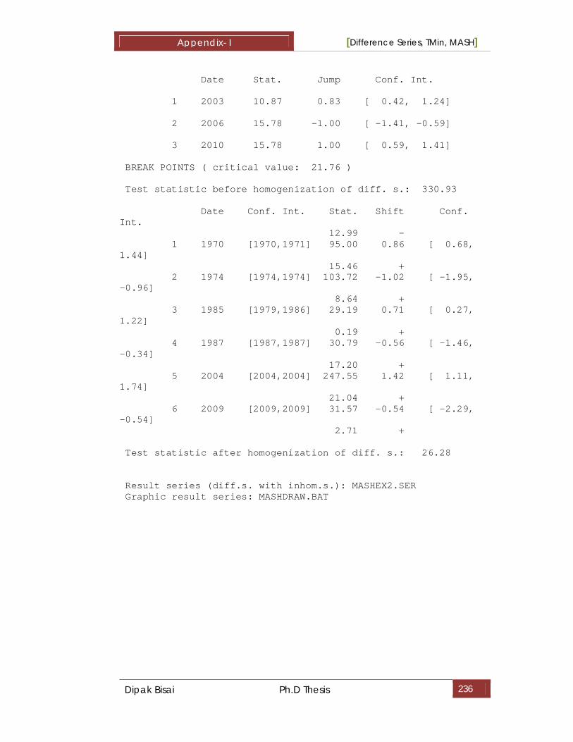
Appendix- I [Difference Series, TMin, MASH]
Dipak Bisai Ph.D Thesis 236
Date Stat. Jump Conf. Int. 1 2003 10.87 0.83 [ 0.42, 1.24] 2 2006 15.78 -1.00 [ -1.41, -0.59] 3 2010 15.78 1.00 [ 0.59, 1.41] BREAK POINTS ( critical value: 21.76 ) Test statistic before homogenization of diff. s.: 330.93 Date Conf. Int. Stat. Shift Conf. Int. 12.99 - 1 1970 [1970,1971] 95.00 0.86 [ 0.68, 1.44] 15.46 + 2 1974 [1974,1974] 103.72 -1.02 [ -1.95, -0.96] 8.64 + 3 1985 [1979,1986] 29.19 0.71 [ 0.27, 1.22] 0.19 + 4 1987 [1987,1987] 30.79 -0.56 [ -1.46, -0.34] 17.20 + 5 2004 [2004,2004] 247.55 1.42 [ 1.11, 1.74] 21.04 + 6 2009 [2009,2009] 31.57 -0.54 [ -2.29, -0.54] 2.71 + Test statistic after homogenization of diff. s.: 26.28 Result series (diff.s. with inhom.s.): MASHEX2.SER Graphic result series: MASHDRAW.BAT

Appendix- I [Difference Series, TMin, MASH]
Dipak Bisai Ph.D Thesis 237
(6) Difference Series, Malda, August, Series no-8.
CANDIDATE SERIES: 88888 (Index: 8) NUMBER OF DIFFERENCE SERIES: 2 REFERENCE SERIES, WEIGHTING FACTORS, VARIANCE OF DIFFERENCE SERIES 44444 Variance Deviation 88888 1.00000 0.63205 0.79502 21212 Variance Deviation 88888 1.00000 0.17128 0.41386 NO FORMER ESTIMATED BREAKS EXAMINATION OF DIFFERENCE SERIES 1. DIFFERENCE SERIES OUTLIERS ( critical value: 8.20 ) Date Stat. Jump Conf. Int. 1 2006 35.50 3.00 [ 2.17, 3.83] BREAK POINTS ( critical value: 21.76 ) Test statistic before homogenization of diff. s.: 429.69 Date Conf. Int. Stat. Shift Conf. Int. 16.05 - 1 2003 [2003,2003] 52.62 2.55 [ 1.36, 3.84] 2 2004 [2004,2004] 289.14 -7.41 [ -8.92, -5.90] 2.71 - 3 2006 [2006,2006] 157.68 4.08 [ 2.96, 5.21] 5.26 + 4 2009 [2009,2009] 96.64 -3.17 [ -4.73, -2.27] 3.94 - Test statistic after homogenization of diff. s.: 16.05 2. DIFFERENCE SERIES BREAK POINTS ( critical value: 21.76 ) Test statistic before homogenization of diff. s.: 61.61

Appendix- I [Difference Series, TMin, MASH]
Dipak Bisai Ph.D Thesis 238
Date Conf. Int. Stat. Shift Conf. Int. 16.70 - 1 1970 [1969,1972] 58.19 1.31 [ 0.77, 2.05] 11.11 + 2 1974 [1974,1974] 61.03 -1.27 [ -3.22, -1.24] 20.32 + 3 2002 [2000,2003] 53.15 -0.81 [ -1.82, -0.65] 9.47 + Test statistic after homogenization of diff. s.: 20.32 Result series (diff.s. with inhom.s.): MASHEX2.SER Graphic result series: MASHDRAW.BAT (7) Difference Series, Midnapore, August, Serial no. 9
CANDIDATE SERIES: 99999 (Index: 9) NUMBER OF DIFFERENCE SERIES: 2 REFERENCE SERIES, WEIGHTING FACTORS, VARIANCE OF DIFFERENCE SERIES 31313 44444 21212 Variance Deviation 99999 0.12878 0.13144 0.73978 0.03428 0.18514 55555 Variance Deviation 99999 1.00000 0.03364 0.18341 NO FORMER ESTIMATED BREAKS EXAMINATION OF DIFFERENCE SERIES 1. DIFFERENCE SERIES BREAK POINTS ( critical value: 21.76 ) Test statistic before homogenization of diff. s.: 189.37 Date Conf. Int. Stat. Shift Conf. Int. 15.00 - 1 1984 [1982,1984] 42.28 0.49 [ 0.25, 0.83] 1.76 - 2 1987 [1985,1992] 32.06 -0.45 [ -0.77, -0.19]

Appendix- I [Difference Series, TMin, MASH]
Dipak Bisai Ph.D Thesis 239
5.66 + 3 2004 [1996,2004] 24.21 0.42 [ 0.20, 1.16] 7.60 - 4 2006 [2006,2006] 30.56 0.40 [ 0.39, 1.71] 15.20 + Test statistic after homogenization of diff. s.: 15.20 2. DIFFERENCE SERIES BREAK POINTS ( critical value: 21.76 ) Test statistic before homogenization of diff. s.: 754.97 Date Conf. Int. Stat. Shift Conf. Int. 8.03 - 1 1971 [1960,1973] 31.04 -0.39 [ -0.68, -0.16] 2.31 + 2 1974 [1972,1977] 25.65 0.39 [ 0.14, 0.76] 9.62 - 3 1984 [1981,1984] 31.45 0.44 [ 0.20, 0.83] 2.66 - 4 1987 [1985,1994] 28.20 -0.40 [ -0.70, -0.15] 4.79 + 5 2004 [2004,2004] 43.12 -0.84 [ -1.41, -0.44] 6 2005 [2005,2005] 43.50 -0.91 [ -1.55, -0.48] 4.19 + 7 2008 [2007,2008] 62.93 0.91 [ 0.51, 1.31] 0.00 - 8 2010 [2010,2010] 42.22 -1.00 [ -1.53, -0.47] Test statistic after homogenization of diff. s.: 9.62 Result series (diff.s. with inhom.s.): MASHEX2.SER Graphic result series: MASHDRAW.BAT

Appendix- I [Difference Series, TMin, MASH]
Dipak Bisai Ph.D Thesis 240
(8) Difference Series, Bankura, Monsoon, Serial no-3.
CANDIDATE SERIES: 33333 (Index: 3) NUMBER OF DIFFERENCE SERIES: 2 REFERENCE SERIES, WEIGHTING FACTORS, VARIANCE OF DIFFERENCE SERIES 21212 Variance Deviation 33333 1.00000 0.01923 0.13869 55555 Variance Deviation 33333 1.00000 0.01359 0.11658 NO FORMER ESTIMATED BREAKS EXAMINATION OF DIFFERENCE SERIES 1. DIFFERENCE SERIES OUTLIERS ( critical value: 8.20 ) Date Stat. Jump Conf. Int. 1 2006 8.43 -0.43 [ -0.67, -0.19] BREAK POINTS ( critical value: 21.76 ) Test statistic before homogenization of diff. s.: 96.13 Date Conf. Int. Stat. Shift Conf. Int. 14.62 + 1 1964 [1961,1965] 33.83 -0.22 [ -0.41, -0.11] 11.21 + 2 1971 [1970,1971] 85.85 0.67 [ 0.42, 0.92] 1.48 - 3 1974 [1974,1974] 96.13 -0.61 [ -0.88, -0.42] 18.29 - 4 2003 [2003,2004] 78.97 0.42 [ 0.25, 0.58] 6.42 + 5 2009 [2009,2010] 22.85 -0.39 [ -0.75, -0.12] 0.02 - Test statistic after homogenization of diff. s.: 18.29 2. DIFFERENCE SERIES

Appendix- I [Difference Series, TMin, MASH]
Dipak Bisai Ph.D Thesis 241
OUTLIERS ( critical value: 8.20 ) Date Stat. Jump Conf. Int. 1 1966 14.64 0.34 [ 0.19, 0.49] BREAK POINTS ( critical value: 21.76 ) Test statistic before homogenization of diff. s.: 209.94 Date Conf. Int. Stat. Shift Conf. Int. 4.44 - 1 1917 [1903,1926] 24.04 -0.08 [ -0.20, -0.03] 14.58 + 2 1951 [1949,1953] 28.67 0.20 [ 0.07, 0.33] 3.08 + 3 1954 [1953,1957] 23.28 -0.17 [ -0.45, -0.07] 18.11 - 4 1971 [1971,1971] 114.89 0.42 [ 0.31, 0.61] 1.82 - 5 1974 [1974,1974] 155.13 -0.45 [ -0.71, -0.40] 20.27 + 6 2002 [2002,2002] 113.12 -0.65 [ -0.94, -0.48] 7 2003 [2003,2003] 42.61 0.58 [ 0.27, 0.89] 8 2004 [2004,2004] 27.98 -0.40 [ -0.78, -0.16] 2.14 + 9 2006 [2006,2006] 98.19 0.57 [ 0.37, 0.77] 1.82 - 10 2009 [2009,2009] 80.11 -0.51 [ -0.71, -0.31] 0.46 - Test statistic after homogenization of diff. s.: 24.75 Result series (diff.s. with inhom.s.): MASHEX2.SER Graphic result series: MASHDRAW.BAT

Appendix-II [R_Scripts]
Dipak Bisai Ph.D Thesis 242
Cumulative deviation test for whole year, months and seasons.
(R_Script for Cumulative Deciation Test for Whole Year ) x=read.csv(file="D:/TMaxdata/current.csv",header=FALSE) jan=matrix(x[[2]]) n.jan=length(jan) j.jan=mean(jan) sd.jan=sd(jan)
k.jan=NULL for(i in 1:n.jan){k.jan[i]=sum((jan[1:i])-j.jan) {sk.jan=k.jan[1:i]/sd.jan }} sk.jan.abs=abs(sk.jan) feb=matrix(x[[3]]) n.feb=length(feb) j.feb=mean(feb) sd.feb=sd(feb) k.feb=NULL for(i in 1:n.feb){k.feb[i]=sum((feb[1:i])-j.feb) {sk.feb=k.feb[1:i]/sd.feb }} sk.feb.abs=abs(sk.feb) mar=matrix(x[[4]]) n.mar=length(mar) j.mar=mean(mar) sd.mar=sd(mar) k.mar=NULL for(i in 1:n.mar){k.mar[i]=sum((mar[1:i])-j.mar) {sk.mar=k.mar[1:i]/sd.mar }} sk.mar.abs=abs(sk.mar) apr=matrix(x[[5]]) n.apr=length(apr) j.apr=mean(apr) sd.apr=sd(apr) k.apr=NULL for(i in 1:n.apr){k.apr[i]=sum((apr[1:i])-j.apr) {sk.apr=k.apr[1:i]/sd.apr }} sk.apr.abs=abs(sk.apr) may=matrix(x[[6]]) n.may=length(may) j.may=mean(may) sd.may=sd(may) k.may=NULL for(i in 1:n.may){k.may[i]=sum((may[1:i])-j.may) {sk.may=k.may[1:i]/sd.may }} sk.may.abs=abs(sk.may) jun=matrix(x[[7]]) n.jun=length(jun) j.jun=mean(jun) sd.jun=sd(jun) k.jun=NULL for(i in 1:n.jun){k.jun[i]=sum((jun[1:i])-j.jun)

Appendix-II [R_Scripts]
Dipak Bisai Ph.D Thesis 243
{sk.jun=k.jun[1:i]/sd.jun }} sk.jun.abs=abs(sk.jun) jul=matrix(x[[8]]) n.jul=length(jul) j.jul=mean(jul) sd.jul=sd(jul) k.jul=NULL for(i in 1:n.jul){k.jul[i]=sum((jul[1:i])-j.jul) {sk.jul=k.jul[1:i]/sd.jul }} sk.jul.abs=abs(sk.jul) aug=matrix(x[[9]]) n.aug=length(aug) j.aug=mean(aug) sd.aug=sd(aug) k.aug=NULL for(i in 1:n.aug){k.aug[i]=sum((aug[1:i])-j.aug) {sk.aug=k.aug[1:i]/sd.aug }} sk.aug.abs=abs(sk.aug) sep=matrix(x[[10]]) n.sep=length(sep) j.sep=mean(sep) sd.sep=sd(sep) k.sep=NULL for(i in 1:n.sep){k.sep[i]=sum((sep[1:i])-j.sep) {sk.sep=k.sep[1:i]/sd.sep }} sk.sep.abs=abs(sk.sep) oct=matrix(x[[11]]) n.oct=length(oct) j.oct=mean(oct) sd.oct=sd(oct) k.oct=NULL for(i in 1:n.oct){k.oct[i]=sum((oct[1:i])-j.oct) {sk.oct=k.oct[1:i]/sd.oct }} sk.oct.abs=abs(sk.oct) nov=matrix(x[[12]]) n.nov=length(nov) j.nov=mean(nov) sd.nov=sd(nov) k.nov=NULL for(i in 1:n.nov){k.nov[i]=sum((nov[1:i])-j.nov) {sk.nov=k.nov[1:i]/sd.nov }} sk.nov.abs=abs(sk.nov) dec=matrix(x[[13]]) n.dec=length(dec) j.dec=mean(dec) sd.dec=sd(dec) k.dec=NULL for(i in 1:n.dec){k.dec[i]=sum((dec[1:i])-j.dec) {sk.dec=k.dec[1:i]/sd.dec }} sk.dec.abs=abs(sk.dec) tot=matrix(x[[14]])

Appendix-II [R_Scripts]
Dipak Bisai Ph.D Thesis 244
n.tot=length(tot) j.tot=mean(tot) sd.tot=sd(tot) k.tot=NULL for(i in 1:n.tot){k.tot[i]=sum((tot[1:i])-j.tot) {sk.tot=k.tot[1:i]/sd.tot }} sk.tot.abs=abs(sk.tot) win=matrix(x[[15]]) n.win=length(win) j.win=mean(win) sd.win=sd(win) k.win=NULL for(i in 1:n.win){k.win[i]=sum((win[1:i])-j.win) {sk.win=k.win[1:i]/sd.win }} sk.win.abs=abs(sk.win) sum=matrix(x[[16]]) n.sum=length(sum) j.sum=mean(sum) sd.sum=sd(sum) k.sum=NULL for(i in 1:n.sum){k.sum[i]=sum((sum[1:i])-j.sum) {sk.sum=k.sum[1:i]/sd.sum }} sk.sum.abs=abs(sk.sum) mon=matrix(x[[17]]) n.mon=length(mon) j.mon=mean(mon) sd.mon=sd(mon) k.mon=NULL for(i in 1:n.mon){k.mon[i]=sum((mon[1:i])-j.mon) {sk.mon=k.mon[1:i]/sd.mon }} sk.mon.abs=abs(sk.mon) pmon=matrix(x[[18]]) n.pmon=length(pmon) j.pmon=mean(pmon) sd.pmon=sd(pmon) k.pmon=NULL for(i in 1:n.pmon){k.pmon[i]=sum((pmon[1:i])-j.pmon) {sk.pmon=k.pmon[1:i]/sd.pmon }} sk.pmon.abs=abs(sk.pmon) print((max(sk.jan.abs)/sqrt(n.jan))) print((max(sk.feb.abs)/sqrt(n.feb))) print((max(sk.mar.abs)/sqrt(n.mar))) print((max(sk.apr.abs)/sqrt(n.apr))) print((max(sk.may.abs)/sqrt(n.may))) print((max(sk.jun.abs)/sqrt(n.jun))) print((max(sk.jul.abs)/sqrt(n.jul))) print((max(sk.aug.abs)/sqrt(n.aug))) print((max(sk.sep.abs)/sqrt(n.sep))) print((max(sk.oct.abs)/sqrt(n.oct))) print((max(sk.nov.abs)/sqrt(n.nov))) print((max(sk.dec.abs)/sqrt(n.dec))) print((max(sk.tot.abs)/sqrt(n.tot))) print((max(sk.win.abs)/sqrt(n.win)))

Appendix-II [R_Scripts]
Dipak Bisai Ph.D Thesis 245
print((max(sk.sum.abs)/sqrt(n.sum))) print((max(sk.mon.abs)/sqrt(n.mon))) print((max(sk.pmon.abs)/sqrt(n.pmon))) Q.jan=max((sk.jan.abs)/sqrt(n.jan)) Q.feb=max((sk.feb.abs)/sqrt(n.feb)) Q.mar=max((sk.mar.abs)/sqrt(n.mar)) Q.apr=max((sk.apr.abs)/sqrt(n.apr)) Q.may=max((sk.may.abs)/sqrt(n.may)) Q.jun=max((sk.jun.abs)/sqrt(n.jun)) Q.jul=max((sk.jul.abs)/sqrt(n.jul)) Q.aug=max((sk.aug.abs)/sqrt(n.aug)) Q.sep=max((sk.sep.abs)/sqrt(n.sep)) Q.oct=max((sk.oct.abs)/sqrt(n.oct)) Q.nov=max((sk.nov.abs)/sqrt(n.nov)) Q.dec=max((sk.dec.abs)/sqrt(n.dec)) Q.tot=max((sk.tot.abs)/sqrt(n.tot)) Q.win=max((sk.win.abs)/sqrt(n.win)) Q.sum=max((sk.sum.abs)/sqrt(n.sum)) Q.mon=max((sk.mon.abs)/sqrt(n.mon)) Q.pmon=max((sk.pmon.abs)/sqrt(n.pmon)) result<-c(Q.jan, Q.feb, Q.mar, Q.apr, Q.may, Q.jun, Q.jul, Q.aug, Q.sep, Q.oct, Q.nov, Q.dec, Q.tot,Q.win,Q.sum, Q.mon, Q.pmon) print(result) output=matrix(result, ncol=1, byrow=TRUE, dimnames=list(c("January","February","March","April","May","June","July","August","September","October","Novmber","December","Annual","Winter","Summer", "Monsoon", "Post-Monsoon"),c("Q Max"))) write.csv(output, file="D:/Result/CumDevTest.csv")

Appendix-II [R_Scripts]
Dipak Bisai Ph.D Thesis 246
Mann-Kendall Trend.
require(Kendall, quietly = FALSE) MKtau<-function(z) MannKendall(z)$tau MKp<-function(x) MannKendall(x)$sl x=read.csv(file="D:/TMaxdata/Current.csv",header=FALSE) k=NULL m=NULL for (i in 2:18){k[i]=MKtau(x[[i]]) m[i]=MKp(x[[i]]) } result=as.matrix(cbind(k,m)) result=na.omit(result) dimnames(result)=NULL rownames(result)=c("January", "February", "March", "April", "May", "June", "July", "August", "September", "October", "November", "December", "Yearly", "Winter", "Pre-Monsoon", "Monsoon", "Post-Monsoon") colnames(result)=c("Kendall-Z", "p-Value") print(result) write.csv(result, file="D:/Result/Mann_Kendall Trend.csv")

Appendix-II [R_Scripts]
Dipak Bisai Ph.D Thesis 247
Moving Average.
tara<-function(x,y){ reg=lm(x~y) coeff=as.numeric(reg$coeff[2]) confi=confint(reg,"y",level=0.95) return(c(coeff,confi)) } a=read.csv(file="D:/TMaxdata/Current.csv",header=FALSE) x.jan=a[[1]] y.jan=a[[2]] n.jan=length(x.jan) k.jan=NULL m1.jan=NULL for(i in 1:n.jan){k.jan=x.jan[1:i] l.jan=y.jan[1:i] m.jan=tara(k.jan,l.jan) m1.jan=rbind(m1.jan,m.jan) } x.feb=a[[1]] y.feb=a[[3]] n.feb=length(x.feb) k.feb=NULL m1.feb=NULL for(i in 1:n.feb){k.feb=x.feb[1:i] l.feb=y.feb[1:i] m.feb=tara(k.feb,l.feb) m1.feb=rbind(m1.feb,m.feb) } x.mar=a[[1]] y.mar=a[[4]] n.mar=length(x.mar) k.mar=NULL m1.mar=NULL for(i in 1:n.mar){k.mar=x.mar[1:i] l.mar=y.mar[1:i] m.mar=tara(k.mar,l.mar) m1.mar=rbind(m1.mar,m.mar) } x.apr=a[[1]] y.apr=a[[5]] n.apr=length(x.apr) k.apr=NULL m1.apr=NULL for(i in 1:n.apr){k.apr=x.apr[1:i] l.apr=y.apr[1:i] m.apr=tara(k.apr,l.apr) m1.apr=rbind(m1.apr,m.apr) } x.may=a[[1]] y.may=a[[6]] n.may=length(x.may) k.may=NULL

Appendix-II [R_Scripts]
Dipak Bisai Ph.D Thesis 248
m1.may=NULL for(i in 1:n.may){k.may=x.may[1:i] l.may=y.may[1:i] m.may=tara(k.may,l.may) m1.may=rbind(m1.may,m.may) } x.jun=a[[1]] y.jun=a[[7]] n.jun=length(x.jun) k.jun=NULL m1.jun=NULL for(i in 1:n.jun){k.jun=x.jun[1:i] l.jun=y.jun[1:i] m.jun=tara(k.jun,l.jun) m1.jun=rbind(m1.jun,m.jun) } x.jul=a[[1]] y.jul=a[[8]] n.jul=length(x.jul) k.jul=NULL m1.jul=NULL for(i in 1:n.jul){k.jul=x.jul[1:i] l.jul=y.jul[1:i] m.jul=tara(k.jul,l.jul) m1.jul=rbind(m1.jul,m.jul) } x.aug=a[[1]] y.aug=a[[9]] n.aug=length(x.aug) k.aug=NULL m1.aug=NULL for(i in 1:n.aug){k.aug=x.aug[1:i] l.aug=y.aug[1:i] m.aug=tara(k.aug,l.aug) m1.aug=rbind(m1.aug,m.aug) } x.sep=a[[1]] y.sep=a[[10]] n.sep=length(x.sep) k.sep=NULL m1.sep=NULL for(i in 1:n.sep){k.sep=x.sep[1:i] l.sep=y.sep[1:i] m.sep=tara(k.sep,l.sep) m1.sep=rbind(m1.sep,m.sep) } x.oct=a[[1]] y.oct=a[[11]] n.oct=length(x.oct) k.oct=NULL m1.oct=NULL for(i in 1:n.oct){k.oct=x.oct[1:i] l.oct=y.oct[1:i]

Appendix-II [R_Scripts]
Dipak Bisai Ph.D Thesis 249
m.oct=tara(k.oct,l.oct) m1.oct=rbind(m1.oct,m.oct) } x.nov=a[[1]] y.nov=a[[12]] n.nov=length(x.nov) k.nov=NULL m1.nov=NULL for(i in 1:n.nov){k.nov=x.nov[1:i] l.nov=y.nov[1:i] m.nov=tara(k.nov,l.nov) m1.nov=rbind(m1.nov,m.nov) } x.dec=a[[1]] y.dec=a[[13]] n.dec=length(x.dec) k.dec=NULL m1.dec=NULL for(i in 1:n.dec){k.dec=x.dec[1:i] l.dec=y.dec[1:i] m.dec=tara(k.dec,l.dec) m1.dec=rbind(m1.dec,m.dec) } x.year=a[[1]] y.year=a[[14]] n.year=length(x.year) k.year=NULL m1.year=NULL for(i in 1:n.year){k.year=x.year[1:i] l.year=y.year[1:i] m.year=tara(k.year,l.year) m1.year=rbind(m1.year,m.year) } x.winter=a[[1]] y.winter=a[[15]] n.winter=length(x.winter) k.winter=NULL m1.winter=NULL for(i in 1:n.winter){k.winter=x.winter[1:i] l.winter=y.winter[1:i] m.winter=tara(k.winter,l.winter) m1.winter=rbind(m1.winter,m.winter) } x.sum=a[[1]] y.sum=a[[16]] n.sum=length(x.sum) k.sum=NULL m1.sum=NULL for(i in 1:n.sum){k.sum=x.sum[1:i] l.sum=y.sum[1:i] m.sum=tara(k.sum,l.sum) m1.sum=rbind(m1.sum,m.sum) }

Appendix-II [R_Scripts]
Dipak Bisai Ph.D Thesis 250
x.mon=a[[1]] y.mon=a[[16]] n.mon=length(x.mon) k.mon=NULL m1.mon=NULL for(i in 1:n.mon){k.mon=x.mon[1:i] l.mon=y.mon[1:i] m.mon=tara(k.mon,l.mon) m1.mon=rbind(m1.mon,m.mon) } x.pstmon=a[[1]] y.pstmon=a[[17]] n.pstmon=length(x.pstmon) k.pstmon=NULL m1.pstmon=NULL for(i in 1:n.pstmon){k.pstmon=x.pstmon[1:i] l.pstmon=y.pstmon[1:i] m.pstmon=tara(k.pstmon,l.pstmon) m1.pstmon=rbind(m1.pstmon,m.pstmon) } result=cbind(m1.jan, m1.feb, m1.mar, m1.apr, m1.may, m1.jun, m1.jul, m1.aug, m1.sep, m1.oct, m1.nov, m1.dec, m1.year, m1.winter, m1.sum, m1.mon, m1.pstmon) rownames(result)=c(a[[1]]) colnames(result)=c("Jan b-value", "Jan_Lwr", "Jan_Upr", "Feb b-value", "Feb_Lwr", "Feb_Upr", "Mar b-value", "Mar_Lwr", "Mar_Upr", "Apr b-value", "Apr_Lwr", "Apr_Upr", "May b-value", "May_Lwr", "May_Upr", "Jun b-value", "Jun_Lwr", "Jun_Upr", "Jul b-value", "Jul_Lwr", "Jul_Upr", "Aug b-value", "Aug_Lwr", "Aug_Upr", "Sep b-value", "Sep_Lwr", "Sep_Upr", "Oct b-value", "Oct_Lwr", "Oct_Upr", "Nov b-value", "Nov_Lwr", "Nov_Upr", "Dec b-value", "Dec_Lwr", "Dec_Upr", "Year b-value", "Year_Lwr", "Year_Upr","Win b-Value", "Win_Lwr", "Win_Upr", "Sum b-Value", "Sum_Lwr", "Sum_Upr", "Mon b-Value", "Mon_Lwr", "Mon_Upr", "Postmon b-Value", "Postmon_Lwr", "Postmon_Upr") write.csv(result, file="D:/Result/Regression.csv")

Appendix-II [R_Scripts]
Dipak Bisai Ph.D Thesis 251
Plot Time Series.
#Graph of Original Series and ACF and PACF require(Kendall) require(boot) x=read.csv(file="D:/TMaxdata/Current.csv", header=FALSE) a=as.matrix(x[2:13]) rain=as.vector(t(a)) raints=ts(rain, start=c(1901,1), end=c(2011,12), frequency=12) png(file="D:/Result/1Tol_Series.png") plot(raints, col="Darkgrey") lines(lowess(time(raints),raints),lwd=2, col="blue") title("TMax 1901 - 2011") dev.off() a.jan=as.matrix(x[[2]]) rain.jan=as.vector(t(a.jan)) raints.jan=ts(rain.jan, start=c(1901), end=c(2011), frequency=1) png(file="D:/Result/2jan.png") plot(raints.jan, col="Darkgrey") lines(lowess(time(raints.jan),raints.jan),lwd=2, col="blue") title("January 1901 - 2011") dev.off() a.feb=as.matrix(x[[3]]) rain.feb=as.vector(t(a.feb)) raints.feb=ts(rain.feb, start=c(1901), end=c(2011), frequency=1) png(file="D:/Result/3feb.png") plot(raints.feb, col="Darkgrey") lines(lowess(time(raints.feb),raints.feb),lwd=2, col="blue") title("february 1901 - 2011") dev.off() a.mar=as.matrix(x[[4]]) rain.mar=as.vector(t(a.mar)) raints.mar=ts(rain.mar, start=c(1901), end=c(2011), frequency=1) png(file="D:/Result/4mar.png") plot(raints.mar, col="Darkgrey") lines(lowess(time(raints.mar),raints.mar),lwd=2, col="blue") title("March 1901 - 2011") dev.off() a.apr=as.matrix(x[[5]]) rain.apr=as.vector(t(a.apr)) raints.apr=ts(rain.apr, start=c(1901), end=c(2011), frequency=1) png(file="D:/Result/5apr.png") plot(raints.apr, col="Darkgrey") lines(lowess(time(raints.apr),raints.apr),lwd=2, col="blue") title("April 1901 - 2011") dev.off() a.may=as.matrix(x[[6]]) rain.may=as.vector(t(a.may)) raints.may=ts(rain.may, start=c(1901), end=c(2011), frequency=1) png(file="D:/result/6may.png") plot(raints.may, col="Darkgrey") lines(lowess(time(raints.may),raints.may),lwd=2, col="blue") title("May 1901 - 2011")

Appendix-II [R_Scripts]
Dipak Bisai Ph.D Thesis 252
dev.off() a.jun=as.matrix(x[[7]]) rain.jun=as.vector(t(a.jun)) raints.jun=ts(rain.jun, start=c(1901), end=c(2011), frequency=1) png(file="D:/Result/7jun.png") plot(raints.jun, col="Darkgrey") lines(lowess(time(raints.jun),raints.jun),lwd=2, col="blue") title("June 1901 - 2011") dev.off() a.jul=as.matrix(x[[8]]) rain.jul=as.vector(t(a.jul)) raints.jul=ts(rain.jul, start=c(1901), end=c(2011), frequency=1) png(file="D:/Result/8jul.png") plot(raints.jul, col="Darkgrey") lines(lowess(time(raints.jul),raints.jul),lwd=2, col="blue") title("July 1901 - 2011") dev.off() a.aug=as.matrix(x[[9]]) rain.aug=as.vector(t(a.aug)) raints.aug=ts(rain.aug, start=c(1901), end=c(2011), frequency=1) png(file="D:/Result/9aug.png") plot(raints.aug, col="Darkgrey") lines(lowess(time(raints.aug),raints.aug),lwd=2, col="blue") title("August 1901 - 2011") dev.off() a.sep=as.matrix(x[[10]]) rain.sep=as.vector(t(a.sep)) raints.sep=ts(rain.sep, start=c(1901), end=c(2011), frequency=1) png(file="D:/Result/10sep.png") plot(raints.sep, col="Darkgrey") lines(lowess(time(raints.sep),raints.sep),lwd=2, col="blue") title("September 1901 - 2011") dev.off() a.oct=as.matrix(x[[11]]) rain.oct=as.vector(t(a.oct)) raints.oct=ts(rain.oct, start=c(1901), end=c(2011), frequency=1) png(file="D:/Result/11oct.png") plot(raints.oct, col="Darkgrey") lines(lowess(time(raints.oct),raints.oct),lwd=2, col="blue") title("October 1901 - 2011") dev.off() a.nov=as.matrix(x[[12]]) rain.nov=as.vector(t(a.nov)) raints.nov=ts(rain.nov, start=c(1901), end=c(2011), frequency=1) png(file="D:/Result/12nov.png") plot(raints.nov, col="Darkgrey") lines(lowess(time(raints.nov),raints.nov),lwd=2, col="blue") title("November 1901 - 2011") dev.off() a.dec=as.matrix(x[[13]]) rain.dec=as.vector(t(a.dec))

Appendix-II [R_Scripts]
Dipak Bisai Ph.D Thesis 253
raints.dec=ts(rain.dec, start=c(1901), end=c(2011), frequency=1) png(file="D:/Result/13dec.png") plot(raints.dec, col="Darkgrey") lines(lowess(time(raints.dec),raints.dec),lwd=2, col="blue") title("December 1901 - 2011") dev.off() a.win=as.matrix(x[[15]]) rain.win=as.vector(t(a.win)) raints.win=ts(rain.win, start=c(1901), end=c(2011), frequency=1) png(file="D:/Result/14win.png") plot(raints.win, col="Darkgrey") lines(lowess(time(raints.win),raints.win),lwd=2, col="blue") title("Winter 1901 - 2011") dev.off() a.sum=as.matrix(x[[16]]) rain.sum=as.vector(t(a.sum)) raints.sum=ts(rain.sum, start=c(1901), end=c(2011), frequency=1) png(file="D:/Result/15sum.png") plot(raints.sum, col="Darkgrey") lines(lowess(time(raints.sum),raints.sum),lwd=2, col="blue") title("Summer 1901 - 2011") dev.off() a.mon=as.matrix(x[[17]]) rain.mon=as.vector(t(a.mon)) raints.mon=ts(rain.mon, start=c(1901), end=c(2011), frequency=1) png(file="D:/Result/16mon.png") plot(raints.mon, col="Darkgrey") lines(lowess(time(raints.mon),raints.mon),lwd=2, col="blue") title("Monsoon 1901 - 2011") dev.off() a.pstmon=as.matrix(x[[18]]) rain.pstmon=as.vector(t(a.pstmon)) raints.pstmon=ts(rain.pstmon, start=c(1901), end=c(2011), frequency=1) png(file="D:/Result/17pstmon.png") plot(raints.pstmon, col="Darkgrey") lines(lowess(time(raints.pstmon),raints.pstmon),lwd=2, col="blue") title("Post-pstmonsoon 1901 - 2011") dev.off() png(file="D:/Result/18acf.year.png") acf(raints) dev.off() png(file="D:/Result/19pacf.year.png") pacf(raints) dev.off() png(file="D:/Result/20acf.jan.png") acf(raints.jan) dev.off() png(file="D:/Result/21pacf.jan.png") pacf(raints.jan) dev.off()

Appendix-II [R_Scripts]
Dipak Bisai Ph.D Thesis 254
png(file="D:/Result/22acf.feb.png") acf(raints.feb) dev.off() png(file="D:/Result/23pacf.feb.png") pacf(raints.feb) dev.off() png(file="D:/Result/24acf.mar.png") acf(raints.mar) dev.off() png(file="D:/Result/25pacf.mar.png") pacf(raints.mar) dev.off() png(file="D:/Result/26acf.apr.png") acf(raints.apr) dev.off() png(file="D:/Result/27pacf.apr.png") pacf(raints.apr) dev.off() png(file="D:/Result/28acf.may.png") acf(raints.may) dev.off() png(file="D:/Result/29pacf.may.png") pacf(raints.may) dev.off() png(file="D:/Result/30acf.jun.png") acf(raints.jun) dev.off() png(file="D:/Result/31pacf.jun.png") pacf(raints.jun) dev.off() png(file="D:/Result/32acf.jul.png") acf(raints.jul) dev.off() png(file="D:/Result/33pacf.jul.png") pacf(raints.jul) dev.off() png(file="D:/Result/34acf.aug.png") acf(raints.aug) dev.off() png(file="D:/Result/35pacf.aug.png") pacf(raints.aug) dev.off() png(file="D:/Result/36acf.sep.png") acf(raints.sep) dev.off() png(file="D:/Result/37pacf.sep.png") pacf(raints.sep) dev.off() png(file="D:/Result/38acf.oct.png")

Appendix-II [R_Scripts]
Dipak Bisai Ph.D Thesis 255
acf(raints.oct) dev.off() png(file="D:/Result/39pacf.oct.png") pacf(raints.oct) dev.off() png(file="D:/Result/40acf.nov.png") acf(raints.nov) dev.off() png(file="D:/Result/41pacf.nov.png") pacf(raints.nov) dev.off() png(file="D:/Result/42acf.dec.png") acf(raints.dec) dev.off() png(file="D:/Result/43pacf.dec.png") pacf(raints.dec) dev.off() png(file="D:/Result/44acf.win.png") acf(raints.win) dev.off() png(file="D:/Result/45pacf.win.png") pacf(raints.win) dev.off() png(file="D:/Result/46acf.sum.png") acf(raints.sum) dev.off() png(file="D:/Result/47pacf.sum.png") pacf(raints.sum) dev.off() png(file="D:/Result/48acf.mon.png") acf(raints.mon) dev.off() png(file="D:/Result/49pacf.mon.png") pacf(raints.mon) dev.off() png(file="D:/Result/50acf.pstmon.png") acf(raints.pstmon) dev.off() png(file="D:/Result/51pacf.pstmon.png") pacf(raints.pstmon) dev.off() #Calculation of Original MK Values and Bootstrap confidence interval 95% MKtau<-function(z) MannKendall(z)$tau boot.jan=tsboot(tseries = raints.jan, statistic = MKtau, R = 500, l = 5, sim = "fixed") boot.jan.conf=as.numeric(boot.ci(boot.jan, type="norm")$normal) orig.tau.jan=as.numeric(boot.jan$t0) result.jan=c(orig.tau.jan, boot.jan.conf)

Appendix-II [R_Scripts]
Dipak Bisai Ph.D Thesis 256
boot.feb=tsboot(tseries = raints.feb, statistic = MKtau, R = 500, l = 5, sim = "fixed") boot.feb.conf=as.numeric(boot.ci(boot.feb, type="norm")$normal) orig.tau.feb=as.numeric(boot.feb$t0) result.feb=c(orig.tau.feb, boot.feb.conf) boot.mar=tsboot(tseries = raints.mar, statistic = MKtau, R = 500, l = 5, sim = "fixed") boot.mar.conf=as.numeric(boot.ci(boot.mar, type="norm")$normal) orig.tau.mar=as.numeric(boot.mar$t0) result.mar=c(orig.tau.mar, boot.mar.conf) boot.apr=tsboot(tseries = raints.apr, statistic = MKtau, R = 500, l = 5, sim = "fixed") boot.apr.conf=as.numeric(boot.ci(boot.apr, type="norm")$normal) orig.tau.apr=as.numeric(boot.apr$t0) result.apr=c(orig.tau.apr, boot.apr.conf) boot.may=tsboot(tseries = raints.may, statistic = MKtau, R = 500, l = 5, sim = "fixed") boot.may.conf=as.numeric(boot.ci(boot.may, type="norm")$normal) orig.tau.may=as.numeric(boot.may$t0) result.may=c(orig.tau.may, boot.may.conf) boot.jun=tsboot(tseries = raints.jun, statistic = MKtau, R = 500, l = 5, sim = "fixed") boot.jun.conf=as.numeric(boot.ci(boot.jun, type="norm")$normal) orig.tau.jun=as.numeric(boot.jun$t0) result.jun=c(orig.tau.jun, boot.jun.conf) boot.jul=tsboot(tseries = raints.jul, statistic = MKtau, R = 500, l = 5, sim = "fixed") boot.jul.conf=as.numeric(boot.ci(boot.jul, type="norm")$normal) orig.tau.jul=as.numeric(boot.jul$t0) result.jul=c(orig.tau.jul, boot.jul.conf) boot.aug=tsboot(tseries = raints.aug, statistic = MKtau, R = 500, l = 5, sim = "fixed") boot.aug.conf=as.numeric(boot.ci(boot.aug, type="norm")$normal) orig.tau.aug=as.numeric(boot.aug$t0) result.aug=c(orig.tau.aug, boot.aug.conf) boot.sep=tsboot(tseries = raints.sep, statistic = MKtau, R = 500, l = 5, sim = "fixed") boot.sep.conf=as.numeric(boot.ci(boot.sep, type="norm")$normal) orig.tau.sep=as.numeric(boot.sep$t0) result.sep=c(orig.tau.sep, boot.sep.conf) boot.oct=tsboot(tseries = raints.oct, statistic = MKtau, R = 500, l = 5, sim = "fixed") boot.oct.conf=as.numeric(boot.ci(boot.oct, type="norm")$normal) orig.tau.oct=as.numeric(boot.oct$t0) result.oct=c(orig.tau.oct, boot.oct.conf) boot.nov=tsboot(tseries = raints.nov, statistic = MKtau, R = 500, l = 5, sim = "fixed") boot.nov.conf=as.numeric(boot.ci(boot.nov, type="norm")$normal) orig.tau.nov=as.numeric(boot.nov$t0) result.nov=c(orig.tau.nov, boot.nov.conf) boot.dec=tsboot(tseries = raints.dec, statistic = MKtau, R = 500, l = 5, sim = "fixed") boot.dec.conf=as.numeric(boot.ci(boot.dec, type="norm")$normal) orig.tau.dec=as.numeric(boot.dec$t0) result.dec=c(orig.tau.dec, boot.dec.conf) boot.win=tsboot(tseries = raints.win, statistic = MKtau, R = 500, l = 5, sim = "fixed") boot.win.conf=as.numeric(boot.ci(boot.win, type="norm")$normal)

Appendix-II [R_Scripts]
Dipak Bisai Ph.D Thesis 257
orig.tau.win=as.numeric(boot.win$t0) result.win=c(orig.tau.win, boot.win.conf) boot.sum=tsboot(tseries = raints.sum, statistic = MKtau, R = 500, l = 5, sim = "fixed") boot.sum.conf=as.numeric(boot.ci(boot.sum, type="norm")$normal) orig.tau.sum=as.numeric(boot.sum$t0) result.sum=c(orig.tau.sum, boot.sum.conf) boot.mon=tsboot(tseries = raints.mon, statistic = MKtau, R = 500, l = 5, sim = "fixed") boot.mon.conf=as.numeric(boot.ci(boot.mon, type="norm")$normal) orig.tau.mon=as.numeric(boot.mon$t0) result.mon=c(orig.tau.mon, boot.mon.conf) boot.pstmon=tsboot(tseries = raints.pstmon, statistic = MKtau, R = 500, l = 5, sim = "fixed") boot.pstmon.conf=as.numeric(boot.ci(boot.pstmon, type="norm")$normal) orig.tau.pstmon=as.numeric(boot.pstmon$t0) result.pstmon=c(orig.tau.pstmon, boot.pstmon.conf) z<-matrix(raints, ncol=12, byrow=12) zm<-apply(z, MARGIN=2, FUN=mean) zs<-apply(z, MARGIN=2, FUN=sd) z2<-sweep(z, MARGIN=2, STATS=zm) #subtract monthly means z3<-sweep(z2, MARGIN=2, STATS=zs, FUN="/") #divide by monthly sd zds<-c(t(z3)) attributes(zds)<-attributes(raints) png(file="D:/Result/51deseasonalized.png") plot(zds) dev.off() #do Mann-Kendall trend test deseason.MK=MannKendall(zds) #check robustness by applying block bootstrap MKtau<-function(z) MannKendall(z)$tau boot.deseason=tsboot(zds, MKtau, R=500, l=12, sim="fixed") boot.deseason.conf=as.numeric(boot.ci(boot.deseason, type="norm")$normal) orig.tau.deseason=as.numeric(boot.deseason$t0) result.deseason=c(orig.tau.deseason, boot.deseason.conf) print(deseason.MK) result=rbind(result.jan, result.feb, result.mar, result.apr, result.may, result.jun, result.jul, result.aug, result.sep, result.oct, result.nov, result.dec, result.win, result.sum, result.mon, result.pstmon,result.deseason) dimnames(result)=NULL rownames(result)=c("January", "February", "March", "April", "May", "June", "July", "August", "September", "October", "November", "December", "Winter", "Pre-Monsoon", "Monsoon","Post-Monsoon","Deseasonalized") colnames(result)=c("MK-Tau","Confidence Level", "Lower Bound", "Upper Bound") print(result) write.csv(result, "D:/Result/MK_Test_Result.csv")

Appendix-II [R_Scripts]
Dipak Bisai Ph.D Thesis 258
Sen’s Slope and Mann-Kendall Test.
require(wq) require(Kendall) x=read.csv(file="D:/TMaxdata/Current.csv", header=FALSE) a=as.matrix(x[2:13]) b=as.vector(t(a)) pptn=ts(b, start=c(1901,1), end=c(2011,12), frequency=12) jan=as.matrix(x[2]) jan.ts=ts(jan, start=c(1901), end=c(2011), frequency=1) feb=as.matrix(x[3]) feb.ts=ts(feb, start=c(1901), end=c(2011), frequency=1) mar=as.matrix(x[4]) mar.ts=ts(mar, start=c(1901), end=c(2011), frequency=1) apr=as.matrix(x[5]) apr.ts=ts(apr, start=c(1901), end=c(2011), frequency=1) may=as.matrix(x[6]) may.ts=ts(may, start=c(1901), end=c(2011), frequency=1) jun=as.matrix(x[7]) jun.ts=ts(jun, start=c(1901), end=c(2011), frequency=1) jul=as.matrix(x[8]) jul.ts=ts(jul, start=c(1901), end=c(2011), frequency=1) aug=as.matrix(x[9]) aug.ts=ts(aug, start=c(1901), end=c(2011), frequency=1) sep=as.matrix(x[10]) sep.ts=ts(sep, start=c(1901), end=c(2011), frequency=1) oct=as.matrix(x[11]) oct.ts=ts(oct, start=c(1901), end=c(2011), frequency=1) nov=as.matrix(x[12]) nov.ts=ts(nov, start=c(1901), end=c(2011), frequency=1) dec=as.matrix(x[13]) dec.ts=ts(dec, start=c(1901), end=c(2011), frequency=1) tot=as.matrix(x[14]) tot.ts=ts(tot, start=c(1901), end=c(2011), frequency=1) win=as.matrix(x[15]) win.ts=ts(win, start=c(1901), end=c(2011), frequency=1) sum=as.matrix(x[16]) sum.ts=ts(sum, start=c(1901), end=c(2011), frequency=1) mon=as.matrix(x[17]) mon.ts=ts(mon, start=c(1901), end=c(2011), frequency=1) pstmon=as.matrix(x[18]) pstmon.ts=ts(pstmon, start=c(1901), end=c(2011), frequency=1) #Deseasonalization of monthly Time Series require(boot) z<-matrix(pptn, ncol=12, byrow=12) zm<-apply(z, MARGIN=2, FUN=mean) zs<-apply(z, MARGIN=2, FUN=sd) z2<-sweep(z, MARGIN=2, STATS=zm) #subtract monthly means z3<-sweep(z2, MARGIN=2, STATS=zs, FUN="/") #divide by monthly sd zds<-c(t(z3)) attributes(zds)<-attributes(pptn) sen.slope=function(ts){ c(amount=mannKen(ts)$sen.slope, p.value=mannKen(ts)$p.value) } sen.pptn=as.numeric(sen.slope(pptn)) sen.jan=as.numeric(sen.slope(jan.ts)) sen.feb=as.numeric(sen.slope(feb.ts))

Appendix-II [R_Scripts]
Dipak Bisai Ph.D Thesis 259
sen.mar=as.numeric(sen.slope(mar.ts)) sen.apr=as.numeric(sen.slope(apr.ts)) sen.may=as.numeric(sen.slope(may.ts)) sen.jun=as.numeric(sen.slope(jun.ts)) sen.jul=as.numeric(sen.slope(jul.ts)) sen.aug=as.numeric(sen.slope(aug.ts)) sen.sep=as.numeric(sen.slope(sep.ts)) sen.oct=as.numeric(sen.slope(oct.ts)) sen.nov=as.numeric(sen.slope(nov.ts)) sen.dec=as.numeric(sen.slope(dec.ts)) sen.tot=as.numeric(sen.slope(tot.ts)) sen.win=as.numeric(sen.slope(win.ts)) sen.sum=as.numeric(sen.slope(sum.ts)) sen.mon=as.numeric(sen.slope(mon.ts)) sen.pstmon=as.numeric(sen.slope(pstmon.ts)) sen.zds=as.numeric(sen.slope(zds)) sen.out=rbind(sen.pptn,sen.jan,sen.feb,sen.mar,sen.apr,sen.may,sen.jun,sen.jul,sen.aug,sen.sep,sen.oct,sen.nov,sen.dec,sen.tot,sen.win,sen.sum,sen.mon,sen.pstmon,sen.zds) dimnames(sen.out)<-NULL rownames(sen.out)=c("Rain.orig_MonthlyTS", "January","February","March","April","May","June","July","August","September","October","November","December","YearlyTot","Winter","Pre-Monsoon","Monsoon","Post-Monsoon","Deseasonilzed MothlyTS") colnames(sen.out)=c("Sen Slope","p_value") cv=function(amp){ c(cv.mon=phenoAmp(amp, mon.range = c(6, 10))$cv, cv.year= phenoAmp(amp, mon.range = c(1, 12))$cv) } amp=cv(pptn) phenoamp=matrix(amp, ncol=2, byrow=F) dimnames(phenoamp)<-NULL rownames(phenoamp)=c(x[[1]]) colnames(phenoamp)=c("Monsoon Rainfall CV","Yearly Rainfall CV") fulcrum=phenoPhase(pptn, mon.range = c(1, 12)) png(file="D:/Result/Plotseason.png") plotSeason(pptn, type = "by.era", num.era = 4, same.plot = TRUE, ylab = NULL, num.col = 3) dev.off() Seasontrend=seasonTrend(pptn, 1901, 2011, type = "slope", method = "mk") write.csv(Seasontrend,file="D:/Result/Season_SenSlope.csv") write.csv(fulcrum, file="D:/Result/Gravity_Centre.csv") write.csv(phenoamp, file="D:/Result/Rainfall_Variation.csv") write.csv(sen.out, file="D:/Result/SenSlope Result.csv")

Appendix-II [R_Scripts]
Dipak Bisai Ph.D Thesis 260
Sequential Mann-Kendall Test.
require(pheno, quietly = FALSE) x=read.csv(file="D:/TMaxdata/Current.csv",header=FALSE) jan=x[[2]] result.jan=seqMK(jan) jan.prog=result.jan$prog jan.retro=result.jan$retr feb=x[[3]] result.feb=seqMK(feb) feb.prog=result.feb$prog feb.retro=result.feb$retr mar=x[[4]] result.mar=seqMK(mar) mar.prog=result.mar$prog mar.retro=result.mar$retr apr=x[[5]] result.apr=seqMK(apr) apr.prog=result.apr$prog apr.retro=result.apr$retr may=x[[6]] result.may=seqMK(may) may.prog=result.may$prog may.retro=result.may$retr jun=x[[7]] result.jun=seqMK(jun) jun.prog=result.jun$prog jun.retro=result.jun$retr jul=x[[8]] result.jul=seqMK(jul) jul.prog=result.jul$prog jul.retro=result.jul$retr aug=x[[9]] result.aug=seqMK(aug) aug.prog=result.aug$prog aug.retro=result.aug$retr sep=x[[10]] result.sep=seqMK(sep) sep.prog=result.sep$prog sep.retro=result.sep$retr oct=x[[11]] result.oct=seqMK(oct) oct.prog=result.oct$prog oct.retro=result.oct$retr nov=x[[12]] result.nov=seqMK(nov) nov.prog=result.nov$prog nov.retro=result.nov$retr

Appendix-II [R_Scripts]
Dipak Bisai Ph.D Thesis 261
dec=x[[13]] result.dec=seqMK(dec) dec.prog=result.dec$prog dec.retro=result.dec$retr tot=x[[14]] result.tot=seqMK(tot) tot.prog=result.tot$prog tot.retro=result.tot$retr win=x[[15]] result.win=seqMK(win) win.prog=result.win$prog win.retro=result.win$retr sum=x[[16]] result.sum=seqMK(sum) sum.prog=result.sum$prog sum.retro=result.sum$retr mon=x[[17]] result.mon=seqMK(mon) mon.prog=result.mon$prog mon.retro=result.mon$retr pstmon=x[[18]] result.pstmon=seqMK(pstmon) pstmon.prog=result.pstmon$prog pstmon.retro=result.pstmon$retr output<-c(jan.prog,jan.retro,feb.prog,feb.retro,mar.prog,mar.retro,apr.prog,apr.retro,may.prog,may.retro,jun.prog,jun.retro,jul.prog,jul.retro,aug.prog,aug.retro,sep.prog,sep.retro,oct.prog,oct.retro,nov.prog,nov.retro,dec.prog,dec.retro,tot.prog,tot.retro,win.prog,win.retro,sum.prog,sum.retro,mon.prog,mon.retro,pstmon.prog,pstmon.retro) final=matrix(output, ncol=34,byrow=F) rownames(final)=c(x[[1]]) colnames(final, do.NULL=T) colnames(final)<-c("January.Prog","January.Retro","February.Prog","February.Retro","March.Prog","March.Retro","April.Prog","April.Retro","May.Prog","May.Retro","June.Prog","June.Retro","July.Prog","July.Retro","August.Prog","August.Retro","September.Prog","September.Retro","October.Prog","October.Retro","November.Prog","November.Retro","December.Prog","December.Retro","Year.Prog","Year.Retro","Win.Prog","Win.Retro","Sum.Prog","Sum.Retro","Mon.Prog","Mon.Retro","PostMon.Prog","PostMon.Retro") write.csv(final, file="D:/Result/SeqMann_Kendall_result.csv")

Appendix-II [R_Scripts]
Dipak Bisai Ph.D Thesis 262
Von Neumann Test of Normality for Trend.
require(randtests, quietly = FALSE) x=read.csv(file="D:/TMaxdata/Current.csv",header=FALSE) jan=x[[2]] result.jan=bartels.rank.test(jan, "left.sided", pvalue="normal") statistic.jan=as.numeric(result.jan$statistic) p.jan=result.jan$p.value feb=x[[3]] result.feb=bartels.rank.test(feb, "left.sided", pvalue="normal") statistic.feb=as.numeric(result.feb$statistic) p.feb=result.feb$p.value mar=x[[4]] result.mar=bartels.rank.test(mar, "left.sided", pvalue="normal") statistic.mar=as.numeric(result.mar$statistic) p.mar=result.mar$p.value apr=x[[5]] result.apr=bartels.rank.test(apr, "left.sided", pvalue="normal") statistic.apr=as.numeric(result.apr$statistic) p.apr=result.apr$p.value may=x[[6]] result.may=bartels.rank.test(may, "left.sided", pvalue="normal") statistic.may=as.numeric(result.may$statistic) p.may=result.may$p.value jun=x[[7]] result.jun=bartels.rank.test(jun, "left.sided", pvalue="normal") statistic.jun=as.numeric(result.jun$statistic) p.jun=result.jun$p.value jul=x[[8]] result.jul=bartels.rank.test(jul, "left.sided", pvalue="normal") statistic.jul=as.numeric(result.jul$statistic) p.jul=result.jul$p.value aug=x[[9]] result.aug=bartels.rank.test(aug, "left.sided", pvalue="normal") statistic.aug=as.numeric(result.aug$statistic) p.aug=result.aug$p.value sep=x[[10]] result.sep=bartels.rank.test(sep, "left.sided", pvalue="normal") statistic.sep=as.numeric(result.sep$statistic) p.sep=result.sep$p.value oct=x[[11]] result.oct=bartels.rank.test(oct, "left.sided", pvalue="normal") statistic.oct=as.numeric(result.oct$statistic) p.oct=result.oct$p.value nov=x[[12]] result.nov=bartels.rank.test(nov, "left.sided", pvalue="normal") statistic.nov=as.numeric(result.nov$statistic) p.nov=result.nov$p.value dec=x[[13]] result.dec=bartels.rank.test(dec, "left.sided", pvalue="normal") statistic.dec=as.numeric(result.dec$statistic) p.dec=result.dec$p.value year=x[[14]] result.year=bartels.rank.test(year, "left.sided", pvalue="normal") statistic.year=as.numeric(result.year$statistic) p.year=result.year$p.value

Appendix-II [R_Scripts]
Dipak Bisai Ph.D Thesis 263
output<-c(statistic.jan,p.jan,statistic.feb,p.feb,statistic.mar,p.mar,statistic.apr,p.apr,statistic.may,p.may,statistic.jun,p.jun,statistic.jul,p.jul,statistic.aug,p.aug,statistic.sep,p.sep,statistic.oct,p.oct,statistic.nov,p.nov,statistic.dec,p.dec,statistic.year,p.year) final=matrix(output, ncol=2,byrow=TRUE,dimnames=list(c("January","February","March","April","May","June","July","August","September","October","Novmber","December","Yearly"),c("NeumannStatistic","p-value"))) write.csv(final, file="D:/Result/Neumannresult.csv")

Appendix-III [Cumulative Deviation Result after MASH Game]
Dipak Bisai Ph.D Thesis 264
(A) Results of Cumulative Deviation for ݔܯ Series after MASH Game.
(B) Results of Cumulative Deviation for ܯ Series after MASH Game.
Ban Bir Bur Hoo How Kol Mal Mid Mur Nad N 24 Pga Pur S 24 Pga
Jan 0.91 1.01 0.94 0.95 1.00 0.83 0.97 0.95 1.26 0.64 1.20 1.12 1.22
Feb 1.34 1.09 1.29 1.26 1.03 1.33 1.25 1.32 1.01 0.88 1.07 1.28 0.93
Mar 1.09 0.92 1.01 0.66 1.05 1.03 1.02 1.35 1.26 0.86 1.15 1.01 1.27
Apr 0.73 0.48 0.53 0.57 1.25 1.00 1.07 1.06 0.83 0.62 1.22 0.70 1.08
May 0.82 1.27 1.25 0.98 1.35 0.93 1.15 1.10 1.10 1.10 0.76 0.96 1.24
June 0.92 1.19 1.10 1.16 1.14 1.06 0.98 1.04 1.24 1.06 1.31 1.15 1.28
July 1.62 1.29 1.14 0.88 1.26 1.10 1.35 1.20 1.31 1.21 1.32 0.67 1.08
Aug 0.72 1.01 1.16 1.36 1.07 0.87 1.34 1.24 1.25 1.35 1.21 0.64 1.32
Sep 0.81 0.86 1.08 0.95 1.25 1.18 1.33 1.27 1.05 0.78 0.91 0.56 1.22
Oct 0.94 1.05 1.21 0.99 1.06 0.90 0.95 0.87 0.50 1.34 0.85 1.14 0.95
Nov 0.82 0.96 1.05 1.30 1.26 1.19 0.47 1.06 1.25 1.18 1.23 1.13 1.18
Dec 1.05 1.21 1.16 1.11 1.36 1.28 1.20 1.14 1.25 1.26 1.32 1.24 1.22
AA 1.15 1.32 1.06 1.00 1.15 1.32 1.06 1.07 1.00 1.00 1.32 1.07 1.34
Win 1.27 1.29 1.17 1.20 1.27 1.29 1.17 1.18 1.20 1.20 1.29 1.18 1.36
Sum 1.13 1.31 1.13 1.09 1.13 1.38 1.13 1.33 1.27 1.27 1.02 1.33 1.09
Mon 1.23 1.37 1.06 1.52 1.23 1.37 1.06 0.72 0.87 0.87 1.37 0.72 1.26
PM 1.29 0.98 0.86 1.02 1.29 0.98 0.86 0.86 1.01 1.01 0.98 1.21 1.08
Ban Bir Bur Hoo How Kol Mal Mid Mur Nad N 24 Pga Pur S 24 Pga
Jan 0.97 0.97 0.99 1.07 1.10 1.22 0.94 0.87 1.16 1.12 1.10 1.29 1.28
Feb 1.13 1.05 0.99 1.12 1.07 1.20 1.04 1.07 1.30 1.36 1.36 1.11 1.33
Mar 0.87 1.10 0.92 1.25 1.11 0.80 0.81 0.96 1.28 1.34 1.34 1.02 1.27
Apr 1.22 1.10 1.35 1.26 1.12 0.93 1.22 0.59 1.34 1.25 1.25 1.17 1.23
May 1.12 0.89 1.06 0.80 0.73 1.01 1.25 1.23 1.15 1.24 1.14 0.70 1.31
June 0.59 0.62 0.71 0.57 0.58 0.51 0.80 0.61 0.92 0.74 0.74 0.54 1.24
July 0.66 0.56 0.54 0.65 0.85 1.15 0.87 1.35 0.64 1.15 1.15 0.74 1.26
Aug 1.02 1.36 1.15 1.23 1.11 0.92 1.09 1.99 1.72 1.15 1.15 1.13 0.74
Sep 0.60 0.64 0.43 1.03 0.89 0.92 0.73 1.26 1.05 1.17 1.17 0.90 1.08
Oct 1.01 0.73 1.10 1.00 1.29 1.17 0.74 1.33 1.19 1.13 1.23 1.03 0.67
Nov 1.31 1.31 1.28 1.19 1.33 1.27 0.84 1.33 1.30 1.20 1.30 0.93 0.68
Dec 1.34 1.33 1.24 1.06 1.09 0.93 1.33 1.24 1.30 1.27 1.27 1.14 1.14
AA 1.24 1.30 1.08 1.17 1.28 1.15 1.18 1.13 1.16 1.29 1.06 1.02 1.20
Win 0.95 1.18 1.36 1.19 0.63 1.01 0.85 1.12 1.12 1.31 1.26 1.02 0.78
Sum 0.88 1.16 1.21 1.32 1.20 1.15 1.03 1.18 1.35 1.12 0.87 1.27 0.89
Mon 1.05 0.80 0.72 1.14 1.12 0.84 1.05 0.99 0.90 1.12 0.89 1.03 0.97
PM 0.95 1.18 1.36 1.19 0.63 1.01 0.85 1.12 1.12 1.31 1.26 1.02 0.78

Appendix-III [Cumulative Deviation Result after MASH Game]
Dipak Bisai Ph.D Thesis 265
(C) Results of Cumulative Deviation for Series after MASH Game.
Ban Bir Bur Hoo How Kol Mal Mid Mur Nad N 24 Pga Pur S 24 Pga
Jan 0.74 0.67 0.64 0.60 0.59 0.49 0.81 0.44 0.67 0.46 0.51 0.73 0.54
Feb 1.19 1.40 1.22 1.01 0.86 0.88 1.24 0.81 1.33 1.06 0.82 1.30 0.68
Mar 0.67 0.61 0.64 0.64 0.64 0.71 0.41 0.52 0.59 0.61 0.54 0.82 0.61
Apr 0.62 0.87 0.69 0.50 0.59 0.72 0.75 0.45 0.82 0.56 0.52 0.47 0.63
May 1.17 1.11 1.19 1.00 1.01 1.21 1.20 0.89 1.07 0.80 0.86 1.03 1.02
June 0.86 1.06 0.96 0.79 0.68 0.65 1.30 0.69 0.96 0.83 0.74 1.09 0.80
July 0.59 0.72 0.52 0.62 1.04 1.09 0.96 0.97 0.86 0.83 1.00 0.64 1.23
Aug 1.33 1.27 1.39 0.93 0.73 0.60 1.36 0.81 1.36 1.05 0.71 1.35 0.91
Sep 1.05 0.88 1.00 0.93 0.97 1.10 0.73 0.99 1.06 1.28 1.06 0.94 1.08
Oct 0.79 0.73 0.78 0.81 0.89 0.95 0.90 0.83 0.75 0.87 0.83 0.76 0.95
Nov 0.42 0.66 0.66 0.47 0.53 0.78 0.61 0.47 0.83 0.51 1.29 0.47 0.58
Dec 1.31 1.25 1.30 0.95 0.98 0.83 1.20 1.23 1.14 1.23 1.06 1.33 1.14
AA 0.60 0.88 0.62 0.94 1.31 1.21 0.93 0.99 0.49 0.74 1.22 1.06 1.20
Win 1.21 0.88 1.26 0.90 0.90 0.61 1.17 0.68 0.98 1.05 0.53 1.20 0.52
Sum 0.90 0.99 1.03 1.06 1.06 0.96 0.92 0.89 0.90 1.04 1.01 0.98 0.99
Mon 0.70 0.77 0.65 0.98 0.98 1.36 1.34 0.83 0.74 0.73 1.04 0.86 0.04
PM 0.70 0.77 0.65 0.98 0.98 1.36 1.34 0.83 0.74 0.73 1.04 0.86 1.22

Appendix-IV [Subject Index]
Dipak Bisai Ph.D Thesis 266
Subject Index
A- Andhi is a strong, hot and dry summer afternoon wind from the west which blows over the western Indo-Gangetic Plain region of North India and Pakistan. It is especially strong in the months of May and June. Due to its very high temperatures (45 °C–50 °C or 115°F-120°F), exposure to it often leads to fatal heatstrokes.
Ajay River is a major river in Jharkhand and West Bengal. The word “Ajay” means “Not conquered”.
B- Brahmani is a major seasonal river in the Odisha state of Eastern India. Bihar is an East state in India. BRT- Buishand Range Test.
C. Chota Nagpur Plateau is a plateau in eastern India, which covers much of Jharkhand state as well as adjacent parts of Odisha, West Bengal, Bihar and Chhattisgarh. The Indo-Gangetic plain lies to the north and east of the plateau, and the basin of the Mahanadi River lies to the south. The total area of the Chota Plateau is approximately 65,000 square kilometres (25,000 sq mi). Chhattisgarh is a central state in India. D. Damodar River is a river flowing across the Indian states of West Bengal and Jharkhand. Rich in mineral resources, the valley is home to large-scale mining and industrial activity. Earlier known as the Sorrow of Bengal, because of its ravaging floods in the plains of West Bengal, the Damodar and its tributaries have been somewhat tamed with the construction of several dams.
Darjeeling is a town and a municipality in the Indian state of West Bengal. It is located in the Mahabharat Range or Lesser Himalaya at an elevation of 6,700 ft (2,042.2 m).
Dwarakeswar River (also known as Dhalkisor) is a major river in the western part of the Indian state of West Bengal.
G. Gangetic - Low-lying plains region India & Bangladesh formed by Ganges River & its tributaries.
H. Haldi River is a tributary of Hooghly River flowing through Purba Medinipur district of the Indian state of West Bengal. The Keleghai joins the Kansai at Tangrakhali under Mahisadal police station in Tamluk subdivision.
Hooghly River is a distributary of the Ganga river in West Bengal, India.

Appendix-IV [Subject Index]
Dipak Bisai Ph.D Thesis 267
J. Jalangi River is a branch of the Ganges river in Murshidabad and Nadia districts in the Indian state of West Bengal. Jharkhand is a state in India.
K. Kal Baisakhi, or Nor'westers (a mass of thick black clouds or kal) a term used in West Bengal, are thundershowers known to arrive from the north or northwest direction, bringing good rain with squally winds during early summers.
Kalimpong is a hill station in the Indian state of West Bengal. It is located at an average elevation of 1,250 metres (4,101 ft).
Kanyakumari a town in Kanyakumari district in Tamil Nadu state, India. Formerly known as “Cape Comorin”.
Karnataka is a state in India.
Keleghai River originates at Baminigram, near Dudhkundi, under Sankrail police station, in Jhargram subdivision of Paschim Medinipur district in the Indian state of West Bengal.
Kerala is a state in India.
Kosai River is a small river located near Kharagpur in the Indian state of West Bengal. Kutch district (also spelled as Kachchh) is a district of Gujarat state in western India. Covering an area of 45,652 km, it is the largest district of India.
M. Monsoon depression is one of the most important synoptic scale disturbances on the quasi-stationary planetary scale monsoon trough over the Indian region during the summer monsoon season (June to September).
Mayurakshi River (also called Mor River) is a major river in West Bengal, India, with a long history of devastating flood.
P. Panagarh is the easternmost suburb of Durgapur, located in Kanksa police station of Durgapur subdivision in Bardhaman Districtof West Bengal.
Patna is the capital and largest city of the state of Bihar in India. Patna is the second largest city ineastern India after Kolkata.
Punjab is a state in North India.

Appendix-IV [Subject Index]
Dipak Bisai Ph.D Thesis 268
R. Rupnarayan is a river in India. It begins as the Dhaleswari (Dhalkisor) in the Chhota Nagpur plateau foothills northeast of the town of Purulia. It then follows a tortuous southeasterly course past the town of Bankura, where it is known as the Dwarakeswar river. Near the town of Ghatal it is joined by the Shilabati river, where it takes the name Rupnarayan. Finally, it joins the Hoogli River. It is famous for the Hilsa fish that live in it and are used in Bengali cuisine. It is also notable for the West Bengal Power Development Corporation Limited (WBPDCL) thermal power plant built along its bank at Kolaghat in West Bengal.
S. Sagar Island is an island in the Ganges delta, lying on the continental shelf of Bay of Bengal about 100 km (54 nautical miles) south of Kolkata. This Island under South 24 Parganas District in India State West Bengal.
Silabati River (also known as Silai) originates in the terrain of the Chhota Nagpur Plateau in the Purulia district of the state of West Bengal in eastern India.
Suri is the capital of Birbhum district in the Indian state of West Bengal, India.
Subarnarekha River (also called Swarnarekha River) flows through the Indian states of Jharkhand, West Bengal and Odisha.
SW-South Western.
SNHT-1- Standard Normal Homogeneity Test-1.
T. That Desert is the Great Indian Desert. It is the 7th largest desert in the world. 85% area covers by India and 15% area covers by Pakisthan.
Tamil Nadu is a state southern state in India.
V. VNR- Von-Neumann Ratio test.
W. West Bengal is a state in Eastern India.

Appendix-IV [Subject Index]
Dipak Bisai Ph.D Thesis 269
Considered Observatories List.
SL No.
Name of Observatories Short form
1 Bankura Ban 2 Birbhum Bir 3 Burdwan Bur 4 Hooghly Hoo 5 Howrah How 6 Kolkata Kol 7 Malda Mal 8 Midnapore Mid 9 Murshidabad Mur
10 Nadia Nad 11 North 24 Pargana N 24 pgs 12 Purulia Pur 13 South 24 Pargana S 24 Pgs
Seasons List
SL No.
Name of Seasons Short form
1 Winter W 2 Summer S 3 Monsoon M 4 Post-Monsoon PM

Publications [Peer Reviewed & Referred Journals]
Dipak Bisai Ph.D Thesis 270
LIST OF RESEARCH PAPERS IN PEER REVIEWED REFERRED JOURNALS
PAPERS PUBLISHED
1. Chatterjee, S., Bisai, D., and Khan, A. (2014) Detection of Approximate Potential Trend Turning Points in Temperature Time Series (1941-2010) for Asansol Weather Observation Station, West Bengal, India, Atmospheric and Climate Sciences, ISSN (Online): 2160-0422. ISSN (Print): 2160-0414. www.scirp.org/journal/acs. Published online January, 2014: http://ds.doi.org/10.4236/acs. 2014.41009..
2. Bisai, D., Chatterjee, S., Khan, A. (2014) Determination of Undocumented Change Point in Monthly Average Temperature Time Series (1941-2010) for Krishnanagar Weather Observation Station, West Bengal, India, International Journal of Engineering Research and Technology (IJERT), ISSN: 2278-0181. Vol. 3 Issue1, January-2014,
3. Chatterjee, S., Bisai, D., and Khan, A. (2014) Detection of recognizing events in lower atmospheric temperature time series (1941-2010) of Midnapore Observatory, West Bengal, India, Journal of Environment and Earth Sciences, www.iiste.org ISSN: 2225-0948 (Online). ISSN 2224-3216 (Paper). Vol. 4, No. 3, 2014.
4. Khan, A., Chatterjee, S., and Bisai, D., and Barman, N.K. (2014) Analysis of Change Point in Surface Temperature Time Series Using Cumulative Sum Chart and Bootstrapping for Asansol Weather Observation Station, West Bengal, India , American Journal of Climate Change,2014,3,83-94. Published Online March 2014 in SciRes. http://www.scirp.org/journal/ajcc. http://dx.doi.org/10.4236/ajcc.2014.31008. ISSN (Online): 2167-9509. ISSN (Print): 2167-9495.
5. Bisai, D., Chatterjee, S., Khan, A., Barman, N.K. (2014) Application of Sequential Mann-Kendall Test for Detection of Approximate Significant Change Point in Surface Air Temperature for Kolkata Weather Observatory, West Bengal, India, International Journal of Current Research, ISSN: 0975-833X. http://www.journalcra.com. Vol.6, Issue, 02, pp. 5319-5324, February, 2014.
6. Khan, A., Chatterjee, S., Bisai, D. (2014) Book Review: The City and the
Coming Climate, Journal of Urban and Regional Analysis, ISSN: 2068-9969. vol. VI, 1, 2014, p. 103 – 108.
7. Barman, N.K., Chatterjee, S., and Khan, A. Bisai, D.(2014) Determining the Degree of Flood Hazard Risks in the Baliapal Coastal Block, Odisha, India: A Quantitative Approach, Coastal Engineering Journal,Vol.1, Number-1, October, 2014 ISSN: 1793-6292.

Publications [Peer Reviewed & Referred Journals]
Dipak Bisai Ph.D Thesis 271
8. Bisai, D., Chatterjee, S., Khan, A. (2014) Statistical Analysis of Trend and Change Point in Surface Air Temperature Time Series for Midnapore Weather Observatory, West Bengal India, Hydrology: Current Research, http://dx.doi.org/10.4172/2157-7587.1000169. ISSN: 2157-7587. Impact
9. Bisai, D., Chatterjee, S., Khan, A. (2014) Long Term Temperature Trend and
Change Point: A Statistical Approach, OPEN JOURNAL OF ATMOSPHERIC AND CLIMATE CHANGE, http://www.scipublish.com/journals/ACC/ Volume 1, Number 1, MAY 2014, ISSN(Print): 2374-3794. ISSN (Online): 2374-3808.
10. Bisai, D., Chatterjee, S., Khan, A. (2014) Long-term Trends in Mean Annual Surface, Mean Annual Maximum and Mean Annual Minimum Air Temperatures for Kolkata during 1941-2010, Journal of Earth Science and Climatic Change, 5: 197. doi:10.4172/2157-7617.1000197. ISSN: 2157-7617. Published April 11, 2014.
11. Barman, N.K., Chatterjee, S., and Khan, A., Bisai, D. (2014) Spatial facet of Coastal Vulnerability in the Coastal extend of Balasore District, Odisha, India, Journal of Coastal Development, ISSN: 1410-5217.
12. Khan, A., Chatterjee, S., and Bisai, D. (2013) Preparing the Socio-economic
development Index using PCA for Paschim Medinipur District West Bengal, Indian Journal of Applied Research, ISSN: 2249-555X.
13. Khan, A., Chatterjee, S., and Bisai, D. (2013) Block Level Assessment of Human Vulnerability in Paschim Medinipur District, W.B: Regional Mapping of Social Contours Quantitively, Journal of Business Management and Social Sciences Research (JBM & SSR), ISSN: 2319-5614. Volume 2, No. 11, November 2013.
14. Khan, A., Chatterjee, S., Bisai, D. (2013) Measuring the Health inequality in Paschim Medinipur in Paschim Medinipur District, West Bengal, Asia-Pacific Journal of Public Health, ISSN:1010- 5395.
Related Documents


