AnAdaptive Solution for Wireless LAN Distributed Power Saving Modes

An Adaptive Solution for Wireless LAN Distributed Power SavingModes

Daniel Camps Mur∗, Xavier Perez-Costa, Sebastia Sallent RibesNEC Europe Laboratories, Germany, and Technical University of Catalonia (UPC), Spain

Abstract

The current trend to incorporate the Wireless LAN technology in increasingly smaller mobile devices poses new challenges, interms of QoS and power consumption requirements, for the design of such devices. IEEE 802.11 and 802.11e define mechanismsto address these challenges but do not provide any guidance about how to design the algorithms required to make use of themto achieve an optimum performance. The work presented in this paper focuses on the design of an adaptive algorithm for thedistributed power saving mechanisms of Wireless LANs when facing the challenge of providing QoS to devices in a power savemode. Our main contributions are i) an analytical model thatcaptures the dependencies between the QoS experienced and theconfiguration of the Wireless LAN distributed power saving mechanisms, ii) a generic algorithm based on the steepest descentmethod that, using only information available in the MAC layer, adapts to the applications’ characteristics and configures apower saving mechanism in order to provide a satisfactory QoS experience, iii) an analysis of the convergence properties of theproposed algorithm that provides the optimum values of its configurable parameters, and iv) a thorough simulative studythatdemonstrates the suitability of our adaptive solution in todays typical Wi-Fi deployments and its advantages in front of existentsolutions in the state of the art.

Key words: Wireless LAN, QoS, Power Saving, Adaptive Configuration, Steepest Descent Algorithm

1. Introduction

The increasing popularity of wireless Internet accessin mobile devices like PDA’s or mobile phones is fos-tering their incorporation of the widely spread WirelessLAN (WLAN) technology. These devices though posetwo fundamental challenges that have to be addressedin order to achieve a satisfactory user experience. First,users expect to be able to run applications that havestringent QoS requirements, e.g. VoIP. Second, users ex-pect talk and standby times similar to those of cellularphones.

∗ Corresponding author. Address: NEC Europe Laboratories,Kurfuersten-Anlage 36, Heidelberg, Germany.

Email addresses:[email protected] (Daniel Camps Mur),[email protected] (Xavier Perez-Costa),[email protected] (Sebastia Sallent Ribes).

In order to address the need for QoS provisioning,IEEE developed the 802.11e [2] standard. This standarddefines the Hybrid Coordination Function (HCF), thatincludes two different access methods: a contention-based channel access method called the Enhanced Dis-tributed Channel Access (EDCA) and a contention-freechannel access method referred to as HCF ControlledChannel Access (HCCA). While EDCA is a distributedscheme that provides prioritized QoS, HCCA is a cen-tralized scheme that allows parameterized QoS provi-sioning. A thorough overview of the 802.11e QoS en-hancements can be found in [4].

Regarding power saving mechanisms to extend bat-tery life, IEEE 802.11 defines a power save mode thatallows stations to switch off their radio during inac-tivity periods in order to save power. In the rest ofthe paper we will refer to this power save mode as802.11 power save mode. IEEE 802.11e defines an en-

Preprint submitted to Elsevier 16 March 2009

hancement of the 802.11 power save mode, AutomaticPower Save Delivery (APSD), that takes advantage ofthe QoS mechanisms of 802.11e in order to providean improved QoS experience when this power savingmode is used. Two modes of operation are available un-der APSD: Unscheduled and Scheduled.UnscheduledAPSD (U-APSD) can be used only by stations access-ing the channel using EDCA whileScheduledAPSD(S-APSD) can be used with both access mechanisms,EDCA and HCCA.

New mobile devices incorporating 802.11e function-ality are more likely to include first thedistributedmechanisms of 802.11e, i.e., EDCA and U-APSD, thanthecentralizedones, i.e., HCCA and S-APSD. This canbe seen for instance in the fact that the Wi-FiTM Al-liance [3] has released first the Wi-FiTM Multimedia(EDCA) and the WMM Power SaveTM (EDCA plusU-APSD) certifications while HCCA and S-APSD cer-tifications are being deferred. Based on this, we focusin this paper in the distributed mechanisms defined forWireless LANs when facing the challenge of providinga seamless QoS experience to devices in a power savemode.

In this paper we design and analyze a generic solutionto adaptively configure distributed power saving mech-anisms in order to meet the expected QoS required bythe applications using only information available at theMAC layer. Previous work in the area of power savingfor WLANs has mainly targeted non real-time applica-tions. In [7] and [8] different algorithms are proposedthat adapt the waking up pattern of the stations assum-ing web-like traffic in the downlink. In [9] a power sav-ing manager is defined that reduces power consump-tion during inactivity periods. Our work is orthogonalto many of these proposals in that we aim at trading offQoS and power consumption when there are active ap-plications, not during inactivity periods, and target bothreal-time and non-real time traffic. In [10] several de-livery strategies in the Access Point (AP) for U-APSDare studied but no U-APSD algorithm is proposed sinceonly symmetric VoIP conversations and FTP sessionsare considered which do not require one. In our previ-ous work [5,6], we first analyzed the effect that 802.11power save mode and U-APSD have on the QoS per-ceived by the application layer, and then in [11,12] con-sidered the problem of adaptively configuring 802.11power save mode and U-APSD providing heuristic so-lutions for each case.

The paper at hand extends our previous work andthe results already existing in the literature by: i) Pro-viding an analytical model of the effect of the WLANdistributed power saving mechanisms on the delay and

jitter experienced by applications, ii) designing an adap-tive algorithm based on the steepest descent method thatcan be used to configure a WLAN distributed powersaving mechanism such that QoS is provided withoutrequiring knowledge from the applications, iii) analyt-ically studying the convergence properties of the pro-posed algorithm and iv) evaluating by means of simula-tions the performance benefits of the proposed adaptivealgorithm in front of existing solutions which requireknowledge about the applications’ characteristics.

Throughout this paper a basic knowledge of the802.11 power saving mode and of 802.11e EDCA andU-APSD is assumed. An overview of these functional-ities can be found in [4] for 802.11e EDCA and in [6]for 802.11 power save mode and U-APSD.

The rest of this paper is structured as follows. In Sec-tion 2 the need for an adaptive solution to configuredistributed power saving mechanisms based only on in-formation available at the MAC layer is motivated. Sec-tion 3 presents an analytical model of the effect of dis-tributed power saving mechanisms on QoS. The require-ments described in Section 2 and the model derived inSection 3 are used in Section 4 to design an algorithmthat adapts to applications characteristics. The proper-ties of the adaptive algorithm are analytically studiedin Section 5 and a thorough performance evaluation isprovided in Section 6. Finally, Section 7 summarizesthe results and concludes the paper.

2. Problem Statement

In order to analyze the effect that distributed powersaving mechanisms (U-APSD and 802.11 power savemode) have on the QoS perceived by applications, adeeper understanding on these schemes is needed. Themain idea behind these mechanisms is the following.To increase battery life, stations switch off their radiotransmitter and receiver to a sleep state of low powerconsumption whenever they have no pending transmis-sions in uplink or downlink. In the downlink direction(AP→station), the AP buffers the frames addressed tothe power saving stations and only delivers them whenthe stations wake up and generate explicit requests fortheir transmission. In this paper we refer to these re-quests astrigger frames. The procedure of sending regu-lar data frames in the uplink (station→AP) is not alteredby the power saving mechanisms. The current WLANdistributed power saving schemes, i.e 802.11 power savemode and U-APSD, differ in the actual way the stationsdiscover wether they have frames buffered in the AP’spower save buffer and on the kind of frames that can

2

be used as trigger frames. In 802.11 power save mode,stations in power save mode wake up regularly to listento Beacon transmissions and use the Traffic IndicationMap (TIM) information to check whether there are anyframes addressed to them buffered at the AP. The trig-ger frames issued by the stations are signaling framescalled Power Save Polls (PS-Polls) and upon the recep-tion of one poll the AP delivers one buffered frame tothe station. A station can realize whether further framesare buffered in the AP by checking the More Data bitin the WLAN header of the received packets and issuePS-Polls accordingly.

In the case of U-APSD, the 802.11 power save modecapabilities are extended and enhanced in several ways.First, U-APSD allows for a reduction of the signalingintroduced in 802.11 power save mode in a twofoldmanner: i) in addition to signaling frames, called QoSNulls, data frames sent in the uplink by a station can bealso configured to act as trigger frames and ii) a singletrigger frame can retrieve from the AP not only one butup to a certain amount of buffered packets1 . Second,the U-APSD mechanism allows a station to enable ordisable U-APSD on a per Access Category (AC) basis.

Thus, it can be seen that the QoS experienced by ap-plications in the downlink will become highly depen-dent on the algorithms that decide when to poll an AP inorder to retrieve the buffered frames. On the one hand,if a station does not generate enough trigger frames,an application can suffer from an excessive delay inthe downlink direction. On the other hand, if a stationtransmits too many unnecessary triggers, power savingis penalized and the congestion level in the networkincreases. As usual, the 802.11 and 802.11e standardsleave open the algorithms to generate trigger frames toallow vendor differentiation.

Different approaches to solve this problem are con-sidered today by WLAN mobile devices vendors. Theseapproaches can be mainly classified into static and dy-namic cross-layer approaches. Static approaches aimat bounding the delay of applications in the downlinkusing afixed polling interval. Such a static approachthough can not be optimal if different applications withdifferent QoS requirements are used in the same mobiledevice. Dynamic cross-layer approaches can overcomethis problem by re-configuring the MAC’s layer pollinginterval every time a new application starts in order tomeet its specific requirements. However, several issuesneed to be considered that limit the suitability of the

1 The MaxSP Length parameter configured at association defineshow many packets the AP can deliver upon receiving a triggerframe: 2,4,6 or All

cross-layer approach for multi-purpose WLAN devicesin practice:- No generic framework is available for the application

layer to become aware of the QoS requirements ofthe applications.

- No generic interface is available for communicationbetween the application layer and the MAC layer.Recently, the UPnP Forum [13] has started some

work in the direction of achieving a standard cross-layercommunication framework. However, this is a complextask that will not be completed in the near future becauseit requires the agreement of both software and hardwarevendors in a technical specification and a certificationprogram in order to ensure interoperability. Currently,due to the absence of a generic cross-layer framework,the dynamic cross-layer solution is not scalable becausenew functionality has to be added in the devices everytime a new application needs to be supported.

The solution proposed in this paper solves the issueof dynamically configuring a Wireless LAN distributedpower saving mechanism without requiring any cross-layer communication. In Section 4 we describe our pro-posed solution based only on information available atthe MAC layer.

3. Modeling the effect of distributed power savingmechanisms on applications with QoS requirements

This section introduces an abstracted model that willallow us to quantify the effect that distributed powersaving mechanisms have on the delay and jitter experi-enced in the downlink direction (AP→station) by appli-cations with QoS requirements. The dependencies de-rived with this model will be used in the next sectionto design an algorithm that adapts to the traffic charac-teristics of the applications in order to meet their QoSneeds. Although our focus is on guaranteeing that ap-plications with QoS requirements can be run satisfacto-rily in mobile devices using a Wireless LAN distributedpower saving mode, we will also show that the samealgorithm can improve the performance of applicationswith lower QoS requirements, e.g., Web browsing andFTP downloads.

The main characteristics of Wireless LAN distributedpower saving mechanisms are:i) Frames addressed to power saving stations are

buffered in a network entity.ii) Stations are regularly informed through signaling

messages about whether frames have been bufferedfor them.

iii) Stations can request the delivery of their buffered

3

frames at any time by generating signaling triggersand in the U-APSD case also by reusing data frametransmissions in the uplink.

iv) Stations’ uplink data transmissions are not affectedby the power saving mechanisms.In order to simplify the derivation of an analytical

model of the delay and jitter introduced in the downlinkby the Wireless LAN distributed power saving mecha-nisms we make two approximations. The first approxi-mation is that the traffic characteristics in the downlinkof applications with QoS requirements can be modeledas a stream of packets, of fixed or variable size, thatarrive at the AP with a constant interarrival time. Notethat codec-based applications would fit in this model.In Section 5 we relax this assumption by consideringjitter and drops in the incoming stream. The second ap-proximation is that the delay experienced by a down-link frame is the time since the data frame was insertedin the AP’s buffer until a station sent the correspondingtrigger frame, i.e., the time to get access to the channelis negligible compared to the buffering time and the sta-tion trigger generation interval. This last approximationholds true when the level of congestion in the chan-nel is moderated which is the working area of interestwhen QoS requirements need to be satisfied. The effectof congestion in the WLAN will be further studied inSection 6.

Two different cases are distinguished in the analysis.The case where uplink data frames can not be used astrigger frames (802.11 power save mode) and the casewhere uplink data triggers can be used as trigger frames(U-APSD).

3.1. No uplink data triggers

Let us consider the case where downlink frames ar-rive at the buffering entity with an interarrival time rep-resented by∆DL and stations in power saving poll theAP with a trigger interval equal to∆trig. 2

In order to model the delay experienced by the down-link stream the following can be derived. Given a trig-ger frame sent by a station and assuming that only oneframe was retrieved from the AP as a result of thattrigger, the delay experienced by this frame can be ex-pressed asd(k) = ttrig(k) − tarr(k). Wheretarr(k)represents the arrival time of thek-th downlink data at

2 In 802.11 PSM a station would generate extra PS-Polls whena frame with the More Data bit set is received. In the presentedanalysis we collapse these extra triggers into a single one,which isthe case of U-APSD.

the AP, andttrig(k) represents the reception time of thetrigger sent by the station.

To understand the dynamics ofd(k) we consider thedelay experienced by a reference frame in the downlink,d0, and observe that no delay above the station’s pollinginterval, ∆trig, can be obtained in our model. Hencethe delay experienced by the downlink frames can beexpressed like:

d(k) = (d0 + kǫ) mod ∆trig (1)

Wherek represents thek-th downlink frame arrived atthe AP after the reference frame andǫ = ∆trig−∆DL,represents the difference between the polling intervalused by the station and the interarrival time of the down-link stream.

In order to prove Equation 1 consider that thek-thdownlink frame is retrieved by thel-th trigger framegenerated by the station. Applying the modulo function:

d(k) = ttrig(k)− tarr(k) = d0 + l∆trig − k∆DL ↔

↔ d(k) + (k − l)∆trig = d0 + kǫ↔

↔ d(k) = (d0 + kǫ) mod ∆trig

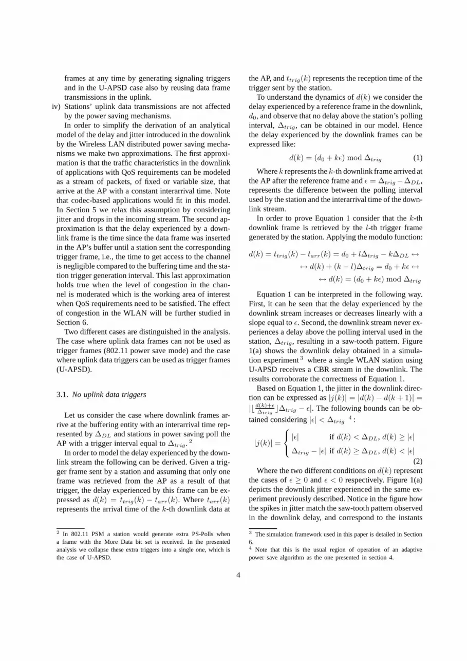
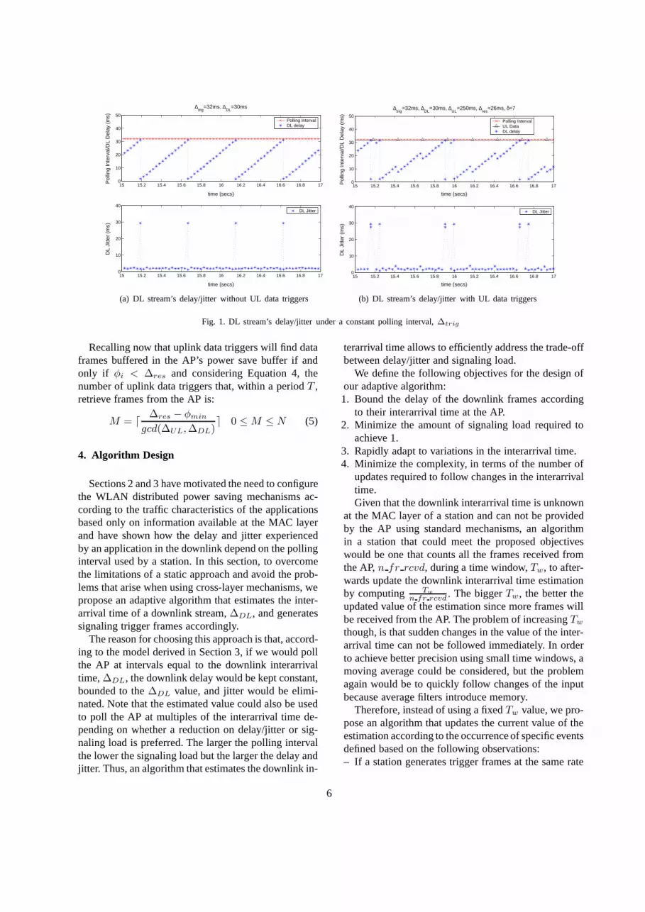
Equation 1 can be interpreted in the following way.First, it can be seen that the delay experienced by thedownlink stream increases or decreases linearly with aslope equal toǫ. Second, the downlink stream never ex-periences a delay above the polling interval used in thestation,∆trig, resulting in a saw-tooth pattern. Figure1(a) shows the downlink delay obtained in a simula-tion experiment3 where a single WLAN station usingU-APSD receives a CBR stream in the downlink. Theresults corroborate the correctness of Equation 1.

Based on Equation 1, the jitter in the downlink direc-tion can be expressed as|j(k)| = |d(k) − d(k + 1)| =

|⌊d(k)+ǫ

∆trig⌋∆trig − ǫ|. The following bounds can be ob-

tained considering|ǫ| < ∆trig4 :

|j(k)| =

|ǫ| if d(k) < ∆DL, d(k) ≥ |ǫ|

∆trig − |ǫ| if d(k) ≥ ∆DL, d(k) < |ǫ|

(2)Where the two different conditions ond(k) represent

the cases ofǫ ≥ 0 andǫ < 0 respectively. Figure 1(a)depicts the downlink jitter experienced in the same ex-periment previously described. Notice in the figure howthe spikes in jitter match the saw-tooth pattern observedin the downlink delay, and correspond to the instants

3 The simulation framework used in this paper is detailed in Section6.4 Note that this is the usual region of operation of an adaptivepower save algorithm as the one presented in section 4.

4

where the station generates a trigger frame retrievingmore than one data frame from the AP.

3.2. Uplink data triggers

Consider now the case where a station reuses uplinkdata frames as triggers. In this case a periodic triggergeneration solution turns out not to be optimal since trig-ger frames would be generated more often than∆trig.Thus, in order to avoid the introduction of unnecessarysignaling, are-schedulingmechanism should be used asit was proposed in [6]. This solution consists in schedul-ing a periodic generation of signaling triggers and re-scheduling the pending signaling trigger transmissionevery time a data trigger is sent in the uplink.

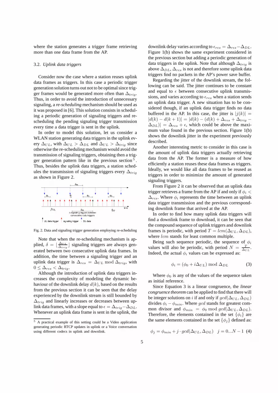
In order to model this solution, let us consider aWLAN station generating data triggers in the uplink ev-ery ∆UL, with ∆UL > ∆DL and∆UL > ∆trig sinceotherwise the re-scheduling mechanism would avoid thetransmission of signaling triggers, obtaining then a trig-ger generation pattern like in the previous section5 .Thus, besides the uplink data triggers, a station sched-ules the transmission of signaling triggers every∆trig

as shown in Figure 2.

Fig. 2. Data and signaling trigger generation employing re-scheduling

Note that when the re-scheduling mechanism is ap-plied, δ = ⌊ ∆UL

∆trig⌋ signaling triggers are always gen-

erated between two consecutive uplink data frames. Inaddition, the time between a signaling trigger and anuplink data trigger is∆res = ∆UL mod ∆trig, with0 ≤ ∆res < ∆trig.

Although the introduction of uplink data triggers in-creases the complexity of modeling the dynamic be-haviour of the downlink delayd(k), based on the resultsfrom the previous section it can be seen that the delayexperienced by the downlink stream is still bounded by∆trig and linearly increases or decreases between up-link data frames, with a slope equal toǫ = ∆trig−∆DL.Whenever an uplink data frame is sent in the uplink, the

5 A practical example of this setting could be a Video applicationgenerating periodic RTCP updates in uplink or a Voice conversationusing different codecs in uplink and downlink.

downlink delay varies according toǫres = ∆res−∆DL.Figure 1(b) shows the same experiment considered inthe previous section but adding a periodic generation ofdata triggers in the uplink. Note that although∆trig isabove∆DL, ∆res is not and therefore some uplink datatriggers find no packets in the AP’s power save buffer.

Regarding the jitter of the downlink stream, the fol-lowing can be said. The jitter continues to be constantand equal toǫ between consecutive uplink transmis-sions, and varies according toǫres when a station sendsan uplink data trigger. A new situation has to be con-sidered though, if an uplink data trigger finds no databuffered in the AP. In this case, the jitter is|j(k)| =|d(k) − d(k + 1)| = |d(k) − (d(k) + ∆res + ∆trig −∆DL)| = ∆res + ǫ, which could be above the maxi-mum value found in the previous section. Figure 1(b)shows the downlink jitter in the experiment previouslydescribed.

Another interesting metric to consider in this case isthe amount of uplink data triggers actually retrievingdata from the AP. The former is a measure of howefficiently a station reuses these data frames as triggers.Ideally, we would like all data frames to be reused astriggers in order to minimize the amount of generatedsignaling triggers.

From Figure 2 it can be observed that an uplink datatrigger retrieves a frame from the AP if and only ifφi <

∆res. Whereφi represents the time between an uplinkdata trigger transmission and the previous correspond-ing downlink frame that arrived at the AP.

In order to find how many uplink data triggers willfind a downlink frame to download, it can be seen thatthe compound sequence of uplink triggers and downlinkframes is periodic, with periodT = lcm(∆UL, ∆DL),wherelcm stands for least common multiple.

Being such sequence periodic, the sequence ofφi

values will also be periodic, with periodN = T∆UL

.Indeed, the actualφi values can be expressed as:

φi = (φ0 + i∆UL) mod ∆DL (3)

Whereφ0 is any of the values of the sequence takenas initial reference.

Since Equation 3 is a linear congruence, thelinearcongruence theoremcan be applied to find that there willbe integer solutions oni if and only if gcd(∆UL, ∆DL)dividesφi −φmin. Wheregcd stands for greatest com-mon divisor andφmin = φ0 mod gcd(∆UL, ∆DL).Therefore, the elements contained in the set{φi} arethe same elements contained in the set{φj} defined as:

φj = φmin + j · gcd(∆UL, ∆DL) j = 0...N − 1 (4)

5

15 15.2 15.4 15.6 15.8 16 16.2 16.4 16.6 16.8 170

10

20

30

40

50

time (secs)

Pol

ling

Inte

rval

/DL

Del

ay (

ms)

∆trig

=32ms, ∆DL

=30ms

15 15.2 15.4 15.6 15.8 16 16.2 16.4 16.6 16.8 170

10

20

30

40

time (secs)

DL

Jitte

r (m

s)

Polling IntervalDL delay

DL Jitter

(a) DL stream’s delay/jitter without UL data triggers

15 15.2 15.4 15.6 15.8 16 16.2 16.4 16.6 16.8 170

10

20

30

40

50

time (secs)

Pol

ling

Inte

rval

/DL

Del

ay (

ms)

∆trig

=32ms, ∆DL

=30ms, ∆UL

=250ms, ∆res

=26ms, δ=7

15 15.2 15.4 15.6 15.8 16 16.2 16.4 16.6 16.8 170

10

20

30

40

time (secs)

DL

Jitte

r (m

s)

DL Jitter

Polling IntervalUL DataDL delay

(b) DL stream’s delay/jitter with UL data triggers

Fig. 1. DL stream’s delay/jitter under a constant polling interval, ∆trig

Recalling now that uplink data triggers will find dataframes buffered in the AP’s power save buffer if andonly if φi < ∆res and considering Equation 4, thenumber of uplink data triggers that, within a periodT ,retrieve frames from the AP is:

M = ⌈∆res − φmin

gcd(∆UL, ∆DL)⌉ 0 ≤M ≤ N (5)

4. Algorithm Design

Sections 2 and 3 have motivated the need to configurethe WLAN distributed power saving mechanisms ac-cording to the traffic characteristics of the applicationsbased only on information available at the MAC layerand have shown how the delay and jitter experiencedby an application in the downlink depend on the pollinginterval used by a station. In this section, to overcomethe limitations of a static approach and avoid the prob-lems that arise when using cross-layer mechanisms, wepropose an adaptive algorithm that estimates the inter-arrival time of a downlink stream,∆DL, and generatessignaling trigger frames accordingly.

The reason for choosing this approach is that, accord-ing to the model derived in Section 3, if we would pollthe AP at intervals equal to the downlink interarrivaltime,∆DL, the downlink delay would be kept constant,bounded to the∆DL value, and jitter would be elimi-nated. Note that the estimated value could also be usedto poll the AP at multiples of the interarrival time de-pending on whether a reduction on delay/jitter or sig-naling load is preferred. The larger the polling intervalthe lower the signaling load but the larger the delay andjitter. Thus, an algorithm that estimates the downlink in-

terarrival time allows to efficiently address the trade-offbetween delay/jitter and signaling load.

We define the following objectives for the design ofour adaptive algorithm:1. Bound the delay of the downlink frames according

to their interarrival time at the AP.2. Minimize the amount of signaling load required to

achieve 1.3. Rapidly adapt to variations in the interarrival time.4. Minimize the complexity, in terms of the number of

updates required to follow changes in the interarrivaltime.Given that the downlink interarrival time is unknown

at the MAC layer of a station and can not be providedby the AP using standard mechanisms, an algorithmin a station that could meet the proposed objectiveswould be one that counts all the frames received fromthe AP,n fr rcvd, during a time window,Tw, to after-wards update the downlink interarrival time estimationby computing Tw

n fr rcvd. The biggerTw, the better the

updated value of the estimation since more frames willbe received from the AP. The problem of increasingTw

though, is that sudden changes in the value of the inter-arrival time can not be followed immediately. In orderto achieve better precision using small time windows, amoving average could be considered, but the problemagain would be to quickly follow changes of the inputbecause average filters introduce memory.

Therefore, instead of using a fixedTw value, we pro-pose an algorithm that updates the current value of theestimation according to the occurrence of specific eventsdefined based on the following observations:– If a station generates trigger frames at the same rate

6

that downlink frames arrive at the AP, each triggerframe will always result in a single frame deliveredby the AP.

– If a station generates trigger frames at a rate that isabove the rate of arrivals at the AP, each trigger framewill result in either one or no frames delivered by theAP.

– If a station generates trigger frames at a rate belowthe rate of arrivals at the AP, each trigger frame willresult in either one or more frames delivered by theAP.According to the above observations, two types of

events can be defined that univocally identify whetherthe estimation in the station is above or below the actualinterarrival time of the downlink packets at the AP.– No Data event: If a trigger is sent by a station and

no frame is delivered by the AP. This event impliesthat the station holds an estimation below the actualdownlink interarrival time.

– More Data event: If a trigger is sent by a stationand more than one frame is delivered by the AP.This event implies that the station holds an estimationabove the actual downlink interarrival time.These two events can be recognized at the MAC layer

of the stations using any of the distributed power sav-ing mechanisms available today. TheNo Dataevent canbe recognized because the AP delivers an empty frame,QoS Null, when a trigger is received but no data isbuffered. A more efficient method to signal this eventhas been proposed in [14], where the need to send ex-plicit signaling is avoided by making use of a bit avail-able in the ACK frames. Regarding the More Data event,it can be recognized by simply counting the number offrames received before getting a frame with the EOSPbit 6 set to 1 in the case of U-APSD, or monitoring theMore Data bit in the case of 802.11 power save mode.

An algorithm that aims to estimate the downlink in-terarrival time can be therefore proposed that increasesits current estimation whenever a No Data event occurs,and decreases its current estimation whenever a MoreData event occurs. The problem hence is to investigatehow the current value of the estimation,∆trig(n), has tobe updated every time an event occurs in order to con-verge to the actual downlink interarrival time. Where∆trig(n) represents the polling interval used by a sta-tion after then-th estimation update,n ∈ Z.

Our proposal is to use ansteepest descentalgorithmto update the estimation and converge to∆DL. Theidea behind the steepest descent algorithm is to esti-

6 The End Of Service Period (EOSP) bit signals the end of a ServicePeriod and allows a station to go back to sleep mode in U-APSD.

mate at each iteration the error between the current es-timation,∆trig(n), and the actual downlink interarrivaltime,∆DL, and use this information to update∆trig(n)in order to get closer to∆DL.

A steepest descent algorithm for a single variable, inthis case the variable∆trig, can be expressed as:

∆trig(n+1) = ∆trig(n)−γ∂

∂∆trig

J(∆trig(n)) (6)

Where∆trig(n) represents the current value of theestimation,γ > 0 is the adaptation step that controls thespeed of convergence andJ(∆trig) is a derivable andconvex error function that has a minimum at the pointwhere the algorithm converges. To avoid converging toa value other than∆DL we select an error function thathas only one minimum:

J(∆trig(n)) = (∆trig(n)− ∆DL)2 (7)

Where∆DL is an estimator of∆DL, that has to beused because the actual value of∆DL is the unknownvalue we are looking for. Thus, the successful conver-gence of the algorithm will depend on whether∆DL isa good estimation of∆DL. We consider:

∆DL =∆t(n)

n fr rcvd(n)(8)

Where ∆t(n) is the time measured at a stationbetween the current event and the previous one andn fr rcvd(n) is the number of frames that a stationhas retrieved from the AP during∆t(n), using a pollinginterval∆trig(n).

Based on the previous equations, our proposed algo-rithm will update the estimation every time an eventoccurs according to:

∆trig

(n+1) = ∆trig

(n)−γ(∆trig

(n)−∆

t(n)

n fr rcvd(n))

(9)The routine described in Algorithm 1 illustrates our

proposed implementation. This routine is executed bythe power saving stations every time a service period(SP7 ) completes.

Several points deserve special attention in Algorithm1. First, it can be observed in steps 16 and 25 that a dif-ferent value for the adaptation step is used dependingon whether the station experiences a More Data event,

7 We extend the U-APSD definition of Service Period in the contextof this paper to be used also in the case of 802.11 power save mode.Service Period is defined as the period of time that starts when astation sends a trigger frame and ends when a frame with EOSP=1in case of U-APSD or MD=0 in case of legacy power save modeis received from the AP.

7

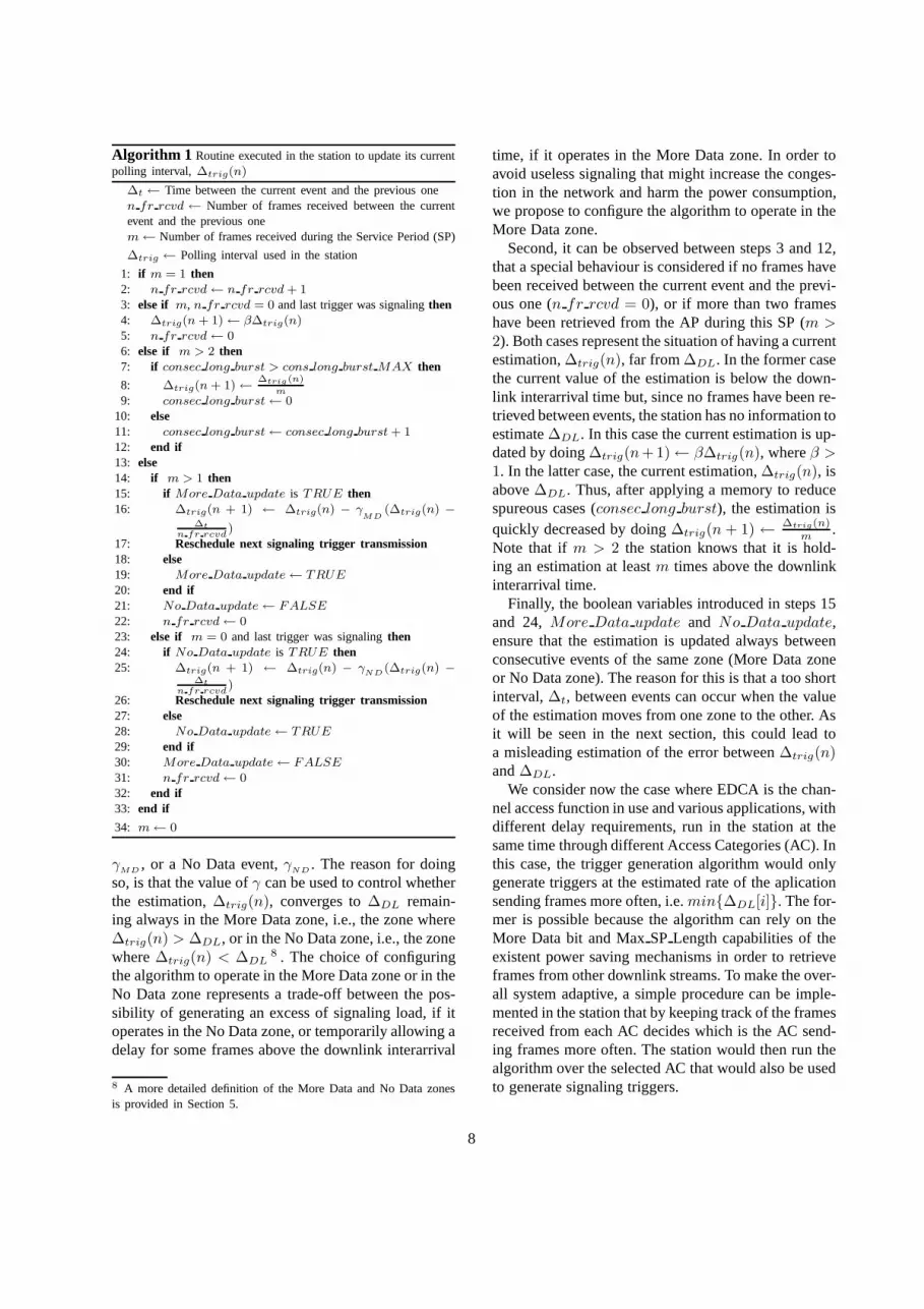
Algorithm 1 Routine executed in the station to update its currentpolling interval, ∆trig(n)

∆t ← Time between the current event and the previous onen fr rcvd ← Number of frames received between the currentevent and the previous onem← Number of frames received during the Service Period (SP)

∆trig ← Polling interval used in the station

1: if m = 1 then2: n fr rcvd← n fr rcvd + 13: else if m, n fr rcvd = 0 and last trigger was signalingthen4: ∆trig(n + 1)← β∆trig(n)5: n fr rcvd← 06: else if m > 2 then7: if consec long burst > cons long burst MAX then

8: ∆trig(n + 1)←∆trig(n)

m

9: consec long burst← 010: else11: consec long burst← consec long burst + 112: end if13: else14: if m > 1 then15: if More Data update is TRUE then16: ∆trig(n + 1) ← ∆trig(n) − γ

MD(∆trig(n) −

∆t

n fr rcvd)

17: Reschedule next signaling trigger transmission18: else19: More Data update← TRUE

20: end if21: No Data update← FALSE

22: n fr rcvd← 023: else if m = 0 and last trigger was signalingthen24: if No Data update is TRUE then25: ∆trig(n + 1) ← ∆trig(n) − γ

ND(∆trig(n) −

∆t

n fr rcvd)

26: Reschedule next signaling trigger transmission27: else28: No Data update← TRUE

29: end if30: More Data update← FALSE

31: n fr rcvd← 032: end if33: end if

34: m← 0

γMD

, or a No Data event,γND

. The reason for doingso, is that the value ofγ can be used to control whetherthe estimation,∆trig(n), converges to∆DL remain-ing always in the More Data zone, i.e., the zone where∆trig(n) > ∆DL, or in the No Data zone, i.e., the zonewhere∆trig(n) < ∆DL

8 . The choice of configuringthe algorithm to operate in the More Data zone or in theNo Data zone represents a trade-off between the pos-sibility of generating an excess of signaling load, if itoperates in the No Data zone, or temporarily allowing adelay for some frames above the downlink interarrival

8 A more detailed definition of the More Data and No Data zonesis provided in Section 5.

time, if it operates in the More Data zone. In order toavoid useless signaling that might increase the conges-tion in the network and harm the power consumption,we propose to configure the algorithm to operate in theMore Data zone.

Second, it can be observed between steps 3 and 12,that a special behaviour is considered if no frames havebeen received between the current event and the previ-ous one (n fr rcvd = 0), or if more than two frameshave been retrieved from the AP during this SP (m >

2). Both cases represent the situation of having a currentestimation,∆trig(n), far from∆DL. In the former casethe current value of the estimation is below the down-link interarrival time but, since no frames have been re-trieved between events, the station has no information toestimate∆DL. In this case the current estimation is up-dated by doing∆trig(n+1)← β∆trig(n), whereβ >

1. In the latter case, the current estimation,∆trig(n), isabove∆DL. Thus, after applying a memory to reducespureous cases (consec long burst), the estimation isquickly decreased by doing∆trig(n + 1) ←

∆trig(n)m

.Note that if m > 2 the station knows that it is hold-ing an estimation at leastm times above the downlinkinterarrival time.

Finally, the boolean variables introduced in steps 15and 24,More Data update and No Data update,ensure that the estimation is updated always betweenconsecutive events of the same zone (More Data zoneor No Data zone). The reason for this is that a too shortinterval,∆t, between events can occur when the valueof the estimation moves from one zone to the other. Asit will be seen in the next section, this could lead toa misleading estimation of the error between∆trig(n)and∆DL.

We consider now the case where EDCA is the chan-nel access function in use and various applications, withdifferent delay requirements, run in the station at thesame time through different Access Categories (AC). Inthis case, the trigger generation algorithm would onlygenerate triggers at the estimated rate of the aplicationsending frames more often, i.e.min{∆DL[i]}. The for-mer is possible because the algorithm can rely on theMore Data bit and MaxSPLength capabilities of theexistent power saving mechanisms in order to retrieveframes from other downlink streams. To make the over-all system adaptive, a simple procedure can be imple-mented in the station that by keeping track of the framesreceived from each AC decides which is the AC send-ing frames more often. The station would then run thealgorithm over the selected AC that would also be usedto generate signaling triggers.

8

The complete cycle of activity in a station can be sum-marized in the following terms. When a station is idleno trigger frames are generated. Once a Beacon frameis received anouncing the presence of buffered framesin the AP, a station starts generating trigger frames withan initial polling interval,∆trig(0), that is then dynam-ically adjusted by means of Algorithm 1. After sendinga certain number of consecutive trigger frames receiv-ing only empty frames from the AP a station considersthat the application has finished and switches back toidle mode again.

Finally, we conclude this section discussing a simpleheuristic that can be used to improve the performance ofthe algorithm when applications sending large packetsare considered. Large packets in the application layer,e.g. like those generated by video codecs, are in manycases fragmented resulting in bursts of packets arrivingat the AP which can mislead the algorithm into falseMore Data events. However, if the minimum MTU be-tween the application generating packets and the APis assumed to be known at the terminal, which with areasonable probability can be considered to be the Eth-ernet MTU, the misleading effect of large packets canbe reduced by remembering the size in the MAC layerof the packets downloaded during a service period, andconsidering as a single packet adjacent packets of sizeequal to the expected MTU9 .

4.1. Convergence to a multiple of the interarrivaltime: ∆trig → k∆DL

If a delay and jitter above∆DL can be afforded,further power saving and signaling load enhancementscan be obtained by modifying Algorithm 1 to convergeto a multiple of the downlink interarrival time,∆trig →k∆DL, wherek is an integer bigger than1. The largerthe value ofk can be set, the larger the potential increasein power saving and reduction of signaling load.

In order to achieve this, Equation 9 has to be modi-fied such that the equilibrium state is reached when thetrigger interval used by a station,∆trig, equals the de-sired multiple of the interarrival time:

∆trig

(n+1) = ∆trig

(n)−γ(∆trig

(n)−k∆

t(n)

n fr rcvd(n))

(10)In addition, theNo DataandMore Dataevents gen-

eration, which trigger an update of the current polling

9 This heuristic would fail if packets of size equal to the MTUminus overheads are generated by the applications, but we considerthis probability to be small.

interval, also need to be adjusted accordingly. In thiscase,No Dataevents will be generated when less thank frames are received within one service period whileMore Dataevents will be generated when more thank

frames are received within one service period.In the rest of the paper we focus in the case of the

polling interval converging to the downlink interarrivaltime, k = 1, since it is the one with the most stringentQoS requirements and thus, the most demanding for theproposed adaptive algorithm.

5. Algorithm Analysis

In this section we use the model presented in Section3 in order to gain a deeper understanding on the proper-ties of the adaptive algorithm presented in the previoussection. First, we study under which conditions the al-gorithm converges. Second, the convergence speed ofthe algorithm is analyzed providing a worst case boundon the required number of iterations. Finally, we discusshow the performance of the algorithm degrades whenthe assumptions of the model do not hold.

5.1. Proof of Convergence

For the analysis, we defineconvergenceas theprocess of making the estimation,∆trig(n), continu-ously approach at each iteration the actual downlinkinterarrival time, ∆DL, while always guaranteeing∆trig(n) ≥ ∆DL. Some of the reasons for preferringto keep∆trig(n) ≥ ∆DL have already been providedin Section 4. Additionally, further reasons will begiven in this section. The same analysis presented herethough, could be also applied if it would be preferredthat the algorithm converges to∆DL guaranteeing∆trig(n) ≤ ∆DL.

Throughout the analysis we refer to the set of valuesof the estimation,∆trig(n), that are above∆DL as theMore datazone, since only More Data events can beobserved by the station in this zone. Similarly, the set ofvalues of the estimation below∆DL are referred to asthe No Datazone. The different zones of convergenceare depicted in Figure 3.

To demonstrate the convergence of the algorithm wewill prove that if the current value of the estimation,∆trig(n), is above the downlink interarrival time,∆DL,the next estimation update will result in a smaller value,∆trig(n+1), either above or equal to∆DL. It is impor-tant to note though that when the algorithm starts thestation’s initial polling interval,∆trig(0), could be be-low the downlink interarrival time. If the initial value is

9

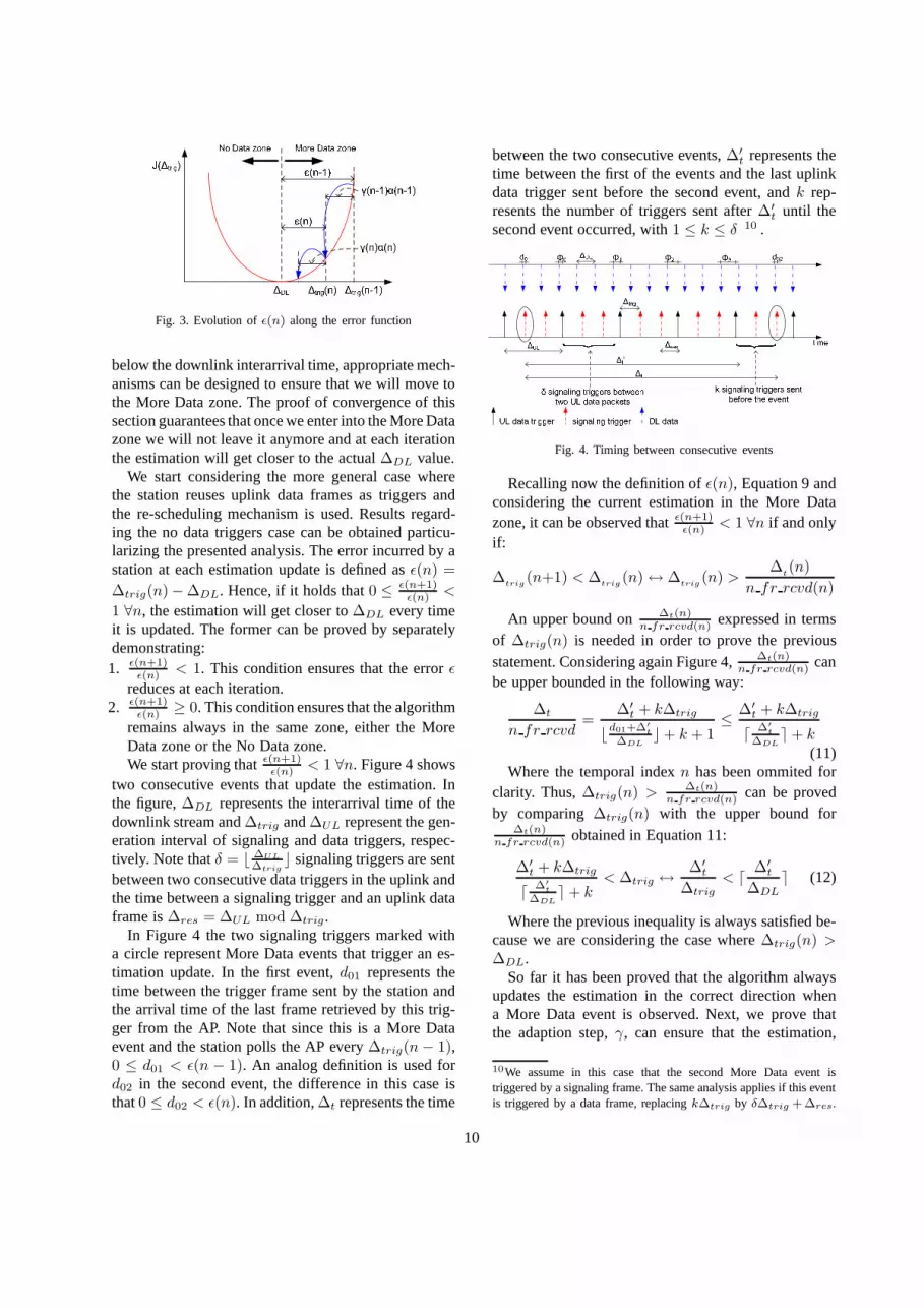
Fig. 3. Evolution ofǫ(n) along the error function

below the downlink interarrival time, appropriate mech-anisms can be designed to ensure that we will move tothe More Data zone. The proof of convergence of thissection guarantees that once we enter into the More Datazone we will not leave it anymore and at each iterationthe estimation will get closer to the actual∆DL value.

We start considering the more general case wherethe station reuses uplink data frames as triggers andthe re-scheduling mechanism is used. Results regard-ing the no data triggers case can be obtained particu-larizing the presented analysis. The error incurred by astation at each estimation update is defined asǫ(n) =

∆trig(n)−∆DL. Hence, if it holds that0 ≤ ǫ(n+1)ǫ(n) <

1 ∀n, the estimation will get closer to∆DL every timeit is updated. The former can be proved by separatelydemonstrating:1. ǫ(n+1)

ǫ(n) < 1. This condition ensures that the errorǫ

reduces at each iteration.2. ǫ(n+1)

ǫ(n) ≥ 0. This condition ensures that the algorithmremains always in the same zone, either the MoreData zone or the No Data zone.We start proving thatǫ(n+1)

ǫ(n) < 1 ∀n. Figure 4 showstwo consecutive events that update the estimation. Inthe figure,∆DL represents the interarrival time of thedownlink stream and∆trig and∆UL represent the gen-eration interval of signaling and data triggers, respec-tively. Note thatδ = ⌊ ∆UL

∆trig⌋ signaling triggers are sent

between two consecutive data triggers in the uplink andthe time between a signaling trigger and an uplink dataframe is∆res = ∆UL mod ∆trig.

In Figure 4 the two signaling triggers marked witha circle represent More Data events that trigger an es-timation update. In the first event,d01 represents thetime between the trigger frame sent by the station andthe arrival time of the last frame retrieved by this trig-ger from the AP. Note that since this is a More Dataevent and the station polls the AP every∆trig(n− 1),0 ≤ d01 < ǫ(n − 1). An analog definition is used ford02 in the second event, the difference in this case isthat0 ≤ d02 < ǫ(n). In addition,∆t represents the time

between the two consecutive events,∆′

t represents thetime between the first of the events and the last uplinkdata trigger sent before the second event, andk rep-resents the number of triggers sent after∆′

t until thesecond event occurred, with1 ≤ k ≤ δ 10 .

Fig. 4. Timing between consecutive events

Recalling now the definition ofǫ(n), Equation 9 andconsidering the current estimation in the More Datazone, it can be observed thatǫ(n+1)

ǫ(n) < 1 ∀n if and onlyif:

∆trig

(n+1) < ∆trig

(n)↔ ∆trig

(n) >∆

t(n)

n fr rcvd(n)

An upper bound on ∆t(n)n fr rcvd(n) expressed in terms

of ∆trig(n) is needed in order to prove the previous

statement. Considering again Figure 4,∆t(n)n fr rcvd(n) can

be upper bounded in the following way:

∆t

n fr rcvd=

∆′

t + k∆trig

⌊d01+∆′

t

∆DL⌋+ k + 1

≤∆′

t + k∆trig

⌈∆′

t

∆DL⌉+ k

(11)Where the temporal indexn has been ommited for

clarity. Thus,∆trig(n) >∆t(n)

n fr rcvd(n) can be provedby comparing∆trig(n) with the upper bound for

∆t(n)n fr rcvd(n) obtained in Equation 11:

∆′

t + k∆trig

⌈∆′

t

∆DL⌉+ k

< ∆trig ↔∆′

t

∆trig

< ⌈∆′

t

∆DL

⌉ (12)

Where the previous inequality is always satisfied be-cause we are considering the case where∆trig(n) >

∆DL.So far it has been proved that the algorithm always

updates the estimation in the correct direction whena More Data event is observed. Next, we prove thatthe adaption step,γ, can ensure that the estimation,

10We assume in this case that the second More Data event istriggered by a signaling frame. The same analysis applies ifthis eventis triggered by a data frame, replacingk∆trig by δ∆trig + ∆res.

10

∆trig(n), does not bounce between the More Data and

the No Data zones, i.e.,ǫ(n+1)ǫ(n) ≥ 0.

Considering Equation 9, it can be seen that theef-fectivestep taken by the algorithm to update the cur-rent estimation isγ(n)α(n), with α(n) = ∆trig(n) −

∆t(n)n fr rcvd(n) . From Figure 3 and assuming a value of theestimation in the More Data zone, it can be observedthat the updated value of the estimation,∆trig(n + 1),will remain in the More Data zone if and only if thestep taken by the algorithm at this iteration is smallerthan the current error, i.e.,γ(n)α(n) ≤ ǫ(n).

In order to obtain an upper bound onγ(n) that en-sures∆trig(n + 1) ≥ ∆DL, note first that based onthe relations illustrated in Figure 4, ∆t(n)

n fr rcvd(n) can beexpressed as:

∆t(n)

n fr rcvd(n)= ∆DL +

d02 − d01

n fr rcvd(n)(13)

Recalling the definition ofα(n) and the previous equa-tion we can expressα(n) as:

α(n) = ∆trig(n)−∆t(n)

n fr rcvd(n)=

= ǫ(n)−d02 − d01

n fr rcvd(n)(14)

Considering now that0 ≤ d01 < ǫ(n−1) and that, fromEquation 9,ǫ(n − 1) can be expressed asǫ(n − 1) =ǫ(n) + γ(n − 1)α(n − 1), the following upper boundon α(n) can be obtained:

α(n) < ǫ(n)n fr rcvd(n) + 1

n fr rcvd(n)+

γ(n− 1)α(n− 1)

n fr rcvd(n)

Thus, the previous upper bound onα(n) can be turnedinto a lower bound onǫ(n) and recalling the conditionto keep the next value of the estimation in the MoreData zone,γ(n)α(n) < ǫ(n), a conservativeγ(n) canbe found,γ

CONS(n), that keeps the estimation always

in the desired zone of convergence:

γ(n) <n fr rcvd(n) − γ(n− 1)α(n−1)

α(n)

n fr rcvd(n) + 1= γ

CONS(n)

(15)Continuing with the previous reasoning and going

back to Equation 14 while recalling that0 ≤ d02 <

ǫ(n), a lower bound onα(n) can be obtained. Applyingthe same analysis to this bound, an aggressive bound onγ(n) that forces the estimation to jump from one zoneto the other can also be obtained, being:

γ(n) >n fr rcvd(n)

n fr rcvd(n) − 1= γ

AGGR(n) (16)

Although the previous bounds,γCONS

(n) andγ

AGGR(n), have been derived under the assumption of

having the estimation in the More Data zone, Equations15 and 16 hold true also in the No Data zone.

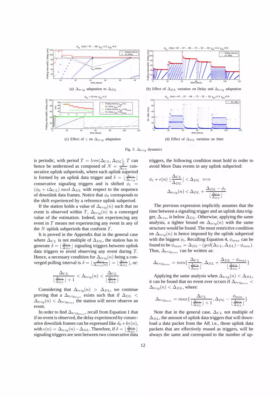
To illustrate how the algorithm updates the estima-tion while keeping always a value in the More Datazone, Figure 5(a) depicts the delay and polling intervalexperienced by a WLAN station using U-APSD thatretrieves a CBR stream from the AP. The values ofγ

in the More Data and No Data zone,γMD

and γND

,are constant and chosen below and above the corre-spondingγ

CONSandγ

AGGRthresholds. From the fig-

ure, it is worth noting how the time between events in-creases as the error in the estimation reduces, as pre-dicted by the model introduced in Section 3. This prop-erty of the algorithm has the interesting consequencethat, in the limit, the sequence of uplink triggers gener-ated by the station and downlink frames arriving at theAP would synchronize, i.e.,limt→∞ d(k) = 0. Notethough, that if the algorithm would converge from theNo Data zone, the behaviour in the limit would be dif-ferent, i.e.limt→∞ d(k) = ∆DL. Hence this is anotherreason to make the algorithm converge from the MoreData zone.

It has been proved so far thatǫ(n) reduces at eachestimation update. In order to update the estimationthough, the station has to keep observing new events.Hence, a new question arises that is whether the sta-tion will always observe enough events to make the es-timation converge to∆DL. We prove in the followingparagraphs that:1. If no data triggers in the uplink are considered, the

proposed algorithm always converges to∆DL.2. If data triggers in the uplink are considered, the pro-

posed algorithm can converge to a compact set ofvalues around∆DL. In this case though, all the algo-rithm’s requirements described in section 4 are alsofulfilled.To prove the previous statements, the case where the

station generates uplink data triggers is considered. Theresults obtained are afterwards particularized to the casewith no data triggers in the uplink.

The convergedvalues of ∆trig(n) are defined asthose values that prevent the station from observing anyfurther event. In order to find those values we defineφi, 0 ≤ φi < ∆DL, which represent the time differ-ence between an uplink data trigger sent by a stationand the last downlink arrival at the AP. See Figure 4 fora graphical representation.

As mentioned in Section 3, the compound sequenceof uplink triggers and downlink frames in our model

11

41 42 43 44 45 46

20

40

60

80

100

120

time (secs)

Pol

ling

Inte

rval

/DL

Del

ay (

ms)

∆DL

(ms) = 67 → 86, γND

=1.5, γMD

=0.5

Polling IntervalDL Delay

∆trig

updates

(a) ∆trig adaptation to∆DL

0 20 40 60 80 100 1200

20

40

60

80

100

120

time (secs)

Pol

ling

Inte

rval

/DL

Del

ay (

ms)

∆DL

(ms) = 42 → 67 → 86 → 73 → 52 → 33, γND

=1.5, γMD

=0.5

Polling IntervalDL delay

(b) Effect of ∆DL variation on Delay and∆trig adaptation

0 20 40 60 80 100 1200

20

40

60

80

100

time (secs)

Pol

ling

Inte

rval

/DL

Del

ay (

ms)

∆DL

= 42 ms, γND

=1.5

1 2 3 4 5

42

44

46

48

(ms)

Polling Interval, γMD

=0.2 DL Delay, γ

MD=0.2

Polling Interval, γMD

=0.9γCONS

DL Delay, γMD

=0.9γCONS

(c) Effect of γ on ∆trig adaptation

0 20 40 60 80 100 1200

20

40

60

80

100

time (secs)

DL

Jitte

r (m

s)

∆DL

(ms) = 42 → 67 → 86 → 73 → 52 → 33, γND

=1.5, γMD

=0.5

DL Jitter

(d) Effect of ∆DL variation on Jitter

Fig. 5. ∆trig dynamics

is periodic, with periodT = lcm(∆UL, ∆DL). T canhence be understood as composed ofN = T

∆ULcon-

secutive uplink subperiods, where each uplink superiodis formed by an uplink data trigger andδ = ⌊ ∆UL

∆trig⌋

consecutive signaling triggers and is shiftedφi =(φ0 + i∆UL) mod ∆DL with respect to the sequenceof downlink data frames. Notice thatφ0 corresponds tothe shift experienced by a reference uplink subperiod.

If the station holds a value of∆trig(n) such that noevent is observed withinT , ∆trig(n) is a convergedvalue of the estimation. Indeed, not experiencing anyevent inT means not experiencing any event in any oftheN uplink subperiods that conformT .

It is proved in the Appendix that in the general casewhere∆UL is not multiple of∆DL, the station has togenerateδ = ⌊∆UL

∆DL⌋ signaling triggers between uplink

data triggers to avoid observing any event duringT .Hence, a necessary condition for∆trig(n) being a con-verged polling interval isδ = ⌊ ∆UL

∆trig(n)⌋ = ⌊∆UL

∆DL⌋, or:

∆UL

⌊∆UL

∆DL⌋+ 1

< ∆trig(n) <∆UL

⌊∆UL

∆DL⌋

Considering that∆trig(n) > ∆DL, we continueproving that a∆trigmax

exists such that if∆DL <

∆trig(n) < ∆trigmaxthe station will never observe an

event.In order to find∆trigmax

, recall from Equation 1 thatif no event is observed, the delay experienced by consec-utive downlink frames can be expressed liked0+kǫ(n),with ǫ(n) = ∆trig(n)−∆DL. Therefore, ifδ = ⌊∆UL

∆DL⌋

signaling triggers are sent between two consecutive data

triggers, the following condition must hold in order toavoid More Data events in any uplink subperiod:

φi + ǫ(n) ⌊∆UL

∆DL

⌋< ∆DL ⇐⇒

∆trig(n) < ∆DL +∆DL − φi

⌊∆UL

∆DL⌋

The previous expression implicitly assumes that thetime between a signaling trigger and an uplink data trig-ger,∆res, is below∆DL. Otherwise, applying the sameanalysis, a tighter bound on∆trig(n) with the samestructure would be found. The most restrictive conditionon ∆trig(n) is hence imposed by the uplink subperiodwith the biggestφi. Recalling Equation 4,φmax can befound to beφmax = ∆DL−(gcd(∆UL, ∆DL)−φmin).Thus,∆trigmax

can be written as:

∆trigmax= min{

∆UL

⌊∆UL

∆DL⌋, ∆DL +

∆DL − φmax

⌊∆UL

∆DL⌋}

Applying the same analysis when∆trig(n) < ∆DL,it can be found that no event ever occurs if∆trigmin

<

∆trig(n) < ∆DL, where:

∆trigmin= max{

∆UL

⌊∆UL

∆DL⌋+ 1

, ∆DL −φmin

⌊∆UL

∆DL⌋}

Note that in the general case,∆UL not multiple of∆DL, the amount of uplink data triggers that will down-load a data packet from the AP, i.e., those uplink datapackets that are effectively reused as triggers, will bealways the same and correspond to the number of up-

12

link subperiods where⌈∆UL

∆DL⌉ downlink frames arrive

at the AP. This number is found in the Appendix.In the particular case where∆UL is a multiple of

∆DL, the same analysis can be applied to find a newconvergedvalue of∆trig located above∆DL, ∆′

trigmax,

such that onlyδ = ⌊∆UL

∆DL⌋ − 1 signaling triggers are

generated by a station between uplink data triggers. Thisis again another argument to prefer the convergence ofthe algorithm from the More Data zone.

Note that regardless of the final converged value esti-mated in the station, the original requirements of the al-gorithm are always being fulfilled by the way the eventshave been defined. First, if a More Data event never oc-curs, the delay is effectively bounded to the downlinkinterarrival time. Second, if a No Data event never oc-curs, no useless signaling is generated.

The converged values of∆trig(n) when no uplinkdata frames are reused as triggers can be obtained fromthe expressions of∆trigmin

and∆trigmaxby observing

that:

lim∆UL→∞

∆trigmin= lim

∆UL→∞

∆trigmax= ∆DL

Therefore, without uplink data triggers, the only con-verged value of∆trig(n) that refrains the station fromobserving any event is∆trig(n) = ∆DL.

Finally, to illustrate the analysis of convergence in-troduced in this section, Figures 5(b) and 5(d) depictthe delay and jitter experienced by a downlink streamwhose interarrival time is changed in a step-like fash-ion. The WLAN station is configured as in the experi-ment for Figure 5(a) and generates data triggers in theuplink every 90ms during the time intervals (20,40) and(80,100) seconds.

As predicted in the analysis, it can be observed bythe constantly decreasing slope of the delay curves that,when no uplink data triggers are considered, the algo-rithm constantly approaches∆DL. In the time intervalswhere the station sends uplink data triggers though, thepredicted periodic situation in the channel is observed.Note that the different jitter levels observed in Figure5(d) correspond to the different values predicted in themodel introduced in Section 3.

5.2. Speed of Convergence

In the previous section it has been proved that theproposed algorithm always converges to a value thatfulfills our design objectives. In this section we studythe speed of the algorithm to converge to such a value.

Our goal is to find an upper bound on the number ofupdates needed in order to reduce an initial errorǫ(0)

to ǫ(n) < α∆DL, whereα is a variable defined for thepurpose of this analysis,0 < α < 1.

Assuming that our algorithm operates in the MoreData zone, as recommended, and recalling Equation 13,the error experienced in the next estimation update canbe expressed and upper bounded in the following way:

ǫ(n + 1) = ǫ(n)(1 − γ) + γd02 − d01

n fr rcvd(n)<

< ǫ(n)(1 − γΨ(n))

WhereΨ(n) = n fr rcvd(n)−1n fr rcvd(n) and0 ≤ d02 < ǫ(n).

Note thatΨ(n) is a monotonically growing functionof n fr rcdv(n) and since the minimum number offrames that a station can retrieve from the AP be-tween two consecutive More Data events is2 then12 < Ψ(n) < 1.

Based on that, a lower bound on the speed with whichthe error decreases can be obtained as:

ǫ(n + k)

ǫ(n)<

k−1∏

j=0

(1 − γΨ(n + j)) < (1−1

2γ)k

Where a constant adaptation step,γ has been as-sumed. If γ would be adaptive, its minimum valueshould be considered in order to obtain the previousbound.

Note that the adaptation step,γ, can be effectivelyused to control the speed of convergence. Neverthe-less, an upper bound,γ

CONS, was found in the previous

section in order to guarantee the convergence keepingthe value of the estimation always in the same zone.A trade-off between speed of convergence and stabilitycontrolled by the adaptation step is an intrinsic charac-teristic of the steepest descent algorithm.

If the algorithm converges faster than(1− 12γ)k, an

upper bound on the number of updates needed to reducethe error of the estimation fromǫ(0) to α∆DL, can befound as:

Kmax = − log(ǫ(0)

α∆DL

)1

log(1− 12γ)

The former upper bound holds true regardless ofwhether the station generates uplink data triggers ornot. The difference will be on the time needed to reachthe critical number of estimation updates,Kmax. Thereason is that the time between consecutive events isdifferent depending on whether uplink data triggers areconsidered or not. In any case though, the time betweenevents increases when the error in the estimation,ǫ(n),decreases.

The benefits of updating the estimation in a wayproportional to 1

ǫ(n) are indeed twofold. On the one

13

hand, the algorithm will react fast when there are sud-den changes in the downlink interarrival time, becausethe error,ǫ(n), will increase. On the other hand, if thedownlink interarrival time remains stable, the algorithmminimizes the required computational load by relaxingthe frequency of updates asǫ(n) decreases.

Finally, to illustrate how the adaptation step can beused to tune the speed of convergence, in Figure 5(c) weshow how a WLAN station using U-APSD estimates aninterarrival time of 42ms using two different values ofγ

MD, γ

MD= 0.2 andγ

MD= 0.9γ

CONS. A noticeable

faster estimation is observed whenγMD

= 0.9γCONS

,while keeping the estimation always in the More Datazone.

5.3. Relaxing the Assumptions of the Model

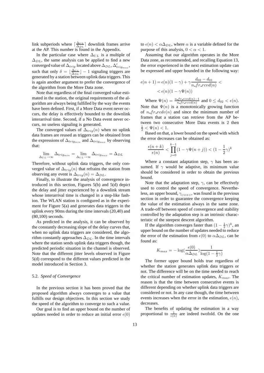
In order to derive the convergence properties of ouradaptive algorithm we have assumed so far that thedownlink and uplink data streams were essentially pe-riodic. However, this strong assumption only holds inreality when congestion in the wired and wireless partsof the network is kept very low. In this section we takea simulative approach in order to analyze the degrada-tion experienced by the algorithm when the previousassumptions are not valid.

We consider the same scenario used for Figure 5(a),but having a downlink stream with an interarrival timeof 30ms and introducing behind the AP a virtual nodewhich delays every incoming packet by a random valueuniformly distributed between0 and Jms, and dropsevery incoming packet with probabilityP . Thus, wewant to study the robustness of the adaptive algorithmto increasing values ofJ andP .

Figure 6(a) depicts the dynamics of the algorithm inthe presence of jitter (upper graph) and packet drops(lower graph). The first remarkable point is that as ob-served in both graphs the essential behavior predicted inSection 3, a saw-tooth pattern for delay, is maintainedin the presence of jitter and packet drops. The actualdynamics though slightly differ in either case. In bothcases, jitter or drops, if a trigger is sent and no frameis present in the AP the algorithm will experience a NoData event. On the one hand, if the missing frame wasdelayed due to jitter, the next time the station triggersthe AP it will probably retrieve two frames, thus expe-riencing a More Data event. Since the algorithm is de-signed to only update the estimation between consecu-tive events of the same type (see Algorithm 1), No Dataevents and More Data events cancel out in the case ofjitter resulting in a very stable estimation. On the other

hand, if the No Data event was due to a packet drop thealgorithm will not experience a More Data event in thenext trigger which results in sporadic increases of theestimation above the target polling interval.

To better quantify the effects of jitter and packetdrops on the algorithm performance we increaseJ from0ms → 50ms andP from 0.1% → 20%. This rangefor jitter and drops covers the margins recommendedby ITU-T in [15]. Figure 6(b) illustrates for this exper-iment the worst case downlink delay and the amountof null triggers (triggers sent by the station which findno data in the AP). The results show how the algo-rithm can maintain a bounded delay for the downlinkstream for a large range of jitter and drops,J < 40ms

andP < 10%. However, as the jitter and packet dropsincrease, degradation unavoidably appears in terms ofnull triggers which could result in an increased level ofcongestion in the network.

6. Performance Evaluation

In this section we present a performance evaluationof our proposed adaptive algorithm. We divide this per-formance evaluation in two subsections. First, subsec-tion 6.1 discusses the behavior of our adaptive algo-rithm when used with different applications in a typicalWi-Fi deployment. Second, subsection 6.2 analyzes thescalability and peformance of our adaptive algorithm ascongestion in the WLAN increases.

The analysis has been performed via simulations. Weextended the 802.11 libraries provided by OPNET [16]to include the power saving extensions defined in 802.11and 802.11e and our proposed adaptive trigger genera-tion algorithm.

We consider infrastructure mode WLANs, with anAP beacon interval of 100ms. The physical layer cho-sen in our simulations is 802.11b with all stations trans-mitting at 11Mbps.

Next, we present a definition of atraffic mix that weconsider representative of todays typical Wi-Fi deploy-ments. Throughout this section we will consider sta-tions using one/various of the applications that conformthis traffic mix. Sometimes we will use the concept of aclusterof stations, which we define as a group of fourstations where each station runs one of the applicationsdefined in our traffic mix. Together with each appli-cation we indicate the EDCA access category used totransmit traffic of this application:– AC VO: G.711 Voice codec with silence suppression.

Data rate: 64kbps. Frame length: 20ms. Talk spurtexponential with mean 0.35s and silence spurt expo-

14

18 20 22 24 26 28 30 32 34 36 38 400

10

20

30

40

50

(ms)

Impact of Jitter (uniform(0,10ms))

18 20 22 24 26 28 30 32 34 36 38 400

20

40

60

80

Time (secs)

(ms)

Impact of Packet Drops (5%)

Polling IntervalDL delay

Polling IntervalDL delay

(a) Dynamics of the algorithm in presence of jitter or drops

0 5 10 15 20 25 30 35 40 45 500

10

20

30

40

50

60

CD

F 9

5 D

elay

(m

s)

0 5 10 15 20 25 30 35 40 45 500

0.5

1

1.5

2

2.5

Maximum Jitter, X (ms)

Effect of Jitter

0

10

20

30

40

50

60

10−1

100

101

0

0.5

1

1.5

2

2.5Effect of Packet Drops

Packet Drops(%)

Nul

l Trig

gers

(pa

cket

s/se

c)

CDF95 DelayNull Triggers Rate

CDF95 DelayNull Triggers Rate

(b) Performance with varying jitter and drops

Fig. 6. Behavior of the algorithm when relaxing the assumptions of the model

nential with mean 0.65s.– AC VI: Streaming video download. MPEG-4 real

traces of the movie ’Star Trek: First Contact’ obtainedfrom [17]. Target rate: 64kbps. Frame generation in-terval: 40ms.

– AC BE: Web traffic. Page interarrival time exponen-tially distributed with mean 60s. Page size 10KB plus1 to 5 images of a size uniformly distributed between10KB and 100KB.

– AC BK: FTP download. File size of 1 MB. Interre-quest time exponentially distributed with mean 60s.For our experiments we consider that stations in the

WLAN communicate through the AP with stations in awired domain. The wired domain is modeled as an Eth-ernet segment behind the AP and a virtual node whichrepresents the backbone of the wired network and in-troduces jitter and drops. Based on [15] we considerthat the Voice and Video traffic traversing the backbonenetwork suffer a maximum delay variation of5ms anda 0.1% packet drop probability. Additionally Web andFTP applications communicate with a server using TCPNew Reno and experiencing an RTT of 20ms.

As previously mentioned the channel access functionconsidered in our simulations is EDCA. We assume afixed configuration of the EDCA QoS parameters basedon the 802.11e standard recommendation [2]. The pa-rameters used are detailed in Table 1.

Throughout this section our adaptive algorithm willbe configured in the following way. The initial pollinginterval,∆trig(0), is set to 10ms,consecutive long burst

is 2,β is set to 1.5 and the algorithm switches off aftersending three consecutive triggers without finding datain the AP.

In addition we will consider that all the trigger gen-

EDCA AIFS CWmin CWmax TXOP length

AC VO 2 31 63 3.264 ms

AC VI 2 63 127 6.016 ms

AC BE 3 127 1023 0

AC BK 7 127 1023 0

Table 1EDCA configuration for the different ACs

eration algorithms studied in this section use U-APSD,configured withMax SPLengthset toAll, instead ofLegacy Power Save Mode, due to its better support forQoS.

6.1. Dynamics of the algorithm with realisticapplications

In order to study how our adaptive algorithm behaveswith different applications we consider the followingscenario. A set of five clusters, which results in a totalof 20 stations in the network, generate traffic accordingto our defined traffic mix. This traffic is considered to bebackground load in the WLAN. In addition we considera tagged station configured to run the specific applica-tion that we want to study. In this section we will con-sider this station running the following applications: i)VoIP with silence suppression, ii) Video Streaming, iii)TCP download and iv) a mix of different applications.

6.1.1. VoIP with VADA G.711 voice codec with voice activity detection

(VAD) has been considered in our experiments.

15

30 30.5 31 31.5 32 32.5 33 33.5 340

20

40

60

Time (secs)

Pol

ling

Inte

rval

/DL

Del

ay (

ms)

G.711@20ms with VAD

Polling Interval (∆trig

)

Voice DL DelayUL Voice Data

(a) Adaptive algorithm behavior with VoIP and VAD

160 165 170 175 180 185 190 195 2000

20

40

60

80

100

Time (secs)

Pol

ling

Inte

rval

/DL

Del

ay (

ms)

Streaming Video

160 165 170 175 180 185 190 195 2000

1.52

4

(KB

s)

Polling Interval wo. MTU Heur.Polling Interval w. MTU Heur.DL delay w. MTU Heur.

(b) Adaptive algorithm behavior with MPEG 4 Video Streaming

20 20.1 20.2 20.3 20.4 20.5 20.6 20.7 20.8 20.9 21 21.1 21.2 21.3 21.4 21.50

100

200

300

400

500

600

700

Time (secs)

Rec

eive

d D

ata

(Kbi

ts)

RTT = 20ms

Active ModeBeacon−based PSMAdaptive

(c) TCP download comparison

20 40 60 80 100 120 140 160 180 2002

3

4

5

6

7

8

RTT (ms)

(sec

onds

)

Download Time of a 500KB file

Active ModeBeacon−based PSMAdaptive−2Adaptive−5

(d) Effect of the RTT on the TCP download time

138 139 140 141 142 143 144 1450

20

40

60

80

100

Time (secs)

Pol

ling

Inte

rval

/DL

Del

ay (

ms)

Simultaneous Video and Web

Polling Interval (∆trig

)

Video DL DelayDL Web Arrivals

(e) Simultaneous Video and Web

11 12 13 14 15 16 170

20

40

60

80

100

120

Time (secs)

Pol

ling

Inte

rval

/DL

Del

ay (

ms)

Simultaneous Video and Voice with VAD

Polling Interval (∆trig

)

Video DL DelayUL Voice DataDL Voice Data

Case 1 Case 2

(f) Simultaneous Video and Voice with VAD

Fig. 7. Instantaneous Adaptive algorithm behaviour

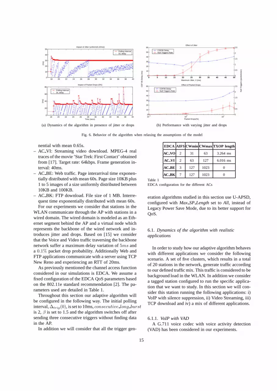
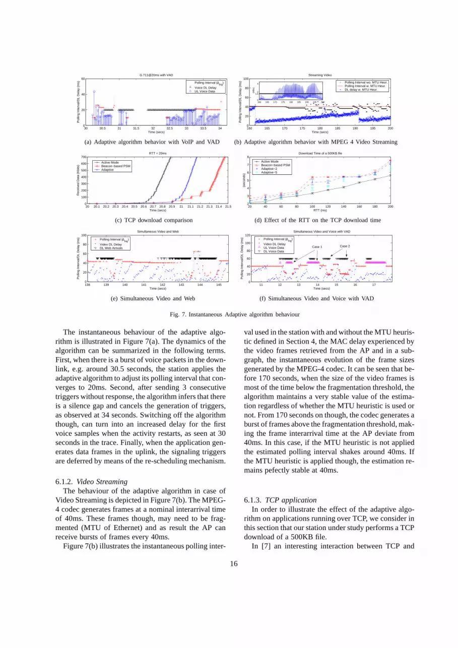
The instantaneous behaviour of the adaptive algo-rithm is illustrated in Figure 7(a). The dynamics of thealgorithm can be summarized in the following terms.First, when there is a burst of voice packets in the down-link, e.g. around 30.5 seconds, the station applies theadaptive algorithm to adjust its polling interval that con-verges to 20ms. Second, after sending 3 consecutivetriggers without response, the algorithm infers that thereis a silence gap and cancels the generation of triggers,as observed at 34 seconds. Switching off the algorithmthough, can turn into an increased delay for the firstvoice samples when the activity restarts, as seen at 30seconds in the trace. Finally, when the application gen-erates data frames in the uplink, the signaling triggersare deferred by means of the re-scheduling mechanism.

6.1.2. Video StreamingThe behaviour of the adaptive algorithm in case of

Video Streaming is depicted in Figure 7(b). The MPEG-4 codec generates frames at a nominal interarrival timeof 40ms. These frames though, may need to be frag-mented (MTU of Ethernet) and as result the AP canreceive bursts of frames every 40ms.

Figure 7(b) illustrates the instantaneous polling inter-

val used in the station with and without the MTU heuris-tic defined in Section 4, the MAC delay experienced bythe video frames retrieved from the AP and in a sub-graph, the instantaneous evolution of the frame sizesgenerated by the MPEG-4 codec. It can be seen that be-fore 170 seconds, when the size of the video frames ismost of the time below the fragmentation threshold, thealgorithm maintains a very stable value of the estima-tion regardless of whether the MTU heuristic is used ornot. From 170 seconds on though, the codec generates aburst of frames above the fragmentation threshold, mak-ing the frame interarrival time at the AP deviate from40ms. In this case, if the MTU heuristic is not appliedthe estimated polling interval shakes around 40ms. Ifthe MTU heuristic is applied though, the estimation re-mains pefectly stable at 40ms.

6.1.3. TCP applicationIn order to illustrate the effect of the adaptive algo-

rithm on applications running over TCP, we consider inthis section that our station under study performs a TCPdownload of a 500KB file.

In [7] an interesting interaction between TCP and

16

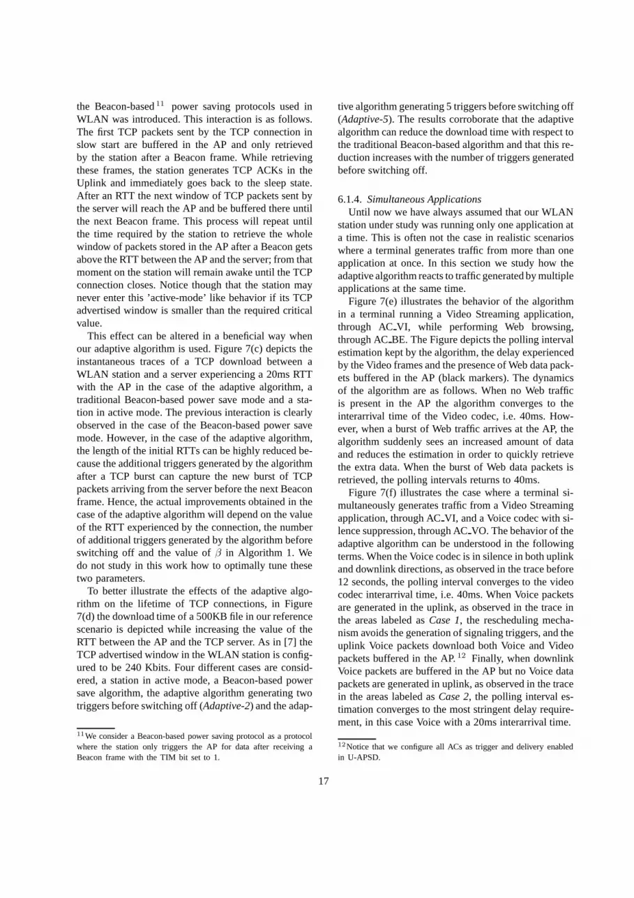
the Beacon-based11 power saving protocols used inWLAN was introduced. This interaction is as follows.The first TCP packets sent by the TCP connection inslow start are buffered in the AP and only retrievedby the station after a Beacon frame. While retrievingthese frames, the station generates TCP ACKs in theUplink and immediately goes back to the sleep state.After an RTT the next window of TCP packets sent bythe server will reach the AP and be buffered there untilthe next Beacon frame. This process will repeat untilthe time required by the station to retrieve the wholewindow of packets stored in the AP after a Beacon getsabove the RTT between the AP and the server; from thatmoment on the station will remain awake until the TCPconnection closes. Notice though that the station maynever enter this ’active-mode’ like behavior if its TCPadvertised window is smaller than the required criticalvalue.

This effect can be altered in a beneficial way whenour adaptive algorithm is used. Figure 7(c) depicts theinstantaneous traces of a TCP download between aWLAN station and a server experiencing a 20ms RTTwith the AP in the case of the adaptive algorithm, atraditional Beacon-based power save mode and a sta-tion in active mode. The previous interaction is clearlyobserved in the case of the Beacon-based power savemode. However, in the case of the adaptive algorithm,the length of the initial RTTs can be highly reduced be-cause the additional triggers generated by the algorithmafter a TCP burst can capture the new burst of TCPpackets arriving from the server before the next Beaconframe. Hence, the actual improvements obtained in thecase of the adaptive algorithm will depend on the valueof the RTT experienced by the connection, the numberof additional triggers generated by the algorithm beforeswitching off and the value ofβ in Algorithm 1. Wedo not study in this work how to optimally tune thesetwo parameters.

To better illustrate the effects of the adaptive algo-rithm on the lifetime of TCP connections, in Figure7(d) the download time of a 500KB file in our referencescenario is depicted while increasing the value of theRTT between the AP and the TCP server. As in [7] theTCP advertised window in the WLAN station is config-ured to be 240 Kbits. Four different cases are consid-ered, a station in active mode, a Beacon-based powersave algorithm, the adaptive algorithm generating twotriggers before switching off (Adaptive-2) and the adap-

11We consider a Beacon-based power saving protocol as a protocolwhere the station only triggers the AP for data after receiving aBeacon frame with the TIM bit set to 1.

tive algorithm generating 5 triggers before switching off(Adaptive-5). The results corroborate that the adaptivealgorithm can reduce the download time with respect tothe traditional Beacon-based algorithm and that this re-duction increases with the number of triggers generatedbefore switching off.

6.1.4. Simultaneous ApplicationsUntil now we have always assumed that our WLAN

station under study was running only one application ata time. This is often not the case in realistic scenarioswhere a terminal generates traffic from more than oneapplication at once. In this section we study how theadaptive algorithm reacts to traffic generated by multipleapplications at the same time.

Figure 7(e) illustrates the behavior of the algorithmin a terminal running a Video Streaming application,through ACVI, while performing Web browsing,through ACBE. The Figure depicts the polling intervalestimation kept by the algorithm, the delay experiencedby the Video frames and the presence of Web data pack-ets buffered in the AP (black markers). The dynamicsof the algorithm are as follows. When no Web trafficis present in the AP the algorithm converges to theinterarrival time of the Video codec, i.e. 40ms. How-ever, when a burst of Web traffic arrives at the AP, thealgorithm suddenly sees an increased amount of dataand reduces the estimation in order to quickly retrievethe extra data. When the burst of Web data packets isretrieved, the polling intervals returns to 40ms.

Figure 7(f) illustrates the case where a terminal si-multaneously generates traffic from a Video Streamingapplication, through ACVI, and a Voice codec with si-lence suppression, through ACVO. The behavior of theadaptive algorithm can be understood in the followingterms. When the Voice codec is in silence in both uplinkand downlink directions, as observed in the trace before12 seconds, the polling interval converges to the videocodec interarrival time, i.e. 40ms. When Voice packetsare generated in the uplink, as observed in the trace inthe areas labeled asCase 1, the rescheduling mecha-nism avoids the generation of signaling triggers, and theuplink Voice packets download both Voice and Videopackets buffered in the AP.12 Finally, when downlinkVoice packets are buffered in the AP but no Voice datapackets are generated in uplink, as observed in the tracein the areas labeled asCase 2, the polling interval es-timation converges to the most stringent delay require-ment, in this case Voice with a 20ms interarrival time.

12Notice that we configure all ACs as trigger and delivery enabledin U-APSD.

17

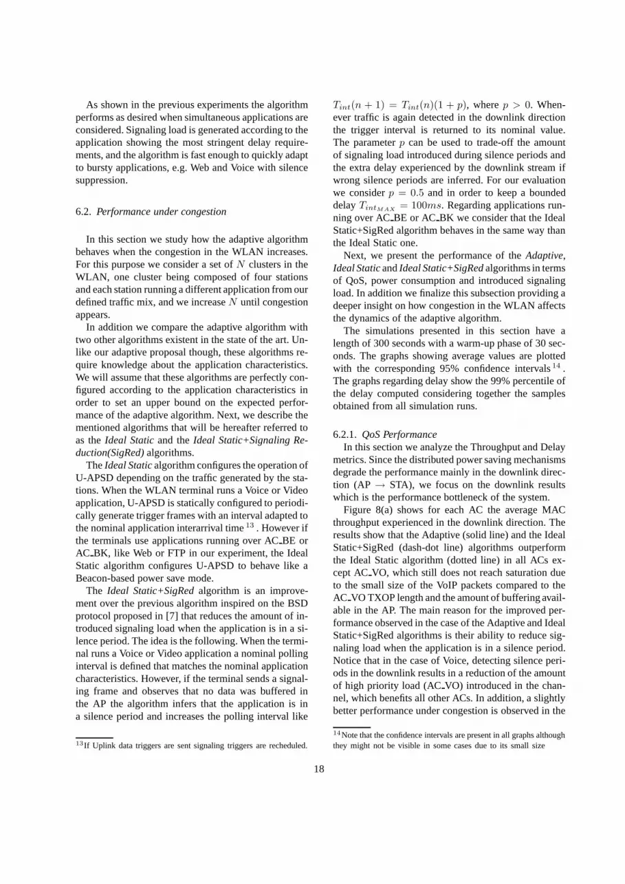
As shown in the previous experiments the algorithmperforms as desired when simultaneous applications areconsidered. Signaling load is generated according to theapplication showing the most stringent delay require-ments, and the algorithm is fast enough to quickly adaptto bursty applications, e.g. Web and Voice with silencesuppression.

6.2. Performance under congestion

In this section we study how the adaptive algorithmbehaves when the congestion in the WLAN increases.For this purpose we consider a set ofN clusters in theWLAN, one cluster being composed of four stationsand each station running a different application from ourdefined traffic mix, and we increaseN until congestionappears.

In addition we compare the adaptive algorithm withtwo other algorithms existent in the state of the art. Un-like our adaptive proposal though, these algorithms re-quire knowledge about the application characteristics.We will assume that these algorithms are perfectly con-figured according to the application characteristics inorder to set an upper bound on the expected perfor-mance of the adaptive algorithm. Next, we describe thementioned algorithms that will be hereafter referred toas theIdeal Staticand theIdeal Static+Signaling Re-duction(SigRed)algorithms.

TheIdeal Staticalgorithm configures the operation ofU-APSD depending on the traffic generated by the sta-tions. When the WLAN terminal runs a Voice or Videoapplication, U-APSD is statically configured to periodi-cally generate trigger frames with an interval adapted tothe nominal application interarrival time13 . However ifthe terminals use applications running over ACBE orAC BK, like Web or FTP in our experiment, the IdealStatic algorithm configures U-APSD to behave like aBeacon-based power save mode.

The Ideal Static+SigRedalgorithm is an improve-ment over the previous algorithm inspired on the BSDprotocol proposed in [7] that reduces the amount of in-troduced signaling load when the application is in a si-lence period. The idea is the following. When the termi-nal runs a Voice or Video application a nominal pollinginterval is defined that matches the nominal applicationcharacteristics. However, if the terminal sends a signal-ing frame and observes that no data was buffered inthe AP the algorithm infers that the application is ina silence period and increases the polling interval like

13 If Uplink data triggers are sent signaling triggers are recheduled.

Tint(n + 1) = Tint(n)(1 + p), wherep > 0. When-ever traffic is again detected in the downlink directionthe trigger interval is returned to its nominal value.The parameterp can be used to trade-off the amountof signaling load introduced during silence periods andthe extra delay experienced by the downlink stream ifwrong silence periods are inferred. For our evaluationwe considerp = 0.5 and in order to keep a boundeddelayTintMAX

= 100ms. Regarding applications run-ning over ACBE or AC BK we consider that the IdealStatic+SigRed algorithm behaves in the same way thanthe Ideal Static one.

Next, we present the performance of theAdaptive,Ideal StaticandIdeal Static+SigRedalgorithms in termsof QoS, power consumption and introduced signalingload. In addition we finalize this subsection providing adeeper insight on how congestion in the WLAN affectsthe dynamics of the adaptive algorithm.

The simulations presented in this section have alength of 300 seconds with a warm-up phase of 30 sec-onds. The graphs showing average values are plottedwith the corresponding 95% confidence intervals14 .The graphs regarding delay show the 99% percentile ofthe delay computed considering together the samplesobtained from all simulation runs.

6.2.1. QoS PerformanceIn this section we analyze the Throughput and Delay

metrics. Since the distributed power saving mechanismsdegrade the performance mainly in the downlink direc-tion (AP→ STA), we focus on the downlink resultswhich is the performance bottleneck of the system.

Figure 8(a) shows for each AC the average MACthroughput experienced in the downlink direction. Theresults show that the Adaptive (solid line) and the IdealStatic+SigRed (dash-dot line) algorithms outperformthe Ideal Static algorithm (dotted line) in all ACs ex-cept ACVO, which still does not reach saturation dueto the small size of the VoIP packets compared to theAC VO TXOP length and the amount of buffering avail-able in the AP. The main reason for the improved per-formance observed in the case of the Adaptive and IdealStatic+SigRed algorithms is their ability to reduce sig-naling load when the application is in a silence period.Notice that in the case of Voice, detecting silence peri-ods in the downlink results in a reduction of the amountof high priority load (ACVO) introduced in the chan-nel, which benefits all other ACs. In addition, a slightlybetter performance under congestion is observed in the

14Note that the confidence intervals are present in all graphs althoughthey might not be visible in some cases due to its small size

18

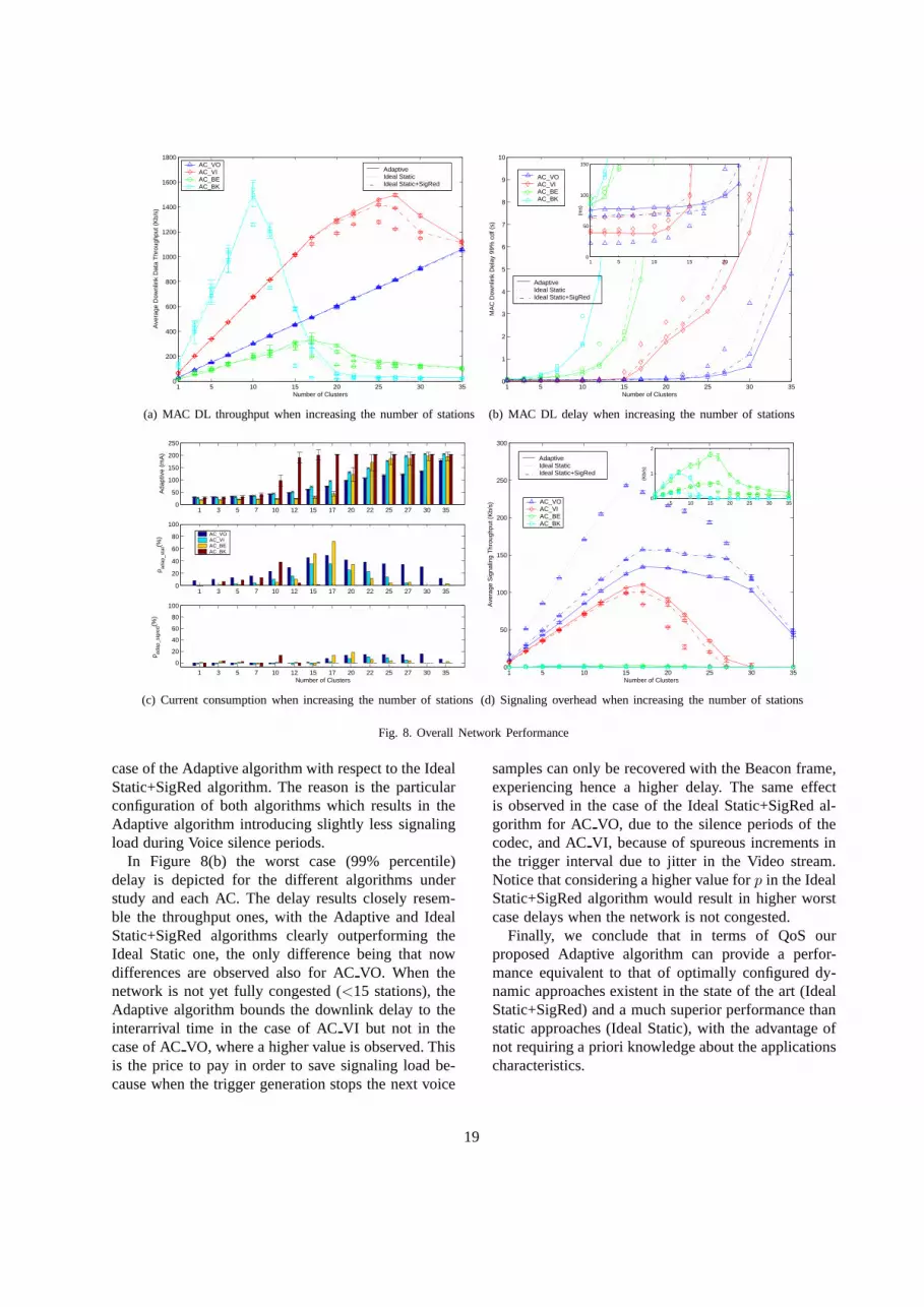
1 5 10 15 20 25 30 350

200

400

600

800

1000

1200

1400

1600

1800

Number of Clusters

Ave

rage

Dow

nlin

k D

ata

Thr

ough

put (

Kb/

s)

AC_VOAC_VIAC_BEAC_BK

Adaptive Ideal Static Ideal Static+SigRed

(a) MAC DL throughput when increasing the number of stations

1 5 10 15 20 25 30 350

1

2

3

4

5

6

7

8

9

10

Number of Clusters

MA

C D

ownl

ink

Del

ay 9

9% c

df (

s)

1 5 10 15 200

50

100

150

(ms)

Adaptive Ideal Static Ideal Static+SigRed

AC_VOAC_VIAC_BEAC_BK

(b) MAC DL delay when increasing the number of stations

1 3 5 7 10 12 15 17 20 22 25 27 30 350

50

100

150

200

250

Ada

ptiv

e (m

A)

1 3 5 7 10 12 15 17 20 22 25 27 30 350

20

40

60

80

100

ρ adap

_sta

t(%)

1 3 5 7 10 12 15 17 20 22 25 27 30 35

0

20

40

60

80

100

Number of Clusters

ρ adap

_sig

red(%

)

AC_VOAC_VIAC_BEAC_BK

(c) Current consumption when increasing the number of stations

1 5 10 15 20 25 30 350

50

100

150

200

250

300

Number of Clusters

Ave

rage

Sig

nalin

g T

hrou

ghpu

t (K

b/s) 5 10 15 20 25 30 35

0

1

2

(Kb/

s)

Adaptive Ideal Static Ideal Static+SigRed

AC_VOAC_VIAC_BEAC_BK

(d) Signaling overhead when increasing the number of stations

Fig. 8. Overall Network Performance

case of the Adaptive algorithm with respect to the IdealStatic+SigRed algorithm. The reason is the particularconfiguration of both algorithms which results in theAdaptive algorithm introducing slightly less signalingload during Voice silence periods.

In Figure 8(b) the worst case (99% percentile)delay is depicted for the different algorithms understudy and each AC. The delay results closely resem-ble the throughput ones, with the Adaptive and IdealStatic+SigRed algorithms clearly outperforming theIdeal Static one, the only difference being that nowdifferences are observed also for ACVO. When thenetwork is not yet fully congested (<15 stations), theAdaptive algorithm bounds the downlink delay to theinterarrival time in the case of ACVI but not in thecase of ACVO, where a higher value is observed. Thisis the price to pay in order to save signaling load be-cause when the trigger generation stops the next voice

samples can only be recovered with the Beacon frame,experiencing hence a higher delay. The same effectis observed in the case of the Ideal Static+SigRed al-gorithm for AC VO, due to the silence periods of thecodec, and ACVI, because of spureous increments inthe trigger interval due to jitter in the Video stream.Notice that considering a higher value forp in the IdealStatic+SigRed algorithm would result in higher worstcase delays when the network is not congested.

Finally, we conclude that in terms of QoS ourproposed Adaptive algorithm can provide a perfor-mance equivalent to that of optimally configured dy-namic approaches existent in the state of the art (IdealStatic+SigRed) and a much superior performance thanstatic approaches (Ideal Static), with the advantage ofnot requiring a priori knowledge about the applicationscharacteristics.

19

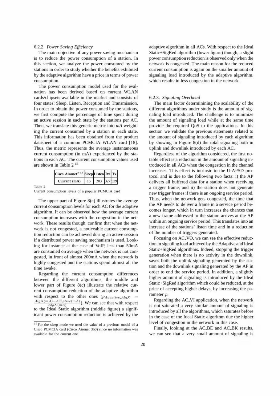
6.2.2. Power Saving EfficiencyThe main objective of any power saving mechanism

is to reduce the power consumption of a station. Inthis section, we analyze the power consumed by thestations in order to study whether the benefits exhibitedby the adaptive algorithm have a price in terms of powerconsumption.

The power consumption model used for the eval-uation has been derived based on current WLANcards/chipsets available in the market and consists offour states: Sleep, Listen, Reception and Transmission.In order to obtain the power consumed by the stations,we first compute the percentage of time spent duringan active session in each state by the stations per AC.Then, we translate this generic metric intomAweight-ing the current consumed by a station in each state.This information has been obtained from the productdatasheet of a common PCMCIA WLAN card [18].Thus, the metric represents the average instantaneouscurrent consumption (in mA) experienced by the sta-tions in each AC. The current consumption values usedare shown in Table 215

Cisco AironetTM Sleep Listen Rx Tx

Current (mA) 15 203 327539

Table 2Current consumption levels of a popular PCMCIA card

The upper part of Figure 8(c) illustrates the averagecurrent consumption levels for each AC for the adaptivealgorithm. It can be observed how the average currentconsumption increases with the congestion in the net-work. These results though, confirm that when the net-work is not congested, a noticeable current consump-tion reduction can be achieved during an active sessionif a distributed power saving mechanism is used. Look-ing for instance at the case of VoIP, less than 50mAare consumed on average when the network is not con-gested, in front of almost 200mA when the network ishighly congested and the stations spend almost all thetime awake.

Regarding the current consumption differencesbetween the different algorithms, the middle andlower part of Figure 8(c) illustrate the relative cur-rent consumption reduction of the adaptive algorithmwith respect to the other ones (ρAdaptive AlgX =AlgX(mA)−Adaptive(mA)

AlgX(mA) ). We can see that with respectto the Ideal Static algorithm (middle figure) a signif-icant power consumption reduction is achieved by the

15For the sleep mode we used the value of a previous model of aCisco PCMCIA card (Cisco Aironet 350) since no information wasavailable for the current one

adaptive algorithm in all ACs. With respect to the IdealStatic+SigRed algorithm (lower figure) though, a slightpower consumption reduction is observed only when thenetwork is congested. The main reason for the reducedcurrent consumption is again on the smaller amount ofsignaling load introduced by the adaptive algorithm,which results in less congestion in the network.

6.2.3. Signaling OverheadThe main factor determinining the scalability of the

different algorithms under study is the amount of sig-naling load introduced. The challenge is to minimizethe amount of signaling load while at the same timeprovide the required QoS to the applications. In thissection we validate the previous statements related tothe amount of signaling introduced by each algorithmby showing in Figure 8(d) the total signaling both inuplink and downlink introduced by each AC.

Regardless of the algorithm considered, the first no-table effect is a reduction in the amount of signaling in-troduced in all ACs when the congestion in the channelincreases. This effect is intrinsic to the U-APSD pro-tocol and is due to the following two facts: i) the APdelivers all buffered data for a station when receivinga trigger frame, and ii) the station does not generatenew trigger frames if there is an ongoing service period.Thus, when the network gets congested, the time thatthe AP needs to deliver a frame in a service period be-comes longer, which in turn increases the chances thata new frame addressed to the station arrives at the APwithin an ongoing service period. This translates into anincrease of the stations’ listen time and in a reductionof the number of triggers generated.

Focusing on ACVO, we can see the effective reduc-tion in signaling load achieved by the Adaptive and IdealStatic+SigRed algorithms. Indeed, stopping the triggergeneration when there is no activity in the downlink,saves both the uplink signaling generated by the sta-tion and the downlink signaling generated by the AP inorder to end the service period. In addition, a slightlyhigher amount of signaling is introduced by the IdealStatic+SigRed algorithm which could be reduced, at theprice of accepting higher delays, by increasing the pa-rameterp.

Regarding the ACVI application, when the networkis not saturated a very similar amount of signaling isintroduced by all the algorithms, which saturates beforein the case of the Ideal Static algorithm due the higherlevel of congestion in the network in this case.

Finally, looking at the ACBE and ACBK results,we can see that a very small amount of signaling is

20

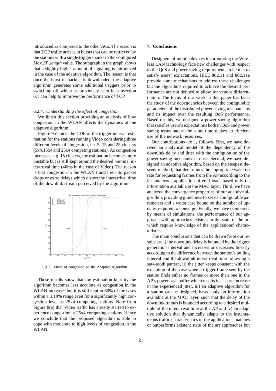
introduced as compared to the other ACs. The reason isthat TCP traffic arrives in bursts that can be retrieved bythe stations with a single trigger thanks to the configuredMax SP lengthvalue. The subgraph in the graph showsthat a slightly higher amount of signaling is introducedin the case of the adaptive algorithm. The reason is thatonce the burst of packets is downloaded, the adaptivealgorithm generates some additional triggers prior toswitching off which as previously seen in subsection6.1 can help to improve the performance of TCP.

6.2.4. Understanding the effect of congestionWe finish this section providing an analysis of how

congestion in the WLAN affects the dynamics of theadaptive algorithm.

Figure 9 depicts the CDF of the trigger interval esti-mation for the stations running Video considering threedifferent levels of congestion, i.e. 5, 15 and 25 clusters(5x4,15x4 and 25x4 competing stations). As congestionincreases, e.g. 15 clusters, the estimation becomes moreunstable but is still kept around the desired nominal in-terarrival time (40ms in the case of Video). The reasonis that congestion in the WLAN translates into packetdrops or extra delays which distort the interarrival timeof the downlink stream perceived by the algorithm.

30 32 34 36 38 40 42 44 46 48 500

0.1

0.2

0.3

0.4

0.5

0.6

0.7

0.8

0.9

1

∆trig

(ms)

F(x

)

CDF of algorithm estimation on a 40ms Video stream

5 Clusters15 Clusters25 Clusters

+10% −10%

Fig. 9. Effect of congestion on the Adaptive Algorithm

These results show that the estimation kept by thealgorithm becomes less accurate as congestion in theWLAN increases but it is still kept in 80% of the caseswithin a±10% range even for a significantly high con-gestion level as 25x4 competing stations. Note fromFigure 8(a) that Video traffic has already started to ex-perience congestion at 25x4 competing stations. Hencewe conclude that the proposed algorithm is able tocope with moderate to high levels of congestion in theWLAN.

7. Conclusions

Designers of mobile devices incorporating the Wire-less LAN technology face new challenges with respectto the QoS and power saving requirements to be met tosatisfy users’ expectations. IEEE 802.11 and 802.11eprovide some mechanisms to address these challengesbut the algorithms required to achieve the desired per-formance are not defined to allow for vendor differen-tiation. The focus of our work in this paper has beenthe study of the dependencies between the configurableparameters of the distributed power saving mechanismsand its impact over the resulting QoS performance.Based on this, we designed a power saving algorithmthat satisfies users’s expectations both in QoS and powersaving terms and at the same time makes an efficientuse of the network resources.

Our contributions are as follows. First, we have de-rived an analytical model of the dependency of thedownlink delay and jitter with the configuration of thepower saving mechanism in use. Second, we have de-signed an adaptive algorithm, based on the steepest de-scent method, that determines the appropriate wake uprate for requesting frames from the AP according to theinstantaneous application offered load, based only oninformation available at the MAC layer. Third, we haveanalyzed the convergence properties of our adaptive al-gorithm, providing guidelines to set its configurable pa-rameters and a worst case bound on the number of up-dates required to converge. Finally, we have compared,by means of simulations, the performance of our ap-proach with approaches existent in the state of the artwhich require knowledge of the applications’ charac-teristics.

The main conclusions that can be drawn from our re-sults are i) the downlink delay is bounded by the triggergeneration interval and increases or decreases linearlyaccording to the difference between the station’s pollinginterval and the downlink interarrival time following asaw-tooth pattern, ii) the jitter keeps constant with theexception of the case when a trigger frame sent by thestation finds either no frames or more than one in theAP’s power save buffer which results in a sharp increasein the experienced jitter, iii) an adaptive algorithm fora station can be designed, based only on informationavailable at the MAC layer, such that the delay of thedownlink frames is bounded according to a desired mul-tiple of the interarrival time at the AP and iv) an adap-tive solution that dynamically adapts to the instanta-neous traffic characteristics of the applications matchesor outperforms existent state of the art approaches but

21

with the significant advantage of not requiring any apriori knowledge of the applications’ characteristics.

8. APPENDIX

Assuming the definitions introduced in Section 5,Ki

frames arrive at the AP during uplink subperiodi, whereKi = ⌊

∆UL+φi

∆DL⌋. Hence:

Ki = ⌊∆UL

∆DL

⌋+ ⌊∆UL mod ∆DL + φ

i

∆DL

⌋

Thus:

Ki =

⌊∆UL

∆DL

⌋ if φi < ∆DL −∆UL mod ∆DL

⌈∆UL

∆DL

⌉ if φi ≥ ∆DL −∆UL mod ∆DL

Assuming the general case where∆UL is not multi-ple of ∆DL (∆UL 6= n∆DL, n ∈ Z), and recalling0 ≤ φi < ∆DL, the channel situation periodicT =lcm(∆UL, ∆DL) = M∆DL = N∆UL, andT com-posed byN consecutive uplink subperiods, duringl > 0andj > 0 uplink subperiods⌊∆UL

∆DL⌋ and⌈∆UL

∆DL⌉ down-

link frames are received at the AP respectively, with:

l⌊∆UL

∆DL

⌋+ j⌈∆UL

∆DL

⌉ = M

l + j = N

Therefore:

l = N(⌊∆UL

∆DL

⌋+ 1)−M

j = M −N⌊∆UL

∆DL

⌋

Thus, withinT there are both uplink subperiods re-ceiving⌊∆UL

∆DL⌋ and⌈∆UL

∆DL⌉ data frames in the downlink.

Therefore the station must generateδ = ⌊∆UL

∆DL⌋ signal-

ing triggers between two consecutive data triggers inorder not to generate any event in any uplink subperiod.Hence, the reuse of uplink data triggers in this case isjN

.In the case that∆UL = n∆DL, n ∈ Z, the same

number of data frames arrive at the AP in all uplinksubperiods,∆UL

∆DL, and a converged value of∆trig can

be obtained generatingδ = ∆UL

∆DLor δ = ∆UL

∆DL− 1

signaling triggers between uplink data triggers. Thus,the reuse of uplink data trigers in this case will be0 or1 respectively.

References

[1] IEEE 802.11 WG,Wireless LAN Medium Access Control (MAC)and Physical Layer (PHY) Specifications, IEEE Standard 802.11,June 1999.

[2] IEEE 802.11 WG,Wireless LAN Medium Access Control (MAC)and Physical Layer (PHY) specifications. Amendment 8: MediumAccess Control (MAC) Quality of Service Enhancements, IEEEStandard 802.11e, November 2005.

[3] http://www.wi-fi.org.[4] S.Mangold and S.Choi and G.R.Hiertz and O.Klein and B.Walke,

Analysis of IEEE 802.11e for QoS Support in Wireless LANs,IEEE Wireless Communications Magazine, December 2003.

[5] X.Perez-Costa, D.Camps-Mur and T.Sashihara.Analysis of theIntegration of IEEE 802.11e Capabilities in Battery LimitedMobile Devices. IEEE Wireless Communications Magazine(WirComMag), special issue on Internetworking Wireless LANand Cellular Networks, Volume 12, Issue 6, December 2005.

[6] X.Perez-Costa, D.Camps-Mur, A. Vidal.SU-APSD: Static IEEE802.11e Unscheduled Automatic Power Save Delivery. ComputerNetworks Volume 51, Issue 9, 20 June 2007, Pages 2326-2344.

[7] R.Krashinsky and H.Balakrishnan,Minimizing energy forwireless web access with bounded slowdown, Wireless Networksarchive Volume 11 , Issue 1-2 (January 2005).

[8] D.Qiao and K.G.Shin,Smart Power Saving Mode for IEEE802.11 Wireless LANs, Proceedings of IEEE INFOCOM, March2005.

[9] G. Anastasi, M. Conti, E. Gregori, A. Passarella802.11powersaving mode for mobile computing in WiFi hotspots:limitations, enhancements and open issues, Wireless NetworksVolume 14 , Issue 6 (December 2008).

[10] Y.Chen and S.Emeott,Investigation into Packet DeliveryOptions for WLAN Acess Points Implementing UnscheduledPower Save Delivery, Proceedings of IEEE Globecom, November2005.

[11] X.Perez-Costa and D.Camps-Mur,APSM: Bounding theDownlink Delay for 802.11 Power Save Mode, In Proceedings ofIEEE International Conference on Communications (ICC), May2005.

[12] X.Perez-Costa and D.Camps-Mur,AU-APSD: Adaptive IEEE802.11e Unscheduled Automatic Power Save Delivery,In Proceedings of IEEE International Conference onCommunications (ICC), June 2006.

[13] UPnP Forum,UPnP QoS Architecture V2.0, October 2006.[14] Xavier Perez Costa, Daniel Camps Mur.A protocol

Enhancement for IEEE 802.11 Distributed Power SavingMechanisms. No Data Acknowledgement. IST summit 2007,Budapest, July 2007.

[15] ITU-T Recommendation Y.1541[16] OPNET Technologies,http://www.opnet.com.[17] F.H.P. Fitzek and M.Reisslein,MPEG-4 and H.263 Video Traces

for Network Performance Evaluation, IEEE Network, Vol. 15,No. 6, pages 40-54, November/December 2001.

[18] Cisco Aironet 802.11a/b/g Wireless CardBus Adapter,http://www.cisco.com/.

22