Runuran An R Interface to the UNU.RAN Library for Universal Random Variate Generators Josef Leydold Wolfgang H¨ ormann Halis Sak Department of Statistics and Mathematics, WU Wien, Austria Department for Industrial Engineering, Bo˘ gazi¸ci University, Istanbul, Turkey Version 0.20.0 – Sep 10, 2012 Abstract Runuran is a wrapper to UNU.RAN (Universal Non-Uniform RANdom variate generators ), a library for generating random variates for large classes of distributions. It also allows to compute quantiles (inverse cumulative distribution functions) of these distributions effi- ciently. In addition it can be used to compute (approximate) values of the density function or the distribution function. In order to use UNU.RAN one must supply some data like the density about the target distribution which are then used to draw random samples. Runuran functions provide both a simplified interface to this library for common distributions as well access to the full power of this library. Table of Contents 0. Introduction 2 1. Runuran – Special Generator 4 2. Runuran – Universal 6 3. Runuran – Distributions 12 4. Runuran – Advanced 14 A. A Short Introduction to Random Variate Generation 21 B. Pitfalls 29 C. Glossary 31 References 33 1

Welcome message from author
This document is posted to help you gain knowledge. Please leave a comment to let me know what you think about it! Share it to your friends and learn new things together.
Transcript
Runuran
An R Interface to the UNU.RAN Library forUniversal Random Variate Generators
Josef Leydold Wolfgang Hormann Halis Sak
Department of Statistics and Mathematics, WU Wien, AustriaDepartment for Industrial Engineering, Bogazici University, Istanbul, Turkey
Version 0.20.0 – Sep 10, 2012
Abstract
Runuran is a wrapper to UNU.RAN (Universal Non-Uniform RANdom variate generators),a library for generating random variates for large classes of distributions. It also allowsto compute quantiles (inverse cumulative distribution functions) of these distributions effi-ciently. In addition it can be used to compute (approximate) values of the density functionor the distribution function.
In order to use UNU.RAN one must supply some data like the density about the targetdistribution which are then used to draw random samples. Runuran functions provide botha simplified interface to this library for common distributions as well access to the fullpower of this library.
Table of Contents
0. Introduction 2
1. Runuran – Special Generator 4
2. Runuran – Universal 6
3. Runuran – Distributions 12
4. Runuran – Advanced 14
A. A Short Introduction to Random Variate Generation 21
B. Pitfalls 29
C. Glossary 31
References 33
1

0. Introduction
0. Introduction
The R package Runuran is a wrapper to UNU.RAN (Universal Non-Uniform RANdom variategenerators), a library for generating random variates for large classes of distributions. It alsoallows to compute quantiles (inverse cumulative distribution functions) of these distributionsefficiently. This is in particular a prerequisite for quasi-Monte Carlo integration and copulamethods. UNU.RAN implements so called universal (automatic or black-box ) generators. Inorder to use UNU.RAN one must supply some data about the target distribution, usually thedensity, probability vector or cumulative distribution function and (optionally) some otherinformation (such as the mode of the distribution). These are then used to draw randomsamples. Runuran functions provide both a simplified interface to this library for commondistributions as well access to the full power of this library.
Runuran functions are alternatives to standard built-in functions in R which are faster or aresuitable for particular applications. Runuran is the package you are looking for if you need
• robust and easy-to-use sampling and quantile functions for continuous and discrete dis-tributions (such as Normal, Beta, Gamma, Generalized Hyperbolic, Binomial, . . . distri-butions);
• to draw samples from truncated distributions;
• random samples for special applications like variate reduction techniques, QMC or copulamethods;
• simulate random variates from some unusual distribution that you just found in a paperor derived from your statistical model;
• to find out properties of various generation methods (such as speed, quality of generatedpoint set, conservation of structures, . . . ).
If your aim is just (1) and you are not keen on learning more about universal generatorsplease proceed to Section 3.Universal algorithms for non-uniform random variate generation work for quite large classes
of distributions but require the following three steps:
(U1) Information gathering: The user has to provide some information about the distri-bution. The kind of information depends on the chosen method.
(U2) Creation of tables: In the setup tables are created. These adjust the algorithm forsampling from the target distribution. The table size depends on the chosen method butcan be controlled to some extend.
(U3) Generation of a random sample: These tables are then used to generate a randomsample.
It is obvious that table size, setup time, and marginal generation time strongly depend onthe chosen method. By a rule-of-thumb methods with large tables have very fast marginalgeneration times that hardly depend on (or are even independent from) the given targetdistribution. But then they have an expensive setup. Vice versa, when the table is small wehave fast setup and slow marginal generation times or the generated points are less accurate incase of approximate methods. Many of the algorithms allow to control the table size to someextend.
The choice of the generation method itself depends on the application for which the randomsample is requested. Of course, the target distribution has to satisfy certain conditions for each
2
0. Introduction
of these algorithms. We refer the user to our extensive monograph [2] for detailed informationabout these generation methods. For convenience we have added a (very) short survey on thebasic principles of random variate generation in Appendix A (A Short Introduction to RandomVariate Generation). Terms and concepts that are used in the description of the methods inthis manual are listed in Appendix C (Glossary).
We have compiled a collection of such universal algorithms in UNU.RAN. The source codeand a detailed manual can be found in [4]. The library is written in ANSI C and providesan interface to Steps (U1)–(U3) for such universal algorithms. The setup is sometimes quiteexpensive even if the required table is small, since there are checks whether the conditions forthe chosen method (e.g., log-concavity) are satisfied as well as checks for the consistency of thegiven data for the target distribution. Thus the setup and the generation are split, such thatthe former part creates an object that can be used many times for creating random samples.R package Runuran provides a wrapper to the UNU.RAN library1. The package implements
four sets of functions of increasing power (and thus complexity):
• Runuran – Special Generator (Section 1):
These functions provide easy-to-use sampling algorithms for particular distributions.Their syntax is similar to the built-in sampling algorithms (but usually have an additionaldomain argument). They can be used as replacements for the respective R functions (ifthe latter exists), e.g., urnorm can be used instead of rnorm for generating normal randomvariates. These functions also show the interested user how we used the more powerfulfunctions below.
• Runuran – Universal (Section 2):
These functions provide more flexibility. They offer an interface to use a carefully selectedcollection of UNU.RAN methods with their most important variants. Their argumentsallow setting all required data and parameters. Thus they combine Steps (U1) and (U2)in a single function. On the contrary to functions like urnorm, they do not return arandom sample but a UNU.RAN generator object that can be used for sampling usingur or uq (Step U3). For example, the function tdr.new creates a generator object thatapplies the transformed density rejection (TDR) method.
• Runuran – Distribution (Section 3):
Coding the required functions for particular distributions can be tedious. Thus we havecompiled a set of functions that create UNU.RAN distribution objects that can directlybe used with the functions from section Universal (Section 2).
• Runuran – Advanced (Section 4):
These functions implement a wrapper to the UNU.RAN string API and is thus themost powerful interface. Thus more generation methods and more parameters for allUNU.RAN methods are available. Now Steps (U1) and (U2) are split in two differenttasks.
Uniform random numbers. All UNU.RAN methods use the R built-in uniform random num-ber generator as the source of (pseudo-) random numbers. Thus the generated samples dependon the state .Random.seed and can be controlled by the R functions RNGkind and set.seed.
1We first described such a package in [6]. However, the interface has been changed and extended since then.
3
1. Runuran – Special Generator
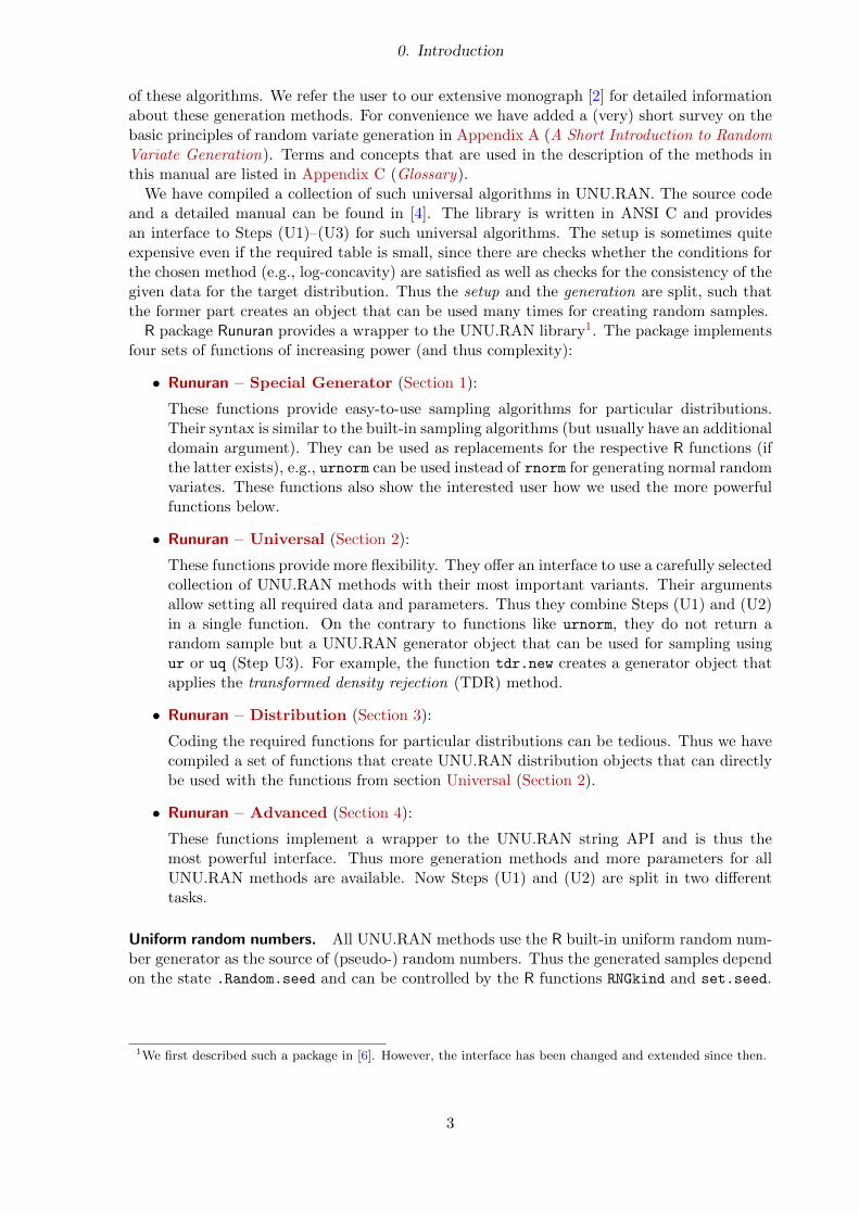
1. Runuran – Special Generator
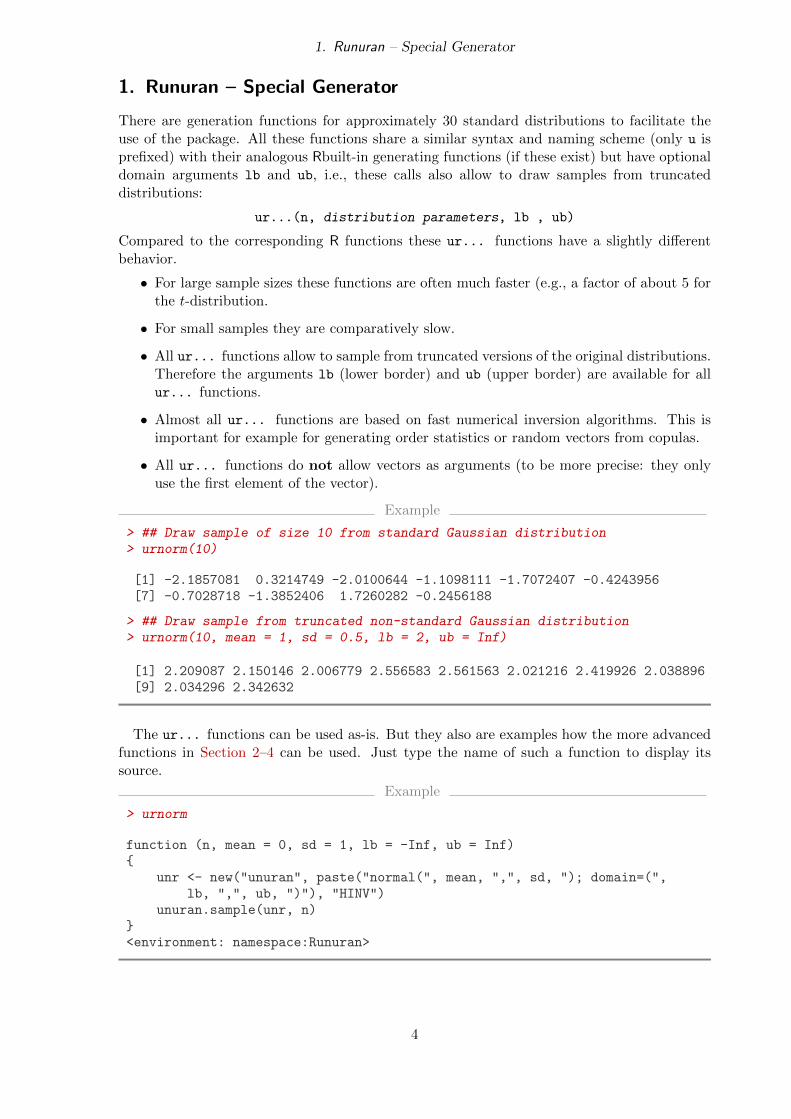
There are generation functions for approximately 30 standard distributions to facilitate theuse of the package. All these functions share a similar syntax and naming scheme (only u isprefixed) with their analogous Rbuilt-in generating functions (if these exist) but have optionaldomain arguments lb and ub, i.e., these calls also allow to draw samples from truncateddistributions:
ur...(n, distribution parameters, lb , ub)
Compared to the corresponding R functions these ur... functions have a slightly differentbehavior.
• For large sample sizes these functions are often much faster (e.g., a factor of about 5 forthe t-distribution.
• For small samples they are comparatively slow.
• All ur... functions allow to sample from truncated versions of the original distributions.Therefore the arguments lb (lower border) and ub (upper border) are available for allur... functions.
• Almost all ur... functions are based on fast numerical inversion algorithms. This isimportant for example for generating order statistics or random vectors from copulas.
• All ur... functions do not allow vectors as arguments (to be more precise: they onlyuse the first element of the vector).
Example
> ## Draw sample of size 10 from standard Gaussian distribution> urnorm(10)
[1] -2.1857081 0.3214749 -2.0100644 -1.1098111 -1.7072407 -0.4243956[7] -0.7028718 -1.3852406 1.7260282 -0.2456188
> ## Draw sample from truncated non-standard Gaussian distribution> urnorm(10, mean = 1, sd = 0.5, lb = 2, ub = Inf)
[1] 2.209087 2.150146 2.006779 2.556583 2.561563 2.021216 2.419926 2.038896[9] 2.034296 2.342632
The ur... functions can be used as-is. But they also are examples how the more advancedfunctions in Section 2–4 can be used. Just type the name of such a function to display itssource.
Example
> urnorm
function (n, mean = 0, sd = 1, lb = -Inf, ub = Inf){
unr <- new("unuran", paste("normal(", mean, ",", sd, "); domain=(",lb, ",", ub, ")"), "HINV")
unuran.sample(unr, n)}<environment: namespace:Runuran>
4
1. Runuran – Special Generator
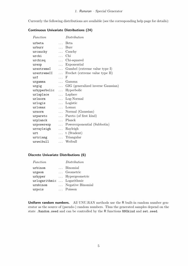
Currently the following distributions are available (see the corresponding help page for details):
Continuous Univariate Distributions (24)
Function Distribution
urbeta . . . Betaurburr . . . Burrurcauchy . . . Cauchyurchi . . . Chiurchisq . . . Chi-squaredurexp . . . ExponentialurextremeI . . . Gumbel (extreme value type I)urextremeII . . . Frechet (extreme value type II)urf . . . Furgamma . . . Gammaurgig . . . GIG (generalized inverse Gaussian)urhyperbolic . . . Hyperbolicurlaplace . . . Laplaceurlnorm . . . Log-Normalurlogis . . . Logisticurlomax . . . Lomaxurnorm . . . Normal (Gaussian)urpareto . . . Pareto (of first kind)urplanck . . . Planckurpowerexp . . . Powerexponential (Subbotin)urrayleigh . . . Rayleighurt . . . t (Student)urtriang . . . Triangularurweibull . . . Weibull
Discrete Univariate Distributions (6)
Function Distribution
urbinom . . . Binomialurgeom . . . Geometricurhyper . . . Hypergeometricurlogarithmic . . . Logarithmicurnbinom . . . Negative Binomialurpois . . . Poisson
Uniform random numbers. All UNU.RAN methods use the R built-in random number gen-erator as the source of (pseudo-) random numbers. Thus the generated samples depend on thestate .Random.seed and can be controlled by the R functions RNGkind and set.seed.
5
2. Runuran – Universal
2. Runuran – Universal
The power of UNU.RAN does not lie in a collection of generators for some standard distribu-tions but in a collection of universal generation methods that allow drawing samples of pseudo-random variates for particular purposes. For example, it is possible to generate samples thatfollow some non-standard distributions for which no special generation methods exist. Theseblack-box methods are also well suited for standard distributions (e.g., some of our methodsare much faster when applied to some distributions compared to the corresponding R built-infunctions).
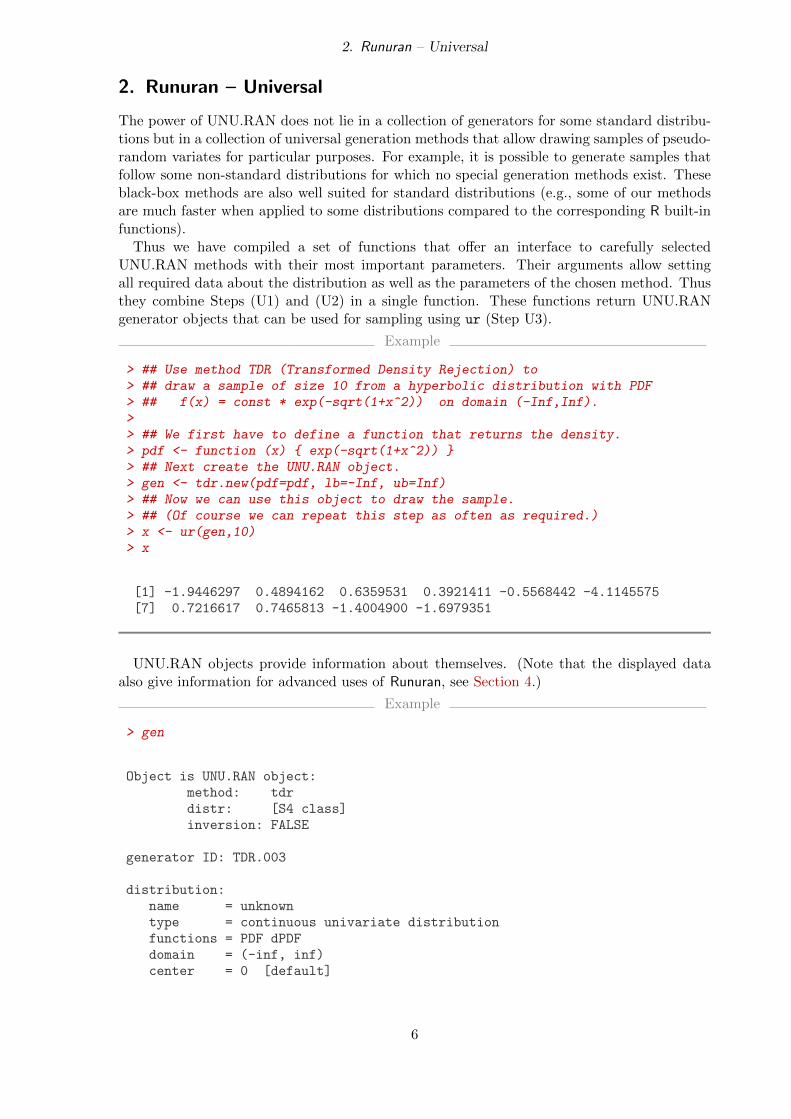
Thus we have compiled a set of functions that offer an interface to carefully selectedUNU.RAN methods with their most important parameters. Their arguments allow settingall required data about the distribution as well as the parameters of the chosen method. Thusthey combine Steps (U1) and (U2) in a single function. These functions return UNU.RANgenerator objects that can be used for sampling using ur (Step U3).
Example
> ## Use method TDR (Transformed Density Rejection) to> ## draw a sample of size 10 from a hyperbolic distribution with PDF> ## f(x) = const * exp(-sqrt(1+x^2)) on domain (-Inf,Inf).>> ## We first have to define a function that returns the density.> pdf <- function (x) { exp(-sqrt(1+x^2)) }> ## Next create the UNU.RAN object.> gen <- tdr.new(pdf=pdf, lb=-Inf, ub=Inf)> ## Now we can use this object to draw the sample.> ## (Of course we can repeat this step as often as required.)> x <- ur(gen,10)> x
[1] -1.9446297 0.4894162 0.6359531 0.3921411 -0.5568442 -4.1145575[7] 0.7216617 0.7465813 -1.4004900 -1.6979351
UNU.RAN objects provide information about themselves. (Note that the displayed dataalso give information for advanced uses of Runuran, see Section 4.)
Example
> gen
Object is UNU.RAN object:method: tdrdistr: [S4 class]inversion: FALSE
generator ID: TDR.003
distribution:name = unknowntype = continuous univariate distributionfunctions = PDF dPDFdomain = (-inf, inf)center = 0 [default]
6
2. Runuran – Universal
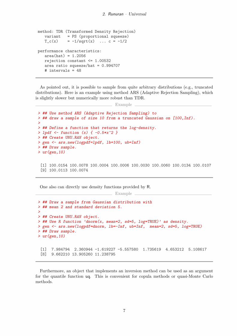
method: TDR (Transformed Density Rejection)variant = PS (proportional squeeze)T_c(x) = -1/sqrt(x) ... c = -1/2
performance characteristics:area(hat) = 1.2056rejection constant <= 1.00532area ratio squeeze/hat = 0.994707# intervals = 48
As pointed out, it is possible to sample from quite arbitrary distributions (e.g., truncateddistributions). Here is an example using method ARS (Adaptive Rejection Sampling), whichis slightly slower but numerically more robust than TDR.
Example
> ## Use method ARS (Adaptive Rejection Sampling) to> ## draw a sample of size 10 from a truncated Gaussian on [100,Inf).>> ## Define a function that returns the log-density.> lpdf <- function (x) { -0.5*x^2 }> ## Create UNU.RAN object.> gen <- ars.new(logpdf=lpdf, lb=100, ub=Inf)> ## Draw sample.> ur(gen,10)
[1] 100.0154 100.0078 100.0004 100.0006 100.0030 100.0060 100.0134 100.0107[9] 100.0113 100.0074
One also can directly use density functions provided by R.
Example
> ## Draw a sample from Gaussian distribution with> ## mean 2 and standard deviation 5.>> ## Create UNU.RAN object.> ## Use R function ’dnorm(x, mean=2, sd=5, log=TRUE)’ as density.> gen <- ars.new(logpdf=dnorm, lb=-Inf, ub=Inf, mean=2, sd=5, log=TRUE)> ## Draw sample.> ur(gen,10)
[1] 7.984794 2.360944 -1.619227 -5.557580 1.735619 4.653212 5.108617[8] 9.662210 13.905260 11.238795
Furthermore, an object that implements an inversion method can be used as an argumentfor the quantile function uq. This is convenient for copula methods or quasi-Monte Carlomethods.
7
2. Runuran – Universal
Example
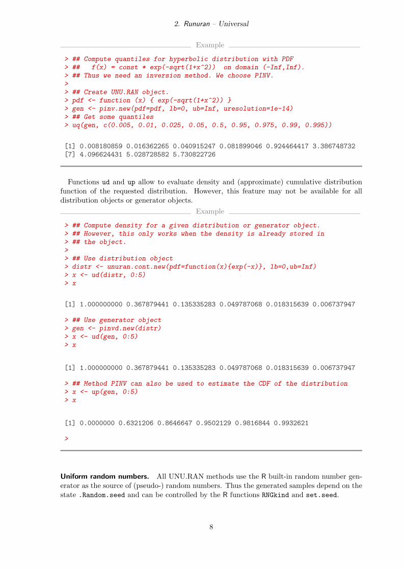
> ## Compute quantiles for hyperbolic distribution with PDF> ## f(x) = const * exp(-sqrt(1+x^2)) on domain (-Inf,Inf).> ## Thus we need an inversion method. We choose PINV.>> ## Create UNU.RAN object.> pdf <- function (x) { exp(-sqrt(1+x^2)) }> gen <- pinv.new(pdf=pdf, lb=0, ub=Inf, uresolution=1e-14)> ## Get some quantiles> uq(gen, c(0.005, 0.01, 0.025, 0.05, 0.5, 0.95, 0.975, 0.99, 0.995))
[1] 0.008180859 0.016362265 0.040915247 0.081899046 0.924464417 3.386748732[7] 4.096624431 5.028728582 5.730822726
Functions ud and up allow to evaluate density and (approximate) cumulative distributionfunction of the requested distribution. However, this feature may not be available for alldistribution objects or generator objects.
Example
> ## Compute density for a given distribution or generator object.> ## However, this only works when the density is already stored in> ## the object.>> ## Use distribution object> distr <- unuran.cont.new(pdf=function(x){exp(-x)}, lb=0,ub=Inf)> x <- ud(distr, 0:5)> x
[1] 1.000000000 0.367879441 0.135335283 0.049787068 0.018315639 0.006737947
> ## Use generator object> gen <- pinvd.new(distr)> x <- ud(gen, 0:5)> x
[1] 1.000000000 0.367879441 0.135335283 0.049787068 0.018315639 0.006737947
> ## Method PINV can also be used to estimate the CDF of the distribution> x <- up(gen, 0:5)> x
[1] 0.0000000 0.6321206 0.8646647 0.9502129 0.9816844 0.9932621
>
Uniform random numbers. All UNU.RAN methods use the R built-in random number gen-erator as the source of (pseudo-) random numbers. Thus the generated samples depend on thestate .Random.seed and can be controlled by the R functions RNGkind and set.seed.
8
2. Runuran – Universal
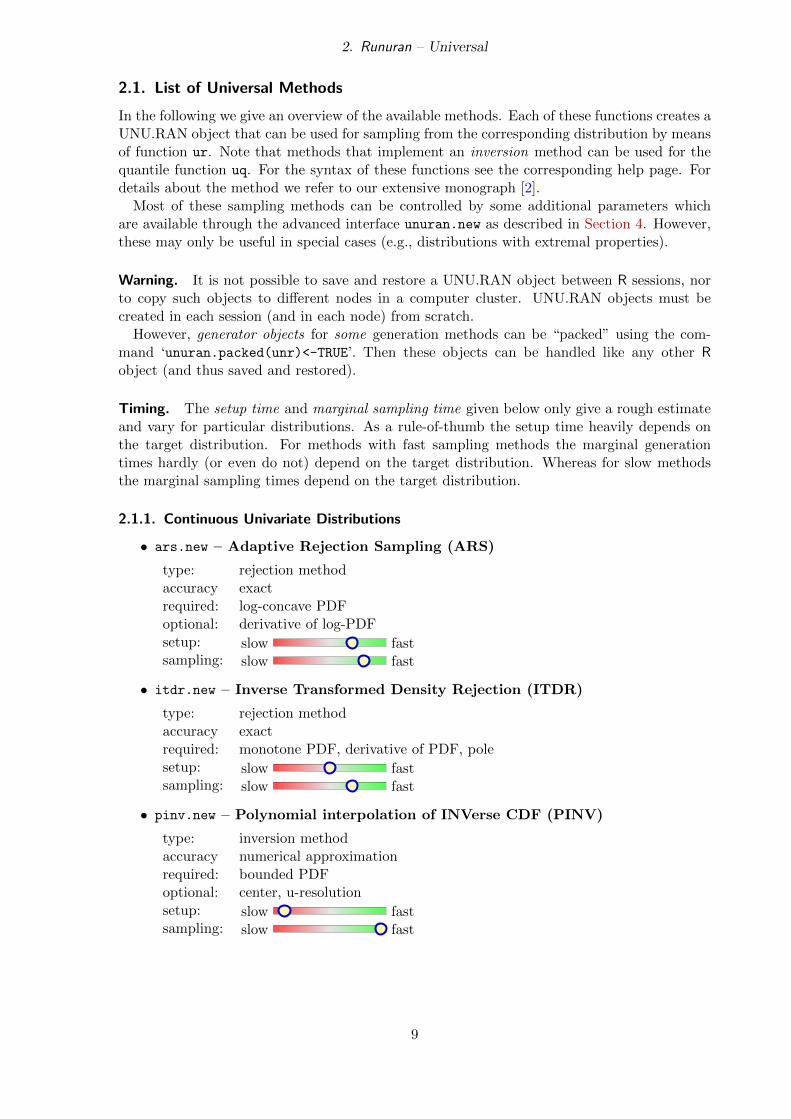
2.1. List of Universal Methods
In the following we give an overview of the available methods. Each of these functions creates aUNU.RAN object that can be used for sampling from the corresponding distribution by meansof function ur. Note that methods that implement an inversion method can be used for thequantile function uq. For the syntax of these functions see the corresponding help page. Fordetails about the method we refer to our extensive monograph [2].
Most of these sampling methods can be controlled by some additional parameters whichare available through the advanced interface unuran.new as described in Section 4. However,these may only be useful in special cases (e.g., distributions with extremal properties).
Warning. It is not possible to save and restore a UNU.RAN object between R sessions, norto copy such objects to different nodes in a computer cluster. UNU.RAN objects must becreated in each session (and in each node) from scratch.
However, generator objects for some generation methods can be “packed” using the com-mand ‘unuran.packed(unr)<-TRUE’. Then these objects can be handled like any other Robject (and thus saved and restored).
Timing. The setup time and marginal sampling time given below only give a rough estimateand vary for particular distributions. As a rule-of-thumb the setup time heavily depends onthe target distribution. For methods with fast sampling methods the marginal generationtimes hardly (or even do not) depend on the target distribution. Whereas for slow methodsthe marginal sampling times depend on the target distribution.
2.1.1. Continuous Univariate Distributions
• ars.new – Adaptive Rejection Sampling (ARS)
type: rejection methodaccuracy exactrequired: log-concave PDFoptional: derivative of log-PDFsetup: slow fastsampling: slow fast
• itdr.new – Inverse Transformed Density Rejection (ITDR)
type: rejection methodaccuracy exactrequired: monotone PDF, derivative of PDF, polesetup: slow fastsampling: slow fast
• pinv.new – Polynomial interpolation of INVerse CDF (PINV)
type: inversion methodaccuracy numerical approximationrequired: bounded PDFoptional: center, u-resolutionsetup: slow fastsampling: slow fast
9
2. Runuran – Universal
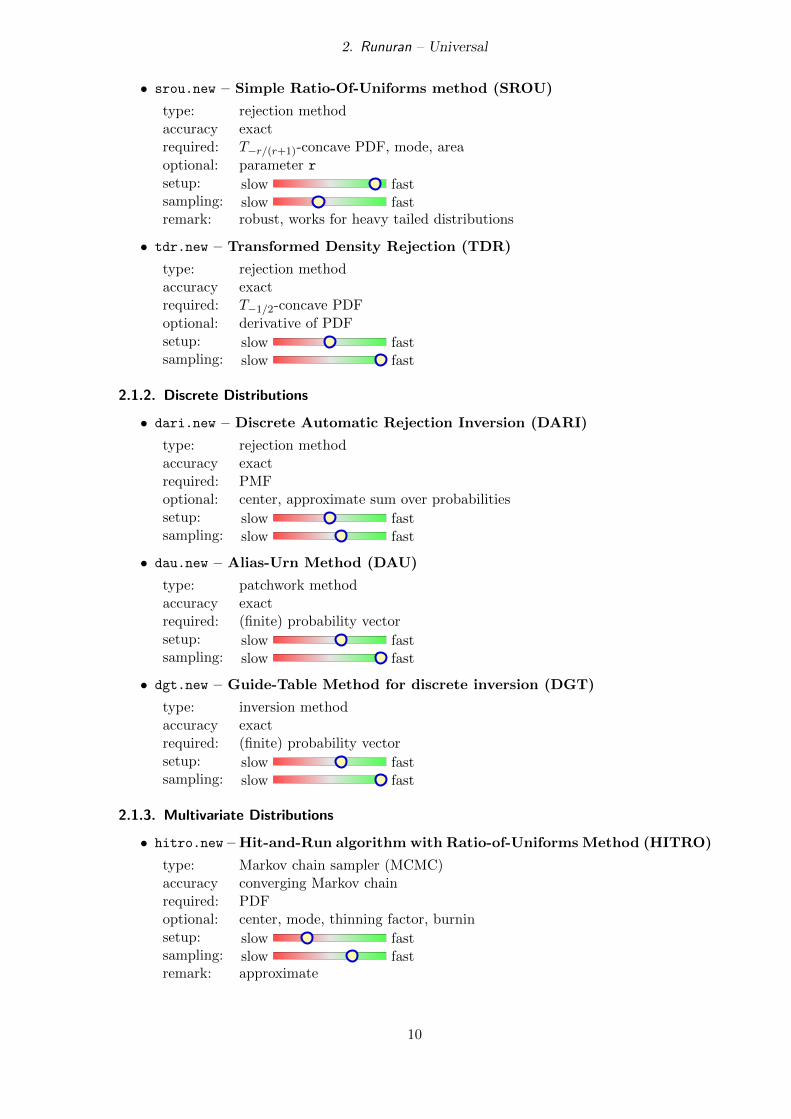
• srou.new – Simple Ratio-Of-Uniforms method (SROU)
type: rejection methodaccuracy exactrequired: T−r/(r+1)-concave PDF, mode, area
optional: parameter rsetup: slow fastsampling: slow fastremark: robust, works for heavy tailed distributions
• tdr.new – Transformed Density Rejection (TDR)
type: rejection methodaccuracy exactrequired: T−1/2-concave PDF
optional: derivative of PDFsetup: slow fastsampling: slow fast
2.1.2. Discrete Distributions
• dari.new – Discrete Automatic Rejection Inversion (DARI)
type: rejection methodaccuracy exactrequired: PMFoptional: center, approximate sum over probabilitiessetup: slow fastsampling: slow fast
• dau.new – Alias-Urn Method (DAU)
type: patchwork methodaccuracy exactrequired: (finite) probability vectorsetup: slow fastsampling: slow fast
• dgt.new – Guide-Table Method for discrete inversion (DGT)
type: inversion methodaccuracy exactrequired: (finite) probability vectorsetup: slow fastsampling: slow fast
2.1.3. Multivariate Distributions
• hitro.new – Hit-and-Run algorithm with Ratio-of-Uniforms Method (HITRO)
type: Markov chain sampler (MCMC)accuracy converging Markov chainrequired: PDFoptional: center, mode, thinning factor, burninsetup: slow fastsampling: slow fastremark: approximate
10
2. Runuran – Universal
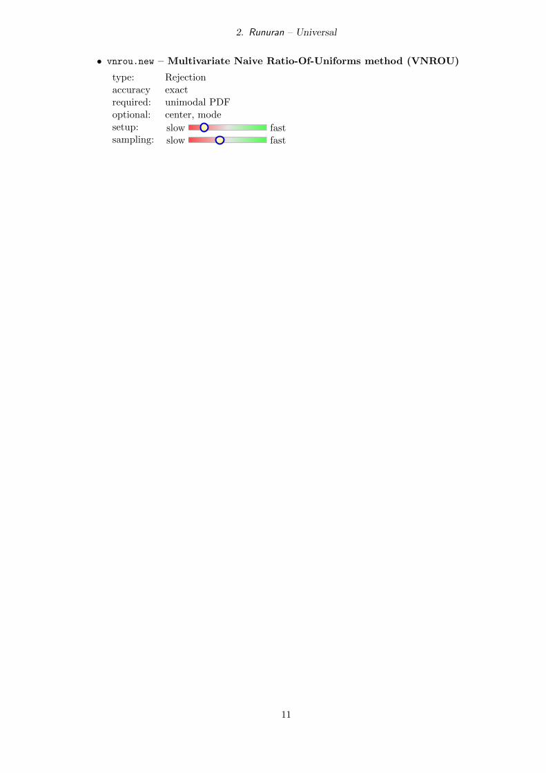
• vnrou.new – Multivariate Naive Ratio-Of-Uniforms method (VNROU)
type: Rejectionaccuracy exactrequired: unimodal PDFoptional: center, modesetup: slow fastsampling: slow fast
11
3. Runuran – Distributions
3. Runuran – Distributions
Coding the required functions for the routines in Section 2 can sometimes a bit tedious espe-cially if the target distribution has a more complex density function. Thus we have compileda set of functions that provides ready-to-use distribution objects. These objects can either beused as argument for unuran.new (see Section 4) or an alternative form of the functions fromSection 2.
These functions share a similar syntax and naming scheme (only ud is prefixed) with anal-ogous Rbuilt-in functions that provide density, distribution function and quantile:
ud...(distribution parameters, lb , ub)
Example
> ## Create an object for a gamma distribution with shape parameter 5.> distr <- udgamma(shape=5)> ## Create the UNU.RAN generator object. use method PINV (inversion).> gen <- pinvd.new(distr)> ## Draw a sample of size 100> x <- ur(gen,100)> ## Compute some quantiles for Monte Carlo methods> x <- uq(gen, (1:9)/10)
Currently the following distributions are available (see the corresponding help page for details):
Continuous Univariate Distributions (26)
Function Distribution
udbeta . . . Betaudcauchy . . . Cauchyudchi . . . Chiudchisq . . . Chi-squaredudexp . . . Exponentialudf . . . Fudfrechet . . . Frechet (Extreme value type II)udgamma . . . Gammaudghyp . . . Generalized Hyperbolicudgig . . . Generalized Inverse Gaussianudgumbel . . . Gumbel (Extreme value type I)udhyperbolic . . . Hyperbolicudig . . . Inverse Gaussian (Wald)udlaplace . . . Laplace (double exponential)udlnorm . . . Log Normaludlogis . . . Logisticudlomax . . . Lomax (Pareto of second kind)udmeixner . . . Meixnerudnorm . . . Normal (Gaussian)udpareto . . . Pareto (of first kind)udpowerexp . . . Powerexponential (Subbotin)udrayleigh . . . Rayleigh
12
3. Runuran – Distributions
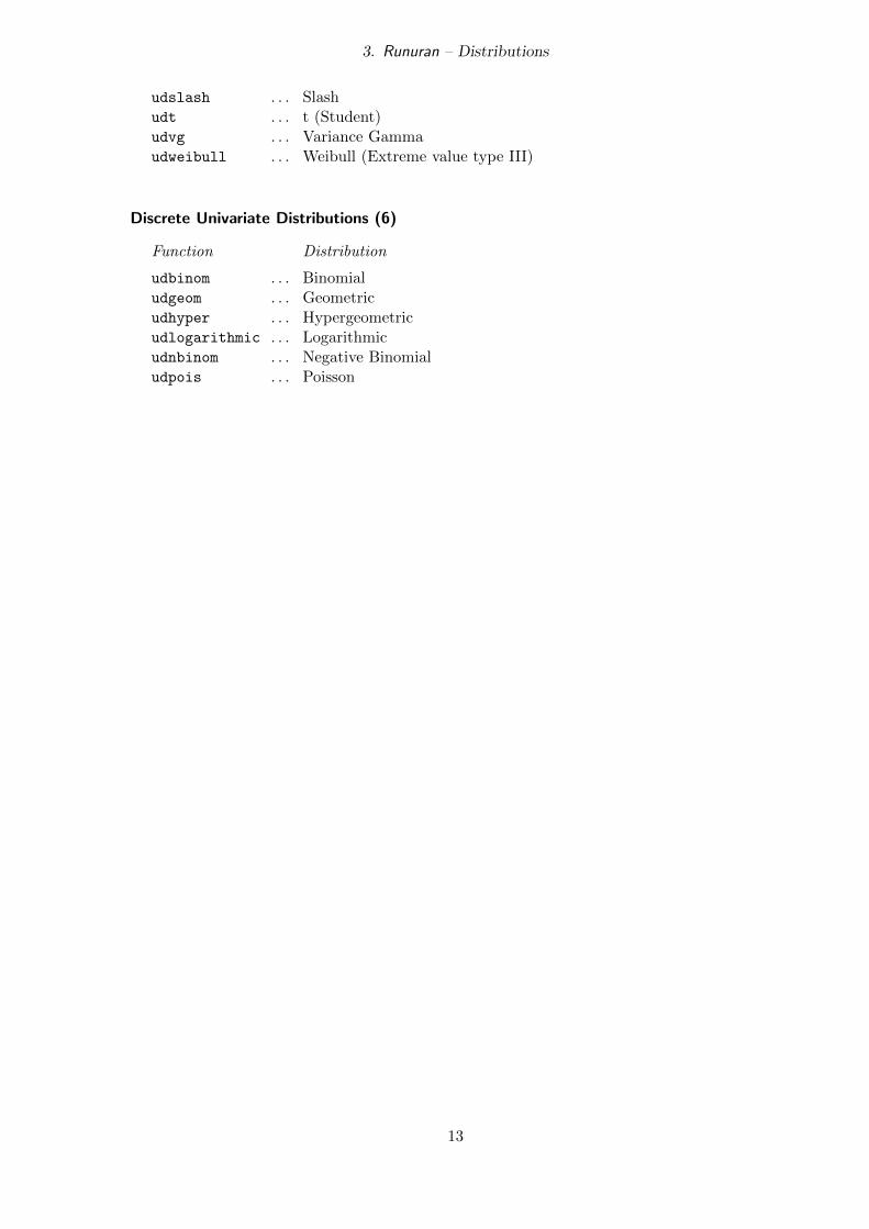
udslash . . . Slashudt . . . t (Student)udvg . . . Variance Gammaudweibull . . . Weibull (Extreme value type III)
Discrete Univariate Distributions (6)
Function Distribution
udbinom . . . Binomialudgeom . . . Geometricudhyper . . . Hypergeometricudlogarithmic . . . Logarithmicudnbinom . . . Negative Binomialudpois . . . Poisson
13
4. Runuran – Advanced
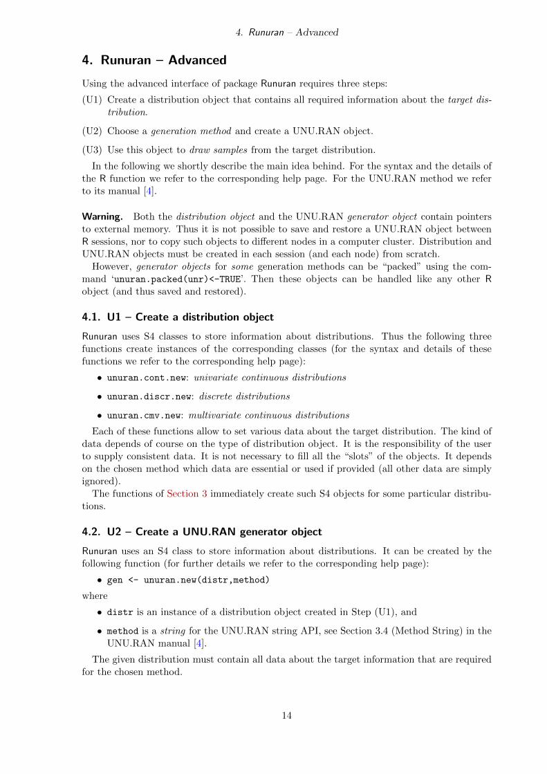
4. Runuran – Advanced
Using the advanced interface of package Runuran requires three steps:
(U1) Create a distribution object that contains all required information about the target dis-tribution.
(U2) Choose a generation method and create a UNU.RAN object.
(U3) Use this object to draw samples from the target distribution.
In the following we shortly describe the main idea behind. For the syntax and the details ofthe R function we refer to the corresponding help page. For the UNU.RAN method we referto its manual [4].
Warning. Both the distribution object and the UNU.RAN generator object contain pointersto external memory. Thus it is not possible to save and restore a UNU.RAN object betweenR sessions, nor to copy such objects to different nodes in a computer cluster. Distribution andUNU.RAN objects must be created in each session (and each node) from scratch.
However, generator objects for some generation methods can be “packed” using the com-mand ‘unuran.packed(unr)<-TRUE’. Then these objects can be handled like any other Robject (and thus saved and restored).
4.1. U1 – Create a distribution object
Runuran uses S4 classes to store information about distributions. Thus the following threefunctions create instances of the corresponding classes (for the syntax and details of thesefunctions we refer to the corresponding help page):
• unuran.cont.new: univariate continuous distributions
• unuran.discr.new: discrete distributions
• unuran.cmv.new: multivariate continuous distributions
Each of these functions allow to set various data about the target distribution. The kind ofdata depends of course on the type of distribution object. It is the responsibility of the userto supply consistent data. It is not necessary to fill all the “slots” of the objects. It dependson the chosen method which data are essential or used if provided (all other data are simplyignored).
The functions of Section 3 immediately create such S4 objects for some particular distribu-tions.
4.2. U2 – Create a UNU.RAN generator object
Runuran uses an S4 class to store information about distributions. It can be created by thefollowing function (for further details we refer to the corresponding help page):
• gen <- unuran.new(distr,method)
where
• distr is an instance of a distribution object created in Step (U1), and
• method is a string for the UNU.RAN string API, see Section 3.4 (Method String) in theUNU.RAN manual [4].
The given distribution must contain all data about the target information that are requiredfor the chosen method.
14
4. Runuran – Advanced
Remark. UNU.RAN also has a string API for distributions, see Section 3.2 (DistributionString) in the UNU.RAN manual [4]. Thus distr can also be such a string. However, besidessome special cases the approach described in Section 4.1 above is more flexible inside R.
4.3. U3 – Draw samples
The UNU.RAN object created in Step (U2) can then be used to draw samples from the targetdistribution. Let gen such a generator object.
• ur(gen,n) draws a pseudo-random sample of size n.
• uq(gen,u) computes quantiles (inverse CDFs) for the u values given in vector u. How-ever, this requires that the method (gen) we are using implements an inversion methodlike PINV or DGT.
In addition it is possible to get some information about the generator object.
• show(gen) (or simply gen) prints some information about the used data of the distribu-tion as well as sampling method and performance characteristics of the generator objecton the screen.
• unuran.details(gen) is more verbose and additionally prints parameter settings forthe chosen method (including default values) and some hints for changing (improving)its performance.
Uniform random numbers. All UNU.RAN methods use the R built-in random number gen-erator as the source of (pseudo-) random numbers. Thus the generated samples depend on thestate .Random.seed and can be controlled by the R functions RNGkind and set.seed.
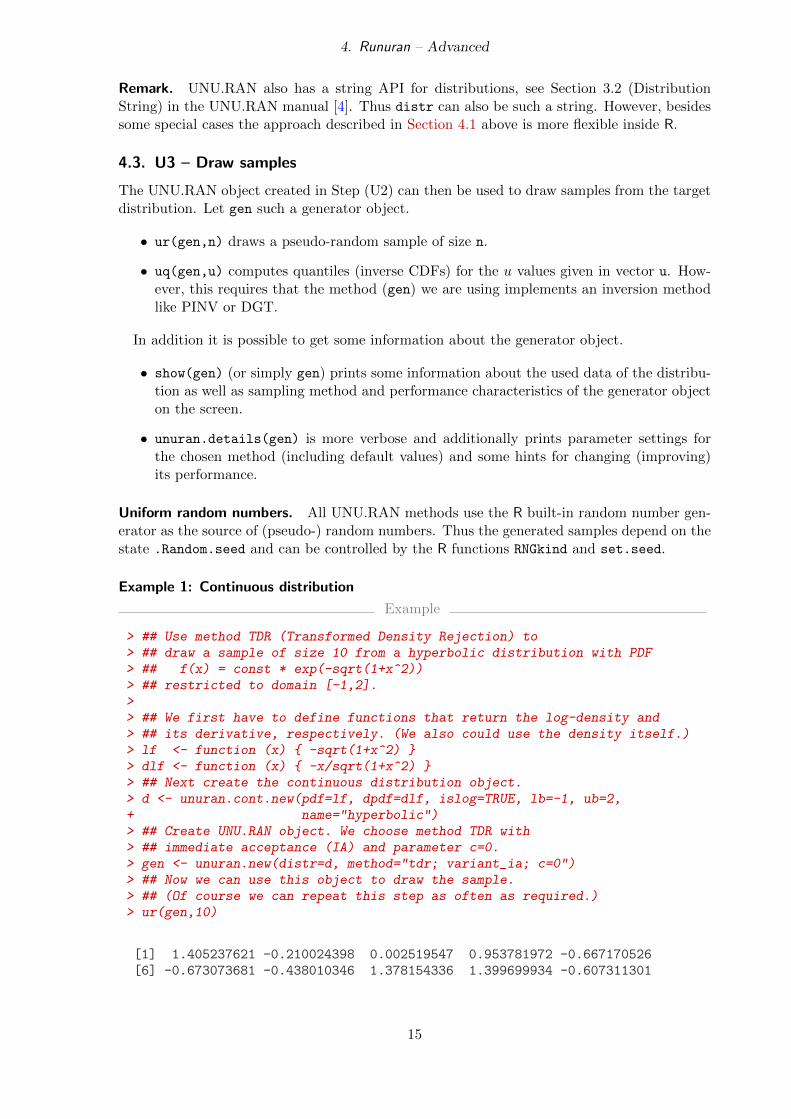
Example 1: Continuous distribution
Example
> ## Use method TDR (Transformed Density Rejection) to> ## draw a sample of size 10 from a hyperbolic distribution with PDF> ## f(x) = const * exp(-sqrt(1+x^2))> ## restricted to domain [-1,2].>> ## We first have to define functions that return the log-density and> ## its derivative, respectively. (We also could use the density itself.)> lf <- function (x) { -sqrt(1+x^2) }> dlf <- function (x) { -x/sqrt(1+x^2) }> ## Next create the continuous distribution object.> d <- unuran.cont.new(pdf=lf, dpdf=dlf, islog=TRUE, lb=-1, ub=2,+ name="hyperbolic")> ## Create UNU.RAN object. We choose method TDR with> ## immediate acceptance (IA) and parameter c=0.> gen <- unuran.new(distr=d, method="tdr; variant_ia; c=0")> ## Now we can use this object to draw the sample.> ## (Of course we can repeat this step as often as required.)> ur(gen,10)
[1] 1.405237621 -0.210024398 0.002519547 0.953781972 -0.667170526[6] -0.673073681 -0.438010346 1.378154336 1.399699934 -0.607311301
15
4. Runuran – Advanced
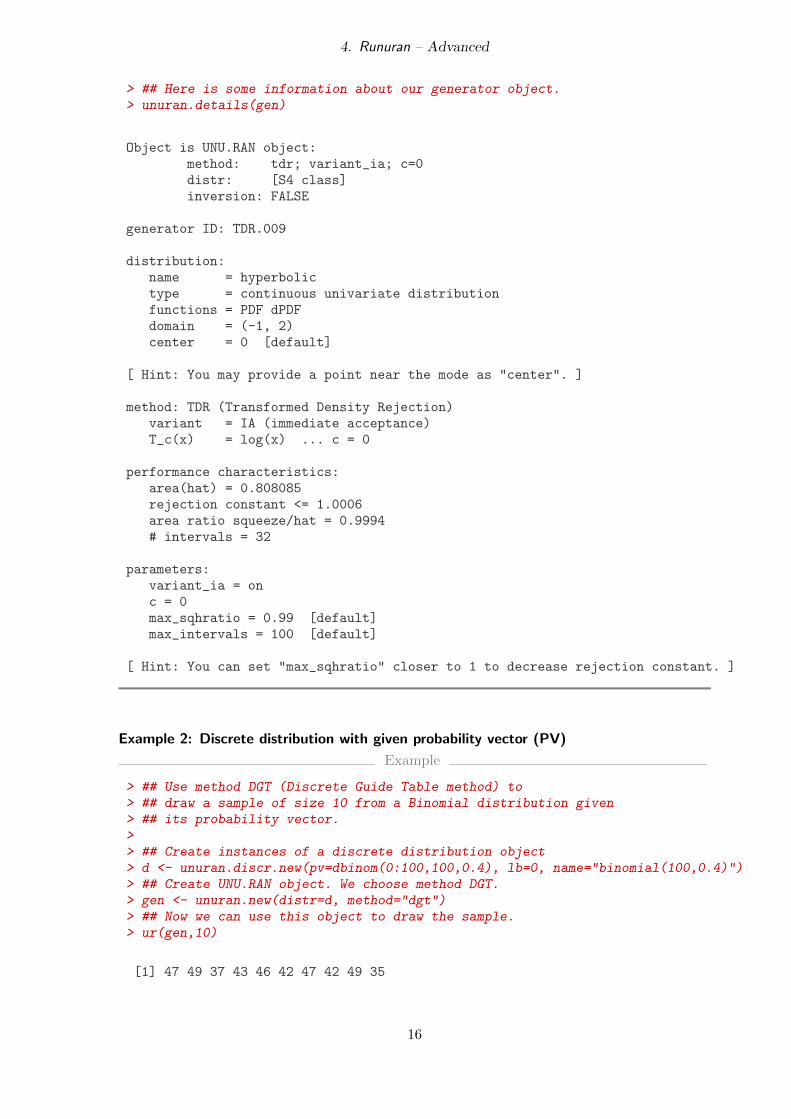
> ## Here is some information about our generator object.> unuran.details(gen)
Object is UNU.RAN object:method: tdr; variant_ia; c=0distr: [S4 class]inversion: FALSE
generator ID: TDR.009
distribution:name = hyperbolictype = continuous univariate distributionfunctions = PDF dPDFdomain = (-1, 2)center = 0 [default]
[ Hint: You may provide a point near the mode as "center". ]
method: TDR (Transformed Density Rejection)variant = IA (immediate acceptance)T_c(x) = log(x) ... c = 0
performance characteristics:area(hat) = 0.808085rejection constant <= 1.0006area ratio squeeze/hat = 0.9994# intervals = 32
parameters:variant_ia = onc = 0max_sqhratio = 0.99 [default]max_intervals = 100 [default]
[ Hint: You can set "max_sqhratio" closer to 1 to decrease rejection constant. ]
Example 2: Discrete distribution with given probability vector (PV)
Example
> ## Use method DGT (Discrete Guide Table method) to> ## draw a sample of size 10 from a Binomial distribution given> ## its probability vector.>> ## Create instances of a discrete distribution object> d <- unuran.discr.new(pv=dbinom(0:100,100,0.4), lb=0, name="binomial(100,0.4)")> ## Create UNU.RAN object. We choose method DGT.> gen <- unuran.new(distr=d, method="dgt")> ## Now we can use this object to draw the sample.> ur(gen,10)
[1] 47 49 37 43 46 42 47 42 49 35
16
4. Runuran – Advanced
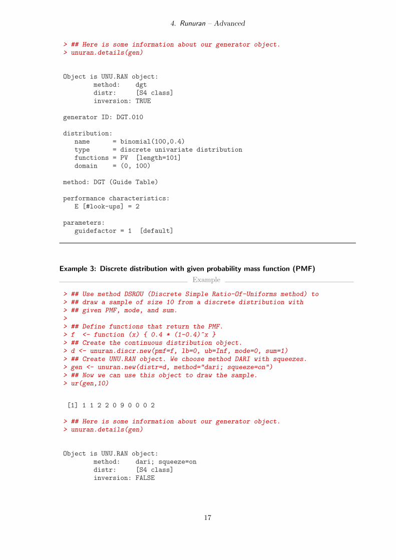
> ## Here is some information about our generator object.> unuran.details(gen)
Object is UNU.RAN object:method: dgtdistr: [S4 class]inversion: TRUE
generator ID: DGT.010
distribution:name = binomial(100,0.4)type = discrete univariate distributionfunctions = PV [length=101]domain = (0, 100)
method: DGT (Guide Table)
performance characteristics:E [#look-ups] = 2
parameters:guidefactor = 1 [default]
Example 3: Discrete distribution with given probability mass function (PMF)
Example
> ## Use method DSROU (Discrete Simple Ratio-Of-Uniforms method) to> ## draw a sample of size 10 from a discrete distribution with> ## given PMF, mode, and sum.>> ## Define functions that return the PMF.> f <- function (x) { 0.4 * (1-0.4)^x }> ## Create the continuous distribution object.> d <- unuran.discr.new(pmf=f, lb=0, ub=Inf, mode=0, sum=1)> ## Create UNU.RAN object. We choose method DARI with squeezes.> gen <- unuran.new(distr=d, method="dari; squeeze=on")> ## Now we can use this object to draw the sample.> ur(gen,10)
[1] 1 1 2 2 0 9 0 0 0 2
> ## Here is some information about our generator object.> unuran.details(gen)
Object is UNU.RAN object:method: dari; squeeze=ondistr: [S4 class]inversion: FALSE
17
4. Runuran – Advanced
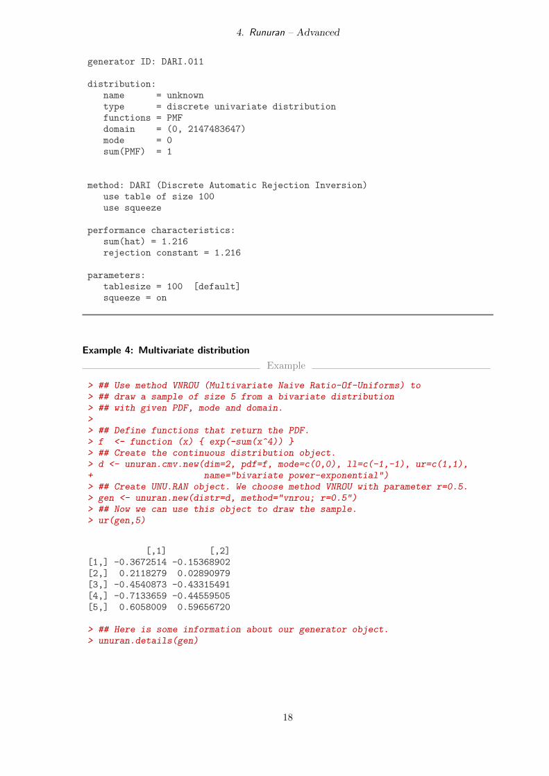
generator ID: DARI.011
distribution:name = unknowntype = discrete univariate distributionfunctions = PMFdomain = (0, 2147483647)mode = 0sum(PMF) = 1
method: DARI (Discrete Automatic Rejection Inversion)use table of size 100use squeeze
performance characteristics:sum(hat) = 1.216rejection constant = 1.216
parameters:tablesize = 100 [default]squeeze = on
Example 4: Multivariate distribution
Example
> ## Use method VNROU (Multivariate Naive Ratio-Of-Uniforms) to> ## draw a sample of size 5 from a bivariate distribution> ## with given PDF, mode and domain.>> ## Define functions that return the PDF.> f <- function (x) { exp(-sum(x^4)) }> ## Create the continuous distribution object.> d <- unuran.cmv.new(dim=2, pdf=f, mode=c(0,0), ll=c(-1,-1), ur=c(1,1),+ name="bivariate power-exponential")> ## Create UNU.RAN object. We choose method VNROU with parameter r=0.5.> gen <- unuran.new(distr=d, method="vnrou; r=0.5")> ## Now we can use this object to draw the sample.> ur(gen,5)
[,1] [,2][1,] -0.3672514 -0.15368902[2,] 0.2118279 0.02890979[3,] -0.4540873 -0.43315491[4,] -0.7133659 -0.44559505[5,] 0.6058009 0.59656720
> ## Here is some information about our generator object.> unuran.details(gen)
18
4. Runuran – Advanced
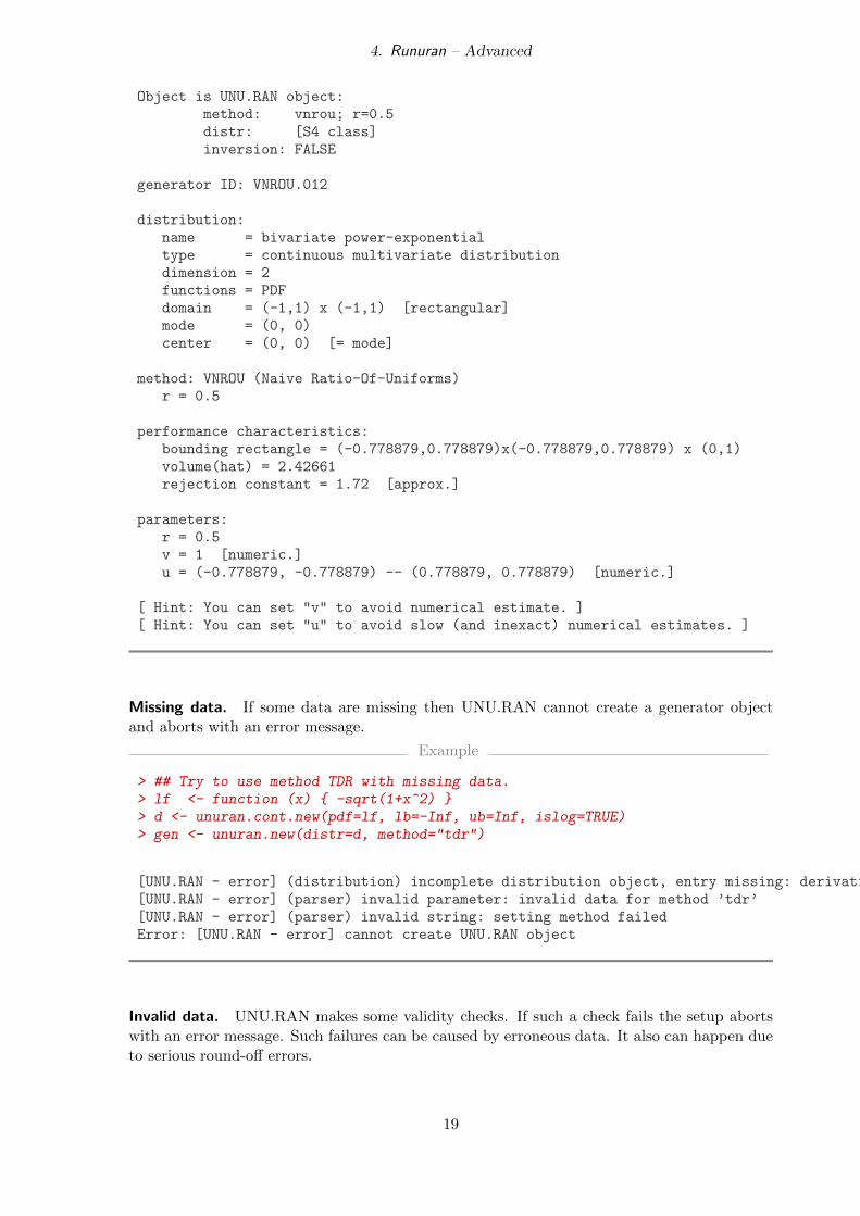
Object is UNU.RAN object:method: vnrou; r=0.5distr: [S4 class]inversion: FALSE
generator ID: VNROU.012
distribution:name = bivariate power-exponentialtype = continuous multivariate distributiondimension = 2functions = PDFdomain = (-1,1) x (-1,1) [rectangular]mode = (0, 0)center = (0, 0) [= mode]
method: VNROU (Naive Ratio-Of-Uniforms)r = 0.5
performance characteristics:bounding rectangle = (-0.778879,0.778879)x(-0.778879,0.778879) x (0,1)volume(hat) = 2.42661rejection constant = 1.72 [approx.]
parameters:r = 0.5v = 1 [numeric.]u = (-0.778879, -0.778879) -- (0.778879, 0.778879) [numeric.]
[ Hint: You can set "v" to avoid numerical estimate. ][ Hint: You can set "u" to avoid slow (and inexact) numerical estimates. ]
Missing data. If some data are missing then UNU.RAN cannot create a generator objectand aborts with an error message.
Example
> ## Try to use method TDR with missing data.> lf <- function (x) { -sqrt(1+x^2) }> d <- unuran.cont.new(pdf=lf, lb=-Inf, ub=Inf, islog=TRUE)> gen <- unuran.new(distr=d, method="tdr")
[UNU.RAN - error] (distribution) incomplete distribution object, entry missing: derivative of PDF[UNU.RAN - error] (parser) invalid parameter: invalid data for method ’tdr’[UNU.RAN - error] (parser) invalid string: setting method failedError: [UNU.RAN - error] cannot create UNU.RAN object
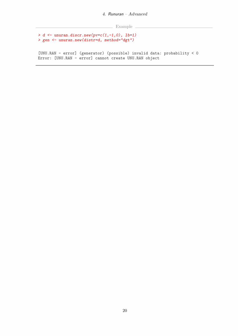
Invalid data. UNU.RAN makes some validity checks. If such a check fails the setup abortswith an error message. Such failures can be caused by erroneous data. It also can happen dueto serious round-off errors.
19
4. Runuran – Advanced
Example
> d <- unuran.discr.new(pv=c(1,-1,0), lb=1)> gen <- unuran.new(distr=d, method="dgt")
[UNU.RAN - error] (generator) (possible) invalid data: probability < 0Error: [UNU.RAN - error] cannot create UNU.RAN object
20
A. A Short Introduction to Random Variate Generation
A. A Short Introduction to Random Variate Generation
Random variate generation is the small field of research that deals with algorithms to generaterandom variates from various distributions. It is common to assume that a uniform randomnumber generator is available, that is, a program that produces a sequence of independent andidentically distributed continuous U(0, 1) random variates (i.e., uniform random variates onthe interval (0, 1)). Of course real world computers can never generate ideal random numbersand they cannot produce numbers of arbitrary precision but state-of-the-art uniform randomnumber generators come close to this aim. Thus random variate generation deals with theproblem of transforming such a sequence of uniform random numbers into non-uniform randomvariates.
In this section we shortly explain the basic ideas of the inversion, rejection, and the ratioof uniforms method. How these ideas can be used to design a particular automatic randomvariate generation algorithms that can be applied to large classes of distributions is shortlyexplained in the description of the different methods included in this manual.
For a deeper treatment of the ideas presented here, for other basic methods and for automaticgenerators we refer the interested reader to our book [2].
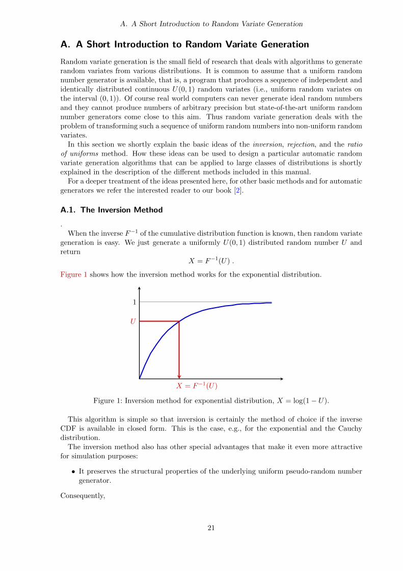
A.1. The Inversion Method
.When the inverse F−1 of the cumulative distribution function is known, then random variate
generation is easy. We just generate a uniformly U(0, 1) distributed random number U andreturn
X = F−1(U) .
Figure 1 shows how the inversion method works for the exponential distribution.
1
U
X = F−1(U)
Figure 1: Inversion method for exponential distribution, X = log(1− U).
This algorithm is simple so that inversion is certainly the method of choice if the inverseCDF is available in closed form. This is the case, e.g., for the exponential and the Cauchydistribution.
The inversion method also has other special advantages that make it even more attractivefor simulation purposes:
• It preserves the structural properties of the underlying uniform pseudo-random numbergenerator.
Consequently,
21
A. A Short Introduction to Random Variate Generation
• it can be used for variance reduction techniques;
• it is easy to sample from truncated distributions;
• it is easy to sample from marginal distributions and thus is suitable for using with copulæ;
• the quality of the generated random variables depends only on the underlying uniform(pseudo-) random number generator.
Another important advantage of the inversion method is that we can easily characterize itsperformance. To generate one random variate we always need exactly one uniform variate andone evaluation of the inverse CDF. So its speed mainly depends on the costs for evaluatingthe inverse CDF. Hence inversion is often considered as the method of choice in the simulationliterature.
Unfortunately computing the inverse CDF is often comparatively difficult and slow, e.g., forstandard distributions like normal, student, gamma, and beta distributions. Often no suchroutines are available in standard programming libraries. Then numerical methods for invert-ing the CDF are necessary, e.g., Newton’s method or interpolation. Such procedures, however,have the disadvantage that they may be slow or not exact, i.e. they compute approximatevalues. The methods HINV, HINV and PINV of UNU.RAN are such numerical inversion methods.
A.1.1. Approximation Errors
For numerical inversion methods the approximation error is important for the quality of thegenerated point set. Let X = G−1(U) denote the approximate inverse CDF, and let F andF−1 be the exact CDF and inverse CDF of the distribution, resp. There are three measuresfor the approximation error:
u-error – is given byu-error = |U − F (G−1(U))|
Goodness-of-fit tests like the Kolmogorov-Smirnov test or the chi-squared test look atthis type of error. We are also convinced that it is the most suitable error measure forMonte Carlo simulations as pseudo-random numbers and points of low discrepancy setsare located on a grid of restricted resolution.
x-error – is given by
absolute x-error = |F−1(U)−G−1(U)|relative x-error = |F−1(U)−G−1(U)| · |F−1(U)|
The x-error measure the deviation of G−1(U) from the exact result. This measure issuitable when the inverse CDF is used as a quantile function in some computations.The main problem with the x-error is that we have to use the absolute x-error forX = F−1(U) close to zero and the relative x-error in the tails.
We use the terms u-resolution and x-resolution as the maximal tolerated u-error and x-error,resp.
UNU.RAN allows to set u-resolution and x-resolution independently. Both requirementsmust be fulfilled. We use the following strategy for checking whether the precision goal isreached:
22
A. A Short Introduction to Random Variate Generation
checking u-error: The u-error must be slightly smaller than the given u-resolution:
|U − F (G−1(U))| < 0.9 · u-resolution .
There is no necessity to consider the relative u-error as we have 0 < U < 1.
checking x-error: We combine absolute and relative x-error and use the criterion
|F−1(U)−G−1(U)| < x-resolution · (|G−1(U)|+ x-resolution)
Remark. It should be noted here that the criterion based on the u-error is too stringent wherethe CDF is extremely steep (and thus the PDF has a pole or a high and narrow peak). This isin particular a problem for distributions with a pole (e.g., the gamma distribution with shapeparameter less than 0.5). On the other hand using a criterion based on the x-error causesproblems where the CDF is extremely flat. This is in particular the case in the (far) tails ofheavy-tailed distributions (e.g., for the Cauchy distribution).
A.2. The Acceptance-Rejection Method
The acceptance-rejection method has been suggested by John von Neumann in 1951 [7]. Sincethen it has been proven to be the most flexible and most efficient method to generate variatesfrom continuous distributions.
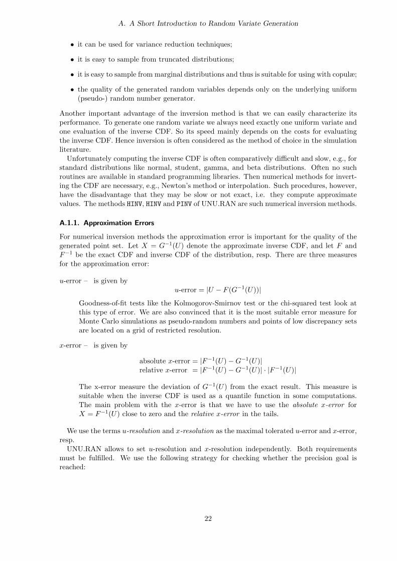
We explain the rejection principle first for the density f(x) = sin(x)/2 on the interval (0, π).To generate random variates from this distribution we also can sample random points that areuniformly distributed in the region between the graph of f(x) and the x-axis, i.e., the shadedregion in Figure 2.
12
π
Figure 2: Acceptance-rejection method. Points are drawn randomly in [0, π] × [0, 1]. Pointsabove the density (◦) are rejected; points below the density (•) are accepted andtheir x-coordinates are returned. Notice that there is no need to evaluate the densitywhenever a points falls into the region below the dashed triangle (squeeze).
In general this is not a trivial task but in this example we can easily use the rejectiontrick: Sample a random point (X,Y ) uniformly in the bounding rectangle (0, π) × (0, 1/2).This is easy since each coordinate can be sampled independently from the respective uniform
23
A. A Short Introduction to Random Variate Generation
distributions U(0, π) and U(0, 1/2). Whenever the point falls into the shaded region below thegraph (indicated by dots in the figure), i.e., when Y < sin(X)/2, we accept it and return Xas a random variate from the distribution with density f(x). Otherwise we have to reject thepoint (indicated by small circles in the figure), and try again.
It is quite clear that this idea works for every distribution with a bounded density on abounded domain. Moreover, we can use this procedure with any multiple of the density, i.e.,with any positive bounded function with bounded integral and it is not necessary to know theintegral of this function. So we use the term density in the sequel for any positive functionwith bounded integral.
From the figure we can conclude that the performance of a rejection algorithm dependsheavily on the area of the enveloping rectangle. Moreover, the method does not work if thetarget distribution has infinite tails (or is unbounded). Hence non-rectangular shaped regionsfor the envelopes are important and we have to solve the problem of sampling points uniformlyfrom such domains. Looking again at the example above we notice that the x-coordinate of therandom point (X,Y ) was sampled by inversion from the uniform distribution on the domainof the given density. This motivates us to replace the density of the uniform distributionby the (multiple of a) density h(x) of some other appropriate distribution. We only have totake care that it is chosen such that it is always an upper bound, i.e., h(x) >= f(x) for allx in the domain of the distribution. To generate the pair (X,Y ) we generate X from thedistribution with density proportional to h(x) and Y uniformly between 0 and h(X). The firststep (generate X) is usually done by inversion, see Section A.1.
Thus the general rejection algorithm for a hat h(x) with inverse CDF H−1 consists of thefollowing steps:
1. Generate a U(0, 1) random number U .
2. Set X ← H−1(U).
3. Generate a U(0, 1) random number V .
4. Set Y ← V h(X).
5. If Y ≤ f(X) accept and return X.
6. Else try again.
If the evaluation of the density f(x) is expensive (i.e., time consuming) it is possible to usea simple lower bound of the density as so called squeeze function s(x) (the triangular shapedfunction in Figure 2 is an example for such a squeeze). We can then accept X when Y ≤ s(X)and can thus often save the evaluation of the density.
We have seen so far that the rejection principle leads to short and simple generation al-gorithms. The main practical problem to apply the rejection algorithm is the search for agood fitting hat function and squeezes. We do not discuss these topics here as they are theheart of the different automatic algorithms implemented in UNU.RAN. Information about theconstruction of hat and squeeze can therefore be found in the descriptions of the methods.
The performance characteristics of rejection algorithms mainly depend on the fit of the hatand the squeeze. It is not difficult to prove that:
• The expected number of trials to generate one variate is the ratio between the area belowthe hat and the area below the density.
• The expected number of evaluations of the density necessary to generate one variate isequal to the ratio between the area below the hat and the area below the density, when
24
A. A Short Introduction to Random Variate Generation
no squeeze is used. Otherwise, when a squeeze is given it is equal to the ratio betweenthe area between hat and squeeze and the area below the hat.
• The sqhratio (i.e., the ratio between the area below the squeeze and the area belowthe hat) used in some of the UNU.RAN methods is easy to compute. It is useful as itsreciprocal is an upper bound for the expected number of trials of the rejection algorithm.The expected number of evaluations of the density is bounded by (1/sqhratio)− 1.
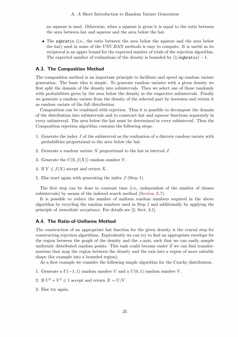
A.3. The Composition Method
The composition method is an important principle to facilitate and speed up random variategeneration. The basic idea is simple. To generate random variates with a given density wefirst split the domain of the density into subintervals. Then we select one of these randomlywith probabilities given by the area below the density in the respective subintervals. Finallywe generate a random variate from the density of the selected part by inversion and return itas random variate of the full distribution.
Composition can be combined with rejection. Thus it is possible to decompose the domainof the distribution into subintervals and to construct hat and squeeze functions separately inevery subinterval. The area below the hat must be determined in every subinterval. Then theComposition rejection algorithm contains the following steps:
1. Generate the index J of the subinterval as the realization of a discrete random variate withprobabilities proportional to the area below the hat.
2. Generate a random variate X proportional to the hat in interval J .
3. Generate the U(0, f(X)) random number Y .
4. If Y ≤ f(X) accept and return X.
5. Else start again with generating the index J (Step 1).
The first step can be done in constant time (i.e., independent of the number of chosensubintervals) by means of the indexed search method (Section A.7).
It is possible to reduce the number of uniform random numbers required in the abovealgorithm by recycling the random numbers used in Step 1 and additionally by applying theprinciple of immediate acceptance. For details see [2, Sect. 3.1].
A.4. The Ratio-of-Uniforms Method
The construction of an appropriate hat function for the given density is the crucial step forconstructing rejection algorithms. Equivalently we can try to find an appropriate envelope forthe region between the graph of the density and the x-axis, such that we can easily sampleuniformly distributed random points. This task could become easier if we can find transfor-mations that map the region between the density and the axis into a region of more suitableshape (for example into a bounded region).
As a first example we consider the following simple algorithm for the Cauchy distribution.
1. Generate a U(−1, 1) random number U and a U(0, 1) random number V .
2. If U2 + V 2 ≤ 1 accept and return X = U/V .
3. Else try again.
25
A. A Short Introduction to Random Variate Generation
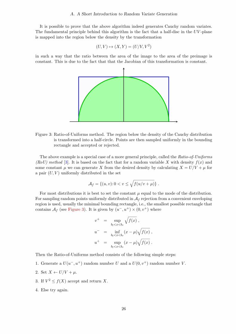
It is possible to prove that the above algorithm indeed generates Cauchy random variates.The fundamental principle behind this algorithm is the fact that a half-disc in the UV -planeis mapped into the region below the density by the transformation
(U, V ) 7→ (X,Y ) = (U/V, V 2)
in such a way that the ratio between the area of the image to the area of the preimage isconstant. This is due to the fact that that the Jacobian of this transformation is constant.
Figure 3: Ratio-of-Uniforms method. The region below the density of the Cauchy distributionis transformed into a half-circle. Points are then sampled uniformly in the boundingrectangle and accepted or rejected.
The above example is a special case of a more general principle, called the Ratio-of-Uniforms(RoU) method [3]. It is based on the fact that for a random variable X with density f(x) andsome constant µ we can generate X from the desired density by calculating X = U/V + µ fora pair (U, V ) uniformly distributed in the set
Af = {(u, v): 0 < v ≤√f(u/v + µ)} .
For most distributions it is best to set the constant µ equal to the mode of the distribution.For sampling random points uniformly distributed inAf rejection from a convenient envelopingregion is used, usually the minimal bounding rectangle, i.e., the smallest possible rectangle thatcontains Af (see Figure 3). It is given by (u−, u+)× (0, v+) where
v+ = supbl<x<br
√f(x) ,
u− = infbl<x<br
(x− µ)√f(x) ,
u+ = supbl<x<br
(x− µ)√f(x) .
Then the Ratio-of-Uniforms method consists of the following simple steps:
1. Generate a U(u−, u+) random number U and a U(0, v+) random number V .
2. Set X ← U/V + µ.
3. If V 2 ≤ f(X) accept and return X.
4. Else try again.
26
A. A Short Introduction to Random Variate Generation
To apply the Ratio-of-Uniforms algorithm to a certain density we have to solve the simpleoptimization problems in the definitions above to obtain the design constants u−, u+, and v+.This simple algorithm works for all distributions with bounded densities that have subquadratictails (i.e., tails like 1/x2 or lower). For most standard distributions it has quite good rejectionconstants (e.g., 1.3688 for the normal and 1.4715 for the exponential distribution).
Nevertheless, we use more sophisticated method that construct better fitting envelopes, likemethod AROU, or even avoid the computation of these design constants and thus have almostno setup, like method SROU.
A.5. The Generalized Ratio-of-Uniforms Method
The Ratio-of-Uniforms method can be generalized in the following way [5, 8]: If a point (U, V )is uniformly distributed in the set
Af = {(u, v): 0 < v ≤ (f(u/vr + µ))1/(r+1)}
for some real number r > 0, then X = U/V r +µ has the density f(x). The minimal boundingrectangle of this region is given by (u−, u+)× (0, v+) where
v+ = supbl<x<br
(f(x))1/(r+1) ,
u− = infbl<x<br
(x− µ)(f(x))r/(r+1) ,
u+ = supbl<x<br
(x− µ)(f(x))r/(r+1) .
The above algorithm has then to be adjusted accordingly. Notice that the original Ratio-of-Uniforms method is the special case with r = 1.
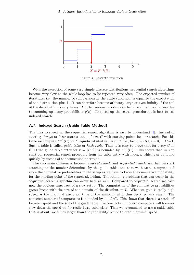
A.6. Inversion for Discrete Distributions
We have already presented the idea of the inversion method to generate from continuousrandom variables (Section A.1). For a discrete random variable X we can write it formally inthe same way:
X = F−1(U) ,
where F is the CDF of the desired distribution and U is a uniform U(0, 1) random number.The difference compared to the continuous case is that F is now a step-function. The followingfigure illustrates the idea of discrete inversion for a simple distribution.
To realize this idea on a computer we have to use a search algorithm. For the simplest versioncalled Sequential Search the CDF is computed on-the-fly as sum of the probabilities p(k), sincethis is usually much cheaper than computing the CDF directly. It is obvious that the basicform of the search algorithm only works for discrete random variables with probability massfunctions p(k) for nonnegative k. The sequential search algorithm consists of the followingbasic steps:
1. Generate a U(0, 1) random number U .
2. Set X ← 0 and P ← p(0).
3. Do while U > P
4. Set X ← X + 1 and P ← P + p(X).
5. Return X.
27
A. A Short Introduction to Random Variate Generation
1
0 1 2 3 4 5
U
X = F−1(U)
Figure 4: Discrete inversion
With the exception of some very simple discrete distributions, sequential search algorithmsbecome very slow as the while-loop has to be repeated very often. The expected number ofiterations, i.e., the number of comparisons in the while condition, is equal to the expectationof the distribution plus 1. It can therefore become arbitrary large or even infinity if the tailof the distribution is very heavy. Another serious problem can be critical round-off errors dueto summing up many probabilities p(k). To speed up the search procedure it is best to useindexed search.
A.7. Indexed Search (Guide Table Method)
The idea to speed up the sequential search algorithm is easy to understand [1]. Instead ofstarting always at 0 we store a table of size C with starting points for our search. For thistable we compute F−1(U) for C equidistributed values of U , i.e., for ui = i/C, i = 0, ..., C− 1.Such a table is called guide table or hash table. Then it is easy to prove that for every U in(0, 1) the guide table entry for k = bU Cc is bounded by F−1(U). This shows that we canstart our sequential search procedure from the table entry with index k which can be foundquickly by means of the truncation operation.
The two main differences between indexed search and sequential search are that we startsearching at the number determined by the guide table, and that we have to compute andstore the cumulative probabilities in the setup as we have to know the cumulative probabilityfor the starting point of the search algorithm. The rounding problems that can occur in thesequential search algorithm can occur here as well. Compared to sequential search we havenow the obvious drawback of a slow setup. The computation of the cumulative probabilitiesgrows linear with the size of the domain of the distribution L. What we gain is really highspeed as the marginal execution time of the sampling algorithm becomes very small. Theexpected number of comparisons is bounded by 1 + L/C. This shows that there is a trade-offbetween speed and the size of the guide table. Cache-effects in modern computers will howeverslow down the speed-up for really large table sizes. Thus we recommend to use a guide tablethat is about two times larger than the probability vector to obtain optimal speed.
28
B. Pitfalls
B. Pitfalls
Libraries like Runuran that provide a flexible interface also have the risk of possible traps andpitfalls. Besides the obvious case where the chosen method cannot be used for sampling fromthe target distribution we observed that users sometimes forget to change the default values ofthe function arguments, e.g., they do not set the center (a “typical point” of the distribution)when the domain does not contain 0. Then it may happen that the chosen generation methoddoes not work or (the worst case!) does not work as expected.
Check argument defaults whenever you use an Runuran function!
Here is an examples2 of possible problems and how to fix these.
Shifted center. Some methods require a “typical” point of the distribution, called center.By default this is set to center=0. The PDF at the center must not be too small. Thus ifpdf(center) returns 0 the chosen method does not work.
Example
> pdf <- function (x) { x^2 / (1+x^2)^2 }> gen <- pinv.new(pdf=pdf,lb=0,ub=Inf)
[UNU.RAN - error] (generator) condition for method violated: PDF(center) <= 0.Error: [UNU.RAN - error] cannot create UNU.RAN object
Solution: Set center to (a point near) the mode of the distribution.
Example
> pdf <- function (x) { x^2 / (1+x^2)^2 }> gen <- pinv.new(pdf=pdf,lb=0,ub=Inf, center=1 ) ## Add ’center’> x <- ur(gen,10)> x
[1] 0.2046206 2.5224216 10.9688719 3.9461917 1.2944052 0.4987049[7] 1.6116184 1.8517735 41.3293269 1.9838912
Broken Runuran objects. Runuran objects contain pointers to external objects. Conse-quently, it is not possible to save and restore an Runuran object between R sessions, nor tocopy such objects to different nodes in a computer cluster. Runuran objects must be newlycreated in each session (and in each node) from scratch. Otherwise, the object is broken andur and uq refuse do not work.
However, generator objects for some generation methods can be packed. Then these objectscan be handled like any other R object (and thus saved and restored).
Here is an example how a generator object can be packed.
2Please sent us examples where you had problems with the concept of Runuran.
29
B. Pitfalls
Example
> ## create a unuran object using method ’PINV’> gen <- pinv.new(dnorm,lb=0,ub=Inf)> ## such an object can be packed> unuran.packed(gen) <- TRUE> ## it can be still used to draw a random sample> x <- ur(gen,10)> x
[1] 0.2959399 1.6119795 1.3637418 0.8237170 1.2283152 0.5578596 0.3019846[8] 0.6153025 0.3013844 0.2793911
> ## we also can check whether a unuran object is packed> unuran.packed(gen)
[1] TRUE
Now we can save or R session and start a new one with the previously saved workspacerestored. Then we can reuse object gen (after loading library Runuran).
Without packing gen, it would be broken after restoring the saved workspace.
Example
[Previously saved workspace restored]
> library(Runuran)> ur(gen,10)
Error in ur(gen, 10) : [UNU.RAN - error] broken UNU.RAN object
30
C. Glossary
C. Glossary
CDF – cumulative distribution function.
center – “typical point” of distribution (“near the mode”).
HR – hazard rate (or failure rate).
inverse local concavity – local concavity of inverse PDF f−1(y) expressed in term ofx = f−1(y). Is is given by
ilcf (x) = 1 + x f ′′(x)/f ′(x) .
mode – maximum of PDF.
local concavity – maximum value of c such that PDF f(x) is Tc-concave. Is is given by
lcf (x) = 1− f ′′(x) f(x)/f ′(x)2 .
log-concave – a PDF f(x) (and hence the corresponding distribution) is called log-concave iflog(f(x)) is concave, i.e., if (log(f(x))′′ ≤ 0. See also T0-concave.
For discrete distributions, a PMF p is log-concave if and only if
pi ≥√pi−1 pi+1 for all i.
PDF – probability density function.
PMF – probability mass function.
PV – (finite) probability vector.
URNG – uniform random number generator.
U(a, b) – continuous uniform distribution on the interval (a, b).
Tc-concave – a PDF f(x) is called T -concave if the transformed function T (f(x)) is concave.We only deal with transformations Tc, where
c transformation
c = 0 T0(x) = log(x)c = −1/2 T−1/2(x) = −1/
√x
c 6= 0 Tc(x) = sgn(c) · xc
In particular, a PDF f(x) is Tc-concave when its local concavity is less than c,i.e., lcf (x) ≤ c.
u-error – for a given approximate inverse CDF X = G−1(U) the u-error is given as
u-error = |U − F (G−1(U))|
where F denotes the exact CDF. Goodness-of-fit tests like the Kolmogorov-Smirnov test or the chi-squared test look at this type of error.
u-resolution – the maximal tolerated u-error for an approximate inverse CDF.
31
C. Glossary
x-error – for a given approximate inverse CDF X = G−1(U) the x-error is given as
x-error = |F−1(U)−G−1(U)|
where F−1 denotes the exact inverse CDF. The x-error measure the deviationof G−1(U) from the exact result. Notice that we have to distinguish betweenabsolute and relative x-error. In UNU.RAN we use the absolute x-error near 0and the relative x-error otherwise, see Section A.1.1 for more details.
x-resolution – the maximal tolerated x-error for an approximate inverse CDF.
32
References
References
[1] H. C. Chen and Y. Asau. On generating random variates from an empirical distribution.AIIE Trans., 6:163–166, 1974.
[2] W. Hormann, J. Leydold, and G. Derflinger. Automatic Nonuniform Random VariateGeneration. Springer-Verlag, Berlin Heidelberg, 2004.
[3] A. J. Kinderman and J. F. Monahan. Computer generation of random variables using theratio of uniform deviates. ACM Trans. Math. Softw., 3(3):257–260, 1977.
[4] J. Leydold and W. Hormann. UNU.RAN User Manual. Department of Statistics andMathematics, WU Wien, Augasse 2–6, A-1090 Wien, Austria. http://statmath.wu.ac.
at/unuran/.
[5] S. Stefanescu and I. Vaduva. On computer generation of random vectors by transformationsof uniformly distributed vectors. Computing, 39:141–153, 1987.
[6] G. Tirler and J. Leydold. Automatic nonuniform random variate generation in r. InK. Hornik and F. Leisch, editors, Proceedings of the 3rd International Workshop on Dis-tributed Statistical Computing (DSC 2003), 2003. URL http://www.ci.tuwien.ac.at/
Conferences/DSC-2003/Proceedings/. March 20–22, Vienna, Austria.
[7] J. von Neumann. Various techniques used in connection with random digits. In A. S.Householder et al., editors, The Monte Carlo Method, number 12 in Nat. Bur. StandardsAppl. Math. Ser., pages 36–38. 1951.
[8] J. C. Wakefield, A. E. Gelfand, and A. F. M. Smith. Efficient generation of random variatesvia the ratio-of-uniforms method. Statist. Comput., 1(2):129–133, 1991.
33
Related Documents