An overview of soil heterogeneity: quantification and implications on geotechnical field problems

An overview of soil heterogeneity: quantificationand implications on geotechnical field problems

Tamer Elkateb, Rick Chalaturnyk, and Peter K. Robertson

Abstract: Engineering judgment and reliance on factors of safety have been the conventional tools for dealing withsoil heterogeneity in geotechnical practice. This paper presents a review of recent advances in treating soil variability.It presents the implications of geostatistical techniques and up-scaling methods used for quantifying the heterogeneouspermeability of soil as addressed in the petroleum industry. Moreover, the interest of geotechnical practice to incorpo-rate the statistical properties of soil in a probabilistic design framework is also discussed. This ranges from conven-tional Monte Carlo simulation based design and stochastic finite element analysis to the recent techniques that take intoaccount the effect of spatial correlation of soil properties. Example applications of these techniques to different typesof field problems, such as foundation settlement, seepage flow, and liquefaction assessment, are discussed with empha-sis on the limitations of the current practice and trends for future research. In addition, different decision making algo-rithms are addressed with examples of their applications to geotechnical field problems.

Key words: heterogeneity, spatial variability, geostatistics, stochastic analysis, decision making.

Résumé : Le jugement de l’ingénieur et la confiance que l’on peut porter aux coefficients de sécurité ont été à ce jourles outils conventionnels pour traiter de l’hétérogénéité des sols dans la pratique de l’ingénieur. Cet article présente unerevue des progrès récents dans le traitement de la variabilité des sols. Il présente les implications des techniques géos-tatistiques et des méthodes d’agrandissement d’échelle utilisées pour quantifier la perméabilité hétérogène du sol tellesqu’utilisées dans l’industrie pétrolière. De plus, on discute aussi de l’intérêt pour la pratique géotechnique d’incorporerles propriétés statistiques des sols dans un cadre de calcul probabilistique. Ceci s’étend de l’analyse stochastique enéléments finis et du calcul basé sur la simulation conventionnelle de Monte-Carlo, jusqu’aux techniques récentes quiprennent en compte l’effet de la corrélation spatiale des propriétés des sols. On discute d’exemples d’applications deces techniques à différents types de problèmes de terrain, tels que le tassement d’une fondation, l’infiltration, etl’évaluation de la liquéfaction, avec emphase sur les limitations de la pratique courante et les tendances pour la re-cherche future. De plus, on traite de différents algorithmes de décisions avec des exemples de leurs applications à desproblèmes géotechniques sur le terrain.

Mots clés : hétérogénéité, variabilité spatiale, géostatistique, analyse stochastique, prise de décisions.

[Traduit par la Rédaction] Elkateb et al. 15

Introduction

Almost all natural soils are highly variable in their proper-ties and rarely homogeneous. Soil heterogeneity can be clas-sified into two main categories. The first is lithologicalheterogeneity, which can be manifested in the form of thinsoft/stiff layers embedded in a stiffer/softer media or the in-clusion of pockets of different lithology within a more uni-form soil mass. The second source of heterogeneity can beattributed to inherent spatial soil variability, which is thevariation of soil properties from one point to another inspace due to different deposition conditions and differentloading histories.

Early attention to the problem of soil nonhomogeneityemerged from the field of petroleum engineering where ef-forts were devoted towards assessing the effect of heteroge-neity on the production of oil fields. Geostatistical theoriesand up-scaling techniques were implemented to estimateequivalent permeabilities for the fields of interest that hon-ored detailed reservoir heterogeneity.

The conventional tools for dealing with ground heteroge-neity in the field of geotechnical engineering have been thereliance upon high safety factors and local experience.Morgenstern (2000) introduced case histories for differentgeotechnical applications where relying solely on engineer-ing judgment resulted in poor to bad predictions in up to70% of the cases considered. As a result, it has been readilyaccepted that there is a need to develop more reliable toolsto incorporate ground heterogeneity in a rather quantitativescheme amenable to engineering design. Early attempts torationally deal with the variability of soil properties ingeotechnical engineering involved the introduction of reli-ability-based design methods that combined limit equilib-rium analysis with Monte Carlo simulation techniques. Inaddition, the stochastic finite element method was intro-

Can. Geotech. J. 40: 1–15 (2003) doi: 10.1139/T02-090 © 2002 NRC Canada

1

Received 12 December 2001. Accepted 6 August 2002.Published on the NRC Research Press Web site athttp://cgj.nrc.ca on 20 December 2002.

T. Elkateb, R. Chalaturnyk,1 and P.K. Robertson.Department of Civil and Environmental Engineering,University of Alberta, Edmonton, AB T6G 2G7, Canada.

1Corresponding author (e-mail: [email protected]).

duced as an effective way to incorporate soil variability intoa numerical analysis framework. Recently, attempts havebeen made to incorporate spatial correlation between soilproperties into a statistical design scheme using either of theabove approaches or by implementing the outcome of MonteCarlo simulations into deterministic numerical analysisschemes. It is worth noting that almost no attention has beengiven to assess the effect of lithological heterogeneity on themacro (overall) behavior of heterogeneous soil media. Thetreatment of such heterogeneity has been exclusively left tolocal experience and engineering judgment.

The main objective of this paper is to discuss the differenttechniques developed to deal with soil heterogeneity in bothpetroleum and geotechnical engineering and their applicabil-ity to geotechnical field problems. In addition, attempts willbe made to identify the difficulties associated with obtainingrepresentative parameters that honor detailed ground hetero-geneity. In the following sections, techniques developed inthe petroleum literature to deal with lithological heterogene-ity are discussed. Then, different elements of inherent soilvariability will be presented along with their implications ongeotechnical field problems, such as settlement of shallowfoundation, liquefaction susceptibility, and seepage flow.Limitations of the current practice will be addressed, and po-tential trends for future studies will be suggested. Finally,different decision algorithms will be discussed together withexamples of their applications in geotechnical analyses.

Lithological heterogeneity

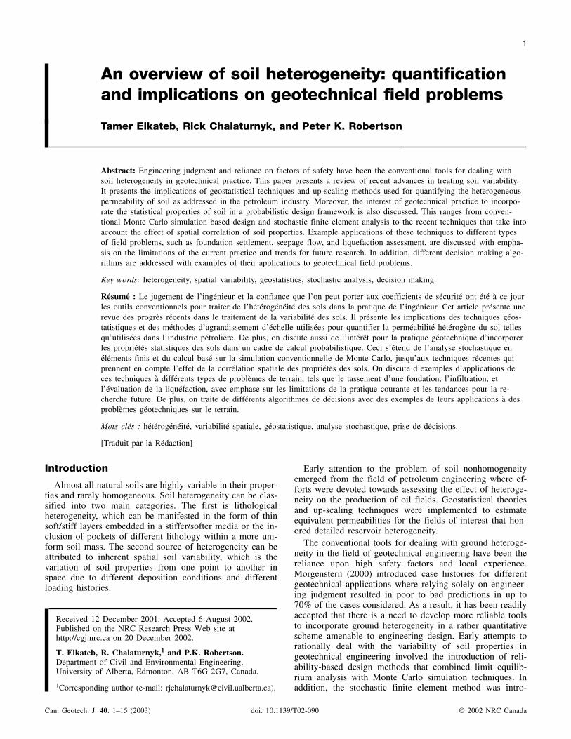
The impact of lithological heterogeneity of the ground onthe production of oil and gas reservoirs has been a majorarea of study in petroleum engineering practice. Several up-scaling techniques were developed to deal with complexground profiles, such as the sand shale sequence shown inFig. 1. The main aim of these techniques was to scale-upfine scale permeability to coarser scales amenable to flowsimulation and engineering calculations. These averagingtechniques can be classified into the following methods:

(1) Empirical techniques, such as the power averagingtechnique (Deutsch 1989). These are the simplest forms ofup-scaling laws.

(2) Semi-empirical methods, such as the renormalization(King 1989) and the representative elementary volume(REV) – renormalization (Norris et al. 1991). They are moresophisticated than the previous type but have limited theoret-ical basis.

(3) Analytical techniques, such as that proposed by War-ren and Price (1961). These methods are rather cumbersometo implement in practice.

The power averaging method was obtained through non-linear regression of the results obtained from a three-dimensional numerical simulation of flow through sand-stone–shale formations. The analysis was carried out underdifferent target shale volumes, and the equivalent permeabil-ity was regarded as that of a homogeneous soil mass produc-ing similar flow under the same head difference andboundary conditions. This equivalent permeability, ke, wasfound to satisfy the relation

[1] k V k V ke sh sh sh ss= + −[ ( ) ] /ω ω ω1 1

where ksh and kss are the permeabilities of the shale andsandstone, respectively; Vsh is the volume fraction of shale;and ω is an averaging power.

The value of ω was suggested to range from –1 to 1 de-pending on the direction of flow and the geometrical aniso-tropy of the shale, i.e., the ratio between the vertical to thelateral extent of shale. The major advantage of this methodis its simplicity, while the main drawback is that the shaleblocks were assumed to be uncorrelated to each other.

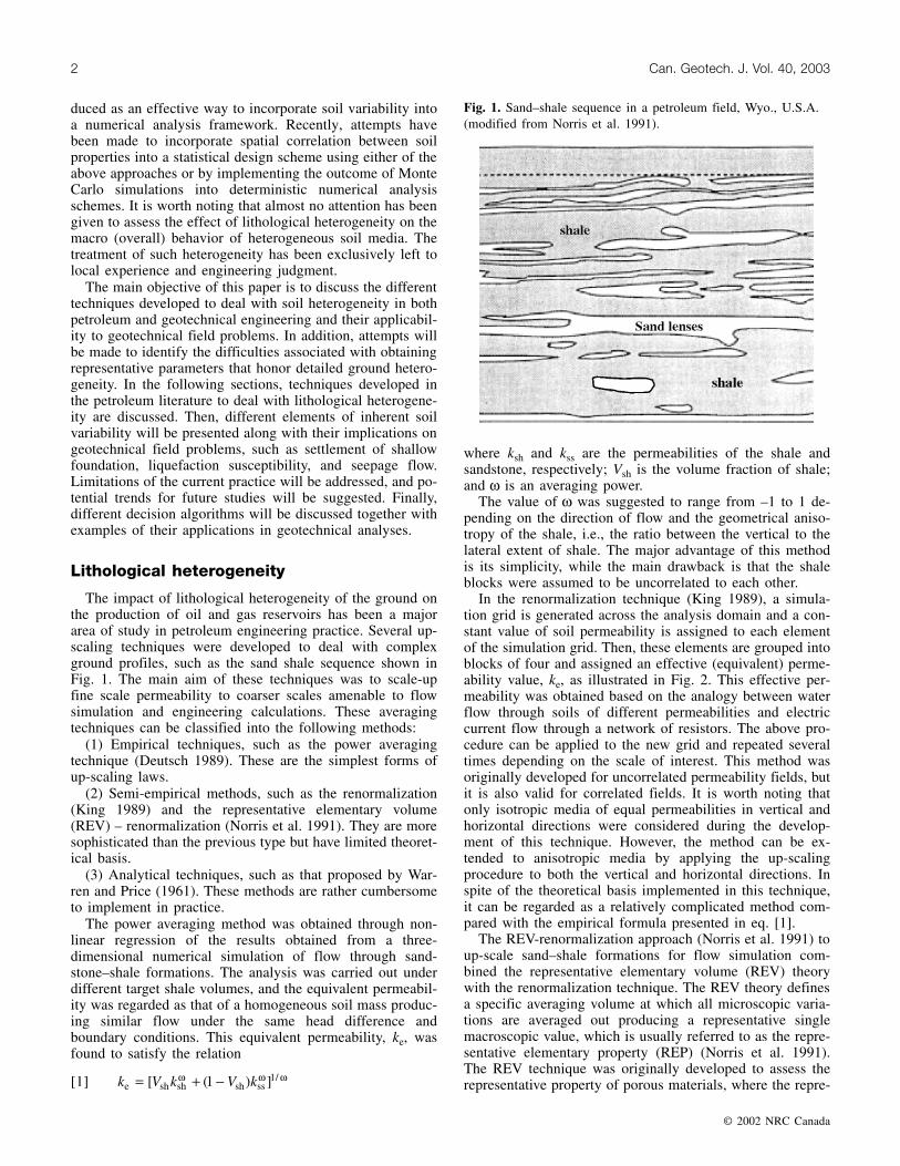
In the renormalization technique (King 1989), a simula-tion grid is generated across the analysis domain and a con-stant value of soil permeability is assigned to each elementof the simulation grid. Then, these elements are grouped intoblocks of four and assigned an effective (equivalent) perme-ability value, ke, as illustrated in Fig. 2. This effective per-meability was obtained based on the analogy between waterflow through soils of different permeabilities and electriccurrent flow through a network of resistors. The above pro-cedure can be applied to the new grid and repeated severaltimes depending on the scale of interest. This method wasoriginally developed for uncorrelated permeability fields, butit is also valid for correlated fields. It is worth noting thatonly isotropic media of equal permeabilities in vertical andhorizontal directions were considered during the develop-ment of this technique. However, the method can be ex-tended to anisotropic media by applying the up-scalingprocedure to both the vertical and horizontal directions. Inspite of the theoretical basis implemented in this technique,it can be regarded as a relatively complicated method com-pared with the empirical formula presented in eq. [1].

The REV-renormalization approach (Norris et al. 1991) toup-scale sand–shale formations for flow simulation com-bined the representative elementary volume (REV) theorywith the renormalization technique. The REV theory definesa specific averaging volume at which all microscopic varia-tions are averaged out producing a representative singlemacroscopic value, which is usually referred to as the repre-sentative elementary property (REP) (Norris et al. 1991).The REV technique was originally developed to assess therepresentative property of porous materials, where the repre-

© 2002 NRC Canada

2 Can. Geotech. J. Vol. 40, 2003

Fig. 1. Sand–shale sequence in a petroleum field, Wyo., U.S.A.(modified from Norris et al. 1991).

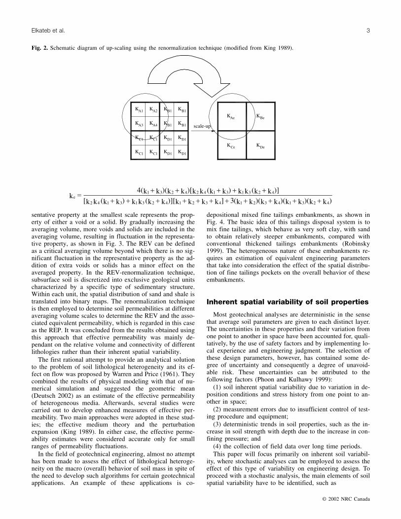
sentative property at the smallest scale represents the prop-erty of either a void or a solid. By gradually increasing theaveraging volume, more voids and solids are included in theaveraging volume, resulting in fluctuation in the representa-tive property, as shown in Fig. 3. The REV can be definedas a critical averaging volume beyond which there is no sig-nificant fluctuation in the representative property as the ad-dition of extra voids or solids has a minor effect on theaveraged property. In the REV-renormalization technique,subsurface soil is discretized into exclusive geological unitscharacterized by a specific type of sedimentary structure.Within each unit, the spatial distribution of sand and shale istranslated into binary maps. The renormalization techniqueis then employed to determine soil permeabilities at differentaveraging volume scales to determine the REV and the asso-ciated equivalent permeability, which is regarded in this caseas the REP. It was concluded from the results obtained usingthis approach that effective permeability was mainly de-pendant on the relative volume and connectivity of differentlithologies rather than their inherent spatial variability.

The first rational attempt to provide an analytical solutionto the problem of soil lithological heterogeneity and its ef-fect on flow was proposed by Warren and Price (1961). Theycombined the results of physical modeling with that of nu-merical simulation and suggested the geometric mean(Deutsch 2002) as an estimate of the effective permeabilityof heterogeneous media. Afterwards, several studies werecarried out to develop enhanced measures of effective per-meability. Two main approaches were adopted in these stud-ies; the effective medium theory and the perturbationexpansion (King 1989). In either case, the effective perme-ability estimates were considered accurate only for smallranges of permeability fluctuations.

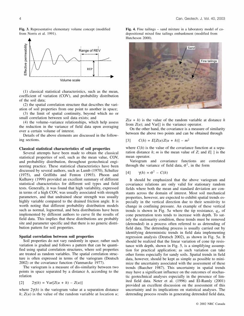
In the field of geotechnical engineering, almost no attempthas been made to assess the effect of lithological heteroge-neity on the macro (overall) behavior of soil mass in spite ofthe need to develop such algorithms for certain geotechnicalapplications. An example of these applications is co-

depositional mixed fine tailings embankments, as shown inFig. 4. The basic idea of this tailings disposal system is tomix fine tailings, which behave as very soft clay, with sandto obtain relatively steeper embankments, compared withconventional thickened tailings embankments (Robinsky1999). The heterogeneous nature of these embankments re-quires an estimation of equivalent engineering parametersthat take into consideration the effect of the spatial distribu-tion of fine tailings pockets on the overall behavior of theseembankments.

Inherent spatial variability of soil properties

Most geotechnical analyses are deterministic in the sensethat average soil parameters are given to each distinct layer.The uncertainties in these properties and their variation fromone point to another in space have been accounted for, quali-tatively, by the use of safety factors and by implementing lo-cal experience and engineering judgment. The selection ofthese design parameters, however, has contained some de-gree of uncertainty and consequently a degree of unavoid-able risk. These uncertainties can be attributed to thefollowing factors (Phoon and Kulhawy 1999):

(1) soil inherent spatial variability due to variation in de-position conditions and stress history from one point to an-other in space;

(2) measurement errors due to insufficient control of test-ing procedure and equipment;

(3) deterministic trends in soil properties, such as the in-crease in soil strength with depth due to the increase in con-fining pressure; and

(4) the collection of field data over long time periods.This paper will focus primarily on inherent soil variabil-

ity, where stochastic analyses can be employed to assess theeffect of this type of variability on engineering design. Toproceed with a stochastic analysis, the main elements of soilspatial variability have to be identified, such as

© 2002 NRC Canada

Elkateb et al. 3

Fig. 2. Schematic diagram of up-scaling using the renormalization technique (modified from King 1989).

(1) classical statistical characteristics, such as the mean,coefficient of variation (COV), and probability distributionof the soil data;

(2) the spatial correlation structure that describes the vari-ation of soil properties from one point to another in space;

(3) the limit of spatial continuity, beyond which no orsmall correlation between soil data exists; and

(4) the volume–variance relationships, which help assessthe reduction in the variance of field data upon averagingover a certain volume of interest.

Details of the above elements are discussed in the follow-ing sections.

Classical statistical characteristics of soil propertiesSeveral attempts have been made to obtain the classical

statistical properties of soil, such as the mean value, COV,and probability distribution, throughout geotechnical engi-neering practice. These statistical characteristics have beendiscussed by several authors, such as Lumb (1970), Schultze(1975), and Griffiths and Fenton (1993). Phoon andKulhawy (1999) provided an excellent summary of differentstatistical characteristics for different soil types and fieldtests. Generally, it was found that high variability, expressedin terms of a high COV, was usually associated with strengthparameters, and that undrained shear strength was usuallyhighly variable compared to the drained friction angle. It isworth noting that different probability distribution modelssuch as normal, lognormal, and beta distributions have beenimplemented by different authors to curve fit the results offield data. This implies that these distributions are probablysite and parameter specific and that there is no generic distri-bution pattern for soil properties.

Spatial correlation between soil propertiesSoil properties do not vary randomly in space; rather such

variation is gradual and follows a pattern that can be quanti-fied using spatial correlation structures, where soil propertiesare treated as random variables. The spatial correlation struc-ture is often expressed in terms of the variogram (Deutsch2002) or the covariance function (Vanmarcke 1977).

The variogram is a measure of dis-similarity between twopoints in space separated by a distance h, according to therelation

[2] 2γ(h) = Var[Z(u + h) – Z(u)]

where 2γ(h) is the variogram value at a separation distanceh; Z(u) is the value of the random variable at location u;

Z(u + h) is the value of the random variable at distance hfrom Z(u); and Var[] is the variance operator.

On the other hand, the covariance is a measure of similaritybetween the above two points and can be obtained through

[3] C(h) = E[Z(u)Z(u + h)] – m2

where C(h) is the value of the covariance function at a sepa-ration distance h; m is the mean value of Z; and E[ ] is themean operator.

Variogram and covariance functions are correlatedthrough the variance of field data, σ2 , in the form

[4] γ(h) = σ2 – C(h)

It should be emphasized that the above variogram andcovariance relations are only valid for stationary randomfields where both the mean and standard deviation are con-stants across the domain of interest. Most soil mechanicalproperties, however, are expected to exhibit spatial trends es-pecially in the vertical direction due to their sensitivity tochange in confining pressure. An example of these verticaltrends is shown in Fig. 5a where the tip resistance, qc, ofcone penetration tests tends to increase with depth. To sat-isfy the stationarity condition, these trends must be removed(detrended) in a process often referred to as detrending offield data. The detrending process is usually carried out byidentifying deterministic trends in field data implementingregression analysis (Deutsch 2002), as shown in Fig. 5a. Itshould be realized that the linear variation of cone tip resis-tance with depth, shown in Fig. 5, is a simplifying assump-tion for practical application; as such variation can takeother forms especially for sandy soils. Spatial trends in fielddata, however, should be kept as simple as possible to mini-mize the uncertainty associated with the assessment of thesetrends (Baecher 1987). This uncertainty in spatial trendsmay have a significant influence on the outcomes of stochas-tic geotechnical analyses especially in the presence of lim-ited field data. Neter et al. (1996) and El-Ramly (2001)provided an excellent discussion on the assessment of thisuncertainty and its implications on statistical analyses. Thedetrending process results in generating detrended field data,

© 2002 NRC Canada


Fig. 3. Representative elementary volume concept (modifiedfrom Norris et al. 1991).

Fig. 4. Fine tailings – sand mixture in a laboratory model of co-depositional mixed fine tailings embankment (modified fromHutcheson 2000).

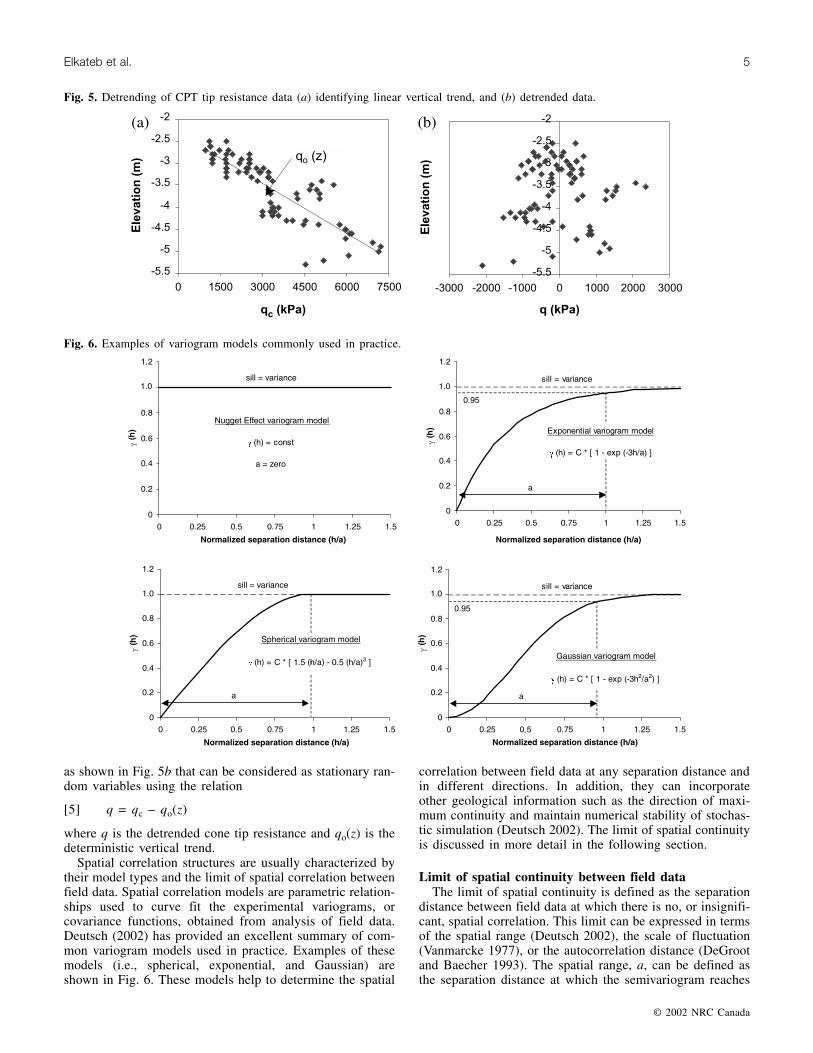
as shown in Fig. 5b that can be considered as stationary ran-dom variables using the relation

[5] q = qc – qo(z)

where q is the detrended cone tip resistance and qo(z) is thedeterministic vertical trend.

Spatial correlation structures are usually characterized bytheir model types and the limit of spatial correlation betweenfield data. Spatial correlation models are parametric relation-ships used to curve fit the experimental variograms, orcovariance functions, obtained from analysis of field data.Deutsch (2002) has provided an excellent summary of com-mon variogram models used in practice. Examples of thesemodels (i.e., spherical, exponential, and Gaussian) areshown in Fig. 6. These models help to determine the spatial

correlation between field data at any separation distance andin different directions. In addition, they can incorporateother geological information such as the direction of maxi-mum continuity and maintain numerical stability of stochas-tic simulation (Deutsch 2002). The limit of spatial continuityis discussed in more detail in the following section.

Limit of spatial continuity between field dataThe limit of spatial continuity is defined as the separation

distance between field data at which there is no, or insignifi-cant, spatial correlation. This limit can be expressed in termsof the spatial range (Deutsch 2002), the scale of fluctuation(Vanmarcke 1977), or the autocorrelation distance (DeGrootand Baecher 1993). The spatial range, a, can be defined asthe separation distance at which the semivariogram reaches

© 2002 NRC Canada

Elkateb et al. 5

Fig. 5. Detrending of CPT tip resistance data (a) identifying linear vertical trend, and (b) detrended data.

Fig. 6. Examples of variogram models commonly used in practice.

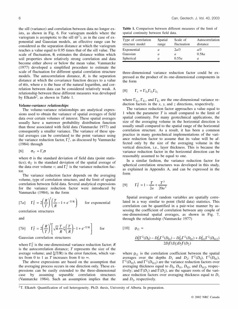
the sill (variance) and correlation between data no longer ex-ists, as shown in Fig. 6. For variogram models where thevariogram is asymptotic to the sill (σ2), as in the case of ex-ponential and Gaussian models, an effective range can beconsidered as the separation distance at which the variogramreaches a value equal to 0.95 times that of the sill value. Thescale of fluctuation, θ, estimates the distance within whichsoil properties show relatively strong correlation and databecome either above or below the mean value. Vanmarcke(1977) developed a simplified procedure to estimate thescale of fluctuation for different spatial correlation structuremodels. The autocorrelation distance, R, is the separationdistance at which the covariance function decays to a valueof σ/e, where e is the base of the natural logarithm, and cor-relation between data can be considered relatively weak. Arelationship between these different measures was developedby Elkateb2, as shown in Table 1.

Volume-variance relationshipsThe volume-variance relationships are analytical expres-

sions used to obtain the variance of spatial averages of fielddata over certain volumes of interest. These spatial averagesusually have a narrower probability distribution functionthan those associated with field data (Vanmarcke 1977) andconsequently a smaller variance. The variance of these spa-tial averages can be correlated to the point variance usingthe variance reduction factor, Γv

2 , as discussed by Vanmarcke(1984) through

[6] σ σΓ Γ= v

where σ is the standard deviation of field data (point statis-tics); σΓ is the standard deviation of the spatial average ofthe data over volume v; and Γv

2 is the variance reduction fac-tor.

The variance reduction factor depends on the averagingvolume, type of correlation structure, and the limit of spatialcorrelation between field data. Several analytical expressionsfor the variance reduction factor were introduced byVanmarcke (1984), in the form

[7a] ΓTT/ Re2

2

2 1=

− +

−RT

TR

for exponential

correlation structures

and

[7b] ΓTT/ Re2

2

2 1=

− +

−RT

TR

TR

π ξ for

Gaussian correlation structures

where ΓT2 is the one-dimensional variance reduction factor; R

is the autocorrelation distance; T represents the size of theaverage volume; and ξ(T/R) is the error function, which var-ies from 0 to 1 as T increases from 0 to ∞.

The above expressions are based on the assumption thatthe averaging process occurs in one direction only. These ex-pressions can be easily extended to the three-dimensionalcase by assuming separable correlation structures(Vanmarcke 1984). Such an assumption implies that the

three-dimensional variance reduction factor could be ex-pressed as the product of its one-dimensional components inthe form

[8] Γ Γ Γ Γv T T T= x y z

where ΓTx, ΓTy, and ΓTz are the one-dimensional variance re-duction factors in the x, y, and z directions, respectively.

The variance reduction factor approaches a value equal to1 when the parameter T is small compared to the limit ofspatial continuity. For many geotechnical applications, thesize of the averaging volume in the horizontal direction isusually small compared to the spatial range of the horizontalcorrelation structure. As a result, it has been a commonpractice in many geotechnical implementations of the vari-ance reduction factor to assume that its value will be af-fected only by the size of the averaging volume in thevertical direction, i.e., layer thickness. This is because thevariance reduction factor in the horizontal direction can bereasonably assumed to be equal to one.

In a similar fashion, the variance reduction factor forspherical correlation structures was developed in this study,as explained in Appendix A, and can be expressed in theform

[9] ΓT2

3

31

2 20= − +T

aT

a

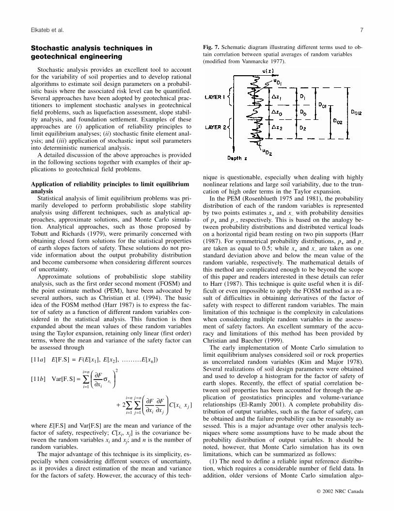
Spatial averages of random variables are spatially corre-lated in a way similar to point (field data) statistics. Thiscorrelation can be quantified in a pair-wise manner by as-sessing the coefficient of correlation between any couple ofone-dimensional spatial averages, as shown in Fig. 7,through the relationship (Vanmarcke 1977)

[10] ρ12 =

D D D D D D D DD

02 2

0 012 2

01 022 2

02 0122 2

012

12Γ Γ Γ Γ( ) ( ) ( ) ( )− − +

Γ Γ( ) ( )D D D1 2 2

where ρ12 is the correlation coefficient between the spatialaverages over the depths D1 and D2; Γ2(D0), Γ2(D01),Γ2(D02), and Γ2(D012) are the variance reduction factors overaveraging thickness equal to D0, D01, D02, and D012, respec-tively; and Γ(D1) and Γ(D2), are the square roots of the vari-ance reduction factors over averaging thickness equal to D1and D2, respectively.

© 2002 NRC Canada


Type of correlationstructure model

Spatialrange

Scale offluctuation

Autocorrelationdistance

Exponential a 2a/3 a/3Gaussian a a 0.58aSpherical a 0.55a a

Table 1. Comparison between different measures of the limit ofspatial continuity between field data.

2 T. Elkateb. Quantification of soil heterogeneity. Ph.D. thesis, University of Alberta. In preparation.

Stochastic analysis techniques ingeotechnical engineering

Stochastic analysis provides an excellent tool to accountfor the variability of soil properties and to develop rationalalgorithms to estimate soil design parameters on a probabil-istic basis where the associated risk level can be quantified.Several approaches have been adopted by geotechnical prac-titioners to implement stochastic analyses in geotechnicalfield problems, such as liquefaction assessment, slope stabil-ity analysis, and foundation settlement. Examples of theseapproaches are (i) application of reliability principles tolimit equilibrium analyses; (ii) stochastic finite element anal-ysis; and (iii) application of stochastic input soil parametersinto deterministic numerical analysis.

A detailed discussion of the above approaches is providedin the following sections together with examples of their ap-plications to geotechnical field problems.

Application of reliability principles to limit equilibriumanalysis

Statistical analysis of limit equilibrium problems was pri-marily developed to perform probabilistic slope stabilityanalysis using different techniques, such as analytical ap-proaches, approximate solutions, and Monte Carlo simula-tion. Analytical approaches, such as those proposed byTobutt and Richards (1979), were primarily concerned withobtaining closed form solutions for the statistical propertiesof earth slopes factors of safety. These solutions do not pro-vide information about the output probability distributionand become cumbersome when considering different sourcesof uncertainty.

Approximate solutions of probabilistic slope stabilityanalysis, such as the first order second moment (FOSM) andthe point estimate method (PEM), have been advocated byseveral authors, such as Christian et al. (1994). The basicidea of the FOSM method (Harr 1987) is to express the fac-tor of safety as a function of different random variables con-sidered in the statistical analysis. This function is thenexpanded about the mean values of these random variablesusing the Taylor expansion, retaining only linear (first order)terms, where the mean and variance of the safety factor canbe assessed through

[11a] E[F.S] = F(E[x1], E[x2], ………E[xn])

[11b] Var[F.S] = ∂∂

=

=

∑ Fxi

xi

i n

iσ

2

1

+ ∂∂

∂∂

=

=

=

=

∑∑211

Fx

Fx

C x xi jj

j n

i

i n

i j[ ],

where E[F.S] and Var[F.S] are the mean and variance of thefactor of safety, respectively; C[xi, xj] is the covariance be-tween the random variables xi and xj; and n is the number ofrandom variables.

The major advantage of this technique is its simplicity, es-pecially when considering different sources of uncertainty,as it provides a direct estimation of the mean and variancefor the factors of safety. However, the accuracy of this tech-

nique is questionable, especially when dealing with highlynonlinear relations and large soil variability, due to the trun-cation of high order terms in the Taylor expansion.

In the PEM (Rosenblueth 1975 and 1981), the probabilitydistribution of each of the random variables is representedby two points estimates x+ and x– with probability densitiesof p+ and p–, respectively. This is based on the analogy be-tween probability distributions and distributed vertical loadson a horizontal rigid beam resting on two pin supports (Harr(1987). For symmetrical probability distributions, p+ and p–are taken as equal to 0.5; while x+ and x– are taken as onestandard deviation above and below the mean value of therandom variable, respectively. The mathematical details ofthis method are complicated enough to be beyond the scopeof this paper and readers interested in these details can referto Harr (1987). This technique is quite useful when it is dif-ficult or even impossible to apply the FOSM method as a re-sult of difficulties in obtaining derivatives of the factor ofsafety with respect to different random variables. The mainlimitation of this technique is the complexity in calculationswhen considering multiple random variables in the assess-ment of safety factors. An excellent summary of the accu-racy and limitations of this method has been provided byChristian and Baecher (1999).

The early implementation of Monte Carlo simulation tolimit equilibrium analyses considered soil or rock propertiesas uncorrelated random variables (Kim and Major 1978).Several realizations of soil design parameters were obtainedand used to develop a histogram for the factor of safety ofearth slopes. Recently, the effect of spatial correlation be-tween soil properties has been accounted for through the ap-plication of geostatistics principles and volume-variancerelationships (El-Ramly 2001). A complete probability dis-tribution of output variables, such as the factor of safety, canbe obtained and the failure probability can be reasonably as-sessed. This is a major advantage over other analysis tech-niques where some assumptions have to be made about theprobability distribution of output variables. It should benoted, however, that Monte Carlo simulation has its ownlimitations, which can be summarized as follows:

(1) The need to define a reliable input reference distribu-tion, which requires a considerable number of field data. Inaddition, older versions of Monte Carlo simulation algo-

© 2002 NRC Canada

Elkateb et al. 7

Fig. 7. Schematic diagram illustrating different terms used to ob-tain correlation between spatial averages of random variables(modified from Vanmarcke 1977).

rithms used to deal only with parametric probability distri-bution functions, i.e., probability distributions that can bedefined through mathematical relationships such as normaland log-normal distribution. Field data, however, do not nec-essarily fit into any of these parametric distributions. Thisproblem has been overcome by recent versions of MonteCarlo simulations, such as that of Deutsch and Journel(1998) that are capable of dealing with nonparametric distri-bution functions directly inferred from field data;

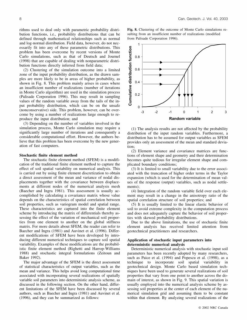
(2) Clustering of the simulation outcome into a limitedzone of the input probability distribution, as the drawn sam-ples are more likely to be in areas of higher probability, asshown in Fig. 8. This problem mainly arises in cases wherean insufficient number of realizations (number of iterationsin Monte Carlo algorithm) are used in the simulation process(Palisade Corporation 1996). This may result in samplingvalues of the random variable away from the tails of the in-put probability distribution, which can be on the unsafe(nonconservative) side. This problem, however, can be over-come by using a number of realizations large enough to re-produce the input distribution; and

(3) Depending on the number of variables involved in thesimulation process, Monte Carlo simulation may require asignificantly large number of iterations and consequently aconsiderable computational effort. However, the authors be-lieve that this problem has been overcome by the new gener-ation of fast computers.

Stochastic finite element methodThe stochastic finite element method (SFEM) is a modifi-

cation of the traditional finite element method to capture theeffect of soil spatial variability on numerical analysis. Thisis carried out by using finite element discretization to obtaina direct assessment of the mean and variance of nodal dis-placements together with the covariance between displace-ments at different nodes of the numerical analysis mesh(Baecher and Ingra 1981). This assessment is usually ac-complished by calculating a covariance matrix whose valuedepends on the characteristics of spatial correlation betweensoil properties, such as variogram model and spatial range.These characteristics are captured into the finite elementscheme by introducing the matrix of differentials thereby as-sessing the effect of the variation of mechanical soil proper-ties from one element to another on the global stiffnessmatrix. For more details about SFEM, the reader can refer toBaecher and Ingra (1981) and Auvinet et al. (1996). Differ-ent modifications of SFEM have been developed by intro-ducing different numerical techniques to capture soil spatialvariability. Examples of these modifications are the probabil-istic finite element method (Righetti and Harrop-Williams1988) and stochastic integral formulations (Zeitoun andBaker 1992).

The major advantage of the SFEM is the direct assessmentof statistical characteristics of output variables, such as themean and variance. This helps avoid long computational timeassociated with incorporating several realizations of spatiallyvariable soil parameters into deterministic analysis scheme, asdiscussed in the following section. On the other hand, differ-ent limitations of the SFEM have been discussed by severalauthors, such as Baecher and Ingra (1981) and Auvinet et al.(1996), and they can be summarized as follows:

(1) The analysis results are not affected by the probabilitydistribution of the input random variables. Furthermore, adistribution has to be assumed for output variables as SFEMprovides only an assessment of the mean and standard devia-tion;

(2) Element variance and covariance matrices are func-tions of element shape and geometry and their determinationbecomes quite tedious for irregular element shape and com-plicated boundary conditions;

(3) It is limited to small variability due to the error associ-ated with the truncation of higher order terms in the Taylorexpansion (which is used for the determination of mean val-ues of the response (output) variables, such as nodal settle-ments);

(4) Integration of the random variable field over each ele-ment may result in a change in the anisotropy ratio of thespatial correlation structure of soil properties; and

(5) It is usually limited to the linear elastic behavior ofsoil to avoid extreme complexity in the computation processand does not adequately capture the behavior of soil proper-ties with skewed probability distributions.

Due to the above limitations, the use of stochastic finiteelement analysis has received limited attention fromgeotechnical practitioners and researchers.

Application of stochastic input parameters intodeterministic numerical analysis

Deterministic numerical analysis with stochastic input soilparameters has been recently adopted by many researchers,such as Paice et al. (1994) and Popescu et al. (1998), as atechnique to incorporate soil spatial variability ingeotechnical design. Monte Carlo based simulation tech-niques have been used to generate several realizations of soilproperties that vary from one point to another across the do-main of interest, as shown in Fig. 9. This spatial variation isusually employed into the numerical analysis scheme by as-sessing soil properties at the center of each element of the nu-merical simulation grid and assuming them to be constantwithin that element. By analyzing several realizations of the

© 2002 NRC Canada


Fig. 8. Clustering of the outcome of Monte Carlo simulations re-sulting from an insufficient number of realizations (modifiedfrom Palisade Corporation 1996).

spatially variable soil medium, histograms of response (out-put) variables can be obtained. Examples of the simulation al-gorithms used in practice are the sequential Gaussian, thesequential indicator simulations (Deutsch 2002), and the localaverage subdivision technique (Fenton and Vanmarcke 1990).

The sequential Gaussian simulation (SGS) is the mostcommonly used technique, especially in the field of petro-leum engineering. The basic idea of this technique is illus-trated in Fig. 10. Input random variables are transformedinto standardized normally distributed random variables withzero means and unit variances for which different variogramcharacteristics are assessed. Simulated values of a standard-ized variable, Z, can be determined at any node of the simu-lation grid according to the relationship

[12] Zs(u) = Z*(u) + R(u)

where Zs(u) is the simulated value of the variable Z at loca-tion u; Z*(u) is the krigged estimate of the variable Z at lo-cation u; and R(u) is a random residual.

The krigged estimate is a linear estimator of the variable Zat location u in space, where the value of Z is unknown, us-ing the krigging interpolation techniques (Journel andHuijbregts 1978). This estimate depends on different charac-teristics of spatial correlation structure (variogram) and doesnot vary from one realization to another. It can be assessedthrough

[13] Z u Z ui ii

n

* ( ) ( )==∑ λ

1

where Z(ui) is a known value of Z at location ui in space, ei-ther from field data at that location or previously simulatednodes; and λ i is a weight given to field data at location uithat depends on the characteristics of the spatial correlationstructure.

The random residual R(u) follows a normal distributionwith zero mean and a variance equal to the krigging variance(Deutsch 2002). A different value of R(u) is obtained in eachrealization using Monte Carlo simulation resulting in a vari-ation of the simulated value of the random variable, Z(u),from one realization to another. A random path is followedto assess the value of the standardized random variable ateach node of the numerical simulation grid. The simulatedvalues across the analysis domain are then back-transformedto their original probability distribution. By repeating the

© 2002 NRC Canada

Elkateb et al. 9

Fig. 9. Deformed mesh with spatially variable elastic modulus below flexible strip footing (modified from Paice et al. 1994).

Fig. 10. The basic idea of the sequential Gaussian simulation.

above procedure, several realizations of soil spatial variationacross the analysis domain can be obtained.

Application of stochastic analysis togeotechnical field problems

The stochastic analysis techniques discussed in the previ-ous sections have been implemented in several applicationsthroughout the history of geotechnical engineering practiceto assess the impact of ground variability on geotechnicalfield problems. In the following sections, an attempt is madeto address the current state of practice in some of these ap-plications and its limitations together with potential trendsfor future research.

Stochastic analysis of shallow foundation settlementEarly attempts to perform probabilistic analysis of foun-

dation settlement started in the late 1960s. Wu and Kraft(1967) estimated the uncertainty in soil bearing capacity andfoundation settlement through assessing the uncertainty inapplied load, soil strength, and deformation parameters. Theuncertainty in soil strength was estimated by assessing thevariability of laboratory undrained shear strength for clayeysoils and that of SPT data for sandy soils. Resendiz andHerrera (1969) carried out a probabilistic analysis of settle-ment and rotation of flexible and rigid footings over ran-domly variable compressible soils. A one-dimensionalsettlement model was adopted in which the coefficient ofvolume change was characterized as a normally distributedrandom variable. The analysis results were used to obtaindesign parameters that satisfied tolerable settlements and ro-tations criteria together with the minimum expected mone-tary loss. These studies can be considered as a good starttowards addressing such a complex problem. However, theywere fairly primitive as some elements of soil inherent vari-ability, such as spatial correlation between soil properties,were not adequately considered.

The modern approach to deal with ground variability andits implications on foundation settlement started in the early1980s with the pioneer work of Baecher and Ingra (1981). Intheir study, two-dimensional stochastic finite element analy-ses were carried out to assess the uncertainty in total and dif-ferential settlement. Soil elastic modulus was treated as arandom variable, whereas Poisson’s ratio was assumed to beconstant across the soil mass. Two spatial correlation mod-els, the exponential and the squared exponential (Gaussian),were considered and the response variables (total and differ-ential settlement) were assumed to be normally distributed.A limiting assumption of the study was the linear elastic soilbehavior, which implies, together with the use of SFEM, asmall variation in soil properties to avoid the development ofplastic zones and the onset of nonlinear constitutive behav-ior. In addition, the effect of different probability distribu-tions of soil properties on the expected uncertainty was notassessed.

In a similar fashion, Zeitoun and Baker (1992) proposed astochastic approach for settlement prediction of shallowfoundations using the stochastic integral formulation (SIF)technique, which is a modification of the SFEM. It was as-sumed that soil would exhibit linear elastic behavior under

both axisymmetrical and plane strain conditions. Soil shearmodulus was treated as a random variable and the Gaussianmodel was chosen to represent the spatial variation of shearmodulus across the problem domain. The technique used inthe study had serious limitations as unrealistic spatial corre-lations were assumed either through the use of a very highhorizontal autocorrelation distance or by considering the soilmedium to be in the form of concentric rings of constantelastic modulus. Furthermore, no information was providedabout the probability distribution of output variables, and theeffect of different spatial correlation structures was not ac-counted for. Finally, the use of SFEM implied some restric-tions on the range of soil variability used in the analysis toprevent development of plastic zones as discussed in theprevious paragraph.

The effect of random soil stiffness on foundation settle-ment was reinvestigated by Paice et al. (1994) through theuse of deterministic finite element analysis with stochasticinput soil parameters. Soil elastic modulus was regarded as aspatially random variable resulting in a ground profile aspreviously shown in Fig. 9. The elastic modulus was as-sumed to follow a lognormal probability distribution and ex-ponential correlation structure. This study has some limitingassumptions such as the linear elastic soil behavior, the iso-tropic correlation structure, and the symmetry of spatial dis-tribution of elastic modulus around the footing centerline. Inaddition, the effect of different types of correlation struc-tures and the sensitivity of the results to the number of real-izations were not considered.

The effect of random fluctuations of the interface betweensoil layers on the uncertainty in foundation settlements hasbeen accounted for by Brzakala and Pula (1996). This uncer-tainty in soil geometry was converted into a new randomfield expressed in terms of the interface fluctuation and wasincorporated into the stochastic finite element analysis. Themain limitations of the study lie in the linear elastic soil be-havior and neglecting the inherent soil variability within lay-ers. In addition, the effect of different types of probabilitydistributions and correlation structures on the stochasticanalyses outcomes was not accounted for.

It is worth noting that the above studies have not consid-ered the effect of changing the state of stresses in soil masson the outcome of statistical analyses. In other words, thesensitivity of the statistical characteristics of output variablesto wide ranges of applied vertical and horizontal stresseswas not adequately addressed. In addition, no attempt hasbeen made to provide risk-based representative soil parame-ters that can be implemented in deterministic analyses whilecontinuing to honor detailed ground heterogeneity.

Stochastic analysis of liquefaction problemsThe early attempts to quantify the stochastic nature of liq-

uefaction problems were focused on developing analyticalexpressions to estimate the uncertainty in liquefaction poten-tial assessment. Yegian and Whitman (1978) conducted a pi-oneer study to provide a statistical evaluation of the annualprobability of failure for potentially liquefiable sites. Thiswas carried out by combining the annual probability ofgiven earthquakes with the probability of ground failure un-der these earthquakes. In addition, an analytical expression

© 2002 NRC Canada


was developed to assess the uncertainty in a limit state pa-rameter, proposed to estimate the maximum shear resistanceof the ground. A major limitation of that study was that theeffect of spatial correlation between soil properties was notaccounted for and that the uncertainty in the results were as-sumed to be insensitive to the probability distribution of theinput random variables. Furthermore, the derivation of theexpression for the limit state parameter was based on the as-sumption that the soil shear resistance and vertical effectivestress were two independent random variables.

Recently, the use of deterministic finite element analysiswith stochastic input soil parameters has gained muchpopularity in the field of probabilistic liquefaction analysis.Several attempts have been made to apply this technique tostudy case histories that involved potentially liquefiableground conditions.

Fenton and Vanmarcke (1991) performed one-dimensionalfinite element analyses to assess the effect of inherent vari-ability of soil properties on liquefaction potential at theWildlife site, California. Soil properties, such as porosity,Poisson’s ratio, elastic modulus, permeability, and the dila-tion angle, were considered as random variables. The firsttwo properties were considered to be normally distributed,whereas the rest were assumed to follow a lognormal distri-bution. The effect of correlation structure was taken intoconsideration through the application of the variance reduc-tion factor proposed by Vanmarcke (1977). Several realiza-tions of soil properties were generated using the localaverage subdivision technique, and were excited by variousearthquake motions applied at the base of the soil columnsusing DYNA1D software. A main limitation of the study isthat the results sensitivity to the number of realizations wasnot taken into consideration. Moreover, the effect of differ-ent probability distributions of soil properties was not ac-counted for together with the use of one-dimensionalanalysis, in which the analysis domain was divided into soilcolumns neglecting the coupling between soil elements.

Popescu et al. (1996) carried out one of the pioneer inves-tigations on the effect of soil spatial variability on liquefac-tion assessment using the results of cone penetration tests,where the cone tip resistance, qc, and the cone index, Ic,were treated as random variables. A simulation algorithmwas developed in the study for the simulation of non-Gaussian multivariate random fields. A nonlinear regressionalgorithm was adopted to determine the probability distribu-tion and the correlation structure of the random variables.The problem was analysed using the DYNAFLOW softwareimplementing stochastic input soil parameters obtained us-ing the correlations between soil properties and CPT data.For comparison, a deterministic numerical analysis was car-ried out using the mean values of soil parameters. A charac-teristic percentile of cone tip resistance was proposed for usein deterministic analyses to predict the same maximum porepressure obtained from stochastic analysis. The major limita-tion of the study lies in the use of only four realizations toquantify the effect of soil variability, which may not be suffi-cient to sample the expected range of response, as discussedearlier. In addition, the effect of spatial correlation range onthe study outcomes was not accounted for. The authors be-lieve, however, that this spatial range may have a profound

effect on liquefaction susceptibility and needs to be consid-ered in future stochastic liquefaction studies. In addition, thestrength percentile proposed for use in deterministic analysisto capture the effect of soil spatial variability was subjec-tively assessed.

Popescu et al. (1998) extended the previous study to pro-vide risk-based liquefaction potential measures through two-dimensional stochastic analysis where cone tip resistancewas treated as a spatially random variable. The effect of in-herent variability was assessed through 25 realizations of thespatial distribution of CPT data across the site. A series ofdeterministic finite element analysis was carried out, usingdifferent percentiles of the recorded CPT data, to estimateequivalent (representative) soil parameters that can capturethe implications of soil spatial variability. These parameterswere considered to be associated with the upper limit of theMonte Carlo simulation response range. It was concludedthat the initiation of soil liquefaction could not be accuratelypredicted by deterministic models, which could not accountfor the presence of loose pockets within soil masses. Thisstudy, as in the case of the previous one, did not take intoconsideration the sensitivity of the analysis to the number ofrealizations of soil properties. In addition, the proposedequivalent parameters could be considered overconservative,as they were associated with the most critical response of thestochastic analysis. Moreover, the effect of the type of corre-lation structure and its spatial limit was not accounted for.

Once again, the effect of changing the state of stresses insoil mass on the outcome of stochastic analyses has not beenadequately considered in any of the above studies. For exam-ple, more investigation is needed to ascertain whether or notthe same values of the representative cone tip resistance per-centiles of Popescu et al. (1998) would be obtained if poten-tially liquefiable layers were at different depths belowground surface.

Stochastic analyses of seepage flowThe problem of water flow through heterogeneous porous

media has been studied thoroughly along the history of pe-troleum engineering and water resources research. One ofthe pioneer attempts to apply the principles of geostatisticsinto the geotechnical engineering practice to study the effectof soil spatial variability on seepage flow was made byGriffiths and Fenton (1993). In their study, the local averagesubdivision simulation technique was used to generate 1000realizations of spatially variable hydraulic conductivity be-low a water retaining structure. The resulting field was thenmapped onto a finite element mesh to perform numericalanalysis of the problem under deterministic boundary condi-tions. The hydraulic conductivity, k, was assumed to followlognormal probability distribution, and the effect of spatialcorrelation structure was accounted for through quantifyingthe influence of the scale of fluctuation on different response(output) variables. The limitations of the study lie in the useof an isotropic correlation structure where vertical and hori-zontal ranges were assumed equal, and the effect of differentprobability distributions and correlation structure modelswere not accounted for. Furthermore, the sensitivity of theanalysis to the number of realizations of the random vari-able, hydraulic conductivity, was not considered.

© 2002 NRC Canada

Elkateb et al. 11

Decision making in geotechnicalengineering

One of the major challenges that faces geotechnical engi-neers is the need to make decisions regarding the soil param-eter to be used in engineering analysis. These decisions haveto be based on information that invariably has a certain de-gree of uncertainty. Consequently, the decision making pro-cess is considered to be governed by two factors, theuncertainty in the decision variables and the risk level of theproject. Several decision making algorithms have been usedthroughout the history of geotechnical engineering practice,such as the worst case and quasi worst case approaches, reli-ability-based techniques, confidence interval approach, andBayesian decision analyses. Details of these algorithms willbe discussed in the following paragraphs.

The worst case approach aims at achieving the absolutesafety of the project and relies on the notion of maximumloss and maximum expected hazards, often referred to as themaxi-max criterion (Ang and Tang 1984). For example, ifthe range of the measured friction angle of a sandy depositat a certain site ranges from 30–40°, the design value willbe assessed as 30°. This approach is over-conservative andrarely used in practice. On the other hand, the quasi worstcase approach (Pate-Cornell 1987) tries to apply some kindof engineering judgment into the above approach to providean upper bound for the risk level. Revisiting the above ex-ample, the sandy soil at the site is classified (say mediumdense sand) and the minimum value associated with suchclassification (say 33°) will be used as the design value. Acommon problem of the two approaches is that no informa-tion can be obtained about the risk level associated with thedesign value.

The reliability-based approach relies on selecting designparameters that satisfy a desired degree of reliability or acertain probability of failure. This approach has been com-monly used in slope stability analysis. Wolff (1996) pro-posed soil design parameters to be associated with areliability index, β, of 3 for routine slopes and 4 for criticalslopes such as dams. The reliability index can be obtainedthrough

[14] βσ

= −m LFS

FS

where mFS is the mean factor of safety; L is a limit statevalue usually equal to 1; and σFS is the standard deviation ofthe factor of safety.

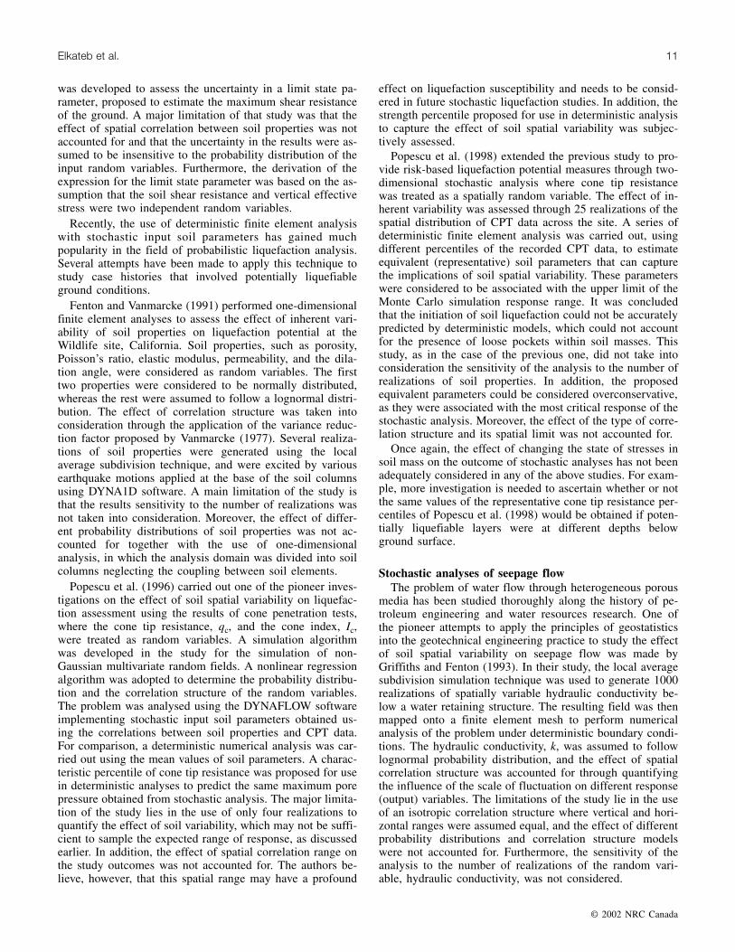
In a similar fashion, the US Army Corps of Engineers(1995) proposed an assessment of the performance level ofembankments depending on the target reliability index andthe corresponding failure probability, as shown in Table 2.Comparing the recommendation presented in Table 2 withthe suggested values of reliability index of Wolff (1996) im-plies that the selection of design parameters for earth slopesshould be associated with critical failure probabilities nomore than 0.1%. British Columbia (BC) Hydro developed asimilar approach for dam design based on a thorough reviewof different potential hazards (Whitman 2000). In their crite-rion, critical failure probabilities were assessed as a functionof potential number of fatalities, as shown in Fig. 11. On the

other hand, El-Ramly (2001) concluded that critical failureprobabilities developed in geotechnical literature were over-conservative and that a critical failure probability of 2%could be regarded as an upper bound for the satisfactory per-formance of earth slopes. This critical value was assessedbased on extensive probabilistic slope stability analyses ofseveral case histories in North America and Hong Kong.

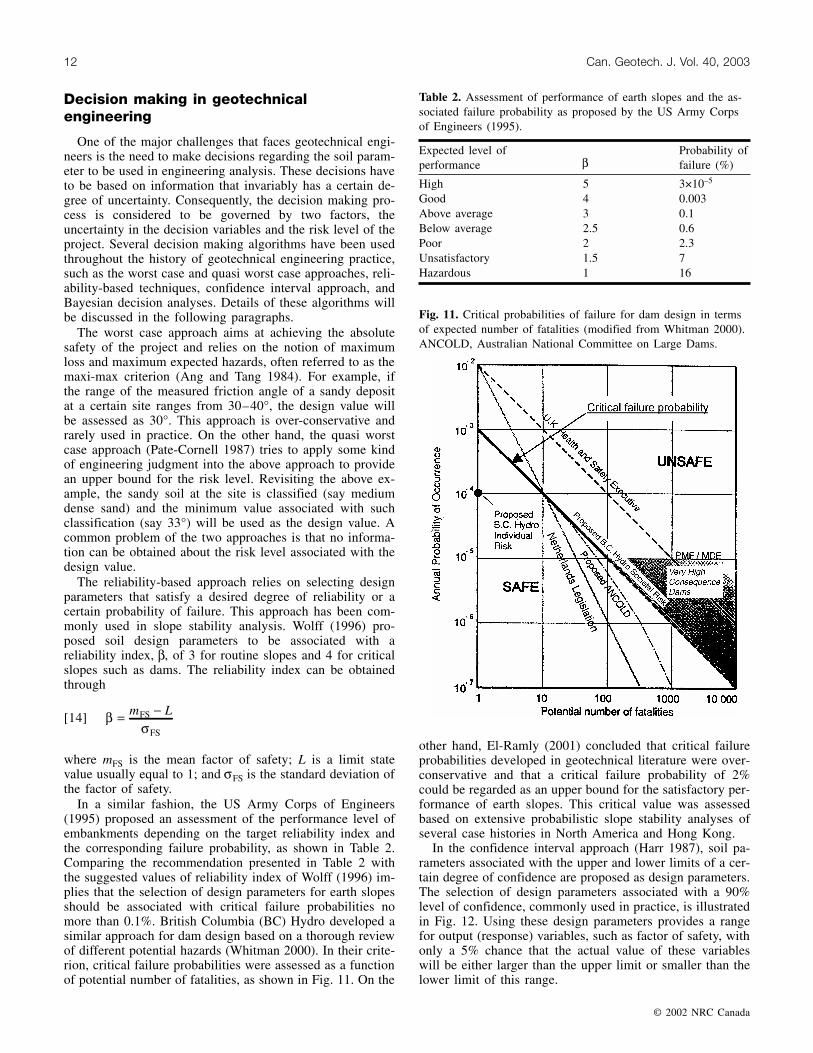
In the confidence interval approach (Harr 1987), soil pa-rameters associated with the upper and lower limits of a cer-tain degree of confidence are proposed as design parameters.The selection of design parameters associated with a 90%level of confidence, commonly used in practice, is illustratedin Fig. 12. Using these design parameters provides a rangefor output (response) variables, such as factor of safety, withonly a 5% chance that the actual value of these variableswill be either larger than the upper limit or smaller than thelower limit of this range.

© 2002 NRC Canada


Expected level ofperformance β

Probability offailure (%)

High 5 3×10–5

Good 4 0.003Above average 3 0.1Below average 2.5 0.6Poor 2 2.3Unsatisfactory 1.5 7Hazardous 1 16

Table 2. Assessment of performance of earth slopes and the as-sociated failure probability as proposed by the US Army Corpsof Engineers (1995).

Fig. 11. Critical probabilities of failure for dam design in termsof expected number of fatalities (modified from Whitman 2000).ANCOLD, Australian National Committee on Large Dams.

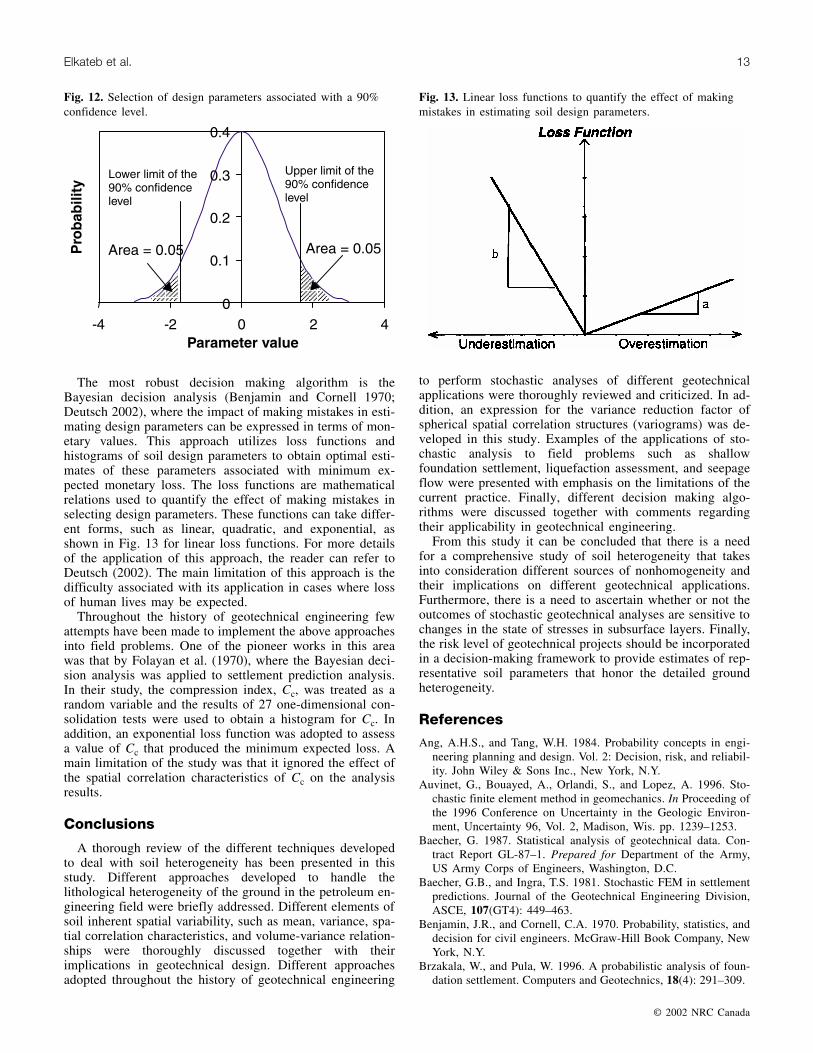
The most robust decision making algorithm is theBayesian decision analysis (Benjamin and Cornell 1970;Deutsch 2002), where the impact of making mistakes in esti-mating design parameters can be expressed in terms of mon-etary values. This approach utilizes loss functions andhistograms of soil design parameters to obtain optimal esti-mates of these parameters associated with minimum ex-pected monetary loss. The loss functions are mathematicalrelations used to quantify the effect of making mistakes inselecting design parameters. These functions can take differ-ent forms, such as linear, quadratic, and exponential, asshown in Fig. 13 for linear loss functions. For more detailsof the application of this approach, the reader can refer toDeutsch (2002). The main limitation of this approach is thedifficulty associated with its application in cases where lossof human lives may be expected.

Throughout the history of geotechnical engineering fewattempts have been made to implement the above approachesinto field problems. One of the pioneer works in this areawas that by Folayan et al. (1970), where the Bayesian deci-sion analysis was applied to settlement prediction analysis.In their study, the compression index, Cc, was treated as arandom variable and the results of 27 one-dimensional con-solidation tests were used to obtain a histogram for Cc. Inaddition, an exponential loss function was adopted to assessa value of Cc that produced the minimum expected loss. Amain limitation of the study was that it ignored the effect ofthe spatial correlation characteristics of Cc on the analysisresults.

Conclusions

A thorough review of the different techniques developedto deal with soil heterogeneity has been presented in thisstudy. Different approaches developed to handle thelithological heterogeneity of the ground in the petroleum en-gineering field were briefly addressed. Different elements ofsoil inherent spatial variability, such as mean, variance, spa-tial correlation characteristics, and volume-variance relation-ships were thoroughly discussed together with theirimplications in geotechnical design. Different approachesadopted throughout the history of geotechnical engineering

to perform stochastic analyses of different geotechnicalapplications were thoroughly reviewed and criticized. In ad-dition, an expression for the variance reduction factor ofspherical spatial correlation structures (variograms) was de-veloped in this study. Examples of the applications of sto-chastic analysis to field problems such as shallowfoundation settlement, liquefaction assessment, and seepageflow were presented with emphasis on the limitations of thecurrent practice. Finally, different decision making algo-rithms were discussed together with comments regardingtheir applicability in geotechnical engineering.

From this study it can be concluded that there is a needfor a comprehensive study of soil heterogeneity that takesinto consideration different sources of nonhomogeneity andtheir implications on different geotechnical applications.Furthermore, there is a need to ascertain whether or not theoutcomes of stochastic geotechnical analyses are sensitive tochanges in the state of stresses in subsurface layers. Finally,the risk level of geotechnical projects should be incorporatedin a decision-making framework to provide estimates of rep-resentative soil parameters that honor the detailed groundheterogeneity.

References

Ang, A.H.S., and Tang, W.H. 1984. Probability concepts in engi-neering planning and design. Vol. 2: Decision, risk, and reliabil-ity. John Wiley & Sons Inc., New York, N.Y.

Auvinet, G., Bouayed, A., Orlandi, S., and Lopez, A. 1996. Sto-chastic finite element method in geomechanics. In Proceeding ofthe 1996 Conference on Uncertainty in the Geologic Environ-ment, Uncertainty 96, Vol. 2, Madison, Wis. pp. 1239–1253.

Baecher, G. 1987. Statistical analysis of geotechnical data. Con-tract Report GL-87–1. Prepared for Department of the Army,US Army Corps of Engineers, Washington, D.C.

Baecher, G.B., and Ingra, T.S. 1981. Stochastic FEM in settlementpredictions. Journal of the Geotechnical Engineering Division,ASCE, 107(GT4): 449–463.

Benjamin, J.R., and Cornell, C.A. 1970. Probability, statistics, anddecision for civil engineers. McGraw-Hill Book Company, NewYork, N.Y.

Brzakala, W., and Pula, W. 1996. A probabilistic analysis of foun-dation settlement. Computers and Geotechnics, 18(4): 291–309.

© 2002 NRC Canada

Elkateb et al. 13

Fig. 12. Selection of design parameters associated with a 90%confidence level.

Fig. 13. Linear loss functions to quantify the effect of makingmistakes in estimating soil design parameters.

Christian, J.T., and Baecher, G.B. 1999. Point estimate method asnumerical quadrature. Journal of the Geotechnical andGeoenvironmental Engineering Division, ASCE, 125(GT9):779–786.

Christian, J.T., Ladd, C.C., and Baecher, G.B. 1994. Reliability andprobability in stability analysis. Journal of the Geotechnical En-gineering Division, ASCE, 120(GT2): 1071–1111.

DeGroot, D.J., and Baecher, G.B. 1993. Estimating autocovarianceof in-situ soil properties. Journal of the Geotechnical Engi-neering Division, ASCE, 119(GT1): 147–166.

Deutsch, C. 1989. Calculating effective absolute permeability in sand-stone/shale sequences. SPE Formation Evaluation, 4: 343–348.

Deutsch, C.V. 2002. Geostatistical reservoir modeling. Oxford Uni-versity Press, Oxford, N.Y.

Deutsch, C.V., and Journel, A.G. 1998. GSLIB geostatistical soft-ware library. Oxford University Press, Oxford, New York.

El-Ramly, H. 2001. Probabilistic and quantitative risk analysis forearth slopes. Ph.D. thesis, University of Alberta, Edmonton,Alta.

Fenton, G.A., and Vanmarcke, E. 1990. Simulation of randomfields via local average subdivision. Journal of Engineering Me-chanics, 116(8): 1733–1749.

Fenton, G.A., and Vanmarcke, E.H. 1991. Spatial variation in liq-uefaction risk assessment. In Proceedings of the GeotechnicalEngineering Congress, Boulder, Colo. Geotechnical SpecialPublications, No. 27, Vol. 1, pp. 594–607.

Folayan, J.I., Hoeg, K, and Benjamin, J.R. 1970. Decision theoryapplied to settlement predictions. Journal of the Soil Mechanicsand Foundation Division, ASCE, 96(SM4): 1127–1141.

Griffiths, D.V., and Fenton, A. 1993. Seepage beneath water retain-ing structures founded on spatially random soil. Géotechnique,43(4): 577–587.

Harr, M.E. 1987. Reliability-based design in civil engineering.McGraw-Hill Book Company, New York, N.Y.

Hutcheson, H. 2000. Depositional and geotechnical characteris-tics of mineral sands thickened/paste tailings. In Proceedingsof the Transportation and Deposition of Thickened/Paste Tail-ings Learning Seminar. University of Alberta, Edmonton, Alta.23–24 Oct.

Journel, A.G., and Huijbregts, C.J. 1978. Mining geostatistics. Ac-ademic Press, New York, N.Y.

Kim, H., and Major, G. 1978. Application of Monte Carlo tech-niques to slope stability analysis. In Proceedings of the 19thU.S. Rock Mechanics Symposium, Reno, Nev., 1–3 May,pp. 28–39.

King, P.R. 1989. The use of renormalization for calculating effec-tive permeability. Transport in Porous Media, 4: 37–58.

Lumb, P. 1970. Safety factors and the probability distribution ofsoil strength. Canadian Geotechnical Journal, 7(3): 225–242.

Morgenstern, N.R. 2000. Performance in geotechnical practice.The inaugural Lumb lecture. Hong Kong Institution of Engi-neers, May 2000, 59 pp.

Neter, J., Kutner, M.H., Nachtsheim, C.J., and Wasserman, W.1996. Applied linear statistical models. McGraw-Hill BookCompany, New York, N.Y.

Norris, R.J., Lewis, J.M., and Heriot-Watt, U. 1991. The geologicalmodeling of effective permeability in complex heterolithic fa-cies. In Proceedings of the 66th Annual Technical Conferenceand Exhibition, SPE 22692, Dallas, Tex. Vol. W, pp. 359–374.

Paice, G.M., Griffiths, D.V., and Fenton, G.A. 1994. Influence ofspatially random soil stiffness on foundation settlement. In Pro-ceedings of the Conference on Vertical and Horizontal Deforma-tion of Foundations and Embankments, Part 1 (of 2), CollegeStation, Tex. pp. 628–639.

Palisade Corporation. 1996. @Risk: Risk analysis and simulationadd-in for Microsoft Excel or Lotus 1–2–3. Palisade Corpora-tion, N.Y.

Pate-Cornell, M.E. 1987. Risk uncertainties in safety decisions.Reliability and risk analysis in civil engineering. In Proceedingsof the ICASP5, the 5th International Conference on the Applica-tion of Statistics and Probability in Soil and Structural Engi-neering, Vancouver, B.C. Vol. 1, pp. 538–545.

Phoon, K.-K., and Kulhawy, F.H. 1999. Characterization ofgeotechnical variability. Canadian Geotechnical Journal, 36(4):612–624.

Popescu, R., Prevost, J.H., and Deodatis, G. 1996. Influence ofspatial variability of soil properties on seismically induced liq-uefaction. In Proceeding of the 1996 Conference on Uncertaintyin the Geologic Environment, Uncertainty 96, Part 2 (of 2),Madison, Wis. pp. 1098–1112.

Popescu, R., Prevost, J.H., and Deodatis, G. 1998. Characteristicpercentile of soil strength for dynamic analysis. In Proceedingof the 1998 Conference on Geotechnical Earthquake Engi-neering and Soil Dynamics III, Part 2 (of 2), Seattle, Wash.pp. 1461–1471.

Resendiz, D., and Herrera, I. 1969. A probabilistic formulation ofsettlement control design. In Proceedings of the 7th Interna-tional Conference on Soil Mechanics and Foundation Engi-neering, Mexico City, Mexico, Sociedad Mexicana de Mecánicade Suelos, August. pp. 217–225.

Righetti, G., and Harrop-Williams, K. 1988. Finite element analy-sis for random soil media. Journal of the Geotechnical Engi-neering Division, ASCE 114(GT1): 59–75.

Robinsky, E.I. 1999. Thickened tailings disposal in the mining in-dustry. E.I. Robinsky Associates, Toronto, Ont.

Rosenblueth, E. 1975. Point estimate for probability moments. InProceedings of the National Academy of Sciences of the UnitedStates of America, 72(10): 3812–3814.

Rosenblueth, E. 1981. Two-point estimates in probabilities. Ap-plied Mathematical Modeling, 5: 329–335.

Schultze, E. 1975. Some aspects concerning the application of sta-tistics and probability to foundation structures. In Proceeding ofthe 2nd International Conference on the Applications of Statis-tics and Probability in Soil and Structure Engineering, Aachen,Germany, 15–18 Sept., pp. 457–494.

Tobutt, D.C., and Richards, E. 1979. The reliability of earth slopes.International Journal for Numerical and Analytical Methods inGeomechanics, 3: 323–354.

US Army Corps of Engineers. 1995. Introduction to probabilityand reliability methods for use in geotechnical engineering. En-gineering Technical Letter No.1110–2–547, Washington D.C.

Vanmarcke, E. 1977. Probabilistic modeling of soil profiles. Jour-nal of the Geotechnical Engineering Division, ASCE,103(GT11): 1227–1245.

Vanmarcke, E.H. 1984. Random fields, analysis and synthesis.MIT Press, Cambridge, Mass.

Warren, J.E., and Price, H.S. 1961. Flow in heterogeneous porousmedia. Society of Petroleum Engineers Journal, 2: 153–169.

Whitman, R.V. 2000. Organizing and evaluating uncertainty ingeotechnical engineering. Journal of the Geotechnical Engi-neering Division, ASCE, 126(GT7): 583–593.

Wolff, T.F. 1996. Probabilistic slope stability in theory and prac-tice. In Proceedings of the 1996 Conference on Uncertainty inthe Geologic Environment, Uncertainty 96, Part 1 (of 2), Madi-son, Wis. pp. 419–433.

Wu, T.H., and Kraft, L.M. 1967. The probability of foundationsafety. Journal of the Soil Mechanics and Foundation Division,ASCE, 93(SM5): 213–231.

© 2002 NRC Canada


© 2002 NRC Canada

Elkateb et al. 15

Yegian, M.K., and Whitman, R.V. 1978. Risk analysis for groundfailure by liquefaction. Journal of the Geotechnical EngineeringDivision, ASCE, 104(GT7): 921–937.

Zeitoun, D.G., and Baker, R. 1992. A stochastic approach for set-tlement predictions of shallow foundations. Géotechnique,42(4): 617–629.

Appendix A

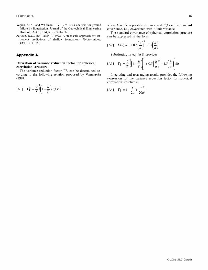
Derivation of variance reduction factor for sphericalcorrelation structure

The variance reduction factor, Γ2 , can be determined ac-cording to the following relation proposed by Vanmarcke(1984):

[A1] ΓT0

T

d2 21= ∫ −

T

hT

C h h( )

where h is the separation distance and C(h) is the standardcovariance, i.e., covariance with a unit variance.

The standard covariance of spherical correlation structurecan be expressed in the form

[A2] C hha

ha

( ) . .= +

−

1 0 5 1 53

Substituting in eq. [A1] provides

[A3] ΓT0

T2

32

1 1 0 5 1 5= ∫ −

+

−

ThT

ha

ha

. .dh

Integrating and rearranging results provides the followingexpression for the variance reduction factor for sphericalcorrelation structures:

[A4] ΓT2

3

31

2 20= − +T

aT

a

An overview of soil heterogeneity: quantification and implications on geotechnical field problems

Documents