An Overview of Multi-agent Reinforcement Learning ... - arXiv

An Overview of Multi-agent Reinforcement Learningfrom Game Theoretical Perspective

Yaodong Yang∗1,2 and Jun Wang1,2

1University College London, 2Huawei R&D U.K.

Abstract

Following the remarkable success of the AlphaGO series, 2019 was a boom-ing year that witnessed significant advances in multi-agent reinforcement learning(MARL) techniques. MARL corresponds to the learning problem in a multi-agentsystem in which multiple agents learn simultaneously. It is an interdisciplinary do-main with a long history that includes game theory, machine learning, stochasticcontrol, psychology, and optimisation. Although MARL has achieved considerableempirical success in solving real-world games, there is a lack of a self-containedoverview in the literature that elaborates the game theoretical foundations of mod-ern MARL methods and summarises the recent advances. In fact, the majorityof existing surveys are outdated and do not fully cover the recent developmentssince 2010. In this work, we provide a monograph on MARL that covers both thefundamentals and the latest developments in the research frontier.

Our work is separated into two parts. From §1 to §4, we present the self-contained fundamental knowledge of MARL, including problem formulations, basicsolutions, and existing challenges. Specifically, we present the MARL formulationsthrough two representative frameworks, namely, stochastic games and extensive-form games, along with different variations of games that can be addressed. Thegoal of this part is to enable the readers, even those with minimal related back-ground, to grasp the key ideas in MARL research. From §5 to §9, we present anoverview of recent developments of MARL algorithms. Starting from new tax-onomies for MARL methods, we conduct a survey of previous survey papers. Inlater sections, we highlight several modern topics in MARL research, includingQ-function factorisation, multi-agent soft learning, networked multi-agent MDP,stochastic potential games, zero-sum continuous games, online MDP, turn-basedstochastic games, policy space response oracle, approximation methods in general-sum games, and mean-field type learning in games with infinite agents. Withineach topic, we select both the most fundamental and cutting-edge algorithms.

The goal of our monograph is to provide a self-contained assessment of thecurrent state-of-the-art MARL techniques from a game theoretical perspective. Weexpect this work to serve as a stepping stone for both new researchers who areabout to enter this fast-growing domain and existing domain experts who want toobtain a panoramic view and identify new directions based on recent advances.

∗This manuscript is under actively development. We appreciated any constructive comments andsuggestions corresponding to: <[email protected]>.

1

arX

iv:2

011.

0058

3v3

[cs

.MA

] 1

8 M

ar 2

021

Contents

1 Introduction 4

1.1 A Short History of RL . . . . . . . . . . . . . . . . . . . . . . . . . . . . 5

1.2 2019: A Booming Year for MARL . . . . . . . . . . . . . . . . . . . . . . 8

2 Single-Agent RL 9

2.1 Problem Formulation: Markov Decision Process . . . . . . . . . . . . . . 10

2.2 Justification of Reward Maximisation . . . . . . . . . . . . . . . . . . . . 11

2.3 Solving Markov Decision Processes . . . . . . . . . . . . . . . . . . . . . 12

2.3.1 Value-Based Methods . . . . . . . . . . . . . . . . . . . . . . . . . 13

2.3.2 Policy-Based Methods . . . . . . . . . . . . . . . . . . . . . . . . 14

3 Multi-Agent RL 15

3.1 Problem Formulation: Stochastic Game . . . . . . . . . . . . . . . . . . . 16

3.2 Solving Stochastic Games . . . . . . . . . . . . . . . . . . . . . . . . . . 17

3.2.1 Value-Based MARL Methods . . . . . . . . . . . . . . . . . . . . 18

3.2.2 Policy-Based MARL Methods . . . . . . . . . . . . . . . . . . . . 19

3.2.3 Solution Concept of the Nash Equilibrium . . . . . . . . . . . . . 19

3.2.4 Special Types of Stochastic Games . . . . . . . . . . . . . . . . . 22

3.2.5 Partially Observable Settings . . . . . . . . . . . . . . . . . . . . 26

3.3 Problem Formulation: Extensive-Form Game . . . . . . . . . . . . . . . . 28

3.3.1 Normal-Form Representation . . . . . . . . . . . . . . . . . . . . 31

3.3.2 Sequence-Form Representation . . . . . . . . . . . . . . . . . . . . 32

3.4 Solving Extensive-Form Games . . . . . . . . . . . . . . . . . . . . . . . 35

3.4.1 Perfect-Information Games . . . . . . . . . . . . . . . . . . . . . . 35

3.4.2 Imperfect-Information Games . . . . . . . . . . . . . . . . . . . . 36

4 Grand Challenges of MARL 38

4.1 The Combinatorial Complexity . . . . . . . . . . . . . . . . . . . . . . . 39

4.2 The Multi-Dimensional Learning Objectives . . . . . . . . . . . . . . . . 40

4.3 The Non-Stationarity Issue . . . . . . . . . . . . . . . . . . . . . . . . . . 41

4.4 The Scalability Issue when N 2 . . . . . . . . . . . . . . . . . . . . . . 43

5 A Survey of MARL Surveys 44

5.1 Taxonomy of MARL Algorithms . . . . . . . . . . . . . . . . . . . . . . . 44

5.2 A Survey of Surveys . . . . . . . . . . . . . . . . . . . . . . . . . . . . . 47

6 Learning in Identical-Interest Games 50

6.1 Stochastic Team Games . . . . . . . . . . . . . . . . . . . . . . . . . . . 50

2

6.1.1 Solutions via Q-function Factorisation . . . . . . . . . . . . . . . 51

6.1.2 Solutions via Multi-Agent Soft Learning . . . . . . . . . . . . . . 53

6.2 Dec-POMDPs . . . . . . . . . . . . . . . . . . . . . . . . . . . . . . . . . 56

6.3 Networked Multi-Agent MDPs . . . . . . . . . . . . . . . . . . . . . . . . 57

6.4 Stochastic Potential Games . . . . . . . . . . . . . . . . . . . . . . . . . 59

7 Learning in Zero-Sum Games 61

7.1 Discrete State-Action Games . . . . . . . . . . . . . . . . . . . . . . . . . 62

7.2 Continuous State-Action Games . . . . . . . . . . . . . . . . . . . . . . . 63

7.3 Extensive-Form Games . . . . . . . . . . . . . . . . . . . . . . . . . . . . 66

7.3.1 Variations of Fictitious Play . . . . . . . . . . . . . . . . . . . . . 67

7.3.2 Counterfactual Regret Minimisation . . . . . . . . . . . . . . . . . 70

7.4 Online Markov Decision Processes . . . . . . . . . . . . . . . . . . . . . . 74

7.5 Turn-Based Stochastic Games . . . . . . . . . . . . . . . . . . . . . . . . 77

7.6 Open-Ended Meta-Games . . . . . . . . . . . . . . . . . . . . . . . . . . 78

8 Learning in General-Sum Games 82

8.1 Solutions by Mathematical Programming . . . . . . . . . . . . . . . . . . 82

8.2 Solutions by Value-Based Methods . . . . . . . . . . . . . . . . . . . . . 84

8.3 Solutions by Two-Timescale Analysis . . . . . . . . . . . . . . . . . . . . 84

8.4 Solutions by Policy-Based Methods . . . . . . . . . . . . . . . . . . . . . 85

9 Learning in Games when N → +∞ 87

9.1 Non-cooperative Mean-Field Game . . . . . . . . . . . . . . . . . . . . . 90

9.2 Cooperative Mean-Field Control . . . . . . . . . . . . . . . . . . . . . . . 93

9.3 Mean-Field MARL . . . . . . . . . . . . . . . . . . . . . . . . . . . . . . 95

10 Future Directions of Interest 98

Bibliography 101

3

1 Introduction

Machine learning can be considered as the process of converting data into knowledge

(Shalev-Shwartz and Ben-David, 2014). The input of a learning algorithm is training data

(for example, images containing cats), and the output is some knowledge (for example,

rules about how to detect cats in an image). This knowledge is usually represented

as a computer program that can perform certain task(s) (for example, an automatic

cat detector). In the past decade, considerable progress has been made by means of a

special kind of machine learning technique: deep learning (LeCun et al., 2015). One

of the critical embodiments of deep learning is different kinds of deep neural networks

(DNNs) (Schmidhuber, 2015) that can find disentangled representations (Bengio, 2009)

in high-dimensional data, which allows the software to train itself to perform new tasks

rather than merely relying on the programmer for designing hand-crafted rules. An

uncountable number of breakthroughs in real-world AI applications have been achieved

through the usage of DNNs, with the domains of computer vision (Krizhevsky et al.,

2012) and natural language processing (Brown et al., 2020; Devlin et al., 2018) being the

greatest beneficiaries.

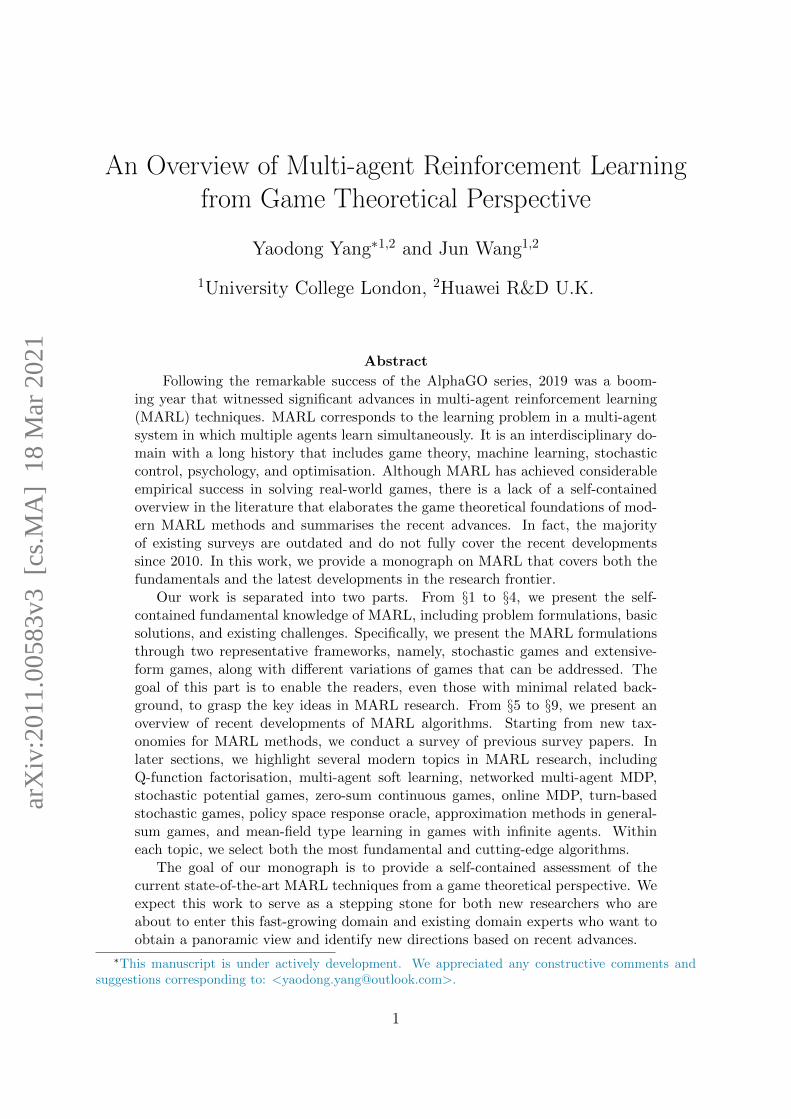
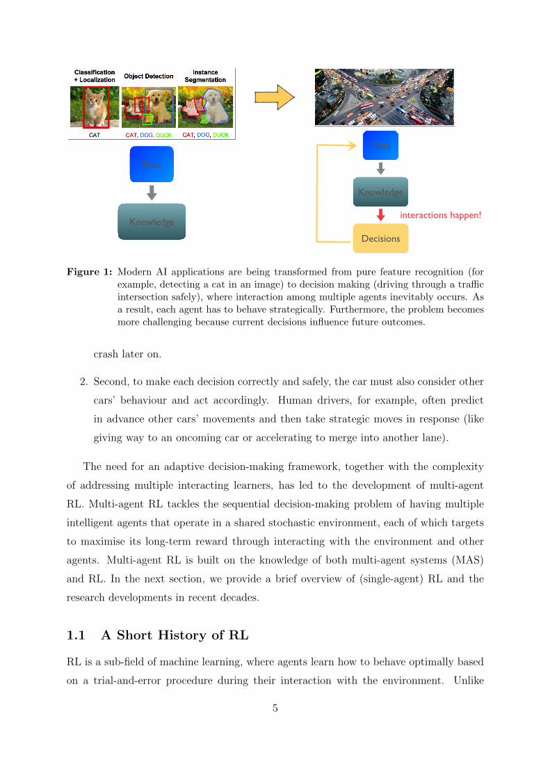
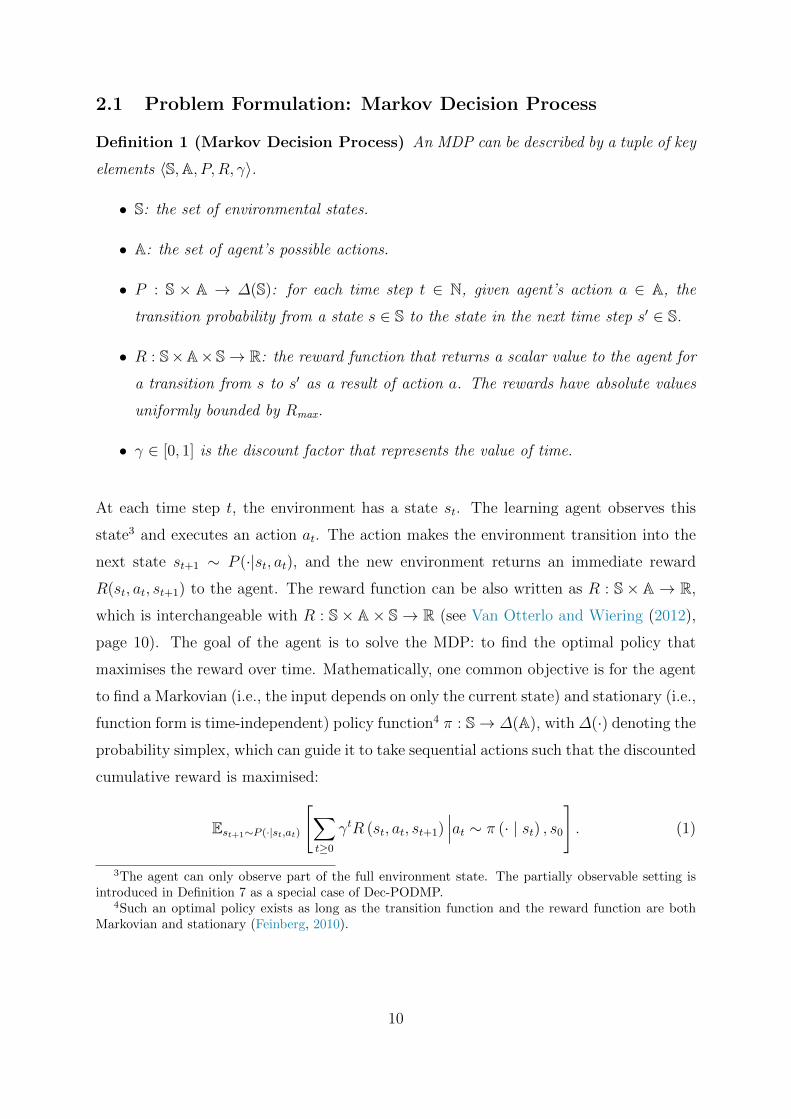
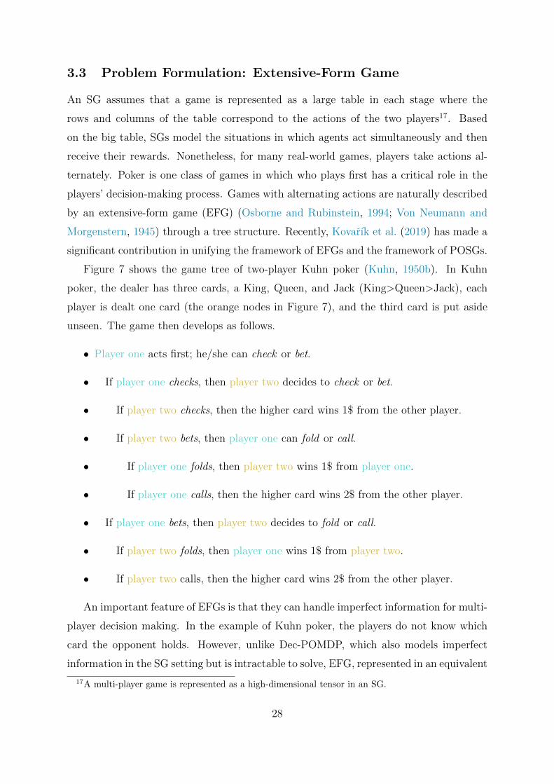
In addition to feature recognition from existing data, modern AI applications often

require computer programs to make decisions based on acquired knowledge (see Figure

1). To illustrate the key components of decision making, let us consider the real-world

example of controlling a car to drive safely through an intersection. At each time step, a

robot car can move by steering, accelerating and braking. The goal is to safely exit the

intersection and reach the destination (with possible decisions of going straight or turning

left/right into another lane). Therefore, in addition to being able to detect objects, such

as traffic lights, lane markings, and other cars (by converting data to knowledge), we aim

to find a steering policy that can control the car to make a sequence of manoeuvres to

achieve the goal (making decisions based on the knowledge gained). In a decision-making

setting such as this, two additional challenges arise:

1. First, during the decision-making process, at each time step, the robot car should

consider not only the immediate value of its current action but also the consequences

of its current action in the future. For example, in the case of driving through an

intersection, it would be detrimental to have a policy that chooses to steer in a

“safe” direction at the beginning of the process if it would eventually lead to a car

4

Data

Knowledge

Data

Decisions

Knowledge

interactions happen!

Figure 1: Modern AI applications are being transformed from pure feature recognition (forexample, detecting a cat in an image) to decision making (driving through a trafficintersection safely), where interaction among multiple agents inevitably occurs. Asa result, each agent has to behave strategically. Furthermore, the problem becomesmore challenging because current decisions influence future outcomes.

crash later on.

2. Second, to make each decision correctly and safely, the car must also consider other

cars’ behaviour and act accordingly. Human drivers, for example, often predict

in advance other cars’ movements and then take strategic moves in response (like

giving way to an oncoming car or accelerating to merge into another lane).

The need for an adaptive decision-making framework, together with the complexity

of addressing multiple interacting learners, has led to the development of multi-agent

RL. Multi-agent RL tackles the sequential decision-making problem of having multiple

intelligent agents that operate in a shared stochastic environment, each of which targets

to maximise its long-term reward through interacting with the environment and other

agents. Multi-agent RL is built on the knowledge of both multi-agent systems (MAS)

and RL. In the next section, we provide a brief overview of (single-agent) RL and the

research developments in recent decades.

1.1 A Short History of RL

RL is a sub-field of machine learning, where agents learn how to behave optimally based

on a trial-and-error procedure during their interaction with the environment. Unlike

5

supervised learning, which takes labelled data as the input (for example, an image labelled

with cats), RL is goal-oriented: it constructs a learning model that learns to achieve the

optimal long-term goal by improvement through trial and error, with the learner having

no labelled data to obtain knowledge from. The word “reinforcement” refers to the

learning mechanism since the actions that lead to satisfactory outcomes are reinforced in

the learner’s set of behaviours.

Historically, the RL mechanism was originally developed based on studying cats’ be-

haviour in a puzzle box (Thorndike, 1898). Minsky (1954) first proposed the compu-

tational model of RL in his Ph.D. thesis and named his resulting analog machine the

stochastic neural-analog reinforcement calculator. Several years later, he first suggested

the connection between dynamic programming (Bellman, 1952) and RL (Minsky, 1961).

In 1972, Klopf (1972) integrated the trial-and-error learning process with the finding of

temporal difference (TD) learning from psychology. TD learning quickly became indis-

pensable in scaling RL for larger systems. On the basis of dynamic programming and

TD learning, Watkins and Dayan (1992) laid the foundations for present day RL using

the Markov decision process (MDP) and proposing the famous Q-learning method as the

solver. As a dynamic programming method, the original Q-learning process inherits Bell-

man’s “curse of dimensionality” (Bellman, 1952), which strongly limits its applications

when the number of state variables is large. To overcome such a bottleneck, Bertsekas and

Tsitsiklis (1996) proposed approximate dynamic programming methods based on neural

networks. More recently, Mnih et al. (2015) from DeepMind made a significant break-

through by introducing the deep Q-learning (DQN) architecture, which leverages the

representation power of DNNs for approximate dynamic programming methods. DQN

has demonstrated human-level performance on 49 Atari games. Since then, deep RL

techniques have become common in machine learning/AI and have attracted consider-

able attention from the research community.

RL originates from an understanding of animal behaviour where animals use trial-

and-error to reinforce beneficial behaviours, which they then perform more frequently.

During its development, computational RL incorporated ideas such as optimal control

theory and other findings from psychology that help mimic the way humans make deci-

sions to maximise the long-term profit of decision-making tasks. As a result, RL methods

can naturally be used to train a computer program (an agent) to a performance level com-

parable to that of a human on certain tasks. The earliest success of RL methods against

6

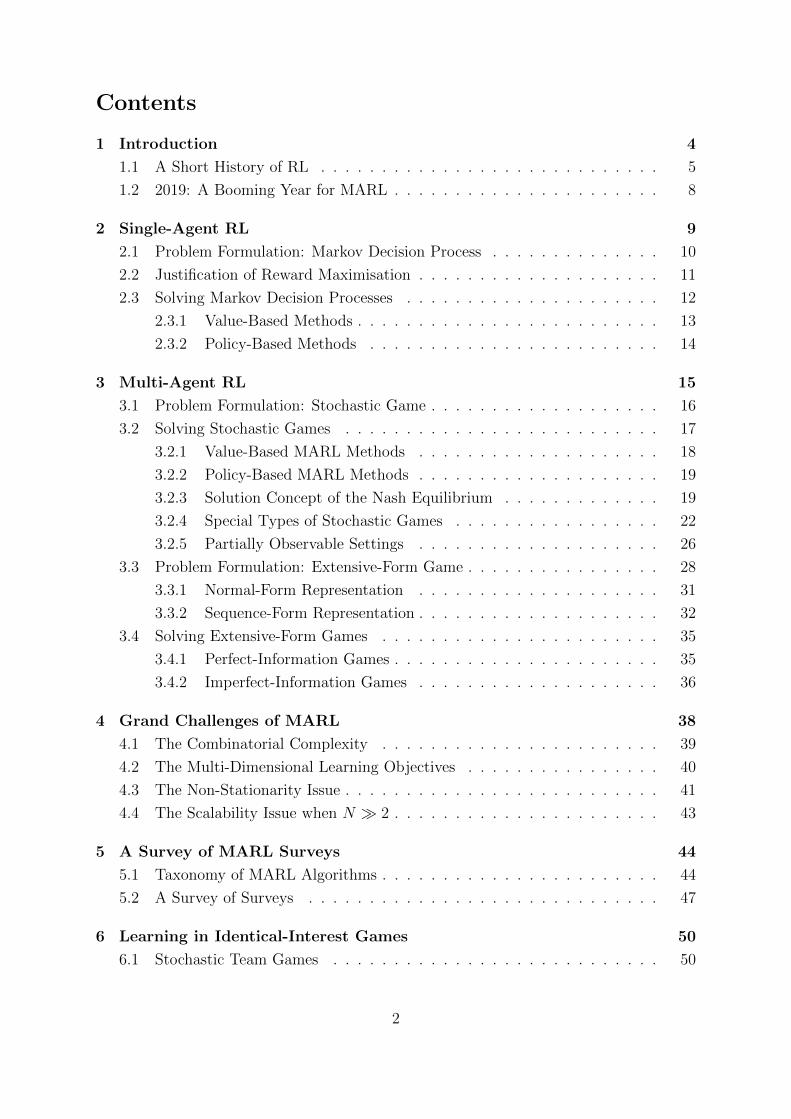
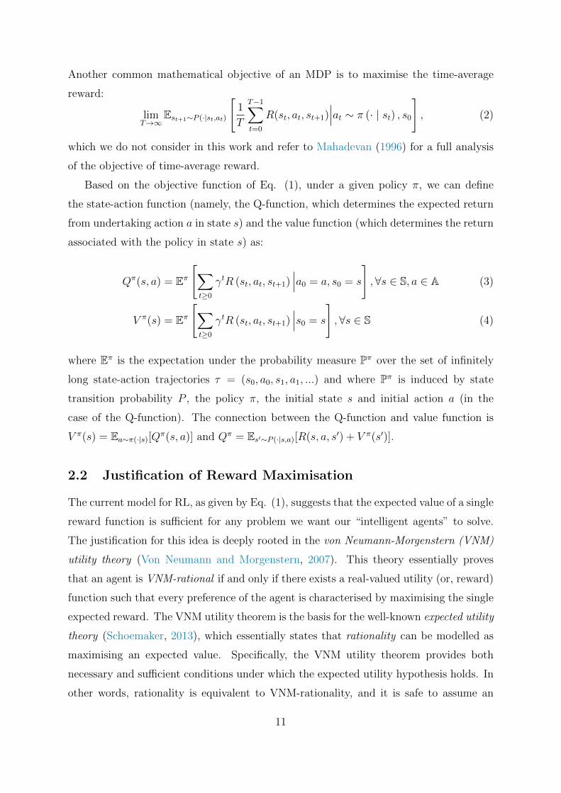
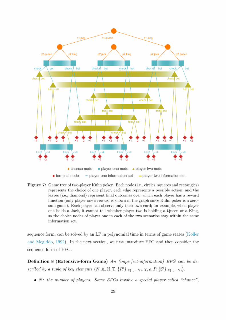
Jan 2016 Dec 2017

milestone of single-agent decision-making technique

AlphaGO Series

July 2018

Capture-the-flag (DeepMind)

Great advances have been made in 2019 !

Jan 2019 Apr 2019 July 2019 Sep 2019

AlphaStar (DeepMind)

Dota2 (OpenAI)

Pluribus Poker (FAIR)

Hide and Seek (OpenAI)

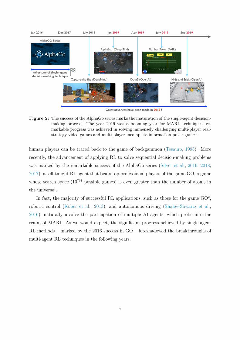
Figure 2: The success of the AlphaGo series marks the maturation of the single-agent decision-making process. The year 2019 was a booming year for MARL techniques; re-markable progress was achieved in solving immensely challenging multi-player real-strategy video games and multi-player incomplete-information poker games.

human players can be traced back to the game of backgammon (Tesauro, 1995). More

recently, the advancement of applying RL to solve sequential decision-making problems

was marked by the remarkable success of the AlphaGo series (Silver et al., 2016, 2018,

2017), a self-taught RL agent that beats top professional players of the game GO, a game

whose search space (10761 possible games) is even greater than the number of atoms in

the universe1.

In fact, the majority of successful RL applications, such as those for the game GO2,

robotic control (Kober et al., 2013), and autonomous driving (Shalev-Shwartz et al.,

2016), naturally involve the participation of multiple AI agents, which probe into the

realm of MARL. As we would expect, the significant progress achieved by single-agent

RL methods – marked by the 2016 success in GO – foreshadowed the breakthroughs of

multi-agent RL techniques in the following years.

7

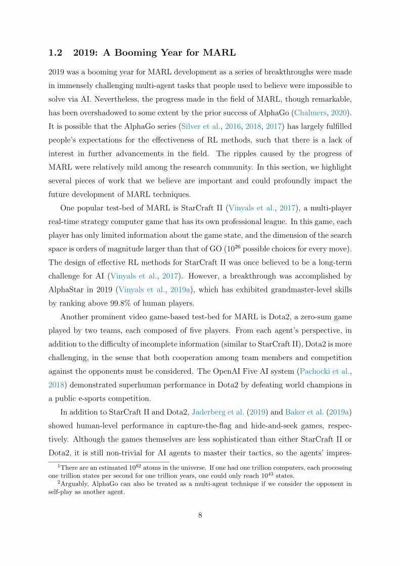
1.2 2019: A Booming Year for MARL

2019 was a booming year for MARL development as a series of breakthroughs were made

in immensely challenging multi-agent tasks that people used to believe were impossible to

solve via AI. Nevertheless, the progress made in the field of MARL, though remarkable,

has been overshadowed to some extent by the prior success of AlphaGo (Chalmers, 2020).

It is possible that the AlphaGo series (Silver et al., 2016, 2018, 2017) has largely fulfilled

people’s expectations for the effectiveness of RL methods, such that there is a lack of

interest in further advancements in the field. The ripples caused by the progress of

MARL were relatively mild among the research community. In this section, we highlight

several pieces of work that we believe are important and could profoundly impact the

future development of MARL techniques.

One popular test-bed of MARL is StarCraft II (Vinyals et al., 2017), a multi-player

real-time strategy computer game that has its own professional league. In this game, each

player has only limited information about the game state, and the dimension of the search

space is orders of magnitude larger than that of GO (1026 possible choices for every move).

The design of effective RL methods for StarCraft II was once believed to be a long-term

challenge for AI (Vinyals et al., 2017). However, a breakthrough was accomplished by

AlphaStar in 2019 (Vinyals et al., 2019a), which has exhibited grandmaster-level skills

by ranking above 99.8% of human players.

Another prominent video game-based test-bed for MARL is Dota2, a zero-sum game

played by two teams, each composed of five players. From each agent’s perspective, in

addition to the difficulty of incomplete information (similar to StarCraft II), Dota2 is more

challenging, in the sense that both cooperation among team members and competition

against the opponents must be considered. The OpenAI Five AI system (Pachocki et al.,

2018) demonstrated superhuman performance in Dota2 by defeating world champions in

a public e-sports competition.

In addition to StarCraft II and Dota2, Jaderberg et al. (2019) and Baker et al. (2019a)

showed human-level performance in capture-the-flag and hide-and-seek games, respec-

tively. Although the games themselves are less sophisticated than either StarCraft II or

Dota2, it is still non-trivial for AI agents to master their tactics, so the agents’ impres-

1There are an estimated 1082 atoms in the universe. If one had one trillion computers, each processingone trillion states per second for one trillion years, one could only reach 1043 states.

2Arguably, AlphaGo can also be treated as a multi-agent technique if we consider the opponent inself-play as another agent.

8

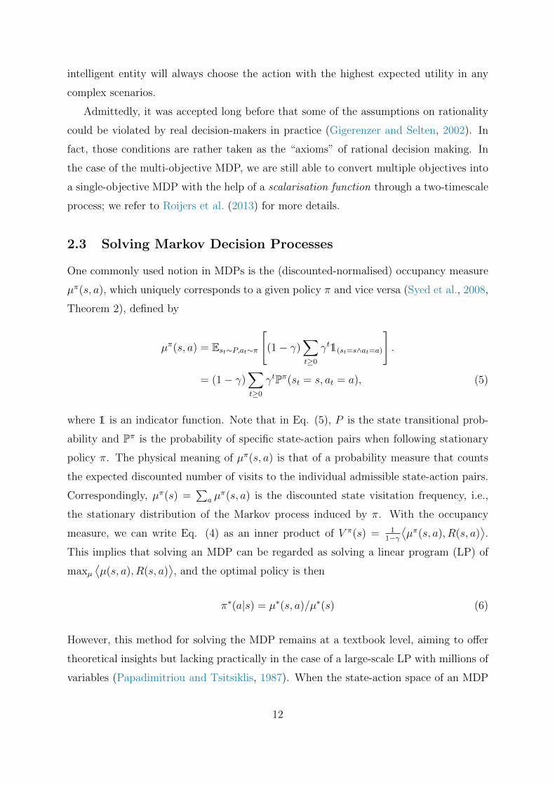
State, RewardAction

Agent

Environment

… …

Many agents

Environment

ActionState, Reward

Action

State, Reward Action

State, Reward

Figure 3: Diagram of a single-agent MDP (left) and a multi-agent MDP (right).

sive performance again demonstrates the efficacy of MARL. Interestingly, both authors

reported emergent behaviours induced by their proposed MARL methods that humans

can understand and are grounded in physical theory.

One last remarkable achievement of MARL worth mentioning is its application to the

poker game Texas hold’ em, which is a multi-player extensive-form game with incomplete

information accessible to the player. Heads-up (namely, two player) no-limit hold’em has

more than 6 × 10161 information states. Only recently have ground-breaking achieve-

ments in the game been made, thanks to MARL. Two independent programs, DeepStack

(Moravcık et al., 2017) and Libratus (Brown and Sandholm, 2018), are able to beat pro-

fessional human players. Even more recently, Libratus was upgraded to Pluribus (Brown

and Sandholm, 2019) and showed remarkable performance by winning over one million

dollars from five elite human professionals in a no-limit setting.

For a deeper understanding of RL and MARL, mathematical notation and deconstruc-

tion of the concepts are needed. In the next section, we provide mathematical formu-

lations for these concepts, starting from single-agent RL and progressing to multi-agent

RL methods.

2 Single-Agent RL

Through trial and error, an RL agent attempts to find the optimal policy to maximise

its long-term reward. This process is formulated by Markov Decision Processes.

9

2.1 Problem Formulation: Markov Decision Process

Definition 1 (Markov Decision Process) An MDP can be described by a tuple of key

elements 〈S,A, P, R, γ〉.

• S: the set of environmental states.

• A: the set of agent’s possible actions.

• P : S × A → ∆(S): for each time step t ∈ N, given agent’s action a ∈ A, the

transition probability from a state s ∈ S to the state in the next time step s′ ∈ S.

• R : S×A× S→ R: the reward function that returns a scalar value to the agent for

a transition from s to s′ as a result of action a. The rewards have absolute values

uniformly bounded by Rmax.

• γ ∈ [0, 1] is the discount factor that represents the value of time.

At each time step t, the environment has a state st. The learning agent observes this

state3 and executes an action at. The action makes the environment transition into the

next state st+1 ∼ P (·|st, at), and the new environment returns an immediate reward

R(st, at, st+1) to the agent. The reward function can be also written as R : S × A → R,

which is interchangeable with R : S× A× S → R (see Van Otterlo and Wiering (2012),

page 10). The goal of the agent is to solve the MDP: to find the optimal policy that

maximises the reward over time. Mathematically, one common objective is for the agent

to find a Markovian (i.e., the input depends on only the current state) and stationary (i.e.,

function form is time-independent) policy function4 π : S→ ∆(A), with ∆(·) denoting the

probability simplex, which can guide it to take sequential actions such that the discounted

cumulative reward is maximised:

Est+1∼P (·|st,at)

[∑

t≥0

γtR (st, at, st+1)∣∣∣at ∼ π (· | st) , s0

]. (1)

3The agent can only observe part of the full environment state. The partially observable setting isintroduced in Definition 7 as a special case of Dec-PODMP.

4Such an optimal policy exists as long as the transition function and the reward function are bothMarkovian and stationary (Feinberg, 2010).

10

Another common mathematical objective of an MDP is to maximise the time-average

reward:

limT→∞

Est+1∼P (·|st,at)

[1

T

T−1∑

t=0

R(st, at, st+1)∣∣∣at ∼ π (· | st) , s0

], (2)

which we do not consider in this work and refer to Mahadevan (1996) for a full analysis

of the objective of time-average reward.

Based on the objective function of Eq. (1), under a given policy π, we can define

the state-action function (namely, the Q-function, which determines the expected return

from undertaking action a in state s) and the value function (which determines the return

associated with the policy in state s) as:

Qπ(s, a) = Eπ[∑

t≥0

γtR (st, at, st+1)∣∣∣a0 = a, s0 = s

],∀s ∈ S, a ∈ A (3)

V π(s) = Eπ[∑

t≥0

γtR (st, at, st+1)∣∣∣s0 = s

],∀s ∈ S (4)

where Eπ is the expectation under the probability measure Pπ over the set of infinitely

long state-action trajectories τ = (s0, a0, s1, a1, ...) and where Pπ is induced by state

transition probability P , the policy π, the initial state s and initial action a (in the

case of the Q-function). The connection between the Q-function and value function is

V π(s) = Ea∼π(·|s)[Qπ(s, a)] and Qπ = Es′∼P (·|s,a)[R(s, a, s′) + V π(s′)].

2.2 Justification of Reward Maximisation

The current model for RL, as given by Eq. (1), suggests that the expected value of a single

reward function is sufficient for any problem we want our “intelligent agents” to solve.

The justification for this idea is deeply rooted in the von Neumann-Morgenstern (VNM)

utility theory (Von Neumann and Morgenstern, 2007). This theory essentially proves

that an agent is VNM-rational if and only if there exists a real-valued utility (or, reward)

function such that every preference of the agent is characterised by maximising the single

expected reward. The VNM utility theorem is the basis for the well-known expected utility

theory (Schoemaker, 2013), which essentially states that rationality can be modelled as

maximising an expected value. Specifically, the VNM utility theorem provides both

necessary and sufficient conditions under which the expected utility hypothesis holds. In

other words, rationality is equivalent to VNM-rationality, and it is safe to assume an

11

intelligent entity will always choose the action with the highest expected utility in any

complex scenarios.

Admittedly, it was accepted long before that some of the assumptions on rationality

could be violated by real decision-makers in practice (Gigerenzer and Selten, 2002). In

fact, those conditions are rather taken as the “axioms” of rational decision making. In

the case of the multi-objective MDP, we are still able to convert multiple objectives into

a single-objective MDP with the help of a scalarisation function through a two-timescale

process; we refer to Roijers et al. (2013) for more details.

2.3 Solving Markov Decision Processes

One commonly used notion in MDPs is the (discounted-normalised) occupancy measure

µπ(s, a), which uniquely corresponds to a given policy π and vice versa (Syed et al., 2008,

Theorem 2), defined by

µπ(s, a) = Est∼P,at∼π

[(1− γ)

∑

t≥0

γt1(st=s∧at=a)

].

= (1− γ)∑

t≥0

γtPπ(st = s, at = a), (5)

where 1 is an indicator function. Note that in Eq. (5), P is the state transitional prob-

ability and Pπ is the probability of specific state-action pairs when following stationary

policy π. The physical meaning of µπ(s, a) is that of a probability measure that counts

the expected discounted number of visits to the individual admissible state-action pairs.

Correspondingly, µπ(s) =∑

a µπ(s, a) is the discounted state visitation frequency, i.e.,

the stationary distribution of the Markov process induced by π. With the occupancy

measure, we can write Eq. (4) as an inner product of V π(s) = 11−γ

⟨µπ(s, a), R(s, a)

⟩.

This implies that solving an MDP can be regarded as solving a linear program (LP) of

maxµ⟨µ(s, a), R(s, a)

⟩, and the optimal policy is then

π∗(a|s) = µ∗(s, a)/µ∗(s) (6)

However, this method for solving the MDP remains at a textbook level, aiming to offer

theoretical insights but lacking practically in the case of a large-scale LP with millions of

variables (Papadimitriou and Tsitsiklis, 1987). When the state-action space of an MDP

12

is continuous, LP formulation cannot help solve either.

In the context of optimal control (Bertsekas, 2005), dynamic-programming approaches,

such as policy iteration and value iteration, can also be applied to solve for the optimal

policy that maximises Eq. (3) & Eq. (4), but these approaches require knowledge of

the exact form of the model: the transition function P (·|s, a), and the reward function

R(s, a, s′) .

On the other hand, in the setting of RL, the agent learns the optimal policy by

a trial-and-error process during its interaction with the environment rather than using

prior knowledge of the model. The word “learning” essentially means that the agent

turns its experience gained during the interaction into knowledge about the model of

the environment. Based on the solution target, either the optimal policy or the optimal

value function, RL algorithms can be categorised into two types: value-based methods

and policy-based methods.

2.3.1 Value-Based Methods

For all MDPs with finite states and actions, there exists at least one deterministic sta-

tionary optimal policy (Sutton and Barto, 1998; Szepesvari, 2010). Value-based methods

are introduced to find the optimal Q-function Q∗ that maximises Eq. (3). Correspond-

ingly, the optimal policy can be derived from the Q-function by taking the greedy action

of π∗ = arg maxaQ∗(s, a). The classic Q-learning algorithm (Watkins and Dayan, 1992)

approximates Q∗ by Q, and updates its value via temporal-difference learning (Sutton,

1988).

Q(st, at)︸ ︷︷ ︸new value

← Q(st, at)︸ ︷︷ ︸old value

+ α︸︷︷︸learning rate

·

temporal difference error︷ ︸︸ ︷(Rt + γ ·max

a∈AQ(st+1, a)

︸ ︷︷ ︸temporal difference target

− Q(st, at)︸ ︷︷ ︸old value

)(7)

Theoretically, given the Bellman optimality operator H∗, defined by

(H∗Q)(s, a) =∑

s′

P (s′|s, a)

[R(s, a, s′) + γmax

b∈AQ(s, b)

], (8)

13

we know it is a contraction mapping and the optimal Q-function is the unique5 fixed

point, i.e., H∗(Q∗) = Q∗. The Q-learning algorithm draws random samples of (s, a, R, s′)

in Eq. (7) to approximate Eq. (8), but is still guaranteed to converge to the optimal Q-

function (Szepesvari and Littman, 1999) under the assumptions that the state-action sets

are discrete and finite and are visited an infinite number of times. Munos and Szepesvari

(2008) extended the convergence result to a more realistic setting by deriving the high

probability error bound for an infinite state space with a finite number of samples.

Recently, Mnih et al. (2015) applied neural networks as a function approximator for

the Q-function in updating Eq. (7). Specifically, DQN optimises the following equation:

minθ

E(st,at,Rt,st+1)∼D

[(Rt + γmax

a∈AQθ− (st+1, a)−Qθ (st, at)

)2]. (9)

The neural network parameters θ is fitted by drawing i.i.d. samples from the replay

buffer D and then updating in a supervised learning fashion. Qθ− is a slowly updated

target network that helps stabilise training. The convergence property and finite sample

analysis of DQN have been studied by Yang et al. (2019c).

2.3.2 Policy-Based Methods

Policy-based methods are designed to directly search over the policy space to find the op-

timal policy π∗. One can parameterise the policy expression π∗ ≈ πθ(·|s) and update the

parameter θ in the direction that maximises the cumulative reward θ ← θ+α∇θVπθ(s) to

find the optimal policy. However, the gradient will depend on the unknown effects of pol-

icy changes on the state distribution. The famous policy gradient (PG) theorem (Sutton

et al., 2000) derives an analytical solution that does not involve the state distribution,

that is:

∇θVπθ(s) = Es∼µπθ (·),a∼πθ(·|s)

[∇θ log πθ(a|s) ·Qπθ(s, a)

](10)

where µπθ is the state occupancy measure under policy πθ and ∇ log πθ(a|s) is the updat-

ing score of the policy. When the policy is deterministic and the action set is continuous,

one obtains the deterministic policy gradient (DPG) theorem (Silver et al., 2014) as

∇θVπθ(s) = Es∼µπθ (·)

[∇θπθ(a|s) · ∇aQ

πθ(s, a)∣∣a=πθ(s)

]. (11)

5Note that although the optimal Q-function is unique, its corresponding optimal policies may havemultiple candidates.

14

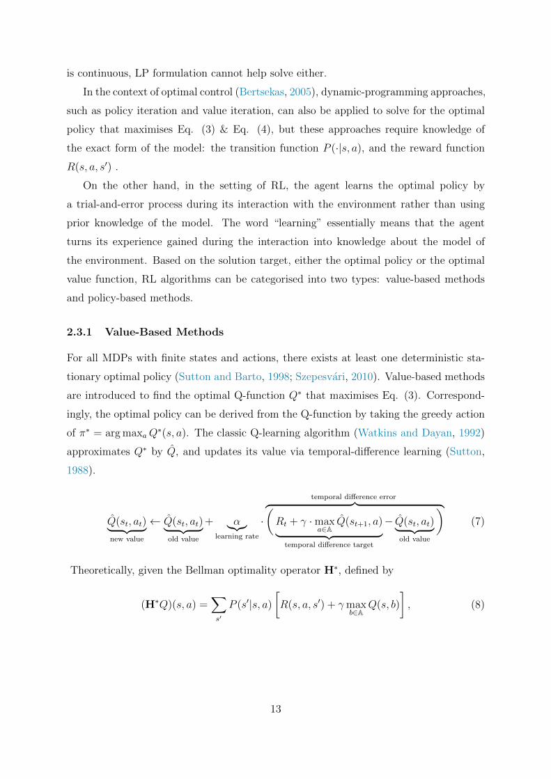
(0, 0) (1, 2)(2, 1) (0, 0)

Yield

Rush

Yield Rush

normal-form gamegame scenariotraffic intersection

Figure 4: A snapshot of stochastic time in the intersection example. The scenario is abstractedsuch that there are two cars, with each car taking one of two possible actions: toyield or to rush. The outcome of each joint action pair is represented by a normal-form game, with the reward value for the row player denoted in red and that for thecolumn player denoted in black. The Nash equilibria (NE) of this game are (rush,yield) and (yield, rush). If both cars maximise their own reward selfishly withoutconsidering the others, they will end up in an accident.

A classic implementation of the PG theorem is REINFORCE (Williams, 1992), which

uses a sample return Rt =∑T

i=t γi−tri to estimate Qπθ . Alternatively, one can use a

model of Qω (also called critic) to approximate the true Qπθ and update the parameter

ω via TD learning. This approach gives rise to the famous actor-critic methods (Konda

and Tsitsiklis, 2000; Peters and Schaal, 2008). Important variants of actor-critic methods

include trust-region methods (Schulman et al., 2015, 2017), PG with optimal baselines

(Weaver and Tao, 2001; Zhao et al., 2011), soft actor-critic methods (Haarnoja et al.,

2018), and deep deterministic policy gradient (DDPG) methods (Lillicrap et al., 2015).

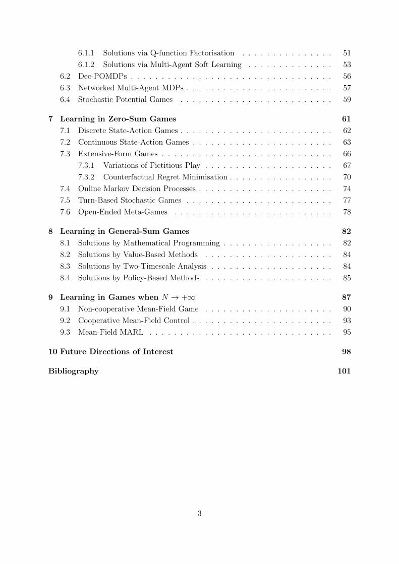
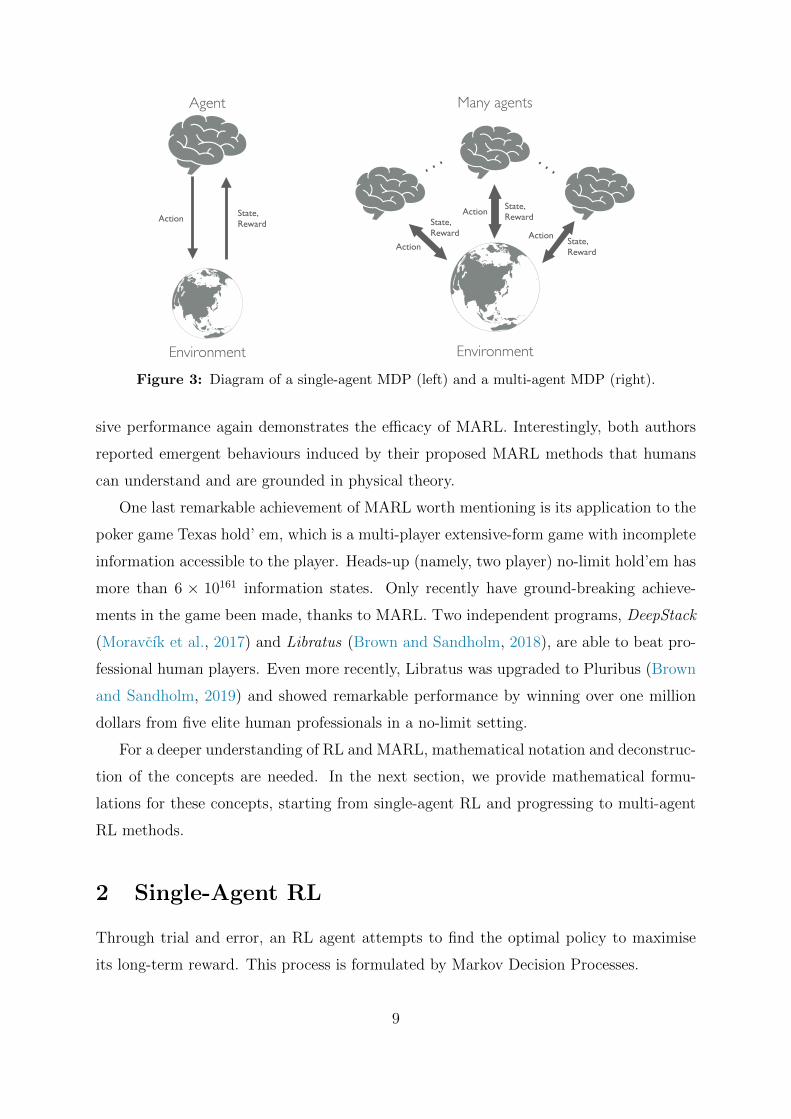
3 Multi-Agent RL

In the multi-agent scenario, much like in the single-agent scenario, each agent is still trying

to solve the sequential decision-making problem through a trial-and-error procedure. The

difference is that the evolution of the environmental state and the reward function that

each agent receives is now determined by all agents’ joint actions (see Figure 3). As a

result, agents need to take into account and interact with not only the environment but

also other learning agents. A decision-making process that involves multiple agents is

usually modelled through a stochastic game (Shapley, 1953), also known as a Markov

game (Littman, 1994).

15

3.1 Problem Formulation: Stochastic Game

Definition 2 (Stochastic Game) A stochastic game can be regarded as a multi-player6

extension to the MDP in Definition 1. Therefore, it is also defined by a set of key elements

〈N, S, Aii∈1,...,N, P, Rii∈1,...,N, γ〉.

• N : the number of agents, N = 1 degenerates to a single-agent MDP, N 2 is

referred as many-agent cases in this paper.

• S: the set of environmental states shared by all agents.

• Ai: the set of actions of agent i. We denote AAA := A1 × · · · × AN .

• P : S×AAA→ ∆(S): for each time step t ∈ N, given agents’ joint actions a ∈ AAA, the

transition probability from state s ∈ S to state s′ ∈ S in the next time step.

• Ri : S ×AAA × S → R: the reward function that returns a scalar value to the i − thagent for a transition from (s,a) to s′. The rewards have absolute values uniformly

bounded by Rmax.

• γ ∈ [0, 1] is the discount factor that represents the value of time.

We use the superscript of (·i, ·−i) (for example, a = (ai, a−i)), when it is necessary to

distinguish between agent i and all other N − 1 opponents.

Ultimately, the stochastic game (SG) acts as a framework that allows simultaneous

moves from agents in a decision-making scenario7. The game can be described sequen-

tially, as follows: At each time step t, the environment has a state st, and given st, each

agent executes its action ait, simultaneously with all other agents. The joint action from

all agents makes the environment transition into the next state st+1 ∼ P (·|st,at); then,

the environment determines an immediate reward Ri(st,at, st+1) for each agent. As seen

in the single-agent MDP scenario, the goal of each agent i is to solve the SG. In other

words, each agent aims to find a behavioural policy (or, a mixed strategy8 in game theory

6Player is a common word used in game theory; agent is more commonly used in machine learning.We do not discriminate between their usages in this work. The same holds for strategy vs policy andutility/payoff vs reward. Each pair refers to the game theory usage vs machine learning usage.

7Extensive-form games allow agents to take sequential moves; the full description can be found in(Shoham and Leyton-Brown, 2008, Chapter 5).

8A behavioural policy refers to a function map from the history (s0, ai0, s1, a

i1, ..., st−1) to an action.

The policy is typically assumed to be Markovian such that it depends on only the current state st rather

16

terminology (Osborne and Rubinstein, 1994)), that is, πi ∈ Π i : S → ∆(Ai) that can

guide the agent to take sequential actions such that the discounted cumulative reward9 in

Eq. (12) is maximised. Here, ∆(·) is the probability simplex on a set. In game theory, πi

is also called a pure strategy (vs a mixed strategy) if ∆(·) is replaced by a Dirac measure.

V πi,π−i(s) = Est+1∼P (·|st,at),a−i∼π−i(·|st)

[∑

t≥0

γtRit (st,at, st+1)

∣∣∣ait ∼ πi (· | st) , s0

]. (12)

Comparison of Eq. (12) with Eq. (4) indicates that the optimal policy of each agent

is influenced by not only its own policy but also the policies of the other agents in the

game. This scenario leads to fundamental differences in the solution concept between

single-agent RL and multi-agent RL.

3.2 Solving Stochastic Games

An SG can be considered as a sequence of normal-form games, which are games that

can be represented in a matrix. Take the original intersection scenario as an example

(see Figure 4). A snapshot of the SG at time t (stage game) can be represented as a

normal-form game in a matrix format. The rows correspond to the action set A1 for

agent 1, and the columns correspond to the action set A2 for agent 2. The values of the

matrix are the rewards given for each of the joint action pairs. In this scenario, if both

agents care only about maximising their own possible reward with no consideration of

other agents (the solution concept in a single-agent RL problem) and choose the action to

rush, they will reach the outcome of crashing into each other. Clearly, this state is unsafe

and is thus sub-optimal for each agent, despite the fact that the possible reward was the

highest for each agent when rushing. Therefore, to solve an SG and truly maximise the

cumulative reward, each agent must take strategic actions with consideration of others

when determining their policies.

Unfortunately, in contrast to MDPs, which have polynomial time-solvable linear-

programming formulations, solving SGs usually involves applying Newton’s method for

solving nonlinear programs. However, there are two special cases of two-player general-

than the entire history. A mixed strategy refers to a randomisation over pure strategies (for example, theactions). In SGs, the behavioural policy and mixed policy are exactly the same. In extensive-form games,they are different, but if the agent retains the history of previous actions and states (has perfect recall),each behavioural strategy has a realisation-equivalent mixed strategy, and vice versa (Kuhn, 1950a).

9Similar to single-agent MDP, we can adopt the objective of time-average rewards.

17

sum discounted-reward SGs that can still be written as LPs (Shoham and Leyton-Brown,

2008, Chapter 6.2)10. They are as follows:

• single-controller SG : the transition dynamics are determined by a single player, i.e.,

P (·|a, s) = P (·|ai, s) if the i-th index in the vector a is a[i] = ai,∀s ∈ S,∀a ∈ AAA.

• separable reward state independent transition (SR-SIT) SG : the states and the ac-

tions have independent effects on the reward function and the transition function

depends on only the joint actions, i.e., ∃α : S→ R, β : AAA→ R such that these two

conditions hold: 1) Ri(s,a) = α(s) + β(a),∀i ∈ 1, ..., N,∀s ∈ S,∀a ∈ AAA, and

2) P (·|s′,a) = P (·|s,a),∀a ∈ AAA,∀s, s′ ∈ S.

3.2.1 Value-Based MARL Methods

The single-agent Q-learning update in Eq. (7) still holds in the multi-agent case. In the

t-th iteration, for each agent i, given the transition data

(st,at, Ri, st+1)

t≥0

sampled

from the replay buffer, it updates only the value of Q(st,at) and keeps the other entries

of the Q-function unchanged. Specifically, we have

Qi(st,at)← Qi(st,at) + α·(Ri + γ · evali

(Qi(st+1, ·)

i∈1,...,N

)−Qi(st,at)

). (13)

Compared to Eq. (7), the max operator is changed to evali(Qi(st+1, ·)i∈1,...,N

)in

Eq. (13) to reflect the fact that each agent can no longer consider only itself but must

evaluate the situation of the stage game at time step t + 1 by considering all agents’

interests, as represented by the set of their Q-functions. Then, the optimal policy can

be solved by solvei(Qi(st+1, ·)i∈1,...,N

)= πi,∗. Therefore, we can further write the

evaluation operator as

evali(Qi(st+1, ·)

i∈1,...,N

)= V i

(st+1,

solvei

(Qi(st+1, ·)i∈1,...,N

)i∈1,...,N

).

(14)

In summary, solvei returns agent i′s part of the optimal policy at some equilibrium

point (not necessarily corresponding to its largest possible reward), and evali gives agent

i’s expected long-term reward under this equilibrium, assuming all other agents agree to

10According to Filar and Vrieze (2012) [Section 3.5], single-controller SG is solvable in polynomial timeonly under zero-sum cases rather than general-sum cases, which contradicts the result in Shoham andLeyton-Brown (2008) [Chapter 6.2], and we believe Shoham and Leyton-Brown (2008) made a typo.

18

play the same equilibrium.

3.2.2 Policy-Based MARL Methods

The value-based approach suffers from the curse of dimensionality due to the combi-

natorial nature of multi-agent systems (for further discussion, see Section 4.1). This

characteristic necessitates the development of policy-based algorithms with function ap-

proximations. Specifically, each agent learns its own optimal policy πiθi : S → ∆(Ai) by

updating the parameter θi of, for example, a neural network. Let θ = (θi)i∈1,...,N repre-

sent the collection of policy parameters for all agents, and let πθ :=∏

i∈1,...,N πiθi(a

i|s)be the joint policy. To optimise the parameter θi, the policy gradient theorem in Section

2.3.2 can be extended to the multi-agent context. Given agent i’s objective function

J i(θ) = Es∼P,a∼πθ[∑

t≥0 γtRit

], we have:

∇θiJi(θ) = Es∼µπθ (·),a∼πθ(·|s)

[∇θi log πθi(a

i|s) ·Qi,πθ(s,a)]. (15)

Considering a continuous action set with a deterministic policy, we have the multi-agent

deterministic policy gradient (MADDPG) (Lowe et al., 2017) written as

∇θiJi(θ) = Es∼µπθ (·)

[∇θi log πθi(a

i|s) · ∇aiQi,πθ(s,a)

∣∣a=πθ(s)

]. (16)

Note that in both Eqs. (15) & (16), the expectation over the joint policy πθ implies

that other agents’ policies must be observed; this is often a strong assumption for many

real-world applications.

3.2.3 Solution Concept of the Nash Equilibrium

Game theory plays an essential role in multi-agent learning by offering so-called solution

concepts that describe the outcomes of a game by showing which strategies will finally be

adopted by players. Many types of solution concepts exist for MARL (see Section 4.2),

among which the most famous is probably the Nash equilibrium (NE) in non-cooperative

game theory (Nash, 1951). The word “non-cooperative” does not mean agents cannot

collaborate or have to fight against each other all the time, it merely means that each agent

maximises its own reward independently and that agents cannot group into coalitions to

make collective decisions.

19

In a normal-form game, the NE characterises an equilibrium point of the joint strategy

profile (π1,∗, ..., πN,∗), where each agent acts according to their best response to the

others. The best response produces the optimal outcome for the player once all other

players’ strategies have been considered. Player i’s best response11 to π−i is a set of

policies in which the following condition is satisfied.

πi,∗ ∈ Br(π−i) :=

arg maxπ∈∆(Ai)

Eπi,π−i[Ri(ai, a−i)

]. (17)

NE states that if all players are perfectly rational, none of them will have a motivation

to deviate from their best response πi,∗ given others are playing π−i,∗. Note that NE is

defined in terms of the best response, which relies on relative reward values, suggesting

that the exact values of rewards are not required for identifying NE. In fact, NE is

invariant under positive affine transformations of a players’ reward functions. By applying

Brouwer’s fixed point theorem, Nash (1951) proved that a mixed-strategy NE always

exists for any games with a finite set of actions. In the example of driving through an

intersection in Figure 4, the NE are (yield, rush) and (rush, yield).

For a SG, one commonly used equilibrium is a stronger version of the NE, called the

Markov perfect NE (Maskin and Tirole, 2001), which is defined by:

Definition 3 (Nash Equilibrium for Stochastic Game) A Markovian strategy pro-

file π∗ = (πi,∗, π−i,∗) is a Markov perfect NE of a SG defined in Definition 2 if the following

condition holds

V πi,∗,π−i,∗(s) ≥ V πi,π−i,∗(s), ∀s ∈ S,∀πi ∈ Π i,∀i ∈ 1, ..., N. (18)

“Markovian” means the Nash policies are measurable with respect to a particular parti-

tion of possible histories (usually referring to the last state). The word “perfect” means

that the equilibrium is also subgame-perfect (Selten, 1965) regardless of the starting

state. Considering the sequential nature of SGs, these assumptions are necessary, while

still maintaining generality. Hereafter, the Markov perfect NE will be referred to as NE.

A mixed-strategy NE12 always exists for both discounted and average-reward13 SGs

11Best responses may not be unique; if a mixed-strategy best response exists, there must be at leastone best response that is also a pure strategy.

12Note that this is different from a single-agent MDP, where a single, “pure” strategy optimal policyalways exists. A simple example is the rock-paper-scissors game, where none of the pure strategies is theNE and the only NE is to mix between the three equally.

13Average-reward SGs entail more subtleties because the limit of Eq. (2) in the multi-agent setting

20

(Filar and Vrieze, 2012), though they may not be unique. In fact, checking for uniqueness

is NP -hard (Conitzer and Sandholm, 2002). With the NE as the solution concept of

optimality, we can re-write Eq. (14) as:

evaliNash

(Qi(st+1, ·)

i∈1,...,N

)= V i

(st+1,

Nashi

(Qi(st+1, ·)i∈1,...,N

)i∈1,...,N

). (19)

In the above equation, Nashi(·) = πi,∗ computes the NE of agent i’s strategy, and

V i(s, Nashii∈1,...,N

)is the expected payoff for agent i from state s onwards under

this equilibrium. Eq. (19) and Eq. (13) form the learning steps of Nash Q-learning (Hu

et al., 1998). This process essentially leads to the outcome of a learnt set of optimal

policies that reach NE for every single-stage game encountered. In the case when NE is

not unique, Nash-Q adopts hand-crafted rules for equilibrium selection (e.g., all players

choose the first NE). Furthermore, similar to normal Q-learning, the Nash-Q operator

defined in Eq. (20) is also proved to be a contraction mapping, and the stochastic

updating rule provably converges to the NE for all states when the NE is unique:

(HNashQ)(s, a) =∑

s′

P (s′|s, a)

[R(s, a, s′) + γ · evaliNash

(Qi(st+1, ·)

i∈1,...,N

)]. (20)

The process of finding a NE in a two-player general-sum game can be formulated as

a linear complementarity problem (LCP), which can then be solved using the Lemke-

Howson algorithm (Shapley, 1974). However, the exact solution for games with more

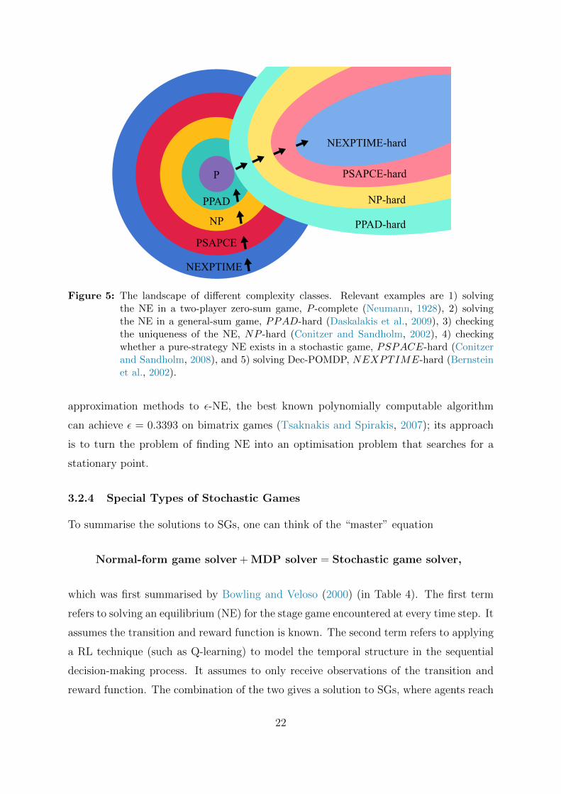
than three players is unknown. In fact, the process of finding the NE is computationally

demanding. Even in the case of two-player games, the complexity of solving the NE is

PPAD-hard (polynomial parity arguments on directed graphs) (Chen and Deng, 2006;

Daskalakis et al., 2009); therefore, in the worst-case scenario, the solution could take time

that is exponential in relation to the game size. This complexity14 prohibits any brute

force or exhaustive search solutions unless P = NP (see Figure 5). As we would expect,

the NE is much more difficult to solve for general SGs, where determining whether a

pure-strategy NE exists is PSPACE-hard. Even if the SG has a finite-time horizon,

the calculation remains NP -hard (Conitzer and Sandholm, 2008). When it comes to

may be a cycle and thus not exist. Instead, NE are proved to exist on a special class of irreducible SGs,where every stage game can be reached regardless of the adopted policy.

14The class of NP -complete is not suitable to describe the complexity of solving the NE because the NEis proven to always exist (Nash, 1951), while a typical NP -complete problem – the travelling salesmanproblem (TSP), for example – searches for the solution to the question: “Given a distance matrix and abudget B, find a tour that is cheaper than B, or report that none exists (Daskalakis et al., 2009).”

21

P

PPAD

NP

PSAPCE

NEXPTIME

PPAD-hard

NP-hard

PSAPCE-hard

NEXPTIME-hard

Figure 5: The landscape of different complexity classes. Relevant examples are 1) solvingthe NE in a two-player zero-sum game, P -complete (Neumann, 1928), 2) solvingthe NE in a general-sum game, PPAD-hard (Daskalakis et al., 2009), 3) checkingthe uniqueness of the NE, NP -hard (Conitzer and Sandholm, 2002), 4) checkingwhether a pure-strategy NE exists in a stochastic game, PSPACE-hard (Conitzerand Sandholm, 2008), and 5) solving Dec-POMDP, NEXPTIME-hard (Bernsteinet al., 2002).

approximation methods to ε-NE, the best known polynomially computable algorithm

can achieve ε = 0.3393 on bimatrix games (Tsaknakis and Spirakis, 2007); its approach

is to turn the problem of finding NE into an optimisation problem that searches for a

stationary point.

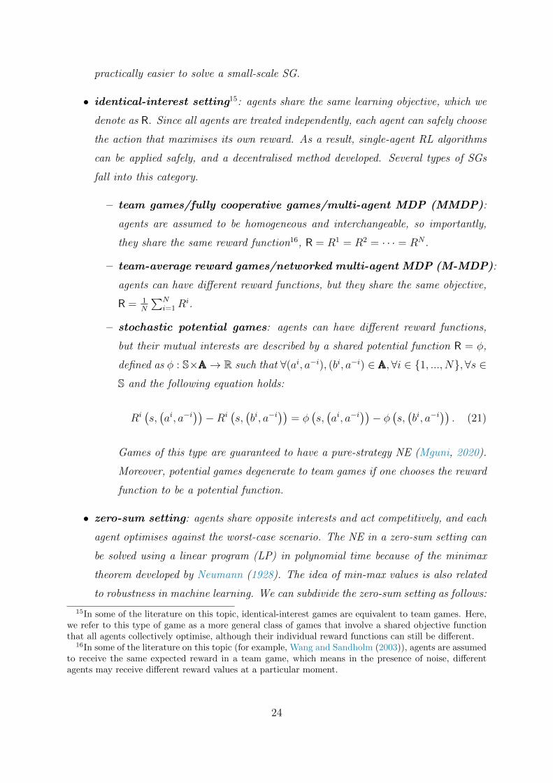
3.2.4 Special Types of Stochastic Games

To summarise the solutions to SGs, one can think of the “master” equation

Normal-form game solver + MDP solver = Stochastic game solver,

which was first summarised by Bowling and Veloso (2000) (in Table 4). The first term

refers to solving an equilibrium (NE) for the stage game encountered at every time step. It

assumes the transition and reward function is known. The second term refers to applying

a RL technique (such as Q-learning) to model the temporal structure in the sequential

decision-making process. It assumes to only receive observations of the transition and

reward function. The combination of the two gives a solution to SGs, where agents reach

22

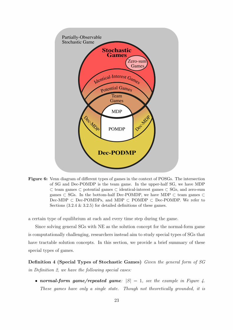
TeamGames

MDP

POMDP Dec-MDPDec-MDP

Dec-PODMP

StochasticGames

Partially-Observable Stochastic Game

Zero-sum Games

Identical-Interest Games

Potential Games

Figure 6: Venn diagram of different types of games in the context of POSGs. The intersectionof SG and Dec-POMDP is the team game. In the upper-half SG, we have MDP⊂ team games ⊂ potential games ⊂ identical-interest games ⊂ SGs, and zero-sumgames ⊂ SGs. In the bottom-half Dec-POMDP, we have MDP ⊂ team games ⊂Dec-MDP ⊂ Dec-POMDPs, and MDP ⊂ POMDP ⊂ Dec-POMDP. We refer toSections (3.2.4 & 3.2.5) for detailed definitions of these games.

a certain type of equilibrium at each and every time step during the game.

Since solving general SGs with NE as the solution concept for the normal-form game

is computationally challenging, researchers instead aim to study special types of SGs that

have tractable solution concepts. In this section, we provide a brief summary of these

special types of games.

Definition 4 (Special Types of Stochastic Games) Given the general form of SG

in Definition 2, we have the following special cases:

• normal-form game/repeated game: |S| = 1, see the example in Figure 4.

These games have only a single state. Though not theoretically grounded, it is

23

practically easier to solve a small-scale SG.

• identical-interest setting15: agents share the same learning objective, which we

denote as R. Since all agents are treated independently, each agent can safely choose

the action that maximises its own reward. As a result, single-agent RL algorithms

can be applied safely, and a decentralised method developed. Several types of SGs

fall into this category.

– team games/fully cooperative games/multi-agent MDP (MMDP):

agents are assumed to be homogeneous and interchangeable, so importantly,

they share the same reward function16, R = R1 = R2 = · · · = RN .

– team-average reward games/networked multi-agent MDP (M-MDP):

agents can have different reward functions, but they share the same objective,

R = 1N

∑Ni=1R

i.

– stochastic potential games: agents can have different reward functions,

but their mutual interests are described by a shared potential function R = φ,

defined as φ : S×AAA→ R such that ∀(ai, a−i), (bi, a−i) ∈ AAA, ∀i ∈ 1, ..., N,∀s ∈S and the following equation holds:

Ri(s,(ai, a−i

))−Ri

(s,(bi, a−i

))= φ

(s,(ai, a−i

))− φ

(s,(bi, a−i

)). (21)

Games of this type are guaranteed to have a pure-strategy NE (Mguni, 2020).

Moreover, potential games degenerate to team games if one chooses the reward

function to be a potential function.

• zero-sum setting: agents share opposite interests and act competitively, and each

agent optimises against the worst-case scenario. The NE in a zero-sum setting can

be solved using a linear program (LP) in polynomial time because of the minimax

theorem developed by Neumann (1928). The idea of min-max values is also related

to robustness in machine learning. We can subdivide the zero-sum setting as follows:

15In some of the literature on this topic, identical-interest games are equivalent to team games. Here,we refer to this type of game as a more general class of games that involve a shared objective functionthat all agents collectively optimise, although their individual reward functions can still be different.

16In some of the literature on this topic (for example, Wang and Sandholm (2003)), agents are assumedto receive the same expected reward in a team game, which means in the presence of noise, differentagents may receive different reward values at a particular moment.

24

– two-player constant-sum games: R1(s, a, s′) + R2(s, a, s′) = c,∀(s, a, s′),

where c is a constant and usually c = 0. For cases when c 6= 0, one can always

subtract the constant c for all payoff entries to make the game zero-sum.

– two-team competitive games: two teams compete against each other, with

team sizes N1 and N2. Their reward functions are:

R1,1, ..., R1,N1 , R2,1, ..., R2,N2.

Team members within a team share the same objective of either

R1 =∑

i∈1,...,N1

R1,i/N1,

or

R2 =∑

j∈1,...,N2

R2,j/N2,

and R1 + R2 = 0.

– harmonic games: Any normal-form game can be decomposed into a potential

game plus a harmonic game (Candogan et al., 2011). A harmonic game (for

example, rock-paper-scissors) can be regarded as a general class of zero-sum

games with a harmonic property. Let ∀p ∈ AAA be a joint pure-strategy profile,

and let AAA[−i] = q ∈ AAA : qi 6= pi, q−i = p−i be the set of strategies that differ

from p on agent i; then, the harmonic property is:

∑

i∈1,...,N

∑

q∈AAA[−i]

(Ri(p)−Ri(q)

)= 0, ∀p ∈ AAA.

• linear-quadratic (LQ) setting: the transition model follows linear dynamics,

and the reward function is quadratic with respect to the states and actions. Com-

pared to a black-box reward function, LQ games offer a simple setting. For example,

actor-critic methods are known to facilitate convergence to the NE of zero-sum LQ

games (Al-Tamimi et al., 2007). Again, the LQ setting can be subdivided as follows:

– two-player zero-sum LQ games: Q ∈ R|S|, U1 ∈ R|A1| and W 2 ∈ R|A2| are

the known cost matrices for the state and action spaces, respectively, while the

matrices A ∈ R|S|×|S|, B ∈ R|S|×|A1|, C ∈ R|S|×|A2| are usually unknown to the

25

agent:

st+1 = Ast +Ba1t + Ca2

t , s0 ∼ P0,

R1(a1t , a

2t ) = −R2(a1

t , a2t ) = −Es0∼P0

[∑

t≥0

sTt Qst + a1tTU1a1

t − a2tTW 2a2

t

].

(22)

– multi-player general-sum LQ games: the difference with respect to a two-

player game is that the summation of the agents’ rewards does not necessarily

equal zero:

st+1 = Ast +Bat, s0 ∼ P0,

Ri(a) = −Es0∼P0

[∑

t≥0

sTt Qist + ait

TU iait

]. (23)

3.2.5 Partially Observable Settings

A partially observable stochastic game (POSG) assumes that agents have no access to the

exact environmental state but only an observation of the true state through an observation

function. Formally, this scenario is defined by:

Definition 5 (partially-observable stochastic games) A POSG is defined by the set

〈N, S, Aii∈1,...,N, P, Rii∈1,...,N, γ, Oii∈1,...,N, O︸ ︷︷ ︸newly added

〉. In addition to the SG defined in

Definition 2, POSGs add the following terms:

• Oi: an observation set for each agent i. The joint observation set is defined as

OOO := O1 × · · · ×ON .

• O : S × AAA → ∆(OOO): an observation function O(o|a, s′) denotes the probability

of observing o ∈ OOO given the action a ∈ AAA, and the new state s′ ∈ S from the

environment transition.

Each agent’s policy now changes to πi ∈ Π i : O→ ∆(Ai).

Although the added partial-observability constraint is common in practice for many

real-world applications, theoretically it exacerbates the difficulty of solving SGs. Even

26

in the simplest setting of a two-player fully cooperative finite-horizon game, solving a

POSG is NEXP -hard (see Figure 5), which means it requires super-exponential time

to solve in the worst-case scenario (Bernstein et al., 2002). However, the benefits of

studying games in the partially observable setting come from the algorithmic advantages.

Centralised-training-with-decentralised-execution methods (Foerster et al., 2017a; Lowe

et al., 2017; Oliehoek et al., 2016; Rashid et al., 2018; Yang et al., 2020) have achieved

many empirical successes, and together with DNNs, they hold great promise.

A POSG is one of the most general classes of games. An important subclass of POSGs

is decentralised partially observable MDP (Dec-POMDP), where all agents share the same

reward. Formally, this scenario is defined as follows:

Definition 6 (Dec-POMDP) A Dec-POMDP is a special type of POSG defined in

Definition 5 with R1 = R2 = · · · = RN .

Dec-POMDPs are related to single-agent MDPs through the partial observability

condition, and they are also related to stochastic team games through the assumption

of identical rewards. In other words, versions of both single-agent MDPs and stochastic

team games are particular types of Dec-POMDPs (see Figure 6).

Definition 7 (Special types of Dec-POMDPs) The following games are special types

of Dec-POMDPs.

• partially observable MDP (POMDP): there is only one agent of interest,

N = 1. This scenario is equivalent to a single-agent MDP in Definition 1 with a

partial-observability constraint.

• decentralised MDP (Dec-MDP): the agents in a Dec-MDP have joint full

observability. That is, if all agents share their observations, they can recover the

state of the Dec-MDP unanimously. Mathematically, we have ∀o ∈ OOO,∃s ∈ S such

that P(St = s|OOOt = o) = 1.

• fully cooperative stochastic games: assuming each agent has full observability,

∀i = 1, ..., N,∀oi ∈ Oi,∃s ∈ S such that P(St = s|Ot = oi) = 1. The fully-

cooperative SG from Definition 4 is a type of Dec-POMDP.

I conclude Section 3 by presenting the relationships between the many different types

of POSGs through a Venn diagram in Figure 6.

27

3.3 Problem Formulation: Extensive-Form Game

An SG assumes that a game is represented as a large table in each stage where the

rows and columns of the table correspond to the actions of the two players17. Based

on the big table, SGs model the situations in which agents act simultaneously and then

receive their rewards. Nonetheless, for many real-world games, players take actions al-

ternately. Poker is one class of games in which who plays first has a critical role in the

players’ decision-making process. Games with alternating actions are naturally described

by an extensive-form game (EFG) (Osborne and Rubinstein, 1994; Von Neumann and

Morgenstern, 1945) through a tree structure. Recently, Kovarık et al. (2019) has made a

significant contribution in unifying the framework of EFGs and the framework of POSGs.

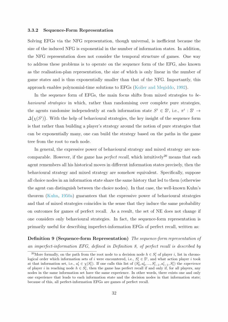
Figure 7 shows the game tree of two-player Kuhn poker (Kuhn, 1950b). In Kuhn

poker, the dealer has three cards, a King, Queen, and Jack (King>Queen>Jack), each

player is dealt one card (the orange nodes in Figure 7), and the third card is put aside

unseen. The game then develops as follows.

• Player one acts first; he/she can check or bet.

• If player one checks, then player two decides to check or bet.

• If player two checks, then the higher card wins 1$ from the other player.

• If player two bets, then player one can fold or call.

• If player one folds, then player two wins 1$ from player one.

• If player one calls, then the higher card wins 2$ from the other player.

• If player one bets, then player two decides to fold or call.

• If player two folds, then player one wins 1$ from player two.

• If player two calls, then the higher card wins 2$ from the other player.

An important feature of EFGs is that they can handle imperfect information for multi-

player decision making. In the example of Kuhn poker, the players do not know which

card the opponent holds. However, unlike Dec-POMDP, which also models imperfect

information in the SG setting but is intractable to solve, EFG, represented in an equivalent

17A multi-player game is represented as a high-dimensional tensor in an SG.

28

check betcheck bet check bet check betcheck bet

p1 jack p1 queen p1 king

p2 queen p2 king p2 jack p2 king p2 jack p2 queen

check bet

check

fold

bet

call

-1 +1 -2

-1 -2

fold call

check

fold

bet

call

-1 +1 -2

-1 -2

fold call

check

fold

bet

call

-1 +1 -2

-1 -2

fold call

check

fold

bet

call

+1 +1 +2

-1 +2

fold call

check

fold

bet

call

+1 +1 +2

-1 +2

fold call

check

fold

bet

call

+1 +1 +2

-1 +2

fold call

chance node player one node

player one information set player two information set

player two node

terminal node

Figure 7: Game tree of two-player Kuhn poker. Each node (i.e., circles, squares and rectangles)represents the choice of one player, each edge represents a possible action, and theleaves (i.e., diamond) represent final outcomes over which each player has a rewardfunction (only player one’s reward is shown in the graph since Kuhn poker is a zero-sum game). Each player can observe only their own card; for example, when playerone holds a Jack, it cannot tell whether player two is holding a Queen or a King,so the choice nodes of player one in each of the two scenarios stay within the sameinformation set.

sequence form, can be solved by an LP in polynomial time in terms of game states (Koller

and Megiddo, 1992). In the next section, we first introduce EFG and then consider the

sequence form of EFG.

Definition 8 (Extensive-form Game) An (imperfect-information) EFG can be de-

scribed by a tuple of key elements 〈N,A,H,T, Rii∈1,...,N, χ, ρ, P, Sii∈1,...,N〉.

• N : the number of players. Some EFGs involve a special player called “chance”,

29

which has a fixed stochastic policy that represents the randomness of the environ-

ment. For example, the chance player in Kuhn poker is the dealer, who distributes

cards to the players at the beginning.

• A: the (finite) set of all agents’ possible actions.

• H: the (finite) set of non-terminal choice nodes.

• T: the (finite) set of terminal choice nodes, disjoint from H.

• χ : H→ 2|A| is the action function that assigns a set of valid actions to each choice

node.

• ρ : H → 1, ..., N is the player indicating function that assigns, to each non-

terminal node, a player who is due to choose an action at that node.

• P : H × A → H ∪ T is the transition function that maps a choice node and an

action to a new choice/terminal node such that ∀h1, h2 ∈ H and ∀a1, a2 ∈ A, if

P (h1, a1) = P (h2, a2), then h1 = h2 and a1 = a2.

• Ri : T→ R is a real-valued reward function for player i on the terminal node. Kuhn

poker is a zero-sum game since R1 +R2 = 0.

• Si: a set of equivalence classes/partitions Si = (Si1, ..., Siki) for agent i on h ∈ H :

ρ(h) = i with the property that ∀j ∈ 1, ..., ki,∀h, h′ ∈ Sij, we have χ(h) = χ(h′)

and ρ(h) = ρ(h′). The set Sij is also called an information state. The physical

meaning of the information state is that the choice nodes of an information state

are indistinguishable. In other words, the set of valid actions and agent identities

for the choice nodes within an information state are the same; one can thus use

χ(Sij), ρ(Sij) to denote χ(h), ρ(h),∀h ∈ Sij.

Inclusion of the information sets in EFG helps to model the imperfect-information

cases in which players have only partial or no knowledge about their opponents. In the

case of Kuhn poker, each player can only observe their own card. For example, when

player one holds a Jack,it cannot tell whether player two is holding a Queen or a King,

so the choice nodes of player one under each of the two scenarios (Queen or King) stay

within the same information set. Perfect-information EFGs (e.g., GO or chess) are a

30

special case where the information set is a singleton, i.e., |Sij| = 1,∀j, so a choice node

can be equated to the unique history that leads to it. Imperfect-information EFGs (e.g.,

Kuhn poker or Texas hold’em) are those in which there exists i, j such that |Sij| ≥ 1, so

the information state can represent more than one possible history. However, with the

assumption of perfect recall (described later), the history that leads to an information

state is still unique.

3.3.1 Normal-Form Representation

A (simultaneous-move) NFG can be equivalently transformed into an imperfect-information

EFG18 (Shoham and Leyton-Brown, 2008) [Chapter 5]. Specifically, since the choices of

actions by other agents are unknown to the central agent, this could potentially leads to

different histories (triggered by other agents) that can be aggregated into one information

state for the central agent.

On the other direction, an imperfect-information EFG can also be transformed into an

equivalent NFG in which the pure strategies of each agent i are defined by the Cartesian

product∏

Sij∈Siχ(Sij), which is a complete specification19 of which action to take at every

information state of that agent. In the Kuhn poker example, one pure strategy for

player one can be check-bet-check-fold-call-fold; altogether, player one has 26 = 64 pure

strategies, corresponding to 3× 23 = 24 pure strategies for the chance node and 26 = 64

pure strategies for player two. The mixed strategy of each player is then a distribution

over all its pure strategies. In this way, the NE in NFG in Eq. (17) can still be applied to

the EFG, and the NE of an EFG can be solved in two steps: first, convert the EFG into an

NFG; second, solve the NE of the induced NFG by means of the Lemke-Howson algorithm

(Shapley, 1974). If one further restricts the action space to be state-dependent and adopts

the discounted accumulated reward at the terminal node, then the EFG recovers to an

SG. While the NE of an EFG can be solved through its equivalent normal form, the

computational benefit can be achieved by dealing with the extensive form directly; this

motivates the adoption of the sequence-form representation of EFGs.

18Note that this transformation is not unique, but they share the same equilibria as the original game.Moreover, this transformation from NFG to EFG does not hold for perfect-information EFGs.

19One subtlety of the pure strategy is that it designates a decision at each choice node, regardless ofwhether it is possible to reach that node given the other choice nodes.

31

3.3.2 Sequence-Form Representation

Solving EFGs via the NFG representation, though universal, is inefficient because the

size of the induced NFG is exponential in the number of information states. In addition,

the NFG representation does not consider the temporal structure of games. One way

to address these problems is to operate on the sequence form of the EFG, also known

as the realisation-plan representation, the size of which is only linear in the number of

game states and is thus exponentially smaller than that of the NFG. Importantly, this

approach enables polynomial-time solutions to EFGs (Koller and Megiddo, 1992).

In the sequence form of EFGs, the main focus shifts from mixed strategies to be-

havioural strategies in which, rather than randomising over complete pure strategies,

the agents randomise independently at each information state Si ∈ Si, i.e., πi : Si →∆(χ(Si)

). With the help of behavioural strategies, the key insight of the sequence form

is that rather than building a player’s strategy around the notion of pure strategies that

can be exponentially many, one can build the strategy based on the paths in the game

tree from the root to each node.

In general, the expressive power of behavioural strategy and mixed strategy are non-

comparable. However, if the game has perfect recall, which intuitively20 means that each

agent remembers all his historical moves in different information states precisely, then the

behavioural strategy and mixed strategy are somehow equivalent. Specifically, suppose

all choice nodes in an information state share the same history that led to them (otherwise

the agent can distinguish between the choice nodes). In that case, the well-known Kuhn’s

theorem (Kuhn, 1950a) guarantees that the expressive power of behavioural strategies

and that of mixed strategies coincides in the sense that they induce the same probability

on outcomes for games of perfect recall. As a result, the set of NE does not change if

one considers only behavioural strategies. In fact, the sequence-form representation is

primarily useful for describing imperfect-information EFGs of perfect recall, written as:

Definition 9 (Sequence-form Representation) The sequence-form representation of

an imperfect-information EFG, defined in Definition 8, of perfect recall is described by

20More formally, on the path from the root node to a decision node h ∈ Sit of player i, list in chrono-

logical order which information sets of i were encountered, i.e., Sit ∈ Si, and what action player i took

at that information set, i.e., ait ∈ χ(Sit). If one calls this list of (Si

0, ai0, ..., S

it−1, a

it−1, S

it) the experience

of player i in reaching node h ∈ Sit , then the game has perfect recall if and only if, for all players, any

nodes in the same information set have the same experience. In other words, there exists one and onlyone experience that leads to each information state and the decision nodes in that information state;because of this, all perfect-information EFGs are games of perfect recall.

32

(N,Σ, Gii∈1,...,N, πii∈1,...,N, µπii∈1,...,N, Cii∈1,...,N) where

• N : the number of agents, including the chance node, if any, denoted by c.

• Σ =∏N

i=1Σi: where Σi is the set of sequences available to agent i. A sequence of

actions of player i, σi ∈ Σi, defined by a choice node h ∈ H ∪ T, is the ordered

set of player i’s actions that has been taken from the root to node h. Let ∅ be the

sequence that corresponds to the root node.

Note that other players’ actions are not part of agent i’s sequence. In the example

of Kuhn poker, Σc = ∅, Jack, Queen, King, Jack-Queen, Jack-King, Queen-Jack,

Queen-King, King-Jack, King-Queen, Σ1 = ∅, check, bet, check-fold, check-bet,and Σ2 = ∅, check, bet, fold, call.

• πi: Si → ∆(χ(Si)

)is the behavioural policy that assigns a probability of taking a

valid action ai ∈ χ(Si) at an information state Si ∈ Si. This policy randomises

independently over different information states. In the example of Kuhn poker, each

player has six information states; their behavioural strategy is therefore a list of six

independent probability distributions.

• µπi: Σi → [0, 1] is the realisation plan that provides the realisation probability,

i.e., µπi(σi) =

∏c∈σi π

i(c), that a sequence σi ∈ Σi would arise under a given

behavioural policy πi of player i. In the Kuhn poker case, the realisation probability

that player one chooses the sequence of check and then fold is µπ1(check-fold) =

π1(check)× π1(fold).

Based on the realisation plan, one can recover the underlying behavioural strategy21

(an idea similar to Eq. (6)). To do so, we need three additional pieces of notation.

Let Seq : Si → Σi return the sequence σi ∈ Σi that leads to a given information

state Si ∈ Si. Since the game assumes perfect recall, Seq(Si) is known to be unique.

Let σiai denote a sequence that consists of the sequence σi followed by the single

action ai. Since there are many possible actions ai to choose, let Ext : Σi → 2Σi

denote the set of all possible sequences that extend the given sequence by taking one

additional action. It is trivial to see that sequences that include a terminal node

cannot be extended, i.e., Ext(T ) = ∅. Finally, we can write the behavioural policy

21Empirically, it is often the case that working on the realisation plan of a behavioural strategy is morecomputationally friendly than working on the behavioural strategy directly.

33

πi for an information state Si as

πi(ai ∈ χ(Si)

)=µπ

i(Seq(Si)ai

)

µπi(Seq(Si)

) , ∀Si ∈ Si, ∀(Seq(Si)ai

)∈ Ext

(Seq(Si)

). (24)

• Gi : Σ → R is the reward function for agent i given by Gi(σ) = Ri(T ) if a terminal

node T ∈ T is reached when each player plays their part of the sequence in σ ∈ Σ,

and Gi(σ) = 0 if non-terminal nodes are reached.

Note that since each payoff that corresponds to a terminal node is stored only once

in the sequence-form representation (due to the perfect recall, each terminal node

has only one sequence that leads to it), compared to the normal-form representation,

which is a Cartesian product over all information sets for each agent and is thus

exponential in size, the sequence form is only linear in the size of the EFG. In the

example of Kuhn poker, the normal-form representation is a tensor with 64×64×32

elements, while in the sequence-form representation, since there are 30 terminal

nodes and each node has only one unique sequence leading to it, the payoff tensor

has only 30 elements (plus ∅ for each player).

• Ci: is a set of linear constraints on the realisation probability of µπi. Under the

notations of Seq and Ext defined in the bullet points of µπi, we know the realisation

plan must meet the condition that

µπi(∅)

= 1, µπi(σi)≥ 0, ∀σi ∈ Σi

µπi(Seq(Si)

)=

∑

σi∈Ext(Seq(Si)

)µπi(σi), ∀Si ∈ Si. (25)

The first constraint requires that µπi

is a proper probability distribution. In addition,

the second constraint in Eq. (25) indicates that in order for a realisation plan to

be valid to recover a behavioural strategy, at each information state of agent i,

the probability of reaching that information state must equal the summation of the

realisation probabilities of all the extended sequences. In the example of Kuhn poker,

we have C1 for player one by µπ1(check) = µπ

1(check-fold) + µπ

1(check-call).

34

3.4 Solving Extensive-Form Games

In the sequence-form EFG, given a joint (behavioural) policy π = (π1, ..., πN), we can

write the realisation probability of agents reaching a terminal node T ∈ T, assuming

the sequence that leads to the node T is σT , in which each player, including the chance

player, follows its own path σiT as

µπ(σT)

=∏

i∈1,...,N

µπi(σiT). (26)

The expected reward for agent i, which covers all possible terminal nodes following the

joint policy π, is thus given by Eq. (27).

Ri(π) =∑

T∈T

µπ(σT)·Gi(σT ) =

∑

T∈T

µπ(σT)·Ri(T ). (27)

If we denote the expected reward by Ri(π) for simplicity, then the solution concept of

NE for the EFG can be written as

Ri(πi,∗, π−i,∗) ≥ Ri(πi, π−i,∗), for any policy πi of agent i and for all i. (28)

3.4.1 Perfect-Information Games

Every finite perfect-information EFG has a pure-strategy NE (Zermelo and Borel, 1913).

Since players take turns and every agent sees everything that has occurred thus far, it

is unnecessary to introduce randomness or mixed strategies into the action selection.

However, the NE can be too weak of a solution concept for the EFG. In contrast to

that in NFGs, the NE in EFGs can represent non-credible threats, which represent the

situation where the Nash strategy is not executed as claimed if agents truly reach that

decision node. A refinement of the NE in the perfect-information EFG is a subgame-

perfect equilibrium (SPE). The SPE rules out non-credible threats by picking only the

NE that is the best response at every subgame of the original game.

The fundamental principle in solving the SPE is backward induction, which identifies

the NE from the bottom-most subgame and assumes those NE will be played as considers

increasingly large trees. Specifically, backward induction can be implemented through a

depth-first search algorithm on the game tree, which requires time that is only linear in

the size of the EFG. In contrast, finding NE in NFG is known to be PPAD-hard, let

35

alone the NFG representation is exponential in the size of an EFG.

In the case of two-player zero-sum EFGs, backward induction needs to propagate only

a single payoff from the terminal node to the root node in the game tree. Furthermore,

due to the strictly opposing interests between players, one can further prune the backward

induction process by recognising that certain subtrees will never be reached in NE, even

without examining those subtree nodes22, which leads to the well-known Alpha-Beta-

Pruning algorithm (Shoham and Leyton-Brown, 2008, Chapter 5.1). For games with

very deep game trees, such as Chess or GO, a common approach is to search only nodes

up to certain depths and use an approximate value function to estimate those nodes’

value without roll outing to the end (Silver et al., 2016).

Finally, backward induction can identify one NE in linear time; yet, it does not provide

an effective way to find all NE. A theoretical result suggests that finding all NE in a two-

player perfect-information EFG (not necessarily zero-sum) requires O(|T|3), which is still

tractable (Shoham and Leyton-Brown, 2008, Theorem 5.1.6).

3.4.2 Imperfect-Information Games

By means of the sequence-form representation, one can write the solution of a two-player

EFG as a LP. Given a fixed behavioural strategy of player two, in the form of realisation

plan µπ2, the best response for player one can be written as

maxµπ1

∑

σ1∈Σ1

µπ1 (σ1)( ∑

σ2∈Σ2

g1(σ1, σ2

)µπ

2 (σ2))

subject to the constraints in Eq. (25). In NE, player one and player two form a mutual

best response. However, if we treat both µπ1

and µπ2

as variables, then the objective

becomes nonlinear. The key to address this issue is to adopt the dual form of the LP

(Koller and Megiddo, 1996), which is written as

min v0

s.t. vI(σ1) −∑

I′∈I(Ext(σ1)

) vI′ ≥

∑

σ2∈Σ2

g1(σ1, σ2

)µπ

2 (σ2), ∀σ1 ∈ Σ1 (29)

22This occurs, for example, in the case that the worst case of one player in one subgame is better thanthe best case of that player in another subgame.

36

where I : Σi → Si is a mapping function that returns the information set23 encountered

when the final action in σi was taken. With slight abuse of notation, we let I(Ext(σ1)

)24

denote the set of final information states encountered in the set of the extension of σi. The

variable v0 represents, given µπ2, player one’s expected reward under its own realisation

plan µπ1

, and vI′ can be considered as the part of this expected utility in the subgame

starting from information state I ′. Note that the constraint needs to hold for every

sequence of player one.

In the dual form of best response in Eq. (29), if one treats µπ2

as an optimising

variable rather than a constant, which means µπ2

must meet the requirements in Eq.

(25) to be a proper realisation plan, then the LP formulation for a two-player zero-sum

EFG can be written as follows.

min v0 (30)

s.t. vI(σ1) −∑

I′∈I(Ext(σ1)

) vI′ ≥

∑

σ2∈Σ2

g1(σ1, σ2

)µπ

2 (σ2), ∀σ1 ∈ Σ1 (31)

µπ2(∅

)= 1, µπ

2(σ2)≥ 0, ∀σ2 ∈ Σ2 (32)

µπ2(Seq(S2)

)=

∑

σ2∈Ext(Seq(S2)

)µπ2(

σ2), ∀S2 ∈ S2. (33)

Player two’s realisation plan is now selected to minimise player one’s expected utility.

Based on the minimax theorem (Von Neumann and Morgenstern, 1945), we know this

process will lead to a NE. Notably, though the zero-sum EFG and zero-sum SG (see

the formulation in Eq. (51)) both adopt the LP formulation to solve the NE and can

be solved in polynomial time, the size of the representation for the game itself is very

different. If one chooses first to transform the EFG into an NFG presentation and then

solve it by LP, then the time complexity would in fact become exponential in the size of

the original EFG.

The solution to a two-player general-sum EFG can also be formulated using an ap-

proach similar to that used for the zero-sum EFG. The difference is that there will be no

objective function such as Eq. (30) since in the general-sum context, one agent’s reward

can no longer be determined based on the other player’s reward. The LP with only Eqs.

(31 - 33) thus becomes a constraint satisfaction problem. Specifically, one would need

23Recall that this information set is unique under the assumption of perfect recall.24Recall that Ext(σ1) is the set of all possible sequences that extend σ1 one step ahead.

37

to repeat Eqs. (31 - 33) twice to consider each player independently. One final sub-

tlety required in solving the two-player general-sum EFG is that to ensure v1 and v2 are

bounded25, a complementary slack condition must be further imposed; we have ∀σ1 ∈ Σ1

(vice versa ∀σ2 ∈ Σ2 for player two):

µπ1

(σ1)

[(v1I(σ1) −

∑

I′∈I(Ext(σ1)

) v1I′

)−( ∑

σ2∈Σ2

g1(σ1, σ2

)µπ

2 (σ2) )]

= 0. (34)

The above condition indicates that for each player, either the sequence σi is never played,

i.e., µπi(σi) = 0, or all sequences that are played by that player with positive probability

must induce the same expected payoff such that vi takes arbitrarily large values, thus

being bounded. Eqs. (31 - 33), together with Eq. (34), turns the solution to the NE into

an LCP problem that can be solved by the generalised Lemke-Howson method (Lemke

and Howson, 1964). Although in the worst case, polynomial time complexity cannot

be achieved, as can for zero-sum games, this approach is still exponentially faster than

running the Lemke-Howson method to solve the NE in a normal-form representation.

For a perfect-information EFG, recall that the SPE is a more informative solution con-

cept than NE. Extending SPE to the imperfect-information scenario is therefore valuable.

However, such an extension is non-trivial because a well-defined notion of a subgame is

lacking. However, for EFGs with perfect recall, the intuition of subgame perfection can

be effectively extended to a new solution concept, named the sequential equilibrium (SE)

(Kreps and Wilson, 1982), which is guaranteed to exist and coincides with the SPE if all

players in the game have perfect information.

4 Grand Challenges of MARL

Compared to single-agent RL, multi-agent RL is a general framework that better matches

the broad scope of real-world AI applications. However, due to the existence of multiple

agents that learn simultaneously, MARL methods pose more theoretical challenges, in

addition to those already present in single-agent RL. Compared to classic MARL settings

where there are usually two agents, solving a many-agent RL problem is even more

challenging. As a matter of fact, 1 the combinatorial complexity, 2 the multi-

25Since the constraints are linear, they remain satisfied when both v1 and v2 are increased by the sameconstant to any arbitrarily large values.

38

dimensional learning objectives, and 3 the issue of non-stationarity all result

in the majority of MARL algorithms being capable of solving games with 4 only two

players, in particular, two-player zero-sum games. In this section, I will elaborate each

of the grand challenge in many-agent RL.

4.1 The Combinatorial Complexity

In the context of multi-agent learning, each agent has to consider the other opponents’

actions when determining the best response; this characteristic is deeply rooted in each

agent’s reward function and for example is represented by the joint action a in their Q-

function Qi(s,a) in Eq. (13). The size of the joint action space, |A|N , grows exponentially

with the number of agents and thus largely constrains the scalability of MARL methods.

Furthermore, the combinatorial complexity is worsened by the fact that solving a NE

in game theory is PPAD-hard, even for two-player games. Therefore, for multi-player

general-sum games (neither team games nor zero-sum games), it is non-trivial to find an

applicable solution concept.

One common way to address this issue is by assuming specific factorised structures

on action dependency such that the reward function or Q-function can be significantly

simplified. For example, a graphical game assumes an agent’s reward is affected by only

its neighbouring agents, as defined by the graph from (Kearns, 2007). This assumption

leads directly to a polynomial-time solution for the computation of a NE in specific tree

graphs (Kearns et al., 2013), though the scope of applications is somewhat limited beyond

this specific scenario.

Recent progress has also been made toward leveraging particular neural network ar-

chitectures for Q-function decomposition (Rashid et al., 2018; Sunehag et al., 2018; Yang

et al., 2020). In addition to the fact that these methods work only for the team-game

setting, the majority of them lack theoretical backing. There remain open questions to

answer, such as understanding the representational power (the approximation error) of

the factorised Q-functions in a multi-agent task and how factorisation itself can be learnt

from scratch.

39

4.2 The Multi-Dimensional Learning Objectives

Compared to single-agent RL, where the only goal is to maximise the learning agent’s

long-term reward, the learning goals in MARL are naturally multi-dimensional, as the

objective of all agents are not necessarily aligned by one metric. Bowling and Veloso

(2001, 2002) proposed to classify the goals of the learning task into two types: rationality

and convergence. Rationality ensures an agent takes the best possible response to the

opponents when they are stationary, and convergence ensures the learning dynamics

eventually lead to a stable policy against a given class of opponents. Reaching both

rationality and convergence gives rise to reaching the NE.

In terms of rationality, the NE characterises a fixed point of a joint optimal strategy

profile from which no agents would be motivated to deviate as long as they are all perfectly

rational. However, in practice, an agent’s rationality can easily be bound by either

cognitive limitations and/or the tractability of the decision problem. In these scenarios,

the rationality assumption can be relaxed to include other types of solution concepts, such

as the recursive reasoning equilibrium, which results from modelling the reasoning process

recursively among agents with finite levels of hierarchical thinking (for example, an agent

may reason in the following way: I believe that you believe that I believe ...) (Wen

et al., 2019, 2018); best response against a target type of opponent (Powers and Shoham,

2005b); the mean-field game equilibrium, which describes multi-agent interactions as a

two-agent interaction between each agent itself and the population mean (Guo et al.,

2019; Yang et al., 2018a,b); evolutionary stable strategies, which describe an equilibrium

strategy based on its evolutionary advantage of resisting invasion by rare emerging mutant

strategies (Bloembergen et al., 2015; Maynard Smith, 1972; Tuyls and Nowe, 2005; Tuyls

and Parsons, 2007); Stackelberg equilibrium (Zhang et al., 2019a), which assumes specific

sequential order when agents take decisions; and the robust equilibrium (also called the

trembling-hand perfect equilibrium in game theory), which is stable against adversarial

disturbance (Goodfellow et al., 2014b; Li et al., 2019b; Yabu et al., 2007).

In terms of convergence, although most MARL algorithms are contrived to converge to

the NE, the majority either lack a rigorous convergence guarantee (Zhang et al., 2019b),

potentially converge only under strong assumptions such as the existence of a unique

NE (Hu and Wellman, 2003; Littman, 2001b), or are provably non-convergent in all cases

(Mazumdar et al., 2019a). Zinkevich et al. (2006) identified the non-convergent behaviour

of value-iteration methods in general-sum SGs and instead proposed an alternative solu-

40

tion concept to the NE – cyclic equilibria – that value-based methods converge to. The

concept of no regret (also called the Hannan consistency in game theory (Hansen et al.,

2003)), measures convergence by comparison against the best possible strategy in hind-

sight. This was also proposed as a new criterion to evaluate convergence in zero-sum

self-plays (Bowling, 2005; Hart and Mas-Colell, 2001; Zinkevich et al., 2008). In two-

player zero-sum games with a non-convex non-concave loss landscape (training GANs

(Goodfellow et al., 2014a)), gradient-descent-ascent methods are found to reach a Stack-

elberg equilibrium (Fiez et al., 2019; Lin et al., 2019) or a local differential NE (Mazumdar

et al., 2019b) rather than the general NE.

Finally, although the above solution concepts account for convergence, building a

convergent objective for MARL methods with DNNs remains an uncharted area. This

is partly because the global convergence result of a single-agent deep RL algorithm, for

example, neural policy gradient methods (Liu et al., 2019; Wang et al., 2019) and neural

TD learning algorithms (Cai et al., 2019b), has not been extensively studied yet.

4.3 The Non-Stationarity Issue

The most well-known challenge of multi-agent learning versus single-agent learning is

probably the non-stationarity issue. Since multiple agents concurrently improve their

policies according to their own interests, from each agent’s perspective, the environmen-

tal dynamics become non-stationary and challenging to interpret when learning. This

problem occurs because the agent itself cannot tell whether the state transition – or

the change in reward – is an actual outcome due to its own action or if it is due to its

opponent’s explorations. Although learning independently by completely ignoring the

other agents can sometimes yield surprisingly powerful empirical performance (Matignon

et al., 2012; Papoudakis et al., 2020), this approach essentially harms the stationarity

assumption that supports the theoretical convergence guarantee of single-agent learning

methods (Tan, 1993). As a result, the Markovian property of the environment is lost,

and the state occupancy measure of the stationary policy in Eq. (5) no longer exists.

For example, the convergence result of single-agent policy gradient methods in MARL is

provably non-convergent in simple linear-quadratic games (Mazumdar et al., 2019b).

The non-stationarity issue can be further aggravated by TD learning, which occurs

with the replay buffer that most deep RL methods currently adopt (Foerster et al., 2017b).

In single-agent TD learning (see Eq. (9)), the agent bootstraps the current estimate of the

41

Deep Learning

Multi-agentIntelligence

Reinforcement Learning

GameTheory

Figure 8: The scope of multi-agent intelligence, as described here, consists of three pillars.Deep learning serves as a powerful function approximation tool for the learningprocess. Game theory provides an effective approach to describe learning outcomes.RL offers a valid approach to describe agents’ incentives in multi-agent systems.

TD error, saves it in the replay buffer, and samples the data in the replay buffer to update

the value function. In the context of multi-agent learning, since the value function for one

agent also depends on other agents’ actions, the bootstrap process in TD learning also

requires sampling other agents’ actions, which leads to two problems. First, the sampled

actions barely represent the full behaviour of other agents’ underlying policies across

different states. Second, an agent’s policy can change during training, so the samples

in the replay buffer can quickly become outdated. Therefore, the dynamics that yielded

the data in the agent’s replay buffer must be constantly updated to reflect the current

dynamics in which it is learning. This process further exacerbates the non-stationarity

issue.

In general, the non-stationarity issue forbids the reuse of the same mathematical tool

for analysing single-agent algorithms in the multi-agent context. However, one exception

exists: the identical-interest game in Definition 4. In such settings, each agent can safely

perform selfishly without considering other agents’ policies since the agent knows the

other agents will also act in their own interest. The stationarity is thus maintained, so

single-agent RL algorithms can still be applied.

42

4.4 The Scalability Issue when N 2

Combinatorial complexity, multi-dimensional learning objectives, and the issue of non-

stationarity all result in the majority of MARL algorithms being capable of solving games

with only two players, in particular, two-player zero-sum games (Zhang et al., 2019b).

As a result, solutions to general-sum settings with more than two agents (for example,

the many-agent problem) remain an open challenge. This challenge must be addressed

from all three perspectives of multi-agent intelligence (see Figure (8)): game theory,

which provides realistic and tractable solution concepts to describe learning outcomes of

a many-agent system; RL algorithms, which offer provably convergent learning algorithms

that can reach stable and rational equilibria in the sequential decision-making process;

and finally deep learning techniques, which provide the learning algorithms expressive

function approximators.

43

5 A Survey of MARL Surveys

In this section, I provide a non-comprehensive review of MARL algorithms. To begin, I

introduce different taxonomies that can be applied to categorise prior approaches. Given

multiple high-quality, comprehensive surveys on MARL methods already exist, a survey

of those surveys is provided. Based on the proposed taxonomy, I review related MARL

algorithms, covering works on identical interest games, zero-sum games, and games with

an infinite number of players. This section is written to be selective, focusing on the

algorithms that have theoretical guarantees and less focus on those with only empirical

success or those that are purely driven by specific applications.

5.1 Taxonomy of MARL Algorithms

One significant difference between the taxonomy of single-agent RL algorithms and MARL

algorithms is that in the single-agent setting, since the problem is unanimously defined,

the taxonomy is driven mainly by the type of solution (Kaelbling et al., 1996; Li, 2017),

for example, model-free vs model-based, on-policy vs off-policy, TD learning vs Monte-

Carlo methods. By contrast, in the multi-agent setting, due to the existence of multiple

learning objectives (see Section 4.2), the taxonomy is driven mainly by the type of prob-

lem rather than the solution. In fact, asking the right question for MARL algorithms is

itself a research problem, which is referred to as the problem problem (Balduzzi et al.,

2018b; Shoham et al., 2007).

Based on Stage Games Types. Since the solution concept varies considerably ac-

cording to the game type, one principal component of the MARL taxonomy is the nature

of stage games. A common division26 includes team games (more generally, potential

games), zero-sum games (more generally, harmonic games), and a mixed setting of the

two games, namely, general-sum games. Other types of “exotic” games, such as potential

games (Monderer and Shapley, 1996) and mean-field games (Lasry and Lions, 2007), that

originate from non-game-theoretical research domains exist and have recently attracted

tremendous attention. Based on the type of stage game, the taxonomy can be further

enriched by how many times they are played. A repeated game is where one stage game

26Such a division is complementary because any multi-player normal-form game can be decomposedinto a potential game plus a harmonic game (Candogan et al., 2011) (also see Definition 4); in thetwo-player case, it corresponds to a team game plus a zero-sum game.

44

Table 1: Common assumptions on the level of local knowledge made by MARL algorithms.

Levels Assumptions

0 Each agent observes the reward of his selected action.1 Each agent observes the rewards of all possible actions.2 Each agent observes others’ selected actions.3 Each agent observes others’ reward values.4 Each agent knows others’ exact policies.5 Each agent knows others’ exact reward functions.6 Each agent knows the equilibrium of the stage game.

is played repeatedly without considering the state transition. An SG is a sequence of

stage games, which can be infinitely long, with the order of the games to play determined

by the state-transition probability. Since solving a general-sum SG is at least PSPACE-

hard (Conitzer and Sandholm, 2002), MARL algorithms usually have a clear boundary

on what types of game they can solve. For general-sum games, there are few MARL

algorithms that have a provable convergence guarantee without strong, even unrealistic,

assumptions (e.g., the NE is unique) (Shoham et al., 2007; Zhang et al., 2019b).

Based on Level of Local Knowledge. The assumption on the level of local knowl-

edge, i.e., what agents can and cannot know during training and execution time, is

another major component to differentiate MARL algorithms. Having access to different

levels of local knowledge leads to different local behaviours by agents and various levels

of difficulty in developing theoretical analysis. I list the common assumptions that most

MARL methods adopt in Table (1). The seven levels of assumptions are ranked based

on how strong, or unrealistic, they are in general. The two extreme cases are that the

agent can observe nothing apart from itself and that the agent knows the equilibrium

point, i.e., the direct answer of the game. Among the multiple levels, the nuance between

level 0 and level 1, which has been mainly investigated in the online learning literature,

is referred to as the bandit setting vs full-information setting. In addition, knowledge

of the agents’ exact policy/reward function forms is a much stronger assumption than

being able to observe their sampled actions/rewards. In fact, knowing the exact policy

parameters of other agents in most cases are only possible in simulations. Furthermore,

from an applicability perspective, observing other agents’ rewards is also more unrealistic

than observing their actions.

45

Agent1

Agent2

AgentN

Central Controller ...

Environoment

Agent1

Agent2

AgentN

...

Environoment

Agent1

Agent2

AgentN

Environoment

Agent3

Agent4

...

Agent1

Agent2

AgentN

Environoment

Agent3

Agent4

...

Agent2

AgentN

Agent1

...

Environoment

Agent1

Environoment

Agent3

Agent4

...

Agent2

AgentN

Agent3

Agent3

Agent4

Agent4

(1) (2) (3)

(4) (5) (6)

Figure 9: Common learning paradigms of MARL algorithms. (1) Independent learners withshared policy. (2) Independent learners with independent policies (i.e., denoted bythe difference in wheels). (3) Independent learners with shared policy within a group.(4) One central controller controls all agents: agents can exchange information withany other agents at any time. (5) Centralised training with decentralised execution(CTDE): only during training, agents can exchange information with others; dur-ing execution, they act independently. (6) Decentralised training with networkedagents: during training, agents can exchange information with their neighbours inthe network; during execution, they act independently.

Based on Learning Paradigms. In addition to various levels of local knowledge,

MARL algorithms can be classified based on the learning paradigm, as shown in Figure

9. For example, the 4th learning paradigm addresses multi-agent problems by build-

ing a single-agent controller, which takes the joint information from all agents as inputs

and outputs the joint policies for all agents. In this paradigm, agents can exchange any

information with any other opponent through the central controller. The information

that can be exchanged depends on the assumptions about the level of local knowledge

described in Table (1), e.g., private observations from each agent, the reward value, or

policy parameters for each agent. The 5th learning paradigm allows agents to exchange

information with other agents only during training; during execution, each agent has to

act in a decentralised manner, making decisions based on its own observations only. The

6th paradigm can be regarded as a particular case of Paradigm 5 in that agents are as-

sumed to be interconnected via a (time-varying) network such that information can still

spread across the whole network if agents communicate with their neighbours. The most

46

general case is Paradigm 2, where agents are fully decentralised, with no information

exchange of any kind allowed at any time, and each agent executes its own policy. Re-

laxation of Paradigm 2 yields the 1st and the 3rd paradigms, where the agents, although

they cannot exchange information, share a single set of policy parameters, or, within a

pre-defined group, share a single set of policy parameters.

Based on Five AI Agendas. In order for MARL researchers to be specific about

the problem being addressed and the associated evaluation criteria, Shoham et al. (2007)

identified five coherent agendas for MARL studies, each of which has a clear motivation

and success criterion. Though proposed more than a decade ago, these five distinct goals

are still useful in evaluating and categorising recent contributions. I, therefore, choose to

incorporate them into the taxonomy of MARL algorithms.

5.2 A Survey of Surveys

A multi-agent system (MAS) is a generic concept that could refer to many different

domains of research across different academic subjects; general overviews are given by

Weiss (1999), Wooldridge (2009), and Shoham and Leyton-Brown (2008). Due to the

many possible ways of categorising multi-agent (reinforcement) learning algorithms, it

is impossible to have a single survey that includes all relevant works considering all

directions of categorisations. In the past two decades, there has been no lack of survey

papers that summarise the current progress of specific categories of multi-agent learning

research. In fact, there are so many that these surveys themselves deserve a comprehensive

review. Before proceeding to review MARL algorithms based on the proposed taxonomy

in Section 5.1, in this section, I provide an overview of relevant surveys that study multi-

agent systems from the machine learning, in particular, the RL, perspective.

One of the earliest studies that surveyed MASs in the context of machine learning/AI

was published by Stone and Veloso (2000): the research works up to that time were

summarised into four major scenarios considering whether agents were homogeneous or

heterogeneous and whether or not agents were allowed to communicate with each other.

Shoham et al. (2007) considered the game theory and RL perspective and introspectively

asked the question of “if multi-agent learning is the answer, what is the question?”. Upon

failing to find a single answer, Shoham et al. (2007) proposed the famous five AI agendas

for future research work to address. Stone (2007) tried to answer Shoham’s question

47

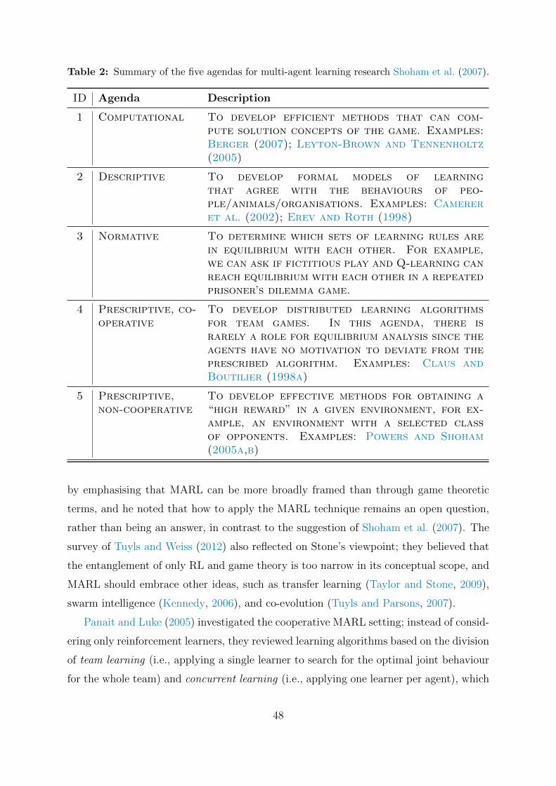
Table 2: Summary of the five agendas for multi-agent learning research Shoham et al. (2007).

ID Agenda Description

1 Computational To develop efficient methods that can com-pute solution concepts of the game. Examples:Berger (2007); Leyton-Brown and Tennenholtz(2005)

2 Descriptive To develop formal models of learningthat agree with the behaviours of peo-ple/animals/organisations. Examples: Camereret al. (2002); Erev and Roth (1998)

3 Normative To determine which sets of learning rules arein equilibrium with each other. For example,we can ask if fictitious play and Q-learning canreach equilibrium with each other in a repeatedprisoner’s dilemma game.

4 Prescriptive, co-operative

To develop distributed learning algorithmsfor team games. In this agenda, there israrely a role for equilibrium analysis since theagents have no motivation to deviate from theprescribed algorithm. Examples: Claus andBoutilier (1998a)

5 Prescriptive,non-cooperative

To develop effective methods for obtaining a“high reward” in a given environment, for ex-ample, an environment with a selected classof opponents. Examples: Powers and Shoham(2005a,b)

by emphasising that MARL can be more broadly framed than through game theoretic

terms, and he noted that how to apply the MARL technique remains an open question,

rather than being an answer, in contrast to the suggestion of Shoham et al. (2007). The

survey of Tuyls and Weiss (2012) also reflected on Stone’s viewpoint; they believed that

the entanglement of only RL and game theory is too narrow in its conceptual scope, and

MARL should embrace other ideas, such as transfer learning (Taylor and Stone, 2009),

swarm intelligence (Kennedy, 2006), and co-evolution (Tuyls and Parsons, 2007).

Panait and Luke (2005) investigated the cooperative MARL setting; instead of consid-

ering only reinforcement learners, they reviewed learning algorithms based on the division

of team learning (i.e., applying a single learner to search for the optimal joint behaviour

for the whole team) and concurrent learning (i.e., applying one learner per agent), which

48

includes broader areas of evolutionary computation, complex systems, etc. Matignon

et al. (2012) surveyed the solutions for fully-cooperative games only; in particular, they

focused on evaluating independent RL solutions powered by Q-learning and its many

variants. Jan’t Hoen et al. (2005) conducted an overview with a similar scope; moreover,

they extended the work to include fully competitive games in addition to fully cooper-

ative games. Busoniu et al. (2010), to the best of my knowledge, presented the first

comprehensive survey on MARL techniques, covering both value iteration-based and pol-

icy search-based methods, together with their strengths and weaknesses. In their survey,

they considered not only fully cooperative or competitive games but also the effectiveness

of different algorithms in the general-sum setting. Nowe et al. (2012), in the 14th chapter,

addressed the same topic as Busoniu et al. (2010) but with a much narrower coverage of

multi-agent RL algorithms.

Tuyls and Nowe (2005) and Bloembergen et al. (2015) both surveyed the dynamic

models that have been derived for various MARL algorithms and revealed the deep con-

nection between evolutionary game theory and MARL methods. We refer to Table 1 in

Tuyls and Nowe (2005) for a summary of this connection.

Hernandez-Leal et al. (2017) provided a different perspective on the taxonomy of how

existing MARL algorithms cope with the issue of non-stationarity induced by opponents.

On the basis of the opponent and environment characteristics, they categorised the MARL

algorithms according to the type of opponent modelling.

Da Silva and Costa (2019) introduced a new perspective of reviewing MARL algo-

rithms based on how knowledge is reused, i.e., transfer learning. Specifically, they grouped

the surveyed algorithms into intra-agent and inter-agent methods, which correspond to

the reuse of knowledge from experience gathered from the agent itself and that acquired

from other agents, respectively.

Most recently, deep MARL techniques have received considerable attention. Nguyen

et al. (2020) surveyed how deep learning techniques were used to address the challenges

in multi-agent learning, such as partial observability, continuous state and action spaces,

and transfer learning. OroojlooyJadid and Hajinezhad (2019) reviewed the application of

deep MARL techniques in fully cooperative games: the survey on this setting is thorough.

Hernandez-Leal et al. (2019) summarised how the classic ideas from traditional MAS re-

search, such as emergent behaviour, learning communication, and opponent modelling,

were incorporated into deep MARL domains, based on which they proposed a new cate-

49

gorisation for deep MARL methods. Zhang et al. (2019b) performed a selective survey on

MARL algorithms that have theoretical convergence guarantees and complexity analysis.

To the best of my knowledge, their review is the only one to cover more advanced topics

such as decentralised MARL with networked agents, mean-field MARL, and MARL for

stochastic potential games.

On the application side, Muller and Fischer (2014) surveyed 152 real-world applica-

tions in various sectors powered by MAS techniques. Campos-Rodriguez et al. (2017)

reviewed the application of multi-agent techniques for automotive industry applications,

such as traffic coordination and route balancing. Derakhshan and Yousefi (2019) focused

on real-world applications for wireless sensor networks, Shakshuki and Reid (2015) studied

multi-agent applications for the healthcare industry, and Kober et al. (2013) investigated

the application of robotic control and summarised profitable RL approaches that can be

applied to robots in the real world.

6 Learning in Identical-Interest Games

The majority of MARL algorithms assume that agents collaborate with each other to

achieve shared goals. In this setting, agents are usually considered homogeneous and

play an interchangeable role in the environmental dynamics. In a two-player normal-

form game or repeated game, for example, this means the payoff matrix is symmetrical.

6.1 Stochastic Team Games

One benefit of studying identical interest games is that single-agent RL algorithms with

a theoretical guarantee can be safely applied. For example, in the team game27 setting,

since all agents’ rewards are always the same, the Q-functions are identical among all

agents. As a result, one can simply apply the single-agent RL algorithms over the joint

action space a ∈ AAA, equivalently, Eq. (14) can be written as

evali(Qi(st+1, ·)

i∈1,...,N

)= V i

(st+1, arg max

a∈AAAQi(st+1,a

)). (35)

27The terms Markov team games, stochastic team games, and dynamic team games are interchangeablyused across different domains of the literature.

50

Littman (1994) first studied this approach in SGs. However, one issue with this ap-

proach is that when multiple equilibria exist (e.g., a normal-form game with reward

R =[ 0, 0 2, 2

2, 2 0, 0

]), unless the selection process is coordinated among agents, the agents’

optimal policy can end up with a worse scenario even though their value functions have

reached the optimal values. To address this issue, Claus and Boutilier (1998b) proposed

to build belief models about other agents’ policies. Similar to fictitious play (Berger,

2007), each agent chooses actions in accordance with its belief about the other agents.

Empirical effectiveness, as well as convergence, have been reported for repeated games;

however, the convergent equilibrium may not be optimal. In solving this problem, Wang

and Sandholm (2003) proposed optimal adaptive learning (OAL) methods that provably

converge to the optimal NE almost surely in any team SG. The main novelty of OAL is

that it learns the game structure by building so-called weakly acyclic games that elim-

inate all the joint actions with sub-optimal NE values and then applies adaptive play

(Young, 1993) to address the equilibrium selection problem for weakly acyclic games

specifically. Following this approach, Arslan and Yuksel (2016) proposed decentralised

Q-learning algorithms that, under the help of two-timescale analysis (Leslie et al., 2003),

converge to an equilibrium policy for weakly acyclic SGs. To avoid sub-optimal equi-

libria for weakly acyclic SGs, Yongacoglu et al. (2019) further refined the decentralised

Q-learners and derived theorems with stronger almost-surely convergence guarantees for

optimal policies.

6.1.1 Solutions via Q-function Factorisation

Another vital reason that team games have been repeatedly studied is that solving team

games is a crucial step in building distributed AI (DAI) (Gasser and Huhns, 2014; Huhns,

2012). The logic is that if each agent only needs to maintain the Q-function of Qi(s, ai),

which depends on the state and local action ai, rather than joint action a, then the

combinatorial nature of multi-agent problems can be avoided. Unfortunately, Tan (1993)

previously noted that such independent Q-learning methods do not converge in team

games. Lauer and Riedmiller (2000) reported similar negative results; however, when the

state transition dynamics are deterministic, independent learning through distributed Q-

learning can still obtain a convergence guarantee. No additional expense is needed in

comparison to the non-distributed case for computing the optimal policies.

51

Factorised MDPs (Boutilier et al., 1999) are an effective way to avoid exponential

blowups. For a coordination task, if the joint-Q function can be naturally written as

Q = Q1(a1, a2) +Q2(a2, a4) +Q3(a1, a3) +Q4(a3, a4),

then the nested structure can be exploited. For example, Q1 and Q3 are irrelevant in

finding the optimal a4; thus, given a4, Q1 becomes irrelevant for optimising a3. Given

a3, a4, one can then optimise a1, a2. Inspired by this result, Guestrin et al. (2002a,b); Kok

and Vlassis (2004) studied the idea of coordination graphs, which combine value function

approximation with a message-passing scheme by which agents can efficiently find the

globally optimal joint action.

However, the coordination graph may not always be available in real-world applica-

tions; thus, the ideal approach is to let agents learn the Q-function factorisation from

the tasks automatically. Deep neural networks are an effective way to learn such factori-

sations. Specifically, the scope of the problem is then narrowed to the so-called decen-

tralisable tasks in the Dec-POMDP setting, that is, ∃Qi

i∈1,...,N ∀o ∈ OOO,a ∈ AAA, the

following condition holds.

arg maxa

Qπ(o,a) =

arg maxa1 Q1(o1, a1)

...

arg maxaN QN(oN , aN)

. (36)

Eq. (36) suggests that a task is decentralisable only if the local maxima on the individual

value function per every agent amounts to the global maximum on the joint value function.

Different structural constraints, enforced by particular neural architectures, have been

proposed to satisfy this condition. For example, VDN (Sunehag et al., 2018) maintains an

additivity structure by making Qπ(o,a) :=∑N

i=1 Qi(oi, ai). QMIX (Rashid et al., 2018)

adopts a monotonic structure by means of a mixing network to ensure ∂Qπ(o,a)∂Qi(oi,ai)

≥ 0,∀i ∈1, ..., N. QTRAN (Son et al., 2019) introduces a more rigorous learning objective on

top of QMIX that proves to be a sufficient condition for Eq. (36). However, these

structure constraints heavily depend on specially designed neural architectures, which

makes understanding the representational power (i.e., the approximation error) of the

above methods almost infeasible. Another drawback is that the structure constraint also

damages agents’ efficient exploration during training. To mitigate these issues, Yang et al.

52

s<latexit sha1_base64="(null)">(null)</latexit><latexit sha1_base64="(null)">(null)</latexit><latexit sha1_base64="(null)">(null)</latexit><latexit sha1_base64="(null)">(null)</latexit>

s<latexit sha1_base64="(null)">(null)</latexit><latexit sha1_base64="(null)">(null)</latexit><latexit sha1_base64="(null)">(null)</latexit><latexit sha1_base64="(null)">(null)</latexit>

Level 1 Level 2

Recursive Reasoning Step

s<latexit sha1_base64="(null)">(null)</latexit><latexit sha1_base64="(null)">(null)</latexit><latexit sha1_base64="(null)">(null)</latexit><latexit sha1_base64="(null)">(null)</latexit>

Level k

i1

ai|s, ai

<latexit sha1_base64="YdDGQ30EVswBQqIw/bE3BURGEc8=">AAACOHicdZC7SgNBFIZn4y3G26qlzWAQEtCwK4KWAS0sI5gLJDHMTmaTITO7y8xZIax5Bp/GxkKfw85ObK0snU22MBEPDHz85zLn/F4kuAbHebNyS8srq2v59cLG5tb2jr2719BhrCir01CEquURzQQPWB04CNaKFCPSE6zpjS7TfPOeKc3D4BbGEetKMgi4zykBI/XscifivcSd3CV80hHMhxJJET9gfYwNnhhZ8cEQyj276FScaeC/4GZQRFnUevZ3px/SWLIAqCBat10ngm5CFHAq2KTQiTWLCB2RAWsbDIhkuptMT5rgI6P0sR8q8wLAU/V3R0Kk1mPpmUpJYKgXc6n4Xy6dqOf+Tzy5sA/4F92EB1EMLKCzdfxYYAhx6iLuc8UoiLEBQhU3F2E6JIpQMF4XjFXuojF/oXFacZ2Ke3NWrF5lpuXRATpEJeSic1RF16iG6oiiR/SEXtCr9Wy9Wx/W56w0Z2U9+2gurK8ffnStiQ==</latexit><latexit sha1_base64="YdDGQ30EVswBQqIw/bE3BURGEc8=">AAACOHicdZC7SgNBFIZn4y3G26qlzWAQEtCwK4KWAS0sI5gLJDHMTmaTITO7y8xZIax5Bp/GxkKfw85ObK0snU22MBEPDHz85zLn/F4kuAbHebNyS8srq2v59cLG5tb2jr2719BhrCir01CEquURzQQPWB04CNaKFCPSE6zpjS7TfPOeKc3D4BbGEetKMgi4zykBI/XscifivcSd3CV80hHMhxJJET9gfYwNnhhZ8cEQyj276FScaeC/4GZQRFnUevZ3px/SWLIAqCBat10ngm5CFHAq2KTQiTWLCB2RAWsbDIhkuptMT5rgI6P0sR8q8wLAU/V3R0Kk1mPpmUpJYKgXc6n4Xy6dqOf+Tzy5sA/4F92EB1EMLKCzdfxYYAhx6iLuc8UoiLEBQhU3F2E6JIpQMF4XjFXuojF/oXFacZ2Ke3NWrF5lpuXRATpEJeSic1RF16iG6oiiR/SEXtCr9Wy9Wx/W56w0Z2U9+2gurK8ffnStiQ==</latexit><latexit sha1_base64="YdDGQ30EVswBQqIw/bE3BURGEc8=">AAACOHicdZC7SgNBFIZn4y3G26qlzWAQEtCwK4KWAS0sI5gLJDHMTmaTITO7y8xZIax5Bp/GxkKfw85ObK0snU22MBEPDHz85zLn/F4kuAbHebNyS8srq2v59cLG5tb2jr2719BhrCir01CEquURzQQPWB04CNaKFCPSE6zpjS7TfPOeKc3D4BbGEetKMgi4zykBI/XscifivcSd3CV80hHMhxJJET9gfYwNnhhZ8cEQyj276FScaeC/4GZQRFnUevZ3px/SWLIAqCBat10ngm5CFHAq2KTQiTWLCB2RAWsbDIhkuptMT5rgI6P0sR8q8wLAU/V3R0Kk1mPpmUpJYKgXc6n4Xy6dqOf+Tzy5sA/4F92EB1EMLKCzdfxYYAhx6iLuc8UoiLEBQhU3F2E6JIpQMF4XjFXuojF/oXFacZ2Ke3NWrF5lpuXRATpEJeSic1RF16iG6oiiR/SEXtCr9Wy9Wx/W56w0Z2U9+2gurK8ffnStiQ==</latexit><latexit sha1_base64="YdDGQ30EVswBQqIw/bE3BURGEc8=">AAACOHicdZC7SgNBFIZn4y3G26qlzWAQEtCwK4KWAS0sI5gLJDHMTmaTITO7y8xZIax5Bp/GxkKfw85ObK0snU22MBEPDHz85zLn/F4kuAbHebNyS8srq2v59cLG5tb2jr2719BhrCir01CEquURzQQPWB04CNaKFCPSE6zpjS7TfPOeKc3D4BbGEetKMgi4zykBI/XscifivcSd3CV80hHMhxJJET9gfYwNnhhZ8cEQyj276FScaeC/4GZQRFnUevZ3px/SWLIAqCBat10ngm5CFHAq2KTQiTWLCB2RAWsbDIhkuptMT5rgI6P0sR8q8wLAU/V3R0Kk1mPpmUpJYKgXc6n4Xy6dqOf+Tzy5sA/4F92EB1EMLKCzdfxYYAhx6iLuc8UoiLEBQhU3F2E6JIpQMF4XjFXuojF/oXFacZ2Ke3NWrF5lpuXRATpEJeSic1RF16iG6oiiR/SEXtCr9Wy9Wx/W56w0Z2U9+2gurK8ffnStiQ==</latexit>

ai1

<latexit sha1_base64="Rq8EZ8MmegtItEmbbsZR/fL633s=">AAACFXicdVDLSgMxFL1TX7W+qi7dBIvgxjIjBV0WdOGygn1AO5ZMmmlDk8yQZIQy9CfcuNBfcSduXfsnLs20s7AtHggczrk3OTlBzJk2rvvtFNbWNza3itulnd29/YPy4VFLR4kitEkiHqlOgDXlTNKmYYbTTqwoFgGn7WB8k/ntJ6o0i+SDmcTUF3goWcgINlbq4L73mF6wab9ccavuDGiVeDmpQI5Gv/zTG0QkEVQawrHWXc+NjZ9iZRjhdFrqJZrGmIzxkHYtlVhQ7aezvFN0ZpUBCiNljzRopv7dSLHQeiICOymwGellLxP/87Ib9cL7aSCW8pjw2k+ZjBNDJZnHCROOTISyitCAKUoMn1iCiWL2R4iMsMLE2CJLtipvuZhV0rqsem7Vu69V6rd5aUU4gVM4Bw+uoA530IAmEODwDK/w5rw4786H8zkfLTj5zjEswPn6BXZJn7U=</latexit><latexit sha1_base64="Rq8EZ8MmegtItEmbbsZR/fL633s=">AAACFXicdVDLSgMxFL1TX7W+qi7dBIvgxjIjBV0WdOGygn1AO5ZMmmlDk8yQZIQy9CfcuNBfcSduXfsnLs20s7AtHggczrk3OTlBzJk2rvvtFNbWNza3itulnd29/YPy4VFLR4kitEkiHqlOgDXlTNKmYYbTTqwoFgGn7WB8k/ntJ6o0i+SDmcTUF3goWcgINlbq4L73mF6wab9ccavuDGiVeDmpQI5Gv/zTG0QkEVQawrHWXc+NjZ9iZRjhdFrqJZrGmIzxkHYtlVhQ7aezvFN0ZpUBCiNljzRopv7dSLHQeiICOymwGellLxP/87Ib9cL7aSCW8pjw2k+ZjBNDJZnHCROOTISyitCAKUoMn1iCiWL2R4iMsMLE2CJLtipvuZhV0rqsem7Vu69V6rd5aUU4gVM4Bw+uoA530IAmEODwDK/w5rw4786H8zkfLTj5zjEswPn6BXZJn7U=</latexit><latexit sha1_base64="Rq8EZ8MmegtItEmbbsZR/fL633s=">AAACFXicdVDLSgMxFL1TX7W+qi7dBIvgxjIjBV0WdOGygn1AO5ZMmmlDk8yQZIQy9CfcuNBfcSduXfsnLs20s7AtHggczrk3OTlBzJk2rvvtFNbWNza3itulnd29/YPy4VFLR4kitEkiHqlOgDXlTNKmYYbTTqwoFgGn7WB8k/ntJ6o0i+SDmcTUF3goWcgINlbq4L73mF6wab9ccavuDGiVeDmpQI5Gv/zTG0QkEVQawrHWXc+NjZ9iZRjhdFrqJZrGmIzxkHYtlVhQ7aezvFN0ZpUBCiNljzRopv7dSLHQeiICOymwGellLxP/87Ib9cL7aSCW8pjw2k+ZjBNDJZnHCROOTISyitCAKUoMn1iCiWL2R4iMsMLE2CJLtipvuZhV0rqsem7Vu69V6rd5aUU4gVM4Bw+uoA530IAmEODwDK/w5rw4786H8zkfLTj5zjEswPn6BXZJn7U=</latexit><latexit sha1_base64="Rq8EZ8MmegtItEmbbsZR/fL633s=">AAACFXicdVDLSgMxFL1TX7W+qi7dBIvgxjIjBV0WdOGygn1AO5ZMmmlDk8yQZIQy9CfcuNBfcSduXfsnLs20s7AtHggczrk3OTlBzJk2rvvtFNbWNza3itulnd29/YPy4VFLR4kitEkiHqlOgDXlTNKmYYbTTqwoFgGn7WB8k/ntJ6o0i+SDmcTUF3goWcgINlbq4L73mF6wab9ccavuDGiVeDmpQI5Gv/zTG0QkEVQawrHWXc+NjZ9iZRjhdFrqJZrGmIzxkHYtlVhQ7aezvFN0ZpUBCiNljzRopv7dSLHQeiICOymwGellLxP/87Ib9cL7aSCW8pjw2k+ZjBNDJZnHCROOTISyitCAKUoMn1iCiWL2R4iMsMLE2CJLtipvuZhV0rqsem7Vu69V6rd5aUU4gVM4Bw+uoA530IAmEODwDK/w5rw4786H8zkfLTj5zjEswPn6BXZJn7U=</latexit>

ai2

<latexit sha1_base64="uYufwldEp1Q9hQTvjLDGJxdpgQg=">AAACFHicdVDLSgMxFL1TX7W+qi7dBIvgqswUoS4LunBZwT6gHUsmzbShSWZIMkIZ+hFuXOivuBO37v0Tl2baWdgWDwQO59ybnJwg5kwb1/12ChubW9s7xd3S3v7B4VH5+KSto0QR2iIRj1Q3wJpyJmnLMMNpN1YUi4DTTjC5yfzOE1WaRfLBTGPqCzySLGQEGyt18KD2mLLZoFxxq+4caJ14OalAjuag/NMfRiQRVBrCsdY9z42Nn2JlGOF0VuonmsaYTPCI9iyVWFDtp/O4M3RhlSEKI2WPNGiu/t1IsdB6KgI7KbAZ61UvE//zshv10vtpIFbymPDaT5mME0MlWcQJE45MhLKG0JApSgyfWoKJYvZHiIyxwsTYHku2Km+1mHXSrlU9t+rdX1Uat3lpRTiDc7gED+rQgDtoQgsITOAZXuHNeXHenQ/nczFacPKdU1iC8/ULBduffw==</latexit><latexit sha1_base64="uYufwldEp1Q9hQTvjLDGJxdpgQg=">AAACFHicdVDLSgMxFL1TX7W+qi7dBIvgqswUoS4LunBZwT6gHUsmzbShSWZIMkIZ+hFuXOivuBO37v0Tl2baWdgWDwQO59ybnJwg5kwb1/12ChubW9s7xd3S3v7B4VH5+KSto0QR2iIRj1Q3wJpyJmnLMMNpN1YUi4DTTjC5yfzOE1WaRfLBTGPqCzySLGQEGyt18KD2mLLZoFxxq+4caJ14OalAjuag/NMfRiQRVBrCsdY9z42Nn2JlGOF0VuonmsaYTPCI9iyVWFDtp/O4M3RhlSEKI2WPNGiu/t1IsdB6KgI7KbAZ61UvE//zshv10vtpIFbymPDaT5mME0MlWcQJE45MhLKG0JApSgyfWoKJYvZHiIyxwsTYHku2Km+1mHXSrlU9t+rdX1Uat3lpRTiDc7gED+rQgDtoQgsITOAZXuHNeXHenQ/nczFacPKdU1iC8/ULBduffw==</latexit><latexit sha1_base64="uYufwldEp1Q9hQTvjLDGJxdpgQg=">AAACFHicdVDLSgMxFL1TX7W+qi7dBIvgqswUoS4LunBZwT6gHUsmzbShSWZIMkIZ+hFuXOivuBO37v0Tl2baWdgWDwQO59ybnJwg5kwb1/12ChubW9s7xd3S3v7B4VH5+KSto0QR2iIRj1Q3wJpyJmnLMMNpN1YUi4DTTjC5yfzOE1WaRfLBTGPqCzySLGQEGyt18KD2mLLZoFxxq+4caJ14OalAjuag/NMfRiQRVBrCsdY9z42Nn2JlGOF0VuonmsaYTPCI9iyVWFDtp/O4M3RhlSEKI2WPNGiu/t1IsdB6KgI7KbAZ61UvE//zshv10vtpIFbymPDaT5mME0MlWcQJE45MhLKG0JApSgyfWoKJYvZHiIyxwsTYHku2Km+1mHXSrlU9t+rdX1Uat3lpRTiDc7gED+rQgDtoQgsITOAZXuHNeXHenQ/nczFacPKdU1iC8/ULBduffw==</latexit><latexit sha1_base64="uYufwldEp1Q9hQTvjLDGJxdpgQg=">AAACFHicdVDLSgMxFL1TX7W+qi7dBIvgqswUoS4LunBZwT6gHUsmzbShSWZIMkIZ+hFuXOivuBO37v0Tl2baWdgWDwQO59ybnJwg5kwb1/12ChubW9s7xd3S3v7B4VH5+KSto0QR2iIRj1Q3wJpyJmnLMMNpN1YUi4DTTjC5yfzOE1WaRfLBTGPqCzySLGQEGyt18KD2mLLZoFxxq+4caJ14OalAjuag/NMfRiQRVBrCsdY9z42Nn2JlGOF0VuonmsaYTPCI9iyVWFDtp/O4M3RhlSEKI2WPNGiu/t1IsdB6KgI7KbAZ61UvE//zshv10vtpIFbymPDaT5mME0MlWcQJE45MhLKG0JApSgyfWoKJYvZHiIyxwsTYHku2Km+1mHXSrlU9t+rdX1Uat3lpRTiDc7gED+rQgDtoQgsITOAZXuHNeXHenQ/nczFacPKdU1iC8/ULBduffw==</latexit>

ai0

<latexit sha1_base64="v6xVz1RbnV1VYMdSU0sdvKCFJYU=">AAACFHicdVDLSgMxFL1TX7W+Rl26CRbBVZkRQZcFXbisYB/QjiWTZtrQJDMkGaEM/Qg3LvRX3Ilb9/6JSzPtLGyLBwKHc+5NTk6YcKaN5307pbX1jc2t8nZlZ3dv/8A9PGrpOFWENknMY9UJsaacSdo0zHDaSRTFIuS0HY5vcr/9RJVmsXwwk4QGAg8lixjBxkpt/Jixad/ru1Wv5s2AVolfkCoUaPTdn94gJqmg0hCOte76XmKCDCvDCKfTSi/VNMFkjIe0a6nEguogm8WdojOrDFAUK3ukQTP170aGhdYTEdpJgc1IL3u5+J+X36gX3s9CsZTHRNdBxmSSGirJPE6UcmRilDeEBkxRYvjEEkwUsz9CZIQVJsb2WLFV+cvFrJLWRc33av79ZbV+W5RWhhM4hXPw4QrqcAcNaAKBMTzDK7w5L8678+F8zkdLTrFzDAtwvn4BA8GffQ==</latexit><latexit sha1_base64="v6xVz1RbnV1VYMdSU0sdvKCFJYU=">AAACFHicdVDLSgMxFL1TX7W+Rl26CRbBVZkRQZcFXbisYB/QjiWTZtrQJDMkGaEM/Qg3LvRX3Ilb9/6JSzPtLGyLBwKHc+5NTk6YcKaN5307pbX1jc2t8nZlZ3dv/8A9PGrpOFWENknMY9UJsaacSdo0zHDaSRTFIuS0HY5vcr/9RJVmsXwwk4QGAg8lixjBxkpt/Jixad/ru1Wv5s2AVolfkCoUaPTdn94gJqmg0hCOte76XmKCDCvDCKfTSi/VNMFkjIe0a6nEguogm8WdojOrDFAUK3ukQTP170aGhdYTEdpJgc1IL3u5+J+X36gX3s9CsZTHRNdBxmSSGirJPE6UcmRilDeEBkxRYvjEEkwUsz9CZIQVJsb2WLFV+cvFrJLWRc33av79ZbV+W5RWhhM4hXPw4QrqcAcNaAKBMTzDK7w5L8678+F8zkdLTrFzDAtwvn4BA8GffQ==</latexit><latexit sha1_base64="v6xVz1RbnV1VYMdSU0sdvKCFJYU=">AAACFHicdVDLSgMxFL1TX7W+Rl26CRbBVZkRQZcFXbisYB/QjiWTZtrQJDMkGaEM/Qg3LvRX3Ilb9/6JSzPtLGyLBwKHc+5NTk6YcKaN5307pbX1jc2t8nZlZ3dv/8A9PGrpOFWENknMY9UJsaacSdo0zHDaSRTFIuS0HY5vcr/9RJVmsXwwk4QGAg8lixjBxkpt/Jixad/ru1Wv5s2AVolfkCoUaPTdn94gJqmg0hCOte76XmKCDCvDCKfTSi/VNMFkjIe0a6nEguogm8WdojOrDFAUK3ukQTP170aGhdYTEdpJgc1IL3u5+J+X36gX3s9CsZTHRNdBxmSSGirJPE6UcmRilDeEBkxRYvjEEkwUsz9CZIQVJsb2WLFV+cvFrJLWRc33av79ZbV+W5RWhhM4hXPw4QrqcAcNaAKBMTzDK7w5L8678+F8zkdLTrFzDAtwvn4BA8GffQ==</latexit><latexit sha1_base64="v6xVz1RbnV1VYMdSU0sdvKCFJYU=">AAACFHicdVDLSgMxFL1TX7W+Rl26CRbBVZkRQZcFXbisYB/QjiWTZtrQJDMkGaEM/Qg3LvRX3Ilb9/6JSzPtLGyLBwKHc+5NTk6YcKaN5307pbX1jc2t8nZlZ3dv/8A9PGrpOFWENknMY9UJsaacSdo0zHDaSRTFIuS0HY5vcr/9RJVmsXwwk4QGAg8lixjBxkpt/Jixad/ru1Wv5s2AVolfkCoUaPTdn94gJqmg0hCOte76XmKCDCvDCKfTSi/VNMFkjIe0a6nEguogm8WdojOrDFAUK3ukQTP170aGhdYTEdpJgc1IL3u5+J+X36gX3s9CsZTHRNdBxmSSGirJPE6UcmRilDeEBkxRYvjEEkwUsz9CZIQVJsb2WLFV+cvFrJLWRc33av79ZbV+W5RWhhM4hXPw4QrqcAcNaAKBMTzDK7w5L8678+F8zkdLTrFzDAtwvn4BA8GffQ==</latexit>

ai0

<latexit sha1_base64="609iJVpj636NCGPnCMPfJta3EFk=">AAACFXicdVDLSgMxFL1TX7W+qi7dBIvgxjIjBV0WdOGygn1AO5ZMmmlDk8yQZIQy9CfcuNBfcSduXfsnLs20s7AtHggczrk3OTlBzJk2rvvtFNbWNza3itulnd29/YPy4VFLR4kitEkiHqlOgDXlTNKmYYbTTqwoFgGn7WB8k/ntJ6o0i+SDmcTUF3goWcgINlbq4L77mF6wab9ccavuDGiVeDmpQI5Gv/zTG0QkEVQawrHWXc+NjZ9iZRjhdFrqJZrGmIzxkHYtlVhQ7aezvFN0ZpUBCiNljzRopv7dSLHQeiICOymwGellLxP/87Ib9cL7aSCW8pjw2k+ZjBNDJZnHCROOTISyitCAKUoMn1iCiWL2R4iMsMLE2CJLtipvuZhV0rqsem7Vu69V6rd5aUU4gVM4Bw+uoA530IAmEODwDK/w5rw4786H8zkfLTj5zjEswPn6BXSan7Q=</latexit><latexit sha1_base64="609iJVpj636NCGPnCMPfJta3EFk=">AAACFXicdVDLSgMxFL1TX7W+qi7dBIvgxjIjBV0WdOGygn1AO5ZMmmlDk8yQZIQy9CfcuNBfcSduXfsnLs20s7AtHggczrk3OTlBzJk2rvvtFNbWNza3itulnd29/YPy4VFLR4kitEkiHqlOgDXlTNKmYYbTTqwoFgGn7WB8k/ntJ6o0i+SDmcTUF3goWcgINlbq4L77mF6wab9ccavuDGiVeDmpQI5Gv/zTG0QkEVQawrHWXc+NjZ9iZRjhdFrqJZrGmIzxkHYtlVhQ7aezvFN0ZpUBCiNljzRopv7dSLHQeiICOymwGellLxP/87Ib9cL7aSCW8pjw2k+ZjBNDJZnHCROOTISyitCAKUoMn1iCiWL2R4iMsMLE2CJLtipvuZhV0rqsem7Vu69V6rd5aUU4gVM4Bw+uoA530IAmEODwDK/w5rw4786H8zkfLTj5zjEswPn6BXSan7Q=</latexit><latexit sha1_base64="609iJVpj636NCGPnCMPfJta3EFk=">AAACFXicdVDLSgMxFL1TX7W+qi7dBIvgxjIjBV0WdOGygn1AO5ZMmmlDk8yQZIQy9CfcuNBfcSduXfsnLs20s7AtHggczrk3OTlBzJk2rvvtFNbWNza3itulnd29/YPy4VFLR4kitEkiHqlOgDXlTNKmYYbTTqwoFgGn7WB8k/ntJ6o0i+SDmcTUF3goWcgINlbq4L77mF6wab9ccavuDGiVeDmpQI5Gv/zTG0QkEVQawrHWXc+NjZ9iZRjhdFrqJZrGmIzxkHYtlVhQ7aezvFN0ZpUBCiNljzRopv7dSLHQeiICOymwGellLxP/87Ib9cL7aSCW8pjw2k+ZjBNDJZnHCROOTISyitCAKUoMn1iCiWL2R4iMsMLE2CJLtipvuZhV0rqsem7Vu69V6rd5aUU4gVM4Bw+uoA530IAmEODwDK/w5rw4786H8zkfLTj5zjEswPn6BXSan7Q=</latexit><latexit sha1_base64="609iJVpj636NCGPnCMPfJta3EFk=">AAACFXicdVDLSgMxFL1TX7W+qi7dBIvgxjIjBV0WdOGygn1AO5ZMmmlDk8yQZIQy9CfcuNBfcSduXfsnLs20s7AtHggczrk3OTlBzJk2rvvtFNbWNza3itulnd29/YPy4VFLR4kitEkiHqlOgDXlTNKmYYbTTqwoFgGn7WB8k/ntJ6o0i+SDmcTUF3goWcgINlbq4L77mF6wab9ccavuDGiVeDmpQI5Gv/zTG0QkEVQawrHWXc+NjZ9iZRjhdFrqJZrGmIzxkHYtlVhQ7aezvFN0ZpUBCiNljzRopv7dSLHQeiICOymwGellLxP/87Ib9cL7aSCW8pjw2k+ZjBNDJZnHCROOTISyitCAKUoMn1iCiWL2R4iMsMLE2CJLtipvuZhV0rqsem7Vu69V6rd5aUU4gVM4Bw+uoA530IAmEODwDK/w5rw4786H8zkfLTj5zjEswPn6BXSan7Q=</latexit>

i2

ai|s, ai

<latexit sha1_base64="TbiNGgqKNpzlAB/7RIEZeg5HAIc=">AAACOHicdZC7SgNBFIZn4y3G26qlzWAQEtCwGwQtA1pYRjAXSNYwO5lNhsxemDkrhDXP4NPYWOhz2NmJrZWls8kWJsEDAx//ucw5vxsJrsCy3o3cyura+kZ+s7C1vbO7Z+4fNFUYS8oaNBShbLtEMcED1gAOgrUjyYjvCtZyR1dpvvXApOJhcAfjiDk+GQTc45SAlnpmuRvxXlKd3Cd80hXMgxJJET9idYo1nmlZ8sEQyj2zaFWsaeBlsDMooizqPfOn2w9p7LMAqCBKdWwrAichEjgVbFLoxopFhI7IgHU0BsRnykmmJ03wiVb62AulfgHgqfq3IyG+UmPf1ZU+gaFazKXif7l0opr7P3H9hX3Au3QSHkQxsIDO1vFigSHEqYu4zyWjIMYaCJVcX4TpkEhCQXtd0FbZi8YsQ7Nasa2KfXterF1npuXRETpGJWSjC1RDN6iOGoiiJ/SMXtGb8WJ8GJ/G16w0Z2Q9h2gujO9fgEGtig==</latexit><latexit sha1_base64="TbiNGgqKNpzlAB/7RIEZeg5HAIc=">AAACOHicdZC7SgNBFIZn4y3G26qlzWAQEtCwGwQtA1pYRjAXSNYwO5lNhsxemDkrhDXP4NPYWOhz2NmJrZWls8kWJsEDAx//ucw5vxsJrsCy3o3cyura+kZ+s7C1vbO7Z+4fNFUYS8oaNBShbLtEMcED1gAOgrUjyYjvCtZyR1dpvvXApOJhcAfjiDk+GQTc45SAlnpmuRvxXlKd3Cd80hXMgxJJET9idYo1nmlZ8sEQyj2zaFWsaeBlsDMooizqPfOn2w9p7LMAqCBKdWwrAichEjgVbFLoxopFhI7IgHU0BsRnykmmJ03wiVb62AulfgHgqfq3IyG+UmPf1ZU+gaFazKXif7l0opr7P3H9hX3Au3QSHkQxsIDO1vFigSHEqYu4zyWjIMYaCJVcX4TpkEhCQXtd0FbZi8YsQ7Nasa2KfXterF1npuXRETpGJWSjC1RDN6iOGoiiJ/SMXtGb8WJ8GJ/G16w0Z2Q9h2gujO9fgEGtig==</latexit><latexit sha1_base64="TbiNGgqKNpzlAB/7RIEZeg5HAIc=">AAACOHicdZC7SgNBFIZn4y3G26qlzWAQEtCwGwQtA1pYRjAXSNYwO5lNhsxemDkrhDXP4NPYWOhz2NmJrZWls8kWJsEDAx//ucw5vxsJrsCy3o3cyura+kZ+s7C1vbO7Z+4fNFUYS8oaNBShbLtEMcED1gAOgrUjyYjvCtZyR1dpvvXApOJhcAfjiDk+GQTc45SAlnpmuRvxXlKd3Cd80hXMgxJJET9idYo1nmlZ8sEQyj2zaFWsaeBlsDMooizqPfOn2w9p7LMAqCBKdWwrAichEjgVbFLoxopFhI7IgHU0BsRnykmmJ03wiVb62AulfgHgqfq3IyG+UmPf1ZU+gaFazKXif7l0opr7P3H9hX3Au3QSHkQxsIDO1vFigSHEqYu4zyWjIMYaCJVcX4TpkEhCQXtd0FbZi8YsQ7Nasa2KfXterF1npuXRETpGJWSjC1RDN6iOGoiiJ/SMXtGb8WJ8GJ/G16w0Z2Q9h2gujO9fgEGtig==</latexit><latexit sha1_base64="TbiNGgqKNpzlAB/7RIEZeg5HAIc=">AAACOHicdZC7SgNBFIZn4y3G26qlzWAQEtCwGwQtA1pYRjAXSNYwO5lNhsxemDkrhDXP4NPYWOhz2NmJrZWls8kWJsEDAx//ucw5vxsJrsCy3o3cyura+kZ+s7C1vbO7Z+4fNFUYS8oaNBShbLtEMcED1gAOgrUjyYjvCtZyR1dpvvXApOJhcAfjiDk+GQTc45SAlnpmuRvxXlKd3Cd80hXMgxJJET9idYo1nmlZ8sEQyj2zaFWsaeBlsDMooizqPfOn2w9p7LMAqCBKdWwrAichEjgVbFLoxopFhI7IgHU0BsRnykmmJ03wiVb62AulfgHgqfq3IyG+UmPf1ZU+gaFazKXif7l0opr7P3H9hX3Au3QSHkQxsIDO1vFigSHEqYu4zyWjIMYaCJVcX4TpkEhCQXtd0FbZi8YsQ7Nasa2KfXterF1npuXRETpGJWSjC1RDN6iOGoiiJ/SMXtGb8WJ8GJ/G16w0Z2Q9h2gujO9fgEGtig==</latexit>

· · ·

<latexit sha1_base64="BvS/csT9y3Dk9UOrn89bX+Y6sIY=">AAACE3icdVDLSgMxFM3UV62vqks3wSK4KjNSUHcFN11WsA9oh5LJpG1skhmSO0IZ+g9uXOivuBO3foB/4tJMOwvb4oHA4Zx7k5MTxIIbcN1vp7CxubW9U9wt7e0fHB6Vj0/aJko0ZS0aiUh3A2KY4Iq1gINg3VgzIgPBOsHkLvM7T0wbHqkHmMbMl2Sk+JBTAlZq92kYgRmUK27VnQOvEy8nFZSjOSj/9MOIJpIpoIIY0/PcGPyUaOBUsFmpnxgWEzohI9azVBHJjJ/O087whVVCPIy0PQrwXP27kRJpzFQGdlISGJtVLxP/87IbzdL7aSBX8sDwxk+5ihNgii7iDBOBIcJZQTjkmlEQU0sI1dz+CNMx0YSCrbFkq/JWi1kn7auqV6ve3tcq9UZeWhGdoXN0iTx0jeqogZqohSh6RM/oFb05L8678+F8LkYLTr5zipbgfP0ChxCfTQ==</latexit>

...

<latexit sha1_base64="XwuzlXUQXAOJ62EF/POSLlqqRYM=">AAACE3icdVDLSgMxFM3UV62vqks3wSK4KjMiqLuCmy4r2Ae0Q8lk0jY2yQzJnUIZ+g9uXOivuBO3foB/4tJMOwvb4oHA4Zx7k5MTxIIbcN1vp7CxubW9U9wt7e0fHB6Vj09aJko0ZU0aiUh3AmKY4Io1gYNgnVgzIgPB2sH4PvPbE6YNj9QjTGPmSzJUfMApASu1epMwAtMvV9yqOwdeJ15OKihHo1/+6YURTSRTQAUxpuu5Mfgp0cCpYLNSLzEsJnRMhqxrqSKSGT+dp53hC6uEeBBpexTgufp3IyXSmKkM7KQkMDKrXib+52U3mqX300Cu5IHBrZ9yFSfAFF3EGSQCQ4SzgnDINaMgppYQqrn9EaYjogkFW2PJVuWtFrNOWldV77p693BdqdXz0oroDJ2jS+ShG1RDddRATUTRE3pGr+jNeXHenQ/nczFacPKdU7QE5+sXpvqfYA==</latexit>

ik2

ai|s, ai

<latexit sha1_base64="aYxib1cqzouGMIb9ZTQGOEdxcOE=">AAACOnicdZC7SgNBFIZn4y3GW9TSZjAIEU3YDYKWAS0sI5gLJOsyO5lNhsxemDkrhDUP4dPYWOhj2NqJrYWls8kWJuKBgY//XOac340EV2Cab0ZuaXlldS2/XtjY3NreKe7utVQYS8qaNBSh7LhEMcED1gQOgnUiyYjvCtZ2R5dpvn3PpOJhcAvjiNk+GQTc45SAlpziSS/iTjKq1CZ3CZ/0BPOgTFLED1idYo0VLUs+GMKxUyyZVXMa+C9YGZRQFg2n+N3rhzT2WQBUEKW6lhmBnRAJnAo2KfRixSJCR2TAuhoD4jNlJ9OjJvhIK33shVK/APBU/d2REF+pse/qSp/AUC3mUvG/XDpRzf2fuP7CPuBd2AkPohhYQGfreLHAEOLUR9znklEQYw2ESq4vwnRIJKGg3S5oq6xFY/5Cq1a1zKp1c1aqX2Wm5dEBOkRlZKFzVEfXqIGaiKJH9IRe0KvxbLwbH8bnrDRnZD37aC6Mrx/iHa42</latexit><latexit sha1_base64="aYxib1cqzouGMIb9ZTQGOEdxcOE=">AAACOnicdZC7SgNBFIZn4y3GW9TSZjAIEU3YDYKWAS0sI5gLJOsyO5lNhsxemDkrhDUP4dPYWOhj2NqJrYWls8kWJuKBgY//XOac340EV2Cab0ZuaXlldS2/XtjY3NreKe7utVQYS8qaNBSh7LhEMcED1gQOgnUiyYjvCtZ2R5dpvn3PpOJhcAvjiNk+GQTc45SAlpziSS/iTjKq1CZ3CZ/0BPOgTFLED1idYo0VLUs+GMKxUyyZVXMa+C9YGZRQFg2n+N3rhzT2WQBUEKW6lhmBnRAJnAo2KfRixSJCR2TAuhoD4jNlJ9OjJvhIK33shVK/APBU/d2REF+pse/qSp/AUC3mUvG/XDpRzf2fuP7CPuBd2AkPohhYQGfreLHAEOLUR9znklEQYw2ESq4vwnRIJKGg3S5oq6xFY/5Cq1a1zKp1c1aqX2Wm5dEBOkRlZKFzVEfXqIGaiKJH9IRe0KvxbLwbH8bnrDRnZD37aC6Mrx/iHa42</latexit><latexit sha1_base64="aYxib1cqzouGMIb9ZTQGOEdxcOE=">AAACOnicdZC7SgNBFIZn4y3GW9TSZjAIEU3YDYKWAS0sI5gLJOsyO5lNhsxemDkrhDUP4dPYWOhj2NqJrYWls8kWJuKBgY//XOac340EV2Cab0ZuaXlldS2/XtjY3NreKe7utVQYS8qaNBSh7LhEMcED1gQOgnUiyYjvCtZ2R5dpvn3PpOJhcAvjiNk+GQTc45SAlpziSS/iTjKq1CZ3CZ/0BPOgTFLED1idYo0VLUs+GMKxUyyZVXMa+C9YGZRQFg2n+N3rhzT2WQBUEKW6lhmBnRAJnAo2KfRixSJCR2TAuhoD4jNlJ9OjJvhIK33shVK/APBU/d2REF+pse/qSp/AUC3mUvG/XDpRzf2fuP7CPuBd2AkPohhYQGfreLHAEOLUR9znklEQYw2ESq4vwnRIJKGg3S5oq6xFY/5Cq1a1zKp1c1aqX2Wm5dEBOkRlZKFzVEfXqIGaiKJH9IRe0KvxbLwbH8bnrDRnZD37aC6Mrx/iHa42</latexit><latexit sha1_base64="aYxib1cqzouGMIb9ZTQGOEdxcOE=">AAACOnicdZC7SgNBFIZn4y3GW9TSZjAIEU3YDYKWAS0sI5gLJOsyO5lNhsxemDkrhDUP4dPYWOhj2NqJrYWls8kWJuKBgY//XOac340EV2Cab0ZuaXlldS2/XtjY3NreKe7utVQYS8qaNBSh7LhEMcED1gQOgnUiyYjvCtZ2R5dpvn3PpOJhcAvjiNk+GQTc45SAlpziSS/iTjKq1CZ3CZ/0BPOgTFLED1idYo0VLUs+GMKxUyyZVXMa+C9YGZRQFg2n+N3rhzT2WQBUEKW6lhmBnRAJnAo2KfRixSJCR2TAuhoD4jNlJ9OjJvhIK33shVK/APBU/d2REF+pse/qSp/AUC3mUvG/XDpRzf2fuP7CPuBd2AkPohhYQGfreLHAEOLUR9znklEQYw2ESq4vwnRIJKGg3S5oq6xFY/5Cq1a1zKp1c1aqX2Wm5dEBOkRlZKFzVEfXqIGaiKJH9IRe0KvxbLwbH8bnrDRnZD37aC6Mrx/iHa42</latexit>

i0

ai|s

<latexit sha1_base64="YfEiQmgWA7DE6xGzDf3XZI1BYjs=">AAACM3icdVDLSsNAFJ3UV62vqEs3g1WoC0sigi4LunBZwT6giWEynbRDJw9mboQS+wN+jRsX+ifiTty6d+mk7cK2eGDgcM69d+49fiK4Ast6NwpLyyura8X10sbm1vaOubvXVHEqKWvQWMSy7RPFBI9YAzgI1k4kI6EvWMsfXOV+64FJxePoDoYJc0PSi3jAKQEteeaRI/uxl1mj++yUjxzBAqiQMcePWDmS9/pw4pllq2qNgReJPSVlNEXdM3+cbkzTkEVABVGqY1sJuBmRwKlgo5KTKpYQOiA91tE0IiFTbja+ZoSPtdLFQSz1iwCP1b8dGQmVGoa+rgwJ9NW8l4v/eflENfN/5odz+0Bw6WY8SlJgEZ2sE6QCQ4zzAHGXS0ZBDDUhVHJ9EaZ9IgkFHXNJR2XPB7NImmdV26rat+fl2vU0tCI6QIeogmx0gWroBtVRA1H0hJ7RK3ozXowP49P4mpQWjGnPPpqB8f0Ldpmrhw==</latexit><latexit sha1_base64="YfEiQmgWA7DE6xGzDf3XZI1BYjs=">AAACM3icdVDLSsNAFJ3UV62vqEs3g1WoC0sigi4LunBZwT6giWEynbRDJw9mboQS+wN+jRsX+ifiTty6d+mk7cK2eGDgcM69d+49fiK4Ast6NwpLyyura8X10sbm1vaOubvXVHEqKWvQWMSy7RPFBI9YAzgI1k4kI6EvWMsfXOV+64FJxePoDoYJc0PSi3jAKQEteeaRI/uxl1mj++yUjxzBAqiQMcePWDmS9/pw4pllq2qNgReJPSVlNEXdM3+cbkzTkEVABVGqY1sJuBmRwKlgo5KTKpYQOiA91tE0IiFTbja+ZoSPtdLFQSz1iwCP1b8dGQmVGoa+rgwJ9NW8l4v/eflENfN/5odz+0Bw6WY8SlJgEZ2sE6QCQ4zzAHGXS0ZBDDUhVHJ9EaZ9IgkFHXNJR2XPB7NImmdV26rat+fl2vU0tCI6QIeogmx0gWroBtVRA1H0hJ7RK3ozXowP49P4mpQWjGnPPpqB8f0Ldpmrhw==</latexit><latexit sha1_base64="YfEiQmgWA7DE6xGzDf3XZI1BYjs=">AAACM3icdVDLSsNAFJ3UV62vqEs3g1WoC0sigi4LunBZwT6giWEynbRDJw9mboQS+wN+jRsX+ifiTty6d+mk7cK2eGDgcM69d+49fiK4Ast6NwpLyyura8X10sbm1vaOubvXVHEqKWvQWMSy7RPFBI9YAzgI1k4kI6EvWMsfXOV+64FJxePoDoYJc0PSi3jAKQEteeaRI/uxl1mj++yUjxzBAqiQMcePWDmS9/pw4pllq2qNgReJPSVlNEXdM3+cbkzTkEVABVGqY1sJuBmRwKlgo5KTKpYQOiA91tE0IiFTbja+ZoSPtdLFQSz1iwCP1b8dGQmVGoa+rgwJ9NW8l4v/eflENfN/5odz+0Bw6WY8SlJgEZ2sE6QCQ4zzAHGXS0ZBDDUhVHJ9EaZ9IgkFHXNJR2XPB7NImmdV26rat+fl2vU0tCI6QIeogmx0gWroBtVRA1H0hJ7RK3ozXowP49P4mpQWjGnPPpqB8f0Ldpmrhw==</latexit><latexit sha1_base64="YfEiQmgWA7DE6xGzDf3XZI1BYjs=">AAACM3icdVDLSsNAFJ3UV62vqEs3g1WoC0sigi4LunBZwT6giWEynbRDJw9mboQS+wN+jRsX+ifiTty6d+mk7cK2eGDgcM69d+49fiK4Ast6NwpLyyura8X10sbm1vaOubvXVHEqKWvQWMSy7RPFBI9YAzgI1k4kI6EvWMsfXOV+64FJxePoDoYJc0PSi3jAKQEteeaRI/uxl1mj++yUjxzBAqiQMcePWDmS9/pw4pllq2qNgReJPSVlNEXdM3+cbkzTkEVABVGqY1sJuBmRwKlgo5KTKpYQOiA91tE0IiFTbja+ZoSPtdLFQSz1iwCP1b8dGQmVGoa+rgwJ9NW8l4v/eflENfN/5odz+0Bw6WY8SlJgEZ2sE6QCQ4zzAHGXS0ZBDDUhVHJ9EaZ9IgkFHXNJR2XPB7NImmdV26rat+fl2vU0tCI6QIeogmx0gWroBtVRA1H0hJ7RK3ozXowP49P4mpQWjGnPPpqB8f0Ldpmrhw==</latexit>

/

<latexit sha1_base64="NitxOdTNYI4UJy9Iwu66HuBFm9g=">AAACDnicdVDNSgMxGPy2/tX6V/XoJVgET3VXCuqtoAePLdhaaJeSTbNtaJJdkqxQlj6BFw/6Kt7Eq6/gm3g02+7BtjgQGGa+L5lMEHOmjet+O4W19Y3NreJ2aWd3b/+gfHjU1lGiCG2RiEeqE2BNOZO0ZZjhtBMrikXA6WMwvs38xyeqNIvkg5nE1Bd4KFnICDZWal70yxW36s6AVomXkwrkaPTLP71BRBJBpSEca9313Nj4KVaGEU6npV6iaYzJGA9p11KJBdV+Ogs6RWdWGaAwUvZIg2bq340UC60nIrCTApuRXvYy8T8vu1EvvJ8GYimPCa/9lMk4MVSSeZww4chEKOsGDZiixPCJJZgoZn+EyAgrTIxtsGSr8paLWSXty6pXq940a5X6XV5aEU7gFM7Bgyuowz00oAUEKDzDK7w5L8678+F8zkcLTr5zDAtwvn4B91GczQ==</latexit>

ik

ai|s, ai

<latexit sha1_base64="NY/bIdAKpJmH2+LzmviRtuEq6PE=">AAACOHicdZC7SgNBFIZn4y3G26qlzWAQEtCwK4KWAS0sI5gLJOsyO5lNhsxemDkrhDXP4NPYWOhz2NmJrZWls8kWJuKBgY//XOac34sFV2BZb0ZhaXllda24XtrY3NreMXf3WipKJGVNGolIdjyimOAhawIHwTqxZCTwBGt7o8ss375nUvEovIVxzJyADELuc0pAS65Z7cXcTUeTu5RPeoL5UCEZ4gesjrHGEy1LPhhC1TXLVs2aBv4Ldg5llEfDNb97/YgmAQuBCqJU17ZicFIigVPBJqVeolhM6IgMWFdjSAKmnHR60gQfaaWP/UjqFwKeqr87UhIoNQ48XRkQGKrFXCb+l8smqrn/Uy9Y2Af8CyflYZwAC+lsHT8RGCKcuYj7XDIKYqyBUMn1RZgOiSQUtNclbZW9aMxfaJ3WbKtm35yV61e5aUV0gA5RBdnoHNXRNWqgJqLoET2hF/RqPBvvxofxOSstGHnPPpoL4+sH5uatww==</latexit><latexit sha1_base64="NY/bIdAKpJmH2+LzmviRtuEq6PE=">AAACOHicdZC7SgNBFIZn4y3G26qlzWAQEtCwK4KWAS0sI5gLJOsyO5lNhsxemDkrhDXP4NPYWOhz2NmJrZWls8kWJuKBgY//XOac34sFV2BZb0ZhaXllda24XtrY3NreMXf3WipKJGVNGolIdjyimOAhawIHwTqxZCTwBGt7o8ss375nUvEovIVxzJyADELuc0pAS65Z7cXcTUeTu5RPeoL5UCEZ4gesjrHGEy1LPhhC1TXLVs2aBv4Ldg5llEfDNb97/YgmAQuBCqJU17ZicFIigVPBJqVeolhM6IgMWFdjSAKmnHR60gQfaaWP/UjqFwKeqr87UhIoNQ48XRkQGKrFXCb+l8smqrn/Uy9Y2Af8CyflYZwAC+lsHT8RGCKcuYj7XDIKYqyBUMn1RZgOiSQUtNclbZW9aMxfaJ3WbKtm35yV61e5aUV0gA5RBdnoHNXRNWqgJqLoET2hF/RqPBvvxofxOSstGHnPPpoL4+sH5uatww==</latexit><latexit sha1_base64="NY/bIdAKpJmH2+LzmviRtuEq6PE=">AAACOHicdZC7SgNBFIZn4y3G26qlzWAQEtCwK4KWAS0sI5gLJOsyO5lNhsxemDkrhDXP4NPYWOhz2NmJrZWls8kWJuKBgY//XOac34sFV2BZb0ZhaXllda24XtrY3NreMXf3WipKJGVNGolIdjyimOAhawIHwTqxZCTwBGt7o8ss375nUvEovIVxzJyADELuc0pAS65Z7cXcTUeTu5RPeoL5UCEZ4gesjrHGEy1LPhhC1TXLVs2aBv4Ldg5llEfDNb97/YgmAQuBCqJU17ZicFIigVPBJqVeolhM6IgMWFdjSAKmnHR60gQfaaWP/UjqFwKeqr87UhIoNQ48XRkQGKrFXCb+l8smqrn/Uy9Y2Af8CyflYZwAC+lsHT8RGCKcuYj7XDIKYqyBUMn1RZgOiSQUtNclbZW9aMxfaJ3WbKtm35yV61e5aUV0gA5RBdnoHNXRNWqgJqLoET2hF/RqPBvvxofxOSstGHnPPpoL4+sH5uatww==</latexit><latexit sha1_base64="NY/bIdAKpJmH2+LzmviRtuEq6PE=">AAACOHicdZC7SgNBFIZn4y3G26qlzWAQEtCwK4KWAS0sI5gLJOsyO5lNhsxemDkrhDXP4NPYWOhz2NmJrZWls8kWJuKBgY//XOac34sFV2BZb0ZhaXllda24XtrY3NreMXf3WipKJGVNGolIdjyimOAhawIHwTqxZCTwBGt7o8ss375nUvEovIVxzJyADELuc0pAS65Z7cXcTUeTu5RPeoL5UCEZ4gesjrHGEy1LPhhC1TXLVs2aBv4Ldg5llEfDNb97/YgmAQuBCqJU17ZicFIigVPBJqVeolhM6IgMWFdjSAKmnHR60gQfaaWP/UjqFwKeqr87UhIoNQ48XRkQGKrFXCb+l8smqrn/Uy9Y2Af8CyflYZwAC+lsHT8RGCKcuYj7XDIKYqyBUMn1RZgOiSQUtNclbZW9aMxfaJ3WbKtm35yV61e5aUV0gA5RBdnoHNXRNWqgJqLoET2hF/RqPBvvxofxOSstGHnPPpoL4+sH5uatww==</latexit>

aik2

<latexit sha1_base64="g9M0JWbFW3j/1SRCbZXItt0KNcU=">AAACFnicdVDLSgMxFL3js9ZX1aWbYBHcWGaKoCspuHFZwT6kHUsmzbShSWZIMkIZ+hVuXOivuBO3bv0Tl2baWdgWDwQO59ybnJwg5kwb1/12VlbX1jc2C1vF7Z3dvf3SwWFTR4kitEEiHql2gDXlTNKGYYbTdqwoFgGnrWB0k/mtJ6o0i+S9GcfUF3ggWcgINlZ6wI+sl47Oq5NeqexW3CnQMvFyUoYc9V7pp9uPSCKoNIRjrTueGxs/xcowwumk2E00jTEZ4QHtWCqxoNpPp4En6NQqfRRGyh5p0FT9u5FiofVYBHZSYDPUi14m/udlN+q599NALOQx4ZWfMhknhkoyixMmHJkIZR2hPlOUGD62BBPF7I8QGWKFibFNFm1V3mIxy6RZrXhuxbu7KNeu89IKcAwncAYeXEINbqEODSAg4Ble4c15cd6dD+dzNrri5DtHMAfn6xdRfKAl</latexit><latexit sha1_base64="g9M0JWbFW3j/1SRCbZXItt0KNcU=">AAACFnicdVDLSgMxFL3js9ZX1aWbYBHcWGaKoCspuHFZwT6kHUsmzbShSWZIMkIZ+hVuXOivuBO3bv0Tl2baWdgWDwQO59ybnJwg5kwb1/12VlbX1jc2C1vF7Z3dvf3SwWFTR4kitEEiHql2gDXlTNKGYYbTdqwoFgGnrWB0k/mtJ6o0i+S9GcfUF3ggWcgINlZ6wI+sl47Oq5NeqexW3CnQMvFyUoYc9V7pp9uPSCKoNIRjrTueGxs/xcowwumk2E00jTEZ4QHtWCqxoNpPp4En6NQqfRRGyh5p0FT9u5FiofVYBHZSYDPUi14m/udlN+q599NALOQx4ZWfMhknhkoyixMmHJkIZR2hPlOUGD62BBPF7I8QGWKFibFNFm1V3mIxy6RZrXhuxbu7KNeu89IKcAwncAYeXEINbqEODSAg4Ble4c15cd6dD+dzNrri5DtHMAfn6xdRfKAl</latexit><latexit sha1_base64="g9M0JWbFW3j/1SRCbZXItt0KNcU=">AAACFnicdVDLSgMxFL3js9ZX1aWbYBHcWGaKoCspuHFZwT6kHUsmzbShSWZIMkIZ+hVuXOivuBO3bv0Tl2baWdgWDwQO59ybnJwg5kwb1/12VlbX1jc2C1vF7Z3dvf3SwWFTR4kitEEiHql2gDXlTNKGYYbTdqwoFgGnrWB0k/mtJ6o0i+S9GcfUF3ggWcgINlZ6wI+sl47Oq5NeqexW3CnQMvFyUoYc9V7pp9uPSCKoNIRjrTueGxs/xcowwumk2E00jTEZ4QHtWCqxoNpPp4En6NQqfRRGyh5p0FT9u5FiofVYBHZSYDPUi14m/udlN+q599NALOQx4ZWfMhknhkoyixMmHJkIZR2hPlOUGD62BBPF7I8QGWKFibFNFm1V3mIxy6RZrXhuxbu7KNeu89IKcAwncAYeXEINbqEODSAg4Ble4c15cd6dD+dzNrri5DtHMAfn6xdRfKAl</latexit><latexit sha1_base64="g9M0JWbFW3j/1SRCbZXItt0KNcU=">AAACFnicdVDLSgMxFL3js9ZX1aWbYBHcWGaKoCspuHFZwT6kHUsmzbShSWZIMkIZ+hVuXOivuBO3bv0Tl2baWdgWDwQO59ybnJwg5kwb1/12VlbX1jc2C1vF7Z3dvf3SwWFTR4kitEEiHql2gDXlTNKGYYbTdqwoFgGnrWB0k/mtJ6o0i+S9GcfUF3ggWcgINlZ6wI+sl47Oq5NeqexW3CnQMvFyUoYc9V7pp9uPSCKoNIRjrTueGxs/xcowwumk2E00jTEZ4QHtWCqxoNpPp4En6NQqfRRGyh5p0FT9u5FiofVYBHZSYDPUi14m/udlN+q599NALOQx4ZWfMhknhkoyixMmHJkIZR2hPlOUGD62BBPF7I8QGWKFibFNFm1V3mIxy6RZrXhuxbu7KNeu89IKcAwncAYeXEINbqEODSAg4Ble4c15cd6dD+dzNrri5DtHMAfn6xdRfKAl</latexit>

aik1

<latexit sha1_base64="NTtciCwc6VEi2XRpAz+JZELjkQQ=">AAACGXicdVDLSgMxFL3js9ZX1aWbYBHctMyIoMuCG5cV7APasWTSTBuaZIYkI5RhfsONC/0Vd+LWlX/i0kw7C9vigcDhnHuTkxPEnGnjut/O2vrG5tZ2aae8u7d/cFg5Om7rKFGEtkjEI9UNsKacSdoyzHDajRXFIuC0E0xuc7/zRJVmkXww05j6Ao8kCxnBxkp9/JjWWDZIJzUvG1Sqbt2dAa0SryBVKNAcVH76w4gkgkpDONa657mx8VOsDCOcZuV+ommMyQSPaM9SiQXVfjrLnKFzqwxRGCl7pEEz9e9GioXWUxHYSYHNWC97ufifl9+oF95PA7GUx4Q3fspknBgqyTxOmHBkIpTXhIZMUWL41BJMFLM/QmSMFSbGllm2VXnLxayS9mXdc+ve/VW10ShKK8EpnMEFeHANDbiDJrSAQAzP8Apvzovz7nw4n/PRNafYOYEFOF+/sr6haQ==</latexit><latexit sha1_base64="NTtciCwc6VEi2XRpAz+JZELjkQQ=">AAACGXicdVDLSgMxFL3js9ZX1aWbYBHctMyIoMuCG5cV7APasWTSTBuaZIYkI5RhfsONC/0Vd+LWlX/i0kw7C9vigcDhnHuTkxPEnGnjut/O2vrG5tZ2aae8u7d/cFg5Om7rKFGEtkjEI9UNsKacSdoyzHDajRXFIuC0E0xuc7/zRJVmkXww05j6Ao8kCxnBxkp9/JjWWDZIJzUvG1Sqbt2dAa0SryBVKNAcVH76w4gkgkpDONa657mx8VOsDCOcZuV+ommMyQSPaM9SiQXVfjrLnKFzqwxRGCl7pEEz9e9GioXWUxHYSYHNWC97ufifl9+oF95PA7GUx4Q3fspknBgqyTxOmHBkIpTXhIZMUWL41BJMFLM/QmSMFSbGllm2VXnLxayS9mXdc+ve/VW10ShKK8EpnMEFeHANDbiDJrSAQAzP8Apvzovz7nw4n/PRNafYOYEFOF+/sr6haQ==</latexit><latexit sha1_base64="NTtciCwc6VEi2XRpAz+JZELjkQQ=">AAACGXicdVDLSgMxFL3js9ZX1aWbYBHctMyIoMuCG5cV7APasWTSTBuaZIYkI5RhfsONC/0Vd+LWlX/i0kw7C9vigcDhnHuTkxPEnGnjut/O2vrG5tZ2aae8u7d/cFg5Om7rKFGEtkjEI9UNsKacSdoyzHDajRXFIuC0E0xuc7/zRJVmkXww05j6Ao8kCxnBxkp9/JjWWDZIJzUvG1Sqbt2dAa0SryBVKNAcVH76w4gkgkpDONa657mx8VOsDCOcZuV+ommMyQSPaM9SiQXVfjrLnKFzqwxRGCl7pEEz9e9GioXWUxHYSYHNWC97ufifl9+oF95PA7GUx4Q3fspknBgqyTxOmHBkIpTXhIZMUWL41BJMFLM/QmSMFSbGllm2VXnLxayS9mXdc+ve/VW10ShKK8EpnMEFeHANDbiDJrSAQAzP8Apvzovz7nw4n/PRNafYOYEFOF+/sr6haQ==</latexit><latexit sha1_base64="NTtciCwc6VEi2XRpAz+JZELjkQQ=">AAACGXicdVDLSgMxFL3js9ZX1aWbYBHctMyIoMuCG5cV7APasWTSTBuaZIYkI5RhfsONC/0Vd+LWlX/i0kw7C9vigcDhnHuTkxPEnGnjut/O2vrG5tZ2aae8u7d/cFg5Om7rKFGEtkjEI9UNsKacSdoyzHDajRXFIuC0E0xuc7/zRJVmkXww05j6Ao8kCxnBxkp9/JjWWDZIJzUvG1Sqbt2dAa0SryBVKNAcVH76w4gkgkpDONa657mx8VOsDCOcZuV+ommMyQSPaM9SiQXVfjrLnKFzqwxRGCl7pEEz9e9GioXWUxHYSYHNWC97ufifl9+oF95PA7GUx4Q3fspknBgqyTxOmHBkIpTXhIZMUWL41BJMFLM/QmSMFSbGllm2VXnLxayS9mXdc+ve/VW10ShKK8EpnMEFeHANDbiDJrSAQAzP8Apvzovz7nw4n/PRNafYOYEFOF+/sr6haQ==</latexit>

aik

<latexit sha1_base64="LfdokDIBLoecuI60kL7PaBTugVY=">AAACFHicdVDLSgMxFL1TX7W+qi7dBIvgqsyIoMuCLlxWsA9ox5JJM22YJDMkGaEM/Qg3LvRX3Ilb9/6JSzPtLGyLBwKHc+5NTk6QcKaN6347pbX1jc2t8nZlZ3dv/6B6eNTWcaoIbZGYx6obYE05k7RlmOG0myiKRcBpJ4hucr/zRJVmsXwwk4T6Ao8kCxnBxkod/MgGWTQdVGtu3Z0BrRKvIDUo0BxUf/rDmKSCSkM41rrnuYnxM6wMI5xOK/1U0wSTCI9oz1KJBdV+Nos7RWdWGaIwVvZIg2bq340MC60nIrCTApuxXvZy8T8vv1EvvJ8FYimPCa/9jMkkNVSSeZww5cjEKG8IDZmixPCJJZgoZn+EyBgrTIztsWKr8paLWSXti7rn1r37y1rjtiitDCdwCufgwRU04A6a0AICETzDK7w5L8678+F8zkdLTrFzDAtwvn4BZZGfuA==</latexit><latexit sha1_base64="LfdokDIBLoecuI60kL7PaBTugVY=">AAACFHicdVDLSgMxFL1TX7W+qi7dBIvgqsyIoMuCLlxWsA9ox5JJM22YJDMkGaEM/Qg3LvRX3Ilb9/6JSzPtLGyLBwKHc+5NTk6QcKaN6347pbX1jc2t8nZlZ3dv/6B6eNTWcaoIbZGYx6obYE05k7RlmOG0myiKRcBpJ4hucr/zRJVmsXwwk4T6Ao8kCxnBxkod/MgGWTQdVGtu3Z0BrRKvIDUo0BxUf/rDmKSCSkM41rrnuYnxM6wMI5xOK/1U0wSTCI9oz1KJBdV+Nos7RWdWGaIwVvZIg2bq340MC60nIrCTApuxXvZy8T8vv1EvvJ8FYimPCa/9jMkkNVSSeZww5cjEKG8IDZmixPCJJZgoZn+EyBgrTIztsWKr8paLWSXti7rn1r37y1rjtiitDCdwCufgwRU04A6a0AICETzDK7w5L8678+F8zkdLTrFzDAtwvn4BZZGfuA==</latexit><latexit sha1_base64="LfdokDIBLoecuI60kL7PaBTugVY=">AAACFHicdVDLSgMxFL1TX7W+qi7dBIvgqsyIoMuCLlxWsA9ox5JJM22YJDMkGaEM/Qg3LvRX3Ilb9/6JSzPtLGyLBwKHc+5NTk6QcKaN6347pbX1jc2t8nZlZ3dv/6B6eNTWcaoIbZGYx6obYE05k7RlmOG0myiKRcBpJ4hucr/zRJVmsXwwk4T6Ao8kCxnBxkod/MgGWTQdVGtu3Z0BrRKvIDUo0BxUf/rDmKSCSkM41rrnuYnxM6wMI5xOK/1U0wSTCI9oz1KJBdV+Nos7RWdWGaIwVvZIg2bq340MC60nIrCTApuxXvZy8T8vv1EvvJ8FYimPCa/9jMkkNVSSeZww5cjEKG8IDZmixPCJJZgoZn+EyBgrTIztsWKr8paLWSXti7rn1r37y1rjtiitDCdwCufgwRU04A6a0AICETzDK7w5L8678+F8zkdLTrFzDAtwvn4BZZGfuA==</latexit><latexit sha1_base64="LfdokDIBLoecuI60kL7PaBTugVY=">AAACFHicdVDLSgMxFL1TX7W+qi7dBIvgqsyIoMuCLlxWsA9ox5JJM22YJDMkGaEM/Qg3LvRX3Ilb9/6JSzPtLGyLBwKHc+5NTk6QcKaN6347pbX1jc2t8nZlZ3dv/6B6eNTWcaoIbZGYx6obYE05k7RlmOG0myiKRcBpJ4hucr/zRJVmsXwwk4T6Ao8kCxnBxkod/MgGWTQdVGtu3Z0BrRKvIDUo0BxUf/rDmKSCSkM41rrnuYnxM6wMI5xOK/1U0wSTCI9oz1KJBdV+Nos7RWdWGaIwVvZIg2bq340MC60nIrCTApuxXvZy8T8vv1EvvJ8FYimPCa/9jMkkNVSSeZww5cjEKG8IDZmixPCJJZgoZn+EyBgrTIztsWKr8paLWSXti7rn1r37y1rjtiitDCdwCufgwRU04A6a0AICETzDK7w5L8678+F8zkdLTrFzDAtwvn4BZZGfuA==</latexit>

Oi<latexit sha1_base64="OwsedO/aZM2lY25YD1mglnKDFLY=">AAACEHicdVDLSgMxFL1TX7W+qi7dBIvgqsyIoMuCLtxZ0T6gHUsmzbShSWZIMkIZ+gluXOivuBO3/oF/4tJMOwvb4oHA4Zx7k5MTxJxp47rfTmFldW19o7hZ2tre2d0r7x80dZQoQhsk4pFqB1hTziRtGGY4bceKYhFw2gpGV5nfeqJKs0g+mHFMfYEHkoWMYGOl+9tH1itX3Ko7BVomXk4qkKPeK/90+xFJBJWGcKx1x3Nj46dYGUY4nZS6iaYxJiM8oB1LJRZU++k06gSdWKWPwkjZIw2aqn83Uiy0HovATgpshnrRy8T/vOxGPfd+GoiFPCa89FMm48RQSWZxwoQjE6GsHdRnihLDx5Zgopj9ESJDrDAxtsOSrcpbLGaZNM+qnlv17s4rteu8tCIcwTGcggcXUIMbqEMDCAzgGV7hzXlx3p0P53M2WnDynUOYg/P1C78Hnbw=</latexit><latexit sha1_base64="OwsedO/aZM2lY25YD1mglnKDFLY=">AAACEHicdVDLSgMxFL1TX7W+qi7dBIvgqsyIoMuCLtxZ0T6gHUsmzbShSWZIMkIZ+gluXOivuBO3/oF/4tJMOwvb4oHA4Zx7k5MTxJxp47rfTmFldW19o7hZ2tre2d0r7x80dZQoQhsk4pFqB1hTziRtGGY4bceKYhFw2gpGV5nfeqJKs0g+mHFMfYEHkoWMYGOl+9tH1itX3Ko7BVomXk4qkKPeK/90+xFJBJWGcKx1x3Nj46dYGUY4nZS6iaYxJiM8oB1LJRZU++k06gSdWKWPwkjZIw2aqn83Uiy0HovATgpshnrRy8T/vOxGPfd+GoiFPCa89FMm48RQSWZxwoQjE6GsHdRnihLDx5Zgopj9ESJDrDAxtsOSrcpbLGaZNM+qnlv17s4rteu8tCIcwTGcggcXUIMbqEMDCAzgGV7hzXlx3p0P53M2WnDynUOYg/P1C78Hnbw=</latexit><latexit sha1_base64="OwsedO/aZM2lY25YD1mglnKDFLY=">AAACEHicdVDLSgMxFL1TX7W+qi7dBIvgqsyIoMuCLtxZ0T6gHUsmzbShSWZIMkIZ+gluXOivuBO3/oF/4tJMOwvb4oHA4Zx7k5MTxJxp47rfTmFldW19o7hZ2tre2d0r7x80dZQoQhsk4pFqB1hTziRtGGY4bceKYhFw2gpGV5nfeqJKs0g+mHFMfYEHkoWMYGOl+9tH1itX3Ko7BVomXk4qkKPeK/90+xFJBJWGcKx1x3Nj46dYGUY4nZS6iaYxJiM8oB1LJRZU++k06gSdWKWPwkjZIw2aqn83Uiy0HovATgpshnrRy8T/vOxGPfd+GoiFPCa89FMm48RQSWZxwoQjE6GsHdRnihLDx5Zgopj9ESJDrDAxtsOSrcpbLGaZNM+qnlv17s4rteu8tCIcwTGcggcXUIMbqEMDCAzgGV7hzXlx3p0P53M2WnDynUOYg/P1C78Hnbw=</latexit><latexit sha1_base64="OwsedO/aZM2lY25YD1mglnKDFLY=">AAACEHicdVDLSgMxFL1TX7W+qi7dBIvgqsyIoMuCLtxZ0T6gHUsmzbShSWZIMkIZ+gluXOivuBO3/oF/4tJMOwvb4oHA4Zx7k5MTxJxp47rfTmFldW19o7hZ2tre2d0r7x80dZQoQhsk4pFqB1hTziRtGGY4bceKYhFw2gpGV5nfeqJKs0g+mHFMfYEHkoWMYGOl+9tH1itX3Ko7BVomXk4qkKPeK/90+xFJBJWGcKx1x3Nj46dYGUY4nZS6iaYxJiM8oB1LJRZU++k06gSdWKWPwkjZIw2aqn83Uiy0HovATgpshnrRy8T/vOxGPfd+GoiFPCa89FMm48RQSWZxwoQjE6GsHdRnihLDx5Zgopj9ESJDrDAxtsOSrcpbLGaZNM+qnlv17s4rteu8tCIcwTGcggcXUIMbqEMDCAzgGV7hzXlx3p0P53M2WnDynUOYg/P1C78Hnbw=</latexit>

Oi<latexit sha1_base64="OwsedO/aZM2lY25YD1mglnKDFLY=">AAACEHicdVDLSgMxFL1TX7W+qi7dBIvgqsyIoMuCLtxZ0T6gHUsmzbShSWZIMkIZ+gluXOivuBO3/oF/4tJMOwvb4oHA4Zx7k5MTxJxp47rfTmFldW19o7hZ2tre2d0r7x80dZQoQhsk4pFqB1hTziRtGGY4bceKYhFw2gpGV5nfeqJKs0g+mHFMfYEHkoWMYGOl+9tH1itX3Ko7BVomXk4qkKPeK/90+xFJBJWGcKx1x3Nj46dYGUY4nZS6iaYxJiM8oB1LJRZU++k06gSdWKWPwkjZIw2aqn83Uiy0HovATgpshnrRy8T/vOxGPfd+GoiFPCa89FMm48RQSWZxwoQjE6GsHdRnihLDx5Zgopj9ESJDrDAxtsOSrcpbLGaZNM+qnlv17s4rteu8tCIcwTGcggcXUIMbqEMDCAzgGV7hzXlx3p0P53M2WnDynUOYg/P1C78Hnbw=</latexit><latexit sha1_base64="OwsedO/aZM2lY25YD1mglnKDFLY=">AAACEHicdVDLSgMxFL1TX7W+qi7dBIvgqsyIoMuCLtxZ0T6gHUsmzbShSWZIMkIZ+gluXOivuBO3/oF/4tJMOwvb4oHA4Zx7k5MTxJxp47rfTmFldW19o7hZ2tre2d0r7x80dZQoQhsk4pFqB1hTziRtGGY4bceKYhFw2gpGV5nfeqJKs0g+mHFMfYEHkoWMYGOl+9tH1itX3Ko7BVomXk4qkKPeK/90+xFJBJWGcKx1x3Nj46dYGUY4nZS6iaYxJiM8oB1LJRZU++k06gSdWKWPwkjZIw2aqn83Uiy0HovATgpshnrRy8T/vOxGPfd+GoiFPCa89FMm48RQSWZxwoQjE6GsHdRnihLDx5Zgopj9ESJDrDAxtsOSrcpbLGaZNM+qnlv17s4rteu8tCIcwTGcggcXUIMbqEMDCAzgGV7hzXlx3p0P53M2WnDynUOYg/P1C78Hnbw=</latexit><latexit sha1_base64="OwsedO/aZM2lY25YD1mglnKDFLY=">AAACEHicdVDLSgMxFL1TX7W+qi7dBIvgqsyIoMuCLtxZ0T6gHUsmzbShSWZIMkIZ+gluXOivuBO3/oF/4tJMOwvb4oHA4Zx7k5MTxJxp47rfTmFldW19o7hZ2tre2d0r7x80dZQoQhsk4pFqB1hTziRtGGY4bceKYhFw2gpGV5nfeqJKs0g+mHFMfYEHkoWMYGOl+9tH1itX3Ko7BVomXk4qkKPeK/90+xFJBJWGcKx1x3Nj46dYGUY4nZS6iaYxJiM8oB1LJRZU++k06gSdWKWPwkjZIw2aqn83Uiy0HovATgpshnrRy8T/vOxGPfd+GoiFPCa89FMm48RQSWZxwoQjE6GsHdRnihLDx5Zgopj9ESJDrDAxtsOSrcpbLGaZNM+qnlv17s4rteu8tCIcwTGcggcXUIMbqEMDCAzgGV7hzXlx3p0P53M2WnDynUOYg/P1C78Hnbw=</latexit><latexit sha1_base64="OwsedO/aZM2lY25YD1mglnKDFLY=">AAACEHicdVDLSgMxFL1TX7W+qi7dBIvgqsyIoMuCLtxZ0T6gHUsmzbShSWZIMkIZ+gluXOivuBO3/oF/4tJMOwvb4oHA4Zx7k5MTxJxp47rfTmFldW19o7hZ2tre2d0r7x80dZQoQhsk4pFqB1hTziRtGGY4bceKYhFw2gpGV5nfeqJKs0g+mHFMfYEHkoWMYGOl+9tH1itX3Ko7BVomXk4qkKPeK/90+xFJBJWGcKx1x3Nj46dYGUY4nZS6iaYxJiM8oB1LJRZU++k06gSdWKWPwkjZIw2aqn83Uiy0HovATgpshnrRy8T/vOxGPfd+GoiFPCa89FMm48RQSWZxwoQjE6GsHdRnihLDx5Zgopj9ESJDrDAxtsOSrcpbLGaZNM+qnlv17s4rteu8tCIcwTGcggcXUIMbqEMDCAzgGV7hzXlx3p0P53M2WnDynUOYg/P1C78Hnbw=</latexit>

Oi<latexit sha1_base64="OwsedO/aZM2lY25YD1mglnKDFLY=">AAACEHicdVDLSgMxFL1TX7W+qi7dBIvgqsyIoMuCLtxZ0T6gHUsmzbShSWZIMkIZ+gluXOivuBO3/oF/4tJMOwvb4oHA4Zx7k5MTxJxp47rfTmFldW19o7hZ2tre2d0r7x80dZQoQhsk4pFqB1hTziRtGGY4bceKYhFw2gpGV5nfeqJKs0g+mHFMfYEHkoWMYGOl+9tH1itX3Ko7BVomXk4qkKPeK/90+xFJBJWGcKx1x3Nj46dYGUY4nZS6iaYxJiM8oB1LJRZU++k06gSdWKWPwkjZIw2aqn83Uiy0HovATgpshnrRy8T/vOxGPfd+GoiFPCa89FMm48RQSWZxwoQjE6GsHdRnihLDx5Zgopj9ESJDrDAxtsOSrcpbLGaZNM+qnlv17s4rteu8tCIcwTGcggcXUIMbqEMDCAzgGV7hzXlx3p0P53M2WnDynUOYg/P1C78Hnbw=</latexit><latexit sha1_base64="OwsedO/aZM2lY25YD1mglnKDFLY=">AAACEHicdVDLSgMxFL1TX7W+qi7dBIvgqsyIoMuCLtxZ0T6gHUsmzbShSWZIMkIZ+gluXOivuBO3/oF/4tJMOwvb4oHA4Zx7k5MTxJxp47rfTmFldW19o7hZ2tre2d0r7x80dZQoQhsk4pFqB1hTziRtGGY4bceKYhFw2gpGV5nfeqJKs0g+mHFMfYEHkoWMYGOl+9tH1itX3Ko7BVomXk4qkKPeK/90+xFJBJWGcKx1x3Nj46dYGUY4nZS6iaYxJiM8oB1LJRZU++k06gSdWKWPwkjZIw2aqn83Uiy0HovATgpshnrRy8T/vOxGPfd+GoiFPCa89FMm48RQSWZxwoQjE6GsHdRnihLDx5Zgopj9ESJDrDAxtsOSrcpbLGaZNM+qnlv17s4rteu8tCIcwTGcggcXUIMbqEMDCAzgGV7hzXlx3p0P53M2WnDynUOYg/P1C78Hnbw=</latexit><latexit sha1_base64="OwsedO/aZM2lY25YD1mglnKDFLY=">AAACEHicdVDLSgMxFL1TX7W+qi7dBIvgqsyIoMuCLtxZ0T6gHUsmzbShSWZIMkIZ+gluXOivuBO3/oF/4tJMOwvb4oHA4Zx7k5MTxJxp47rfTmFldW19o7hZ2tre2d0r7x80dZQoQhsk4pFqB1hTziRtGGY4bceKYhFw2gpGV5nfeqJKs0g+mHFMfYEHkoWMYGOl+9tH1itX3Ko7BVomXk4qkKPeK/90+xFJBJWGcKx1x3Nj46dYGUY4nZS6iaYxJiM8oB1LJRZU++k06gSdWKWPwkjZIw2aqn83Uiy0HovATgpshnrRy8T/vOxGPfd+GoiFPCa89FMm48RQSWZxwoQjE6GsHdRnihLDx5Zgopj9ESJDrDAxtsOSrcpbLGaZNM+qnlv17s4rteu8tCIcwTGcggcXUIMbqEMDCAzgGV7hzXlx3p0P53M2WnDynUOYg/P1C78Hnbw=</latexit><latexit sha1_base64="OwsedO/aZM2lY25YD1mglnKDFLY=">AAACEHicdVDLSgMxFL1TX7W+qi7dBIvgqsyIoMuCLtxZ0T6gHUsmzbShSWZIMkIZ+gluXOivuBO3/oF/4tJMOwvb4oHA4Zx7k5MTxJxp47rfTmFldW19o7hZ2tre2d0r7x80dZQoQhsk4pFqB1hTziRtGGY4bceKYhFw2gpGV5nfeqJKs0g+mHFMfYEHkoWMYGOl+9tH1itX3Ko7BVomXk4qkKPeK/90+xFJBJWGcKx1x3Nj46dYGUY4nZS6iaYxJiM8oB1LJRZU++k06gSdWKWPwkjZIw2aqn83Uiy0HovATgpshnrRy8T/vOxGPfd+GoiFPCa89FMm48RQSWZxwoQjE6GsHdRnihLDx5Zgopj9ESJDrDAxtsOSrcpbLGaZNM+qnlv17s4rteu8tCIcwTGcggcXUIMbqEMDCAzgGV7hzXlx3p0P53M2WnDynUOYg/P1C78Hnbw=</latexit>

ai<latexit sha1_base64="YoL6T8x9yeecPWqD+hHItotmbmU=">AAAB7XicbZDLSgMxFIbP1Futt1GXboJFcGOZcaM7K25cVrAXaMeaSTNtbCYZkoxQhj6Dblwo4tb3EHwBd76N6WWhrT8EPv7/HHLOCRPOtPG8bye3sLi0vJJfLaytb2xuuds7NS1TRWiVSC5VI8SaciZo1TDDaSNRFMchp/WwfzHK6/dUaSbFtRkkNIhxV7CIEWysVcM32REbtt2iV/LGQvPgT6F49vnxcAsAlbb71epIksZUGMKx1k3fS0yQYWUY4XRYaKWaJpj0cZc2LQocUx1k42mH6MA6HRRJZZ8waOz+7shwrPUgDm1ljE1Pz2Yj87+smZroNMiYSFJDBZl8FKUcGYlGq6MOU5QYPrCAiWJ2VkR6WGFi7IEK9gj+7MrzUDsu+V7Jv/KK5XOYKA97sA+H4MMJlOESKlAFAnfwCM/w4kjnyXl13ialOWfaswt/5Lz/ABKnkbM=</latexit><latexit sha1_base64="mtTisajUYuRxKQW//mCXgqALL64=">AAAB7XicbZDLSgMxFIbP1Futt6pLN8EidGOZcaM7K25cVrAXaMeSSTNtbCYZkoxQhj6Dblwo4tb3UHwBdz6Ie9PLQlt/CHz8/znknBPEnGnjul9OZmFxaXklu5pbW9/Y3Mpv79S0TBShVSK5VI0Aa8qZoFXDDKeNWFEcBZzWg/75KK/fUqWZFFdmEFM/wl3BQkawsVYNX6eHbNjOF9ySOxaaB28KhdOPt7tW8fu90s5/tjqSJBEVhnCsddNzY+OnWBlGOB3mWommMSZ93KVNiwJHVPvpeNohOrBOB4VS2ScMGru/O1IcaT2IAlsZYdPTs9nI/C9rJiY88VMm4sRQQSYfhQlHRqLR6qjDFCWGDyxgopidFZEeVpgYe6CcPYI3u/I81I5KnlvyLt1C+QwmysIe7EMRPDiGMlxABapA4Abu4RGeHOk8OM/Oy6Q040x7duGPnNcfjgqTjw==</latexit><latexit sha1_base64="mtTisajUYuRxKQW//mCXgqALL64=">AAAB7XicbZDLSgMxFIbP1Futt6pLN8EidGOZcaM7K25cVrAXaMeSSTNtbCYZkoxQhj6Dblwo4tb3UHwBdz6Ie9PLQlt/CHz8/znknBPEnGnjul9OZmFxaXklu5pbW9/Y3Mpv79S0TBShVSK5VI0Aa8qZoFXDDKeNWFEcBZzWg/75KK/fUqWZFFdmEFM/wl3BQkawsVYNX6eHbNjOF9ySOxaaB28KhdOPt7tW8fu90s5/tjqSJBEVhnCsddNzY+OnWBlGOB3mWommMSZ93KVNiwJHVPvpeNohOrBOB4VS2ScMGru/O1IcaT2IAlsZYdPTs9nI/C9rJiY88VMm4sRQQSYfhQlHRqLR6qjDFCWGDyxgopidFZEeVpgYe6CcPYI3u/I81I5KnlvyLt1C+QwmysIe7EMRPDiGMlxABapA4Abu4RGeHOk8OM/Oy6Q040x7duGPnNcfjgqTjw==</latexit><latexit sha1_base64="TEn/TdjgNlUm/yJ59XV4omr87/A=">AAAB7XicbVDLSgNBEOz1GeMr6tHLYBC8GHa96DHixWME84BkDb2T2WTM7MwyMyuEJf/gxYMiXv0fb/6Nk8dBEwsaiqpuuruiVHBjff/bW1ldW9/YLGwVt3d29/ZLB4cNozJNWZ0qoXQrQsMEl6xuuRWslWqGSSRYMxreTPzmE9OGK3lvRykLE+xLHnOK1kkNfMjP+bhbKvsVfwqyTII5KcMctW7pq9NTNEuYtFSgMe3AT22Yo7acCjYudjLDUqRD7LO2oxITZsJ8eu2YnDqlR2KlXUlLpurviRwTY0ZJ5DoTtAOz6E3E/7x2ZuOrMOcyzSyTdLYozgSxikxeJz2uGbVi5AhSzd2thA5QI7UuoKILIVh8eZk0LiqBXwnu/HL1eh5HAY7hBM4ggEuowi3UoA4UHuEZXuHNU96L9+59zFpXvPnMEfyB9/kDadWO/g==</latexit>

ai<latexit sha1_base64="YoL6T8x9yeecPWqD+hHItotmbmU=">AAAB7XicbZDLSgMxFIbP1Futt1GXboJFcGOZcaM7K25cVrAXaMeaSTNtbCYZkoxQhj6Dblwo4tb3EHwBd76N6WWhrT8EPv7/HHLOCRPOtPG8bye3sLi0vJJfLaytb2xuuds7NS1TRWiVSC5VI8SaciZo1TDDaSNRFMchp/WwfzHK6/dUaSbFtRkkNIhxV7CIEWysVcM32REbtt2iV/LGQvPgT6F49vnxcAsAlbb71epIksZUGMKx1k3fS0yQYWUY4XRYaKWaJpj0cZc2LQocUx1k42mH6MA6HRRJZZ8waOz+7shwrPUgDm1ljE1Pz2Yj87+smZroNMiYSFJDBZl8FKUcGYlGq6MOU5QYPrCAiWJ2VkR6WGFi7IEK9gj+7MrzUDsu+V7Jv/KK5XOYKA97sA+H4MMJlOESKlAFAnfwCM/w4kjnyXl13ialOWfaswt/5Lz/ABKnkbM=</latexit><latexit sha1_base64="mtTisajUYuRxKQW//mCXgqALL64=">AAAB7XicbZDLSgMxFIbP1Futt6pLN8EidGOZcaM7K25cVrAXaMeSSTNtbCYZkoxQhj6Dblwo4tb3UHwBdz6Ie9PLQlt/CHz8/znknBPEnGnjul9OZmFxaXklu5pbW9/Y3Mpv79S0TBShVSK5VI0Aa8qZoFXDDKeNWFEcBZzWg/75KK/fUqWZFFdmEFM/wl3BQkawsVYNX6eHbNjOF9ySOxaaB28KhdOPt7tW8fu90s5/tjqSJBEVhnCsddNzY+OnWBlGOB3mWommMSZ93KVNiwJHVPvpeNohOrBOB4VS2ScMGru/O1IcaT2IAlsZYdPTs9nI/C9rJiY88VMm4sRQQSYfhQlHRqLR6qjDFCWGDyxgopidFZEeVpgYe6CcPYI3u/I81I5KnlvyLt1C+QwmysIe7EMRPDiGMlxABapA4Abu4RGeHOk8OM/Oy6Q040x7duGPnNcfjgqTjw==</latexit><latexit sha1_base64="mtTisajUYuRxKQW//mCXgqALL64=">AAAB7XicbZDLSgMxFIbP1Futt6pLN8EidGOZcaM7K25cVrAXaMeSSTNtbCYZkoxQhj6Dblwo4tb3UHwBdz6Ie9PLQlt/CHz8/znknBPEnGnjul9OZmFxaXklu5pbW9/Y3Mpv79S0TBShVSK5VI0Aa8qZoFXDDKeNWFEcBZzWg/75KK/fUqWZFFdmEFM/wl3BQkawsVYNX6eHbNjOF9ySOxaaB28KhdOPt7tW8fu90s5/tjqSJBEVhnCsddNzY+OnWBlGOB3mWommMSZ93KVNiwJHVPvpeNohOrBOB4VS2ScMGru/O1IcaT2IAlsZYdPTs9nI/C9rJiY88VMm4sRQQSYfhQlHRqLR6qjDFCWGDyxgopidFZEeVpgYe6CcPYI3u/I81I5KnlvyLt1C+QwmysIe7EMRPDiGMlxABapA4Abu4RGeHOk8OM/Oy6Q040x7duGPnNcfjgqTjw==</latexit><latexit sha1_base64="TEn/TdjgNlUm/yJ59XV4omr87/A=">AAAB7XicbVDLSgNBEOz1GeMr6tHLYBC8GHa96DHixWME84BkDb2T2WTM7MwyMyuEJf/gxYMiXv0fb/6Nk8dBEwsaiqpuuruiVHBjff/bW1ldW9/YLGwVt3d29/ZLB4cNozJNWZ0qoXQrQsMEl6xuuRWslWqGSSRYMxreTPzmE9OGK3lvRykLE+xLHnOK1kkNfMjP+bhbKvsVfwqyTII5KcMctW7pq9NTNEuYtFSgMe3AT22Yo7acCjYudjLDUqRD7LO2oxITZsJ8eu2YnDqlR2KlXUlLpurviRwTY0ZJ5DoTtAOz6E3E/7x2ZuOrMOcyzSyTdLYozgSxikxeJz2uGbVi5AhSzd2thA5QI7UuoKILIVh8eZk0LiqBXwnu/HL1eh5HAY7hBM4ggEuowi3UoA4UHuEZXuHNU96L9+59zFpXvPnMEfyB9/kDadWO/g==</latexit>

ai<latexit sha1_base64="YoL6T8x9yeecPWqD+hHItotmbmU=">AAAB7XicbZDLSgMxFIbP1Futt1GXboJFcGOZcaM7K25cVrAXaMeaSTNtbCYZkoxQhj6Dblwo4tb3EHwBd76N6WWhrT8EPv7/HHLOCRPOtPG8bye3sLi0vJJfLaytb2xuuds7NS1TRWiVSC5VI8SaciZo1TDDaSNRFMchp/WwfzHK6/dUaSbFtRkkNIhxV7CIEWysVcM32REbtt2iV/LGQvPgT6F49vnxcAsAlbb71epIksZUGMKx1k3fS0yQYWUY4XRYaKWaJpj0cZc2LQocUx1k42mH6MA6HRRJZZ8waOz+7shwrPUgDm1ljE1Pz2Yj87+smZroNMiYSFJDBZl8FKUcGYlGq6MOU5QYPrCAiWJ2VkR6WGFi7IEK9gj+7MrzUDsu+V7Jv/KK5XOYKA97sA+H4MMJlOESKlAFAnfwCM/w4kjnyXl13ialOWfaswt/5Lz/ABKnkbM=</latexit><latexit sha1_base64="mtTisajUYuRxKQW//mCXgqALL64=">AAAB7XicbZDLSgMxFIbP1Futt6pLN8EidGOZcaM7K25cVrAXaMeSSTNtbCYZkoxQhj6Dblwo4tb3UHwBdz6Ie9PLQlt/CHz8/znknBPEnGnjul9OZmFxaXklu5pbW9/Y3Mpv79S0TBShVSK5VI0Aa8qZoFXDDKeNWFEcBZzWg/75KK/fUqWZFFdmEFM/wl3BQkawsVYNX6eHbNjOF9ySOxaaB28KhdOPt7tW8fu90s5/tjqSJBEVhnCsddNzY+OnWBlGOB3mWommMSZ93KVNiwJHVPvpeNohOrBOB4VS2ScMGru/O1IcaT2IAlsZYdPTs9nI/C9rJiY88VMm4sRQQSYfhQlHRqLR6qjDFCWGDyxgopidFZEeVpgYe6CcPYI3u/I81I5KnlvyLt1C+QwmysIe7EMRPDiGMlxABapA4Abu4RGeHOk8OM/Oy6Q040x7duGPnNcfjgqTjw==</latexit><latexit sha1_base64="mtTisajUYuRxKQW//mCXgqALL64=">AAAB7XicbZDLSgMxFIbP1Futt6pLN8EidGOZcaM7K25cVrAXaMeSSTNtbCYZkoxQhj6Dblwo4tb3UHwBdz6Ie9PLQlt/CHz8/znknBPEnGnjul9OZmFxaXklu5pbW9/Y3Mpv79S0TBShVSK5VI0Aa8qZoFXDDKeNWFEcBZzWg/75KK/fUqWZFFdmEFM/wl3BQkawsVYNX6eHbNjOF9ySOxaaB28KhdOPt7tW8fu90s5/tjqSJBEVhnCsddNzY+OnWBlGOB3mWommMSZ93KVNiwJHVPvpeNohOrBOB4VS2ScMGru/O1IcaT2IAlsZYdPTs9nI/C9rJiY88VMm4sRQQSYfhQlHRqLR6qjDFCWGDyxgopidFZEeVpgYe6CcPYI3u/I81I5KnlvyLt1C+QwmysIe7EMRPDiGMlxABapA4Abu4RGeHOk8OM/Oy6Q040x7duGPnNcfjgqTjw==</latexit><latexit sha1_base64="TEn/TdjgNlUm/yJ59XV4omr87/A=">AAAB7XicbVDLSgNBEOz1GeMr6tHLYBC8GHa96DHixWME84BkDb2T2WTM7MwyMyuEJf/gxYMiXv0fb/6Nk8dBEwsaiqpuuruiVHBjff/bW1ldW9/YLGwVt3d29/ZLB4cNozJNWZ0qoXQrQsMEl6xuuRWslWqGSSRYMxreTPzmE9OGK3lvRykLE+xLHnOK1kkNfMjP+bhbKvsVfwqyTII5KcMctW7pq9NTNEuYtFSgMe3AT22Yo7acCjYudjLDUqRD7LO2oxITZsJ8eu2YnDqlR2KlXUlLpurviRwTY0ZJ5DoTtAOz6E3E/7x2ZuOrMOcyzSyTdLYozgSxikxeJz2uGbVi5AhSzd2thA5QI7UuoKILIVh8eZk0LiqBXwnu/HL1eh5HAY7hBM4ggEuowi3UoA4UHuEZXuHNU96L9+59zFpXvPnMEfyB9/kDadWO/g==</latexit>

ai1

<latexit sha1_base64="Nr4hK/Vg2YgSg5sZgbJEnDq5oUs=">AAAB7nicbVDLSgNBEOz1GeMr6tHLYBS8GHa96DGgB48RzAOSNfROZpMhM7PLzKwQlnyEFw+KePV7vPk3Th4HTSxoKKq66e6KUsGN9f1vb2V1bX1js7BV3N7Z3dsvHRw2TJJpyuo0EYluRWiY4IrVLbeCtVLNUEaCNaPhzcRvPjFteKIe7ChlocS+4jGnaJ3UxMecj7tBt1T2K/4UZJkEc1Kunl7EBABq3dJXp5fQTDJlqUBj2oGf2jBHbTkVbFzsZIalSIfYZ21HFUpmwnx67picOaVH4kS7UpZM1d8TOUpjRjJynRLtwCx6E/E/r53Z+DrMuUozyxSdLYozQWxCJr+THteMWjFyBKnm7lZCB6iRWpdQ0YUQLL68TBqXlcCvBPcujVuYoQDHcALnEMAVVOEOalAHCkN4hld481LvxXv3PmatK9585gj+wPv8AaHzkIU=</latexit><latexit sha1_base64="MgwRdUksmCiNCh+jaUtNXa897+M=">AAAB7nicbVDLSgNBEOyNrxhfUY9eBqPoxbDrRY8BFTxGMA9I1jA7mU2GzM4uM71CWPMRXjwo4tWP8eTNv3HyOGi0oKGo6qa7K0ikMOi6X05uYXFpeSW/Wlhb39jcKm7v1E2casZrLJaxbgbUcCkUr6FAyZuJ5jQKJG8Eg4ux37jn2ohY3eIw4X5Ee0qEglG0UoPeZWLU8TrFklt2JyB/iTcjpcrBSXj0cPVR7RQ/292YpRFXyCQ1puW5CfoZ1SiY5KNCOzU8oWxAe7xlqaIRN342OXdEDq3SJWGsbSkkE/XnREYjY4ZRYDsjin0z743F/7xWiuG5nwmVpMgVmy4KU0kwJuPfSVdozlAOLaFMC3srYX2qKUObUMGG4M2//JfUT8ueW/ZubBqXMEUe9mAfjsGDM6jANVShBgwG8AjP8OIkzpPz6rxNW3PObGYXfsF5/wa9h5IZ</latexit><latexit sha1_base64="MgwRdUksmCiNCh+jaUtNXa897+M=">AAAB7nicbVDLSgNBEOyNrxhfUY9eBqPoxbDrRY8BFTxGMA9I1jA7mU2GzM4uM71CWPMRXjwo4tWP8eTNv3HyOGi0oKGo6qa7K0ikMOi6X05uYXFpeSW/Wlhb39jcKm7v1E2casZrLJaxbgbUcCkUr6FAyZuJ5jQKJG8Eg4ux37jn2ohY3eIw4X5Ee0qEglG0UoPeZWLU8TrFklt2JyB/iTcjpcrBSXj0cPVR7RQ/292YpRFXyCQ1puW5CfoZ1SiY5KNCOzU8oWxAe7xlqaIRN342OXdEDq3SJWGsbSkkE/XnREYjY4ZRYDsjin0z743F/7xWiuG5nwmVpMgVmy4KU0kwJuPfSVdozlAOLaFMC3srYX2qKUObUMGG4M2//JfUT8ueW/ZubBqXMEUe9mAfjsGDM6jANVShBgwG8AjP8OIkzpPz6rxNW3PObGYXfsF5/wa9h5IZ</latexit><latexit sha1_base64="yovDPZ91hhc80/tgFClkE/BH5VU=">AAAB7nicbVA9SwNBEJ2LXzF+RS1tFoNgFW5ttAxoYRnBJEJyhr3NXLJkb+/Y3RPCkR9hY6GIrb/Hzn/jJrlCEx8MPN6bYWZemEphrO9/e6W19Y3NrfJ2ZWd3b/+genjUNkmmObZ4IhP9EDKDUihsWWElPqQaWRxK7ITj65nfeUJtRKLu7STFIGZDJSLBmXVShz3mYtqn/WrNr/tzkFVCC1KDAs1+9as3SHgWo7JcMmO61E9tkDNtBZc4rfQygynjYzbErqOKxWiCfH7ulJw5ZUCiRLtSlszV3xM5i42ZxKHrjJkdmWVvJv7ndTMbXQW5UGlmUfHFoiiTxCZk9jsZCI3cyokjjGvhbiV8xDTj1iVUcSHQ5ZdXSfuiTv06vfNrjZsijjKcwCmcA4VLaMAtNKEFHMbwDK/w5qXei/fufSxaS14xcwx/4H3+ACjQj24=</latexit>

i0

ai|s

<latexit sha1_base64="kKSlYWmM25OAMo1hxTKvjwyREZ4=">AAACDXicbZC7SwNBEMbn4ivGV9TSZjEKETTc2WgZ0MIygnlALoa9zV6yuPdgd04IZ0obG/8VGwtFbO3t7PxT3DwKTfxg4cc3M8zO58VSaLTtLyszN7+wuJRdzq2srq1v5De3ajpKFONVFslINTyquRQhr6JAyRux4jTwJK97N2fDev2WKy2i8Ar7MW8FtBsKXzCKxmrn91zVi9qpPbhOj8TAldzHIh0xuSPaVaLbw4N2vmCX7JHILDgTKJQP/ftvAKi0859uJ2JJwENkkmrddOwYWylVKJjkg5ybaB5TdkO7vGkwpAHXrXR0zYDsG6dD/EiZFyIZub8nUhpo3Q880xlQ7Onp2tD8r9ZM0D9tpSKME+QhGy/yE0kwIsNoSEcozlD2DVCmhPkrYT2qKEMTYM6E4EyfPAu145Jjl5xLk8Y5jJWFHdiFIjhwAmW4gApUgcEDPMELvFqP1rP1Zr2PWzPWZGYb/sj6+AH23p2u</latexit><latexit sha1_base64="bjhOn6sUAfnlL6oWE5poc8qb9TI=">AAACDXicbZA7SwNBFIVn4yvGV9TSZjAKETTs2mgZ0MIygnlANi6zk9lkyOyDmbuBsG5pY+NfEcRCCbb2duKfcfIoNPHAwMe593LnHjcSXIFpfhmZhcWl5ZXsam5tfWNzK7+9U1NhLCmr0lCEsuESxQQPWBU4CNaIJCO+K1jd7V2M6vU+k4qHwQ0MItbySSfgHqcEtOXkD2zZDZ3ETG+TE57agnlQJGPGd1jZkne6cOTkC2bJHAvPgzWFQvnYu//uPw8rTv7Tboc09lkAVBClmpYZQSshEjgVLM3ZsWIRoT3SYU2NAfGZaiXja1J8qJ029kKpXwB47P6eSIiv1MB3dadPoKtmayPzv1ozBu+8lfAgioEFdLLIiwWGEI+iwW0uGQUx0ECo5PqvmHaJJBR0gDkdgjV78jzUTkuWWbKudRqXaKIs2kP7qIgsdIbK6ApVUBVR9ICe0Ct6Mx6NF2NovE9aM8Z0Zhf9kfHxA3f7n44=</latexit><latexit sha1_base64="bjhOn6sUAfnlL6oWE5poc8qb9TI=">AAACDXicbZA7SwNBFIVn4yvGV9TSZjAKETTs2mgZ0MIygnlANi6zk9lkyOyDmbuBsG5pY+NfEcRCCbb2duKfcfIoNPHAwMe593LnHjcSXIFpfhmZhcWl5ZXsam5tfWNzK7+9U1NhLCmr0lCEsuESxQQPWBU4CNaIJCO+K1jd7V2M6vU+k4qHwQ0MItbySSfgHqcEtOXkD2zZDZ3ETG+TE57agnlQJGPGd1jZkne6cOTkC2bJHAvPgzWFQvnYu//uPw8rTv7Tboc09lkAVBClmpYZQSshEjgVLM3ZsWIRoT3SYU2NAfGZaiXja1J8qJ029kKpXwB47P6eSIiv1MB3dadPoKtmayPzv1ozBu+8lfAgioEFdLLIiwWGEI+iwW0uGQUx0ECo5PqvmHaJJBR0gDkdgjV78jzUTkuWWbKudRqXaKIs2kP7qIgsdIbK6ApVUBVR9ICe0Ct6Mx6NF2NovE9aM8Z0Zhf9kfHxA3f7n44=</latexit><latexit sha1_base64="+zHCE7TyX8Rbfts57ErQD1qMKv4=">AAACDXicbZC7TsMwFIadcivlFmBksShIZaBKWGCsBANjkehFakLluE5j1bnIPkGqQl6AhVdhYQAhVnY23ga3zQAtv2Tp03/O0fH5vURwBZb1bZSWlldW18rrlY3Nre0dc3evreJUUtaisYhl1yOKCR6xFnAQrJtIRkJPsI43upzUO/dMKh5HtzBOmBuSYcR9Tgloq28eOTKI+5mV32WnPHcE86FGpowfsHIkHwZw0jerVt2aCi+CXUAVFWr2zS9nENM0ZBFQQZTq2VYCbkYkcCpYXnFSxRJCR2TIehojEjLlZtNrcnysnQH2Y6lfBHjq/p7ISKjUOPR0Z0ggUPO1iflfrZeCf+FmPEpSYBGdLfJTgSHGk2jwgEtGQYw1ECq5/iumAZGEgg6wokOw509ehPZZ3bbq9o1VbVwVcZTRATpENWSjc9RA16iJWoiiR/SMXtGb8WS8GO/Gx6y1ZBQz++iPjM8f+fSbdw==</latexit>

i1

ai|s, ai

<latexit sha1_base64="thW0T5sDJbLU1fn0dVLiwwCu1Ec=">AAACFHicbZC7SgNBFIbPxluMt6ilzWAQIsawa6NlQAvLCOYCSQyzk9lkyOyFmbNCWFP6ADa+io2FIrYWdnY+ipNLoYk/DHz85xzOnN+NpNBo219WamFxaXklvZpZW9/Y3Mpu71R1GCvGKyyUoaq7VHMpAl5BgZLXI8Wp70pec/vno3rtlistwuAaBxFv+bQbCE8wisZqZ4+aqhe2E2d4kxyLYVNyD/N0zOSO6AIxbGwluj08bGdzdtEei8yDM4VcqeDdfwNAuZ39bHZCFvs8QCap1g3HjrCVUIWCST7MNGPNI8r6tMsbBgPqc91KxkcNyYFxOsQLlXkBkrH7eyKhvtYD3zWdPsWenq2NzP9qjRi9s1YigihGHrDJIi+WBEMySoh0hOIM5cAAZUqYvxLWo4oyNDlmTAjO7MnzUD0pOnbRuTJpXMBEadiDfciDA6dQgksoQwUYPMATvMCr9Wg9W2/W+6Q1ZU1nduGPrI8fC6egYQ==</latexit><latexit sha1_base64="cSWNcDNTKjRshx3UQUIhvcIyVmw=">AAACFHicbZC7SgNBFIZn4y3G26qlzWAQIsawa6NlQAvLCOYCSQyzk9lkyOyFmbOBsG7pA9j4IhY2KRSxtbATX8bJJoVGfxj4+M85nDm/EwquwLI+jczC4tLySnY1t7a+sbllbu/UVBBJyqo0EIFsOEQxwX1WBQ6CNULJiOcIVncG55N6fcik4oF/DaOQtT3S87nLKQFtdcyjluwHndhObuJjnrQEc6FAUsa3WBWxZm1L3uvDYcfMWyUrFf4L9gzy5aJ79zV8HFc65kerG9DIYz5QQZRq2lYI7ZhI4FSwJNeKFAsJHZAea2r0icdUO06PSvCBdrrYDaR+PuDU/TkRE0+pkefoTo9AX83XJuZ/tWYE7lk75n4YAfPpdJEbCQwBniSEu1wyCmKkgVDJ9V8x7RNJKOgcczoEe/7kv1A7KdlWyb7SaVygqbJoD+2jArLRKSqjS1RBVUTRPXpCz+jFeDDGxqvxNm3NGLOZXfRLxvs3jLWiQQ==</latexit><latexit sha1_base64="cSWNcDNTKjRshx3UQUIhvcIyVmw=">AAACFHicbZC7SgNBFIZn4y3G26qlzWAQIsawa6NlQAvLCOYCSQyzk9lkyOyFmbOBsG7pA9j4IhY2KRSxtbATX8bJJoVGfxj4+M85nDm/EwquwLI+jczC4tLySnY1t7a+sbllbu/UVBBJyqo0EIFsOEQxwX1WBQ6CNULJiOcIVncG55N6fcik4oF/DaOQtT3S87nLKQFtdcyjluwHndhObuJjnrQEc6FAUsa3WBWxZm1L3uvDYcfMWyUrFf4L9gzy5aJ79zV8HFc65kerG9DIYz5QQZRq2lYI7ZhI4FSwJNeKFAsJHZAea2r0icdUO06PSvCBdrrYDaR+PuDU/TkRE0+pkefoTo9AX83XJuZ/tWYE7lk75n4YAfPpdJEbCQwBniSEu1wyCmKkgVDJ9V8x7RNJKOgcczoEe/7kv1A7KdlWyb7SaVygqbJoD+2jArLRKSqjS1RBVUTRPXpCz+jFeDDGxqvxNm3NGLOZXfRLxvs3jLWiQQ==</latexit><latexit sha1_base64="Vo3rLb/SxKzsgfHjt9bkDQffgNQ=">AAACFHicbZDLSsNAFIYn9VbrrerSzWARKmpJ3OiyoAuXFewFmhgm00kzOLkwcyKUmIdw46u4caGIWxfufBunbRba+sPAx3/O4cz5vURwBab5bZQWFpeWV8qrlbX1jc2t6vZOR8WppKxNYxHLnkcUEzxibeAgWC+RjISeYF3v7mJc794zqXgc3cAoYU5IhhH3OSWgLbd6ZMsgdjMrv81OeG4L5kOdTBg/YHWMNWtb8mEAh261ZjbMifA8WAXUUKGWW/2yBzFNQxYBFUSpvmUm4GREAqeC5RU7VSwh9I4MWV9jREKmnGxyVI4PtDPAfiz1iwBP3N8TGQmVGoWe7gwJBGq2Njb/q/VT8M+djEdJCiyi00V+KjDEeJwQHnDJKIiRBkIl13/FNCCSUNA5VnQI1uzJ89A5bVhmw7o2a83LIo4y2kP7qI4sdIaa6Aq1UBtR9Iie0St6M56MF+Pd+Ji2loxiZhf9kfH5Aw69nio=</latexit>

ik1

ai|s, ai

<latexit sha1_base64="PVGIk3ZvTz8t3j+00T50LIiSO0A=">AAACFnicbZC7SgNBFIbPeo1RY9TSZjAIEUzc1ULLgBaWEcwFkhhmJ7PJkNkLM2eFsAZ8BxtfxcZCEVux822cXApN/GHg4z/ncOb8biSFRtv+thYWl5ZXVlNr6fWNzcxWdnunqsNYMV5hoQxV3aWaSxHwCgqUvB4pTn1X8prbvxjVa3dcaREGNziIeMun3UB4glE0VjtbaKpe2E76BWd4mxTEsCm5h3k6ZnJP9BExbGwluj08bGdzdtEei8yDM4Vc6fg08wAA5Xb2q9kJWezzAJmkWjccO8JWQhUKJvkw3Yw1jyjr0y5vGAyoz3UrGZ81JAfG6RAvVOYFSMbu74mE+loPfNd0+hR7erY2Mv+rNWL0zluJCKIYecAmi7xYEgzJKCPSEYozlAMDlClh/kpYjyrK0CSZNiE4syfPQ/Wk6NhF59qkcQkTpWAP9iEPDpxBCa6gDBVg8AjP8Apv1pP1Yr1bH5PWBWs6swt/ZH3+APXNoAY=</latexit><latexit sha1_base64="KsjTEH21cKvfL84tzaPJY8VoR9Y=">AAACFnicbZC7SgNBFIZn4y1GjVFLm8EgRDBxVwstA1pYRjAXyMYwO5lNhsxemDkrhHWx8BFsfAEfwsZCEVux80HsnVwKTfxh4OM/53Dm/E4ouALT/DJSc/MLi0vp5czK6lp2PbexWVNBJCmr0kAEsuEQxQT3WRU4CNYIJSOeI1jd6Z8O6/VrJhUP/EsYhKzlka7PXU4JaKudK9qyF7TjftFKruIiT2zBXCiQEeMbrPaxZm1L3u3BXjuXN0vmSHgWrAnkywdH2dvvu8dKO/dpdwIaecwHKohSTcsMoRUTCZwKlmTsSLGQ0D7psqZGn3hMteLRWQne1U4Hu4HUzwc8cn9PxMRTauA5utMj0FPTtaH5X60ZgXvSirkfRsB8Ol7kRgJDgIcZ4Q6XjIIYaCBUcv1XTHtEEgo6yYwOwZo+eRZqhyXLLFkXOo0zNFYabaMdVEAWOkZldI4qqIooukdP6AW9Gg/Gs/FmvI9bU8ZkZgv9kfHxA8ewoiI=</latexit><latexit sha1_base64="KsjTEH21cKvfL84tzaPJY8VoR9Y=">AAACFnicbZC7SgNBFIZn4y1GjVFLm8EgRDBxVwstA1pYRjAXyMYwO5lNhsxemDkrhHWx8BFsfAEfwsZCEVux80HsnVwKTfxh4OM/53Dm/E4ouALT/DJSc/MLi0vp5czK6lp2PbexWVNBJCmr0kAEsuEQxQT3WRU4CNYIJSOeI1jd6Z8O6/VrJhUP/EsYhKzlka7PXU4JaKudK9qyF7TjftFKruIiT2zBXCiQEeMbrPaxZm1L3u3BXjuXN0vmSHgWrAnkywdH2dvvu8dKO/dpdwIaecwHKohSTcsMoRUTCZwKlmTsSLGQ0D7psqZGn3hMteLRWQne1U4Hu4HUzwc8cn9PxMRTauA5utMj0FPTtaH5X60ZgXvSirkfRsB8Ol7kRgJDgIcZ4Q6XjIIYaCBUcv1XTHtEEgo6yYwOwZo+eRZqhyXLLFkXOo0zNFYabaMdVEAWOkZldI4qqIooukdP6AW9Gg/Gs/FmvI9bU8ZkZgv9kfHxA8ewoiI=</latexit><latexit sha1_base64="s60FJ83mo5MXdPfxZbjt1nzXZys=">AAACFnicbZDLSsNAFIYnXmu9RV26GSxCBVsSN7os6MJlBXuBNpbJdNIMnVyYORFKzFO48VXcuFDErbjzbZymWWjrDwMf/zmHM+d3Y8EVWNa3sbS8srq2Xtoob25t7+yae/ttFSWSshaNRCS7LlFM8JC1gINg3VgyEriCddzx5bTeuWdS8Si8hUnMnICMQu5xSkBbA7PWl340SMc1O7tLazzrC+ZBleSMH7A6xZq1LfnIh5OBWbHqVi68CHYBFVSoOTC/+sOIJgELgQqiVM+2YnBSIoFTwbJyP1EsJnRMRqynMSQBU06an5XhY+0MsRdJ/ULAuft7IiWBUpPA1Z0BAV/N16bmf7VeAt6Fk/IwToCFdLbISwSGCE8zwkMuGQUx0UCo5PqvmPpEEgo6ybIOwZ4/eRHaZ3Xbqts3VqVxVcRRQofoCFWRjc5RA12jJmohih7RM3pFb8aT8WK8Gx+z1iWjmDlAf2R8/gBbPZ7W</latexit>

i0

ai|s

<latexit sha1_base64="fXsO6W2Kr52HKcDwC/eFo7vx5J4=">AAACCnicbZC7SgNBFIbPxluMt6ilzWgQIkjYtdEyoIVlBHOBbAyzk9lkyOyFmbNCWFOKja9iY6GIrU9gZ+ejOLkUmvjDwMd/zuHM+b1YCo22/WVlFhaXlleyq7m19Y3Nrfz2Tk1HiWK8yiIZqYZHNZci5FUUKHkjVpwGnuR1r38+qtdvudIiCq9xEPNWQLuh8AWjaKx2ft+NRTu1hzepGLqS+1ikIyR3RLtKdHt41M4X7JI9FpkHZwqF8rF//w0AlXb+0+1ELAl4iExSrZuOHWMrpQoFk3yYcxPNY8r6tMubBkMacN1Kx6cMyaFxOsSPlHkhkrH7eyKlgdaDwDOdAcWenq2NzP9qzQT9s1YqwjhBHrLJIj+RBCMyyoV0hOIM5cAAZUqYvxLWo4oyNOnlTAjO7MnzUDspOXbJuTJpXMBEWdiDAyiCA6dQhkuoQBUYPMATvMCr9Wg9W2/W+6Q1Y01nduGPrI8fM3mcxg==</latexit><latexit sha1_base64="hjjfFYl6QE9sJaG1StQeKnz7oEs=">AAACCnicbZC7SgNBFIZn4y3G26qlzWgQIkjYtdEyoIVlBHOB7BpmJ7PJkNkLM2cDYU0pNr6KjYIiWvoEduLLOJuk0OgPAx//OYcz5/diwRVY1qeRm5tfWFzKLxdWVtfWN8zNrbqKEklZjUYikk2PKCZ4yGrAQbBmLBkJPMEaXv80qzcGTCoehZcwjJkbkG7IfU4JaKtt7joxb6fW6CrlI0cwH0okQ3yNlSN5twcHbbNola2x8F+wp1CsHPo3X4PHt2rb/HA6EU0CFgIVRKmWbcXgpkQCp4KNCk6iWExon3RZS2NIAqbcdHzKCO9rp4P9SOoXAh67PydSEig1DDzdGRDoqdlaZv5XayXgn7gpD+MEWEgni/xEYIhwlgvucMkoiKEGQiXXf8W0RyShoNMr6BDs2ZP/Qv2obFtl+0KncYYmyqMdtIdKyEbHqILOURXVEEW36B49oWfjzngwXozXSWvOmM5so18y3r8BtIeepg==</latexit><latexit sha1_base64="hjjfFYl6QE9sJaG1StQeKnz7oEs=">AAACCnicbZC7SgNBFIZn4y3G26qlzWgQIkjYtdEyoIVlBHOB7BpmJ7PJkNkLM2cDYU0pNr6KjYIiWvoEduLLOJuk0OgPAx//OYcz5/diwRVY1qeRm5tfWFzKLxdWVtfWN8zNrbqKEklZjUYikk2PKCZ4yGrAQbBmLBkJPMEaXv80qzcGTCoehZcwjJkbkG7IfU4JaKtt7joxb6fW6CrlI0cwH0okQ3yNlSN5twcHbbNola2x8F+wp1CsHPo3X4PHt2rb/HA6EU0CFgIVRKmWbcXgpkQCp4KNCk6iWExon3RZS2NIAqbcdHzKCO9rp4P9SOoXAh67PydSEig1DDzdGRDoqdlaZv5XayXgn7gpD+MEWEgni/xEYIhwlgvucMkoiKEGQiXXf8W0RyShoNMr6BDs2ZP/Qv2obFtl+0KncYYmyqMdtIdKyEbHqILOURXVEEW36B49oWfjzngwXozXSWvOmM5so18y3r8BtIeepg==</latexit><latexit sha1_base64="EfL1Aw5buNvLhLfAQFlxmRgx6EE=">AAACCnicbZC7TsMwFIYdrqXcAowshgqpLFXCAmMlGBiLRC9SEyLHdVqrzkX2CVIVMrPwKiwMIMTKE7DxNjhtBmj5JUuf/nOOjs/vJ4IrsKxvY2l5ZXVtvbJR3dza3tk19/Y7Kk4lZW0ai1j2fKKY4BFrAwfBeolkJPQF6/rjy6LevWdS8Ti6hUnC3JAMIx5wSkBbnnnkJNzLrPwu47kjWAB1UiB+wMqRfDiCU8+sWQ1rKrwIdgk1VKrlmV/OIKZpyCKggijVt60E3IxI4FSwvOqkiiWEjsmQ9TVGJGTKzaan5PhEOwMcxFK/CPDU/T2RkVCpSejrzpDASM3XCvO/Wj+F4MLNeJSkwCI6WxSkAkOMi1zwgEtGQUw0ECq5/iumIyIJBZ1eVYdgz5+8CJ2zhm017Bur1rwq46igQ3SM6shG56iJrlELtRFFj+gZvaI348l4Md6Nj1nrklHOHKA/Mj5/ADaPmo8=</latexit>

i0

ai|s

<latexit sha1_base64="fXsO6W2Kr52HKcDwC/eFo7vx5J4=">AAACCnicbZC7SgNBFIbPxluMt6ilzWgQIkjYtdEyoIVlBHOBbAyzk9lkyOyFmbNCWFOKja9iY6GIrU9gZ+ejOLkUmvjDwMd/zuHM+b1YCo22/WVlFhaXlleyq7m19Y3Nrfz2Tk1HiWK8yiIZqYZHNZci5FUUKHkjVpwGnuR1r38+qtdvudIiCq9xEPNWQLuh8AWjaKx2ft+NRTu1hzepGLqS+1ikIyR3RLtKdHt41M4X7JI9FpkHZwqF8rF//w0AlXb+0+1ELAl4iExSrZuOHWMrpQoFk3yYcxPNY8r6tMubBkMacN1Kx6cMyaFxOsSPlHkhkrH7eyKlgdaDwDOdAcWenq2NzP9qzQT9s1YqwjhBHrLJIj+RBCMyyoV0hOIM5cAAZUqYvxLWo4oyNOnlTAjO7MnzUDspOXbJuTJpXMBEWdiDAyiCA6dQhkuoQBUYPMATvMCr9Wg9W2/W+6Q1Y01nduGPrI8fM3mcxg==</latexit><latexit sha1_base64="hjjfFYl6QE9sJaG1StQeKnz7oEs=">AAACCnicbZC7SgNBFIZn4y3G26qlzWgQIkjYtdEyoIVlBHOB7BpmJ7PJkNkLM2cDYU0pNr6KjYIiWvoEduLLOJuk0OgPAx//OYcz5/diwRVY1qeRm5tfWFzKLxdWVtfWN8zNrbqKEklZjUYikk2PKCZ4yGrAQbBmLBkJPMEaXv80qzcGTCoehZcwjJkbkG7IfU4JaKtt7joxb6fW6CrlI0cwH0okQ3yNlSN5twcHbbNola2x8F+wp1CsHPo3X4PHt2rb/HA6EU0CFgIVRKmWbcXgpkQCp4KNCk6iWExon3RZS2NIAqbcdHzKCO9rp4P9SOoXAh67PydSEig1DDzdGRDoqdlaZv5XayXgn7gpD+MEWEgni/xEYIhwlgvucMkoiKEGQiXXf8W0RyShoNMr6BDs2ZP/Qv2obFtl+0KncYYmyqMdtIdKyEbHqILOURXVEEW36B49oWfjzngwXozXSWvOmM5so18y3r8BtIeepg==</latexit><latexit sha1_base64="hjjfFYl6QE9sJaG1StQeKnz7oEs=">AAACCnicbZC7SgNBFIZn4y3G26qlzWgQIkjYtdEyoIVlBHOB7BpmJ7PJkNkLM2cDYU0pNr6KjYIiWvoEduLLOJuk0OgPAx//OYcz5/diwRVY1qeRm5tfWFzKLxdWVtfWN8zNrbqKEklZjUYikk2PKCZ4yGrAQbBmLBkJPMEaXv80qzcGTCoehZcwjJkbkG7IfU4JaKtt7joxb6fW6CrlI0cwH0okQ3yNlSN5twcHbbNola2x8F+wp1CsHPo3X4PHt2rb/HA6EU0CFgIVRKmWbcXgpkQCp4KNCk6iWExon3RZS2NIAqbcdHzKCO9rp4P9SOoXAh67PydSEig1DDzdGRDoqdlaZv5XayXgn7gpD+MEWEgni/xEYIhwlgvucMkoiKEGQiXXf8W0RyShoNMr6BDs2ZP/Qv2obFtl+0KncYYmyqMdtIdKyEbHqILOURXVEEW36B49oWfjzngwXozXSWvOmM5so18y3r8BtIeepg==</latexit><latexit sha1_base64="EfL1Aw5buNvLhLfAQFlxmRgx6EE=">AAACCnicbZC7TsMwFIYdrqXcAowshgqpLFXCAmMlGBiLRC9SEyLHdVqrzkX2CVIVMrPwKiwMIMTKE7DxNjhtBmj5JUuf/nOOjs/vJ4IrsKxvY2l5ZXVtvbJR3dza3tk19/Y7Kk4lZW0ai1j2fKKY4BFrAwfBeolkJPQF6/rjy6LevWdS8Ti6hUnC3JAMIx5wSkBbnnnkJNzLrPwu47kjWAB1UiB+wMqRfDiCU8+sWQ1rKrwIdgk1VKrlmV/OIKZpyCKggijVt60E3IxI4FSwvOqkiiWEjsmQ9TVGJGTKzaan5PhEOwMcxFK/CPDU/T2RkVCpSejrzpDASM3XCvO/Wj+F4MLNeJSkwCI6WxSkAkOMi1zwgEtGQUw0ECq5/iumIyIJBZ1eVYdgz5+8CJ2zhm017Bur1rwq46igQ3SM6shG56iJrlELtRFFj+gZvaI348l4Md6Nj1nrklHOHKA/Mj5/ADaPmo8=</latexit>

a0<latexit sha1_base64="TYdxGLpcStVfNKV/LG4wQm2Ev0A=">AAAB6nicbVDLSgNBEOyNrxhfq14EL4NB8BR2vegxoAePEc0DkiX0TmaTIbOzy8ysEJZ8ghcPinj1N/wDT978GyePgyYWNBRV3XR3hang2njet1NYWV1b3yhulra2d3b33P2Dhk4yRVmdJiJRrRA1E1yyuuFGsFaqGMahYM1weDXxmw9MaZ7IezNKWRBjX/KIUzRWusOu13XLXsWbgiwTf07K1aPPD7Codd2vTi+hWcykoQK1bvteaoIcleFUsHGpk2mWIh1in7UtlRgzHeTTU8fk1Co9EiXKljRkqv6eyDHWehSHtjNGM9CL3kT8z2tnJroMci7TzDBJZ4uiTBCTkMnfpMcVo0aMLEGquL2V0AEqpMamU7Ih+IsvL5PGecX3Kv6tTeMaZijCMZzAGfhwAVW4gRrUgUIfHuEZXhzhPDmvztusteDMZw7hD5z3H3CPj2c=</latexit><latexit sha1_base64="CzPSQtpuwHPyW83IBvecOUH2RlY=">AAAB6nicbVDLSgNBEOyNrxhfMV4EL0OC4CnsetFjwBw8RjQPSJbQO5kkQ2Znl5lZISz5BC8eFPEq/oV/4Mmbf+PkcdDEgoaiqpvuriAWXBvX/XYya+sbm1vZ7dzO7t7+Qf6w0NBRoiir00hEqhWgZoJLVjfcCNaKFcMwEKwZjK6mfvOeKc0jeWfGMfNDHEje5xSNlW6x63bzJbfszkBWibcgpcrx50eh+l6sdfNfnV5Ek5BJQwVq3fbc2PgpKsOpYJNcJ9EsRjrCAWtbKjFk2k9np07IqVV6pB8pW9KQmfp7IsVQ63EY2M4QzVAve1PxP6+dmP6ln3IZJ4ZJOl/UTwQxEZn+TXpcMWrE2BKkittbCR2iQmpsOjkbgrf88ippnJc9t+zd2DSqMEcWTqAIZ+DBBVTgGmpQBwoDeIAneHaE8+i8OK/z1oyzmDmCP3DefgDu+JCF</latexit><latexit sha1_base64="CzPSQtpuwHPyW83IBvecOUH2RlY=">AAAB6nicbVDLSgNBEOyNrxhfMV4EL0OC4CnsetFjwBw8RjQPSJbQO5kkQ2Znl5lZISz5BC8eFPEq/oV/4Mmbf+PkcdDEgoaiqpvuriAWXBvX/XYya+sbm1vZ7dzO7t7+Qf6w0NBRoiir00hEqhWgZoJLVjfcCNaKFcMwEKwZjK6mfvOeKc0jeWfGMfNDHEje5xSNlW6x63bzJbfszkBWibcgpcrx50eh+l6sdfNfnV5Ek5BJQwVq3fbc2PgpKsOpYJNcJ9EsRjrCAWtbKjFk2k9np07IqVV6pB8pW9KQmfp7IsVQ63EY2M4QzVAve1PxP6+dmP6ln3IZJ4ZJOl/UTwQxEZn+TXpcMWrE2BKkittbCR2iQmpsOjkbgrf88ippnJc9t+zd2DSqMEcWTqAIZ+DBBVTgGmpQBwoDeIAneHaE8+i8OK/z1oyzmDmCP3DefgDu+JCF</latexit><latexit sha1_base64="rFjKwl6/qk6tHe40WL7ob1sBUC8=">AAAB6nicbVA9SwNBEJ2LXzF+RS1tFoNgFfZstAxoYRnRxEByhLnNXrJkb+/Y3RPCkZ9gY6GIrb/Izn/jJrlCEx8MPN6bYWZemEphLKXfXmltfWNzq7xd2dnd2z+oHh61TZJpxlsskYnuhGi4FIq3rLCSd1LNMQ4lfwzH1zP/8YlrIxL1YCcpD2IcKhEJhtZJ99in/WqN1ukcZJX4BalBgWa/+tUbJCyLubJMojFdn6Y2yFFbwSSfVnqZ4SmyMQ5511GFMTdBPj91Ss6cMiBRol0pS+bq74kcY2Mmceg6Y7Qjs+zNxP+8bmajqyAXKs0sV2yxKMoksQmZ/U0GQnNm5cQRZFq4WwkboUZmXToVF4K//PIqaV/UfVr372itcVPEUYYTOIVz8OESGnALTWgBgyE8wyu8edJ78d69j0VryStmjuEPvM8f5m2Nhg==</latexit>

Figure 10: Graphical model of the level-k reasoning model (Wen et al., 2019). The red partis the equivalent graphical model for the multi-agent learning problem. The bluepart corresponds to the recursive reasoning steps. Subscript a∗ stands for the levelof thinking, not the time step. The opponent policies are approximated by ρ−i.The omitted level-0 model considers opponents that are fully randomised. Agenti rolls out the recursive reasoning about opponents in its mind (blue area). In therecursion, agents with higher-level beliefs take the best response to the lower-levelagents. The higher-level models conduct all the computations that the lower-levelmodels have done, e.g., the level-2 model contains the level-1 model by integratingout πi0(ai|s).

(2020) proposed Q-DPP, which eradicates the structure constraints by approximating the

Q-function through a determinantal point process (DPP) (Kulesza et al., 2012). DPP

pushes agents to explore and acquire diverse behaviours; consequently, it leads to natural

decomposition of the joint Q-function with no need for a priori structure constraints. In

fact, VDN/QMIX/QTRAN prove to be the exceptional cases of Q-DPP.

6.1.2 Solutions via Multi-Agent Soft Learning

In single-agent RL, the process of finding the optimal policy can be equivalently trans-

formed into a probabilistic inference problem on a graphical model (Levine, 2018). The

pivotal insight is that by introducing an additional binary random variable P (O =

53

1|st, at) ∝ exp(R(st, at)), which denotes the optimality of the state-action pair at time

step t, one can draw an equal connection between searching the optimal policies by RL

methods and computing the marginal probability of p(Oit = 1) by probabilistic inference

methods, such as message passing or variational inference (Blei et al., 2017). This equiv-

alence between optimal control and probabilistic inference also holds in the multi-agent

setting (Grau-Moya et al., 2018; Shi et al., 2019; Tian et al., 2019; Wen et al., 2019,

2018). In the context of SG (see the red part in Figure 10), the optimality variable for

each agent i is defined by p(Oit = 1|O−it = 1, τ it

)∝ exp

(ri(st, a

it, a−it

) ), which implies

that the optimality of trajectory τ it = (s0, ai0, a−i0 , ..., st, a

it, a−it ) depends on whether agent

i acts according to its best response against other agents, and O−it = 1 indicates that all

other agents are perfectly rational and attempt to maximise their rewards. Therefore,

from each agent’s perspective, its objective becomes maximising p(Oi1:T = 1|O−i1:T = 1).

As we assume no knowledge of the optimal policies and the model of the environment,

we treat states and actions as latent variables and apply variational inference (Blei et al.,

2017) to approximate this objective, which leads to

maxθi

J(πθ) = log p(Oi1:T = 1|O−i1:T = 1)

≥T∑

t=1

Es∼P (·|s,a),a∼πθ(s)

[ri(st, a

it, a−it

)+H

(πθ(a

it, a−it |st)

)]. (37)

One major difference from traditional RL is the additional entropy term28 in Eq. (37).

Under this new objective, the value function is written as V i(s) = Eπθ[Qi(st, a

it, a−it ) −

log(πθ(a

it, a−it |st)

)], and the corresponding optimal Bellman operator is

(HsoftQi

)(s, ai, a−i

), ri

(s, ai, a−i

)+ γ · Es′∼P (·|s,a)

[log∑

a

Qi(s′,a

)]. (38)

This process is called soft learning because log∑a exp

(Q(s,a)

)≈ maxaQ

(s,a).

One substantial benefit of developing a probabilistic framework for multi-agent learn-

ing is that it can help model the bounded rationality (Simon, 1972). Instead of assuming

perfect rationality and agents reaching NE, bounded rationality accounts for situations

in which rationality is compromised; it can be constrained by either the difficulty of the

decision problem or the agents’ own cognitive limitations. One intuitive example is the

28Soft learning is also called maximum-entropy RL (Haarnoja et al., 2018).

54

psychological experiment of the Keynes beauty contest (Keynes, 1936), in which all play-

ers are asked to guess a number between 0 and 100 and the winner is the person whose

number is closest to the 1/2 of the average number of all guesses. Readers are recom-

mended to pause here and think about which number you would guess. Although the

NE of this game is 0, the majority of people guess a number between 13 and 25 (Coricelli

and Nagel, 2009), which suggests that human beings tend to reason only by 1-2 levels of

recursion in strategic games Camerer et al. (2004), i.e., “I believe how you believe how I

believe”.

Wen et al. (2018) developed the first MARL powered reasoning model that accounts

for bounded rationality, which they called probabilistic recursive reasoning (PR2). The

key idea of PR2 is that a dependency structure is assumed when splitting the joint policy

πθ, written by

πθ(ai, a−i|s

)= πiθi

(ai|s)ρ−iθ−i

(a−i|s, ai

)(PR2, Level-1), (39)

that is, the opponent is considering how the learning agent is going to affect its actions,

i.e., a Level-1 model. The unobserved opponent model is approximated by a best-fit

model ρθ−i when optimising Eq. (37). In the team game setting, since agents’ ob-

jectives are fully aligned, the optimal ρφ−i has a closed-form solution ρ−iφ−i(a

−i|s, ai) ∝exp (Qi(s, ai, a−i)−Qi(s, ai)). Following the direction of recursive reasoning, Tian et al.

(2019) proposed an algorithm named ROMMEO that splits the joint policy by

πθ(ai, a−i|s

)= πiθi

(ai|s, a−i

)ρ−iθ−i

(a−i|s

)(ROMMEO, Level-1), (40)

in which a Level-1 model is built from the learning agent’s perspective. Grau-Moya et al.

(2018); Shi et al. (2019) introduced a Level-0 model where no explicit recursive reasoning

is considered.

πθ(ai, a−i|s

)= πiθi

(ai|s)ρ−iθ−i

(a−i|s

)(Level-0). (41)

However, they generalised the multi-agent soft learning framework to include the zero-

sum setting. Wen et al. (2019) recently proposed a mixture of hierarchy Level-k models

in which agents can reason at different recursion levels, and higher-level agents make the

best response to lower-level agents (see the blue part in Figure 10). They called this

55

method generalised recursive reasoning (GR2).

πik(aik|s) ∝

∫

a−ik−1

πik(a

ik|s, a−ik−1) ·

∫

aik−2

[ρ−ik−1(a−ik−1|s, aik−2)πik−2(aik−2|s)

]daik−2

︸ ︷︷ ︸opponents of level k-1 best responds to agent i of level k-2

da−ik−1. (GR2, Level-K). (42)

In GR2, practical multi-agent soft actor-critic methods with convergence guarantee were

introduced to make large-K reasoning tractable.

6.2 Dec-POMDPs

Dec-POMDP is a stochastic team game with partial observability. However, optimally

solving Dec-POMDPs is a challenging combinatorial problem that is NEXP -complete

(Bernstein et al., 2002). As the horizon increases, the doubly exponential growth in the

number of possible policies quickly makes solution methods intractable. Most of the so-

lution algorithms for Dec-POMDPs, including the above VDN/QMIX/QTRAN/Q-DPP,

are based on the learning paradigm of centralised training with decentralised execution

(CTDE) (Oliehoek et al., 2016). CTDE methods assume a centralised controller that

can access observations across all agents during training. A typical implementation is

through a centralised critic with a decentralised actor (Lowe et al., 2017). In represent-

ing agents’ local policies, stochastic finite-state controllers and a correlation device are

commonly applied (Bernstein et al., 2009). Through this representation, Dec-POMDP

can be formulated as non-linear programmes (Amato et al., 2010); this process allows

the use of a wide range of off-the-shelf optimisation algorithms. Dibangoye and Buffet

(2018); Dibangoye et al. (2016); Szer et al. (2005) introduced the transformation from

Dec-POMDP into a continuous-state MDP, named the occupancy-state MDP (oMDP).

The occupancy state is essentially a distribution over hidden states and the joint histo-

ries of observation-action pairs. In contrast to the standard MDP, where the agent learns

an optimal value function that maps histories (or states) to real values, the learner in

oMDP learns an optimal value function that maps occupancy states and joint actions to

real values (they call the corresponding policy a plan). These value functions in oMDP

are piece-wise linear and convex. Importantly, the benefit of restricting attention on the

occupancy state is that the resulting algorithms are guaranteed to converge to a near-

56

optimal plan for any finite Dec-POMDP with a probability of one, while traditional RL

methods, such as REINFORCE, may only converge towards a local optimum.

In addition to CTDE methods, famous approximation solutions to Dec-POMDP in-

clude the Monte Carlo policy iteration method (Wu et al., 2010), which enjoys linear-time

complexity in terms of the number of agents, planning by maximum-likelihood methods

(Toussaint et al., 2008; Wu et al., 2013), which easily scales up to thousands of agents,

and a method that decentralises POMDP by maintaining shared memory among agents

(Nayyar et al., 2013).

6.3 Networked Multi-Agent MDPs

A rapidly growing area in the optimisation domain for addressing decentralised learn-

ing for cooperative tasks is the networked multi-agent MDP (M-MDP). In the context

of M-MDP, agents are considered heterogeneous rather than homogeneous; they have

different reward functions but still form a team to maximise the team-average reward

R = 1N

∑Ni=1R

i(s,a, s′). Furthermore, in M-MDP, the centralised controller is assumed

to be non-existent; instead, agents can only exchange information with their neighbours

in a time-varying communication network defined by Gt = ([N ], Et), where Et represents

the set of all communicative links between any two of the N neighbouring agents at time

step t. The states and joint actions are assumed to be globally observable, but each

agent’s reward is only locally observable to itself. Compared to stochastic team games,

this setting is believed to be more realistic for real-world applications such as smart grids

(Dall’Anese et al., 2013) or transport management (Adler and Blue, 2002).

The cooperative goal of the agents in M-MDP is to maximise the team average cu-

mulative discounted reward obtained by all agents over the network, that is,

maxπ

1

N

N∑

i=1

E[∑

t≥0

γtRit(st,at)

]. (43)

Accordingly, under the joint policy π =∏

i∈1,...,N πi(ai|s), the Q-function is defined as

Qπ(s,a) =1

N

N∑

i=1

Eat∼π(·|st),st∼P (·|st,at)

[∑

t≥0

γtRit(st,at)

∣∣∣s0 = s, a0 = a

]. (44)

57

To optimise Eq. (50), the optimal Bellman operator is written as

(HM-MDPQ

)(s,a) =

1

N

N∑

i=1

Ri(s,a) + γ · Es′∼P (·|s,a)

[maxa′∼AAA

Q (s′,a′)]. (45)

However, since agents can know only their own reward, they do not share the estimation

of the Q function but rather maintain their own copy. Therefore, from each agent’s

perspective, the individual optimal Bellman operator is written as

(HM-MDP,iQi

)(s,a) = Ri(s,a) + γ · Es′∼P (·|s,a)

[maxa′∼AAA

Qi (s′,a′)]. (46)

To solve the optimal joint policy π∗, the agents must reach consensus over the global

optimal policy estimation, that is, if Q1 = · · · = QN = Q∗, we know

(HM-MDPQ∗

)(s,a) =

1

N

N∑

i=1

(HM-MDP,iQi

). (47)

To satisfy Eq. (47), Zhang et al. (2018b) proposed a method based on neural fitted-Q

iteration (FQI) (Riedmiller, 2005) in the batch RL setting (Lange et al., 2012). Specif-

ically, let Fθ denote the parametric function class of neural networks that approximate

Q-functions, let D = (sk,aik, s′k) be the replay buffer that contains all the transition

data available to all agents, and let Rik be the local reward known only to each agent.

The objective of FQI can be written as

minf∈Fθ

1

N

N∑

i=1

1

2K

K∑

j=1

[yik − f(sk,ak; θ)

]2

, with yik = Rik + γ ·max

a∈AAAQik(s′k,a). (48)

In each iteration, K samples are drawn from D. Since yik is known only to each agent

i, Eq. (48) becomes a typical consensus optimisation problem (i.e., consensus must be

reached for θ) (Nedic and Ozdaglar, 2009). Multiple effective distributed optimisers can

be applied to solve this problem, including the DIGing algorithm (Nedic et al., 2017).

Let gi(θi) = 12K

∑Kj=1

[yik − f(sk,ak; θ)

]2, α be the learning rate, and G([N ], El) be the

topology of the network in the lst iteration; the DIGing algorithm designs the gradient

58

updates for each agent i as

θil+1 =N∑

j=1

El(i, j) · θjl − α · ρil, ρil+1 =N∑

j=1

El(i, j) · ρjl +∇gi(θil+1

)−∇gi

(θil). (49)

Intuitively, Eq. (49) implies that if all agents aim to reach a consensus on θ, they

must incorporate a weighted combination of their neighbours’ estimates into their own

gradient updates. However, due to the usage of neural networks, the agents may not

reach an exact consensus. Zhang et al. (2018b) also studied the finite-sample bound in a

high-probability sense that quantifies the generalisation error of the proposed neural FQI

algorithm.

The idea of reaching consensus can be directly applied to solving Eq. (43) via policy-

gradient methods. Zhang et al. (2018c) proposed an actor-critic algorithm in which the

global Q-function is approximated individually by each agent. On the basis of Eq. (15),

the critic of Qi,πθ(s,a) is modelled by another neural network parameterised by ωi, i.e.,

Qi(·, ·;ωi), and the parameter ωi is updated as

ωit+1 =N∑

j=1

Et(i, j) ·(ωjt + α · δjt · ∇ωQ

jt(ω

jt ))

(50)

where δjt = Rjt + γ · maxa∈AAAQ

jt(s′t,a;ωjt ) − Qj

t(s′t,a;ωjt ) is the TD error. Similar to

Eq. (49), the update in Eq. (50) is a weighted sum of all the neighbouring gradients.

The same group of authors later extended this approach to cover the continuous-action

space in which a deterministic policy gradient method of Eq. (16) is applied (Zhang

et al., 2018a). Moreover, (Zhang et al., 2018c) and (Zhang et al., 2018a) applied a linear

function approximation to achieve an almost sure convergence guarantee. Following this

thread, Suttle et al. (2019) and Zhang and Zavlanos (2019) extended the actor-critic

method to an off-policy setting, rendering more data-efficient MARL algorithms.

6.4 Stochastic Potential Games

The potential game (PG) first appeared in Monderer and Shapley (1996). The physi-

cal meaning of Eq. (21) is that if any agent changes its policy unilaterally, the changes

in reward will be represented on the potential function shared by all agents. A PG is

guaranteed to have a pure-strategy NE – a desirable property that does not generally

59

hold in normal-form games. Many efforts have since been dedicated to finding the NE

of (static) PGs (La et al., 2016), among which fictitious play (Berger, 2007) and gener-

alised weakened fictitious play (Leslie and Collins, 2006) are probably the most common

solutions.

Generally, stochastic PGs (SPGs)29 can be regarded as the “single-agent component”

of a multi-agent stochastic game (Candogan et al., 2011) since all agents’ interests in

SPGs are described by a single potential function. However, the analysis of SPGs is

exceptionally sparse. Zazo et al. (2015) studied an SPG with deterministic transition

dynamics in which agents consider only open-loop policies30. In fact, generalising a PG

to the stochastic setting is further complicated because agents must now execute policies

that depend on the state and consider the actions of other players. In this setting,

Gonzalez-Sanchez and Hernandez-Lerma (2013) investigated a type of SPG in which they

derive a sufficient condition for NE, but it requires each agent’s reward function to be a

concave function of the state and the transition function to be invertible. Macua et al.

(2018) studied a general form of SPG where a closed-loop NE can be found. Although

they demonstrated the equivalence between solving the closed-loop NE and solving a

single-agent optimal control problem, the agents’ policies must depend only on disjoint

subsets of components of the state. Notably, both Gonzalez-Sanchez and Hernandez-

Lerma (2013) and Macua et al. (2018) proposed centralised methods; optimisation over

the joint action space surely results in a combinatorial complexity when solving the SPGs.

In addition, they do not consider an RL setting in which the system is a priori unknown.

The work of Mguni (2020) is probably the most comprehensive treatment of SPGs

in a model-free setting. Similar to Macua et al. (2018), the authors revealed that the

NE of the PG in pure strategies could be found by solving a dual-form MDP, but they

reached the conclusion without the disjoint state assumption: the transition dynamics and

potential function must be known. Specifically, they provided an algorithm to estimate

the potential function based on the reward samples. To avoid combinatorial explosion,

they also proposed a distributed policy-gradient method based on generalised weakened

fictitious play (Leslie and Collins, 2006) that has linear-time complexity.

Recently, Mazumdar and Ratliff (2018) studied the dynamics of gradient-based learn-

29As with team games, stochastic PG is also called dynamic PG or Markov PG.30Open loop means that agents’ actions are a function of time only. By contrast, close-loop policies

take into account the state. In deterministic systems, these policies can be optimal and coincide in value.For a stochastic system, an open-loop strategy is unlikely to be optimal since it cannot adapt to statetransitions.

60

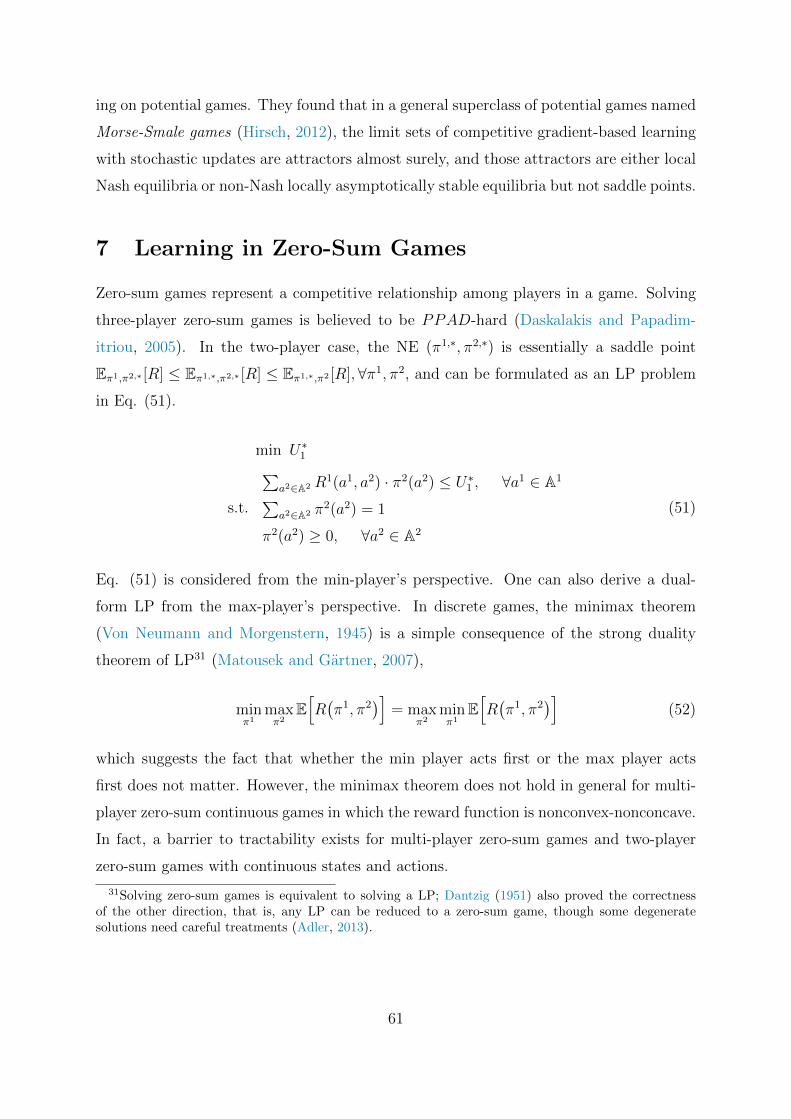
ing on potential games. They found that in a general superclass of potential games named

Morse-Smale games (Hirsch, 2012), the limit sets of competitive gradient-based learning

with stochastic updates are attractors almost surely, and those attractors are either local

Nash equilibria or non-Nash locally asymptotically stable equilibria but not saddle points.

7 Learning in Zero-Sum Games

Zero-sum games represent a competitive relationship among players in a game. Solving

three-player zero-sum games is believed to be PPAD-hard (Daskalakis and Papadim-

itriou, 2005). In the two-player case, the NE (π1,∗, π2,∗) is essentially a saddle point

Eπ1,π2,∗ [R] ≤ Eπ1,∗,π2,∗ [R] ≤ Eπ1,∗,π2 [R],∀π1, π2, and can be formulated as an LP problem

in Eq. (51).

min U∗1

s.t.

∑a2∈A2 R1(a1, a2) · π2(a2) ≤ U∗1 , ∀a1 ∈ A1

∑a2∈A2 π2(a2) = 1

π2(a2) ≥ 0, ∀a2 ∈ A2

(51)

Eq. (51) is considered from the min-player’s perspective. One can also derive a dual-

form LP from the max-player’s perspective. In discrete games, the minimax theorem

(Von Neumann and Morgenstern, 1945) is a simple consequence of the strong duality

theorem of LP31 (Matousek and Gartner, 2007),

minπ1

maxπ2

E[R(π1, π2

)]= max

π2minπ1

E[R(π1, π2

)](52)

which suggests the fact that whether the min player acts first or the max player acts

first does not matter. However, the minimax theorem does not hold in general for multi-

player zero-sum continuous games in which the reward function is nonconvex-nonconcave.

In fact, a barrier to tractability exists for multi-player zero-sum games and two-player

zero-sum games with continuous states and actions.

31Solving zero-sum games is equivalent to solving a LP; Dantzig (1951) also proved the correctnessof the other direction, that is, any LP can be reduced to a zero-sum game, though some degeneratesolutions need careful treatments (Adler, 2013).

61

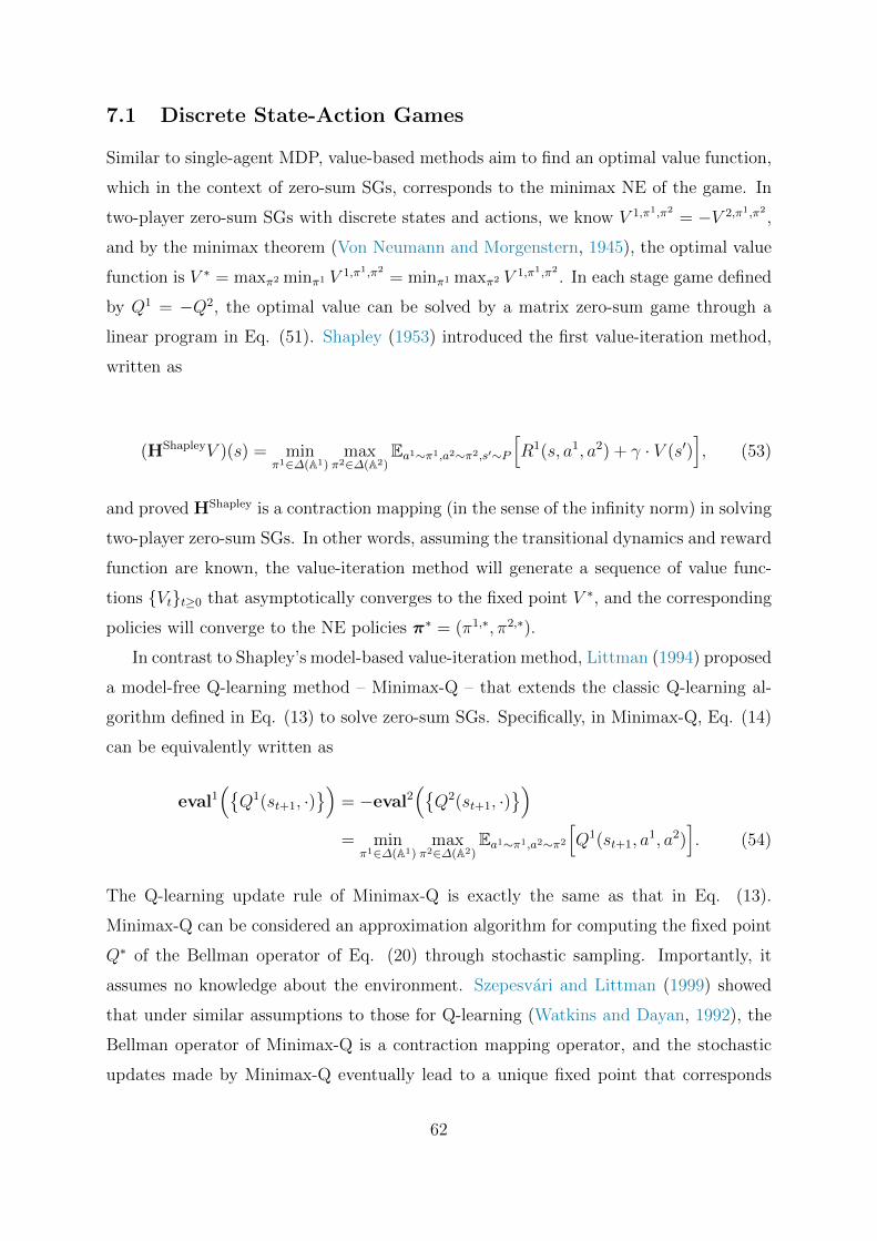
7.1 Discrete State-Action Games

Similar to single-agent MDP, value-based methods aim to find an optimal value function,

which in the context of zero-sum SGs, corresponds to the minimax NE of the game. In

two-player zero-sum SGs with discrete states and actions, we know V 1,π1,π2= −V 2,π1,π2

,

and by the minimax theorem (Von Neumann and Morgenstern, 1945), the optimal value

function is V ∗ = maxπ2 minπ1 V 1,π1,π2= minπ1 maxπ2 V 1,π1,π2

. In each stage game defined

by Q1 = −Q2, the optimal value can be solved by a matrix zero-sum game through a

linear program in Eq. (51). Shapley (1953) introduced the first value-iteration method,

written as

(HShapleyV )(s) = minπ1∈∆(A1)

maxπ2∈∆(A2)

Ea1∼π1,a2∼π2,s′∼P

[R1(s, a1, a2) + γ · V (s′)

], (53)

and proved HShapley is a contraction mapping (in the sense of the infinity norm) in solving

two-player zero-sum SGs. In other words, assuming the transitional dynamics and reward

function are known, the value-iteration method will generate a sequence of value func-

tions Vtt≥0 that asymptotically converges to the fixed point V ∗, and the corresponding

policies will converge to the NE policies π∗ = (π1,∗, π2,∗).

In contrast to Shapley’s model-based value-iteration method, Littman (1994) proposed

a model-free Q-learning method – Minimax-Q – that extends the classic Q-learning al-

gorithm defined in Eq. (13) to solve zero-sum SGs. Specifically, in Minimax-Q, Eq. (14)

can be equivalently written as

eval1(Q1(st+1, ·)

)= −eval2

(Q2(st+1, ·)

)

= minπ1∈∆(A1)

maxπ2∈∆(A2)

Ea1∼π1,a2∼π2

[Q1(st+1, a

1, a2)]. (54)

The Q-learning update rule of Minimax-Q is exactly the same as that in Eq. (13).

Minimax-Q can be considered an approximation algorithm for computing the fixed point

Q∗ of the Bellman operator of Eq. (20) through stochastic sampling. Importantly, it

assumes no knowledge about the environment. Szepesvari and Littman (1999) showed

that under similar assumptions to those for Q-learning (Watkins and Dayan, 1992), the

Bellman operator of Minimax-Q is a contraction mapping operator, and the stochastic

updates made by Minimax-Q eventually lead to a unique fixed point that corresponds

62

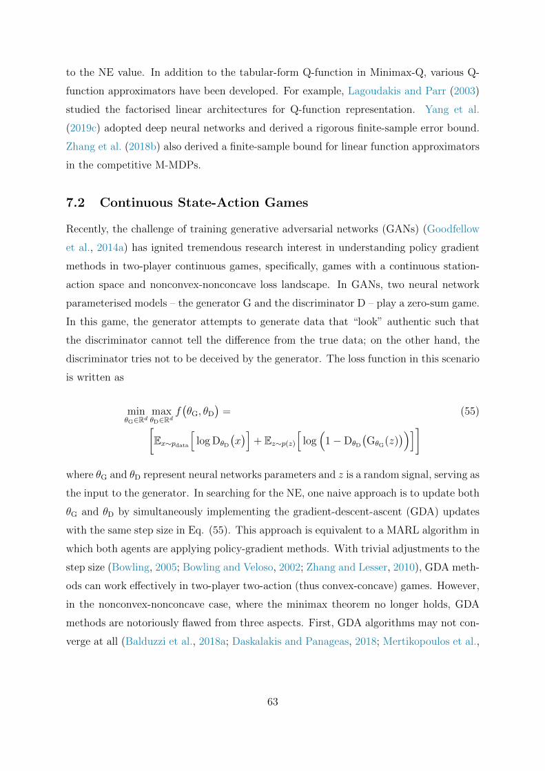
to the NE value. In addition to the tabular-form Q-function in Minimax-Q, various Q-

function approximators have been developed. For example, Lagoudakis and Parr (2003)

studied the factorised linear architectures for Q-function representation. Yang et al.

(2019c) adopted deep neural networks and derived a rigorous finite-sample error bound.

Zhang et al. (2018b) also derived a finite-sample bound for linear function approximators

in the competitive M-MDPs.

7.2 Continuous State-Action Games

Recently, the challenge of training generative adversarial networks (GANs) (Goodfellow

et al., 2014a) has ignited tremendous research interest in understanding policy gradient

methods in two-player continuous games, specifically, games with a continuous station-

action space and nonconvex-nonconcave loss landscape. In GANs, two neural network

parameterised models – the generator G and the discriminator D – play a zero-sum game.

In this game, the generator attempts to generate data that “look” authentic such that

the discriminator cannot tell the difference from the true data; on the other hand, the

discriminator tries not to be deceived by the generator. The loss function in this scenario

is written as

minθG∈Rd

maxθD∈Rd

f(θG, θD

)= (55)

[Ex∼pdata

[log DθD

(x)]

+ Ez∼p(z)[

log(

1−DθD

(GθG(z)

))]]

where θG and θD represent neural networks parameters and z is a random signal, serving as

the input to the generator. In searching for the NE, one naive approach is to update both

θG and θD by simultaneously implementing the gradient-descent-ascent (GDA) updates

with the same step size in Eq. (55). This approach is equivalent to a MARL algorithm in

which both agents are applying policy-gradient methods. With trivial adjustments to the

step size (Bowling, 2005; Bowling and Veloso, 2002; Zhang and Lesser, 2010), GDA meth-

ods can work effectively in two-player two-action (thus convex-concave) games. However,

in the nonconvex-nonconcave case, where the minimax theorem no longer holds, GDA

methods are notoriously flawed from three aspects. First, GDA algorithms may not con-

verge at all (Balduzzi et al., 2018a; Daskalakis and Panageas, 2018; Mertikopoulos et al.,

63

2018), resulting in limited cycles32 in which even the time average33 does not coincide with

NE (Mazumdar et al., 2019a). Second, there exist undesired stable stationary points for

the GDA algorithms that are not local optima of the game (Adolphs et al., 2019; Mazum-

dar et al., 2019a). Third, there exist games whose equilibria are not the attractors of

GDA methods at all (Mazumdar et al., 2019a). These problems are partly caused by the

intransitive dynamics (e.g., a typical intransitive game is rock-paper-scissors game) that

are inherent in zero-sum games (Balduzzi et al., 2018a; Omidshafiei et al., 2020) and the

fact that each agent may have a non-smooth objective function. In fact, even in simple

linear-quadratic games, the reward function cannot satisfy the smoothness condition34

globally, and the games are surprisingly not convex either (Fazel et al., 2018; Mazumdar

et al., 2019a; Zhang et al., 2019c).

Three mainstream approaches have been followed to develop algorithms that have at

least a local convergence guarantee. One natural idea is to make the inner loop solvable

at a reasonably high level and then focus on a simpler type of game. In other words,

the algorithm tries to find a stationary point of the function Φ(·) := maxθD∈Rd f(·, θD

),

instead of Eq. (55). For example, by considering games with a nonconvex and (strongly)

concave loss landscape, Kong and Monteiro (2019); Lin et al. (2019); Lu et al. (2020a);

Nouiehed et al. (2019); Rafique et al. (2018); Thekumparampil et al. (2019) presented

an affirmative answer that GDA methods can converge to a stationary point in the

outer loop of optimising Φ(·) := maxθD∈Rd f(·, θD

). Based on this understanding, they

developed various GDA variants that apply the “best response” in the inner loop while

maintaining an inexact gradient descent in the outer loop. We refer to Lin et al. (2019)

[Table 1] for a detailed summary of the time complexity of the above methods.

The second mainstream idea is to shift the equilibrium of interest from the NE, which

is induced by simultaneous gradient updates, to the Stackelberg equilibrium, which is

a solution concept in leader-follower (i.e., alternating update) games. Jin et al. (2019)

introduced the concept of the local Stackelberg equilibrium, named local minimax, based

on which he established the connection to GDA methods by showing that all stable limit

points of GDA are exactly local minimax points. Fiez et al. (2019) also built connections

between the NE and Stackelberg equilibrium by formulating the conditions under which

32Limited cycle is a terminology in the study of dynamical systems, which describes oscillatory systems.In game theory, an example of limit cycles in the strategy space can be found in Rock-Paper-Scissor game.

33In two-player two-action games, Singh et al. (2000) showed that the time average payoffs wouldconverge to a NE value if their policies do not.

34A differentiable function is said to be smooth if the gradients of the function are continuous.

64

attracting points of GDA dynamics are Stackelberg equilibria in zero-sum games. When

the loss function is bilinear, theoretical evidence was found that alternating updates

converge faster than simultaneous GDA methods (Zhang and Yu, 2019).

The third mainstream idea is to analyse the loss landscape from a game-theoretic per-

spective and design corresponding algorithms that mitigate oscillatory behaviour. Com-

pared to the previous two mainstream ideas, which helped generate more theoretical

insights than applicable algorithms, works within this stream demonstrate strong em-

pirical improvements in training GANs. Mescheder et al. (2017) investigated the game

Hessian and identified that issues on the eigenvalues trigger the limited cycles. As a

result, they proposed a new type of update rule based on consensus optimisation, to-

gether with a convergence guarantee to a local NE in smooth two-player zero-sum games.

Adolphs et al. (2019) leveraged the curvature information of the loss landscape to pro-

pose algorithms in which all stable limit points are guaranteed to be local NEs. Similarly,

Mazumdar et al. (2019b) took advantage of the differential structure of the game and

constructed an algorithm for which the local NEs are the only attracting fixed points.

In addition, Daskalakis et al. (2017); Mertikopoulos et al. (2018) addressed the issue of

limit cycling behaviour in training GANs by proposing the technique of optimistic mirror

descent (OMD). OMD achieves the last-iterate convergent guarantee in bilinear convex-

concave games. Specifically, at each time step, OMD adjusts the gradient of that time

step by considering the opponent policy at the next time step. Let Mt+1 be the predictor

of the next iteration gradient35; we can write OMD as follows.

θG,t+1 = θG,t + α ·(∇θG,tf

(θG, θD

)+MθG,t+1 −MθG,t

)

θD,t+1 = θG,t − α ·(∇θD,tf

(θG, θD

)+MθD,t+1 −MθD,t

)(56)

In fact, the pivotal idea of opponent prediction in OMD, developed in the optimisa-

tion domain, resembles the idea of approximate policy prediction in the MARL domain

(Foerster et al., 2018a; Zhang and Lesser, 2010).

Thus far, the most promising results are probably those of Bu et al. (2019) and Zhang

et al. (2019c), which reported the first results in solving zero-sum LQ games with a global

convergence guarantee. Specifically, Zhang et al. (2019c) developed the solution through

projected nested-gradient methods, while Bu et al. (2019) solved the problem through

35In practice, it is usually set as the last iteration gradient.

65

a projection-free Stackelberg leadership model. Both of the models achieve a sublinear

rate for convergence.

7.3 Extensive-Form Games

As briefly introduced in Section 3.4, zero-sum EFG with imperfect information can be

efficiently solved via LP in sequence form representations (Koller and Megiddo, 1992,

1996). However, these approaches are limited to solving only small-scale problems (e.g.,

games with O(107) information states). In fact, considerable additional effort is needed to

address real-world games (e.g., limit Texas hold’em, which has O(1018) game states); to

name a few, Monte Carlo Tree Search (MCTS) techniques36 (Browne et al., 2012; Cowling

et al., 2012; Silver et al., 2016), isomorphic abstraction techniques (Billings et al., 2003;

Gilpin and Sandholm, 2006), and iterative (policy) gradient-based approaches (Gilpin

et al., 2007; Gordon, 2007; Zinkevich, 2003).

A central idea of iterative policy gradient-based methods is minimising regret37. A

learning rule achieves no-regret, also called Hannan consistency in game theoretical terms

(Hannan, 1957), if, intuitively speaking, against any set of opponents it yields a payoff

that is no less than the payoff the learning agent could have obtained by playing any

one of its pure strategies in hindsight. Recall the reward function under a given policy

π = (πi, π−i) in Eq. (27); the (average) regret of player i is defined by:

RegiT =1

Tmaxπi

T∑

t=1

[Ri(πi, π−it )−Ri(πit, π

−it )]. (57)

A no-regret algorithm satisfies RegiT → 0 as T →∞ with probability 1. When Eq. (57)

equals zero, all agents are acting with their best response to others, which essentially

forms a NE. Therefore, one can regard regret as a type of “distance” to NE. As one would

expect, the single-agent Q-learning procedure can be shown to be Hannan consistent in

a stochastic game against opponents playing stationary policies (Shoham and Leyton-

Brown, 2008) [Chapter 7] since the optimal Q-function guarantees the best response. In

36Notably, though MCTS methods such as UCT (Kocsis and Szepesvari, 2006) work remarkably wellin turn-based EFGs, such as GO and chess, they cannot converge to a NE trivially in (even perfect-information) simultaneous-move games (Schaeffer et al., 2009). See a rigorous treatment for remedy inLisy et al. (2013).

37One can regard minimising regret as one solution concept for multi-agent learning problems, similarto the reward maximisation in single-agent learning.

66

contrast, the Minimax-Q algorithm in Eq. (54) is not Hannan consistent because if the

opponent plays a sub-optimal strategy, Minimax-Q is unable to exploit the opponent due

to the over-conservativeness in terms of over-estimating its opponents.

An important result about regret states is that in a zero-sum game at time T , if both

players’ average regret is less than ε, then their average strategy constitutes a 2ε-NE of the

game (Zinkevich et al., 2008, Theorem 2). In general-sum games, the average strategy of

the ε-regret algorithm will reach an ε-coarse correlated equilibrium of the game (Michael,

2020, Theorem 6.3.1). This result essentially implies that regret-minimising algorithms

(or, algorithms with Hannan consistency) applied in a self-play manner can be used

as a general technique to approximate the NE of zero-sum games. Building upon this

finding, two families of methods are developed, namely, fictitious play types of methods

(Berger, 2007) and counterfactual regret minimisation (Zinkevich et al., 2008), which lay

the theoretical foundations for modern techniques to solve real-world games.

7.3.1 Variations of Fictitious Play

Fictitious play (FP) (Berger, 2007) is one of the oldest learning procedures in game

theory that is provably convergent for zero-sum games, potential games, and two-player

n-action games with generic payoffs. In FP, each player maintains a belief about the

empirical mean of the opponents’ average policy, based on which the player selects the

best response. With the best response defined in Eq. (17), we can write the FP updates

as

ai,∗t ∈ Bri(π−it =

1

t

t−1∑

τ=0

1a−iτ = a, a ∈ A

), πit+1 =

(1− 1

t

)πit +

1

tai,∗t , ∀i. (58)

In the FP scheme, each agent is oblivious to the other agents’ reward; however, they

need full access to their own payoff matrix in the stage game. In the continuous case with

an infinitesimal learning rate of 1/t→ 0, Eq. (58) is equivalent to dπt/dt ∈ Br(πt)−πt

in which Br(πt) =(Br(π−1

t ), ...,Br(π−Nt )). Viossat and Zapechelnyuk (2013) proved

that continuous FP leads to no regret and is thus Hannan consistent. If the empirical

distribution of each πit converges in FP, then it converges to a NE38.

38Note that the convergence in Nash strategy does not necessarily mean the agents will receive theexpected payoff value at NE. In the example of Rock-Paper-Scissor games, agents’ actions are stillmiscorrelated after convergence, flipping between one of the three strategies, though their average policiesdo converge to (1/3, 1/3, 1/3).

67

Although standard discrete-time FP is not Hannan consistent (Cesa-Bianchi and Lu-

gosi, 2006, Exercise 3.8), various extensions have been proposed that guarantee such a

property; see a full list summarised in Hart (2013) [Section 10.9]. Smooth FP (Fudenberg

and Kreps, 1993; Fudenberg and Levine, 1995) is a stochastic variant of FP (thus also

called stochastic FP) that considers a smooth ε-best response in which the probability

of each action is a softmax function of that action’s utility/reward against the histori-

cal frequency of the opponents’ play. In smooth FP, each player’s strategy is a genuine

mixed strategy. Let Ri(ai1, π−it ) be the expected reward of player i’s action ai1 ∈ Ai under

opponents’ strategy π−i; the probability of playing ai1 in the best response is written as

Briλ(π−it ) :=

exp(

1λRi(ai1, π

−it

))∑|Ai|

k=1 exp(

1λRi(aik, π

−it

)) . (59)

Benaım and Faure (2013) verified the Hannan consistency of the smooth best response

with the smoothing parameter λ being time dependent and vanishing asymptotically. In

potential games, smooth FP is known to converge to a neighbourhood of the set of NE

(Hofbauer and Sandholm, 2002). Recently, Swenson and Poor (2019) showed a generic

result that in almost allN×2 potential games, smooth FP converges to the neighbourhood

of a pure-strategy NE with a probability of one.

In fact, “smoothing” the cumulative payoffs before computing the best response is

crucial to designing learning procedures that achieve Hannan consistency (Kaniovski and

Young, 1995). One way to achieve such smoothness is through stochastic smoothing or

adding perturbations39. For example, the smooth best response in Eq. (59) is a closed-

form solution if one perturbs the cumulative reward by an additional entropy function,

that is,

πi,∗ ∈ Br(π−i) =

arg maxπ∈∆(Ai)

Eπi,π−i[Ri + λ · log(π)

]. (60)

Apart from smooth FP, another way to add perturbation is the sampled FP in which

during each round, the player samples historical time points using a randomised sampling

scheme, and plays the best response to the other players’ moves, restricted to the set of

sampled time points. Sampled FP is shown to be Hannan consistent when used with

Bernoulli sampling (Li and Tewari, 2018).

Among the many extensions of FP, the most important is probably generalised weak-

39The physical meaning of perturbing the cumulative payoff is to consider the incomplete informationabout what the opponent has been playing, variability in their payoffs, and unexplained trembles.

68

ened FP (GWFP) (Leslie and Collins, 2006), which releases the standard FP by allowing

both approximate best response and perturbed average strategy updates. Specifically, if

we write the ε-best response of player i as

Ri(Brε(π

−i), π−i)≥ sup

π∈∆(Ai)Ri(π, π−i

)− ε. (61)

then the GWFP updating steps change from Eq. (58) to

πit+1 =(

1− αt+1)πit + αt+1

(Briε(π

−i) +M it+1

), ∀i. (62)

GWFP is Hannan consistent if αt → 0, εt → 0,∑

αt= ∞ when t → ∞, and Mt

meets limt→∞ supk∥∥∑k−1

i=t αi+1M i+1

∥∥ s.t.∑k−1

i=t αi+1 ≤ T

= 0. It is trivial to see that

GWFP recovers FP when αt = 1/t, εt = 0,Mt = 0. GWFP is an important extension

of FP in that it provides two key components for bridging game theoretic ideas with

RL techniques. With the approximate best response (highlighted in blue, also named

as the “weakened” term), this approach allows one to adopt a model-free RL algorithm,

such as deep Q-learning, to compute the best response. Moreover, the perturbation term

(highlighted in red, also named as the “generalised” term) enables one to incorporate

policy exploration; if one applies an entropy term as the perturbation in addition to the

best response (in which the smooth FP in Eq. (60) is also recovered), the scheme of

maximum-entropy RL methods (Haarnoja et al., 2018) is recovered. In fact, the gener-

alised term also accounts for the perturbation that comes from the fact the beliefs are not

updated towards the exact mixed strategy π−i but instead towards the observed actions

(Benaım and Hirsch, 1999). As a direct application, Perolat et al. (2018) implemented

the GWFP process through an actor-critic framework (Konda and Tsitsiklis, 2000) in the

MARL setting.

Brown’s original version of FP (Berger, 2007) describes alternating updates by play-

ers; yet, the modern usage of FP involves players updating their beliefs simultaneously

(Berger, 2007). In fact, Heinrich et al. (2015) only recently proposed the first FP algo-

rithm for EFG using the sequence-form representation. The extensive-form FP is essen-

tially an adaptation of GWFP from NFG to EFG based on the insight that a mixture

of normal-form strategies can be implemented by a weighted combination of behavioural

strategies that have the same realisation plan (recall Section 3.3.2). Specifically, let π

69

and β be two behavioural strategies, Π and B be the two realisation-equivalent mixed

strategies40, and α ∈ R+; then, for each information state S, we have

π(S) = π(S) +αµβ(σS)

(1− α)µπ(σS) + αµβ(σS)

(β(S)− π(S)

), ∀S ∈ S, (63)

where σS is the sequence leading to S, µπ/β(σS) is the realisation probability of σS under

a given policy, and π(S) defines a new behaviour that is realisation equivalent to the

mixed strategy (1 − α)Π + αB. The extensive-form FP essentially iterates between

Eq. (61), which computes the ε-best response, and Eq. (63), which updates the old

behavioural strategy with a step size of α. Note that these two steps must iterate over

all information states of the game in each iteration. Similar to the normal-form FP in

Eq. (58), extensive-form FP generates a sequence of πtt≥1 that provably converges to

the NE of a zero-sum game under self-play if the step size α goes to zero asymptotically.

As a further enhancement, Heinrich and Silver (2016) implemented neural fictitious self-

play (NFSP), in which the best response step is computed by deep Q-learning (Mnih

et al., 2015) and the policy mixture step is computed through supervised learning. NFSP

requires the storage of large replay buffers of past experiences; Lockhart et al. (2019)

removes this requirement by obtaining the policy mixture for each player through an

independent policy-gradient step against the respective best-responding opponent. All

these amendments help make extensive-form FP applicable to real-world games with

large-scale information states.

7.3.2 Counterfactual Regret Minimisation

Another family of methods achieve Hannan consistency by directly minimising the regret,

in particular, a special kind of regret named counterfactual regret (CFR) (Zinkevich

et al., 2008). Unlike FP methods, which are developed from the stochastic approximation

perspective and generally have asymptotic convergence guarantees, CFR methods are

established on the framework of online learning and online convex optimisation (Shalev-

Shwartz et al., 2011), which makes analysing the speed of convergence, i.e., the regret

bound, to the NE possible.

The key insight from CFR methods is that in order to minimise the total regret in Eq.

40Recall that in games with perfect recall, Kuhn’s theorem (Kuhn, 1950a) suggests that the behaviouralstrategy and mixed strategies are equivalent in terms of the realisation probability of different outcomes.

70

(57) to approximate the NE, it suffices to minimise the immediate counterfactual regret

at the level of each information state. Mathematically, Zinkevich et al. (2008) [Theo-

rem 3] shows that the sum of the immediate counterfactual regret over all encountered

information states provides an upper bound for the total regret in Eq. (57), i.e.,

RegiT ≤∑

S∈Simax

RegiT,imm(S), 0

, ∀i. (64)

To fully describe RegiT,imm(S), we need two additional notations. Let µπ(σS → σT ) de-

note, given agents’ behavioural policies π, the realisation probability of going from the

sequence σS41, which leads to the information state S ∈ Si to its extended sequence σT ,

which continues from S and reaches the terminal state T . Let vi(π, S) be the counter-

factual value function, i.e., the expected reward of agent i in non-terminal information

state S, which is written as

vi(π, S

)=

∑

s∈S,T∈T

µπ−i(σs)µπ(σs → σT )Ri(T ). (65)

Note that in Eq. (65), the contribution from player i in realising σs is excluded; we treat

whatever action current player i needs to reach state s as having a probability of one, that

is, µπi(σs) = 1. The motivation is that now one can make the value function vi

(π, S

)

“counterfactual” simply by writing the consequence of player i not playing action a in

the information state S as(vi(π|S→a, S) − vi(π, S)

), in which π|S→a is a joint strategy

profile identical to π, except player i always chooses action a when information state S

is encountered. Finally, based on Eq. (65), the immediate counterfactual regret can be

expressed as

RegiT,imm(S) = maxa∈χ(S)

RegiT (S, a), RegiT (S, a) =1

T

T∑

t=1

(vi(πt|S→a, S)− vi(πt, S)

). (66)

Note that the T in Eq. (65) is different from that in Eq. (66).

Since minimising the immediate counterfactual regret minimises the overall regret,

we can find an approximate NE by choosing a specific behavioural policy πi(S) that

minimises Eq. (66). To this end, one can apply Blackwell’s approachability theorem

41Recall that for games of perfect recall, the sequence that leads to the information state, includingall the choice nodes within that information state, is unique.

71

(Blackwell et al., 1956) to minimise the regret independently on each information set,

also known as regret matching (Hart and Mas-Colell, 2001). As we are most concerned

with positive regret, denoted by b·c+, we have ∀S ∈ Si,∀a ∈ χ(S), the strategy of player

i at time T + 1 as Eq. (67).

πiT+1(S, a) =

bRegiT(S, a)c+∑

a∈χ(S)bRegiT(S, a)c+

if∑

a∈χ(S)bRegiT (S, a)c+ > 0

1

|χ(S)| otherwise

. (67)

In the standard CFR algorithm, for each information set, Eq. (67) is used to com-

pute action probabilities in proportion to the positive cumulative regrets. In addition

to regret matching, another online learning tool that minimises regret is Hedge (Freund

and Schapire, 1997; Littlestone and Warmuth, 1994), in which an exponentially weighted

function is used to derive a new strategy, which is

πt+1(ak) =πt(ak)e

−ηRt(ak)

∑Kj=1 πt(aj)e

−ηRt(aj), π1(·) =

1

K. (68)

In computing Eq. (68), Hedge needs access to the full information of the reward values

for all actions, including those that are not selected. EXP3 (Auer et al., 1995) extended

the Hedge algorithm for a partial information game in which the player knows only the

reward of the the chosen action (i.e., a bandit version) and has to estimate the loss of

the actions that it does not select. Brown et al. (2017) augmented the Hedge algorithm

with a tree-pruning technique based on dynamic thresholding. Gordon (2007) developed

Lagrangian hedging, which unifies no-regret algorithms, including both regret matching

and Hedge, through a class of potential functions. We recommend Cesa-Bianchi and

Lugosi (2006) for a comprehensive overview of no-regret algorithms.

No-regret algorithms, under the framework of online learning, offer a natural way to

study the regret bound (i.e., how fast the regret decays with time). For example, CFR

and its variants ensure a counterfactual regret bound of O(√T )42, as a result of Eq.

(64), the convergence rate for the total regret is upper bounded by O(√T · |S|), which is

linear in the number of information states. In other words, the average policy of applying

42According to Zinkevich (2003), any online convex optimisation problem can be made to incur RegT =Ω(√T ).

72

CFR-type methods in a two-player zero-sum EFG generates an O(|S|/√T )-approximate

NE after T steps through self-play43.

Compared with the LP approach (recall Eq. (33)), which is applicable only for small-

scale EFGs, the standard CFR method can be applied to limit Texas hold’em with as

many as 1012 states. CFR+, the fastest implementation of CFR, can solve games with up

to 1014 states (Tammelin et al., 2015). However, CFR methods still have a bottleneck in

that computing Eq. (65) requires a traversal of the entire game tree to the terminal nodes

in each iteration. Pruning the sub-optimal paths in the game tree is a natural solution

(Brown et al., 2017; Brown and Sandholm, 2015, 2017). Many CFR variants have been

developed to improve computational efficiency further. Lanctot et al. (2009) integrated

Monte Carlo sampling with CFR (MCCFR) to significantly reduce the per iteration time

cost of CFR by traversing a smaller sampled portion of the tree. Burch et al. (2012)

improved MCCFR by sampling only a subset of a player’s actions, which provides even

faster convergence rate in games that contain many player actions. Gibson et al. (2012);

Schmid et al. (2019) investigated the sampling variance and proposed MCCFR variants

with a variance reduction module. Johanson et al. (2012b) introduced a more accurate

MCCFR sampler by considering the set of outcomes from the chance node, rather than

sampling only one outcome, as in all previous methods. Apart from Monte Carlo methods,

function approximation methods have also been introduced (Jin et al., 2018; Waugh et al.,

2014). The idea of these methods is to predict regret directly, and the no-regret algorithm

then uses these predictions in place of the true regret to define a sequence of policies. To

this end, the application of deep neural networks has led to great success (Brown et al.,

2019).

Interestingly, there exists a hidden equivalence between model-free policy-based/actor-

critic MARL methods and the CFR algorithm (Jin et al., 2018; Srinivasan et al., 2018).

In particular, if we consider the counterfactual value function in Eq. (65) to be explicitly

dependent on the action a that player i chooses at state S, in which we have vi(π, S) =∑

a∈χ(S) πi(S, a)qi(π, S, a), then it is shown in Srinivasan et al. (2018) [Section 3.2] that

the Q-function in standard MARL Qi,π(s, a) = Es′∼P,a∼π[∑

t γtRi(s, a, s′)|s, a

]differs

43The self-play assumption can in fact be released. Johanson et al. (2012a) shows that in two-playerzero-sum games, as long as both agents minimise their regret, not necessarily through the same algorithm,their time-average policies will converge to NE with the same regret bound O(

√T ). An example is to

let a CFR player play against a best-response opponent.

73

from qi(π, S, a) in CFR only by a constant of the probability of reaching S, that is,

Qi,π(s, a)

=qi(π, S, a

)∑

s∈S µπ−i(σs) . (69)

Subtracting a value function on both sides of Eq. (69) leads to the fact that the coun-

terfactual regret of RegiT (S, a) in Eq. (66) differs from the advantage function in MARL,

i.e., Qi,π(s, ai, a−i) − V i,π(s, a−i), only by a constant of the realisation probability. As

a result, the multi-agent actor-critic algorithm (Foerster et al., 2018b) can be formu-

lated as a special type of CFR method, thus sharing a similar convergence guarantee

and regret bound in two-player zero-sum games. The equivalence has also been found by

(Hennes et al., 2019), where the CFR method with Hedge can be written as a particular

actor-critic method that computes the policy gradient through replicator dynamics.

7.4 Online Markov Decision Processes

A common situation in which online learning techniques are applied is in stateless games,

where the learning agent faces an identical decision problem in each trial (e.g., playing

a multi-arm bandit in the casino). However, real-world decision problems often occur

in a dynamic and changing environment. Such an environment is commonly captured

by a state variable which, when incorporated into online learning, leads to an online

MDP. Online MDP (Auer et al., 2009; Even-Dar et al., 2009; Yu et al., 2009), also called

adversarial MDP44, focuses on the problem in which the reward and transition dynamics

can change over time, i.e., they are non-stationary and time-dependent.

In contrast to an ordinary stochastic game, the opponent/adversary in an online MDP

is not necessarily rational or even self-optimising. The aim of studying online MDP is

to provide the agent with policies that perform well against every possible opponent

(including but not limited to adversarial opponents), and the objective of the learning

agent is to minimise its average loss during the learning process. Quantitatively, the

loss is measured by how worse off the agent is compared to the best stationary policy in

retrospect. The expected regret is thus different from Eq. (57) (unless in repeated games)

44The word “adversarial” is inherited from the online learning literature, i.e., stochastic bandit vsadversarial bandit (Auer et al., 2002). Adversary means there exists a virtual adversary (or, nature)who has complete control over the reward function and transition dynamics, and the adversary does notnecessarily maintain a fully competitive relationship with the learning agent.

74

and is written as

RegT =1

Tsupπ∈Π

Eπ[ T∑

t=1

Rt

(s∗t , a

∗t

)−Rt

(st, at

)](70)

where Eπ denotes the expectation over the sequence of (s∗t , a∗t ) induced by the stationary

policy π. Note that the reward function sequence and the transition kernel sequence are

given by the adversary, and they are not influenced by the retrospective sequence (s∗t , a∗t ).

The goal is to find a no-regret algorithm that can satisfy RegT → 0 as T → ∞ with

probability 1. A sufficient condition that ensures the existence of no-regret algorithms

for online MDPs is the oblivious assumption – both the reward functions and transition

kernels are fixed in advance, although they are unknown to the learning agent. This

scenario is in contrast to the stateless setting in which no-regret is achievable, even

if the opponent is allowed to be adaptive/non-oblivious : they can choose the reward

function and transition kernels in accordance to (s0, a0, ..., st) from the learning agent.

In short, Mannor and Shimkin (2003); Yu et al. (2009) demonstrated that in order to

achieve sub-linear regret, it is essential that the changing rewards are chosen obliviously.

Furthermore, Yadkori et al. (2013) showed with the example of an online shortest path

problem that there does not exist a polynomial-time solution (in terms of the size of

the state-action space) where both the reward functions and transition dynamics are

adversarially chosen, even if the adversary is oblivious (i.e., it cannot adapt to the other

agent’s historical actions). Most recently, Cheung et al. (2020); Ortner et al. (2020)

investigated online MDPs where the transitional dynamics are allowed to change slowly

(i.e., the total variation does not exceed a specific budget). Therefore, the majority of

existing no-regret algorithms for online MDP focus on an oblivious adversary for the

reward function only. The nuances of different algorithms lie in whether the transitional

kernel is assumed to be known to the learning agent and whether the feedback reward

that the agent receives is in the full-information setting or in the bandit setting (i.e., one

can only observe the reward of a taken action).

Two design principles can lead to no-regret algorithms that solve online MDPs with

an oblivious adversary controlling the reward function. One is to leverage the local-

global regret decomposition result (Even-Dar et al., 2005, 2009) [Lemma 5.4], which

demonstrates that one can in fact achieve no regret globally by running a local regret-

minimisation algorithm at each state; a similar result is observed for the CFR algorithm

described in Eq. (66). Let µ∗(·) denote the state occupancy induced by policy π∗; we

75

then obtain the decomposition result by

RegT =∑

s∈S

µ∗(s)T∑

t=1

∑

a∈A

(π∗(a | s)− πt(a | s)

)Qt

(s, a)

︸ ︷︷ ︸local regret in state s with reward function Qt(s, ·)

. (71)

Under full knowledge of the transition function and full-information feedback about the

reward, Even-Dar et al. (2009) proposed the famous MDP-Expert (MDP-E) algorithm,

which adopts Hedge (Freund and Schapire, 1997) as the regret minimiser and achieves

O(√τ 3T ln |A|) regret, where τ is the bound on the mixing time of MDP 45. For compar-

ison, the theoretical lower bound for regret in a fixed MDP (i.e., no adversary perturbs

the reward function) is Ω(√|S||A|T )46 (Auer et al., 2009). Interestingly, Neu et al. (2017)

showed that there in fact exists an equivalence between TRPO methods (Schulman et al.,

2015) and MDP-E methods. Under bandit feedback, Neu et al. (2010) analysed MDP-

EXP3, which achieves a regret bound of O(√τ 3T |A| log |A|/β), where β is a lower bound

on the probability of reaching a certain state under a given policy. Later, Neu et al. (2014)

removed the dependency on β and achieved O(√T log T ) regret. One major advantage

of local-global design principle is that it can work seamlessly with function approxima-

tion methods (Bertsekas and Tsitsiklis, 1996). For example, Yu et al. (2009) eliminated

the requirement of knowing the transition kernel by incorporating Q-learning methods;

their proposed Q-follow the perturbed leader (Q-FPL) method achieved O(T 2/3) regret.

Abbasi-Yadkori et al. (2019) proposed POLITEX, which adopted a least square policy

evaluation (LSPE) with linear function approximation and achieved O(T 3/4 +ε0T ) regret,

in which ε0 is the worst-case approximation error, and Cai et al. (2019a) used the same

LSPE method. However, the proposed OPPO algorithm achieves O(√T ) regret.

Apart from the local-global decomposition principle, another design principle is to

formulate the regret minimisation problem as an online linear optimisation (OLO) prob-

lem and then apply gradient-descent type methods. Specifically, since the regret in Eq.

(71) can be further written as the inner product of RegT =∑T

t=1〈µ∗ − µt, Rt〉, one can

run the gradient descent method by

µt+1 = arg maxµ∈U

⟨µ,Rt

⟩− 1

ηD(µ|µt

), (72)

45Roughly, it can be considered as the time that a policy needs to reach the stationary status in MDPs.See a precise definition in Even-Dar et al. (2009) [Assumption 3.1].

46This lower bound has recently been achieved by Azar et al. (2017) up to a logarithmic factor.

76

where U =µ ∈ ∆S×A :

∑a µ(s, a) =

∑s′,a′ P (s|s′, a′)µ(s′, a′)

is the set of all valid sta-

tionary distributions47, whereD denotes a certain form of divergence and the policy can be

extracted by πt+1(a|s) = µt+1(s, a)/µ(s). One significant advantage of this type of method

is that it can flexibly handle different model constraints and extensions. If one uses Breg-

man divergence as D, then online mirror descent is recovered (Nemirovsky and Yudin,

1983) and is guaranteed to achieve a nearly optimal regret for OLO problems (Srebro

et al., 2011). Zimin and Neu (2013) and Dick et al. (2014) adopted a relative entropy for

D; the subsequent online relative entropy policy search (O-REPS) algorithm achieves an

O(√τT log(|S||A|)) regret in the full-information setting and an O(

√T |S||A| log(|S||A|))

regret in the bandit setting. For comparison, the aforementioned MDP-E algorithm

achieves O(√τ 3T ln |A|) and O(

√τ 3T |A| log |A|/β), respectively. When the transition

dynamics are unknown to the agent, Rosenberg and Mansour (2019) extended O-REPS

by incorporating the classic idea of optimism in the face of uncertainty in Auer et al.

(2009), and the induced UC-O-REPS algorithm achieved O(|S|√|A|T ) regret.

7.5 Turn-Based Stochastic Games

An important class of games that lie in the middle of SG and EFG is the two-player zero-

sum turn-based SG (2-TBSG). In TBSG, the state space is split between two agents,

S = S1 ∪ S2, S1 ∩ S2 = ∅, and in every time step, the game is in exactly one of the

states, either S1 or S2. Two players alternate taking turns to make decisions, and each

state is controlled48 by only one of the players πi : Si → Ai, i = 1, 2. The state then

transitions into the next state with probability P : Si × Ai → Sj, i, j = 1, 2. Given a

joint policy π = (π1, π2), the first player seeks to maximise the value function V π(s) =

E[∑∞

t=0 γtR(st, π(st)

)|s0 = s

], while the second player seeks to minimise it, and the

saddle point is the NE of the game.

Research on 2-TBSG leads to many important finite-sample bounds, i.e., how many

samples one would need before reaching the NE at a given precision, for understanding

multi-agent learning algorithms. Hansen et al. (2013) extended Ye (2005, 2010)’s result

from single-agent MDP to 2-TBSG and proved that the strongly polynomial time com-

plexity of policy iteration algorithms also holds in the context of 2-TBSG if the payoff

47In the online MDP literature, it is generally assumed that every policy reaches its stationary distri-bution immediately; see the policy mixing time assumption in Yu et al. (2009) [Assumption 2.1].

48Note that since the game is turned based, the Nash policies are deterministic.

77

Algorithm 1 A General Solver for Open-Ended Meta-Games

1: Initialise: the “high-level” policy set S =∏

i∈N Si, the meta-game payoff M,∀S ∈ S,and meta-policy πi = UNIFORM(Si).

2: for iteration t ∈ 1, 2, ... do:3: for each player i ∈ N do:4: Compute the meta-policy πt by meta-game solver S(Mt).5: Find a new policy against others by Oracle: Sit = Oi(π−it ).6: Expand Sit+1 ← Sit ∪ Sit and update meta-payoff Mt+1.7: terminate if: Sit+1 = Sit,∀i ∈ N .8: Return: π and S.

matrix is fully accessible. In the RL setting, in which the transition model is unknown,

Sidford et al. (2018, 2020) provided a near-optimal Q-learning algorithm that computes an

ε-optimal strategy with high-probability given O((1− γ)−3ε−2

)samples from the transi-

tion function for each state-action pair. This result of polynomial-time sample complexity

is remarkable since it was believed to hold for only single-agent MDPs. Recently, Jia et al.

(2019) showed that if the transition model can be embedded in some state-action feature

space, i.e., ∃ψk(s′) such that P (s′|s, a) =∑K

k=1 φk(s, a)ψk(s′),∀s′ ∈ S, (s, a) ∈ S×A, then

the sample complexity of the two-player Q-learning algorithm towards finding an ε-NE is

only linear to the number of features O(K/(ε2(1− γ)4)

).

All the above works focus on the offline domain, where they assume that there exists

an oracle that can unconditionally provide state-action transition samples. Wei et al.

(2017) studied an online setting in an averaged-reward two-player SG. They achieved a

polynomial sample-complexity bound if the opponent plays an optimistic best response,

and a sublinear regret round against an arbitrary opponent.

7.6 Open-Ended Meta-Games

In solving real-world zero-sum games, such as GO or StarCraft, since the number of

atomic pure strategy can be prohibitively large, one feasible approach instead is to focus

on meta-games. A meta-game is constructed by simulating games that cover combina-

tions of “high-level” policies in the policy space (e.g., “bluff” in Poker or “rushing” in

StarCraft), with entries corresponding to the players’ empirical payoffs under a certain

joint “high-level” policy profile; therefore, meta-game analysis is often called as empirical

game-theoretic analysis (EGTA) (Tuyls et al., 2018; Wellman, 2006). Analysing meta-

games is a practical approach to tackling games that have huge pure-strategy space, since

78

Table 3: Variations of Different Meta-Game Solvers

Method S O Game type

Self-play(Fudenberg et al., 1998)

[0, ..., 0, 1]N Br(·) multi-playerpotential

GWFP(Leslie and Collins, 2006)

UNIFORM Brε(·) two-playerzero-sum /potential

Double Oracle(McMahan et al., 2003)

NE Br(·) two-playerzero-sum

PSRON

(Lanctot et al., 2017)NE Brε(·) two-player

zero-sumPSROrN

(Balduzzi et al., 2019)NE Rectified Brε(·) symmetric

zero-sumα-PSRO(Muller et al., 2019)

α-Rank PBr(·) multi-playergeneral-sum

the number of “high-level” policies is usually far smaller than the number of pure strate-

gies. For example, the number of tactics in StarCraft is at hundreds, compared to the

vast raw action space of approximately 108 possibilities (Vinyals et al., 2017). Tradi-

tional game-theoretical concepts such as NE can still be computed on meta-games, but

in a much more scalable manner; this is because the number of “higher-level” strategies

in the meta-game is usually far smaller than the number of atomic actions of the under-

lying game. Furthermore, it has been shown that an ε-NE of the meta-game is in fact a

2ε-NE of the underlying game (Tuyls et al., 2018). Meta-games are often open-ended

because in general there exists an infinite number of policies to play a real-world game,

and, as new strategies will be discovered and added to agents’ strategy sets during train-

ing, the dimension of the meta-game payoff table will also be expanded. If one writes

the game evaluation engine as φ : S1 × S2 → R such that if S1 ∈ S1 beats S2 ∈ S2, we

have φ(S1, S2) > 0, and φ < 0, φ = 0 refers to losses and ties, then the meta-game payoff

can be represented by M =φ(S1, S2) : (S1, S2) ∈ S1 × S2

. The sets of S1 and S2

can be regarded as, for example, two populations of deep neural networks (DNNs) and

each S1, S2 is a DNN with independent weights. In such a context, the goal of learning

in meta-games is to find Si and policy πi ∈ ∆(Si) such that the exploitability can be

79

minimised, which is,

Exploitability(π)

=∑

i∈1,2

[Mi(Bri(π−i),π−i

)−Mi

(π)]. (73)

It is easy to see Eq. (73) reaches zero when π is a NE.

A general solver for open-ended meta-games is the policy space response oracle (PSRO)

(Lanctot et al., 2017). Inspired by the double oracle algorithm (McMahan et al., 2003),

which leverages the Benders’ decomposition (Benders, 1962) on solving large-scale lin-

ear programming for two-player zero-sum games, PSRO is a direct extension of double

oracle (McMahan et al., 2003) by incorporating an RL subroutine as an approximate

best response. Specifically, one can write PSRO and its variations in Algorithm 1, which

essentially involves an iterative two-step process of solving for the meta-policy first (e.g.,

Nash over the meta-game), and then based on the meta-policy, finding a new better-

performing policy, against the opponent’s current meta-policy, to augment the existing

population. The meta-policy solver, denoted as S(·), computes a joint meta-policy profile

π based on the current payoff M where different solution concepts can be adopted (e.g.,

NE). Finding a new policy is equivalent to solving a single-player optimisation problem

given opponents’ policy sets S−i and meta-policies π−i, which are fixed and known. One

can regard a new policy as given by an Oracle, denoted by O. In two-player zero-sum

cases, an oracle represents O1(π2) = S1 :∑

S2∈S2 π2(S2) · φ(S1, S2) > 0. Generally,

Oracles can be implemented through optimisation subroutines such as RL algorithms.

Finally, after a new policy is found, the payoff table M is expanded, and the missing

entries are filled by running new game simulations. The above two-step process loops

over each player at each iteration, and it terminates if no new policies can be found for

any players.

Algorithm 1 is a general framework, with appropriate choices of meta-game solver

S and Oracle O, it can represent solvers for different types of meta-games. We sum-

marise variations of meta-game solvers in Table 3. For example, it is trivial to see that

FP/GWFP is recovered when S = UNIFORM(·) and Oi = Bri(·)/Briε(·). The double

oracle (McMahan et al., 2003) and PSRO methods (Lanctot et al., 2017) refer to the

cases when the meta-solver computes NE. On solving symmetric zero-sum games (i.e.,

S1 = S2, and φ(S1, S2) = −φ(S2, S1),∀S1, S2 ∈ S1), Balduzzi et al. (2019) proposed the

80

rectified best response to promote behavioural diversity, written as

Rectified Brε(π2)⊆ arg max

S1

∑

S2∈S2π2,∗(S2) · bφ(S1, S2)c+. (74)

Through rectifying only the positive values on φ(S1, S2) in Eq. (74), player 1 is encour-

aged to amplify its strengths and ignore its weaknesses in finding a new policy when it

plays with the NE of player 2 during training; this turns out to be a critical component

to tackle zero-sum games with strong non-transitive dynamics49.

Double oracle and PSRO methods can only solve zero-sum games. When it comes

to multi-player general-sum games, a new solution concept named α-Rank (Omidshafiei

et al., 2019) can be used to replace the intractable NE. The idea of α-Rank is built on

the response graph of a game. On the response graph, each joint pure-strategy profile is

a node, and a directed edge points from node σ ∈ S to node S ∈ S if 1) σ and S differ

in only one single player’s strategy, and 2) that deviating player, denoted by i, benefits

from deviating from S to σ such that Mi(σ) > Mi(S). The sink strongly-connected

components (SSCC) nodes on the response graph that have only incoming edges but no

outgoing edges are of great interest. To find those SSCC nodes, α-Rank constructs a

random walk along the directed response graph, which can be equivalently described by

a Markov chain, with the transition probability matrix C being:

CS,σ =

η1−exp

(−α(Mk(σ)−Mk(s)

))

1−exp

(−αm

(Mk(σ)−Mk(s)

)) if Mk(σ) 6= Mk(S)

η

motherwise

,

CS,S = 1−∑

i∈N

CS,σ (75)

η = (∑

i∈N (|Si| − 1))−1, m ∈ N, α > 0 are three constants. Large α ensures the Markov

chain is irreducible, and thus guarantees the existence and uniqueness of the α-Rank

solution, which is the resulting unique stationary distribution π of the Markov chain,

C>π = π. The probability mass of each joint strategy in π can be interpreted as the

49Any symmetric zero-sum games consist of both transitive and non-transitive components (Balduzziet al., 2019). A game is transitive if the φ can be represented by a monotonic rating function f suchthat performance on the game is the difference in ratings: φ(S1, S2) = f(S1) − f(S2), and it is non-transitive if φ satisfies

∫S2∈S2 φ(S1, S2) · dS2 = 0, meaning that winning against some strategies will be

counterbalanced with losses against other strategies in the population.

81

longevity of that strategy during an evolution process (Omidshafiei et al., 2019). The

main advantage of α-Rank is that it is unique and its solution is P -complete even on

multi-player general-sum games. αα-Rank developed by Yang et al. (2019a) computes α-

Rank based on stochastic gradient methods such that there is no need to store the whole

transition matrix in Eq. (75) before getting the final output of π, this is particularly

important when meta-games are prohibitively large in real-world domains.

When PSRO adopts α-Rank as the meta-solver, it is found that a simple best response

fails to converge to the SSCC of a response graph before termination (Muller et al., 2019).

To suit α-Rank, Muller et al. (2019) later proposed preference-based best response oracle,

written as

PBri(π−i)⊆ arg max

σ∈SiES−i∼π−i

[1[Mi(σ, S−i

)>Mi

(Si, S−i

) ]], (76)

and the combination of α-Rank with PBr(·) in Eq. (76) is called α-PSRO. Due to the

tractability of α-Rank on general-sum games, the α-PSRO is credited as a generalised

training approach for multi-agent learning.

8 Learning in General-Sum Games

Solving general-sum SGs entails an entirely different level of difficulty than solving team

games or zero-sum games. In a static two-player normal-form game, finding the NE is

known to be PPAD-complete (Chen and Deng, 2006).

8.1 Solutions by Mathematical Programming

To solve a two-player general-sum discounted stochastic game with discrete states and

discrete actions, Filar and Vrieze (2012) [Chapter 3.8] formulated the problem as a non-

linear programme; the matrix form is written as follows:

minV,π f(V,π) =∑2

i=1 1T|S|

[V i −

(Ri(π) + γ ·P(π)V i

)]

s.t.

(a) π2(s)T[R1(s) + γ ·∑s′ P(s′|s)V 1(s′)

]≤ V 1(s)1T|A1|, ∀s ∈ S

(b)[R2(s) + γ ·∑s′ P(s′|s)V 2(s′)

]π1(s) ≤ V 2(s)1|A2|, ∀s ∈ S

(c) π1 (s) ≥ 0, π1(s)T1|A1| = 1, ∀s ∈ S

(d) π2 (s) ≥ 0, π2(s)T1|A2| = 1, ∀s ∈ S

(77)

82

where

• V = 〈V i : i = 1, 2〉 is the vector of agents’ values over all states, V i = 〈V i(s) : s ∈ S〉is the value vector for the i-th agent.

• π = 〈πi : i = 1, 2〉 and πi = 〈πi(s) : s ∈ S〉, where πi(s) = 〈πi(a|s) : a ∈ Ai〉 is the

vector representing the stochastic policy in state s ∈ S for the i-th agent.

• Ri(s) = [Ri (s, a1, a2) : a1 ∈ A1, a2 ∈ A2] is the reward matrix for the ith agent in

state s ∈ S. The rows correspond to the actions of the second agent, and the

columns correspond to those of the first agent. With a slight abuse of notation, we

use Ri(π) = Ri (〈π1, π2〉) =⟨π2(s)TRi(s)π1(s) : s ∈ S

⟩to represent the expected

reward vector over all states under joint policy π.

• P(s′|s) = [P (s′|s,a) : a = 〈a1, a2〉 , a1 ∈ A1, a2 ∈ A2] is a matrix representing the

probability of transitioning from the current state s ∈ S to the next state s′ ∈ S.

The rows represent the actions of the second agent, and the columns represent those

of the first agent. With a slight abuse of notation, we use P(π) = P (〈π1, π2〉) =[π2(s)TP(s′|s)π1(s) : s ∈ S, s′ ∈ S

]to represent the expected transition probability

over all state pairs under joint policy π.

This is a nonlinear programme because the inequality constraints in the optimisation

problem are quadratic in V and π. The objective function in Eq. (77) aims to minimise

the TD error for a given policy π over all states, similar to the policy evaluation step in

the traditional policy iteration method, and the constraints of (a) and (b) in Eq. (77)

act as the policy improvement step, which satisfies the equation when the optimal value

function is achieved. Finally, constraints (c) and (d) ensure the policy is properly defined.

Although the NE is proved to exist in general-sum SGs in the form of stationary

strategies, solving Eq. (77) in the two-player case is notoriously challenging. First,

Eq. (77) has a non-convex feasible region; second, only the global optimum50 of Eq.

(77) corresponds to the NE of SGs, while the common gradient-descent type of methods

can only guarantee convergence to a local minimum. Apart from the efforts by Filar and

Vrieze (2012), Breton et al. (1986) [Chapter 4] developed a formulation that has nonlinear

objectives but linear constraints. Furthermore, Dermed and Isbell (2009) formulated the

NE solution as multi-objective linear program. Herings and Peeters (2010); Herings et al.

50Note that in the zero-sum case, every local optimum is global.

83

(2004) proposed an algorithm in which a homotopic path between the equilibrium points

of N independent MDPs and the N -player SG is traced numerically. This approach yields

a Nash equilibrium point of the stochastic game of interest. However, all these methods

are tractable only in small-size SGs with at most tens of states and only two players.

8.2 Solutions by Value-Based Methods

A series of value-based methods have been proposed to address general-sum SGs. A

majority of these methods adopt classic Q-learning (Watkins and Dayan, 1992) as a

centralised controller, with the differences being what solution concept the central Q-

learner should apply to guide the agents to converge in each iteration. For example, the

Nash-Q learner in Eqs. (19 & 20) applies NE as the solution concept, the correlated-

Q learner adopts correlated equilibrium (Greenwald et al., 2003), and the friend-or-foe

learner considers both cooperative (see Eq. (35)) and competitive equilibrium (see Eq.

(54)) (Littman, 2001a). Although many algorithms come with convergence guarantees,

the corresponding assumptions are often overly restrictive to be applicable in general.

When Nash-Q learning was first proposed (Hu et al., 1998), it required the NE of the SG

be unique such that the convergence property could hold. Though strong, this assumption

was still noted by Bowling (2000) to be insufficient to justify the convergence of the

Nash-Q algorithm. Later, Hu and Wellman (2003) corrected her convergence proof by

tightening the assumption even further; the uniqueness of the NE must hold for every

single stage game encountered during state transitions. Years later, a strikingly negative

result by Zinkevich et al. (2006) concluded that the entire class of value-iteration methods

could be excluded from consideration for computing stationary equilibria, including both

NE and correlated equilibrium, in general-sum SGs. Unlike those in single-agent RL, the

Q values in the multi-agent case are inherently defective for reconstructing the equilibrium

policy.

8.3 Solutions by Two-Timescale Analysis

In addition to the centralised Q-learning approach, decentralised Q-learning algorithms

have recently received considerable attention because of their potential for scalability. Al-

though independent learners have been accused of having convergence issues (Tan, 1993),

decentralised methods have made substantial progress with the help of two-timescale

84

stochastic analysis (Borkar, 1997) and its application in RL (Borkar, 2002).

Two-timescale stochastic analysis is a set of tools certifying that, in a system with

two coupled stochastic processes that evolve at different speeds, if the fast process con-

verges to a unique limit point for any particular fixed value of the slow process, we can,

quantitatively, analyse the asymptotic behaviour of the algorithm as if the fast process

is always fully calibrated to the current value of the slow process (Borkar, 1997). As a

direct application, Leslie et al. (2003); Leslie and Collins (2005) noted that independent

Q-learners with agent-dependent learning rates could break the symmetry that leads to

the non-convergent limited cycles; as a result, they can converge almost surely to the NE

in two-player collaboration games, two-player zero-sum games, and multi-player match-

ing pennies. Similarly, Prasad et al. (2015) introduced a two-timescale update rule that

ensures the training dynamics reach a stationary local NE in general-sum SGs if the critic

learns faster than the actor. Later, Perkins et al. (2015) proposed a distributed actor-critic

algorithm that enjoys provable convergence in solving static potential games with contin-

uous actions. Similarly, Arslan and Yuksel (2016) developed a two-timescale variant of

Q-learning that is guaranteed to converge to an equilibrium in SGs with weakly acyclic

characteristics, which generalises potential games. Other applications include develop-

ing two-timescale update rules for training GANs (Heusel et al., 2017) and developing

a two-timescale algorithm with guaranteed asymptotic convergence to the Stackelberg

equilibrium in general-sum Stackelberg games.

8.4 Solutions by Policy-Based Methods

Convergence to NE via direct policy search has been extensively studied; however, early

results were limited mainly by stateless two-player two-action games (Abdallah and

Lesser, 2008; Bowling, 2005; Bowling and Veloso, 2002; Conitzer and Sandholm, 2007;

Singh et al., 2000; Zhang and Lesser, 2010). Recently, GAN training has posed a new

challenge, thereby rekindling interest in understanding the policy gradient dynamics of

continuous games (Heusel et al., 2017; Mescheder et al., 2018, 2017; Nagarajan and Kolter,

2017).

Analysing gradient-based algorithms through dynamic systems (Shub, 2013) is a nat-

ural approach to yield more significant insights into convergence behaviour. However, a

fundamental difference is observed when one attempts to apply the same analysis from

the single-agent case to the multi-agent case because the combined dynamics of gradient-

85

based learning schemes in multi-agent games do not necessarily correspond to a proper

gradient flow – a critical premise for almost sure convergence to a local minimum. In

fact, the difficulty of solving general-sum continuous games is exacerbated by the usage

of deep networks with stochastic gradient descent. In this context, a key equilibrium

concept of interest is the local NE (Ratliff et al., 2013) or differential NE (Ratliff et al.,

2014), defined as follows.

Definition 10 (Local Nash Equilibrium) For an N-player continuous game denoted

by `i : Rd → Ri∈1,...,N with each agent’s loss `i being twice continuously differentiable,

the parameters are w = (w1, ...,wn) ∈ Rd, and each player controls wi ∈ Rdi ,∑

i di = d.

Let ξ(w) = (∇w1`1, . . . ,∇wn`n) ∈ Rd be the simultaneous gradient of the losses w.r.t. the

parameters of the respective players, and let H(w) := ∇w · ξ(w)> be the (d× d) Hessian

matrix of the gradient, written as

H(w) =

∇2w1`1 ∇2

w1,w2`1 · · · ∇2

w1,wn`1

∇2w2,w1

`2 ∇2w2`2 · · · ∇2

w2,wn`2...

...

∇2wn,w1

`n ∇2wn,w2

`n · · · ∇2wn`n

where ∇2wi,wj

`k is the (di × dj) block of 2nd-order derivatives. A differentiable NE for

the game is w∗ if ξ(w∗) = 0 and ∇2wi`i 0, ∀i ∈ 1, ..., N; furthermore, this result is

a local NE if det H(w∗) 6= 0.

A recent result by Mazumdar and Ratliff (2018) suggested that gradient-based algorithms

can almost surely avoid a subset of local NE in general-sum games; even worse, there exist

non-Nash stationary points. As a tentative treatment, Balduzzi et al. (2018a) applied

Helmholtz decomposition51 to decompose the game Hessian H(w) into a potential part

plus a Hamiltonian part. Based on the decomposition, they designed a gradient-based

method to address each part and combined them into symplectic gradient adjustment

(GDA), which is able to find all local NE for zero-sum games and a subset of local NE for

general-sum games. More recently, Chasnov et al. (2019) separately considered the cases

of 1) agents with oracle access to the exact gradient ξ(w) and 2) agents with only an

unbiased estimator for ξ(w). In the first case, they provided asymptotic and finite-time

51This approach is similar in ideology to the work by Candogan et al. (2011), where they leverage thecombinatorial Hodge decomposition to decompose any multi-player normal-form game into a potentialgame plus a harmonic game. However, their equivalence is an open question.

86

convergence rates for the gradient-based learning process to reach the differential NE. In

the second case, they derived concentration bounds guaranteeing with high probability

that agents will converge to a neighbourhood of a stable local NE in finite time. In

the same framework, Fiez et al. (2019) studied Stackelberg games in which agents take

turns to conduct the gradient update rather than acting simultaneously and established

the connection under which the equilibrium points of simultaneous gradient descent are

Stackelberg equilibria in zero-sum games. Mertikopoulos and Zhou (2019) investigated

the local convergence of no-regret learning and found local NE is attracting under gradient

play if and only if a NE satisfies a property known as variational stability. This idea is

inspired by the seminal notion of evolutionary stability observed in animal populations

(Smith and Price, 1973).

Finally, it is worth highlighting that the above theoretical analysis of the performance

of gradient-based methods on stateless continuous games cannot be taken for granted in

SGs. The main reason is that the assumption on the differentiability of the loss function

required in continuous games may not hold in general-sum SGs. As clearly noted by

Fazel et al. (2018); Mazumdar et al. (2019a); Zhang et al. (2019c), even in the extreme

setting of linear-quadratic games, the value functions are not guaranteed to be globally

smooth (w.r.t. each agent’s policy parameter).

9 Learning in Games when N → +∞As detailed in Section 4, designing learning algorithms in a multi-agent system with

N 2 is a challenging task. One major reason is that the solution concept, such as

Nash equilibrium, is difficult to compute in general due to the curse of dimensionality

of the multi-agent problem itself. However, if one considers a continuum of agents with

N → +∞, then the learning problem becomes surprisingly tractable. The intuition is

that one can effectively transform a many-body interaction problem into a two-body

interaction problem (i.e., agent vs the population mean) via mean-field approximation.

The idea of mean-field approximation, which considers the behaviour of large num-

bers of particles where individual particles have a negligible impact on the system, origi-

nated from physics. Important applications include solving Ising models52 (Kadanoff,

52An Ising model is a model used to study magnetic phase transitions under different system temper-atures. In a 2D Ising model, one can imagine the magnetic spins are laid out on a lattice, and each spincan have one of two directions, either up or down. When the system temperature is high, the direction

87

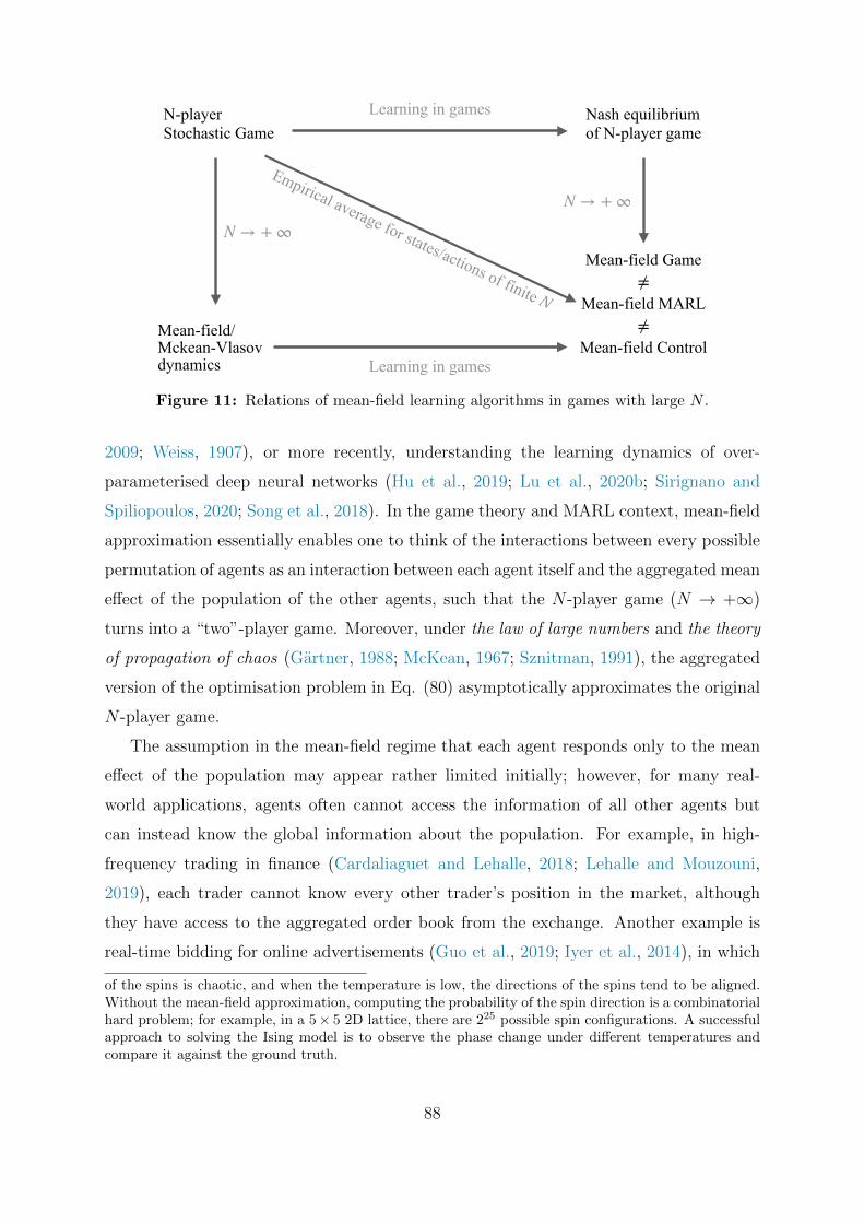
N-player Stochastic Game

Learning in games Nash equilibrium of N-player game

N → + ∞N → + ∞

Mean-field/Mckean-Vlasov dynamics Learning in games

Mean-field Game

Mean-field Control

Mean-field MARL≠

≠

Empirical average for states/actions of finite N

Figure 11: Relations of mean-field learning algorithms in games with large N .

2009; Weiss, 1907), or more recently, understanding the learning dynamics of over-

parameterised deep neural networks (Hu et al., 2019; Lu et al., 2020b; Sirignano and

Spiliopoulos, 2020; Song et al., 2018). In the game theory and MARL context, mean-field

approximation essentially enables one to think of the interactions between every possible

permutation of agents as an interaction between each agent itself and the aggregated mean

effect of the population of the other agents, such that the N -player game (N → +∞)

turns into a “two”-player game. Moreover, under the law of large numbers and the theory

of propagation of chaos (Gartner, 1988; McKean, 1967; Sznitman, 1991), the aggregated

version of the optimisation problem in Eq. (80) asymptotically approximates the original

N -player game.

The assumption in the mean-field regime that each agent responds only to the mean

effect of the population may appear rather limited initially; however, for many real-

world applications, agents often cannot access the information of all other agents but

can instead know the global information about the population. For example, in high-

frequency trading in finance (Cardaliaguet and Lehalle, 2018; Lehalle and Mouzouni,

2019), each trader cannot know every other trader’s position in the market, although

they have access to the aggregated order book from the exchange. Another example is

real-time bidding for online advertisements (Guo et al., 2019; Iyer et al., 2014), in which

of the spins is chaotic, and when the temperature is low, the directions of the spins tend to be aligned.Without the mean-field approximation, computing the probability of the spin direction is a combinatorialhard problem; for example, in a 5× 5 2D lattice, there are 225 possible spin configurations. A successfulapproach to solving the Ising model is to observe the phase change under different temperatures andcompare it against the ground truth.

88

participants can only observe, for example, the second-best prize that wins the auction

but not the individual bids from other participants.

There is a subtlety associated with types of games in which one applies the mean-field

theory. If one applies the mean-field type theory in non-cooperative53 games, in which

agents act independently to maximise their own individual reward, and the solution

concept is NE, then the scenario is usually referred to as a mean-field game (MFG)

(Gueant et al., 2011; Huang et al., 2006; Jovanovic and Rosenthal, 1988; Lasry and

Lions, 2007). If one applies mean-field theory in cooperative games in which there exists

a central controller to control all agents cooperatively to reach some Pareto optima,

then the situation is usually referred to as mean-field control (MFC) (Andersson and

Djehiche, 2011; Bensoussan et al., 2013), or McKean-Vlasov dynamics (MKV) control.

If one applies the mean-field approximation to solve a standard SG through MARL,

specifically, to factorise each agent’s reward function or the joint-Q function, such that

they depend only on the agent’s local state and the mean action of others, then it is

called mean-field MARL (MF-MARL) (Subramanian et al., 2020; Yang et al., 2018b;

Zhou et al., 2019).

Despite the difference in the applicable game types, technically, the differences among

MFG/MFC/MF-MARL can be elaborated from the perspective of the order in which

the equilibrium is learned (optimised) and the limit as N → +∞ is taken (Carmona

et al., 2013). MFG learns the equilibrium of the game first and then takes the limit as

N → +∞, while MFC takes the limit first and optimises the equilibrium later. MF-

MARL is somewhat in between. The mean-field in MF-MARL refers to the empirical

average of the states and/or actions of a finite population; N does not have to reach

infinity, though the approximation converges asymptotically to the original game when

N is large. This result is in contrast to the mean-field in MFG and MFC, which is

essentially a probability distribution of states and/or actions of an infinite population

(i.e., the Mckean-Vlasov dynamics). Before providing more details, we summarise the

relationships of MFG, MFC, and MF-MARL in Figure 11. Readers are recommended to

revisit their differences after finishing reading the below subsections.

53Note that the word “non-cooperative” does not mean agents cannot collaborate to complete a task,it means agents cannot collude to form a coalition: they have to behave independently.

89

9.1 Non-cooperative Mean-Field Game

MFGs have been widely studied in different domains, including physics, economics, and

stochastic control (Carmona et al., 2018; Gueant et al., 2011). An intuitive example to

quickly illustrate the idea of MFG is the problem of when does the meeting start (Gueant

et al., 2011). For a meeting in the real world, people often schedule a calendar time t in

advance, and the actual start time T depends on when the majority of participants (e.g.,

90%) arrive. Each participant plans to arrive at τ i, and the actual arrival time, τ i = τ i +

σiεi, is often influenced by some uncontrolled factors σiεi, εi ∼ N (0, 1), such as weather

or traffic. Assuming all players are rational, they do not want to be later than either t or

T ; moreover, they do not want to arrive too early and have to wait. The cost function of

each individual can be written as ci(t, T, τ i) = E[αbτ i− tc+ + βbτ i− T c+ + γbT − τ ic+

],

where α, β, γ are constants. The key question to ask is when is the best time for an agent

to arrive, as a result, when will the meeting actually start, i.e., what is T?

The challenge of the above problem lies in the coupled relationship between T and

τ i; that is, in order to compute T , we need to know τ i, which is based on T itself.

Therefore, solving the time T is essentially equivalent to finding the fixed point, if it

exists, of the stochastic process that generates T . In fact, T can be effectively computed

through a two-step iterative process, and we denote as Γ 1 and Γ 2. At Γ 1, given the

current54 value of T , each agent solves their optimal arrival time τ i by minimising their

cost Ri(t, T, τ i). At Γ 2, agents calibrate the new estimate of T based on all τ i values

that were computed in Γ 1. Γ 1 and Γ 2 continue iterating until T converges to a fixed

point, i.e., Γ 2 Γ 1(T ∗) = T ∗. The key insight is that the interaction with other agents is

captured simply by the mean-field quantity. Since the meeting starts only when 90% of

the people arrive, if one considers a continuum of players with N → +∞, T becomes the

90th quantile of a distribution, and each agent can easily find the best response. This

result contrasts to the cases of a finite number of players, in which the ordered statistic

is intractable, especially when N is large (but still finite).

Approximating an N -player SG by letting N → +∞ and letting each player choose

an optimal strategy in response to the population’s macroscopic information (i.e., the

mean field), though analytically friendly, is not cost-free. In fact, MFG makes two ma-

jor assumptions: 1) the impact of each player’s action on the outcome is infinitesimal,

54At time step 0, it can be a random guess. Since the fixed point exists, the final convergence resultis irrelevant to the initial guess.

90

resulting in all agents being identical, interchangeable, and indistinguishable; 2) each

player maintains weak interactions with others only through a mean field, denoted by

Li ∈ ∆|S||A|, which is essentially a population state-action joint distribution

Li =(µ−i(·), α−i(·)

)= lim

N→+∞

(∑j 6=i 1(sj = ·)N − 1

,

∑j 6=i 1(aj = ·)N − 1

)(78)

where sj and aj player j’s local state55 and local action. Therefore, for SGs that do

not share the homogeneity assumption56 and weak interaction assumption, MFG is not

an effective approximation. Furthermore, since agents have no identity in MFG, one can

choose a representative agent (the agent index is thus omitted) and write the formulation57

of the MFG as

V(s, π,

Lt∞t=0

):= E

[∞∑

t=0

γtR (st, at, Lt)∣∣∣s0 = s

]

subject to st+1 ∼ P (st, at, Lt) , at ∼ πt (st) . (79)

Each agent applies a local policy58 πt : S→ ∆(A), which assumes the population state is

not observable. Note that both the reward function and the transition dynamics depend

on the sequence of the mean-field terms Lt∞t=0. From each agent’s perspective, the MDP

is time-varying and is determined by all other agents.

The solution concept in MFG is a variant of the (Markov perfect) NE named the mean-

field equilibrium, which is a pair of π∗t , L∗tt≥0 that satisfies two conditions: 1) for fixed

L∗ = L∗t, π∗ = π∗t is the optimal policy, that is, V (s, π∗, L∗) ≥ V (s, π, L∗), ∀π, s; 2)

L∗ matches with the generated mean field when agents follow π∗. The two-step iteration

process in the meeting start-time example applied in MFG is then expressed as Γ 1(Lt) =

π∗t and Γ 2(Lt, π∗t ) = Lt+1, and it terminates when Γ 2 Γ 1(L) = L = L∗. Mean-field

55Note that in mean-field learning in games, the state is not assumed to be global. This is differentfrom Dec-POMDP, in which there exists an observation function that maps the global state to the localobservation for each agent.

56In fact, the homogeneity in MFG can be relaxed to allow agents to have (finite) different types(Lacker and Zariphopoulou, 2019), though within each type, agents must be homogeneous.

57MFG is more commonly formulated in a continuous-time setting in the domain of optimal control,where it is typically composed by a backward Hamilton-Jacobi-Bellman equation (e.g., the Bellman equa-tion in RL is its discrete-time counterpart) that describes the optimal control problem of an individualagent and a forward Fokker-Planck equation that describes the dynamics of the aggregate distribution(i.e., the mean field) of the population.

58A general non-local policy π(s, L) : S × ∆|S||A| → ∆(A) is also valid for MFG, and it makes thelearning easier by assuming L is fully observable.

91

equilibrium is essentially a fixed point of MFG, its existence for discrete-time59 discounted

MFGs has been verified by Saldi et al. (2018) in the infinite-population limit N →+∞ and also in the partially observable setting (Saldi et al., 2019). However, these

works consider the case where the mean field in MFG includes only the population state.

Recently, Guo et al. (2019) demonstrated the existence of NE in MFG, taking into account

both the population states and actions distributions. In addition, they proved that if Γ 1

and Γ 2 meet small parameter conditions (Huang et al., 2006), then the NE is unique in

the sense of L∗. In terms of uniqueness, a common result is based on assuming monotonic

cost functions (Lasry and Lions, 2007). In general, MFGs admit multiple equilibria (Nutz

et al., 2020); the reachability of multiple equilibria is studied when the cost functions are

anti-monotonic (Cecchin et al., 2019) or quadratic (Delarue and Tchuendom, 2020).

Based on the two-step fixed-point iteration in MFGs, various model-free RL algo-

rithms have been proposed for learning the NE. The idea is that in the step Γ 1, one can

approximate the optimal πt given Lt through single-agent RL algorithms60 such as (deep)

Q-learning (Anahtarcı et al., 2019; Anahtarci et al., 2020; Guo et al., 2019), (deep) policy-

gradient methods (Elie et al., 2020; Guo et al., 2020; Subramanian and Mahajan, 2019;

uz Zaman et al., 2020), and actor-critic methods (Fu et al., 2019; Yang et al., 2019b).

Then, in step Γ 2, one can compute the forward Lt+1 by sampling the new πt directly

or via fictitious play (Cardaliaguet and Hadikhanloo, 2017; Elie et al., 2019; Hadikhan-

loo and Silva, 2019). A surprisingly good result is that the sample complexity of both

value-based and policy-based learning methods for MFG in fact shares the same order of

magnitude as those of single-agent RL algorithms (Guo et al., 2020). However, one major

subtlety of these learning algorithms for MFGs is how to obtain stable samples for Lt+1.

For example, Guo et al. (2020) discovered that applying a softmax policy for each agent

and projecting the mean-field quantity on an ε-net with finite cover help to significantly

stabilise the forward propagation of Lt+1.

59The existence of equilibrium in continuous-time MFGs is widely studied in the area of stochasticcontrol (Cardaliaguet et al., 2015; Carmona and Delarue, 2013; Carmona et al., 2016, 2015b; Fischeret al., 2017; Huang et al., 2006; Lacker, 2015, 2018; Lasry and Lions, 2007), though it may be of lessinterest to RL researchers.

60Since agents in MFG are homogeneous, if the representative agent reaches convergence, then thejoint policy is the NE. Additionally, given Lt, the MDP to the representative agent is stationary.

92

9.2 Cooperative Mean-Field Control

MFC maintains the same homogeneity assumption and weak interaction assumption as

MFG. However, unlike MFG, in which each agent behaves independently, there is a

central controller that coordinates all agents’ behaviours in the context of MFC. In coop-

erative multi-agent learning, assuming each agent observes only a local state, the central

controller maximises the aggregated accumulative reward:

supπ

1

N

N∑

i=1

Est+1∼P,at∼π

[∑

t

γtRi(st,at)∣∣∣s0 = s

]. (80)

Solving Eq. (80) is a combinatorial problem. Clearly, the sample complexity of applying

the Q-learning algorithm grows exponentially in N (Even-Dar and Mansour, 2003). To

avoid the curse of dimensionality in N , MFC (Carmona et al., 2018; Gu et al., 2019)

pushes N → +∞, and under the law of large numbers and the theory of propagation of

chaos (Gartner, 1988; McKean, 1967; Sznitman, 1991), the optimisation problem in Eq.

(80), in the view of a representative agent, can be equivalently written as

supπ

E[∑

t

γtR(st, at, µt, αt)∣∣∣s0 ∼ µ

]

subject to st+1 ∼ P (st, at, µt, αt) , at ∼ πt (st, µt) . (81)

in which (µt, αt) is the respective state and action marginal distribution of the mean-

field quantity, µt(·) = limN→+∞∑N

i=1 1(sit = ·)/N , αt(·) =∑

s∈S µt(s) · πt (s, µt) (·), and

R = limN→+∞∑

iRi/N. The MFC approach is attractive not only because the dimension

of MFC is independent of N , but also because MFC has shown to approximate the

original cooperative game in terms of both game values and optimal strategies (Lacker,

2017; Motte and Pham, 2019).

Although the MFC formulation in Eq. (81) appears similar to the MFG formulation in

Eq. (79), their underlying physical meaning is fundamentally different. As is illustrated

in Figure 11, the difference is which operation is performed first: learning the equilibrium

of the N -player game or taking the limit as N → +∞. In the fixed-point iteration of

MFG, one first assumes Lt is given and then lets the (infinite) number of agents find the

best response to Lt, while in MFC, one assumes an infinite number of agents to avoid the

curse of dimensionality in cooperative MARL and then finds the optimal policy for each

93

agent from a central controller perspective. In addition, compared to mean-field NE in

MFG, the solution concept of the central controller in MFC is the Pareto optimum61, an

equilibrium point where no individual can be better off without making others worse off.

Finally, other differences between MFG and MFC can be found in Carmona et al. (2013).

In MFC, since the marginal distribution of states serves as an input in the agent’s

policy and is no longer assumed to be known in each iteration (in contrast to MFG),

the dynamic programming principle no longer holds in MFC due to its non-Markovian

nature (Andersson and Djehiche, 2011; Buckdahn et al., 2011; Carmona et al., 2015a).

That is, MFC problems are inherently time-inconsistent. A counter-example of the failure

of standard Q-learning in MFC can be found in Gu et al. (2019). One solution is to

learn MFC by adding common noise to the underlying dynamics such that all existing

theory on learning MDP with stochastic dynamics can be applied, such as Q-learning

(Carmona et al., 2019b). In the special class of linear-quadratic MFCs, Carmona et al.

(2019a) studied the policy-gradient method and its convergence, and Luo et al. (2019)

explored an actor-critic algorithm. However, this approach of adding common noise still

suffers from high sample complexity and weak empirical performance (Gu et al., 2019).

Importantly, applying dynamic programming in this setting lacks rigorous verifications,

leaving aside the measurability issues and the existence of a stationary optimal policy.

Another way to address the time inconsistency in MFCs is to consider an enlarged

state-action space (Djete et al., 2019; Gu et al., 2019; Lauriere and Pironneau, 2014;

Pham and Wei, 2016, 2017, 2018). This technique is also called “lift up”, which essentially

means to lift up the state space and the action space into their corresponding probability

measure spaces in which dynamic programming principles hold. For example, Gu et al.

(2019); Motte and Pham (2019) proposed to lift the finite state-action space S and A to a

compact state-action space embedded in Euclidean space denoted by C := ∆(S)×H and

H :=h : S→ ∆(A)

, and the optimal Q-function associated with the MFC problem in

Eq. (81) is

QC(µ, h) = supπ

E

[ ∞∑

t=0

γtR(st, at, µt, αt

)∣∣∣s0 ∼ µ, u0 ∼ α, at ∼ πt],∀(µ, h) ∼ C. (82)

The physical meaning of H is the set of all possible local policies h : S→ ∆(A) over all

different states. Note that after lift up, the mean-field term µt in πt of Eq. (81) no longer

exists as an input to h. Although the support of each h is |∆(A)||S|, it proves to be the

61The Pareto optimum is a subset of NE.

94

minimum space under which the Bellman equation can hold. The Bellman equation for

QC : C → R is

QC(µ, h) = R(µ, h

)+ γ sup

h∈HQC

(Φ(µ, h), h

)(83)

where R and Φ are the reward function and transition dynamics written as

R(µ, h

)=∑

s∈S

∑

a∈A

R(s, a, µ, α(µ, h)

)· µ(s) · h(s)(a) (84)

Φ(µ, h

)=∑

s∈S

∑

a∈A

P(s, a, µ, α(µ, h)

)· µ(s) · h(s)(a) (85)

with α(µ, h)(·) :=∑

s∈S µ(s) · h(s)(·) representing the marginal distribution of the mean-

field quantity in action. The optimal value function is V ∗(µ) = maxh∈HQC(µ, h

). Since

both µ and h are probability distributions, the difficulty of learning MFC then changes to

how to deal with continuous state and continuous action inputs to QC(µ, h), which is still

an open research question. Gu et al. (2020) tried to discretise the lifted space C through

ε-net and then adopted the kernel regression on top of the discretisation; impressively,

the sample complexity of the induced Q-learning algorithm is independent of the number

of agents N .

9.3 Mean-Field MARL

The scalability issue of multi-agent learning in non-cooperative general-sum games can

also be alleviated by applying the mean-field approximation directly to each agent’s Q-

function (Subramanian et al., 2020; Yang et al., 2018b; Zhou et al., 2019). In fact, Yang

et al. (2018b) was the first to combine mean-field theory with the MARL algorithm. The

idea is to first factorise the Q-function using only the local pairwise interactions between

agents (see Eq. (86)) and then apply the mean-field approximation; specifically, one

can write the neighbouring agent’s action ak as the sum of the mean action aj and a

fluctuation term δaj,k, i.e., ak = aj + δaj,k, aj = 1Nj

∑k a

k, in which N (j) is the set of

neighbouring agents of the learning agent j with its size being N j = |N j|. With the above

two processes, we can reach the mean-field Q-function Qj(s, aj, aj) that approximates

95

Qj(s, a) as follows

Qj(s,a)

=1

N j

∑

k

Qj(s, aj , ak

)(86)

=1

N j

∑

k

[Qj(s, aj , aj

)+∇ajQj

(s, aj , aj

)· δaj,k

+1

2δaj,k · ∇2

aj,kQj(s, aj , aj,k

)· δaj,k

](87)

= Qj(s, aj , aj

)+∇ajQj

(s, aj , aj

)·[

1

N j

∑

k

δaj,k]

+1

2N j

∑

k

[δaj,k · ∇2

aj,kQj(s, aj , aj,k

)· δaj,k

](88)

= Qj(s, aj , aj

)+

1

2N j

∑

k

Rjs,aj

(ak)

≈ Qj(s, aj , aj

). (89)

The second term in Eq. (88) is zero by definition, and the third term can be bounded if

the Q-function is smooth, and it is neglected on purpose. The mean-field action aj can

be interpreted as the empirical distribution of the actions taken by agent j’s neighbours.

However, unlike the mean-field quantity in MFG or MFC, this quantity does not have to

assume an infinite population of agents, which is more friendly for many real-world tasks,

although a large N can reduce the approximation error between ak and aj due to the law

of large numbers. In addition, the mean-field term in MF-MARL does not include the

state distribution, unlike MFG or MFC.

Based on the mean-field Q-function, one can write the Q-learning update as

Qjt+1

(s, aj , aj

)=(1− α

)Qjt(s, aj , aj

)+ α

[Rj + γvj,MF

t

(s′)]

vj,MFt

(s′)

=∑

aj

πjt(aj | s′, aj

)· E

aj(a−j)∼π−jt

[Qjt(s′, aj , aj

)]. (90)

The mean action aj depends on aj, j ∈ N (j), which itself depends on the mean action.

The chicken-and-egg problem is essentially the time inconsistency that also occurs in

MFC. To avoid coupling between aj and aj, Yang et al. (2018b) proposed a filtration

such that in each stage game Qt, the mean action aj is computed first using each

agents’ current policies, i.e., aj = 1Nj

∑k a

k, ak ∼ πkt , and then given aj , each agent finds

96

the best response by

πjt(aj | s, aj

)=

exp(βQjt

(s, aj , aj

))

∑aj∈Aj exp

(βQjt (s, aj′ , aj )

) . (91)

For large β, the Boltzmann policy in Eq. (91) proves to be a contraction mapping, which

means the optimal action aj is unique given aj ; therefore, the chicken-and-egg problem

is resolved62.

MF-Q can be regarded as a modification of the Nash-Q learning algorithm (Hu

and Wellman, 2003), with the solution concept changed from NE to mean-field NE

(see the definition in MFG). As a result, under the same conditions, which include

the strong assumption that there exists a unique NE at every stage game encountered,

HMFQ(s,a) = Es′∼p[R(s,a) + γvMF (s′)

]proves to be a contraction operator. Further-

more, the asymptotic convergence of the MF-Q learning update in Eq. (90) has also been

established.

Considering only pairwise interactions in MF-Q may appear rather limited. How-

ever, it has been noted that the pairwise approximation of the agent and its neighbours,

while significantly reducing the complexity of the interactions among agents, can still

preserve global interactions between any pair of agents (Blume, 1993). In fact, such an

approach is widely adopted in other machine learning domains, for example, factorisa-

tion machines (Rendle, 2010) and learning to rank (Cao et al., 2007). Based on MF-Q,

Li et al. (2019a) solved the real-world taxi order dispatching task for Uber China and

demonstrated strong empirical performance against humans. Subramanian and Mahajan

(2019) extended MF-Q to include multiple types of agents and applied the method to

a large-scale predator-prey simulation scenario. Ganapathi Subramanian et al. (2020)

further relaxed the assumption that agents have access to exact cumulative metrics re-

garding the mean-field behaviour of the system, and proposed partially observable MF-Q

that maintains a distribution to model the uncertainty regarding the mean field of the

system.

62Coincidentally, the techniques of fixing the mean-field term first and adopting the Boltzmann policyfor each agent were discovered by Guo et al. (2019) in learning MFGs at the same time.

97

10 Future Directions of Interest

MARL Theory. In contrast to the remarkable empirical success of MARL methods,

developing theoretical understandings of MARL techniques are very much under-explored

in the literature. Although many early works have been conducted on understanding the

convergence property and the finite-sample bound of single-agent RL algorithms (Bert-

sekas and Tsitsiklis, 1996), extending those results into multi-agent, even many-agent,

settings seem to be non-trivial. Furthermore, it has become a common practice nowa-

days to use DNNs to represent value functions in RL and multi-agent RL. In fact, many

recent remarkable successes of multi-agent RL benefit from the success of deep learning

techniques (Baker et al., 2019b; Pachocki et al., 2018; Vinyals et al., 2019b). Therefore,

there are pressing needs to develop theories that could explain and offer insights into

the effectiveness of deep MARL methods. Overall, I believe there is an approximate

ten-year gap between the theoretical developments of single-agent RL and multi-agent

RL algorithms. Learning the lessons from single-agent RL theories and extending them

into multi-agent settings, especially understanding the incurred difficulty due to involv-

ing multiple agents, and then generalising the theoretical results to include DNNs could

probably act as a practical road map in developing MARL theories. Along this thread,

I recommend the work of Zhang et al. (2019b) for a comprehensive summary of existing

MARL algorithms that come with theoretical convergence guarantee.

Safe and Robust MARL. Although RL provides a general framework for optimal

decision making, it has to incorporate certain types of constraints when RL models are

truly to be deployed in the real-world environment. I believe it is critical to firstly account

for MARL with robustness and safety constraints; one direct example is on autonomous

driving. At a very high level, robustness refers to the property that an algorithm can

generalise and maintain robust performance in settings that are different from the training

environment (Abdullah et al., 2019; Morimoto and Doya, 2005). And safety refers to the

property that an algorithm can only act in a pre-defined safety zone with minimum

times of violations even during training time (Garcıa and Fernandez, 2015). In fact, the

community is still at the early stage of developing theoretical frameworks to encompass

either robust or safe constraint in single-agent settings. In the multi-agent setting, the

problem could only become more challenging because the solution now requires to take

into account the coupling effect between agents, especially those agents that have conflict

98

interests (Li et al., 2019b). In addition to opponents, one should also consider robustness

towards the uncertainty of environmental dynamics (Zhang et al., 2020), which in turn

will change the behaviours of opponents and pose a more significant challenge.

Model-Based MARL. Most of the algorithms I have introduced in this monograph

are model-free, in the sense that the RL agent does not need to know how the envi-

ronment works and it can learn how to behave optimally through purely interacting

with the environment. In the classic control domain, model-based approaches have been

extensively studied in which the learning agent will first build an explicit state-space

“model” to understand how the environment works in terms of state-transition dynam-

ics and reward function, and then learn from the “model”. The benefit of model-based

algorithms lies in the fact that they often require much fewer data samples from the en-

vironment (Deisenroth and Rasmussen, 2011). The MARL community has initially come

up with model-based approaches, for example the famous R-MAX algorithm (Brafman

and Tennenholtz, 2002), nearly two decades ago. Surprisingly, the developments along

the model-based thread halted ever since. Given the impressive results that model-based

approaches have demonstrated on single-agent RL tasks (Hafner et al., 2019a,b; Schrit-

twieser et al., 2020), model-based MARL approaches deserves more attention from the

community.

Multi-Agent Meta-RL. Throughout this monograph, I have introduced many MARL

applications; each task needs a bespoke MARL model to solve. A natural question to

ask is whether we can use one model that can generalise across multiple tasks. For

example, Terry et al. (2020) has put together almost one hundred MARL tasks, including

Atari, robotics, and various kinds of board games and pokers into a Gym API. An

ambitious goal is to develop algorithms that can solve all of the tasks in one or a few

shots. This requires multi-agent meta-RL techniques. Meta-learning aims to train a

generalised model on a variety of learning tasks, such that it can solve new learning

tasks with few or without additional training samples. Fortunately, Finn et al. (2017)

has proposed a general meta-learning framework – MAML – that is compatible with any

model trained with gradient-descent based methods. Although MAML works well on

supervised learning tasks, developing meta-RL algorithms seems to be highly non-trivial

(Rothfuss et al., 2018), and introducing the meta-learning framework on top of MARL is

99

even an uncharted territory. I expect multi-agent meta-RL to be a challenging yet fruitful

research topic, since making a group of agents master multiple games necessarily requires

agents to automatically discover their identities and roles when playing different games;

this itself is a hot research idea. Besides, the meta-learner in the outer loop would need to

figure out how to compute the gradients with respect to the entire inner-loop subroutine,

which must be a MARL algorithm such as multi-agent policy gradient method or mean-

field Q-learning, and, this would probably lead to exciting enhancements to the existing

meta-learning framework.

100

References

Abbasi-Yadkori, Y., Bartlett, P., Bhatia, K., Lazic, N., Szepesvari, C., and Weisz, G.(2019). Politex: Regret bounds for policy iteration using expert prediction. In Inter-national Conference on Machine Learning, pages 3692–3702.

Abdallah, S. and Lesser, V. (2008). A multiagent reinforcement learning algorithm withnon-linear dynamics. Journal of Artificial Intelligence Research, 33:521–549.

Abdullah, M. A., Ren, H., Ammar, H. B., Milenkovic, V., Luo, R., Zhang, M., and Wang,J. (2019). Wasserstein robust reinforcement learning. arXiv preprint arXiv:1907.13196.

Adler, I. (2013). The equivalence of linear programs and zero-sum games. InternationalJournal of Game Theory, 42(1):165–177.

Adler, J. L. and Blue, V. J. (2002). A cooperative multi-agent transportation managementand route guidance system. Transportation Research Part C: Emerging Technologies,10(5-6):433–454.

Adolphs, L., Daneshmand, H., Lucchi, A., and Hofmann, T. (2019). Local saddle pointoptimization: A curvature exploitation approach. In The 22nd International Confer-ence on Artificial Intelligence and Statistics, pages 486–495.

Al-Tamimi, A., Lewis, F. L., and Abu-Khalaf, M. (2007). Model-free q-learning designs forlinear discrete-time zero-sum games with application to h-infinity control. Automatica,43(3):473–481.

Amato, C., Bernstein, D. S., and Zilberstein, S. (2010). Optimizing fixed-size stochasticcontrollers for pomdps and decentralized pomdps. Autonomous Agents and Multi-AgentSystems, 21(3):293–320.

Anahtarcı, B., Karıksız, C. D., and Saldi, N. (2019). Fitted q-learning in mean-fieldgames. arXiv preprint arXiv:1912.13309.

Anahtarci, B., Kariksiz, C. D., and Saldi, N. (2020). Q-learning in regularized mean-fieldgames. arXiv preprint arXiv:2003.12151.

Andersson, D. and Djehiche, B. (2011). A maximum principle for sdes of mean-field type.Applied Mathematics & Optimization, 63(3):341–356.

Arslan, G. and Yuksel, S. (2016). Decentralized q-learning for stochastic teams andgames. IEEE Transactions on Automatic Control, 62(4):1545–1558.

Auer, P., Cesa-Bianchi, N., Freund, Y., and Schapire, R. E. (1995). Gambling in a riggedcasino: The adversarial multi-armed bandit problem. In Proceedings of IEEE 36thAnnual Foundations of Computer Science, pages 322–331. IEEE.

Auer, P., Cesa-Bianchi, N., Freund, Y., and Schapire, R. E. (2002). The nonstochasticmultiarmed bandit problem. SIAM journal on computing, 32(1):48–77.

101

Auer, P., Jaksch, T., and Ortner, R. (2009). Near-optimal regret bounds for reinforcementlearning. In Advances in neural information processing systems, pages 89–96.

Azar, M. G., Osband, I., and Munos, R. (2017). Minimax regret bounds for reinforcementlearning. In International Conference on Machine Learning, pages 263–272.

Baker, B., Kanitscheider, I., Markov, T., Wu, Y., Powell, G., McGrew, B., and Mor-datch, I. (2019a). Emergent tool use from multi-agent autocurricula. In InternationalConference on Learning Representations.

Baker, B., Kanitscheider, I., Markov, T. M., Wu, Y., Powell, G., McGrew, B., andMordatch, I. (2019b). Emergent tool use from multi-agent autocurricula. CoRR,abs/1909.07528.

Balduzzi, D., Garnelo, M., Bachrach, Y., Czarnecki, W., Perolat, J., Jaderberg, M., andGraepel, T. (2019). Open-ended learning in symmetric zero-sum games. In ICML,volume 97, pages 434–443. PMLR.

Balduzzi, D., Racaniere, S., Martens, J., Foerster, J., Tuyls, K., and Graepel, T. (2018a).The mechanics of n-player differentiable games. In ICML, volume 80, pages 363–372.JMLR. org.

Balduzzi, D., Tuyls, K., Perolat, J., and Graepel, T. (2018b). Re-evaluating evaluation.In Advances in Neural Information Processing Systems, pages 3268–3279.

Bellman, R. (1952). On the theory of dynamic programming. Proceedings of the NationalAcademy of Sciences of the United States of America, 38(8):716.

Benaım, M. and Faure, M. (2013). Consistency of vanishingly smooth fictitious play.Mathematics of Operations Research, 38(3):437–450.

Benaım, M. and Hirsch, M. W. (1999). Mixed equilibria and dynamical systems arisingfrom fictitious play in perturbed games. Games and Economic Behavior, 29(1-2):36–72.

Benders, J. (1962). Partitioning procedures for solving mixed-variable program-mingproblems, numerische matkematic 4.

Bengio, Y. (2009). Learning deep architectures for AI. Now Publishers Inc.

Bensoussan, A., Frehse, J., Yam, P., et al. (2013). Mean field games and mean field typecontrol theory, volume 101. Springer.

Berger, U. (2007). Brown’s original fictitious play. Journal of Economic Theory,135(1):572–578.

Bernstein, D. S., Amato, C., Hansen, E. A., and Zilberstein, S. (2009). Policy iterationfor decentralized control of markov decision processes. Journal of Artificial IntelligenceResearch, 34:89–132.

Bernstein, D. S., Givan, R., Immerman, N., and Zilberstein, S. (2002). The complexity ofdecentralized control of markov decision processes. Mathematics of operations research,27(4):819–840.

102

Bertsekas, D. P. (2005). The dynamic programming algorithm. Dynamic Programmingand Optimal Control; Athena Scientific: Nashua, NH, USA, pages 2–51.

Bertsekas, D. P. and Tsitsiklis, J. N. (1996). Neuro-dynamic programming. AthenaScientific.

Billings, D., Burch, N., Davidson, A., Holte, R., Schaeffer, J., Schauenberg, T., andSzafron, D. (2003). Approximating game-theoretic optimal strategies for full-scalepoker. In IJCAI, volume 3, page 661.

Blackwell, D. et al. (1956). An analog of the minimax theorem for vector payoffs. PacificJournal of Mathematics, 6(1):1–8.

Blei, D. M., Kucukelbir, A., and McAuliffe, J. D. (2017). Variational inference: A reviewfor statisticians. Journal of the American statistical Association, 112(518):859–877.

Bloembergen, D., Tuyls, K., Hennes, D., and Kaisers, M. (2015). Evolutionary dynamicsof multi-agent learning: A survey. Journal of Artificial Intelligence Research, 53:659–697.

Blume, L. E. (1993). The statistical mechanics of strategic interaction. Games andeconomic behavior, 5(3):387–424.

Borkar, V. S. (1997). Stochastic approximation with two time scales. Systems & ControlLetters, 29(5):291–294.

Borkar, V. S. (2002). Reinforcement learning in markovian evolutionary games. Advancesin Complex Systems, 5(01):55–72.

Boutilier, C., Dean, T., and Hanks, S. (1999). Decision-theoretic planning: Structuralassumptions and computational leverage. Journal of Artificial Intelligence Research,11:1–94.

Bowling, M. (2000). Convergence problems of general-sum multiagent reinforcementlearning. In ICML, pages 89–94.

Bowling, M. (2005). Convergence and no-regret in multiagent learning. In Advances inneural information processing systems, pages 209–216.

Bowling, M. and Veloso, M. (2000). An analysis of stochastic game theory for multiagentreinforcement learning. Technical report, Carnegie-Mellon Univ Pittsburgh Pa Schoolof Computer Science.

Bowling, M. and Veloso, M. (2001). Rational and convergent learning in stochastic games.In International joint conference on artificial intelligence, volume 17, pages 1021–1026.Lawrence Erlbaum Associates Ltd.

Bowling, M. and Veloso, M. (2002). Multiagent learning using a variable learning rate.Artificial Intelligence, 136(2):215–250.

103

Brafman, R. I. and Tennenholtz, M. (2002). R-max-a general polynomial time algo-rithm for near-optimal reinforcement learning. Journal of Machine Learning Research,3(Oct):213–231.

Breton, M., Filar, J. A., Haurle, A., and Schultz, T. A. (1986). On the computation ofequilibria in discounted stochastic dynamic games. In Dynamic games and applicationsin economics, pages 64–87. Springer.

Brown, N., Kroer, C., and Sandholm, T. (2017). Dynamic thresholding and pruning forregret minimization. In AAAI, pages 421–429.

Brown, N., Lerer, A., Gross, S., and Sandholm, T. (2019). Deep counterfactual regretminimization. In International Conference on Machine Learning, pages 793–802.

Brown, N. and Sandholm, T. (2015). Regret-based pruning in extensive-form games. InAdvances in Neural Information Processing Systems, pages 1972–1980.

Brown, N. and Sandholm, T. (2017). Reduced space and faster convergence in imperfect-information games via pruning. In International conference on machine learning, pages596–604.

Brown, N. and Sandholm, T. (2018). Superhuman ai for heads-up no-limit poker: Libratusbeats top professionals. Science, 359(6374):418–424.

Brown, N. and Sandholm, T. (2019). Superhuman ai for multiplayer poker. Science,365(6456):885–890.

Brown, T. B., Mann, B., Ryder, N., Subbiah, M., Kaplan, J., Dhariwal, P., Neelakantan,A., Shyam, P., Sastry, G., Askell, A., et al. (2020). Language models are few-shotlearners. arXiv preprint arXiv:2005.14165.

Browne, C. B., Powley, E., Whitehouse, D., Lucas, S. M., Cowling, P. I., Rohlfshagen,P., Tavener, S., Perez, D., Samothrakis, S., and Colton, S. (2012). A survey of montecarlo tree search methods. IEEE Transactions on Computational Intelligence and AIin games, 4(1):1–43.

Bu, J., Ratliff, L. J., and Mesbahi, M. (2019). Global convergence of policy gradient forsequential zero-sum linear quadratic dynamic games. arXiv, pages arXiv–1911.

Buckdahn, R., Djehiche, B., and Li, J. (2011). A general stochastic maximum principlefor sdes of mean-field type. Applied Mathematics & Optimization, 64(2):197–216.

Burch, N., Lanctot, M., Szafron, D., and Gibson, R. G. (2012). Efficient monte carlocounterfactual regret minimization in games with many player actions. In Advances inNeural Information Processing Systems, pages 1880–1888.

Busoniu, L., Babuska, R., and De Schutter, B. (2010). Multi-agent reinforcement learning:An overview. In Innovations in multi-agent systems and applications-1, pages 183–221.Springer.

104

Cai, Q., Yang, Z., Jin, C., and Wang, Z. (2019a). Provably efficient exploration in policyoptimization. arXiv preprint arXiv:1912.05830.

Cai, Q., Yang, Z., Lee, J. D., and Wang, Z. (2019b). Neural temporal-difference learningconverges to global optima. In Advances in Neural Information Processing Systems,pages 11315–11326.

Camerer, C. F., Ho, T.-H., and Chong, J.-K. (2002). Sophisticated experience-weightedattraction learning and strategic teaching in repeated games. Journal of Economictheory, 104(1):137–188.

Camerer, C. F., Ho, T.-H., and Chong, J.-K. (2004). A cognitive hierarchy model ofgames. The Quarterly Journal of Economics.

Campos-Rodriguez, R., Gonzalez-Jimenez, L., Cervantes-Alvarez, F., Amezcua-Garcia,F., and Fernandez-Garcia, M. (2017). Multiagent systems in automotive applications.Multi-agent Systems, page 43.

Candogan, O., Menache, I., Ozdaglar, A., and Parrilo, P. A. (2011). Flows and decompo-sitions of games: Harmonic and potential games. Mathematics of Operations Research,36(3):474–503.

Cao, Z., Qin, T., Liu, T.-Y., Tsai, M.-F., and Li, H. (2007). Learning to rank: from pair-wise approach to listwise approach. In Proceedings of the 24th international conferenceon Machine learning, pages 129–136. ACM.

Cardaliaguet, P., Delarue, F., Lasry, J.-M., and Lions, P.-L. (2015). The master equationand the convergence problem in mean field games. arXiv preprint arXiv:1509.02505.

Cardaliaguet, P. and Hadikhanloo, S. (2017). Learning in mean field games: the fictitiousplay. ESAIM: Control, Optimisation and Calculus of Variations, 23(2):569–591.

Cardaliaguet, P. and Lehalle, C.-A. (2018). Mean field game of controls and an applicationto trade crowding. Mathematics and Financial Economics, 12(3):335–363.

Carmona, R. and Delarue, F. (2013). Probabilistic analysis of mean-field games. SIAMJournal on Control and Optimization, 51(4):2705–2734.

Carmona, R., Delarue, F., et al. (2015a). Forward–backward stochastic differential equa-tions and controlled mckean–vlasov dynamics. The Annals of Probability, 43(5):2647–2700.

Carmona, R., Delarue, F., et al. (2018). Probabilistic Theory of Mean Field Games withApplications I-II. Springer.

Carmona, R., Delarue, F., and Lachapelle, A. (2013). Control of mckean–vlasov dynamicsversus mean field games. Mathematics and Financial Economics, 7(2):131–166.

Carmona, R., Delarue, F., Lacker, D., et al. (2016). Mean field games with commonnoise. The Annals of Probability, 44(6):3740–3803.

105

Carmona, R., Lacker, D., et al. (2015b). A probabilistic weak formulation of mean fieldgames and applications. The Annals of Applied Probability, 25(3):1189–1231.

Carmona, R., Lauriere, M., and Tan, Z. (2019a). Linear-quadratic mean-field re-inforcement learning: convergence of policy gradient methods. arXiv preprintarXiv:1910.04295.

Carmona, R., Lauriere, M., and Tan, Z. (2019b). Model-free mean-field reinforcementlearning: mean-field mdp and mean-field q-learning. arXiv preprint arXiv:1910.12802.

Cecchin, A., Pra, P. D., Fischer, M., and Pelino, G. (2019). On the convergence problemin mean field games: a two state model without uniqueness. SIAM Journal on Controland Optimization, 57(4):2443–2466.

Cesa-Bianchi, N. and Lugosi, G. (2006). Prediction, learning, and games. Cambridgeuniversity press.

Chalmers, C. (2020). Is reinforcement learning worth the hype? 2020.URL https://www.capgemini.com/gb-en/2020/05/is-reinforcement-learning-worth-the-hype/.

Chasnov, B., Ratliff, L. J., Mazumdar, E., and Burden, S. A. (2019). Convergenceanalysis of gradient-based learning with non-uniform learning rates in non-cooperativemulti-agent settings. arXiv preprint arXiv:1906.00731.

Chen, X. and Deng, X. (2006). Settling the complexity of two-player nash equilibrium. In2006 47th Annual IEEE Symposium on Foundations of Computer Science (FOCS’06),pages 261–272. IEEE.

Cheung, W. C., Simchi-Levi, D., and Zhu, R. (2020). Reinforcement learning for non-stationary markov decision processes: The blessing of (more) optimism. ICML.

Claus, C. and Boutilier, C. (1998a). The dynamics of reinforcement learning in coopera-tive multiagent systems. AAAI/IAAI, 1998:746–752.

Claus, C. and Boutilier, C. (1998b). The dynamics of reinforcement learning in coopera-tive multiagent systems. AAAI/IAAI, 1998:746–752.

Conitzer, V. and Sandholm, T. (2002). Complexity results about nash equilibria. arXivpreprint cs/0205074.

Conitzer, V. and Sandholm, T. (2007). Awesome: A general multiagent learning algo-rithm that converges in self-play and learns a best response against stationary oppo-nents. Machine Learning, 67(1-2):23–43.

Conitzer, V. and Sandholm, T. (2008). New complexity results about nash equilibria.Games and Economic Behavior, 63(2):621–641.

Coricelli, G. and Nagel, R. (2009). Neural correlates of depth of strategic reasoning in me-dial prefrontal cortex. Proceedings of the National Academy of Sciences, 106(23):9163–9168.

106

Cowling, P. I., Powley, E. J., and Whitehouse, D. (2012). Information set monte carlo treesearch. IEEE Transactions on Computational Intelligence and AI in Games, 4(2):120–143.

Da Silva, F. L. and Costa, A. H. R. (2019). A survey on transfer learning for multiagentreinforcement learning systems. Journal of Artificial Intelligence Research, 64:645–703.

Dall’Anese, E., Zhu, H., and Giannakis, G. B. (2013). Distributed optimal power flowfor smart microgrids. IEEE Transactions on Smart Grid, 4(3):1464–1475.

Dantzig, G. (1951). A proof of the equivalence of the programming problem and thegame problem, in “activity analysis of production and allocation”(ed. tc koopmans),cowles commission monograph, no. 13.

Daskalakis, C., Goldberg, P. W., and Papadimitriou, C. H. (2009). The complexity ofcomputing a nash equilibrium. SIAM Journal on Computing, 39(1):195–259.

Daskalakis, C., Ilyas, A., Syrgkanis, V., and Zeng, H. (2017). Training gans with opti-mism. arXiv, pages arXiv–1711.

Daskalakis, C. and Panageas, I. (2018). The limit points of (optimistic) gradient descentin min-max optimization. In Advances in Neural Information Processing Systems, pages9236–9246.

Daskalakis, C. and Papadimitriou, C. H. (2005). Three-player games are hard. In Elec-tronic colloquium on computational complexity, volume 139, pages 81–87.

Deisenroth, M. and Rasmussen, C. E. (2011). Pilco: A model-based and data-efficientapproach to policy search. In Proceedings of the 28th International Conference onmachine learning (ICML-11), pages 465–472.

Delarue, F. and Tchuendom, R. F. (2020). Selection of equilibria in a linear quadraticmean-field game. Stochastic Processes and their Applications, 130(2):1000–1040.

Derakhshan, F. and Yousefi, S. (2019). A review on the applications of multiagent systemsin wireless sensor networks. International Journal of Distributed Sensor Networks,15(5):1550147719850767.

Dermed, L. M. and Isbell, C. L. (2009). Solving stochastic games. In Advances in NeuralInformation Processing Systems, pages 1186–1194.

Devlin, J., Chang, M.-W., Lee, K., and Toutanova, K. (2018). Bert: Pre-trainingof deep bidirectional transformers for language understanding. arXiv preprintarXiv:1810.04805.

Dibangoye, J. and Buffet, O. (2018). Learning to act in decentralized partially observablemdps. In International Conference on Machine Learning, pages 1233–1242.

Dibangoye, J. S., Amato, C., Buffet, O., and Charpillet, F. (2016). Optimally solving dec-pomdps as continuous-state mdps. Journal of Artificial Intelligence Research, 55:443–497.

107

Dick, T., Gyorgy, A., and Szepesvari, C. (2014). Online learning in markov decision pro-cesses with changing cost sequences. In International Conference on Machine Learning,pages 512–520.

Djete, M. F., Possamaı, D., and Tan, X. (2019). Mckean-vlasov optimal control: thedynamic programming principle. arXiv preprint arXiv:1907.08860.

Elie, R., Perolat, J., Lauriere, M., Geist, M., and Pietquin, O. (2019). Approximatefictitious play for mean field games. arXiv preprint arXiv:1907.02633.

Elie, R., Perolat, J., Lauriere, M., Geist, M., and Pietquin, O. (2020). On the convergenceof model free learning in mean field games. In AAAI, pages 7143–7150.

Erev, I. and Roth, A. E. (1998). Predicting how people play games: Reinforcement learn-ing in experimental games with unique, mixed strategy equilibria. American economicreview, pages 848–881.

Even-Dar, E., Kakade, S. M., and Mansour, Y. (2005). Experts in a markov decisionprocess. In Advances in neural information processing systems, pages 401–408.

Even-Dar, E., Kakade, S. M., and Mansour, Y. (2009). Online markov decision processes.Mathematics of Operations Research, 34(3):726–736.

Even-Dar, E. and Mansour, Y. (2003). Learning rates for q-learning. Journal of machinelearning Research, 5(Dec):1–25.

Fazel, M., Ge, R., Kakade, S., and Mesbahi, M. (2018). Global convergence of policygradient methods for the linear quadratic regulator. In International Conference onMachine Learning, pages 1467–1476.

Feinberg, E. A. (2010). Total expected discounted reward mdps: existence of optimalpolicies. Wiley Encyclopedia of Operations Research and Management Science.

Fiez, T., Chasnov, B., and Ratliff, L. J. (2019). Convergence of learning dynamics instackelberg games. arXiv, pages arXiv–1906.

Filar, J. and Vrieze, K. (2012). Competitive Markov decision processes. Springer Science& Business Media.

Finn, C., Abbeel, P., and Levine, S. (2017). Model-agnostic meta-learning for fast adap-tation of deep networks. In ICML.

Fischer, M. et al. (2017). On the connection between symmetric n-player games andmean field games. The Annals of Applied Probability, 27(2):757–810.

Foerster, J., Chen, R. Y., Al-Shedivat, M., Whiteson, S., Abbeel, P., and Mordatch,I. (2018a). Learning with opponent-learning awareness. In Proceedings of the 17thInternational Conference on Autonomous Agents and MultiAgent Systems, pages 122–130.

108

Foerster, J., Farquhar, G., Afouras, T., Nardelli, N., and Whiteson, S. (2017a). Counter-factual multi-agent policy gradients. arXiv preprint arXiv:1705.08926.

Foerster, J., Nardelli, N., Farquhar, G., Afouras, T., Torr, P. H., Kohli, P., and Whiteson,S. (2017b). Stabilising experience replay for deep multi-agent reinforcement learning.In Proceedings of the 34th International Conference on Machine Learning-Volume 70,pages 1146–1155.

Foerster, J. N., Farquhar, G., Afouras, T., Nardelli, N., and Whiteson, S. (2018b). Coun-terfactual multi-agent policy gradients. In McIlraith, S. A. and Weinberger, K. Q.,editors, Proceedings of the Thirty-Second AAAI Conference on Artificial Intelligence,New Orleans, Louisiana, USA, February 2-7, 2018. AAAI Press.

Freund, Y. and Schapire, R. E. (1997). A decision-theoretic generalization of on-linelearning and an application to boosting. Journal of computer and system sciences,55(1):119–139.

Fu, Z., Yang, Z., Chen, Y., and Wang, Z. (2019). Actor-critic provably finds nash equi-libria of linear-quadratic mean-field games. arXiv preprint arXiv:1910.07498.

Fudenberg, D., Drew, F., Levine, D. K., and Levine, D. K. (1998). The theory of learningin games, volume 2. MIT press.

Fudenberg, D. and Kreps, D. M. (1993). Learning mixed equilibria. Games and economicbehavior, 5(3):320–367.

Fudenberg, D. and Levine, D. (1995). Consistency and cautious fictitious play. Journalof Economic Dynamics and Control.

Ganapathi Subramanian, S., Taylor, M. E., Crowley, M., and Poupart, P. (2020). Partiallyobservable mean field reinforcement learning. arXiv e-prints, pages arXiv–2012.

Garcıa, J. and Fernandez, F. (2015). A comprehensive survey on safe reinforcementlearning. Journal of Machine Learning Research, 16(1):1437–1480.

Gartner, J. (1988). On the mckean-vlasov limit for interacting diffusions. MathematischeNachrichten, 137(1):197–248.

Gasser, R. and Huhns, M. N. (2014). Distributed Artificial Intelligence: Volume II,volume 2. Morgan Kaufmann.

Gibson, R. G., Lanctot, M., Burch, N., Szafron, D., and Bowling, M. (2012). Generalizedsampling and variance in counterfactual regret minimization. In AAAI.

Gigerenzer, G. and Selten, R. (2002). Bounded rationality: The adaptive toolbox. MITpress.

Gilpin, A., Hoda, S., Pena, J., and Sandholm, T. (2007). Gradient-based algorithms forfinding nash equilibria in extensive form games. In International Workshop on Weband Internet Economics, pages 57–69. Springer.

109

Gilpin, A. and Sandholm, T. (2006). Finding equilibria in large sequential games of im-perfect information. In Proceedings of the 7th ACM conference on Electronic commerce,pages 160–169.

Gonzalez-Sanchez, D. and Hernandez-Lerma, O. (2013). Discrete–time stochastic con-trol and dynamic potential games: the Euler–Equation approach. Springer Science &Business Media.

Goodfellow, I., Pouget-Abadie, J., Mirza, M., Xu, B., Warde-Farley, D., Ozair, S.,Courville, A., and Bengio, Y. (2014a). Generative adversarial nets. In NIPS, pages2672–2680.

Goodfellow, I. J., Shlens, J., and Szegedy, C. (2014b). Explaining and harnessing adver-sarial examples. arXiv preprint arXiv:1412.6572.

Gordon, G. J. (2007). No-regret algorithms for online convex programs. In Advances inNeural Information Processing Systems, pages 489–496.

Grau-Moya, J., Leibfried, F., and Bou-Ammar, H. (2018). Balancing two-player stochasticgames with soft q-learning. IJCAI.

Greenwald, A., Hall, K., and Serrano, R. (2003). Correlated q-learning. In ICML,volume 20, page 242.

Gu, H., Guo, X., Wei, X., and Xu, R. (2019). Dynamic programming principles forlearning mfcs. arXiv preprint arXiv:1911.07314.

Gu, H., Guo, X., Wei, X., and Xu, R. (2020). Q-learning for mean-field controls. arXivpreprint arXiv:2002.04131.

Gueant, O., Lasry, J.-M., and Lions, P.-L. (2011). Mean field games and applications. InParis-Princeton lectures on mathematical finance 2010, pages 205–266. Springer.

Guestrin, C., Koller, D., and Parr, R. (2002a). Multiagent planning with factored mdps.In Advances in neural information processing systems, pages 1523–1530.

Guestrin, C., Lagoudakis, M., and Parr, R. (2002b). Coordinated reinforcement learning.In ICML, volume 2, pages 227–234. Citeseer.

Guo, X., Hu, A., Xu, R., and Zhang, J. (2019). Learning mean-field games. In Advancesin Neural Information Processing Systems, pages 4966–4976.

Guo, X., Hu, A., Xu, R., and Zhang, J. (2020). A general framework for learning mean-field games. arXiv preprint arXiv:2003.06069.

Haarnoja, T., Zhou, A., Abbeel, P., and Levine, S. (2018). Soft actor-critic: Off-policymaximum entropy deep reinforcement learning with a stochastic actor. In InternationalConference on Machine Learning, pages 1861–1870.

Hadikhanloo, S. and Silva, F. J. (2019). Finite mean field games: fictitious play andconvergence to a first order continuous mean field game. Journal de MathematiquesPures et Appliquees, 132:369–397.

110

Hafner, D., Lillicrap, T., Ba, J., and Norouzi, M. (2019a). Dream to control: Learningbehaviors by latent imagination. In International Conference on Learning Representa-tions.

Hafner, D., Lillicrap, T., Fischer, I., Villegas, R., Ha, D., Lee, H., and Davidson, J.(2019b). Learning latent dynamics for planning from pixels. In International Confer-ence on Machine Learning, pages 2555–2565. PMLR.

Hannan, J. (1957). Approximation to bayes risk in repeated play. Contributions to theTheory of Games, 3:97–139.

Hansen, N., Muller, S. D., and Koumoutsakos, P. (2003). Reducing the time complexityof the derandomized evolution strategy with covariance matrix adaptation (cma-es).Evolutionary computation, 11(1):1–18.

Hansen, T. D., Miltersen, P. B., and Zwick, U. (2013). Strategy iteration is stronglypolynomial for 2-player turn-based stochastic games with a constant discount factor.Journal of the ACM (JACM), 60(1):1–16.

Hart, S. (2013). Simple adaptive strategies: from regret-matching to uncoupled dynamics,volume 4. World Scientific.

Hart, S. and Mas-Colell, A. (2001). A reinforcement procedure leading to correlatedequilibrium. In Economics Essays, pages 181–200. Springer.

Heinrich, J., Lanctot, M., and Silver, D. (2015). Fictitious self-play in extensive-formgames. In ICML, pages 805–813.

Heinrich, J. and Silver, D. (2016). Deep reinforcement learning from self-play in imperfect-information games. arXiv preprint arXiv:1603.01121.

Hennes, D., Morrill, D., Omidshafiei, S., Munos, R., Perolat, J., Lanctot, M., Gruslys,A., Lespiau, J.-B., Parmas, P., Duenez-Guzman, E., et al. (2019). Neural replicatordynamics. arXiv preprint arXiv:1906.00190.

Herings, P. J.-J. and Peeters, R. (2010). Homotopy methods to compute equilibria ingame theory. Economic Theory, 42(1):119–156.

Herings, P. J.-J., Peeters, R. J., et al. (2004). Stationary equilibria in stochastic games:Structure, selection, and computation. Journal of Economic Theory, 118(1):32–60.

Hernandez-Leal, P., Kaisers, M., Baarslag, T., and de Cote, E. M. (2017). A survey oflearning in multiagent environments: Dealing with non-stationarity. arXiv preprintarXiv:1707.09183.

Hernandez-Leal, P., Kartal, B., and Taylor, M. E. (2019). A survey and critique ofmultiagent deep reinforcement learning. Autonomous Agents and Multi-Agent Systems,33(6):750–797.

111

Heusel, M., Ramsauer, H., Unterthiner, T., Nessler, B., and Hochreiter, S. (2017). Ganstrained by a two time-scale update rule converge to a local nash equilibrium. In Ad-vances in neural information processing systems, pages 6626–6637.

Hirsch, M. W. (2012). Differential topology, volume 33. Springer Science & BusinessMedia.

Hofbauer, J. and Sandholm, W. H. (2002). On the global convergence of stochasticfictitious play. Econometrica, 70(6):2265–2294.

Hu, J. and Wellman, M. P. (2003). Nash q-learning for general-sum stochastic games.Journal of Machine learning research, 4(Nov):1039–1069.

Hu, J., Wellman, M. P., et al. (1998). Multiagent reinforcement learning: theoreticalframework and an algorithm. In ICML, volume 98, pages 242–250.

Hu, K., Ren, Z., Siska, D., and Szpruch, L. (2019). Mean-field langevin dynamics andenergy landscape of neural networks. arXiv preprint arXiv:1905.07769.

Huang, M., Malhame, R. P., Caines, P. E., et al. (2006). Large population stochasticdynamic games: closed-loop mckean-vlasov systems and the nash certainty equivalenceprinciple. Communications in Information & Systems, 6(3):221–252.

Huhns, M. N. (2012). Distributed Artificial Intelligence: Volume I, volume 1. Elsevier.

Iyer, K., Johari, R., and Sundararajan, M. (2014). Mean field equilibria of dynamicauctions with learning. Management Science, 60(12):2949–2970.

Jaderberg, M., Czarnecki, W. M., Dunning, I., Marris, L., Lever, G., Castaneda, A. G.,Beattie, C., Rabinowitz, N. C., Morcos, A. S., Ruderman, A., et al. (2019). Human-levelperformance in 3d multiplayer games with population-based reinforcement learning.Science, 364(6443):859–865.

Jan’t Hoen, P., Tuyls, K., Panait, L., Luke, S., and La Poutre, J. A. (2005). An overviewof cooperative and competitive multiagent learning. In International Workshop onLearning and Adaption in Multi-Agent Systems, pages 1–46. Springer.

Jia, Z., Yang, L. F., and Wang, M. (2019). Feature-based q-learning for two-playerstochastic games. arXiv, pages arXiv–1906.

Jin, C., Netrapalli, P., and Jordan, M. I. (2019). What is local optimality in nonconvex-nonconcave minimax optimization? arXiv, pages arXiv–1902.

Jin, P., Keutzer, K., and Levine, S. (2018). Regret minimization for partially observabledeep reinforcement learning. In International Conference on Machine Learning, pages2342–2351.

Johanson, M., Bard, N., Burch, N., and Bowling, M. (2012a). Finding optimal abstractstrategies in extensive-form games. In AAAI. Citeseer.

112

Johanson, M., Bard, N., Lanctot, M., Gibson, R. G., and Bowling, M. (2012b). Efficientnash equilibrium approximation through monte carlo counterfactual regret minimiza-tion. In AAMAS, pages 837–846.

Jovanovic, B. and Rosenthal, R. W. (1988). Anonymous sequential games. Journal ofMathematical Economics, 17(1):77–87.

Kadanoff, L. P. (2009). More is the same; phase transitions and mean field theories.Journal of Statistical Physics, 137(5-6):777.

Kaelbling, L. P., Littman, M. L., and Moore, A. W. (1996). Reinforcement learning: Asurvey. Journal of artificial intelligence research, 4:237–285.

Kaniovski, Y. M. and Young, H. P. (1995). Learning dynamics in games with stochasticperturbations. Games and economic behavior, 11(2):330–363.

Kearns, M. (2007). Graphical games. Algorithmic game theory, 3:159–180.

Kearns, M., Littman, M. L., and Singh, S. (2013). Graphical models for game theory.arXiv preprint arXiv:1301.2281.

Kennedy, J. (2006). Swarm intelligence. In Handbook of nature-inspired and innovativecomputing, pages 187–219. Springer.

Keynes, J. M. (1936). The General Theory of Employment, Interest and Money. Macmil-lan. 14th edition, 1973.

Klopf, A. H. (1972). Brain function and adaptive systems: a heterostatic theory. Num-ber 133. Air Force Cambridge Research Laboratories, Air Force Systems Command,United . . . .

Kober, J., Bagnell, J. A., and Peters, J. (2013). Reinforcement learning in robotics: Asurvey. The International Journal of Robotics Research, 32(11):1238–1274.

Kocsis, L. and Szepesvari, C. (2006). Bandit based monte-carlo planning. In Europeanconference on machine learning, pages 282–293. Springer.

Kok, J. R. and Vlassis, N. (2004). Sparse cooperative q-learning. In Proceedings of thetwenty-first international conference on Machine learning, page 61.

Koller, D. and Megiddo, N. (1992). The complexity of two-person zero-sum games inextensive form. Games and economic behavior, 4(4):528–552.

Koller, D. and Megiddo, N. (1996). Finding mixed strategies with small supports inextensive form games. International Journal of Game Theory, 25(1):73–92.

Konda, V. R. and Tsitsiklis, J. N. (2000). Actor-critic algorithms. In Advances in neuralinformation processing systems, pages 1008–1014.

Kong, W. and Monteiro, R. D. (2019). An accelerated inexact proximal point methodfor solving nonconvex-concave min-max problems. arXiv, pages arXiv–1905.

113

Kovarık, V., Schmid, M., Burch, N., Bowling, M., and Lisy, V. (2019). Rethinkingformal models of partially observable multiagent decision making. arXiv preprintarXiv:1906.11110.

Kreps, D. M. and Wilson, R. (1982). Reputation and imperfect information. Journal ofeconomic theory, 27(2):253–279.

Krizhevsky, A., Sutskever, I., and Hinton, G. E. (2012). Imagenet classification with deepconvolutional neural networks. In Advances in neural information processing systems,pages 1097–1105.

Kuhn, H. W. (1950a). Extensive games. Proceedings of the National Academy of Sciencesof the United States of America, 36(10):570.

Kuhn, H. W. (1950b). A simplified two-person poker. Contributions to the Theory ofGames, 1:97–103.

Kulesza, A., Taskar, B., et al. (2012). Determinantal point processes for machine learning.Foundations and Trends® in Machine Learning, 5(2–3):123–286.

La, Q. D., Chew, Y. H., and Soong, B.-H. (2016). Potential Game Theory. Springer.

Lacker, D. (2015). Mean field games via controlled martingale problems: existence ofmarkovian equilibria. Stochastic Processes and their Applications, 125(7):2856–2894.

Lacker, D. (2017). Limit theory for controlled mckean–vlasov dynamics. SIAM Journalon Control and Optimization, 55(3):1641–1672.

Lacker, D. (2018). On the convergence of closed-loop nash equilibria to the mean fieldgame limit. arXiv preprint arXiv:1808.02745.

Lacker, D. and Zariphopoulou, T. (2019). Mean field and n-agent games for optimalinvestment under relative performance criteria. Mathematical Finance, 29(4):1003–1038.

Lagoudakis, M. G. and Parr, R. (2003). Learning in zero-sum team markov games usingfactored value functions. In Advances in Neural Information Processing Systems, pages1659–1666.

Lanctot, M., Waugh, K., Zinkevich, M., and Bowling, M. (2009). Monte carlo sampling forregret minimization in extensive games. In Advances in neural information processingsystems, pages 1078–1086.

Lanctot, M., Zambaldi, V., Gruslys, A., Lazaridou, A., Tuyls, K., Perolat, J., Silver, D.,and Graepel, T. (2017). A unified game-theoretic approach to multiagent reinforcementlearning. In Advances in neural information processing systems, pages 4190–4203.

Lange, S., Gabel, T., and Riedmiller, M. (2012). Batch reinforcement learning. InReinforcement learning, pages 45–73. Springer.

114

Lasry, J.-M. and Lions, P.-L. (2007). Mean field games. Japanese journal of mathematics,2(1):229–260.

Lauer, M. and Riedmiller, M. (2000). An algorithm for distributed reinforcement learningin cooperative multi-agent systems. In ICML. Citeseer.

Lauriere, M. and Pironneau, O. (2014). Dynamic programming for mean-field type con-trol. Comptes Rendus Mathematique, 352(9):707–713.

LeCun, Y., Bengio, Y., and Hinton, G. (2015). Deep learning. nature, 521(7553):436–444.

Lehalle, C.-A. and Mouzouni, C. (2019). A mean field game of portfolio trading and itsconsequences on perceived correlations. arXiv preprint arXiv:1902.09606.

Lemke, C. E. and Howson, Jr, J. T. (1964). Equilibrium points of bimatrix games. Journalof the Society for Industrial and Applied Mathematics, 12(2):413–423.

Leslie, D. S., Collins, E., et al. (2003). Convergent multiple-timescales reinforce-ment learning algorithms in normal form games. The Annals of Applied Probability,13(4):1231–1251.

Leslie, D. S. and Collins, E. J. (2005). Individual q-learning in normal form games. SIAMJournal on Control and Optimization, 44(2):495–514.

Leslie, D. S. and Collins, E. J. (2006). Generalised weakened fictitious play. Games andEconomic Behavior, 56(2):285–298.

Levine, S. (2018). Reinforcement learning and control as probabilistic inference: Tutorialand review. arXiv preprint arXiv:1805.00909.

Leyton-Brown, K. and Tennenholtz, M. (2005). Local-effect games. In Dagstuhl SeminarProceedings. Schloss Dagstuhl-Leibniz-Zentrum fur Informatik.

Li, M., Qin, Z., Jiao, Y., Yang, Y., Wang, J., Wang, C., Wu, G., and Ye, J. (2019a). Effi-cient ridesharing order dispatching with mean field multi-agent reinforcement learning.In The World Wide Web Conference, pages 983–994.

Li, S., Wu, Y., Cui, X., Dong, H., Fang, F., and Russell, S. (2019b). Robust multi-agentreinforcement learning via minimax deep deterministic policy gradient. In Proceedingsof the AAAI Conference on Artificial Intelligence, volume 33, pages 4213–4220.

Li, Y. (2017). Deep reinforcement learning: An overview. arXiv preprintarXiv:1701.07274.

Li, Z. and Tewari, A. (2018). Sampled fictitious play is hannan consistent. Games andEconomic Behavior, 109:401–412.

Lillicrap, T. P., Hunt, J. J., Pritzel, A., Heess, N., Erez, T., Tassa, Y., Silver, D., andWierstra, D. (2015). Continuous control with deep reinforcement learning. arXivpreprint arXiv:1509.02971.

115

Lin, T., Jin, C., and Jordan, M. I. (2019). On gradient descent ascent for nonconvex-concave minimax problems. arXiv preprint arXiv:1906.00331.

Lisy, V., Kovarik, V., Lanctot, M., and Bosansky, B. (2013). Convergence of monte carlotree search in simultaneous move games. In Advances in Neural Information ProcessingSystems, pages 2112–2120.

Littlestone, N. and Warmuth, M. K. (1994). The weighted majority algorithm. Informa-tion and computation, 108(2):212–261.

Littman, M. L. (1994). Markov games as a framework for multi-agent reinforcementlearning. In Proceedings of the eleventh international conference on machine learning,volume 157, pages 157–163.

Littman, M. L. (2001a). Friend-or-foe q-learning in general-sum games. In ICML, vol-ume 1, pages 322–328.

Littman, M. L. (2001b). Value-function reinforcement learning in markov games. Cogni-tive Systems Research, 2(1):55–66.

Liu, B., Cai, Q., Yang, Z., and Wang, Z. (2019). Neural proximal/trust region policyoptimization attains globally optimal policy. arXiv preprint arXiv:1906.10306.

Lockhart, E., Lanctot, M., Perolat, J., Lespiau, J.-B., Morrill, D., Timbers, F., andTuyls, K. (2019). Computing approximate equilibria in sequential adversarial gamesby exploitability descent. arXiv preprint arXiv:1903.05614.

Lowe, R., Wu, Y., Tamar, A., Harb, J., Abbeel, O. P., and Mordatch, I. (2017). Multi-agent actor-critic for mixed cooperative-competitive environments. In NIPS, pages6382–6393.

Lu, S., Tsaknakis, I., Hong, M., and Chen, Y. (2020a). Hybrid block successive approx-imation for one-sided non-convex min-max problems: algorithms and applications.IEEE Transactions on Signal Processing.

Lu, Y., Ma, C., Lu, Y., Lu, J., and Ying, L. (2020b). A mean-field analysis of deep resnetand beyond: Towards provable optimization via overparameterization from depth.arXiv preprint arXiv:2003.05508.

Luo, Y., Yang, Z., Wang, Z., and Kolar, M. (2019). Natural actor-critic converges globallyfor hierarchical linear quadratic regulator. arXiv preprint arXiv:1912.06875.

Macua, S. V., Zazo, J., and Zazo, S. (2018). Learning parametric closed-loop policies formarkov potential games. In International Conference on Learning Representations.

Mahadevan, S. (1996). Average reward reinforcement learning: Foundations, algorithms,and empirical results. Machine learning, 22(1-3):159–195.

Mannor, S. and Shimkin, N. (2003). The empirical bayes envelope and regret minimiza-tion in competitive markov decision processes. Mathematics of Operations Research,28(2):327–345.

116

Maskin, E. and Tirole, J. (2001). Markov perfect equilibrium: I. observable actions.Journal of Economic Theory, 100(2):191–219.

Matignon, L., Laurent, G. J., and Le Fort-Piat, N. (2012). Independent reinforcementlearners in cooperative markov games: a survey regarding coordination problems. TheKnowledge Engineering Review, 27(1):1–31.

Matousek, J. and Gartner, B. (2007). Understanding and using linear programming.Springer Science & Business Media.

Maynard Smith, J. (1972). On evolution.

Mazumdar, E. and Ratliff, L. J. (2018). On the convergence of gradient-based learningin continuous games. arXiv, pages arXiv–1804.

Mazumdar, E., Ratliff, L. J., Sastry, S., and Jordan, M. I. (2019a). Policy gradientin linear quadratic dynamic games has no convergence guarantees. Smooth GamesOptimization and Machine Learning Workshop: Bridging Game . . . .

Mazumdar, E. V., Jordan, M. I., and Sastry, S. S. (2019b). On finding local nash equilibria(and only local nash equilibria) in zero-sum games. arXiv preprint arXiv:1901.00838.

McKean, H. P. (1967). Propagation of chaos for a class of non-linear parabolic equations.Stochastic Differential Equations (Lecture Series in Differential Equations, Session 7,Catholic Univ., 1967), pages 41–57.

McMahan, H. B., Gordon, G. J., and Blum, A. (2003). Planning in the presence ofcost functions controlled by an adversary. In Proceedings of the 20th InternationalConference on Machine Learning (ICML-03), pages 536–543.

Mertikopoulos, P., Lecouat, B., Zenati, H., Foo, C.-S., Chandrasekhar, V., and Piliouras,G. (2018). Optimistic mirror descent in saddle-point problems: Going the extra (gra-dient) mile. In International Conference on Learning Representations.

Mertikopoulos, P. and Zhou, Z. (2019). Learning in games with continuous action setsand unknown payoff functions. Mathematical Programming, 173(1-2):465–507.

Mescheder, L., Geiger, A., and Nowozin, S. (2018). Which training methods for gans doactually converge? arXiv preprint arXiv:1801.04406.

Mescheder, L., Nowozin, S., and Geiger, A. (2017). The numerics of gans. In Advancesin Neural Information Processing Systems, pages 1825–1835.

Mguni, D. (2020). Stochastic potential games. arXiv preprint arXiv:2005.13527.

Michael, D. (2020). Algorithmic game theory lecture notes.http://www.cs.jhu.edu/ mdinitz/classes/AGT/Spring2020/Lectures/lecture6.pdf.

Minsky, M. (1961). Steps toward artificial intelligence. Proceedings of the IRE, 49(1):8–30.

Minsky, M. L. (1954). Theory of neural-analog reinforcement systems and its applicationto the brain model problem. Princeton University.

117

Mnih, V., Kavukcuoglu, K., Silver, D., Rusu, A. A., Veness, J., Bellemare, M. G., Graves,A., Riedmiller, M., Fidjeland, A. K., Ostrovski, G., et al. (2015). Human-level controlthrough deep reinforcement learning. nature, 518(7540):529–533.

Monderer, D. and Shapley, L. S. (1996). Potential games. Games and economic behavior,14(1):124–143.

Moravcık, M., Schmid, M., Burch, N., Lisy, V., Morrill, D., Bard, N., Davis, T., Waugh,K., Johanson, M., and Bowling, M. (2017). Deepstack: Expert-level artificial intelli-gence in heads-up no-limit poker. Science, 356(6337):508–513.

Morimoto, J. and Doya, K. (2005). Robust reinforcement learning. Neural computation,17(2):335–359.

Motte, M. and Pham, H. (2019). Mean-field markov decision processes with commonnoise and open-loop controls. arXiv preprint arXiv:1912.07883.

Muller, J. P. and Fischer, K. (2014). Application impact of multi-agent systems andtechnologies: A survey. In Agent-oriented software engineering, pages 27–53. Springer.

Muller, P., Omidshafiei, S., Rowland, M., Tuyls, K., Perolat, J., Liu, S., Hennes, D.,Marris, L., Lanctot, M., Hughes, E., et al. (2019). A generalized training approach formultiagent learning. In International Conference on Learning Representations.

Munos, R. and Szepesvari, C. (2008). Finite-time bounds for fitted value iteration. Jour-nal of Machine Learning Research, 9(May):815–857.

Nagarajan, V. and Kolter, J. Z. (2017). Gradient descent gan optimization is locallystable. In Advances in neural information processing systems, pages 5585–5595.

Nash, J. (1951). Non-cooperative games. Annals of mathematics, pages 286–295.

Nayyar, A., Mahajan, A., and Teneketzis, D. (2013). Decentralized stochastic controlwith partial history sharing: A common information approach. IEEE Transactions onAutomatic Control, 58(7):1644–1658.

Nedic, A., Olshevsky, A., and Shi, W. (2017). Achieving geometric convergence fordistributed optimization over time-varying graphs. SIAM Journal on Optimization,27(4):2597–2633.

Nedic, A. and Ozdaglar, A. (2009). Distributed subgradient methods for multi-agentoptimization. IEEE Transactions on Automatic Control, 54(1):48–61.

Nemirovsky, A. S. and Yudin, D. B. (1983). Problem complexity and method efficiencyin optimization.

Neu, G., Antos, A., Gyorgy, A., and Szepesvari, C. (2010). Online markov decision pro-cesses under bandit feedback. In Advances in Neural Information Processing Systems,pages 1804–1812.

118

Neu, G., Gyorgy, A., Szepesvari, C., and Antos, A. (2014). Online markov decisionprocesses under bandit feedback. IEEE Transactions on Automatic Control, 3(59):676–691.

Neu, G., Jonsson, A., and Gomez, V. (2017). A unified view of entropy-regularizedmarkov decision processes. NIPS.

Neumann, J. v. (1928). Zur theorie der gesellschaftsspiele. Mathematische annalen,100(1):295–320.

Nguyen, T. T., Nguyen, N. D., and Nahavandi, S. (2020). Deep reinforcement learningfor multiagent systems: A review of challenges, solutions, and applications. IEEEtransactions on cybernetics.

Nouiehed, M., Sanjabi, M., Huang, T., Lee, J. D., and Razaviyayn, M. (2019). Solvinga class of non-convex min-max games using iterative first order methods. In Advancesin Neural Information Processing Systems, pages 14934–14942.

Nowe, A., Vrancx, P., and De Hauwere, Y.-M. (2012). Game theory and multi-agentreinforcement learning. In Reinforcement Learning, pages 441–470. Springer.

Nutz, M., San Martin, J., Tan, X., et al. (2020). Convergence to the mean field gamelimit: a case study. The Annals of Applied Probability, 30(1):259–286.

Oliehoek, F. A., Amato, C., et al. (2016). A concise introduction to decentralizedPOMDPs, volume 1. Springer.

Omidshafiei, S., Papadimitriou, C., Piliouras, G., Tuyls, K., Rowland, M., Lespiau, J.-B.,Czarnecki, W. M., Lanctot, M., Perolat, J., and Munos, R. (2019). α-rank: Multi-agentevaluation by evolution.

Omidshafiei, S., Tuyls, K., Czarnecki, W. M., Santos, F. C., Rowland, M., Connor,J., Hennes, D., Muller, P., Perolat, J., De Vylder, B., et al. (2020). Navigating thelandscape of games. arXiv preprint arXiv:2005.01642.

OroojlooyJadid, A. and Hajinezhad, D. (2019). A review of cooperative multi-agent deepreinforcement learning. arXiv preprint arXiv:1908.03963.

Ortner, R., Gajane, P., and Auer, P. (2020). Variational regret bounds for reinforcementlearning. In Uncertainty in Artificial Intelligence, pages 81–90. PMLR.

Osborne, M. J. and Rubinstein, A. (1994). A course in game theory. MIT press.

Pachocki, J., Brockman, G., Raiman, J., Zhang, S., Ponde, H., Tang, J., Wolski, F.,Dennison, C., Jozefowicz, R., Debiak, P., et al. (2018). Openai five, 2018. URLhttps://blog. openai. com/openai-five.

Panait, L. and Luke, S. (2005). Cooperative multi-agent learning: The state of the art.Autonomous agents and multi-agent systems, 11(3):387–434.

119

Papadimitriou, C. H. and Tsitsiklis, J. N. (1987). The complexity of markov decisionprocesses. Mathematics of operations research, 12(3):441–450.

Papoudakis, G., Christianos, F., Schafer, L., and Albrecht, S. V. (2020). Compara-tive evaluation of multi-agent deep reinforcement learning algorithms. arXiv preprintarXiv:2006.07869.

Perkins, S., Mertikopoulos, P., and Leslie, D. S. (2015). Mixed-strategy learning withcontinuous action sets. IEEE Transactions on Automatic Control, 62(1):379–384.

Perolat, J., Piot, B., and Pietquin, O. (2018). Actor-critic fictitious play in simultaneousmove multistage games. In International Conference on Artificial Intelligence andStatistics, pages 919–928. PMLR.

Peters, J. and Schaal, S. (2008). Natural actor-critic. Neurocomputing, 71(7-9):1180–1190.

Pham, H. and Wei, X. (2016). Discrete time mckean–vlasov control problem: a dynamicprogramming approach. Applied Mathematics & Optimization, 74(3):487–506.

Pham, H. and Wei, X. (2017). Dynamic programming for optimal control of stochasticmckean–vlasov dynamics. SIAM Journal on Control and Optimization, 55(2):1069–1101.

Pham, H. and Wei, X. (2018). Bellman equation and viscosity solutions for mean-fieldstochastic control problem. ESAIM: Control, Optimisation and Calculus of Variations,24(1):437–461.

Powers, R. and Shoham, Y. (2005a). Learning against opponents with bounded memory.In IJCAI, volume 5, pages 817–822.

Powers, R. and Shoham, Y. (2005b). New criteria and a new algorithm for learningin multi-agent systems. In Advances in neural information processing systems, pages1089–1096.

Prasad, H., LA, P., and Bhatnagar, S. (2015). Two-timescale algorithms for learning nashequilibria in general-sum stochastic games. In Proceedings of the 2015 InternationalConference on Autonomous Agents and Multiagent Systems, pages 1371–1379.

Rafique, H., Liu, M., Lin, Q., and Yang, T. (2018). Non-convex min-max optimization:Provable algorithms and applications in machine learning. arXiv, pages arXiv–1810.

Rashid, T., Samvelyan, M., Schroeder, C., Farquhar, G., Foerster, J., and Whiteson, S.(2018). Qmix: Monotonic value function factorisation for deep multi-agent reinforce-ment learning. In International Conference on Machine Learning, pages 4295–4304.

Ratliff, L. J., Burden, S. A., and Sastry, S. S. (2013). Characterization and computationof local nash equilibria in continuous games. In 2013 51st Annual Allerton Conferenceon Communication, Control, and Computing (Allerton), pages 917–924. IEEE.

120

Ratliff, L. J., Burden, S. A., and Sastry, S. S. (2014). Genericity and structural stabilityof non-degenerate differential nash equilibria. In 2014 American Control Conference,pages 3990–3995. IEEE.

Rendle, S. (2010). Factorization machines. In 2010 IEEE International Conference onData Mining, pages 995–1000. IEEE.

Riedmiller, M. (2005). Neural fitted q iteration–first experiences with a data efficientneural reinforcement learning method. In European Conference on Machine Learning,pages 317–328. Springer.

Roijers, D. M., Vamplew, P., Whiteson, S., and Dazeley, R. (2013). A survey of multi-objective sequential decision-making. Journal of Artificial Intelligence Research, 48:67–113.

Rosenberg, A. and Mansour, Y. (2019). Online convex optimization in adversarial markovdecision processes. In International Conference on Machine Learning, pages 5478–5486.

Rothfuss, J., Lee, D., Clavera, I., Asfour, T., and Abbeel, P. (2018). Promp: Proximalmeta-policy search. In International Conference on Learning Representations.

Saldi, N., Basar, T., and Raginsky, M. (2018). Markov–nash equilibria in mean-fieldgames with discounted cost. SIAM Journal on Control and Optimization, 56(6):4256–4287.

Saldi, N., Basar, T., and Raginsky, M. (2019). Approximate nash equilibria in partiallyobserved stochastic games with mean-field interactions. Mathematics of OperationsResearch, 44(3):1006–1033.

Schaeffer, M. S. N. S. J., Shafiei, N., et al. (2009). Comparing uct versus cfr in simulta-neous games.

Schmid, M., Burch, N., Lanctot, M., Moravcik, M., Kadlec, R., and Bowling, M. (2019).Variance reduction in monte carlo counterfactual regret minimization (vr-mccfr) forextensive form games using baselines. In Proceedings of the AAAI Conference onArtificial Intelligence, volume 33, pages 2157–2164.

Schmidhuber, J. (2015). Deep learning in neural networks: An overview. Neural networks,61:85–117.

Schoemaker, P. J. (2013). Experiments on decisions under risk: The expected utilityhypothesis. Springer Science & Business Media.

Schrittwieser, J., Antonoglou, I., Hubert, T., Simonyan, K., Sifre, L., Schmitt, S., Guez,A., Lockhart, E., Hassabis, D., Graepel, T., et al. (2020). Mastering atari, go, chessand shogi by planning with a learned model. Nature, 588(7839):604–609.

Schulman, J., Levine, S., Abbeel, P., Jordan, M., and Moritz, P. (2015). Trust regionpolicy optimization. In International conference on machine learning, pages 1889–1897.

121

Schulman, J., Wolski, F., Dhariwal, P., Radford, A., and Klimov, O. (2017). Proximalpolicy optimization algorithms. arXiv preprint arXiv:1707.06347.

Selten, R. (1965). Spieltheoretische behandlung eines oligopolmodells mit nach-fragetragheit: Teil i: Bestimmung des dynamischen preisgleichgewichts. Zeitschriftfur die gesamte Staatswissenschaft/Journal of Institutional and Theoretical Economics,(H. 2):301–324.

Shakshuki, E. M. and Reid, M. (2015). Multi-agent system applications in healthcare:current technology and future roadmap. In ANT/SEIT, pages 252–261.

Shalev-Shwartz, S. and Ben-David, S. (2014). Understanding machine learning: Fromtheory to algorithms. Cambridge university press.

Shalev-Shwartz, S. et al. (2011). Online learning and online convex optimization. Foun-dations and trends in Machine Learning, 4(2):107–194.

Shalev-Shwartz, S., Shammah, S., and Shashua, A. (2016). Safe, multi-agent, reinforce-ment learning for autonomous driving. arXiv preprint arXiv:1610.03295.

Shapley, L. S. (1953). Stochastic games. Proceedings of the national academy of sciences,39(10):1095–1100.

Shapley, L. S. (1974). A note on the lemke-howson algorithm. In Pivoting and Extension,pages 175–189. Springer.

Shi, W., Song, S., and Wu, C. (2019). Soft policy gradient method for maximum entropydeep reinforcement learning. In Proceedings of the 28th International Joint Conferenceon Artificial Intelligence, pages 3425–3431. AAAI Press.

Shoham, Y. and Leyton-Brown, K. (2008). Multiagent systems: Algorithmic, game-theoretic, and logical foundations. Cambridge University Press.

Shoham, Y., Powers, R., and Grenager, T. (2007). If multi-agent learning is the answer,what is the question? Artificial intelligence, 171(7):365–377.

Shub, M. (2013). Global stability of dynamical systems. Springer Science & BusinessMedia.

Sidford, A., Wang, M., Wu, X., Yang, L., and Ye, Y. (2018). Near-optimal time andsample complexities for solving markov decision processes with a generative model. InAdvances in Neural Information Processing Systems, pages 5186–5196.

Sidford, A., Wang, M., Yang, L., and Ye, Y. (2020). Solving discounted stochastictwo-player games with near-optimal time and sample complexity. In InternationalConference on Artificial Intelligence and Statistics, pages 2992–3002.

Silver, D., Huang, A., Maddison, C. J., Guez, A., Sifre, L., Van Den Driessche, G., Schrit-twieser, J., Antonoglou, I., Panneershelvam, V., Lanctot, M., et al. (2016). Masteringthe game of go with deep neural networks and tree search. nature, 529(7587):484–489.

122

Silver, D., Hubert, T., Schrittwieser, J., Antonoglou, I., Lai, M., Guez, A., Lanctot, M.,Sifre, L., Kumaran, D., Graepel, T., et al. (2018). A general reinforcement learningalgorithm that masters chess, shogi, and go through self-play. Science, 362(6419):1140–1144.

Silver, D., Lever, G., Heess, N., Degris, T., Wierstra, D., and Riedmiller, M. (2014).Deterministic policy gradient algorithms. In ICML, pages 387–395.

Silver, D., Schrittwieser, J., Simonyan, K., Antonoglou, I., Huang, A., Guez, A., Hubert,T., Baker, L., Lai, M., Bolton, A., et al. (2017). Mastering the game of go withouthuman knowledge. Nature, 550(7676):354–359.

Simon, H. A. (1972). Theories of bounded rationality. Decision and organization,1(1):161–176.

Singh, S. P., Kearns, M. J., and Mansour, Y. (2000). Nash convergence of gradientdynamics in general-sum games. In UAI, pages 541–548.

Sirignano, J. and Spiliopoulos, K. (2020). Mean field analysis of neural networks: A lawof large numbers. SIAM Journal on Applied Mathematics, 80(2):725–752.

Smith, J. M. and Price, G. R. (1973). The logic of animal conflict. Nature, 246(5427):15–18.

Son, K., Kim, D., Kang, W. J., Hostallero, D. E., and Yi, Y. (2019). Qtran: Learningto factorize with transformation for cooperative multi-agent reinforcement learning. InInternational Conference on Machine Learning, pages 5887–5896.

Song, M., Montanari, A., and Nguyen, P. (2018). A mean field view of the land-scape of two-layers neural networks. Proceedings of the National Academy of Sciences,115:E7665–E7671.

Srebro, N., Sridharan, K., and Tewari, A. (2011). On the universality of online mirrordescent. In Advances in neural information processing systems, pages 2645–2653.

Srinivasan, S., Lanctot, M., Zambaldi, V., Perolat, J., Tuyls, K., Munos, R., and Bowling,M. (2018). Actor-critic policy optimization in partially observable multiagent environ-ments. In Advances in neural information processing systems, pages 3422–3435.

Stone, P. (2007). Multiagent learning is not the answer. it is the question. ArtificialIntelligence, 171(7):402–405.

Stone, P. and Veloso, M. (2000). Multiagent systems: A survey from a machine learningperspective. Autonomous Robots, 8(3):345–383.

Subramanian, J. and Mahajan, A. (2019). Reinforcement learning in stationary mean-field games. In Proceedings of the 18th International Conference on Autonomous Agentsand MultiAgent Systems, pages 251–259.

Subramanian, S. G., Poupart, P., Taylor, M. E., and Hegde, N. (2020). Multi type meanfield reinforcement learning. arXiv preprint arXiv:2002.02513.

123

Sunehag, P., Lever, G., Gruslys, A., Czarnecki, W. M., Zambaldi, V. F., Jaderberg, M.,Lanctot, M., Sonnerat, N., Leibo, J. Z., Tuyls, K., et al. (2018). Value-decompositionnetworks for cooperative multi-agent learning based on team reward. In AAMAS, pages2085–2087.

Suttle, W., Yang, Z., Zhang, K., Wang, Z., Basar, T., and Liu, J. (2019). A multi-agentoff-policy actor-critic algorithm for distributed reinforcement learning. arXiv preprintarXiv:1903.06372.

Sutton, R. S. (1988). Learning to predict by the methods of temporal differences. Machinelearning, 3(1):9–44.

Sutton, R. S. and Barto, A. G. (1998). Reinforcement learning: An introduction, vol-ume 1. MIT press Cambridge.

Sutton, R. S., McAllester, D. A., Singh, S. P., and Mansour, Y. (2000). Policy gradientmethods for reinforcement learning with function approximation. In Advances in neuralinformation processing systems, pages 1057–1063.

Swenson, B. and Poor, H. V. (2019). Smooth fictitious play in n× 2 potential games. In2019 53rd Asilomar Conference on Signals, Systems, and Computers, pages 1739–1743.IEEE.

Syed, U., Bowling, M., and Schapire, R. E. (2008). Apprenticeship learning using linearprogramming. In Proceedings of the 25th international conference on Machine learning,pages 1032–1039.

Szepesvari, C. (2010). Algorithms for reinforcement learning. Synthesis lectures on arti-ficial intelligence and machine learning, 4(1):1–103.

Szepesvari, C. and Littman, M. L. (1999). A unified analysis of value-function-basedreinforcement-learning algorithms. Neural computation, 11(8):2017–2060.

Szer, D., Charpillet, F., and Zilberstein, S. (2005). Maa*: A heuristic search algorithmfor solving decentralized pomdps.

Sznitman, A.-S. (1991). Topics in propagation of chaos. In Ecole d’ete de probabilites deSaint-Flour XIX—1989, pages 165–251. Springer.

Tammelin, O., Burch, N., Johanson, M., and Bowling, M. (2015). Solving heads-uplimit texas hold’em. In Twenty-Fourth International Joint Conference on ArtificialIntelligence.

Tan, M. (1993). Multi-agent reinforcement learning: Independent vs. cooperative agents.In Proceedings of the tenth international conference on machine learning, pages 330–337.

Taylor, M. E. and Stone, P. (2009). Transfer learning for reinforcement learning domains:A survey. Journal of Machine Learning Research, 10(7).

124

Terry, J. K., Black, B., Jayakumar, M., Hari, A., Santos, L., Dieffendahl, C., Williams,N. L., Lokesh, Y., Sullivan, R., Horsch, C., and Ravi, P. (2020). Pettingzoo: Gym formulti-agent reinforcement learning. arXiv preprint arXiv:2009.14471.

Tesauro, G. (1995). Temporal difference learning and td-gammon. Communications ofthe ACM, 38(3):58–68.

Thekumparampil, K. K., Jain, P., Netrapalli, P., and Oh, S. (2019). Efficient algorithmsfor smooth minimax optimization. In Advances in Neural Information Processing Sys-tems, pages 12680–12691.

Thorndike, E. L. (1898). Animal intelligence: an experimental study of the associativeprocesses in animals. The Psychological Review: Monograph Supplements, 2(4):i.

Tian, Z., Wen, Y., Gong, Z., Punakkath, F., Zou, S., and Wang, J. (2019). A regu-larized opponent model with maximum entropy objective. In Proceedings of the 28thInternational Joint Conference on Artificial Intelligence, pages 602–608. AAAI Press.

Toussaint, M., Charlin, L., and Poupart, P. (2008). Hierarchical pomdp controller opti-mization by likelihood maximization. In UAI, volume 24, pages 562–570.

Tsaknakis, H. and Spirakis, P. G. (2007). An optimization approach for approximatenash equilibria. In International Workshop on Web and Internet Economics, pages42–56. Springer.

Tuyls, K. and Nowe, A. (2005). Evolutionary game theory and multi-agent reinforcementlearning.

Tuyls, K. and Parsons, S. (2007). What evolutionary game theory tells us about multia-gent learning. Artificial Intelligence, 171(7):406–416.

Tuyls, K., Perolat, J., Lanctot, M., Leibo, J. Z., and Graepel, T. (2018). A generalisedmethod for empirical game theoretic analysis. In Proceedings of the 17th InternationalConference on Autonomous Agents and MultiAgent Systems, pages 77–85.

Tuyls, K. and Weiss, G. (2012). Multiagent learning: Basics, challenges, and prospects.Ai Magazine, 33(3):41–41.

uz Zaman, M. A., Zhang, K., Miehling, E., and Basar, T. (2020). Approximate equilib-rium computation for discrete-time linear-quadratic mean-field games. In 2020 Amer-ican Control Conference (ACC), pages 333–339. IEEE.

Van Otterlo, M. and Wiering, M. (2012). Reinforcement learning and markov decisionprocesses. In Reinforcement Learning, pages 3–42. Springer.

Vinyals, O., Babuschkin, I., Czarnecki, W. M., Mathieu, M., Dudzik, A., Chung, J.,Choi, D. H., Powell, R., Ewalds, T., Georgiev, P., et al. (2019a). Grandmaster level instarcraft ii using multi-agent reinforcement learning. Nature, 575(7782):350–354.

125

Vinyals, O., Babuschkin, I., Czarnecki, W. M., Mathieu, M., Dudzik, A., Chung, J.,Choi, D. H., Powell, R., Ewalds, T., Georgiev, P., et al. (2019b). Grandmaster level inStarCraft II using multi-agent reinforcement learning. Nature, 575(7782):350–354.

Vinyals, O., Ewalds, T., Bartunov, S., Georgiev, P., Vezhnevets, A. S., Yeo, M.,Makhzani, A., Kuttler, H., Agapiou, J., Schrittwieser, J., et al. (2017). Starcraftii: A new challenge for reinforcement learning. arXiv preprint arXiv:1708.04782.

Viossat, Y. and Zapechelnyuk, A. (2013). No-regret dynamics and fictitious play. Journalof Economic Theory, 148(2):825–842.

Von Neumann, J. and Morgenstern, O. (1945). Theory of games and economic behavior.Princeton University Press Princeton, NJ.

Von Neumann, J. and Morgenstern, O. (2007). Theory of games and economic behavior(commemorative edition). Princeton university press.

Wang, L., Cai, Q., Yang, Z., and Wang, Z. (2019). Neural policy gradient methods:Global optimality and rates of convergence. In International Conference on LearningRepresentations.

Wang, X. and Sandholm, T. (2003). Reinforcement learning to play an optimal nashequilibrium in team markov games. In Advances in neural information processingsystems, pages 1603–1610.

Watkins, C. J. and Dayan, P. (1992). Q-learning. Machine learning, 8(3-4):279–292.

Waugh, K., Morrill, D., Bagnell, J. A., and Bowling, M. (2014). Solving games withfunctional regret estimation. arXiv preprint arXiv:1411.7974.

Weaver, L. and Tao, N. (2001). The optimal reward baseline for gradient-based reinforce-ment learning. In Proceedings of the Seventeenth conference on Uncertainty in artificialintelligence, pages 538–545.

Wei, C.-Y., Hong, Y.-T., and Lu, C.-J. (2017). Online reinforcement learning in stochasticgames. In Advances in Neural Information Processing Systems, pages 4987–4997.

Weiss, G. (1999). Multiagent systems: a modern approach to distributed artificial intelli-gence. MIT press.

Weiss, P. (1907). L’hypothese du champ moleculaire et la propriete ferromagnetique.

Wellman, M. P. (2006). Methods for empirical game-theoretic analysis. In AAAI, pages1552–1556.

Wen, Y., Yang, Y., Luo, R., and Wang, J. (2019). Modelling bounded rationality inmulti-agent interactions by generalized recursive reasoning. IJCAI, pages arXiv–1901.

Wen, Y., Yang, Y., Luo, R., Wang, J., and Pan, W. (2018). Probabilistic recursive rea-soning for multi-agent reinforcement learning. In International Conference on LearningRepresentations.

126

Williams, R. J. (1992). Simple statistical gradient-following algorithms for connectionistreinforcement learning. Machine learning, 8(3-4):229–256.

Wooldridge, M. (2009). An introduction to multiagent systems. John Wiley & Sons.

Wu, F., Zilberstein, S., and Chen, X. (2010). Rollout sampling policy iteration fordecentralized pomdps. In Proceedings of the Twenty-Sixth Conference on Uncertaintyin Artificial Intelligence, pages 666–673.

Wu, F., Zilberstein, S., and Jennings, N. R. (2013). Monte-carlo expectation maximiza-tion for decentralized pomdps. In Twenty-Third International Joint Conference onArtificial Intelligence.

Yabu, Y., Yokoo, M., and Iwasaki, A. (2007). Multiagent planning with trembling-handperfect equilibrium in multiagent pomdps. In Pacific Rim International Conference onMulti-Agents, pages 13–24. Springer.

Yadkori, Y. A., Bartlett, P. L., Kanade, V., Seldin, Y., and Szepesvari, C. (2013). Onlinelearning in markov decision processes with adversarially chosen transition probabilitydistributions. In Advances in neural information processing systems, pages 2508–2516.

Yang, J., Ye, X., Trivedi, R., Xu, H., and Zha, H. (2018a). Learning deep mean fieldgames for modeling large population behavior. In International Conference on LearningRepresentations.

Yang, Y., Luo, R., Li, M., Zhou, M., Zhang, W., and Wang, J. (2018b). Mean fieldmulti-agent reinforcement learning. In International Conference on Machine Learning,pages 5571–5580.

Yang, Y., Tutunov, R., Sakulwongtana, P., Ammar, H. B., and Wang, J. (2019a). Alpha-alpha-rank: Scalable multi-agent evaluation through evolution.

Yang, Y., Wen, Y., Chen, L., Wang, J., Shao, K., Mguni, D., and Zhang, W. (2020).Multi-agent determinantal q-learning. ICML.

Yang, Z., Chen, Y., Hong, M., and Wang, Z. (2019b). Provably global convergence ofactor-critic: A case for linear quadratic regulator with ergodic cost. In Advances inNeural Information Processing Systems, pages 8353–8365.

Yang, Z., Xie, Y., and Wang, Z. (2019c). A theoretical analysis of deep q-learning. arXivpreprint arXiv:1901.00137.

Ye, Y. (2005). A new complexity result on solving the markov decision problem. Mathe-matics of Operations Research, 30(3):733–749.

Ye, Y. (2010). The simplex method is strongly polynomial for the markov decisionproblem with a fixed discount rate.

Yongacoglu, B., Arslan, G., and Yuksel, S. (2019). Learning team-optimality for decen-tralized stochastic control and dynamic games. arXiv preprint arXiv:1903.05812.

127

Young, H. P. (1993). The evolution of conventions. Econometrica: Journal of the Econo-metric Society, pages 57–84.

Yu, J. Y., Mannor, S., and Shimkin, N. (2009). Markov decision processes with arbitraryreward processes. Mathematics of Operations Research, 34(3):737–757.

Zazo, S., Valcarcel Macua, S., Sanchez-Fernandez, M., and Zazo, J. (2015). Dynamicpotential games in communications: Fundamentals and applications. arXiv, pagesarXiv–1509.

Zermelo, E. and Borel, E. (1913). On an application of set theory to the theory of thegame of chess. In Congress of Mathematicians, pages 501–504. CUP.

Zhang, C. and Lesser, V. (2010). Multi-agent learning with policy prediction. In Pro-ceedings of the AAAI Conference on Artificial Intelligence, volume 24.

Zhang, G. and Yu, Y. (2019). Convergence of gradient methods on bilinear zero-sumgames. arXiv e-prints, pages arXiv–1908.

Zhang, H., Chen, W., Huang, Z., Li, M., Yang, Y., Zhang, W., and Wang, J. (2019a).Bi-level actor-critic for multi-agent coordination. arXiv preprint arXiv:1909.03510.

Zhang, K., Sun, T., Tao, Y., Genc, S., Mallya, S., and Basar, T. (2020). Robust multi-agent reinforcement learning with model uncertainty. Advances in Neural InformationProcessing Systems, 33.

Zhang, K., Yang, Z., and Basar, T. (2018a). Networked multi-agent reinforcement learn-ing in continuous spaces. In 2018 IEEE Conference on Decision and Control (CDC),pages 2771–2776. IEEE.

Zhang, K., Yang, Z., and Basar, T. (2019b). Multi-agent reinforcement learning: Aselective overview of theories and algorithms. arXiv preprint arXiv:1911.10635.

Zhang, K., Yang, Z., and Basar, T. (2019c). Policy optimization provably converges tonash equilibria in zero-sum linear quadratic games. In Advances in Neural InformationProcessing Systems, pages 11602–11614.

Zhang, K., Yang, Z., Liu, H., Zhang, T., and Basar, T. (2018b). Finite-sample analysis fordecentralized batch multi-agent reinforcement learning with networked agents. arXivpreprint arXiv:1812.02783.

Zhang, K., Yang, Z., Liu, H., Zhang, T., and Basar, T. (2018c). Fully decentralized multi-agent reinforcement learning with networked agents. In International Conference onMachine Learning, pages 5872–5881.

Zhang, Y. and Zavlanos, M. M. (2019). Distributed off-policy actor-critic reinforcementlearning with policy consensus. In 2019 IEEE 58th Conference on Decision and Control(CDC), pages 4674–4679. IEEE.

128

Zhao, T., Hachiya, H., Niu, G., and Sugiyama, M. (2011). Analysis and improvementof policy gradient estimation. In Advances in Neural Information Processing Systems,pages 262–270.

Zhou, M., Chen, Y., Wen, Y., Yang, Y., Su, Y., Zhang, W., Zhang, D., and Wang, J.(2019). Factorized q-learning for large-scale multi-agent systems. In Proceedings of theFirst International Conference on Distributed Artificial Intelligence, pages 1–7.

Zimin, A. and Neu, G. (2013). Online learning in episodic markovian decision processes byrelative entropy policy search. In Advances in neural information processing systems,pages 1583–1591.

Zinkevich, M. (2003). Online convex programming and generalized infinitesimal gradientascent. In Proceedings of the 20th international conference on machine learning (icml-03), pages 928–936.

Zinkevich, M., Greenwald, A., and Littman, M. L. (2006). Cyclic equilibria in markovgames. In Advances in Neural Information Processing Systems, pages 1641–1648.

Zinkevich, M., Johanson, M., Bowling, M., and Piccione, C. (2008). Regret minimizationin games with incomplete information. In Advances in neural information processingsystems, pages 1729–1736.

129