An optimal IV technique for identifying continuous-time transfer function model of multiple input systems

Final version accepted to

Control Engineering Practice

Vol. 15 (4): 471-486, 2007.DOI link: http://dx.doi.org/10.1016/j.conengprac.2006.09.004

An optimal IV technique for identifying continuous-time

transfer function model of multiple input systems

H. Garnier‡1, M. Gilson‡, P.C. Young†∗, E. Huselstein‡

Abstract : An instrumental variable method for continuous-time model identification is proposedfor multiple input single output systems where the characteristic polynomials of the transfer func-tions associated with each input are not constrained to be identical. An associated model orderdetermination procedure is shown to be reasonably successful. Monte Carlo simulation analysis areused to demonstrate the properties and general robustness of the model order selection and param-eter estimation schemes. The results obtained to model a winding process and an industrial binarydistillation column illustrate the practical applicability of the proposed identification scheme.

Keywords: distillation column; continuous-time systems; identification; instrumental variable;linear differential equation; multiple input systems; parameter estimation; sampled data; windingprocess.

‡ Centre de Recherche en Automatique de Nancy (CRAN UMR 7039), Nancy-Universite,CNRS, BP 239, F-54506 Vandœuvre-les-Nancy Cedex, France, {hugues.garnier,marion.gilson}@cran.uhp-nancy.fr

† Centre for Research on Environmental Systems and Statistics, Lancaster University, LancasterLA1 4YQ, U.K., [email protected]

∗ Centre for Resource and Environmental Studies, Australian National University, Canberra,Australia.

1Corresponding author

1

hal-0

0151

323,

ver

sion

1 -

4 Ju

n 20

07Author manuscript, published in "Control Engineering Practice 15, 4 (2007) 471-486"

DOI : 10.1016/j.conengprac.2006.09.004

1 Introduction

System identification is an established field in the area of systems analysis and control. It aims atdetermining mathematical models for dynamical systems based on observed inputs and outputs.Although dynamical systems in the physical world are normally formulated in the continuous-time(CT) domain, as differential equations, most system identification schemes have been based in thepast on discrete-time (DT) models without concern for the merits of the more natural continuous-time models. The development of CT model identification techniques originated in the last century(see e.g. (Young 1970) which adumbrates the methodology described in the present paper) but wasovershadowed by the overwhelming developments of DT model identification methods. This wasmainly due to the ‘go completely digital’ trend that was spurred by parallel developments in digitalcomputers. Interest in CT approaches to system identification has however been growing in therecent years (Garnier et al. 2003), (Li et al. 2003), (Wang et al. 2004), (Garnier and Young 2004),(Moussaoui et al. 2005), (Mensler et al. 2006), (Young and Garnier 2006), (Mahata and Garnier2006), (Rao and Unbehauen 2006), (Garnier and Wang 2007).

In this paper, a new identification method is developed for multiple input single output (MISO)continuous-time linear systems. In DT model identification, the approaches dedicated to multipletransfer function model identification combine either extensions of linear regression techniques likepseudo-linear, multi-linear regression, filtering, instrumental variable, or non linear optimizationtechniques (Ljung 1999). For the CT case, as far as the authors are aware, the only proceduredeveloped to handle the MISO identification problem is based on non linear optimization techniqueswhich minimize the output error. However, the technique may critically rely on a good initialparameter set to converge to the global minimum of the cost function. The linear regression-basedalgorithms should offer an interesting solution to overcome this drawback. However, the parameterestimation procedures for MISO systems have usually been developed by a straightforward extensionof procedures devoted to SISO systems, which only allows transfer function estimation with acommon denominator. Since this case is not very realistic in many practical applications, this paperpresents a new method to estimate MISO systems described by multiple CT transfer functions withdifferent denominators.

When looking at methods that can consistently identify systems while relying on simple lin-ear regression algorithms, instrumental variable (IV) techniques seem to be rather attractive((Soderstrom and Stoica 1983), (Young 1984) or (Gilson and Van den Hof 2005) for a recentreference). Moreover, when dealing with highly complex processes that are high dimensional interms of inputs and outputs, it can be rather attractive to rely on methods that do not requirenon-convex optimization.

Several IV estimators have been developed for CT SISO system identification (Garnier et al.2003). Amongst these, the Simplified Refined Instrumental Variable for Continuous-time systems(Young and Jakeman 1980), denoted by SRIVC from hereon, presents the advantage of yieldingasymptotically efficient estimates in the presence of white measurement noise. Therefore, the mainobjective in this paper is to develop a SRIVC version dedicated to CT multiple transfer functionmodel identification, which is a CT version of a similar SRIV algorithm for DT systems (Youngand Jakeman 1979), (Jakeman et al. 1980). Another interesting advantage of using this refined IVmethod is that a procedure based on the properties of the instrumental product matrix (Young etal. 1980) can be used for identifying the model structure prior to parameter estimation.

The paper is organized in the following way. Section 2 states the problem. The proposedmethod is described in Section 3. The properties of the proposed algorithm are illustrated throughMonte Carlo simulation in Section 4. The robustness of the proposed estimation scheme againstthe initial parameter set is also illustrated and compared with a traditional output error technique.Sections 5 and 6 present the results of the identification of a winding process and an industrial

2

hal-0

0151

323,

ver

sion

1 -

4 Ju

n 20

07

binary distillation column respectively. Finally, Section 7 gives some concluding remarks.

2 Problem statement

Go2(p)

Gonu

(p)

Go1(p)

v(t)

y(t)

u1(t)

u2(t)

unu(t)

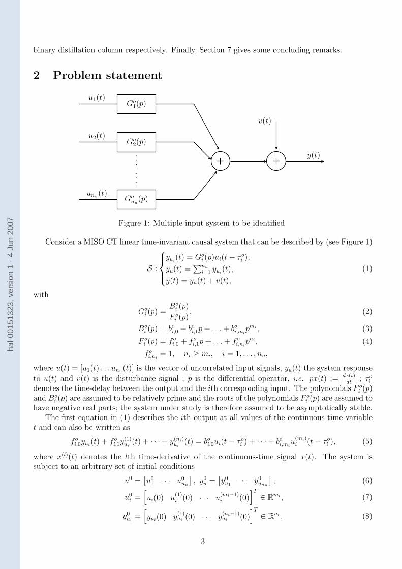
Figure 1: Multiple input system to be identified

Consider a MISO CT linear time-invariant causal system that can be described by (see Figure 1)

S :

yui(t) = Go

i (p)ui(t − τ oi ),

yu(t) =∑nu

i=1 yui(t),

y(t) = yu(t) + v(t),

(1)

with

Goi (p) =

Boi (p)

F oi (p)

, (2)

Boi (p) = bo

i,0 + boi,1p + . . . + bo

i,mipmi , (3)

F oi (p) = f o

i,0 + f oi,1p + . . . + f o

i,nipni , (4)

f oi,ni

= 1, ni ≥ mi, i = 1, . . . , nu,

where u(t) = [u1(t) . . . unu(t)] is the vector of uncorrelated input signals, yu(t) the system response

to u(t) and v(t) is the disturbance signal ; p is the differential operator, i.e. px(t) := dx(t)dt

; τ oi

denotes the time-delay between the output and the ith corresponding input. The polynomials F oi (p)

and Boi (p) are assumed to be relatively prime and the roots of the polynomials F o

i (p) are assumed tohave negative real parts; the system under study is therefore assumed to be asymptotically stable.

The first equation in (1) describes the ith output at all values of the continuous-time variablet and can also be written as

f oi,0yui

(t) + f oi,1y

(1)ui

(t) + · · · + y(ni)ui

(t) = boi,0ui(t − τ o

i ) + · · · + boi,mi

u(mi)i (t − τ o

i ), (5)

where x(l)(t) denotes the lth time-derivative of the continuous-time signal x(t). The system issubject to an arbitrary set of initial conditions

u0 =[

u01 · · · u0

nu

]

, y0u =

[

y0u1

· · · y0unu

]

, (6)

u0i =

[

ui(0) u(1)i (0) · · · u

(mi−1)i (0)

]T

∈ Rmi , (7)

y0ui

=[

yui(0) y

(1)ui (0) · · · y

(ni−1)ui (0)

]T

∈ Rni . (8)

3

hal-0

0151

323,

ver

sion

1 -

4 Ju

n 20

07

It is furthermore assumed that the disturbances that cannot be explained from the input signal canbe lumped into the additive term v(t) (1). The disturbance term v(t) is assumed to be independentof the inputs ui(t), i.e. the case of the open-loop operation of the system is considered. For theidentification problem, it is also assumed that the continuous-time signals ui(t) and y(t) are sampledat regular time-interval Ts.

The goal is then to build a model of equation (1) based on sampled input and output data.Models of the following form are considered

G :

yui(tk, θi) = Gi(p, θi)ui(tk − τi),

yu(tk, θi) =∑nu

i=1 yui(tk, θi),

y(tk) = yu(tk, θi) + v(tk),

(9)

where x(tk) denotes the sample of the continuous-time signal x(t) at time-instant t = kTs andGi(p, θi) is the ith transfer function given by

Gi(p, θi) =Bi(p)

Fi(p)=

bi,0 + bi,1p + · · · + bi,mipmi

fi,0 + fi,1p + · · · + fi,nipni

, (10)

fi,ni= 1, ni ≥ mi, i = 1, . . . , nu,

and θi = [bi,mi. . . bi,0 fi,ni−1 . . . fi,0]

T ∈ Rnpi , with npi

= ni + mi + 1, where ni and mi denotethe denominator and numerator orders of Gi(p, θi) respectively. Therefore, the sought parametervector is

θ =[

θT1 . . . θT

nu

]T∈ R

np×1, (11)

with np =∑nu

i=1 npi.

Note that estimation methods presented in this paper focus on identifying the parameters of eachplant transfer function Gi(p, θi) rather than the additive noise appearing in (1). The disturbanceterm is assumed here to be a zero-mean discrete-time noise sequence denoted as v(tk). Moreover, thepure time-delays are supposed to be known and multiple integers of the sampling period τi = nki

Ts.The identification problem can now be stated as follows: determine the orders (ni and mi)

and the parameter vector θ =[

θT1 · · · θT

nu

]Tof the continuous-time plant model from N sampled

measurements of the input and the output ZN = {y(tk)u1(tk) . . . unu(tk)}

N

k=1.

3 Refined IV methods for continuous-time transfer func-

tion model

3.1 Continuous-time transfer function model identification

There are mainly two time-domain approaches to determine a CT model from sampled data. Thefirst is to estimate a DT model which is then converted into a CT model. The second approachconsists in identifying directly a CT model from the DT data. In comparison with the DT coun-terpart, CT model identification raises several technical issues. The first is related to the fact thatunlike the difference equation model, the differential equation model is not a linear combination ofsamples of only the measurable process input and output signals. It also contains input and outputtime-derivatives which are not available as measurement data in most practical cases. Various typesof continuous-time filters, such as the traditional State-Variable Filter (SVF) method, have beendevised to circumvent the need to reconstruct these time-derivatives (Garnier et al. 2003). TheCONtinuous-Time System IDentification (CONTSID) toolbox has been developed on the basis ofthese methods (Garnier et al. 2006).

4

hal-0

0151

323,

ver

sion

1 -

4 Ju

n 20

07

Most of these CT model identification methods present the following drawbacks. First, theycan handle the case of MISO common denominator (CD) transfer function models only. Secondly,these approaches require the a priori choice of a design parameter which can be difficult from apractical point of view. Thirdly they disregard the properties of the additive noise and thereforerepresent a sub-optimal solution to the estimation problem. One particularly successful stochasticidentification method is the iterative SRIVC method (see (Young and Jakeman 1980), (Young2002)), where it is referred to as RIVC). This approach involves a method of adaptive prefilteringbased on an optimal2 statistical solution to the problem when the additive noise v(tk) is white,but which also yields consistent and relatively low variance parameter estimates in the case ofcoloured noise. This estimation technique was first proposed for DT model identification in theform of the Refined Instrumental Variable (RIV) algorithm3 (Young 1976), (Young 1984) andthen extended for DT MISO systems with different denominators (Jakeman et al. 1980). TheCT MISO algorithm described in the present paper uses the same type of iterative, relaxationalgorithm as that used in this DT MISO algorithm. The RIV approach was extended for SISOCT model identification at the time of its original development (Young and Jakeman 1980). It hasrecently been revisited (Young 2002) and adapted to handle the case of irregularly sampled data(Huselstein and Garnier 2002) (see also (Raghavan et al. 2006) for a recent review of identificationapproaches for handling irregularly sampled data). This IV-type of method has often proved to beparticularly useful in practical applications (see e.g. (Young 1998)). This method not only ensuresthat the estimate converges to statistically optimum values in the case of additive white noise,it also generates information on the parametric error covariance matrix which can be used in anassociated procedure to identify the orders of the component transfer function models. SRIVC isalso a logical extension of the traditional and more heuristically defined SVF approach but presentsthe advantage of not requiring manual specification of prefilter parameters.

In the following section, the SRIVC version for SISO transfer function model is first brieflyrecalled and then extended to handle the case of multiple transfer function models.

3.2 SRIVC for SISO transfer function models

Consider a SISO system with a white measurement noise on the output. The SRIVC method isbased on the Maximum Likelihood (ML) approach where the error function is given by the outputerror

v(tk, θ) = y(tk) −B(p, θ)

F (p, θ)u(tk − τ), (12)

with

F (p, θ) =n−1∑

l=0

flpl + pn and B(p, θ) =

m∑

l=0

blpl. (13)

Minimisation of a least squares criterion function in v(tk, θ) provides the basis for the output errorestimation methods. However, v(tk, θ) can also be rewritten as

v(tk, θ) =1

F (p, θ)[F (p, θ)y(tk) − B(p, θ)u(tk − τ)] . (14)

2Strictly, the method is quasi-optimal because true optimality would require optimal interpolation of the inputsignal u(t) over the sampling interval, whereas only simple interpolation is used in the SRIVC implementation.However, this normally produces very good, near optimal estimation results.

3The RIV algorithm for DT model identification is available in the CAPTAIN toolbox (seehttp://www.es.lancs.ac.uk/cres/captain/).

5

hal-0

0151

323,

ver

sion

1 -

4 Ju

n 20

07

Therefore, the output error given in (12) can be transformed in this manner to yield an equationerror expression of the form,

v(tk, θ) = F (p, θ)y(tk) − B(p, θ)u(tk − τ), (15)

where y(tk) and u(tk) are the variables pre-filtered by L(p, θ) = 1F (p,θ)

. The problem with this

formulation is that θ and therefore F (p, θ) are unknown a priori. This problem can be convenientlysolved by employing an iterative optimization procedure which aims at adjusting an initial estimateθ0 of θ adaptively until it converges on an optimal estimate. Therefore, at each step, a linear inthe unknown parameter vector θ equation has to be solved

y(n)(tk, θj) = φT (tk, θ

j)θj+1 + ε(tk, θj), (16)

where θj is the parameter vector estimated at the jth step of the algorithm, θj+1 is the parametervector to be estimated and

φT (tk, θj) =

[

u(m)(tk − τ, θj) . . . u(tk − τ, θj) − y(n−1)(tk, θj) . . . − y(tk, θ

j)]

, (17)

where

x(i)(tk, θj) =

pi

F (p, θj)x(tk, θ

j) (18)

The use of the conventional least squares method to solve (16) will give biased results when theoutput measurement is corrupted by noise. A solution is to use an IV-type of method to overcomethe bias problem. However, the choice of the instruments, denoted by ZT (tk) here, was shownto have considerable effect on the parametric covariance matrix Pi. The lower bound of Pi forany unbiased identification method is given by the Cramer-Rao bound, which is specified (see e.g.(Ljung 1999) and (Soderstrom and Stoica 1983))

Pi ≥ Popti (19)

with4

Popti = σ2

ε [E¯φ(tk)

¯φT (tk)]

−1 (20)

where ¯φ(tk) = L(p)φ(tk) and φ(tk) is the noise-free part of φ(tk). The minimum variance can then

be achieved by the following choice of design variables (see (Young and Jakeman 1980)) where thesefilters are defined by a special maximum likelihood solution to the problem):

L(p) =1

F o(p)

ZT (tk) =1

F o(p)φ(tk)

(21)

Since the exact model F o(p) is not known, it has to be replaced by its estimate obtained at theprevious iteration: i.e.,

L(p, θj) =1

F (p, θj)

ZT (tk, θj) =

[

u(m)(tk − τ, θj) . . . u(tk − τ, θj) − yu(n−1)(tk, θ

j) . . . − yu(tk, θj)]

,

(22)

4The notation E[.] = limN→∞

1

N

∑

N−1

k=0E[.] is adopted from the prediction error framework of (Ljung 1999).

6

hal-0

0151

323,

ver

sion

1 -

4 Ju

n 20

07

where the filtered auxiliary model output is obtained from

yu(tk, θj) =

B(p, θj)

F (p, θj)u(tk − τ) (23)

ZT (tk, θj) is thus an estimation of the filtered noise-free part of the regressor φ(tk). The optimal

IV-based parameter estimates are then given by

θj+1 =

[

N∑

k=1

Z(tk, θj)φT (tk, θ

j)

]−1 N∑

k=1

ZT (tk, θj)y(n)(tk, θ

j), (24)

The main steps of the SRIVC algorithm dedicated to SISO5 transfer function model are pre-sented in (Young and Jakeman 1980) and (Young 2002). It may be noted that since the instrumentsare correlated with the input/output data but uncorrelated with the noise, the proposed IV algo-rithm delivers consistent parameters even if the additive noise is a colored noise process. However,it only gives asymptotically efficient estimates in the case of a white noise. In practical situations,the additive noise will not have the nice white noise properties assumed above: it is likely that thenoise will be a colored noise process v(t) = Ho(p)e(t). In such a case, (21) becomes

L(p) =1

Ho(p)F o(p)

ZT (tk) =1

Ho(p)F o(p)φ(tk)

(25)

The exact noise model is unknown in practice but could be estimated by extending to thecontinuous-time case the procedure used in the full discrete-time RIV version (see (Young 1984) or(Jakeman et al. 1980)) where an AR or ARMA model for the noise part is estimated and used inthe prefiltering operation. This would lead to the identification of a hybrid model where the plantmodel would be in continuous-time while the noise part would be in discrete-time, as suggestedrecently (Young et al. 2006).

3.3 SRIVC for multiple transfer function models

The proposed method derives from the equivalent iterative, relaxation algorithm for DT models in(Young and Jakeman 1980) and (Jakeman et al. 1980). It aims at identifying MISO model withdifferent denominators (DD) for each input (9), which is more realistic than assuming an identicaldenominator for all transfer function. However, the model is no longer linear in the parametersand the proposed MISO version of SRIVC lies, therefore, in the domain of multi-linear regression.The MISO model (9) can be converted into nu SISO models as follows

vi(tk, θ) = ξi(tk, θ) − yui(tk, θi) for i = 1 . . . nu, (26)

ξi(tk, θ) = y(tk) −nu∑

j=1,j 6=i

yuj(tk, θj) (27)

The parameter vector θ is partitioned6 into classes θ1, . . . , θnusuch that the error is affine with

respect to the parameters of any of these classes when the parameters of all others are fixed (Walter

5The case of multiple transfer function models with common denominators can be handled in a straightforwardmanner.

6The partition of θ into sub-vectors θi is related to the model order problem discussed further in Section 3.4.

7

hal-0

0151

323,

ver

sion

1 -

4 Ju

n 20

07

and Pronzato 1997). It is then possible to search for θ by applying successively the SISO versionof the SRIVC algorithm to estimate the parameters of each class in turn, with a cyclic explorationof all classes. This is achieved by following the same type of ‘relaxation’ procedure described inSection 3.2

ξ(ni)i (tk, θ

j) = φTi (tk, θ

j)θj+1i + εi(tk, θ

j) (28)

φTi (tk, θ

j) =[

u(mi)i (tk − τi, θ

j) . . . ui(tk − τi, θj) − ξ

(ni−1)i (tk, θ

j) . . . − ξi(tk, θj)]

(29)

where the filter is Li(p, θji ) = 1

Fi(p,θji )

. This equation is then solved by using the IV estimator

described in the previous section.

The main steps of the proposed iterative SRIVC method can be summarized by the followingalgorithm7.

1. Estimate the initial parameter vectors

θ0i =

[

b0i,mi

. . . b0i,0 f 0

i,ni−1 . . . f 0i,0

]T

for i = 1 . . . nu, (30)

between the output y(tk) and each input ui(tk).

Calculate the auxiliary model outputs

yui(tk, θ

0i ) =

Bi(p, θ0i )

Fi(p, θ0i )

ui(tk − τi).

2. j = 0 . . . Niter − 1, i = 1 . . . nu

(a) Generate an estimate ξui(tk, θ

ji ) of the noisy response to ui,

ξui(tk, θ

ji ) = y(tk) −

nu∑

l=1,l 6=i

yul(tk, θ

jl ).

Filter the latter variable, the input signal and the auxiliary model output

ξui(tk, θ

ji ) =

1

Fi(p, θji )

ξui(tk, θ

ji ),

ui(tk, θji ) =

1

Fi(p, θji )

ui(tk),

yui(tk, θ

ji ) =

1

Fi(p, θji )

yui(tk, θ

ji ).

(b) Build up the regressor (29) and the instruments

ZTi (tk, θ

ji ) =

[

u(mi)i (tk − τi, θ

ji ) . . . ui(tk − τi, θ

ji ) − ξ(ni−1)

ui(tk, θ

ji ) . . . − ξui

(tk, θji )]

. (31)

Calculate the IV estimate of the parameter vector θj+1i

θj+1i =

[

N∑

k=1

Zi(tk, θji )φ

Ti (tk, θ

ji )

]−1 N∑

k=1

ZTi (tk, θ

ji )ξ

(ni)i (tk, θ

ji ). (32)

7This can also be considered as a ’backfitting’ algorithm: see (Young et al. 2001), where a similar device is usedto identify nonlinear, state-dependent parameter systems.

8

hal-0

0151

323,

ver

sion

1 -

4 Ju

n 20

07

Use θj+1i to generate the auxiliary model output

yui(tk, θ

j+1i ) =

Bi(p, θj+1i )

Fi(p, θj+1i )

ui(tk − τi).

Repeat step 2 until the relative error on the parameters is sufficiently small

nu∑

i=1

npi∑

l=1

∣

∣

∣

∣

∣

θj+1i,l − θ

ji,l

θji,l

∣

∣

∣

∣

∣

< ǫ, (33)

where θji,l denotes the lth element of the parameter θ

ji , ǫ is a given tolerance and Niter is the

final iteration number.

3. For i = 1 . . . nu, θi = θNiter

i . Compute an estimate of the parametric covariance matrix Pi (see(Young 2002) for example)

Pi = σ2ε

[

N∑

k=1

Zi(tk, θi)ZTi (tk, θi)

]−1

(34)

where σ2ε denotes the empirical variance of the simulation error

ε(tk, θ) = y(tk) − yu(tk, θ).

The parameter vector and parametric covariance matrix estimates are given by

θ = [θT1 . . . θT

nu]T (35)

P =

P1 0 · · · 0

0. . . . . .

......

. . . . . . 0

0 · · · 0 Pnu

(36)

Remarks

1. For the initialisation of the algorithm, estimates for a particular transfer function i can beobtained using SISO modeling of the output y(tk) against each input ui(tk) in turn. This isnot a difficult task and there are several alternatives available to the user in the CONTSIDtoolbox. An automatic option is to use the DT version (SRIV) of the SRIVC method, whichhas the advantage of not requiring any design parameters to be specified. The estimateddiscrete-time model is then first used to generate the auxiliary model outputs yui

(tk, θ0i ) and

also converted to continuous-time form to provide the Fi(p, θ0i ) polynomials. Two alternatives

include the user specification of a single cut-off frequency used in either the traditional leastsquares-based SVF or the basic IV-based GPMF methods (see (Garnier et al. 2003) forexample).

2. This method is an IV-type estimation technique. Therefore, upon convergence, it yields consis-tent estimates, when the model belongs to the system class (Go ∈ G8).

3. The proposed approach can be implemented recursively (Young and Jakeman 1980).

8This notation is adopted from (Ljung 1999).

9

hal-0

0151

323,

ver

sion

1 -

4 Ju

n 20

07

4. An indication of the estimated parameter uncertainties is given which makes it possible to assessthe model quality. Note, however, that there is an implicit assumption, introduced by thenature of the algorithm, that the parameter estimates of each component TF are statisticallyindependent (see (36)).

5. The proposed estimation scheme is implemented in both CONTSID9 and CAPTAIN10 toolboxesfor Matlab.

6. If the measurement noise v(tk) is coloured, then the method is not optimal in statistical terms.However, experience has shown that it is robust and normally yields estimates with reasonablestatistical efficiency (i.e. low but not minimum variance). In the colored noise situation, it ispossible to use, albeit at the cost of increased complexity, a hybrid approach where the noisemodelling, as well as the noise-derived parts of the prefiltering, are carried out in discrete-timeterms, as suggested recently (Young et al. 2006).

3.4 Model order estimation

A key point to be solved in the identification procedure concerns the model order selection. Themethod available for SISO systems (see e.g. (Young 1989), (Young 2002)) is extended to the caseof MISO systems. While models are estimated from a given data set, two statistical measures arecomputed and used to choose between a range of model orders. These are R2

T and Y IC, which aredefined as follows,

R2T = 1 −

σ2ε

σ2y

,

Y IC = loge

{

σ2ε

σ2y

}

+ loge

1

np

nu∑

i=1

npi∑

l=1

σ2ε σ

2θi,l

θ2i,l

(37)

where σ2y , σ2

ε denote, respectively, the variance of the measured output and the variance of the

simulation error; θ2i,l is the squared value of the lth element of the estimated parameter vector θi;

σ2θi,l

is the lth diagonal element of the SRIVC estimated parametric covariance matrix Pi; and np is

the total number of parameters. R2T is recognized as the coefficient of determination based on the

simulation error. It is a measure of how well the model output explains to the system output andwill be close to 1 in low noise situations. However, R2

T does not provide a clear indication of thebest model order and can suggest over-parameterized models. The Young’s Information Criterion(Y IC) is more complex and provides a measure of how well the parameters are defined statistically(see (Young 1996) for example): the more negative the Y IC, the better the definition. Howeverit may lead to underestimate the model orders. Both criteria are inspected to find the orders forwhich R2

T is sufficiently high to indicate a good explanation of the data and the Y IC is sufficientlynegative to indicate well defined parameter estimates.

Note that the proposed procedure, based on the two criteria, is not always completely un-ambiguous, as all model order procedures and other factors, such as physical considerations andparsimony, need also to be taken into account in the final selection of the model order. However,as illustrated in the next Section, the proposed SRIVC-based model order selection procedure ishelpful and is shown to be reasonably successful for the multiple input transfer function model,although the procedure is not as clearly defined as in the equivalent SISO situation.

9see http://www.cran.uhp-nancy.fr/contsid/10see http://www.es.lancs.ac.uk/cres/captain/

10

hal-0

0151

323,

ver

sion

1 -

4 Ju

n 20

07

4 Simulation examples

Two simulation examples are considered in this section. The system orders are first assumed to beknown and Monte Carlo simulations are used to illustrate the relevance of the proposed SRIVC es-timation scheme in comparison to the traditional identification method for MISO transfer functionmodel with common denominators. The performance of the proposed approach is also comparedwith the direct CT model identification method for MISO transfer finction model with different de-nominators minimizing the Output Error (COE)11. The model order selection procedure describedin Section 3.4 is then evaluated. The first system has two transfer functions with approximately thesame bandwidth; while the second example has two transfer functions with clearly distinguishedbandwidths.

4.1 Simulation example 1

The first system considered (S1) is a two input, one output system, with second-order non-minimum phase transfer functions

S1:

yu(t) =−0.5p + 1

p2 + 0.6p + 1u1(t) +

−3p + 2

p2 + 4p + 3u2(t)

y(tk) = yu(tk) + v(tk),(38)

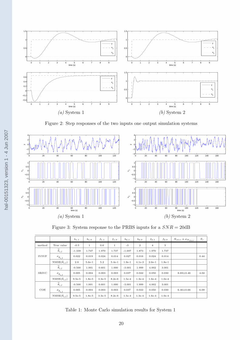
The first transfer function presents a resonant mode, with a damping coefficient of 0.3 and a naturalfrequency of 1 rad/s, while the second has two time constants equal to 1 and 3 s. The dynamiccharacteristics between the two inputs and the output are quite similar, as can be observed fromthe step response of both transfer functions displayed in Figure 2(a).

The measured output y(tk) consists of the noise-free output yu(t) sampled at time tk, to whichis added a zero-mean independent identically distributed (i.i.d.) Gaussian sequence v(tk). Notethat S1 is formulated with the model structure assumed in both SRIVC and COE methods. Thesampling period is equal to Ts = 50 ms. The system is excited by two uncorrelated PRBS ofmaximum length. The characteristics of the PRBS signals, whose amplitude switches between −1and +1, are the following: the number of stages of the shift register is set to ns1 = 6, the clockperiod is set to np1 = 40 for the first input, while ns2 = 7 and np2 = 20 for the second input. Thefirst input is duplicated and then truncated in order to have the same number of points N = 2540for both inputs. Note that the noise-free system response to the PRBS has been calculated exactlyat the sampling instances by discretizing the continuous-time transfer function model, assuming azero-order hold on the inputs.

The variance of the additive noise v(tk) on the measured output is adjusted in order to obtaina signal-to-noise ratio (SNR) of 20dB. The SNR is defined as

SNR = 10logPyu

Pv

, (39)

where Pv represents the average power of the zero-mean additive noise on the system output (i.e.the variance) while Pyu

denotes the average power of the noise-free output fluctuations. The noisysystem response, along with the two PRBS inputs, are displayed in Figure 3(a).

The estimation results12 from a Monte Carlo simulation with Nexp = 200 experiments are shownin Table 1. The aim here is first to illustrate the relevance of the proposed approach dedicated

11This algorithm is also available in the CONTSID toolbox where the parameters of MISO models are estimatedby using the Levenberg-Marquardt algorithm via sensitivity functions.

12All of the identification results were computed using version 4.0 of the CONTSID toolbox on Matlab 7.0.1.

11

hal-0

0151

323,

ver

sion

1 -

4 Ju

n 20

07

to MISO transfer function model with different denominators. The estimation results obtainedwith the proposed SRIVC and with the traditional Instrumental Variable-based State VariableFilter (IVSVF)13 method (Garnier et al. 2003) for MISO transfer function models with commondenominators are presented in Table 1. The estimation results obtained with the COE method14

are also included in Table 1 for comparison purposes. Note that both SRIVC and COE routinesare initialised in the same way from an initial estimate obtained by using the IV-based GPMFalgorithm (see (Garnier et al. 2003) for example) since the automatic option based on the use ofthe discrete-time version SRIV is not available in the COE method.

To compare the statistical performance of the different approaches, the computed mean θi,l

and standard deviation σθi,lof the estimated parameters are presented, as well as the empirical

normalised mean square error (NMSE) which is defined as

NMSE(θi,l) =1

Nexp

Nexp∑

j=1

(

θoi,l − θi,l(j)

θoi,l

)2

, (40)

where θi,l(j) is the lth element of the estimated parameter vector at the jth Monte Carlo simu-

lation experiment θi(j) (i = 1 or 2 here) while ‘o’ denotes the true value of the parameter. Theaverage iteration number Niter, the standard deviation of iterations σNiter

and the average compu-tational time Tc for the iterative methods to converge are also considered later in the analysis ofthe estimation results.

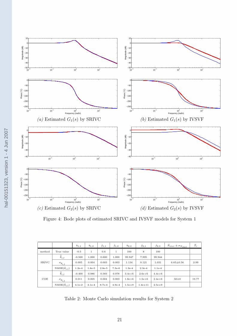
The comparison of the estimation results displayed in Table 1 obtained by the SRIVC andIVSVF methods show, as expected, the relevance of the proposed SRIVC algorithm dedicated todifferent denominator transfer function models. It can be seen that the IVSVF method assumingcommon denominators fails to give a good estimate because the same dynamic is used for the twotransfer functions. In contrast to this, the SRIVC algorithm, which considers different denomina-tors, gives very accurate results with no bias and very low standard errors. This analysis is furtherillustrated by the Bode plots of the 200 estimated models for both SRIVC and IVSVF estimationtechniques displayed in Figure 4.

Table 1 shows also that, for this system with quite similar dynamic characteristics, there isnothing to choose between the SRIVC and COE methods. The two methods dedicated to differentdenominator transfer function model identification are consistent with very low estimated standarderrors and give their best performance when applied to simulated data that conform with the as-sumptions made in their derivation, which is clearly the case in this additive Gaussian measurementnoise example.

4.2 Simulation example 2

The second system considered (S2) is also a two input, one output system given by

S2:

yu(t) =−0.5p + 1

p2 + 0.6p + 1u1(t) +

100

p2 + 8p + 100u2(t)

y(tk) = yu(tk) + v(tk),(41)

The first transfer function is identical to the one used in S1, while the second transfer function isnow a minimum phase, second order which has a resonant mode, with a damping coefficient of 0.4

13This algorithm is also available in the CONTSID toolbox.14Both SRIVC and COE iterative searches are automatically stopped by using the procedure presented in Section

3.3. (see (33)).

12

hal-0

0151

323,

ver

sion

1 -

4 Ju

n 20

07

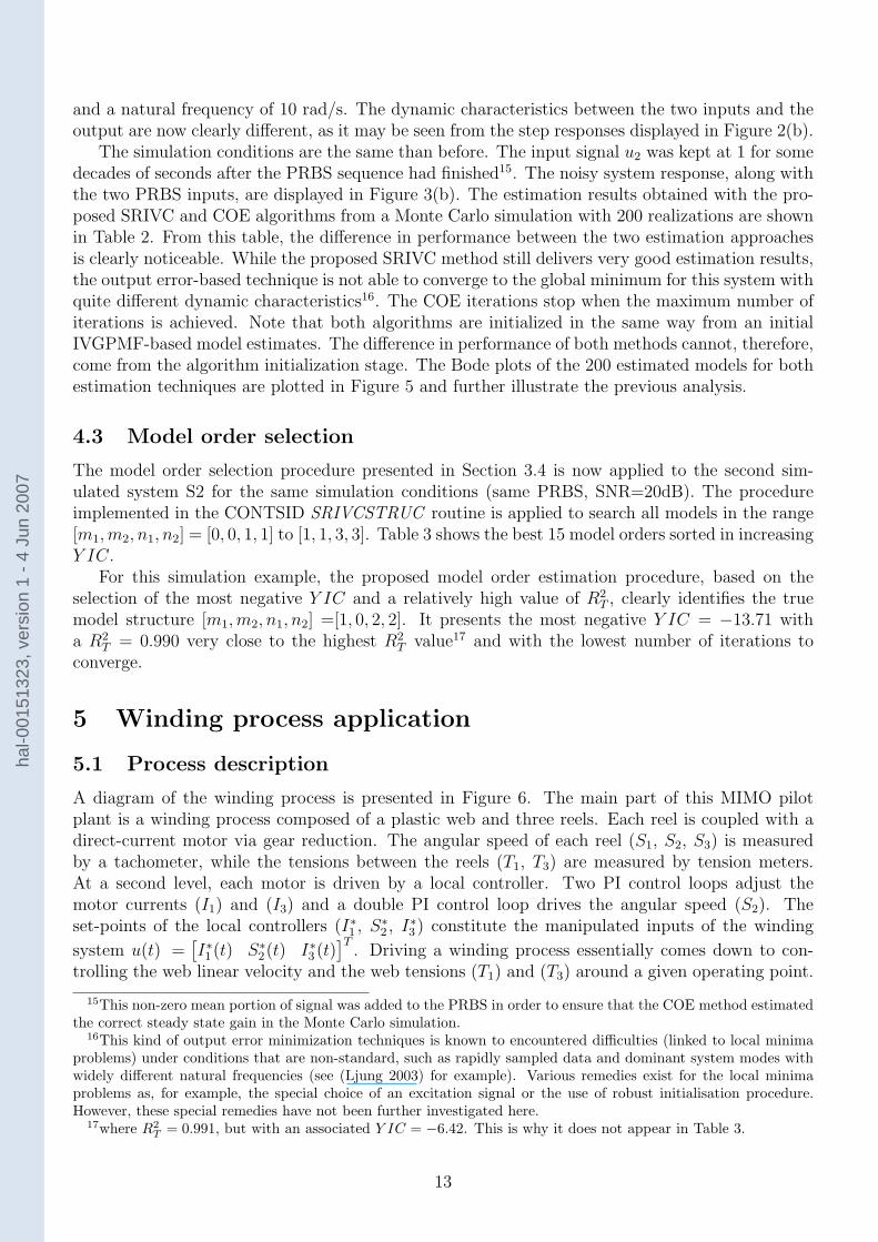
and a natural frequency of 10 rad/s. The dynamic characteristics between the two inputs and theoutput are now clearly different, as it may be seen from the step responses displayed in Figure 2(b).

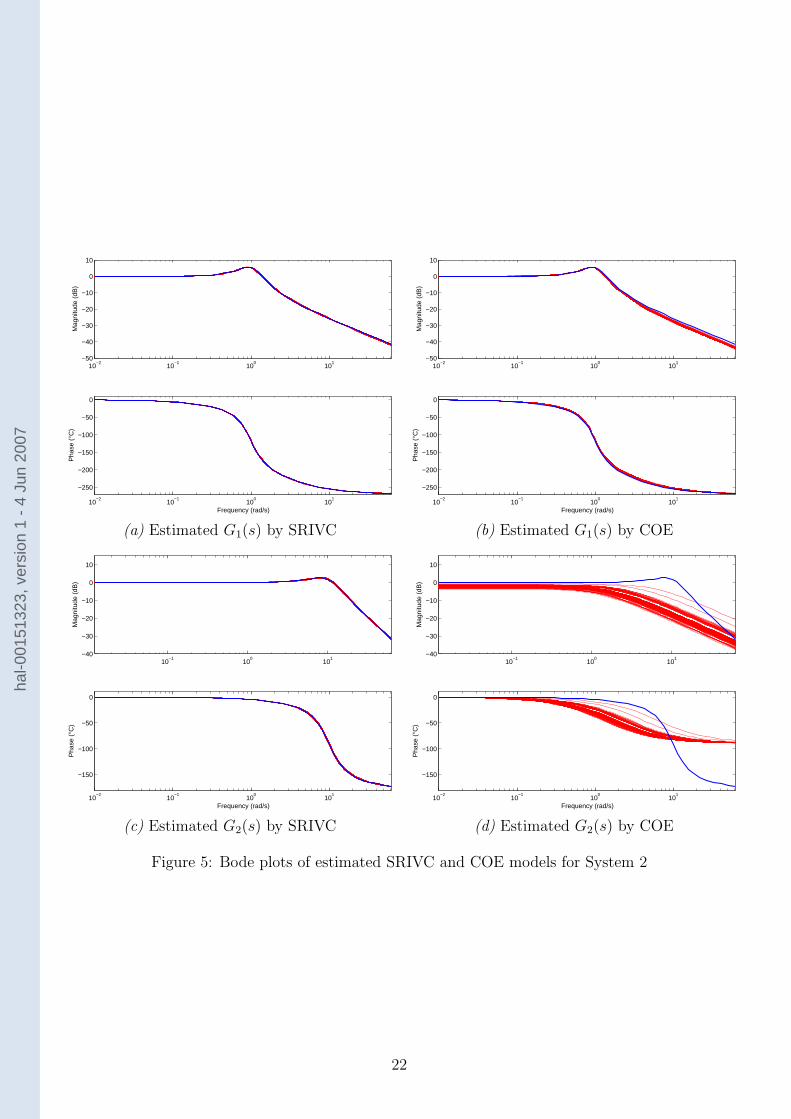
The simulation conditions are the same than before. The input signal u2 was kept at 1 for somedecades of seconds after the PRBS sequence had finished15. The noisy system response, along withthe two PRBS inputs, are displayed in Figure 3(b). The estimation results obtained with the pro-posed SRIVC and COE algorithms from a Monte Carlo simulation with 200 realizations are shownin Table 2. From this table, the difference in performance between the two estimation approachesis clearly noticeable. While the proposed SRIVC method still delivers very good estimation results,the output error-based technique is not able to converge to the global minimum for this system withquite different dynamic characteristics16. The COE iterations stop when the maximum number ofiterations is achieved. Note that both algorithms are initialized in the same way from an initialIVGPMF-based model estimates. The difference in performance of both methods cannot, therefore,come from the algorithm initialization stage. The Bode plots of the 200 estimated models for bothestimation techniques are plotted in Figure 5 and further illustrate the previous analysis.

4.3 Model order selection

The model order selection procedure presented in Section 3.4 is now applied to the second sim-ulated system S2 for the same simulation conditions (same PRBS, SNR=20dB). The procedureimplemented in the CONTSID SRIVCSTRUC routine is applied to search all models in the range[m1,m2, n1, n2] = [0, 0, 1, 1] to [1, 1, 3, 3]. Table 3 shows the best 15 model orders sorted in increasingY IC.

For this simulation example, the proposed model order estimation procedure, based on theselection of the most negative Y IC and a relatively high value of R2

T , clearly identifies the truemodel structure [m1,m2, n1, n2] =[1, 0, 2, 2]. It presents the most negative Y IC = −13.71 witha R2

T = 0.990 very close to the highest R2T value17 and with the lowest number of iterations to

converge.

5 Winding process application

5.1 Process description

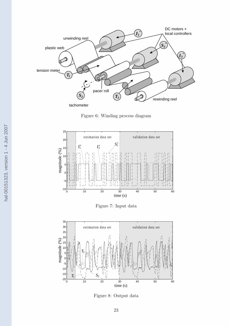
A diagram of the winding process is presented in Figure 6. The main part of this MIMO pilotplant is a winding process composed of a plastic web and three reels. Each reel is coupled with adirect-current motor via gear reduction. The angular speed of each reel (S1, S2, S3) is measuredby a tachometer, while the tensions between the reels (T1, T3) are measured by tension meters.At a second level, each motor is driven by a local controller. Two PI control loops adjust themotor currents (I1) and (I3) and a double PI control loop drives the angular speed (S2). Theset-points of the local controllers (I∗

1 , S∗2 , I∗

3 ) constitute the manipulated inputs of the winding

system u(t) =[

I∗1 (t) S∗

2(t) I∗3 (t)

]T. Driving a winding process essentially comes down to con-

trolling the web linear velocity and the web tensions (T1) and (T3) around a given operating point.

15This non-zero mean portion of signal was added to the PRBS in order to ensure that the COE method estimatedthe correct steady state gain in the Monte Carlo simulation.

16This kind of output error minimization techniques is known to encountered difficulties (linked to local minimaproblems) under conditions that are non-standard, such as rapidly sampled data and dominant system modes withwidely different natural frequencies (see (Ljung 2003) for example). Various remedies exist for the local minimaproblems as, for example, the special choice of an excitation signal or the use of robust initialisation procedure.However, these special remedies have not been further investigated here.

17where R2

T= 0.991, but with an associated Y IC = −6.42. This is why it does not appear in Table 3.

13

hal-0

0151

323,

ver

sion

1 -

4 Ju

n 20

07

Consequently, the output variables of the winding system are y(t) =[

T1(t) T3(t) S2(t)]T

. Theprocess is described in more detail in (Bastogne et al. 1998).

5.2 Experiment design

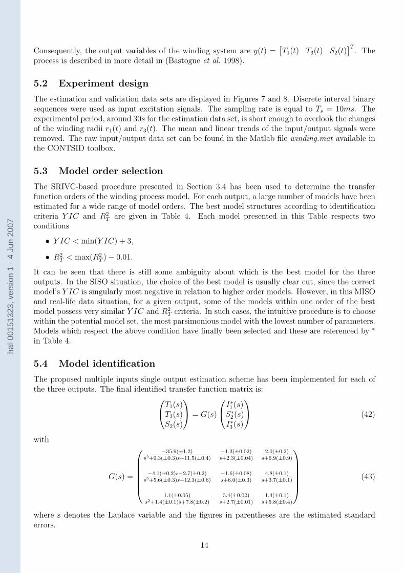
The estimation and validation data sets are displayed in Figures 7 and 8. Discrete interval binarysequences were used as input excitation signals. The sampling rate is equal to Ts = 10ms. Theexperimental period, around 30s for the estimation data set, is short enough to overlook the changesof the winding radii r1(t) and r3(t). The mean and linear trends of the input/output signals wereremoved. The raw input/output data set can be found in the Matlab file winding.mat available inthe CONTSID toolbox.

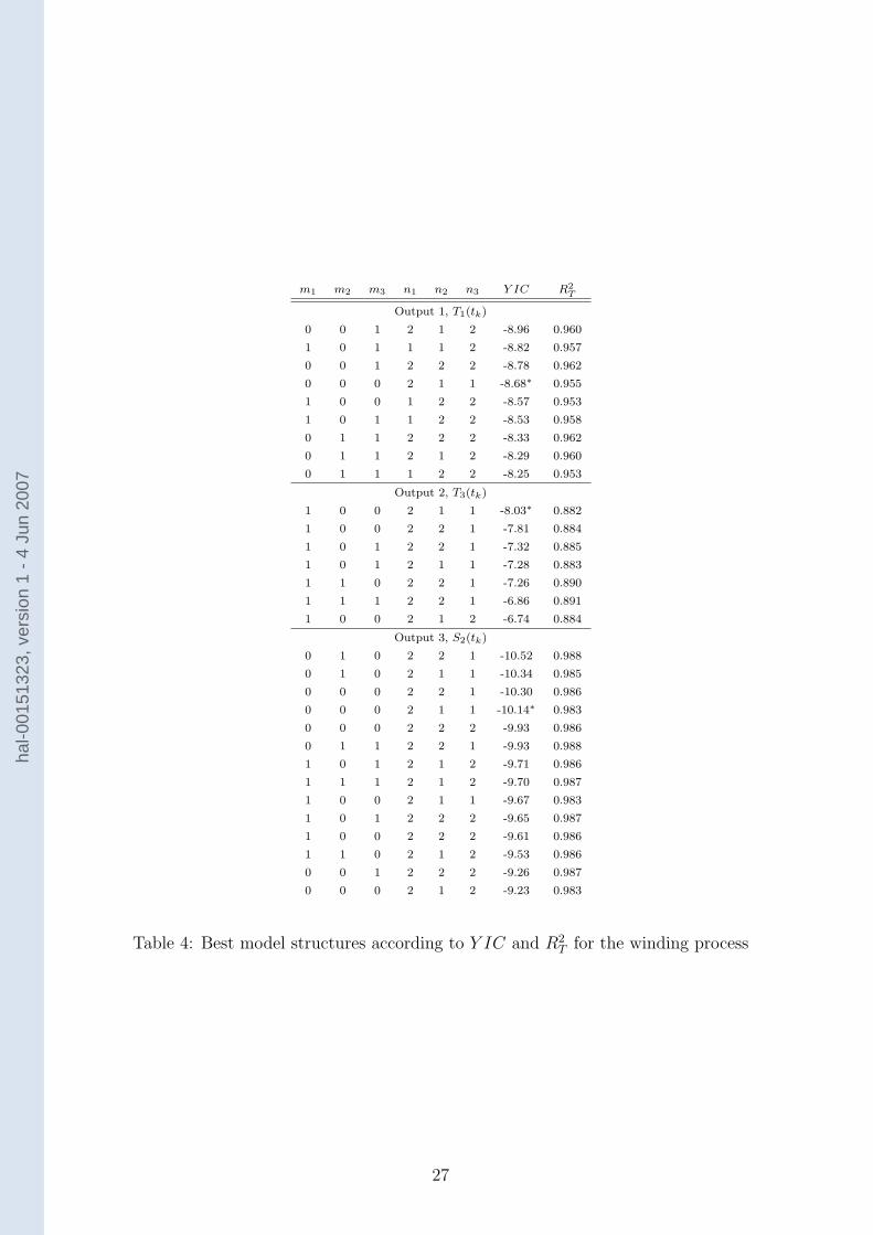
5.3 Model order selection

The SRIVC-based procedure presented in Section 3.4 has been used to determine the transferfunction orders of the winding process model. For each output, a large number of models have beenestimated for a wide range of model orders. The best model structures according to identificationcriteria Y IC and R2

T are given in Table 4. Each model presented in this Table respects twoconditions

• Y IC < min(Y IC) + 3,

• R2T < max(R2

T ) − 0.01.

It can be seen that there is still some ambiguity about which is the best model for the threeoutputs. In the SISO situation, the choice of the best model is usually clear cut, since the correctmodel’s Y IC is singularly most negative in relation to higher order models. However, in this MISOand real-life data situation, for a given output, some of the models within one order of the bestmodel possess very similar Y IC and R2

T criteria. In such cases, the intuitive procedure is to choosewithin the potential model set, the most parsimonious model with the lowest number of parameters.Models which respect the above condition have finally been selected and these are referenced by ∗

in Table 4.

5.4 Model identification

The proposed multiple inputs single output estimation scheme has been implemented for each ofthe three outputs. The final identified transfer function matrix is:

T1(s)T3(s)S2(s)

= G(s)

I∗1 (s)

S∗2(s)

I∗3 (s)

(42)

with

G(s) =

−35.9(±1.2)s2+9.3(±0.3)s+11.5(±0.4)

−1.3(±0.02)s+2.3(±0.04)

2.0(±0.2)s+6.9(±0.9)

−4.1(±0.2)s−2.7(±0.2)s2+5.6(±0.3)s+12.3(±0.6)

−1.6(±0.08)s+6.0(±0.3)

4.8(±0.1)s+3.7(±0.1)

1.1(±0.05)s2+1.4(±0.1)s+7.8(±0.2)

3.4(±0.02)s+2.7(±0.01)

1.4(±0.1)s+5.8(±0.4)

(43)

where s denotes the Laplace variable and the figures in parentheses are the estimated standarderrors.

14

hal-0

0151

323,

ver

sion

1 -

4 Ju

n 20

07

5.5 Cross-validation results

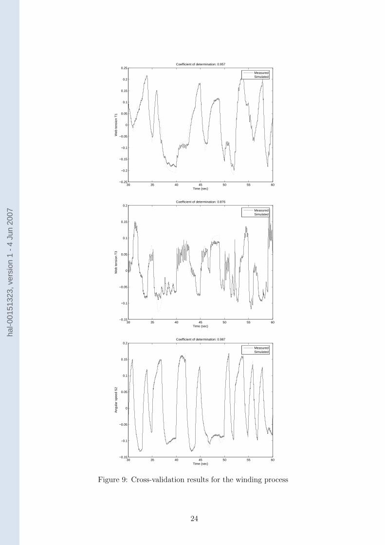
To evaluate the quality of the estimated transfer function models, a cross-validation procedure hasbeen applied to data that were not used to build the model. Cross-validation results are plottedin Figure 9, where it may be observed that there is a satisfactory reproduction of the multipleoutput behaviour by the transfer function models. These results demonstrate the applicability ofthe proposed SRIVC algorithm for the identification of reduced-order, continuous-time, multipletransfer function models. Note that the oscillatory character of the output (T3) is not modeledas well as the first two outputs. However, this problem is not due to the estimation algorithm.Indeed, it has been shown in (Bastogne and Sibille 1998) that the tension (T3) has non lineartransient behaviour depending on the sign of the steps on the input (I∗

1 ). These input dependentdynamics cannot, therefore, be captured by a linear model identification procedure, although theymay be captured if a nonlinear input transformation and this is being investigated using the statedependent parameter estimation approach to modelling nonlinear systems (see e.g. Young et al,2001).

6 Industrial distillation column application

6.1 Column description

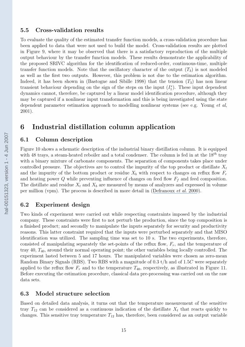
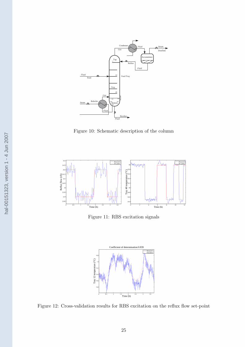
Figure 10 shows a schematic description of the industrial binary distillation column. It is equippedwith 48 trays, a steam-heated reboiler and a total condenser. The column is fed in at the 18th traywith a binary mixture of carbonate components. The separation of components takes place undercontrolled pressure. The objectives are to control the impurity of the top product or distillate Xt

and the impurity of the bottom product or residue Xb with respect to changes on reflux flow Fr

and heating power Q while preventing influence of changes on feed flow Ff and feed composition.The distillate and residue Xt and Xb are measured by means of analyzers and expressed in volumeper million (vpm). The process is described in more detail in (Defranoux et al. 2000).

6.2 Experiment design

Two kinds of experiment were carried out while respecting constraints imposed by the industrialcompany. These constraints were first to not perturb the production, since the top composition isa finished product; and secondly to manipulate the inputs separately for security and productivityreasons. This latter constraint required that the inputs were perturbed separately and that MISOidentification was utilized. The sampling time was set to 10 s. The two experiments, therefore,consisted of manipulating separately the set-points of the reflux flow, Fr, and the temperature oftray 40, T40, around their normal operating point; the other variables being locally controlled. Theexperiment lasted between 5 and 17 hours. The manipulated variables were chosen as zero-meanRandom Binary Signals (RBS). Two RBS with a magnitude of 0.3 t/h and of 1.5C were separatelyapplied to the reflux flow Fr and to the temperature T40, respectively, as illustrated in Figure 11.Before executing the estimation procedure, classical data pre-processing was carried out on the rawdata sets.

6.3 Model structure selection

Based on detailed data analysis, it turns out that the temperature measurement of the sensitivetray T12 can be considered as a continuous indication of the distillate Xt that reacts quickly tochanges. This sensitive tray temperature T12 has, therefore, been considered as an output variable

15

hal-0

0151

323,

ver

sion

1 -

4 Ju

n 20

07

instead of the distillate. However, no temperature tray could represent a continuous indication ofthe residue Xb, which constitutes the second output of the model. Classically, the reflux flow Fr

and heating power represented by the controlled temperature T40 are used as input variables forthe system. The most important disturbance entering this distillation column is a change in thefeed flow rate. Since the feed flow rate Ff is measured, therefore, it has been included as a thirdinput variable for the model. The multivariable coupling in the process can be then be describedby the following model:

(

T12(s)Xb(s)

)

=

(

H11(s) H12(s) H13(s)H21(s) H22(s) H23(s)

)

Fr(s)T40(s)Ff (s)

(44)

6.4 Model identification

The measured reflux flow and tray 40 temperature rather than the set-points for these variables wereconsidered in the identification procedure. Time delays from input to output variables and modelorders were previously estimated from step responses and from previous identification (Defranouxet al. 2000) respectively. During the experiment, the feed flow changes did not disturb explicitlythe bottom product composition of the column. The distant position of the feed tray (Figure 10)in respect to the bottom of the column probably explains this phenomenon. The transfer functionH23 was not, therefore, considered in the estimation procedure and was set to zero. Furthermore,no coupling between the reflux flow Fr and the residue Xb could be demonstrated. Consequently,the transfer function H21 was also set to zero and was not considered in the estimation procedure.This explains why there is no cross-validation plot for Xb in the case of excitation on the reflux flowset-point. The proposed multiple input, single output estimation scheme has been implemented foreach of the two outputs.

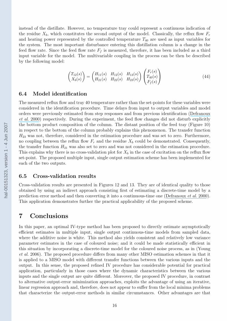
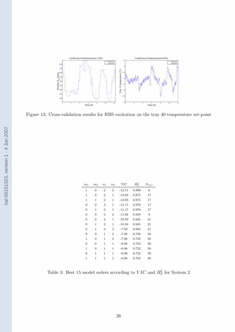
6.5 Cross-validation results

Cross-validation results are presented in Figures 12 and 13. They are of identical quality to thoseobtained by using an indirect approach consisting first of estimating a discrete-time model by aprediction error method and then converting it into a continuous-time one (Defranoux et al. 2000).This application demonstrates further the practical applicability of the proposed scheme.

7 Conclusions

In this paper, an optimal IV-type method has been proposed to directly estimate asymptoticallyefficient estimates in multiple input, single output continuous-time models from sampled data,where the additive noise is white. This method also yields consistent and relatively low varianceparameter estimates in the case of coloured noise; and it could be made statistically efficient inthis situation by incorporating a discrete-time model for the coloured noise process, as in (Younget al. 2006). The proposed procedure differs from many other MISO estimation schemes in that itis applied to a MISO model with different transfer functions between the various inputs and theoutput. In this sense, the proposed refined IV procedure has considerable potential for practicalapplication, particularly in those cases where the dynamic characteristics between the variousinputs and the single output are quite different. Moreover, the proposed IV procedure, in contrastto alternative output-error minimization approaches, exploits the advantage of using an iterative,linear regression approach and, therefore, does not appear to suffer from the local minima problemsthat characterize the output-error methods in similar circumstances. Other advantages are that

16

hal-0

0151

323,

ver

sion

1 -

4 Ju

n 20

07

the proposed approach can easily handle non-uniformly sampled data and the refined IV methodallows for the use of the YIC model structure identification criterion, which based on the propertiesof the instrumental product matrix and helps to identify the most appropriate model orders, priorto parameter estimation. All of these interesting properties have been illustrated via Monte Carlosimulations and the application to both a winding process and an industrial binary distillationcolumn. Another successful application of the proposed estimation scheme to identify a two input-two output flexible robotic arm designed for heart-beating tracking is also reported in Cuvillon etal. (2006), demonstrating the wide practical applicability of the proposed identification approach.

8 Acknowledgment

The first two authors wish to thank their colleague Thierry Bastogne for supplying the windingprocess data.

References

Bastogne, T. and P. Sibille (1998). Identification of the input dependent dynamics of winding ten-sions. In: IFAC conference on system structure and control. Vol. 2. Nantes (France). pp. 255–260.

Bastogne, T., H. Noura, P. Sibille and A. Richard (1998). Multivariable identification of a windingprocess by subspace methods for a tension control. Control Engineering practice 6(9), 1077–1088.

Cuvillon, L., E. Laroche, H. Garnier, J. Gangloff and M. de Mathelin (2006). Continuous-timemodel identification of robot flexibilities for fast visual servoing. In: Proceedings of the 14thIFAC Symposium on System Identification (SYSID’2006). Newcastle (Australia).

Defranoux, C., H. Garnier and P. Sibille (2000). Identification and control of an industrial binarydistillation column: a case study. Chemical Engineering and Technology 23(9), 745–750.

Garnier, H. and L. Wang (2007). Continuous-time model identification from sampled data. SpringerVerlag. To be published.

Garnier, H. and P.C. Young (2004). Time-domain approaches for continuous-time model identi-fication from sampled data. In: Invited tutorial paper for the American Control Conference(ACC’2004). Boston, MA (USA).

Garnier, H., M. Gilson and O. Cervellin (2006). Latest developments for the Matlab CONTSIDtoolbox. In: Proceedings of the 14th IFAC Symposium on System Identification (SYSID’2006).Newcastle (Australia).

Garnier, H., M. Mensler and A. Richard (2003). Continuous-time model identification from sampleddata. Implementation issues and performance evaluation. International Journal of Control76(13), 1337–1357.

Gilson, M. and P. Van den Hof (2005). Instrumental variable methods for closed-loop systemidentification. Automatica 41(2), 241–249.

17

hal-0

0151

323,

ver

sion

1 -

4 Ju

n 20

07

Huselstein, E. and H. Garnier (2002). An approach to continuous-time model identification fromnon-uniformly sampled data. In: 41st IEEE Conference on Decision and Control (CDC’02).Las-Vegas, Nevada (USA).

Jakeman, A.J., L.P. Steele and P.C. Young (1980). Instrumental variable algorithms for multipleinput systems described by multiple transfer functions. IEEE Transactions on Systems, Man,and Cybernetics SMC-10, 593–602.

Li, W., H. Raghavan and S. Shah (2003). Subspace identification of continuous time models forprocess fault detection and isolation. Journal of Process Control 13(5), 407–421.

Ljung, L. (1999). System identification. Theory for the user. 2nd ed.. Prentice Hall. Upper SaddleRiver.

Ljung, L. (2003). Initialisation aspects for subspace and output-error identification methods. In:European Control Conference (ECC’2003). Cambridge (U.K.).

Mahata, K. and H. Garnier (2006). Identification of continuous-time errors-in-variables models.Automatica.

Mensler, M., S. Joe and T. Kawabe (2006). Identification of a toroidal continuously variable trans-mission using continuous-time system identification methods. Control Engineering practice14(1), 45–58.

Moussaoui, S., D. Brie and A. Richard (2005). Regularization aspects in continuous-time modelidentification. Automatica 41(2), 197–208.

Raghavan, H., A.K. Tangirala, R.B. Gopaluni and S.L. Shah (2006). Identification of chemicalprocesses with irregular output sampling. Control Engineering practice 14(5), 467–480.

Rao, G.P. and H. Unbehauen (2006). Identification of continuous-time systems. IEE Proceedings -Control theory and applications 153(2), 185–220.

Soderstrom, T. and P. Stoica (1983). Instrumental variable methods for system identification.Springer Verlag. New York.

Walter, E. and L. Pronzato (1997). Identification of parametric models from experimental data.Springer Verlag.

Wang, L., P. Gawthrop, C. Chessari, T. Podsiadly and A. Giles (2004). Indirect approach tocontinuous time system identification of food extruder. Journal of Process Control 14(6), 603–615.

Young, P.C. (1970). An instrumental variable method for real-time identification of a noisy process.Automatica 6, 271–287.

Young, P.C. (1976). Some observations on instrumental variable methods of time-series analysis.International Journal of Control 23, 593–612.

Young, P.C. (1984). Recursive estimation and time-series analysis. Springer-Verlag. Berlin.

Young, P.C. (1989). Control and Dynamic Systems: Advances in Theory and Applications. Chap.Recursive estimation, forecasting and adaptive control, pp. 119–166. C.T. Leondes ed.. Aca-demic Press.

18

hal-0

0151

323,

ver

sion

1 -

4 Ju

n 20

07

Young, P.C. (1996). Identification, estimation and control of continuous-time and delta operatorsystems. In: Conference on Identification of Engineering Systems. Swansea (Wales). pp. 1–17.

Young, P.C. (1998). Data-based mechanistic modeling of environmental, ecological, economic andengineering systems. Journal of Modelling & Software 13, 105–122.

Young, P.C. (2002). Optimal IV identification and estimation of continuous-time TF models. In:15th Triennial IFAC World Congress on Automatic Control. Barcelona (Spain).

Young, P.C., A.J. Jakeman and R. McMurtries (1980). An instrumental variable method for modelorder identification. Automatica 16, 281–296.

Young, P.C. and A.J. Jakeman (1979). Refined instrumental variable methods of time-series anal-ysis: Part I, SISO systems. International Journal of Control 29, 1–30.

Young, P.C. and A.J. Jakeman (1980). Refined instrumental variable methods of time-series anal-ysis: Part III, extensions. International Journal of Control 31, 741–764.

Young, P.C. and H. Garnier (2006). Identification and estimation of continuous-time data-basedmechanistic (DBM) models for environmental systems. Environmental Modelling and Software21(8), 1055–1072.

Young, P.C., H. Garnier and M. Gilson (2006). An optimal instrumental variable approach foridentifying hybrid continuous-time Box-Jenkins model. In: Proceedings of the 14th IFAC Sym-posium on System Identification (SYSID’2006). Newcastle (Australia).

Young, P.C., P. McKenna and J. Bruun (2001). Identification of nonlinear stochastic systems bystate dependent parameter estimation. International Journal of Control 74, 1837–1857.

19

hal-0

0151

323,

ver

sion

1 -

4 Ju

n 20

07

0 1 2 3 4 5 6 7 8 9

0

0.5

1

1.5

time (s)

y

u1

u2

0 1 2 3 4 5 6 7 8 9

−0.4

−0.2

0

0.2

0.4

0.6

time (s)

y

u1

u2

(a) System 1

0 1 2 3 4 5 6 7 8 9

0

0.5

1

1.5

time (s)

y

u1

u2

0 1 2 3 4 5 6 7 8 9

0

0.5

1

1.5

time (s)

y

u1

u2

(b) System 2

Figure 2: Step responses of the two inputs one output simulation systems

0 20 40 60 80 100 120−4

−2

0

2

4

y

0 20 40 60 80 100 120

−1

−0.5

0

0.5

1

u 1

0 20 40 60 80 100 120

−1

−0.5

0

0.5

1

u 2

time (s)

(a) System 1

0 20 40 60 80 100 120 140 160−4

−2

0

2

4

y

0 20 40 60 80 100 120 140 160

−1

−0.5

0

0.5

1

u 1

0 20 40 60 80 100 120 140 160

−1

−0.5

0

0.5

1

u 2

time (s)

(b) System 2

Figure 3: System response to the PRBS inputs for a SNR = 20dB

b1,1 b1,0 f1,1 f1,0 b2,1 b2,0 f2,1 f2,0 Niter ± σNiterTc

method True value -0.5 1 0.6 1 -3 2 4 3

θi,l -1.339 1.747 1.970 1.737 -1.697 1.873 1.970 1.737

IVSVF σθi,l

0.022 0.019 0.024 0.014 0.027 0.016 0.024 0.014 0.44

NMSE(θi,l) 2.8 5.6e-1 5.2 5.4e-1 1.9e-1 4.1e-3 2.6e-1 1.8e-1

θi,l -0.500 1.001 0.601 1.000 -3.001 1.999 4.002 3.001

SRIVC σθi,l

0.005 0.004 0.003 0.003 0.037 0.022 0.050 0.030 8.69±0.46 4.02

NMSE(θi,l) 9.5e-5 1.8e-5 3.3e-5 8.2e-6 1.5e-4 1.3e-4 1.6e-4 1.0e-4

θi,l -0.500 1.001 0.601 1.000 -3.001 1.999 4.002 3.001

COE σθi,l

0.005 0.004 0.003 0.003 0.037 0.022 0.050 0.030 6.46±0.66 6.09

NMSE(θi,l) 9.5e-5 1.8e-5 3.3e-5 8.2e-6 1.5e-4 1.3e-4 1.6e-4 1.0e-4

Table 1: Monte Carlo simulation results for System 1

20

hal-0

0151

323,

ver

sion

1 -

4 Ju

n 20

07

10−2

10−1

100

101

−50

−40

−30

−20

−10

0

10

Mag

nitu

de (

dB)

10−2

10−1

100

101

−250

−200

−150

−100

−50

0

Frequency (rad/s)

Pha

se (

°C)

(a) Estimated G1(s) by SRIVC

10−2

10−1

100

101

−50

−40

−30

−20

−10

0

10

Mag

nitu

de (

dB)

10−2

10−1

100

101

−250

−200

−150

−100

−50

0

Frequency (rad/s)

Pha

se (

°C)

(b) Estimated G1(s) by IVSVF

10−1

100

101

−40

−30

−20

−10

0

Mag

nitu

de (

dB)

10−2

10−1

100

101

−250

−200

−150

−100

−50

0

Frequency (rad/s)

Pha

se (

°C)

(c) Estimated G2(s) by SRIVC

10−1

100

101

−40

−30

−20

−10

0

Mag

nitu

de (

dB)

10−2

10−1

100

101

−250

−200

−150

−100

−50

0

Frequency (rad/s)

Pha

se (

°C)

(d) Estimated G2(s) by IVSVF

Figure 4: Bode plots of estimated SRIVC and IVSVF models for System 1

b1,1 b1,0 f1,1 f1,0 b2,0 f2,1 f2,0 Niter ± σNiterTc

method True value -0.5 1 0.6 1 100 8 100

θi,l -0.500 1.000 0.600 1.000 99.947 7.995 99.944

SRIVC σθi,l

0.005 0.004 0.003 0.003 1.134 0.121 1.031 6.65±0.56 2.99

NMSE(θi,l) 1.2e-4 1.8e-5 2.8e-5 7.3e-6 1.3e-4 2.3e-4 1.1e-4

θi,l -0.400 0.986 0.583 0.978 3.4e+6 2.6e+6 4.4e+6

COE σθi,l

0.011 0.005 0.004 0.003 1.8e+6 1.5e+6 2.4e+6 50±0 19.77

NMSE(θi,l) 4.1e-2 2.1e-4 8.7e-4 4.9e-4 1.5e+9 1.4e+11 2.5e+9

Table 2: Monte Carlo simulation results for System 2

21

hal-0

0151

323,

ver

sion

1 -

4 Ju

n 20

07

10−2

10−1

100

101

−50

−40

−30

−20

−10

0

10

Mag

nitu

de (

dB)

10−2

10−1

100

101

−250

−200

−150

−100

−50

0

Frequency (rad/s)

Pha

se (

°C)

(a) Estimated G1(s) by SRIVC

10−2

10−1

100

101

−50

−40

−30

−20

−10

0

10

Mag

nitu

de (

dB)

10−2

10−1

100

101

−250

−200

−150

−100

−50

0

Frequency (rad/s)

Pha

se (

°C)

(b) Estimated G1(s) by COE

10−1

100

101

−40

−30

−20

−10

0

10

Mag

nitu

de (

dB)

10−2

10−1

100

101

−150

−100

−50

0

Frequency (rad/s)

Pha

se (

°C)

(c) Estimated G2(s) by SRIVC

10−1

100

101

−40

−30

−20

−10

0

10

Mag

nitu

de (

dB)

10−2

10−1

100

101

−150

−100

−50

0

Frequency (rad/s)

Pha

se (

°C)

(d) Estimated G2(s) by COE

Figure 5: Bode plots of estimated SRIVC and COE models for System 2

22

hal-0

0151

323,

ver

sion

1 -

4 Ju

n 20

07

rewinding reel

unwinding reel

pacer roll

T1

T3

I3*

I1*

S2*

S2

DC motors +local controllers

tension meter

tachometer

plastic web

Figure 6: Winding process diagram

est imat ion data set val idat ion data set

0 10 20 30 40 50 60-10

-5

0

5

10

15

20

25

time (s)

mag

nitu

de (

%) I1

* I3* S2

*

Figure 7: Input data

0 10 20 30 40 50 60-20

-15

-10

-5

0

5

10

15

20

25

30

35

time (s)

mag

nitu

de (

%)

T1

T3

S2

est imat ion data set val idat ion data set

Figure 8: Output data

23

hal-0

0151

323,

ver

sion

1 -

4 Ju

n 20

07

30 35 40 45 50 55 60−0.25

−0.2

−0.15

−0.1

−0.05

0

0.05

0.1

0.15

0.2

0.25

Time (sec)

Coefficient of determination: 0.957

Web

tens

ion

T1

MeasuredSimulated

30 35 40 45 50 55 60−0.15

−0.1

−0.05

0

0.05

0.1

0.15

0.2

Time (sec)

Coefficient of determination: 0.876

Web

tens

ion

T3

MeasuredSimulated

30 35 40 45 50 55 60−0.15

−0.1

−0.05

0

0.05

0.1

0.15

0.2

Time (sec)

Coefficient of determination: 0.987

Ang

ular

spe

ed S

2

MeasuredSimulated

Figure 9: Cross-validation results for the winding process

24

hal-0

0151

323,

ver

sion

1 -

4 Ju

n 20

07

Reflux

Tray

Condenser

Distillate

Feed Tray

Residue

Accumulator

Bottom Reboiler

Steam

Feed

Top

Fluid

Fluid

Fluid

Fluid

Fluid

Steam

Gas

Gas

1

18

48

Figure 10: Schematic description of the column

0 0.5 1 1.5 2 2.5 3 3.5

23.85

23.9

23.95

24

24.05

24.1

24.15

24.2

24.25

24.3

Time (h)

Ref

lux

flow

(t/h

)

MeasuredSet−point

0 2 4 6 8 10 12

64.4

64.6

64.8

65

65.2

65.4

65.6

65.8

66

Time (h)

Tra

y 40

tem

pera

ture

(°C

)

MeasuredSet−point

Figure 11: RBS excitation signals

0 0.5 1 1.5 2 2.5 3 3.5

−9.8

−9.6

−9.4

−9.2

−9

−8.8

Time (h)

Coefficient of determination:0.839

Tra

y 12

tem

pera

ture

(°C

)

MeasuredSimulated

Figure 12: Cross-validation results for RBS excitation on the reflux flow set-point

25

hal-0

0151

323,

ver

sion

1 -

4 Ju

n 20

07

0 2 4 6 8 10 12

1400

1500

1600

1700

1800

1900

2000

2100

2200

Time (h)

Coefficient of determination: 0.841R

esid

ue X b (

vpm

)

MeasuredSimulated

0 2 4 6 8 10 12−11

−10.5

−10

−9.5

−9

−8.5

−8

−7.5

Time (h)

Coefficient of determination:0.812

Tra

y 12

tem

pera

ture

(°C

)

MeasuredSimulated

Figure 13: Cross-validation results for RBS excitation on the tray 40 temperature set-point

m1 m2 n1 n2 YIC R2T Niter

1 0 2 2 -13.71 0.990 6

1 0 2 1 -12.03 0.975 17

1 1 2 1 -12.03 0.975 17

0 0 3 1 -11.17 0.970 17

0 1 3 1 -11.17 0.970 17

0 0 2 2 -11.06 0.959 9

0 0 2 1 -10.50 0.945 21

0 1 2 1 -10.50 0.945 21

0 1 3 3 -7.92 0.985 21

0 0 1 2 -7.08 0.738 50

1 0 1 2 -7.08 0.738 50

0 0 1 1 -6.96 0.722 50

1 0 1 1 -6.96 0.722 50

0 1 1 1 -6.96 0.722 50

1 1 1 1 -6.96 0.722 50

Table 3: Best 15 model orders according to Y IC and R2T for System 2

26

hal-0

0151

323,

ver

sion

1 -

4 Ju

n 20

07

m1 m2 m3 n1 n2 n3 Y IC R2T

Output 1, T1(tk)

0 0 1 2 1 2 -8.96 0.960

1 0 1 1 1 2 -8.82 0.957

0 0 1 2 2 2 -8.78 0.962

0 0 0 2 1 1 -8.68∗ 0.955

1 0 0 1 2 2 -8.57 0.953

1 0 1 1 2 2 -8.53 0.958

0 1 1 2 2 2 -8.33 0.962

0 1 1 2 1 2 -8.29 0.960

0 1 1 1 2 2 -8.25 0.953

Output 2, T3(tk)

1 0 0 2 1 1 -8.03∗ 0.882

1 0 0 2 2 1 -7.81 0.884

1 0 1 2 2 1 -7.32 0.885

1 0 1 2 1 1 -7.28 0.883

1 1 0 2 2 1 -7.26 0.890

1 1 1 2 2 1 -6.86 0.891

1 0 0 2 1 2 -6.74 0.884

Output 3, S2(tk)

0 1 0 2 2 1 -10.52 0.988

0 1 0 2 1 1 -10.34 0.985

0 0 0 2 2 1 -10.30 0.986

0 0 0 2 1 1 -10.14∗ 0.983

0 0 0 2 2 2 -9.93 0.986

0 1 1 2 2 1 -9.93 0.988

1 0 1 2 1 2 -9.71 0.986

1 1 1 2 1 2 -9.70 0.987

1 0 0 2 1 1 -9.67 0.983

1 0 1 2 2 2 -9.65 0.987

1 0 0 2 2 2 -9.61 0.986

1 1 0 2 1 2 -9.53 0.986

0 0 1 2 2 2 -9.26 0.987

0 0 0 2 1 2 -9.23 0.983

Table 4: Best model structures according to Y IC and R2T for the winding process

27

hal-0

0151

323,

ver

sion

1 -

4 Ju

n 20

07