An Investigation into Bicycle Performance and Design Thesis submitted in fulfilment of a PhD Auckland University of Technology Te Wānanga Aronui o Tamaki Makau Rau Auckland New Zealand By John Prince Prof Ahmed Al-Jumaily, Primary Supervisor July 2014

Welcome message from author
This document is posted to help you gain knowledge. Please leave a comment to let me know what you think about it! Share it to your friends and learn new things together.
Transcript

An Investigation into
Bicycle Performance and Design
Thesis submitted in fulfilment of a PhD
Auckland University of Technology
Te Wānanga Aronui o Tamaki Makau Rau
Auckland
New Zealand
By John Prince
Prof Ahmed Al-Jumaily, Primary Supervisor
July 2014

ABSTRACT
Research into bicycle dynamics has been evolving for many years, yet many questions still need to be
resolved. This field has proved to be a fertile area for scientific discovery encompassing the disciplines
of: design, control, rigid body dynamics, computer simulation and practical experimentation. In this
thesis, first the literature in the field of bicycle rigid body dynamics, control and design was examined in
detail to find out what was known and what was yet to be discovered.
The main hypothesis of this thesis was to determine to what extent mathematical modelling could
influence the dynamics of the bicycle and improve handling performance. Hence a main objective was
to develop valid and effective design tools that bicycle manufacturers could use to optimise their
designs.
To do this equations of motion for a bicycle were developed and solved using Simulink in a Matlab
environment and appropriate physical parameters were used to find the dynamic response of the bicycle
in terms of yaw and roll. Using this model it was possible to investigate and understand the following
issues:
• the dynamic responses of the bicycle and how they relate to the rider
• which terms in the equations are critical to the design process
• the effectiveness of the model in determining bicycle performance
• how the bicycle can be optimised in terms of specific performance criteria?
A design methodology was developed that designers could use to guide their bicycle design decisions.
The proposed design methodology consists of four Design Charts covering:
1. Steering geometry (head tube angle, rake and trail)
2. Wheel properties (diameter and moment of inertia)
3. Frame geometry (vertical and longitudinal position of the mass and wheelbase)
4. Mass and roil inertia (bicycle mass and moment of inertia of the rear assembly)
The validity of these Design Charts was confirmed by comparing them to historical design practice and
then to elite riders and bicycles from the 2013 Tour de France bicycle race. This comparison showed
that these bicycle designs conformed to the Charts, indicating the Charts’ relevance and usefulness.
The Charts also display appropriate design envelopes for designers’ guidance.
ATTESTATION OF AUTHORSHIP
I state that this submission is my own work and contains no material previously published or written by
another person, except where defined in the acknowledgements, nor any material which to a substantial
extent has been submitted for any other degree or qualification from a University or Institution of higher
learning.
John Prince, July 2014
ACKNOWLEDGEMENTS
In completing this investigation I received help from many different people. I must thank Auckland
University of Technology (AUT) and its Engineering School for a wide range of assistance. The
University gave me significant support for my studies by awarding me a Vice Chancellor’s Doctoral
Scholarship. This enabled me to write my thesis with a degree of calm and reflection. My colleagues in
the Engineering School also gave generously in time and in discussions about my work.
Special thanks go to my supervisor, Professor Ahmed AI-Jumaily, who strongly encouraged me during
this research. During the course of my investigation, Ahmed maintained his enthusiasm for my work
despite the usual (and predictable) setbacks that most PhD students encounter. He provided sound
advice on how to proceed and on how I could successfully complete this investigation.
Associate Professor Loulin Huang as one of my two secondary supervisors was of great help in
providing feedback and advice as this work progressed.
I must also thank the Head of AUT’s Engineering School, Professor John Raine, for the School’s
generous support during the course of my studies. Professor Raine, who was my other secondary
supervisor, has been very understanding about the demands my studies have had on my time.
Another colleague and friend Julie Douglas kindly agreed to step into my professional role at the
University for six months while I focussed solely on this thesis. Thank you Julie and I hope I can return
the favour one day.
Bachelor of Engineering Technology student, Karan Grewal gave me permission to study the bicycle
database that he completed as part of his Third Year Project. His work helped with my Tour de France
bicycle database.
Finally a thanks to all my cycling friends over many years, Stan, Richard, Perry, Tim, Bridget, Bugsy,
Adrian, Ross, Peter and many others, who helped to spark my initial interest in this fascinating field.
John Prince, July 2014

TABLE OF CONTENTS
ABSTRACT ............................................................................................................................................. 2
ATTESTATION OF AUTHORSHIP ......................................................................................................... 3
ACKNOWLEDGEMENTS ....................................................................................................................... 4
TABLE OF FIGURES .............................................................................................................................. 8
LIST OF TABLES .................................................................................................................................. 12
NOMENCLATURE ................................................................................................................................ 15
GLOSSARY .......................................................................................................................................... 20
1. RATIONALE AND SIGNIFICANCE OF THE STUDY ................................................................... 26
1.1. HYPOTHESIS ........................................................................................................................... 26
1.2. REVIEW OF LITERATURE ....................................................................................................... 27
1.3. MATHEMATICAL MODELLING ................................................................................................ 28
1.4. DESIGN METHODLOGY .......................................................................................................... 28
2. LITERATURE SURVEY ................................................................................................................ 30
2.1. INTRODUCTION ....................................................................................................................... 30
2.2. EARLY EXPLANATIONS OF BICYCLE MOTION .................................................................... 30
2.3. DEVELOPMENT OF EQUATIONS OF MOTION ..................................................................... 32
2.4. BICYCLE MYTHS ..................................................................................................................... 34
2.5. EXPERIMENTAL WORK .......................................................................................................... 35
2.6. BICYCLE MULTI BODY DYNAMICS ........................................................................................ 39
2.7. CONTROL ENGINEERING APPROACHES ............................................................................ 40
2.8. COMPUTER MODELLING ....................................................................................................... 44
2.9. CHRONOLOGICAL REVIEWS ................................................................................................. 45
2.10. REMARKS ............................................................................................................................. 45
2.11. INVESTIGATION OBJECTIVES ........................................................................................... 46
2.12. CLOSURE ............................................................................................................................. 47
3. BICYCLE MODEL FORMULATION .............................................................................................. 48
3.1. INTRODUCTION ....................................................................................................................... 48
3.2. MODEL FORMULATION .......................................................................................................... 48
3.3. MODEL ASSUMPTIONS .......................................................................................................... 51
3.4. BICYCLE EQUATIONS OF MOTION ....................................................................................... 54
3.4.1. BASIC LAWS ........................................................................................................................ 54
3.4.2. THE EULER EQUATIONS OF MOTION .............................................................................. 55
3.4.3. GOVERNING EQUATION DEVELOPMENT ........................................................................ 56
3.5. SIMULINK EQUATIONS ........................................................................................................... 63
3.6. CLOSURE ................................................................................................................................. 64
4. SIMULATION AND VALIDATION ................................................................................................. 66

4.1. INTRODUCTION AND OVERVIEW ......................................................................................... 66
4.2. INPUT VARIABLE FORMULATION.......................................................................................... 67
4.3. PARAMETER FORMULATION ................................................................................................. 72
4.3.1. FRAME SIZE ......................................................................................................................... 73
4.3.2. SEAT TUBE ANGLE ............................................................................................................. 74
4.4. BENCHMARK PARAMETERS ................................................................................................. 77
4.4.1. SUPPORTING EVIDENCE FOR PARAMETER SELECTION ............................................. 77
4.4.2. BENCHMARK VALUES ........................................................................................................ 79
4.5. PRELIMINARY CALCULATIONS – PART A ............................................................................ 84
4.6. INTERMEDIATE CONSTANTS – PARTS B, C, D & E............................................................. 85
4.7. INTERMEDIATE CALCULATIONS – PARTS F, G & H............................................................ 85
4.8. FINAL CALCULATIONS – PARTS I, J & K ............................................................................... 86
4.9. SIMULINK OUTPUTS ............................................................................................................... 97
4.10. ADDITIONAL MODEL FEATURES....................................................................................... 97
4.11. VALIDATION WITH LITERATURE ....................................................................................... 99
4.12. EXPERIMENTAL VALIDATION .......................................................................................... 103
4.13. REMARKS ........................................................................................................................... 107
5. BICYCLE MODEL ANALYSIS .................................................................................................... 111
5.1. INTRODUCTION ..................................................................................................................... 111
5.2. BICYCLE PERFORMANCE SIMULATIONS .......................................................................... 112
5.2.1. STEERING GEOMETRY AND DAMPING .......................................................................... 112
5.2.2. SPEED AND STEERING TORQUE ................................................................................... 121
5.3. SIGNIFICANCE OF TORQUE TERMS .................................................................................. 125
5.3.1. FIRST EQUATION – MOMENTS ABOUT THE YAW AXIS FOR A ................................... 125
5.3.2. SECOND EQUATION - MOMENTS ABOUT THE ROLL AXIS FOR A .............................. 129
5.3.3. EQUATION THREE - MOMENTS ABOUT THE ROLL AXIS FOR B ................................. 132
5.3.4. TORQUE SIGNIFICANCE REMARKS ............................................................................... 136
5.4. SENSITIVITY STUDY ............................................................................................................. 137
5.4.1. WHEEL DIAMETER ............................................................................................................ 141
5.4.2. REMAINING PARAMETERS .............................................................................................. 146
5.4.3. SENSITIVITY REMARKS ................................................................................................... 155
5.5. REMARKS ............................................................................................................................... 156
6. BICYCLE DESIGN METHODOLOGY ........................................................................................ 158
6.1. INTRODUCTION ..................................................................................................................... 158
6.2. CURRENT APPROACHES ..................................................................................................... 158
6.3. ALTERNATIVE DESIGN METHODOLOGIES ........................................................................ 160
6.3.1. DESIGN CRITERIA ............................................................................................................. 160
6.3.2. DESIGN TABLES ................................................................................................................ 165
6.3.3. DESIGN EQUATIONS ........................................................................................................ 166
6.4. DESIGN CHARTS ................................................................................................................... 166
6.4.1. DEVELOPMENT ................................................................................................................. 170
6.4.2. STEERING GEOMETRY DESIGN CHART ........................................................................ 171
6.4.3. WHEEL PROPERTIES DESIGN CHART ........................................................................... 181
6.4.4. FRAME GEOMETRY DESIGN CHART .............................................................................. 187
6.4.4.1. UCI 5 CM LIMIT .............................................................................................................. 188
6.4.4.2. TOE OVERLAP LIMIT ..................................................................................................... 190
6.4.5. MASS AND ROLL INERTIA DESIGN CHART ................................................................... 196
6.5. DESIGN CHART REMARKS .................................................................................................. 199
7. DESIGN CHART VALIDATION ................................................................................................... 200
7.1. INTRODUCTION ..................................................................................................................... 200
7.2. HISTORICAL DESIGN PRACTICE ........................................................................................ 200
7.3. TOUR DE FRANCE 2013 BICYCLES .................................................................................... 208
7.3.1. MEDIUM SIZED BICYCLES ............................................................................................... 210
7.3.2. THE FULL BICYCLE SIZE RANGE .................................................................................... 213
7.4. WHEEL PROPERTIES DESIGN CHART ............................................................................... 220
7.5. FRAME GEOMETRY DESIGN CHART .................................................................................. 220
7.6. MASS AND ROLL INERTIA DESIGN CHART ....................................................................... 221
7.7. REMARKS ............................................................................................................................... 226
8. CONCLUSIONS AND RECOMMENDATIONS ........................................................................... 227
8.1. INTRODUCTION ..................................................................................................................... 227
8.2. COMMENTS ON OBJECTIVES ............................................................................................. 227
8.2.1. REVIEW OF LITERATURE ................................................................................................. 227
8.2.2. DYNAMIC BICYCLE MODEL ............................................................................................. 228
8.2.3. SENSITIVITY STUDY ......................................................................................................... 228
8.2.4. DESIGN METHODOLOGY ................................................................................................. 229
8.2.5. DESIGN METHODOLOGY VALIDATION .......................................................................... 230
8.3. RECOMMENDATIONS FOR FUTURE STUDY ..................................................................... 230
8.4. CONCLUSIONS ...................................................................................................................... 231
APPENDIX A – SIMULINK MODEL .................................................................................................... 232
APPENDIX B – FRAME GEOMETRY RELATIONSHIPS .................................................................. 239
APPENDIX C – EXPERIMENTAL DETERMINATION OF PARAMETERS ....................................... 251
APPENDIX D –STABILITY ANALYSIS ............................................................................................... 280
APPENDIX E – WHEEL AND TYRE MANUFACTURER SPECIFICATIONS .................................... 292
APPENDIX F – TOUR DE FRANCE 2013 BICYCLE SPECIFICATIONS .......................................... 294
APPENDIX G – DESIGN TABLE SERIES & DESIGN EQUATION ................................................... 309
BIBLIOGRAPHY ................................................................................................................................. 317
TABLE OF FIGURES
FIGURE 1 A SIX PART BICYCLE RIDER MODEL ............................................................................................................................. 49
FIGURE 2 BICYCLE TERMS FOR THE SELECTED MODEL, SEE TABLE 5 ........................................................................................... 50
FIGURE 3 BICYCLE AXES FOR THE SELECTED MODEL, POSITIVE DIRECTIONS SHOWN, PER ISO 8855 (1) .......................................... 53
FIGURE 4 CORNERING BICYCLE GEOMETRY INDICATED THE RELATIONSHIPS BETWEEN L, Σ AND R ................................................... 57
FIGURE 5 THE KINK TORQUE RESULTS FROM THREE DIFFERENT TRAJECTORIES A), B) AND C) ......................................................... 62
FIGURE 6 OVERVIEW OF THE SIMULINK COMPUTER SIMULATION MODEL, SHOWING THE INPUTS AND THREE OUTPUTS ...................... 68
FIGURE 7 SCHEMATIC BREAKDOWN OF THE SIMULINK MODEL, SHOWING THE MAIN ELEMENTS OR PARTS ......................................... 69
FIGURE 8 BICYCLE HANDLEBAR STEERING TORQUE INPUT FOR THE STANDARD SIMULATION ............................................................ 70
FIGURE 9 THE STEERING TORQUE SUBASSEMBLY THAT PRODUCES THE STANDARD STEERING TORQUE SHOWN IN FIGURE 8 .............. 71
FIGURE 10 THE CYCLIST’S INSEAM MEASUREMENT USED TO DETERMINE THE CORRECT BICYCLE SIZE .............................................. 75
FIGURE 11 DEFINING A BICYCLE’S FRAME SIZE DIMENSION AND SEAT TUBE ANGLE ......................................................................... 75
FIGURE 12 GIANT TCR BICYCLE FRAME OF 1997 CLEARLY SHOWING THE SLOPING TOP TUBE (76) ................................................. 76
FIGURE 13 DEFINING A BICYCLE’S STACK AND REACH DIMENSIONS .............................................................................................. 76
FIGURE 14 HANAVAN’S REPORT LISTS THE ABOVE POSITION AS # 18 (POSITIVE X Y Z DIRECTIONS INDICATED) ................................ 80
FIGURE 15 PART A, SHOWING THE INITIAL CALCULATIONS USING SIMULINK ................................................................................... 87
FIGURE 16 PART B, SHOWING AN OVERVIEW OF THE SIMULINK CALCULATIONS OF COEFFICIENTS AN, BN & CN ................................. 88
FIGURE 17 PART C, SHOWING SIMULINK CALCULATIONS OF COEFFICIENTS A1, A2, A3 & A5 ............................................................ 89
FIGURE 18 PART D, SHOWING THE SIMULINK CALCULATIONS OF COEFFICIENTS B2, B3 & B4 ........................................................... 90
FIGURE 19 PART E, SHOWING THE SIMULINK CALCULATIONS OF COEFFICIENTS C2, C3, C4, C5 & C6 ................................................. 91
FIGURE 20 SIMULINK PART F, OUTLINING THE CALCULATIONS OF THE TERMS REQUIRED FOR EQUATION (28) ................................... 92
FIGURE 21 SIMULINK PART G, OUTLINING THE CALCULATIONS OF THE TERMS REQUIRED FOR EQUATION (29) .................................. 93
FIGURE 22 SIMULINK PART H, OUTLINING THE CALCULATIONS OF THE TERMS REQUIRED FOR EQUATION (32) ................................... 94
FIGURE 23 SIMULINK PART I, CALCULATION OF YAW Σ TERMS...................................................................................................... 95
FIGURE 24 SIMULINK PART J, CALCULATION OF FRAME TORQUE TF ............................................................................................. 95
FIGURE 25 SIMULINK PART K CALCULATION OF ROLL Λ TERMS .................................................................................................... 96
FIGURE 26 A TYPICAL SIMULINK SIMULATION WITH OUTPUTS OF YAW (STEERING ANGLE) AND ROLL ANGLES ..................................... 98
FIGURE 27 THE BENCHMARK BICYCLE’S STEERING GEOMETRY .................................................................................................. 100
FIGURE 28 FAJANS’ SIMPLE BICYCLE STEERING GEOMETRY ...................................................................................................... 100
FIGURE 29 COMPARISON OF THE SIMPLIFIED SIMULINK AND FAJANS MODELS (WITH THE SIMULINK RESULTS OFFSET BY 5 SEC) ....... 101
FIGURE 30 DIFFERENCE BETWEEN THE YAW AND ROLL ANGLES OF THE SIMPLIFIED SIMULINK AND FAJANS MODELS ....................... 102
FIGURE 31 EXPERIMENTAL BICYCLE SETUP USED TO VALIDATE SIMULINK MODEL......................................................................... 104
FIGURE 32 IR SENSOR AND DATA LOGGER USED TO MEASURE THE ROLL ANGLE .......................................................................... 104
FIGURE 33 YAW ANGLE SENSOR MEASURING FRONT WHEEL YAW .............................................................................................. 105
FIGURE 34 BICYCLE ROLL SENSOR EMITS AND RECEIVES IR LIGHT ............................................................................................. 106
FIGURE 35 ROLL ANGLE IS DETERMINED FROM THE CHANGED ANGLE OF THE REFLECTED LIGHT .................................................... 106
FIGURE 36 YAW (STEER) ANGLE OUTPUT DURING AN EXPERIMENTAL COUNTER-STEER CORNERING MANOEUVRE ............................ 108
8
FIGURE 37 ROLL ANGLE OUTPUT DURING THE SAME EXPERIMENTAL COUNTER-STEER CORNERING MANOEUVRE ............................. 108
FIGURE 38 YAW (STEER) ANGLE OUTPUT FOR A SECOND EXPERIMENTAL COUNTER-STEER CORNERING MANOEUVRE ...................... 109
FIGURE 39 ROLL ANGLE OUTPUT DURING THE SECOND EXPERIMENTAL COUNTER-STEER MANOEUVRE ........................................... 109
FIGURE 40 YAW (STEER) ANGLE OUTPUT FOR PART OF A TYPICAL EXPERIMENTAL ROAD RIDE ....................................................... 110
FIGURE 41 ROLL ANGLE OUTPUT DURING THE SAME EXPERIMENTAL ROAD RIDE .......................................................................... 110
FIGURE 42 BICYCLE STEERING GEOMETRY TERMS FOR THE FRONT WHEEL ................................................................................. 114
FIGURE 43 SIMULINK RESULT FOR THE BENCHMARK BICYCLE ON A STANDARD RUN, CASE ONE...................................................... 117
FIGURE 44 FAJANS MODEL FOR A STANDARD SIMULATION ......................................................................................................... 117
FIGURE 45 CASE TWO SIMULATION WITH REDUCED TRAIL ......................................................................................................... 118
FIGURE 46 CASE THREE SIMULATION WITH INCREASED TRAIL .................................................................................................... 118
FIGURE 47 CASE FOUR SIMULATION WITH LOW DAMPING OF Г = 0.05 JS .................................................................................... 119
FIGURE 48 CASE ONE SIMULATION WITH LOW DAMPING OF Г = 0.05 JS ...................................................................................... 119
FIGURE 49 CASE FIVE SIMULATION WITH A LOW DAMPING OF Г = 0.05 JS ................................................................................... 120
FIGURE 50 CASE FIVE SIMULATION WITH VERY LOW DAMPING OF Г = 0.005 JS ........................................................................... 120
FIGURE 51 CASE ONE LOW SPEED SIMULATION V = 5 KM/HR AND TS ≈ +/- 0.45 NM ................................................................... 122
FIGURE 52 CASE ONE LOW SPEED SIMULATION V = 5 KM/HR AND TS ≈ +/- 0.0025 NM ............................................................... 122
FIGURE 53 CASE ONE HIGH SPEED SIMULATION V = 85 KM/HR AND TS ≈ +/- 0.45 NM ................................................................. 123
FIGURE 54 TRAIL VS. HEAD TUBE ANGLE FRONT WHEEL GEOMETRY CHART (WHEEL DIA. ALL 675 MM & RAKE LINES AT 5 MM INTERVALS) ................................................................................................................................................................................. 124
FIGURE 55 MAJOR TORQUE TERMS FROM EQUATION (18) ......................................................................................................... 126
FIGURE 56 MINOR TORQUE TERMS FROM EQUATION (18) ......................................................................................................... 128
FIGURE 57 NEGLIGIBLE TORQUE TERMS FROM EQUATION (18) .................................................................................................. 128
FIGURE 58 MAJOR TORQUE TERMS FROM EQUATION (23) ......................................................................................................... 131
FIGURE 59 MINOR TORQUE TERMS FROM EQUATION (23) ......................................................................................................... 131
FIGURE 60 NEGLIGIBLE TORQUE TERMS FROM EQUATION (23) .................................................................................................. 132
FIGURE 61 MAJOR TORQUE TERMS FROM EQUATION (26) ......................................................................................................... 133
FIGURE 62 MINOR TORQUE TERMS FROM EQUATION (26) ......................................................................................................... 133
FIGURE 63 NEGLIGIBLE TORQUE TERMS FROM EQUATION (26) .................................................................................................. 135
FIGURE 64 ILLUSTRATING HOW LARGER WHEELS COULD BE FITTED TO THE BICYCLE MODEL WITHOUT ALTERING OTHER PARAMETERS139
FIGURE 65 THE UNIT IMPULSE FUNCTION ................................................................................................................................ 140
FIGURE 66 THE FRONT WHEEL YAW RESPONSE (FOR THE BENCHMARK BICYCLE) TO A UNIT IMPULSE FOUND USING SIMULINK’S LINEAR
ANALYSIS CAPABILITY ................................................................................................................................................... 143
FIGURE 67 THE 2% SETTLING TIMES FOR WHEELS OF DIFFERENT DIAMETERS (WITH LINE OF BEST FIT EQUATION AND R2 VALUE) ...... 145
FIGURE 68 SETTLING TIME RESULTS FOR DIFFERENT HEAD TUBE ANGLES (WITH LINE OF BEST FIT EQUATION, R2 VALUE) ................. 150
FIGURE 69 SETTLING TIME RESULTS FOR DIFFERENT DISTANCES “B” .......................................................................................... 150
FIGURE 70 SETTLING TIME RESULTS FOR DIFFERENT MOMENTS OF INERTIA FOR THE WHEELS ....................................................... 151
FIGURE 71 SETTLING TIME RESULTS FOR DIFFERENT MASSES ................................................................................................... 151
FIGURE 72 SETTLING TIME RESULTS FOR DIFFERENT WHEELBASES ............................................................................................ 152
FIGURE 73 SETTLING TIME RESULTS FOR DIFFERENT RAKES ..................................................................................................... 152
9
FIGURE 74 SETTLING TIME RESULTS FOR DIFFERENT DISTANCES “H” (NOTE THE STEPPING) .......................................................... 153
FIGURE 75 SETTLING TIME RESULTS FOR DIFFERENT MOMENTS OF INERTIA OF B ABOUT THE X AXIS (NOTE STEPPING) .................... 153
FIGURE 76 SETTLING TIME RESULTS FOR DIFFERENT MOMENTS OF INERTIA OF A ABOUT THE Z AXIS (NOTE STEPPING) .................... 154
FIGURE 77 SETTLING TIME RESULTS FOR DIFFERENT MOMENTS OF INERTIA OF A ABOUT THE X AXIS (NOTE STEPPING) .................... 154
FIGURE 78 BICYCLE STEERING GEOMETRY PARAMETERS DEFINED ............................................................................................. 171
FIGURE 79 VAN DER PLAS STEERING GEOMETRY CHARTS FOR THE FRONT WHEEL ....................................................................... 173
FIGURE 80 THE FRONT PROJECTION TERM DEFINED BY JONES .................................................................................................. 174
FIGURE 81 FRONT FORK DROP DUE TO YAW AND ROLL ANGLE CHANGES..................................................................................... 175
FIGURE 82 HEAD TUBE ANGLE VS. FRONT PROJECTION WITH JONES STABILITY CRITERION LINES ................................................... 175
FIGURE 83 MOULTON’S PROPOSED HEAD TUBE ANGLE VS. TRAIL CHART AND IDEAL HANDLING LINE ............................................... 176
FIGURE 84 STEERING GEOMETRY DESIGN CHART WITH ISO-HANDLING AND CONSTANT RAKE LINES (675 MM WHEEL DIA.) .............. 178
FIGURE 85 STEERING GEOMETRY DESIGN CHART WITH FIVE BICYCLES (CASES A TO E) PLOTTED FROM TABLE 33......................... 180
FIGURE 86 PARTS OF THE WHEEL THAT ARE USED TO DETERMINE ITS MOMENT OF INERTIA ........................................................... 182
FIGURE 87 WHEEL RIM DEFINITIONS OF W, P AND T ................................................................................................................. 183
FIGURE 88 ADDITIONAL WHEEL RIM DEFINITIONS OF R1, R2, R1 AND R2 ....................................................................................... 183
FIGURE 89 WHEEL PROPERTIES DESIGN CHART, WHEEL MOMENT OF INERTIA VS. DIAMETER AND RIM SHAPE P/W .......................... 184
FIGURE 90 WHEEL PROPERTIES DESIGN CHART, PLOTTING THE WHEELS (EXPERIMENTAL VALUES) FROM TABLE 34, ISO-HANDLING
LINES SHOWN .............................................................................................................................................................. 186
FIGURE 91 FRAME GEOMETRY DESIGN CHART RELATING SEAT TUBE ANGLE, WHEELBASE AND MASS POSITION (DISTANCES B & H) .. 189
FIGURE 92 THE UCI 5 CM RULE DEFINES THE MAXIMUM SEAT TUBE ANGLE PERMITTED ................................................................ 190
FIGURE 93 A TOE OVERLAP BETWEEN THE FRONT WHEEL AND SHOE CAN EXIST FOR SMALL BICYCLE FRAMES ................................. 191
FIGURE 94 FRAME GEOMETRY DESIGN CHART, INDICATING ISO-HANDLING LINES, ALSO UCI 5CM AND TOE OVERLAP LIMITS ............ 195
FIGURE 95 MASS AND ROLL INERTIA DESIGN CHART, FOR LINES OF CONSTANT MASS HEIGHT (H) ALSO ISO-HANDLING LINES SHOWN 198
FIGURE 96 STEERING GEOMETRY DESIGN CHART, INDICATING TABLE 38 RECOMMENDATIONS, REFERENCE NUMBERS ARE IN
BRACKETS, SEE BIBLIOGRAPHY ...................................................................................................................................... 205
FIGURE 97 FRAME GEOMETRY DESIGN CHART, INDICATING TABLE 38 RECOMMENDATIONS, REFERENCE NUMBERS ARE IN BRACKETS, SEE BIBLIOGRAPHY ...................................................................................................................................................... 206
FIGURE 98 STEERING GEOMETRY DESIGN CHART, INDICATING THE 30 MEDIUM SIZE BICYCLES MODELS FROM THE 2013 TDF (675 MM
WHEEL DIA), REFERENCE NUMBERS ARE IN BRACKETS, SEE BIBLIOGRAPHY ......................................................................... 212
FIGURE 99 TDF PINARELLO, ORBEA & CANNONDALE STEERING GEOMETRIES FOR DIFFERENT SIZED BICYCLE FRAMES, WHEEL DIA. 675
MM ............................................................................................................................................................................. 216
FIGURE 100 STEERING GEOMETRY DESIGN CHART TDF BICYCLES, ALL SIZES FROM SELECTED MANUFACTURERS (675 MM WHEEL DIA.) ................................................................................................................................................................................. 218
FIGURE 101 FRAME GEOMETRY DESIGN CHART, INDICATING THE 2013 TDF TOP TEN INDIVIDUAL FINISHERS ................................ 224
FIGURE 102 MASS AND ROLL INERTIA DESIGN CHART, INDICATING THE 2013 TDF TOP TEN INDIVIDUAL FINISHERS ........................ 225
FIGURE 103 THE STANDARD SIMULINK MODEL, WITHOUT ADDED ELEMENTS FOR DETAILED ANALYSIS ............................................ 234
FIGURE 104 THE FAJANS SIMULINK MODEL, CAPABLE OF BASIC DYNAMIC MODELLING OF A SIMPLE BICYCLE ................................... 235
FIGURE 105 A SIMPLIFIED SIMULINK MODEL ABLE TO REPRODUCE FAJANS’ RESULTS ................................................................... 236
FIGURE 106 A MORE COMPLEX SIMULINK MODEL, WITH ALL ELEMENTS ADDED FOR ANALYSIS OF TORQUE TERMS AND SENSITIVITY OF
PARAMETERS .............................................................................................................................................................. 237
FIGURE 107 SIMULINK STEERING TORQUE SUBASSEMBLY, CAPABLE OF BEING ADJUSTED FOR DIFFERENT AMPLITUDE AND TIME LAG
VALUES ...................................................................................................................................................................... 238
10

FIGURE 108 DEFINING THE TERMS REQUIRED TO CALCULATE THE SEAT TUBE ANGLE AND SADDLE HEIGHT FROM BASIC DIMENSIONS . 246
FIGURE 109 TOE OVERLAP DEFINITIONS AND TERMS, USED TO DEFINE THE TOE OVERLAP LIMIT ON THE FRAME GEOMETRY CHART .. 247
FIGURE 110 TOP VIEW OF BICYCLE SHOWING TOE OVERLAP AND ASSOCIATED DIMENSIONS .......................................................... 248
FIGURE 111 CLOSEUP OF TOE OVERLAP IN FIGURE ABOVE ........................................................................................................ 248
FIGURE 112 BICYCLE TERM DEFINITIONS AND ASSEMBLIES A AND B .......................................................................................... 249
FIGURE 113 DEFINING THE BICYCLE FRAME SIZE, SADDLE HEIGHT AND SEAT TUBE ANGLE ............................................................ 250
FIGURE 114 A COMPOUND PENDULUM SETUP TO DETERMINE THE BICYCLE WHEEL’S MOMENT OF INERTIA ...................................... 259
FIGURE 115 BICYCLE FRAME SUSPENDED IN THE FIRST POSITION .............................................................................................. 264
FIGURE 116 BICYCLE FRAME SUSPENDED IN THE SECOND POSITION .......................................................................................... 265
FIGURE 117 THE LOCATION OF THE CENTRE OF MASS IS INDICATED BY THE INTERSECTION POINT ................................................. 266
FIGURE 118 THE BIFILAR PENDULUM EXPERIMENTAL APPARATUS .............................................................................................. 268
FIGURE 119 OUTPUT VOLTAGE VS. DISTANCE FOR THE IR DISTANCE SENSOR (MODEL GP2D12) ................................................. 274
FIGURE 120 IR SENSOR ROLL ANGLE VS. DIGITAL OUTPUT ........................................................................................................ 275
FIGURE 121 ........................................................................................................................................................................ 275
FIGURE 122 BODE DIAGRAMS OF MAGNITUDE AND PHASE FOR THE BENCHMARK BICYCLE SIMULINK MODEL.................................... 291
FIGURE 123 RELATIONSHIP OF TYRE WIDTH AND ACTUAL WHEEL DIAMETER FOR 700C WHEELS, FROM ......................................... 293
FIGURE 124 RELATIONSHIP BETWEEN WHEELBASE AND FRAME SIZE FOR THIRTY 2013 TDF BICYCLE MODELS IN TABLE 73 ............. 303
FIGURE 125 RELATIONSHIP BETWEEN HEAD TUBE ANGLE AND FRAME SIZE FOR THIRTY 2013 TDF BICYCLE MODELS IN TABLE 73 .... 304
FIGURE 126 RELATIONSHIP BETWEEN TRAIL AND FRAME SIZE FOR THIRTY 2013 TDF BICYCLE MODELS IN TABLE 73 ....................... 305
FIGURE 127 CYCLIST INSEAM DIMENSION MEASURED ALONG THE INSIDE OF THE LEG ................................................................... 309
FIGURE 128 FRAME SIZE (FS) VS. INSEAM (IS) WITH BANDS OF INSEAM RANGES, FROM TABLE 76 ................................................ 310
11
LIST OF TABLES
TABLE 1 LIST OF VARIABLES .................................................................................................................................................... 15
TABLE 2 LIST OF VARIABLES (GREEK SYMBOLS) ........................................................................................................................ 18
TABLE 3 NOTATION USED ........................................................................................................................................................ 19
TABLE 4 DEFINITIONS OF TERMS .............................................................................................................................................. 20
TABLE 5 BICYCLE MODEL DEFINITIONS, SEE FIGURE 2 ................................................................................................................ 51
TABLE 6 TERMS IN (14 ............................................................................................................................................................ 60
TABLE 7 TERMS IN (19 ............................................................................................................................................................ 61
TABLE 8 TERMS IN (24 ............................................................................................................................................................ 61
TABLE 9 COEFFICIENTS AN, BN AND CN ................................................................................................................................... 65
TABLE 10 MODEL VARIABLE INPUTS ......................................................................................................................................... 67
TABLE 11 BICYCLE PARAMETERS ............................................................................................................................................. 72
TABLE 12 SECONDARY PARAMETERS ....................................................................................................................................... 73
TABLE 13 BENCHMARK BICYCLE PARAMETERS AND OTHER TERMS ............................................................................................... 81
TABLE 14 COMPARISON OF PARAMETERS FROM VARIOUS SOURCES, PART I ................................................................................. 82
TABLE 15 COMPARISON OF PARAMETERS FROM VARIOUS SOURCES CONTINUED, PART II ............................................................... 83
TABLE 16 DETAILS OF SIMULINK PARTS A TO E ......................................................................................................................... 84
TABLE 17 DETAILS OF PARTS F, G AND H ................................................................................................................................ 85
TABLE 18 DETAILS OF PARTS I, J AND K ................................................................................................................................... 86
TABLE 19 MODEL ASSUMPTIONS ............................................................................................................................................. 99
TABLE 20 STEERING GEOMETRY TERMS: ................................................................................................................................ 113
TABLE 21 STEERING GEOMETRY CASES .................................................................................................................................. 115
TABLE 22 THE TERMS FROM EQUATION (18) AND THEIR SIGNIFICANCE ....................................................................................... 127
TABLE 23 THE TERMS FROM EQUATION (23) AND THEIR SIGNIFICANCE ....................................................................................... 130
TABLE 24 THE TERMS FROM EQUATION (26) AND THEIR SIGNIFICANCE ....................................................................................... 134
TABLE 25 SUMMARY OF NUMBER OF TORQUE TERMS USED ....................................................................................................... 136
TABLE 26 TYPICAL ROAD BICYCLE TYRE VALUES (64, 81) ......................................................................................................... 142
TABLE 27 WHEEL DIAMETER SETTLING TIMES, USED TO PLOT FIGURE 67 ................................................................................... 144
TABLE 28 SENSITIVITY RESULTS ............................................................................................................................................ 149
TABLE 29 BICYCLE DESIGN CRITERIA ..................................................................................................................................... 162
TABLE 30 DESIGN CRITERIA PROCEDURE ............................................................................................................................... 164
TABLE 31 ROAD BICYCLE DESIGN TABLE - 550 MM FRAME SIZE ................................................................................................ 165
TABLE 32 DESIGN CHART PARAMETERS ................................................................................................................................. 169
TABLE 33 FIVE BICYCLES PLOTTED IN FIGURE 85. ................................................................................................................... 179
TABLE 34 TYRE AND WHEEL EXPERIMENTAL VALUES ................................................................................................................ 185
TABLE 35 TERMS FOR WHEELBASE AND SADDLE HEIGHT RELATIONSHIP ..................................................................................... 192
TABLE 36 SENSITIVITY OF M, IXB AND H .................................................................................................................................. 196
TABLE 37 SECOND MOMENT OF INERTIA VALUES ...................................................................................................................... 197
12

TABLE 38 HISTORICAL DESIGN PRACTICE1 .............................................................................................................................. 204
TABLE 39 COMPARISON OF BICYCLES FROM 1930 TO 2013 (75, 106, 107) ............................................................................... 207
TABLE 40 TOUR DE FRANCE 2013 TEAMS AND BICYCLES ......................................................................................................... 209
TABLE 41 MANUFACTURERS’ TRENDS AS FRAME SIZES INCREASE .............................................................................................. 215
TABLE 42 SUMMARY OF VALUES FOR THE SMALLEST AND LARGEST FRAMES FROM ALL MANUFACTURERS ....................................... 217
TABLE 43 COMPARISON OF THE TDF 2013 BICYCLES TO HISTORICAL PRACTICE ......................................................................... 217
TABLE 44 PARAMETERS VALUES FOR SMALLEST AND LARGEST FRAMES ..................................................................................... 219
TABLE 45 TOUR DE FRANCE 2013 TOP TEN INDIVIDUAL FINISHERS (PUBLISHED DETAILS) ............................................................. 222
TABLE 46 TOUR DE FRANCE 2013 TOP TEN INDIVIDUAL FINISHERS (CALCULATED DETAILS) .......................................................... 223
TABLE 47 DETAILS OF SIMULINK FIGURES ............................................................................................................................... 233
TABLE 48 DEFINITIONS OF THE TERMS REQUIRED TO CALCULATE THE SEAT TUBE ANGLE AND SADDLE HEIGHT ................................ 244
TABLE 49 METHODOLOGIES EMPLOYED TO FIND EACH BICYCLE PARAMETER ............................................................................... 252
TABLE 50 DETAILS OF TECHNIQUES AND ACCURACY................................................................................................................. 253
TABLE 51 PHYSICAL PROPERTIES OF THE HUMAN BODY ............................................................................................................ 256
TABLE 52 TERMS USED IN COMPOUND PENDULUM EQUATIONS ................................................................................................... 258
TABLE 53 FRONT WHEEL EXPERIMENTAL RESULTS FOR MASS AND MOMENTS OF INERTIA.............................................................. 260
TABLE 54 REAR WHEEL EXPERIMENTAL RESULTS FOR MASS AND MOMENTS OF INERTIA ............................................................... 261
TABLE 55 TYRE ONLY EXPERIMENTAL RESULTS FOR MASS AND MOMENTS OF INERTIA .................................................................. 262
TABLE 56 LITERATURE RESULTS FOR WHEEL MASS AND MOMENTS OF INERTIA ............................................................................ 263
TABLE 57 BIFILAR PENDULUM TERMS ..................................................................................................................................... 267
TABLE 58 BIKE AND FRAME EXPERIMENTAL RESULTS FOR MASS AND MOMENTS OF INERTIA .......................................................... 269
TABLE 59 FRONT FORK ENGINEERING CALCULATIONS RESULTS FOR MASS AND MOMENTS OF INERTIA ............................................ 270
TABLE 60 LITERATURE RESULTS FOR BICYCLES, FRAMES & SUBASSEMBLIES FOR MASS AND MOMENTS OF INERTIA ......................... 271
TABLE 61 EXPERIMENTAL EQUIPMENT LIST ............................................................................................................................. 272
TABLE 62 IR SENSOR ROLL OUTPUT VALUES VS. ROLL ANGLE .................................................................................................... 275
TABLE 63 RECORD OF THE CALIBRATION DATA FOR THE ROLL ANGLE SENSOR ........................................................................... 278
TABLE 64 RECORD OF THE CALIBRATION DATA FOR THE YAW ANGLE SENSOR ............................................................................ 278
TABLE 65 COEFFICIENTS FOR EN, FN AND GN .......................................................................................................................... 284
TABLE 66 COEFFICIENTS FOR MN, UN AND VN ........................................................................................................................ 285
TABLE 67 ROUTH ARRAY OF COEFFICIENTS ............................................................................................................................. 288
TABLE 68 ROUTH ARRAY OF COEFFICIENTS, SHOWING EFFECT OF A REDUCTION IN SPEED FROM 6.944 M/S (ABOUT 25 KM/HR) TO 2.2
M/S (7.92 KM/HR) ........................................................................................................................................................ 289
TABLE 69 SUMMARY OF PARAMETER CHANGES REQUIRED TO CAUSE INSTABILITY, AS INDICATED BY THE ROUTH STABILITY CRITERION
................................................................................................................................................................................. 289
TABLE 70 TYPICAL ROAD BICYCLE TYRE PROPERTIES ............................................................................................................... 292
TABLE 71 TOUR DE FRANCE 2013 TEAMS AND BICYCLES ......................................................................................................... 295
TABLE 72 TOUR DE FRANCE BICYCLES OF 2013 MEDIUM SIZED FRAMES ONLY (NOMINAL FS 55 CM) ............................................. 296
TABLE 73 DETAILS OF THE ENTIRE SIZE RANGE FOR 8 SELECTED MANUFACTURERS’ 2013 TDF BICYCLES ...................................... 298
TABLE 74 TOUR DE FRANCE 2013 TOP TEN INDIVIDUAL FINISHERS AND THEIR RECORDED DETAILS ............................................... 306
TABLE 75 TOUR DE FRANCE 2013 TOP TEN INDIVIDUAL FINISHERS AND THEIR CALCULATED DETAILS ............................................. 307
13
TABLE 76 FRAME SIZE TABLE – INDICATES THE CORRECT FRAME SIZE FOR RANGE OF INSEAM MEASUREMENTS .............................. 310
TABLE 77 DESIGN TABLE - FOR 490 MM FRAME SIZE ROAD BICYCLES......................................................................................... 311
TABLE 78 DESIGN TABLE - FOR 520 MM FRAME SIZE ROAD BICYCLES......................................................................................... 311
TABLE 79 DESIGN TABLE - FOR 550 MM FRAME SIZE ROAD BICYCLES......................................................................................... 312
TABLE 80 DESIGN TABLE - FOR 580 MM FRAME SIZE ROAD BICYCLES......................................................................................... 312
TABLE 81 DESIGN TABLE - FOR 610 MM FRAME SIZE ROAD BICYCLES......................................................................................... 313
TABLE 82 HANDLING EQUATION RESULTS FOR THREE NEW DESIGNS A, B & C ............................................................................ 316
14

NOMENCLATURE
This nomenclature section defines all the variables, notations and terms used in this thesis
Table 1 List of variables
Symbol Meaning Units
a linear acceleration m/s2
a horizontal distance from centre of front wheel to centre of mass m
b horizontal distance from centre of rear wheel to centre of mass m
c clearance distance between seat tube centreline and outside of rear wheel mm
d1 crank sideways offset mm
d2 crank length mm
d3 shoe extension mm
D wheel diameter m (or mm)
F force N
FS frame size cm or mm
g acceleration due to gravity = 9.81m/s2 m/s2
G linear momentum kgm/s
G change in linear momentum kgm/s2
h vertical distance from ground to centre of mass m
h1 distance vertically from rear wheel hub to B mm
h2 distance vertically from ground level to B mm
h3 distance vertically from ground level to C mm
h4 distance vertically from wheel hubs to C (bottom bracket drop) mm
H angular momentum kgm2/s
�̇�𝐻 change in angular momentum kgm2/s2
H vertical distance from ground to centre of front wheel hub m
i distance from A to D mm
I mass moment of inertia (also MOI) kgm2
IS inseam leg measurement of the rider mm
15

IXA moment of inertia of assembly A about X axis (roll) kgm2
IZA moment of inertia of assembly A about Z axis (yaw) kgm2
IXB moment of inertia of assembly B about X axis (roll) kgm2
IXF moment of inertia of front wheel about X axis (roll) kgm2
IYF moment of inertia of front wheel about Y axis (rotational) kgm2
IZF moment of inertia of front wheel about Z axis (yaw) kgm2
IXR moment of inertia of rear wheel about X axis (roll) kgm2
IYR moment of inertia of rear wheel about Y axis (rotational) kgm2
IZR moment of inertia of rear wheel about Z axis (yaw) kgm2
IXW moment of inertia of wheel about X axis (roll) kgm2
IYW moment of inertia of wheel about Y axis (rotational) kgm2
IZW moment of inertia of wheel about Z axis (yaw) kgm2
j distance from J to K measured parallel to seat tube mm
k radius of gyration mm
k distance from K to centre of mass measured perpendicular to seat tube mm
L bicycle wheelbase m
L1 distance horizontally from rear wheel hub to A mm
L2 distance horizontally from A to centre of mass mm
L3 distance horizontally from rear wheel hub to C mm
L4 distance horizontally from rear wheel hub to D mm
L5 distance horizontally from C to D mm
m mass kg
M mass of the bicycle and rider kg
MOI mass moment of inertia (also I) kgm2
O distance from A to bottom bracket spindle centreline measured parallel to
seat tube
mm
P depth of wheel rim m (or mm)
r radius of the bicycle wheel m (or mm)
r1 clearance radius of rear wheel mm
16

r2 adjusted radius of front wheel allowing for bottom bracket drop (h4) mm
r3 reduced radius of front wheel allowing for crank sideways offset (d1) mm
R radius of the corner m
STA seat tube angle also called γ (gamma) degrees
t wall thickness of wheel rim m
t period of oscillation sec/cycle
T torque Nm
v linear speed of the bicycle (velocity) m/s
TFrame or 𝑇𝑇𝑓𝑓
the torque one assembly exerts on the other assembly corrected for the
head tube angle
i.e. the torque assembly A exerts on assembly B is equal in magnitude
but opposite in direction to the torque assembly B exerts on A
Nm
TSteer or 𝑇𝑇𝑆𝑆
the steering torque input by rider, corrected for the head tube angle
Nm
�̇�𝑣 change in velocity m/s2
w width of wheel rim m (or mm)
17
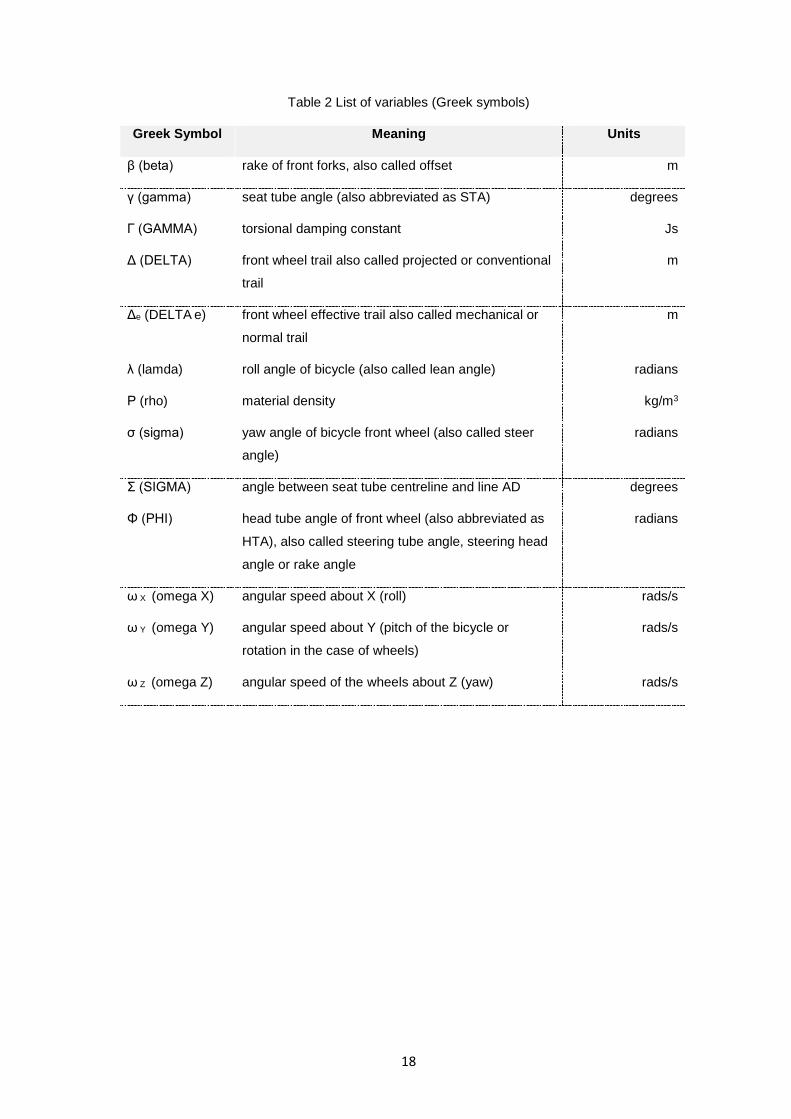
Table 2 List of variables (Greek symbols)
Greek Symbol Meaning Units
β (beta) rake of front forks, also called offset m
γ (gamma) seat tube angle (also abbreviated as STA) degrees
Г (GAMMA) torsional damping constant Js
Δ (DELTA) front wheel trail also called projected or conventional
trail
m
Δe (DELTA e) front wheel effective trail also called mechanical or
normal trail
m
λ (lamda) roll angle of bicycle (also called lean angle) radians
Ρ (rho) material density kg/m3
σ (sigma) yaw angle of bicycle front wheel (also called steer
angle)
radians
Σ (SIGMA) angle between seat tube centreline and line AD degrees
Φ (PHI) head tube angle of front wheel (also abbreviated as
HTA), also called steering tube angle, steering head
angle or rake angle
radians
ω X (omega X) angular speed about X (roll) rads/s
ω Y (omega Y) angular speed about Y (pitch of the bicycle or
rotation in the case of wheels)
rads/s
ω Z (omega Z) angular speed of the wheels about Z (yaw) rads/s
18

Table 3 Notation used
Symbol Meaning Units
A the front wheel, front forks, handlebars assembly
A Intersection of seat tube centreline with ground
B the frame, seat and seat post, rear wheel, transmission, rider assembly
B intersection of seat tube centreline with vertical line passing through rear
wheel hub centreline
BM refers to the benchmark bicycle with all parameters defined
C the % change in impulse response settling time for each 1% change in a
parameter
C bottom bracket spindle centreline position
COG centre of gravity position
COM centre of mass position
D Intersection of ground and a vertical line tangential to rear of front wheel
K position located along the seat post between the bottom bracket and the
top of the seat post, used to define the centre of mass position
R2 coefficient of determination, which describes the strength of the linear
relationship between two variables
ratio
S the 2% settling time of the impulse response second
u the Jones stability criterion, used to define the steering stability of
individual bicycles
ratio
X horizontal longitudinal axis as defined by the International Standard ISO
8855 (1) 1
Y horizontal transverse axis as defined by ISO 8855
Z vertical axis as defined by ISO 8855
1 See corresponding reference number in the Bibliography Section
19
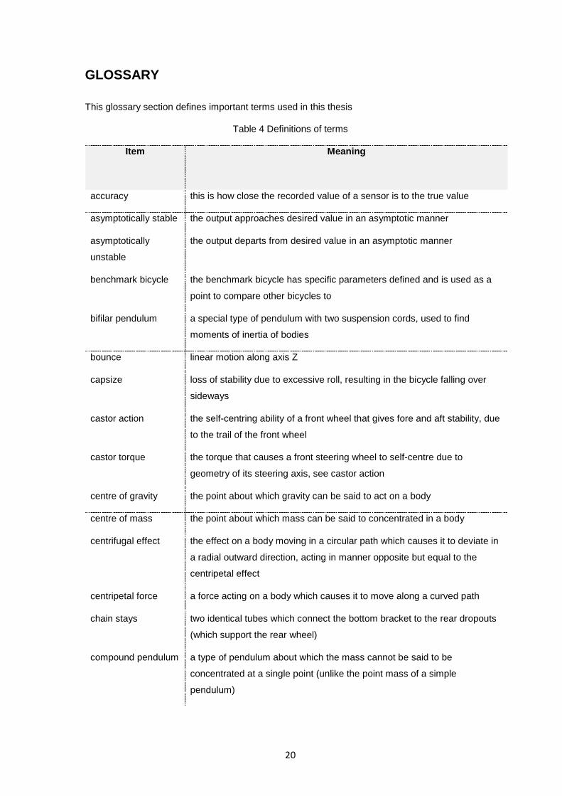
GLOSSARY
This glossary section defines important terms used in this thesis
Table 4 Definitions of terms
Item
Meaning
accuracy this is how close the recorded value of a sensor is to the true value
asymptotically stable the output approaches desired value in an asymptotic manner
asymptotically
unstable
the output departs from desired value in an asymptotic manner
benchmark bicycle the benchmark bicycle has specific parameters defined and is used as a
point to compare other bicycles to
bifilar pendulum a special type of pendulum with two suspension cords, used to find
moments of inertia of bodies
bounce linear motion along axis Z
capsize loss of stability due to excessive roll, resulting in the bicycle falling over
sideways
castor action the self-centring ability of a front wheel that gives fore and aft stability, due
to the trail of the front wheel
castor torque the torque that causes a front steering wheel to self-centre due to
geometry of its steering axis, see castor action
centre of gravity the point about which gravity can be said to act on a body
centre of mass the point about which mass can be said to concentrated in a body
centrifugal effect the effect on a body moving in a circular path which causes it to deviate in
a radial outward direction, acting in manner opposite but equal to the
centripetal effect
centripetal force a force acting on a body which causes it to move along a curved path
chain stays two identical tubes which connect the bottom bracket to the rear dropouts
(which support the rear wheel)
compound pendulum a type of pendulum about which the mass cannot be said to be
concentrated at a single point (unlike the point mass of a simple
pendulum)
20

Coriolis effect the Coriolis effect on a moving body in a rotating reference frame causes it
to deviate perpendicular to its velocity vector
counter-steer the bicycle turning manoeuvre where the bike initially turns slightly away
from the intended turn direction before coming back and following the
correct path
damping the ability of a system to suppress vibrations by dissipating energy
design chart a chart indicating the relationships between important design parameters
and bicycling handling performance (defined by the 2% settling time)
directional stability the degree with which a vehicle proceeds along a straight course despite
external disturbing forces
down tube the bicycle frame tube that connects the head tube to the bottom bracket
effective trail the distance between the vertical projection of the front wheel centre and
the projection of the front fork steering axis, measured perpendicular to the
steering axis
Euler equations the general momentum equations of rigid body motion can be simplified to
the Euler equations when the reference axes X-Y-Z coincide with the
principal axes
ETRTO European Tyre and Rim Technical Organisation, responsible for defining
bicycle tyre sizes in Europe, also widely used internationally
frequency response an analysis of the output responses of a system measured across a range
of inputs with different frequencies
frame size traditionally measured parallel to the seat tube being the distance from the
centre of the bottom bracket to centre of top tube (assuming the top tube is
horizontal and not inclined)
front fork the curved tubular assembly that the bicycle front wheel is directly fitted to,
attached to a steerer tube and handle bars, it is free to rotate
gravitational torque torque due to the pull of earth’s gravity
gyroscopic effect the effect that occurs when the axis about which a body is rotating is itself
rotated about another axis
gyroscopic torque torque due to the gyroscopic effect
head tube the part of the bicycle frame that the steering tube fits within
head tube angle the angle the bicycle head tube makes with the horizontal plane, generally
for bicycles it lies between 70 and 75 degrees, also see rake angle
21

heave linear motion about the Z axis
hip steer a bicycle turning manoeuvre made by a rider, riding without using their
hands where the bike turns in the same direction that the rider’s hips are
moved in
holonomic systems systems whose equations of constraint contain only co-ordinates, or co-
ordinates and time
hub a rotating assembly at the centre of each wheel, it contains a wheel axle
and bearings and the hub flanges that the wheel spokes fit into
impulse input an input that has infinite magnitude over zero time (mathematically
possible, but not physically achievable) in practice an impulse of
sufficiently large magnitude and of a very short time duration is considered
to be an impulse response, also see unit impulse
inseam the inside length of a person’s leg measured when standing, used to
determine the correct size of bicycle
iso-handling lines lines of constant 2% settling time displayed on the design charts
ISO International Organization for Standardization, the body responsible for the
international system of measurements and standards
Jones torque the torque that causes a front steering wheel turn into a leaned corner,
named after Jones the first researcher to describe it, see also trail steer (2)
Jones stability
criterion
the term used by Jones to define the steering stability of individual
bicycles, also called the Jones stability parameter (with the symbol u)
kink torque a torque that causes the bike to roll and is due a Coriolis effect caused by
to the difference in paths followed by different parts of the bike according
to their longitudinal position i.e. the difference between the circular paths
of the front wheel, the centre of mass and the rear wheel
lean angle see roll angle
linearity error also called an angularity error, there should be a linear relationship
between a set of true readings and the corresponding sensor readings, if
there isn’t, then a linearity error exists
mass the quantity of matter in a body
moments of inertia also called products of inertia and equal to the sum of Σ𝑚𝑚𝑟𝑟2 taken over all
particles of a body, where ‘m’ is mass and ‘r’ is the radius from a specified
centre
22
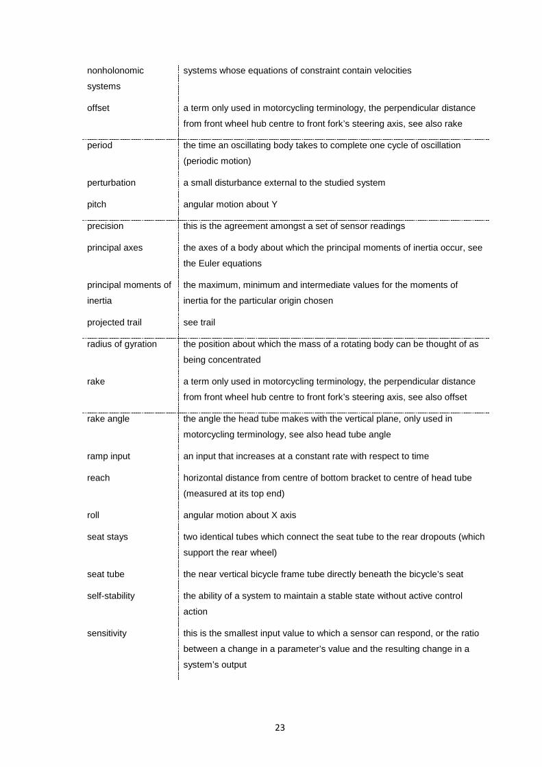
nonholonomic
systems
systems whose equations of constraint contain velocities
offset a term only used in motorcycling terminology, the perpendicular distance
from front wheel hub centre to front fork’s steering axis, see also rake
period the time an oscillating body takes to complete one cycle of oscillation
(periodic motion)
perturbation a small disturbance external to the studied system
pitch angular motion about Y
precision this is the agreement amongst a set of sensor readings
principal axes the axes of a body about which the principal moments of inertia occur, see
the Euler equations
principal moments of
inertia
the maximum, minimum and intermediate values for the moments of
inertia for the particular origin chosen
projected trail see trail
radius of gyration the position about which the mass of a rotating body can be thought of as
being concentrated
rake a term only used in motorcycling terminology, the perpendicular distance
from front wheel hub centre to front fork’s steering axis, see also offset
rake angle the angle the head tube makes with the vertical plane, only used in
motorcycling terminology, see also head tube angle
ramp input an input that increases at a constant rate with respect to time
reach horizontal distance from centre of bottom bracket to centre of head tube
(measured at its top end)
roll angular motion about X axis
seat stays two identical tubes which connect the seat tube to the rear dropouts (which
support the rear wheel)
seat tube the near vertical bicycle frame tube directly beneath the bicycle’s seat
self-stability the ability of a system to maintain a stable state without active control
action
sensitivity this is the smallest input value to which a sensor can respond, or the ratio
between a change in a parameter’s value and the resulting change in a
system’s output
23

settling time the time taken for a system to reach a certain percentage (usually 5% or
2%) of a desired value after a defined step or impulse input
side slip linear motion about Z axis
six degrees of
freedom
the three linear degrees of freedom about axes X, Y & Z and the three
rotational degrees of freedom in the a, b & c directions
stack vertical distance from centre of bottom bracket to centre of head tube
(measured at its top end)
span error occurs when the sensor doesn’t change value at the correct rate, i.e. a one
degree change in true temperature value should show as a one degree
change in sensor reading, also called a range error
speed wobble oscillations of a vehicle front wheel about the steering axis
steering angle the angle the bicycle front steering wheel makes with the longitudinal
centreline of the frame and rear wheel, it is measured in the vertical plane,
see also yaw angle
steering geometry relevant dimensions and angles of the front steering wheel assembly
namely, the steering tube angle, rake, trail and wheel diameter
steering response the nature of the dynamic output of a bicycle in response to a steering
input
steering torque the input torque provided by the rider to control and steer a bicycle
steerer tube the tube attached to the top of the bicycle front forks which is aligned by
headset bearings and mated within the head tube, also called steering
tube
step input an input that increases instantaneously from a constant value to another
constant value
stiffness the ability of a system to resist deflection or displacement
surge linear motion about X axis
sway linear motion about Y axis, see also side slip
TdF the Tour de France race which is the pre-eminent international bicycle
race and one of the three grand tours of road racing
trail the distance between the vertical projection of the front wheel centre and
the projection of the front fork steering axis measured horizontally along
the road, see also projected trail
24

trail steer the torque that causes a front steering wheel turn into a leaned corner, see
also Jones torque (2)
top tube the near horizontal bicycle frame tube at the top of the frame and below
the rider
UCI Union Cycliste International is the international body authorised to
regulate, control and run the majority of cycle sports (3)
unit impulse an impulse where the area A under the graph is equal to 1 is called the
unit impulse function and is written as 𝛿𝛿(𝑡𝑡)
weave yaw oscillations of the rider and rear frame of the bicycle (assembly B)
wheel base horizontal distance between the centres of the bicycle’s front and rear
wheels
wobble oscillations of a vehicle front wheel about the steering axis
yaw angular motion about Z axis
yaw angle the angle the bicycle front steering wheel makes with the longitudinal
centreline of the frame and rear wheel, see also steering angle
zero error sensor’s reading should return to zero when the input is zero, if it doesn’t a
zero error is present
25
1. RATIONALE AND SIGNIFICANCE OF THE STUDY
This Chapter outlines the main hypothesis of this investigation and summarises the methods used
and the results achieved.
1.1. HYPOTHESIS
The main hypothesis of this thesis is to determine to what extent mathematical modelling can
influence the dynamics of bicycle design characteristics and also improve handling performance for
the rider. The objective is to develop effective and valid design tools that bicycle manufacturers can
make use of to optimise their designs. At the moment manufactures rely heavily on past experience
and empirical techniques and as far as is known there are no scientifically rigorous design
methodologies. Existing literature does contain some techniques and advice, but their use would
be problematic in many respects.
Of particular interest is the question of how and why a bicycle’s steering remains stable. This needs
further understanding and analysis (4, 5)2. This investigation examines the effects of different
steering geometries, on steering response, system stability and frequency response of bicycles.
Research into bicycle dynamics has been evolving for many years, but even so many questions still
need to be resolved (5-9). “The bicycle has been in existence for over a century but yet many
mysteries surround the bicycle. Upon reflection, the bicycle is a deceptive object as it looks simple
and yet it isn’t (5).”
“While 150 years of evolution have turned the standard, two wheeled velocipede into a thing of
beauty, we still don’t understand exactly how it works. We have the equations, it’s just we don’t
know what they mean. Why does the bicycle steer the proper amounts at the proper times to assure
self-stability? We have found no simple physical explanation (9).”
Some key questions on quantifying bicycle performance are still unanswered. What effect and
importance do the different design parameters such as head tube angle, trial, and wheelbase have?
How can a designer systematically assess bicycle performance and base design decisions on
scientific theories as opposed to the empirical methods currently used?
Wilson says “unfortunately the equations purporting to describe bicycle motion and self-stability are
difficult and have not been validated experimentally, so design guidance remains highly empirical”
(10).
“You can't possibly get a good technology going without an enormous number of failures. It's a
universal rule. If you look at bicycles, there were thousands of weird models built and tried before
they found the one that really worked. You could never design a bicycle theoretically. Even now,
after we've been building them for 100 years, it's very difficult to understand just why a bicycle works
- it's even difficult to formulate it as a mathematical problem. But just by trial and error, we found out
2 See corresponding reference number in the Bibliography Section
26
how to do it, and the error was essential. The same is true of airplanes.” Freeman Dyson, British
Physicist and author (11)
How can we assess various bicycles and understand how and why they are different from each
other? This research develops general design principles and methodologies that will show how the
handling performance of bicycles can be described and optimised.
An important issue is to determine what sort of handling performance is desirable. Too much
directional stability in a bicycle is as much a problem as too little and while the beginner wants a
stable, insensitive bicycle, the more expert rider wants a sensitive bicycle that can respond quickly
when taking rapid evasive action to avoid a hazard.
While it is clear that certain myths about bicycle motion still persist and more work needs to be done
at least some key questions about bicycle dynamics and control have been answered and valid
equations to describe bicycle motion have been independently formulated by several researchers
(12-15).
One surprising myth is that many people suppose that bicycles are inherently unstable and must
have active rider control to remain upright. In fact it can be shown that riderless bicycles moving
above a critical speed have a large amount of self-stability. They can remain upright and will travel
in an approximately straight line for a considerable distance before their speed drops below a critical
value and they capsize. They can even recover from large yaw and roll disturbances and make
corrective actions and still continue upright (16).
Another myth is that it is commonly assumed that a front wheel castor is essential for bicycle
stability. In fact bicycles with zero trail and even 90 degree head angles though not ideal, are quite
rideable and the very first bicycle, the Hobbyhorse of 1817 was one such bicycle (6).
The incorrect notion that bicycles depend on gyroscopic effects in order to be rideable still persists
(17). This is despite numerous researchers showing both experimentally and mathematically that
gyroscopic action, while it exists, is completely unnecessary for stability and the best known
demonstration of this was Jones’ zero-gyroscopic bicycle (2). Despite the bicycle’s self-stability they
are challenging for beginners to learn to ride. The often heard advice from parents to children “to
ride faster” (in order to reach a critical velocity) is correct in one sense but also unhelpful as novices
don’t understand counter-steering. The necessary counter-steering action is counter intuitive and
not is immediately mastered. Riding a bicycle is a complex task “all in all ‘as easy as riding a bike’
is turning out to be a rather misleading saying. “I have a colleague who studies how pilots control
aircraft and he says riding a bike is much more complex” says Mont Hubbard. “We’re trying to
answer an important question, how complicated a system can a human deal with (18)?” What can
a thorough review of the literature tell us about such issues?
1.2. REVIEW OF LITERATURE
A review was made of the current state of knowledge including the development of equations of
motion for bicycles, stability and sensitivity analysis and the current design tools. The field happily
27
remains a rich area for scientific discovery encompassing the disciplines of: design, control theory,
rigid body dynamics and practical experimentation. Over 70 major papers about bicycle motion have
been written and it has attracted some famous names: Rankine, Whipple, Timoshenko and F. Klein
to name a few and it remains a challenging problem to study. At the undergraduate level it is perhaps
too challenging, unless many simplifying assumptions are used which may compromise the validity
of the analysis. This thesis makes suggestions as to what sorts of assumptions are sensible for
different applications. Chapter Two examines in more detail the literature in this field and identifies
what has been done and what remains to be done.
1.3. MATHEMATICAL MODELLING
In this investigation the physical laws of nature were applied to a bicycle to obtain a mathematical
formulation for the complete dynamic model. Simulink computer software was then used to solve
the resulting multibody dynamic equations of motion and this is described in Chapters Three and
Four. The Simulink model ran many simulations using different combinations of system parameters
and physical scenarios to investigate the dynamic responses. This model can simulate different
bicycle designs, allowing different steering geometries (and other terms) to be quantified in terms
of performance. This model was validated in Chapter Four from data available in the literature and
from an experimental investigation conducted using a specially adapted bicycle fitted with
measurement sensors to record yaw and roll angles.
Design parameters were examined in detail in Chapters Five where their actual importance was
determined by systematically changing each parameter one at a time while keeping all others
constant. Large variations in roll and yaw responses showed how sensitive bicycles are to small
changes of key parameters such as the head tube angles and rake dimensions. At higher speeds
the observed steering responses support the common observation that bicycles are more stable
and easier to ride at higher velocities. These simulations showed the importance of correctly
selecting the bicycle’s parameters in order to optimise handling performance.
1.4. DESIGN METHODLOGY
Designers need to be able to use a design methodology based on scientific theories as opposed to
the current empirical methods. This is so their design decisions can be based on a clear
understanding of how sensitive the bicycle is to changes key parameters. According to Meijaard et
al “Through trial and error, bicycles had evolved by 1890 to be stable enough to survive to the
present day with essentially no modification. Because bicycle design has been based on tinkering
rather than equations, there has been little scrutiny of bicycle analyses” (14).
This research was used to develop in Chapter Six, several design methodologies that indicate how
the handling performance of bicycles can be optimised. The design methodologies considered
included: design criteria, design tables, handling equation (from simplified equations of motion) and
design charts. After consideration of a range of requirements this thesis recommends the use of
four Design Charts associated with: the steering geometry, wheel properties, frame geometry and
28

the mass/roll inertia. Used together these four Design Charts provide a designer with a robust
methodology to select the best combinations of parameters for a desired purpose.
The Design Charts were validated in Chapter Seven by comparing them to bicycles designed
according to historical design practice and secondly to riders and bicycles from the 2013 Tour de
France bicycle race. These comparisons showed that the Charts’ are relevant and useful and can
offer designers valuable guidance.
29
2. LITERATURE SURVEY
2.1. INTRODUCTION
This Chapter examines in detail the literature in the field of bicycle dynamic motion, it reviews what
is known and what is yet to be discovered. Many papers about bicycle dynamics have been written
and the topic has interested some famous names such as: Rankine, Whipple, F. Klein, and
Timoshenko, but it still remains challenging. Why does such a supposedly simple object as a bicycle
remain a puzzle in terms of its dynamics and stability?
Richard E. Klein when discussing the complexity of bicycle dynamics wrote “issues complicating
the bicycle include the nonholomonic (or velocity) constraints, the algebraically coupled higher
derivative terms, the vague nature of the lateral tyre road forces which are so hard to quantify and
the often misunderstood role of gyroscopic effects (5).”
Later Moon wrote in his text on multibody dynamics: “in spite of the ubiquitous nature of the bicycle
and the recent improvements in the so called mountain bicycle, very little hard dynamic knowledge
is known about this system apart from empirical trials and observations (19).”
This agrees with the author’s view that little qualitative work has been done to guide the bicycle
designer in making good design decisions. But while it is clear that misconceptions about bicycle
motion persist, many questions about bicycle dynamics and control have been answered in the past
twenty years, using equations independently formulated that describe the important external and
internal torques acting on a bicycle (13, 14). For example it has been established by several
researchers that the inverted pendulum model gives a good explanation of bicycle stability in terms
of the sideways capsize (20). Also many researchers have shown conclusively that gyroscopic
effects cannot account for the stability of bicycles and clear explanations for the increased stability
or rideability of bicycles at higher speeds have been proposed (2, 5, 20, 21).
This survey has been arranged into themes covering the following eight areas: early explanations
for bicycle motion, development of the equations of motion, bicycle myths, experimental work,
multibody dynamics, control engineering approaches, computer modelling of bicycles and
chronological reviews of paper. The decision to use these themes was made because it was felt to
be more relevant to discussing this dynamic problem than the more common chronological
approach.
2.2. EARLY EXPLANATIONS OF BICYCLE MOTION
One of the earliest explanations for the stability of a bicycle in motion was proposed in 1869 by
Rankine who argued that centrifugal forces resulted in sufficient torque to balance the gravitational
overturning moment. He then described the inverted pendulum model for balance and the motion
of a bicycle attempting to follow a straight course as “the plain wavy line represents the actual track
of the centre of mass.” This was the first time that this fundamentally important concept was
described. He then gave a description of counter-steering stating “it is obvious, that the first thing to
30

be done is to incline the fore-wheel in the direction opposite to that of the intended curvature, in
order that the base point may be displaced and give rise to centripetal force. The effect of this is to
deflect the base-track away from the intended centre of curvature (22).”
Later towards the end of the nineteenth century, Bourlet wrote one of the earliest books on the
design and analysis of bicycles and followed this up with a paper outlining a mathematical study of
bicycle motion (23, 24). Bourlet described equations for a bicycle with a vertical steering axis and
no trail. Much later Meijaard et al reviewed Bourlet’s work as part of their history of bicycle steer
and dynamic equations (14). They found that when linearized Bourlet’s non-linear roll equations
were correct except for omitting the front wheel gyroscopic term associated with the steer rate.
Sharp’s book “Bicycles and Tricycles, An Elementary Treatise On Their Design And Construction”
was an interesting and detailed description of early bicycle development up to the end of the 19th
Century (7). This book discussed the science relevant to bicycles such as: statics, dynamics,
material properties and system behaviour. He described basic bicycle stability equations that used
centrifugal forces in the way proposed by Rankine in 1869. The author then examined bicycle
stability, steering action, motion over rough surfaces and resistance to motion. The text included a
detailed description of the development of bicycles from the first Hobbyhorse of 1817 up to the end
of the 19th century, including the Rover Safety bicycle of 1885. The last section of this book
examined specific technical developments in the areas of: gearing, tyres, pedals, brakes and
frames.
In 1899 Whipple wrote a paper on bicycle dynamics in which he briefly discussed Bourlet’s and
McGraw’s independent papers on bicycle stability (15, 23). Note that McGraw’s paper published in
the journal “Engineer” on 09 Dec 1898 has not been obtained and is not referenced. Whipple stated
“no satisfactory explanation on mathematical lines has been given of the practicality and ease of
riding a bicycle.” He then developed non-linear equations of motion for a bicycle assuming that: the
roll angles were small, the bicycle consisted of only two rigid bodies, the motion was steady and
that any turns have large radii. From his nonlinear equations he developed linear equations of
motion for a bicycle. These were analysed to find unstable roots and he identified four critical
velocities which required different control input modes on the part of the rider in order to maintain
stability. The highest critical velocity was v1 (5.5 m/s), then v2 (4.6 m/s), v3 (3.8 m/s) and finally v4
(3.3 m/s). Between v1 and v2 the bicycle was only stable by turning the front wheel into the roll or
by moving the body away from the roll. Between v2 and v3 stability was achieved by moving the
body into the roll. Below v2 the bicycle was unstable if ridden with the hands off (i.e. a steering input
is required for stability). Finally below the lowest critical velocity was v4 (3.3 m/s) the rider must use
a combination of body motion and steering input to remain upright. Meijaard et al recently reviewed
Whipple’s paper as part of their history of bicycle equations (14). They found that except for small
errors, Whipple’s non-linear governing equations were nearly correct.
31

2.3. DEVELOPMENT OF EQUATIONS OF MOTION
Little more was done in regards to bicycle dynamics until Timoshenko and Young included a short
analysis in their classic engineering text “Advanced Dynamics” in 1948 (20). Their bicycle analysis
produced equations of motion that could cope with large angles of yaw and roll and their work is
much cited by researchers in this field. They described a model for balancing a bicycle similar to
that of balancing an inverted pendulum in that the rider must steer the bicycle to make use of
centrifugal forces to position the centre of mass over the tyres and so correct any capsize tendency.
Their equations clearly showed that in order for the bicycle to remain upright the rider must steer
the front wheel into the direction of any roll, exactly as proposed by Rankine, Sharp and Whipple.
This model for stability is still thought to be valid as a simple analysis of straight-line travel. Their
equations did not include many of the real life complications of bicycles such as the steering
geometry variables that later researchers have added.
Psiaki wrote about the dynamics of bicycle and derived full non-linear equations for its motion (25).
He conducted computer numerical analysis (using Fortran IV) and examined the effects on stability
in a straight line using different design parameters. Secondly he solved the characteristic equation
for the case of a steady turn. He studied stability by varying the following parameters: head tube
angle, trail, wheelbase, height and longitudinal position of mass, speed and several moments of
inertia, one at a time. Meijaard et al have compared Psiaki’s eigenvalues in a forward speed range
with their model and have stated that his results agreed with theirs within plotting accuracy (14).
Lowell and McKell used Timoshenko and Young’s analysis as a starting basis for their investigation
(20, 21). They simplified the equations by only considering small angles of yaw and roll and by
modelling the steering geometry of their bicycle as a simple trailing castor wheel. They derived
simplified equations for bicycle yaw and roll angles which were solved using a fourth order Runga-
Kutta method to obtain numerical solutions, plotting angular responses against time. No damping
term is included in their model and only the front wheel gyroscopic term due to yaw is included. The
gyroscopic torque on the front wheel due to roll and the gyroscopic torque on the rear frame and
rider due to cornering are neglected, potentially serious omissions which will be discussed later. As
their results didn’t demonstrate counter-steering action or self-righting stability it is believed that
their analysis is incorrect. Meijaard et al concludes “when our equations are simplified to correspond
to their model the equations do not agree... it is incorrect (14).”
Hand presented new equations of motion for a bicycle with a model consisting of four rigid bodies
(26). He used Lagrangian equations to develop linearized equations of motion for hands off riding
i.e. with no steering input from the rider. He then applied the Routh Stability Criterion to establish
stable and unstable combinations of design parameters. A PC based Fortran programme was
developed to apply the Routh Stability Criterion stability to specific designs. According to Meijaard
et al, Hand's equations agreed with their bench marked equations but Hand's Fortran program for
calculating stability eigenvalues had errors (14).
32

Franke, Suhr and Rieß developed a general bicycle model with the following simplifying
assumptions: a rigid bicycle frame, no tyre slip or friction, thin disc wheels, a level road and no wind
(27). Their model allowed for the steering geometry of rake and trail and it had five rigid bodies; the
frame, the rear wheel, the rider, the handlebar/front fork assembly and the front wheel. They
investigated stable and unstable riding conditions and the ability of the bicycle to stabilise itself and
their model only examined hands off riding with a zero input steering torque. The momentum
approach was used to develop final equations of motion consisting of second derivatives for velocity,
yaw and roll and these equations were solved by computer using the Runga-Kutta procedure which
produced eigenvalues for the system. They concluded that gyroscopic wheel effects were essential
for inherent stability though it is clear from other researchers’ work that this is not the case. They
also said that steering stability increased linearly with trail but it is known from the literature that too
large a trail can cause an over correction of the front wheel and so can reduce stability (28).
Fajans described the equations of motion for bicycles and motorcycles and explained the
phenomena of counter-steer and hip steer (12). A counter-steer manoeuvre (first described by
Rankine) is when the steering wheel is initially turned away from the desired direction of turn causing
the bicycle to lean into the corner (22). The three equations of motion Fajans developed describe
the dynamic motion of the bicycle for specific steering inputs and were derived from the works of
Timoshenko & Young and later Lowell & McKell. These equations were dynamically unstable unless
a small damping term was added. In practice this damping is due to the front tyre and the rider’s
arms (12, 29) The author then discussed the limitations of these equations because of the
unaccounted for effects of tyre deformation, head tube angles and friction.
Fajans examined in: a road racing bicycle and a large motorcycle. With the exception of the driving
power, motorcycle dynamics share many similarities with bicycle dynamics, therefore some studies
of motorcycles are of relevance to this investigation. Input values for steering torque and various
physical parameters such as mass and wheelbase length were selected and used to obtain the
dynamic outputs of yaw and roll. The author concluded that gyroscopic effects only have a small
part to play in assisting cornering and are not required for system stability. A no hands turn using
hip steer was investigated and the oscillations that occur for “no hands” riding were modelled. These
oscillations were usually suppressed by the mass and damping provided by the rider’s arms.
Jackson and Dragovan also developed equations of motion that were derived from Timoshenko &
Young and Lowell & McKell (20, 21, 30). Their model allowed for more realistic steering geometries
than other available models, for example Fajans (12). They stated they undertook experimental
work that measured the motion of a bicycle, but their theoretical and experimental results were not
included in the paper. Like many others they concluded that gyroscopic terms were unimportant for
stability (12).
Fajans’ equations were modified by Prince (the author of this thesis) by adding terms to account for
changes in steering geometry due to head tube angle and front fork rake (31, 32). Two approaches
were adopted to validate this modified model. First a simplified Simulink model was prepared that
used exactly the same assumptions as Fajans: i.e. no Coriolis terms and the same head tube angle
33
and rake values. This model showed nearly identical results to Fajans in terms of: yaw vs. time and
roll vs. time with identical time lags, rise times, amplitudes, overshoots, and oscillations. Next an
experiment was carried out to measure the actual steering and roll angles of a moving bicycle. A
bicycle was fitted with transducers to measure yaw and roll angles and a data logger recorded the
results. The results of both validation procedures confirmed key parts of the theory and helped
validate the model. The final complex Simulink model produced more realistic results and displayed
more system stability than the Fajans model. As stated by many others the gyroscopic terms were
shown to be insignificant and could not account for bicycle stability.
Meijaard, Papadopoulos, Ruina and Schwab developed linearized equations of motion for a rigid
four body bicycle system (rear wheel, rear frame & rider, front fork and front wheel) including the
use of realistic front wheel geometry (14). Their model used three degrees of freedom (roll, steer
and forward velocity) and includes 25 parameters. They validated their theoretical approach using
two different computer simulations: Spacar (in Fortran 77) and Autosim. The eigenvalues obtained
from the linearized stability analysis of their bicycle model showed regions of stability and instability
for different forward speeds and also the nature of any instability present e.g. capsize, wobble or
weave. Capsize was defined as the bicycle toppling over, wobble is a high frequency vibration of
the front wheel only and weave is a medium frequency rolling and yawing of the rear assembly of
the bicycle (33). The authors spent some effort solving their final equations (using two different
methods) and checking the results against previous researchers’ work, eventually finding close
agreement by both their methods. They reviewed the work of many previous researchers in the field
and compared their approach to these researchers in a detailed supplementary appendix. They
also compared their results to what had been achieved experimentally by Kooijman et al (34). As a
result they were confident that their equations could be used as a benchmark against which other
studies could be compared and verified. They aided such a benchmarking process by providing
eigenvalues to an accuracy of 15 significant figures.
2.4. BICYCLE MYTHS
One of the most persistent myths about bicycle stability is the importance of gyroscopic effects.
When discussing bicycle stability R. E. Klein mentions “the often misunderstood role of gyroscopic
effects (5). Two Germans, mathematician F. Klein (famous for describing the Klein bottle) and
physicist Sommerfeld wrote a four part treatise “On the Theory of Gyroscopes” which was published
between 1897 and 1910. A review of this paper by Meijaard et al concludes that its general
statement in reference to bicycles “gyroscopic effects ...are indispensable for self-stability” is not
correct (16).
As recently as 1998 researchers have incorrectly explained the dynamic motion of bicycles and
their stability by using the gyroscopic effects of their wheels (17, 27, 35). One example of such an
incorrect explanation was made by Higbie who described the cornering motion of a motorcycles,
particularly the counter-steer manoeuvre, entirely by using gyroscopic action (35). No other torques,
internal or external, were mentioned by this author except for a brief mention of the effect of
34

gravitational torque on front wheel yaw. This was a simplistic and incomplete discussion and
repeated the myth of the importance of the gyroscopic term.
Later on, Cox described the cornering motion of a motorcycles particularly the counter-steer
manoeuvre, as being due to two effects, firstly the conical shape of the tyre caused the bicycle to
roll around a central point and secondly the gyroscopic action of the wheels due to gravitational
torque (17). Cox added the angular momentum vector from the steering torque to the angular
momentum of the wheel and argued that this caused the bicycle to lean over. It is believed that this
is not the correct way to apply gyroscopic theory to this physical problem. In addition it has been
verified by computer modelling that the steering torque can be very small (e.g. in order of 0.5 Nm
for a bicycle) and so would not cause the bicycle to lean over as was claimed (31). Cox correctly
described the effect of gyroscopic torque on the front wheel but includes no other internal or external
torques such as the inertia torque or castor torque.
Overall the role of gyroscopic effects in bicycle stability are often misunderstood and overstated
(17). Such claims about the importance of gyroscopic effects have been shown by many other
researchers to be incorrect both by mathematical modelling and by the use of experimental zero
gyroscopic bicycles. It is very clear that gyroscopic forces are not essential for self-stability nor do
they allow bicycles to be ridden (2, 36, 37). Jones was the first to demonstrate the unimportance of
gyroscopic effects and R. E. Klein has further confirmed these findings experimentally several times
(2, 4).
2.5. EXPERIMENTAL WORK
Surprisingly few experimental investigations of bicycles have been described in the open literature.
One of the most cited was performed by Jones who examined the basic question of why is it possible
to ride a bicycle and keep it upright and why it seems easier to balance it when riding at higher
speeds (2). Jones demonstrated the relative unimportance of gyroscopic effects with his famous
experiment (2, 38). He built a special bicycle that had a second wheel fitted alongside the front
wheel. This wheel didn’t touch the ground and was linked by gears to the front wheel so that it
rotated at the same speed but in the opposite direction. As this second wheel was nearly identical
to the original wheel almost all of the gyroscopic effects were cancelled out. Jones found that it was
a simple matter to ride this zero gyroscopic bicycle and that it did not feel substantially different from
an unmodified bicycle. Jones could successfully ride it without his hands on the steering handlebars,
showing conclusively that gyroscopic effects are not required for the ride stability of bicycles.
Jones then considered the well-known observation that the front wheel of a bicycle turns into the
direction of any roll (i.e. into the corner). He explained that this occurs because as the front wheel
turns (due to a twisting gravitational torque) the bicycle lowers its centre of mass and so lowers its
potential energy. Calculations were made to find this change in the height the mass for different roll
and steering angles. These calculations showed that when the steering wheel is pointing straight
ahead the twisting gravitational torque increases linearly for increased roll angles. It was concluded
that as the roll angle increases the bicycle provides a greater twisting torque that steers the wheel
35

into the corner. This effect helps to counteract the leaning over of the bicycle due to the inverted
pendulum effect. He also found that different steering geometries have different rates of increase in
this twisting torque and he used these results to plot a graph indicating stable and unstable
geometries. A stability criterion was proposed that is discussed in Chapter Six, Jones tested his
ideas by purposely building another experimental bicycle designed to be unstable and as predicted
he found that it was unstable. Finally Jones built a bicycle to investigate whether front wheels can
self-centre. He concluded that far from self-centring the rest of the bicycle swung in behind the new
altered track of the front wheel and continued on a new stable course. The experimental work of
Jones has been widely referred to by many later researchers (12, 21, 39, 40).
Kirshner examined Jones’ paper but disagreed with some of his conclusions (39). The Jones
stability criterion was shown to be approximately equal to the trail of the bicycle allowing for the
steer angle and roll angle. Kirshner disagreed as to the cause of the apparent self-centring effect
Jones observed in his final experiment and concluded that Jones’ theory for bicycle stability was
not valid. Kirshner then concluded that gyroscopic effect of the front wheel does contribute to bicycle
stability but did not provide any positive analysis to justify this claim other than to say “we attempt
to verify a nongyroscopic theory of bicycle stability and fail.” Given the widespread experimental
and theoretical support for Jones’ conclusion about the unimportance of the gyroscopic effect it is
hard to agree with Krishner.
Le Hénaff spent the first part of his paper discussing the history of research into bicycle stability
including references to Jones’ work (40). He discussed the Jones stability criterion and plotted
dynamic stability curves of the “height of wheel hub / wheel radius” versus lean angle for different
speeds (2). He concluded that these curves explain why a bicycle is more stable at higher speeds
because they show that a smaller steering angle is required to generate the required stabilising
centrifugal force. He also concluded that though gyroscopic forces on the wheel are “negligible and
unable by themselves to account for equilibrium” they do enable a bicycle to be ridden hands off.
Hunt inspired by Jones’ zero gyroscopic experiment, also showed that cancelling the gyroscopic
component of the bicycle’s front wheel made no difference to the rideability of the bicycle (36). Hunt
fitted a second wheel to the front forks alongside the front wheel, arranged to spin in the opposite
direction, hence cancelling the gyroscopic couple. Care was taken to align the gyroscopic vectors
and to make sure that the gyroscopic torques were inline. A brass adaptor was made to perfectly
align the front and counter rotating wheels. Extra weight was added to ensure that the moment of
inertia of the counter rotating wheel was close to that of the front wheel. The second wheel was
spun by hand at the desired speed and direction before starting to ride the bicycle. Hunt described
the experiment and concluded that the addition of this reverse spinning wheel made no difference
to the bicycle’s rideability. He described in brief terms: balancing stability, steering and countering-
steering and the only calculations given were basic but clearly showed that the magnitude of any
gyroscopic couple was insignificant compared to the gravitational couple.
R.E. Klein is an Engineering Professor at the University of Illinois who has used the study of bicycles
to teach students about dynamic systems. He has developed student projects that designed and
36
built interesting and unique bicycles that examined various dynamic issues. These have included
numerous zero-gyroscopic bicycles, naive bicycles (with a 90o head tube angle and no trail), easy
to ride bicycles for beginners, rear steered bicycles and exaggerated gyroscopic bicycles (4, 5, 13,
37). Klein’s work is covered in more detail in a later section in this Chapter on control engineering
approaches.
Foale and Willoughby’s well known book “Motorcycle Chassis Design: the Theory and the Practice”
discussed experimental and empirical work on the subject of motorcycle design and handling
performance (41). The book described in great detail many practical aspects of motorcycle chassis
design with the use of: diagrams, photos and experimental work, though no mathematical analysis
is provided. Front wheel speed wobbles were discussed as to the likely causes and solutions, but
only in practical terms not in theoretical ones. One chapter discussed an experiment involving the
radical modification of the front wheel geometry of a motorcycle and the effects on handling
performance. They asked why the then current motorcycles used head tube angles of between 60o
and 65o. They concluded that it is a combination of convenience of construction, lack of imagination
and fear of customer resistance. Using a BMW R75/5 motorcycle (circa 1970) they increased its
head tube angle from 63o to 75o and then to 90o and also adjusted the rake from 49 mm to 0 mm
and then to –49 mm so that the trail remained at a value of 89 mm for all three cases. Considerable
road testing was done (over 3000 km) with five different riders and qualitative analysis was made
of the riders’ descriptive feedback though no quantitative analysis was made. The modified
geometry showed increased stability but also insensitivity to and better damping of outside
perturbations. The front fork suspension was also more effective but fork juddering occurred under
heavy braking. The authors concluded that steering geometries other than those arrived at by rule
of thumb and accepted practice may have advantages.
Lignoski completed an interesting experiment to determine whether the bicycle steering angle is
proportional to the lean angle (42). This is a common assumption made by researchers to simplify
their equations of motion (21, 43). Lignoski used Lowell and McKell’s equations and treated the
motion of a bicycle as a damped simple harmonic oscillator and the gyroscopic torque of the front
and rear wheels due to rolling and due to cornering were not included in his model. Though the
equations are overly simplified, the experiment and its purpose is interesting. It consisted of rigidly
mounting a video camera to a post attached to a bicycle and videoing the bicycle and surrounding
walls as the bicycle was ridden. From the video recording produced, the lean angle was determined
from the difference between the camera’s frame of reference and vertical lines marked on nearby
walls. In a similar way the steering angle was calculated from the video by comparing the projected
length of the handlebars to the projected length of the handlebars at several known angles. The
resulting experiment recorded only one very short run of two seconds in duration and Lignoski had
problems getting accurate results as lots of practical problems were experienced including signal
noise which increased the uncertainty of the results. Lignoski’s experiment, while ingenuous,
appears inconclusive but he reached the tentative conclusion that steering angles were proportional
to lean angles, with the constant of proportionality equal to 2.40 +/- 0.15.
37

Kooijman et al completed an experimental validation for a numerical model of an uncontrolled
bicycle (34). Many theoretical models simplify the bicycle problem by ignoring effects such as frame
and wheel flexibility, the play in bearings, tyre effects and wheel slip. This practical research
examined whether these simplifications are valid, an important consideration. Their model had three
stated degrees of freedom (roll of rear frame, steering angle of front wheel and rotation of rear
wheel) and produced linearized equations of motion for the upright steady motion of a bicycle with
only small outside perturbations. Their experiment consisted of a fully instrumented bicycle which
recorded roll, yaw, steering angle and rear wheel rotation. The bicycle had no rider but was pushed
along a dry level floor by a person running alongside it. A total of 76 experimental runs were made
with a maximum run length of 40 metres. From the recorded results the bicycle’s eigenvalues were
found from the plotted data and these experimental eigenvalues compared well to the theoretical
values. They concluded that the theoretical model was valid when compared to the experimental
results and that the assumptions made to simplify the model were reasonable.
Further experiments by Koojiman et al involved an instrumented rider and bicycle on a road and
later on a treadmill and concluded that the rider steers and stabilises the bicycle mainly by steering
inputs via the arms and with very little upper body lean or knee movement (44). Only at very low
speeds (1.4 m/s) was any lateral knee movement observed at all. The steering inputs were
performed at a similar frequency to the pedalling frequency and their amplitude increased as forward
speed decreased.
Moore et al also wished to test the hypotheses that riders principally use direct steering input for
control and make little use of upper body movements to control the bicycle (45). To examine this
question they used a motion capture technique to examine three different riders riding a bicycle on
a large rolling road. The experiments examined a cyclist riding at steady speeds ranging from 2 to
30 km/hr. Matlab was used to analyse the riders’ movements from the data collected by the motion
capture cameras. The motions of different parts of the rider were examined using frequency analysis
to determine whether they were contributing to steering control. They concluded that steering
control was mainly done by the arms through the handlebars but at low speeds some steering
control was exerted by a lateral knee motion, agreeing with Koojiman (44). No upper body lateral
motion was observed contributing to steering control thereby proving their hypotheses.
Moore and Hubbard looked at the importance of front wheel diameter, head tube angle, trail and
wheelbase on the self-stability of a bicycle (46). They used a mathematical model that they
benchmarked to work of Meijaard et al [18]. They considered bicycle self-stability and assumed the
rider to be a rigid body with no piloting or control action and investigated a narrow speed range of
12.9 - 17.6 km/hr and two instability modes, capsize and weave (but not the wobble mode). They
found the stable speed range between the two modes (capsize and weave) for four main parameters
(wheel diameter, head tube angle, trail and wheelbase). An interesting and unexpected result
obtained was that the stable speed range was close to the minimum value when the front wheel
diameter was 700 mm (which is very close to a standard road bicycle 700C wheel diameter). They
found for such a 700 mm wheel the stable speed range was between 4 and 5.5 m/s. In fact common
38
empirical observations show that the stable speed range is much wider than this. They say “a more
robust assessment of handling qualities is needed.”
Later Moore et al conducted a series of interesting experiments to determine a range of physical
parameters for the bicycle rider system including: mass, centres of mass, moments of inertia of the
bicycle components (frame, front fork and wheels) and the rider properties (47). They used a
combination of experimental measurement and the use of previously published data to determine
these values. Comments were made about the practical difficulty of measuring the bicycle’s physical
parameters. For example the centres of mass of the bicycle are given as +/- 20mm accuracy which
could be considered a significant error. Unfortunately the bicycle chosen for measurement was not
a high performance bicycle. Therefore the results in this paper are not especially helpful for
evaluating high performance handling, though the methods for obtaining them are interesting.
In addition to these studies of the bicycle system, experimental investigations of the human rider
are of interest as about 80% of the mass of the bicycle rider system is contributed by the rider. One
US Air Force sponsored study undertaken by Hanavan developed a mathematical model to
calculate the properties of humans of different builds (48). More details of this and similar work are
given in Chapter Five when discussing the formulation of key bicycle design parameters.
2.6. BICYCLE MULTI BODY DYNAMICS
Wilson’s book “Bicycling Science Ergonomics and Mechanics” has become a standard reference
for those interested in bicycles. The first edition co-authored with Whitt, covered general aspects of
ergonomics and human power generation as applied to bicycles and other pedal powered vehicles
(6). The coverage of bicycle mechanics included: resistance to motion (e.g. wind, rolling and friction
resistance), braking, balancing and steering stability. Other topics included: bicycle frame materials,
human powered vehicles (HPV) and future HPV developments. The section on balancing and
steering briefly discusses many previously mentioned researchers (2, 15, 20, 49). It defined various
terms and steering geometry parameters and gave formulae from both Davison and Bourlet that
calculate a front wheel geometry which neither rises or falls when the front wheel is turned though
no justification was provided as to why this geometry would be useful for stability (50, 51). The
second edition, written only by Wilson, describes in detail Jones’ paper and Lynch’s computer
simulation of bicycle motion (49). The third edition by Wilson (with contributions from Papadopoulos)
discusses stability theories in more detail with good descriptions of: inverted pendulums, Jones’
experiments, counter-steering and a short discussion of the work of Papadopoulos (52). Front wheel
wobble (shimmy) is discussed in detail with references to Den Hartog (29).
Doebellin’s text “System Modelling and Response: Theoretical and Experimental Approaches”
contained a section that discussed the stability of four wheeled vehicles (53). The author described
in detail how to build several different dynamic models of four wheeled vehicles from the general
equations of motion. Care was taken to include such things as: tyre effects, inertia effects caused
by roll (including suspension effects) and the effect of a shifting payload. The final developed models
were analysed for steering response and instability using a CSMP (Continuous System Modelling
39
Programme) simulation. This work has relevance to this investigation as it clearly showed how
equations of motion for multi body systems, like cars and bicycles, can be derived from fundamental
first principles.
Cocco’s book “Motorcycles Design and Technology: How and Why” included diagrams and
equations to illustrate the principles of motorcycling design, riding techniques and handling
performance and was based on the work of both R. S. Sharp and Prof Cossalter (8, 54), (55). The
author examined the effects of changes to motorcycle design on performance. Specifically this book
considered: balancing on two wheels, cornering, accelerating, braking, vibration, aerodynamics,
engines, frame and suspension design. The approach taken by this author was to discuss the
concepts with diagrams and terms at a basic level. Though the treatment uses many simplifying
assumptions the anecdotal information was interesting. The descriptive section which discussed
front wheel design, steering geometry, speed wobbles and weaves was relevant to this
investigation. Basic formulae were given (sometimes without proof or references) which enable
useful effects to be found such as the frequency of a high speed wobble and the amount of fork
drop that occurs when turning the front wheel.
2.7. CONTROL ENGINEERING APPROACHES
Other researchers have looked at bicycles from a control engineering perspective with an emphasis
on stability and rideability. Some such as R. E. Klein have treated the bicycle as an interesting
engineering system worthy of study using the control engineering approach (4). Others such as
Suryanarayanan et al, have designed bicycle autopilot controllers, (56). Another group have made
use of control theory to investigate bicycle instability and to determine measures of rideability, such
as Seffen (28).
According to R. E. Klein, “the bicycle is not a trivial topic, as one might suppose at first glance, but
it is a rather formidable subject worthy of study“ (5). His paper discussed new ways to teach the
concepts of dynamic systems using bicycle motion as a practical everyday problem to study. This
approach to teaching undergraduate students used theory lectures and computer simulation
techniques to cover the necessary control theory. Klein’s paper concentrated on the effectiveness
of this teaching approach and recommended it because it stimulated student interest in the field of
control. Different aspects of bicycle motion are mentioned to give examples of how this teaching
method worked in the classroom. Laboratories were also used to help students build up proficiency
in the use of Fortran simulation e.g. modelling a bicycle counter-steering manoeuvre. Finally the
students were required to write an original essay on a selected aspect of bicycle motion such as the
relative importance of gyroscopic effects when riding a bicycle. Students also completed the
construction and testing of various experimental bicycles of their own design e.g. rear steered, zero
gyroscopic, and bicycles with accentuated gyroscopic effects. This construction assignment allowed
students to test out original ideas that they had first generated from theory and computer simulation.
Another paper by Klein expanded on the use of bicycle motion to teach the concepts of dynamic
systems (4). The paper described three basic transfer functions that could be used to build up a
40
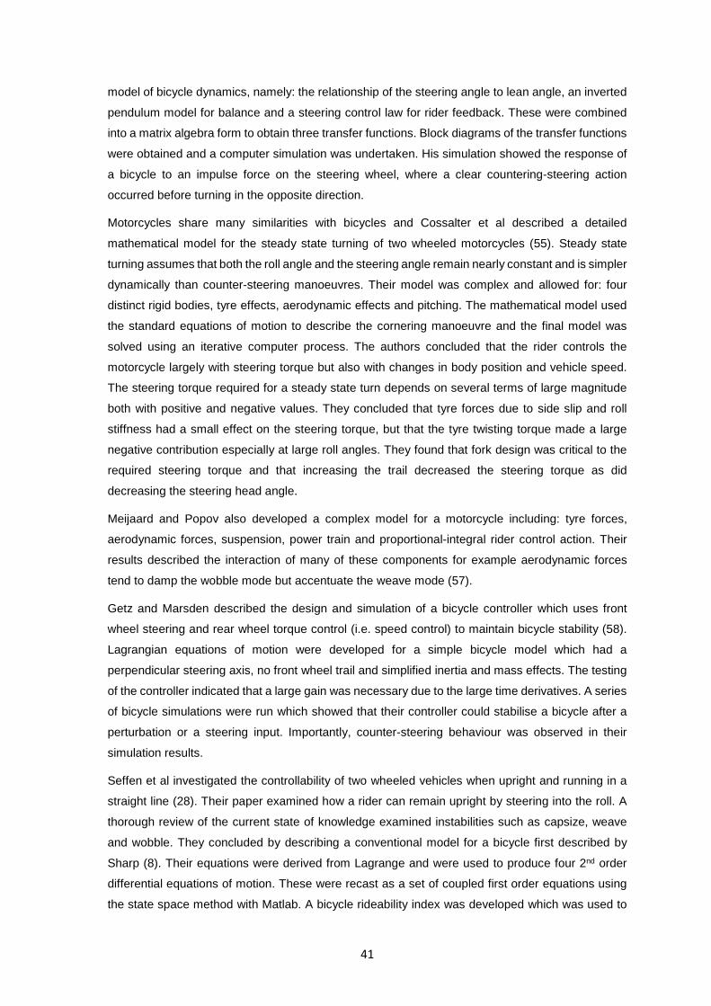
model of bicycle dynamics, namely: the relationship of the steering angle to lean angle, an inverted
pendulum model for balance and a steering control law for rider feedback. These were combined
into a matrix algebra form to obtain three transfer functions. Block diagrams of the transfer functions
were obtained and a computer simulation was undertaken. His simulation showed the response of
a bicycle to an impulse force on the steering wheel, where a clear countering-steering action
occurred before turning in the opposite direction.
Motorcycles share many similarities with bicycles and Cossalter et al described a detailed
mathematical model for the steady state turning of two wheeled motorcycles (55). Steady state
turning assumes that both the roll angle and the steering angle remain nearly constant and is simpler
dynamically than counter-steering manoeuvres. Their model was complex and allowed for: four
distinct rigid bodies, tyre effects, aerodynamic effects and pitching. The mathematical model used
the standard equations of motion to describe the cornering manoeuvre and the final model was
solved using an iterative computer process. The authors concluded that the rider controls the
motorcycle largely with steering torque but also with changes in body position and vehicle speed.
The steering torque required for a steady state turn depends on several terms of large magnitude
both with positive and negative values. They concluded that tyre forces due to side slip and roll
stiffness had a small effect on the steering torque, but that the tyre twisting torque made a large
negative contribution especially at large roll angles. They found that fork design was critical to the
required steering torque and that increasing the trail decreased the steering torque as did
decreasing the steering head angle.
Meijaard and Popov also developed a complex model for a motorcycle including: tyre forces,
aerodynamic forces, suspension, power train and proportional-integral rider control action. Their
results described the interaction of many of these components for example aerodynamic forces
tend to damp the wobble mode but accentuate the weave mode (57).
Getz and Marsden described the design and simulation of a bicycle controller which uses front
wheel steering and rear wheel torque control (i.e. speed control) to maintain bicycle stability (58).
Lagrangian equations of motion were developed for a simple bicycle model which had a
perpendicular steering axis, no front wheel trail and simplified inertia and mass effects. The testing
of the controller indicated that a large gain was necessary due to the large time derivatives. A series
of bicycle simulations were run which showed that their controller could stabilise a bicycle after a
perturbation or a steering input. Importantly, counter-steering behaviour was observed in their
simulation results.
Seffen et al investigated the controllability of two wheeled vehicles when upright and running in a
straight line (28). Their paper examined how a rider can remain upright by steering into the roll. A
thorough review of the current state of knowledge examined instabilities such as capsize, weave
and wobble. They concluded by describing a conventional model for a bicycle first described by
Sharp (8). Their equations were derived from Lagrange and were used to produce four 2nd order
differential equations of motion. These were recast as a set of coupled first order equations using
the state space method with Matlab. A bicycle rideability index was developed which was used to
41

examine the effect of changing the: front wheel trail, moments of inertia and head tube angle had
on controllability and this index is explained further in Chapter Six.
Suryanarayanan et al examined the system dynamics involved in the directional control of a two
wheeled human powered vehicle (HPV) (56). HPVs are specialist bicycles designed to break
specific straight line speed records such as the one hour HPV record (currently set at 91.55 km)
and are regulated by either the World Human Powered Vehicle Association (WHPVA) or the
International Human Powered Vehicle Association (IHPVA) (59). Typically HPVs place the rider in
a prone position within a fairing to minimise aerodynamic drag. Manoeuvrability and handling are
much less important than the ultimate top speed. But the very high speeds attained mean that high
speed instabilities such as weave and wobble can be a problem.
Their objective was to design an autopilot for a HPV capable of speeds of 100-160 km/hr. Previous
HPVs had experienced control problems at high speed due to their human pilots’ limitations,
principally their slow speed of response. These researchers concluded that using a steering wheel
trail value similar to a conventional bicycle makes a HPV unstable in cross winds. They concluded
that a lateral crosswind would induce a torque that would cause the front steering wheel to turn
away from the wind leading to increased yaw and instability. Ideally a bicycle should lean into the
wind and the front wheel should yaw into this roll. The rider can then easily balance the force of the
crosswind on the bicycle by adjusting how much front wheel yaw is needed and hence maintain
upright balance and steer a straight course. A HPV with an aerodynamic body fairing could use
increased fin area at the rear of the bicycle in order to make the bicycle yaw into the wind. This
places the aerodynamic centre of pressure aft of the centre of the tyre grip. However they concluded
that this would only be effective within a limited speed range. Presumably this is because the
aerodynamic forces on the fairing vary according to velocity squared so are subject to large
variations. The authors speculate that by reducing or eliminating front wheel steering trail crosswind
vulnerability would be reduced. However this would cause other directional stability problems due
to the lack of feedback and would warrant automatic control. The authors mathematically modelled
a bicycle using kinematic equations based on an inverted pendulum model. They then examined
the yaw and roll dynamics for three different HPV designs; a conventional front wheel steered HPV
with trail, a conventional front wheel steered HPV without trail and finally an unconventional rear
wheel steered HPV. From the results of this modelling the authors designed a steering controller
for a front wheel steered HPV suitable for a 16-160 km/hr speed range. They concluded that an
automatic steering controller was feasible and that the front wheel steering configuration gave the
best performance but they gave no details of the results of the different steering geometries. They
also proved that the rear wheel steered bicycle was unstable under most conditions because it has
an odd number of real unstable poles.
Chen et al produced bicycle equations with nine degrees of freedom (six for the rear frame and
rider, two more rotational ones around both wheels and a ninth around the steering axis) using
Lagrangian equations and the energy approach (60). They developed balancing and path tracking
strategies for the bicycle using steering controllers with both PID and fuzzy logic control action and
42

details were given of the control schemes and rules table. Outputs using control action showed the
bicycle roll angle, X & Y coordinate position and speed against time, but surprisingly not the yaw
angle. It was stated that the bicycle path followed showed the model displayed counter-steering
action but the scale of their graph makes this hard to discern. The controllers were successful in
maintaining balance and following a desired path but the second controller was more able to
accurately follow the desired path as it took the yaw angle of the bicycle into account.
A long article by Astrom et al examined in depth the issues of bicycle stability from a control
engineering perspective (13). The authors have all used bicycles to teach undergraduate students
control engineering in a way that combines theory with hands on experiments. The article discussed
rider control, proportionality constants, transfer delays and gyroscopic effects. They developed
several increasingly more realistic mathematical bicycle models including one that allowed for front
wheel steering angle and trail, but neglected the stabilizing effects of the front fork and any
gyroscopic effects. An early model demonstrated that bicycles are unstable without rider feedback
or damping. This simple model was a naive bicycle that used a steering angle of 90o just like the
Fajans model discussed earlier (12). A piloting model was developed that assumed the rider was a
proportional controller who balanced the bicycle by applying a steering torque proportional to the
roll angle as proposed by Lignoski (42). They say that in practice riders also use lean actions, though
results from Moore’s experiments indicate otherwise (45).
Another of their bicycle models examined rear wheel steering and demonstrated why rear wheel
steered bicycles are so difficult for riders to control. By examining the model carefully eventually a
successful rear wheel steered bicycle was built by their students which could be ridden in some
circumstances, demonstrating the value of a control engineering approach. This bicycle had the
rider placed very high and very far forward, significantly changing the mass position. Also the bicycle
needed to be ridden at some speed just as their equations had shown. This was presented as an
interesting and instructive mathematical control problem. They discussed a series of bicycles built
as student projects including zero gyroscopic bikes which again proved experimentally that a bicycle
can be successfully ridden without gyroscopic assistance. Another section of this paper examined
the difficulty of teaching young children to ride bicycles and trialled various modified bicycles
designed to make learning easier.
Sharma and Umashankar designed a controller for a bicycle system that stabilises the roll of a
bicycle by steering the bicycle into the roll using equations developed from Lowell and McKell (21,
43). Their aim was to see if a fuzzy controller could control an unstable system like a bicycle. Their
controller used fifty fuzzy logic rules to determine the required control action for stabilisation. The
computer simulation of their controller displayed only marginal stability and showed steady (not
decaying) and substantial oscillations of the yaw and roll angles. Three separate very low speed
values were used to test the controller (5.4 km/hr, 7.2 km/hr and 9 km/hr) and such low speeds
were likely to be a hard test for a controller to achieve system stability. Their equations did not
contain a front wheel twisting gravitational torque term and appear to repeat the errors of Lowell
43

and McKell (21). As their results didn’t display any counter-steering action and it is thought that their
investigation contains significant errors.
Ringwood and Feng wrote an interesting paper examining front wheel instability at high speeds
(61). They used the bicycle equations of Astrom et al and spent some time obtaining experimentally
the values for the position of centre of mass from actual road bicycles. Their model didn’t include
frame compliance, the mass of the front fork or any rider intervention such as feedback. They
described the pole variations for different riding conditions and made suggestions regarding stability
and this is discussed later in Chapter Six.
2.8. COMPUTER MODELLING
Lynch and Roland’s aim was to simulate the motion of a bicycle using a computer and to use the
results to generate realistic computer graphics of bicycle motion, an early example of computer
animation (49). It was intended that the simulation and graphics could be used to assist in the design
and development of new bicycle designs particularly with regard to stability and manoeuvrability.
This study was one of the few financed by a bicycle company (the Schwinn Bicycle Company USA).
They derived non-linear equations for a bicycle model which consisted of three rigid masses and
ten degrees of freedom (six for the rear frame, two more rotational ones around both wheels, a ninth
around the steering axis and the tenth for the rider about the roll axis) though they state there are
only eight. It included 44 input parameters including: dimensions, masses, moments of inertia,
gyroscopic effects, tyre side forces (slip and inclination) and tyre radial and lateral stiffness effects.
Only basic details are given in this paper of their equations and no analysis of results is given. Their
equations of motion contained several algebraic and typographical errors according to Meijaard et
al. for example the side-slip angle of the front wheel did not contain the steering rate angle and this
will have led to significant errors (14).
Their equations of motion were solved by computer using the Runga-Kutta procedure and were
then used to generate a bicycle graphic animation. The paper showed the results of a bicycle
undertaking a slalom manoeuvre and it was stated that the simulation compared well to full scale
experimental results and this is shown in a series of figures and photos but no more details or
quantification was provided. The authors stated that the limitations of the then available computers
(1972) restricted the application of this model due to the high costs of producing a simulation. They
stated that one useful outcome was that the generated graphic allowed nontechnical people to more
easily understand the bicycle dynamics by observing the computer graphic of the bicycle’s motion.
Donida et al developed a specific motorcycle computer model using ten packages from the Modelica
Multibody software library (62). The equations of motion used in the model were based on both
Cossalter’s and Sharp’s equations (8, 55). It is unclear from this paper how much these authors
independently developed and how much was already available from the existing Motorcycle
Dynamics library. Ten Modelica packages were used, namely: an eleven degrees of freedom (which
are not defined in the paper) motorcycle package and other packages for: the chassis, suspension,
rear swinging arm, wheels, tyre road interaction, braking systems, aerodynamics, road environment
44

and the driver. These ten packages were parametric, allowing a manufacturer to perform virtual
prototyping of a proposed motorcycle design. This approach could be adapted and used for bicycle
design.
2.9. CHRONOLOGICAL REVIEWS
At least two major papers chronologically reviewing studies into bicycle motion have been written.
Sharp’s earlier paper was a chronological review of research into bicycle dynamics covering over a
hundred years up until 1985 (8). It looks at forty five papers by researchers in this field including the
author’s other publications. It summarised the main contributions and conclusions of each paper
but didn’t present any numerical results or conclusions on bicycle stability or performance. It stated
that at the time of writing (1985) a good understanding of bicycle dynamics had been achieved but
that some important aspects were still not understood. The following areas that needed better
understanding were mentioned: the rider bicycle interaction, the structural properties of the rider
and frame flexibility.
More recently Meijaard et al reviewed the work of many researchers and over 70 papers in this field
from 1866 till 2006 and compared historical equations and models to their own work in a detailed
supplementary appendix (63). They conclude “Although many reports, theses and papers have
models at least almost as general as Whipple’s model, and many of these are largely correct, as
yet there is no consensus that any peer-reviewed paper in English has correct equations.” As
already mentioned they stated that their other work can be used to benchmark other researchers’
bicycle models (14).
2.10. REMARKS
This literature survey concludes that there has been intensive research on bicycle dynamics and
stability including the development of suitable equations of motion that can describe bicycle motion.
Work on how various control methodologies can be made to pilot bicycles have been completed
and some have had apparent success when applied to the experimental area. However the
literature lacks information about how this available research can be used to develop proper design
methodologies. Designers lack clear guidelines on how to improve and optimise their designs and
so still rely on empirical observations and trial and error. Some of the studies into bicycle instability
and the sensitivity of the bicycle to changes in key parameters are contradictory and need resolving.
This is a major area of interest which will be examined further in this thesis. As most of today’s
evaluations of bicycle performance are subjective and not quantified, another objective is to develop
methodologies that will define bicycle handling performance.
The following main points are raised:
1. The equations are complicated with some terms being important while others much less so. To
make a suitable design methodology it is appropriate that only the critical terms be considered
45

2. The literature includes many examples of dynamic equations for the bicycle but these are not
well correlated to design parameters.
3. The dynamic analysis of motion has not been looked at in detail in relation to bicycle design
2.11. INVESTIGATION OBJECTIVES
Considering the above remarks the main objectives of this work may be summarised as follows:
1. Investigate the possibility of developing a set of simplified yet still relatively accurate equations
of motion with the flexibility to use in developing design methodologies. This is achieved by
formulating an appropriate dynamic model which will be used to:
a. look at the dynamic responses of the bicycle and to see how they relate to the rider
b. investigate which terms in these equations are critical for the design process
c. determine the effectiveness of the model in determining bicycle performance
d. see if the bicycle can be optimised in terms of specific performance criteria
e. simulate the above equations and validate them and then determine the realistic
behaviour of the bicycle when using practical design parameters
2. Investigate the bicycle’s performance in terms of its sensitivity to design parameters changes:
a. first by formulating appropriate values for these design parameters which can then
be used to develop an appropriate sensitivity methodology
b. using this sensitivity methodology to identify critical design parameters and quantify
their effects
c. and determining which ones must be considered and which ones can be ignored
so that the dynamic equations can be simplified while still maintaining a model that
can accurately simulate bicycle behaviour
3. Develop a scientifically based design methodology which designers can use as a standard
method, this includes:
a. evaluation of alternative design methodologies including: criteria, tables, equations
and charts
b. developing and making appropriate recommendations for a suitable standardised
design methodology
c. and collecting design specifications from highly regarded bicycles for validation of
this recommended design methodology
46
2.12. CLOSURE
In this Chapter a comprehensive literature survey has been completed which concluded with
important remarks used to develop the objectives of this research. Chapter Three will continue this
investigation by developing equations of motion for a bicycle that can be solved using a Simulink
computer model. This model will be able to simulate different bicycle designs allowing key design
parameters to be quantified in terms of their effect on handling performance. This analysis will then
be used to develop a suitable design methodology.
47

3. BICYCLE MODEL FORMULATION
3.1. INTRODUCTION
This Chapter explains the theory behind the bicycle dynamic model used in this work. The
assumptions used in the model are explained and justified. Finally it describes how the equations
of motion for the model were developed, formulated and solved. One important feature of the
proposed model is it can isolate and examine individual terms and design parameters allowing
quantitative comparisons to be made. It is possible to easily adjust these individual terms in the
model in order to undertake an evaluation of the significance of each torque term and a sensitivity
study.
3.2. MODEL FORMULATION
A bicycle is a surprisingly complex problem which exhibits both yaw and significant roll, both of
which are interrelated. It consists of at least six rigid bodies, see Figure 1:
1. front wheel
2. rear wheel
3. front fork and handlebar
4. main frame
5. lower part of rider
6. upper part of rider
However simplifying it down into two bodies is a common approach in the literature and this Chapter
assumes the bicycle can be modelled as two bodies or assemblies A and B, see Figure 2 and Table
13 (12, 21, 37).
1. Assembly “A” consists of the front wheel, the front forks and the handlebars. These all turn and
move together with one exception, the front wheel is free to rotate about its axle.
2. The other assembly “B” consists of the main triangular frame, the rear wheel and the rider. The
frame and the rear wheel move together as one, except the rear wheel is free to rotate about
its axle (12, 21, 30).
Assemblies A and B are linked by the steerer and head tubes acting as a hinge that is free to move
about an axis defined by the head tube angle. Despite the rider not being a fixed body, it is common
practice to treat the rider as a rigid body fixed to the rear frame and the justification for this was
established experimentally by Kooijman et al (12, 21, 30, 44).
48
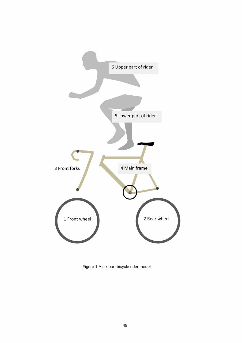
Figure 1 A six part bicycle rider model
2 Rear wheel 1 Front wheel
3 Front forks 4 Main frame
5 Lower part of rider
6 Upper part of rider
49

Figure 2 Bicycle terms for the selected model, see Table 5
h
b a
L
∆
ᵩ ᵦ FS
STA
Assembly B
Assembly A
50
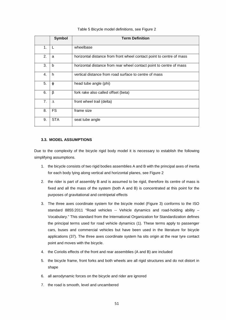
Table 5 Bicycle model definitions, see Figure 2
Symbol Term Definition
1. L wheelbase
2. a horizontal distance from front wheel contact point to centre of mass
3. b horizontal distance from rear wheel contact point to centre of mass
4. h vertical distance from road surface to centre of mass
5. ϕ head tube angle (phi)
6. β fork rake also called offset (beta)
7. ∆ front wheel trail (delta)
8. FS frame size
9. STA seat tube angle
3.3. MODEL ASSUMPTIONS
Due to the complexity of the bicycle rigid body model it is necessary to establish the following
simplifying assumptions.
1. the bicycle consists of two rigid bodies assemblies A and B with the principal axes of inertia
for each body lying along vertical and horizontal planes, see Figure 2
2. the rider is part of assembly B and is assumed to be rigid, therefore its centre of mass is
fixed and all the mass of the system (both A and B) is concentrated at this point for the
purposes of gravitational and centripetal effects
3. The three axes coordinate system for the bicycle model (Figure 3) conforms to the ISO
standard 8855:2011 “Road vehicles -- Vehicle dynamics and road-holding ability –
Vocabulary.” This standard from the International Organization for Standardization defines
the principal terms used for road vehicle dynamics (1). These terms apply to passenger
cars, buses and commercial vehicles but have been used in the literature for bicycle
applications (37). The three axes coordinate system ha sits origin at the rear tyre contact
point and moves with the bicycle.
4. the Coriolis effects of the front and rear assemblies (A and B) are included
5. the bicycle frame, front forks and both wheels are all rigid structures and do not distort in
shape
6. all aerodynamic forces on the bicycle and rider are ignored
7. the road is smooth, level and uncambered
51

8. the bicycle is travelling at a constant speed, it is not pitching or bouncing and both the roll
and steering angles are small i.e. less than 10 degrees
9. the tyres are thin and do not distort or slip sideways when cornering or slip in the direction
of travel
10. all moments are assumed to be pure couples including steering torque which is applied by
the rider and the bicycle is capable of undertaking a counter-steer cornering manoeuvre
11. the front tyre, rear tyre and centre of mass turn through the same radius when cornering
12. the radius of cornering is much larger than the bicycle wheelbase
13. realistic steering geometry can be used i.e. the fork rake and head tube angle can be varied
to model realistic bicycles
Most of the above assumptions are self-explanatory, however some need clarification.The second
assumption is that the human rider is a rigid body attached solidly to the rear frame (all of which is
called assembly B). Kooijman et al have demonstrated that the rider steers and stabilises the bicycle
mainly by steering inputs with very little upper body lean (44). Therefore no pedalling action and no
counterbalancing using the rider’s torso (called hip flick by Fajans) was considered in this model
and the only piloting aspect of the human rider is that of a simple steering torque action (12).
To explain assumption six, the intention was to investigate the characteristics of the bicycle rider
system and so it was not necessary to complicate the problem by considering external forces such
as aerodynamic forces.
Regarding assumption nine, many researchers of road bicycles have assumed that the wheels to
be thin discs and have ignored tyre effects (12-14, 21). Furthermore, after Koojiman et al ran an
instrumented bicycle on a rolling road they concluded when referring to their maths model that “the
most dubious assumption that was validated in this model was the replacement of the tyres by knife
edge wheels rolling without slipping” (14, 34). On the other hand it is common for complex tyre
models to be used when modelling motorcycles (33, 55, 62). Given that road bicycle tyres are much
smaller in width (20 mm vs. 180 mm) and operate at higher inflation pressures than motorcycles (7
bar vs. 2 bar) it is reasonable to expect that they distort less and therefore could be modelled as
thin discs. Experimental work by Dressel and Rahman found that the tyre relaxation length of a
bicycle was only between 40 and 60 mm and this compares to the much larger tyre relaxation length
of motorcycles which are between 100 and 500 mm (64). The tyre relaxation length is a measure
of delay between when the front wheel is turned and when the tyre cornering force reaches a steady
state value. The shorter this length, the shorter the delay and the more like a thin disc the wheel
behaves.
However, previous work has indicated that the model requires some dampening for stability (12).
Thus in this current work this tyre damping effect is included by adding a dampening term to the
model.
52

Longitudinal wheel slip (in the direction of travel) has been ignored as it is assumed that such slip
only occurs when braking or accelerating (65). Sideways tyre friction is present in the model and is
essential in order for the bicycle to corner and to be stable. However, the current model ignores tyre
rolling resistance as it is assumed that the speed is constant.
Figure 3 Bicycle axes for the selected model, positive directions shown, per ISO 8855 (1)
Z
X
Y
Roll angle
Yaw angle
Yawing
Pitching
Rolling
53
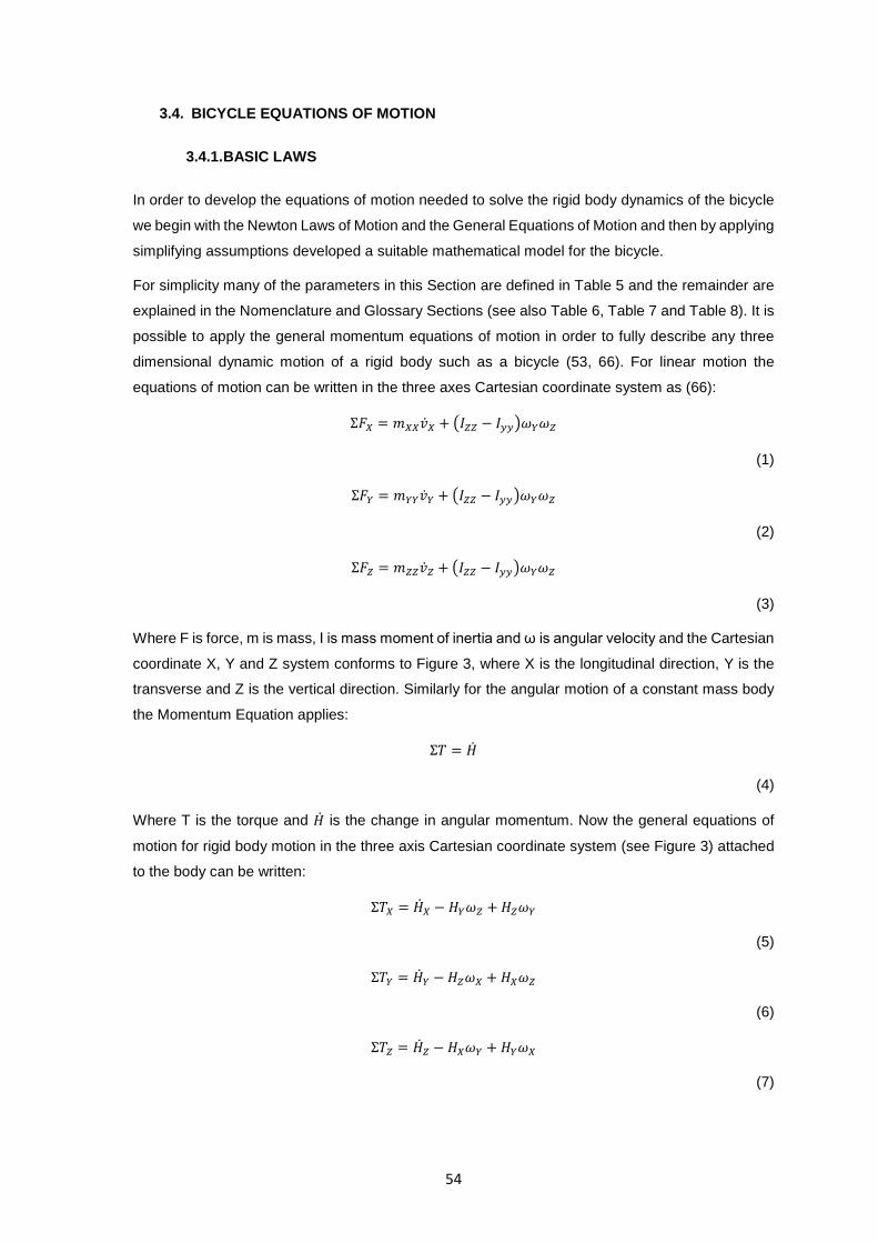
3.4. BICYCLE EQUATIONS OF MOTION
3.4.1. BASIC LAWS
In order to develop the equations of motion needed to solve the rigid body dynamics of the bicycle
we begin with the Newton Laws of Motion and the General Equations of Motion and then by applying
simplifying assumptions developed a suitable mathematical model for the bicycle.
For simplicity many of the parameters in this Section are defined in Table 5 and the remainder are
explained in the Nomenclature and Glossary Sections (see also Table 6, Table 7 and Table 8). It is
possible to apply the general momentum equations of motion in order to fully describe any three
dimensional dynamic motion of a rigid body such as a bicycle (53, 66). For linear motion the
equations of motion can be written in the three axes Cartesian coordinate system as (66):
Σ𝐹𝐹𝑋𝑋 = 𝑚𝑚𝑋𝑋𝑋𝑋�̇�𝑣𝑋𝑋 + �𝐼𝐼𝑍𝑍𝑍𝑍 − 𝐼𝐼𝑦𝑦𝑦𝑦�𝜔𝜔𝑌𝑌𝜔𝜔𝑍𝑍
(1)
Σ𝐹𝐹𝑌𝑌 = 𝑚𝑚𝑌𝑌𝑌𝑌�̇�𝑣𝑌𝑌 + �𝐼𝐼𝑍𝑍𝑍𝑍 − 𝐼𝐼𝑦𝑦𝑦𝑦�𝜔𝜔𝑌𝑌𝜔𝜔𝑍𝑍
(2)
Σ𝐹𝐹𝑍𝑍 = 𝑚𝑚𝑍𝑍𝑍𝑍�̇�𝑣𝑍𝑍 + �𝐼𝐼𝑍𝑍𝑍𝑍 − 𝐼𝐼𝑦𝑦𝑦𝑦�𝜔𝜔𝑌𝑌𝜔𝜔𝑍𝑍
(3)
Where F is force, m is mass, I is mass moment of inertia and ω is angular velocity and the Cartesian
coordinate X, Y and Z system conforms to Figure 3, where X is the longitudinal direction, Y is the
transverse and Z is the vertical direction. Similarly for the angular motion of a constant mass body
the Momentum Equation applies:
Σ𝑇𝑇 = �̇�𝐻
(4)
Where T is the torque and �̇�𝐻 is the change in angular momentum. Now the general equations of
motion for rigid body motion in the three axis Cartesian coordinate system (see Figure 3) attached
to the body can be written:
Σ𝑇𝑇𝑋𝑋 = �̇�𝐻𝑋𝑋 − 𝐻𝐻𝑌𝑌𝜔𝜔𝑍𝑍 + 𝐻𝐻𝑍𝑍𝜔𝜔𝑌𝑌
(5)
Σ𝑇𝑇𝑌𝑌 = �̇�𝐻𝑌𝑌 − 𝐻𝐻𝑍𝑍𝜔𝜔𝑋𝑋 + 𝐻𝐻𝑋𝑋𝜔𝜔𝑍𝑍
(6)
Σ𝑇𝑇𝑍𝑍 = �̇�𝐻𝑍𝑍 − 𝐻𝐻𝑋𝑋𝜔𝜔𝑌𝑌 + 𝐻𝐻𝑌𝑌𝜔𝜔𝑋𝑋
(7)
54

Where the three components of angular momentum are:
�̇�𝐻𝑋𝑋 = 𝐼𝐼𝑋𝑋𝑋𝑋�̇�𝜔𝑋𝑋 − 𝐼𝐼𝑌𝑌𝑍𝑍�̇�𝜔𝑌𝑌 − 𝐼𝐼𝑍𝑍𝑋𝑋�̇�𝜔𝑍𝑍
(8)
�̇�𝐻𝑌𝑌 = −𝐼𝐼𝑋𝑋𝑌𝑌�̇�𝜔𝑋𝑋 − 𝐼𝐼𝑌𝑌𝑌𝑌�̇�𝜔𝑌𝑌 − 𝐼𝐼𝑌𝑌𝑍𝑍�̇�𝜔𝑍𝑍
(9)
�̇�𝐻𝑍𝑍 = −𝐼𝐼𝑍𝑍𝑋𝑋�̇�𝜔𝑋𝑋 − 𝐼𝐼𝑌𝑌𝑍𝑍�̇�𝜔𝑌𝑌 + 𝐼𝐼𝑍𝑍𝑍𝑍�̇�𝜔𝑍𝑍
(10)
These equations state that the sum of the torques equal the change in angular momentum for
bodies of constant mass.
3.4.2. THE EULER EQUATIONS OF MOTION
The principal axes of inertia of a body are defined as those about which the maximum values for
the mass moments of inertia occur. For symmetrical bodies the principal axes occur on planes of
symmetry (53, 66). In the case of body like a cylinder, as the body is symmetrical about the X, Y
and Z axes they are all principal axes. And as the origin of the reference axes X, Y and Z coincide
with the centre of mass, then the inertia tensors IXY, IYZ and IXZ all equal zero and the General
Equations of Motion simplify to the Euler Equations of Motion.
So if the bicycle model can be assumed to be symmetrical about X, Y and Z the three momentum
equations of motion, (8 to (10 may be simplified into the Euler equations, but is this a reasonable
proposition?
• Considering the rider alone (which is the dominant mass in the system) Hanavan records
values for the inertia tensors as follows; IXZ = -1.7218 kgm2, IXY = IYZ = 0 kgm.2
• Similarly Meijaard et al records the following values the inertia tensors for their equivalent
of assembly B, as IXZ = 2.4 kgm2, IXY = IYZ = 0 kgm.2 (14, 48).
• Therefore in both these cases two of the three tensors equal zero and the third tensor IXZ
has a value of about 25% of the principal moment of inertia IXX.
• Also the bicycle by itself (without a rider) is symmetrical about the longitudinal X axis and is
approximately symmetrical about the vertical Z located through the centre of mass.
Therefore the assumption to use Euler Equations for the bicycle model can be justified and this
greatly simplifies the equations of motion. Also it is common practice in the study of automobile
vehicle dynamics to assume that the Euler equations apply (53).
The Euler Equation of Motion about the X axis is:
Σ𝑇𝑇𝑋𝑋 = 𝐼𝐼𝑋𝑋𝑋𝑋�̇�𝜔𝑋𝑋 + 𝐼𝐼𝑍𝑍𝑍𝑍𝜔𝜔𝑌𝑌𝜔𝜔𝑍𝑍 − 𝐼𝐼𝑌𝑌𝑌𝑌𝜔𝜔𝑌𝑌𝜔𝜔𝑍𝑍
(11)
55
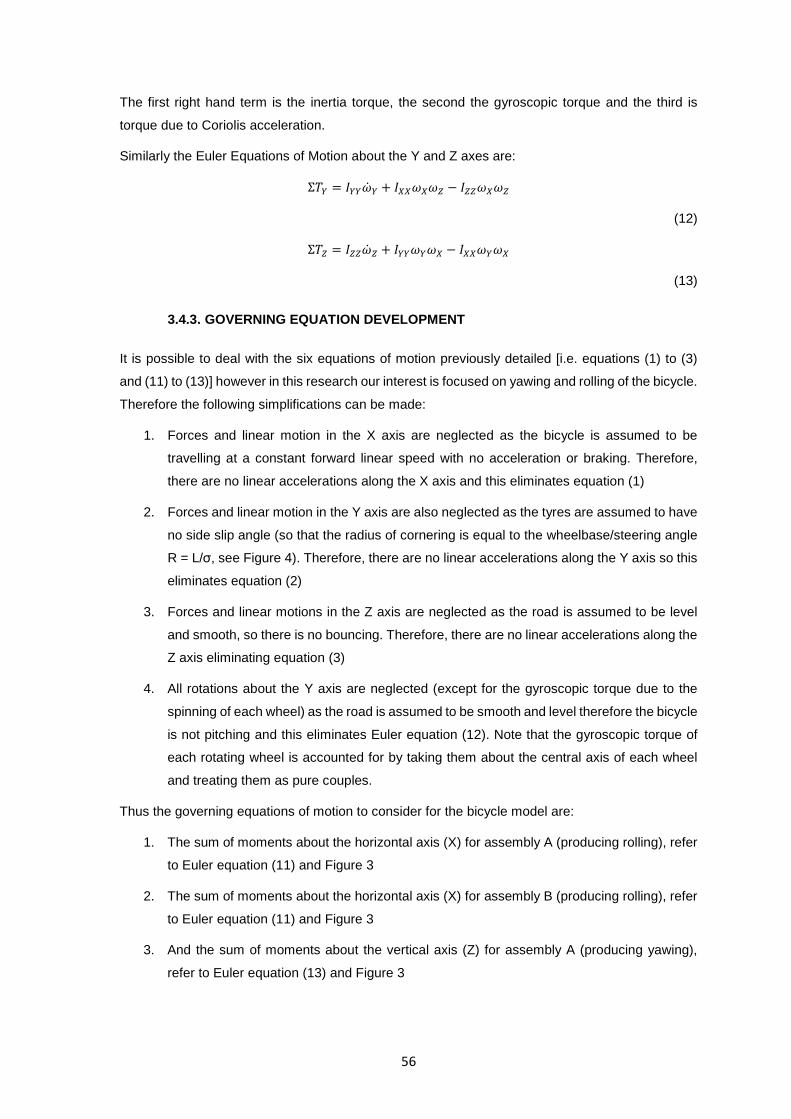
The first right hand term is the inertia torque, the second the gyroscopic torque and the third is
torque due to Coriolis acceleration.
Similarly the Euler Equations of Motion about the Y and Z axes are:
Σ𝑇𝑇𝑌𝑌 = 𝐼𝐼𝑌𝑌𝑌𝑌�̇�𝜔𝑌𝑌 + 𝐼𝐼𝑋𝑋𝑋𝑋𝜔𝜔𝑋𝑋𝜔𝜔𝑍𝑍 − 𝐼𝐼𝑍𝑍𝑍𝑍𝜔𝜔𝑋𝑋𝜔𝜔𝑍𝑍
(12)
Σ𝑇𝑇𝑍𝑍 = 𝐼𝐼𝑍𝑍𝑍𝑍�̇�𝜔𝑍𝑍 + 𝐼𝐼𝑌𝑌𝑌𝑌𝜔𝜔𝑌𝑌𝜔𝜔𝑋𝑋 − 𝐼𝐼𝑋𝑋𝑋𝑋𝜔𝜔𝑌𝑌𝜔𝜔𝑋𝑋
(13)
3.4.3. GOVERNING EQUATION DEVELOPMENT
It is possible to deal with the six equations of motion previously detailed [i.e. equations (1) to (3)
and (11) to (13)] however in this research our interest is focused on yawing and rolling of the bicycle.
Therefore the following simplifications can be made:
1. Forces and linear motion in the X axis are neglected as the bicycle is assumed to be
travelling at a constant forward linear speed with no acceleration or braking. Therefore,
there are no linear accelerations along the X axis and this eliminates equation (1)
2. Forces and linear motion in the Y axis are also neglected as the tyres are assumed to have
no side slip angle (so that the radius of cornering is equal to the wheelbase/steering angle
R = L/σ, see Figure 4). Therefore, there are no linear accelerations along the Y axis so this
eliminates equation (2)
3. Forces and linear motions in the Z axis are neglected as the road is assumed to be level
and smooth, so there is no bouncing. Therefore, there are no linear accelerations along the
Z axis eliminating equation (3)
4. All rotations about the Y axis are neglected (except for the gyroscopic torque due to the
spinning of each wheel) as the road is assumed to be smooth and level therefore the bicycle
is not pitching and this eliminates Euler equation (12). Note that the gyroscopic torque of
each rotating wheel is accounted for by taking them about the central axis of each wheel
and treating them as pure couples.
Thus the governing equations of motion to consider for the bicycle model are:
1. The sum of moments about the horizontal axis (X) for assembly A (producing rolling), refer
to Euler equation (11) and Figure 3
2. The sum of moments about the horizontal axis (X) for assembly B (producing rolling), refer
to Euler equation (11) and Figure 3
3. And the sum of moments about the vertical axis (Z) for assembly A (producing yawing),
refer to Euler equation (13) and Figure 3
56

Front wheel Rear wheel
Direction of travel
Centre of corner
Radius of corner R
Yaw angle σ
Yaw angle σ
Wheelbase L
Figure 4 Cornering bicycle geometry indicated the relationships between L, σ and R
57
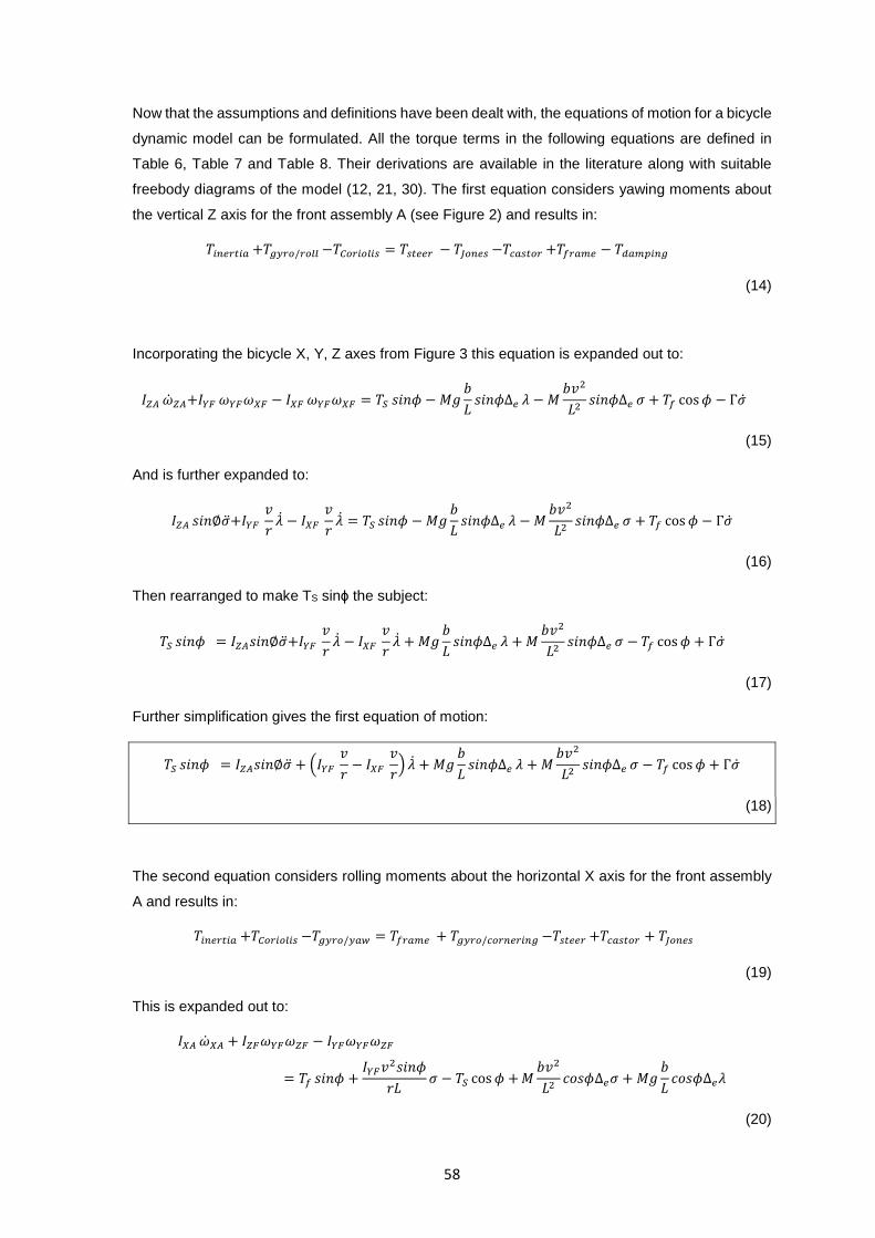
Now that the assumptions and definitions have been dealt with, the equations of motion for a bicycle
dynamic model can be formulated. All the torque terms in the following equations are defined in
Table 6, Table 7 and Table 8. Their derivations are available in the literature along with suitable
freebody diagrams of the model (12, 21, 30). The first equation considers yawing moments about
the vertical Z axis for the front assembly A (see Figure 2) and results in:
𝑇𝑇𝑖𝑖𝑖𝑖𝑖𝑖𝑖𝑖𝑖𝑖𝑖𝑖𝑖𝑖 +𝑇𝑇𝑔𝑔𝑦𝑦𝑖𝑖𝑔𝑔/𝑖𝑖𝑔𝑔𝑟𝑟𝑟𝑟 −𝑇𝑇𝐶𝐶𝑔𝑔𝑖𝑖𝑖𝑖𝑔𝑔𝑟𝑟𝑖𝑖𝐶𝐶 = 𝑇𝑇𝐶𝐶𝑖𝑖𝑖𝑖𝑖𝑖𝑖𝑖 − 𝑇𝑇𝐽𝐽𝑔𝑔𝑖𝑖𝑖𝑖𝐶𝐶 −𝑇𝑇𝑐𝑐𝑖𝑖𝐶𝐶𝑖𝑖𝑔𝑔𝑖𝑖 +𝑇𝑇𝑓𝑓𝑖𝑖𝑖𝑖𝑓𝑓𝑖𝑖 − 𝑇𝑇𝑑𝑑𝑖𝑖𝑓𝑓𝑑𝑑𝑖𝑖𝑖𝑖𝑔𝑔
(14)
Incorporating the bicycle X, Y, Z axes from Figure 3 this equation is expanded out to:
𝐼𝐼𝑍𝑍𝑍𝑍 �̇�𝜔𝑍𝑍𝑍𝑍+𝐼𝐼𝑌𝑌𝑌𝑌 𝜔𝜔𝑌𝑌𝑌𝑌𝜔𝜔𝑋𝑋𝑌𝑌 − 𝐼𝐼𝑋𝑋𝑌𝑌 𝜔𝜔𝑌𝑌𝑌𝑌𝜔𝜔𝑋𝑋𝑌𝑌 = 𝑇𝑇𝑆𝑆 𝑠𝑠𝑠𝑠𝑠𝑠𝑠𝑠 − 𝑀𝑀𝑀𝑀𝑏𝑏𝐿𝐿𝑠𝑠𝑠𝑠𝑠𝑠𝑠𝑠Δ𝑖𝑖 𝜆𝜆 − 𝑀𝑀
𝑏𝑏𝑣𝑣2
𝐿𝐿2𝑠𝑠𝑠𝑠𝑠𝑠𝑠𝑠Δ𝑖𝑖 𝜎𝜎 + 𝑇𝑇𝑓𝑓 cos𝑠𝑠 − Γ�̇�𝜎
(15)
And is further expanded to:
𝐼𝐼𝑍𝑍𝑍𝑍 𝑠𝑠𝑠𝑠𝑠𝑠∅�̈�𝜎+𝐼𝐼𝑌𝑌𝑌𝑌 𝑣𝑣𝑟𝑟�̇�𝜆 − 𝐼𝐼𝑋𝑋𝑌𝑌
𝑣𝑣𝑟𝑟�̇�𝜆 = 𝑇𝑇𝑆𝑆 𝑠𝑠𝑠𝑠𝑠𝑠𝑠𝑠 − 𝑀𝑀𝑀𝑀
𝑏𝑏𝐿𝐿𝑠𝑠𝑠𝑠𝑠𝑠𝑠𝑠Δ𝑖𝑖 𝜆𝜆 − 𝑀𝑀
𝑏𝑏𝑣𝑣2
𝐿𝐿2𝑠𝑠𝑠𝑠𝑠𝑠𝑠𝑠Δ𝑖𝑖 𝜎𝜎 + 𝑇𝑇𝑓𝑓 cos𝑠𝑠 − Γ�̇�𝜎
(16)
Then rearranged to make TS sinϕ the subject:
𝑇𝑇𝑆𝑆 𝑠𝑠𝑠𝑠𝑠𝑠𝑠𝑠 = 𝐼𝐼𝑍𝑍𝑍𝑍𝑠𝑠𝑠𝑠𝑠𝑠∅�̈�𝜎+𝐼𝐼𝑌𝑌𝑌𝑌 𝑣𝑣𝑟𝑟�̇�𝜆 − 𝐼𝐼𝑋𝑋𝑌𝑌
𝑣𝑣𝑟𝑟�̇�𝜆 + 𝑀𝑀𝑀𝑀
𝑏𝑏𝐿𝐿𝑠𝑠𝑠𝑠𝑠𝑠𝑠𝑠Δ𝑖𝑖 𝜆𝜆 + 𝑀𝑀
𝑏𝑏𝑣𝑣2
𝐿𝐿2𝑠𝑠𝑠𝑠𝑠𝑠𝑠𝑠Δ𝑖𝑖 𝜎𝜎 − 𝑇𝑇𝑓𝑓 cos𝑠𝑠 + Γ�̇�𝜎
(17)
Further simplification gives the first equation of motion:
𝑇𝑇𝑆𝑆 𝑠𝑠𝑠𝑠𝑠𝑠𝑠𝑠 = 𝐼𝐼𝑍𝑍𝑍𝑍𝑠𝑠𝑠𝑠𝑠𝑠∅�̈�𝜎 + �𝐼𝐼𝑌𝑌𝑌𝑌 𝑣𝑣𝑟𝑟− 𝐼𝐼𝑋𝑋𝑌𝑌
𝑣𝑣𝑟𝑟� �̇�𝜆 + 𝑀𝑀𝑀𝑀
𝑏𝑏𝐿𝐿𝑠𝑠𝑠𝑠𝑠𝑠𝑠𝑠Δ𝑖𝑖 𝜆𝜆 + 𝑀𝑀
𝑏𝑏𝑣𝑣2
𝐿𝐿2𝑠𝑠𝑠𝑠𝑠𝑠𝑠𝑠Δ𝑖𝑖 𝜎𝜎 − 𝑇𝑇𝑓𝑓 cos𝑠𝑠 + Γ�̇�𝜎
(18)
The second equation considers rolling moments about the horizontal X axis for the front assembly
A and results in:
𝑇𝑇𝑖𝑖𝑖𝑖𝑖𝑖𝑖𝑖𝑖𝑖𝑖𝑖𝑖𝑖 +𝑇𝑇𝐶𝐶𝑔𝑔𝑖𝑖𝑖𝑖𝑔𝑔𝑟𝑟𝑖𝑖𝐶𝐶 −𝑇𝑇𝑔𝑔𝑦𝑦𝑖𝑖𝑔𝑔/𝑦𝑦𝑖𝑖𝑦𝑦 = 𝑇𝑇𝑓𝑓𝑖𝑖𝑖𝑖𝑓𝑓𝑖𝑖 + 𝑇𝑇𝑔𝑔𝑦𝑦𝑖𝑖𝑔𝑔/𝑐𝑐𝑔𝑔𝑖𝑖𝑖𝑖𝑖𝑖𝑖𝑖𝑖𝑖𝑖𝑖𝑔𝑔 −𝑇𝑇𝐶𝐶𝑖𝑖𝑖𝑖𝑖𝑖𝑖𝑖 +𝑇𝑇𝑐𝑐𝑖𝑖𝐶𝐶𝑖𝑖𝑔𝑔𝑖𝑖 + 𝑇𝑇𝐽𝐽𝑔𝑔𝑖𝑖𝑖𝑖𝐶𝐶
(19)
This is expanded out to:
𝐼𝐼𝑋𝑋𝑍𝑍 �̇�𝜔𝑋𝑋𝑍𝑍 + 𝐼𝐼𝑍𝑍𝑌𝑌𝜔𝜔𝑌𝑌𝑌𝑌𝜔𝜔𝑍𝑍𝑌𝑌 − 𝐼𝐼𝑌𝑌𝑌𝑌𝜔𝜔𝑌𝑌𝑌𝑌𝜔𝜔𝑍𝑍𝑌𝑌
= 𝑇𝑇𝑓𝑓 𝑠𝑠𝑠𝑠𝑠𝑠𝑠𝑠 +𝐼𝐼𝑌𝑌𝑌𝑌𝑣𝑣2𝑠𝑠𝑠𝑠𝑠𝑠𝑠𝑠
𝑟𝑟𝐿𝐿𝜎𝜎 − 𝑇𝑇𝑆𝑆 cos𝑠𝑠 +𝑀𝑀
𝑏𝑏𝑣𝑣2
𝐿𝐿2𝑐𝑐𝑐𝑐𝑠𝑠𝑠𝑠Δ𝑖𝑖𝜎𝜎 + 𝑀𝑀𝑀𝑀
𝑏𝑏𝐿𝐿𝑐𝑐𝑐𝑐𝑠𝑠𝑠𝑠Δ𝑖𝑖𝜆𝜆
(20)
58

Using the bicycle X, Y, Z axes this equation is expanded out to:
𝐼𝐼𝑋𝑋𝑍𝑍 �̈�𝜆 + 𝐼𝐼𝑍𝑍𝑌𝑌𝑣𝑣𝑟𝑟𝑠𝑠𝑠𝑠𝑠𝑠𝑠𝑠�̇�𝜎 − 𝐼𝐼𝑌𝑌𝑌𝑌
𝑣𝑣𝑟𝑟𝑠𝑠𝑠𝑠𝑠𝑠𝑠𝑠�̇�𝜎
= 𝑇𝑇𝑓𝑓 𝑠𝑠𝑠𝑠𝑠𝑠𝑠𝑠 +𝐼𝐼𝑌𝑌𝑌𝑌𝑣𝑣2𝑠𝑠𝑠𝑠𝑠𝑠𝑠𝑠
𝑟𝑟𝐿𝐿𝜎𝜎 − 𝑇𝑇𝐶𝐶 cos𝑠𝑠 +𝑀𝑀
𝑏𝑏𝑣𝑣2
𝐿𝐿2𝑐𝑐𝑐𝑐𝑠𝑠𝑠𝑠Δ𝑖𝑖𝜎𝜎 + 𝑀𝑀𝑀𝑀
𝑏𝑏𝐿𝐿𝑐𝑐𝑐𝑐𝑠𝑠𝑠𝑠Δ𝑖𝑖𝜆𝜆
(21)
This is rearranged to make Tf sinϕ the subject:
𝑇𝑇𝑓𝑓 𝑠𝑠𝑠𝑠𝑠𝑠𝑠𝑠 = 𝐼𝐼𝑋𝑋𝑍𝑍�̈�𝜆 + 𝐼𝐼𝑍𝑍𝑌𝑌𝑣𝑣𝑟𝑟𝑠𝑠𝑠𝑠𝑠𝑠𝑠𝑠�̇�𝜎 − 𝐼𝐼𝑌𝑌𝑌𝑌
𝑣𝑣𝑟𝑟𝑠𝑠𝑠𝑠𝑠𝑠𝑠𝑠�̇�𝜎 −
𝐼𝐼𝑌𝑌𝑌𝑌𝑣𝑣2𝑠𝑠𝑠𝑠𝑠𝑠𝑠𝑠𝑟𝑟𝐿𝐿
𝜎𝜎 + 𝑇𝑇𝐶𝐶 cos𝑠𝑠 −𝑀𝑀𝑏𝑏𝑣𝑣2
𝐿𝐿2𝑐𝑐𝑐𝑐𝑠𝑠𝑠𝑠Δ𝑖𝑖𝜎𝜎
− 𝑀𝑀𝑀𝑀𝑏𝑏𝐿𝐿𝑐𝑐𝑐𝑐𝑠𝑠𝑠𝑠Δ𝑖𝑖𝜆𝜆
(22)
Simplification gives the second equation of motion:
𝑇𝑇𝑓𝑓 𝑠𝑠𝑠𝑠𝑠𝑠𝑠𝑠 = 𝐼𝐼𝑋𝑋𝑍𝑍�̈�𝜆 − 𝑀𝑀𝑀𝑀𝑏𝑏𝐿𝐿𝑐𝑐𝑐𝑐𝑠𝑠𝑠𝑠Δ𝑖𝑖𝜆𝜆 + �𝐼𝐼𝑍𝑍𝑌𝑌
𝑣𝑣𝑟𝑟𝑠𝑠𝑠𝑠𝑠𝑠𝑠𝑠 − 𝐼𝐼𝑌𝑌𝑌𝑌
𝑣𝑣𝑟𝑟𝑠𝑠𝑠𝑠𝑠𝑠𝑠𝑠� �̇�𝜎 − �
𝐼𝐼𝑌𝑌𝑌𝑌𝑣𝑣2𝑠𝑠𝑠𝑠𝑠𝑠𝑠𝑠𝑟𝑟𝐿𝐿
+ 𝑀𝑀𝑏𝑏𝑣𝑣2
𝐿𝐿2𝑐𝑐𝑐𝑐𝑠𝑠𝑠𝑠Δ𝑖𝑖� 𝜎𝜎
+ 𝑇𝑇𝐶𝐶 cos𝑠𝑠
(23)
Finally the third equation considers rolling moments about the horizontal X axis for the rear
assembly B (see Figure 2) resulting in:
𝑇𝑇𝑖𝑖𝑖𝑖𝑖𝑖𝑖𝑖𝑖𝑖𝑖𝑖𝑖𝑖 +𝑇𝑇𝐶𝐶𝑔𝑔𝑖𝑖𝑖𝑖𝑔𝑔𝑟𝑟𝑖𝑖𝐶𝐶 −𝑇𝑇𝑔𝑔𝑦𝑦𝑖𝑖𝑔𝑔/𝑐𝑐𝑔𝑔𝑖𝑖𝑖𝑖𝑖𝑖𝑖𝑖𝑖𝑖𝑖𝑖𝑔𝑔 = −𝑇𝑇𝑓𝑓𝑖𝑖𝑖𝑖𝑓𝑓𝑖𝑖 + 𝑇𝑇𝑐𝑐𝑖𝑖𝑖𝑖𝑖𝑖𝑖𝑖𝑖𝑖𝑓𝑓𝑐𝑐𝑔𝑔𝑖𝑖𝑟𝑟 +𝑇𝑇𝑔𝑔𝑖𝑖𝑖𝑖𝑔𝑔𝑖𝑖𝑖𝑖𝑦𝑦 +𝑇𝑇𝑘𝑘𝑖𝑖𝑖𝑖𝑘𝑘
(24)
Applying the bicycle X, Y, Z axes this equation is expanded out to:
𝐼𝐼𝑋𝑋𝑋𝑋 �̇�𝜔𝑋𝑋𝑋𝑋 + 𝐼𝐼𝑍𝑍𝑍𝑍𝜔𝜔𝑌𝑌𝑍𝑍𝜔𝜔𝑍𝑍𝑍𝑍 − 𝐼𝐼𝑌𝑌𝑍𝑍𝜔𝜔𝑌𝑌𝑍𝑍𝜔𝜔𝑍𝑍𝑍𝑍 = −𝑇𝑇𝑓𝑓 sin𝑠𝑠 +𝑀𝑀𝑣𝑣2𝑠𝑠𝑠𝑠𝑠𝑠𝑠𝑠ℎ
𝐿𝐿𝑐𝑐𝑐𝑐𝑠𝑠𝜆𝜆𝜎𝜎 + 𝑀𝑀𝑀𝑀ℎ sin 𝜆𝜆 +
𝑀𝑀ℎ𝑏𝑏𝑣𝑣𝐿𝐿
�̇�𝜎
(25)
And is further expanded to become the third equation of motion:
𝐼𝐼𝑋𝑋𝑋𝑋 �̈�𝜆 + 𝐼𝐼𝑍𝑍𝑍𝑍𝑔𝑔𝑖𝑖𝜎𝜎 − 𝐼𝐼𝑌𝑌𝑍𝑍
𝑔𝑔2
𝑖𝑖𝑟𝑟𝜎𝜎 = −𝑇𝑇𝑓𝑓 sin𝑠𝑠 + 𝑀𝑀𝑔𝑔2𝐶𝐶𝑖𝑖𝑖𝑖𝑠𝑠ℎ
𝑟𝑟𝑐𝑐𝑐𝑐𝑠𝑠𝜆𝜆𝜎𝜎 +𝑀𝑀𝑀𝑀ℎ sin 𝜆𝜆+Mhbv
Lσ̇
(26)
Equations (18), (23) and (26) have σ (sigma, yaw) and λ (lamda, roll) as the main outputs and TS
(steering torque) as the main input. Because Tf (frame torque) is the torque of interaction between
assemblies A and B it can be eliminated in these preceding equations.
59
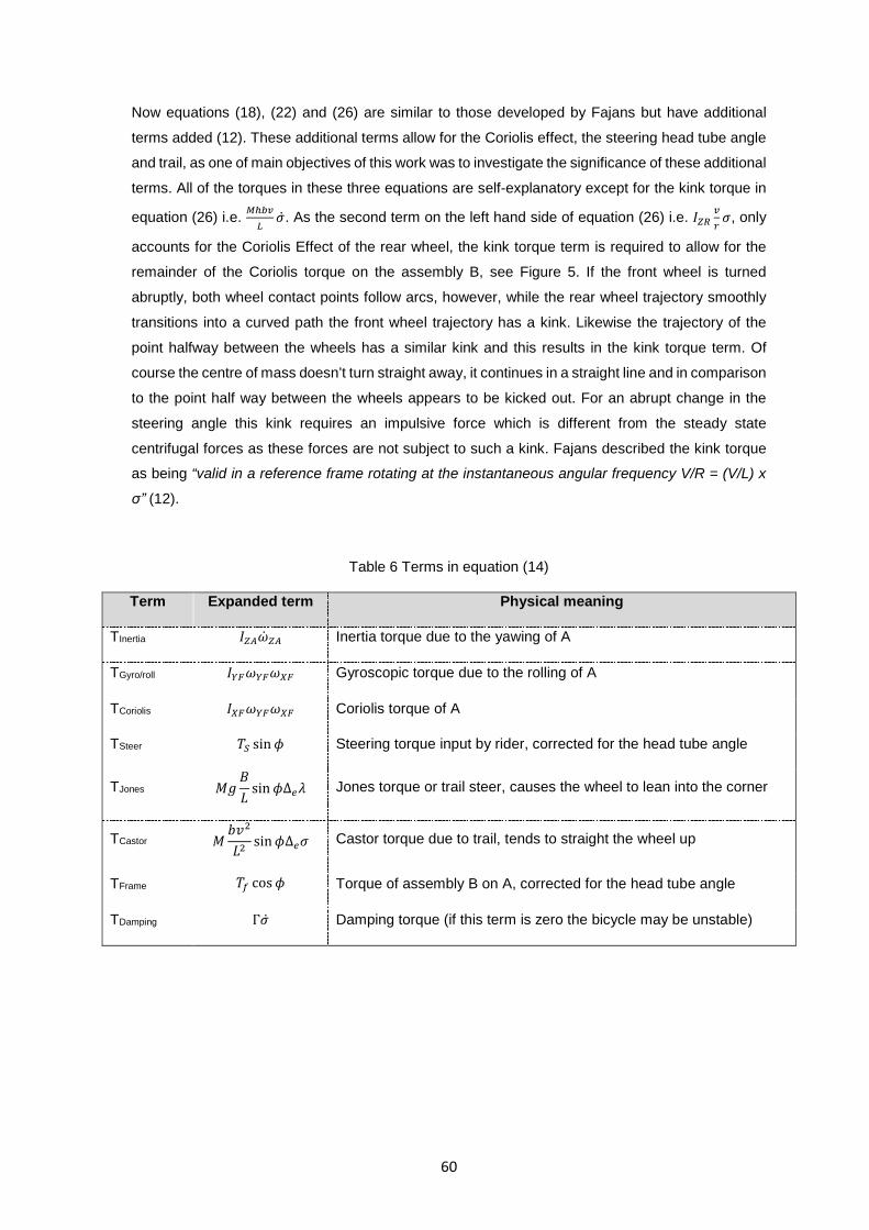
Now equations (18), (22) and (26) are similar to those developed by Fajans but have additional
terms added (12). These additional terms allow for the Coriolis effect, the steering head tube angle
and trail, as one of main objectives of this work was to investigate the significance of these additional
terms. All of the torques in these three equations are self-explanatory except for the kink torque in
equation (26) i.e. 𝑀𝑀ℎ𝑏𝑏𝑔𝑔𝑟𝑟
�̇�𝜎. As the second term on the left hand side of equation (26) i.e. 𝐼𝐼𝑍𝑍𝑍𝑍𝑔𝑔𝑖𝑖𝜎𝜎, only
accounts for the Coriolis Effect of the rear wheel, the kink torque term is required to allow for the
remainder of the Coriolis torque on the assembly B, see Figure 5. If the front wheel is turned
abruptly, both wheel contact points follow arcs, however, while the rear wheel trajectory smoothly
transitions into a curved path the front wheel trajectory has a kink. Likewise the trajectory of the
point halfway between the wheels has a similar kink and this results in the kink torque term. Of
course the centre of mass doesn’t turn straight away, it continues in a straight line and in comparison
to the point half way between the wheels appears to be kicked out. For an abrupt change in the
steering angle this kink requires an impulsive force which is different from the steady state
centrifugal forces as these forces are not subject to such a kink. Fajans described the kink torque
as being “valid in a reference frame rotating at the instantaneous angular frequency V/R = (V/L) x
σ” (12).
Table 6 Terms in equation (14)
Term Expanded term Physical meaning
TInertia 𝐼𝐼𝑍𝑍𝑍𝑍�̇�𝜔𝑍𝑍𝑍𝑍 Inertia torque due to the yawing of A
TGyro/roll 𝐼𝐼𝑌𝑌𝑌𝑌𝜔𝜔𝑌𝑌𝑌𝑌𝜔𝜔𝑋𝑋𝑌𝑌 Gyroscopic torque due to the rolling of A
TCoriolis 𝐼𝐼𝑋𝑋𝑌𝑌𝜔𝜔𝑌𝑌𝑌𝑌𝜔𝜔𝑋𝑋𝑌𝑌 Coriolis torque of A
TSteer 𝑇𝑇𝑆𝑆 sin𝑠𝑠 Steering torque input by rider, corrected for the head tube angle
TJones 𝑀𝑀𝑀𝑀𝐵𝐵𝐿𝐿
sin𝑠𝑠Δ𝑖𝑖𝜆𝜆 Jones torque or trail steer, causes the wheel to lean into the corner
TCastor 𝑀𝑀𝑏𝑏𝑣𝑣2
𝐿𝐿2sin𝑠𝑠Δ𝑖𝑖𝜎𝜎 Castor torque due to trail, tends to straight the wheel up
TFrame 𝑇𝑇𝑓𝑓 cos𝑠𝑠 Torque of assembly B on A, corrected for the head tube angle
TDamping Γ�̇�𝜎 Damping torque (if this term is zero the bicycle may be unstable)
60

Table 7 Terms in equation (19)
Term Expanded term Physical meaning
TInertia 𝐼𝐼𝑋𝑋𝑍𝑍�̇�𝜔𝑋𝑋𝑍𝑍 Inertia torque of the front wheel due to rolling of A
TCoriolis 𝐼𝐼𝑍𝑍𝑌𝑌𝜔𝜔𝑌𝑌𝑌𝑌𝜔𝜔𝑍𝑍𝑌𝑌 Coriolis Torque of A
TGyro/yaw 𝐼𝐼𝑌𝑌𝑌𝑌𝜔𝜔𝑌𝑌𝑌𝑌𝜔𝜔𝑍𝑍𝑌𝑌 Gyroscopic torque of front wheel due to yawing of A
TFrame 𝑇𝑇𝑓𝑓 sin𝑠𝑠 Torque Assembly B exerts on A corrected for the head tube angle
TGyro/cornering IYFv2 sinϕ
rLσ Gyroscopic torque of front wheel due to cornering
TSteer 𝑇𝑇𝑆𝑆 cos𝑠𝑠 Steering Torque corrected for the head tube angle
TCastor 𝑀𝑀𝑏𝑏𝑣𝑣2
𝐿𝐿2cos𝑠𝑠Δ𝑖𝑖𝜎𝜎 Castor torque corrected for the head tube angle
TJones 𝑀𝑀𝑀𝑀𝑏𝑏𝐿𝐿
cos𝑠𝑠Δ𝑖𝑖𝜆𝜆 Jones torque corrected for the head tube angle
Table 8 Terms in equation (24)
Term Expanded Term Physical Meaning
TInertia 𝐼𝐼𝑋𝑋𝑋𝑋�̇�𝜔𝑋𝑋𝑋𝑋 Inertia torque of frame , rider and rear wheel due to rolling of B
TCoriolis 𝐼𝐼𝑍𝑍𝑍𝑍𝜔𝜔𝑌𝑌𝑍𝑍𝜔𝜔𝑍𝑍𝑍𝑍 Coriolis Torque of the rear wheel
TGyro/cornering 𝐼𝐼𝑌𝑌𝑍𝑍𝜔𝜔𝑌𝑌𝑍𝑍𝜔𝜔𝑍𝑍𝑍𝑍 Gyroscopic torque of rear wheel due to cornering
TFrame 𝑇𝑇𝑓𝑓 sin𝑠𝑠 Torque Assembly A exerts on Assembly B corrected for the head tube angle
TCentrifugal 𝑀𝑀𝑣𝑣2ℎ sin𝑠𝑠
𝐿𝐿cos 𝜆𝜆𝜎𝜎 Centrifugal torque
TGravity 𝑀𝑀𝑀𝑀ℎ sin 𝜆𝜆 Gravitational torque
TKink 𝑀𝑀ℎ𝑏𝑏𝑣𝑣𝐿𝐿
�̇�𝜎 Kink torque (Coriolis torque of assembly B less rear wheel)
61

Front wheel Rear wheel
Direction of travel
Centre of corner
Radius of corner R
Yaw angle σ
Yaw angle σ
a) Rear wheel trajectory
b) Centre of mass trajectory
c) Front wheel trajectory
Kink in trajectory
Figure 5 The kink torque results from three different trajectories a), b) and c)
62
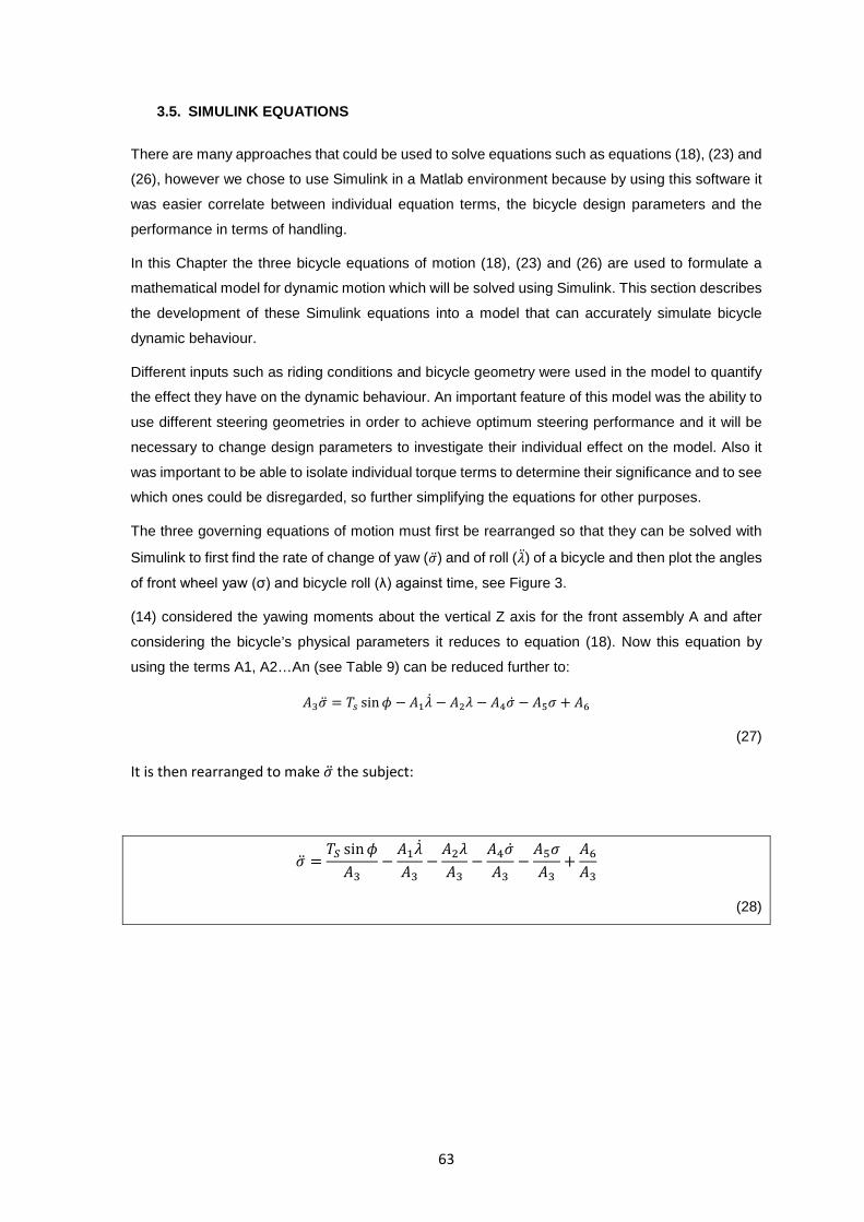
3.5. SIMULINK EQUATIONS
There are many approaches that could be used to solve equations such as equations (18), (23) and
(26), however we chose to use Simulink in a Matlab environment because by using this software it
was easier correlate between individual equation terms, the bicycle design parameters and the
performance in terms of handling.
In this Chapter the three bicycle equations of motion (18), (23) and (26) are used to formulate a
mathematical model for dynamic motion which will be solved using Simulink. This section describes
the development of these Simulink equations into a model that can accurately simulate bicycle
dynamic behaviour.
Different inputs such as riding conditions and bicycle geometry were used in the model to quantify
the effect they have on the dynamic behaviour. An important feature of this model was the ability to
use different steering geometries in order to achieve optimum steering performance and it will be
necessary to change design parameters to investigate their individual effect on the model. Also it
was important to be able to isolate individual torque terms to determine their significance and to see
which ones could be disregarded, so further simplifying the equations for other purposes.
The three governing equations of motion must first be rearranged so that they can be solved with
Simulink to first find the rate of change of yaw (�̈�𝜎) and of roll (�̈�𝜆) of a bicycle and then plot the angles
of front wheel yaw (σ) and bicycle roll (λ) against time, see Figure 3.
(14) considered the yawing moments about the vertical Z axis for the front assembly A and after
considering the bicycle’s physical parameters it reduces to equation (18). Now this equation by
using the terms A1, A2…An (see Table 9) can be reduced further to:
𝐴𝐴3�̈�𝜎 = 𝑇𝑇𝐶𝐶 sin𝑠𝑠 − 𝐴𝐴1�̇�𝜆 − 𝐴𝐴2𝜆𝜆 − 𝐴𝐴4�̇�𝜎 − 𝐴𝐴5𝜎𝜎 + 𝐴𝐴6
(27)
It is then rearranged to make �̈�𝜎 the subject:
�̈�𝜎 =𝑇𝑇𝑆𝑆 sin𝑠𝑠𝐴𝐴3
−𝐴𝐴1�̇�𝜆𝐴𝐴3
−𝐴𝐴2𝜆𝜆𝐴𝐴3
−𝐴𝐴4�̇�𝜎𝐴𝐴3
−𝐴𝐴5𝜎𝜎𝐴𝐴3
+𝐴𝐴6𝐴𝐴3
(28)
63

Similarly equations (19) and (22) which allow for the roll of assembly A about X, reduce to:
𝑇𝑇𝑓𝑓 sin𝑠𝑠 = 𝐵𝐵1�̈�𝜆 − 𝐵𝐵2𝜆𝜆 + 𝐵𝐵3�̇�𝜎 + 𝐵𝐵4𝜎𝜎 + 𝑇𝑇𝐶𝐶 cos𝑠𝑠
(29)
Where terms B1, B2…Bn have been substituted (see Table 9)
Next equations (24) and (26) which allow for the roll of assembly B about X, can be reduced by
using terms C1, C2…Cn (see Table 9) to:
𝑇𝑇𝑓𝑓 sin𝑠𝑠 = −𝐶𝐶1 �̈�𝜆 − 𝐶𝐶2𝜎𝜎 + 𝐶𝐶3 sin 𝜆𝜆 + 𝐶𝐶4𝑐𝑐𝑐𝑐𝑠𝑠𝜆𝜆𝜎𝜎 + 𝐶𝐶5�̇�𝜎 + 𝐶𝐶6𝜎𝜎
(30)
Equating equations (29) and (30) gives:
𝐵𝐵1�̈�𝜆 − 𝐵𝐵2𝜆𝜆 + 𝐵𝐵3�̇�𝜎 + 𝐵𝐵4𝜎𝜎 + 𝑇𝑇𝐶𝐶 cos𝑠𝑠 = −𝐶𝐶1 �̈�𝜆 − 𝐶𝐶2𝜎𝜎 + 𝐶𝐶3 sin 𝜆𝜆 + 𝐶𝐶4𝑐𝑐𝑐𝑐𝑠𝑠𝜆𝜆𝜎𝜎 + 𝐶𝐶5�̇�𝜎 + 𝐶𝐶6𝜎𝜎
(31)
Which is rearranged to make �̈�𝜆 the subject giving:
�̈�𝜆 =−𝐶𝐶2𝜎𝜎
(𝐵𝐵1 + 𝐶𝐶1) +𝐵𝐵2𝜆𝜆
(𝐵𝐵1 + 𝐶𝐶1) +𝐶𝐶3 sin 𝜆𝜆
(𝐵𝐵1 + 𝐶𝐶1) +(𝐶𝐶5 − 𝐵𝐵3)�̇�𝜎(𝐵𝐵1 + 𝐶𝐶1) +
(𝐶𝐶6 − 𝐵𝐵4)𝜎𝜎(𝐵𝐵1 + 𝐶𝐶1) +
𝐶𝐶4 cos 𝜆𝜆𝜎𝜎(𝐵𝐵1 + 𝐶𝐶1) −
𝑇𝑇𝐶𝐶 cos𝑠𝑠(𝐵𝐵1 + 𝐶𝐶1)
(32)
It is equations (28), (29) and (32) that Simulink will solve to find the dynamic behaviour of the bicycle.
3.6. CLOSURE
This Chapter has developed the three equations of motion that solve the rigid body dynamics for
the bicycle, beginning with the Newton Laws of Motion and the General Equations of Motion. Euler
equations were used in the bicycle model, which is reasonable as the bicycle is symmetrical about
the X Z plane and is approximately symmetrical in the other planes. Suitable simplifying
assumptions were made to develop a mathematical model for the bicycle leaving three equations
left to be solved: one to consider yawing moments about the Z axis for the front assembly A, the
second considering rolling moments about the X axis for front assembly A and the final third
equation considering rolling moments about the X axis for rear assembly B. These equations were
reframed into a suitable form for Simulink and in the next Chapter they will be solved.
64
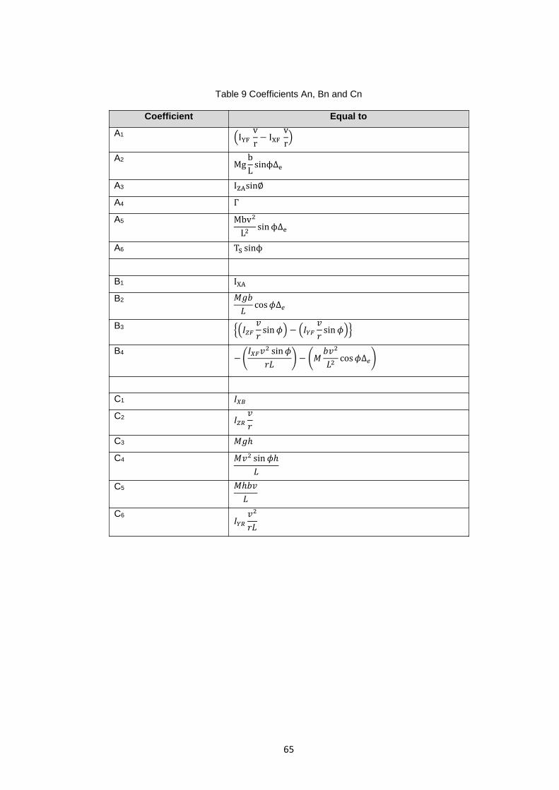
Table 9 Coefficients An, Bn and Cn
Coefficient Equal to
A1 �IYF vr− IXF
vr�
A2 MgbL
sinϕΔe
A3 IZAsin∅
A4 Γ
A5 Mbv2
L2sinϕΔe
A6 TS sinϕ
B1 IXA
B2 𝑀𝑀𝑀𝑀𝑏𝑏𝐿𝐿
cos𝑠𝑠Δ𝑖𝑖
B3 ��𝐼𝐼𝑍𝑍𝑌𝑌𝑣𝑣𝑟𝑟
sin𝑠𝑠� − �𝐼𝐼𝑌𝑌𝑌𝑌𝑣𝑣𝑟𝑟
sin𝑠𝑠��
B4 −�
𝐼𝐼𝑋𝑋𝑌𝑌𝑣𝑣2 sin𝑠𝑠𝑟𝑟𝐿𝐿
� − �𝑀𝑀𝑏𝑏𝑣𝑣2
𝐿𝐿2cos𝑠𝑠Δ𝑖𝑖�
C1 𝐼𝐼𝑋𝑋𝑋𝑋
C2 𝐼𝐼𝑍𝑍𝑍𝑍𝑣𝑣𝑟𝑟
C3 𝑀𝑀𝑀𝑀ℎ
C4 𝑀𝑀𝑣𝑣2 sin𝑠𝑠ℎ𝐿𝐿
C5 𝑀𝑀ℎ𝑏𝑏𝑣𝑣𝐿𝐿
C6 𝐼𝐼𝑌𝑌𝑍𝑍
𝑣𝑣2
𝑟𝑟𝐿𝐿
65

4. SIMULATION AND VALIDATION
4.1. INTRODUCTION AND OVERVIEW
Now that the equations of motion for a bicycle have been developed and reframed into a suitable
form they can be solved using Simulink in a Matlab environment. This Chapter describes how the
model based on equations (18), (23) and (26) from Chapter Three is solved using Simulink.
The Simulink model takes the input from the rider (the steering torque) and after applying
appropriate variables and parameters (such as speed, bicycle total mass, wheelbase length, head
tube angle, rake) it can find the dynamic response of the bicycle in terms of yaw and roll. An
overview of the Simulink computer model is shown in Figure 6 and more detailed diagrams are
described later in this Chapter (see also Appendix A).
The models’ input variables and design parameters can be easily varied to determine their
importance and simulate different manoeuvres, bicycles and riders. This is an important feature of
the model as one of the main objectives of this research is to determine appropriate steering
geometries in order to achieve optimum steering performance. In addition the damping term can be
varied or disregarded to investigate its effect on stability and the results of this computer modelling
will be shown in detail in Chapter Five. This Simulink model is made up of six distinct parts which
are described below and are also shown in schematic form in Figure 7.
1. Model inputs
a. The variable inputs (3 in number) see Table 10
1. Steering torque from the rider (using a Simulink subassembly)
2. Bicycle velocity
3. Damping torque
b. The bicycle parameters (13 terms) shown Table 11
2. Preliminary calculations of the: velocity, steering geometry and wheelbase terms
3. Calculations of the intermediate constants An ,Bn & Cn which are shown Table 9
4. Intermediate calculations to find terms for equations (28), (29) and (32)
5. Final calculations of equations (28), (29) and (32) that produce the bicycle model outputs
of yaw and roll
6. Simulink bicycle model outputs plotting angles vs. time for:
a. Yaw or σ
b. Roll or λ
c. Frame torque or TF
66

The six parts are clearly shown in Figure 7 and they will now be explained more fully in this Chapter
along with more detailed diagrams, see also Appendix A.
4.2. INPUT VARIABLE FORMULATION
As already mentioned it has been known for two hundred years that small changes to a bicycle’s
design have an enormous effect on performance (2, 6, 32, 61). But changes to these design
parameters are still largely made on a trial and error basis. “Bicycles are subject to such complex
and variable forces that the bicycle can really only be designed through trial and error and not just
by computer modelling (67).“ Therefore appropriate parameter and variable values must be selected
for use in the model in order for any simulations to be meaningful.
The Simulink model has three variable inputs: steering torque, speed and damping, which are
shown Table 10. The steering torque from the rider can be modelled as any type of common torque
input (e.g. impulse, ramp and step) and Figure 8 shows a suitable torque consisting of two impulses
(approximately so) the first initiates the turn while the second completes it and stabilises the bicycle
in a new direction. A standard steering torque input used for many simulations consists of two small
impulses of maximum magnitude + 0.45 Nm and - 0.414 Nm. These two values were found by trial
and error to produce a reasonable cornering manoeuvre which returns the bicycle back to an upright
position within a reasonable time frame (of 15 to 20 seconds) but of course other values could be
used.
A simple Simulink subassembly that can produce this standard steering torque is shown in Figure
9. A second more adaptable subassembly was also developed to allow the steering torque to be
easily adjusted in its amplitude and time lag values and details of this second assembly is shown in
Appendix A.
Table 10 Model variable inputs
Symbol Variable inputs definition Units
1. TSteer Steering torque (from the rider) Nm
2. v Velocity m/s
3. Γ Damping torque Js
67
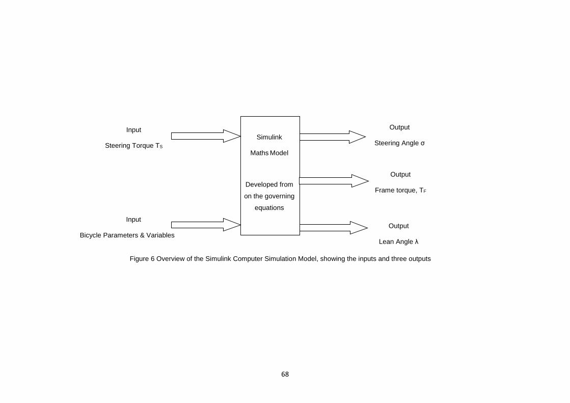
Input
Steering Torque TS
Simulink
Maths Model
Developed from
on the governing
equations
Output
Steering Angle σ
Output
Frame torque, TF
Input
Bicycle Parameters & Variables Output
Lean Angle λ
Figure 6 Overview of the Simulink Computer Simulation Model, showing the inputs and three outputs
68

Figure 7 Schematic breakdown of the Simulink Model, showing the main elements or parts
Steering Torque
Input, TS
Steering Angle Output, σ
Roll Angle Output, λ
Bicycle
Parameters &
variables
Frame torque Output TF
Preliminary
calculations
of the
first terms
2. Initial calculations
Part A
1. Inputs 5. Final
calculations
3. Calculations of terms
An, Bn & Cn
Part B
4. Intermediate
calculations
Finds terms
for eqn 28 Solves
eqn 28
Part D
Finds terms
for eqn 29
Finds terms
for eqn 32
Solves
eqn 29
Solves
eqn 32
Terms An
Terms Bn
Terms Cn
Part F
Part H
Part G
Part K
Part J
Part I
6. Outputs
Part C
Part E
69
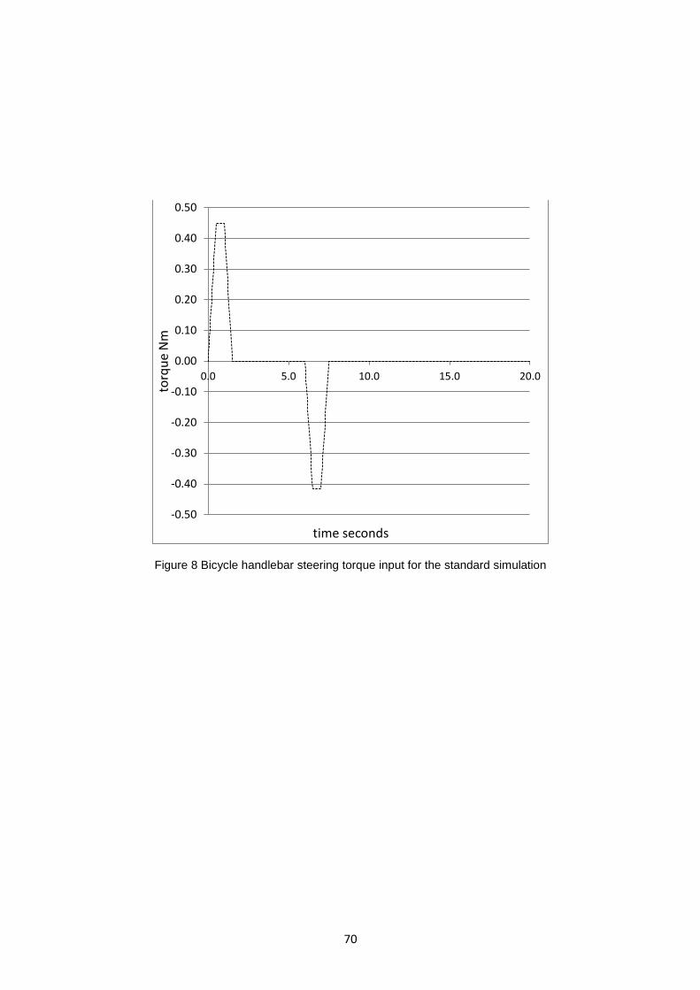
Figure 8 Bicycle handlebar steering torque input for the standard simulation
-0.50
-0.40
-0.30
-0.20
-0.10
0.00
0.10
0.20
0.30
0.40
0.50
0.0 5.0 10.0 15.0 20.0
torq
ue N
m
time seconds
70

Figure 9 The steering torque subassembly that produces the standard steering torque shown in Figure 8
Final output TS
First impulse + 0.45 Nm
Initial ramp inputs
Correcting impulse
– 0.414 Nm
Produces the first impulse of +0.45 Nm
Produces the second impulse of +0.414 Nm
71
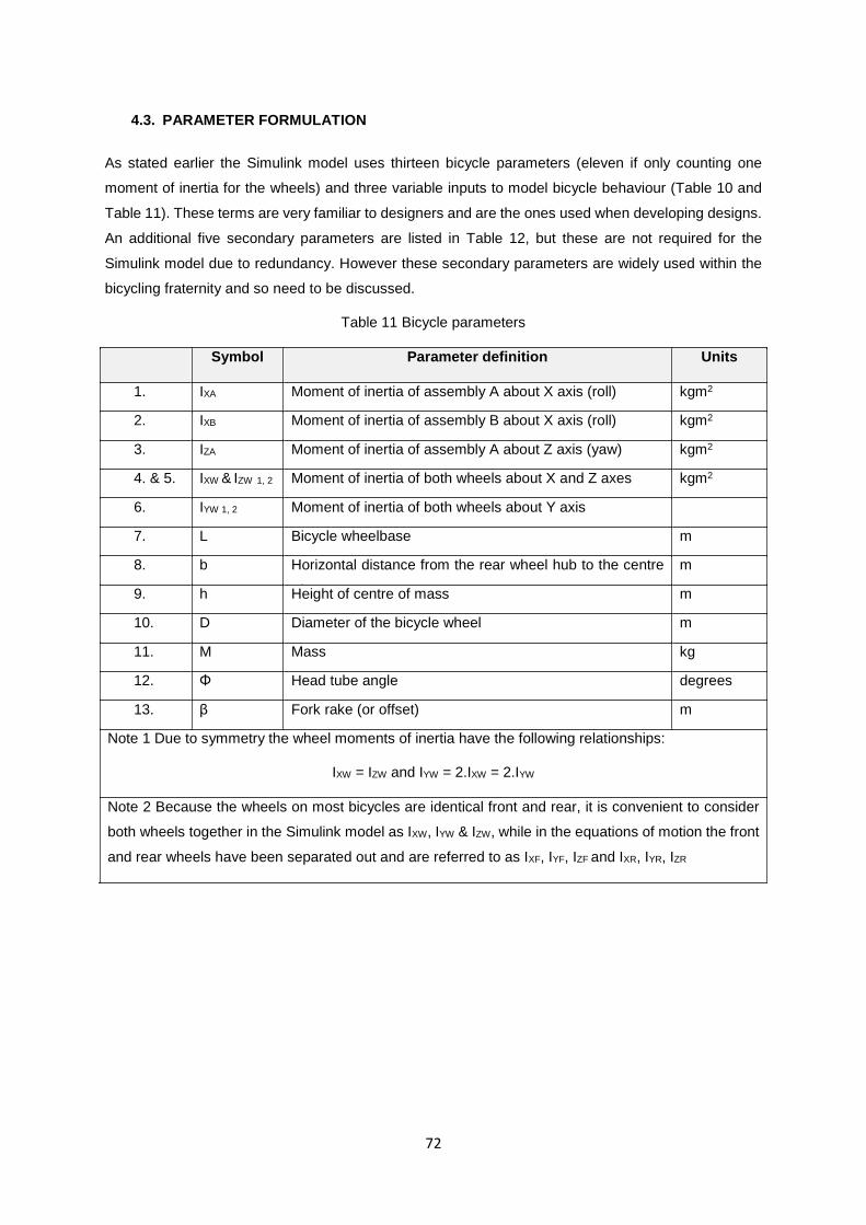
4.3. PARAMETER FORMULATION
As stated earlier the Simulink model uses thirteen bicycle parameters (eleven if only counting one
moment of inertia for the wheels) and three variable inputs to model bicycle behaviour (Table 10 and
Table 11). These terms are very familiar to designers and are the ones used when developing designs.
An additional five secondary parameters are listed in Table 12, but these are not required for the
Simulink model due to redundancy. However these secondary parameters are widely used within the
bicycling fraternity and so need to be discussed.
Table 11 Bicycle parameters
Symbol Parameter definition Units
1. IXA Moment of inertia of assembly A about X axis (roll) kgm2
2. IXB Moment of inertia of assembly B about X axis (roll) kgm2
3. IZA Moment of inertia of assembly A about Z axis (yaw) kgm2
4. & 5. IXW & IZW 1, 2 Moment of inertia of both wheels about X and Z axes kgm2
6. IYW 1, 2 Moment of inertia of both wheels about Y axis
7. L Bicycle wheelbase m
8. b Horizontal distance from the rear wheel hub to the centre
f
m
9. h Height of centre of mass m
10. D Diameter of the bicycle wheel m
11. M Mass kg
12. Φ Head tube angle degrees
13. β Fork rake (or offset) m
Note 1 Due to symmetry the wheel moments of inertia have the following relationships:
IXW = IZW and IYW = 2.IXW = 2.IYW
Note 2 Because the wheels on most bicycles are identical front and rear, it is convenient to consider
both wheels together in the Simulink model as IXW, IYW & IZW, while in the equations of motion the front
and rear wheels have been separated out and are referred to as IXF, IYF, IZF and IXR, IYR, IZR
72
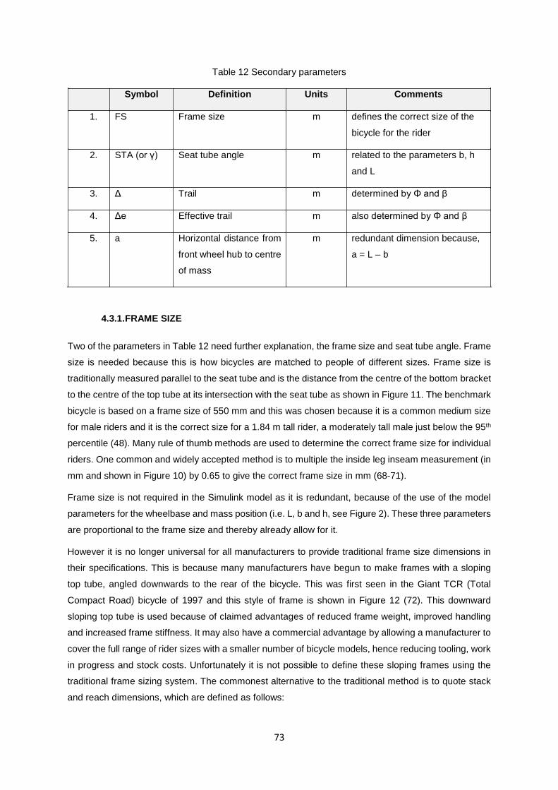
Table 12 Secondary parameters
Symbol Definition Units Comments
1. FS Frame size m defines the correct size of the
bicycle for the rider
2. STA (or γ) Seat tube angle m related to the parameters b, h
and L
3. Δ Trail m determined by Φ and β
4. Δe Effective trail m also determined by Φ and β
5. a Horizontal distance from
front wheel hub to centre
of mass
m redundant dimension because,
a = L – b
4.3.1. FRAME SIZE
Two of the parameters in Table 12 need further explanation, the frame size and seat tube angle. Frame
size is needed because this is how bicycles are matched to people of different sizes. Frame size is
traditionally measured parallel to the seat tube and is the distance from the centre of the bottom bracket
to the centre of the top tube at its intersection with the seat tube as shown in Figure 11. The benchmark
bicycle is based on a frame size of 550 mm and this was chosen because it is a common medium size
for male riders and it is the correct size for a 1.84 m tall rider, a moderately tall male just below the 95th
percentile (48). Many rule of thumb methods are used to determine the correct frame size for individual
riders. One common and widely accepted method is to multiple the inside leg inseam measurement (in
mm and shown in Figure 10) by 0.65 to give the correct frame size in mm (68-71).
Frame size is not required in the Simulink model as it is redundant, because of the use of the model
parameters for the wheelbase and mass position (i.e. L, b and h, see Figure 2). These three parameters
are proportional to the frame size and thereby already allow for it.
However it is no longer universal for all manufacturers to provide traditional frame size dimensions in
their specifications. This is because many manufacturers have begun to make frames with a sloping
top tube, angled downwards to the rear of the bicycle. This was first seen in the Giant TCR (Total
Compact Road) bicycle of 1997 and this style of frame is shown in Figure 12 (72). This downward
sloping top tube is used because of claimed advantages of reduced frame weight, improved handling
and increased frame stiffness. It may also have a commercial advantage by allowing a manufacturer to
cover the full range of rider sizes with a smaller number of bicycle models, hence reducing tooling, work
in progress and stock costs. Unfortunately it is not possible to define these sloping frames using the
traditional frame sizing system. The commonest alternative to the traditional method is to quote stack
and reach dimensions, which are defined as follows:
73

• stack is the vertical distance from centre of the bottom bracket to centre of the head tube
measured at its top end, see Figure 13
• and reach is the horizontal distance from centre of the bottom bracket to centre of the head
tube measured at its top end, see Figure 13
This alternative sizing method is now used by many (but not all) manufacturers now that sloping frames
have become common. But sizing methods are confusing to many riders and many are unsure as to
which frame size they should purchase (73). Some sort of internationally recognised standardisation in
frame sizing would appear desirable but this is outside the scope of this investigation.
4.3.2. SEAT TUBE ANGLE
The second parameter, seat tube angle, is the angle the seat tube makes relative to the horizontal plane
see Figure 11. It is an important manufacturing parameter that enables easy fabrication of conventional
frames and it also determines the seat and rider position. The seat tube angle is also a much discussed
parameter within the bicycling fraternity and many claims are made as to its influence on handling and
comfort, see later discussions in Chapter Seven (69, 74, 75). As with the frame size parameter, the
Simulink model allows for the seat tube angle through the use of the terms “b” and “h” (that define the
mass position). The seat tube angle can be related back to “b” and “h” by using a combination of
trigonometry and empirically derived relationships and the full details of how this can be done is shown
in the Appendix B.
74

measurement
Figure 10 The cyclist’s inseam measurement used to determine the correct bicycle size
Figure 11 Defining a bicycle’s frame size dimension and seat tube angle
Bottom bracket spindle
Frame Size
Seat tube angle
Seat tube
Down tube
Top tube
75
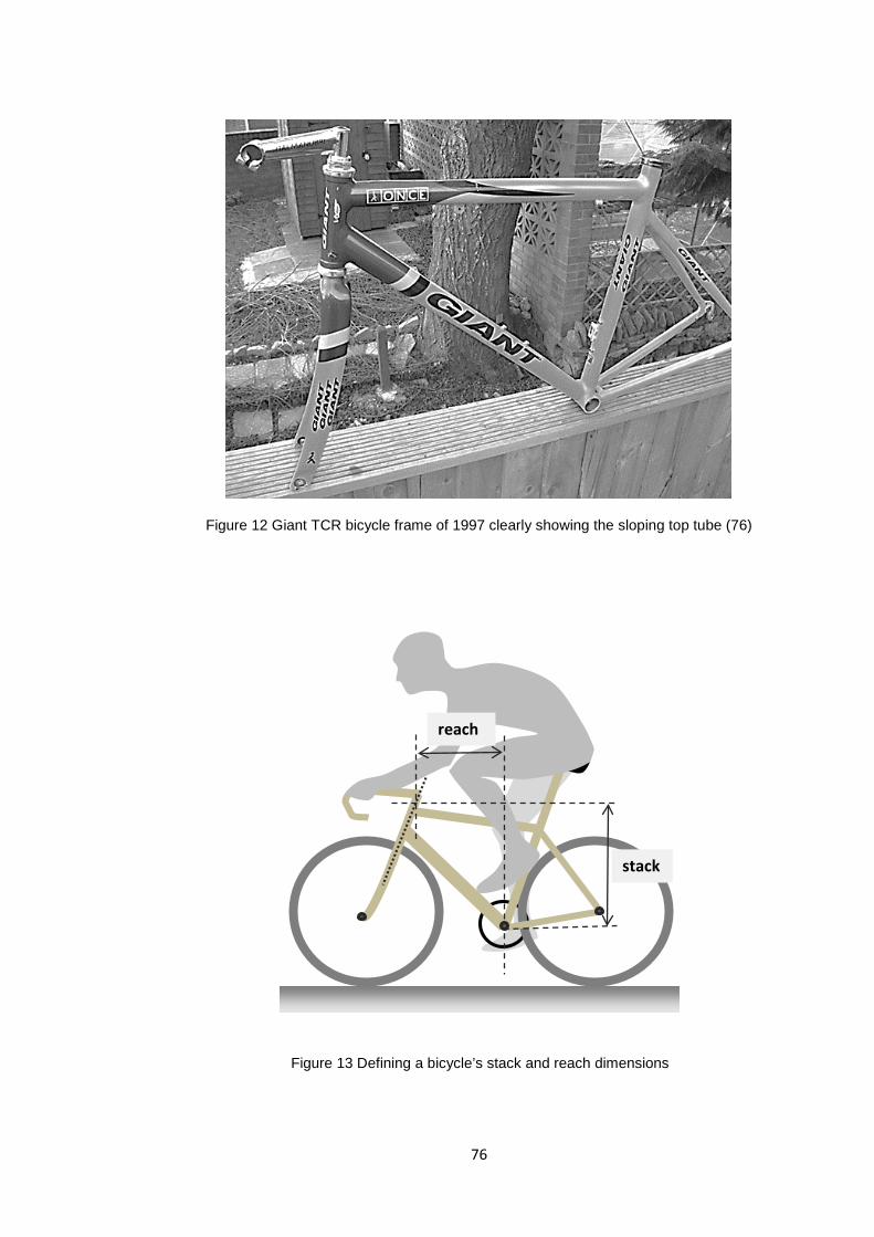
Figure 12 Giant TCR bicycle frame of 1997 clearly showing the sloping top tube (76)
reach
stack
Figure 13 Defining a bicycle’s stack and reach dimensions
76

4.4. BENCHMARK PARAMETERS
It is necessary to select appropriate values for all 13 parameters and 3 variables, ones that will
be representative of modern high performing road bicycles in order that realistic simulations can
be made. Appropriate values are also needed in order for the sensitivity study to be undertaken.
Of particular importance was the choosing of appropriate and representative values for a
reference point, the benchmark bicycle. The benchmark values are not intended to be thought of
as optimum values but rather should be typical of well-designed road bicycles, somewhere in the
middle of the range of values. The benchmark bicycle will also be useful when examining the
differences between individual bicycle designs (such as the Tour de France bicycles examined in
Chapter Seven) as it can be a datum point. Also the four bicycle design charts developed and
discussed later in Chapter Six, all use iso-handling lines referenced back to the benchmark
bicycle’s iso-handling line.
4.4.1. SUPPORTING EVIDENCE FOR PARAMETER SELECTION
The following comments are supporting evidence as to why particular benchmark values were
selected.
• First a review of the literature was undertaken to find out what parameter values other
researchers had used. Moore et al determined a range of values for physical bicycle
parameters including: mass, the position of the mass, moments of inertia of bicycle
components (frame, front fork, wheels and rider). They were found by experimental
measurement and from previously published data. (47). The bicycle they chose to
measure was a 2008 Batavus Browser and from the details given it is clear this is not a
high performance bicycle. For example the total bicycle weight is given as 23.5 kg, which
is very high when compared to a top road bicycle such as a Trek Madone 7.7 weighing
only 6.54 kg (77). Also the Batavus also has a very long wheelbase (1.120 m) and a
shallow head tube angle (68.5o). Similarly when measuring the human rider they have
chosen a subject weighing 72 kg but give no indication of their height or body mass index,
so it is hard to know how representative they are of the riding population. Therefore the
results given in this paper need to be considered with these comments in mind.
• Ringwood and Feng’s paper obtained experimentally values for the position of centres of
mass of actual road bicycles e.g. Trek 5200, Trek 1000, Trek Madone, Klein and
Litespeed (61). When finding the vertical centre of mass position they assumed that the
bicycle rider system was a simple pendulum when it is actually a compound pendulum.
As a consequence their estimate for the vertical position of the centre of mass has a
significant error and places it about 160 mm too low.
• Fajans’ paper on the motion of bicycles and motorcycles used several values for centres
of mass and moments of inertia (12). He referenced some sources but said others were
inferred, but did not include any details. Using these values in his derived equations
Fajans examined in detail a road racing bicycle and a large motorcycle.
77

• Chen’s paper on bicycle balancing and path tracking strategies used parameter values
which they found experimentally but no details of how this was done was given (60). The
wheel masses are very high at 2.09 and 3.93 kg (front and rear respectively) and this was
because the bicycle was not a high performance design and also a rotary encoder was
attached to the front wheel.
• Damavandi et al presented a short report that summaries seven methods for finding the
moments of inertia of a human subject (78). This has relevance when determining
moments of inertia and mass and its position of the bicycle rider system. This is a difficult
theoretical and experimental problem due to the wide range of human body shapes and
the difficulty of measuring and defining the human body. Their purpose was to find the
most efficient way of determining an individual’s moments of inertia for clinical
evaluations. The usual method is to estimate these values from anthropomorphic tables
but this has problems because the tables do not accurately describe adolescent, obese
or elderly populations. They did not describe the theory or procedures employed with any
of the seven methods they listed. The report concluded that the inverse dynamic
pendulum and the angular momentum methods gave results within the average of the
others, but this was not quantified precisely. They recommended that these two methods
could be used with confidence in the clinical environment to estimate the moments of
inertia for individual subjects.
• Dempster undertook a three year long United States Air Force sponsored investigation
published in 1955, whose purpose was to determine the space requirements for seated
male air crew (79). It was also hoped that the kinematic information would assist in
designing ergonomic controls and cockpits so that under extreme conditions of flight,
effective control would still be possible. Dempster undertook the detailed examination of
eight male cadavers (all older males of slight build). This involved the examination of
dissected body parts (torso, head, upper and lower limbs). He measured and recorded
details of: dimensions, volumes, masses, centre of mass positions and moments of
inertia. The centres of mass were found by the suspension method and moments of
inertia by the compound pendulum method. The resulting data was arranged in tables of
anthropomorphic data listed for each body segment but was not combined into a
complete mathematical model of the human body. Therefore it cannot be used for this
current study unless further work was done. His information could be used to construct a
simple mathematical model of a person in any posture that could calculate mass, mass
position and moments of inertia. But because the cadavers were older males (ranging
from 52 to 83 years) and of slight build (50 to 70 kg) they are not representative of young,
athletic male bicycle riders nor female riders. Therefore this information is considered to
have limited use for this study other than as a comparison with other results.
• Hanavan’s United States Air Force study developed a complete mathematical model that
can find masses, centres of mass, products and moments of inertia for humans of
different builds and in different postures (48). The study’s purpose was to determine the
inertial properties for space crew to help design equipment for the weightless environment 78

of outer space (such as self-manoeuvring units for extra-vehicular work). His
mathematical model breaks the body down into fifteen segments that are simplified as
easily calculated hemispherical, cylindrical or conical shapes. These are then used to
calculate the required properties for a complete human body. Importantly and usefully he
summarised these human body properties into a design guide. His guide lists different
combinations of standing and sitting positions (with limbs in various positions). In total the
mass and inertial properties for 31 different body positions are included in his design
guide. For each position full values for composite subjects of the 5th, 25th, 50th, 75th and
95th percentile groups are given. Hanavan body position number 18 closely approaches
that of a rider in the seated pedalling position and those results are used in this study,
see Figure 14. The Hanavan model was validated by comparing it to existing data
available from the previous research of Hansen and Cornog (not cited) that had measured
66 subjects (US Air Force male flight crew of the 1950’s). The Hanavan mathematical
model was found to be accurate within 18 mm for the position of the centre of mass and
generally within 10% for the moments of inertia when compared with anthropomorphic
data. Full details of the computer programme written in Fortran II & IV code are supplied
in Hanavan’s report.
4.4.2. BENCHMARK VALUES
The choice of the benchmark values was made after considering experimental measurements
and calculations, other researchers’ work and manufacturers’ published specifications about their
own bicycles. For the developed Simulink model in this study, the benchmark parameter values
selected are listed in Table 13. These selected benchmark parameter values are not proposed
as highly precise values but they are believed to be sufficiently true and accurate for their purpose
as defined by ISO standard 5725-1. Rounding has been used on the benchmark values, generally
to 2 significant figures. According to ISO standard 5725-1, the international standard defining the
vocabulary of metrology, the terms trueness and precision have a specific meaning when
describing the accuracy of a measurement process (80). Precision refers to the closeness of
agreement within series of individual measurements while trueness is the closeness of the
average of a series of measurements to the true value. Consequently accuracy refers to both
trueness and precision and to be accurate a series of measurements must be sufficiently true and
precise for the purpose.
Justification for why these values were selected are summarised in Table 14 and Table 15 (parts
I and II) and these two tables show a complete picture of the range of these values, so that
decisions about future variations to the model can be made with knowledge and confidence. As
already noted many researchers have used values which are not representative of high
performing bicycles. This can be attributed to the fact that many of the bicycles used for
experiments are of average or below average design and construction. Also some researchers
deliberately exaggerated some values, for example wheel mass, in order to investigate the effect
of individual terms such as gyroscopic effects (14). Typically values are overly heavy and in the
case of dimensions such as wheel diameters and wheelbases are inaccurate.
79

Reflecting on this it was decided that it was necessary to apply rigour in order to obtain appropriate
values for this study and a combination of experiments, calculations and extensive reference to
the literature has allowed this to be achieved with some confidence. Engineering calculations
were possible on some components, namely the moments of inertia of wheels, front forks, bicycle
frame and rider, see Appendix C. These calculations had close agreement to the experimental
values which allows confidence in advancing the selected values for the benchmark bicycle
shown in Table 13.
Figure 14 Hanavan’s Report lists the above position as # 18 (positive X Y Z directions indicated)
Z
Y
X
80

Table 13 Benchmark bicycle parameters and other terms
Symbol Parameter Definition BM Value 1
Units Source
1. IXA Moment of inertia of assembly A about XA axis (roll) 0.2 kgm2 from calculation and comparison to
Fajans (12) 2. IXB Moment of inertia of assembly B
about XB axis (roll) 100 kgm2 from calculation and comparison to
Fajans (12) 3. IZA Moment of inertia of assembly A
about ZA axis (yaw) 0.08 kgm2 from calculation and comparison to
Fajans (12) 4. IXW Moment of inertia of both wheels
about X axis (roll) 0.05 kgm2 from experimental measurement, see Appendix C
5. IYW Moment of inertia of both wheels about Y axis (rotational) 0.10 kgm2 from experimental measurement,
see Appendix C 6. IZW Moment of inertia of both wheels
about Z axis (yaw) 0.05 kgm2 from experimental measurement, see Appendix C
7. L bicycle wheelbase 1.0 m selected from comparison to database, see Chapter Seven
8. b Horizontal distance from centre of rear wheel to centre of mass 0.33 m from calculation and comparison to
Fajans & Ringwood (12) 9. h Height of centre of mass 1.1 m from calculation and comparison to
Fajans & Ringwood (12) 10. D Diameter of the bicycle wheel 0.675 m from manufacturers’ data, see
Appendix E 11. M Mass
80.0 kg based on a bicycle of 7kg and a rider of 73kg see Appendix F
12. Φ Head tube angle 73.0 degrees selected from comparison to database, see Appendix F
13. β Fork rake 0.045 m selected from comparison to database, see Appendix F
Secondary Parameter Definition
1. FS Frame Size 0.55 m Not a model input but estimated from L and h
2. STA Seat tube angle 74.0 degrees Not a model input but estimated from L and h
3. Δ Trail 0.05613 m
Not a model input but calculated using the trail formula from the head tube angle and rake
4. Δe Effective trail 0.05368 m
Not a model input but calculated using the trail formula from the head tube angle and rake
5. a Horizontal distance from centre of front wheel to centre of mass 0.67 m Not a model input but calculated
from L and b Variable Definition 1. TSteer Steering torque 2 variable Nm from selection and comparison to
Fajans (12) 2. v Velocity
25 km/hr
A selected value, but other values have been used in some simulations and this is made clear in the text
3. Γ Damping torque term 0.65 Js see Fajans (12)
Other Definition g Acceleration due to gravity 9.81 m/s2 A constant at the standard value
Note 1 BM or benchmark bicycle value
Note 2 variable term which can be adjusted in the Simulink model as required
81
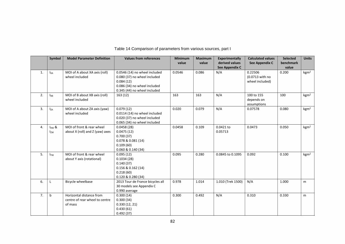
Table 14 Comparison of parameters from various sources, part I
Symbol Model Parameter Definition Values from references Minimum value
Maximum value
Experimentally derived values See Appendix C
Calculated values See Appendix C
Selected benchmark
value
Units
1. IXA MOI of A about XA axis (roll) wheel included
0.0546 (14) no wheel included 0.080 (37) no wheel included 0.084 (12) 0.086 (34) no wheel included 0.345 (44) no wheel included
0.0546 0.086 N/A 0.22506 (0.0713 with no wheel included)
0.200 kgm2
2. IXB MOI of B about XB axis (roll) wheel included
163 (12)
163 163 N/A 100 to 155 depends on assumptions
100 kgm2
3. IZA MOI of A about ZA axis (yaw) wheel included
0.079 (12) 0.0114 (14) no wheel included 0.020 (37) no wheel included 0.065 (34) no wheel included
0.020 0.079 N/A 0.07578 0.080 kgm2
4. IXW & IZW
MOI of front & rear wheel about X (roll) and Z (yaw) axes
0.0458 (28) 0.0475 (12) 0.700 (37) 0.078 & 0.081 (14) 0.109 (60) 0.060 & 0.140 (34)
0.0458 0.109 0.0421 to 0.05713
0.0473 0.050 kgm2
5. IYW MOI of front & rear wheel about Y axis (rotational)
0.095 (12) 0.1034 (28) 0.140 (37) 0.156 & 0.162 (14) 0.218 (60) 0.120 & 0.280 (34)
0.095 0.280 0.0845 to 0.1095 0.092 0.100 kgm2
6. L Bicycle wheelbase 2013 Tour de France bicycles all 30 models see Appendix C 0.990 average
0.978 1.014 1.010 (Trek 1500) N/A 1.000 m
7. b Horizontal distance from centre of rear wheel to centre of mass
0.300 (14) 0.300 (34) 0.330 (12, 21) 0.430 (61) 0.492 (37)
0.300 0.492 N/A 0.310 0.330 m
82

Table 15 Comparison of parameters from various sources continued, part II
Symbol Model Parameter Definition Values from references Minimum value
Maximum value
Experimentally derived values See Appendix
C
Calculated values See Appendix C
Selected benchmark
value
Units
8. h Height of centre of mass 0.867 (61) 0.900 (14) 1.08 (34) 1.028 (37) 1.25 (12) 1.5 (21)
0.867 1.500 1.030 1.090 1.100 m
9. D Diameter of the bicycle wheel 700C x25 wheel
0.67004 (81) 0.67959 (64) (0.6748 average)
0.67004 0.67959
0.675 N/A 0.675 m
10. M Mass made up of the bicycle and the rider
27.9 bicycle only (34) 81.6 bicycle & rider (21) 87 bicycle & rider (14) 88.5 bicycle & rider (37) 100 bicycle & rider (12)
81.6 100.0 N/A N/A 80 kg
Bicycle only 6.8 kg min UCI weight (3)
6.8 7.3 8.5 (Trek 1500) N/A 7.0
Tour de France 2013 Riders Average weight 68.83 kg for all 219 riders (82) See Appendix C
56.0 84.0 N/A N/A 73.0
11. Φ Head tube angle 2013 Tour de France bicycles all 30 models see Appendix C 73.2 average
71.9 74.0 N/A N/A 73.0 degrees
12. β Fork rake 2013 Tour de France bicycles all 30 models see Appendix C 0.0449 average
0.039 0.053 N/A N/A 0.045 m
13. Δe Effective trail 2013 Tour de France bicycles all 30 models see Appendix C 0.05515 average
0.0447 0.06342 N/A N/A 0.05368 m
83
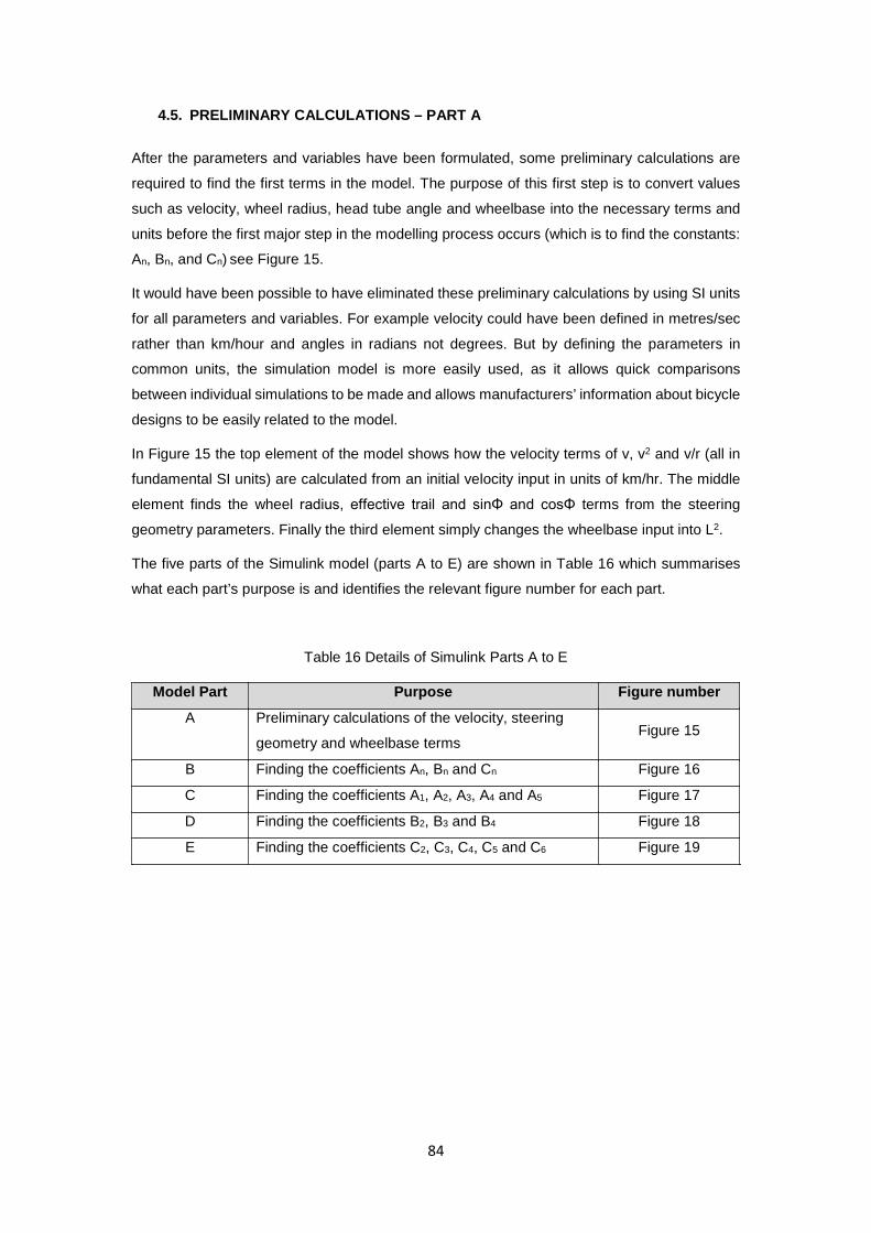
4.5. PRELIMINARY CALCULATIONS – PART A
After the parameters and variables have been formulated, some preliminary calculations are
required to find the first terms in the model. The purpose of this first step is to convert values
such as velocity, wheel radius, head tube angle and wheelbase into the necessary terms and
units before the first major step in the modelling process occurs (which is to find the constants:
An, Bn, and Cn) see Figure 15.
It would have been possible to have eliminated these preliminary calculations by using SI units
for all parameters and variables. For example velocity could have been defined in metres/sec
rather than km/hour and angles in radians not degrees. But by defining the parameters in
common units, the simulation model is more easily used, as it allows quick comparisons
between individual simulations to be made and allows manufacturers’ information about bicycle
designs to be easily related to the model.
In Figure 15 the top element of the model shows how the velocity terms of v, v2 and v/r (all in
fundamental SI units) are calculated from an initial velocity input in units of km/hr. The middle
element finds the wheel radius, effective trail and sinΦ and cosΦ terms from the steering
geometry parameters. Finally the third element simply changes the wheelbase input into L2.
The five parts of the Simulink model (parts A to E) are shown in Table 16 which summarises
what each part’s purpose is and identifies the relevant figure number for each part.
Table 16 Details of Simulink Parts A to E
Model Part Purpose Figure number
A Preliminary calculations of the velocity, steering
geometry and wheelbase terms Figure 15
B Finding the coefficients An, Bn and Cn Figure 16
C Finding the coefficients A1, A2, A3, A4 and A5 Figure 17
D Finding the coefficients B2, B3 and B4 Figure 18
E Finding the coefficients C2, C3, C4, C5 and C6 Figure 19
84

4.6. INTERMEDIATE CONSTANTS – PARTS B, C, D & E
After the preliminary calculation steps have been completed the next step can proceed. This
first major modelling step calculates the intermediate constants, An, Bn, and Cn which have been
defined in Table 9 (and an overview of these steps is shown in Figure 16). These intermediate
constants are required in order to solve the equations of motion. This step is further broken
down into three subparts: C, D and E, details of which are shown in Figure 17, Figure 18 and
Figure 19. Note that not all the An, Bn, and Cn constants have to be calculated as the following
three constants are already known (A4 = Γ, B1 = IXA and C1 = IXB).
In Figure 15 the top element (Part C) finds the coefficients A1, A2, A3 and A5 which will be
used to help solve (28, Part C is shown in more detail in Figure 17. The middle element is Part
D which calculates coefficients B2, B3 and B4 to solve equation (29) more details of which are
shown in Figure 18. The final element of Figure 15 is Part E used to calculate coefficients C2,
C3, C4, C5 and C6 which will be used to solve equation (32) and Part E is also shown Figure
19.
4.7. INTERMEDIATE CALCULATIONS – PARTS F, G & H
Once the constants (An, Bn and Cn) have been found the intermediate calculations can
proceed. There are three parts (F, G and H) to these intermediate calculations which are listed
in Table 17. Each part takes one group of the intermediate constants, An or Bn, or Cn (plus any
necessary initial terms) and calculates the further individual terms required for each of
equations (28), (29) and (32) (see also Figure 20, Figure 21 and Figure 23).
Table 17 Details of Parts F, G and H
Model Part Purpose Figure
F Finding the terms for (28 Figure 20
G Finding the terms for (29 Figure 21
H Finding the terms for (32 Figure 22
In Figure 20 which shows Part F, coefficients A1, A2, A3, A4, A5 and A6 and other terms are used
to produce the individual terms of equation (28). Next in Figure 21, Part G, coefficients B1, B2,
B3 and B4 and other terms are used to produce the individual terms of equation (29). Finally in
Figure 22, Part H, coefficients B1, B2, B3 and B4 and coefficients C1, C2, C3, C4, C5 and C6 plus
other terms are used to produce the individual terms of equation (32).
85

4.8. FINAL CALCULATIONS – PARTS I, J & K
The last step in the Simulink model is to take all the previously calculated terms and use them
to find the bicycle dynamic response in terms of yaw and roll. The three parts that do this are I,
J and K and their purposes are described in the (see also Table 18, Figure 23, Figure 24 and
Figure 25).
Table 18 Details of Parts I, J and K
Model Part Purpose Figure
I Finds the yaw angle of the front wheel (σ) Figure 23
J Finds the frame torque (Tf sin Φ) Figure 24
K Finds the roll angle (λ) Figure 25
The final steps are shown in next three figures starting with Figure 23 (Part I) which using the
terms from equation (28) finds the yaw angle of the front wheel. Then in Figure 24 (Part J) the
frame torque is found from equation (29). The last Figure 25 (Part K) finds the roll angle using
equation (32).
86
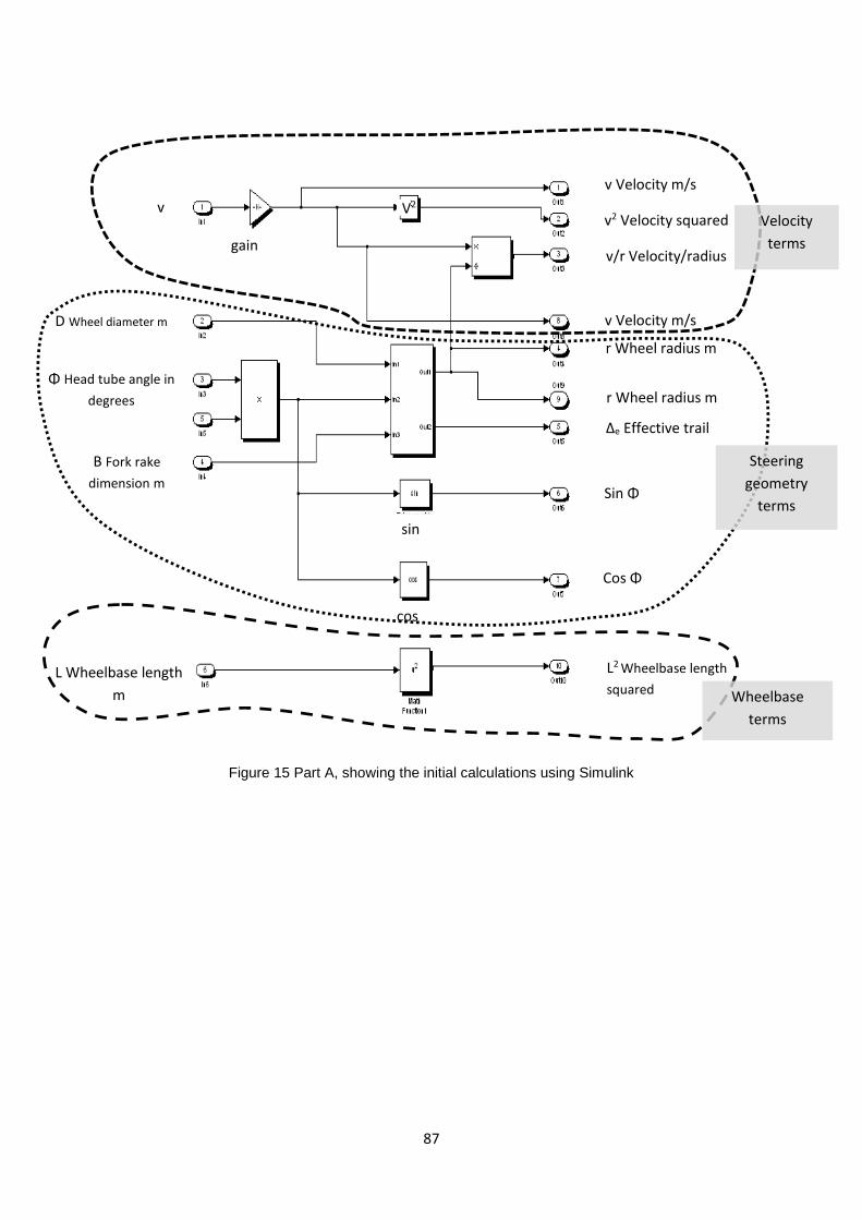
Figure 15 Part A, showing the initial calculations using Simulink
Β Fork rake dimension m
L Wheelbase length m
D Wheel diameter m
Φ Head tube angle in
degrees
v
v Velocity m/s
v/r Velocity/radius
v2 Velocity squared
Δe Effective trail
Cos Φ
L2 Wheelbase length squared
Sin Φ
v Velocity m/s
r Wheel radius m
r Wheel radius m
V2
gain
cos
sin
Velocity terms
Steering geometry
terms
Wheelbase terms
87

Figure 16 Part B, showing an overview of the Simulink calculations of coefficients An, Bn & Cn
Calculation of coefficients
Bn
Calculation of coefficients
An
Calculation
of
coefficients
Cn
B2
C6
A5
A2
A3
A1
B4
B3
C3
C4
C2
C5
Part C see also Figure 17
Part D see also Figure 18
Part E see also Figure 19
88
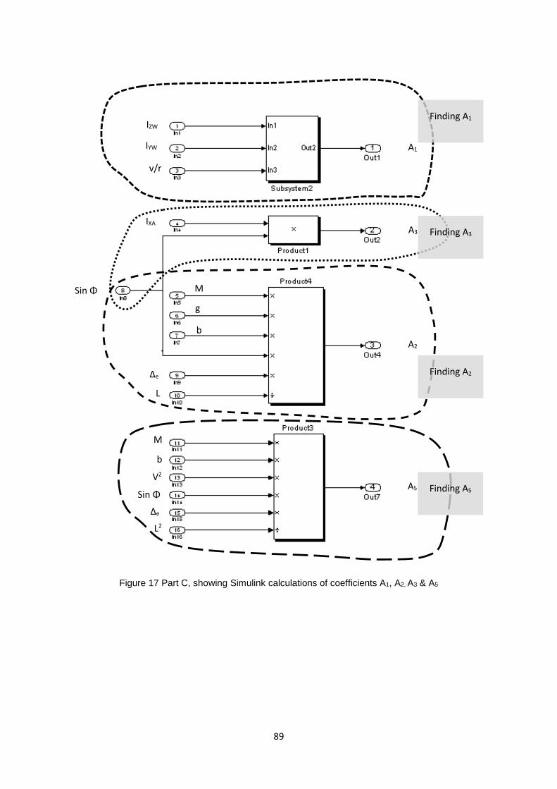
Figure 17 Part C, showing Simulink calculations of coefficients A1, A2, A3 & A5
A1
A3
A2
A5
IZW
IYW
IXA
v/r
b
Sin Φ
L
g
M
Δe
L2
V2
Sin Φ
M
b
Δe
Finding A1
Finding A3
Finding A2
Finding A5
89

Figure 18 Part D, showing the Simulink calculations of coefficients B2, B3 & B4
B3
B2
B4
M
b
Δe L2
L
IZW
IZW
v/r
v/r
Sin Φ
Sin Φ
Sin Φ r
v2
g
M L
Cos Φ Δe
b
Cos Φ
Finding B3
Finding B4
Finding B2
90
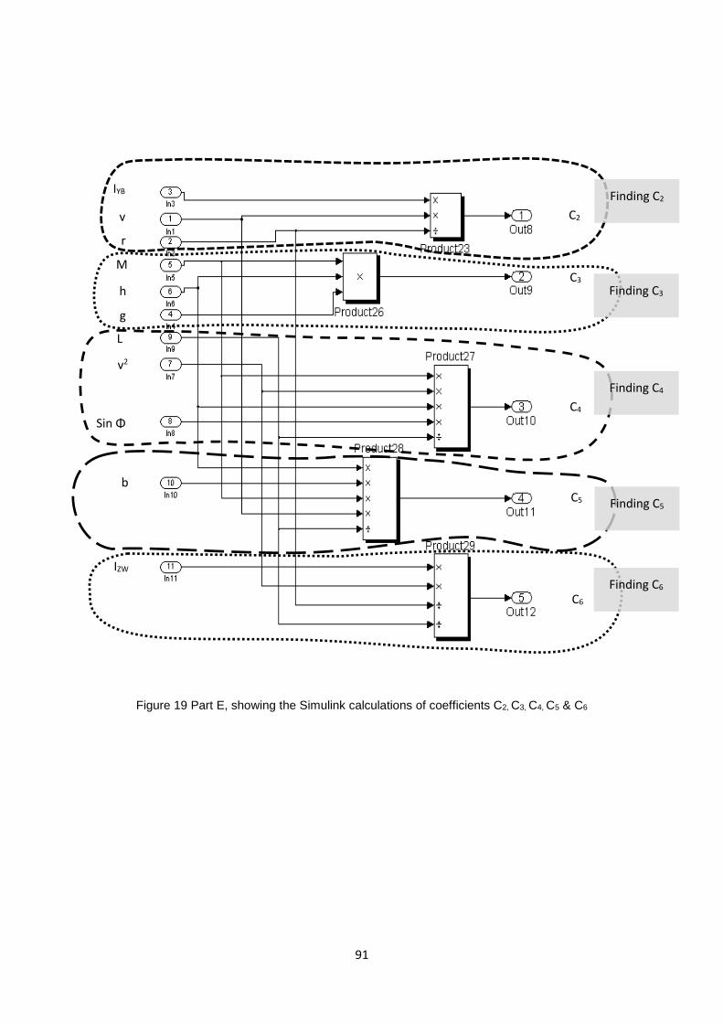
Figure 19 Part E, showing the Simulink calculations of coefficients C2, C3, C4, C5 & C6
C3
C2
C4
C5
C6
IZW
IYB
Sin Φ
v
g
r
h
M
L
v2
b
Finding C2
Finding C3
Finding C4
Finding C5
Finding C6
91

Figure 20 Simulink Part F, outlining the calculations of the terms required for equation (28)
A6
A2
A4
A3
A5
Cos Φ
TS Sin Φ
A1
A3
TS Sin Φ/A3
TF
A6/A3 A1 /A3 A2 /A3 A4 /A3 A5 /A3
𝐴𝐴1�̇�𝜆
𝐴𝐴4�̇�𝜎 𝐴𝐴2𝜆𝜆
𝐴𝐴3
𝐴𝐴5𝜎𝜎
Takes A1 to A5 and other terms and…
…produces the terms for equation (28)
92
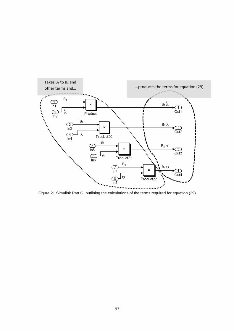
Figure 21 Simulink Part G, outlining the calculations of the terms required for equation (29)
B1
B2
B3
B4
B1
B2
B3
B4
Takes B1 to B4 and other terms and… …produces the terms for equation (29)
93

cos
TS cos Φ
sin
B1 + C1
B1 + C1
B1 + C1
B1 + C1
B1 + C1
B1 + C1
B1 + C1
sin
B2
B1
C2
C1
B4
B3
C4
C3
C5
C6
TS cos Φ/ ( B1 + C1)
C2 /( B1 + C1)
B2 /( B1 + C1)
C3sin /( B1 + C1)
(C5 - B3) /( B1 + C1)
C4 cos /( B1 + C1)
(C6 - B4) /( B1 + C1)
Figure 22 Simulink Part H, outlining the calculations of the terms required for equation (32)
…produces the terms for equation (32) Takes Bn & Cn and other terms and…
94

Figure 23 Simulink Part I, calculation of yaw σ terms
Figure 24 Simulink Part J, calculation of frame torque TF
TS Sin Φ/A3
A1λ /A3 A2λ /A3 A4σ /A3 A5σ /A3 A6/A3
σ
σ
σ
B4σ B3σ B2λ
B1λ sinΦTF
TS cos Φ
σ
equation (29)
equation (28)
Tf SinΦ term output
Yaw outputs
95

Figure 25 Simulink Part K calculation of roll λ terms
C4σ cosλ /( B1 + C1) (C5 - B3)σ /( B1 + C1)
B2λ /( B1 + C1)
(C6 - B4)σ /( B1 + C1) C3sinλ /( B1 + C1)
C2λ /( B1 + C1)
λ
TS cos Φ/( B1 + C1)
λ
λ
equation (32)
Roll outputs
96

4.9. SIMULINK OUTPUTS
Once all the Simulink calculations have been completed, two final outputs are obtained: the
front wheel yaw (σ) and bicycle roll (λ) with respect to time and these can be plotted on a
Simulink Scope or saved to a Matlab workspace file for further analysis and processing. In
Figure 26 a typical output of yaw and roll angles is shown plotted against time for the benchmark
bicycle using a standard steering torque input (as per Figure 8).
The counter-steer cornering manoeuvre was described in Chapter Two when discussing the
literature (12, 41, 54). To review this manoeuvre, consider the situation where a bicycle is
required to corner to the right, the rider first has to turn the front wheel very slightly to the left,
which is opposite to the direction of the turn. This small movement of the wheel will initiate a
very small turn to the left. As the bicycle starts this small left hand turn, the centrifugal force
induced on the bicycle and rider mass causes the bicycle to roll to the right. Once this happens,
both the Jones and castor torques combine to cause the front wheel to now turn rightwards into
the roll. The bicycle will now turn right and complete the desired right hand turning manoeuvre
(2, 12, 41, 54). Clear evidence of such a counter-steering action is evident at the start of the
simulation in Figure 26, where for the first 2 seconds the front wheel has yawed in a positive
direction (to the left) before the desired negative (or right hand) yaw occurs.
Counter-steering is a counter-intuitive action and this may be one reason why it is hard for
people to learn to ride bicycles, as it is not possible to corner a bicycle without initially turning
the steering in the opposite direction. This action is something that most bicycle riders
eventually will learn to do instinctively without consciously realising they are doing it. In fact it is
common when discussing this topic even for experienced riders to claim that they do not
countersteer when cornering.
4.10. ADDITIONAL MODEL FEATURES
Two additional features were added to the Simulink model which assisted the detailed analysis
of various characteristics.
1. Parameter gain blocks
The physical parameters were linked via gain blocks to the model in order to allow easy
adjustment of their values for both sensitivity and stability analysis. Details of these
gain blocks are shown in Appendix A. The Simulink model is therefore able to be run
using different physical parameters so that model assumptions could be very quickly
changed as required. This capability enables:
• The model to be more easily checked against other work in this area
• A variety of different bicycle manoeuvres to be tested and evaluated
• Different designs to be quickly compared
97
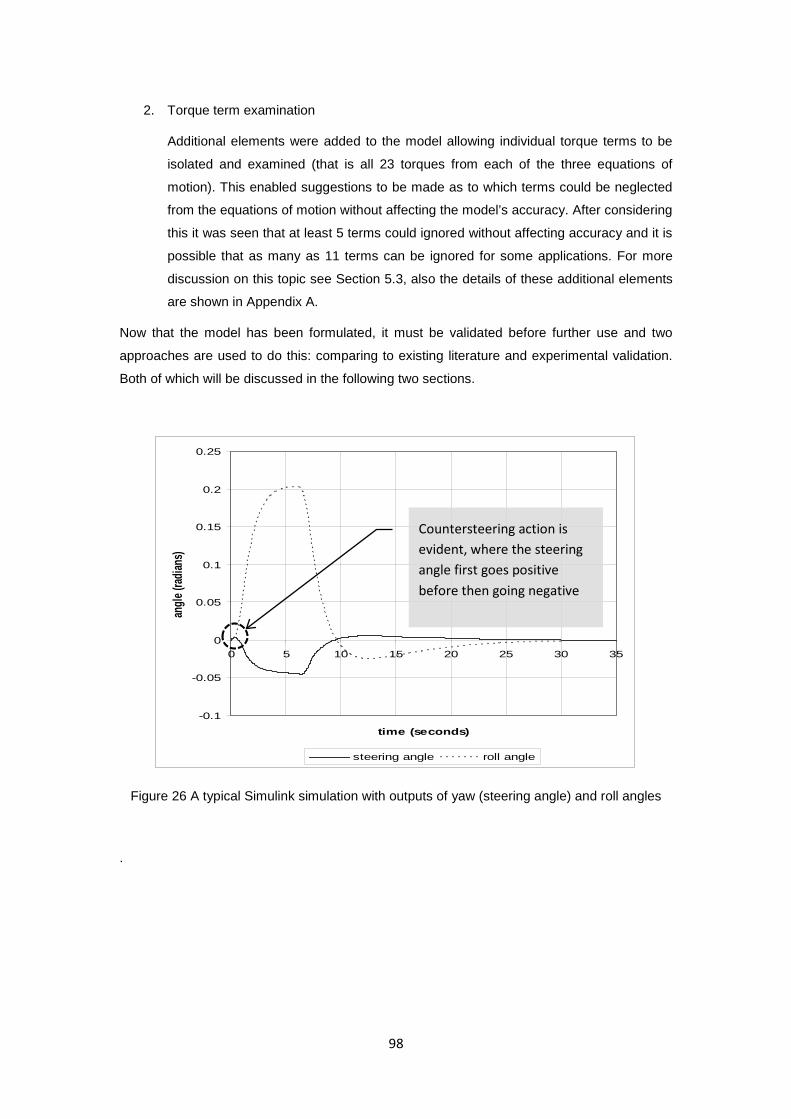
2. Torque term examination
Additional elements were added to the model allowing individual torque terms to be
isolated and examined (that is all 23 torques from each of the three equations of
motion). This enabled suggestions to be made as to which terms could be neglected
from the equations of motion without affecting the model’s accuracy. After considering
this it was seen that at least 5 terms could ignored without affecting accuracy and it is
possible that as many as 11 terms can be ignored for some applications. For more
discussion on this topic see Section 5.3, also the details of these additional elements
are shown in Appendix A.
Now that the model has been formulated, it must be validated before further use and two
approaches are used to do this: comparing to existing literature and experimental validation.
Both of which will be discussed in the following two sections.
Figure 26 A typical Simulink simulation with outputs of yaw (steering angle) and roll angles
.
-0.1
-0.05
0
0.05
0.1
0.15
0.2
0.25
0 5 10 15 20 25 30 35
time (seconds)
angle
(rad
ians)
steering angle roll angle
Countersteering action is evident, where the steering angle first goes positive before then going negative
98

4.11. VALIDATION WITH LITERATURE
Now that a computer simulation model has been developed it needs to be validated and the
theoretical approach chosen was to compare it with the literature. This was done by running a
simplified Simulink model that used the same assumptions as Fajans, that is setting the new terms
that allowed for Coriolis effects and the steering head tube angle to zero and using the same
values for input torques, parameters and variables, see Table 19 (12). The key differences
between Fajans and the more complex Simulink model are summarised as follows:
1. The Fajans steering head tube angle is set at 90 degrees i.e. the axis is vertical, whereas
in the benchmark model it is set at 73 degrees with typical ranges for road bicycles being
between 71.5 to 76 degrees. Because of its simplified steering geometry the Fajans model
cannot be used to optimise steering geometry, a critical area of bicycle design.
2. Fajans uses a negative rake to provide the required trail, where in practice road bicycles
have positive values of between 33 and 60 mm, see Chapter Seven.
3. Fajans neglects all the Coriolis torque terms, whereas the complete Simulink model
includes all Coriolis torque terms.
Table 19 shows these assumptions for all three models and drawings of the steering geometries
for a Fajans bicycle and a typical road bicycle are displayed Figure 28 and Figure 27.
Table 19 Model Assumptions
Assumptions The Fajans model Simplified
Simulink model Complex Simulink
model
HTA degrees 90.0 89.91 73.0
Rake mm -20.0 -19.42 45.0
Trail mm 20.0 20.0 56.13
Coriolis terms included no no yes
Note 1, the model could not run with a 90 degree HTA angle, so 89.9 degrees was used instead
as being the closest practical value
A simulation using this simplified model was run and then compared with Fajans with the simplified
model showing nearly identical output responses in terms of yaw and roll to Fajans, with very
similar time lags, rise times, amplitudes, overshoots and oscillations, see Figure 29 (note that the
simplified Simulink results are offset by 5 seconds to make the comparison clearer). The
differences between them are quantified in Figure 30 where it can be seen that for most of the
manoeuvre the yaw difference is within 2.5% (0.001/0.4) and the roll difference within 1%
(0.002/0.2). This confirms agreement between this Simulink model’s basic assumptions and
Fajans but doesn’t say anything about the validity of the added terms or other modifications.
Simulink is a mature programme and it is reasonable to have a high degree of confidence in these
99
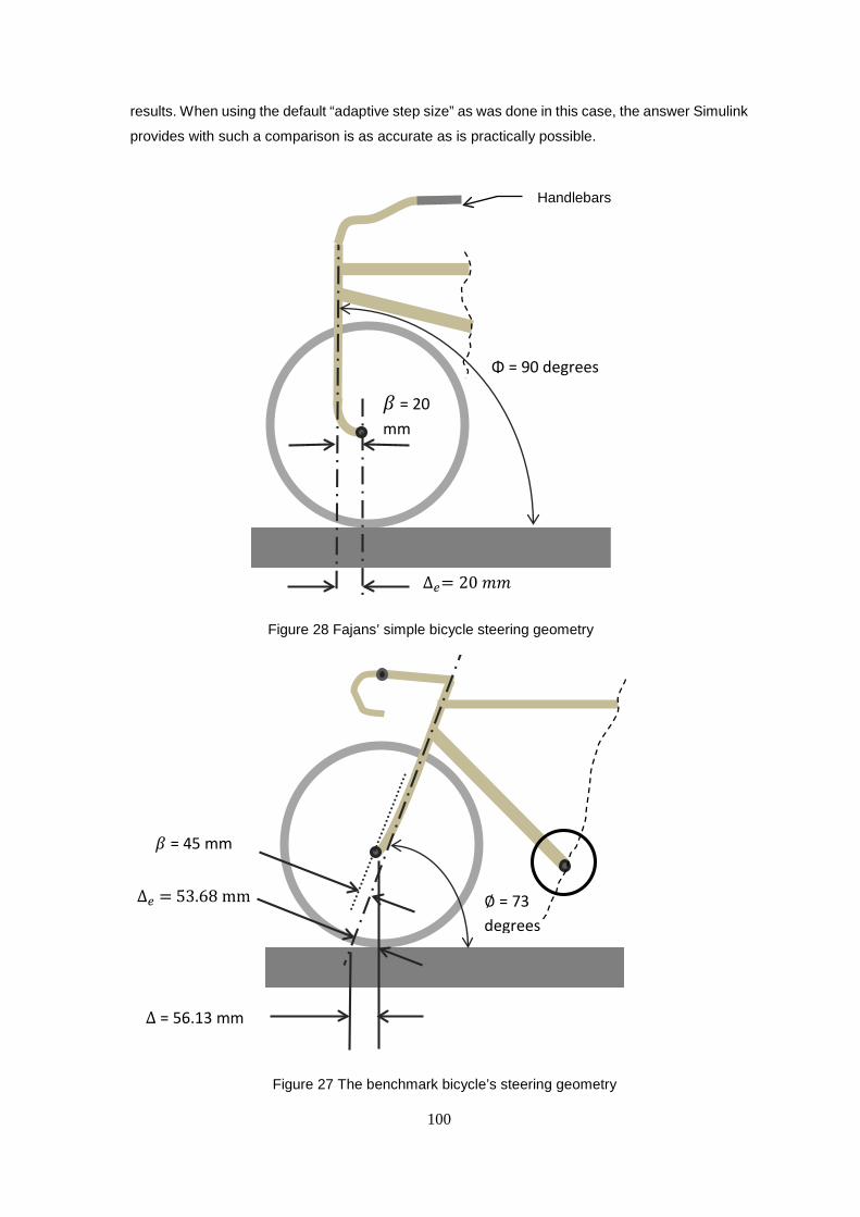
results. When using the default “adaptive step size” as was done in this case, the answer Simulink
provides with such a comparison is as accurate as is practically possible.
Figure 27 The benchmark bicycle’s steering geometry
∅ = 73 degrees
𝛽𝛽 = 45 mm
∆ = 56.13 mm
∆𝑖𝑖 = 53.68 mm
Figure 28 Fajans’ simple bicycle steering geometry
𝛽𝛽 = 20 mm
∆𝑖𝑖= 20 𝑚𝑚𝑚𝑚
Φ = 90 degrees
Handlebars
100

Figure 29 Comparison of the Simplified Simulink and Fajans models (with the Simulink results offset by 5 sec)
-0.1
-0.05
0
0.05
0.1
0.15
0.2
0.25
angl
e (r
adia
ns)
time (lines at 5 second intervals)
Fajans yaw angle
Simplified Simulink Modelyaw angle
Fajans roll angle
Simplified Simulink model rollangle
101

Figure 30 Difference between the yaw and roll angles of the Simplified Simulink and Fajans models
-0.006
-0.004
-0.002
0
0.002
0.004
0.006
0.008
0.01
0.012
0.014
0 5 10 15 20 25
angu
lar d
iffer
ence
(ra
dian
s)
time (seconds)
Simplified Simulink Model minus Fajans Model
Difference in yaw angle Difference in roll angle
102
4.12. EXPERIMENTAL VALIDATION
In addition to the theoretical validation the Simulink model was validated by comparing it to an
experimental investigation (31). In this part of the investigation a bicycle was adapted for
experimental work by being fitted with transducers to measure front wheel yaw (or steering angle)
and roll angles while a data logger recorded the results. This experimental bicycle test rig could
record yaw and roll angles against time for test runs of up to 30 seconds and this rig is illustrated
in Figure 31, Figure 32 and Figure 33.
The yaw angle was measured using a rotary electrical potentiometer with its input shaft directly
attached to the steering stem by a simple coupling, see Figure 33. The potentiometer’s output was
proportional to the front wheel’s yaw angle.
The roll angle was measured using a custom made infra-red (IR) distance measuring sensor
mounted on a short bracket at the rear of the bicycle, see Figure 32. A pulse of IR light was emitted
from the sensor and travelled downwards and once it hit the road surface it was reflected back.
The reflected IR light returned to the sensor at a different angle from the transmitted angle and
this angle was proportional to the distance to the road surface, as in Figure 34. As the bicycle
rolled, the IR sensor detected a change in the angle of the reflected light beam and this was used
to determine the roll angle, shown in Figure 35. For more details of this experiment and the
apparatus used see Appendix C.
Using this bicycle different experimental scenarios were investigated under controlled conditions,
first counter-steered cornering was considered which showed exactly the same characteristics for
roll and yaw as predicted by the computer simulation. A counter-steered manoeuvre was always
preceded by the tell-tale yaw of the front wheel in the opposite direction to the turn, followed by a
quick yaw reversal as the turn continues. It can also be noted that the same effect occurs during
the correcting part of the manoeuvre as the bicycle comes back to a straight course and this is
clearly indicated in Figure 36 through to Figure 41. A total of 68 experimental runs were
undertaken and the best and most representative runs are presented in this Chapter as a summary
of the results.
To get good experimental results, it was necessary to take care to ride the bicycle as smoothly
and upright as possible, prior to making the turn. The turn should be a slow gentle sweeping
manoeuvre through at least 180 degrees as smaller, tighter turns were hard to interpret amongst
the background signals of normal riding.
A second series of experiments involved testing on the road. From these tests it is apparent that
constant steering corrections are required for balance when riding along the uneven surface of a
typical road. As most road surfaces are highly irregular, changes in yaw and roll of the bicycle
must cope with this irregularity, while the bicycle/rider system must obey the inverted pendulum
rule in order to remain upright. The rider must constantly correct for changes in the bicycle’s roll
angle by using the yaw of the front wheel to steer the wheels under the centre of mass, this is
103

particularly evident in Figure 40 and Figure 41. A careful comparison of these figures shows that
the maximum positive values of roll match the maximum negative values of yaw and vice versa.
Figure 31 Experimental bicycle setup used to validate Simulink model
Figure 32 IR sensor and data logger used to measure the roll angle
IR roll angle sensor
Data logger
104

Figure 33 Yaw angle sensor measuring front wheel yaw
Yaw angle sensor
105

Rear wheel
IR sensor
Initial angle of the
reflected IR light
Figure 34 Bicycle roll sensor emits and receives IR light
Bicycle is
rolled to the
right
Figure 35 Roll angle is determined from the changed angle of the reflected light
The angular change of the
reflected light is proportional
to the roll angle
106

In principle, this series of experiments illustrates trends (e.g. the counter-steering action) as it was
very difficult to statistically correlate the data due to the irregular road surface and the large
measurement noise and error signals that resulted. However, the results of the experiments and
the comparison with other work indicate that the present computer model is acceptable to study
bicycle dynamics [10].
From the results obtained it was possible to comment on the validity of the Simulink model. Both
the theoretical and experimental validation shows the expected dynamic responses to a steering
input. One very interesting point is that the yaw angle shows the same type of counter-steer both
at the start and the end of the cornering manoeuvre, as the model. The roll angle also varies at
the same rate as yaw and mirrors the model’s response with regards to trends. It was not possible
to quantify these responses with regards to the steering torque as the torque was not recorded.
In fact the problem of recording steering torque is not a simple one, as the steering forces are very
small compared to the vertical forces exerted on the handlebar by the rider.
4.13. REMARKS
This Chapter has described the structure and main elements of a Simulink model that can solve
the equations of motion developed in Chapter Three. The model takes the rider’s steering torque
input and after applying appropriate physical parameters (such as mass, wheelbase length, head
tube angle, rake and trail distance) finds the yaw and roll responses of the bicycle.
This Chapter also describes the validation of the model using both theoretical and experimental
approaches. The theoretical approach to validate this model was to compare it with Fajans using
identical parameters and variables and from the results obtained it can be seen that it showed
nearly identical responses to Fajans.
The Simulink model was also validated by comparing it to the results of the experimental
investigation where a bicycle was fitted with transducers to measure yaw and roll angles recorded
on a data logger. From the results obtained it was possible to comment on the validity of the
Simulink model as the experiments showed the expected dynamic responses to a steering input.
The model is now ready to be used for a detailed analysis of bicycle dynamic behaviour and this
is described in the next Chapter.
107

Figure 36 Yaw (steer) angle output during an experimental counter-steer cornering manoeuvre
Figure 37 Roll angle output during the same experimental counter-steer cornering manoeuvre
Error signals and measurement noise
this roll to the left corresponds to the left hand yaw above
Roll
angl
e (d
egre
es)
Countersteer of front wheel
Turn to the left
Countersteer of front wheel
Start of manoeuvre End of manoeuvre
108

Figure 38 Yaw (steer) angle output for a second experimental counter-steer cornering manoeuvre
Figure 39 Roll angle output during the second experimental counter-steer manoeuvre
Counter steer of front wheel
Error signals
Corresponding roll to the left
Turn to the left
Roll
angl
e (d
egre
es)
109

Figure 40 Yaw (steer) angle output for part of a typical experimental road ride
Figure 41 Roll angle output during the same experimental road ride
Roll
angl
e (d
egre
es)
Corresponding roll to the left
Corresponding roll to the right
Turn to the left
Turn to the right
110

5. BICYCLE MODEL ANALYSIS
5.1. INTRODUCTION
This Chapter considers the bicycle design process and asks how it can be correlated with the
model in Chapter Four? Given the large number of terms and parameters in the equations, what
sort of simplifications and manipulations can be justified? Since a design process in most cases
is based on approximations and empirical approaches it is logical to simplify the equations of
motion to obtain a more practical and useful formulation. There is no sense in having long and
overly complicated equations if the final design process later on requires significant simplifications
and approximations. Furthermore as there are no unique values for the design parameters such
approximations are normally acceptable. But before these simplifications can occur we need to
determine how sensitive the analysis is to changes in these parameters. This Chapter uses the
bicycle dynamic model developed and described in Chapters Three and Four to investigate and
understand the following issues:
1. the effectiveness of the model in determining bicycle dynamic behaviour
2. the importance and significance of each torque term in the equations of motion
3. the sensitivity of the bicycle’s performance to changes in design parameters
We ask the following important questions. How can the bicycle be optimised in terms of specific
performance criteria? Can the equations of motion be simplified by ignoring any of the torque
terms? It is important to understand how sensitive the bicycle is to changes in assumptions and
parameter values. Finally how stable is the bicycle dynamically and is it possible to identify and
avoid unstable design regions? Such questions need to be systematically examined and to provide
answers the Simulink model was used to conduct the following:
1. Bicycle performance simulations
The purpose of these simulations was to demonstrate the basic capabilities of the
model and to see if it could effectively reproduce realistic bicycle dynamic behaviour,
especially the reactions of the bicycle to changes in steering geometry, damping,
speed and steering torque.
2. Torque term evaluations
The significance and importance of individual torque terms in the dynamic model was
examined by analysing the results of Simulink trials. By focusing on individual torque
terms it was possible to determine the significant and insignificant terms so that
recommendations about simplifications to the equations of motion could be made.
111

3. Sensitivity study
This study identified critical design parameters and quantified their effects on bicycle
handling performance. It determined their minimum and maximum acceptable limits
and examined their relative importance in terms of their overall effects. These results
are later used in Chapter Six to develop practical design charts for designers.
4. Stability study using the characteristic equation
For completeness in this study the characteristic equation of the bicycle system was
found as its roots determine the character of the time response and the natural
transient response of the system, hence why it is called the characteristic equation. A
necessary requirement for stability is for all of the roots of the characteristic equation
to have negative real parts. Once the characteristic equation has been found the
Routh Stability Criterion can be used to find out if it has any unstable roots without
actually solving them and this procedure is shown in Appendix D.
5.2. BICYCLE PERFORMANCE SIMULATIONS
This section describes the results of a series of Simulink simulations that demonstrated the
model’s basic capability. These simulations demonstrate the application of the model and
reproduce realistic bicycle dynamic behaviour, especially the reactions of the bicycle to changes
in key parameters. Does the model show the same sort of results as expected from the literature
and previous experiments? This section examines the following two areas of interest in order to
understand bicycle performance:
1. the steering geometry terms (head tube angle, rake and trail) and the damping term
2. and speed and steering torque
5.2.1. STEERING GEOMETRY AND DAMPING
First consider the effect of steering geometry and damping, how do they affect each other? It is
well known that steering geometry is a critically important factor in bicycle design (10, 83). This
geometry is defined by: the wheel radius, head tube angle and rake values, from which the trail
(and effective trail) can be calculated using the four equations below [equations (33 to (36)] see
also Table 20 and Figure 42.
112

Trail equation
∆=𝑟𝑟 − 𝛽𝛽
cos∅tan∅
(33)
Alternative trail equation
∆=𝑟𝑟 cos∅ − 𝛽𝛽
sin∅
(34)
Effective trail equation
∆𝑖𝑖= ∆ sin∅
(35)
Alternative effective trail equation
∆𝑖𝑖= 𝑟𝑟 cos∅ − 𝛽𝛽
(36)
Table 20 Steering geometry terms:
Symbol Steering geometry definition Units
Φ Head tube angle degrees
β Fork rake (or offset) m
r Wheel radius m
Δ Trail m
Δe Effective trail m
113

∅ 𝛽𝛽
∆
∆𝑖𝑖
𝑟𝑟
Figure 42 Bicycle steering geometry terms for the front wheel
114

In this section, five different steering geometry cases are examined and their dynamic responses
are compared with one another (their specific geometries are shown in Table 21).
Table 21 Steering geometry cases
Case No
Head tube angle
degrees
Rake
mm
Trail
mm
Comments Outcomes Relevant figures
One 73 45 56.128 Benchmark
bicycle1
Stable even with no
damping
Figure 43, Figure 48,
Figure 51, Figure 52
and Figure 53
Two 73 75 24.757 reduced trail Marginal, requires a
precise steering
input
Figure 45
Three
73 15 87.499 Increased trail Highly unstable Figure 46
Four 90 -20 20.000 Fajans bicycle Unstable at low
damping values
Figure 44
Figure 47
Five 89 -50 55.899 Fajans with
increased trail
Marginal stability
with low damping
Figure 49
Figure 50
Note 1 the benchmark bicycle has the standard geometry
Unless otherwise noted the standard steering torque of +0.45/-0.414 Nm is used (see Figure 8
First consider the effects of trail with the first three cases.
• For case one (the benchmark bicycle) when using a standard steering torque, the bicycle
successfully completed a counter-steered manoeuvre and exhibited acceptable
behaviour, with a rapid steering response and small overshoots and this is displayed in
Figure 43. This means that this bicycle is easy to precisely control and steer. As discussed
in Chapter Three the Simulink model (i.e. case one) includes new terms often ignored by
others. With these new terms the dynamic results differed to the Fajans model and others,
though the fundamental aspects remained (12). Overall, case one shows a slower
cornering response with greater time lags and slower rates of change than Fajans, see
Figure 44. The graph shapes are more rounded and less angular, which is what would be
intuitively expected and this shows the significance of using assumptions previously not
considered, such as realistic steering geometry.
115
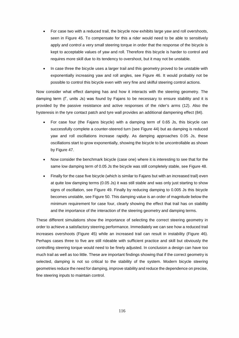
• For case two with a reduced trail, the bicycle now exhibits large yaw and roll overshoots,
seen in Figure 45. To compensate for this a rider would need to be able to sensitively
apply and control a very small steering torque in order that the response of the bicycle is
kept to acceptable values of yaw and roll. Therefore this bicycle is harder to control and
requires more skill due to its tendency to overshoot, but it may not be unstable.
• In case three the bicycle uses a larger trail and this geometry proved to be unstable with
exponentially increasing yaw and roll angles, see Figure 46. It would probably not be
possible to control this bicycle even with very fine and skilful steering control actions.
Now consider what effect damping has and how it interacts with the steering geometry. The
damping term (Γ, units Js) was found by Fajans to be necessary to ensure stability and it is
provided by the passive resistance and active responses of the rider’s arms (12). Also the
hysteresis in the tyre contact patch and tyre wall provides an additional dampening effect (84).
• For case four (the Fajans bicycle) with a damping term of 0.65 Js, this bicycle can
successfully complete a counter-steered turn (see Figure 44) but as damping is reduced
yaw and roll oscillations increase rapidly. As damping approaches 0.05 Js, these
oscillations start to grow exponentially, showing the bicycle to be uncontrollable as shown
by Figure 47.
• Now consider the benchmark bicycle (case one) where it is interesting to see that for the
same low damping term of 0.05 Js the bicycle was still completely stable, see Figure 48.
• Finally for the case five bicycle (which is similar to Fajans but with an increased trail) even
at quite low damping terms (0.05 Js) it was still stable and was only just starting to show
signs of oscillation, see Figure 49. Finally by reducing damping to 0.005 Js this bicycle
becomes unstable, see Figure 50. This damping value is an order of magnitude below the
minimum requirement for case four, clearly showing the effect that trail has on stability
and the importance of the interaction of the steering geometry and damping terms.
These different simulations show the importance of selecting the correct steering geometry in
order to achieve a satisfactory steering performance. Immediately we can see how a reduced trail
increases overshoots (Figure 45) while an increased trail can result in instability (Figure 46).
Perhaps cases three to five are still rideable with sufficient practice and skill but obviously the
controlling steering torque would need to be finely adjusted. In conclusion a design can have too
much trail as well as too little. These are important findings showing that if the correct geometry is
selected, damping is not so critical to the stability of the system. Modern bicycle steering
geometries reduce the need for damping, improve stability and reduce the dependence on precise,
fine steering inputs to maintain control.
116

Figure 43 Simulink result for the benchmark bicycle on a standard run, case one
Figure 44 Fajans model for a standard simulation
-0.1
-0.05
0
0.05
0.1
0.15
0.2
0.25
0 5 10 15 20 25 30 35
time (seconds)
angle
(rad
ians)
steering angle roll angle
-0.1
-0.05
0
0.05
0.1
0.15
0.2
0.25
0 5 10 15 20 25
time (seconds)
angle
(rad
ians)
steering angle roll angle
117

Figure 45 Case two simulation with reduced trail
Figure 46 Case three simulation with increased trail
-0.15
-0.1
-0.05
0
0.05
0.1
0.15
0.2
0 5 10 15 20 25
time (seconds)
Angl
e (ra
dian
s)
steering angle roll angle
-0.1
-0.05
0
0.05
0.1
0.15
0.2
0.25
0.3
0.35
0.4
0 5 10 15 20 25
time (seconds)
Angl
e (ra
dian
s)
steering angle roll angle
118
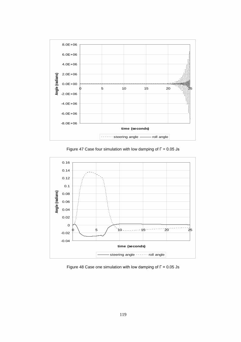
Figure 47 Case four simulation with low damping of Г = 0.05 Js
Figure 48 Case one simulation with low damping of Г = 0.05 Js
-8.0E+06
-6.0E+06
-4.0E+06
-2.0E+06
0.0E+00
2.0E+06
4.0E+06
6.0E+06
8.0E+06
0 5 10 15 20 25
time (seconds)
Angl
e (ra
dian
s)
steering angle roll angle
-0.04
-0.02
0
0.02
0.04
0.06
0.08
0.1
0.12
0.14
0.16
0 5 10 15 20 25
time (seconds)
Angl
e (ra
dian
s)
steering angle roll angle
119

Figure 49 Case five simulation with a low damping of Г = 0.05 Js
Figure 50 Case five simulation with very low damping of Г = 0.005 Js
-0.05
0
0.05
0.1
0.15
0.2
0 5 10 15 20 25
time (seconds)
Angl
e (ra
dian
s)
steering angle roll angle
-0.05
0
0.05
0.1
0.15
0.2
0 5 10 15 20 25
time (seconds)
Angl
e (ra
dian
s))
steering angle roll angle
Small oscillations
120

5.2.2. SPEED AND STEERING TORQUE
It is commonly reported that bicycles are more stable at higher speeds (2, 5, 20, 21). But does the
model developed show this behaviour? This investigation now considers the effect of speed and
the associated steering torque required for control.
• For case one with all terms in the model unchanged, except for speed, it was found that
at 5 km/hr the bicycle became unstable when the steering torque remained at the standard
value (+0.45 / -0.414 Nm) see Figure 51.
• Only by reducing the steering torque down to +/- 0.0025 Nm (or 0.6% of the standard
value) was it possible to control the case one bicycle at this lower speed, see Figure 52.
This torque is equivalent to a couple comprising of two oppositely opposed 0.57 gram
forces set 450 mm apart on the handlebars. Of course such a very small torque value
would be difficult for a rider to apply and control but it is not impossible with practice.
Therefore it is concluded that as the speed reduces the steering torque required to control
the bicycle must also dramatically reduce.
• Conversely as the speed increases above 25 km/hr the torque required to steer the bicycle
around a corner increased. When speed increased to 85 km/hr (with all other terms
unchanged) it was found that the bicycle became incredible stable in a straight line. The
standard steering torque of +0.45 / -0.414 Nm, only produced very small yaw and roll
responses of 0.060 (0.001 radians) and 3.20 (0.055 radians) respectively, in other words
the steering input hardly produced a change in direction and this is shown Figure 53.
This supports the common empirical observation that bicycles are more stable and easier to ride
at higher speeds (2, 5, 20, 21). It also means that to undertake a large course variation at high
speed a large steering torque is required. In addition outside perturbations have less effect on
bicycles and will not affect their course as much and so the bicycle is more self-stable.
An important objective for this study was to find ways to optimise bicycle steering geometry and
to improve performance. After consideration of the five cases just examined it can be seen that
careful selection of the steering geometry parameters is critical, also as they are interrelated wrong
combinations can dramatically affect the steering response and stability. The advantage of the
Simulink model is it allows different geometries to be checked for any potential stability problems
before a design is built.
By plotting the trail and the head tube angle onto a chart it will be possible to indicate unstable
regions and such a chart could be used to design successful geometries and avoid mistakes. In
Figure 54 such a chart is drawn and on it is displayed lines of constant rake. Cases one to five
from Table 21 have been plotted on this chart.
A region of stability is approximately indicated within the dotted line. At this stage the boundary
between stable and unstable geometries is not precisely known. Obviously the negative trail region
is completely unstable and has not been plotted. Though the exact boundaries between stable
121

and unstable regions are not yet known this will be explored by further investigations in Chapters
Six and Seven. Out of interest the 1817 Hobbyhorse is also plotted, with a head tube angle of 90
degree, 0 mm trail and 0 mm rake, it is marginally unstable according to the chart but in practice
is still rideable.
Figure 51 Case one low speed simulation v = 5 km/hr and TS ≈ +/- 0.45 Nm
Figure 52 Case one low speed simulation v = 5 km/hr and TS ≈ +/- 0.0025 Nm
-6
-4
-2
0
2
4
6
0 5 10 15 20 25
time (seconds)
Angl
e (ra
dian
s)
steering angle roll angle
-0.00005
0
0.00005
0.0001
0.00015
0.0002
0.00025
0.0003
0.00035
0 5 10 15 20 25
time (seconds)
Angl
e (ra
dian
s)
steering angle roll angle
122
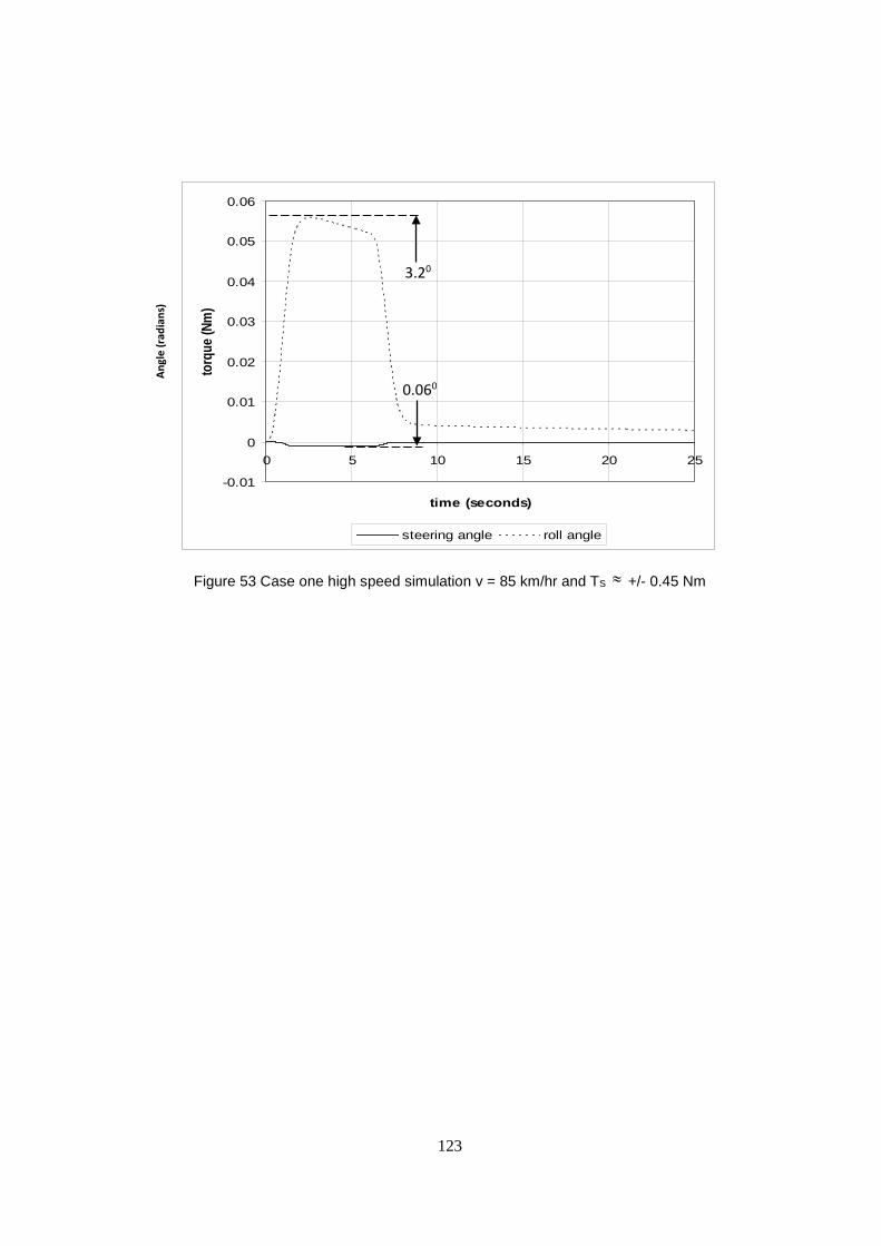
Figure 53 Case one high speed simulation v = 85 km/hr and TS ≈ +/- 0.45 Nm
-0.01
0
0.01
0.02
0.03
0.04
0.05
0.06
0 5 10 15 20 25
time (seconds)
torq
ue (N
m)
steering angle roll angle
0.060
3.20
Angl
e (r
adia
ns)
123

Figure 54 Trail vs. head tube angle front wheel geometry chart (wheel dia. all 675 mm & rake lines at 5 mm intervals)
0.00
10.00
20.00
30.00
40.00
50.00
60.00
70.00
80.00
90.00
100.00
110.00
120.00
65 66 67 68 69 70 71 72 73 74 75 76 77 78 79 80 81 82 83 84 85 86 87 88 89 90 91
Trai
l (m
m)
Head tube angle (degrees)
Trail vs. head tube angle chart
an undefined stable region within the dotted lines
Case 3 highly unstable
Case 2 marginally unstable
Case 1 stable
Case 4 marginally unstable
Case 5 marginally unstable
1817 Hobbyhorse HTA = 90 deg trail = 0 mm Rake = 0 mm
124
5.3. SIGNIFICANCE OF TORQUE TERMS
An evaluation of the significance of each torque term is important because the full equations of
motion [equations (14, (19 and (24)] are complicated (having a total of 23 individual torque terms
even after our simplifying assumptions) and it would be difficult to use these equations for design
purposes without further simplification. Simplification is also justified because the design process
itself is an approximation process that can tolerate small variations. So we need to find out which
terms can be ignored without affecting the dynamic model results.
In order to determine this the terms were isolated within the Simulink model without affecting its
functionality and simulations were run so the magnitude of each torque could be compared and
decisions made as to which are the most significant and which could be ignored from the model.
If some torques can be ignored without adversely affecting the accuracy of the dynamic modelling
this would simplify further analysis. Also a very simplified set of equations would enable more
appropriate equations to be used for some purposes. For example undergraduate teaching,
because though the problem of bicycle motion engages students, the current complicated
equations interfere with many worthwhile educational outcomes.
Each of the three fundamental equations of motion [i.e. equations (18, (23 and (26)] are now
examined in turn and suggestions as to appropriate simplifications are made.
5.3.1. FIRST EQUATION – MOMENTS ABOUT THE YAW AXIS FOR A
The first equation (18) considers the yawing about the vertical Z axis for the front assembly A. It
has eight torques terms in total, two of which are new compared to the Fajans model (the Coriolis
and frame torques) but which torques can be ignored? First the peak values for each individual
torque term were found and torque with the largest peak value was identified. Then the peak
values of each torque were compared to this maximum torque term. It was decided to consider
excluding any torque which had a peak value of 10% or less of that of the maximum torque term’s
peak value, unless there was a good reason to include it. This is an order of magnitude less than
the maximum torque’s value. The suggestions as to which terms in equation (18) to ignore are
shown in Table 22 and comments about this now follows:
• the castor torque, Jones torque and the steering torque input from the rider are of major
importance and are shown in Figure 55
• the castor and Jones torques are by far the most significant terms in this equation and
dominate the yaw of assembly A
• the gyroscopic torque of the front wheel due to rolling, the Coriolis torque and the frame
torque that B exerts on A are an order of magnitude less than the most important terms
and have a minor effect, they are shown in Figure 56
• the Coriolis and frame torque are new terms introduced into this model
125
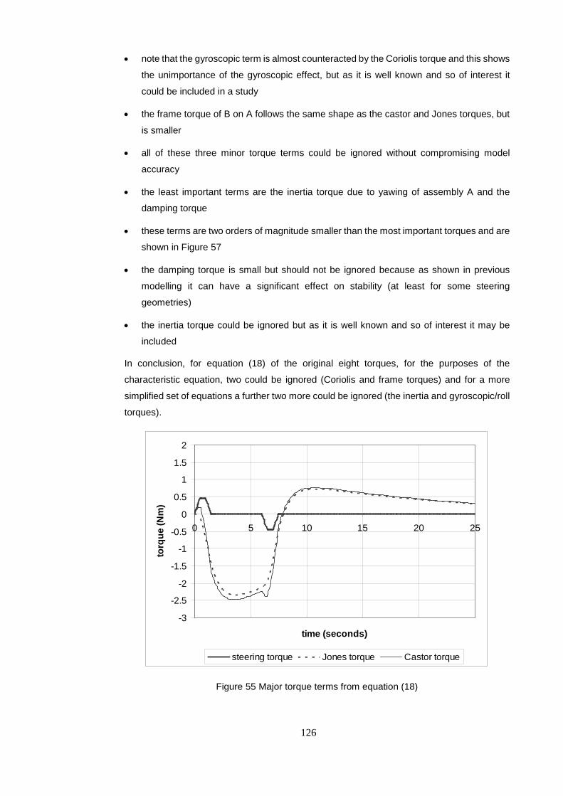
• note that the gyroscopic term is almost counteracted by the Coriolis torque and this shows
the unimportance of the gyroscopic effect, but as it is well known and so of interest it
could be included in a study
• the frame torque of B on A follows the same shape as the castor and Jones torques, but
is smaller
• all of these three minor torque terms could be ignored without compromising model
accuracy
• the least important terms are the inertia torque due to yawing of assembly A and the
damping torque
• these terms are two orders of magnitude smaller than the most important torques and are
shown in Figure 57
• the damping torque is small but should not be ignored because as shown in previous
modelling it can have a significant effect on stability (at least for some steering
geometries)
• the inertia torque could be ignored but as it is well known and so of interest it may be
included
In conclusion, for equation (18) of the original eight torques, for the purposes of the
characteristic equation, two could be ignored (Coriolis and frame torques) and for a more
simplified set of equations a further two more could be ignored (the inertia and gyroscopic/roll
torques).
Figure 55 Major torque terms from equation (18)
-3
-2.5
-2
-1.5
-1
-0.5
0
0.5
1
1.5
2
0 5 10 15 20 25
time (seconds)
torq
ue (N
m)
steering torque Jones torque Castor torque
126

Table 22 The terms from equation (18) and their significance
Torque Expanded term Relevant
figure number
Description and comments Max torque value Nm (%)
Assumptions Significance of the term
1. TInertia 𝐼𝐼𝑍𝑍𝑍𝑍�̇�𝜔𝑍𝑍𝑍𝑍 Figure 57 Inertia torque due to the yawing of A +/- 0.023
(0.92%)
very small and could be ignored but included
as it is well known and so of interest
negligible effect
2. TGyro/roll 𝐼𝐼𝑌𝑌𝑌𝑌𝜔𝜔𝑌𝑌𝑌𝑌𝜔𝜔𝑋𝑋𝑌𝑌 Figure 56 Gyroscopic torque due to the rolling of
A
+ 0.2 (8%) small and could be ignored but included as it
is well known and so of interest
minor effect
3. TCoriolis 𝐼𝐼𝑋𝑋𝑌𝑌𝜔𝜔𝑌𝑌𝑌𝑌𝜔𝜔𝑋𝑋𝑌𝑌 Figure 56 Coriolis torque of A + 0.09 (3.6%) can be ignored minor effect
4. TSteer 𝑇𝑇𝑆𝑆 sin𝑠𝑠 Figure 55 Steering torque input by rider, corrected
for the head tube angle
+ 0.45 (18%) must be included major effect
5. TJones 𝑀𝑀𝑀𝑀𝐵𝐵𝐿𝐿 sin𝑠𝑠Δ𝑖𝑖𝜆𝜆 Figure 55 Jones’ torque or trail steer, causes the
wheel to lean into the corner
+ 2.3 (92%) must be included
major effect
6. TCastor 𝑀𝑀𝑏𝑏𝑣𝑣2
𝐿𝐿2 sin𝑠𝑠Δ𝑖𝑖𝜎𝜎 Figure 55 Castor torque due to trail, tends to
straight the wheel up
- 2.5 (100%) the maximum torque and must of course be
included
major effect
7. TFrame 𝑇𝑇𝑓𝑓 cos𝑠𝑠 Figure 56 Torque of assembly B on A, corrected
for the head tube angle
+ 0.125 (5%) can be ignored minor effect
8. TDamping Γ�̇�𝜎 Figure 57 Damping torque (if this term is zero the
bicycle may be unstable)
+/- 0.018
(0.72%)
small but included as found to be essential
for dynamic stability
negligible effect
127

Figure 56 Minor torque terms from equation (18)
Figure 57 Negligible torque terms from equation (18)
-0.2
-0.15
-0.1
-0.05
0
0.05
0.1
0.15
0.2
0.25
0.3
0 5 10 15 20 25
time (seconds)
torq
ue (N
m)
gyro due to roll torque Coriolis torque Torque of B on A
-0.03
-0.02
-0.01
0
0.01
0.02
0.03
0 5 10 15 20 25
time (seconds)
torq
ue (N
m)
damping torque inertia torque
128

5.3.2. SECOND EQUATION - MOMENTS ABOUT THE ROLL AXIS FOR A
The second equation considers the rolling moments about the horizontal X axis for the front
assembly A [equation (23)] and has eight terms in total, four of which are new: the Coriolis, steer,
castor and Jones torques (the last three were added to account for realistic steering geometry).
The suggestions as to which terms in equation (23) to ignore are shown in Table 23, along with
the following comments:
• the major terms are: the gyroscopic torque of front wheel due to cornering, castor torque,
Jones torque and the frame torque of B on A, shown in Figure 58
• this is one case where a gyroscopic torque has a major effect, but on its own it still does
not account for the stability of the bicycle
• two of these terms, the castor torque and the Jones torque are new ones introduced due
to considerations of steering geometry and they both oppose and more than counteract
the gyroscopic term due to cornering
• the next most important terms in order of magnitude are the minor torques of: steering
torque and the inertia torque of assembly A due to rolling, see Figure 59
• the steering torque is new and was introduced due to considerations of steering geometry
• both these torques (steering torque and Inertia torque) could be ignored
• the least important terms are: the Coriolis torque and gyroscopic torque of front wheel
due to yawing (refer to Figure 60) and the Coriolis term is a new torque added to this
model
• again this shows the unimportance of the gyroscopic effect and both these terms are
negligible in their effect and could be ignored
In conclusion, for equation (23) of the original eight torques, for the application of the characteristic
equation, two could be ignored (Coriolis and steer torques) and for a more simplified set of
equations a further two more could be ignored (the inertia and gyroscopic/corner torques).
129

Table 23 The terms from equation (23) and their significance
Torque Expanded term Relevant
figure number
Description and comments Max torque value Nm (%)
Assumptions Significance of the term
1. TInertia 𝐼𝐼𝑋𝑋𝑍𝑍�̇�𝜔𝑋𝑋𝑍𝑍 Figure 59 Inertia torque of the front wheel due to
rolling of A
+/- 0.12
(10.0%)
small and could be ignored but included as
it is well known and so of interest
minor effect
2. TCoriolis 𝐼𝐼𝑍𝑍𝑌𝑌𝜔𝜔𝑌𝑌𝑌𝑌𝜔𝜔𝑍𝑍𝑌𝑌 Figure 60 Coriolis Torque of A +/- 0.035
(2.92%)
could be ignored negligible effect
3. TGyro/yaw 𝐼𝐼𝑌𝑌𝑌𝑌𝜔𝜔𝑌𝑌𝑌𝑌𝜔𝜔𝑍𝑍𝑌𝑌 Figure 60 Gyroscopic torque of front wheel due
to yawing of A
+ 0.07 (5.8%) small and could be ignored but included as
it is well known and so of interest
negligible effect
4. TFrame 𝑇𝑇𝑓𝑓 sin𝑠𝑠 Figure 58 Torque Assembly B exerts on A
corrected for the head tube angle
+ 0.4 (33.3%) must be included major effect
5. TGyro/cornering IYF
v2 sinϕrL σ
Figure 58 Gyroscopic torque of front wheel due
to cornering
+ 1.2 (100%) maximum torque, unusually for a gyro term
it has a major effect
major effect
6. TSteer 𝑇𝑇𝑆𝑆 cos𝑠𝑠 Figure 59 Steering Torque corrected for the head
tube angle
+/- 0.13
(10.8%)
could be ignored minor effect
7. TCastor 𝑀𝑀𝑏𝑏𝑣𝑣2
𝐿𝐿2 cos𝑠𝑠Δ𝑖𝑖𝜎𝜎 Figure 58 Castor torque corrected for the head
tube angle
- 0.75 (62.5%) must be included major effect
8. TJones 𝑀𝑀𝑀𝑀
𝑏𝑏𝐿𝐿 cos𝑠𝑠Δ𝑖𝑖𝜆𝜆
Figure 58 Jones torque corrected for the head
tube angle - 0.7 (58.3%) must be included major effect
130

Figure 58 Major torque terms from equation (23)
Figure 59 Minor torque terms from equation (23)
-1
-0.5
0
0.5
1
1.5
0 5 10 15 20 25
Time (seconds)
Torq
ue (N
m)
Gyroscopic torque due to cornering Torque of B on AJones torque Castor torque
-0.15
-0.1
-0.05
0
0.05
0.1
0.15
0 5 10 15 20 25
time (seconds)
torq
ue (N
m)
steering torque inertia torque
131

Figure 60 Negligible torque terms from equation (23)
5.3.3. EQUATION THREE - MOMENTS ABOUT THE ROLL AXIS FOR B
Finally the third equation deals with the rolling moments about the horizontal X axis for the rear
assembly B [equation (24)] and this third equation currently has seven terms, one of which is new,
the Coriolis torque. The suggestions as to which terms to ignore are shown in Table 24 and other
comments are shown below:
• the most important terms in this equation in order of magnitude are: the centrifugal torque
due to cornering and the gravitational torque due to rolling and these major torques are
shown in Figure 61, these two torques must balance each other during the cornering
manoeuvre to enable cornering to occur without capsizing or falling over occurring
• the next most important terms in order of magnitude are: the inertia torque of assembly
B due to rolling and the kink torque, see Figure 62, these are of an order magnitude less
than the most important terms, however they are not insignificant and should be
considered
• the least important terms in order of magnitude are: frame torque of A on B, gyroscopic
torque of the rear wheel due to cornering (yawing) and the Coriolis torque of assembly B
• these three negligible torques are shown in for the standard simulation run in Figure 63
• again the gyroscopic effect is unimportant
• these are all very small terms that are four orders of magnitude smaller than the most
important torques and can be ignored
• the Coriolis term is the only new torque added to this model
-0.08
-0.06
-0.04
-0.02
0
0.02
0.04
0.06
0.08
0 5 10 15 20 25
time (seconds)
torq
ue (N
m)
Coriolis torque gyroscopic torque due to yaw
132
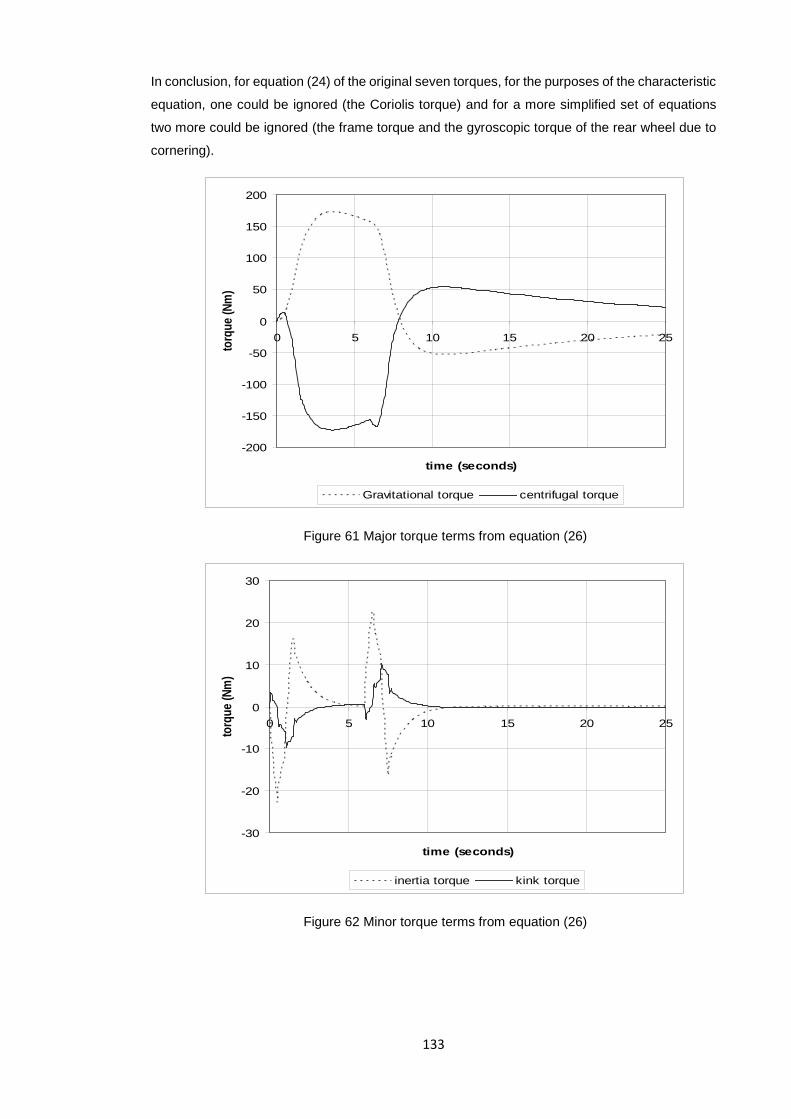
In conclusion, for equation (24) of the original seven torques, for the purposes of the characteristic
equation, one could be ignored (the Coriolis torque) and for a more simplified set of equations
two more could be ignored (the frame torque and the gyroscopic torque of the rear wheel due to
cornering).
Figure 61 Major torque terms from equation (26)
Figure 62 Minor torque terms from equation (26)
-200
-150
-100
-50
0
50
100
150
200
0 5 10 15 20 25
time (seconds)
torq
ue (N
m)
Gravitational torque centrifugal torque
-30
-20
-10
0
10
20
30
0 5 10 15 20 25
time (seconds)
torq
ue (N
m)
inertia torque kink torque
133

Table 24 The terms from equation (26) and their significance
Torque Expanded term Relevant
figure number
Description and comments Max torque value Nm (%)
Assumptions Significance of the term
1. TInertia 𝐼𝐼𝑋𝑋𝑋𝑋�̇�𝜔𝑋𝑋𝑋𝑋
Figure 62
Inertia torque of frame , rider and
rear wheel due to rolling of B
+/- 23.0
(13.1%)
must be included Minor effect
2. TCoriolis 𝐼𝐼𝑍𝑍𝑍𝑍𝜔𝜔𝑌𝑌𝑍𝑍𝜔𝜔𝑍𝑍𝑍𝑍 Figure 63 Coriolis Torque of the rear wheel +/- 0.10
(0.06%)
can be ignored Negligible effect
3. TGyro/cornering 𝐼𝐼𝑌𝑌𝑍𝑍𝜔𝜔𝑌𝑌𝑍𝑍𝜔𝜔𝑍𝑍𝑍𝑍 Figure 63 Gyroscopic torque of rear wheel due
to cornering
- 0.40 (0.23%) very small and could be ignored but
included as it is well known and so of
interest
Negligible effect
4. TFrame 𝑇𝑇𝑓𝑓 sin𝑠𝑠 Figure 63 Torque Assembly A exerts on Assembly B corrected for the head tube angle
+ 0.40
(0.23%)
could be ignored for some purposes Negligible effect
5. TCentrifugal 𝑀𝑀𝑣𝑣2ℎ sin𝑠𝑠
𝐿𝐿 cos 𝜆𝜆𝜎𝜎
Figure 61
Centrifugal torque - 175.0
(100%)
maximum torque Major effect
6. TGravity 𝑀𝑀𝑀𝑀ℎ sin 𝜆𝜆
Figure 61
Gravitational torque + 175.0
(100%)
maximum torque Major effect
7. TKink 𝑀𝑀ℎ𝑏𝑏𝑣𝑣𝐿𝐿 �̇�𝜎
Figure 62
Kink torque (Coriolis torque of assembly B less rear wheel)
+/- 10.0
(5.7%)
could be included Minor effect
134

Figure 63 Negligible torque terms from equation (26)
-0.5
-0.3
-0.1
0.1
0.3
0.5
0 5 10 15 20 25
time (seconds)
torqu
e (Nm
)
torque of A on BCoriolis torquegyroscopic torque due to cornering
135
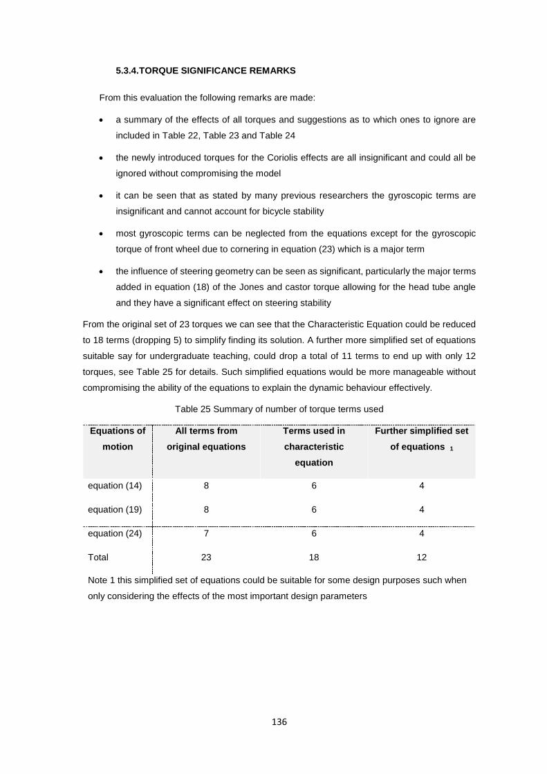
5.3.4. TORQUE SIGNIFICANCE REMARKS
From this evaluation the following remarks are made:
• a summary of the effects of all torques and suggestions as to which ones to ignore are
included in Table 22, Table 23 and Table 24
• the newly introduced torques for the Coriolis effects are all insignificant and could all be
ignored without compromising the model
• it can be seen that as stated by many previous researchers the gyroscopic terms are
insignificant and cannot account for bicycle stability
• most gyroscopic terms can be neglected from the equations except for the gyroscopic
torque of front wheel due to cornering in equation (23) which is a major term
• the influence of steering geometry can be seen as significant, particularly the major terms
added in equation (18) of the Jones and castor torque allowing for the head tube angle
and they have a significant effect on steering stability
From the original set of 23 torques we can see that the Characteristic Equation could be reduced
to 18 terms (dropping 5) to simplify finding its solution. A further more simplified set of equations
suitable say for undergraduate teaching, could drop a total of 11 terms to end up with only 12
torques, see Table 25 for details. Such simplified equations would be more manageable without
compromising the ability of the equations to explain the dynamic behaviour effectively.
Table 25 Summary of number of torque terms used
Equations of motion
All terms from original equations
Terms used in characteristic
equation
Further simplified set of equations 1
equation (14) 8 6 4
equation (19) 8 6 4
equation (24) 7 6 4
Total 23 18 12
Note 1 this simplified set of equations could be suitable for some design purposes such when
only considering the effects of the most important design parameters
136

5.4. SENSITIVITY STUDY
Now that the benchmark parameter values have been determined in Chapter Four, the Simulink
modelling can proceed to the sensitivity study. The object of this study is to determine the
significance of each parameter so that recommendations can be made about optimising bicycle
designs. Which parameters are most important to the designer and how can their significance be
quantified?
In order to study parameter sensitivity it is necessary to be able to vary them one at a time without
changing the other parameters in order to see their individual effect on the model’s dynamic
responses. In practice changing one parameter would usually affect several others. For example
fitting larger diameter wheels to an existing bicycle would immediately increase the height of the
mass and moments of inertia. But it is possible to imagine a theoretical bicycle being fitted with
larger diameter wheels which would not affect other parameters. This could be done by changing
the frame geometry and wheel rim construction so as to ensure that all other parameters remain
unaltered and this scenario is shown in Figure 64. Similarly for most of the remaining parameters
it is possible to imagine (at least theoretically) a bicycle which only changes parameters one at a
time. Hence the Simulink model was arranged so that each parameter could be individually
isolated and incrementally changed to highlight their effect on bicycle performance and to indicate
the bicycle’s sensitivity to them.
In order to quantify sensitivity, an appropriate approach to measuring handling performance is
needed. A key issue is to determine what sort of handling performance is desirable and then to
define it. According to Minorsky “It is an old adage that a stable ship is hard to steer” (85). In other
words too much directional stability in a ship (or a bicycle) is as much a problem as too little. A
beginner wants a stable, insensitive bicycle that easily holds a straight course, but the expert rider
wants a bicycle that can respond quickly to a steering input, for example when taking rapid evasive
action to avoid a hazard.
What is of interest in this study is the sort of handling expected of a top performing road racing
bicycle as anticipated by top level riders. To the best of the author’s knowledge no quantitative
research has been done to find out what sort of handling top riders expect. The only information
on this topic at all is qualitative and is discussed in Chapter Seven and what this reveals is the
desire for a bicycle with highly responsive handling consistent with stability, particularly at speed.
Riders expect to be able to react quickly to avoid an obstacle, such as a rider in the peleton falling
over in front of them (the peleton is a large group of riders) but also handling that is predictable to
give them confidence to ride at speed around corners. Riding comfort and maximum directional
stability are not attributes that are desired by this group of riders.
The best way of measuring bicycle handling performance was determined to be an impulse
response test. An impulse test closely resembles a realistic sudden input on the bicycle and is
also a useful “test signal” for investigating unknown systems, since all frequencies are excited
equally and the true nature of the system is revealed by the response (86). This is because the
137

intrinsic behaviour of a system can be discovered by abruptly disturbing the system when it is at
rest with an impulse (87). Theoretically an impulse has infinite magnitude over zero time which
while mathematically possible, is not physically achievable. In practice an impulse of sufficiently
large magnitude and of a very short time duration can be considered to be an impulse response
(88). “The impracticality of the impulse response differs only in degree, not kind, from that of as
step response, they are both approximations to reality when used to model the behaviour of real
systems (53).”
The impulse response has value in terms of bicycles because most of the disturbances that occur
when riding initiate from sudden external yaw perturbations to the front wheel. This can be due to
changes in the road surface such as bumps and hollows etc. Roll perturbations also occur but
these are less common in practice and are mainly due to side winds causing the bicycle to
suddenly roll. As this model assumes there are no aerodynamic forces or windage it follows that
there are no side winds, so it is reasonable in this model to ignore the roll response.
An impulse where the area “A” under the graph is equal to “1” is called the unit impulse function
and is written as 𝛿𝛿(𝑡𝑡), see Figure 65 (53). If the unit impulse is known, then the response to an
impulse of any strength “A” is equal to "Aδ(t)” (53). So by subjecting the bicycle model to a unit
impulse input and measuring the response, the true dynamic characteristics of the bicycle can be
studied. For example it can indicate how quickly the front wheel will stabilise after a sudden
external steering torque perturbation. This stabilisation is best indicated by the settling time as this
shows how quickly the front wheel yaw decays back towards the steady state position. Settling
time is defined as the time taken for the response to fall to a within either 5% or 2% of the initial
peak response. The 2% settling time was chosen because although the relative difference
between two bicycles will be the same whether using a 5% or a 2 % settling time, the lower value
(2%) was preferred because it is closer to the eventual steady state position of a zero angle.
Simulink can quickly find the front wheel yaw response (and its sensitivity) to an impulse by using
Simulink’s linear analysis capability, which calculates and plots the unit impulse response and
finds the 2% settling time. It was necessary to do this multiple times for all the eleven parameters
investigated.
138
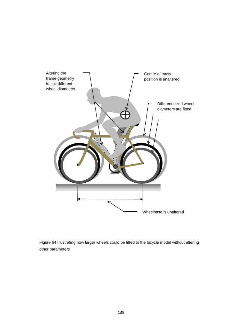
Different sized wheel diameters are fitted
Altering the frame geometry to suit different wheel diameters
Centre of mass position is unaltered
Wheelbase is unaltered
Figure 64 Illustrating how larger wheels could be fitted to the bicycle model without altering
other parameters
139

time
amplitude
Area under the graph
A = 1.0 unit
Figure 65 The unit impulse function
140

5.4.1. WHEEL DIAMETER
To undertake this sensitivity study, multiple Simulink trials for all eleven bicycle parameters were
needed. But for reasons of brevity the methodology used will be described for one parameter only,
wheel diameter. The remaining ten parameters were studied in the same way and the full results
for all parameters are presented in this Chapter.
When considering the wheel diameter first we must refer to the internationally accepted standard
wheel and tyre system for road bicycles, designated as ISO 700C (6). The 700C designation
means that the nominal wheel diameter is 700 mm (though the actual diameter is smaller than
this). The benchmark bicycle uses an ISO 700C x 25 wheel and tyre where 25 refers to the tyre
width (in this case of 25 mm). The 700C x 25 wheel was found by direct measurement to have an
actual outside diameter of 675 mm, but small variations in diameters for between different tyres
and different manufacturers do occur. Two manufacturers did record slightly different diameter
values for a 700 C x 25 tyre (one slightly higher and the other lower) but when averaged out they
are consistent with the experimentally measured value of 675 mm shown in Table 26.
Now that the actual benchmark wheel diameter has been determined it is possible to vary
diameters and record the different settling times that the Simulink model calculates. A series of
unit impulse responses was found for a range of diameters from 697.5 mm (90% of the
benchmark) up to 742.5 mm (110%).
Simulink was used find the front wheel yaw response (and its sensitivity) to an impulse by using
Simulink’s linear analysis capability, which calculates and plots the unit impulse response and
finds the 2% (or other selected value) settling time. The linear analysis capability computes a linear
system from the non-linear Simulink bicycle model and plots a linear unit impulse response
between the specified input and output points.
The 2% settling time was calculated and recorded for each change in diameter and these are
shown in Table 27. The impulse response for the benchmark wheel (675 mm diameter) produced
a 2% settling time of 10.1 seconds which is shown in Figure 66. The different diameters were
referenced to the benchmark and the change in settling time across the range of diameters was
plotted on a graph, see Figure 67. A line of best fit for the data points was plotted and its slope is
an indication of model’s sensitivity to the parameter and is expressed as the % response change
per 1% change of the parameter, making the analysis non-dimensional. For each 1% increase in
wheel diameter it was found that the settling time increased on average by 5.75% (across a +/-
10% range with a R2 value of 0.936) making this a significant parameter. This high sensitivity of
the bicycle to changes in wheel diameter is an unexpected and interesting result.
141

Table 26 Typical road bicycle tyre values (64, 81)
ISO/ETRTO Code
Tyre width mm
D
Actual wheel
diameter mm 1
D/DBM 2
700 X 18C 18 658.90 0.976
700 X 19C 19 662.09 0.981
700 X 20C 20 666.22 0.987
700 X 23C 23 671.79 0.995
700 X 25C 25 674.82 3 1.000
700 X 28C 28 682.14 1.011
700 X 30C 30 685.32 1.015
700 X 32C 32 688.35 1.020
700 X 35C 35 692.80 1.026
700 X 37C 37 700.28 1.037
700 X 38C 38 693.92 1.028
700 X 40C 40 703.47 1.042
ETRTO (European Tyre and Rim Technical Organisation)
Note 1 these are the averaged results from two manufacturers see Appendix E (64, 81)
Note 2 DBM = benchmark diameter
Note 3 rounded up to 675.00 mm in this study
142

Figure 66 The front wheel yaw response (for the benchmark bicycle) to a unit impulse found
using Simulink’s linear analysis capability
Peak response value set at 100%
2% settling time (=10.1 sec)
Front wheel yaw response
143

Table 27 Wheel diameter settling times, used to plot Figure 67
Wheel diameter %
D Wheel dia. mm
S 2% settling time seconds
S/SBM 1
90 607.5 6.58 0.65
91 614.3 6.83 0.68
92 621.0 7.09 0.70
93 627.8 7.37 0.73
94 634.5 7.67 0.76
95 641.3 7.99 0.79
96 648.0 8.34 0.83
97 654.8 8.72 0.86
98 661.5 9.12 0.90
99 668.3 9.57 0.95
1002 675.0 10.10 1.00
101 681.8 10.60 1.05
102 688.5 11.20 1.11
103 695.3 11.80 1.17
104 702.0 12.50 1.24
105 708.8 13.30 1.32
106 715.5 14.20 1.41
107 722.3 15.20 1.50
108 729.0 16.30 1.61
109 735.8 17.60 1.74
110 742.5 19.10 1.89
Note 1 S/SBM = 2% settling time/2% settling time of benchmark wheel
Note 2 benchmark wheel diameter (675 mm = 100%)
144
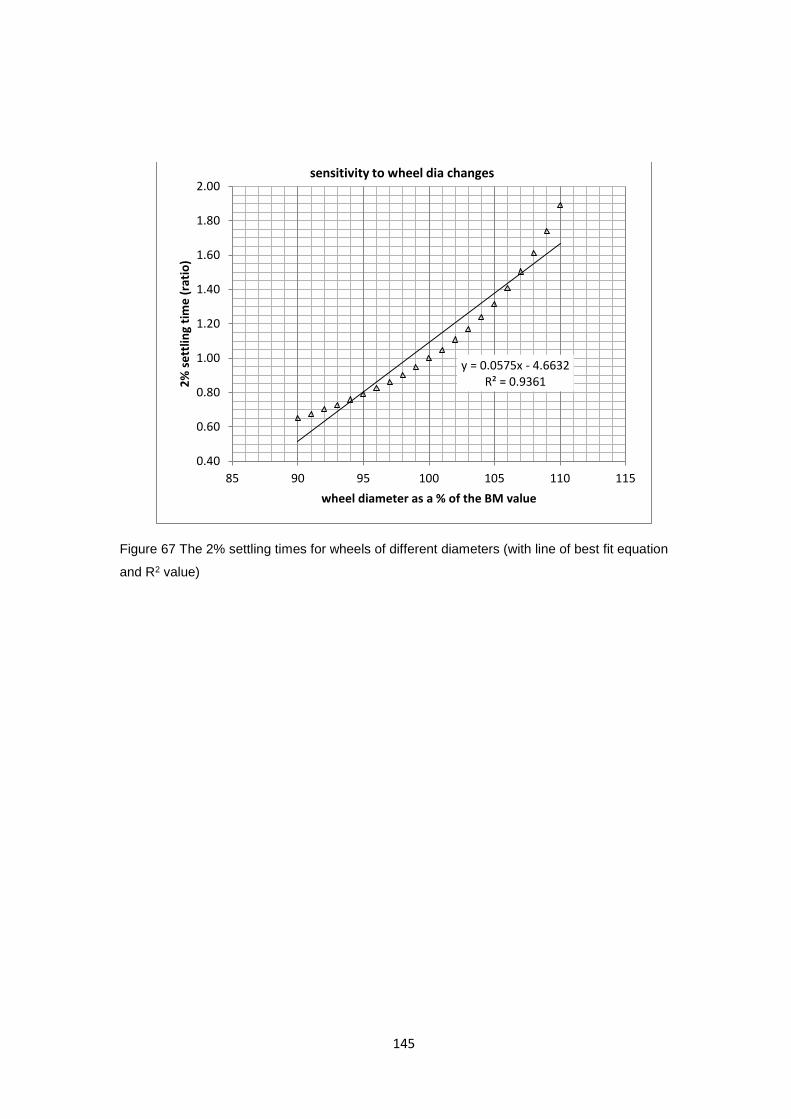
Figure 67 The 2% settling times for wheels of different diameters (with line of best fit equation
and R2 value)
y = 0.0575x - 4.6632R² = 0.9361
0.40
0.60
0.80
1.00
1.20
1.40
1.60
1.80
2.00
85 90 95 100 105 110 115
2% se
ttlin
g tim
e (r
atio
)
wheel diameter as a % of the BM value
sensitivity to wheel dia changes
145
5.4.2. REMAINING PARAMETERS
This section now presents the full results of the sensitivity study for all eleven parameters. After
the wheel diameter sensitivity was determined all the remaining ten parameters were analysed in
the same way and full results are shown in Table 28 and Figure 67 through to Figure 77.
Figure 77From these results several critical design parameters were identified and their effects
quantified. The parameters have also been collated into four groups:
1. Steering geometry parameters
2. Wheel parameters
3. Mass and wheelbase parameters
4. All others
Steering geometry parameters
As expected and reported by many other researchers the parameters defining the steering
geometry are important (head tube angle and rake) and the study of their effects was a major goal
of this investigation (2, 13, 32, 55). It was found that:
• For a 1% increase in head tube angle (Φ) the front wheel yaw 2% settling time decreased
by a significant 5.93% (across a -2% to + 10% range with a determination coefficient R2
value of 0.830) see Figure 68.
• Similarly for a 1% increase in rake (β) it was found that the settling time decreased by a
moderately significant 1.41% (across a +/- 10% range with a R2 value of 0.996) see Figure
73.
• This is perhaps an unexpectedly small value for rake but when the steering geometry
equations are inspected more closely the reason is immediately apparent. A 10% change
in head tube angle causes the effective trail to change by about 75% whereas a 10%
change in rake only changes the effective trail by 8%.
• As the effective trail (which is a function of wheel radius, head tube angle and rake)
appears in four of the twenty three torque terms of the equations of motion it is no surprise
the model is highly sensitive to changes in trail and the single parameter (head tube angle)
that most affects it.
Wheel properties parameters
• As just determined the wheel diameter is a significant parameter, see Figure 67. A 1%
increase in wheel diameter increased the settling time by a significant 5.75% (for a -10%
to + 10% range and a R2 of 0.936)
• A 1% increase in the wheel moment of inertia decreased the settling time by a moderately
significant 2.02% (for a -10% to + 10% range and a R2 of 0.982) see Figure 70.
146

• Because of the symmetry of the wheels it was unnecessary to isolate the moments of
inertia about X, Y and Z axes (and it is not physically or theoretically possible to do so).
So all three moments of inertia are linked and vary together (IWX + IWZ = IWY, due to the
parallel axis theorem).
Mass position and wheelbase parameters
An interesting result is the obvious interaction of the parameters defining the magnitude and
position of the mass (M, b and h) and a fourth parameter defining the wheelbase (L).
• For a 1% increase in the longitudinal position “b” of the mass the 2% settling time
increased by a moderately significant 2.07% (for a -10% to + 10% range and a R2 of
0.995) see Figure 69
• A 1% increase in the magnitude of the mass the 2% settling time increased by a
moderately significant 1.98% (for a -10% to + 10% range with a R2 of 0.994) see Figure
71
• A 1% increase in the wheelbase “L” the 2% settling time decreased by 1.57% (for a -10%
to + 10% range with a R2 of 0.986) which is moderately significant, see Figure 72
• Surprisingly a 1% increase in the height of the mass “h” the 2% settling time only increased
by 0.27% (for a -10% to + 10% range with a R2 of 0.983) which is not significant, see
Figure 74
• The interaction between these parameters opens the possibility of tuning a rider’s position
to optimise handling performance. For example, reducing a downhill mountain bicycle’s
settling time could be achieved by reducing the mass and moving it lower and to the rear
and increasing the wheelbase.
• Note that the secondary parameters of frame size and seat tube angle can be linked to
the parameters h, b and L, see Appendix B.
Finally considering the remaining three parameters (all others)
• For a 1% increase in the IXB parameter the 2% settling time decreased by a not significant
0.11% (for a -10% to + 10% range and a R2 of 0.857) see Figure 75
• For a 1% increase in the IZA parameter the 2% settling time increased by a not significant
0.10% (for a -10% to + 10% range and a R2 of 0.857) see Figure 76
• Finally for a 1% increase in the IXA parameter the 2% settling time increased by a not
significant 0.06% (for a -10% to + 10% range and a R2 of 0.668) see Figure 77
Full details of each parameter’s significance and the sensitivity of the bicycle model to any
changes is shown in Table 28 where they are ranked in order of significance.
For some parameters, stepping is evident in the graphs which occurs when several settling times
apparently share the same value and then suddenly steps up to another value (see IXA, IXB, IZA
147

and h). This occurred because the Simulink analysis “only” gave settling time results within an
accuracy of 1/100ths of a second and it was not possible to obtain a more precise result when the
values were very low, as they were in these 4 cases. But as these are insignificant parameters it
doesn’t affect the validity of the study.
The only significant parameter which exhibits strong nonlinearity was the head tube angle (with
an R2 = 0.830) and this is why its limits were set at between -2% to +10% which corresponded to
the most linear part of its response. Three other insignificant parameters (IXA, IXB, and IZA) also had
low R2 values recording 0.668, 0.857 and 0.857 respectively, but this is not of great interest.
148

Table 28 Sensitivity results
Ranking Symbol Definition Benchmark Value/s
Units C1 C/CHTA 2 R2 Value 3
Comments 4
1. Φ Head tube angle 73 degrees -5.93% 1.0000 0.830 significant term
2. D Diameter of the wheel 0.675 m +5.75% 0.9696 0.936 significant term
3. b Horizontal distance from rear wheel hub to centre of mass
0.33 m +2.07% 0.3491 0.955 moderately significant
4. IW 5 MOI of wheels 0.05/010 kgm2 -2.02% 0.3406 0.982 moderately significant
5. M Mass 80 kg +1.98% 0.3339 0.994 moderately significant
6. L Wheelbase 1 m -1.57% 0.2648 0.986 moderately significant
7. β Rake 0.045 m -1.41% 0.2378 0.996 moderately significant
8. h Height of centre of mass 1.1 m +0.27% 0.0455 0.995 not significant
9. IXB MOI of B about X axis (roll) 100 kgm2 -0.11% 0.0185 0.857 not significant
10. IZA MOI of A about Z axis (yaw) 0.08 kgm2 +0.10% 0.0169 0.857 not significant
11. IXA MOI of A about X axis (roll) 0.2 kgm2 0.06% 0.0100 0.668 not significant
The parameters are ranked in order of greatest sensitivity
Note 1 C is the % change in the 2% settling time for each 1% increase of a parameter
Note 2 C/CHTA is C referenced to the head tube angle parameter (absolute values)
Note 3 R2 is the coefficient of determination, a measure of the strength of the linear relationship between two variables
Note 4 significant is defined as a change in C greater than 3%, moderately significant means a change between 1 and 3% and not significant means less
than a 1% change
Note 5 due to symmetry, the wheel MOI have the following relationships, IX = IZ and IY = 2IX = 2IZ, therefore the wheels’ MOI has been included once
and not three times
149

Figure 68 Settling time results for different head tube angles (with line of best fit equation, R2
value)
Figure 69 Settling time results for different distances “b”
y = -0.0592x + 6.9511R² = 0.8298
0.40
0.60
0.80
1.00
1.20
1.40
1.60
1.80
2.00
85 90 95 100 105 110 115
2% se
ttlin
g tim
e (r
atio
)
HTA as a % of the BM value
sensitivity to HTA changes
y = 0.0207x - 1.0657R² = 0.9950
0.40
0.60
0.80
1.00
1.20
1.40
1.60
1.80
2.00
85 90 95 100 105 110 115
2% se
ttlin
g tim
e (r
atio
)
distance b as a % of the BM value
sensitivity to distance "b" changes
150

Figure 70 Settling time results for different moments of inertia for the wheels
Figure 71 Settling time results for different masses
y = -0.0202x + 3.0355R² = 0.9819
0.40
0.60
0.80
1.00
1.20
1.40
1.60
1.80
2.00
85 90 95 100 105 110 115
2% se
ttlin
g tim
e (r
atio
)
Wheel MOI as a % of the BM value
sensitivity to Wheel "IW" changes
y = 0.0198x - 0.9686R² = 0.9936
0.40
0.60
0.80
1.00
1.20
1.40
1.60
1.80
2.00
85 90 95 100 105 110 115
2% se
ttlin
g tim
e (r
atio
)
Mass as a % of the BM value
sensitivity to Mass "m" changes
151

Figure 72 Settling time results for different wheelbases
Figure 73 Settling time results for different rakes
y = -0.0157x + 2.5726R² = 0.9860
0.40
0.60
0.80
1.00
1.20
1.40
1.60
1.80
2.00
85 90 95 100 105 110 115
2% se
ttlin
g tim
e (r
atio
)
Wheelbase L as a % of the BM value
sensitivity to Wheelbase "L" changes
y = -0.0141x + 2.4123R² = 0.9961
0.40
0.60
0.80
1.00
1.20
1.40
1.60
1.80
2.00
85 90 95 100 105 110 115
2% se
ttlin
g tim
e (r
atio
)
Rake as a % of the BM value
sensitivity to Rake "Δ"changes
152

Figure 74 Settling time results for different distances “h” (note the stepping)
Figure 75 Settling time results for different moments of inertia of B about the X axis (note
stepping)
y = 0.0027x + 0.7254R² = 0.9829
0.95
0.96
0.97
0.98
0.99
1.00
1.01
1.02
1.03
85 90 95 100 105 110 115
2% se
ttlin
g tim
e (r
atio
)
height as a % of the BM value
sensitivity to Height "h" changes
y = -0.0011x + 1.1025R² = 0.8567
0.95
0.96
0.97
0.98
0.99
1.00
1.01
1.02
1.03
85 90 95 100 105 110 115
2% se
ttlin
g tim
e (r
atio
)
MOI XB as a % of the BM value
sensitivity to "IXB"changes
153

Figure 76 Settling time results for different moments of inertia of A about the Z axis (note
stepping)
Figure 77 Settling time results for different moments of inertia of A about the X axis (note
stepping)
y = 0.0010x + 0.8911R² = 0.8573
0.95
0.96
0.97
0.98
0.99
1.00
1.01
1.02
1.03
85 90 95 100 105 110 115
2% se
ttlin
g tim
e (r
atio
)
MOI ZA as a % of the BM value
sensitivity to "IZA"changes
y = 0.0006x + 0.9337R² = 0.6682
0.95
0.96
0.97
0.98
0.99
1.00
1.01
1.02
1.03
85 90 95 100 105 110 115
2% se
ttlin
g tim
e (r
atio
)
MOI XA as a % of the BM value
sensitivity to "IXA"changes
154
5.4.3. SENSITIVITY REMARKS
This sensitivity study has quantified the effects of all eleven parameters and classified them as
either significant, moderately significant or not significant and this quantification and classification
is shown in Table 28. Significant parameters are defined as having a value of C of 3% or more (C
is the % change in settling time for each 1% change in the parameter). Moderately significant
parameters have a C of between 1% and 3%, and insignificant parameters have a C of less than
1%.
From this sensitivity study the significant parameters in order of most importance are:
1. Head tube angle
2. Wheel diameter
The moderately significant parameters are:
3. Mass horizontal distance from rear wheel hub “b”
4. Wheel moment of inertia
5. Mass
6. Wheelbase
7. Rake
And the other parameters that are not significant are:
8. Height of mass “h”
9. Moment of inertia of B about X (roll)
10. Moment of inertia of A about Z (yaw)
11. Moment of inertia of A about X (roll)
What this physically means is illustrated by the case of an existing bicycle with a handling
problem. In such a case only a few options are practical, as all the design parameters are fixed
except for those affected by wheel, tyre and front fork properties. So if new tyres are fitted it is
possible to change the wheel diameter and perhaps wheel moments of inertia. If new wheels of
a different construction are fitted this can affect the wheel’s moments of inertia. Finally if a new
fork is fitted (a more expensive solution but possibly worth considering) it can change the rake
value. So the wheel diameter, moments of inertia and possibly fork rake are the only possibilities
to adjust. Small adjustments to the rider’s position (changing h and b) are also possible but they
will be too small to have any significant effect. Therefore the following broad recommendations
can be made to deal with a bicycle handling problem (first assuming that the bicycle is in good
mechanical order).
If a bicycle has been found to have sluggish steering (with a slow settling time) then:
1. it would be worth trying a slightly smaller tyre to decrease the diameter
2. alternatively increasing the wheel moments of inertia will help
155

But doing both at once though may cancel each other out, So careful wheel and tyre selection is
necessary in order to have an positive combined effect.
3. for example a sufficiently smaller diameter tyre and a new wheel with a heavier rim could
reduce settling times, as wheel MOI’s vary by at least +/- 10% and typical road bicycle
tyre diameters by +/- 12% this is possibly an effective solution, see Chapter Six for details
on how this can be systematically done using the Design Charts
4. a more radical (and expensive) solution would be to fit a new fork with less rake which
increases trail, e.g.changing from a 40 mm to a 45 mm rake (a increase of 12.5%) reduces
settling time by nearly 18%
Conversly if there is too quick a steering response and we wish to increase the settling times, the
advice is reversed, that is add a larger diameter tyre with a lighter rim wheel and decrease the
fork rake.
Completing this sensitivity study allows a scientifically based design methodology to be developed
and this will be presented in the Chapter Six and this will make it possible to guide design
decisions for new bicycles. It will give designers a practical means to determine what effect design
changes have on bicycle handling.
This study can also be used to make practical suggestions on how to troubleshoot and cure
steering problems with existing bicycles. Individual bicycles and riders can be experimentally
measured to find actual values of mass, wheelbase, moments of inertia, etc. Then the Simulink™
model could be used to investigate the stability or instability of each particular case and small
changes in key individual parameters may give insights on how to cure an existing problem.
For completeness in this sensitivity study the characteristic equation of the bicycle system was
determined and the Routh Stability Criterion then used to find out if any unstable roots exist.
Details of this procedure and the results are shown in Appendix D and they give the range of
stability for the current system.
5.5. REMARKS
This chapter has examined the bicycle dynamic model and investigated:
1. the effectiveness of the model in determining bicycle performance
2. the significance of each torque term in the equations of motion
3. the sensitivity of the bicycle’s performance to changes in design parameter
From this work it was found that:
1. Bicycle performance simulations demonstrated the capabilities of the model which was able
to reproduce realistic bicycle dynamic behaviour.
2. Torque term evaluation determined the significant and insignificant terms and
recommendations about simplifications of the equations of motion were made.
156

3. The sensitivity study identified the critical design parameters and quantified their effects on
bicycle handling performance. It determined their minimum and maximum acceptable limits
and examined their relative importance in terms of their overall effects. These results will later
be used in Chapter Six to develop practical design charts for designers.
Now it remains to use the results of this Chapter, particularly the sensitivity study to develop a
suitable design methodology for bicycles and the next Chapter continues this work.
157
6. BICYCLE DESIGN METHODOLOGY
6.1. INTRODUCTION
One objective of this investigation was to develop a suitable design methodology that
manufacturers and designers could use to guide their bicycle design decisions. The current lack
of a suitable methodology means that most manufacturers rely heavily on empirical rules of
thumb, a practice which may stifle development. “Because bicycle design has been based on
tinkering rather than equations, there has been little scrutiny of bicycle analyses (14).”
Design methodologies are common in engineering and can be in the form of: criteria, tables,
equations and charts, all of which can be used when designing products. All these methodologies
consider critical design parameters and prescribe ways of adjusting them within acceptable limits.
A variety of methodologies will be examined in this Chapter to consider their suitability for
designing road bicycles. These methodologies will be based on the sensitivity study from Chapter
Five which identified critical design parameters. These methodologies will be discussed,
evaluated and then a recommendation will be made as to the best approach.
As demonstrated in Chapter Five, bicycles are highly sensitive to changes in: the head tube angle,
fork rake and the wheel diameter. Also significant is the wheel moment of inertia about the axis
of rotation. The mass and its longitudinal position are moderately important but the mass height
is less so. Designers need to consider these parameters when designing and comparing new
designs and need to try to optimise their values for particular applications.
6.2. CURRENT APPROACHES
Most designers currently use a combination of experience and empirical evidence to design new
bicycles. But the literature does have some suggestions as to how to approach this issue, mostly
of a highly theoretical nature.
Meijaard et al obtained eigenvalues from their modelling which they say can be used to check
alternative designs and which indicate critical speeds for three modes of instability (front wheel
wobble, rear end wobble and capsize). In our view the level of mathematical understanding
required would limit how useful most designers would find this approach.
Ringwood et al devised some design guidelines to indicate when an unstable condition is being
approached particularly with regard to a front wheel high speed wobble (61). They suggested that
stability decreased when any one of the following occurred: the bicycle frame got larger, the centre
of mass moved to the rear, the centre of mass moved higher and the velocity increased. Their
suggestion that stability decreased as velocity increased contradicts many popular observations
but it is important to remember that the instability they investigated was a high speed front wheel
wobble, so this may be a valid proposition. However the lack of an easy way to convert their work
onto recommendations about appropriate parameter values means their approach is incomplete
as a practical design tool.
158

Seffen et al proposed a bicycle rideability index which was used to quantify the effect of changing
the front wheel parameters of trail, moment of inertia and head tube angle on controllability (28).
Their index was plotted against velocity for different parameter values and compared with a
benchmark bicycle to quantify how easy it would be to ride a specific bicycle. They found that for
a given speed, as trail increases, rideability improved up to an optimum value and then
deteriorated. Importantly they found that no single value of trail gave optimum rideability across
all speeds. They also concluded that rideability improved as speed increased which contrasts
with Ringwood. Their rideability index has no simple physical meaning as it is the square root of
the ratio of the maximum and minimum singularity values of a complex matrix derived from the
equations of motion. While their rideability index was useful from a theoretical engineering point
of view, this measure of bicycle stability would not be a helpful aid for designers seeking to
understand their designs or wishing to describe the attributes of their products to customers. The
difficulty of explaining the mathematical concepts behind the rideability index and relating the
index to observable physical effects limits its usefulness as a design tool.
Jones is a much cited author in this field which is remarkable given the length of time since his
article was written and its brevity (2). His practical experiments have obviously captured people’s
attention in a way that a purely mathematical treatment would have failed to do. He proposed a
steering stability parameter, based on the drop in height of the front wheel hub, the steering angle
and the roll angle. Wilson’s second edition of his text “Bicycling Science Ergonomics and
Mechanics” describes in detail Jones’ paper and calls his stability parameter, the Jones stability
criterion or “u” (2, 10). He continues with a discussion about common steering geometries for a
variety of bicycles and calculates “u” values for them. The third edition of this text discusses
stability theories in more detail and contains good descriptions of: inverted pendulums, Jones’
experiments, counter-steering and the work of Papadopoulos et al (52). The Jones stability
criterion is commented on as follows, “to sum up, Jones’ experiments were very revealing, but his
premise was faulty. Nonetheless “u” can be recognized as a very important stability quantity
among bicycles with two wheels of the same size (52).” Confusingly it then says the Jones stability
criterion formula given in the second edition is wrong, but does not provide a clear correction (10).
Despite this, some frame builders continue to find the ”u” equation from Wilson’s second edition
useful. BikeCAD (a computer aided bicycle design programme) continues to calculate values for
the Jones stability criterion despite the possible formula errors “some users of BikeCAD Pro have
requested that it be left in as they have already developed a sense of what Jones stability values
work for them.” (89). This statement shows the real need for some practical and scientific way of
determining stability and quantifying handling performance.
159

6.3. ALTERNATIVE DESIGN METHODOLOGIES
Several design methodologies are now considered and evaluated to determine their suitability for
practical use. All these methodologies consider critical design parameters and describe ways of
adjusting them and setting acceptable limits using practical and straightforward methods. The
following alternative design methodologies were evaluated as to their suitability:
1. Design Criteria
2. Design Tables
3. Design Equation
4. Design Charts
The final recommendation as to a preferred method is made later in this Chapter and is based on
a number of practical factors, as each method has different advantages and disadvantages. Each
alternative method is a stand-alone technique that could be used together with or independently
of the others.
6.3.1. DESIGN CRITERIA
The first alternative we considered was a Design Criteria methodology, which is a method
intended to provide designers with a summary of the empirical knowledge including acceptable
values and limits for key design parameters. A designer would consult a series of Design Criteria
and systematically adjust the key parameters until it was judged that an acceptable solution had
been reached. The final judgement would be based on past experience and the degree of
willingness to push close to or beyond any boundaries.
The sensitivity study identified several key parameters which have significant effects on bicycle
handling (e.g. head tube angle, rake, wheel diameter, wheel polar moment of inertia, wheelbase,
mass and the mass position). The Design Criteria rules for setting values for these parameters
were made after examining the database of Tour de France (TdF) road bicycles described in
Appendix F. Where possible parameter recommendations are based on the equations for lines of
best fit from the plotted values of these bicycles. The resulting Design Criteria methodology is
shown in Table 29 and follows the procedural steps outlined in Table 30.
The advantages of the Design Criteria approach include:
• it codifies current knowledge and experience so that it can be retained and passed on
• it can be adapted and changed to reflect empirical improvements
• it is simple to follow and easy to explain
• it is conservative, safe and unlikely to result in poor designs
160

However its disadvantages are:
• it makes no allowance for the interaction of several parameters, a major limitation
• it has no scientific or mathematical rationale beyond line fitting equations from the TdF
bicycle database
• it is silent on what happens if a design strays beyond the maximum or minimum limits
• it can’t indicate likely or worthwhile areas for design innovation
• it is by nature conservative so it must follow design trends rather that assist in innovation,
therefore it may inhibit improvements and advances in design
161
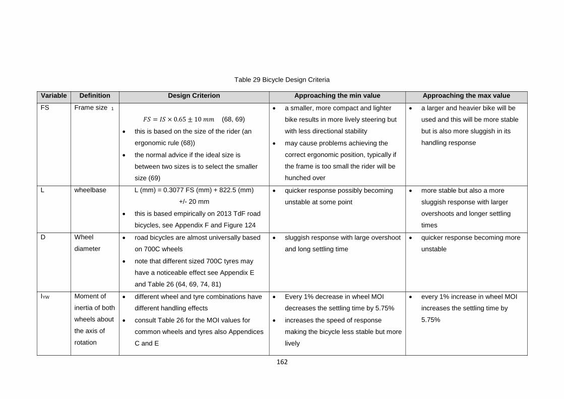
Table 29 Bicycle Design Criteria
Variable Definition Design Criterion Approaching the min value Approaching the max value
FS Frame size 1
𝐹𝐹𝑆𝑆 = 𝐼𝐼𝑆𝑆 × 0.65 ± 10 𝑚𝑚𝑚𝑚 (68, 69)
• this is based on the size of the rider (an
ergonomic rule (68))
• the normal advice if the ideal size is
between two sizes is to select the smaller
size (69)
• a smaller, more compact and lighter
bike results in more lively steering but
with less directional stability
• may cause problems achieving the
correct ergonomic position, typically if
the frame is too small the rider will be
hunched over
• a larger and heavier bike will be
used and this will be more stable
but is also more sluggish in its
handling response
L wheelbase L (mm) = 0.3077 FS (mm) + 822.5 (mm)
+/- 20 mm
• this is based empirically on 2013 TdF road
bicycles, see Appendix F and Figure 124
• quicker response possibly becoming
unstable at some point
• more stable but also a more
sluggish response with larger
overshoots and longer settling
times
D Wheel
diameter • road bicycles are almost universally based
on 700C wheels
• note that different sized 700C tyres may
have a noticeable effect see Appendix E
and Table 26 (64, 69, 74, 81)
• sluggish response with large overshoot
and long settling time
• quicker response becoming more
unstable
IYW Moment of
inertia of both
wheels about
the axis of
rotation
• different wheel and tyre combinations have
different handling effects
• consult Table 26 for the MOI values for
common wheels and tyres also Appendices
C and E
• Every 1% decrease in wheel MOI
decreases the settling time by 5.75%
• increases the speed of response
making the bicycle less stable but more
lively
• every 1% increase in wheel MOI
increases the settling time by
5.75%
162

• the wheel’s MOI can be determined by a
compound pendulum experiment
• at some point instability will occur • reduces the speed of response
making the bicycle more stable
but less lively
Delta
Δ
Trail Δ (mm) = - 0.035 FS (mm) + 76.3 (mm)
+/- 10 mm
• based on Appendix F, see Figure 126
• quicker response becoming possibly
unstable at some point
• more stable but also more
sluggish response with larger
overshoots and longer settling
times
Beta
β
Fork rake (or
offset)
β (mm) = 45.3 mm +/- 3.5 mm
min 40.0 mm max 53.0 mm
• based on Appendix F and Table 72
• sluggish response with larger
overshoots and a longer settling time
• quicker response but becoming
more unstable
Phi
Φ
Head tube
angle
Φ (o) = 0.074 FS (mm) + 68.8o
+/- 1.5o
• based on Appendix F and Figure 125
• sluggish response with larger
overshoots and a longer settling time
• quicker response but becoming
more unstable
STA Seat tube
angle 2
STA (o) = 73.3o +/- 1.1o,
min 69.2o mm max 75.5o
• based on Appendix F see Table 72
• sluggish response with large overshoot
and long settling time
• quicker response but becoming
more unstable
Note 1 Frame size (FS) is explained in Chapter Four
Note 2 Seat tube angle (STA) is explained in Chapter Four
163
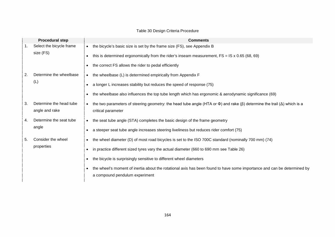
Table 30 Design Criteria Procedure
Procedural step Comments 1. Select the bicycle frame
size (FS) • the bicycle’s basic size is set by the frame size (FS), see Appendix B
• this is determined ergonomically from the rider’s inseam measurement, FS = IS x 0.65 (68, 69)
• the correct FS allows the rider to pedal efficiently
2. Determine the wheelbase
(L) • the wheelbase (L) is determined empirically from Appendix F
• a longer L increases stability but reduces the speed of response (75)
• the wheelbase also influences the top tube length which has ergonomic & aerodynamic significance (69)
3. Determine the head tube
angle and rake • the two parameters of steering geometry: the head tube angle (HTA or Φ) and rake (β) determine the trail (Δ) which is a
critical parameter
4. Determine the seat tube
angle • the seat tube angle (STA) completes the basic design of the frame geometry
• a steeper seat tube angle increases steering liveliness but reduces rider comfort (75)
5. Consider the wheel
properties
• the wheel diameter (D) of most road bicycles is set to the ISO 700C standard (nominally 700 mm) (74)
• in practice different sized tyres vary the actual diameter (660 to 690 mm see Table 26)
• the bicycle is surprisingly sensitive to different wheel diameters
• the wheel’s moment of inertia about the rotational axis has been found to have some importance and can be determined by
a compound pendulum experiment
164
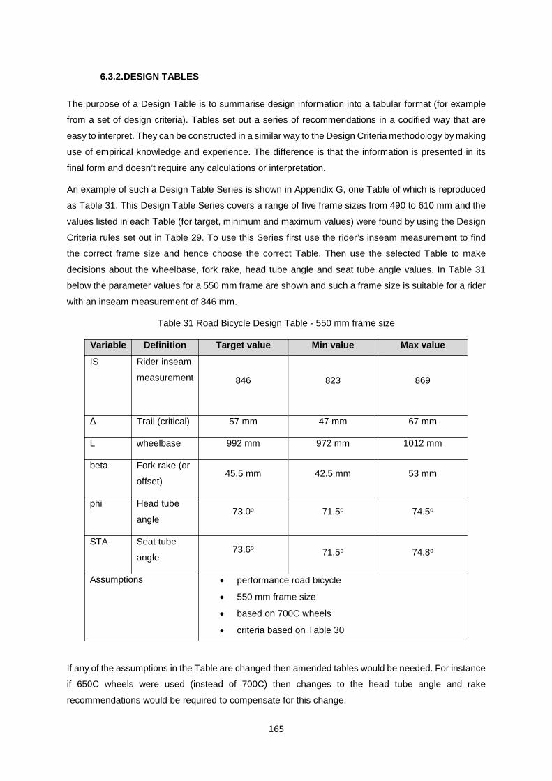
6.3.2. DESIGN TABLES
The purpose of a Design Table is to summarise design information into a tabular format (for example
from a set of design criteria). Tables set out a series of recommendations in a codified way that are
easy to interpret. They can be constructed in a similar way to the Design Criteria methodology by making
use of empirical knowledge and experience. The difference is that the information is presented in its
final form and doesn’t require any calculations or interpretation.
An example of such a Design Table Series is shown in Appendix G, one Table of which is reproduced
as Table 31. This Design Table Series covers a range of five frame sizes from 490 to 610 mm and the
values listed in each Table (for target, minimum and maximum values) were found by using the Design
Criteria rules set out in Table 29. To use this Series first use the rider’s inseam measurement to find
the correct frame size and hence choose the correct Table. Then use the selected Table to make
decisions about the wheelbase, fork rake, head tube angle and seat tube angle values. In Table 31
below the parameter values for a 550 mm frame are shown and such a frame size is suitable for a rider
with an inseam measurement of 846 mm.
Table 31 Road Bicycle Design Table - 550 mm frame size
Variable Definition Target value Min value Max value
IS Rider inseam
measurement
846 823 869
Δ Trail (critical) 57 mm 47 mm 67 mm
L wheelbase 992 mm 972 mm 1012 mm
beta Fork rake (or
offset) 45.5 mm 42.5 mm 53 mm
phi Head tube
angle 73.0o 71.5o 74.5o
STA Seat tube
angle 73.6o 71.5o 74.8o
Assumptions • performance road bicycle
• 550 mm frame size
• based on 700C wheels
• criteria based on Table 30
If any of the assumptions in the Table are changed then amended tables would be needed. For instance
if 650C wheels were used (instead of 700C) then changes to the head tube angle and rake
recommendations would be required to compensate for this change.
165

The advantages of using Design Tables include:
• they require minimal calculations as the target, minimum and maximum values are all given to
the user
• all the information for each parameter is listed so they are very clear and easy to use
The disadvantages are:
• just like the Design Criteria method they makes no allowance for the interaction of parameters
which is a major limitation
• they offers no guidance as to the likely effect on handling if certain limits are reached or
exceeded
Apart from these points they share all the advantages and disadvantages of the Design Criteria method
that have been mentioned.
6.3.3. DESIGN EQUATIONS
An attempt was made to develop a closed form equation for quantifying handling performance but it
was unhelpful. The equation was based on the results of the sensitivity study but after evaluation it was
decided that this approach was unsuitable. A brief description is included for completeness in Appendix
G.
6.4. DESIGN CHARTS
Design charts are commonly used by engineers and plot important parameters and indicate
performance in some manner. For example a Pump Selection Design Chart plots pump head against
flow rate and is used to select the best pump for a specific application. Once a pump selection has been
made, the correct impellor size, power requirements, efficiencies and other parameters can be read
directly from the Design Chart and its associated charts. Design Charts are constructed by first selecting
the most appropriate parameters to combine on two (or more) axes and often include lines of constant
parameter value drawn across them (e.g. lines of constant pump efficiency).
After considering all the other proposed design methodologies it was decided to develop and
recommend the Design Chart concept because of its clear advantages (i.e. ease of use, ability to
consider multiple parameters and scientific basis). The advantages and disadvantages of Design
Charts are listed below.
Their advantages include:
• they are scientifically based and justified
• they are relatively easy to use with the minimum of calculations required
• they enable a wide audience to understand the design process and its outcomes
• they allow several parameters can be concurrently considered, so interactions can be studied
166
• a wider range of design decisions can be contemplated at once
• scientifically based iso-handling lines can be plotted on the chart to indicate handling
performance
• the effect of moving a design in a particular direction on the chart is clearly shown i.e. it becomes
more or less stable
• it may be possible to develop 3-D or contour style Design Charts, allowing even more
parameters to be concurrently assessed
While their disadvantages include:
• assumptions have to be clearly known and adhered to
• design boundaries may be hard to define and so unsafe designs may be produced (so the
design charts are not necessarily conservative)
The use of Design Charts for bicycles will allow a wide range of people to participate in and understand
the design process and its outcomes as these Charts can be easily interpreted and can provide
quantifiable evaluation of individual bicycles such as a settling time value. Individual bicycles design
specifications can be plotted onto the Charts and this can provide riders with an easy way to compare
new designs to bicycles they are already familiar with. Bicycles close to boundaries or limits on the
charts are inevitably in grey areas and further methods are needed to determine exactly where the
boundaries are. The Charts will allow designers to understand and quantify in meaningful ways any
design changes they are considering and they need not be used in conjunction with any of the other
methodologies discussed (that is criteria or tables or equations).
To produce relevant Design Charts, it was first necessary to examine the sensitivity study to see which
parameters are the most important and also to consider which ones the cycling fraternity consider to be
significant. From the results of the sensitivity study we can see in Table 32 that key parameters can be
logically grouped together in terms of their interaction and overall significance (see also Table 28).
The first group are the terms that define the steering geometry, that is the head tube angle and rake
(the head tube angle is commonly known to be highly significant). These two terms give the important
third term trail (again considered highly significant by manufacturers) from a simple geometrical
relationship. The second group concern the wheel diameter and wheel moments of inertia which the
sensitivity study show to be important. The third group relates to the important area of frame geometry
and considers the vertical and longitudinal position of the mass (h and b) and the wheelbase. These
terms can be used to indirectly define the seat tube angle which is held to be a very significant term by
the bicycle fraternity (73). The last group covers the related terms of mass and the moment of inertia of
the rear assembly B. These two parameters have the least significance of the terms we are considering.
This leaves two remaining parameters out of the original eleven, the two moments of inertia for the front
assembly A (about the yaw and roll axes) which have been shown to be insignificant and therefore are
not incorporated into a Chart.
167

In summary the four proposed Design Charts cover the design areas of:
1. Steering geometry (head tube angle, rake and trail)
2. Wheel properties (wheel diameter and moment of inertia)
3. Frame geometry (vertical and longitudinal position of the mass, wheelbase and seat tube angle)
4. Mass and roll inertia (mass and moment of inertia of B)
These four Design Charts are ranked above (from 1 to 4) according to their parameter sensitivity (as
per Table 32) and they can be used together or independently as appropriate to the circumstances. But
in the case of a new bicycle design probably the first two (steering geometry and wheel properties)
would initially be heavily scrutinised. Followed by consideration of the frame geometry and mass and
roll inertia Charts.
168

Table 32 Design Chart parameters
Relevant design chart
Symbol Parameter definition
Benchmark value/s
Units C % change 1
Comments 2
1. Steering Geometry Design Chart
Φ head tube angle 73 degrees 5.93% significant term
β fork rake 0.045 m 1.41% moderately significant
2. Wheel Properties Design Chart
D diameter of the bicycle wheel
0.675 m 5.75% significant term
IW MOI of wheels about X, Y and Z 3
0.10 kgm2 2.02% moderately significant
3. Frame Geometry Design Chart 4
b horizontal distance of rear wheel hub centre to the centre of mass
0.330 m 2.07% moderately significant
L bicycle wheelbase
1.000 m 1.57% moderately significant
h height of centre of mass
1.100 m 0.27% not significant
4. Mass and Roll Inertia Design Chart
M mass 80.0 kg 1.98% moderately significant
IXB MOI of B about XB axis (roll)
100.0 kgm2 0.11% not significant
Parameters not considered
IZA MOI of A about ZA axis (yaw)
0.08 kgm2 0.10% not significant
IXA MOI of A about XA axis (roll)
0.20 kgm2 0.06% not significant
Note 1 C = % change in the 2% settling time for each 1% increase in the parameter
Note 2 definitions of the importance of each parameter
significant is defined as a greater than 3% change for each 1% increase in the parameter (of C)
moderately significant is between a 0.5% and 3% change of C
not significant is less than a 0.5% change of C
Note 3 due to symmetry of both wheels, IX = IY and IZ = 2IX = 2IY, therefore the wheel’s moment of inertia property has been included once not three times
Note 4 this chart also includes the seat tube angle (STA) secondary parameter
169

6.4.1. DEVELOPMENT
Once the main parameters for the Charts had been decided upon in Table 32, a decision must be made
as to which one is the independent variable and which the dependent variable. For the Steering
Geometry Design Chart the independent variable is the head tube angle (plotted on the x axis) and the
dependent variable is trail (the Y axis). Consideration was given as to what other possible parameters
could be displayed in order to make each Chart as useful as possible. In the case of the Frame
Geometry Design Chart the independent variable is b and the dependent variable is h, also plotted are
lines of constant wheelbase and seat tube angle. So the Frame Geometry Chart contains four
parameters (b, h, L and STA) and additionally has two boundaries defined by the UCI 5 cm rule and the
toe overlap limit.
In Chapter Five the settling time of the unit impulse response was used as a measure of handling and
this indicates how the bicycle will react to a sudden front wheel steering yaw perturbation. The unit
impulse response of the benchmark bicycle was found to have a 2% settling time of 10.1 seconds which
was equated to 100% and all other responses were referenced to this, making the study non-
dimensional. Given that this was the bicycle’s response to a unit impulse of infinite value across zero
time, it is not surprising that the relatively long settling time of 10.1 seconds was obtained for the
benchmark. In practice when using a jerk impulse of 0.5 Nm over 1.25 sec, a very similar 2% settling
time of 10 seconds was obtained. But the analysis was not based on this jerk input because the torque
was arbitrarily selected and it is felt that the Simulink unit impulse approach is more universal as well
as being quicker to execute.
Initially the 2% settling time was recorded in seconds for a range of discrete parameter points in the
early versions of the Design Charts. But this produced iso-handling line values with values in seconds.
Therefore it was necessary to non-dimensionalise Chart settling times to make them universally
applicable. From these initial charts it was possible to interpolate between the known points of trail and
head tube angles to find any desired settling time value and therefore it was possible to convert the
settling times from seconds to any desired percentage of the benchmark bicycle. An iterative process
was used to complete all the charts in this manner.
This process resulted in the four Design Charts now presented, which display iso-handling lines
expressed as percentages of the benchmark response (e.g. 70 % to 140%). This gives manufacturers
a practical means to determine what effect a design change will have. In Chapter Seven different road
bicycles will be plotted onto these Design Charts to compare current practice with Chart predictions
about handling.
170

6.4.2. STEERING GEOMETRY DESIGN CHART
This first Chart examines the effect of different steering geometries on bicycle handling. The Chart plots
the geometric relationships of head tube angle, trail and rake and the relevant steering geometry
equations and definitions are now repeated (90).
Tail equation
∆= 𝑖𝑖 cos∅−𝛽𝛽sin∅
(34)
Effective trail equation
∆𝑖𝑖= 𝑟𝑟 cos∅ − 𝛽𝛽
(36)
Figure 78 Bicycle steering geometry parameters defined
∅ 𝛽𝛽
∆
∆𝑖𝑖
𝑟𝑟
171

Somewhat similar charts to the proposed Steering Geometry Design Chart are available in the literature
(2, 90, 91). For example, van der Plas includes several in his text “Bicycle Technology” see Figure 79
(90). Van der Plas arranges the axes differently to show rake vs. trail for lines of constant head tube
angle. Though he states that stability increases with trail, this is a simplification and is only true for a
small range of trail, as above a certain trail value an instability mode appears (28). He discusses the
significance of the effective trail versus trail claiming that the effective trail gives a more accurate
indication of stability, but he does not quantify this in any way.
As discussed earlier Jones devised a stability criterion and developed an interesting chart, see Figure
81, showing the drop in height of the front fork due to changes in the steering angle and roll (note roll is
referred to as lean and a different notation has been used in his graphs). His second chart shows the
head tube angle vs. front projection, plotted on lines of constant stability, Figure 82. Where front
projection is a modified rake term expressed as a fraction of the wheel radius and is shown in Figure
80. The lines of constant stability are equal to dH2/dσdλ, (H = front fork height, σ = yaw angle and λ =
roll angle) and are the rate at which the front wheel drops in height due to changes in yaw and roll
angles (10). These lines are referred to as the Jones stability criterion (u) by Wilson in his second edition
and are defined by a calculation, though the third edition states this earlier calculation was incorrect
(10, 52, 92).
Meijaard et al have cast doubt on Jones’ analysis of bicycle stability (16). They point out that Jones has
ignored the effect of the mass of the front assembly. They claim this can be important and may either
be a negative or positive torque depending on the lever arm of the assembly’s centre of mass. In their
view a more important objection is that Jones assumes the torque on a leaning front wheel is the same
whether the bicycle is stationary or moving. But the ground reaction forces on the wheel change
direction when the bicycle starts to move forward and this will change the twisting torque, so the Jones
Charts cannot be completely correct,.
One significant practical problem with the Jones stability graph is that it is not expressed in terms of
head tube angle, rake or trail. Rather it is based on the distance the front wheel fork drops in height due
to the roll and steering angles. As Jones says “it turns out that defining the height of the fork points of a
bicycle in terms of steering geometry and angles of lean and steer is a remarkably tricky little problem.”
So either a computer solution is required (iteratively solving the simultaneous trigonometric equations)
or an experimental procedure is called for to measure a bicycle’s fork point drop as the bicycle rolls and
yaws. From practical experience we can state that such an experiment is not easy to perform with any
accuracy without a custom built measuring rig being used.
172
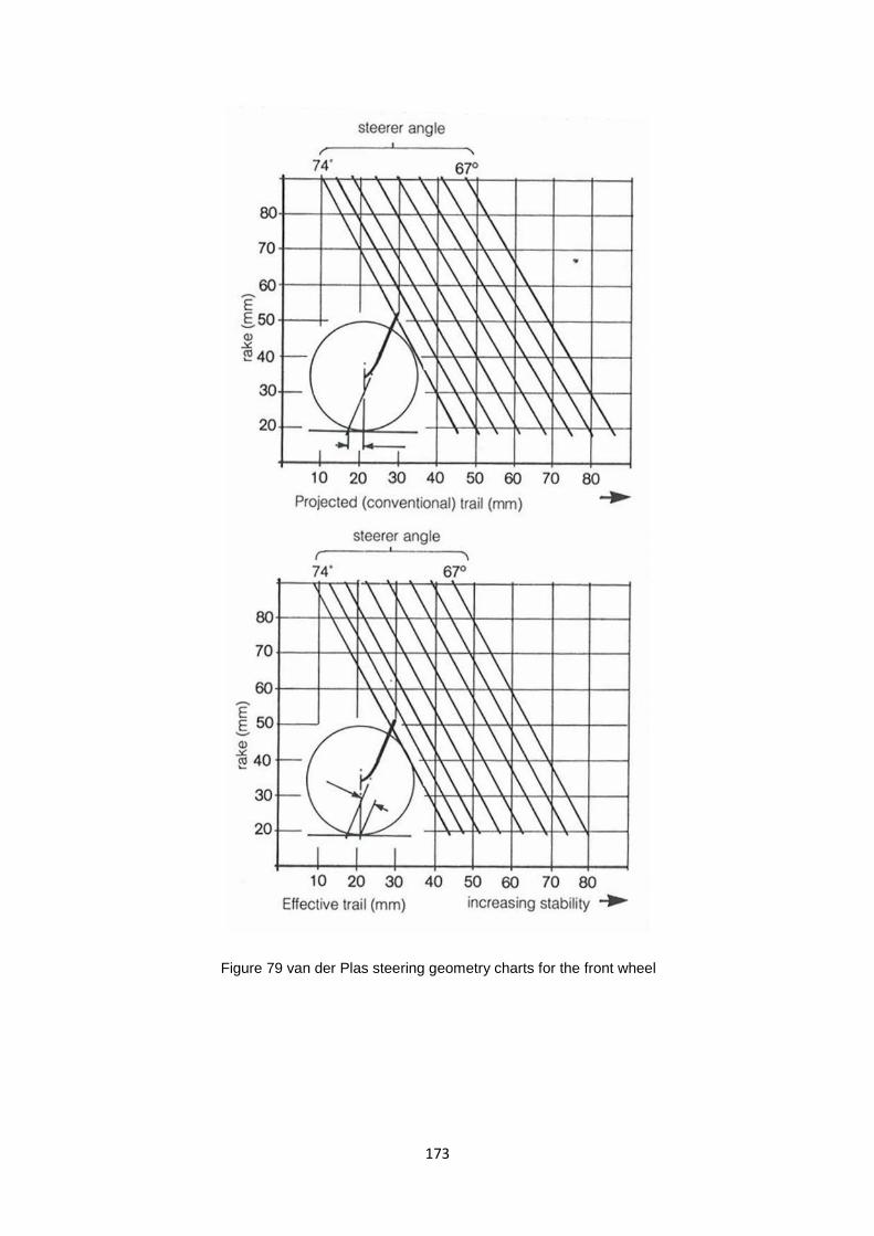
Figure 79 van der Plas steering geometry charts for the front wheel
173

Figure 80 The front projection term defined by Jones
Front projection
174
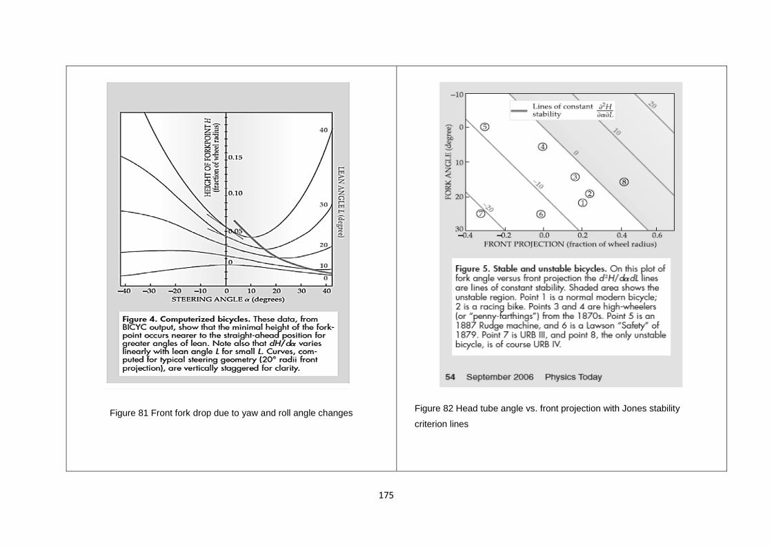
Figure 81 Front fork drop due to yaw and roll angle changes
Figure 82 Head tube angle vs. front projection with Jones stability
criterion lines
175

Moulton, a well-known but now retired frame builder (based in the UK and USA) has produced the
interesting steering geometry chart shown in Figure 83. Moulton’s bicycles have been used in top
international competitions including the Tour de France and the Olympics. A frequent writer with his
own web blog about bicycles, he describes this chart in one of his 2010 entries (91). The axes
orientation he chose are reversed from our proposed Design Chart. On his chart is displayed a line of
“ideal handling” (this passes a point defined by a 73O head tube angle, a 35 mm rake giving a 67.3 mm
trail). Interestingly his line is very close to the 140% iso-handling line on the proposed Design Chart. No
supporting analysis or evidence as to the selection of this particular line is included other than
mentioning his empirical observations about steering geometry. “In time I found there was an “optimum
handling” line that I could draw on my graph, that would show me the fork rake needed for a given head
angle (91).”
Figure 83 Moulton’s proposed head tube angle vs. trail chart and ideal handling line
176

The proposed Steering Geometry Design Chart began as a chart showing trail vs. head tube angles
plotted along lines of constant rake, similar to both the van der Plas and Moulton Charts, see Figure 79,
Figure 83 and Figure 84 (90, 91). What is new about this Chart is the addition of a series of iso-handling
lines (spaced at 10% intervals from 50 % to 150%). Each iso-handling lines connects points of constant
settling time (based on the Simulink unit impulse response 2% settling time) and so indicates the
bicycle’s handling performance. The Chart assumes that all other design parameters are constant (that
is wheelbase, mass, position of mass, moments of inertia, speed and wheel diameter). The iso-handling
lines only indicate equivalent performances, they don’t indicate any optimum design position. But they
do allow easy and meaningful comparisons of individual bicycles and they can be used to compare
design solutions quantitatively.
It is possible to plot existing designs onto the Chart to gain an insight as to what the different regions of
the Chart will mean in terms of performance and by plotting successful bicycle geometries a suitable
design envelope can be proposed.
The Chart in Figure 84 displays trail and head tube angle values that range from 0 to 120 mm and 62
to 80 degrees respectively with rake dimensions ranging from 0 to 75 mm. Of course it is the
combination and interaction of these three parameters which is interest and this is what this Chart
clearly displays.
Eleven iso-handling lines are drawn covering the area of interest, that is head tube angles between 69
and 77 degrees and trail values between 20 and 70 mm. The iso-handling line that passes through the
benchmark bicycle is labelled the 100% line and it connects geometry combinations which have the
same settling time and the other iso-handling lines are referenced to this 100% line. The overall trend
is that as the trail increases (and rake decreases) the settling times increase or in the terms of van der
Plas, stability has increased. But is this always a good thing? Sometimes a certain amount of sensitivity
in handling (or instability) is desirable.
177
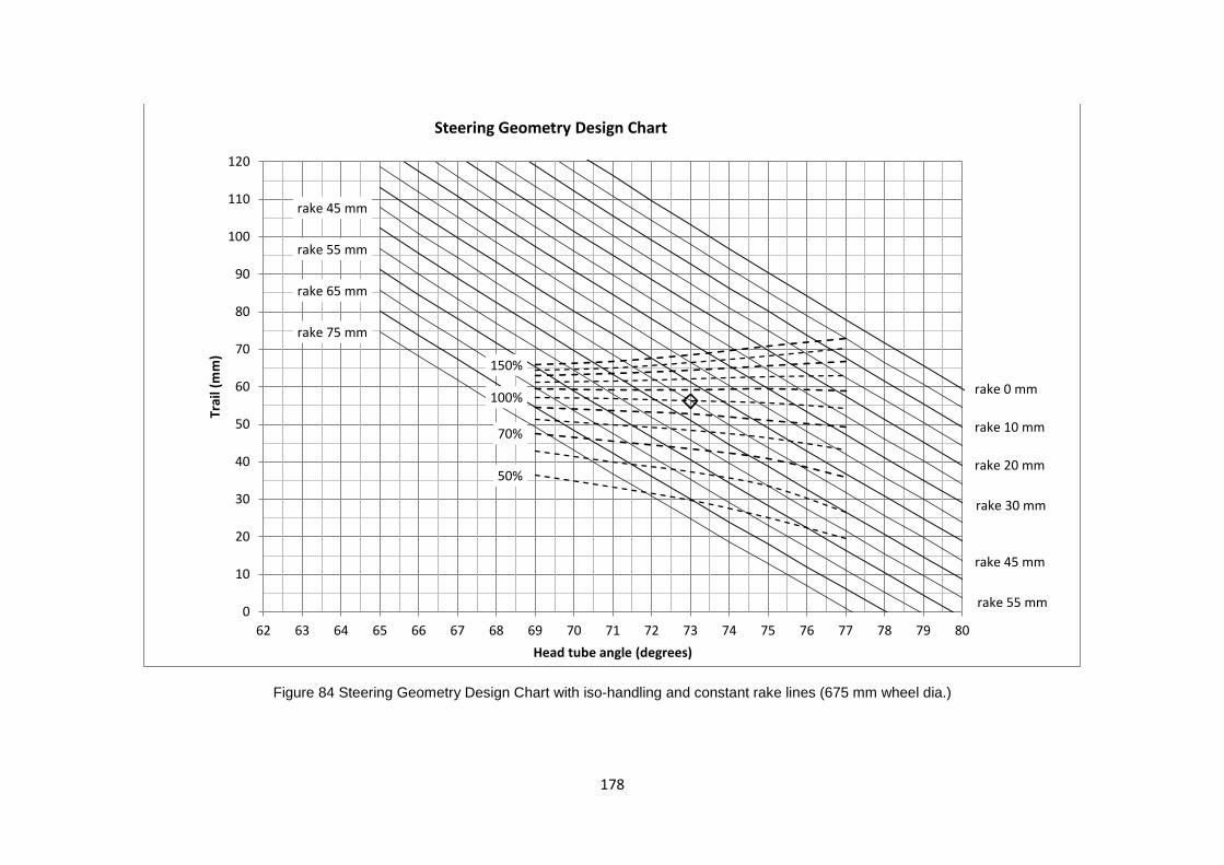
Figure 84 Steering Geometry Design Chart with iso-handling and constant rake lines (675 mm wheel dia.)
rake 0 mm
rake 10 mm
rake 20 mm
rake 30 mm
rake 45 mm
rake 45 mm
rake 55 mm
rake 55 mm
rake 65 mm
rake 75 mm
50%
70%
100%
150%
0
10
20
30
40
50
60
70
80
90
100
110
120
62 63 64 65 66 67 68 69 70 71 72 73 74 75 76 77 78 79 80
Trai
l (m
m)
Head tube angle (degrees)
Steering Geometry Design Chart
178

Consider the five different bicycles in Table 33 all with different geometries. On the enlarged Steering
Geometry Design Chart in Figure 85 these three bicycles (cases A, B and C) with different combinations
of head tube angles and rake all lie along the 100% iso-handling line. Assuming all other parameters
are the same (wheelbase, mass, speed, mass position and moments of inertia) they will all have the
same 2% settling time.
Consider a second scenario, where the benchmark bicycle’s geometry (case A) is changed slightly.
First keep the head tube angle unchanged at 73 degrees but change the rake from 45 mm to 50 mm
(thus causing the trail to decrease to 50.9 mm) this is case D in Table 33 and Figure 85. This new
geometry moves from the 100% iso-handling line to approximately 85%, which is a 15% drop. Next, in
case E, keep the rake unchanged but change the head tube angle from 73 to 73.5 degrees this causes
the settling time to drop from the 100% line to just above 90%, a decrease of nearly 10%. In both cases
D and E, the rider would experience a much quicker settling down after a disturbance, which is a good
thing up to a point. But the downside is both bikes would be more sensitive to disturbances. What this
physically means is that for the benchmark bicycle (case A) and cases B and C under a unit impulse
they would all take 10.1 sec (100%) to settle down to 2% of the maximum response. But for case D,
such a bicycle would take 8.585 sec (85%) to settle and for case E it would take 9.09 sec (90%) to settle
down after a unit impulse.
Chapter Seven will have a detailed discussion as to the application of this Chart to the elite road bicycles
used in the Tour de France 2013 race.
Table 33 Five bicycles plotted in Figure 85.
Case Head tube angle
degrees
Rake mm Trail mm C
2% settling time
Marker
A 73.0 45 56.130 100% diamond (benchmark)
B 69.0 67 57.300 100% circle
C 77.0 23 54.310 100% triangle
D 73.0 50 50.900 85% cross
E 73.5 45 53.039 90% square
179
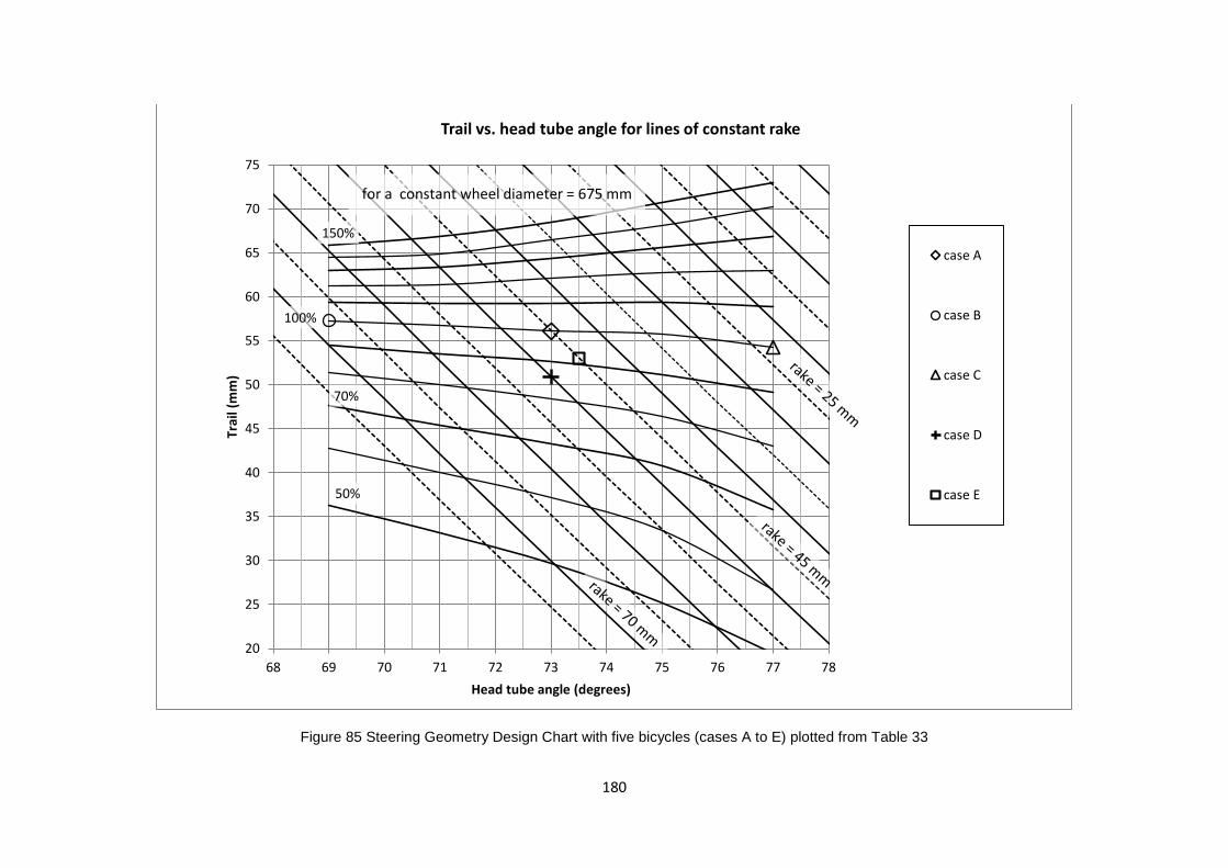
Figure 85 Steering Geometry Design Chart with five bicycles (cases A to E) plotted from Table 33
50%
70%
100%
150%
20
25
30
35
40
45
50
55
60
65
70
75
68 69 70 71 72 73 74 75 76 77 78
Trai
l (m
m)
Head tube angle (degrees)
Trail vs. head tube angle for lines of constant rake
case A
case B
case C
case D
case E
for a constant wheel diameter = 675 mm
180
6.4.3. WHEEL PROPERTIES DESIGN CHART
The second proposed Chart shows the effect and interaction of the two important wheel properties,
namely diameter and the moment of inertia about the rotational or polar axis Y, see Figure 89. These
two wheel properties have a significant effect on settling time with bicycles being surprisingly sensitive
to different wheel diameters (every 1% increase increasing the settling time by 5.75%). Also the wheel’s
moment of inertia about Y is important with every 1% increase, decreasing the settling time by 2.02%.
However these effects tend to cancel each other out because increasing the wheel diameter usually
increases its moment of inertia. So if the wheel diameter was increased but no change to its construction
was made (i.e. materials, rim wall thickness and rim width to depth ratio all unchanged) the result may
be that no change in handling occurs. The Wheel Properties Design Chart illustrates this interaction
and gives guidance of how a handling may be improved by careful wheel selection. As far as is known,
no similar chart to this has been proposed in the literature.
The Wheel Properties Design Chart was prepared using equations relating wheel diameter to the polar
moment of inertia and making basic assumptions about wheel construction and material. Again, iso-
handling lines of constant settling time are plotted and referenced to the benchmark wheel and they
indicate equivalent performance, but they don’t indicate an optimum wheel design. This Chart assumes
the head tube angle, trail, rake, mass (and its position) speed and all other moments of inertia are
constant.
To construct the Chart the following assumptions were made:
1. The contribution of the rim to overall moment of inertia is assumed to be 50% (experimentally
this has been shown to be between 45% and 50% of the total). Hence the contribution of the
tyre to the moment of inertia is allowed for by using this ratio. The hub and spoke moments of
inertia contribution are small, typically in the order of 0.5% of the total and hence they can be
ignored (see Figure 86).
2. The rim section is a hollow rectangular box of constant wall thickness (t) and material
3. The ratio of the rim section depth (P) to rim width (w) is defined by the P/w ratio (Figure 87) and
ranges from 0.5 to 2.5 are shown on the Chart
4. The rim material and its density are known (e.g. 6106 series aluminium is a typical rim alloy
with a density of 2700 kg/m2)
5. The rim section width (w) is known, assumed to be 25 mm
6. The rim wall thickness (t) is known, assumed to be 1 mm
7. The tyre diameter (td) is known and the actual wheel diameter is given by:
𝑎𝑎𝑐𝑐𝑡𝑡𝑎𝑎𝑎𝑎𝑎𝑎 𝑤𝑤ℎ𝑒𝑒𝑒𝑒𝑎𝑎 𝑑𝑑𝑠𝑠𝑎𝑎𝑚𝑚𝑒𝑒𝑡𝑡𝑒𝑒𝑟𝑟 = 1.8925 𝑋𝑋 𝑡𝑡𝑑𝑑 + 627.27 (mm)
(37)
181
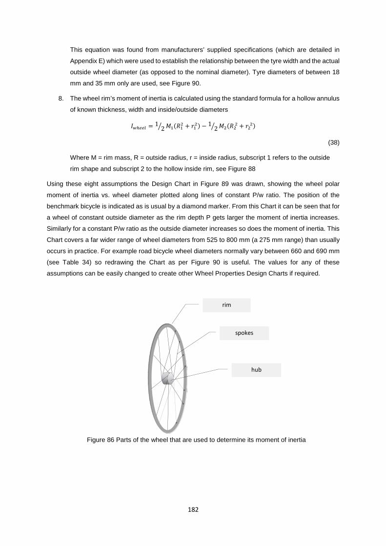
This equation was found from manufacturers’ supplied specifications (which are detailed in
Appendix E) which were used to establish the relationship between the tyre width and the actual
outside wheel diameter (as opposed to the nominal diameter). Tyre diameters of between 18
mm and 35 mm only are used, see Figure 90.
8. The wheel rim’s moment of inertia is calculated using the standard formula for a hollow annulus
of known thickness, width and inside/outside diameters
𝐼𝐼𝑦𝑦ℎ𝑖𝑖𝑖𝑖𝑟𝑟 = 12� 𝑀𝑀1(𝑅𝑅12 + 𝑟𝑟12) − 1
2� 𝑀𝑀2(𝑅𝑅2 2 + 𝑟𝑟2 2)
(38)
Where M = rim mass, R = outside radius, r = inside radius, subscript 1 refers to the outside
rim shape and subscript 2 to the hollow inside rim, see Figure 88
Using these eight assumptions the Design Chart in Figure 89 was drawn, showing the wheel polar
moment of inertia vs. wheel diameter plotted along lines of constant P/w ratio. The position of the
benchmark bicycle is indicated as is usual by a diamond marker. From this Chart it can be seen that for
a wheel of constant outside diameter as the rim depth P gets larger the moment of inertia increases.
Similarly for a constant P/w ratio as the outside diameter increases so does the moment of inertia. This
Chart covers a far wider range of wheel diameters from 525 to 800 mm (a 275 mm range) than usually
occurs in practice. For example road bicycle wheel diameters normally vary between 660 and 690 mm
(see Table 34) so redrawing the Chart as per Figure 90 is useful. The values for any of these
assumptions can be easily changed to create other Wheel Properties Design Charts if required.
rim
hub
spokes
Figure 86 Parts of the wheel that are used to determine its moment of inertia
182

P
t
w
Figure 87 Wheel rim definitions of w, P and t
r2
R1
R2
r1
Figure 88 Additional wheel rim definitions of R1, R2, r1 and r2
183
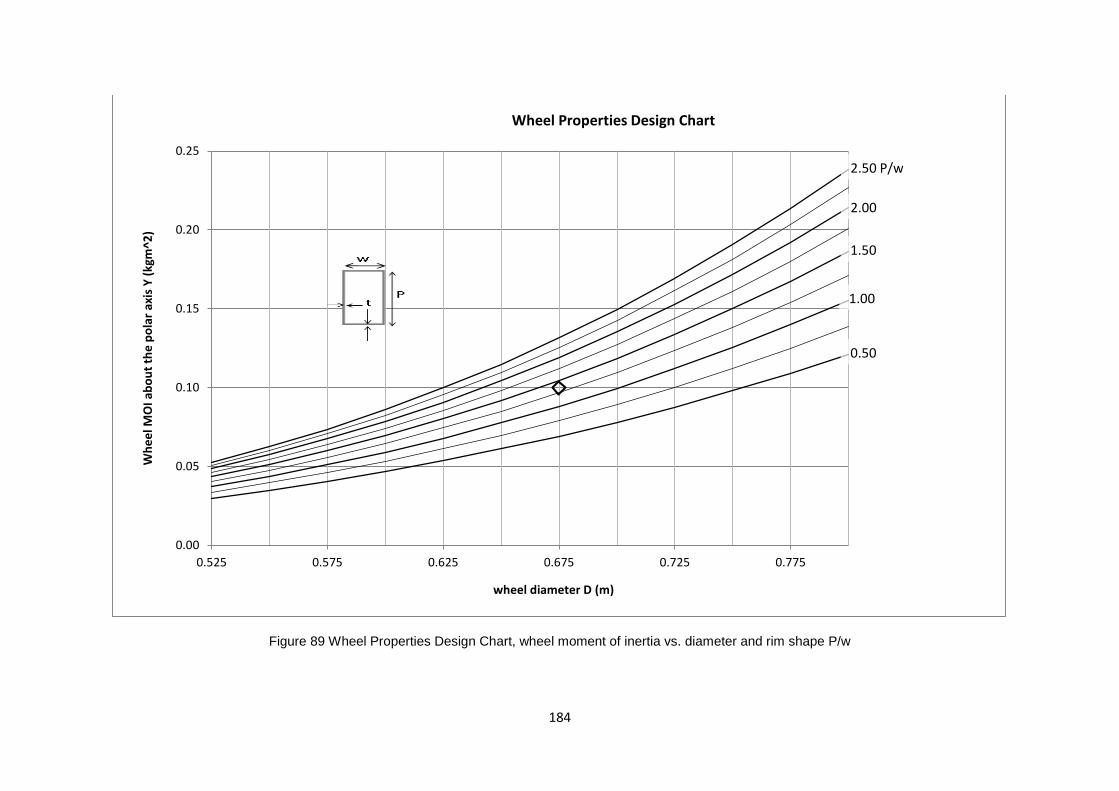
Figure 89 Wheel Properties Design Chart, wheel moment of inertia vs. diameter and rim shape P/w
0.00
0.05
0.10
0.15
0.20
0.25
0.525 0.575 0.625 0.675 0.725 0.775
Whe
el M
OI a
bout
the
pola
r axi
s Y
(kgm
^2)
wheel diameter D (m)
Wheel Properties Design Chart
2.50 P/w
2.00
0.50
1.00
1.50
184

The Chart in Figure 90 plots several wheels that have been measured experimentally and their details
are shown in Table 34. This Table and Chart clearly shows how the settling times vary from 75% to a
maximum of 135% of the benchmark wheel, also that the wheel outside diameters range from 675 mm
to 687.8 mm and the P/w ratio from approximately 0.50 to 2.5.
Table 34 Tyre and wheel experimental values
Wheel type
Fron
t/Rea
r Tyre MOI Y axis kgm2
D Actual Wheel
Outside Diameter mm
C %
settling time 1
Approx P/w
Ratio 2
Mavic SUP Open Pro F 700C x 23 0.0871 675.00 135% 0.50
Altx 2800 F 700C x 23 0.0845 675.00 125% 0.75
Altx 2800 R 700C x 23 0.0979 675.00 105% 1.50
Benchmark wheel F 700C x 25 0.1000 675.00 100% 1.50
Airline Vuelta F 700C x 23 0.1006 675.00 100% 1.50
Mavic SUP R 700C x 23 0.1017 675.00 95% 1.75
Mavic Aksium R 700C x 23 0.1020 675.00 95% 1.75
Shimano 105 R 700C x 23 0.1054 675.00 95% 2.00
Mavic MA3 F 700C x 23 0.1077 675.00 90% 2.25
Shimano 105 F 700C x 23 0.1095 675.00 85% 2.30
Mavic MA3 F 700C x 28 0.1213 680.30 80% 2.50
Mavic MA3 F 700C x 32 0.1304 687.80 75% 2.25
Note 1 C given to the nearest 5%
Note 2 P/w given to nearest 0.25
185

Figure 90 Wheel Properties Design Chart, plotting the wheels (experimental values) from Table 34, iso-handling lines shown
0.075
0.085
0.095
0.105
0.115
0.125
0.135
0.145
660 665 670 675 680 685 690
Whe
el M
OI a
bout
the
pola
r axi
s Y
(kgm
^2)
Wheel diameter D (mm)
Wheel Properties Design Chart
0.50
1.00
1.50
2.00
P/w = 2.50
70%
80%
85%
90%
100%
110%
120%
140%
186

6.4.4. FRAME GEOMETRY DESIGN CHART
The third proposed Design Chart examining frame geometry looks at a new aspect of design and as far
as is known is entirely new and original. This Chart shows the effect of the mass position (vertically and
longitudinally) and its interaction with the wheelbase and seat tube angle. The proposed Design Chart
applies to road bicycles but could be adapted to apply to other types of bicycles such as mountain
bicycles.
In order to draw this Chart it was necessary to establish relationships between the mass position, the
wheel base and the seat tube angle. This was done by using frame relationships derived from geometric
and empirical relationships, and is fully explained in Appendices B and F. Many of the assumptions
about these relationships were made using the benchmark bicycle as a starting point.
The first important relationship to examine is between the mass position (b and h) and the seat tube
angle. It has been frequently claimed that a steeper seat tube angle results in a bicycle that is more
compact and lively (but also less stable) (69, 74). Next to consider is the relationship between these
three parameters (b, h and STA) and the wheelbase. The Chart’s assumptions regarding seat tube
angle, wheel base and mass position are as follows:
1. A standard road bicycle 700C x 25 wheel is used (with an actual diameter of 675 mm) (74)
2. The distance between the centreline of the seat tube and the outer circumference of the rear
wheel is set at 32.5 mm and this allows for a suitable clearance between the seat tube and the
tyre. Smaller values are sometimes used but can present construction and operational
difficulties as road debris can become trapped between the seat tube and the tyre.
3. In order to minimise the wheelbase the seat tube angle is the steepest angle that can be fitted
against the rear wheel while still conforming to assumptions 1 & 2 (75)
4. The bottom bracket drop is 67.5 mm, making the distance between the bottom bracket spindle
and the road 270 mm (this is a standard value, see Appendix F)
5. The centre of mass position is defined by the main parameters h and b (already defined) and
the additional terms k and j, which are defined in Appendix B
6. The ratio k/P is set at 0.2099, where P is the saddle height, this k/P value was selected to
conform to the benchmark bicycle’s known centre of mass position
7. And ratio j/P is 0.0912, again selected to conform to the benchmark bicycle’s known centre of
mass position
8. The relationship of wheelbase L (mm) to saddle height P (mm) is given by the empirical
relationship, justified in Appendix B and F
𝐿𝐿 = 0.3077 × 𝑃𝑃 + 822.5 ± 20
(39)
187

The Frame Geometry Design Chart in Figure 91 shows the vertical mass position vs. horizontal mass
position (h vs. b) plotted along lines of constant seat tube angle (STA) and constant wheelbase (L).
Once again the position of the benchmark bicycle is indicated by a diamond marker and this Chart
assumes that all other parameters are constant (head tube angle, rake, mass, moments of inertia,
speed and wheel diameter).
The next stage in developing the Frame Geometry Design Chart is to plot two important boundaries or
limits. These limits not determined by the model dynamics but are nonetheless important design
considerations and are:
1. The Union Cycliste Internationale (UCI) 5 cm limit, which restricts the maximum seat tube angle
that is permitted for any bicycle competing in UCI sanctioned races
2. The toe overlap limit, which is an ergonomics consideration important for smaller riders
6.4.4.1. UCI 5 CM LIMIT
The Union Cycliste International (UCI) is the international body authorised to regulate, control and run
the majority of cycle sports (3). The main exceptions to their authority being human powered vehicle
record attempts (covered by two independent bodies, IHVPA and WHPVA (59, 93)) and triathlon events,
covered by the International Triathlon Union (94).
The UCI 5cm limit is determined by UCI Regulation 1.3.013 “Saddle Setback” which states that “the
peak of the saddle should be a minimum of 5 cm to the rear of a vertical plane passing through the
bottom bracket spindle” (95). In other words there is a maximum seat tube angle that must not be
exceeded and this varies with the wheelbase and this is made clear by examining Figure 92. The
intention of this regulation (and several other UCI rules) is to ensure that bicycles conform to a basic
double triangle design and it prohibits what the UCI considers to be extreme designs, such as the one
hour record and time trial bicycles of the 1990’s.
The maximum seat tube angle given by this UCI Regulation can found from the following equation (see
Appendix B).
𝑆𝑆𝑇𝑇𝐴𝐴 = 90 − sin−1 (5 + 𝑠𝑠𝑒𝑒𝑎𝑎𝑡𝑡 𝑒𝑒𝑒𝑒𝑡𝑡𝑒𝑒𝑠𝑠𝑠𝑠𝑠𝑠𝑐𝑐𝑠𝑠) 𝑠𝑠𝑎𝑎𝑑𝑑𝑑𝑑𝑎𝑎𝑒𝑒 ℎ𝑒𝑒𝑠𝑠𝑀𝑀ℎ𝑡𝑡 ⁄ (in centimetres and degrees)
(40)
This equation was used to plot the UCI 5 cm limit on the right hand side of the Design Chart Figure 94.
The equation give the maximum seat tube angle for any given saddle height and then this is related to
the position of the mass (h and b) using the relationships defined in Appendix B.
188

Figure 91 Frame Geometry Design Chart relating seat tube angle, wheelbase and mass position (distances b & h)
800
900
1000
1100
1200
1300
1400
200 225 250 275 300 325 350 375 400 425 450
Vert
ical
dis
tanc
e to
CO
G "
h" (m
m)
Horizontal distance to COG "b" (mm)
Frame Geometry Design Chart
L = 1050 mm
980 mm
960 mm
1030 mm
1000 mm80 degrees
189

6.4.4.2. TOE OVERLAP LIMIT
This second limit is an ergonomic consideration that is relevant to smaller riders. Toe overlap can be a
significant problem for riders especially when frame sizes are below 52 cm and is commented in the
literature (96, 97). When a pedal crank is in the 9 o’clock position a toe overlap exists if the front wheel
overlaps the rider’s toe. When the handlebar is turned this will contact the shoe and can cause the rider
to lose control and crash, shown in Figure 93. The degree of overlap that can be tolerated seems to
vary between individuals with some claiming no overlap at all is tolerable and others saying up to 25
mm is tolerable (96).
Bottom bracket spindle
5 cm minimum
Seat extension
Maximum seat tube angle
Saddle height
Figure 92 The UCI 5 cm rule defines the maximum seat tube angle permitted
190

Figure 93 A toe overlap between the front wheel and shoe can exist for small bicycle frames
L2
Toe overlap
191
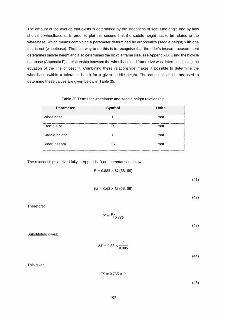
The amount of toe overlap that exists is determined by the steepness of seat tube angle and by how
short the wheelbase is. In order to plot this second limit the saddle height has to be related to the
wheelbase, which means combining a parameter determined by ergonomics (saddle height) with one
that is not (wheelbase). The best way to do this is to recognise that the rider’s inseam measurement
determines saddle height and also determines the bicycle frame size, see Appendix B. Using the bicycle
database (Appendix F) a relationship between the wheelbase and frame size was determined using the
equation of the line of best fit. Combining these relationships makes it possible to determine the
wheelbase (within a tolerance band) for a given saddle height. The equations and terms used to
determine these values are given below in Table 35.
Table 35 Terms for wheelbase and saddle height relationship
Parameter Symbol Units
Wheelbase L mm
Frame size FS mm
Saddle height P mm
Rider inseam IS mm
The relationships derived fully in Appendix B are summarised below:
𝑃𝑃 = 0.885 × 𝐼𝐼𝑆𝑆 (68, 69)
(41)
𝐹𝐹𝑆𝑆 = 0.65 × 𝐼𝐼𝑆𝑆 (68, 69)
(42)
Therefore:
𝐼𝐼𝑆𝑆 = 𝑃𝑃0.885�
(43)
Substituting gives:
𝐹𝐹𝑆𝑆 = 0.65 ×𝑃𝑃
0.885
(44)
This gives:
𝐹𝐹𝑆𝑆 = 0.735 × 𝑃𝑃
(45)
192

Considering the 2013 Tour de France road bicycles in Appendix F, the empirical relationship between
frame size and wheelbase was found and this gives the following equation, see Figure 124
𝐿𝐿 = 0.3077 × 𝐹𝐹𝑆𝑆 + 822.5 ± 20 𝑅𝑅2 = 0.652
(39)
For the benchmark bicycle with a 550 mm frame size this equation gives a wheelbase of 991.74 mm
(-/+ 20 mm) or between 971.74 and 1011.74 mm) which is close to the chosen benchmark wheelbase
of 1000 mm, see below.
𝐿𝐿 = 0.3077 × 550 𝑚𝑚𝑚𝑚 + 822.5 𝑚𝑚𝑚𝑚 ± 20 𝑚𝑚𝑚𝑚
𝐿𝐿 = 991.74 𝑚𝑚𝑚𝑚 ± 20 𝑚𝑚𝑚𝑚
By substituting equation (45) for the saddle height P equation (39) becomes:
𝐿𝐿 = 0.3077 × (0.735 × 𝑃𝑃) + 822.5 ± 20
(46)
Which gives the final equation necessary to find the toe overlap boundary:
𝐿𝐿 = 0.226 × 𝑃𝑃 + 822.5 ± 20
(47)
To plot the toe limit line the following seven assumptions were used (explanations of these particular
assumptions is given in Appendix B):
1. Actual wheel diameter D is 675 mm
2. Bottom bracket drop is 67.5 mm
3. Clearance between seat tube centreline and rear wheel is 32.5 mm
4. Crank length is 165 mm (measured experimentally)
5. Shoe extension in front of the pedal spindle centreline is 120 mm (measured experimentally)
6. Centreline of shoe is 130 mm from centreline of bicycle in a transverse direction (measured
experimentally)
7. Maximum permitted overlap between wheel and shoe is 10 mm (96)
Using these equations and assumptions gives the toe overlap limit shown on the Design Chart in Figure
94. This final version of the Frame Geometry Design Chart includes a series of iso-handling lines (from
60 % to 160%) connecting points of constant 2% settling time. Again these iso-handling lines indicate
equivalent settling times and show the important interacting effect of changing the position of the mass
(h and b), the wheel base and the seat tube angle all on one Chart.
It has been claimed for a long time that a steeper seat tube angle means the bicycle is more compact
and lively (but also less stable) (68, 69, 74, 75). But this Frame Geometry Design Chart is indicating
that as the seat tube angle gets steeper the settling time actually increases which appears contradictory.
193
Perhaps what the literature is referring to is that a more favourable front wheel/rear wheel weight
distribution is achieved as the seat tube angle steepens and this would mean the bicycle would have a
lower moment of inertia about the yaw axis and so would be more easily turned about this axis. This
investigation did not examine this aspect of bicycle dynamics and so this needs more study. But in
terms of the Simulink impulse response it is clear that steeper seat tube angles cause settling times to
increase.
This raises again the issue of what is desirable in terms of bicycle handling. Is it longitudinal stability
meaning a high degree of self-stability and directional stability in a straight line? Or is it the speed of
response and the ability to quickly take evasive action to avoid an obstacle? Is it predictability and the
lack of unpleasant surprises such as sudden or increasing front wheel oscillations? Or is it a short
settling time and the ability to settle down quickly after a disturbance? Finally is it a quick yaw response
(the ability to corner) which is related to a low moment of inertia about the vertical axis road and the
resistance of the tyres skidding sideways? It must inevitably involve a compromise of many of these
attributes and of course will vary according to the type of bicycle and rider involved. This is an important
area which needs close examination.
194

Figure 94 Frame Geometry Design Chart, indicating iso-handling lines, also UCI 5cm and toe overlap limits
800
900
1000
1100
1200
1300
1400
200 225 250 275 300 325 350 375 400 425 450
Vert
ical
dis
tanc
e to
CO
G "
h" (m
m)
Horizontal distance to COG "b" (mm)
Frame Geometry Design Chart
980 mm
960 mm
70o
1030 mm
1000 mm
L = 1050 mmSTA = 68o72o 74o 76o 78o 80o
UCI 5cm limit
195

6.4.5. MASS AND ROLL INERTIA DESIGN CHART
The fourth and last Design Chart examines the relationship between the bicycle’s total mass (M), its
vertical height (h) and the moment of inertia of rear assembly B about the roll axis (IXB). This Chart
completes the proposed design methodology and examines the last moderately significant parameter,
mass. The sensitivity study shows that while the bicycle’s mass is moderately significant, but both the
mass vertical height and moment of inertia IXB are not significant, see Table 36.
Table 36 Sensitivity of M, IXB and h
Relevant design chart
Symbol Parameter definition
Benchmark value/s
Units C% change 1
Comments
Mass and Roll Inertia Design Chart
M Mass 80 kg +1.98% moderately significant
h Height of centre of mass 1.1 m - 0.27% not significant
IXB MOI of B about XB axis (roll) 100 kgm2 +0.11% not significant
Note 1 C is the % change in the 2% settling time for each 1% increase in the parameter
In order to draw this Chart it was necessary to find a way to easily calculate IXB. After investigation it
was found that a reasonable approximation was to assume that IXB is equal to Mh2 and this is justified
in the following calculations. Consider a bicycle with a mass of 80 kg with a vertical height h of 1.100 m
(i.e. the benchmark bicycle) if it is assumed that IXB is equal to Mh2 we get:
𝐼𝐼𝑋𝑋𝑋𝑋 = 𝑀𝑀ℎ2
(48)
𝐼𝐼𝑋𝑋𝑋𝑋 = 80(𝑘𝑘𝑀𝑀)1.1(𝑚𝑚)2
𝐼𝐼𝑋𝑋𝑋𝑋 = 96.8 𝑘𝑘𝑀𝑀𝑚𝑚2
A more complex calculation could assume that the parallel axis theorem applies and make use of the
experimental values of Appendix C and Hanavan to give a second answer (48).
196

Table 37 Second moment of inertia values
Symbol Parameter definition Value Units Source
MRider Mass of rider 73.0 kg Chapter 4
hRider Height of centre of mass of rider 1.100 m Chapter 4
IXRider MOI rider about their centre of mass 8.0 kgm2 (48)
MBicycle Mass of bike (less forks & front wheel) 5.0 kg Chapter 4
hBicycle Height of centre of mass of bike (less forks & front wheel) 0.600 m from experiments
see Appendix C
IXBicycle MOI of bike (less forks & front wheel) about centre of mass of B 2.0 kgm2 from experiments
see Appendix C
Using the values in Table 37 we get:
𝐼𝐼𝑋𝑋𝑋𝑋 = 𝐼𝐼𝑍𝑍𝑖𝑖𝑑𝑑𝑖𝑖𝑖𝑖 + 𝐼𝐼𝑋𝑋𝑖𝑖𝑐𝑐𝑦𝑦𝑐𝑐𝑟𝑟𝑖𝑖
𝐼𝐼𝑋𝑋𝑋𝑋 = (𝐼𝐼𝑍𝑍𝑖𝑖𝑑𝑑𝑖𝑖𝑖𝑖 + 𝑀𝑀ℎ2) + �𝐼𝐼𝑋𝑋𝑖𝑖𝑐𝑐𝑦𝑦𝑐𝑐𝑟𝑟𝑖𝑖 + 𝑀𝑀ℎ2�
(49)
𝐼𝐼𝑋𝑋𝑋𝑋 = (8 + 73 × 1.12) + (2 + 5 × 0.62)
𝐼𝐼𝑋𝑋𝑋𝑋 = 100.13 𝑘𝑘𝑀𝑀𝑚𝑚2
This second answer of 100.13 kgm2 is within 3.5% of the first calculated result of 96.8 kgm2 and this
shows that the use of Mh2 is an acceptable way to find IXB.
The completed Mass and Roll Inertia Design Chart in Figure 95 shows lines of constant mass height
(h) drawn on a Chart plotting IXB vs. mass. The iso-handling lines show the effect on handling caused
by varying the mass and its height, clearly showing that while mass has a moderately significant effect
on handling changing, height and moment of inertia have much less effect and are not significant.
Different vertical positions of the mass can be due to factors such as:
• changes in seat positions
• different front steering stem lengths and heights
• changes to the rider’s posture
• the carrying of higher loads on the rider (such as water bottles, nutrition, back packs etc.)
197
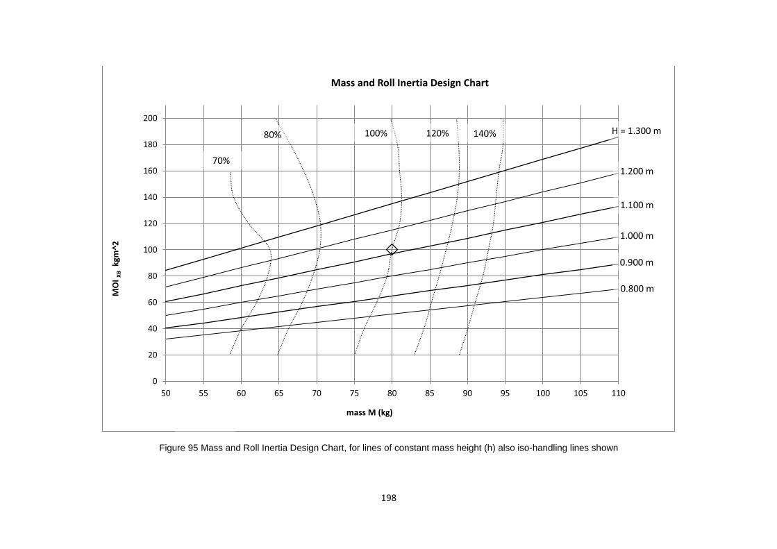
Figure 95 Mass and Roll Inertia Design Chart, for lines of constant mass height (h) also iso-handling lines shown
0
20
40
60
80
100
120
140
160
180
200
50 55 60 65 70 75 80 85 90 95 100 105 110
MO
I XB
kgm
^2
mass M (kg)
Mass and Roll Inertia Design Chart
100% 80%
70%
120% 140% H = 1.300 m
1.200 m
1.100 m
1.000 m
0.900 m
0.800 m
198

6.5. DESIGN CHART REMARKS
The four Design Charts described in this Chapter make use of the high level mathematical analysis of
the Simulink model and present handling information (as iso-handling lines) in a way that is suitable for
the bicycle fraternity to interpret. Use of these Design Charts allows bicycle designers to explore the
implications of design choices with more confidence about the outcome than was previously possible.
These Charts study the key parameters shown to be the important ones affecting dynamic responses.
Below they are ranked from 1st to 4th according to their parameter sensitivity and they can be used
independently of one another or together and cover the important design areas of:
1. Steering geometry (head tube angle, rake and trail)
2. Wheel properties (wheel diameter and moment of inertia)
3. Frame geometry (vertical and longitudinal position of the mass and wheelbase)
4. Mass and roil inertia (mass and moment of inertia of B)
The main advantages of these design charts are:
• they are scientifically based and justified
• they are relatively easy to use with the minimum of calculations required
• they enable a wider audience the ability to understand the design process and its outcomes
• they allow several parameters can be concurrently considered, so interactions can be studied
While their main disadvantages are:
• assumptions have to be clearly known and adhered to
• design boundaries may be hard to define and so unsafe designs may be produced (they are
not necessarily conservative)
The next Chapter will consider how modern road bicycles fit onto the Charts, as represented by bicycles
from historical approaches and by the 2013 Tour de France race. This will validate the Charts and
illustrate their application and value.
Now that these Charts have been developed it is intended to seek comments from the bicycle fraternity
including manufacturers to see how useful these design charts will in practice be to industry. Of course
it is hoped they will prove of value and be easy to use and interpret.
199

7. DESIGN CHART VALIDATION
7.1. INTRODUCTION
This Chapter examines the validity of the four Design Charts proposed in Chapter Six. It was felt that
the best way to do this was to apply the Charts to actual bicycle designs, first considering historical
design practice and secondly by examining the bicycles that competed in the 2013 Tour de France
(TdF) bicycle race.
Historical design practice is of particular interest for the following reasons:
• does the accepted “design lore of bicycles” say the same sorts of things about bicycles that the
Charts indicate?
• and is there evidence of the sort of design evolution occurring over time that is predicted by the
Charts?
And examining the 2013 Tour de France bicycles means that:
• the predictions of the Design Charts can be compared to the decisions made by designers of
the latest top level bicycles
• the variations between different elite bicycle manufacturers can be examined with the Charts
and any performance differences quantified
• it should be possible to see how close individual designs get to the various Chart limits
The specifications of the bicycles examined (both the historical and TdF bicycles) were obtained from
cycling literature such as magazines, books, textbooks and websites. The sort of information required
included details of wheelbase, wheel diameter, head tube angle, fork rake, frame size and seat tube
angles. Information about two secondary parameters, frame size and seat tube angle were included,
because even though they are not part of the Simulink mathematical model, they are commonly used
within the industry.
7.2. HISTORICAL DESIGN PRACTICE
This section summarises the historical practices of manufacturers and designers regarding their bicycle
design practice. By comparing their practices with the Design Charts, judgements can be made as to
the validity of the Charts. How have bicycles changed over recent years and what have been the trends
in design? Do the Charts and in particular their iso-handling lines make sense in terms of what the
historical commentary says about bicycle performance?
Most manufacturers rely heavily on past practises, for example when referring to some recent work
done by Schwab to improve bicycle geometry the Dutch manufacturer Batavus was reported as saying
“we had been using a trial and error system, this is the first chance we have had to do it a scientific way
(9).”
200

To find out about historical practice, the available literature was reviewed, focussing on the comments
from elite riders and manufacturers. After reviewing their ideas and recommendations the following
general observations were noted:
• while there was reasonable agreement on the head tubes angles (ranging between 71.5 and
76 degrees) there were wider variations suggested for the rake and trail values (40 to 67 mm
and 33 to 60 mm respectively)
• reasonable agreement existed as a suitable seat tube angle range (between 71.5 to 76
degrees)
• but it is interesting that there was little acknowledgement of the UCI 5 cm or toe overlap limits
by many sources
• most sources were silent on a wheelbase recommendation, which is interesting given that the
sensitivity study rates wheelbase as a moderately significant parameter
Covering their views in more detail with regards to steering geometry, it is commonly believed that:
• the head tube angle is an important angle that defines the steering geometry and most
suggested it should be between 72 and 74.5 degrees (10, 83)
• steeper head tube angles give faster handling (74, 75)
• also different types of bicycles require different steering geometries:
o racing bicycles (such as those used in the Tour de France) require steep head tube
angles (74, 83, 90)
o and racing bicycles dedicated for climbing steep roads can use even steeper head tube
angles with less rake (74, 75)
o criterium bicycles (used for specialised road racing on tight street circuits) require quick
handling around tight road circuits and have very steep head tube angles of up to 75
degrees with small fork rakes of 38 mm or less, resulting in trails of less than 50 mm
(74)
o time trial bicycles (used by individual riders racing against the clock) can make use of
shallower head tube angles for more stability (74)
o track bicycles (racing on banked, oval velodrome tracks) need slightly steeper head
tube angles (98)
o touring road bicycles (used for travelling over long distances on multiday camping trips)
have the greatest need for stability and comfort and use shallower head tube angles
(99)
• An argument was made by some for neutral handling where the bicycle would be neither twitchy
nor sluggish; rather it would handle in a stable way. It was claimed that this occurs with a
combination of rake and head tube angle that yield a 60 mm trail (91, 98).
201
With regards to frame geometry (and the associated wheelbase and seat tube angle parameters) it is
commonly believed that:
• longer wheelbases and shallower seat tube angles are more comfortable (83, 90)
• regards the desired weight distribution (which is affected by both the wheelbase and the seat
tube angle) two sources recommend a 45/55 front to rear weight distribution for the best
handling, but no justification for this was provided (75, 100).
• but it is believed from: experimental work, Simulink model and Design Charts that this 45/55
ratio is not physically possible for conventional road bicycles, for example the benchmark
bicycle has a 33/67 distribution and to achieve a 45/55 distribution the centre of mass would
need to move forward by 120 mm, a distance which would be impossible to achieve on the BM
bicycle
• steeper angles, shorter wheelbases and shorter fork rakes all make frames more rigid, stiffer
and improve the ride and power transmission (75)
• also steeper seat tubes tend to shorten the wheelbase and make the bicycle more responsive
(69)
• smaller frames need steeper seat tube angles to keep the wheelbase short (83)
• it was claimed that shorter riders have a proportionally shorter upper bodies and so need to be
placed further forward over their pedals by using steeper seat tube angles (69).
• but the real reason may be that the almost universal use of stock 700C wheels which forces
designers to squeeze everything together on a small bicycle in order to achieve an acceptably
short wheelbase and top tube (101).
• different types of bicycles have different frame geometry requirements:
o track bicycles need steeper seat tube angles and shorter wheelbases (69, 74, 90)
o racing bicycles require moderately short wheelbases and steep seat tube angles (74,
83, 90)
o touring road bicycles with a need for stability and comfort use shallower seat tube
angles and longer wheelbases (74)
Pedalling efficiency is said by some to be affected by the seat tube angle:
o according to LeMond, seat tube angles of 74 degrees or less are required for efficient
pedalling (69)
o but Ballantine says seat tube angle is partly determined by the length of the rider’s
thigh, so smaller bicycles have steeper seat tube angles (74)
202

o the Association of British Cycling Coaches (ABCC) gives the following formula to find
the correct seat tube angle, to the nearest 0.5 degree (102)
𝑆𝑆𝑒𝑒𝑎𝑎𝑡𝑡 𝑇𝑇𝑎𝑎𝑏𝑏𝑒𝑒 𝐴𝐴𝑠𝑠𝑀𝑀𝑎𝑎𝑒𝑒 = cos−1 (0.264×𝑖𝑖ℎ𝑖𝑖𝑔𝑔ℎ 𝑟𝑟𝑖𝑖𝑖𝑖𝑔𝑔𝑖𝑖ℎ)𝑟𝑟𝑔𝑔𝑦𝑦𝑖𝑖𝑖𝑖 𝑟𝑟𝑖𝑖𝑔𝑔 𝑟𝑟𝑖𝑖𝑖𝑖𝑔𝑔𝑖𝑖ℎ
(50)
For a benchmark rider (with a 184 cm height) with a thigh length of 62.5 cm and a lower
leg length of 55.6 cm this becomes:
𝑆𝑆𝑒𝑒𝑎𝑎𝑡𝑡 𝑇𝑇𝑎𝑎𝑏𝑏𝑒𝑒 𝐴𝐴𝑠𝑠𝑀𝑀𝑎𝑎𝑒𝑒 = cos−1(0.264 × 62.5)
55.6= 72.75 𝑐𝑐𝑟𝑟 73 𝑑𝑑𝑒𝑒𝑀𝑀𝑟𝑟𝑒𝑒𝑒𝑒𝑠𝑠
Note that the benchmark bicycle has a seat tube angle of 74 degrees. This ABCC
method is clearly anatomically based and is related to pedalling efficiency and not to
any handling requirements. Pedalling efficiency is an interesting issue in its own right
with many factors coming into play. To the author’s best knowledge no agreement
exists as to how best to measure this efficiency. The best available guides are those of
Hinault and LeMond but these are over 25 years old, it seems that coaching advice on
this issue remains a closely guarded secret (68, 69).
o Ricard et al compared the effect of different seat tube angles on triathletes’
performances and concluded that increasing the seat tube angle from 72 to 82 degrees
did not improve cycling power output but did improve running times on the next leg of
the race. They recommended a seat tube angle for triathlon bicycles of at least 76
degrees (103).
o other researchers have claimed that triathletes using higher seat tube angles up to 80
degrees outperformed those with lower angles during the cycling leg of the race (104)
o and this is supported by the design of Boardman’s Lotus 108 bicycle which had an
effective seat tube angle of 80 degrees when used to break the One Hour Record in
1996 by covering 56.375 km in 60 minutes (83)
There is close agreement between these sources on the head tube angles and seat tube angles, but it
surprising to see such a variation in the rake and trail values which have been shown to be so critical
to the performance of the bicycle. The main recommendations for parameter values for road bicycles
from these various sources are summarised in Table 38. By plotting these recommendations on the
Steering Geometry and Frame Geometry Design Charts (see Figure 96 and Figure 97) it is possible to
see what agreement exists between these sources and also to identify on these Charts what regions
are regarded historically as desirable design envelopes.
From the plotted regions on the Design Charts in Figure 96 and Figure 97 it is clear that the
recommendations are varied and have an arbitrary appearance, but perhaps this is to be expected
given their empirical origin. People will have had different experiences and opinions as designers and
riders and will also have different subjective responses to the same bicycles.
203

Table 38 Historical design practice 1
Head tube angle
degrees
Seat tube angle
degrees
Rake
mm
Trail
mm
Wheelbase
mm
Iso-handling line from Chart %
Source
72 to 74.5 N/A (68)
72.5 to 74.5 71.5 to 74 N/A (69)
73 to 76 72 to 76 40 to 45 43 to 54 980 65% to 100% (74)
73 to 74 50 to 67 33 to 51 55% to 85% (52)
72 to 74 72 47 to 50 45 to 60 1015 to 1065 70% to 110% (75)
71.5 to 72.5 74 to 74.5 N/A (105)
73.2 40 60 110% (98)
71.5 to 76 71.5 to 76 40 to 67 33 to 60 980 to 1065 55% to 110% range of
values
Note 1 includes road, criterium, track, time trail and triathlon racing and touring bicycles
204

Figure 96 Steering Geometry Design Chart, indicating Table 38 recommendations, reference numbers are in brackets, see bibliography
50%
70%
100%
150%
20
30
40
50
60
70
68 69 70 71 72 73 74 75 76 77 78
Trai
l (m
m)
Head tube angle (degrees)
Steering Geometry Design Chart
(69)
(68)
(105)
(74)
(52)
(75)
(98)
BM bicycle
205

Figure 97 Frame Geometry Design Chart, indicating Table 38 recommendations, reference numbers are in brackets, see bibliography
800
900
1000
1100
1200
1300
1400
200 225 250 275 300 325 350 375 400 425 450
Vert
ical
dis
tanc
e to
CO
G "
h" (m
m)
Horizontal distance to COG "b" (mm)
Frame Geometry Design Chart
980 mm
960 mm
70o
1030 mm
1000 mm
L = 1050 mm
Toe overlap limit line
UCI 5 cm rule line
STA = 68o74o 78o76o72o
(75)
BM bicycle
206

Finally by comparing three bicycles from different eras (1930, 1950 and 2013) it was interesting to see
how frame geometry has changed over eighty years, see Table 39. Steeper angles are now used along
with shorter wheelbases and a reduction in trail has also occurred. We can see that seat tube angles
over this time have gone from 68 degrees to 73.5 degrees, a 5.5 degree increase. Trail dropped from
70 mm to 47.15 mm and then rose to 59 23 mm (overall a 10.77 mm decrease). While the wheelbase
has changed dramatically going from 1170 mm to 984 mm, a 186 mm reduction.
According to the Design Charts this would mean a significant reduction on settling time (and an increase
in responsiveness). Comparing the 1930 English custom racing bicycle to the 2013 Bianchi Oltre and
just allowing for the steering geometry changes the Oltre has 39% less settling time (180% vs. 110%).
But when looking at the frame geometry the Oltre has 100% more settling time (100% vs. 50%)
according to the Charts. So the change in steering geometry is compensated somewhat by changes in
frame geometry showing the effect of interaction.
Kossack comments that what was once considered acceptable only for track bicycles has over time
become acceptable for road bicycles and this is due to the big improvements in road surfaces. This has
made the handling more responsive (75).
Table 39 Comparison of bicycles from 1930 to 2013 (75, 106, 107)
Bike Head tube angle
degrees
Seat tube angle
degrees
Rake
mm
Trail
Mm
Wheelbase
mm
1930 English custom
racing bike 68.0 68.0 64.0 70.0 1120 to 11703
1950 Bianchi 54.5 cm
frame 1 72.0 72.5 52.5 47.15 1020 to 1050 3
2013 Bianchi Oltre 55
cm frame 2 72.5 73.5 45.0 59.23 984
Note 1 used by Coppi to win the 1950 Paris-Roubaix race
Note 2 used in the 2013 TdF
Note 3 different wheelbases were necessary as adjustments were used to tighten up the chain
207

7.3. TOUR DE FRANCE 2013 BICYCLES
This next section considers the elite group of high performance road bicycles and riders that participated
in the 2013 edition of the Tour de France (TdF) bicycle race which were chosen because:
• they participated in the world’s most prestigious bicycle race and so they will have been
designed with only the best performance in mind
• the different bicycle manufacturers represented at the TdF supplied their best bicycle design
from their product ranges, the designs which best showcased all their knowledge and
experience at this influential event
Validation of the Charts requires the parameter values of these elite bicycles to be compared using the
Design Charts and this section asks the following questions:
• how do the latest designs measure up with regard to the handling predictions of the Design
Charts?
• what are the differences in performance between the different manufacturers’ designs?
• how close to the Design Chart limits do these bicycles get?
The Tour de France (TdF) is the pre-eminent international cycle race and is one of the three grand tours
of road racing, the others being the Giro d’Italia (Tour of Italy) and the Vuelta a Espana (Tour of Spain)
(108). These three races represent the pinnacle of international road cycle racing with the elite of
professional cyclists competing. The 100th anniversary edition of the Tour de France road cycling race
began on 29 July 2013, when 219 riders from 22 professional teams started from Porto-Vecchio in
Corsica and it finished 23 days and 3400 km later in Paris with169 finishers.
The Tour is legendary for its gruelling, unforgiving nature and the toll it takes on the cyclists. “I had
always heard the Tour de France was hard, but that’s when I realised it required an unimaginable level
of strength, toughness and suffering” a quote from Tyler Hamilton (multiple TdF rider) referring to a
typical hard day in a recent Tour (109).
The 2013 TdF race was won by Chris Froome riding for the Sky Procycling Team and he averaged 40.6
km/hr over 21 days of racing (110). The group of TdF bicycles examined includes nearly all 30 models
ridden by all 22 participating TdF teams. The bicycles and their respective teams are listed in Table 40.
By examining these bicycles it should be possible to see what range of parameter values are considered
desirable by the world’s best manufacturers and riders. In order to do this it was first necessary to obtain
a complete list of specifications for each model. Most of this information was obtained directly from
manufacturers’ official websites or specialist sector sources and where specifications were missing, it
was possible by using other known dimensions to determine them either by calculation or by completing
full size drawings.
It is variously estimated that there are about 1 billion bicycles in use in the world and about 20% of
these could be classified as road bicycles. So the total market is large at about 200 million road bicycles,
the balance being mainly mountain bicycles and hybrid bicycles.
208

Table 40 Tour de France 2013 teams and bicycles
No Bicycle manufacturer
Bicycle model 1 TdF Team 2013
1 BH G6 Ultegra D12 Sojasun
2 BH Ultralight Ultegra D12 Sojasun
3 Bianchi Oltre Vacansoleil-DCM
4 BMC Teammachine SLR01 BMC Racing Team
5 BMC Timemachine TMR01 BMC Racing Team
6 Cannondale Supersix Evo Cannondale
7 Canyon Aeroad CF 9.0 Katusha Team
8 Canyon Ultimate CF SLX Katusha Team
9 Cervelo R5 Garmin Sharp
10 Cervelo RCA Garmin Sharp
11 Cervelo S5 Garmin Sharp
12 Colnago C59 Team Europcar
13 Felt F2 2 Team Argos-Shimano
14 Focus Bikes Izalco Team SL Carbon AG2r La Mondiale
15 Giant Propel Belkin Pro Cycling
16 Giant TCR Advanced Belkin Pro Cycling
17 Lapierre Ultimate di2 FDJ.FR
18 Lapierre Xelius Efi 800 FDJ.FR
19 Look 695 Aerolight Cofidis Solutions Credits
20 Merida Sculptura SL 909 Lampre-Merida
21 Orbea Orca Euskatel-Euskadi
22 Pinarello Dogma 65.1 Think 2 Sky Procycling, Movistar
23 Ridley Helium SL Lotto-Belisol
24 Ridley Noah FAST Lotto-Belisol
25 Scott Addict SL Orica-Greenedge
26 Scott Foil 40 Orica-Greenedge
27 Specialized Tarmac SL 4 Astana Pro team, Team Saxo-Tinkoff 3 & Omega
Pharm-Quick Step
28 Specialized Venge Team Saxo-Tinkoff & Omega Pharm-Quick Step
29 Trek Domane 6.9 Radioshack-Leopard
30 Trek Madone 7.9 Radioshack-Leopard
Note 1 includes all 30 models ridden by all 22 TdF teams, excepting Note 2
Note 2 the Felt F1 model used is not available commercially and the only information available was for
the Felt F2 model, which was said to be very similar to the F1
Note 3 Saxo Tinkoff changed their name to Tinkoff Saxo in 2014
Sources (108, 110)
209
It seems that manufacturers are releasing less information about their bicycles’ geometry than was
common in the past. From a review of internet discussion forums this is frustrating to many riders (who
wish to compare bicycles in detail before making their purchases) and it is hard to know why
manufacturers are doing this.
In many cases manufacturers supplied two different models of their top bicycles for each TdF team.
• a very lightweight bicycle for the mountain stages, which makes it easier to climb as mass
dominates
• and another more aerodynamic model for the individual time trial stages (where lone riders race
against the clock) were aerodynamic drag dominates
• each rider had at least three individual machines allocated to them and the TdF “road train”
included over 650 bicycles (costing close to 10 million NZD) as well as team cars and buses
7.3.1. MEDIUM SIZED BICYCLES
This first part of the analysis considers only the medium size TdF bicycles from each manufacturer,
where medium size is defined as being the bicycle from each manufacturer as close as possible to a
traditionally measured 550 mm frame. These medium sized bicycles were looked at first because they
avoid the extreme parameter values of the large or small frames.
As there is no universal sizing system for bicycles and also because not all manufacturers supply the
same sizes across their range, it was necessary to use a variety of ways to select a suitable medium
sized bicycle from each manufacturer. Where conventional frame size information is provided by
manufacturers it is used directly in this section. Where it was unavailable, best endeavours have been
made to use other information (such as stack and reach dimensions) to choose equivalent sized
bicycles from the manufacturers’ ranges to allow a fair comparison to be made. The process used for
selection is as follows:
• where a manufacturer defined their frame sizes (FS) in the traditional manner, a 550 mm bicycle
was chosen or the next closest size (either a 540 or 560 mm)
• where stack dimensions only were given (Figure 13) a stack dimension as close as possible to
565 mm was chosen
• in a few remaining cases a best judgement decision was made after comparing a number of
dimensions, to choose the frame closest to the medium size
After selection of this medium sized group, consideration was given was to how well they aligned with
the Design Charts. First each bicycle was plotted onto the Steering Geometry Design Chart and this is
shown in Figure 98. The plotted crosses indicate the 30 medium sized Tour de France 2013 bicycles
(from Table 72 of Appendix F) with the diamond marker indicating the benchmark bicycle.
210
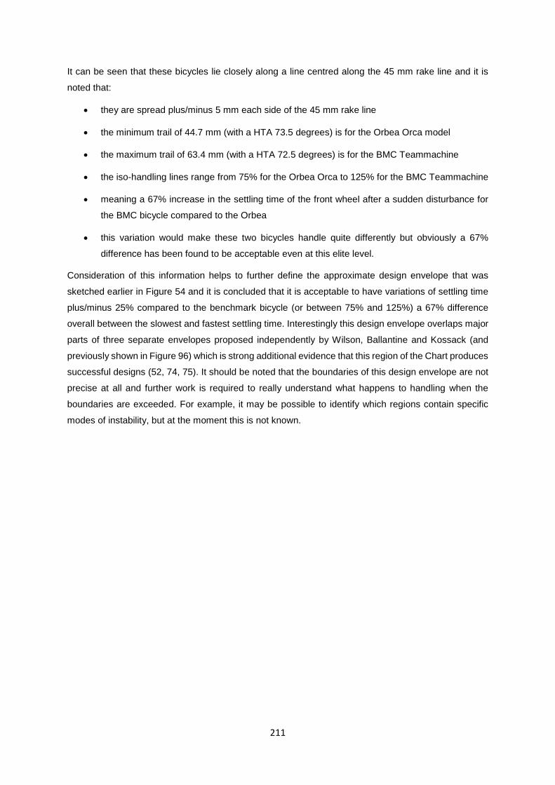
It can be seen that these bicycles lie closely along a line centred along the 45 mm rake line and it is
noted that:
• they are spread plus/minus 5 mm each side of the 45 mm rake line
• the minimum trail of 44.7 mm (with a HTA 73.5 degrees) is for the Orbea Orca model
• the maximum trail of 63.4 mm (with a HTA 72.5 degrees) is for the BMC Teammachine
• the iso-handling lines range from 75% for the Orbea Orca to 125% for the BMC Teammachine
• meaning a 67% increase in the settling time of the front wheel after a sudden disturbance for
the BMC bicycle compared to the Orbea
• this variation would make these two bicycles handle quite differently but obviously a 67%
difference has been found to be acceptable even at this elite level.
Consideration of this information helps to further define the approximate design envelope that was
sketched earlier in Figure 54 and it is concluded that it is acceptable to have variations of settling time
plus/minus 25% compared to the benchmark bicycle (or between 75% and 125%) a 67% difference
overall between the slowest and fastest settling time. Interestingly this design envelope overlaps major
parts of three separate envelopes proposed independently by Wilson, Ballantine and Kossack (and
previously shown in Figure 96) which is strong additional evidence that this region of the Chart produces
successful designs (52, 74, 75). It should be noted that the boundaries of this design envelope are not
precise at all and further work is required to really understand what happens to handling when the
boundaries are exceeded. For example, it may be possible to identify which regions contain specific
modes of instability, but at the moment this is not known.
211

Figure 98 Steering Geometry Design Chart, indicating the 30 medium size bicycles models from the 2013 TdF (675 mm wheel dia), reference numbers are in
brackets, see bibliography
40
45
50
55
60
65
71 71.5 72 72.5 73 73.5 74 74.5 75
Trai
l (m
m)
Head tube angle (degrees)
Steering Geometry Design Chart
100%
120%
80%
BMC Teammachine
TdF design envelope
Orbea Orca (52)
(74)
(75)
212

7.3.2. THE FULL BICYCLE SIZE RANGE
The second part of this section considers how TdF bicycle geometries change across the entire size
range. How do manufacturers treat the geometries of their smallest bicycles compared to their largest
and are there any common trends evident amongst the manufacturers?
Eight 2013 TdF manufacturers provided enough information for this type of analysis to be done and
their information is listed in Appendix F and this includes ten model ranges and 69 individual bicycle
products. The remaining eleven TdF manufacturers were not included as their published specifications
lacked the necessary details.
We will first consider the following three manufacturers in detail before considering all the models
together.
1. Pinarello (a past and current winner of the TdF) is of interest because of some unique geometry
2. next Orbea is examined, also possessing an alternative and unique geometry
3. and finally Cannondale is considered as being representative of the majority of manufacturers
Pinarello is one of the most prestigious names in bicycle manufacturing and racing and was founded in
1952 and is based at Treviso in northern Italy. Famous for its success in racing, it has had the winning
bicycle in 11 TdF races since 1988, including the 2013 Tdf where in addition to 1st place, Pinarello
secured the 2nd and 8th places.
Pinarello has 13 sizes in its top of the line Dogma TdF model, with sizes ranging from 420 mm to 620
mm. Compare this to other manufacturers, most of whom only have 6 to 9 sizes in their ranges. Pinarello
obviously places great importance in getting as perfect fit as possible for each rider by providing the
greatest possible choice in sizes. They are also the only manufacturer who increases the front wheel
trail value as frame sizes get larger while decreasing the head tube angle. All others do the opposite,
that is they decrease trail for their larger frames, see Figure 99 and Table 41. The reason why Pinarello
does this is not known and this means that the Pinarello larger sizes will have longer settling times. This
is interesting because larger frames inherently have longer settling times due to their larger b and M
values.
The second manufacturer Orbea is based in Mallabia in the Basque part of Spain and was founded in
1840, originally as a rifle and gun producer. Orbea began manufacturing bicycles in the 1930s and is
part of the famous Mondragón Corporation, a workers’ co-operative run on unusual ownership lines.
Orbea bicycles have had great success in road, mountain bicycle and triathlon racing and have won
world championships and Olympic medals. Orbea has a similar geometry to the other manufacturers,
in that as the frames get larger, the head tube angles get larger, the seat tube angles smaller and the
trail gets smaller. But Orbea is unusual because their rake gets larger with larger frames unlike all other
manufacturers in this group, see Figure 99 and Table 41.
The third manufacturer Cannondale is the American division of Canadian Dorel Industries and was
founded in 1971. Its bicycles are manufactured in China and Taiwan but its headquarters are in
213

Connecticut USA. Cannondale was a pioneer in introducing aluminium bicycle frames to the market but
now makes many carbon fibre bicycles as well. They have been participating at the top level of road
racing for many years and have been very successful. Their approach to frame geometry is
representative of the majority of manufacturers at the top level. As Cannondale frames get larger, head
tube angles get larger, seat tube angles get smaller and trail decreases, also Cannondale uses one
rake dimension across its size range (which is not uncommon amongst manufacturers) see Figure 99
and Table 41.
The Steering Geometry Design Chart in Figure 100 plots individual bicycle types from all eight 2013
TdF manufacturers (covering ten model ranges) to clearly show overall how geometries vary with frame
size as shown in Table 41. Note that because Specialized’s “Tarmac” and “Venge” models have nearly
identical geometry they were only plotted once per frame size (not twice).
The large range of TdF parameter and iso-handling values shown in Table 42 that quite a difference
exists as to what sort of handling is considered desirable and different strategies employed amongst
these manufacturers. The settling times vary from 75% to 160% compared to the benchmark bicycle
and quite a range in the critical trail parameter is apparent (from 44.696 mm to 70.733mm).
It is interesting to compare this TdF group with the historical practise (discussed earlier in this Chapter)
as they have many similarities and this is shown in Table 43. Considering two critical measures (trail
and settling times) the TdF have a slightly wider range, which is interesting. Perhaps it would be
expected that for such elite bicycles a tighter range would have occurred and there would be more
agreement amongst the manufacturers than is actually evident.
The strategies of these TdF manufacturers are summarised in Table 41 and it can be seen that six
manufacturers (Cannondale, Focus, Look, Specialised, Trek and Trek) have the same broad strategy,
as their frames get larger the following changes occur:
• head tube angles get steeper
• seat tube angles get shallower
• trails decrease
• and rakes either don’t change or get smaller
• most manufacturers use one rake size though Specialized and Orbea use two and Trek and
Felt use four rake sizes
• where rake does change it remains the same across several frame sizes and then jumps to the
next value rather than increasing progressively
• perhaps manufacturers prefer to keep only a few standard fork rakes and choose to vary the
geometry by adjusting the head tube angle to achieve the desire outcome
214

The main exceptions to this strategy are Orbea and Pinarello
• for Orbea the rake gets larger (not smaller) as frames sizes increase
• Pinarello’s larger frames have larger trails, a significant difference
• also Pinarello head tube angles get smaller and seat tube angles get larger the opposite of all
the seven others
Table 41 Manufacturers’ trends as frame sizes increase
Manufacturer Head tube angle
Seat tube angle Rake Trail
1. Pinarello gets smaller gets larger no change in size gets larger
2. Orbea larger smaller larger, 2 sizes smaller
3. Cannondale larger smaller no change Gets smaller
4. Focus Bikes larger smaller no change smaller
5. Look larger smaller no change smaller
6. Specialized larger smaller smaller, 2 sizes smaller
7. Trek larger smaller or same smaller, 4 sizes smaller
8. Felt larger smaller smaller, 4 sizes smaller
exceptions to the general trends are underlined
215
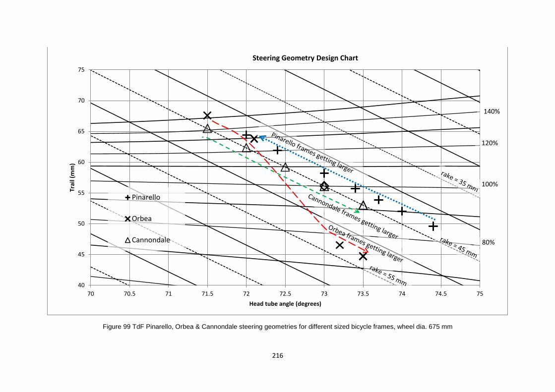
Figure 99 TdF Pinarello, Orbea & Cannondale steering geometries for different sized bicycle frames, wheel dia. 675 mm
40
45
50
55
60
65
70
75
70 70.5 71 71.5 72 72.5 73 73.5 74 74.5 75
Trai
l (m
m)
Head tube angle (degrees)
Steering Geometry Design Chart
Pinarello
Orbea
Cannondale
100%
120%
80%
140%
216

Table 42 Summary of values for the smallest and largest frames from all manufacturers
Parameter Smallest frames Largest frames
Min value Max value Min value Max value
Conventional Frame Size cm 42.00 49.00 58.00 62.00
Head Tube Angle degrees 70.30 74.40 72.00 74.00
Seat Tube Angle degrees 69.15 75.5 73.50 74.0
Rake mm 43.0 53.0 40.0 53.0
Trail mm 49.587 70.733 44.696 64.448
Settling times % 85 160 75 135
Table 43 Comparison of the TdF 2013 bicycles to historical practice
Parameter TdF bicycles 2013
Historical Practice (Table 38)
Comments
Head tube angle
degree 70.3 to 74.4 71.5 to 76 Tdf have lower min & max values
Seat Tube Angle
degree 69.15 to 75.5 71.5 to 76 Tdf have a lower min value
Rake mm 40 to 53 40 to 67 Tdf have a lower max value
Trail mm 44.7 to 70.7 33 to 60 Tdf have higher min & max values
Settling times % 75% to 160% 50% to 110% Tdf have higher min & max values
217

Figure 100 Steering Geometry Design Chart TdF bicycles, all sizes from selected manufacturers (675 mm wheel dia.)
40
45
50
55
60
65
70
75
70 70.5 71 71.5 72 72.5 73 73.5 74 74.5
Trai
l (m
m)
Head tube angle (degrees)
Steering Geometry Design Chart
Cannondale TdF Felt TdF
Focus Look
Orbea Pinarello
Specialized Trek Domane
Trek Madone
100%
140%
120%
80%
tend to be the smaller bicycles
tend to be the larger bicycles
218

Table 44 Parameters values for smallest and largest frames
Company & Model Parameters
Frame Size cm Head Tube Angle degrees
Seat Tube Angle degrees
Rake mm Trail mm
smallest largest smallest largest smallest largest smallest largest smallest largest
Pinarello Dogma 65.1 Think 2 42.0 62.0 74.40 72.00 69.15 73.40 43.0 43.0 49.587 64.448
Orbea Orca 48.0 60.0 71.50 73.50 74.75 73.20 43.0 53.0 67.583 44.696
Cannondale Supersix Evo 48.0 62.0 71.50 73.50 74.50 72.00 45.0 45.0 65.474 53.039
Focus Bikes Izalco Team SL
Carbon 48.0 60.0 71.25 73.50 74.80 73.50 46.0 46.0 66.836 52.737
Look 695 Aerolight 1 47.0 58.0 71.00 73.00 74.80 73.00 43.0 43.0 70.733 58.219
Specialized Tarmac SL 4 &
Venge 49.0 60.0 72.25 74.00 75.50 72.50 45.0 43.0 60.785 52.044
Trek Domane 6.9 44.0 62.0 70.30 72.10 73.30 73.30 53.0 48.0 64.548 58.568
Trek Madone 7.9 47.0 62.0 71.20 73.90 74.60 72.50 45.0 40.0 67.358 55.781
Felt F2 48.0 60.0 71.00 74.00 74.50 73.00 52.0 43.0 61.214 52.044
Sources see Appendix F Note 1 Look specifies FS using a letter system (XS to XXL) a dimension in cm is estimated from other information
219

7.4. WHEEL PROPERTIES DESIGN CHART
Unfortunately it wasn’t possible to see how the TdF bicycles conform to this Chart which considers the
effect of the wheel diameter and polar moment of inertia on handling. This is because the necessary
information (exact wheel diameters and moments of inertia for individual bicycles) was not available.
Therefore it was not possible to define a TdF design envelope on this Chart and this thesis is left with
the experimental work outlined in Chapter Six and Appendix C. This considered a small number of
experimentally measured wheels and used them to outline an approximate design envelope. More
detailed work in this area needs to be done.
7.5. FRAME GEOMETRY DESIGN CHART
Next for consideration is the Frame Geometry Design Chart and because this Chart includes the rider
influenced parameters of b and h it was necessary to look at individual riders as well as specific bicycles.
It was decided to focus only on the top ten finishers from the 2013 TdF and to use their publically
available physical characteristics and bicycle choices to define a design/rider envelope (their details are
shown in Table 45 and Appendix F). Using this information it was possible to calculate the additional
parameters required for plotting onto the Chart. These calculated results are shown in Table 46 and are
based on the following assumptions:
1. inseam = height x 0.461 (based on the average anthropomorphic relationship for males (48))
2. saddle height = inseam x 0.885 (based on competitive coaching advice (68))
3. bicycle frame size = inseam x 0.65 (based on competitive coaching advice (68))
4. the wheelbase and seat tube angle are taken from each manufacturer’s specifications after the
frame size is found as per step 3
5. mass height h is calculated as per Appendix B
6. mass distance from the rear wheel b is calculated as per Appendix B
From the Design Chart in Figure 101 it can be seen that these ten TdF riders are strongly clustered
towards the bottom of the Chart and are bunched near the toe overlap limit line, with one rider (Joaquin
Rodriguez Oliver) right on this boundary. This implies that riders and designers are choosing to use
bicycles that have as short a wheelbase and as shallow a seat tube angle as it is physically possible
for them to ride without encroaching across the toe overlap limit. These bicycles will tend to be lively in
their handling as they are between the 90% and 105% iso-handling lines.
220

The limits for this group of riders and their bicycles are:
• seat tube angles are between 72.5 to 74 degrees (which are similar to Hinault and Ballantine’s
recommendations in Table 38 (68, 74))
• wheelbases range from 980 to 1000 mm (similar to Ballantine’s recommendation in Table 38
(74))
• and the iso-handling lines are 97% plus/minus 7.5% (90% to 105%)
This tight clustering is at least partly due to the similar physical characteristics of these riders who are
all of average height or below and have very low male body masses, (the average height and mass is
177 cm and 63 kg respectively, see Table 45).
7.6. MASS AND ROLL INERTIA DESIGN CHART
The final part of this section looks at the Mass and Roll Inertia Design Chart and once again by
considering the top ten individual riders from the 2013 TdF it was possible to define a design/rider
envelope. These ten riders were plotted using the assumptions and equations from Appendices B and
F plus these two following assumptions.
1. the moment of inertia of assembly B about the roll axis X (IXB) is given by:
𝐼𝐼𝑋𝑋𝑋𝑋 = (𝑀𝑀𝑖𝑖𝑖𝑖𝑑𝑑𝑖𝑖𝑖𝑖 + 𝑀𝑀𝑏𝑏𝑖𝑖𝑘𝑘𝑖𝑖)ℎ 2
(51)
note that h is the calculated value from Table 46 and this method of calculating the IXB (as Mh2)
has been shown in Chapter Six to within 3.5 % of the actual value
2. the bike has a mass of 6.8 kg which equals the minimum weight allowed by UCI regulations (3)
The completed Chart in Figure 102 shows a tight clustering of riders and bicycles
• centred about the line h = 1100mm plus/minus 50mm
• along this line’s axis the rider and bike mass range from 64 to 76 kg (this includes the 6.8 kg
mass of the bicycle)
• this also means the iso-handling lines range from 70 to 95% (80% plus15% minus 10%) which
in comparison to some other results is a tight cluster
• this again highlights the fact that the riders are of slight weight and this combined with a low h
value (1100 mm) and a low bicycle weight (6.8 kg) gives an acceptable handling performance,
which tends to be on the responsive side
221

Table 45 Tour de France 2013 top ten individual finishers (published details)
TdF 2013 position
Rider surname First name Team Bicycle manufacturer Rider height mm Rider mass kg
1 Froome Chris Sky Procycling Pinarello 1860 69.0
2 Quintana Rojas Nairo Movistar Team Pinarello 1660 57.3
3 Rodriguez Oliver Joaquin Katusha Team Canyon 1690 57.0
4 Contador Alberto Team Saxo-Tinkoff Specialized 1760 62.0
5 Kreuziger Roman Team Saxo-Tinkoff Specialized 1830 65.0
6 Mollema Bauke Belkin Pro Cycling Giant 1810 64.0
7 Fuglsang Jakob Astana Pro team Specialized 1820 70.0
8 Valverde Alejandro Movistar Team Pinarello 1780 61.0
9 Navarro Daniel Cofidos Solutions Credits Look 1750 61.0
10 Talansky Andrew Garmin Sharp Cervelo 1750 63.0
average 1771 62.93
standard deviation 59.41 4.09
Source (108)
222
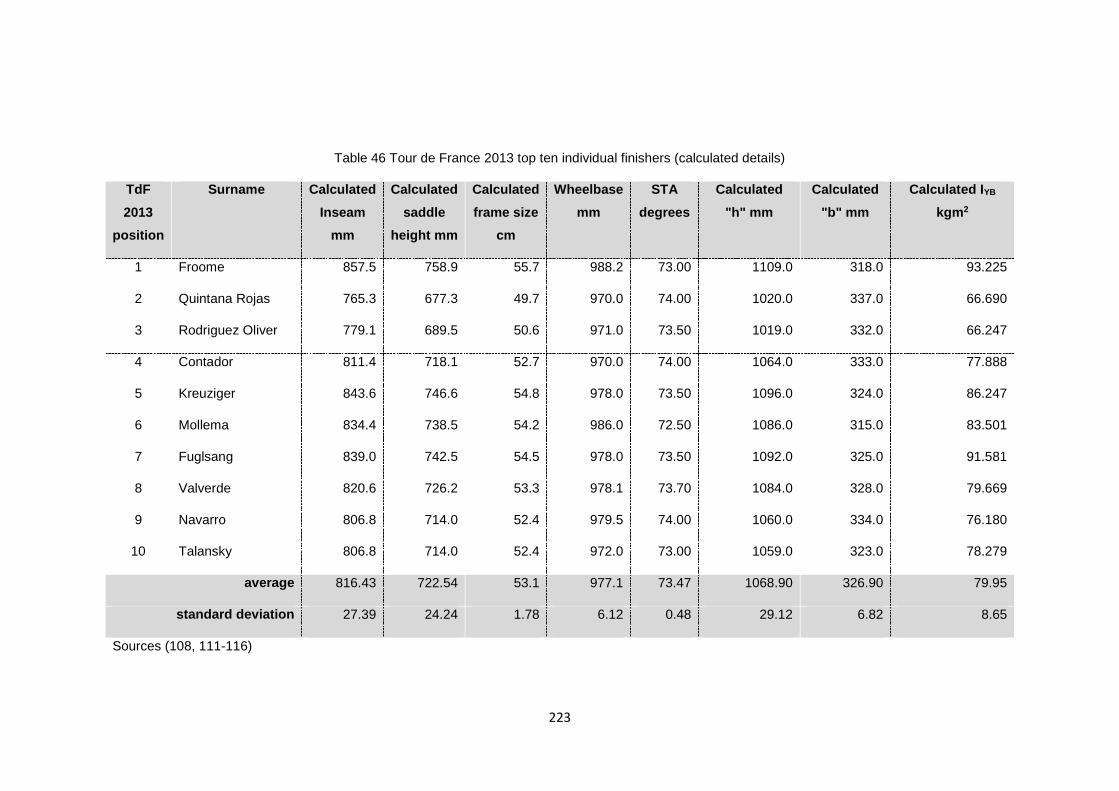
Table 46 Tour de France 2013 top ten individual finishers (calculated details)
TdF 2013
position
Surname Calculated Inseam
mm
Calculated saddle
height mm
Calculated frame size
cm
Wheelbase mm
STA degrees
Calculated "h" mm
Calculated "b" mm
Calculated IYB kgm2
1 Froome 857.5 758.9 55.7 988.2 73.00 1109.0 318.0 93.225
2 Quintana Rojas 765.3 677.3 49.7 970.0 74.00 1020.0 337.0 66.690
3 Rodriguez Oliver 779.1 689.5 50.6 971.0 73.50 1019.0 332.0 66.247
4 Contador 811.4 718.1 52.7 970.0 74.00 1064.0 333.0 77.888
5 Kreuziger 843.6 746.6 54.8 978.0 73.50 1096.0 324.0 86.247
6 Mollema 834.4 738.5 54.2 986.0 72.50 1086.0 315.0 83.501
7 Fuglsang 839.0 742.5 54.5 978.0 73.50 1092.0 325.0 91.581
8 Valverde 820.6 726.2 53.3 978.1 73.70 1084.0 328.0 79.669
9 Navarro 806.8 714.0 52.4 979.5 74.00 1060.0 334.0 76.180
10 Talansky 806.8 714.0 52.4 972.0 73.00 1059.0 323.0 78.279
average 816.43 722.54 53.1 977.1 73.47 1068.90 326.90 79.95
standard deviation 27.39 24.24 1.78 6.12 0.48 29.12 6.82 8.65
Sources (108, 111-116)
223
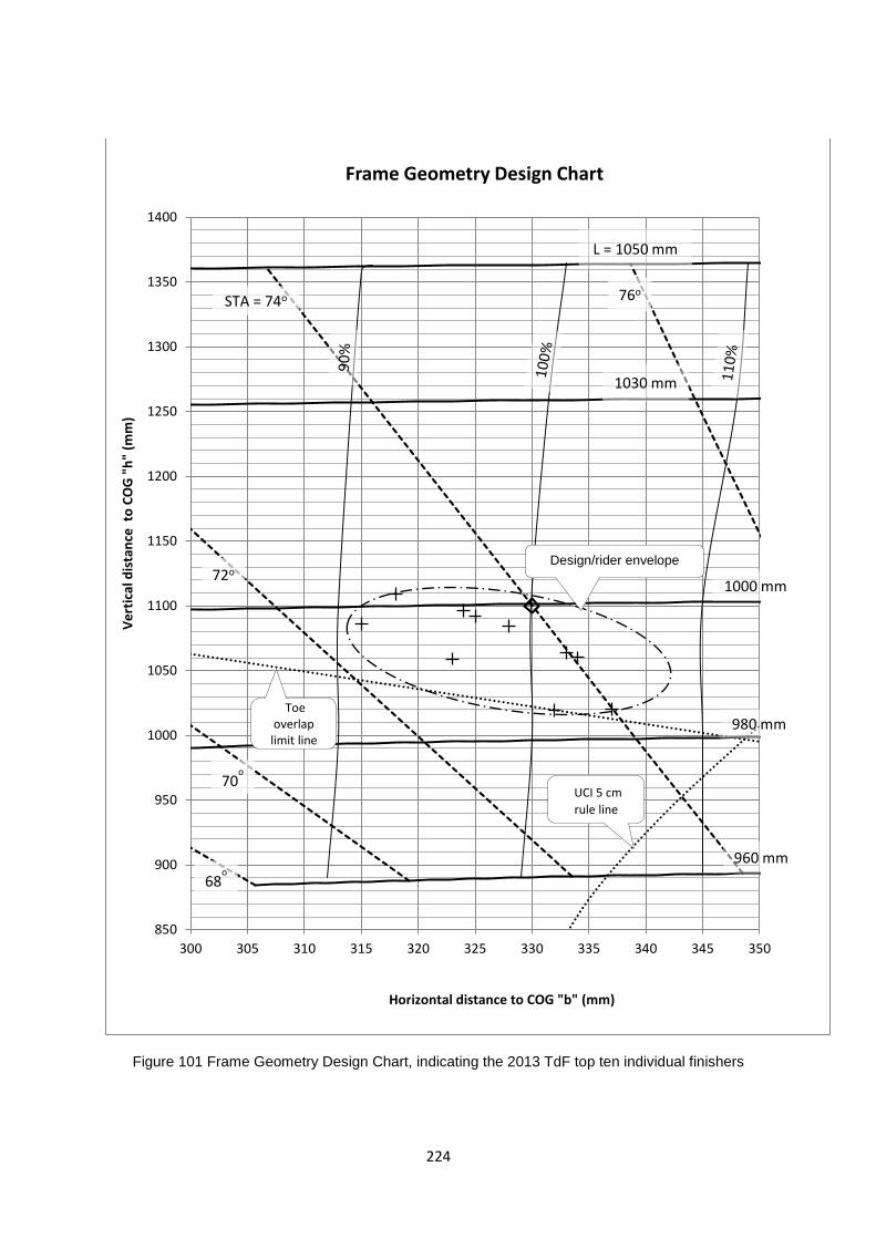
Figure 101 Frame Geometry Design Chart, indicating the 2013 TdF top ten individual finishers
850
900
950
1000
1050
1100
1150
1200
1250
1300
1350
1400
300 305 310 315 320 325 330 335 340 345 350
Vert
ical
dis
tanc
e to
CO
G "
h" (m
m)
Horizontal distance to COG "b" (mm)
Frame Geometry Design Chart
980 mm
960 mm
1030 mm
1000 mm
L = 1050 mm
Toe overlap
limit line
UCI 5 cm rule line
STA = 74o
72o
76o
Design/rider envelope
70o
68o
224

Figure 102 Mass and Roll Inertia Design Chart, indicating the 2013 TdF top ten individual finishers
20
40
60
80
100
120
140
160
180
50 55 60 65 70 75 80 85 90 95 100
I XB
kgm
^2
mass M (kg)
Mass and Roll Inertia Design Chart
1.000 m
h = 1.300 m
1.200 m
1.100 m
0.900 m
0.800 m
Design/rider envelope
225
7.7. REMARKS
The use of these Design Charts with their iso-handling lines takes the high level mathematical
approach of the Simulink model and presents it in a way that is very easy to interpret. These
Charts allow designers to explore the implications of different design choices with more
confidence about the outcome than previously possible. All 11 parameters are important and can’t
be considered in isolation and these Charts are a way of combining up to 4 parameters so they
can be considered together and displaying them in graphical way that is easy to follow.
This Chapter has shown that the bicycle manufacturers, as evidenced by historical practices and
by elite TDF riders and bicycles, conform to the Charts and this indicates their relevance and
usefulness. The results indicate appropriate design envelopes for designers to consider. The next
Chapter will conclude this investigation and make overall comments about important findings.
226
8. CONCLUSIONS AND RECOMMENDATIONS
8.1. INTRODUCTION
This Chapter concludes the investigation into determining to what extent mathematical modelling
can influence the dynamics of bicycle design and improve handling. Comments will be made
about the development of a dynamic bicycle model and the implications for design. A new design
methodology has been developed and that includes four new Design Charts with design
envelopes that can guide bicycle designers.
8.2. COMMENTS ON OBJECTIVES
The main hypothesis of this investigation was to determine if mathematical modelling could
influence bicycle design characteristics and improve handling performance. A key objective was
to develop effective and valid design tools that bicycle designers could use to optimise their
designs. In summary the objectives outlined in Chapter One have been met and this will now be
discussed.
8.2.1. REVIEW OF LITERATURE
One early objective was to review the literature to see what was known and what remained to be
done. The literature survey in Chapter Two examined the extensive research on bicycle dynamics
and stability and that includes the development of equations of motion to describe bicycle motion.
But the literature lacked information about how this research could be used to develop proper
design methodologies. Designers lacked clear guidelines on how to optimise their designs and
still relied on empirical observations and trial and error. Some of the studies on instability and the
sensitivity of bicycles to design parameter changes were contradictory and needed resolving.
Most of the evaluations of bicycle handling performance were subjective and were not quantified.
So one objective was to develop a methodology that would define bicycle handling performance.
From the literature survey the following main points were noted:
• the literature included many examples of dynamic equations for bicycles but these were
not well correlated to design parameters
• the equations are complicated with some parameters being important while others much
less so
• to develop a suitable design methodology it is essential that only the critical parameters
be considered
• the dynamic analysis of motion had not been looked at in relation to bicycle design
227

8.2.2. DYNAMIC BICYCLE MODEL
Chapter Three explained a dynamic bicycle model and described how it was developed and
formulated and it justified the simplifications used to produce an appropriate model that could be
solved but was still realistic enough to be relevant. The governing equations of motion and the
resulting mathematical model of bicycle dynamics were described in more detail in Chapter Four
and was solved using Simulink in a Matlab environment. This Simulink model included realistic
steering geometry and could take the rider’s steering input and after applying appropriate physical
parameters (such as head tube angle, mass, wheelbase, etc.) it could find the dynamic response
in terms of yaw and roll. Therefore it is capable of simulating bicycle motion, particularly counter-
steering manoeuvres accurately predicting the dynamic response of different bicycles for a range
of manoeuvres. It is adaptable and capable of analysing a wide range of designs. The model was
validated by comparison with existing theory and then with an experimental investigation.
This Simulink bicycle model was used specifically to:
• look at the dynamic responses of the bicycle and see how they related to the rider
• investigate which design parameters in the equations were critical and which others less
so
• determine the effectiveness of the model in examining bicycle performance
• determine the importance and significance of each torque term in the equations of motion
• examine the model’s stability from its characteristic equation
8.2.3. SENSITIVITY STUDY
In Chapter Five a sensitivity study was undertaken to determine the Simulink model’s sensitivity
to changes in the key design parameters. This study was used to determine the effect each
parameter had on the dynamic response in order to:
• to correlate the design parameters to the dynamic equations for the bicycle
• and to determine which parameters must be considered and which ones can be ignored
so that the dynamic equations can be simplified while still maintaining a model that can
accurately simulate bicycle behaviour
• develop a useful and valid design methodology to guide designers
• and to see if the bicycle could be optimised in terms of specific performance criteria
Before this study commenced it was necessary to obtain realistic, accurate benchmark values for
each design parameters and this was done using experimental and theoretical methods. It was
interesting to note that much of the literature used unsuitable values for these parameters which
typically were derived from low performance bicycles.
From this study it was found that the most significant parameters were (in order of importance):
228

1. Head tube angle
2. Wheel diameter
3. Horizontal position of mass
4. Moment of inertia of wheels (about the X, Y and Z axes)
5. Mass
6. Wheelbase
7. Rake
The following four parameters that were found to be much less significant (in order of
significance):
8. Height of mass
9. Moment of inertia of rear assembly B about roll axis
10. Moment of inertia of front assembly A about yaw axis
11. Moment of inertia of front assembly A about roll axis
8.2.4. DESIGN METHODOLOGY
One major aim of this investigation was to develop suitable design tools that manufacturers and
designers could use to guide their bicycle design decisions. Designers need design
methodologies based on scientific theories as opposed to the current empirical methods. Chapter
Six developed a suitable design methodology based on the mathematical analysis of Chapters
Three to Five.
The results of the model simulations have shown the importance of geometry on stability
(particularly the head tube angles and rake dimensions). These results enabled practical design
suggestions to be made that were eventually summarised in a series of bicycle design charts. But
several design methodologies were first considered and evaluated to determine their suitability
for practical use, and these included: criteria, tables, equations and charts. After consideration it
was decided to recommend and develop the Design Chart methodology because of its clear
advantages which include:
• it is scientifically based and justified
• it is easy to use and it allows a wide audience an understanding of the design process
• several parameters can be concurrently considered, so interactions can be studied and
a wide range of design decisions can be contemplated at once
• its iso-handling lines quantify handling performance and are scientifically rigorous
The four Design Charts proposed in Chapter Six cover the design areas of:
1. Steering geometry (head tube angle, rake and trail)
2. Wheel properties (wheel diameter and moment of inertia) 229

3. Frame geometry (vertical and longitudinal position of the mass and wheelbase)
4. Mass and roil inertia (mass and moment of inertia of the rear assembly)
These four Design Charts can be used together in any order or separately. The results from the
simulation study was analysed in order to see what combinations of key parameter values gave
optimum performance in terms of handling. Handling performance was quantified by using an
impulse response test and the 2% settling time for each design combination was recorded and
compared to a benchmark bicycle. From these tests it was possible to plot non dimensional iso-
handling line on the Charts.
8.2.5. DESIGN METHODOLOGY VALIDATION
Chapter Seven considered the validity the proposed Design Charts from Chapter Six. This was
done by first considering historical design practice and secondly the elite group of riders and
bicycles that competed in the 2013 Tour de France bicycle race. This Chapter showed that
successful bicycle designs conformed well to the Charts and this confirms the Charts’ relevance
and usefulness. Individual bicycle designs can be plotted onto the Charts to determine their
acceptability. These results helped to define appropriate design envelopes in the Charts for use
as guidelines.
8.3. RECOMMENDATIONS FOR FUTURE STUDY
While this thesis has been successful in analysing bicycle motion in relation to design, a number
of future developments could be considered.
• More simulation trials could be made using different combinations of geometry to add
more detail to the Bicycle Design Charts.
• A steering feedback control loop could be added to the computer simulation model to
check for the influence of rider feedback on instability.
• To date, little experimental work has been performed in the field of bicycle dynamics and
this is a rich field to investigate.
o experimental self-stability trials could further validate the model and the Design
Charts.
o dynamic examination of experimental bicycles close to the extremes of the charts
(e.g. close to the edges of the design envelopes) could give more insights as to
dynamic behaviour
o experimental measurement of design parameters would provide more precision
to the charts and the design envelopes
• It would be interesting to obtain more detailed information about elite riders and bicycles.
For example exact mass positions, wheel diameters and moments of inertia. This would
make it possible to further define the rider/design envelopes on these Charts.
230

8.4. CONCLUSIONS
This investigation has successfully developed a computer model for bicycle motion which can be
used to study bicycle performance and stability. Performance was examined in terms of handling
and the settling time after a disturbance. A main contribution of this research is the inclusion of
realistic steering geometry and other parameters into the computer simulation model. Previous
research used simplified bicycle models and inappropriate parameter values that yielded little
insight into parameter selection and design. This has enabled important conclusions and
recommendations to be made resulting in a new and original bicycle design methodology. The
conclusions about bicycle performance have been summarised into four bicycle Design Charts
which can be used to help design bicycles of good handling performance.
231

APPENDICES
232

APPENDIX A – SIMULINK MODEL
In this Appendix more complete details of the Simulink model are given than was provided in
Chapter Four.
Table 47 Details of Simulink figures
Purpose
Figure
Standard Simulink model without added elements Figure 103
The Fajans Simulink model Figure 104
Simplified Simulink model to reproduce Fajans results Figure 105
Complex Simulink model, all elements added Figure 106
Steering torque subassembly, easily adjustable for different
amplitude and time lag values Figure 107
233

Figure 103 The standard Simulink model, without added elements for detailed analysis
234
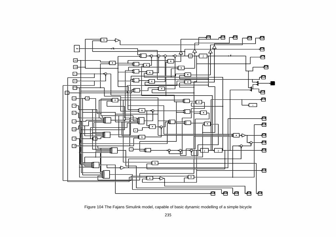
Figure 104 The Fajans Simulink model, capable of basic dynamic modelling of a simple bicycle
235

Figure 105 A simplified Simulink model able to reproduce Fajans’ results
236

Figure 106 A more complex Simulink model, with all elements added for analysis of torque terms and sensitivity of parameters
237

Figure 107 Simulink steering torque subassembly, capable of being adjusted for different amplitude and time lag values
Produces a ramp of any defined gain & delay (in this case
Squares off the ramp at a constant value
Produces a negative ramp of the same gain (in this case
1.11)
Repeats the first jerk input at any gain and transport value
238
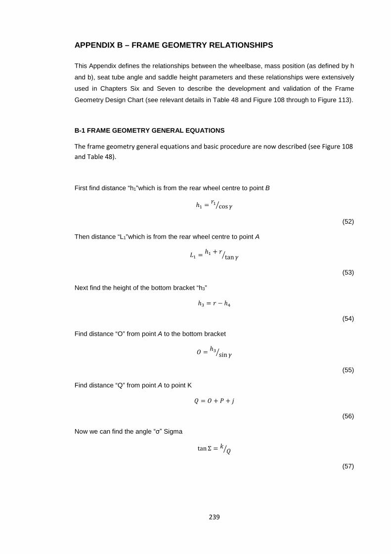
APPENDIX B – FRAME GEOMETRY RELATIONSHIPS
This Appendix defines the relationships between the wheelbase, mass position (as defined by h
and b), seat tube angle and saddle height parameters and these relationships were extensively
used in Chapters Six and Seven to describe the development and validation of the Frame
Geometry Design Chart (see relevant details in Table 48 and Figure 108 through to Figure 113).
B-1 FRAME GEOMETRY GENERAL EQUATIONS
The frame geometry general equations and basic procedure are now described (see Figure 108 and Table 48).
First find distance “h1”which is from the rear wheel centre to point B
ℎ1 = 𝑟𝑟1 cos 𝛾𝛾�
(52)
Then distance “L1”which is from the rear wheel centre to point A
𝐿𝐿1 = ℎ1 + 𝑟𝑟tan 𝛾𝛾�
(53)
Next find the height of the bottom bracket “h3”
ℎ3 = 𝑟𝑟 − ℎ4
(54)
Find distance “O” from point A to the bottom bracket
𝑂𝑂 = ℎ3sin 𝛾𝛾�
(55)
Find distance “Q” from point A to point K
𝑄𝑄 = 𝑂𝑂 + 𝑃𝑃 + 𝑗𝑗
(56)
Now we can find the angle “σ” Sigma
tan Σ = 𝑘𝑘𝑄𝑄�
(57)
239

This allows distance “i” to be found (from the bottom bracket to centre of mass or COM)
𝑠𝑠 = 𝑄𝑄 cosΣ
(58)
Find intermediate horizontal distance “L2”
𝐿𝐿2 = 𝑠𝑠 cos(Σ + 𝛾𝛾)
(59)
This allows the important dimension “b” to be found (the horizontal distance from the centre of the
rear wheel to the centre of mass)
𝑏𝑏 = 𝐿𝐿1 − 𝐿𝐿2
(60)
Also equation (60) can be expanded out to:
𝑏𝑏 = �(𝑟𝑟1 cos 𝛾𝛾⁄ ) + 𝑟𝑟
tan 𝛾𝛾� − �
� ℎ3sin 𝛾𝛾� + 𝑃𝑃 + 𝑗𝑗
tan 𝛾𝛾� cos(Σ + 𝛾𝛾)
(61)
Finally distance “h” can be found (the vertical distance from the ground to the centre of mass)
ℎ = 𝑠𝑠 sin(Σ + 𝛾𝛾)
(62)
And equation (62) can be expanded out to
ℎ = �� ℎ3
sin 𝛾𝛾� + 𝑃𝑃 + 𝑗𝑗
cos Σ� sin(Σ + 𝛾𝛾)
(63)
The frame size, wheelbase and saddle height relationships used in Chapter Six are summarised
as follows:
Saddle height “P” equals:
𝑃𝑃 = 0.885 × 𝐼𝐼𝑆𝑆
(41)
Frame size “FS” equals:
𝐹𝐹𝑆𝑆 = 0.65 × 𝐼𝐼𝑆𝑆
(42)
240

Therefore:
𝐼𝐼𝑆𝑆 = 𝑃𝑃0.885�
(43)
Substitution gives:
𝐹𝐹𝑆𝑆 = �0.650.885� � × 𝑃𝑃
(44)
𝐹𝐹𝑆𝑆 = 0.735 × 𝑃𝑃
(45)
From 2013 Tour de France road bicycles (Appendix F) the empirical relationship between frame
size and wheelbase was found and giving the following line of best fit, see Figure 124
𝐿𝐿 = 0.3077 × 𝐹𝐹𝑆𝑆 + 822.5 ± 20
(39)
For the benchmark bicycle which has a frame size of 550 mm this equation gives a wheelbase of
991.74 mm (-/+ 20 or between 971.74 and 1011.74 mm) which is close to the actual benchmark
value used of 1000 mm
𝐿𝐿 = 0.3077 × 550 𝑚𝑚𝑚𝑚 + 822.5 𝑚𝑚𝑚𝑚 ± 20 𝑚𝑚𝑚𝑚
𝐿𝐿 = 991.74 𝑚𝑚𝑚𝑚 ± 20 𝑚𝑚𝑚𝑚
By substituting “P” from equation (45) the wheelbase equation becomes:
𝐿𝐿 = 0.3077 × (0.735 × 𝑃𝑃) + 822.5 ± 20
(46)
Which becomes the final equation necessary to find the toe overlap boundary:
𝐿𝐿 = 0.226 × 𝑃𝑃 + 822.5 ± 20
(47)
241

B-2 TOE LIMIT LINE RELATIONSHIPS
This section of the Appendix uses the relationships between the wheelbase, mass position (as
defined by h and b), seat tube angle and saddle height (P) parameters and to plot the toe limit
line onto the Frame Geometry Design Chart, where the following assumptions were used:
1. Wheel diameter is 675 mm (2r)
2. Bottom bracket drop is 67.5 mm (h4)
3. Clearance between seat tube centreline and rear wheel is 32.5 mm
4. Centreline of shoe is 130 mm from centreline of bicycle in a transverse direction “d2” (this
was measured experimentally)
5. Crank length is 165 mm “d2” (measured experimentally)
6. Shoe extension from pedal spindle centreline is 120 mm”d3” (measured experimentally)
7. Maximum permitted overlap between wheel and shoe is an allowance of 10 mm, an
assumption based on rider preference (96)
The process using these equations to find the toe overlap limit line on the Frame Geometry Design
Chart was:
First find vertical distance “h1” which is from the rear wheel centre to point B
ℎ1 = 𝑟𝑟1 cos 𝛾𝛾�
(52)
Then find intermediate horizontal distance “L3” from the rear wheel centre to the bottom bracket
𝐿𝐿3 = (ℎ1 + ℎ4) tan 𝛾𝛾
(64)
Now we can find the angle “α” alpha
𝛼𝛼 = sin−1 ℎ2 𝑟𝑟�
(65)
Find intermediate radius “r2”, which allows for the vertical drop of the shoe below the centre of the
front wheel
𝑟𝑟2 = 𝑟𝑟 cos𝛼𝛼
(66)
242

Now we can find the angle “σ” sigma, which is the maximum amount of turn of the front wheel
before contact with the shoe
σ = sin−1 𝑑𝑑1 𝑟𝑟2⁄
(67)
Find the second intermediate radius “r3” which corrects the front wheel radius for turning through
angle sigma
𝑟𝑟3 = 𝑑𝑑1 tan𝜎𝜎⁄
(68)
Next find the intermediate horizontal distance “L4” (the distance from the bottom bracket centre to
the tip of the shoe) this is the space required for the shoe
𝐿𝐿4 = 𝑑𝑑2 + 𝑑𝑑3 + 𝐿𝐿3
(69)
Finally find final horizontal distance “L5” (from the centre of the rear wheel to the edge of the front
wheel when turned and allowing for the drop of the bottom bracket) this is the clearance gap
available
𝐿𝐿5 = 𝐿𝐿 − 𝑟𝑟3
(70)
Comments on the toe overlap
• if L4 (the space required) equals L5 (the gap available) then the tip of the shoe just touches
the front wheel when it is turned through angle sigma
• if L4 < L5 then there is a gap between the wheel and the shoe
• if L4 < L5 then a toe overlap occurs
• some sources say an overlap of up to 10 mm (the allowance) is tolerable (96)
• and the Frame Geometry Design Chart of Chapter Six assumes the allowance is 10 mm,
• so the toe overlap limit line in the Frame Geometry Design Chart in Chapter Six is when:
𝐿𝐿4 = 𝐿𝐿5 + 𝑎𝑎𝑎𝑎𝑎𝑎𝑐𝑐𝑤𝑤𝑎𝑎𝑠𝑠𝑐𝑐𝑒𝑒
(71)
𝑎𝑎𝑠𝑠𝑑𝑑 𝑡𝑡ℎ𝑒𝑒 𝑎𝑎𝑎𝑎𝑎𝑎𝑐𝑐𝑤𝑤𝑎𝑎𝑠𝑠𝑐𝑐𝑒𝑒 = 10 𝑚𝑚𝑚𝑚
243

Table 48 Definitions of the terms required to calculate the seat tube angle and saddle height
Symbol Parameter Units
A Intersection of seat tube centreline with ground
b Distance horizontally from rear wheel hub to centre of mass mm
B Intersection of seat tube centreline with vertical line passing
through rear wheel hub centreline
c Clearance distance between seat tube centreline and outside
of rear wheel
mm
C Point on the ground directly below the rear wheel hub’s centre
COM Centre of mass
d1 Crank sideways offset mm
d2 Crank length mm
d3 Shoe extension, from the centreline of the pedal spindle mm
D Intersection of ground and a vertical line tangential to rear of
front wheel
h Distance vertically from ground to centre of mass mm
h1 Distance vertically from rear wheel hub to B mm
h2 Distance vertically from ground to B mm
h3 Distance vertically from ground to bottom bracket spindle
centreline
mm
h4 Distance vertically from wheel hub to bottom bracket spindle
centreline (bottom bracket drop)
mm
i Distance from A to COM mm
j Distance from J to K measured parallel to seat tube mm
k Distance from K to COM measured perpendicular to seat
tube
mm
L Wheelbase mm
L1 Distance horizontally from rear wheel hub to A mm
L2 Horizontal distance from A to COM mm
L3 Distance horizontally from rear wheel hub to centre of bottom
bracket
mm
L4 Distance horizontally from C to D mm
244
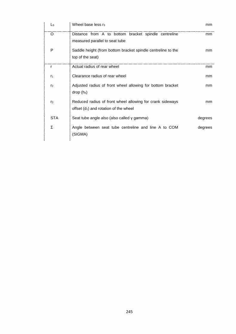
L5 Wheel base less r3 mm
O Distance from A to bottom bracket spindle centreline
measured parallel to seat tube
mm
P Saddle height (from bottom bracket spindle centreline to the
top of the seat)
mm
r Actual radius of rear wheel mm
r1 Clearance radius of rear wheel mm
r2 Adjusted radius of front wheel allowing for bottom bracket
drop (h4)
mm
r3 Reduced radius of front wheel allowing for crank sideways
offset (d1) and rotation of the wheel
mm
STA Seat tube angle also (also called γ gamma) degrees
Σ Angle between seat tube centreline and line A to COM
(SIGMA)
degrees
245

Figure 108 Defining the terms required to calculate the seat tube angle and saddle height from basic dimensions
h1
r1
h
r
h2
b
L1
L
L2
k
O
h4
h3
j
i
P
seat tube angle γ
angle Σ
centre of mass
K
A
B
C
J
246

Figure 109 Toe overlap definitions and terms, used to define the toe overlap limit on the Frame
Geometry Chart
L3
γ
h3
h4
α r
r2 r1
L
h1 h2
L - r
247
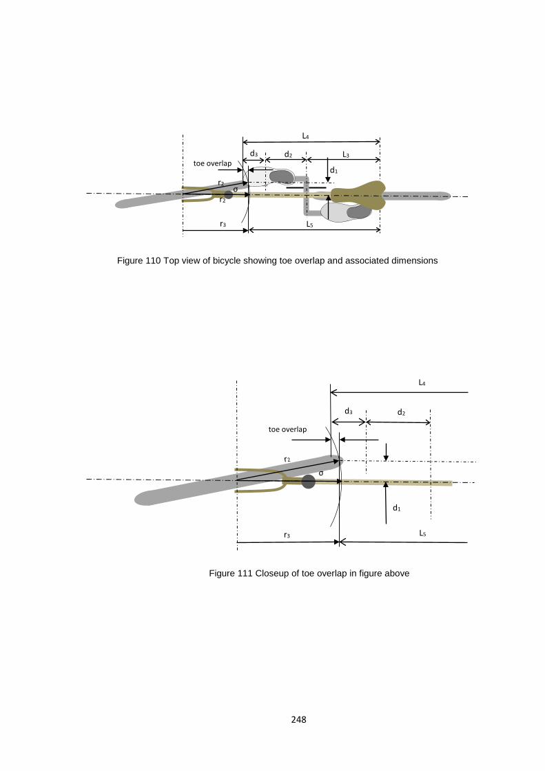
r2 σ
L5
L4
L3 d2 d3
r3
r2
toe overlap
Figure 110 Top view of bicycle showing toe overlap and associated dimensions
d1
Figure 111 Closeup of toe overlap in figure above
σ
L5
L4
d2 d3
r3
toe overlap
d1
248

Other useful terms are shown in Figure 112 and Figure 113
Figure 112 Bicycle term definitions and assemblies A and B
h
b a
L
∆
FS
STA
Assembly B
Assembly A
β
Φ
249

Figure 113 Defining the bicycle frame size, saddle height and seat tube angle
Bottom bracket spindle
Seat tube angle STA
Frame Size FS
Saddle height P
250
APPENDIX C – EXPERIMENTAL DETERMINATION OF PARAMETERS
The bicycle model needs appropriate parameter values to be determined in order for realistic
dynamic simulations to occur and also in order for the sensitivity study to be undertaken. This
Appendix discusses how these bicycle parameters were determined from: experiments,
calculations and the literature. All the parameters, their definitions and values (as used in the
Simulink model) are listed in Table 11 and Table 12.
The literature publishes a range of parameter values for actual bicycles but it is clear that many
of the bicycles studied were not representative of modern high performance road bicycles.
Typically the values are overly heavy and in the case of dimensions such as wheel diameters and
wheelbases often inaccurate. Therefore it was necessary to apply more rigour to parameter
determination in order to obtain the values necessary for this study.
It was convenient in this Appendix to group the parameters into three categories:
1. those associated with the rider (the human parameters)
2. the wheel parameters
3. and the parameters associated with rest of the bicycle, that is the bicycle main frame and
the front forks
A combination of suitable methodologies was used to determine suitable parameter values and
they enabled the determination to be achieved with some confidence. The following three
methods were used:
1. experimental methods
2. engineering calculations
3. and evaluation of the literature
The following Table 49 lists which methods were used for each individual parameter, while Table
50 provides more details on the techniques and typical accuracy.
251

Table 49 Methodologies employed to find each bicycle parameter
Symbol Parameter definition Units Methodologies used
human parameters M mass of rider kg • experimental method using scales
• reference to literature b horizontal distance from the
rear wheel hub to the centre of rider mass
m • experimental method using suspension technique
• calculations • reference to literature
h height of centre of rider mass m • experimental method using suspension technique
• calculations • reference to literature
- Rider height, inseam length, torso length, leg and arm lengths
m • experimental method using rule and tape
IX moment of inertia of rider about X axis (roll)
kgm2 • calculations • reference to literature
IZ moment of inertia of rider about Z axis (yaw)
kgm2 • calculations • reference to literature
wheel parameters Iw moment of inertia of wheels
about X, Y and Z axes kgm2 • experimental method using compound
pendulum • calculations • reference to literature
D diameter of the bicycle wheel m • experimental method using rule • reference to literature
parameters associated with rest of the bicycle IXA moment of inertia of
assembly A (excluding rider) about X axis (roll)
kgm2 • experimental method using compound & bifilar pendulum
• reference to literature IXB moment of inertia of
assembly B (excluding rider) about X axis (roll)
kgm2 • experimental method using compound & bifilar pendulum
• calculations • reference to literature
IZA moment of inertia of assembly A (excluding rider) about Z axis (yaw)
kgm2 • experimental method using compound & bifilar pendulum
• reference to literature L bicycle wheelbase m • experimental method using tape
• reference to literature b horizontal distance from the
rear wheel hub to the centre of mass of bicycle
m • experimental method using suspension technique
• calculations • reference to literature
h height of centre of mass of bicycle
m • experimental method using suspension technique
• calculations • reference to literature
M mass of bicycle kg • experimental method using scales • reference to literature
Φ head tube angle degrees • experimental method using angle protractor • reference to literature
β fork rake (or offset) m • experimental method using rule and straight edge
• reference to literature 252
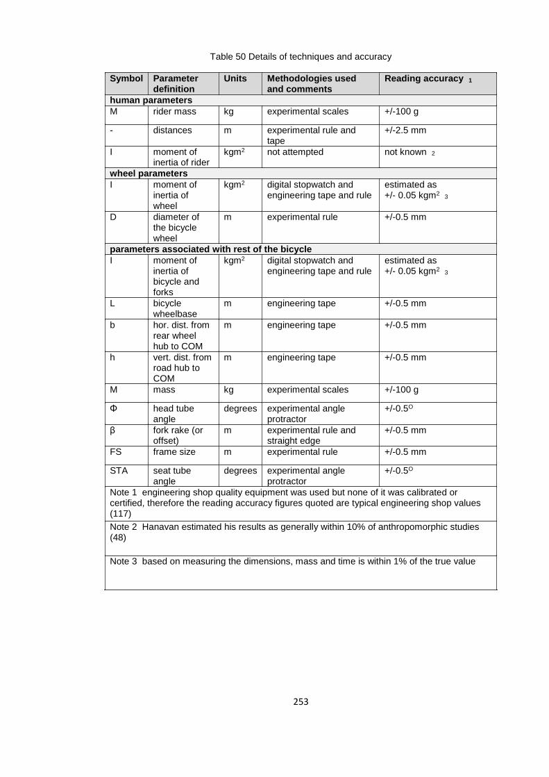
Table 50 Details of techniques and accuracy
Symbol Parameter definition
Units Methodologies used and comments
Reading accuracy 1
human parameters M rider mass kg experimental scales +/-100 g
- distances m experimental rule and tape
+/-2.5 mm
I moment of inertia of rider
kgm2 not attempted not known 2
wheel parameters I moment of
inertia of wheel
kgm2 digital stopwatch and engineering tape and rule
estimated as +/- 0.05 kgm2 3
D diameter of the bicycle wheel
m experimental rule +/-0.5 mm
parameters associated with rest of the bicycle I moment of
inertia of bicycle and forks
kgm2 digital stopwatch and engineering tape and rule
estimated as +/- 0.05 kgm2 3
L bicycle wheelbase
m engineering tape +/-0.5 mm
b hor. dist. from rear wheel hub to COM
m engineering tape +/-0.5 mm
h vert. dist. from road hub to COM
m engineering tape +/-0.5 mm
M mass kg experimental scales +/-100 g
Φ head tube angle
degrees experimental angle protractor
+/-0.5O
β fork rake (or offset)
m experimental rule and straight edge
+/-0.5 mm
FS frame size m experimental rule +/-0.5 mm
STA seat tube angle
degrees experimental angle protractor
+/-0.5O
Note 1 engineering shop quality equipment was used but none of it was calibrated or certified, therefore the reading accuracy figures quoted are typical engineering shop values (117) Note 2 Hanavan estimated his results as generally within 10% of anthropomorphic studies (48)
Note 3 based on measuring the dimensions, mass and time is within 1% of the true value
253
C-1 HUMAN PARAMETERS
The model requires values for various human body parameters namely: mass, mass position and
moments of inertia and though human subjects are simple to measure in terms of mass and
dimensions such as height, they are more problematic with regards to measuring moments of
inertia, particularly when a subject is in a cycling posture.
Some unsuccessful attempts were made to experimentally measure human moments of inertia
using the bifiliar pendulum method. But it was found to be surprisingly difficult to obtain even
approximate results due to the practical difficulties encountered and no useful results were
obtained. It proved to be physically difficult to effectively suspend a person in the available
workshop space due to a lack of headroom. In addition the slight changes in posture of a non-
rigid human subject meant a wide variation in the recorded period was observed. Trying to sit still
in a position that approximates the position of a seated rider on a bicycle was not easy.
Rather than spend more time trying to solve these problems it was decided after reviewing the
available literature to rely on the exhaustive and authoritative work of Hanavan and others (48,
79). These studies have examined a large group of subjects with a wide range of body shapes
and weights (covering the 5th, 25th, 50th, 75th and 95th percentile groups) and have collated detailed
tables for body heights, other dimensions, masses, COM positions and moments of inertia for
many standard human postures, including several closely approximating a rider on a bicycle. One
limitation of this study was that the subject population was exclusively male, so more work needs
to be done to obtain accurate parameter values for female riders. We note one simple method
found in the literature was claimed to be reasonably accurate for a standing subject. This was the
Brenière method for calculating moments of inertia and uses the following two equations, where
m is the subject’s mass and H is the subject’s height (118):
𝐼𝐼𝑋𝑋 = 0.0572𝑚𝑚𝐻𝐻2
(72)
𝐼𝐼𝑌𝑌 = 0.0533𝑚𝑚𝐻𝐻2
(73)
Unfortunately this is no help for determining the moment of inertia for a rider on a bicycle because
these formulas apply to only a standing person.
254

From this evaluation of the literature the human body parameter values used in this study are
outlined in Table 51 and the values of particular interest for the benchmark bicycle are:
• It is assumed to be for Hanavan position no 18 (approximating a sitting rider, see Figure
14)
• The rider is a 95% male
• Height when standing = 1.857 m
• Total Mass = 91.05 kg
• Vertical position of COM measured from top of head = 0.686 m (or 1.171 m from
ground)
• IX lateral axis= 9.84 kgm2
• IY transverse axis= 11.34 kgm2
• IZ longitudinal axis= 3.84 kgm2
255
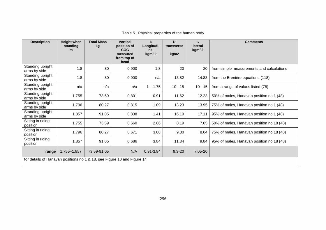
Table 51 Physical properties of the human body
Description Height when standing
m
Total Mass kg
Vertical position of
COG measured
from top of head
IZ Longitudi-
nal kgm^2
IY transverse
kgm2
IX lateral kgm^2
Comments
Standing upright arms by side 1.8 80 0.900 1.8 20 20 from simple measurements and calculations
Standing upright arms by side 1.8 80 0.900 n/a 13.82 14.83 from the Brenière equations (118)
Standing upright arms by side n/a n/a n/a 1 – 1.75 10 - 15 10 - 15 from a range of values listed (78)
Standing upright arms by side 1.755 73.59 0.801 0.91 11.62 12.23 50% of males, Hanavan position no 1 (48)
Standing upright arms by side 1.796 80.27 0.815 1.09 13.23 13.95 75% of males, Hanavan position no 1 (48)
Standing upright arms by side 1.857 91.05 0.838 1.41 16.19 17.11 95% of males, Hanavan position no 1 (48)
Sitting in riding position 1.755 73.59 0.660 2.66 8.19 7.05 50% of males, Hanavan position no 18 (48)
Sitting in riding position 1.796 80.27 0.671 3.08 9.30 8.04 75% of males, Hanavan position no 18 (48)
Sitting in riding position 1.857 91.05 0.686 3.84 11.34 9.84 95% of males, Hanavan position no 18 (48)
range 1.755–1.857 73.59-91.05 N/A 0.91-3.84 9.3-20 7.05-20
for details of Hanavan positions no 1 & 18, see Figure 10 and Figure 14
256
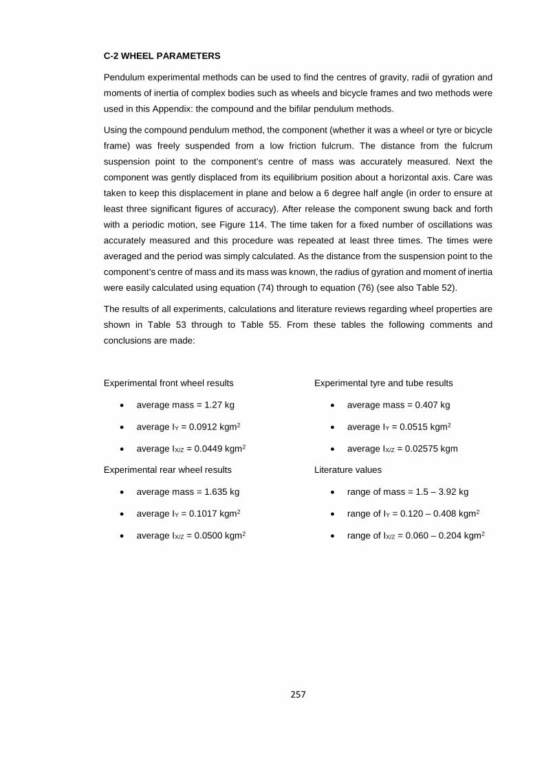
C-2 WHEEL PARAMETERS
Pendulum experimental methods can be used to find the centres of gravity, radii of gyration and
moments of inertia of complex bodies such as wheels and bicycle frames and two methods were
used in this Appendix: the compound and the bifilar pendulum methods.
Using the compound pendulum method, the component (whether it was a wheel or tyre or bicycle
frame) was freely suspended from a low friction fulcrum. The distance from the fulcrum
suspension point to the component’s centre of mass was accurately measured. Next the
component was gently displaced from its equilibrium position about a horizontal axis. Care was
taken to keep this displacement in plane and below a 6 degree half angle (in order to ensure at
least three significant figures of accuracy). After release the component swung back and forth
with a periodic motion, see Figure 114. The time taken for a fixed number of oscillations was
accurately measured and this procedure was repeated at least three times. The times were
averaged and the period was simply calculated. As the distance from the suspension point to the
component’s centre of mass and its mass was known, the radius of gyration and moment of inertia
were easily calculated using equation (74) through to equation (76) (see also Table 52).
The results of all experiments, calculations and literature reviews regarding wheel properties are
shown in Table 53 through to Table 55. From these tables the following comments and
conclusions are made:
Experimental front wheel results
• average mass = 1.27 kg
• average IY = 0.0912 kgm2
• average IX/Z = 0.0449 kgm2
Experimental rear wheel results
• average mass = 1.635 kg
• average IY = 0.1017 kgm2
• average IX/Z = 0.0500 kgm2
Experimental tyre and tube results
• average mass = 0.407 kg
• average IY = 0.0515 kgm2
• average IX/Z = 0.02575 kgm
Literature values
• range of mass = 1.5 – 3.92 kg
• range of IY = 0.120 – 0.408 kgm2
• range of IX/Z = 0.060 – 0.204 kgm2
257

Overall comments:
1. The experimental results show that the rear wheels are slightly heavier than the front wheels
with slightly higher moment of inertia, but a reasonable approximation of values for both front
and rear wheels is:
a. mass = 1.4 kg
b. IY = 0.100 kgm2
c. IX/Z = 0.050 kgm2
2. The experimental values of tyres/tubes show that they contribution between 45 to 55% of the
total moment of inertia of the complete wheel system (rim, spokes, hub, tyre and tube)
3. The values from the literature are without exception not appropriate for modern high
performance road bicycles with the values being far too high for masses and moments of
inertia (from 20 to 400% too high)
Compound pendulum equations
𝑡𝑡 = 2𝜋𝜋��𝑘𝑘𝑌𝑌 + ℎ2𝑀𝑀ℎ� �
(74)
𝑘𝑘𝑌𝑌 = ��𝑀𝑀ℎ𝑡𝑡2
4𝜋𝜋2� � − ℎ2
(75)
𝐼𝐼𝑌𝑌 = 𝑀𝑀𝑘𝑘𝑌𝑌2
(76)
Table 52 terms used in compound pendulum equations
Symbol Term definition Units
t period of oscillation sec/cycle
kY radius of gyration about Y axis m
h distance from suspension point to centre of mass
m
M mass of body (wheel) kg
I wheels moment of inertia of body (wheel) about Y axis kgm2
258

Freely suspended body oscillating
h
Rigid suspension point
Figure 114 A compound pendulum setup to determine the bicycle wheel’s moment of inertia
259

Table 53 Front wheel experimental results for mass and moments of inertia
Wheel type
Tyre type Mass kg
IY Pitch/rotational
kgm^2
IX/IZ yaw/roll kgm^2
Comments
700C x 23 wheel 700Cx23 1.220 0.0918 0.0473 I values from a simple engineering calculation
Mavic SUP Open Pro Suntour hub Hutchinson 700Cx23 1.424 0.0871 0.0492 from compound pendulum
experiments
Mavic MA3 Campagnola Chorus hub Hutchinson 700Cx23 1.440 0.1077 0.0520
from compound pendulum experiments
Mavic MA3 Campagnola Chorus hub none 0.958 0.0571 0.0286 1
from compound pendulum experiments
Shimano 105 rim & hub Hutchinson 700Cx23 1.397 0.1095 0.0506 from compound pendulum experiments
ALTX 2800 A class Hub Michelin Dynamic 700Cx23 1.162 0.0845 0.0421
from compound pendulum experiments
Airline Vuelta Shimano Ultegra hub Clement Ultra performance 700Cx23 1.292 0.1006 0.0445
from compound pendulum experiments
average 1.2704 0.0912 0.0449
Note 1 this value was not found experimentally but was calculated from IX = ½ IY
All wheels are 700C
260

Table 54 Rear wheel experimental results for mass and moments of inertia
Wheel type
Gear cluster Tyre type Mass kg
IY kgm^2
pitch/rotational
IX/IZ kgm^2 yaw/roll
Comments
Mavic Aksium Race rim & hub No gears Hutchinson 700Cx23 1.494 0.1020 0.0489
from compound pendulum experiments
Mavic SUP Campagnola Chorus hub
10 speed Campagnola Chorus cluster
Hutchinson 700Cx23 1.766 0.1017 0.0499 from compound pendulum experiments
Mavic SUP Shimano Ultegra hub No gears Clement Ultra
performance 700Cx23 1.536 0.1014 0.0507 1 from compound pendulum experiments
Shimano 105 rim & hub 9 speed Shimano cluster Hutchinson 700Cx23 1.894 0.1054 0.0527
from compound pendulum experiments
ALTX 2800 A class Hub No gears or skewer Hutchinson 700Cx23 1.487 0.0979 0.0477
from compound pendulum experiments
average 1.635 0.1017 0.0500
Note 1 this value was not found experimentally but was calculated from IX = ½ IY
All wheels are 700C
261

Table 55 Tyre and tube only experimental results for mass and moments of inertia
Tyre type Tyre condition Tube type Total Mass kg
IY kgm^2
pitch/rotational
Comments
700Cx23 n/a 700Cx23 0.359 0.0459 I values from a simple calculation
Hutchinson 700Cx23 new Continental Race
700Cx18/25 0.496 0.0522 from compound pendulum experiments
WTB Carmino 700Cx23 worn Continental Race
700Cx18/25 0.406 0.0421 from compound pendulum experiments
Maxxis Detonator 700Cx23 worn Continental Race
700Cx18/25 0.377 0.0401 from compound pendulum experiments
Maxxis Detonator 700Cx23 worn Continental Race
700Cx18/25 0.379 0.0427 from compound pendulum experiments
Michelin Select 700Cx28 worn Continental Race
700Cx18/25 0.601 0.0642 from compound pendulum experiments
Michelin World Tour 700Cx32
new Continental Race 700Cx18/25 0.674 0.0733
from compound pendulum experiments
average 0.4703 0.0515
these results are for the tyres and tubes only and all are 700C, it excludes the wheel rim, hub and spokes
262

Table 56 Literature results for wheel mass and moments of inertia
Wheel type Radius
m
Total Mass
kg
IY pitch/rotational
kgm^2
IX/IZ yaw/roll kgm^2
Comments Source
front wheel 0.350 3.00 0.280 0.140 Front wheel carrying measuring apparatus which increases weight (14)
front wheel 0.342 2.02 0.162 0.081 heavy and small diameter (44)
front wheel 0.325 2.09 0.218 0.109 heavy and very small diameter (60)
front & rear wheels 0.350 1.50 0.140 0.070 small diameter (13)
front & rear wheels n/a 2.15 0.134 0.046 heavy (28)
front & rear wheels n/a n/a 0.095 n/a (12)
rear wheel 0.300 2.00 0.120 0.060 very small diameter (14)
rear wheel 0.342 3.12 0.156 0.078 heavy and small diameter (44)
rear wheel 0.325 3.92 0.408 0.204 very heavy and very small diameter (60)
263
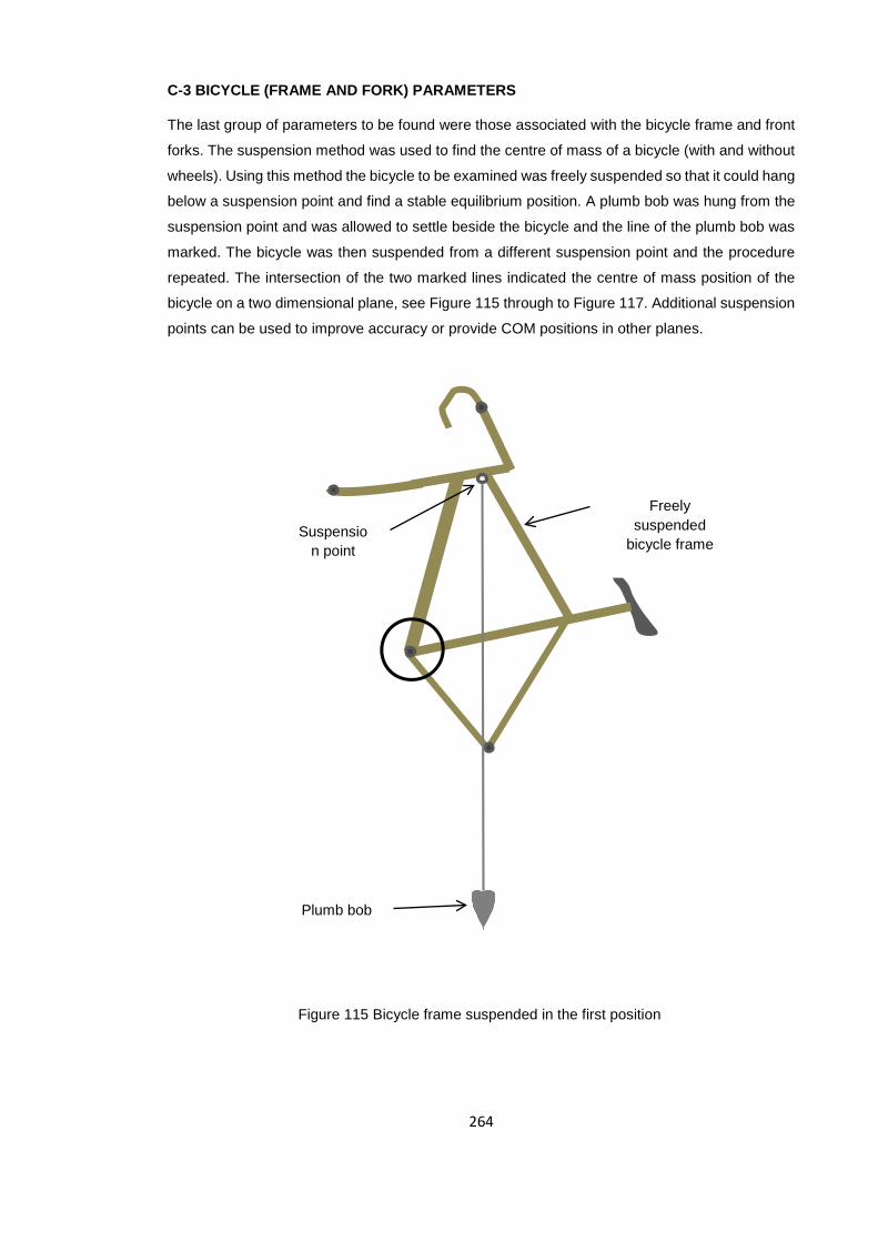
C-3 BICYCLE (FRAME AND FORK) PARAMETERS
The last group of parameters to be found were those associated with the bicycle frame and front
forks. The suspension method was used to find the centre of mass of a bicycle (with and without
wheels). Using this method the bicycle to be examined was freely suspended so that it could hang
below a suspension point and find a stable equilibrium position. A plumb bob was hung from the
suspension point and was allowed to settle beside the bicycle and the line of the plumb bob was
marked. The bicycle was then suspended from a different suspension point and the procedure
repeated. The intersection of the two marked lines indicated the centre of mass position of the
bicycle on a two dimensional plane, see Figure 115 through to Figure 117. Additional suspension
points can be used to improve accuracy or provide COM positions in other planes.
Suspension point
Plumb bob
Freely suspended
bicycle frame
Figure 115 Bicycle frame suspended in the first position
264

Figure 116 Bicycle frame suspended in the second position
Freely suspended bicycle frame in a second position
265

Centre of mass at the intersection
point
First marked
vertical line
Figure 117 The location of the centre of mass is indicated by the intersection point
266

The bifilar pendulum method was used to find the moment of inertia of the bicycle and uses a
similar procedure to the compound pendulum method. This time though the component (the
bicycle frame) was freely suspended from two light and equal length cables. The length of each
cable and the horizontal position of the bicycle frame’s centre of gravity (previously found) relative
to each cable was measured. The bicycle frame was gently displaced from its equilibrium position,
this time about a vertical axis and again the displacement is in plane and below a 6 degree half
angle. After release the bicycle frame swung backwards and forwards in a periodic motion and
the time taken for a number of oscillations was accurately measured (again this was repeated at
least three times and the results averaged and the period calculated). Having measured the length
of each cable, the distance from each cable to the component’s centre of gravity and the mass,
the radius of gyration and moment of inertia are calculated using equation (77) through to equation
(79).
𝑡𝑡 = 2𝜋𝜋�𝐼𝐼𝐿𝐿 𝑀𝑀𝑀𝑀𝑎𝑎𝑏𝑏�
(77)
𝐼𝐼 = �𝑡𝑡
2𝜋𝜋�2 𝑀𝑀𝑀𝑀𝑎𝑎𝑏𝑏
𝐿𝐿
(78)
𝐼𝐼 = 𝑀𝑀𝑘𝑘2
(79)
Table 57 Bifilar pendulum terms
Symbol Term definition Units
t Period of oscillation sec/cycle
k Radius of gyration about a vertical axis (Z) m
L Distance from suspension points to centre of mass (length of each cord)
m
a Horizontal distance from left hand cord to the body’s centre of mass
m
b Horizontal distance from right hand cord to the body’s centre of mass
m
M Mass of body kg
I Moment of inertia of body about a vertical (Z) axis
kgm2
note it is often possible to arrange values a and b so they are equal and this simplifies the experiment
267

It can be seen from these tables (Table 58 and Table 59 ) that more work needs to be done to
obtain a greater range of experimental and calculated results, but they are better values than
those of the literature (Table 60). The values in this table are incomplete and as is common in the
literature, the wheel values are based on non-competitive bicycles that have less relevance to
this study.
Freely suspended oscillating body (bicycle frame)
One of two suspension points
One of two equal length cords
L
b
a
Figure 118 The bifilar pendulum experimental apparatus
268
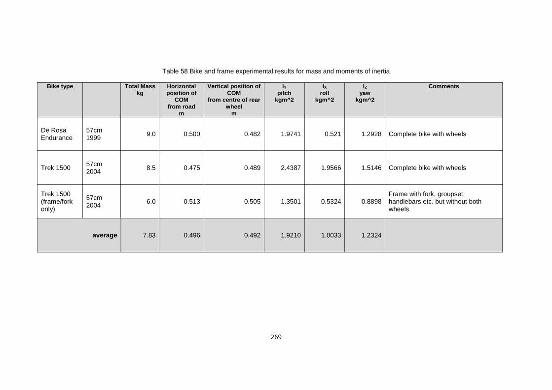
Table 58 Bike and frame experimental results for mass and moments of inertia
Bike type Total Mass kg
Horizontal position of
COM from road
m
Vertical position of COM
from centre of rear wheel
m
IY pitch
kgm^2
IX roll
kgm^2
IZ yaw
kgm^2
Comments
De Rosa Endurance
57cm 1999 9.0 0.500 0.482 1.9741 0.521 1.2928 Complete bike with wheels
Trek 1500 57cm 2004 8.5 0.475 0.489 2.4387 1.9566 1.5146 Complete bike with wheels
Trek 1500 (frame/fork only)
57cm 2004 6.0 0.513 0.505 1.3501 0.5324 0.8898
Frame with fork, groupset, handlebars etc. but without both wheels
average 7.83 0.496 0.492 1.9210 1.0033 1.2324
269

Table 59 Front fork engineering calculations results for mass and moments of inertia
Bike type for fork, stem, Handlebars &
wheel (assembly A)
Total Mass
kg
Horizontal position of COM from road m
Vertical position of COM from centre of front wheel m
IY pitch
kgm^2
IX roll
kgm^2
IZ yaw
kgm^2
Comments
Generic type 2.200 0.444 0.106 n/a 0.2250 0.0758 values from a simple calculation
De Rosa Endurance 57cm 1999 year
1.693 0.4495 0.053 n/a 0.6554 0.3851 calculated using experimentally measure values for
wheels and forks (but not the handlebar and stem)
average 1.9465 0.44675 0.0795 n/a 0.4402 0.2305
270

Table 60 Literature results for bicycles, frames & subassemblies for mass and moments of inertia
Assembly Total Mass
kg
IY pitch
kgm^2
IX roll
kgm^2
IZ yaw
kgm^2
Comments Source
Front fork assembly n/a n/a 0.84 0.079 (12)
Front fork assembly 4.0 0.06 0.0546 0.0114 excessively heavy (14)
Front fork assembly 2.0 3.88 3.28 0.566 (13)
Front fork assembly 4.3 n/a 0.345 0.065 excessively heavy (44)
Front fork assembly 4.04 0.384 0.421 0.041 excessively heavy (60)
Rear assembly only (no wheel or rider) 11.05 1.934 0.407 1.558 excessively heavy (60)
Rear assembly & rider n/a n/a 163.0 n/a about roll axis at road level not about axis through COM (12)
Rear assembly & rider 87.0 n/a n/a n/a moderately heavy (13)
Rear assembly & rider 85.0 11.0 9.20 2.80 moderately heavy (14)
Rear assembly & rider 116 n/a 16.784 6.035 excessively heavy (44)
271
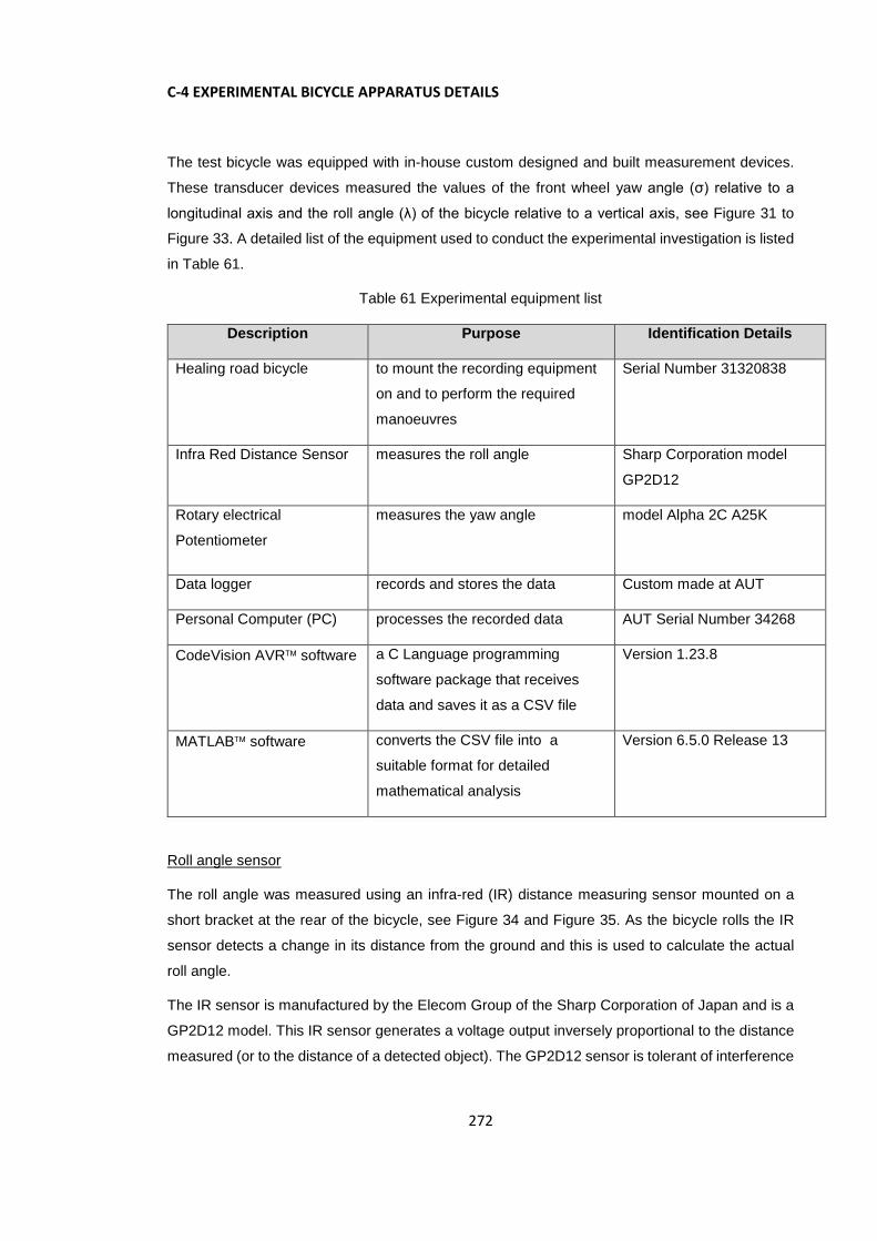
C-4 EXPERIMENTAL BICYCLE APPARATUS DETAILS
The test bicycle was equipped with in-house custom designed and built measurement devices.
These transducer devices measured the values of the front wheel yaw angle (σ) relative to a
longitudinal axis and the roll angle (λ) of the bicycle relative to a vertical axis, see Figure 31 to
Figure 33. A detailed list of the equipment used to conduct the experimental investigation is listed
in Table 61.
Table 61 Experimental equipment list
Description Purpose Identification Details
Healing road bicycle to mount the recording equipment
on and to perform the required
manoeuvres
Serial Number 31320838
Infra Red Distance Sensor measures the roll angle Sharp Corporation model
GP2D12
Rotary electrical
Potentiometer
measures the yaw angle model Alpha 2C A25K
Data logger records and stores the data Custom made at AUT
Personal Computer (PC) processes the recorded data AUT Serial Number 34268
CodeVision AVR software a C Language programming
software package that receives
data and saves it as a CSV file
Version 1.23.8
MATLAB software converts the CSV file into a
suitable format for detailed
mathematical analysis
Version 6.5.0 Release 13
Roll angle sensor
The roll angle was measured using an infra-red (IR) distance measuring sensor mounted on a
short bracket at the rear of the bicycle, see Figure 34 and Figure 35. As the bicycle rolls the IR
sensor detects a change in its distance from the ground and this is used to calculate the actual
roll angle.
The IR sensor is manufactured by the Elecom Group of the Sharp Corporation of Japan and is a
GP2D12 model. This IR sensor generates a voltage output inversely proportional to the distance
measured (or to the distance of a detected object). The GP2D12 sensor is tolerant of interference
272

from ambient light and differences in the color of objects being detected. For example it is possible
to detect a black wall in full sunlight.
The output voltage signal from the CCD array will vary depending upon the amount of surface
exposed to the IR beam. This voltage signal is used to determine the angle of reflection and
therefore the distance to the surface. The angle of reflection can be found using the tan
relationship and this indicates a non-linear relationship.
The graph shown in Figure 119 is of the output voltage vs. distance for the IR distance sensor
and clearly shows that the output within the manufacturer’s stated range of 10 cm - 80 cm, is not
linear but is approximately logarithmic. It is necessary to calibrate and linearise the sensor’s
output using either a lookup table or a parametric function.
The graph also shows that once the sensor moves inside a certain distance range (i.e. below 10
cm); the output drops rapidly and starts to repeat values matching long range readings. The
solution to this problem is to attach the sensor to the bicycle so that it will always be at least 10
cm above the ground even when the bicycle rolls to the maximum angle of 10o. From Figure 119
it is clear that the best resolution for this sensor is when the distance measured ranges between
10 to 20 mm. This is because within this range the slope of the graph is steepest and is
approximately linear.
Roll Angle Calculations
The IR distance sensor is located on a cantilevered bracket in a fixed position, making it possible
to calculate the roll angle. The transverse position of the sensor (distance N) is fixed at 150 mm
from the bicycle’s centreline while the vertical position (distance K) is fixed at 140 mm above the
ground. These positions have been calculated to give the best performance in terms of the IR
sensor’s performance. As the bicycle rolls, the IR sensor measures the change in distance to the
ground (distance M), see Figure 34 and Figure 35. The roll angle λ is calculated from the following
formula:
−
=λ −
NMK1tan
(80)
From the values in Table 62, the worst IR sensor resolution is calculated as 0.357 degree per
digital output value, [5 degrees ÷ (158-144) = 0.357]. The graph shown in Figure 120 represents
the relation between the roll angle and the digital output and shows an approximately linear
relation between them. Note that the maximum roll angle required to be measured was set at +/-
10° due to the limitations of the IR sensor.
273

Figure 119 Output voltage vs. distance for the IR distance sensor (model GP2D12)
274

Table 62 IR sensor roll output values vs. roll angle
Roll angle of the bicycle
(degrees)
Sensor distance M (mm)
Analogue output voltage (V)
Digital output 1
-10o 113.55 2.1577 158
-5o 127.00 1.9662 144
0o 140.00 1.8140 133
5o 153.12 1.6900 124
10o 166.45 1.5830 116
Note 1 using 8 bit resolution and converted from the analogue voltage
0
50
100
150
200
-20 -15 -10 -5 0 5 10 15 20 roll angle (degrees)
dig
ita
l o
utp
ut
Figure 120 IR sensor roll angle vs. digital output
275

Memory Capacity Calculations
The sensor outputs are converted into a digital format by the microcontroller and stored in an
external SRAM (static random access memory) ready for further processing. Since the memory
used in this project is a 32K x 8 bits SRAM, it contains 32768 (32 x 1024) memory positions or
spaces to store information. Both the roll and yaw angle values come in an 8-bit format and are
stored in two different memory positions, therefore two memory positions are required every time
a sample is made. So the maximum possible number of samples will be, 32768 ÷2 = 16384
samples.
The sampling rate is set at once per 10 ms and therefore 100 samples are made every second.
This means that the maximum memory capacity is: 16384 samples ÷100 samples/sec = 163.84
seconds and this means the data logger can record a maximum of 2.73 minutes of experimental
run time.
Yaw angle sensor
The yaw angle was measured using a rotary electrical potentiometer, of model type Alpha 2C A25K.
The measurement principle employed by a potentiometer is that a change in resistance occurs
as the steering stem is rotated making it possible to get an output proportional to the yaw angle
of the front wheel. The potentiometer was directly attached to the steering stem using a simple
rubber coupling, see Figure 33. The potentiometer (with a range of 0-20 MΩ, MegaOhms) was
arranged so that a 10 MΩ output equals the zero degrees yaw angle. This places the straight ahead
position of the handlebars exactly halfway within the operating range. Therefore an output signal of
between 0-10 MΩ indicates left hand turns while a 10-20 MΩ signal indicates right hand turns.
Sensor calibration
When describing the performance of any measurement sensor, three main terms are frequently
used:
• accuracy i.e. how close the recorded value is to the true value
• sensitivity i.e. the smallest input to which the sensor can respond
• precision i.e. the agreement amongst a set of readings
In order to define a particular sensor in relation to these terms it is necessary to calibrate the
sensor. Calibration will measure each particular type of error for the sensors and allow corrective
adjustments to be made. The standard procedure to calibrate a sensor is to adjust linearity at 50
% of the full scale range. Next, the span is adjusted at 90 % of the full scale range and finally any
zero error is corrected at 10 % of the scale. The span and zero errors continue to be corrected
until no further adjustment is needed. See the glossary for a definition of these calibration terms.
276

Calibration Procedure
A calibration record plotting the sensor’s reading against the true value should be prepared for
the sensor over its working range. The roll angle and yaw angle sensors were calibrated to give
error free results and the calibration apparatus that was used included:
1. engineer’s level
2. steel rule
3. plumb bob
4. assorted engineering clamps
5. flexible tape measure, twenty metres long
Both sensors were first checked to make sure their sign values (plus or minus) were correct.
These can be easily changed by changing sign terms in the Matlab programme that converts the
CSV file into a series of angular readings in degrees.
The IR sensor for measuring roll was checked for zero error. The bicycle was held firmly upright
in a level position that was checked by both a level and plumb bob. The data logger was switched
on and a recording was made of the roll angle. This was downloaded to a PC and processed by
Matlab to give a sensor roll angle reading in degrees. If the sensor did not read zero the position
of the roll angle transducer was moved to correct the signal. For example if the reading was
greater than zero the sensor was moved down, if it was less then zero it was moved up. As a final
check a rider was placed on the bicycle to compress the tyres to their operating condition and the
zero test repeated. The pressure in the tyres drops slowly over time and so the sensor’s height
drops which means the zero calibration should be repeated frequently.
When checking the zero error of the yaw angle sensor, the bicycle was wheeled along a marked
straight line with the handlebars locked in a fixed position. The handlebar position was adjusted
until the bicycle would follow the straight marked line for at least twenty metres. This indicated
that the steering handlebar was locked in the zero degrees position. Once this was done the data
logger was switched on and a recording made of the yaw angle. Again this was downloaded to a
PC and processed by Matlab to give yaw angle sensor reading in degrees. If the reading was not
equal to zero the position of the yaw angle transducer was rotated to correct the signal. For a
positive yaw angle error the potentiometer was rotated clockwise (when viewed from above), for
a negative reading it was rotated anticlockwise.
Due to the difficulty experienced in adjusting both sensors, the zero error was not able to be
eliminated. This experience suggests that a priority for any future investigations would be to
improve the ability of this equipment to be easily and accurately calibrated.
Records of both sensor’s calibration results were made, these tables compare recorded values
to actual values and are shown in Table 63 and Table 64.
277

Table 63 Record of the calibration data for the Roll Angle Sensor
Actual angle
(degrees)
Sensor recorded angle
(degrees)
-10 -9
-5 -4
0 +1
+5 +6
+10 +11
The roll angle sensor zero error = +1
Table 64 Record of the calibration data for the Yaw Angle Sensor
Actual angle
(degrees)
Sensor recorded angle
(degrees)
-30 -25
-20 -15
-10 -5
0 +5
+10 +15
+20 +25
+30 +35
The yaw angle sensor zero error = +50
278

C-5 REMARKS
The easiest components to experimentally check are the wheels and the tyres by using the
compound and bifilar pendulum methods which were successfully used to find values of radii of
gyration and moments of inertia. Overall the experimental values agreed closely with most of the
literature and with basic engineering calculations. The experiments were also very repeatable
with period time readings often agreeing to within 0.05 seconds.
However the experiments are moderately sensitive to measurement error of the period or mass
or dimensions. For example a 1% error in measuring the period of a bifilar pendulum leads to
about a 2% error in the value of the moment of inertia.
It was also found that different manufacturers’ wheels, rims, spoke arrangements and tyres can
make a considerable change to the moments of inertia of up to +/- 15%. This is significant because
as mentioned in Chapter 6 the wheel’s moment of inertia about the rotational axis (IZF) was found
to have some importance, a 1% increase decreases the settling time by a moderately significant
2% as noted in Chapter Five. Interestingly tyre contributes about 50% a wheel’s overall moments
of inertia. Also it was observed that even for the small selection considered in Table 55, different
manufacturers’ tyres can be over 100 grams lighter than others tyres and this will make a
subsequent 20% reduction in the moment of inertia. This was for 700 x 23 tyres and 700C X 18/25
tubes only.
Engineering calculations were possible on some components, namely wheel moments of inertia,
front forks, bicycle frame and these calculations had close agreement to the experimental values
which allows some confidence in advancing the selected values for the benchmark bicycle.
Using the methods outlined in this Appendix it was possible to select realistic parameter values
for the model including the moments of inertia for the main subassemblies of the bicycle model.
These values are now presented in the benchmark bicycle in Table 13. In addition a more
complete picture of the normal range of values has been obtained so that decisions about future
variations to the model can be made with knowledge and confidence.
279

APPENDIX D –STABILITY ANALYSIS
This Appendix details the characteristic equation, applies the Routh Stability Criterion and
performs a frequency analysis of the bicycle system.
D-1 CHARACTERISTIC EQUATION
For completeness in this Chapter the characteristic equation of the bicycle system was found as
its roots determine the character of the time response of the system and they can be used to
understand the natural transient response of the system. By equating the denominator of the
system’s transfer function equation to zero the characteristic equation is obtained. The
characteristic equation’s roots (poles) along with the roots of the numerator polynomial (zeros)
are the critical frequencies of the system.
A necessary requirement for stability is for all of the roots of the characteristic equation to have
negative real parts. So once the characteristic equation has been found the Routh Stability
Criterion can be used to find out if it has any unstable roots without actually solving them and this
is shown in this Appendix.
To find the characteristic equation from the current three equations of motion ((14, (19 and (24) it
is helpful to ignore any terms which are very small.
The first equation considers yawing moments about the vertical Z axis for the front assembly A,
equation (14) and has 8 terms, but which ones can be ignored? It was previously decided when
evaluating the significance of each torque term in section 5.3 to consider excluding any term
which has a maximum value of 10% or less of the maximum value of the largest term, unless
there is a good reason to include it. The subsequent torque term analysis concluded that two
terms could be ignored in (14: the Coriolis torque and the frame torque. This gave a simplified
version of equation (14) with only 6 terms, see below:
𝑇𝑇𝑖𝑖𝑖𝑖𝑖𝑖𝑖𝑖𝑖𝑖𝑖𝑖𝑖𝑖 +𝑇𝑇𝑔𝑔𝑦𝑦𝑖𝑖𝑔𝑔/𝑖𝑖𝑔𝑔𝑟𝑟𝑟𝑟 = 𝑇𝑇𝐶𝐶𝑖𝑖𝑖𝑖𝑖𝑖𝑖𝑖 − 𝑇𝑇𝐽𝐽𝑔𝑔𝑖𝑖𝑖𝑖𝐶𝐶 −𝑇𝑇𝑐𝑐𝑖𝑖𝐶𝐶𝑖𝑖𝑔𝑔𝑖𝑖 − 𝑇𝑇𝑑𝑑𝑖𝑖𝑓𝑓𝑑𝑑𝑖𝑖𝑖𝑖𝑔𝑔
(81)
Using coefficients E1, E2…En this becomes (see Table 62 for the En definitions)
(𝐸𝐸1 𝐷𝐷2+𝐸𝐸5 𝐷𝐷 + E4 )𝜎𝜎 + (𝐸𝐸2 𝐷𝐷 + E3)𝜆𝜆 = 𝑇𝑇𝑆𝑆
(82)
The second equation considers rolling moments about the horizontal X axis for the front assembly
A ((19) and has 8 terms, The torque term analysis concluded that two terms could be ignored: the
Coriolis torque and the steer torque. The simplified equation (19) with 6 terms, becomes:
𝑇𝑇𝑖𝑖𝑖𝑖𝑖𝑖𝑖𝑖𝑖𝑖𝑖𝑖𝑖𝑖 −𝑇𝑇𝑔𝑔𝑦𝑦𝑖𝑖𝑔𝑔/𝑦𝑦𝑖𝑖𝑦𝑦 = 𝑇𝑇𝑓𝑓𝑖𝑖𝑖𝑖𝑓𝑓𝑖𝑖 + 𝑇𝑇𝑔𝑔𝑦𝑦𝑖𝑖𝑔𝑔/𝑐𝑐𝑔𝑔𝑖𝑖𝑖𝑖𝑖𝑖𝑖𝑖𝑖𝑖𝑖𝑖𝑔𝑔 +𝑇𝑇𝑐𝑐𝑖𝑖𝐶𝐶𝑖𝑖𝑔𝑔𝑖𝑖 + 𝑇𝑇𝐽𝐽𝑔𝑔𝑖𝑖𝑖𝑖𝐶𝐶
(83)
280
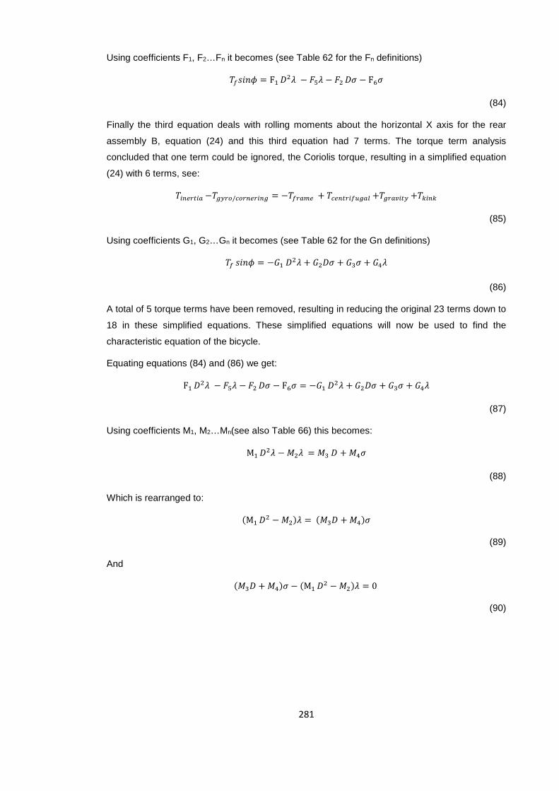
Using coefficients F1, F2…Fn it becomes (see Table 62 for the Fn definitions)
𝑇𝑇𝑓𝑓𝑠𝑠𝑠𝑠𝑠𝑠𝑠𝑠 = F1 𝐷𝐷2𝜆𝜆 − 𝐹𝐹5𝜆𝜆 − 𝐹𝐹2 𝐷𝐷𝜎𝜎 − F6𝜎𝜎
(84)
Finally the third equation deals with rolling moments about the horizontal X axis for the rear
assembly B, equation (24) and this third equation had 7 terms. The torque term analysis
concluded that one term could be ignored, the Coriolis torque, resulting in a simplified equation
(24) with 6 terms, see:
𝑇𝑇𝑖𝑖𝑖𝑖𝑖𝑖𝑖𝑖𝑖𝑖𝑖𝑖𝑖𝑖 −𝑇𝑇𝑔𝑔𝑦𝑦𝑖𝑖𝑔𝑔/𝑐𝑐𝑔𝑔𝑖𝑖𝑖𝑖𝑖𝑖𝑖𝑖𝑖𝑖𝑖𝑖𝑔𝑔 = −𝑇𝑇𝑓𝑓𝑖𝑖𝑖𝑖𝑓𝑓𝑖𝑖 + 𝑇𝑇𝑐𝑐𝑖𝑖𝑖𝑖𝑖𝑖𝑖𝑖𝑖𝑖𝑓𝑓𝑐𝑐𝑔𝑔𝑖𝑖𝑟𝑟 +𝑇𝑇𝑔𝑔𝑖𝑖𝑖𝑖𝑔𝑔𝑖𝑖𝑖𝑖𝑦𝑦 +𝑇𝑇𝑘𝑘𝑖𝑖𝑖𝑖𝑘𝑘
(85)
Using coefficients G1, G2…Gn it becomes (see Table 62 for the Gn definitions)
𝑇𝑇𝑓𝑓 𝑠𝑠𝑠𝑠𝑠𝑠𝑠𝑠 = −𝐺𝐺1 𝐷𝐷2𝜆𝜆 + 𝐺𝐺2𝐷𝐷𝜎𝜎 + 𝐺𝐺3𝜎𝜎 + 𝐺𝐺4𝜆𝜆
(86)
A total of 5 torque terms have been removed, resulting in reducing the original 23 terms down to
18 in these simplified equations. These simplified equations will now be used to find the
characteristic equation of the bicycle.
Equating equations (84) and (86) we get:
F1 𝐷𝐷2𝜆𝜆 − 𝐹𝐹5𝜆𝜆 − 𝐹𝐹2 𝐷𝐷𝜎𝜎 − F6𝜎𝜎 = −𝐺𝐺1 𝐷𝐷2𝜆𝜆 + 𝐺𝐺2𝐷𝐷𝜎𝜎 + 𝐺𝐺3𝜎𝜎 + 𝐺𝐺4𝜆𝜆
(87)
Using coefficients M1, M2…Mn(see also Table 66) this becomes:
M1 𝐷𝐷2𝜆𝜆 − 𝑀𝑀2𝜆𝜆 = 𝑀𝑀3 𝐷𝐷 + 𝑀𝑀4𝜎𝜎
(88)
Which is rearranged to:
(M1 𝐷𝐷2 − 𝑀𝑀2)𝜆𝜆 = (𝑀𝑀3𝐷𝐷 + 𝑀𝑀4)𝜎𝜎
(89)
And
(𝑀𝑀3𝐷𝐷 + 𝑀𝑀4)𝜎𝜎 − (M1 𝐷𝐷2 − 𝑀𝑀2)𝜆𝜆 = 0
(90)
281

Or
(𝑀𝑀3𝐷𝐷 + 𝑀𝑀4)𝜎𝜎 + (−M1 𝐷𝐷2 + 𝑀𝑀2)𝜆𝜆 = 0
(91)
Considering equations (82) and (91) these can be rewritten as:
𝑈𝑈1𝜎𝜎 + 𝑈𝑈2𝜆𝜆 = 𝑇𝑇𝑆𝑆
(92)
𝑉𝑉1𝜎𝜎 + 𝑉𝑉2𝜆𝜆 = 0
(93)
Converting this to a matrix form using coefficients Un and Vn (see Table 66) we get:
𝜎𝜎 + 𝑈𝑈2𝜆𝜆 = 𝑇𝑇𝑆𝑆
(94)
𝑉𝑉1𝜎𝜎 + 𝑉𝑉2𝜆𝜆 = 0
(95)
�𝑈𝑈1 𝑈𝑈2𝑉𝑉1 𝑉𝑉 2
� �𝜎𝜎𝜆𝜆� = �𝑇𝑇𝑆𝑆0 �
(96)
�(𝐸𝐸1𝐷𝐷2 − 𝐸𝐸5𝐷𝐷 + 𝐸𝐸4) (𝐸𝐸2𝐷𝐷 + 𝐸𝐸3)
(𝑀𝑀3𝐷𝐷 + 𝑀𝑀4) (𝑀𝑀2 −𝑀𝑀1𝐷𝐷2) � �𝜎𝜎𝜆𝜆� = �𝑇𝑇𝑆𝑆0 �
(97)
𝜎𝜎 =�𝑇𝑇𝑆𝑆 𝑈𝑈2
0 𝑉𝑉 2�
Δ=
𝑉𝑉2𝑇𝑇𝑆𝑆𝑈𝑈1𝑉𝑉2 − 𝑉𝑉1𝑈𝑈2
(98)
𝜆𝜆 =�𝑈𝑈1 𝑇𝑇𝑆𝑆𝑉𝑉1 0 �
Δ=
𝑉𝑉1𝑇𝑇𝑆𝑆𝑈𝑈1𝑉𝑉2 − 𝑉𝑉1𝑈𝑈2
(99)
282

The determinant of �𝑈𝑈1 𝑈𝑈2𝑉𝑉1 𝑉𝑉 2
� is equal to:
Δ = 𝑈𝑈1𝑉𝑉2 − 𝑉𝑉1𝑈𝑈2
(100)
And is the characteristic equation of the system
Δ = (𝐸𝐸1𝐷𝐷2 + 𝐸𝐸5𝐷𝐷 + 𝐸𝐸4)(𝑀𝑀2 −𝑀𝑀1𝐷𝐷2) − (𝑀𝑀3𝐷𝐷 + 𝑀𝑀4)(𝐸𝐸2𝐷𝐷 + 𝐸𝐸3)
(101)
The values for En and Mn are given in Table 65.
Also
Δ = −𝐸𝐸1𝑀𝑀1𝐷𝐷4 − 𝐸𝐸5𝑀𝑀1𝐷𝐷3 + [(𝐸𝐸1𝑀𝑀2)− (𝐸𝐸4𝑀𝑀1)− (𝐸𝐸2𝑀𝑀3)]𝐷𝐷2
+ [(𝐸𝐸5𝑀𝑀2)− (𝐸𝐸3𝑀𝑀3)− (𝐸𝐸2𝑀𝑀4)]𝐷𝐷 + 𝐸𝐸4𝑀𝑀2 − 𝐸𝐸3𝑀𝑀4
(102)
And
Δ = �𝐼𝐼𝑍𝑍𝑍𝑍𝐷𝐷2 +Γ
sin𝑠𝑠𝐷𝐷 + 𝑀𝑀
bv2
L2Δ𝑖𝑖� ��𝑀𝑀𝑀𝑀
𝑏𝑏𝐿𝐿
cos∅∆𝑖𝑖 + 𝑀𝑀𝑀𝑀ℎ� − (𝐼𝐼𝑋𝑋𝑍𝑍 + 𝐼𝐼𝑋𝑋𝑋𝑋)𝐷𝐷2�
− ��𝐼𝐼𝑌𝑌𝑌𝑌𝑣𝑣𝑟𝑟
sin∅ +𝑀𝑀ℎ𝑏𝑏𝑣𝑣𝐿𝐿
�𝐷𝐷
+ ��𝐼𝐼𝑌𝑌𝑌𝑌𝑣𝑣2
𝑟𝑟𝐿𝐿sin∅ +
𝑀𝑀𝑏𝑏𝑣𝑣2
𝐿𝐿2cos∅∆𝑖𝑖� + �
𝑀𝑀ℎ𝑣𝑣2
𝐿𝐿sin∅ + 𝐼𝐼𝑌𝑌𝑍𝑍
𝑣𝑣2
𝑟𝑟𝐿𝐿sin∅��� �𝐼𝐼𝑌𝑌𝑍𝑍
𝑣𝑣𝑟𝑟 sin𝑠𝑠
𝐷𝐷
+ 𝑀𝑀𝑀𝑀𝑏𝑏𝐿𝐿Δ𝑖𝑖�
(103)
283

Table 65 Coefficients for En, Fn and Gn
Coefficient Equal to
E1 𝐼𝐼𝑍𝑍𝑍𝑍
E2 𝐼𝐼𝑌𝑌𝑍𝑍𝑣𝑣
𝑟𝑟 sin𝑠𝑠
E3 𝑀𝑀𝑀𝑀𝑏𝑏𝐿𝐿Δ𝑖𝑖
E4 𝑀𝑀
bv2
L2Δ𝑖𝑖
E5 Γsin𝑠𝑠
F1 𝐼𝐼𝑋𝑋𝑍𝑍
F2 𝐼𝐼𝑌𝑌𝑌𝑌𝑣𝑣𝑟𝑟𝑠𝑠𝑠𝑠𝑠𝑠 𝑠𝑠
F3 𝐼𝐼𝑌𝑌𝑌𝑌
𝑣𝑣2
𝑟𝑟𝐿𝐿sin𝑠𝑠
F4 Mbv2
L2cos𝑠𝑠Δ𝑖𝑖
F5 MgbL
cos𝑠𝑠 Δ𝑖𝑖
F6 𝐹𝐹3 + 𝐹𝐹4 = 𝐼𝐼𝑌𝑌𝑌𝑌
𝑣𝑣2
𝑟𝑟𝐿𝐿sin𝑠𝑠 +
Mbv2
L2cos𝑠𝑠Δ𝑖𝑖
G1 𝐼𝐼𝑋𝑋𝑋𝑋
G2 𝑀𝑀ℎ𝑏𝑏𝑣𝑣𝐿𝐿
G3 𝑀𝑀ℎ𝑣𝑣2
𝐿𝐿sin∅ + 𝐼𝐼𝑌𝑌𝑍𝑍
𝑣𝑣2
𝑟𝑟𝐿𝐿sin∅
G4 𝑀𝑀𝑀𝑀ℎ
284
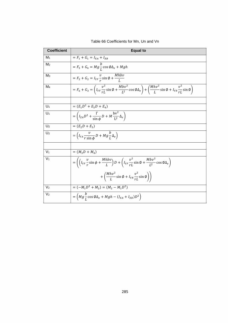
Table 66 Coefficients for Mn, Un and Vn
Coefficient Equal to
M1 = 𝐹𝐹1 + 𝐺𝐺1 = 𝐼𝐼𝑋𝑋𝑍𝑍 + 𝐼𝐼𝑋𝑋𝑋𝑋
M2 = 𝐹𝐹5 + 𝐺𝐺4 = 𝑀𝑀𝑀𝑀𝑏𝑏𝐿𝐿
cos∅∆𝑖𝑖 + 𝑀𝑀𝑀𝑀ℎ
M3 = 𝐹𝐹2 + 𝐺𝐺2 = 𝐼𝐼𝑌𝑌𝑌𝑌𝑣𝑣𝑟𝑟
sin∅ +𝑀𝑀ℎ𝑏𝑏𝑣𝑣𝐿𝐿
M4 = 𝐹𝐹6 + 𝐺𝐺3 = �𝐼𝐼𝑌𝑌𝑌𝑌
𝑣𝑣2
𝑟𝑟𝐿𝐿sin∅ +
𝑀𝑀𝑏𝑏𝑣𝑣2
𝐿𝐿2cos∅∆𝑖𝑖� + �
𝑀𝑀ℎ𝑣𝑣2
𝐿𝐿sin∅ + 𝐼𝐼𝑌𝑌𝑍𝑍
𝑣𝑣2
𝑟𝑟𝐿𝐿sin∅�
U1 = (𝐸𝐸1𝐷𝐷2 + 𝐸𝐸5𝐷𝐷 + 𝐸𝐸4)
U1 = �𝐼𝐼𝑍𝑍𝑍𝑍𝐷𝐷2 +
Γsin𝑠𝑠
𝐷𝐷 + 𝑀𝑀bv2
L2Δ𝑖𝑖�
U2 = (𝐸𝐸2𝐷𝐷 + 𝐸𝐸3)
U2 = �𝐼𝐼𝑌𝑌𝑍𝑍𝑣𝑣
𝑟𝑟 sin𝑠𝑠𝐷𝐷 + 𝑀𝑀𝑀𝑀
𝑏𝑏𝐿𝐿Δ𝑖𝑖�
V1 = (𝑀𝑀3𝐷𝐷 + 𝑀𝑀4)
V1 = ��𝐼𝐼𝑌𝑌𝑌𝑌
𝑣𝑣𝑟𝑟
sin𝑠𝑠 +𝑀𝑀ℎ𝑏𝑏𝑣𝑣𝐿𝐿
�𝐷𝐷 + �𝐼𝐼𝑌𝑌𝑌𝑌𝑣𝑣2
𝑟𝑟𝐿𝐿sin∅ +
𝑀𝑀𝑏𝑏𝑣𝑣2
𝐿𝐿2cos∅∆𝑖𝑖�
+ �𝑀𝑀ℎ𝑣𝑣2
𝐿𝐿sin∅ + 𝐼𝐼𝑌𝑌𝑍𝑍
𝑣𝑣2
𝑟𝑟𝐿𝐿sin∅��
V2 = (−𝑀𝑀1𝐷𝐷2 + 𝑀𝑀2) = (𝑀𝑀2 −𝑀𝑀1𝐷𝐷2)
V2 = �𝑀𝑀𝑀𝑀𝑏𝑏𝐿𝐿
cos∅∆𝑖𝑖 + 𝑀𝑀𝑀𝑀ℎ − (𝐼𝐼𝑋𝑋𝑍𝑍 + 𝐼𝐼𝑋𝑋𝑋𝑋)𝐷𝐷2�
285
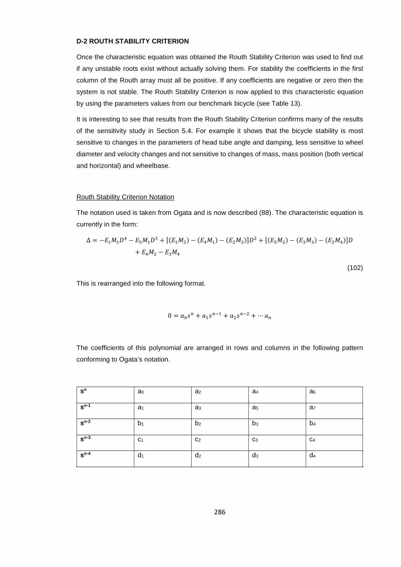
D-2 ROUTH STABILITY CRITERION
Once the characteristic equation was obtained the Routh Stability Criterion was used to find out
if any unstable roots exist without actually solving them. For stability the coefficients in the first
column of the Routh array must all be positive. If any coefficients are negative or zero then the
system is not stable. The Routh Stability Criterion is now applied to this characteristic equation
by using the parameters values from our benchmark bicycle (see Table 13).
It is interesting to see that results from the Routh Stability Criterion confirms many of the results
of the sensitivity study in Section 5.4. For example it shows that the bicycle stability is most
sensitive to changes in the parameters of head tube angle and damping, less sensitive to wheel
diameter and velocity changes and not sensitive to changes of mass, mass position (both vertical
and horizontal) and wheelbase.
Routh Stability Criterion Notation
The notation used is taken from Ogata and is now described (88). The characteristic equation is
currently in the form:
Δ = −𝐸𝐸1𝑀𝑀1𝐷𝐷4 − 𝐸𝐸5𝑀𝑀1𝐷𝐷3 + [(𝐸𝐸1𝑀𝑀2) − (𝐸𝐸4𝑀𝑀1) − (𝐸𝐸2𝑀𝑀3)]𝐷𝐷2 + [(𝐸𝐸5𝑀𝑀2) − (𝐸𝐸3𝑀𝑀3) − (𝐸𝐸2𝑀𝑀4)]𝐷𝐷
+ 𝐸𝐸4𝑀𝑀2 − 𝐸𝐸3𝑀𝑀4
(102)
This is rearranged into the following format.
0 = 𝑎𝑎0𝑠𝑠𝑖𝑖 + 𝑎𝑎1𝑠𝑠𝑖𝑖−1 + 𝑎𝑎2𝑠𝑠𝑖𝑖−2 + ⋯𝑎𝑎𝑖𝑖
The coefficients of this polynomial are arranged in rows and columns in the following pattern
conforming to Ogata’s notation.
sn a0 a2 a4 a6
sn-1 a1 a3 a5 a7
sn-2 b1 b2 b3 b4
sn-3 c1 c2 c3 c4
sn-4 d1 d2 d3 d4
286

The coefficients b1, b2, b3...bn can be found as follows:
𝑏𝑏1 =𝑎𝑎1𝑎𝑎2 − 𝑎𝑎0𝑎𝑎3
𝑎𝑎1
𝑏𝑏2 =𝑎𝑎1𝑎𝑎4 − 𝑎𝑎0𝑎𝑎5
𝑎𝑎1
𝑏𝑏3 =𝑎𝑎1𝑎𝑎6 − 𝑎𝑎0𝑎𝑎7
𝑎𝑎1
Coefficients c1, c2, c3...cn are:
𝑐𝑐1 =𝑏𝑏1𝑎𝑎3 − 𝑎𝑎1𝑏𝑏2
𝑏𝑏1
𝑐𝑐2 =𝑏𝑏1𝑎𝑎5 − 𝑎𝑎1𝑏𝑏3
𝑏𝑏1
𝑐𝑐3 =𝑏𝑏1𝑎𝑎2 − 𝑎𝑎1𝑏𝑏4
𝑏𝑏1
And:
𝑑𝑑1 =𝑐𝑐1𝑏𝑏2 − 𝑏𝑏1𝑐𝑐2
𝑐𝑐1
𝑑𝑑2 =𝑐𝑐1𝑏𝑏3 − 𝑏𝑏1𝑐𝑐3
𝑐𝑐1
And so on as required until all necessary coefficients have been found.
287

Using the benchmark parameter values for the bicycle as given in Table 13 the Routh Stability
Criterion gives the array of coefficients in Table 67.
Table 67 Routh array of coefficients
ao a2 a4 a6
s4 -8.0 -7215.2 -55200.3 0.0
a1 a3 a5 a7
s3 -68.1 -11073.3 0.0 0.0
b1 b2 b3
s2 -5911.9 -55200.3 0.0
c1 c2 c3
s1 -10437.4 0.0
d1 d2
s0 -55200.3 0.0
From the first column it can be seen that there are no sign changes so the bicycle is stable (self-
stable) under these benchmark conditions.
But if the velocity falls from the benchmark value of 6.944 m/s (about 25 km/hr) to 2.2 m/s (7.92
km/hr) the array changes to Table 68, there are two sign changes in the left-hand column
indicating that the bicycle has become unstable.
What about the effect of other key parameters such as: head tube angle, wheel diameter and
wheel moment of inertia? By changing each one of these parameters (one at a time) until a sign
change occurs we can see how sensitive the bicycle is to these parameters. It is interesting to
compare this to the sensitivity study completed in Chapter Six and note the obvious similarities.
The Routh Stability Criterion shows that the bicycle is sensitive to changes in head tube angle
and rake, somewhat sensitive to wheel diameter and not sensitive to the other parameters. A full
summary of the parameter changes required to make the bicycle unstable (according to Routh)
are shown in Table 69.
288

Table 68 Routh array of coefficients, showing effect of a reduction in speed from 6.944
m/s (about 25 km/hr) to 2.2 m/s (7.92 km/hr)
ao a2 a4 a6
s4 -8.0 -661.8 -5136.8 0.0
a1 a3 a5 a7
s3 -68.1 -588.1 0.0 0.0
b1 b2 b3
s2 -592.6 -5136.8 0.0
c1 c2 c3
s1 2.3 0.0
d1 d2
s0 -5136.8 0.0
Table 69 Summary of parameter changes required to cause instability, as indicated by
the Routh Stability Criterion
Parameter BM value Value when sign changes
comments
Head tube angle 73.0 O 81.5 o possible to be achieved
Wheel diameter 0.675 m 0.37 m very small but possible
Wheel moment of
inertia Y 0.10 kgm2 1.04 kgm2 not possible
Mass 80.0 kg 1495.0 kg not possible
Wheelbase 1.000 m 12.000 m not possible
Rake 0.045 m 0.0938 m possible 1
Height of mass 1.100 m 8.150 m not possible
MOI XB 100 kgm2 13.5 kgm2 very small
MOI ZA 0,08 kgm2 0.425 kgm2 large but possible
MOI XA 0.2 kgm2 - no value caused instability
Note 1 this rake produces a trail of 0.512 mm when HTA is 73 degrees
289

D-3 FREQUENCY ANALYSIS
The computer model can also be evaluated using Simulink to determine the system
characteristics using a detailed frequency analysis. The enabled the response of the output yaw
angle to a steering torque input across a range of frequencies to be plotted on Bode diagrams of
magnitude and phase and this is shown in Figure 122.
The Bode diagram shows the typical -20dB/decade and -40dB/decade slopes of a 2nd order
transfer function. A resonance peak of about 5 Hz is observed which is similar to the empirical
observations of this researcher in the field where on two occasions very strong resonant
oscillations of the front wheel occurred at speeds of 45 km/hr with a frequency in the order of 5
cycles per second. Note that when the wheel circumference for a 675 mm diameter is divided by
a speed of 12.5 m/s (45 km/hr) this gives a frequency of 5.894 Hz. So any excitation of the rotating
front wheel at a speed of 45 km/hr would be close to the right frequency to cause a resonance
condition.
At lower frequencies (below 5 Hz) the 1st order part of the transfer equation dominates, while
above the resonant frequency the 2nd order portion dominates. The time constant from the 1st
order part of the transfer function is at approximately 66.67 seconds/cycle (1/T = 1.5 x 10⁻² Hz).
Finally the phase change diagram shows the expected phase shifts as the frequency changes.
290

Figure 122 Bode diagrams of magnitude and phase for the benchmark bicycle Simulink model
1/time delay = 1.5X10⁻² Hz
Natural frequency = 5 Hz
291

APPENDIX E – WHEEL AND TYRE MANUFACTURER SPECIFICATIONS
This Appendix summarises manufacturers’ specifications for road bicycle tyres based on the 700C
standard wheel size. The specifications are used to establish relationships between the tyre width and
actual outside wheel diameter (as opposed to the nominal diameter).
Table 70 Typical road bicycle tyre properties
ISO/ETRTO Code 1
Tyre width mm
D 2 actual wheel diameter mm DN/DBM 3
700 X 18C 18 658.90 0.976
700 X 19C 19 662.09 0.981
700 X 20C 20 666.22 0.987
700 X 23C 23 671.79 0.995
700 X 25C 25 674.82 1.000
700 X 28C 28 682.14 1.011
700 X 30C 30 685.32 1.015
700 X 32C 32 688.35 1.020
700 X 35C 35 692.80 1.026
700 X 37C 37 700.28 1.037
700 X 38C 38 693.92 1.028
700 X 40C 40 703.47 1.042
Note 1 ETRTO (European Tyre and Rim Technical Organisation) code = tyre size
Note 2 actual diameter varies from the nominal 700mm value and actual BM wheel diameter
Note 3 is the variation from the 675 mm benchmark wheel where DN = actual wheel diameter for
indicated ETRTO code size and DBM = actual diameter for benchmark wheel
These are the averaged results from two manufacturers (64, 81)
292

Figure 123 Relationship of tyre width and actual wheel diameter for 700C wheels, from
Table 70
y = 1.892x + 627.266R² = 0.979
655
660
665
670
675
680
685
690
695
700
705
710
10 15 20 25 30 35 40 45
Whe
el a
ctua
l dia
met
er m
m
Tyre width mm
Wheel actual diameter vs. tyre width
293

APPENDIX F – TOUR DE FRANCE 2013 BICYCLE SPECIFICATIONS
This Appendix lists all the information from the 2013 Tour de France used in this Thesis including: the
teams, the top 10 finishers and their bicycle models including their specifications. This information was
made use of in Chapter Seven which validated the Design Charts described in Chapter Six.
The Tour de France (TdF) is the pre-eminent international cycle race and is one of the three grand tours
of road racing, the others being the Giro d’Italia (Tour of Italy) and the Vuelta a Espana (Tour of Spain)
(108). These three races represent the pinnacle of international road cycle racing with the elite of
professional cyclists competing. The 100th anniversary edition of the Tour de France road cycling race
began on 29 July 2013, when 219 riders from 22 professional teams started from Porto-Vecchio in
Corsica and it finished 23 days and 3400 km later in Paris with169 finishers.
The 2013 TdF race was won by Chris Froome riding for the Sky Procycling Team and he averaged 40.6
km/hr over 21 days of racing (110). The group of TdF bicycles examined includes nearly all 30 models
ridden by all 22 participating TdF teams. The bicycles and their respective teams are listed in Table 71.
By examining these bicycles it should be possible to see what range of parameter values are considered
desirable by the world’s best manufacturers and riders. In order to do this it was first necessary to obtain
a complete list of specifications for each model. Most of this information was obtained directly from
manufacturers’ official websites or specialist sector sources and where specifications were missing, it
was possible by using other known dimensions to determine them either by calculation or by completing
full size drawings.
294
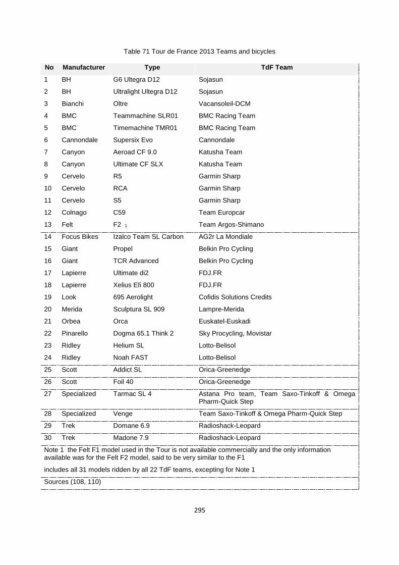
Table 71 Tour de France 2013 Teams and bicycles
No Manufacturer Type TdF Team
1 BH G6 Ultegra D12 Sojasun
2 BH Ultralight Ultegra D12 Sojasun
3 Bianchi Oltre Vacansoleil-DCM
4 BMC Teammachine SLR01 BMC Racing Team
5 BMC Timemachine TMR01 BMC Racing Team
6 Cannondale Supersix Evo Cannondale
7 Canyon Aeroad CF 9.0 Katusha Team
8 Canyon Ultimate CF SLX Katusha Team
9 Cervelo R5 Garmin Sharp
10 Cervelo RCA Garmin Sharp
11 Cervelo S5 Garmin Sharp
12 Colnago C59 Team Europcar
13 Felt F2 1 Team Argos-Shimano
14 Focus Bikes Izalco Team SL Carbon AG2r La Mondiale
15 Giant Propel Belkin Pro Cycling
16 Giant TCR Advanced Belkin Pro Cycling
17 Lapierre Ultimate di2 FDJ.FR
18 Lapierre Xelius Efi 800 FDJ.FR
19 Look 695 Aerolight Cofidis Solutions Credits
20 Merida Sculptura SL 909 Lampre-Merida
21 Orbea Orca Euskatel-Euskadi
22 Pinarello Dogma 65.1 Think 2 Sky Procycling, Movistar
23 Ridley Helium SL Lotto-Belisol
24 Ridley Noah FAST Lotto-Belisol
25 Scott Addict SL Orica-Greenedge
26 Scott Foil 40 Orica-Greenedge
27 Specialized Tarmac SL 4 Astana Pro team, Team Saxo-Tinkoff & Omega Pharm-Quick Step
28 Specialized Venge Team Saxo-Tinkoff & Omega Pharm-Quick Step
29 Trek Domane 6.9 Radioshack-Leopard
30 Trek Madone 7.9 Radioshack-Leopard
Note 1 the Felt F1 model used in the Tour is not available commercially and the only information available was for the Felt F2 model, said to be very similar to the F1
includes all 31 models ridden by all 22 TdF teams, excepting for Note 1
Sources (108, 110)
295
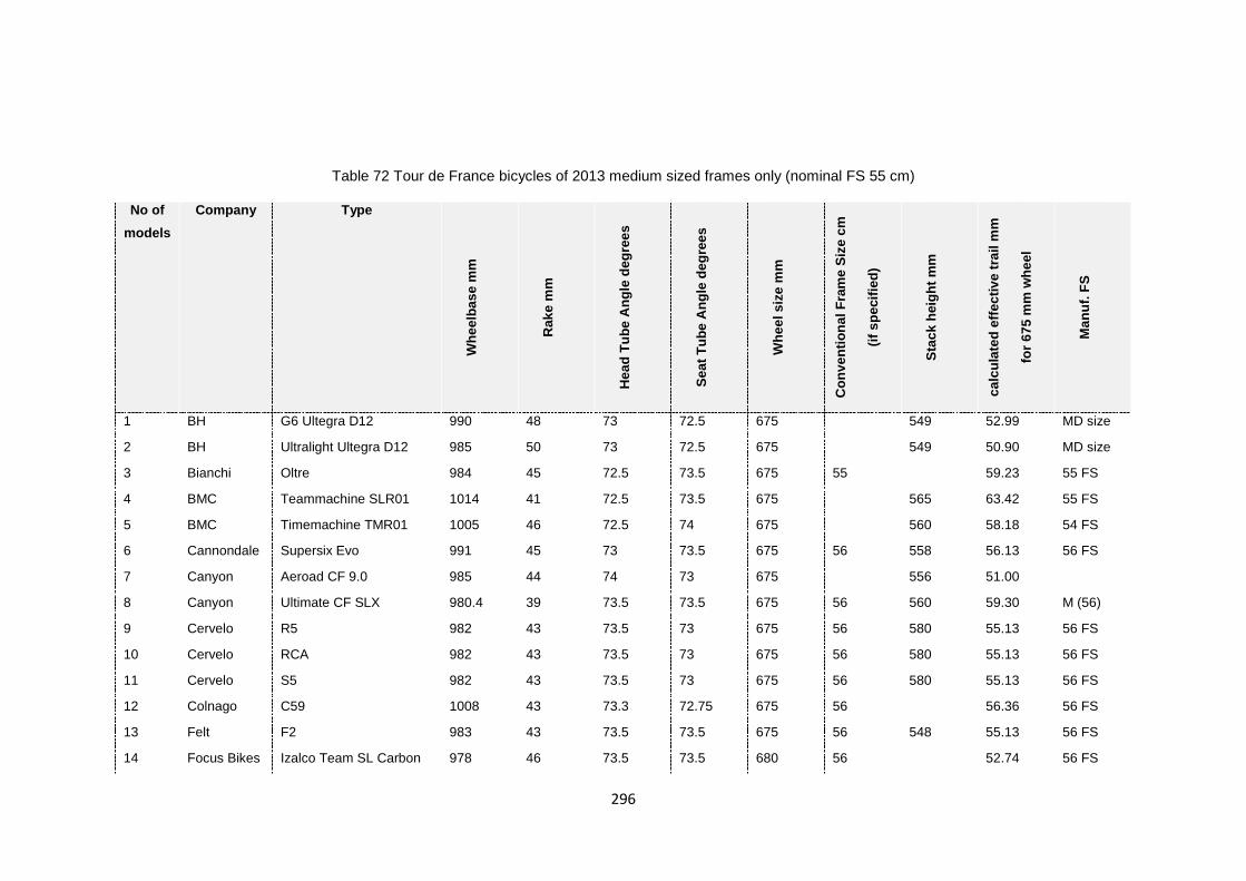
Table 72 Tour de France bicycles of 2013 medium sized frames only (nominal FS 55 cm)
No of models
Company Type
Whe
elba
se m
m
Rak
e m
m
Hea
d Tu
be A
ngle
deg
rees
Seat
Tub
e A
ngle
deg
rees
Whe
el s
ize
mm
Con
vent
iona
l Fra
me
Size
cm
(if s
peci
fied)
Stac
k he
ight
mm
calc
ulat
ed e
ffect
ive
trai
l mm
for 6
75 m
m w
heel
Man
uf. F
S
1 BH G6 Ultegra D12 990 48 73 72.5 675 549 52.99 MD size
2 BH Ultralight Ultegra D12 985 50 73 72.5 675 549 50.90 MD size
3 Bianchi Oltre 984 45 72.5 73.5 675 55 59.23 55 FS
4 BMC Teammachine SLR01 1014 41 72.5 73.5 675 565 63.42 55 FS
5 BMC Timemachine TMR01 1005 46 72.5 74 675 560 58.18 54 FS
6 Cannondale Supersix Evo 991 45 73 73.5 675 56 558 56.13 56 FS
7 Canyon Aeroad CF 9.0 985 44 74 73 675 556 51.00
8 Canyon Ultimate CF SLX 980.4 39 73.5 73.5 675 56 560 59.30 M (56)
9 Cervelo R5 982 43 73.5 73 675 56 580 55.13 56 FS
10 Cervelo RCA 982 43 73.5 73 675 56 580 55.13 56 FS
11 Cervelo S5 982 43 73.5 73 675 56 580 55.13 56 FS
12 Colnago C59 1008 43 73.3 72.75 675 56 56.36 56 FS
13 Felt F2 983 43 73.5 73.5 675 56 548 55.13 56 FS
14 Focus Bikes Izalco Team SL Carbon 978 46 73.5 73.5 680 56 52.74 56 FS
296
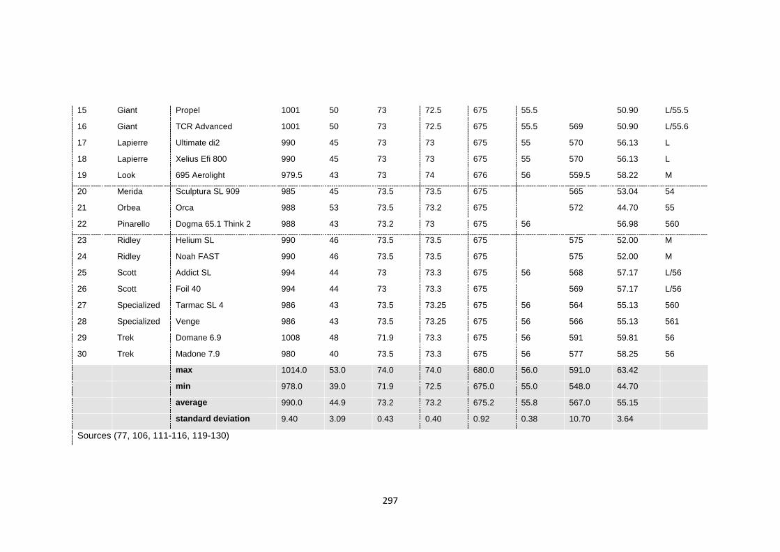
15 Giant Propel 1001 50 73 72.5 675 55.5 50.90 L/55.5
16 Giant TCR Advanced 1001 50 73 72.5 675 55.5 569 50.90 L/55.6
17 Lapierre Ultimate di2 990 45 73 73 675 55 570 56.13 L
18 Lapierre Xelius Efi 800 990 45 73 73 675 55 570 56.13 L
19 Look 695 Aerolight 979.5 43 73 74 676 56 559.5 58.22 M
20 Merida Sculptura SL 909 985 45 73.5 73.5 675 565 53.04 54
21 Orbea Orca 988 53 73.5 73.2 675 572 44.70 55
22 Pinarello Dogma 65.1 Think 2 988 43 73.2 73 675 56 56.98 560
23 Ridley Helium SL 990 46 73.5 73.5 675 575 52.00 M
24 Ridley Noah FAST 990 46 73.5 73.5 675 575 52.00 M
25 Scott Addict SL 994 44 73 73.3 675 56 568 57.17 L/56
26 Scott Foil 40 994 44 73 73.3 675 569 57.17 L/56
27 Specialized Tarmac SL 4 986 43 73.5 73.25 675 56 564 55.13 560
28 Specialized Venge 986 43 73.5 73.25 675 56 566 55.13 561
29 Trek Domane 6.9 1008 48 71.9 73.3 675 56 591 59.81 56
30 Trek Madone 7.9 980 40 73.5 73.3 675 56 577 58.25 56
max 1014.0 53.0 74.0 74.0 680.0 56.0 591.0 63.42
min 978.0 39.0 71.9 72.5 675.0 55.0 548.0 44.70
average 990.0 44.9 73.2 73.2 675.2 55.8 567.0 55.15
standard deviation 9.40 3.09 0.43 0.40 0.92 0.38 10.70 3.64
Sources (77, 106, 111-116, 119-130)
297

Table 73 Details of the entire size range for 8 selected manufacturers’ 2013 TdF bicycles
No
of m
odel
s
Com
pany
Type
Man
ufac
ture
r FS
Whe
elba
se m
m
Rak
e m
m
Hea
d Tu
be A
ngle
deg
rees
Seat
Tub
e A
ngle
deg
rees
Whe
el s
ize
mm
Con
vent
iona
l Fra
me
Size
cm
(if s
peci
fied)
Stac
k he
ight
mm
calc
ulat
ed tr
ail m
m fo
r
675
mm
whe
el
1 Cannondale Supersix Evo 48 961 45 71.50 74.50 675 48 513 65.474
2 Cannondale Supersix Evo 50 967 45 72.00 74.50 675 50 519 62.345
3 Cannondale Supersix Evo 52 973 45 72.50 74.00 675 52 526 59.230
4 Cannondale Supersix Evo 54 975 45 73.00 73.50 675 54 544 56.128
5 Cannondale Supersix Evo 56 991 45 73.00 73.50 675 56 558 56.128
6 Cannondale Supersix Evo 58 996 45 73.50 73.00 675 58 577 53.039
7 Cannondale Supersix Evo 60 1008 45 73.50 72.50 675 60 596 53.039
8 Cannondale Supersix Evo 62 1012 45 73.50 72.00 675 62 620 53.039
1 Felt F2 1 48 969 52 71.00 74.50 675 500 61.214
2 Felt F2 51 971 50 72.00 74.00 675 514 57.087
298
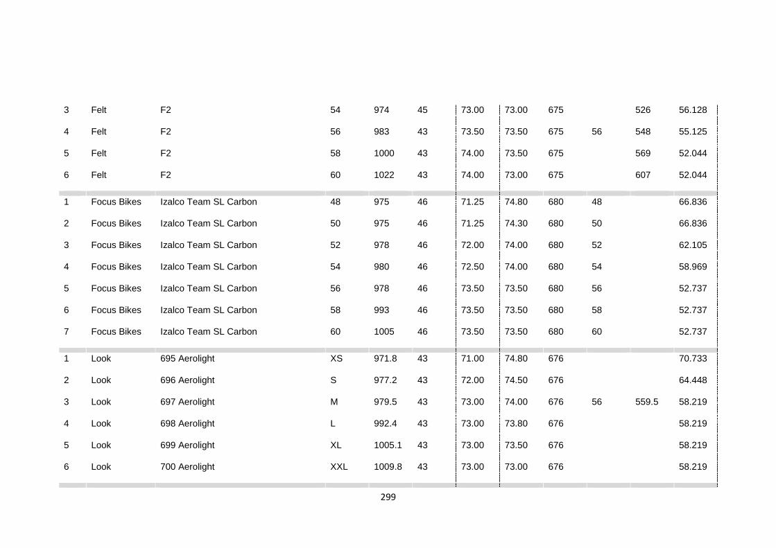
3 Felt F2 54 974 45 73.00 73.00 675 526 56.128
4 Felt F2 56 983 43 73.50 73.50 675 56 548 55.125
5 Felt F2 58 1000 43 74.00 73.50 675 569 52.044
6 Felt F2 60 1022 43 74.00 73.00 675 607 52.044
1 Focus Bikes Izalco Team SL Carbon 48 975 46 71.25 74.80 680 48 66.836
2 Focus Bikes Izalco Team SL Carbon 50 975 46 71.25 74.30 680 50 66.836
3 Focus Bikes Izalco Team SL Carbon 52 978 46 72.00 74.00 680 52 62.105
4 Focus Bikes Izalco Team SL Carbon 54 980 46 72.50 74.00 680 54 58.969
5 Focus Bikes Izalco Team SL Carbon 56 978 46 73.50 73.50 680 56 52.737
6 Focus Bikes Izalco Team SL Carbon 58 993 46 73.50 73.50 680 58 52.737
7 Focus Bikes Izalco Team SL Carbon 60 1005 46 73.50 73.50 680 60 52.737
1 Look 695 Aerolight XS 971.8 43 71.00 74.80 676 70.733
2 Look 696 Aerolight S 977.2 43 72.00 74.50 676 64.448
3 Look 697 Aerolight M 979.5 43 73.00 74.00 676 56 559.5 58.219
4 Look 698 Aerolight L 992.4 43 73.00 73.80 676 58.219
5 Look 699 Aerolight XL 1005.1 43 73.00 73.50 676 58.219
6 Look 700 Aerolight XXL 1009.8 43 73.00 73.00 676 58.219
299
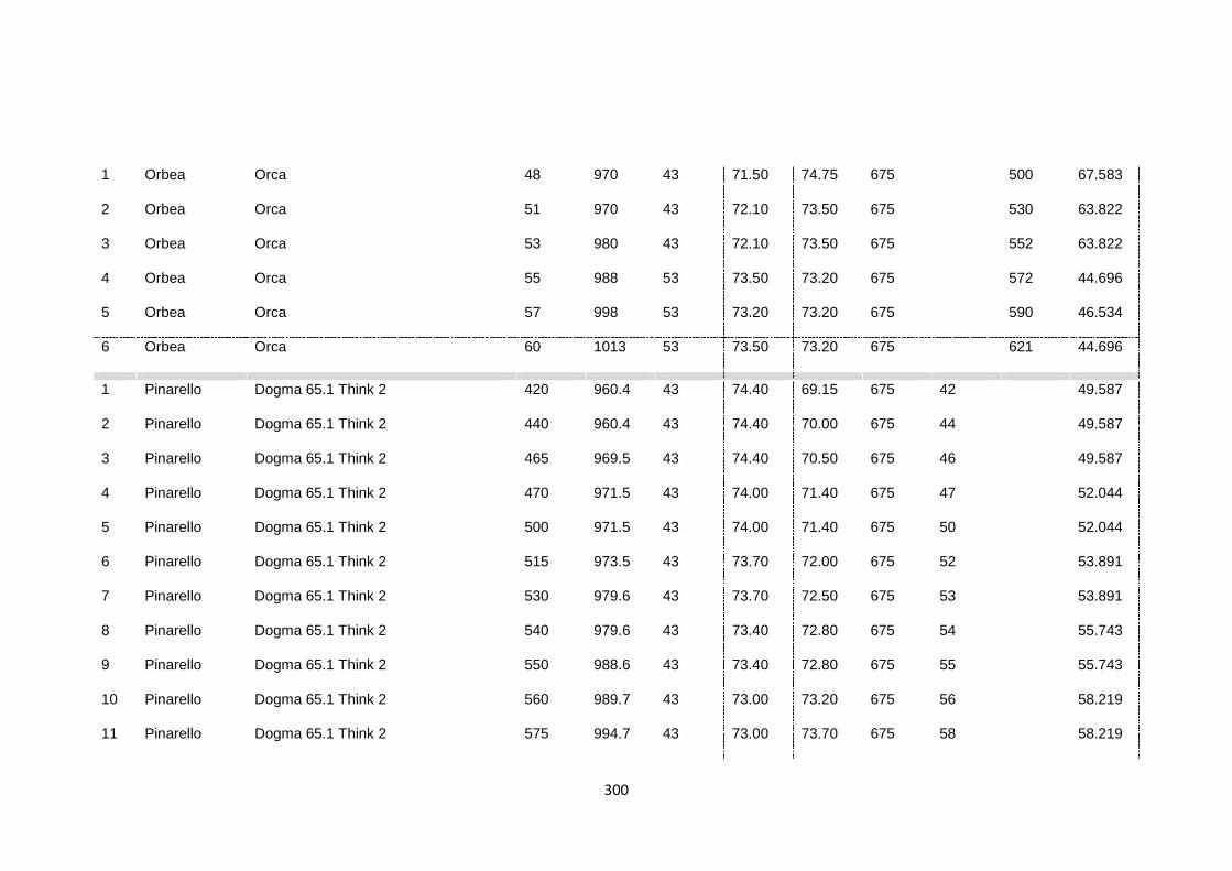
1 Orbea Orca 48 970 43 71.50 74.75 675 500 67.583
2 Orbea Orca 51 970 43 72.10 73.50 675 530 63.822
3 Orbea Orca 53 980 43 72.10 73.50 675 552 63.822
4 Orbea Orca 55 988 53 73.50 73.20 675 572 44.696
5 Orbea Orca 57 998 53 73.20 73.20 675 590 46.534
6 Orbea Orca 60 1013 53 73.50 73.20 675 621 44.696
1 Pinarello Dogma 65.1 Think 2 420 960.4 43 74.40 69.15 675 42 49.587
2 Pinarello Dogma 65.1 Think 2 440 960.4 43 74.40 70.00 675 44 49.587
3 Pinarello Dogma 65.1 Think 2 465 969.5 43 74.40 70.50 675 46 49.587
4 Pinarello Dogma 65.1 Think 2 470 971.5 43 74.00 71.40 675 47 52.044
5 Pinarello Dogma 65.1 Think 2 500 971.5 43 74.00 71.40 675 50 52.044
6 Pinarello Dogma 65.1 Think 2 515 973.5 43 73.70 72.00 675 52 53.891
7 Pinarello Dogma 65.1 Think 2 530 979.6 43 73.70 72.50 675 53 53.891
8 Pinarello Dogma 65.1 Think 2 540 979.6 43 73.40 72.80 675 54 55.743
9 Pinarello Dogma 65.1 Think 2 550 988.6 43 73.40 72.80 675 55 55.743
10 Pinarello Dogma 65.1 Think 2 560 989.7 43 73.00 73.20 675 56 58.219
11 Pinarello Dogma 65.1 Think 2 575 994.7 43 73.00 73.70 675 58 58.219
300
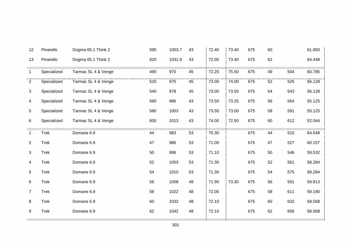
12 Pinarello Dogma 65.1 Think 2 595 1003.7 43 72.40 73.40 675 60 61.950
13 Pinarello Dogma 65.1 Think 2 620 1031.9 43 72.00 73.40 675 62 64.448
1 Specialized Tarmac SL 4 & Venge 490 970 45 72.25 75.50 675 49 504 60.785
2 Specialized Tarmac SL 4 & Venge 520 970 45 73.00 74.00 675 52 526 56.128
3 Specialized Tarmac SL 4 & Venge 540 978 45 73.00 73.50 675 54 543 56.128
4 Specialized Tarmac SL 4 & Venge 560 986 43 73.50 73.25 675 56 564 55.125
5 Specialized Tarmac SL 4 & Venge 580 1003 43 73.50 73.00 675 58 591 55.125
6 Specialized Tarmac SL 4 & Venge 600 1013 43 74.00 72.50 675 60 612 52.044
1 Trek Domane 6.9 44 983 53 70.30 675 44 510 64.548
2 Trek Domane 6.9 47 986 53 71.00 675 47 527 60.157
3 Trek Domane 6.9 50 996 53 71.10 675 50 546 59.532
4 Trek Domane 6.9 52 1003 53 71.30 675 52 561 58.284
5 Trek Domane 6.9 54 1010 53 71.30 675 54 575 58.284
6 Trek Domane 6.9 56 1008 48 71.90 73.30 675 56 591 59.813
7 Trek Domane 6.9 58 1022 48 72.00 675 58 611 59.190
8 Trek Domane 6.9 60 1032 48 72.10 675 60 632 58.568
9 Trek Domane 6.9 62 1042 48 72.10 675 62 656 58.568
301
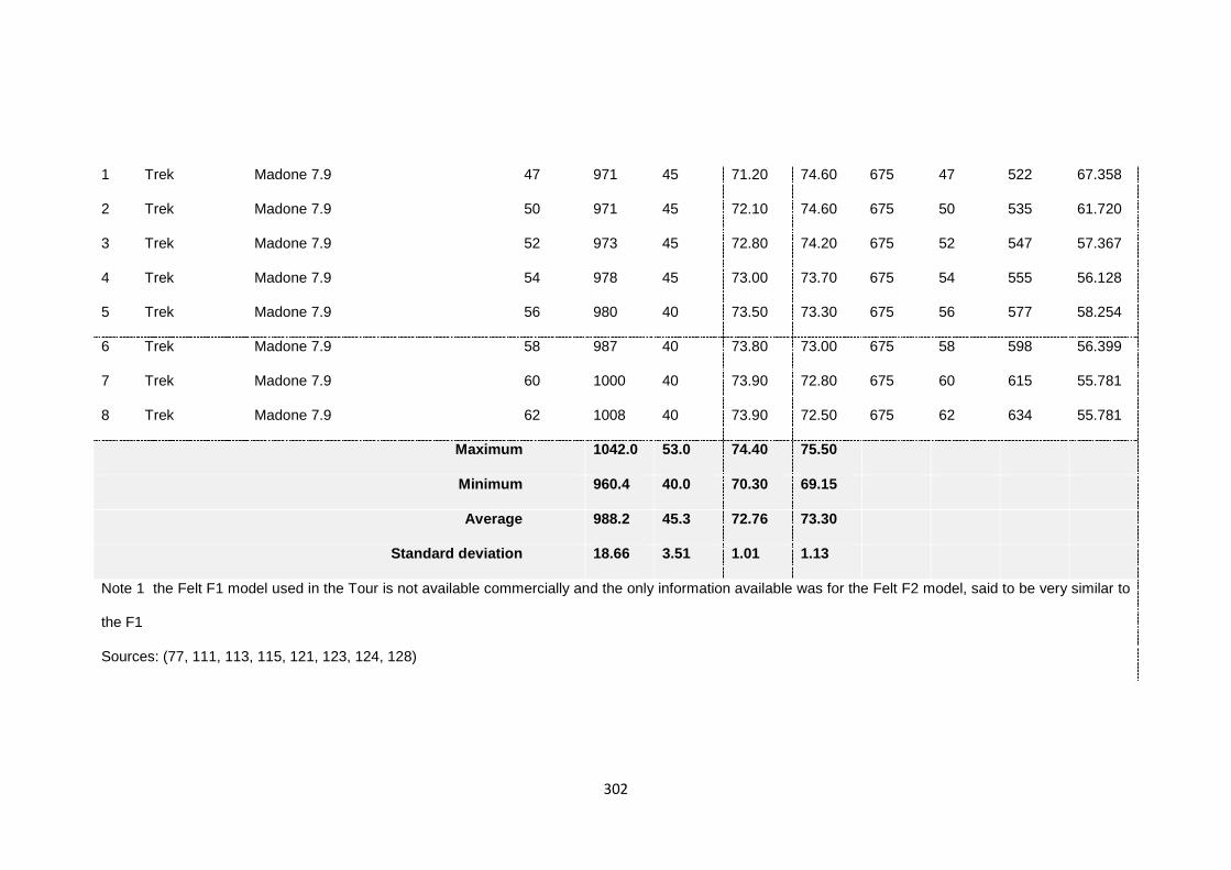
1 Trek Madone 7.9 47 971 45 71.20 74.60 675 47 522 67.358
2 Trek Madone 7.9 50 971 45 72.10 74.60 675 50 535 61.720
3 Trek Madone 7.9 52 973 45 72.80 74.20 675 52 547 57.367
4 Trek Madone 7.9 54 978 45 73.00 73.70 675 54 555 56.128
5 Trek Madone 7.9 56 980 40 73.50 73.30 675 56 577 58.254
6 Trek Madone 7.9 58 987 40 73.80 73.00 675 58 598 56.399
7 Trek Madone 7.9 60 1000 40 73.90 72.80 675 60 615 55.781
8 Trek Madone 7.9 62 1008 40 73.90 72.50 675 62 634 55.781
Maximum 1042.0 53.0 74.40 75.50
Minimum 960.4 40.0 70.30 69.15
Average 988.2 45.3 72.76 73.30
Standard deviation 18.66 3.51 1.01 1.13
Note 1 the Felt F1 model used in the Tour is not available commercially and the only information available was for the Felt F2 model, said to be very similar to
the F1
Sources: (77, 111, 113, 115, 121, 123, 124, 128)
302

Figure 124 Relationship between wheelbase and frame size for thirty 2013 TdF bicycle models in Table 73
y = 3.077x + 822.481R² = 0.652
935
945
955
965
975
985
995
1005
1015
1025
1035
1045
40 45 50 55 60 65
whe
elba
se m
m
frame size cm
wheelbase vs. frame size - 2013 TdF road bicycles
303
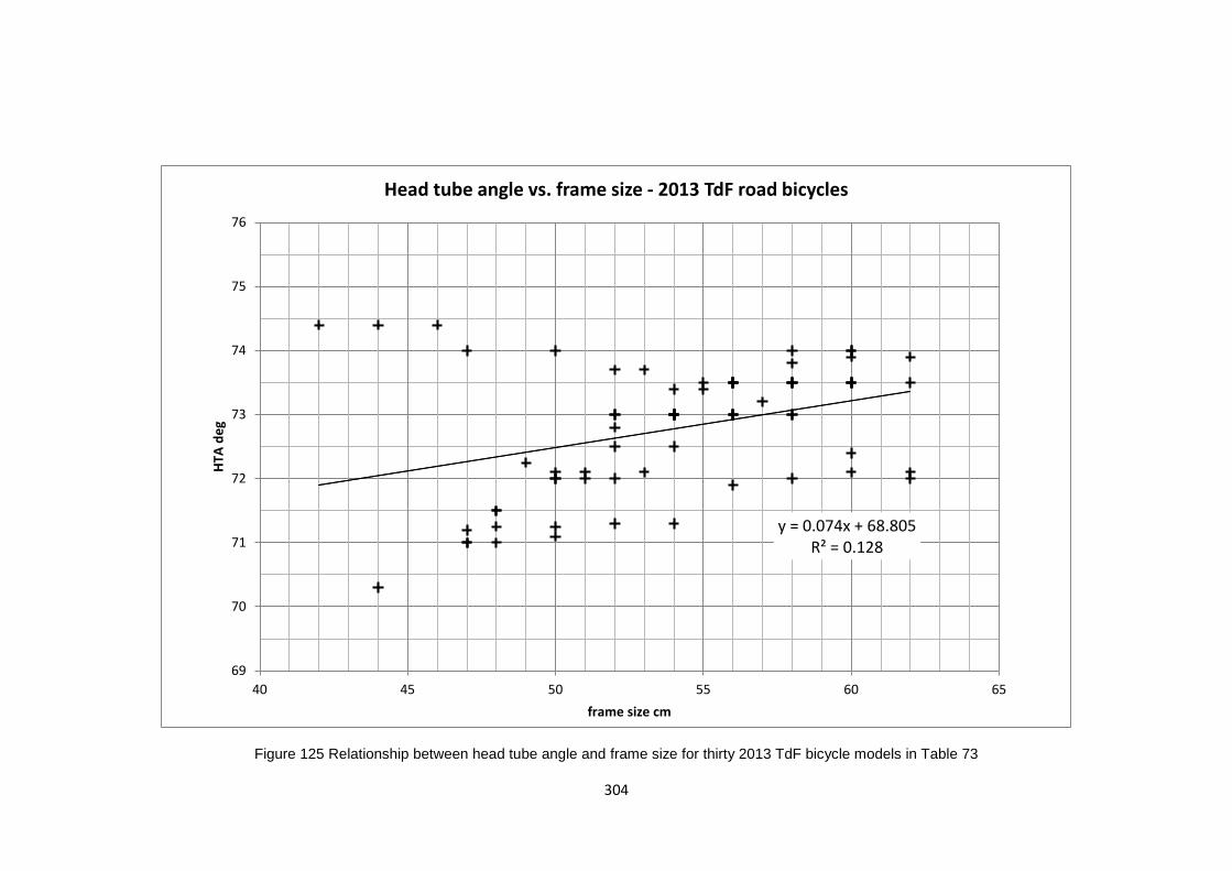
Figure 125 Relationship between head tube angle and frame size for thirty 2013 TdF bicycle models in Table 73
y = 0.074x + 68.805R² = 0.128
69
70
71
72
73
74
75
76
40 45 50 55 60 65
HTA
deg
frame size cm
Head tube angle vs. frame size - 2013 TdF road bicycles
304
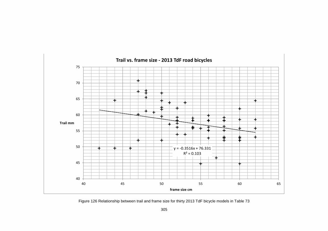
Figure 126 Relationship between trail and frame size for thirty 2013 TdF bicycle models in Table 73
y = -0.3516x + 76.331R² = 0.103
40
45
50
55
60
65
70
75
40 45 50 55 60 65
Trail mm
frame size cm
Trail vs. frame size - 2013 TdF road bicycles
305
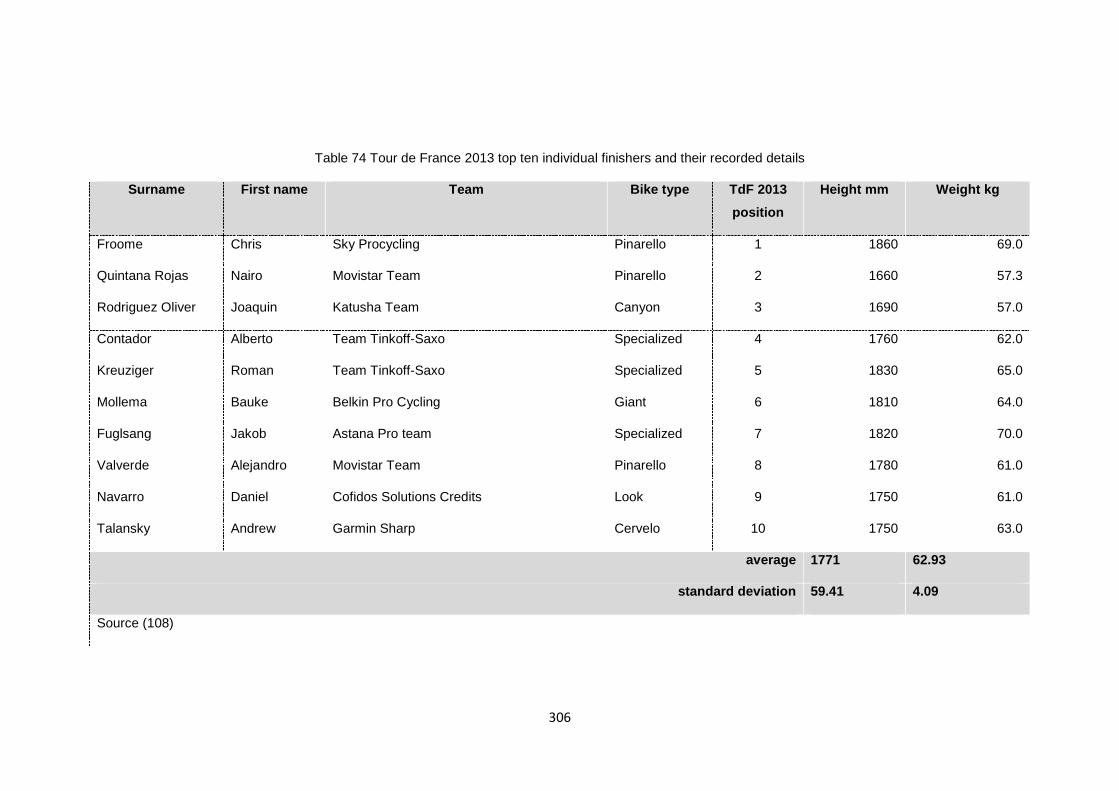
Table 74 Tour de France 2013 top ten individual finishers and their recorded details
Surname First name Team Bike type TdF 2013 position
Height mm Weight kg
Froome Chris Sky Procycling Pinarello 1 1860 69.0
Quintana Rojas Nairo Movistar Team Pinarello 2 1660 57.3
Rodriguez Oliver Joaquin Katusha Team Canyon 3 1690 57.0
Contador Alberto Team Tinkoff-Saxo Specialized 4 1760 62.0
Kreuziger Roman Team Tinkoff-Saxo Specialized 5 1830 65.0
Mollema Bauke Belkin Pro Cycling Giant 6 1810 64.0
Fuglsang Jakob Astana Pro team Specialized 7 1820 70.0
Valverde Alejandro Movistar Team Pinarello 8 1780 61.0
Navarro Daniel Cofidos Solutions Credits Look 9 1750 61.0
Talansky Andrew Garmin Sharp Cervelo 10 1750 63.0
average 1771 62.93
standard deviation 59.41 4.09
Source (108)
306

Table 75 Tour de France 2013 top ten individual finishers and their calculated details
Surname TdF 2013
position
Calc. Inseam
mm
Calc. saddle height
mm
Calculated frame size
cm
Wheelbase mm
STA degrees
Calculated "h" mm
Calculated "b" mm
Calculated MOIYB kgm^2
Froome 1 857.5 758.9 55.7 988.2 73.00 1109.0 318.0 93.225
Quintana Rojas 2 765.3 677.3 49.7 970.0 74.00 1020.0 337.0 66.690
Rodriguez Oliver 3 779.1 689.5 50.6 971.0 73.50 1019.0 332.0 66.247
Contador 4 811.4 718.1 52.7 970.0 74.00 1064.0 333.0 77.888
Kreuziger 5 843.6 746.6 54.8 978.0 73.50 1096.0 324.0 86.247
Mollema 6 834.4 738.5 54.2 986.0 72.50 1086.0 315.0 83.501
Fuglsang 7 839.0 742.5 54.5 978.0 73.50 1092.0 325.0 91.581
Valverde 8 820.6 726.2 53.3 978.1 73.70 1084.0 328.0 79.669
Navarro 9 806.8 714.0 52.4 979.5 74.00 1060.0 334.0 76.180
Talansky 10 806.8 714.0 52.4 972.0 73.00 1059.0 323.0 78.279
average 816.43 722.54 53.1 977.1 73.47 1068.90 326.90 79.95
standard deviation 27.39 24.24 1.78 6.12 0.48 29.12 6.82 8.65
Sources (108, 111-116)
307

The calculations in Table 75 are based on the following assumptions:
1. Inseam = height X 0.461 (48)
2. Saddle height = inseam X 0.885 (68)
3. Bicycle frame size = inseam X 0.65 (68)
4. Wheelbase is taken from manufacturers’ specifications after the frame size is calculated
5. Seat Tube Angle is taken from manufacturers’ specifications
6. h calculated as per Appendix B
7. b calculated as per Appendix B
8. IXB = (mass of rider + mass of bike) x h2
9. mass of bike = 6.8 kg- (equals the UCI limit)
308

APPENDIX G – DESIGN TABLE SERIES & DESIGN EQUATION
This Appendix details two additional design methodologies one based on the use of design tables
and second on a design equation.
G-1 DESIGN TABLE SERIES
This Design Table Series summarises recommendations about bicycle design in a tabular format.
1. this Road Bicycle Design Table Series consists of five tables prepared for frame sizes (FS)
between 490 to 610 mm
2. the recommendations are set out in a codified way for the designer to use
3. the design criteria they are based on uses empirical knowledge and experience
4. these five Tables are based on the same guidelines already detailed in Design Criteria Table
30 from Chapter Six.
5. the correct Design Table is found by using the inseam (IS) measurement (see Figure 127) to
calculate the preferred frame size, see Table 76 and Figure 128
Once the correct frame size has been found, choose its corresponding Design Table to make
decisions about the following parameters, wheelbase, fork rake, head tube angle and seat tube
angle, see Table 76 to Table 81.
Inseam measurement
Figure 127 Cyclist inseam dimension measured along the inside of the leg
309

Table 76 Frame size table – indicates the correct frame size for range of inseam measurements
Ideal inseam (mm) Min to max inseam ranges (mm) Recommended Frame Size (mm)
754 730 to 777 490
800 778 to 822 520
846 823 to 869 550
892 870 to 914 580
938 915 to 960 610
Figure 128 Frame size (FS) vs. inseam (IS) with bands of inseam ranges, from Table 76
The selection of the correct frame size is based on a factor of 0.65 as per the formula below:
𝐹𝐹𝑆𝑆 = 0.65 × 𝐼𝐼𝑆𝑆
(60)
y = 0.65xR² = 1
400
450
500
550
600
650
700
700 750 800 850 900 950 1000
Fram
e si
ze (m
m)
Inseam (mm)
ranges
FS vs. IS
310
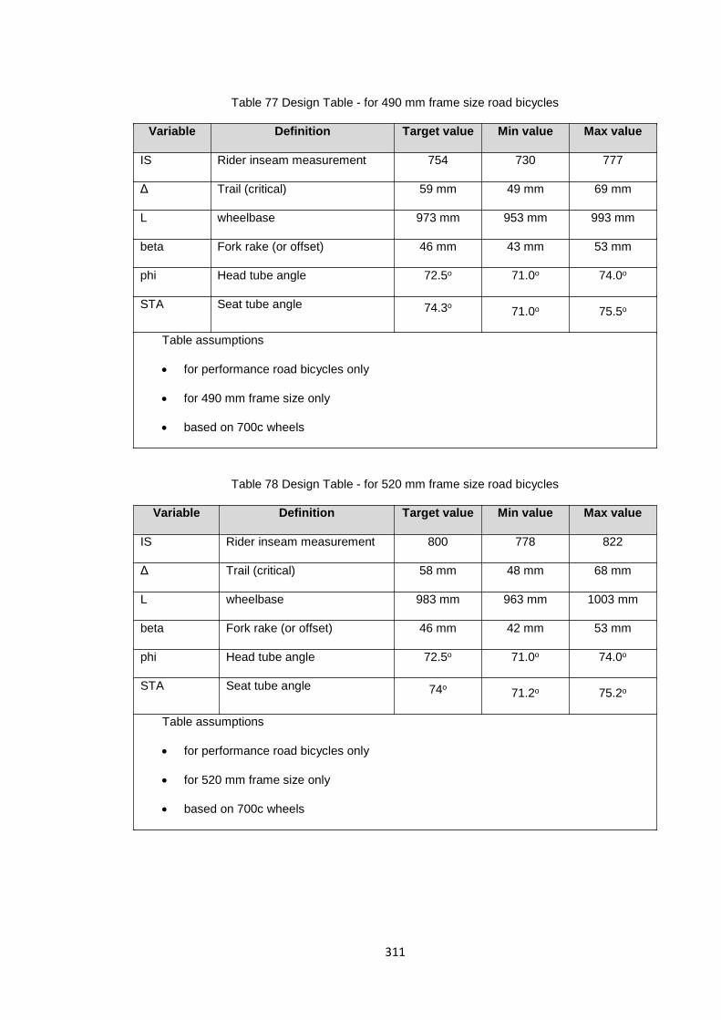
Table 77 Design Table - for 490 mm frame size road bicycles
Variable Definition Target value Min value Max value
IS Rider inseam measurement 754 730 777
Δ Trail (critical) 59 mm 49 mm 69 mm
L wheelbase 973 mm 953 mm 993 mm
beta Fork rake (or offset) 46 mm 43 mm 53 mm
phi Head tube angle 72.5o 71.0o 74.0o
STA Seat tube angle 74.3o 71.0o 75.5o
Table assumptions
• for performance road bicycles only
• for 490 mm frame size only
• based on 700c wheels
Table 78 Design Table - for 520 mm frame size road bicycles
Variable Definition Target value Min value Max value
IS Rider inseam measurement 800 778 822
Δ Trail (critical) 58 mm 48 mm 68 mm
L wheelbase 983 mm 963 mm 1003 mm
beta Fork rake (or offset) 46 mm 42 mm 53 mm
phi Head tube angle 72.5o 71.0o 74.0o
STA Seat tube angle 74o 71.2o 75.2o
Table assumptions
• for performance road bicycles only
• for 520 mm frame size only
• based on 700c wheels
311
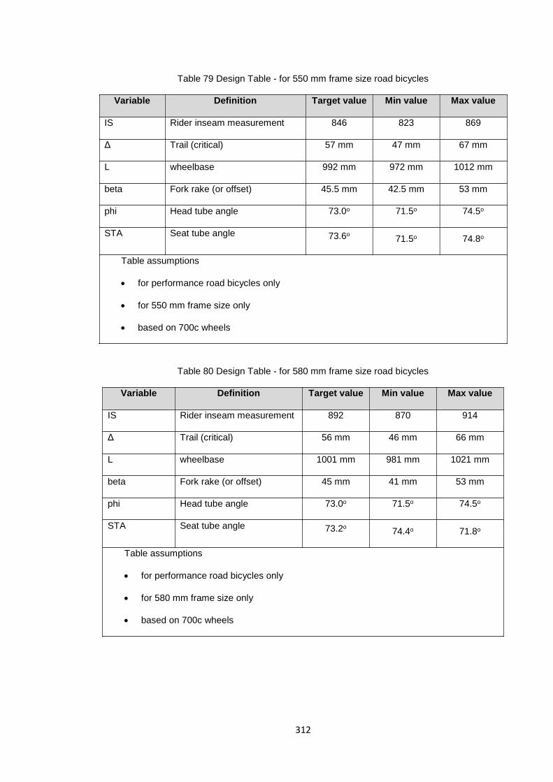
Table 79 Design Table - for 550 mm frame size road bicycles
Variable Definition Target value Min value Max value
IS Rider inseam measurement 846 823 869
Δ Trail (critical) 57 mm 47 mm 67 mm
L wheelbase 992 mm 972 mm 1012 mm
beta Fork rake (or offset) 45.5 mm 42.5 mm 53 mm
phi Head tube angle 73.0o 71.5o 74.5o
STA Seat tube angle 73.6o 71.5o 74.8o
Table assumptions
• for performance road bicycles only
• for 550 mm frame size only
• based on 700c wheels
Table 80 Design Table - for 580 mm frame size road bicycles
Variable Definition Target value Min value Max value
IS Rider inseam measurement 892 870 914
Δ Trail (critical) 56 mm 46 mm 66 mm
L wheelbase 1001 mm 981 mm 1021 mm
beta Fork rake (or offset) 45 mm 41 mm 53 mm
phi Head tube angle 73.0o 71.5o 74.5o
STA Seat tube angle 73.2o 74.4o 71.8o
Table assumptions
• for performance road bicycles only
• for 580 mm frame size only
• based on 700c wheels
312

Table 81 Design Table - for 610 mm frame size road bicycles
Variable Definition Target value Min value Max value
IS Rider inseam measurement 938 915 960
L wheelbase 1010 mm 990 mm 1030 mm
Δ Trail (critical) 55 mm 45 mm 65 mm
beta Fork rake (or offset) 45 mm 40 mm 53 mm
phi Head tube angle 73.5o 72.0o 75.0o
STA Seat tube angle 72.8o 72.0o 74.0o
Table assumptions
• for performance road bicycles only
• for 610 mm frame size only
• based on 700c wheels
313

G-2 DESIGN EQUATION
Consideration was given as to whether an overall design equation could be developed. After
evaluation it was decided that this approach was unsuitable but a brief description is included in
this Appendix for completeness.
Mathematical equations such as those used to develop the Simulink model used in this
investigation would of course provide the most accurate analysis. But a Simulink model is not
considered to be a suitable design technique, rather it is a modelling method which requires
experience on the part of the user and access to Matlab and Simulink. A major problem with
Simulink models is they are hard to use, not easily interpreted and require training and
experience.
However once the sensitivity study in Chapter Five was completed it seemed worth considering
if its results could be used to formulate a simple equation to predict the handling performance of
any specific bicycle design. Such a design equation if successful, could potentially allow a
designer to quickly evaluate the effect of changing one or more parameters. It was hoped that
this could be better method than using Design Criteria or Design Tables as the interaction of
several parameters could be examined. In addition it would not be based on equations and rules
taken from past experience rather it would be based on dynamic responses.
The design equation formulated from the sensitivity study is:
𝐻𝐻𝑎𝑎𝑠𝑠𝑑𝑑𝑎𝑎𝑠𝑠𝑠𝑠𝑀𝑀 𝐼𝐼𝑠𝑠𝑑𝑑𝑒𝑒𝑒𝑒 = 𝐶𝐶𝐷𝐷∆𝐷𝐷𝑁𝑁𝐷𝐷𝑂𝑂
+ 𝐶𝐶𝑏𝑏∆𝑏𝑏𝑁𝑁𝑏𝑏𝑂𝑂
+ 𝐶𝐶𝑀𝑀∆𝑀𝑀𝑁𝑁
𝑀𝑀𝑂𝑂+ 𝐶𝐶ℎ
∆ℎ𝑁𝑁ℎ𝑂𝑂
+ 𝐶𝐶𝐼𝐼𝐼𝐼𝑖𝑖∆𝐼𝐼𝐼𝐼𝑎𝑎𝑁𝑁𝐼𝐼𝐼𝐼𝑎𝑎𝑂𝑂
+ 𝐶𝐶𝐼𝐼𝐼𝐼𝑖𝑖∆𝐼𝐼𝑒𝑒𝑎𝑎𝑁𝑁𝐼𝐼𝑒𝑒𝑎𝑎𝑂𝑂
+ 𝐶𝐶𝐼𝐼𝐼𝐼𝑏𝑏∆𝐼𝐼𝑒𝑒𝑏𝑏𝑁𝑁𝐼𝐼𝑒𝑒𝑏𝑏𝑂𝑂
+ 𝐶𝐶𝛽𝛽∆𝛽𝛽𝑁𝑁𝛽𝛽𝑂𝑂
+ 𝐶𝐶𝑟𝑟∆𝐿𝐿𝑁𝑁𝐿𝐿𝑂𝑂
+ 𝐶𝐶𝐼𝐼𝐼𝐼𝑓𝑓∆𝐼𝐼𝐼𝐼𝐼𝐼𝑁𝑁𝐼𝐼𝐼𝐼𝐼𝐼𝑂𝑂
+ 𝐶𝐶𝑠𝑠∆𝑠𝑠𝑁𝑁𝑠𝑠𝑂𝑂
(104)
• where CD, Cb, CM etc. are coefficients taken from the sensitivity study of the Chapter Five,
note that they are linear terms and therefore are only valid across a short range (Table
28)
• parameters D, b, M etc. are defined in Table 82
• subscript N refers to the parameter value of the new bicycle design that is to be examined
• and subscript O refers to the “old” parameter value of the benchmark bicycle (see Table
82)
Using the coefficients given in Table 28 this equation becomes:
𝐻𝐻𝑎𝑎𝑠𝑠𝑑𝑑𝑎𝑎𝑠𝑠𝑠𝑠𝑀𝑀 𝐼𝐼𝑠𝑠𝑑𝑑𝑒𝑒𝑒𝑒 = 0.05753∆𝐷𝐷𝑁𝑁𝐷𝐷𝑂𝑂
+ 0.02072∆𝑏𝑏𝑁𝑁𝑏𝑏𝑂𝑂
+ 0.01976∆𝑀𝑀𝑁𝑁
𝑀𝑀𝑂𝑂+ 0.002698
∆ℎ𝑁𝑁ℎ𝑂𝑂
+ 0.001038∆𝐼𝐼𝐼𝐼𝑎𝑎𝑁𝑁𝐼𝐼𝐼𝐼𝑎𝑎𝑂𝑂
+ 0.00063∆𝐼𝐼𝑒𝑒𝑎𝑎𝑁𝑁𝐼𝐼𝑒𝑒𝑎𝑎𝑂𝑂
+ (−0.001067)∆𝐼𝐼𝑒𝑒𝑏𝑏𝑁𝑁𝐼𝐼𝑒𝑒𝑏𝑏𝑂𝑂
+ (−0.01412)∆𝛽𝛽𝑁𝑁𝛽𝛽𝑂𝑂
+ (−0.01565)∆𝐿𝐿𝑁𝑁𝐿𝐿𝑂𝑂
+ (−0.02021)∆𝐼𝐼𝐼𝐼𝐼𝐼𝑁𝑁𝐼𝐼𝐼𝐼𝐼𝐼𝑂𝑂
+ (−0.05925)∆𝑠𝑠𝑁𝑁𝑠𝑠𝑂𝑂
(105)
314
The equation’s output, the handling index, is a non-dimensionalised number (which is expressed
as a ratio or percentage of the benchmark settling time) and this gives an overall handling score.
Unfortunately after using this equation several times it was found to be a poor predictor of the
Simulink results, even for very small parameter changes. But perhaps this should not be a
surprise given the nonlinear dynamic behaviour of a bicycle.
The results of four calculations using the equation are summarised in Table 79 , in which all three
new designs (A, B and C) showed significant variances when compared to the results of Simulink
simulations. The design equation’s calculation of the 2% settling time had an error of between 6
to 40% over that of the value given by Simulink, unacceptable errors and therefore this approach
was discontinued.
315

Table 82 Handling equation results for three new designs A, B & C
Parameter Units Benchmark bicycle values
Design A Design B Design C
D Diameter of the bicycle
wheel
m 0.675 0.670 0.674 0.670
b Hori dist. C of rear
wheel to COM
m 0.330 0.320 0.329 0.330
M Mass kg 80.00 78.00 79.00 80.00
h Height of centre of
mass (COM)
m 1.100 1.050 1.110 1.100
IZA MOI of A about Z axis
(yaw)
kgm2 0.080 0.081 0.081 0.080
IXA MOI of A about X axis
(roll)
kgm2 0.200 0.210 0.210 0.200
IXB MOI of B about X axis
(roll)
kgm2 100.00 95.00 99.00 100.00
β fork rake m 0.045 0.043 0.044 0.045
L bicycle wheelbase m 1.000 0.990 0.995 1.000
IZW MOI of wheels kgm2 0.100 0.098 0.099 0.100
Φ head tube angle degrees 73.00 73.50 73.75 76.00
Handling Equation Score 0.000 -0.00079 -0.00033 -0.05426
Predicted 2% Settling time sec 10.1 10.092 10.0967 9.5520
Actual 2% Settling time from
the Simulink simulation
sec 10.1 8.95 9.47 6.81
Variance between prediction and Simulink
% 0% 1 +12.76% +6.62% +40.26%
Note 1 this is a trivial result
316

BIBLIOGRAPHY
1. ISO 8855:2011 Road vehicles vehicle dynamics & road-holding ability Vocabulary (2011).
2. Jones DEH. The Stability of the Bicycle. Physics Today. 1970;23(4):34 - 40. 3. Union Cycliste Internationale UCI 2013. Available from:
http://www.uci.ch/templates/UCI/UCI8/layout.asp?MenuId=MTYzMDQ&LangId=1. 4. Klein RE. Using Bicycles to teach System Dynamics. IEEE Control Systems Magazine.
1989;9(3):4-9. 5. Klein RE, editor Novel systems and dynamics teaching techniques using bicycles.
Proceedings of the American Control Conference; 1988. 6. Whitt FR, Wilson DG. Bicycling Science: Ergonomics and Mechanics: MIT Press (MA);
1974. 7. Sharp A, editor. Bicycles and Tricycles, An Elementary Treatise On Their Design And
Construction: London: Longmans, Green; 1896. 8. Sharp RS. The Lateral Dynamics of Motorcycles and Bicycles. Vehicle System
Dynamics. 1985;14(4):265-83. 9. Brooks M. Easy Rider. New Scientist. 2011;No 2814 (28 May 2011):4. 10. Whitt FR, Wilson DG. Bicycling Science 2nd Ed. 2nd ed. Cambridge, USA: MIT Press
(MA); 1982. 11. Brand S. Freeman Dyson's Brain [Online interview]. Feb 1998 [updated 22 Aug 2013].
Available from: http://www.wired.com/wired/archive/6.02/dyson_pr.html. 12. Fajans J. Steering in Bicycles and Motorcycles. American Journal of Physics.
2000;68(7):654 - 9. 13. Astrom KJ, Klein, R. E., Lennartsson, A. Bicycle Dynamics and Control. IEEE Control
Systems Magazine. 2005 (Aug 2005):26-47. 14. Meijaard JP, Papadopoulos JM, Ruina A, Schwab AL. Linearized Dynamics Equations
for the Balance and Steer of a Bicycle: A Benchmark and Review. Proceedings of the Royal Society of London-A. 2007;463(2084):1955-82.
15. Whipple FJW. The stability of the motion of a bicycle. The Quarterly Journal of Pure and Applied Mathematics. 1899;30(120):312–48.
16. Meijaard JP, Papadopoulos J, Ruina A, Schwab AL. Historical Review of Thoughts of Bicycle Self-Stability. Cornell University, 2011.
17. Cox AJ. Angular Momentum and Motorcycle Counter Steering,: A Discussion and Demonstration. American Journal of Physics. 1998;66:1018 - 21.
18. Brooks. Easy Rider. New Scientist. 2011 28 May 2011;2814(28 May 2011):4. 19. Moon FC. Applied Dynamics: With Applications to Multibody and Mechatronic Systems:
John Wiley & Sons, USA; 1998. 20. Timoshenko S, Young DH, editors. Advanced Dynamics. USA: McGraw-Hill; 1948. 21. Lowell J, McKell HD. The Stability of Bicycles. American Journal of Physics.
1982;50(12):1106–12. 22. Rankine WJM. On the Dynamic Principles of the Motion of Velocipedes. The Engineer.
1869 6 Aug 1869;28(79):5. 23. Bourlet C. Traité des bicycles et bicyclettes, suivi d'une application à la construction des
vélodromes: Gauthier-Villars et fils; 1895. 24. Bourlet C. Étude Théoretique sur la Bicyclette. Bulletin de la Societe Mathematique de
France. 1899;27:47 - 67 & 76 - 96. 25. Psiaki ML. Bicycle Stability, A Mathematical and Numerical Analsis [Bachelor of Arts in
Physics]. Princeton NJ: Princeton University; 1979. 26. Hand RS. Comparisons and Stability Analysis of Linearized Equations of Motion for a
Basic Bicycle Model [Master of Science]: Cornell University NY; 1988. 27. Franke G, Suhr W, Rieß F. An advanced model of bicycle dynamics. European Journal
of Physics. 1990;11:116-21. 28. Seffen KA, Parks GT, Clarkson PJ. Observations on the Controllability of Motion of
Two-wheelers. Proceedings of the Institution of Mechanical Engineers, Part I: Journal of Systems and Control Engineering. 2001;215(2):143-56.
29. Den Hartog JP. Mechanical Vibrations. New York: Dover Publishers; 1985. 30. Jackson AW, Dragovan M. An Experimental Investigation of Bicycle Dynamics. 1998.
317

31. Prince J. An Investigation into Bicycle Steering and Roll Responses [Master of Engineering]. Auckland: Auckland University of Technology; 2004.
32. Prince PJ, Al-Jumaily AM. Bicycle Steering and Roll Responses. Journal Title: Journal of Multi-body Dynamics, Proceedings of the Institution of Mechanical Engineers Part K [PIK]. 2012 June 2012;226(2):95-107. Epub June 2012.
33. Sharp RS. The Stability and Control of Motorcycles. Journal of Mechanical Engineering Science. 1971;13(5):316–29.
34. Kooijman JDG, Schwab AL, Meijaard JP. Experimental Validation of a Model of an Uncontrolled Bicycle. Multibody System Dynamics. 2008;19(1):115-32.
35. Higbie J. The Motorcycle as a Gyroscope. American Journal of Physics. 1974;42:701 - 2.
36. Hunt H. A Bike with a Reverse-spinning Wheel 2006. Available from: http://www2.eng.cam.ac.uk/~hemh/gyrobike.htm.
37. Astrom KJ, Klein RE, Lennartsson A. Bicycle Dynamics and Control: Adapted Bicycles for Education and Research. IEEE Control Systems Magazine. 2005;25(4):26-47.
38. Klein RE, editor The University of Illinois bicycle project1992: Pergamon. 39. Kirshner D. Some Nonexplanations of Bicycle Stability. American Journal of Physics.
1980;48:36 - 8. 40. Le Henaff Y. Dynamical Stability of the Bicycle. European Journal of Physics.
1987;8:207-10. 41. Foale T, Willoughby V. Motorcycle Chassis Design: The Theory and the Practice:
Osprey, UK; 1988. 42. Lignoski B. Bicycle Stability, Is the Steering Angle Proportional to the Lean? Physics
Department, The College of Wooster, Wooster, Ohio. 2002;44691. 43. Sharma HD, Umashankar N, editors. A Fuzzy Controller Design for an Autonomous
Bicycle System. Proceedings of IEEE International Conference on Engineering of Intelligent Systems; 2006; Islamabad.
44. Kooijman JDG, Schwab AL, Moore JK, editors. Some observations on human control of a bicycle2009.
45. Moore JK, Kooijman JDG, Schwab AL. Rider Motion Identification during normal Bicycling by means of Principal Component Analysis Multibody Dynamics 2009, Eccomas Thematic Conference; Warsaw, Poland2009.
46. Moore J, Hubbard M. Parametric Study of Bicycle Stability (P207). The Engineering of Sport 7. 2008:311-8.
47. Moore JK, Hubbard M, Kooijman JDG, Schwab AL, editors. A Method for Estimating the Physical Properties of a Combined Bicycle and Rider. Proceedings of the ASME 2009 International Design Engineering Technical Conferences & Computers and Information in Engineering Conference, DETC2009 2009; San Diego CA.
48. Hanavan EP. A Mathematical Model of the Human Body. Ohio: Aerospace Medical Division, USAF, 1964 October 1964. Report No.: AMRL-TR-64-102.
49. Lynch JP, Roland RD. Computer animation of a bicycle simulation. ACM, 1972. 50. Bourlet C. La bicyclettes, sa construction et sa forme: Gauthier-Villars et fils; 1899. 51. Davison RCR, A C. Upright Frames and Steering. Cycling. 1935;03 July:5. 52. Wilson DG, Papadopoulos J. Bicycling Science 3rd Ed. 3rd ed. Cambridge, USA: The
MIT Press; 2004 2004. 472 p. 53. Doebellin EO, editor. System Modelling and Response: Theoretical and Experimental
Approaches: Ohio State University; 1980. 54. Cocco G. Motorcycle Design and Technology: How and Why. Milan: Giorga Nada
Editore Publisher; 1999. 55. Cossalter V, Dora A, Lot R. Steady turning of two wheeled Vehicles. Vehicla Systems
dynamics. 1999;31:157 -81. 56. Suryanarayanan S, Tomizuka M, Weaver M, editors. System Dynamics and Control of
Bicycles at High Speeds. Proceedings of the American Control Conference; 2002; Anchorage Alaska.
57. Meijaard JP, Popov AA. Multi-body modelling and analysis into the non-linear behaviour of modern motorcycles. Proceedings of the Institution of Mechanical Engineers, Part K: Journal of Multi-body Dynamics. 2007;221(1):63-76.
58. Getz NH, Marsden JE, editors. Control for an Autonomous Bicycle. Proc of the IEEE International Conference on Robotics and Automation; 1995: Citeseer.
59. WHPVA. World Human Powered Vehicle Association 2013. Available from: http://www.whpva.org/land.html#300.
318

60. Chen CK, Dao TS, editors. Dynamics and Path-Tracking Control of an Unmanned Bicycle. Proceedings of ASME 2005 International Design Engineering Technical Conferences & Computers and Information in Engineering Conference; 2005; Long Beach, California USA.
61. Ringwood JV, Feng R, editors. Bicycle Wheel Wobble A Case Study in Dynamics. Proceedings of 4th International Conference on Informatics in Control, Automation and Robotics; 2007; Angers, France.
62. Donida F, Ferreti G, Savaresi SM, Tanelli M, Schiavo F, editors. Motorcycle dynamics library in modelica. Proceedings of 5th International Modelica Conference; 2006; Vienna.
63. Meijaard JP, Papadopoulos JM, Ruina A, Schwab AL. Supplementary Appendices. Proceedings of the Royal Society Series A. 2007.
64. Dressel A, Rahman A. Measuring sideslip and camber charactersitics of bicycle tyres. Vehicle System Dynamics. 2011 2011;2011(1-14).
65. Gillespie TD. Fundamentals of Vehicle Dynamics. 1st ed. Warrendale PA: Society of Automotive Engineers Inc; 1992 1992.
66. Meriam JL, Kraige LG. Engineering Mechanics - Dynamics. 3rd ed: John Wiley & Sons; 1998 1993.
67. TALU. Introduction: Bicycle Design & the Recumbent Bicycle 2010. Available from: http://talu.com/introduction.php.
68. Hinault B, Genzling C. Road Racing: Techniques and Training: Springfield Books; 1988. 69. LeMond G. GK. Greg LeMond's Complete Book of Bicycling: Penguin Group USA;
1987. 70. Glaskin M. Cycling Science. 1st ed. Lewes: Frances Lincoln Ltd; 2012 2012. 71. Pruitt AL, Matheny F. Andy Pruitt's Medical Guide For Cyclists: RbR Publishing Co.
Available from: http://www,RoadBikeRider.com. 72. Taylor R. Taylor's Bike Shop. Available from:
http://taylorsbikeshop.com/about/competition-road-pg521.htm. 73. Clark J, Joss W. Cyclosportives - A Competitor's Guide. Ramsbury: The Crowood Press
Ltd; 2011. 74. Ballantine R, Grant R. Richard's Ultimate Bicycle Book: DK Publishing; 1992. 75. Kossack J. Bicycle Frame: World Publications, California, USA; 1975. 76. Guru R. Original Giant Once Edition updated 2012. Available from:
http://www.retrobike.co.uk/forum/viewtopic.php?t=182820. 77. Trek Bikes 2013. Available from: http://www.trekbikes.com/nz/en/. 78. Damavandi M, Allard P, Barbier F, Leboucher J, Rivard CH, Farahpour N. Estimation of
Whole Body Momement of Inertia Using Self-imposed Oscillations. 79. Dempster WT. Space Requirements of the Seated Operator. Ohio: Wright Air
Development Center, USAF, 1955 July 1955. Report No.: 55-159 Contract No.: 55-159. 80. ISO 5725-1 Accuracy (trueness and precison) measurement methods and results, ISO
5725-1(1994). 81. Cateye. Tire Size Chart 2012. Available from:
http://www.cateye.com/en/support/manual/. 82. Mercier J, http://visual.ly/tour-de-france-2013-cyclists-profiles. What are the cyclists
profiles in the Tour de France 2013? Available from: http://visual.ly/tour-de-france-2013-cyclists-profiles.
83. Burke ER. High Tech Cycling. 2nd ed. Burke ER, editor: Human Kinetics Publishing; 2003.
84. Peng C, Cowell, P. A., Chisholm, C. J., Lines, J. A. Lateral Tyre Dynamic Characteristics. Journal of Terramechanics. 1994 1994;31(6):20.
85. Minorsky N. Directional Stability of Automatically Steered Bodies. Journal of American Society of Naval Engineers. 1922 1922;34 (2).
86. Doebellin EO. Measurement Systems Application and Design. 5th Ed ed. New York: McGraw-Hill; 2004 2004. 1078 p.
87. Dorsey J. Continuous and Discrete Control Systems. 1st ed: McGraw Hill; 2002. 88. Ogata K. Modern Control Engineering. 4th ed: Prentice Hall; 2002. 89. Curry B. BikeCAD 2013. Available from: http://www.bikecad.ca/jones_stability. 90. van der Plas R. Bicycling Technology: Bicycle Books Inc; 1991 1991. 91. Moulton D. The Ideal handling Bicycle 2010 [updated 03 June 2010]. Available from:
http://davesbikeblog.squarespace.com/blog/category/bicycle-design?currentPage=2. 92. Wilson DG. Bicycling Science. 3rd ed. Cambridge, USA: The MIT Press; 2004 2004.
472 p.
319
93. IHPVA. International Human Powered Vehicle Association 2013. Available from: http://www.ihpva.org/home/.
94. ITU. International Triathlon Union 2013. Available from: http://www.triathlon.org/. 95. 01.02.2013 UR. UCI Cycling Regulations Version 01.02.2013 2013. Available from:
http://www.uci.ch/Modules/BUILTIN/getObject.asp?MenuId=MTY2NjU&ObjTypeCode=FILE&type=FILE&id=34033&LangId=1.
96. Moulton D. Toe overlap: no problem 2006. Available from: http://davesbikeblog.squarespace.com/blog/2006/11/5/toe-overlap-no-problem.html.
97. Hogg S. Sensitive Issues. Available from: http://www.stevehoggbikefitting.com/wp-content/uploads/2011/06/sensitive_issues.pdf.
98. Walker D. The Truth about Track Bike Frame Geometry by Don Walker 2013. Available from: http://www.urbanvelo.org/issue3/urbanvelo3_p44-45.html.
99. Ringer B. New Zealand by Bike: Reed; 1994. 100. Kolin MJ, de la Rosa DM. The Custom Bicycle. Press R, editor: Rodale Press; 1979
1979. 101. Rodriguez A, Erickson G. 650 versus 700C wheels 2010. Available from:
http://www.rodbikes.com/articles/toeoverlap.html. 102. Asso of British Cycling Coaches, How to Set Up Your Road Bike 2013. Available from:
http://www.abcc.co.uk/how-to-set-up-your-road-bike/. 103. Ricard MD, Hills-Meyer P, Miller MG, Michael TJ. The Effects of Bicycle Frame
Geometry on Muscle Activation and Power during a Wingate Anaerobic Test. Journal of Sports Science and medicine. 2006;01 March 2006(5):25 - 32.
104. Price D, Donne B. Effect of variation in seat tube angle at different seat heights on submaximal cycling performance in man. Journal of Sports Science. 1997;15:395 - 402.
105. Woods D, Guinness R. The Dean Woods Manual of Cycling: Angus & Robertson; 1995. 106. Bianchi Bikes 2013. Available from: http://www.bianchi.com/nz/home/home.aspx. 107. Griffiths G. Now and Then. Bicycling Australia. 2003 May/June 2003. 108. Le Tour de France 100 official website. official website of the Tour de France]. Available
from: http://www.letour.fr/le-tour/2013/us/overall-route.html. 109. Hamilton T, Coyle, D. The Secret Race. 1st ed. London: Transworld, Random House,
London; 2012. 382 p. 110. Farrelly A. Tour de France Team Bike round-up: All the road bikes in this year's race
2013 [updated 5 July 2013]. Available from: http://road.cc/content/feature/85959-tour-de-france-team-bike-round-all-road-bikes-years-race.
111. Pinarello Bikes 2013. Available from: http://www.pinarello.com/it. 112. Canyon Bikes 2013. Available from: http://www.canyon.com/_en/shop/. 113. Bikes S. Specialized Bikes 2013. Available from:
http://www.specialized.com/us/en/bikes/road. 114. Giant Bicycles 2013. Available from: http://www.giant-bicycles.com/en-nz/. 115. Look Cycle 2013. Available from: http://www.lookcycle.com/en/int.html. 116. Cervelo Bikes 2013. Available from: http://www.cervelo.com/en/. 117. Timings RL. Manufacturing Technology Vol 1 2nd ed. Harlow: Longman Scientific &
Technical; 1992 1992. 412 p. 118. Brenière Y. Why we walk the way we do. Journal of Model Behaviour. 1996 1996;28(4). 119. BH Bikes 2013. Available from: http://bhbikes-us.com/. 120. BMC Bikes 2013. Available from: http://www.bmc-racing.com/int-en/home/. 121. Cannondale Bikes 2013. Available from: http://www.cannondale.com/nzl/. 122. Colnago Bikes. 2013. 123. Felt Bicycles 2013. Available from: http://www.feltbicycles.com/. 124. Focus Bikes 2013. Available from: http://www.focus-bikes.com/. 125. Lapierre Bicycles 2013. Available from: http://www.lapierrebicycles.com/road. 126. Ritchey Bikes 2013. Available from: http://ritcheylogic.com/. 127. Merida. Merida Bikes 2013. Available from: http://2014.merida-bikes.com/#country-
selection. 128. Orbea Bikes 2013. Available from: http://www.orbea.com/. 129. Ridley Bikes 2013. Available from: http://www.ridley-bikes.com/be/nl/intro. 130. Scott Bikes 2013. Available from: http://www.scott-sports.com/de/en/category/bike/.
320
Related Documents