An Introductory Single Variable Real Analysis: A Learning Approach through Problem Solving

An Introductory Single Variable Real Analysis:A Learning Approach through Problem

Solving

Marcel B. FinanArkansas Tech University

c©All Rights Reserved

2

Preface

The present manuscript is designed for an introductory course in real analysissuitable to upper sophomore or junior levels students who already had thecalculus sequel as well as a course in discrete mathematics or an equivalentcourse in mathematical proof. The content is considered a moderate level ofdifficulty.The manuscript evolved from a class I taught at Arkansas Tech University.The approach adopted in this book is a modified Moore method. It has theobjectives of enhancing the student’s mathematical thinking and problem-solving ability. The basic results in single-variable analysis were submitted tothe students in the form of definitions and short problems that the studentswere asked to solve and present their findings to their peers during class time.

Marcel B FinanMay 2009

Contents

Preface . . . . . . . . . . . . . . . . . . . . . . . . . . . . . . . . . . 2

Properties of Real Numbers 51 Basic Properties of Absolute Value . . . . . . . . . . . . . . . . . 52 Important Properties of R . . . . . . . . . . . . . . . . . . . . . . 9

Sequences 153 Sequences and their Convergence . . . . . . . . . . . . . . . . . . 154 Arithmetic Operations on Sequences . . . . . . . . . . . . . . . . 215 Monotone and Bounded Sequences . . . . . . . . . . . . . . . . . 256 Subsequences and the Bolzano-Weierstrass Theorem . . . . . . . . 287 Cauchy Sequences . . . . . . . . . . . . . . . . . . . . . . . . . . 31

Limits 358 The Limit of a Function . . . . . . . . . . . . . . . . . . . . . . . 359 Properties of Limits . . . . . . . . . . . . . . . . . . . . . . . . . 3810 Connection Between the Limit of a Function and the Limit of a

Sequence . . . . . . . . . . . . . . . . . . . . . . . . . . . . . . 42

Continuity 4711 Continuity of a Function at a Point . . . . . . . . . . . . . . . . 4712 Properties of Continuous Functions . . . . . . . . . . . . . . . . 5113 Uniform Continuity . . . . . . . . . . . . . . . . . . . . . . . . . 5414 Under What Conditions a Continuous Function is Uniformly

continuous? . . . . . . . . . . . . . . . . . . . . . . . . . . . . 5815 More Continuity Results: The Intermediate Value Theorem . . . 61

Derivatives 6516 The Derivative of a Function . . . . . . . . . . . . . . . . . . . . 65

3

4 CONTENTS

17 Extreme values of a Function and Related Theorems . . . . . . . 7018 The Mean Value Theorem and its Applications . . . . . . . . . . 7419 L’Hopital’s Rule and the Inverse Function Theorem . . . . . . . 79

Riemann Integrals 8320 The Theory of Riemann Integral . . . . . . . . . . . . . . . . . . 8321 Classes of Riemann Integrable Functions . . . . . . . . . . . . . 9022 Riemann Sums . . . . . . . . . . . . . . . . . . . . . . . . . . . . 9423 The Algebra of Riemann Integrals . . . . . . . . . . . . . . . . . 9924 Composition of Riemann Integrable Functions and its Applications10325 The Derivative of an Integral . . . . . . . . . . . . . . . . . . . . 107

Series 11326 Series and Convergence . . . . . . . . . . . . . . . . . . . . . . . 11327 Series with Non-negative Terms . . . . . . . . . . . . . . . . . . 11728 Alternating Series . . . . . . . . . . . . . . . . . . . . . . . . . . 12029 Absolute and Conditional Convergence . . . . . . . . . . . . . . 12230 The Integral Test for Convergence . . . . . . . . . . . . . . . . . 12431 The Ratio Test and the nth Root Test . . . . . . . . . . . . . . 126

Series of Functions 12932 Sequences of Functions: Pointwise and Uniform Convergence . . 12933 Power Series and their Convergence . . . . . . . . . . . . . . . . 13934 Taylor Series Approximations . . . . . . . . . . . . . . . . . . . 14435 Taylor Series of Some Special Functions . . . . . . . . . . . . . . 14836 Uniform Convergence of Series of Functions: Weierstrass M Test 15237 Continuity, Integration and Differentiation of Power Series . . . 155

Properties of Real Numbers

In this chapter we review the important properties of real numbers that areneeded in this course.

1 Basic Properties of Absolute Value

In this section, we introduce the absolute value function and we discuss someof its properties. The use of absolute value will be apparent in many of thediscussions of this course.

Definition 1Let a ∈ R. We define the absolute value of a, denoted by |a|, to be thelargest of the two numbers a and −a. That is,

|a| = max{−a, a}.

Exercise 1.1Show that |a| ≥ a and |a| ≥ −a.

Exercise 1.2Show that

|a| ={

a if a ≥ 0−a if a < 0

That is, the absolute value function is a piecewise defined function. Graphthis function in the rectangular coordinate system.

Exercise 1.3Show that |a| ≥ 0 with |a| = 0 if and only if a = 0.

Exercise 1.4Show that if |a| = |b| then a = ±b.

5

6 PROPERTIES OF REAL NUMBERS

Exercise 1.5Solve the equation |3x− 2| = |5x + 4|.

Exercise 1.6Show that | − a| = |a|.

Exercise 1.7Show that |ab| = |a| · |b|.


∣∣ 1a

∣∣ = 1|a| , where a 6= 0.


∣∣ab

∣∣ = |a||b| where b 6= 0.

Exercise 1.10Show that for any two real numbers a and b we have ab ≤ |a| · |b|.

Exercise 1.11Recall that a number b ≥ 0 is the square root of a number a, written√

a = b, if and only if a = b2. Show that

√a2 = |a|.

Exercise 1.12suppose that A and B are points on a coordinate line that have coordinatesa and b, respectively. Show that |a− b| is the distance between the points Aand B. Thus, if b = 0, |a| measures the distance from the number a to theorigin.

Exercise 1.13Graph the portion of the real line given by the inequality(a) |x− a| < δ(b) 0 < |x− a| < δwhere δ > 0. Represent each graph in interval notation.

Exercise 1.14Show that |x− a| < k if and only if a− k < x < a + k, where k > 0.

1 BASIC PROPERTIES OF ABSOLUTE VALUE 7

Exercise 1.15Show that |x− a| > k if and only if x < a− k or x > a + k, where k ≥ 0.

The statements in the above two exercises remain true if < and > are replacedby ≤ and ≥ .

Exercise 1.16Solve each of the following inequalities: (a) |2x− 3| < 5 and (b) |x + 4| > 2.

Exercise 1.17 (Triangle inequality)Use Exercise 1.1, Exercise 1.7, and the expansion of (|a + b|)2 to establishthe inequality

|a + b| ≤ |a|+ |b|,

where a and b are arbitrary real numbers.

Exercise 1.18Show that for any real numbers a and b we have |a| − |b| ≤ |a − b|. Hint:Note that a = (a− b) + b.


Practice Problems

Exercise 1.19Let a ∈ R. Show that max{a, 0} = 1

2(a + |a|) and min{a, 0} = 1

2(a− |a|).

Exercise 1.20Show that |a + b| = |a|+ |b| if and only if ab ≥ 0.

Exercise 1.21Suppose 0 < x < 1

2. Simplify x+3

|2x2+5x−3| .

Exercise 1.22Write the function f(x) = |x + 2| + |x − 4| as a piecewise defined function(i.e. without using absolute value symbols). Sketch its graph.

Exercise 1.23Prove that ||a| − |b|| ≤ |a− b| for any real numbers a and b.

Exercise 1.24Solve the equation 4|x− 3|2 − 3|x− 3| = 1.

Exercise 1.25What is the range of the function f(x) = |x|

xfor all x 6= 0?

Exercise 1.26Solve 3 ≤ |x− 2| ≤ 7. Write your answer in interval notation.

Exercise 1.27Simplify

√x2

|x| .

Exercise 1.28Solve the inequality

∣∣x+1x−2

∣∣ < 3. Write your answer in interval notation.

Exercise 1.29Suppose x and y are real numbers such that |x− y| < |x|. Show that xy > 0.

2 IMPORTANT PROPERTIES OF R 9

2 Important Properties of RIn this section we will discuss some of the important properties of real num-bers. We assume that the reader is familiar with the basic operations of realnumbers (i.e. addition, subtraction, multiplication, division, and inequali-ties) and their properties (i.e. commutative, associative, reflexive, symmetry,etc.)

Definition 2A set A ⊂ R is said to be bounded from below if and only if there is areal number m such that m ≤ x for all x ∈ A. We call m a lower bound ofA. A set A is said to be bounded from above if and only if there is a realnumber M such that x ≤ M for all x ∈ A. In this case, we call M an upperbound. A is said to be bounded if and only if it is bounded from belowand from above.

Exercise 2.1Prove that A is bounded if and only if there is a positive constant C suchthat |x| ≤ C for all x ∈ A.

Exercise 2.2Let A = [0, 1].(a) Find an upper bound of A. How many upper bounds are there?(b) Find a lower bound of A. How many lower bounds are there?

By the previous exercise, we see that a set might have an infinite number ofboth upper bounds and lower bounds. This leads to the following definition.

Definition 3Suppose A is a bounded subset of R. A number α that satisfies the twoconditions(i) α is an upper bound of A(ii) For every upper bound γ of A we have α ≤ γis called the supremum or the least upper bound of A and is denoted byα = sup A. Thus, the supremum is the smallest upper bound of A.A number β that satisfies the two conditions(i) β is a lower bound of A(ii) For every lower bound γ of A we have γ ≤ βis called the infimum or the greatest lower bound of A and is denoted


by β = inf A. Thus, the infimum is the largest lower bound of A.The supremum may or may not be an element of A. If it is in A then thesupremum is called the maximum value of A. Likewise, if the infimum isin A then we call it the minimum value of A.

Exercise 2.3Consider the set A = { 1

n: n ∈ N}.

(a) Show that A is bounded from above. Find the supremum. Is this supre-mum a maximum of A?(b) Show that A is bounded from below. Find the infimum. Is this infimuma minimum of A?

Exercise 2.4Consider the set A = {1− 1

n: n ∈ N}.

(a) Show that 1 is an upper bound of A.(b) Suppose L < 1 is another upper bound of A. Let n be a positive integersuch that n > 1

1−L. Such a number n exist by the Archimedian property

which we will discuss below. Show that this leads to a contradiction. Thus,L ≥ 1. This shows that 1 is the least upper bound of A and hence sup A = 1.

Among the most important fact about the real number system is the so-calledCompleteness Axiom of R: Any subset of R that is bounded from abovehas a least upper bound and any subset of R that is bounded from below hasa greatest lower bound.The first consequence of this axiom is the so-called Archimedean Property.This is the property responsible for the fact that given any real number wecan find an integer which exceeds it.

Exercise 2.5Let a, b ∈ R with a > 0.(a) Suppose that na ≤ b for all n ∈ N. Show that the set A = {na : n ∈ N}has a supremum. Call it c.(b) Show that na ≤ c− a for all n ∈ N. That is, c− a is an upper bound ofA. Hint: n + 1 ∈ N for all n ∈ N.(c) Conclude from (b) that there must be a positive integer n such thatna > b.

A consequence of the Archimedean property is the fact that between any tworeal numbers there is a rational number. We say that the set of rationals isdense in R. We prove this result next.


Exercise 2.6Let a and b be two real numbers such that a < b.(a) Let [a] denote the greatest integer less than or equal to a. Show that[a]− 1 < a < [a] + 1.(b) Let n be a positive integer such that n > 1

b−a. Show that na + 1 < nb.

(c) Let m = [na] + 1. Show that na < m < nb. Thus, a < mn

< b. We seethat between any two distinct real numbers there is a rational number.


Practice Problems

Exercise 2.7Consider the set A = { (−1)n

n: n ∈ N}.

(a) Show that A is bounded from above. Find the supremum. Is this supre-mum a maximum of A?(b) Show that A is bounded from below. Find the infimum. Is this infimuma minimum of A?

Exercise 2.8Consider the set A = {x ∈ R : 1 < x < 2}.(a) Show that A is bounded from above. Find the supremum. Is this supre-mum a maximum of A?(b) Show that A is bounded from below. Find the infimum. Is this infimuma minimum of A?

Exercise 2.9Consider the set A = {x ∈ R : x2 > 4}.(a) Show x ∈ A and x < 2 leads to a contradiction. Hence, we must havethat x ≥ 2 for all x ∈ A. That is, 2 is a lower bound of A.(b) Let L be a lower bound of A such that L > 2. Let y = L+2

2. Show that

2 < y < L.(c) Use (a) to show that y ∈ A and L ≤ y. Show that this leads to acontradiction. Hence, we must have L ≤ 2 which means that 2 is the infimumof A.

Exercise 2.10Show that for any real number x there is a positive integer n such that n > x.

Exercise 2.11Let a and b be any two real numbers such that a < b.(a) Let w be a fixed positive irrational number. Show that there is a rationalnumber r such that a < wr < b.(e) Show that wr is irrational. Hence, between any two distinct real numbersthere is an irrational number.

Exercise 2.12Suppose that α = sup A < ∞. Let ε > 0 be given. Prove that there is anx ∈ A such that α− ε < x.


Exercise 2.13Suppose that β = inf A < ∞. Let ε > 0 be given. Prove that there is anx ∈ A such that β + ε > x.

Exercise 2.14For each of the following sets S find sup{S} and inf{S} if they exist.(a) S = {x ∈ R : x2 < 5}.(b) S = {x ∈ R : x2 > 7}.(c) S = {− 1

n: n ∈ N}.


Sequences

3 Sequences and their Convergence

In this section, we introduce sequences and study their convergence.

Definition 4A sequence is a function with domain N = {1, 2, 3, · · · } and range a subsetof R. That is,

a :N 7−→ Rn 7−→ a(n) = an

We write a = {an}∞n=1 and we call an the nth term of the sequence.

Exercise 3.1Find a simple expression for the general term of each sequence.(a) 1,−1

2, 1

3,−1

4, · · ·

(b) 2, 32, 4

3, 5

4, · · ·

(c) 1, 13, 1

5, 1

7, 1

9, · · ·

(d) −1, 1,−1, 1,−1, 1, · · ·

Definition 5A sequence {an}∞n=1 is said to converge to a number L if and only if forevery positive number ε there exists a positive integer N = N(ε) (dependingon ε) such that

n ≥ N =⇒ |an − L| < ε.

We writelim

n→∞an = L.

We say that the sequence is convergent. If a sequence is not convergentthen it is said to be divergent.

15

16 SEQUENCES

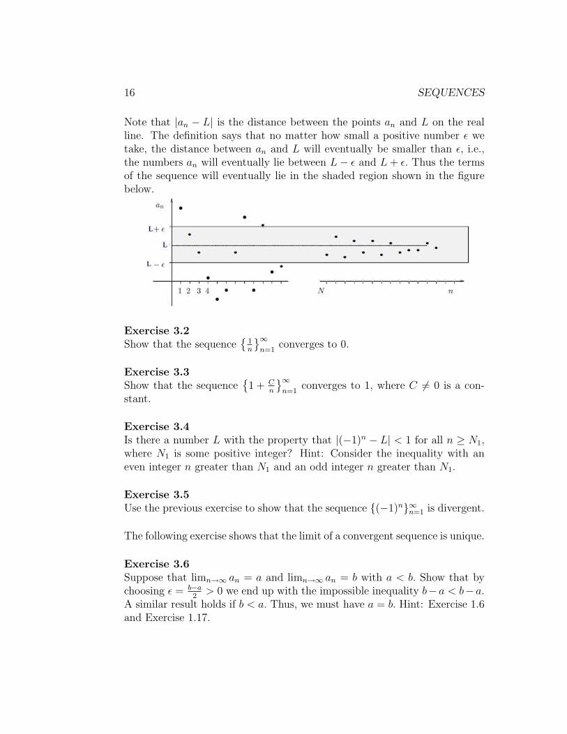
Note that |an − L| is the distance between the points an and L on the realline. The definition says that no matter how small a positive number ε wetake, the distance between an and L will eventually be smaller than ε, i.e.,the numbers an will eventually lie between L− ε and L + ε. Thus the termsof the sequence will eventually lie in the shaded region shown in the figurebelow.

Exercise 3.2Show that the sequence

{1n

}∞n=1

converges to 0.

Exercise 3.3Show that the sequence

{1 + C

n

}∞n=1

converges to 1, where C 6= 0 is a con-stant.

Exercise 3.4Is there a number L with the property that |(−1)n − L| < 1 for all n ≥ N1,where N1 is some positive integer? Hint: Consider the inequality with aneven integer n greater than N1 and an odd integer n greater than N1.

Exercise 3.5Use the previous exercise to show that the sequence {(−1)n}∞n=1 is divergent.

The following exercise shows that the limit of a convergent sequence is unique.

Exercise 3.6Suppose that limn→∞ an = a and limn→∞ an = b with a < b. Show that bychoosing ε = b−a

2> 0 we end up with the impossible inequality b−a < b−a.

A similar result holds if b < a. Thus, we must have a = b. Hint: Exercise 1.6and Exercise 1.17.

3 SEQUENCES AND THEIR CONVERGENCE 17

We next introduce the concept of a bounded sequence. This concept providesus with a divergence test for sequences. We will see that if a sequence is notbounded then it is divergent.

Definition 6A sequence {an}∞n=1 is said to be bounded if there is a positive constant Msuch that |an| ≤ M for all n ∈ N.

Exercise 3.7Show that each of the following sequences is bounded. Identify M in eachcase.(a) an = (−1)n.(b) an = 1√

n ln (n+1).

Exercise 3.8Let {an}∞n=1 be a sequence such that |an| ≤ K for all n ≥ N. Show that thissequence is bounded. Identify your M.

Exercise 3.9Show that a convergent sequence is bounded. Hint: use the definition ofconvergence with ε = 1.

The converse of the above result is not always true. That is, a boundedsequence need not be convergent.

Exercise 3.10Give an example of a bounded sequence that is divergent.

The following result is known as the squeeze rule.

Exercise 3.11Let {an}∞n=1 , {bn}∞n=1 , {cn}∞n=1 be three sequences with the following condi-tions:(1) bn ≤ an ≤ cn for all n ≥ K, where K is some positive integer.(2) limn→∞ bn = limn→∞ cn = L.Show that limn→∞ an = L. Hint: Use the definition of convergence alongwith Exercise 1.14

18 SEQUENCES

Exercise 3.12An expansion of (a+b)n, where n is a positive integer is given by the Binomialformula

(a + b)n =n∑

k=0

C(n, k)akbn−k

where C(n, k) = n!k!(n−k)!

.

(a) Use the Binomial formula to establish the inequality

(1 + x)1n ≤ 1 +

x

n, x ≥ 0

(b) Show that if a ≥ 1 then limn→∞ a1n = 1. Hint: Use Exercise 3.3.

3 SEQUENCES AND THEIR CONVERGENCE 19

Practice Problems

Exercise 3.13Prove that the sequence {cos (nπ)}∞n=1 is divergent.

Exercise 3.14Let {an}∞n=1 be the sequence defined by an = n for all n ∈ N. Explain whythe sequence {an}∞n=1 does not converge to any limit.

Exercise 3.15(a) Show that for all n ∈ N we have

n!

nn≤ 1

n.

(b) Show that the sequence {an}∞n=1 where an = n!nn is convergent and find

its limit.

Exercise 3.16Using only the definition of convergence show that

limn→∞

3√

n− 50013√

n− 1001= 1.

Exercise 3.17Consider the sequence defined recursively by a1 = 1 and an+1 =

√2 + an for

all n ∈ N. Show that an ≤ 2 for all n ∈ N.

Exercise 3.18Calculate limn→∞

(n2+1) cos nn3 .

Exercise 3.19Calculate limn→∞

2(−1)n+3√

n.

Exercise 3.20Suppose that limn→∞ an = L with L > 0. Show that there is a positiveinteger N such that 2xN > x.

20 SEQUENCES

Exercise 3.21Let a ∈ R and n ∈ N. Clearly, a < a + 1

n.

(a) Show that there is a1 ∈ Q such that a < a1 < a + 1n. Hint: Exercise

2.6(c).(b) Show that there is a2 ∈ Q such that a < a2 < a1.(c) Continuiung the above process we can find a sequence {an}∞n=1 such thata < an < a + 1

nfor all n ∈ N. Show that this sequence converges to a.

We have proved that if a is a real number then there is a sequence of rationalnumbers converging a. We say that the set Q is dense in R.

4 ARITHMETIC OPERATIONS ON SEQUENCES 21

4 Arithmetic Operations on Sequences

In this section we discuss the operations of addition, subtration, scalar multi-plication, multiplication, reciprocal, and the ratio of two sequences. Our firstresult concerns the convergence of the sum or difference of two sequences.

Exercise 4.1Suppose that limn→∞ an = A and limn→∞ bn = B. Show that

limn→∞

an ± bn = A±B.

The next result concerns the product of two sequences.

Exercise 4.2Suppose that limn→∞ an = A and limn→∞ bn = B.(a) Show that |bn| ≤ M for all n ∈ N, where M is a positive constant.(b) Show that anbn − AB = (an − A)bn + A(bn −B).(c) Let ε > 0 be arbitrary and K = M +|A|. Show that there exists a positiveinteger N1 such that |an − A| < ε

2Kfor all n ≥ N1.

(d) Let ε > 0 and K be as in (c). Show that there exists a positive integerN2 such that |bn −B| < ε

2Kfor all n ≥ N2.

(e) Show that limn→∞ anbn = AB.

Exercise 4.3Give an example of two divergent sequences {an}∞n=1 and {bn}∞n=1 such that{anbn} and {an + bn} are convergent.

Exercise 4.4Let k be an arbitrary constant and limn→∞ an = A. Show that limn→∞ kan =kA.

Exercise 4.5Suppose that limn→∞ an = 0 and {bn}∞n=1 is bounded. Show that limn→∞ anbn =0.

Exercise 4.6(a) Use the previous exercise to show that limn→∞

sin nn

= 0.(b) Show that limn→∞

sin nn

= 0 using the squeeze rule.

22 SEQUENCES

Exercise 4.7Suppose that limn→∞ an = A with A 6= 0. Show that there is a positiveinteger N such that |an| > |A|

2for all n ≥ N. Hint: Use Exercise 1.18.

Exercise 4.8Let {an}∞n=1 be a sequence with the following conditions:(1) an 6= 0 for all n ≥ 1.(2) limn→∞ an = A, with A 6= 0.(a) Show that there is a positive integer N1 such that for all n ≥ N1 we have∣∣∣∣ 1

an

− 1

A

∣∣∣∣ <2

|A|2|an − A|.

(b) Let ε > 0 be arbitrary. Show that there is a positive integer N2 such thatfor all n ≥ N2 we have

|an − A| < |A|2

2ε.

(c) Using (a) and (b), show that

limn→∞

1

an

=1

A.

Exercise 4.9Let 0 < a < 1. Show that limn→∞ a

1n = 1. Hint: Use Exercise 3.12 (b).

Exercise 4.10Show that if limn→∞ an = A and limn→∞ bn = B with bn 6= 0 for all n ≥ 1and B 6= 0, then

limn→∞

an

bn

=A

B.

Hint: Note that an

bn= an · 1

bn.

Exercise 4.11Given that limn→∞ an = A and limn→∞ bn = B with an ≤ bn for all n ≥ 1.(a) Suppose that B < A. Let ε = A−B

2> 0. Show that there exist positive

integers N1 and N2 such that A − ε < an < A + ε for n ≥ N1 and B − ε <bn < B + ε for n ≥ N2.(b) Let N = N1 + N2. Show that for n ≥ N we obtain the contradictionbn < an. Thus, we must have A ≤ B.

4 ARITHMETIC OPERATIONS ON SEQUENCES 23

Practice Problems

Exercise 4.12Suppose that limn→∞

an

bn= L and limn→∞ bn = 0 where bn 6= 0 for all n ∈ N.

Find limn→∞ an.

Exercise 4.13The Fibonacci numbers are defined recursively as follows:

a1 = a2 = 1 and an+2 = an+1 + an for all n ∈ N.

Suppose that limn→∞an+1

an= L. Find the value of L.

Exercise 4.14Show that the sequence defined by

an =n

n + 1+ (−1)n n2 + 3

n2 + 7

have two limits by finding limn→∞ a2n and limn→∞ a2n+1.

Exercise 4.15Use the properties of this section to find

limn→∞

√2n2 + 5n

n + 4.

Exercise 4.16Find the limit of the sequence defined by

an = n1

2 ln n .

Exercise 4.17Consider the sequence defined by

an =1√1

+1√2

+ · · ·+ 1√n

.

(a) Show that an ≥√

n for all n ∈ N.(b) Show that the sequence {an}∞n=1 is divergent. Hint: Exercise 4.11

24 SEQUENCES


an = ln (2n +√

n)− ln n.

Exercise 4.19Consider the sequence defined by an = n

√3n + 1.

(a) Show that 3 < an < 3 n√

2 for all n ∈ N.(b) Find the limit of an as n →∞.

Exercise 4.20Let {an}∞n=1 be a convergent sequence of nonnegative terms with limit L.Suppose that the terms of sequence satisfy the recursive relation anan+1 =an + 2 for all N ∈ N. Find L.


an = cos1

n+

sin n

n.

Exercise 4.22Suppose that an+1 = a2

n+1an

. Show that the sequence {an}∞n=1 is divergent.

5 MONOTONE AND BOUNDED SEQUENCES 25

5 Monotone and Bounded Sequences

One of the problems with deciding if a sequence is convergent is that youneed to have a limit before you can test the definition. However, it is oftenthe case that it is more important to know if a sequence converges than whatit converges to. In this and the next section, we look at two ways to prove asequence converges without knowing its limit. That is convergence is solelybased on the terms of the sequence.

Definition 7A sequence {an}∞n=1 is said to be increasing if and only if an ≤ an+1 for alln ≥ 1.A sequence {an}∞n=1 is said to be decreasing if and only if an ≥ an+1 for alln ≥ 1.A sequence that is either increasing or decreasing is said to be monotone.

Exercise 5.1Show that the sequence { 1

n}∞n=1 is decreasing.


1+e−n}∞n=1 is increasing.

Definition 8A sequence {an}∞n=1 is said to be bounded from below if and only if thereis a constant m such that m ≤ an for all n ≥ 1. We call m a lower bound.A sequence {an}∞n=1 is said to be bounded from above if and only if thereis a constant M such that an ≤ M for all n ≥ 1. We call M an upperbound.


n}∞n=1 is bounded from below. What is a lower

bound? Are there more than one lower bound?


1+e−n}∞n=1 is bounded from above. What is an upperbound? Are there more than one upper bound?

Suppose that N ≤ an ≤ M for all n ≥ 1. That is, the sequence is boundedfrom above and below. As we have seen from the previous two exercises, thesequence may have many lower and upper bounds.

26 SEQUENCES

Definition 9The largest lower bound is called the greatest lower bound ( or the infi-mum) denoted by inf{an : n ≥ 1}. Note that the infimum is a lower bound.Moreover, for any lower bound m of {an}∞n=1 we have m ≤ inf{an : n ≥ 1}.The smallest upper bound is called the least upper bound ( or the supre-mum) denoted by sup{an : n ≥ 1}. Note that the supremum is an upperbound. Moreover, for any upper bound M of {an}∞n=1 we have sup{an : n ≥1} ≤ M.

The next result shows that an increasing sequence that is bounded fromabove is always convergent.

Exercise 5.5Let {an}∞n=1 be an increasing sequence that is bounded from above.(a) Show that there is a finite number M such that M = sup{an : n ≥ 1}.(b) Let ε > 0 be arbitrary. Show that M − ε cannot be an upper bound ofthe sequence.(c) Show that there is a positive integer N such that M − ε < aN .(d) Show that M − ε < an for all n ≥ N.(e) Show that M − ε < an < M + ε for all n ≥ N.(f) Show that limn→∞ an = M. That is, the given sequence is convergent.

Exercise 5.6Consider the sequence {an}∞n=1 defined recursively by a1 = 3

2and an+1 =

12an + 1 for n ≥ 1.

(a) Show by induction on n ≥ 1, that an+1 = an + 12n+1 .

(b) Show that this sequence is increasing.(c) Show that {an}∞n=1 is bounded from above. What is an upper bound?(d) Show that {an}∞n=1 is convergent. What is its limit? Hint: In finding thelimit, use the arithmetic operations of sequences.

Exercise 5.7Let {an}∞n=1 be a decreasing sequence such that m ≤ an for all n ≥ 1. Showthat {an}∞n=1 is convergent. Hint: Let bn = −an and use Exercise 5.5 andExercise 4.4.

Exercise 5.8Show that a monotone sequence is convergent if and only if it is bounded.

5 MONOTONE AND BOUNDED SEQUENCES 27

Practice Problems

Exercise 5.9Let an be defined by a1 =

√2 and an+1 =

√2 + an for n ∈ N.

(a) Show that an ≤ 2 for all n ∈ N. That is, {an}∞n=1 is bounded from above.(b) Show that an+1 ≥ an for all n ∈ N. That is, {an}∞n=1 is increasing.(c) Conclude that {an}∞n=1 is convergent. Find its limit.

Exercise 5.10Let an =

∑nk=1

1k2 .

(a) Show that an < 2 for all n ∈ N. Hint: Recall that∑n

k=11

(n+1)n= 1− 1

n+1.

(b) Show that {an}∞n=1 is increasing.(c) Conclude that {an}∞n=1 is convergent.

Exercise 5.11Consider the sequence {an}∞n=1 defined recursively as follows

a1 = 2 and 7an+1 = 2a2n + 3 for all n ∈ N.

(a) show that 12

< an < 3 for all n ∈ N.(b) Show that an+1 ≤ an for all n ∈ N.(c) Deduce that {an}∞n=1 is convergent and find its limit.

Exercise 5.12Let {an}∞n=1 be an increasing sequence. Define bn = a1+a2+···+an

n. Show that

the sequence {bn}∞n=1 is increasing.

Exercise 5.13Give an example of a monotone sequence that is divergent.

Exercise 5.14Consider the sequence defined recursively by a1 = 1 and an+1 = 3 + an

2for

all n ∈ N.(a) Show that an ≤ 6 for all n ∈ N.(b) Show that {an}∞n=1 is increasing.(c) Conclude that the sequence is convergent. Find its limit.

Exercise 5.15Give an example of two monotone sequences whose sum is not monotone.

28 SEQUENCES

6 Subsequences and the Bolzano-Weierstrass

Theorem

In this section we consider a sequence contained in another sequence. Moreformally we have

Definition 10Consider a sequence {an}∞n=1. A sequence consisting of terms of the givensequence of the form {ank

}∞k=1 where n1 < n2 < n3 < · · · is called a subse-quence.

Exercise 6.1Let {ank

}∞k=1 be a subsequence of a sequence {an}∞n=1. Use induction on k toshow that nk ≥ k for all k ∈ N.

Exercise 6.2Let {an}∞n=1 be a sequence of real numbers that converges to a number L.Let {ank

}∞k=1 be any subsequence of {an}∞n=1.(a) Let ε > 0 be given. Show that there is a positive integer N ′ such that ifn ≥ N ′ then |an − L| < ε.(b) Let N be the first positive integer such that nN ≥ N ′. Show that if k ≥ Nthen |ank

−L| < ε. That is, the subsequence {ank}∞k=1 converges to L. Hence,

every subsequence of a convergent sequence is convergent to the same limitof the original sequence.

The next result shows that every sequence has a monotonic subsequence.

Exercise 6.3Let {an}∞n=1 be a sequence of real numbers. Let S = {n ∈ N : an > amfor allm > n}.(a) Suppose that S is infinite. Then there is a sequence n1 < n2 < n3 < · · ·such nk ∈ S. Show that ank+1

< ank. Thus, the subsequence {ank

}∞k=1 isdecreasing.(b) Suppose that S is finite. Let n1 be the first positive integer such thatn1 6∈ S. Show that the subsequence {ank

}∞k=1 is increasing.

As a corollary to the previous exercise we obtain the following famous resultwhich says that every bounded sequence of real numbers has a convergentsubsequence.

6 SUBSEQUENCES AND THE BOLZANO-WEIERSTRASS THEOREM29

Exercise 6.4 (Bolzano-Weierstrass)Every bounded sequence has a convergent subsequence. Hint: Exercise 5.8

Exercise 6.5Show that the sequence {esin n}∞n=1 has a convergent subsequence.

30 SEQUENCES

Practice Problems

Exercise 6.6Prove that the sequence {an}∞n=1 where an = cos nπ

2is divergent.

Exercise 6.7Prove that the sequence {an}∞n=1 where

an =(n2 + 20n + 35) sin n3

n2 + n + 1

has a convergent subsequence. Hint: Show that {an}∞n=1 is bounded.

Exercise 6.8Show that the sequence defined by an = 2 cos n − sin n has a convergentsubsequence.

Exercise 6.9True or false: There is a sequence that converges to 6 but contains a subse-quence converging to 0. Justify your answer.

Exercise 6.10Give an example of an unbounded sequence with a bounded subsequence.

Exercise 6.11Show that the sequence {(−1)n}∞n=1 is divergent by using subsequences.

7 CAUCHY SEQUENCES 31

7 Cauchy Sequences

The notion of a Cauchy sequence provides us with a characterization of con-vergence in terms of just the terms in the sequence without explicit referenceto the limit.

Definition 11A sequence {an}∞n=1 is called a Cauchy sequence if for every ε > 0 thereexists a positive integer N = N(ε) such that

if n, m ≥ N then |an − am| < ε.

Thus, for a sequence to be Cauchy, we don’t require that the terms of thesequence to be eventually all close to a certain limit, just that the terms ofthe sequence to be eventually all close to one another.

Exercise 7.1Consider the sequence whose nth term is given by an = 1

n. Let ε > 0 be

arbitrary and choose N > 2ε. Show that for m,n ≥ N we have |am− an| < ε.

That is, the above sequence is a Cauchy sequence. Hint: Exercise 1.17.

The next result shows that Cauchy sequences are bounded sequences.

Exercise 7.2Show that any Cauchy sequence is bounded. Hint: Let ε = 1 and use Exercise1.18.

Exercise 7.3Show that if limn→∞ an = A then {an}∞n=1 is a Cauchy sequence. Thus, everyconvergent sequence is a Cauchy sequence.

Now, consider a Cauchy sequence {an}∞n=1. Create new sequences as follows:For each n ≥ 1, a new sequence is obtained by deleting the previous n − 1terms from the original sequence. For example, if n = 1, the new sequenceis just the original sequence, for n = 2 the new sequence is {a2, a3, · · · }, forn = 3 the new sequence is {a3, a4 · · · } and so on.

Exercise 7.4(a) Using Exercise 7.2, show that for each n ≥ 1, the sequence {an, an+1, · · · }is bounded.(b) Show that for each n ≥ 1 the infimum of {an, an+1, · · · } exists. Call itbn.

32 SEQUENCES

Exercise 7.5(a) Show that the sequence {bn}∞n=1 is bounded from above.(b) Show that the sequence {bn}∞n=1 is increasing. Hint: Show that bn is alower bound of the sequence {an+1, an+2, · · · }.

Exercise 7.6Show that the sequence {bn}∞n=1 is convergent. Call the limit B.

Exercise 7.7(a) Let ε > 0 be arbitrary. Using the definition of Cauchy sequences andExercise ??, show that there is a positive integer N such that aN − ε

2< an <

aN + ε2

for all n ≥ N.(b) Using (a), show that aN− ε

2is a lower bound of the sequence {aN , aN+1, · · · }

Thus, aN − ε2≤ bn for all n ≥ N.

(c) Again, using (a) show that bn < aN + ε2

for all n ≥ N. Thus, combining(b) and (c), we obtain aN − ε

2≤ bn < aN + ε

2.

(d) Using Exercise 4.11, show that aN − ε2≤ B ≤ aN + ε

2.

(e) Using (a), (d), and Exercise 1.17, show that limn→∞ an = B. Thus, everyCauchy sequence is convergent.

7 CAUCHY SEQUENCES 33

Practice Problems

Exercise 7.8(a) Show that if {an}∞n=1 is Cauchy then {a2

n}∞n=1 is also Cauchy.(b) Give an example of Cauchy sequence {a2

n}∞n=1 such that {an}∞n=1 is notCauchy.

Exercise 7.9Let {an}∞n=1 be a Cauchy sequence such that an is an integer for all n ∈ N.Show that there is a positive integer N such that an = C for all n ≥ N,where C is a constant.

Exercise 7.10Let {an}∞n=1 be a sequence that satisfies

|an+2 − an+1| < c2|an+1 − an| for all n ∈ N

where 0 < c < 1.(a) Show that |an+1 − an| < cn|a2 − a1| for all n ≥ 2.(b) Show that {an}∞n=1 is a Cauchy sequence.

Exercise 7.11What does it mean for a sequence {an}∞n=1 to not be Cauchy?

Exercise 7.12Let {an}∞n=1 and {bn}∞n=1 be two Cauchy sequences. Define cn = |an − bn|.Show that {cn}∞n=1 is a Cauchy sequence.

Exercise 7.13Suppose {an}∞n=1 is a Cauchy sequence. Suppose an ≥ 0 for infinitely manyn and an ≤ 0 for infinitely many n. Prove that limn→∞ an = 0.

Exercise 7.14Explain why the sequence defined by an = (−1)n is not a Cauchy sequence.

34 SEQUENCES

Limits

8 The Limit of a Function

A fundamental concept in single variable calculus is the concept of the limitof a function. In this section, we introduce the definition of limit and discusssome of its properties.

Definition 12Let f be a function with domain D ⊂ R. Let a be a point in D. We say that fhas a limit L at a if and only if for every ε > 0 there exists a positive numberδ depending on ε such that for any x ∈ D with the property 0 < |x− a| < δwe have |f(x)− L| < ε. In symbol we write

limx→a

f(x) = L

or f(x) → L as x → a.

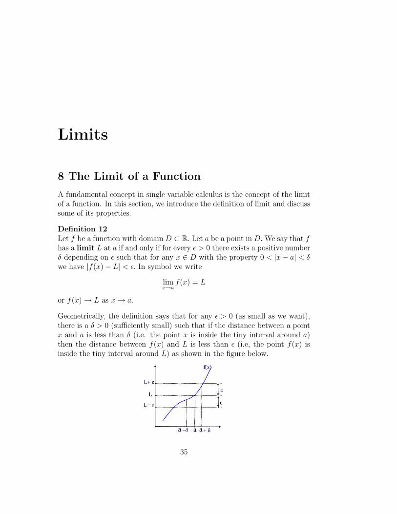
Geometrically, the definition says that for any ε > 0 (as small as we want),there is a δ > 0 (sufficiently small) such that if the distance between a pointx and a is less than δ (i.e. the point x is inside the tiny interval around a)then the distance between f(x) and L is less than ε (i.e, the point f(x) isinside the tiny interval around L) as shown in the figure below.

35

36 LIMITS

Exercise 8.1Show that limx→1

x2−1x−1

= 2.

The limit of a function may not exist as shown in the next example.

Exercise 8.2Let f(x) = |x|

x. Suppose that limx→0 f(x) = L.

(a) Show that there is a positive number δ such that if 0 < |x| < δ then∣∣∣ |x|x− L

∣∣∣ < 14.

(b) Let x1 = δ4

and x2 = − δ4. Compute the value of |f(x1)− f(x2)|.

(c) Use (a) to show that |f(x1)− f(x2)| < 12.

(d) Conclude that L does not exist. That is, limx→0|x|x

does not exist.

Exercise 8.3Let f(x) = sin

(1x

). Suppose that limx→0 f(x) = L.

(a) Show that there is a positive number δ such that if 0 < |x| < δ then∣∣sin (1x

)− L

∣∣ < 14.

(b) Let n be a positive integer such that x1 = 2(2n+1)π

< δ and x2 = 1(2n+1)π

<

δ. Compute the value of |f(x1)− f(x2)|.(c) Use (a) to show that |f(x1)− f(x2)| < 1

2.

(d) Conclude that L does not exist. That is, limx→0 sin(

1x

)does not exist.

The next exercise shows that the a function can have only one limit, if sucha limit exists.

Exercise 8.4Suppose that limx→a f(x) exists. Also, suppose that limx→a f(x) = L1 andlimx→a f(x) = L2. So either L1 = L2 or L1 6= L2.(a) Suppose that L1 6= L2. Show that there exist positive constants δ1 and δ2

such that if 0 < |x−a| < δ1 then |f(x)−L1| < |L1−L2|2

and if 0 < |x−a| < δ2

then |f(x)− L2| < |L1−L2|2

.(b) Let δ = min{δ1, δ2} so that δ ≤ δ1 and δ ≤ δ2. Show that if 0 < |x−a| < δthen |L1 − L2| < |L1 − L2| which is impossible.(c) Conclude that L1 = L2. That is, whenever a function has a limit, thatlimit is unique.

8 THE LIMIT OF A FUNCTION 37

Practice Problems

Exercise 8.5Using the εδ definition of limit to show that

limx→−1

(2x2 + x + 1) = 2.

Exercise 8.6Prove directly from the definition that limx→1

xx+3

= 14.

Exercise 8.7In this exercise we discuss the concept of sided limits.(a) We say that L is the left side limit of f as x approaches a from the leftif and only if

∀ε > 0,∃δ > 0 such that 0 < a− x < δ ⇒ |f(x)− L| < ε

and we write limx→a− f(x) = L. Show that limx→0−|x|x

= −1.(b) We say that L is the right side limit of f as x approaches a from theright if and only if

∀ε > 0,∃δ > 0 such that 0 < x− a < δ ⇒ |f(x)− L| < ε

and we write limx→a+ f(x) = L. Show that limx→0+|x|x

= 1.

Exercise 8.8Prove that L = limx→a f(x) if and only if limx→a− f(x) = limx→a+ f(x) = L.

Exercise 8.9Using ε and δ, what does it mean that limx→a f(x) 6= L?

38 LIMITS

9 Properties of Limits

When computing limits, one uses some established properties rather thanthe εδ definition of limit. In this section, we discuss these basic properties.

Exercise 9.1Suppose that limx→a f(x) = L1 and limx→a g(x) = L2. Show that

limx→a

[f(x)± g(x)] = L1 ± L2.

Exercise 9.2Suppose that limx→a f(x) = L1 and limx→a g(x) = L2. Show the following:(a) There is a δ1 > 0 such that

0 < |x− a| < δ1 =⇒ |f(x)| < 1 + |L1|.

Hint: Notice that f(x) = (f(x)− L1) + L1.(b) Given ε > 0, there is a δ2 > 0 such that

0 < |x− a| < δ2 =⇒ |f(x)− L1| <ε

2(1 + |L2|).

Exercise 9.3Suppose that limx→a f(x) = L1 and limx→a g(x) = L2.(a) Show that f(x)g(x)− L1L2 = f(x)(g(x)− L2) + L2(f(x)− L1).(b) Show that |f(x)g(x)− L1L2| ≤ |f(x)||g(x)− L2|+ |L2||f(x)− L1|.(c) Show that limx→a f(x)g(x) = L1L2. Hint: Use the previous exercise.

Exercise 9.4(a) Suppose that |f(x)| ≤ M for all x in its domain and limx→a g(x) = 0.Show that

limx→a

f(x)g(x) = 0.

Hint: Recall Exercise 4.5(b) Show that limx→0 x sin

(1x

)= 0.

The following exercise says that when a function approaches a nonzero num-ber as the variable x approaches a, then there is an open interval around awhere the function is always different from zero in that interval.

9 PROPERTIES OF LIMITS 39

Exercise 9.5Suppose that limx→a f(x) = L with L 6= 0. Show that there exists a δ > 0such that

0 < |x− a| < δ =⇒ |f(x)| > |L|2

> 0.

Hint: Recall the solution to Exercise 4.7

Exercise 9.6Let g(x) be a function with the following conditions:(1) g(x) 6= 0 for all x in the domain of g.(2) limx→a g(x) = L2, with L2 6= 0.(a) Show that there is a δ1 > 0 such that if 0 < |x− a| < δ1 then∣∣∣∣ 1

g(x)− 1

L2

∣∣∣∣ <2

|L2|2|g(x)− L2|.

(b) Let ε > 0 be arbitrary. Show that there is δ2 > 0 such that if 0 < |x−a| <δ2 then

|g(x)− L2| <|L2|2

2ε.

(c) Using (a) and (b), show that

limx→a

1

g(x)=

1

L2

.

Hint: Recall Exercise 4.8

Exercise 9.7Show that if limx→a f(x) = L1 and limx→a g(x) = L2 where g(x) 6= 0 in itsdomain and L2 6= 0 then

limx→a

f(x)

g(x)=

L1

L2

.

Hint: Recall Exercise 4.10.

Exercise 9.8Let f(x) and g(x) be two functions with a common domain D and a a pointin D. Suppose that f(x) ≤ g(x) for all x in D. Show that if limx→a f(x) = L1

and limx→a g(x) = L2 then L1 ≤ L2. Hint: Recall Exercise 4.11

40 LIMITS

Practice Problems

Exercise 9.9Let D be the domain of a function f(x). Suppose that f(x) ≥ 0 for all x inD and limx→a f(x) = L with L > 0.(a) Show that √

f(x)−√

L =f(x)− L√f(x) +

√L

.

(b) Let ε > 0. Show that there exists δ > 0 such that |f(x) − L| < ε√

Lwhenever 0 < |x− a| < δ.(c) Show that

limx→a

√f(x) =

√L.

Exercise 9.10 (Squeeze Rule)Let f(x), g(x) and h(x) be three functions with common domain D and a bea point in D. Suppose that(1) g(x) ≤ f(x) ≤ h(x) for all x in D.(2) limx→a g(x) = limx→a h(x) = L.Show that limx→a f(x) = L. Hint: Recall Exercise 3.11

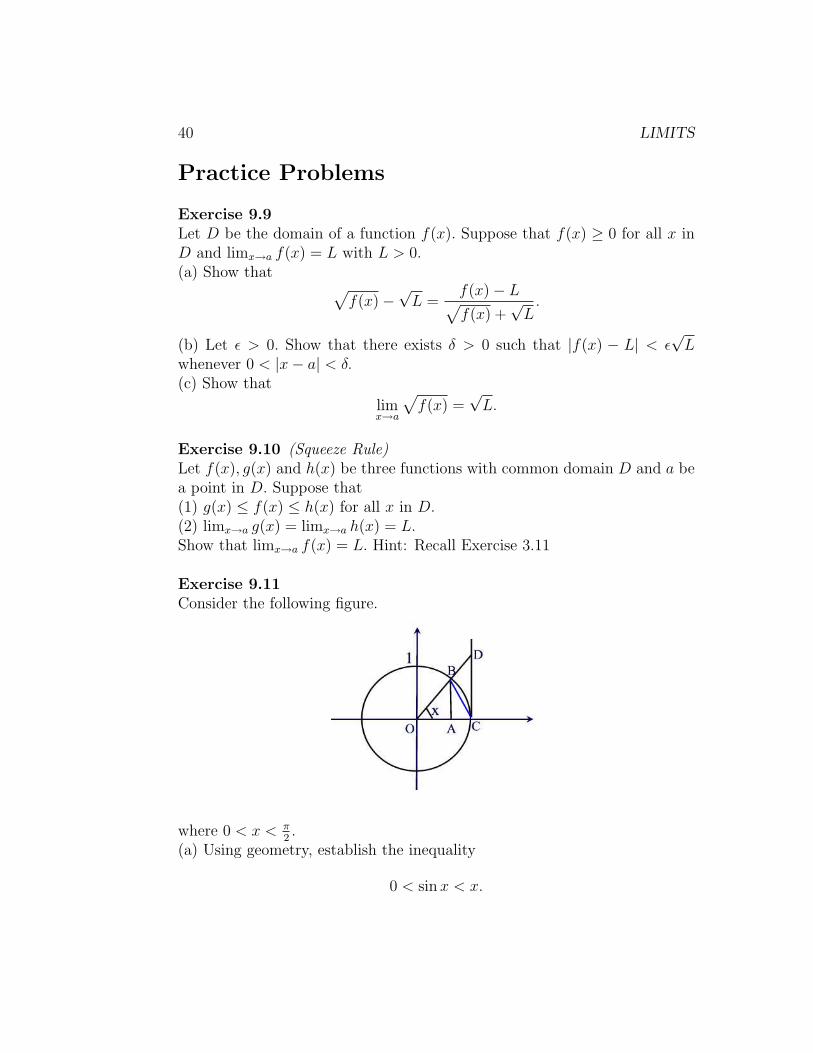
Exercise 9.11Consider the following figure.

where 0 < x < π2.

(a) Using geometry, establish the inequality

0 < sin x < x.

9 PROPERTIES OF LIMITS 41

Hint: The area of a circular sector with radius r and central angle θ is givenby the formula 1

2r2θ.

(b) Show that limx→0+ sin x = 0.(c) Show that limx→0− sin x = 0. Thus, we conclude that limx→0 sin x = 0.Hint: Recall that the sine function is an odd function.(d) Show that limx→0 cos x = 1. Hint: cos2 x + sin2 x = 1.(e) Using geometry, establish the double inequality

sin x cos x

2<

x

2<

tan x

2.

(f) Using (a) show that

cos x <sin x

x<

1

cos x.

(g) Show that

limx→0+

sin x

x= 1.

(h) Show that for −π2

< x < 0 we have also

limx→0−

sin x

x= 1.

Exercise 9.12Find each of the following limits:

(1) limx→1

√x2+3−2

√x

x2−1.

(2) limx→2−x−2

|x2−5x+6| .

Exercise 9.13Find limx→∞

x2+xx2−x

by using the change of variable u = 1x.

Exercise 9.14Find limx→0

3√

x sin 1x.

Exercise 9.15Find limx→0 x2 tan x.

Exercise 9.16Let n be a positive integer. Prove that limx→a[f(x)]n = [limx→a f(x)]n .

42 LIMITS

10 Connection Between the Limit of a Func-

tion and the Limit of a Sequence

The limit of a function given so far is known as the εδ definition. In thissection, we will establish an equivalent definition that involves the limit of asequence.

Exercise 10.1Suppose that limx→a f(x) = L, where a is in the domain of f. Let {an}∞n=1

be a sequence whose terms belong to the domain of f and are different froma and suppose that limn→∞ an = a.(a) Let ε > 0 be arbitrary. Show that there exist a positive integer N anda positive number δ such that for n ≥ N we have |an − a| < δ and for0 < |x− a| < δ we have |f(x)− L| < ε.(b) Use (a) to conclude that for a given ε > 0 there is a positive integer Nsuch that if n ≥ N then |f(an)− L| < ε. That is, limn→∞ f(an) = L.

Using Definition 9, what do we mean by limx→a f(x) 6= L? This means thatthere is an interval centered at L such that for any interval centered at a wecan find a point x in that interval and in the domain of f such that f(x) isnot in the interval centered at L. This is the same thing as saying that wecan find an ε > 0 such for all δ > 0 there is xδ (in the domain of f) with theproperty that 0 < |xδ − a| < δ but |f(xδ)− L| ≥ ε.

Exercise 10.2Let f : D → R be a function with the property that for any sequence {an}∞n=1

(with an 6= a for all n ≥ 1) if limn→∞ an = a then limn→∞ f(an) = L. Wewant to show that

limx→a

f(x) = L

(a) Suppose first that limx→a f(x) 6= L. Show that there is an ε > 0 and asequence {an}∞n=1 of terms in the domain of f such that 0 < |an−a| < 1

nand

|f(an)− L| ≥ ε.(b) Use the squeeze rule to show that limn→∞ |an − a| = 0.(c) Use the fact that −|a| ≤ a ≤ |a| for any number a and the squeeze ruleto show that limn→∞(an − a) = 0.(d) Use Exercise 4.1 to show that limn→∞ an = a.(e) Using (a), (d), the given hypothesis and Exercise 4.11, show that ε ≤ 0.

10 CONNECTION BETWEEN THE LIMIT OF A FUNCTION AND THE LIMIT OF A SEQUENCE43

Thus, this contradiction shows that limx→a f(x) 6= L cannot happen. Weconclude that

limx→a

f(x) = L

The above two exercises establish that the sequence version and the εδ versionare equivalent.In many cases, one is interested in knowing that the limit of a function existwithout the need of knowing the value of the limit. In what follows, we willestablish a result that uses Cauchy sequences to provide a test for establishingthat the limit of a function exists.

Exercise 10.3Let f be a function with domain D and a be a point in D. Suppose that fsatisfies the following Property:

(P) If {an}∞n=1, with an in D, an 6= a for all n ≥ 1 and limn→∞ an = a then{f(an)}∞n=1 is a Cauchy sequence.

(a) Let {an}∞n=1 be a sequence of elements of D such that an 6= a for all n ≥ 1and limn→∞ an = a. Show that the sequence {f(an)}∞n=1 is convergent. Callthe limit L. Hint: See Exercise 7.7(b) Let {bn}∞n=1 be a sequence of elements of D such that bn 6= a for all n ≥ 1and limn→∞ bn = a. Show that the sequence {f(bn)}∞n=1 converges to somenumber L′.

Exercise 10.4Let {an}∞n=1 and {bn}∞n=1 be the two sequences of the previous exercise. Definethe sequence

{cn} = {b1, a1, b2, a2, b3, a3, · · · }.That is, cn = ak if n = 2k and cn = bk if n = 2k + 1 where k ≥ 0.(a) Show that for all n ≥ 1 we have cn ∈ D and cn 6= a.(b) Let ε > 0. Show that there exist positive integers N1 and N2 such that ifn ≥ N1 then |an − a| < ε and if n ≥ N2 then |bn − a| < ε.(c) Let N = 2N1 + 2N2 + 1. Show that if n ≥ N then |cn − a| < ε. Hence,limn→∞ cn = a. Hint: Consider the cases n = 2k or n = 2k + 1.(d) Show that limn→∞ f(cn) = L′′ for some number L′′.

The next exercise establishes the fact that the two sequences {f(an)}∞n=1 and{f(bn)}∞n=1 converge to the same limit.

44 LIMITS

Exercise 10.5Let {an}∞n=1, {bn}∞n=1, and {cn}∞n=1 be as in the previous exercise.(a) Compare {an}∞n=1 and {cn}∞n=1.(b) Let ε > 0 be arbitrary. Show that there is a positive integer N such thatif n ≥ N then |f(cn)− L′′| < ε.(c) Let N1 be a positive integer such that N1 ≥ N

2. Show that if n ≥ N1 then

|f(an)− L′′| < ε. Hence, limn→∞ f(an) = L′′.(d) Show that limn→∞ f(bn) = L′′. Thus, by Exercise 3.6, we must haveL = L′ = L′′.

Exercise 10.6Prove that if a function f satisfies property (P) then limx→a f(x) exists. Hint:Use Exercise 10.2.

10 CONNECTION BETWEEN THE LIMIT OF A FUNCTION AND THE LIMIT OF A SEQUENCE45

Practice Problems

Exercise 10.7Consider the function f : R → R defined by

f(x) =

{sin 1

xif x 6= 0

1 if x = 0

Let {an}∞n=1 and {bn}∞n=1 be the two sequences defined by an = 12nπ

andbn = 1

(2n+ 12)π

. Clearly, an, bn 6= 0 for all n ∈ N, an → 0 and bn → 0. Show

that limx→0 f(x) does not exist.

Exercise 10.8Let {an}∞n=1 be a sequence such that an 6= 2 for all n ∈ N and limn→∞ an = 2.

(a) Find limn→∞a2

n−4an+2

= 4.

(b) Find limx→2x2−4x+2

.

Exercise 10.9Consider the floor function f : [0, 1] → R given by f(x) = bxc, where bxcdenote the largest integer less than or equal to x. Find limx→1bxc usingsequences.

Exercise 10.10Consider the floor function f : R → R given by f(x) = bxc, where bxc denotethe largest integer less than or equal to x.(a) Let an = 1 − 1

nand bn = 1 + 1

nfor all n ∈ N. Find limn→∞ f(an) and

limn→∞ f(bn).(b) Does limx→1bxc exist?

46 LIMITS

Continuity

11 Continuity of a Function at a Point

In this section we introduce the notion of continuity of a function at a pointin its domain and study the various equivalent definitions of this notion.

Definition 13Let f be a real-valued function with domain D and a a point in D. Wesay that f is continuous at a if and only if for any given ε we can findδ = δ(ε) > 0 such that

for all x in D if |x− a| < δ then |f(x)− f(a)| < ε.

If f is continuous at every point in D, then we say that f is continuous inD.

Exercise 11.1Show that the function f(x) = x2 is continuous at x = 0.

The next result provides a definition of continuity in terms of limits.

Exercise 11.2Show that f is continuous at x = a if and only if limx→a f(x) = f(a).

Definition 14A function f that is not continuous at a is said to be discontinuous there.In terms of Definition 10, f is discontinuous at x = a if and only if there isan ε > 0 such that for all δ > 0 there is an x = xδ in D such that |x− a| < δand |f(x)− f(a)| ≥ ε.

47

48 CONTINUITY

Exercise 11.3Consider the function

f(x) =

{x2−4x−2

if x 6= 2

0 if x = 2

Show that f is discontinuous at x = 2.

Exercise 11.4Suppose that f is discontinuous at x = a.(a) Show that there is a sequence {an}∞n=1 of elements in D such that 0 ≤|an − a| < 1

nand |f(an)− f(a)| ≥ ε.

(b) Show that limn→∞ |an − a| = 0.(c) Show that limn→∞ an = a.

The next two results provide a definition of continuity in terms of sequences.

Exercise 11.5Suppose that f is continuous at x = a. Let {an}∞n=1 be a sequence of elementsin D converging to a.(a) Let ε > 0 be given. Show that there is a δ > 0 such that for any x in Dsuch that |x− a| < δ we have |f(x)− f(a)| < ε.(b) With the ε and δ as in (a), show that there is a positive integer N suchthat if n ≥ N then |an − a| < δ.(c) Conclude that limn→∞ f(an) = f(a).

Exercise 11.6Suppose that for any sequence {an}∞n=1 of elements in D that converges to a,the sequence {f(an)}∞n=1 converges to f(a). Then either f is continuous at aor f is discontinuous at a.(a) Suppose that f is discontinuous at a. Show that there is an ε > 0 anda sequence {an}∞n=1 of elements in D such that limn→∞ an = a and |f(an)−f(a)| ≥ ε for all n ≥ 1.(b) Show that limn→∞ f(an) = f(a).(c) Show that by (a) and (b) we conclude that ε ≤ 0, a contradiction. Thus,f must be continuous at x = a.

11 CONTINUITY OF A FUNCTION AT A POINT 49

Practice Problems


f(x) =

{1 if x ≥ 00 if x < 0

(a) Let an = − 1n. Find limn→∞ an and limn→∞ f(an).

(b) Is f continuous at x = 0?

Exercise 11.8Give an example of a continuous function f : R → R and a sequence {an}∞n=1

such that limn→∞ f(an) exists, but limn→∞ an does not exist.

Exercise 11.9Determine the values of a and b that makes the function f continuous every-where.

f(x) =

2 sin x

xif x < 0

a if x = 0b cos x if x > 0

Exercise 11.10Using the ε-δ definition of continuity show that f(x) = x3 is continuous atx = 1. Hint: x3 − 1 = (x− 1)(x2 + x + 1).

Exercise 11.11Consider the function f(x) = cos

(1x

).

(a) Let an = 12nπ

and bn = 1(n+ 1

2)π

. Find limn→∞ an, limn→∞ bn, limn→∞ f(an),

and limn→∞ f(bn).(b) Is f continuous at x = 0?


f(x) =

{x sin

(1x

)if x 6= 0

0 if x = 0

Show that this function is continuous at x = 0 by using the ε-δ definition.

Exercise 11.13Prove that if f is continuous at x = a so does |f |. Hint: Exercise 1.23.

50 CONTINUITY

Exercise 11.14Suppose f, g : R → R are continuous on R. Suppose h : R → R satisfiesf(x) ≤ h(x) ≤ g(x) for all x ∈ R. If f(c) = g(c), prove that h is continuousat c.

Exercise 11.15Let f : [0,∞) → R be defined by f(x) =

√x. Show that f is continuous on

[0,∞).

12 PROPERTIES OF CONTINUOUS FUNCTIONS 51

12 Properties of Continuous Functions

In this section, we discuss the various properties that continuous functionsenjoy.

Exercise 12.1Let f(x) and g(x) be two functions with common domain D . Suppose thatf and g are continuous at a point a in D. Show the following properties:(i) f ± g is continuous at a.(ii) f · g is continuous at a.(iii) f

gis continuous at a provided that g(a) 6= 0.

Exercise 12.2Let f be continuous at a point a in its domain with f(a) 6= 0. Show thatthere exists a δ > 0 such that

|x− a| < δ =⇒ |f(x)| > |f(a)|2

.

That is, there is an open interval centered at a where the function is alwaysdifferent from zero there. Hint: Look at Exercise 4.7

Exercise 12.3Let f : D → R and g : D′ → R with the range of f contained in D′. Thus,g ◦ f : D → R is a function with domain D. Suppose that f is continuous ata and g is continuous at f(a).(a) Let ε > 0 be given. Show that there is a δ′ > 0 such that for all y in D′

satisfying |y − f(a)| < δ′ we have |g(y)− g(f(a))| < ε.(b) Show that there is a δ′′ > 0 such that if |x−a| < δ′′ then |f(x)−f(a)| < δ′.(c) Show that there is a δ > 0 such that if |x−a| < δ then |g(f(x))−g(f(a))| <ε. In other words, the composite function g(f(x)) is continuous at a. Hence,the composition of two continuous functions is a continuous function.

Exercise 12.4In Exercise 9.11, we established that limx→0 sin x = 0 = sin 0. That is, thesine function is continuous at 0.(a) Using the trigonometric identity

sin (a + b) = sin a cos b + cos a sin b

show that the sine function is continuous at every number a. Hint: Use thesubstitution u = x− a and note that u → 0 as x → a.

52 CONTINUITY

(b) Show that the cosine function is continuous for every number a. Hint:Note that cos x = sin

(π2− x

)and use Exercise 12.3.

12 PROPERTIES OF CONTINUOUS FUNCTIONS 53

Practice Problems

Exercise 12.5Suppose that f : R → R is continuous such that f(x) = 0 for all x ∈ Q.Prove that f(x) = 0 for all x ∈ R. Hint: Exercise 3.21


f(x) =

{x if x ∈ Q0 if x 6∈ Q

(a) Prove that f is continuous at x = 0.(b) Let a 6= 0. Prove that f is discontinuous at x = a.

Exercise 12.7Suppose f, g : R → R are continuous functions and f(x) = g(x) for everyx ∈ Q. Show that f(x) = g(x) for every x ∈ R.

Exercise 12.8Use continuity to evaluate limx→π sin (x + sin x).

Exercise 12.9Give an example of two functions f and g that are not continuous on theinterval (0, 1) but their sum f + g is continuous on (0, 1).

Exercise 12.10Let f : R → R be a continuous function that satisfies f(x+ y) = f(x)+ f(y)for all x, y ∈ R.(a) Show that f(0) = 0 and f(n) = an for all n ∈ N where a = f(1).(b) Show f

(mn

)= a · m

nwhere m and n are integers with n 6= 0. That is,

f(x) = ax for all x ∈ Q.(c) Show that f(x) = ax for all x ∈ R. Hint: Exercise 12.5 applied to thefunction g(x) = f(x)− ax.

Exercise 12.11Prove that if f is continuous on [a, b], then either f(x) = 0 for some x ∈ [a, b],or there is a number ε > 0 such that |f(x)| ≥ ε for all x ∈ [a, b].

54 CONTINUITY

13 Uniform Continuity

Recall that a function f : D → R is continuous at point a in D if and onlyif for any ε > 0 there is a δ > 0 such that

if |x− a| < δ =⇒ |f(x)− f(a)| < ε.

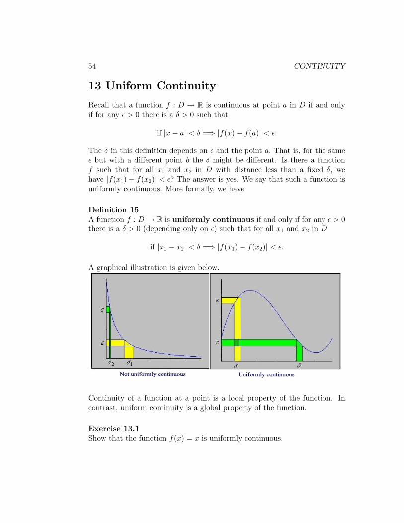
The δ in this definition depends on ε and the point a. That is, for the sameε but with a different point b the δ might be different. Is there a functionf such that for all x1 and x2 in D with distance less than a fixed δ, wehave |f(x1)− f(x2)| < ε? The answer is yes. We say that such a function isuniformly continuous. More formally, we have

Definition 15A function f : D → R is uniformly continuous if and only if for any ε > 0there is a δ > 0 (depending only on ε) such that for all x1 and x2 in D

if |x1 − x2| < δ =⇒ |f(x1)− f(x2)| < ε.

A graphical illustration is given below.

Continuity of a function at a point is a local property of the function. Incontrast, uniform continuity is a global property of the function.

Exercise 13.1Show that the function f(x) = x is uniformly continuous.

13 UNIFORM CONTINUITY 55

Exercise 13.2Consider the function f(x) = 1

xon the set x > 0. Let δ > 0 be any number

and define α = min{2, δ}. Then α ≤ 2 and α ≤ δ. Let x1 = α3

> 0 andx2 = α

6> 0.

(a) Show that |x1 − x2| < δ but |f(x1)− f(x2)| ≥ 1.(b) Conclude from (a) that f is not uniformly continuous on the interval0 < x < ∞.

Exercise 13.3(a) Show that if f is uniformly continuous on D then f is continuous at everypoint in D.(b) Using properties of continuous functions, show that the function f(x) = 1

x

is continuous on the interval 0 < x < ∞.(c) Is the converse of (a) always true? That is, every continuous function isuniformly continuous.

Exercise 13.4Show that if f, g : D → R are uniformly continuous then f + g : D → R isalso uniformly continuous.

Exercise 13.5Let f(x) = x2. Suppose that there is a δ > 0 such that |x1 − x2| < δ for allreal numbers x1 and x2. In addition, suppose we want |x2

1− x22| = 1. That is,

|x1− x2||x1 + x2| = 1. One way to achieve that is by setting x1− x2 = δ2

andx1 + x2 = 2

δ.

(a) Find x1 and x2 in terms of δ.(b) Show that f is not uniformly continuous. Hint: Let ε = 1

2in Definition

12.

Exercise 13.6Give an example of two functions f, g : D → R that are uniformly continuousbut the product function f · g is not.

Exercise 13.7Let f, g : D → R be uniformly continuous and bounded, say |f(x)| ≤ M1

and |g(x)| ≤ M2 for all x in D. Let ε > 0 be arbitrary.(a) Show that there is a δ1 > 0 such that

if |x− u| < δ1 =⇒ |f(x)− f(u)| < ε2M2

for all x, u in D.

56 CONTINUITY

(b) Show that there is a δ2 > 0 such that

if |x− u| < δ2 =⇒ |g(x)− g(u)| < ε2M1

for all x, u in D.

(c) Show that f · g : D → R is also uniformly continuous. Note that bound-edness is crucial in this result. Hint: Note that f(x)g(x) − f(u)g(u) =(f(x)− f(u))g(x) + f(u)(g(x)− g(u)).

Exercise 13.8Suppose that f : D → R is uniformly continuous. Let {an}∞n=1 be a Cauchysequence of terms in D.(a) Let ε > 0 be arbitrary. Show that there is a δ > 0 such that

If |x1 − x2| < δ =⇒ |f(x1)− f(x2)| < ε for all x1, x2 in D.

(b) Show that there is a positive integer N such that

If n, m ≥ N =⇒ |an − am| < δ.

(c) Show that {f(an)}∞n=1 is a Cauchy sequence in R (and therefore by Ex-ercise 7.7 is convergent).

Exercise 13.9Consider the function f(x) = tan x on the interval −π

2< x < π

2.

(a) Show that the sequence {π2− 1

n}∞n=1 is convergent.

(b) Show that the sequence in (a) is also Cauchy.(c) Show that the sequence {f

(π2− 1

n

)}∞n=1 is not Cauchy.

(d) Show that the function f(x) = tan x is not uniformly continuous on theinterval −π

2< x < π

2.

Exercise 13.10Let f : D → R and g : D′ → R be two uniformly continuous functions withthe range of f contained in D′. Looking closely at Exercise 12.3, show thatthe composite function g(f(x)) is also uniformly continuous.

13 UNIFORM CONTINUITY 57

Practice Problems

Exercise 13.11Consider the function f(x) = sin x defined on the interval −π

2< x < π

2.

(a) Use Exercise 9.11(a) to show that | sin x| ≤ |x| on the interval −π2

< x <π2.

(b) Using the trigonometric identity sin a − sin b = 2 sin(

a−b2

)cos

(a+b2

)and

(a) to show that| sin a− sin b| ≤ |a− b|.

(c) Show that f is uniformly continuous on the −π2

< x < π2.

Exercise 13.12Using Exercise 13.10 and Exercise 13.11, show that the function g(x) = cos xis uniformly continuous in the interval −π

2< x < π

2.

Exercise 13.13Give an example of two uniformly continuous functions f and g such thatf(x)g(x)

is not uniformly continuous.

Exercise 13.14Let g : D → R be a uniformly continuous function with |g(x)| ≥ M > 0 forall x ∈ D. Hence, the function 1

g(x)is bounded and g(x) 6= 0 for all x in D.

Show that 1g(x)

is uniformly continuous.

Exercise 13.15Let f, g : D → R be two uniformly continuous functions such that f(x) is

bounded and |g(x)| ≥ M > 0 for all x ∈ D. Show that the function f(x)g(x)

isuniformly continuous on D.

Exercise 13.16A function f : D → R is said to be Lipschitz if there is a constant K > 0such that |f(x) − f(y)| ≤ K|x − y| for all x, y ∈ D. Show that a Lipschitzfunction is uniformly continuous.

58 CONTINUITY

14 Under What Conditions a Continuous Func-

tion is Uniformly continuous?

We have seem (Exercise 13.3(a)) that a function f : D → R uniformlycontinuous on D is continuous on D. However, the converse is not alwaystrue as seen from Exercise 13.3(c). In this section, we will show that anycontinuous function on the interval [a, b] is uniformly continuous there.Suppose not, then there is an ε > 0 such that for all δ > 0 there are u and vin [a, b] such that

if |u− v| < δ =⇒ |f(u)− f(v)| ≥ ε.

In particular, for each positive integer n we can let δ = 1n

and thus obtaintwo sequences {un}∞n=1 and {vn}∞n=1 of numbers in [a, b] such that

|un − vn| <1

n=⇒ |f(un)− f(vn)| ≥ ε. (14.1)

Exercise 14.1(a) Let c0 = a+b

2. Then either [a, c0] or [c0, b] contains an infinite members of

{vn}∞n=1. Let’s call the interval [a1, b1]. Show that b1 − a1 = b−a2

.

(b) Let c1 = a1+b12

. Then either [a1, c1] or [c1, b1] contains an infinite membersof {vn}∞n=1. Let’s call the interval [a2, b2]. Show that b2 − a2 = b−a

22 . Comparea1 and a2. Compare b1 and b2.(c) Let c2 = a2+b2

2. Then either [a2, c2] or [c2, b2] contains an infinite members

of {vn}∞n=1. Let’s call the interval [a3, b3]. Show that b3 − a3 = b−a23 . Compare

a1, a2 and a3. Compare b1, b2 and b3.

Continuing the process of the previous exercise we can find intervals [an, bn] ⊂[a, b] such that bn − an = b−a

2n with the sequence {an}∞n=1 being increasingand the sequence {bn}∞n=1 being decreasing. Moreover, the interval [an, bn]contains an infinite terms of the sequence {vn}∞n=1.

Exercise 14.2(a) Show that the sequence {an}∞n=1 is bounded from above. What is anupper bound?(b) Show that there is a constant M such that M = sup{a1, a2, · · · }.(c) Show that a ≤ M ≤ b.

14 UNDER WHAT CONDITIONS A CONTINUOUS FUNCTION IS UNIFORMLY CONTINUOUS?59

Exercise 14.3(a) Show that there is δ > 0 such that for any a ≤ x ≤ b if |x−M | < δ then|f(x)− f(M)| < ε

2.

(b) Show that for all u and v in [a, b] if |u −M | < δ and |v −M | < δ then|f(u)− f(v)| < ε.

Exercise 14.4(a) Let wn = b−a

2n . Show that limn→∞ wn = 0. Hint: Squeeze rule.(b) Show that there is a positive integer N such that b−a

2N < δ2

and |x−M | < δ2

for all aN ≤ x ≤ bN .

Exercise 14.5(a) Using Exercise 14.4, show that there is a large n such that 1

n< δ

2and

aN ≤ vn ≤ bN .(b) For the n found in (a), show that |un − vn| < 1

n< δ

2and |vn −M | < δ

2.

(c) For the n found in (a), Show that |un −M | < δ.(d) Using (b), (c), and Exericse 14.3(b), show that |f(un)− f(vn)| < ε.Conclusion: The result in (d), contradicts (14.1). Hence, f must be uniformlycontinuous.

60 CONTINUITY

Practice Problems

Exercise 14.6Show that the function f : [0, 1] → R defined by f(x) =

√x is uniformly

continuous.

Exercise 14.7(a) A function f : D → R is said to be Lipschitz if there is a constant K > 0such that |f(x)− f(y)| ≤ K|x− y| for all x, y ∈ D. Show that the functionf(x) =

√x is not Lipschitz on [0, 1]. Hint: Assume the contrary and get a

contradiction.(b) Give an example of a uniformly continuous function that is not Lipschitz.Thus, the converse to Exercise 13.16 is false.

Exercise 14.8Show, using the definition of uniform continuity (epsilon-delta definition) thefunction f(x) = x

x+1is uniformly continuous on [0, 2].

Exercise 14.9Conisder the function f : [0, 1] → R defined by

f(x) =

{sin x

xif 0 < x ≤ 1

1 if x = 0

Show that f is uniformly continuous on [0, 1].

Exercise 14.10Show that the function f : (−2, 1] → R defined by f(x) = x2 is Lipschitz on(−2, 1].

15 MORE CONTINUITY RESULTS: THE INTERMEDIATE VALUE THEOREM61

15 More Continuity Results: The Intermedi-

ate Value Theorem

In this section we proceed with establishing more properties of continuousand uniformly continuous functions. We first define what we mean by abounded set.

Definition 16A set D ⊆ R is said to be bounded if and only if there is a positive realnumber M such that

For all x in D we have |x| ≤ M.

That is, for all x is D we have −M ≤ x ≤ M. This says that D is containedin the closed interval [−M, M ].

The first result shows that a continuous function does not necessarily mapbounded sets to bounded sets.

Exercise 15.1Give an example of a continuous f : D → R with D a bounded set (i.e.|x| ≤ M for some M > 0 and for all x in D) but f(D) is not bounded.

The following result shows that uniformly continuous functions preserveboundedness. That is, the range of a bounded set under a uniformly contin-uous function is bounded.

Exercise 15.2Let D be a bounded subset of R with |x| ≤ M for all x ∈ D. Suppose thatf : D → R is uniformly continuous.(a) Show that there is a δ > 0 such that if u and v belong to D such that|u− v| < δ then |f(u)− f(v)| < 1.(b) Let n be a positive integer such that n > 2M

δ. Divide the interval

[−M, M ] into n equal subintervals:[x0, x1], [x1, x2], · · · , [xn−1, xn]. Show thatxk − xk−1 < δ for all k = 1, 2, · · · , n(c) Let [a1, b1], [a2, b2], · · · , [ak, bk] be those intervals in (b) that intersect D.That is, D ⊆ [a1, b1]∪ [a2, b2]∪· · ·∪ [ak, bk]. For 1 ≤ i ≤ k let ui ∈ [ai, bi]∩D.Show that if v is in D then there is an 1 ≤ i ≤ k such that |v − ui| < δ and|f(v)| < 1 + |f(ui)|.(d) Show that |f(v)| ≤ M for all v in D. That is, f(D) is bounded.

62 CONTINUITY

Exercise 15.3Show that if f : [a, b] → R is continuous then f([a, b]) is bounded. Hint:Exercises 14.5 and 15.2.

If D is a bounded set, then by the Completeness Axiom of real numbers thereexist finite numbers I and S such that

I = inf{x ∈ D} and S = sup{x ∈ D}

Exercise 15.4Show that if f : [a, b] → R is continuous then inf{f(x) : a ≤ x ≤ b} andsup{f(x) : a ≤ x ≤ b} exist.

Exercise 15.5Let f : [a, b] → R be continuous. Let I = inf{f(x) : a ≤ x ≤ b}. Note that Iexists by Exercise 15.4. Suppose that I < f(x) for all x ∈ [a, b]. That is, theinfimum can not be attained in [a, b]. Define the function g : [a, b] → R by

g(x) =1

f(x)− I.

(a) Show that g is continuous on [a, b].(b) Show that there is a positive number M such that |g(x)| ≤ M for allx ∈ [a, b].(c) Show that I + 1

Mis a lower bound of f([a, b]) and this leads to a contra-

diction.Conclusion: There must be a number x1 ∈ [a, b] such that f(x1) = inf{f(x) :a ≤ x ≤ b}.

Exercise 15.6Let f : [a, b] → R be continuous. Let S = sup{f(x) : a ≤ x ≤ b}. Notethat S exists by Exercise 15.4. Show that there exists x2 ∈ [a, b] such thatf(x2) = S. Hint: Mimic Exercise 15.5.

From the previous two exercises, we have seen that extreme values of a func-tion continuous on [a, b] are attained in [a, b]. What can we say about possi-ble values between these? The following result, known as the intermediatevalue theorem, addresses this question.

15 MORE CONTINUITY RESULTS: THE INTERMEDIATE VALUE THEOREM63

Exercise 15.7Let f : [a, b] → R be continuous. Let f(a) ≤ c ≤ f(b).(a) Let D = {x ∈ [a, b] : f(x) ≤ c}. Show that D is non-empty and that Dis bounded from above. By the Completeness Axiom of real numbers thereis a number d such that d = sup{x ∈ D}.(b) Show that d ∈ [a, b].(c) Suppose that f(d) > c. Show that there is a δ > 0 such that if |x−d| < δthen |f(x)− f(d)| < f(d)− c.(d) Show that for x ∈ [a, b] and |x − d| < δ we must have f(x) > c. Hint:Exercise 1.14.(e) Using (d), show that d− δ is an upper bound of D. Thus, f(d) > c leadsto a contradiction.(f) Suppose that f(d) < c. Show that there is a δ > 0 such that if d − δ <x < d + δ and x ∈ [a, b] we must have f(x) < c.(g) Show that f(d + δ

2) < c. Why this leads to a contradiction?

Conclusion: We must have f(d) = c.

Exercise 15.8Let f : [a, b] → R be continuous. By Exercise 15.5, there exist x1 ∈ [a, b] andx2 ∈ [a, b] such that m = f(x1) = inf{f(x) : x ∈ [a, b]} and M = sup{f(x) :x ∈ [a, b]}.(a) Show that f([a, b]) ⊆ [m, M ].(b) Use Exercise 15.7 (restricted to the interval [x1, x2]) to show that [m, M ] ⊆f([a, b]).Conclusion: f([a, b]) = [m, M ].

64 CONTINUITY

Practice Problems

Exercise 15.9Prove that there exists a number c ∈

(0, π

2

)such that 2c− 1 = sin

(c2 + π

4

).

Exercise 15.10Let f : [a, b] → [a, b] be a continuous function. Prove that there is c ∈ [a, b]such that f(c) = c. We call c a fixed point of f. Hint: Intermediate ValueTheorem applied to a specific function F (to be found) defined on [a, b].

Exercise 15.11Using the Intermediate Value Theorem, show that(a) the equation 3 tan x = 2 + sin x has a solution in the interval [0, π

4].

(b) the polynomial p(x) = −x4 + 2x3 + 2 has at least two real roots.

Exercise 15.12Let f, g : [a, b] → R be continuous functions such that f(a) ≤ g(a) andf(b) ≥ g(b). Show that there is a c ∈ [a, b] such that f(c) = g(c).

Exercise 15.13Let f : [a, b] → R be continuous such that f(a) ≤ a and f(b) ≥ b. Prove thatthere is a c ∈ [a, b] such that f(c) = c. We call c a fixed point of f.

Exercise 15.14Let f : [a, b] → Q be continuous. Prove that f must be a constant function.Hint: Exercise 2.6(c).

Exercise 15.15Prove that a polynomial of odd degree considered as a function from the realsto the reals has at least one real root.

Exercise 15.16Suppose f(x) is continuous on the interval [0, 2] and f(0) = f(2) : Provethere must be a number c between 0 and 1 so that f(c + 1) = f(c). Hint:Consider the function g(x) = f(x + 1)− f(x) on [0, 1].

Derivatives

16 The Derivative of a Function

In this section we introduce the concept of the derivative of a function anddiscuss some of its properties.

Definition 17Let f : D → R and x ∈ D. We say that f is differentiable at a if and onlyif

limh→0

f(a + h)− f(a)

h

exists. Symbolically, we write

f ′(a) = limh→0

f(a + h)− f(a)

h.

We call f ′(a) the derivative of f at a. If f ′(a) exists, we say that f isdifferentiable at a. A function that is not differentiable at a is said tobe non-diffferentiable. If f ′(a) exists for every a ∈ D, we say that f isdifferentiable on D. The process of finding the derivative is referred to asdifferentiation.


f(x) =

{x sin

(1x

)if x 6= 0

0 if x = 0

Show that f is not differentiable at a = 0.

65

66 DERIVATIVES


f(x) =

{x2 sin

(1x

)if x 6= 0

0 if x = 0

Show that f is differentiable at a = 0. What is f ′(0)?

Exercise 16.3Show that f(x) = |x| is not differentiable at 0.

Exercise 16.4Find the derivative of f(x) = sin x. Hint: Recall the trigonometric identitysin a− sin b = 2 cos

(a+b2

)sin

(a−b2

)and use Exercise 9.11.

The following exercise shows that every differentiable function is continuous.

Exercise 16.5Let f : D → R be differentiable at a.(a) Show that

limx→a

[f(x)− f(a)] = limh→0

[f(h + a)− f(a)].

(b) Show that f is continuous at a. That is,

limx→a

[f(x)− f(a)] = 0.

Exercise 16.6Give an example of a function f : D → R that is continuous at a but notdifferentiable there.

Exercise 16.7Suppose that f, g : D → R are differentiable at a. Show that the functionsf ± g are also differentiable at a.

Exercise 16.8 (Product Rule)Suppose that f, g : D → R are differentiable at a.(a) Show that (fg)(a+h)− (fg)(a) = [f(a+h)− f(a)]g(a+h)+ f(a)[g(a+h)− g(a)].(b) Show that the function f · g is also differentiable at a.

16 THE DERIVATIVE OF A FUNCTION 67

Exercise 16.9 (Quotient Rule)Suppose that f, g : D → R are differentiable at a with g(a) 6= 0.(a) Show that(

fg

)(a + h)−

(fg

)(a)

h=

f(a + h)− f(a)

h· 1

g(a + h)−g(a + h)− g(a)

h·f(a)

g(a)· 1

g(a + h).

(b) Show that (f

g

)′

(a) =f ′(a)g(a)− f(a)g′(a)

g(a)2.

Exercise 16.10 (Chain Rule)Let f : D → R and g : D′ → R be two functions with f(D) ⊆ D′. Supposethat f is differentiable at a and g is differentiable at f(a).(a) Define w : D′ → R by

w(y) =

{g(y)−g(f(a))

y−f(a)if y 6= f(a)

g′(f(a)) if y = f(a).

Show that w is continuous at f(a). That is,

limh→0

w(h + f(a)) = w(f(a)).

(b) Show that (w ◦ f)(x) is continuous at a.(c) Show that

(g ◦ f)(a + h)− (g ◦ f)(a)

h= (w ◦ f)(a + h) · f(a + h)− f(a)

h.

(d) Show that(g ◦ f)′(a) = g′(f(a)) · f ′(a).

Exercise 16.11Let f(x) = xn where n is a non-negative integer.(a) By letting h = ax− x, show that

f ′(x) = lima→1

f(ax)− f(x)

ax− x.

(b) What is the quotient of the division of an−1 by a−1? Hint: use syntheticdivision.(c) Use (a) and (b) to show that f ′(x) = nxn−1.

68 DERIVATIVES

Practice Problems

Exercise 16.12(a) Show that the derivative of a constant function is zero and that thederivative of f(x) = x is f ′(x) = 1.(b) Show that the function h(x) = x sin

(1x

)is differentiable for all x 6= 0.

Exercise 16.13Let f(x) =

√2x− 1. Find f ′(2) by using only the definition of derivative.

Exercise 16.14Let

f(x) =

{2x + 5 if x ≤ 19x2 − 2 if x > 1.

Show that f(x) is continuous but not differentiable at x = 1.

Exercise 16.15Find constants a and b such that the piecewise defined function

f(x) =

{ax2 − 4 if x ≤ 1bx + a if x > 1

is differentiable at x = 1.

Exercise 16.16Let f(x) = x2 cos

(1x

)if x 6= 0 and f(0) = 0. Show that f is differentiable at

x = 0 and find f ′(0).

Exercise 16.17(a) Let f(x) = xn with n a negative integer. Prove that f ′(x) = nxn−1.

(b) Let f(x) = xpq where p and q are integers with q 6= 0. Prove that f ′(x) =

pqx

pq−1. Hint: Let y = x

pq so that yq = xp and use Exercise 16.10.

Exercise 16.18We define the number e to be the unique number satisfying

limh→0

eh − 1

h= 1.

It is an irrational number whose value is approximately 2.718281828459045.Define the function f(x) = ex. Find f ′(x) using the definition of the deriva-tive.

16 THE DERIVATIVE OF A FUNCTION 69

Exercise 16.19The natural logarithmic function is the function f(x) = ln x definedas follows: y = ln x if and only if x = ey. Find the derivative of f. Hint:Differentiate x = ey with respect to x.

Exercise 16.20Consider the function f(x) = xn where n is a real number.(a) Suppose that x > 0 and x in the domain of f. Using the fact thatxn = en ln x, show that f ′(x) = nxn−1.(b) Suppose that x < 0 and x in the domain of f. Show that f ′(x) = nxn−1.Hint: xn = (−1)n(−x)n.

70 DERIVATIVES

17 Extreme values of a Function and Related

Theorems

Points of interest on the graph of a function are those points that are thehighest on the curve, or the lowest, in a specific interval. Such points arecalled local extrema.

Definition 18Let f : D → R. We say that f has a local maximum or a relativemaximum at a ∈ D if there is an ε > 0 such that f(x) ≤ f(a) for allx ∈ (a− ε, a + ε) ∩D.We say that f has a local minimum or a relative minimum at a ∈ D ifthere is an ε > 0 such that f(a) ≤ f(x) for all x ∈ (a− ε, a + ε) ∩D.

Exercise 17.1(a) Find the local extrema (if they exist) of the function f(x) = |x|.(b) Find the local extrema (if they exist) of the function f(x) = x3.(c) Find the local extrema (if they exist) of the function f(x) = x on theinterval [0, 1].

The following exercise shows that if a differentiable function has a local ex-trema (that is not a boundary point) then the derivative at that point mustbe zero.

Exercise 17.2Let f : [a, b] → R. Suppose that c ∈ (a, b) is a local maximum (or localminimum) of f such that f ′(c) exists. Let ε > 0 such that f(x) ≤ f(c) forall x ∈ (c− ε, c + ε) ⊆ [a, b].(a) Let h > 0 be small enough so that c + h ∈ (c− ε, c + ε). Using Exercise9.8, show that f ′(c) ≤ 0.(b) Let h < 0 be large enough so that c + h ∈ (c − ε, c + ε). Using Exercise9.8, show that 0 ≤ f ′(c) and therefore f ′(c) = 0.

Exercise 17.3The condition a < c < b is critical in the previous exercise. Give an exampleof a function f : [a, b] → R such that either a or b is a local extremum butwith non-zero derivative there.

17 EXTREME VALUES OF A FUNCTION AND RELATED THEOREMS71

Definition 19A point (c, f(c)) such that either f ′(c) does not exist or f ′(c) = 0 is called acritical point. Exercise 17.2 tells us that potential local extrema are criticalpoints.

By Exercise 15.8, if f : [a, b] → R is continuous then there exists x1, x2 ∈ [a, b]such that

f(x1) ≤ f(x) ≤ f(x2)

for all x ∈ [a, b]. That is, x1 is a local minimum and x2 is a local maximum.The following exercise tells us where to look for x1 and x2.

Exercise 17.4Suppose f : [a, b] → R is continuous. Then there exists x1, x2 ∈ [a, b] suchthat

f(x1) ≤ f(x) ≤ f(x2)

for all x ∈ [a, b]. Show that x1 and x2 are either the endpoints of [a, b] orcritical points of f in a < x < b.

Exercise 17.5 (Rolle’s Theorem)Suppose f : [a, b] → R is continuous for a ≤ x ≤ b and differentiable fora < x < b. By Exercise 15.8 there exist a ≤ x1 ≤ b and a ≤ x2 ≤ b such thatf(x1) ≤ f(x) ≤ f(x2) for all x ∈ [a, b]. Suppose that f(a) = f(b).(a) Show that if f(x) = C for all a ≤ x ≤ b then there is at least a numbera < c < b such that f ′(c) = 0.(b) Suppose that f is a non-constant function. Let d ∈ [a, b] such thatf(d) 6= f(a). Show that if f(d) < f(a) then a < x1 < b. What can you sayabout the value of f ′(x1)?(c) Show that if f(a) < f(d) then a < x2 < b. What can you say about thevalue of f ′(x2)?

Geometrically, Rolle’s theorem claims that if f : [a, b] → R is continuous fora ≤ x ≤ b and differentiable for a < x < b and f(a) = f(b), somewherebetween a and b the graph of f has a horizontal tangent line. See Figurebelow.

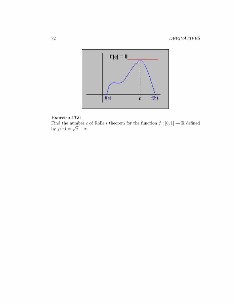
72 DERIVATIVES

Exercise 17.6Find the number c of Rolle’s theorem for the function f : [0, 1] → R definedby f(x) =

√x− x.

17 EXTREME VALUES OF A FUNCTION AND RELATED THEOREMS73

Practice Problems

Exercise 17.7Assume a0, a1, · · · , an are real numbers such that

an

n + 1+

an−1

n+ · · ·+ a1

2+ a0 = 0

Show that the polynomial function

f(x) = anxn + an−1x

n−1 + · · ·+ a1x + a0

has at least one root in (0, 1).

Exercise 17.8(a) Show that the function f(x) = x3 − 4x2 − 3x + 1 has a root in [0, 2].(b) Use Rolle’s theorem to show that there is exactly one root in [0, 2].

Exercise 17.9Let f, g : R → R be differentiable, and let a, b ∈ R be such that a < b. Showthat there is a c ∈ (a, b) such that

f ′(c)[g(b)− g(a)] = g′(c)[f(b)− f(a)].

Hint: Apply Rolle’s theorem to the function h(x) = f(x)[g(b) − g(a)] −g(x)[f(b)− f(a)].

Exercise 17.10Suppose f : [a, b] → R is continuous for a ≤ x ≤ b and differentiable fora < x < b. Show that there is a < c < b such that

f ′(c) =f(b)− f(a)

b− a.

Hint: Apply Rolle’s theorem to the function g : [a, b] → R defined by

g(x) = f(x)− f(a)−(

f(b)− f(a)

b− a

)(x− a).

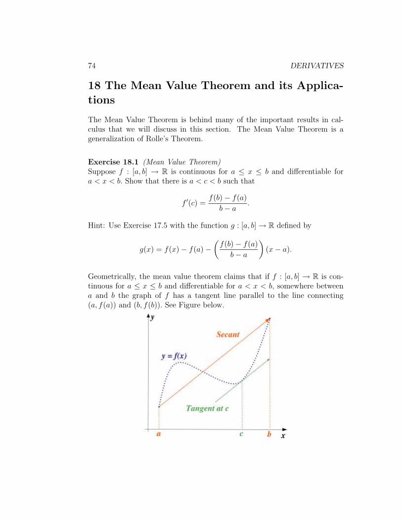
74 DERIVATIVES

18 The Mean Value Theorem and its Applica-

tions

The Mean Value Theorem is behind many of the important results in cal-culus that we will discuss in this section. The Mean Value Theorem is ageneralization of Rolle’s Theorem.

Exercise 18.1 (Mean Value Theorem)Suppose f : [a, b] → R is continuous for a ≤ x ≤ b and differentiable fora < x < b. Show that there is a < c < b such that

f ′(c) =f(b)− f(a)

b− a.

Hint: Use Exercise 17.5 with the function g : [a, b] → R defined by

g(x) = f(x)− f(a)−(

f(b)− f(a)

b− a

)(x− a).

Geometrically, the mean value theorem claims that if f : [a, b] → R is con-tinuous for a ≤ x ≤ b and differentiable for a < x < b, somewhere betweena and b the graph of f has a tangent line parallel to the line connecting(a, f(a)) and (b, f(b)). See Figure below.

18 THE MEAN VALUE THEOREM AND ITS APPLICATIONS 75

Exercise 18.2 (Cauchy Mean Value Theorem)Suppose f, g : [a, b] → R are continuous for a ≤ x ≤ b and differentiable fora < x < b. Show that there is a < c < b such that

[g(b)− g(a)]f ′(c) = [f(b)− f(a)]g′(c).

Hint: Use Exercise 17.5 with the function h : [a, b] → R defined by

h(x) = [f(b)− f(a)]g(x)− [g(b)− g(a)]f(x).

Exercise 18.3Let f : [a, b] → R be continuous for a ≤ x ≤ b and differentiable for a <x < b. We say that f is one-to-one if and only if for any a ≤ x1 ≤ b anda ≤ x2 ≤ b such that f(x1) = f(x2) we must have x1 = x2. Suppose thatf ′(x) 6= 0 for all a < x < b.(a) Let a ≤ x1 ≤ b and a ≤ x2 ≤ b such that f(x1) = f(x2). Show thatif x1 < x2 then there is a < x1 < c < x2 < b such that f ′(c) = 0 whichcontradicts the assumption that f ′(x) 6= 0 for all a < x < b. Hint: Use theMean Value Theorem on the interval [x1, x2].(b) Answer the same question for x2 < x1.Conclusion: We must have x1 = x2. This shows that f is 1-1.

Exercise 18.4Let f : [a, b] → R be continuous for a ≤ x ≤ b and differentiable for a < x <b. We say that f is increasing in [a, b] if and only if for every x1 and x2 in[a, b], if x1 ≤ x2 then f(x1) ≤ f(x2). Show that if f ′(x) ≥ 0 for all a < x < bthen f(x) is increasing in [a, b]. Hint: Use the MVT restricted to the interval[x1, x2].

Definition 20We say that f : [a, b] → R is differentiable in [a, b] if and only if f is differ-entiable in a < x < b and the following limits exist

f ′(a) = limh→0+f(a+h)−f(a)

hand f ′(b) = limh→0−

f(b+h)−f(b)h

Suppose that f : [a, b] → R is differentiable such that f ′(x) 6= 0 for alla < x < b. We know from Exercise 18.3 that f is one-to-one on [a, b]. Wewant to show that f is monotone as well on [a, b].To say that f is not monotone on [a, b] means that one of the following cases

76 DERIVATIVES

applies:(i) There are x, y, z ∈ [a, b] such that x < y < z and f(x) < f(y), f(z) < f(y).That is the graph of f is increasing on [x, y] and decreasing on [y, z].(ii) There are x, y, z ∈ [a, b] such that x < y < z and f(x) > f(y), f(y) <f(z). That is the graph of f is decreasing on [x, y] and increasing on [y, z].

Exercise 18.5Consider Case (i). We have either f(x) < f(z) < f(y) or f(z) < f(x) < f(y).(a) Suppose that f(z) < f(x) < f(y). Use the Intermediate Value theoremrestricted to [y, z] to show that such a double inequality can not occur.(b) Suppose that f(x) < f(z) < f(y). Use the Intermediate Value theoremrestricted to [x, y] to show that such a double inequality can not occur.We conclude that Case (i) does not hold.

Exercise 18.6Consider Case (ii). We have either f(y) < f(x) < f(z) or f(y) < f(z) <f(x).(a) Suppose that f(y) < f(x) < f(z). Use the Intermediate Value theoremrestricted to [y, z] to show that such a double inequality can not occur.(b) Suppose that f(y) < f(z) < f(x). Use the Intermediate Value theoremrestricted to [x, y] to show that such a double inequality can not occur.We conclude that Case (ii) does not hold.

We conclude from the previous two exercises that f must be monotone in[a, b].

Exercise 18.7Suppose that f : [a, b] → R is differentiable such that f ′(x) 6= 0 for alla < x < b. We know from the above discussion that f is monotone.(a) Show that if f is increasing in [a, b] then f ′(x) ≥ 0 for all a ≤ x ≤ b. Hint:Let x ∈ [a, b) and choose h > 0 small enough so that x + h ∈ [a, b). If x = b,choose h < 0 so that b + h < b. Now use the definition of the derivative.(b) Show that if f is decreasing in [a, b] then f ′(x) ≤ 0 for all a ≤ x ≤ b.

18 THE MEAN VALUE THEOREM AND ITS APPLICATIONS 77

Practice Problems

Exercise 18.8Let f : [a, b] → R be continuous for a ≤ x ≤ b and differentiable for a <x < b. We say that f is a constant function on [a, b] if and only if there is aconstant C such that f(x) = C for all a ≤ x ≤ b. Suppose that f ′(x) = 0 forall a < x < b.Let x1 and x2 be any two numbers in the interval [a, b] with x1 < x2. Supposethat f(x1) 6= f(x2). Show that by applying the Mean Value Theorem on theinterval [x1, x2] we obtain the contradiction f(x1) = f(x2). Thus, we musthave f(x1) = f(x2) = C for any x1 and x2 in [a, b]. That is, f(x) = C for alla ≤ x ≤ b.

Exercise 18.9Let f : [a, b] → R be continuous for a ≤ x ≤ b and differentiable for a < x <b. Suppose that f ′(x) = g′(x) for all a < x < b. Show that f(x) = g(x) + Cfor all a ≤ x ≤ b, where C is a constant. Hint: Exercise 18.8

Exercise 18.10Let f : [a, b] → R be continuous for a ≤ x ≤ b and differentiable for a < x <b. We say that f is decreasing in [a, b] if and only if for every x1 and x2 in[a, b], if x1 ≤ x2 then f(x1) ≥ f(x2). Show that if f ′(x) ≤ 0 for all a < x < bthen f(x) is decreasing in [a, b]. Hint: Use the MVT restricted to the interval[x1, x2].

Exercise 18.11Consider the function f(x) = (1 + x)p where 0 < p < 1. Let h > 0.(a) Apply the MVT to the interval [0, h] to show that f(h) = p(1+ t)p−1h+1for some 0 < t < h.(b) Use (a) to show that (1 + h)p < 1 + ph.In annuity theory, (1 + h)p may represent compound interest and 1 + phrepresent simple interest. A result in annuity theory says that for time pless than a year compound interest formula can be estimated by the simpleinterest formula.

Exercise 18.12Suppose that f : [a, b] → R is differentiable in [a, b]. Let λ be a real numbersuch that either f ′(a) < λ < f ′(b) or f ′(b) < λ < f ′(a).(a) Define g(x) = f(x) − λx. Show that if f ′(a) < λ < f ′(b) then g′(x)

78 DERIVATIVES

changes sign between a and b.(b) Establish the same result for f ′(b) < λ < f ′(a).(c) Show that the condition g′(c) 6= 0 for all c ∈ [a, b] leads to a contradiction.Hint: Exercise 18.7. Conclude that there must be a a < c < b such thatf ′(c) = λ.

Exercise 18.13Let f, g : [a, b] → R be two differentiable functions on [a, b] such that f(a) =g(a). Show that if f ′(x) = g′(x) for all x ∈ (a, b) then f(x) = g(x) for allx ∈ [a, b]. Hint: Exercise 18.8.

Exercise 18.14Let f : R → R be differentiable such that |f ′(x)| < 1 for all x ∈ R. Showthat f can have at most one fixed point. That is, There is at most one c ∈ Rsuch that f(c) = c. Hint: Mean Value Theorem.

Exercise 18.15Let f : R → R be differentiable everywhere and that f ′(a) < 0 and f ′(b) > 0for some a < b. Prove that there is a c ∈ (a, b) such that f ′(c) = 0.

Exercise 18.16Let f : R → R be differentiable and |f ′(x)| ≤ K < 1 for all x ∈ R. Leta0 ∈ R. Define the numbers an = f(an−1).(a) Show that |an+1 − an| ≤ Kn|a1 − a0| for all n ∈ N.(b) Show that for all m,n ∈ N such that m > n we have

|am − an| ≤Kn

1−K.

Exercise 18.17Show that if 0 < a < b then 1− a

b< ln

(ba

)< b

a− 1. Hint: Apply the MVT

for the function f(x) = ln x.

19 L’HOPITAL’S RULE AND THE INVERSE FUNCTION THEOREM79

19 L’Hopital’s Rule and the Inverse Function

Theorem

The following result known as L’Hopital’s Rule uses derivatives to evaluatelimits of the ratio of two functions with limit of the form 0

0.

Exercise 19.1Let f, g : [a, b] → R be continuous on [a, b] and differentiable in a < x < bwith g′(x) 6= 0 for all a < x < b. Suppose that f(c) = g(c) = 0 for somea ≤ c ≤ b. Also, suppose that

limx→c

f ′(x)

g′(x)= A.

(a) Let {cn}∞n=1 ⊂ [a, b] be an arbitrary sequence with the properties cn 6= cfor all n ≥ 1 and limn→∞ cn = c. Show that there is a dn between cn and csuch that

[f(cn)− f(c)]g′(dn) = [g(cn)− g(c)]f ′(dn).

(b) Show that dn 6= c for all n ≥ 1 and limn→∞ dn = c.(c) Show that g(dn) 6= g(c) for all n ≥ 1. Hint: Exercise 18.3.(d) Show that

f ′(dn)

g′(dn)=

f(cn)

g(cn).

(e) Show that limn→∞f ′(dn)g′(dn)

= A. Hint: See Exercise 10.1.

(f) Show that limn→∞f(cn)g(cn)

= A.

(g) Show that limx→cf(x)g(x)

= A.

Exercise 19.2Find

limx→2

√x−

√2 +

√x− 2√

x2 − 4.

Definition 21Let f : D → R. We say that f is invertible if and only if there is a functiong : D′ → R such that the following two statements are true

f(g(x)) = x for all x in D′

80 DERIVATIVES

and

g(f(x)) = x for all x in D.

We Write g = f−1 and we call f−1 the inverse function of f.

Exercise 19.3Let f : [a, b] → R be a one-to-one function.(a) Define g : f([a, b]) → [a, b] by g(y) = x if and only if f(x) = y. Show thatg is indeed a function. That is, if y1, y2 ∈ f([a, b]) are such that y1 = y2 theng(y1) = g(y2).(b) Show that f(g(y)) = y for all y ∈ f([a, b]) and g(f(x)) = x for allx ∈ [a, b]. Thus, conclude that f is invertible.

Exercise 19.4Let f : [a, b] → R be continuous in [a, b] and differentiable in [a, b] withf ′(x) 6= 0 for all a < x < b. Let the range of f be denoted by [m,M ].(a) Show that f is one-to-one, monotone, and invertible with inverse f−1 :[m, M ] → [a, b].(b) Assume that f is strictly increasing. That is, if x1 < x2 then f(x1) <f(x2). In this case, [m, M ] = [f(a), f(b)]. Let f(a) < y0 < f(b). Show thatthere is a a < x0 < b such that f(x0) = y0.(c) Let ε > 0 be given. Let ε1 = min{ε, x0−a, b−x0}. Show that if x satisfies|x− x0| < ε1 then a < x < b and |x− x0| < ε.(d) Let y1 = f(x0− ε1) and y2 = f(x0 + ε1). Show that f [(x0− ε1, x0 + ε1)] =(y1, y2).(e) Choose a δ > 0 so that (y0− δ, y0 + δ) ⊂ (y1, y2). Show that if |y−y0| < δthen |f−1(y)−f−1(y0)| < ε. This shows that f−1 is continuous in (f(a), f(b)).(f) Show that f−1 is right continuous at f(a) and left continuous at f(b).We conclude from this problem that f−1 is continuous on the closed interval[f(a), f(b)].

Remark 1A similar result holds if f is strictly decreasing.

Exercise 19.5 (Inverse Function Theorem)Let f : [a, b] → R be continuous in [a, b] and differentiable in [a, b] withf ′(x) 6= 0 for all a < x < b. Let c ∈ f([a, b]). Then there is a d ∈ [a, b] suchthat f(d) = c.

19 L’HOPITAL’S RULE AND THE INVERSE FUNCTION THEOREM81

(a) Let {cn}∞n=1 ⊆ f([a, b]) such that cn 6= c for all n ≥ 1 and limn→∞ cn = c.Show that there is a sequence {dn}∞n=1 ⊆ [a, b] such that

limn→∞

dn = d.

Hint: Exercise 19.4(b).(b) Show that dn 6= d for all n ≥ 1.(c) Show that

limn→∞

f(dn)− f(d)

dn − d= f ′(d).

Hint: Exercise 10.1.(d) Show that f(dn)−f(d)

dn−d6= 0 for all n ≥ 1. Hint: Exercise 18.3.

(e) Show that

limn→∞

f−1(cn)− f−1(c)

cn − c=

1

f ′(d).

Thus, conclude that

(f−1)′(f(d)) =1

f ′(d)

for all d ∈ [a, b]. That is f−1 is differentiable in f([a, b]). Hint: Exercise 10.2.

82 DERIVATIVES

Practice Problems

Exercise 19.6Find limx→∞

(ln xx· sin

(xπ+2

2x

)).

Exercise 19.7Let f, g : [a, b] → R be continuous on [a, b] and differentiable in a < x < bwith g′(x) 6= 0 for all a < x < b. Suppose that limx→c f(x) = limx→c g(x) =∞ for some a ≤ c ≤ b. Also, suppose that

limx→c

f ′(x)

g′(x)= A.

Prove that

limx→c

f(x)

g(x)= A.

Exercise 19.8Use L’Hopital’s rule to evaluate limx→0+ xx. Note that 00 is an undeterminateform.

Exercise 19.9Let f and g be invertible differentiable functions such that

f(1) = 2; g(2) = 1; f ′(1) = g′(2) = 3.

Find the derivative (f−1 ◦ g−1)′(1).

Exercise 19.10Let f(x) = x tan2 x for x ∈ (0, π

2). Calculate (f−1)′(π). Note that f(π

3) = π.

Riemann Integrals

20 The Theory of Riemann Integral

The Riemann integral, as it is called today, is the one usually discussed inintroductory calculus. Throughout this section, it is assumed that we areworking with a bounded function f on a closed interval [a, b], meaning thatthere exist real numbers m and M such that m ≤ f(x) ≤ M for all x ∈ [a, b].

Definition 22A partition P of [a, b] is a finite, ordered set

P = {a = x0 < x1 < x2 < · · · < xn = b}.

If Q is another partition of [a, b] such that P ⊂ Q then we call Q a refine-ment of P.For each subinterval [xk−1, xk] of P, let

mk(f) = inf{f(x) : x ∈ [xk−1, xk]} and Mk(f) = sup{f(x) : x ∈ [xk−1, xk]}

The Riemann lower sum of f with respect to P is given by

L(f, P ) =n∑

i=1

mi(f)(xi − xi−1).

Likewise, we define the Riemann upper sum of f with respect to P by

U(f, P ) =n∑

i=1

Mi(f)(xi − xi−1).

Exercise 20.1(a) Show that m ≤ mi(f) ≤ Mi(f) ≤ M.(b) Show that m(b− a) ≤ L(f, P ) ≤ U(f, P ) ≤ M(b− a).

83

84 RIEMANN INTEGRALS

Exercise 20.2Let Q be a refinement of P. Suppose that P = {a = x0 < x1 < · · · < xn−1 <xn = b} and Q = {a = x0 < x1 < · · · < xi−1 < z < xi < · · · < xn = b}.(a) Show that U(f, Q) ≤ U(f, P ).(b) Show that L(f, P ) ≤ L(f, Q).

Definition 23We define

SU = {U(f, P ) : P a partition of [a, b]}

and

SL = {L(f, P ) : P a partition of [a, b]}

Then SU is bounded from below by m(b− a). By the completeness axiom ofR, inf SU is a finite number. We define the upper Riemann integral to be∫ b

a

f(x)dx = inf SU .

Likewise, SL is bounded from above by M(b−a). By the completeness axiomof R, sup SL is a finite number. We define the lower Riemann integral tobe ∫ b

a

f(x)dx = sup SL.

Exercise 20.3Suppose that f is bounded on [a, b]. Show that

∫ b

af(x)dx ≤

∫ b

af(x)dx. Hint:

Exercise 20.2.

Definition 24We say that a bounded function f : [a, b] → R is Riemann integrable on[a, b] if and only if ∫ b

a

f(x)dx =

∫ b

a

f(x)dx.

We write ∫ b

a

f(x)dx =

∫ b

a

f(x)dx =

∫ b

a

f(x)dx

and we call∫ b

af(x)dx the Riemann integral of f on [a, b].

20 THE THEORY OF RIEMANN INTEGRAL 85

Exercise 20.4Consider the function f : [a, b] → R defined by

f(x) =

{2 if a ≤ x < b3 if x = b

(a) Find two numbers m and M such that m ≤ f(x) ≤ M for all x ∈ [a, b]?(b) Show that for any partition P of [a, b] we have L(f, P ) = 2(b − a).Conclude that ∫ b

a

f(x)dx = 2(b− a).

(c) Show that∫ b

af(x)dx ≥ 2(b− a).

(d) Suppose∫ b

af(x)dx > 2(b − a). Let ε =

∫ b

af(x)dx − 2(b − a) > 0. Let Q

be the partition

Q = {a = x0 < x1 < x2 < · · · < xn = b}

such that b − xn−1 < ε. Show that U(f, Q) <∫ b

af(x)dx. Why this is impos-

sible?(e) Is f(x) Riemann integrable? If so, what is the value of the integral∫ b

af(x)dx?

The above example shows that a discontinuous function can be Riemannintegrable.Next, we present an example of a function that is not Riemann integrable.

Exercise 20.5Consider the function f : [0, 1] → R defined by f(x) = 1 if x is rational andf(x) = 0 if x is irrational.(a) Compute the upper Riemann integral and the lower Riemann integral.Hint: Exercise 2.6(c).(b) Is f Riemann integrable on [0, 1]?

Exercise 20.6Let f : [a, b] → R be a bounded function. Suppose that f is Riemannintegrable. We want to show that f satisfies the following property, knownas Riemann criterion:


(P)∀ε > 0, there is a partition P of [a, b] such that U(f, P )− L(f, P ) < ε.

(a) Let ε > 0 be given. Show that there is a partition P of [a, b] such that∫ b

a

f(x)dx− ε

2< L(f, P ).

Hint: Assume the contrary and get a contradiction.(b) Show that there is a partition Q of [a, b] such that

U(f, Q) <

∫ b

a

f(x)dx +ε

2.

(c) Let R = P ∪Q. Use Exercise 20.2 to show that∫ b

a

f(x)dx− ε

2< L(f, R) ≤ U(f, R) <

∫ b

a

f(x)dx +ε

2.

(d) Show that∣∣∣L(f, R)−∫ b

af(x)dx

∣∣∣ < ε2

and∣∣∣U(f, R)−

∫ b

af(x)dx

∣∣∣ < ε2

(e) Use the triangle inequality to show that U(f, R)− L(f, R) < ε.

Exercise 20.7Let f : [a, b] → R be a bounded function. Suppose that f satisfies property(P) above.(a) Show that for each positive integer n, there is a partition Pn such that

U(f, Pn)− L(f, Pn) <1

n.

(b) Using (a), show that

L(f, Pn) ≤∫ b

a

f(x)dx ≤∫ b

a

f(x)dx < L(f, Pn) +1

n.

(c) Show that

0 ≤∫ b

a

f(x)dx−∫ b

a

f(x)dx <1

n.


(d) Show that ∫ b

a

f(x)dx =

∫ b

a

f(x)dx.

Hint: Squeeze rule. We conclude that any bounded function that satisfiesproperty (P) is Riemann integrable.

Exercise 20.8Let f : [0, 1] → R be the function f(x) = x2. For any ε > 0, choose apartition P = {0 = x0 < x1 < · · · < xn = 1} such that

xi − xi−1 < ε2

for all 1 ≤ i ≤ n

Show that U(f, P )− L(f, P ) < ε. Hence, f is Riemann integrable.


Practice Problems

Exercise 20.9Suppose that f(x) = x for x ∈ [1, 2].(a) Find U(f, P ) and L(f, P ). Hint: Consider a partition with equal subin-tervals.(b) Show that f is Riemann integrable. Hint: Exercise 20.7.(c) Show that U(f, P ) ≥ 3

2and L(f, P ) ≤ 3

2.

(d) Find∫ 2

1xdx.

Exercise 20.10Let f : [a, b] → R be bounded. Let P and Q be any two partitions of [a, b].Prove that L(f, P ) ≤ U(f, Q).

Exercise 20.11Let f : [a, b] → R be such that m ≤ f(x) ≤ M for all x ∈ [a, b]. Prove that∫ b

a

f(x)dx−∫ b

a

f(x)dx ≤ (M −m)(b− a).

Exercise 20.12Let f : [a, b] → R be bounded functions such that f(x) ≤ g(x) for allx ∈ [a, b]. Prove the following:

(a)∫ b

af(x)dx ≤

∫ b

ag(x)dx

(b)∫ b

af(x)dx ≤

∫ b

ag(x)dx

Exercise 20.13Let f : [a, b] → R be bounded functions. Let P be any partition of [a, b].Prove

U(f + g, P ) ≤ U(f, P ) + U(g, P ).

Exercise 20.14Let f : [a, b] → R be Riemann integrable. Prove that there is a sequence of

partitions {Pn}∞n=1 such that limn→∞ U(f, Pn) = limn→∞ L(f, Pn) =∫ b

af(x)dx.

Exercise 20.15Consider the function f : [0, 1] → R defined by f(x) = ax+b where a > 0 andb > 0. Assume that this function is Riemann integrable. For each positive


integer n consider the partition Pn = {0 = x0 < x1 < · · · < xn = 1} withequal subintervals.(a) Compute L(f, Pn) and U(f, Pn).

(b) Show that∫ 1

0f(x)dx = a

2+ b.


21 Classes of Riemann Integrable Functions

In this section we discuss some families of Riemann integrable functions,namely, monotone and continuous functions.

Exercise 21.1Let f : [a, b] → R be an increasing function on [a, b].(a) Show that f is bounded on [a, b].

(b) Let ε > 0 be given. Choose a positive integer N such that f(b)−f(a)N

< ε.Let P = {a = x0 < x1 < · · · < xn = b} be a partition of [a, b] such thatxi−xi−1 < 1

Nfor all 1 ≤ i ≤ n. For each 1 ≤ i ≤ n, express Mi(f) and mi(f)

in terms of f(x).(c) Show that U(f, P ) − L(f, P ) < ε. Thus, conclude that f is Riemannintegrable.

Exercise 21.2Let f : [a, b] → R be a continuous function on [a, b].(a) Show that there exist numbers m and M such that m ≤ f(x) ≤ M forall a ≤ x ≤ b. That is, f is bounded on [a, b].(b) Show that f is uniformly continuous on [a, b].(c) Let ε > 0. Show that there is a positive number δ > 0 such that if|u− v| < δ then |f(u)− f(v)| < ε

b−a.

(d) Choose a partition P = {a = x0 < x1 < · · · < xn = b} such thatxi − xi−1 < δ for all 1 ≤ i ≤ n. Show that for each interval [xi, xi−1] thereexist si, ti ∈ [xi, xi−1] such that Mi(f) = f(ti) and mi(f) = f(si). Hint:Exercise 17.4.(e) Show that Mi(f)−mi(f) < ε

b−afor each 1 ≤ i ≤ n.

(f) Using (e), show that U(f, P ) − L(f, P ) < ε. Hence, conclude that f isRiemann integrable.

We have seen that a continuous function f : [a, b] → R is Riemann integrableon [a, b] (Exercise 21.2.) We have also seen that a function f : [a, b] → Rcontinuous on [a, b] except at one single point is still Riemann integrable(Exercise 20.4.) This results extends to a function with a finite number ofdiscontinuity. That is, a bounded function f : [a, b] → R that is continuousexcept at the point c1, c2, · · · , cn ∈ [a, b] is Riemann integrable. In the nexttwo problems we will establish such a result.Let f : [a, b] → R be bounded with |f(x)| ≤ M for all x ∈ [a, b].

21 CLASSES OF RIEMANN INTEGRABLE FUNCTIONS 91

Exercise 21.3Suppose f is continuous except at a point c in [a, b]. Let ε > 0 be given andconsider a partition Q = {a = x0 < x1 < · · · < xk−1 < c < xk+1 < · · · <xn = b} such that µ(Q) < ε

12M.

(a) Prove that |xk−1 − xk + 1| < ε6M

.(b) Show that there exist δ′ > 0 and δ′′ > 0 such that for all x, y ∈ [a, xk−1]with |x − y| < δ′ we have |f(x) − f(y)| < ε

3(b−a)and for all x, y ∈ [xk+1, b]

with |x− y| < δ′′ we have |f(x)− f(y)| < ε3(b−a)

.

(c) Let P1 be a refinement of Q on [a, xk−1] such that µ(P1) < δ′ and P2 bea refinement of P on [xk+1, b] such that µ(P2) < δ′′. Let P = P1 ∪ P2. Thenwe have

U(f, P )− L(f, P ) =k−1∑i=1

(Mi −mi)(xi − xi−1) + (Mk −mk)(c− xk−1)

+(Mk+1 −mk+1(xk+1 − c) +n∑

i=k+2

(Mi −mi)(xi − xi−1).

Show thatk−1∑i=1

(Mi −mi)(xi − xi−1) <ε

3

(Mk −mk)(c− xk−1) + (Mk+1 −mk+1(xk+1 − c) <ε

3

andn∑

i=k+2

(Mi −mi)(xi − xi−1) <ε

3

(d) Conclude that U(f, P ) − L(f, P ) < ε and therefore f is Riemann inte-grable.

Exercise 21.4Suppose f is continuous except at points c1, c2, · · · , cn in [a, b]. We wantto show that f is Riemann integrable on [a, b]. The proof is by inductionon n. For n = 1 the result holds by the previous exercise. Suppose thatthe result holds for c1, c2, · · · , cn. Suppose that f is continuous except atc1 < c2 < · · · < cn < cn+1. Let ε > 0. Choose δ > 0 small enough so thatδ < ε

8Mand (cn+1 − δ, cn+1 + δ) ⊂ [cn, b].

(a) Show that there is a partition P1 of [a, cn+1 − δ] such that U(f, P1) −


L(f, P1) < ε4

and a partition P2 of [cn+1, b] such that U(f, P2)−L(f, P2) < ε4.

(b) Let P = P1 ∪P2. Show that U(f, P )−L(f, P ) < ε. Hence, f is Riemannintegrable on [a, b].

21 CLASSES OF RIEMANN INTEGRABLE FUNCTIONS 93

Practice Problems

Exercise 21.5Let f : [a, b] → R be a increasing function on [a, b].(a) Show that f is bounded on [a, b].

(b) Let ε > 0 be given. Choose a positive integer N such that f(a)−f(b)N

< ε.Let P = {a = x0 < x1 < · · · < xn = b} be a partition of [a, b] such thatxi−xi−1 < 1

Nfor all 1 ≤ i ≤ n. For each 1 ≤ i ≤ n, express Mi(f) and mi(f)

in terms of f(x).(c) Show that U(f, P ) − L(f, P ) < ε. Thus, conclude that f is Riemannintegrable.

Exercise 21.6Suppose f : [a, b] → R is continuous and f ≥ 0 on [a, b]. Let [c, d] ⊂ [a, b].

Prove that∫ b

af(x)dx ≥

∫ d

cf(x)dx.

Exercise 21.7(a) Suppose f : [0, 1] → R is continuous and f ≥ 0 on [0, 1]. Let a ∈ [0, 1] be

such that f(a) > 0. Show that∫ 1

0f(x)dx > 0.

(b) Construct a nonnegative function f on [0, 1] such that f(0.5) > 0 but∫ 1

0f(x)dx = 0.

Exercise 21.8Suppose that f : [a, b] → R is differentiable on [a, b]. Prove that f is Riemannintegrable on [a, b].

Exercise 21.9Let f : [a, b] → R be defined by

f(x) =

{1 if x is rational−1 if x is irrational

(a) Prove that f is not Riemann integrable on [a, b]. Hint Show that the lowerRiemann integral is different from the upper Riemann integral.(b) Prove that |f | is Riemann integrable.

Exercise 21.10Suppose f is a continuous function on [a, b] and that f(x) ≥ 0 for all x ∈ [a, b].

Show that if∫ b

af(x)dx = 0, then f(x) = 0 for all x ∈ [a, b]. Hint: Assume

the contrary and get a contradiction.


22 Riemann Sums

The Riemann sum approach is another common method for defining Riemannintegrals.

Definition 25Let f : [a, b] → R. Let P = {a = x0 < x1 < · · · < xn = b} be a partition of[a, b]. For each 1 ≤ i ≤ n, let ti ∈ [xi−1, xi]. The sum

S(f, P ) =n∑

i=1

f(ti)(xi − xi−1)

is called a Riemann sum for f.

Remark 2(a) Since mi(f) ≤ f(ti) ≤ Mi(f) for all 1 ≤ i ≤ n, one can easily see thatL(f, P ) ≤ S(f, P ) ≤ U(f, P ).(b) Note also that in the definition, the function f need not be bounded.(c) Note that S(f, P ) depends on the choice of the t′is.(d) If the function f is positive on [a, b], a Riemann Sum geometrically cor-responds to a summation of areas of rectangles with length xi − xi−1 andheight f(ti).(e) Riemann sums have the practical disadvantage that we do not know whichpoint to take inside each subinterval. To remedy that one could agree to al-ways take the left endpoint (resulting in what is called the left Riemannsum) or always the right one (resulting in the right Riemann sum). An-other two are the upper Riemann sum and the lower Riemann sum asdefined before.

Definition 26Let f : [a, b] → R. For any partition P = {a = x0 < x1 < · · · < xn = b} wedefine the norm of P to be the length of the largest interval in the partition,that is,

µ(P ) = max1≤i≤n

(xi − xi−1).

Exercise 22.1Let f : [a, b] → R be a bounded function. Suppose that limµ(P )→0 S(f, P ) =A.

22 RIEMANN SUMS 95

(a) Let ε > 0. Show that there is a δ > 0 such that for any partition P of[a, b] such that µ(P ) < δ we must have |S(f, P )− A| < ε

4.

(b) Let Q = {a = x0 < x1 < · · · < xn = b} be a partition of [a, b] such thatµ(Q) < δ, that is, xi − xi−1 < δ for all 1 ≤ i ≤ n. Fix 1 ≤ i ≤ n. Showthat if f(ui) ≥ mi(f) + ε

4(b−a)for all xi−1 ≤ ui ≤ xi then this contradicts the

definition of mi(f).(c) With Q as above, show that if f(vi) ≤ Mi(f)− ε

4(b−a)for all xi−1 ≤ vi ≤ xi

then this contradicts the definition of Mi(f).(d) Show that for every 1 ≤ i ≤ n, there exists ui, vi ∈ [xi−1, xi] such thatf(ui) < mi(f) + ε

4(b−a)and f(vi) > Mi(f)− ε

4(b−a)

(e) Show that∑n

i=1 f(ui)(xi−xi−1) < L(f, Q)+ ε4

and∑n

i=1 f(vi)(xi−xi−1) >U(f, Q)− ε

4

(f) Show that

A− ε4

<∑n

i=1 f(ui)(xi − xi−1) < A + ε4

andA− ε

4<

∑ni=1 f(vi)(xi − xi−1) < A + ε

4

(g) Use (f) to show that

A− ε

2< L(f, Q) ≤ U(f, Q) < A +

ε

2.

(h) Show that U(f, Q)− L(f, Q) < ε. That is, f is Riemann integrable.(i) Show that ∣∣∣∣∫ b

a

f(x)dx− A

∣∣∣∣ < ε.

(k) Use the Squeeze rule to show that∫ b

af(x)dx = A.

Conclusion: Suppose that there is a number A such that limµ(P )→0 S(f, P ) =

A. Then f is Riemann integrable with∫ b

af(x)dx = A.

Let f : [a, b] → R be a bounded Riemann integrable function with |f(x)| ≤ M

for all x ∈ [a, b]. Let∫ b

af(x)dx = A. The goal of the next four problems is to

show thatlim

µ(P )→0S(f, P ) = A.

Let ε > 0. If U(f, P ) ≥∫ b

af(x)dx + ε

2for all partitions of [a, b], then∫ b

af(x)dx + ε

2is a lower bound of SU . But

∫ b

af(x)dx is the largest lower

bound of SU . Thus, we must have∫ b

af(x)dx+ ε

2<

∫ b

af(x)dx, a contradiction.


Hence, there is a partition P1 such that U(f, P1) <∫ b

af(x)dx + ε

2= A + ε

2.

Similarly, there is partition P2 such that L(f, P2) >∫ b

af(x)dx− ε

2= A− ε

2.

Let P = P1 ∪ P2 = {a = x0 < x1 < · · · < xn = b}. From Exercise 20.2 wehave U(f, P ) < U(f, P1) < A + ε

2and L(f, P ) > L(f, P2) > A− ε

2.

Let δ = ε4Mn

and Q = {a = z0 < z1 < · · · < zm = b} be a partition of [a, b]such that µ(Q) < δ. Consider the partition R = P ∪Q.

Exercise 22.2Prove that A− L(f, R) < ε

2and U(f, R)− A < ε

2.

Because R is a refinment of Q, for each i = 1, 2, · · · , m we let Ri denote thepartition of [zi−1, zi] induced by R. Clearly, we have

L(f, R)− L(f, Q) =m∑

i=1

[L(f, Ri)−mi(zi − zi−1)]

and

U(f, Q)− U(f, R) =m∑

i=1

[Mi(zi − zi−1)− U(f, Ri)].

Because P has at most n − 1 partition points that are not partition pointsof Q, there are at most n − 1 subintervals [zi−1, zi]of Q such that (zi−1, zi)contains at least one point from P. For the remaining subintervals the termsin the above sums are zero.

Exercise 22.3(a) For 1 ≤ i ≤ m such that L(f, Ri)−mi(zi− zi−1) 6= 0 and Mi(zi− zi−1)−U(f, Ri) prove that

L(f, Ri)−mi(zi − zi−1) < 2Mδ and Mi(zi − zi−1)− U(f, Ri) < 2Mδ.

(b) Use (a) and the sums above to show that

L(f, R)− L(f, Q) < ε2

and U(f, Q)− U(f, R) < ε2

>

Exercise 22.4Use Exercise 22.2 and 22.3 to prove that

U(f, Q) < A + ε and L(f, Q) > A− ε.

22 RIEMANN SUMS 97

Exercise 22.5Using the previous problem, show that

A− ε < S(f, Q) < A + ε.

That is,|S(f, Q)− A| < ε.

Exercise 22.6Suppose that f : [a, b] → R is bounded and Riemann integrable. The goal ofthis problem is to show that for any sequence {Pn}∞n=1 of partitions of [a, b]

such that limn→∞ µ(Pn) = 0 we have limn→∞ S(f, Pn) =∫ b

af(x)dx.

(a) Let ε > 0. Show that there is a δ > 0 such that if P is a partition of [a, b]with µ(P ) < δ we have ∣∣∣∣S(f, P )−

∫ b

a

f(x)dx

∣∣∣∣ < ε.

(b) Show that there is a positive integer N such that if n ≥ N then µ(Pn) < δ.(c) Use (a) and (b) to conclude that for n ≥ N we have∣∣∣∣S(f, Pn)−

∫ b

a

f(x)dx

∣∣∣∣ < ε.

Hence,

limn→∞

S(f, Pn) =

∫ b

a

f(x)dx.


Practice Problems

Exercise 22.7Let f : [a, b] → R be bounded and Riemann integrable. Let ε > 0 be given.Show that there is a δ > 0 such that for any partition P of [a, b] with µ(P ) < δwe have

U(f, P )− L(f, P ) < ε.

Exercise 22.8Suppose that f : [a, b] → R is differentiable in [a, b] and that f ′ : [a, b] → R isRiemann integrable. Let Pn = {a = x0 < x1 < · · · < xn = b} be a partitionof [a, b] such that xi − xi−1 = b−a

n.

(a) For each 1 ≤ i ≤ n, show that there exists xi−1 < ti < xi such thatf(xi)− f(xi−1) = f ′(ti)(xi − xi−1).(b) Show that S(f ′, Pn) =

∑ni=1 f ′(ti)(xi − xi−1) = f(b)− f(a).

(c) Show that limn→∞ µ(Pn) = 0.

(d) Show that limn→∞ S(f ′, Pn) =∫ b

af ′(x)dx.

(e) Show that ∫ b

a

f ′(x)dx = f(b)− f(a).

Exercise 22.9 (Fundamental Theorem of Calculus)Suppose that f : [a, b] → R is continuous and let F : [a, b] → R be adifferentiable function such that F ′(x) = f(x) for all a ≤ x ≤ b. Show that∫ b

a

f(x)dx = F (b)− F (a).

The function F (x) is called an antiderivative of f.

23 THE ALGEBRA OF RIEMANN INTEGRALS 99

23 The Algebra of Riemann Integrals

In this section we discuss the various properties of Riemann integrals.

Exercise 23.1Let f, g : [a, b] → R be Riemann integrable functions and α, β be real num-bers. Let ε > 0.(a) Show that there is a δ1 > 0 such that if µ(P ) < δ1 then

∣∣∣S(f, P )−∫ b

af(x)dx

∣∣∣ <ε

|α|+|β| .

(b) Show that there is a δ2 > 0 such that if µ(P ) < δ2 then∣∣∣S(g, P )−

∫ b

ag(x)dx

∣∣∣ <ε

|α|+|β| .

(c) Show that there is a δ > 0 such that if µ(P ) < δ then∣∣∣∣S(αf + βg, P )−[α

∫ b

a

f(x)dx + β

∫ b

a

g(x)dx

]∣∣∣∣ < ε.

We conclude that αf + βg is Riemann integrable and∫ b

a

(αf(x) + βg(x))dx = α

∫ b

a

f(x)dx + β

∫ b

a

g(x)dx.

Exercise 23.2Let f, g : [a, b] → R be Riemann integrable functions such that f(x) ≤ g(x)for all x ∈ [a, b].(a) Show that for any partition P of [a, b] we have L(f, P ) ≤ L(g, P ).

(b) Show that∫ b

af(x)dx ≤

∫ b

ag(x)dx.

(c) Show that∫ b

af(x)dx ≤

∫ b

ag(x)dx.

Exercise 23.3Let f : [a, b] → R be a Riemann integrable function such that m ≤ f(x) ≤ Mfor all x ∈ [a, b].(a) Show that m(b − a) ≤ L(f, P ) ≤ U(f, P ) ≤ M(b − a) for any partitionP of [a, b].

(b) Show that∫ b

af(x)dx =

∫ b

af(x)dx ≤ M(b− a).

(c) Show that m(b− a) ≤∫ b

af(x)dx =

∫ b

af(x)dx.

Conclusion: m(b− a) ≤∫ b

af(x)dx ≤ M(b− a).


Exercise 23.4Let f : [a, b] → R be a Riemann integrable function and a < c < b.(a) Let ε > 0. Show that there is a partition P of [a, b] such that U(f, P )−L(f, P ) < ε.(b) Let Q = P ∪ {c}, Q1 = Q ∩ [a, c], and Q2 = Q ∩ [c, b]. That is, Q ispartition of [a, b], Q1 is a partition of [a, c], and Q2 is a partition of [c, b].Show that

[U(f, Q1)− L(f, Q1)] + [U(f, Q2)− L(f, Q2)] < ε.

(c) Show that U(f, Q1) − L(f, Q1) < ε. Thus, by Exercise 21.1,∫ c

af(x)dx

exists and is finite.(d) Show that U(f, Q2) − L(f, Q2) < ε. Thus, by Exercise 21.1,

∫ b

cf(x)dx

exists and is finite.

Exercise 23.5Let f : [a, b] → R be a Riemann integrable function and a < c < b. Let ε > 0.(a) Show that there is a δ1 > 0 such that if P1 is a partition of [a, c] suchthat µ(P1) < δ1 then

∣∣S(f, P1)−∫ c

af(x)dx

∣∣ < ε2.

(b) Show that there is a δ2 > 0 such that if P2 is a partition of [c, b] such

that µ(P2) < δ2 then∣∣∣S(f, P2)−

∫ b

cf(x)dx

∣∣∣ < ε2.

(c) Let P = P1 ∪ P2. Then P is a partition of [a, b]. Show that there is δ > 0such that µ(P ) < δ and∣∣∣∣S(f, P )−

[∫ c

a

f(x)dx +

∫ b

c

f(x)dx

]∣∣∣∣ < ε.

That is, ∫ b

a

f(x)dx =

∫ c

a

f(x)dx +

∫ b

c

f(x)dx.

23 THE ALGEBRA OF RIEMANN INTEGRALS 101

Practice Problems

Exercise 23.6Let f : [a, b] → R be continuous. Use the Intermediate Value Theorem toprove the existence of a number c ∈ [a, b] such that∫ b

a

f(x)dx = (b− a)f(c).

The number f(c) is called the average value of f on [a, b].

Exercise 23.7Suppose that f and g are continuous function on [a, b] such that

∫ b

af(x)dx =∫ b

ag(x)dx. Prove there is a c ∈ [a, b] such that f(c) = g(c).

Exercise 23.8(a) For any set S, one can see that M(f, S)−m(f, S) = sups,t∈S |f(s)−f(t)|.Let f be a function defined on a set S. Show that M(|f |, S) − m(|f |, S) ≤M(f, S)−m(f, S).(b) Suppose that f : [a, b] → R is Riemann integrable. Show that |f is alsoRiemann integrable.

Exercise 23.9Let f : [a, b] → R be defined by

f(x) =

{1 if x ∈ Q−1 if x 6∈ Q

(a) Compute∫ b

af(x)dx and

∫ b

af(x)dx.

(b) Is f Riemann integrable?(c) Show that |f | is Riemann integrable.

Exercise 23.10Let f : [a, b] → R be Riemann integrable with |f(x)| ≤ M for all x ∈ [a, b].(a) Prove that |f 2(x) − f 2(y)| ≤ 2M |f(x) − f(y)| for all x, y ∈ [a, b] wheref 2(x) = (f(x))2.(b) Let ε > 0. Show that there is a partition P of [a, b] such that

U(f, P )− L(f, P ) <ε

2M.

(c) Prove that U(f 2, P )− L(f 2, P ) < ε. That is, f 2 is Riemann integrable.


Exercise 23.11Let f, g : [a, b] → R be two Riemann integrable functions.(a) Show that

f · g =1

2[(f + g)2 − f 2 − g2].

(b) Prove that f · g is Riemann integrable.

24 COMPOSITION OF RIEMANN INTEGRABLE FUNCTIONS AND ITS APPLICATIONS103

24 Composition of Riemann Integrable Func-

tions and its Applications

We have seen that the composition of two continuous functions is continuousand the composition of two differentiable functions is differentiable. Thisproperty does not hold in general for Riemann integrable functions. That is,the composition of two integrable functions is not necessarily integrable (SeeExercises 24.5 - 24.7).So under what conditions the composition of two functions is Riemann inte-grable?

Exercise 24.1Suppose that f : [a, b] → [c, d] is a Riemann integrable function on [a, b] andthat g : [c, d] → R is continuous (and hence integrable by Exercise 21.2).(a) Show that the set {|g(x)| : x ∈ [c, d]} is bounded. Hence, by the Com-pleteness Axiom of R there exists K > 0 such that K = sup{|g(x)| : x ∈[c, d]}.(b) Let ε > 0. Chosse ε′ so that ε′ < ε

b−a+2K. Show that there is a δ < ε′ such

that if |s− t| < δ, where s, t ∈ [c, d], then |g(s)− g(t)| < ε′.(c) Show that there is a partition P = {a = x0 < x1 < · · · < xn = b} of [a, b]such that U(f, P )− L(f, P ) < δ2.(d) Let A = {1 ≤ i ≤ n : Mi(f) − mi(f) < δ}. Show that if i ∈ A thenMi(g ◦ f)−mi(g ◦ f)| < ε′.(e) Let B = {1 ≤ i ≤ n : Mi(f)−mi(f) ≥ δ}. Show that δ

∑i∈B(xi−xi−1) <

δ2 and hence∑

i∈B(xi − xi−1) < δ.(f) Show that for all 1 ≤ i ≤ n we have Mi(g ◦ f) −mi(g ◦ f) < 2K. Hint:Use Exercise 15.8 and the triangle inequality.(g) Use (d) (e) and (f) to show that U(g ◦ f, P )−L(g ◦ f, P ) < ε. Hence, byExercise 20.7, g ◦ f : [a, b] → R is Riemann integrable.

We next discuss few applications of composition.

Exercise 24.2Let f, g : [a, b] → R be Riemann integrable and bounded such that |f(x)| ≤M1 and |g(x)| ≤ M2 for all x ∈ [a, b].(a) Find a positive constant M such that |f(x)| ≤ M and |g(x)| ≤ M. Thus,f([a, b]) ⊆ [−M, M ] and g([a, b]) ⊆ [−M, M ](b) Consider the continuous function h : [−2M, 2M ] → R given by h(x) = x2.


Show that (f + g)2 and (f − g)2 are Riemann integrable on [a, b]. Hint: Notethat h ◦ (f + g) = (f + g)2 and h ◦ (f − g) = (f − g)2.(c) Show that f · g is Riemann integrable on [a, b].

Exercise 24.3Let f : [a, b] → R be Riemann integrable and bounded such that |f(x)| ≤ Mfor all x ∈ [a, b].(a) consider the continuous function g : [−M, M ] → R defined by g(x) = |x|.Show that |f | is Riemann integrable on [a, b].(b) Using the fact that −|f(x)| ≤ f(x) ≤ |f(x)| for all x ∈ [a, b], show that

−∫ b

a

|f(x)|dx ≤∫ b

a

f(x)dx ≤∫ b

a

|f(x)|dx.

Hence, show that ∣∣∣∣∫ b

a

f(x)dx

∣∣∣∣ ≤ ∫ b

a

|f(x)|dx.

Exercise 24.4 (Integration by Parts)Let f, g : [a, b] → R be continuous and f ′, g′ : [a, b] → R be Riemannintegrable.(a) Show that f and g are Riemann integrable on [a, b].(b) Show that f ′ · g and f · g′ are Riemann integrable on [a, b].

(c) Show that∫ b

af ′gdx +

∫ b

afg′dx = (fg)(b) − (fg)(a). Hint: Use product

rule and Exercise 22.8.

24 COMPOSITION OF RIEMANN INTEGRABLE FUNCTIONS AND ITS APPLICATIONS105

Practice Problems

Exercise 24.5Consider the function f : [0, 1] → R defined by

f(x) =

{1 if 0 < x ≤ 10 if x = 0.

Show that f is Riemann integrable on [0, 1]. What is the value of∫ 1

0f(x)dx?

Exercise 24.6Consider the function g : [0, 1] → R defined by

g(x) =

1 if x = 0 or x = 11q

if x = pq

is rational with p and q > 0 in lowest terms

0 if x is irrational.

(a) Let ε > 0 and ε′ = min{0.5, ε}. Thus, 0 < ε′ ≤ 0.5 and 0 < ε′ ≤ ε. Showthat there is a finite number of rationals in [0, 1] such that g(x) ≥ ε′

2. Denote

the rationals by {r0, r1, · · · , rn} where r0 = 0 and rn = 1.(b) Define the partition Q = {0 = x0 < x1 < x2 < · · · < x2n < x2n+1 = 1}where x0 = 0; x1 < r1 with x1 < ε′

2(n+1); x1 < x2 < r1 < x3 with x3 − x2 <

ε′

2(n+1); · · · ; x2n−2 < rn−1 < x2n−1 with x2n−1 − x2n−2 < ε′

2(n+1); x2n−1 < x2n <

1 with 1 − x2n < ε′

2(n+1)and x2n+1 = 1. Show that U(g,Q) < ε′. Hint: Note

that the sum involves intervals containing r′is and those that do not.(c) Show that L(g,Q) = 0. Hint: Exercise 2.6.(d) Using (b) and (c) show that U(g,Q)− L(g,Q) < ε. Thus, g is Riemannintegrable.(e) What is the value of the integral

∫ 1

0g(x)dx?

Exercise 24.7Consider the functions f and g introduced in the previous two exercises. Leth(x) = (f ◦ g)(x).(a) Write explicitly the formula of h(x) as a piecewise defined function.(b) Show that h is not Riemann integrable on [0, 1].

Exercise 24.8Let f, g : [a, b] → R be Riemann integrable.

(a) Show that max{f(x), g(x)} = |f(x)−g(x)|+f(x)+g(x)2

.(b) Show that the function max{f(x), g(x)} is Riemann integrable.


Exercise 24.9Let f, g : [a, b] → R be Riemann integrable.

(a) Show that min{f(x), g(x)} = f(x)+g(x)−|f(x)−g(x)|2

.(b) Show that the function min{f(x), g(x)} is Riemann integrable.

25 THE DERIVATIVE OF AN INTEGRAL 107

25 The Derivative of an Integral

In this section we introduce functions that are represented by integrals.

Definition 27Let f : [a, b] → R be bounded and Riemann integrable on [a, b]. We definethe function F : [a, b] → R by

F (x) =

∫ x

a

f(t)dt.

We also define ∫ c

cf(x)dx = 0 and

∫ b

af(x)dx = −

∫ a

bf(x)dx.

Exercise 25.1Let f and F as defined in Definition 27. Let M be such that |f(x)| ≤ M forall x ∈ [a, b]. Fix c in [a, b].(a) Show that for any x ∈ [a, b] we have

−M(x− c) ≤∫ x

c

f(t)dt ≤ M(x− c).

Hence, we can write ∣∣∣∣∫ x

c

f(t)dt

∣∣∣∣ ≤ M |x− c|.

Hint: Exercise 23.2.(b) Let ε > 0 and δ = ε

M. Show that for any x ∈ [a, b] such that |x− c| < δ

we must have |F (x) − F (c)| < ε. Hence, F is continuous at c. Since c wasarbitrary in [a, b], we conclude that F is continuous on [a, b].

Exercise 25.2Let f and F as above. Suppose furthermore that f is continuous at c ∈ [a, b].(a) Show that

F (c + h)− F (c)

h− f(c) =

1

h

∫ c+h

c

[f(t)− f(c)]dt.

(b) Show that F ′(c) exists and is equal to f(c).


Exercise 25.3Suppose that f : [a, b] → R is differentiable on [a, b] and f ′ continuous on[a, b].(a) Show that f ′ is Riemann integrable on [a, b].(b) Define F : [a, b] → R by F (x) =

∫ x

af ′(t)dt. Show that F ′(x) = f ′(x) for

all x ∈ [a, b].(c) Show that F (x) = f(x)− f(a) for all x ∈ [a, b].(d) Use (c) to show that ∫ b

a

f ′(x)dx = f(b)− f(a).

Exercise 25.4Suppose that f : [a, b] → R is continuous on [a, b] and g : [c, d] → [a, b] isdifferentiable on [a, b]. Define F : [c, d] → R by

F (x) =

∫ g(x)

a

f(t)dt.

(a) Show that f is Riemann integrable on [a, b].(b) Define G : [a, b] → R by G(x) =

∫ x

af(t)dt. Show that G is differentiable

and G′(x) = f(x) for all x ∈ [a, b].(c) Write F in terms of G and g. Show that F is differentiable on [c, d] with

F ′(x) = f(g(x)) · g′(x).

Exercise 25.5 (Mean Value Theorem for Integrals)Let f : [a, b] → R be continuous.(a) Show that f is Riemann integrable on [a, b].(b) Define F : [a, b] → R by

F (x) =

∫ x

a

f(t)dt.

Show that F is differentiable with F ′(x) = f(x).(c) Show that there is a < c < b such that F (b)− F (a) = F ′(c)(b− a).(d) Use (c) to show that ∫ b

a

f(x)dx = f(c)(b− a).


Exercise 25.6 (Change of Variables Formula)Let φ : [a, b] → [c, d] be differentiable with continuous derivative and suchthat φ(a) = c, φ(b) = d. Let f : [c, d] → R be continuous.(a) Show that the functions f and (f ◦ φ) · φ′ are Riemann integrable.(b) Define F (x) =

∫ x

cf(t)dt. Show that F is differentiable with F ′(x) = f(x)

for all x ∈ [c, d].(c) Define G(x) =

∫ x

af(φ(t))φ′(t)dt. Show that G is differentiable with

G′(x) = f(φ(x))φ′(x) for all x ∈ [a, b].(d) Show that F ◦ φ is differentiable on [a, b] with (F ◦ φ)′(x) = G′(x) for allx ∈ [a, b]. Hint:Exercise 18.1.(e) Use (d) and Exercise 18.9 to show that (F ◦φ)(x) = G(x) for all x ∈ [a, b].(f) Use (e) to show that∫ b

a

f(φ(x))φ′(x)dx =

∫ d

c

f(x)dx.


Practice Problems

Exercise 25.7Find the derivative of

F (x) =

∫ √x

1

cos (t2)dt.

Exercise 25.8 (Mean Value Theorem for Monotone Functions)Let f : [a, b] → R be increasing on [a, b].(a) Show that f is Riemann integrable on [a, b].(b) Define g : [a, b] → R by g(x) = f(a)(x− a) + f(b)(b− x). Show that g iscontinuous on [a, b].

(c) Show that g(b) ≤∫ b

af(x)dx ≤ g(a).

(d) Show that there is c ∈ [a, b] such that∫ b

a

f(x)dx = f(a)(c− a) + f(b)(c− b).

Exercise 25.9Use change of variables to evaluate

∫ 3

1(3x + 1)100dx.

Exercise 25.10Find the smallest positive critical point of

F (x) =

∫ x

0

cos (t32 )dt.

Exercise 25.11Suppose f : R → R is continuous at a ∈ R. Find

limx→a

1

x− a

∫ x

a

f(t)dt.

Exercise 25.12Let f : R → R be continuous and A, B : R → R be differentiable functions.Define g : R → R by

g(x) =

∫ B(x)

A(x)

f(t)dt.

Prove that g is differentiable and find a formula for g′(x).


Exercise 25.13Suppose f : R → R is continuous at 2 and f(2) = 4. Find

limx→2

1

x− 2

∫ x

2

xf(t)dt.

Exercise 25.14Use a definite integral to define a function F (x) having derivative cos 2x3

√1+x4 for

all x and satisfying F ( 3√

2) = 0.


Series

26 Series and Convergence

In this section we introduce the general definition of a series and study itsconvergence.

Definition 28Let {an}∞n=1 be a given sequence. The sum of the term of the sequence iscalled a series, denoted by

Σ∞n=1an = a1 + a2 + · · ·+ an + · · ·

To determine whether this series converges or not we consider the sequenceof partial sums defined as follows:

S1 = a1

S2 = a1 + a2...

Sn = a1 + a2 + · · ·+ an....

We say that a series Σ∞n=1an converges to a number L if and only if the

sequence {Sn}∞n=1 converges to L and we write

Σ∞n=1an = lim

n→∞Sn = L.

A series which is not convergent is said to diverge.

Exercise 26.1Show that the series

∑∞n=1

1n(n+1)

converges to 1. Hint: Show that for each

n ≥ 1 we have Sn = 1− 1n+1

.

113

114 SERIES

Exercise 26.2Is the series Σ∞

n=1(−1)n convergent or divergent?

The following result provides a procedure for testing the divergence of aseries. This is known as the the nth term test for convergence.

Exercise 26.3Suppose that

∑∞i=1 an = L. Show that limn→∞ an = 0. Hint: Note that

Sn+1 − Sn = an.

The test states that if we know the series is convergent then limn→∞ an = 0.The converse is not true in general. That is, the condition limn→∞ an = 0does not necessarily imply that the series

∑∞n=1 an is convergent.

Exercise 26.4Consider the series

∑ni=1 log

(n+1

n

).

(a) Show that limn→∞ an = 0.(b) Show that limn→∞ Sn = ∞. Hence, the series is divergent.

Exercise 26.5Consider the sequence {rn}∞n=1.(a) Show that if r = −1 the sequence is divergent.(b) Show that if |r| > 1, i.e. r < −1 or r > 1, the sequence is divergent.(c) Show that if |r| < 1, the sequence is convergent.

Exercise 26.6The series

∑∞n=1 arn−1 is called a geometric series with ratio r.

(a) Show that

Sn = a1−rn+1

1−rfor r 6= 1.

Hint: Calculate Sn − rSn.(b) Show that the series converges to a

1−rfor |r| < 1 and diverges for |r| ≥ 1.

Exercise 26.7 (Harmonic Series)Consider the Harmonic series

∑∞n=1

1n.

(a) Let n = 2m where m is a positive integer. Then

Sn =1 +1

2+

1

3+ · · ·+ 1

2m

=1 +1

2+

(1

3+

1

4

)+

(1

5+

1

6+

1

7+

1

8

)+ · · ·+

(1

2m−1 + 1+ · · ·+ 1

2m

)

26 SERIES AND CONVERGENCE 115

Show that Sn ≥ 1 + m2.

(b) Use (a) to show that limn→∞ Sn = ∞. Thus, the Harmonic series isdivergent.

Exercise 26.8Show that if

∑∞n=1 an = L1 and

∑∞n=1 bn = L2 then

∑∞n=1(αan + βbn) =

αL1 + βL2 for all α, β ∈ R.

116 SERIES

Practice Problems

Exercise 26.9Find the value of the infinite sum

∑∞n=1

(34n + 5

n(n+1)

).

Exercise 26.10Show that the sequence {

√n2 − 1− n}∞n=1 is convergent and find its limit.

Exercise 26.11Let

∑∞n=1 an be a conditionally convergent series. Define bn = 1

2(an+|an|) and

cn = 12(an − |an|). Prove that the two series

∑∞n=1 and

∑∞n=1 are divergent.

Exercise 26.12Let Sn be the n-th partial sum of the series

∑∞n=1

n−2n(n+1)(n+2)

.

(a) Show that Sn = 3n+1

− 2n+1

− 2n+2

. Hint: Partial fractions.

(b) Find the value of the series∑∞

n=1n−2

n(n+1)(n+2).

Exercise 26.13Let {an}∞n=1 be a decreasing sequence such that


(a) Show that an ≥ 0 for all n ∈ N.(b) Let ε > 0. Show that there is a positive integer N such that if n > m ≥ Nwe have

|am+1 + am+2 + · · ·+ an| < ε.

(c) Show that (n−N)an < ε.(d) Let n > 2N. Show that n

2< n−N.

(e) Show that nan

2< ε.

(f) Show that limn→∞ nan = 0.

Exercise 26.14Let N be a positive integer. Suppose that an = bn for all n ≥ N. Thenthe series

∑∞n=1 an and

∑∞n=1 bn either both converge or both diverge. Thus,

changing a finite number of terms in a series does not change whether or notit converges, although it may change the value of its sum if it does converge.

27 SERIES WITH NON-NEGATIVE TERMS 117

27 Series with Non-negative Terms

In this section we consider the question of convergence of series with non-negative terms.

Exercise 27.1 (Comparison test))Let {an}∞n=1 and {bn}∞n=1 be two series such that 0 ≤ an ≤ bn for all n ≥ 1.Let {Sn}∞n=1 be the sequence of partial sums of {an}∞n=1 and {Tn}∞n=1 that of{bn}∞n=1.(a) Show that the sequences {Sn}∞n=1 and {Tn}∞n=1 are increasing.(b) Show that Sn ≤ Tn for all n ≥ 1.(c) Show that if {bn}∞n=1 is convergent then {Sn}∞n=1 and {Tn}∞n=1 are bounded.(d) Show that if {bn}∞n=1 is convergent then {an}∞n=1 is also convergent.(e) Show that if {an}∞n=1 is divergent then {bn}∞n=1 is also divergent.

Exercise 27.2(a) Show that for n ≥ 1 we have 1

(n+1)2≤ 1

n(n+1).

(b) Show that the series∑∞

n=11

(n+1)2is convergent.


∑∞n=1

1√n2−n+1

is divergent.

The difficulty with the comparison test is that when the nth term of a series∑∞n=1 an is complicated then it might be difficult to figure out the series∑∞n=1 bn that need to be compared with. The following comparison test is

often easier to apply, because after deciding on∑∞

n=1 bn we need only take alimit of the quotient an

bnas n →∞.

Exercise 27.4 (Limit Comparison Test)Let

∑∞n=1 an and

∑∞n=1 bn be two series with positive terms. Suppose that

limn→∞

an

bn

= L > 0

(a) Let ε = L2. Show that there exists a positive integer N such that∣∣∣an

bn− L

∣∣∣ < L2

for all n ≥ N.

(b) Use (a) to establish

118 SERIES

L2bn < an < 3

2Lbn for all n ≥ N.

(c) Show that∑∞

n=1 an is divergent if and only if∑∞

n=1 bn is divergent.

Exercise 27.5Determine whether the series

∑∞n=1

3n+14n3+n2−2

converges or diverges.

27 SERIES WITH NON-NEGATIVE TERMS 119

Practice Problems

Exercise 27.6Let {an}∞n=1 be a bounded sequence of nonnegative terms. Show that if theseries

∑∞n=1 an is divergent so does the series

∑∞n=1

an

1+an. Hint: Comparison

test.

Exercise 27.7Use the limit comparison test to show that the series

∑∞i=1

12n+ln n

is divergent.

Exercise 27.8Suppose that an ≥ 0 for all n ∈ N and that the series

∑∞n=1 an diverges. Sup-

pose that {an}∞n=1 is unbounded. Show that limn→∞an

1+an6= 0. Hint: assume

the contrary and get a contradction. Conclude that the series∑∞

n=1an

1+anis

divergent.

Exercise 27.9Suppose that an ≥ 0 for all n ∈ N and that the series

∑∞n=1 an converges.

(a) Show that there is a positive integer N such that an < 1 for all n ≥ N.(b) Show that the series

∑∞n=1 a2

n converges.

Exercise 27.10Use comparison test to show that the series

∑∞n=1(

√n2 + 1−n) is divergent.

120 SERIES

28 Alternating Series

By an alternating series we mean a series of the form∑∞

n=1(−1)n−1an

where an > 0. For instance, the series∑∞

n=1(−1)n−1

n. Here an = 1

n. The

following result provides a way for testing alternating series for convergence.

Exercise 28.1 (Alternating Series Test)Let {an}∞n=1 be a sequence of positive numbers such that(i) an ≥ an+1, that is the sequence {an}∞n=1 is decreasing.(ii) limn→∞ an = 0.Let {Sn}∞n=1 be the sequence of partial sums of the series

∑∞n=1(−1)n−1an.

That is, Sn =∑n

k=1(−1)k−1ak.(a) Show that for each n ≥ 1 we have S2n ≤ S2n+2. That is, the sequence{S2n}∞n=1 is increasing. Hint: Show that S2n+2 − S2n ≥ 0.(b) Show that the sequence {S2n+1}∞n=1 is decreasing.(c) Show that for all n ≥ 1, we have S2n ≤ a1. Hence, the sequence {S2n}∞n=1

is bounded from above. Conclude that the sequence {S2n}∞n=1 is convergent,say to L1.(d) Show that for all n ≥ 1, we have S2n+1 ≥ (a1 − a2). Hence, the sequence{S2n+1}∞n=1 is bounded from below. Conclude that the sequence {S2n+1}∞n=1

is convergent, say to L2.(e) Show that L1 = L2. Hint: S2n+1 = S2n + a2n+1.(f) Let L = L1 = L2. Show that limn→∞ Sn = L. We conclude that theseries

∑∞n=1(−1)n−1an is convergent. Hint: Look at the sequence {cn}∞n=1 in

Exercise 10.4.


∑∞n=1

(−1)n−1

nis convergent.


∑∞n=1

(−1)n−1

n(n+1)is convergent.

It is imporatant to keep in mind that the tests used so far are basically usedto test for convergence. However, when a series is convergent these tests donot provide a value for the sum.

28 ALTERNATING SERIES 121

Practice Problems


∑∞n=1(−1)n−1 n

n+1converges or diverges.


∑∞n=1(−1)n−1 ln (4n)

nconverges or diverges.

Exercise 28.6(a) Show that nn

n!≥ 1 for all n ≥ 1.

(b) Show that ther series∑∞

n=1(−1)n−1 nn

n!is divergent.


∑∞n=1(−1)n−1 3n+1+2n+1

3n−ndiverges.

122 SERIES

29 Absolute and Conditional Convergence

In this section we consider types of convergence for series with positive andnegative terms.

Definition 29Consider a series

∑∞n=1 an which has both positive and negative terms. We

say that this series is absolutely convergent if and only if the series ofabsolute values

∑∞n=1 |an| is convergent.


∑∞n=1

(−1)n−1

n(n+1)is absolutely convergent.

The following result provides a test of convergence for series of the abovetype.

Exercise 29.2Let

∑∞n=1 an be an absolutely convergent series. Define the sequence

∑∞n=1 bn

by bn = |an| and note that an ≤ bn. Show that the sequence∑∞

n=1 an isconvergent. That is, absolute convergence implies convergence.

The converse of the above result is not true in general. That is, it is possibleto have a series that is convergent but not absolutely convergent.

Exercise 29.3Give an example of a series that is convergent but not absolutely convergent.

Definition 30Consider a series

∑∞n=1 an which has both positive and negative terms. We

say that this series is conditionally convergent if and only if the series ofabsolute values

∑∞n=1 |an| is divergent whereas the series

∑∞n=1 an is conver-

gent.

Exercise 29.4Give an example of a series that is conditionally convergent.

29 ABSOLUTE AND CONDITIONAL CONVERGENCE 123

Practice Problems


∑∞n=1 an is absolutely convergent.

(a) Show that 0 ≤ |an|+an

2≤ |an| and 0 ≤ |an|−an

2≤ |an|


n=1

(|an|+an

2

)and

∑∞n=1

(|an|−an

2

)are convergent.

Exercise 29.6(a) Show that if

∑∞n=1 an is absolutely convergent then the series

∑∞n=1 a2

n isalso absolutely convergent.(b) Give an example of a convergent series

∑∞n=1 an for which

∑∞n=1 a2

n isdivergent.


∑∞n=1 an is absolutely convergent and {bn}∞n=1 is bounded.

Show that∑∞

n=1 anbn is absolutely convergent (and thus convergent).

Exercise 29.8Test the following series for absolute convergence, conditional convergence,or divergence.(a)

∑∞n=1

sin nn2n .

(b)∑∞

n=1(−1)n 5nn2+2n

.

(c)∑∞

n=1(−1)n 2n−2−n

2n+2−n .


∑∞n=1(−1)n−1 ln 4n

nis absolutely convergent.

Exercise 29.10Suppose that the sequence {an}∞n=1 is monotone decreasing with limn→∞ an =0. Let {bn}∞n=1 be a sequence such that |bn| ≤ an − an+1 for all n ∈ N. Showthat

∑∞n=1 bn is absolutely convergent.

124 SERIES

30 The Integral Test for Convergence

The integral test for convergence is a method used to test infinite series ofpositive terms for convergence.

Exercise 30.1 (Integral Test)Let

∑∞n=1 an be a series of positive terms and suppose that there is a function

f : [1,∞) → R such that f is decreasing and positive with f(n) = an for alln ≥ 1.(a) Show that {Sn}∞n=1 is increasing.(b) Define F : [1,∞) → R by F (x) =

∫ x

1f(t)dt. Show that F is increasing.

(c) For n ≥ 2 and x ∈ [n − 1, n], show that an ≤ f(x) ≤ an−1 and an ≤∫ n

n−1f(x)dx ≤ an−1.

(d) Show that Sn − a1 ≤ F (n) ≤ Sn−1.(e) Suppose that

∫∞1

f(x)dx = L. Since F is increasing we can write F (n) ≤ Lfor all n ≥ 1. Show that {Sn}∞n=1 is bounded. Hint: Use (d).(f) Show that {Sn}∞n=1 is convergent. Hence,


(g) Conversely, suppose that the series∑∞

n=1 an converges to a number S.Show that for any positive integer n ≥ 2 we have

F (n) ≤ S.

(h) Show that for all R ≥ 1 we have F (R) ≤ S. Thus,∫∞

1f(x)dx =

limR→∞∫ R

1f(x)dx is convergent. Hint: For any R ≥ 1 we have R ≤ [R] + 1

with [R] + 1 ≥ 2.

Exercise 30.2 (p-series)(a) Show that the series

∑∞n=1

1np is convergent for p > 1.


n=11np is divergent for p ≤ 1.

30 THE INTEGRAL TEST FOR CONVERGENCE 125

Practice Problems


∑∞n=1

n(n2+1)(ln (n2+1))a is convergent for all a > 1. Hint:

The integral test.

Exercise 30.4Use the integral test to test the convergence of the series

∑∞n=4

1n ln n ln (ln n)

.

Exercise 30.5Use the Integral Test to show that

∑∞n=1 n2e−n3

is convergent.

Exercise 30.6Use the integral test to show that the series

∑∞n=1 e−n2

is convergent.

Exercise 30.7Use the integral test to show that the series

∑∞n=1

(ln n)2

nis divergent.

126 SERIES

31 The Ratio Test and the nth Root Test

The integral test is hard to apply when the integrand involves factorials orcomplicated expressions. In this section we introduce two tests that can beused to help determine convergence or divergence of series when the previ-ously discussed tests are not applicable.

Exercise 31.1 (Ratio Test)

Let∑∞

n=1 an be a series of non-zero terms and suppose that limn→∞

∣∣∣an+1

an

∣∣∣ =

L ≥ 0.(a) Suppose 0 ≤ L < 1. Let ε = 1−L

2. Show that there is a positive integer N

such that ∣∣∣an+1

an

∣∣∣ < 1+L2

for all n ≥ N.

Hint: Use definition of convergence and Exercise 1.18.(b) Let r = 1+L

2. Show that 0 < r < 1 and |aN+k| < rk|aN | for all k =

1, 2, · · · .(c) Find the value of the sum

∞∑n=1

rn|aN |.

(d) Let bn =∑n

k=1 |ak|. Show that the sequence {bn}∞n=1 is increasing.

(e) Let M = bN + r|aN |1−r

. Show that |bn| ≤ M for all n ≥ 1.(f) Show that the sequence {bn}∞n=1 is convergent. Conclude that the series{an}∞n=1 is absolutely convergent and hence convergent.

Exercise 31.2 (Ratio Test)

Let∑∞

n=1 an be a series of non-zero terms and suppose that limn→∞

∣∣∣an+1

an

∣∣∣ =

L ≥ 0.(a) Suppose L > 1. Let ε = L − 1. Show that there is a positive integer Nsuch that

L−∣∣∣an+1

an

∣∣∣ < ε for all n ≥ N.

(b) Show that |an+1| > |aN | > 0 for all n ≥ N.(c) Show that the series

∑∞n=1 an is divergent. Hint: The nth term test.

31 THE RATIO TEST AND THE NTH ROOT TEST 127

What about the case L = 1? Unfortunately, the test is inconclusive for thiscase. That is, for L = 1 it is possible to have a convergent sequence as wellas a divergent sequence. We will illustrate this in the next two examples.

Exercise 31.3Consider the harmoninc series

∑∞n=1

1n

which we know it is divergent. Findlimn→∞

an+1

an.

Exercise 31.4Consider the series

∑∞n=1

1n2 .

(a) Show that this series is convergent.(b) Find limn→∞

an+1

an.

Exercise 31.5Use the ratio test to determine the convergence of the series

∑∞n=1(−1)n 100n

n!.

Exercise 31.6Use the ratio test to determine the convergence of the series

∑∞n=1

2nn!nn . Hint:

limn→∞(1 + 1

n

)n= e.

Remark 3When testing a series for convergence, normally concentrate on the nth termtest and the ratio test. Use the comparison test, the limit comparison testor the integral test only when both tests fail.

128 SERIES

Practice Problems

Exercise 31.7Find limn→∞

n!n2 .

Exercise 31.8 (nth root test)

Consider a series∑∞

n=1 an. Define L = limn→∞ |an|1n .

(a) Suppose first that 0 ≥ L < 1. Let ε = 1−L2

. Show that there is a positiveinteger N such that

|an|1n < 1+L

2for all n ≥ N.

(b) Let r = 1+L2

. Show that 0 < r < 1 and |an| < rn for all n ≥ N.(c) Use (b) to conclude that

∑∞n=1 an is absolutely convergent and hence

convergent.

Exercise 31.9 (nth root test)Suppose that L > 1 in the previous exercise. Prove that the series

∑∞n=1 an

is divergent. Hint: nth term test.

Exercise 31.10The root test is inconclusive if L = 1.(a) We know that the series

∑∞n=1

1n2 is absolutely convergent. Show that

L = 1.(b) We know that the series

∑∞n=1(−1)n−1 1

nis conditionally convergent. Show

that L = 1.(c) We know that the series

∑∞n=1

1n

is divergent. Show that L = 1.

Exercise 31.11Use the root test to show that the series

∑∞n=1

nn

31+2n is divergent.

Exercise 31.12Use the root test to show that the series

∑∞n=1

(5n−3n3

7n3+2

)n

is absolutely con-

vergent.

Series of Functions

32 Sequences of Functions: Pointwise and Uni-

form Convergence

Earlier in the course, we have studied sequences of real numbers. Now wediscuss the topic of sequences of real valued functions.A sequence of functions {fn}∞n=1 is a list of functions {f1, f2, · · · } such thateach fn maps a given subset D of R into R.For sequences of functions one considers two types of convergenve: Pointwiseconvergence and uniform convergence.

Definition 31Let D be a subset of R and let {fn} be a sequence of functions defined on D.We say that {fn}∞n=1 converges pointwise on D to a function f : D → Rif and only if for all ε > 0 there is a positive integer N = N(x, ε) such thatif n ≥ N then |fn(x)− f(x)| < ε.

Exercise 32.1Define fn : [0,∞) → R by fn(x) = nx

1+n2x2 . Show that the sequence {fn}∞n=1

converges pointwise to the function f(x) = 0 for all x ≥ 0.

Exercise 32.2For each positive integer n let fn : (0,∞) → ∞ be given by fn(x) = nx.Show that {fn}∞n=1 does not converge pointwise on D.

For pointwise convergence, the positive integer N depends on both the givenx and ε. A stronger convergence concept can be defined where N dependsonly on ε.

129

130 SERIES OF FUNCTIONS

Definition 32Let D be a subset of R and let {fn}∞n=1 be a sequence of functions defined onD. We say that {fn}∞n=1 converges uniformly on D to a function f : D → Rif and only if for all ε > 0 there is a positive integer N = N(ε) such that ifn ≥ N then |fn(x)− f(x)| < ε for all x ∈ D.

Exercise 32.3For each positive integer n let fn : [0, 1] → ∞ be given by fn(x) = x

n. Show

that {fn}∞n=1 converges uniformly to the zero function. Hint: For a given ε,choose N such that N > 1

ε.

Clearly, uniform convergence implies pointwise convergence. However, theconverse is not true in general.

Exercise 32.4Define fn : [0,∞) → R by fn(x) = nx

1+n2x2 . By Exercise 32.1, this sequence

converges pointwise to f(x) = 0. Let ε = 13. Show that there is no positive

integer N with the property n ≥ N implies |fn(x)− f(x)| < ε for all x ≥ 0.Hence, the given sequence does not converge uniformly to f(x).

We showed earlier in the course that a function that is continuous on a closedinterval is automatically uniformly continuous. Is that true also for pointwiseand uniform convergence, i.e. is a sequence that converges pointwise on aclosed interval automatically uniformly convergent?

Exercise 32.5Define fn : [0, 1] → R by fn(x) = xn. Define f : [0, 1] → R by

f(x) =

{0 if 0 ≤ x < 11 if x = 1

(a) Show that the sequence {fn}∞n=1 converges pointwise to f.(b) Show that the sequence {fn}∞n=1 does not converge uniformly to f. Hint:Suppose otherwise. Let ε = 0.5 and get a contradiction by using a point(0.5)

1N < x < 1.

Exercise 32.6Give an example of a sequence of continuous functions {fn}∞n=1 that convergespointwise to a discontinuous function f.

32 SEQUENCES OF FUNCTIONS: POINTWISE AND UNIFORM CONVERGENCE131

It follows from the previous exercise that pointwise convergence does notpreserve the property of continuity. One of the interesting features of uniformconvergence is that it preserves continuity as shown in the next exercise.

Exercise 32.7Suppose that for each n ≥ 1 the function fn : D → R is continuous in D.Suppose that {fn}∞n=1 converges uniformly to f. Let a ∈ D.(a) Let ε > 0 be given. Show that there is a positive integer N such that ifn ≥ N then |fn(x)− f(x)| < ε

3for all x ∈ D.

(b) Show that there is a δ > 0 such that for all |x− a| < δ we have |fN(x)−fN(a)| < ε

3

(c) Using (a) and (b) show that for |x − a| < δ we have |f(x) − f(a)| < ε.Hence, f is continuous in D since a was arbitrary. Symbolically we write

limx→a

limn→∞

fn(x) = limn→∞

limx→a

fn(x)

We have seen above that pointwise convergence does not preserve continu-ity. What about integrability? That is, if a sequence of Riemann integrablefunctions {fn}∞n=1 converges pointwise to a function f , does it follow auto-matically that f is also Riemann integrable? The answer is no as seen in thenext exercise.

Exercise 32.8Consider the interval [0, 1] and let the rationals in this interval be labeledr1, r2, · · · arranged in increasing order. For each positive integer n we definethe function fn : [0, 1] → R by

fn(x) =

{1 if x ∈ {r1, r2, · · · , rn}0 otherwise.

(a) Show that fn is Riemann integrable on [0, 1]. Hint: Remark 3.(b) Show that {fn}∞n=1 converges pointwise to the function

f(x) =

{1 if x is rational0 if x is irrational

(c) Show that f is not Riemann integrable.


It is possible that a sequence of Riemann integrable functions converges point-wise to a Riemann integrable function. Does it automatically follow that

limn→∞

∫D

fn(x)dx =

∫D

limn→∞

fn(x)dx =

∫D

f(x)dx? (32.2)

That is, can we interchange limit and integration? The answer is no as seenin the next exercise.

Exercise 32.9Consider the functions fn : [0, 1] →∞ defined by fn(x) = n2xe−nx.(a) Show that {fn}∞n=1 converges pointwise to f(x) = 0. Hint: L’Hopital’srule.(b) Find limn→∞

∫ 1

0fn(x)dx. Hint: Integration by parts.

(c) Show that limn→∞∫ 1

0fn(x)dx 6=

∫ 1

0limn→∞ fn(x)dx.

Contrary to pointwise convergence, uniform convergence preserves integra-tion as seen in the next exercise. Moreover, limits and integration can beinterchanged as given in (32.2).

Exercise 32.10Let {fn}∞n=1 be a sequence of Riemann integrable functions on [a, b] thatconverges uniformly to a f defined on [a, b].(a) Let ε > 0 be given. Show that there is a positive integer N such that forall n ≥ N we have

|fn(x)− f(x)| < ε4(b−a)

for all x ∈ [a, b].

(b) Let n ≥ N. Show that there is a partition P of [a, b] such that

U(fn, P )− L(fn, P ) <ε

2.

(c) Suppose n ≥ N and P as in (b). Show that

U(f, P ) ≤ U(fn, P ) +ε

4

and thereforeL(f, P ) ≥ L(fn, P )− ε

4.

Hint: |f(x)| ≤ |fn(x)|+ ε4(b−a)

and |fn(x)| ≤ |f(x)|+ ε4(b−a)

(d) Conclude that U(f, P ) − L(f, P ) < ε and therefore f is Riemann inte-grable on [a, b].


Exercise 32.11Let {fn}∞n=1 and f be as in the previous exercise.(a) Let ε > 0 be given. Show that there is a positive integer N such that ifn ≥ N then

|fn(x)− f(x)| ≤ εb−a


(b) Show that for every n ≥ N we have∣∣∣∣∫ b

a

fn(x)dx−∫ b

a

f(x)dx

∣∣∣∣ < ε.

Thus, (32.2) holds. Hint: Exercise 23.1 and Exercise 24.3

Exercise 32.12Give an example of a sequence of differentiable functions {fn}∞n=1 that con-verges pointwise to a non-differentiable function f.

It follows from the previous exercise that pointwise convergence does notpreserve the property of differentiablity. What about uniform convergence?The answer is still no as seen in the next exercise.

Exercise 32.13

Consider the family of functions fn : [−1, 1] given by fn(x) =√

x2 + 1n.

(a) Show that fn is differentiable for each n ≥ 1.(b) Show that for all x ∈ [−1, 1] we have

|fn(x)− f(x)| ≤ 1√n

where f(x) = |x|. Hint: Note that√

x2 + 1n

+√

x2 ≥ 1√n.

(c) Let ε > 0 be given. Show that there is a positive integer N such that forn ≥ N we have

|fn(x)− f(x)| < ε for all x ∈ [−1, 1].

Thus, {fn}∞n=1 converges uniformly to the non-differentiable function f(x) =|x|.


Exercise 32.14Give an example of a sequence of differentiable functions {fn}∞n=1 that con-verges uniformly to a a differentiable function f such that limn→∞ f ′n(x) 6=f ′(x) = [limn→∞ fn(x)]′ . That is, one cannot, in general, interchange limitsand derivatives. Hint: Exercise 32.2

Pointwise convergence was not enough to preserve differentiability, and nei-ther was uniform convergence by itself. Even with uniform convergence theprocess of interchanging limits with derivatives is not true in general. How-ever, if we combine pointwise convergence with uniform convergence we canindeed preserve differentiability and also switch the limit process with theprocess of differentiation. In order to prove such a result we need the follow-ing

Definition 33A sequence of functions {fn}∞n=1 defined on a set D is said to be uniformlyCauchy if and only if for every ε > 0 there is a positive integer N = N(ε)such that for all m, n ≥ N we have

|fm(x)− fn(x)| < ε for all x ∈ D.

Note that this is the version of Cauchy sequences for functions. Recall thatevery Cauchy sequence of numbers is convergent. The following results showsthat every uniform Cauchy sequence is uniformly convergent.

Exercise 32.15Let {fn}∞n=1 defined on a set D be uniformly Cauchy.(a) Show that for each x ∈ D, the sequence of numbers {fn(x)}∞n=1 is con-vergent. Call the limit f(x). Thus, we can define a function f : D → R suchthat f(x) = limn→∞ fn(x). Hint: Exercise 7.7(b) Show that {fn}∞n=1 converges pointwise to f.(c) Let ε > 0 be given. Show that there is a positive integer N such that forall m, n ≥ N we have

|fm(x)− fn(x)| < ε2

for all x ∈ D.

(d) Fix x ∈ D. Show that there is a positive integer m ≥ N such that|fm(x)− f(x)| < ε

2.

(e) For the fixed x in (d), let n ≥ N. Show that |fn(x)− f(x)| < ε.(f) Conclude that {fn}∞n=1 converges uniformly to f.


Exercise 32.16Let {fn}∞n=1 be a sequence of differentiable functions on [a, b] such that{fn(c)}∞n=1 converges for some c ∈ [a, b]. Assume also that {f ′n}∞n=1 convergesuniformly to g in [a, b].(a) Let ε > 0 be given. Show that there is a positive integer N1 such that forall m, n ≥ N1 we have

|f ′m(x)− f ′n(x)| < ε2(b−a)


(b) Show that there is a positive integer N2 such that for all m,n ≥ N2 wehave

|fm(c)− fn(c)| < ε

2.

Hint: Exercise 7.3(c) Show that for all x ∈ [a, b] there is a d between c and x such that

fm(x)− fn(x) = fm(c)− fn(c) + (x− c)[f ′m(d)− fn(d)].

Hint: Apply the Mean Value theorem to the function fm − fn restricted tothe interval [c, x].(d) Let N = N1 + N2. Use (a) - (c) to show that for n ≥ N we have

|fm(x)− fn(x)| < ε for all x ∈ [a, b].

That is, the sequence {fn}∞n=1 is uniformly Cauchy.(e) Show that the sequence {fn}∞n=1 converges uniformly to a a function f.

Exercise 32.17In this exercise we want to show that f of the previous exercise is differen-tiable in [a, b] and f ′ = g.(a) Show that there is a positive integer N1 such that for all n ≥ N1 we have

|f ′m(x)− f ′n(x)| < ε3


(b) Let x0 ∈ [a, b]. Use the MVT to the function fm−fn to show the existenceof a point d between x0 and x such that

fm(x)− fn(x) = fm(x)− fn(x0) + (x− x0)[f′m(d)− f ′n(d)].

(c) Use (a) and (b) to show that∣∣∣∣fm(x)− fn(x0)

x− x0

− fn(x)− fn(x0)

x− x0

∣∣∣∣ <ε

3.


(d) Show that ∣∣∣∣f(x)− f(x0)

x− x0

− fn(x)− fn(x0)

x− x0

∣∣∣∣ ≤ ε

3.

(e) Show that there is a positive integer N2 such that for all n ≥ N2 we have

|f ′n(x0)− g(x0)| <ε

3.

(f) Let N = N1 + N2. Show that there is a δ > 0 such that

If 0 < |x− x0| < δ then∣∣∣fN (x)−fN (x0)

x−x0− f ′N(x0)

∣∣∣ < ε3.

(g) Use (d) - (f) to conclude that

If 0 < |x− x0| < δ then∣∣∣f(x)−f(x0)

x−x0− g(x0)

∣∣∣ < ε.

That is, f is differentiable at x0 with f ′(x0) = g(x0).


Practice Problems

Exercise 32.18Consider the sequence of functions fn(x) = x− xn

ndefined on [0, 1).

(a) Does {fn}∞n=1 converge to some limit function? If so, find the limit func-tion and show whether the convergence is pointwise or uniform.(b) Does {f ′n}∞n=1 converge to some limit function? If so, find the limit func-tion and show whether the convergence is pointwise or uniform.

Exercise 32.19Suppose that each fn is uniformly continuous on D and that fn → f uni-formly on D. Prove that f is uniformly continuous on D.

Exercise 32.20Let fn(x) = xn

1+xn for x ∈ [0, 2].(a) Find the pointwise limit f(x) = limn→∞ fn(x) on [0, 2].(b) Does fn → f uniformly on [0, 2]?

Exercise 32.21Prove that if fn → f and gn → g uniformly on a set D then fn + gn → f + guniformly on D.

Exercise 32.22Prove that if fn → f uniformly on a set D then {fn}∞n=1 uniformly Cauchyon D.

Exercise 32.23Suppose that {fn}∞n=1 is uniformly convergent on a set D where each fn isbounded on D, that is |fn(x)| ≤ Mn for all x ∈ D. Show that there is apositive constant M such that |fn(x)| ≤ M for all n ∈ N and all x ∈ D.

Exercise 32.24Suppose that fn → f and gn → g uniformly on D. Moreover, suppose that|fn(x)| ≤ Mn and |gn(x)| ≤ Mn for all n ∈ N and all x ∈ D. Prove thatfngn → fg uniformly on D.

Exercise 32.25Let fn(x) = x + 1

nfor all x ∈ R and gn(x) =

(x + 1

n

)2.

(a) Show that fn → f uniformly where f(x) = x.(b) Show that gn does not converge uniformly to the function g(x) = x2.


Exercise 32.26Give an example of a sequence {fn}∞n=1 and a function f such that fn → funiformly but f 2

n does not converge uniformly to f 2.

Exercise 32.27Give an example of two sequences {fn}∞n=1 and {gn}∞n=1 such that fn → fand gn → g uniformly but fngn does not converge uniformly to fg. Thus,the condition of boundedness in Exercise 32.24 is crucial.

33 POWER SERIES AND THEIR CONVERGENCE 139

33 Power Series and their Convergence

Power series are example of series of functions where the terms of the seriesare power funtions.Let {an}∞n=0 be a sequence of numbers. Then a power series about x = ais a series of the form

∞∑n=0

an(x− a)n = a0 + a1(x− a) + a2(x− a)2 + · · ·

Example1. A polynomial of degree m is a power series about x = 0 since

p(x) = a0 + a1x + a2x2 + · · ·+ amxm.

Note that an = 0 for n ≥ m + 1.2. The geometric series 1 + x + x2 + · · · is a power series about x = 0 withan = 1 for all n.3. The series 1

x+ 1

x2 + 1x3 + · · · is not a power series since it has negative

powers of x.4. The series 1 + x + (x− 1)2 + (x− 2)3 + (x− 3)4 + · · · is not a power seriessince each term is a power of a different quantity.

To study the convergence of a power series about x = a one starts by fixingx and then constructing the partial sums

S0(x) =a0,

S1(x) =a0 + a1(x− a),

S2(x) =a0 + a1(x− a) + a2(x− a)2,

...

Sn(x) =a0 + a1(x− a) + a2(x− a)2 + · · ·+ an(x− a)n.

...

Thus obtaining the sequence {Sn(x)}∞n=0. If this sequence converges (point-wise) to a number L, i.e. limn→∞ Sn(x) = L, then we say that the power


series converges to L for the specific value of x. Otherwise, we say that thepower series diverges.Power series may converge for some values of x and diverge for other values.We next discuss results that provide a tool for determining the values of xfor which a power series converges and those for which it diverges. Note thata power series about x = a always converges at x = a with sum equals to a0.


∑∞n=0 an(x − a)n is a power series that converges for x = c.

Note that the series converges to a0 if c = a. So we will assume that c 6= a.(a) What is the value of the limit limn→∞ an(c− a)n?(b) Show that there is a positive integer N such that |an(c− a)n| < 1 for alln ≥ N.(c) Let M =

∑N−1n=0 |an(c−a)n|+1. Show that |an(c−a)n| ≤ M for all n ≥ 0.

(d) Let x be such that |x− a| < |c− a|. Show that for any n ≥ 0 we have

|an(x− a)n| ≤ M

∣∣∣∣x− a

c− a

∣∣∣∣n .

(e) Show that the series∑∞

n=0 M∣∣x−a

c

∣∣n is convergent.(f) Show that the series

∑∞n=0 an(x− a)n is absolutely convergent and hence

convergent.We conclude that if a power series

∑∞n=0 an(x− a)n converges for x = c it is

convergent for any x satisfying |x− a| < |c− a|.


∑∞n=0 an(x − a)n is a power series that diverges for x = d.

Let x be a number satisfying |x − a| > |d − a|. Show that the assumption∑∞n=0 an(x − a)n converges at x leads to a contradiction. Hence, the series∑∞n=0 an(x− a)n must be divergent. Hint: Use Exercise 33.1.

Exercise 33.3Consider a power series

∑∞n=0 an(x− a)n. Let C be the collection of all real

numbers at which the series∑∞

n=0 an(x− a)n converges. That is,

C = {x ∈ R :∞∑

n=0

an(x− a)n converges}.

(a) Show that C 6= ∅.(b) Explain in words the meaning that C = {a}.


(c) Explain in words the meaning that C = (−∞,∞) = R.(d) Suppose that C 6= {a} and C 6= R. That is, there is a real number d 6= asuch that

∑∞n=0 an(d−a)n diverges. Show that if x ∈ C then |x−a| ≤ |d−a|.

Conclude that {|x−a| : x ∈ C} is bounded from above with an upper boundM. What is the value of M?(e) Show that there is a finite number R such that R is the least upper boundof {|x− a| : x ∈ C}. Thus, |x− a| ≤ R for all x ∈ C. Show that R > 0.(f) Show that for any real number x such that |x − a| > R, the series∑∞

n=0 an(x− a)n is divergent.(g) Show that for any real number x such that |x − a| < R, the series∑∞

n=0 an(x − a)n is convergent. Hint: Let ε = R − |x − a| and use the def-inition of supremum to show that there exist an x0 ∈ C such that R − ε <|x0 − a| ≤ R.

The above results states the following: For any given power series∑∞

n=0 an(x−a)n, one and only one of the following holds:(i) The series converges only at x = a;(ii) the series converges for all x;(iii) There is some positive number R such that the series converges ab-solutely for |x− a| < R and diverges for |x− a| > R. The series may or maynot converge for |x−a| = R. That is for the values x = a−R and x = a+R.

Definition 34The number R is called the radius of convergence of the power series. In(i), R = 0 and in (ii) R = ∞. The interval (−R,R) along with neither, one,or both endpoints is called the interval of convergence of a power series.

Exercise 33.4Find the radius of convergence of each of the following series:(a)

∑∞n=0

xn

n!.

(b)∑∞

n=0 n!xn.(c)

∑∞n=0 xn.

The next result gives a method for computing the radius of convergence ofmany power series.

Exercise 33.5 (Absolute Ratio Test)Suppose that

∑∞n=0 an(x − a)n is a power series with an 6= 0 for all n ≥ 0.


Suppose that

limn→∞

∣∣∣∣an+1

an

∣∣∣∣ = L ≥ 0.

(a) Find limn→∞

∣∣∣an+1(x−a)n+1

an(x−a)n

∣∣∣ .

(b) Suppose that L = 0. Show that R = ∞. That is, a power series convergesfor all x ∈ R.(c) Suppose that L > 0. Show that R = 1

L.

(d) Suppose that L = ∞. Show that R = 0, that is, the series diverges forall x 6= a.

It follows from the previous result that the redius of convergence satisfies

1

R= lim

n→∞

∣∣∣∣an+1

an

∣∣∣∣ .

Exercise 33.6Find the interval of convergence of the power series

∑∞n=1(−1)n (x−1)n

n.


Practice Problems


∑∞n=1

nn2+2

xn.


∑∞n=1

(−1)n−1xn

n2+1.


∑∞n=1(−1)n−1

(e2

)n (x−1)n

n.

Exercise 33.10Suppose that the power series

∑∞n=0 anx

n converges if x = −3 and divergesif x = 7. Indicate which of the following statements must be true, cannot betrue, or may be true.(a) The power series converges if x = −10.(b) The power series diverges if x = 3.(c) The power series converges if x = 6.(d) The power series diverges if x = 2.(e) The power series diverges if x = −7.(f) The power series converges if x = −4.

Exercise 33.11Give an example of a power series that converges on the interval [−11,−3).

Exercise 33.12Determine all the values of the real number x for which the series

∞∑n=1

xn

3nn(log (3n))3

converges


34 Taylor Series Approximations

In this section we study a special family of power series known as Taylorseries. Taylor series is a representation of a function as an infinite sum ofterms calculated from the values of its derivatives at a single point.Let f(x) be a function with derivatives of any order at x = a, that is, f isan infinitely differentiable function. Fix a value of x near a and considerthe sequence of Taylor ploynomials {Pn(x)}∞n=0 where

Pn(x) = f(a) +f ′(a)

1!(x− a) +

f ′′(a)

2!(x− a)2 + · · ·+ f (n)(a)

n!(x− a)n.

If limn→∞ Pn(x) exists and is equal to f(x) then we write

f(x) =∞∑

n=0

f (n)(a)

n!(x− a)n. (34.3)

Definition 35The right-hand series is called the Taylor series expansion of f(x) about

x = a. We call f (n)(a)n!

(x−a)n the general term of the series. It is a formulathat gives any term in the series. If a = 0 the Taylor series in known as theMacLaurin series.

Exercise 34.1Find the Taylor series of f(x) = 1

1−x, where −1 < x < 1.

For a given function f at a given x, it is possible that the Taylor seriesconverges to a value different from f(x). However, the Taylor series of mostof the functions discussed in this section do converge to the original function.


f(x) =

{0 if x = 0

e−2

x2 if x 6= 0

(a) Find the Taylor polynomial of order n of f at x = 0.(b) Show that f(x) 6= limn→∞ Pn(x) for all x near 0. That is, the Taylorseries of f about x = 0 does not converge to f(x) for number very close to 0.

34 TAYLOR SERIES APPROXIMATIONS 145

When does a Taylor series converge to its generating function? To answerthis question we need the following result known as Taylor’s Theorem:Let f : [a, a + h] → R be a function such that all derivatives of f up to ordern+1 exist and are continuous on [a, a+h]. For any x ∈ [a, a+h] there existsa point c ∈ [a, x] such that

f(x) = f(a)+f ′(a)

1!(x−a)+

f ′′(a)

2!(x−a)2 + · · ·+ f (n)(a)

n!(x−a)n +Rn+1(x)

where

Rn+1(x) =1

n!

∫ x

a

f (n+1)(t)(x− t)ndt.

We prove the above result by induction on n.

Exercise 34.3(a) Show that the above result holds for n = 0. Hint: Apply the FundamentalTheorem of Caculus on the interval [a, x].(b) Suppose that the result holds for up to n. That is, for any x ∈ [a, a + h]we can estimate f(x) by Pn(x) for x near a :

f(x) = f(a)+f ′(a)

1!(x−a)+

f ′′(a)

2!(x−a)2 + · · ·+ f (n)(a)

n!(x−a)n +Rn+1(x)

Suppose that f has continuous derivatives up to order n+2. Use integrationby parts to show that

Rn+1(x) =f (n+1)(a)

(n + 1)!(x− a)n+1 + Rn+2(x).

Hence,

f(x) = f(a)+f ′(a)

1!(x−a)+

f ′′(a)

2!(x−a)2+· · ·+f (n+1)(a)

(n + 1)!(x−a)n+1+Rn+2(x).

Exercise 34.4 (Lagrange’s Form of Remainder)(a) Show that there exist x1, x2 ∈ [a, x] such that f (n+1)(x1) ≤ f (n+1)(t) ≤f (n+1)(x2) for all t ∈ [a, x].(b) Use (a) to show that

f (n+1)(x1)

(n + 1)!(x− a)n+1 ≤ Rn+1(x) ≤ f (n+1)(x2)

(n + 1)!(x− a)n+1


where

Rn+1(x) =1

n!

∫ x

a

f (n+1)(t)(x− t)ndt.

(c) Show that

f (n+1)(x1) ≤ Rn+1(x)(n + 1)!

(x− a)n+1≤ f (n+1)(x2).

(d) Show that there is a c ∈ [a, x] such that

f (n+1)(c) = Rn+1(x)(n + 1)!

(x− a)n+1

and therefore

Rn+1(x) =f (n+1)(c)

(n + 1)!(x− a)n+1.

Thus, we can writef(x) = Pn(x) + Rn+1(x).

Exercise 34.5 (Estimating Rn+1(x))Suppose that there is M > 0 such that |f (n+1)(x)| ≤ M for all x ∈ [a, a + h].(a) Show that for all x ∈ [a, a + h] we have

|Rn+1(x)| ≤ M

(n + 1)!||x− a|n+1.

(b) Show thatlim

n→∞Rn+1(x) = 0.

Hint: Exercise 1.14 and Squeeze rulw.

Suppose that f : [a, a + h] → R is infinitely differentiable on [a, a + h]. ByExercise 33.3 there is R > 0 such that limn→∞ Pn(x) converges (absolutely)for |x−a| < R and diverges for |x−a| > R. Thus, if limn→∞ Rn+1(x) = 0 forall x ∈ [a, a + h] such that |x − a| < R then the Taylor series will convergeto the generating function.

34 TAYLOR SERIES APPROXIMATIONS 147

Practice Problems

Exercise 34.6Let f : R → R be a function such that f, f ′, f ′′ exist and are continuous.Furthermore, f ≥ 0 and f ′′ ≤ 0. Show that f is a constant function.

Exercise 34.7Find the Taylor polynomial of order n about 0 for f(x) = ex, and write downthe corresponding remainder term.

Exercise 34.8Find the Taylor Polynomial of order 3 for the function f(x) = cos x centeredat x = π

6.

Exercise 34.9Find the Lagrange form of the remainder Rn(x) for the function f(x) = 1

1+x.

Exercise 34.10Let g(x) be a function such that g(5) = 3, g′(5) = −1, g′′(5) = 1 and g′′′(5) =−3.(a) What is the Taylor polynomial of degree 3 for g(x) near 5?(b) Use (a) to approximate g(4.9).

Exercise 34.11Suppose that the function f(x) is approximated near x = 0 by a sixth degreeTaylor polynomial

P6(x) = 3x− 4x3 + 5x6.

Find the value of the following:(a) f(0) (b) f ′(0) (c) f ′′′(0) (d) f (5)(0) (e) f (6)(0)

Exercise 34.12Find the third degree Taylor polynomial approximating

f(x) = arctan x,

near a = 0.

Exercise 34.13Find the fifth degree Taylor polynomial approximating

f(x) = ln (1 + x),

near a = 0.


35 Taylor Series of Some Special Functions

In this section we introduce the Taylor series of some special functions thatare encountered very frequently in analysis. The first one is the functionf(x) = 1

1−xwhose Taylor series was discussed in Exercise 34.1 and is given

by1

1− x= 1 + x + x2 + · · · =

∞∑n=0

xn

which is valid only for −1 < x < 1.

Exercise 35.1Let f(x) = cos x.(a) Using successive differentiation find a formula for f (n)(0).(b) Show that

P2n(x) = P2n+1(x) = 1− 1

2!x2 +

1

4!x4 − · · ·+ (−1)n x2n

(2n)!=

n∑k=0

(−1)k x2k

(2k)!.

(c) Find the radius of convergence of the series

∞∑n=0

(−1)n x2n

(2n)!= 1− x2

2!+

x4

4!− · · ·

(d) Show that

|Rn+1(x)| ≤ |x|n+1

(n + 1)!.

(e) Show that limn→∞ Rn+1(x) = 0. Hence, conclude that

cos x = 1− x2

2!+

x4

4!− · · ·+ (−1)n x2n

(2n)!+ · · ·

Exercise 35.2Let f(x) = ex.(a) Find f (n)(0) for all n ≥ 0.(b) Find an expression for Pn(x).(c) Consider the series

∞∑n=0

xn

n!= 1 +

x

1!+

x2

2!+ · · · .

35 TAYLOR SERIES OF SOME SPECIAL FUNCTIONS 149

Find the radius of convergence.(d) Find an expression for Rn+1(x) and show that

limn→∞

Rn+1(x) = 0.

Hence, conclude that

ex = 1 +x

1!+

x2

2!+ · · · =

∞∑n=0

xn

n!.

Exercise 35.3Let f(x) = ln (1 + x).(a) Find f (n)(0) for all n ≥ 0.(b) Find an expression for Pn(x).(c) Consider the series

∞∑n=0

(−1)n−1xn

n= 1 +

x

1!+

x2

2!+ · · · .

Find the radius of convergence.(d) Show that

|Rn+1(x)| ≤ 1

|1 + c|n+1· |x|n+1

(n + 1)!.

(e) Show thatlim

n→∞Rn+1(x) = 0.

Hence, conclude that

ln (1 + x) =∞∑

n=1

(−1)n−1xn

n, − 1 < x ≤ 1.

New series can be found using prviously known series.

Exercise 35.4Find the Taylor series of x

ex about x = 0.

Exercise 35.5Find the Taylor series of f(x) = 1

1+x2 about x = 0.


Practice Problems

Exercise 35.6Let f(x) = sin x.(a) Using successive differentiation find a formula for f (n)(0).(b) Show that

P2n(x) = P2n+1(x) = x− x3

3!+

x5

5!−· · ·+ (−1)n

(2n + 1)!x2n+1 =

n∑k=0

(−1)k x2k+1

(2k + 1)!.

(c) Find the radius of convergence of the series

∞∑n=0

(−1)n

(2n + 1)!x2n+1 = x− x3

3!+

x5

5!+ · · · .

(d) Show that

|Rn+1(x)| ≤ |x|n+1

(n + 1)!.

(e) Show that limn→∞ Rn+1(x) = 0. Hence, conclude that

sin x =n∑

k=0

(−1)k x2k+1

(2k + 1)!.

Exercise 35.7Find the MacLaurin series of x

1−2x.

Exercise 35.8Find the coefficient of (x − 2)2 in the Taylor series expansion of f(x) = 1

x

about x = 2.

Exercise 35.9Find the Maclaurin series for the function f(x) = x6e−x2

. Give your answerin sigma notation.

Exercise 35.10Compute each of the following sums in terms of known functions:

(a)∑∞

n=0(−1)nx4n+1

n!

(b)∑∞

n=1(−1)nx4n+1

(2n+1)!

(c)∑∞

n=0(−1)nx6n

(2n+2)!

35 TAYLOR SERIES OF SOME SPECIAL FUNCTIONS 151

Exercise 35.11The hyperbolic cosine of x is defined to be the function cosh x = ex+e−x

2. Find

the MacLaurin series of cosh x.

Exercise 35.12The hyperbolic sine of x is defined to be the function sinh x = ex−e−x

2. Find

the MacLaurin series of sinh x.

Exercise 35.13 (Binomial Series)Consider the function f(x) = (1 + x)n where n ∈ R.(a) Using successive differentiation show that f (k)(0) = k(k−1) · · · (k−n+1).

Thus, f (k)(0)k!

= C(n, k) where

C(n, k) = n!k!(n−k)!

and C(n, 0) = 1.

(b) Find the interval of convergence of the binomial series (1+x)n =∑∞

k=0 C(n, k)xk.

Exercise 35.14Find the MacLaurin series of f(x) = 1√

x+1.


36 Uniform Convergence of Series of Functions:

Weierstrass M Test

The Weierstrass M Test is a test used to show uniform convergence of seriesof functions. It has many applications that will be discussed in next section.

Definition 36For each positive integer n ≥ 1 we let fn : D → R. We say that the series∑∞

n=1 fn(x) converges uniformly in D if and only if the sequence of partialsums

Sn(x) =n∑

k=1

fn(x)

converges uniformly in D.


∑∞n=1 fn(x) converges uniformly on D. For each x ∈ D let

f(x) =∑∞

n=1 fn(x). That is, {Sn}∞n=1 converges uniformly to f.(a) Let ε > 0 be given. Show that there is a positive integer N such that ifn ≥ N we have ∣∣∣∣∣

n∑k=1

fk(x)− f(x)

∣∣∣∣∣ <ε

2

for all x ∈ D.(b) Show that for n > m ≥ N we have∣∣∣∣∣

n∑k=m+1

fk(x)

∣∣∣∣∣ =

∣∣∣∣∣n∑

k=1

fk(x)−m∑

k=1

fk(x)

∣∣∣∣∣ < ε

for all x ∈ D.

Exercise 36.2 (Weierstrass)For each positive integer n ≥ 1, let fn : D → R be a continuous functionthat is bounded on D with |fn(x)| ≤ Mn for all x ∈ D. Suppose that theseries of numbers

∑∞n=1 Mn is convergent. For each positive integer n define

the partial sum

Sn(x) =n∑

k=1

fk(x).

36 UNIFORM CONVERGENCE OF SERIES OF FUNCTIONS: WEIERSTRASS M TEST153

(a) Let ε > 0 be given. Show that there is a positive integer N such that forall m, n ≥ N we have ∣∣∣∣∣

n∑k=1

Mk −m∑

k=1

Mk

∣∣∣∣∣ < ε.

Hint: The sequence {∑n

k=1 Mk}∞n=1 is Cauchy.(b) Suppose that n > m ≥ N. By (a) we have |

∑nk=m+1 Mk| < ε. Show that

for all x ∈ D we have|Sn(x)− Sm(x)| < ε

Hence, the sequence {Sn}∞n=1 is uniformly Cauchy.(c) Conclude that the series

∑∞n=1 fn is uniformly convergent. Hint: Exercise

32.15

Exercise 36.3Use Weierstrass M test to show that the series

∑∞n=0

xn

3n converges uniformlyon [−2, 2].

An important application of the Weierstrass M test is the following result.

Exercise 36.4Let

∑∞n=0 anx

n be a power series with radius of convergence R. Let 0 < c < Rand D = [−c, c].(a) Define fn(x) = anx

n and Mn = |ancn|. Clearly, fn is continuous in D and

Mn > 0 for all integer n ≥ 0. Show that∑∞

n=0 Mn converges. Hint: Exercise33.1(f)(b) Let x ∈ D. Show that if x ∈ [0, c] then |gn(x)| ≤ Mn. Hint: xn isincreasing for x ≥ 0.(c) Answer the same question if x ∈ [−c, 0]. (d) Conclude that the series isuniformly convergent on D.

Remark 4(1) For a series about x = a, D = [a− c, a + c].(2) The previous result says that the series converges uniformly on any closedinterval centered at a and contained in (a−R, a + R).


Practice Problems

Exercise 36.5Show that the following series converges uniformly.

∞∑n=0

x2

3n(x2 + 1).

Exercise 36.6Let {an}∞n=1 be a bounded sequence with |an| ≤ M for all n ∈ N. Show thatther series

∑∞n=1

an

nx converges uniformly for all x ≥ c > 1.


∑∞n=1

sin nxn2 converges uniformly for all x ∈ R.

Exercise 36.8Suppose that {fn}∞n=1 is a sequence of functions defined on a set D such that|fn+1(x) − fn(x)| ≤ Mn for all x ∈ D and n ∈ N. Assume that

∑∞n=1 Mn is

convergent. Show that the series∑∞

n=1 fn(x) is uniformly convergent on D.


∑∞n=1

x(1+x)n converges uniformly on [1, 2].

Exercise 36.10Prove that

∑∞n=1 sin

(xn2

)converges uniformly on any bounded interval [a, b].


∑∞n=1

13n cos

(x3n

)converges uniformly on R.

37 CONTINUITY, INTEGRATION AND DIFFERENTIATION OF POWER SERIES155

37 Continuity, Integration and Differentiation

of Power Series

Since a power series is a function, it is natural to ask if the function is contin-uous, differentiable or integrable. In this section we answer these questions.Let R be the radius of convergence of a power series

∑∞n=0 an(x− a)n. Thus,

for each x in D = {x ∈ R : |x − a| < R} there is a unique numberf(x) =

∑∞n=0 an(x− a)n. Hence, we can define a function f : D → R.

The next result shows that this function f is a continuous function.

Exercise 37.1Let c ∈ D. Let R0 > 0 be a number such that |c− a| < R0 < R. By Exercise36.4, the power series

∑∞n=0 an(x − a)n converges uniformly on the interval

[a−R0, a + R0].(a) Let ε > 0 be given. Show that there is a positive integer N such that forall n > m ≥ N we have∣∣∑n

k=0 ak(x− a)k −∑n

k=0 ak(x− a)k∣∣ =

∣∣∑nk=m+1 ak(x− a)k

∣∣ < ε3

for allx ∈ [a−R0, a + R0].

Hint: Exercise 36.1(b) Show that there is a δ1 > 0 such that if |x− a| < δ1 then∣∣∣∣∣

N∑k=0

ak(x− a)k −N∑

k=0

ak(c− a)k

∣∣∣∣∣ <ε

3.

(c) Let δ = min{δ1, R0 − |c− a|}. Show that for |x− a| < δ we have

|f(x)− f(c)| < ε.

Hence, the function f(x) =∑∞

n=0 an(x− a)n is continuous on D.

Our next result concerns integrating term-by-term a given power series toyield a new power series with the same radius of convergence.


∑∞n=0 an(x−a)n where the power series converges for |x−a| < R

and diverges for |x − a| > R. Let F (x) =∫ x

af(t)dt. Suppose that a − R <

x ≤ a. A similar result holds for a ≤ x < a + R. (a) Show that {Sn}∞n=1


converges uniformly to f on [x, a].(b) Evaluate

∫ a

xSn(t)dt.

(c) Show that the power series∑∞

n=0an(x−a)n+1

n+1has radius of convergence R.

(d) Show that F (x) =∑∞

n=0an(x−a)n+1

n+1. Hint: Exercise 32.11

We conclude this section by showing that integration term-by-term of a powerseries yields a new power series with the same radius of convergence.


∑∞n=0 an(x−a)n where the power series converges for |x−a| < R

and diverges for |x− a| > R.(a) Show that the power series g(x) =

∑∞n=1 nan(x − a)n−1 has radius of

convergence R.(b) Let G(x) =

∫ x

ag(t)dt. Show that G(x) = f(x)− a0 for |x− a| < R. Hint:

Exercise 37.2.(c) Show that g(x) = f ′(x) for all |x− a| < R. Hint: Exercise 25.2

37 CONTINUITY, INTEGRATION AND DIFFERENTIATION OF POWER SERIES157

Practice Problems


∑∞n=1

xn

n22n has radius of convergence 2 and show that the seriesconverges uniformly to a continuous function on [−2, 2].

Exercise 37.5Let g(x) =

∑∞n=1

sin (3x)3n . Prove that the series converges for all x ∈ R and

that g(x) is continuous everywhere.


∑∞n=1

1n2+x2 converges to a continuous function for all x ∈ R.

Exercise 37.7Find the Taylor series about x = 0 of cos x from the series of sin x.

Exercise 37.8Find the Taylor’s series about x = 0 for arctan x from the series for 1

1+x2 .

Exercise 37.9Use the first 500 terms of series of arctan x and a calculator to estimate thenumerical value of π.

Exercise 37.10Estimate the value of

∫ 1

0sin (x2)dx.

An Introductory Single Variable Real Analysis: A Learning Approach through Problem Solving

Documents