An Introduction to Statistical Inference and Experimental ...

Statistical Methods for Psychologists, Part 1:

An Introduction to Statistical Inference

and Experimental Design

Douglas G. Bonett

University of California, Santa Cruz

2021

© All Rights Reserved

Contents

Chapter 1 Statistical Inference 1

1.1 Introduction 1

1.2 Study Population 1

1.3 Measurement Properties 2

1.4 Population Parameter 3

1.5 Random Samples and Parameter Estimates 4

1.6 Standard Error 5

1.7 Confidence Interval for a Population Mean 6

1.8 Confidence Interval for a Population Total Quantity 7

1.9 Prediction Interval 8

1.10 Choosing a Confidence Level 8

1.11 Hypothesis Testing 9

1.12 p-value 10

1.13 Normal (Gaussian) Curve 11

1.14 Skewness and Kurtosis 13

1.15 Sampling Distribution of �̂� 14

1.16 Illustration of the Central Limit Theorem 16

1.17 Probability 18

1.18 Uncertainty in Statistical Results 19

1.19 Power of a Hypothesis Test 20

1.20 Target Population 22

1.21 Nonrandom Samples 24

1.22 Assumptions for Confidence Intervals and Tests 25

1.23 Assessing the Normality Assumption 26

1.24 Data Transformations 27

1.25 Distribution-free Methods 28

1.26 Variability Assessment 30

1.27 Sample Size Planning 32

1.28 Sampling in Two Stages 35

1.29 Specifying Planning Values 35

Key Terms 36

Concept Questions 37

Data Analysis Problems 39

Chapter 2 Two-group Designs 41

2.1 Two-group Experimental Designs 41

2.2 Two-group Nonexperimental Designs 42

2.3 Confidence Interval for a Population Mean Difference 43

2.4 Confidence Interval for a Population Standardized Mean Difference 45

2.5 Confidence Interval for a Ratio of Population Means 47

2.6 Prediction Interval 48

2.7 Directional Two-sided Test 49

2.8 Equivalence Test 50

2.9 Superiority and Noninferiority Tests 51


2.11 Assumptions 54


2.13 Sample Size Requirements for Desired Precision 58

2.14 Sample Size Requirements for Desired Power 59

2.15 Unequal Sample Sizes 62

2.16 Graphing Results 63

2.17 Internal Validity 64

2.18 External Validity 65

2.19 Multiple Response Variables 66

2.20 Ethical Issues 67

Key Terms 71



Chapter 3 Single-factor and Factorial Designs 79

3.1 One-factor Experimental Design 79

3.2 Classification Factors 81

3.3 Linear Contrasts 81

3.4 Standardized Linear Contrasts 83

3.5 Simultaneous Directional Two-sided Tests 84

3.6 Hypothesis Tests for Linear Contrasts 85

3.7 One-way Analysis of Variance 86

3.8 Two-factor Designs 89

3.9 Definition of Effects in Two-factor Designs 91

3.10 Main Effect and Simple Main Effect Pairwise Comparisons 92

3.11 Main Effect and Simple Effect Linear Contrasts 93

3.12 Two-way Analysis of Variance 94

3.13 Analysis Strategies for Two-factor Designs 97

3.14 Three-factor Designs 98

3.15 Three-way Analysis of Variance 100

3.16 Analysis Strategies for Two-factor Designs 102

3.17 Subpopulation Size Weighting 103

3.18 One-way Random Effects ANOVA 104

3.19 Two-factor Design with a Random Classification Factor 107

3.20 Assumptions 109


3.22 Multiple Confidence Intervals and Hypothesis Tests in Factorial Designs 111



3.25 Data Transformations and Interaction Effects 116


Key Terms 119



Chapter 4 Within-subjects Designs 127

4.1 Within-subject Experiments 127 4.2 Confidence Interval for a Population Mean Difference 128

4.3 Confidence Interval for a Population Standardized Mean Difference 129

4.4 Confidence Interval for a Ratio of Population Means 130

4.5 Linear Contrasts 130

4.6 Standardized Linear Contrasts 132

4.7 Directional Two-sided Test 132

4.8 Equivalence Test 133

4.9 Superiority and Noninferiority Tests 134

4.10 One-way Within-subjects Analysis of Variance 134

4.11 Wide and Long Data Formats 136

4.12 Pretest-posttest Designs 137

4.13 Two-factor Within-subjects Experiments 138

4.14 Two-way Within-subjects Analysis of Variance 140

4.15 Two-factor Mixed Designs 141

4.16 Two-way Mixed Analysis of Variance 144

4.17 Counterbalancing 145

4.18 Reliability Designs 148

4.19 Effects of Measurement Error 151

4.20 Assumptions 153

4.21 Missing Data 154






Key Terms 164



Appendix A. Tables 171

Appendix B. Glossary 175

Appendix C. Answers to Concept Questions 185

Appendix D. Answers to Data Analysis Questions 203

1

Chapter 1

Statistical Inference

1.1 Introduction

This chapter introduces some basic principles and methods of statistical inference.

We begin by defining a population of objects and a process of assigning a

numerical score to each object in the population. Several different ways to

summarize all of the scores in the population will be presented. Some summaries

describe the center of the distribution of scores, and other summaries describe the

variability of the scores. The researcher will want to know the value of a summary

description for the entire population but often will not have the time or resources

to measure every object in the population. In these situations, the researcher could

assign numerical scores to a small fraction of the objects in the population.

Statistical inference methods use the information in the sample of objects to make

an inference about specific summary descriptions for the entire population.

Although inferences about a population that are based on sample information will

not be perfectly precise and must be made with some degree of uncertainty, it is

possible to design a study that will nevertheless provide useful practical or

scientific information about an entire population. The development of statistical

inference methods has been lauded as one of the greatest 20th century

achievements, and today these methods are routinely used in virtually every field

of study.

1.2 Study Population

A study population is a clearly defined collection of objects. The objects could be

animate (e.g., people, animals, plants) or inanimate (e.g., newspaper articles, TV

shows, community gardens). In psychological research, a study population

usually consists of a specific group of people such as all UCSC undergraduate

students, all preschool children in San Jose, or all Arizona public school teachers.

Unless otherwise stated, all of the study populations considered here will consist

of a specific group of people.

2

1.3 Measurement Properties

In addition to specifying the study population of interest, a researcher will specify

some attribute to measure. When studying human populations, the attribute of

interest could be a specific type of academic ability, a personality trait, a type of

psychopathology, some particular behavior (e.g., texting, volunteer work, hours

of TV watching), an attitude, an interest, an opinion, or a physiological measure.

The measurement of the attribute that the researcher wants to examine is called

the response variable (or dependent variable).

To “measure” some attribute of a person’s behavior is to assign a numerical value

to that person. These measurements can have different properties. A ratio scale

measurement has the following three properties: 1) a score of 0 represents a

complete absence of the attribute being measured, 2) a ratio of any two scores

correctly describes the ratio of attribute quantities, and 3) a difference between two

scores correctly describes the difference in attribute quantities. For example, heart

rate is a ratio scale measurement because a score of 0 beats per minute (bmp)

represents a stopped heart and a heart rate of, say, 100 bpm is twice as fast as a

heart rate of 50 bpm. In addition, the difference between two heart rates of, say, 50

and 60 bmp describes the same change in heart rate as the difference between 70

and 80 bpm.

With interval scale measurements, a score of 0 does not represent a complete

absence of the attribute being measured and a ratio of two scores does not correctly

describe the ratio of attribute quantities. However, a difference between two

interval scale scores will correctly describe the difference in attribute quantities.

For example, suppose a life satisfaction questionnaire is scored on a 0 to 50 scale

with higher scores representing higher levels of life satisfaction. A score of 0 does

not indicate a complete absence of life satisfaction nor does a score of, say, 40

represent twice the amount of life satisfaction as a score of 20. However, it is

assumed that a difference between two life satisfaction scores correctly describes

the difference in life satisfaction so that a student who obtained a score of, say, 30

while in college and then obtained a score 35 after graduation is assumed to have

the same level of improvement as a student who scored 20 in college and 25 after

3

graduation. Ratio and interval scale measurements will henceforth be referred to

as quantitative scores.

With nominal scale measurements, the numbers are simply names for qualitatively

different attributes. For example, Democrat, Republican, and Libertarian voters

could be described using nominal scale scores of 1, 2, and 3. A dichotomous scale is

a nominal scale with only two categories (e.g., disagree/agree, pass/fail, or

correct/incorrect). A nominal scale measurement is also called a categorical

measurement.

A categorical measurement can be a nominal scale measurement or an ordinal scale

measurement. With an ordinal scale categorical measurement, the numbers

assigned to each category reflect an ordering of the attribute. For example, with

ordinal scale measurements of 1, 2, and 3 corresponding to a response of

"disagree", "neutral", or "agree", a score of 3 indicates greater agreement than a

score of 2, and a score of 2 indicates greater agreement than a score of 1.

Ordinal scale measurements lack important properties of interval scale and ratio

scale measurements. Unlike an interval scale measurement, the difference between

ordinal scores of 1 and 2 does not necessarily represent the same difference in the

attribute as the difference between ordinal scores of 2 and 3 or the difference

between ordinal scores of 3 and 4. Unlike a ratio scale measurement, an ordinal

scale score of 0 does not represent a complete absence of the attribute.

1.4 Population Parameter

A population parameter is a single unknown numeric value that summarizes the

measurements that could have been assigned to all N people in a specific study

population. Researchers would like to know the value of a population parameter

because this information could be used to make an important decision or to

advance knowledge in some area of research. The population mean, denoted by the

Greek letter 𝜇 (mu), is a population parameter that is frequently of interest.

Imagine every person in a study population of size N being assigned a quantitative

score. A population mean (𝜇) is the average of these N scores. For example, suppose

the study population consists of all 2,450 elementary school teachers in a particular

4

school district. Imagine giving a job burnout questionnaire (scored on a

quantitative scale of 1 to 25) to all 2,450 teachers. The population mean job burnout

score would be

𝜇 = ∑ 𝑦𝑖

𝑁𝑖=1

𝑁 (1.1)

where iy is the quantitative burnout score for the ith teacher. The summation

notation ∑ 𝑦𝑖𝑁𝑖=1 is a more compact way of writing 𝑦1 + 𝑦2 + ⋯ + 𝑦𝑁 and is used in

many statistical formulas. The quantitative response variable scores 𝑦1, 𝑦2… will

be referred to as y scores.

Another important population parameter is the population standard deviation which

is defined as

𝜎 = √∑ (𝑦𝑖 − 𝜇)2𝑁

𝑖=1

𝑁 (1.2)

and describes the variability of the y scores. Note that 𝜎 (the Greek letter sigma)

cannot be negative. The summation notation ∑ (𝑦𝑖 − 𝜇)2𝑁𝑖=1 is a more compact way

of writing (𝑦1 − 𝜇)2 + (𝑦2 − 𝜇)2 + ⋯ + (𝑦𝑁 − 𝜇)2. Note also that if all N scores

are identical (i.e., no variability), every 𝑦𝑖 value would equal 𝜇 and then 𝜎 would

be zero. The squared standard deviation (𝜎2) occurs frequently in statistical

formulas and is called the variance.

1.5 Random Samples and Parameter Estimates

In applications where the study population is large or the cost of measurement is

high, the researcher may not have the necessary resources to measure all N people

in the study population. In these applications, the researcher could instead take a

random sample of n people from the study population of N people. In studies where

random sampling is used, the study population is defined as the population from

which the random sample was obtained. A random sample of size n is selected in

such a way that every possible sample of size n will have the same chance of being

selected. Computer programs can be used to obtain a random sample of size n

from a study population of size N. These programs will randomly generate n

integers in the range 1 to N and the integers are then matched to participant

5

identification numbers. The random.sample function in the statpsych package

will generate a random sample of n integers in the range 1 to N.

A population mean can be estimated from a random sample. The sample mean

�̂� = ∑ 𝑦𝑖

𝑛𝑖=1

𝑛 (1.3)

is an estimate of 𝜇 (some statistics texts use �̅� to denote the sample mean). The

sample mean is an unbiased estimate of 𝜇 because it is just as likely for �̂� to be larger

than 𝜇 as it is to be smaller than 𝜇.

A standard deviation can be estimated from a random sample. The sample standard

deviation

�̂� = √∑ (𝑦𝑖 − �̂�)2𝑛

𝑖=1

𝑛 − 1 (1.4)

is an estimate of 𝜎 (some statistics texts use s to denote the sample standard

deviation), and �̂�2 is the sample variance. Using n – 1 rather than n in the

denominator of Equation 1.4 reduces the bias of the estimate. A caret (^) is placed

over the Greek letter to indicate that it is an estimate of the population parameter

and not the actual value of population parameter.

Of course, researchers would like to know the exact value of 𝜇 but they must settle

for an estimate of 𝜇 if the study population size is either too large or the

measurement process is too costly. However, the sample mean by itself can be

misleading because �̂� – 𝜇 will be positive or negative and the direction of the error

will be unknown. In other words, the researcher will not know if the sample mean

has overestimated or underestimated the population mean. Furthermore, the

magnitude of �̂� – 𝜇 will be unknown. The sample mean can be too small or too

large, and it might be close to or very different from the value of 𝜇.

1.6 Standard Error

The standard error of a parameter estimate numerically describes the accuracy of a

parameter estimate. A small value for the standard error indicates that the

6

parameter estimate is likely to be close to the unknown population parameter

value (e.g., �̂� is close to 𝜇), while a large standard error value indicates that the

parameter estimate could be very different from the study population parameter

value.

A standard error of a parameter estimate can be estimated from a random sample.

The estimated standard error of �̂� is given below.

𝑆𝐸�̂� = √�̂�2

𝑛 (1.5)

From Equation 1.5 it is clear that increasing the sample size (n) will decrease the

value of the standard error and increase the accuracy of the sample mean. From

Equation 1.5, it also can be seen that variability in the quantitative scores affects

the accuracy of �̂� with larger variability leading to less accuracy and smaller

variability leading to greater accuracy for a given sample size.

1.7 Confidence Interval for a Population Mean

By using an estimate of 𝜇 (Equation 1.3) and its estimated standard error (Equation

1.4), it is possible to say something about the unknown value of 𝜇 in the form of a

confidence interval. A confidence interval is a range of values that is believed to

contain an unknown population parameter value with some specified degree of

confidence.

A 100(1 − 𝛼)% confidence interval for 𝜇 is

�̂� ± 𝑡𝛼/2;𝑑𝑓𝑆𝐸�̂� (1.6)

where 𝑡𝛼/2;𝑑𝑓 is a two-sided critical t-value. The value of 𝑡𝛼/2;𝑑𝑓 can be found in a

table of critical t-values (see Table 2 in Appendix A) or can be computed using the

qt function in R. The symbol df refers to degrees of freedom and is equal to n – 1 in

this type of application. The value 100(1 − 𝛼)% is called the confidence level. The

width of the confidence interval (upper limit minus lower limit) divided by 2 is

called the margin of error. Formula 1.6 can be computed using SPSS or R from a

sample of y scores. Formula 1.6 also can be computed from the sample mean and

standard deviation using the ci.mean1 function in the statpsych package.

7

There are two important properties of confidence intervals: increasing the sample

size will tend to decrease the width of the confidence interval, and increasing the

level of confidence (e.g., from 95% to 99%) will increase the width of the confidence

interval.

Example 1.1. A random sample of n = 10 second-year students was obtained from a UCSC

directory of about 4,000 second-year students. The 10 students were contacted and asked

to complete a Sense of Belonging questionnaire (scored from 15 to 45). The scores for the

10 students are given below.

25 26 34 44 33 26 15 31 30 19

The sample mean, sample variance, and standard error for this sample of 10 students are

computed below.

�̂� = (25 + 26 + … + 19)/10 = 28.3

�̂�2 = [(25 – 28.3)2 + (26 – 28.3)2 + … + (19 – 28.3)2]/(10 – 1) = 66.23

𝑆𝐸�̂� = √�̂�2/𝑛 = √66.23/10 = 2.57

For df = n – 1 = 9, the critical t-value (t.05/2;9) can be computed using the R command

qt(1 - .05/2, 9)which returns 2.26. The 95% lower and upper confidence limits are

given below.

lower 95% limit = 28.3 – 2.26(2.57) = 22.5

upper 95% limit = 28.3 + 2.26(2.57) = 34.1

We can be 95% confident that the mean Sense of Belonging score for the 4,000 UCSC

second-year students is between 22.5 and 34.1.

1.8 Confidence Interval for a Population Total Quantity

Recall that the population mean is defined as 𝜇 = ∑ 𝑦𝑖/𝑁𝑁𝑖=1 . In studies where the

response variable represents a ratio-scale quantity (e.g., dollar amount, ounces of

alcohol consumed, hours of TV viewing per week, etc.) and the exact size of the

study population (N) is known, a population total quantity defined as N𝜇 = ∑ 𝑦𝑖𝑁𝑖=1 ,

could be an interesting value to estimate. An estimate of the total quantity is N�̂�,

and a confidence interval for the population total is obtained by simply

multiplying the endpoints of Formula 1.6 by N.

8

Example 1.2. A random sample of n = 200 students was taken from the UCSC student

directory of about 17,500 undergraduate students. Every student in the sample was

contacted and asked how much they spent on textbooks in the previous quarter. The 95%

confidence interval for 𝜇 is [$365.10, $496.53], and a 95% confidence interval for the total

textbook expenditure for all 17,500 students in one quarter is [$6389250, $8689275].

1.9 Prediction Interval

In studies where a random sample of size n has been obtained, the researcher

might want to predict the response variable value for a single member of the study

population. A 100(1 − 𝛼)% prediction interval is a range of plausible scores for one

randomly selected member of the study population and is equal to

�̂� ± 𝑡𝛼/2;𝑑𝑓√�̂�2 +�̂�2

𝑛 (1.7)

where df = n – 1. A prediction interval for a single score will never be narrower,

and is often much wider, than a confidence interval for 𝜇. Formula 1.7 can be

computed using the pi.score1 function in the statpsych package.

Example 1.3. A test anxiety questionnaire was given to a random sample of 10 first-year

UCSC students. The sample mean was 34.7, the sample variance was 144.0, and the 95%

confidence interval for the population mean test anxiety score was [26.2, 43.3]. A 95%

prediction interval for the test anxiety score for any one randomly selected first-year

student is

34.7 ± 2.26√144.0 +144.0

10 = [6.3, 63.1]

We can be 95% confident that for any one randomly selected first-year student, that

student's test anxiety score will be between 6.3 and 63.1.

1.10 Choosing a Confidence Level

A larger confidence level is more compelling than a smaller confidence level (e.g.,

90% vs 95%), and a narrower confidence interval width (upper limit minus lower

limit) is more informative than a wider. A 95% confidence interval represents a

good compromise between the level of confidence and the confidence interval

9

width, as shown in Figure 1.1. Notice that the confidence interval width increases

almost linearly up to a confidence level of about 95% and then the confidence

interval width begins to increase dramatically with increasing confidence. Thus,

small increases in the level of confidence beyond 95% produce large increases in

the confidence interval width.

Confidence

Figure 1.1 Relation between confidence interval width and confidence level

1.11 Hypothesis Testing

In some applications, the researcher simply needs to decide if the population mean

is either greater than some value or less than some value. If the population mean

is greater than some value, this could provide support for one theory or one course

of action; if the population mean is less than some value, then this could provide

support for another theory or another course of action. This type of decision is

called a directional two-sided test.

The following notation is used to specify a set of hypotheses regarding 𝜇

H0: 𝜇 = h H1: 𝜇 > h H2: 𝜇 < h

where h is some number specified by the researcher and H0 is called the null

hypothesis. H1 and H2 are called the alternative hypotheses. In virtually all

applications, H0 is known to be false because it is extremely unlikely that 𝜇 will

exactly equal h and the researcher’s goal is to decide if H1 is true or if H2 is true.

A confidence interval for 𝜇 can be used to choose between H1: 𝜇 > h and H2: 𝜇 < h

using the following rules.

10

If the upper limit of a 100(1 − 𝛼)% confidence interval is less than h, then H0

is rejected and H2 is accepted.

If the lower limit of a 100(1 − 𝛼)% confidence interval is greater than h, then

H0 is rejected and H1 is accepted.

If the confidence interval includes the value of h, then H0 cannot be rejected.

A failure to reject H0 is an inconclusive result because we could not decide if 𝜇 > h

or 𝜇 < h.

In general, a 100(1 − 𝛼)% confidence interval for 𝜇 is the set of all values of h for

which H0 cannot be rejected. All values of h that are not included in the confidence

interval are values for which H0 would have been rejected at the specified 𝛼 level.

For example, if a 95% confidence interval for 𝜇 is [14.2, 18.5], then all tests of H0: 𝜇

= h will not reject H0 if h is any value in the range 14.2 to 18.5 but will reject H0 for

any value of h that is less than 14.2 or greater than 18.5.

A one-sample t-test can be used to perform a directional two-sided test for a single

population mean. The one-sample t-test uses a test statistic rather than a confidence

interval. To test H0: 𝜇 = h for a specified value of 𝛼, the test statistic is

t = �̂� −ℎ

𝑆𝐸�̂� (1.8)

and the following decision rule is used.

accept H1: 𝜇 > h if t > 𝑡𝛼/2;𝑑𝑓

accept H2: 𝜇 < h if t < -𝑡𝛼/2;𝑑𝑓

fail to reject H0 if |𝑡| < 𝑡𝛼/2;𝑑𝑓

The above decision rule will lead to exactly the same conclusion obtained from a

confidence interval. Equation 1.8 can be computed using SPSS or R from a sample

of y scores.

1.12 p-value

SPSS and R will compute a p-value that corresponds to the value of t in Equation

1.8 (in SPSS output, the p-value is labeled "sig"). The p-value is simply a

11

transformation of the t-value into a scale of 0 to 1. The p-value in combination with

the sign of t can be used to perform a directional two-sided test without referring

to a table of critical t-values. Specifically, H0 is rejected if the p-value is less than 𝛼.

If H0 is rejected, then H1: 𝜇 > h is accepted if t > 0 or H2: 𝜇 < h is accepted if t < 0. If

the p-value is greater than 𝛼, then the results are inconclusive.

The p-value will equal to 1 when t = 0 and gets closer to 0 for larger absolute values

of t. The p-value will equal 𝛼 if |t| = 𝑡𝛼/2;𝑑𝑓 and will be less than 𝛼 if |t| > 𝑡𝛼/2;𝑑𝑓.

The p-values corresponding to some t-values are given below for n = 20 (df = 19).

t-value: 0 0.32 0.69 1.19 1.73 2.09 2.86 3.88

p-value: 1 .75 .50 .25 .10 .05 .01 .001

It is common practice to report the result of a hypothesis test to be “significant” if

the p-value is less than .05 and “nonsignificant” if the p-value is greater than .05. If

the p-value is less than .01, some researchers describe the result of a hypothesis

test to be "highly significant".

A "significant" p-value does not indicate that an important result has been

obtained. A p-value less than .05 simply indicates that the sample size was large

enough to reject the null hypothesis, which is known to be false in virtually all

applications, and does not indicate that the population mean is meaningfully

different from the hypothesized value. A "nonsignificant" result should not be

interpreted as evidence that the null hypothesis is true.

Example 1.4. A random sample of n = 100 UCSC undergraduate social science students

completed an advising satisfaction questionnaire that was scored on a 0 to 10 scale. The

sample mean was �̂� = 7.9 and the sample standard deviation was 3.05. If the population

mean advising satisfaction score is less than 7, more advisers will be hired and all advisers

will be given addition training. The 95% confidence interval for 𝜇 is [7.3, 8.5]. H0: 𝜇 = 7 can

be rejected and H1: 𝜇 > 7 can be accepted. The same conclusion could be have been

obtained using the one-sample t-test where the test statistic is t = (7.9 − 7)/√3.052/100 =

2.95 and the critical two-sided t-value for 𝛼 = .05 is 𝑡.05/2;99 = 1.98. Since 2.95 > 1.98,

H0: 𝜇 = 7 can be rejected and H1: 𝜇 > 7 can be accepted. Instead of comparing 2.95 with 1.98,

we can compare the p-value with 𝛼. Using the pt function in R (see Table 2 of Appendix

A), the p-value for t = 2.95 is .004. This p-value is less than .05 and so we can reject

H0: 𝜇 = 7 and because t > 0 we accept H1: 𝜇 > 7.

12

1.13 Normal (Gaussian) Curve

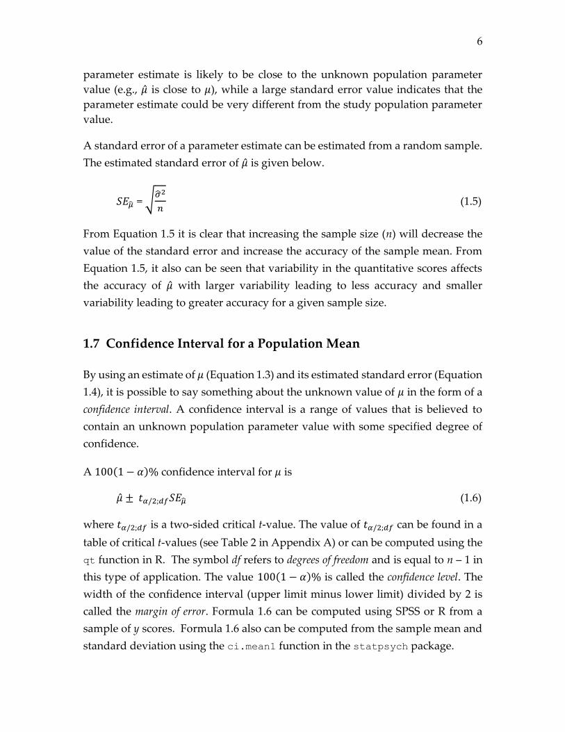
A histogram is a graph that visually describes the shape of a distribution of

quantitative scores. A histogram is constructed by specifying several equal-length

intervals of the quantitative scores and then counting the number of people who

have quantitative scores that fall within each interval. An example of a histogram

of scores on the Attention Deficit Checklist for 3,910 high school students is shown

in Figure 1.2.

Figure 1.2 Histogram of test scores

Scientists discovered decades ago that histograms for many different types of

quantitative scores could be closely approximated by a certain type of symmetric

bell-shaped curve called a normal (or Gaussian) curve. The histogram of attention

deficit scores in Figure 1.2 includes a graph of a normal curve that, in this example,

closely approximates the shape of the histogram.

If a set of quantitative scores is approximately normal, the scores will have the

following characteristics:

about half of the scores are above the mean and about half are below the mean

about 68% of the scores are within 1 standard deviation of the mean

about 95% of the scores are within 2 standard deviations of the mean

almost all (99.7%) of the scores are within 3 standard deviations of the mean

Furthermore, the two points where the normal curve changes from bending down

to bending up, called the inflection points, are one standard deviation above and

13

below the mean on the normal curve. A visual inspection of Figure 1.2 suggests

that the mean is about 10 and the standard deviation is about 4.

A normal distribution with a mean of 0 and a standard deviation of 1 is called a

standard normal distribution. If the y scores have an approximate normal

distribution, then the standardized scores (𝑦 − 𝜇)/𝜎 will have an approximate

standard normal distribution. The symbol 𝑧𝛼/2 will be used to denote the point on

a standard normal distribution for which 100(1 − 𝛼)% of the distribution is

between -𝑧𝛼/2 and 𝑧𝛼/2. For example, 95% of the standard normal distribution is

between -𝑧.05/2 and 𝑧.05/2 where 𝑧.05/2 = 1.96.

1.14 Skewness and Kurtosis

The normal distribution is symmetric. In a symmetric distribution, the left half of

the distribution is a mirror image of the right half. The asymmetry in a set of

quantitative scores can be described using a coefficient of skewness. The population

coefficient of skewness is equal to skew(y) = ∑ 𝑧𝑖3/𝑁𝑁

𝑖=1 where 𝑧𝑖 = (𝑦𝑖 − 𝜇)/𝜎. A

skewness coefficient will equal zero if the scores are perfectly symmetric. A

skewness coefficient will be positive if the y scores are skewed to the right and will

be negative if the y scores are skewed to the left. An example of a positively skewed

distribution and a negatively skewed distribution is shown in Figure 1.3.

Figure 1.3 Example of a positively skewed (left) and a negatively skewed (right) distribution

14

A distribution of quantitative scores can be non-normal even if the distribution is

symmetric. The coefficient of kurtosis describes the degree to which a distribution is

more or less peaked than a normal distribution. The kurtosis of a distribution can

be described by a coefficient of kurtosis which is equal to 3 in a normal

distribution. The population coefficient of kurtosis is equal to kur(y) = ∑ 𝑧𝑖4/𝑁𝑁

𝑖=1 .

SPSS (but not R) subtracts 3 from the kurtosis coefficient so that it will equal 0 in

normal distributions. To avoid confusion, a kurtosis coefficient minus 3 is called

excess kurtosis. Leptokurtic distributions have excess kurtosis greater than 0 and are

more peaked or have longer tails than a normal distribution. Platykurtic

distributions have excess kurtosis less than 0 and are less peaked or have shorter

tails than a normal distribution. An example of a platykurtic distribution of

y scores is shown in Figure 1.4 on the left, and an example of a leptokurtic

distribution of y scores is shown on the right. A normal curve is added to each

graph for comparison.

Figure 1.4 Example of a platykurtic (left) and a leptokurtic (right) distribution

1.15 Sampling Distribution of �̂�

Consider a study population consisting of N people with 𝑦𝑖 representing some

quantitative measurement of the ith person. Imagine taking a sample of n people

from this study population, recording their y scores, and then computing the

sample mean (�̂�). Now imagine doing this for every possible sample of size n. The

set of all possible sample means, for samples of size n, is called the sampling

distribution of the sample mean.

15

The sampling distribution of �̂� has three important features:

The mean of the sampling distribution is equal to the population mean 𝜇

If the sample size is sufficiently large, the sampling distribution will be

closely approximated by a normal distribution regardless of the shape of

the distribution of y scores (central limit theorem)

The standard deviation of the sampling distribution of the sample means is

equal to √𝜎2/𝑛√(𝑁 − 𝑛)/(𝑁 − 1)

Because the mean of the sampling distribution of �̂� is equal to the population

mean 𝜇, the sample mean �̂� is said to be unbiased. Unbiased estimates are attractive

because they are just as likely to overestimate the population parameter as to

underestimate the population parameter.

The standard deviation of the sampling distribution of �̂� decreases as the sample

size increases. If the sample size is large, the sample means in a sampling

distribution will have similar values and, because the sample mean is unbiased,

they will all tend to be close to the population mean.

In typical applications where n is a small fraction of N, the finite population

correction factor √(𝑁 − 𝑛)/(𝑁 − 1) will be close to 1 and can be ignored. Ignoring

the correction factor, the standard deviation of the sampling distribution of �̂� is

√𝜎2/𝑛. Note that the standard error of �̂� defined in Equation 1.5 is an estimate of

the standard deviation of the sampling distribution of �̂� ignoring the finite

population correction. It is remarkable that that standard error of �̂�, which is

computed from one random sample, provides an estimate of the standard

deviation of the sampling distribution of sample means of all possible samples.

A sampling distribution of �̂� consists of N!/[(N – n)!n!] values of �̂�, which is an

astronomically large number in typical applications (Note: n! = n × (n – 1) × (n – 2)

× … × 1; e.g., 4! = 4 × 3 × 2 × 1 = 24). To concretely illustrate some properties of a

sampling distribution, consider a very small population of N = 5 people who have

quantitative scores of 𝑦1 = 14, 𝑦2 = 13, 𝑦3 = 11, 𝑦4 = 15 and 𝑦5 = 12 where the

population mean is 𝜇 = (14 + 13 + 11 + 15 + 14)/5 = 13, and the population variance

is 𝜎2 = [(14 – 13)2 + (13 – 13)2 + (11 – 13)2 + (15 – 13)2 + (12 – 13)2]/5 = 2. The standard

16

error of �̂� for n = 2 (not ignoring the finite correction factor) is

√𝜎2/𝑛√(𝑁 − 𝑛)/(𝑁 − 1) = √2/2√3/4 = √3/2. With N = 5 and n = 2, the sampling

distribution of �̂� consists of only N!/[(N – n)!n!] = 5!/(3!2!) = 10 sample means which

are shown below.

Sample Participants Sample Scores �̂�

1 1 and 2 14, 13 13.5

2 1 and 3 14, 11 12.5

3 1 and 4 14, 15 14.5

4 1 and 5 14, 12 13.0

5 2 and 3 13, 11 12.0

6 2 and 4 13, 15 14.0

7 2 and 5 13, 12 12.5

8 3 and 4 11, 15 13.0

9 3 and 5 11, 12 11.5

10 4 and 5 15, 12 13.5

________________________________________________

The mean of all possible sample means is (13.5 + 12.5 + … 13.5)/10 = 13, which is

identical to the population mean. Furthermore, the standard deviation of all

possible means is √[(13.3 – 13)2 + (12.5 – 13)2 + … + (13.5 – 13)2]/10 = √0.75 =

√3/2, which is identical to the standard error of the sample mean.

1.16 Illustration of the Central Limit Theorem

A very important theorem in statistical theory is the central limit theorem. The

central limit theorem states that with a sufficiently large sample size, the shape of

the sampling distribution of �̂� is approximately normal regardless of the shape of

the distribution of quantitative scores in the study population. Furthermore, the

larger the sample size, the more closely the sampling distribution will

approximate a normal distribution. Figure 1.5 illustrates a highly non-normal

distribution of response variable scores in a study population.

17

Figure 1.5 Histogram of y scores in a study population

Figures 1.6 - 1.8 illustrate sampling distributions of �̂� based on samples of n = 5,

n = 15, and n = 30 (these sampling distributions were approximated by taking 1,000

random samples of a give size from the study population rather than all possible

samples). A normal curve is included in each graph for comparison. Note that with

samples of size n = 5, the sampling distribution of �̂� is not well approximated by a

normal distribution.

Figure 1.6 Sampling distribution of �̂� for n = 5

Note how the sampling distribution of �̂� for n = 15 is more symmetric and more

closely approximates a normal distribution.


18

With samples of size n = 30, the sampling distribution of �̂� closely approximates a

normal distribution even though the scores in the study population are highly

non-normal.


In the above example, the distribution of y scores in the study population is

extremely non-normal, but the sampling distribution of �̂� is closely approximated

by a normal distribution with a sample size of 30. If the distribution of y scores in

the study population is not extremely non-normal, the sampling distribution of �̂�

will closely approximate the normal distribution with sample sizes less than 30.

It can be shown that the skewness of a sampling distribution of �̂� is equal to

skew(y)/√𝑛, and the excess kurtosis of a sampling distribution of �̂� is [kur(y) – 3]/n.

As n increases, the excess kurtosis of a sampling distribution of �̂� decreases faster

than the skewness of a sampling distribution of �̂�. Because of this, skew(y) is more

of a concern than kur(y) when computing a confidence interval for 𝜇 or performing

a hypothesis test regarding the value of 𝜇.

1.17 Probability

There is an intrinsic amount of uncertainty in all confidence interval and

hypothesis testing results. Researchers need to understand and accurately

quantify this uncertainly in any reported confidence interval or hypothesis testing

result. The uncertainty of a specific outcome can be quantified on a probability scale

from 0 to 1 where a probability of 0 indicates that some outcome definitely will not

occur and a probability of 1 indicates that the event definitely will occur. Two

different interpretations of probability, relative frequency and subjective, are

commonly used to describe probability values between 0 and 1.

19

To illustrate the relative frequency approach, imagine an infinitely large

population and imagine computing a confidence interval for 𝜇 in K different

samples from the population. Let f be the number of the K confidence intervals

that capture the value of 𝜇. According the relative frequency definition, the

probability that a confidence interval will capture 𝜇 is equal to f/K as K approaches

infinity. The relative frequency definition of probability is useful in theoretical

statistics where populations are assumed to be infinitely large and confidence

intervals and hypothesis tests are described in terms of imaginary samples from a

population. The relative frequency approach is not useful in applied statistics

where the populations are finite and it is necessary to describe the uncertainty of

a specific confidence interval or hypothesis test result that has been observed in a

single study.

A subjective probability is based on an individual's personal judgment and

knowledge about a specific outcome. Unlike the relative frequency interpretation,

a subjective interpretation can be used to describe a single outcome. This is

important in applied statistics where the researcher conducts one study and must

interpret the uncertainty of the confidence interval or hypothesis testing results.

Confidence can be defined by multiplying a subjective probability by 100%.

When subjective probabilities are assigned to complex phenomena, such as stock

prices or weather, people will have differing subjective probabilities about specific

outcomes. This lack of consensus is a major criticism of subjective probability. But

for very simple phenomena, many individuals can have a consensus opinion about

the probability of a specific outcome. For example, suppose a jar contains many

green and red marbles that are the same size and weight. The marbles are

thoroughly mixed and with eyes closed one marble is removed from the jar. Given

that the marbles were thoroughly mixed and have the same size and weight, and

one was selected with eyes closed, most people would subjectively agree that

every marble had the same probability of being selected. This marble example will

be more similar to confidence interval and hypothesis testing problems if we also

imagine that the marble turns white as soon as it is removed from the jar and that

its original color will never be known. Suppose we are told that the proportion of

green marbles is .95. In this application, most people would say that they are 95%

confident that the selected marble was green. In the following section, subjective

20

probability is used to quantify a researcher's uncertainty regarding confidence

interval or hypothesis testing results obtained in a single study.

1.18 Uncertainty in Statistical Results

The subjective probability in the marble example can be used to interpret a

100(1 − 𝛼)% confidence interval for 𝜇. If a 100(1 − 𝛼)% confidence interval for 𝜇

was computed from every possible sample of size n in a given study population,

we know from statistical theory that about 100(1 − 𝛼)% of these confidence

intervals will capture the unknown value of 𝜇. With random sampling, we assume

that every possible sample of size n has the same subjective probability of being

selected (which is analogous to randomly selecting one marble). We know that

each sample will be one of two types: samples where the 100(1 − 𝛼)% confidence

interval contains the value of 𝜇 and samples where the 100(1 − 𝛼)% confidence

interval does not contain the value of 𝜇 (which is analogous to marbles being either

green or red). Furthermore, the percentage of all possible samples for which a

100(1 − 𝛼)% confidence interval contains the value of 𝜇 is known to be about

100(1 − 𝛼)% (which is analogous to knowing to proportion of green marbles).

Knowing that a 100(1 − 𝛼)% confidence interval for 𝜇 will capture the value of 𝜇

in about 100(1 − 𝛼)% of all possible samples of a given size, and assuming that

the one sample the researcher has used to compute the 100(1 − 𝛼)% confidence

interval is a random sample, we can then say that we are 100(1 − 𝛼)% confident

that the computed confidence interval includes the value 𝜇.

In a directional two-sided test, a directional error occurs when H1: 𝜇 > h has been

accepted but H2: 𝜇 < h is true or when H2: 𝜇 < h has been accepted but H1: 𝜇 > h is

true. For any specified value of 𝛼, if a directional two-sided test was performed

from every possible sample of size n in a given study population, we know from

statistical theory that at most 100𝛼/2% of these hypothesis tests will result in a

directional error. The probability of a directional error is close to 𝛼/2 if 𝜇 is close to

h but will be less than 𝛼/2 if 𝜇 is not close to h. If we obtain one random sample

from the study population and we accept one of the two alternative hypotheses,

our subjective probability that we have made a directional error is at most 𝛼/2. We

also could say that we are at least 100(1 – 𝛼/2)% confident that we have not made

a directional error.

21

The above subjective interpretations of confidence interval and hypothesis testing

results assumed that 100(1 − 𝛼)% of the confidence intervals from all possible

samples of a given size will capture the unknown value of 𝜇, and at most 100𝛼/2%

of the hypothesis tests from all possible samples of given size will result in a

directional error. The conditions required for these claims to be true are described

in Section 1.23.

1.19 Power of a Hypothesis Test

In hypothesis testing applications, the goal is to reject H0: 𝜇 = h and then choose

either H1: 𝜇 > h or H2: 𝜇 < h. It is reasonable to assume that H0: 𝜇 = h is false in any

real application because it is extremely unlikely that 𝜇 will exactly equal h. The

power of a hypothesis test is the probability of avoiding an inconclusive result. In

a study where the goal is to choose H1: 𝜇 > h or H2: 𝜇 < h, an inconclusive result

would be disappointing. If the power of a hypothesis test is high, then the

probability of an inconclusive result will be low. The researcher will want to use a

sample size that is large enough to keep the probability of an inconclusive result

at an acceptably low level.

The power of a directional two-sided test for 𝜇 depends on the sample size, the

absolute value of 𝜇 − ℎ, and the 𝛼 level. Increasing the sample size will increase

the power of the test as illustrated in Figure 1.9 for 𝛼 = .05, 𝜇 − ℎ = 0.5, and 𝜎 = 1.

Note that increasing the sample size will dramatically increase the power of the

hypothesis test up to a point. We typically want the smallest sample size that will

produce adequate power. A method for finding the sample size required to

achieve desired power is described in Section 1.27.

Figure 1.9 Relation between power and sample size

22

Decreasing 𝛼 will reduce the probability of a directional error (which is desirable)

but will also decrease the power of the directional two-sided test (which is

undesirable) as illustrated in Figure 1.10 for n = 30, 𝜇 − ℎ = 0.5, and 𝜎 = 1. Note

that there is little loss in power for reductions in 𝛼 down to about .10. But the

power decreases substantially for 𝛼 values below .05. This relation between power

and 𝛼 explains why 𝛼 = .05 is a popular choice in psychological research.

𝛼

Figure 1.10 Relation between power and 𝜶

For a given sample size and 𝛼 level, Figure 1.11 shows how the power of a

directional two-sided test increases as the absolute value of 𝜇 − ℎ increases for

n = 30, 𝛼 = .05, and 𝜎 = 1.

|𝝁 − 𝒉|

Figure 1.11 Relation between power and |𝝁 − 𝒉|

1.20 Target Population

The confidence intervals and hypothesis tests provide information about the study

population from which the random sample was taken. In most applications, the

study population will be a small subset of some larger and more interesting

population called the target population (see Figure 1.12). It is important to

23

remember that the sample mean (�̂�) is an estimate of the study population mean

(𝜇). Furthermore, the target population mean, which will be denoted here as 𝜇∗, is

not necessarily similar to the study population mean.

Suppose a researcher obtains a random sample of 100 undergraduate students

from a university research participant pool consisting of about 1,000 students.

Confidence interval and hypothesis testing results will apply only to those 1,000

undergraduate students, but the researcher is surely more interested in the mean

of the response variable for a target population that consists of all undergraduate

students.

Figure 1.12. The correspondence among target population, study population, and sample

It might be possible for the researcher to make a persuasive argument that the

study population mean should be very similar to the target population mean. If

the difference between 𝜇 and 𝜇∗ is assumed to be trivial, then the confidence

interval and hypothesis testing results for 𝜇 would then also apply to 𝜇∗. For

example, suppose the researcher measured the eye pupil diameter of 100 college

students in a small room lit only by a 40-watt light bulb. The researcher could

argue that the mean pupil diameter in the study population of 1,000

undergraduate students should be no different than the mean pupil diameter in a

target population of all undergraduate students. In this study, it should be easy to

convince others that the difference between 𝜇 and 𝜇∗ is trivial.

Now consider an example where it would be unreasonable to assume that the

value of 𝜇 – 𝜇∗ is trivial. Suppose that the researcher instead gave the 100 students

a questionnaire to gauge their attitudes about abortion, and also suppose that the

Target Population (𝜇∗)

Study Population (𝜇)

Sample (�̂�)

24

university is a Jesuit university. In this study it would not be appropriate to

assume that the confidence interval and hypothesis testing results for 𝜇 also apply

to a target population of all undergraduate students.

In studies involving sensation, perception, and basic cognitive processes, the value

of 𝜇 – 𝜇∗ is typically assumed to be trivial, and researchers in these fields seldom

make a distinction between the study and target populations. In contrast,

psychologists who study complex human behavior cannot automatically assume

that the value of 𝜇 – 𝜇∗ is trivial. In applications where 𝜇 – 𝜇∗ is unlikely to be

trivial, the researcher must clearly describe the relevant characteristics of the study

population and present the confidence interval and hypothesis testing results in a

way that does not give a misleading impression about the generality of the

findings.

1.21 Nonrandom Samples

Psychologists are usually only interested in some target population, but it can be

extremely difficult to obtain a random sample from the target population of

interest. Instead of taking a random sample from a smaller and more accessible

study population and then arguing that the population parameter in the study

population (e.g., 𝜇 ) should be similar to the population parameter in the target

population (e.g., 𝜇∗), psychologists more often obtain a convenient sample of

participants and then "assume" that the sample is random sample from the target

population of interest. This assumption is usually very difficult to justify, but in

some applications this assumption is easily justified. Consider the previous

example where a researcher obtained a random sample of 100 college students

from a study population of 1,000 students and measured their eye pupil diameters.

Instead of taking a random sample, suppose the researcher instead obtained a

nonrandom sample of 100 students who were enrolled in an introductory statistics

class. The researcher could argue that the nonrandom sample of 100 eye pupil

diameters can be thought of as a random sample of the eye pupil diameters that

would be obtained in a target population of all young adults. Eye physiology

experts would agree with this argument.

25

It should be noted that a nonrandom sample might be considered a random

sample for one response variable but not for other response variables. For

example, if the 100 college students in the nonrandom sample described above

were given a test to assess their knowledge of basic statistical methods, the test

scores for these 100 students is obviously not a random sample of test scores in a

target population of all young adults. Examples where a nonrandom sample will

yield an interpretable confidence interval or hypothesis testing result are common

in studies of sensation, perception, and basic cognitive processes but are rare in

studies involving complex human behavior.

1.22 Assumptions for Confidence Intervals and Tests

The confidence interval and hypothesis test for 𝜇 require three assumptions. The

importance of obtaining a random sample (the random sampling assumption) was

made clear in Section 1.18. If the sample is not a random sample from a specific

study population and it is not reasonable to assume that the nonrandom sample

of scores for a specific response variable could be a random sample of scores from

some definable target population, then the confidence interval and hypothesis test

results will be uninterpretable. A failure to satisfy the random sampling

assumption is partly responsible for the "replication crisis" in psychology.

In all possible samples of a given size, a 100(1 – 𝛼)% confidence will contain 𝜇 in

about 100(1 – 𝛼)% of the samples and a directional two-sided test will result in a

directional error in at most 100𝛼/2% of the samples if two additional assumptions

are satisfied. The independence assumption requires the responses from each

participant in the sample to be independent of one another. In other words, no

participant in the study should influence the responses of any other participant in

the study. The normality assumption requires the y scores in the study population

to have an approximate normal distribution (Note: exact normality would require

an infinitely large study population).

Confidence interval and hypothesis test results will not have the desired

interpretation if the independence assumption has been violated. When the

independence assumption is violated, the percent of samples in which a

100(1 − 𝛼)% confidence interval contains 𝜇 can be far less than 100(1 − 𝛼)%, and

26

the percent of samples in which a directional two-sided test produces a directional

error can be far greater than 100𝛼/2%. Although the consequences of violating the

independence assumption are serious, this assumption usually can be easily

satisfied by measuring participants one at a time and instructing them not to

discuss their responses with any other participants in the study.

One consequence of the central limit theorem is that violating the normality

assumption will have little effect on the confidence interval and hypothesis test for

𝜇 if the distribution of y scores in the study population is at most moderately non-

normal and the sample size is not too small (n > 30). If the sample size is small and

the distribution of quantitative scores in the study population is highly non-

normal, the percent of all possible 100(1 − 𝛼)% confidence intervals that would

capture 𝜇 can be much less than 100(1 − 𝛼)%, and percent of samples in which a

directional two-sided test produces a directional error can be far greater than

100𝛼/2%.

Unlike a confidence interval or a hypothesis test for 𝜇, a prediction interval for a

single score is not protected by the central limit theorem. A prediction interval can

have a coverage probability that is lower than the specified level of confidence,

even with a large sample size, if the distribution of y scores in the study population

is not approximately normal.

1.23 Assessing the Normality Assumption

The confidence interval and hypothesis test for 𝜇 assumes that the distribution of

the response variable scores in the study population has an approximate normal

distribution, or that the sample size is large enough that the central limit theorem

will provide some assurance that the sampling distribution of the sample mean

will be approximately normal. Prediction intervals and some other statistical

methods described in subsequent chapters require normality of the response

variable scores in the study population, but these methods will not be protected

by the central limit theorem. For these statistical methods, the normality

assumption must be taken more seriously and researchers must struggle with the

fact that the normality assumption can be difficult to assess using only sample

data. In the absence of prior information about the shape of the population

27

distribution, the shape of the distribution of the y scores in the sample can provide

some vague clues about the shape of the population distribution. The estimated

skewness coefficient and the estimated kurtosis coefficient can be used to assess

the shape of the population distribution. However, estimates of skewness and

kurtosis can be inaccurate in small samples.

SPSS and R provide a test of the null hypothesis that the population skewness

coefficient is zero. If the p-value for the test is less than .05, the researcher can

conclude that the population scores are skewed to the left or to the right according

to the sign of the estimated skewness coefficient. Although a p-value greater than

.05 for the test of skewness does not imply that the null hypothesis is true, if the

sample size is large (at least 100) and the p-value is substantially greater than .05,

one could cautiously argue that the population skewness is small.

SPSS and R provide a test of the null hypothesis that the population kurtosis

coefficient is zero. If the p-value for the test is less than .05, the researcher can

conclude that the population scores are either leptokurtic or platykurtic according

the value of estimated kurtosis coefficient. Although a p-value greater than .05 for

the test of kurtosis does not imply that the null hypothesis is true, if the sample

size is large (at least 100) and the p-value is substantially greater than .05, one could

cautiously argue that the population excess kurtosis is small.

1.24 Data Transformations

Nonlinear data transformations may reduce non-normality in the y scores. When

the score is a frequency count for each participant, such as the number of facts that

can be recalled or the number of spelling errors in a writing sample, a square root

transformation (√𝑦𝑖) may reduce skewness and kurtosis. When the score is a time-

to-event, such as the time required to solve a problem or a reaction time, a log

transformation (ln(𝑦𝑖)) or a reciprocal transformation (1/𝑦𝑖) may reduce skewness

and kurtosis. In a linear data transformation, each y score is multiplied or divided

by a number or a number is added to or subtracted from each y score. A linear data

transformation will change the mean and variance of the y scores but will have no

effect on skewness or kurtosis.

28

Example 1.5. A histogram of 200 highly skewed food insecurity scores is shown below

(left). A histogram of log-transformed scores (right) is more symmetric and more closely

approximates a normal distribution.

Although nonlinear data transformations may reduce non-normality, the mean of

the transformed scores could then be difficult to interpret. However, in some

applications the value of 𝜇 might be interpretable after a data transformation. For

example, if y is measured in squared units, such as the brain surface area showing

activity measured in squared centimeters, then √𝑦 could be interpreted as the

“size” of the activated area. Or if y is the time to respond measured in seconds,

then 60/y could be interpreted as responses per minute.

1.25 Distribution-free Methods

If the response variable is highly skewed, a population median (denoted as 𝜃) could

be a more meaningful parameter to estimate than a population mean. The median

is useful because it is the value that divides a distribution in half. In skewed

distributions, the mean is strongly influenced by a few unusually small or large

scores and can give a misleading description of the center of a distribution.

The median also is useful in describing time-to-event scores (e.g., years until

divorce, months until next promotion, etc.) which are typically skewed. In a time-

to-event study (also called a survival analysis) where participants are studied over

a fixed period of time, some of the participants will not exhibit the event of interest

during the study period. We say that the time-to-event scores for these participants

are right censored because the time-to-event score is some unknown value greater

than study period time. If any of the scores are censored, it is not possible to

estimate the population mean time-to-event, but if less than 50% of the scores are

censored the population median time-to-event can be estimated.

29

To compute a confidence interval for 𝜃 from a random sample n participants with

quantitative scores 𝑦1, 𝑦2, … , 𝑦𝑛, first rank order the scores from smallest to largest

which will be denoted as 𝑦(1) , 𝑦(2), … , 𝑦(𝑛) where 𝑦(1) is the smallest score, 𝑦(2) is

the next smallest score, and 𝑦(𝑛) is the largest score. Next, compute

𝑜1 = (n – 𝑧𝛼/2√𝑛)/2 (which is rounded to the nearest integer but not below 1) and

𝑜2 = n – 𝑜1 + 1. An approximate 100(1 − 𝛼)% confidence interval for 𝜃 is

[𝑦(𝑜1), 𝑦(𝑜2)] (1.9)

which assumes random sampling and independence among participants. In a

time-to-event study with censored time scores, Formula 1.9 requires 𝑦(𝑜2) to be less

than the study period time. Formula 1.9 can be computed using the ci.median1

function in the statpsych package.

Example 1.6. In Example 1.1, the researcher estimated the mean Sense of Belonging score

in a study population of about 2,000 UCSC second-year students. The belonging scores in

the random sample of 10 students are rank ordered below from smallest to largest

15 19 25 26 26 30 31 33 34 44

where 𝑦(1) = 15, 𝑦(2) = 19, … , 𝑦(9) = 34, 𝑦(10) = 44. To obtain a 95% confidence interval for

𝜃, compute 𝑜1 = (10 – 1.96√10 )/2 = 1.9 (round to 2) and 𝑜2 = 10 – 𝑜1 + 1 = 9. The 95%

confidence interval for 𝜃 is [𝑦(2), 𝑦(9)] = [19, 34]. The researcher can be 95% confident that

the median Sense of Belonging score in the study population of 2,000 UCSC second-year

students is between 19 and 34.

The sample median is an estimate of the population median and is denoted as 𝜃.

If n is an odd number, 𝜃 is the middle rank ordered score. If n is an even number,

𝜃 is the average of the two middle rank ordered scores. For the 10 belonging scores

given above, 𝜃 = (26 + 30)/2 = 28.

Formula 1.9 can be used to test the following hypotheses regarding the population

median

H0: 𝜃 = h H1: 𝜃 > h H2: 𝜃 < h

where h is some number specified by the researcher. Specifically, if the upper limit

of the confidence interval is less than h, then H0 is rejected and H2 is accepted; if

30

the lower limit of the confidence interval is greater than h, then H0 is rejected and

H1 is accepted; and if the confidence interval includes h, then H0 cannot be rejected.

The sign test is a distribution-free alternative to the one-sample t-test. The sign test

is a test of the null hypothesis H0: 𝜃 = h. Statistical packages will compute the

p-value for the sign test that can be used to decide if H0 can be rejected. The sign

test is preferred to the one-sample t-test in applications where the response

variable is known to be highly skewed and the sample size is small. The power of

the sign test is usually much less than the power of the one-sample t-test, but the

sign test can have greater power than the t-test if the y scores are highly

leptokurtic.

The null hypothesis H0: 𝜃 = h for a sign test also can be expressed as H0: 𝜋 = .5

where 𝜋 is the proportion of people in the study population who have scores

greater than h. The results of the sign test can be supplemented with the following

approximate 100(1 − 𝛼)% confidence interval for 𝜋

�̂� ± 𝑧𝛼/2√�̂�(1 − �̂�)

𝑛 (1.11)

where 𝑧𝛼/2 is a two-sided critical z-value, �̂� = (f + 2)/(n + 4) and f is the number of

participants in the sample with y scores that are greater than h. The ci.prop1

function in the psychstat package can be used to compute Formula 1.11.

1.26 Variability Assessment

The population mean only describes the center of a population of y scores, and it

would be a mistake to ignore individual differences and assume that most people

have y scores that are similar to the population mean. It is important to describe

the population variability of the y scores in addition to the population mean. The

population standard deviation (𝜎) is a common measure of variability. If 𝜎 is small,

then most people will have y scores that are similar to the population mean. But if

𝜎 is large, then some people will have y scores that are much smaller and much

larger than the population mean.

The value of the population standard deviation is usually unknown and must be

estimated from a random sample (see Equation 1.4). The traditional confidence

31

interval for 𝜎 assumes that the population y scores have a normal distribution. This

confidence interval will have a coverage probability that can be far less than 1 – 𝛼

if the y scores are leptokurtic and increasing the sample size will not rectify the

problem.

The mean absolute deviation from the median (MAD) is an alternative measure of

variability that has a simple interpretation and for which a useful confidence

interval can be computed. The population MAD is

𝜏 = ∑ |𝑦𝑖 − 𝜃|𝑁

𝑖=1

𝑁 (1.12)

where 𝜃 is the population median of the y scores. The summation notation

∑ |𝑦𝑖 − 𝜃|𝑁𝑖=1 is a more compact way of writing |𝑦1 − 𝜃| + |𝑦2 − 𝜃| + ⋯ +

|𝑦𝑁 − 𝜃| where the pair of vertical bars represents an absolute value. Thus, the

population MAD is simply the average absolute difference between the y scores

and the population median. The value of the population MAD is unknown and

must be estimated from a random sample. The sample MAD is

�̂� = ∑ |𝑦𝑖 − �̂�|𝑛

𝑖=1

𝑛 (1.13)

where 𝜃 is the sample median.

An approximate 100(1 – 𝛼)% confidence interval for 𝜏 is

exp[ln(c�̂�) ± 𝑧𝛼/2𝑆𝐸𝑙𝑛(�̂�)] (1.14)

where c = n/(n – 1) and 𝑆𝐸𝑙𝑛(�̂�) = √[(𝜇 ̂− �̂�)2

�̂�2 +�̂�2

�̂�2 − 1]/𝑛. Formula 1.14 assumes the

y scores have an approximate normal distribution in the study population, but this

assumption is not a concern if n ≥ 30 and the y scores in the study population are

not extremely non-normal. A less biased estimate of 𝜏 is c�̂�. (Note: ln(x) is the

natural logarithm of x and exp(x) = ex where e ≈ 2.718). Formula 1.14 can be

computed using the ci.mad1 function in the statpsych package.

32

Example 1.7. A "Feelings of Powerless" questionnaire, scored from 0 to 40, was given to

a random sample of 90 students taken from a study population of 1,780 students at a large

high school. Scores between 15 and 25 are considered typical, scores above 30 are

considered to represent high levels of powerlessness, and scores below 10 are considered

to represent low levels of powerlessness. High levels of powerlessness have been

associated with susceptibility to conspiracy theories, and low levels of powerlessness have

been associated with low susceptibility to conspiracy theories. The 95% confidence

interval for the median powerlessness score in the high school student study population

is [17.1, 23.5] which is within the typical range. However, the confidence interval for the

population MAD is [11.5, 18.8] indicating that there is considerable variability in the

powerless scores. The researcher can be 95% confident that the MAD of the powerless

scores is between 11.5 and 18.8 points in the study population of 1,780 high school

students. Future research will attempt to identify characteristics of those students who

exhibit low levels of powerlessness to gain insights that could help develop training

programs to reduce susceptibility to conspiracy theories.

1.27 Sample Size Planning

Larger sample sizes give narrower confidence intervals, and it is possible to

approximate the sample size that will give the desired width (w) of a confidence

interval (i.e., upper limit minus lower limit) for a desired level of confidence. The

sample size needed to obtain a 100(1 − 𝛼)% confidence interval for 𝜇 having a

desired width of w is approximately

n = 4�̃�2(𝑧𝛼/2

𝑤)

2+

𝑧𝛼/22

2 (1.15)

where �̃�2 is a planning value of the response variable variance and 𝑧𝛼/2 is a two-

sided critical z-value. Equation 1.15 shows that larger sample sizes are needed with

1) narrower confidence interval widths, 2) greater levels of confidence, and 3)

greater variability of the response variable. Equation 1.15 can be computed using

the size.ci.mean1 function in the statpsych package.

Example 1.8. A researcher wants to estimate the mean empathy score for a population of

4,782 public school teachers. The researcher plans to use an empathy questionnaire

(measured on a 1 to 10 scale) that has been used in previous studies. A review of the

literature suggests that the variance of the empathy scale is about 6.0. The researcher

would like the 95% confidence interval for 𝜇 (the mean empathy score for all 4,782

teachers) to have a width of about 1.5. The required sample size is approximately

n = 4(6.0)(1.96/1.5)2 + 1.92 = 42.9 ≈ 43.

33

The sample size needed in a directional two-sided test of 𝜇 with desired power

and a specified value of 𝛼 is approximately

n = �̃�2 (𝑧𝛼/2 + 𝑧𝛽)2

(�̃� − ℎ)2 +

𝑧𝛼/22

2 (1.16)

where 1 – 𝛽 is the desired power of the test, 𝜇 is a planning value of the population

mean, and 𝑧𝛽 is a one-sided critical z-value. The value of 𝜇 − ℎ is the effect size.

Equation 1.16 shows that larger sample sizes are needed with smaller values of 𝛼,

greater desired power, values of 𝜇 that are closer to h, and greater variability of the

response variable. Equation 1.16 can be computed using the size.test.mean1

function in the statpsych package. SPSS can compute the required sample size

for desired power or the power of the one-sample t-test for a given sample size.

Equations 1.15 and 1.16 show that larger values of �̃�2 require a larger sample size.

Some researchers prefer to sample from homogeneous study populations (e.g.,

first and second year psychology majors) rather than heterogeneous study

populations (e.g., working adults) because 𝜎2 will be smaller in the homogeneous

study population and hence the sample size requirement will be smaller.

However, hypothesis test and confidence interval results apply to the study

population from which the random sample was taken, and the results may have

less practical or scientific importance in a homogeneous study population than a

more heterogeneous population. This tradeoff should be given serious

consideration when planning a study.

Example 1.9. A researcher knows that the ACT mathematics scores in a study population

of 5,374 first-year college students has a mean of 24.5 and a variance of 8.2. The researcher

plans to take a random sample from this study population and then give the sampled

students supplementary mathematics training to improve their math skills. The

researcher believes that the population mean ACT score would increase from 24.5 to 26.0

if all 5,374 first-year college students were given the supplementary mathematics training.

To test H0: 𝜇 = 24.5 for 𝛼 = .05 and a desired power of .90, the required sample size is

approximately n = 8.2(1.96 + 1.28)2/(26.0 – 24.5)2 + 1.92 = 40.2 ≈ 41.

The sample size needed to test H0: 𝜃 = h with desired power using the sign test is

approximately

n = (𝑧𝛼/2 + 𝑧𝛽)

2

4(𝜋 ̃− .5)2 (1.17)

34

where �̃� is a planning value of the proportion of people in the study population

who have y scores that are greater than the hypothesized median (h). The effect

size for a sign test is 𝜋 ̃ − .5.

Note that Equations 1.15 - 1.17 do not show the effect of the study population size

(N) on the sample size requirement. Some specialized statistical software will

compute confidence intervals using a finite population correction. If a finite

population correction will be used in a confidence interval, the required sample

size is n′ = n/(1 + n/N) where n is given by Equations 1.15, 1.16, or 1.17. If n is a

small fraction of N, the size of the study population (N) has very little effect on the

required sample size. For example, suppose Equation 1.15, 1.16, or 1.17 gave a

required sample size of n = 100 and suppose that the study population size is 5,000.

If a finite population correction factor will be used in the test or confidence

interval, the sample size requirement drops slightly from 100 to 98 ≈

100/(1 + 100/5000). All of the standard statistical methods that are implemented in

SPSS and R do not use finite population corrections. The sample size formulas

given in Equations 1.15, 1.16, and 1.17, which do not use finite population

corrections, should be used when planning a study.

1.28 Sampling in Two Stages

In applications where sample data can be collected in two stages, the confidence

interval obtained in the first stage can be used to determine how many more

participants should be sampled in the second stage. If the 100(1 − 𝛼)% confidence

interval width from a first-stage sample size of n is 𝑤0 and 𝑤0 is larger than the

desired width (w), then the number of participants that should be added to the

original sample (n+) in order to obtain a 100(1 − 𝛼)% confidence interval width of

w is approximately

𝑛+ = [(𝑤0

𝑤)

2

− 1] 𝑛. (1.18)

The size.second function in the statpsych package can be used to compute

Equation 1.18. This methods is general and can be applied to any of the confidence

interval problems in Chapters 2 - 4.

35

Example 1.10. A researcher computed a 95% confidence interval for a gender ideology

score in a population of 1,800 high school students using a random sample of 25 high

school students. The width of the confidence interval was 4.38. The results of this study

are unlikely to be published because the confidence interval is too wide. The researcher

would like to obtain a 95% confidence interval for the population mean that has a width

of 2.0. To achieve this goal, the number of high school students that should be added to

the initial sample is [(4.38/2.0)2 – 1]25 = 94.9 ≈ 95 to give a final sample size of 25 + 95 =

120.

1.29 Specifying Planning Values

The variance planning value in Equation 1.15 is a subjective estimate of the sample

variance that is likely to be observed in the planned study. The variance planning

value in Equation 1.16 is a subjective estimate of the population variance. In

practice, the researcher will not know the value of the population variance or what

the sample variance will happen to be in a planned study.

Subjective variance planning values can be obtained from expert opinion, pilot

studies, or a review of published studies that have used the same response variable

that will be used in the planned study. If the maximum and minimum possible

values of the response variable scale are known, [(max – min)/4]2 provides a crude

planning value of the population variance.

A variance estimate from a pilot study or a published study contains sampling

error and the variance estimate might understate the value of the population

variance. One option is to compute an upper one-sided confidence limit for the

population variance. The ci.var.upper function in the statpsych package will

perform this computation using the sample standard deviation and sample size

from a pilot study or published study. The sample size requirement using an

upper limit variance planning value could be prohibitively large.

Two different approaches can be used to specify the effect size in Equation 1.16.

One approach sets the planning value of the mean to its most likely value. Another

approach sets the planning value of the mean such that 𝜇 − ℎ represents the

smallest value, called the minimally interesting effect size, that would still represent

a useful or interesting effect. The sample size requirement for a minimally

interesting effect size could be prohibitively large.

36

Key Terms

study population

response variable

ratio scale

interval scale

ordinal scale

nominal scale

population parameter

population mean

population standard deviation

random sample

sample mean

standard error

confidence interval

prediction interval

directional two-sided hypothesis

one-sample t-test

p-value

probability

directional error

power

histogram

normal (Gaussian) curve

sampling distribution

central limit theorem

target population (18)

nonrandom sample (19)

random sampling assumption

independence assumption

normality assumption

coefficient of skewness

coefficient of kurtosis

data transformations

population median

sign test

planning value

37

Concept Questions

1. Explain in words how to compute a sample variance.

2. Increasing the sample size will have what effect on the width of the confidence

interval?

3. Increasing the level of confidence will have what effect on the width of the

confidence interval?

4. Increasing the sample size will have what effect on the value of the standard

error?

5. Explain in words how a confidence interval for 𝜇 can be used to test a two-sided

directional hypothesis where H0: 𝜇 = 100.

6. Increasing the sample size will have what effect on the power of a test?

7. Explain in words how to compute a 95% confidence interval for a population

mean after you have computed the sample mean and variance in a sample of

n = 20.

8. When planning a future study to estimate 𝜇, what is the effect of decreasing the

desired confidence interval width on the sample size requirement?

9. When planning a future study to estimate 𝜇, what is the effect of increasing the

desired level of confidence on the sample size requirement?

10. When planning a future study to estimate 𝜇, what is the effect of using �̃�2 = 50

rather than �̃�2 = 75 on the sample size requirement?

11. When planning a future study to test H0: 𝜇 = h, how does the desired power

affect the sample size requirement?

12. When planning a future study to test H0: 𝜇 = h, how does the 𝛼 value affect the

sample size requirement?

13. Why are narrow confidence intervals desirable?

14. Why are confidence interval results more informative than a directional

two-sided test?

15. Describe the standard error in the context of a sampling distribution.

38

16. Why is the 95% level of confidence a popular choice?

17. What are the assumptions of a confidence interval or test for 𝜇, and what are

the effects of violating those assumptions?

18. What are some ways to obtain a planning value for 𝜎?

19. Explain why a confidence interval might be uninterpretable if a nonrandom

sample is used.

20. Suppose a 95% confidence interval for 𝜇 is [1.5, 4.8]. In a test of the null

hypothesis H0: 𝜇 = h, for which of the following values of h would H0 be rejected:

1.20, 3.30, 4.1, or 5.0?

21. How does the size of the study population effect the sample size requirement

when n/N is small?

22. Why are data transformations sometimes used?

23. Is it appropriate to declare a null hypothesis such as H0: 𝜇 = h to be true if the

results are “nonsignificant”? Why?

24. When testing a null hypothesis such as H0: 𝜇 = h, what can be said about a

“significant” result?

25. What is the relation between the size of the p-value and the sample size?

26. When would a confidence interval for a population median be preferred to a

confidence interval for a population mean?

27. Why is it important to assess the variability of the responses variable and not

just the mean or median of the response variable?

28. What are the implications of the central limit theorem in terms of how a

confidence interval for 𝜇 will perform?

29. About 1.8 million people visit the Monterey Bay Aquarium each year. Exit

interviews were conducted in 2013 for a random sample of 2,417 visitors. One

question asked respondents to rate the quality of the educational experience on a

1 to 10 scale. The 95% confidence interval for 𝜇 was [8.78, 8.89]. Interpret this result.

39

30. Explain why each of the following interpretations of [8.78, 8.89] in the above

example is incorrect or inadequate.

a) We are 95% confident that the 1.8 million visitor ratings are between 8.78 and 8.89.

b) We are 95% confident that a typical visitor rating will be between 8.78 and 8.89.

c) We are 95% confident that the mean rating of the 2,417 visitors is between 8.78 and 8.89.

d) We are 95% confident that 𝜇 is between 8.78 and 8.89.

e) We are 95% confident that 95% of the scores are between 8.78 and 8.89.

Data Analysis Problems

1-1. A researcher wants to estimate the average dollar amount that an Watsonville

resident would donate to a local homeless shelter. Twenty residents were

randomly selected from the Watsonville directory of residential addresses which

contains about 13,800 addresses. The 20 randomly selected residents were

contacted by mail and asked how much they would be willing to donate. Their

responses (in dollars) are given below.

30 20 15 10 10 60 20 25 20 30 10 5 50 40 20 10 10 0 20 50

a) Describe the study population.

b) Describe 𝜇 in the context of this study.

c) A volunteer group has agreed to contact all 13,800 addresses and ask for a donation if

there is strong evidence to suggest that 𝜇 > 15. Use SPSS or R to test H0: 𝜇 = 15 with 𝛼 =

.05. Report t, df, and p-value in APA style and state your conclusion.

d) Use R or SPSS to compute a 95% confidence interval for 𝜇 and interpret the result.

e) Hand compute a 95% confidence interval for the total dollar amount that the volunteer

group should receive if they contact all 13,800 addresses.

f) Use R to compute a 95% confidence interval for the population median donation

amount and interpret the result.

g) A similar study is being planned for the city of San Luis Obispo. How many addresses

should be contacted to obtain a 95% confidence interval for 𝜇 that has a width of $10.00?

Use the sample variance (the squared standard deviation) from the Watsonville study as

the planning value for the population variance.

40

1-2. A national survey suggests that adults sleep an average of 6.8 hours during

workdays. Adults who routinely get less than 6 hours of sleep have an increased

risk of depression, memory loss, illness, and reduced job performance. A

researcher suspects that women living in low-income households may sleep less

than the national average. Fifteen women were randomly selected from a social

services directory of about 4,000 low-income women in Oakland, CA. Each woman

was asked to estimate the number of hours slept on a typical workday. The

number of hours reported by each woman is given below.

5.5 5.0 6.5 7.0 4.5 6.0 5.0 7.5 5.0 6.0 8.0 5.0 6.5 5.5 7.0



c) Use SPSS or R to test H0: 𝜇 = 6.8 with 𝛼 = .05. Report t, df, and p-value in APA style and

state your conclusion.

d) Use SPSS or R to compute a 95% confidence interval for 𝜇 and interpret the result.

e) Use R to compute a 95% confidence interval for 𝜃 (mean absolute deviation) and

interpret the result.

f) A similar study is being planned for Dallas, TX. How many low-income women

should be sampled to obtain a 95% confidence interval for 𝜇 that has a width of 0.5? Use

the sample variance (squared standard deviation) from the Oakland study as the planning

value for the population variance.

1-3. A Cultural Sensitivity questionnaire was given to a random sample of 250

adults taken from a listing of 94,800 Santa Cruz county households. Possible scores

range from 0 to 50 with higher scores reflecting higher levels of cultural sensitivity.

The sample mean is 41.2 and the sample standard deviation is 2.37.



c) Use R to compute a 95% confidence interval for 𝜇 and interpret the result.

d) Use R to compute a 95% prediction interval for one adult and interpret the result.

41

Chapter 2

Two-group Designs

2.1 Two-group Experimental Designs

The goal of most research is to assess a possible causal relation between the

response variable and another variable called the independent variable. Three basic

conditions must be satisfied to demonstrate a causal relation between a response

variable and an independent variable. First, there must be a relation between the

response variable and the independent variable. Second, there can be no variable

that has a causal effect on both the response variable and the independent variable.

Third, variation of the independent variable must occur prior to any observed

variation in the response variable.

An experiment can be used to assess a causal relation. The simplest type of

experiment involves just two treatment conditions that represent the levels of the

independent variable. In a two-group experiment, a random sample of n

participants is selected from a study population. The random sample is then

randomly divided into two groups of sizes 𝑛1 and 𝑛2. The group sample sizes are

usually – but are not necessarily – equal. Each group then receives one of the two

treatments with participants treated identically within each group. If one group

does not receive any treatment, it is called a control group. Following treatment, a

measurement of the response variable is obtained for each participant.

In a two-group experiment with a quantitative response variable, a population

mean could be estimated from each group. In an experimental design, the

population means have interesting and important interpretations: 𝜇1 is the

population mean of the response variable assuming everyone in the study

population had received level 1 of the independent variable (treatment 1), and 𝜇2

is the population mean of the response variable assuming everyone in the same

study population had instead received level 2 of the independent variable

(treatment 2).

42

The difference in population means for the two treatment conditions, 𝜇1 − 𝜇2, is

called the effect size and describes the strength of the relation between the response

variable and the independent variable. In an experiment, a nonzero effect size is

evidence that the independent variable has a causal effect on the response variable

because all three conditions required for a causal relation will have been satisfied:

1) a nonzero effect size implies a relation between the response variable and the

independent variable, 2) because the participants are randomly assigned to the

levels of the independent variable, no variable can have a causal effect on

independent variable, and 3) any observed difference in the means of the response

variable occurs after the independent variable was varied. A confidence interval

for 𝜇1 − 𝜇2 provides information about the direction and magnitude of the effect

size.

2.2 Two-group Nonexperimental Designs

The benefits of an experiment can be more fully appreciated by considering a two-

group nonexperimental design where participants are classified into two groups

according to some preexisting characteristic (e.g., Democrat/Republican,

male/female, sophomore/junior, etc.) rather than being randomly assigned into the

treatment conditions. Some of the designs in Chapter 3 use a combination of

classification and random assignment.

In nonexperimental designs, the magnitude of 𝜇1 − 𝜇2 describes the strength of a

relation between the response variable and independent variable, but this relation

cannot be interpreted as a causal relation. In a nonexperimental design, a relation

between the independent variable could be a consequence of one or more

variables, called confounding variables, that have a causal effect on both the response

variable and the independent variable. For example, suppose a study finds that

mean GPA for students living off campus is higher the mean GPA of student living

on campus. Students living on campus and off campus might differ in terms of

their age, maturity, or study habits. It is possible that one or more of these variables

has a causal effect on GPA and where the student chooses to live. If a relation

between an independent variable and a response variable is detected in a

nonexperimental design, there is no reason to expect that a person's score on the

response variable would change if that person could be placed into the other level

43

of the independent variable. For example, a students living on campus should

expect to see their GPAs increase if they move off campus.

In a nonexperimental design, the parameters also have a different interpretation.

Specifically, 𝜇1 is the population mean of the response variable for all people in

one study population who belong to one category of the independent variable

(e.g., male, Democrat, sophomore), and 𝜇2 is the population mean of the response

variable for all people in a second study population who belong to the other

category of the independent variable (e.g., female, Republican, junior). The

members of the study populations within each category are referred to as

subpopulations. The subtle but important parameter interpretation differences in

experimental and nonexperimental designs will affect how the researcher

describes the results of a confidence interval or hypothesis test.

Two types of sampling can be used in a nonexperimental design. With simple

random sampling described in Chapter 1, a random sample of size n is selected

from the study population and the participants are then classified into two groups

according to some preexisting characteristic. With simple random sampling, the

groups sample sizes (𝑛1 and 𝑛2) will not be known in advance and it is possible

that one group size could be very small. An alternative sampling method is

stratified random sampling where the study population is stratified into two

subpopulations of sizes 𝑁1 and 𝑁2. Then a random sample of size 𝑛1 is taken from

subpopulation 1 and a random sample of size 𝑛2 is taken from subpopulation 2.

With stratified random sampling the values of 𝑛1 and 𝑛2 are determined by the

researcher.

2.3 Confidence Interval for a Population Mean Difference

A 100(1 − 𝛼)% confidence interval for 𝜇1 − 𝜇2 is

�̂�1 − �̂�2 ± 𝑡𝛼/2;𝑑𝑓𝑆𝐸�̂�1−�̂�2 (2.1)

where 𝑡𝛼/2;𝑑𝑓 is a critical t-value, 𝑑𝑓 = (�̂�1

2

𝑛1+

�̂�22

𝑛2)

2

/[�̂�1

4

𝑛12(𝑛1 − 1)

+�̂�2

4

𝑛22(𝑛2 − 1)

], and

𝑆𝐸�̂�1− �̂�2 =√

�̂�12

𝑛1+

�̂�22

𝑛2 is a separate-variance standard error. If the population

variances are assumed to be equal, then the separate-variance standard error could

44

be replaced with an equal-variance standard error 𝑆𝐸�̂�1− �̂�2 =√

�̂�𝑝2

𝑛1+

�̂�𝑝2

𝑛2 where

df = 𝑛1 + 𝑛2 – 2, and �̂�𝑝2 = [(𝑛1 − 1)�̂�1

2 + (𝑛2 − 1)�̂�22]/𝑑𝑓. The within-group variance

estimates, �̂�12 and �̂�2

2, represent the variability in the response variable that is not

explained by the independent variable. The within-group variance is also referred

to as error variance. SPSS and R will compute both the equal variance and unequal

variance versions of Formula 2.1 using the y scores in each group. The ci.mean2

function in the statpsych package will compute Formula 2.1 using the sample

means and standard deviations from each group.

Example 2.1. A random sample of 80 first-year college students was randomly selected

from a population of about 4,000 new students who are all required to take a 2-week

orientation course. The 80 students were randomly divided into two groups of equal size.

Group 1 was given a set of cultural sensitivity readings and group 2 received a cultural

sensitivity presentation with video demonstrations. Two months later, all 80 students

were asked to fill out a cultural sensitivity behavior checklist, scored from 0 to 20, where

they indicated if they had or had not engaged in any of 20 different culturally insensitive

behaviors in the last two months (lower scores are better). The sample means and

standard deviations are given below.

Group 1 Group 2

�̂�1 = 19.4 �̂�2 = 11.3

�̂�1 = 2.7 �̂�2 = 2.1

The 95% confidence interval for 𝜇1 − 𝜇2 is

19.4 – 11.3 ± 𝑡.05/2;𝑑𝑓√2.72

40+

2.12

40 = [7.02, 9.18]

where df = (2.72

40+

2.12

40)2/[

2.74

402(39)+

2.14

402(39)] = 73.5 and 𝑡.05/2;73.5 = 2.00. The researcher is 95%

confident that in the study population of 4,000 new college students, the mean score on

the cultural sensitivity checklist would be 7.02 to 9.18 lower if they had all received the

presentation with videos rather than a reading list.

2.4 Confidence Interval for a Population Standardized Mean

Difference

If the scale of the response variable is easy to understand (e.g., reaction time,

number of questions answered correctly, hours of study), the confidence interval

for 𝜇1 − 𝜇2 will provide a useful description of the magnitude and importance of

45

the effect of the independent variable. However, many response variables used by

psychologists have scales that may not be well understood by other researchers.

In these cases the confidence interval for 𝜇1 − 𝜇2 may not provide easily

interpretable information about the magnitude and importance of the effect of the

independent variable. For example, suppose a researcher compared two different

counseling approaches for test anxiety. Following counseling, the researcher

administered a test anxiety questionnaire to all student participants and obtained

a 95% confidence interval for 𝜇1 − 𝜇2 equal to [4.23, 7.37]. Is this an important

effect? The importance of this result is impossible to describe in the absence of

information about the test anxiety scale. To understand the psychological

importance of a confidence interval for 𝜇1 − 𝜇2, it would be necessary to at least

know the mean and standard deviation of the response variable. In addition, it

would be helpful to understand the psychological meaning of different response

variable values.

In applications where the psychological meaning of the 𝜇1 − 𝜇2 value might be

unclear to the intended audience, it will be helpful to report a confidence interval

for a standardized mean difference. One type of population standardized mean

difference that is appropriate for experimental designs is

𝛿 = (𝜇1− 𝜇2)

√(𝜎12 + 𝜎2

2)/2

(2.2)

and the denominator of Equation 2.2 is called the standardizer. An approximate

100(1 − 𝛼)% confidence interval for 𝛿 is

𝛿 ± 𝑧𝛼/2𝑆𝐸�̂� (2.3)

where 𝛿 = (�̂�1 − �̂�2)/�̂�, 𝑆𝐸�̂� =

√�̂�2(

�̂�14

𝑛1 −1 +

�̂�24

𝑛2 −1)

8�̂�4 +�̂�1

2

�̂�2(𝑛1 − 1)+

�̂�22

�̂�2(𝑛2 − 1) , and

�̂� = √(�̂�12 + �̂�2

2)/2 .

The following population standardized mean difference uses a weighted variance

standardizer and is appropriate for nonexperimental designs

𝛿′ = (𝜇1− 𝜇2)

√𝜋1𝜎12 + 𝜋2𝜎2

2

(2.4)

46

where 𝜋1 is the proportion of the study population that belong to subpopulation 1

and 𝜋2 is the proportion of the study population that belong to subpopulation 2.

An approximate 100(1 − 𝛼)% confidence interval for 𝛿′ is

𝛿′̂ ± 𝑧𝛼/2𝑆𝐸�̂� (2.5)

where 𝛿′̂ = (�̂�1 − �̂�2)/�̂�𝑝 and 𝑆𝐸�̂� =√

�̂�′2(1

𝑛1−1 +

1

𝑛2−1)

8+

�̂�12

�̂�𝑝2𝑛1

+�̂�2

2

�̂�𝑝2𝑛2

. The estimate 𝛿′̂ is

also known as Cohen's d.

Formulas 2.3 and 2.5 do not assume equal population variances. Formula 2.5

assumes simple random sampling. If the population variances are approximately

equal, Formula 2.5 also can be used in nonexperimental designs with stratified

random sampling or experimental designs.

A third type of standardized mean difference, referred to as Glass's delta, can be

used in either experimental or nonexperimental designs and is defined as the

difference in means divided by the standard deviation in one group (usually the

control group). The ci.stdmean2 function in the statpsych package will

compute confidence intervals for all three types of standardized mean differences.

SPSS will compute a confidence interval for 𝛿′ using a method that assumes equal

population variances.

The estimates of 𝛿 and 𝛿′ have a slight positive bias in small samples. The bias

can be reduced by multiplying 𝛿 and 𝛿′ by 1 – 3/[4(𝑛1 + 𝑛2 ) − 9]. The bias

adjustment for Glass's delta is 1 – 3/[4𝑛𝑗 − 5] where 𝑛𝑗 is the sample size of the

group used to specify the standardizer. Note that bias adjustments are not needed

or recommended in the confidence interval computations.

Example 2.2. A random sample of 80 students diagnosed with test anxiety were randomly

assigned to two treatment conditions (counseling method 1 and counseling method 2) and

then completed a test anxiety assessment questionnaire following counseling. The sample

means and standard deviations are given below (𝑛1 = 𝑛2 = 40).

Treatment 1 Treatment 2

�̂�1 = 21.9 �̂�2 = 16.1

�̂�1 = 3.85 �̂�2 = 3.19 (continued)

47

The estimate of 𝛿 is 1.64 and the 95% confidence interval for 𝛿 is [1.13, 2.16]. The researcher

is 95% confident that, in the study population of students with test anxiety, the mean test

anxiety score would be 1.13 to 2.16 standard deviations greater if all students with test

anxiety were given counseling method 1 rather than counseling method 2.

To interpret the confidence interval for 𝛿 in Example 2.2, imagine two normal

(Gaussian) curves – one curve for a population distribution of test anxiety scores

for counseling method 1 and a second curve for a population distribution of test

anxiety scores for counseling method 2. Now visualize the normal distribution for

counseling method 1 shifted to the right of the normal distribution for counseling

method 2 at least 1.13 standard deviations and at most 2.16 standard deviations.

To visualize the magnitude of this shift, use the fact that one standard deviation

from the mean is the point where the normal curve changes from concave down

to concave up (the inflection point). Knowing that the point of inflection on a

normal curve is one standard deviation from the mean, a researcher can then easily

visualize two normal distributions that are separated by a specified number of

standard deviations. Although the confidence intervals for 𝛿 and 𝛿′ do not require

equal population variances, the useful interpretations of 𝛿 and 𝛿′ require

approximate within-group normality of the response variable and similar

population variances. Glass's delta has a useful interpretation under less restrictive

conditions – it only requires approximate normality of the response variable in the

group used to compute the standardizer.

In psychological research, values of 𝛿 or 𝛿′ equal to about 0.2, 0.5, and 0.8 are

typically described as "small", "medium", and "large" effect sizes, respectively.

However, in some studies even a "small" effect size could have important scientific

or practical implications. For example, an inexpensive mentoring program for first

generation college students that would increase their population mean GPA by 0.2

standard deviations could also meaningfully increase their graduation rate and

starting salaries.

The value of 𝛿 or 𝛿′ can be transformed into a "common language effect size",

denoted as 𝜋, where 𝜋 is the proportion of people in the study population who

would have a larger y score if they had received Treatment 1 rather than Treatment

2. The interpretation of 𝜋 is more complicated in a two-group nonexperimental

design with subpopulations sizes 𝑁1 and 𝑁2. In a nonexperimental design, 𝜋 is the

48

proportion of all 𝑁1𝑁2 pairs of scores where the score for a person from

subpopulation 1 is greater than the score for a person from subpopulation 2.

To transform 𝛿 (or 𝛿′) into 𝜋, simply find the area under the standard normal curve

that is less than 𝛿/√2 (or 𝛿′/√2) . The pnorm function in R is useful for this

purpose. This transformation can be applied to the lower confidence limit for 𝛿

and the upper confidence limit for 𝛿 to obtain a confidence interval for 𝜋. In

Example 2.2, pnorm(1.13/√2) = .788 and pnorm(2.15/√2) = .936. We can be 95%

confident that between 78.8% and 93.6% of all students in the study population

would have a larger test anxiety score if they had all received counseling method

1 rather than counseling method 2.

2.5 Confidence Interval for a Ratio of Population Means

If the response variable is measured on a ratio scale, a ratio of population means

𝜇1/𝜇2 is a unitless measure of effect size that could be more meaningful and easier

to interpret than a standardized mean difference. An approximate 100(1 − 𝛼)%

confidence interval for 𝜇1/𝜇2 that does not assume equal population variances is

𝑒𝑥𝑝 [𝑙𝑛(�̂�1

�̂�2) ± 𝑡𝛼/2;𝑑𝑓√

�̂�12

�̂�12𝑛1

+�̂�2

2

�̂�22𝑛2

] (2.6)

where df = [�̂�1

2

�̂�12𝑛1

+�̂�2

2

�̂�22𝑛2

]2/[�̂�1

4

�̂�14𝑛1

2(𝑛1 − 1)+

�̂�24

�̂�24𝑛2

2(𝑛2 − 1)]. If the sample sizes are

approximately equal and it can be assumed that the study population variances

are not highly dissimilar, then �̂�𝑗2 in Formula 2.6 could be replaced with �̂�𝑝

2 and

then df simplifies to 𝑛1 + 𝑛2 – 2. Ratios greater than 1 are usually easier to

understand and describe than ratios less than 1. To convert a confidence for 𝜇1/𝜇2

into a confidence interval for 𝜇2/𝜇1 take the reciprocals of the confidence limits for

𝜇1/𝜇2. The ci.ratio.mean2 function in the statpsych package will compute

Formula 2.6.

Suppose a 95% confidence interval for 𝜇1/𝜇2 in a particular study is [1.51, 1.78].

This confidence interval has a simple interpretation: the researcher can be 95%

confident that 𝜇1 is 1.51 to 1.78 times as large as 𝜇2.

49

2.6 Prediction Interval

In some experiments, the researcher might want estimate how the response

variable score for one randomly selected person would differ under the two

treatment conditions. For example, how much better will a particular child

perform if given training method A instead of training method B? A 100(1 − 𝛼)%

prediction interval for this difference is

�̂�1 − �̂�2 𝑡𝛼/2;𝑑𝑓√2�̂�𝑝2 + �̂�𝑝

2/𝑛1 + �̂�𝑝2/𝑛2 (2.7)

where df = 𝑛1 + 𝑛2 – 2 and �̂�𝑝2 is the pooled-variance estimate described previously.

Formula 2.7 assumes equal population variances. There exists another version of

this prediction interval that does not assume equal population variance but the df

formula is complicated. A prediction interval for the difference in scores for one

person will be wider than a confidence interval for the difference in population

means. The pi.score2 function in the statpsych package will compute Formula

2.7 and an unequal variance version of Formula 2.7.

Example 2.3. In the two-group experiment described in Example 2.1 where first year

college students were given either a cultural sensitivity reading list or a cultural sensitivity

presentation with videos, the 95% confidence interval for 𝜇1 − 𝜇2 was [5.02, 7.18]. This

confidence interval suggests that the mean number of culturally insensitive behaviors

would be 7.02 to 9.18 less if all students in the study population received the presentation

with videos rather than the reading list. Now the researcher wants to estimate how much

better one randomly selected student from the study population would behave if given

the presentation with videos rather than a reading list. The 95% prediction interval is

[1.2, 14.9] and indicates that any one randomly selected student from the study population

should exhibit about 1 to 15 fewer culturally insensitive behaviors during the 2-month

period if given a cultural sensitivity presentation with videos rather than a cultural

sensitivity reading list.

2.7 Directional Two-sided Test

A 100(1 − 𝛼)% confidence interval for 𝜇1 − 𝜇2 can be used to perform a directional

two-sided test of the following hypotheses.

H0: 𝜇1 = 𝜇2 H1: 𝜇1 > 𝜇2 H2: 𝜇1 < 𝜇2

50

If the lower limit for 𝜇1 − 𝜇2 is greater than 0, reject H0 and accept H1: 𝜇1 > 𝜇2; if the

upper limit for 𝜇1 − 𝜇2 is less than 0, reject H0 and accept H2: 𝜇1 < 𝜇2. The results

are inconclusive if the confidence interval includes 0. Note that it is not necessary

to develop special hypothesis testing rules for the value of 𝛿 (or 𝛿′) because 𝜇1 = 𝜇2

implies 𝛿 = 0, 𝜇1 > 𝜇2 implies 𝛿 > 0, and 𝜇1 < 𝜇2 implies 𝛿 < 0.

A directional two-sided test for the difference of two population means in a two-

group design also can be performed using an independent-samples t-test. The test

statistic

t = (�̂�1 − �̂�2)/𝑆𝐸�̂�1−�̂�2

is used to select H1 or H2 using the following rules.

reject H0 and accept H1: 𝜇1 > 𝜇2 if t > 𝑡𝛼/2;𝑑𝑓

reject H0 and accept H2: 𝜇1 < 𝜇2 if t < -𝑡𝛼/2;𝑑𝑓

fail to reject H0 (i.e., an inconclusive result) if |t| < 𝑡𝛼/2;𝑑𝑓

The t statistic can be computed using either the separate-variance standard error

or the pooled-variance standard error. SPSS and R will compute the p-value for

the t statistic. If the p-value is less than 𝛼, then it follows that |t| > 𝑡𝛼/2;𝑑𝑓 and the

null hypothesis can be rejected.

2.8 Equivalence Test

A 100(1 − 𝛼)% confidence interval for 𝜇1 − 𝜇2 also can be used to determine if

𝜇1 and 𝜇2 are similar. For example, a confidence interval for 𝜇1 − 𝜇2 can be used to

choose between the following two hypotheses in an equivalence test

H1: |𝜇1 − 𝜇2| < ℎ H2: |𝜇1 − 𝜇2| ≥ ℎ

where ℎ is some value specified by the researcher. Usually ℎ represents a value of

𝜇1 − 𝜇2 that would be considered by experts to be small or unimportant. The

interval -h to h is called the region of practical equivalence. If the confidence interval

for 𝜇1 − 𝜇2 is completely contained within the range –h to h, then H1 is accepted; if

the confidence interval for 𝜇1 − 𝜇2 is completely outside the interval -h to h, then

H2 is accepted; otherwise, the results are inconclusive. The probability of falsely

accepting H1: |𝜇1 − 𝜇2| < ℎ is at most 𝛼/2.

51

In equivalence testing applications where it is difficult to specify a value of

𝜇1 − 𝜇2 that would be considered by experts to be small or unimportant, it might

be easier to specify a value of 𝛿 that would be considered small or unimportant. A

confidence interval for 𝛿 can be used to choose between the following two

hypotheses

H1: |𝛿| < ℎ H2: |𝛿| ≥ ℎ

where ℎ represents a value of 𝛿 that would be considered by experts to be small or

unimportant. If the confidence interval for 𝛿 is completely contained within the

interval -h to h, then H1 is accepted; if the confidence interval for 𝛿 is completely

outside the interval -h to h, then H2 is accepted; otherwise, the results are

inconclusive. In a nonexperimental design, the region of practical equivalence can

be specified in terms of 𝛿′.

Example 2.4. A random sample of 180 high school students taking Algebra II was

randomly divided into two groups of equal size. The first group received supplemental

computer-assisted instruction and the second group received supplemental instruction

from a student teacher. At the end of the course, all 180 students were given the same

final comprehensive examination which was scored from 0 to 100. If the difference in

population means is between -4 and 4, the two instructional methods will be considered

equivalent. The 95% confidence interval for 𝜇1 − 𝜇2 was [-3.7, 2.6] and suggests that the

two supplemental teaching methods are equivalent in terms of their effectiveness.

2.9 Superiority and Noninferiority Tests

In a directional hypothesis test the goal is to accept either H1: 𝜇1 − 𝜇2 > 0 or

H2: 𝜇1 − 𝜇2 < 0. If, for example, H1 is accepted, then all that can be said is that

𝜇1 is greater than 𝜇2 and it is possible that 𝜇1 exceeds 𝜇2 by a trivial amount. In

applications where a range of practical equivalence can be specified, the following

hypotheses are used to perform a superiority test.

H0: 𝜇1 – 𝜇2 = h H1: 𝜇1 – 𝜇2 > h H2: 𝜇1 – 𝜇2 < h

If H1: 𝜇1 – 𝜇2 > h can be accepted, we can conclude that Treatment 1 is superior to

Treatment 2 and the magnitude of the difference in population means is more than

trivial. If H2: 𝜇1 – 𝜇2 < h is accepted, we conclude that Treatment 1 is not superior

to Treatment 2.

52

A confidence interval for 𝜇1 − 𝜇2 can be used to implement a superiority test. If the

lower limit for 𝜇1 − 𝜇2 is greater than h, reject H0 and accept H1: 𝜇1 – 𝜇2 > h (i.e.,

Treatment 1 is superior to Treatment 2); if the upper limit for 𝜇1 − 𝜇2 is less than

h, reject H0 and accept H2: 𝜇1 – 𝜇2 < h (i.e., Treatment 1 is not superior to Treatment

2). The results are inconclusive if the confidence interval includes h.

In some applications the goal is to show that a less expensive or controversial

treatment is not unacceptably worse than a more expensive or controversial

treatment. The following hypotheses are used to perform a noninferiority test.

H0: 𝜇1 – 𝜇2 = -h H1: 𝜇1 – 𝜇2 > -h H2: 𝜇1 – 𝜇2 < -h

and a confidence interval for 𝜇1 – 𝜇2 can be used to implement this test. If the lower

limit for 𝜇1 − 𝜇2 is greater than -h, reject H0 and accept H1: 𝜇1 – 𝜇2 > -h (i.e.,

Treatment 1 is not inferior to Treatment 2); if the upper limit for 𝜇1 − 𝜇2 is less than

-h, reject H0 and accept H2: 𝜇1 – 𝜇2 < -h (i.e., Treatment 1 is inferior to Treatment 2).

The results are inconclusive if the confidence interval includes -h.

A directional error in a noninferiority or superiority test occurs if H1 is accepted

when H2 is true or if H2 is accepted when H1 is true. The probability of making a

directional error in a noninferiority or superiority test is at most 𝛼/2.

In applications where it is difficult to specify a value of 𝜇1 − 𝜇2 that would be

considered to be small or unimportant, it might be easier to specify a region of

practical equivalence for 𝛿. A confidence interval for 𝛿 could then used to decide

of Treatment A is noninferior to Treatment B in a noninferiority test or decide if

Treatment A is superior to Treatment B in a superiority test.

Example 2.5. A 2-hour cyber security online training program is currently required of all

University of California faculty. A sample of 60 faculty were randomly selected from the

UC faculty database and randomly divided into two groups of equal size. The first group

was given a new and improved 25-minute online training program and the second groups

was given the old 90-minute program. After training, a cyber security test (scored 0 to 50)

was given to all 60 faculty. If the population mean test score for the 25-minute program is

no more than 2 points worse than the population mean test score for the 90-minute

program, then the 25-minute training program will be recommended for future use. The

95% confidence interval for 𝜇1 − 𝜇2 is [-0.7, 4.6] and suggests that the 25-minute training

program is not inferior to the 90-minute training program and can be recommended for

future use.

53


In addition to hypothesis tests or confidence intervals for population means or

medians, it is informative to also examine confidence intervals for 𝜏𝑗 (Formula 1.14

in Chapter 1) and a confidence interval for 𝜏1/𝜏2 where 𝜏𝑗 is the population MAD

under treatment j (in an experimental design) or subpopulation j (in a

nonexperimental design).

In an experimental design, if one treatment causes an improvement in the

population mean, the benefits of that treatment would be even more compelling if

that treatment also caused a reduction in the variability of the response variable.

Alternatively, if the variability is substantially greater for one of the treatment

conditions, then that treatment might cause certain types of people to score higher

and others to score lower. Future research could focus on discovering which type

of person is most affected or least affected by the treatment.

In nonexperimental designs, confidence intervals for 𝜏𝑗 and 𝜏1/𝜏2 provide

important information about individual differences within each subpopulation,

and this information can help researchers avoid making a stereotyped description

of some subpopulation of people that is based only on the subpopulation mean.

For example, it might be the case that the mean performance on a certain task is

greater for men than women but it would be misleading to say "men perform

better than women" on this task if there is substantial variability in the scores.

Unless the skewness or kurtosis of the response variable is substantially different

in the two treatment conditions or the two subpopulations, 𝜏1/𝜏2 will be

approximately equal to 𝜎1/𝜎2.

An approximate 100(1 – 𝛼)% confidence interval for 𝜏1/𝜏2 is

exp[ln(𝑐1�̂�1

𝑐2�̂�2) ± 𝑧𝛼/2𝑆𝐸𝑙𝑛(�̂�1/�̂�2)] (2.8)

where 𝑆𝐸𝑙𝑛(�̂�1/�̂�2) = √[(�̂�1 − 𝜃1)2

/�̂�12

+ �̂�12/�̂�1

2− 1]/𝑛1 + [(�̂�2 − 𝜃2)

2/�̂�2

2+ �̂�2

2/�̂�22

− 1]/𝑛2 and

𝑐𝑗 = 𝑛𝑗/(𝑛𝑗 – 1). To convert a confidence for 𝜏1/𝜏2 into a confidence interval for 𝜏2/𝜏1

take the reciprocal of the confidence limits for 𝜏1/𝜏2. The ci.mad2 function in the

statpsych package will compute Formula 2.8.

54

A confidence interval for 𝜏1/𝜏2 can be used to decide if 𝜏1 > 𝜏2 or 𝜏1 < 𝜏2. If the

lower limit is greater than 1, then accept 𝜏1 > 𝜏2; if the upper limit is less than 1

then accept 𝜏1 < 𝜏2; otherwise, the results are inconclusive. An inconclusive result

does justify the use of an equal-variance hypothesis test or confidence interval for

𝜇1 − 𝜇2. However, a narrow confidence interval for 𝜏1/𝜏2 which suggests that 𝜏1 is

very similar to 𝜏2 could justify the use of the equal-variance hypothesis test or

confidence interval for 𝜇1 − 𝜇2.

Example 2.6. A sample of 400 UCSC students were randomly selected from the

psychology department's research participant pool and then randomly divided into two

groups of equal size. The students were randomly paired to form 100 two-person teams

within each group. Every team was given the same task which involved searching the

internet for specific facts about homelessness and then writing a brief proposal for

assisting the homeless population in Santa Cruz. Each member of a two-person team

worked in a separate room. The teams communicated using Zoom in group 1, and the

teams communicated using email in group 2. After each team completed its task, the team

proposal was graded on a 0 to 50 scale. The 95% confidence interval for 𝜇1 − 𝜇2 is [0.67,

2.52] indicating that the population mean score would be 0.67 to 2.52 points greater if the

team members used Zoom rather than email. However, the 95% confidence interval for

𝜏1/𝜏2 is [1.25, 2.65]. This result indicates that the population MAD of performance scores

is 1.25 to 2.65 times as large in the Zoom condition than the email condition. The greater

variability in performance scores using Zoom suggests that some teams perform

extremely well using Zoom while other teams perform very poorly and future research

should attempt to identify the types of teams that perform best with Zoom or with email.

2.11 Assumptions

The separate-variance and pooled-variance confidence intervals and hypothesis

tests for 𝜇1 − 𝜇2 assume random sampling and independence of observations.

These confidence intervals for 𝜇1 − 𝜇2 also assume that the response variable has

an approximate normal distribution in the study population within each treatment

condition in an experimental design or within each subpopulation in a

nonexperimental design.

The pooled-variance confidence interval and hypothesis test for 𝜇1 − 𝜇2 requires

an additional assumption of equal population variances under each treatment

condition (or within each subpopulation) and is called the homoscedasticity

assumption. The pooled-variance confidence interval and test can be misleading

55

when the population variances are unequal and the sample sizes are unequal.

Specifically, the percent of all possible random samples for which a pooled-

variance 100(1 − 𝛼)% confidence interval for 𝜇1 − 𝜇2 will capture the value of

𝜇1 − 𝜇2 can be much less than 100(1 − 𝛼)% when the population variances are

unequal and the smaller sample size is used in the group with the larger

population variance. If the population variances are unequal and the larger sample

size is used in the group with the larger population variance, the pooled-variance

confidence interval will be too wide. The pooled-variance hypothesis test and

confidence interval for 𝜇1 − 𝜇2 could be used if the sample sizes are approximately

equal and a confidence interval for 𝜏1/𝜏2 is completely within a 0.5 to 2.0 range;

otherwise, the separate-variance hypothesis test and confidence interval for

𝜇1 − 𝜇2 should be used.

Violating the normality assumption is usually not a problem for hypothesis tests

or confidence intervals regarding population means if the sample sizes are not too

small. Confidence intervals for 𝜇1 − 𝜇2 and 𝜇1/𝜇2 are negatively affected more by

skewness rather than kurtosis. With sample sizes of 20 or more per group, the

separate-variance confidence intervals for 𝜇1 − 𝜇2 and 𝜇1/𝜇2 will perform properly

even when the response variable is markedly skewed.

The confidence intervals for 𝛿 and 𝛿′ (Formulas 2.3 and 2.5) are sensitive to a

violation of the normality assumption, and increasing the sample size will not

mitigate the problem. These confidence intervals tend to be too narrow with

within-group leptokurtosis and too wide with within-group platykurtosis. The

confidence intervals for 𝛿 and 𝛿′ should not be used unless the response variable

or some transformation of the response variable is at most mildly non-normal.

If the response variable is measured on a ratio scale, a confidence interval for 𝜇1/𝜇2

is an attractive alternative to a confidence interval for 𝛿 or 𝛿′ because the

confidence interval for 𝜇1/𝜇2 is robust to violations of the normality assumption

with sample sizes of 20 or more per group.

The prediction interval for a difference in scores (Formula 2.7) is sensitive to a

violation of the normality assumption, and increasing the sample size will not

mitigate the problem. The prediction interval tends to be too narrow with within-

group leptokurtosis and too wide with within-group platykurtosis. The prediction

56

interval for a difference in scores should not be used unless the response variable

or some transformation of the response variable is at most mildly non-normal.

The confidence interval for 𝜏1/𝜏2 assumes the response variable scores in each

treatment condition or in each subpopulation have a normal distribution. This

assumption is not a concern if 𝑛𝑗 ≥ 20 and the response variable scores within each

group are not extremely non-normal.

To informally assess the degree of non-normality in a two-group design, subtract

�̂�1 from all of the group 1 scores and subtract �̂�2 from all of the group 2 scores.

Then estimate the skewness and kurtosis coefficients from these 𝑛1 + 𝑛2 deviation

scores. If the deviation scores are skewed, it may be possible to reduce the

skewness by transforming (e.g., log, square-root, reciprocal) the response variable

scores.

The values of 𝜇1 and 𝜇2 could be difficult to interpret if the response variable scores

have been transformed in an effort to reduce non-normality. Consequently, a

confidence interval for 𝜇1 − 𝜇2 could be difficult to interpret and the researcher

may want to report only a hypothesis testing result, which does not require an

interpretation of the effect size magnitude. However, confidence intervals for 𝛿,

𝛿′, and 𝜇1/𝜇2 remain interpretable with transformed data because they are unitless

measures of effect size.


If the response variable is highly skewed, a difference in population medians

could be a more appropriate and meaningful measure of effect size than a

difference in population means. An approximate 100(1 − 𝛼)% confidence interval

for 𝜃1 − 𝜃2 is

𝜃1 − 𝜃2 ± 𝑧𝛼/2√𝑆𝐸�̂�1

2 + 𝑆𝐸�̂�2

2 (2.9)

where 𝑆𝐸�̂�𝑗

2 was defined in Equation 1.9 of Chapter 1. This confidence interval only

assumes random sampling and independence among participants. Formula 2.9

can be used for testing H0: 𝜃1 = 𝜃2 and to decide if 𝜃1 > 𝜃2 or 𝜃1 < 𝜃2. Formula 2.9

57

also can be used to conduct an equivalence test, a noninferiority test, or a

superiority test. Formula 2.9 can be computed using the ci.median2 function in

the statpsych package.

If the response variable is measured on a ratio scale, a ratio of population medians

is a useful standardized measure of effect size. To obtain a confidence interval for

𝜃1/𝜃2, compute Formula 2.9 from log-transformed response variable scores and

then exponentiate the lower and upper limits. A confidence interval for 𝜃1/𝜃2 can

be computed using the ci.ratio.median2 function in the statpsych package.

Formula 2.9 can be useful in time-to event studies. If the study ends before some

of the participants have exhibited the event, the scores for those participants are

then right censored. Formula 2.9 requires 𝑦(𝑜2) ≤ 𝑚𝑎𝑥 in both groups where 𝑜2 is

defined in Formula 1.9 of Chapter 1 and max is the maximum possible time value

for the study period. The ci.ratio.median2 function can be used with right

censored data if the censored score are set to some value greater than max and it

has first been verified that 𝑦(𝑜2) ≤ 𝑚𝑎𝑥.

Example 2.7. A random sample of 20 social science graduates and 20 engineering

graduates from UCSC agreed to participate in a 36 month study of post-graduation

employment. The number of months each participant stayed in their first job was

determined for each participant. Some participants had not left their first job at the end of

the 36-month study period and are recorded as 37. The rank-ordered time-to-event scores

(in months) are given below.

Social Science: 2, 4, 6, 8, 10, 12, 12, 13, 15, 15, 20, 21, 24, 30, 30, 34, 34, 35, 36, 37

Engineering: 6, 15, 16, 17, 18, 18, 19, 21, 22, 22, 24, 25, 30, 21, 32, 35, 37, 37, 37, 37

Some scores have been censored and we must first verify that 𝑦(𝑜2) ≤ 36 in both groups.

From Formula 1.9 (Chapter 1), we compute 𝑜2 = 15 and find that 𝑦(15) = 30 in group 1 and

𝑦(15) = 32 in group 2 which satisfies the requirement. A 95% confidence interval for

𝜃1 − 𝜃2 is [-15.5, 6.5]. The confidence interval includes 0 and is too wide. The study needs

to be replicated using a larger sample size.

The Mann-Whitney test (also called the Wilcoxon rank sum test) is a distribution-free

test of H0: 𝜋 = .5 where 𝜋 is the common language effect size described in Section

2.4. The Mann-Whitney test only assumes random sampling and independence

among participants. Statistical packages will compute a p-value for the Mann-

58

Whitney test that can be used to decide if the null hypothesis can be rejected. The

Mann-Whitney test is usually a little less powerful than the independent samples

t-test, but it can be more powerful than the t-test if the response variable is highly

leptokurtic. The Mann-Whitney test is usually more powerful than the test of

H0: 𝜃1 = 𝜃2 based on a confidence interval for a difference in medians.

In applications where the response variable does not have, and cannot be

transformed to have, an approximate normal distribution, the standardized mean

difference will be difficult to interpret because then it is not possible to visualize

one standard deviation from the mean. In these situations 𝜋 is a useful measure of

effect size because it has a clear and simple interpretation for any distribution

shape. A distribution-free confidence interval for 𝜋 does not have a simple formula

but it can be computed using the ci.mann function in the statpsych package.

Example 2.8. A random sample of 20 male marijuana users was obtained from a university

research participant pool and randomly divided into two groups of equal size. Group 1

was given a placebo and group 2 was given 2.5 mg of edible THC. Amygdala activity

levels of all participants were obtained while participants listened to an audio tape with

high emotional content. The activity scores for two participants in the control group were

lost due to a random equipment malfunction. The activity scores are shown below.

Control: 14.6 5.1 8.1 22.7 6.4 4.4 19.0 3.2

THC: 9.4 10.3 58.3 106.0 31.0 46.2 12.0 19.0 135.0 159.0

The p-value for the Mann-Whitney test is .006 and the 95% confidence interval for 𝜋 is

[.629, 1.00]. The sample medians are 7.25 and 38.6 for groups 1 and 2, respectively. A 95%

confidence interval for 𝜃1 − 𝜃2 is [-85.1, 22.4]. Note that the Mann-Whitney test rejects the

null hypothesis, but a 95% confidence interval for 𝜃1 − 𝜃2 does not reject the null

hypothesis. The contradictory results are due to the fact that the Mann-Whitney test is

usually more powerful than a test of H0: 𝜃1 = 𝜃2 based on a confidence interval for 𝜃1 − 𝜃2

The researcher can be 95% confident that the proportion of all user/non-user pairs in the

two subpopulations where a non-user has a higher activity score than a user is between

62.9% and 100%. The activity scores are highly skewed but a log transformation effectively

removes the skewness. An estimate of 𝛿′ for log-transformed scores is -1.61 and the 95%

confidence interval is [-2.73, -0.49]. The confidence intervals for 𝛿 and 𝜋 remain

interpretable with transformed scores.

59

2.13 Sample Size Requirement for Desired Precision

The sample size requirement per group to estimate 𝜇1 − 𝜇2 with desired

confidence and precision is approximately

𝑛𝑗 = 8�̃�2(𝑧𝛼/2

𝑤)2 +

𝑧𝛼/22

4 (2.10)

where �̃�2 is a planning value of the average within-group variance of the response

variable for the two groups and w is the desired confidence interval width. The

strategies for specifying a variance planning value described in section 1.29 also

can be used to specify a within-group variance planning value. Equation 2.10 can

be computed using the size.ci.mean2 function in the statpsych package.

The sample size requirement per group to estimate 𝛿 or 𝛿′ with desired confidence

and desired confidence interval width (w) is approximately

𝑛𝑗 = (𝛿2 + 8)(𝑧𝛼/2

𝑤)2 (2.11)

where 𝛿 is a planning value of the standardized mean difference. The planning

value can be specified using information from published research reports, a pilot

study, or expert opinion. Equation 2.11 can be computed using the

size.ci.sdtmean2 function in the statpsych package. A larger value of 𝛿2 will

give larger sample size requirement. Set 𝛿2 to its largest likely value for a

conservatively large sample size requirement. Equation 2.11 also can be used to

approximate the sample size required to estimate 𝜇1 − 𝜇2 if the variance planning

value required in Equation 2.10 is difficult to specify.

Example 2.9. A researcher wants to conduct a study to determine the effect of

“achievement motivation” on the types of tasks one chooses to undertake. The study will

ask participants to play a ring-toss game where they try to throw a small plastic ring over

an upright post. The participants will choose how far away from the post they are when

they make their tosses. The chosen distance from the post is the response variable. The

independent variable is degree of achievement motivation (high or low) and will be

manipulated by the type of instructions given to the participants. The results of a pilot

study suggest that the standard deviation of the distance scores is about 0.75 foot within

each condition. The researcher wants the 99% confidence interval for 𝜇1 − 𝜇2 to have a

width of about 1 foot. The required sample size per group is approximately

𝑛𝑗 = 8(0.752)(2.58/1)2 + 1.66 = 31.6 ≈ 32.

60

Example 2.10. A researcher will compare two methods of treating homelessness-induced

PTSD in adolescents and will use a new measure of PTSD as the response variable. Given

the novelty of the new PTSD measure, it is difficult for the researcher to specify a desired

width of a confidence interval for 𝜇1 − 𝜇2. However, the researcher expects 𝛿 to be 1.0 and

would like a 95% confidence interval for 𝛿 to have a width of about 0.5. The required

sample size per group is approximately 𝑛𝑗 = (12 + 8)(1.96/0.5 )2 = 138.3 ≈ 139.

It is often easier to specify the desired width of a confidence interval for 𝛿 or 𝛿′

rather than a confidence interval for 𝜇1 − 𝜇2. If the researcher plans to report a

confidence interval for 𝜇1 − 𝜇2 and finds it easier to specify the desired confidence

interval width for 𝛿 or 𝛿′, then multiplying the desired confidence interval width

for 𝛿 or 𝛿′ by √�̃�2 gives the corresponding desired confidence interval width for

𝜇1 − 𝜇2 which can be used in Equation 2.10.

With a ratio-scale response variable, the sample size requirement per group to

estimate 𝜇1/𝜇2 with desired confidence and precision is approximately

𝑛𝑗 = 8�̃�2 (1

�̃�12 +

1

�̃�22) [

𝑧𝛼/2

𝑙𝑛(�̃�/�̃�)]2 +

𝑧𝛼/22

4 (2.12)

where 𝜇𝑗 is a planning value of 𝜇𝑗, �̃� is the desired upper confidence limit and �̃� is

the desired lower confidence limit, and ln(�̃�/�̃�) is the natural logarithm of �̃�/�̃�. For

example, if 𝜇1/𝜇2 is expected to about 1.3, the researcher may want the lower and

upper confidence interval limits to be about 1.1 and 1.5 and �̃�/�̃� would then be set

to 1.5/1.1 = 1.36. Equation 2.12 can be computed using the size.ci.ratio.mean2


Example 2.11. A researcher will compare two methods of encouraging parents to read to

their preschool children. The number of reading minutes per week is the response

variable. The researcher plans to compute a 95% confidence interval for 𝜇1/𝜇2 and would

like the upper to lower interval endpoint ratio to be about 1.5. After reviewing the

literature, the researcher set �̃�2 = 200, �̃�12 = 50, and �̃�2

2 = 70. The required sample size per

group is approximately 𝑛𝑗 = 8(200)(1/502 + 1/702)[1.96/ln(1.5)]2 + 0.96 = 23.5 ≈ 24.

2.14 Sample Size Requirement for Desired Power

The sample size requirement per group to perform a directional two-sided test for

the difference in two population means with a specified level of 𝛼 and desired

power is approximately

61

𝑛𝑗 = 2�̃�2 (𝑧𝛼/2 + 𝑧𝛽)2

(�̃�1 − �̃�2)2 + 𝑧𝛼/2

2

4 (2.13)

where 1 – β is the desired power of the test and 𝜇1 − 𝜇2 is a planning value of the

anticipated effect size. Note that Equation 2.13 only requires a planning value for

the difference in population means (i.e., the effect size) and does not require a

planning value for each population mean.

In applications where it is difficult to specify 𝜇1 − 𝜇2 or �̃�2, Equation 2.13 can be

expressed in terms of a standardized mean difference planning value, as shown

below.

𝑛𝑗 = 2(𝑧𝛼/2 + 𝑧𝛽)

2

�̃�2 + 𝑧𝛼/2

2

4 (2.14)

Equation 2.13 can be computed using the size.test.mean2 function in the

statpsych package. Equation 2.14 also can be computed using the

size.test.mean2 function by setting 𝜇1 = 𝛿, 𝜇2 = 0, and �̃�2 = 1.

SPSS has an option to compute the required sample size for desired power of an

independent-samples t-test. The strategies for specifying an effect size described

in section 1.29 also can be used to specify the effect size in Equations 2.13 and 2.14.

Example 2.12. A researcher wants to compare two xenophobia treatments and wants the

power of the test to be .9 with α = .05. The researcher expects the standardized mean

difference to be about 0.5. The required number of participants per group is

approximately 𝑛𝑗 = 2(1.96 + 1.28)2/0.52 + 0.96 = 84.9 ≈ 85.

Example 2.13. A random sample of homeless adults in Los Angeles will be randomly

assigned to single-site or scattered-site permanent housing. A nine-item mental health

questionnaire (scored 0 to 27) will be given to all participants after six months. The

researcher sets �̃�2 = 25 and expects a 3-point difference in the population mean mental

health scores. For α = .05 and power of 1 – 𝛽 = .95, the required number of homeless

individuals per group is approximately 𝑛𝑗 = 2(25)(1.96 + 1.65)2/32 + 0.96 = 73.4 ≈ 74.

For Equations 2.15 – 2.17, let –h to h represent the region of practical equivalence.

The sample size requirement per group to perform an equivalence test for the

difference in two population means with a specified level of 𝛼 and desired power

is approximately

62

𝑛𝑗 = 2�̃�2 (𝑧𝛼 + 𝑧𝛽/2)2

(ℎ − |�̃�1 − �̃�2|)2 +

𝑧𝛼2

4 (2.15)

where |𝜇1 − 𝜇2| is the expected effect size that must be smaller than h. Equivalence

tests usually require very large sample sizes. Equation 2.15 can be computed using

the size.equiv.mean2 function in the statpsych package.

Example 2.14. A researcher wants to show that women and men have similar population

means on a newly developed test of analytical reasoning. The test is scored on a 50 to 150

scale and the researcher believes that a 5-point difference in means would be small and

unimportant. The required sample size per group to test H1: |𝜇1 − 𝜇2| < 5 with power of

.8, α = .10, an expected effect size of 1, and a standard deviation planning value of 15 is

approximately 𝑛𝑗 = 2(225)(1.28 + 1.28)2/(1 – 5)2 + 0.41 = 184.7 ≈ 185.

The sample size requirement per group to perform a superiority test for the

difference in two population means with a specified level of 𝛼 and desired power

is approximately

𝑛𝑗 = 2�̃�2 (𝑧𝛼/2 + 𝑧𝛽)2

(�̃�1 − �̃�2− ℎ)2 +

𝑧𝛼/22

4 (2.16)

where 𝜇1 − 𝜇2 is the expected effect size that is assumed to be greater than h.

Equation 2.16 can be computed using the size.supinf.mean2 function in the

statpsych package. Equation 2.16 also can be used for a noninferiorty test by

replacing h with -h and specifying a value for 𝜇1 − 𝜇2 that is greater than -h.

Compared to the sample size requirement for a directional two-sided test where

the goal, for example, is to show that 𝜇1 > 𝜇2, a larger sample is required to show

that 𝜇1 − 𝜇2 > h in a superiority test and a smaller sample size is required to show

that 𝜇1 − 𝜇2 > -h in a noninferiority test.

The sample size requirement per group to perform a Mann-Whitney with a

specified level of 𝛼 and desired power is approximately

𝑛𝑗 = (𝑧𝛼/2 + 𝑧𝛽)

2

[6(�̃� − .5)2] (2.17)

where �̃� is a planning value of 𝜋. Recall that for experimental designs, 𝜋 is the

proportion of people in the study population who would have a larger y score if

63

they had received Treatment 2 rather than Treatment 1. In a nonexperimental

design, 𝜋 can be thought of as the probability of a randomly selected person from

the second subpopulation having a y score that is less than a randomly selected

person from the first subpopulation. Equation 2.17 can be computed using the

size.test.mann function in the statpsych package. The effect size for the Mann-

Whitney test is 𝜋 ̃ − .5 and setting this effect size to a minimally interesting value

will give a conservatively large sample size requirement.

2.15 Unequal Sample Sizes

Using equal sample sizes has three major benefits: 1) if the population variances

are approximately equal and for a given total sample size, confidence intervals are

narrowest and hypothesis tests are most powerful when the sample sizes are

equal, 2) when the pooled-variance confidence interval or hypothesis test is used,

the negative effects of violating the equal variance assumption are less severe

when the sample sizes are equal, and 3) confidence intervals and hypothesis tests

for a difference in population means are most robust to nonnormality when the

sample sizes are equal. However, there are situations when equal sample sizes are

less desirable. If one treatment is more expensive or risky than another treatment,

the researcher might want to use fewer participants in the more expensive or risky

treatment condition. Also, in experiments that include a control group, it could be

easy and inexpensive to obtain a larger sample size for the control group.

The sample size formulas given above assume equal sample sizes per group.

Suppose the researcher requires 𝑛2/𝑛1 = R (i.e., 𝑛2 should be R times as large as

𝑛1). The approximate sample size requirement for group 1 to estimate 𝜇1 − 𝜇2 with

desired precision is

𝑛1 = 4�̃�2(1 + 1/𝑅)(𝑧𝛼/2

𝑤)2 +

𝑧𝛼/22

4 (2.18)

and the required sample size for group 1 to estimate 𝛿 with desired precision is

𝑛1 = 4[𝛿2(1 + 1/𝑅)/8 + (1 + 1/𝑅)(𝑧𝛼/2

𝑤)2 (2.19)

with 𝑛2 set equal to 𝑛1𝑅.

64

To test H0: 𝜇1 = 𝜇2 with desired power, the approximate sample size requirement

for group 1 is

𝑛1 = �̃�2(1 + 1/𝑅)(𝑧𝛼/2 + 𝑧𝛽)2/(�̃�1 − 𝜇2)2 + 𝑧𝛼/2

2

4 (2.20)

or equivalently, in the case where 𝜇1 − 𝜇2 or �̃�2 is difficult to specify,

𝑛1 = (1 + 1/𝑅)(𝑧𝛼/2 + 𝑧𝛽)2/𝛿2 + 𝑧𝛼/2

2

4 (2.21)

with 𝑛2 set equal to 𝑛1𝑅.

Example 2.15. A researcher wants to estimate 𝜇1 − 𝜇2 with 95% confidence and a desired

confidence interval width of 2.5 with a variance planning value of 4.0. The researcher also

wants 𝑛2 to be 2 times the size of 𝑛1. The sample size requirement for group 1 is

approximately 𝑛1 = 4(4.0)(1 + 2)(1.96/2.5)2 + 0.96 = 15.7 ≈ 16 and then 𝑛2 = 2(16) = 32

participants are required in group 2.

Example 2.16. A researcher wants to test H0: 𝜇1 = 𝜇2 with α = .05 and power of .95. The

researcher also wants 𝑛2 to be about one-fourth the size of 𝑛1. The researcher expects the

standardized mean difference to be 0.75. The sample size requirement for group 1 is

approximately 𝑛1 = (1 + 1/0.25)(1.96 + 1.65)2 /0.752 + 0.96 = 165.8 ≈ 117 and then

𝑛2 = (1/4)(117) ≈ 29 participants are required in group 2.

2.16 Graphing Results

The sample means for each group can be presented graphically using a bar chart.

A bar chart for two groups consists of two bars, one for each group, with the height

of each bar representing the value of the sample mean. Bar charts of sample means

can be misleading because the sample means contain sampling error of unknown

magnitude and direction. There is a tendency to incorrectly interpret a difference

in bar heights as representing a difference in population means. This

misinterpretation can be avoided by graphically presenting the imprecision of the

sample means with 95% confidence interval lines for each population mean, as

shown in the graph below.

65

Non-overlapping 95% confidence interval lines for the individual means implies a

p-value less than .05 for the test of H0: 𝜇1 = 𝜇2. However, overlapping confidence

interval lines do not necessarily imply a nonsignificant test of H0: 𝜇1 = 𝜇2. With

approximately equal sample sizes and standard deviations, if the amount of

overlap is less than about one-half the length of the 95% confidence interval lines

then the p-value for the test of H0: 𝜇1 = 𝜇2 can still be less than .05.

The confidence interval lines for each bar provide useful information in both

experimental and nonexperimental designs. In an experimental design, the

confidence interval line for a treatment j describes a range of plausible values for

the population mean assuming every person in the population had received

treatment j. In a nonexperimental design, the confidence interval line for group j

describes a range of plausible values for the population mean in subpopulation j.

The scale of the vertical axis should be selected in a way that does not give an

exaggerated impression of the mean difference. Suppose the response variable is

measured on a 1 to 50 scale and the sample means are �̂�1 = 25.4 and �̂�1 = 25.6. This

small difference in sample means will appear misleadingly large in a bar chart

where the minimum and maximum values of vertical axis have been set to 25 and

26. If the response variable is measure on a 1 to 5 or 1 to 7 Likert scale, setting the

vertical axis range equal to the response variable range can avoid a misleading

impression of the mean difference. In other situations, the minimum value of the

vertical axis could be set to the smallest sample mean minus one standard

deviation (but not less than the minimum possible value) and the maximum value

of the vertical axis could be set to the largest sample mean plus one standard

deviation (but not greater than the maximum possible value).

66

SPSS has an option to produce bar charts with "Standard Error" lines which are

shorter than 95% confidence interval line. Standard error lines are approximate

68% confidence interval lines and their use is difficult to justify.

2.17 Internal Validity

To make a claim that an observed relation between an independent variable and a

response variable is a causal relation, it would be necessary to show that no other

variable is related to both the independent variable and the response variable. In

other words, there must be no confounding variables. When this requirement is

not satisfied, we say the internal validity of the study has been compromised. In

nonexperimental designs, there will be many obvious confounding variables. For

example, in a two-group study that compares two teaching methods using

students in two different classrooms with one teacher using the first method and

the another teacher using the second method, a non-zero value of 𝜇1 − 𝜇2 could be

attributed to a difference in student abilities in the two classrooms or a difference

in teacher effectiveness. Confounding variables also can be present in

experimental designs. Consider a two-group experiment for the treatment of

anxiety where one group receives a widely-used medication and the second group

receives a promising new drug. Suppose a statistical analysis suggests that the new

drug is more effective in reducing anxiety than the old drug. However, the

researchers cannot be sure that the new drug will cause an improvement in anxiety

because patients who received the new drug also received extra safety precautions

to monitor for possible negative side effects. These extra precautions involved

more supervision and patient contact. It is possible that the improvement was

caused by the additional supervision and not the new drug.

Differential nonrandom attrition is another problem that threatens the internal

validity of a study. Differential nonrandom attrition occurs when the independent

variable causes certain types of participants to withdraw from one treatment with

higher probability than in another treatment. With differential nonrandom

attrition, participants who complete the study could differ across treatment

conditions in terms of some important attribute that would then be confounded

with the independent variable. Consider the following example. Suppose a

researcher conducts an experiment to evaluate two different methods of helping

67

people overcome their fear of public speaking. One method requires participants

to practice with an audience of size 20 and the other method requires participants

to practice with an audience of size 5. Fifty participants were randomly assigned

to each of these two training conditions, but ten dropped out of the first group and

only one dropped out of the second group. The results showed that public

speaking fear was lower under the first method (audience size of 20) of training.

However, it is possible that participants who stayed in the first group were initially

less fearful than those who dropped out and that this produced the lower fear

scores in the first training condition.

2.18 External Validity

External validity is the extent to which the results of a study can be generalized to

different types of participants and different types of research settings. In terms of

random sampling, it is usually easier to sample from a small homogeneous study

population than a larger and more heterogeneous study population. However, the

external validity of the study will be greater if the researcher samples from a larger

and more diverse study population. Researchers often go to great lengths to

minimize variability in the research setting for participants within a treatment

condition by, for instance, having the same researcher or lab assistant interact with

all participants, minimizing variability in laboratory lighting and temperature, or

testing participants at about the same time of the day. These efforts have a

desirable effect of reducing within-treatment (error) variability, which in turn

produces narrower confidence intervals and greater power of statistical tests.

However, these same efforts could simultaneously have the undesirable effect of

reducing the external validity of the study.

Non-differential nonrandom attrition occurs when certain types of participants drop

out of the study with a higher probability than other participants but drop out

with about the same probability across groups. With non-differential nonrandom

attrition, the participants who complete the study are no longer a random sample

from the original study population. The remaining participants could be assumed

to be a random sample from a smaller study population of participants who would

have completed the study. This change in the size and nature of the study

population decreases the external validity of the study.

68

Random attrition is a random loss of participants from one or both groups. Random

attrition will reduce the planned sample size, which in turn will decrease power

of a hypothesis test and increase the width of a confidence interval, but will have

no effect on the external or internal validity of the study.

2.19 Multiple Response Variables

All of the methods described in this chapter and the other three chapters are

illustrated using a single response variable. In some studies, the analysis of two or

more response variables may be required to answer certain research questions. For

example, in a one-group design a researcher may want to estimate the mean scores

of five personality traits (e.g., neuroticism, extroversion, openness, agreeableness,

conscientiousness) in a study population of gambling addicts. Or in a two-group

design, a researcher may want to determine if the means of resilience scores and

ambition scores are both greater in a study population of first generation college

students than in a study population of continuing generation college students.

For any single 100(1 − 𝛼)% confidence interval, we can be 100(1 − 𝛼)% confident

that the confidence interval has captured the population parameter value (if all

assumptions have been satisfied). However, if a 100(1 − 𝛼)% confidence interval

is computed for k different response variables, it can be shown that we can be at

least 100(1 − 𝑘𝛼)% confident that all k confidence intervals have captured their

population parameters. For example, if five 95% confidence intervals are

computed, we can be at least 100(1 − 𝑘𝛼)% = 100(1 – .25)% = 75% confident that

all five confidence intervals have captured their population parameter values.

Researchers usually want to be at least 100(1 − 𝛼)% confident, rather than at least

100(1 − 𝑘𝛼)% confident, that all k confidence intervals have captured their

population parameters. One simple way to achieve this is to use 𝛼* = 𝛼/k rather

than 𝛼 in the critical t-value (in Equation 2.1) or critical z-value (in Equations 2.2

or 2.6) for each confidence interval. The adjusted alpha level 𝛼/k is called a

Bonferroni adjustment. Multiple confidence intervals that use a Bonferroni adjusted

confidence level of 1 – 𝛼* are called simultaneous confidence intervals.

69

Example 2.17. Eighty randomly selected middle school children were randomly divided

into two groups of equal size. All 80 participants watched one of two 5-minute anti-

smoking videos that described the negative health consequences of smoking. Group 1

viewed video 1 and group 2 viewed video 2. After viewing a video, all participants were

given a quiz to assess their knowledge of the negative health consequences of smoking.

The participants also were given an "attitude towards smokers" questionnaire (higher

scores represent greater negative attitudes) and an "intention to smoke" questionnaire

(lower scores represent less intention). Simultaneous 95% confidence intervals were

computed for the differences in population means (video 1 vs. video 2) for each of three

response variables. Using 𝛼∗ = .05/3 = .0167, the simultaneous 95% confidence interval

results for knowledge, attitude, and intention were [5.1, 9.2], [2.5, 7.6], and [-4.9, -1.3],

respectively. These results indicate that video 1 is more effective than video 2 in

communicating the negative health consequences of smoking, producing more negative

attitudes towards smokers, and reducing the intention to smoke.

2.20 Ethical Issues

Any study that uses human subjects should advance knowledge and potentially

lead to improvements in quality of life – but the researcher also has an obligation

to protect the rights and welfare of the participants in the study. These two goals

are often in conflict and lead to ethical dilemmas. The most widely used approach

to resolving ethical dilemmas is to weigh the potential benefits of the research

against the costs to the participants. Evaluating the costs and benefits of a

proposed research project that involves human subjects can be extremely difficult

and this task is assigned to the Institutional Review Board (IRB) at most universities.

Researchers who plan to use human subjects in their research must submit a

written proposal to the IRB for approval. The IRB will carefully examine research

proposals in terms of the following issues:

Informed Consent – Will participants be informed of the nature of the study, will

they explicitly agree to participate, and will they be allowed to freely decline to

participate?

Coercion to participate – Will participants be coerced into participating or offered

excessive inducements?

Confidentiality – Will the data collected from participants be used only for research

purposes and not divulged to others?

70

Physical and mental stress – Does the study involve more than minimal risk? Minimal

risk is defined as risk that is no greater in probability or severity than ordinarily

encountered in daily life or during a routine physical or psychological exam.

Deception – Is deception needed in the study? If deception is used, are participants

debriefed after the study? Debriefing is used to clarify the nature of the study to the

participants and reduce any stress or anxiety to the participants caused by the

study.

In addition to principles governing the treatment of human subjects, researchers

are bound by a set of ethical standards. Violation of these standards is called

scientific misconduct. There are three basic types of scientific misconduct:

Scientific dishonesty – Examples include: the fabrication or falsification of data and

plagiarism. Plagiarism is the use of another person's ideas, processes, results, or

words without giving appropriate credit.

Unethical behavior – Examples include: sexual harassment of research assistants or

research participants; abuse of authority; failure to follow university or

government regulations; and inappropriately including or excluding authors on a

research report or conference presentation.

Deceptive research practices – Examples include: performing an exploratory analysis

of multiple response variables without an 𝛼 correction and reporting only the

results for the response variables that yield a “significant” result; failure to assess

critical assumptions for statistical tests or confidence intervals; claiming to have

predicted an unexpected finding; deleting legitimate data in an effort to obtain

desired results; presenting an inconclusive result as if it supports the researcher's

hypothesis of a zero effect; using language in the written report that downplays

negative results; and exaggerating the generality of the results.

One of the deceptive research practices described above concerns the exploratory

analysis of multiple response variables without an 𝛼 correction. This problem also

applies in studies that perform an exploratory analyses of multiple independent

variables. A Bonferroni correction also should be made in an exploratory search

for independent variables that have a "significant" relation with one or more

response variables. Reporting only those independent variables that yield

significant results without a Bonferroni correction is a deceptive research practice

that applies to the two-group experimental and nonexperimental designs in this

chapter and also to the designs in Chapters 3 and 4.

71

In experimental designs there are ethical costs associated with randomly assigning

participants to treatment and control groups where the treatment is expected to be

beneficial. The goal of these studies is to estimate the magnitude of the beneficial

effect rather than test a directional two-sided hypothesis. One way to reduce the

ethical costs in this type of experiment is to use a waitlist control group where the

control group is compared with the treated group. Then, after all the analyses have

been completed, the control group also receives the beneficial treatment.

In experiments where two treatments will be assessed and one treatment is

believed to be more beneficial than the other treatment, ethical costs can be

reduced by randomly assigning more participants to the more beneficial treatment

and fewer participants to the less beneficial treatment.

A Zelen design can be used to reduce the ethical costs of an experiment if the only

goal of the study is to determine the direction of the treatment effect (using a two-

sided directional test) and not to estimate the magnitude of the treatment effect. In

a Zelen design, participants are randomly assigned to a standard treatment or a

new experimental treatment but participants in the new experimental treatment

condition are given the option to receive the standard treatment. A directional

two-sided test of H0: 𝜇1 = 𝜇2 compares the two original groups formed by random

assignment even though some of the participants in new experimental treatment

condition will have received the standard treatment. This contamination of

treatments will reduce the magnitude of 𝜇1 − 𝜇2 (and hence the power of the test)

but will not change the sign of 𝜇1 − 𝜇2. The Zelen design requires a larger sample

size to compensate for the reduction in effect size due to treatment contamination.

Another strategy for reducing the ethical costs of an experiment is to ask

participants if they are willing or unwilling to be randomly assigned to treatment

conditions. The unwilling participants can choose which treatment condition they

prefer and the willing participants are randomly assigned to treatment conditions.

The resulting design is a two factor design with "self-select" and "randomize" as

the two levels of one factor and the treatment conditions as levels of the second

factor. Two-factor designs are described in Chapter 3.

The ethical costs associated with randomly assigning participants to a control

group or a potentially beneficial treatment group can be eliminated using the

pretest-posttest design described in Chapter 4 where all participants are measured

on one or more occasions prior to treatment and then on one or more occasions

following treatment.

72

Key Terms

independent variable

dependent variable

randomized

experimental design

control group

effect size

nonexperimental design

stratified random sampling

confounding variable

subpopulation

error variance

Cohen’s d

independent-samples t-test

equivalence test

noninferiority test

homoscedasticity assumption

Mann-Whitney test

bar chart

internal validity

differential nonrandom attrition

external validity

non-differential nonrandom attrition

random attrition

Bonferroni adjustment

simultaneous confidence intervals

informed consent

minimal risk

debriefing

scientific misconduct

deceptive research practices

waitlist control group

73

Concept Questions

1. What are the three conditions that must be satisfied to show that one variable

is causally related to another variable?

2. Explain how the results of an experiment can provide evidence that the

independent variable has a causal effect on the response variable.

3. How can a confidence interval for 𝜇1 − 𝜇2 be used to test H0: 𝜇1 − 𝜇2 = 0 and

then select H1: 𝜇1 − 𝜇2 > 0 or H2: 𝜇1 − 𝜇2 < 0?

4. How can a confidence interval for 𝛿 be used to test H1: |𝛿| < 0.1 against

H2: |𝛿| ≥ 0.1?

5. How can a confidence interval for 𝜇1 − 𝜇2 be used to select H1: |𝜇1 − 𝜇2| < 2.5 or

H2: |𝜇1 − 𝜇2| ≥ 2.5?

6. How can a confidence interval for 𝜇1 − 𝜇2 be used to test H0: 𝜇1 − 𝜇2 = -5 and

then select H1: 𝜇1 − 𝜇2 > -5 or H2: 𝜇1 − 𝜇2 < -5?

7. What information can be obtained from a confidence interval for 𝜇1 − 𝜇2 that

cannot be obtained from an independent-samples t-test?

8. When would a researcher prefer to report a confidence interval for a

standardized mean difference rather than an unstandardized mean difference?

9. What does it mean when a researcher declares the results of an independent-

samples t-test to be “significant”? How should a “nonsignificant” result be

interpreted?

10. What are the assumptions for a confidence interval or test for a difference in

population means using the pooled-variance method?

11. What are the assumptions for a confidence interval or test for a difference in

population means using the unequal-variance method?

12. Explain how 𝜇1 and 𝜇2 are interpreted differently in an experimental design

compared to a nonexperimental design.

74

13. What are the consequences of participants randomly dropping out from both

groups in a two-group experiment?

14. What are the consequences of certain types of participants dropping out only

from one group in a two-group experiment?

15. What are the consequences of certain types of participants dropping out

equally from both groups in a two-group experiment?

16. What are the advantages and disadvantages of sampling from a small study

population?

17. Why is a violation of the normality assumption not a major concern when

testing or estimating 𝜇1 − 𝜇2 when the sample sizes are not small?

18. Why are confidence interval lines recommended in bar charts?

19. How does the value of 𝜇1 − 𝜇2 affect the sample size requirement for testing

H0: 𝜇1 = 𝜇2 with desired power?

20. When would a Mann-Whitney test be preferred to an independent samples

t-test?

21. When would a confidence interval for a difference in population medians be

preferred to a confidence interval for a difference in population means?

22. What useful informative could be obtained by examining a confidence interval

for a ratio of population MADs in a two-group design?

23. A random sample of 30 students was obtained from a research participant pool

of about 5,000 undergraduates at UC Santa Barbara. The sample was randomized

into two groups of equal size. Group 1 received a daily meditation app and group

2 received a daily planner app. After two weeks, the Perceived Stress Scale (scored

from 0 to 40 with higher scores representing greater stress) was given to all 30

participants. A 95% confidence interval for 𝜇1 − 𝜇2 was [-3.4, -0.7]. Interpret this

result.

75

24. Explain why each of the following interpretations of [-3.4, -0.7] in the above


a) We are 95% confident that the mean stress score of the 30 students would be between

0.7 and 3.4 greater if they had used the daily planner app rather than the daily meditation

app.

b) We are 95% confident that the mediation app will reduce a student's stress score

between 0.7 and 3.4 points.

c) We are 95% confident that if all 5,000 students had used the daily meditation app for

two weeks, the difference in the mean stress scores would be between -3.4 and -0.7

compared to a placebo.

d) We are 95% confident that 𝜇1 − 𝜇2 is between -3.4 and -0.7.

76


2-1. There are more than 8,000 teenage driver fatalities in the U.S. each year. A new

driver training simulator has been developed to provide training in basic driving

skills, night driving, and hazard detection. If the training simulator is shown to be

effective, researchers will begin work on a home version of the simulator. A

random sample of 20 high school students was obtained from a list of about 6,000

Fresno county students enrolled in a driver’s education course. The students were

randomized into two groups of equal size. One group received the traditional

driver’s education course and the second group was given 35 hours of simulator

training. After training, all 20 students were given a driving skills exam that was

scored on a 0 to 50 point scale. The driving skills scores are shown below.

Group 1: 32 39 26 35 43 27 40 37 34 29

Group 2: 36 44 47 42 49 39 46 31 33 48


b) Describe the population means (𝜇1 and 𝜇2) in the context of this study.

c) Use SPSS or R to test H0: 𝜇1 = 𝜇2 with 𝛼 = .05. Report t, df, and p-value in APA style

and state your conclusion. Do not assume equal population variances.

d) Use SPSS or R to compute a 95% confidence interval for 𝜇1 − 𝜇2 and interpret the result.

Do not assume equal population variances.

e) The additional simulation training will be considered superior to the traditional driver's

education course if 𝜇2 − 𝜇1 > 1. Use the 95% confidence interval for 𝜇1 − 𝜇2 to decide if

the additional simulator training is superior to the traditional course.

f) Use R to compute a 95% prediction interval for the difference in scores under the two

training methods for a single student. Do not assume equal variances. Interpret the result.

g) Use SPSS or R to produce a bar chart for the two means with 95% confidence interval

lines for the population means.

h) The researcher wants to conduct a similar study in a larger city such as Chicago. How

many driver education students per group would be needed to test H0: 𝜇1 = 𝜇2 with

power of .9 at 𝛼 = .05 assuming a 5-point difference in population means? Use the average

of the sample variances from this experiment as your planning value of the average

within-group error variance.

77

2-2. A widely used scale to measures a person's "character" contains a "courage"

subscale. Women tend to score lower on this subscale which is inconsistent with

psychological theory. A new courage subscale was developed using only gender-

neutral terms. A stratified random sample of 200 men and 200 women was

obtained from a labor union directory of about 160,000 men and 140,000 women.

The 400 participants were asked to answer the new 10-item courage subscale

which is scored on a 1 to 50 scale. The sample means and standard deviations of

the courage subscale scores are given below.

Men Women

�̂�1 = 30.2 �̂�2 = 30.8

�̂�1 = 10.5 �̂�2 = 11.2

a) Describe the two study populations.


c) Use the ci.mean2 function in the statpsych package to compute a 95% confidence

interval for 𝜇1 − 𝜇2 and interpret the result. Do not assume equal population variances.

d) Use the ci.stdmean.strat function in the statpsych package to compute a 95%

confidence interval for the population standardized mean difference and interpret the

result (set p1 = 160,000/300,000 = .533).

e) The researchers will claim that the new courage subscale is not gender biased if they

can accept H1: |𝜇1 − 𝜇2| < 3 with 𝛼 = .05. Use the 95% confidence interval for 𝜇1 − 𝜇2 to

decide if H1: |𝜇1 − 𝜇2| < 3 can be accepted and state your conclusion.

78

2-3. Crime suspects often confess under lengthy interrogation and then later recant

their confession. Some juries are more willing to ignore the original confession but

others are not. A researcher suspects that the physical characteristics of the

defendant might affect a juror's willingness to ignore a recanted confession. Thirty

college students were randomly selected from a university research participant

pool of about 1,000 undergraduate students. The 30 participants were randomly

divided into two groups of equal size. Each participant read one of two vignettes

about a hit-and-run driver who was harshly interrogated by police for five hours

and then confessed to the crime. The following day, the suspect recanted his

confession. In both vignettes the driver was described as a white 22 year old male

with brown eyes and brown hair. The first group read vignette 1 where the driver

was described as "average height and frail". The second group read vignette 2

where the driver was described as "tall and muscular". The participants were

asked to imagine themselves as jurors in this hit-and-run trail and to rate on a 1 to

10 scale their willingness to ignore the original confession (where 1 represent

extremely unwilling and 10 represents extremely willing). Their scores are shown

below.

Group 1: 6 9 9 7 8 8 10 9 5 7 5 6 7 8 5

Group 2: 3 9 2 5 4 7 4 3 3 2 4 1 4 5 2



c) Use SPSS or R to compute a 95% confidence interval for 𝜇1 − 𝜇2 and interpret the result.

Do not assume equal population variances.

d) Use SPSS or R to test H0: 𝜇1 = 𝜇2 with 𝛼 = .05. Report t, df, and p-value in APA style


e) Use R to compute a 95% confidence interval for the population standardize mean

difference (unweighted variance standardizer) and interpret the result.

f) Use SPSS or R to compute the Mann-Whitney test and report the p-value.

g) The researcher wants to replicate this study using a larger sample size at a different

university. How many participants are needed per group (with equal sample sizes) to

obtain a 95% confidence interval for 𝜇1 − 𝜇2 that has a width of 2? Use the average of the

sample variances from this experiment as your planning value for the average within-

group error variance.

79

Chapter 3

Single-factor and Factorial Designs

3.1 One-factor Experimental Designs

A between-subjects treatment factor is an independent variable with a 2 levels

where participants are randomly divided into a groups. Each group receives one

of the a levels of the independent variable with participants being treated

identically in every other respect. It is common, but not necessary, to have an

equal number of participants in each group. The two-group experiment

considered previously is a special case of a one-factor experimental design.

A one-factor experiment has one treatment factor with a levels. The population

parameters that can be estimated in a one-factor experiment are 𝜇1, 𝜇2, … , 𝜇𝑎

where 𝜇𝑗 (j = 1 to a) is the population mean of the response variable if all members

of the study population had received level j of the independent variable. One

methods of assessing the differences among the a population means is to compute

confidence intervals for all possible pairs of differences. For example, with a = 3

the following pairwise comparisons of population means could be examined.

𝜇1 – 𝜇2 𝜇1 – 𝜇3 𝜇2 – 𝜇3

In a one-factor experiment with a levels there are a(a – 1)/2 pairwise comparisons.

Confidence intervals for any of the two-group measures of effects size (e.g., mean

difference, standardized mean difference, mean ratio, median difference, median

ratio) described in Chapter 2 can be used to analyze any pair of groups.

Simultaneous confidence intervals for k pairwise comparisons can be obtained by

using a Bonferroni adjustment 𝛼* = 𝛼/k rather than 𝛼 in the critical t-value or critical

z-value for each confidence interval. In the special case where the researcher will

examine all a(a – 1)/2 pairwise differences in population means, the Tukey-Kramer

method can be used to obtain simultaneous confidence intervals that are narrower

than the Bonferroni confidence intervals.

80

The classical Tukey-Kramer method for comparing all possible pairs of means

assumes equal population variances, but a version of the Tukey-Kramer method

that does not require equal population variances can be computed using the

ci.tukey function in the statpsych package. SPSS provides an option to

compute Games-Howell confidence intervals for all pairwise comparisons of means

that are the same as the unequal variance version of the Tukey-Kramer confidence

intervals. The Tukey-Kramer and Games-Howell methods are used only when the

researcher is interested in examining all possible pairwise differences.

A Bonferroni confidence interval will be narrower than a Tukey-Kramer or

Games-Howell confidence interval if, prior to an examination of the sample results,

the researcher is interested in only a subset of the a(a – 1)/2 pairwise comparisons.

These types of comparisons are called planned comparisons. For k planned

comparisons, the Bonferroni adjustment is 𝛼* = 𝛼/k. However, if k of the a(a – 1)/2

possible pairwise comparisons appeared interesting after an examination of the

sample results, it is necessary to use 𝛼* = 𝛼/[a(a – 1)/2] and not 𝛼* = 𝛼/k.

Example 3.1. There is considerable variability in measures of cognitive ability among

college students. One psychologist believes that some of this variability can be explained

by differences in how students expect to perform on these tests. Ninety undergraduates

were randomly selected from a list of about 5,400 undergraduates. The 90 students were

randomly divided into three groups of equal size and all 90 students were given a

nonverbal intelligence test (Raven’s Progressive Matrices) under identical testing

conditions. The raw scores for this test range from 0 to 60. The students in group 1 were

told that they were taking a "very difficult intelligence test". The students in group 2 were

told that they were taking an interesting type of “puzzle”. The students in group 3 were

not told anything. Simultaneous Tukey-Kramer confidence intervals for all pairwise

comparisons of population means are given below.

Comparison 95% Lower Limit 95% Upper Limit

𝜇1 – 𝜇2 -5.4 -3.1

𝜇1 – 𝜇3 -3.2 -1.4

𝜇2 – 𝜇3 1.2 3.5

The researcher is 95% confident that the mean intelligence score would be 3.1 to 5.4 greater

if all 5,400 undergraduates had been told that the test was a puzzle instead of a difficult

IQ test, 1.4 to 3.2 greater if they all had been told nothing instead of being told that the test

is a difficult IQ test, and 1.2 to 3.5 greater if they all had been told the test was a puzzle

instead of being told nothing. The simultaneous confidence intervals allow the researcher

to be 95% confident regarding all three conclusions.

81

3.2 Classification Factors

Instead of randomly assigning participants to the levels of a treatment factor, a

random sample of participants could be classified into a 2 groups according to

some pre-existing characteristic (e.g., ethnicity, gender, political affiliation). These

groups define the levels of a between-subjects classification factor. As explained in

Section 2.2, either simple random sampling or stratified random sampling can be

used to obtain a sample of participants within each level of the classification factor.

If simple random sampling is used, the number of participants in each group will

not be known in advance and the sample sizes in some groups could be very small.

Stratified random sampling is usually more difficult to implement but it has the

advantage of obtaining the desired number of participants in each group. A study

with a single classification factor is a nonexperimental design and is a

generalization of the two-group nonexperimental design described in Section 2.2.

As explained in Section 2.2, the population means are interpreted differently in

experimental and nonexperimental designs. In a nonexperimental design, 𝜇𝑗

describes the mean of the response variable for the subpopulation of people who

belong to level j of the classification factor. Experimental designs that include both

a treatment factor and a classification factor are described in Sections 3.8 and 3.12.

3.3 Linear Contrasts

Some research questions can be expressed in terms of a linear contrast of population

means, ∑ 𝑣𝑗𝜇𝑗𝑎𝑗=1 , where 𝑣𝑗

is called a contrast coefficient and ∑ 𝑣𝑗𝑎𝑗=1 = 0. For

example, in an experiment that compares two costly treatments (Treatments 1 and

2) with a new inexpensive treatment (Treatment 3), a confidence interval for

(𝜇1 + 𝜇2)/2 – 𝜇3 may provide valuable information regarding the relative costs and

benefits of the new treatment. Some statistical formulas and procedures in SPSS

and R require linear contrasts to be expressed as ∑ 𝑣𝑗𝜇𝑗𝑎𝑗=1 which requires the

specification of the contrast coefficients. For example, (𝜇1 + 𝜇2)/2 – 𝜇3 can be

expressed as (½)𝜇1 + (½)𝜇2 + (-1)𝜇3 so that 𝑣1 = .5, 𝑣2 = .5, and 𝑣3 = -1. Consider

another example where Treatment 1 is delivered to groups 1 and 2 by

experimenters E1 and E2 and Treatment 2 is delivered to groups 3 and 4 by

experimenters E3 and E4. In this study we may want to estimate (𝜇1 + 𝜇2)/2 –

82

(𝜇3 + 𝜇4)/2 which can be expressed as (½)𝜇1 + (½)𝜇2 + (-½)𝜇3 + (-½)𝜇4 which

implies contrast coefficients of 𝑣1 = .5, 𝑣2 = .5, 𝑣3 = -.5, and 𝑣4 = -.5. A pairwise

comparison is a special case of a linear contrast where one contrast coefficient is

equal to 1 and a second contrast coefficient is equal to -1.

A 100(1 − 𝛼)% confidence interval for ∑ 𝑣𝑗𝜇𝑗𝑎𝑗=1 is

∑ 𝑣𝑗�̂�𝑗𝑎𝑗=1 𝑡𝛼/2;𝑑𝑓𝑆𝐸∑ 𝑣𝑗�̂�𝑗

𝑎𝑗=1

(3.1)

where df = [∑𝑣𝑗

2�̂�𝑗2

𝑛𝑗

𝑎𝑗=1 ]

2

/[ ∑𝑣𝑗

4�̂�𝑗4

𝑛𝑗2(𝑛𝑗−1)

𝑎𝑗=1 ] and 𝑆𝐸∑ 𝑣𝑗�̂�𝑗

𝑎𝑗=1

= √ ∑𝑣𝑗

2�̂�𝑗2

𝑛𝑗

𝑎𝑗=1 is the standard

error of the estimated linear contrast.

The 𝑣𝑗 coefficients in Formula 3.1 are not required to sum to 0. If the 𝑣𝑗 coefficients

do not sum to 0, ∑ 𝑣𝑗𝜇𝑗𝑎𝑗=1 is referred to as a linear function of means and the

coefficients will be referred to as weights. Examples of linear functions of means

are given in section 3.17.

If the sample sizes are approximately equal and the population variances are

assumed to be similar, then the standard error in Formula 3.1 could be replaced

with an equal-variance standard error of √�̂�𝑝2 ∑ 𝑣𝑗

2/𝑛𝑗𝑎𝑗=1 where �̂�𝑝

2 = [∑ (𝑛𝑗 −𝑎𝑗=1

1) �̂�𝑗2]/𝑑𝑓 and df = (∑ 𝑛𝑗) − 𝑎𝑎

𝑗=1 . The ci.lc.mean.bs function in the statpsych

package computes both versions of Formula 3.1.

If k planned linear contrasts are computed, 𝛼 in Formula 3.1 can be replaced with

𝛼* = 𝛼/k to obtain a set of simultaneous confidence intervals. In an exploratory

analysis where no linear contrasts are planned in advance and one or more linear

contrasts appear interesting after an examination of the sample results, it is

necessary to replace 𝑡𝛼/2;𝑑𝑓 in Formula 3.1 with a Scheffé critical value

√(𝑎 − 1)𝐹𝛼;𝑎−1;𝑛−𝑎 where 𝐹𝛼;𝑎−1;𝑛−𝑎 is a critical F-value (see Appendix A).

Example 3.2. Ninety students were randomly selected from a research participant pool

and randomized into three groups. All three groups were given the same set of boring

tasks for 20 minutes. Then all students listened to an audio recording that listed the names

of 40 people who will be attending a party and the names of 20 people who will not be

attending the party in random order. The participants were told to simply write down the

names of the people who will attend the party as they hear them. (continued)

83

In group 1, the participants were asked to draw copies of complex geometric figures while

they were listening to the audio recording and writing. In group 2, the participants were

not told to draw anything while listening and writing. In group 3, the participants were

told to draw squares while listening and writing. The number of correctly recorded

attendees was obtained from each participant. The sample means and variances are given

below.

Complex Drawing No Drawing Simple Drawing

�̂�1 = 24.9 �̂�2 = 23.1 �̂�3 = 31.6

�̂�12 = 27.2 �̂�2

2 = 21.8 �̂�32 = 24.8

𝑛1 = 30 𝑛2 = 30 𝑛3 = 30

The 95% confidence interval for (𝜇1 + 𝜇2)/2 – 𝜇3 is [-9.82, -5.38]. The researcher is 95%

confident that the population mean number of correctly recorded attendees averaged

across the no drawing and complex drawing conditions is 5.38 to 9.82 lower than the

population mean correctly recorded attendees under the simple drawing condition.

3.4 Standardized Linear Contrasts

In applications where the scale of the response variable might be unfamiliar to the

intended audience, it could be helpful to report a confidence interval for a

standardized linear contrast of population means. The following standardized linear

contrast is appropriate for experimental designs and is a generalization of

Equation 2.2.

𝜑 = ∑ 𝑣𝑗𝜇𝑗

𝑎𝑗=1

√(∑ 𝜎𝑗2𝑎

𝑗=1 )/𝑎 (3.2)

An approximate 100(1 − 𝛼)% confidence interval for 𝜑 is

�̂� ± 𝑧𝛼/2𝑆𝐸�̂� (3.3)

where �̂� = ∑ 𝑣𝑗�̂�𝑗𝑎𝑗=1 /�̂�, 𝑆𝐸�̂� = √(�̂�2/2𝑎2) ∑

�̂�𝑗4

�̂�4(𝑛𝑗 −1)+ ∑

𝑣𝑗2�̂�𝑗

2

�̂�2(𝑛𝑗 −1)𝑎𝑗=1

𝑎𝑗=1 , and

�̂� = √(∑ �̂�𝑗2𝑎

𝑗=1 )/𝑎. Note that �̂� is the square root of an unweighted average of

variances.

The following standardized linear contrast is appropriate for nonexperimental

designs with simple random sampling and is a generalization of Equation 2.4.

84

𝜑′ = ∑ 𝑣𝑗𝜇𝑗

𝑎𝑗=1

√∑ 𝜋𝑗𝜎𝑗2𝑎

𝑗=1

(3.4)

where 𝜋𝑗 is the proportion of the study population that belongs to level j of the

classification factor. An approximate 100(1 − 𝛼)% confidence interval for 𝜑′ is

𝜑′̂ ± 𝑧𝛼/2𝑆𝐸�̂� (3.5)

where 𝜑′̂ = ∑ 𝑣𝑗�̂�𝑗𝑎𝑗=1 /�̂�𝑝 and 𝑆𝐸�̂� = √(�̂�2/2𝑎2) ∑

1

(𝑛𝑗 −1)+ ∑

𝑣𝑗2�̂�𝑗

2

�̂�𝑝2𝑛𝑗

𝑎𝑗=1

𝑎𝑗=1 . Note that

�̂�𝑝 is the square root of a weighted average of variances.

Formula 3.3 and 3.5 do not assume equal population variances. Formula 3.5 is also

appropriate for nonexperimental designs with stratified random sampling or for

experimental designs if the population variances are approximately equal. The

ci.lc.stdmean.bs function in the statpsych package will compute Formula 3.3

and 3.5. SPSS can compute a confidence interval for 𝜑′ using a method that

assumes equal population variances.

The estimates of 𝜑 and 𝜑′ have a slight positive bias in small samples. The bias can

be reduced by multiplying �̂� and �̂�′ by 1 – 3/[4(∑ 𝑛𝑗𝑎𝑗=1 ) − 4𝑎 − 1]. Note that the

bias adjustment is not needed or recommended in Formulas 3.3 and 3.5.

Example 3.3. One hundred and sixty students were randomly selected from a research

participant pool of about 2,000 students and randomized into four group of equal size. In

each group, participants were told to study a picture for 30 seconds and be ready to

answer questions about the objects in the picture. Each group viewed a different picture.

Group 1 viewed a picture of a car with 5 men in the background, group 2 viewed a picture

of a car with 5 women in the background, group 3 viewed a picture of a car with 5 dogs

in the background, and group 4 viewed a picture of a car with 5 cats in the background.

An eye tracker was used to measure the amount of eye movement during the 30-second

viewing period. The sample means and standard deviations are given below.

Group 1 Group 2 Group 3 Group 4

�̂�1 = 6.94 �̂�2 = 7.15 �̂�3 = 4.60 �̂�4 = 3.68

�̂�1 = 2.21 �̂�2 = 2.83 �̂�3 = 2.29 �̂�4 = 1.90

The researcher is interested in assessing the linear contrast (𝜇1 + 𝜇2)/2 – (𝜇3 − 𝜇4)/2 and

will report a confidence interval for the standardized linear contrast.

(continued)

85

The estimated standardized linear contrast is 1.24 and the 95% confidence interval is [0.90,

1.59]. In the population of 2,000 students, the researcher is 95% confident that the average

of the two eye movement population means for pictures with men and women in the

background is 0.90 to 1.59 standard deviations greater than the average of the two eye

movement population means for pictures with dogs and cats in the background.

3.5 Simultaneous Two-sided Directional Tests

Simultaneous confidence intervals could be used to test multiple hypotheses and

keep the familywise directional error rate (FWDER) at or below 𝛼/2. FWDER is the

probability of making one or more directional errors when testing multiple null

hypotheses. The Holm test is more powerful than tests based on simultaneous

confidence intervals and also keeps the FWDER at or below 𝛼/2.

To perform a Holm test of k null hypotheses, rank order the p-values for the k tests

from smallest to largest. If the smallest p-value is less than 𝛼/k, then reject H0 for

that test and examine the next smallest p-value; otherwise, do not reject H0 for that

test or any of the remaining k – 1 null hypotheses. If the second smallest p-value

is less than 𝛼/(k – 1), then reject H0 for that test and examine the next smallest

p-value; otherwise, do not reject H0 or any of the remaining k – 2 null hypotheses.

If the third smallest p-value is less than 𝛼/(k – 2), then reject H0 for that test and

examine the next smallest p-value; otherwise, do not reject H0 or any of the

remaining k – 3 null hypotheses (and so on). Suppose the ranked p-values for three

(k = 3) tests of linear contrasts are .004, .028, and .031. For 𝛼 = .05, the first null

hypothesis is rejected because .004 < .05/3. The second null hypothesis is not

rejected because .028 > .05/2. The third null hypothesis also is not rejected because

the second null hypothesis was not rejected even though .031 < .05/1.

The Bonferroni method also could be used to perform simultaneous two-sided

directional tests to keep the FWDER at or below 𝛼/2. To obtain simultaneous

Bonferroni tests, each p-value is compared with 𝛼/k. The Holm test is the

recommended method because it is more powerful than the Bonferroni method.

86

3.6 Hypothesis Tests for Linear Contrasts

A confidence interval for ∑ 𝑣𝑗𝜇𝑗𝑎𝑗=1 can be used to perform a directional two-sided

test of the following hypotheses.

H0: ∑ 𝑣𝑗𝜇𝑗𝑎𝑗=1 = 0 H1: ∑ 𝑣𝑗𝜇𝑗

𝑎𝑗=1 > 0 H2: ∑ 𝑣𝑗𝜇𝑗

𝑎𝑗=1 < 0

If the lower limit for ∑ 𝑣𝑗𝜇𝑗𝑎𝑗=1 is greater than 0, then reject H0 and accept H1. If the

upper limit for ∑ 𝑣𝑗𝜇𝑗𝑎𝑗=1 is less than 0, then reject H0 and accept H2. The results are

inconclusive if the confidence interval includes 0. Note that it is not necessary to

develop special hypothesis testing rules for 𝜑 because ∑ 𝑣𝑗𝜇𝑗𝑎𝑗=1 = 0 implies 𝜑 = 0,

∑ 𝑣𝑗𝜇𝑗𝑎𝑗=1 > 0 implies 𝜑 > 0, and ∑ 𝑣𝑗𝜇𝑗

𝑎𝑗=1 < 0 implies 𝜑 < 0. The test statistic for a

linear contrast is t = ∑ 𝑣𝑗�̂�𝑗𝑎𝑗=1 /𝑆𝐸∑ 𝑣𝑗𝜇𝑗

𝑎𝑗=1

. SPSS will compute t and its p-value for a

test of H0: ∑ 𝑣𝑗𝜇𝑗𝑎𝑗=1 = 0.

If k tests of linear contrasts are planned, the Holm test can be used to keep the

FWDER at or below 𝛼/2. In an exploratory analysis where no linear contrasts are

planned in advance and one or more linear contrasts appear interesting after an

examination of the sample results, it is necessary to compare the test statistic with

the Scheffé critical value described in Section 3.3.

3.7 One-way Analysis of Variance

The variability in the response variable scores in a one-factor design can be

decomposed into two sources of variability – the variance of scores within

treatments (called the error variance or residual variance) and the variance due to

mean differences across treatments (also called between-group variance). The

decomposition of variability in a one-factor design can be summarized in a one-

way analysis of variance (one-way ANOVA) table, as shown below, where n is the

total sample size (n = 𝑛1 + 𝑛2 + … + 𝑛𝑎 ), SS stands for sum of squares, and MS stands

for mean square. The between-group factor (i.e., the independent variable) will be

referred to as "Factor A". The components of the ANOVA table for a one-factor

design are shown below.

87

Source SS df MS F ____________________________________________________________________________

A SSA dfA = a – 1 MSA = SSA/dfA MSA/MSE

ERROR SSE dfE = n – a MSE = SSE/dfE

TOTAL SST dfT = n – 1 ___________________________________________________________________________

The sum of squares (SS) formulas are given below.

SSA = ∑ 𝑛𝑗(�̂�𝑗 − �̂�+)2𝑎

𝑗=1 where �̂�+ = ∑ ∑ 𝑦𝑖𝑗/ ∑ 𝑛𝑗𝑎𝑗=1

𝑛𝑗

𝑖=1𝑎𝑗=1 (3.6)

SSE = ∑ ∑ (𝑦𝑖𝑗 − �̂�𝑗)2𝑛𝑗

𝑖=1𝑎𝑗=1 = ∑ (𝑛𝑗 − 1)𝑎

𝑗=1 �̂�𝑗2 (3.7)

SST = ∑ ∑ (𝑦𝑖𝑗 − �̂�+)2𝑛𝑗

𝑖=1𝑎𝑗=1 = SSA + SSE (3.8)

SSA will equal zero if all sample means are equal and will be large if the sample

means are highly unequal. MSE = SSE/dfE is called the mean squared error and is equal

to the pooled within-group variance (�̂�𝑝2) that was defined previously.

The SS values in the ANOVA table can be used to estimate a standardized measure

of effect size called eta-squared which can be defined as 𝜂2 = 1 – 𝜎𝐸2/𝜎𝑇

2. In a

nonexperimental design, 𝜎𝑇2 is the variance of the response variable for everyone

in the study population and 𝜎𝐸2 is the variance of the response variable within each

subpopulation of the study population. In an experimental design, 𝜎𝐸2 is the

variance of the response variable for every person in the study population

assuming they all received a particular treatment and 𝜎𝑇2 = 𝜎𝜇

2 + 𝜎𝐸2 where 𝜎𝜇

2 is the

variance of the population means (𝜇1, 𝜇2, … , 𝜇𝑎) under the a treatment conditions.

Eta-squared was originally developed for nonexperimental designs where it can

be interpreted as a measure of association between a quantitative response

variable and a qualitative predictor variable. Eta-squared is frequently used in

experimental designs, but its interpretation is less meaningful because the total

variance of the response variable (𝜎𝑇2 = 𝜎𝜇

2 + 𝜎𝐸2) is determined by the effect of the

independent variable. Unlike pairwise comparisons or linear contrasts, 𝜂2 does not

provide any information about how the population means differ.

An estimate of 𝜂2 can be computed using any of the following four formulas

�̂�2 = 1 – 𝑆𝑆E

𝑆𝑆𝐓 =

𝑆𝑆A

𝑆𝑆A + 𝑆𝑆E =

𝑆𝑆A

𝑆𝑆T =

𝑑𝑓A 𝑥 𝐹

𝑑𝑓A 𝑥 𝐹 + 𝑑𝑓E (3.9)

88

where F = MSA/MSE. The value of �̂�2 can range from 0 to 1 (because SSE has a

possible range of 0 to SST) and describes the proportion of the response variable

variance in the sample that is predictable from the between-group factor. The

estimate of 𝜂2 in Equation 3.9 is positively biased and tends to overstate the value

of 𝜂2. The following adjusted eta-squared is less biased

adj �̂�2 = 1 – (𝑑𝑓A + 𝑑𝑓E)(1 – �̂�2)/𝑑𝑓E (3.10)

and should reported along with a confidence interval for 𝜂2. The etasqr.adj in

the statpsych package function will compute Equation 3.10. The confidence

interval for 𝜂2 does not have a simple formula but can be computed using SPSS

and R.

A 𝜂2 value less than about .05 could be interpreted as a "small" effect size. In some

applications the researcher wants to show that the population means (𝜇1, 𝜇2, … ,

𝜇𝑎) all have similar values. To assess similarity, equivalence tests for all pairs of

population means could be performed. Alternatively, if a confidence interval for

𝜂2 has an upper limit that is less than .05, this suggests that the population means

all have similar values. When only the upper limit is of interest, it is customary to

use 𝛼 = .10 which gives a one-sided 95% upper confidence limit.

Example 3.4. Sixty undergraduates were randomly selected from a study population of

4,350 college students and then classified into three groups according to their political

affiliation (Democrat, Republican, Independent). A stereotyping questionnaire was given

to all 60 participants. A one-way ANOVA detected differences in the three population

means (F(2, 57) = 5.02, p = .010, adj �̂�2 = .12, 95% CI [.01, .30]). The researcher can be 95%

confident that 1% to 30% of the variance in the stereotyping scores of the 4,350 college

students can be predicted from knowledge of their political affiliation. This study needs

to be replicated with a larger sample size because the lower limit for 𝜂2 suggests that the

effect of political affiliation could be trivial while the upper limit suggests that the effect

could be important.

The F statistic from the ANOVA table is traditionally used to test the null

hypothesis H0: 𝜇1 = 𝜇2 = … = 𝜇𝑎 against an alternative hypothesis that at least one

pair of population means is not equal. This type of hypothesis test is referred to as

an omnibus test. If a = 2, then the F statistic is equal to the squared equal-variance t

statistic defined in section 2.7. The null and alternative hypotheses also can be

expressed as H0: 𝜂2 = 0 and H1: 𝜂2 > 0. SPSS and R will compute the p-value for the

89

F statistic that is used to decide if H0 can be rejected. The use of the F statistic to

test H0 is often referred to as an F test. It is important to remember that rejecting

H0: 𝜂2 = 0 in a one-factor design does not reveal anything about how the population

means are ordered or the magnitudes of the population mean differences. In one-

factor studies where the F test is "significant", a common mistake is to assume that

the order of the population means corresponds to the order of the sample means.

The rejection of H0: 𝜂2 = 0 is not a scientifically important finding because this null

hypothesis is known to be false in almost every study. Furthermore, a

"nonsignificant" result should not be interpreted as evidence that H0: 𝜂2 = 0 is true.

The F test is sometimes useful in exploratory studies. If H0: 𝜂2 = 0 cannot be

rejected, then no further exploratory analyses are required because every possible

linear contrast confidence interval using a Scheffé critical value will include 0.

Some researchers conduct a preliminary test of H0: 𝜂2 = 0 and follow-up with tests

or confidence intervals of pairwise comparisons or linear contrasts only if the test

of test of H0: 𝜂2 = 0 is "significant". This preliminary test approach is not required

or recommended when using the Holm, Bonferroni, or Scheffé methods. However,

in the special case of a = 3, if H0: 𝜇1 = 𝜇2 = 𝜇3 is rejected then no correction is needed

for any follow-up hypothesis tests of pairwise comparisons or linear contrasts to

keep the FWDER at or below 𝛼/2. Uncorrected hypothesis tests following a

rejection of H0: 𝜇1 = 𝜇2 = 𝜇3 are called Fisher protected tests and can be more powerful

than tests based on the Holm, Bonferroni, or Scheffé methods. The Fisher protected

test is useful because many psychological studies use factors that have three levels.

3.8 Two-Factor Designs

In a one-factor experiment, the researcher is able to assess the causal effect of only

one independent variable on the response variable. The effect of two independent

variables on the response variable can be assessed in a two-factor experiment. The

two factors will be referred generically to as Factor A and Factor B. The simplest

type of two-factor experiment has two levels of Factor A and two levels of Factor

B. We call this a 2 × 2 factorial experiment. If Factor A had 4 levels and Factor B

had 3 levels, it would be called a 4 × 3 factorial experiment. In general, an a × b

factorial experiment has a levels of Factor A and b levels of Factor B.

90

There are three types of two-factor between-subjects experiments. In one case, both

factors are between-subjects treatment factors and participants are randomly

assigned to the combinations of treatment conditions. A second type of two-factor

experiment uses one treatment factor and one classification factor where stratified

random sampling has been used to sample from the levels of the classification

factor. In this type of experiment, a random sample of participants is obtained

from each level of the classification factor and are then randomly assigned to the

treatment conditions within each level of the classification factor. A third type of

two-factor experiment uses on treatment factor and one classification factor where

simple random sampling is used to obtain a single sample of participants. The

participants are first classified into the levels of the classification factor and are

then randomly assigned to the treatment conditions within each level of the

classification factor. A study also could have two classification factors, but then it

would be a two-factor nonexperimental design.

Example 3.5. An experiment with two treatment factors takes randomly sampled low-

income students and randomizes them to one of four treatment conditions: 1) faculty

mentor and a student learning community, 2) graduate student mentor and a student

learning community, 3) faculty mentor and no student learning community, and 4)

graduate student mentor and no student learning community. One treatment factor is the

type of mentor (faculty or graduate student) and the other treatment factor is participation

or nonparticipation in a student learning community. The response variable is the score

on an academic self-efficacy questionnaire.

Example 3.6. An experiment with one classification factor and one treatment factor uses a

stratified random sample of 30 men and 30 women from a volunteer list of students taking

introductory psychology. The samples of men and women are each randomized into two

groups with one group receiving 2 hours and the other group receiving 6 hours of

supplemental instruction with a female graduate student instructor. The treatment factor

is the amount of review (2 or 6 hours) and the classification factor is gender. The response

variable is the score on the final comprehensive exam.

Example 3.7. An experiment with one classification factor and one treatment factor

obtained a simple random sample of undergraduate college students and classified them

into first-generation and continuing-generation groups. Then each group of students was

randomly assigned to receive mentoring from a graduate student or a faculty member.

The response variable is the score on an academic self-efficacy questionnaire.

91

One advantage of a two-factor experiment is that the effects of both Factor A and

Factor B can be assessed in a single study. Questions about the effects of Factor A

and Factor B could be answered using two separate one-factor experiments.

However, two one-factor experiments would require at least twice the total

number of participants to obtain confidence intervals with the same precision or

hypothesis tests with the same power that could be obtained from a single two-

factor experiment. Thus, a single two-factor experiment is more economical than

two one-factor experiments.

A two-factor experiment also can provide information that cannot be obtained

from two one-factor experiments. Specifically, a two-factor experiment can

provide unique information about the interaction effect between Factor A and

Factor B. An interaction effect occurs when the effect of Factor A is not the same

across the levels of Factor B or effect of Factor B is not the same across the levels of

Factor A.

Adding a second factor can improve the external validity of an experiment. For

example, if there is a concern that participants might perform a particular task

differently in the morning than in the afternoon, then time of day (e.g., morning

vs. afternoon) could serve as a second 2-level factor in the experiment. If the

interaction effect between the Factor A and the time-of-day factor (Factor B) is

small, then the effect of Factor A would generalize to both morning and afternoon

testing conditions, thus increasing the external validity of the results for Factor A.

The external validity of an experiment also can be improved by including a

classification factor. If the interaction between the classification factor and the

treatment factor is small, then the effect of the treatment factor can be generalized

to the multiple study populations, thereby increasing the external validity of the

results for the treatment factor.

Adding a classification factor to an experiment can reduce the error variance

(MSE), which will in turn increase the power of statistical tests and reduce the

widths of confidence intervals. For example, in a one-factor experiment with male

and female subjects, if women tend to score higher than men, then this will

increase the error variance (the variance of scores within treatments). If gender is

added as a classification factor, the error variance will then be determined by the

92

variability of scores within each treatment and within each gender, which will

result in a smaller MSE.

3.9 Definition of Effects in Two-Factor Designs

Consider the special case of a 2 × 2 factorial design. The population means for this

design are shown below.

Factor B

𝑏1 𝑏2

𝑎1 Factor A

𝑎2

𝜇11 𝜇12

𝜇21 𝜇22

The main effects of Factor A and Factor B and the AB interaction effect are defined

below.

A: (𝜇11 + 𝜇12)/2 – (𝜇21 + 𝜇22)/2

B: (𝜇11 + 𝜇21)/2 – (𝜇12 + 𝜇22)/2

AB: (𝜇11 − 𝜇12) – (𝜇21 − 𝜇22) = (𝜇11 − 𝜇21) – (𝜇12 − 𝜇22)

The simple main effects of A and B are defined below.

A at 𝑏1: 𝜇11 − 𝜇21 B at 𝑎1: 𝜇11 − 𝜇12

A at 𝑏2: 𝜇12 − 𝜇22 B at 𝑎2: 𝜇21 − 𝜇22

The interaction effect can be expressed as a difference in simple main effects,

specifically (𝜇11 − 𝜇12) – (𝜇21 − 𝜇22) = (B at 𝑎1) – (B at 𝑎2), or equivalently,

(𝜇11 − 𝜇21) – (𝜇12 − 𝜇22) = (A at 𝑏1) – (A at 𝑏2). The main effects can be expressed as

averages of simple main effects. The main effect of A is (A at 𝑏1 + A at 𝑏2)/2 =

(𝜇11 − 𝜇21 + 𝜇12 − 𝜇22)/2 = (𝜇11 + 𝜇12)/2 – (𝜇21 + 𝜇22)/2. The main effect of B is

(B at 𝑎1 + B at 𝑎2)/2 = (𝜇11 − 𝜇12 + 𝜇21 − 𝜇22)/2 = (𝜇11 + 𝜇21)/2 – (𝜇12 + 𝜇22)/2. All of

the above effects are special cases of a linear contrast of means, and confidence

intervals for these effects can be obtained using Formula 3.1.

If the AB interaction effect is large, the main effect of A (which is the average of A

at 𝑏1 and A at 𝑏2) could be misleading because A at 𝑏1 and A at 𝑏2 will be highly

93

dissimilar. Likewise, the main effect of B (which is the average of B at 𝑎1 and B

at 𝑎2) could be misleading if the AB interaction is large because B at 𝑎1 and B at

𝑎2 will be highly dissimilar. If the AB interaction effect is large, then an analysis of

simple main effects will be more meaningful than an analysis of main effects. If

the AB interaction is small, then the main effects will not be misleading and an

analysis of simple main effects will be unnecessary.

3.10 Pairwise Main Effects and Simple Main Effects

In experiments where Factor A or Factor B has more than two levels, various

pairwise comparisons can be examined. Consider a 2 × 3 design where the main

effects of Factor B are of interest. The population means are given below.

Factor B

𝑏1 𝑏2 𝑏3

𝑎1 Factor A

𝑎2

𝜇11 𝜇12 𝜇13

𝜇21 𝜇22 𝜇23

The following three pairwise main effects can be defined for Factor B

B12: (𝜇11 + 𝜇21)/2 – (𝜇12 + 𝜇22)/2

B13: (𝜇11 + 𝜇21)/2 – (𝜇13 + 𝜇23)/2

B23: (𝜇12 + 𝜇22)/2 – (𝜇13 + 𝜇23)/2

where the subscripts of B represent the levels of the factor being compared.

If one or both factors have more than two levels, then more than one interaction

effect can be defined. An interaction effect can be defined for any two levels of

Factor A and any two levels of Factor B. For example, in the 2 × 3 design described

above, the following three pairwise interaction effects can be defined

A12B12: (𝜇11 − 𝜇12) − (𝜇21 − 𝜇22)

A12B13: (𝜇11 − 𝜇13) − (𝜇21 − 𝜇23)

A12B23: (𝜇12 − 𝜇13) − (𝜇22 − 𝜇23)

94

where the subscripts of AB represent the levels of Factor A and Factor B being

compared. The number of pairwise interaction effects can be overwhelming in

larger designs. For examples, in a 4 × 3 design, there are six pairs of Factor A levels

and three pairs of Factor B levels from which 6 × 3 = 18 pairwise interaction effects

could be examined.

If an AB interaction effect is large, then the simple main effects of Factor A or the

simple main effects of Factor B provide useful information. Suppose the simple

main effects of Factor B are to be examined and Factor B has more than two levels.

In this situation, pairwise simple main effects can be examined. In the 2 × 3 design

described above, Factor B has three levels and the pairwise simple main effects of

Factor B are defined below.

B12 at 𝑎1: 𝜇11 − 𝜇12 B12 at 𝑎2: 𝜇21 − 𝜇22

B13 at 𝑎1: 𝜇11 − 𝜇13 B13 at 𝑎2: 𝜇21 − 𝜇23

B23 at 𝑎1: 𝜇12 − 𝜇13 B23 at 𝑎2: 𝜇22 − 𝜇23

3.11 Main Effect and Simple Main Effect Linear Contrasts

If any factor in a two-factor design has three or more levels, a main effect linear

contrast or simple main effect linear contrast could be more interesting than main

effect or simple main effect pairwise comparisons. Suppose the 4-level factor in a

2 × 4 design has the following levels: 𝑏1 = teaching method 1 with instructor 1,

𝑏2 = teaching method 1 with instructor 2, 𝑏3= teaching method 2 with instructor 3,

and 𝑏4 = teaching method 2 with instructor 4. The population means for this 2 × 4

design are given below.

Factor B

𝑏1 𝑏2 𝑏3 𝑏4

𝑎1 Factor A

𝑎2

𝜇11 𝜇12 𝜇13 𝜇14

𝜇21 𝜇22 𝜇23 𝜇24

In this study the researcher is most interested in comparing teaching method 1

with teaching method 2 and also comparing the two instructors within each

teaching method. Suppose an analysis of the AB interaction suggests that main

effects should be examined. The main effect linear contrast to compare the two

95

teaching methods is (𝜇11 + 𝜇21

2+

𝜇12 + 𝜇22

2)/2 − (

𝜇13 + 𝜇23

2+

𝜇14 + 𝜇24

2)/2. The two main

effect linear contrasts to compare instructors within teaching method are

(𝜇11+ 𝜇21

2−

𝜇12+ 𝜇22

2) and (

𝜇13+ 𝜇23

2−

𝜇14+ 𝜇24

2).

Suppose an analysis of the AB interaction suggests that simple main effects should

be examined. The simple linear contrasts to compare the two teaching methods are

(𝜇11 + 𝜇12)/2 − (𝜇13 + 𝜇14)/2 at 𝑎1 and (𝜇21 + 𝜇22)/2 − (𝜇23 + 𝜇24)/2 at 𝑎2. The

simple linear contrasts comparing instructor 1 with instructor 2 are 𝜇11 − 𝜇12 at 𝑎1

and 𝜇21 − 𝜇22 at 𝑎2. The simple linear contrasts comparing instructor 3 with

instructor 4 are 𝜇13 − 𝜇14 at 𝑎1 and 𝜇23 − 𝜇24 at 𝑎2.

Confidence intervals for all of the effects in Section 3.10 and this section can be

expressed as ∑ 𝑣𝑗𝑎𝑏𝑗 𝜇𝑗 where ab is the total number of groups and can be computed

using Formula 3.1. A confidence interval for ∑ 𝑣𝑗𝑎𝑏𝑗 𝜇𝑗 can also be used to test a

variety of hypotheses regarding the value of ∑ 𝑣𝑗𝑎𝑏𝑗 𝜇𝑗. For example, the contrast

coefficients that define (𝜇11 + 𝜇21

2+

𝜇12 + 𝜇22

2)/2 − (

𝜇13 + 𝜇23

2+

𝜇14 + 𝜇24

2)/2 (assuming

the means in the 2 × 4 table are ordered left to right and then top to bottom) are

1/4, 1/4, -1/4, -1/4, 1/4, 1/4, -1/4, and -1/4.

3.12 Two-Way Analysis of Variance

Now consider a general a × b factorial design. The variability of the response

variable scores in a two-factor design can be decomposed into four sources of

variability: the variance due to differences in means across the levels of Factor A,

the variance due to differences in means across the levels of Factor B, the variance

due to differences in simple main effects of one factor across the levels of the other

factor (the AB interaction), and the variance of scores within treatments (the error

variance). The decomposition of the total variance in a two-factor design can be

summarized in the following two-way analysis of variance (two-way ANOVA)

table where n is the total sample size.

96

Source SS df MS F

____________________________________________________________________


B SSB dfB = b – 1 MSB = SSB/dfB MSB/MSE

AB SSAB dfAB = (a – 1)(b – 1) MSAB = SSAB/dfAB MSAB/MSE

ERROR SSE dfE = n – ab MSE = SSE/dfE

TOTAL SST dfT = n – 1

_____________________________________________________________________

The TOTAL and ERROR sum of squares (SS) formulas in a two-way ANOVA shown

below are conceptually similar to the one-way ANOVA formulas

SST = ∑ ∑ ∑ (𝑦𝑖𝑗𝑘 − �̂�++)2𝑛𝑗𝑘

𝑖=1𝑎𝑗=1

𝑏𝑘=1

(3.11)

SSE = ∑ ∑ ∑ (𝑦𝑖𝑗𝑘 − �̂�𝑗𝑘)2𝑛𝑗𝑘

𝑖=1𝑎𝑗=1

𝑏𝑘=1 (3.12)

where �̂�++=(∑ ∑ ∑ 𝑦𝑖𝑗𝑘)/(∑ ∑ 𝑛𝑗𝑘𝑎𝑗=1 )𝑏

𝑘=1𝑛𝑗𝑘

𝑖=1𝑎𝑗=1

𝑏𝑘=1 is the mean of all y scores

ignoring group membership. The formulas for SSA, SSB, and SSAB are complicated

unless the sample sizes are equal. If all sample sizes are equal to 𝑛0, the formulas

for SSA, SSB, and SSAB simplify as shown below.

SSA = 𝑏𝑛0 ∑ (�̂�𝑗+ − �̂�++)2𝑎

𝑗=1 where �̂�𝑗+ = ∑ ∑ 𝑦𝑖𝑗/𝑏𝑛0𝑛0𝑖=1

𝑏𝑘=1 (3.13)

SSB = 𝑎𝑛0 ∑ (�̂�+𝑘 − �̂�++)2𝑏𝑘=1 where �̂�+𝑘 = ∑ ∑ 𝑦𝑖𝑗/𝑎𝑛0

𝑛0𝑖=1

𝑎𝑗=1 (3.14)

SSAB = SST – SSE – SSA – SSB. (3.15)

If both factors are treatment factors, partial eta-squared estimates are computed

from the sum of squares estimates as shown below.

�̂�A2 = SSA/(SST – SSB – SSAB) = SSA/(SSA + SSE) (3.16a)

�̂�B2 = SSB/(SST – SSA – SSAB) = SSB/(SSB + SSE) (3.16b)

�̂�AB2 = SSAB/(SST – SSB – SSA) = SSAB/(SSAB + SSE) (3.16c)

These measures are called “partial” effect sizes because the denominator for a

particular factor removes the effects of all other factors. For example, SSB and SSAB

are subtracted from SST to obtain �̂�𝐴2, and SSA and SSAB are subtracted from SST to

obtain �̂�𝐵2 .

97

Now suppose Factor A is a treatment factor and Factor B is a classification factor.

The following generalized eta-squared measures of effect size are recommend.

�̂�A2 = SSA/(SSA + SSB + SSAB + SSE) = SSA/SST (3.17a)

�̂�B2 = SSB/(SSB + SSAB + SSE) (3.17b)

�̂�AB2 = SSAB/(SSAB + SSB + SSE) (3.17c)

Generalized eta-squared estimates are recommended in factorial designs that have

a classification factor because the SS for the classification factor and its interaction

with the treatment factor describes natural variation among participants that

should not be removed from SST. If both factors are classification factors (a

nonexperimental design), the recommended generalized eta-squared estimates

are

�̂�A2 = SSA/(SSA + SSB + SSAB + SSE) = SSA/SST (3.18a)

�̂�B2 = SSB/(SSA + SSB + SSAB + SSE) = SSB/SST (3.18b)

�̂�AB2 = SSAB/(SSA + SSB + SSAB + SSE) = SSAB/SST. (3.18c)

All of the above eta-squared estimates are positively biased. The adjusted eta-

square estimate for factor A in Equation 3.10, is given below for any effect and

reduces the bias of both partial and generalized eta-squared estimates.

adj �̂�effect2 = 1 – (𝑑𝑓effect + 𝑑𝑓E)(1 – �̂�effect

2 )/ 𝑑𝑓E (3.19)

It is important to accompany an eta-squared estimate (preferably the adjusted

estimate) with a confidence interval for the population eta-squared value. A

confidence interval for a population partial or generalized eta-squared value can

be obtained in R.

The F statistics for the main effect of Factor A, the main effect of Factor B, and the

AB interaction effect, test null hypotheses regarding population eta-squared

values: H0: 𝜂𝐴2 = 0, H0: 𝜂𝐵

2 = 0, and H0: 𝜂𝐴𝐵2 = 0. Tests of these omnibus null

hypotheses suffer from the same problem as the test of the omnibus null

hypothesis in a one-way ANOVA. Specifically, a “significant” result does not

indicate that a scientifically important result has been obtained, and a

98

“nonsignificant” result does not imply that the effect is zero. The F statistics and

p-values for each effect should be supplemented with confidence intervals for

population eta-squared values, linear contrasts of population means, or linear

contrasts of unstandardized linear population means.

3.13 Analysis Strategies for Two-factor Designs

An examination of the AB interaction is usually the first step in the analysis of a

two-factor design. The AB interaction can be assessed using the p-value for AB

interaction effect in a two-way ANOVA along with a confidence interval for 𝜂𝐴𝐵2 .

If the test for the AB interaction effect is significant, it is customary to only analyze

simple main effects or pairwise simple main effects. However, a main effect could

be interesting, even if the AB interaction effect is significant, if the main effect is

substantially larger than the interaction effect as assessed by the appropriate eta-

squared estimates and confidence intervals.

Although a nonsignificant test for the AB interaction effect does not imply that the

population interaction effect is zero, it is customary to examine main effects rather

than simple main effects if the AB interaction test is inconclusive. However, if the

study was specifically designed to assess the direction and magnitude of simple

main effects, then simple main effects should be examined even if the interaction

effect is nonsignificant.

Directional hypothesis tests for simple main effects also can be used to decide if

main effects should be examined. If the directional tests for the simple main effects

of Factor A do not lead to different directional conclusions at different levels of

Factor B, then it could be appropriate to examine the main effects of Factor A.

Likewise, if the directional tests for the simple main effects of Factor B do not lead

to different directional conclusions at different levels of factor A, then it could be

appropriate to examine the main effects of Factor B.

3.14 Three-factor Designs

The effects of three independent variables on the response variable can be assessed

in a three-factor design. The three factors will be referred to as Factor A, Factor B,

and Factor C. Like a two-factor design, a three-factor design provides information

99

about main effects and two-way interaction effects. Specifically, the main effects

of Factors A, B, and C can be estimated as well as the AB, AC, and BC two-way

interactions. These main effects and two-way interaction effects could be

estimated from three separate two-factor studies. A three-factor study has the

advantage of providing all this information in a single study and also provides

information about a three-way interaction (ABC) that could not be obtained from

separate two-factor studies. The factors in a three-factor design can be treatment

factors or classification factors. In an experimental design, at least one of the three

factors is a treatment factor.

The simplest type of three-factor design has two levels of each factor and is called

a 2 × 2 × 2 factorial design. In general, a × b × c factorial designs have a levels of

Factor A, b levels of Factor B, and c levels of Factor C. A table of population means

is shown below for a 2 × 2 × 2 factorial design.

Factor C

𝑐1 𝑐2 Factor B Factor B

𝑏1 𝑏2 𝑏1 𝑏2

𝑎1 Factor A

𝑎2

𝜇111 𝜇121 𝜇112 𝜇122

𝜇211 𝜇221 𝜇212 𝜇222

The main effects of Factors A, B, and C are defined as,

A: (𝜇111 + 𝜇121 + 𝜇112 + 𝜇122)/4 – (𝜇211 + 𝜇221 + 𝜇212 + 𝜇222)/4

B: (𝜇111 + 𝜇211 + 𝜇112 + 𝜇212)/4 – (𝜇121 + 𝜇221 + 𝜇122 + 𝜇222)/4

C: (𝜇111 + 𝜇211 + 𝜇121 + 𝜇221)/4 – (𝜇112 + 𝜇212 + 𝜇122 + 𝜇222)/4,

the three two-way interaction effects are defined as,

AB: (𝜇111 + 𝜇112)/2 – (𝜇121 + 𝜇122)/2 – (𝜇211 + 𝜇212)/2 + (𝜇221 + 𝜇222)/2

AC: (𝜇111 + 𝜇121)/2 – (𝜇112 + 𝜇122)/2 – (𝜇211 + 𝜇221)/2 + (𝜇212 + 𝜇222)/2

BC: (𝜇111 + 𝜇211)/2 – (𝜇112 + 𝜇212)/2 – (𝜇121 + 𝜇221)/2 + (𝜇122 + 𝜇222)/2,

and the three-way interaction effect is defined as

ABC: 𝜇111 − 𝜇121 − 𝜇211 + 𝜇221 − 𝜇112 + 𝜇122 + 𝜇212 − 𝜇222.

100

The simple main effects of Factors A, B, and C are defined below.

A at 𝑏1: (𝜇111 + 𝜇112)/2 – (𝜇211 + 𝜇212)/2

A at 𝑏2: (𝜇121 + 𝜇122)/2 – (𝜇221 + 𝜇222)/2

A at 𝑐1: (𝜇111 + 𝜇121)/2 – (𝜇211 + 𝜇221)/2

A at 𝑐2: (𝜇112 + 𝜇122)/2 – (𝜇212 + 𝜇222)/2

B at 𝑎1: (𝜇111 + 𝜇112)/2 – (𝜇121 + 𝜇122)/2

B at 𝑎2: (𝜇211 + 𝜇212)/2 – (𝜇221 + 𝜇222)/2

B at 𝑐1: (𝜇111 + 𝜇211)/2 – (𝜇121 + 𝜇221)/2

B at 𝑐2: (𝜇112 + 𝜇212)/2 – (𝜇122 + 𝜇222)/2

C at 𝑎1: (𝜇111 + 𝜇121)/2 – (𝜇112 + 𝜇122)/2

C at 𝑎1: (𝜇211+ 𝜇221)/2 – (𝜇212 + 𝜇222)/2

C at 𝑏1: (𝜇111 + 𝜇211)/2 – (𝜇112 + 𝜇212)/2

C at 𝑏2: (𝜇121 + 𝜇221)/2 – (𝜇122 + 𝜇222)/2

The simple-simple main effects of Factors A, B, and C are defined as,

A at 𝑏1𝑐1: 𝜇111 − 𝜇211 B at 𝑎1𝑐1: 𝜇111 − 𝜇121 C at 𝑎1𝑏1: 𝜇111 − 𝜇112



A at 𝑏2𝑐2: 𝜇122 − 𝜇222 B at 𝑎2𝑐2: 𝜇212 − 𝜇222 C at 𝑎2𝑏2: 𝜇221 − 𝜇222,

and the simple two-way interaction effects are defined as

AB at 𝑐1: (𝜇111 − 𝜇121) − (𝜇211 − 𝜇221) AB at 𝑐2: (𝜇112 − 𝜇122) − (𝜇212 − 𝜇222)

AC at 𝑏1: (𝜇111 − 𝜇211) − (𝜇112 − 𝜇212) AC at 𝑏2: (𝜇121 − 𝜇221) − (𝜇122 − 𝜇222)

BC at 𝑎1: (𝜇111 − 𝜇121) − (𝜇112 − 𝜇122) BC at 𝑎2: (𝜇211 − 𝜇221) − (𝜇212 − 𝜇222).

The ABC interaction in a 2 × 2 × 2 design can be conceptualized as a difference in

simple two-way interaction effects. Specifically, the ABC interaction is the

difference between AB at 𝑐1 and AB at 𝑐2, or the difference between AC at 𝑏1 and

AC at 𝑏2, or the difference between BC at 𝑎1 and BC at 𝑎2. Although the meaning

of a three-way interaction is not easy to grasp, its meaning becomes clearer when

it is viewed as the difference in simple two-way interaction effects with each

simple two-way interaction interpreted as a difference in simple-simple main

effects.

101

The two-way interaction effects in a three-factor design are conceptually the same

as in a two-factor design. Two-way interactions in a three-factor design are defined

by collapsing the three-dimensional table of population means to create a two-

dimensional table of means with cell means that have been averaged over the

collapsed dimension. For example, a table of averaged population means after

collapsing Factor C gives the following 2 × 2 table from which the AB interaction

can be defined in terms of the averaged population means.

Factor B

𝑏1 𝑏2

𝑎1 Factor A

𝑎2

(𝜇111 + 𝜇112)/2 (𝜇121 + 𝜇122)/2

(𝜇211 + 𝜇212)/2 (𝜇221+ 𝜇222)/2

3.15 Three-Way Analysis of Variance

The variability of the response variable in a three-factor design can be decomposed

into eight sources of variability: three main effects, three two-way interactions,

one three-way interaction, and the within-group error variance. The

decomposition of the total variance in a three-factor design can be summarized in

the following three-way analysis of variance (three-way ANOVA) table where n is

the total sample size.

Source SS df MS F

____________________________________________________________________


B SSB dfB = b – 1 MSB = SSB/dfB MSB/MSE

C SSC dfC = c – 1 MSC = SSC/dfC MSC/MSE

AB SSAB dfAB = (a – 1)(b – 1) MSAB = SSAB/dfAB MSAB/MSE

AC SSAC dfAC = (a – 1)(c – 1) MSAC = SSAC/dfAC MSAC/MSE

BC SSBC dfBC = (b – 1)(c – 1) MSBC = SSBC/dfBC MSBC/MSE

ABC SSABC dfABC = dfAdfBdfC MSABC = SSABC/dfABC MSABC/MSE

ERROR SSE dfE = n – abc MSE = SSE/dfE

TOTAL SST dfT = n – 1

_____________________________________________________________________

102

A partial eta-squared estimate can be computed for each of the seven effects in a

three-way ANOVA. These partial eta-squared estimates are computed the same

way they are computed in a two-way ANOVA. For example, �̂�𝐴2 = SSA/(SSA + SSE)

and �̂�𝐴𝐵𝐶2 = SSABC/(SSABC + SSE). If any of the factors are classification factors, then

generalized eta-squared estimates are usually recommended. The denominators

of the generalized eta-squared estimates include the SS estimates for all main

effects and interaction effects that involve a classification factor. For example, if

Factor C is a classification factor, then �̂�𝐴2 = SSA/(SSA + SSC + SSAC + SSBC + SSABC +

SSE). Equation 3.19 can be used to reduce the positive bias in partial and

generalized eta-squared estimates in three-factor designs.

The seven omnibus F tests in the three-way ANOVA suffer from the same problem

as the omnibus F tests in the one-way and two-way ANOVA. These tests should

be supplemented with confidence intervals for population eta-squared values,

linear contrast of population means, or standardized linear contrasts of population

means to provide information regarding the magnitude of each effect.

3.16 Analysis Strategies for Three-factor Designs

The results from a three-way ANOVA can be used to determine a variety of

different follow-up analyses as summarized below.

● If the ABC test is significant, then simple two-way interactions or simple-simple

main effects should be examined.

● If the ABC test is inconclusive, then the AB, AC, and BC interactions should be

examined.

● If the ABC test is inconclusive and if all three two-way interactions are significant,

then simple-simple main effects should be examined.

● If the ABC test is inconclusive and only two of the two-way interactions are

significant, then the appropriate simple main effects should be examined. For

example, if the BC interaction is the one nonsignificant interaction, then it would

not be necessary to examine the simple main effects of B at 𝑐1 and 𝑐2 or the simple

main effects of C at 𝑏1 and 𝑏2.

103

● If the ABC test is inconclusive only one of two-way interactions is significant,

then simple main effects for the two interacting factors should be examined and

the main effect for the third factor should be examined.

● If the tests for the ABC, AB, AC, and BC interactions are all inconclusive, then

the main effects of A, B, and C should be examined.

It is customary to base the above rules on p-values, but these rules can be modified

based on eta-squared estimates. For example, if the ABC test is significant but the

estimates of 𝜂𝐴𝐵2 is substantially larger than the estimate of 𝜂𝐴𝐵𝐶

2 , then it might be

appropriate to examine the AB interaction rather than the simple AB interactions.

Likewise, an analysis of a main effect can be justified even if that factor interacts

with another factor if the eta-squared estimates for the main effect is substantially

larger than the interaction effect.

Directional tests of simple effects also can be used to determine the appropriate

effect to analyze. As one example, if directional tests for the simple AB interaction

effects at each level of Factor C do not lead to different directional conclusions,

then it could be appropriate to examine the AB interaction effect. As another

example, if the simple-simple main effects of A at each combination of Factor B

and Factor C levels do not lead to different directional conclusions, it could be

appropriate to example the main effect of A.

If a study is specifically designed to assess simple effects (e.g., simple interaction

effects, simple main effects, or simple-simple main effects) because of their

theoretical or practical importance, these simple effects can be analyzed even if

preliminary interaction tests are inconclusive. This alternative analysis strategy is

justified in terms of sample size planning because the sample size required to test

an interaction effect with desired power can be substantially larger than the

sample required to test a simple effect (see section 3.23).

3.17 Subpopulation Size Weighting

If a study includes a classification factor, the means at each level of the

classification factor can be weighted by known subpopulation sizes to define a

mean for the total population. Consider a two-group nonexperimental design that

104

obtained a random sample of first generation students, another random sample of

continuing generation students, and students in both samples were give a campus

safety opinion questionnaire. The main purpose of the study was to compare the

means of the first and continuing generation students but a secondary purpose

was to estimate the mean opinion score in the total population of first and

continuing generation students. Suppose the researcher knows that 21% of all

students on campus are first generation students and 79% are continuing

education students. The total population mean can then be defined as .21𝜇1 + .79𝜇2,

and Formula 3.1 can be used to compute a confidence interval for this linear

function of means.

Subpopulation size weighting also can be used in factorial designs that have one

or more classification factors. Consider a 2 x 3 factorial design with a 2-level

treatment factor (in-person instruction and remote instruction) and a 3-level

classification factor (Caucasian, Hispanic, and Other). Suppose an analysis of the

interaction effect suggests that the main effect of treatment should be examined.

Referring to the 2 x 3 table of population means in section 3.10, the traditional main

effect of treatment is defined as (𝜇11 + 𝜇12 + 𝜇13)/3 − (𝜇21 + 𝜇22 + 𝜇23)/3. This

definition gives equal importance to all three ethnicities which the researcher

might argue is most appropriate. Alternatively, the main effect of treatment in the

total population of Caucasian, Hispanic, and Other students requires

subpopulation size weighting. Suppose the proportion of Caucasian, Hispanic,

and Other students on campus is .68, .21, and .11, respectively. The main effect of

treatment for the total population is then defined as .68(𝜇11 − 𝜇21) + .21(𝜇12 −

𝜇22) + .11(𝜇13 − 𝜇23) = . 68𝜇11 + .21𝜇12 +. 11𝜇13 – . 68𝜇21 − .21𝜇22 −. 11𝜇23, and

Formula 3.1 can be used to compute a confidence interval for this linear function

of means.

Example 3.8. A random sample of 60 first year female social science students and a

random sample of 60 first year male social science students were randomly assigned to

learning community housing for social science students (Treatment 1) or regular housing

(Treatment 2). GPA at the end of the first year was determined for all 120 students. The

interaction effect was small and the main effect of housing type for all first year social

science students was examined. At this university, the proportion of first year female

social science students was .65 and the proportion of first year male social science students

was .35. (continued)

105

The main effect of housing type (Treatment 1 vs Treatment 2) for all first year social science

students is . 65𝜇11 + .35𝜇12 – . 65𝜇21 − .35𝜇22, and the 95% confidence interval for

this linear function of means was [0.25, 0.41]. This result suggests that if all first

year social students could live in a social science learning community, their mean

GPA at the end of the first year would be 0.25 to 0.41 higher than if they had

instead all lived in regular housing.

3.18 One-way Random Effects ANOVA

All of the factors considered up to this point have been fixed factors because it was

assumed that the factor levels used in the study were deliberately selected and

were the only factor levels of interest. In comparison, the levels of a random factor

are randomly selected from a population of M possible factor levels. The appeal of

using a random factor is that the statistical results apply to all M levels of the

random factor even though only a small subset of the factor levels are used in the

study.

Recall that a factor can be a classification factor or a treatment factor. Recall also

that the levels of a classification factor define different subpopulations. Although

a random factor can be a classification factor or a treatment factor, most random

factors in psychology are classification factors and only random classification

factors will be illustrated here.

In studies where M subpopulations could be examined, such as all schools in a

state, all neighborhoods in a large city, or all branch offices of a large organization,

it could be costly or impractical to take a random sample of participants from each

of the M subpopulations. In these situations, the researcher could randomly select

a subpopulations from the set of M subpopulations and then take a random sample

of 𝑛𝑗 participants from each of the a subpopulations. This type of sampling is called

two-stage cluster sampling.

In a one-way random effects ANOVA, the subpopulation means of interest are 𝜇1, 𝜇2,

… , 𝜇𝑀. The grand mean is 𝜇 = (𝜇1 + 𝜇2 + … + 𝜇𝑀)/𝑀, and the standard deviation of

the M subpopulation means is 𝜎𝜇 =√∑ (𝜇𝑗 − 𝜇)2𝑀𝑗=1 /𝑀. A one-way random effects

ANOVA provides estimates of 𝜇1, 𝜇2, … , 𝜇𝑎 where these a subpopulation means

106

are a random sample from the M subpopulation means. In the one-way random

effects ANOVA, 𝜎𝜇 is a measure of effect size because larger values of 𝜎𝜇 indicate

larger differences among the M subpopulation means. A standardized measure of

effect size in a one-way random effects ANOVA is 𝜔2 = 𝜎𝜇2/(𝜎𝜇

2 + 𝜎𝑒2) where 𝜎𝑒

2 is

the within-subpopulation variance.

Like 𝜂2 for nonexperimental designs, 𝜔2 describes the proportion of variance of

the y scores in the total population that is explained by differences in the

subpopulation means. Although 𝜂2 and 𝜔2 have the same basic interpretation in

nonexperimental designs, different symbols are used because the confidence

intervals for 𝜂2 and 𝜔2 are different. Also, 𝜔2 describes the proportion of explained

variance for all M subpopulations while 𝜂2 describes the proportion of explained

variance in the a < M subpopulations.

The one-way random effects ANOVA table is identical to the one-way (fixed

effects) ANOVA table described in Section 3.7. If the sample sizes in each of the a

randomly selected subpopulations are equal, then the parameter estimate and

confidence interval formulas for the one-way random effects ANOVA are greatly

simplified.

Although only a of the M population means can be estimated in a study that uses

a random classification factor, it is possible to obtain a confidence interval for

𝜇 = (𝜇1 + 𝜇2 + … + 𝜇𝑀)/𝑀. With equal sample sizes per group, a 100(1 − 𝛼)%

confidence interval for 𝜇 is

�̂� ± 𝑡𝛼/2;(𝑎−1)√𝑀𝑆𝐴/𝑎𝑛0 (3.20)

where 𝑛0 is the sample size per group, �̂� = (�̂�1 + �̂�2 + … + �̂�𝑎)/𝑎, and MSA is the

mean square estimate for the one-way fixed effects ANOVA given in Section 3.7.

The MS estimates in the one-way fixed-effects ANOVA table can be used to

estimate 𝜎𝑒2, 𝜎𝜇 , and 𝜔2 as shown below.

�̂�𝑒2 = MSE (3.21)

�̂�𝜇2 = (𝑀𝑆A – 𝑀𝑆E)/𝑛0 (3.22)

�̂�2 = (𝑀𝑆A – 𝑀𝑆E)/[𝑀𝑆A + (𝑛0 − 1)𝑀𝑆E] (3.23)

107

Unlike �̂�2, �̂�2 is nearly unbiased and does not require a bias adjustment.

Approximate 100(1 − 𝛼)% confidence intervals for 𝜎𝑒 and 𝜎𝜇 are

√𝑒𝑥𝑝[𝑙𝑛(�̂�𝑒2) ± 𝑧𝛼/2𝑆𝐸�̂�𝑒

2/�̂�𝑒2] (3.24)

√𝑒𝑥𝑝[𝑙𝑛(�̂�𝜇2) ± 𝑧𝛼/2𝑆𝐸�̂�𝜇

2/�̂�𝜇2] (3.25)

where 𝑆𝐸�̂�𝑒2 = √

2𝑀𝑆𝐸2

𝑎(𝑛0−1) and 𝑆𝐸�̂�𝜇

2 = √2𝑀𝑆𝐸

2

𝑛𝑜2𝑎(𝑛0 − 1)

+2𝑀𝑆𝐴

2

𝑛𝑜2(𝑎 − 1)

. SPSS will compute

versions of Formula 3.24 and 3.25 that do not require equal sample sizes.

The 100(1 − 𝛼)% lower (L) and upper (U) confidence limits for 𝜔2 are

L = (F/𝐹𝛼/2; 𝑑𝑓1,𝑑𝑓2 – 1)/(𝑛0 + F/𝐹𝛼/2; 𝑑𝑓1,𝑑𝑓2

– 1) (3.26a)

U = (F/𝐹1−𝛼/2; 𝑑𝑓1,𝑑𝑓2 – 1)/(𝑛0 + F/𝐹1−𝛼/2; 𝑑𝑓1,𝑑𝑓2

– 1) (3.26b)

where 𝐹𝛼/2; 𝑑𝑓1,𝑑𝑓2 and 𝐹1−𝛼/2; 𝑑𝑓1,𝑑𝑓2

are critical F values (see Appendix Table 4) with

𝑑𝑓1 = a – 1 and 𝑑𝑓2 = a(𝑛0 – 1) and F = MSA/MSE. The ci.random.anova1 function

in the statpsych package will compute Formulas 3.20, 3.24, 3.25, and 3.26ab for

equal sample sizes.

The widths of the confidence interval 𝜔2 is determined primarily by the number

of factor levels and not the sample size per group. This confidence interval will be

substantially narrower if, for example, a random sample of 𝑛0 = 5 participants is

obtained from a = 30 randomly selected subpopulations rather than a random

sample of 𝑛0 = 30 participants from a = 5 randomly selected subpopulations.

Example 3.8. A researcher obtained a random sample of 50 elementary schools from a set

of about 9,000 elementary schools in California. A random sample of 30 students was

obtained from each of the 50 randomly selected schools and a food insecurity

questionnaire (scored 0 to 20) was given to the 1,500 randomly selected students. A 95%

confidence interval for the grand mean food insecurity score is [14.82, 16.15]. We can be

95% confident that the average of the 9,000 elementary school food insecurity means is

between 14.82 and 16.15. A 95% confidence interval for 𝜔2 is [.215, .432]. The researcher

can be 95% confident that 21.5% to 43.2% of the total variance in student food insecurity

scores is related to the subpopulation means of the 9,000 schools.

108

The null hypothesis in a one-way random effects ANOVA is H0: 𝜇1 = 𝜇2 = … = 𝜇𝑀

which can be expressed as H0: 𝜎𝜇 = 0. Rejecting H0: 𝜎𝜇 = 0 does not provide useful

scientific information because we are virtually certain that 𝜎𝜇 will not exactly equal

0. If H0: 𝜎𝜇 = 0 is rejected, some researchers might want conduct an exploratory

analysis to search for characteristics of the selected subpopulations that might be

related to the response variable. Note that an exploratory analysis of the selected

factors levels (i.e., the selected subpopulations) assumes that the factor is fixed

rather than random. Confidence intervals for linear contrasts of population means

using a Scheffé critical value can be used to perform this type of exploratory

analysis and the results apply only to the selected subpopulations and not the M

subpopulations.

3.19 Two-factor Design with a Random Classification Factor

As explained in Section 3.8, adding a fixed classification factor to an experiment

will increase the generality of the results. For example, random samples of

children could be obtained at three different elementary schools and then

randomly assigned to different treatments within each school. If the interaction

between the school and treatment factors is small, then the main effect of the

treatment factor can be generalized to the study populations of all three schools.

The use of a random classification factor can provide even greater levels of

generalization. For example, if a random sample of elementary schools is sampled

from a large set of M elementary schools and students are randomly assigned to

treatments within each of the randomly selected schools, then the main effect of

treatment will generalize to all M study populations if the interaction effect is

small.

The SS and MS estimates in the two-way ANOVA table are computed in exactly

the same way with a fixed classification factor or a random classification factor.

However, the F statistic for the main effect of treatment is computed differently.

Suppose Factor A is the treatment factor and Factor B is the classification factor.

Recall from Section 3.8, where both factors are fixed, that the F statistic for the main

effect of Factor A is F = MSA/MSE with a – 1 and n – a degrees of freedom. If Factor

B is a random classification factor, then the F statistic for the main effect of Factor

A is F = MSA/MSAB with a – 1 and (a – 1)(b – 1) degrees of freedom. The F statistic

109

for the AB interaction is computed the same way for a fixed or random

classification factor.

There is some controversy regarding the computation of the F statistic for the main

effect of the random classification factor. The majority of statistics texts

recommend using F = MSB/MSE but the GLM procedure in SPSS will compute

F = MSB/MSAB. The arguments favoring the use of F = MSB/MSE are compelling and

this test statistic is recommended here. The controversy is much less of an issue

when the primary goal of the study is to assess the main effect of the fixed

treatment factor. Furthermore, this test is a test of a null hypothesis that the

population means are identical in all M study populations, and this null

hypothesis will be false in virtually all applications.

Linear contrasts for the treatment main effect can be obtained using Formula 3.1

with the equal-variance standard error, the variance estimate (�̂�𝑝2) replaced with

MSAB, and the df for the critical t-value set to (a – 1)(b – 1). The confidence interval

results for these linear contrasts apply to all M study populations.

The widths of the confidence intervals for linear contrasts of the fixed treatment

are determined primarily by the number of levels of the random classification and

not the sample size per group.

The generalized eta-square estimate for Factor A in a two-factor design with fixed

factors is also recommended for a two-factor design where Factor A is fixed and

Factor B is a random classification factor. The positive bias in this estimate can be

reduced using Equation 3.19.

3.20 Assumptions

In addition to the random sampling, independence assumptions, and normality

assumptions, the ANOVA F tests, the equal-variance Tukey-Kramer confidence

intervals for pairwise comparison, and the equal-variance confidence interval for

∑ 𝑣𝑗𝜇𝑗𝑎𝑗=1 all assume equality of population variances across treatment conditions.

Violating the equal variance assumption is serious if the sample sizes are unequal

and less serious if the sample sizes are approximately equal. The unequal-variance

110

methods for pairwise comparisons, linear contrasts, and standardized linear

contrasts are usually preferred to the equal-variance methods.

The Welch F test is an alternative to the one-way ANOVA F test that relaxes the

equal variance assumption. With a = 3, the Welch F test can be used in place of the

one-way ANOVA F-test when performing a Fisher protected test.

The adverse effects of violating the normality assumption on the F tests, tests and

confidence intervals for pairwise comparisons, and tests and confidence intervals

for ∑ 𝑣𝑗𝜇𝑗𝑎𝑗=1 are usually not serious unless the response variable is highly skewed

and the sample size per group is small (𝑛𝑗 < 20). However, the actual coverage

probability of a 95% confidence interval for 𝜂2, 𝜑, or 𝜑′ can be much smaller than

.95 if the response variable is leptokurtic within groups. Furthermore, the adverse

effect of leptokurtosis on these confidence intervals is not diminished in large

sample sizes. Data transformations are sometimes helpful in reducing within-

group leptokurtosis in distributions that are also skewed.

In addition to the assumptions for a one-way fixed effects ANOVA, the one-way

random effects ANOVA also assumes that the distribution of subpopulation

means is approximately normal. A 95% confidence interval for the mean of

subpopulation means can have an actual coverage probability less than .95 if the

distribution of subpopulation means is highly skewed and the number of factor

levels is small. Increasing the number of random factor levels will reduce the

negative effects of skewed subpopulation means. The actual coverage probability

of a 95% confidence interval for 𝜎𝑒 can be much smaller than .95 if the response

variable is leptokurtic within groups. The actual coverage probability of 95%

confidence intervals for 𝜎𝜇 and 𝜔2 can be much smaller than .95 if the distribution

of subpopulation means is leptokurtic. Increasing the sample size or the number

of random factor levels will not mitigate the negative effects of leptokurtosis on

the confidence intervals for 𝜎𝑒, 𝜎𝜇, and 𝜔2.

To informally assess the degree of within-group non-normality in a design with

a ≥ 2 groups, subtract �̂�𝑗 from all of the group j scores then estimate the skewness

and kurtosis coefficients from these 𝑛1 + 𝑛2 + ⋯ + 𝑛𝑎 deviation scores. If the

deviation scores are skewed, it may be possible to reduce the skewness by

transforming (e.g., log, square-root, reciprocal) the response variable scores.

111


If the response variable is skewed, a confidence interval for a linear contrast of

population medians may be more appropriate and meaningful than a confidence

interval for a linear contrast of population means. An approximate 100(1 − 𝛼)%

confidence interval for ∑ 𝑣𝑗𝜃𝑗𝑎𝑗=1 is

∑ 𝑣𝑗𝜃𝑗𝑎𝑗=1 ± 𝑧𝛼/2√∑ 𝑣𝑗

2𝑆𝐸�̂�𝑗

2𝑎𝑗=1 (3.28)


2 was defined in Equation 1.10 of Chapter 1. This confidence interval

only assumes random sampling and independence among participants. Formula

3.28 can be used to determine if H0: ∑ 𝑣𝑗𝑎𝑗=1 𝜃𝑗 = 0 can be rejected and decide if

∑ 𝑣𝑗𝑎𝑗=1 𝜃𝑗 > 0 or ∑ 𝑣𝑗

𝑎𝑗=1 𝜃𝑗 < 0 can be accepted. The ci.lc.median.bs function in

the statpsych package will compute Formula 3.28.

The Kruskal-Wallis test is a test of the null hypothesis that the response variable

distribution is identical (same location, variance, and shape) in all a treatment

conditions (or all a subpopulations in a nonexperimental design). A rejection of

the null hypothesis implies differences in the location, variance, or shape of the

response variable distribution in at least two of the treatment conditions or

subpopulations.

The Kruskal-Wallis test is used as a distribution-free alternative to the F test in the

one-way ANOVA and suffers from the same problem as the F test because the null

hypothesis is known to be false in virtually every study and accepting the

alternative hypothesis does indicate how the population distributions differ. In

designs with more than two groups, useful information can be obtained by

performing multiple Mann-Whitney tests for some or all pairwise comparisons

using the Holm procedure. Simultaneous confidence intervals for pairwise

differences or ratios of medians, the Mann-Whitney parameter (𝜋) for pairwise

comparisons, or linear contrasts of medians are informative alternatives to the

Kruskal-Wallis test.

112

3.22 Multiple Confidence Intervals and Hypothesis Tests in

Factorial Designs

Methods for computing simultaneous confidence intervals or controlling the

FWDER is fairly straightforward in one-factor designs, but the problem is far more

complicated and controversial in factorial designs. Some practical suggestions are

given here.

Consider a 2 × 4 factorial design. The AB interaction can be tested using an

unadjusted 𝛼 value (usually .05) to decide if main effects or simple main effects

should be examined. Suppose the test for AB interaction is inconclusive and the

two main effects will be examined. There is one main effect for the 2-level factor

and 4(3)/2 = 6 pairwise main effect comparisons for the 4-level factor. Confidence

intervals for these seven main effects can be computed using 𝛼* = 𝛼/7.

Now suppose the AB interaction in the 2 × 4 design was significant and simple

main effects will be examined. The researcher could compute simultaneous

confidence intervals for the four simple main effects of factor A using 𝛼* = 𝛼/4 or

the six pairwise comparisons for factor B at each of the two levels of factor A using

𝛼* = 𝛼/12. If both factors are treatment factors and either set of simple main effects

provides a useful description of the nature of the interaction effect, then the four

simple main effects of A would be preferred to analysis of the 12 simple pairwise

main effects of B because 𝛼* is smaller for the analysis of 12 simple pairwise main

effects.

If the researcher is interested only in hypothesis testing for the simple main effects

or main effects, then the Holm test could be used where the effect with the smallest

p-value would be tested using 𝛼*. For example, if the four simple main effects of

factor A are examined, the smallest p-value would be compared with 𝛼/4, the

second smallest p-value would be compared with 𝛼/3, the third smallest p-value

would be compared with 𝛼/2, and the largest p-value would be compared with 𝛼.

If the p-value at a particular step is greater than the adjusted 𝛼 value for that step,

then that null hypothesis cannot be rejected and all other remaining null

hypotheses also are not rejected.

113

In hypothesis testing applications, the greater power of the Fisher protected test

relative to the Holm test can be exploited in a 2 × 3 or 3 × 3 design. The AB

interaction is tested using an unadjusted 𝛼 value. If the main effects should be

examined, then omnibus tests of the two main effects will use 𝛼* = 𝛼/2. If the

p-value for the omnibus test for factor B is less than 𝛼/2, then pairwise comparisons

or linear contrasts for factor B also can be tested using 𝛼/2. If simple main effects

should be examined, the three simple main effects of factor A could be tested using

𝛼* = 𝛼/3 or the two omnibus simple main effects of factor B could be tested using

𝛼* = 𝛼/2. If the p-value for an omnibus simple main effect of factor B is less than

𝛼* = 𝛼/2, then simple pairwise comparisons or simple linear contrasts also could

be tested using 𝛼* = 𝛼/2.

Methods for computing simultaneous confidence intervals or controlling the

FWDER in three-factor designs follows the same general approach as in two-factor

designs. Use an unadjusted 𝛼 value to test the three-way and two-way interaction

effects to determine if main effects, simple main effects, or simple-simple main

effects should be examined. Then determine how many effects need to be

examined and divide the 𝛼 value by this number. Consider a 2 × 2 × 2 design and

suppose the interaction tests suggest that simple-simple main effects should be

examined. If the researcher decides that the simple-simple main effects of A at 𝑏1𝑐1,

𝑏2𝑐1, 𝑏1𝑐2, and 𝑏2𝑐2 are the most interesting, then set 𝛼* = 𝛼/4. If the interaction

tests had instead suggested that the three main effect should be examined, then set

𝛼* = 𝛼/3.

An additional adjustment to the 𝛼 value is required if q response variables are

analyzed. With q response variables and a set of k effects to examine, the adjusted

𝛼 value is 𝛼* = 𝛼/qk.

The value of 𝛼* is determined by the number of response variables, the number of

factors, and the number of factor levels. A smaller 𝛼* value decreases the power of

the hypothesis tests and increases the widths of the confidence intervals.

Alternatively, a smaller 𝛼* will increase the sample size requirement to achieve

desired hypothesis testing power or desired confidence interval precision. In the

following sections on sample size planning, 𝛼 can be replaced with 𝛼* to achieve

desired widths of simultaneous confidence intervals or to test multiple directional

two-sided hypotheses while maintaining the FWDER. However, if 𝛼* is very small,

114

the sample size requirement can be prohibitively large and the researcher will

want to carefully assess the importance of every proposed response variable and

every proposed factor level.

3.23 Sample Size Requirements for Desired Precision

In a single-factor or factorial design with a total of m groups, the sample size

requirement per group to estimate a linear contrast of population means with

desired confidence and desired confidence interval width (w) is approximately

𝑛𝑗 = 4�̃�2(∑ 𝑣𝑗2)(

𝑧𝛼/2

𝑤)2 𝑚

𝑗=1 + 𝑧𝛼/2

2

2𝑚∗ (3.29)

where �̃�2 is a planning value of the average within-group variance and 𝑚∗ is the

number of non-zero 𝑣𝑗 values. Note that Equation 3.29 reduces to Equation 2.5 in

Chapter 2 for the special case of comparing two means. The m groups can

represent the levels of a single factor or the combination of levels in a factorial

design. The MSE from previous research could be used to specify the planning

value for the average within-group variance. The strategies for specifying a

variance planning value described in section 1.29 also can be used to specify a

within-group variance planning value. The size.ci.lc.mean.bs function in the

statpsych package will compute Equation 3.29.

Example 3.10. In a proposed study of gender ideology, the researcher wants to estimate

(𝜇11 + 𝜇12)/2 – (𝜇21 + 𝜇22)/2 in a 2 × 2 factorial experiment with 95% confidence, a desired

confidence interval width of 3.0, and a planning value of 8.0 for the average within-group

error variance. The contrast coefficients are 1/2, 1/2, -1/2, and -1/2. The sample size

requirement per group is approximately 𝑛𝑗 = 4(8.0)(1/4 + 1/4 + 1/4 + 1/4)(1.96/3.0)2 + 0.48 =

14.2 ≈ 15.

The sample size requirement per group to estimate a standardized linear contrast

of population means (𝜑) with desired confidence and desired confidence interval

width (w) is approximately

𝑛𝑗 = [2�̃�2/𝑚 + 4(∑ 𝑣𝑗2)](

𝑧𝛼/2

𝑤)2𝑚

𝑗=1 (3.30)

115

where �̃� is a planning value of 𝜑. Note that this sample size formula reduces to

Equation 2.6 in Chapter 2 for the special case of a standardized mean difference.

The size.ci.lc.stdmean.bs function in the statpsych package will compute

Equation 3.30. Set �̃�2 to its largest likely value for a conservatively large sample

size requirement. Equation 3.30 also can be used to approximate the sample size

required to estimate ∑ 𝑣𝑗𝜇𝑗𝑎𝑗=1 if the variance planning value required in Equation

3.29 is difficult to specify.

It is often easier to specify the desired width of a confidence interval for 𝜑 rather

than a confidence interval for ∑ 𝑣𝑗𝜇𝑗𝑚𝑗=1 . If the researcher plans to report a

confidence interval for ∑ 𝑣𝑗𝜇𝑗𝑚𝑗=1 and finds it easier to specify the desired

confidence interval width for 𝜑, then multiplying the desired confidence interval

width for 𝜑 by √�̃�2 gives the corresponding desired confidence interval width for

∑ 𝑣𝑗𝜇𝑗𝑚𝑗=1 which can be used in Equation 3.29.

Example 3.11. In a proposed racial stereotype study, a researcher wants to estimate 𝜑 in a

one-factor experiment (a = 3) with 95% confidence, a desired confidence interval width of

0.6, and �̃� = 0.8. The contrast coefficients are 1/2, 1/2, and -1. The sample size requirement

per group is approximately 𝑛𝑗 = [2(0.64)/3 + 4(1/4 + 1/4 + 1)](1.96/0.6)2 = 68.6 ≈ 69.

A simple formula for approximating the sample size needed to obtain a confidence

interval for eta-squared (partial or generalized) having a desired width is currently

not available. However, if sample data can be obtained in two stages, then the

confidence interval width for eta-squared obtained in the first-stage sample can be

used in Equation 1.18 to approximate the additional number of participants

needed in the second-stage sample to achieve the desired confidence interval

width.

Example 3.12. A one-factor experiment with 12 DACA college students per group gave a

95% confidence interval for 𝜂2 with a width of 0.51. The researcher would like to obtain a

95% confidence interval for 𝜂2 that has a width of about 0.30. To achieve this goal,

[(0.51/0.30)2 – 1]12 = 22.7 ≈ 23 additional DACA students per group are needed.

116

3.24 Sample Size Requirements for Desired Power

The sample size requirement per group for a directional two-sided test of

H0: ∑ 𝑣𝑗𝜇𝑗𝑚𝑗=1 = 0 with a specified 𝛼 value and desired power is approximately

𝑛𝑗 = �̃�2(∑ 𝑣𝑗2)(𝑧𝛼/2

𝑚𝑗=1 + 𝑧𝛽)2/(∑ 𝑣𝑗

𝑚𝑗=1 𝜇𝑗)2 +

𝑧𝛼/22

2𝑚∗ (3.31)

where �̃�2 is the planning value of the average within-group variance, ∑ 𝑣𝑗𝑚𝑗=1 𝜇𝑗 is

the anticipated effect size value, and 𝑚∗ is the number of non-zero 𝑣𝑗 values. This

sample size formula reduces to Equation 2.7 in Chapter 2 when the contrast

involves the comparison of two means. In applications where ∑ 𝑣𝑗𝑚𝑗=1 𝜇𝑗

or �̃�2 is

difficult for the researcher to specify, Equation 3.31 can be expressed in terms of a

planning value for 𝜑, as shown below

𝑛𝑗 = (∑ 𝑣𝑗2)(𝑧𝛼/2

𝑚𝑗=1 + 𝑧𝛽)2/�̃�2 +

𝑧𝛼/22

2𝑚∗ (3.32)

which simplifies to Equation 2.8 in Chapter 2 when the contrast involves the

comparison of two means. The size.test.lc.mean.bs in the statpsych

package function will compute Equation 3.31. This function also can be used to

compute Equation 3.32 by setting the variance planning value to 1 and setting the

effect size to �̃�. For a test of a linear contrast, SPSS can compute the required

sample size for desired power or the power of the test for a given sample size. The

strategies for specifying an effect size described in section 1.29 also can be used to

specify the effect size in Equations 3.31 and 3.32.

Example 3.13. In a proposed study of retrieval-induced forgetting, a researcher wants to

test H0: (𝜇1 + 𝜇2 + 𝜇3 + 𝜇4)/4 − 𝜇5 in a one-factor experiment with power of .90, 𝛼 = .05,

and an anticipated standardized linear contrast value of 0.5. The contrast coefficients are

1/4, 1/4, 1/4, 1/4, and -1. The sample size requirement per group is approximately

𝑛𝑗 = 1.25(1.96 + 1.28)2 /0.52 + 0.38 = 52.9 ≈ 53.

Equations 3.29 - 3.32 contain the term ∑ 𝑣𝑗2𝑚

𝑗=1 where a larger value of ∑ 𝑣𝑗2𝑚

𝑗=1

corresponds to a larger sample size requirement. This has important implications

when designing a study with two or more factors. For example, in a 2 x 2 design,

∑ 𝑣𝑗2𝑚

𝑗=1 = 12 + −12 + −12 + 12 = 4 for the interaction effect, ∑ 𝑣𝑗2𝑚

𝑗=1 = 12 + −12 + 02

+ 02 = 2 for a simple main effect, and ∑ 𝑣𝑗2𝑚

𝑗=1 = 1/22 + 1/22 + −1/22 + −1/22 = 1 for

117

a main effect. The sample size required to analyze a two-way or three-way

interaction could be prohibitively large and the researcher might then decide to

design the study so that main effects, simple main effects, or simple-simple main

effects can be estimated with desired precision or tested with desired power.

3.25 Data Transformations and Interaction Effects

Data transformations were described in Chapter 1 as a way to reduce non-

normality. Most psychological measures are assumed to be interval-scale

measurements but they might actually be ordinal-scale measurements. Interval-

scale measurements are assumed to be linearly related to the attribute they claim

to measure while ordinal-scale measurements are assumed to be monotonically

related to the attribute. If the y scores have a positive are linear relation with the

attribute, then every 1-point increase in y will correspond to the same increase in

the attribute. But if the y scores have a positive monotonic relation with the

attribute, then different 1-point increases in y (e.g., 2 to 3, 8 to 9, etc.) will

correspond to different increases in the attribute. A monotonic transformation of the

y scores (e.g., log, square-root, reciprocal) will not change the rank ordering of the

y scores. If any monotonic transformation of the y scores substantially reduces the

magnitude of an interaction effect, this suggests that the interaction might simply

be due to ordinal characteristics of the measurement scale. Consider the following

example of a 2 × 2 design with three participants per group (the sample means are

given in parentheses).

Factor B

𝑏1 𝑏2

𝑎1 Factor A

𝑎2

49, 64, 81

(�̂�11 = 64.67)

100, 121, 144

(�̂�12 = 121.67)

1, 4, 9

(�̂�21 = 4.67)

16, 25, 36

(�̂�22 = 25.67)

The simple main effect of A at 𝑏1 is 64.67 – 4.67 = 60 and the simple main effect of

A at 𝑏2 is 121.67 – 25.67 = 96, which indicates a nonzero interaction effect in this

sample. After taking a square root transformation of the data, the sample means

118

are �̂�11 = 8, �̂�12 = 11, �̂�21 = 2, and �̂�22 = 5. After the data transformation, the simple

main effect of A at 𝑏1 is 8 – 2 = 6 and the simple main effect of A at 𝑏2 is 11 – 5 = 6,

which indicates a zero interaction effect. In this example, the estimated interaction

effect was reduced to zero by a monotonic transformation of the data.

Interaction effects can be classified as removable or non-removable. A removable

interaction effect (also called an ordinal interaction effect) can be reduced to zero by

some monotonic data transformation. A non-removable interaction effect (also

called a disordinal interaction effect) cannot be reduced to zero by a monotonic data

transformation. In a two-factor design, if the simple main effects (or simple

pairwise main effects) of Factor A have different signs at different levels of Factor

B, or the simple main effects (or simple pairwise main effects) of Factor B have

different signs at different levels of Factor A, then the interaction effect is non-

removable. Otherwise, the interaction effect is potentially removable by some

monotonic data transformation.

In studies where an interaction effect has an important theoretical implication, a

more compelling theoretical argument can be made if it can be shown, based on

confidence intervals for the simple main effects, that the population interaction

effect is non-removable. If all of the confidence intervals for the population simple

main effects of Factor A exclude 0 and indicate that these population simple main

effects have different signs, then the interaction effect is non-removable.

Alternatively, if all of the confidence intervals for the population simple main

effects of Factor B exclude 0 and indicate that these population simple main effects

have different signs, then the interaction effect is non-removable.


Results of a two-factor design can be illustrated using a clustered bar chart where

the means for the levels of one factor are represented by a cluster of contiguous

bars (with different colors, shades, or patterns) and the levels of the second factor

are represented by different clusters of contiguous bars.

In a clustered bar chart, it is easier to visually compare means within clusters than

across clusters. For example, in the above chart it is easy to see the difference in

means between the levels of Factor A within each level of Factor B. If the study has

119

two treatment factors but one factor is more interesting than the other factor, the

more interesting factor should be used as the within-cluster factor. If the study has

one treatment factor and one classification factor, the treatment factor is usually

the most interesting factor and would be used as the within-cluster factor. If two

factors are equally interesting, use the factor with the largest eta-squared as the

within-cluster factor. Alternatively, if two factors are equally interesting, the

clustered bar chart more compact and easier to interpret if the factor with the

largest number of levels is used as the within-cluster factor. An example of a

clustered bar chart for a 2 × 2 design is shown below where the levels of Factor B

define the two clusters.

120

Key Terms

between-subjects treatment factor

pairwise comparisons

Tukey-Kramer method

Games-Howell method

family-wise directional error rate (FWDER)

linear contrast

contrast coefficient

standardized linear contrast

Holm test

one-way ANOVA

F test

Fisher protected test

mean squared error

eta-squared

adjusted eta-squared estimate

2 × 2 factorial experiment

classification factor

main effect

interaction effect

simple main effect

pairwise main effect comparisons

pairwise interaction effects

pairwise simple main effects

two-way ANOVA

partial eta-squared

generalized eta-squared

three-factor experiment

three-way interaction

simple-simple main effect

simple two-way interaction

three-way ANOVA

random factor

one-way random effects ANOVA

two-stage cluster sampling

meta-analysis

Welch test

121

Kruskal-Wallis test

removable interaction

clustered bar chart

Concept Questions

1. What are the advantages of computing confidence intervals for all pairwise

differences among population means instead of reporting the p-value for a

one-way ANOVA?

2. What are the assumptions for the F test of equal population means in the

one-way ANOVA?

3. What are the assumptions of an equal-variance confidence interval for a linear

contrast of population means?

4. What are the assumptions of an unequal-variance confidence interval for a linear

contrast of population means?

5. What are the assumptions for a confidence interval of eta-squared?

6. If two-group design is analyzed using a one-way ANOVA, how will the F-ratio

and its p-value compare with the equal-variance t-statistic and its p-value?

7. Explain how the error variance can be reduced by including a classification

factor.

8. What statistical method can be used to test H0: 𝜇1 = 𝜇2 = 𝜇3 when each mean is

estimated from a different group?

9. If the AB interaction effect in a two-factor design is large, what effects would

you want to estimate and what effects may not be interesting?

10. If the test for the AB interaction effect in a two-factor design is inconclusive,

what effects would you want to estimate and what effects may not be interesting?

11. How can you show in a convincing way that four population means are

approximately equal? Explain why a “nonsignificant” one-way ANOVA result

does not provide evidence of similarity.

122

12. Draw a clustered bar chart of population means in a 2 × 2 design where the

interaction effect is large. Draw a second bar chart where the interaction effect is

zero but one of the main effects is large.

(For questions 13-17) Consider the following 2 × 2 factorial design with

population means given in each cell.

Factor A

𝑎1 𝑎2

𝑏1 Factor B

𝑏2

𝜇1 𝜇2

𝜇3 𝜇4

13. Define the main effect of A in terms of the population means.

14. Define the main effect of B in terms of the population means.

15. Define the AB interaction effect in terms of the population means.

16. Define the simple main effect of A at b1 in terms of the population means.

17. Define the simple main effect of B at a2 in terms of the population means.

18. Consider a one-way ANOVA summary table for a 4-group experiment with

ten participants per group. Fill in the missing values.

Source SS df MS F

A 210 ___ ___ ___

ERROR ___ ___ ___

TOTAL 570

19. Suppose a researcher uses a one-way ANOVA to test H0: 𝜇1 = 𝜇2 = 𝜇3 and

reports that the results are “significant”. What does this mean?

20. For a 2 × 2 factorial design, give examples of the four population means that

would produce the following conditions:

a) large main effect of A, zero main effect of B, zero AB interaction

b) zero main effect of A, zero main effect of B, zero AB interaction

c) large main effect of A, large main effect of B, zero AB interaction

d) zero main effect of A, zero main effect of B, large AB interaction

e) large main effect of A, zero main effect of B, large AB interaction

123

21. Consider a two-way ANOVA summary table for a 4 × 5 factorial experiment

with 5 participants per group. Fill in the missing values.

Source SS df MS F

A 15 ___ ___ ___

B 20 ___ ___ ___

AB 24 ___ ___ ___

ERROR ___ ___ ___

TOTAL 159

22. If the test for an ABC interaction effect is inconclusive, what effects would you

want to examine next?

23. If an ABC interaction effect is detected, what effects would you want to

examine next?

24. If the tests for the ABC, AB, AC, and BC interaction effects are all inconclusive,

what effects would you want to examine?

25. If an AB interaction effect is detected but the tests for the ABC, AC and BC

interactions are inconclusive, what effects would you want to examine next?

26. When would a test or confidence interval for a linear contrast of population

medians be preferred to a test or linear contrast of population means?

27. What is the distribution-free alternative to the one-way ANOVA?

28. What is unequal-variance alternative to the one-way ANOVA?

29. Explain how you could show that an A × B interaction effect in a 2 × 2 design

is non-removable.

30. What are the advantages and disadvantages of using a random factor rather

than a fixed factor?

124


3-1. Twenty-one participants were randomly selected from a university research

participant pool of about 4,500 students. The 21 participants were randomly

assigned to three groups of equal size. All participants viewed the same very short

(2-second) video of a moving car hitting a stopped car and were later asked to

estimate the speed (in MPH) of the moving car when the moving car “bumped into

the stopped car” (group 1), “crashed into the stopped car” (group 2) or “smashed

into the stopped car” (group 3). The MPH estimates are shown below.

Bumped: 17 8 10 12 16 14 13

Crashed: 12 22 20 12 19 18 20

Smashed: 25 26 22 32 30 22 27


b) Describe the population means (𝜇1, 𝜇2, and 𝜇3) in the context of this study.

c) Use SPSS or R to test H0: 𝜇1 = 𝜇2 = 𝜇3 with 𝛼 = .05. Report F, degrees of freedom, and

p-value in APA style.

d) Compute unequal variance Tukey-Kramer (using R) or Games-Howell (using SPSS)

pairwise confidence intervals and interpret the results.

e) Use SPSS or R to compute a 95% confidence interval for 𝜇3 − (𝜇1 + 𝜇2)/2 and interpret

this result. Do not assume equal population variances.

f) Use SPSS or R to compute a 95% confidence interval for the standardized contrast

𝜇3 − (𝜇1 + 𝜇2)/2 and interpret this result.

g) Use SPSS or R to compute a 95% confidence interval for the population eta-squared

(𝜂2) and interpret this result.

h) Use SPSS to test H0: 𝜇1 = 𝜇2 = 𝜇3 with 𝛼 = .05 using Welch test. Report F, degrees of

freedom, and p-value in APA style.

i) How many participants would be needed in a future replication of this study to obtain

Bonferroni 95% confidence intervals for all pairwise differences in population means with

widths of 5.0? Use the MSE from this study as the planning value of the average within-

group error variance.

125

3-2. It has been suggested that men are more motivated by money than women.

Twenty male students and twenty female students were randomly selected from

a university research participant pool consisting of about 2,100 men and 2,200

women. The sample of male participants and the sample of female participants

were each randomized into two groups of equal size. In the first group,

participants were paid $5 to show up for the study and an additional $25 to

complete a 30-item SAT-type math test. In the second group, participants were

paid $5 to show up and an additional $2 for every question they answered

correctly. The test scores for each of the four groups are shown below.

Factor A: Factor B:

Gender Payment Test Score

Male Flat rate 14 15 11 7 16 12 15 16 10 9

Per item 18 24 14 18 22 21 16 17 14 13

Female Flat rate 16 11 10 17 13 18 12 16 6 15

Per item 18 17 11 9 9 13 18 15 14 11

_________________________________________________________


b) Describe the population means (𝜇11, 𝜇12, 𝜇21, and 𝜇22) in the context of this study.

c) Use SPSS or R to test the interaction effect in a two-way ANOVA. Report F, degrees of

freedom, and p-value for the interaction effect in APA style. What effects should be

examined next?

d) Use SPSS or R to compute Bonferroni 95% confidence intervals for the simple main

effects of Payment at Male and at Female. Interpret the results. Do not assume equal


e) Use SPSS or R to produce a clustered bar chart with Payment as the within-cluster

factor. Include 95% confidence interval bars.

f) How many participants would be needed in a future study to conduct Bonferroni tests

of the two simple main effects of Payment with power of .95, 𝛼 = .05, and an effect size of

3.0? Use the MSE from this study as a planning value of the average within-group error

variance.

126

3-3. Electronic versions of textbooks do not need to follow the same printing

conventions as hard-copy textbooks. A traditional textbook is printed using

techniques that reduce the number of pages and printing costs. It has been

suggested that electronic textbooks could present text in nontraditional ways that

might increase reading speed and comprehension. A 2 × 2 × 2 factorial experiment

was conducted with text presented on a computer screen using an Arial or Times

font style in a 12-point or 10-point font size with left justification or full

justification. Forty students were randomly selected from a university research

participant pool of about 5,000 students and were randomly assigned into eight

groups of equal size. Each participant was presented a short story in one of the

eight possible text presentation formats. The time (in seconds) to read the story

was recorded for each participant. The reading times are given below.

Style Size Justification Reading Time (seconds)

Arial 12 Left 305 300 305 270 240

Full 259 292 298 297 293

Arial 10 Left 245 251 210 214 290

Full 255 280 235 295 293

Times 12 Left 324 292 258 301 298

Full 260 337 300 344 345

Times 10 Left 240 264 255 285 290

Full 300 300 259 325 336

________________________________________________________

a) Describe the study population

b) Use SPSS or R to test all main effects and interaction effects in a three-way ANOVA.

For which effects can the null hypothesis be rejected and what effects have inconclusive

results?

c) Use SPSS or R to compute Bonferroni 95% confidence intervals for the three main effects

and interpret the results. Do not assume equal variances.

d) The researcher wants to replicate this study using a larger sample size. About how

many participants are needed in each group to obtain Bonferroni 95% confidence intervals

with widths of 20 seconds for the three main effects? Use the MSE from this study as a

planning value of the average within-group error variance.

127

Chapter 4

Within-subject Designs

4.1 Within-subject Experiments

An experiment where each participant is measured under all a 2 treatment

conditions is called a within-subjects experiment. The independent variable in a

within-subjects experiment is called a within-subjects factor. With the same

participants used in all a treatment conditions, the total sample size in a within-

subjects experiment will be a times smaller than a comparable between-subjects

experiment where participants are randomized into a groups and each participant

receives only one treatment. For example, suppose a researcher wants to compare

two PTSD medications. Instead of using 20 participants per group in a two-group

experiment (total of 40 participants) where the first group receives one medication

and the second group receive the other medication, one group of 20 participants

could be evaluated after receiving one medication, and then later the same group

of participants could be evaluated after receiving the other medication.

Another type of within-subjects experiment uses pairs of similar participants and

randomly assigns one member of the pair to Treatment 1 and the other member to

Treatment 2. Some examples of naturally occurring pairs are twins, married

couples, and roommates. Alternatively, a sample of n participants (where n is an

even number) could be arranged into n/2 matched pairs of participants who have

similar quantitative characteristics. For example, the two youngest participates are

matched to form pair 1, the next two youngest participants are matched to form

pair 2, and so on. A within-subjects experiment with a = 2 levels is also called a

paired-samples design.

In a 2-level within-subjects experiment, the goal is to estimate 𝜇1 − 𝜇2 where 𝜇1 is

the mean of the response variable if everyone in the study population had received

Treatment 1, and 𝜇2 is the mean of the response variable if everyone in the study

population had received Treatment 2. These interpretations of 𝜇1 and 𝜇2 assume

no practice effect, fatigue effect, or carryover effect. A carryover effect occurs when

the effect of one treatment persists during exposure to a second treatment. When

128

carryover occurs, 𝜇2 will reflect the combined effects of Treatment 1 and Treatment

2. A practice effect will make the second treatment appear better than it I, and a

fatigue effect will make the second treatment appear worse than it is. If there are

no practice, fatigue, or carryover effects, the interpretations of 𝜇1 and 𝜇2 in a

within-subjects experiment are the same as in a between-subjects experiment. If

practice, fatigue, or carryover effects are possible, then treatment counterbalancing

(described in Section 4.18) should be used.

4.2 Confidence Interval for a Population Mean Difference

Consider a random sample of n participants who have been measured under two

treatment conditions. The two measurements for participant i are 𝑦𝑖1 and 𝑦𝑖2.

Compute a difference score 𝑑𝑖 = 𝑦𝑖1 – 𝑦𝑖2 for each of the n participants. Let �̂�𝑑 be

the sample mean of the n difference scores and let �̂�𝑑2 be the sample variance of the

n difference scores. It can be shown that �̂�𝑑 = �̂�1 − �̂�2, that is, the mean of the

difference scores is equal to a difference in the means. A 100(1 − 𝛼)% confidence

interval for 𝜇1 − 𝜇2 is

�̂�𝑑 ± 𝑡𝛼/2;𝑑𝑓√�̂�𝑑

2

𝑛 (4.1)

where df = n – 1 and √�̂�𝑑2/𝑛 is the estimated standard error of �̂�1 − �̂�2. SPSS and R

will compute Formula 4.1. Note that Formula 4.1 is the same as Formula 1.6

applied to difference scores.

It can be shown that �̂�𝑑2 = �̂�1

2 + �̂�22 − 2�̂�12�̂�1�̂�2 where �̂�12 is the sample Pearson

correlation between the two measurements (a Pearson correlation is a measure of

association between two quantitative variables that has a rage of -1 to 1). From this

equation we see that the variance of the difference scores is smaller for larger

values of �̂�12. It is common for the two measurements in a within-subjects

experiment to be moderately or highly correlated, and �̂�𝑑2 is often much smaller

than the variance of either 𝑦1 or 𝑦2. From Formula 4.1, it is clear that smaller values

of �̂�𝑑2 give narrower confidence intervals for 𝜇1 − 𝜇2. The interpretation of a

confidence interval for 𝜇1 − 𝜇2 in a within-subjects experimental design and a two-

group experimental design are the same if there are no practice, fatigue, or

carryover effects.

129

4.3 Confidence Interval for a Population Standardized Mean

Difference

The population standardized mean difference in a within-subjects experiment is

defined in exactly the same way as in a between-subjects experiment (see Equation

2.2 in Chapter 2). A standardized mean difference may be easier to explain than

𝜇1 − 𝜇2 in applications where the scale of the response variable is not familiar to

the intended audience.

A 100(1 − 𝛼)% confidence interval for 𝛿 = (𝜇1 − 𝜇2)/√(𝜎12 + 𝜎2

2)/2 that is

appropriate for a paired-samples experimental design is

𝛿 ± 𝑧𝛼/2𝑆𝐸�̂� (4.2)

where 𝛿 = (�̂�1 − �̂�2)/�̂�, 𝑆𝐸�̂� = √

�̂�2(�̂�14 + �̂�2

4 + 2�̂�122 �̂�1

2�̂�22)

8(𝑛 − 1)�̂�4 +�̂�𝑑

2

(𝑛 − 1)�̂�2 , and �̂� = √(�̂�12 + �̂�2

2)/2.

Formula 4.2 does not assume equal population variances. Glass's delta is an

alternative to 𝛿 that uses the standard deviation from one treatment condition

(usually a control condition) as the standardizer. Glass's delta is easier to interpret

when the population variances are not similar. The ci.stdmean.ps function in

the statpsych package will compute a confidence interval for 𝛿 and Glass's delta.

Example 4.1. Eight participants were randomly selected from a study population of about

1,500 college students. Participants pressed button 1 as soon as they saw the letter E

displayed on a computer screen and pressed button 2 if the letter E was displayed

backwards. The Es and backwards Es were displayed two ways: upright (zero rotation)

and rotated 600. The reaction times (in milliseconds) to the backwards Es are given below.

00 : 621 589 604 543 588 647 638 589

600 : 704 690 741 635 724 736 780 635

The 95% confidence interval for 𝜇1 − 𝜇2 is [-131, -70]. The researcher is 95% confident that

the mean reaction time to the rotated backwards E is 70 to 131 ms longer than the mean

reaction time to the non-rotated backwards E in the study population of 1,500 college

students. The 95% confidence interval for 𝛿 is [-3.42, -0.99]. The researcher is 95% confident

that the mean reaction time to the rotated backwards E is 0.99 to 3.42 standard deviations

greater than the mean reaction time to the non-rotated backwards E in the study

population of 1,500 college students. In this example, the researcher would report the

confidence interval for 𝜇1 − 𝜇2 rather than the confidence interval for 𝛿 because reaction

time in milliseconds is an easily understood measurement.

130

The estimate of 𝛿 has a slight positive bias in small samples. The bias can be

reduced by multiplying 𝛿 by √(𝑛 − 2)/(𝑛 − 1). Note that the bias adjustment is

not needed or recommended in Formula 4.2. The bias adjustment for Glass's delta

is 1 – 3/[4𝑛 − 5].

4.4 Confidence Interval for a Ratio of Population Means

If the response variable is measured on a ratio scale, a ratio of population means

𝜇1/𝜇2 is a unitless measure of effect size could be more meaningful and easier to

interpret than a standardized mean difference. An approximate 100(1 − 𝛼)%

confidence interval for 𝜇1/𝜇2 is

𝑒𝑥𝑝[𝑙𝑛(�̂�1/�̂�2) ± 𝑡𝛼/2;𝑑𝑓√�̂�1

2

�̂�12𝑛

+�̂�2

2

�̂�22𝑛

−2�̂�12�̂�1�̂�2

�̂�1�̂�2𝑛 ] (4.3)

where df = n – 1. The ci.mean.ratio.ps function in the statpsych package will

compute Formula 4.3.

Example 4.2. A sample of 12 college students were shown a cartoon face on the left side of

a compute screen and were asked to draw a copy of the face on the right side of the screen.

Then the students were shown the same face upside down and were asked to draw a copy

of the inverted face. A drawing error score for each participant was computed from

angular differences between points on the drawn face and corresponding points on the

target face. These error scores do not have a simple interpretation and a ratio of means

serves as a useful unitless measure of effect size. The sample data are given below

Inverted: 76.41 66.91 81.06 74.78 83.76 89.31 78.78 87.06 82.61 76.74 88.33 86.18

Upright: 59.85 60.64 84.86 68.16 71.53 86.18 67.30 65.46 83.50 66.76 88.37 65.02

A 95% confidence interval for 𝜇1/𝜇2 is [1.04, 1.21]. This result indicates that the population

mean drawing error for the inverted face is 1.04 to 1.21 times as large as the population

mean drawing error for the upright face.

4.5 Linear Contrasts

In a within-subjects study with a levels, participant i produces a scores (𝑦𝑖1, 𝑦𝑖2,

…, 𝑦𝑖𝑎) and a linear contrast score for participant i is

𝑙𝑖 = ∑ 𝑞𝑗𝑦𝑖𝑗𝑎𝑗=1 (4.4)

131

where 𝑞𝑗 are contrast coefficients specified by the researcher. Note that 𝑙𝑖

specializes to a difference score (𝑑𝑖) when one coefficient is 1, another coefficient

is -1, and all other coefficients are zero. It can be shown that the mean of the linear

contrast scores is equal to a linear contrast of sample means

�̂�𝑙 = ∑ 𝑞𝑗�̂�𝑗𝑎𝑗=1 (4.5)

and the estimated variance of the linear contrast scores is

�̂�𝑙2 = ∑ (𝑙𝑖 − �̂�𝑙)

2/(𝑛 − 1)𝑛𝑖=1 . (4.6)

A 100(1 − 𝛼)% confidence interval for ∑ 𝑞𝑗𝜇𝑗𝑎𝑗=1 is

�̂�𝑙 ± 𝑡𝛼/2;𝑑𝑓√�̂�𝑙2

𝑛 (4.7)

where df = n – 1 and √�̂�𝑙2/𝑛 is the estimated standard error of ∑ 𝑞𝑗�̂�𝑗

𝑎𝑗=1 . A

Bonferroni adjustment to 𝛼 in the critical t-value of Formula 4.7 can be used when

two or more simultaneous confidence intervals are required.

Example 4.3. Six participants were randomly selected from a study population of about

870 4th year psychology majors and were given detailed descriptions of the human

resource departments at four San Francisco based manufacturing companies. The first two

companies produced electronic products and the second two companies produced

clothing products. The students were asked to rate their interest in working in the human

resource department of each company on a 1 to 50 scale. The ratings are given below.

Student Company 1 Company 2 Company 3 Company 4 l

1 24 27 21 20 5.0

2 37 35 31 29 6.0

3 20 18 17 18 1.5

4 45 48 40 41 6.0

5 49 52 43 40 9.0

6 32 34 30 27 4.5

The researcher wants a 95% confidence interval for the linear contrast (𝜇1 + 𝜇2)/2 –

(𝜇3 + 𝜇4)/2. The linear contrast score 𝑙𝑖 = (𝑦𝑖1 + 𝑦𝑖2)/2 – (𝑦𝑖3 + 𝑦𝑖4)/2 was computed and is

reported in the last column. The sample mean of the linear contrast scores is 5.33 with a

sample variance of 5.97. A 95% confidence interval for (𝜇1 + 𝜇2)/2 – (𝜇3 + 𝜇4)/2 is [2.8, 7.9].

The researcher is 95% confident that the mean rating, averaged over the two electronic

manufacturing companies, is 2.8 to 7.9 greater than the mean rating, averaged over the

two clothing manufacturing companies, in the study population of 870 4th year college

students.

132

4.6 Standardized Linear Contrasts

In applications where a linear contrast of means could be difficult to explain

because the scale of the response variable is not familiar to the intended audience,

it may be helpful to report a confidence interval for a standardized linear contrast

of population means

𝜑 = ∑ 𝑞𝑗𝜇𝑗𝑎𝑗=1 /√∑ 𝜎𝑗

2𝑎𝑗=1 /𝑎 (4.8)

which is a generalization of Equation 4.2. A 100(1 − 𝛼)% confidence interval for 𝜑

that assumes equal population variances and equal population correlations is

�̂� ± 𝑧𝛼/2𝑆𝐸�̂� (4.9)

where �̂� = ∑ 𝑞𝑗�̂�𝑗𝑎𝑗=1 /√∑ �̂�𝑗

2𝑎𝑗=1 /𝑎, 𝑆𝐸�̂� =√�̂�2[1 + (𝑎 − 1)�̂�2]

2𝑎(𝑛 − 1)+

(1 − �̂� ) ∑ 𝑞𝑗2𝑎

𝑗=1

𝑛, and �̂� is the

average of the sample correlations for the a(a – 1)/2 pairs of measurements. The

ci.lc.stdmean.ws function in the statpsych package will compute Formula 4.9

and an alternative confidence interval that does not assume equal population

variances.

4.7 Directional Two-sided Test

The confidence interval for 𝜇1 − 𝜇2 (Formula 4.1) can be used to perform a

directional two-sided test of the following hypotheses.

H0: 𝜇1 = 𝜇2 H1: 𝜇1 > 𝜇2 H2: 𝜇1 < 𝜇2

If the lower confidence limit for 𝜇1 − 𝜇2 is greater than 0, then reject H0 and accept

H1: 𝜇1 > 𝜇2; if the upper confidence limit for 𝜇1 − 𝜇2 is less than 0, then reject H0

and accept H2: 𝜇1 < 𝜇2. The results are inconclusive if the confidence interval

includes 0.

A directional two-sided test for a difference in population means in a within-

subjects design also can be performed using a paired-samples t-test. SPSS and R will

compute the test statistic

t = (�̂�1 − �̂�2)/𝑆𝐸�̂�1−�̂�2 = �̂�𝑑/√�̂�𝑑

2/𝑛 (4.10)

133

and its associated p-value. If the p-value is less than 𝛼, then H0 is rejected and then

either H1 or H2 is accepted depending on the sign of t.

The confidence interval for ∑ 𝑞𝑗𝜇𝑗𝑎𝑗=1 (Formula 4.7) can be used to perform a

directional two-sided test of the following hypotheses.

H0: ∑ 𝑞𝑗𝜇𝑗𝑎𝑗=1 = 0 H1: ∑ 𝑞𝑗𝜇𝑗

𝑎𝑗=1 > 0 H2: ∑ 𝑞𝑗𝜇𝑗

𝑎𝑗=1 < 0

If the lower confidence limit for ∑ 𝑞𝑗𝜇𝑗𝑎𝑗=1 is greater than 0, reject H0 and accept

H1: ∑ 𝑞𝑗𝜇𝑗𝑎𝑗=1 > 0; if the upper confidence limit for ∑ 𝑞𝑗𝜇𝑗

𝑎𝑗=1 is less than 0, reject H0

and accept H2: ∑ 𝑞𝑗𝜇𝑗𝑎𝑗=1 < 0. The results are inconclusive if the confidence interval

includes 0.

The test statistic for the one-sample t-test described in Chapter 1, when applied to

linear contrast scores, is t = (�̂�𝑙 − 0)/√�̂�𝑙2/𝑛 and is equal to t = ∑ 𝑞𝑗�̂�𝑗

𝑎𝑗=1 /𝑆𝐸∑ 𝑞𝑗�̂�𝑗

𝑎𝑗=1

.

The p-value for the one-sample t-test is used to decide if H0: ∑ 𝑞𝑗𝜇𝑗𝑎𝑗=1 = 0 can be

rejected or not. If H0 can be rejected, then H1 or H2 is accepted depending on the

sign of t. For a directional two-sided test of H0: 𝜇1 = 𝜇2 or H0: ∑ 𝑞𝑗𝜇𝑗𝑎𝑗=1 = 0, the

confidence interval approach and the test statistic approach always lead to the

same conclusion.

The probability of making a directional error using a single paired-samples t-test

or a single test of a linear contrast is at most 𝛼/2. If two or more hypotheses are

tested, the Holm method described in Chapter 3 can be used to keep the FWDER

below 𝛼/2.

4.8 Equivalence Test

A confidence interval for 𝜇1 − 𝜇2 in a paired-samples design can be used to choose

between the following two hypotheses in an equivalence test

H1: |𝜇1 − 𝜇2| < ℎ H2: |𝜇1 − 𝜇2| ≥ ℎ

where ℎ is some value specified by the researcher. Usually ℎ represents the value

of 𝜇1 − 𝜇2 that would be considered by experts to be small or unimportant. If the

confidence interval for 𝜇1 − 𝜇2 is completely contained within the range -h to h,

134

then H1 is accepted; if the confidence interval for 𝜇1 − 𝜇2 is completely outside the

range -h to h, then H2 is accepted; otherwise, the results are inconclusive. The

probability of falsely accepting H1: |𝜇1 − 𝜇2| < ℎ is at most 𝛼/2.

Example 4.4. Fifty participants were randomly selected from a study population of about

12,500 college students who were shown two different 30-second public service

announcements about HIV pre-exposure prophylaxis. The two announcements used

different actors and settings. After viewing both announcements, each participant rated

the effectiveness of each announcement on a 0 to 10 scale. If the population mean

difference is less than 1, both announcements will be used. The 95% confidence interval

for the population mean difference is [-0.87, 0.650] which suggest that both

announcements have similar perceived effectiveness and both will be used.

4.9 Superiority and Noninferiority Tests

The superiority and noninferiority tests described in section 2.9 for two-group

experiments also can be applied to paired-samples experiments. If the goal of the

study is to show that some treatment is meaningfully better than another

treatment, then the hypotheses can be set up in the form of a superiority test. If the

goal of the study is to show that a less costly treatment is not meaningfully worse

than a more costly treatment, then the hypotheses can be set up in the form of a

noninferiority test. The confidence interval for 𝜇1 − 𝜇2 given in Formula 4.1 can be

used to perform a superiority or a noninferiority test. As in the case of a 2-group

design, the probability of making a directional error in a noninferiority test or a

superiority test in a paired-samples design is at most 𝛼/2.

In a test of noninferiority or superiority where it is difficult to specify a value of

𝜇1 − 𝜇2 that would be considered to be small or unimportant, it might be easier to

specify a region of practical equivalence for 𝛿. A confidence interval for 𝛿 using

Formula 4.2 could then be used to decide of Treatment 1 is noninferior to

Treatment 2 in a noninferiority test or decide if Treatment 1 is superior to

Treatment 2 in a superiority test.

4.10 One-way Within-subjects Analysis of Variance

The variability of the y scores across participants and treatments in a one-factor

within-subjects study can be decomposed into three sources of variability as

shown in the within-subjects ANOVA table below. The levels of Factor S are the n

135

participants. Factor S is a random factor because the n participants are assumed to

be a random sample from some study population. Note that the MS for the AS

interaction is used as the error variance for the main effect of A.

Source SS df MS F

_________________________________________________________________

A SSA dfA = a – 1 MSA = SSA/dfA MSA/MSAS

S SSS dfS = n – 1 MSS = SSS/df S

AS SSAS dfAS = (a – 1)( n – 1) MSAS = SSAS/dfAS

_________________________________________________________________

The sum of squares (SS) in the ANOVA table can be computed using the following

formulas

SSA = 𝑛 ∑ (�̂�+𝑗 − �̂�++)2𝑎

𝑗=1 (4.11)

SSS = 𝑎 ∑ (�̂�𝑖+ − �̂�++)2𝑛𝑖=1 (4.12)

SSAS = ∑ ∑ (𝑦𝑖𝑗 − �̂�++)2𝑛

𝑖=1𝑎𝑗=1 – SSA – SSS (4.13)

where �̂�++= ∑ ∑ 𝑦𝑖𝑗/𝑎𝑛𝑛𝑖=1

𝑎𝑗=1 , �̂�+𝑗 = ∑ 𝑦𝑖𝑗/𝑛𝑛

𝑖=1 and �̂�𝑖+ = ∑ 𝑦𝑖𝑗/𝑎𝑎𝑗=1 .

The recommended estimate of 𝜂𝐴2 for the within-subjects factor is

�̂�𝐴2 = SSA/(SSA + SSS + SSAS). (4.14)

Note that Equation 4.14 is a generalized eta-squared estimate and not a partial eta-

squared estimate. Equation 3.19 can be used to reduce the positive bias of �̂�𝐴2.

The F statistic from the ANOVA table can be used to test the omnibus null

hypothesis H0: 𝜇1 = 𝜇2 = … = 𝜇𝑎. The alternative hypothesis states that there is at

least one pair of population means that are not identical. SPSS and R will report a

p-value for the F statistic that is used to decide if the null hypothesis can be

rejected. A test of this hypothesis in the within-subjects ANOVA suffers from the

same problem as the test of equal population means in the between-subjects

ANOVA. Specially, we know with near certainty that H0: 𝜇1 = 𝜇2 = … = 𝜇𝑎 will

almost never be true (or equivalently, we know that 𝜂𝐴2 will almost never be exactly

zero). Thus a statistical test that simply rejects or fails to reject the null hypothesis

of equal population means does not provide useful scientific information.

136

Pairwise comparisons or other linear contrasts of the within-subjects means

(standardized or unstandardized) are the recommended supplements or

replacements to the within-subjects ANOVA omnibus test.

The F test is useful in the special case of a = 3 for conducting a Fisher protected test,

which can be more powerful than the Holm test. If H0: 𝜇1 = 𝜇2 = 𝜇3 is rejected then

follow-up hypothesis tests of pairwise comparisons or linear contrasts without a

Bonferroni correction will keep the FWDER below 𝛼/2.

4.11 Wide and Long Data Formats

Most confidence intervals and test statistics for within-subjects designs require the

data to be in "wide format" but some analyses require the data to be in "long

format". For example, some statistical programs will compute a one-way within-

subjects ANOVA using data in wide format but the ANOVA table will not include

the source due to participants which is needed to compute the generalized

eta-squared estimate and the reliability estimate described in Section 4.26. To

illustrate the difference between wide and long data formats, consider a study

with n = 4 participants who are each measured under two treatment conditions.

Hypothetical data in wide format are shown below.

Participant Treatment 1 Treatment 2

1 10 14

2 15 18

3 12 13

4 14 20

The same data in long format are shown below. Participant Treatment Score

1 1 10

1 2 14

2 1 15

2 2 18

3 1 12

3 2 13

4 1 14

4 2 20

137

4.12 Pretest-posttest Designs

Another type of within-subjects design is the pretest-posttest design where the

response variable is measured on one or more occasions prior to treatment and on

one or more occasions following treatment. The pretest-posttest design is a more

ethical alternative to the two-group experiment with a control group in

applications where the treatment is expected to be beneficial. In the simplest

version of this design, each participant is measured once prior to treatment (the

pretest) and once following treatment (the posttest). The two measurements can

be used to construct a confidence interval for 𝜇1 − 𝜇2 or to test H0: 𝜇1 = 𝜇2 where

𝜇1 is the population mean of the response variable prior to treatment and 𝜇2 is the

population mean of the response variable after treatment.

If the confidence interval excludes 0, it is tempting to conclude that the treatment

caused the mean of the response variable to change. Recall from Chapter 2 that

causality require an absence of any confounding variable. In a pretest-posttest

design, there are two types of confounding variables. A time-invariant confounding

variable, such as gender or ethnicity, remains constant over the pretest and

posttest periods. A time-varying confounding variable does not remains constant

over the pretest and posttest periods. The pretest-posttest design is called a quasi-

experimental design because it controls for all time-invariant confounding variables

that do not interact with the treatment but does not control for time-varying

confounding variables.

If more than one pretest or more than one posttest measurements can be obtained,

it may be possible to rule out certain time-varying confounding variables. For

example, suppose that two pretest measurements (𝑦1 and 𝑦2) and two posttest

measurement (𝑦3 and 𝑦4) are obtained for each participant. Furthermore, suppose

that the treatment (which is given between Time 2 and Time 3) is expected to have

a long term effect on the response variable. In this study, the researcher expects

the difference between 𝜇1 and 𝜇2 to be small, the difference between 𝜇2 and 𝜇3 to

be meaningfully large, and the difference between 𝜇3 and 𝜇4 to be small. If

confidence intervals for these three pairwise comparisons are consistent with the

predictions, then this would provide compelling evidence of a causal effect of

treatment. This causal claim would be difficult to challenge because a skeptic

138

would need to propose the existence of a specific time-varying variable that also

remained constant from Time 1 to Time 2, changed from Time 2 to Time 3, and

then remained constant from Time 3 to Time 4.

In a pretest-posttest design with multiple pretests and posttests, the researcher can

propose very specific changes in population means that would be expected if there

was a causal effect of treatment. If these predictions are confirmed in a set of

Bonferroni confidence intervals, then it might be reasonable to cautiously conclude

that the treatment has a causal effect on the response variable.

Example 4.5. Thirty participants were randomly selected from a study population of about

2,700 first year college students and were given a cultural sensitivity questionnaire (scored

0 to 100). The 30 students then participated in a cultural sensitivity workshop. Eight weeks

after the workshop ended, the 30 students were given the cultural sensitivity

questionnaire again. The 95% confidence interval for 𝜇1 − 𝜇2 is [-7.24, -3.68]. The

researcher is 95% confident that the mean cultural sensitivity score would increase 3.38 to

7.24 points if all 2,700 first year students participated in the workshop.

4.13 Two-factor Within-subjects Experiments

In a two-factor within-subjects experiment, all participants are measured under all

combinations of the two factors. In the simple case of a 2 × 2 factorial experiment,

all participants are measured under four conditions (𝑎1𝑏1, 𝑎1𝑏2, 𝑎2𝑏1, 𝑎2𝑏2) with

scores for participant i denoted as 𝑦𝑖11, 𝑦𝑖12, 𝑦𝑖21, and 𝑦𝑖22. The population means

under these four conditions are 𝜇11, 𝜇12, 𝜇21, and 𝜇22. The main effects and

interaction effects that were previously defined for a 2 × 2 between-subjects design

also apply to a 2 × 2 within-subjects design as shown below.

AB interaction effect: (𝜇11 − 𝜇12) – (𝜇21 − 𝜇22)

Main effect of Factor A: (𝜇11 + 𝜇12)/2 – (𝜇21+ 𝜇22)/2

Main effect of Factor B: (𝜇11 + 𝜇21)/2 – (𝜇12+ 𝜇22)/2

The main effects could be misleading if there is an AB interaction effect. Simple

main effects should be examined if an AB interaction effect has been detected. The

simple main effects that were previously defined for a 2 × 2 between-subjects

design also apply to a 2 × 2 within-subjects design as shown below.

139

A at 𝑏1: 𝜇11 − 𝜇21

A at 𝑏2: 𝜇12 − 𝜇22

B at 𝑎1: 𝜇11 − 𝜇12

B at 𝑎2: 𝜇21 − 𝜇22

Confidence intervals for the above effects are obtained by computing the

appropriate linear contrast score for all n participants and then applying Formula

4.7. For example, to obtain a confidence interval for the AB interaction effect, the

linear contrast score for participant i would be 𝑙𝑖 = 𝑦𝑖11 − 𝑦𝑖12 – 𝑦𝑖21 + 𝑦𝑖22.

In two-factor within-subject designs where one or both factors have more than two

levels, pairwise main effects, pairwise interaction effects, or pairwise simple main

effects could be examined. These pairwise effects are defined in exactly the same

way as they were in the case of a two-factor between-subjects design. Consider the

following population means for a 3 × 3 within-subjects design.

Factor B 𝑏1 𝑏2 𝑏3 𝑎1

Factor A 𝑎2

𝑎3

𝜇11 𝜇12 𝜇13

𝜇21 𝜇22 𝜇23

𝜇31 𝜇32 𝜇33

The main effect comparison of levels 1 and 2 of Factor A is (𝜇11 + 𝜇12 + 𝜇13)/3 –

(𝜇21 + 𝜇22 + 𝜇23)/3 and the corresponding linear contrast score for participant i is

𝑙𝑖 = (𝑦𝑖11 + 𝑦𝑖12 + 𝑦𝑖13)/3 – (𝑦𝑖21 + 𝑦𝑖22 + 𝑦𝑖23)/3.

The simple main effect comparison of levels 1 and 2 of Factor A at level 1 of factor

B is 𝜇11 − 𝜇21 and the corresponding linear contrast score for participant i is

𝑙𝑖 = 𝑦𝑖11 − 𝑦𝑖21.

The interaction comparison of levels 1 and 2 of Factor A and levels 2 and 3 of Factor

B is 𝜇12 − 𝜇13 − 𝜇22 + 𝜇23 and the corresponding linear contrast score for

participant i is 𝑙𝑖 = 𝑦𝑖12 − 𝑦𝑖13 − 𝑦𝑖22 + 𝑦𝑖23. A confidence interval for any of these

effects is obtained by computing the appropriate linear contrast score for all n

participants and then applying Formula 4.7.

140

4.14 Two-way Within-subjects Analysis of Variance

The variability of the y scores across participants and the two within-subject

factors can be decomposed into seven sources of variability, as shown in the two-

way within-subjects ANOVA table below. Note that the error variances for A, B,

and AB are MSAS, MSBS, and MSABS, respectively.

Source SS df MS F

_______________________________________________________________________

A SSA dfA = a – 1 MSA = SSA/dfA MSA/MSAS

B SSB dfB = b – 1 MSB = SSB/dfB MSB/MSBS

AB SSAB dfAB = (a – 1)(b – 1) MSAB = SSAB/dfAB MSAB/MSABS

S SSS dfS = n – 1 MSS = SSS/dfS

AS SSAS dfAS = (a – 1)(n – 1) MSAS = SSAS/dfAS

BS SSBS dfBS = (b – 1)(n – 1) MSBS = SSBS/dfBS

ABS SSABSP dfABS = (a – 1)(b – 1)(n – 1) MSABS = SSABS/dfABS

_______________________________________________________________________

The following generalized eta-squared estimates are recommended for a two-way

within-subjects design. Equation 3.11 can be used to reduce the positive bias of

these estimates.

�̂�𝐴2 = SSA/(SSA + SSS + SSAS + SSBS + SSABS) (4.15a)

�̂�𝐵2 = SSB/( SSB + SSS + SSAS + SSBS + SSABS) (4.15b)

�̂�𝐴𝐵2 = SSAB/(SSAB + SSS + SSAS + SSBS + SSABS) (4.15c)

A two-way within-subjects ANOVA can be used to test three omnibus null

hypotheses: a zero main effect of Factor A, a zero main effect of Factor B, and a

zero AB interaction effect. Hypothesis testing in the two-way within-subjects

ANOVA suffers from the same problems as the two-way between-subjects

ANOVA. Remember that a p-value less than .05 for a particular effect does not

imply that the effect is large or important, and a p-value greater than .05 does not

imply that the effect is zero. Confidence intervals for linear contrasts of means, or

standardized linear contrasts of means are the recommended alternatives or

supplements to the F tests. The same analysis strategy for a two-factor between-

subjects design that was described in section 3.13 also applies to the two-factor

within-subjects design.

141

4.15 Two-factor Mixed Designs

A mixed two-factor design has one between-subjects factor and one within-subjects

factor. This design is also called a split plot design. The mixed design often provides

greater power and narrower confidence intervals than a two-factor between-

subjects design. The mixed design may be preferred to a two-factor within-subjects

design if there is a concern of carryover effects for one of the factors. A mixed

design also may be preferred in studies where the levels of one factor are most

conveniently applied to each participant and the levels of the other factor are most

conveniently or appropriately applied to different groups of participants. The two-

factor mixed design is useful in studies where participants may have difficulty

responding to all a × b levels of two within-subject factors. For example, instead of

measuring participants under all six treatment conditions of a 2 × 3 within-subjects

design, participants could be randomly divided into two groups with one group

receiving treatment 𝑎1, the other group receiving treatment 𝑎2, and all participants

receiving just three within-subject treatments 𝑏1, 𝑏2, and 𝑏3.

The within-subjects factor can be a treatment factor, where participants are

measured under all treatment conditions, or a pretest-posttest factor where

participants are measured on two or more occasions before and after exposure to

a single treatment. The between-subjects factor can be a treatment factor or a

classification factor. Adding a classification factor to a within-subjects experiment

can increase the generalizability of results for the treatment factor. The levels of

the classification factor could represent different sets of stimuli for the within-

subjects conditions or different types of participants.

The 2 × 2 mixed design is the most simple mixed two-factor design. Consider the

following 2 × 2 mixed design where Factor A is the within-subjects factor and

Factor B is the between-subjects factor.

Factor B

𝑏1 𝑏2

𝑎1 Factor A

𝑎2

𝜇11 𝜇12

𝜇21 𝜇22

142

All of the effects that were previously defined for the 2 × 2 between-subjects design

and the 2 × 2 within-subjects design also apply to the 2 × 2 mixed design.

Confidence intervals for these effects can be computed using a combination of

methods and principles described previously. A confidence interval for the AB

interaction is obtained by first computing a difference score for each participant

(𝑞1 = 1 and 𝑞2 = -1) and then applying Formula 2.1 (Chapter 2) or Formula 3.1

(Chapter 3) with 𝑣1 = 1 and 𝑣2 = -1. The population mean of the difference scores

for participants at level 𝑏1 is 𝜇11 – 𝜇21, and the population mean of the difference

scores for participants at level 𝑏2 is 𝜇12 – 𝜇22. Thus, a confidence interval for the

difference in population mean difference scores gives a confidence interval for

(𝜇11 − 𝜇12) – (𝜇21 − 𝜇22) which is the AB interaction effect.

A confidence interval for the main effect of Factor B (the between-subjects factor)

is obtained by computing an average within-subjects score (𝑞1 = 1/2 and 𝑞2 = 1/2)

for each participant and then applying Formula 2.1 or Formula 3.1 with 𝑣1 = 1 and

𝑣2 = -1. The population mean of the average of the two scores for participants at

level 𝑏1 is (𝜇11 + 𝜇21)/2, and the mean of the average of the two scores for

participants at level 𝑏2 is (𝜇12 + 𝜇22)/2. Thus, a confidence interval for the

difference in population mean average scores gives a confidence interval for

(𝜇11 + 𝜇21)/2 – (𝜇12 + 𝜇22)/2, which is the main effect of Factor B.

A confidence interval for the main effect of Factor A (the within-subjects factor) is

obtained by computing a difference score for each participant (𝑞1 = 1 and 𝑞2 = -1)

and then applying Formula 3.1 with 𝑣1 = 1/2 and 𝑣2 = 1/2. The population mean of

the difference scores at level 𝑏1 is 𝜇11 − 𝜇21, and the population mean of the

difference scores at level 𝑏2 is 𝜇12 − 𝜇22. Thus, a confidence interval for an average

of two population difference scores gives a confidence interval for (𝜇11 − 𝜇21)/2 +

(𝜇12 − 𝜇22)/2. This is equal to (𝜇11 + 𝜇12)/2 – (𝜇21+ 𝜇22)/2 which is the main effect of

Factor A.

A confidence interval for the simple main effect of A at 𝑏1 is obtained by

computing a difference score for each participant (𝑞1 = 1 and 𝑞2 = -1) and applying

Formula 1.6 (Chapter 1) to the participants at level 𝑏1 or using Formula 3.1 with

𝑣1 = 1 and 𝑣2 = 0. Likewise, a confidence interval for the simple main effect of A at

𝑏2 is obtained by computing a difference score for each participant (𝑞1 = 1 and

143

𝑞2 = -1) and applying Formula 1.6 to the participants at level 𝑏2 or using Formula

3.1 with 𝑣1 = 0 and 𝑣2 = 1.

A confidence interval for the simple main effect of B at 𝑎1 is obtained by computing

a linear contrast score using 𝑞1 = 1 and 𝑞2 = 0 and applying Formula 2.1 or Formula

3.1 with 𝑣1 = 1 and 𝑣2 = -1. Likewise, a confidence interval for the simple main

effect of B at 𝑎2 is obtained by computing a linear contrast score using 𝑞1 = 0 and

𝑞2 = 1 and applying Formula 2.1 or Formula 3.1 with 𝑣1 = 1 and 𝑣2 = -1.

The procedures described above suggest a general approach for computing

confidence intervals for the effects in a 2 × 2 mixed design. The basic idea is to

compute an appropriate linear contrast score for the within-subject factor and then

estimate an appropriate function of population means for the between-subjects

factor. The following table summarizes the coefficients that define the effects in a

2 × 2 mixed design where the 𝑣𝑗 coefficients are applied to the levels of the

between-subjects factor (Factor A) and the 𝑞𝑗 coefficients define a linear contrast

score for the within-subjects factor (Factor B).

𝑣1 𝑣2 𝑞1 𝑞2 Effect

_____________________________________________________

1/2 1/2 1 -1 Main effect of A

1 -1 1/2 1/2 Main effect of B

1 -1 1 -1 AB interaction effect

1 -1 1 0 Simple main effect of B at a1

1 -1 0 1 Simple main effect of B at a2

1 0 1 -1 Simple main effect of A at b1

0 1 1 -1 Simple main effect of A at b2

_____________________________________________________

This approach can be used to estimate a wide range of interesting effects in a

general a × b mixed design. Consider a 3 × 4 mixed design where the between-

subject factor (Factor A) has 3 levels and the within-subjects factor (Factor B) has 4

levels. A pairwise main effect comparing levels 1 and 2 of Factor B would use

𝑣1 = 1/3, 𝑣2 = 1/3, 𝑣3 = 1/3, 𝑞1 = 1, 𝑞2 = -1, 𝑞3 = 0, and 𝑞4 = 0. A pairwise main effect

comparing levels 2 and 3 of Factor A would use 𝑣1 = 0, 𝑣2 = 1, 𝑣3 = -1, 𝑞1 = 1/4,

𝑞2 = 1/4, 𝑞3 = 1/4, and 𝑞4 = 1/4. A pairwise interaction effect comparing levels 1 and

2 of Factor A and levels 1 and 2 of Factor B would use 𝑣1 = 1, 𝑣2 = -1, 𝑣3 = 0, 𝑞1 = 1,

144

𝑞2 = -1, 𝑞3 = 0, and 𝑞4 = 0. A Factor B main effect contrast that compares the average

of levels 1 and 2 with level 3 would use 𝑣1 = 1/3, 𝑣2 = 1/3, 𝑣3 = 1/3, 𝑞1 = 1/2, 𝑞2 = 1/2,

𝑞3 = -1, and 𝑞4 = 0.

4.16 Two-way Analysis of Variance for Mixed Designs

The ANOVA table for a two-factor mixed design, where Factor B is a between-

subjects factor and Factor A is a within-subjects factor, is shown below where n is

the total sample size. The notation S(B) indicates that Factor S, the random

“Subject” factor, is nested within the levels of Factor B (the between-subjects factor).

One factor is said to be nested within another factor if only some levels of the first

factor occur within each level of the second factor (e.g., one group of participants

are in level 1 of Factor B and another group of participants are in level 2 of Factor

B). The notation AS(B) indicates that the combination of within-subjects factor

levels (Factor A) and the levels of Factor S are nested within the levels of the

between-subjects factor (Factor B).

Source SS df MS F

________________________________________________________________________

A SSA dfA = a – 1 MSA = SSA/dfA MSA/MSAS(B)

B SSB dfB = b – 1 MSB = SSB/dfB MSB/MSA(B)

S(B) SSS(B) dfS(B) = n – b MSS(B) = SSS(B)/dfS(B)

AB SSAB dfAB = (a – 1)(b – 1) MSAB = SSAB/dfAB MSAB/MSAS(B)

AS(B) SSAS(B) dfAS(B) = (a – 1)(n – b) MSAS(B) = SSAS(B)/dfAS(B)

________________________________________________________________________

The following generalized eta-squared estimates can be computed from the

ANOVA table for a two-way mixed design. Equation 3.11 can be used to reduce

the positive bias of these estimates.

�̂�𝐴2 = SSA/(SSA + SSS(B) + SSAS(B)) (4.16a)

�̂�𝐵2 = SSB/(SSB + SSS(B) + SSAS(B)) (4.16b)

�̂�𝐴𝐵2 = SSAB/(SSAB + SSS(B) + SSAS(B)) (4.16c)

145

A two-way ANOVA for a mixed design can be used to test three omnibus null

hypotheses: a zero main effect of Factor A, a zero main effect of Factor B, and a

zero AB interaction effect. Hypothesis testing in the two-way ANOVA for a mixed

design suffers from the same problems as the two-way between-subjects ANOVA.

Confidence intervals for standardized or unstandardized linear contrasts are

recommended supplements to the F tests. The same analysis strategy for a two-

factor between-subjects design that was described in section 3.13 also applies to

the two-factor mixed design.

4.17 Counterbalancing

The usefulness of a within-subject experimental design is limited by the

assumption of no practice, fatigue, or carryover effects. It is possible to completely

control for practice, fatigue, and a specific type of carryover effects by

counterbalancing the order of the treatment conditions. For example, with a = 2

treatment conditions, one group of participants receives treatment 𝑎1 followed by

treatment 𝑎2 (𝑎1 -> 𝑎2) and a second group receives treatment 𝑎2 followed by

treatment 𝑎1 (𝑎2 -> 𝑎1). A design that uses all possible order conditions is called a

completely counterbalanced design. With a = 3 treatments, the six possible orders are

given below.

𝑎1 -> 𝑎2 -> 𝑎3 𝑎2 -> 𝑎3 -> 𝑎1

𝑎1 -> 𝑎3 -> 𝑎2 𝑎3 -> 𝑎1 -> 𝑎2

𝑎2 -> 𝑎1 -> 𝑎3 𝑎3 -> 𝑎2 -> 𝑎1

With a = 4 treatments there are 24 possible treatment conditions. This requires a

sample size that is a multiple of 24 which could be difficult to achieve. Instead of

using all possible orders, a particular subset of the 24 possible orders can used to

control for practice, fatigue, and a specific type of carryover effects. With a = 4

treatments, the following four order conditions are recommended.

𝑎1 -> 𝑎2 -> 𝑎4 -> 𝑎3

𝑎2 -> 𝑎3 -> 𝑎1 -> 𝑎4

𝑎3 -> 𝑎4 -> 𝑎2 -> 𝑎1

𝑎4 -> 𝑎1 -> 𝑎3 -> 𝑎2.

146

This particular subset of order conditions is called balanced Latin Square (BLS)

counterbalancing in which each treatment condition immediately follows every

other treatment condition in only one (for a even) or two (for a odd) of the order

conditions. Using the above four order conditions, the sample size can be a

multiple of 4 rather than 24. BLS counterbalancing requires only a order conditions

for even values of a but 2a order conditions are needed for odd values of a. With

a = 5 treatments, the following ten order conditions provide BLS counterbalancing.

𝑎1 -> 𝑎2 -> 𝑎5 -> 𝑎3 -> 𝑎4 𝑎4 -> 𝑎3 -> 𝑎5 -> 𝑎2 -> 𝑎1

𝑎2 -> 𝑎3 -> 𝑎1 -> 𝑎4 -> 𝑎5 𝑎5 -> 𝑎4 -> 𝑎1 -> 𝑎3 -> 𝑎2

𝑎3 -> 𝑎4 -> 𝑎2 -> 𝑎5 -> 𝑎1 𝑎1 -> 𝑎5 -> 𝑎2 -> 𝑎4 -> 𝑎3

𝑎4 -> 𝑎5 -> 𝑎3 -> 𝑎1 -> 𝑎2 𝑎2 -> 𝑎1 -> 𝑎3 -> 𝑎5-> 𝑎4

𝑎5 -> 𝑎1 -> 𝑎4 -> 𝑎2 -> 𝑎3 𝑎3 -> 𝑎2 -> 𝑎4 -> 𝑎1-> 𝑎5.

With complete or BLS counterbalanced designs, an equal number of participants

should be randomly assigned to each order condition.

To illustrate how counterbalancing can control for practice, fatigue, and a specific

type of carryover effect, consider a 2 × 2 mixed design where the within-subjects

factor (A) has two treatment conditions (𝑎1 and 𝑎2) and the between-subjects factor

(B) has two order conditions (𝑏1 = 𝑎1 -> 𝑎2 and 𝑏2 = 𝑎2 -> 𝑎1). A carryover effect can

be symmetric or asymmetric. With a symmetric carryover effect, the carryover from

treatment 𝑎1 to 𝑎2 is equal to the carryover from treatment 𝑎2 to 𝑎1. With an

asymmetric carryover effect, the carryover from treatment 𝑎1 to 𝑎2 is not equal to

the carryover from treatment 𝑎2 to 𝑎1. Let o be the value of a practice effect, a

fatigue effect, or a symmetric carryover effect. The population means for the 2 × 2

mixed design are given below.

Factor B (Order)

𝑏1 𝑏2

𝑎1 Factor A

(Treatment) 𝑎2

𝜇1 𝜇1 + 𝜍

𝜇2 + 𝜍 𝜇2

The main effect of Factor A is equal to (𝜇1 + 𝜇1 + 𝜍)/2 – (𝜇2 + 𝜍 + 𝜇2)/2 = 𝜇1 − 𝜇2

and the effects of practice, fatigue, or symmetric carryover has been eliminated by

147

counterbalancing. Recall from Chapter 2 that in a two-group experiment the

population mean of the response variable under the 𝑎1 treatment is equal to 𝜇1,

and the population mean of the response variable under the 𝑎2 treatment is equal

to 𝜇2. Thus, the main effect of Factor A in this 2 × 2 mixed design is identical to the

effect that would be estimated using a two-group experimental design. In this

2 × 2 mixed design, we do not follow the convention of analyzing simple main

effects if an AB interaction effect is detected because the simple main effects of

Factor A in this design are biased estimates of 𝜇1 − 𝜇2. The main effect of Factor A

should always be examined in this type of design regardless of the size of the AB

interaction.

With asymmetric carryover, the main effect of Factor A will not equal 𝜇1 − 𝜇2. Let

𝜍1 be the carryover from 𝑎1 to 𝑎2 and let 𝜍2 be the carryover from 𝑎2 to 𝑎1. With

asymmetric carryover, the main effect of A is equal to (𝜇1 + 𝜇1 + 𝜍1)/2 – (𝜇2 + 𝜇2 +

𝜍2)/2 = 𝜇1 − 𝜇2 + (𝜍1 − 𝜍2)/2 and the estimate of 𝜇1 − 𝜇2 is biased by an amount

equal to (𝜍1 − 𝜍2)/2. Thus, complete counterbalancing will not control for

asymmetric carryover. The main effect of Factor B (the order factor), which is equal

to (𝜇1 + 𝜇2 + 𝜍2)/2 – (𝜇1 + 𝜇2 + 𝜍1)/2 = (𝜍2 − 𝜍1)/2, describes the degree of

carryover asymmetry.

With a > 2, complete and BLS counterbalanced designs control for symmetric

carryover and any pattern of practice or fatigue effects. For example, the practice

effect could be large after the first treatment but smaller for subsequent treatments;

or there might not be any fatigue effect until the last treatment. Complete and BLS

counterbalancing also controls for some specific patterns of asymmetric carryover

effects. For example, with a = 3 the following table describes all possible carryover

effects from one treatment to the treatment that immediately follows.

Carryover from:

𝑎1 𝑎2 𝑎3

𝑎1

To: 𝑎2

𝑎3

--- 𝜍3 𝜍5

𝜍1 --- 𝜍6

𝜍2 𝜍4 ---

148

If it is reasonable to assume that 𝜍3 + 𝜍5 = 𝜍1 + 𝜍6 = 𝜍2 + 𝜍4, then estimates of all

pairwise differences among the a = 3 treatment means will be unbiased in a mixed

design with complete or BLS counterbalancing. Some researchers are willing to

assume that there is a common symmetric carryover effect for all pairs of

treatments. This assumption implies 𝜍1 = 𝜍2 = 𝜍3 = 𝜍4 = 𝜍5 = 𝜍6 which is more

restrictive than necessary when complete or BLS counterbalancing is used.

In studies that use a within-subjects treatment factor, complete or BLS

counterbalancing of the treatment orders is recommended unless there is a

compelling argument that there will be no practice, fatigue, or carryover effects.

When complete or BLS counterbalancing is used, the data should be analyzed

using a mixed design rather than a single factor within-subjects design. The mixed

design will provide more powerful tests and narrower confidence intervals of the

treatment effects than the statistical methods for a single factor within-subject

design. The lack of power and precision in the single-factor design is due to an

addition of a practice, fatigue, or carryover effect to only some of the participant

scores within each treatment condition. This increases the variance of the response

variable within each treatment condition and also decreases the correlation

between any two treatment conditions. The increased variance and decreased

correlation produces a larger standard error which in turn results in less powerful

tests and wider confidence intervals.

Complete and BLS counterbalancing only controls for specific types of asymmetric

carryover effects. It might be possible to reduce all types of carryover effects by

increasing the length of time between treatments or requiring participants to

complete some unrelated task between treatments. If these precautionary

measures are impractical or could be ineffective, then a between-subjects

treatment factor should be used instead of a within-subjects treatment factor.

4.18 Reliability Designs

In the physical sciences, attributes such as weight, length, time, volume, and

pressure can be measured with great accuracy. When measuring the weight of an

object, two laboratory-grade scales will yield virtually the same value, two

different technicians using the same scale will obtain virtually the same value, or

149

the same technician using the same scale will obtain virtually the same value on

two different occasions. In the behavioral sciences, however, psychological

attributes cannot be measured with high accuracy. For example, if a particular

student takes two forms of the ACT, or takes the same form of the ACT on two

different occasions, or if two expert graders both evaluate the student’s written

essay, the two scores could be substantially different.

Measurement error for person i is the unknown and unpredictable difference

between that person’s true score (𝑇𝑖) for some attribute and a measurement of the

attribute for that person. For person i, the measured attribute score is 𝑦𝑖, the true

score is 𝑇𝑖 and the measurement error is 𝑒𝑖. In any given study population, the

variance of the observed measurements 𝜎𝑦2 is assumed to equal the variance of the

true scores (𝜎𝑇2) plus the variance of the measurement errors (𝜎𝑒

2). The reliability

coefficient of a single measurement, denoted as 𝜌𝑦, is defined as the true score

variance divided by the observed score variance 𝜌𝑦 = 𝜎𝑇2/𝜎𝑦

2 = 𝜎𝑇2/(𝜎𝑇

2 + 𝜎𝑒2) and

has a range of 0 to 1. A reliability coefficient of 1 indicates that the measurements

contain no measurement error and a reliability coefficient of 0 indicates that the

measurements are pure measurement error.

The reliability of a measurement is a function of the true score variance, but the

true scores will be unknown in behavioral science applications. A fundamental

theorem in psychometrics shows that the reliability of a measurement can be

estimated using multiple measurements of the same attribute. In a reliability

design where a ≥ 2 equally reliable measurements are obtained from a random

sample of n participants, a one-way within-subjects ANOVA can be used to

estimate the reliability of any single measurement where the levels of Factor A

represent the multiple measurements. The a measurements per participant could

be ratings from a ≥ 2 different raters (to estimate interrater reliability), scores on a

particular questionnaire at a = 2 points in time (to estimate test-retest reliability),

scores from a ≥ 2 different forms of a test or questionnaire (to estimate alternate

form reliability), or the responses to a ≥ 2 quantitatively scored items of a

questionnaire (to estimate internal consistency reliability).

150

If two or more measurements of an attributed are obtained from a sample of n

participants, the following estimate of 𝜌𝑦 can be obtained from a one-way within-

subjects ANOVA table.

�̂�𝑦 = 𝑀𝑆𝑆 – 𝑀𝑆𝐴𝑆

𝑀𝑆𝑆 + (𝑎 – 1)𝑀𝑆𝐴𝑆 (4.17)

The reliability of a sum (or average) of a ≥ 2 equally reliable measures, denoted as

𝜌𝑎, is estimated as

�̂�𝑎 = 1 – 𝑀𝑆𝐴𝑆

𝑀𝑆𝑆 (4.18)

and is referred to as coefficient alpha (or Cronbach’s alpha).

The reliability of a sum (or average) of a ≥ 2 equally reliable measures will be more

reliable than any single measurement. The following Spearman-Brown formulas

show the relation between 𝜌𝑎 and 𝜌𝑦

𝜌𝑎 = 𝑎𝜌𝑦

1 + (𝑎 − 1)𝜌𝑦 (4.19)

𝜌𝑦 = 𝜌𝑎

𝑎 − (𝑎 − 1)𝜌𝑎 (4.20)

To illustrate the use of the Spearman-Brown formulas, suppose the reliability of a

single measurement is 0.5, then the reliability of the sum or average of a = 3 equally

reliable measurements is 3(0.5)/[1 + 2(0.5)] = 0.75. Or suppose the reliability of a

5-item questionnaire score has a reliability of 0.9. Assuming equally reliable items,

the reliability of a single item is 0.9/[5 – 4(0.9)] = 0.643.

When the measurements represent different forms or raters, the reliability of a

single measurement (𝜌𝑦) is usually of primary interest. When the measurements

represent the items of a questionnaire, the reliability of the sum or average (𝜌𝑎) of

the multiple item scores will be of primary interest.

An approximate 100(1 – 𝛼)% confidence interval for 𝜌𝑎 is

1 – exp[ln(1 – �̂�𝑎) – ln{n/(n – 1)} ± 𝑧𝛼/2√2𝑎

(𝑎 − 1)(𝑛 − 2) ] (4.21)

and a 100(1 – 𝛼)% confidence interval for 𝜌𝑦 is obtained by transforming the

endpoints of the confidence interval for 𝜌𝑎 using Equation 4.20. An exact

151

confidence interval for 𝜌𝑎 can be computed in SPSS and or using the ci.cronbach


Example 4.8. Two parole officers independently assigned recidivism scores to a random

sample of 50 sex offenders taken from a Midwest prison population of about 16,000 sex

offenders. The estimate of 𝜌𝑎 is 0.87. An approximate 95% confidence interval for 𝜌𝑎 is

[0.77, 0.93]. The researcher is 95% confident that the reliability of the average of these two

parole officer ratings in the population of sex offenders is between 0.77 and 0.93. A 95%

confidence interval for the reliability of a single parole officer rating is [0.62, 0.87].

4.19 Effects of Measurement Error

Measurement error increases the variance of the response variable within

treatment conditions, which reduces the power of statistical tests and increases the

widths of confidence intervals. Measurement error also attenuates the estimates of

𝛿, 𝜑, and 𝜂2. In within-subject designs, measurement error has the additional

detrimental effect of attenuating the correlations among the measurements, which

contributes to a further decrease in power and an increase in confidence interval

width. An important consequence of measurement error in a between-subject or

within-subject design is the need for a larger sample size.

The sample size requirement can be reduced if the reliability of the response

variable can be improved. Using a sum (or average) of two or more equally reliable

measurements of the response variable is one way to increase the reliability of the

response variable. The table below illustrates the effect of increasing the number

of equally reliable measurements per participant on the required sample size in a

two-group design where the researcher wants a 95% confidence interval for

𝜇1 − 𝜇2 to have a width of 1.0 and assumes the within-group variance of the true

scores is 1.0. The sample size requirements are given for three different values of

𝜌𝑦 and a = 1 to 4 equally reliable measurements.

a 𝜌𝑦 = .4 𝜌𝑦 = .6 𝜌𝑦 = .8

_________________________________________________

1 78 53 40

2 55 42 36

3 48 39 35

4 44 37 34

_________________________________________________

152

If the reliability of a single measurement is low, increasing the number of equally

reliable measurements per participant can substantially decrease the sample size

requirement. For example, if the reliability of a single measurement is 0.4, the

sample size requirement can be reduced from 78 to 44 by taking four equally

reliable measurements per participant.

Measurement error is more serious in within-subjects designs because

measurement error attenuates the correlation among the paired observations and

larger sample sizes are needed with smaller correlations. The following table

illustrates the effect of increasing the number of equally reliable measurements per

participant on the sample size requirement in a paired-samples design where the

researcher wants a 95% confidence interval for 𝜇1 − 𝜇2 to have a width of 1.0 and

assumes the within-group variance of the true scores is 1.0. The sample size

requirements are given below for three values of 𝜌𝑦 and two values of the

correlation between the within-subject true scores (𝜌𝑇1𝑇2).

𝜌𝑇1𝑇2 = .7 𝜌𝑇1𝑇2

= .9

____________________________________________________________________________________

a 𝜌𝑦 = .4 𝜌𝑦 = .6 𝜌𝑦 = .8 𝜌𝑦 = .4 𝜌𝑦 = .6 𝜌𝑦 = .8

______________________________________________________________________________________________

1 58 32 19 52 26 13

2 35 22 15 29 16 9

3 27 18 14 21 12 8

4 23 17 14 17 11 7

______________________________________________________________________________________________

Suppose the reliability of a single measurement is 0.4 and the correlation between

the within-subject true scores is .7, the above table shows that the sample size

requirement can be reduced from 58 to 23 by taking four equally reliable

measurements per participant.

When designing a study to achieve desired power or confidence interval precision,

the researcher can choose to use a less reliable response variable and take a larger

sample size or use a more reliable response variable and take a smaller sample

size. If the cost of a treatment is high or if certain types of participants are difficult

to obtain, the total cost of the study could be reduced by using a more costly but

more reliable response variable.

153

4.20 Assumptions

In addition to the random sampling and independence of participants

assumptions, the paired-samples t-test assumes that the difference scores have an

approximate normal distribution in the study population. For within-subjects

design with three or more levels, the within-subjects ANOVA F tests require three

assumptions in addition to random sampling and independence among

participants: 1) the population variances of the response variable are assumed to

be equal across the levels of the within-subjects factors, 2) the population

correlation between each pair of within-subject measurements are assumed to be

equal for all pairs, and 3) the response variable in the study population is assumed

to have an approximate normal distribution within each level of the independent

variable. The equal variance and equal correlation assumptions together are called

the compound symmetry assumption. The within-subjects ANOVA F tests actually

assume a less restrictive form of compound symmetry called sphericity. The

sphericity assumption implies that all pairs of within-subject difference scores

have equal variances. The confidence interval for Cronbach's reliability coefficient

(Formula 4.17) assumes compound symmetry but should perform properly under

mild assumption violations.

The within-subjects ANOVA F test will not perform properly when the sphericity

assumption has been violated, even in large samples. Furthermore, the traditional

diagnostic tests for sphericity or compound symmetry are not helpful because they

will frequently fail to detect a serious assumption violation. If the number of

participants is greater than the number of within-subject conditions, a multivariate

test is the recommended alternative to the within-subjects ANOVA F test. The

multivariate test does not require any assumptions about the variances or

correlations. The within-subjects ANOVA F test and the multivariate test are

sensitive to within-condition skewness of the response variable, but these tests will

perform properly unless the response variable is highly skewed and the sample

size is small.

The confidence interval for a linear contrast of means (Formula 4.7) requires only

one assumption in addition to the random sampling and independence

assumptions. The only additional assumption is that the linear contrast scores

154

have an approximate normal distribution in the study population. Skewness,

rather than kurtosis, of the linear contrast scores is the major concern. The

confidence interval will perform properly unless the contrast scores are highly

skewed and the sample size is small (n < 20). Greater amounts of skewness can be

tolerated with larger sample sizes.

The confidence intervals for 𝛿 and 𝜑 are very sensitive to a violation of the

normality assumption (primarily leptokurtosis) regardless of sample size. The

confidence interval for a ratio of means, which is a unitless measure of effect size

for ratio scale data, performs properly with moderate nonnormality in small

samples (n < 30) and more extreme nonnormality in larger samples.

In addition to the random sampling, independence, and normality assumptions,

the two-way mixed ANOVA F tests for the within-subject factor and the

interaction assume sphericity within each level of the between-subjects factor and

also assumes that the within-subjects variances and correlations are equal across

the levels of the between-subjects factor. Hypothesis tests in the mixed ANOVA

will not perform properly when the sphericity assumption or the assumption of

equal variances and correlations across group has been violated, even in large

samples. A multivariate test is recommended for mixed designs. The multivariate

test does not assume sphericity but it does assume that the within-subjects

variances and covariances are equal across groups.

4.21 Missing Data

Missing data is more of a problem in a within-subjects ANOVA than a between-

subjects ANOVA. If a participant fails to produce a score for any of the within-

subject conditions, that participant is dropped from the analysis (this is called

listwise deletion). Missing data is less of a problem with pairwise comparisons

because this analysis only needs to drop participants who do not have the two

scores required for a particular pairwise comparison (this is called pairwise

deletion). As in between-subjects designs, a random loss of data does not affect the

internal or external validity of a within-subjects study but it will decrease the

power of statistical tests and increase confidence interval widths. If a nonrandom

subset of participants have one or more missing scores and must be dropped from

155

the analysis, then the remaining participants are no longer a random sample from

the specified study population.


If the response variable is skewed, a difference in medians (𝜃1 − 𝜃2) could be a

more meaningful measure of effect size than a difference in means. An

approximate 100(1 − 𝛼)% confidence interval for 𝜃1 − 𝜃2 in a within-subjects

design is

𝜃1 − 𝜃2 ± 𝑧𝛼/2√𝑆𝐸�̂�1

2 + 𝑆𝐸�̂�2

2 − 2(4𝑝00 – 1)𝑆𝐸�̂�1𝑆𝐸�̂�2

(4.22)


2 was defined in Equation 1.10 of Chapter 1 and 𝑝00 is the sample

proportion of paired observations for which 𝑦1 < 𝜃1 and 𝑦2 < 𝜃2. Formula 4.22 only

assumes random sampling and independence among participants. Formula 4.22

can be used for testing H0: 𝜃1 = 𝜃2 and to decide if 𝜃1 > 𝜃2 or 𝜃1 < 𝜃2. Formula 4.22

also can be used to perform an equivalence test, a noninferiority test, or a

superiority test. The ci.median.ps function in the statpsych package will

compute Formula 4.22.

If the scale of the response variable values is not familiar to the intended audience,

the difference in medians may not have a clear interpretation. In these situations,

an alternative is to estimate the proportion of people in the study population who

have 𝑦1 scores that are greater than their 𝑦2 scores. The population proportion is

denoted as 𝜋 and is estimated as �̂� = (f + 2)/(n + 4) where f is the number of

participants in the sample with 𝑦1 scores that are greater than their 𝑦2 scores.

Formula 1.11 can be used to obtain an approximate confidence interval for 𝜋. The

ci.prop1 function in the psychstat package can be used to compute a confidence

interval for 𝜋.

Example 4.9. Ten participants were randomly selected from a study population of about

1,200 college bound seniors and were paid to record their hours of study during the month

of April and then paid again one year later (also during the month of April) at college.

Their average weekly hours of study are shown below.

(continued)

156

Student: 1 2 3 4 5 6 7 8 9 10

High School 4.1 6.9 12.2 9.7 7.6 11.5 29.8 10.5 3.0 24.2

College 6.3 12.0 14.7 8.5 13.0 18.4 35.9 16.2 5.8 30.5

The 95% confidence interval for population median high school study time minus the

population median college study time is [-5.5, -2.0]. In this example, the 95% confidence

interval for 𝜇1 − 𝜇2 is [-5.99, -2.36] which slightly wider than the confidence interval for

𝜃1 − 𝜃2 which is not uncommon when the scores are highly skewed or a few scores have

extreme values.

If the response variable is measured on a ratio scale and the response variable is

skewed, a ratio of population medians (𝜃1/𝜃2) could be a more meaningful

measure of effect size than a ratio of means. Like a ratio of means, a ratio of

medians is a unitless measure of effect size. To obtain a confidence interval for

𝜃1/𝜃2, compute Formula 4.22 from log-transformed response variable scores and

then exponentiate the lower and upper limits. The ci.ratio.median.ps function

in the statpsych package will compute a confidence interval for 𝜃1/𝜃2.

Example 4.10. In Example 4.2, a face drawing error score was measured under an upright

and inverted condition in a within-subjects design. The 95% confidence interval for a ratio

of population median drawing accuracy scores is [1.06, 1.36]. This result indicates that the

population median drawing error is 1.06 to 1.36 times as large for an inverted face as an

upright face.

For a paired-samples design, the sign test of Chapter 1 can be applied to the

difference scores to test H0: 𝜃 = 0 where 𝜃 is the population median of the difference

scores. The Wilcoxon signed rank test is a more powerful test of H0: 𝜃 = 0 than the

sign test and assumes that the distribution of difference scores is symmetric. The

Wilcoxon signed rank test is usually a little less powerful than the paired-samples

t-test, but it can be more powerful than the t-test if the response variable is highly

leptokurtic.

For within-subjects design with a > 2, the Friedman test is a distribution-free

alternative to the F test in the one-way within-subjects ANOVA. The Friedman test

is an omnibus test of the null hypothesis that the response variable distribution

has the same location, variance, and shape at each level of the within-subjects

factor. Although the Friedman test might be preferred to the F test in situations

157

where the response variable is skewed and the sample size is small, it does not

provide useful scientific information because the null hypothesis is known to be

false in virtually every study. An alternative to the Friedman test involves

performing Wilcoxon signed rank tests for some or all pairwise comparisons using

a Holm procedure. In the special case of a = 3 within-subject conditions, if the

p-value for the Friedman test is less than .05, then the three pairwise Wilcoxon sign

rank tests can be performed without any Bonferroni correction. SPSS and R will

compute the Wilcoxon signed rank test and the Friedman test.


Variability assessment is just as important in within-subjects designs as between-

subjects designs. In addition to hypothesis tests or confidence intervals for a

difference in population means or standardized means, it is informative to also

examine confidence intervals for 𝜏𝑗 (using Formula 1.14 in Chapter 1) and 𝜏1/𝜏2

where 𝜏𝑗 is the population MAD under treatment j or occasion j. In a within-

subjects experiment, a treatment that improves the mean of the response variable

and also reduces the variability of the response variable is usually more beneficial

than a treatment that only improves the mean of the response variable.

An approximate 100(1 – 𝛼)% confidence interval for 𝜏1/𝜏2 in a within-subjects

design is

exp[ln(�̂�1/�̂�2) ± 𝑧𝛼/2𝑆𝐸𝑙𝑛(�̂�1/�̂�2)] (4.23)

where 𝑆𝐸𝑙𝑛(�̂�1/�̂�2) = √(𝑉1 + 𝑉2 − 2�̂�√𝑉1𝑉2)/𝑛, 𝑉1 = (�̂�1 − �̂�1)2/�̂�12 + �̂�1

2/�̂�12 − 1,

𝑉2 = (�̂�2 − 𝜃2)2

/�̂�22 + �̂�2

2/�̂�22 − 1, and �̂�𝑑1𝑑2

is the estimated Pearson correlation

between the |𝑦1𝑖 − �̂�1| and |𝑦2𝑖 − �̂�2| absolute deviation scores. Formula 4.23

assumes the y scores in have an approximate normal distribution in the study

population, but this assumption is not a concern if n ≥ 30 and the population y

scores are not extremely non-normal within each treatment condition or occasion.

The ci.mad2.ps function in the statpsych package will compute Formula 4.23.

158

Example 4.11. A high school in Los Angeles has about 900 students who are recent

immigrants from Central America. Eighty of these students were randomly sampled and

given 6 months of a new type of English language instruction. The participants were given

an English language proficiency test (scored on a 0 to 70 scale) before and after training.

The 95% confidence interval for 𝜇1 − 𝜇2 was [-9.33, -6.44], and the 95% confidence interval

for 𝜃1/𝜃2 was [1.47, 2.70]. These results indicate that the new type of instruction will

improve the population mean English language proficiency. Furthermore, the population

MAD prior to training will be 1.47 to 2.70 times as large as the population MAD after

training. Thus, the new training would not only increase the population mean of the

proficiency scores but would also reduce the population variability in proficiency scores.


The sample means for each level of a within-subjects factor can be presented

graphically using a bar chart with 95% confidence interval lines for the population

means. The data must be in long format to produce this type of bar chart in SPSS.

A bar chart with 95% confidence interval lines for the single-factor within-subject

study in Example 4.3 is shown below.

The sample means for a two-factor within-subject designs can be presented

graphically using a clustered bar chart with 95% confidence intervals for the

population means. Consider a 2 × 2 within-subjects study where participants tried

to correctly identify a vowel or a consonant heard under low and high white noise

conditions. The response variable is the number of errors in 80 trials. A clustered

bar chart for the results is shown below.

159

In this example, the comparison of vowels with consonants is more interesting

than the comparison of low and high noise and so the vowel and consonant

conditions are displayed within the noise clusters. The data must be in long format

to produce a clustered bar chart in SPSS.

4.25 Sample Size Requirement for Desired Precision

The width of the confidence interval for 𝜇1 − 𝜇2 in a paired-samples design

depends on the correlation between the two measurements with a larger

correlation producing a narrower width. The required sample size to estimate

𝜇1 − 𝜇2 with desired precision and desired confidence interval width (w) in a

paired-samples design is approximately

n = 8�̃�2(1 − �̃�12)(𝑧𝛼/2

𝑤)2 +

𝑧𝛼/22

2 (4.24)

where �̃�12 is a planning value of the Pearson correlation between the two

measurements, and �̃�2 is a planning value of the average within-group variance.

Note that the sample size requirement is larger for smaller values of �̃�12. Using the

smallest likely correlation planning value will give a conservatively large sample

size requirement. The size.ci.mean.ps function in the statpsych package

computes Equation 4.24.

Example 4.12. A researcher wants to compare married men's and women's opinions about

including issues of sexual stereotypes in elementary school curriculums. The researcher

wants to estimate 𝜇1 − 𝜇2 with 95% confidence and wants the width of the interval to be

about 2. From previous research, the researcher decides to set �̃�2 = 5.0 and �̃�12 = .5. To

estimate 𝜇1 − 𝜇2 using a within-subjects study of husbands and wives, the required

number of couples to sample is approximately 8(5.0)(1 – .5)(1.96/2)2 + 1.92 = 21.1 ≈ 22.

160

The approximate sample size required to estimate 𝛿 in a paired-samples design

with desired confidence and desired confidence interval width (w) is

n = 4[𝛿2(1 + �̃�122 )/4 + 2(1 − �̃�12)](

𝑧𝛼/2

𝑤)2 (4.25)

where 𝛿 is a planning value of 𝛿. The size.ci.stdmean.ps function in the

statpsych package computes Equation 4.25. Using the largest likely value for

𝛿2 and the smallest likely value for �̃�122 will give a conservatively large sample size

requirement. Equation 4.25 also can be used to approximate the sample size

required to estimate 𝜇1 − 𝜇2 if the variance planning value required in Equation

4.24 is difficult to specify.

It is often easier to specify the desired width of a confidence interval for 𝛿 rather

than a confidence interval for 𝜇1 − 𝜇2. If the researcher plans to report a confidence

interval for 𝜇1 − 𝜇2 and finds it easier to specify the desired confidence interval

width for 𝛿, then multiplying the desired confidence interval width for 𝛿 by √�̃�2

gives the corresponding desired confidence interval width for 𝜇1 − 𝜇2 that can be

used in Equation 4.24

The approximate sample size required to estimate 𝜇1/𝜇2 in a paired-samples

design with desired confidence and precision is

n = 8�̃�2 (1

�̃�12 +

1

�̃�22 −

2�̃�12

�̃�1�̃�2) [

𝑧𝛼/2

𝑙𝑛(�̃�/�̃�)]2 +

𝑧𝛼/22

2 (4.26)

where 𝜇𝑗 is a planning value of 𝜇𝑗, �̃� is the desired upper limit, and �̃� is the desired

lower limit. Unlike Equation 4.24, Equation 4.26 requires an accurate planning

value for each population mean. The size.ci.ratio.mean.ps function in the

statpsych package computes Equation 4.26.

In a single-factor or factorial within-subjects design with a total of m within-subject

levels, the approximate sample size requirement to estimate ∑ 𝑞𝑗𝜇𝑗𝑚𝑗=1 with desired

confidence and desired confidence interval width (w) in a within-subjects study is

n = 4�̃�2(∑ 𝑞𝑗2𝑚

𝑗=1 )(1 − �̃�)(𝑧𝛼/2/𝑤)2 + 𝑧𝛼/2

2

2 (4.27)

where �̃�2 is a planning value of the average within-treatment variance, and �̃� is a

planning value of the average correlation among all pairs of measurements. A

161

Bonferroni adjustment to 𝛼 in the critical z-value can be used when two or more

simultaneous confidence intervals are required. The size.ci.lc.mean.ws

function in the statpsych package computes Equation 4.27.

Example 4.13. A researcher wants to replicate a published study that compared four

graphical user interfaces. The researcher wants a 95% confidence interval for (𝜇1 + 𝜇2)/2 –

(𝜇3+ 𝜇4)/2 that has a width of about 4.0. Using the sample variances and correlations from

the original study as planning values, interface 2 had the largest sample variance (161.9)

and the smallest sample correlation was between interfaces 2 and 4 (0.77). The required

number of participants is approximately n = 4(161.9)(¼ + ¼ + ¼ + ¼ )(1 – 0.77)(1.96/4.0)2 +

1.92 = 37.7 ≈ 38.

The sample size required to estimate a standardized linear contrast of means (𝜑)

with desired confidence and desired confidence interval width (w) in a within-

subjects design with m within-subject levels study is approximately

n = 4[ �̃�2[1 + (𝑚 − 1)�̃�2]

2𝑚+ (1 − �̃�) ∑ 𝑞𝑚

𝑗=1 𝑗

2](

𝑧𝛼/2

𝑤)2 (4.28)

where �̃� is a planning value for 𝜑 and �̃� is a planning value for the average

correlation among all pairs of measurements. A Bonferroni adjustment to 𝛼 in the

critical z-value can be used when two or more simultaneous confidence intervals

will be computed. Equation 4.28 also can be used to approximate the sample size

required to estimate ∑ 𝑞𝑗𝜇𝑗𝑚𝑗=1 if the variance planning value required in Equation

4.27 is difficult to specify. Equations 4.27 and 4.28 assume ∑ 𝑞𝑗𝑚𝑗=1 = 0 (unlike the

sample size formulas for a linear contrast of means in a between-subjects design

which do not require ∑ 𝑣𝑗𝑚𝑗=1 = 0). The size.ci.lc.stdmean.ws function in the

statpsych package computes Equation 4.28.

It is often easier to specify the desired width of a confidence interval for 𝜑 rather

than a confidence interval for ∑ 𝑞𝑗𝜇𝑗𝑚𝑗=1 . If the researcher plans to report a

confidence interval for ∑ 𝑞𝑗𝜇𝑗𝑚𝑗=1 and finds it easier to specify the desired

confidence interval width for 𝜑, then multiplying the desired confidence interval

width for 𝜑 by √�̃�2 gives the corresponding desired confidence interval width for

∑ 𝑞𝑗𝜇𝑗𝑚𝑗=1 than can be used in Equation 4.27

162

Example 4.14. A researcher wants to estimate 𝜑 in a 4-level within-subject experiment

with 95% confidence and contrast coefficients 1/3, 1/3, 1/3, and -1. After reviewing

previous research, the researcher decides to set �̃� = 0.5, �̃� = 0.7, and w = 0.4. The required

sample size is approximately n = 4[0.25{1 + 3(0.49)}/8 + 0.3(1.33)](1.96/0.4)2 = 45.8 ≈ 46.

The sample size required to estimate Cronbach's reliability (𝜌𝑎) with desired

confidence and desired confidence interval width (w) in a within-subjects design

for an a-item questionnaire is approximately

n = 8[a/(a – 1)](1 − �̃�𝑎)2 (𝑧𝛼/2

𝑤)2 + 2 (4.29)

where �̃�𝑎 is a planning value for 𝜌𝑎. The size.ci.cronbach function in the

statpsych package uses Equation 4.29 as a first-step sample size approximation

and then makes an adjustment to improve its accuracy. Using the smallest likely

value for �̃�𝑎 will give a conservatively large sample size requirement.

Example 4.15. A researcher wants to estimate Cronbach's reliability for a 5-item

questionnaire with 95% confidence and a desired width of .15. The researcher set �̃�𝑎 = .75.

The required sample size is approximately n = 8[5/4](1 – .75)2(1.96/0.15)2 = 108.7 ≈ 109.

For this example, the size.ci.cronbach function gives the same result.

4.26 Sample Size Requirement for Desired Power

The sample size required to perform a paired-samples t-test with a specified 𝛼

value and desired power is approximately

n = 2�̃�2(1 − �̃�12)(𝑧𝛼/2 + 𝑧𝛽)2/(�̃�1 − 𝜇2)2 + 𝑧𝛼/2

2

2 (4.30)

where �̃�12 is a planning value of the Pearson correlation between the two

measurements, �̃�2 is a planning value of the average within-group variance, and

𝜇1 − 𝜇2 is a planning value of the effect size. Note that the sample size requirement

is larger for smaller values of �̃�12, smaller effect sizes, and greater desired power.

Equation 4.30 can be computed using the size.test.mean.ps function in the

statpsych package.

Multiplying the result from Equation 4.30 by 1.05 approximates the sample size

requirement for the Wilcoxon signed rank test when the difference scores are

163

approximately normal. If the difference scores are highly leptokurtic, this

approximation gives a conservatively large sample size requirement.

The sample size required to perform a directional two-sided test for a linear

contrast of population means in a within-subjects design with a specified 𝛼 value

and desired power is approximately

n = �̃�2(∑ 𝑞𝑗2𝑚

𝑗=1 )(1 − �̃�)(𝑧𝛼/2 + 𝑧𝛽)2/(∑ 𝑞𝑗𝜇𝑗)𝑚𝑗=1

2+

𝑧𝛼/22

2 (4.31)

where �̃�2 is a planning value for the average variance of the a measurements, �̃� is

a planning value for the average correlation among all pairs of measurements, and

∑ 𝑞𝑗𝜇𝑗𝑚𝑗=1 is a planning value of the effect size. This formula assumes ∑ 𝑞𝑗

𝑚𝑗=1 = 0.

In applications where ∑ 𝑞𝑗𝜇𝑗 𝑚𝑗=1 or �̃�2

is difficult to specify, Equation 4.31 can be

expressed more simply in terms of a planning value for 𝜑, as shown below

n = (∑ 𝑞𝑗2𝑚

𝑗=1 )(1 − �̃�)(𝑧𝛼/2 + 𝑧𝛽)2/�̃�2 + 𝑧𝛼/2

2

2 (4.32)

which specializes to

n = 2(1 − �̃�12)(𝑧𝛼/2 + 𝑧𝛽)2/𝛿2 + 𝑧𝛼/2

2

2 (4.33)

for a paired-samples design or pairwise comparisons. Equation 4.33 can be

computed using the size.test.lc.mean.ws function in the statpsych package.

For a paired-samples t-test, SPSS can compute the required sample size for desired

power or the power of the test for a given sample size. The strategies for specifying

an effect size in section 1.29 also can be used to specify the effect size in Equations

4.30 - 4.33.

Example 4.15. A researcher is planning a 2 × 2 within-subjects facial recognition

experiment and wants to reject the null hypothesis of a zero two-way interaction effect

with power of .95 at 𝛼 = .05. After conducting a pilot study and reviewing previous

research, it was decided to set �̃�2 = 15 and �̃� = 0.8. The expected size of the interaction

contrast is 3.0. The required sample size is approximately n = 15(4)(1 – 0.8)(1.96 + 1.65)2/3.02

+ 1.92 = 21.2 ≈ 22.

164

The sample size requirement to perform an equivalence test for the difference in

two population means in a paired-samples design with a specified level of 𝛼 and

desired power is approximately

n = 2�̃�2(1 − �̃�)(𝑧𝛼 + 𝑧𝛽/2)2

/(ℎ − |�̃�1 − 𝜇2|)2 + 𝑧𝛼

2

2 (4.35)

where 𝜇1 − 𝜇2 is the expected effect size which must be smaller than h and –h to h

is the region of practical equivalence. Equivalence tests usually require large

sample sizes. The size.equiv.mean.ps function in the statpsych package

computes Equation 4.35.

Example 4.16. A researcher wants to show that two prototype navigation programs have

similar usability mean ratings. A sample of participants will use both programs for 20

days and then rate each program on a 1 to 30 scale. The researcher believes that a 3 point

difference in mean ratings is small and unimportant. The required sample size to test

H0: |𝜇1 − 𝜇2| ≤ 3 with power of .9, 𝛼 = .10, an expected effect size of 0.5, and a standard

deviation planning value of 5 is approximately n = 2(25)(1.28 + 1.65)2/(0.5 – 3)2 + 0.64 = 69.3

≈ 70.

The sample size requirement to perform a superiority test for the difference in two

population means in a paired-samples design with a specified level of 𝛼 and

desired power is approximately

n = 2�̃�2(1 − �̃�)(𝑧𝛼/2 + 𝑧𝛽)2

/(�̃�1 − 𝜇2 − ℎ)2 + 𝑧𝛼/2

2

2 (4.36)

where 𝜇1 − 𝜇2 is the expected (positive) effect size. The size.supinf.mean.ps

function in the statpsych package computes Equation 4.36. Equation 4.36 also

can be used for a noninferiorty test by replacing h with -h and specifying a value

for 𝜇1 − 𝜇2 that is greater than -h. Compared to Equation 4.30, the sample size

given by Equation 4.36 will be larger for a superiority test and smaller for a

noninferiority test.

165

Key Terms

within-subjects experiment (randomized block design)

within-subjects factor

carryover effect

linear contrast score

one-way within-subjects ANOVA

longitudinal design

pretest-posttest designs

two-factor within-subjects experiment

two-way within-subjects ANOVA

mixed two-factor design (split plot design)

two-way mixed ANOVA

completely counterbalanced design

balanced Latin square counterbalancing

symmetric carryover effects

asymmetric carryover effects

compound symmetry assumption

measurement error

reliability coefficient

interrater reliability

alternate form reliability

test-retest reliability

internal consistency reliability

coefficient alpha (Cronbach’s alpha)

Spearman-Brown formulas

listwise deletion

pairwise deletion

Wilcoxon signed rank test

Friedman test

Concept Questions

1. How is a within-subjects design different from a between-subjects design?

2. Explain in words how a confidence interval for 𝜇1 − 𝜇2 in a paired-samples

design is computed.

166

3. How does the correlation between measurements in within-subjects designs

affect the sample size requirement for a confidence interval of 𝜇1 − 𝜇2?

4. What are the assumptions of the one-way within-subjects ANOVA hypothesis

test for equal population means?

5. What are the assumptions for a confidence interval for a linear contrast of

population means in a within-subjects design?

6. Why is a confidence interval for a linear contrast of means preferred to the test

of equal population means in within-subjects designs?

7. How could a confidence interval for the AB interaction effect in a 2 × 2 mixed

design be computed?

8. How can a confidence interval for the main effect of the between-subjects factor

in a 2 × 2 mixed design be computed?

9. For a 2 × 2 within-subjects experiment, specify the linear contrast scores to

estimate or test the following effects in terms of the four scores per participant

(𝑦11, 𝑦12, 𝑦21, and 𝑦22). The first subscript specifies the levels of Factor A and the

second subscript specifies the levels of Factor B.

a) A × B interaction

b) main effect of A

c) main effect of B

d) simple main effect of A at b1

e) simple main effect of A at b2

f) simple main effect of B at a1

g) simple main effect of B at a2

10. What is one way to control for carryover effects?

11. What hypothesis tests can be performed using a confidence interval for 𝜇1 − 𝜇2

in a within-subjects experiment?

12. Why is a pretest-posttest design more ethical than a two-group experiment

with a control group when the treatment is expected to be beneficial?

13. What are some important uses of a mixed design?

167

14. How does missing data affect the one-way within-subjects ANOVA vs

pairwise comparisons?

15. What distribution-free methods could be used to analyze data from a one-way

within-subjects design? When would these methods be preferred to a one-way

within-subjects ANOVA or pair-wise comparisons using paired-samples t-tests?

16. What is the effect of measurement error on the width of confidence intervals

and the power of tests in between-subjects and within-subjects designs?

17. What is the effect of measurement error on estimates of 𝛿, 𝜑, and 𝜂2?

18. The blood pressure measurement devices used in most behavioral labs are not

highly reliable. Suppose the reliability of a single blood pressure reading is .81.

What is the reliability of the average of two blood pressure measurements?

19. Fifty UCSC freshman were randomly selected from the entering class of about

4,500 freshman and were given a public speaking examination (scored 0 to 100) in

the Fall quarter of their first year (time 1). These 50 students were given the same

examination during the Fall quarter of their third year (time 2). A 95% confidence

interval for 𝜇1 − 𝜇2 was [-8.9, -3.7]. Interpret this result.

20. Explain why each of the following interpretations of [-8.9, -3.7] in the above


a) We are 95% confident that the mean public speaking score of the 50 students increased

3.7 to 8.9 points from their first year to their third year.

b) We are 95% confident that a typical UCSC student will have a public speaking score

that will improve 3.7 to 8.9 points from their first year to their third year.

c) We are 95% confident that the mean public speaking score for all 4,500 freshman drops

3.7 to 8.9 points in their third year.

d) We are 95% confident that the difference in population means is between -8.9 and

-3.7.

168


4-1. Eight 3rd year UCSC psychology students were randomly selected from the

psychology department's student database which contains the names of about 600

3rd year psychology majors. Each student was asked to rate on a 1 to 50 scale their

degree of satisfaction with their non-psychology courses, their required

psychology courses, and their elective psychology courses. The ratings are given

below.

Student non-psych req-psych elect-psych 1 15 20 25

2 17 16 20

3 30 32 39

4 22 23 29

5 14 14 18

6 19 19 22

7 19 20 25

8 26 25 30

_________________________________________


b) Describe the population means (𝜇1, 𝜇2, and 𝜇3) in the context of this study.

c) Use SPSS to compute the multivariate test of H0: 𝜇1 = 𝜇2 = 𝜇3. Report F, degrees of


d) Use SPSS or R to compute paired-samples t-tests for all three pairs of mean differences.

Report t, degrees of freedom, and p-value in APA style for each test.

e) Use SPSS or R to compute Bonferroni 95% confidence interval for all three pairs of mean

differences and interpret the results.

f) Use R to compute Bonferroni 95% confidence interval for all three pairs of standardized

mean differences and interpret the results.

g) If the study is to be replicated at another university, how many 3rd year psychology

students would be needed to obtain a 95% confidence interval for difference in any two

population means that has a width of about 1.0? Use the largest variance and the smallest

correlation from this study as planning values.

169

4-2. Previous research has shown that scores on a driving simulator are lower

when the driver uses a cell phone. A new study examined the effects of traffic

conditions and the effects of sending or receiving a call on driving +performance.

Twelve participants were randomly sampled from a volunteer pool of 2,560

undergraduate students and were tested in a driving simulator under four

different conditions. Two of the conditions simulated light traffic and two

conditions simulated heavy traffic. Under each traffic condition, the participant

was required to send a call and also to answer a call on their own cell phone. The

12 participants were randomly assigned to four balanced Latin square order

conditions. Assume the practice, fatigue, and carryover effects are negligible so

that the between-subject order factor can be ignored. Driving performance scores

(higher scores represent better performance) were obtained for 2-minute periods

following the sending and receiving of calls in each of the two traffic conditions.

The driving performance scores are shown below.

Light Traffic Heavy Traffic

Student Order Receive Send Receive Send 1 1 21 20 21 17

2 1 39 36 36 33

3 1 32 33 30 28

4 2 29 27 27 27

5 2 27 28 28 27

6 2 17 14 15 16

7 3 27 30 27 26

8 3 21 20 18 20

9 3 28 27 29 25

10 4 17 15 16 15

11 4 12 11 11 13

12 4 27 22 22 22

__________________________________________________


b) Describe the population means (𝜇1, 𝜇2, 𝜇3, and 𝜇4) in the context of this study.

c) Use SPSS or R to compute a test of the two-way within-subject interaction using a linear

contrast score. Report t, degrees of freedom, and p-value in APA style.

d) Use SPSS or R to compute Bonferroni 95% confidence intervals for the two main effects.

Interpret the results.

170

4-3. Eighteen participants were randomly selected from a university research

participant pool consisting of about 3,800 undergraduate students. The 18

participants were randomly divided into three groups of equal size. In the first

two groups, participants were briefly presented 20 3-letter and 20 5-letter strings

in random order and then asked if the string included some particular letter. In

group 1, the letter strings were 3-letter or 5-letter words (e.g., cat, great). In group

2, the strings were 3-letter or 5-letter non-words (e.g., tca, aetgr). In group 3,

participants were briefly presented 20 3-digit and 20 5-digit numbers in random

order and then asked if the number included some particular digit. The researcher

wants to show that it is easier to determine if a particular letter was contained in a

word than in a non-word. The researcher also believes that strings of 3 and 5

numbers are encoded in a manner similar to words so that a 3-digit number such

as 527 would be encoded as a single entity “five hundred and twenty seven” rather

than “five-two-seven”. Each participant received a score from 0 to 20, representing

the number of correct responses. The scores are shown below.

Participant: 1 2 3 4 5 6

3 letter words 19 20 20 20 20 19 Group 1 (words)

5 letter words 19 18 19 20 17 16

____________________________________________

Participant: 7 8 9 10 11 12

3 letter non-words 19 16 16 14 16 18 Group 2 (non-words)

5 letter non-words 16 10 12 9 13 15

____________________________________________

Participant: 13 14 15 16 17 18

3 digit number 20 17 19 20 19 20 Group 3 (numbers)

5 digit number 20 16 17 19 18 19

_____________________________________________


b) Describe the population means (𝜇1, … , 𝜇6) in the context of this study.

c) Use SPSS or R to test the string length by string type interaction (this can be done using

a two-way mixed ANOVA or a one-way ANOVA on the difference scores). Report F,

degrees of freedom, and p-value in APA style for the interaction effect. What effects

should be examined next?


effects of string length at words, non-words, and numbers. Interpret the results.

171

Appendix A. Tables

Table 1a Two-sided critical z-values (𝑧𝛼/2) 1 - 𝛼 ________________________________________

.80 .90 .95 .99 .999

1.28 1.65 1.96 2.58 3.29

_________________________________________

Table 1b One-sided critical z-values (𝑧𝛽)

1 – 𝛽 _______________________________________

.80 .90 .95 .99 .999

0.84 1.28 1.65 2.33 3.09

_______________________________________

R Functions

Use qnorm(1 - 𝜶/𝟐) for 2-sided critical z-value.

Example: 𝛼 = .005

qnorm(1 - .005/2)

2.807034

Use qnorm(1 - 𝜷) for 1-sided critical z-value.

Example: β = .25

qnorm(1 - .25)

0.6744898

Use 2*(1 - pnorm(abs(z))) to compute 2-sided p-value for z statistic.

Example: z = 2.32

2*(1 - pnorm(2.32))

0.02034088

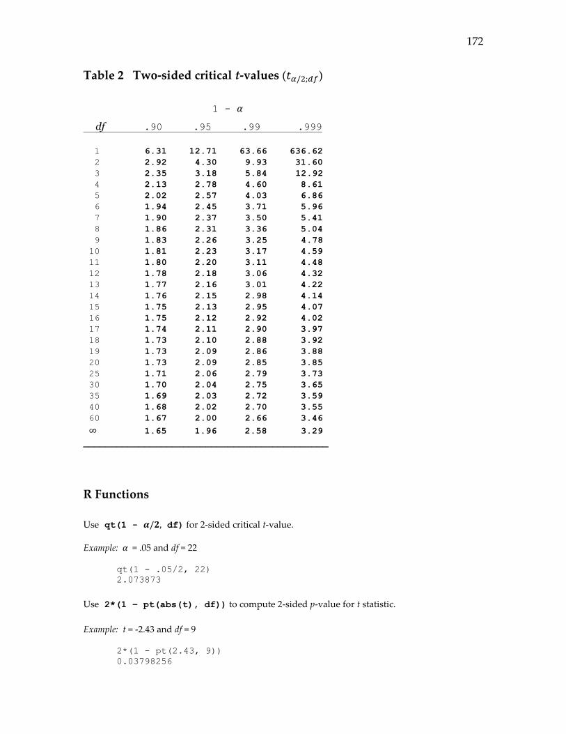
172

Table 2 Two-sided critical t-values (𝑡𝛼/2;𝑑𝑓)

1 - 𝛼

df .90 .95 .99 .999

1 6.31 12.71 63.66 636.62

2 2.92 4.30 9.93 31.60

3 2.35 3.18 5.84 12.92

4 2.13 2.78 4.60 8.61

5 2.02 2.57 4.03 6.86

6 1.94 2.45 3.71 5.96

7 1.90 2.37 3.50 5.41

8 1.86 2.31 3.36 5.04

9 1.83 2.26 3.25 4.78

10 1.81 2.23 3.17 4.59

11 1.80 2.20 3.11 4.48

12 1.78 2.18 3.06 4.32

13 1.77 2.16 3.01 4.22

14 1.76 2.15 2.98 4.14

15 1.75 2.13 2.95 4.07

16 1.75 2.12 2.92 4.02

17 1.74 2.11 2.90 3.97

18 1.73 2.10 2.88 3.92

19 1.73 2.09 2.86 3.88

20 1.73 2.09 2.85 3.85

25 1.71 2.06 2.79 3.73

30 1.70 2.04 2.75 3.65

35 1.69 2.03 2.72 3.59

40 1.68 2.02 2.70 3.55

60 1.67 2.00 2.66 3.46

∞ 1.65 1.96 2.58 3.29

____________________________________________

R Functions

Use qt(1 - 𝜶/𝟐, df) for 2-sided critical t-value.

Example: 𝛼 = .05 and df = 22

qt(1 - .05/2, 22)

2.073873

Use 2*(1 – pt(abs(t), df)) to compute 2-sided p-value for t statistic.

Example: t = -2.43 and df = 9

2*(1 - pt(2.43, 9))

0.03798256

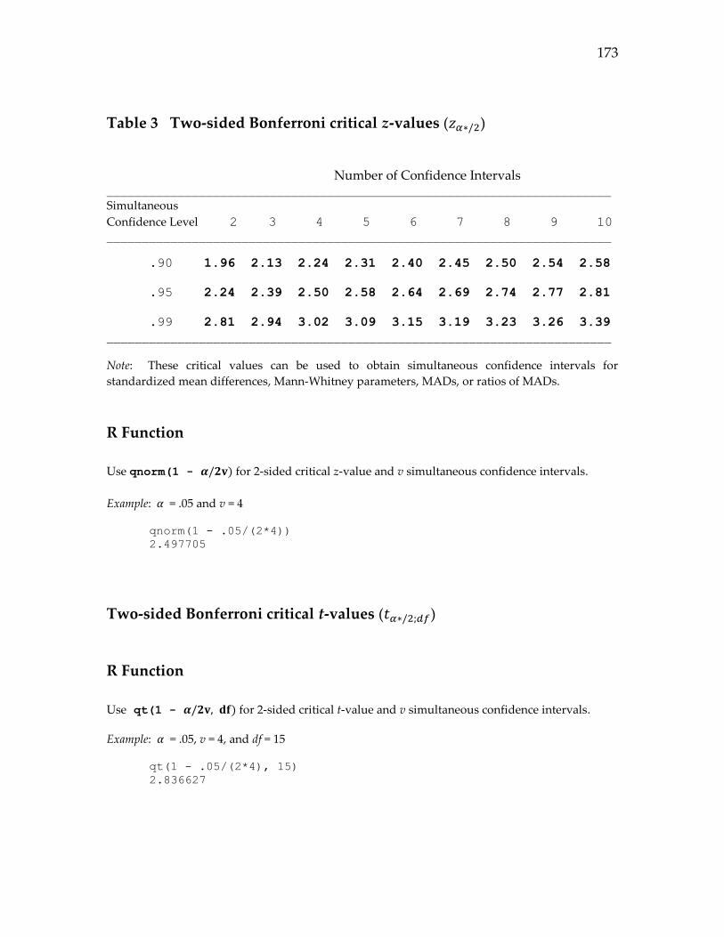
173

Table 3 Two-sided Bonferroni critical z-values (𝑧𝛼∗/2)

Number of Confidence Intervals _______________________________________________________________________

Simultaneous

Confidence Level 2 3 4 5 6 7 8 9 10 _______________________________________________________________________

.90 1.96 2.13 2.24 2.31 2.40 2.45 2.50 2.54 2.58

.95 2.24 2.39 2.50 2.58 2.64 2.69 2.74 2.77 2.81

.99 2.81 2.94 3.02 3.09 3.15 3.19 3.23 3.26 3.39

_______________________________________________________________________

Note: These critical values can be used to obtain simultaneous confidence intervals for

standardized mean differences, Mann-Whitney parameters, MADs, or ratios of MADs.

R Function

Use qnorm(1 - 𝜶/𝟐𝐯) for 2-sided critical z-value and v simultaneous confidence intervals.

Example: 𝛼 = .05 and v = 4

qnorm(1 - .05/(2*4))

2.497705

Two-sided Bonferroni critical t-values (𝑡𝛼∗/2;𝑑𝑓)

R Function

Use qt(1 - 𝜶/𝟐𝐯, 𝐝𝐟) for 2-sided critical t-value and v simultaneous confidence intervals.

Example: 𝛼 = .05, v = 4, and df = 15

qt(1 - .05/(2*4), 15)

2.836627

174

Table 4 Critical F values (𝛼 = .05) dfA

____________________________

dfE 1 2 3 4

______________________________________

2 18.51 19.00 19.16 19.25

3 10.13 9.55 9.28 9.12

4 7.71 6.94 6.59 6.39

5 6.61 5.79 5.41 5.19

6 5.99 5.14 4.76 4.53

7 5.59 4.74 4.35 4.12

8 5.32 4.46 4.07 3.84

9 5.12 4.26 3.86 3.63

10 4.96 4.10 3.71 3.48

11 4.84 3.98 3.59 3.36

12 4.75 3.89 3.49 3.26

13 4.67 3.81 3.41 3.18

14 4.60 3.74 3.34 3.11

15 4.54 3.68 3.29 3.06

16 4.49 3.63 3.24 3.01

17 4.45 3.59 3.20 2.96

18 4.41 3.55 3.16 2.93

19 4.38 3.52 3.13 2.90

20 4.35 3.49 3.10 2.87

∞ 3.84 3.00 2.61 2.37

______________________________________

R Functions

Use qf(1 - 𝜶, df1, df2) for critical F value.

Example: 𝛼 = .01, df1 = 2, and df2 = 27

qf(1 - .01, 2, 27)

5.488118

Use 1 - pf(F, df1, df2) to compute p-value for F statistic.

Example: F = 4.74, df1 = 2, and df2 = 10

1 - pf(4.74, 2, 10)

0.03564965

175

Appendix B. Glossary

adjusted eta-squared – a correction to an eta-squared estimate that reduces its positive bias

alternate form reliability – the correlation between two alternative forms of a test or

questionnaire that each assess the same attribute

asymmetric carryover effect – when the carryover effect from Treatment 1 to Treatment 2

(for example) is not the same as the carryover effect from treatment 2 to 1 in a within-

subjects design

balanced Latin square counterbalancing – a type of partial counterbalanced within-subjects

design that controls for practice effects, fatigue effects, and certain types of carryover

effects

bar chart – a graph that illustrates the parameter estimates (e.g., sample means) in two or

more groups using bars with lengths that represents the values of the estimates

between-subjects treatment factor – an independent variable in a between-subjects

experiment where participants are randomly assigned to the levels of the independent

variable

Bonferroni adjustment – used to obtain simultaneous tests or confidence intervals by

dividing 𝛼 by the number of tests or confidence intervals to be examined

carryover effect – when participants are exposed sequentially to more than one treatment,

the effect of one treatment persists during other treatments

central limit theorem – a theorem stating that the shape of a sampling distribution of a mean

has an approximate normal distribution if the sample size is sufficiently large regardless

of the shape of the distribution of quantitative scores in the population

classification factor – a type of factor in which participants are classified into two or more

groups according to some participant characteristic such as conservative/liberal or

male/female

clustered bar chart – a graph that illustrates the means in a two-factor design using bars

with lengths that represents the values of the means

coefficient alpha (Cronbach's alpha)– a measure of the reliability of a sum or average of two

or more measurements (the multiple measurements are often item scores of a

questionnaire)

coefficient of skewness – a measure of the asymmetry of a set of quantitative scores; the

coefficient is equal to zero if the scores have a symmetric distribution

176

coefficient of kurtosis – a measure of the peakedness and tail thickness in a set of quantitative

scores

Cohen's d – a mean difference divided by a standard deviation; a unitless measure of effect

size

completely counterbalanced design – a within-subjects design where subsets of participants

receive the within-subject treatments in one of every possible order

compound symmetry assumption – the assumption in a within-subjects design that the

variances are equal across all within-subject levels and correlations are equal between all

pairs of levels.

confidence interval – a range of values (an upper limit and a lower limit) that will include

the population parameter, or function of population parameters, with a specified level of

confidence

confidence interval width – the upper limit minus the lower limit of a confidence interval

confidence level – a subjective probability that a computed confidence interval will contain

the value of some unknown population parameter

confounding variable – a variable that is related to both the response variable and the

explanatory variable

contrast coefficient – the 𝑣1, 𝑣2, … , 𝑣𝑎 values that define a linear contrast (e.g., 𝑣1𝜇1 + 𝑣2𝜇2 +

⋯ + 𝑣𝑎𝜇𝑎) where ∑ 𝑣𝑗𝑎𝑗=1 = 0

control group – a group of participants who do not receive any treatment

data transformation – a nonlinear transformation of scores, such as ln(y), 1/y, √𝑦, that can

reduce the degree of non-normality in a set of scores

debriefing – a short interview with the participants immediately following completion of

a study to insure that the that participants are fully informed about, and not harmed in

any way by, their experience in the study

dependent variable – a variable assumed to be predictable from by one or more independent

variables (the dependent variable is also called a response variable or outcome variable)

differential nonrandom attrition – when the probability of a participant failing to complete

the study is not the same across treatment conditions

directional error – accepting one alternative hypothesis when the other alternative

hypothesis is true (e.g., accepting H1: 𝜇1 > 𝜇2 when H2: 𝜇1 < 𝜇2 is true)

177

directional two-sided hypothesis – a test of a null hypothesis with two directional alternative

hypotheses

effect size – some examples of an effect size are: 𝜇 − ℎ, 𝜇1 − 𝜇2, ∑ 𝑣𝑗𝜇𝑗𝑎𝑗=1 , standardized

mean difference, standardize linear contrast of means, eta-squared, difference of medians

equivalence test – a test of one hypothesis that the difference between two parameters (e.g.,

means, medians) is small against another hypothesis that the difference is not small

error variance – in a multiple group design, the error variance is the within-group variance

eta-squared – a standardized measure of effect size in a one-way ANOVA that describes

the proportion of variance in the response variable that is predictable by the independent

variable

experimental design – a study where participants are randomly assigned into the levels of

an independent variable

external validity – the extent to which the results of a study apply to different types of

participants and different settings

F ratio – a test statistic; in a one-way ANOVA the F ratio is equal to the between-group

mean square divided by the within-group (error) mean square

factor – an independent variable with a predetermined number of levels

factorial design – a design with two or more factors

family-wise directional error rate – the probability of making one or more directional errors

in a set of two or more directional two-sided hypothesis tests

F test – The use of an F statistic from an ANOVA table to test a null hypothesis that some

effect is zero

Fisher protected test – the use of non-simultaneous tests of pairwise comparisons for a

particular factor only if the omnibus null hypothesis for the factor has been rejected;

recommended only for factors with three levels

Friedman test – a distribution-free alternative to the one-way within-subjects ANOVA

Games-Howell – simultaneous tests and confidence intervals for all pair-wise differences

of populations means that does not assume equal population variances

generalized eta-squared – a standardized measure of effect size that describes the proportion

of variance in the response variable that is predictable by the independent variable

without removing the variability in the response variable that is due to any of the

classification factors in the design

178

histogram – a graph of the number of quantitative scores that fall into specified intervals

and illustrates the shape of the distribution of quantitative scores

Holm method – a method of testing multiple hypotheses that keeps the family-wise

direction error rate at some specified value

homoscedasticity assumption – the assumption of approximately equal population variances

across treatment conditions or subpopulations

independence assumption – the assumption that the response of each participant in the

sample has no effect on the response of any other participant in the sample

independent-samples t-test – a test of H0: 𝜇1 = 𝜇2 where 𝜇1 and 𝜇2 are unknown population

means; the test is used to decide if 𝜇1 > 𝜇2 or 𝜇1 < 𝜇2. The parameters 𝜇1 and 𝜇2 are

estimated from two different groups of participants.

independent variable – a variable that is assumed to predict the response variable (the

independent variable is also called the explanatory variable or predictor variable)

informed consent – making all relevant information available before obtaining consent to

participate in a study

interaction effect – the difference in effects of one factor across the levels of a second factor

(e.g., in a 2 × 2 design, the interaction effect is (𝜇11 − 𝜇12) − (𝜇21 − 𝜇22))

internal consistency reliability – the reliability of a multi-item questionnaire that uses the

individual item responses to estimate the reliability

internal validity – the extent to which a predictor variable can be assumed to have a causal

effect on the response variable

interrater reliability – the correlation between two ratings of the same attribute

interval scale – a scale where a difference in scores correctly describes a difference in the

attribute but a score of 0 does not represents a complete absence of the attribute

IRB (Institutional Review Board) – a committee of experts who evaluate the ethical issues

in studies involving human subjects

linear contrast (of means) – a linear combination of means 𝑣1𝜇1 + 𝑣2𝜇2 + ⋯ + 𝑣𝑘𝜇𝑘 where

the 𝑣1, 𝑣2, … , 𝑣𝑘 values are contrast coefficients specified by the researcher

linear contrast score – a linear combination of scores 𝑞1𝑦1 + 𝑞2𝑦2 + ⋯ + 𝑞𝑎𝑦𝑎 in a within-

subject design where the 𝑞1, 𝑞2, … , 𝑞𝑎values are contrast coefficients specified by the

researcher

179

listwise deletion – deleting a participant from the analysis in a within-subjects design if the

participant has missing scores at any of the within-subject levels

longitudinal design – a within-subjects design where participants are measured on two or

more occasions and do not receive any treatment between occasions

main effect – the differences in mean values across the levels of one factor across the levels

of all other factors in the design

Mann-Whitney test – a distribution-free alternative to the independent-samples t-test

matched-pairs design – a 2-level within-subjects design where each pair of similar

participants is randomly assigned to two treatment conditions

mean absolute deviation from median (MAD) – a measure of variability that is equal to the

average absolute deviations of the quantitative scores from the median of the quantitative

scores

mean squared error – an estimate of the average within-group variance

measurement error – the difference between a person’s true attribute score and some

measurement of the attribute

meta-analysis – a statistical analysis that combines results from two or more studies

minimal risk – a level of risk that is similar to that which would be incurred during a routine

physical or psychological examination

minimally interesting effect size – the smallest value of an effect size that would still

represent an interesting, useful, or important effect size

mixed two-factor design – a design with one between-subjects factor and one within-subjects

factor

mixed two-way ANOVA – used to test three separate hypotheses in a mixed two-factor:

equal population means across levels of Factor A, equal population means across levels

of Factor B, and zero interaction between Factors A and B

monotonic transformation – a transformation that does not change the rank ordering of the

scores

nondifferential nonrandom attrition – when a certain type participant is more likely to drop

out of a study than other types of participants

nonexperimental design – a study where participants are not randomly assigned to the levels

of an independent variable

180

noninferiority test – a test of one hypothesis that Treatment 1 is not unacceptably worse

than Treatment 2 against another hypothesis that Treatment 1 is unacceptably worse than

Treatment 2

nonrandom sample – a sample that is not a random sample from some specific population

non-removable interaction – an interaction effect that cannot be made small or unimportant

by transforming the response variable

normal (Gaussian) curve – a symmetric bell-shaped curve

normality assumption – the assumption that the scores have an approximate normal

(Gaussian) distribution in the study population

null hypothesis – a statement that some population parameter, or some function of

populations parameters (e.g., a difference or linear contrast) is equal to a specific

numerical value

omnibus test – a test of a null hypothesis that specifies the quality of two or more

parameters; tests of main effects and interaction effects for factors with three or more

levels are examples of omnibus tests

one-sample t-test – a test of H0: 𝜇 = h where 𝜇 is an unknown population mean and h is a

specified number; test is used to decide if 𝜇 > h or if 𝜇 < h

one-way ANOVA – a test of H0: 𝜇1 = 𝜇2 = ... = 𝜇𝑎 in a between-subjects design where 𝜇𝑗 is

an unknown population mean; also used to obtain an estimate of an eta-squared

coefficient

one-way random effects ANOVA – a test of H0: 𝜇1 = 𝜇2 = ... = 𝜇𝑀 in a between-subjects design

where 𝜇𝑗 is an unknown subpopulation mean and M is a large set of subpopulations

one-way within-subjects ANOVA – a test of H0: 𝜇1 = 𝜇2 = ... = 𝜇𝑎 in a within-subjects design

where 𝜇𝑗 is an unknown population mean

paired-samples t-test – a test of H0: 𝜇1 = 𝜇2 where 𝜇1 and 𝜇2 are unknown population means

that are estimated from a single group and is used to decide if 𝜇1 > 𝜇2 or 𝜇1 < 𝜇2

pairwise comparison – a difference between two parameter values (e.g., 𝜇1 – 𝜇2, 𝜇1 − 𝜇4, etc.)

pairwise deletion – deleting a participant from a within-subject analysis that involves a pair

of within-subject levels if the participant has a missing score on either of the two levels

pairwise interaction effect – an interaction effect at two levels of one factor and two levels of

a second factor

181

pairwise main effect comparison – a difference in means for two levels of one factor after

averaging over the levels of a second factor

pairwise simple main effects – a difference in means for two levels of one factor at one level

of a second factor

partial eta squared – a measure of effect size in a factorial ANOVA that describes the

proportion of response variable variance than can be predicted by one treatment factor

after removing the variability in the response variable due to all other treatment factors in

the design

planning value – an assumed value of a population parameter, obtained from previous

research or expert opinion, that is used in sample size formulas

population – in psychological research, the population is usually some well-defined large

group of people that the researcher wants to study

population parameter – a single number, such as a population mean, population variance,

or population median, that is defined for all members of a specific population

population mean – the mean of the response variable for all members of the population

population median – a value that is greater than half the scores and less than half the scores

in a population

power – the probability that a statistical test will lead to the rejection of the null hypothesis

practice effect – an improvement in posttest scores that is the result of taking a pretest

prediction interval – a range of values that will include the score for a single person

predictor variable – a variable that may account for some of the variability in the response

variable (the predictor variable is also called the explanatory variable or independent

variable)

pretest-posttest design – a within-subjects design where participants are measured on two

or more occasions and receive a treatment sometime after the first occasion and before the

last occasion

probability – a number in the range 0 to 1 that describes the likelihood of a specific event

p-value – a number that is a transformation of the test statistic and used to decide if a null

hypothesis can be rejected (e.g., if the p-value is less than . 05 then reject H0)

quantitative score – a score that is measured on either an interval or a ratio scale

random attrition – a random loss of participants

182

random factor – a factor where the levels have been randomly selected from a large set of

possible levels

random sample – a subset of the population selected in a way that every sample of given

size has the same chance of being selected

random sampling assumption – the assumption that the sample used to compute a test or

confidence interval is a random sample or assumed to be a random sample

randomized – the random assignment of participants into the levels of an independent

variable

ratio scale – a scale where a score of 0 represents a complete absence of the attribute and

where differences and ratios of scores correctly describe differences and ratios of the

attribute

region of practical equivalence – a range of values for a difference in population parameters,

–h to h, where h is a value that represents a small or unimportant difference

reliability coefficient – an index defined on a range of 0 to 1 that describes the proportion of

variance in the true scores that can be predicted by the observed scores

removable interaction – an interaction effect that becomes small or unimportant after the

response variable has been transformed

response variable – a variable to be explained or predicted (also called a dependent variable

or outcome variable)

sample mean – the mean of n quantitative scores in a sample; the sum of n scores divided

by n

sample standard deviation – the square root of the sample variance

sample variance – the mean of n squared deviations from the sample mean

sampling distribution – a distribution of parameter estimates for all possible samples of a

given size

Scheffé method – provides simultaneous confidence and controls FWDER for all possible

linear contrasts in a single-factor design; useful in exploratory research

scientific misconduct – inappropriate or unethical behavior of the researcher

sign test – a distribution-free alternative to the one-sample t-test

simple main effect – the differences in mean values across levels of one factor at a specific

level of the second factor in a two-factor design

183

simple-simple main effect – the differences in mean values across levels of one factor at a

specific combination of levels of a second and third factor in a three-factor design

Spearman-Brown formulas – classic psychometric formulas that show the relation between

the reliability of a single measurement and the reliability of a sum or average of multiple

measurements

superiority test – a test of one hypothesis that Treatment 1 is superior by an nontrivial

amount to Treatment 2 against another hypothesis that Treatment 1 is not superior by a

nontrivial amount to Treatment 2

symmetric carryover effect – when the carryover effect from Treatment 1 to Treatment 2 (for

example) is the same as the carryover effect from Treatment 2 to Treatment 1 in a within-

subjects design

two-way interaction effect – a measure of how the effect of one factor differs across the levels

of a second factor at one level of a third factor

standard error – the standard deviation of a sampling distribution; a measure of the

precision of a parameter estimate and used in the construction of confidence intervals

standardized linear contrast – a linear contrast of means divided by a standard deviation

stratified random sampling – taking a random sample from two or more subpopulations

study population – the population of units (e.g., people) from which the random sample

was taken

subpopulation – a subset of the study population

target population – a population of theoretical interest that subsumes the study population

test-retest reliability – the correlation between a specific test or questionnaire that was given

to each participant on two different occasions

test statistic – a number computed from the sample that is used in a decision rule to reject

or fail to reject a null hypothesis

three-factor experiment – an experiment with three independent variables

three-way ANOVA – used to test hypotheses regarding the main effect of Factor A, main

effect of Factor B, main effect of Factor C, AB interaction, AC interaction, BC interaction,

and ABC interaction; also used to obtain estimates of partial or generalized eta-squared

coefficients

three-way interaction – a difference in simple two-way interactions across the levels of a

third factor

184

treatment factor – a factor with treatment levels to which participants have been randomly

assigned

Tukey-Kramer method – simultaneous tests and confidence intervals for all pair-wise

differences of populations means (the classical version assumes equal population

variances)

two-factor within-subjects – a study with two within-subject factors and no between-subject

factors

two-stage cluster sampling – taking random samples from a random sample of

subpopulations

two-way ANOVA – used to test three separate hypotheses in a two-factor between-subjects

design: equal population means across levels of Factor A, equal population means across

levels of Factor B, and zero interaction between Factors A and B; also used to obtain

estimates of partial eta-squared coefficients

two-way interaction effect – a measure of how the effect of one factor differs across the levels

of a second factor

two-way ANOVA – used to test three separate hypotheses in a two-factor within-subjects

design: equal population means across levels of Factor A, equal population means across

levels of Factor B, and zero interaction between Factors A and B

unbiased estimate – an estimate for which the mean of its sampling distribution is equal to

the population parameter value

waitlist control group – a control group that is given a potentially beneficial treatment after

they have been compared with the treated group

Welch test – an alternative to the one-way ANOVA that does not assume equal variances

Wilcoxon signed rank test – a distribution-free alternative to the paired-samples t-test

within-subjects factor – a factor in which the same group of participants are measured at all

levels of the factor

within-subjects experiment – an experiment where each participant receives all treatment

conditions, usually in counterbalanced order (also called a randomized block design)

Zelen design – a more ethical design that allows participants who were randomly assigned

to a one treatment condition to switch to a preferred treatment condition

2 × 2 factorial experiment – an experiment with two independent variables where each

independent variable has two levels

185

Appendix C. Answers to Concept Questions

Chapter 1 1. Explain in words how to compute a sample variance.

Compute the sample mean, subtract each score from the sample mean and square the difference,

sum the n squared differences and divided the sum by n – 1.

2. Increasing the sample size will have what effect on the width of the confidence interval?

The confidence interval width will tend to decrease

3. Increasing the level of confidence will have what effect on the width of the confidence

interval?

The confidence interval width will increase

4. Increasing the sample size will have what effect on the value of the standard error?

The SE will tend to decrease

5. Explain in words how a confidence interval for 𝝁 can be used to test a two-sided directional

hypothesis where H0: 𝝁 = 100.

If the lower limit is greater than 100 then reject the null hypothesis and accept the alternative

hypothesis that 𝜇 > 100. If the upper limit is less than 100 then reject the null hypothesis and accept

the alternative hypothesis that 𝜇 < 100.

6. Increasing the sample size will have what effect on the power of a test?

The power will increase

7. Explain in words how to compute a 95% confidence interval for a population mean after you

have computed the sample mean and its standard error in a sample of n = 20.

Find the critical t-value for alpha = .05 and df = 19. Multiply the critical t-value by the standard

error. Add this product to the sample mean to get the upper limit and subtract this product to get

the lower limit.

8. When planning a future study to estimate 𝝁, what is the effect of decreasing the desired

confidence interval width on the sample size requirement?

A larger sample size requirement

186

9. When planning a future study to estimate 𝝁, what is the effect of increasing the desired level

of confidence on the sample size requirement?

A larger sample size requirement

10. When planning a future study to estimate 𝝁, what is the effect of using �̃�𝟐 = 50 rather than

�̃�𝟐= 75 on the sample size requirement?

A smaller sample size requirement

11. When planning a future study to test H0: 𝝁 = h, how does the desired power affect the sample

size requirement?

Greater desired power requires a larger sample size

12. When planning a future study to test H0: 𝝁 = h, how does the 𝜶 value affect the sample size

requirement?

A smaller 𝛼 value requires a larger sample size

13. Why are narrow confidence intervals desirable?

Narrower confidence intervals are more informative because they provide a more precise

description of the population parameter

14. Why are confidence interval results more informative than a directional two-sided

hypothesis test?

Because the confidence interval results provide information about the value of the population

parameter while the directional two-sided test can only tell us if the parameter is less than some

value or greater than some value.

15. Describe the standard error in the context of a sampling distribution.

The standard error is equal to the standard deviation of the sampling distribution.

16. Why is the 95% level of confidence a popular choice?

It provide a good compromise between confidence and precision.

17. What are the assumptions of a confidence interval or test for 𝝁, and what are the effects of

violating those assumptions?

Random sample, independence among participant, and approximate normality of the response

variable. Violating the random sample and independence assumptions can invalidate the results.

Violating the normality assumption is usually not a problem unless the sample size is small.

187

18. What are some ways to obtain a planning value for 𝝈?

Expert opinion, prior research, pilot study or, if the response variable range is known,

(max – min)/4

19. Explain why a confidence interval might be uninterpretable if a nonrandom sample is used.

Unless the random can be assumed to be random sample from some describable population, the

confidence interval and hypothesis test results are uninterpretable.

20. Suppose a 95% confidence interval for 𝝁 is [1.5, 4.8]. In a test of the null hypothesis

H0: 𝝁 = h, for which of the following values of b would H0 be rejected: 1.20, 3.30, 4.1, or 5.0?

1.20 and 5.0 because these values are outside the confidence interval range

21. How does the size of the study population effect the sample size requirement when n/N is

small?

Virtually no effect

22. Why are data transformations sometimes used?

To reduce non-normality of the response variable.

23. Is it appropriate to declare a null hypothesis such as H0: 𝝁 = h to be true if the results are

“nonsignificant”? Why?

No, because a failure to reject this type of null hypothesis (i.e., a nonsignificant result) does not

imply that the null hypothesis is true. Also, this type of null hypothesis is almost never true because

it is virtually impossible for 𝜇 to exactly equal the value of h.

24. When testing a null hypothesis such as H0: 𝝁 = h, what can be said about a “significant”

result?

This only indicates that 𝜇 ≠ h

25. What is the relation between the size of the p-value and the sample size?

Increasing the sample size tends to decrease the p-value.

26. When would a confidence interval for a population median be preferred to a confidence

interval for a population mean?

When the response variable is highly skewed

188

27. Why is it important to assess the variability of the responses variable and not just the mean

or median of the response variable?

The mean and median describe the center of a distribution of scores and can be misinterpreted as

a description of how every member of the population would score. A measure of variability

provides additional information about individual differences among members of the population.

28. What are the implications of the central limit theorem in terms of how a confidence interval

for 𝝁 will perform?

The confidence interval for 𝜇 requires the sampling distribution to be approximate normal, and the

central limit theorem guarantees that the sampling distribution will be approximate normal if the

sample size is sufficiently large.

29. About 1.8 million people visit the Monterey Bay Aquarium each year. Exit interviews were

conducted in 2013 for a random sample of 2,417 visitors. One question asked respondents to rate

the quality of the educational experience on a 1 to 10 scale. The 95% confidence interval for 𝝁

was [8.78, 8.89]. Interpret this result.

We are 95% confident that the mean educational experience rating of the 1.8 million visitors is

between 8.78 and 8.89.

30. Explain why each of the following interpretations of [8.78, 8.89] in the above example is

incorrect or inadequate.

a) We are 95% confident that the 1.8 million visitor ratings are between 8.78 and 8.89.

b) We are 95% confident that a visitor's rating will be between 8.78 and 8.89.

c) We are 95% confident that the mean rating of the 2,417 visitors is between 8.78 and 8.89.

d) We are 95% confident that 𝝁 is between 8.78 and 8.89.

e) We are 95% confident that 95% of the scores are between 8.78 and 8.89.

a) The 1.8 million ratings would be between 1 and 10. The confidence interval describes the

plausible range of the mean of the 1.8 ratings.

b) This interpretation is correct for a prediction interval but not for a confidence interval.

c) The confidence interval describe the mean of the 1.8 million ratings and not the mean of the 2,417

ratings.

d) The interpretation is inadequate because 𝜇 needs to be defined for the reader.

e) 95% of the scores would be in a much wider range. The confidence interval describes the

plausible range of the mean of the 1.8 ratings.

189

Chapter 2

1. What are the three conditions that must be satisfied to show that the independent variable is

causally related to the response variable?

The two variables must be related, there exists no other variable that is related to both the

independent and response variable, and variation of the independent variable must occur prior

any observed change in the response variable.

2. Explain how the results of an experiment can provide evidence that the independent variable

has a causal effect on the response variable.

A two-group experiment can show if there is a relation between the independent variable and the

response variable; since participants are randomly assigned to groups, there can be no other

variable that is related to the independent variable; and participants are first exposed to different

levels of the independent variable and then later their responses are recorded.

3. How can a confidence interval for 𝝁𝟏 − 𝝁𝟐 be used to test H0: 𝝁𝟏 − 𝝁𝟐 = 0 and then select

H1: 𝝁𝟏 − 𝝁𝟐 > 0 or H2: 𝝁𝟏 − 𝝁𝟐 < 0?

If the lower limit for 𝜇1 − 𝜇2 is greater than 0, then reject the null hypothesis and accept

H1: 𝜇1 − 𝜇2 > 0. If the upper limit for 𝜇1 − 𝜇2 is less than 0, then reject the null hypothesis and accept

H2: 𝜇1 − 𝜇2 < 0.

4. How can a confidence interval for 𝜹 be used to test H0: |𝜹| ≤ 𝟎. 𝟏 against H1: |𝜹| > 𝟎. 𝟏?

If the confidence interval for 𝛿 is completely within a -0.1 to 0.1 range, then accept H0: |𝛿| ≤ 0.1. If

the confidence interval for 𝛿 is completely outside the -0.1 to 0.1 range, then accept H1: |𝛿| > 0.1.

5. How can a confidence interval for 𝝁𝟏 − 𝝁𝟐 be used to select H0: |𝝁𝟏 − 𝝁𝟐| ≤ 𝟐. 𝟓 or

H1: |𝝁𝟏 − 𝝁𝟐| > 𝟐. 𝟓?

If the confidence interval for 𝜇1 − 𝜇2 is completely within a -2.5 to 2.5 range, then accept

H0: |𝜇1 − 𝜇2| ≤ 2.5. If the confidence interval for 𝜇1 − 𝜇2 is completely outside the -2.5 to 2.5 range,

then accept H1: |𝜇1 − 𝜇2| > 2.5.

6. How can a confidence interval for 𝝁𝟏 − 𝝁𝟐 be used to test H0: 𝝁𝟏 − 𝝁𝟐 = -5 and then select

H1: 𝝁𝟏 − 𝝁𝟐 > -5 or H2: 𝝁𝟏 − 𝝁𝟐< -5?

If the lower limit for 𝜇1 − 𝜇2 is greater than -5, then reject the null hypothesis and accept

H1: 𝜇1 − 𝜇2 > -5. If the upper limit for 𝜇1 − 𝜇2 is less than -5, then reject the null hypothesis and

accept H2: 𝜇1 − 𝜇2 < -5.

190

7. What information can be obtained from a confidence interval for 𝝁𝟏 − 𝝁𝟐 that cannot be

obtained from an independent-samples t-test?

The confidence interval for 𝜇1 − 𝜇2 provides information about the magnitude and direction of the

difference while the t-test only provides information about the direction of the difference.

8. When would a researcher prefer to report a confidence interval for a standardized mean

difference rather than an unstandardized mean difference?

If the scale of the response variable is not familiar to the intended audience, a standardized mean

difference would be preferred.

9. What does it mean when a researcher declares the results of an independent-samples t-test to

be “significant”? How should a “nonsignificant” result be interpreted?

A significant results simply means that the null hypothesis of identical population means has been

rejected. A nonsignificant result should be interpreted as an inconclusive result and not as evidence

that the null hypothesis is true.

10. What are the assumptions for a confidence interval or test for a difference in population

means using the equal-variance method?

Random sample, independence among participants, equal variances in the two conditions,

approximate normality of the response variable within each condition.

11. What are the assumptions for a confidence interval or test for a difference in population

means using the unequal-variance method?

Random sample, independence among participants, approximate normality of the response

variable within each condition.

12. Explain how 𝝁𝟏 and 𝝁𝟐 are interpreted differently in an experimental design compared to a

nonexperimental design.

In an experimental design 𝜇1 and 𝜇2 describe the same study population under two different

experimental situations. In a nonexperimental design 𝜇1 and 𝜇2 describe two different study

populations.

13. What are the consequences of participants randomly dropping out from both groups in a

two-group experiment?

A loss of power and confidence interval precision but no effect on internal or external validity.

14. What are the consequences of certain types of participants dropping out only from one group

in a two-group experiment?

The internal validity of the study has been compromised.

191

15. What are the consequences of certain types of participants dropping out equally from both

groups in a two-group experiment?

The external validity of the study has been reduced.

16. What are the advantages and disadvantages of sampling from a small study population?

It is usually easier and less costly to sample from a small study population but then the hypothesis

testing and confidence interval results apply to a small study population that could have less

scientific importance than a larger study population.

17. Why is a violation of the normality assumption not a major concern when testing or

estimating 𝝁𝟏 − 𝝁𝟐 when the sample sizes are not small?

The central limit theorem tells us that the sampling distribution of the difference in sample means

will be approximately normal with moderate size samples even when the response variable is

highly non-normal.

18. Why are confidence interval lines recommended in bar charts?

So that the reader will see the plausible range of population means and not just the sample means.

19. How does the value of �̃�𝟏 − �̃�𝟐 affect the sample size requirement for testing H0: 𝝁𝟏 = 𝝁𝟐 with

desired power?

A smaller value of �̃�1 − �̃�2 (the expected effects size) requires a larger sample size.

20. When would a Mann-Whitney test be preferred to an independent samples t-test?

When the response variable is highly skewed and the sample size is small.

21. When would a confidence interval for a difference in population medians be preferred to a

confidence interval for a difference in population means?

When the response variable is highly skewed.

22. What useful informative could be obtained by examining a confidence interval for a ratio

of population MADs in a two-group design?

A ratio of population mean absolute deviations provides important information about the relative

variability of the response variable in each of the two conditions.

23. A random sample of 30 students was obtained from a research participant pool of about

5,000 undergraduates at UC Santa Barbara. The sample was randomized into two groups of

equal size. Group 1 received a daily meditation app and group 2 received a daily planner app.

After two weeks, the Perceived Stress Scale (scored from 0 to 40 with higher scores representing

greater stress) was given to all 30 participants. A 95% confidence interval for 𝝁𝟏 − 𝝁𝟐 was [-3.4, -

0.7]. Interpret this result.

192

We can be 95% confident that if all 5,000 UCSB students used the daily meditation app for two

weeks, their mean perceived stress score would be 0.7 to 3.4 lower than if they had all used the

daily planner app for two weeks.

24. Explain why each of the following interpretations of [-3.4, -0.7] in the above example is


a) We are 95% confident that the mean stress score of the 30 students would be between 0.7

and 3.4 greater if they had used the daily planner app rather than the daily meditation app.

b) We are 95% confident that the mediation app will reduce a student's stress score between 0.7

and 3.4 points.

c) We are 95% confident that if all 5,000 students had used the daily meditation app for two

weeks, the difference in the mean stress scores would be between -3.4 and -0.7 compared to a

placebo.

d) We are 95% confident that 𝝁𝟏 − 𝝁𝟐 is between -3.4 and -0.7.

a) The confidence interval is a statement about the population of 5,000 students and not the sample

of 30 students.

b) The confidence interval describes how the population mean of the population of 5,000 students

would differ under the two treatment conditions and not how one student's score would differ.

c) Saying "the difference" does not tell us which condition is best.

d) Inadequate because 𝜇1 and 𝜇2 are not defined.

193

Chapter 3

1. What are the advantages of computing confidence intervals for all pairwise differences among

population means instead of reporting the p-value for a one-way ANOVA?

The confidence intervals provide information about the order of the population mean and the

differences among the population mean. The p-value just indicates if the null hypothesis of

identical population means can be rejected.

2. What are the assumptions for the F test of equal population means in the one-way ANOVA?

Random sample, independence among participants, equal variances across conditions,

approximate normality of response variable within each condition

3. What are the assumptions of an equal-variance confidence interval for a linear contrast of

population means?



4. What are the assumptions of an unequal-variance confidence interval for a linear contrast of

population means?

Random sample, independence among participants, approximate normality of response variable

within each condition

5. What are the assumptions for a confidence interval of eta-squared?



6. If two-group design is analyzed using a one-way ANOVA, how will the F-ratio and its p-value

compare with the equal-variance t-statistic and its p-value?

The p-values will be identical and the F value will equal the squared t value

7. Explain how the error variance can be reduced by including a classification factor.

If there are mean differences among any demographic groups (e.g., gender, ethnicity, etc.) within

the study, those mean differences will inflate the within-group error variance. If a demographic

factor is included as a classification factor, then the error variance is then defined within each

treatment and demographic groups and this error variance could be substantially smaller.

8. What statistical method can be used to test H0: 𝝁𝟏 = 𝝁𝟐 = 𝝁𝟑 when each mean is estimated from

a different group?

one-way ANOVA

194

9. If the AB interaction effect in a two-factor design is large, what effects would you want to

estimate and what effects may not be interesting?

Estimate the simple main effects of A at each level of B and/or the simple main effects of B at each

level of A. The main effects of A and B could be misleading.

10. If the test for the AB interaction effect in a two-factor design is inconclusive, what effects

would you want to estimate and what effects may not be interesting?

Estimate the two main effects, the simple main effects may not be interesting

11. How can you show in a convincing way that four population means are approximately

equal? Explain why a “nonsignificant” one-way ANOVA result does not provide evidence of

similarity.

Compute simultaneous confidence intervals for all pairwise comparisons. If all confidence

intervals include 0 and are narrow, this suggests that the four population means are similar. A

nonsignificant one-way ANOVA results could be due to low power.

12. Draw a clustered bar chart of population means in a 2 × 2 design where the interaction effect

is large. Draw a second bar chart where the interaction effect is zero but one of the main effects

is large.

195

13. Define the main effect of A in terms of the population means.

(𝜇1 + 𝜇3)/2 – (𝜇2+ 𝜇4)/2

14. Define the main effect of B in terms of the population means.

(𝜇1 + 𝜇2)/2 – (𝜇3+ 𝜇4)/2

15. Define the AB interaction effect in terms of the population means.

(𝜇1 - 𝜇3) – (𝜇2 - 𝜇4) or (𝜇1 - 𝜇2) – (𝜇3 - 𝜇4) or 𝜇1 – 𝜇2 – 𝜇3 + 𝜇4

16. Define the simple main effect of A at b1 in terms of the population means.

𝜇1 − 𝜇2

17. Define the simple main effect of B at a2 in terms of the population means.

𝜇2 – 𝜇4

18. Consider a one-way ANOVA summary table for a 4-group experiment with 10 participants

per group. Fill in the missing values.

Source SS df MS F

A 210 3 70 7

ERROR 360 36 10

TOTAL 570

19. Suppose a researcher uses a one-way ANOVA to test H0: 𝝁𝟏 = 𝝁𝟐 = 𝝁𝟑 and reports that the

results are “significant”. What does this mean?

It only indicates that the three population means are not all identical. It does not tell us how the

means are ordered or how different they are.

20. For a 2 × 2 factorial design, give examples of the four population means that would produce

the following conditions:

a) large main effect of A, zero main effect of B, zero AB interaction

b) zero main effect of A, zero main effect of B, zero AB interaction

c) large main effect of A, large main effect of B, zero AB interaction

d) zero main effect of A, zero main effect of B, large AB interaction

e) large main effect of A, zero main effect of B, large AB interaction

196

a) A b) A a1 a2 a1 a2

___________ _____________

b1 10 5 b1 10 10

B ___________ B _____________

b2 10 5 b2 10 10

___________ _____________

c) A d) A

a1 a2 a1 a2

___________ _____________

b1 20 5 b1 10 5

B ___________ B _____________

b2 20 15 b2 5 10

___________ _____________

e) A

a1 a2

___________

b1 10 25

B ___________

b2 20 15

___________

21. Consider a two-way ANOVA summary table for a 4 × 5 factorial experiment with 5

participants per group. Fill in the missing values.

Source SS df MS F

A 15 3 5 4

B 20 4 5 4

AB 24 12 2 1.6

ERROR 100 80 1.25

TOTAL 159

22. If the test for an ABC interaction effect is inconclusive, what effects would you want to

examine next?

The three two-way interaction effects

23. If an ABC interaction effect is detected, what effects would you want to examine next?

Simple two-way interactions or simple-simple main effects

24. If the tests for the ABC, AB, AC, and BC interaction effects are all inconclusive, what effects

would you want to examine?

The three main effects

197

25. If an AB interaction effect is detected but the tests for the ABC, AC and BC interactions are

inconclusive, what effects would you want to examine next?

The simple main effects of A at each level of B and/or the simple main effects of B at each level of

A. Also, the main effect of C should be examined.

26. When would a test or confidence interval for a linear contrast of population medians be

preferred to a test or linear contrast of population means?

If the response variable is highly skewed.

27. What is the distribution-free alternative to the one-way ANOVA?

Kruskal-Wallis test

28. What is unequal-variance alternative to the one-way ANOVA?

Welch test

29. Explain how you could show that an A × B interaction effect in a 2 × 2 design is non-

removable.

If the confidence interval for the simple main effects of A at b1 and A at b2 indicate that these two

population effect effects have opposite signs, or if the confidence interval for the simple main

effects of B at a1 and B at a2 indicate that these two population effect effects have opposite signs.

30. What are the advantages and disadvantages of using a random factor rather than a fixed

factor?

Confidence interval and hypothesis testing results for a random factor apply to all levels of the

factor and not just the levels that were used in the study. A larger number of levels of the random

factor is usually needed to obtain a usefully narrow confidence interval for the random factor effect

size.

198

Chapter 4 1. How is a within-subjects design different from a between-subjects design?

A within-subjects design uses one group of participants and all participants are measured under

all treatment conditions. A between-subjects design uses two or more groups of participants with

each group being measured under only one treatment condition.

2. Explain in words how a confidence interval for 𝝁𝟏 − 𝝁𝟐 in a paired-samples design is

computed.

Compute a difference score from the pair of scores for each participant. Compute a confidence

interval for the population mean difference score.

3. How does the correlation between measurements in within-subjects designs affect the

sample size requirement for a confidence interval of 𝝁𝟏 − 𝝁𝟐?

A smaller sample size is needed with a larger correlation.

4. What are the assumptions of the one-way within-subjects ANOVA hypothesis test for equal

population means?

Random sample, independence among participants, equal variances across levels of within-

subjects factor, equal correlations for all pairs of within-subjects factor levels, normal distribution

of response variable within each level of the within-subjects factor.

5. What are the assumptions for a confidence interval for a linear contrast of population means

in a within-subjects design?

Random sample, independence among participants, normal distribution of linear contrast scores

6. Why is a confidence interval for a linear contrast of means preferred to the test of equal

population means in within-subjects designs?

Fewer assumptions (see above) and the confidence interval provide useful information about the

direction and magnitude of the effect.

7. How could a confidence interval for the AB interaction effect in a 2 × 2 mixed design be

computed?

Compute a difference score from the within-subject pair of scores for each participant and then

compute a two-group group confidence interval for the difference in mean difference scores.

8. How can a confidence interval for the main effect of the between-subjects factor in a 2 × 2

mixed design be computed?

Compute an average of the within-subject pair of scores for each participant and then compute a

two-group group confidence interval for the difference in mean average scores.

199

9. For a 2 × 2 within-subjects experiment, specify the linear contrast scores to estimate or test

the following effects in terms of the four scores per participant (𝒚𝟏𝟏, 𝒚𝟏𝟐, 𝒚𝟐𝟏, and 𝒚𝟐𝟐). The first

subscript specifies the levels of Factor A and the second subscript specifies the levels of Factor

B.

a) A × B interaction 𝑦11 − 𝑦12 − 𝑦21 + 𝑦22

b) main effect of A (𝑦11 + 𝑦12)/2 − (𝑦21 + 𝑦22)/2

c) main effect of B (𝑦11 + 𝑦21)/2 − (𝑦12 + 𝑦22)/2

d) simple main effect of A at b1 𝑦11 − 𝑦21

e) simple main effect of A at b2 𝑦12 − 𝑦22

f) simple main effect of B at a1 𝑦11 − 𝑦12

g) simple main effect of B at a2 𝑦21 − 𝑦22

10. What is one way to control for carryover effects?

Use counterbalancing

11. What hypothesis tests can be performed using a confidence interval for 𝝁𝟏 − 𝝁𝟐 in a within-

subjects experiment?

Two-sided directional tests, equivalence tests, noninferiority tests, and superiority tests

12. Why is a pretest-posttest design more ethical than a two-group experiment with a control

group when the treatment is expected to be beneficial?

Because all participants will receive the beneficial treatment in a pretest-posttest design

13. What are some important uses of a mixed design?

The between-subjects factor will not be susceptible to carryover effects and a between-subjects

classification factor can increase the generalizability of the within-subjects treatment results.

14. How does missing data affect the one-way within-subjects ANOVA vs pairwise

comparisons?

If a participant has a missing score on any of the within-subject conditions, then that participant is

dropped from the one-way within-subjects ANOVA analysis. With pairwise comparisons, a

participant is dropped only if this is missing data for the particular pair of conditions being

analyzed.

200

15. What distribution-free methods could be used to analyze data from a one-way within-

subjects design? When would these methods be preferred to a one-way within-subjects

ANOVA or pair-wise comparisons using paired-samples t-tests?

Friedman test as an alternative to a one-way within-subjects ANOVA, pairwise Wilcoxon sign rank

tests as an alternative to pairwise paired-samples t-tests, and confidence intervals for pairwise

differences in medians rather than pairwise differences in means.

16. What is the effect of measurement error on the width of confidence intervals and the power

of tests in between-subjects and within-subjects designs?

Greater measurement error (lower reliability) increases the widths of confidence interval and

decreases the power of tests in both between-subjects and within-subjects designs but the negative

effects can be more pronounced in within-subjects designs.

17. What is the effect of measurement error on estimates of 𝜹, 𝝋, and 𝜼𝟐?

Estimate of all of these measures are attenuated when the response variable contains measurement

error.

18. The blood pressure measurement devices used in most behavioral labs are not highly

reliable. Suppose the reliability of a single blood pressure reading is .81. What is the reliability

of the average of two blood pressure measurements?

Using the Spearman-Brown formula gives: 2(.81)/(1 + (2 – 1)*.81) ≈ .9

19. Fifty UCSC freshman were randomly selected from the entering class of about 4,500

freshman and were given a public speaking examination (scored 0 to 100) in the Fall quarter of

their first year (time 1). These 50 students were given the same examination during the Fall

quarter of their third year (time 2). A 95% confidence interval for 𝝁𝟏 − 𝝁𝟐 was [-8.9, -3.7].

Interpret this result.

We are 95% confident that the mean public speaking score for all 4,500 students in their first year

is 3.7 to 8.9 lower than their mean public speaking score in their third year.

20. Explain why each of the following interpretations of [-8.9, -3.7] in the above example is


a) We are 95% confident that the mean public speaking score of the 50 students increased 3.7 to

8.9 points from their first year to their third year.

b) We are 95% confident that a typical UCSC student will have a public speaking score that will

improve 3.7 to 8.9 points from their third year to the third year.

c) We are 95% confident that the mean public speaking score for all 4,500 freshman drops 3.7 to

8.9 points in their third year.

d) We are 95% confident that the difference in population means is between -8.9 and -3.7.

201

a) The confidence interval describes the population of 4,500 students and not the sample of 50

students.

b) The confidence interval describes the mean score of the 4,500 students and not a score for a single

student.

c) The confidence interval describes the time 1 mean minus the time 2 mean. The endpoints are

negative indicating that the time 2 mean is greater than the time 1 mean.

d) This is inadequate because "the difference" does not tell us if the population mean increased or

decreased over time.

202

203

Appendix D. Answers to Data Analysis Problems

Problem 1-1


The 13,800 addresses in the Watsonville database

b) Describe 𝝁 in the context of this study.

𝜇 is the mean donation amount of the 13,800 Watsonville addresses

c) A volunteer group has agreed to call all 13,800 addresses and ask for a donation if

there is strong evidence to suggest that 𝝁 > 15. Use SPSS or R to test H0: 𝝁 = 15 with

𝜶 = .05. Report t, df, and p-value in APA style and state your conclusion.

t(19) = 2.13, p = .046. We can reject the null hypothesis and accept the alternative

hypothesis that the mean donation amount of the 13,800 Watsonville addresses is greater

than $15.

d) Use SPSS or R to compute a 95% confidence interval for 𝝁 and interpret the result.

95% CI [15.14, 30.36]. We can be 95% confident that the mean donation amount of the

13,800 Watsonville addresses is between $15.14 and $30.36.

e) Hand compute a 95% confidence interval for the total dollar amount that the

volunteer group should receive if they contact all 13,800 residents.

We can be 95% confident that the total donation amount for the 13,800 Watsonville

addresses is between $208,929 and $418,970.

f) Use R to compute a 95% confidence interval for the population median donation

amount and interpret the result.

95% CI [10, 30]. We can be 95% confident that the median donation amount of the 13,800

Watsonville addresses is between $10.00 and $30.00.

g) A similar study is being planned for the city of San Luis Obispo. How many

residents should be contacted to obtain a 95% confidence interval for 𝝁 that has a width

of $10.00? Use the sample variance (the squared standard deviation) from the

Watsonville study as the planning value for the population variance.

A random sample of 43 San Luis Obispo addresses should be contacted.

204

Problem 1-2


4,000 low-income women in Oakland, CA


𝜇 is the mean hours of sleep for the 4,000 low-income women in Oakland, CA

c) Use SPSS or R to test H0: 𝝁 = 6.8 with 𝜶 = .05. Report t, df, and p-value in APA style

and state your conclusion.

t(14) = -2.94, p = .011. We can reject the null hypothesis and accept the alternative

hypothesis that the mean hours of sleep for the 4,000 low-income Oakland women is less

than 6.8 hours per night.

d) Use SPSS or R to compute a 95% confidence interval for 𝝁 and interpret the result.

95% CI [5.42, 6.58]. We can be 95% confident that the mean hours of sleep for the 4,000

low-income Oakland women is between 5.42 and 6.58 hours per night.

e) Use R to compute a 95% confidence interval for 𝜽 and interpret the result.

95% CI [0.66, 1.32]. We can be 95% confident that the mean absolute deviation in hours

of sleep for the 4,000 low-income Oakland women is between 0.66 and 1.32 hours.

f) A similar study is being planned for Dallas, TX. How many low-income women

should be sampled to obtain a 95% confidence interval for 𝝁 that has a width of 0.5?

Use the sample variance (squared standard deviation) from the Oakland study as the

planning value for the population variance.

A random sample of 71 low-income Dallas women should be obtained.

205

Problem 1-3


94,800 Santa Cruz county adults


𝜇 is the mean Cultural Sensitivity score for 94,800 Santa Cruz county adults.

c) Use R to compute a 95% confidence interval for 𝝁 and interpret the result.

95% CI [40.8, 41.4]. We are 95% confident that the mean Cultural Sensitivity score for

94,800 Santa Cruz county adult is between 40.8 and 41.4.

d) Use R to compute a 95% prediction interval for one adult and interpret the result.

95% PI [36.5, 45.9]. We are 95% confident that the Cultural sensitivity score for any one

randomly selected Santa Cruz county adult would be between 37 and 46.

Problem 2-1 a) Describe the study population.

6,000 Fresno county students enrolled in a driver's education course

b) Describe the population means (𝝁𝟏 and 𝝁𝟐) in the context of this study.

𝜇1 is the mean driving skill score if all 6,000 students were given the training

simulator program

𝜇2 is the mean driving skill score if all 6,000 students were given a traditional driver's

education course

c) Use SPSS or R to test H0: 𝝁𝟏 = 𝝁𝟐 with 𝜶 = .05. Report t, df, and p-value in APA style


t(17.74) = -2.68, p = .015. We can reject the null hypothesis and conclude that the mean

driver skill score of the 6,000 students would be larger if they all received the simulation

program than if they all received a traditional driver's education class.

206

d) Use SPSS or R to compute a 95% confidence interval for 𝝁𝟏 − 𝝁𝟐 and interpret the

result. Do not assume equal population variances.

95% CI [-13.03, -1.57]. We are 95% confident that if all 6,000 students were trained using

the driving simulator program, their mean driving skills score would be 1.57 to 13.03

greater than if they had all been trained by the traditional method.

e) The additional simulation training will be considered superior to the traditional

driver's education course if 𝝁𝟐 − 𝝁𝟏 > 𝟏. Use the 95% confidence interval for 𝝁𝟏 − 𝝁𝟐

to decide if additional simulation training is superior to the traditional course.

95% CI for 𝜇2 − 𝜇1 [1.57, 13.03]. The lower 95% confidence limit for 𝜇2 − 𝜇1 is 1.57 which

is greater than 1 and we can conclude that the additional simulation training is superior

to the traditional training method.

f) Use R to compute a 95% prediction interval for the difference in scores under the two

training methods for single student and interpret the result. Do not assume equal


95% PI [-25.98, 11.39]. We can be 95% confidence that any one student in the study

population of 6,000 students could score 26 points higher to 11 points lower with the

driving simulator program than with the traditional training method.

g) Use SPSS or R to produce a bar chart for the two means with 95% confidence interval

lines for the population means.

h) The researcher wants to conduct a similar study in a larger city such as Chicago. How

many driver education students per group (with equal sample sizes) would be needed

to test H0: 𝝁𝟏 = 𝝁𝟐 with power of .9 at 𝜶 = .05 assuming a 5-point difference in

population means? Use the average of the sample variances from this experiment as

your planning value of the average within-group error variance.

A random sample of 66 students should be obtained and then randomly divided into two

groups of 33.

207

Problem 2-2


The 160,000 men in the labor union directory and the 140,000 women in the labor union

directory


𝜇1 is the mean courage score for all 160,000 men

𝜇2 is the mean courage score for all 140,000 women

c) Use R to compute a 95% confidence interval for 𝝁𝟏 − 𝝁𝟐. Do not assume equal

population variances. Interpret the result.

95% CI [-2.73, 1.53]. We can be 95% confident that the population mean courage score for

the 160,000 men is between 2.73 smaller to 1.53 larger than the population mean courage

score for the 140,000 women.

d) Use R to compute a 95% confidence interval for the population standardized mean

difference and interpret the result. Do not assume equal population variances.

95% CI [-0.252, 0.141]. We are 95% confident that the mean courage score for the 160,000

men is 0.252 standard deviation less than to 0.141 standard deviations greater than the

mean courage score for the 140,000 women.

e) The researchers will claim that the new courage subscale is not gender biased if they

can accept H1: |𝝁𝟏 − 𝝁𝟐| < 3 with 𝜶 = .05. Use the 95% confidence interval for 𝝁𝟏 − 𝝁𝟐 to

decide if H1: |𝝁𝟏 − 𝝁𝟐| < 3 can be accepted and state your conclusion.

accept H1: |𝜇1 − 𝜇2| < 3 and conclude that the new courage subscale is not gender biased.

Problem 2-3


The 1,000 undergraduate students in the research participation pool


𝜇1 is the mean willingness to ignore confession score of the 1,000 undergraduate

students if they had all read vignette 1

𝜇2 is the mean willingness to ignore confession score of the 1,000 undergraduate

students if they had all read vignette 2

208

c) Use SPSS or R to compute a 95% confidence interval for 𝝁𝟏 − 𝝁𝟐. Do not assume equal

population variances. Interpret the results.

95% CI [2.01, 4.79]. We are 95% confident that the mean willingness to ignore confession

score of the 1,000 undergraduate students would be 2.01 to 4.79 greater if they had all read

the vignette that described the suspect as extremely thin rather than the vignette that

described the suspect as tall and muscular.

d) Use SPSS or R to test H0: 𝝁𝟏 = 𝝁𝟐 with 𝜶 = .05. Report t, df, and p-value in APA style


t(26.5) = 5.01, p < .001. We can reject the null hypothesis and conclude that the mean

willingness to ignore confession scores in the population of 1,000 undergraduate students

would be greater if they had all read the vignette that described the suspect as extremely

thin rather than the vignette that described the suspect as tall and muscular.

e) Use R to compute a 95% confidence interval for the standardized mean difference

and interpret the result.

95% CI [0.92, 2.72]. We are 95% confident that the mean willingness to ignore confession

score of the 1,000 undergraduate students would be 0.92 to 2.72 standard deviations

greater if they had all read the vignette that described the suspect as extremely thin rather

than the vignette that described the suspect as tall and muscular.

f) Use SPSS or R to compute the Mann-Whitney test and report the p-value.

p < .001

g) The researcher wants to replicate this study using a larger sample size at a different

university. How many students are needed per group (with equal sample sizes) to

obtain a 95% confidence interval for 𝝁𝟏 − 𝝁𝟐 that has a width of 2? Use the average of

the sample variances from this experiment as your planning value for the average

within-group error variance.

A random sample of 56 college students should be obtained and then randomly divided

into two groups of 28 students.

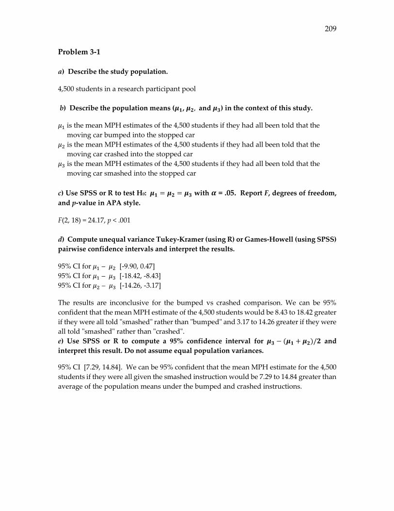
209

Problem 3-1


4,500 students in a research participant pool

b) Describe the population means (𝝁𝟏, 𝝁𝟐, and 𝝁𝟑) in the context of this study.

𝜇1 is the mean MPH estimates of the 4,500 students if they had all been told that the

moving car bumped into the stopped car


moving car crashed into the stopped car


moving car smashed into the stopped car

c) Use SPSS or R to test H0: 𝝁𝟏 = 𝝁𝟐 = 𝝁𝟑 with 𝜶 = .05. Report F, degrees of freedom,

and p-value in APA style.

F(2, 18) = 24.17, p < .001

d) Compute unequal variance Tukey-Kramer (using R) or Games-Howell (using SPSS)

pairwise confidence intervals and interpret the results.

95% CI for 𝜇1 – 𝜇2 [-9.90, 0.47]

95% CI for 𝜇1 – 𝜇3 [-18.42, -8.43]

95% CI for 𝜇2 – 𝜇3 [-14.26, -3.17]

The results are inconclusive for the bumped vs crashed comparison. We can be 95%

confident that the mean MPH estimate of the 4,500 students would be 8.43 to 18.42 greater

if they were all told "smashed" rather than "bumped" and 3.17 to 14.26 greater if they were

all told "smashed" rather than "crashed".

e) Use SPSS or R to compute a 95% confidence interval for 𝝁𝟑 − (𝝁𝟏 + 𝝁𝟐)/𝟐 and

interpret this result. Do not assume equal population variances.

95% CI [7.29, 14.84]. We can be 95% confident that the mean MPH estimate for the 4,500

students if they were all given the smashed instruction would be 7.29 to 14.84 greater than

average of the population means under the bumped and crashed instructions.

210

f) Use R to compute a 95% confidence interval for the standardized contrast

𝝁𝟑 − (𝝁𝟏 + 𝝁𝟐)/𝟐 and interpret this result. Do not assume equal population variances.

95% CI [1.61, 4.43]. We can be 95% confident that the mean MPH estimate for the 4,500

students if they were all given the smashed instruction would be 1.61 to 4.43 standard

deviations greater than average of the population means under the bumped and crashed

instructions.

g) Use R to compute a 95% confidence interval for the population eta-squared (𝜼𝟐) and

interpret the result.

95% CI [.409, .822]. We can be 95% confident that the proportion of the MPH variance in

the population of 4,500 students that is predictable from the instructions is between .409

and .822.

h) Use SPSS to test H0: 𝝁𝟏 = 𝝁𝟐 = 𝝁𝟑 with 𝜶 = .05 using the Welch test. Report F, degrees

of freedom, and p-value in APA style.

F(2, 11.9) = 24.63, p < .001

i) How many participants would be needed in a future replication of this study to

obtain Bonferroni 95% confidence intervals for all pairwise differences in population

means with widths of 5.0? Use the MSE from this study as the planning value of the

average within-group error variance.

A random sample of 78 students should be obtained and then randomly divided into three

groups of 26.

Problem 3-2


The 2,100 male student and 2,200 female students in the university subject pool

b) Describe the population means (𝝁𝟏𝟏, 𝝁𝟏𝟐, 𝝁𝟐𝟏, and 𝝁𝟐𝟐) in the context of this study.

𝜇11 is the mean score of the 2,100 male students if they had all had been tested under a

flat rate condition

𝜇12 is the mean score of the 2,100 male students if they had all had been tested under a

per item condition

𝜇21 is the mean score of the 2,200 female students if they had all had been tested under

a flat rate condition

𝜇22 is the mean score of the 2,200 female students if they had all had been tested under

a per item condition

211

c) Test the interaction effect in a two-way ANOVA. Report F, degrees of freedom, and

p-value for the interaction effect in APA style. What effects should be examined next?

F(1, 36) = 5.26, p = .028

Examine the simple main effects next. For example, the simple main effect of payment

type at male and female.

d) Compute Bonferroni 95% confidence intervals for the simple main effects of

Payment at Male and at Female. Interpret the results. Do not assume equal population

variances.

95% CI at Male [-8.96, -1.43] 95% CI at Female [-4.03, 3.83]

We can be 95% confident that if all 2,100 male students where tested under the per item

payment condition, their mean test score would be 1.43 to 8.96 larger than if they had all

been tested under the flat rate payment condition. The effect of payment for the 2,200

female students is inconclusive.

e) Produce a clustered bar chart with Payment as the within-cluster factor. Include 95%

confidence interval bars.

f) How many participants would be needed in a future study to conduct Bonferroni

tests of the two simple main effects of Payment with power of .95, 𝜶 = .05, and an effect

size of 3.0? Use the MSE from this study as a planning value of the average within-group

error variance.

A random sample of 86 male students and 86 female students should be obtained. The

male students would be randomly divided into two groups of 43 and the female students

would be randomly divided into two groups of 43.

0

5

10

15

20

Female Male

Gender

Mean

Payment

Flat

Per_Item

212

Problem 3-3


The 5,000 students in the university research participant pool

b) Test all main effects and interaction effects in a three-way ANOVA. For which

effects can the null hypothesis be rejected and what effects have inconclusive results?

The tests for the three-way interaction and all three two-way interaction effects are

inconclusive. The null hypothesis can be rejected for all three main effects.

c) Compute Bonferroni 95% confidence intervals for the three main effects and

interpret the results. Do not assume equal variances.

95% CI for Style: [-46.49, -2.11] 95% CI at Size: [2.61, 46.99] 95% CI at Font: [-45.49, -1.11]

We are 95% confident that if all 5,000 students read the story in an Arial font, their mean

time to read the story would be 2.11 to 46.49 seconds faster than if they had all read the

story in a Times font, regardless of font size or justification.

We are 95% confident that if all 5,000 students read the story in a 12 point font, their mean

time to read the story would be 2.61 to 46.99 seconds faster than if they had all read the

story in a 10 point font, regardless of font type or justification.

We are 95% confident that if all 5,000 students read the story in a left justified format, their

mean time to read the story would be 1.11 to 45.49 seconds faster than if they had all read

the story in a full justified format, regardless of font type or font size.

d) The researcher wants to replicate this study using a larger sample size. About how

many participants are needed in each group to obtain Bonferroni 95% confidence

intervals (𝜶* = .05/3) with widths of 20 seconds for the three main effects? Use the MSE

from this study as a planning value of the average within-group error variance.

A random sample 184 students should be obtained. The 184 students would then be

randomly divided into the eight treatment conditions with 23 students per condition.

213

Problem 4-1


The 600 3rd year UCSC psychology majors

b) Describe the population means (𝝁𝟏, 𝝁𝟐, and 𝝁𝟑) in the context of this study.

𝜇1 is the mean satisfaction score of the 600 3rd year psychology majors for non-psychology

courses

𝜇2 is the mean satisfaction score of the 600 3rd year psychology majors for required

psychology courses

𝜇3 is the mean satisfaction score of the 600 3rd year psychology majors for elective

psychology courses

c) Use SPSS to compute the multivariate test of H0: 𝝁𝟏 = 𝝁𝟐 = 𝝁𝟑. Report F, degrees of


F(2,6) = 57.64, p < .001

d) Use SPSS or R to compute paired-samples t-tests for all three pairwise comparisons.

Report t, degrees of freedom, and p-value in APA style for each test.

non-psych vs req-psych: t(7) = - 1.26, p = .247

non-psych vs elect-psych: t(7) = -5.99, p = .001

req-psych vs elect-psych: t(7) = -11.06, p < .001

e) Use SPSS or R to compute Bonferroni 95% confidence interval for all three pairs of

mean differences and interpret the results.

non-psych vs req-psych: 95% CI [-3.04, 1.29]

non-psych vs elect-psych: 95% CI [-8.75, -2.75]

req-psych vs elect-psych: 95% CI [-6.25, -3.50]

We are 95% confident that the mean course satisfaction rating for non-psychology courses

is between 3.04 points smaller and 1.29 points larger than the mean course satisfaction

rating for required psychology courses in the study population of 600 3rd year psychology

students.

We are 95% confident that the mean course satisfaction rating for elective psychology

courses is between 2.75 and 8.75 points larger than the mean course satisfaction rating for

non- psychology courses in the study population of 600 3rd year psychology students.

214


courses is between 3.50 and 6.25 points larger than the mean course satisfaction rating for

required psychology courses in the study population of 600 3rd year psychology students.

f) Use R to compute Bonferroni 95% confidence interval for all three pairs of

standardized mean differences and interpret the results.

non-psych vs req-psych: 95% CI [-0.43, 0.12]

non-psych vs elect-psych: 95% CI [-1.52, -0.36]

req-psych vs elect-psych: 95% CI [-1.22, -0.35]

We are 95% confident that the mean course satisfaction rating for non-psychology courses

is between 0.43 standard deviations smaller and 0.12 standard deviations larger than the

mean course satisfaction rating for required psychology courses in the study population

of 600 3rd year psychology students.


courses is between 0.36 and 1.52 standard deviations larger than the mean course

satisfaction rating for non- psychology courses in the study population of 600 3rd year

psychology students.


courses is between 0.35 and 1.22 standard deviations larger than the mean course

satisfaction rating for required psychology courses in the study population of 600 3rd year

psychology students.

h) If the study is to be replicated at another university, how many 3rd year psychology

students would be needed to obtain a 95% confidence interval for a difference in two

population means that has a width of about 1.0? Use the largest variance and the

smallest correlation from this study as planning values.

Using a variance planning value of 6.667 and a correlation planning value of .919, the

required number of 3rd year psychology students to sample is 19.

215

Problem 4-2


A volunteer pool of 2,560 undergraduate students

b) Describe the four population means (𝝁𝟏, 𝝁𝟐, 𝝁𝟑, and 𝝁𝟒) in the context of this

study.

𝜇1 is the mean driving performance score of the 2,560 undergraduate students if they

were tested under a light traffic and receive condition


were tested under a light traffic and send condition


were tested under a heavy traffic and receive condition


were tested under a heavy traffic and send condition

c) Use SPSS or R to compute a test of the two-way within-subject interaction. Report t,

degrees of freedom, and p-value in APA style. What effects should be examined next?

t(11) = 0.27, p = .789. The two main effects should be examined next.

d) Use SPSS or R to compute Bonferroni 95% confidence intervals for the two main

effects. Interpret the results.

95% CI for Traffic [0.34, 2.24] 95% CI for Mode [0.01, 2.07]

We are 95% confident that the mean driving performance score for the 2,560 students

would be 0.34 to 2.24 greater if they had all been tested under a light traffic condition

rather than a heavy traffic condition when either sending or receiving a call. We are 95%

confident that the mean driving performance score for the 2,560 students would be 0.01

to 2.07 greater if they had all been tested under a call sending condition rather than a call

receiving condition in either light or heavy traffic.

216

Problem 4-3


The 3,800 students in the university research participant pool

b) Describe the six population means (𝝁𝟏, … , 𝝁𝟔) in the context of this study.

𝜇1 is the mean number correct of the 3,800 undergraduate students if they were given

the 3-letter word condition


the 5-letter word condition


the 3-letter non-word condition


the 5-letter non-word condition


the 3-digit number condition


the 5-digit number condition

c) Use SPSS or R to test the string length by string type interaction (this can be done

using a two-way mixed ANOVA or a one-way ANOVA on the difference scores).

Report F, degrees of freedom, and p-value in APA style for the interaction effect. What

effects should be examined next?

F(2, 15) = 11.92, p < .001. The simple main effects of string length at words, non-words,

and numbers could be examined next.


effects of string length at words, non-words, and numbers. Interpret the results.

95% CI for length at word: [-0.49, 3.49]

95% CI for length at non-word: [2.18, 5.82]

95% CI for length at number: [0.09, 1.91]

The results are inconclusive for word. We are 95% confident that the mean number of

correct answers for the 3,800 students would be 2.18 to 5.82 greater with a 3-letter non-

word than a 5-letter non-word. We are 95% confident that the mean number of correct

answers for the 3,800 students would be 0.09 to 1.91 greater with a 3-digit number than a

5-digit number.

An Introduction to Statistical Inference and Experimental ...

Documents