An Introduction to R for the Geosciences: Ordination

An Introduction to R for the Geosciences:Ordination

Gavin Simpson

Institute of Environmental Change & Societyand

Department of BiologyUniversity of Regina

30th April — 3rd May 2013

Gavin Simpson (U. Regina) McMaster 2013 30th April — 3rd May 2013 1 / 58

Outline

1 OrdinationPrincipal Components AnalysisCorrespondence Analysis

2 Vegan usageBasic usageUnconstrained ordinationThe basic plot

3 Constrained OrdinationConstrained ordination in veganPermutation testsLinear ordination methods

4 Methods based on dissimilaritiesPrincipal Coordinates AnalysisConstrained Principal Coordinates AnalysisNon-Metric Multidimensional Scaling


Ordination

Ordination comes from the German word ordnung, meaning to putthings in order

This is exactly what we we do in ordination — we arrange oursamples along gradients by fitting lines and planes through the datathat describe the main patterns in those data

Linear and unimodal methods

Principle Components Analysis (PCA) is a linear method — mostuseful for environmental data or sometimes with species data andshort gradients

Correspondence Analysis (CA) is a unimodal method — most usefulfor species data, especially where non-linear responses are observed


Ordination

Regression gives us a basis from which to work

Instead of doing many regressions, do one with all the species dataonce

Only now we don’t have any explanatory variables, we wish touncover these underlying gradients

PCA fits a line through our cloud of data in such a way that itmaximises the variance in the data captured by that line(i.e. minimises the distance between the fitted line and theobservations)

Then we fit a second line to form a plane, and so on, until we haveone PCA line or axis for each of our species

Each of these subsequent axes is uncorrelated with previous axes —they are orthogonal — so the variance each axis explains isuncorrelated


Ordination


Vegetation in lichen pastures — PCAData are cover values of 44 understorey species recorded at 24locations in lichen pastures within dry Pinus sylvestris forests

−1 0 1 2 3

−2

−1

01

PC1

PC

2 Cal.vul

Emp.nig

Led.pal

Vac.myr

Vac.vit

Pin.syl

Des.fle

Bet.pub

Vac.uli

Dip.mon

Dic.sp

Dic.fus

Dic.pol

Hyl.splPle.sch

Pol.pil

Pol.junPol.com

Poh.nut

Pti.cilBar.lyc

Cla.arbCla.ran

Cla.ste

Cla.unc

Cla.coc

Cla.cor

Cla.graCla.fimCla.cri

Cla.chl

Cla.botCla.ama

Cla.spCet.eri

Cet.isl

Cet.niv

Nep.arc

Ste.spPel.aph

Ich.eri

Cla.cer

Cla.def

Cla.phy

18

15

24

27

23

1922

16

28

13

14

20

25

7

5 6

3

4

2

9

12

1011

21


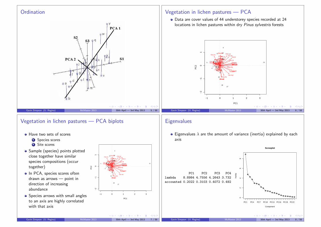
Vegetation in lichen pastures — PCA biplots

Have two sets of scores1 Species scores2 Site scores

Sample (species) points plottedclose together have similarspecies compositions (occurtogether)

In PCA, species scores oftendrawn as arrows — point indirection of increasingabundance

Species arrows with small anglesto an axis are highly correlatedwith that axis

−1 0 1 2 3

−2

−1

01

PC1

PC

2 Cal.vul

Emp.nig

Led.pal

Vac.myr

Vac.vit

Pin.syl

Des.fle

Bet.pub

Vac.uli

Dip.mon

Dic.sp

Dic.fus

Dic.pol

Hyl.splPle.sch

Pol.pil

Pol.junPol.com

Poh.nut

Pti.cilBar.lyc

Cla.arbCla.ran

Cla.ste

Cla.unc

Cla.coc

Cla.cor

Cla.graCla.fimCla.cri

Cla.chl

Cla.botCla.ama

Cla.spCet.eri

Cet.isl

Cet.niv

Nep.arc

Ste.spPel.aph

Ich.eri

Cla.cer

Cla.def

Cla.phy

18

15

24

27

23

1922

16

28

13

14

20

25

7

5 6

3

4

2

9

12

1011

21


Eigenvalues

Eigenvalues λ are the amount of variance (inertia) explained by eachaxis

PC1 PC2 PC3 PC4

lambda 8.8984 4.7556 4.2643 3.732

accounted 0.2022 0.3103 0.4072 0.492

●

●

●

●

● ●●

●●

● ● ●● ●

●●

●● ● ● ● ● ●

Screeplot

Component

Iner

tia

02

46

8

PC1 PC4 PC7 PC10 PC13 PC16 PC19 PC22


Correspondence Analysis


Vegetation in lichen pastures — CA biplots

Have two sets of scores1 Species scores2 Site scores

Sample (species) points plottedclose together have similarspecies compositions (occurtogether)

In CA, species scores drawn aspoints — this is the fittedoptima along the gradients

Abundance of species declines inconcentric circles away from theoptima

−1 0 1 2

−2.

0−

1.5

−1.

0−

0.5

0.0

0.5

1.0

1.5

CA1

CA

2

Cal.vul

Emp.nig

Led.palVac.myr

Vac.vit

Pin.syl

Des.fle

Bet.pub

Vac.uli

Dip.mon

Dic.sp

Dic.fus

Dic.pol

Hyl.spl

Ple.sch

Pol.pil

Pol.jun

Pol.com

Poh.nut

Pti.cil

Bar.lyc

Cla.arb

Cla.ran

Cla.ste

Cla.unc

Cla.coc

Cla.corCla.gra

Cla.fim

Cla.cri

Cla.chlCla.bot

Cla.ama

Cla.sp

Cet.eri

Cet.isl

Cet.niv

Nep.arc

Ste.sp

Pel.aph

Ich.eri

Cla.cer

Cla.def

Cla.phy

18

15

24

27

23

19

22

16

28

13

14

20

25

7

5

6

3

4

2

9

12

10

11

21


Vegetation in lichen pastures — CA biplots

Species scores plotted as weighted averages of site scores, or

Site scores plotted as weighted averages of species scores, or

A symmetric plot

−1 0 1 2

−2.

0−

1.5

−1.

0−

0.5

0.0

0.5

1.0

1.5

CA1

CA

2

Cal.vul

Emp.nig

Led.palVac.myr

Vac.vit

Pin.syl

Des.fle

Bet.pub

Vac.uli

Dip.mon

Dic.sp

Dic.fus

Dic.pol

Hyl.spl

Ple.sch

Pol.pil

Pol.jun

Pol.com

Poh.nut

Pti.cil

Bar.lyc

Cla.arb

Cla.ran

Cla.ste

Cla.unc

Cla.coc

Cla.corCla.gra

Cla.fim

Cla.cri

Cla.chlCla.bot

Cla.ama

Cla.sp

Cet.eri

Cet.isl

Cet.niv

Nep.arc

Ste.sp

Pel.aph

Ich.eri

Cla.cer

Cla.def

Cla.phy

18

15

24

27

23

19

22

16

28

13

14

20

25

7

5

6

3

4

2

9

12

10

11

21

−2 −1 0 1 2 3

−2

−1

01

2

CA1

CA

2

Cal.vul

Emp.nig

Led.palVac.myr

Vac.vit

Pin.syl

Des.fle

Bet.pub

Vac.uli

Dip.mon

Dic.sp

Dic.fus

Dic.pol

Hyl.spl

Ple.sch

Pol.pil

Pol.jun

Pol.com

Poh.nut

Pti.cil

Bar.lyc

Cla.arb

Cla.ran

Cla.ste

Cla.unc

Cla.coc

Cla.corCla.gra

Cla.fim

Cla.cri

Cla.chlCla.bot

Cla.ama

Cla.sp

Cet.eri

Cet.isl

Cet.niv

Nep.arc

Ste.sp

Pel.aph

Ich.eri

Cla.cer

Cla.def

Cla.phy

18

15

24

27

23

19

22

16

28

1314

20

25

75

6

3

4

2

9

12

10

11

21


Outline






Vegan basics

The majority of vegan functions work with a single vector, or morecommonly an entire data frame

This data frame may contain the species abundances

Where subsidiary data is used/required, these two are supplied asdata frames

For example; the environmental constraints in a CCA

It is not a problem if you have all your data in a single file/object; justsubset it into two data frames after reading it into R

> spp <- allMyData[, 1:20] ## columns 1-20 contain the species data

> env <- allMyData[, 21:26] ## columns 21-26 contain the environmental data


Loading vegan for use

As with any package, vegan needs to be loaded into the R sessionbefore it can be used

When vegan loads it displays a simple message showing the versionnumber

Note also that vegan depends upon the permute package

> library("vegan")


Simple vegan usage; basic ordination

First we start with a simple correspondence analysis (CA) to illustratethe basic features

Here I am using one of the in-built data sets on lichen pastures

For various reasons to fit a CA we use the cca() function

Store the fitted CA in ca1 and print it to view the results

> data(varespec)

> ca1 <- cca(varespec)

> ca1

Call: cca(X = varespec)

Inertia Rank

Total 2.083

Unconstrained 2.083 23

Inertia is mean squared contingency coefficient

Eigenvalues for unconstrained axes:

CA1 CA2 CA3 CA4 CA5 CA6 CA7 CA8

0.5249 0.3568 0.2344 0.1955 0.1776 0.1216 0.1155 0.0889

(Showed only 8 of all 23 unconstrained eigenvalues)


Simple vegan usage; basic ordination

> class(ca1)

[1] "cca"

> str(ca1, max = 1) ## top level components

List of 10

$ call : language cca(X = varespec)

$ grand.total: num 2418

$ rowsum : Named num [1:24] 0.0369 0.0372 0.039 0.052 0.0374 ...

..- attr(*, "names")= chr [1:24] "18" "15" "24" "27" ...

$ colsum : Named num [1:44] 0.01864 0.06287 0.00347 0.02097 0.11376 ...

..- attr(*, "names")= chr [1:44] "Cal.vul" "Emp.nig" "Led.pal" "Vac.myr" ...

$ tot.chi : num 2.08

$ pCCA : NULL

$ CCA : NULL

$ CA :List of 8

$ method : chr "cca"

$ inertia : chr "mean squared contingency coefficient"

- attr(*, "class")= chr "cca"


The CCA object ?cca.object

Objects of class "cca" are complex with many components

Entire class described in ?cca.object

Depending on what analysis performed some components may beNULL

Used for (C)CA, PCA, RDA, and CAP (capscale())

ca1 has:I $call how the function was calledI $grand.total in (C)CA sum of rowsumI $rowsum the row sumsI $colsum the column sumsI $tot.chi total inertia, sum of EigenvaluesI $pCCA Conditioned (partialled out) componentsI $CCA Constrained componentsI $CA Unconstrained componentsI $method Ordination method usedI $inertia Description of what inertia is


The CCA object ?cca.object

The $pCCA $CCA, and $CA components contain a number of othercomponents

Most usefully the Eigenvalues are found here plus the species(variables) and site (samples) score

ca1$CA has:I $eig the Eigenvalues (λ)I $u (weighted) orthonormal site scoresI $v (weighted) orthonormal species scoresI $u.eig u scaled by λI $v.eig v scaled by λI $rank the rank or dimension of component (number of axes)I $tot.chi sum of λ for this componentI $Xbar the standardised data matrix after previous stages of analysis

*.eig may disappear in a future version of vegan

There are many other components that may be present in morecomplex analyses (e.g. CCA)


Extractor functions — eigenvals()

Thankfully we don’t need to remember all those components ingeneral use — extractor functions

To extract the eigenvalues use eigenvals():

> eigenvals(ca1)


0.5249320 0.3567980 0.2344375 0.1954632 0.1776197 0.1215603 0.1154922 0.0889385


0.0731751 0.0575174 0.0443421 0.0254635 0.0171030 0.0148963 0.0101598 0.0078298

CA17 CA18 CA19 CA20 CA21 CA22 CA23

0.0060323 0.0040079 0.0028650 0.0019275 0.0018074 0.0005864 0.0002434


Extractor functions — scores()

The scores() function is an important extractor if you want toaccess any of the results for use elsewhereTakes an ordination object as the first argumentchoices: which axes to return scores for, defaults to c(1,2)

display: character vector of the type(s) of scores to return> str(scores(ca1, choices = 1:4, display = c("species","sites")))

List of 2

$ species: num [1:44, 1:4] 0.022 0.0544 0.8008 1.0589 0.1064 ...

..- attr(*, "dimnames")=List of 2

.. ..$ : chr [1:44] "Cal.vul" "Emp.nig" "Led.pal" "Vac.myr" ...

.. ..$ : chr [1:4] "CA1" "CA2" "CA3" "CA4"

$ sites : num [1:24, 1:4] -0.149 0.962 1.363 1.176 0.497 ...

..- attr(*, "dimnames")=List of 2

.. ..$ : chr [1:24] "18" "15" "24" "27" ...

.. ..$ : chr [1:4] "CA1" "CA2" "CA3" "CA4"

> head(scores(ca1, choices = 1:2, display = "sites"))

CA1 CA2

18 -0.149231732 -0.89909538

15 0.962176641 -0.24176673

24 1.363110128 0.25182197

27 1.175623286 0.83540787

23 0.496714476 -0.09389079

19 0.004893311 0.61971266Gavin Simpson (U. Regina) McMaster 2013 30th April — 3rd May 2013 20 / 58

scores() & scaling in cca(), rda()

When we draw the results of many ordinations we display 2 or moresets of data

Can’t display all of these and maintain relationships between thescores

Solution; scale one set of scores relative to the other

Controlled via the scaling argumentI scaling = 1 — Focus on species, scale site scores by λiI scaling = 2 — Focus on sites, scale species scores by λiI scaling = 3 — Symmetric scaling, scale both scores by

√λi

I scaling = -1 — As above, butI scaling = -2 — For cca() multiply results by

√(1/(1− λi))

I scaling = -3 — this is Hill’s scalingI scaling < 0 — For rda() divide species scores by species’ σI scaling = 0 — raw scores

> scores(ca1, choices = 1:2, display = "species", scaling = 3)


Basic ordination plots

Basic plotting can be done using theplot() method

choices = 1:2 — select which axesto plot

scaling = 3 — scaling to use

display = c("sites","species")

— which scores (default is both)

type = "text" — display scoresusing labels or points ("points")

Other graphics arguments can besupplied but the apply for all scores

See ?plot.cca for details

Customisation tricky — better to plotby hand (tomorrow)

> plot(ca1, scaling = 3)

−1 0 1 2

−2.

0−

1.5

−1.

0−

0.5

0.0

0.5

1.0

1.5

CA1

CA

2

Cal.vul

Emp.nig

Led.palVac.myr

Vac.vit

Pin.syl

Des.fle

Bet.pub

Vac.uli

Dip.mon

Dic.sp

Dic.fus

Dic.pol

Hyl.spl

Ple.sch

Pol.pil

Pol.jun

Pol.com

Poh.nut

Pti.cil

Bar.lyc

Cla.arb

Cla.ran

Cla.ste

Cla.unc

Cla.coc

Cla.corCla.gra

Cla.fim

Cla.cri

Cla.chlCla.bot

Cla.ama

Cla.sp

Cet.eri

Cet.isl

Cet.niv

Nep.arc

Ste.sp

Pel.aph

Ich.eri

Cla.cer

Cla.def

Cla.phy

18

15

24

27

23

19

22

16

28

1314

20

25

7

5

6

3

4

2

9

12

10

11

21


Outline






Indirect gradient analysis

PCA and CA are indirect gradient analysis methods

First extract the hypothetical gradients (axes), then relate thesegradients to measured environmental data using regression

But what happens if the gradients extracted are only partly explainedby your measured data?

Or, what if your measured data do not explain the main patterns (axes1 and 2 say) in the species data, but are important on later axes?

Direct gradient analysis allows us to do the ordination and regressionin one single step

As before there are linear and unimodal methods:I Redundancy Analysis (RDA) is a linear method, the counterpart to PCAI Canonical (Constrained) Correspondence Analysis (CCA) is a unimodal

method, the counterpart to CA


Direct gradient analysis

In PCA and CA we fitted lines and curves that fitted the data best —explained most variance

In RDA and CCA we still fit lines and curves, but we are constrainedin how we can fit these axes

In RDA/CCA we can only fit axes that are linear combinations of ourmeasured environmental data

By linear combinations, we mean (2× pH) + (1.5×moisture)

In other words, we constrain the ordination axes such that thepatterns/gradients extracted are restricted to those that we canexplain with the measured data


Vegetation in lichen pastures — CCA

Now we fit a CCA to the lichen pasture data, constrained by themeasured environmental data

−2 −1 0 1 2

−2

−1

01

CCA1

CC

A2

Cal.vul

Emp.nigLed.pal

Vac.myr

Vac.vitPin.sylDes.fle

Bet.pub

Vac.uli

Dip.mon

Dic.sp

Dic.fus

Dic.pol

Hyl.spl

Ple.sch

Pol.pil

Pol.junPol.com

Poh.nut

Pti.cilBar.lyc

Cla.arbCla.ran

Cla.ste

Cla.unc

Cla.coc

Cla.cor

Cla.graCla.fim

Cla.cri

Cla.chl

Cla.bot

Cla.ama

Cla.sp

Cet.eri

Cet.isl

Cet.niv

Nep.arc

Ste.sp

Pel.aph

Ich.eri

Cla.cerCla.def

Cla.phy

18

15

24

27

23

19

22

16

28

13

14

20

25

7

5

6

3

4

2

9

12

10

11

21

N

P

KCaMg

S

AlFe

MnZn

Mo

Baresoil

Humdepth

pH

−1

0


Vegetation in lichen pastures — CCA triplots

Triplots show 3 bits ofinformation — compromise

Species and site scores plottedalong side biplot arrows forenvironmental data

Sites close together have similarspecies and environments

Species close together occurtogether

Angles between arrows reflectcorrelations between envvariables

Length of arrows indicateimportance of variable — longervariables more important

−2 −1 0 1 2

−2

−1

01

CCA1

CC

A2

Cal.vul

Emp.nigLed.pal

Vac.myr

Vac.vitPin.sylDes.fle

Bet.pub

Vac.uli

Dip.mon

Dic.sp

Dic.fus

Dic.pol

Hyl.spl

Ple.sch

Pol.pil

Pol.junPol.com

Poh.nut

Pti.cilBar.lyc

Cla.arbCla.ran

Cla.ste

Cla.unc

Cla.coc

Cla.cor

Cla.graCla.fim

Cla.cri

Cla.chl

Cla.bot

Cla.ama

Cla.sp

Cet.eri

Cet.isl

Cet.niv

Nep.arc

Ste.sp

Pel.aph

Ich.eri

Cla.cerCla.def

Cla.phy

18

15

24

27

23

19

22

16

28

13

14

20

25

7

5

6

3

4

2

9

12

10

11

21

N

P

KCaMg

S

AlFe

MnZn

Mo

Baresoil

Humdepth

pH

−1

0


Vegetation in lichen pastures — CCA

Eigenvalues, and their contribution

CCA1 CCA2 CCA3 CCA4

lambda 0.4389 0.2918 0.1628 0.1421

accounted 0.2107 0.3507 0.4289 0.4971

Again, Eigenvalues λ are measured of variance explained

As this is constrained, λ will be lower than in unconstrained methods

One problem is that as we increase the number of environmentalvariables as explanatory variable, we actually reduce the constraintson the ordination

Can only have min(nspecies, nsamples)− 1 CCA axes but thenconstraints are 0 and we have the same result as CA

As CCA/RDA are regression techniques, we should try to reduce thenumber of explanatory variables down to only those variables that areimportant for explaining the species composition


Fitting constrained ordinationsVegan has two interfaces to specify the model fitted; basic,> data(varechem)

> cca1 <- cca(X = varespec, Y = varechem)

or formula> cca1 <- cca(varespec ~ ., data = varechem)

Formula interface is more powerful and is recommended

> cca1

Call: cca(formula = varespec ~ N + P + K + Ca + Mg + S + Al + Fe + Mn +

Zn + Mo + Baresoil + Humdepth + pH, data = varechem)

Inertia Proportion Rank

Total 2.0832 1.0000

Constrained 1.4415 0.6920 14

Unconstrained 0.6417 0.3080 9


Eigenvalues for constrained axes:

CCA1 CCA2 CCA3 CCA4 CCA5 CCA6 CCA7 CCA8 CCA9 CCA10 CCA11

0.4389 0.2918 0.1628 0.1421 0.1180 0.0890 0.0703 0.0584 0.0311 0.0133 0.0084

CCA12 CCA13 CCA14

0.0065 0.0062 0.0047


CA1 CA2 CA3 CA4 CA5 CA6 CA7 CA8 CA9

0.19776 0.14193 0.10117 0.07079 0.05330 0.03330 0.01887 0.01510 0.00949


Fitting constrained ordinations

A better approach is to think about the important variables andinclude only those

The formula interface allows you to create interaction or quadraticterms easily (though be careful with latter)

It also handles factor or class constraints automatically unlike thebasic interface

> vare.cca <- cca(varespec ~ Al + P*(K + Baresoil), data = varechem)

> vare.cca

Call: cca(formula = varespec ~ Al + P * (K + Baresoil), data =

varechem)


Total 2.083 1.000

Constrained 1.046 0.502 6




CCA1 CCA2 CCA3 CCA4 CCA5 CCA6

0.3756 0.2342 0.1407 0.1323 0.1068 0.0561



0.27577 0.15411 0.13536 0.11803 0.08887 0.05511 0.04919 0.03781



Fitting partial constrained ordinations

The effect of one or more variables can be partialled out by supplyingthem as object Z in the basic interface

The formula interface can be used too, via a special functionCondition()

> pcca <- cca(varespec ~ Ca + Condition(pH), data = varechem)

> pcca

Call: cca(formula = varespec ~ Ca + Condition(pH), data = varechem)


Total 2.0832 1.0000

Conditional 0.1458 0.0700 1





CCA1

0.18269



0.3834 0.2749 0.2123 0.1760 0.1701 0.1161 0.1089 0.0880



Model Building

Automatic approaches to model building should be used cautiously

The standard step() function can be used as vegan provides twohelper methods; deviance() and extractAIC() used by step()

Vegan also provides methods for class "cca" for add1() anddrop1().

To use, we define an upper and lower model scope, say the full modeland the null modelTo step from the lower scope or null model we use

> upr <- cca(varespec ~ ., data = varechem)

> lwr <- cca(varespec ~ 1, data = varechem)

> mods <- step(lwr, scope = formula(upr), test = "perm", trace = 0)

trace = 0 is used her to turn off printing of progress

test = "perm" indicates permutation tests are used (more on theselater); the theory for an AIC for ordination is somewhat loose


Model Building

The object returned by step() is a standard "cca" object with anextra component $anova

The $anova component contains a summary of the steps involved inautomatic model building

> mods

Call: cca(formula = varespec ~ Al + P + K, data = varechem)


Total 2.0832 1.0000





CCA1 CCA2 CCA3

0.3616 0.1700 0.1126



0.3500 0.2201 0.1851 0.1551 0.1351 0.1003 0.0773 0.0537



Model Building


> mods$anova

Step Df Deviance Resid. Df Resid. Dev AIC

1 NA NA 23 5036.590 130.3143

2 + Al -1 720.9014 22 4315.689 128.6070

3 + P -1 459.1399 21 3856.549 127.9074

4 + K -1 377.2927 20 3479.256 127.4365


Model Building

Step-wise model selection is fairly fragile; if we start from the fullmodel we won’t end up with the same final model

> mods2 <- step(upr, scope = list(lower = formula(lwr), upper = formula(upr)), trace = 0,

+ test = "perm")

> mods2

Call: cca(formula = varespec ~ P + K + Mg + S + Mn + Mo + Baresoil +

Humdepth, data = varechem)


Total 2.0832 1.0000





CCA1 CCA2 CCA3 CCA4 CCA5 CCA6 CCA7 CCA8

0.4007 0.2488 0.1488 0.1266 0.0875 0.0661 0.0250 0.0130


CA1 CA2 CA3 CA4 CA5 CA6 CA7 CA8 CA9 CA10

0.25821 0.18813 0.11927 0.10204 0.08791 0.06085 0.04461 0.02782 0.02691 0.01646

CA11 CA12 CA13 CA14 CA15

0.01364 0.00823 0.00655 0.00365 0.00238


Model Building


> mods2$anova

Step Df Deviance Resid. Df Resid. Dev AIC

1 NA NA 9 1551.483 130.0539

2 - Fe 1 115.2085 10 1666.692 129.7730

3 - Al 1 105.9602 11 1772.652 129.2523

4 - N 1 117.5382 12 1890.190 128.7931

5 - pH 1 140.4399 13 2030.630 128.5131

6 - Ca 1 141.2450 14 2171.875 128.1270

7 - Zn 1 165.2596 15 2337.135 127.8871


Permutation tests — the anova() method

We have little good theory with which to evaluate the significance ofordination models or terms thereinInstead we use permutation tests

I If there are no conditioning variables then the species data are shuffledI If there are constraining variables then two options are possible, both

permute residuals of model fitsF Full model; residuals from the model Y = X + Z + εF Reduced model; residuals from the model Y = Z + ε

I These two essentially produce the same results

In vegan these are achieved via the method argument using"direct", "full", "reduced".

A test statistic is required; vegan uses a pseudo-F statistics

F =χ2model/dfmodel

χ2resid/dfresid

Evaluate whether F is unusually large relative to the null(permutation) distribution of F



The main user function is the anova() method

It is an interface to the lower-level function permutest.cca()

At its most simplest, the anova() method tests whether the “model”as a whole is significant

F =1.4415/14

0.6417/9= 1.4441

> set.seed(42)

> anova(cca1)

Permutation test for cca under reduced model

Model: cca(formula = varespec ~ N + P + K + Ca + Mg + S + Al + Fe + Mn + Zn + Mo + Baresoil + Humdepth + pH, data = varechem)

Df Chisq F N.Perm Pr(>F)

Model 14 1.4415 1.4441 1599 0.03562 *

Residual 9 0.6417

---

Signif. codes: 0 ‘***’ 0.001 ‘**’ 0.01 ‘*’ 0.05 ‘.’ 0.1 ‘ ’ 1



anova() will continue permuting only as long as it is uncertainwhether the the p-value is above or below the chosen threshold (sayp = 0.05)

If the function is sure the permuted p is above the threshold anova()

may return after only a few hundred permutations

In other cases many hundreds or thousands of permutations may berequired to say whether the model is above or below the threshold

In the example, 1599 permutations were required



anova.cca() has a number of arguments

> args(anova.cca)

function (object, alpha = 0.05, beta = 0.01, step = 100, perm.max = 9999,

by = NULL, ...)

NULL

alpha is the desired p value threshold (Type I)

beta is the Type II error rate

Permuting stops if the result is different from alpha for the givenbeta

This is evaluated every step permutations

perm.max sets a limit on the number of permutations

by determines what is tested; the default is to test the model

More direct control can be achieved via permutest.cca()


Permutation tests — testing canonical axes

The canonical axes can be individually tested by specifying by =

"axis"

The first axis is tested in terms of variance explained compared toresidual variance

The second axis is tested after partialling out the first axis, . . .

> set.seed(1)

> anova(mods, by = "axis")

Model: cca(formula = varespec ~ Al + P + K, data = varechem)


CCA1 1 0.3616 5.0249 199 0.00500 **

CCA2 1 0.1700 2.3621 299 0.01667 *

CCA3 1 0.1126 1.5651 99 0.16000

Residual 20 1.4391

---

Signif. codes: 0 ‘***’ 0.001 ‘**’ 0.01 ‘*’ 0.05 ‘.’ 0.1 ‘ ’ 1


Permutation tests — testing terms

The individual terms in the model can be tested using by = "terms"

The terms are assessed in the order they were specified in the model,sequentially from first to last

It is important to note that the order of the terms will affect theresults

> set.seed(5)

> anova(mods, by = "terms")


Terms added sequentially (first to last)



Al 1 0.2982 4.1440 99 0.01 **

P 1 0.1899 2.6393 99 0.01 **

K 1 0.1561 2.1688 99 0.03 *

Residual 20 1.4391

---

Signif. codes: 0 ‘***’ 0.001 ‘**’ 0.01 ‘*’ 0.05 ‘.’ 0.1 ‘ ’ 1


Permutation tests — testing marginal terms

The marginal ”effect” of a model term can be assessed using by =

"margin"

The marginal ”effect” is the effect of a particular term when all othermodel terms are included in the model

> set.seed(5)

> anova(mods, by = "margin")


Marginal effects of terms



Al 1 0.3118 4.3340 199 0.005 **

P 1 0.1681 2.3362 199 0.010 **

K 1 0.1561 2.1688 399 0.020 *

Residual 20 1.4391

---

Signif. codes: 0 ‘***’ 0.001 ‘**’ 0.01 ‘*’ 0.05 ‘.’ 0.1 ‘ ’ 1


Diagnostics for constrained ordination

Vegan provides a series of diagnostics functions to help assess themodel fit

goodness() computes two goodness of fit statistics for species orsites

I statistic = "explained" — cumulative proportion of varianceexplained by each axis

I statistic = "distance" — the residual distance between the”fitted” location in ordination space and the full dimensional space

inertiacomp() decomposes the variance for each species or site intopartial, constrained and unexplained components

intersetcor() computes the interset correlations, the (weighted)correlation between the weighted average site scores and the linearcombination site scores

vif.cca() computes variance inflation factors for model constrains.Variables with V > 10 are linearly dependent on other variables in themodel


Linear methodsVegan can also fit the linear methods PCA and RDA

Linear based ordination methods are handled in the same way as theirunimodal counter parts

The rda() function is used to fit these two techniques

Interface is the same as & the object returned is as described forcca()

Class c("rda","cca")

> data(dune); data(dune.env)

> (pca1 <- rda(dune, scale = TRUE))

Call: rda(X = dune, scale = TRUE)

Inertia Rank

Total 30

Unconstrained 30 19

Inertia is correlations


PC1 PC2 PC3 PC4 PC5 PC6 PC7 PC8

7.032 4.997 3.555 2.644 2.139 1.758 1.478 1.316



Linear methods

The scale argument controls whether the response data arestandardised prior to analysis. Vegan always performs a centred

PCA/RDA

> (rda1 <- rda(dune ~ Manure, dune.env, scale = TRUE))

Call: rda(formula = dune ~ Manure, data = dune.env, scale = TRUE)


Total 30.0000 1.0000



Inertia is correlations


RDA1 RDA2 RDA3 RDA4

4.374 2.078 1.449 0.896


PC1 PC2 PC3 PC4 PC5 PC6 PC7 PC8 PC9 PC10 PC11 PC12 PC13

5.133 3.447 2.462 1.924 1.662 1.366 1.357 0.926 0.839 0.585 0.511 0.439 0.308

PC14 PC15

0.159 0.084


Outline






Dissimilarities

dist() is the basic R function for computing dissimilarity or distancematrices

Few, if any, of the included metrics are suitable for communityecology dataVegan provides vegdist() as a drop-in alternative with numeroususeful metrics

I Bray-CurtisI JaccardI GowerI KulczynskiI Give good gradient separation for ecological data

Returns an object of class "dist" which can be used in many other Rfunctions & packages

> dis <- vegdist(varespec, method = "bray")

> dis2 <- vegdist(varespec, method = "gower")

> class(dis)

[1] "dist"


Ecologically meaningful transformations

Legendre & Gallagher (Oecologia, 2001) show that many ecologicallyuseful dissimilarities are in Euclidean form

They are equivalent to calculating the Euclidean distance ontransformed data

Two of the suggested metrics included in vegan’s decostand()function

I Chi-squareI Hellinger

> dis3 <- vegdist(decostand(varespec, method = "hellinger"))


Principal coordinates analysis

Principal Coordinates Analysis (PCoA) (AKA classic or metricmultidimensional scaling) is PCA applied to a dissimilarity matrix

Several functions in R available for this (e.g. cmdscale())

Vegan has capscale() for constrained analysis of principalcoordinates (CAP)

Works exactly the same way as rda()

Can supply a dissimilarity matrix as the response or the communitydata and tell vegan which dissimilarity to compute

Several new argumentsI distance & dfun indicate which dissimilarity to compute and which

function to use to compute itI sqrt.dist & add allow handling of negative λ (not needed but can be

used)I comm the community data is a dissimilarity matrix used in the model

formula; allows species scores to be addedI metaMDSdist process the community data before analysis using

metaMDSdist(); allows transformations & extended dissimilarities


Principal coordinates analysis

To use capscale() for PCoA provide a formula with an intercept only

LHS of formula is community data or dissimilarity matrix

> (pcoa <- capscale(varespec ~ 1, dist = "bray", metaMDS = TRUE))

Square root transformation

Wisconsin double standardization

Call: capscale(formula = varespec ~ 1, distance = "bray", metaMDSdist =

TRUE)

Inertia Rank

Total 2.54753

Real Total 2.59500

Unconstrained 2.59500 19

Imaginary -0.04747 4

Inertia is squared Bray distance


MDS1 MDS2 MDS3 MDS4 MDS5 MDS6 MDS7 MDS8

0.6075 0.3820 0.3335 0.2046 0.1731 0.1684 0.1505 0.1163


metaMDSdist transformed data: wisconsin(sqrt(varespec))

> class(pcoa)

[1] "capscale" "rda" "cca"


Constrained Principal coordinates analysis

Constrained Analysis of Principal Coordinates (CAP)

Constrained form of PCoA (as RDA is to PCA, CCA is to CA, etc.)

Similar to CAP of Anderson & Willis (2003, Ecology 84, 511–525)but with a couple of enhancements

I Uses PCoA axes weighted by λi so ordination distances bestapproximate the original dissimilarities (CAP uses orthonormal PCoAaxes; noise!)

I CAP uses a subset of axes, capscale() uses all real PCoA axesI capscale() adds species scores as weighted sums of community data


Constrained Principal coordinates analysis

Constrained Analysis of Principal Coordinates (CAP)

> (vare.cap <- capscale(varespec ~ N + P + K + Condition(Al), varechem,

+ dist = "bray"))

Call: capscale(formula = varespec ~ N + P + K + Condition(Al), data =

varechem, distance = "bray")


Total 4.5444

Real Total 4.8034 1.0000

Conditional 0.9772 0.2034 1



Imaginary -0.2590 8

Inertia is squared Bray distance


CAP1 CAP2 CAP3

0.5413 0.3265 0.1293


MDS1 MDS2 MDS3 MDS4 MDS5 MDS6 MDS7 MDS8 MDS9 MDS10 MDS11

0.9065 0.5127 0.3379 0.2626 0.2032 0.1618 0.1242 0.0856 0.0689 0.0583 0.0501

MDS12 MDS13 MDS14 MDS15

0.0277 0.0208 0.0073 0.0013


Non-Metric Multidimensional Scaling

Aim is to find a low-dimensional mapping of dissimilarities

Similar idea to PCoA, but does not use the actual dissimilarities

NMDS attempts to find a low-dimensional mapping that preserves asbest as possible the rank order of the original dissimilarities (dij )

Solution with minimal stress is sought; a measure of how well theNMDS mapping fits the dij

Stress is sum of squared residuals of monotonic regression betweendistances in NMDS space (d∗

ij ) & dij

Non-linear regression can cope with non-linear responses in speciesdata

Iterative solution; convergence is not guaranteed

Must solve separately different dimensionality solutions


Non-Metric Multidimensional ScalingUse an appropriate dissimilarity metric that gives good gradientseparation rankindex()

I Bray-CurtisI JaccardI Kulczynski

Wisconsin transformation useful; Standardize species to equalmaxima, then sites to equal totals wisconsin()

Iterative solution; use many random starts and look at the fits withlowest stress

Only conclude solution reached if lowest stress solutions are similar(Procrsutes rotation)

Fit NMDS for 1, 2, 3, . . . dimensions; stop after a sudden drop instress observed in a screeplot

NMDS solutions can be rotated at will; common to rotate to principalcomponents

Also scale axes in half-change units; samples separated by a distanceof 1 correspond, on average, to a 50% turnover in composition


NMDS in vegan

Vegan implements all these ideas via the metaMDS() wrapper

> library("vegan"); data(dune)

> set.seed(42)

> (sol <- metaMDS(dune))

Run 0 stress 0.1192678


... New best solution

... procrustes: rmse 0.02026936 max resid 0.06495232



... procrustes: rmse 5.509367e-06 max resid 1.511849e-05

*** Solution reached

Call:

metaMDS(comm = dune)

global Multidimensional Scaling using monoMDS

Data: dune

Distance: bray

Dimensions: 2

Stress: 0.1183186

Stress type 1, weak ties

Two convergent solutions found after 3 tries

Scaling: centring, PC rotation, halfchange scaling

Species: expanded scores based on ‘dune’


NMDS in vegan

If no convergent solutions, continue iterations from previous bestsolution

> (sol <- metaMDS(dune, previous.best = sol))

Starting from 2-dimensional configuration



... procrustes: rmse 1.919781e-05 max resid 6.3831e-05

*** Solution reached

Call:

metaMDS(comm = dune, previous.best = sol)

global Multidimensional Scaling using monoMDS

Data: dune

Distance: bray

Dimensions: 2

Stress: 0.1183186

Stress type 1, weak ties

Two convergent solutions found after 4 tries

Scaling: centring, PC rotation, halfchange scaling

Species: expanded scores based on ‘dune’


NMDS in vegan

> layout(matrix(1:2, ncol = 2))

> plot(sol, main = "Dune NMDS plot")

> stressplot(sol, main = "Shepard plot")

> layout(1)

−0.5 0.0 0.5 1.0 1.5

−1.

0−

0.5

0.0

0.5

1.0

1.5

Dune NMDS plot

NMDS1

NM

DS

2

●

●

●

●

●

●

●

●

●

●

●

●

●

●

●

●

●

●

●

●

+

+

+

+

+

+

+

+

++

+

+

+

+

+

+

+ +

+

+

+

+

+

+

+

+

++

+

+

●

● ●●

●

●●

●

●

●

●

●

●●

●

●

●

●●

●

●

●

●

●

●●

●

●

●

●

●

●

●

●

●●

●

●●●●●

●

●

●

●

●●

●

●●

●

●

●●●●●●

●

●

●●●

●

●

●

●

●

●

●

●

●

●

●

●

●

●●

●

●

●

●

●

●

●

●

●●

●

●

●

●

●

●

●

●●

●●

●●

●

●

●

●

●

●

●

●

●

●

●

●

●

●

●

●●

●

●

●

●●

●

●

●●

●

●●●

●

●

●

●

●

●●

●

●

●

●

●

●●

●

●

●

●●●

●

●

●

●

●

●

●

●

●

●

●

●●●●●●●

●

●●

●●

●●

●●

●

●

●

●

●

●

●

●

●●

●

0.2 0.4 0.6 0.8 1.0

0.5

1.0

1.5

2.0

2.5

3.0

Shepard plot

Observed Dissimilarity

Ord

inat

ion

Dis

tanc

e

Non−metric fit, R2 = 0.986 Linear fit, R2 = 0.927


An Introduction to R for the Geosciences: Ordination

Documents