Draft from February 14, 2005 An Introduction to Optimization: Foundations and Fundamental Algorithms Niclas Andr´ easson, Anton Evgrafov, and Michael Patriksson

Welcome message from author
This document is posted to help you gain knowledge. Please leave a comment to let me know what you think about it! Share it to your friends and learn new things together.
Transcript
Draft from February 14, 2005
An Introduction to Optimization:
Foundations and Fundamental Algorithms
Niclas Andreasson, Anton Evgrafov, and Michael Patriksson
Draft from February 14, 2005
Preface
The present book has been developed from course notes, continuouslyupdated and used in optimization courses during the past several yearsat Chalmers University of Technology, Goteborg (Gothenburg), Sweden.
A note to the instructor: The book serves to provide lecture and ex-ercise material in a first course on optimization for second to fourth yearstudents at the university. (Computer exercises and projects are pro-vided at course home pages on the local web site.) The book’s focus lieson providing a solid basis for the analysis of optimization models and ofcandidate optimal solutions, especially for continuous optimization mod-els. The main part of the mathematical material therefore concerns theanalysis and algebra that underlie the workings of convexity and dual-ity, and necessary/sufficient local/global optimality conditions for uncon-strained and constrained optimization. Natural and most often classicalgorithms are then developed from these principles, and their conver-gence characteristics analyzed. The book answers many more questionsof the form “Why/why not?” than “How?”.
This choice of focus is in contrast to books mainly providing nu-merical guidelines as to how these optimization problems should besolved. The number of algorithms for linear and nonlinear optimizationproblems—the two main topics covered in this book—are kept quite low;those that are discussed are considered classical, and serve to illustratethe basic principles for solving such classes of optimization problems andtheir links to the fundamental theory of optimality. Any course basedon this book therefore should add project work on concrete optimizationproblems, including their modelling, analysis, solution, and interpreta-tion.
A note to the student: The material assumes some familiarity withalgebra, real analysis, and logic. In algebra, we assume an active knowl-edge of bases, norms, and matrix algebra and calculus. In real analysis,we assume an active knowledge of sequences, the basic topology of sets,
Draft from February 14, 2005
Preface
real- and vector-valued functions and their calculus of differentiation. Wealso assume a familiarity with basic predicate logic, especially becauseproofs are based on it. A summary of the most important backgroundtopics is found in Chapter 2, which also serves as an introduction to themathematical notation. The student is advised to refresh any unfamiliaror forgotten material of this chapter before reading the rest of the book.
A detailed road map of the contents of the book’s chapters, and di-dactic statements as well, are provided at the end of Chapter 1. Eachchapter ends with a selected number of exercises which either illustratethe theory and algorithms with numerical examples or develop the theoryslightly further. In Appendix B solutions are given to most of them, in afew cases in detail. (Those exercises marked “exam” together with a dateare examples of exam questions given in the course “Applied optimiza-tion” at Goteborg University and Chalmers University of Technologysince 1997.) Sections with supplementary (but nevertheless important)material are marked with an asterisk.
In our work on this book we have benefited from discussions withDr. Ann-Brith Stromberg, presently at the Fraunhofer–Chalmers Re-search Centre for Industrial Mathematics (FCC), Goteborg, and for-merly at mathematics at Chalmers University of Technology. We thankthe heads of undergraduate studies at mathematics, Goteborg Universityand Chalmers University of Technology, Jan-Erik Andersson and SvenJarner respectively, for reducing our teaching duties while preparing thisbook.
Goteborg, XX 2005 Anton Evgrafov
Niclas Andreasson
Michael Patriksson
vi
Draft from February 14, 2005
Contents
I Introduction 1
1 Modelling and classification 31.1 Modelling of optimization problems . . . . . . . . . . . . . 3
1.1.1 What does it mean to optimize? . . . . . . . . . . 31.1.2 Application examples . . . . . . . . . . . . . . . . 5
1.2 A quick glance at optimization history . . . . . . . . . . . 91.3 Classification of optimization models . . . . . . . . . . . . 111.4 Conventions . . . . . . . . . . . . . . . . . . . . . . . . . . 141.5 Applications and modelling examples . . . . . . . . . . . . 161.6 Defining the field . . . . . . . . . . . . . . . . . . . . . . . 161.7 Soft and hard constraints . . . . . . . . . . . . . . . . . . 17
1.7.1 Definitions . . . . . . . . . . . . . . . . . . . . . . 171.7.2 A derivation of the exterior penalty function . . . 18
1.8 A road map through the material . . . . . . . . . . . . . . 191.9 On the background of this book and a didactics statement 251.10 Notes and further reading . . . . . . . . . . . . . . . . . . 261.11 Exercises . . . . . . . . . . . . . . . . . . . . . . . . . . . 27
II Fundamentals 31
2 Analysis and algebra—A summary 332.1 Reductio ad absurdum . . . . . . . . . . . . . . . . . . . . 332.2 Linear algebra . . . . . . . . . . . . . . . . . . . . . . . . . 342.3 Analysis . . . . . . . . . . . . . . . . . . . . . . . . . . . . 37
3 Convex analysis 413.1 Convexity of sets . . . . . . . . . . . . . . . . . . . . . . . 413.2 Polyhedral theory . . . . . . . . . . . . . . . . . . . . . . . 42
3.2.1 Convex hulls . . . . . . . . . . . . . . . . . . . . . 42
Draft from February 14, 2005
Contents
3.2.2 Polytopes . . . . . . . . . . . . . . . . . . . . . . . 453.2.3 Polyhedra . . . . . . . . . . . . . . . . . . . . . . . 473.2.4 The Separation Theorem and Farkas’ Lemma . . . 52
3.3 Convex functions . . . . . . . . . . . . . . . . . . . . . . . 573.4 Application: the projection of a vector onto a convex set . 663.5 Notes and further reading . . . . . . . . . . . . . . . . . . 673.6 Exercises . . . . . . . . . . . . . . . . . . . . . . . . . . . 68
III Optimality Conditions 73
4 An introduction to optimality conditions 754.1 Local and global optimality . . . . . . . . . . . . . . . . . 754.2 Existence of optimal solutions . . . . . . . . . . . . . . . . 784.3 Optimality in unconstrained optimization . . . . . . . . . 844.4 Optimality for optimization over convex sets . . . . . . . . 884.5 Near-optimality in convex optimization . . . . . . . . . . . 954.6 Applications . . . . . . . . . . . . . . . . . . . . . . . . . . 96
4.6.1 ∗Continuity of convex functions . . . . . . . . . . . 964.6.2 The Separation Theorem . . . . . . . . . . . . . . 984.6.3 Euclidean projection . . . . . . . . . . . . . . . . . 994.6.4 Fixed point theorems . . . . . . . . . . . . . . . . 100
4.7 Notes and further reading . . . . . . . . . . . . . . . . . . 1064.8 Exercises . . . . . . . . . . . . . . . . . . . . . . . . . . . 106
5 Optimality conditions 1115.1 Relations between optimality conditions (OCs) and CQs
at a glance . . . . . . . . . . . . . . . . . . . . . . . . . . 1115.2 A note of caution . . . . . . . . . . . . . . . . . . . . . . . 1125.3 Geometric optimality conditions . . . . . . . . . . . . . . 1145.4 The Fritz–John conditions . . . . . . . . . . . . . . . . . . 1185.5 The Karush–Kuhn–Tucker conditions . . . . . . . . . . . . 1245.6 Proper treatment of equality constraints . . . . . . . . . . 1285.7 Constraint qualifications . . . . . . . . . . . . . . . . . . . 130
5.7.1 Mangasarian–Fromovitz CQ (MFCQ) . . . . . . . 1305.7.2 Slater CQ . . . . . . . . . . . . . . . . . . . . . . . 131
5.7.3 Linear independence CQ (LICQ) . . . . . . . . . . 1315.7.4 Affine constraints . . . . . . . . . . . . . . . . . . . 132
5.8 Sufficiency of KKT–conditions under convexity . . . . . . 1325.9 Applications and examples . . . . . . . . . . . . . . . . . . 1345.10 Notes and further reading . . . . . . . . . . . . . . . . . . 1365.11 Exercises . . . . . . . . . . . . . . . . . . . . . . . . . . . 137
viii
Draft from February 14, 2005
Contents
6 Lagrangian duality 141
6.1 The relaxation theorem . . . . . . . . . . . . . . . . . . . 141
6.2 Lagrangian duality . . . . . . . . . . . . . . . . . . . . . . 142
6.2.1 Lagrangian relaxation and the dual problem . . . . 142
6.2.2 Global optimality conditions . . . . . . . . . . . . 146
6.2.3 Strong duality for convex programs . . . . . . . . . 148
6.2.4 Strong duality for linear and quadratic programs . 153
6.3 Illustrative examples . . . . . . . . . . . . . . . . . . . . . 155
6.3.1 Two numerical examples . . . . . . . . . . . . . . . 155
6.3.2 An application to combinatorial optimization . . . 157
6.4 ∗Differentiability properties of the dual function . . . . . . 162
6.4.1 Sub-differentiability of convex functions . . . . . . 162
6.4.2 Differentiability of the Lagrangian dual function . 164
6.5 Subgradient optimization methods . . . . . . . . . . . . . 167
6.5.1 Convex problems . . . . . . . . . . . . . . . . . . . 168
6.5.2 Application to the Lagrangian dual problem . . . . 174
6.6 ∗Obtaining a primal solution . . . . . . . . . . . . . . . . 177
6.6.1 Differentiability at the optimal solution . . . . . . 177
6.6.2 Everett’s Theorem . . . . . . . . . . . . . . . . . . 179
6.7 ∗Sensitivity analysis . . . . . . . . . . . . . . . . . . . . . 180
6.7.1 Analysis for convex problems . . . . . . . . . . . . 180
6.7.2 Analysis for differentiable problems . . . . . . . . . 182
6.8 Notes and further reading . . . . . . . . . . . . . . . . . . 184
6.9 Exercises . . . . . . . . . . . . . . . . . . . . . . . . . . . 185
IV Linear Optimization 191
7 Linear programming: An introduction 193
7.1 The manufacturing problem . . . . . . . . . . . . . . . . . 193
7.2 A linear programming model . . . . . . . . . . . . . . . . 194
7.3 Graphical solution . . . . . . . . . . . . . . . . . . . . . . 195
7.4 Sensitivity analysis . . . . . . . . . . . . . . . . . . . . . . 195
7.4.1 An increase in the number of large pieces available 196
7.4.2 An increase in the number of small pieces available 197
7.4.3 A decrease in the price of the tables . . . . . . . . 197
7.5 The dual of the manufacturing problem . . . . . . . . . . 198
7.5.1 A competitor . . . . . . . . . . . . . . . . . . . . . 198
7.5.2 A dual problem . . . . . . . . . . . . . . . . . . . . 199
7.5.3 Interpretations of the dual optimal solution . . . . 199
ix
Draft from February 14, 2005
Contents
8 Linear programming models 2018.1 Linear programming modelling . . . . . . . . . . . . . . . 2018.2 The geometry of linear programming . . . . . . . . . . . . 206
8.2.1 Standard form . . . . . . . . . . . . . . . . . . . . 2078.2.2 Basic feasible solutions and the Representation The-
orem . . . . . . . . . . . . . . . . . . . . . . . . . . 2108.2.3 Adjacent extreme points . . . . . . . . . . . . . . . 216
8.3 Notes and further reading . . . . . . . . . . . . . . . . . . 2188.4 Exercises . . . . . . . . . . . . . . . . . . . . . . . . . . . 218
9 The simplex method 2219.1 The algorithm . . . . . . . . . . . . . . . . . . . . . . . . . 221
9.1.1 A BFS is known . . . . . . . . . . . . . . . . . . . 2229.1.2 A BFS is not known: Phase I & II . . . . . . . . . 2299.1.3 Alternative optimal solutions . . . . . . . . . . . . 233
9.2 Termination . . . . . . . . . . . . . . . . . . . . . . . . . . 2339.3 Computational complexity . . . . . . . . . . . . . . . . . . 2349.4 Notes and further reading . . . . . . . . . . . . . . . . . . 2359.5 Exercises . . . . . . . . . . . . . . . . . . . . . . . . . . . 236
10 LP duality and sensitivity analysis 23910.1 Introduction . . . . . . . . . . . . . . . . . . . . . . . . . . 23910.2 The linear programming dual . . . . . . . . . . . . . . . . 240
10.2.1 Canonical form . . . . . . . . . . . . . . . . . . . . 24110.2.2 Constructing the dual . . . . . . . . . . . . . . . . 241
10.3 Linear programming duality theory . . . . . . . . . . . . . 24510.3.1 Weak and strong duality . . . . . . . . . . . . . . . 24510.3.2 Complementary slackness . . . . . . . . . . . . . . 249
10.4 The Dual Simplex method . . . . . . . . . . . . . . . . . . 25210.5 Sensitivity analysis . . . . . . . . . . . . . . . . . . . . . . 256
10.5.1 Perturbations in the objective function . . . . . . . 25610.5.2 Perturbations in the right-hand side coefficients . . 257
10.6 Notes and further reading . . . . . . . . . . . . . . . . . . 25910.7 Exercises . . . . . . . . . . . . . . . . . . . . . . . . . . . 259
V Optimization over Convex Sets 265
11 Unconstrained optimization 26711.1 Introduction . . . . . . . . . . . . . . . . . . . . . . . . . . 26711.2 Descent directions . . . . . . . . . . . . . . . . . . . . . . 269
11.2.1 Basic ideas . . . . . . . . . . . . . . . . . . . . . . 26911.2.2 Less basic ideas . . . . . . . . . . . . . . . . . . . . 272
x
Draft from February 14, 2005
Contents
11.3 Line searches . . . . . . . . . . . . . . . . . . . . . . . . . 27711.3.1 Introduction . . . . . . . . . . . . . . . . . . . . . 27711.3.2 Approximate line search strategies . . . . . . . . . 278
11.4 Convergent algorithms . . . . . . . . . . . . . . . . . . . . 28011.4.1 Basic convergence results . . . . . . . . . . . . . . 280
11.5 Finite termination criteria . . . . . . . . . . . . . . . . . . 28311.6 A comment on non-differentiability . . . . . . . . . . . . . 28411.7 Trust region methods . . . . . . . . . . . . . . . . . . . . . 28611.8 Conjugate gradient methods . . . . . . . . . . . . . . . . . 287
11.8.1 Conjugate directions . . . . . . . . . . . . . . . . . 28811.8.2 Conjugate direction methods . . . . . . . . . . . . 28911.8.3 Generating conjugate directions . . . . . . . . . . . 29011.8.4 Conjugate gradient methods . . . . . . . . . . . . . 29111.8.5 Extension to non-quadratic problems . . . . . . . . 294
11.9 A quasi-Newton method . . . . . . . . . . . . . . . . . . . 29511.9.1 Introduction . . . . . . . . . . . . . . . . . . . . . 29511.9.2 The Davidon–Fletcher–Powell method . . . . . . . 295
11.10Convergence rates . . . . . . . . . . . . . . . . . . . . . . 29811.11Implicit functions . . . . . . . . . . . . . . . . . . . . . . . 29811.12Notes and further reading . . . . . . . . . . . . . . . . . . 29911.13Exercises . . . . . . . . . . . . . . . . . . . . . . . . . . . 300
12 Optimization over convex sets 30712.1 Feasible direction methods . . . . . . . . . . . . . . . . . . 30712.2 The Frank–Wolfe method . . . . . . . . . . . . . . . . . . 30912.3 The simplicial decomposition method . . . . . . . . . . . . 31212.4 The gradient projection algorithm . . . . . . . . . . . . . 315
12.4.1 The algorithm and its convergence . . . . . . . . . 31512.4.2 A method for the projection problem . . . . . . . . 319
12.5 Notes and further reading . . . . . . . . . . . . . . . . . . 32112.6 Exercises . . . . . . . . . . . . . . . . . . . . . . . . . . . 322
VI Optimization over General Sets 325
13 Constrained optimization 32713.1 Penalty methods . . . . . . . . . . . . . . . . . . . . . . . 327
13.1.1 Exterior penalty methods . . . . . . . . . . . . . . 32813.1.2 Interior penalty methods . . . . . . . . . . . . . . 33213.1.3 Computational considerations . . . . . . . . . . . . 33513.1.4 Applications and examples . . . . . . . . . . . . . 335
13.2 Sequential quadratic programming . . . . . . . . . . . . . 34013.2.1 Introduction . . . . . . . . . . . . . . . . . . . . . 340
xi
Draft from February 14, 2005
Contents
13.2.2 A penalty-function based SQP algorithm . . . . . 34213.2.3 A numerical example on the MSQP algorithm . . . 34613.2.4 On recent developments in SQP algorithms . . . . 347
13.3 A summary and comparison . . . . . . . . . . . . . . . . . 34813.4 Notes and further reading . . . . . . . . . . . . . . . . . . 34913.5 Exercises . . . . . . . . . . . . . . . . . . . . . . . . . . . 350
VII Appendices 353
A Introduction to LP using LEGO 355
A.1 The manufacturing problem . . . . . . . . . . . . . . . . . 355A.2 Solving the model using LEGO . . . . . . . . . . . . . . . 355A.3 Sensitivity analysis using LEGO . . . . . . . . . . . . . . 356A.4 Geometric solution of the model . . . . . . . . . . . . . . 357
A.4.1 Geometric sensitivity analysis . . . . . . . . . . . . 357A.5 The Simplex method and sensitivity analysis in LP . . . . 357
A.5.1 Slack, dependent, independent variables and ex-treme points . . . . . . . . . . . . . . . . . . . . . 357
A.5.2 The simplex method . . . . . . . . . . . . . . . . . 361
A.5.3 The example problem . . . . . . . . . . . . . . . . 362A.5.4 Sensitivity analysis . . . . . . . . . . . . . . . . . . 363
A.6 Linear programming duality . . . . . . . . . . . . . . . . . 364A.6.1 A competitor . . . . . . . . . . . . . . . . . . . . . 364A.6.2 A dual problem . . . . . . . . . . . . . . . . . . . . 365A.6.3 Interpretations of the dual optimal solution . . . . 365A.6.4 Dual problems . . . . . . . . . . . . . . . . . . . . 366A.6.5 Duality theory . . . . . . . . . . . . . . . . . . . . 366A.6.6 Farkas’ Lemma and the strong duality theorem . . 367
B Answers to the exercises 371Chapter 1: Modelling and classification . . . . . . . . . . . . . 371Chapter 3: Convexity . . . . . . . . . . . . . . . . . . . . . . . 374Chapter 4: An introduction to optimality conditions . . . . . . 377Chapter 5: Optimality conditions . . . . . . . . . . . . . . . . . 378Chapter 6: Lagrangian duality . . . . . . . . . . . . . . . . . . 380
Chapter 8: Linear programming models . . . . . . . . . . . . . 381Chapter 9: The simplex method . . . . . . . . . . . . . . . . . 383Chapter 10: LP duality and sensitivity analysis . . . . . . . . . 384Chapter 11: Unconstrained optimization . . . . . . . . . . . . . 386Chapter 12: Optimization over convex sets . . . . . . . . . . . 387Chapter 13: Constrained optimization . . . . . . . . . . . . . . 388
xii

Draft from February 14, 2005
Contents
References 391
Index 401
xiii

Draft from February 14, 2005
Part I
Introduction

Draft from February 14, 2005
Draft from February 14, 2005
Modelling andclassification
I
1.1 Modelling of optimization problems
1.1.1 What does it mean to optimize?
The word “optimum” is Latin, and means “the ultimate ideal;” similarly,“optimus” means “the best.” Therefore, to optimize refers to trying tobring whatever we are dealing with towards its ultimate state. Let ustake a closer look at what that means in terms of an example, and atthe same time bring the definition of the term optimization forward, asthe scientific field understands and uses it.
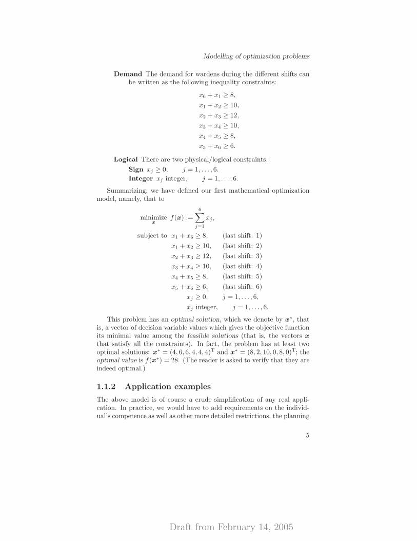
Example 1.1 (a staff planning problem) Consider a hospital ward whichoperates 24 hours a day. At different times of day, the staff requirementdiffers. Table 1.1 shows the demand for reserve wardens during six workshifts.
Shift 1 2 3 4 5 6Hours 0–4 4–8 8–12 12–16 16–20 20–24
Demand 8 10 12 10 8 6
Table 1.1: Staff requirements at a hospital ward.
Each member of staff works in 8 hour shifts. The goal is to fulfill thedemand with the least total number of reserve wardens.
Consider now the following interpretation of the term “to optimize:”
To optimize = to do something as well as is possible.
Draft from February 14, 2005
Modelling and classification
We utilize this description to identify the mathematical problem associ-ated with Example 1.1; in other words, we create a mathematical modelof the above problem.
Do something We identify, in the decision problem, activities whichwe can control and influence. Each such activity is associated witha variable whose value (or, activity level) is to be decided upon(that is, optimized). The remaining quantities are constants in theproblem.
Well How good a vector of activity levels is is measured by a real-valuedfunction of the variable values. This quantity is to be given a high-est or lowest value, that is, we minimize or maximize, dependingon our goal; this defines the objective function.
Possible Normally, the activity levels cannot be arbitrarily large, sincean activity often is associated with the utilization of resources(time, money, raw materials, labour, etcetera) that are limited;there may also be requirements of a least activity level, resultingfrom a demand. Some variables must also fulfill technical/logicalrestrictions, and/or relationships among themselves. The formercan be associated with a variable necessarily being integer-valuedor non-negative, by definition. The latter is the case when prod-ucts are blended, a task is performed for several types of products,or a process requires the input from more than one source. Theserestrictions on activities form constraints on the possible choicesof the variable values.
Looking again at the problem described in Example 1.1, this is thenour declaration of a mathematical model thereof:
Variables We define
xj := number of reserve wardens whose first shift is j,
j = 1, 2, . . . , 6.
Objective function We wish to minimize the total number of reservewardens, that is, the objective function, which we call f , is to
minimize f(x) := x1 + x2 + · · · + x6 =
6∑
j=1
xj .
Constraints There are two types of constraints:
4
Draft from February 14, 2005
Modelling of optimization problems
Demand The demand for wardens during the different shifts canbe written as the following inequality constraints:
x6 + x1 ≥ 8,
x1 + x2 ≥ 10,
x2 + x3 ≥ 12,
x3 + x4 ≥ 10,
x4 + x5 ≥ 8,
x5 + x6 ≥ 6.
Logical There are two physical/logical constraints:
Sign xj ≥ 0, j = 1, . . . , 6.
Integer xj integer, j = 1, . . . , 6.
Summarizing, we have defined our first mathematical optimizationmodel, namely, that to
minimizex
f(x) :=
6∑
j=1
xj ,
subject to x1 + x6 ≥ 8, (last shift: 1)
x1 + x2 ≥ 10, (last shift: 2)
x2 + x3 ≥ 12, (last shift: 3)
x3 + x4 ≥ 10, (last shift: 4)
x4 + x5 ≥ 8, (last shift: 5)
x5 + x6 ≥ 6, (last shift: 6)
xj ≥ 0, j = 1, . . . , 6,
xj integer, j = 1, . . . , 6.
This problem has an optimal solution, which we denote by x∗, thatis, a vector of decision variable values which gives the objective functionits minimal value among the feasible solutions (that is, the vectors x
that satisfy all the constraints). In fact, the problem has at least twooptimal solutions: x∗ = (4, 6, 6, 4, 4, 4)T and x∗ = (8, 2, 10, 0, 8, 0)T; theoptimal value is f(x∗) = 28. (The reader is asked to verify that they areindeed optimal.)
1.1.2 Application examples
The above model is of course a crude simplification of any real appli-cation. In practice, we would have to add requirements on the individ-ual’s competence as well as other more detailed restrictions, the planning
5
Draft from February 14, 2005
Modelling and classification
horizon is usually longer, employment rules and other conditions apply,etcetera, which all contribute to a more complex model. We mention afew successful applications of staffing problems below.
Example 1.2 (applications of staffing optimization problems) (a) It hasbeen reported that a 1990 staffing problem application for the Montrealmunicipality bus company, employing 3,000 bus drivers and 1,000 metrodrivers and ticket salespersons and guards, saved some 4 million Cana-dian dollars per year.
(b) Together with the San Francisco police department a group ofoperations research scientists developed in 1989 a planning tool basedon a heuristic solution of the staff planning and police vehicle allocationproblem. It has been reported that it gave a 20% faster planning andsavings in the order of 11 million US dollars per year.
(c) In an application from 1986, scientists collaborating with UnitedAirlines considered their crew scheduling problem. This is a very com-plex problem, where the time horizon is long (typically, 30 minute inter-vals during 7 days), and the constraints that define a feasible pattern ofallocating staff to airplanes are defined by, among others, complicatedwork regulations. The savings reported then was 6 million US dollars peryear. The company Carmen Systems AB in Gothenburg develops andmarkets such a tool; buyers include American Airlines, Lufthansa, SAS,and SJ; this company has one of the largest concentrations of optimizersin Sweden.
Remark 1.3 (on the complexity of the variable definition) The variablesxj defined in Example 1.1 are decision variables; we say that, since theselection of the values of these variables are immediately connected tothe decisions to be made in the decision problem, and they also contain,within their very definition, a substantial amount of information aboutthe problem at hand (such as shifts being eight hours long).
In the application examples discussed in Example 1.2 the variabledefinitions are much more complex than in our simple example. A typ-ical decision variable arising in a crew scheduling problem is associatedwith a specific staff member, his/her home base, information about thecrew team he/she works with, a current position in time and space, aflight leg specified by flight number(s), additional information about thestaff member’s previous work schedule and work contract, and so on.The number of possible combinations of work schedules for a given staffmember is nowadays so huge that not all variables in a crew schedul-ing problem can even be defined! (That is, the complete problem wewish to solve cannot be written down.) The philosophy in solving acrew scheduling problem is instead to algorithmically generate variables
6
Draft from February 14, 2005
Modelling of optimization problems
that one believes may receive a non-zero optimal value, and most of thecomputational effort lies in defining and solving good variable genera-tion problems, whose result is (part of) a feasible work schedule for givenstaff member. The term column generation is the operations researcher’sname for this process of generating variables in a decision problem.
Remark 1.4 (non-decision variables) Not all variables in a mathemati-cal optimization model are decision variables:
In linear programming, we will utilize slack variables whose role is totake on the difference between the left-hand and the right-hand side ofan inequality constraint; the slack variable thereby aids in the transfor-mation of the inequality constraint to an equality constraint, which ismore appropriate to work with in linear programming.
Other variables can be introduced into a mathematical model simplyin order to make the model more easy to state or interpret, or to improveupon the properties of the model. As an example of the latter, considerthe following simple problem: we wish to minimize over R the specialone-variable function f(x) := maximum {x2, x + 2}. (Plot the functionto see where the optimum is.) This is an example of a non-differentiablefunction: at x = −2, for example, both the functions f1(x) := x2 andf2(x) := x+2 define the value of the function f , but they have differentderivatives there. One way to turn this problem into a differentiable oneis by introducing an additional variable. We let z take on the value ofthe largest of f1(x) and f2(x) for a given value of x, and instead writethe problem as that to minimize z, subject to z ∈ R, x ∈ R, and theadditional constraints that x2 ≤ z and x + 2 ≤ z. Convince yourselfthat this transformation is equivalent to the original problem in termsof the set of optimal solutions in x, and that the transformed problemis differentiable.
Figure 1.1 illustrates several issues in the modelling process, whichare forthwith discussed.
The decision problem faced in the “fluffy” reality is turned into anoptimization model, through a process with several stages. By commu-nicating with those who have raised the issue of solving the problem inthe first place, one reaches an understanding about the problem to besolved. In order to identify and describe the components of a mathe-matical model which is also tractable, it is often necessary to simplifyand also limit the problem somewhat, and to quantify any remainingqualitative statements.
The modelling process does not come without difficulties. The com-munication can often be difficult, simply because the two parties speakdifferent languages in terms of describing the problem. The optimization
7
Draft from February 14, 2005
Modelling and classification
CommunicationSimplificationQuantification
Limitation
Data
Modification
Algorithms
Interpretation
Reality
Evaluation
Optimization model Results
Figure 1.1: Flow chart of the modelling process
problem quite often have uncertainties in the data, which moreover arenot always easy to collect or to quantify. Perhaps the uncertainties arethere for a purpose (such as in financial decision problems), but it maybe that the data is uncertain because not enough effort has been putinto providing a good enough accuracy. Further, there is often a conflictbetween problem solvability and problem realism.
The problem actually solved through the use of an optimizationmethodology must be supplied with data, providing model constantsand parameters in functions describing the objective function and per-haps also some of the constraints. For this optimization problem, anoptimization algorithm then yields a result in the form of an optimalvalue and/or optimal solution, if an optimal solution exists. This re-sult is then interpreted and evaluated, which may lead to alterations ofthe model, and certainly to questions regarding the applicability of theoptimal solution. The optimization model can also be altered slightlyon purpose in order to answer “what if?” type questions, for examplesensitivity analysis questions concerning the effect of small variations indata.
The final problems that we will mention come at this stage: it iscrucial that the interpretation of the result makes sense to those whowants to use the solution, and, finally, it must be possible to transfer thesolution back into the “fluffy” world where the problem came from.
The art of forming good optimization models is as much an art as ascience, and an optimization course can only really cover the latter. Onthe other hand, this part of the modelling process should not be glossed
8
Draft from February 14, 2005
A quick glance at optimization history
over; it is often possible to construct more than one form of an mathemat-ical model that represents the same problem equally accurately, and thecomputational complexity can differ substantially between them. Form-ing a good model is in fact as crucial to the success of the application asthe modelling exercise itself.
Optimization problems can be grouped together in classes, accordingto their properties. According to this classification, the staffing problemis a linear integer optimization problem. In Section 1.3 we present themajor distinguishing factors between different problem classes.
1.2 A quick glance at optimization history
At Chalmers, the courses in optimization are mainly given at the math-ematics department. “Mainly” is the important word here, becausecourses that have a substantial content of optimization theory and/ormethodology can be found also at other departments, such as com-puter science, the mechanical, industrial and chemical engineering de-partments, and at the Gothenburg School of Economics. The reason isthat optimization is so broad in its applications.
From the mathematical standpoint, optimization, or mathematicalprogramming as it is sometimes called, rests on several legs: analysis,topology, algebra, discrete mathematics, etcetera, build the foundationof the theory, and applied mathematics subjects such as numerical anal-ysis and mathematical parts of computer science build the bridge tothe algorithmic side of the subject. On the other side, then, with opti-mization we solve problems in a huge variety of areas, in the technical,natural, life and engineering sciences, and in economics.
Before moving on, we would just like to point out that the term“program” has nothing to do with “computer program;” a program isunderstood to be a “decision program,” that is, a strategy or decisionrule. A “mathematical program” therefore is a mathematical problemdesigned to produce a decision program.
The history of optimization is also very long. Many very oftengeometrical or mechanical problems (and quite often related to war-fare!) that Archimedes, Euclid, Heron, and other masters from antiq-uity formulated and also solved, are optimization problems. For ex-ample, we mention the problem of maximizing the volume of a closedthree-dimensional object (such as a sphere or a cylinder) built from atwo-dimensional sheet of metal with a given area.
The masters of two millenia later, like Bernoulli, Lagrange, Euler, andWeierstrass developed variational calculus, studying problems in appliedphysics (and still often with a mind towards warfare!) such as how to
9
Draft from February 14, 2005
Modelling and classification
find the best trajectory for a flying object.
The notion of optimality and especially how to characterize an opti-mal solution, began to be developed at the same time. Characterizationsof various forms of optimal solutions are indeed a crucial part of any basicoptimization course.
The scientific subject operations research refers to the study of deci-sion problems regarding operations, in the sense of controlling complexsystems and phenomena. The term was coined in the 1940s at the heightof World War 2 (WW2), when the US and British military commandshired scientists from several disciplines in order to try to solve complexproblems regarding the best way to construct convoys in order to avoid,or protect the cargo ships from, enemy (read: German) submarines,how to best cover the British isles with radar equipment given the scarceavailability of radar systems, and so on. The multi-disciplinarity of thesequestions, and the common topic of maximizing or minimizing some ob-jective subject to constraints, can be seen as being the defining momentof the scientific field. A better term than operations research is decisionscience, which better reflects the scope of the problems that can be, andare, attacked using optimization methods.
Among the scientists that took part in the WW2 effort in the USand Great Britain, some were the great pioneers in placing optimizationon the map after WW2. Among them, we find several researchers inmathematics, physics, and economics, who contributed greatly to thefoundations of the field as we now know it. We mention just a few here.George W. Dantzig invented the simplex method for solving linear op-timization problems during his WW2 efforts at Pentagon, as well as thewhole machinery of modelling such problems.1 Dantzig was originallya statistician and famously, as a young Ph.D. student, provided solu-tions to some then unsolved problems in mathematical statistics thathe found on the blackboard when he arrived late to a lecture, believ-ing they were home work assignments in the course. Building on theknowledge of duality in the theory of two-person zero-sum games, whichwas developed by the world-famous mathematician John von Neumannin the 1920s, Dantzig was very much involved in developing the theoryof duality in linear programming, together with the various characteri-zations of an optimal solution that is brought out from that theory. Alarge part of the duality theory was developed in collaboration with themathematician Albert W. Tucker.
1As Dantzig explains in [Dan57], linear programming formulations in fact can firstbe found in the work of the first theoretical economists in France, such as F. Quesnayin 1760; they explained the relationships between the landlord, the peasant and theartisan. The first practical linear programming problem solved with the simplexmethod was the famous diet problem.
10
Draft from February 14, 2005
Classification of optimization models
Several researchers interested in national economics studied trans-portation models at the same time, modelling them as special linearoptimization problems. Two of them, the mathematician Leonid W.Kantorovich and the statistician Tjalling C. Koopmans received TheBank of Sweden Prize in Economic Sciences in Memory of Alfred Nobelin 1975 “for their contributions to the theory of optimum allocation ofresources.” They had, in fact, both worked out some of the basics of lin-ear programming, independently of Dantzig, at roughly the same time.(Dantzig stands out among the three especially for creating an efficientalgorithm for solving such problems.)2
1.3 Classification of optimization models
We here develop a subset of problem classes that can be set up by con-trasting certain aspects of a general optimization problem. We let
x ∈ Rn : vector of decision variables xj , j = 1, 2, . . . , n;
f : Rn → R ∪ {±∞} : objective function;
X ⊆ Rn : ground set defined logically/physically;
gi : Rn → R : constraint function defining restriction on x :
gi(x) ≥ bi, i ∈ I; (inequality constraints)
gi(x) = di, i ∈ E . (equality constraints)
We let bi ∈ R (i ∈ I) and di ∈ R (i ∈ E) denote the right-hand sidesof these constraints; without loss of generality, we could actually letthem all be equal to zero, as any constants can be incorporated into thedefinitions of the functions gi (i ∈ I ∪ E).
The optimization problem then is to
minimizex
f(x), (1.1a)
subject to gi(x) ≥ bi, i ∈ I, (1.1b)gi(x) = di, i ∈ E , (1.1c)
x ∈ X. (1.1d)
(If it is really a maximization problem, then we change the sign of f .)
2Incidentally, several other laureates in economics have worked with the tools ofoptimization: Paul A. Samuelson (1970, linear programming), Kenneth J. Arrow(1972, game theory), Wassily Leontief (1973, linear transportation models), GerardDebreu (1983, game theory), Harry M. Markowitz (1990, quadratic programming infinance), John F. Nash Jr. (1994, game theory), William Vickrey (1996, economet-rics), and Daniel L. McFadden (2000, microeconomics).
11
Draft from February 14, 2005
Modelling and classification
The problem type depends on the nature of the functions f and gi,and the set X . Let us look at some examples.
(LP) Linear programming Objective function linear: f(x) = cTx =∑nj=1 cjxj (c ∈ Rn); constraint functions affine: gi(x) = aT
i x − bi(ai ∈ Rn, bi ∈ R, i ∈ I ∪ E)); X = {x ∈ Rn | xj ≥ 0, j = 1, 2, . . . , n }.
(NLP) Nonlinear programming Some function(s) f, gi (i ∈ I ∪ E)are nonlinear.
Continuous optimization f, gi (i ∈ I∪E) are continuous on an openset containing X ; X is closed and convex.
(IP) Integer programming X ⊆ {0, 1}n (binary) or X ⊆ Zn (inte-ger).
Unconstrained optimization I ∪ E = ∅; X = Rn.
Constrained optimization I ∪ E 6= ∅ and/or X ⊂ Rn.
Differentiable optimization f, gi (i ∈ I ∪ E) are at least once con-tinuously differentiable on an open set containing X (that is, “in C1
on X ,” which means that ∇f and ∇gi (i ∈ I ∪ E) exist there and thegradients are continuous); further, X is closed and convex.
Non-differentiable optimization At least one of f, gi (i ∈ I ∪ E) isnon-differentiable.
(CP) Convex programming f is convex; gi (i ∈ I) are concave; gi
(i ∈ E) are affine; and X is closed and convex.
Non-convex programming The complement of the above
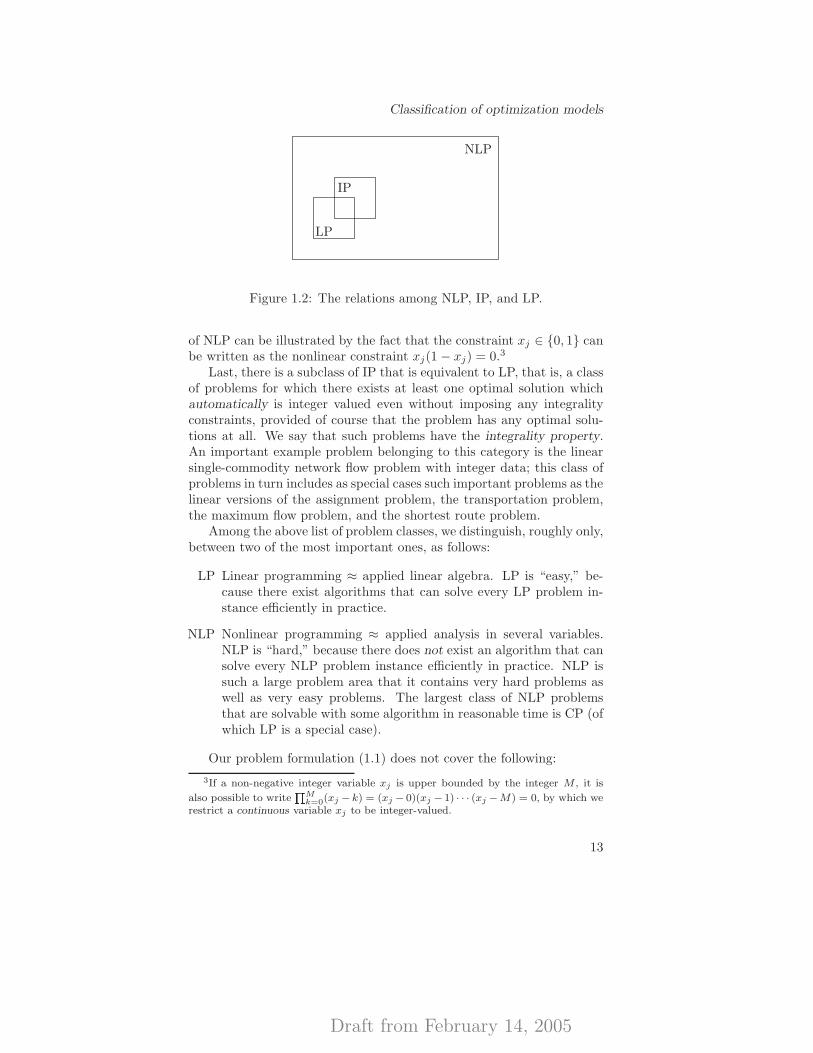
In Figure 1.2 we show how the problem types NLP, IP, and LP arerelated.
That LP is a special case of NLP is clear by the fact that a linearfunction is a special kind of nonlinear function; that IP is a special case
12
Draft from February 14, 2005
Classification of optimization models
NLP
IP
LP
Figure 1.2: The relations among NLP, IP, and LP.
of NLP can be illustrated by the fact that the constraint xj ∈ {0, 1} canbe written as the nonlinear constraint xj(1 − xj) = 0.3
Last, there is a subclass of IP that is equivalent to LP, that is, a classof problems for which there exists at least one optimal solution whichautomatically is integer valued even without imposing any integralityconstraints, provided of course that the problem has any optimal solu-tions at all. We say that such problems have the integrality property.An important example problem belonging to this category is the linearsingle-commodity network flow problem with integer data; this class ofproblems in turn includes as special cases such important problems as thelinear versions of the assignment problem, the transportation problem,the maximum flow problem, and the shortest route problem.
Among the above list of problem classes, we distinguish, roughly only,between two of the most important ones, as follows:
LP Linear programming ≈ applied linear algebra. LP is “easy,” be-cause there exist algorithms that can solve every LP problem in-stance efficiently in practice.
NLP Nonlinear programming ≈ applied analysis in several variables.NLP is “hard,” because there does not exist an algorithm that cansolve every NLP problem instance efficiently in practice. NLP issuch a large problem area that it contains very hard problems aswell as very easy problems. The largest class of NLP problemsthat are solvable with some algorithm in reasonable time is CP (ofwhich LP is a special case).
Our problem formulation (1.1) does not cover the following:
3If a non-negative integer variable xj is upper bounded by the integer M , it is
also possible to writeQM
k=0(xj − k) = (xj − 0)(xj − 1) · · · (xj −M) = 0, by which werestrict a continuous variable xj to be integer-valued.
13
Draft from February 14, 2005
Modelling and classification� infinite-dimensional problems (that is, problems formulated in func-tional spaces rather than vector spaces);� implicit functions f and/or gi (i ∈ I∪E): then, no explicit formulacan then be written down; this is typical in engineering applica-tions, where the value of, say, f(x) can be the result of a simulation;� multiple-objective optimization:
“minimize {f1(x), f2(x), . . . , fp(x)}”;� optimization under uncertainty, or, stochastic programming (thatis, where some of f , gi (i ∈ I∪E) are only known probabilistically).
1.4 Conventions
Let us denote the set of vectors satisfying the constraints (1.1b)–(1.1d)by S ⊆ Rn, that is, the set of feasible solutions to the problem (1.1).What exactly do we mean by solving the problem to
minimizex∈S
f(x)? (1.2)
Since there is no explicit operation involved here, the question is war-ranted. The following two operations are however well-defined:
f∗ := infimumx∈S
f(x)
denotes the infimum value of the function f over the set S; if and onlyif the infimum value is attained at some point x∗ in S (and then bothf∗ and x∗ necessarily are finite) we can write that
f∗ := minimumx∈S
f(x), (1.3)
and then we of course have that f(x∗) = f∗. (When considering maxi-mization problems, we obtain the analogous definitions of the supremumand the maximum.)
The second operation defines the set of optimal solutions to the prob-lem at hand:
S∗ := arg minimumx∈S
f(x);
the set S∗ ⊆ S is nonempty if and only if the infimum value f∗ isattained. Finding at least one optimal solution,
x∗ ∈ argminimumx∈S
f(x), (1.4)
14
Draft from February 14, 2005
Conventions
is a special case which moreover defines an often much more simple task.
As an example, consider the problem instance where S = { x ∈ R |x ≥ 0 } and
f(x) =
{1/x, if x > 0,
+∞, otherwise.
For this problem f∗ = 0 but S∗ = ∅, because the value 0 is not attainedfor a finite value of x—the problem has a finite infimum value but notan optimal solution.
These examples lead to our convention in reading the problem (1.2):the statement “solve the problem (1.2)” means “find f∗ and an x∗ ∈ S∗,or conclude that S∗ = ∅.”
Hence, it is implicit in the formulation that we are interested bothin the infimum value and in (at least) one optimal solution if one exists.Whenever we are certain that only one of the two is of interest thenwe will state so explicitly. We are aware that the formulation has, inthe past, been considered “vague” since no operation is visible; so, tosummarize and clarify our convention, it in fact includes two operations,(1.3) and (1.4).
There is a second reason for stating the optimization problem (1.1)in the way it is, a reason which is computational. To solve the problem,we almost always need to solve a sequence of relaxations/simplificationsof the original problem in order to eventually reach a solution. (Theseproblem manipulations include Lagrangian relaxation, penalization, andobjective function linearization, which will be developed later on.) Whendescribing the particular relaxation/simplification utilized, having accessto constraint identifiers [such as (1.1c)] certainly makes the presentationeasier and clearer. That will become especially valuable when dealingwith various forms of duality, when (subsets of) the constraints are re-laxed.
A last comment on conventions: as it is stated prior to the prob-lem formulation (1.1) the objective function f can in general take onboth ±∞ as values. Since we are generally going to study minimiza-tion problem, we will only be interested in objective functions f havingthe properties that (a) f(x) 6= −∞ for every feasible vector x, and (b)f(x) < +∞ for at least one feasible vector x. Such functions are knownas proper functions (which makes sense, as it is impossible to performa proper optimization unless these two properties hold). We will sometimes refer to these properties, in particular by stating explicitly when fcan take on the value +∞, but we will assume throughout that f doesnot take on the value −∞. So, in effect then, we assume implicitly thatthe objective function f is proper.
15
Draft from February 14, 2005
Modelling and classification
1.5 Applications and modelling examples
To give but a quick view of the scope of applications of optimization, hereis a subset of the past few years of applied master’s or doctoral projects,performed either at Linkoping University or at Chalmers University ofTechnology:� Planning routes for snow removal machines� Planning routes for disabled persons transportation� Planning of production of energy in power plants� Scheduling production and distribution of electricity� Scheduling of empty freight cars in railways� Scheduling log cutting in forests� Optimizing paper production in paper mills� Scheduling paper cutting in paper mills� Optimization of engine performance for aircraft, boats, and cars� Portfolio optimization under uncertainty for pension funds� Analysis of investment in future energy systems� Network design for mobile telecommunication, optical and internet
protocol networks� Optimal wave-length and routing in optimal networks� Scheduling of production of circuit boards� Scheduling of time tables in schools� Optimal packing and distribution of gas� Bin packing of objects in freight cars, truck, and cargo ships� Routing of vehicles for road carriers� Optimal congestion pricing in urban traffic networks
1.6 Defining the field
To define what the subject area of optimization encompasses is difficult,given that it is connected to so many scientific areas in the natural andtechnical sciences.
An obvious distinguishing factor is that an optimization model alwayshas an objective function and a group of constraints. On the other handby letting f ≡ 0 and E = ∅ then the generic problem (1.1) is thatof a feasibility problem for equality constraints, and by instead lettingI ∪E = ∅ we obtain an unconstrained optimization problem. Both thesespecial cases are classic problems in numerical analysis, which most oftendeal with the solution of a linear or non-linear system of equations.
16
Draft from February 14, 2005
Soft and hard constraints
We can here identify a distinguishing element between optimizationand numerical analysis—that an optimization problem often involve in-equality constraints while a problem in numerical analysis does not. Whydoes that make a difference? The reason is that while in the lattercase the analysis is performed on a manifold—possibly even a linearsubspace—the analysis of an optimization problem must deal with thefact that there are feasible regions residing in different dimensions be-cause of the nature of inequality constraints being either active or inac-tive. As a result, there will always be some kind of non-differentiabilitiespresent in some associated functionals, while numerical analysis typicallyis “smooth.”
As an illustration, although this is beyond the scope of this book, weask the reader to ask herself what the proper extension of the famousImplicit Function Theorem is when we replace the system h(x,y) = 0ℓ
with, say, h(x,y) ≤ 0m?
1.7 Soft and hard constraints
1.7.1 Definitions
So far, we have not discussed much about the role of different types ofconstraints. In the set covering problem, for example, the constraintsare of the form
∑nj=1 aijxj ≥ 1, i = 1, 2, . . . ,m, where aij ∈ {0, 1}.
These, as well as constraints of the form xj ≥ 0 and xj ∈ {0, 1} are hardconstraints, meaning that if they are violated then the solution does notmake much sense. Typical such constraints are technological ones; forexample, if xj is associated with the level of production, then a negativevalue has no meaning, and therefore a negative value is never acceptable.A binary variable, xj ∈ {0, 1}, is often logical, associated with the choicebetween something being “on” or “off,” such as a production facility, acity being visited by a traveling salesman, and so on; again, a fractionalvalue like 0.7 makes no sense, and binary restrictions almost always arehard.
Consider now a collection of constraints that are associated with thecapacity of production, and suppose it has the form
∑nj=1 uijxij ≤ ci, i =
1, 2, . . . ,m, where xij denotes the level of production of an item/productj using a production process i, uij is a positive number associated withthe use of a resource (man hours, hours before inspection of the machine,etcetera) per unit of production of the item, and ci is the available ca-pacity of this resource in the production process. In some circumstances,it is not unnatural to allow for the left-hand side to become larger thanthe capacity, because that production plan might still be feasible, pro-
17
Draft from February 14, 2005
Modelling and classification
vided however that additional resources are made available. We considertwo types of ways to allow for this violation, and which give rise to twodifferent types of solution.
The first, which we are not quite ready to discuss here from a tech-nical standpoint, is connected to the Lagrangian relaxation of the ca-pacity constraints. If, when solving the corresponding Lagrangian dualoptimization problem, we terminate the solution process prematurely,we will typically have a terminal primal vector that violates some ofthe capacity constraints slightly. Since the capacity constraints are soft,this solution may be acceptable.4 See Chapter 6 for further details onLagrangian duality.
Since it is however natural that additional resources come only at anadditional cost, an increase in the violation of this soft constraint shouldhave the effect of an additional, increasing cost in the objective function.In other words, violating a constraint should come with a penalty. Givena measure of the cost of violating the constraints, that is, the unit costof additional resource, we may transform the resulting problem to anunconstrained problem with a penalty function representing the originalconstraint.
Below, we relate soft constraints to exterior penalties.
1.7.2 A derivation of the exterior penalty function
Consider the standard nonlinear programming problem to
minimizex
f(x), (1.5a)
subject to gi(x) ≥ 0, i = 1, . . . ,m, (1.5b)
where f and gi (i = 1, . . . ,m) are real-valued functions.Consider the following relaxation of (1.5), where ρ > 0:
minimize(x ,s)
f(x) + ρ
m∑
i=1
si, (1.6a)
subject to gi(x) ≥ −si, i = 1, . . . ,m, (1.6b)
si ≥ 0, i = 1, . . . ,m. (1.6c)
We interpret this problem as follows: by allowing the variable si tobecome positive, we allow for extra slack in the constraint, at a positivecost, ρsi, proportional to the violation.
4One interesting application arises when making capacity expansion deci-sions in production and work force planning problems (e.g., Johnson and Mont-gomery [JoM74, Example 4-14]) and in forest management scheduling (Hauer andHoganson [HaH96]).
18
Draft from February 14, 2005
A road map through the material
How do we solve this problem, for a given value of ρ > 0? Whatwe will develop below is a specialization of the following result (see, forexample, [RoW97, Proposition 1.35]): for a function φ : Rn × Rm →R ∪ {+∞} one has in terms of p(s) = infimumx φ(x, s) and q(x) =infimums φ(x, s) that
infimum(x ,s)
φ(x, s) = infimumx
q(x) = infimums
p(s).
In other words, we can solve an optimization problem in two types ofvariables x and s by “eliminating” one of them (in our case, s) throughoptimization, and then determine the best value of the remaining one.
Suppose then that we for a moment keep x fixed to an arbitraryvalue. The above problem (1.6) then reduces to that to
minimizes
ρ
m∑
i=1
si, (1.7a)
subject to si ≥ −gi(x), i = 1, . . . ,m, (1.7b)
si ≥ 0, i = 1, . . . ,m, (1.7c)
which clearly separates into the m independent problems to
minimizesi
ρsi, (1.8a)
subject to si ≥ −gi(x), (1.8b)
si ≥ 0. (1.8c)
This problem is trivially solvable: si := maximum {0,−gi(x)}, that is, si
takes on the role of a slack variable for the constraint. Replacing si withthis expression in x in the problem (1.6) we finally obtain the problemto
minimizex
f(x) + ρ
m∑
i=1
maximum {0,−gi(x)}, (1.9a)
subject to x ∈ Rn. (1.9b)
If the constraints instead are of the form gi(x) ≤ 0, then the resultingpenalty function is of the form ρ
∑mi=1 maximum {0, gi(x)}.
See Section 13.1 for a thorough discussion on and analysis of penaltyfunctions and methods.
1.8 A road map through the material
Chapter 2 gives a short overview of some basic material from calculusand linear algebra that is used throughout the book. Familiarity withthese topics is therefore very important.
19
Draft from February 14, 2005
Modelling and classification
Chapter 3 is devoted to the study of convexity, a subject known asconvex analysis. We characterize the convexity of sets and real-valuedfunctions and show their relations. We provide an overview of the spe-cial convex sets called polyhedra, which can be described by linear con-straints. Parts of the theory covered, such as the Representation Theo-rem, Farkas’ Lemma and the Separation Theorem, build the foundationof the study of optimality conditions in Chapter 5, the theory of strongduality in Chapter 6 and of linear programming in Chapters 7–10.
Chapter 4 gives a gentle overview of topics associated with optimal-ity, including the very important result that locally optimal solutionsare globally optimal solution in a convex problem. We establish basicresults regarding the existence of optimal solutions, including the famousWeierstrass Theorem, and establish basic logical relationships betweenlocally optimal solutions and characterizations in terms of conditionsof “stationarity”. The latter includes the standard result in differen-tiable, unconstrained optimization that says that a locally optimal solu-tion must have the property that the gradient of the objective functionthere is zero. Along the way, we define important concepts such as thenormal cone, the variational inequality, and the Euclidean projection ofa vector onto a convex set, and outline fixed point theorems and theirapplications.
Chapter 5 collects results leading up to the central Karush–Kuhn–Tucker (KKT) Theorem on the necessary conditions for the local opti-mality of a feasible point in a constrained optimization problem. Es-sentially, these conditions state that a given feasible vector x can onlybe a local minimum if it is feasible in the problem and if there is nodescent direction at x which simultaneously is a feasible direction. Inorder to state the KKT conditions in algebraic terms such that it can bechecked in practice and such that as few interesting vectors x as possiblesatisfy them, we must restrict our study to problems and vectors satis-fying some regularity properties. These properties are called constraintqualifications (CQs); among them, the classic one is that “the active con-straints are linearly independent” which is familiar from the LagrangeMultiplier Theorem in differential calculus. Our treatment however ismore general and covers weaker (that is, better) CQs as well. The chap-ter begins with a schematic road map for these results to further help inthe study of this material.
Chapter 6 presents a rather broad picture of the theory of Lagrangianduality. Associated with the KKT conditions in the previous chapter isa vector, known as the Lagrange multiplier vector, denoted µ (λ) for in-equality (equality) constraints. The Lagrange multipliers are associatedwith an optimization problem which is referred to as the Lagrangian
20
Draft from February 14, 2005
A road map through the material
dual, or simply dual, problem.5 The role of the dual problem is to definea largest lower bound on the primal value f∗ of the primal (original)problem. This chapter establishes the basic properties of this dual prob-lem. In particular, it is always a convex problem. It is therefore anappealing problem to solve in order to extract the optimal solution tothe primal problem. This chapter is in fact almost entirely devoted tothe topic of analyzing when it is possible to generate, from an optimaldual solution µ∗, in a rather simple manner an optimal primal solutionx∗. The most important term in this context then is “strong duality”which refers to the occasion when the optimal values in the two problemsare equal—only then is the “translation” relatively easy. Some of theresults established here are immediately transferable to the importantcase of linear programming, so the link between this chapter and Chap-ter 10 is very strong. The main difference is that in the present chapterwe must work with more general tools, while for linear programming wehave access to a more specialized analysis; therefore, proof techniques,for example in establishing the Strong Duality Theorem, will be quite dif-ferent. Additional topics include an analysis of optimization algorithmsfor the solution of the Lagrangian dual problem, and sensitivity analysiswith respect to changes in the right-hand sides of inequality constraints.
Chapters 7–10 are devoted to the study of linear programming (LP)models and methods. Its importance is unquestionable: it has beenstated that in the 1980s LP problems was the scientific problem thatate the most computing power in the world. While the efficiency of LPsolvers have multiplied since then, so has the speed of computers, and LPmodels still define the most important problem area in optimization inpractice. (Partly, this is also due to the fact that integer programmingmodels, where some, or all, variables are required to take on integervalues, use LP techniques.) It is not only for this reason however thatwe devote special chapters to this topic. Their optimal solutions can befound using quite special techniques that are not common to nonlinearprogramming. As was shown in Chapter 3 linear programs have optimalsolutions at the extreme points of the polyhedral feasible set. This fact,together with the linearity of the objective function and the constraints,means that a feasible-direction (descent) method can be very cleverlydevised. Since we know that only extreme points are of interest, westart at one extreme point, and then only consider as candidate search
5The dual problem was first discovered in the study of (linear) matrix games byJohn von Neumann in the 1920s, but had for a long time implicitly been used also fornonlinear optimization problems before it was properly stated and studied by Arrow,Hurwicz, Uzawa, Everett, Falk, Rockafellar, etcetera, starting in earnest in the 1950s.By the way, the original problem is then referred to as the primal problem, a namegiven by George Dantzig’s father, a Greek scholar.
21
Draft from February 14, 2005
Modelling and classification
directions those that point towards another (in fact, adjacent) extremepoint. We can generate such directions extremely efficiently by usinga basis representation of the extreme points, and the move from oneextreme point to the other is then associated with a very simple basischange. This special procedure is known as the Simplex method, whichwas invented by George Dantzig in the 1940s.
In Chapter 7 a simple manufacturing problem is used to illustratethe basics of linear programming. The problem is graphically solvedand it turns out that the optimal solution is an extreme point. Weinvestigate how the optimal solution changes if the data of the problem ischanged, and the linear programming dual to the manufacturing problemis derived by using economical arguments.
Chapter 8 begins with a presentation of the axioms underlying the useof LP models, and a general modelling technique is discussed. The restof the chapter deals with the geometry of LP models. It is shown thatevery linear program can be transformed into the standard form whichis the form that the Simplex method uses. We introduce the conceptof basic feasible solution and discuss its connection to extreme points.A version of the Representation Theorem adapted to the standard formis presented, and we show that if there exists an optimal solution to alinear program in standard form, then there exists an optimal solutionamong the basic feasible solutions. Finally, we define adjacency betweenextreme points and give an algebraic characterization of adjacency whichactually proves that the Simplex method at each iteration step movesfrom one extreme point to an adjacent one.
Chapter 9 presents the Simplex method. First it is assumed thata basic feasible solution (BFS) is known at the start of the algorithm,and then we describe what to do when a BFS is not known from thebeginning. Termination characteristics of the algorithm is discussed andit is shown that if all the BFSs of the problem are non-degenerate, thenthe basic algorithm terminates. However, if there exist degenerate BFSsthere is a possibility that the basic algorithm cycles between degenerateBFSs and hence never terminates. We give a simple rule, called Bland’srule, that eliminates cycling. We close the chapter by discussing thecomputational complexity of the Simplex algorithm.
In Chapter 10 linear programming duality is studied. We discusshow to construct the linear programming dual to a general linear pro-gram and present duality theory, such as weak and strong duality andcomplementary slackness. The dual simplex method is developed, andwe discuss how the optimal solution of a linear program changes if theright-hand side or the objective function coefficients are modified.
Chapter 11 presents basic algorithms for differentiable, unconstrained
22
Draft from February 14, 2005
A road map through the material
optimization problems. The typical optimization algorithm is iterative,which means that a solution is approached through a sequence of trialvectors, typically such that each consecutive objective value is strictlylower than the previous one in a minimization problem. This improve-ment is possible because we can generate improving search directions—descent (ascent) directions in a minimization (maximization) problem—by means of solving an approximation of the original problem or the op-timality conditions. This approximate problem (for example, the systemof Newton equations) is then combined with a line search, which approx-imately solve the original problem over the line segment defined by thecurrent iterate and the search direction. This idea of combining approx-imation (or, relaxation) with a line search (or, coordination) is the basicmethodology also for constrained optimization problems. Also, whileour opinion is that the subject of differentiable unconstrained optimiza-tion largely is a subject within numerical analysis rather than within theoptimization field, its understanding is important because the approx-imations/relaxations that we utilize in constrained optimization oftenresult in (essentially) unconstrained optimization subproblems. We de-velop a class of quasi-Newton methods in detail, to illustrate a classicanalysis.
Chapter 12 presents some natural algorithms for differentiable nonlin-ear optimization over polyhedral sets, which utilize LP techniques whensearching for an improving direction. The basic algorithm is known asthe Frank–Wolfe algorithm, or the conditional gradient method; it uti-lizes ∇f(xk) as the linear cost vector at iteration k, and the directiontowards any optimal extreme point yk has already in Chapter 4 beenshown to be a feasible direction of descent whenever xk is not stationary.A line search in the line segment [xk,yk] completes an iteration. Becauseof the work involved in repeatedly solving LPs a natural improvementof this algorithm is to keep in memory all, or some of, the previouslygenerated extreme points y0,y1, . . . ,yk−1, and to generate the next it-eration point as the optimal solution within the convex hull of the unionof them, the current iterate xk and the new extreme point yk. The gra-dient projection method extends the steepest descent method for uncon-strained optimization problem in a natural manner. The subproblemshere are Euclidean projection problems which in this case are strictlyconvex quadratic programming problems that can be solved efficientlyfor some types of polyhedral sets. The convergence results reached showthat convexity of the problem is crucial in reaching good convergenceresults—not only regarding the global optimality of limit points but re-garding the nature of the set of limit points as well.
Chapter 13 begins by describing natural approaches to nonlinearly
23
Draft from February 14, 2005
Modelling and classification
constrained optimization problems, wherein all (or, a subset of) the con-straints are replaced by penalties. The resulting penalized problem isthen possible to solve by using techniques for unconstrained problems orproblems with convex feasible sets, like those we have presented in Chap-ters 11 and 12. In order to force the penalized problems to more and moreresemble the original one, the penalties are more and more strictly en-forced. There are essentially two types of penalty functions, exterior andinterior penalties. Exterior penalty methods were devised mainly in the1960s, and are perhaps the most natural ones; they are valid for almostevery type of explicit constraint, and is therefore amenable to solvingalso non-convex problems. The penalty terms are gradually enforced byletting larger and larger weights be associated with the constraints incomparison with the objective function. Under some circumstances, onecan show that a finite value of the these penalty parameters are needed,but in general they must tend to infinity. Therefore, these algorithmsare often burdened by numerical accuracy problems, which however, insome cases can be limited when Newton methods are used for the sub-problems. Interior penalty methods are also amenable to the solutionof non-convex problems, but are perhaps most naturally associated withconvex problems, where they are quite effective. In particular, the bestmethods for linear programming in terms of their worst-case complexityare interior point methods which are based on interior penalty functions.In this type of method, the interior penalties are asymptotes with respectto the constraint boundaries; a decreasing value of the penalty param-eters then allow for the boundaries to be approached at the same timeas the original objective function come more and more into play. Forboth types of methods, we reach convergence results on the convergenceto KKT points in the general case—including estimates of the Lagrangemultipliers—, and global convergence results in the convex case.
Chapter 13 continues by describing a basic and quite popular classof algorithms for general nonlinear programming problems with twicedifferentiable objective and constraint functions. It is called SequentialQuadratic Programming (SQP) and is, essentially, Newton’s method ap-plied to the KKT conditions of the problem; there are, however, somemodifications necessary. For example, because of the linearization of theconstraints, it is in general difficult to maintain feasibility in the pro-cess, and therefore convergence cannot merely be based on line searchesin the objective function; instead one must devise a measure of “good-ness” that take constraint violation into account. The classic approachis to utilize a penalty function so that a constraint violation comes witha price, and as such the SQP method ties in with the penalty methodsabove. Another approach which is gaining popularity is to use a type of
24
Draft from February 14, 2005
On the background of this book and a didactics statement
bi-criterion method where a new iterate is “accepted” based both on itsobjective value and its constraint violation; this is referred to as a filterSQP method. In any case, in this type of method one strives for feasibil-ity and optimality simultaneously, like Lagrangian relaxation methodsdo; in fact, there are strong relationships between the methods in thischapter and Lagrangian methods.
Each chapter ends with exercises on its contents, through numericalexamples or extensions of the theory developed; we have also includeda few previous exam questions from the course Applied Optimizationtought at Chalmers and Gothenburg University.
1.9 On the background of this book and a
didactics statement
This book’s foundation is the collection of lecture notes written by thethird author and used in basic optimization courses for about ten years atLinkoping University, Chalmers University of Technology, and Gothen-burg University. With the same lecturer the course Applied Optimiza-tion has been given at Chalmers University of Technology and Gothen-burg University since 1997, and the lecture notes have developed moreand more from one based on algorithms to one that mainly covers thefundamentals of optimization. With the addition of the first two authorshas come a further development of these fundamentals into the presentbook, in which also our didactic wishes has begun to come true.
The third author’s main inspiration in shaping the lecture notes andthe book came from the excellent text book by Bazaraa, Sherali, andShetty [BSS93]. The authors separate the basic theory (convexity, poly-hedral theory, separation, optimality, etcetera) from the algorithms de-vised for solving nonlinear optimization problems, and they develop thetheory based on first principles, in a natural order. (The book is how-ever too advanced to be used in a first optimization course, it does notcover linear programming, and the algorithmic part is getting old insome parts.)
In writing the book we have also made a few additional didactic de-velopments. In almost every text book on optimization the topic of linearoptimization is developed before that of nonlinear and convex optimiza-tion, and linear programming duality is developed before Lagrangianduality. Teaching in this order may however feel unnatural both for thelecturer and for the students: since Lagrangian duality is more general,but similar, to linear programming duality, the feeling is that more orless the same material is repeated, or, which is even worse, the feeling is
25
Draft from February 14, 2005
Modelling and classification
that linear programming is a rather strange special case that we developbecause we must, but not because it is an interesting topic. We have de-veloped the material in this book such that linear programming emergesas a natural special case of general convex programming, having a dual-ity theory which is even richer than that of general convex programmingduality.
In keeping with this idea of developing nonlinear programming beforelinear programming, we should also have covered the simplex method lastin the book. This is a possibly conflicting situation, because we believethat the simplex method should not be described merely as a feasible-direction method; its combinatorial nature is important, and the subjectof degeneracy is more naturally treated and understood by developingthe simplex method immediately following the development of the con-nections between the geometry and algebra of linear programming. Thishas been our choice, and we have consequently also decided that it-erative algorithms for general nonlinear optimization over convex sets,especially polyhedra, should be developed before those for more generalconstraints, the reason being that linear programming is an importantbasis for these algorithms.
1.10 Notes and further reading
Extensive collections of optimization applications and models can befound in several basic text books in operations research, such as [Wag75,BHM77, Mur95, Rar98, Tah03]. The optimization modelling book byWilliams [Wil99] is a classic, now in its fourth edition. Modelling booksalso exist for certain categories of applications; for example, the book[EHL01] concerns the mathematical modelling and solution of optimiza-tion problem arising in chemical engineering applications.
Several accounts have been written during the past few years on theorigins of operations research and mathematical programming, the rea-sons being that we recently celebrated the 50th anniversary of the simplexmethod (1997), the 80th birthday of its inventor George Dantzig (1994),the 50th anniversary of the creation of ORSA (the Operations ResearchSociety of America) (2002), and the 50th anniversary of the OperationalResearch Society (2003). The special issue of the journal OperationsResearch, vol. 50, no. 1 (2002), is filled with historical anecdotes, as isthe book History of Mathematical Programming ([LRS91]).
26
Draft from February 14, 2005
Exercises
1.11 Exercises
Exercise 1.1 (modelling, exam 980819) A new producer of perfume wishto get a break into a lucrative market. An exclusive fragrance, Chinelle,is to be produced and marketed for maximum profit. With the equip-ment available it is possible to produce the perfume using two alternativeprocesses, and the company also consider utilizing the services of a fa-mous model when launching it. In order to simplify the problem, letus assume that the perfume is manufactured by the use of two mainingredients—the first a secret substance called MO and the second amore well-known mixture of ingredients. The first of the two processesavailable provides three grams of perfume for every unit of MO and twounits of the standard substance, while the other process gives five gramsof perfume for every two (respectively, three) units of the two main in-gredients. The company has at its disposal manufacturing processes thatcan produce at most 20,000 units of MO during the planning period and35,000 units of the standard mixture. Every unit of MO costs threeEUR (it is manufactured in France) to produce, and the other mixtureonly two EUR per unit. One gram of the new perfume will cost fiftyEUR. Even without any advertising the company thinks they can sell1000 grams of the perfume, simply because of the news value. A famousmodel can be contracted for commercials, costing 5,000 EUR per photosession (which takes half an hour), and the company thinks that a cam-paign using his image can raise the demand by about 200 grams per halfhour of his time, but not exceeding three hours (he has too many otheroffers).
Formulate the problem of choosing the best production strategy asan LP problem.
Exercise 1.2 (modelling) A computer company has estimated the num-ber of service hours needed during the next five months, according toTable 1.2.
Month # Service hoursJanuary 6000February 7000March 8000April 9500May 11,500
Table 1.2: Number of service hours per month; Exercise 1.2.
The service is performed by hired technicians; their number is 50 at
27
Draft from February 14, 2005
Modelling and classification
the beginning of January. Each technician can work up to 160 hoursper month. In order to cover the future demand of technicians new onesmust be hired. Before a technician is hired he/she undergoes a period oftraining, which takes a month and requires 50 hours of supervision by atrained technician. A trained technician has a salary of 15,000 SEK permonth (regardless of the number of working hours) and a trainee has amonthly salary of 7500 SEK. At the end of each month on average 5%of the technicians quit to work for another company.
Formulate an LP problem whose optimal solution will minimize thetotal salary costs during the given time period, given that the numberof available service hours are enough to cover the demand.
Exercise 1.3 (modelling, exam 010821) The advertising agency ZAP (Zetter-strom, Anderson, and Pettersson) is designing their new office with anopen office space. The office is rectangular, with length l meters andwidth b meters. Somewhat simplified, we may assume that each workingspace requires a circle of diameter d and that the working spaces mustnot overlap. In addition, each working space must be connected to thetelecom and computer network at one of the two possible connectionpoints in the office. As the three telephones have limited cable lengths(the agency is concerned with the possible radiation danger associatedwith hands-free phones and therefore do not use cordless phones)—ai
meters, respectively, i = 1, . . . , 3—the work spaces must be placed quitenear the connection points.6 See Figure 1.3 for a simple picture of theoffice.
For simplicity we assume that the phone is placed at the center of thework place. One of the office’s walls is a large panorama window and thethree partners all want to sit as close as possible to it. Therefore, theydecide to try to minimize the distance to the window for the workplacethat is the furthest away from it.
Formulate the problem of placing the three work places so that themaximum distance to the panorama window is minimized, subject to allthe necessary constraints.
Exercise 1.4 (modelling, exam 010523) A large chain of department storeswants to build a number of distribution centers (warehouses) which willsupply 30 department stores with goods. They have 10 possible locationsto choose between. To build a warehouse at location i (i = 1, . . . , 10)costs ci MEUR and the capacity of a warehouse at that location wouldbe ki volume units per week. Department store j has a demand of ej vol-ume units per week. The distance between warehouse i and department
6All the money went to other interior designs of the office space, so there is nomoney left to buy more cable.
28
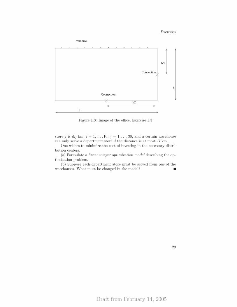
Draft from February 14, 2005
Exercises
Window
l
b
b/2
Connection
Connection
l/2
Figure 1.3: Image of the office; Exercise 1.3
store j is dij km, i = 1, . . . , 10, j = 1, . . . , 30, and a certain warehousecan only serve a department store if the distance is at most D km.
One wishes to minimize the cost of investing in the necessary distri-bution centers.
(a) Formulate a linear integer optimization model describing the op-timization problem.
(b) Suppose each department store must be served from one of thewarehouses. What must be changed in the model?
29

Draft from February 14, 2005
Modelling and classification
30
Draft from February 14, 2005
Part II
Fundamentals

Draft from February 14, 2005
Draft from February 14, 2005
Analysis andalgebra—A summary
II
The analysis of optimization problems and related optimization algo-rithms requires the basic understanding of formal logic, linear algebra,and multidimensional analysis. This chapter is not intended as a substi-tution for the basic courses on these subjects but rather to give a briefreview of the notation, definitions, and basic facts which will be used inthe subsequent parts without any further notice. If you feel inconvenientwith the limited summaries presented in this chapter, contact any of theabundant number of basic text books on the subject.
2.1 Reductio ad absurdum
Together with the absolute majority of contemporary mathematicianswe accept proofs by contradiction. The proofs in this group essentiallyappeal to Aristotles law of the excluded middle, which states that anyproposition is either true or false. Thus, if some statement can be shownto lead to a contradiction, we conclude that the original statement isfalse.
Formally, proofs by contradictions amount to the following:
(A =⇒ B) ⇐⇒ (¬A ∨B) ⇐⇒ (¬¬B ∨ ¬A) ⇐⇒ (¬B =⇒ ¬A).
In the same spirit, when proving A⇐⇒ B, that is, (A =⇒ B)∧(B =⇒A), we often argue that (A =⇒ B) ∧ (¬A =⇒ ¬B) (see, for example,the proof of Farkas’ Lemma 3.30).
Draft from February 14, 2005
Analysis and algebra—A summary
2.2 Linear algebra
We will always work with finite dimensional Eucledian vector spaces Rn,the natural number n denoting the dimension of the space. Elementsv ∈ Rn will be referred to as vectors, and we will always think of themas of n real numbers stacked on top of each other, i.e., v = (v1, . . . , vn)T,vi being real numbers, and T denoting the “transpose” sign. The basicoperations defined for two vectors a = (a1, . . . , an)T ∈ Rn and b =(b1, . . . , bn)T ∈ Rn, and an arbitrary scalar α ∈ R are as follows:� addition: a + b = (a1 + b1, . . . , an + bn)T ∈ Rn;� multiplication by a scalar: αa = (αa1, . . . , αan)T ∈ Rn;� scalar product between two vectors: (a, b) =
∑ni=1 aibi ∈ R.
Scalar product will most often be denoted as aTb in the subse-quent chapters.
A linear subspace L ⊂ Rn is a set enjoying the following two proper-ties:� for every a, b ∈ L it holds that a + b ∈ L, and� for every α ∈ R,a ∈ L it holds that αa ∈ L.
An affine subspace A ⊂ Rn is any set that can be represented as v+L :={ v + x | x ∈ L } for some vector v ∈ Rn and some linear subspaceL ⊂ Rn.
We associate a norm, or length, of a vector v ∈ Rn with a scalarproduct as:
‖v‖ =√
(v,v).
We will often write |v| in place of ‖v‖. The Cauchy–Bunyakowski–Schwarz inequality says that (a, b) ≤ ‖a‖‖b‖ for a, b ∈ Rn; thus wemay define an angle θ between two vectors via cos θ = (a, b)/(‖a‖‖b‖).Thus, we say that a ∈ Rn is orthogonal to b ∈ Rn iff (a, b) = 0 (i.e,when cos θ = 0). The only vector orthogonal to itself is the zero vector0n = (0, . . . , 0)T ∈ Rn; moreover, this is the only vector with zero norm.
The scalar product is symmetric and bilinear, i.e., for every a, b, c,d ∈Rn, α, β, γ, δ ∈ R it holds that (a, b) = (b,a), and (αa + βb, γc + δd) =αγ(a, c) + βγ(b, c) + αδ(a,d) + βδ(b,d).
A collection of vectors (v1, . . . ,vk) is said to be linearly independent
iff the equality∑k
i=1 αivi = 0n, where α1, . . . , αk are arbitrary realnumbers, implies that α1 = · · · = αk = 0. Similarly, a collection ofvectors (v1, . . . ,vk) is said to be affinely independent iff the collection(v2 − v1, . . . ,vk − v1) is linearly independent.
34
Draft from February 14, 2005
Linear algebra
The largest number of linearly independent vectors in Rn is n; anycollection of n linearly independent vectors from Rn is referred to asbasis. The basis (v1, . . . ,vn) is said to be orthogonal if (vi,vj) = 0 forall i, j = 1, . . . , n, i 6= j. If, in addition, it holds that ‖vi‖ = 1 for alli = 1, . . . , n, the basis is called orthonormal.
Given the basis (v1, . . . ,vn) in Rn, every vector v ∈ Rn can be writ-ten in a unique way as v =
∑ni=1 αivi, and the n-tuple (α1, . . . , αn)T will
be referred to as coordinates of v in this basis. If the basis (v1, . . . ,vn)is orthonormal, the coordinates αi are computed as αi = (v,vi), i =1, . . . , n.
The space Rn will typically be equipped with the standard basis(e1, . . . , en), where
ei = ( 0, . . . , 0︸ ︷︷ ︸i − 1 zeros
, 1, 0, . . . , 0︸ ︷︷ ︸n − i zeros
)T ∈ Rn.
This basis is orthogonal, and for every vector v = (v1, . . . , vn)T ∈ Rn wehave (v, ei) = vi, i = 1, . . . , n, which allows us to identify vectors andtheir coordinates.
Now, consider two spaces Rn and Rk. All linear functions from Rn
to Rk may be described using a linear space of real matrices Rk×n (i.e.,with k rows and n columns). Given a matrix A ∈ Rk×n it will oftenbe convenient to view it as a row of its columns, which are thus vectorsin Rk. Namely, let A ∈ Rk×n have elements aij , i = 1, . . . , k, j =1, . . . , n, then we write A = (a1, . . . ,an), where ai = (a1i, . . . , aki)
T ∈Rk, i = 1, . . . , k, j = 1, . . . , n. The addition of two matrices and scalar-matrix multiplication are defined in a straightforward way. For v =(v1, . . . , vn) ∈ Rn we define Av =
∑ni=1 viai ∈ Rk, where ai ∈ Rk are
the columns of A. We also define norm of the matrix by
‖A‖ = maxv∈Rn,‖v‖=1
‖Av‖.
Well, this is an example of an optimization problem already!For a given matrix A ∈ Rk×n with elements aij we define AT ∈ Rn×k
as the matrix with elements aji i = 1, . . . , k, j = 1, . . . , n. We can give
a more elegant, but less straightforward definition: AT is the uniquematrix, satisfying the equality (Av,u) = (v,ATu) for all v ∈ Rn, u ∈Rk. From this definition it should be clear that ‖A‖ = ‖AT‖, and that(AT)T = A.
Given two matrices A ∈ Rk×n and B ∈ Rn×m, we define the prod-uct C = AB ∈ Rk×m elementwise by cij =
∑nℓ=1 aiℓbℓj , i = 1, . . . , k,
j = 1, . . . ,m. In other words, C = AB if and only if for all v ∈ Rn,Cv = A(Bv). By definition, the matrix product is associative (that is,
35
Draft from February 14, 2005
Analysis and algebra—A summary
A(BC) = (AB)C) for matrices of compatible sizes, but not commuta-tive (that is, AB 6= BA) in general. It is easy (and instructive) to checkthat ‖AB‖ ≤ ‖A‖‖B‖, and that (AB)T = BTAT. Vectors v ∈ Rn canbe (and sometimes will be) viewed as matrices v ∈ Rn×1. Check thatthis embedding is norm-preserving, i.e., the norm of v viewed as a vectorequals the norm of v viewed as a matrix with one column.
Of course, no discussion about norms could escape mentioning thetriangle inequality: for all a, b ∈ Rn : ‖a+ b‖ ≤ ‖a‖+ ‖b‖, as well as itsconsequence (check this!) for all A,B ∈ Rk×n : ‖A +B‖ ≤ ‖A‖+ ‖B‖.It will often be used in a little bit different form: for all a, b ∈ Rn :‖b‖ − ‖a‖ ≤ ‖b − a‖.
For quadratic matrices A ∈ Rn×n we can discuss the existence ofthe unique matrix A−1, called the inverse of A, verifying the equalitythat for all v ∈ Rn : A−1Av = AA−1v = v. If the inverse of a givenmatrix exists, we call the latter nonsingular. The inverse matrix existsiff the columns of A are linearly independent; iff the columns of AT
are linearly independent; iff the system of linear equations Ax = v
has a unique solution for every v ∈ Rn; iff the homogeneous systemof equations Ax = 0n has x = 0n as its unique solution. From thisdefinition it follows that A is nonsingular iff AT is nonsingular, and,furthermore, (A−1)T = (AT)−1 and therefore will be denoted simply asA−T . At last, if A and B are two nonsingular matrices of the same size,then AB is nonsingular (check!) and (AB)−1 = B−1A−1.
If for some vector v ∈ Rn, and some scalar α ∈ R it holds thatAv = αv, we call α an eigenvalue of A and v an eigenvector, correspond-ing to eigenvalue α. Eigenvectors, corresponding to a given eigenvalue,form a linear subspace of Rn; two nonzero eigenvectors, correspondingto two distinct eigenvalues are linearly independent. In general, ev-ery matrix A ∈ Rn×n has n eigenvalues (counted with multiplicity),maybe complex, which are furthermore roots of the characteristic equa-tion det(A− λIn) = 0, where In ∈ Rn×n is the identity matrix, charac-terized by the fact that for all v ∈ Rn : Inv = v. The norm of the matrixis in fact equal to the largest absolute value of its eigenvalues. The ma-trix A is nonsingular iff none of its eigenvalues are equal to zero, and inthis case the eigenvalues of A−1 are equal to the inverted eigenvalues ofA. The eigenvalues of AT are equal to the eigenvalues of A.
We call A symmetric iff AT = A. All eigenvalues of symmetricmatrices are real, and eigenvectors corresponding to distinct eigenvaluesare orthogonal.
Even if A is not quadratic, then ATA as well as AAT are quadraticand symmetric. If the columns of A are linearly independent, then ATA
is nonsingular. (Similarly, if the columns of AT are linearly independent,
36
Draft from February 14, 2005
Analysis
then AAT is nonsingular.)Sometimes, we will use the following simple fact: for every A ∈ Rk×n
with elements aij , i = 1, . . . , k, j = 1, . . . , n, it holds that aij = (ei,Aej),where (e1, . . . , ek) is the standard basis in Rk, and (e1, . . . , en) is thestandard basis in Rn, i = 1, . . . , k, j = 1, . . . , n.
We will say that A ∈ Rn×n is positive semidefinite (resp., positivedefinite), and denote this by A � 0 (resp., A ≻ 0) iff for all v ∈ Rn :(v,Av) ≥ 0 (resp., for all v ∈ Rn,v 6= 0n : (v,Av) > 0). The matrixA is positive semidefinite (resp. positive definite) iff its eigenvalues arenonnegative (resp., positive).
For two symmetric matrices A,B ∈ Rn×n we will write A � B
(resp., A ≻ B) iff A − B � 0 (resp., A − B ≻ 0).
2.3 Analysis
Consider a sequence {xk} ⊂ Rn. We will write limk→∞ xk = x, forsome x ∈ Rn, or just xk → x, iff limk→∞ ‖xk − x‖ = 0. We will say inthis case that {xk} converges to x, or, equivalently, that x is the limitof {xk}. Owing to the triangle inequality, every sequence might have atmost one limit (check this!). At the same time, there are sequences thatdo not converge. Moreover, an arbitrary non-converging sequence mightcontain converging subsequence (or even subsequences). We will referto the limits of such converging subsequences as limit points of a givensequence {xk}.
A subset S ⊂ Rn is called bounded if there exist a constant C > 0such that for all x ∈ S : ‖x‖ ≤ C; otherwise, the set will be calledunbounded. Now, let S ⊂ Rn be bounded. An interesting and veryimportant fact about the bounded subsets of Rn is that every sequence{xk} ⊂ S contains a convergent subsequence.
The set Bε(x) = {y ∈ Rn | ‖x − y‖ < ε } is called an open ball ofradius ε > 0 with center x ∈ Rn. A set S ⊂ Rn is called open iff for allx ∈ S ∃ ε > 0 : Bε(x) ⊂ S. A set S is closed iff its complement Rn \ Sis open. An equivalent definition of closedness in terms of sequences is:a set S ∈ Rn is closed iff all the limit points of any sequence {xk} ⊂ Sbelong to S. There exist sets which are neither closed nor open. The setRn is both open and closed (why?).
The closure of a set S ⊂ Rn (notation: clS) is the smallest closedset containing S; equivalently, it can be defined as the intersection of allclosed sets in Rn containing S. More constructively, the closure clS canbe obtained by considering all limit points of all sequences in S. Theclosure is a closed set, and, quite naturally, the closure of a closed setequals the set itself.
37
Draft from February 14, 2005
Analysis and algebra—A summary
The interior of a set S ⊂ Rn (notation: intS) is the largest open setcontained in S. The interior of an open set equals the set itself.
Finally, the boundary of a set S ⊂ Rn (notation: bdS, or ∂S) is theset difference clS \ intS.
A neighbourhood of a point x ∈ Rn is an arbitrary open set contain-ing x.
Consider a function f : S → R, where S ⊂ Rn. We say that f iscontinuous at x0 ∈ S iff for every sequence {xk} ⊂ S such that xk → x0
it holds that limk→∞ f(xk) = f(x0). We say that f is continuous on Siff f is continuous at every point of S.
Now, let f : S → R be a continuous function defined on some openset S. We say that f ′(x0; d) ∈ R is a directional derivative of f at x0 ∈ Sin the direction d ∈ Rn if the following limit exists:
f ′(x0,d) = limt↓0
f(x0 + td) − f(x0)
t,
and then f will be called directionally differentiable at x0 ∈ S in thedirection d. Clearly, if we fix x0 ∈ S and assume that f ′(x0; d) existsfor some d, then for every α ≥ 0 we have that f ′(x0;αd) = αf ′(x0; d).If further f ′(x0; d) is linear in d, then there exists a vector called thegradient of f at x0 ∈ S, denoted as ∇f(x0) ∈ Rn such that f ′(x0; d) =(∇f(x0),d) and f is called differentiable at x0 ∈ S. Naturally, we saythat f is differentiable on S if it is differentiable at every point in S.
Equivalently, the gradient∇f(x0) can be defined as follows: ∇f(x0) ∈Rn is the gradient of f at x0 iff there exists a function o : R → R suchthat
f(x) = f(x0) + (∇f(x0),x − x0) + o(‖x − x0‖), (2.1)
and moreover,
limt↓0
o(t)
t= 0. (2.2)
For a differentiable function f : S → R we can go one step furtherand define second derivatives of f . Namely, a differentiable function fwill be called twice differentiable at x0 ∈ S iff there exists a symmetricmatrix denoted by ∇2f(x0), referred to as the Hessian matrix, and afunction o : R → R verifying (2.2), such that
f(x) = f(x0)+(∇f(x0),x−x0)+1
2(x−x0,∇2f(x0)(x−x0))+o(‖x−x0‖2).
(2.3)Some times it will be convenient to discuss vector-valued functions
f : S → Rk. We say that f = (f1, . . . , fk)T is continuous if every fi,
38
Draft from February 14, 2005
Analysis
i = 1, . . . , k is; similarly we define differentiability. In the latter case, by∇f ∈ Rn×k we denote a matrix with columns (∇f1, . . . ,∇fk).
We call a continuous function f : S → R continuously differen-tiable [notation: f ∈ C1(S)] if it is differentiable on S and the gradient∇f : S → Rn is continuous on S. We call f : S → R twice continuouslydifferentiable [notation: f ∈ C2(S)], if it is continuously differentiableand in addition every component of ∇f : S → Rn is continuously differ-entiable.
The following alternative forms of (2.1) and (2.3) will be useful sometimes. If f : S → R is once continuously differentiable on S, and x0 ∈ S,then for every x in some neighborhood of x0 we have
f(x) = f(x0) + (∇f(ξ),x − x0), (2.4)
where ξ = λx0 +(1−λ)x, for some 0 ≤ λ ≤ 1, is a point between x andx0. (This result is also known as the mean-value theorem.) Similarly,for twice differentiable functions we have
f(x) = f(x0) + (∇f(x0),x − x0) +1
2(x − x0,∇2f(ξ)(x − x0)), (2.5)
with the same notation.If f, g : Rn → R are both differentiable, then f + g and fg are, and
∇(f + g) = ∇f +∇g, ∇(fg) = g∇f + f∇g. Moreover, if g is never zero,then f/g is differentiable and ∇(f/g) = (g∇f − f∇g)/g2.
If both F : Rn → Rk and h : Rk → R are differentiable, then h(F )is, and (∇h(F ))(x) = (∇F )(x) · (∇h)(F (x)).
Finally, consider a vector-valued function F : Rk+n → Rk. Assumethat F is continuously differentiable in some neighbourhood Nu × Nx
of the point (u0,x0) ∈ Rk × Rn, and that F (u0,x0) = 0k. If thesquare matrix ∇uF (u0,x0) is nonsingular, then there exists a uniquefunction ϕ : N ′
x → N ′u such that F (ϕ(x),x) ≡ 0k in N ′
x , where N ′u ×
N ′x ⊂ Nu ×Nx is another neighbourhood of (u0,x0). Furthermore, ϕ is
differentiable at x0, and
∇ϕ(x0) = −(∇uF (u0,x0))−1∇xF (u0,x0).
The function ϕ is known as the implicit function defined by the systemof equations F (u,x) = 0k.
Now we consider two special but very important cases.Let for some a ∈ Rn define a linear function f : Rn → R via f(x) =
(a,x). By the Cauchy–Bunyakowski–Schwarz inequality this function iscontinuous, and writing f(x)−f(x0) = (a,x−x0) for every x0 ∈ Rn weimmediately identify from the definitions of the gradient and the Hessianthat ∇f = a, ∇2f = 0n×n.
39

Draft from February 14, 2005
Analysis and algebra—A summary
Similarly, for some A ∈ Rn×n define a quadratic function f(x) =(x,Ax). This function is also continuous, and since f(x) − f(x0) =(Ax0,x−x0)+(x0,A(x−x0))+(x−x0,A(x−x0)) = ((A+AT)x0,x−x0)+0.5(x−x0, (A+AT)(x−x0)), we identify ∇f(x0) = (A+AT)x0,∇2f(x0) = A + AT. If the matrix A is symmetric, these expressionsreduce to ∇f(x0) = 2Ax0, ∇2f(x0) = 2A.
40
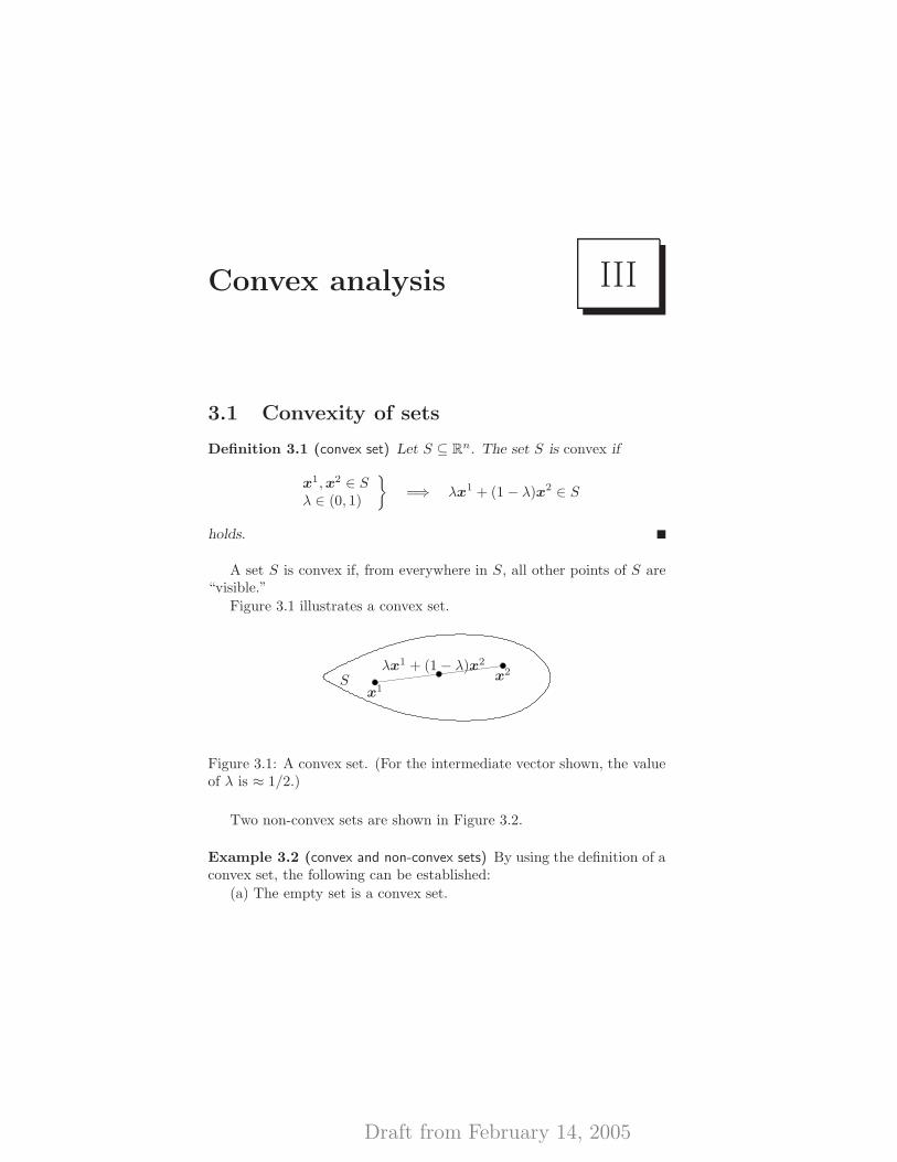
Draft from February 14, 2005
Convex analysis III
3.1 Convexity of sets
Definition 3.1 (convex set) Let S ⊆ Rn. The set S is convex if
x1,x2 ∈ Sλ ∈ (0, 1)
}=⇒ λx1 + (1 − λ)x2 ∈ S
holds.
A set S is convex if, from everywhere in S, all other points of S are“visible.”
Figure 3.1 illustrates a convex set.
Sx1
x2λx1 + (1 − λ)x2
Figure 3.1: A convex set. (For the intermediate vector shown, the valueof λ is ≈ 1/2.)
Two non-convex sets are shown in Figure 3.2.
Example 3.2 (convex and non-convex sets) By using the definition of aconvex set, the following can be established:
(a) The empty set is a convex set.
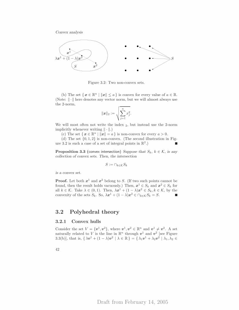
Draft from February 14, 2005
Convex analysis
S
x1
x2
λx1 + (1 − λ)x2 S
Figure 3.2: Two non-convex sets.
(b) The set {x ∈ Rn | ‖x‖ ≤ a } is convex for every value of a ∈ R.(Note: ‖ · ‖ here denotes any vector norm, but we will almost always usethe 2-norm,
‖x‖2 :=
√√√√n∑
j=1
x2j .
We will most often not write the index 2, but instead use the 2-normimplicitly whenever writing ‖ · ‖.)
(c) The set {x ∈ Rn | ‖x‖ = a } is non-convex for every a > 0.(d) The set {0, 1, 2} is non-convex. (The second illustration in Fig-
ure 3.2 is such a case of a set of integral points in R2.)
Proposition 3.3 (convex intersection) Suppose that Sk, k ∈ K, is anycollection of convex sets. Then, the intersection
S := ∩k∈KSk
is a convex set.
Proof. Let both x1 and x2 belong to S. (If two such points cannot befound, then the result holds vacuously.) Then, x1 ∈ Sk and x2 ∈ Sk forall k ∈ K. Take λ ∈ (0, 1). Then, λx1 + (1 − λ)x2 ∈ Sk, k ∈ K, by theconvexity of the sets Sk. So, λx1 + (1 − λ)x2 ∈ ∩k∈KSk = S.
3.2 Polyhedral theory
3.2.1 Convex hulls
Consider the set V = {v1,v2}, where v1,v2 ∈ Rn and v1 6= v2. A setnaturally related to V is the line in Rn through v1 and v2 [see Figure3.3(b)], that is, {λv1 + (1 − λ)v2 | λ ∈ R } = {λ1v
1 + λ2v2 | λ1, λ2 ∈
42
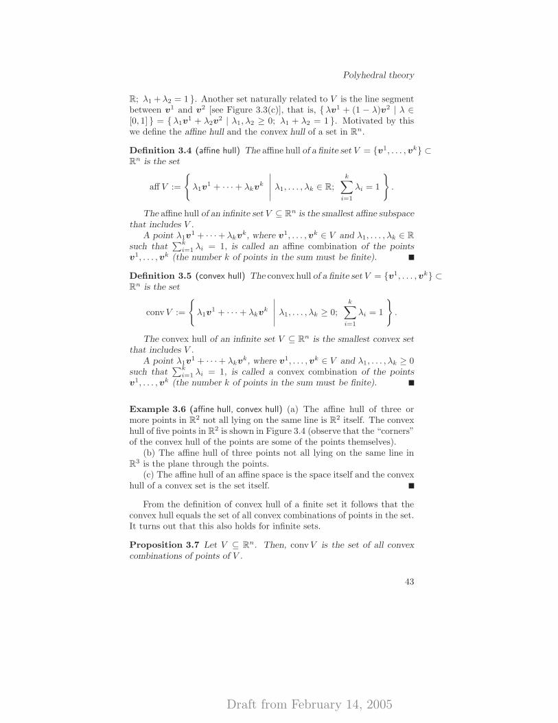
Draft from February 14, 2005
Polyhedral theory
R; λ1 +λ2 = 1 }. Another set naturally related to V is the line segmentbetween v1 and v2 [see Figure 3.3(c)], that is, {λv1 + (1 − λ)v2 | λ ∈[0, 1] } = {λ1v
1 + λ2v2 | λ1, λ2 ≥ 0; λ1 + λ2 = 1 }. Motivated by this
we define the affine hull and the convex hull of a set in Rn.
Definition 3.4 (affine hull) The affine hull of a finite set V = {v1, . . . ,vk} ⊂Rn is the set
aff V :=
{λ1v
1 + · · · + λkvk
∣∣∣∣∣ λ1, . . . , λk ∈ R;k∑
i=1
λi = 1
}.
The affine hull of an infinite set V ⊆ Rn is the smallest affine subspacethat includes V .
A point λ1v1 + · · ·+ λkvk, where v1, . . . ,vk ∈ V and λ1, . . . , λk ∈ R
such that∑k
i=1 λi = 1, is called an affine combination of the pointsv1, . . . ,vk (the number k of points in the sum must be finite).
Definition 3.5 (convex hull) The convex hull of a finite set V = {v1, . . . ,vk} ⊂Rn is the set
convV :=
{λ1v
1 + · · · + λkvk
∣∣∣∣∣ λ1, . . . , λk ≥ 0;
k∑
i=1
λi = 1
}.
The convex hull of an infinite set V ⊆ Rn is the smallest convex setthat includes V .
A point λ1v1 + · · ·+ λkvk, where v1, . . . ,vk ∈ V and λ1, . . . , λk ≥ 0
such that∑k
i=1 λi = 1, is called a convex combination of the pointsv1, . . . ,vk (the number k of points in the sum must be finite).
Example 3.6 (affine hull, convex hull) (a) The affine hull of three ormore points in R2 not all lying on the same line is R2 itself. The convexhull of five points in R2 is shown in Figure 3.4 (observe that the “corners”of the convex hull of the points are some of the points themselves).
(b) The affine hull of three points not all lying on the same line inR3 is the plane through the points.
(c) The affine hull of an affine space is the space itself and the convexhull of a convex set is the set itself.
From the definition of convex hull of a finite set it follows that theconvex hull equals the set of all convex combinations of points in the set.It turns out that this also holds for infinite sets.
Proposition 3.7 Let V ⊆ Rn. Then, convV is the set of all convexcombinations of points of V .
43
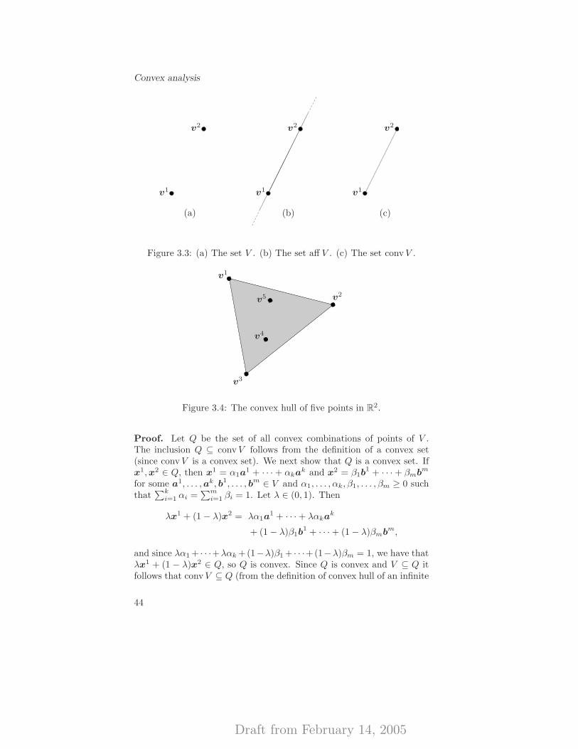
Draft from February 14, 2005
Convex analysis
(a) (b) (c)
v1 v1 v1
v2v2 v2
Figure 3.3: (a) The set V . (b) The set aff V . (c) The set convV .
v1
v2
v3
v4
v5
Figure 3.4: The convex hull of five points in R2.
Proof. Let Q be the set of all convex combinations of points of V .The inclusion Q ⊆ convV follows from the definition of a convex set(since convV is a convex set). We next show that Q is a convex set. Ifx1,x2 ∈ Q, then x1 = α1a
1 + · · · + αkak and x2 = β1b1 + · · · + βmbm
for some a1, . . . ,ak, b1, . . . , bm ∈ V and α1, . . . , αk, β1, . . . , βm ≥ 0 suchthat
∑ki=1 αi =
∑mi=1 βi = 1. Let λ ∈ (0, 1). Then
λx1 + (1 − λ)x2 = λα1a1 + · · · + λαkak
+ (1 − λ)β1b1 + · · · + (1 − λ)βmbm,
and since λα1 + · · ·+λαk +(1−λ)β1 + · · ·+(1−λ)βm = 1, we have thatλx1 + (1 − λ)x2 ∈ Q, so Q is convex. Since Q is convex and V ⊆ Q itfollows that convV ⊆ Q (from the definition of convex hull of an infinite
44
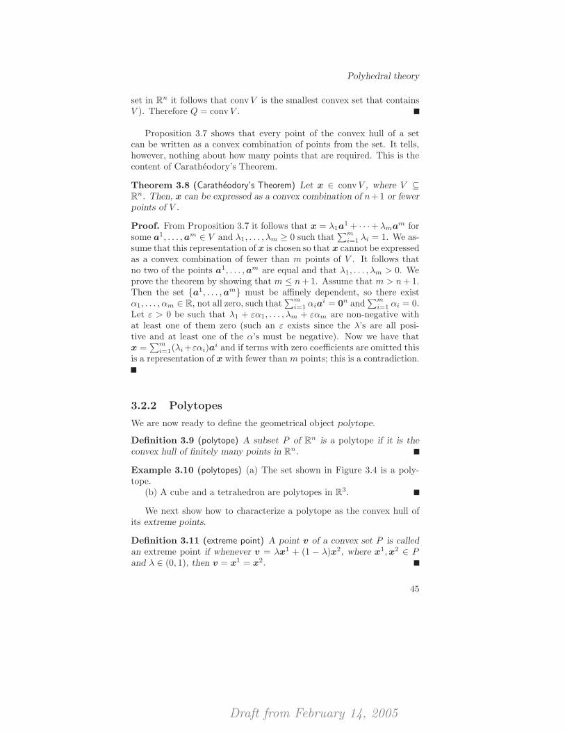
Draft from February 14, 2005
Polyhedral theory
set in Rn it follows that convV is the smallest convex set that containsV ). Therefore Q = convV .
Proposition 3.7 shows that every point of the convex hull of a setcan be written as a convex combination of points from the set. It tells,however, nothing about how many points that are required. This is thecontent of Caratheodory’s Theorem.
Theorem 3.8 (Caratheodory’s Theorem) Let x ∈ convV , where V ⊆Rn. Then, x can be expressed as a convex combination of n+1 or fewerpoints of V .
Proof. From Proposition 3.7 it follows that x = λ1a1 + · · ·+ λmam for
some a1, . . . ,am ∈ V and λ1, . . . , λm ≥ 0 such that∑m
i=1 λi = 1. We as-sume that this representation of x is chosen so that x cannot be expressedas a convex combination of fewer than m points of V . It follows thatno two of the points a1, . . . ,am are equal and that λ1, . . . , λm > 0. Weprove the theorem by showing that m ≤ n+ 1. Assume that m > n+ 1.Then the set {a1, . . . ,am} must be affinely dependent, so there existα1, . . . , αm ∈ R, not all zero, such that
∑mi=1 αia
i = 0n and∑m
i=1 αi = 0.Let ε > 0 be such that λ1 + εα1, . . . , λm + εαm are non-negative withat least one of them zero (such an ε exists since the λ’s are all posi-tive and at least one of the α’s must be negative). Now we have thatx =
∑mi=1(λi +εαi)a
i and if terms with zero coefficients are omitted thisis a representation of x with fewer than m points; this is a contradiction.
3.2.2 Polytopes
We are now ready to define the geometrical object polytope.
Definition 3.9 (polytope) A subset P of Rn is a polytope if it is theconvex hull of finitely many points in Rn.
Example 3.10 (polytopes) (a) The set shown in Figure 3.4 is a poly-tope.
(b) A cube and a tetrahedron are polytopes in R3.
We next show how to characterize a polytope as the convex hull ofits extreme points.
Definition 3.11 (extreme point) A point v of a convex set P is calledan extreme point if whenever v = λx1 + (1 − λ)x2, where x1,x2 ∈ Pand λ ∈ (0, 1), then v = x1 = x2.
45

Draft from February 14, 2005
Convex analysis
Example 3.12 (extreme points) The set shown in Figure 3.3(c) has theextreme points v1 and v2. The set shown in Figure 3.4 has the extremepoints v1, v2, and v3. The set shown in Figure 3.3(b) do not have anyextreme points.
Lemma 3.13 Let P be the polytope convV , where V = {v1, . . . ,vk} ⊂Rn. Then, each extreme point of P lies in V .
Proof. Assume that w /∈ V is an extreme point of P . We have thatw =
∑ki=1 λiv
i, for some λi ≥ 0 such that∑k
i=1 λi = 1. At least one ofthe λi’s must be nonzero, say λ1. If λ1 = 1 then w = v1, a contradiction,so λ1 ∈ (0, 1). We have that
w = λ1v1 + (1 − λ1)
k∑
i=2
λi
1 − λ1vi.
Since∑k
i=2 λi/(1 − λ1) = 1 we have that∑k
i=2 λi/(1 − λ1)vi ∈ P , but
w is an extreme point of P so w = v1, a contradiction.
Proposition 3.14 Let P be the polytope convV , where V = {v1, . . . ,vk} ⊂Rn. Then P is equal to the convex hull of its extreme points.
Proof. Let Q be the set of extreme points of P . If vi ∈ Q for all i =1, . . . , k we are done, so assume that v1 /∈ Q. Then v1 = λu + (1− λ)w
for some λ ∈ (0, 1) and u,w ∈ P , u 6= w. Further, u =∑k
i=1 αivi and
w =∑k
i=1 βivi, for some α1, . . . , αk, β1, . . . , βk ≥ 0 such that
∑ki=1 αi =∑k
i=1 βi = 1. Hence
v1 = λ
k∑
i=1
αivi + (1 − λ)
k∑
i=1
βivi =
k∑
i=1
(λαi + (1 − λ)βi)vi.
It must hold that α1, β1 6= 1, since otherwise u = w = v1, a contradic-tion. Therefore
v1 =
k∑
i=2
λαi + (1 − λ)βi
1 − (λα1 + (1 − λ)β1)vi,
and since∑k
i=2(λαi +(1−λ)βi)/(1−λα1− (1−λ)β1) = 1 it follows thatconvV = conv (V \ {v1}). Similarly every vi /∈ Q can be removed andwe end up with a set T ⊆ V such that convT = convV and T ⊆ Q. Butfrom Lemma 3.13 we have that every extreme point of the set convT liesin T and since convT = convV it follows that Q is the set of extremepoints of convT , so Q ⊆ T . Hence T = Q and we are done.
46
Draft from February 14, 2005
Polyhedral theory
3.2.3 Polyhedra
Closely related to the polytope is the polyhedron. We will show thatevery polyhedron is the sum of a polytope and a convex cone. In thenext subsection we show that a set is a polytope if and only if it is abounded polyhedron.
Definition 3.15 (polyhedron) A subset P of Rn is a polyhedron if thereexist a matrix A ∈ Rm×n and a vector b ∈ Rm such that
P = {x ∈ Rn | Ax ≤ b }.
The importance of polyhedra is obvious, since the set of feasiblesolutions of every linear programming problem is a polyhedron.
Example 3.16 (polyhedra) (a) Figure 3.5 shows the bounded polyhe-dron P = {x ∈ R2 | x1 ≥ 2; x1 + x2 ≤ 6; 2x1 − x2 ≤ 4 }.
(b) The unbounded polyhedron P = {x ∈ R2 | x1+x2 ≥ 2; x1−x2 ≤2; 3x1 − x2 ≥ 0 } is shown in Figure 3.6.
Often it is hard to decide whether a point in a convex set is an extremepoint or not. This is not the case for the polyhedron since there is analgebraic characterization of the extreme points of a polyhedron. Givenan x ∈ {x ∈ Rn | Ax ≤ b } we call to the rows of Ax ≤ b that arefulfilled with equality as the equality subsystem of Ax ≤ b, and denoteit by Ax = b. The number of rows in A is denoted by m.
Theorem 3.17 (algebraic characterization of extreme points) Let x ∈ P ={x ∈ Rn | Ax ≤ b }, where A ∈ Rm×n has rankA = n and b ∈ Rm.Further, let Ax = b be the equality subsystem of Ax ≤ b. Then x is anextreme point of P if and only if rank A = n.
Proof. [=⇒] Suppose that x is an extreme point of P . If Ax < b
then x + ε1n, x − ε1n ∈ P if ε > 0 is sufficiently small. But x =1/2(x+ε1n)+1/2(x−ε1n) which contradicts that x is an extreme point,so assume that at least one of the rows in Ax ≤ b is fulfilled with equality.If Ax = b is the equality subsystem of Ax ≤ b and rank A ≤ n − 1,then there exists a w 6= 0n such that Aw = 0m, so x + εw, x− εw ∈ Pif ε > 0 is sufficiently small. But x = 1/2(x+ εw)+1/2(x− εw), whichcontradicts that x is an extreme point. Hence rank A = n.
[⇐=] Assume that rank A = n. Then x is the unique solutionto Ax = b. If x is not an extreme point of P it follows that x =λu + (1 − λ)v for some λ ∈ (0, 1) and u,v ∈ P , u 6= v. This yields
47
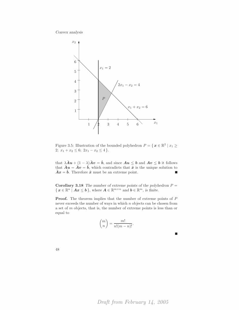
Draft from February 14, 2005
Convex analysis
1
1
2
2 3
3
4
4
5
5
6
6 x1
x2
x1 + x2 = 6
2x1 − x2 = 4
x1 = 2
P
Figure 3.5: Illustration of the bounded polyhedron P = {x ∈ R2 | x1 ≥2; x1 + x2 ≤ 6; 2x1 − x2 ≤ 4 }.
that λAu + (1 − λ)Av = b, and since Au ≤ b and Av ≤ b it followsthat Au = Av = b, which contradicts that x is the unique solution toAx = b. Therefore x must be an extreme point.
Corollary 3.18 The number of extreme points of the polyhedron P ={x ∈ Rn | Ax ≤ b }, where A ∈ Rm×n and b ∈ Rm, is finite.
Proof. The theorem implies that the number of extreme points of Pnever exceeds the number of ways in which n objects can be chosen froma set of m objects, that is, the number of extreme points is less than orequal to
(mn
)=
m!
n!(m− n)!.
48
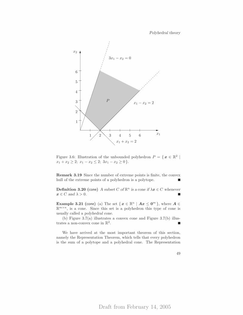
Draft from February 14, 2005
Polyhedral theory
1
1
2
2
3
3
4
4
5
5
6
6
x1
x2
x1 + x2 = 2
x1 − x2 = 2
3x1 − x2 = 0
P
Figure 3.6: Illustration of the unbounded polyhedron P = {x ∈ R2 |x1 + x2 ≥ 2; x1 − x2 ≤ 2; 3x1 − x2 ≥ 0 }.
Remark 3.19 Since the number of extreme points is finite, the convexhull of the extreme points of a polyhedron is a polytope.
Definition 3.20 (cone) A subset C of Rn is a cone if λx ∈ C wheneverx ∈ C and λ > 0.
Example 3.21 (cone) (a) The set {x ∈ Rn | Ax ≤ 0m }, where A ∈Rm×n, is a cone. Since this set is a polyhedron this type of cone isusually called a polyhedral cone.
(b) Figure 3.7(a) illustrates a convex cone and Figure 3.7(b) illus-trates a non-convex cone in R2.
We have arrived at the most important theorem of this section,namely the Representation Theorem, which tells that every polyhedronis the sum of a polytope and a polyhedral cone. The Representation
49
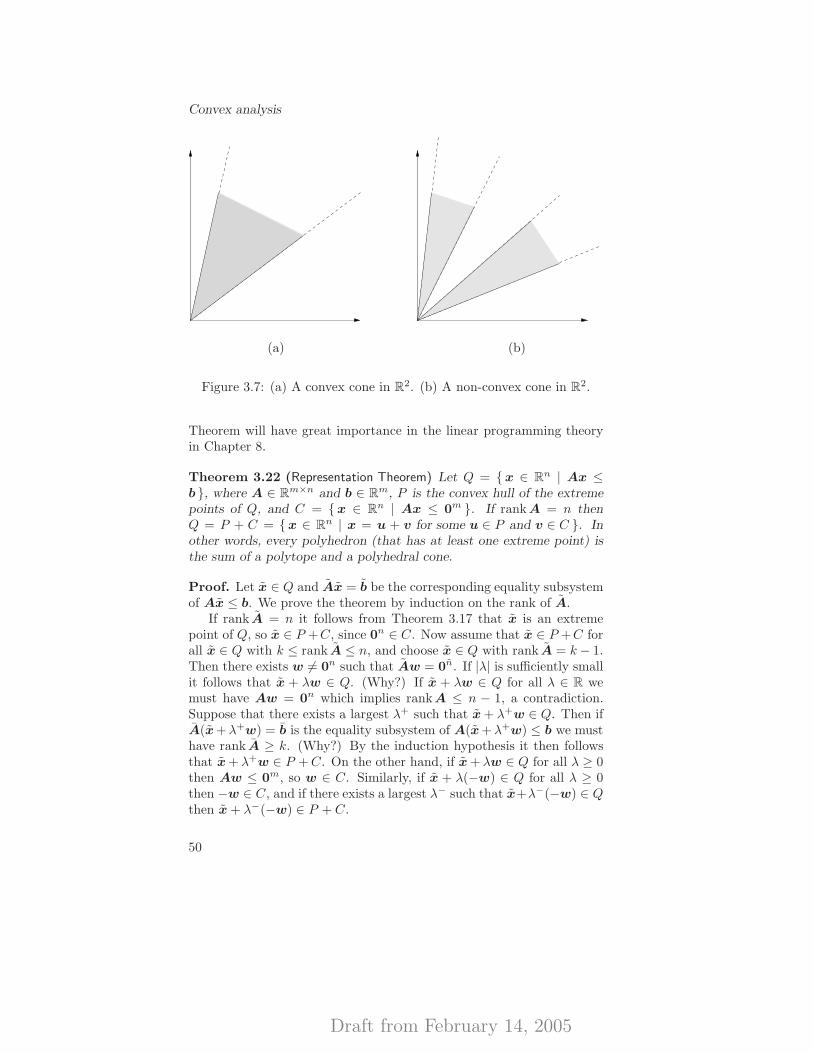
Draft from February 14, 2005
Convex analysis
(a) (b)
Figure 3.7: (a) A convex cone in R2. (b) A non-convex cone in R2.
Theorem will have great importance in the linear programming theoryin Chapter 8.
Theorem 3.22 (Representation Theorem) Let Q = {x ∈ Rn | Ax ≤b }, where A ∈ Rm×n and b ∈ Rm, P is the convex hull of the extremepoints of Q, and C = {x ∈ Rn | Ax ≤ 0m }. If rankA = n thenQ = P + C = {x ∈ Rn | x = u + v for some u ∈ P and v ∈ C }. Inother words, every polyhedron (that has at least one extreme point) isthe sum of a polytope and a polyhedral cone.
Proof. Let x ∈ Q and Ax = b be the corresponding equality subsystemof Ax ≤ b. We prove the theorem by induction on the rank of A.
If rank A = n it follows from Theorem 3.17 that x is an extremepoint of Q, so x ∈ P +C, since 0n ∈ C. Now assume that x ∈ P +C forall x ∈ Q with k ≤ rank A ≤ n, and choose x ∈ Q with rank A = k− 1.Then there exists w 6= 0n such that Aw = 0n. If |λ| is sufficiently smallit follows that x + λw ∈ Q. (Why?) If x + λw ∈ Q for all λ ∈ R wemust have Aw = 0n which implies rankA ≤ n − 1, a contradiction.Suppose that there exists a largest λ+ such that x + λ+w ∈ Q. Then ifA(x +λ+w) = b is the equality subsystem of A(x +λ+w) ≤ b we musthave rank A ≥ k. (Why?) By the induction hypothesis it then followsthat x + λ+w ∈ P +C. On the other hand, if x + λw ∈ Q for all λ ≥ 0then Aw ≤ 0m, so w ∈ C. Similarly, if x + λ(−w) ∈ Q for all λ ≥ 0then −w ∈ C, and if there exists a largest λ− such that x+λ−(−w) ∈ Qthen x + λ−(−w) ∈ P + C.
50
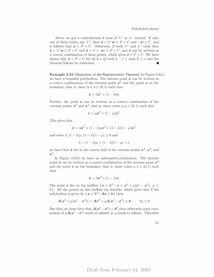
Draft from February 14, 2005
Polyhedral theory
Above we got a contradiction if none of λ+ or λ− existed. If onlyone of them exists, say λ+, then x + λ+w ∈ P + C and −w ∈ C, andit follows that x ∈ P + C. Otherwise, if both λ+ and λ− exist thenx + λ+w ∈ P + C and x + λ−(−w) ∈ P + C, and x can be written asa convex combination of these points, which gives x ∈ P + C. We haveshown that x ∈ P + C for all x ∈ Q with k − 1 ≤ rank A ≤ n and thetheorem follows by induction.
Example 3.23 (illustration of the Representation Theorem) In Figure 3.8(a)we have a bounded polyhedron. The interior point x can be written asa convex combination of the extreme point x5 and the point v on theboundary, that is, there is a λ ∈ (0, 1) such that
x = λx5 + (1 − λ)v.
Further, the point v can be written as a convex combination of theextreme points x2 and x3, that is, there exists a µ ∈ (0, 1) such that
v = µx2 + (1 − µ)x3.
This gives that
x = λx5 + (1 − λ)µx2 + (1 − λ)(1 − µ)x3,
and since λ, (1 − λ)µ, (1 − λ)(1 − µ) ≥ 0 and
λ+ (1 − λ)µ+ (1 − λ)(1 − µ) = 1
we have that x lies in the convex hull of the extreme points x2, x3, andx5.
In Figure 3.8(b) we have an unbounded polyhedron. The interiorpoint x can be written as a convex combination of the extreme point x3
and the point v on the boundary, that is, there exists a λ ∈ (0, 1) suchthat
x = λx3 + (1 − λ)v.
The point v lies on the halfline {x ∈ R2 | x = x2 + µ(x1 − x2), µ ≥0 }. All the points on this halfline are feasible, which gives that if thepolyhedron is given by {x ∈ R2 | Ax ≤ b } then
A(x2 + µ(x1 − x2)) = Ax2 + µA(x1 − x2) ≤ b, ∀µ ≥ 0.
But then we must have that A(x1−x2) ≤ 02 since otherwise some com-ponent of µA(x1 −x2) tends to infinity as µ tends to infinity. Therefore
51
Draft from February 14, 2005
Convex analysis
x1 − x2 lies in the cone C = {x ∈ R2 | Ax ≤ 02 }. Now there exists aµ ∈ (0, 1) such that
v = x2 + µ(x1 − x2),
and it follows that
x = λx3 + (1 − λ)x2 + (1 − λ)µ(x1 − x2),
so since (1 − λ)µ ≥ 0 and x1 − x2 ∈ C, x is the sum of a point in theconvex hull of the extreme points and a point in the polyhedral cone C.
(a) (b)
x1x1
x2
x2
x3
x3
x4
x4
x5
x
v
x
v
Figure 3.8: Illustration of the Representation Theorem (a) in thebounded case, and (b) in the unbounded case.
3.2.4 The Separation Theorem and Farkas’ Lemma
We introduce the important concept of separation and use it to showthat every polytope is a polyhedron.
Theorem 3.24 (Separation Theorem) Suppose that the set C ⊆ Rn isclosed and convex, and that the point y does not lie in C. Then there
52
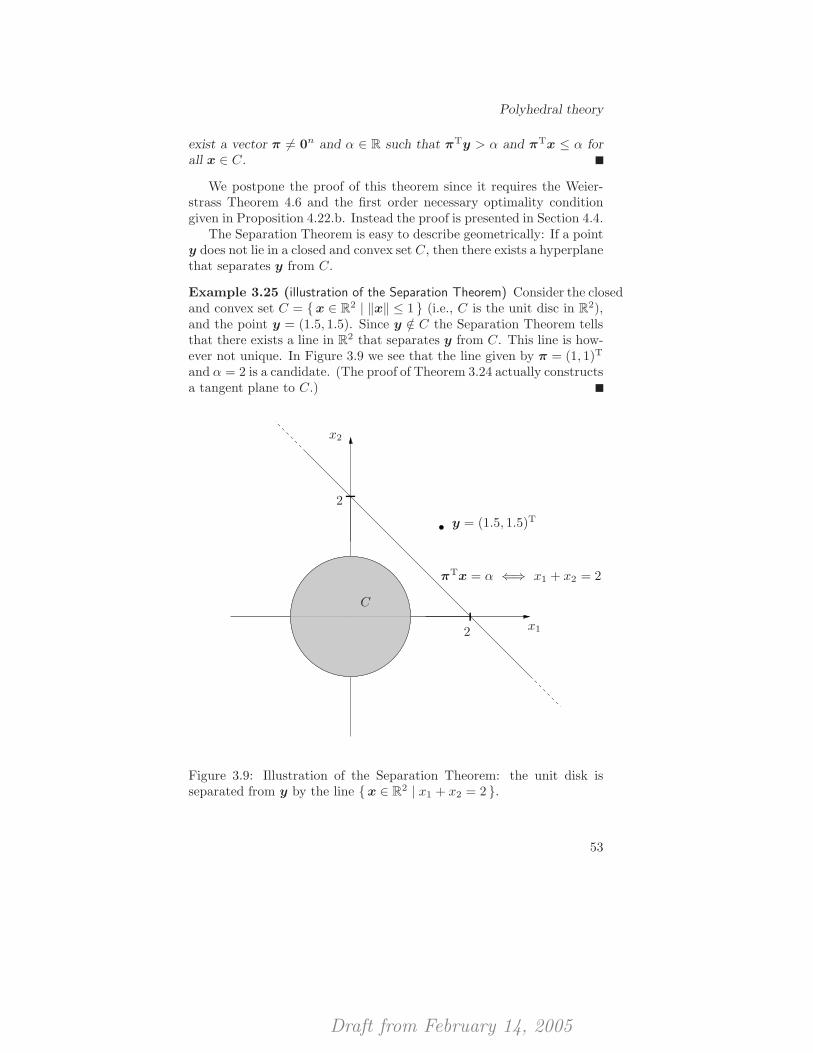
Draft from February 14, 2005
Polyhedral theory
exist a vector π 6= 0n and α ∈ R such that πTy > α and πTx ≤ α forall x ∈ C.
We postpone the proof of this theorem since it requires the Weier-strass Theorem 4.6 and the first order necessary optimality conditiongiven in Proposition 4.22.b. Instead the proof is presented in Section 4.4.
The Separation Theorem is easy to describe geometrically: If a pointy does not lie in a closed and convex set C, then there exists a hyperplanethat separates y from C.
Example 3.25 (illustration of the Separation Theorem) Consider the closedand convex set C = {x ∈ R2 | ‖x‖ ≤ 1 } (i.e., C is the unit disc in R2),and the point y = (1.5, 1.5). Since y /∈ C the Separation Theorem tellsthat there exists a line in R2 that separates y from C. This line is how-ever not unique. In Figure 3.9 we see that the line given by π = (1, 1)T
and α = 2 is a candidate. (The proof of Theorem 3.24 actually constructsa tangent plane to C.)
x1
x2
2
2
C
y = (1.5, 1.5)T
πTx = α ⇐⇒ x1 + x2 = 2
Figure 3.9: Illustration of the Separation Theorem: the unit disk isseparated from y by the line {x ∈ R2 | x1 + x2 = 2 }.
53
Draft from February 14, 2005
Convex analysis
Theorem 3.26 A set P is a polytope if and only if it is a boundedpolyhedron.
Proof. [⇐=] From the Representation Theorem 3.22 we get that abounded polyhedron is the convex hull of its extreme points and henceby Remark 3.19 a polytope.
[=⇒] Let V = {v1, . . . ,vk} ⊂ Rn and let P be the polytope convV .In order to prove that P is a polyhedron we must show that P is the solu-tion set of some system of linear inequalities. The idea of the proof is todefine a bounded polyhedron consisting of the coefficients and right-handsides of all valid inequalities for P and then apply the RepresentationTheorem to select a finite subset of those valid inequalities.
To carry this out, consider the set Q ⊂ Rn+1 defined as{ (
a
b
) ∣∣∣∣ a ∈ Rn; b ∈ R; −1n ≤ a ≤ 1n; −1 ≤ b ≤ 1; aTv ≤ b, v ∈ V
}.
Since V is a finite set, Q is a polyhedron. Further Q is bounded, so bythe Representation Theorem we know that Q is the convex hull of itsextreme points
(a1
b1
), . . . ,
(am
bm
).
We will prove that the linear system
(a1)Tx ≤ b1, . . . , (am)Tx ≤ bm, (3.1)
defines P . We first show that P is contained in the solution set of(3.1). So, suppose that x ∈ P . Then x = λ1v
1 + · · · + λkvk for some
λ1, . . . , λk ≥ 0 such that∑k
i=1 λi = 1. Thus, for each i = 1, . . . ,m, wehave
(ai)Tx = (ai)T(λ1v1 + · · · + λkvk) = λ1(a
i)Tv1 + · · · + λk(ai)Tvk
≤ λ1bi + · · · + λkbi = bi,
so x satisfies all inequalities in (3.1).In order to show that the solution set of (3.1) is contained in P , let x
be a solution to (3.1) and suppose that x /∈ P . Then, by the SeparationTheorem 3.24 there exist a vector π 6= 0n and α ∈ R such that πTx > αand πTx ≤ α for all x ∈ P . By scaling πTx ≤ α by a positive constantif necessary, we may assume that −1n ≤ π ≤ 1n and −1 ≤ α ≤ 1. That
is, we may assume that
(π
α
)∈ Q. So we may write
(π
α
)= λ1
(a1
b1
)+ · · · + λm
(am
bm
),
54
Draft from February 14, 2005
Polyhedral theory
for some λ1, . . . , λm ≥ 0 such that∑m
i=1 λi = 1. Therefore,
πTx = λ1(a1)Tx + · · · + λm(am)Tx ≤ λ1b1 + · · · + λmbm = α.
But this is a contradiction, since πTx > α. So x ∈ P , which completesthe proof.
We introduce the concept of finitely generated cones. In the proof ofFarkas’ Lemma below we will use that finitely generated cones are convexand closed and in order to show that we prove that finitely generatedcones are polyhedral sets.
Definition 3.27 (finitely generated cone) A finitely generated cone isone that is generated by a finite set, that is, a cone of the form
cone {v1, . . . ,vm} := {λ1v1 + · · · + λmvm | λ1, . . . , λm ≥ 0 },
where v1, . . . ,vm ∈ Rn. Note that if A is an m× n matrix, then the set{y ∈ Rm | y = Ax, x ≥ 0n } is a finitely generated cone.
Recall that a cone that is a polyhedron is called a polyhedral cone.We show that a finitely generated cone is always a polyhedral cone andvice versa.
Theorem 3.28 A convex cone in Rn is finitely generated if and only ifit is polyhedral.
Proof. [=⇒] Assume that C is the finitely generated cone
cone {v1, . . . ,vm},
where v1, . . . ,vm ∈ Rn. From Theorem 3.26 we know that polytopesare polyhedral sets, so conv {0n,v1, . . . ,vm} is the solution set of somelinear inequalities
(a1)Tx ≤ b1, . . . , (ak)Tx ≤ bk. (3.2)
Since the solution set of these inequalities contains 0n we must haveb1, . . . , bk ≥ 0. We show that C is the polyhedral cone A that equalsthe solution set of the inequalities of (3.2) for which bi = 0. Sincev1, . . . ,vm ∈ A we have C ⊆ A. In order to show that A ⊆ C, assumethat w ∈ A. Then λw is in the solution set of (3.2) if λ > 0 is sufficientlysmall. Hence there exists a λ > 0 such that
λw ∈ {x ∈ Rn | (a1)Tx ≤ b1, . . . , (ak)Tx ≤ bk }
= conv {0n,v1, . . . ,vm} ⊆ C,
55
Draft from February 14, 2005
Convex analysis
so w ∈ (1/λ)C = C. Hence A ⊆ C, and C = A.[⇐=] Suppose that C is a polyhedral cone in Rn. Let P be a poly-
tope in Rn such that 0n ∈ intP (that is, 0n lies in the interior of P ).Then C ∩ P is a bounded polyhedron and hence the representation the-orem gives that C ∩ P = conv {v1, . . . ,vm}, where v1, . . . ,vm is theextreme points of C ∩ P . We show that C is the finitely generated conecone {v1, . . . ,vm}. Since v1, . . . ,vm ∈ C and C is a polyhedral cone weget that cone {v1, . . . ,vm} ⊆ C. If c ∈ C, then, since 0n ∈ intP , thereexists a λ > 0 such that λc ∈ P . Thus
λc ∈ C ∩ P = conv {v1, . . . ,vm} ⊆ cone {v1, . . . ,vm},
and so c ∈ (1/λ)cone {v1, . . . ,vm} = cone {v1, . . . ,vm}. Hence it fol-lows that C ⊆ cone {v1, . . . ,vm}, and C = cone {v1, . . . ,vm}.
Corollary 3.29 Finitely generated cones in Rn are convex and closed.
Proof. Halfspaces, that is, sets of the form {x ∈ Rn | aTx ≤ b } forsome vector a ∈ Rn and b ∈ R, are convex and closed. (Why?) Bythe theorem a finitely generated cone is the intersection of finitely manyhalfspaces and thus the corollary follows from Proposition 3.3 and thefact that intersections of closed sets are closed.
We close this section by proving the famous Farkas’ Lemma by usingthe Separation Theorem 3.24 and the fact that finitely generated conesare convex and closed.
Theorem 3.30 (Farkas’ Lemma) Let A ∈ Rm×n and b ∈ Rm. Then,exactly one of the systems
Ax = b, (I)
x ≥ 0n,
and
ATπ ≤ 0n, (II)
bTπ > 0,
has a feasible solution, and the other system is inconsistent.
Proof. Let C = {y ∈ Rm | y = Ax, x ≥ 0n }. If (I) is infeasible thenb /∈ C. The set C is a finitely generated cone. Hence, by Corollary 3.29,it follows that C is convex and closed so by the Separation Theorem 3.24
56
Draft from February 14, 2005
Convex functions
there exist a vector π ∈ Rm and α ∈ R such that bTπ > α and yTπ ≤ αfor all y ∈ C, that is,
xTATπ ≤ α, ∀x ≥ 0n. (3.3)
Since 0m ∈ C it follows that α ≥ 0, so bTπ > 0, and if there exists anx ≥ 0n such that xTATπ > 0 then (3.3) cannot hold for any α (if λ ≥ 0then λx ≥ 0n and (λx)TATπ = λxTATπ tends to infinity as λ tends toinfinity). Therefore we must have that xTATπ ≤ 0 for all x ≥ 0n, andthis holds if and only if ATπ ≤ 0n, which means that (II) is feasible.
On the other hand, if (I) has a feasible solution, say x ≥ 0n, thenAx = b, so if there is a solution to (II), say π, then xTATπ = bTπ > 0.But then ATπ > 0n (since x ≥ 0n), a contradiction. Hence (II) is in-feasible.
3.3 Convex functions
Definition 3.31 (convex function) Suppose that S ⊆ Rn. A functionf : Rn → R ∪ {+∞} is convex at x ∈ S if
x ∈ Sλ ∈ (0, 1)λx + (1 − λ)x ∈ S
=⇒ f(λx + (1 − λ)x) ≤ λf(x) + (1 − λ)f(x).
The function f is convex on S if it is convex at every x ∈ S.
In other words, a convex function is such that a linear interpolationnever is lower than the function itself.1
From the definition follows that a function f : Rn → R ∪ {+∞} isconvex on a convex set S ⊆ Rn if and only if
x1,x2 ∈ Sλ ∈ (0, 1)
}=⇒ f(λx1 + (1 − λ)x)2 ≤ λf(x1) + (1 − λ)f(x2).
Definition 3.32 (concave function) Suppose that S ⊆ Rn. A functionf : Rn → R ∪ {+∞} is concave at x ∈ S if −f is convex at x.
The function f is concave on S if it is concave at every x ∈ S.
1Words like “lower” and “above” should be understood in the sense of the com-parison between the y-coordinates of the respective function at the same coordinatesin x.
57
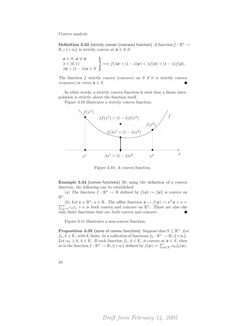
Draft from February 14, 2005
Convex analysis
Definition 3.33 (strictly convex (concave) function) A function f : Rn →R ∪ {+∞} is strictly convex at x ∈ S if
x ∈ S, x 6= x
λ ∈ (0, 1)λx + (1 − λ)x ∈ S
=⇒ f(λx + (1 − λ)x) < λf(x) + (1 − λ)f(x).
The function f strictly convex (concave) on S if it is strictly convex(concave) at every x ∈ S.
In other words, a strictly convex function is such that a linear inter-polation is strictly above the function itself.
Figure 3.10 illustrates a strictly convex function.
f(x1)f
x
f(x2)
f(λx1 + (1 − λ)x2)
λf(x1) + (1 − λ)f(x2)
x1 x2λx1 + (1 − λ)x2
Figure 3.10: A convex function.
Example 3.34 (convex functions) By using the definition of a convexfunction, the following can be established:
(a) The function f : Rn → R defined by f(x) := ‖x‖ is convex onRn.
(b) Let c ∈ Rn, a ∈ R. The affine function x 7→ f(x) := cTx + a =∑nj=1 cjxj + a is both convex and concave on Rn. These are also the
only finite functions that are both convex and concave.
Figure 3.11 illustrates a non-convex function.
Proposition 3.35 (sums of convex functions) Suppose that S ⊆ Rn. Letfk, k ∈ K, with K finite, be a collection of functions fk : Rn → R∪{+∞}.Let αk ≥ 0, k ∈ K. If each function fk, k ∈ K, is convex at x ∈ S, thenso is the function f : Rn → R∪{+∞} defined by f(x) :=
∑k∈K αkfk(x).
58
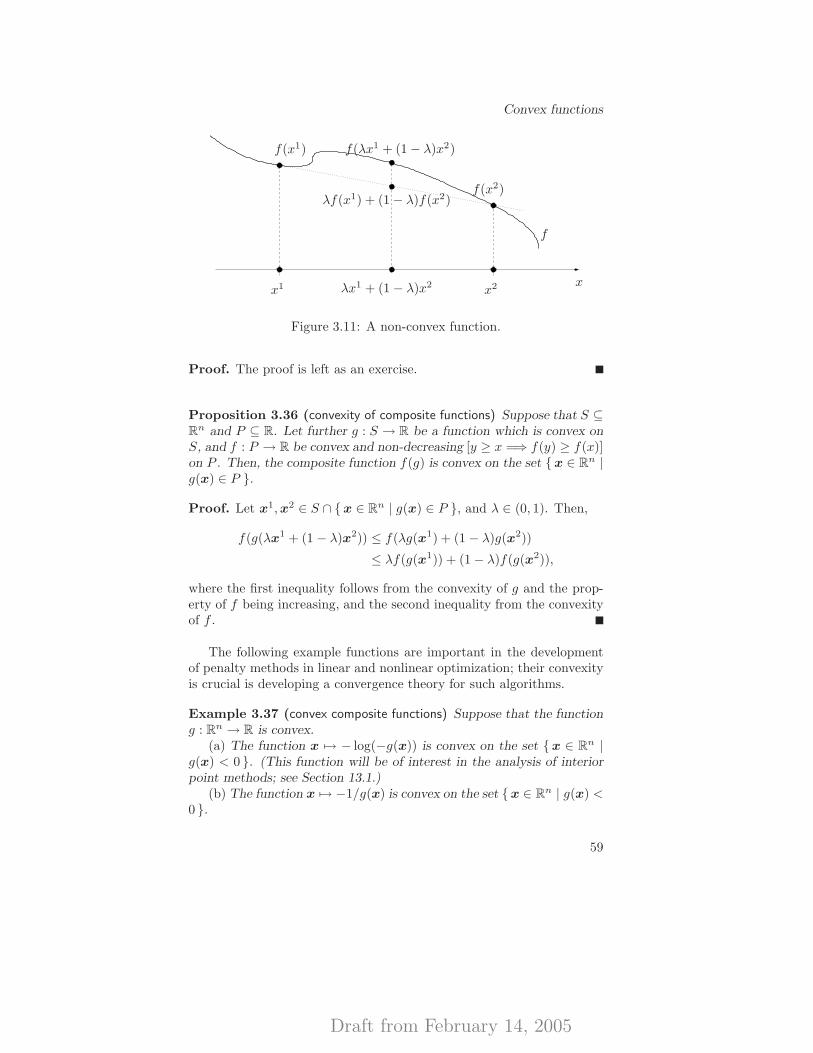
Draft from February 14, 2005
Convex functions
f(x1)
f
x
f(x2)
f(λx1 + (1 − λ)x2)
λf(x1) + (1 − λ)f(x2)
x1 x2λx1 + (1 − λ)x2
Figure 3.11: A non-convex function.
Proof. The proof is left as an exercise.
Proposition 3.36 (convexity of composite functions) Suppose that S ⊆Rn and P ⊆ R. Let further g : S → R be a function which is convex onS, and f : P → R be convex and non-decreasing [y ≥ x =⇒ f(y) ≥ f(x)]on P . Then, the composite function f(g) is convex on the set {x ∈ Rn |g(x) ∈ P }.
Proof. Let x1,x2 ∈ S ∩ {x ∈ Rn | g(x) ∈ P }, and λ ∈ (0, 1). Then,
f(g(λx1 + (1 − λ)x2)) ≤ f(λg(x1) + (1 − λ)g(x2))
≤ λf(g(x1)) + (1 − λ)f(g(x2)),
where the first inequality follows from the convexity of g and the prop-erty of f being increasing, and the second inequality from the convexityof f .
The following example functions are important in the developmentof penalty methods in linear and nonlinear optimization; their convexityis crucial is developing a convergence theory for such algorithms.
Example 3.37 (convex composite functions) Suppose that the functiong : Rn → R is convex.
(a) The function x 7→ − log(−g(x)) is convex on the set {x ∈ Rn |g(x) < 0 }. (This function will be of interest in the analysis of interiorpoint methods; see Section 13.1.)
(b) The function x 7→ −1/g(x) is convex on the set {x ∈ Rn | g(x) <0 }.
59
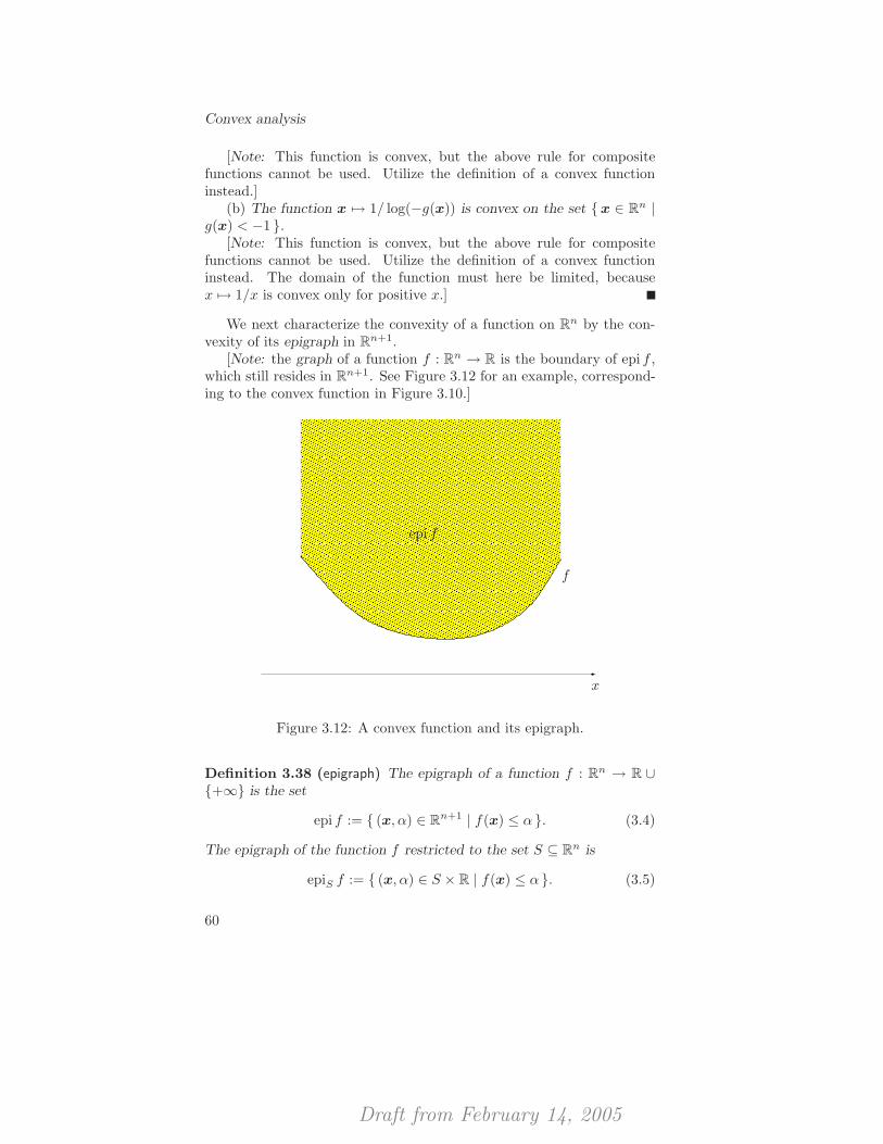
Draft from February 14, 2005
Convex analysis
[Note: This function is convex, but the above rule for compositefunctions cannot be used. Utilize the definition of a convex functioninstead.]
(b) The function x 7→ 1/ log(−g(x)) is convex on the set {x ∈ Rn |g(x) < −1 }.
[Note: This function is convex, but the above rule for compositefunctions cannot be used. Utilize the definition of a convex functioninstead. The domain of the function must here be limited, becausex 7→ 1/x is convex only for positive x.]
We next characterize the convexity of a function on Rn by the con-vexity of its epigraph in Rn+1.
[Note: the graph of a function f : Rn → R is the boundary of epi f ,which still resides in Rn+1. See Figure 3.12 for an example, correspond-ing to the convex function in Figure 3.10.]
����������������������������������������������������������������������������������������������������������������������������������������������������������������������������������������������������������������������������������������������������������������������������������������������������������������������������������������������������������������������������������������������������������������������������������������������������������������������������������������������������������������������������������������������������������������������������������������������������������������������������������������������������������������������������������������������������������������������������������������������������������������������������������������������������������������������������������������������������������������������������������������������������������������������������������������������������������������������������������������������������������������������������������������������������������������������������������������������������������������������������������������������������������������������������������������������������������������������������������������������������������������������������������������������������������
����������������������������������������������������������������������������������������������������������������������������������������������������������������������������������������������������������������������������������������������������������������������������������������������������������������������������������������������������������������������������������������������������������������������������������������������������������������������������������������������������������������������������������������������������������������������������������������������������������������������������������������������������������������������������������������������������������������������������������������������������������������������������������������������������������������������������������������������������������������������������������������������������������������������������������������������������������������������������������������������������������������������������������������������������������������������������������������������������������������������������������������������������������������������������������������������������������������������������������������������������������������������������������������������������������
��������������������������������������������������������������������������������������������������������������������������������������������������������������������������������������������������������������������������������������������������������������������������������������������������������������������������������������������������������������������������������������������������������������������������������������������������������������������������������������������������������������������������������������������������������������������������������������������������������������������������������������������������������������������������������������������������������������������������������������������������������������������������������������������������������������
��������������������������������������������������������������������������������������������������������������������������������������������������������������������������������������������������������������������������������������������������������������������������������������������������������������������������������������������������������������������������������������������������������������������������������������������������������������������������������������������������������������������������������������������������������������������������������������������������������������������������������������������������������������������������������������������������������������������������������������������������������������������������������������������������������������
epi f
f
x
Figure 3.12: A convex function and its epigraph.
Definition 3.38 (epigraph) The epigraph of a function f : Rn → R ∪{+∞} is the set
epi f := { (x, α) ∈ Rn+1 | f(x) ≤ α }. (3.4)
The epigraph of the function f restricted to the set S ⊆ Rn is
epiS f := { (x, α) ∈ S × R | f(x) ≤ α }. (3.5)
60
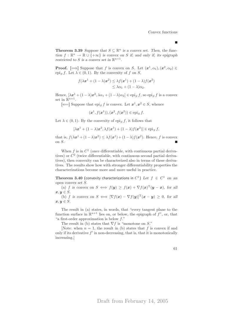
Draft from February 14, 2005
Convex functions
Theorem 3.39 Suppose that S ⊆ Rn is a convex set. Then, the func-tion f : Rn → R ∪ {+∞} is convex on S if, and only if, its epigraphrestricted to S is a convex set in Rn+1.
Proof. [=⇒] Suppose that f is convex on S. Let (x1, α1), (x2, α2) ∈
epiS f . Let λ ∈ (0, 1). By the convexity of f on S,
f(λx1 + (1 − λ)x2) ≤ λf(x1) + (1 − λ)f(x2)
≤ λα1 + (1 − λ)α2.
Hence, [λx1 + (1−λ)x2, λα1 + (1−λ)α2] ∈ epiS f , so epiS f is a convexset in Rn+1.
[⇐=] Suppose that epiS f is convex. Let x1,x2 ∈ S, whence
(x1, f(x1)), (x2, f(x2)) ∈ epiS f.
Let λ ∈ (0, 1). By the convexity of epiS f , it follows that
[λx1 + (1 − λ)x2, λf(x1) + (1 − λ)f(x2)] ∈ epiS f,
that is, f(λx1 +(1−λ)x2) ≤ λf(x1)+ (1−λ)f(x2). Hence, f is convexon S.
When f is in C1 (once differentiable, with continuous partial deriva-tives) or C2 (twice differentiable, with continuous second partial deriva-tives), then convexity can be characterized also in terms of these deriva-tives. The results show how with stronger differentiability properties thecharacterizations become more and more useful in practice.
Theorem 3.40 (convexity characterizations in C1) Let f ∈ C1 on anopen convex set S.
(a) f is convex on S ⇐⇒ f(y) ≥ f(x) + ∇f(x)T(y − x), for allx,y ∈ S.
(b) f is convex on S ⇐⇒ [∇f(x) − ∇f(y)]T(x − y) ≥ 0, for allx,y ∈ S.
The result in (a) states, in words, that “every tangent plane to thefunction surface in Rn+1 lies on, or below, the epigraph of f”, or, that“a first-order approximation is below f .”
The result in (b) states that ∇f is “monotone on S.”[Note: when n = 1, the result in (b) states that f is convex if and
only if its derivative f ′ in non-decreasing, that is, that it is monotonicallyincreasing.]
61
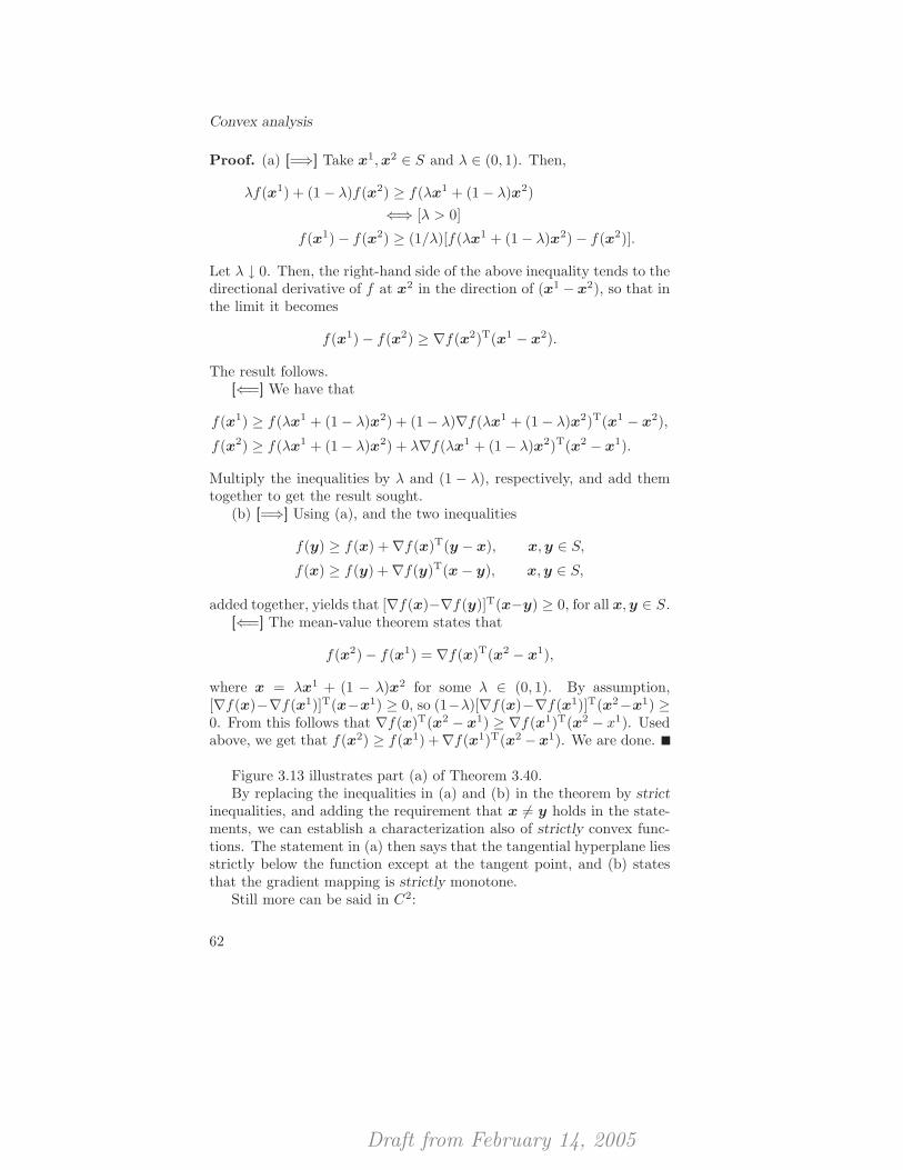
Draft from February 14, 2005
Convex analysis
Proof. (a) [=⇒] Take x1,x2 ∈ S and λ ∈ (0, 1). Then,
λf(x1) + (1 − λ)f(x2) ≥ f(λx1 + (1 − λ)x2)
⇐⇒ [λ > 0]
f(x1) − f(x2) ≥ (1/λ)[f(λx1 + (1 − λ)x2) − f(x2)].
Let λ ↓ 0. Then, the right-hand side of the above inequality tends to thedirectional derivative of f at x2 in the direction of (x1 −x2), so that inthe limit it becomes
f(x1) − f(x2) ≥ ∇f(x2)T(x1 − x2).
The result follows.[⇐=] We have that
f(x1) ≥ f(λx1 + (1 − λ)x2) + (1 − λ)∇f(λx1 + (1 − λ)x2)T(x1 − x2),
f(x2) ≥ f(λx1 + (1 − λ)x2) + λ∇f(λx1 + (1 − λ)x2)T(x2 − x1).
Multiply the inequalities by λ and (1 − λ), respectively, and add themtogether to get the result sought.
(b) [=⇒] Using (a), and the two inequalities
f(y) ≥ f(x) + ∇f(x)T(y − x), x,y ∈ S,
f(x) ≥ f(y) + ∇f(y)T(x − y), x,y ∈ S,
added together, yields that [∇f(x)−∇f(y)]T(x−y) ≥ 0, for all x,y ∈ S.[⇐=] The mean-value theorem states that
f(x2) − f(x1) = ∇f(x)T(x2 − x1),
where x = λx1 + (1 − λ)x2 for some λ ∈ (0, 1). By assumption,[∇f(x)−∇f(x1)]T(x−x1) ≥ 0, so (1−λ)[∇f(x)−∇f(x1)]T(x2−x1) ≥0. From this follows that ∇f(x)T(x2 − x1) ≥ ∇f(x1)T(x2 − x1). Usedabove, we get that f(x2) ≥ f(x1) +∇f(x1)T(x2 −x1). We are done.
Figure 3.13 illustrates part (a) of Theorem 3.40.By replacing the inequalities in (a) and (b) in the theorem by strict
inequalities, and adding the requirement that x 6= y holds in the state-ments, we can establish a characterization also of strictly convex func-tions. The statement in (a) then says that the tangential hyperplane liesstrictly below the function except at the tangent point, and (b) statesthat the gradient mapping is strictly monotone.
Still more can be said in C2:
62
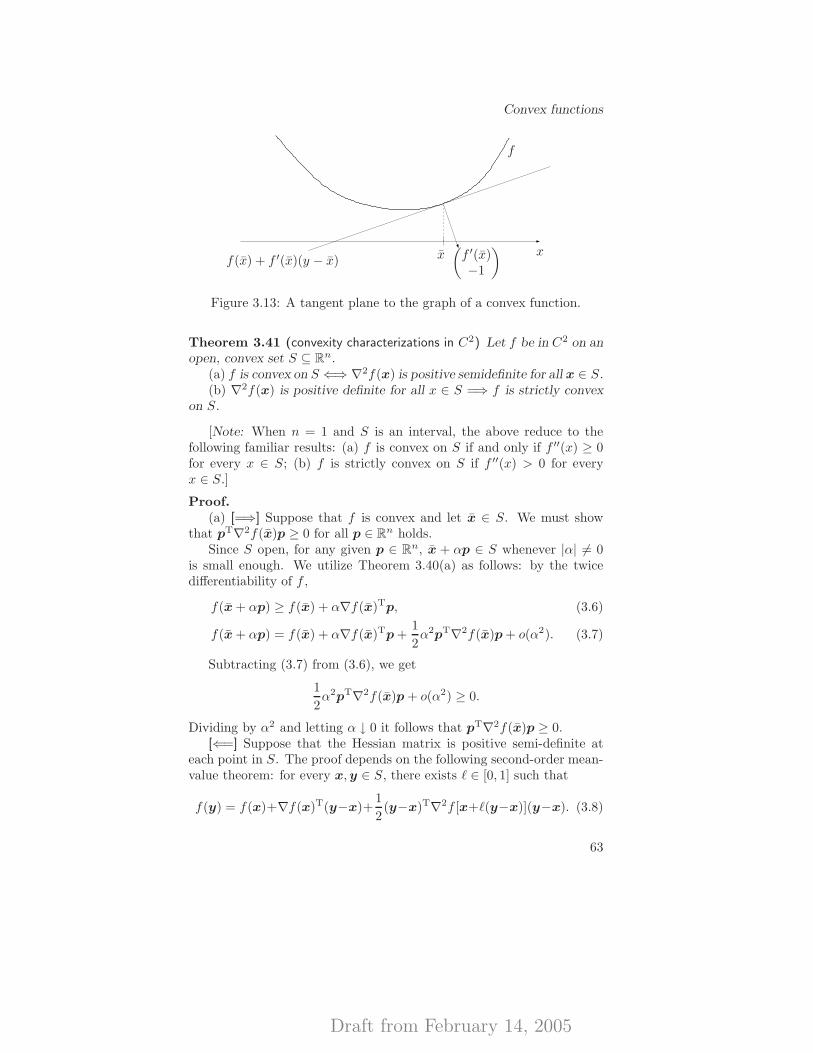
Draft from February 14, 2005
Convex functions
f
f(x) + f ′(x)(y − x) x(f ′(x)−1
)x
Figure 3.13: A tangent plane to the graph of a convex function.
Theorem 3.41 (convexity characterizations in C2) Let f be in C2 on anopen, convex set S ⊆ Rn.
(a) f is convex on S ⇐⇒ ∇2f(x) is positive semidefinite for all x ∈ S.(b) ∇2f(x) is positive definite for all x ∈ S =⇒ f is strictly convex
on S.
[Note: When n = 1 and S is an interval, the above reduce to thefollowing familiar results: (a) f is convex on S if and only if f ′′(x) ≥ 0for every x ∈ S; (b) f is strictly convex on S if f ′′(x) > 0 for everyx ∈ S.]
Proof.(a) [=⇒] Suppose that f is convex and let x ∈ S. We must show
that pT∇2f(x)p ≥ 0 for all p ∈ Rn holds.Since S open, for any given p ∈ Rn, x + αp ∈ S whenever |α| 6= 0
is small enough. We utilize Theorem 3.40(a) as follows: by the twicedifferentiability of f ,
f(x + αp) ≥ f(x) + α∇f(x)Tp, (3.6)
f(x + αp) = f(x) + α∇f(x)Tp +1
2α2pT∇2f(x)p + o(α2). (3.7)
Subtracting (3.7) from (3.6), we get
1
2α2pT∇2f(x)p + o(α2) ≥ 0.
Dividing by α2 and letting α ↓ 0 it follows that pT∇2f(x)p ≥ 0.[⇐=] Suppose that the Hessian matrix is positive semi-definite at
each point in S. The proof depends on the following second-order mean-value theorem: for every x,y ∈ S, there exists ℓ ∈ [0, 1] such that
f(y) = f(x)+∇f(x)T(y−x)+1
2(y−x)T∇2f [x+ℓ(y−x)](y−x). (3.8)
63
Draft from February 14, 2005
Convex analysis
By assumption, the last term in (3.8) is non-negative, whence we obtainthe convexity characterization in Theorem 3.40(a).
(b) [=⇒] By the assumptions, the last term in (3.8) is always positivewhen y 6= x, whence we obtain the strict convexity characterization inC1.
It is important to note that the opposite direction in the result (b) isfalse. A simple example that establishes this fact is the function definedby f(x) = x4, S = R; f is strictly convex on R (why?), but its secondderivative at zero is f ′′(0) = 0!
The case of quadratic functions f is interesting to mention in partic-ular. For quadratic functions, that is, functions of the form
f(x) = (1/2)xTQx − qTx + a,
for some symmetric matrix Q ∈ Rn×n, vector q ∈ Rn and constanta ∈ R, it holds that ∇2f(x) ≡ Q for every x where f is defined, so thevalue ∇2f(x) does not depend on x. In this case, we can state a strongerresult than in Theorem 3.41: the quadratic function f is convex on theopen, convex set S ⊆ Rn if and only if Q is positive semi-definite; f isstrictly convex on S if and only if Q is positive definite. To prove thisresult is simple from the above result for general C2 functions, and isleft as an exercise.
What happens when S is not full-dimensional (which is often thecase)? Take, for example, f(x) := x2
1 − x22 and S := {x ∈ R2 | x1 ∈
R; x2 = 0 }. Then, f is convex on S but ∇2f(x) is not positive semi-definite anywhere on S. The below result covers this type of case. Itsproof is left as an exercise.
Theorem 3.42 (convexity characterizations in C2, part II) Let S ⊆ Rn
be a nonempty convex set and f : Rn → R be in C2 on Rn. Let C bethe subspace parallel to the affine hull of S. Then,
f is convex on S ⇐⇒ pT∇2f(x)p ≥ 0 for every x ∈ S and p ∈ C.
In particular, when S has a nonempty interior, f is convex if and onlyif ∇2f(x) is positive semi-definite for every x ∈ S.
We have already seen that the convexity of a function is intimatelyconnected to the convexity of a certain set, namely the epigraph of thefunction. The following result shows that a particular type of set, definedby those vectors that bound a convex function from above, is a convexset. Later, we will utilize this result to establish the convexity of feasiblesets in some optimization problems.
64
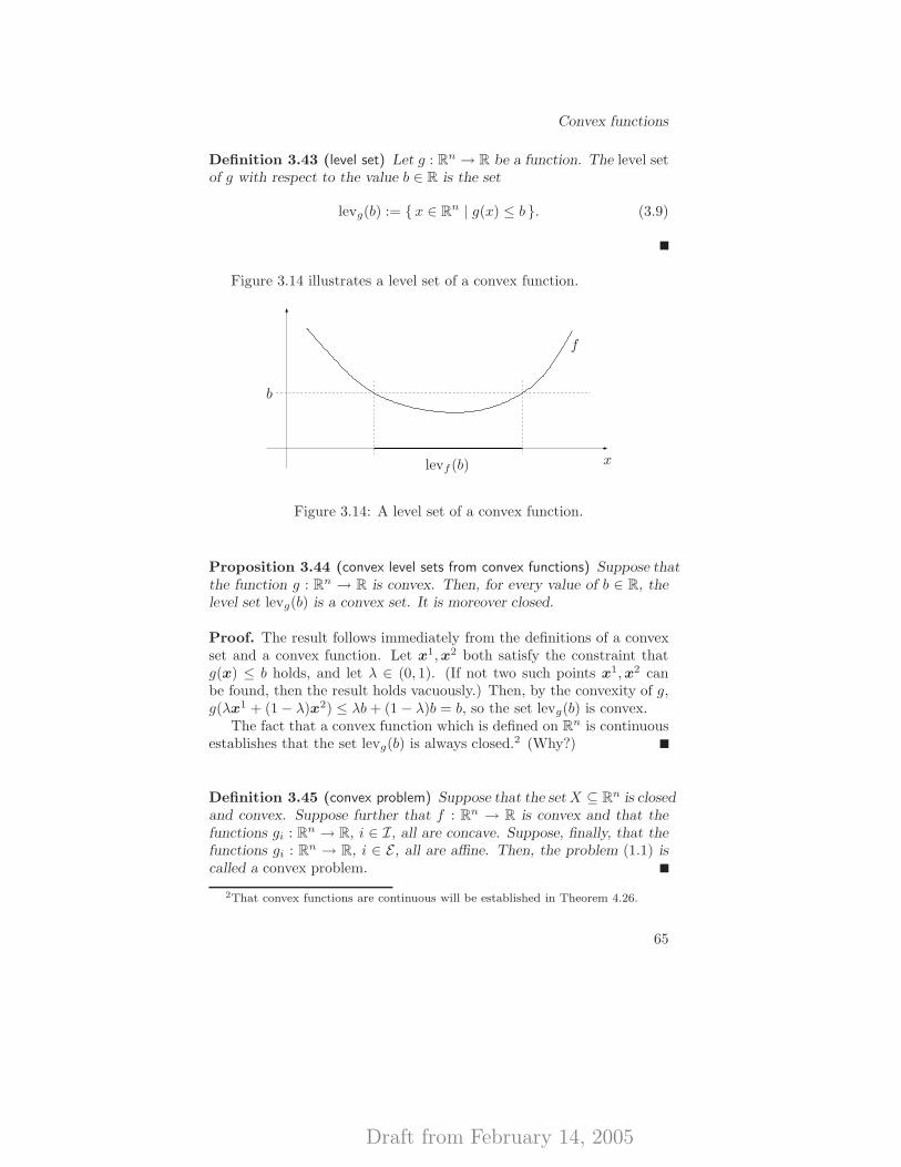
Draft from February 14, 2005
Convex functions
Definition 3.43 (level set) Let g : Rn → R be a function. The level setof g with respect to the value b ∈ R is the set
levg(b) := { x ∈ Rn | g(x) ≤ b }. (3.9)
Figure 3.14 illustrates a level set of a convex function.
f
levf (b)
b
x
Figure 3.14: A level set of a convex function.
Proposition 3.44 (convex level sets from convex functions) Suppose thatthe function g : Rn → R is convex. Then, for every value of b ∈ R, thelevel set levg(b) is a convex set. It is moreover closed.
Proof. The result follows immediately from the definitions of a convexset and a convex function. Let x1,x2 both satisfy the constraint thatg(x) ≤ b holds, and let λ ∈ (0, 1). (If not two such points x1,x2 canbe found, then the result holds vacuously.) Then, by the convexity of g,g(λx1 + (1 − λ)x2) ≤ λb+ (1 − λ)b = b, so the set levg(b) is convex.
The fact that a convex function which is defined on Rn is continuousestablishes that the set levg(b) is always closed.2 (Why?)
Definition 3.45 (convex problem) Suppose that the setX ⊆ Rn is closedand convex. Suppose further that f : Rn → R is convex and that thefunctions gi : Rn → R, i ∈ I, all are concave. Suppose, finally, that thefunctions gi : Rn → R, i ∈ E , all are affine. Then, the problem (1.1) iscalled a convex problem.
2That convex functions are continuous will be established in Theorem 4.26.
65
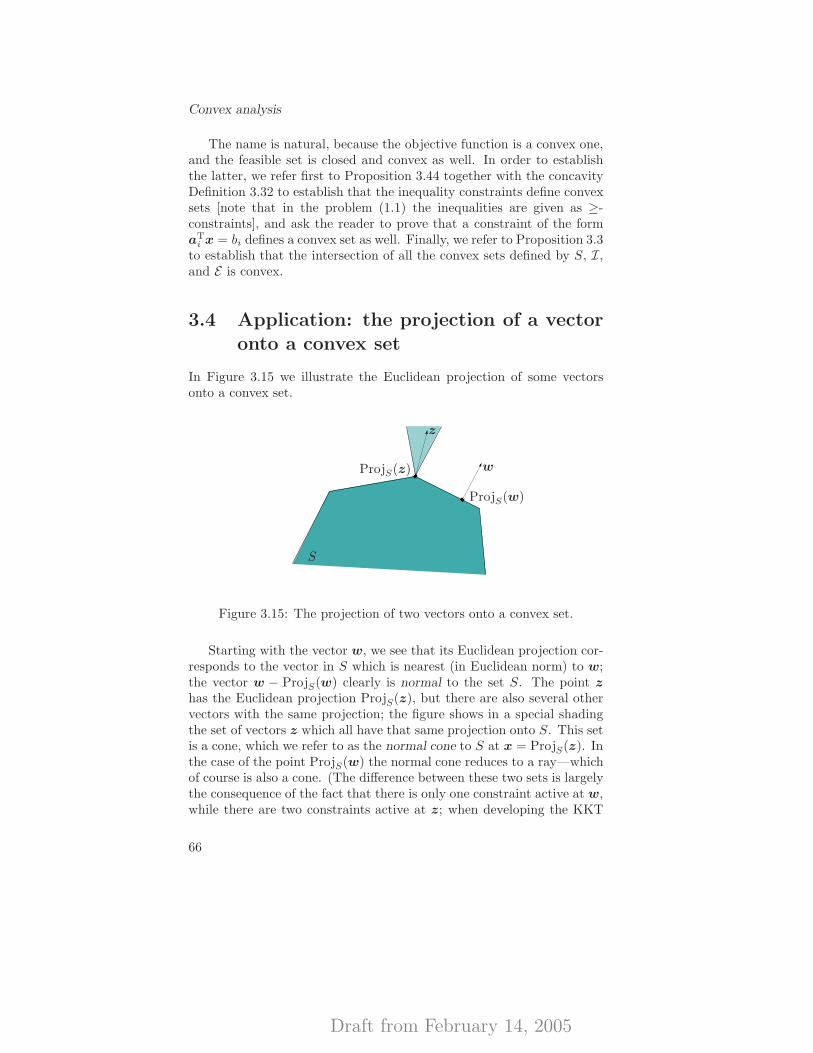
Draft from February 14, 2005
Convex analysis
The name is natural, because the objective function is a convex one,and the feasible set is closed and convex as well. In order to establishthe latter, we refer first to Proposition 3.44 together with the concavityDefinition 3.32 to establish that the inequality constraints define convexsets [note that in the problem (1.1) the inequalities are given as ≥-constraints], and ask the reader to prove that a constraint of the formaT
i x = bi defines a convex set as well. Finally, we refer to Proposition 3.3to establish that the intersection of all the convex sets defined by S, I,and E is convex.
3.4 Application: the projection of a vector
onto a convex set
In Figure 3.15 we illustrate the Euclidean projection of some vectorsonto a convex set.
y
����
����
S
w
ProjS(w)
z
ProjS(z)
Figure 3.15: The projection of two vectors onto a convex set.
Starting with the vector w, we see that its Euclidean projection cor-responds to the vector in S which is nearest (in Euclidean norm) to w;the vector w − ProjS(w) clearly is normal to the set S. The point z
has the Euclidean projection ProjS(z), but there are also several othervectors with the same projection; the figure shows in a special shadingthe set of vectors z which all have that same projection onto S. This setis a cone, which we refer to as the normal cone to S at x = ProjS(z). Inthe case of the point ProjS(w) the normal cone reduces to a ray—whichof course is also a cone. (The difference between these two sets is largelythe consequence of the fact that there is only one constraint active at w,while there are two constraints active at z; when developing the KKT
66

Draft from February 14, 2005
Notes and further reading
conditions in Chapter 5 we shall see how strongly the number of activeconstraints influence the appearance of the optimality conditions.)
We will also return to this image already in Section 4.6.3, becauseit contains the building blocks of the optimality conditions for an op-timization problem with an objective function in C1 over a convex set.For now, we will establish only one property of the projection operationProjS , namely that the distance function, distS , defined by
distS(x) := ‖x− ProjS(x)‖, x ∈ Rn, (3.10)
is a convex function on Rn. In particular, then, this function is continu-ous. (Later, we will establish also that the projection operation ProjS isa well-defined operation whenever S is nonempty, closed and convex, andthat the operation has particularly nice continuity properties. Before wecan do so, however, we need to establish some results on the existenceof optimal solutions.)
Let x1,x2 ∈ Rn, and λ ∈ (0, 1). Then,
distS(λx1 + (1 − λ)x2) = ‖(λx1 + (1 − λ)x2)
− ProjS(λx1 + (1 − λ)x2)‖≤ ‖(λx1 + (1 − λ)x2)
− (λProjS(x1) + (1 − λ)ProjS(x2))‖≤ λ‖x1 − ProjS(x1)‖
+ (1 − λ)‖x2 − ProjS(x2)‖= λdistS(x1) + (1 − λ)distS(x2),
where the first inequality comes from the fact that λProjS(x1) + (1 −λ)ProjS(x2) ∈ S, but it does not necessarily define ProjS(λx1 + (1 −λ)x2) (it may have a longer distance), and the second is the triangleinequality.
The proof is illustrated in Figure 3.16.
3.5 Notes and further reading
The subject of this chapter—convex analysis—has a long history, goingback about a century. Much of the early work on convex sets and func-tions, for example, the theory of separation of convex sets, go back to thework of Minkowski [Min10, Min11]. More modern expositions are foundin [Fen51, Roc70, StW70], which all are classical in the field. More easilyaccessible are the modern books [BoL00, BNO03]. Lighter introductions
67
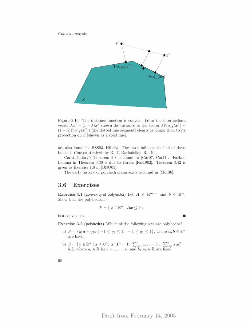
Draft from February 14, 2005
Convex analysis
����
����
����
����
����
����
����
S
x1
x2
ProjS(x1)
ProjS(x2)
Figure 3.16: The distance function is convex. From the intermediatevector λx1 + (1 − λ)x2 shown the distance to the vector λProjS(x1) +(1 − λ)ProjS(x2)) [the dotted line segment] clearly is longer than to itsprojection on S [shown as a solid line].
are also found in [BSS93, HiL93]. The most influencial of all of thesebooks is Convex Analysis by R. T. Rockafellar [Roc70].
Caratheodory’s Theorem 3.8 is found in [Car07, Car11]. Farkas’Lemma in Theorem 3.30 is due to Farkas [Far1902]. Theorem 3.42 isgiven as Exercise 1.8 in [BNO03].
The early history of polyhedral convexity is found in [Mot36].
3.6 Exercises
Exercise 3.1 (convexity of polyhedra) Let A ∈ Rm×n and b ∈ Rm.Show that the polyhedron
P = {x ∈ Rn | Ax ≤ b },
is a convex set.
Exercise 3.2 (polyhedra) Which of the following sets are polyhedra?
a) S = {y1a + y2b | −1 ≤ y1 ≤ 1, − 1 ≤ y2 ≤ 1}, where a, b ∈ Rn
are fixed.
b) S = {x ∈ Rn | x ≥ 0n, xT1n = 1,∑n
i=1 xiai = b1,∑n
i=1 xia2i =
b2}, where ai ∈ R for i = 1, . . . , n, and b1, b2 ∈ R are fixed.
68
Draft from February 14, 2005
Exercises
c) S = {x ∈ Rn | x ≥ 0n, xTy ≤ 1 for all y such that ‖y‖2 = 1}.
d) S = {x ∈ Rn | x ≥ 0n, xTy ≤ 1 for all y such that∑n
i=1 |yi| = 1}.
e) S = {x ∈ Rn | ‖x − x0‖2 ≤ ‖x − x1‖2}, where x0,x1 ∈ Rn arefixed.
f) S = {x ∈ Rn | ‖x − x0‖2 ≤ ‖x − xi‖2, i = 1, . . . , k}, wherex0, . . . ,xk ∈ Rn are fixed.
Exercise 3.3 (extreme points) Consider the polyhedron P defined by
x1 + x2 ≤ 2,
x2 ≤ 1,
x3 ≤ 2,
x2 + x3 ≤ 2.
a) Is x1 = (1, 1, 0)T an extreme point to P?
b) Is x2 = (1, 1, 1)T an extreme point to P?
Exercise 3.4 (existence of extreme points in LPs) Let A ∈ Rm×n be suchthat rankA = m, and let b ∈ Rm. Show that if the polyhedron
P = {x ∈ Rn | Ax = b; x ≥ 0n }
has a feasible solution, then it has an extreme point.
Exercise 3.5 (illustration of the Representation Theorem) Let
Q = {x ∈ R2 | −2x1 + x2 ≤ 1; x1 − x2 ≤ 1; −x1 − x2 ≤ −1 },C = {x ∈ R2 | −2x1 + x2 ≤ 0; x1 − x2 ≤ 0; −x1 − x2 ≤ 0 },
and P be the convex hull of the extreme points of Q. Show that thefeasible point x = (1, 1)T can be written as
x = p + c,
where p ∈ P and c ∈ C.
69
Draft from February 14, 2005
Convex analysis
Exercise 3.6 (separation) Show that there is only one hyperplane in R3
which separates the disjoint closed convex sets A and B defined by theequations
A = { (0, x2, 1)T | x2 ∈ R }, B = {x ∈ R3 | x ≥ 03, x1x2 ≥ x23 }
and that this hyperplane meets both A and B.
Exercise 3.7 (separation) Show that each closed convex set A in Rn isthe intersection of all the closed halfspaces in Rn containing A.
Exercise 3.8 (application of Farkas’ Lemma) In a paper submitted forpublication in an operations research journal, the author considered theset
P =
{(x
y
)∈ Rn+m
∣∣∣∣ Ax + By ≥ c; x ≥ 0n; y ≥ 0m
},
where A is an m × n matrix, B a positive semi-definite m ×m matrixand c ∈ Rm. The author explicitly assumed that the set P is compactin Rn+m. A reviewer of the paper pointed out that the only compact setof the above form is the empty set. Prove the reviewer’s assertion.
Exercise 3.9 (convex sets) Let S1 := {x ∈ R2 | x1 + x2 ≤ 1; x1 ≥ 0 },S2 := {x ∈ R2 | x1 − x2 ≥ 0; x1 ≤ 1 }, and S := S1 ∪ S2. Prove thatS1 and S2 are convex sets and that S is not convex. Hence, the unionof convex sets is not necessarily a convex set.
Exercise 3.10 (convex functions) Determine if the function f definedby f(x) := 2x2
1 − 3x1x2 +5x22 − 2x1 +6x2 is convex, concave, or neither,
on R2.
Exercise 3.11 (convex functions) Let a > 0. Consider the followingfunctions in one variable:
a) f(x) := lnx, for x > 0;b) f(x) := − lnx, for x > 0;c) f(x) := − ln(1 − e−ax), for x > 0;d) f(x) := ln(1 + eax);e) f(x) := eax;f) f(x) := x lnx, for x > 0.Which of these functions are convex (respectively, strictly convex)?
Exercise 3.12 (convex functions) Consider the following functions: a)f(x) := ln(ex1 + ex2);
70
Draft from February 14, 2005
Exercises
b) f(x) := ln∑n
j=1 eajxj , where aj , j = 1, . . . , n, are constants;
c) f(x) :=
√√√√n∑
j=1
x2j ;
d) f(x) := x21/x2, for x2 > 0;
e) f(x) := −√x1x2, for x1, x2 > 0;
f) f(x) := −
n∏
j=1
xj
1/n
, for xj > 0, j = 1, . . . , n.
Which of these functions are convex (respectively, strictly convex)?
Exercise 3.13 (convex functions) Consider the following function:
f(x, y) := 2x2 − 2xy +1
2y2 + 3x− y.
a) Express the function in matrix–vector form.
b) Is the Hessian singular?
c) Is f a convex function?
Exercise 3.14 (convex sets) Consider the following sets:
a) {x ∈ R2 | x21 + x2
2 ≤ 1; x21 + x2
2 ≥ 1/4 };b) {x ∈ Rn | xj ≥ 0, j = 1, . . . , n };c) {x ∈ Rn | x2
1 + x22 + · · · + x2
n = 1 };d) {x ∈ R2 | x1 + x2
2 ≤ 5; x21 − x2 ≤ 10; x1 ≥ 0; x2 ≥ 0 };
e) {x ∈ R2 | x1 − x22 ≥ 1; x3
1 + x22 ≤ 10; 2x1 + x2 ≤ 8; x1 ≥ 1; x2 ≥
0 }.Investigate whether each of them is convex or not. In the latter case,
provide a counter-example.
Exercise 3.15 (convex sets) Is the set defined by
S := {x ∈ R2 | 2e−x1+x22 ≤ 4, −x2
1 + 3x1x2 − 3x22 ≥ −1 }
a convex set?
Exercise 3.16 (convex sets) Is the set defined by
S := {x ∈ R2 | x1−x22 ≥ 1, x3
1+x22 ≤ 10, 2x1+x2 ≤ 8, x1 ≥ 1, x2 ≥ 0 }
a convex set?
71
Draft from February 14, 2005
Convex analysis
Exercise 3.17 (convex problem) Suppose that the function g : Rn → Ris convex on Rn and that d ∈ Rn. Is the problem to
maximize −n∑
j=1
x2j ,
subject to − 1
ln(−g(x))≥ 0,
dTx = 2,
g(x) ≤ −2,
x ≥ 0n
a convex problem?
Exercise 3.18 (convex problem) Is the problem to
maximize x1 lnx1,
subject to x21 + x2
2 ≥ 0,
x ≥ 02
a convex problem?
72

Draft from February 14, 2005
Part III
Optimality Conditions

Draft from February 14, 2005
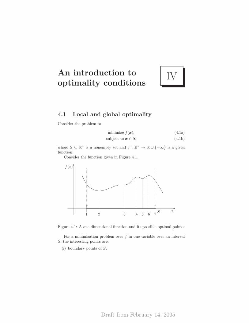
Draft from February 14, 2005
An introduction tooptimality conditions
IV
4.1 Local and global optimality
Consider the problem to
minimize f(x), (4.1a)
subject to x ∈ S, (4.1b)
where S ⊆ Rn is a nonempty set and f : Rn → R ∪ {+∞} is a givenfunction.
Consider the function given in Figure 4.1.
x
f(x)
1 2 3 4 5 6 7S
Figure 4.1: A one-dimensional function and its possible optimal points.
For a minimization problem over f in one variable over an intervalS, the interesting points are:
(i) boundary points of S;
Draft from February 14, 2005
An introduction to optimality conditions
(ii) stationary points, that is, where f ′(x) = 0;
(iii) discontinuities in f or f ′.
In the case of the function in Figure 4.1 we have:
(i) 1, 7;
(ii) 2, 3, 4, 5, 6;
(iii) none.
Definition 4.1 (global minimum) Consider the problem (4.1). Let x∗ ∈S. Then, we say that x∗ is a global minimum of f over S if it attainsthe lowest value of f over S.
In other words, x∗ ∈ S is a global minimum of f over S if
f(x∗) ≤ f(x), x ∈ S, (4.2)
holds.
Let Bε(x∗) := {y ∈ Rn | ‖y − x∗‖ < ε } be the Euclidean ball with
radius ε centered at x∗.
Definition 4.2 (local minimum) Consider the problem (4.1). Let x∗ ∈S.
(a) We say that x∗ is a local minimum of f over S if there exists asmall enough ball intersected with S around x∗ such that it is a globallyoptimal solution in that smaller set.
In other words, x∗ ∈ S is a local minimum of f over S if
∃ε > 0 such that f(x∗) ≤ f(x), x ∈ S ∩Bε(x∗). (4.3)
(b) We say that x∗ ∈ S is a strict local minimum of f over S if, in(4.3), the inequality holds strictly for x 6= x∗.
Note that a global minimum in particular is a local minimum. Whenis a local minimum a global one? This question is resolved in the caseof convex problems, as the following fundamental theorem shows.
Theorem 4.3 (Fundamental Theorem of global optimality) Consider theproblem (4.1), where S is a convex set and f is convex on S. Then, everylocal minimum of f over S is also a global minimum.
Proof. Suppose that x∗ is a local minimum but not a global one, whilex is a global minimum. Then, f(x) < f(x∗). Let λ ∈ (0, 1). By theconvexity of S and f , λx + (1 − λ)x∗ ∈ S, and f(λx + (1 − λ)x∗) ≤λf(x) + (1−λ)f(x∗) < f(x∗). Choosing λ > 0 small enough then leads
76
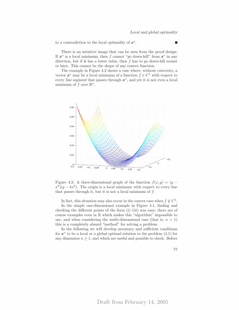
Draft from February 14, 2005
Local and global optimality
to a contradiction to the local optimality of x∗.
There is an intuitive image that can be seen from the proof design:If x∗ is a local minimum, then f cannot “go down-hill” from x∗ in anydirection, but if x has a lower value, then f has to go down-hill sooneror later. This cannot be the shape of any convex function.
The example in Figure 4.2 shows a case where, without convexity, avector x∗ may be a local minimum of a function f ∈ C1 with respect toevery line segment that passes through x∗, and yet it is not even a localminimum of f over Rn.
−0.1
0
0.1−0.2 −0.15 −0.1 −0.05 0 0.05 0.1 0.15 0.2
0
0.01
0.02
0.03
0.04
0.05
0.06
Figure 4.2: A three-dimensional graph of the function f(x, y) = (y −x2)(y − 4x2). The origin is a local minimum with respect to every linethat passes through it, but it is not a local minimum of f .
In fact, this situation may also occur in the convex case when f /∈ C1.In the simple one-dimensional example in Figure 4.1, finding and
checking the different points of the form (i)–(iii) was easy; there are ofcourse examples even in R which makes this “algorithm” impossible touse, and when considering the multi-dimensional case (that is, n > 1)this is a completely absurd “method” for solving a problem.
In the following we will develop necessary and sufficient conditionsfor x∗ to be a local or a global optimal solution to the problem (4.1) forany dimension n ≥ 1, and which are useful and possible to check. Before
77
Draft from February 14, 2005
An introduction to optimality conditions
we do that, however, we will establish exactly when a globally optimalsolution to the problem (4.1) exists.
4.2 Existence of optimal solutions
We first pave the way for a classic result from calculus: Weierstrass’Theorem.
Definition 4.4 (weakly coercive, coercive functions) Let S ⊆ Rn be anonempty and closed set, and f : S → R be a given function.
(a) We say that f is weakly coercive with respect to the set S ifS is bounded or the sequence {f(xk)} tends to infinity whenever thesequence {xk} ⊂ S tends to infinity in norm.
In other words, f is weakly coercive if either S is bounded or
lim‖xk‖→∞
xk∈S
f(xk) = ∞
holds.
(b) We say that f is coercive with respect to the set S if S is boundedor the sequence {f(xk)/‖xk‖} tends to infinity whenever the sequence{xk} ⊂ S tends to infinity in norm.
In other words, f is coercive if either S is bounded or
lim‖xk‖→∞
xk∈S
f(xk)/‖xk‖ = ∞
holds.
The weak coercivity of f : S → R is (for nonempty sets S) equiv-alent to the property that f has bounded level sets restricted to S (cf.Definition 3.43). (Why?)
A coercive function clearly grows faster than any linear function.In fact, for convex functions f , f being coercive is equivalent to x 7→f(x)−aTx being weakly coercive for every vector a ∈ Rn. This propertyis a very useful one for certain analyses in the context of Lagrangianduality.1
We next introduce two extended notions of continuity.
1For example, in Section 6.4.2 we suppose that the ground set X is compact inorder for the Lagrangian dual function q to be finite. It is possible to replace theboundedness condition on X with a coercivity condition on f .
78
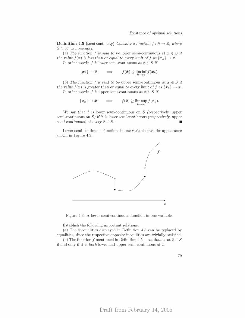
Draft from February 14, 2005
Existence of optimal solutions
Definition 4.5 (semi-continuity) Consider a function f : S → R, whereS ⊆ Rn is nonempty.
(a) The function f is said to be lower semi-continuous at x ∈ S ifthe value f(x) is less than or equal to every limit of f as {xk} → x.
In other words, f is lower semi-continuous at x ∈ S if
{xk} → x =⇒ f(x) ≤ lim infk→∞
f(xk).
(b) The function f is said to be upper semi-continuous at x ∈ S ifthe value f(x) is greater than or equal to every limit of f as {xk} → x.
In other words, f is upper semi-continuous at x ∈ S if
{xk} → x =⇒ f(x) ≥ lim supk→∞
f(xk).
We say that f is lower semi-continuous on S (respectively, uppersemi-continuous on S) if it is lower semi-continuous (respectively, uppersemi-continuous) at every x ∈ S.
Lower semi-continuous functions in one variable have the appearanceshown in Figure 4.3.
x
f
Figure 4.3: A lower semi-continuous function in one variable.
Establish the following important relations:(a) The inequalities displayed in Definition 4.5 can be replaced by
equalities, since the respective opposite inequlities are trivially satisfied.(b) The function f mentioned in Definition 4.5 is continuous at x ∈ S
if and only if it is both lower and upper semi-continuous at x.
79
Draft from February 14, 2005
An introduction to optimality conditions
(c) Lower semi-continuity of f is equivalent to the closedness of allits level sets levf (b), b ∈ R (cf. Definition 3.43), as well as the closednessof its epigraph (cf. Definition 3.38).
Next follows the famous existence theorem credited to Karl Weier-strass (see, however, Section 4.7).
Theorem 4.6 (Weierstrass’ Theorem) Let S ⊆ Rn be a nonempty andclosed set, and f : S → R be a lower semi-continuous function on S.If f is weakly coercive with respect to S, then there exists a nonempty,closed and bounded (thus compact) set of globally optimal solutions tothe problem (4.1).
Proof. We first assume that S is bounded, and proceed by choosing asequence {xk} in S such that
limk→∞
f(xk) = infx∈S
f(x).
(The infimum of f over S is the lowest limit of all sequences of the form{f(xk)} with {xk} ⊂ S, so such a sequence of xk is what we here arechoosing.)
Due to the boundedness of S, the sequence {xk} must have limitpoints, all of which lie in S because of the closedness of S. Let x be anarbitrary limit point of {xk}, corresponding to the subsequence K ⊆ Z+.Then, by the lower semi-continuity of f ,
f(x) ≤ limk∈K
f(xk) = infx∈S
f(x).
Since x attains the infimum of f over S, x is a global minimum of fover S. This limit point of {xk} was arbitrarily chosen; any other choice(provided more than one exists) has the same (optimal) objective value.
Suppose next that f is weakly coercive, and consider the same se-quence {xk} in S. Then, by the weak coercivity assumption, either {xk}is bounded or the sequence {f(xk)} tends to infinity. The non-emptinessof S implies that infx∈S f(x) < ∞ holds, and hence we conclude that{xk} is bounded. We can then utilize the same arguments as in theprevious paragraph and conclude that also in this case there exists aglobally optimal solution. We are done.
Before moving on we take a closer look at the proof of this result,because it is important in order to understand the importance of someof the assumptions that we make about the optimization models thatwe pose. We notice that the closedness of S is really crucial; if it is notthen a sequence generated in S may converge to a point outside of S,
80
Draft from February 14, 2005
Existence of optimal solutions
which means that we would converge to an infeasible and of course alsonon-optimal solution. This is the reason why the generic optimizationmodel (1.1) stated in Chapter 1 does not contain any constraints of theform
gi(x) < 0, i ∈ SI,where SI denotes strict inequality. The reason is that such constraintsin general may describe non-closed sets.
Weierstrass’ Theorem 4.6 is next improved for special classes of theproblem (4.1). The main purpose of presenting these results is to showthe role of convexity and to illustrate the special properties of convexquadratic programs and linear programs. The proofs are rather complexand are therefore left out.
Theorem 4.7 (existence of solutions, convex polynomials) Suppose thatf : Rn → R is a convex polynomial function. Suppose further that theset S can be described by inequality constraints of the form gi(x) ≤ 0,i = 1, . . . ,m, where each function gi is convex and polynomial. Theproblem (4.1) then is convex. Moreover, it has a nonempty (as well asclosed and convex) set of globally optimal solutions if and only if f islower bounded on S.
In the following result, we let S be a nonempty polyhedron, andsuppose that it is possible to describe it as the following finite (cf. Defi-nition 3.15) set of linear constraints:
S = {x ∈ Rn | Ax ≤ b; Ex = d }, (4.4)
where A ∈ Rm×n, E ∈ Rℓ×n, b ∈ Rm, and d ∈ Rℓ. The recessioncone to S then is the following set, defining the set of directions that arefeasible at every point in S:2
recS := {p ∈ Rn | Ap ≤ 0m; Ep = 0ℓ }. (4.5)
(For the definition of the set of feasible directions at a given vector x,see Definition 4.19.)
We also suppose that
f(x) :=1
2xTQx + qTx, x ∈ Rn, (4.6)
where Q ∈ Rn×n is a symmetric and positive semi-definite matrix andq ∈ Rn. We define the recession cone to any convex function f : Rn → Ras follows: the recession cone to f is the recession cone to the level
2Recall the cone C in the Representation Theorem 3.22.
81
Draft from February 14, 2005
An introduction to optimality conditions
set of f (cf. Definition 3.43), defined for any value of b for which thecorresponding level set of f is nonempty. (Check that this cone actuallyis independent of the value of b under this only requirement. Also confirmthat if the level set levf (b) is (nonempty and) bounded for some b ∈ Rthen it is bounded for every b ∈ R, thanks to the convexity of f .) In thespecial case of the convex quadratic function given in (4.6),
recf = {p ∈ Rn | Qp = 0n; qTp ≤ 0 }.
This is the set of directions that nowhere are ascent directions to f .
Corollary 4.8 (the Frank–Wolfe Theorem) Suppose that S is the poly-hedron described by (4.4) and f is the convex quadratic function givenby (4.6), so that the problem (4.1) is a convex quadratic programmingproblem. Then, the following three statements are equivalent.
(a) The problem (4.1) has a nonempty (as well as a closed and convex)set of globally optimal solutions.
(b) f is lower bounded on S.(c) For every vector p in the intersection of the recession cone recS
to S and the null space N(Q) of the matrix Q, it holds that qTp ≥ 0.In other words,
p ∈ recS ∩N(Q) =⇒ qTp ≥ 0
holds.
The statement in (c) shows that the conditions for the existence ofan optimal solution in the case of convex quadratic programs are milderthan in the general convex case. In the latter case, we can state a slightimprovement over the Weierstrass Theorem 4.6 that if, in the problem(4.1), f is convex on S where the latter is nonempty, closed and convex,then the problem has a nonempty, convex and compact set of globallyoptimal solutions if and only if recS ∩ recf = {0n}. The improvementsin the above results for polyhedral, in particular quadratic, programsstems from the fact that convex polynomial functions cannot be lowerbounded and yet not have a global minimum.
[Note: Consider the special case of the problem (4.1) where f(x) :=1/x and S := [1,+∞). It is clear that f is bounded from below on S,in fact by the value zero which is the infimum of f over S, but it neverattains the value zero on S, and therefore this problem has no optimalsolution. Of course, f is not a polynomial function.]
Corollary 4.9 (a fundamental theorem in linear programming) Suppose,in the Frank–Wolfe Theorem, that f is linear, that is, that Q = 0n×n.
82
Draft from February 14, 2005
Existence of optimal solutions
Then, the problem (4.1) is identical to a linear programming (LP) prob-lem. Then, the following three statements are equivalent.
(a) The problem (4.1) has a nonempty (as well as a closed and convexpolyhedral) set of globally optimal solutions.
(b) f is lower bounded on S.(c) For every vector p in the recession cone recS to S, it holds that
qTp ≥ 0. In other words,
p ∈ recS =⇒ qTp ≥ 0
holds.
Corollary 4.9 will in fact be established later on in Theorem 8.10, bythe use of polyhedral convexity, when we specialize our treatment of non-linear optimization to that of linear optimization. Since we have alreadyestablished the Representation Theorem 3.22, proving Corollary 4.9 forthe case of LP will be easy: since the objective function is linear, everyfeasible direction p ∈ recS with qTp < 0 leads to an unbounded solutionfrom any vector x ∈ S.
Under strict convexity, we can finally establish the following result.
Proposition 4.10 (unique solution under strict convexity) Suppose thatin the problem (4.1) f is strictly convex on S and the set S is convex.Then, there can be at most one globally optimal solution.
Proof. Suppose, by means of contradiction, that x∗ and x∗∗ are twodifferent globally optimal solutions. Then, for every λ ∈ (0, 1), we havethat
f(λx ∗ + (1 − λ)x ∗∗) < λf(x∗) + (1 − λ)f(x∗∗) = f(x∗) [ = f(x∗∗)].
Since λx∗ + (1 − λ)x∗∗ ∈ S, we have found an entire interval of pointswhich are strictly better than x∗ or x∗∗. This is impossible, whence weare done.
We finally characterize a class of optimization problems over poly-topes whose optimal solution set, if nonempty, includes an extreme point.
Consider the optimization problem to
maximize f(x), (4.7)
subject to x ∈ P,
where f : Rn → R is a convex function and P ⊂ Rn is a nonempty,bounded polyhedron (that is, a polytope). Then, from the Represen-tation Theorem 3.22 it follows below that an optimal solution can be
83
Draft from February 14, 2005
An introduction to optimality conditions
found among the extreme points of P . Theorem 8.10 establishes a cor-responding result for linear programs that does not rely on Weierstrass’Theorem.
Theorem 4.11 (optimal extreme point) An optimal solution to (4.7) canbe found among the extreme points of P .
Proof. The function f is continuous (since it is convex, cf. Theorem 4.26below); further, P is a nonempty and compact set. Hence, there exists anoptimal solution x to (4.7) by Weierstrass’ Theorem 4.6. The Represen-tation Theorem 3.22 implies that x = λ1v
1+· · ·+λkvk for some extremepoints v1, . . . ,vk of P and λ1, . . . , λk ≥ 0 such that
∑ki=1 λi = 1. But
then (from the convexity of f)
f(x) = f(λ1v1 + · · · + λkvk) ≤ λ1f(v1) + · · · + λkf(vk)
≤ λ1f(x) + · · · + λkf(x) = f(x),
which gives that f(x) = f(vi) for some i = 1, . . . , k.
Remark 4.12 Every linear function is convex, so Theorem 4.11 implies,in particular, that every linear program over a nonempty and boundedpolyhedron has an optimal extreme point.
4.3 Optimality in unconstrained optimiza-
tion
In Theorem 4.3 we have established that locally optimal solutions alsoare global in the convex case. What are the necessary and sufficientconditions for a vector x∗ to be a local optimum? This is an impor-tant question, because the algorithms that we will investigate for solvingimportant classes of optimization problems are always devised based onthose conditions that we would like to fulfill. This is a statement thatseems to be true universally: efficient, locally or globally convergent it-erative algorithms for an optimization problem are directly based on itsnecessary and/or sufficient local optimality conditions.
We begin by establishing these conditions for the case of uncon-strained optimization, where the objective function is in C1. Every proofis based on the Taylor expansion up to order one or two.
Our problem here is the following:
minimizex∈Rn
f(x), (4.8)
where f is in C1 on Rn [for short we say: in C1].
84
Draft from February 14, 2005
Optimality in unconstrained optimization
Theorem 4.13 (necessary optimality conditions, C1 case) Suppose thatf : Rn → R is in C1 on Rn. Then,
x∗ is a local minimum of f on Rn =⇒ ∇f(x∗) = 0n.
Note that
∇f(x) =(∂f(x)
∂xj
)n
j=1,
so the requirement thus is that ∂f(x∗)∂xj
= 0, j = 1, . . . , n.
Just as for the case n = 1, we refer to this condition as x∗ being astationary point of f .
[Note: For n = 1, Theorem 4.13 reduces to: x∗ ∈ R is a local mini-mum =⇒ f ′(x∗) = 0.]
Proof. (By contradiction.) Suppose that x∗ is a local minimum, butthat ∇f(x∗) 6= 0n. Let p := −∇f(x∗), and study the Taylor expansionaround x = x∗ in the direction of p:
f(x∗ + αp) = f(x∗) + α∇f(x∗)Tp + o(α),
where o : R → R is such that o(s)/s→ 0 when s ↓ 0. We get that
f(x∗ + αp) = f(x∗) − α‖∇f(x∗)‖2 + o(α)
< f(x∗) for all small enough α > 0,
since ‖∇f(x∗)‖ 6= 0. This completes the proof.
The opposite direction is false. Take, for example, f(x) = x3. Then,x = 0 is stationary, but it is neither a local minimum or a local maximum.
The proof is instrumental in that it provides a sufficient conditionfor a vector p to define a descent direction, that is, a direction such thata small step along it yields a lower objective value. We first define thisnotion properly.
Definition 4.14 (descent direction) Let the function f : Rn → R ∪{±∞} be given. Let x ∈ Rn be a vector such that f(x) is finite. Letp ∈ Rn. We say that the vector p ∈ Rn is a descent direction withrespect to f at x if
∃δ > 0 such that f(x + αp) < f(x) for every α ∈ (0, δ]
holds.
85
Draft from February 14, 2005
An introduction to optimality conditions
Proposition 4.15 (sufficient condition for descent) Suppose that f : Rn →R ∪ {+∞} is in C1 around a point x for which f(x) < +∞, and thatp ∈ Rn. If ∇f(x)Tp < 0 then the vector p defines a direction of descentwith respect to f at x.
Proof. Since f is in C1 around x, we can construct a Taylor expansionof f , as above:
f(x + αp) = f(x) + α∇f(x)Tp + o(α).
Since ∇f(x)Tp < 0, we obtain that f(x+αp) < f(x) for all sufficientlysmall values of α > 0.
Notice that at a point x ∈ Rn there may be other descent directionsp ∈ Rn beside those satisfying that ∇f(x)Tp < 0; in Example 11.2(b) weshow how directions of negative curvature stemming from eigenvectorscorresponding to negative eigenvalues of the Hessian matrix ∇2f(x) canbe utilized.
If f has stronger differentiability properties, then we can say evenmore what a local optimum must be like.
Theorem 4.16 (necessary optimality conditions, C2 case) Suppose thatf : Rn → R is in C2 on Rn. Then,
x∗ is a local minimum of f =⇒{∇f(x∗) = 0n
∇2f(x∗) is positive semi-definite.
[Note: For n = 1, Theorem 4.16 reduces to: x∗ ∈ R is a local mini-mum =⇒ f ′(x∗) = 0 and f ′′(x∗) ≥ 0.]
Proof. Consider the Taylor expansion of f up to order two around x∗
and in the direction of a vector p ∈ Rn:
f(x∗ + αp) = f(x∗) + α∇f(x∗)Tp +α2
2pT∇2f(x∗)p + o(α2).
Suppose that x∗ satisfies ∇f(x∗) = 0n, but that there is a vector p 6= 0n
with pT∇2f(x∗)p < 0, that is, ∇2f(x∗) is not positive semidefinite.Then the above yields that f(x∗ + αp) < f(x∗) for all small enoughα > 0, whence x∗ cannot be a local minimum.
Also in this case, the opposite direction is false; the same counter-example as that after Theorem 4.13 applies.
86
Draft from February 14, 2005
Optimality in unconstrained optimization
In Example 11.2(b) we provide an example descent direction thathas the form provided in the above proof; it is based on p being aneigenvector corresponding to a negative eigenvalue of ∇2f(x∗).
The next result shows that under some circumstances, we can estab-lish local optimality for a stationary point.
Theorem 4.17 (sufficient optimality conditions, C2 case) Suppose thatf : Rn → R is in C2 on Rn. Then,
∇f(x∗) = 0n
∇2f(x∗) is positive definite
}=⇒ x∗ is a strict local minimum of f.
[Note: For n = 1, Theorem 4.17 reduces to: f ′(x∗) = 0 and f ′′(x∗) >0 =⇒ x∗ ∈ R is a strict local minimum.]
Proof. Suppose that ∇f(x∗) = 0n and ∇2f(x∗) is positive definite.Take an arbitrary vector p ∈ Rn,p 6= 0n. Then,
f(x∗ + αp) = f(x∗) + α∇f(x ∗)Tp︸ ︷︷ ︸=0
+α2
2pT∇2f(x ∗)p︸ ︷︷ ︸
>0
+o(α2)
> f(x∗), for all small enough α > 0.
As p was arbitrary, it implies that x∗ is a strict local minimum.
We naturally face the following question: When is a stationary pointa global minimum? The answer is given next. (It is instrumental to in-vestigate the connection between this result and the Fundamental The-orem 4.3.)
Theorem 4.18 (necessary and sufficient global optimality conditions) Letf ∈ C1, and let f be convex. Then,
x∗ is a global minimum of f ⇐⇒ ∇f(x∗) = 0n.
Proof. [=⇒] This has already be shown in Theorem 4.13, since a globalminimum is a local minimum.
[⇐=] The convexity of f yields that for every y ∈ Rn,
f(y) ≥ f(x∗) + ∇f(x∗)T(y − x∗)
= f(x∗),
where the equality stems from the property that ∇f(x∗) = 0n, by as-sumption.
87
Draft from February 14, 2005
An introduction to optimality conditions
4.4 Optimality for optimization over con-vex sets
We consider a quite general optimization problem of the form:
minimize f(x), (4.9a)
subject to x ∈ S, (4.9b)
where S ⊆ Rn is nonempty, closed and convex, and f : Rn → R∪{+∞}is in C1 on S.
A noticeable difference to unconstrained optimization is the fact thatwhether a vector p ∈ Rn can be used as a direction of movement froma point x ∈ S depends on the constraints defining S; if x is an interiorpoint of S then every p ∈ Rn is a feasible direction, otherwise onlycertain directions will be feasible. That is, it all depends on whetherthere are any active constraints of S at x or not. We will define theseterms in detail next, and then develop necessary and sufficient optimalityconditions based on them. These conditions are natural extensions ofthose for the case of unconstrained optimization and reduces to themwhen S = Rn. Further, we will develop a way of measuring the distanceto an optimal solution in terms of the value of the objective function fwhich is valid for convex problems. As a result of this development, wewill also be able to finally establish the Separation Theorem 3.24, whoseproof has been postponed until now. (See Section 4.6.2 for the proof.)
Definition 4.19 (feasible direction) Suppose that x ∈ S, where S ⊆Rn, and that p ∈ Rn. Then, the vector p defines a feasible direction atx if a small enough step in the direction of p does not lead outside ofthe set S.
In other words, the vector p defines a feasible direction at x ∈ S if
∃δ > 0 such that x + αp ∈ S for all α ∈ [0, δ]
holds.
Recall that in the discussion following Theorem 4.7 we defined theset of feasible directions of a polyhedral set, that is, the set of directionsthat are feasible at every feasible point. For a general set S it wouldhence be the set
{p ∈ Rm | ∀x ∈ S ∃δ > 0 such that x + αp ∈ S for all α ∈ [0, δ] }.
For nonempty, closed and convex sets S, this set is nonempty if and onlyif the set S also is unbounded. (Why?)
88
Draft from February 14, 2005
Optimality for optimization over convex sets
Definition 4.20 (active constraints) Suppose that the set S ⊂ Rn isdefined by a finite collection of equality and inequality constraints:
S = {x ∈ Rn | gi(x) = 0, i ∈ E ; gi(x) ≤ 0, i ∈ I },
where gi : Rn → R (i ∈ E ∪ I) are given functions. Suppose thatx ∈ S. The set of active constraints at x is the union of all the equalityconstraints and the set of inequality constraints that are satisfied withequality at x, that is, the set E ∪ I(x), where I(x) := { i ∈ I | gi(x) =0 }.
Example 4.21 (feasible directions for linear constraints) Suppose, as a spe-cial case, that the constraints are all linear, that is, that for everyi ∈ E , gi(x) := eT
i x − di (ei ∈ Rn; di ∈ R), and for every i ∈ I,gi(x) := aT
i x− bi (ai ∈ Rn; bi ∈ R). In other words, in matrix notation,S = {x ∈ Rn | Ex = d; Ax ≤ b }.
Suppose further that x ∈ S. Then, the set of feasible directions at x
is the set{p ∈ Rn | Ep = 0ℓ; aT
i p ≤ 0, i ∈ I(x) }.Just as S, this is a polyhedron. Moreover, it is a polyhedral cone.
Clearly, the set of feasible directions of the polyhedral set S (or, therecession cone of S) is
recS := {p ∈ Rn | Ep = 0ℓ; Ap ≤ 0m },
as stated in (4.5). Note moreover that the above set recS represents thecone C in the Representation Theorem 3.22.3
We can now more or less repeat the arguments for the unconstrainedcase in order to establish a necessary optimality condition for constrainedoptimization problems. This condition will immediately be refined forconvex feasible sets, then later on in Chapter 5 be given a generalstatement for the case of explicit constraints in the form of the famousKarush–Kuhn–Tucker conditions in nonlinear programming.
Proposition 4.22 (necessary optimality conditions, C1 case) Suppose thatS ⊆ Rn and that f : Rn → R∪ {+∞} is in C1 around a point x ∈ S forwhich f(x) < +∞.
(a) If x∗ ∈ S is a local minimum of f on S then ∇f(x∗)Tp ≥ 0 holdsfor every feasible direction p at x∗.
3While that theorem was stated for sets defined only by linear inequalities, we canalways rewrite the equalities Ex = d as Ex ≤ d, −Ex ≤ −d; the correspondingfeasible directions are then given by Ep ≤ 0
ℓ, −Ep ≤ 0ℓ, that is, Ep = 0
ℓ.
89
Draft from February 14, 2005
An introduction to optimality conditions
(b) Suppose that S is convex and that f is in C1 on S. If x∗ ∈ S isa local minimum of f on S then
∇f(x∗)T(x − x∗) ≥ 0, x ∈ S, (4.10)
holds.
Notice that we above in (4.10) say that ∇f(x∗)T(x − x∗) ≥ 0 holdsfor every x ∈ S; the quantifier ∀ is not explicitly stated.
Proof. (a) We again utilize the Taylor expansion of f around x∗:
f(x∗ + αp) = f(x∗) + α∇f(x∗)Tp + o(α).
The proof is by contradiction. As was shown in Proposition 4.15, if thereis a direction p for which it holds that ∇f(x∗)Tp < 0, then f(x∗+αp) <f(x∗) for all sufficiently small values of α > 0. It suffices here to statethat p should also be a feasible direction in order to reach a contradictionto the local optimality of x∗.
(b) If S is convex then every feasible direction p can be written as apositive scalar times the vector x − x∗ for some vector x ∈ S. (Why?)The expression (4.10) then follows from the statement in (a).
The inequality (4.10) is sometimes referred to as a variational in-equality. We will utilize it for several purposes: (i) to derive equivalentoptimality conditions involving a linear optimization problem as well asthe Euclidean projection operation ProjS introduced in Section 3.4; (ii)to derive a descent algorithm for the problem (4.9); (iii) to derive a near-optimality condition for convex optimization problems; and (iv) we willextend it to non-convex sets in the form of the Karush–Kuhn–Tuckerconditions.
In Theorem 4.13 we established that for unconstrained C1 optimiza-tion the necessary optimality condition is that ∇f(x∗) = 0n holds. No-tice that that is exactly what becomes of the variational inequality (4.10)when S = Rn, because the only way in which that inequality can holdfor every x ∈ Rn is that ∇f(x∗) = 0n holds. Just as we did in the caseof unconstrained optimization, we will call a vector x∗ ∈ S satisfying(4.10) a stationary point.
We will next provide two statements equivalent to the variationalinequality (4.10). First up, though, we will provide the extension toTheorem 4.18 to the convex constrained case. Notice the resemblance oftheir respective proofs.
Theorem 4.23 (necessary and sufficient global optimality conditions) Supposethat S ⊆ Rn is nonempty and convex. Let f ∈ C1 on S, and let f be
90
Draft from February 14, 2005
Optimality for optimization over convex sets
convex. Then,
x∗ is a global minimum of f on S ⇐⇒ (4.10) holds.
Proof. [=⇒] This has already been shown in Proposition 4.22(b), sincea global minimum is a local minimum.
[⇐=] The convexity of f yields [cf. Theorem 3.40(a)] that for everyy ∈ S,
f(y) ≥ f(x∗) + ∇f(x∗)T(y − x∗)
≥ f(x∗),
where the second inequality stems from (4.10), by assumption.
First, we will provide the connection to the projection of a vectoronto a convex set, discussed in Section 3.4. We claim that the property(4.10) is equivalent to
x∗ = ProjS [x∗ −∇f(x∗)], (4.11)
or, more generally,
x∗ = ProjS [x∗ − α∇f(x∗)], α > 0.
In other words, a point is stationary if and only if a step in the directionof the steepest descent direction followed by a Euclidean projection ontoS means that we have not moved at all. To prove this, we will utilizeProposition 4.22(b) for the optimization problem corresponding to thisprojection. We are interested in finding the point x ∈ S that minimizesthe distance to the vector z := x∗ − ∇f(x∗). We can write this as astrictly convex optimization problem as follows:
minimizex∈S
h(x) :=1
2‖x − z‖2. (4.12)
The necessary optimality conditions for this problem, as stated in Propo-sition 4.22(b), is that
∇h(x)T(y − x) ≥ 0, y ∈ S, (4.13)
holds. Here, ∇h(x) = x − z = x − [x∗ − ∇f(x∗)]. Since h is convex,by Theorem 4.23, we know that the variational inequality (4.13) char-acterizes x as the globally optimal solution to the projection problem.We claimed that x = x∗ is the solution to this problem if and only if x∗
91
Draft from February 14, 2005
An introduction to optimality conditions
is stationary in the problem (4.9). But this follows immediately, sincethe variational inequality (4.13), for the special choice of h and x = x∗,becomes
∇f(x∗)T(y − x∗) ≥ 0, y ∈ S,
that is, a statement identical to (4.10). The characterization (4.11) isinteresting in that it states that if x∗ is not stationary, then the projec-tion operation defined therein then must provide a step away from x∗;this step will in fact yield a reduced value of f under some additionalconditions on the step length α, and so it defines a descent algorithm for(4.9); see Exercise 4.5, and the text in Section 12.4.
So far, we have two equivalent characterizations of a stationary pointof f at x∗: (4.10) and (4.11). The following one is based on a linearoptimization problem.
Notice that (4.10) states that ∇f(x∗)Tx ≥ ∇f(x∗)Tx∗ for everyx ∈ S. Since we obtain equality by setting x = x∗ we see that x∗ infact is a globally optimal solution to the problem to
minimizex∈S
∇f(x∗)Tx.
In other words, (4.10) is equivalent to the statement
minimumx∈S
∇f(x∗)T(x − x∗) = 0. (4.14)
It is quite obvious that if at some point x ∈ S,
minimumy∈S
∇f(x)T(y − x) < 0,
then the direction of p := y−x is a feasible descent direction with respectto f at x. Again, we have a building block of a descent algorithm for theproblem (4.9). [The algorithms that immediately spring out from thischaracterization are called the Frank–Wolfe and Simplicial decomposi-tion algorithms, when S is polyhedral; we notice that in the polyhedralcase, the linear minimization problem is an LP problem. Read moreabout these algorithms in Sections 12.2 and 12.3.] Now having got threeequivalent stationarity conditions, (4.10), (4.11), and (4.14), we finallyprovide a fourth one. This one is intimately associated with the projec-tion operation, and it introduces an important geometric concept intothe theory of optimality, namely the normal cone to a convex set S.
We studied a particular choice of z above, but let us consider anextension of Figure 3.15 which provided an image of the Euclidean pro-jection.
92
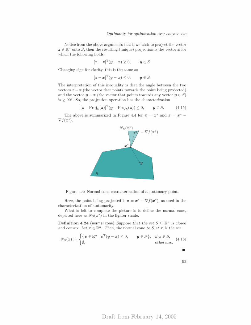
Draft from February 14, 2005
Optimality for optimization over convex sets
Notice from the above arguments that if we wish to project the vectorz ∈ Rn onto S, then the resulting (unique) projection is the vector x forwhich the following holds:
[x − z]T(y − x) ≥ 0, y ∈ S.
Changing sign for clarity, this is the same as
[z − x]T(y − x) ≤ 0, y ∈ S.
The interpretation of this inequality is that the angle between the twovectors z−x (the vector that points towards the point being projected)and the vector y − x (the vector that points towards any vector y ∈ S)is ≥ 90◦. So, the projection operation has the characterization
[z − ProjS(z)]T(y − ProjS(z)) ≤ 0, y ∈ S. (4.15)
The above is summarized in Figure 4.4 for x = x∗ and z = x∗ −∇f(x∗).
����
S
y
x∗ −∇f(x∗)
x∗
NS(x∗)
Figure 4.4: Normal cone characterization of a stationary point.
Here, the point being projected is z = x∗ − ∇f(x∗), as used in thecharacterization of stationarity.
What is left to complete the picture is to define the normal cone,depicted here as NS(x∗) in the lighter shade.
Definition 4.24 (normal cone) Suppose that the set S ⊆ Rn is closedand convex. Let x ∈ Rn. Then, the normal cone to S at x is the set
NS(x) :=
{{ v ∈ Rn | vT(y − x) ≤ 0, y ∈ S }, if x ∈ S,
∅, otherwise.(4.16)
93
Draft from February 14, 2005
An introduction to optimality conditions
According to the definition, we can now define our fourth character-ization of a stationary point at x∗ as follows:
−∇f(x∗) ∈ NS(x∗). (4.17)
What this condition states geometrically is that the angle between thenegative gradient and any feasible direction is ≥ 90◦, which, of course, isthe same as stating that at x∗ there exist no feasible descent directions.The four conditions (4.10), (4.11), (4.14), and (4.17) are equivalent, andso according to Theorem 4.23(b) they all are also both necessary andsufficient for the global optimality of x∗ as soon as f is convex.
We remark that in the special case when S is an affine subspace (suchas the solution set of a number of linear equations, S := {x ∈ Rn | Ex =d }), the statement (4.17) means that at a stationary point x∗, ∇f(x∗)is parallel to the normal of the subspace.
The normal cone inclusion (4.17) will later be extended to more gen-eral sets, where S is described by a finite collection of possibly non-convex constraints. The extension will lead us to the famous Karush–Kuhn–Tucker conditions in Chapter 5. [It turns out to be much moreconvenient to extend (4.17) than the other three characterizations ofstationarity.]
We finish this section by proving a proposition on the behaviour ofthe gradient of the objective function f on the solution set S∗ to convexproblems of the form (4.1). The below result shows that ∇f enjoys astability property, and it also extends the result from the unconstrainedcase where the value of ∇f always is zero on the solution set.
Proposition 4.25 (invariance of ∇f on the solution set of convex programs)Suppose that S ⊆ Rn is convex and that f : Rn → R is convex and inC1 on S. Then, the value of ∇f(x) is constant on the optimal solutionset S∗.
Further, suppose that x∗ ∈ S∗. Then,
S∗ = {x ∈ S | ∇f(x∗)T(x − x∗) = 0 and ∇f(x) = ∇f(x∗) }.
Proof. Let x∗ ∈ S∗. The definition of the convexity of f shows that
f(x) − f(x∗) ≥ ∇f(x∗)T(x − x∗), x ∈ Rn. (4.18)
Let x ∈ S∗. Then, it follows that ∇f(x∗)T(x−x∗) = 0. By substituting∇f(x∗)Tx∗ with ∇f(x∗)Tx in (4.18) and using that f(x∗) = f(x), weobtain that
f(x) − f(x) ≥ ∇f(x∗)T(x − x), x ∈ Rn,
94
Draft from February 14, 2005
Near-optimality in convex optimization
which is equivalent to the statement that ∇f(x) = ∇f(x∗). We aredone.
4.5 Near-optimality in convex optimization
We will here utilize Theorem 4.23 in order to provide a measure of thedistance to the optimal solution in terms of the value of f at any feasiblepoint x.
Let x ∈ S, and suppose that f is convex on S. Suppose also thatx∗ ∈ S is an arbitrary globally optimal solution, which we suppose exists.From the necessary optimality conditions stated in Proposition 4.22(b),it is clear that unless x solves (4.9) there exists a y ∈ S such that∇f(x)T(y−x) < 0, and hence p := y−x is a feasible descent direction.
Suppose now that
y ∈ arg minimumy∈S
z(y) := ∇f(x)T(y − x). (4.19)
Consider the following string of inequalities and equalities:
f(x) + z(y) = f(x) + minimumy∈S
z(y)
≤ f(x) + z(x∗)
≤ f(x∗)
≤ f(x).
The equality follows by definition; the first inequality stems from thefact that y solves the linear minimization problem, while the vector x∗
may not; the second inequality follows from the convexity of f on S [cf.Theorem 3.40(a)]; the final inequality follows from the global optimalityof x∗ and the feasibility of x.
From the above, we obtain a closed interval wherein we know that theoptimal value of the problem (4.9) lies. Let f∗ := minimumx∈S f(x) =f(x∗). Then, for every x ∈ S,
f∗ ∈ [f(x) + z(y), f(x)]. (4.20)
Clearly, the length of the interval is defined by how far from zero the valueof z(y) is. Suppose then that z(y) ≥ −ε, for some small value ε > 0. (Inan algorithm where a sequence {xk} is constructed such that it convergesto an optimal solution, this will eventually happen for every ε > 0.)Then, from the above we obtain that f(x∗) ≥ f(x) + z(y) ≥ f(x) − ε;in short,
f(x∗) ≥ f(x) − ε, or, f(x) ≤ f∗ + ε. (4.21)
95
Draft from February 14, 2005
An introduction to optimality conditions
We refer to a vector x ∈ S satisfying the inequality (4.21) as an ε-optimalsolution. From the above LP problem we hence have a simple instrumentfor evaluating the quality of a feasible solution in our problem. Note,again, that convexity is a crucial property enabling this possibility.
As far as iterative algorithms go, it is quite often the case that forthe problem (4.9) involving a convex feasible set the sequences {xk} ofiterates do not necessarily stay inside the feasible set S. The reason isthat even if the constraints are convex inequalities it is difficult to checkwhen one reaches the boundary of S. We mention however two caseswhere feasible algorithms (that is, those for which {xk} ⊂ S holds) areviable:
(I) When S is a polyhedral set, then it is only a matter of solving a se-ries of simple linear systems to check for the maximum step lengthalong a feasible direction. Among the algorithms that actuallyare feasible we count the simplex method for linear programming(LP) problems, the Frank–Wolfe method which builds on the factthat the lower bounds and descent directions discussed above relyon solving such LP problems, and the projection methods whichbuild on the property investigated in Exercise 4.5. More on thesealgorithms will be said in Chapter 12.
(II) When the set S has an interior point, we may replace the con-straints with an interior penalty function which has an asymptotewhenever approaching the boundary, thus automatically ensuringthat iterates stay (strictly) feasible. More on a class of methodsbased on this penalty function is said in Chapter 13.
4.6 Applications
4.6.1 ∗Continuity of convex functions
A remarkable property of any convex function is that without any addi-tional assumptions it can be shown to be continuous relative to any openconvex set in the intersection of its effective domain and its affine hull.4
We establish a special case below, in which relative interior is replacedby interior for simplicity.
Theorem 4.26 (continuity of convex functions) Suppose that f : Rn →R ∪ {+∞} is a convex function, and consider an open convex subset Sof its effective domain. The function f is continuous on S.
4In other words, it is continuous relative to any relatively open convex subset ofits effective domain.
96
Draft from February 14, 2005
Applications
Proof. Let x ∈ S. To establish continuity of f at x, we must showthat given ε > 0, there exists δ > 0 such that ‖x − x‖ ≤ δ implies that|f(x) − f(x)| ≤ ε. We establish this property in two parts, by showingthat f is both lower and upper semi-continuous at x.
[upper semi-continuity] By the openness of S, there exists δ′ > 0 with‖x − x‖ ≤ δ, implying x ∈ S. Construct the value of the scalar γ asfollows:
γ := maximumi∈{1,2,...,n}
{maximum {f(x + δ′ei) − f(x), f(x − δ′ei) − f(x)}} ,(4.22)
where ei is the ith unit vector in Rn. Note that 0 ≤ γ <∞. Let now
δ := minimum
{δ′
n,εδ′
γn
}. (4.23)
Choose an x with ‖x − x‖ ≤ δ. For every i ∈ {1, 2, . . . , n}, if xi ≥ xi
then define zi := δ′ei, otherwise zi := −δ′ei. Then,
x − x =
n∑
i=1
αizi,
where αi ≥ 0 for all i. Moreover,
‖x− x‖ = δ′‖α‖. (4.24)
From (4.23), and since ‖x − x‖ ≤ δ, it follows that αi ≤ 1/n for all i.Hence, by the convexity of f and since 0 ≤ αin ≤ 1, we get
f(x) = f
(x +
n∑
i=1
αizi
)= f
[1
n
n∑
i=1
(x + αinzi)
]
≤ 1
n
n∑
i=1
f(x + αinzi)
=1
n
n∑
i=1
f [(1 − αin)x + αin(x + zi)]
≤ 1
n
n∑
i=1
[(1 − αin)f(x) + αinf(x + zi)].
Therefore, f(x) − f(x) ≤ ∑ni=1 αi[f(x + zi) − f(x)]. From (4.22) it is
obvious that f(x+zi)− f(x) ≤ γ for each i; and since αi ≥ 0, it followsthat
f(x) − f(x) ≤ γ
n∑
i=1
αi. (4.25)
97
Draft from February 14, 2005
An introduction to optimality conditions
Noting (4.23), (4.24), it follows that αi ≤ ε/nγ, and (4.25) implies thatf(x) − f(x) ≤ ε. Hence, we have so far shown that ‖x − x‖ ≤ δimplies that f(x) − f(x) ≤ ε. By Definition 4.5(b), f hence is uppersemi-continuous at x.
[lower semi-continuity] Let y := 2x − x, and note that ‖y − x‖ ≤ δ.Therefore, as above,
f(y) − f(x) ≤ ε. (4.26)
But x = 12y + 1
2x, and by the convexity of f ,
f(x) ≤ 1
2f(y) +
1
2f(x)
follows. Combining this inequality with (4.26), it follows that f(x) −f(x) ≤ ε, whence Definition 4.5(b) applies. We are done.
Note that convex functions need not be continuous everywhere; bythe above theorem we know however that points of non-continuity mustoccur at the boundary of the effective domain of f . For example, checkthe continuity of the following function:
f(x) :=
{x2, for |x| < 1,
2, for |x| = 1.
4.6.2 The Separation Theorem
The previously established Weierstrass Theorem 4.6 will now be utilizedtogether with the above variational inequality characterization (4.10)of stationary points in order to finally establish the Separation Theo-rem 3.24. For simplicity, we rephrase the theorem.
Theorem 4.27 (Separation Theorem) Suppose that the set S ⊆ Rn isclosed and convex, and that the point y does not lie in S. Then thereexist a vector π 6= 0n and α ∈ R such that πTy > α and πTx ≤ α forall x ∈ S.
Proof. We may assume that S is nonempty, and define a functionf : Rn → R through f(x) = ‖x − y‖2/2, x ∈ Rn. Now by Weier-strass’ Theorem 4.6) there exists a minimizer x of f over S, whichby the first order necessary condition [see Proposition 4.22(b)] satisfies(y− x)T(x− x) ≤ 0 for all x ∈ S (since −∇f(x) = y− x). Now settingπ = y − x and α = (y − x)Tx gives the result sought.
A slightly different separation theorem will be used in the Lagrangianduality theory in Chapter 6. We state it without proof.
98
Draft from February 14, 2005
Applications
Theorem 4.28 (separation of convex sets) Each pair of disjoint nonemptyconvex sets A and B in Rn can be separated by a hyperplane in Rn, thatis, there exists a vector π ∈ Rn and α ∈ R such that πTx ≤ α for allx ∈ A and πTy ≥ α for all y ∈ B.
Remark 4.29 The main difference between the Separation Theorems 3.24and 4.28 is that in Theorem 3.24 there exists a hyperplane that infact strictly separates the point y and the closed convex set C, thatis, there exists a vector π ∈ Rn and an α ∈ R such that πTy > α whileπTx < α holds for all x ∈ C. In Theorem 4.28, however, this is nottrue. Consider, for example, the sets A = {x ∈ R2 | x2 ≤ 0 } andB = {x ∈ R2 | x1 > 0; x2 ≥ 1/x1 }. Then, the line {x ∈ R2 | x2 = 0 }separates A and B, but the sets can not be strictly separated.
4.6.3 Euclidean projection
We will finish our discussions on the projection operation, which wasdefined in Section 3.4, by establishing an interesting continuity property.
Definition 4.30 (non-expansive operator) Suppose that S ⊆ Rn is closedand convex. Let f : S → S denote a vector-valued operator from S to S.We say that f is non-expansive if, as a result of applying the mappingf , the distance between any two vectors x and y in S does not increase.
In other words, the operator f is non-expansive on S if
‖f(x) − f (y)‖ ≤ ‖x − y‖, x,y ∈ S, (4.27)
holds.
Theorem 4.31 (the projection operation is non-expansive) Let S be a nonempty,closed and convex set in Rn. For every x ∈ Rn, its projection ProjS(x)is uniquely defined. The operator ProjS : Rn → S is non-expansive onRn, and therefore in particular continuous.
Proof. The uniqueness of the operation is the result of the fact thatthe objective function x 7→ ‖x − z‖ (or, x 7→ ‖x − z‖2) is both weaklycoercive and strictly convex on S, so there exists a unique optimal so-lution to the projection problem for every z ∈ Rn. (Cf. Weierstrass’Theorem 4.6 and Proposition 4.10, respectively.)
Next, take x1,x2 ∈ Rn. Then, by the characterization (4.15) of theEuclidean projection,
[ProjS(x2) − ProjS(x1)]T(x1 − ProjS(x2)) ≤ 0,
[ProjS(x1) − ProjS(x2)]T(x2 − ProjS(x1)) ≤ 0.
99
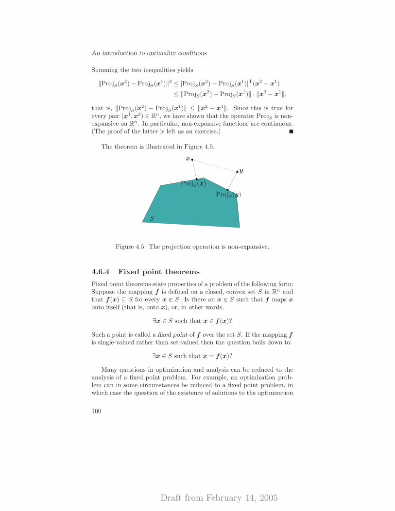
Draft from February 14, 2005
An introduction to optimality conditions
Summing the two inequalities yields
‖ProjS(x2) − ProjS(x1)‖2 ≤ [ProjS(x2) − ProjS(x1)]T(x2 − x1)
≤ ‖ProjS(x2) − ProjS(x1)‖ · ‖x2 − x1‖,
that is, ‖ProjS(x2) − ProjS(x1)‖ ≤ ‖x2 − x1‖. Since this is true forevery pair (x1,x2) ∈ Rn, we have shown that the operator ProjS is non-expansive on Rn. In particular, non-expansive functions are continuous.(The proof of the latter is left as an exercise.)
The theorem is illustrated in Figure 4.5.
����
����
����
����
S
x
y
ProjS(x)
ProjS(y)
Figure 4.5: The projection operation is non-expansive.
4.6.4 Fixed point theorems
Fixed point theorems state properties of a problem of the following form:Suppose the mapping f is defined on a closed, convex set S in Rn andthat f(x) ⊆ S for every x ∈ S. Is there an x ∈ S such that f maps x
onto itself (that is, onto x), or, in other words,
∃x ∈ S such that x ∈ f (x)?
Such a point is called a fixed point of f over the set S. If the mapping f
is single-valued rather than set-valued then the question boils down to:
∃x ∈ S such that x = f(x)?
Many questions in optimization and analysis can be reduced to theanalysis of a fixed point problem. For example, an optimization prob-lem can in some circumstances be reduced to a fixed point problem, inwhich case the question of the existence of solutions to the optimization
100
Draft from February 14, 2005
Applications
problem can be answered by studying the fixed point problem. Further,the optimality conditions analyzed in Section 4.4 can be written as thesolution to a fixed point problem; we can therefore equate the searchfor a stationary point with that of finding a fixed point of a particularfunction f . This type of analysis is quite useful also when analyzing theconvergence of iterative algorithms for optimization problems.
4.6.4.1 Theory
We begin by studying some classical fixed point theorems, and then weprovide examples of the connections between the results in Section 4.4with fixed point theory.
Definition 4.32 (contractive operator) Let S be a nonempty, closed andconvex set in Rn. Let f be a mapping from S to S. We say that f iscontractive on S if, as a result of applying the mapping f , the distancebetween any two distinct vectors x and y in S decreases.
In other words, the operator f is contractive on S if there existsα ∈ [0, 1) such that
‖f(x) − f(y)‖ ≤ α‖x − y‖, x,y ∈ S, (4.28)
holds.
Clearly, a contractive operator is non-expansive.In the below result we utilize the notion of a geometric convergence
rate; while its definition is in fact given in the result below, we also referto Sections 6.5.1 and 11.10 for more detailed discussions on convergencerates.
Theorem 4.33 (fixed point theorems) Let S be a nonempty, closed andconvex set in Rn.
(a) [Banach’s Theorem] Let f be a contraction mapping from S toS. Then, f has a unique fixed point x∗ ∈ S. Further, for every initialvector x0 ∈ S, the iteration sequence {xk} defined by the fixed-pointiteration
xk+1 := f(xk), k = 0, 1, . . . , (4.29)
converges geometrically to the unique fixed point x∗. In particular,
‖xk − x∗‖ ≤ αk‖x0 − x∗‖, k = 0, 1, . . . .
(b) [Brouwer’s Theorem] Let S further be bounded, and assume merelythat f is continuous. Then, f has a fixed point.
101
Draft from February 14, 2005
An introduction to optimality conditions
Proof. (a) For any x0 ∈ S, consider the sequence {xk} defined by(4.29). Then, for any p ≥ 1,
‖xk+p − xk‖ ≤p∑
i=1
‖xk+i − xk+i−1‖
≤ (αp−1 + · · · + 1)‖xk+1 − xk‖ ≤ [αk/(1 − α)]‖x1 − x0‖.
Hence, {xk} is a Cauchy sequence and thus converges. By continuity,the limit point is the unique fixed point.
The convergence speed follows from the identification
‖xk − x∗‖ = ‖f(xk−1) − f(x∗)‖ ≤ α‖xk−1 − x∗‖, k = 1, 2, . . . .
Applying this relation recursively yields the result.(b) [Sketch] In short, the proof is to first establish that any C1 func-
tion on the unit ball has a fixed point there. Extending the reason-ing to merely continuous operators is possible, because of the Stone–Weierstrass Theorem (which states that for any continuous operator de-fined on the unit ball there is a sequence of C1 functions defined on theunit ball that uniformly converges to it). Each of these functions canbe established to have a fixed point, and because of the compactness ofthe unit ball, so does the merely continuous limit function. For our finalargument, we can assume that the set S has a nonempty interior. Thenthere exists a homeomorphism5 h : S → B, where B is the unit ball.Since the composite mapping h◦f ◦h−1 is a continuous operator from Bto B it has a fixed point y in B; therefore, h−1(y) is a fixed point of f .
The result in (a) is due to Banach [Ban22]; the result in (b) is dueto Brouwer [Bro09, Bro12], and Hadamard [Had10].
A special case in one variable of the result in (b) is illustrated inFigure 4.6.
4.6.4.2 Applications
Particularly the result of Theorem 4.33(b) is quite remarkably strong.We provide some sample consequences of it below. In each case, we askthe reader to find the pair (S,f ) defining the corresponding fixed pointproblem.� [Mountaineering] You climb a mountain, following a trail, in six
hours (noon to 6 PM). You camp on top overnight. Then at noon
5The given function h is a homeomorphism if it is a continuous operator which isonto—that is, its range, h(S), is identical to the set B defining its image set—andhas a continuous inverse.
102
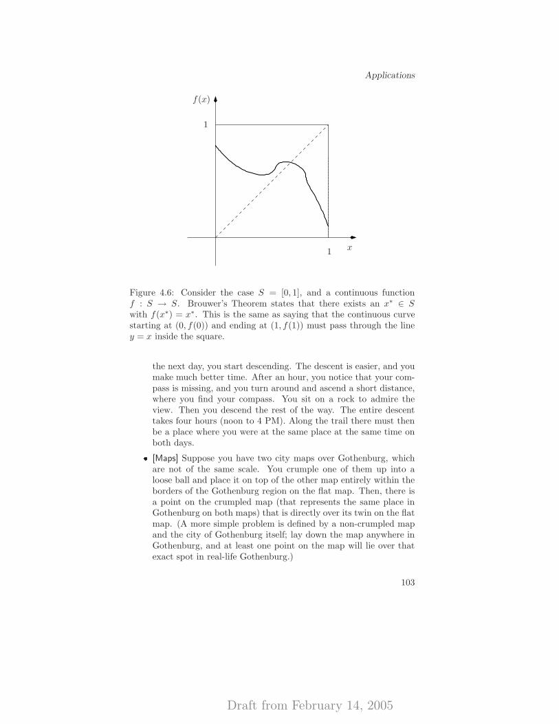
Draft from February 14, 2005
Applications
x
f(x)
1
1
Figure 4.6: Consider the case S = [0, 1], and a continuous functionf : S → S. Brouwer’s Theorem states that there exists an x∗ ∈ Swith f(x∗) = x∗. This is the same as saying that the continuous curvestarting at (0, f(0)) and ending at (1, f(1)) must pass through the liney = x inside the square.
the next day, you start descending. The descent is easier, and youmake much better time. After an hour, you notice that your com-pass is missing, and you turn around and ascend a short distance,where you find your compass. You sit on a rock to admire theview. Then you descend the rest of the way. The entire descenttakes four hours (noon to 4 PM). Along the trail there must thenbe a place where you were at the same place at the same time onboth days.� [Maps] Suppose you have two city maps over Gothenburg, whichare not of the same scale. You crumple one of them up into aloose ball and place it on top of the other map entirely within theborders of the Gothenburg region on the flat map. Then, there isa point on the crumpled map (that represents the same place inGothenburg on both maps) that is directly over its twin on the flatmap. (A more simple problem is defined by a non-crumpled mapand the city of Gothenburg itself; lay down the map anywhere inGothenburg, and at least one point on the map will lie over thatexact spot in real-life Gothenburg.)
103
Draft from February 14, 2005
An introduction to optimality conditions� [Raking of gravel] Suppose you wish to rake the gravel in yourgarden; if the area is, say, circular, then any continuous rakingwill leave at least one tiny stone (which one is a function of time)in the same place.� [Stirring coffee] Stirring the contents of a (convex) coffee cup in acontinuous way, no matter how long you stir, some particle (whichone is a function of time) will stay in the same position as it didbefore you began stirring.6� [Meteorology] Even as the wind blows across the Earth there willbe one location where the wind is perfectly vertical (or, perfectlycalm). This fact actually implies the existence of cyclones; not tomention whorls, or crowns, in your hair no matter how you combit. (The latter result also bears its own name: The Hairy BallTheorem; cf. [BoL00, pp. 186–187].)
Applying fixed point theorems to our own development of this book,we take a look at the variational inequality (4.10). Rephrasing it in amore general form, the variational inequality problem is to find x∗ ∈ Ssuch that
f(x∗)T(x − x∗) ≥ 0, x ∈ S. (4.30)
In order to turn it into a fixed point problem, we construct the fol-lowing composite operator from Rn to S:
F := (In − f) ◦ ProjS ,
or, in other words,
F (x) := ProjS(x − f(x)), x ∈ Rn,
and consider finding a fixed point of F on S. Why is this operator acorrect one? Because it is equivalent to the statement that
ProjS(x − f(x)) = x!
The special case for f = ∇f is found in (4.11). Applying a fixedpoint theorem to the above problem then proves that the variationalinequality problem (4.30) has solutions whenever f is continuous andS is nonempty, convex and compact. (Moreover, we have immediatelyfound an iterative algorithm for the variational inequality problem: ifthe operator x 7→ ProjS(x−αf (x)) is contractive for some α > 0, thenit defines a convergent algorithm.)
6Ever wondered why adding lots of sugar does not always help improve the tasteof coffee?
104
Draft from February 14, 2005
Applications
At the same time, we saw that the fixed point problem was definedthrough the same type of stationarity condition that we derived in Sec-tion 4.4 for differentiable optimization problems over convex sets. Wehave thereby also illustrated that stationarity in an optimization prob-lem is intimately associated with fixed points of a particular operator.7
As an exercise, we consider the problem to find an x ∈ R such thatf(x) = 0, where f : R → R is twice differentiable. The classic Newton–Raphson algorithm has an iteration formula of the form
x0 ∈ R; xk+1 = xk − f(xk)
f ′(xk), k = 0, 1, . . . .
If we assume that there exists a zero at x∗ at which f ′(x∗) > 0, thenby starting close enough to x∗ we can prove that the above iterationformula defines a contraction, and hence we can establish local conver-gence. (Why?) Further analyses of Newton methods will be performedin Chapter 11.
A similar technique can be used to establish that a system of linearequations with a symmetric matrix is solvable by the classic Jacobi al-gorithm in numerical analysis if the matrix is diagonally dominant; thiscondition is equivalent to the Jacobi algorithm’s algorithm-defining op-erator being a contraction. (Similar, but stronger, results can also beobtained for the Gauss–Seidel algorithm; cf. [Kre78, BeT89].)
An elegant application of fixed point theorems is the analysis of ma-trix games. The famous Minimax Theorem of von Neumann is asso-ciated with the existence of a saddle point of a function of the form(v,w) 7→ L(v,w) := vTAw. Von Neumann’s minimax theorem statesthat if V and W both are nonempty, convex and compact, then
minimumv∈V
maximumw∈W
vTAw = maximumw∈W
minimumv∈V
vTAw.
In order to prove this theorem we can use the above existence theoremfor variational inequalities. Let
x =
(v
w
); f (x) =
(−ATv
Aw
); S = V ×W.
It is a reasonably simple exercise to prove that the variational in-equality (4.30) with the above identifications is equivalent to the saddlepoint conditions, which can also be written as the existence of a pair(v∗,w∗) ∈ V ×W such that
(v∗)TAw ≤ (v∗)TAw∗ ≤ vTAw∗, (v,w) ∈ V ×W ;
7The book [Pat98] analyzes a large variety of optimization algorithms by utilizingthis connection.
105
Draft from February 14, 2005
An introduction to optimality conditions
and we are done immediately.
Saddle point results will be returned to in the study of (Lagrangian)duality in the coming chapters, especially for linear programming (whichwas also von Neumann’s special interest).
4.7 Notes and further reading
Most of the material of this chapter is elementary (as is relies mostlyon the Taylor expansion of differentiable functions), and can be foundin most basic books on nonlinear optimization, such as [Man69, Zan69,Avr76, BSS93, Ber99].
Weierstrass’ Theorem 4.6 is the strongest existence result for optimalsolutions that does not utilize convexity. The result is credited to KarlWeierstrass, but it was in fact known already by Bernard Bolzano in1817 (although then only available in manuscript form); it has strongconnections to the theorem of the existence of intermediate values as wellas to that on the existence of limit points of every bounded sequence (nowoften referred to as the Bolzano–Weierstrass Theorem), and the notion ofCauchy sequences, often also credited to Weierstrass and Augustin-LouisCauchy, respectively.
The Frank–Wolfe Theorem in Corollary 4.8 is found in [FrW56]. Thestronger result in Theorem 4.7 is found in [Eav71, BlO72]. Proposi-tion 4.25 on the invariance of the gradient on the solution set is foundin [Man88, BuF91].
Fixed point theorems are developed in greater detail in [GrD03].Non-cooperative game theory was developed in work by John von Neu-mann, together with Oskar Morgenstern (see [vNe28, vNM43]), and byJohn Nash [Nas50, Nas51].
4.8 Exercises
Exercise 4.1 (redundant constraints) Consider the problem to
minimize f(x),
subject to g(x) ≤ b,
where f : Rn → R and g : Rn → R are continuous functions, and b ∈ R.Suppose that this problem has a globally optimal solution, x∗, and thatg(x∗) < b holds.
106
Draft from February 14, 2005
Exercises
Claim: The vector x∗ is also a globally optimal solution to the un-constrained problem to
minimize f(x),
subject to x ∈ Rn.
Is the claim true?
Exercise 4.2 (unconstrained optimization, exam 020826) Consider the un-constrained optimization problem to minimize the function
f(x) :=3
2(x2
1 + x22) + (1 + a)x1x2 − (x1 + x2) + b
over R2, where a and b are real-valued parameters. Find all values of aand b such that the problem has a unique optimal solution.
Exercise 4.3 (spectral theory and unconstrained optimization) Let A bea symmetric n × n matrix. For x ∈ Rn, x 6= 0n, consider the function
ρ(x) := xTAxxTx , and the related optimization problem to
minimizex 6=0n
ρ(x). (P)
Determine all the stationary points as well as the global minima inthe minimization problem (P). Interpret the result in terms of linearalgebra.
Exercise 4.4 (non-convex QP over subspaces) The Frank–Wolfe Theo-rem 4.8 can be further improved for some special cases of linear con-straints. Suppose that f(x) := 1
2xTQx − qTx, where Q ∈ Rn×n is asymmetric matrix and q ∈ Rn. Suppose further that the constraintsare equalities, that is, that the ℓ constraints define the linear systemEx = d, where E ∈ Rℓ×n and d ∈ Rℓ. Note that the problem may notbe convex, as we have not assumed that Q is positive semi-definite.
For this set-up, establish the following:
(a) Every locally optimal solution is a globally optimal solution.(b) A locally [hence globally, by (a)] optimal solution exists if and
only if f is lower bounded on S := {x ∈ Rn | Ex = d }.
Exercise 4.5 (descent from projection) Consider the problem (4.9), wheref is in C1 on the convex set S. Let x ∈ S. Let α > 0, and define
p := ProjS [x − α∇f(x)] − x.
107
Draft from February 14, 2005
An introduction to optimality conditions
Notice that p is a feasible direction at x. Establish that
∇f(x)Tp ≤ − 1
α‖p‖2
holds. Hence, p is zero if and only if x is stationary [according to thecharacterization in (4.11)], and if p is non-zero then it defines a feasibledescent direction with respect to f at x.
Exercise 4.6 (optimality conditions for a special problem) Suppose thatf ∈ C1 on the set S := {x ∈ Rn | xj ≥ 0, j = 1, 2, . . . , n }, andconsider the problem of finding a minimum of f(x) over S. Develop thenecessary optimality conditions for this problem in a compact form.
Exercise 4.7 (optimality conditions for a special problem) Consider the prob-lem to
maximize f(x) := xa1
1 xa2
2 · · ·xann ,
subject to
n∑
j=1
xj = 1,
xj ≥ 0, j = 1, . . . , n,
where the values of aj (j = 1, . . . , n) are positive. Find a global maxi-mum and show that it is unique.
Exercise 4.8 (extensions of convexity, exam 040602) We have stressed thatconvexity is a crucial property of functions when analyzing optimiza-tion models in general and studying optimality conditions in particu-lar. There are, however, certain properties of convex functions that areshared also by classes of non-convex functions. The purpose of this ex-ercise is to relate the convex functions to two such classes of non-convexfunctions by means of some example properties.
Suppose that S ⊆ Rn and that f : Rn → R is continuous on S.(a) Suppose further that f is in C1 on S. We say that the function
f is pseudo-convex on S if, for every x,y ∈ S,
∇f(x)T(y − x) ≥ 0 =⇒ f(y) ≥ f(x).
Establish the following two statements: (1) if f is a convex functionon S then f is pseudo-convex on S (that is, “convexity implies pseudo-convexity”); (2) the reverse statement (“pseudo-convexity implies con-vexity”) is not true.
[Hint: On the statement (2) you may construct an explicit or graph-ical counter-example.]
108
Draft from February 14, 2005
Exercises
[Note: Pseudo-convex functions were introduced by Mangasarian[Man65].]
(b) A well-known property of a differentiable convex function is itsrole in necessary and sufficient conditions for globally optimal solutions.Suppose now that S is convex. If f is a convex function on Rn which isin C1 on S then Theorem 4.23 applies. Establish that the equivalencerelation of this theorem still holds if the convexity of f on S is replacedby the pseudo-convexity of f on S.
(c) Let S be convex. We say that the function f is quasi-convex onS if its level sets are convex. In other words, f is quasi-convex on S if
levSf (b) := {x ∈ S | f(x) ≤ b }
is convex for every b ∈ R.Establish the following two statements for a function f which is in
C1 on S: (1) if f is convex function on S then f is quasi-convex on S(that is, “convexity implies quasi-convexity”); (2) the reverse statement(“quasi-convexity implies convexity”) is not true.
[Hint: On the statement (2) you may construct an explicit or graph-ical counter-example.]
[Note: Pseudo-convex functions were introduced by De Finetti [DeF49].]
Exercise 4.9 (illustrations of fixed point results) (a) Let S := { x ∈ R |x ≥ 1 } and f(x) := x/2 + 1/x. Show that f is a contraction and findthe smallest value of α.
(b) In analysis, a usual condition for the convergence of an iterationxk = g(xk−1) is that g be continuously differentiable and
|g′(x)| ≤ α < 1.
Verify this by the use of Banach’s Theorem 4.33(a).(c) Show that a fixed-point iteration for calculating the square root
of a given positive number c is
x0 > 0; xk+1 = g(xk) :=1
2
(xk +
c
xk
), k = 0, 1, . . . .
What condition do we get from (b)? Starting at x0 = 1, calculateapproximations x1, x2, x3, x4 of
√2.
109

Draft from February 14, 2005
An introduction to optimality conditions
110
Draft from February 14, 2005
Optimality conditions V
5.1 Relations between optimality conditions
(OCs) and CQs at a glance
Optimality conditions are introduced as an attempt to construct an eas-ily verifiable criterion that allows us to examine points in a feasible set,one after another, and classify them into optimal and non-optimal ones.Unfortunately, this is impossible in practice, and not only due to thefact that there are far too many feasible points, but also because it isimpossible to construct such a universal criterion. It is usually possibleto construct either practical (that is, computationally verifiable) condi-tions that admit some mistakes in the characterization, or perfect oneswhich are impossible to use in the computations. It is of course the firstgroup that is of practical value for us, and it may further be classifiedinto two distinct subgroups based on the type of mistakes allowed in thedecision-making process. Namely, optimality conditions encountered inpractice are divided into two classes, known as necessary and sufficientconditions.
Necessary conditions must be satisfied at every locally optimal point;on the other hand, we cannot guarantee that every point satisfying thenecessary optimality conditions is indeed locally optimal. On the con-trary, sufficient optimality conditions provide such guarantees; however,there are some locally optimal points that violate the optimality con-ditions. Arguably, it is much more important to be able to find a fewcandidates for local minima that can be further investigated by othermeans, than to eliminate some local (or even global) minima from thebeginning. Therefore, this chapter is dedicated to the development ofnecessary optimality conditions. However, for convex optimization prob-lems these conditions turn out to be sufficient.
Draft from February 14, 2005
Optimality conditions
Now, we can concentrate on what should be meant by easily verifiableconditions. A human being can immediately state whether a given pointbelongs to a simple set or not, by just glancing at a picture of it; for a nu-merical algorithm, a clear algebraic description of a set in terms of equal-ities and inequalities is vital. Therefore, we start our development withgeometric optimality conditions (Section 5.3), to gain an understandingabout the relationships between the gradient of the objective functionand the feasible set that must hold at every local minimum point. Givena specific description of a feasible set in terms of inequalities, the ge-ometric conditions immediately imply some relationships between thegradients of the objective functions and the constraints that are bindingat the point under consideration (see Section 5.4); these conditions areknown as the Fritz–John optimality conditions, and are rather weak (i.e.,they can be satisfied by many points that have nothing in common withlocally optimal points). However, if we assume an additional regularity ofthe system of inequalities and equalities that define our feasible set, thenthe geometric optimality conditions imply stronger conditions, known asthe Karush–Kuhn–Tucker optimality conditions (see Section 5.5). Theadditional regularity assumptions are known under the name constraintqualifications (CQs), and they vary from very abstract and difficult tocheck, but enjoyed by many feasible sets (such as, e.g., Abadie’s CQ,see Definition 5.23) to more specific, easily verifiable but also somewhatrestrictive in many situations (such as the linear independence CQ (seeDefinition 5.41), or the Slater CQ, see Definition 5.38). In Section 5.8we show that for convex problems the KKT conditions are sufficient forlocal, hence global, optimality.
The contents of this chapter are in principle summarized in the flow-chart in Figure 5.1. Various optimality conditions and constraint qual-ifications that are discussed in this chapter constitute the nodes of theflow-chart. Logical relationships between them are denoted with edges,and the direction of the arrow shows the direction of the logical implica-tion; each implication is further labeled with the result that establishesit. We note that the KKT conditions “follow” from both geometricconditions and constraint qualifications satisfied at a given point; also,global optimality holds if both the KKT conditions are verified and theoptimization problem is convex.
5.2 A note of caution
In this chapter we will discuss various necessary optimality conditions fora given point to be a local minimum to a nonlinear programming model.If the NLP is a convex program, any point satisfying these necessary
112
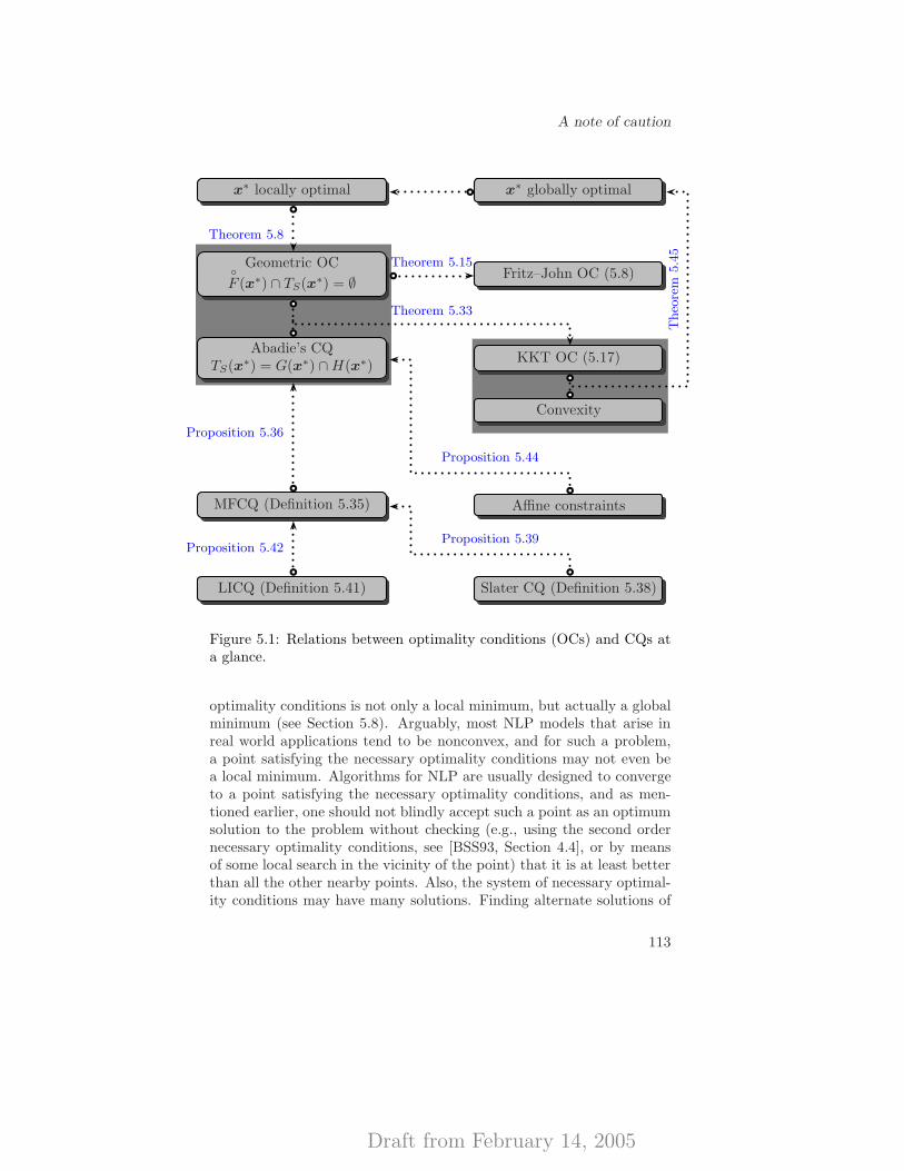
Draft from February 14, 2005
A note of caution
x∗ locally optimal x∗ globally optimal
Geometric OC◦F (x∗) ∩ TS(x∗) = ∅ Fritz–John OC (5.8)
Abadie’s CQTS(x∗) = G(x∗) ∩H(x∗)
KKT OC (5.17)
Convexity
MFCQ (Definition 5.35) Affine constraints
LICQ (Definition 5.41) Slater CQ (Definition 5.38)
Theorem 5.8
Theorem 5.15
Theorem 5.33
Proposition 5.36
Proposition 5.44
Proposition 5.42Proposition 5.39
Theo
rem
5.4
5
Figure 5.1: Relations between optimality conditions (OCs) and CQs ata glance.
optimality conditions is not only a local minimum, but actually a globalminimum (see Section 5.8). Arguably, most NLP models that arise inreal world applications tend to be nonconvex, and for such a problem,a point satisfying the necessary optimality conditions may not even bea local minimum. Algorithms for NLP are usually designed to convergeto a point satisfying the necessary optimality conditions, and as men-tioned earlier, one should not blindly accept such a point as an optimumsolution to the problem without checking (e.g., using the second ordernecessary optimality conditions, see [BSS93, Section 4.4], or by meansof some local search in the vicinity of the point) that it is at least betterthan all the other nearby points. Also, the system of necessary optimal-ity conditions may have many solutions. Finding alternate solutions of
113
Draft from February 14, 2005
Optimality conditions
this system, and selecting the best among them, usually leads to a goodpoint to investigate further.
We will illustrate the importance of this with the story of US AirForce’s controversial B-2 Stealth bomber program in the Reagan era ofthe 1980s. There were many design variables such as the various di-mensions, the distribution of volume between the wing and the fuselage,flying speed, thrust, fuel consumption, drag, lift, air density, etc., thatcould be manipulated for obtaining the best range (i.e., the distance itcan fly starting with full tanks, without refueling). The problem of max-imizing the range subject to all the constraints was modeled as an NLPin a secret Air Force study going back to the 1940s. A solution to thenecessary optimality conditions of this problem was found; it specifiedvalues for the design variables that put almost all of the total volume inthe wing, leading to the flying wing design for the B-2 bomber. Afterspending billions of dollars, building test planes, etc., it was found thatthe design solution implemented works, but that its range was too low incomparison with other bomber designs being experimented subsequentlyin the US and abroad.
A careful review of the model was then carried out. The review indi-cated that all the formulas used, and the model itself, are perfectly valid.However, the model was a nonconvex NLP, and the review revealed asecond solution to the system of necessary optimality conditions for it,besides the one found and implemented as a result of earlier studies. Thesecond solution makes the wing volume much less than the total volume,and seems to maximize the range; while the first solution that is imple-mented for the B-2 bomber seems to actually minimize the range. (Thesecond solution also looked like an airplane should, while the flying wingdesign was counter-intuitive.) In other words, the design implementedwas the aerodynamically worst possible choice of configuration, leadingto a very costly error.
For an account, see the research news item “Skeleton Alleged in theStealth Bomber’s Closet,” Science, vol. 244, 12 May 1989 issue, pages650–651.
5.3 Geometric optimality conditions
In this section we will discuss the optimality conditions for the followingoptimization problem [cf. (4.1)]:
minimize f(x),
subject to x ∈ S,(5.1)
114
Draft from February 14, 2005
Geometric optimality conditions
where S ⊂ Rn is a nonempty closed set and f : Rn → R is a givendifferentiable function. Since we do not have any particular descriptionof the feasible set S in terms of equality or inequality constraints, theoptimality conditions will be based on purely geometrical ideas. Beingquite general, the optimality conditions we will develop in this sectionare almost useless when it comes to computations, because they are alsonot very easy, even impossible, to verify for an optimization algorithm.Therefore, in the sections that follow, we will use an algebraic descrip-tion of the set S and geometric optimality conditions to further developclassical Fritz–John and Karush–Kuhn–Tucker optimality conditions inthe form of easily verifiable systems of equations and inequalities.
The basic idea behind the optimality conditions is that if the pointx∗ ∈ S is a point of local minimum for f over S, it should not be possibleto draw a curve, or, more generally, a sequence of points, starting atthe point x∗ inside S, such that f decreases along it. Linearizing theobjective function and the constraints along such curves, we eventuallyestablish relationships between their gradients that are necessary to holdat points of local minima.
We start by defining the meaning of “possible to draw a curve startingat x∗ inside S”. Arguably, the simplest curves are the straight lines; thefollowing definition gives exactly the set of lines that locally around x∗
belong to S.
Definition 5.1 (cone of feasible directions) Let S ⊂ Rn be a nonemptyclosed set. The cone of feasible directions for S at x ∈ Rn, known alsoas the radial cone, is defined as:
RS(x) := {p ∈ Rn | ∃ δ > 0 such that x + δp ∈ S, 0 ≤ δ ≤ δ }. (5.2)
Thus, this is nothing else but the cone containing all feasible directionsin the sense of Definition 4.19.
This cone is used in some optimization algorithms, but unfortunatelyit is too small to develop optimality conditions that are general enough.Therefore, we consider less intuitive, but bigger and more well-behavingsets (cf. Proposition 5.3 and the examples that follow).
Definition 5.2 (tangent cone) Let S ⊂ Rn be a nonempty closed set.The tangent cone for S at x ∈ Rn is defined as
TS(x) := {p ∈ Rn | ∃ {xk} ⊂ S, {λk} ⊂ (0,∞) : limk→∞
xk = x,
limk→∞
λk(xk − x) = p }.(5.3)
115
Draft from February 14, 2005
Optimality conditions
Thus, to construct a tangent cone we consider all the sequences {xk}in S that converge to the given x ∈ Rn, and then calculate all the direc-tions p ∈ Rn that are tangential to the sequences at x; such tangentialvectors are described as the limits of {λk(xk −x)} for arbitrary positivesequences {λk}. Note that to generate a nonzero vector p ∈ TS(x) thesequence {λk} must converge to +∞.
While it is possible that clRS(x) = TS(x), or even that RS(x) =TS(x), in general we have only the following proposition, and examplesthat follow show that the two cones might be very different.
Proposition 5.3 (relationship between the radial and the tangent cones)The tangent cone is a closed set, and the inclusion clRS(x) ⊂ TS(x)holds for every x ∈ Rn.
Proof. Consider a sequence {pk} ⊂ TS(x), and assume that pk → p.Since every pk ∈ TS(x), there exists xk ∈ S and λk > 0, such that‖xk−x‖ < k−1 and ‖λ(xk−x)−pk‖ < k−1. Then, clearly, xk → x, and,by the triangle inequality, ‖λ(xk−x)−p‖ ≤ ‖λ(xk−x)−pk‖+‖pk−p‖ →0, which implies that p ∈ TS(x) and thus the latter set is closed.
In view of the closedness of the tangent cone, it is enough to show theinclusion RS(x) ⊂ TS(x). Let p ∈ RS(x). Then, for all large integers kit holds that x + k−1p ∈ S, and, therefore, setting xk = x + k−1p andλk = k we see that p ∈ TS(x) as defined by Definition 5.2.
Example 5.4 Let S = {x ∈ R2 | −x1 ≤ 0, (x1 − 1)2 + x22 ≤ 1 }. Then,
RS(02) = {p ∈ R2 | p1 > 0 }, and TS(02) = {p ∈ R2 | p1 ≥ 0 }, i.e.,TS(02) = clRS(02) (see Figure 5.2).
Example 5.5 (complementarity constraint) Let S = {x ∈ R2 | −x1 ≤0,−x2 ≤ 0, x1x2 ≤ 0 }. In this case, S is a (non-convex) cone, andRS(02) = TS(02) = S (see Figure 5.3).
Example 5.6 Let S = {x ∈ R2 | −x31 + x2 ≤ 0, x5
1 − x2 ≤ 0,−x2 ≤ 0 }.Then, RS(02) = ∅, TS(02) = {p ∈ R2 | p1 ≥ 0, p2 = 0 } (see Figure 5.4).
Example 5.7 Let S = {x ∈ R2 | −x2 ≤ 0, (x1 − 1)2 + x22 = 1 }. Then,
RS(02) = ∅, TS(02) = {p ∈ R2 | p1 = 0, p2 ≥ 0 } (see Figure 5.5).
We already know that f decreases along any descent direction (cf. Def-inition 4.14), and that for a vector p ∈ Rn it is sufficient to verify theinequality ∇f(x∗)Tp < 0 to be a descent direction for f at x∗ ∈ Rn
(see Proposition 4.15). Even though this condition is not necessary, it
116
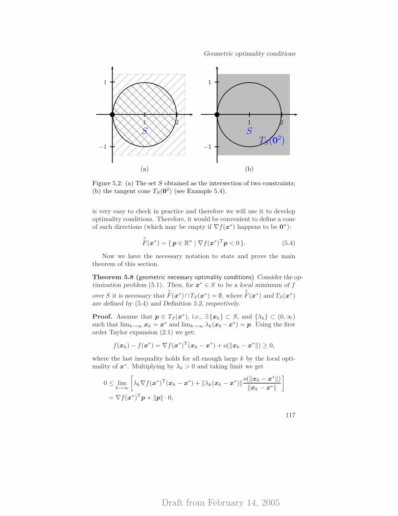
Draft from February 14, 2005
Geometric optimality conditions
1 2
1
−1
S
1 2
1
−1
S
TS(02)
(a) (b)
Figure 5.2: (a) The set S obtained as the intersection of two constraints;(b) the tangent cone TS(02) (see Example 5.4).
is very easy to check in practice and therefore we will use it to developoptimality conditions. Therefore, it would be convenient to define a coneof such directions (which may be empty if ∇f(x∗) happens to be 0n):
◦F (x∗) = {p ∈ Rn | ∇f(x∗)Tp < 0 }. (5.4)
Now we have the necessary notation to state and prove the maintheorem of this section.
Theorem 5.8 (geometric necessary optimality conditions) Consider the op-timization problem (5.1). Then, for x∗ ∈ S to be a local minimum of f
over S it is necessary that◦F (x∗)∩TS(x∗) = ∅, where
◦F (x∗) and TS(x∗)
are defined by (5.4) and Definition 5.2, respectively.
Proof. Assume that p ∈ TS(x∗), i.e., ∃ {xk} ⊂ S, and {λk} ⊂ (0,∞)such that limk→∞ xk = x∗ and limk→∞ λk(xk−x∗) = p. Using the firstorder Taylor expansion (2.1) we get:
f(xk) − f(x∗) = ∇f(x∗)T(xk − x∗) + o(‖xk − x∗‖) ≥ 0,
where the last inequality holds for all enough large k by the local opti-mality of x∗. Multiplying by λk > 0 and taking limit we get
0 ≤ limk→∞
[λk∇f(x∗)T(xk − x∗) + ‖λk(xk − x∗)‖o(‖xk − x∗‖)
‖xk − x∗‖
]
= ∇f(x∗)Tp + ‖p‖ · 0,
117
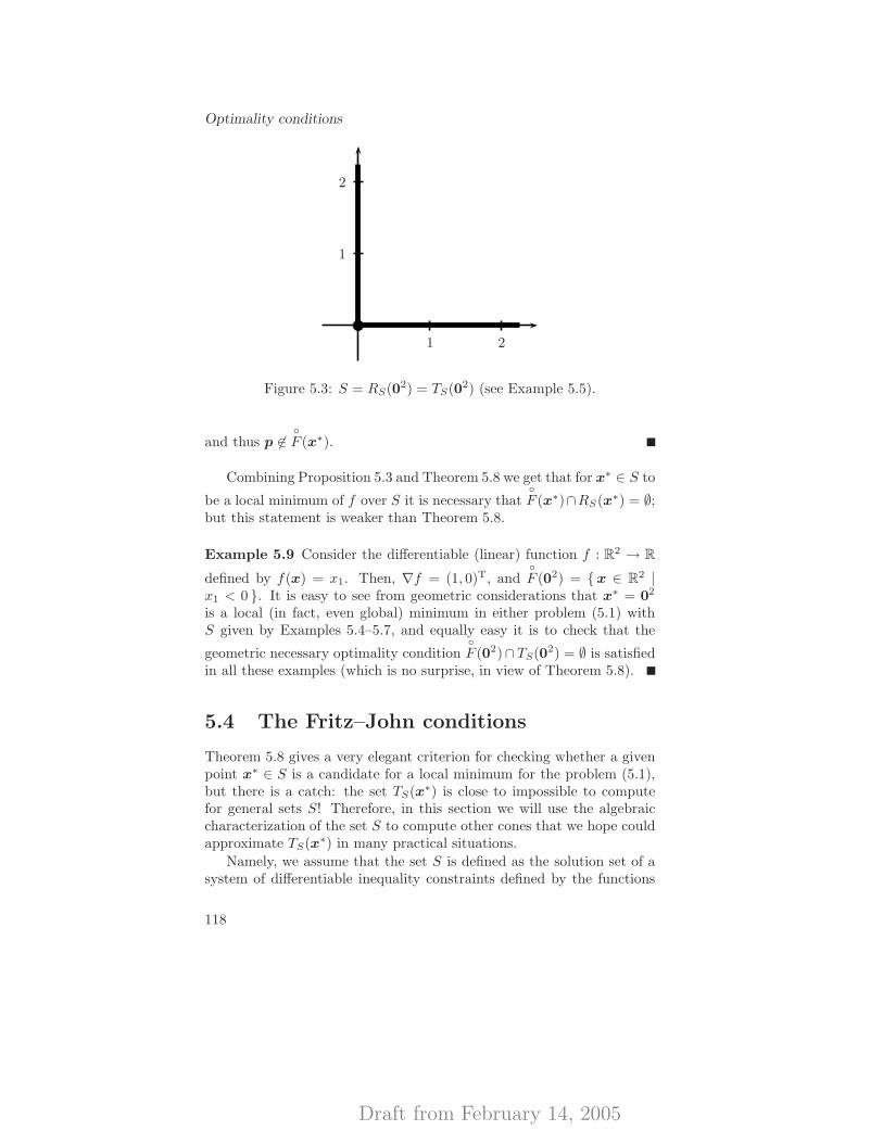
Draft from February 14, 2005
Optimality conditions
1 2
1
2
Figure 5.3: S = RS(02) = TS(02) (see Example 5.5).
and thus p 6∈◦F (x∗).
Combining Proposition 5.3 and Theorem 5.8 we get that for x∗ ∈ S to
be a local minimum of f over S it is necessary that◦F (x∗)∩RS(x∗) = ∅;
but this statement is weaker than Theorem 5.8.
Example 5.9 Consider the differentiable (linear) function f : R2 → R
defined by f(x) = x1. Then, ∇f = (1, 0)T, and◦F (02) = {x ∈ R2 |
x1 < 0 }. It is easy to see from geometric considerations that x∗ = 02
is a local (in fact, even global) minimum in either problem (5.1) withS given by Examples 5.4–5.7, and equally easy it is to check that the
geometric necessary optimality condition◦F (02)∩ TS(02) = ∅ is satisfied
in all these examples (which is no surprise, in view of Theorem 5.8).
5.4 The Fritz–John conditions
Theorem 5.8 gives a very elegant criterion for checking whether a givenpoint x∗ ∈ S is a candidate for a local minimum for the problem (5.1),but there is a catch: the set TS(x∗) is close to impossible to computefor general sets S! Therefore, in this section we will use the algebraiccharacterization of the set S to compute other cones that we hope couldapproximate TS(x∗) in many practical situations.
Namely, we assume that the set S is defined as the solution set of asystem of differentiable inequality constraints defined by the functions
118
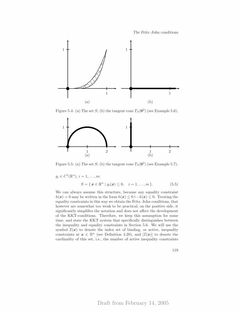
Draft from February 14, 2005
The Fritz–John conditions
1
1
1
1
(a) (b)
Figure 5.4: (a) The set S; (b) the tangent cone TS(02) (see Example 5.6).
1 2
1
1 2
1
(a) (b)
Figure 5.5: (a) The set S; (b) the tangent cone TS(02) (see Example 5.7).
gi ∈ C1(Rn), i = 1, . . . ,m:
S = {x ∈ Rn | gi(x) ≤ 0, i = 1, . . . ,m }. (5.5)
We can always assume this structure, because any equality constrainth(x) = 0 may be written in the form h(x) ≤ 0∧−h(x) ≤ 0. Treating theequality constraints in this way we obtain the Fritz–John conditions, thathowever are somewhat too weak to be practical; on the positive side, itsignificantly simplifies the notation and does not affect the developmentof the KKT-conditions. Therefore, we keep this assumption for sometime, and state the KKT system that specifically distinguishes betweenthe inequality and equality constraints in Section 5.6. We will use thesymbol I(x) to denote the index set of binding, or active, inequalityconstraints at x ∈ Rn (see Definition 4.20), and |I(x)| to denote thecardinality of this set, i.e., the number of active inequality constraints
119
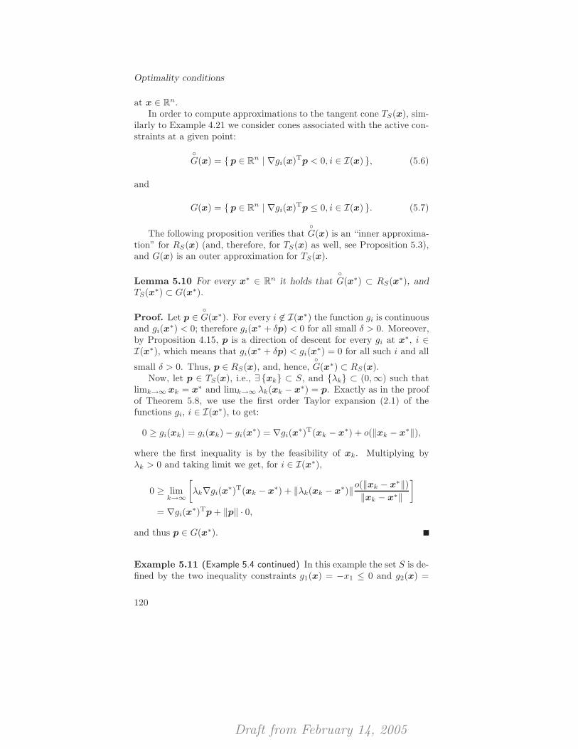
Draft from February 14, 2005
Optimality conditions
at x ∈ Rn.In order to compute approximations to the tangent cone TS(x), sim-
ilarly to Example 4.21 we consider cones associated with the active con-straints at a given point:
◦G(x) = {p ∈ Rn | ∇gi(x)Tp < 0, i ∈ I(x) }, (5.6)
and
G(x) = {p ∈ Rn | ∇gi(x)Tp ≤ 0, i ∈ I(x) }. (5.7)
The following proposition verifies that◦G(x) is an “inner approxima-
tion” for RS(x) (and, therefore, for TS(x) as well, see Proposition 5.3),and G(x) is an outer approximation for TS(x).
Lemma 5.10 For every x∗ ∈ Rn it holds that◦G(x∗) ⊂ RS(x∗), and
TS(x∗) ⊂ G(x∗).
Proof. Let p ∈◦G(x∗). For every i 6∈ I(x∗) the function gi is continuous
and gi(x∗) < 0; therefore gi(x
∗ + δp) < 0 for all small δ > 0. Moreover,by Proposition 4.15, p is a direction of descent for every gi at x∗, i ∈I(x∗), which means that gi(x
∗ + δp) < gi(x∗) = 0 for all such i and all
small δ > 0. Thus, p ∈ RS(x), and, hence,◦G(x∗) ⊂ RS(x).
Now, let p ∈ TS(x), i.e., ∃ {xk} ⊂ S, and {λk} ⊂ (0,∞) such thatlimk→∞ xk = x∗ and limk→∞ λk(xk − x∗) = p. Exactly as in the proofof Theorem 5.8, we use the first order Taylor expansion (2.1) of thefunctions gi, i ∈ I(x∗), to get:
0 ≥ gi(xk) = gi(xk) − gi(x∗) = ∇gi(x
∗)T(xk − x∗) + o(‖xk − x∗‖),
where the first inequality is by the feasibility of xk. Multiplying byλk > 0 and taking limit we get, for i ∈ I(x∗),
0 ≥ limk→∞
[λk∇gi(x
∗)T(xk − x∗) + ‖λk(xk − x∗)‖o(‖xk − x∗‖)‖xk − x∗‖
]
= ∇gi(x∗)Tp + ‖p‖ · 0,
and thus p ∈ G(x∗).
Example 5.11 (Example 5.4 continued) In this example the set S is de-fined by the two inequality constraints g1(x) = −x1 ≤ 0 and g2(x) =
120
Draft from February 14, 2005
The Fritz–John conditions
(x1−1)2+x22−1 ≤ 0. Let us calculate
◦G(02) andG(02). Both constraints
are satisfied with equality at the given point, so that I(x) = {1, 2}.Then, ∇g1(02) = (−1, 0)T, ∇g2(02) = (−2, 0)T, and thus
◦G(02) = {x ∈
R2 | x1 > 0 } = RS(02), G(02) = {x ∈ R2 | x1 ≥ 0 } = TS(02) in thiscase.
Example 5.12 (Example 5.5 continued) S is defined by the three in-equality constraints g1(x) = −x1 ≤ 0, g2(x) = −x2 ≤ 0, g3(x) = x1x2 ≤0, which are all binding at x∗ = 02; ∇g1(02) = (−1, 0)T, ∇g2(02) =
(0,−1)T, and ∇g3(02) = (0, 0)T. Therefore,◦G(02) = ∅ ( RS(02), and
G(02) = {x ∈ R2 | x1 ≥ 0, x2 ≥ 0 } ) TS(02).
Example 5.13 (Example 5.6 continued) S is defined by the three in-equality constraints g1(x) = −x3
1 + x2 ≤ 0, g2(x) = x51 − x2 ≤ 0,
g3(x) = −x2 ≤ 0, which are all binding at x∗ = 02; ∇g1(02) = (0, 1)T,
∇g2(02) = (0,−1)T, and ∇g3(02) = (0,−1)T. Therefore,◦G(02) = ∅ =
RS(02), and G(02) = {x ∈ R2 | x2 = 0 } ) TS(02).
Example 5.14 (Example 5.7 continued) In this example, the set S isdefined by the inequality constraint g1(x) = −x2 ≤ 0, and one equalityconstraint h1(x) = (x1 − 1)2 + x2
2 − 1 = 0; we split the latter intotwo inequality constraints g2(x) = h1(x) ≤ 0, and g3(x) = −h1(x) ≤0. Thus, we end up with three binding inequality constraints at x∗ =02; ∇g1(02) = (0,−1)T, ∇g2(02) = (−2, 0)T, and ∇g3(02) = (2, 0)T.
Therefore,◦G(02) = ∅ = RS(02), and G(02) = {x ∈ R2 | x1 = 0, x2 ≥
0 } = TS(02).
Now we are ready to establish the Fritz–John optimality conditions.
Theorem 5.15 (Fritz–John necessary optimality conditions) Let the setS be defined by (5.5). Then, for x∗ ∈ S to be a local minimum of f overS it is necessary that there exist multipliers µ0 ∈ R, µ ∈ Rm, such that
µ0∇f(x∗) +m∑
i=1
µi∇gi(x∗) = 0n, (5.8a)
µigi(x∗) = 0, i = 1, . . . ,m, (5.8b)
µ0, µi ≥ 0, i = 1, . . . ,m, (5.8c)
(µ0,µT)T 6= 0m+1. (5.8d)
121
Draft from February 14, 2005
Optimality conditions
Proof. Combining the results of Lemma 5.10 with the geometric opti-mality conditions provided by Theorem 5.8, we conclude that there isno direction p ∈ Rn such that ∇f(x∗)Tp < 0 and ∇gi(x
∗)Tp < 0, i ∈I(x∗). Define the matrix A with columns ∇f(x∗), ∇gi(x
∗), i ∈ I(x∗);then the system ATp < 01+|I(x∗)| is unsolvable. By Farkas’ Lemma(cf. Theorem 3.30) there exists a nonzero vector λ ∈ R1+|I(x∗)| suchthat λ ≥ 01+|I(x∗)| and Aλ = 0n. Now, let (µ0,µ
TI(x∗))
T = λ, and set
µi = 0 for i 6∈ I(x∗). It is an easy exercise now to verify that so definedµ0 and µ satisfy the conditions (5.8).
Remark 5.16 (terminology) The solutions (µ0,µ) to the system (5.8)are known as Lagrange multipliers (or just multipliers) associated witha given candidate x∗ ∈ Rn for a local minimum. Note, that every mul-tiplier (except µ0) corresponds to some constraint in the algebraic rep-resentation of S. The conditions (5.8a) and (5.8c) are known as thedual feasibility, and (5.8b) as the complementarity constraints, respec-tively; this terminology will become more clear in Chapter 6. Owingto the complementarity constraints, the multipliers µi corresponding toinactive inequality constraints i 6∈ I(x∗) must be zero. In general, theLagrange multiplier µi bears the important information about how sen-sitive a particular local minimum is with respect to small changes in theconstraint gi.
In the following examples, as before, we assume that f(x) = x1, sothat ∇f = (1, 0)T and x∗ = 02 is the point of local minimum.
Example 5.17 (Example 5.4 continued) The Fritz–John system (5.8) atthe point x∗ = 02 in this case reduces to:
µ0
(10
)+
(−1 −20 0
)µ = 02,
(µ0,µT)T 03,
where µ ∈ R2 is a vector of Lagrange multipliers for the inequalityconstraints. We do not write the complementarity constraints (5.8b),because in our case all three constraints are active, and therefore theequation (5.8b) is automatically satisfied for all µ. The solutions to thissystem are described as pairs (µ0,µ), with µ = (µ1, 2
−1(µ0 − µ1))T,
for every µ0 > 0, 0 ≤ µ1 ≤ µ0. There are infinitely many Lagrangemultipliers, that even form an unbounded set, but µ0 must always bepositive.
122

Draft from February 14, 2005
The Fritz–John conditions
Example 5.18 (Example 5.5 continued) Similarly to the previous ex-ample, the Fritz–John system (5.8) at the point x∗ = 02 in this casereduces to:
µ0
(10
)+
(−1 0 00 −1 0
)µ = 02,
(µ0,µT)T 04,
where µ ∈ R3 is a vector of Lagrange multipliers for the inequalityconstraints. The solution to the Fritz–John system is every pair (µ0,µ)with µ = (µ0, 0, µ3)
T for every µ0 ≥ 0, µ3 ≥ 0 such that either of themis strictly bigger than zero. That is, there are infinitely many Lagrangemultipliers, that even form an unbounded set, and it is possible for µ0
to assume the value zero.
Example 5.19 (Example 5.6 continued) The Fritz–John system (5.8) atthe point x∗ = 02 in this case reduces to:
µ0
(10
)+
(0 0 01 −1 −1
)µ = 02,
(µ0,µT)T 04,
where µ ∈ R3 is a vector of Lagrange multipliers for the inequalityconstraints. Thus, µ0 = 0, µ = (µ1, µ2, µ1 − µ2)
T for every µ1 > 0,0 ≤ µ2 ≤ µ1. That is, there are infinitely many Lagrange multipliers,that even form an unbounded set, and µ0 must assume the value zero.
Example 5.20 (Example 5.7 continued) The Fritz–John system (5.8) atthe point x∗ = 02 in this case reduces to:
µ0
(10
)+
(0 −2 2−1 0 0
)µ = 02,
(µ0,µT)T 04,
where µ ∈ R3 is a vector of Lagrange multipliers for the inequalityconstraints. The solution to the Fritz–John system is every pair (µ0,µ)with µ = (0, µ2, µ2 − 2−1µ0)
T for every µ2 > 0, 0 ≤ µ0 ≤ 2µ2. Thatis, there are infinitely many Lagrange multipliers, that even form anunbounded set, and it is possible for µ0 to assume the value zero.
The fact that µ0 may be zero in the system (5.8) essentially meansthat the objective function f plays no role in the optimality conditions.This is of course a rather unexpected and unwanted situation, and the
123
Draft from February 14, 2005
Optimality conditions
rest of the chapter is in principle dedicated to describing how one canavoid it.
Since the cone of feasible directions RS(x) may be a bad approxi-
mation of the tangent cone TS(x), so may◦G(x) owing to Lemma 5.10.
Therefore, in the most general case we cannot improve on the condi-tions (5.8); however, it is possible to improve upon (5.8) if we assume
that the set S is “regular” in some sense, i.e., that either◦G(x) or G(x)
is a tight enough approximation of TS(x). Requirements of this typeare called constraint qualifications, and they will be discussed in moredetail in Section 5.7. However, to get a feeling of what can be achievedwith a regular constraint sets S, we show that the multiplier µ0 in thesystem (5.8) cannot vanish (i.e., KKT conditions hold, see Section 5.5) if
the constraint qualification◦G(x∗) 6= ∅ holds (which is quite a restrictive
one, in view of Example 5.22; however, see the similar, but much weaker,assumption MFCQ in Section 5.7 dedicated to constraint qualifications).
Proposition 5.21 (KKT optimality conditions – preview) Assume the con-
ditions of Theorem 5.8, and assume that◦G(x∗) 6= ∅. Then, the multiplier
µ0 in (5.8) cannot be zero; dividing all equations by µ0 we may assumethat it equals one.
Proof. Assume that µ0 = 0 in (5.8), and define the matrix A withcolumns ∇gi(x
∗), i ∈ I(x∗). Since Aµ = 0n, µ ≥ 0|I(x∗)|, andµ 6= 0|I(x∗)|, the system ATp < 0|I(x∗)| is unsolvable (see Farkas’
Lemma, Theorem 3.30), i.e.,◦G(x∗) = ∅.
Example 5.22 Out of the four Examples 5.4–5.7, only the first one
verifies the condition◦G(x∗) 6= ∅ assumed in Proposition 5.21, while as
we see later (and as Examples 5.17–5.20 may suggest), three out of fourproblems admit solutions to the corresponding KKT systems.
5.5 The Karush–Kuhn–Tucker conditions
In this section we develop the famous and classic Karush–Kuhn–Tuckeroptimality conditions for constrained optimization problems with in-equality constraints, which are essentially the Fritz–John conditions (5.8)with the additional requirement µ0 6= 0. We establish these conditionsas before, for inequality constrained problems (5.5) (which we do with-out any loss of generality or sharpness of the theory), and then discuss
124
Draft from February 14, 2005
The Karush–Kuhn–Tucker conditions
the possible modifications of the conditions if one wants to specificallydistinguish between equality and inequality constraints in Section 5.6.Abadie’s constraint qualification (see Definition 5.23) which we imposeis very abstract and extremely general (this is almost the weakest con-dition one can require); of course it is impossible to check it when itcomes to practical problems. Therefore, in Section 5.7 we list some com-putationally verifiable assumptions that all imply Abadie’s constraintqualification.
We start with a formal definition.
Definition 5.23 (Abadie’s constraint qualification) We say that at thepoint x ∈ S Abadie’s constraint qualification holds if TS(x) = G(x),where TS(x) is defined by Definition 5.2 and G(x) by (5.7).
Example 5.24 Out of the four Examples 5.4–5.7, the first and the lastsatisfy Abadie’s constraint qualification (see Examples 5.11–5.14).
Then, we are ready to prove the main theorem in this chapter.
Theorem 5.25 (Karush–Kuhn–Tucker optimality conditions) Assume thatat a given point x∗ ∈ S Abadie’s constraint qualification holds. Then,for x∗ ∈ S to be a local minimum of f over S it is necessary that thereexists µ ∈ Rm, such that
∇f(x∗) +
m∑
i=1
µi∇gi(x∗) = 0n, (5.9a)
µigi(x∗) = 0, i = 1, . . . ,m, (5.9b)
µ ≥ 0m, (5.9c)
the system bearing the name of Karush–Kuhn–Tucker optimality condi-tions.
Proof. By Theorem 5.8 we have that◦F (x∗) ∩ TS(x∗) = ∅, which due
to our assumptions implies that◦F (x∗) ∩G(x∗) = ∅.
As in the proof of Theorem 5.15, construct a matrix A with columns∇gi(x
∗), i ∈ I(x∗). Then, the system ATp ≤ 0|I(x∗)| and −∇f(x∗)Tp >0 has no solutions. By Farkas’ Lemma (cf. Theorem 3.30), the systemAξ = −∇f(x∗), ξ ≥ 0|I(x∗)| has a solution. Thus, define µI(x∗) = ξ,and µi = 0, for i 6∈ I(x∗). Then, then so defined µ verifies the KKTconditions (5.9).
125
Draft from February 14, 2005
Optimality conditions
Remark 5.26 (terminology) Similar to the case of the Fritz–John nec-essary optimality conditions, the solutions µ to the system (5.9) areknown as Lagrange multipliers (or just multipliers) associated with agiven candidate x∗ ∈ Rn for a local minimum. The conditions (5.9a)and (5.9c) are known as the dual feasibility, and (5.9b) as the comple-mentarity constraints, respectively; this terminology will become moreclear in Chapter 6. Owing to the complementarity constraints, the mul-tipliers µi corresponding to inactive inequality constraints i 6∈ I(x∗)must be zero. In general, the Lagrange multiplier µi bears the impor-tant information about how sensitive a particular local minimum is withrespect to small changes in the constraint gi.
Remark 5.27 (geometric interpretation) The system of equations andinequalities defining (5.9) can (and should) be interpreted geometricallyas −∇f(x∗) ∈ NS(x∗) (see Figure 5.6), the latter cone being the normalcone to S at x∗ ∈ S (see Definition 4.24); according to the figure, thenormal cone to S at x∗ is furthermore spanned by the gradients of theactive constraints at x∗.
Notice the specific roles played by the different parts of the sys-tem (5.9) in this respect: the complementarity conditions (5.9b) forceµi to be equal to 0 for the inactive constraints, whence the summationin the left-hand side of the linear system (5.9a) involves the active con-straints only. Further, the sign conditions in (5.9c) ensures that eachvector µi∇gi(x
∗), i ∈ I(x∗), is an outward normal to S at x∗.
Remark 5.28 Note that in the unconstrained case the KKT system (5.9)reduces to the single requirement ∇f(x∗) = 0n, which we have alreadyencountered in Theorem 4.13.
It is possible to further develop the KKT-theory (with some technicalcomplications) for two times differentiable functions as it has been donefor the unconstrained case in Theorem 4.16. We refer the interestedreader to [BSS93, Section 4.4].
Example 5.29 (Example 5.4 continued) In this example Abadie’s con-straint qualification is fulfilled, therefore the KKT-system must be solv-able. Indeed, the system
(10
)+
(−1 −20 0
)µ = 02,
µ ≥ 02,
possesses solutions µ = (µ1, 2−1(1 − µ1))
T for every 0 ≤ µ1 ≤ 1. There-fore, there are infinitely many multipliers, that all belong to a boundedset.
126
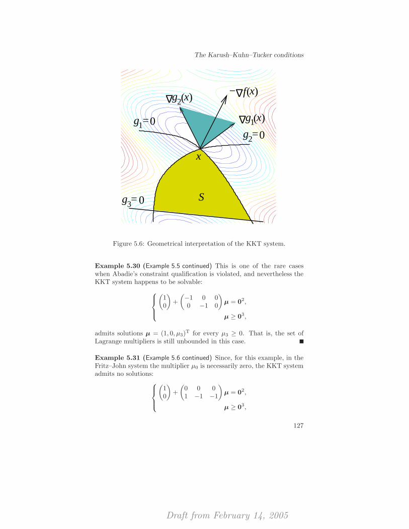
Draft from February 14, 2005
The Karush–Kuhn–Tucker conditions
x)∆
1g =0
3g =0
(x)f∆−
g1(x)∆
2g =0
x
g2(
S
Figure 5.6: Geometrical interpretation of the KKT system.
Example 5.30 (Example 5.5 continued) This is one of the rare caseswhen Abadie’s constraint qualification is violated, and nevertheless theKKT system happens to be solvable:
(10
)+
(−1 0 00 −1 0
)µ = 02,
µ ≥ 03,
admits solutions µ = (1, 0, µ3)T for every µ3 ≥ 0. That is, the set of
Lagrange multipliers is still unbounded in this case.
Example 5.31 (Example 5.6 continued) Since, for this example, in theFritz–John system the multiplier µ0 is necessarily zero, the KKT systemadmits no solutions:
(10
)+
(0 0 01 −1 −1
)µ = 02,
µ ≥ 03,
127
Draft from February 14, 2005
Optimality conditions
is clearly inconsistent. In this example the very basic Abadie’s con-straint qualifications is violated, and therefore the lack of KKT multi-pliers should not be a big surprise.
Example 5.32 (Example 5.7 continued) This example also satisfies Abadie’sconstraint qualification, therefore the KKT-system is necessarily solv-able:
(10
)+
(0 −2 2−1 0 0
)µ = 02,
µ ≥ 03,
admits the solutions µ = (0, µ2, µ2 − 2−1)T, for all µ2 ≥ 2−1. The set ofLagrange multipliers is unbounded in this case, but this is because wehave split the original equality constraint into two inequalities. In Sec-tion 5.6 we formulate the KKT-system that keeps the original equality-representation of the set, and thus reduce the number of multipliers tojust one!
5.6 Proper treatment of equality constraints
Now we consider both inequality and equality constraints, i.e., we assumethat the feasible set S is given by
S = {x ∈ Rn | gi(x) ≤ 0, i = 1, . . . ,m,
hj(x) = 0, j = 1, . . . , ℓ }, (5.10)
instead of (5.5), where gi ∈ C1(Rn), i = 1, . . . ,m, and hj ∈ C1(Rn), j =1, . . . , ℓ. As it was done in Section 5.4, we write S using only inequalityconstraints, by defining the functions gi ∈ C1(Rn), i = 1, . . . ,m + 2ℓ,via:
gi =
gi, i = 1, . . . ,m,
hi−m, i = m+ 1, . . . ,m+ ℓ,
−hi−m−ℓ, i = m+ ℓ+ 1, . . . ,m+ 2ℓ,
(5.11)
so thatS = {x ∈ Rn | gi(x) ≤ 0, i = 1, . . . ,m+ 2ℓ }. (5.12)
Now, let G(x) be defined by (5.7) for the inequality representation (5.12)of S. We will use the old notation G(x) for the cone defined only by thegradients of the functions defining the inequality constraints active at x
in the representation (5.10), and in addition define the null space of thematrix defined by the gradients of the functions defining the equalityconstraints:
H(x) = {p ∈ Rn | ∇hi(x)Tp = 0, i = 1, . . . , ℓ }.. (5.13)
128
Draft from February 14, 2005
Proper treatment of equality constraints
Since all inequality constraint functions gi, i = m + 1, . . . ,m + 2ℓ, arenecessarily active at every x ∈ S, it holds that
G(x) = G(x) ∩H(x), (5.14)
and thus Abadie’s constraint qualification (see Definition 5.23) for theset (5.10) may be equivalently written as
TS(x) = G(x) ∩H(x). (5.15)
Assuming that the latter constraint qualification holds we can write theKKT-system (5.9) for x∗ ∈ S, corresponding to the inequality represen-tation (5.12) (see Theorem 5.25):
m∑
i=1
µi∇gi(x∗) +
m+ℓ∑
i=m+1
µi∇hi−m(x∗) −m+2ℓ∑
i=m+ℓ+1
µi∇hi−m−ℓ(x∗)
+∇f(x∗) = 0n, (5.16a)
µigi(x∗) = 0, i = 1, . . . ,m, (5.16b)
µihi−m(x∗) = 0, i = m+ 1, . . . ,m+ ℓ,(5.16c)
−µihi−m−ℓ(x∗) = 0, i = m+ ℓ+ 1, . . . ,m+ 2ℓ,
(5.16d)
µ ≥ 0m+2ℓ. (5.16e)
Define the pair of vectors (µ, λ) ∈ Rm×Rℓ as µi = µi, i = 1, . . . ,m; λj =µm+j − µm+ℓ+j, j = 1, . . . , ℓ. We also note that the equations (5.16c)and (5.16d) are superfluous, because x∗ ∈ S implies that hj(x
∗) = 0,
j = 1, . . . ,m. Therefore, we get the following system for (µ, λ), knownas the KKT necessary optimality conditions for the sets represented bydifferentiable equality and inequality constraints:
∇f(x∗) +
m∑
i=1
µi∇gi(x∗) +
ℓ∑
j=1
λj∇hj(x∗) = 0n, (5.17a)
µigi(x∗) = 0, i = 1, . . . ,m, (5.17b)
µ ≥ 0m. (5.17c)
Thus, we have established the following theorem.
Theorem 5.33 (KKT optimality conditions for inequality and equality constraints)Assume that at a given point x∗ ∈ S Abadie’s constraint qualifica-tion (5.15) holds, where S is given by (5.10). Then, for this point to
129
Draft from February 14, 2005
Optimality conditions
be a local minimum of a differentiable function f over S it is neces-sary that there exists a pair of vectors (µ, λ) ∈ Rm × Rℓ, such that thesystem (5.17) is satisfied.
Example 5.34 (Example 5.32 revisited) Let us write the system of KKT-conditions for the original representation of the set with one inequalityand one equality constraint (see Example 5.14). As has already beenmentioned, Abadie’s constraint qualification is satisfied, therefore theKKT-system is necessarily solvable:
(10
)+ µ1
(0−1
)+ λ1
(−20
)= 02,
µ1 ≥ 0,
which admits the unique solution µ1 = 0, λ1 = 1/2.
5.7 Constraint qualifications
In this section we discuss conditions on the functions involved in therepresentation (5.10) of a given feasible set S, that all imply Abadie’sconstraint qualification (5.15).
5.7.1 Mangasarian–Fromovitz CQ (MFCQ)
Definition 5.35 (Mangasarian–Fromovitz CQ) We say that at the pointx ∈ S, where S is given by (5.10), the Mangasarian–Fromovitz CQholds if the gradients ∇hj(x) of the functions hj , j = 1, . . . , ℓ, definingthe equality constraints, are linearly independent, and the intersection◦G(x) ∩ H(x) is not empty (see Proposition 5.21 for the proof of KKTconditions in the case of inequality-constrained problem).
We state the following result without a “real” proof, but we outlinethe ideas.
Proposition 5.36 The MFCQ implies Abadie’s CQ.
Proof.[sketch] Since the gradients ∇hj(x), j = 1, . . . , ℓ, are linearly
independent, it can be shown that cl(◦G(x) ∩ H(x)) ⊂ TS(x) (in the
absence of equality constraints, it follows directly from Lemma 5.10).Furthermore, from Lemma 5.10 applied to the inequality represen-
tation of S, i.e., to G(x) defined by (5.14), we know that TS(x) ⊂(G(x) ∩H(x)).
130
Draft from February 14, 2005
Constraint qualifications
Finally, since◦G(x) ∩ H(x) 6= ∅, it can be shown that cl(
◦G(x) ∩
H(x)) = G(x) ∩H(x).
Example 5.37 Since MFCQ implies Abadie’s constraint qualification,Example 5.5 and 5.6 must necessarily violate it. On the other hand, bothExamples 5.4 and 5.7 verify it (since they also satisfy stronger constraintqualifications, see Example 5.40 and 5.43).
5.7.2 Slater CQ
Definition 5.38 (Slater CQ) We say that the system of constraints de-scribing the feasible set S via (5.10) satisfies the Slater CQ, if the func-tions gi, i = 1, . . . ,m, defining the inequality constraints are convex,the functions hj , j = 1, . . . , ℓ, defining the equality constraints are affinewith linearly independent gradients ∇hj(x), j = 1, . . . , ℓ, and, finally,that there exists x ∈ S such that gi(x) < 0, for all i ∈ {1, . . . ,m}.
Proposition 5.39 The Slater CQ implies the MFCQ.
Proof. Suppose the Slater CQ holds at x∗ ∈ S. By the convexity of theinequality constraints we get:
0 > gi(x) = gi(x) − gi(x∗) ≥ ∇gi(x
∗)T(x − x∗),
for all i ∈ I(x∗). Furthermore, since the equality constraints are affine,we have that
0 = hj(x) − hj(x∗) = ∇hj(x
∗)T(x − x∗),
j = 1, . . . , ℓ. Then, x − x∗ ∈ G(x∗) ∩H(x∗).
Example 5.40 Only Example 5.4 verifies Slater CQ (which in particu-lar explains why it satisfies MFCQ as well, see Example 5.37).
5.7.3 Linear independence CQ (LICQ)
Definition 5.41 (LICQ) We say that at the point x ∈ S, where S isgiven by (5.10), the linear independence CQ holds if the gradients ∇gi(x)of the functions gi, i ∈ I(x), defining the active inequality constraints,as well as the gradients ∇hj(x) of the functions hj, j = 1, . . . , ℓ, definingthe equality constraints, are linearly independent.
Proposition 5.42 The LICQ implies the MFCQ.
131
Draft from February 14, 2005
Optimality conditions
Proof.[sketch] Assume that◦G(x∗)∩H(x∗) = ∅, i.e., the system GTp <
0|I(x∗)| and HTp = 0ℓ is unsolvable, where G and H are the ma-trices having the gradients of the active inequality and equality con-straints, respectively, as their columns. Using a separation result similarto Farkas’ Lemma (cf. Theorem 3.30) it can be shown that the systemGµ +Hλ = 0n, µ ≥ 0|I(x∗)| has a nonzero solution (µ,λ) ∈ R|I(x∗)|+ℓ,which contradicts the linear independence assumption on the gradients.
In fact, the solution (µ,λ) to the KKT system (5.17), if one exists,is necessarily unique in this case, and therefore LICQ is a rather strongassumption in many practical situations.
Example 5.43 Only Example 5.7 in the original description using bothinequality and equality constraints verifies the LICQ (which in particularexplains why it satisfies the MFCQ, see Example 5.37, and why theLagrange multipliers are unique in this case, see Example 5.34).
5.7.4 Affine constraints
Assume that both the functions gi, i = 1, . . . ,m, defining the inequal-ity constraints and the functions hj , j = 1, . . . , ℓ, defining the equalityconstraints in the representation (5.10), are affine. Then, the radialcone RS(x) (see Definition 5.1) is equal to G(x) ∩ H(x) (see Exam-ple 4.21). Owing to the inclusions RS(x) ⊂ TS(x) (Proposition 5.3) and
TS(x) ⊂ G(x) = G(x)∩H(x) (Lemma 5.10), where G(x) was defined inSection 5.6 (cf. (5.12) and the discussion thereafter), Abadie’s CQ (5.15)holds in this case.
Thus, the following claim is established.
Proposition 5.44 If all (inequality and equality) constraints are affine,then Abadie’s CQ is satisfied.
5.8 Sufficiency of KKT–conditions under con-vexity
In general, the KKT necessary conditions do not imply local optimality,as has been mentioned before (see, e.g., an example right after the proofof Theorem 4.13). However, if the optimization problem (5.1) is convex,then the KKT conditions are sufficient for global optimality.
Theorem 5.45 (sufficiency of the KKT conditions for convex problems)Assume that the problem (5.1) with the feasible set S given by (5.10)
132

Draft from February 14, 2005
Sufficiency of KKT–conditions under convexity
is convex, i.e., the objective function f as well as the functions gi,i = 1, . . . ,m, are convex, and the functions hj, j = 1, . . . , ℓ, are affine.Assume further that for x∗ ∈ S the KKT conditions (5.17) are satisfied.Then, x∗ is a globally optimal solution of the problem (5.1).
Proof. Choose an arbitrary x ∈ S. Then, by the convexity of thefunctions gi, i = 1, . . . ,m, it holds that
−∇gi(x∗)T(x − x∗) ≥ gi(x
∗) − gi(x) = −gi(x) ≥ 0, (5.18)
for all i ∈ I(x∗), and using the affinity of the functions hj , j = 1, . . . , ℓ,we get that
−∇hj(x∗)T(x − x∗) = hj(x
∗) − hj(x) = 0, (5.19)
for all j = 1, . . . , ℓ. Using the convexity of the objective function, equa-tions (5.17a) and (5.17b), non-negativity of the Lagrange multipliers µi,i ∈ I(x∗), and equations (5.18) and (5.19) we obtain the inequality
f(x) − f(x∗) ≥ ∇f(x∗)T(x − x∗)
= −∑
i∈I(x∗)
µi∇gi(x∗)T(x − x∗) −
ℓ∑
j=1
λj∇hj(x∗)T(x − x∗) ≥ 0.
Since the point x ∈ S was arbitrary, this shows the global optimality ofx∗ in (5.1).
Theorem 5.45 combined with the necessity of the KKT conditionsunder appropriate CQ leads to the following statement.
Corollary 5.46 Assume that the problem (5.1) is convex and verifiesthe Slater CQ (Definition 5.38). Then, for x∗ ∈ S to be a globallyoptimal solution of (5.1) it is both necessary and sufficient to verify thesystem (5.17).
Not surprisingly, without the Slater constraint qualification the KKTconditions remain only sufficient (i.e., they are unnecessarily strong), asthe following example demonstrates.
Example 5.47 Consider the optimization problem to
minimize x1,
subject to
{x2
1 + x2 ≤ 0,
−x2 ≤ 0,
133
Draft from February 14, 2005
Optimality conditions
which is convex but has only one feasible point 02 ∈ R2. At this uniquepoint both the inequality constraints are active, and thus the Slater CQis violated, which however does not contradict the global optimality of02. It is easy to check that the KKT system
(10
)+
(0 01 −1
)µ = 02,
µ ≥ 02,
is unsolvable, and therefore the KKT conditions are not necessary with-out a CQ even for convex problems.
5.9 Applications and examples
Example 5.48 Consider a symmetric square matrix A ∈ Rn×n, andthe optimization problem
minimize −xTAx,
subject to xTx ≤ 1.
The only constraint of this problem is convex; furthermore, (0n)T0n =0 < 1, and thus Slater’s CQ (Definition 5.38) is verified. Therefore, theKKT conditions are necessary for the local optimality in this problem.We will find all the possible KKT points, and then choose a globallyoptimal point among them.
∇(−xTAx) = −2Ax (A is symmetric), and ∇(xTx) = 2x. Thus,the KKT system is as follows: xTx ≤ 1 and
−2Ax + 2µx = 0n,
µ ≥ 0,
µ(xTx − 1) = 0.
From the first two equations we immediately see that either x = 0n,or the pair (µ,x) is respectively a nonnegative eigenvalue and a corre-sponding eigenvector of A. In the former case, from the complementaritycondition we deduce that µ = 0.
Thus, we can characterize the KKT-points of the problem into thefollowing groups:
1. Let µ1, . . . , µk be all the positive eigenvalues of A (if any), anddefine Xi = {x ∈ Rn | xTx = 1,Ax = µix } to be the set ofcorresponding eigenvectors of length 1, i = 1, . . . , k. Then, (x, µi)
134
Draft from February 14, 2005
Applications and examples
is a KKT-point with the corresponding multiplier for every x ∈ Xi,i = 1, . . . , k. Moreover, −xTAx = −µix
Tx = −µi < 0, for everyx ∈ Xi, i = 1, . . . , k.
2. Define also X0 = {x ∈ Rn | xTx ≤ 1,Ax = 0n }. Then, thepair (x, 0) is a KKT-point with the corresponding multiplier forevery x ∈ X0. We note that if the matrix A is nonsingular, thenX0 = {0n}. In any case, −xTAx = 0 for every x ∈ X0.
Therefore, if the matrix A has any positive eigenvalue, then the globalminima points of the problem we consider are the eigenvectors of lengthone, corresponding to the largest positive eigenvalue; otherwise, everyvector that satisfies Ax = 0n is globally optimal.
Example 5.49 Similarly to the previous example, consider the follow-ing equality-constrained minimization problem associated with a sym-metric matrix A ∈ Rn×n:
minimize −xTAx,
subject to xTx = 1.
The gradient of the only equality constraint equals 2x, and since 0n isinfeasible, LICQ is satisfied by this problem (Definition 5.41), and theKKT conditions are necessary for local optimality. In this case, the KKTsystem is extremely simple: xTx = 1 and
−2Ax + 2λx = 0n.
Let λ1 < λ2 < · · · < λk denote all distinct eigenvalues of A, and defineas before Xi = {x ∈ Rn | xTx = 1,Ax = λix } to be the set of corre-sponding eigenvectors of length 1, i = 1, . . . , k. Then, (x, λi) is a KKT-point with the corresponding multiplier for every x ∈ Xi, i = 1, . . . , k.Furthermore, since −xTAx = −λi for every x ∈ Xi, i = 1, . . . , k, itholds that every x ∈ Xk, that is, every eigenvector corresponding to thelargest eigenvalue, is globally optimal.
Considering two problems corresponding to A and −A, we may de-duce that ‖A‖ = max1≤i≤n{ |λi| }, a very well known fact in linearalgebra.
Example 5.50 Consider the problem of finding the projection of a givenpoint x∗ onto the hyperplane {x ∈ Rn | Ax = b }, where A ∈ Rk×n,b ∈ Rk. Thus, we consider the following minimization problem withaffine constraints (so that the KKT conditions are necessary for the
135
Draft from February 14, 2005
Optimality conditions
local optimality, see Section 5.7.4):
minimize1
2(x − x∗)T(x − x∗),
subject to Ax = b.
The KKT-system in this case is written as follows:
Ax = b,
(x − x∗) + ATλ = 0n,
for some λ ∈ Rk. Pre-multiplying the last equation with A, and usingthe fact that Ax = b we get:
AATλ = Ax∗ − b.
Substituting an arbitrary solution of this equation into the KKT-system,we calculate x via
x = x∗ − ATλ.
It can be shown that the vector ATλ is constant for every Lagrange mul-tiplier λ, so using this formula we obtain the globally optimal solutionto our minimization problem.
Now assume that the columns of AT are linearly independent, i.e.,LICQ holds. Then, the matrix AAT is nonsingular, and the multiplierλ is therefore unique:
λ = (AAT)−1(Ax∗ − b).
Substituting this into the KKT-system, we finally obtain the well-knownformula for calculating the projection:
x = x∗ − AT(AAT)−1(Ax∗ − b).
5.10 Notes and further reading
One cannot overemphasize the importance of Karush–Kuhn–Tucker typeoptimality conditions for any development in optimization. We essen-tially follow the ideas presented in [BSS93, Chapters 4 and 5]; an alter-native presentation may be found in [Ber99, Chapter 3]. The originalpapers by Fritz John [Joh48], and Kuhn and Tucker [KuT51] might alsobe interesting.
136
Draft from February 14, 2005
Exercises
Various forms of constraint qualifications play especially importantrole in studies of parametric optimization problems [Fia83, BoS00]. Orig-inal presentation of constraint qualifications, some of which we consid-ered in this chapter, may be found in the works of Arrow, Hurwitz, andUzawa [AHU61], Abadie [Aba67], Mangasarian and Fromowitz [MaF67],Guignard [Gui69], Zangwill [Zan69], and Evans [Eva70].
5.11 Exercises
Exercise 5.1 Consider the following problem:
minimize f(x) = 2x21 + 2x1x2 + x2
2 − 10x1 − 10x2,
subject to x21 + x2
2 ≤ 5,
3x1 + x2 ≤ 6.
Verify whether the point x0 = (2, 1)T is a KKT point for this problem.Is this an optimal solution? Which CQ are satisfied at the point x0?
Exercise 5.2 (optimality conditions, exam 020529) (a) Consider the fol-lowing optimization problem:
minimize x2,
subject to sin(x) ≤ −1.(5.20)
Find every locally and every globally optimal solution to this problem.Write down the KKT conditions. Are they necessary/sufficient for thisproblem?
(b) Do the locally/globally optimal solutions to the problem (5.20)satisfy the FJ optimality conditions?
(c) Question the usefulness of the FJ optimality conditions by findinga point (x, y), which satisfies these conditions for the problem:
minimize y,
subject to
{x2 + y2 ≤ 1,
x3 ≥ y4,
but, nevertheless, is neither the local nor the global minimum for thisproblem.
Exercise 5.3 Consider the following linear programming problem:
minimize cTx,
subject to Ax ≥ b.
137
Draft from February 14, 2005
Optimality conditions
State the KKT-conditions for this problem. Verify that at every KKT-point x the following equality is verified:
cTx = bTλ,
where λ is a vector of KKT-multipliers.
Exercise 5.4 (optimality conditions, exam 020826) (a) Consider the non-linear programming problem with equality constraints:
minimize f(x),
subject to
h1(x) = 0,
...
hm(x) = 0,
(5.21)
where f , h1, . . . , hm are continuously differentiable functions.Show that the problem (5.21) is equivalent to the following problem
with one inequality constraint:
minimize f(x),
subject to
m∑
i=1
(hi(x)
)2 ≤ 0.(5.22)
Show (by giving a formal argument or an illustrative example) thatthe KKT conditions for the latter problem are not necessary for localoptimality.
Can Slater’s CQ or LICQ be satisfied for the problem (5.22)?(b) Consider the unconstrained minimization problem
minimize max{f1(x), f2(x)
},
where f1 : Rn → R, f2 : Rn → R are in C1.Show that if x∗ is a local minimum for this problem, then there exist
µ1, µ2 ∈ R such that
µ1 ≥ 0, µ2 ≥ 0, µ1∇f1(x∗) + µ2∇f2(x∗) = 0, µ1 + µ2 = 1,
and µi = 0 if fi(x∗) < max
{f1(x
∗), f2(x∗)}, i = 1, 2.
Exercise 5.5 Consider the following optimization problem:
minimize1
2xTx,
subject to Ax = b.
Assume that the matrix A has full row rank. Find the globally optimalsolution to this problem.
138
Draft from February 14, 2005
Exercises
Exercise 5.6 Consider the following optimization problem:
minimize
n∑
j=1
cjxj ,
subject to
n∑
j=1
x2j ≤ 1,
−xj ≤ 0, j = 1, . . . , n.
(5.23)
Assume that min {c1, . . . , cn} < 0, and let us introduce KKT multipliersλ ≥ 0 and µj ≥ 0, j = 1, . . . , n for the inequality constraints.
(a) Show that the equalities
x∗j = min{0, cj}/(2λ∗), j = 1, . . . , n,
λ∗ =1
2
n∑
j=1
[min {0, cj}]2
1/2
,
µ∗j = max{0, cj}, j = 1, . . . , n,
define a KKT point for (5.23).
(b) Show that there is only one locally optimal solution to the prob-lem (5.23).
Exercise 5.7 (optimality conditions, exam 040308) Consider the follow-ing optimization problem:
minimize f(x, y) =1
2(x− 2)2 +
1
2(y − 1)2,
subject to
x− y ≥ 0,
y ≥ 0,
y(x− y) = 0,
(5.24)
where x, y ∈ R.
(a) Find all points of global and local minima (you may do this graph-ically), as well as all KKT-points. Is this a convex problem? Are theKKT optimality conditions necessary and/or sufficient for local optimal-ity in this problem?
(b) Demonstrate that LICQ is violated at every feasible point of theproblem (5.24). Show that instead of solving the problem (5.24) we cansolve two convex optimization problems that furthermore verify someconstraint qualification, and then choose the best point out of the two.
139
Draft from February 14, 2005
Optimality conditions
(c) Generalize the procedure from the previous part to more generaloptimization problems:
minimize g(x),
subject to
aTi x ≥ bi, i = 1, . . . , n,
xi ≥ 0, i = 1, . . . , n,
xi(aTi x − bi) = 0, i = 1, . . . , n,
where x = (x1, . . . , xn)T ∈ Rn, ai ∈ Rn, bi ∈ R, i = 1, . . . , n, andg : Rn → R is a convex differentiable function.
Exercise 5.8 Determine the values of the parameter c for which thepoint (x, y) = (4, 3) is an optimal solution to the following problem:
minimize cx+ y,
subject to
{x2 + y2 ≤ 25,
x− y ≤ 1,
where x, y ∈ R.
Exercise 5.9 Consider the following optimization problem:
minimize f(x) =n∑
j=1
x2j
cj,
subject to
n∑
j=1
xj = D,
xj ≥ 0, j = 1, . . . , n,
where cj > 0, j = 1, . . . , n, and D > 0. Find the unique globally optimalsolution to this problem.
140
Draft from February 14, 2005
Lagrangian duality VI
This chapter collects some basic results on Lagrangian duality, in par-ticular as it applies to convex programs with no duality gap.
6.1 The relaxation theorem
Given the problem to find
f∗ := infimumx
f(x), (6.1a)
subject to x ∈ S, (6.1b)
where f : Rn → R is a given function and S ⊆ Rn, we define a relaxationto (6.1) to be a problem of the following form: to find
f∗R := infimum
xfR(x), (6.2a)
subject to x ∈ SR, (6.2b)
where fR : Rn → R is a function with the property that fR ≤ f on S,and where SR ⊇ S. For this pair of problems, we have the followingbasic result.
Theorem 6.1 (Relaxation Theorem) (a) [relaxation] f∗R ≤ f∗.
(b) [infeasibility] If (6.2) is infeasible, then so is (6.1).(c) [optimal relaxation] If the problem (6.2) has an optimal solution,
x∗R, for which it holds that
x∗R ∈ S and fR(x∗
R) = f(x∗R), (6.3)
then x∗R is an optimal solution to (6.1) as well.
Draft from February 14, 2005
Lagrangian duality
Proof. The result in (a) is obvious, as every solution feasible in (6.1)is both feasible in (6.2) and has a lower objective value in the latterproblem.
The result in (b) follows for similar reasons.For the result in (c), we note that
f(x∗R) = fR(x∗
R) ≤ fR(x) ≤ f(x), x ∈ S,
from which the result follows.
This basic result will be utilized both in this chapter and later onto motivate why Lagrangian relaxation, objective function linearizationand penalization are relaxations, and to derive optimality conditions andalgorithms based on them.
6.2 Lagrangian duality
In this section we formulate the Lagrangian dual problem and establishits convexity. The Weak Duality Theorem is also established, and weintroduce the terms “Lagrange multiplier” and “duality gap.”
6.2.1 Lagrangian relaxation and the dual problem
Consider the optimization problem to find
f∗ := infimumx
f(x), (6.4a)
subject to x ∈ X, (6.4b)
gi(x) ≤ 0, i = 1, . . . ,m, (6.4c)
where f : Rn → R and gi : Rn → R (i = 1, 2, . . . ,m) are given functions,and X ⊆ Rn.
For this problem, we assume that
−∞ < f∗ <∞, (6.5)
that is, that f is bounded from below and that the problem has at leastone feasible solution.
For an arbitrary vector µ ∈ Rm, we define the Lagrange function
L(x,µ) := f(x) +
m∑
i=1
µigi(x) = f(x) + µTg(x). (6.6)
We call the vector µ∗ ∈ Rm a Lagrange multiplier if it is non-negativeand if f∗ = infx∈X L(x,µ∗) holds.
142
Draft from February 14, 2005
Lagrangian duality
Theorem 6.2 (Lagrange multipliers and global optima) Let µ∗ be a La-grange multiplier. Then, x∗ is an optimal solution to (6.4) if and onlyif x∗ is feasible in (6.4) and
x∗ ∈ arg minx∈X
L(x,µ∗), and µ∗i gi(x
∗) = 0, i = 1, . . . ,m.
(6.7)
Proof. If x∗ is an optimal solution to (6.4), then it is in particularfeasible, and
f∗ = f(x∗) ≥ L(x∗,µ∗) ≥ infimumx∈X
L(x,µ∗),
where the first inequality stems from the feasibility of x∗ and the defini-tion of a Lagrange multiplier. The second part of that definition impliesthat f∗ = infx∈X L(x,µ∗), so that equality holds throughout in theabove line of inequalities. Hence, (6.7) follows.
Conversely, if x∗ is feasible and (6.7) holds, then by the use of thedefinition of a Lagrange multiplier,
f(x∗) = L(x∗,µ∗) = minimumx∈X
L(x,µ∗) = f∗,
so x∗ is a global optimum.
Letq(µ) := infimum
x∈XL(x,µ) (6.8)
be the Lagrangian dual function, defined by the infimum value of theLagrange function over X ; the Lagrangian dual problem is to
maximizeµ
q(µ), (6.9a)
subject to µ ≥ 0m. (6.9b)
For some µ, q(µ) = −∞ is possible; if this is true for all µ ≥ 0m,then
q∗ := supremumµ≥0m
q(µ)
equals −∞.The effective domain of q is
Dq := { µ ∈ Rm | q(µ) > −∞} .
Theorem 6.3 (convex dual problem) The effective domain Dq of q isconvex, and q is concave on Dq.
143
Draft from February 14, 2005
Lagrangian duality
Proof. Let x ∈ Rn, µ, µ ∈ Rm, and α ∈ [0, 1]. We have that
L(x, αµ + (1 − α)µ) = αL(x,µ) + (1 − α)L(x, µ).
Take the infimum over x ∈ X on both sides; then,
infx∈X
L(x, αµ + (1 − α)µ) = infx∈X
{αL(x,µ) + (1 − α)L(x, µ)}
≥ infx∈X
αL(x,µ) + infx∈X
(1 − α)L(x, µ)
= α infx∈X
L(x,µ) + (1 − α) infx∈X
L(x, µ),
due to the fact that α ∈ [0, 1], and that the sum of infimum values maybe smaller than the infimum of the sum, since in the former case we havethe possibility to choose different optimal solutions in the two problems.Hence,
q(αµ + (1 − α)µ) ≥ αq(µ) + (1 − α)q(µ)
holds. This inequality has two implications: if µ and µ belong to Dq,then so does αµ + (1 − α)µ, so Dq is convex, and further, q is concaveon Dq.
That the Lagrangian dual problem always is convex (we indeed max-imize a concave function!) is very good news, because it means that itcan be solved efficiently. What remains of course is to show how a La-grangian dual optimal solution can be used to generate a primal optimalsolution.
Next, we establish that every feasible point in the Lagrangian dualproblem always underestimates the objective function value of every fea-sible point in the primal problem; hence, also their optimal values havethis relationship.
Theorem 6.4 (Weak Duality Theorem) Let x and µ be feasible in (6.4)and (6.9), respectively. Then,
q(µ) ≤ f(x).
In particular,q∗ ≤ f∗
holds.If q(µ) = f(x), then the pair (x,µ) is optimal in its respective prob-
lem.
Proof. For all µ ≥ 0m and x ∈ X with g(x) ≤ 0m,
q(µ) = infimumz∈X
L(z,µ) ≤ f(x) + µTg(x) ≤ f(x),
144
Draft from February 14, 2005
Lagrangian duality
soq∗ = supremum
µ≥0m
q(µ) ≤ infimumx∈X:g(x)≤0m
f(x) = f∗.
The result follows.
Weak duality is also a consequence of the Relaxation Theorem: Forany µ ≥ 0m, let
S := X ∩ {x ∈ Rn | g(x) ≤ 0m }, (6.10a)
SR := X, (6.10b)
fR := L(µ, ·). (6.10c)
Then, the weak duality statement is the result in Theorem 6.1(a), whenceLagrangian relaxation is a relaxation in terms of the definition in Sec-tion 6.1.
If our initial assumption (6.5) is false, then what does weak dualityimply? Suppose that f∗ = −∞. Then, weak duality implies that q(µ) =−∞ for all µ ≥ 0m, that is, the dual problem is infeasible. Supposethen that X 6= ∅ but that X ∩ {x ∈ Rn | g(x) ≤ 0m } is empty. Then,f∗ = ∞, by convention. The dual function satisfies q(µ) < ∞ for allµ ≥ 0m, but it is possible that q∗ = −∞, −∞ < q∗ < ∞, or q∗ = ∞(see [Ber99, Figure 5.1.8]). For linear programs, ∞ < q∗ < ∞ implies∞ < f∗ <∞, see below.
If q∗ = f∗, we say that there is no duality gap. If there existsa Lagrange multiplier vector, then by the weak duality theorem, thisimplies that there is no duality gap. The converse is not true in general:there may be cases where no Lagrange multiplier exists even when thereis no duality gap; in that case though, the Lagrangian dual problemcannot have an optimal solution, as implied by the following result.
Proposition 6.5 (duality gap and the existence of Lagrange multipliers)(a) If there is no duality gap, then the set of Lagrange multipliers equalsthe set of optimal dual solutions (which however may be empty).
(b) If there is a duality gap, then there are no Lagrange multipliers.
Proof. By definition, a vector µ∗ ≥ 0m is a Lagrange multiplier if andonly if f∗ = q(µ∗) ≤ q∗, the equality following from the definition ofq(µ∗) and the inequality from the definition of q∗ as the supremum ofq(µ) over Rm
+ . By weak duality, this relation holds if and only if thereis no duality gap and µ∗ is an optimal dual solution.
Before moving on, we remark on the statement of the problem (6.4).There are several ways in which the original set of constraints of the
145
Draft from February 14, 2005
Lagrangian duality
problem can be placed either within the definition of the ground set X(which is kept intact), or within the explicit constraints defined by thefunctions gi (which are Lagrangian relaxed). How to distinguish betweenthe two, that is, how to decide whether a constraint should be kept orbe Lagrangian relaxed, depends on several factors. For example, keepingmore constraints within X may result in a smaller duality gap, and withfewer multipliers also result in a simpler Lagrangian dual problem. Onthe other hand, the Lagrangian subproblem defining the dual functionsimultaneously becomes more complex and difficult to solve. There areno immediate rules to follow, but experimentation and experience.
6.2.2 Global optimality conditions
The following result characterizes every optimal primal and dual solu-tion. It is applicable only in the presence of Lagrange multipliers; inother words, the system (6.11) is consistent if and only if there exists aLagrange multiplier and there is no duality gap.
Theorem 6.6 (global optimality conditions in the absence of a duality gap)The vector (x∗,µ∗) is a pair of optimal primal solution and Lagrangemultiplier if and only if
µ∗ ≥ 0m, (Dual feasibility) (6.11a)
x∗ ∈ arg minx∈X
L(x,µ∗), (Lagrangian optimality) (6.11b)
x∗ ∈ X, g(x∗) ≤ 0m, (Primal feasibility) (6.11c)
µ∗i gi(x
∗) = 0, i = 1, . . . ,m. (Complementary slackness) (6.11d)
Proof. Suppose that (6.11) is satisfied. We apply the RelaxationTheorem 6.1, as follows. Consider the identification in (6.10), withµ = µ∗ ≥ 0m and xR = x∗. We then note the following equivalences:
1. The relaxed solution, xR, is a Lagrangian optimal solution. (La-grangian optimality is fulfilled.)
2. That xR ∈ S means that it is feasible in the primal problem.(Primal feasibility is fulfilled.)
3. That f∗ = f∗R means that (µ∗)Tg(x∗) = 0. (Complementary
slackness is fulfilled.)
To conclude, if the conditions in (6.11) are satisfied, then Theorem 6.1implies that the vector (x∗,µ∗) is a pair of optimal primal solution andLagrange multiplier.
146
Draft from February 14, 2005
Lagrangian duality
Conversely, if (x∗,µ∗) is a pair of optimal primal solution and La-grange multiplier, then they are obviously primal and dual feasible, re-spectively. The last two equations in (6.11) follow from Theorem 6.2.
Theorem 6.7 (global optimality and saddle points) The vector (x∗,µ∗)is a pair of optimal primal solution and Lagrange multiplier if and onlyif x∗ ∈ X , µ∗ ≥ 0m, and (x∗,µ∗) is a saddle point of the Lagrangianfunction on X × Rm
+ , that is,
L(x∗,µ) ≤ L(x∗,µ∗) ≤ L(x,µ∗), (x,µ) ∈ X × Rm+ , (6.12)
holds.
Proof. We establish that (6.11) and (6.12) are equivalent. The resultthen follows from Theorem 6.6. The first inequality in (6.12) is equivalentto
−g(x∗)T(µ − µ∗) ≥ 0, µ ∈ Rm+ , (6.13)
for the given µ∗ ∈ Rm+ . This variational inequality is equivalent to
stating that0m ≥ g(x∗) ⊥ µ∗ ≥ 0m, (6.14)
where ⊥ denotes orthogonality: that is, for any vectors a, b ∈ Rn, a ⊥ b
means that aTb = 0. Because of the sign restrictions posed on µ andg, that is, the vectors a and b, the relation a ⊥ b actually means thatnot only does it hold that aTb = 0 but in fact ai · bi = 0 must hold forall i = 1, . . . , n.1 This complementarity system is, again, for the givenµ∗ ∈ Rm
+ , the same as (6.11a), (6.11c) and (6.11d). The second inequal-ity in (6.12) is equivalent to (6.11b).
The above two results also state that the set of primal–dual solutions(x∗,µ∗) is a Cartesian product set, that is, that every primal optimalsolution x∗ can be obtained through the system (6.11b) given any dualoptimal solution µ∗, and vice versa.
1We establish the equivalence between (6.13) and (6.14) as follows. (Notice thatthe result is an extension to that of the optimality condition of the line search problemfrom 1 variable to m variables, except for the fact that the first is for a minimizationproblem while we here are dealing with a maximization problem; the proof is in facta natural extension of that given in a footnote in Section 11.3.1.)
First, suppose that (6.14) is fulfilled. Then, −g(x∗)T(� − �∗) = −g(x∗)T� ≥ 0,for all � ≥ 0
m, that is, (6.13) is fulfilled. Conversely, suppose that (6.13) is fulfilled.Setting � = 0
m yields that g(x∗)T�∗ ≥ 0. On the other hand, the choice � = 2�∗
yields that −g(x∗)T�∗ ≥ 0. Hence, g(x∗)T�∗ = 0 holds. Last, let � = �∗ + ei,where ei is the ith unit vector in Rm. Then, −g(x∗)T(�−�∗) = −gi(x∗) ≥ 0. Sincethis is true for all i ∈ {1, 2, . . . , m} we have obtained that −g(x∗) ≥ 0
m, that is,g(x∗) ≤ 0m. We are done.
147
Draft from February 14, 2005
Lagrangian duality
We note that structurally similar results to the above two proposi-tions which are valid for the general problem (6.4) with any size of theduality gap can be found in [LaP05].2
We note finally a practical connection between the KKT system (5.9)and the above system (6.11). The practical use of the KKT system isnormally to investigate whether a primal vector x—obtained perhapsfrom a solver for our problem—is a candidate for a locally optimal so-lution; in other words, we have access to x and generate a vector µ ofLagrange multipliers in the investigation of the KKT system (5.9). Incontrast, the system (6.11) is normally investigated in the reverse order;we formulate and solve the Lagrangian dual problem, thereby obtainingan optimal dual vector µ. Starting from that vector, we investigate theglobal optimality conditions stated in (6.11) to obtain, if possible, anoptimal primal vector x. In the section to follow, we show when this ispossible, and provide strong connections between the systems (5.9) and(6.11) in the convex and differentiable case.
6.2.3 Strong duality for convex programs
So far the results have been rather non-technical to achieve: the con-vexity of the Lagrangian dual problem comes with very few assumptionson the original, primal problem, and the characterization of the primal–dual set of optimal solutions is simple and also quite easily established.In order to establish strong duality, that is, to establish sufficient con-ditions under which there is no duality gap, however takes much more.In particular, as is the case with the KKT conditions we need regularityconditions (that is, constraint qualifications), and we also need to utilizeseparation theorems such as Theorem 4.28. Most importantly, however,is that strong duality is deeply associated with the convexity of the orig-inal problem, and it is in particular under convexity that the primal anddual optimal solutions are linked through the global optimality condi-tions provided in the previous section. We begin by concentrating on theinequality constrained case, proving this result in detail. We will alsospecialize the result to quadratic and linear optimization problems.
Consider the inequality constrained convex program (6.4), where f :Rn → R and gi (i = 1, . . . ,m) are convex functions and X ⊆ Rn isa convex set. For this problem, we introduce the following regularity
2The system (6.11) is there appended with two relaxation parameters which mea-sure, respectively, the near-optimality of x∗ in the Lagrangian subproblem [that is,the ε-optimality in (6.11b)], and the violation of the complementarity conditions(6.11d). The saddle point condition (6.12) is similarly perturbed, and at an optimalsolution, the sum of these two parameters equals the duality gap.
148
Draft from February 14, 2005
Lagrangian duality
condition, due to Slater (cf. Definition 5.38): that
∃x ∈ X with g(x) < 0m. (6.15)
Theorem 6.8 (Strong Duality, inequality constrained convex programs) Supposethat (6.5) and Slater’s constraint qualification (6.15) hold for the convexproblem (6.4).
(a) There is no duality gap and there exists at least one Lagrangemultiplier µ∗. Moreover, the set of Lagrange multipliers is bounded andconvex.
(b) If the infimum in (6.4) is attained at some x∗, then the pair(x∗,µ∗) satisfies the global optimality conditions (6.11).
(c) If further f and g are differentiable at x∗, then the condition(6.11b) can equivalently be written as the variational inequality
∇xL(x∗,µ∗)T(x − x∗) ≥ 0, x ∈ X. (6.16)
If, in addition, X is open (such as is the case when X = Rn), then thisreduces to the condition that
∇xL(x∗,µ∗) = ∇f(x∗) +
m∑
i=1
µ∗i∇gi(x
∗) = 0n, (6.17)
and the global optimality conditions (6.11) reduce to the Karush–Kuhn–Tucker conditions stated in Theorem 5.25.
Proof. (a) We begin by establishing the existence of a Lagrange multi-plier (and the presence of a zero duality gap).3
First, we consider the following subset of Rm+1:
A := {(z1, . . . , zm, w)T |∃x∈ X with gi(x)≤zi, i = 1, . . . ,m; f(x)≤w}.
It is elementary to show that A is convex.Next, we observe that ((0m)T, f∗)T is not an interior point of A;
otherwise, for some ε > 0 the point ((0m)T, f∗ − ε)T ∈ A holds, whichwould contradict the definition of f∗. Therefore, by the (possibly non-proper) separation result in Theorem 4.28, we can find a hyperplanepassing through ((0m)T, f∗)T such that A lies in one of the two corre-sponding halfspaces. In particular, there then exists a vector (µT, β)T 6=((0m)T, 0)T such that
βf∗ ≤ βw + µTz, (zT, w)T ∈ A. (6.18)
3This result is Proposition [Ber99, 5.3.1], whose proof we also utilize.
149
Draft from February 14, 2005
Lagrangian duality
This implies thatβ ≥ 0; µ ≥ 0m, (6.19)
since we have for each (zT, w)T ∈ A that (zT, w+γ)T ∈ A and (z1, . . . , zi−1, zi+γ, zi+1, . . . , zm, w)T ∈ A for all γ > 0 and i = 1, . . . ,m.
We claim that β > 0 in fact holds. Indeed, if it was not the case, thenβ = 0 and (6.18) then implies that µTz ≥ 0 for every pair (zT, w)T ∈A. But since (g(x)T, 0)T ∈ A [where x is such that it satisfies theSlater condition (6.15)], we would obtain that 0 ≤ ∑m
i=1 µigi(x) whichin view of µ ≥ 0m [cf. (6.19)] and the assumption that x satisfies theSlater condition (6.15) implies that µ = 0m. This means, however, that(µT, β)T = ((0m)T, 0)T, arriving at a contradiction. We may thereforeclaim that β > 0. We further, without any loss of generality, assumethat β = 1.
Thus, since (g(x)T, f(x))T ∈ A for every x ∈ X , (6.18) yields that
f∗ ≤ f(x) + µTg(x), x ∈ X.
Taking the infimum over x ∈ X and using the fact that µ ≥ 0m weobtain
f∗ ≤ infimumx∈X
{f(x) + µTg(x)} = q(µ) ≤ supremumµ≥0m
q(µ) = q∗.
Using the Weak Duality Theorem 6.4 it follows that µ is a Lagrangemultiplier vector, and there is no duality gap. This part of the proof isnow done.
Take any vector x ∈ X satisfying (6.15). By the definition of aLagrange multiplier, f∗ ≤ L(x,µ∗) holds, which implies that
m∑
i=1
µ∗i ≤ [f(x) − f∗]
mini=1,...,m{−gi(x)} .
By the non-negativity of µ∗, boundedness follows. As by Proposition 6.5(a)the set of Lagrange multipliers is the same as the set of optimal solutionsto the dual problem (6.9), convexity follows from the identification of thedual solution set with the set of vectors µ ∈ Rm
+ for which
q(µ) ≥ q∗
holds. This is the upper level set for q at the level q∗; this set is convex,by the concavity of q (cf. Theorem 6.3 and Proposition 3.44).
(b) The result follows from Theorem 6.6.(c) The first part follows from Theorem 4.23, as the Lagrangian func-
tion L(·,µ∗) is convex. The second part follows by identification.
150
Draft from February 14, 2005
Lagrangian duality
Consider next the extension of the inequality constrained convex pro-gram (6.4) in which we seek to find
f∗ := infimumx
f(x), (6.20a)
subject to x ∈ X, (6.20b)
gi(x) ≤ 0, i = 1, . . . ,m, (6.20c)
εTj x − dj = 0, j = 1, . . . , ℓ, (6.20d)
under the same conditions as stated following (6.4), and where εj ∈ Rn
(j = 1, . . . , ℓ). For this problem, we replace the Slater condition (6.15)with the following (cf. [BSS93, Theorem 6.2.4]):
∃x ∈ X with g(x) < 0m and 0m ∈ int {Ex − d | x ∈ X }, (6.21)
where E is the m× n matrix with rows εTj and d = (dj)j∈{1,...,ℓ} ∈ Rm.
Note that in the statement (6.21), the “int” can be stricken wheneverX is polyhedral, so that the latter part simply states that Ex = d.
For this problem, the Lagrangian dual problem is to find
q∗ := supremum(µ,λ)
q(µ,λ), (6.22a)
subject to µ ≥ 0m, (6.22b)
where
q(µ,λ) := infimumx
L(x,µ,λ) = f(x) + µTg(x) + λT(Ex − d),
(6.23a)
subject to x ∈ X. (6.23b)
Theorem 6.9 (Strong Duality, general convex programs) Suppose that inaddition to (6.5), Slater’s constraint qualification (6.21) holds for theproblem (6.4).
(a) There is no duality gap and there exists at least one Lagrangemultiplier pair (µ∗,λ∗).
(b) If the infimum in (6.20) is attained at some x∗, then the triple(x∗,µ∗,λ∗) satisfies the global optimality conditions
µ∗ ≥ 0m, (Dual feasibility) (6.24a)
x∗ ∈ arg minx∈X
L(x,µ∗,λ∗), (Lagrangian optimality) (6.24b)
x∗ ∈ X, g(x∗) ≤ 0m, Ex∗ = d, (Primal feasibility) (6.24c)
µ∗i gi(x
∗) = 0, i = 1, . . . ,m. (Complementary slackness) (6.24d)
151
Draft from February 14, 2005
Lagrangian duality
(c) If further f and g are differentiable at x∗, then the condition(6.24b) can equivalently be written as
∇xL(x∗,µ∗,λ∗)T(x − x∗) ≥ 0, x ∈ X. (6.25)
If, in addition, X is open (such as is the case when X = Rn), then thisreduces to the condition that
∇xL(x∗,µ∗,λ∗) = ∇f(x∗) +m∑
i=1
µ∗i ∇gi(x
∗) +ℓ∑
j=1
λ∗jεj = 0n, (6.26)
and the global optimality conditions (6.24) reduce to the Karush–Kuhn–Tucker conditions stated in Theorem 5.33.
Proof. The proof is similar to that of Theorem 6.8.
We finally consider a special case where automatically a regularitycondition holds.
Consider the linearly constrained convex program to find
f∗ := infimumx
f(x), (6.27a)
subject to x ∈ X, (6.27b)
aTi x − bi ≤ 0, i = 1, . . . ,m, (6.27c)
εTj x − dj = 0, j = 1, . . . , ℓ, (6.27d)
where f : Rn → R is convex and X ⊆ Rn is polyhedral.
Theorem 6.10 (Strong Duality, linear constraints) If (6.5) holds for theproblem (6.27), then there is no duality gap and there exists at least oneLagrange multiplier.
Proof. Again, the proof is similar to that of Theorem 6.8, except thatno additional regularity conditions are needed.4
The existence of a multiplier [which by Proposition 6.5 and the ab-sence of a duality gap implies the existence of an optimal solution to thedual problem (6.9)] does not imply the existence of an optimal solutionto the primal problem (6.27) without any additional assumptions (takethe minimization of f(x) := 1/x over x ≥ 1 for example). However,when f is either weakly coercive, quadratic or linear, the existence re-sults are stronger; see the primal existence results in Theorems 4.6, 4.7,and 6.11 below, for example.
4For a detailed proof, see [Ber99, Proposition 5.2.1]. (The special case where f ismoreover differentiable is covered in [Ber99, Proposition 3.4.2].)
152
Draft from February 14, 2005
Lagrangian duality
For convex programs, the Lagrange multipliers defined in this sec-tion, and those that appear in the Karush–Kuhn–Tucker conditions, areidentical. We establish this result for two classes of convex programsbelow.
Next, we specialize the above to linear and quadratic programs.
6.2.4 Strong duality for linear and quadratic pro-grams
The following result will be established and analyzed in detail in Chap-ter 10 on linear programming duality (cf. Theorem 10.6), but can in factalso be established similarly to above. Its proof will however be relegatedto that of Theorem 10.6.
Theorem 6.11 (Strong Duality, linear programs) Assume, in addition tothe conditions of Theorem 6.10, that f is linear, so that (6.27) is a linearprogram. Then, the primal and dual problems have optimal solutionsand there is no duality gap.
Proof. The result follows by applying Farkas’ Lemma 3.30 and theWeak Duality Theorem 6.4, or by analyzing an optimal Simplex tableau.Detailed proofs are found in [BSS93, Theorem 2.7.3] or [Ber99, Proposi-tion 5.2.2], for example.
The above result states a strong duality result for a general linearprogram. The dual problem is however not explicit. We next developan explicit Lagrangian dual problem for a linear program. Again, moredetails on this problem will be covered later.
Consider the linear program to
minimizex
cTx, (6.28a)
subject to Ax = b, (6.28b)
x ≥ 0n, (6.28c)
where A ∈ Rm×n, c ∈ Rn, and b ∈ Rm. If we let X := Rn+, then the
Lagrangian dual problem is to
maximizeλ∈Rm
bTλ, (6.29a)
subject to ATλ ≤ c. (6.29b)
The reason why we can write it in this form is that
q(λ) := infimumx≥0n
{cTx + λT(b − Ax)
}= bTλ + infimum
x≥0n(c−ATλ)Tx,
153
Draft from February 14, 2005
Lagrangian duality
so that
q(λ) =
{bTλ, if ATλ ≤ c,
−∞, otherwise.
(The infimum is attained at zero if and only if these inequalities aresatisfied; otherwise, the inner problem is unbounded below.)
Further, why is it that λ here is not restricted in sign? Suppose wewere to split the system Ax = b into an inequality system of the form
Ax ≤ b,
−Ax ≤ −b.
Let (µ+
µ−
)
be the corresponding vector of multipliers, and take the Lagrangian dualfor this formulation. Then, we would have a Lagrange function of theform
(x,µ+,µ−) 7→ L(x,µ+,µ−) := cTx + (µ+ − µ−)T(b − Ax),
and since µ+−µ− can take on any value in Rm we can simply replace itwith the unrestricted vector λ ∈ Rm. This is what has been done above,and it motivates why the multiplier for an equality constraint never issign restricted; the same was the case, as we saw in Section 5.6, for themultipliers in the KKT conditions.
As applied to this problem, Theorem 6.11 states that if both theprimal or dual problems have feasible solutions, then they both haveoptimal solutions, satisfying strong duality (cTx∗ = bTλ∗). On theother hand, if any of the two problems has an unbounded solution, thenthe other problem is infeasible.
Consider next the quadratic programming problem to
minimizex
{1
2xTQx + cTx
}, (6.30a)
subject to Ax ≤ b, (6.30b)
where Q is a positive definite n×n matrix. We develop an explicit dualproblem under this assumption on Q.
Lagrangian relaxing the inequality constraints, we obtain that theinner problem in x is solved by letting
x = −Q−1(c + ATµ). (6.31)
154
Draft from February 14, 2005
Illustrative examples
Substituting this expression into the Lagrangian function yields the La-grangian dual problem to
maximizeµ
{−1
2µTAQ−1ATµ − (b + AQ−1c)Tµ − 1
2cTQ−1c
},
(6.32a)
subject to µ ≥ 0m, (6.32b)
Strong duality follows for this convex primal–dual pair of quadraticprograms, in much the same way as for linear programming.
Proposition 6.12 (Strong Duality, quadratic programs) For the primal–dual pair of convex quadratic programs (6.30), (6.32), the followingholds:
(a) If both problems have feasible solutions, then both problems alsohave optimal solutions, and the primal problem (6.30) also has a uniqueoptimal solution, given by (6.31) for any optimal Lagrange multiplier,and in the two problems the optimal values are equal.
(b) If either of the two problems has an unbounded solution, thenthe other one is infeasible.
(c) Suppose that Q is positive semi-definite, and that (6.5) holds.Then, both the problem (6.30) and its Lagrangian dual have nonempty,closed and convex sets of optimal solutions, and their optimal values areequal.
In the result (a) it is important to note that the Lagrangian dualproblem (6.32) is not necessarily strictly convex; the matrix AQ−1A
need not be positive definite, especially so when A does not have fullrank. The result (c) extends the strong duality result from linear pro-gramming, since Q in (c) can be the zero matrix. In the case of (c) we ofcourse cannot write the Lagrangian dual problem in the form of (6.32)because Q is not invertible.
6.3 Illustrative examples
6.3.1 Two numerical examples
Example 6.13 (an explicit, differentiable dual problem) Consider the prob-lem to
minimizex
f(x) := x21 + x2
2,
subject to x1 + x2 ≥ 4,
xj ≥ 0, j = 1, 2.
155
Draft from February 14, 2005
Lagrangian duality
We consider the first constraint to be the complicated one, and hencedefine g(x) := −x1 − x2 + 4 and let X := { (x1, x2) | xj ≥ 0, j = 1, 2 }.
Then, the Lagrangian dual function is
q(µ) = minimumx∈X
L(x, µ) := f(x) − µ(x1 + x2 − 4)
= 4µ+ minimumx∈X
{x21 + x2
2 − µx1 − µx2}
= 4µ+ minimumx1≥0
{x21 − µx1} + minimum
x2≥0{x2
2 − µx2}, µ ≥ 0.
For a fixed µ ≥ 0, the minimum is attained at x1(µ) = µ2 , x2(µ) = µ
2 .Substituting this expression into q(µ), we obtain that q(µ) = f(x(µ))−
µ(x1(µ) + x2(µ) − 4) = 4µ− µ2
2 .Note that q is strictly concave, and it is differentiable everywhere (due
to the fact that f, g are differentiable and x(µ) is unique), by Danskin’sTheorem 6.16(d).
We then have that q′(µ) = 4 − µ = 0 ⇐⇒ µ = 4. As µ = 4 ≥ 0, itis the optimum in the dual problem! µ∗ = 4; x∗ = (x1(µ
∗), x2(µ∗))T =
(2, 2)T.Also: f(x∗) = q(µ∗) = 8.
This is an example where the dual function is differentiable, andtherefore we can utilize Proposition 6.25(c). In this case, the optimumx∗ is also unique, so it is automatically given as x∗ = x(µ).
Example 6.14 (an implicit, non-differentiable dual problem) Consider thelinear programming problem to
minimizex
f(x) := −x1 − x2,
subject to 2x1 + 2x2 ≤ 3,
0 ≤ x1 ≤ 2,
0 ≤ x2 ≤ 1.
Check that the optimal solution is that x∗ = (3/2, 0)T, f(x∗) =−3/2.
Consider Lagrangian relaxing the first constraint, obtaining
L(x, µ) = −x1 − x2 + µ(2x1 + 4x2 − 3);
q(µ) = −3µ+ minimum0≤x1≤2
{(−1 + 2µ)x1} + minimum0≤x2≤1
{(−1 + 4µ)x2}
=
−3 + 5µ, 0 ≤ µ ≤ 1/4,−2 + µ, 1/4 ≤ µ ≤ 1/2,
− 3µ, 1/2 ≤ µ.
156
Draft from February 14, 2005
Illustrative examples
Check that µ∗ = 1/2, and hence that q(µ∗) = −3/2. For linearprograms, we have strong duality, but how do we obtain the optimalprimal solution from µ∗? It is clear that q is non-differentiable at µ∗.Let us utilize the characterization given in the system (6.11).
First, at µ∗, it is clear that X(µ∗) is the set {(2α0
)| 0 ≤ α ≤ 1 }.
Among the subproblem solutions, we next have to find one that is primalfeasible as well as complementary.
Primal feasibility means that 2 · 2α+ 2 · 0 ≤ 3 ⇐⇒ α ≤ 3/4.Further, complementarity means that µ∗ · (2x∗1 + 4x∗2 − 3) = 0 ⇐⇒
α = 3/4, since µ∗ 6= 0. We conclude that the only primal vector x
that satisfies the system (6.11) together with the dual optimal solutionµ∗ = 1/2 is x∗ = (3/2, 0)T. Check finally that f∗ = q∗.
In the first example, the Lagrangian dual function is differentiablesince x(µ) is unique. The second one shows that otherwise, there maybe kinks in the function q where there are alternative solutions x(µ); as aresult, to obtain a primal optimal solution becomes more complex. TheDantzig–Wolfe algorithm, for example, represents a means by which toautomatize the process that we have just shown; the algorithm generatesextreme points of X(µ) algorithmically, and constructs the best feasibleconvex combination thereof, obtaining a primal–dual optimal solution ina finite number of iterations for linear programs.
6.3.2 An application to combinatorial optimization
Lagrangian relaxation has shown to be remarkably efficient for somecombinatorial optimization problems. This is surprising when takinginto account that such problems are integer or mixed-integer problems,which suffer from non-zero duality gaps in general. What then lies behindtheir popularity?� One can show that Lagrangian relaxation of an integer program is
always at least as good as that of a continuous relaxation5 (in thesense that fR is higher for Lagrangian relaxation than a continuousrelaxation);� Together with heuristics for finding primal feasible solution, sur-prisingly good feasible solutions are often found;� The Lagrangian relaxed problems can be made computationallymuch simpler than the original problem, while still keeping a lotof the structure of the original problem.
5The continuous relaxation amounts to removing the integrality conditions, re-placing, for example, xj ∈ {0, 1} by xj ∈ [0, 1].
157
Draft from February 14, 2005
Lagrangian duality
The traveling salesman problem We provide an example, takenfrom an application of the traveling salesman problem.
Let cij denote the distance from city i to city j, with i < j, andi, j ∈ N = {1, 2, . . . , n}, and
xij =
{1, if link (i, j) is part of the TSP tour,
0, otherwise.
With these definitions, the complete, undirected traveling salesmanproblem (TSP) is to
minimizex
n∑
i=1
n∑
j=1:j 6=i
cijxij , (6.33a)
subject to∑
i∈S
∑
j∈Sxij ≤ |S| − 1, S ⊂ N , (6.33b)
n∑
i=1
n∑
j=1:j 6=i
xij = n, (6.33c)
n∑
i=1
xij = 2, j ∈ N , (6.33d)
xij ∈ {0, 1}, i, j ∈ N . (6.33e)
The constraints have the following interpretation: (6.33b) impliesthat there can be no sub-tours, that is, a tour where fewer than n citiesare visited (that is, if S ⊂ N then there can be at most |S| − 1 linksbetween nodes in the set S, where |S| is the cardinality–number of mem-bers of–the set S); (6.33c) implies that in total n cities must be visited;and (6.33d) implies that each city is connected to two others, such thatwe make sure to arrive from one city and leave for the next.
This problem is NP-hard, which implies that there is no knownpolynomial algorithm for solving it. We resort therefore to the useof relaxation techniques, in particular Lagrangian relaxation. We havemore than one alternative relaxation to perform: If we Lagrangian re-lax the tree constraints (6.33b) and (6.33c) the remaining problem is a2-matching problem; it can be solved in polynomial time. If we insteadLagrangian relax the degree constraints (6.33d) for every node except forone node the remaining problem is a 1-MST problem, that is, a specialtype of minimum spanning tree problem.
The following definition is classic: a Hamiltonian path (respectivelycycle) is a path (respectively, cycle) which passes every node in the graphexactly once.
Every Hamiltonian cycle is a Hamiltonian path from a node s toanother node, t, followed by a link (t, s); a subgraph which consists of
158
Draft from February 14, 2005
Illustrative examples
a spanning tree plus an extra link such that all nodes have degree two.This is then a feasible solution to the TSP.
A 1-MST problem is the problem to find an MST in the graph thatexcludes node s, followed by the addition of the two least expensive linksfrom node s to that tree. If all nodes happen to get degree two, thenthe 1-MST solution is a traveling salesman tour (that is, Hamiltoniancycle). The idea behind solving the Lagrangian dual problem is thento find proper multiplier values such that the Lagrangian relaxation willproduce feasible solutions.
Lagrangian relaxation of the traveling salesman problem Sup-pose that we Lagrangian relax the degree constraints (3), except for node1.
The subproblem is the following: an 1-MST with the objective func-tion (note that λ1 = 0, corresponding to the starting node of the tour)
q(λ) = minimumx
n∑
i=1
n∑
j=1:j 6=i
cijxij +
n∑
j=2
λj
(2 −
n∑
i=1:i6=j
xij
)
= 2n∑
j=1
λj + minimumx
n∑
i=1
n∑
j=1:j 6=i
(cij − λi − λj)xij .
We see immediately the role of the Lagrange multipliers: a high (low)value of the multiplier λj makes node j attractive (unattractive) in theabove 1-MST problem, and will therefore lead to more (less) links beingattached to it. When solving the Lagrangian dual problem, we will usethe class of subgradient optimization methods, an overview of whichis found in Section 6.5; it is a kind of steepest ascent method for theproblem to maximize the function q over Rn, but where gradients arereplaced by subgradients.
What is the updating step? It is as usual an update in the directionof a subgradient, that is, the direction of
hi(x(λ)) := 2 −n∑
i=1:i6=j
xij , i = 1, . . . , n,
where the value of xij ∈ {0, 1} is the solution to the 1-MST solutionwith link costs cij − λi − λj . We see from the formula for the directionthat it is such that
λj := λj + α
2 −
n∑
i=1:i6=j
xij
, j = 2, . . . , n,
159
Draft from February 14, 2005
Lagrangian duality
where α > 0 is a step length. It is interesting to investigate what theupdate means:
current degree at node j :
> 2 =⇒ λj ↓ (link cost ↑)= 2 =⇒ λj − (link cost constant)< 2 =⇒ λj ↑ (link cost ↓)
In other words, the updating formula in a subgradient method issuch that the link cost in the 1-MST subproblem is shifted upwards(downwards) if there are too many (too few) links connected to node jin the 1-MST. We are hence adjusting the node prices of the nodes insuch a way as to influence the 1-MST problem to always choose 2 linksper node to connect to.
A feasibility heuristic A feasibility heuristic takes the optimal so-lution from the Lagrangian minimization problem over x and adjusts itsuch that a feasible solution to the original problem is constructed. Asone cannot predict if, or when, a primal feasible solution will be founddirectly from the subproblem, the heuristic will provide a solution thatcan be used in place of an optimal one, should one not be found. More-over, as we know from Lagrangian duality theory, we then have accessto both lower and upper bounds on the optimal value f∗ of the origi-nal problem, and so we have a quality measure of the feasible solutionsfound.
A feasibility heuristic which can be used together with our Lagrangianheuristic is as follows.
Identify a path in the 1-MST with many links. Then form a subgraphwith the remaining nodes and find a path that passes all of them. Put thetwo paths together in the best way. The resulting path is a Hamiltoniancycle, that is, a feasible solution. We then have both a lower bound [thevalue of q(λ)] and an upper bound (the original cost of this heuristicallyconstructed traveling salesman tour), and this interval can be used as aquality measure of the feasible solution at termination.
The Philips example In 1987–1988 an MSc project was performed atthe department of mathematics at Linkoping University, in cooperationwith the company Philips, Norrkoping. The project was initiated withthe goal to improve the current practice of solving a production planningproblem.
The problem was as follows: Philips produces circuit boards, perhapsseveral hundreds or thousands of the same type. There is a new batch ofpatterns (holes) to be drilled every day, and perhaps even several suchbatches per day.
160
Draft from February 14, 2005
Illustrative examples
In order to speed up the production process the drilling machine isconnected to a microcomputer that selects the ordering of the holes tobe drilled automatically, given their coordinates. The algorithm for per-forming the sorting used to be a simple sorting operation that found,for every fixed x-coordinate, the corresponding y-coordinates and sortedthem in increasing order. The movement of the drill was therefore fromleft to right, and for each fixed x-coordinate the movement was vertical.The time it took to drill the holes on one circuit board was, however,far too long, simply because the drill traveled around a lot without per-forming any tasks, thus following a path that was too long. (On theother hand, the actual ordering was very fast to produce!) All in all,though, the complete batch production took too long because of thepoorly planned drill movement.
At the beginning of the project it was observed that the produc-tion planning problem actually is a traveling salesman problem, wherethe cities are the holes to be drilled, and the distances between themcorrespond to the Euclidean distances between them. Therefore, an effi-cient TSP heuristic was devised and implemented, for use in conjunctionwith the microcomputer. In fact, it was based on precisely the aboveLagrangian relaxation, a subgradient optimization method, and a graph-search type heuristic of the form discussed above.
A typical run with the algorithm took a few minutes, and was alwaysstopped after a fixed number of subgradient iterations; the generation offeasible solutions with the above-mentioned graph search technique wasperformed at every Kth iteration, where K was set to a value strictlylarger than one. (Moreover, feasible solutions were not generated duringthe first iterations of the dual procedure, because of the poor quality ofλk for low values of k; it is often the case that the traveling salesmantour resulting from the heuristic is better when the multipliers are near-optimal in the Lagrangian dual problem.)
In one of the examples implemented it was found that the optimalpath length was in the order to 2 meters, and that the upper and lowerbounds produced lead to the conclusion that the relative error of thepath length of the best feasible solution found was less than 7 %, a quitegood result, also showing that the duality gap for the problem at hand(together with the Lagrangian relaxation chosen) is quite small.
After implementing the new procedure, Philips could report an in-crease in production by some 70 %. Hence, the slightly longer time ittook to produce the production plan, that is, the traveling salesman tourfor the drill to follow, was more than well compensated by the fact thatthe drilling could be done much faster.
Here is hence an interesting case where Lagrangian relaxation helped
161
Draft from February 14, 2005
Lagrangian duality
to solve a large-scale, complex and difficult problem by utilizing problemstructure.
6.4 ∗Differentiability properties of the dualfunction
We have established that the Lagrangian dual problem (6.9) is a convexone, and further that under some circumstances we can generate a dualoptimal solution that has the same objective value q∗ as the optimalvalue of the original problem f∗. We now turn to study the Lagrangiandual problem in detail, and in particular how it can be solved efficiently.First, we will establish when the dual function q is differentiable. We willsee that differentiability holds only in some special cases, in which wecan recognize the workings of the so-called Lagrange multiplier method.In practice, the function q will be non-differentiable, and then this clas-sic method will fail. This means that we must devise a more generalnumerical method which is not based on gradients but rather subgradi-ents. This type of algorithm is the topic of the next section, while wehere begin by studying the topic of subgradients of convex functions ingeneral.
6.4.1 Sub-differentiability of convex functions
Throughout this section we suppose that f : Rn → R is a convex func-tion, and study its sub-differentiability properties. We will later on applyour findings to the Lagrangian dual function q, or, rather, its negative−q. We first remark that a finite convex function is automatically con-tinuous (cf. Theorem 4.26), in fact even Lipschitz continuous on everybounded subset of Rn.
Definition 6.15 (subgradient) Let f : Rn → R be a convex function.We say that a vector p ∈ Rn is a subgradient of f at x ∈ Rn if
f(y) ≥ f(x) + pT(y − x), y ∈ Rn. (6.34)
The set of such vectors p defines the subdifferential of f at x, and isdenoted ∂f(x).
Notice the connection to the characterization of a convex function inC1 in Theorem 3.40(a). The difference between them is that p is notunique at a non-differentiable point. (Just as the gradient has a role insupporting hyperplanes to the graph of a convex function in C1, the role
162
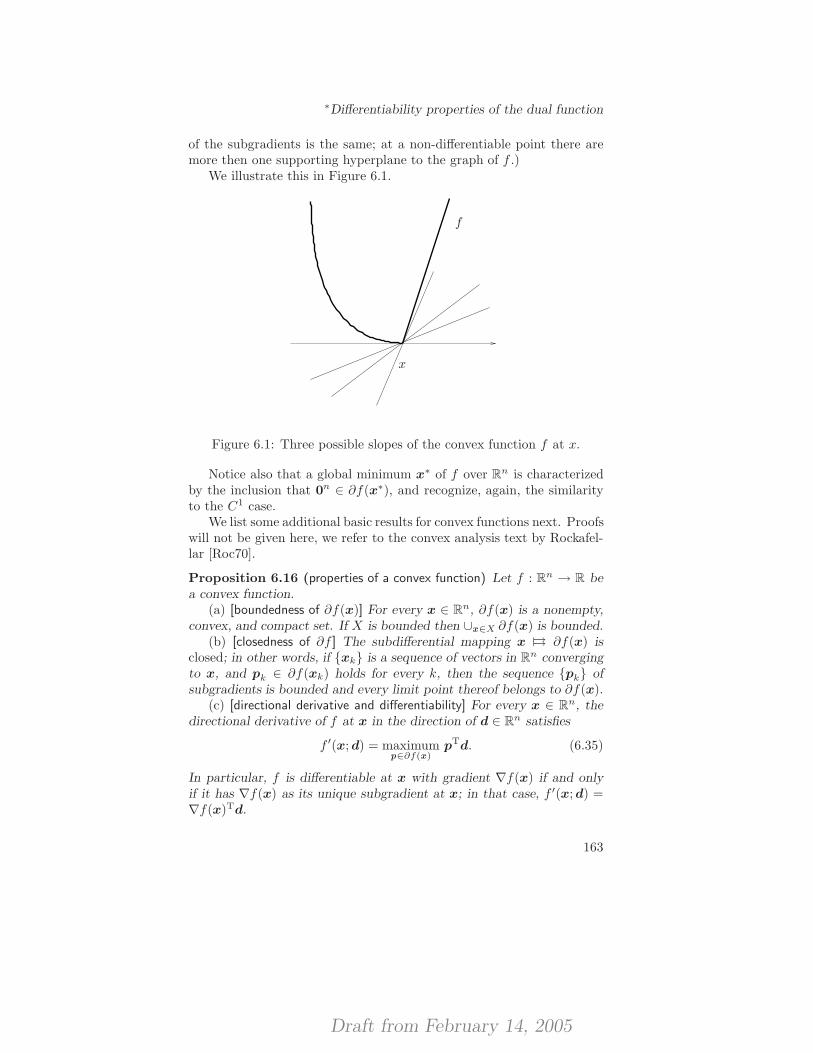
Draft from February 14, 2005
∗Differentiability properties of the dual function
of the subgradients is the same; at a non-differentiable point there aremore then one supporting hyperplane to the graph of f .)
We illustrate this in Figure 6.1.
f
x
Figure 6.1: Three possible slopes of the convex function f at x.
Notice also that a global minimum x∗ of f over Rn is characterizedby the inclusion that 0n ∈ ∂f(x∗), and recognize, again, the similarityto the C1 case.
We list some additional basic results for convex functions next. Proofswill not be given here, we refer to the convex analysis text by Rockafel-lar [Roc70].
Proposition 6.16 (properties of a convex function) Let f : Rn → R bea convex function.
(a) [boundedness of ∂f(x)] For every x ∈ Rn, ∂f(x) is a nonempty,convex, and compact set. If X is bounded then ∪x∈X ∂f(x) is bounded.
(b) [closedness of ∂f ] The subdifferential mapping x 7→7→ ∂f(x) isclosed; in other words, if {xk} is a sequence of vectors in Rn convergingto x, and pk ∈ ∂f(xk) holds for every k, then the sequence {pk} ofsubgradients is bounded and every limit point thereof belongs to ∂f(x).
(c) [directional derivative and differentiability] For every x ∈ Rn, thedirectional derivative of f at x in the direction of d ∈ Rn satisfies
f ′(x; d) = maximump∈∂f(x)
pTd. (6.35)
In particular, f is differentiable at x with gradient ∇f(x) if and onlyif it has ∇f(x) as its unique subgradient at x; in that case, f ′(x; d) =∇f(x)Td.
163
Draft from February 14, 2005
Lagrangian duality
(d) [Danskin’s Theorem—directional derivatives of a convex max func-tion] Let Z be a compact subset of Rm, and let φ : Rn × Z → R becontinuous and such that φ(·, z) : Rn → R is convex for each z ∈ Z. Letthe function f : Rn → R be given by
f(x) := maximumz∈Z
φ(x, z), x ∈ Rn. (6.36)
The function f then is convex on Rn and has a directional derivative atx in the direction of d equal to
f ′(x; d) := maximumz∈Z(x)
φ′(x, z; d), (6.37)
where φ′(x, z; d) is the directional derivative of φ(·, z) at x in the direc-tion of d, and Z(x) := { z ∈ Rm | φ(x, z) = f(x) }.
In particular, if Z(x) contains a single point z and φ(·, z) is differen-tiable at x, then f is differentiable at x, and ∇f(x) = ∇xφ(x, z), where
∇xφ(x, z) is the vector with components ∂φ(x ,z)∂xi
, i = 1, . . . , n.If further φ(·, z) is differentiable for all z ∈ Z and ∇xφ(x, ·) is con-
tinuous on Z for each x, then
∂f(x) = conv {∇xφ(x, z) | z ∈ Z(x) }, x ∈ Rn,
holds.
Proof. (a) This is a special case of [Roc70, Theorem 24.7].(b) This is [Roc70, Theorem 24.5].(c) This is [Roc70, Theorem 23.4 and 25.1].(d) This is [Ber99, Proposition B.25].
Figure 6.2 illustrates the subdifferential of a convex function.
6.4.2 Differentiability of the Lagrangian dual func-tion
We consider the inequality constrained problem (6.4), where we makethe following standing assumption:
f, gi (i = 1, . . . ,m) are continuous; X is nonempty and compact.(6.38)
Under this assumption, the set of solutions to the Lagrangian subprob-lem,
X(µ) := arg minimumx∈X
L(x,µ), µ ∈ Rm, (6.39)
164
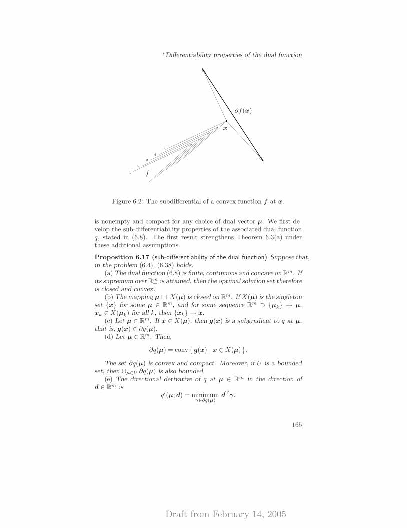
Draft from February 14, 2005
∗Differentiability properties of the dual function
1
2
3
4
5
f
x
∂f(x)
Figure 6.2: The subdifferential of a convex function f at x.
is nonempty and compact for any choice of dual vector µ. We first de-velop the sub-differentiability properties of the associated dual functionq, stated in (6.8). The first result strengthens Theorem 6.3(a) underthese additional assumptions.
Proposition 6.17 (sub-differentiability of the dual function) Suppose that,in the problem (6.4), (6.38) holds.
(a) The dual function (6.8) is finite, continuous and concave on Rm. Ifits supremum over Rm
+ is attained, then the optimal solution set thereforeis closed and convex.
(b) The mapping µ 7→7→ X(µ) is closed on Rm. If X(µ) is the singletonset {x} for some µ ∈ Rm, and for some sequence Rm ⊃ {µk} → µ,xk ∈ X(µk) for all k, then {xk} → x.
(c) Let µ ∈ Rm. If x ∈ X(µ), then g(x) is a subgradient to q at µ,that is, g(x) ∈ ∂q(µ).
(d) Let µ ∈ Rm. Then,
∂q(µ) = conv { g(x) | x ∈ X(µ) }.
The set ∂q(µ) is convex and compact. Moreover, if U is a boundedset, then ∪µ∈U ∂q(µ) is also bounded.
(e) The directional derivative of q at µ ∈ Rm in the direction ofd ∈ Rm is
q′(µ; d) = minimumγ∈∂q(µ)
dTγ.
165
Draft from February 14, 2005
Lagrangian duality
Proof. (a) Theorem 6.3(a) stated the concavity of q on its effectivedomain. Weierstrass’ Theorem 4.6 states that q is finite on Rm, which isthen also its effective domain. The continuity of q follows from that ofany finite concave function, as we have already stated.6 The closednessproperty of the solution set complements that of Theorem 6.8(a), andis a direct consequence of the continuity of q (the upper level set thenautomatically is a closed set).
(b) Let {µk} be a sequence of vectors in Rm, and let xk ∈ X(µk) bearbitrary. Let x be arbitrary in X , and let further x ∈ X be an arbitrarylimit point of {xk} (at least exists from the compactness of X). Fromthe property that for all k,
L(xk,µk) ≤ L(x,µk),
follows by the continuity of L that, in the limit of k in the subsequencein which {xk} converges to x,
L(x, µ) ≤ L(x, µ),
so that x ∈ X(µ), as desired. The special case of a singleton set X(µ)follows.
(c) Let µ ∈ Rm be arbitrary. We have that
q(µ) = infimumy∈X
L(y, µ) ≤ f(x) + µTg(x)
= f(x) + (µ − µ)Tg(x) + µTg(x) = q(µ) + (µ − µ)Tg(x),
which implies that g(x) ∈ ∂q(µ).(d) The inclusion ∂q(µ) ⊆ conv { g(x) | x ∈ X(µ) } follows from (c)
and the convexity of ∂q(µ). The opposite inclusion follows by applyingthe Separation Theorem 3.24.7
(e) See Danskin’s Theorem in Proposition 6.16(d).
The result in (c) is an independent proof of the concavity of q on Rm.The result (d) is particularly interesting, because by Caratheodory’s
Theorem 3.8 it says that every subgradient of q at any point µ is theconvex combination of a finite number (in fact, at most m+1) of vectorsof the form g(xs) with xs ∈ X(µ). Computationally, this has beenutilized to devise efficient (proximal) bundle methods for the Lagrangiandual problem as well as to devise methods to recover primal optimalsolutions.
Next, we establish the differentiability of the dual function underadditional assumptions.
6See [Roc70, Theorem 10.1 and its Corollary 10.1.1].7See [BSS93, Theorem 6.3.7] for a detailed proof.
166
Draft from February 14, 2005
Subgradient optimization methods
Proposition 6.18 (differentiability of the dual function) Suppose that, inthe problem (6.4), (6.38) holds.
(a) Let µ ∈ Rm. The dual function q is differentiable at µ if andonly if { g(x) | x ∈ X(µ) } is a singleton set, that is, if the value of thevector of constraint functions is invariant over the set of solutions X(µ)to the Lagrangian subproblem. Then, we have that
∇q(µ) = g(x),
for every x ∈ X(µ).(b) The result in (a) holds in particular if the Lagrangian subproblem
has a unique solution, that is, X(µ) is a singleton set. In particular, thisproperty is satisfied if further X is a convex set, f is strictly convex onX , and gi (i = 1, . . . ,m) are convex, in which case q is even in C1.
Proof. (a) The concave function q is differentiable at the point µ (whereit is finite) if and only if its subdifferential ∂q(µ) there is a singleton, cf.Proposition 6.16(c).
(b) Under either one of the assumptions stated, X(µ) is a singleton,whence the result follows from (a). Uniqueness follows from the con-vexity of the feasible set and strict convexity of the objective function,according to Proposition 4.10.
Proposition 6.19 (twice differentiability of the dual function) Suppose that,in the problem (6.4), X = Rn, and f and gi (i = 1, . . . ,m) are convexfunctions in C2. Suppose that, at µ ∈ Rm, the solution x to the La-grangian subproblem not only is unique, but also that the partial Hessianof the Lagrangian is positive definite at the pair (x,µ), that is,
∇2xxL(x,µ) is positive definite.
Then, the dual function q is twice differentiable at µ, with
∇2q(µ) = −g(x)T[∇2xxL(x,µ)]−1g(x).
Proof. The result follows from the Implicit Function Theorem, whichis stated in Chapter 2, applied to the Lagrangian subproblem.8
6.5 Subgradient optimization methods
We begin by establishing the convergence of classic subgradient opti-mization methods as applied to a general convex optimization problem.
8See [Ber99, Pages 596–598] for a detailed analysis.
167
Draft from February 14, 2005
Lagrangian duality
6.5.1 Convex problems
Consider the convex optimization problem to
minimizex
f(x), (6.40a)
subject to x ∈ X, (6.40b)
where f : Rn → R is convex and the set X ⊆ Rn is nonempty, closedand convex.
The subgradient projection algorithm is as follows: select x0 ∈ X ,and for k = 0, 1, . . . generate
gk ∈ ∂f(xk), (6.41)
xk+1 = ProjX (xk − αkgk), (6.42)
where the sequence {αk} is generated from one of the following threerules.
The first rule is termed the divergent series step length rule, andrequires that
αk > 0, k = 0, 1, . . . ; limk→∞
αk = 0;
∞∑
k=0
αk = +∞. (6.43)
The second rule adds to the requirements in (6.43) the square-summablerestriction ∞∑
k=0
α2k < +∞. (6.44)
The conditions in (6.43) allow for convergence to any point fromany starting point, since the total step is infinite, but convergence istherefore also quite slow; the additional condition in (6.44) means thatthe fastest among these sequences are selected. An instance of the steplength formulas which satisfies both (6.43) and (6.44) is the following:
αk = β/(k + 1), k = 0, 1, . . . ,
where β > 0.The third step length rule is
σ ≤ αk ≤ 2[f(xk) − f∗]/‖gk‖2 − σ, (6.45)
where f∗ is the optimal value of (6.40). We refer to this step length for-mula as the Polyak step, after the Russian mathematician Boris Polyakwho invented the subgradient method in the 1960s together with Er-mol’ev and Shor.
168
Draft from February 14, 2005
Subgradient optimization methods
How is convergence established for subgradient optimization meth-ods? As shall be demonstrated in Chapters 11 and 12 convergence ofalgorithms for problems with a differentiable objective function is typi-cally based on generating descent directions, and step length rules thatresult in the sequence {xk} of iterates being strictly descending in thevalue of f . For the non-differentiable problem at hand, generating de-scent directions is a difficult task, since it is not true that the negative ofan arbitrarily chosen subgradient of f at a non-optimal vector x definesa descent direction.
In bundle methods one gathers information from more than one sub-gradient (hence the term bundle) around a current iteration point sothat a descent direction can be generated, followed by an inexact linesearch. We concentrate here on the simpler methodology of subgradientoptimization methods, in which we apply the formula (6.52) where thestep length αk is chosen based on very simple rules.
We establish below that if the step length is small enough, an it-eration of the subgradient projection method leads to a vector that iscloser to the set of optimal solutions. This technical result also motivatesthe construction of the Polyak step length rule, and hence shows thatconvergence of subgradient methods are based on the reduction of theEuclidean distance to the optimal solutions rather than on the objectivefunction f .
Proposition 6.20 (decreasing distance to the optimal set) Suppose thatxk ∈ X is not optimal in (6.40), and that xk+1 is given by (6.42) forsome step length αk > 0.
Then, for every optimal solution x∗ in (6.40),
‖xk+1 − x∗‖ < ‖xk − x∗‖holds for every step length αk in the interval
αk ∈ (0, 2[f(xk) − f∗]/‖gk‖2). (6.46)
Proof. We have that
‖xk+1 − x∗‖2 = ‖ProjX (xk − αkgk) − x∗‖2
= ‖ProjX (xk − αkgk) − ProjX (x∗)‖2
≤ ‖xk − αkgk − x∗‖2
= ‖xk − x∗‖2 − 2αk(xk − x∗)Tgk + α2k‖gk‖2
≤ ‖xk − x∗‖2 − 2αk[f(xk) − f∗] + α2k‖gk‖2
< ‖xk − x∗‖2,
169
Draft from February 14, 2005
Lagrangian duality
where we have utilized the property that the Euclidean projection is non-expansive (Theorem 4.31), the subgradient inequality (6.34) for convexfunctions, and the bounds on αk given by (6.46).
Our first convergence result is based on the divergent series steplength formula (6.43), and establishes convergence to the optimal solu-tion set X∗ under an assumption on its boundedness. With the othertwo step length formulas, this condition will be possible to remove.
Recall the definition (3.10) of the minimum distance from a vector toa closed and convex set; our interest is in the distance from an arbitraryvector x ∈ Rn to the solution set X∗:
distX∗ (x) := minimumy∈X∗
‖y − x‖.
Theorem 6.21 (convergence of subgradient optimization methods, I) Let{xk} be generated by the method (6.42), (6.43). If X∗ is bounded andthe sequence {gk} is bounded, then {f(xk)} → f∗ and {distX∗(xk)} → 0holds.
Proof. We show that the iterates will eventually belong to an arbitrarilysmall neighbourhood of the set of optimal solutions to (6.40).
Let δ > 0 and Bδ = {x ∈ Rn | ‖x‖ ≤ δ }. Since f is convex, X isnonempty, closed and convex, andX∗ is bounded, it follows from [Roc70,Theorem 27.2], applied to the lower semi-continuous, proper9 and convexfunction f + χX)10 that there exists an ε = ε(δ) > 0 such that the levelset {x ∈ X | f(x) ≤ f∗ + ε } ⊆ X∗ + Bδ/2; this level set is denoted byXε. Moreover, since for all k, ‖gk‖ ≤ sups{‖gs‖} < ∞, and {αk} → 0,there exists an N(δ) such that αk‖gk‖2 ≤ ε and αk‖gk‖ ≤ δ/2 for allk ≥ N(δ).
The sequel of the proof is based on induction and is organized asfollows. In the first part, we show that there exists a finite k(δ) ≥ N(δ)such that xk(δ) ∈ X∗ + Bδ. In the second part, we establish that if xk
belongs to X∗ + Bδ for some k ≥ N(δ) then so does xk+1, by showingthat either distX∗(xk+1) < distX∗(xk) holds, or xk ∈ Xε so that xk+1 ∈X∗ +Bδ since the step taken is not longer than δ/2.
9A proper function is a function which is finite at least at some vector and nowhereattains the value −∞. See also Section 1.4.
10For any set S ⊂ Rn the function χS is the indicator function of the set S, thatis, χS(x) = 0 if x ∈ S; and χS(x) = +∞ if x 6∈ S.
170
Draft from February 14, 2005
Subgradient optimization methods
Let x∗ ∈ X∗ be arbitrary. In every iteration k we then have
‖x∗ − xk+1‖2= ‖x∗ − ProjX (xk − αkgk)‖2
(6.47a)
≤ ‖x∗ − xk + αkgk‖2 (6.47b)
= ‖x∗ − xk‖2+ αk
(2gT
k (x∗ − xk) + αk ‖gk‖2), (6.47c)
where the inequality follows from the projection property. Now, supposethat
2 gTs (x∗ − xs) + αs ‖gs‖2
< −ε (6.48)
for all s ≥ N(δ). Then, using (6.47) repeatedly, we obtain that for anyk ≥ N(δ),
‖x∗ − xk+1‖2<∥∥x∗ − xN(δ)
∥∥2 − ε
k∑
s=N(δ)
αs,
and from (6.52) it follows that the right-hand side of this inequality tendsto minus infinity as k → ∞, which clearly is impossible. Therefore,
2 gTk (x∗ − xk) + αk ‖gk‖2 ≥ −ε (6.49)
for at least one k ≥ N(δ), say k = k(δ). From the definition of N(δ), itfollows that gT
k(δ)(x∗−xk(δ)) ≥ −ε. From the definition of a subgradient
(cf. Definition 6.15) we have that f(x∗) − f(xk(δ)) ≥ gTt(δ)(x
∗ − xk(δ)),
since x∗,xk(δ) ∈ X . Hence, f(xk(δ)) ≤ f∗ + ε, that is, xk(δ) ∈ Xε ⊆X∗ +Bδ/2 ⊂ X∗ +Bδ.
Now, suppose that xk ∈ X∗ + Bδ for some k ≥ N(δ). If (6.48)holds, then, using (6.47), we have that ‖x∗−xk+1‖ < ‖x∗−xk‖ for anyx∗ ∈ x∗. Hence,
distX∗(xk+1) ≤ ‖ProjX∗ (xk) − xk+1‖ < ‖ProjX∗ (xk) − xk‖= distX∗(xk) ≤ δ.
Thus, xk+1 ∈ X∗+Bδ. Otherwise, (6.49) must hold and, using the samearguments as above, we obtain that f(xk) ≤ f∗ + ε, i.e., xk ∈ Xε ⊆x∗ +Bδ/2. As
‖xk+1 − xk‖ = ‖ProjX (xk − αkgk) − xk‖ ≤ ‖xk − αkgk − xk‖
= αk ‖gk‖ ≤ δ
2
whenever k ≥ N(δ), it follows that xk+1 ∈ X∗+Bδ/2 +Bδ/2 = X∗+Bδ.
171
Draft from February 14, 2005
Lagrangian duality
By induction with respect to k ≥ k(δ), it follows that xk ∈ X∗ +Bδ
for all k ≥ k(δ). Since this holds for arbitrarily small values of δ > 0and f is continuous, the theorem follows.
We next introduce the additional requirement (6.44); the resultingalgorithm’s convergence behaviour is now much more favourable, andthe proof is at the same time less technical.
Theorem 6.22 (convergence of subgradient optimization methods, II) Let{xk} be generated by the method (6.42), (6.43), (6.44). IfX∗ is nonemptyand the sequence {gk} is bounded, then {f(xk)} → f∗ and {xk} → x∗ ∈X∗ holds.
Proof. Let x∗ ∈ X∗ and k ≥ 1. Repeated application of (6.47) yieldsthat
‖x∗ − xk‖2 ≤ ‖x∗ − x0‖2+ 2
k−1∑
s=0
αsgTs (x∗ − xs) +
k−1∑
s=0
α2s ‖gs‖2
.(6.50)
Since x∗ ∈ X∗ and gs ∈ ∂f(xs) for all s ≥ 0 we obtain that
f(xs) ≥ f∗ ≥ f(xs) + gTs (x∗ − xs) , s ≥ 0, (6.51)
and hence that gTs (x∗ − xs) ≤ 0 for all s ≥ 0. Define c := supk{‖gk‖}
and p =∑∞
k=0 α2k, so that ‖gs‖ ≤ c for any s ≥ 0 and
∑k−1s=0 α
2s < p.
From (6.50) we then conclude that ‖x∗ − xk‖2 < ‖x∗ − x0‖2 + pc2 forany k ≥ 1, and thus that the sequence {xk} is bounded.
Assume now that there is no subsequence {xki} of {xk} with {gTki
(x∗−xki
)} → 0. Then there must exist an ε > 0 with gTs (x∗ − xs) ≤ −ε for
all sufficiently large values of s. From (6.50) and the conditions on thestep lengths it follows that {‖x∗−xs‖} → −∞, which clearly is impossi-ble. The sequence {xk} must therefore contain a subsequence {xki
} suchthat {gT
ki(x∗ − xki
)} → 0. From (6.51) it follows that {f(xki)} → f∗.
The boundedness of {xk} implies the existence of an accumulation pointof the subsequence {xki
}, say x∞. From the continuity of f it followsthat x∞ ∈ X∗.
To show that x∞ is the only accumulation point of {xk}, let δ > 0and find an M(δ) such that ‖x∞ − xM(δ)‖2 ≤ δ/2 and
∑∞s=M(δ) α
2s ≤
δ/(2c2). Consider any k > M(δ). Analogously to the derivation of(6.50), and using (6.51), we then obtain that
‖x∞ − xk‖2 ≤∥∥x∞ − xM(δ)
∥∥2+
k−1∑
s=M(δ)
α2s‖gs‖2 <
δ
2+
δ
2c2c2 = δ.
172
Draft from February 14, 2005
Subgradient optimization methods
Since this holds for arbitrarily small values of δ > 0, we are done.
We note that it is possible to remove the boundedness condition on{gk} at the simple price of scaling the length of the search direction; wepreferred to keep the simplicity of the algorithms, however. Note furtherthat this condition is immediately ensured to be fulfilled whenever weknow before-hand that the sequence {xk} is bounded, such as is the casewhen X itself is bounded.
Convergence of this type of method is quite slow. In fact, the steplength rule (6.43) prevents fast convergence to be possible. We say thatthe sequence {xk} converges to x∗ with a geometric rate if there existsM > 0 and q ∈ (0, 1) with
‖xk − x∗‖ ≤Mqk, k = 0, 1, . . . .
Suppose that this speed is possible together with the step length rule(6.43). For all k, the above yields
αk = ‖xk+1 − xk‖ ≤ ‖xk+1 − x∗‖ + ‖xk − x∗‖ ≤M(q + 1)qk;
summing these inequalities up implies
∞∑
k=0
αk ≤M(q + 1)/(1 − q),
which contradicts the divergent series condition (6.43).We finally present the convergence properties of the subgradient pro-
jection method using the Polyak step; it is even stronger than the resultof Theorem 6.22.
Theorem 6.23 (convergence of subgradient optimization methods, III) Let{xk} be generated by the method (6.42), (6.45). If X∗ is nonempty then{f(xk)} → f∗ and {xk} → x∗ ∈ X∗ holds.
Proof. From Proposition 6.20 follows that the sequence {{‖xk−x∗‖} isstrictly decreasing for every x∗ ∈ X∗, and therefore has a limit. By con-struction of the step length, in which the step lengths are bounded awayfrom zero and 2[f(xk)− f∗]/‖gk‖2, it follows from the proof of Proposi-tion 6.20 that {[f(xk)− f∗]/‖gk‖2} → 0 must hold. Since {gk} must bebounded due to the boundedness of {xk}, we have that {f(xk)} → f∗.Further, {xk} is bounded, and due to the continuity properties of f everylimit point must then belong to X∗.
It remains to show that there can be only one limit point. Thisproperty follows from the monotone decrease of the distance ‖xk −x∗‖.
173
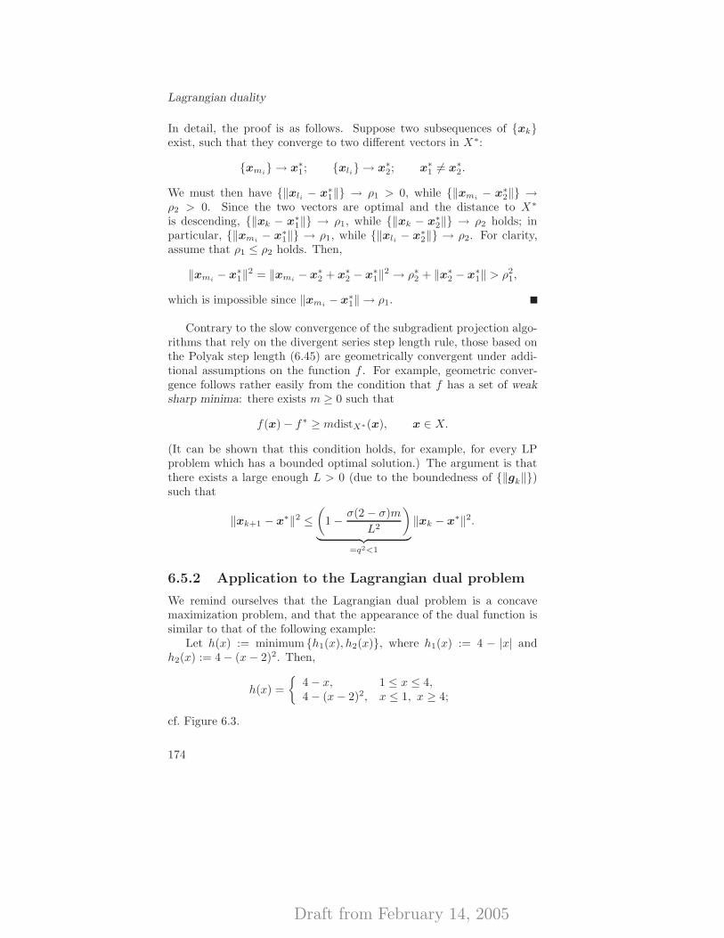
Draft from February 14, 2005
Lagrangian duality
In detail, the proof is as follows. Suppose two subsequences of {xk}exist, such that they converge to two different vectors in X∗:
{xmi} → x∗
1; {xli} → x∗2; x∗
1 6= x∗2.
We must then have {‖xli − x∗1‖} → ρ1 > 0, while {‖xmi
− x∗2‖} →
ρ2 > 0. Since the two vectors are optimal and the distance to X∗
is descending, {‖xk − x∗1‖} → ρ1, while {‖xk − x∗
2‖} → ρ2 holds; inparticular, {‖xmi
− x∗1‖} → ρ1, while {‖xli − x∗
2‖} → ρ2. For clarity,assume that ρ1 ≤ ρ2 holds. Then,
‖xmi− x∗
1‖2 = ‖xmi− x∗
2 + x∗2 − x∗
1‖2 → ρ∗2 + ‖x∗2 − x∗
1‖ > ρ21,
which is impossible since ‖xmi− x∗
1‖ → ρ1.
Contrary to the slow convergence of the subgradient projection algo-rithms that rely on the divergent series step length rule, those based onthe Polyak step length (6.45) are geometrically convergent under addi-tional assumptions on the function f . For example, geometric conver-gence follows rather easily from the condition that f has a set of weaksharp minima: there exists m ≥ 0 such that
f(x) − f∗ ≥ mdistX∗(x), x ∈ X.
(It can be shown that this condition holds, for example, for every LPproblem which has a bounded optimal solution.) The argument is thatthere exists a large enough L > 0 (due to the boundedness of {‖gk‖})such that
‖xk+1 − x∗‖2 ≤(
1 − σ(2 − σ)m
L2
)
︸ ︷︷ ︸=q2<1
‖xk − x∗‖2.
6.5.2 Application to the Lagrangian dual problem
We remind ourselves that the Lagrangian dual problem is a concavemaximization problem, and that the appearance of the dual function issimilar to that of the following example:
Let h(x) := minimum {h1(x), h2(x)}, where h1(x) := 4 − |x| andh2(x) := 4 − (x− 2)2. Then,
h(x) =
{4 − x, 1 ≤ x ≤ 4,4 − (x− 2)2, x ≤ 1, x ≥ 4;
cf. Figure 6.3.
174
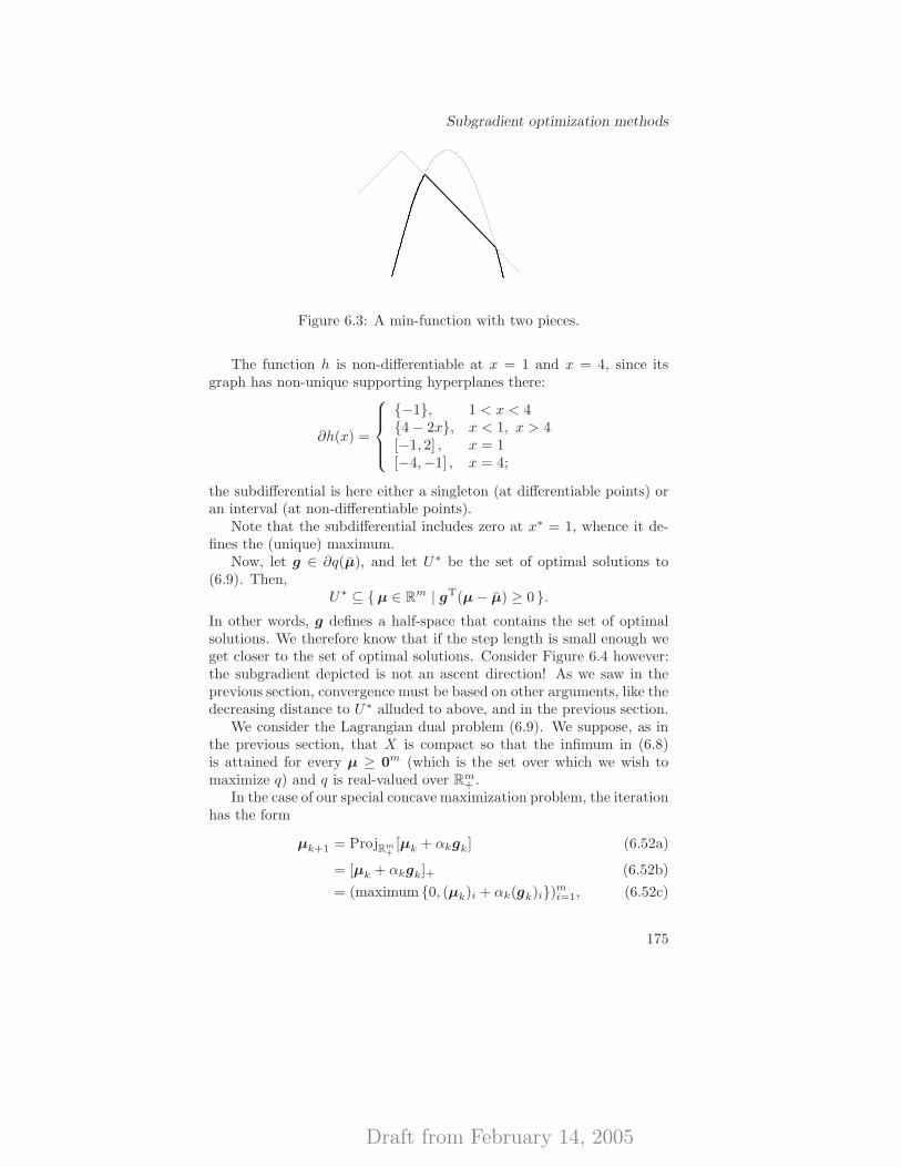
Draft from February 14, 2005
Subgradient optimization methods
Figure 6.3: A min-function with two pieces.
The function h is non-differentiable at x = 1 and x = 4, since itsgraph has non-unique supporting hyperplanes there:
∂h(x) =
{−1}, 1 < x < 4{4 − 2x}, x < 1, x > 4[−1, 2] , x = 1[−4,−1] , x = 4;
the subdifferential is here either a singleton (at differentiable points) oran interval (at non-differentiable points).
Note that the subdifferential includes zero at x∗ = 1, whence it de-fines the (unique) maximum.
Now, let g ∈ ∂q(µ), and let U∗ be the set of optimal solutions to(6.9). Then,
U∗ ⊆ {µ ∈ Rm | gT(µ − µ) ≥ 0 }.In other words, g defines a half-space that contains the set of optimalsolutions. We therefore know that if the step length is small enough weget closer to the set of optimal solutions. Consider Figure 6.4 however:the subgradient depicted is not an ascent direction! As we saw in theprevious section, convergence must be based on other arguments, like thedecreasing distance to U∗ alluded to above, and in the previous section.
We consider the Lagrangian dual problem (6.9). We suppose, as inthe previous section, that X is compact so that the infimum in (6.8)is attained for every µ ≥ 0m (which is the set over which we wish tomaximize q) and q is real-valued over Rm
+ .In the case of our special concave maximization problem, the iteration
has the form
µk+1 = ProjR
m+
[µk + αkgk] (6.52a)
= [µk + αkgk]+ (6.52b)
= (maximum {0, (µk)i + αk(gk)i})mi=1, (6.52c)
175
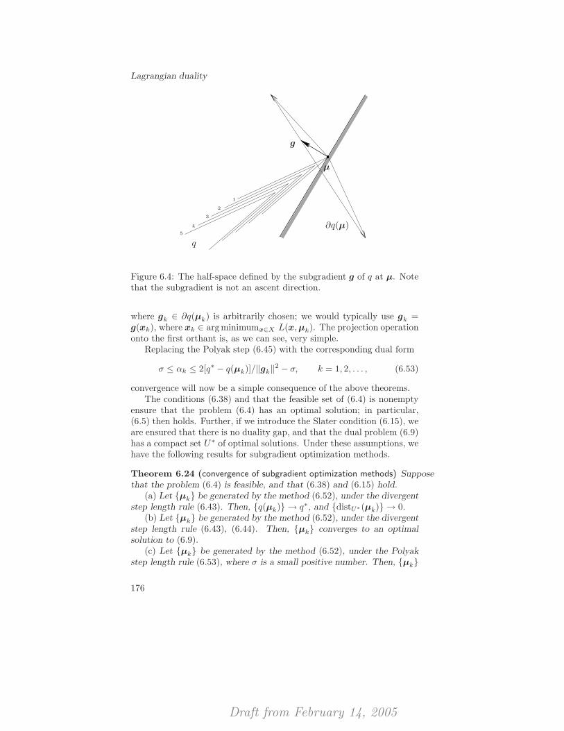
Draft from February 14, 2005
Lagrangian duality
1
2
3
4
5
q
g
µ
∂q(µ)
Figure 6.4: The half-space defined by the subgradient g of q at µ. Notethat the subgradient is not an ascent direction.
where gk ∈ ∂q(µk) is arbitrarily chosen; we would typically use gk =g(xk), where xk ∈ argminimumx∈X L(x,µk). The projection operationonto the first orthant is, as we can see, very simple.
Replacing the Polyak step (6.45) with the corresponding dual form
σ ≤ αk ≤ 2[q∗ − q(µk)]/‖gk‖2 − σ, k = 1, 2, . . . , (6.53)
convergence will now be a simple consequence of the above theorems.The conditions (6.38) and that the feasible set of (6.4) is nonempty
ensure that the problem (6.4) has an optimal solution; in particular,(6.5) then holds. Further, if we introduce the Slater condition (6.15), weare ensured that there is no duality gap, and that the dual problem (6.9)has a compact set U∗ of optimal solutions. Under these assumptions, wehave the following results for subgradient optimization methods.
Theorem 6.24 (convergence of subgradient optimization methods) Supposethat the problem (6.4) is feasible, and that (6.38) and (6.15) hold.
(a) Let {µk} be generated by the method (6.52), under the divergentstep length rule (6.43). Then, {q(µk)} → q∗, and {distU∗(µk)} → 0.
(b) Let {µk} be generated by the method (6.52), under the divergentstep length rule (6.43), (6.44). Then, {µk} converges to an optimalsolution to (6.9).
(c) Let {µk} be generated by the method (6.52), under the Polyakstep length rule (6.53), where σ is a small positive number. Then, {µk}
176
Draft from February 14, 2005
∗Obtaining a primal solution
converges to an optimal solution to (6.9).
Proof. The results follow from Theorems 6.21, 6.22, and 6.23. Notethat in the first two cases, boundedness conditions were assumed for X∗
and the sequence of subgradients. The corresponding conditions for theLagrangian dual problem are fulfilled under the CQs imposed, since theyimply that the search for an optimal solution is done over a compact set;cf. Theorem 6.8(a) and its proof.
6.6 ∗Obtaining a primal solution
It remains for us to show how an optimal dual solution µ∗ can be trans-lated into an optimal primal solution x∗. Obviously, convexity andstrong duality will be needed in general, if we are to be able to utilizethe primal–dual optimality characterization in Theorem 6.6. It turnsout that the generation of a primal optimum is automatic if q is differen-tiable at µ∗, something which we can refer to as the Lagrange multipliermethod. Unfortunately, in many cases, such as for most non-strictlyconvex optimization problems (like linear programming), this will notbe the case, and then the translation work then becomes rather morecomplex.
We start with the ideal case.
6.6.1 Differentiability at the optimal solution
The following results summarize the optimality conditions for the La-grangian dual problem (6.9), and their consequences for the availabilityof a primal optimal solution in the absence of a duality gap.
Proposition 6.25 (optimality conditions for the dual problem) Suppose that,in the problem (6.4), the condition (6.38) holds. Suppose further thatthe Lagrangian dual problem has an optimal solution, µ∗.
(a) The dual optimal solution is characterized by the inclusion
0m ∈ −∂q(µ∗) +NRm+
(µ∗). (6.54)
In other words, there then exists γ∗ ∈ ∂q(µ∗)—an optimality-characterizingsubgradient of q at µ∗—such that
0m ≤ µ∗ ⊥ γ∗ ≤ 0m. (6.55)
177
Draft from February 14, 2005
Lagrangian duality
There exist a finite set of solutions xi ∈ X(µ∗) (i = 1, . . . , k) wherek ≤ m+ 1 such that
γ∗ =
k∑
i=1
αig(xi);
k∑
i=1
αi = 1; αi ≥ 0, i = 1, . . . , k. (6.56)
Hence, we have that
k∑
i=1
αiµ∗i gi(x
i) = 0, j = 1, . . . ,m. (6.57)
(b) If there is a duality gap, then q is non-differentiable at µ∗.(c) If q is differentiable at µ∗, then there is no duality gap. Further,
any vector in X(µ∗) then solves the primal problem (6.4).
Proof. (a) The first result is a direct statement of the optimality condi-tions of the convex and sub-differentiable program (6.9); the complemen-tarity conditions in (6.55) are an equivalent statement of the inclusionin (6.54).
The second result is an application of Caratheodory’s Theorem 3.8to the compact and convex set ∂q(µ∗).
(b) The result is immediately established, once (c) is, since they areequivalent.
(c) Let x be any vector in X(µ∗) for which ∇q(µ∗) = g(x) holds, cf.Proposition 6.18(a). We obtain from (6.55) that
0m ≤ µ∗ ⊥ g(x) ≤ 0m.
Hence, the pair (µ, x) fulfills all the conditions stated in (6.11), so that,by Theorem 6.6, x is an optimal solution to (6.4).
Many interesting problems do not comply with the conditions in(c); for example, linear programming is one where the Lagrangian dualproblem often is non-differentiable at every dual optimal solution.11
This is sometimes called the non-coordinability phenomenon (cf. [Las70,DiJ79]). It was in order to cope with this phenomenon that Dantzig–Wolfe decomposition ([DaW60, Las70]) and other column generation al-gorithms, Benders decomposition ([Ben62, Las70]) and generalized linearprogramming were developed; noticing that the convex combination ofa finite number of candidate primal solutions are sufficient to verify anoptimal primal–dual solution [cf. (6.57)], methodologies were developed
11In other words, even if a Lagrange multiplier vector is known, the Lagrangiansubproblem may not identify a primal optimal solution.
178
Draft from February 14, 2005
∗Obtaining a primal solution
to generate those vectors algorithmically. See also [LPS99] for overviewson the subject of generating primal optimal solutions from dual optimalones, and [BSS93, Theorem 6.5.2] for an LP procedure that providesprimal feasible solutions for convex programs.
Note that the equation (6.57) in (a) reduces to the complementar-ity condition that µ∗
i gi(x) = 0 holds, for the averaged solution, x :=∑ki=1 αix
i, whenever all the functions gi are affine.
6.6.2 Everett’s Theorem
The next result shows that the solution to the Lagrangian subproblemsolves a perturbed version of the original problem. We state the resultfor the general problem to find
f∗ := infimumx
f(x), (6.58a)
subject to x ∈ X, (6.58b)
gi(x) ≤ 0, i = 1, . . . ,m, (6.58c)
hj(x) = 0, j = 1, . . . , ℓ, (6.58d)
where f : Rn → R, gi : Rn → R (i = 1, 2, . . . ,m), and hj : Rn → R(j = 1, 2, . . . , ℓ) are given functions, and X ⊆ Rn.
Theorem 6.26 (Everett’s Theorem) Let (µ,λ) ∈ Rm+ × Rℓ. Consider
the Lagrangian subproblem to
minimizex∈X
{f(x) + µTg(x) + λTh(x)
}. (6.59)
Suppose that x is an optimal solution to this problem, and let I(µ) ⊆{1, . . . ,m} denote the set of indices i for which µi > 0.
(a) x is an optimal solution to the perturbed primal problem to
minimizex
f(x), (6.60a)
subject to x ∈ X, (6.60b)
gi(x) ≤ gi(x), i ∈ I(x), (6.60c)
hj(x) = hj(x), j = 1, . . . , ℓ. (6.60d)
(b) If x is feasible in (6.58) and µTg(x) = 0 holds, then x solves(6.58). Moreover, the pair (µ,λ) then solves the Lagrangian dual prob-lem.
Proof. (a) The proof proceeds by showing that the triple (x,µ,λ) isa saddle point of the function (x,µ,λ) 7→ f(x) + µT[g(x) − g(x)] +λT[h(x) − h(x)] over X × Rm
+ × Rℓ.
179
Draft from February 14, 2005
Lagrangian duality
Let x satisfy the constraints (6.60b)–(6.60d). Since we have thath(x) = h(x) and µTg(x) ≤ µTg(x), the optimality of x in (6.59) yieldsthat
f(x) + µTg(x) + λTh(x) ≥ f(x) + µTg(x) + λTh(x)
≥ f(x) + µTg(x) + λTh(x),
which shows that f(x) ≥ f(x). We are done.(b) µTg(x) = 0 implies that gi(x) = 0 for i ∈ I(µ); from (a) x solves
the problem to
minimizex
f(x), (6.61a)
subject to x ∈ X, (6.61b)
gi(x) ≤ 0, i ∈ I(x), (6.61c)
hj(x) = 0, j = 1, . . . , ℓ. (6.61d)
In particular, then, since the feasible set of (6.58) is contained in that of(6.61) and x is feasible in the former, x must also solve (6.58). That thepair (µ,λ) solves the Lagrangian dual problem follows by the equalitybetween the primal and dual objective functions at (x,µ,λ) and weakduality.
The result is taken from Everett [Eve63]. One important consequenceof the result is that if the right-hand side perturbations gi(x) and hi(x)all are close to zero, the vector x being near-feasible might mean that itis in fact acceptable as an approximate solution to the original problem.(This interpretation hinges on the dualized constraints being soft con-straints, in the sense that a small violation is acceptable. See Section 1.7for an introduction to the topic of soft constraints.)
6.7 ∗Sensitivity analysis
6.7.1 Analysis for convex problems
Consider the inequality constrained convex program (6.4), where f :Rn → R and gi (i = 1, . . . ,m) are convex functions and X ⊆ Rn is aconvex set. Suppose that the problem (6.4) is feasible, that the com-pactness condition (6.38) and Slater condition (6.15) hold. This is theclassic case where there exist multipliers µ∗, according to Theorem 6.8,and strong duality holds.
For certain types of problems where there is no duality gap and wherethere exist primal–dual optimal solutions, we have access to a beautiful
180
Draft from February 14, 2005
∗Sensitivity analysis
theory of sensitivity analysis. The classic meaning of the term is theanswer to the following question: what is the rate of change in f∗ whena constraint right-hand side changes? This question answers importantpractical questions, like the following in manufacturing:� If we buy one unit of additional resource at a given price, or if the
demand of a product that we sell increases by a certain amount,then how much additional profit do we make?
We will here provide a basic result which states when this sensitivityanalysis of the optimal objective value can be performed for the problem(6.4), and establish that the answer is determined precisely by the valueof the Lagrange multiplier vector µ∗, provided that it is unique.
Definition 6.27 (perturbation function) Consider the function p : Rm →R ∪ {±∞} defined by
p(u) := infimumx
f(x), (6.62a)
subject to x ∈ X, (6.62b)
gi(x) ≤ ui, i = 1, . . . ,m, u ∈ Rm; (6.62c)
it is called the perturbation function, or primal function, associated withthe problem (6.4). Its effective domain is the set P := {u ∈ Rm | p(u) <+∞}.
Under the above convexity conditions, we can establish that p is aconvex function. Indeed, it holds that for any value of the Lagrangemultiplier vector µ∗ for the problem (6.4) that
q(µ∗) = infimumx∈X
{f(x) + (µ∗)Tg(x)}
= infimum{ (u,x)∈P×X|g(x)≤u }
{f(x) + (µ∗)Tg(x)}
= infimum{ (u,x)∈P×X|g(x)≤u }
{f(x) + (µ∗)Tu}
= infimumu∈P
infimum{x∈X|g(x)≤u }
{f(x) + (µ∗)Tu}.
Since µ∗ is assumed to be a Lagrange multiplier, we have that q(µ∗) =f∗ = p(0m). By the definition of infimum, then, we have that
p(0m) ≤ p(u) + (µ∗)Tu, u ∈ Rm,
that is, −µ∗ (notice the sign!) is a subgradient of p at u = 0m (seeDefinition 6.15). Moreover, by the result in Proposition 6.16(c), p is
181
Draft from February 14, 2005
Lagrangian duality
differentiable at 0m if and only if p is finite in a neighbourhood of 0m
and µ∗ is a unique Lagrange multiplier vector, that is, the Lagrangiandual problem (6.9) has a unique optimal solution. We have thereforeproved the following result:
Proposition 6.28 (a sensitivity analysis result) Suppose that in the in-equality constrained problem (6.4), f : Rn → R and gi : Rn → R(i = 1, . . . ,m) are convex functions and X ⊆ Rn is a convex set. Sup-pose further that the problem (6.4) is feasible, and that the compactnessassumption (6.38) and Slater condition (6.15) hold. Suppose, finally,that the perturbed problem defined in (6.62) has an optimal solution ina neighbourhood of u = 0m, and that on the set of primal–dual opti-mal solutions to (6.4)–(6.9), the Lagrangian dual optimal solution µ∗ isunique. Then, the perturbation function p is differentiable at u = 0m,and
∇p(0m) = −µ∗
holds.
It is intuitive that the sign of ∇p(0m) should be non-positive; if aright-hand side of the (less-than) inequality constraints in (6.4) increases,then the feasible set becomes larger. [This means that we might be ableto find feasible vectors x in the new problem with f(x) < f∗, where f∗
is the optimal value of the minimization problem (6.4).]
The result specializes immediately to linear programming problems,which is the problem type where this type of analysis is most oftenutilized. The proof of differentiability of the perturbation function atzero for that special case can however be done much more simply. (SeeSection 10.3.1.)
6.7.2 Analysis for differentiable problems
There exist local versions of the analysis valid also for non-convex prob-lems, where we are interested in the effect of a problem perturbationon a KKT point. A special such analysis was recently performed byBertsekas [Ber04], in which he shows that even when the problem isnon-convex and the set of Lagrange multipliers are not unique, a sensi-tivity analysis is available as long as data is differentiable. Suppose thenthat in the problem (6.4) the functions f and gi, i = 1, . . . ,m are inC1 and that X is nonempty. We generalize the concept of a Lagrangemultiplier to here mean that it is a vector µ∗ associated with a local
182
Draft from February 14, 2005
∗Sensitivity analysis
minimum x∗ such that
(∇f(x∗) +
m∑
i=1
µ∗i∇gi(x
∗)
)T
p ≥ 0, p ∈ TX(x∗), (6.63a)
µ∗i ≥ 0, i = 1, . . . ,m, (6.63b)
µ∗i = 0, i 6∈ I(x∗), (6.63c)
where we note that TX(x∗) is the tangent cone to X at x∗ (cf. Defini-tion 5.2). Notice that under an appropriate CQ this is equivalent to theKKT conditions, in which case we are simply requiring here that x∗ isa local minimum.
In the below result we utilize the notation
g+i (x) := maximum {0, gi(x)}, i = 1, . . . ,m,
and let g+(x) be the m-vector of elements g+i (x), i = 1, . . . ,m.
Theorem 6.29 (sensitivity from the minimum norm multiplier) Suppose thatx∗ is a local minimum in the problem (6.4), and that the set of Lagrangemultipliers is nonempty. Let µ∗ denote the Lagrange multiplier of mini-mum Euclidean norm. Then, for every sequence {xk} ⊂ X of infeasiblevectors such that {xk} → x∗ we have that
f(x∗) − f(xk) ≤ ‖µ∗‖ · ‖g+(xk)‖ + o(‖xk − x∗‖). (6.64)
Furthermore, if µ∗ 6= 0m and TX(x∗) is convex, the above inequalityis sharp in the sense that there exists a sequence of infeasible vectors{xk} ⊂ X such that
limk→∞
f(x∗) − f(xk)
‖g+(xk)‖ = ‖µ∗‖,
and for this sequence
limk→∞
g+i (xk)
‖g+(xk)‖ =µ∗
i
‖µ∗‖ , i = 1, . . . ,m,
holds.
Theorem 6.29 establishes the optimal rate of cost improvement withrespect to infeasible constraint perturbations (in effect, those that implyan increase in the feasible set).
We finally remark that under stronger conditions still, even the op-timal solution x∗ is differentiable. Such a result is reminiscent to the
183
Draft from February 14, 2005
Lagrangian duality
Implicit Function Theorem, which however only covers equality systems.If we are to study the sensitivity of x∗ to changes in the right-hand sidesof inequality constraints as well, then the analysis becomes complicateddue to the fact that we must be able to predict if some active constraintsmay become inactive in the process. In some circumstances, different di-rections of change in the right-hand sides may cause different subsets ofthe active constraints I(x∗) at x∗ to become inactive, and this wouldmost probably then be a non-differentiable point. A sufficient (but notnecessary at least in the case of linear constraints) condition when thiscannot happen is when x∗ is strictly complementary, that is, when thereexists a multiplier vector µ∗ where µ∗
i > 0 for every i ∈ I(x∗).
6.8 Notes and further reading
Lagrangian duality has been developed in many sources, including earlydevelopments by Arrow, Hurwicz, and Uzawa [AHU58], Everett [Eve63],and Falk [Fal67], and later on by Rockafellar [Roc70]. Our developmentfollows to a large extent that of portions of the text books by Bert-sekas [Ber99], Bazaraa et al. [BSS93], and Rockafellar [Roc70].
The Relaxation Theorem 6.1 can almost be considered to be folklore,and can be found in a slightly different form in [Wol98, Proposition 2.3].
The traveling salesman problem is an essential model problem incombinatorial optimization. Excellent introductions to the field can befound in [Law76, PaS82, NeW88, Wol98, Sch03]. It was the work in[HWC74, Geo74, Fis81, Fis85], among others, in the 1970s and 1980s onthe traveling salesman problem and its relatives that made Lagrangianrelaxation and subgradient optimization popular, and it remains mostpopular within the combinatorial optimization field.
The differentiability properties of convex functions were developedlargely by Rockafellar [Roc70], whose text we mostly follow.
Subgradient methods were developed in the Soviet Union in the1960s, predominantly by Ermol’ev, Polyak, and Shor. Text book treat-ments of subgradient methods are found, for example, in [Sho85, HiL93,Ber99]. Theorem 6.21 is essentially due to Ermol’ev [Erm66]; the proofstems from [LPS96]. Theorem 6.22 is due to Shepilov [She76]; finally,Theorem 6.23 is due to Polyak [Pol69].
Everett’s Theorem is due to Everett [Eve63].
Theorem 6.29 stems from [Ber04, Proposition 1.1].
184
Draft from February 14, 2005
Exercises
6.9 Exercises
Exercise 6.1 (numerical example of Lagrangian relaxation) Consider theconvex problem to
minimize1
x1+
4
x2,
subject to x1 + x2 ≤ 4,x1, x2 ≥ 0.
(a) Lagrangian relax the first constraint, and write down the resultingimplicit dual objective function and the dual problem. Motivate why therelaxed problem always has a unique optimum, whence the dual objectivefunction is everywhere differentiable.
(b) Solve the implicit Lagrangian dual problem by utilizing that thegradient to a differentiable dual objective function can be expressed byusing the functions that are involved in the relaxed constraints and theunique solution to the relaxed problem.
(c) Write down an explicit Lagrangian dual problem, that is, a dualproblem only in terms of the Lagrange multipliers. Solve it, and confirmthe results in (b).
(d) Find the original problem’s optimal solution.(e) Show that strong duality holds. Why does it?
Exercise 6.2 (global optimality conditions) Consider the problem to
minimize f(x) := x1 + 2x22 + 3x3
3,
subject to x1 + 2x2 + x3 ≤ 3,
2x21 + x2 ≥ 2,
2x1 + x3 = 2,
xj ≥ 0, j = 1, 2, 3.
(a) Formulate the Lagrangian dual problem that results from La-grangian relaxing all but the sign constraints.
(b) State the global primal–dual optimality conditions.
Exercise 6.3 (Lagrangian relaxation) Consider the problem to
minimize f(x) := x21 + 2x2
2,
subject to x1 + x2 ≥ 2,
x21 + x2
2 ≤ 5.
Find an optimal solution through Lagrangian duality.
185
Draft from February 14, 2005
Lagrangian duality
Exercise 6.4 (Lagrangian relaxation) In many circumstances it is of in-terest to calculate the Euclidean projection of a vector onto a subspace.Especially, consider the problem to find the Euclidean projection of thevector y ∈ Rn onto the null space of the matrix A ∈ Rm×n, that is, tofind an x ∈ Rn that solves the problem to
minimize f(x) :=1
2‖y − x‖2,
subject to Ax = 0m,
where A is such that rankA = m.
The solution to this problem is classic: the projection is given explic-itly by
x∗ = y − AT(AAT)−1Ay.
If we let P := In−AT(AAT)−1A, where In ∈ Rn×n is the unit matrix,be the projection matrix, the formula is simply x∗ = Py.
Your task is to derive this formula by utilizing Lagrangian duality.Motivate every step made by showing that the necessary properties arefulfilled.
[Note: This exercise is similar to that in Example 5.50, but utilizesLagrangian duality rather than the KKT conditions to derive the pro-jection formula.]
Exercise 6.5 (Lagrangian relaxation, exam 040823) Consider the follow-ing optimization (linear) problem:
minimize f(x, y) = x− 0.5y,
subject to −x+ y ≤ −1,
−2x+ y ≤ −2,
(x, y) ∈ R2+.
(6.65)
(a) Show that the problem satisfies Slater’s constraint qualification.Derive the Lagrangian dual problem corresponding to the Lagrangianrelaxation of the two linear inequality constraints, and show that its setof optimal solutions is convex and bounded.
(b) Calculate the set of subgradients of the Lagrangian dual functionat the dual points (1/4, 1/3)T and (1, 0)T.
Exercise 6.6 (Lagrangian relaxation) Provide an explicit form of the La-
186

Draft from February 14, 2005
Exercises
grangian dual problem for the problem to
minimizem∑
i=1
n∑
j=1
xij lnxij
subject to
m∑
i=1
xij = bj, j = 1, . . . , n,
n∑
j=1
xij = ai, i = 1, . . . ,m,
xij ≥ 0, i = 1, . . . ,m, j = 1, . . . , n,
where ai > 0, bj > 0 for all i, j, and where the linear equalities areLagrangian relaxed.
Exercise 6.7 (Lagrangian relaxation) Given is the problem to
minimizex
f(x) = 2x21 + x2
2 + x1 − 3x2, (6.66a)
subject to x21 + x2 ≥ 8, (6.66b)
x1 ∈ [1, 3], (6.66c)x2 ∈ [2, 5]. (6.66d)
Lagrangian relax the constraint (6.66b) with a multiplier µ. Formu-late the Lagrangian dual problem and calculate the dual function’s valueat µ = 1, µ = 2, and µ = 3. Within which interval lies the optimal valuef∗? Also, draw the dual function.
Exercise 6.8 (Lagrangian duality for integer problems) Consider the pri-mal problem to
minimize f(x),subject to g(x) ≤ 0m,
x ∈ X,
whereX ⊆ Rn, f : Rn → R, and g : Rn → Rm. If the restrictions g(x) ≤0m are complicating side constraints which are Lagrangian relaxed, weobtain the Lagrangian dual problem to
maximizeµ≥0m
q(µ),
whereq(µ) := minimum
x∈X{f(x) + µTg(x)}, µ ∈ Rm.
(a) Suppose that the set X is finite (for example, consisting of afinite number of integer vectors). Denote the elements of X by xp,p = 1, . . . , P . Show that the dual objective function is piece-wise linear.
187
Draft from February 14, 2005
Lagrangian duality
How many linear segments can it have, at most? Why is it not alwaysbuilt up by that many segments?
[Note: This property holds regardless of any properties of f and g.](b) Illustrate the result in (a) on the linear 0/1 problem to find
z∗ = maximum z = 5x1 + 8x2 + 7x3 + 9x4,subject to 3x1 + 2x2 + 2x3 + 4x4 ≤ 5,
2x1 + x2 + 2x3 + x4 = 3,x1 , x2 , x3 , x4 = 0/1,
where the first constraint is considered complicating.(c) Suppose that the function f and all components of g are linear,
and that the set X is a polytope (that is, a bounded polyhedron). Showthat the dual objective function is also in this case piece-wise linear.How many linear pieces can it be built from, at most?
Exercise 6.9 (Lagrangian relaxation) Consider the problem to
minimize z = 2x1 + x2,subject to x1 + x2 ≥ 5,
x1 ≤ 4,x2 ≤ 4,
x1 , x2 ≥ 0, integer.
Lagrangian relax the all-embracing constraint. Describe the Lagrangianfunction and the dual problem. Calculate the Lagrangian dual functionat these four points: µ = 0, 1, 2, 3. Give the best lower and upper boundson the optimal value of the original problem that you have found.
Exercise 6.10 (surrogate relaxation) Consider an optimization problemof the form
minimize f(x),
subjectto gi(x) ≤ 0, i = 1, . . . ,m, (P )
x ∈ X,
where the functions f, gi : Rn → R are continuous and the set X ⊂ Rn
is closed and bounded. The problem is assumed to have an optimalsolution, x∗. Introduce parameters µi ≥ 0, i = 1, . . . ,m, and define
s(µ) := minimum f(x),
subject to
m∑
i=1
µigi(x) ≤ 0, (S)
x ∈ X.
188

Draft from February 14, 2005
Exercises
This problem therefore has exactly one explicit constraint.(a) [weak duality] Show that x∗ is a feasible solution to the problem
(S) and that s(µ) ≤ z∗ therefore always holds, that is, the problem (S) isa relaxation of the original one. Motivate also why maximumµ≥0m s(µ) ≤z∗ must hold. Explain the potential usefulness of this result!
(b) [example] Consider the linear 0/1 problem
z∗ = maximum z =5x1 + 8x2 +7x3 + 9x4,subject to 3x1 + 2x2 +3x3 + 3x4 ≤ 6, (1)
2x1 + 3x2 +3x3 + 4x4 ≤ 5, (2)2x1 + x2 +2x3 + x4 = 3,x1 , x2 , x3 , x4 =0/1.
Surrogate relax the constraints (1) and (2) with multipliers µ1, µ2 ≥ 0and formulate the problem (S). Let µ = (1, 2)T. Calculate s(µ).
Consider again the original problem and Lagrangian relax the con-straints (1) and (2) with multipliers µ1, µ2 ≥ 0. Calculate the Lagrangiandual objective value at µ = µ.
Compare the two results!(c) [comparison with Lagrangian duality] Let µ ≥ 0m and
q(µ) := minimumx∈X
f(x) +
m∑
i=1
µigi(x).
Show that q(µ) ≤ s(µ), and that
maximumu≥0m
q(µ) ≤ maximumu≥0m
s(µ) ≤ z∗
holds.
189

Draft from February 14, 2005
Lagrangian duality
190
Draft from February 14, 2005
Part IV
Linear Optimization

Draft from February 14, 2005
Draft from February 14, 2005
Linear programming:An introduction
VII
Linear programming (LP) models, that is, the collection of optimizationmodels with linear objective functions and polyhedral feasible regions,are very useful in practice. The reason for this is that many real worldproblems can be described by LP models (even if several approximationsmust be made first) and, perhaps more importantly, there exist efficientalgorithms for solving linear programs; the most famous of them is theSimplex method, which will be presented in Chapter 9. Often, LP modelsdeal with situations where a number of resources (materials, machines,people, land, etcetera) are available and are to be combined to yieldseveral products.
To introduce the concept of linear programming we use a (oversim-plified) manufacturing problem. In Section 7.1 we describe the problem.From the problem description we develop an LP model in Section 7.2.It turns out that the LP model only contains two variables. Hence it ispossible to solve the problem graphically, which is done in Section 7.3. InSection 7.4 we discuss what happens if the data of the problem is mod-ified, namely, we see how the optimal solution changes if the supply ofraw-material or the prices of the products are modified. Finally, in Sec-tion 7.5 we develop what we call the linear programming dual problemto the manufacturing problem.
7.1 The manufacturing problem
A manufacturer produces two pieces of furniture: tables and chairs. Theproduction of the furniture requires the use of two different pieces ofraw-material, large and small pieces. One table is assembled by puttingtogether two pieces of each, while one chair is assembled from one of thelarger pieces and two of the smaller pieces (see Figure 7.1).
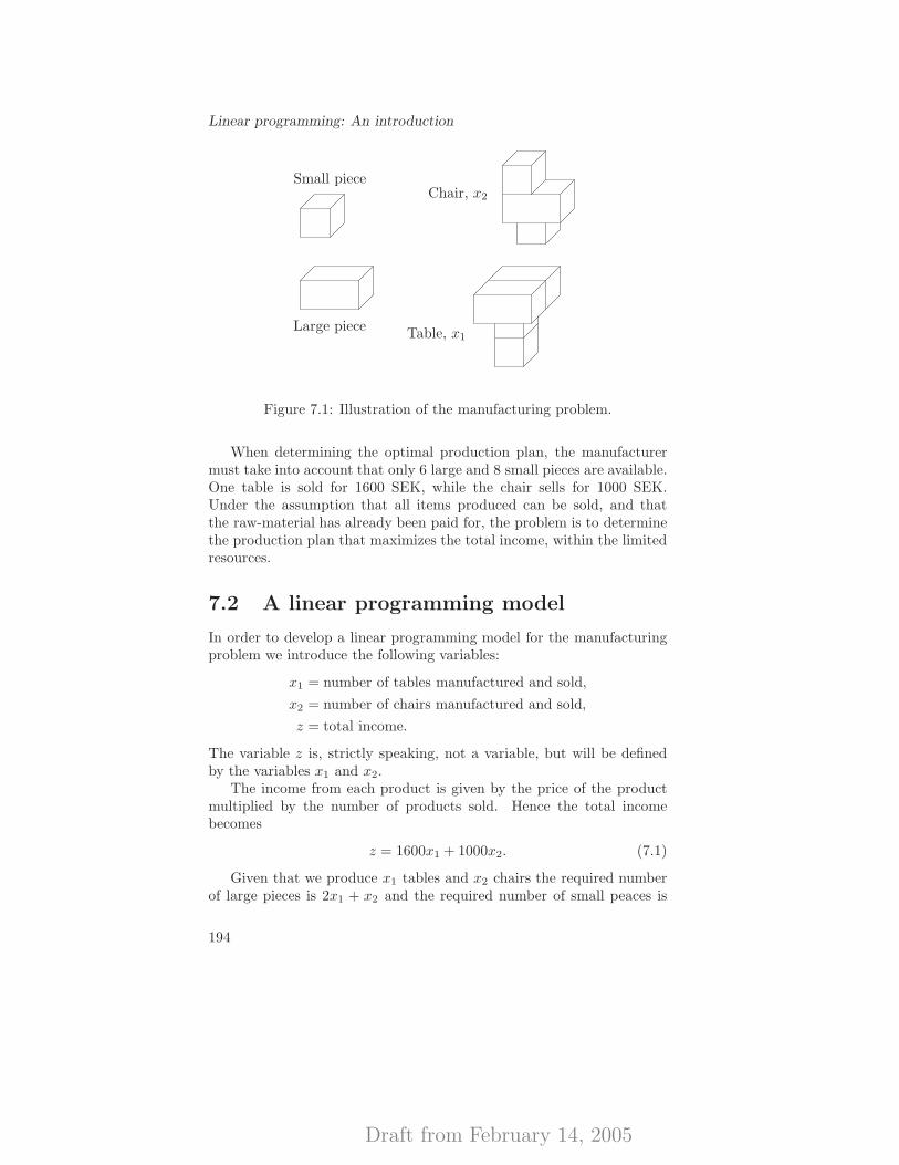
Draft from February 14, 2005
Linear programming: An introduction
Table, x1
Chair, x2
Small piece
Large piece
Figure 7.1: Illustration of the manufacturing problem.
When determining the optimal production plan, the manufacturermust take into account that only 6 large and 8 small pieces are available.One table is sold for 1600 SEK, while the chair sells for 1000 SEK.Under the assumption that all items produced can be sold, and thatthe raw-material has already been paid for, the problem is to determinethe production plan that maximizes the total income, within the limitedresources.
7.2 A linear programming model
In order to develop a linear programming model for the manufacturingproblem we introduce the following variables:
x1 = number of tables manufactured and sold,
x2 = number of chairs manufactured and sold,
z = total income.
The variable z is, strictly speaking, not a variable, but will be definedby the variables x1 and x2.
The income from each product is given by the price of the productmultiplied by the number of products sold. Hence the total incomebecomes
z = 1600x1 + 1000x2. (7.1)
Given that we produce x1 tables and x2 chairs the required numberof large pieces is 2x1 + x2 and the required number of small peaces is
194
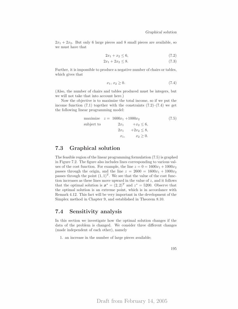
Draft from February 14, 2005
Graphical solution
2x1 + 2x2. But only 6 large pieces and 8 small pieces are available, sowe must have that
2x1 + x2 ≤ 6, (7.2)
2x1 + 2x2 ≤ 8. (7.3)
Further, it is impossible to produce a negative number of chairs or tables,which gives that
x1, x2 ≥ 0. (7.4)
(Also, the number of chairs and tables produced must be integers, butwe will not take that into account here.)
Now the objective is to maximize the total income, so if we put theincome function (7.1) together with the constraints (7.2)–(7.4) we getthe following linear programming model:
maximize z = 1600x1 +1000x2 (7.5)
subject to 2x1 +x2 ≤ 6,
2x1 +2x2 ≤ 8,
x1, x2 ≥ 0.
7.3 Graphical solution
The feasible region of the linear programming formulation (7.5) is graphedin Figure 7.2. The figure also includes lines corresponding to various val-ues of the cost function. For example, the line z = 0 = 1600x1 + 1000x2
passes through the origin, and the line z = 2600 = 1600x1 + 1000x2
passes through the point (1, 1)T. We see that the value of the cost func-tion increases as these lines move upward in the value of z, and it followsthat the optimal solution is x∗ = (2, 2)T and z∗ = 5200. Observe thatthe optimal solution is an extreme point, which is in accordance withRemark 4.12. This fact will be very important in the development of theSimplex method in Chapter 9, and established in Theorem 8.10.
7.4 Sensitivity analysis
In this section we investigate how the optimal solution changes if thedata of the problem is changed. We consider three different changes(made independent of each other), namely
1. an increase in the number of large pieces available;
195
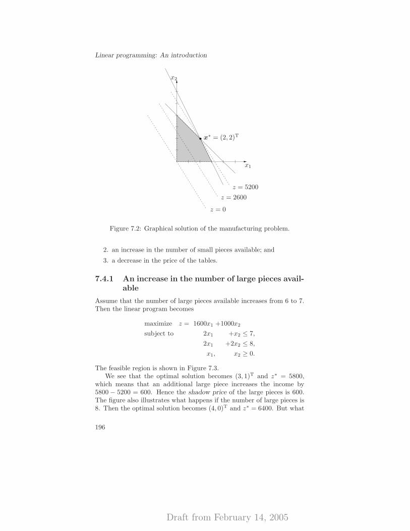
Draft from February 14, 2005
Linear programming: An introduction
x1
x2
z = 0
z = 2600
z = 5200
x∗ = (2, 2)T
Figure 7.2: Graphical solution of the manufacturing problem.
2. an increase in the number of small pieces available; and
3. a decrease in the price of the tables.
7.4.1 An increase in the number of large pieces avail-able
Assume that the number of large pieces available increases from 6 to 7.Then the linear program becomes
maximize z = 1600x1 +1000x2
subject to 2x1 +x2 ≤ 7,
2x1 +2x2 ≤ 8,
x1, x2 ≥ 0.
The feasible region is shown in Figure 7.3.We see that the optimal solution becomes (3, 1)T and z∗ = 5800,
which means that an additional large piece increases the income by5800 − 5200 = 600. Hence the shadow price of the large pieces is 600.The figure also illustrates what happens if the number of large pieces is8. Then the optimal solution becomes (4, 0)T and z∗ = 6400. But what
196
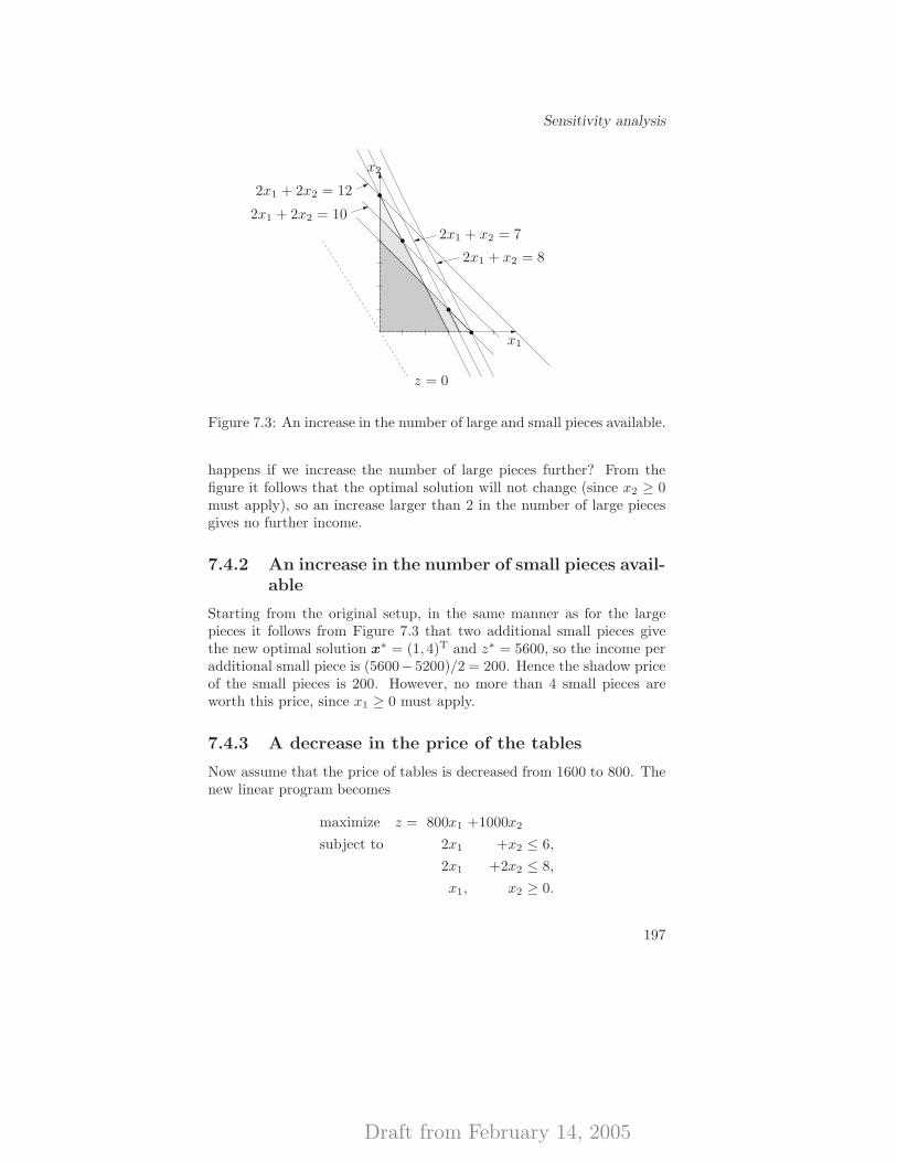
Draft from February 14, 2005
Sensitivity analysis
x1
x2
z = 0
2x1 + x2 = 7
2x1 + x2 = 8
2x1 + 2x2 = 10
2x1 + 2x2 = 12
Figure 7.3: An increase in the number of large and small pieces available.
happens if we increase the number of large pieces further? From thefigure it follows that the optimal solution will not change (since x2 ≥ 0must apply), so an increase larger than 2 in the number of large piecesgives no further income.
7.4.2 An increase in the number of small pieces avail-able
Starting from the original setup, in the same manner as for the largepieces it follows from Figure 7.3 that two additional small pieces givethe new optimal solution x∗ = (1, 4)T and z∗ = 5600, so the income peradditional small piece is (5600−5200)/2 = 200. Hence the shadow priceof the small pieces is 200. However, no more than 4 small pieces areworth this price, since x1 ≥ 0 must apply.
7.4.3 A decrease in the price of the tables
Now assume that the price of tables is decreased from 1600 to 800. Thenew linear program becomes
maximize z = 800x1 +1000x2
subject to 2x1 +x2 ≤ 6,
2x1 +2x2 ≤ 8,
x1, x2 ≥ 0.
197

Draft from February 14, 2005
Linear programming: An introduction
This new situation is illustrated in Figure 7.4, from which we see that
x1
x2
800x1 + 1000x2 = 01600x1 + 1000x2 = 0
Figure 7.4: A decrease in the price of the tables.
the optimal solution is (0, 4)T, that is, we will not produce any tables.This is natural, since it takes the same number of small pieces to producea table and a chair, but the table requires one more large piece, and inaddition the price of a table is lower than that of a chair.
7.5 The dual of the manufacturing problem
7.5.1 A competitor
Suppose that another manufacturer (let us call them Billy) produce bookshelves whose raw material is identical to those used for the table andchairs, that is, the small and large pieces. Billy wish to expand theirproduction, and are interested in acquiring the resources that “our” fac-tory sits on. Let us ask ourselves two questions, which (as we shall see)have identical answers: (1) what is the lowest bid (price) for the totalcapacity at which we are willing to sell?; (2) what is the highest bid(price) that Billy are prepared to offer for the resources? The answer tothose two questions is a measure of the wealth of the company in termsof their resources.
198
Draft from February 14, 2005
The dual of the manufacturing problem
7.5.2 A dual problem
To study the problem, we introduce the variables
y1 = the price which Billy offers for each large piece,
y2 = the price which Billy offers for each small piece,
w = the total bid which Billy offers.
In order to accept to sell our resources, it is reasonable to requirethat the price offered is at least as high as the value that the resourcerepresents in our optimal production plan, as otherwise we would earnmore by using the resource ourselves. Consider, for example, the netincome on a table sold. It is 1600 SEK, and for that we use two largeand two small pieces. The bid would therefore clearly be too low unless2y1 + 2y2 ≥ 1600. The corresponding requirement for the chairs is thaty1 + 2y2 ≥ 1000.
Billy is interested in minimizing the total bid, under the conditionthat the offer is accepted. Observing that y1 and y2 are prices andtherefore non-negative, we have the following mathematical model forBilly’s problem:
minimize w = 6y1 +8y2 (7.6)
subject to 2y1 +2y2 ≥ 1600,
y1 +2y2 ≥ 1000,
y1, y2 ≥ 0.
This is usually called the dual problem of our production planningproblem (which would then be the primal problem).
The optimal solution to this problem is y∗ = (600, 200)T. The totaloffer is w∗ = 5200.
Remark 7.1 (the linear programming dual) Observe that the dual prob-lem (7.6) is in accordance with the Lagrangian duality theory in Section6.2.4. The linear programming dual will be discussed further in Chapter10.
7.5.3 Interpretations of the dual optimal solution
From the above we see that the dual optimal solution is identical to theshadow prices for the resource (capacity) constraints. (This is indeeda general conclusion in linear programming.) To motivate that this isreasonable in our setting, we may consider Billy as a fictitious competitoronly, which we use together with the dual problem to measure the value
199
Draft from February 14, 2005
Linear programming: An introduction
of our resources. This (fictitious) measure can be used to create internalprices in a company in order to utilize limited resources as efficientlyas possible, especially if the resource is common to several independentsub-units. The price that the dual optimal solution provides will thenbe a price directive for the sub-units, that will make them utilize thescarce resource in a manner which is optimal for the overall goal.
We note that the optimal value of the production (z∗ = 5200) agreeswith the total value w∗ = 5200 of the resources in our company. (Thisis also a general result in linear programming; see the Strong DualityTheorem 10.6.) Billy will of course not pay more than what the resourceis worth, but can at the same time not offer less than the profit that ourcompany can make ourselves, since we would then not agree to sell. Itfollows immediately that for each feasible production plan x and pricey, it holds that z ≤ w, since
z = 1600x1 + 1000x2 ≤ (2y1 + 2y2)x1 + (y1 + 2y2)x2
= y1(2x1 + x2) + y2(2x1 + 2x2) ≤ 6y1 + 8y2 = w,
where in the inequalities we utilize all the constraints of the primal anddual problems. (Also this fact is general in linear programming; see theWeak Duality Theorem 10.4.) So, each offer accepted (from our pointof view) must necessarily be an upper bound on our own possible profit,and this upper bound is what Billy wish to minimize in the dual problem.
200

Draft from February 14, 2005
Linear programmingmodels
VIII
We begin this chapter with a presentation of the axioms underlying theuse of linear programming models and discuss the modelling process.Then, in Section 8.2, the geometry of linear programming is studied. Itis shown that every linear program can be transformed into the standardform which is the form that the Simplex method uses. Further, weintroduce the concept of basic feasible solution and discuss its connectionto extreme points. A version of the Representation Theorem adapted tothe standard form is presented, and we show that if there exists anoptimal solution to a linear program in standard form, then there existsan optimal solution among the basic feasible solutions. Finally, we defineadjacency between extreme points and give an algebraic characterizationof adjacency which actually proves that the Simplex method at eachiteration step moves from one extreme point to an adjacent one.
8.1 Linear programming modelling
Many real world situations can be modelled as linear programs. How-ever, the applicability of a linear program requires certain axioms to befulfilled. Hence, often approximations of the real world problem must bemade prior to the formulation of a linear program. The axioms under-lying the use of linear programming models are:� proportionality (linearity, e.g., no economies-of-scales, no fixed costs);� additivity (no substitute-time-effects);� divisibility (continuity); and� determinism (no randomness).
Draft from February 14, 2005
Linear programming models
George Dantzig presented the linear programming model and theSimplex method for solving it at an econometrics conference in Wisconsinin the late 40s. The economist Hotelling stood up, devastatingly smiling,and stated that “But we all know the world is nonlinear.” The younggraduate George Dantzig could not respond, but was defended by Johnvon Neumann, who stood up and concluded that “The speaker titled histalk ’linear programming’ and carefully stated his axioms. If you havean application that satisfies the axioms, well use it. If it does not, thendon’t”; he sat down, and Hotelling was silenced. (See Dantzig’s accountof the early history of linear programming in [LRS91, pp. 19–31].)
Now if the problem considered (perhaps after approximations) ful-fills the axioms above, then it can be formulated as a linear program.However, in practical modelling situations we usually do not talk aboutthe axioms; they naturally appear when a linear program is formulated.
To formulate a real world problem as a linear program is an art initself, and unfortunately there is little theory to help in formulating theproblem in this way. The general approach can however be described bytwo steps:
1. Prepare a list of all the decision variables in the problem. This listmust be complete in the sense that if an optimal solution providingthe values of each of the variables is obtained, then the decisionmaker should be able to translate it into an optimum policy thatcan be implemented.
2. Use the variables from step 1 to formulate all the constraints andthe objective function of the problem.
We illustrate the two-step modelling process by an example.
Example 8.1 (the transportation problem) In the transportation prob-lem we have a set of nodes or places called sources, which have a com-modity available for shipment, and another set of places called demandcenters, or sinks, which require this commodity. The amount of com-modity available at each source and the amount required at each de-mand center are specified, as well as the cost per unit of transportingthe commodity from each source to each demand center. The problemis to determine the quantity to be transported from each source to eachdemand center, so as to meet all the requirements at minimum totalshipping cost.
Consider the problem where the commodity is iron ore, the sourcesare found at mines 1 and 2, where the ore is produced, and the demandcenters are three steel plants. The unit costs of shipping ore from eachmine to each steel plant are given in Table 8.1.
202
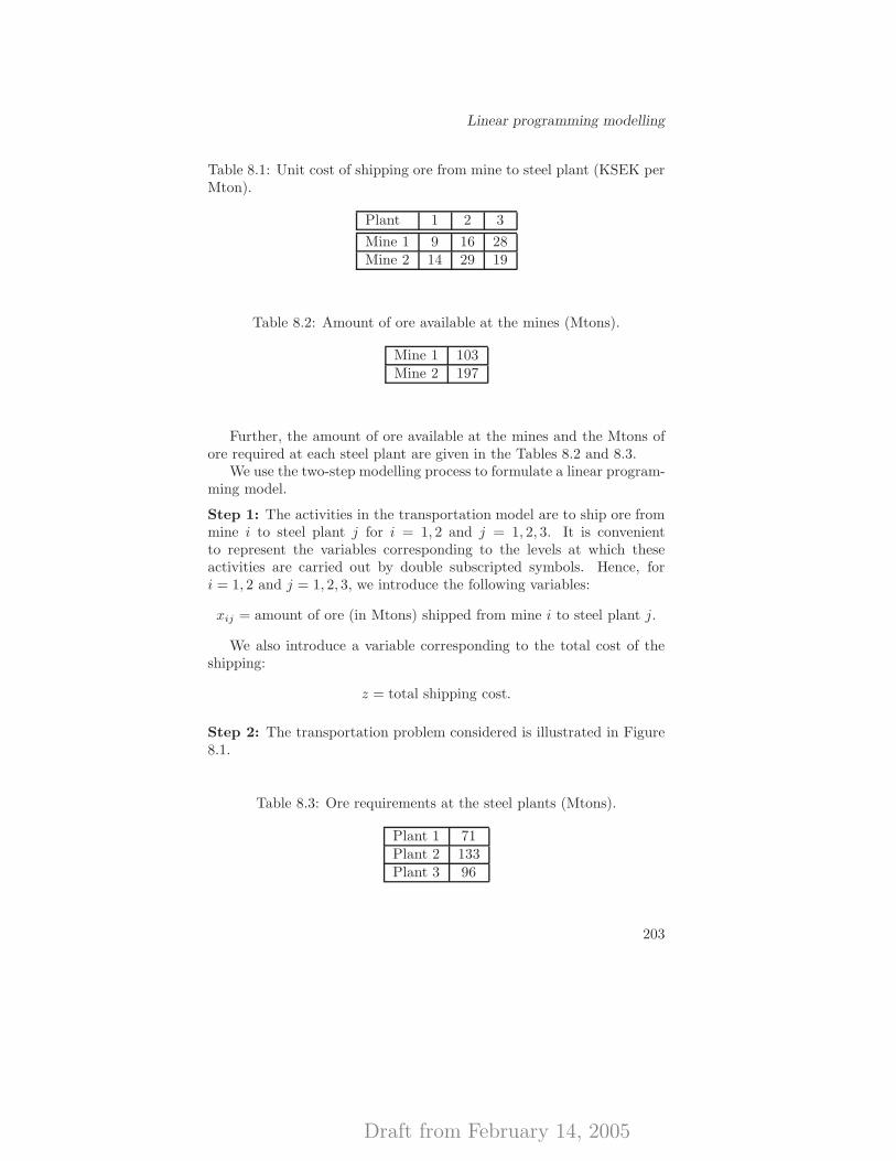
Draft from February 14, 2005
Linear programming modelling
Table 8.1: Unit cost of shipping ore from mine to steel plant (KSEK perMton).
Plant 1 2 3
Mine 1 9 16 28Mine 2 14 29 19
Table 8.2: Amount of ore available at the mines (Mtons).
Mine 1 103Mine 2 197
Further, the amount of ore available at the mines and the Mtons ofore required at each steel plant are given in the Tables 8.2 and 8.3.
We use the two-step modelling process to formulate a linear program-ming model.
Step 1: The activities in the transportation model are to ship ore frommine i to steel plant j for i = 1, 2 and j = 1, 2, 3. It is convenientto represent the variables corresponding to the levels at which theseactivities are carried out by double subscripted symbols. Hence, fori = 1, 2 and j = 1, 2, 3, we introduce the following variables:
xij = amount of ore (in Mtons) shipped from mine i to steel plant j.
We also introduce a variable corresponding to the total cost of theshipping:
z = total shipping cost.
Step 2: The transportation problem considered is illustrated in Figure8.1.
Table 8.3: Ore requirements at the steel plants (Mtons).
Plant 1 71Plant 2 133Plant 3 96
203
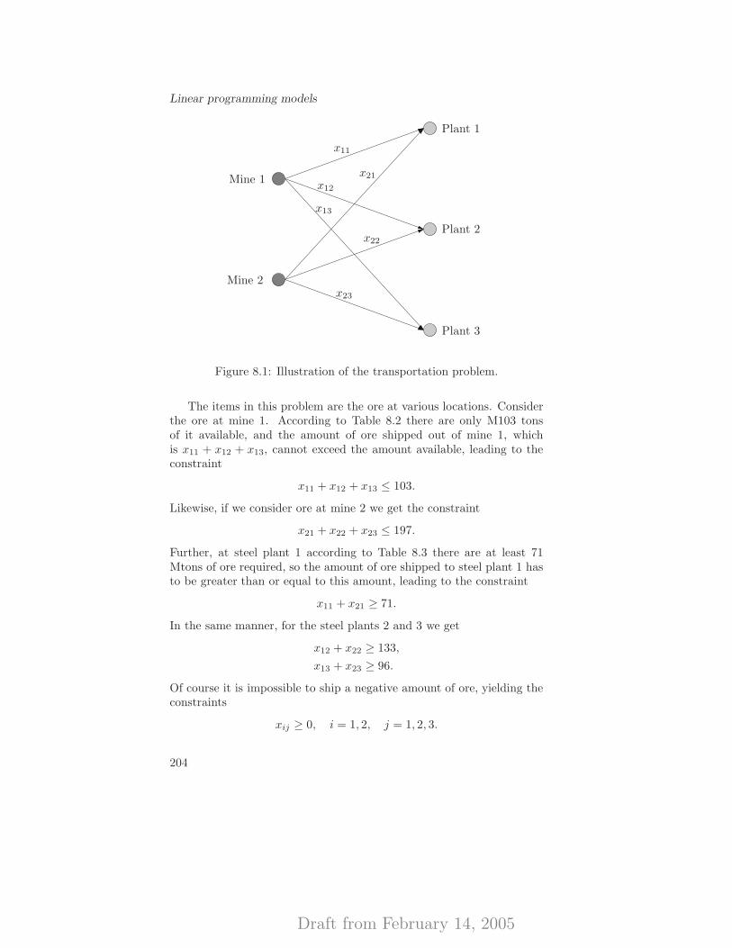
Draft from February 14, 2005
Linear programming models
x11
x12
x13
x21
x22
x23
Mine 1
Mine 2
Plant 1
Plant 2
Plant 3
Figure 8.1: Illustration of the transportation problem.
The items in this problem are the ore at various locations. Considerthe ore at mine 1. According to Table 8.2 there are only M103 tonsof it available, and the amount of ore shipped out of mine 1, whichis x11 + x12 + x13, cannot exceed the amount available, leading to theconstraint
x11 + x12 + x13 ≤ 103.
Likewise, if we consider ore at mine 2 we get the constraint
x21 + x22 + x23 ≤ 197.
Further, at steel plant 1 according to Table 8.3 there are at least 71Mtons of ore required, so the amount of ore shipped to steel plant 1 hasto be greater than or equal to this amount, leading to the constraint
x11 + x21 ≥ 71.
In the same manner, for the steel plants 2 and 3 we get
x12 + x22 ≥ 133,
x13 + x23 ≥ 96.
Of course it is impossible to ship a negative amount of ore, yielding theconstraints
xij ≥ 0, i = 1, 2, j = 1, 2, 3.
204
Draft from February 14, 2005
Linear programming modelling
From Table 8.1 it follows that the total cost of the shipping is (inKSEK)
z = 9x11 + 16x12 + 28x13 + 14x21 + 29x22 + 19x23.
Finally, since the objective is to minimize the total cost we get thefollowing linear programming model:
minimize z = 9x11 +16x12 +28x13 +14x21 +29x22 +19x23
subject to x11 +x12 +x13 ≤ 103,
x21 +x22 +x23 ≤ 197,
x11 +x21 ≥ 71,
x12 +x22 ≥ 133,
x13 +x23 ≥ 96,
x11, x12, x13, x21, x22, x23 ≥ 0.
Normally, transportation problems consider a large number of sourcesand demand centers and then it is convenient to use general notationleading to a compact formulation. Assume that we have N sources andM demand centers. For i = 1, . . . , N and j = 1, . . . ,M , introduce thevariables
xij = amount of commodity shipped from source i to demand center j,
and let
z = total shipping cost.
Further for i = 1, . . . , N and j = 1, . . . ,M introduce the shipping costs
cij = unit cost of shipping commodity from source i to demand center j.
Also, let
si = amount of commodity available at source i, i = 1, . . . , N,
dj = amount of commodity required at demand center j, j = 1, . . . ,M.
Now consider source i. The amount of commodity available is givenby si, which gives the constraint
M∑
j=1
xij ≤ si.
205
Draft from February 14, 2005
Linear programming models
Similarly, the amount of commodity required at demand center j is givenby dj , leading to the constraint
N∑
i=1
xij ≥ dj .
It is impossible to ship a negative amount of commodity, which gives
xij ≥ 0, i = 1, . . . , N, j = 1, . . . ,M.
Finally, the total cost for shipping is
z =N∑
i=1
M∑
j=1
cijxij ,
and we end up with the following linear program:
minimize z =N∑
i=1
M∑
j=1
cijxij
subject to
M∑
j=1
xij ≤ si, i = 1, . . . , N,
N∑
i=1
xij ≥ dj , j = 1, . . . ,M,
xij ≥ 0, i = 1, . . . , N, j = 1, . . . ,M.
If, for some reason, it is impossible to transport any commodities froma source i to a sink j, then we may either remove this variable altogetherfrom the model, or, more simply, give it the unit price cij = +∞.
Note, finally, that there exists a feasible solution to the transportationproblem if and only if
∑Ni=1 si ≥
∑Mj=1 dj .
8.2 The geometry of linear programming
In Section 3.2 we studied the class of feasible sets in linear programming,namely the sets of polyhedra; they are sets of the form
P = {x ∈ Rn | Ax ≤ b },
where A ∈ Rm×n and b ∈ Rm. In particular we proved the Repre-sentation Theorem 3.22 and promised that it would be important in
206
Draft from February 14, 2005
The geometry of linear programming
the development of the Simplex method. In this section we revisit thispolyhedron. Here, however, we will consider polyhedra of the form
P = {x ∈ Rn | Ax = b; x ≥ 0n }, (8.1)
where A ∈ Rm×n, and b ∈ Rm is such that b ≥ 0m. The advantageof this form is that the constraints (except for the non-negativity con-straints) are equalities, which admits pivot operations to to be carriedout. The Simplex method uses pivot operations at each iteration stepand hence it is necessary that the polyhedron (that is, the feasible region)is represented in the form (8.1). This is, however, not a restriction, aswe will see in Section 8.2.1, since every polyhedron can be transformedinto this form! We will use the term standard form when a polyhedronis represented in the form (8.1). In Section 8.2.2 we introduce the con-cept of basic feasible solution and show that each basic feasible solutioncorresponds to an extreme point. We also restate the RepresentationTheorem 3.22 and prove that if there exists an optimal solution to a lin-ear program, then there exists an optimal solution among the extremepoints. Finally, in Section 8.2.3, a strong connection between basic feasi-ble solutions and adjacent extreme points is discussed. This connectionshows that the Simplex method at each iteration step moves from anextreme point to an adjacent extreme point.
8.2.1 Standard form
A linear programming problem in standard form is a problem of the form
minimize z = cTx
subject to Ax = b,
x ≥ 0n,
where A ∈ Rm×n and b ≥ 0m. The purpose of this section is to showthat every linear program can be transformed into the standard form.In order to do that we must� express the objective function in minimization form;� transform all the constraints into equality constraints with non-
negative right-hand sides; and� transform any unrestricted and non-positive variables into non-negative ones.
207
Draft from February 14, 2005
Linear programming models
Objective function
Constant terms in the objective function will not change the set of opti-mal solutions and can therefore be eliminated. If the objective is to
maximize z = cTx,
then change the objective function so that the objective becomes
minimize z = −z = −cTx.
This change does not affect the set of feasible solutions to the problemand the equation
[maximum value of z] = −[minimum value of z]
can be used to get the maximum value of the original objective function.
Inequality constraints and negative right-hand sides
Consider the inequality constraint
aTx ≤ b,
where a ∈ Rn and b ∈ R. By introducing a non-negative slack variables this constraint can be written as
aTx + s = b, (8.2a)
s ≥ 0, (8.2b)
which has the desired form of an equation. Suppose that b < 0. Bymultiplying both sides of (8.2a) by −1 the negativity in the right-handside is eliminated and we are done. Similarly, a constraint of the form
aTx ≥ b,
can be written as
aTx − s = b,
s ≥ 0.
We call such variables s surplus variables.
Remark 8.2 (on the role of slack and surplus variables) Slack and surplusmay appear to be only help variables, but they often have a clear inter-pretation as decision variables. Consider, for example, the model (7.5)
208
Draft from February 14, 2005
The geometry of linear programming
of a furniture production problem. The two inequality constraints areassociated with the capacity of production stemming from the availabil-ity of raw material. Suppose then that we introduce slack variables inthese constraints, which leads to the equivalent problem to
maximize(x ,s)
z = 1600x1 +1000x2, (8.3a)
subject to 2x1 +x2 +s1 = 6, (8.3b)2x1 +2x2 +s2 = 8, (8.3c)x1, x2, s1, s2 ≥ 0. (8.3d)
The new variables s1 and s2 have the following interpretation: thevalue of si (i = 1, 2) is the level of inventory (or, remaining capacity ofraw material of type i) that will be left unused when the production plan(x1, x2) has been implemented. This interpretation makes it clear thatthe values of s1 and s2 are clear consequences of our decision-making.
Surplus variables have a corresponding interpretation. In the case ofthe transportation model of the previous section, a demand constraint(∑N
i=1 xij ≥ dj , j = 1, . . . ,M) may be fulfilled with equality (in whichcase the customer gets an amount exactly according to the demand) orit is fulfilled with strict inequality (in which case the customer gets asurplus of the product asked for).
Unrestricted and non-positive variables
Consider the linear program
minimize z = cTx (8.4)
subject to Ax = b,
x2 ≤ 0,
xj ≥ 0, j = 3, . . . , n,
which is assumed to be of standard form except for the unrestrictedvariable x1 and the non-positive variable x2. The x2-variable can bereplaced by the non-negative variable x2 = −x2. The x1-variable can betransformed into the difference of two non-negative variables. Namely,introduce the variables x+
1 ≥ 0 and x−1 ≥ 0 and let x1 = x+1 − x−1 . Then
by substituting x1 with x+1 −x−1 wherever it occurs we have transformed
the problem into standard form. The drawback of this method to handleunrestricted variables is that often the resulting problem is numericallyunstable. However, there are other techniques to handle unrestrictedvariables that overcome this problem; one of them is given in Exercise8.5.
209
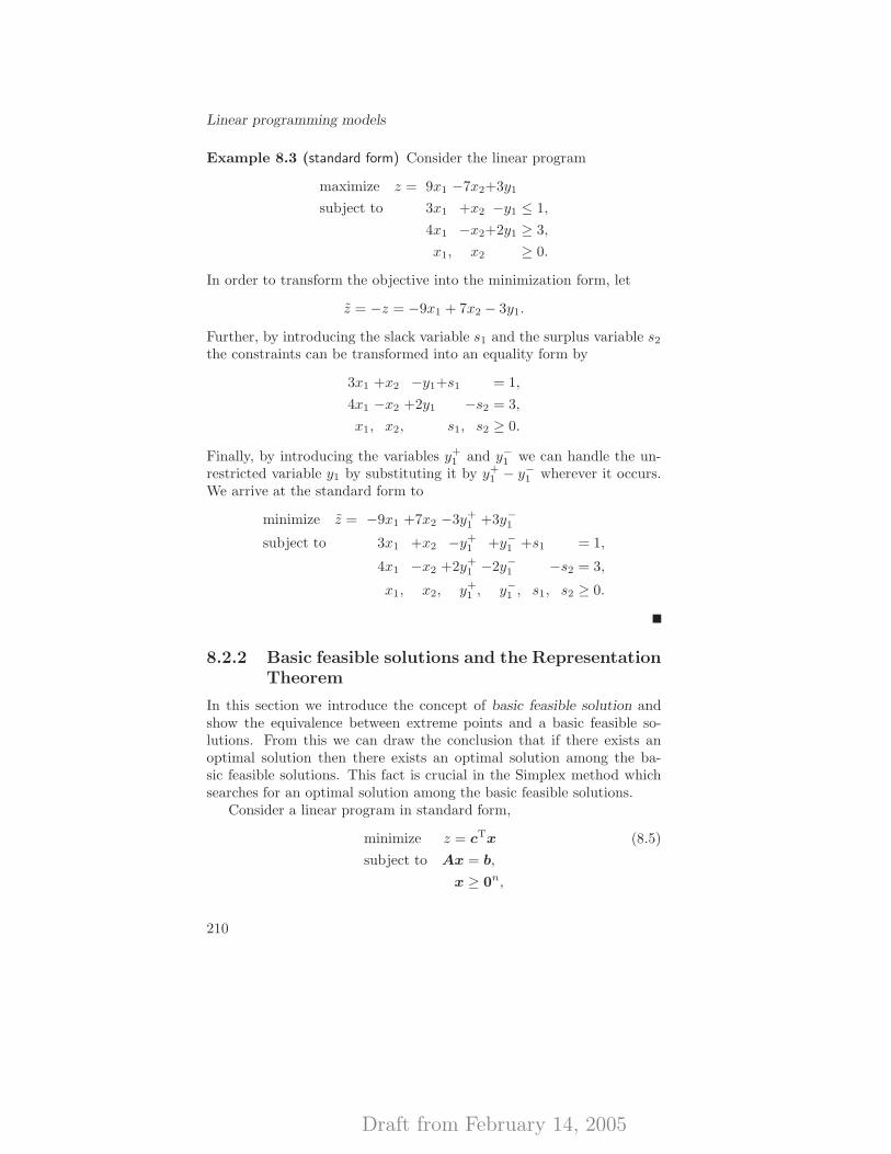
Draft from February 14, 2005
Linear programming models
Example 8.3 (standard form) Consider the linear program
maximize z = 9x1 −7x2+3y1
subject to 3x1 +x2 −y1 ≤ 1,
4x1 −x2+2y1 ≥ 3,
x1, x2 ≥ 0.
In order to transform the objective into the minimization form, let
z = −z = −9x1 + 7x2 − 3y1.
Further, by introducing the slack variable s1 and the surplus variable s2the constraints can be transformed into an equality form by
3x1 +x2 −y1+s1 = 1,
4x1 −x2 +2y1 −s2 = 3,
x1, x2, s1, s2 ≥ 0.
Finally, by introducing the variables y+1 and y−1 we can handle the un-
restricted variable y1 by substituting it by y+1 − y−1 wherever it occurs.
We arrive at the standard form to
minimize z = −9x1 +7x2 −3y+1 +3y−1
subject to 3x1 +x2 −y+1 +y−1 +s1 = 1,
4x1 −x2 +2y+1 −2y−1 −s2 = 3,
x1, x2, y+1 , y−1 , s1, s2 ≥ 0.
8.2.2 Basic feasible solutions and the RepresentationTheorem
In this section we introduce the concept of basic feasible solution andshow the equivalence between extreme points and a basic feasible so-lutions. From this we can draw the conclusion that if there exists anoptimal solution then there exists an optimal solution among the ba-sic feasible solutions. This fact is crucial in the Simplex method whichsearches for an optimal solution among the basic feasible solutions.
Consider a linear program in standard form,
minimize z = cTx (8.5)
subject to Ax = b,
x ≥ 0n,
210
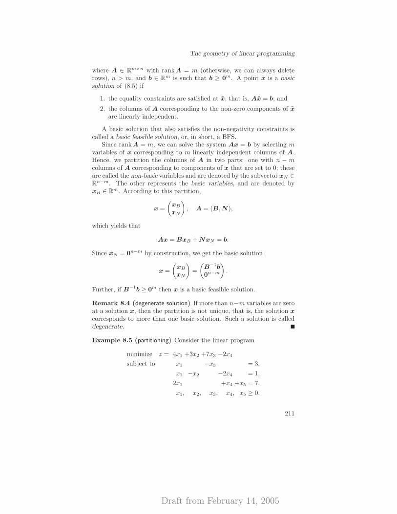
Draft from February 14, 2005
The geometry of linear programming
where A ∈ Rm×n with rankA = m (otherwise, we can always deleterows), n > m, and b ∈ Rm is such that b ≥ 0m. A point x is a basicsolution of (8.5) if
1. the equality constraints are satisfied at x, that is, Ax = b; and
2. the columns of A corresponding to the non-zero components of x
are linearly independent.
A basic solution that also satisfies the non-negativity constraints iscalled a basic feasible solution, or, in short, a BFS.
Since rankA = m, we can solve the system Ax = b by selecting mvariables of x corresponding to m linearly independent columns of A.Hence, we partition the columns of A in two parts: one with n − mcolumns of A corresponding to components of x that are set to 0; theseare called the non-basic variables and are denoted by the subvector xN ∈Rn−m. The other represents the basic variables, and are denoted byxB ∈ Rm. According to this partition,
x =
(xB
xN
), A = (B,N),
which yields that
Ax = BxB + NxN = b.
Since xN = 0n−m by construction, we get the basic solution
x =
(xB
xN
)=
(B−1b
0n−m
).
Further, if B−1b ≥ 0m then x is a basic feasible solution.
Remark 8.4 (degenerate solution) If more than n−m variables are zeroat a solution x, then the partition is not unique, that is, the solution x
corresponds to more than one basic solution. Such a solution is calleddegenerate.
Example 8.5 (partitioning) Consider the linear program
minimize z = 4x1 +3x2 +7x3 −2x4
subject to x1 −x3 = 3,
x1 −x2 −2x4 = 1,
2x1 +x4 +x5 = 7,
x1, x2, x3, x4, x5 ≥ 0.
211
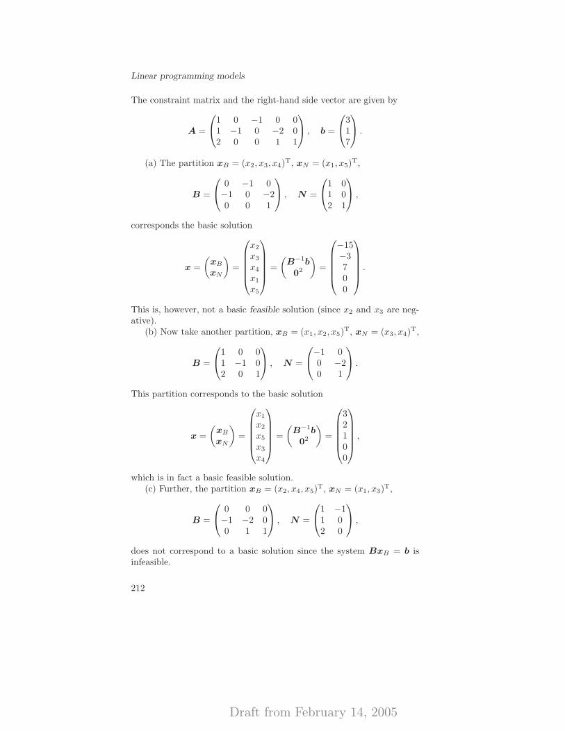
Draft from February 14, 2005
Linear programming models
The constraint matrix and the right-hand side vector are given by
A =
1 0 −1 0 01 −1 0 −2 02 0 0 1 1
, b =
317
.
(a) The partition xB = (x2, x3, x4)T, xN = (x1, x5)
T,
B =
0 −1 0−1 0 −20 0 1
, N =
1 01 02 1
,
corresponds the basic solution
x =
(xB
xN
)=
x2
x3
x4
x1
x5
=
(B−1b
02
)=
−15−3700
.
This is, however, not a basic feasible solution (since x2 and x3 are neg-ative).
(b) Now take another partition, xB = (x1, x2, x5)T, xN = (x3, x4)
T,
B =
1 0 01 −1 02 0 1
, N =
−1 00 −20 1
.
This partition corresponds to the basic solution
x =
(xB
xN
)=
x1
x2
x5
x3
x4
=
(B−1b
02
)=
32100
,
which is in fact a basic feasible solution.(c) Further, the partition xB = (x2, x4, x5)
T, xN = (x1, x3)T,
B =
0 0 0−1 −2 00 1 1
, N =
1 −11 02 0
,
does not correspond to a basic solution since the system BxB = b isinfeasible.
212
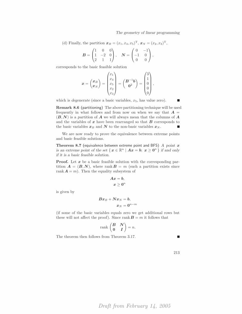
Draft from February 14, 2005
The geometry of linear programming
(d) Finally, the partition xB = (x1, x4, x5)T, xN = (x2, x3)
T,
B =
1 0 01 −2 02 1 1
, N =
0 −1−1 00 0
,
corresponds to the basic feasible solution
x =
(xB
xN
)=
x1
x4
x5
x2
x3
=
(B−1b
02
)=
31000
,
which is degenerate (since a basic variables, x5, has value zero).
Remark 8.6 (partitioning) The above partitioning technique will be usedfrequently in what follows and from now on when we say that A =(B,N ) is a partition of A we will always mean that the columns of A
and the variables of x have been rearranged so that B corresponds tothe basic variables xB and N to the non-basic variables xN .
We are now ready to prove the equivalence between extreme pointsand basic feasible solutions.
Theorem 8.7 (equivalence between extreme point and BFS) A point x
is an extreme point of the set {x ∈ Rn | Ax = b; x ≥ 0n } if and onlyif it is a basic feasible solution.
Proof. Let x be a basic feasible solution with the corresponding par-tition A = (B,N ), where rankB = m (such a partition exists sincerankA = m). Then the equality subsystem of
Ax = b,
x ≥ 0n
is given by
BxB + NxN = b,
xN = 0n−m
(if some of the basic variables equals zero we get additional rows butthese will not affect the proof). Since rankB = m it follows that
rank
(B N
0 I
)= n.
The theorem then follows from Theorem 3.17.
213

Draft from February 14, 2005
Linear programming models
Remark 8.8 (degenerate extreme point) An extreme point that corre-sponds to more than one BFS is degenerate. This typically occurs whenwe have redundant constraints.
We present a reformulation of the Representation Theorem 3.22 thatis adapted to the standard form. Consider the polyhedral cone C ={x ∈ Rn | Ax = 0m; x ≥ 0n }. From Theorem 3.28 it follows that C isfinitely generated, that is, there exist vectors d1, . . . ,dr ∈ Rn such that
C = cone {d1, . . . ,dr} =
{x ∈ Rn
∣∣∣∣∣ x =
r∑
i=1
αidi; α1, . . . , αr ≥ 0
}.
There are, of course, infinitely many ways to generate a certain poly-hedral cone C. Assume that C = cone {d1, . . . ,dr}. If there exists avector di ∈ {d1, . . . ,dr} such that
di ∈ cone{{d1, . . . ,dr} \ {di}
},
then di is not necessarily in the description of C. If we similarly continueto remove vectors from {d1, . . . ,dr} one at a time, we end up with a setgenerating C such that none of the vectors of the set can be written asa non-negative linear combination of the others. Such a set is naturallycalled the set of extreme directions of C (cf. Definition 3.11 of extremepoint).
Theorem 8.9 (Representation Theorem) Let P = {x ∈ Rn | Ax =b; x ≥ 0n} and V = {v1, . . . ,vk} be the set of extreme points of P .If and only if P is nonempty, V is nonempty (and finite). Further, letC = {x ∈ Rn | Ax = 0m; x ≥ 0n } and D = {d1, . . . ,dr} be the set ofextreme directions of C. If and only if P is unbounded D is nonempty(and finite). Every x ∈ P can be represented as the sum of a convexcombination of the points in V and a non-negative linear combinationof the points in D, that is,
x =
k∑
i=1
αivi +
r∑
j=1
βjdj ,
for some α1, . . . , αk ≥ 0 such that∑k
i=1 αi = 1, and β1, . . . , βr ≥ 0.
We have arrived at the important result that if there exists an optimalsolution to a linear program in the standard form then there exists anoptimal solution among the basic feasible solutions.
214
Draft from February 14, 2005
The geometry of linear programming
Theorem 8.10 (existence and properties of optimal solutions) Let the setsP , V and D be defined as in Theorem 8.9 and consider the linear pro-gram
minimize z = cTx
subject to x ∈ P.
This problem has a finite optimal solution if and only if P is nonemptyand z is lower bounded on P , that is, if P is nonempty and cTdj ≥ 0for all dj ∈ D.
If the problem has a finite optimal solution, then there exists anoptimal solution among the extreme points.
Proof. Let x ∈ P . Then it follows from Theorem 8.9 that
x =
k∑
i=1
αivi +
r∑
j=1
βjdj , (8.6)
for some α1, . . . , αk ≥ 0 such that∑k
i=1 αi = 1, and β1, . . . , βr ≥ 0.Hence
cTx =
k∑
i=1
αicTvi +
r∑
j=1
βjcTdj . (8.7)
Now, as x varies over P , the value of z clearly corresponds to variationsof the weights αi and βj . The first term in the right-hand side of (8.7) is
bounded as∑k
i=1 αi = 1. The second term is lower bounded as x varies
over P if and only if cTdj ≥ 0 holds for all dj ∈ D, since otherwise wecould let βj → +∞ for an index j with cTdj < 0, and get that z → −∞.If cTdj ≥ 0 for all dj ∈ D, then it is clearly optimal to choose βj = 0 forj = 1, . . . , r. It remains to search for the optimal solution in the convexhull of V .
Now assume that x ∈ P is an optimal solution and let x be rep-resented as in (8.6). From the above we have that we can chooseβ1 = · · · = βr = 0, so we can assume that
x =
k∑
i=1
αivi.
Further, let
a ∈ arg minimumi∈{1,...,k}
cTvi.
215
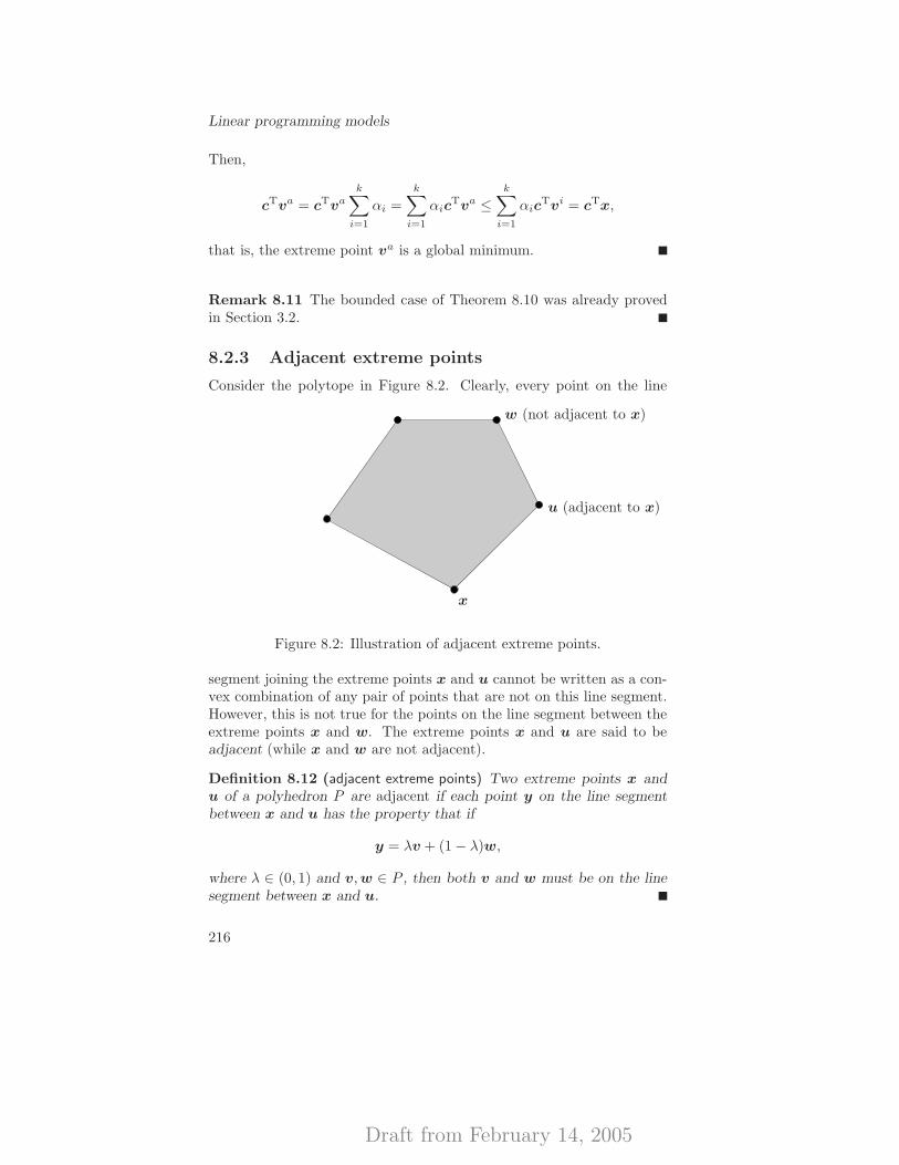
Draft from February 14, 2005
Linear programming models
Then,
cTva = cTvak∑
i=1
αi =
k∑
i=1
αicTva ≤
k∑
i=1
αicTvi = cTx,
that is, the extreme point va is a global minimum.
Remark 8.11 The bounded case of Theorem 8.10 was already provedin Section 3.2.
8.2.3 Adjacent extreme points
Consider the polytope in Figure 8.2. Clearly, every point on the line
x
u (adjacent to x)
w (not adjacent to x)
Figure 8.2: Illustration of adjacent extreme points.
segment joining the extreme points x and u cannot be written as a con-vex combination of any pair of points that are not on this line segment.However, this is not true for the points on the line segment between theextreme points x and w. The extreme points x and u are said to beadjacent (while x and w are not adjacent).
Definition 8.12 (adjacent extreme points) Two extreme points x andu of a polyhedron P are adjacent if each point y on the line segmentbetween x and u has the property that if
y = λv + (1 − λ)w,
where λ ∈ (0, 1) and v,w ∈ P , then both v and w must be on the linesegment between x and u.
216
Draft from February 14, 2005
The geometry of linear programming
Now, consider the polyhedron of standard form,
P = {x ∈ Rn | Ax = b; x ≥ 0n }.
Let u ∈ P be a basic feasible solution (and hence an extreme point ofP ) corresponding to the partition A = (B1,N1), where rankB1 = m,that is,
u =
(uB1
uN1
)=
((B1)−1b
0n−m
).
Further, let B1 = (b1, . . . , bm) and N 1 = (n1, . . . ,nn−m) (that is, bi ∈Rm, i = 1, . . . ,m, and nj ∈ Rn, j = 1, . . . , n −m, are columns of A).Now construct a new partition (B2,N2) by replacing one column of B1,say b1, with one column of N 1, say n1, that is,
B2 = (n1, b2, . . . , bm),
N2 = (b1,n2, . . . ,nn−m).
Assume that the partition (B2,N 2) corresponds to a basic feasible solu-tion v (i.e., v is an extreme point), and that the two extreme points u andv corresponding to (B1,N1) and (B2,N 2), respectively, are not equal.Then we have the following elegant result. (Since the Simplex methodat each iteration performs exactly the above replacement action the the-orem actually shows that the Simplex method at each non-degenerateiteration moves from one extreme point to an adjacent.)
Proposition 8.13 (algebraic characterization of adjacency) Let u and v
be the extreme points that correspond to the partitions (B1,N 1) and(B2,N2) described above. Then u and v are adjacent.
Proof. If the variables of v are ordered in the same way as the variablesof u, then the vectors must be of the form
u = (u1, . . . , um, 0, 0, . . . , 0)T,
v = (0, v2, . . . , vm+1, 0, . . . , 0)T.
Now take a point x on the line segment between u and v, that is,
x = λu + (1 − λ)v
for some λ ∈ (0, 1). In order to prove the theorem we must show thatif x can be written as a convex combination of two feasible points, then
217

Draft from February 14, 2005
Linear programming models
these points must be on the line segment between u and v. So assumethat
x = αy1 + (1 − α)y2
for some feasible points y1 and y2, and α ∈ (0, 1). Then it follows thaty1 and y2 must be solutions to the system
y1b1 + · · · + ymbm + ym+1n
1 = b,
ym+2 = . . . = yn = 0,
y ≥ 0n,
or equivalently [by multiplying both sides of the first row by (B1)−1],
y =
((B1)−1b
0n−m
)+
−ym+1(B
1)−1n1
ym+1
0n−m−1
,
y ≥ 0n.
But this is in fact the line segment between u and v (if ym+1 = 0 theny = u and if ym+1 = vm+1 then y = v). In other words, y1 and y2 areon the line segment between u and v, and we are done.
Remark 8.14 Actually the converse of Proposition 8.13 also holds.Namely, if two extreme points u and v are adjacent, then there ex-ists a partition (B1,N 1) corresponding to u and a partition (B2,N2)corresponding to v such that the columns of B1 and B2 are the sameexcept for one. The proof is similar to that of Proposition 8.13.
8.3 Notes and further reading
The material in this chapter can be found in most books on linear pro-gramming, such as [Dan63, Chv83, Mur83, Sch86, Pad99, Van01, DaT97,DaT03].
8.4 Exercises
Exercise 8.1 (LP modelling) Let A ∈ Rm×n and b ∈ Rm. Formulatethe following problems as linear programming problems.
(a) minimizex∈Rn
∑mi=1 |(Ax − b)i| subject to maxi=1,...,n |xi| ≤ 1.
(b) minimizex∈Rn
∑mi=1 |(Ax − b)i| + maxi=1,...,n |xi|.
218
Draft from February 14, 2005
Exercises
Exercise 8.2 (LP modelling) Consider the sets V = {v1, . . . ,vk} ⊂ Rn
and W = {w1, . . . ,wl} ⊂ Rn. Formulate the following problem as linearprogramming problems.
(a) Construct, if possible, a hyperplane that separates the sets V andW , that is, find a ∈ Rn, with a 6= 0n, and b ∈ R such that
aTv ≤ b, for all v ∈ V ,
aTw ≥ b, for all w ∈W.
(b) Construct, if possible, a sphere that separates the sets V and W ,that is, find a center xc ∈ Rn and a radius R ≥ 0 such that
‖v − xc‖2 ≤ R, for all v ∈ V ,
‖w − xc‖2 ≥ R, for all w ∈W.
Exercise 8.3 (linear-fractional programming) Consider the linear-fractionalprogram
minimize f(x) = (cTx + α)/(dTx + β) (8.8)
subject to Ax ≤ b,
where c,d ∈ Rn, A ∈ Rm×n, and b ∈ Rm. Further, assume that thepolyhedron P = {x ∈ Rn | Ax ≤ b} is bounded and that dTx+β > 0 forall x ∈ P . Show that (8.8) can be solved by solving the linear program
minimize g(y, z) = cTy + αz (8.9)
subject to Ay − zb ≤ 0m,
dTy + βz = 1,
z ≥ 0.
[Hint: Suppose that y∗ together with z∗ are a solution to (8.9), andshow that z∗ > 0 and that y∗/z∗ is a solution to (8.8).]
Exercise 8.4 (standard form) Transform the linear program
minimize z = x1−5x2−7x3
subject to 5x1−2x2+6x3 ≥ 5, (1)
3x1+4x2−9x3 = 3, (2)
7x1+3x2+5x3 ≤ 9, (3)
x1 ≥ −2,
into standard form.
219
Draft from February 14, 2005
Linear programming models
Exercise 8.5 (standard form) Consider the linear program
minimize z = 5x1 +3x2 −7x3
subject to 2x1 +4x2 +6x3 = 11,
3x1 −5x2 +3x3+x4 = 11,
x1, x2, x4 ≥ 0.
(a) Show how to transform this problem into standard form by elim-inating the unrestricted variable x3.
(b) Why cannot this technique be used to eliminate variables withnon-negativity restrictions?
Exercise 8.6 (basic feasible solutions) Suppose that a linear programincludes a free variable xj . When transforming this problem into stan-dard form, xj is replaced by
xj = x+j − x−j ,
x+j , x
−j ≥ 0.
Show that no basic feasible solution can include both x+j and x−j as
non-zero basic variables.
Exercise 8.7 (equivalent systems) Consider the system of equations
n∑
j=1
aijxj = bi, i = 1, . . . ,m. (8.10)
Show that this system is equivalent to the system
n∑
j=1
aijxj ≤ bi, i = 1, . . . ,m, (8.11a)
m∑
i=1
n∑
j=1
aijxj ≥m∑
i=1
bi. (8.11b)
220
Draft from February 14, 2005
The simplex method IX
This chapter presents the Simplex method for solving linear program-ming problems. In Section 9.1 the basic algorithm is presented. First weassume that a basic feasible solution is known at the start of the algo-rithm, and then we describe what to do when a BFS is not known fromthe beginning. In Section 9.2 we discuss termination characteristics ofthe algorithm. It turns out that if all the BFSs of the problem are non-degenerate, then the basic algorithm terminates. However, if there existdegenerate BFSs there is a possibility that the basic algorithm cycles be-tween degenerate BFSs and hence never terminates. Fortunately there isa simple rule, called Bland’s rule, that eliminates cycling. We close thechapter by discussing the computational complexity of the Simplex al-gorithm. In the worst case, the algorithm visits all the extreme points ofthe problem, and since the number of extreme points may be exponentialin the dimension of the problem, the Simplex algorithm does not belongto the desirable polynomial complexity class. The Simplex algorithm istherefore not theoretically satisfactory, but in practice it works very welland thus it frequently appears in commercial linear programming codes.
9.1 The algorithm
Assume that we have a linear program in standard form:
minimize z = cTx
subject to Ax = b,
x ≥ 0n,
where A ∈ Rm×n, n > m and the rank of A is full, and b ∈ Rm is suchthat b ≥ 0m, and c ∈ Rn. (This is not a restriction, as was shown in
Draft from February 14, 2005
The simplex method
Section 8.2.1.) At each iteration the Simplex algorithm starts at a basicfeasible solution (BFS) and moves to an adjacent BFS such that theobjective function value decreases. It terminates with an optimal BFS(if there exists a finite optimal solution), or a direction of unboundedness,that is, a point in C := {p ∈ Rn | Ap = 0m; p ≥ 0n } along which theobjective function diverges to −∞. Observe that if p ∈ C is a directionof unboundedness and x is a feasible solution, then every solution y(α)of the form
y(α) = x + αp, α ≥ 0,
is feasible. Hence if cTp < 0 then z = cTy(α) → −∞ as α→ ∞.
9.1.1 A BFS is known
Assume that a basic feasible solution xT = (xTB,x
TN ) corresponding to
the partition A = (B,N ) is known. Then we have that
Ax = (B,N)
(xB
xN
)= BxB + NxN = b,
or, equivalently,
xB = B−1b − B−1NxN . (9.1)
Further, rearrange the components of c such that cT = (cTB, c
TN ) has the
same ordering as xT = (xTB,x
TN ). Then from (9.1) follows that
cTx = cTBxB + cT
NxN
= cTB(B−1b − B−1NxN ) + cT
NxN
= cTBB−1b + (cT
N − cTBB−1N )xN . (9.2)
The principle of the Simplex algorithm is now easy to describe. Cur-rently we are located at the BFS given by
x =
(xB
xN
)=
(B−1b
0n−m
),
which is an extreme point according to Theorem 8.7. Proposition 8.13gives that if we construct a new partition by replacing one column of B
by one column of N such that the new partition corresponds to a basicfeasible solution, x, not equal to x, then x is adjacent to x. The principleof the Simplex algorithm is to move to an adjacent extreme point suchthat the objective function value decreases. From (9.2) follows that if
222
Draft from February 14, 2005
The algorithm
we increase the jth component of the non-basic vector xN from 0 to 1,then the change in the objective function value becomes
(cN )j := (cTN − cT
BB−1N)j ,
that is, the change in the objective value resulting from a unit increaseof the non-basic variable xj from zero is given by the jth component ofthe vector cT
N − cTBB−1N .
We call (cN )j the reduced cost of the non-basic variable (xN )j for j =1, . . . , n −m. Actually, we can define the reduced cost, cT = (cT
B, cTN ),
of all the variables at the given BFS by
cT := cT − cTBB−1A = (cT
B , cTN ) − cT
BB−1(B,N)
= ((0m)T, cTN − cT
BB−1N);
in particular, we see that the reduced costs of the basic variables arecB = 0m.
Now, if (cN )j ≥ 0 for all j = 1, . . . , n − m, then there exists noadjacent extreme point such that the objective function value decreasesand we stop; x is then an optimal solution.
Proposition 9.1 (optimality in the Simplex method) Let x∗ be the ba-sic feasible solution that corresponds to the partition A = (B,N). If(cN )j ≥ 0 for all j = 1, . . . , n−m, then x∗ is an optimal solution.
Proof. Since cTBB−1b is constant, it follows from (9.2) that the original
linear program is equivalent to
minimize z = cTNxN
subject to xB+B−1NxN = B−1b,
xB ≥ 0m,
xN ≥ 0n−m,
or equivalently [by reducing the xB variables through (9.1)],
minimize z = cTNxN (9.3)
subject to B−1NxN ≤ B−1b,
xN ≥ 0n−m.
Since x∗ is a basic feasible solution it follows that x∗N = 0n−m is a
feasible solution to (9.3). But cN ≥ 0n−m so x∗N = 0n−m is in fact an
optimal solution to (9.3). (Why?) Hence
x∗ =
(B−1b
0n−m
)
223
Draft from February 14, 2005
The simplex method
is an optimal solution to the original problem.
Remark 9.2 (optimality condition) Proposition 9.1 states that if (cN )j ≥0 for all j = 1, . . . , n − m, then x∗ is an optimal extreme point. Butis it true that if x∗ is an optimal extreme point, then (cN )j ≥ 0 for allj = 1, . . . , n−m? The answer to this question is no. Namely, if the op-timal basic feasible solution x∗ is degenerate, then there may exist basisrepresentations of x∗ such that (cN )j < 0 for some j. However, it holdsthat if x∗ is an optimal extreme point, then there exists at least one basisrepresentation of it such that (cN )j ≥ 0 for all j = 1, . . . , n−m. Thatis, Proposition 9.1 can be strengthened to state that x∗ is an optimalextreme point if and only if there exists a basis representation of it suchthat cN ≥ 0n−m.
If some of the reduced costs are strictly negative, we choose the non-basic variable with the least reduced cost to enter the basis. We mustalso choose one variable from xB to leave the basis. Suppose that thevariable (xN )j has been chosen to enter the basis. Then, according to(9.1), when the value of (xN )j is increased from zero we will move alongthe half-line
l(µ) :=
(B−1b
0n−m
)+ µ
(−B−1N j
ej
), µ ≥ 0,
where ej is the jth unit vector. In order to maintain feasibility we musthave that l(µ) ≥ 0n. If l(µ) ≥ 0n for all µ ≥ 0, then z → −∞ as µ→ ∞,that is,
p =
(−B−1N j
ej
)
is a direction of unboundedness and z → −∞ along the half-line l(µ),µ ≥ 0. Observe that this occurs if and only if
B−1N j ≤ 0m.
Otherwise, the maximal value of µ in order to maintain feasibility isgiven by
µ∗ = minimumi∈{ i | (B−1N j)i>0 }
(B−1b)i
(B−1N j)i
.
If µ∗ > 0 it follows that l(µ∗) is an extreme point adjacent to x. Actuallywe move to l(µ∗) by choosing (xB)i, where
i ∈ arg minimumi∈{ i | (B−1N j)i>0 }
(B−1b)i
(B−1N j)i
,
224
Draft from February 14, 2005
The algorithm
to leave the basis.We are now ready to state the Simplex algorithm.
The Simplex Algorithm:
Step 0 (initialization: BFS). Let xT = (xTB,x
TN ) be a BFS correspond-
ing to the partition A = (B,N).
Step 1 (descent direction generation or termination: entering variable, pricing).Calculate the reduced costs of the non-basic variables:
(cN )j = (cTN − cT
BB−1N)j , j = 1, . . . , n−m.
If (cN )j ≥ 0 for all j = 1, . . . , n−m then stop; x is then optimal.Otherwise choose (xN )j , where
j ∈ arg minimumj∈{1,...,n−m}
(cN )j ,
to enter the basis.
Step 2 (line search or termination: leaving variable). If
B−1N j ≤ 0m,
then the problem is unbounded, stop; p := ((−B−1N j)T, eT
j )T isthen a direction of unboundedness. Otherwise choose (xB)i, where
i ∈ arg minimumi∈{ i | (B−1N j)i>0 }
(B−1b)i
(B−1N j)i
,
to leave the basis.
Step 3 (update: change basis). Construct a new partition by swapping(xB)i with (xN)j . Go to Step 1.
Remark 9.3 (the Simplex algorithm as a feasible descent method) In theabove description, we have chosen to use terms similar to those that willbe used for several descent methods in nonlinear optimization that aredescribed in Parts V and VI; see, for example, the algorithm descrip-tion in Section 11.1 for unconstrained nonlinear optimization problems.The Simplex method is a very special type of descent algorithm: in or-der to remain feasible we generate feasible descent directions p (Step1) that follow the boundary of the polyhedron; because of the fact thatthe objective function is linear, a line search would yield an infinite stepunless a new boundary makes such a step infeasible; this is the role ofStep 2. Finally, termination at an optimal solution (Step 2) is basedon a special property of linear programming which allows us to decide
225
Draft from February 14, 2005
The simplex method
on global optimality based on only local information about the currentBFS:s reduced costs. (Of course, the convexity of LP is a crucial prop-erty for this principle to be valid.) More on the characterization of thisoptimality criterion, and its relationships to the optimality principles inthe Chapters 4 and 6 will be discussed in the next chapter.
Remark 9.4 (calculating the reduced costs) When calculating the reducedcosts of the non-basic variables at the pricing Step 1 of the Simplex al-gorithm, it is appropriate to first calculate
yT := cTBB−1,
through the systemBTy = cB,
and then calculate the reduced costs by
cTN = cT
N − yTN .
By this procedure we avoid the matrix–matrix multiplication B−1N .
Remark 9.5 (alternative pricing rules) If n is very large, it can be costlyto compute the reduced costs at the pricing Step 1 of the Simplex algo-rithm. A methodology which saves computations is partial pricing, inwhich only a subset of the elements (cN)j is calculated.
Another problem with the standard pricing rule is that the use ofthe criterion minimizej∈{1,...,n−m} {(cN )j} does not take into accountthe actual improvement that is made. In particular, a different scalingof the variables might mean that one unit change is a dramatic movein one variable, and a very small move in another. The steepest-edgerule eliminates this scaling problem somewhat: With (xN )j being theentering variable we have that
(xB
xN
)new
=
(xB
xN
)+ (xN )jpj , pj =
(−B−1N j
ej
).
Choose j in
arg minimumj∈{1,...,n−m}
cTpj
‖pj‖,
that is, the usual pricing rule based on cTpj = cTB(−B−1N j)+ (cN )j =
(cN )j is replaced by a rule wherein the reduced costs are scaled by thelength of the candidate search directions pj . (Other scaling factors canof course be used.)
226
Draft from February 14, 2005
The algorithm
Remark 9.6 (initial basic feasible solution) Consider the linear program
minimize z = cTx (9.4)
subject to Ax ≤ b,
x ≥ 0n,
where A ∈ Rm×n and b ∈ Rm is such that b ≥ 0m. By introducing slackvariables s we get
minimize z = cTx (9.5)
subject to Ax+Ims = b,
x ≥ 0n,
s ≥ 0m.
Since b ≥ 0m it then follows that the partition (Im,A) corresponds to abasic feasible solution to (9.5), that is, the slack variables s are the basicvariables. (This corresponds to the origin in the problem (9.4), which isclearly feasible when b ≥ 0m.)
Similarly, if we can identify an identity matrix among the columnsof the constraint matrix, then (if the right-hand side is non-negative,which is the case if the problem is of standard form) we get a basicfeasible solution just by taking the variables that correspond to thesecolumns as basic variables.
To illustrate the Simplex algorithm we give an example.
Example 9.7 (illustration of the Simplex method) Consider the linear pro-gram
minimize z = x1 −2x2 −4x3 +4x4
subject to −x2 +2x3 +x4 ≤ 4,−2x1 +x2 +x3 −4x4 ≤ 5,x1 −x2 +2x4 ≤ 3,x1, x2, x3, x4 ≥ 0.
By introducing the slack variables x5, x6 and x7 we get the problem to
minimize z = x1 −2x2 −4x3 +4x4
subject to −x2 +2x3 +x4 +x5 =4,−2x1 +x2 +x3 −4x4 +x6 =5,x1 −x2 +2x4 +x7 =3,x1, x2, x3, x4, x5, x6, x7 ≥ 0.
According to Remark 9.6 we take xB = (x5, x6, x7)T and xN = (x1, x2, x3, x4)
T
as the initial basic and non-basic vector, respectively. The reduced costs
227
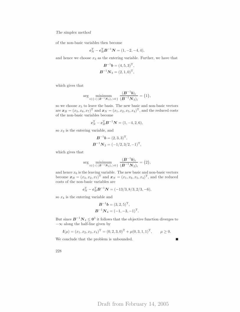
Draft from February 14, 2005
The simplex method
of the non-basic variables then become
cTN − cT
BB−1N = (1,−2,−4, 4),
and hence we choose x3 as the entering variable. Further, we have that
B−1b = (4, 5, 3)T,
B−1N3 = (2, 1, 0)T,
which gives that
arg minimumi∈{ i | (B−1N 3)i>0 }
(B−1b)i
(B−1N3)i
= {1},
so we choose x5 to leave the basis. The new basic and non-basic vectorsare xB = (x3, x6, x7)
T and xN = (x1, x2, x5, x4)T, and the reduced costs
of the non-basic variables become
cTN − cT
BB−1N = (1,−4, 2, 6),
so x2 is the entering variable, and
B−1b = (2, 3, 3)T,
B−1N 2 = (−1/2, 3/2,−1)T,
which gives that
arg minimumi∈{ i | (B−1N 2)i>0 }
(B−1b)i
(B−1N2)i
= {2},
and hence x6 is the leaving variable. The new basic and non-basic vectorsbecome xB = (x3, x2, x7)
T and xN = (x1, x6, x5, x4)T, and the reduced
costs of the non-basic variables are
cTN − cT
BB−1N = (−13/3, 8/3, 2/3,−6),
so x4 is the entering variable and
B−1b = (3, 2, 5)T,
B−1N4 = (−1,−3,−1)T.
But since B−1N4 ≤ 03 it follows that the objective function diverges to−∞ along the half-line given by
l(µ) = (x1, x2, x3, x4)T = (0, 2, 3, 0)T + µ(0, 3, 1, 1)T, µ ≥ 0.
We conclude that the problem is unbounded.
228
Draft from February 14, 2005
The algorithm
9.1.2 A BFS is not known: Phase I & II
Often a basic feasible solution is not known from the beginning. (Infact, only if the origin is feasible in (9.4) we know a BFS immediately.)However, an initial basic feasible solution can be found by solving alinear program that is a pure feasibility problem. We call this the PhaseI problem.
Consider the following linear program in standard form:
minimize z = cTx (9.6)
subject to Ax = b,
x ≥ 0n.
In order to find a basic feasible solution we introduce the artificial vari-ables a ∈ Rm and consider the Phase I problem to
minimize w = (1m)Ta (9.7)
subject to Ax +Ima = b,
x ≥ 0n,
a ≥ 0m.
In other words, we introduce an additional (artificial) variable ai forevery linear constraint i = 1, . . . ,m, and thus construct the unit matrixin Rm×m sought.
We get a basic feasible solution to the Phase I problem (9.7) bytaking the artificial variables a as the basic variables. (Remember thatb ≥ 0m; the simplicity of finding an initial BFS for the Phase I problemis in fact the reason why we require this to hold!) Then the Phase Iproblem (9.7) can be solved by the Simplex method stated in the previoussection. Note that the Phase I problem is bounded from below (since(1m)Ta ≥ 0) which means that an optimal solution to (9.7) always existsby Theorem 8.10.
Assume that the optimal objective function value is w∗. We observethat if and only if the part x∗ of an optimal solution ((x∗)T, (a∗)T)T tothe problem (9.7) is a feasible solution to the original problem (9.6), then((x∗)T, (0m)T)T is an optimal feasible solution to the Phase I problemand w∗ = 0. Hence, if w∗ > 0, then the original linear program isinfeasible. We have the following cases:
1. If w∗ > 0, then the original problem is infeasible.
2. If w∗ = 0, then if the optimal basic feasible solution is (xT,aT)T
we must have that a = 0m, and x corresponds to a basic feasible
229
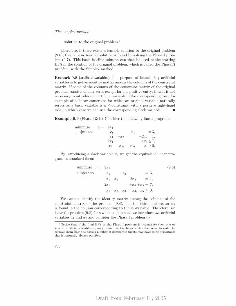
Draft from February 14, 2005
The simplex method
solution to the original problem.1
Therefore, if there exists a feasible solution to the original problem(9.6), then a basic feasible solution is found by solving the Phase I prob-lem (9.7). This basic feasible solution can then be used as the startingBFS in the solution of the original problem, which is called the Phase IIproblem, with the Simplex method.
Remark 9.8 (artificial variables) The purpose of introducing artificialvariables is to get an identity matrix among the columns of the constraintmatrix. If some of the columns of the constraint matrix of the originalproblem consists of only zeros except for one positive entry, then it is notnecessary to introduce an artificial variable in the corresponding row. Anexample of a linear constraint for which an original variable naturallyserves as a basic variable is a ≤-constraint with a positive right-handside, in which case we can use the corresponding slack variable.
Example 9.9 (Phase I & II) Consider the following linear program:
minimize z = 2x1
subject to x1 −x3 = 3,x1 −x2 −2x4 = 1,
2x1 +x4 ≤ 7,x1, x2, x3, x4 ≥ 0.
By introducing a slack variable x5 we get the equivalent linear pro-gram in standard form:
minimize z = 2x1 (9.8)
subject to x1 −x3 = 3,
x1 −x2 −2x4 = 1,
2x1 +x4 +x5 = 7,
x1, x2, x3, x4, x5 ≥ 0.
We cannot identify the identity matrix among the columns of theconstraint matrix of the problem (9.8), but the third unit vector e3
is found in the column corresponding to the x5-variable. Therefore, weleave the problem (9.8) for a while, and instead we introduce two artificialvariables a1 and a2 and consider the Phase I problem to
1Notice that if the final BFS in the Phase I problem is degenerate then one orseveral artificial variables ai may remain in the basis with value zero; in order toremove them from the basis a number of degenerate pivots may have to be performed;this is naturally always possible.
230
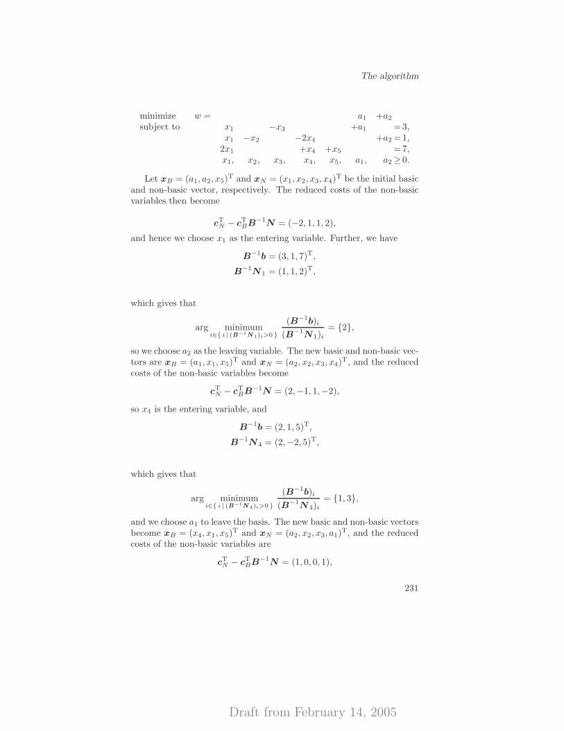
Draft from February 14, 2005
The algorithm
minimize w = a1 +a2
subject to x1 −x3 +a1 =3,x1 −x2 −2x4 +a2 =1,
2x1 +x4 +x5 =7,x1, x2, x3, x4, x5, a1, a2 ≥ 0.
Let xB = (a1, a2, x5)T and xN = (x1, x2, x3, x4)
T be the initial basicand non-basic vector, respectively. The reduced costs of the non-basicvariables then become
cTN − cT
BB−1N = (−2, 1, 1, 2),
and hence we choose x1 as the entering variable. Further, we have
B−1b = (3, 1, 7)T,
B−1N1 = (1, 1, 2)T,
which gives that
arg minimumi∈{ i | (B−1N 1)i>0 }
(B−1b)i
(B−1N1)i
= {2},
so we choose a2 as the leaving variable. The new basic and non-basic vec-tors are xB = (a1, x1, x5)
T and xN = (a2, x2, x3, x4)T, and the reduced
costs of the non-basic variables become
cTN − cT
BB−1N = (2,−1, 1,−2),
so x4 is the entering variable, and
B−1b = (2, 1, 5)T,
B−1N4 = (2,−2, 5)T,
which gives that
arg minimumi∈{ i | (B−1N 4)i>0 }
(B−1b)i
(B−1N4)i
= {1, 3},
and we choose a1 to leave the basis. The new basic and non-basic vectorsbecome xB = (x4, x1, x5)
T and xN = (a2, x2, x3, a1)T, and the reduced
costs of the non-basic variables are
cTN − cT
BB−1N = (1, 0, 0, 1),
231
Draft from February 14, 2005
The simplex method
so by choosing the basic variables as xB = (x4, x1, x5)T we get an optimal
basic feasible solution of the Phase I problem, and w∗ = 0. This meansthat by choosing the basic variables as xB = (x4, x1, x5)
T we get a basicfeasible solution of the Phase II problem (9.8).
We return to the problem (9.8). By letting xB = (x4, x1, x5)T and
xN = (x2, x3)T we get the reduced costs
cTN = cT
N − cTBB−1N = (0, 2),
which means that
x =
(xB
xN
)=
x4
x1
x5
x2
x3
=
(B−1b
02
)=
13000
is an optimal basic feasible solution to the original problem. (Observethat most often the basic feasible solution found when solving the PhaseI problem is not an optimal solution to the Phase II problem!) Butsince the reduced cost of x2 is zero there is a possibility that there arealternative optimal solutions. Let x2 enter the basic vector. We havethat
B−1b = (1, 3, 0)T,
B−1N1 = (0.5, 0,−0.5)T,
which gives that
arg minimumi∈{ i | (B−1N 1)i>0 }
(B−1b)i
(B−1N1)i
= {1},
so x4 is the leaving variable. We get xB = (x2, x1, x5)T and xN =
(x4, x3)T, and the reduced costs become
cTN = cT
N − cTBB−1N = (0, 2),
so
x =
(xB
xN
)=
x2
x1
x5
x4
x3
=
(B−1b
02
)=
23100
is an alternative optimal basic feasible solution.
232
Draft from February 14, 2005
Termination
9.1.3 Alternative optimal solutions
As we saw in Example 9.9 there can be alternative optimal solutions toa linear program. However, this can only happen if some of the reducedcosts of the non-basic variables of an optimal solution is zero.
Proposition 9.10 (unique optimal solutions in linear programming) Considerthe linear program in standard form
minimize z = cTx
subject to Ax = b,
x ≥ 0n.
Let xT = (xTB,x
TN ) be an optimal basic feasible solution that corresponds
to the partition A = (B,N). If the reduced costs of the non-basic vari-ables xN are all strictly positive, then x is the unique optimal solution.
Proof. As in the proof of Proposition 9.1 we have that the originallinear program is equivalent to
minimize z = cTNxN
subject to xB+B−1NxN = B−1b,
xB ≥ 0m,
xN ≥ 0n−m.
Now if the reduced costs of the non-basic variables are all strictly posi-tive, that is, cN > 0n−m, it follows that a solution for which (xN )j > 0for some j = 1, . . . , n−m cannot be optimal. Hence
x =
(xB
xN
)=
(B−1b
0n−m
)
is the unique optimal solution.
9.2 Termination
So far we have not discussed whether the Simplex algorithm terminatesin a finite number of iterations or not. Unfortunately, if there existdegenerate basic feasible solutions it can happen that the Simplex algo-rithm cycles between degenerate solutions and hence never terminates.However, if all of the basic feasible solutions are non-degenerate this kindof cycling never occurs.
233
Draft from February 14, 2005
The simplex method
Theorem 9.11 (finiteness of the Simplex algorithm) If all of the basicfeasible solutions are non-degenerate, then the Simplex algorithm ter-minates after a finite number of iterations.
Proof. If a basic feasible solution is non-degenerate it follows that ithas exactly m strictly positive components, and hence has a uniqueassociated basis. In this case, in the minimum ratio test,
µ∗ = minimumi∈{ i | (B−1N j)i>0 }
(B−1b)i
(B−1N j)i
,
we get that µ∗ > 0. Therefore, at each iteration the objective valuestrictly decreases, and hence a basic feasible solution that has appearedonce can never reappear. Further, from Corollary 3.18 follows that thenumber of extreme points, hence the number of basic feasible solutions,is finite. We are done.
Cycling resulting from degeneracy does not seem to occur often amongthe numerous degenerate linear programs encountered in practical appli-cations. However, the fact that it can occur is not theoretically satisfac-tory. Therefore methods have been developed that avoid cycling. Oneof them is Bland’s rule.
Theorem 9.12 (Bland’s rule) Fix an ordering of the variables. (Thisordering can be arbitrary, but once it has been selected it cannot bechanged.) If at each iteration step the entering and leaving variables arechosen as the first variables that are eligible2 in the ordering, then theSimplex algorithm terminates after a finite number of iteration steps.
9.3 Computational complexity
The Simplex algorithm is very efficient in practice. Although the totalnumber of basic feasible solutions can be as many as
(nm
)=
n!
(n−m)!m!
2By eligible entering variables we mean the variables (xN )j for which ( N )j < 0,and when we have chosen the entering variable j, the eligible leaving variables arethe variables (xB)i such that
i ∈ arg minimumi∈{ i | (B−1N j)i>0 }
(B−1b)i
(B−1N j)i
.
234
Draft from February 14, 2005
Notes and further reading
(the number of different ways m objects can be chosen from n objects),which is a number that grows exponentially, it is rare that more than 3miterations are needed, and practice shows that the expected number is inthe order of 3m/2. Since each iteration costs no more than a polynomial(O(m3) for factorizations and O(mn) for the pricing) the algorithm ispolynomial in practice. Its worst-case behaviour is however very bad, infact exponential.
The bad worst-care behaviour of the simplex method led to a hugeamount of work being laid down to find polynomial algorithms for solv-ing linear programs. Such a polynomial time competitor to the Simplexmethod nowadays is the class of interior point algorithms. Its main fea-ture is that the optimal extreme points are not approached by followingthe edges, but by moving within the interior of the polyhedron. Thefamous Karmarkar algorithm is one, which however has been improvedmuch in recent years. An analysis of interior point methods for lin-ear programs is made in Chapter 13, as they are in fact to be seen asinstances of the interior penalty algorithm in nonlinear programming.
9.4 Notes and further reading
The simplex method was developed by Danzig [Dan51]. The versionof the simplex method we have presented is usually called the revisedsimplex method and was first described by Danzig [Dan53] and Orchard-Hays [Orc54]. The first book describing the simplex method was [Dan63].
In the (revised) simplex algorithm several computations are per-formed using B−1. The major drawback in this approach is that round-off errors accumulates as the algorithm moves from step to step. Thisdrawback can be alleviated by using LU decomposition or Cholesky fac-torization. Most of the software packages for linear programming use LUdecomposition. Early references on numerically stable forms of the sim-plex method are [BaG69, Bar71, GiM73, Sau72]. Books that discussesthe subject are [Mur83, NaS96].
The first example of cycling was constructed by Hoffman [Hof53]. Dif-ferent methods have been developed that avoid cycling, for example theperturbation method by Charnes [Cha52], the lexicographic method byDanzig, Orden and Wolfe [DOW55], and Bland’s rule by Bland [Bla77].In practice, however, cycling is rarely encountered. Instead, the problemis stalling, which means that the value of the objective function doesnot change (or changes very little) for a very large number of iterations3
before it eventually starts to make substantial progress again. So in
3“Very large” normally refers to a number of iterations which is an exponentialfunction of the number of variables of the LP problem.
235
Draft from February 14, 2005
The simplex method
practice, we are interested in methods that primarily prevent stalling,and only secondarily cycling (see, e.g., [GMSW89]).
In 1972, Klee and Minty [KlM72] showed that there exist problems ofarbitrary size that cause the simplex method to examine every possiblebasis when the steepest-descent pricing rule is used, and hence showedthat the simplex method is an exponential algorithm in the worst case. Itis still an open question, however, whether there exists a rule for choosingentering and leaving basic variables that makes the simplex method poly-nomial. The first polynomial-time method for linear programming wasgiven by Khachiyan [Kha79, Kha80], by adapting the ellipsoid methodfor nonlinear programming of Shor [Sho70a, Sho70b, Sho77] and Yudinand Nemirovskii [YuN77]. Karmarkar [Kar84a, Kar84b] showed that in-terior point methods can be used in order to solve linear programmingproblems in polynomial time.
General text books that discusses the simplex method are [Dan63,Chv83, Mur83, Sch86, Pad99, Van01, DaT97, DaT03].
9.5 Exercises
Exercise 9.1 (checking feasibility: phase I) Consider the system
3x1 +2x2 −x3 ≤ −3,
−x1 −x2 +2x3 ≤ −1,
x1, x2, x3 ≥ 0.
Show that this system is infeasible.
Exercise 9.2 (the Simplex algorithm: phase I & II) Consider the linearprogram
minimize z = 3x1 +2x2 +x3
subject to 2x1 +x3 ≥ 3,
2x1 +2x2 +x3 = 5,
x1, x2, x3 ≥ 0.
(a) Solve the linear program by using the Simplex algorithm withPhase I & II.
(b) Is the solution obtained unique?
Exercise 9.3 (the Simplex algorithm) Consider the linear program in stan-
236
Draft from February 14, 2005
Exercises
dard form,
minimize z = cTx
subject to Ax = b,
x ≥ 0n.
Suppose that at a given step of the Simplex algorithm, there is onlyone possible entering variable, (xN )j . Also assume that the current BFSis non-degenerate. Show that (xN )j > 0 in any optimal solution.
237

Draft from February 14, 2005
The simplex method
238
Draft from February 14, 2005
Linear programmingduality and sensitivityanalysis
X
10.1 Introduction
Consider the linear program
minimize z = cTx (10.1)
subject to Ax = b,
x ≥ 0n,
where A ∈ Rm×n, b ∈ Rm, and c ∈ Rn, and assume that this problemhas been solved by the Simplex algorithm. Let x∗ = (xT
B,xTN )T be
an optimal basic feasible solution corresponding to the partition A =(B,N ). Introduce the vector y∗ ∈ Rm through
(y∗)T = cTBB−1.
Since x∗ is an optimal solution it follows that the reduced costs ofthe non-basic variables are greater than or equal to zero, that is,
cTN − cT
BB−1N ≥ (0n−m)T ⇐⇒ cTN − (y∗)TN ≥ (0n−m)T.
Further, cTB − (y∗)TB = cT
B − cTBB−1B = (0m)T, so actually we have
that
cT − (y∗)TA ≥ (0n)T,
or equivalently,
ATy∗ ≤ c.
Draft from February 14, 2005
LP duality and sensitivity analysis
Now, for every y ∈ Rm such that ATy ≤ c and every feasible solutionx to (10.1) it holds that
cTx ≥ yTAx = yTb = bTy.
But
bTy∗ = bT(B−1)TcB = cTBB−1b = cT
BxB ≤ cTx,
for every feasible solution x to (10.1) (since x∗ = (xTB,x
TN )T is optimal),
so in fact we have that y∗ is an optimal solution to the linear program
maximize bTy (10.2)
subject to ATy ≤ c,
y free.
Observe that the linear program (10.2) is exactly the Lagrangian dualproblem to (10.1) (see Section 6.2.4). Also, note that the linear programs(10.1) and (10.2) have the same optimal objective value, which is inaccordance with the Strong Duality Theorem 6.11 (see also Theorem 10.6below for an independent proof).
The linear program (10.2) is called the linear programming dual tothe linear program (10.1) (which is called the primal linear program). Inthis chapter we will study linear programming duality. In Section 10.2we discuss how to construct the linear programming dual to a generallinear program. Section 10.3 presents duality theory, such as weak andstrong duality and complementary slackness. Finally, in Section 10.5we discuss how the optimal solutions of a linear program change if theright-hand side b or the objective function coefficients c are modified.
10.2 The linear programming dual
For every linear program it is possible to construct the Lagrangian dualproblem. From now on we will call this problem the dual linear program.It is quite tedious to construct the Lagrangian dual problem for everyspecial case of a linear program, but fortunately the dual of a generallinear program can be constructed just by following some simple rules.These rules are presented in this section. (It is, however, a good exerciseto show the validity of these rules by constructing the Lagrangian dualin each case.)
240
Draft from February 14, 2005
The linear programming dual
10.2.1 Canonical form
When presenting the rules for constructing the linear programming dualwe will use the notation of canonical form. The canonical form is con-nected with the inequalities of the problem and the objective function. Ifthe objective is to maximize the objective function, then every inequalityof type “≤” is said to be of canonical form. Similarly, if the objective isto minimize the objective function, then every inequality of type “≥” issaid to be of canonical form. Further, we consider non-negative variablesto be variables in canonical form.
Remark 10.1 (mnemonic rule for canonical form) Consider the problemto
minimize z = x1
subject to x1 ≤ 1.
This problem is unbounded from below and hence an optimal solutiondoes not exist. However, if the problem is to
minimize z = x1
subject to x1 ≥ 1,
then an optimal solution exists, namely x1 = 1. Hence it seems natural toconsider inequalities of type “≥” as canonical to minimization problems.Similarly, it is natural that inequalities of type “≤” are canonical tomaximization problems.
10.2.2 Constructing the dual
From the notation of canonical form introduced in Section 10.2.1 we cannow construct the dual, (D), to a general linear program, (P), accordingto the following rules.
Dual variables
To each constraint of (P) a dual variable, yi, is introduced. If the ith
constraint of (P) is an inequality of canonical form, then yi is a non-negative variable, that is, yi ≥ 0. Similarly, if the ith constraint of (P) isan inequality that is not of canonical form, then yi ≤ 0. Finally, if theith constraint of (P) is an equality, then the variable yi is unrestricted.
241
Draft from February 14, 2005
LP duality and sensitivity analysis
Dual objective function
If (P) is a minimization (respectively, a maximization) problem, then (D)is a maximization (respectively, a minimization) problem. The objectivefunction coefficient for the variable yi in the dual problem equals theright-hand side constant of the ith constraint of (P).
Constraints of the dual problem
If A is the constraint matrix of (P), then AT is the constraint matrix of(D). The jth right-hand side constant of (D) equals the jth coefficient inthe objective function of (P). If the jth variable of (P) has non-negativityrestriction, then the jth constraint of (D) is an inequality of canonicalform. If the jth variable of (P) has a non-positivity restriction, then thejth constraint of (D) is an inequality of non-canonical form. Finally, ifthe jth variable of (P) is unrestricted, then the jth constraint of (D) isan equality.
Summary
The rules above can be summarized as follows:
primal/dual constraint dual/primal variable
canonical inequality ⇐⇒ ≥ 0
non-canonical inequality ⇐⇒ ≤ 0
equality ⇐⇒ unrestricted
Consider the following general linear program:
minimize z =
n∑
j=1
cjxj
subject to
n∑
j=1
aijxj ≥ bi, i ∈ C,
n∑
j=1
aijxj ≤ bi, i ∈ NC,
n∑
j=1
aijxj = bi, i ∈ E,
xj ≥ 0, j ∈ P,
xj ≤ 0, j ∈ N,
xj free, j ∈ F,
242
Draft from February 14, 2005
The linear programming dual
where C stands for “canonical”, NC for “non-canonical”, E for “equal-ity”, P for “positive”, N for “negative”, and F for “free”. Note thatP ∪N ∪ F = {1, . . . , n} and C ∪NC ∪E = {1, . . . ,m}. If we apply therules above we get the following dual linear program:
maximize w =
m∑
i=1
biyi
subject tom∑
i=1
aijyi ≤ cj , j ∈ P,
m∑
i=1
aijyi ≥ cj , j ∈ N,
m∑
i=1
aijyi = cj , j ∈ F,
yi ≥ 0, i ∈ C,
yi ≤ 0, i ∈ NC,
yi free, i ∈ E.
From this it is easily established that if we construct the dual of the duallinear program, then we return to the original (primal) linear program.
Examples
In order to illustrate how to construct the dual linear program we presenttwo examples. The first example considers a linear program with blockstructure. This is a usual form of linear programs and it is particularlyeasy to construct the dual linear program. The other example dealswith the transportation problem presented in Section 8.1. The purposeof constructing the dual to this problem is to show how to handle doublesubscripted variables and indexed constraints.
Example 10.2 (the dual to a linear program of block form) Consider thelinear program
maximize cTx+dTy
subject to Ax +By ≤ b,
Dy = e,
x ≥ 0n1 ,
y ≤ 0n2 ,
243
Draft from February 14, 2005
LP duality and sensitivity analysis
where A ∈ Rm1×n1 , D ∈ Rm2×n2 , b ∈ Rm1 , e ∈ Rm2 , c ∈ Rn1 , andd ∈ Rn2 . The dual of this linear program becomes that to
minimize bTu +eTv
subject to ATu ≥ c,
BTu+DTv ≤ d,
u ≥ 0m1 ,
v free.
Observe that the constraint matrix of the primal problem is(
A B
0 D
),
and if we transpose this matrix we get(
AT 0T
BT DT
).
Also note that the vector of objective function coefficients of the primalproblem, (cT,dT)T, is the right-hand side of the dual problem, andthe right-hand side of the primal problem, (bT, eT)T, is the vector ofobjective function coefficients of the dual problem.
Example 10.3 (the dual of the transportation problem) Consider the trans-portation problem (see Example 8.1) to
minimize z =
N∑
i=1
M∑
j=1
cijxij
subject toM∑
j=1
xij ≤ si, i = 1, . . . , N,
N∑
i=1
xij ≥ dj , j = 1, . . . ,M,
xij ≥ 0, i = 1, . . . , N, j = 1, . . . ,M.
The dual linear program is given by
maximize w =N∑
i=1
siui +M∑
j=1
djvj
subject to ui + vj ≤ cij , i = 1, . . . , N, j = 1, . . . ,M,
ui ≤ 0, i = 1, . . . , N,
vj ≥ 0, j = 1, . . . ,M.
244
Draft from February 14, 2005
Linear programming duality theory
Observe that there are N + M constraints in the primal problem andhence there are N +M dual variables. Also, there are NM variables ofthe primal problem, yielding NM constraints in the dual problem. Theform of the constraints in the dual problem arises from the fact that xij
appears twice in the column of the constraint matrix corresponding tothis variable: once in the constraints over i = 1, . . . , N and once in theconstraints over j = 1, . . . ,M . Also note that all the coefficients of theconstraint matrix in the primal problem equal +1, and since we haveone dual constraint for each column, we finally get the dual constraintui + vj ≤ cij .
10.3 Linear programming duality theory
In this section we present some of the most fundamental duality theo-rems. Throughout the section we will consider the primal linear program
minimize z = cTx (P)
subject to Ax = b,
x ≥ 0n,
where A ∈ Rm×n, b ∈ Rm, and c ∈ Rn, and its dual linear program
maximize w = bTy (D)
subject to ATy ≤ c,
y free.
The theorems presented actually hold for every primal–dual pair of linearprograms, and the proofs are similar to those presented here. See alsothe more general statements on the differentiability of the perturbationfunction in Section 6.7.
10.3.1 Weak and strong duality
We begin by proving the Weak Duality Theorem.
Theorem 10.4 (Weak Duality Theorem) If x is a feasible solution to(P) and y a feasible solution to (D), then cTx ≥ bTy.
Proof. We have that
cTx ≥ (ATy)Tx [c ≥ ATy, x ≥ 0n]
= yTAx = yTb [Ax = b]
= bTy,
245
Draft from February 14, 2005
LP duality and sensitivity analysis
and we are done.
Corollary 10.5 If x is feasible solution to (P), y a feasible solution to(D), and cTx = bTy, then x is an optimal solution to (P) and y andoptimal solution to (D).
Next we show that the duality gap is zero, that is, strong dualityholds. Note that this can also be established by the use of the Lagrangianduality theory in Chapter 6.
Theorem 10.6 (Strong Duality Theorem) If one of the problems (P) and(D) has a finite optimal solution, then so does its dual, and their optimalobjective values are equal.
Proof. Suppose that x∗ = (xTB,x
TN )T is an optimal basic feasible solu-
tion to (P) corresponding to the partition A = (B,N). We constructan optimal solution to (D). (Actually we have already done this in detailin Section 10.1.) Let
(y∗)T = cTBB−1.
Since x∗ is an optimal basic feasible solution the reduced costs of thenon-basic variables are non-negative, which gives that (for details seeSection 10.1)
ATy∗ ≤ c.
Hence, y∗ is feasible to (D). Further, we have that
bTy∗ = bT(B−1)TcB = cTBB−1b = cT
BxB = cTx∗,
so by Corollary 10.5 it follows that y∗ is an optimal solution to (D).Now suppose instead that the dual problem has a finite optimal so-
lution. Convert (D) into standard form:
minimize w = −bTy+ + bTy− (D’)
subject to(AT −AT I
)
y+
y−
s
= c,
y+,y− ≥ 0m,
s ≥ 0n.
246
Draft from February 14, 2005
Linear programming duality theory
If there exists an optimal solution y∗ to (D), then there exists an optimalbasic feasible solution to (D’) (with w∗ = −w∗). As in the first part ofthe proof we then get that there exists an x∗ ∈ Rn such that
A
−A
I
x∗ ≤
−b
b
0n
,
and
w∗ = cTx∗.
Hence, by Corollary 10.5, we get that −x∗ is an optimal solution to (P).We are done.
Remark 10.7 (dual solution from the primal solution) Note that the proofof Theorem 10.6 is constructive. We actually construct an optimal dualsolution from an optimal basic feasible solution by
(y∗)T = cTBB−1. (10.3)
When a linear program is solved by the Simplex method we obtain anoptimal basic feasible solution (if the LP is not unbounded or infeasible).Hence from (10.3) we then also—without any additional effort—obtainan optimal dual solution. In fact the dual solution is calculated in thepricing step of the Simplex algorithm.
Interpretation of the optimal dual solution
We have from (10.3) that
bTy∗ = cTBB−1b,
for any optimal basic feasible solution to (P). If xB > 0m, then a smallchange in b does not change the basis, and so the optimal value of (D)(and (P)), namely
v(b) := bTy∗
is linear at, and locally around, the value b. If, however, some (xB)i = 0,then in this degenerate case it could be that the basis changes in a non-differentiable manner with b. We summarize:
247
Draft from February 14, 2005
LP duality and sensitivity analysis
Theorem 10.8 (shadow price) If, for a given b, the optimal solutionto (P) corresponds to a non-degenerate basic feasible solution, then itsoptimal value is differentiable at b, with
∂v(b)
∂bi= y∗i , i = 1, . . . ,m,
that is, ∇v(b) = y∗.
Remark 10.9 (shadow price) The optimal dual solution is indeed theshadow price for the constraints. If a unit change in one right-hand sidebi does not change the optimal basis, then the above states that theoptimal value will change exactly with the amount y∗i .
It is also clear that non-degeneracy at x∗ in (P) implies that theoptimal solution in (D) must be unique. Namely, we can show thatthe function v is convex on its effective domain (why?) and the non-degeneracy property clearly implies that v is also finite in a neighbour-hood of b. Then, its differentiability at b is equivalent to the uniquenessof its subgradients at b; cf. Proposition 6.16(c).
Farkas’ Lemma
In Section 3.2 we proved Farkas’ Lemma 3.30 by using the SeparationTheorem 3.24. However, Farkas’ Lemma 3.30 can easily be proved byusing the Strong Duality Theorem 10.6.
Theorem 10.10 (Farkas’ Lemma) Let A ∈ Rm×n and b ∈ Rm. Then,exactly one of the systems
Ax = b, (I)
x ≥ 0n,
and
ATy ≤ 0n, (II)
bTy > 0,
has a feasible solution, and the other system is inconsistent.
Proof. If (I) has a solution x, then
bTy = xTATy > 0.
But x ≥ 0n, so ATy ≤ 0n cannot hold, which means that (II) is infea-sible.
248
Draft from February 14, 2005
Linear programming duality theory
Assume that (II) is infeasible. Consider the linear program
maximize bTy (10.4)
subject to ATy ≤ 0n,
y free,
and its dual program
minimize (0n)Tx (10.5)
subject to Ax = b,
x ≥ 0n.
Since (II) is infeasible, y = 0m is an optimal solution to (10.4). Hencethe Strong Duality Theorem 10.6 implies that there exists an optimalsolution to (10.5). This solution is feasible to (I).
What we have proved above is the equivalence
(I) ⇐⇒ ¬(II).
Logically, this is equivalent to the statement that
¬(I) ⇐⇒ (II).
We have hence established that precisely one of the two systems (I) and(II) has a solution. We are done.
10.3.2 Complementary slackness
A further relationship between (P) and (D) at an optimal solution isgiven by the Complementary Slackness Theorem.
Theorem 10.11 (Complementary Slackness Theorem) Let x be a feasi-ble solution to (P) and y a feasible solution to (D). Then x is optimalto (P) and y optimal to (D) if and only if
xj(cj − AT·jy) = 0, j = 1, . . . , n, (10.6)
where A·j is the jth column of A.
Proof. If x and y are feasible we get
cTx ≥ (ATy)Tx = yTAx = bTy. (10.7)
249
Draft from February 14, 2005
LP duality and sensitivity analysis
Further, by the Strong Duality Theorem 10.6 and the Weak DualityTheorem 10.4, x and y are optimal if and only if cTx = bTy, so in fact(10.7) holds with equality, that is,
cTx = (ATy)Tx ⇐⇒ xT(c − ATy) = 0.
Since x ≥ 0n and ATy ≤ c, xT(c−ATy) = 0 is equivalent to that eachterm in the sum is zero, that is, (10.6) holds.
Often the Complementary Slackness Theorem is stated for the primal–dual pair given by
maximize cTx (10.8)
subject to Ax ≤ b,
x ≥ 0n,
and
minimize bTy (10.9)
subject to ATy ≥ c,
y ≥ 0m.
The Complementary Slackness Theorem then becomes as follows. (Itsproof is similar to that of Theorem 10.11.)
Theorem 10.12 (Complementary Slackness Theorem) Let x be a feasi-ble solution to (10.8) and y a feasible solution to (10.9). Then x isoptimal to (10.8) and y optimal to (10.9) if and only if
xj(cj − yTA·j) = 0, j = 1, . . . , n, (10.10a)
yi(Ai·x − bi) = 0, i = 1 . . . ,m, (10.10b)
where A·j is the jth column of A and Ai· the ith row of A.
Remark 10.13 (interpretation of the Complementary Slackness Theorem)From the Complementary Slackness Theorem follows that, for an opti-mal primal dual pair of solutions, if there is slack in one constraint, thenthe respective variable in the other problem is zero. Further, if a variableis positive, then there is no slack in the respective constraint in the otherproblem.
The consequence of the Complementary Slackness Theorem is thefollowing characterization of an optimal solution to a linear program.We state it for the primal–dual pair given by (10.8) and (10.9), but itholds as well for each primal dual pair of linear programs.
250
Draft from February 14, 2005
Linear programming duality theory
Theorem 10.14 (necessary and sufficient conditions for global optimality)Take a vector x ∈ Rn. For x to be an optimal solution to the linear pro-gram (10.8), it is both necessary and sufficient that
(a) x is a feasible solution to (10.8);(b) corresponding to x there is a dual feasible solution y ∈ Rm to
(10.9); and(c) the pair (x,y) satisfies the complementarity conditions (10.10).
The simplex method is very well adapted to these conditions. AfterPhase I, (a) holds. Every basic solution (feasible or not) satisfies (c),since if xj is in the basis, then cj = cj − yTA·j = 0, and if cj 6= 0,then xj = 0. So, the only condition that the Simplex method does notsatisfy for every basic feasible solution is (b). The proof of the StrongDuality Theorem 10.6 shows that it is satisfied exactly at an optimalbasic feasible solution. The entering criterion is based on trying to bettersatisfy it. Indeed, by choosing as an entering variable xj such that
j ∈ argminimumj∈{1,...,n}
cj ,
we actually identify a dual constraintm∑
i=1
aijyi ≤ cj ,
which is among the most violated at the complementary solution yT =cT
BB−1 given by the current BFS. After the basis change we will haveequality in this dual constraint, and hence the basis change correspondsto making a currently most violated dual constraint feasible!
Example 10.15 (illustration of complementary slackness) Consider the primal–dual pair given by
maximize z = 3x1 +2x2 (10.11)
subject to x1 +x2 ≤ 80,
2x1 +x2 ≤ 100,
x1 ≤ 40,
x1, x2 ≥ 0,
and
minimize w = 80y1 +100y2 +40y3 (10.12)
subject to y1 +2y2 +y3 ≥ 3,
y1 +y2 ≥ 2,
y1, y2, y3 ≥ 0.
251
Draft from February 14, 2005
LP duality and sensitivity analysis
We use Theorem 10.14 to show that x∗ = (20, 60)T is an optimalsolution to (10.11).
(a) (primal feasibility) Obviously x∗ is a feasible solution to (10.11).(c) (complementary) The complementary conditions must hold, that
is,
y∗1(x∗1 + x∗2 − 80) = 0
y∗2(2x∗1 + x∗2 − 100) = 0
y∗3(x∗1 − 40) = 0 =⇒ y∗3 = 0 [x∗1 = 20 6= 40]
x∗1(y∗1 + 2y∗2 + y∗3 − 3) = 0 =⇒ y∗1 + 2y∗2 = 3 [x∗1 > 0]
x∗2(y∗1 + y∗2 − 2) = 0 =⇒ y∗1 + y∗2 = 2 [x∗2 > 0]
which gives that y∗1 = 1, y∗2 = 1 and y∗3 = 0.
(b) (dual feasibility) Obviously y∗ = (1, 1, 0)T is a feasible solution to(10.12).
From Theorem 10.14 it then follows that x∗ = (20, 60)T is an optimalsolution to (10.11) and y∗ = (1, 1, 0)T an optimal solution to (10.12).
10.4 The Dual Simplex method
The Simplex method presented in Chapter 9, which we here refer toas the primal Simplex method, starts with a basic feasible solution tothe primal linear program and then iterates until the primal optimalityconditions are fulfilled, that is, until a basic feasible solution is foundsuch that the reduced costs
cTN := cT
N − cTBB−1N ≥ (0n−m)T.
This is equivalent to the dual feasibility condition
ATy ≤ c,
where y = (B−1)TcB. We call a basis such that all of the reducedcosts are greater than or equal to zero a dual feasible basis; otherwise wecall it a dual infeasible basis. Hence, the primal Simplex method startswith a primal feasible basis and then moves through a sequence of dualinfeasible (but primal feasible) bases until a dual (and primal) feasiblebasis is found.
The Dual Simplex method is a variant of the primal Simplex methodthat works in a dual manner in the sense that it starts with a dual feasiblebasis and then moves through a sequence of primal infeasible (but dualfeasible) bases until a primal (and dual) feasible basis is found.
252
Draft from February 14, 2005
The Dual Simplex method
In order to derive the Dual Simplex algorithm, let xB be a dualfeasible basis with the corresponding partition (B,N ). If
b = B−1b ≥ 0m,
then xB is primal feasible and since it is also dual feasible all of thereduced costs are greater than or equal to zero; hence, xB is an optimalBFS. Otherwise some of the components of b is strictly negative, say b1,that is,
(xB)1 +n−m∑
j=1
(B−1N)1j(xN )j = b1 < 0,
so (xB)1 < 0 in the current basis and will be the leaving variable. Now,if
(B−1N)1j ≥ 0, j = 1, . . . , n−m, (10.13)
then there exists no primal feasible solution to the problem. (Why?)Hence, if (10.13) is fulfilled, then we say that the primal infeasibilitycriterion is satisfied. Otherwise (B−1N)1j < 0 for some j = 1, . . . , n−m.Assume that (B−1N)1k < 0 and choose (xN )k to replace (xB)1 in thebasis. (Note that this yields that (xN )k = b1/(B
−1N )1k > 0 in the newbasis.) The new reduced costs then become
(cB)1 = − 1
(B−1N)1k
,
(cB)j = 0, j = 2, . . . ,m,
(cN )j = (cN )j − (cN )k(B−1N)1j
(B−1N)1k
, j = 1, . . . , n−m.
Since we want the new basis to be dual feasible it must hold that all ofthe new reduced costs are non-negative, that is,
(cN )j ≥ (cN )k(B−1N)1j
(B−1N)1k
, j = 1, . . . , n−m,
or, equivalently,
(cN )k
(B−1N)1k
≥ (cN )j
(B−1N )1j
, for all j such that (B−1N )1j < 0.
Therefore, in order to preserve dual feasibility, as entering variable wemust choose (xN )k such that
k ∈ arg maximumi∈{ j | (B−1N )1j<0 }
(cN )j
(B−1N )1j
.
253
Draft from February 14, 2005
LP duality and sensitivity analysis
We have now derived an infeasibility criterion and criteria for how tochoose the leaving and the entering variables, and are ready to state theDual Simplex algorithm:
The Dual Simplex Algorithm:
Step 0 (initialization: DFS) Assume that xT = (xTB,x
TN ) is a dual fea-
sible basis corresponding to the partition A = (B,N ).
Step 1 (leaving variable or termination) Calculate
b = B−1b.
If b ≥ 0m, then stop; the current basis is optimal. Otherwise,choose an s such that bs < 0, and let (xB)s be the leaving variable.
Step 2 (entering variable or termination) If
(B−1N)sj ≥ 0, j = 1, . . . , n−m,
then stop; the (primal) problem is infeasible. Otherwise, choose ak such that
k ∈ arg maximumi∈{ j | (B−1N )sj<0 }
(cN )j
(B−1N)sj
,
and let (xN )k be the entering variable.
Step 3 (update: change basis) Construct a new partition by swapping(xB)s with (xN )k. Go to Step 1.
Similarly to the primal Simplex Algorithm it can be shown that theDual Simplex Algorithm terminates in a finite number of steps if cyclingis avoided. Also, there exist rules for choosing the leaving and enteringvariables (among the eligible ones) such that cycling is avoided.
If a dual feasible solution is not available from the start, it is possibleto add a constraint to the original problem, that makes it possible toconstruct a dual feasible basis, and then run the Dual Simplex Algorithmon this modified problem (see Exercise 10.13).
Remark 10.16 (unboundedness of the primal problem) Since the dual prob-lem is known to be feasible, the primal problem cannot be unboundedby the Weak Duality Theorem 10.4. Hence the Dual Simplex Algorithmterminates with a basis that satisfies either the optimality criterion orthe primal infeasibility criterion.
254
Draft from February 14, 2005
The Dual Simplex method
Example 10.17 (illustration of the Dual Simplex Algorithm) Consider thelinear program
minimize 3x1 +4x2 +2x3 +x4 +5x5
subject to x1 −2x2 −x3 +x4 +x5 ≤−3,
−x1 −x2 −x3 +x4 +x5 ≤−2,
x1 +x2 −2x3 +2x4 −3x5 ≤ 4,
x1, x2, x3, x4, x5 ≥ 0.
By introducing the slack variables x6, x7, x8, we get the following linearprogram:
minimize 3x1 +4x2 +2x3 +x4 +5x5
subject to x1 −2x2 −x3 +x4 +x5 +x6 =−3,
−x1 −x2 −x3 +x4 +x5 +x7 =−2,
x1 +x2 −2x3 +2x4 −3x5 +x8 = 4,
x1, x2, x3, x4, x5, x6, x7, x8 ≥ 0.
We see that the basis xB = (x6, x7, x8)T is dual feasible, but primal in-
feasible. Hence we use the Dual Simplex Algorithm to solve the problem.We have that
b = B−1b = (−3,−2, 4)T,
so we choose (xB)1 = x6 to leave the basis. Further we have that
cT = (3, 4, 2, 1, 5, 0, 0, 0),
(B−1A)1,· = (1,−2,−1, 1, 1, 1, 0, 0), [the 1st row of B−1A]
so we choose x2 as the entering variable. The new basis becomes xB =(x2, x7, x8)
T. We get that
b = B−1b = (1.5,−0.5, 2.5)T.
Hence, we choose (xB)2 = x7 as the leaving variable. Further
cT = (5, 0, 0, 3, 7, 2, 0, 0),
(B−1A)2,· = (−1.5, 0,−0.5, 0.5, 0.5,−0.5, 1, 0),
which gives that x3 is the entering variable. The new basis becomesxB = (x2, x3, x8)
T. We get that
b = B−1b = (1, 1, 5)T,
255
Draft from February 14, 2005
LP duality and sensitivity analysis
which means that the optimality criterion (primal feasibility) is satisfied,and an optimal solution to the original problem is given by
x∗ = (x1, x2, x3, x4, x5)T = (0, 1, 1, 0, 0)T.
Check that this is indeed true, for example by using Theorem 10.12.
10.5 Sensitivity analysis
In this section we study two kinds of perturbations of a linear programin standard form,
minimize z = cTx (10.14)
subject to Ax = b,
x ≥ 0n,
namely
1. perturbations in the objective function coefficients cj; and
2. perturbations in the right-hand side coefficients bi.
We assume that x∗ = (xTB,x
TN )T = ((B−1b)T, (0n−m)T)T is an optimal
basic feasible solution to (10.14) with the corresponding partition A =(B,N ).
10.5.1 Perturbations in the objective function
Assume that the objective function coefficients of the linear program(10.14) are perturbed by the vector p ∈ Rn, that is, we consider theperturbed problem to
minimize z = (c + p)Tx (10.15)
subject to Ax = b,
x ≥ 0n.
The optimal solution x∗ to the unperturbed problem (10.14) is obviouslya feasible solution to (10.15), but is it still optimal? To answer this ques-tion, we note that a basic feasible solution is optimal if the reduced costsof the non-basic variables are greater than or equal to zero. The reducedcosts for the non-basic variables of the perturbed problem (10.15) aregiven by [let pT = (pT
B ,pTN )]
cTN = (cN + pN )T − (cB + pB)TB−1N .
Hence, cN ≥ 0n−m is sufficient for x∗ to be an optimal solution tothe perturbed problem (10.15). (Observe, however, that this is not anecessary condition unless x∗ is non-degenerate.)
256
Draft from February 14, 2005
Sensitivity analysis
Perturbations of a non-basic cost coefficient
If only one component of cN is perturbed, that is,
p =
(pB
pN
)=
(0m
εej
),
for some ε ∈ R and j ∈ {1, . . . , n − m}, then we have that x∗ is anoptimal solution to the perturbed problem if
(cN )j + ε− cTBB−1N j ≥ 0 ⇐⇒ ε+ (cN )j ≥ 0,
so in this case we only have to check that the perturbation ε is not lessthan −(cN )j in order to guarantee that x∗ is an optimal solution to theperturbed problem.
Perturbations of a basic cost coefficient
If only one component of cB is perturbed, that is,
p =
(pB
pN
)=
(εej
0n−m
),
for some ε ∈ R and j ∈ {1, . . . ,m}, then we have that x∗ is an optimalsolution to the perturbed problem if
(cN )T − (cTB + εeT
j )B−1N ≥ (0n−m)T ⇐⇒ εeTj B−1N + cN ≥ 0n−m.
In this case all of the reduced costs of the non-basic variables may change,and we must check that the perturbation ε multiplied by the jth row ofB−1N plus the original reduced costs cN is a vector whose componentsall are greater than or equal to zero.
Perturbations that makes x∗ non-optimal
If the perturbation p is such that some of the reduced costs of the per-turbed problem becomes strictly negative for the basis xB , then x∗ isperhaps not an optimal solution anymore. If this happens, let someof the variables with strictly negative reduced cost enter the basis andcontinue the Simplex algorithm until an optimal solution is found.
10.5.2 Perturbations in the right-hand side coeffi-cients
Now, assume that the right-hand side b of the linear program (10.14)is perturbed by the vector p ∈ Rm, that is, we consider the perturbed
257
Draft from February 14, 2005
LP duality and sensitivity analysis
problem to
minimize z = cTx (10.16)
subject to Ax = b + p,
x ≥ 0n.
The original reduced costs do not change as the right-hand side isperturbed, so the basic feasible solution given by the partition A =(B,N ) is optimal to the perturbed problem (10.16) if and only if it isfeasible, that is,
(xB
xN
)=
(B−1(b + p)
0n−m
)≥ 0n,
which means that we have to check that B−1(b + p) ≥ 0m.
Perturbations of one component of the right-hand side
Suppose that only one of the components of the right-hand side is per-turbed, that is,
p = εej ,
for some ε ∈ R and j ∈ {1, . . . ,m}. The basic feasible solution corre-sponding to the partition A = (B,N) is then feasible if and only if
B−1(b + εej) ≥ 0m ⇐⇒ εB−1ej + B−1b ≥ 0m,
so it must hold that ε multiplied by the jth column of B−1 plus thevector B−1b equals a vector whose components all are greater than orequal to zero.
Perturbations that makes x∗ infeasible
If the perturbation p is such that the basis xB becomes infeasible, thensome of the components in the updated right-hand side, B−1(b + p), isstrictly negative. However, the reduced costs are independent of p, sothe basis xB is still a dual feasible basis. Hence, we can continue withthe Dual Simplex algorithm until an optimal solution is found (or untilthe primal infeasibility criterion is satisfied).
258
Draft from February 14, 2005
Notes and further reading
10.6 Notes and further reading
10.7 Exercises
Exercise 10.1 (constructing the LP dual) Consider the linear program
maximize z = 6x1 −3x2−2x3+5x4
subject to 4x1 +3x2−8x3+7x4 = 11,
3x1 +2x2+7x3+6x4 ≥ 23,
7x1 +4x2+3x3+2x4 ≤ 12,
x1, x2 ≥ 0,
x3 ≤ 0,
x4 free.
Construct the linear programming dual.
Exercise 10.2 (constructing the LP dual) Consider the linear program
minimize z = cTx
subject to Ax = b,
l ≤ x ≤ u.
(a) Construct the linear programming dual.
(b) Show that the dual problem is always feasible (independent of A,b, l, and u).
Exercise 10.3 (constructing an optimal dual solution from an optimal BFS)Consider the linear program in standard form
minimize z = cTx (P)
subject to Ax = b,
x ≥ 0n.
Assume that an optimal BFS, x∗ = (xTB,x
TN )T, is given by the partition
A = (B,N). Show that
y = (B−1)TcB
is an optimal solution to the LP dual problem.
259
Draft from February 14, 2005
LP duality and sensitivity analysis
Exercise 10.4 (application of the Weak and Strong Duality Theorems) Considerthe linear program
minimize z = cTx (P)
subject to Ax = b,
x ≥ 0n,
and the perturbed problem to
minimize z = cTx (P’)
subject to Ax = b,
x ≥ 0n.
Show that if (P) has an optimal solution, then the perturbed problem(P’) cannot be unbounded (independent of b).
Exercise 10.5 (application of the Weak and Strong Duality Theorems) Considerthe linear program
minimize z = cTx (P)
subject to Ax ≤ b.
Assume that the objective function vector c cannot be written as a linearcombination of the rows of A. Show that (P) cannot have an optimalsolution.
Exercise 10.6 (application of the Weak and Strong Duality Theorems) Considerthe linear program
minimize z = cTx (P)
subject to Ax ≥ b,
x ≥ 0n.
Construct a polyhedron that equals the set of optimal solutions to (P).
Exercise 10.7 (application of the Weak and Strong Duality Theorems) Considerthe linear program
minimize z = cTx (P)
subject to Ax ≤ b,
x ≥ 0n.
260
Draft from February 14, 2005
Exercises
Let x∗ be an optimal solution to (P) with the optimal objective functionvalue z∗, and let y∗ be an optimal solution to the LP dual of (P). Showthat
z∗ = (y∗)TAx∗.
Exercise 10.8 (linear programming primal-dual optimality conditions) Considerthe linear program
maximize z = −4x2 +3x3 +2x4 −8x5
subject to 3x1 +x2 +2x3 +x4 = 3,
x1 −x2 +x4 −x5 ≥ 2,
x1, x2, x3, x4, x5 ≥ 0.
Find an optimal solution by using the LP primal-dual optimality condi-tions.
Exercise 10.9 (linear programming primal-dual optimality conditions) Considerthe linear program (the continuous knapsack problem)
maximize z = cTx (P)
subject to aTx ≤ b,
x ≤ 1n,
x ≥ 0n,
where c > 0n, a > 0n, b > 0, and
c1a1
≥ c2a2
≥ · · · ≥ cnan.
Show that the feasible solution x given by
xj = 1, j = 1, . . . , r − 1, xr =b −∑r−1
j=1 aj
ar, xj = 0, j = r + 1, . . . , n,
where r is such that∑r−1
j=1 aj < b and∑r
j=1 aj > b, is an optimalsolution.
Exercise 10.10 (characterizations of optimal solutions in linear programming)Assume that x is feasible to (10.8) and y is feasible to (10.9). Show thatthe following are equivalent:
(1) x is an optimal solution to (10.8) and y is an optimal solution to(10.9);
(2) cTx = bTy; and(3) the complementary slackness conditions (10.10) hold.
261
Draft from February 14, 2005
LP duality and sensitivity analysis
Exercise 10.11 (KKT versus LP primal-dual optimality conditions) Considerthe linear program
minimize z = cTx (P)
subject to Ax ≤ b,
where A ∈ Rm×n, c ∈ Rn, and b ∈ Rm. Show that the KKT conditionsare equivalent to the LP primal-dual optimality conditions.
Exercise 10.12 (Lagrangian primal-dual versus LP primal-dual) Considerthe linear program
minimize z = cTx
subject to Ax ≤ b.
Show that the Lagrangian primal-dual optimality conditions are equiv-alent to the LP primal-dual optimality conditions.
Exercise 10.13 (the Dual Simplex Method) Show that by adding theconstraint
x1 + · · · + xn ≤M,
where M is very large positive number, to a linear program in standardform, it is always possible to construct a dual feasible basis.
Exercise 10.14 (sensitivity analysis: perturbations in the objective function)Consider the linear program
maximize z = −x1 +18x2 +c3x3 +c4x4
subject to x1 +2x2 +3x3 +4x4 ≤ 3,
−3x1 +4x2 −5x3 −6x4 ≤ 1,
x1, x2, x3, x4 ≥ 0.
Find the values of c3 and c4 such that the basic solution that correspondsto the partition xB = (x1, x2)
T is an optimal basic feasible solution tothe problem.
Exercise 10.15 (sensitivity analysis: perturbations in the right-hand side)Consider the linear program
minimize z = −x1 +2x2 +x3
subject to 2x1 +x2 −x3 ≤ 7,
−x1 +2x2 +3x3 ≥ 3 + δ,
x1, x2, x3 ≥ 0.
262

Draft from February 14, 2005
Exercises
(a) Show that the basic solution that corresponds to the partitionxB = (x1, x3)
T is an optimal solution to the problem when δ = 0.(b) Find the values of the perturbation δ ∈ R such that the above
BFS is optimal.(c) Find an optimal solution when δ = −7.
263

Draft from February 14, 2005
LP duality and sensitivity analysis
264
Draft from February 14, 2005
Part V
Optimization overConvex Sets

Draft from February 14, 2005
Draft from February 14, 2005
Unconstrainedoptimization
XI
11.1 Introduction
We consider throughout this chapter the unconstrained optimizationproblem to
minimizex∈Rn
f(x), (11.1)
where f ∈ C0 on Rn (f is continuous). Mostly, we will assume that f ∈C1 holds (f is continuously differentiable), in some cases even f ∈ C2.
What are the methods of choice for this problem? It depends onmany factors:� what is the size of the problem (n)?� are ∇f(x) and/or ∇2f(x) available, and if so to what cost?� what it is the solution requirement? (Do we need a global minimum
or a local minimum or simply a stationary point?)� What are the convexity properties of f?� Do we have a good estimate of the location of a stationary pointx∗? (Can we use locally-only convergent methods?)
We will discuss some basic approaches to the problem (11.1) and referto questions such as the ones just mentioned during the development.
Example 11.1 (non-linear least squares data fitting) Suppose that we havem data points (ti, bi) which we believe are related through an algebraicexpression of the form
x1 + x2 exp(x3ti) + x4 exp(x5ti) = bi, i = 1, . . . ,m,
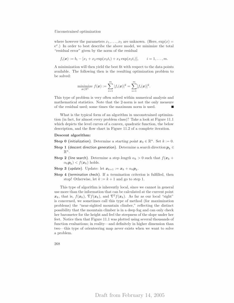
Draft from February 14, 2005
Unconstrained optimization
where however the parameters x1, . . . , x5 are unknown. (Here, exp(x) =ex.) In order to best describe the above model, we minimize the total“residual error” given by the norm of the residual
fi(x) := bi − [x1 + x2 exp(x3ti) + x4 exp(x5ti)], i = 1, . . . ,m.
A minimization will then yield the best fit with respect to the data pointsavailable. The following then is the resulting optimization problem tobe solved:
minimizex∈R5
f(x) :=
m∑
i=1
|fi(x)|2 =
m∑
i=1
[fi(x)]2.
This type of problem is very often solved within numerical analysis andmathematical statistics. Note that the 2-norm is not the only measureof the residual used; some times the maximum norm is used.
What is the typical form of an algorithm in unconstrained optimiza-tion (in fact, for almost every problem class)? Take a look at Figure 11.1which depicts the level curves of a convex, quadratic function, the belowdescription, and the flow chart in Figure 11.2 of a complete iteration.
Descent algorithm:
Step 0 (initialization). Determine a starting point x0 ∈ Rn. Set k := 0.
Step 1 (descent direction generation). Determine a search direction pk ∈Rn.
Step 2 (line search). Determine a step length αk > 0 such that f(xk +αkpk) < f(xk) holds.
Step 3 (update). Update: let xk+1 := xk + αkpk.
Step 4 (termination check). If a termination criterion is fulfilled, thenstop! Otherwise, let k := k + 1 and go to step 1.
This type of algorithm is inherently local, since we cannot in generaluse more than the information that can be calculated at the current pointxk, that is, f(xk), ∇f(xk), and ∇2f(xk). As far as our local “sight”is concerned, we sometimes call this type of method (for maximizationproblems) the “near-sighted mountain climber,” reflecting the distinctpossibility that the mountain climber is in a deep fog and can only checkher barometer for the height and feel the steepness of the slope under herfeet. Notice then that Figure 11.1 was plotted using several thousands offunction evaluations; in reality—and definitely in higher dimension thantwo—this type of orienteering map never exists when we want to solvea problem.
268
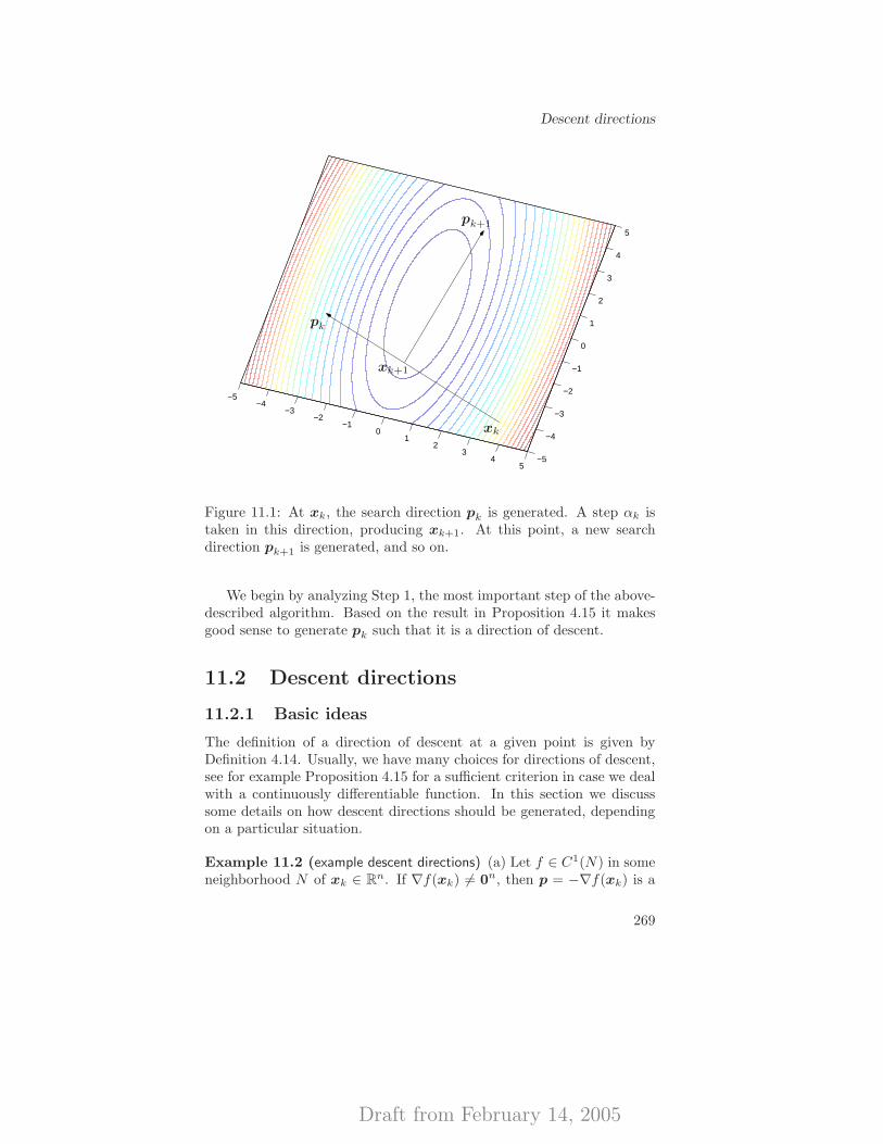
Draft from February 14, 2005
Descent directions
−5−4
−3−2
−10
12
34
5−5
−4
−3
−2
−1
0
1
2
3
4
5
pk
pk+1
xk
xk+1
Figure 11.1: At xk, the search direction pk is generated. A step αk istaken in this direction, producing xk+1. At this point, a new searchdirection pk+1 is generated, and so on.
We begin by analyzing Step 1, the most important step of the above-described algorithm. Based on the result in Proposition 4.15 it makesgood sense to generate pk such that it is a direction of descent.
11.2 Descent directions
11.2.1 Basic ideas
The definition of a direction of descent at a given point is given byDefinition 4.14. Usually, we have many choices for directions of descent,see for example Proposition 4.15 for a sufficient criterion in case we dealwith a continuously differentiable function. In this section we discusssome details on how descent directions should be generated, dependingon a particular situation.
Example 11.2 (example descent directions) (a) Let f ∈ C1(N) in someneighborhood N of xk ∈ Rn. If ∇f(xk) 6= 0n, then p = −∇f(xk) is a
269
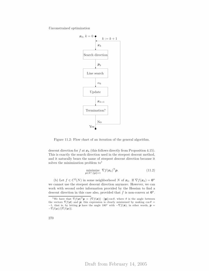
Draft from February 14, 2005
Unconstrained optimization
x0, k = 0
xk
Search direction
pk
Line search
αk
Update
Yes
No
xk+1
Termination?
k := k + 1
Figure 11.2: Flow chart of an iteration of the general algorithm.
descent direction for f at xk (this follows directly from Proposition 4.15).This is exactly the search direction used in the steepest descent method,and it naturally bears the name of steepest descent direction because itsolves the minimization problem to1
minimizep∈Rn:‖p‖=1
∇f(xk)Tp. (11.2)
(b) Let f ∈ C2(N) in some neighborhood N of xk. If ∇f(xk) = 0n
we cannot use the steepest descent direction anymore. However, we canwork with second order information provided by the Hessian to find adescent direction in this case also, provided that f is non-convex at 0n.
1We have that ∇f(x)Tp = ‖∇f(x)‖ · ‖p‖ cos θ, where θ is the angle betweenthe vectors ∇f(x) and p; this expression is clearly minimized by making cos θ =−1, that is, by letting p have the angle 180◦ with −∇f(x); in other words, p =−∇f(x)/‖∇f(x)‖.
270
Draft from February 14, 2005
Descent directions
Assume that ∇2f(xk) is not positive semidefinite (otherwise, xk is likelyto be at the locally optimal solution, see Theorem 4.16). If ∇2f(xk) isindefinite we call the stationary point xk a saddle point of f . Let p be aneigenvector corresponding to a negative eigenvalue of ∇2f(xk). Then,we call p a direction of negative curvature for f at xk, and it can bedemonstrated that it is a descent direction for f at this point [the proofis similar to the one of Proposition 4.15, but uses Taylor expansion (2.5)instead of (2.4)].
(c) Assume the conditions of (a), and let Q ∈ Rn×n be an arbitrarysymmetric, positive definite matrix. Then p = −Q∇f(xk) is a descentdirection for f at xk: ∇f(xk)Tp = −∇f(xk)TQ∇f(xk) < 0, due tothe positive definiteness of Q. (This is of course true only if xk is non-stationary, as assumed.)
Pre-multiplying by Q may be interpreted as a scaling of ∇f if wechoose a diagonal matrix Q; the use of more general matrices is of coursepossible and leads to exceptionally good computational results for cleverchoices of Q. Newton and quasi-Newton methods are based on con-structing directions in this way. Note that setting Q = In (the identitymatrix in Rn×n), we obtain the steepest descent direction.
To find some arbitrary direction of descent is not a very difficulttask as demonstrated by Example 11.2 [in fact, the situation when∇f(xk) = 0n appearing in (b) is quite an exotic one already, so typi-cally one can always use directions constructed in (a), or, more generally(c), as descent directions]. However, in order to secure the convergenceof numerical algorithms we must provide descent directions that “be-have well” numerically. Typical requirements, additional to the basicrequirement of being a direction of descent, are:
|∇f(xk)Tpk| ≥ s1‖∇f(xk)‖2, and ‖pk‖ ≤ s2‖∇f(xk)‖, (11.3)
or
− ∇f(xk)Tpk
‖∇f(xk)‖ · ‖pk‖≥ s1, and ‖pk‖ ≥ s2‖∇f(xk)‖, (11.4)
where s1, s2 > 0, and xk and pk are, respectively, iterates and searchdirections of some iterative algorithm. (In the next section, we shallprovide the basic form of an iterative algorithm.)
The purpose of these condition is to prevent the descent directions todeteriorate in quality in terms of always providing good enough descent.For example, the first condition in (11.3) states that if the directionalderivative of f tends to zero then it must be that the gradient of f alsotends to zero, while the second condition makes sure that a bad direction
271
Draft from February 14, 2005
Unconstrained optimization
in terms of the directional derivative is not compensated by the searchdirection becoming extremely long in norm. The first condition
− ∇f(xk)Tpk
‖∇f(xk)‖ · ‖pk‖≥ s1 (11.5)
in (11.4) is equivalent to the requirement that the cosine of the anglebetween −∇f(xk) and pk is positive and bounded away from zero bythe value of s1, that is, the angle must be acute and not too close toπ/2; this is another way of saying that the direction pk must be steepenough. The purpose of the second condition in (11.4) then is to ensurethat if the search direction vanishes then so does the gradient. Methodssatisfying (11.3), (11.4) are some times referred to as gradient related,since they cannot be based on search directions that are very far fromthose of the steepest descent method.
The choice
pk = −∇f(xk)
fulfills the above conditions, with s1 = s2 = 1.Another example is as follows: set pk = −Qk∇f(xk), where Qk ∈
Rn×n is a symmetric and positive definite matrix such that m‖s‖2 ≤sTQks ≤M‖s‖2, for all s ∈ Rn, holds. [All eigenvalues of Qk lie in theinterval [m,M ] ⊂ (0,∞).] Then, the requirement (11.3) is verified withs1 = m, s2 = M , and (11.4) holds with s1 = m/M , s2 = m.
11.2.2 Less basic ideas
What should a good descent direction do? Roughly speaking, it shouldprovide as large descent as possible, that is, minimize f(x + p) − f(x)over some large enough region of p around the origin. In principle, thisis the idea behind the optimization problem (11.2), because, accordingto (2.1), f(x + p) − f(x) ≈ ∇f(x)Tp.
Therefore, more insights into how the scaling matrices Q appearingin Example 11.2(c) should be constructed and, in particular, reasons whythe steepest descent direction is not a very wise choice, can be gained ifwe consider more general approximations than the ones given by (2.1).Namely, assume that f is C1 near x, and that for some positive definitematrix Q it holds that
f(x + p) − f(x) ≈ ϕx (p) = ∇f(x)Tp +1
2pTQ−1p. (11.6)
For example, if f ∈ C2, ∇2f(x) ≻ 0n×n, and assuming o(‖p‖2) ≈ 0[cf. (2.3)] we may use Q−1 = ∇2f(x).
272
Draft from February 14, 2005
Descent directions
Using the optimality conditions, we can easily check that the searchdirection defined in Example 11.2(c) is a solution to the following opti-mization problem:
minimizep∈Rn
ϕx (p), (11.7)
where ϕx (p) is defined by (11.6). The closer ϕx (p) approximates f(x +p) − f(x), the better the quality of search directions generated by Ex-ample 11.2(c) we can expect.
As was already mentioned, setting Q = In, which absolutely failsto take into account any information about f (that is, it is a “one-size-fits-all” approximation), gives us the steepest descent direction. (Casescan easily be constructed such that the algorithm converges extremelyslowly; convergence can actually be so bad that the authors of the book[BGLS03] decree that the steepest descent method should be forbidden!)On the other hand, the “best” second-order approximation is given bythe Taylor expansion (2.3), and therefore we would like to set Q =[∇2f(x)]−1; this is exactly the choice made in the Newton method.
Remark 11.3 (a motivation for the descent property in Newton’s method)Recall that the search direction in Newton’s method is based on the so-lution of the following linear system of equations: find p ∈ Rn suchthat
∇pϕx (p) = ∇f(x) + ∇2f(x)p = 0n.
Consider the case of n = 1. We should then solve
f ′(x) + f ′′(x)p = 0. (11.8)
It is obvious that unless f ′(x) = 0 (whence we are at a stationary pointand p = 0 solves the equation) we cannot solve (11.8) unless f ′′(x) 6= 0.Then, the solution p := −f ′(x)/f ′′(x) to (11.8) is well-defined. Wedistinguish between two cases:
(a) f ′′(x) > 0. In this case, the derivative of the second-order approx-imation p 7→ f ′(x)p+ 1
2f′′(x)p2 has a positive slope. Hence, if f ′(x) > 0
then p < 0, and if f ′(x) < 0 then instead p > 0 holds. In both cases,therefore, the directional derivative f ′(x)p < 0, that is, p is a descentdirection.
(b) f ′′(x) < 0. In this case, the derivative of the second-order approx-imation p 7→ f ′(x)p+ 1
2f′′(x)p2 has a negative slope. Hence, if f ′(x) > 0
then p > 0, and if f ′(x) < 0 then instead p < 0 holds. In both cases,therefore, the directional derivative f ′(x)p > 0, that is, p is an ascentdirection.
From this derivation it becomes clear that Newton’s method (forn = 1 it is often referred to as the Newton–Raphson method) (cf. Sec-tion 4.6.4.2) provides the same search direction regardless of whether
273

Draft from February 14, 2005
Unconstrained optimization
the optimization problem is a minimization or a maximization problem;the reason is that the search direction is based on the stationarity of thesecond-order approximation and not its minimization/maximization. Wealso see that the Newton direction p is a descent direction if the functionf is of the strictly convex type around x [that is, if f ′′(x) > 0], and anascent direction if it is of the strictly concave type around x [that is, iff ′′(x) < 0]. In other words, if the objective function is (strictly) convexor concave, the Newton equation will give us the right direction, if itgives us a direction at all. Translated to the case of n > 1, Newton’smethod acts as a descent method if the Hessian matrix ∇2f(x) is posi-tive definite, and as an ascent method if it is negative definite, which isappropriate.
An essential problem arises of course if the above-described is notwhat we want; for example, it may be that we are interested in max-imizing a function which is neither convex or concave, and around acurrent point the function is of strictly convex type (that is, the Hessianis positive definite). In this case the Newton direction will not point inan ascent direction, but instead the opposite. How to solve a problemwith a Newton-type method in a non-convex world is the main topic ofwhat follows. As always, we consider minimization to be the directionof interest for f .
So, why might one want to choose a matrix Q differing from the“best” choice [∇2f(x)]−1? There are several reasons:
Lack of positive definiteness The matrix ∇2f(x) might not be pos-itive definite. As a result, the problem (11.7) may even lack optimalsolutions and −[∇2f(x)]−1∇f(x) might in any case not be a directionof descent.
This problem can be cured by adding to ∇2f(x) a diagonal matrixE, so that ∇2f(x) + E is positive definite. For example, E = γIn, for−γ smaller than all the non-positive eigenvalues of ∇2f(x), may be usedbecause such a modification “shifts” the original eigenvalues of ∇2f(x)by γ > 0. The value of γ needed will automatically be found whensolving the “Newton equation” ∇2f(x)p = −∇f(x), since eigenvaluesof ∇2f(x) are pivot elements in Gaussian-elimination procedures. Thismodification bears the name Levenberg–Marquardt.
[Note: as γ becomes large, p resembles more and more the steepestdescent direction.]
Lack of enough differentiability The function f might not be twicedifferentiable, or the matrix of second derivatives might be too costly tocompute/evaluate.
274
Draft from February 14, 2005
Descent directions
Either being the case, quasi-Newton methods approximate the New-ton equation by replacing ∇2f(xk) with a matrix Bk that is cheaper tocompute, typically by only using values of ∇f at the current and someprevious points.
Using a first-order Taylor expansion (2.1) for ∇f(xk) we know that
∇2f(xk)(xk − xk−1) ≈ ∇f(xk) −∇f(xk−1),
so the matrix Bk is taken to satisfy the similar system
Bk(xk − xk−1) = ∇f(xk) −∇f(xk−1).
[Note: For n = 1, this corresponds to the secant method, in which atiteration k we approximate the second derivative as
f ′′(xk) ≈ f ′(xk) − f ′(xk−1)
xk − xk−1
in Newton’s method.]However, the matrix Bk (that is, n2 unknowns) is under-determined
in these n equations, so additional requirements, such as ones that makesure that Bk is symmetric and positive definite, result in particularquasi-Newton methods. Typically, starting from B0 = In, Bk+1 iscalculated from Bk using a rank-one or rank-two update; in particular,this allows us to update the factorization of Bk to efficiently obtain thefactorization of Bk+1 using standard algorithms in linear algebra.
There are infinitely many choices that may be used, and the following(called the Broyden–Fletcher–Goldfarb–Shanno, or BFGS, method afterthe original publications [Bro70, Fle70, Gol70, Sha70]) is considered tobe the most effective:
Bk+1 = Bk − (Bksk)(Bksk)T
sTk Bksk
+ykyT
k
yTk sk
,
where sk = xk+1 − xk, and yk = ∇f(xk+1) − ∇f(xk). Interestinglyenough, should f be quadratic, Bk will be identical to the Hessian of fafter a finite number of steps (namely, n).
Quasi-Newton methods with various update rules for Bk are verypopular for unconstrained optimization.
See Section 11.9 for more details on quasi-Newton methods.
Computational burden The solution of a linear system Bkpk =−∇f(xk), or, which is the same if we identify Q−1 = Bk, finding theoptimum of (11.7), may be too costly. This is exactly the situation when
275
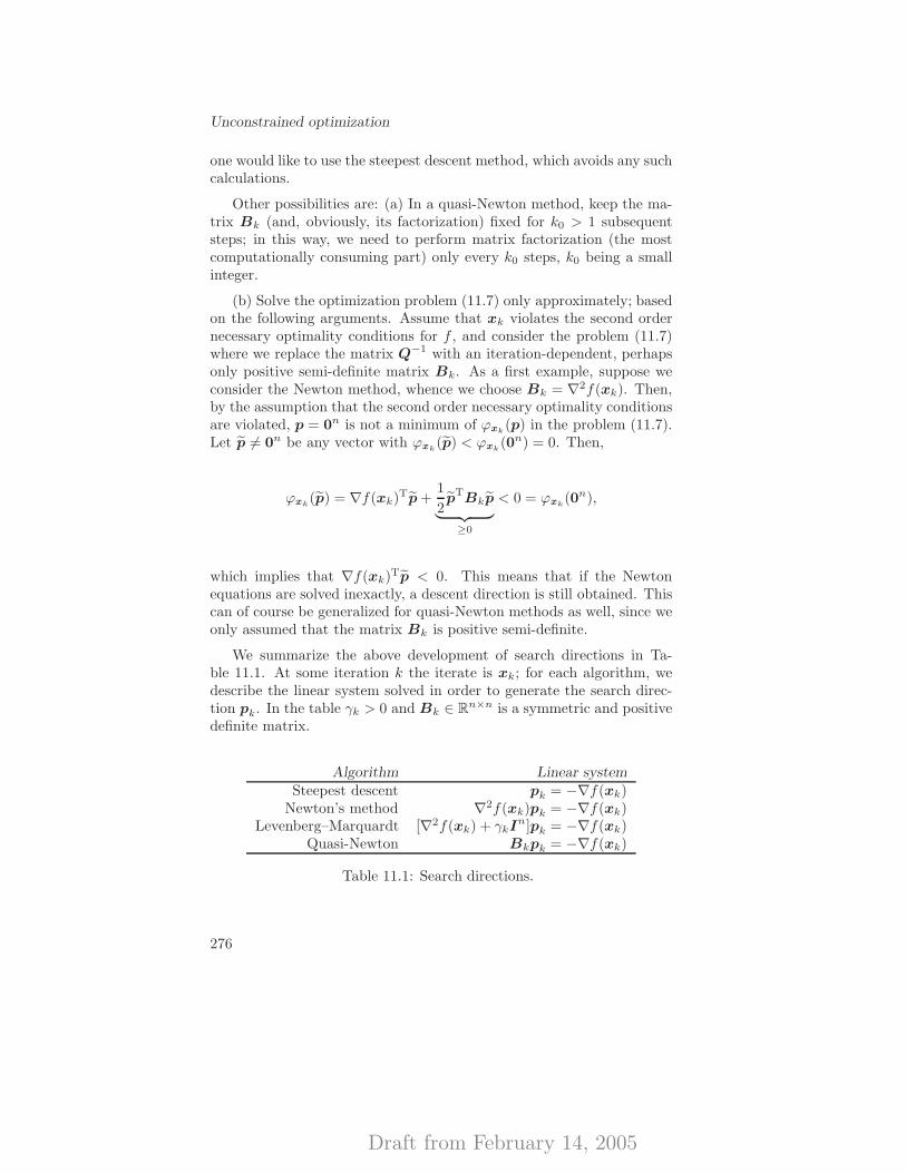
Draft from February 14, 2005
Unconstrained optimization
one would like to use the steepest descent method, which avoids any suchcalculations.
Other possibilities are: (a) In a quasi-Newton method, keep the ma-trix Bk (and, obviously, its factorization) fixed for k0 > 1 subsequentsteps; in this way, we need to perform matrix factorization (the mostcomputationally consuming part) only every k0 steps, k0 being a smallinteger.
(b) Solve the optimization problem (11.7) only approximately; basedon the following arguments. Assume that xk violates the second ordernecessary optimality conditions for f , and consider the problem (11.7)where we replace the matrix Q−1 with an iteration-dependent, perhapsonly positive semi-definite matrix Bk. As a first example, suppose weconsider the Newton method, whence we choose Bk = ∇2f(xk). Then,by the assumption that the second order necessary optimality conditionsare violated, p = 0n is not a minimum of ϕxk
(p) in the problem (11.7).Let p 6= 0n be any vector with ϕxk
(p) < ϕxk(0n) = 0. Then,
ϕxk(p) = ∇f(xk)Tp +
1
2p
TBkp
︸ ︷︷ ︸≥0
< 0 = ϕxk(0n),
which implies that ∇f(xk)Tp < 0. This means that if the Newtonequations are solved inexactly, a descent direction is still obtained. Thiscan of course be generalized for quasi-Newton methods as well, since weonly assumed that the matrix Bk is positive semi-definite.
We summarize the above development of search directions in Ta-ble 11.1. At some iteration k the iterate is xk; for each algorithm, wedescribe the linear system solved in order to generate the search direc-tion pk. In the table γk > 0 and Bk ∈ Rn×n is a symmetric and positivedefinite matrix.
Algorithm Linear systemSteepest descent pk = −∇f(xk)
Newton’s method ∇2f(xk)pk = −∇f(xk)Levenberg–Marquardt [∇2f(xk) + γkIn]pk = −∇f(xk)
Quasi-Newton Bkpk = −∇f(xk)
Table 11.1: Search directions.
276
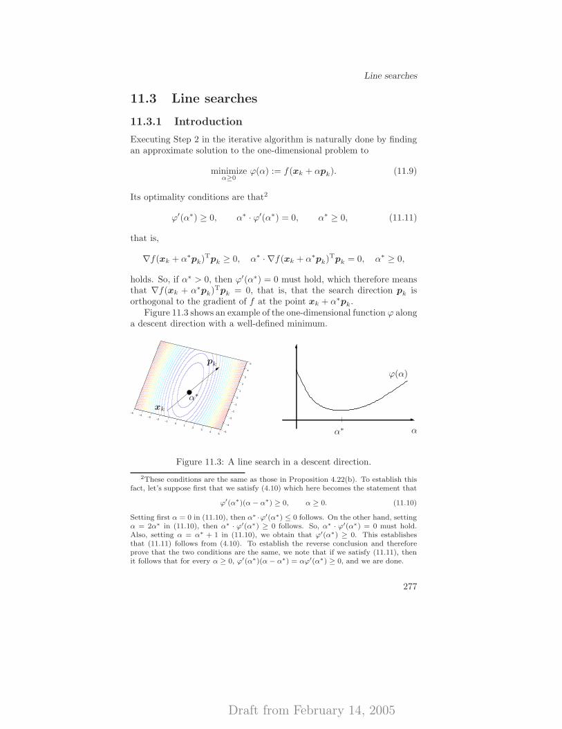
Draft from February 14, 2005
Line searches
11.3 Line searches
11.3.1 Introduction
Executing Step 2 in the iterative algorithm is naturally done by findingan approximate solution to the one-dimensional problem to
minimizeα≥0
ϕ(α) := f(xk + αpk). (11.9)
Its optimality conditions are that2
ϕ′(α∗) ≥ 0, α∗ · ϕ′(α∗) = 0, α∗ ≥ 0, (11.11)
that is,
∇f(xk + α∗pk)Tpk ≥ 0, α∗ · ∇f(xk + α∗pk)Tpk = 0, α∗ ≥ 0,
holds. So, if α∗ > 0, then ϕ′(α∗) = 0 must hold, which therefore meansthat ∇f(xk + α∗pk)Tpk = 0, that is, that the search direction pk isorthogonal to the gradient of f at the point xk + α∗pk.
Figure 11.3 shows an example of the one-dimensional function ϕ alonga descent direction with a well-defined minimum.
−5−4
−3−2
−10
12
34
5−5
−4
−3
−2
−1
0
1
2
3
4
5
α∗
α∗
α
pk
xk
ϕ(α)
Figure 11.3: A line search in a descent direction.
2These conditions are the same as those in Proposition 4.22(b). To establish thisfact, let’s suppose first that we satisfy (4.10) which here becomes the statement that
ϕ′(α∗)(α − α∗) ≥ 0, α ≥ 0. (11.10)
Setting first α = 0 in (11.10), then α∗ ·ϕ′(α∗) ≤ 0 follows. On the other hand, settingα = 2α∗ in (11.10), then α∗ · ϕ′(α∗) ≥ 0 follows. So, α∗ · ϕ′(α∗) = 0 must hold.Also, setting α = α∗ + 1 in (11.10), we obtain that ϕ′(α∗) ≥ 0. This establishesthat (11.11) follows from (4.10). To establish the reverse conclusion and thereforeprove that the two conditions are the same, we note that if we satisfy (11.11), thenit follows that for every α ≥ 0, ϕ′(α∗)(α − α∗) = αϕ′(α∗) ≥ 0, and we are done.
277
Draft from February 14, 2005
Unconstrained optimization
In the quest for a stationary point it is of relatively minor importanceto do a line search accurately—the stationary point is most probablynot situated somewhere along that half-line anyway. Therefore, mostline search strategies used in practice are approximate. It should also benoted that if the function f is non-convex then so is probably the casewith ϕ as well, and globally minimizing a non-convex function is difficulteven in one variable.
11.3.2 Approximate line search strategies
First, we consider the case where f is quadratic; this is the only generalcase where an accurate line search is practical.
Let f(x) = (1/2)xTQx−qTx+a, where the dimensions of Q ∈ Rn×n,q ∈ Rn and a ∈ R are given data. Suppose we wish to minimize thefunction ϕ for this special case. Then, we can solve for ϕ′(α∗) = 0analytically:
ϕ′(α) = ∇f(x + αp)Tp
= [Q(x + αp) − q]Tp
= αpTQp − (q − Qx)Tp
= 0
⇔α = (q − Qx)Tp/pTQp.
Let’s check the validity and meaning of this solution. We suppose nat-urally that p is a descent direction, whence ϕ′(0) = (q − Qx)Tp < 0holds. Therefore, if Q is positive definite, we are guaranteed that thevalue of α will be positive.
Among the classic approximate line searches we mention very brieflythe following:
Interpolation Take f(xk),∇f(xk),∇f(xk)Tpk to model a quadraticfunction approximating f along pk. Minimize it by using the an-alytic formula above.
Newton’s method Repeat the improvements gained from a quadraticapproximation: α := α− ϕ′(α)/ϕ′′(α).
Golden Section The golden section method is a derivative-free methodfor minimizing unimodal functions.3 The method reduces an in-
3ϕ is unimodal in an interval [a, b] of R if it has a unique global minimum in[a, b], and is strictly increasing to the left as well as to the right of the minimum.This notion is equivalent to that of ϕ having a minimum over [a, b] and being strictlyquasi-convex there.
278
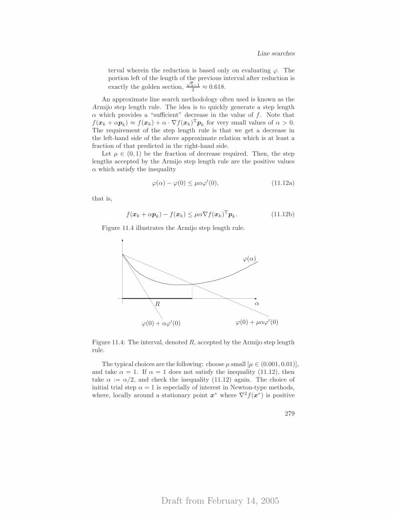
Draft from February 14, 2005
Line searches
terval wherein the reduction is based only on evaluating ϕ. Theportion left of the length of the previous interval after reduction is
exactly the golden section,√
5−12 ≈ 0.618.
An approximate line search methodology often used is known as theArmijo step length rule. The idea is to quickly generate a step lengthα which provides a “sufficient” decrease in the value of f . Note thatf(xk + αpk) ≈ f(xk) + α · ∇f(xk)Tpk for very small values of α > 0.The requirement of the step length rule is that we get a decrease inthe left-hand side of the above approximate relation which is at least afraction of that predicted in the right-hand side.
Let µ ∈ (0, 1) be the fraction of decrease required. Then, the steplengths accepted by the Armijo step length rule are the positive valuesα which satisfy the inequality
ϕ(α) − ϕ(0) ≤ µαϕ′(0), (11.12a)
that is,
f(xk + αpk) − f(xk) ≤ µα∇f(xk)Tpk. (11.12b)
Figure 11.4 illustrates the Armijo step length rule.
αR
ϕ(0) + αϕ′(0) ϕ(0) + µαϕ′(0)
ϕ(α)
Figure 11.4: The interval, denoted R, accepted by the Armijo step lengthrule.
The typical choices are the following: choose µ small [µ ∈ (0.001, 0.01)],and take α = 1. If α = 1 does not satisfy the inequality (11.12), thentake α := α/2, and check the inequality (11.12) again. The choice ofinitial trial step α = 1 is especially of interest in Newton-type methods,where, locally around a stationary point x∗ where ∇2f(x∗) is positive
279
Draft from February 14, 2005
Unconstrained optimization
definite, local convergence with step length one is guaranteed. (See alsoSection 4.6.4.2.)
In theory, however, we can select any starting guess α > 0 and anyfraction β ∈ (0, 1) in place of the choice β = 1
2 made above.The Armijo condition is satisfied for any sufficiently small step length,
provided that the direction pk is a direction of descent. (See Exer-cise 11.1.) In itself it therefore does not guarantee that the next iterateis much better in terms of the objective value than the current one.Often, therefore, it is combined with a condition such that
|ϕ′(αk)| ≤ η|ϕ′(0)|,
that is,|∇f(xk + αpk)Tpk| ≤ η|∇f(xk)Tpk|,
holds for some η ∈ [0, 1). This is called the Wolfe condition. A relaxedcondition, the weak Wolfe condition, of the form
ϕ′(αk) ≥ ηϕ′(0)
is often preferred, since the former takes more computations to fulfill.The choice 0 < µ < η < 1 leads to interesting descent algorithms whenthe Armijo and weak Wolfe conditions are combined, and it is possible(Why?) to find positive step lengths that satisfy these two conditionsprovided only that f is bounded from below and pk is a direction ofdescent.
11.4 Convergent algorithms
11.4.1 Basic convergence results
This section presents two basic convergence results for descent methodsunder different step length rules.
Theorem 11.4 (convergence of a gradient related algorithm) Suppose thatf ∈ C1, and that for the starting point x0 it holds that the level setlevf (f(x0)) = {x ∈ Rn | f(x) ≤ f(x0) } is bounded. Consider theiterative algorithm defined by the description in Section 11.1. In thisalgorithm, suppose we make the following choices that hold for eachiteration k:� the search direction pk satisfies the sufficient descent condition
(11.4);� ‖pk‖ ≤M , where M is some positive constant; and
280
Draft from February 14, 2005
Convergent algorithms� the Armijo step length rule (11.12) is used.
Then, the sequence {xk} is bounded, the sequence {f(xk)} is descending,lower bounded and therefore has a limit, and every limit point of {xk}is stationary.
Proof. That {xk} is bounded follows since the algorithm, as stated, isa descent method, and we assumed that the level set of f at the startingpoint is bounded; therefore, the sequence of iterates must remain in thatset and is therefore bounded.
The rest of the proof is by contradiction. Suppose that x is a limitpoint of {xk} but that ∇f(x) 6= 0n. It is clear that by the continuityof f , the whole sequence {f(xk)} converges to the value f(x). Hence,{f(xk) − f(xk+1)} → 0 must hold. According to the Armijo rule, then,{αk∇f(xk)Tpk} → 0. Here, there are two possibilities. Suppose that{αk} → 0. Then, there must be some iteration k after which the initialstep length is not accepted by the inequality (11.12), and therefore,
f(xk + (αk/β)pk) − f(xk) > µ(αk/β)∇f(xk)Tpk, k ≥ k.
Dividing both sides by 2αk we obtain in the limit that
∇f(x)Tp∞ ≥ 0,
for any limit point p∞ of the bounded sequence {pk}. But in the limit ofthe inequality (11.4) we then clearly reach a contradiction. So, in fact,we must have that {αk} 6→ 0. In this case, then, by the above we musthave that {∇f(xk)Tpk} → 0 holds, so by letting k tend to infinity weobtain that
∇f(x)Tp∞ = 0,
which again produces a contradiction to the initial claim because of(11.4). We conclude that ∇f(x) = 0n must therefore hold, and we aredone.
We note that since the resulting step length from an exact line searchin particular must satisfy the Armijo rule (11.12), the above proof can beused to also establish the result of such a modification of the algorithmgiven in the theorem. We further note that there is no guarantee thatthe limit points x is a local minimum; it may also be a saddle point,that is, a stationary point where ∇2f(x) is indefinite, if it exists.
Another result is cited below from [BeT00]. It allows the Armijo steplength rule to be replaced by a much simpler type of step length rulewhich is also used to minimize a class of non-differentiable functions (cf.Section 6.5). The proof requires the addition of a technical assumption:
281
Draft from February 14, 2005
Unconstrained optimization
Definition 11.5 (Lipschitz continuity) A C1 function f : Rn → R issaid to have a Lipschitz continuous gradient mapping on Rn if thereexists a scalar L ≥ 0 such that
‖∇f(x) −∇f(y)‖ ≤ L‖x− y‖ (11.13)
holds for every x,y ∈ Rn.
Check that the gradient of a C2 function f is Lipschitz continuouswhenever its Hessian matrix is bounded over Rn.
Theorem 11.6 (on the convergence of gradient related methods) Let f ∈C1. Consider the sequence {xk} generated by the formula xk+1 :=xk + αkpk. Suppose that:� ∇f is Lipschitz continuous on Rn;� c1‖∇f(xk)‖2 ≤ −∇f(xk)Tpk, c1 > 0;� ‖pk‖ ≤ c2‖∇f(xk)‖, c2 > 0;� αk > 0 satisfies that {αk} → 0 and limk→∞
∑ks=1 αs = ∞.
Then, either limk→∞ f(xk) = −∞ holds, or limk→∞ f(xk) = f andlimk→∞ ∇f(xk) = 0n holds.
In Theorem 11.4 convergence is only established in terms of thatof subsequences, and the requirements include a level set boundednesscondition that can be difficult to check. A strong convergence result isavailable for the case of convex functions f whenever we know that thereexists at least one optimal solution. It follows readily from Theorem 12.4on the gradient projection method for differentiable optimization overconvex sets, whence we will not establish it here. In fact, for the specialcase of the steepest descent algorithm, we have already seen such a resultin Theorem 6.23 for possibly even non-differentiable convex functions.
Theorem 11.7 (convergence of gradient related algorithms under convexity)Suppose the function f ∈ C1 on Rn. Suppose further that f is convexand that the problem (11.1) has at least one optimal solution. Considerthe iterative algorithm defined by the description in Section 11.1, underthe three additional conditions stated in Theorem 12.4, and where thestep length αk is determined by the Armijo step length rule. Then, thesequence {xk} converges to some optimal solution to (11.1).
We have so far neglected Step 4 in the algorithm description in Sec-tion 11.1 in that we assume in the above results that the sequence {xk}is infinite. A termination criterion must obviously be applied if we areto obtain a result in a finite amount of time. This is the subject of thenext section.
282
Draft from February 14, 2005
Finite termination criteria
11.5 Finite termination criteria
As noted above, convergence to a stationary point is only asymptotic.How does one know when it is wise to terminate? A criterion based onlyon a small size of ‖∇f(xk)‖ is no good—why? Because we compare with0!
The recommendation is the combination of the following:
1. ‖∇f(xk)‖ ≤ ε1(1 + |f(xk)|), ε1 > 0 small;
2. f(xk−1) − f(xk) ≤ ε2(1 + |f(xk)|), ε2 > 0 small; and
3. ‖xk−1 − xk‖ ≤ ε3(1 + ‖xk‖), ε3 > 0 small.
The right-hand sides are constructed in order to eliminate some of thepossible influence of bad scaling of the variable values, of the objectivefunction, and of the gradient, and also of the possibility that some valuesare zero at the optimum solution.
Notice that using the criterion 2. only might mean that we terminatetoo soon if f is very flat; similarly with 3., we terminate prematurely if fis extremely steep around the stationary point we are approaching. Thepresence of the constant 1 is to remove the dependency of the criterionon the absolute values of f and xk, particularly if they are near zero.
We also note that using the ‖ · ‖2 norm may not be good when n isvery large: suppose that ∇f(x) = (γ, γ, . . . , γ)T = γ(1, 1, . . . , 1)T. Then,‖∇f(x)‖2 =
√n · γ, which illustrates that the dimension of the problem
may enter the norm. Better then is to use the ∞-norm: ‖∇f(x)‖∞ :=
max1≤j≤n |∂f(x)∂xj
| = |γ|, which does not depend on n.
Norms have other bad effects. Suppose that
xk−1 = (1.44453, 0.00093, 0.0000079)T,
xk = (1.44441, 0.00012, 0.0000011)T;
then,
‖xk−1 − xk‖∞ = ‖(0.00012, 0.00081, 0.0000068)T‖∞= 0.00081.
Here, the termination test would possibly pass, although the number ofsignificant digits is very small (the first significant digit is still changing!)Norms emphasize larger elements, so small ones may have bad relativeaccuracy. This is a case where scaling is needed.
Suppose we know that x∗ = (1, 10−4, 10−6)T. If, by transformingthe space, we obtain that the optimal solution is x
∗ = (1, 1, 1)T, then
283
Draft from February 14, 2005
Unconstrained optimization
the same relative accuracy would be possible to achieve for all variables.Let then
x =
1 0 00 104 00 0 106
︸ ︷︷ ︸D
x.
Let
f(x) :=1
2xTQx − cTx,
Q :=
8 3 · 104 03 · 104 4 · 108 1010
0 1010 6 · 1012
,
c :=
118 · 104
7 · 106
.
Hence, x∗ = Q−1c = (1, 10−4, 10−6)T.
With x = Dx, we get the transformed problem to minimize f(x) :=12 x
T(D−1QD−1)x − (D−1c)Tx, with
D−1QD−1 =
8 3 03 4 10 1 6
; D−1c =
1187
,
and x∗ = (1, 1, 1)T. Notice the change in condition number in the ma-trix!
The steepest descent algorithm takes only ∇f(x) into account, not∇2f(x). Therefore, if the problem is badly scaled, it will suffer from apoor convergence behaviour. Introducing elements of ∇2f(x) into thesearch direction helps in this respect. This is the precisely the effect ofusing second-order (Newton-type) algorithms.
11.6 A comment on non-differentiability
The subject of non-differentiable optimization will not be taken up ingenerality here; it has been analyzed more fully for Lagrangian dualproblems in Chapter 6. The purpose of this discussion is to explain, bymeans of an example, that things can go terribly wrong if we apply meth-ods for the minimization of differentiable function when the function isnon-differentiable.
284
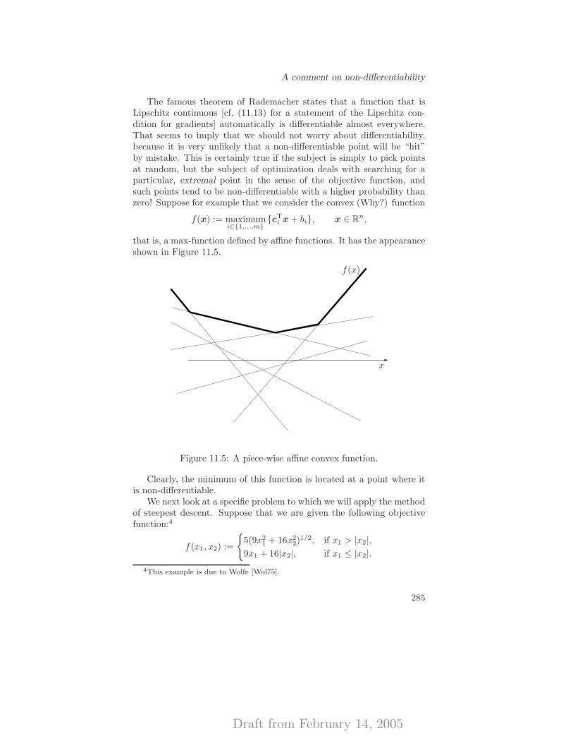
Draft from February 14, 2005
A comment on non-differentiability
The famous theorem of Rademacher states that a function that isLipschitz continuous [cf. (11.13) for a statement of the Lipschitz con-dition for gradients] automatically is differentiable almost everywhere.That seems to imply that we should not worry about differentiability,because it is very unlikely that a non-differentiable point will be “hit”by mistake. This is certainly true if the subject is simply to pick pointsat random, but the subject of optimization deals with searching for aparticular, extremal point in the sense of the objective function, andsuch points tend to be non-differentiable with a higher probability thanzero! Suppose for example that we consider the convex (Why?) function
f(x) := maximumi∈{1,...,m}
{cTi x + bi}, x ∈ Rn,
that is, a max-function defined by affine functions. It has the appearanceshown in Figure 11.5.
f(x)
x
Figure 11.5: A piece-wise affine convex function.
Clearly, the minimum of this function is located at a point where itis non-differentiable.
We next look at a specific problem to which we will apply the methodof steepest descent. Suppose that we are given the following objectivefunction:4
f(x1, x2) :=
{5(9x2
1 + 16x22)
1/2, if x1 > |x2|,9x1 + 16|x2|, if x1 ≤ |x2|.
4This example is due to Wolfe [Wol75].
285
Draft from February 14, 2005
Unconstrained optimization
For x1 > 0, f is actually continuously differentiable! It is also convex,by the way. (Checking these facts is a nice exercise.)
If we start at a point x0 anywhere in the region x1 > |x2| > (9/16)2|x1|then we obtain a sequence generated by steepest descent with exact linesearches that defines a polygonal path with successive orthogonal seg-ments, converging to x = (0, 0)T.
But x is not a stationary point! What is wrong here is that thegradients calculated say very little about the behaviour of f at the limitpoint (0, 0)T. In fact, f is non-differentiable there. In this example, it infact holds that limx1→−∞ f(x1, 0) = −∞, so steepest descent has failedmiserably.
In order to resolve this problem, we need to take some necessarymeasures:
a) At a non-differentiable point, ∇f(x) must be replaced by a well-defined extension. Usually, we would replace it with a subgradient,that is, one of the vectors that define a supporting hyperplane tothe graph of f . At x it is the set defined by the convex hull of thetwo vectors (9, 16)T and (9,−16)T.
b) The step lengths must be chosen differently; exact line searches areclearly forbidden, as we have just seen.
From such considerations, we may develop algorithms that find op-tima to non-differentiable problems. They are referred to a subgradientalgorithms, and are analyzed in Section 6.5.
11.7 Trust region methods
Trust region methods use quadratic models like Newton-type methodsdo, but avoid a line search by instead bounding the length of the searchdirection, thereby also influencing its direction.
Let ψk(p) := f(xk) + ∇f(xk)Tp + 12pT∇2f(xk)p. We say that the
model ψk is trusted in a neighbourhood of xk : ‖p‖ ≤ ∆k. The useof this bound is apparent when ∇2f(xk) is not positive semi-definite.The problem to minimize ψk(p) subject to ‖p‖ ≤ ∆k can be solved(approximately) quite efficiently. The idea is that when ∇2f(xk) isbadly conditioned, the value of ∆k should be kept low—thus turningthe algorithm more into a steepest descent-like method [recall (11.2)]—while if ∇2f(xk) is well conditioned, ∆k should become large and allowunit steps to be taken. (Prove that the direction of pk tends to that ofthe steepest descent method when ∆k → 0!)
286
Draft from February 14, 2005
Conjugate gradient methods
The vector pk which solves the trust region problem satisfies [∇2f(xk)+γkIn]pk = −∇f(xk) for some γk ≥ 0 such that ∇2f(xk) + γIn is pos-itive semidefinite. The bounding enforced hence has a similar effect tothat of the Levenberg–Marquardt strategy discussed in Section 11.2.2.Provided that the value of ∆k is low enough, f(xk + pk) < f(xk) holds.Even if ∇f(xk) = 0n holds, f(xk + pk) < f(xk) still holds, if ∇2f(xk)is not positive definite. So, progress is made also from stationary pointsif they are saddle points or local maxima. The robustness and strongconvergence characteristics have made trust region methods quite pop-ular.
The update of the trust region size is based on the following measureof similarity between the model ψk and f : Let
ρk =f(xk) − f(xk + pk)
f(xk) − ψk(pk)=
actual reduction
predicted reduction.
If ρk ≤ µ let xk+1 = xk (unsuccessful step), elsexk+1 = xk + pk (successful step).
The value of ∆k is updated in the following manner, depending onthe value of ρk:
µ <ρk ≤ µ =⇒ ∆k+1 = 1
2∆k,ρk < η =⇒ ∆k+1 = ∆k,ρk ≥ η =⇒ ∆k+1 = 2∆k.
Here, 0 < µ < η < 1, with typical choices being µ = 14 and η = 3
4 ; µ is abound used for deciding when the model can or cannot be trusted evenwithin the region given, while η is used for deciding when the model isgood enough to be used in a larger neighbourhood.
Figure 11.6 illustrates the trust region subproblem.
11.8 Conjugate gradient methods
When applied to nonlinear unconstrained optimization problems conju-gate direction methods are methods intermediate between the steepestdescent and Newton methods. The motivation behind them is simi-lar to that for quasi-Newton methods: accelerating the steepest descentmethod but avoid the evaluation, storage and inversion of the Hessianmatrix. They are analyzed for quadratic problems only; extensions tonon-quadratic problems utilize that close to an optimal solution everyproblem is nearly quadratic. Even for non-quadratic problems, the lastfew decades of developments have resulted in conjugate direction meth-ods being one of the most efficient general methodologies available.
287
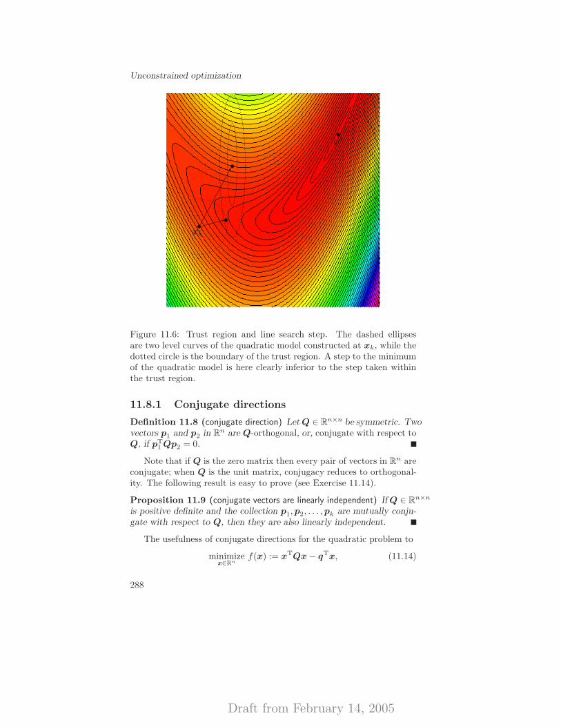
Draft from February 14, 2005
Unconstrained optimization
xk
x∗
Figure 11.6: Trust region and line search step. The dashed ellipsesare two level curves of the quadratic model constructed at xk, while thedotted circle is the boundary of the trust region. A step to the minimumof the quadratic model is here clearly inferior to the step taken withinthe trust region.
11.8.1 Conjugate directions
Definition 11.8 (conjugate direction) Let Q ∈ Rn×n be symmetric. Twovectors p1 and p2 in Rn are Q-orthogonal, or, conjugate with respect toQ, if pT
1 Qp2 = 0.
Note that if Q is the zero matrix then every pair of vectors in Rn areconjugate; when Q is the unit matrix, conjugacy reduces to orthogonal-ity. The following result is easy to prove (see Exercise 11.14).
Proposition 11.9 (conjugate vectors are linearly independent) If Q ∈ Rn×n
is positive definite and the collection p1,p2, . . . ,pk are mutually conju-gate with respect to Q, then they are also linearly independent.
The usefulness of conjugate directions for the quadratic problem to
minimizex∈Rn
f(x) := xTQx − qTx, (11.14)
288
Draft from February 14, 2005
Conjugate gradient methods
where from now on Q is symmetric and positive definite, is clear from thefollowing identification: if the vectors p0,p1, . . . ,pn−1 are Q-orthogonal,then Proposition 11.9 implies that there exists a vector w ∈ Rn with
x∗ =n−1∑
i=0
wipi; (11.15)
multiplying the equation by Q and scalar multiplying the result by pi
yields
wi =pT
i Qx∗
pTi Qpi
=pT
i q
pTi Qpi
, (11.16)
so that
x∗ =
n−1∑
i=0
pTi q
pTi Qpi
pi. (11.17)
Two ideas are embedded in (11.17): by selecting a proper set of orthog-onal vectors pi, and by taking the appropriate scalar product all termsbut i in (11.15) disappear. This could be accomplished by using any n or-thogonal vectors, but (11.16) shows that by making them Q-orthogonalwe can express wi without knowing x∗.
11.8.2 Conjugate direction methods
The corresponding conjugate direction method for (11.14) is given by
xk+1 = xk + αkpk, k = 0, . . . , n− 1,
where x0 ∈ Rn is arbitrary and αk is obtained from an exact line searchwith respect to f in the direction of pk; cf. (11.9). The principal resultabout conjugate direction methods is that successive iterates minimizef over a progressively expanding linear manifold, or subspace, that afterat most n iterations includes the minimizer of f over Rn. In other words,defining
Mk := {x ∈ Rn | x = x0 + subspace spanned by {p0,p1, . . . ,pn−1} },
{xk+1} = argminimumx∈Mk
f(x) (11.18)
holds.To show this, note that by the exact line search rule, for all i,
∂f(xi + αpi)
∂α
∣∣∣∣α=αi
= ∇f(xi+1)Tpi = 0.
289
Draft from February 14, 2005
Unconstrained optimization
and for i = 0, 1, . . . , k − 1,
∇f(xk+1)Tpi = (Qxk+1 − q)Tpi
=
xi+1 +
k∑
j=i+1
αjpj
T
Qpi − qTpi
= xTi+1Qpi − qTpi
= ∇f(xi+1)Tpi,
where we used the conjugacy of pi and pj , j 6= i. Hence, ∇f(xk+1)Tpi =
0 for every i = 0, 1, . . . , k, which verifies (11.18).It is easy to get a picture of what is going on if we look at the case
where Q = In and q = 0n; since the level curves are circles, minimizingover the n coordinates one by one gives us x∗ in n steps; in each iterationwe also identify the optimal value of one of the variables. Conjugatedirections in effect does this, although in a transformed space.5
The discussion so far has been based on an arbitrary selection ofconjugate directions. There are many ways in which conjugate direc-tions could be generated. For example, we could let the vectors pi,i = 0, . . . , n − 1 be defined by the eigenvectors of Q, as they are mutu-ally orthogonal as well as conjugate with respect to Q. (Why?) Such aprocedure would however be too costly in large-scale applications. Theremarkable feature of the conjugate gradient method to be presented be-low is that the new vector pk can be generated directly from the vectorpk−1—there is no need to remember any of the vectors p0, . . . ,pk−2, andyet pk will be conjugate to them all.
11.8.3 Generating conjugate directions
Given a set of linearly independent vectors d0,d1, . . . ,dk we can generatea set of mutually Q-orthogonal vectors p0,p1, . . . ,pk such that they spanthe same subspace, by using the Gram–Schmidt procedure. We start therecursion with p0 = d0. Suppose that for i < k we have d0,d1, . . . ,di
such that they span the same subspace as p0,p1, . . . ,pi. Then, let pi+1
take the following form:
pi+1 = di+1 +
i∑
m=0
ci+1m dm,
5Compare this to Newton’s method as applied to the problem (11.14); its conver-gence in one step corresponds to the convergence in one step of the steepest descentmethod when we first have performed a coordinate transformation such that the levelcurves become circular.
290
Draft from February 14, 2005
Conjugate gradient methods
choosing ci+1m so that pi+1 is Q-orthogonal to p0,p1, . . . ,pi. This will
be true if, for j = 0, 1, . . . , i,
pTi+1Qpj = dT
i+1Qpj +
(i∑
m=0
ci+1m pm
)T
Qpj = 0.
Since p0,p1, . . . ,pi are Q-orthogonal we have that pTmQpj = 0 if m 6= j,
so
ci+1j = −dT
i+1Qpj
pTj Qpj
, j = 0, 1, . . . , i.
Some notes are in order regarding the above development: (a) itholds that pT
j Qpj 6= 0. (b) pi+1 6= 0n; otherwise it would contradictthe linear independence of d0,d1, . . . ,dk. (c) Finally, di+1 lies in thesubspace spanned by p0,p1, . . . ,pi+1, while pi+1 lies in the subspacespanned by d0,d1, . . . ,di+1, since these vectors span the same space.Therefore, the subspace identification above is true for i + 1, and wehave shown that the Gram–Schmidt procedure has the property askedfor.
11.8.4 Conjugate gradient methods
The conjugate gradient method applies the above Gram–Schmidt proce-dure to the vectors
d0 = −∇f(x0), d1 = −∇f(x1), . . . , dn−1 = −∇f(xn−1).
Thus, the conjugate gradient method is to take xk+1 = xk + αkpk,where αk is determined through an exact line search and pk is ob-tained through step k of the Gram–Schmidt procedure to the vectordk = −∇f(xk) and the previous vectors p0,p1, . . . ,pk−1. In particular,
pk = −∇f(xk) +k−1∑
j=0
∇f(xk)TQpj
pTj Qpj
pj . (11.19)
It holds that p0 = −∇f(x0), and termination occurs at step k if ∇f(xk) =0n; the latter happens exactly when pk = 0n. (Why?)
[Note: the search directions are based on negative gradients of f ,
−∇f(xk) = q − Qxk,
which are identical to the residual in the linear system
Qx = q
291
Draft from February 14, 2005
Unconstrained optimization
that identifies the optimal solution to (11.14).]The formula (11.19) can in fact be simplified. The reason is that,
because of the successive optimization over subspaces, ∇f(xk) is or-thogonal to the subspace spanned by p0,p1, . . . ,pk−1.
Proposition 11.10 (the conjugate gradient method) The directions ofthe conjugate gradient method are generated by
p0 = −∇f(x0); (11.20a)
pk = −∇f(xk) + βkpk−1, k = 1, 2, . . . , n− 1, (11.20b)
where
βk =∇f(xk)T∇f(xk)
∇f(xk−1)T∇f(xk−1). (11.20c)
Moreover, the method terminates after at most n steps.
Proof. We first use induction to show that the gradients ∇f(xk) are lin-early independent. It is clearly true for k = 0. Suppose that the methodhas not terminated after k steps, and that ∇f(x0),∇f(x1), . . . ,∇f(xk−1)are linearly independent. Being a conjugate gradient method we knowthat the subspace spanned by these vectors is the same as that spannedby the vectors p0,p1, . . . ,pk−1:
span (p0,p1, . . . ,pk−1) = span (∇f(x0),∇f(x1), . . . ,∇f(xk−1)).(11.21)
Two cases are possible: either ∇f(xk) = 0n, whence the algorithmterminates at the optimal solution, or ∇f(xk) 6= 0n, in which case (bythe expanding manifold property) it is orthogonal to p0,p1, . . . ,pk−1. By(11.21)∇f(xk) is linearly independent of ∇f(x0),∇f(x1), . . . ,∇f(xk−1),completing the induction. Since we have at most n linearly independentvectors in Rn the algorithm must stop after at most n steps.
The proof is completed by showing that the simplification in (11.20c)is possible. For all j with ∇f(xj) 6= 0n we have that
∇f(xj+1) −∇f(xj) = Q(xj+1 − xj) = αjQpj ,
and, since αj 6= 0,
∇f(xi)TQpj =
1
αj∇f(xi)
T[∇f(xj+1) −∇f(xj)]
=
{0, if j = 0, 1, . . . , i− 2,1
αj∇f(xi)
T∇f(xi), if j = i− 1,
292
Draft from February 14, 2005
Conjugate gradient methods
and also that
pTj Qpj =
1
αjpT
j [∇f(xj+1) −∇f(xj)].
Substituting these two relations into the Gram–Schmidt formula, weobtain that (11.20b) holds, with
βk =∇f(xk)T∇f(xk)
pTk−1(pk − pk−1)
.
From (11.20b) follows that pk−1 = −∇f(xk−1) + βk−1pk−2. Using thisequation and the orthogonality of ∇f(xk) and ∇f(xk−1) we can writethe denominator in the expression for βk as desired. We are done.
We can deduce also further interesting properties of the algorithm.If the matrix Q has the eigenvalues λ1 ≤ λ2 ≤ · · · ≤ λn, we have thefollowing estimate of the distance to the optimal solution after iterationk + 1:
‖xk+1 − x∗‖2Q ≤
(λn−k − λ1
λn−k + λ1
)2
‖x0 − x∗‖2Q ,
where ‖z‖2Q = zTQz, z ∈ Rn. What does this estimate tell us about
the behaviour of the conjugate gradient algorithm? Suppose that wehave a situation where the matrix Q has m large eigenvalues, and theremaining n−m eigenvalues all are approximately equal to 1. Then theabove tells us that after m+1 steps of the conjugate gradient algorithm,
‖xm+1 − x∗‖Q ≈ (λn−m − λ1)‖x0 − x∗‖Q .
For a small value of λn−m − λ1 this implies that the algorithm gives agood estimate of x∗ already after m+ 1 steps. The conjugate gradientalgorithm hence eliminates the effect of the largest eigenvalues first, asthe convergence rate after the first m+ 1 steps does not depend on them+ 1 largest eigenvalues.
The exercises offer additional insight into this convergence theory.This is in sharp contrast with the convergence rate of the steepest
descent algorithm, which is known to be
‖xk+1 − x∗‖2Q ≤
(λn − λ1
λn + λ1
)2
‖xk − x∗‖2Q ;
in other words, the rate of convergence worsens as the condition numberof the matrix Q, κ(Q) := λn/λ1, increases.6
6This type of bound on the convergence rate of the steepest descent method can
293
Draft from February 14, 2005
Unconstrained optimization
Nevertheless, the conjugate gradient method often comes with a pre-conditioning, which means that the system system solved is not Qx = q
but MQx = Mq for some invertible square matrix M , constructedsuch that the eigenvalues of MQ are better clustered than Q itself. (Inother words, the condition number is reduced.)
11.8.5 Extension to non-quadratic problems
Due to the orthogonality of ∇f(xk) and ∇f(xk−1), we could rewrite(11.20c) as
βk =∇f(xk)T[∇f(xk) −∇f(xk−1)]
∇f(xk−1)T∇f(xk−1). (11.22)
The formula (11.20c) is often referred to as the Fletcher–Reeves formula(after the paper [FlR64]), while the formula (11.22) is referred to as thePolak–Ribiere formula (after the paper [PoR69]).
For the quadratic programming problem, the two formulas are iden-tical. However, they would not produce the same sequence of iteratesif f were non-quadratic, and the conjugate gradient method has beenextended also to such cases. The normal procedure is then to utilizethe above algorithm for k < n steps, after which a restart is made atthe current iterate using the steepest descent direction; that is, we usethe conjugate gradient algorithm several times in succession, in order tonot lose conjugacy. The algorithm is not any more guaranteed to termi-nate after n steps, of course, but the algorithm has been observed to bequite efficient when the objective function and gradient values are cheapto evaluate; especially, this is true when comparing the algorithm classto that of quasi-Newton. (See [Lue84, Ber99] for further discussions onsuch computational issues.) It is also remarked in several sources thatthe Polak–Ribiere formula (11.22) is preferable in the non-quadratic case.
also be extended to non-quadratic problems: suppose x∗ is the unique optimal solu-tion to the problem of minimizing the C2 function f and that ∇2f(x∗) is positivedefinite. Then, with 0 < λ1 ≤ · · · ≤ λn being the eigenvalues of ∇2f(x∗) we havethat for all k,
f(xk+1) − f(x∗) ≤
�λn − λ1
λn + λ1
�2
[f(xk) − f(x∗)].
294
Draft from February 14, 2005
A quasi-Newton method
11.9 A quasi-Newton method
11.9.1 Introduction
As we have already touched upon in Section 11.2.2, most quasi-Newtonmethods are based on the idea to try to construct the (inverse) Hessian,or an approximation of it, through the use of information gathered in theprocess of solving the problem; the algorithm then works as a deflectedgradient method where the matrix scaling of the negative of the gradientvector is the current approximation of the inverse Hessian matrix.
The BFGS updating formula that was given in Section 11.2.2 is arank-two update of the Hessian matrix. There are several other versionsof the quasi-Newton method, the most popular being based on rank-twoupdates but of the inverse of the Hessian rather than the Hessian matrixitself. We present one such method below.
11.9.2 The Davidon–Fletcher–Powell method
This algorithm is given in the two papers [Dav59, FlP63]. The algorithmis of interest to us here especially because we can show that through aspecial choice of matrix update, the quasi-Newton method implementedwith an exact line search works exactly like a conjugate gradient method!Moreover, since quasi-Newton methods do not rely on exact line searchesfor convergence, we learn that quasi-Newton methods are, in this sense,more general than conjugate gradient methods.
The algorithm can be explained like this: start with a positive definitematrix H0 ∈ Rn×n, a point x0 ∈ Rn, and with k = 0; then set
pk = −Hk∇f(xk); (11.23a)
{αk} = argminimumα≥0
f(xk + αpk); (11.23b)
xk+1 = xk + αkpk; (11.23c)
qk = ∇f(xk+1) −∇f(xk); (11.23d)
Hk+1 = Hk +pkpT
k
pTk qk
− (Hkqk)(qTk Hk)
qTk Hkqk
, (11.23e)
and with k := k + 1 repeat.
We note that the matrix update in (11.23e) is a rank two update,since the two matrices added to Hk both are defined by the outer productof a given vector with itself.
We first demonstrate that the matrices Hk are positive definite. For
295
Draft from February 14, 2005
Unconstrained optimization
any x ∈ Rn we have
xTHk+1x = xTHkx +(xTpk)2
pkqk
− (xTHkqk)2
qTk Hkqk
.
Defining a = H1/2k x and b = H
1/2k qk we can write this as
xTHk+1x =(aTa)(bTb) − (aTb)2
bTb+
(xTpk)2
pTk qk
.
We also have that
pTk qk = pT
k ∇f(xk+1) − pTk ∇f(xk+1) = −pT
k ∇f(xk),
sincepT
k ∇f(xk+1) = 0 (11.24)
due to the line search being exact. Therefore, by the definition of pk,
pTk ∇f(xk) = αk∇f(xk)THk∇f(xk),
and hence
xTHk+1x =(aTa)(bTb) − (aTb)2
bTb+
(xTpk)2
αk∇f(xk)THk∇f(xk).
Both terms in the right-hand side are non-negative (Why?). We mustfinally show that not both can be zero at the same time. The first termdisappears precisely when a and b are proportional. This in turn impliesthat x and qk are proportional, say, x = βqk for some β ∈ R. But thiswould mean that
pTk x = βpT
k qk = βαk∇f(xk)THk∇f(xk) 6= 0,
whence xTHk+1x > 0 holds.Notice that the fact that the line search is exact is not actually used;
it is enough that the αk chosen yields that pTk qk > 0.
The following proposition shows that the Davidon–Fletcher–Powell(DFP) algorithm (11.23) is a conjugate gradient algorithm which pro-vides an optimal solution to (11.14) in at most n steps.
Theorem 11.11 (finite convergence of the DFP algorithm) Consider thealgorithm (11.23) for the problem (11.14). Then,
pTi Qpj = 0, 0 ≤ i < j ≤ k, (11.25a)
HTk+1Qpi = pi, 0 ≤ i ≤ k (11.25b)
holds.
296
Draft from February 14, 2005
A quasi-Newton method
Proof. We have that
qk = ∇f(xk+1) −∇f(xk) = Qxk+1 − Qxk = Qpk, (11.26)
andHk+1Qpk = Hk+1qk = pk, (11.27)
the latter from (11.23e).Proving (11.25) by induction, we see from the above equation that it
is true for k = 0. Assume (11.25) true for k − 1. We have that
∇f(xk) = ∇f(xi+1) + Q(pi+1 + · · · + pk−1).
Therefore, from (11.25a) and (11.24),
pTi ∇f(xk) = pT
i ∇f(xi+1) = 0, 0 ≤ i < k.
Hence from (11.25b)
pTi QHkpk = 0, i < k, (11.28)
which proves (11.25a) for k.Now, since from (11.25b) for k − 1, (11.26), and (11.28)
qTk HkQpi = qT
k pi = pTk Qpi = 0, 0 ≤ i < k,
we have that
Hk+1Qpi = HkQpi = pi, 0 ≤ i < k.
This together with (11.27) proves (11.25b) for k.
Since the pk-vectors are Q-orthogonal and since we minimize f suc-cessively over these directions, the DFP algorithm is a conjugate direc-tion method. Especially, if the initial matrix H0 is taken to be the unitmatrix, it becomes the conjugate gradient method. In any case, however,convergence is obtained after at most n steps.
Finally, we note that (11.25b) shows that the vectors p0,p1, . . . ,pk
are eigenvectors corresponding to unity eigenvalues of the matrix Hk+1Q.These eigenvectors are linearly independent, since they are Q-orthogonal,and therefore we have that
Hn = Q−1.
In other words, with any choice of initial matrix H0 (as long as it ispositive definite) n steps of the 2-rank updates in (11.23e) result in thefinal matrix being identical to the inverse of the Hessian.
297
Draft from February 14, 2005
Unconstrained optimization
11.10 Convergence rates
The local convergence rate is a statement about the speed in which oneiteration takes the guess closer to the solution.
Definition 11.12 (local convergence rate) Suppose that Rn ⊃ {xk} →x∗. Consider for large k the quotients
qk :=‖xk+1 − x∗‖‖xk − x∗‖ .
(a) [linear convergence rate] We say that the speed of convergence islinear if
lim supk→∞
qk < 1.
A linear convergence rate is roughly equivalent to the statement that weget one new correct digit per iteration.
(b) [superlinear convergence rate] We say that the speed of convergenceis superlinear if
limk→∞
qk = 0.
(c) [quadratic convergence rate] We say that the speed of convergenceis quadratic if
lim supk→∞
qk‖xk − x∗‖ ≤ c, c ≥ 0.
A linear convergence rate is roughly equivalent to the statement that thenumber of correct digits is doubled in every iteration.
The steepest descent method has, at most, a linear rate of conver-gence, moreover often with a constant qk near unity. Newton-like al-gorithms have, however, superlinear convergence if ∇2f(x∗) is positivedefinite, and even quadratic local convergence can be achieved for New-ton’s method if ∇2f is Lipschitz continuous in a neighbourhood of x∗.
11.11 Implicit functions
Suppose that the value of f(x) is given through a simulation procedure:
x ∈ Rn
> Simulation > y ∈ Rm, f(x,y(x))
If the response y(x) from the input x is unknown explicitly, then wecannot differentiate x 7→ f(x,y(x)) with respect to x. If, however, we
298
Draft from February 14, 2005
Notes and further reading
believe that y(·) is differentiable, which means that y is very stable withrespect to changes in x, then ∇xy(x), and hence ∇xf(x,y(x)) can becalculated numerically. The use of the Taylor expansion technique thatfollows is only practical if y(x) is “cheap”; if it takes an hour or moreto run the simulation, then it is probably too costly.
Let ei = (0, 0, . . . , 0, 1, 0, . . . , 0)T be the unit vector in Rn where theonly non-zero entry is in position i. Then,
f(x + αei) = f(x) + αeTi ∇f(x) + (α2/2)eT
i ∇2f(x)ei + . . .
= f(x) + α∂f(x)/∂xi + (α2/2)∂2f(x)/∂x2i + . . .
So, for small α > 0,
∂f(x)
∂xi≈ f(x + αei) − f(x)
α(forward difference)
∂f(x)
∂xi≈ f(x + αei) − f(x − αei)
2α(central difference)
The value of α is typically set to a function of the machine precision; ifchosen too large, we get a bad approximation of the partial derivative,while a too small value might result in numerical cancellation.
11.12 Notes and further reading
The material of this chapter is mostly classic; text books covering similarmaterial in more depth include [DeS83, Lue84, Fle87, BSS93, BGLS03].Line search methods were first developed by Newton [New1687], and thesteepest descent method is due to Cauchy [Cau1847]. The Armijo rule isdue to Armijo [Arm66], and the Wolfe condition is due to Wolfe [Wol69].The classic book by Brent [Bre73] analyzes algorithms that do not usederivatives, especially line search methods.
Rademacher’s Theorem, which states that a Lipschitz continuousfunction is differentiable everywhere except on sets of Lebesgue mea-sure zero, is due to Rademacher [Rad19]. The Lipschitz condition isdue to Lipschitz [Lip1877]. Algorithms for the minimization of non-differentiable convex functions are given in [Sho85, HiL93, Ber99, BGLS03].
Trust region methods are given a thorough treatment in the book[CGT00]. The material on the conjugate gradient and BFGS methodswas collected from [Lue84, Ber99]; another good source is [NoW99].
An increasingly popular class of algorithms for problems with animplicit objective function is the class of pattern search methods. Withsuch algorithms the search for a good gradient-like direction is replacedby calculations of the objective function along directions specified by
299
Draft from February 14, 2005
Unconstrained optimization
a pattern of possible points. For a good introduction to this field, see[KLT03].
11.13 Exercises
Exercise 11.1 (well-posedness of the Armijo rule) Establish the follow-ing, through an argument by contradiction: If f ∈ C1, xk ∈ Rn andpk ∈ Rn satisfies ∇f(xk)Tpk < 0, then for every choice of µ ∈ (0, 1)there exists α > 0 such that every α ∈ (0, α] satisfies (11.12). In otherwords, which ever positive first trial step length α we choose, we willfind a step length that satisfies (11.12) in a finite number of trials.
Exercise 11.2 (descent direction) Investigate whether the direction ofp = (2,−1)T is a direction of descent with respect to the function
f(x) = x21 + x1x2 − 4x2
2 + 10
at x = (1, 1)T.
Exercise 11.3 (Newton’s method) Suppose that you wish to solve theunconstrained problem to
minimizex∈Rn
f(x),
where f is twice continuously differentiable. You are naturally interestedin using Newton’s method (with line searches).
(a) At some iteration you get the error message, “Step length is zero.”Which reason(s) can there be for such a message?
(b) At some iteration you get the error message, “Search directiondoes not exist.” Which reason(s) can there be for such a message?
(c) Describe at least one means to modify Newton’s method suchthat neither of the above two error message will ever appear.
Exercise 11.4 (Steepest descent) Is it possible to reach the (unique)optimal solution to the problem of minimizing the function f(x) :=(x1−2)2+5(x2+6)2 over R2 by the use of the steepest descent algorithm,if we first perform a variable substitution? If so, perform it and thus findthe optimal solution.
Exercise 11.5 (Steepest descent with exact line search) Consider the prob-lem to
minimizex∈Rn
f(x) := (2x21 − x2)
2 + 3x21 − x2.
300
Draft from February 14, 2005
Exercises
(a) Perform one iteration of the steepest descent method, starting atx0 := (1/2, 5/4)T.
(b) Is the function convex around x1?(c) Will the method converge to a global optimum? Why/why not?
Exercise 11.6 (Newton’s method with exact line search) Consider the prob-lem to
minimizex∈Rn
f(x) := (x1 + 2x2 − 3)2 + (x1 − 2)2.
(a) Start from x0 := (0, 0)T, and perform one iteration of Newton’smethod with an exact line search.
(b) Are there any descent directions from x1?(c) Is x1 optimal? Why/why not?
Exercise 11.7 (Newton’s method with Armijo line search) Consider theproblem to
minimizex∈Rn
f(x) :=1
2(x1 − 2x2)
2 + x41.
(a) Start from x0 := (2, 1)T, and perform one iteration of Newton’smethod with the Armijo rule, using the fraction requirement µ = 0.1.
(b) Determine the values of µ ∈ (0, 1) such that the step length α = 1will be accepted.
Exercise 11.8 (Newton’s method for nonlinear equations) Suppose the func-tion f : Rn → Rn is continuously differentiable and consider the follow-ing system of nonlinear equations:
f(x) = 0n.
Newton’s method for the solution of unconstrained optimization prob-lems has its correspondence for the above problem.
Given an iterate xk we construct a linear approximation of the nonlin-ear function; this approximation results in an approximate linear systemof equations of the form
f(xk) + ∇f(xk)(x − xk) = 0n,
or, equivalently,
∇f(xk)x = ∇f(xk)xk − f (xk),
where
∇f (x) =
∇f1(x)T
∇f2(x)T
...∇fn(x)T
301
Draft from February 14, 2005
Unconstrained optimization
is the Jacobian of f at x. Assuming that the Jacobian is non-singular,the above linear system has a unique solution, which defines the newiterate, xk+1, that is,
xk+1 = xk −∇f(xk)−1f(xk).
(One can show that if f satisfies some additional requirements, thissequence of iterates will converge to a solution to the original nonlinearsystem, either from any starting point—global convergence—or from apoint sufficiently closed to a solution—local convergence.)
(a) Consider the nonlinear system
f (x1, x2) =
(f1(x1, x2)f2(x1, x2)
)=
(2(x1 − 2)3 + x1 − 2x2
4x2 − 2x1
)=
(00
).
Perform one iteration of the above algorithm, starting from x0 = (1, 0)T.Calculate the value of
‖f(x1, x2)‖ =√f1(x1, x2)2 + f2(x1, x2)2
both at x0 and x1. (Observe that ‖f(x)‖ = 0 if and only if f (x) = 0n,whence the values of ‖f(xk)‖, k = 1, 2, . . . can be used as a measure ofconvergence of the iterates.)
(b) Explain why the above method generalizes Newton’s method forunconstrained optimization to a larger class of problems.
Exercise 11.9 (over-determined linear equations) Consider the problemto
minimizex∈Rn
1
2‖Ax − b‖2,
where A is an m× n matrix and b ∈ Rm. Assume that m ≥ n and thatthe rank of A is n.
(a) Write down the necessary optimality conditions for this problem.Are they also necessary for global optimality? Why/why not?
(b) Write down the globally optimal solution in closed form.
Exercise 11.10 (sufficient descent conditions) Consider the sufficient de-scent condition (11.5). Why does it have that form, and why is thealternative form
−∇f(xk)Tpk ≥ s1
not acceptable?
Exercise 11.11 (Newton’s method under affine transformations) Supposethat we make the following change of variables: y = Ax + b, where
302
Draft from February 14, 2005
Exercises
A ∈ Rn×n is invertible. Show that if we apply Newton’s method to theproblem in y, we obtain exactly the same sequence as when applyingthe method in the original space. In other words, show that Newton’smethod is invariant to such changes of variables.
Exercise 11.12 (Levenberg–Marquardt, exam 990308) Consider the un-constrained optimization problem to
minimize f(x) := qTx +1
2xTQx, (11.29a)
subject to x ∈ Rn, (11.29b)
where Q ∈ Rn×n is positive semi-definite but not positive definite. Weattack the problem through a Levenberg–Marquardt strategy, that is,we utilize a Newton-type method where a multiple γ > 0 of the unitmatrix is added to the Hessian of f (that is, to the matrix Q) in orderto guarantee that the (modified) Newton equation is uniquely solvable.(See Section 11.2.2.) This implies that, given an iteration point xk, thesearch direction pk is determined by solving the linear system
[∇2f(xk) + γIn]p = −∇f(xk), (11.30)
that is,[Q + γIn]p = −(Qxk + q).
(a) Consider the formula
xk+1 := xk + pk, k = 0, 1, . . . , (11.31)
that is, the algorithm that is obtained by utilizing the Newton-like searchdirection pk from (11.30) and the step length 1 in every iteration. Showthat this iterative step is the same as that to let xk+1 be given by thesolution to the problem to
minimize f(y) +γ
2‖y − xk‖2, (11.32a)
subject to y ∈ Rn. (11.32b)
(b) Suppose that an optimal solution to (11.29) exists. Suppose alsothat the sequence {xk} generated by the algorithm (11.31) converges toa point x∞. (This can actually be shown to hold.) Show that x∞ is anoptimal solution to (11.29).
[Note: This algorithm is in fact a special case of the proximal pointalgorithm. Suppose that f is a convex function on Rn and the variablesare constrained to a non-empty, closed and convex set S ⊆ Rn.
303
Draft from February 14, 2005
Unconstrained optimization
We extend the iteration formula (11.32) to the following:
minimize f(y) +γk
2‖y − xk‖2, (11.33a)
subject to y ∈ S, (11.33b)
where {γk} ⊂ (0, 2) is a sequence of positive numbers that is boundedaway from zero, and where xk+1 is taken as the unique vector y solving(11.33). If an optimal solution exists, it is possible to show that thesequence given by (11.33) converges to a solution. See [Pat98, Ber99] foroverviews of this class of methods. (It is called “proximal point” becauseof the above interpretation: that the next iterate is close, proximal, tothe previous one.)]
Exercise 11.13 (unconstrained optimization algorithms, exam 980819) Considerthe unconstrained optimization problem to
minimize f(x),
subject to x ∈ Rn,
where f : Rn → R is in C1.Let {xk} be a sequence of iteration points generated by some algo-
rithm for solving this problem, and suppose that it holds that {∇f(xk)} →0n, that is, the gradient value tends to zero (which of course is a favourablebehaviour of the algorithm). The question is what this means in termsof the convergence of the more important sequence {xk}.
Consider therefore the sequence {xk}, and also the sequence {f(xk)}of function values. Given the assumption that {∇f(xk)} → 0n, is it truethat {xk} and/or {f(xk)} converges or are even bounded? Provide everypossible case in terms of the convergence of these two sequences, and giveexamples, preferably simple ones for n = 1.
Exercise 11.14 (conjugate directions) Prove Proposition 11.9.
Exercise 11.15 (conjugate gradient method) Apply the conjugate gra-dient method to the system Qx = q, where
Q =
2 1 01 2 10 1 2
and q =
111
.
Exercise 11.16 (convergence of the conjugate gradient method, I) In theconjugate gradient method, prove that the vector pi can be written as
304
Draft from February 14, 2005
Exercises
a linear combination of the set of vectors {q,Qq,Q2q, . . . ,Qiq}. Alsoprove that xi+1 minimizes the quadratic function Rn ∋ x 7→ f(x) :=12xTQx − qTx over all the linear combinations of these vectors.
Exercise 11.17 (convergence of the conjugate gradient method, II) Use theresult of the previous problem to establish that the conjugate gradientmethod converges in a number of iterations equal to the number of dis-tinct eigenvalues of the matrix Q.
305

Draft from February 14, 2005
Unconstrained optimization
306
Draft from February 14, 2005
Answers to theexercises
II
Chapter 1: Modelling and classification
Exercise 1.1Variables:
xj = number of units produced in process j, j = 1, 2;
y = number of half hours hiring the model.
Optimization model:
maximize f(x, y) := 50(3x1 + 5x2) − 3(x1 + 2x2) − 2(2x1 + 3x2) − 5000y,
subject to x1 + 2x2 ≤ 20, 000,
2x1 + 3x2 ≤ 35, 000,
3x1 + 5x2 ≤ 1, 000 + 200y
x1 ≥ 0,
x2 ≥ 0,
0 ≤ y ≤ 6.
Exercise 1.2Variables:
xj = number of trainees trained during month j, j = 1, . . . , 5;
yj = number of technicians available at the beginning of month j, j = 1, . . . , 5.
Optimization model:

Draft from February 14, 2005
Answers to the exercises
minimize z =5∑
j=1
(15000yj + 7500xj)
subject to 160y1 − 50x1 ≥ 6000160y2 − 50x2 ≥ 7000160y3 − 50x3 ≥ 8000160y4 − 50x4 ≥ 9500160y5 − 50x5 ≥ 11, 5000.95y1 + x1 = y20.95y2 + x2 = y30.95y3 + x3 = y40.95y4 + x4 = y5
y1 = 50yj, xj ≥ 0, j = 1, . . . , 5.
Exercise 1.3 We declare the following indices:� i, i = 1, . . . , 3: Work place,� k, k = 1, . . . , 2: Connection point,
and variables� (xi, yi): Coordinates for work place i;� ti,k: Indicator variable; its value is defined as 1 if work place i isconnected to the connection point k, and as 0 otherwise;� z: The longest distance to the window.
The problem to minimize the maximum distance to the window isthat to
minimize z, (B.1)
subject to the work spaces being inside the rectangle:
d
2≤ xi ≤ l − d
2, i = 1, . . . , 3, (B.2)
d
2≤ yi ≤ b− d
2, i = 1, . . . , 3, (B.3)
that the work spaces do not overlap:
(xi − xj)2 + (yi − yj)
2 ≥ d2, i = 1, . . . , 3, j = 1, . . . , 3, i 6= j, (B.4)
372
Draft from February 14, 2005
Answers to the exercises
that the cables are long enough:
t1,k
[(xi −
l
2)2 + (yi − 0)2
]≤ a2
i , i = 1, . . . , 3, (B.5)
t2,k
[(xi − l)2 + (yi −
b
2)2]≤ a2
i , i = 1, . . . , 3, (B.6)
that each work space must be connected to a connection point:
ti,1 + ti,2 = 1, i = 1, . . . , 3, (B.7)
ti,k ∈ {0, 1}, i = 1, . . . , 3, k = 1, 2, (B.8)
and finally that the value of z is at least as high as the longest distanceto the window:
b− yi ≥ z, i = 1, . . . , 3. (B.9)
The problem hence is to minimize the objective function in (B.1)under the constraints (B.2)–(B.9).
Exercise 1.4 We declare the following indices:� i: Warehouses (i = 1, . . . , 10),� j: Department stores (j = 1, . . . , 30),
and variables:� xij : portion (between 0 and 1) of the total demand at departmentstore j which is served from warehouse i,� yi: Indicator variable; its value is defined as 1 if warehouse i isbuilt, and 0 otherwise.
We also need the following constants, describing the departmentstores that are within the specified maximum distance from a warehouse:
aij :=
{1, if dij ≤ D,
0, otherwise,i = 1, . . . , 10, j = 1, . . . , 30.
373
Draft from February 14, 2005
Answers to the exercises
(a) The problem becomes:
minimize
10∑
i=1
ciyi,
subject to xij ≤ aijyi, i = 1, . . . , 10, j = 1, . . . , 30,
30∑
j=1
ejxij ≤ kiyi, i = 1, . . . , 10,
10∑
i=1
xij = 1, j = 1, . . . , 30,
xij ≥ 0, j = 1, . . . , 30,
yi ∈ {0, 1}, i = 1, . . . , 10.
The first constraint makes sure that only warehouses that are builtand which lie sufficiently close to a department store can supply anygoods to it.
The second constraint describes the capacity of each warehouse, andthe demand at the various department stores.
The third and fourth constraints describe that the total demand at adepartment store must be a non-negative (in fact, convex) combinationof the contributions from the different warehouses.
(b) Additional constraints: xij ∈ {0, 1} for all i and j.
Chapter 3: Convexity
Exercise 3.1 Use the definition of convexity (Definition 3.1).
Exercise 3.2 a) S is a polyhedron. It is the parallelogram with thecorners a1+a2, a1−a2,−a1+a2,−a1−a2, that is, S = conv {a1+a2, a1−a2,−a1 + a2,−a1 − a2} which is a polytope and hence a polyhedron.
b) S is a polyhedron.c) S is not a polyhedron. Note that although S is defined as an
intersection of halfspaces it is not a polyhedron, since we need infinitelymany halfspaces.
d) S = {x ∈ Rn | −1n ≤ x ≤ 1n}, that is, a polyhedron.e) S is a polyhedron. By squaring both sides of the inequality, it
follows that −2(x0−x1)Tx ≤ ‖x1‖22−‖x0‖2
2, so S is in fact a halfspace.f) S is a polyhedron. Similarly as in e) above it follows that S is the
374
Draft from February 14, 2005
Answers to the exercises
intersection of the halfspaces
−2(x0 − xi)Tx ≤ ‖xi‖22 − ‖x0‖2
2, i = 1, . . . , k.
Exercise 3.3 a) x1 is not an extreme point. b) x2 is an extremepoint. This follows by checking the rank of the equality subsystem andthen using Theorem 3.17.
Exercise 3.4 Let
D =
A
−A
−In
, d =
b
−b
0n
.
Then P is defined by Dx ≤ d. Further, P is nonempty, so let x ∈ P .Now, if x is not an extreme point of P , then the rank of equality subsys-tem i lower than n. By using this it is possible to construct an x′ ∈ Psuch that the rank of the equality subsystem of x′ is at least one largerthan the rank of the equality subsystem of x. If this argument is usedrepeatedly we end up with an extreme point of P .
Exercise 3.5 We have that(
11
)= 0.5
(01
)+ 0.5
(10
)+ 0.5
(11
),
and since (0, 1)T, (1, 0)T ∈ Q and (1, 1)T ∈ C we are done.
Exercise 3.6 Assume that a1, a2, a3, b ∈ R satisfy
a1x1 + a2x2 + a3x3 ≤ b, ∀x ∈ A, (B.10)
a1x1 + a2x2 + a3x3 ≥ b, ∀x ∈ B. (B.11)
From (B.10) it follows that a2 = 0 and that a3 ≤ b. Further, since(1/n, n, 1)T ∈ B for all n > 0, from (B.11) we have that a3 ≥ b. Hence,it holds that a3 = b. Since (0, 0, 0)T, (1, n2, n)T ∈ B for all n ≥ 0, in-equality (B.11) shows that b ≤ 0 and a3 ≥ 0. Hence a2 = a3 = b = 0,and it follows that H = {x ∈ R3} | x1 = 0} is the only hyperplane thatseparates A and B. Finally, A ⊆ H and (0, 0, 0)T ∈ H ∩B, so H meetsboth A and B.
Exercise 3.7 Let B be the intersection of all closed halfspaces inRn containing A. It follows easely that A ⊆ B. In order to show that
375
Draft from February 14, 2005
Answers to the exercises
B ⊆ A, show that Ac ⊆ Bc by using the Separation Theorem 3.24.
Exercise 3.8 Assume that P 6= ∅. Then, by using Farkas’ Lemma(Theorem 3.30), show that there exists a p 6= 0m such that p ≥ 0m
and Bp ≥ 0m. From this it follows that P is unbounded and hence notcompact.
Exercise 3.10 The function is strictly convex on R2.
Exercise 3.11 a) Not convex; b)–f) strictly convex.
Exercise 3.12 a)–f) Strictly convex.
Exercise 3.13 a)
f(x, y) =1
2(x, y)
[4 −2−2 1
] [xy
]+ (3,−1)
[xy
].
b) Yes. c) Yes.
Exercise 3.14 a) Non-convex; b) convex; c) non-convex; d) convex;e) convex.
Exercise 3.15 Yes.
Exercise 3.16 Yes.
Exercise 3.17 We will try to apply Definition 3.45. It is clear thatthe objective function can be written as the minimization of a (strictly)convex function. The constraints are analyzed thus: the first and third,taken together and applying also Example 3.37(c), describe a closed andconvex set; the second and fourth constraint describes a (convex) poly-hedron. By Proposition 3.3 we therefore are done. The answer is Yes.
Exercise 3.18 The first constraint is redundant; the feasible set henceis a nonempty polyedron. Regarding the objective function, it is definedonly for positive x1; the objective function is strictly convex on R++,since its second derivative there equals 1/x1 > 0 [cf. Theorem 3.41(b)].We may extend the definition of x1 lnx1 to a continuous (in fact convex)function, on the whole of R+ by defining 0 ln 0 = 0. With this classicextension, together with the constraint, we see that it is the problem ofmaximizing a convex function over a closed convex set. This is not aconvex problem. The answer is No.
376
Draft from February 14, 2005
Answers to the exercises
Chapter 4: An introduction to optimalityconditions
Exercise 4.1 The claim is False.
Exercise 4.2 Investigating the Hessian matrix yields that a ∈ (−4, 2)and b ∈ R implies that the objective function is strictly convex (in fact,strongly convex, because it is quadratic).
[Note: It would be a mistake to here perform a classic transforma-tion, namely to observe that the problem is symmetric in x1 and x2 andutilize this to eliminate one of the variables through the identificationx∗1 = x∗2. Suppose we do so. We then reduce the problem to that ofminimizing the one-dimensional function x 7→ (4 + a)x2 − 2x+ b over R.The condition for this function to be strictly convex, and therefore havea unique solution (see the above remark on strong convexity), is thata > −4, which is a milder condition than the above. However, if thevalue of a is larger than 2 the original problem has no solution! Indeed,suppose we look at the direction x ∈ R2 in which x1 = −x2 = p. Then,the function f(x) behaves like (2 − a)p2 − 2p + b which clearly tendsto minus infinity whenever |p| tends to infinity, whenever a > 2. It isimportant to notice that the transformation works when the problemhas a solution; otherwise, it is not.]
Exercise 4.3 Let ρ(x) := xTAxxTx . Stationarity for ρ at x means that
2
xTx(Ax − ρ(x) · x) = 0n.
If xi 6= 0n is an eigenvector of A, corresponding to the eigenvalue λi,then ρ(xi) = λi holds. From the above two equations follow that forx 6= 0n to be stationary it is both necessary and sufficient that x is aneigenvector.
The global minimum is therefore an arbitrary nonzero eigenvector,corresponding to the minimal eigenvalue λi of A.
Exercise 4.4 (a) The proof is by contradiction, so suppose that x isa local optimum, x∗ is a global optimum, and that f(x) < f(x∗) holds.We first note that by the local optimality of x and the affine nature ofthe constraints, it must hold that
∇f(x)Tp = 0m, for all vectors p with Ap = 0m.
We will especially look at the vector p := x∗ − x.
377
Draft from February 14, 2005
Answers to the exercises
Next, by assumption, f(x) < f(x∗), which implies that (x−x∗)TQ(x−x∗) < 0 holds. We utilize this strict inequality together with the aboveto last establish that, for every γ > 0,
f(x + γ(x − x∗)) < f(x),
which contradicts the local optimality of x. We are done.
Exercise 4.5 Utilize the variational inequality characterization of theprojection operation.
Exercise 4.6 Utilize Proposition 4.22(b) for this special case of feasibleset. We obtain the following necessary conditions for x∗ ≥ 0n to be localminimum:
0 ≤ x∗j ⊥ ∂f(x∗)
∂xj≥ 0, j = 1, 2, . . . , n,
where (for real values a and b) a ⊥ b means the condition that a · b = 0holds. In other words, if x∗j > 0 then the partial derivative of f at x∗
with respect to xj must be zero; conversely, if this partial derivative ifnon-zero then the value of x∗j must be zero. (This is called complemen-tarity.)
Exercise 4.7 By a logarithmic transformation, we may instead max-imize the function f(x) =
∑nj=1 aj log xj . The optimal solution is
x∗j =aj∑ni=1 ai
, j = 1, . . . , n.
(Check the optimality conditions for a problem defined over a simplex.)We confirm that it is a unique optimal solution by checking that the
objective function is strictly concave where it is defined.
Chapter 5: Optimality conditions
Exercise 5.1 (2, 1)T is a KKT point for this problem with KKTmultipliers (1, 0)T. Since the problem is convex, this is also a globallyoptimal solution (cf. Theorem 5.45). Slater’s CQ (and, in fact, LICQ aswell) is verified.
Exercise 5.2 (a) Feasible set of the problem consits of countably manyisolated points xk = −π/2 + 2πk, k = 1, 2, . . . , each of which is thus a
378
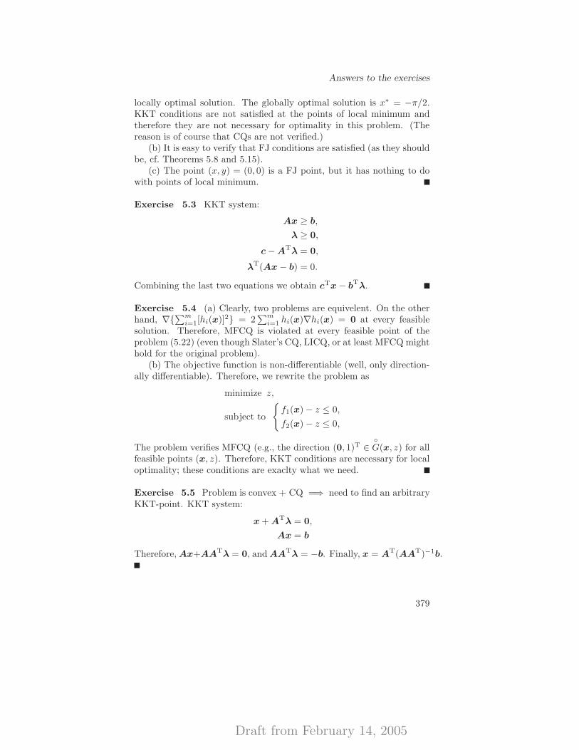
Draft from February 14, 2005
Answers to the exercises
locally optimal solution. The globally optimal solution is x∗ = −π/2.KKT conditions are not satisfied at the points of local minimum andtherefore they are not necessary for optimality in this problem. (Thereason is of course that CQs are not verified.)
(b) It is easy to verify that FJ conditions are satisfied (as they shouldbe, cf. Theorems 5.8 and 5.15).
(c) The point (x, y) = (0, 0) is a FJ point, but it has nothing to dowith points of local minimum.
Exercise 5.3 KKT system:
Ax ≥ b,
λ ≥ 0,
c − ATλ = 0,
λT(Ax − b) = 0.
Combining the last two equations we obtain cTx − bTλ.
Exercise 5.4 (a) Clearly, two problems are equivelent. On the otherhand, ∇{∑m
i=1[hi(x)]2} = 2∑m
i=1 hi(x)∇hi(x) = 0 at every feasiblesolution. Therefore, MFCQ is violated at every feasible point of theproblem (5.22) (even though Slater’s CQ, LICQ, or at least MFCQ mighthold for the original problem).
(b) The objective function is non-differentiable (well, only direction-ally differentiable). Therefore, we rewrite the problem as
minimize z,
subject to
{f1(x) − z ≤ 0,
f2(x) − z ≤ 0,
The problem verifies MFCQ (e.g., the direction (0, 1)T ∈◦G(x, z) for all
feasible points (x, z). Therefore, KKT conditions are necessary for localoptimality; these conditions are exaclty what we need.
Exercise 5.5 Problem is convex + CQ =⇒ need to find an arbitraryKKT-point. KKT system:
x + ATλ = 0,
Ax = b
Therefore, Ax+AATλ = 0, and AATλ = −b. Finally, x = AT(AAT)−1b.
379
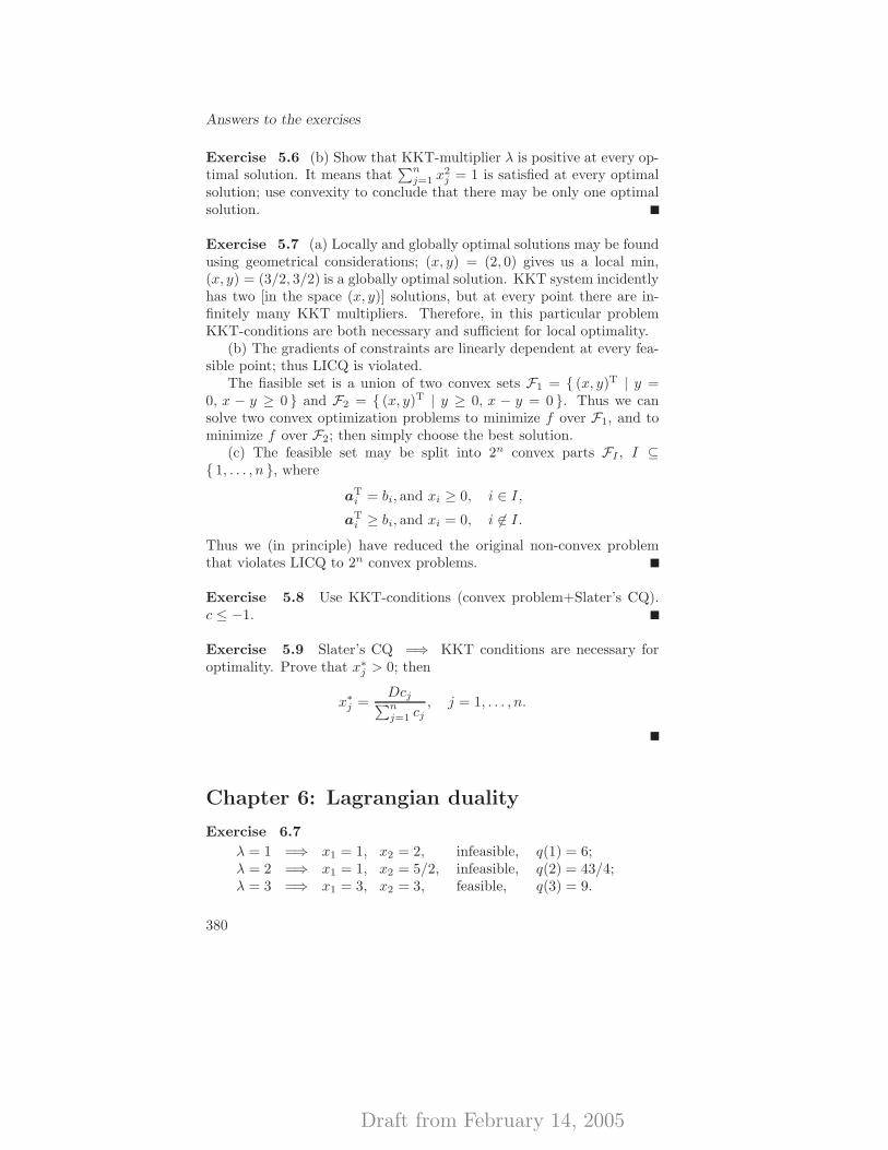
Draft from February 14, 2005
Answers to the exercises
Exercise 5.6 (b) Show that KKT-multiplier λ is positive at every op-timal solution. It means that
∑nj=1 x
2j = 1 is satisfied at every optimal
solution; use convexity to conclude that there may be only one optimalsolution.
Exercise 5.7 (a) Locally and globally optimal solutions may be foundusing geometrical considerations; (x, y) = (2, 0) gives us a local min,(x, y) = (3/2, 3/2) is a globally optimal solution. KKT system incidentlyhas two [in the space (x, y)] solutions, but at every point there are in-finitely many KKT multipliers. Therefore, in this particular problemKKT-conditions are both necessary and sufficient for local optimality.
(b) The gradients of constraints are linearly dependent at every fea-sible point; thus LICQ is violated.
The fiasible set is a union of two convex sets F1 = { (x, y)T | y =0, x − y ≥ 0 } and F2 = { (x, y)T | y ≥ 0, x − y = 0 }. Thus we cansolve two convex optimization problems to minimize f over F1, and tominimize f over F2; then simply choose the best solution.
(c) The feasible set may be split into 2n convex parts FI , I ⊆{ 1, . . . , n }, where
aTi = bi, and xi ≥ 0, i ∈ I,
aTi ≥ bi, and xi = 0, i 6∈ I.
Thus we (in principle) have reduced the original non-convex problemthat violates LICQ to 2n convex problems.
Exercise 5.8 Use KKT-conditions (convex problem+Slater’s CQ).c ≤ −1.
Exercise 5.9 Slater’s CQ =⇒ KKT conditions are necessary foroptimality. Prove that x∗j > 0; then
x∗j =Dcj∑nj=1 cj
, j = 1, . . . , n.
Chapter 6: Lagrangian duality
Exercise 6.7
λ = 1 =⇒ x1 = 1, x2 = 2, infeasible, q(1) = 6;λ = 2 =⇒ x1 = 1, x2 = 5/2, infeasible, q(2) = 43/4;λ = 3 =⇒ x1 = 3, x2 = 3, feasible, q(3) = 9.
380
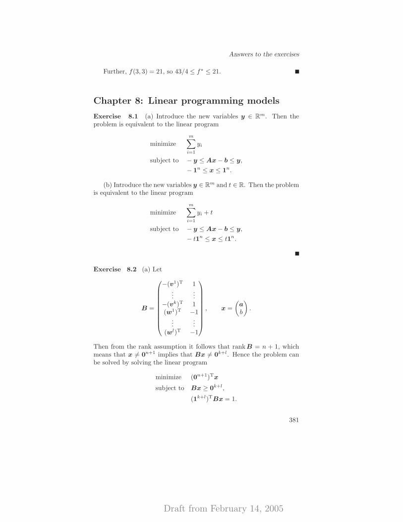
Draft from February 14, 2005
Answers to the exercises
Further, f(3, 3) = 21, so 43/4 ≤ f∗ ≤ 21.
Chapter 8: Linear programming models
Exercise 8.1 (a) Introduce the new variables y ∈ Rm. Then theproblem is equivalent to the linear program
minimize
m∑
i=1
yi
subject to − y ≤ Ax − b ≤ y,
− 1n ≤ x ≤ 1n.
(b) Introduce the new variables y ∈ Rm and t ∈ R. Then the problemis equivalent to the linear program
minimize
m∑
i=1
yi + t
subject to − y ≤ Ax − b ≤ y,
− t1n ≤ x ≤ t1n.
Exercise 8.2 (a) Let
B =
−(v1)T 1...
...−(vk)T 1(w1)T −1
......
(wl)T −1
, x =
(a
b
).
Then from the rank assumption it follows that rankB = n + 1, whichmeans that x 6= 0n+1 implies that Bx 6= 0k+l. Hence the problem canbe solved by solving the linear program
minimize (0n+1)Tx
subject to Bx ≥ 0k+l,
(1k+l)TBx = 1.
381
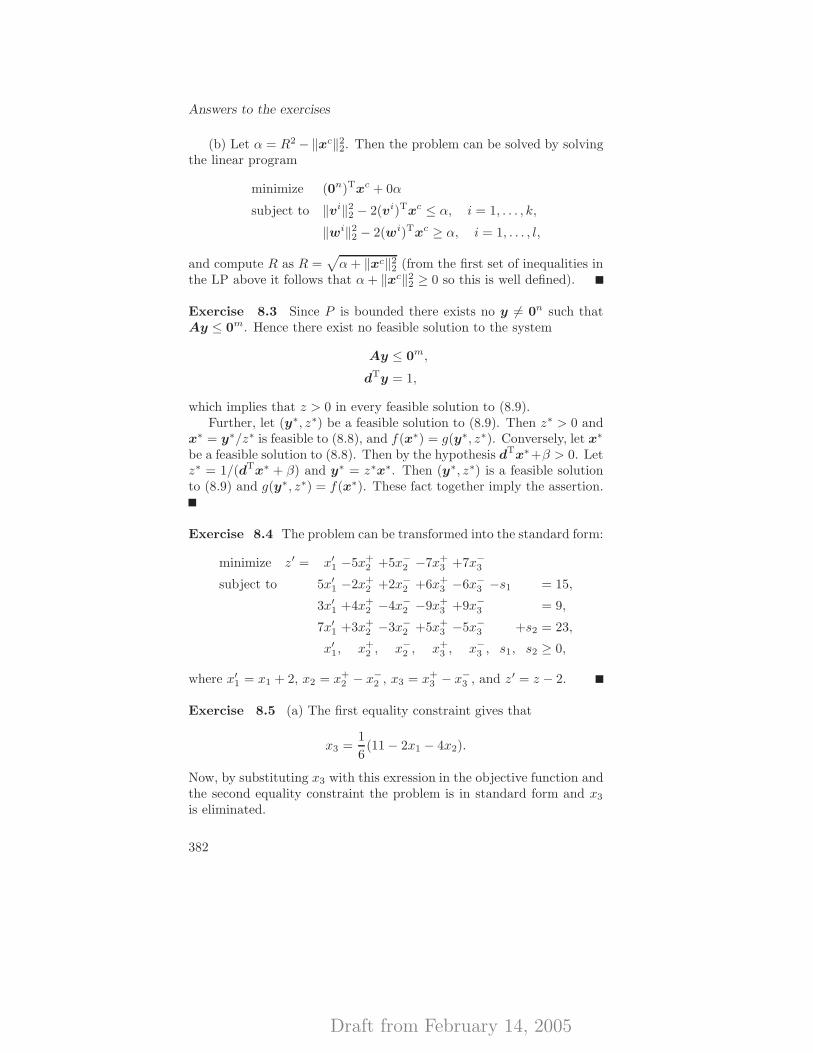
Draft from February 14, 2005
Answers to the exercises
(b) Let α = R2 − ‖xc‖22. Then the problem can be solved by solving
the linear program
minimize (0n)Txc + 0α
subject to ‖vi‖22 − 2(vi)Txc ≤ α, i = 1, . . . , k,
‖wi‖22 − 2(wi)Txc ≥ α, i = 1, . . . , l,
and compute R as R =√α+ ‖xc‖2
2 (from the first set of inequalities inthe LP above it follows that α+ ‖xc‖2
2 ≥ 0 so this is well defined).
Exercise 8.3 Since P is bounded there exists no y 6= 0n such thatAy ≤ 0m. Hence there exist no feasible solution to the system
Ay ≤ 0m,
dTy = 1,
which implies that z > 0 in every feasible solution to (8.9).Further, let (y∗, z∗) be a feasible solution to (8.9). Then z∗ > 0 and
x∗ = y∗/z∗ is feasible to (8.8), and f(x∗) = g(y∗, z∗). Conversely, let x∗
be a feasible solution to (8.8). Then by the hypothesis dTx∗+β > 0. Letz∗ = 1/(dTx∗ + β) and y∗ = z∗x∗. Then (y∗, z∗) is a feasible solutionto (8.9) and g(y∗, z∗) = f(x∗). These fact together imply the assertion.
Exercise 8.4 The problem can be transformed into the standard form:
minimize z′ = x′1 −5x+2 +5x−2 −7x+
3 +7x−3
subject to 5x′1 −2x+2 +2x−2 +6x+
3 −6x−3 −s1 = 15,
3x′1 +4x+2 −4x−2 −9x+
3 +9x−3 = 9,
7x′1 +3x+2 −3x−2 +5x+
3 −5x−3 +s2 = 23,
x′1, x+2 , x−2 , x+
3 , x−3 , s1, s2 ≥ 0,
where x′1 = x1 + 2, x2 = x+2 − x−2 , x3 = x+
3 − x−3 , and z′ = z − 2.
Exercise 8.5 (a) The first equality constraint gives that
x3 =1
6(11 − 2x1 − 4x2).
Now, by substituting x3 with this exression in the objective function andthe second equality constraint the problem is in standard form and x3
is eliminated.
382
Draft from February 14, 2005
Answers to the exercises
(b) If x3 ≥ 0, then we must add the constraint (11−2x1−4x2)/6 ≥ 0to the problem. But this is an inequality, so in order to transform theproblem into standard form we must add a slackvarible.
Exercise 8.6 Assume that the column in the constraint matrix cor-responding to the variable x+
j is aj . Then the column in the constraint
matrix corresponding to the variable x−j is −aj . The statement thenfollows from the definition of basic feasible solution, since aj and −aj
are linearly dependent.
Exercise 8.7 Let P be the set of feasible solutions to (8.10) and Qbe the set of feasible solutions to (8.11). Obviously P ⊆ Q. In order toshow that Q ⊆ P assume that there exists an x ∈ Q such that x /∈ Pand derive a contradiction.
Chapter 9: The simplex method
Exercise 9.1 The phase I problem becomes
minimize w = a1 + a1
subject to − 3x1 − 2x2 + x3 − s1 + a1 = 3,
x1 + x2 − 2x3 − s2 + a2 = 1,
x1, x2, x3, s1, s2, a1, a2 ≥ 0.
From the equality constraints it follows that a1+a2 ≥ 4 for all x1, x2, x3, s1, s2 ≥0. Hence, in particular, it follows that w ≥ 4 for all feasible solutions tothe phase I problem, which means that the original problem is infeasible.
Exercise 9.2 (a) The standard form is given by
minimize 3x1 + 2x2 + x3
subject to 2x1 + x3 − s1 = 3,
2x1 + 2x2 + x3 = 5,
x1, x2, x3, s1 ≥ 0.
By solving the phase I problem with the Simplex algorithm we get thefeasible basis xB = (x1, x2)
T. Then by solving the phase II problem withthe Simplex algorithm we get the optimal solution x∗ = (x1, x2, x3)
T =(0, 1, 3)T.
383
Draft from February 14, 2005
Answers to the exercises
(b) No, the set of all optimal solution is given by the set
{x ∈ R3 | λ(0, 1, 3)T + (1 − λ)(0, 0, 5)T; λ ∈ [0, 1]}.
Exercise 9.3 The reduced cost for all the variables except for xj mustbe greater than or equal to 0. Hence it follows that the current basis isoptimal to the problem that arises if xj is fixed to zero. The assertionthen follows from the fact that the current basis is non-degenerate.
Chapter 10: LP duality and sensitivity anal-ysis
Exercise 10.1 The linear programming dual is given by
minimize 11y1+23y2+12y3
subject to 4y1 +3y2 +7y3 ≥ 6,
3y1 +2y2 +4y3 ≥−3,
−8y1 +7y2 +3y3 ≤−2,
7y1 +6y2 +2y3 = 5,
y2 ≤ 0,
y3 ≥ 0.
Exercise 10.2 (a) The linear programming dual is given by
maximize bTy1 +lTy2+uTy3
subject to ATy1+Iny2 +Iny3 =c,
y2 ≥0n,
y3 ≤0n.
(b) A feasible solution to the linear programming dual is given by
y1 = 0m,
y2 = (max{0, c1}, . . . ,max{0, cn})T,y3 = (min{0, c1}, . . . ,min{0, cn})T.
384
Draft from February 14, 2005
Answers to the exercises
Exercise 10.3 First, check that y = (B−1)TcB is feasible to the LPdual problem. Then show that bTy equals the optimal objective func-tion value for the primal problem. The assertion then follows from theWeak Duality Theorem.
Exercise 10.4 Use the Weak and Stong Duality Theorems.
Exercise 10.5 The LP dual is infeasible. Hence, from the Weak andStrong Duality Theorems it follows that the primal problem is eitherinfesible or unbounded.
Exercise 10.6 By using the Strong Duality Theorem we get thefollowing polyhedron:
Ax ≥ b,
ATy ≤ c,
cTx = bTy,
x ≥ 0n,
y ≤ 0m.
Exercise 10.7 From the Strong Duality Theorem it follows thatcTx∗ = bTy∗. Use this to establish the statement.
Exercise 10.8 The dual problem only contains two varibles and hencecan be solved graphically. We get the optimal solution y∗ = (−2, 0)T.The complementary slackness conditions then implies that x1 = x2 =x3 = x5 = 0. Hence, let xB = (x4, x6)
T. The optimal solution isx∗ = (x1, x2, x3, x4, x5, x6)
T = (0, 0, 0, 3, 0, 1)T.
Exercise 10.9 From the complementary slackness conditions and thefact that c1/a1 ≥ · · · ≥ cn/an it follows that
u =crar,
yj = cj −craraj , j = 1, . . . , r − 1,
yj = 0, j = r, . . . , n,
385
Draft from February 14, 2005
Answers to the exercises
is a dual feasible solution which together with the given primal solutionfulfil the LP primal-dual optimality conditions.
Exercise 10.14 The basis xB = (x1, x2)T is optimal as long as c3 ≤ 5
and c4 ≥ 8.
Exercise 10.15 b) The basis xB = (x1, x3)T is optimal for all
δ ≥ −6.5. c) The basis xB = (x1, x3) is not primal feasible for δ = −7,but it is dual feasible, so by using the Dual Simplex method it followsthat xB = (x1, x5)
T is an optimal basis.
Chapter 11: Unconstrained optimization
Exercise 11.2 The directional derivative is 13 > 0; the answer is No.
Exercise 11.3 (a) The search direction is not a descent direction,for example because the Hessian matrix is indefinite or negative definite.(b) The linear system is unsolvable, for example because the Hessianmatrix is indefinite. [Note: Even for indefinite Hessians, the searchdirection might exist for some right-hand sides.] (c) Use the Levenberg–Marquardt modification.
Exercise 11.4 Let y1 := x1 − 2 and y2 :=√
5(x2 + 6). We then getf(x) = g(y) = y2
1 + y22. At every y ∈ R2 the negative gradient points
towards the optimum!
Exercise 11.5 (a) x1 = (1/2, 1)T. (b) The Hessian matrix is
∇2f(x1) =
(10 −4−4 2
).
The answer is Yes. (c) The answer is Yes.
Exercise 11.6 (a) x1 = (2, 1/2)T. (b) The answer is No. The gradi-ent is zero. (c) The answer is Yes.
Exercise 11.7 (a) (b) µ ∈ (0, 0.6).
Exercise 11.8 (a) f(x0) = (−1,−2)T =⇒ ‖f(x0)‖ =√
5; x1 =(4/3, 2/3)T =⇒ ‖f(x1)‖ = 16/27. (b) If f is the gradient of a C2 func-tion f : Rn 7→ R we obtain that ∇f = ∇2f , that is, Newton’s method
386
Draft from February 14, 2005
Answers to the exercises
for unconstrained optimization is obtained.
Exercise 11.9 (a) x∗ = (ATA)−1ATb. (b) The objective function isconvex, since the Hessian is ATA (which is always positive semi-definite;check!). Therefore, the normal solution in (a) is globally optimal.
Exercise 11.12 (a) We have that
∇f(y) + γ(y − xk) = 0n ⇐⇒ Qy + q + γ(y − xk) = 0n ⇐⇒(Q + γIn)y = γxk − q ⇐⇒ (Q + γIn)(y − xk).
Further,
(Q + γIn)(y − xk) = γxk − q − (Q + γIn)xk = −(Qxk + q).
(b) If {xk} converges to x∞ then {pk} = {xk+1 − xk} must con-verge to zero. From the updating formula we obtain that pk = (Q +γIn)−1∇f(xk) for every k. The sequence {∇f(xk)} converges to ∇f(x∞),since f ∈ C1. If ∇f(x∞) 6= 0n it would hold that {pk} would convergeto (Q + γIn)−1∇f(x∞) 6= 0n, since (Q + γIn)−1 is positive definitewhen Q + γIn is. This leads to a contradiction. Hence, ∇f(x∞) = 0n.Since f is convex x∞ is a global minimum of f over Rn.
Exercise 11.13 Case I: {∇f(xk)} → 0n; {xk} and {f(xk)} diverge.Example: f(x) = − log x; {xk} → ∞; {f(xk)} → −∞; {f ′(xk)} → 0.
Case II: {∇f(xk)} → 0n; {xk} diverges; {f(xk)} converges.Example: f(x) = 1/x; {xk} → ∞; {f(xk)} → 0; {f(xk)} → 0.
Case III: {∇f(xk)} → 0n; {xk} is bounded; {f(xk)} is bounded.
Example: f(x) = 13x
3 − x; xk =
{1 + 1/k, k even−1 − 1/k k odd
{xk} has two limit points: ±1; {f(xk)} has two limit points: ±2/3.
Case IV: {∇f(xk)} → 0n; {xk} is bounded; {f(xk)} converges.Example: f(x) = x2 − 1; xk as above; {f(xk)} → 0.
Case V: {∇f(xk)} → 0n; {xk} and {f(xk)} converge.Example: f as in Case IV; xk = 1 + 1/k.
Chapter 12: Optimization over convex sets
Exercise 12.2 (b) x1 = (12/5, 4/5)T; UBD = f(x1) = 8. The LPproblem defined at x0 gives LBD = 0. Hence, f∗ ∈ [0, 8].
387
Draft from February 14, 2005
References
[Aba67] J. Abadie, On the Kuhn–Tucker theorem, in Nonlinear Program-ming (NATO Summer School, Menton, 1964), North-Holland,Amsterdam, 1967, pp. 19–36.
[Arm66] L. Armijo, Minimization of functions having Lipschitz continuous
first partial derivatives, Pacific Journal of Mathematics, 16 (1966),pp. 1–3.
[AHU58] K. J. Arrow, L. Hurwicz, and H. Uzawa, eds., Studies in
Linear and Non-Linear Programming, Stanford University Press,Stanford, CA, 1958.
[AHU61] K. J. Arrow, L. Hurwicz, and H. Uzawa, Constraint qualifi-
cations in maximization problems, Naval Research Logistics Quar-terly, 8 (1961), pp. 175–191.
[Avr76] M. Avriel, Nonlinear Programming: Analysis and Methods,Prentice Hall Series in Automatic Computation, Prentice Hall,Englewood Cliffs, NJ, 1976.
[Ban22] S. Banach, Sur les operations dans les ensembles abstraits et leur
application aux equations integrales, Fundamenta Mathematicae,3 (1922), pp. 133–181.
[Bar71] R. H. Bartels, A stabilization of the simplex method, NumerischeMathematik, 16 (1971), pp. 414–434.
[BaG69] R. H. Bartels and G. H. Golub, The simplex method of lin-
ear programming using LU-decomposition, Communications of theACM, 12 (1969), pp. 266–268 and 275–278.
[BSS93] M. S. Bazaraa, H. D. Sherali, and C. M. Shetty, Nonlinear
Programming: Theory and Algorithms, John Wiley & Sons, NewYork, NY, second ed., 1993.
[Ben62] J. F. Benders, Partitioning procedures for solving mixed vari-
ables programming problems, Numerische Mathematik, 4 (1962),pp. 238–252.
[Ber99] D. P. Bertsekas, Nonlinear Programming, Athena Scientific,Bellmont, MA, second ed., 1999.
Draft from February 14, 2005
References
[Ber04] , Lagrange multipliers with optimal sensitivity properties in
constrained optimization, Report LIDS 2632, Department of Elec-trical Engineering and Computer Science, Massachusetts Instituteof Technology, Cambridge, MA, 2004.
[BNO03] D. P. Bertsekas, A. Nedic, and A. E. Ozdaglar, Convex
Analysis and Optimization, Athena Scientific, Belmont, MA, 2003.
[BeT89] D. P. Bertsekas and J. N. Tsitsiklis, Parallel and Distributed
Computation: Numerical Methods, Prentice Hall, London, U.K.,1989.
[BeT00] D. P. Bertsekas and J. N. Tsitsiklis, Gradient convergence in
gradient methods with errors, SIAM Journal on Optimization, 10(2000), pp. 627–642.
[Bla77] R. G. Bland, New finite pivoting rules for the simplex method,Mathematics of Operations Research, 2 (1977), pp. 103–107.
[BlO72] E. Blum and W. Oettli, Direct proof of the existence theorem in
quadratic programming, Operations Research, 20 (1972), pp. 165–167.
[BGLS03] J. F. Bonnans, J. C. Gilbert, C. Lemarechal, and C. A.
Sagastizabal, Numerical Optimization: Theoretical and Practi-
cal Aspects, Universitext, Springer-Verlag, Berlin, 2003. Trans-lated from the original French edition, published by Springer-Verlag 1997.
[BoS00] J. F. Bonnans and A. Shapiro, Perturbation Analysis of Op-
timization Problems, Springer Series in Operations Research,Springer-Verlag, New York, NY, 2000.
[BoL00] J. M. Borwein and A. S. Lewis, Convex Analysis and Nonlinear
Optimization: Theory and Examples, CMS Books in Mathematics,Springer-Verlag, New York, NY, 2000.
[BHM77] S. P. Bradley, A. C. Hax, and T. L. Magnanti, Applied
Mathematical Programming, Addison-Wesley, Reading, MA, 1977.
[Bre73] R. P. Brent, Algorithms for Minimization Without Derivatives,Prentice Hall Series in Automatic Computation, Prentice Hall,Englewood Cliffs, NJ, 1973. Reprinted by Dover Publications,Inc., Mineola, NY, 2002.
[Bro09] L. E. J. Brouwer, On continuous vector distributions on sur-
faces, Amsterdam Proceedings, 11 (1909).
[Bro12] , Uber Abbildung von Mannigfaltigkeiten, MathematischeAnnalen, 71 (1912), pp. 97–115.
[Bro70] C. G. Broyden, The convergence of single-rank quasi-Newton
methods, Mathematics of Computation, 24 (1970), pp. 365–382.
[BGIS95] R. Burachik, L. M. G. Drummond, A. N. Iusem, and B. F.
Svaiter, Full convergence of the steepest descent method with in-
exact line searches, Optimization, 32 (1995), pp. 137–146.
392
Draft from February 14, 2005
References
[BuF91] J. V. Burke and M. C. Ferris, Characterization of solution
sets of convex programs, Operations Research Letters, 10 (1991),pp. 57–60.
[Car07] C. Caratheodory, Uber den Variabilitatsbereich der Koeffizien-
ten von Potenzreihen, die gegebene Werte nicht annehmen, Math-ematische Annalen, 64 (1907), pp. 95–115.
[Car11] , Uber den Variabilitatsbereich der Fourier’schen Konstan-
ten von positiven harmonischen Funktionen, Rendiconti del Cir-colo Matematico di Palermo, 32 (1911), pp. 193–217.
[Cau1847] A. Cauchy, Methode generale pour la resolution des systemes
d’equations simultanees, Comptes Rendus Hebdomadaires desSeances de l’Academie des Sciences (Paris), Serie A, 25 (1847),pp. 536–538.
[Cha52] A. Charnes, Optimality and degeneracy in linear programming,Econometrica, 20 (1952), pp. 160–170.
[Chv83] V. Chvatal, Linear Programming, Freeman, New York, 1983.
[CGT00] A. R. Conn, N. I. M. Gould, and P. L. Toint, Trust-Region
Methods, vol. 1 of MPS/SIAM Series on Optimization, SIAM andMathematical Programming Society, Philadelphia, PA, 2000.
[Dan51] G. B. Dantzig, Maximization of a linear function of variables
subject to linear inequalities, in Activity Analysis of Productionand Allocation, T. C. Koopmans, ed., New York, NY, 1951, JohnWiley & Sons, pp. 339–347.
[Dan53] , Computational algorithm of the revised simplex method, Re-port RM 1266, The Rand Corporation, Santa Monica, CA, 1953.
[Dan57] , Concepts, origins, and use of linear programming, in Pro-ceedings of the First International Conference on Operational Re-search, Oxford, 1957, M. Davies, R. T. Eddison, and T. Page, eds.,London, U.K., 1957, The English Universities Press, pp. 100–108.
[Dan63] , Linear Programming and Extensions, Princeton UniversityPress, Princeton, NJ, 1963.
[DOW55] G. B. Dantzig, A. Orden, and P. Wolfe, The generalized sim-
plex method for minimizing a linear form under linear inequality
restraints, Pacific Journal of Mathematics, 5 (1955), pp. 183–195.
[DaT97] G. B. Dantzig and M. N. Thapa, Linear programming 1: In-
troduction, Springer-Verlag, New York, NY, 1997.
[DaT03] , Linear programming 2: Theory and Extensions, Springer-Verlag, New York, NY, 2003.
[DaW60] G. B. Dantzig and P. Wolfe, Decomposition principle for lin-
ear programs, Operations Research, 8 (1960), pp. 101–111.
[Dav59] W. C. Davidon, Variable metric method for minimization, Re-port ANL-5990 Rev, Argonne National Laboratories, Argonne,IL, 1959. Also published in SIAM Journal on Optimization, 1(1991), pp. 1–17.
393
Draft from February 14, 2005
References
[DeF49] B. De Finetti, Sulla stratificazioni convesse, Annali di Matem-atica Pura ed Applicata, 30 (1949), pp. 173–183.
[DeS83] J. E. Dennis and R. E. Schnabel, Numerical Methods for Un-
constrained Optimization and Nonlinear Equations, Prentice Hall,Englewood Cliffs, NJ, 1983.
[DiJ79] Y. M. I. Dirickx and L. P. Jennergren, Systems Analysis by
Multilevel Methods: With Applications to Economics and Manage-
ment, vol. 6 of International Series on Applied Systems Analysis,John Wiley & Sons, Chichester, U.K., 1979.
[DuH78] J. C. Dunn and S. Harshbarger, Conditional gradient algo-
rithms with open loop step size rules, Journal of MathematicalAnalysis and Applications, 62 (1978), pp. 432–444.
[Eav71] B. C. Eaves, On quadratic programming, Management Science,17 (1971), pp. 698–711.
[EHL01] T. F. Edgar, D. M. Himmelblau, and L. S. Lasdon, Op-
timization of Chemical Processes, McGraw-Hill, New York, NY,second ed., 2001.
[Erm66] Y. M. Ermol’ev, Methods for solving nonlinear extremal prob-
lems, Kibernetika, 2 (1966), pp. 1–17. Translated in Cybernetics,2 (1966), pp. 1–14.
[Eva70] J. P. Evans, On constraint qualifications in nonlinear program-
ming, Naval Research Logistics Quarterly, 17 (1970), pp. 281–286.
[Eve63] H. Everett, III, Generalized Lagrange multiplier method for
solving problems of optimum allocation of resources, OperationsResearch, 11 (1963), pp. 399–417.
[Fac95] F. Facchinei, Minimization of SC1 functions and the Maratos
effect, Operations Research Letters, 17 (1995), pp. 131–137.
[Fal67] J. E. Falk, Lagrange multipliers and nonlinear programming,Journal of Mathematical Analysis and Applications, 19 (1967),pp. 141–159.
[Far1902] J. Farkas, Uber die Theorie der einfachen Ungleichungen, Jour-nal fur die Reine und Angewandte Mathematik, 124 (1902), pp. 1–24.
[Fen51] W. Fenchel, Convex cones, sets and functions, mimeographedlecture notes, Princeton University, Princeton, NY, 1951.
[Fia83] A. V. Fiacco, Introduction to sensitivity and stability analysis in
nonlinear programming, vol. 165 of Mathematics in Science andEngineering, Academic Press Inc., Orlando, FL, 1983.
[FiM68] A. V. Fiacco and G. P. McCormick, Nonlinear Programming:
Sequential Unconstrained Minimization Techniques, John Wiley &Sons,, New York, NY, 1968. Also published as volume 4 in theClassics in Applied Mathematics Series, SIAM, Philadelphia, PA,1990.
394
Draft from February 14, 2005
References
[Fis81] M. L. Fisher, The Lagrangian relaxation method for solving inte-
ger programming problems, Management Science, 27 (1981), pp. 1–18.
[Fis85] , An applications oriented guide to Lagrangian relaxation,Interfaces, 15 (1985), pp. 10–21.
[Fle70] R. Fletcher, A new approach to variable metric algorithms,Computer Journal, 13 (1970), pp. 317–322.
[Fle87] , Practical Methods of Optimization, John Wiley & Sons,Chichester, U.K., second ed., 1987.
[FLT02] R. Fletcher, S. Leyffer, and P. L. Toint, On the global con-
vergence of a filter-SQP algorithm, SIAM Journal on Optimiza-tion, 13 (2002), pp. 44–59.
[FlP63] R. Fletcher and M. J. D. Powell, A rapidly convergent
descent method for minimization, Computer Journal, 6 (1963),pp. 163–168.
[FlR64] R. Fletcher and C. M. Reeves, Function minimization by con-
jugate gradients, Computer Journal, 7 (1964), pp. 149–154.
[FrW56] M. Frank and P. Wolfe, An algorithm for quadratic program-
ming, Naval Research Logistics Quarterly, 3 (1956), pp. 95–110.
[Geo74] A. M. Geoffrion, Lagrangean relaxation for integer program-
ming. Approaches to integer programming, Mathematical Pro-gramming Study, 2 (1974), pp. 82–114.
[Gil66] E. G. Gilbert, An iterative procedure for computing the mini-
mum of a quadratic form on a convex set, SIAM Journal on Con-trol, 4 (1966), pp. 61–80.
[GiM73] P. E. Gill and W. Murray, A numerically stable form of the
simplex algorithm, Linear Algebra and Its Applications, 7 (1973),pp. 99–138.
[GMSW89] P. E. Gill, W. Murray, M. A. Saunders, and M. H. Wright,A practical anti-cycling procedure for linearly constrained opti-
mization, Mathematical Programming, 45 (1989), pp. 437–474.
[Gol70] D. Goldfarb, A family of variable-metric methods derived by
variational means, Mathematics of Computation, 24 (1970),pp. 23–26.
[Gol64] A. A. Goldstein, Convex programming in Hilbert space, Bulletinof the American Mathematical Society, 70 (1964), pp. 709–710.
[GrD03] A. Granas and J. Dugundji, Fixed Point Theory, SpringerMonographs in Mathematics, Springer-Verlag, New York, NY,1969.
[Gui69] M. Guignard, Generalized Kuhn–Tucker conditions for mathe-
matical programming problems in a Banach space, SIAM Journalon Control, 7 (1969), pp. 232–241.
[Had10] J. Hadamard, Sur quelques applications de l’indice de Kronecker,in Introduction a la theorie des fonctions d’une variable, J. Tan-nary, ed., vol. 2, Hermann, Paris, 1910, pp. 875–915.
395
Draft from February 14, 2005
References
[Han75] S. P. Han, Penalty Lagrangian methods in a quasi-Newton ap-
proach, Report TR 75-252, Computer Science, Cornell University,Ithaca, NY, 1975.
[HaH96] G. K. Hauer and H. M. Hoganson, Tailoring a decomposition
method to a large forest management scheduling problem in north-
ern Ontario, INFOR, 34 (1996), pp. 209–231.
[HLV87] D. W. Hearn, S. Lawphongpanich, and J. A. Ventura, Re-
stricted simplicial decomposition: Computation and extensions,Mathematical Programming Study, 31 (1987), pp. 99–118.
[HWC74] M. Held, P. Wolfe, and H. P. Crowder, Validation of subgra-
dient optimization, Mathematical Programming, 6 (1974), pp. 62–88.
[HiL93] J.-B. Hiriart-Urruty and C. Lemarechal, Convex Analysis
and Minimization Algorithms, vol. 305–306 of Grundlehren dermathematischen Wissenschaften, Springer-Verlag, Berlin, 1993.
[Hof53] A. Hoffman, Cycling in the simplex algorithm, Report 2974, Na-tional Bureau of Standards, Gaithersburg, MD, 1953.
[Ius03] A. N. Iusem, On the convergence properties of the projected gradi-
ent method for convex optimization, Computational and AppliedMathematics, 22 (2003), pp. 37–52.
[Joh48] F. John, Extremum problems with inequalities as subsidiary con-
ditions, in Studies and Essays Presented to R. Courant on his60th Birthday, January 8, 1948, Interscience Publishers, Inc., NewYork, NY, 1948, pp. 187–204.
[JoM74] L. A. Johnson and D. S. Montgomery, Operations Research
in Production Planning, Scheduling and Inventory Control, JohnWiley & Sons, New York, NY, 1974.
[Kar84a] N. Karmarkar, A new polynomial-time algorithm for linear pro-
gramming, in Proceedings of the Sixteenth Annual ACM Sympo-sium on Theory of Computing, New York, 1984, The Associationfor Computing Machinery, pp. 302–311.
[Kar84b] , A new polynomial-time algorithm for linear programming,Combinatorica, 4 (1984), pp. 373–395.
[Kha79] L. G. Khachiyan, A polynomial algorithm in linear programming,Doklady Akademii Nauk SSSR, 244 (1979), pp. 1093–1096.
[Kha80] , Polynomial algorithms in linear programming, AkademiyaNauk SSSR. Zhurnal Vychislitel’noı Matematiki i Matematich-eskoı Fiziki, 20 (1980), pp. 51–68.
[KlM72] V. Klee and G. J. Minty, How good is the simplex algorithm?,in Inequalities, III, New York, NY, 1972, Academic Press, pp. 159–175.
[KLT03] T. G. Kolda, R. M. Lewis, and V. Torczon, Optimization
by direct search: New perspectives on some classical and modern
methods, SIAM Review, 45 (2003), pp. 385–482.
396
Draft from February 14, 2005
References
[Kre78] E. Kreyszig, Introductory Functional Analysis with Applications,John Wiley & Sons, New York, NY, 1978.
[KuT51] H. W. Kuhn and A. W. Tucker, Nonlinear programming, inProceedings of the Second Berkeley Symposium on MathematicalStatistics and Probability, 1950, Berkeley and Los Angeles, CA,1951, University of California Press, pp. 481–492.
[LaP05] T. Larsson and M. Patriksson, Global optimality conditions
for discrete and nonconvex optimization—with applications to La-
grangian heuristics and column generation, tech. rep., Departmentof Mathematics, Chalmers University of Technology, Gothenburg,Sweden, 2005. To appear in Operations Research.
[LPS96] T. Larsson, M. Patriksson, and A.-B. Stromberg, Condi-
tional subgradient optimization—theory and applications, Euro-pean Journal of Operational Research, 88 (1996), pp. 382–403.
[LPS99] , Ergodic, primal convergence in dual subgradient schemes
for convex programming, Mathematical Programming, 86 (1999),pp. 283–312.
[Las70] L. S. Lasdon, Optimization Theory for Large Systems, Macmil-lan, New York, NY, 1970.
[Law76] E. Lawler, Combinatorial Optimization: Networks and Matroids,Holt, Rinehart and Winston, New York, NY, 1976.
[LRS91] J. K. Lenstra, A. H. G. Rinnooy Kan, and A. Schrijver,eds., History of Mathematical Programming. A Collection of Per-
sonal Reminiscences, North-Holland, Amsterdam, 1991.
[LeP66] E. S. Levitin and B. T. Polyak, Constrained minimization
methods, USSR Computational Mathematics and MathematicalPhysics, 6 (1966), pp. 1–50.
[Lip1877] R. Lipschitz, Lehrbuch der Analysis, Cohn & Sohn, Leipzig, 1877.
[Lue84] D. G. Luenberger, Linear and Nonlinear Programming, AddisonWesley, Reading, MA, second ed., 1984.
[Man65] O. L. Mangasarian, Pseudo-convex functions, SIAM Journal onControl, 3 (1965), pp. 281–290.
[Man69] , Nonlinear Programming, McGraw-Hill, New York, NY,1969. Also published as volume 10 in the Classics in AppliedMathematics Series, SIAM, Philadelphia, PA, 1994.
[Man88] , A simple characterization of solution sets of convex pro-
grams, Operations Research Letters, 7 (1988), pp. 21–26.
[MaF67] O. L. Mangasarian and S. Fromovitz, The Fritz John neces-
sary optimality conditions in the presence of equality and inequal-
ity constraints, Journal of Mathematical Analysis and Applica-tions, 17 (1967), pp. 37–47.
[Mar78] N. Maratos, Exact penalty function algorithms for finite dimen-
sional and control optimization problems, PhD thesis, ImperialCollege of Science and Technology, University of London, London,U.K., 1978.
397
Draft from February 14, 2005
References
[Min10] H. Minkowski, Geometrie der Zahlen, Teubner, Leipzig, 1910.
[Min11] , Gesammelte Abhandlungen, vol. II, Teubner, Leipzig, 1911,ch. Theorie der knovexen Korper, Insbesondere Begrundung ihresOber flachenbegriffs.
[Mot36] T. Motzkin, Beitrage zur Theorie del linearen Ungleichungen,Azriel, Israel, 1936.
[Mur83] K. G. Murty, Linear Programming, John Wiley & Sons, NewYork, NY, 1983.
[Mur95] , Operations Research: Deterministic Optimization Models,Prentice Hall, Englewood Cliffs, NJ, 1995.
[Nas50] J. F. Nash, Jr., Equilibrium points in n-person games, Proceed-ings of the National Academy of Sciences of the United States ofAmerica, 36 (1950), pp. 48–49.
[Nas51] , Non-cooperative games, Annals of Mathematics, 54 (1951),pp. 286–295.
[NaS96] S. G. Nash and A. Sofer, Linear and Nonlinear Programming,MacGraw-Hill, Singapore, 1996.
[NeW88] G. L. Nemhauser and L. Wolsey, Integer and Combinatorial
Optimization, Wiley-Interscience Series in Discrete Mathematicsand Optimization, John Wiley & Sons, New York, NY, 1988.
[New1687] I. S. Newton, Philosophiae Naturalis Principia Mathematica,London, U.K., 1687.
[NoW99] J. Nocedal and S. J. Wright, Numerical Optimization,Springer Series in Operations Research, Springer-Verlag, NewYork, NY, 1999.
[Orc54] W. Orchard-Hays, Background, development and extensions of
the revised simplex method, Report RM 1433, The Rand Corpora-tion, Santa Monica, CA, 1954.
[Pad99] M. Padberg, Linear Optimization and Extensions, no. 12 in Al-gorithms and Combinatorics, Springer-Verlag, Berlin, second ed.,1999.
[PaT91] E. R. Panier and A. L. Tits, Avoiding the Maratos effect by
means of a nonmonotone line search, I. General constrained prob-
lems, SIAM Journal on Numerical Analysis, 28 (1991), pp. 1183–1195.
[PaS82] C. H. Papadimitriou and K. Steiglitz, Combinatorial Opti-
mization: Algorithms and Complexity, Prentice Hall, EnglewoodCliffs, 1982.
[Pat98] M. Patriksson, Nonlinear Programming and Variational In-
equalities: A Unified Approach, vol. 23 of Applied Optimization,Kluwer Academic Publishers, Dordrecht, The Netherlands, 1998.
[PoR69] E. Polak and G. Ribiere, Note sur la convergence de
methodes de directions conjuguees, Revue Francaise d’Informationet Recherche Operationnelle, 3 (1969), pp. 35–43.
398
Draft from February 14, 2005
References
[Pol69] B. T. Polyak, Minimization of unsmooth functionals, USSRComputational Mathematics and Mathematical Physics, 9 (1969),pp. 14–29.
[Pow78] M. J. D. Powell, A fast algorithm for nonlinearly constrained
optimization calculations, in Numerical Analysis, Proceedings ofthe Seventh Biennial Conference held at the University of Dundee,Dundee, June 28–July 1, 1977, G. A. Watson, ed., vol. 630 of Lec-ture Notes in Mathematics, Berlin, 1978, Springer-Verlag, pp. 144–157.
[PsD78] B. N. Pshenichnyj and Y. M. Danilin, Numerical Methods in
Extremal Problems, MIR Publishers, Moscow, 1978.
[Rad19] H. Rademacher, Uber partielle und totale Differenzierbarkeit von
Funktionen mehrerer Variabeln under uber die Transformation der
Doppelintegrale, Mathematische Annalen, 79 (1919), pp. 340–359.
[Rar98] R. L. Rardin, Optimization in Operations Research, PrenticeHall, Englewood Cliffs, NJ, 1998.
[Roc70] R. T. Rockafellar, Convex Analysis, Princeton UniversityPress, Princeton, NJ, 1970.
[RoW97] R. T. Rockafellar and R. J.-B. Wets, Variational Analy-
sis, vol. 317 of Grundlehren der mathematischen Wissenschaften,Springer-Verlag, Berlin, 1997.
[Sau72] M. A. Saunders, Large-scale linear programming using the
Cholesky factorization, Tech. Rep. Stan-cs-72-252, Computer Sci-ences Department, Stanford University, Stanford, 1972.
[Sch86] A. Schrijver, Theory of Linear and Integer Programming, Wiley,Chichester, 1986.
[Sch03] , Combinatorial optimization, vol. 24 of Algorithms andCombinatorics, Springer-Verlag, Berlin, 2003.
[Sha70] D. F. Shanno, Conditioning of quasi-Newton methods for func-
tion minimization, Mathematics of Computation, 24 (1970),pp. 647–656.
[She76] M. A. Shepilov, Method of the generalized gradient for finding the
absolute minimum of a convex function, Cybernetics, 12 (1976),pp. 547–553.
[Sho70a] N. Z. Shor, Convergence rate of the gradient descent method with
dilatation of the space, Cybernetics, 6 (1972), pp. 102–108.
[Sho70b] , Utilization of the operation of space dilatation in the min-
imization of convex functions, Cybernetics, 6 (1972), pp. 7–15.
[Sho77] , Cut-off method with space extension in convex programming
problems, Cybernetics, 13 (1977), pp. 94–96.
[Sho85] , Minimization Methods for Non-Differentiable Functions,Springer-Verlag, Berlin, 1985. Translated from the Russian byK. C. Kiwiel and A. Ruszczynski.
399
Draft from February 14, 2005
References
[StW70] J. Stoer and C. Witzgall, Convexity and Optimization in Fi-
nite Dimensions I, Springer-Verlag, Berlin, 1970.
[Tah03] H. A. Taha, Operations Research: An Introduction, Prentice Hall,Englewood Cliffs, NJ, seventh ed., 2003.
[UUV04] M. Ulbrich, S. Ulbrich, and L. N. Vicente, A globally con-
vergent primal-dual interior-point filter method for nonlinear pro-
gramming, Mathematical Programming, 100 (2004), pp. 379–410.
[Van01] R. J. Vanderbei, Linear Programming. Foundations and Exten-
sions, vol. 37 of International Series in Operations Research &Management Science, Kluwer Academic Publishers, Boston, MA,second ed., 2001.
[vHo77] B. von Hohenbalken, Simplicial decomposition in nonlinear
programming algorithms, Mathematical Programming, 13 (1977),pp. 49–68.
[vNe28] J. von Neumann, Zur Theorie der Gesellschaftsspiele, Mathema-tische Annalen, 100 (1928), pp. 295–320.
[vNM43] J. von Neumann and O. Morgenstern, Theory of Games and
Economic Behavior, Princeton University Press, Princeton, NJ,1943.
[Wag75] H. M. Wagner, Principles of Operations Research: With Appli-
cations to Managerial Decisions, Prentice Hall, Englewood Cliffs,NJ, second ed., 1975.
[Wil99] H. P. Williams, Model Building in Mathematical Programming,John Wiley & Sons, Chichester, UK, fourth ed., 1999.
[Wil63] R. B. Wilson, A simplicial algorithm for concave programming,PhD thesis, Graduate School of Business Administration, HarvardUniversity, Cambridge, MA, 1963.
[Wol69] P. Wolfe, Convergence conditions for ascent methods, SIAM Re-view, 11 (1969), pp. 226–235.
[Wol75] , A method of conjugate subgradients for minimizing nondif-
ferentiable functions, Mathematical Programming Study, 3 (1975),pp. 145–173.
[Wol98] L. A. Wolsey, Integer Programming, Wiley-Interscience Seriesin Discrete Mathematics and Optimization, John Wiley & Sons,New York, NY, 1998.
[YuN77] D. B. Yudin and A. S. Nemirovskii, Informational complexity
and efficient methods for the solution of convex extremal problems,Matekon, 13 (1977), pp. 25–45.
[Zan69] W. I. Zangwill, Nonlinear Programming: A Unified Approach,Prentice Hall, Englewood Cliffs, NJ, 1969.
400
Draft from February 14, 2005
Index
Abadie’s CQ, 125active constraint (I(x)), 89adjacent extreme points, 216affine hull, 43affine combination, 43affine function, 12, 58affine independence, 34affine subspace, 34affine transformation, 303algebraic characterization of adja-
cency, 217approximate line search, 278Armijo step, 279, 300, 316artificial variables, 229augmented Lagrangian function, 352augmented Lagrangian method, 352
Banach’s Theorem, 101barrier function, 332barrier problem, 332basic feasible solution, 211basic solution, 211basic variables, 211basis, 35BFGS method, 275Bland’s rule, 234boundary, 38bounded set, 37Brouwer’s Theorem, 101bundle method, 169
calculus rules, 39canonical form, 241Caratheodory’s Theorem, 45Cartesian product set, 147
central difference formula, 299characterization of nonsingular ma-
trices, 36classification of optimization mod-
els, 11closed mapping, 163closed sets, 37closure, 37coercive function, 78column dropping, 312column generation, 7combinatorial optimization, 157complementarity, 147Complementary Slackness Theorem,
249composite function, 59composite function, 104composite operator, 104concave function, 57cone, 49cone of feasible directions, 115conjugate direction, 288, 296conjugate gradient, 291conjugate gradient method, 291constraints, 4continuity, 96continuous function, 38continuous relaxation, 157continuously differentiable function,
39contractive operator, 101convergence rate, 298
geometric, 101, 173linear, 298quadratic, 298
Draft from February 14, 2005
Index
superlinear, 298convex analysis, 41convex combination, 43convex function, 57, 96, 163convex hull, 43convex programming, 12convex set, 41coordinates, 35CQ, 124
Danskin’s Theorem, 164decision science, 10decision variable, 6degenerate solution, 211descent direction, 85, 169DFP method, 295differentiability, 167differentiable, 38direction of unboundedness, 222directional derivative, 38, 163distance function, 67divergent series step length rule, 168,
311domination, 348dual feasible basis, 252dual infeasible basis, 252dual linear program, 240dual simplex algorithm, 254dual Simplex method, 252duality gap, 145
effective domain, 143efficient frontier, 348eigenvalues and eigenvectors, 36epigraph, 60, 80ε-optimal solution, 96equality constraint, 11equivalent systems, 220Euclidean projection, 66Everett’s Theorem, 179exact penalty function, 342existence of optimal solution, 214extreme direction, 214extreme point, 45
Farkas’ Lemma, 56, 248feasibility heuristic, 160
feasible direction, 88feasible solution, 5, 14feasible-direction methods, 307filter, 348filter-SQP methods, 348finite termination, 283finitely generated cone, 55fixed point, 100Fletcher–Reeves formula, 294forward difference formula, 299Frank–Wolfe algorithm, 309Frank–Wolfe Theorem, 82Fritz–John conditions, 121
Gauss–Seidel method, 105geometric convergence rate, 101, 173global minimum, 76global optimality conditions, 146global optimum, 76
necessary and sufficient con-ditions, 87, 91
Golden section, 278gradient, 38gradient projection algorithm, 315gradient related, 272gradient related method, 280, 282Gram–Schmidt procedure, 290
hard constraint, 17Hessian, 38
I(x), 89identity matrix In, 36ill-conditioning, 348implicit function, 39, 298Implicit Function Theorem, 167indicator function (χS), 170, 327inequality constraint, 11infimum, 14integer programming, 12integrality property, 13interior, 38interior penalty function, 96interior point algorithm, 235interpolation, 278
Jacobi method, 105
402
Draft from February 14, 2005
Index
Karmarkar’s algorithm, 235KKT conditions, 125
Lagrange function, 142Lagrange multiplier, 142, 182Lagrange multipliers, 122Lagrangian dual function, 143Lagrangian dual problem, 143Lagrangian relaxation, 18, 142least-squares data fitting, 267level set, 65, 78, 80Levenberg–Marquardt, 274, 303LICQ, 131limit, 37limit points, 37line search, 277
approximate, 278Armijo step length rule, 279,
300, 316Golden section, 278interpolation, 278Newton’s method, 278
linear convergence rate, 298linear function, 39linear independence, 34linear space, 34linear-fractional programming, 219Lipschitz continuity, 281local convergence, 341local minimum, 76local optimum, 76
necessary conditions, 85, 86,89
sufficient conditions, 87logarithmic barrier, 333logical constraint, 5lower semi-continuity, 79
Maratos effect, 346mathematical model, 4mathematical programming, 9matrices, 35matrix inverse, 36matrix game, 105matrix norm, 35matrix product, 35matrix transpose, 35
max function, 164mean-value theorem, 39merit function, 343method of successive averages (MSA),
321MFCQ, 130minimax theorem, 105minimum, 14minimum distance (distS), 170multi-objective optimization, 14, 348
near-optimality, 95negative curvature, 271neighbourhood, 38Newton’s method, 273, 278, 301Newton–Raphson method, 105, 273Nobel laureates, 11non-basic variables, 211non-coordinability, 178non-differentiable function, 284non-expansive operator, 99nonsingular matrix, 36norm, 34normal cone (NX), 93
objective function, 4open ball, 37open set, 37operations research, 10optimal BFS, 222optimal solution, 5optimal value, 5optimality, 10optimization under uncertainty, 14optimize, 3orthogonality, 34, 147orthonormal basis, 35
partial pricing, 226pattern search methods, 299penalty, 18penalty function, 18penalty parameter, 328perturbation function (p(b)), 245perturbation function (p(u)), 181Phase I, 319Phase I problem, 229
403
Draft from February 14, 2005
Index
physical constraint, 5piece-wise linear function, 285Polak–Ribiere formula, 294Polyak step, 168polyhedral cone, 49polyhedron, 47polytope, 45positive (semi-)definite matrices, 37pre-conditioning, 294primal infeasibility criterion, 253primal Simplex method, 252projection, 66projection arc, 316projection operator, 66, 91, 99projection problem, 319proof by contradiction, 33proper function, 15, 170proximal point algorithm, 303pseudo-convex function, 108Q-orthogonal, 288quadratic convergence rate, 298quadratic function, 40, 64quadratic programming, 319quasi-convex function, 109quasi-Newton methods, 275, 295,
343
Rademacher’s Theorem, 285rank-two update, 295recession cone, 81reduced cost, 223redundant constraint, 106relaxation, 141Relaxation Theorem, 141Representation Theorem, 50, 214,
312restricted master problem, 312restricted simplicial decomposition,
313restrification, 352revised simplex method, 235
saddle point, 105, 147scalar product, 34secant method, 275sensitivity analysis, 181, 182
sensitivity analysis for LP, 256separation of convex sets, 99Separation Theorem, 52, 98, 166sequential linear programming (SLP),
351sequential quadratic programming
(SQP), 343shadow price, 248simplex, 314Simplex method, 221simplex method, 10simplicial decomposition algorithm,
312slack variable, 7Slater CQ, 131SLP algorithm, 351soft constraint, 18, 180SQP algorithm, 343stalling, 235standard basis, 35stationary point, 85, 90steepest descent, 270steepest-edge rule, 226stochastic programming, 14strict inequality, 81strict local minimum, 76strictly convex function, 58strictly quasi-convex function, 278strong duality, 148Strong Duality Theorem, 149, 151–
153, 155, 246sub-differentiability, 165subdifferential, 162subgradient, 162, 286subgradient optimization, 169subgradient projection method, 168superlinear convergence rate, 298symmetric matrices, 36
tangent cone, 115traveling salesman problem, 158triangle inequality, 36trust region methods, 286twice differentiable, 38
unimodal function, 278unique optimum, 83
404
Draft from February 14, 2005
Index
upper semi-continuity, 79
variable, 4variational inequality, 90, 104vector, 34vector-valued functions, 38von Neumann’s Minimax Theorem,
105
Weak Duality Theorem, 144, 245weak sharp minimum, 174weak Wolfe condition, 280weakly coercive function, 78Weierstrass’ Theorem, 80, 166Wolfe condition, 280
405
Related Documents


