An Introduction to Mobile Robotics CSE350/450-011 Sensor Systems (Continued) 2 Sep 03.

An Introduction to Mobile RoboticsCSE350/450-011

Sensor Systems (Continued)2 Sep 03

Objectives for Today

• Any Questions?

• Finish discussion of inertial navigation

• Brief review on discrete/numerical integration

• Review of TOF sensors

• A few thoughts on modeling sensor noise and the Gaussian distribution

Assumptions in our Inertial Navigation Model

• Coriolis effects negligible

• Flat earth

• No effects from vehicle vibration

• “Perfect” sensor orientation– With respect to the vehicle– With respect to the earth’s surface

Transforming Accelerationsinto Position Estimates

• In a perfect world

• It’s not a perfect world. We have noise and bias in our acceleration measurements:

• As a result

dtVxdtAxxt

t

t

t

t

t

t

2

1

2

1 1

112

bAA ˆ

dtdtbtVxdtbAxxt

t

t

t

t

t

t

t

t

t

tt

2

1 1

2

1

2

1 1

)()(ˆ 112

dtttb

xt

t

t

t

t

2

1 12

)( 21

22

2 ERROR TERMS

errata

But what about Orientation?

• In a perfect world:

• It’s not a perfect world. We have noise and bias in our gyroscopic measurements:

• As a Result:

bˆ

dtbt

t 2

1

)(ˆ12

dtttbt

t2

1

)( 122

dtt

t2

1

12

From Local Sensor Measurements to Inertial Frame Position Estimates

y

x

E

N

A

A

A

A

cossin

sincos

E

N

Local frame is attached to the SENSOR

IN THE PLANE

Inertial Frame is FIXED

x

y

The Impact of Orientation Bias

• Ignoring noise:

• Let’s assume that our sensor frame is oriented in an eastwardly direction, and ω=0

bt 22̂

ˆsinˆcos

ˆcosˆsin

ˆsinˆcos

yxE

y

x

E

N

AAA

A

A

A

A

btAA yx

3

6

1btAP y

errorE

ERROR SCALESCUBICLY!!!

Inertial Navigation Strategy

• Noise & bias cannot be eliminated

• Bias in accelerometers/gyros induces errors in position that scale quadratically/cubicly with time

• Bias impact can be reduced through frequent recalibrations to zero out current bias

• Bottom line: – Inertial navigation provide reasonable position estimates

over short distances/time periods– Inertial navigation must be combined with other sensor

inputs for extended position estimation

• QUESTION: How do we perform the integrations with a discrete sensor?

Time-of-Flight SensorsUltrasonic (aka SONAR)

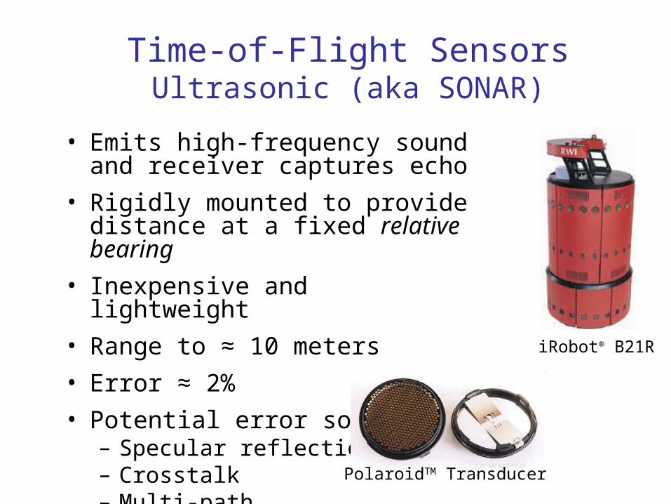
• Emits high-frequency sound and receiver captures echo

• Rigidly mounted to provide distance at a fixed relative bearing

• Inexpensive and lightweight

• Range to ≈ 10 meters

• Error ≈ 2%

• Potential error sources– Specular reflection– Crosstalk– Multi-path

iRobot® B21R

PolaroidTM Transducer

SICK® LMS-200

Time-of-Flight SensorsLaser Range Finders (LRF)

• “Most accurate” exteroceptive sensor available

• Relies on detecting the backscatter from a pulsed IR laser beam

• Range 80 meters

• 180o degree scans at 0.25o resolution

• Error: 5mm SD at ranges < 8 meters

• Negatives – Weight ≈ 10 pounds– Cost ≈ $5K– Power consumption ≈ 20W/160W– Difficulty in detecting transparent or dark

matte surfaces

Modeling Sensor NoiseSome Initial Ideas

• Assume that we can remove sensor bias through calibration

• All sensor measurements are still wrong, as they are corrupted by random sensor noise

• Goal: Develop algorithms which are robust to sensor noise

• Problem: How do we model if its distribution is unknown?

actmeas xx v

v

Modeling Sensor NoiseSome Initial Ideas

• Some Possible Solutions: – Collect empirical data and develop a consistent

model– Gaussian assumption v ~ N(μ,σ2)

2

2

2

)(

22

1)(

x

exf

Some Other Definitions

• Population mean:

• Population mean is also referred to as the expected value for the distribution

ondistributi discretea for )(1

N

iii xpx

ondistributi continuousfor )( dxxxf

N

iixN 1

(average) mean samplea for 1

Some Other Definitions (cont’d)

• Population Variance:

• σ is referred to as the Standard Deviation, and is always positive

ondistributi discretea for )()(1

22

N

iii xpx

ondistributi continuousfor )()( 22 dxxfx

population samplea for )(1

1

22

N

iixN

Why a Gaussian? • Central Limit Theorem

• Mathematical convenience– Gaussian Addition distribution– Gaussian Subtraction Distribution– Gaussian Ratio Distribution– “Invariance” to Convolution– “Invariance” to Linear Transformation

• Empirical Data

• Experimental Support

• “It’s the normal distribution”

The “Standard” 2-D Gaussian

• This formula is only valid when the principle axes of the distribution are aligned with the x-y coordinate frame (more later)

• QUESTION: Assuming that our accelerometers are corrupted by Gaussian noise, would we expect the distribution for position to be Gaussian as well?

2

2

2

2

2

)(

2

)(

222

1)( yx

yx

yx

exf

So how can I sample a Gaussian distribution in Matlab?

randn function>> help randn

RANDN Normally distributed random numbers. RANDN(N) is an N-by-N matrix with random entries, chosen

from a normal distribution with mean zero, variance one and standard deviation one.

>> x = randnx = -1.6656

>> x = randn(2,3)x = 0.1253 -1.1465 1.1892 0.2877 1.1909 -0.0376

QUESTION: How do I generate a general 1D Gaussian distribution from this?

A (very) Brief Overview ofComputer Vision Systems

• Cameras are the natural extension of biological vision to robotics

• Advantages of Cameras– Tremendous amounts of information– Natural medium for human interface– Small Size– Passive– Low power consumption

• Disadvantages of Cameras– Explicit estimates for parameters of interests (e.g. range,

bearing, etc.) are computationally expensive to obtain– Accuracy of estimates strongly tied to calibration– Calibration can be quite cumbersome

Pulnixtm & Pt Greytm Cameras

Sample Robotics Application Obstacle Avoidance

Single Camera System

• After an appropriate calibration, every pixel can be associated with a unique ray in space with an associated azimuth angle θ, and elevation angle φ

• An individual camera provides NO EXPLICIT DISTANCE INFORMATION

Z

X

f

xi

Z

Y

f

yi

Perspective Camera ModelCCD

(xiR,yi

R)

Optical Center

f

CCD

Stereo Vision Geometry

(X,Y,Z)

Optical Center

CCD

B = Baseline

(xiL,yi

L)

x

Z

f=focal lengthB/2

Stereo Geometry (cont’d)

)(2

)(Ri

Li

Ri

Li

xx

xxBfX

)( R

iLi xx

BfZ

Left Image Right Image

disparity = (xiR – xi

L)

)( Ri

Li xx

ByY

(xiL,yi

L) (xiR,yi

R)

(X,Y,Z)

NOTE: This formulation assumes that the two images are already rectified.

* Images from www.ptgrey.com

Sample Stereo ReconstructionFrom Point Grey BumblebeeTM Camera

Next Time…

• How do we extract features from images– Edge Segmentation– Color Segmentation– Corner Extraction