An Introduction to Forecasting with Time Series Models · An Introduction to Forecasting with Time Series Models William R. Bell Time series models have become popular in recent years

An Introduction to Forecasting with Time Series Models

William R. Bell

Time series models have become popular in recent years since

the publication of the book by Box and Jenkins (1970), and the

subsequent development of computer software for applying these

models. nur purpose here is to review the use of time series

models in forecasting. We will emphasize several important

points about forecasting:

1. Forecasting by the fitting and extrapolation of a

deterministic function of time is generally not a good

approach.

? Providing reasonable measures of forecast accuracy is

p.ssential - sometimes it is more important to find out

that a series cannot be forecast than to obtain the

"best" forecast.

3. Subject matter knowledge should not be thrown out the

window when doing time series modelling and forecasting.

We shall demonstrate that the main difficulty with forecasting by

fitting and extrapolating a deterministic function is that such

an approach does not generally provide reasonable measures of

forec~st accuracy. The main advantage to time series models is

not that they necessarily provide better (more accurate)

forecasts, but that they do provide a means for obtaining

reasonable measures of forecast accuracy. The route to better

forecasts does not lie through time series models alone, but

through the combination of time series models with subject matter

-21-

knowledge about the series being forecast. This can be done via

regression plus time series models which we discuss briefly (or

more generally, through multivariate time series models, which we

will not cover here).

1. Difficulties With Using Deterministic Functions To Do

Foreca~

A natural approach to forecasting would seem to be to view

the observed time series as a function of time observed with

error, specify a function of time, f(t), that looks appropri~te

for the data, fit f(t) to the data by least squares (although

other fitting criteria could be used), and forecast by

extrapolating f(t) beyond the observed data. One could also try

to use regression theory to produce co~~idence intervals for the

future observations. However, there are a number of difficulties

with this approach, that we shall discuss in turn. We shall

illustrate these difficulties by using this approach to forecast

the time series of daily IBM stock prices, taking as observations

the data from May 17, lq61 through September 3, 1961.

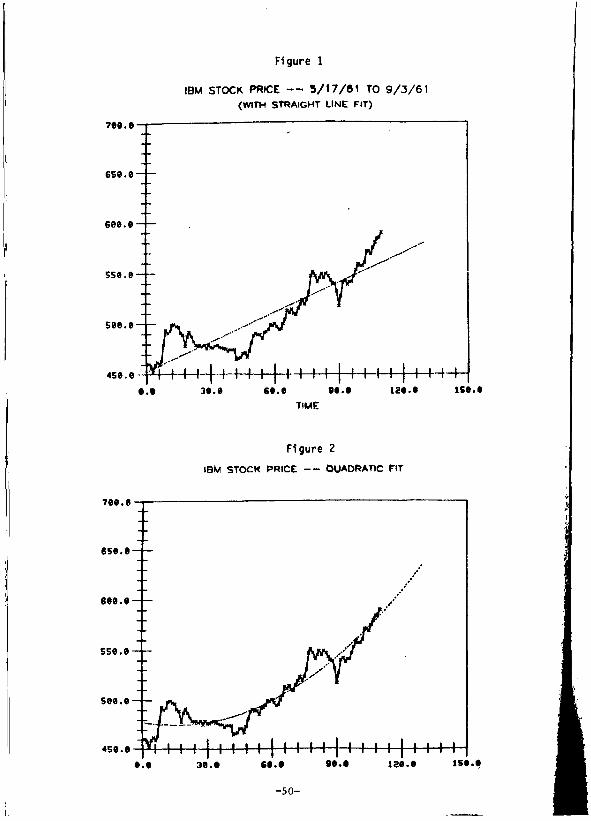
The IBM stock price data plotted in Figure 1 illustrate the

first difficulty with fitting a deterministic function:

1. It is often difficult to find a suitable function of

time.

Although Figure 1 does not suggest any obvious function, as a

first attempt we might try fitting a straight line, f(t)

a + St, to the data. The resulting fit is quite poor, as is also

shown in Figure 1 (with the fitted line extrapolated 20 time

periods (days) beyond the last (110th) observation). The

-22-

quadratic, f(t) = a + at + yt 2 , shown in Figure 2, might be

regarded as a better fit, though there are stretches of the data

over which the quadratic also fits poorly.

The difficulty in finding a suitable f(t) to fit to data for

forecasting is analogous to the same problem in graduation of

data, which is well known to actuaries (see Miller 1942). The

proble~ is more severe in forecasting, since it is easier to find

a suitable function to fit for interpolation within the range of

the observed data, than for extrapolation beyond the range of the

ddta. This proble~ in graduation led to the development of

graduation ~ethods such as Whittaker-Henderson (see Whittaker and

Robin~on (1944)). and that of Kimeldorf and Jones (1967), which

~ake use of local smoothness of an assumed underlying function,

without requiring an explicit form for the function. These

graduation ~ethods can be thought of as analogous to the ARIMA

time series models we shall discuss later.

Figure 2 illustrates another problem with the deterministic

function approach, which is

2. The forecasts can exhibit unreasonable long-run behavior.

The fitted quadratic in Figure 2 approaches + ~ at an increasing

rate as t increases. Thisis a problem in any

given situation will depend on the length of the forecast period

and how fast the fitted function deviates from reasonable

behavior.

A third problem that can arise with the deterministic

function approach is the following:

-23-

3. If the fitted values differ much from the data at the

last few time points, short-run forecasts can be poor.

Another way of saying this, is that if the fit is bad at the end

of the series the first few forecasts are likely to be bad.

Figure 1 shows the straight line fits poorly at the end of the

110 observations used. Figure 3.a shows the last 31 observations

of the data we are using (t = RO to t = 110) along with the next

20 observations to be forecast (t = III to t = 130). We see

th~ initial straight line forecasts are indeed poor, although the

series eventually wanders down closer to the forecasts. The

problem here is that in fitting the linear function (or any other

function) by (ordinary) least squares, all the observations are

given equal weight, so there is no guarantee that the fit will be

good near the end of the series. Generally, time series models

make use of the last few observations in a way that gives the

model a much better chance to produce good short-run forecasts.

One way around the above problem is to only fit to data at

the end of the series. For Figure I, the stretch of data from,

say, t = 91 (August 15, 1961) to t 110 would seem to be more

amenable to the fitting of functions than any longer stretch at

the end of the series. A straight line provides a good fit to

this part of the series as shown in Figure 4. Further analysis

of the stock price data will use this straight line fit to the

last 20 observations.

In addition to forecasting the stock prices, we would like

to estimate forecast error variances, and produce forecast

intervals for the future values (assuming normality). This may

-24-

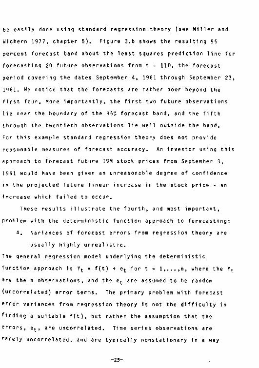
be easily done using standard regression theory (see Miller and

Wichern 1977. chapter 5). Figure 3.b shows the resulting 95

percent forecast band about the least squares prediction line for

forecasting 20 future observations from t ; 110. the forecast

period covering the dates September 4. 1961 through September 23.

lq61. We notice that the forecasts are rather poor beyond the

first four. More importantly. the first two future observations

lie near the boundary of the 95% forecast band. and the fifth

through the twentieth observations lie well outside the band.

For this example standard regression theory does not provide

reasonable measures of forecast accuracy. An investor using this

approach to forecast future IBM stock prices from September 3.

1961 would have been given an unreasonable degree of confidence

in the projected future linear increase in the stock price - an

increase which failed to occur.

These results illustrate the fourth. and most important.

prohlem with the deterministic function approach to forecasting:

4. Variances of forecast errors from regression theory are

usually highly unrealistic.

The general regression model underlying the deterministic

function approach is Yt ; f(t) + et for t ; 1 ••••• n. where the Yt

are the n observations. and the et are assumed to be random

(uncorrelated) error terms. The primary problem with forecast

error variances from regression theory is not the difficulty in

finding a suitable f(t). but rather the assumption that the

errors. et. are uncorrelated. Time series observations are

rarely uncorrelated. and are typically nonstationary in a way

-25-

that implies very high correlation in the observations. Such

high correlation can easily result in grossly understated

prediction error variances.

The goal of time series models is to provide a reasonable

approximation to the correlation structure of the data via a

model with a small number of parameters (in relation to the

length of the series). When this is done it will often he seen

that observed patterns in the data were in fact not due to the

~resence of some underlying smooth function, but merely to the

~igh degree of correlation in the data, which is accounted for by

the time series model.

The preceeding treatment was elementary, but was

deliberately so in an effort to make clear some difficulties with

fitting a deterministic function to a time series for the purpose

of forecasting. Of the difficulties mentioned, we regard the

prohlem of obtaining reasonable forecast error variances (so that

probability statements about the future can be made), as the most

important. In the constant search for forecasting methods to

produce "hetter", i.e., more accurate, forecasts, the problem of

producing good (or just reasonable) estimates of forecast error

variances has frequently been overlooked by forecasters. We

regard the problem of estimating forecast error variances as just

as important as that of estimating future values. Sometimes it

is more important to learn that you cannot forecast a series than

to get the "best" forecast of it.

In the next section we discuss the use of ARIMA time series

models in forecastng. While these models will not necessarily

-26-

lead to more accurate forecasts. they will almost certainly help

the forecaster estimate forecast error variances. something Some

other approaches to forecasting cannot do at all.

2. ARIMA Time Series Models and Forecasting

As noted earlier. time series typically feature correlation

between the observations. Time series models attempt to account

for this correlation over time through a parametric mOdel. Here

we shall discuss the use of ARIMA (autoregressive - integrated -

mDvj~g average) time series models in forecasting. We shall not

provide the rationale behind these models. or discus~ approaches

to modeling. hut refer the reader to the books by Box and Jenkins

(1Q70) and Miller ann Wichern (1977). We will assume the time

series has been modelled and the model is known.

ARIMA monels include the (purely) autoregressive (AR) model

( 2. 1 )

where $1 ••••• $p are parameters. the at's are independent.

identically distributed N(o.a~). and we assume. for now. E(Yt)=O.

Letting B be the backshift operator (BY t = Yt - 1) we can write

(2.1) as

(2.2)

or $(R)Y t = at where $(B) = 1 - $1B - ••• - $pBP. The (purely)

movi n9 average (MA) model is

-27-

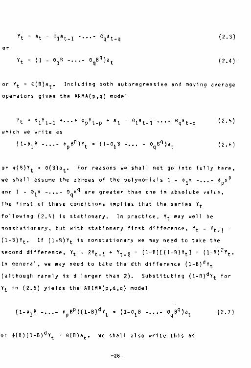
( 2.3 )

or

(2.4) .

or Yt = 0(B)a t • Including both autoregressive and moving average

operators gives the ARMA(p,q) model

Yt = ~lYt-1 + ••• + ~pYt-p + at - 01a t _1-···- 0qa t _q

which we write as

( 2. Ii )

(2. Ii)

or ~(~)Yt = 0(B)a t • For reasons we shall not go into fully here,

we shall assume the zeroes of the polynomials 1 - ~lX -... -and 1 - 01X - .•• - 0qX

q are greater than one in absolute valup.

The first of these conditions implies that the series Yt

following (2.5) is stationary. In practice, Yt may well be

nonstationary, but with stationary first difference, Yt - Yt -1

(l-B)Y t • If (l-B)Y t is nonstationary we may need to take the

second difference, Yt - 2Y t _1 + Yt - 2 = (l-B)[(l-B)Yt J = (1-B)2 yt •

In qeneral, we may need to take the dth difference (l-B)d Yt

(although rarely is d larger than 2). Substituting (l-B)dY t for

Yt in (2.6) yields the ARIMA(p,d,q) model

( 1- 91 B - ••• - 0 Bq) at q

0(B)a t • We shall also write this as

-28-

(2.7)

( 1 - ~lB - ••• - ~ dBP+d)y p+ t (1-01B - ... - 0 Bq)a t q

where 1 - ~lB - ••• - ~P+dBP+d = (l-~lB - ••• - ~p BP)(l_B)d.

(2.A)

If Yt is stationary (d=O) it is usually inappropriate to

assume E(Y t ) = 0, thus, Yt in (2.1) - (2.6) should be replaced by

Yt - \ly (u = E(Y t »· For (2.6) this gives HB)(Y t - lJy ) = 0(B)a t • y

If d > o then (l-B)d(yt - lJ y ) = (l-B)d Yt since (I-Bhy = 0, so we

do not use Yt - lJyin (2.7). !fit turns out that (l-B)d Yt has a

nonzero mean, this can be allowed for by using the model

( 2.9)

In any of the above models Yt could be some transformation of

the original data, such as a power transformation (see Miller

19R4).

2.1 Forecasting With ARIMA Models

To illustrate forecasting with ARIMA models, we shall use

(2.8) written as

(2.10)

for t = n+1. We shall assume we want to forecast Yn+1 for

1 = 1,2, ••• using data Yn , Yn-1"" For simplicity, we are

assuming for now that the data set is long enough so that we may

-29-

effectively assume it extends into the infinite past. (In

practice. given the model. this assumption is typically

innocuous. and it can be dispensed with if necessary - see Ansley

and Newbold (lQS1).) The best (minimum mean squared error)

forecast is given by the conditional expectation E(Y n+ t I Yn •

Yn- 1 •••• ) = Yn(t). From (2.10). Yn(t) satisfies

( 2 • 11 )

+ a n ( t ) - 01 a' n ( t - 1) - ••• - 0 q a n ( t - q ) •

Yn(t) can be computed recursively from (2.11) for t

using

j < 0

j > 0

1.2,3 ••••

j < 0

j > 0

Since at is independent of Yt -1' Yt -2 ••••• an(j) = 0 for j > O.

The at's can be computed from the model using Yt. Yt -1 ••••• as

discussed in Box and Jenkins (1970) (basically at

0(B)-1~(B)(1-B)dYt)' Notice that for t > q we get

t > q (2.12)

which can also be written ~(B)Yn(t) = 0 with B operating on t •

Thus. Yn(t) as a function of t (called the forecast function)

-30-

satisfies a homogeneous difference equation of order p+d for A A

t > q. with starting values Yn(q). Yn(q-1) ••••• Yn(q-p-d+1).

We are also interested in properties of the forecast error

Yn+t - Yn(t). Box anrl Jenkins (1970) observe that

where ~1'~2"" are solved for by equating coefficients of

x.x 2 .x] •..• in

so 1}1

~2 '" 2 .. '" 1 ~1 - (32

etc.

(2.13 )

For j > q I/I j = "'ll/1j_l + ••• + "'p+d1/lj_p_d so the 1/Ij'S siltisfy the

same homogeneous difference equation as the forecast function.

The variance of the t-step ahead forecast error. V(t). is easily

seen from (2.13) to be

v ( t)

Observe that d n+l is the one-step ahead forecast error with

va ri ance 0;. In practice. we substitute estimates of the parameters

( 2.15)

"'j' 8j , and o~ in (2.11) and (2.15) to estimate Yn(t) and V(t).

Assuming normality. we can use these to make probability

-31-

statements about Yn+ t given the data through time n. For

example, a 95 percent forecast interval for Yn+ t is

2.2~ecasting for Some Particular Models

~~odF!l: AR( 1)

For the AR(I) model, Yt - Ily = <P 1 (Y t _1-ll y ) + at with , ,

( 2.16)

l<Pll < 1, we see from (2.11) that (replacing Yn(j) by Yn(j) - Ily)

Y (1) n'

Using these results, it is easy to show that

Using (2.14) it can be shown that tj

v ( t) (1 + ~2 + + ~2(t-1))o2 "'I ••• "'I a·

Notice that as t+~, Yn(t) + Ily and V(t) + o~/(l-<pi), which is

Var(Y t ). For the stationary AR(l) model, the forecast function

damps out exponentially to the series mean, and the forecast

variance converges to the variance of the series.

-32-

(0,1,0) Model: "Random Walk"

For the random wa 1 k model, Yt Yt -1 + at, (2.11) yields

Here the forecast for all lead times is simply the last

observation. Also, 1j!j = 1 j ~ 1 so that V(t) -= (R.-1)0~. Notice

these results are analogous to those for the AR(l) model but

with ~l = 1 and ~y = O. However, unlike the stationary AR(l)

In 0 del. a s t + '" Y" (.~ 1 + Y nan d V ( t ) + ....

~LL~~_ "Exponential Smoothing"

For the (0,1,1) model, Yt = Yt-1 + at - 0 1a t _1 , (2.11)

1 eads to

Y'n ( 1 ) t > 1.

It can be shown that

so that the forecast is an "exponentially weighted moving

average" of the past observations (the weights on the past

observations sum to 1). Forecasting with this model is referred

to as "exponential smoothing". (2.14) leads to tj • 1-91 for all

j so that V(l) = 0; and

-33-

v ( t) t > 2 •

2.3 Properties of Forecast Functions

If Yt follows (2.7) and (2.R), then Yn(t) satisfies the

hOMogeneous difference equation (2.12) with starting A A

values Yn(q), ••• , Yn (q-p-d+l). Fuller (IQ76, section 2.4) gives

properties of solutions to difference equations, which may be • p t d-l

used to show that Yn(t) 1: 8.1;. + (<10 + <1 1 t+ ••• + <1d It ) ;=1 1 1 -

-1 -1 P where 1:1 ""'~p are the zeroes of 1 - <PIx - ... - <Ppx = $(x)

(for simplicity, we assume these are distinct), and the

' .. ()efficients Bl .... ,8p.1l0' ... <1d_l are determined by the stil"ting

values. If Yt follows the model (2.9), then Yn(t) satisfies the

non-homogeneous difference equation obtained by adding 00 to the

right hand side of (2.12). The effect of this on the solution

for Yn(t) is to add a term <1dtd, where <1d = 00

/(1-<P 1 -"'- <l>p)d!.

!Ising (2.12) - (2.IS), and properties of solutions to

difference equations. one can establish the following general

results.

(i) If d=O, so Yt is stationary.

Yn(t) .. Ily and V(t) .. var(Y t ) as t .. GO

(Ily = 00

/(1-<P1 - ••• - <Pp) in (2.9) and is 0 in (2.7))

(ii) If d>O, so Yt is nonstationary. Yn(t) is eventually

dominated by a polynomial of degree d-1 if 00 = 0, and

of degree d if 00 f. 0, and

V ( t) .. GO as t .. GO.

-34-

, I

! I For the particular case of the (O.d.q) model in (2.7).

(2.12) becomes (1_B)d Yn(i) = O. so that Yn(i) exactly follows a

polynomial of degree d-1 for i > q.1 The coefficients of the

polynomial are determined by the starting values.

yn(q)' •••• vn (q-P-d-1), which in turn depend on Yn .Y n- 1 ' ••••

The polynomial is adaptive and need only apply locally. i.e •• its

coefficients are redetermined as each new data point is added.

This contrasts with Simply fitting a single polynomial over the

entire range of the data.

For the model (1-B)d Yt 00 + 0(B)a t ((2.9) with $(B) = 1).

y (~, is a polynomial in £ of degree d. with the coefficient n

of ~d equal to 0o/~!' The forecast function here is non-

adaptive in that the same 00 is used at each time point. If a

"polynomial plus error" model. Yt = aO+a1t+ ••• +adtd+at. is really

appropriate. then the time series modelling process should lead

to the model

d (1-B) Yt

Solving this difference equation for Yt leads back to the

polynomial plus error model (see Box and Abraham (1978)). Thus.

ARIMA models allow for polynomial projection when appropriate.

1 Keyfitz (1972) has suggested one way demographic projections might be done is by passing a polynomial of some degree d through the last d data points. This in fact corresponds to forecasting with an ARIMA(O,d+1.0) model.

-35-

2.4 Example: IBM Stock Price Series

For the IBM stock price data, two models were fitted to the

full stretch of data from May 17, 1961 through September 3, 1961.

These were the (0,1,1) model and the (0,1,1) model with trend:

(l-B)Yt

(l-B)Y t

(l-0 1B)a t

00 + (1-0 1B)a t •

-.29

-.26

26.0

1. 20

Twenty forecasts from September 3, 1961 are shown for these

models in Figures 5 and 6. We notice either of these models

25.3

produces better forecasts than the straight line fits in Fiqures

3a and 3b. However, this is partly due to the fact that we

selected the stretch of data we are using to illustrate the

dangers of fitting and extrapolating a straight line. The

important difference is in the forecast intervals. The intervals

for the time series models are quite wide and increase

substantially with increasing t, allowing for a wide range of

behavior for the future stock prices. The interval from the

straight line model in Figure 5 is clearly too narrow. The

message from the time series models is quite clear: the IBM

stock price series is difficult to forecast. It is much more

important to learn this from the model, than to get the "best"

forecast, which is likely to be inaccurate anyway.

2.5 Seasonal Models

If the series exhibits periodic behavior to some degree (such

as an annual period in monthly or quarterly data) then the ARIMA

-36-

models discussed above need to be enhanced. For a seasonal series

with period s, we can use the seasonal ARIMA(p,d,q) x (P,O,O)s

model as discussed in Box and Jenkins (1970). For example, for

monthly data one useful model is the (0,1,1) x (0,1,1)12 model

Models such as this produce forecast functions

with periodic behavior.

2 • 6 We a k Poi n t s i., the. A R I ~y r 0 a c h

There are some difficulties with using ARIMA models in

forecasting that users should be aware of, especially since

research may suggest improved procedures to deal with these

problems. Since there is no difficulty with the forecasting

mathematics once we know the ARIMA model. the problems have to do

with the fact that we never really know the model.

Even if we know the orders (p.d.q) of the ARIMA model. the

parameters can only be estimated from the data. This introduces

additional error into the forecasts which is not accounted for in

V(t). Fortunately. for long series (large n) the effect of

parameter estimation error on forecasts and forecast error

variances can be shown to be negligible (Fuller 1976. section

8.6). The problem is more important for short series. It has

been investigated by Ansley and Newbold (1981) who suggest a

means of inflating V(t) to allow for parameter estimation

error. Another approach to this problem is to use the bootstrap

-37-

technique to assess the forecast accuracy (see Freedman and

Peters (1982)).

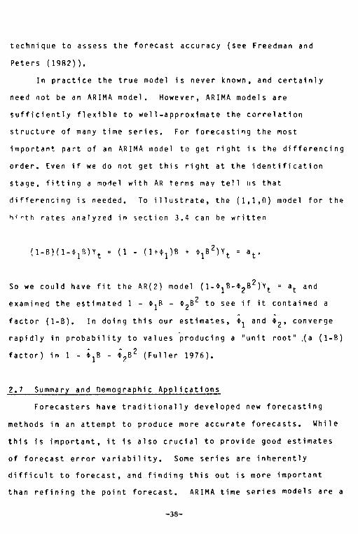
In practice the true model is never known, and certainly

need not be an ARIMA mOdel. However, ARIMA models are

sufficiently flexible to well-approximate the correlation

structure of many time series. For forecasting the most

important part of an ARIMA model to get right is the differencing

order. Even if we do not get this right at the identification

stage, fitting a morlel with AR terms may tell us that

differencing is needed. To illustrate, the (I,I,O) model for the

hirth rates analyzed in section 3.4 can be written

So we could have fit the AR(2) model {1-~IB-~2B2)Yt = at and

examined the estimated 1 - ~IB - ~2B2 to see if it contained a

factor (I-B). In doing this our estimates, ~1 and ~2' converge

rapidly in probability to values producing a "unit root" ,(a (I-B)

factor) in 1 - ;IB - ;~B2 (Fuller 1976).

2.7 Summary and Oemographic Applications

Forecasters have traditionally developed new forecasting

methods in an attempt to produce more accurate forecasts. While

this is important, it is also crucial to provide good estimates

of forecast error variability. Some series are inherently

difficult to forecast, and finding this out is more important

than refining the point forecast. ARIMA time series models are a

-38-

flexible class of models that can be used in many situations to

produce both reasonable forecasts and reasonable estimates of

forecast error variance.

Keyfitz (1972, 19B1) has also argued that providing measures

of the expected ,size of forecast errors is essential, and he

notes that population forecasters have virtually unanimously

failed to do this. Keyfitz (19Bl) prese~ts empirical measures of

forecast accuracy for historical population forecasts as a guide

to accuracy of current and future forecasts. Stoto (19B3) also

analyzes the dccuracy of historical population forecasts. He

an~lyzes the forecast errors to produce estimates of forecast

error variance, and then develops confidence intervals for United

States population through the year 20nn. McDonald (I QB1) uses

ARIMA models to forecast an Australian births series.

3. Use of Subject Matter Knowledge in Forecasting

The forecaster should not discard his or her subject matter

knowledge when using time series models in forecasting. ARIMA

models attempt to account for the correlation over time in time

series data, and then use this correlation in forecasting. They

cannot deal with other forecasting problems that may require

interaction of subject matter knowledge about the series being

forecast with time series models.

3.1 Deciding What Time Series to Forecast

As pointed out by Long (1984), this is a traditional problem

faced by demographers doing population projections. For example,

-39-

consider the basic demographic accounting relation (P t

at time t)

population

Pt Pt - 1 + Births t - Deaths t + Inmigrationt - Outmigrationt.

In forecasting Pt we must decide whether to forecast Pt directly,

or indirectly by forecasting the components. We must also decide

whether to hreak down the series by age, sex, race or other

factors (see Long (1984) for a discussion). Once the series to

be forecast have he en decided upon, time series models can be

II c; e f I) 1 i n d 0 i n q the for e cas tin g .

Another aspect of this is the selection of a transformation

to be used, if any, on the series. To an extent this is a

statistical problem (see Miller 1984), but transformations

involve a rescaling of the dat~, the implications of which should

be considered. For example, if Yt is a series of proportions the

logistic transformation, Zt = In(Yt!(I-Y t )), can be useful. In

logistically transforming the interval (0,1) to (-~,~), the

variation in Yt when it is near 0 or I is enhanced relative to

the variation when Yt is not near the boundary. Forecasting Zt

and transforming back via Yt = exp(zt)!(I+exp(zt)), will produce

forecasts and confidence intervals for Yt that do not stray

outside the interval (0,1).

3.2 Deciding What Part of the Data to Use

Time series methods, like other statistical methods, work

better when more observations are available. However, this

-40-

assumes that all portions of the series follow the same model.

Real series may. for example. be affected by structural changes.

unusual events. or changes of definition. While it is best to

avoirl these difficulties. this conflicts with the need to use as

long a series as possible when modelling. Knowledge about the

series heing forecast can help in deciding how much of the past

to use in modelling.

3.3 Regression Plus Time Series Models

In some cases it is possible to explicitly incorporate

subject matter knowledge into the forecast model. A useful means

of doing this is to use regression plus time series models.

These are closely related to transfer function models (also

called distributed lag models). McDonald (19B1) fits models of

this type to an Australian births series. More generally,

multivariate time series models might be used - see Tiao and Box

(1981) for a general discussion. and Miller (1984) for a

demographic example.

The regression plus ARIMA(p,d.q) time series model is

( 3.1 )

where X1t ••••• Xkt are the independent variables and ~l""'~k the

regression parameters. Inference results for models of the form

(3.1) are given in Pierce (1971). Forecasts can be obtained for

t = 1.2 •••• by writing (3.1) as

-41-

( 3.2)

To produce forecasts of Yn+ t from (3.2) requires future values of

the Xit series. The accuracy of the forecast for any twill

depend on the extent to which the Xit are "know"" through

time 11+1.

The ideal situation is where the Xit are known exactly for

all t. This can happen in practice - ~ell and Hillmer (19B3)

discuss the use of regr&ssion plus time series models for

economic series exhibiting calendar variation, where the Xit ~re

functions of the calendar and thus are known for all time. When

the future Xit'S are not known, they must be forecast as well

(this is really what distinguishes a transfer function model from

a regression plus time series model), and the accuracy of the

resulting forecast of Yn+1 will obviously depend on the accuracy

of the Xi,n+t forecasts. Also, the forecast error variance

should include the additional error variance due to forecasting

the Xi,n+! (see Box and Jenkins (1970, section 11.5)).

An intermediate situation is where Yt depends on the value

of another series, Wt , at an earlier time point. A simple

example would be the model

In this case Wt is a leading indicator for Yt. It will be known

-42-

..

exactly when forecasting Yn+~ for ~

forecast after that.

1 ••••• r. but must be

To clarify the roles of the regression and time series parts

of the model. let the observed data 'i = (Y 1 ••••• Yn)' have mean

vector I!. = (lJ 1 •••.••• lJ n)'. and nxn covariance matrix

r = (Cov(Yi.V j )). Notice lJ t is not constant over time here. To

forecast Yn+t • we use the covariances

!!: = (cov(YnH.Yl), •••• Cov(YnH.Yn)). The best (minimum mean

squared error) forecast of Yn+2 given t is the conditional

expectation. which under the multivariate normal distribution. is

( 1. 3)

The objective of the regression part of the model is to

model lJt as SlX lt + ••• +8 k Xkt • thus getting at lJ nH and l! in (3.3).

Time series models. on the other hand. seek a parametric model to

describe Cov(Yt.Yt+j)' and hence 2' and 1: in (3.3). Thus.

regression models and time series models are complementary and

should not he viewed as competitors. Just as it is unwise to use

pure regression models with correlated data (as was illustrated

in section 1). it is also unwise to blindly apply pure time

series models to a series known to be affected by certain

independent variables.

~.4 Example: Forecasting Birth Rates !nd Births

We shall illustrate some of the considerations mentioned in

the previous sections by using data through 1975 to forecast time

-43-

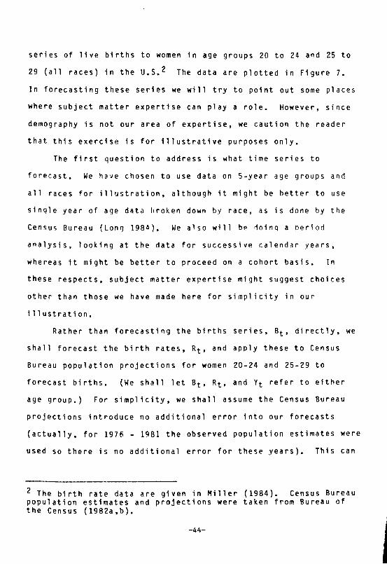
series of live births to women 1n age groups 20 to 24 and 25 to

29 (all races) in the U.S. 2 The data are plotted in Figure 7.

In forecasting these series we will try to point out some places

where subject matter expertise can playa role. However, since

demography is not our area of expertise, we caution the reader

that this exercise is for illustrative purposes only.

The first question to address is what time series to

forecast. We have chosen to use data on 5-year age groups and

all races for illustration, although it might be better to use

sinqle year of age data hroken down by race, as is done by the

Cen~us Bureau (Long 1984). We also will be ~oinq a period

analysis, looking at the data for successive calendar years,

whereas it might be better to proceed on a cohort basis. In

these respects, subject matter expertise might suggest choices

other than those we have made here for simplicity in our

illustration.

Rather than forecasting the births series, Bt , directly, we

shall forecast the birth rates, Rt , and apply these to Census

Bureau population projections for women 20-24 and 25-29 to

forecast births. (We shall let Bt , Rt, and Yt refer to either

age group.) For simplicity, we shall assume the Census Bureau

projections introduce no additional error into our forecasts

(actually, for 1976 - 1981 the observed population estimates were

used so there is no additional error for these years). This can

2 The birth rate data are given in Miller (1984). Census Bureau population estimates and projections were taken from Bureau of the Census (1982a,b).

-44-

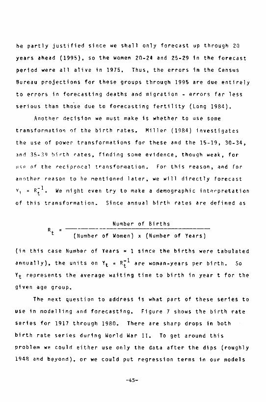
be partly justified since we shall only forecast up through 20

years ahead (1995), so the women 20-24 and 25-29 in the forecast

period were all alive in 1975. Thus, the errors in the Census

Bureau projections for these groups through 1995 are due entirely

to errors in forecasting deaths and migration - errors far less

serious than those due to forecasting fertility (Long 1984).

Another decision we must make is whether to use some

transformation of the birth rates. Miller (1984) investigates

the use of power transformations for these and the 15-19, 30-34,

ann 35-39 hirth rates, finding some evidence, though weak, for

liS" of the reciprocal transformation. For this reason, and for

another reason to he mentioned later, we will directly forecast

_ R- 1 Y t - t • We might even try to make a demographic interpretation

of this transformation. Since annual birth rates are defined as

Number of Births

(Number of Women) x (Number of Years)

(in this case Number of Years = 1 since the births were tabulated

annually), the units on Yt = Rt1 are woman-years per birth. So

Yt represents the average waiting time to birth in year t for the

given age group.

The next question to address is what part of these series to

use in modelling and forecasting. Figure 7 shows the birth rate

series for 1917 through 1980. There are sharp drops in both

birth rate series during World War II. To get around this

problem we could either use only the data after the dips (roughly

194~ and beyond), or we could put regression terms in our models

-45-

involving indicator variables for the affected years. However,

Miller and Hickman (19Bl) found significant evidence of model

change when comparing models for the pre-war and the post-war

"baby boom" data. Therefore, we shall fit the (1,1,0) model

considered by Miller (19B4) to the post-war data. One could

speculate that the "baby boom" was an aberration and that birth

rates have returned to normal, which would suggest fitting the

(1,1,0) models to the pre-war data and then applying theM to the

end of the series to forecast.

The (1,1,0) models were fitted to the 194B - 1975 data with

the following results:

Age 20-24

Age 25-29

(1-.72B)(I-B)Y t

(1-.70B)(I-B)Y t

.591xl0- 7

.56Bxl0- 7•

These models were used to produce forecasts Yn(t), for 1976 -

1995, leaving the five data pOints for 1976 - 19BO for comparing

forecasts to actual data. Upper and lower 95 percent forecast

limits were obtained from U(t) = Yn(t) + 1.96(V(t))~ and

- ~ L(t) = Yn(t) - 1.96 (V(t)) 2 for t = 1, ••• ,20. These were

inverted to point forecasts and forecast limits for the birth

rates:

t 1, ••• ,20

L R (t) U R ( t)

-46-

(Notice .q5 ~ Pr{L{t) < Yn+ t < U{t)) = Pr{U{t)-l < Y~!t < L{t)-l)).

The results are shown in Figures 8 and 9, which show the 1948 -

1980 data, the forecasted birth rates, and the forecast

intervals. We notice the first five forecasts for the 20-24

group are rather accurate, and those for the 25-29 are less so,

the first two there falling on the upper 95 percent liMit. In

both cases the forecast intervals widen rapidly with increasing

t, reflecting considerable uncertainty when forecasting much more

than 5 steps ahead. Long-run forecast accuracy will not come

from the data used here. It will require other knowledge about

the series.

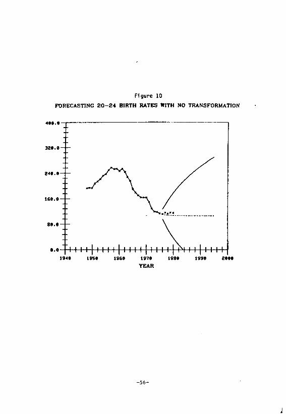
Notice that the forecast intervals in Figures 8 and 9 are

highly asymmetric, widening muc~ faster above the forecasts than

below them. The reciprocal transformation is responsible for

this. It in fact prevents the nonsensical situation of the lower

limit becoming negative, which is the reason for using it alluded

to earlier. Had we chosen to forecast Rt directly using a{l,l,O)

model, the results would be as shown in Figure 10 (for age group

20-24). While the point forecasts are little affected by the

reciprocal transformation, the forecast limits are considerably

different depending on whether or not we transform.

Finally, point forecasts and forecast limits for the births

were obtained as

LB{t) UB{t)

-47-

where Pn+t

is the Census Bureau population projection (assumed

error free). Figures 11 and 12 show the actual births,

forecasts, and forecast intervals for age groups 20-24 and 25-29.

The point forecasts and limits are modulated by the fluctuations

in Pn + t , producing behavior we would not have obtained by

forecasting births directly.

The next step in trying to improve on our forecasts of 20-24

and 25-29 births might be to look for other variables to include

in a regression plus time series model for Yt • We might try

using the 20-24 birth rates as a 5-year leading indicator in a

model for the 25-29 birth rates. This was tried with no

success. While there is a strong contemporaneous linear

relationship between the series (Miller 1984), this will not help

in long-run forecasting since neither of these series is easy to

forecast far ahead. Inclusion of economic variables might

improve short-run forecasts of the birth rates; long-run

forecasts of the birth rates would require long-run forecasts of

the economic variables, which are likely to be quite inaccurate.

3.5 Automatic Forecasting Procedures

Many automatic forecasting procedures have been proposed,

some of which involve the automatic selection and fitting of time

series models, and computer programs have been marketed for their

use. While such procedures may provide reasonable forecasts in

many cases, they have some important disadvantages. One is that

some of the procedures are ad-hoc and do not provide estimates of

forecast error variance. Also, automatic approaches necessarily

-48-

dissociate the forecaster from her or his data, ~aking it

difficult to include subject matter expertise in the forcasting

process, and restricting the forecaster's ability to deal with

unusual prohlems that arise. They also tend to reduce what the

forecaster learns from the data in the forecasting process.

-49-

Fi gure 1

IBM STOCK PRICE -- 5/17/151 TO 9/3/61 (WITH STRAIGHT LINE F"IT)

7 •••• ~--------------------------------------------~

ss •.•

s ••.•

ss •. e

se •. '

4se •• -. ...p4-+--I-f-~ I II I I I II I I I 111-4 ••• l •• ' &t •• II ••• 12 •• ' 15 •• '

TIME

Figure 2

IBM STOCI( PRICE -- OUADRAnc F"IT

7 •••• -T--------------------------------------------~

65 •• '

6 ••• '

ss •.•

5 ••• '

4S ••• -+~~~~4_4_~~~~_4_+_+~~~4_4_~~~~~

••• l •• ' &t.' SIt.' 128.8

-50-

Figure 3.a

. IBM STOCK PRICE: STRAIGHT UNE FORECAST USING ENTIRE SERIES

78a.8~--------------------------------------------~

66e.8

&28.8 -r--T

SS8.8

5048.8

S8.8 98.' lee.8

• a __ .......... . -. a- ------------- ... ----

118.8 128.8 138.8

TIME

Figure 3.b

19M STOCK PRICE -- STRAIGHT LINE I"ORECAST (USING LAST 20 09SERVAnONS)

7e ••• -r-------------------------------------------,

66 •• '

628.8

SS8.8

5048.8

•••• g ••• 1 ....

m04E -51-

ut.'

....... . - .

12 •• ' 13 •• '

t ••••

Sit.'

ss •• '

54 •• '

sa •• '

•

Fi gure 4 IBM STOCK PRICE ... - STRAIGHT LINE FIT

TO LAST 20 OBSERVATlONS

•

s ••.• ~-+~~+-+-~~~~~~+-~~~~~~+-+-~~ SI •• " '5." ...... us .•• u •.•• us ...

TIME

-52-

Figure 5 IBM STOCK PRICE -- (0,1,1) FORECAST

700.0-T----------------------------------------------~

I 660.0+

I

1 620.0 ±

I "I

SSe.0y

.1.

,,,.of

• . . .. . ..... , ...... _ ... _ .............. __ .... _ ..... JIlL.

s0e.a-+I-+'-+-+-+-+-+-+-+-r-r-r-r-r~~~+-+-+-+-+-+-+-+,~1

80.0 Sl0.8 108.8 118.8 128.e 138.8

TlIAE

Figure 6 181.4 STOCK PRICE - - (0.1.1) WITH TREND F'ORECAST

78e •• ~--------------------------------------------~

6se.'

S28.8

SBe.e

S"'.8

88.8 e8.' t ••••

TI .... E

-53-

-.­.. -........... -...... -_ .. -. ....... . ........ .

It •• ' li8 •• 13 •• '

400.0 -

320.0--

240.0

160.0-

80.0

Figure 7 ANNUAL U.S. AGE SPECIFIC BIRTH RATES 1917 - 1980

(PER THOUSAND)

. , ,."'

25-29

: '.'.1 .

---------- -------

.-, - .' . "

1910 1920 1930 1940 1950 1960 1970 1988

YEAR

-54-

Figure 8 FORECASTING 20-24 BIRTH RATES FROM 1975

4".1~--------------------------------------------~

32 •• '

2 .... e

161.e

a8.8

lV68 1S17,

YEAR

Figure 9

lva. 18S1.

FORECASTING 25-29 BIRTH RATES FROM 1975

a ...

"8e.8~---------------------------------------------'

32 •• '

2"'.'

lS8.8

a8.8

1115. lSI68 187. 1S18' 2 ••• YEAR

-55-

Fi gure 10

FORECASTING 20-24 BIRTH RATES WITH NO TRANSFORMATION

~".I~----------------------------

321.1

24'.'

161.'

88.1

1VS' 1V6' 1V71

YEAR

-56-

.~.!~! ........................ .

1va, 1V9' 2'"

Fi gure 11

FORECASTINC 20-24 BIRTHS (IN 1000'S) FROM 1975

3eee~------------------~----------------------~

.1 ..

. . .... ~-.~ ................................... -..... .. ...................... .....

12ee

6ee

15171 11175 198e 11185 111111 tIllS YEAR

Fi gure 12 FORECASTINC 25-29 BIRTHS (IN 10CO'S) FROM 1975

3e88--------------------------------------------~

2<48e

18ee

128e ........................... _ ....................... .

6ee

1871 11175 11181 11185 18111 1SIIIS

YEAR

-57-

REFERENCES

Ansley, C.F. and Newbold, P. (1981) "On the Bias in Estimation of Forecast Mean Squared Error," Journal of the American Statistical Association, 76, 569-578.

Bell, W.R. and Hillmer, S.C. (1983) "Modeling Time Series With Calendar Variation," Journal of the American Statistical Association, 78, 526-534.

Box, G.E.P. and Abraham, B. (1978) "Deterministic and Forecast -Adaptive Time - Dependent Models," Applied Statistics, 27, 120-130.

Box, G.E.P., and Jenkins, G.M. (1970), Time Series Analysis: For e cas tin g _~_ Con t r 0 1, San F ran cis co: H 0' den nay.

Bureau of the Census (lq~2a) "Preliminary Estimates of the Population of the United States, by Age, Sex, and Race: 1970 to lq81" Current ~lation Reports, Series P-25, No. 917, G.P.D., Washington.

(lq82h) Unpublished data consistent with middle series of --~Projections of the Population of the United States: 1982 to

2050 (Advance Report)," Current Population Reports, Series P-25, No. Q22, G.p.n., Washington.

Freedman, D.A. and Peters, S.C. (1982) "Bootstrapping a Regression Equation: Some Empirical Results" Technical Report No. 10, Department of Statistics, University of California, Berkeley.

Fuller, W.A. (1976), Introduction to Statistical Time Series, New York: Wiley.

Granger, C.W.J. and Joyeux, R. (1980) "Introduction to Long -Memory Time Series Models and Fractional Differencing," Journal of Time Series Analysis, I, 15-30.

Keyfitz, N. (1972) "On Future Population," Journal of the American Statistical Association, 67, 347-363.

(lg81) "The Limits of Population Forecasting", Population -----and Development Review, 7, 579-593.

Kimeldorf, G. and Jones, D. (1967), "Bayesian Graduation", Transactions of the Society of Actuaries, 19~ 66-112.

Long, J.F. (1984) "U.S. National Population Projection Methods: A View From Four Forecasting Traditions," included in this volume.

-58-

McDonald, J. (1981) "Modeling Demographic Relationships: An Analysis of Forecast Functions for Australian Births," Journal of the American Statistical Association, 76, 782-792.

Miller, M. (1942), Elements of Graduation, New York, Actuarial Society of America.

Miller, R.B. (1984) "Evaluation of Transformations in Forecasting Age Specific Birth Rates," included in this volume.

Miller, R.B. and Hickman, J.C. (1981), "Time Series Modeling of Births and Birth Rates" Working Paper 8-81-21, Graduate School of Business, University of Wisconsin, Madison.

Miller, R.B. and Wichern, D.W. (1977) Intermediate Business Statistics: Analysis of Variance, Regression, and Time Series, New York: Holt, Rinehart and W1nston.

Pierce, D.A. (1971), "Least Squares Estimation in the Regression Model With Autoregressive - Moving Average Errors," Biometrika, 58, 299-312.

Stoto, M.A. (1983) "The Accuracy of Population Projections," Journal of the American Statistical Association, 78, 13-20.

Tiao, G.C. and Box, G.E.P. (1981) "Modeling Multiple Time Series With Applications" Journal of the American Statistical Association, 76, 802-816.

Whittaker, E.T. and Robinson, G. (1944), The Calculus of Observations, London: Blackie and Sons.

-59-