An Introduction to Evidential Reasoning for Decision Making ...

An Introduction to Evidential Reasoning for Decision Making under

Uncertainty: Bayesian and Belief Functions Perspectives

Rajendra P. Srivastava Ernst & Young Distinguished Professor and Director

Ernst & Young Center for Auditing Research and Advanced Technology

School of Business, The University of Kansas

1300 Sunnyside Avenue, Lawrence, KS 66045

Email: [email protected]

December 8, 2010

International Journal of Accounting Information Systems, Vol. 12: 126–135

1

An Introduction to Evidential Reasoning for Decision Making under

Uncertainty: Bayesian and Belief Functions Perspectives

ABSTRACT

The main purpose of this article is to introduce the evidential reasoning approach, a research

methodology, for decision making under uncertainty. Bayesian framework and Dempster-Shafer

theory of belief functions are used to model uncertainties in the decision problem. We first

introduce the basics of the DS theory and then discuss the evidential reasoning approach and

related concepts. Next, we demonstrate how specific decision models can be developed from the

basic evidential diagrams under the two frameworks. It is interesting to note that it is quite

efficient to develop Bayesian models of the decision problems using the evidential reasoning

approach compared to using the ladder diagram approach as used in the auditing literature. In

addition, we compare the decision models developed in this paper with similar models developed

in the literature.

Key words: Evidential Reasoning, Bayesian, Dempster-Shafer theory, Belief Functions

1. INTRODUCTION

The main purpose of this paper is to introduce a general research methodology called

evidential reasoning for decision making under uncertainty. We use the following two

frameworks for managing uncertainties in the evidence: Bayesian framework and the framework

of Dempster-Shafer (DS) Theory of Belief-Functions (Shafer 1976). Evidential reasoning

basically means reasoning with evidence. Such situations are quite common in the real world

whether we deal with the medical domain, legal domain, or business domain such as auditing

and information systems. Srivastava and his co-researchers have applied this approach to

auditing and information systems domains. They have used this approach to develop models for

assessing risks such as audit risk, fraud risk, information security risk, information quality risk,

information assurance risk, auditor independence risk, risks associated with sustainability

reports, and many others (see. e.g., Srivastava and Shafer 1992; Srivastava and Mock 2010;

Srivastava, Mock and Turner 2007; Gao, Mock, Srivastava 2010; Sun, Srivastava and Mock

2006; Srivastava and Li 2008, Bovee, Srivastava, and Mak 2003, Srivastava and Mock 2000;

2

Srivastava, Mock and Turner 2009a, 2009b; Rao, Srivastava, and Mock 2010; and Mock, Sun,

Srivastava, and Vasarhelyi 2009). Of particular interest to information systems researchers

would be the work of Sun et. al (2006) on information security, and of Srivastava and Li (2008)

on systems security and systems reliability. Recently, Yang, Xu, Xie, and Maddulapalli (2010)

have used evidential reasoning approach in multiple criteria decisions.

We first introduce the basics of the DS theory of belief functions in Section 2. We discuss

the evidential reasoning approach and related concepts in Section 3. We demonstrate how

specific decision models can be developed from the basic evidential diagrams under the two

frameworks, Bayesian and DS theory of belief functions, in Sections 4 and 5, respectively.

Finally, Section 6 provides a conclusion and discusses potential research opportunities.

2. DEMPSTER-SHAFER THEORY OF BELIEF FUNCTIONS

Here we briefly introduce the DS theory and illustrate the use of Dempster's rule to

combine several independent items of evidence pertaining to a variable or objective. The DS

Theory is based on the work of Dempster during the 1960’s and of Shafer during 1970’s (Shafer

1976, see also Dempster, Yager, and Liu 2008). There are three basic functions in the DS theory

that we need to understand for modeling purposes. These are discussed below.

m-values, Belief Functions and Plausibility Functions

The basic difference between probability theory and DS theory of belief functions is the

assignment of uncertainties, the probability mass. In the probability framework, we assign

uncertainties to each state of nature. These states are assumed to be mutually exclusive and

collectively exhaustive. The sum of all these uncertainties assigned to individual state of nature

is one. For example, consider a variable X. It has two values: “x,” and “~x”. Under the

probability framework, we will have P(x) 0 and P(~x) 0, and P(x) + P(~x) = 1. However, in

3

the DS theory of belief functions, we assign uncertainties not only to each state of nature, but

also to all its proper subsets. These assigned uncertainties are called basic belief masses or m-

values and they all add to one. These m-values are also known as the basic probability

assignment function (Shafer 1976). For the variable X, we can have m(x) 0, m(~x) 0, and

m({x,~x}) 0, such that m(x) + m(~x) + m({x,~x)} = 1. In general, if the variable has n-values,

then m-values could exist for all the singletons, all the subsets with two elements, three elements,

and so on, to the entire frame. The entire frame consists of all the elements, i.e., all possible

values of the variable.

Let us consider the following set of m-values pertaining to variable X based on a piece of

evidence, say, E1: m

1(x) = 0.6, m

1(~x) = 0.1, and m

1({x, ~x}) = 0.3. These m-values represent a

mixed piece of evidence; 0.6 level of support that variable X is true; 0.1 level of support that

variable X is not true; and 0.3 level of support is assigned to the entire frame {x,~x},

representing partial ignorance. A positive evidence means that we have only support for ‘x’ and

no support for its negation, i.e., 1>m1(x)>0 and m

1(~x) = 0. A negative evidence means we have

support only for the negation, i.e., m1(x) = 0, and 1>m

1(~x)>0.

Two other functions are important for our purpose in the current discussion, belief

functions and plausibility functions. By definition, belief in a subset or a set of elements, say O,

is equal to the sum of all the m-values for the subsets of elements, say C, that are contained in or

equal to the subset O. Mathematically, we can depict it as:C O

Bel(O) = m(C)

. Also, we know

that Bel(O) + Bel(~O) 1, i.e., belief in O and belief in ~O may not necessarily add to one,

whereas in probability theory P(O) + P(~O) = 1; i.e., the probability that O is true and the

probability that O is not true always add to one. A belief of zero simply means that we lack the

4

evidence, whereas a zero probability means impossibility. Ignorance in probability framework

simply means assigning equal probability to all the state of nature. For example, if there are only

two possible values of a variable X, say {x, ~x}, then ignorance means assigning 0.5 to each

state, i.e., P(x) = 0.5, and P(~x) = 0.5. Under the DS theory, a complete ignorance is represented

by a belief of zero in “x” and in “~x”, i.e., Bel(x) = 0, and Bel(~x) = 0.

In addition, we can easily model partial ignorance under DS theory, whereas it is not

possible to express partial ignorance under probability theory. For example, suppose the auditor

wants to assess the effectiveness of a security system pertaining to a client’s information system.

One piece of evidence the auditor could collect would be to review the policies and procedures

established by the company for the security of the information system. Suppose, based on the

evaluations of the company’s policies and procedures related the systems security, the auditor

decides to assign a low level of support, say 0.3 on a scale of 0-1, that the information system is

secure, represented by ‘x’, and a zero level of support that the system is not secure, represented

by ‘~x’. This assessment can be expressed in terms of belief masses as: m(x) = 0.3, m(~x) = 0,

and m({x, ~x}) = 0.7. The value 0.7 assigned to the entire frame {x,~x} represents the partial

ignorance. However, under probability theory, once you assign 0.3 to the state that x is true, i.e.,

P(x) = 0.3, then by definition the result is P(~x) = 0.7. There is no way to represent partial

ignorance under probability theory.

Consider the earlier example of evidence E1 with the corresponding m-values: m

1(x) =

0.6, m1(~x) = 0.1, and m

1({x, ~x}) = 0.3. Based on this evidence alone, we have 0.6 degree of

support that “x” is true, 0.1 degree of support that “~x” is true, and 0.3 degree of support

uncommitted. Using the definition of belief functions, we can write: Bel1(x) = m

1(x) = 0.6,

Bel1(~x) = m

1(~x) = 0.1, and Bel

1({x, ~x}) = m

1(x) + m

1(~x) + m

1({x, ~x}) = 0.6+0.1+0.3 = 1.

5

Plausibility in a subset, O, is defined to be the sum of all the m-values for the subsets, C,

that have non-zero intersections with O. Mathematically this can be express as:

O C

Pl(O) = m(C) . Also, one can show that Pl(O) = 1 - Bel(~O), i.e., plausibility in O is one

minus the belief in not O. Using the above example of evidence E1, we have m

1(x) = 0.6, m

1(~x)

= 0.1, and m1({x, ~x}) = 0.3. Thus, based on the evidence E

1, we have the plausibility in “x” to

be 1 1 1 1

x C

Pl (x) = m (C) = m (x) + m ({x,~x})

=0.6+0.3 = 0.9, and the plausibility in “~x” to be

Pl1(~x) = m

1(~x) + m

1({x,~x}) = 0.1 + 0.3 = 0.4.

Srivastava and Shafer (1992) tie the plausibility function to the audit risk. More precisely,

plausibility that an account is materially misstated is the belief function interpretation of the audit

risk. In the above example, a plausibility of 0.4 that “~x” is true (Pl1(~x) = 0.4) can be

interpreted as the maximum risk that the variable X is not true, based on what we know now

from evidence E1. Using Srivastava and Shafer definition of risk, Srivastava and Li (2008) define

the systems security risk = Pl(~s) and the systems security reliability = Bel(s), were ‘s’ and ‘~s’,

respectively, represent that the system is secure and is not secure.

Dempster's Rule of Combination

Dempster's rule is used to combine various independent items of evidence bearing on one

variable. For simplicity let us consider just two items of evidence with the corresponding m-

values represented by m1, and m2. Using the Dempster's rule the combined m-values can be

written as (Shafer 1976):

1 2

O = C1 C2

m(O ) = m (C1)m (C2) / K

,

6

where K is the renormalization constant and is given by: 1 2

C1 C2 =

K = 1 m (C1)m (C2)

. The

second term in K represents the conflict between the two items of evidence. If the conflict term is

one, i.e., when the two items of evidence exactly contradict each other, then K = 0 and, in such a

situation, the two items of evidence are not combinable. In other words, Dempster’s rule cannot

be used when K = 0. One can easily generalize Dempster's rule for n items of evidence (see

Shafer 1976 for details).

Let us consider the following sets of m-values based on the two items of evidence

pertaining to the variable X: m1(x)=0.6, m

1(~x)=0.1, and m

1({x, ~x})=0.3; and m

2(x)=0.4,

m2(~x)=0.2, and m

2({x, ~x})=0.4. The renormalization constant K for this case is: K=1-

[m1(x)m

2(~x)+ m

1(~x)m

2(x)]=1-[0.6x0.2+0.1x0.4]= 0.84 and thus the combined m-values are:

m'(x) = [m1(x)m

2(x)+ m

1(x)m

2({x,~x})+ m

1({x,~x})m

2(x)]/K

= [0.6x0.4 + 0.6x0.4 + 0.3x0.4]/0.84 = 0.6/0.84 = 0.71428

m'(~x) = [m1(~x)m

2(~x)+ m

1(~x)m

2({x,~x})+ m

1({x,~x})m

2(~x)]/K

= [0.1x0.2 + 0.1x0.4 + 0.3x0.2]/0.84 = 0.12/0.84 = 0.14286

m'({x,~x}) = m1({x,~x})m

2({x,~x})/K = 0.3x0.4/0.84 = 0.14286.

Thus, by definition, the belief that “x” is true after considering the two items of evidence

is Bel’(x) = m’(x) = 0.71428, and the belief that “~x” is true is 0.14286, i.e., Bel’(~x) = m’(~x) =

0.14286. The plausibility that “~x” is true is 0.28572 (i.e., Pl(~x) = 1Bel(x) = 1 – 0.71428 =

0.28572). We see here that while belief that X is not true is only 0.14286, the plausibility that it

is not true is 0.28572, based on the existing evidence.

7

3. EVIDENTIAL REASONING APROACH

As mentioned earlier, evidential reasoning simply means reasoning with evidence. This

term was coined by SRI International (Lowrance, Garvey, and Strat 1986, fn 1) to denote the

body of techniques specifically designed for manipulating and reasoning from evidential

information. Gordon and Shortliffe (1985) discussed this approach under DS theory in the

context of MYCIN that was being developed “to determine the potential identity of pathogens in

patients with infections and to assist in the selection of a therapeutic regimen appropriate for

treating the organisms under consideration (see Shortliffe and Buchanan 1975, p. 237).” Pearl

(1986) used this approach for analyzing causal models under the Bayesian framework.

There are two basic dimensions of evidential reasoning. One is the structure of evidence

pertaining to the problem of interest. The second is the framework used to represent uncertainties

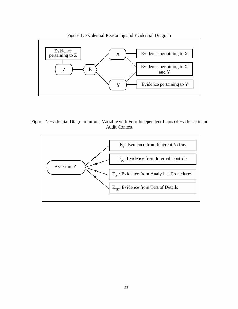
in the evidence and the related calculus to combine the evidence for decision making. Figure 1,

represents a simple evidential diagram with three variables X, Y, and Z, represented by rounded

boxes as variable nodes. These variable nodes may be interrelated through a logical relationship

such as “AND” or “OR” or an uncertain relationship depicted by the relational node, R in a

hexagonal box. The rectangular boxes in Figure 1 represent items of evidence, or evidence

nodes, pertaining to the variables to which they are connected.

In Figure 1, we have one item of evidence for each variable and one item of evidence

pertains to both X and Y. This diagram is a network in structure. If we did not have the evidence

pertaining to both X and Y, then the diagram would be a tree. In general, we may have only

partial knowledge about these variables because of the nature of evidence; the evidence may not

be strong enough to provide conclusive evidence about the status of the variables. This partial

knowledge can be modeled using various frameworks such as fuzzy logic, probability theory or

DS theory of belief functions. We will use probability theory and DS theory to model

8

uncertainties in the evidence in our illustrations. The question is: what can we say about one

variable having partial knowledge of all the variables and their interrelationship in the diagram?

In reference to Figure 1, what can we say about Z if we have partial knowledge about X, Y, and

Z, based on the evidence available in the situation as depicted by rectangular boxes in the figure,

or what can we say about X having the partial knowledge about X, Y, and Z? The partial

knowledge about these variables comes from the evidence that we may have.

In order to answer the question “What can we say about Z?”, we need to propagate the

partial knowledge (uncertainties) about X and Y, through the interrelationship R to variable Z

and combine this knowledge with what we already know about Z from the evidence at Z. Or to

answer the question, “What can we say about X having the partial knowledge about X, Y, and

Z?” basically, we follow the same process. We propagate the partial knowledge (uncertainties)

from Y and Z through the interrelationship R to X and combine this knowledge with what we

already know about X through the evidence at X. In order to propagate uncertainties through an

evidential diagram, we need to understand “vacuous extension,” “marginalization,” and

constructing a Markov tree1 from an evidential diagram. Vacuous extension basically means to

extend the knowledge about a smaller node (a node consisting of fewer variables) to a bigger

node consisting of a larger number of variables, without having any new information about

additional variables in the larger node. The marginalization process is required when the

knowledge about a node is propagated to a smaller node. This process is just opposite to the

vacuous extension; one has to marginalize the knowledge from the state space of the node to the

state space of the smaller node. We illustrate these processes in the following sections. Next, we

1 This topic is beyond the scope of this paper. Interested readers should see Srivastava (1995).

9

describe how to construct an evidential diagram and propagate uncertainties through the

evidential diagram for a problem of interest. There are three main steps:

Step 1-Develop an evidential diagram for the problem. An evidential diagram is a

schematic representation of the variables, their interrelationships, and the items of evidence for

the problem of interest (See Figures 2, see also Sun, Srivastava and Mock. 2006, for more

details). Figure 2 represents an evidential diagram where one variable, Assertion2 A, has four

items of evidence. In this example, all the variables are assumed to be binary. However, the

approach being discussed here is valid for multi-valued variables too.

Step 2-Representation of Uncertainties in Evidence: In this step we represent

uncertainties in the evidence using the corresponding framework. For example, for Bayesian

framework we use probabilities and/or conditional probabilities to represent uncertainties in the

evidence. In DS theory, we use belief masses to represent uncertainties in the evidence. We

express the uncertainties in the evidence pertaining to various variables and also express the

uncertainties pertaining to the relationships used in the evidential diagram. In other words, for

Bayesian framework, we determine the probability information for each variable in the network

based on the evidence, and express the interrelationships among the variables in terms of

probabilities. Similarly for DS theory, we determine the belief masses for each variable in the

network based on the evidence pertaining to the variable, and express the interrelationships

among the variables in terms of belief masses.

Step 3: Propagation of Uncertainties in Evidential Diagram: Shenoy and Shafer

(1990) have developed local computation techniques for propagating uncertainties in a network

2SAS No. 31 (AICPA 1980) defines management assertions as the “representations by management that are

embodied in financial statement components.” According to SAS 31, the management assertions consist of

“Existence or Occurrence,” “Completeness,” “Valuation or Allocation,” “Rights and Obligations,” and “Presentation

and Disclosure.” AICPA has recently issued SAS No. 106 (AICPA 2006), Audit Evidence, to supersede SAS No. 31,

Evidential Matter. The new standard has been in effect since December 15, 2006.

10

of variables, i.e., through the evidential diagram, for both Bayesian framework and DS theory.

Under the local computation technique for Bayesian framework, the partial knowledge about

nodes, i.e., variables, is expressed in terms of probabilities and/or conditional probabilities

known as probability potentials. Under DS theory, this knowledge is expressed in terms of belief

masses defined at these nodes.

Under the local computation technique, the propagation of partial knowledge about

variables in the evidential diagram follows the following techniques: if the partial knowledge is

being propagated from a smaller node (fewer variables) to a larger node (more variables) then

this knowledge needs to be vacuously extended to the state space of the larger node. However, if

the partial knowledge is propagated from a larger node to a smaller node then this knowledge

needs to be marginalized onto the state space of the smaller node. We will demonstrate the use of

these techniques in Section 3 for Bayesian theory and Section 4 for DS theory. It should be noted

that recent developments in propagating partial knowledge through a network of variables using

local computations has made it possible to develop computer software such as Netica

(http://www.norsys.com/) for the Bayesian, and Auditor Assistant (Shafer, Shenoy and

Srivastava 1988) and TBMLAB (Smets 2005) for DS theory to solve complex problems. Also,

this development allows one to develop analytical models for complex problems (e.g., see,

Srivastava, Mock, and Turner 2009, and 2007).

4. EVIDENTIAL REASONING UNDER BAYESIAN FRAMEWORK

In this section, we use the Shenoy and Shafer (1990) approach to derive the traditional

Bayesian audit risk models as derived by Leslie (1984) and Kinney (1984) using a ladder diagram

approach. The reason we select to derive the traditional Bayesian audit risk model and not a model

in the information systems domain is to demonstrate the value of evidential reasoning approach in

11

comparison with the ladder diagram approach as used by Leslie (1984) and Kenney (1984) to

derive the well established Bayesian models. The ladder diagram approach has limited

applicability, especially if there are several interrelated variables. For example, in developing a

model for assessing fraud risk under the Bayesian theory (Srivastava, Mock, and Turner 2009), we

have three fraud triangle variables, Incentives, Attitude, and Opportunities. These variables, in

general, can be considered to be interrelated. And each variable has multiple items of evidence.

Such a situation cannot be handled by the ladder diagram approach for developing analytical

models. Srivastava, Mock, and Turner (2009b) use the evidential reasoning approach to develop a

fraud risk assessment model under the Bayesian framework and analyze the results by considering

several scenarios.

Audit Risk Formula at the Assertion Level

Figure 2 represents an evidential diagram for financial statement audit of an assertion of

an account, say, Assertion A, on the balance sheet, depicted by a rectangular box with rounded

corners. As commonly considered in the auditing literature, we assume that this assertion takes

two values: “a = yes, the assertion A is true”, and “~a = no, the assertion is not true.” In the

present case, we have four items of evidence pertaining to this assertion represented by

rectangular boxes in Figure 2. Evidence EIF

represents the evidence based on the inherent factors

(IF), whether material misstatement is present or not. Evidence EIC

represents the evidence based

on internal controls whether the account balance is materially misstated or not. Similarly, EAP

represents the evidence obtained from analytical procedures (AP) whether the account is

materially misstated or not, and ETD

represents the evidence obtained from performing test of

details of balance (TD). Under Bayesian theory, the audit risk is defined to be the posterior

12

probability, P(~a| EIF

,EIC

,EAP

,ETD

), that the assertion is not true given that we have partial

knowledge about “Assertion A” from the four items of evidence, EIF

, EIC

, EAP

, and ETD

.

To derive the Bayesian audit risk formula, we need to first identify all the probability

information (the partial knowledge) based on the four items of evidence about “Assertion A” and

then combine them using the Shenoy and Shafer (1990) approach. Probability information on a

variable is expressed in terms of what Bayesian literature refers to as probability potentials,

which essentially are probabilities or conditional probabilities associated with the variable based

on the evidence. The following discussion provides the details of the steps involved in

identifying and combining all the potentials at the variable and finally determining the posterior

probabilities.

Step 1- Identify all the Probability Potentials in the Evidential Diagram: Based on the

four items of evidence (see Figure 2), we have the following probability potentials (’s) in terms

of prior probabilities and conditional probabilities at “Assertion A”.

Potentials due to Inherent Factors: IFI

IF

IFI

F

F

φ (a) P (a) = =

P (~a)φ (~a)

(1a)

Potentials due to Internal Controls: IC IC

IC

IC IC

IC

IC

φ (a) P (E |a) = =

P (E |~a)φ (~a)

(1b)

Potentials due to Analytical Procedures: AP APAP

AP

AP APAP

P (E |a)φ (a) = =

P (E |~a)φ (~a)

(1c)

Potentials due to Test of Details: TD TDTD

TD

TD TDTD

φ (a) P (E |a) = =

P (E |~a)φ (~a)

(1d)

The above probability potentials are not necessarily normalized because, in general,

P(E|a) + P(E|~a) 1.

13

Step 2- Combination of Potentials: According to Shenoy and Shafer (1990), the

combined probability potentials at “Assertion A” are determined by point-wise multiplication of

all the potentials at A, which is the process of multiplying each element of the potential by the

corresponding element of the other potentials at the variable. This process yields the following

potentials at “Assertion A”.

IF IC AP TD

A IF IC AP TD

IF IC AP TD

P (a)P(E |a)P(E |a)P(E |a) =

P (~a)P(E |~a)P(E |~a)P(E |~a)

,

(1e)

where the symbol represents the point-wise multiplication of the potentials.

If we normalize the above potentials, we obtain the posterior probabilities obtained by

using Bayes’ Rule, which is given by the following expression:

IF IC AP TDIF IC AP TD

IF IC AP TD IF IC AP TD

P (~a)P(E |~a)P(E |~a)P(E |~a)P(~a|E E E E ) =

P (~a)P(E |~a)P(E |~a)P(E |~a) + P (a)P(E |a)P(E |a)P(E |a). (2)

In terms of the symbols used by Kinney (1984), we can rewrite the above equation as:

IF IC AP TD

IC AP TD

IR.CR.APR.DRP(~a|E E E E ) = AR =

IR.CR.APR.DR + (1-IR)P(E |a)P(E |a)P(E |a). (3)

Equation (3) is the general result derived by Kinney (1984) using the ladder diagram

approach. In the above expression, AR represents the traditional Bayesian audit risk and IR, CR,

APR, and DR, respectively, represent the inherent risk, control risk, analytical procedure risk,

and the detection risk, as defined by Leslie (1984) and Kinney (1984). Leslie (1984), in his

derivation, assumed P(EIC

|a) = P(EAP

|a) = P(ETD

|a) = 1, because internal controls, analytical

procedures, and test of details will find no material misstatement if there is no material

misstatement. However, Kinney (1984) assumed that these conditional probabilities may not

necessarily be one.

14

One can write the audit risk formula in (2) in terms of the likelihood ratios (’s) and prior

odds (a) as:

IF IC AP TD

a IC AP TD

1P(~a|E E E E ) =

1 + π λ λ λ, (4)

where the prior odds are defined as a = P

IF(a)/P

IF(~a), and the likelihood ratios as

IC

=P(EIC

|a)/P(EIC

|~a), AP

=P(EAP

|a)/P(EAP

|~a), and TD

=P(ETD

|a)/P(ETD

|~a). In general, the

likelihood ratio represents the strength of the corresponding evidence (Dutta and Srivastava

1993, 1996, Edwards 1984). A value of >>1 means that the evidence is positive and provides

support in favor of the variable. A values of 1>≥0 means the evidence is negative and supports

the negation of the variable. A value of = 1 represents a neutral item of evidence. It simply

means that there is no information in the evidence about the variable or that we have not

performed the procedure, i.e., we have not collected the corresponding piece of evidence. An

infinitely large value of (i.e., ) means that the evidence in support of the variable is so

strong that the probability of the variable being true is 1.0. For example, as IC∞, P(a|E

IC) 1.

A value of = 0 implies infinitely strong negative item of evidence suggesting that it is

impossible for the variable to be true. For example, if IC

= 0 then P(a|EIC

) = 0, an P(~a| EIC

) = 1.

Equation (4) yields intuitively appealing results. For example, when we have no evidence

about the variable “Assertion A” whether it is true or not true from any of the four sources, i.e.,

when a = 1, and

IC=

AP=

TD= 1, we get P(~a| E

IFE

IC E

AP E

TD) = 0.5, as expected (50-50

chance of the assertion being true or false when we have no information). In order to get the

audit risk to be 0.05 or less, i.e., P(~a| EIF

EIC

EAP

ETD

) ≤ 0.05, the term a

IC

AP

TD in the

denominator in Equation (4) needs to be equal to or greater than 19. Equation (4) can be used for

15

audit planning purposes; depending on how strong the prior information (i.e., a) is and the

strength of internal controls (i.e., IC

), one can plan the nature and extent of the audit procedures

to achieve the desired level of combined strength (i.e., AP

TD) from analytical procedures and

test of details for “Assertion A” to achieve the desired audit risk.

5. EVIDENTIAL REASONING UNDER DS THEORY

The objective of this section is to show how evidential reasoning is performed under the

DS theory. Similar to Bayesian framework, we consider the same example and show how one

can derive the audit risk models at the assertion level under DS theory. Although we could have

chosen an example from the information systems domain such as information security (Sun,

Srivastava and Mock 2006) or systems security and systems reliability (Srivastava and Li 2008),

but for the convenience of the reader we decided to continue with the derivation of the audit risk

model at the assertion level and compare the results with Srivastava and Shafer (1992).

Audit Risk Formula at the Assertion Level

Srivastava and Shafer (1992) developed the audit risk models at various levels of the

account (assertion level, account level, and the balance sheet level) under the DS theory. These

models were developed with the assumption that all the items of evidence were affirmative in

nature, i.e., the items of evidence in their model provided support only in favor of the variables

being true, and no support for the negation. Recently, Srivastava and Mock (2010) developed an

audit risk model under the DS theory for the situation where, in general, all the items of evidence

were assumed to be mixed, i.e., the evidence provided partial support in favor of the variable and

partial support for its negation.

16

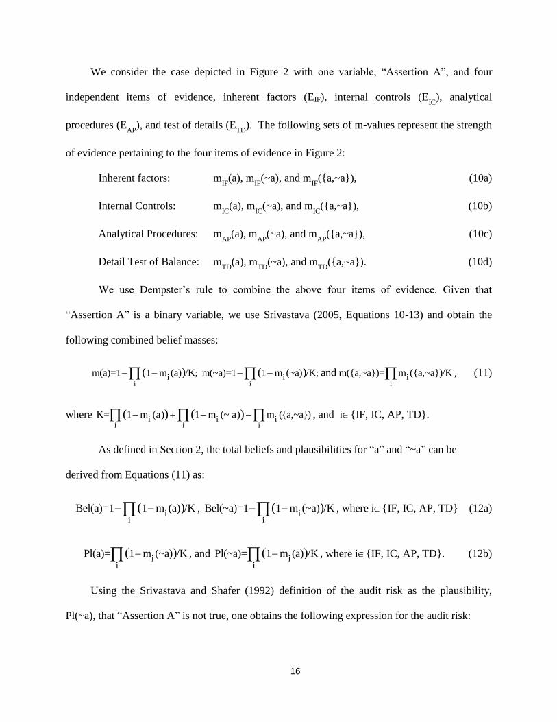
We consider the case depicted in Figure 2 with one variable, “Assertion A”, and four

independent items of evidence, inherent factors (EIF), internal controls (EIC

), analytical

procedures (EAP

), and test of details (ETD

). The following sets of m-values represent the strength

of evidence pertaining to the four items of evidence in Figure 2:

Inherent factors: mIF

(a), mIF

(~a), and mIF

({a,~a}), (10a)

Internal Controls: mIC

(a), mIC

(~a), and mIC

({a,~a}), (10b)

Analytical Procedures: mAP

(a), mAP

(~a), and mAP

({a,~a}), (10c)

Detail Test of Balance: mTD

(a), mTD

(~a), and mTD

({a,~a}). (10d)

We use Dempster’s rule to combine the above four items of evidence. Given that

“Assertion A” is a binary variable, we use Srivastava (2005, Equations 10-13) and obtain the

following combined belief masses:

i i ii i i; ; m(a)=1 1 m (a) /K m(~a)=1 1 m (~a) /K m({a,~a})= m ({a,~a})/Kand ( ) ( ) , (11)

where i i i

i i iK= 1 m (a) 1 m (~ a) m ({a,~a})( ) ( ) , and i{IF, IC, AP, TD}.

As defined in Section 2, the total beliefs and plausibilities for “a” and “~a” can be

derived from Equations (11) as:

ii

Bel(a)=1 1 m (a) /K( ) , i

i

Bel(~a)=1 1 m (~a) /K( ) , where i{IF, IC, AP, TD} (12a)

ii

Pl(a)= 1 m (~a) /K( ) , and i

i

Pl(~a)= 1 m (a) /K( ) , where i{IF, IC, AP, TD}. (12b)

Using the Srivastava and Shafer (1992) definition of the audit risk as the plausibility,

Pl(~a), that “Assertion A” is not true, one obtains the following expression for the audit risk:

17

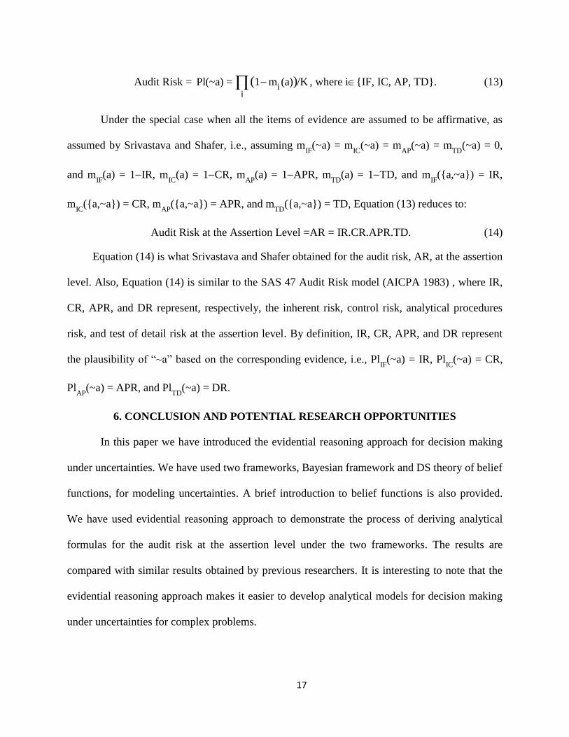
Audit Risk = i

i

Pl(~a) = 1 m (a) /K( ) , where i{IF, IC, AP, TD}. (13)

Under the special case when all the items of evidence are assumed to be affirmative, as

assumed by Srivastava and Shafer, i.e., assuming mIF

(~a) = mIC

(~a) = mAP

(~a) = mTD

(~a) = 0,

and mIF

(a) = 1IR, mIC

(a) = 1CR, mAP

(a) = 1APR, mTD

(a) = 1TD, and mIF

({a,~a}) = IR,

mIC

({a,~a}) = CR, mAP

({a,~a}) = APR, and mTD

({a,~a}) = TD, Equation (13) reduces to:

Audit Risk at the Assertion Level =AR = IR.CR.APR.TD. (14)

Equation (14) is what Srivastava and Shafer obtained for the audit risk, AR, at the assertion

level. Also, Equation (14) is similar to the SAS 47 Audit Risk model (AICPA 1983) , where IR,

CR, APR, and DR represent, respectively, the inherent risk, control risk, analytical procedures

risk, and test of detail risk at the assertion level. By definition, IR, CR, APR, and DR represent

the plausibility of “~a” based on the corresponding evidence, i.e., PlIF

(~a) = IR, PlIC

(~a) = CR,

PlAP

(~a) = APR, and PlTD

(~a) = DR.

6. CONCLUSION AND POTENTIAL RESEARCH OPPORTUNITIES

In this paper we have introduced the evidential reasoning approach for decision making

under uncertainties. We have used two frameworks, Bayesian framework and DS theory of belief

functions, for modeling uncertainties. A brief introduction to belief functions is also provided.

We have used evidential reasoning approach to demonstrate the process of deriving analytical

formulas for the audit risk at the assertion level under the two frameworks. The results are

compared with similar results obtained by previous researchers. It is interesting to note that the

evidential reasoning approach makes it easier to develop analytical models for decision making

under uncertainties for complex problems.

18

In terms of research opportunities, there are lots of interesting problems, both theoretical

and empirical in nature, especially in information systems domain that one could investigate

using the evidential reasoning approach. Some examples of such problems are: How effective

and reliable is the accounting information system of a company? How effective are the internal

accounting controls in an accounting system? Answers to these questions come down to

determining the assertions and sub-assertion relevant to the problem of interest, interrelationships

among these assertions and sub-assertions, and determining the corresponding items of evidence

to assess whether these assertions are true or not. Essentially, this involves creating the

appropriate evidential diagram and using the appropriate framework for representing

uncertainties and then using the evidential reasoning approach to make the decision. Another

area of interest in information system domain is the assessment of trust, trust for regular business

transactions, and trust for ecommerce transactions. Again, such a problem involves determining

the basic assertions of trust, i.e., what are the basic assertions and sub-assertions that constitute

trust and what kinds of relationships exist between these assertions and sub-assertions, and

ultimately what is the structure of evidence? Again, such questions involve both theoretical and

empirical studies.

REFERENCES

Akresh, Abraham D., James K. Loebbecke, and William R. Scott. 1988. Audit Approaches and

Techniques. Research Opportunities in Auditing: The Second Decade edited by A. Rashad

Abdel-khalik and Ira Solomon. American Accounting Association: Auditing Section, pp.

14-55.

American Institute of Public Accountants (AICPA). 2006. Audit Evidence. SAS No. 106. New

York, NY: AICPA.

American Institute of Public Accountants (AICPA). 1980. Evidential Matter. SAS No. 31. New

York, NY: AICPA.

American Institute of Certified Public Accountants, Statements on Auditing Standards, Number

47, AICPA (1983).

19

Bovee, M, R. P. Srivastava, and B. Mak. 2003. A Conceptual Framework and Belief-Function

Approach to Assessing Overall Information Quality. International Journal of Intelligent

Systems, Volume 18, No. 1, January: 51-74.

Dempster, A. P., R. R. Yager, and L. Liu . 2008. The Classic Works on the Dempster-Shafer

Theory of Belief Functions, Springer.

Dutta, S. K., and R. P. Srivastava. 1993. Aggregation of Evidence in Auditing: A Likelihood

Perspective. Auditing: A Journal of Practice and Theory, Vol. 12, Supplement: 137-160.

Edwards, A. W. F. 1984. Likelihood: An Account of the Statistical Concept of Likelihood and its

Application to Scientific Inferences. Cambridge University Press, Cambridge.

Gao, L., T. Mock, and R. P. Srivastava. 2010. An Evidential Reasoning Approach to Fraud Risk

Assessment under Dempster-Shafer Theory: A General Framework. Working Paper,

School of Business, The University of Kansas.

Gordon, J., and E. H. Shortliffe.1985. Method for Managing Evidential Reasoning in a

Hierarchical Hypothesis Space. Artificial Intelligence, pp. 323 – 357.

Kinney, W. R., Jr. 1984. A Discussant Response to ‘An Analysis of the Audit Framework

Focusing on Inherent Risk and the Role Statistical Sampling in Compliance Testing.’

Auditing Symposium VII. University of Kansas: 126-136.

Leslie, D. A. 1984. An Analysis of the Audit Framework Focusing on Inherent Risk and the Role

of Statistical Sampling in Compliance Testing. Proceedings of the 1984 Touche

Ross/University of Kansas Symposium on Auditing Problems (May): 89-125.

Lowrance, J. D., T. D. Garvey, and T. M. Strat. 1986. A Framework for Evidential Reasoning

Systems. Proceedings of the 1986 AAAI Conference: 896-903.

Mock, T., L. Sun, R. P. Srivastava, and M. Vasarhelyi. 2009. An Evidential Reasoning Approach

to Sarbanes-Oxley Mandated Internal Control Risk Assessment under Dempster-Shafer

Theory. International Journal of Accounting Information Systems, Volume 10, Number

2, pp. 65-78.

Pearl, J. 1986. Evidential Reasoning using Stochastic Simulation of Causal Models. Artificial

Intelligence, pp. 245-257.

Rao, S., R. P. Srivastava, and T. J. Mock. 2010. Assurance Services in Sustainability Reporting:

Evidential Structure, Level of Assurance, and Predicted Auditor’s Behavior. Presented at

2010 American Accounting Association Annual Meeting, San Francisco, August 1-4.

Shafer, G. 1976. A Mathematical Theory of Evidence. Princeton University Press.

Shafer, G., P. P. Shenoy, and R. P. Srivastava. 1988. AUDITOR'S ASSISTANT: A Knowledge

Engineering Tool For Audit Decisions. Proceedings of the 1988 Touche Ross University of

Kansas Symposium on Auditing Problems, May: 61-79.

Shafer, G. and R. P. Srivastava. 1990. The Bayesian And Belief-Function Formalisms: A

General Perspective for Auditing. Auditing: A Journal of Practice and Theory

(Supplement): 110-148.

20

Shenoy, P. P. and G. Shafer. 1990. Axioms for Probability and Belief-Function Computation, in

Shachter, R. D., T. S. Levitt, J. F. Lemmer, and L. N. Kanal, eds., Uncertainty in

Artificial Intelligence, 4, North-Holland: 169-198.

Shortliffe, E. H. and B. G. Buchanan. 1975. A Model of Inexact Reasoning in Medicine.

Mathematical Biosciences, 23: 351-379.

Smets, P. 2005. Software for the TBM. http://iridia.ulb.ac.be/~psmets/#G. Accessed July 24,

2010.

Srivastava, R.P. 2005. Alternative Form of Dempster’s Rule for Binary Variables. International

Journal of Intelligent Systems, Vol. 20, No. 8, August 2005, pp. 789-797.

Srivastava, R. P. 1995. The Belief-Function Approach to Aggregating Audit Evidence.

International Journal of Intelligent Systems, Vol. 10, No. 3, March: 329-356.

Srivastava, R. P. and Li, C. 2008. Systems Security Risk and Systems Reliability Formulas under

Dempster-Shafer Theory of Belief Functions. Journal Emerging Technologies in

Accounting, Vol. 5, No. 1, pp. 189-219.

Srivastava, R. P., and T. Mock. 2010. Audit Risk Formula with Mixed Evidence. Proceedings of

the Conference on the Theory of Belief Functions, France, April 1-2, 2010.

Srivastava, R. P. and T. J. Mock. 2000. Evidential Reasoning for WebTrust Assurance Services.

Journal of Management Information Systems, Vol. 16, No. 3, Winter: 11-32.

Srivastava, R. P., T. J. Mock, and J. Turner. 2009. A Fraud Risk Formula for Financial Statement

Audits under the Bayesian Framework. ABACUS, Vol. 45, No. 1, pp. 66-87.

Srivastava, R. P., T. Mock, and J. Turner. 2007. Analytical Formulas for Risk Assessment for a

Class of Problems where Risk Depends on Three Interrelated Variables. International

Journal of Approximate Reasoning Vol. 45, pp. 123–151.

Srivastava, R. P., and G. Shafer. 1992. Belief-Function Formulas for Audit Risk. The

Accounting Review (April): 249-283.

Srivastava, R. P., P. P. Shenoy, and G. Shafer. 1995. Propagating Beliefs in an 'AND' Tree.

International Journal of Intelligent Systems, Vol. 10, 1995, pp. 647-664.

Sun, L., R. P. Srivastava, and T. Mock. 2006. An Information Systems Security Risk Assessment

Model under Dempster-Shafer Theory of Belief Functions. Journal of Management

Information Systems, Vol. 22, No. 4: 109-142.

Yang, Jian-Bo, Dong-Ling Xu, Xinlian Xie, and A. K. Maddulapalli. 2010. Evidence Theory and

Multiple Criteria Decision Making: The Evidential Reasoning Approach. Proceedings of

the Conference on the Theory of Belief Functions, France, April 1-2, 2010.

21

Figure 1: Evidential Reasoning and Evidential Diagram

Figure 2: Evidential Diagram for one Variable with Four Independent Items of Evidence in an

Audit Context

Assertion A

EIC

: Evidence from Internal Controls

EAP

: Evidence from Analytical Procedures

ETD

: Evidence from Test of Details

EIF

: Evidence from Inherent Factors

R

X Evidence pertaining to X

Y Evidence pertaining to Y

Z

Evidence pertaining to Z

Evidence pertaining to X

and Y