An Introduction to Business Statistics - McGraw-Hill

LEARNING OBJECTIVES

After reading this chapter, you should be able to

• understand how and why research samples arecollected

• know the difference between a sample and apopulation

• explain what is meant by the term randomsample and explain how a random sample maybe generated

• describe the four levels of measurement

• list some of the potential problems associatedwith surveys

An Introduction to Business Statistics

The subject of statistics involves the study of how to collect,summarize, and interpret data. Data are numerical facts andfigures from which conclusions can be drawn. Suchconclusions are important to the decision-making processesof many professions and organizations. For example,government officials use conclusions drawn from the latestdata on unemployment and inflation to make policydecisions. Financial planners use recent trends in stock marketprices to make investment decisions. Businesses decide whichproducts to develop and market by using data that revealconsumer preferences. Production supervisors usemanufacturing data to evaluate, control, and improve

product quality. Politicians rely on data from public opinionpolls to formulate legislation and to devise campaignstrategies. Physicians and hospitals use data on theeffectiveness of drugs and surgical procedures to providepatients with the best possible treatment.

In this chapter, we begin to see how we collect andanalyze data. As we proceed through the chapter, weintroduce several case studies. These case studies (and othersto be introduced later, many from Statistics Canada) arerevisited throughout later chapters as we learn the statistical

methods needed to analyze the cases. Briefly, we beginto study four cases:

The Cell Phone Case. A bank estimates its cellularphone costs and decides whether to outsourcemanagement of its wireless resources by studying the call-ing patterns of its employees.

The Marketing Research Case. A bottling company in-vestigates consumer reaction to a new bottle design forone of its popular soft drinks.

The Coffee Temperature Case. A fast-foodrestaurant studies and monitors the temperature

of the coffee it serves.

The Mass of the Loonie. A researcher examines theoverall distribution of the masses (in grams) of the 1989Canadian dollar coin (nicknamed the “loonie”) todetermine the average mass and range of masses.

C H A P T E R 1

CHAPTER OUTLINE

1.1 Populations and Samples

1.2 Sampling a Population of Existing Units

1.3 Sampling a Process

1.4 Levels of Measurement: Nominal, Ordinal,Interval, and Ratio

1.5 A Brief Introduction to Surveys

1.6 An Introduction to Survey Sampling

bow83755_ch01_001-026.qxd 10/30/07 8:52 AM Page 1 Team D 205:MHHE025:bow83755_ch01:

2 Chapter 1 An Introduction to Business Statistics

1In Section 1.4, we discuss two types of quantitative variables (ratio and interval) and two types of qualitative variables(ordinal and nominative). Study Hint: To remember the difference between quantitative and qualitative, remember thatquantitative has the letter “n” and “n is for number.” Qualitative has an ”l” and “l is for letter,” so you have to use wordsto describe the data.

1.1 Populations and SamplesStatistical methods are very useful for learning about populations. Populations can be defined in

various ways, including the following:

A population is a set of existing units (usually people, objects, or events).

Examples of populations include (1) all of last year’s graduates of Sauder School of Business at

UBC, (2) all consumers who bought a cellular phone last year, (3) all accounts receivable in-

voices accumulated last year by Procter & Gamble, (4) all Toyota Corollas that were produced

last year, and (5) all fires reported last month to the Ottawa fire department.

We usually focus on studying one or more characteristics of the population units.

Any characteristic of a population unit is called a variable.

For instance, if we study the starting salaries of last year’s graduates of an MBA program, the

variable of interest is starting salary. If we study the fuel efficiency obtained in city driving by

last year’s Toyota Corolla, the variable of interest is litres per 100 km in city driving.

We carry out a measurement to assign a value of a variable to each population unit. For

example, we might measure the starting salary of an MBA graduate to the nearest dollar. Or we

might measure the fuel efficiency obtained by a car in city driving to the nearest litre per 100 km

by conducting a test on a driving course prescribed by the Ministry of Transportation. If the pos-

sible measurements are numbers that represent quantities (that is, “how much” or “how many”),

then the variable is said to be quantitative. For example, starting salary and fuel efficiency are

both quantitative. However, if we simply record into which of several categories a population

unit falls, then the variable is said to be qualitative or categorical. Examples of categorical vari-

ables include (1) a person’s sex, (2) the make of an automobile, and (3) whether a person who

purchases a product is satisfied with the product.1

If we measure each and every population unit, we have a population of measurements

(sometimes called observations). If the population is small, it is reasonable to do this. For

instance, if 150 students graduated last year from an MBA program, it might be feasible to sur-

vey the graduates and to record all of their starting salaries. In general:

If we examine all of the population measurements, we say that we are conducting a census of

the population.

Often the population that we wish to study is very large, and it is too time-consuming or costly to

conduct a census. In such a situation, we select and analyze a subset (or portion) of the population.

A sample is a subset of the units in a population.

For example, suppose that 8742 students graduated last year from a large university. It would prob-

ably be too time-consuming to take a census of the population of all of their starting salaries.

Therefore, we would select a sample of graduates, and we would obtain and record their starting

salaries. When we measure the units in a sample, we say that we have a sample of measurements.

We often wish to describe a population or sample.

Descriptive statistics is the science of describing the important aspects of a set of measurements.

As an example, if we are studying a set of starting salaries, we might wish to describe (1) how

large or small they tend to be, (2) what a typical salary might be, and (3) how much the salaries

differ from each other.

When the population of interest is small and we can conduct a census of the population, we

will be able to directly describe the important aspects of the population measurements. However,

if the population is large and we need to select a sample from it, then we use what we call

statistical inference.


1.2 Sampling a Population of Existing Units 3

2Actually, there are several different kinds of random samples. The type we will define is sometimes called a simple randomsample. For brevity’s sake, however, we will use the term random sample.

3The authors would like to thank Mr. Doug L. Stevens, Vice President of Sales and Marketing, at MobileSense Inc., WestlakeVillage, California, for his help in developing this case.

Statistical inference is the science of using a sample of measurements to make generalizations

about the important aspects of a population of measurements.

For instance, we might use a sample of starting salaries to estimate the important aspects of a

population of starting salaries. In the next section, we begin to look at how statistical inference

is carried out.

1.2 Sampling a Population of Existing UnitsRandom samples If the information contained in a sample is to accurately reflect the popu-

lation under study, the sample should be randomly selected from the population. To intuitively

illustrate random sampling, suppose that a small company employs 15 people and wishes to ran-

domly select two of them to attend a convention. To make the random selections, we number the

employees from 1 to 15, and we place in a hat 15 identical slips of paper numbered from 1 to

15. We thoroughly mix the slips of paper in the hat and, blindfolded, choose one. The number

on the chosen slip of paper identifies the first randomly selected employee. Then, still blind-

folded, we choose another slip of paper from the hat. The number on the second slip identifies

the second randomly selected employee.

Of course, it is impractical to carry out such a procedure when the population is very large. It

is easier to use a random number table or a computerized random number generator. To show

how to use such a table, we must more formally define a random sample.2

A random sample is selected so that, on each selection from the population, every unit remaining

in the population on that selection has the same chance of being chosen.

To understand this definition, first note that we can randomly select a sample with or without

replacement. If we sample with replacement, we place the unit chosen on any particular selection

back into the population. Thus, we give this unit a chance to be chosen on any succeeding selection.

In such a case, all of the units in the population remain as candidates to be chosen for each and

every selection. Randomly choosing two employees with replacement to attend a convention

would make no sense because we wish to send two different employees to the convention. If we

sample without replacement, we do not place the unit chosen on a particular selection back into

the population. Thus, we do not give this unit a chance to be selected on any succeeding selection.

In this case, the units remaining as candidates for a particular selection are all of the units in the

population except for those that have previously been selected. It is best to sample without re-

placement. Intuitively, because we will use the sample to learn about the population, sampling

without replacement will give us the fullest possible look at the population. This is true because

choosing the sample without replacement guarantees that all of the units in the sample will be dif-

ferent (and that we are looking at as many different units from the population as possible).

In the following example, we illustrate how to use a random number table, or computer-

generated random numbers, to select a random sample.

Example 1.1 The Cell Phone Case: Estimating Cell Phone Costs3

Businesses and students have at least two things in common—both find cellular phones to be

nearly indispensable because of their convenience and mobility, and both often rack up un-

pleasantly high cell phone bills. Students’ high bills are usually the result of overage—a student

uses more minutes than their plan allows. Businesses also lose money due to overage and, in

addition, lose money due to underage when some employees do not use all of the (already-paid-

for) minutes allowed by their plans. Because cellular carriers offer a very large number of rate plans,

C H A P T E R 1



it is nearly impossible for a business to intelligently choose calling plans that will meet its needs

at a reasonable cost.

Rising cell phone costs have forced companies with large numbers of cellular users to hire

services to manage their cellular and other wireless resources. These cellular management services

use sophisticated software and mathematical models to choose cost-efficient cell phone plans for

their clients. One such firm, MobileSense Inc. of Westlake Village, California, specializes in auto-

mated wireless cost management. According to Doug L. Stevens, Vice President of Sales and

Marketing at MobileSense, cell phone carriers count on overage and underage to deliver almost

half of their revenues. As a result, a company’s typical cost of cell phone use can easily exceed

25 cents per minute. However, Mr. Stevens explains that by using MobileSense automated cost

management to select calling plans, this cost can be reduced to 12 cents per minute or less.

In this case, we will demonstrate how a bank can use a random sample of cell phone users to

study its cellular phone costs. Based on this cost information, the bank will decide whether to

hire a cellular management service to choose calling plans for the bank’s employees. While the

bank has over 10,000 employees on a variety of calling plans, the cellular management service

suggests that by studying the calling patterns of cellular users on 500-minute plans, the bank can

accurately assess whether its cell phone costs can be substantially reduced.

The bank has 2,136 employees on a 500-minute-per-month plan with a monthly cost of $50.

The overage charge is 40 cents per minute, and there are additional charges for long distance and

roaming. The bank will estimate its cellular cost per minute for this plan by examining the num-

ber of minutes used last month by each of 100 randomly selected employees on this 500-minute

plan. According to the cellular management service, if the cellular cost per minute for the ran-

dom sample of 100 employees is over 18 cents per minute, the bank should benefit from auto-

mated cellular management of its calling plans.

In order to randomly select the sample of 100 cell phone users, the bank will make a num-

bered list of the 2,136 users on the 500-minute plan. This list is called a frame. The bank can

then use a random number table, such as Table 1.1(a), to select the needed sample. To see how

this is done, note that any single-digit number in the table is assumed to have been randomly

selected from the digits 0 to 9. Any two-digit number in the table is assumed to have been ran-

domly selected from the numbers 00 to 99. Any three-digit number is assumed to have been ran-

domly selected from the numbers 000 to 999, and so forth. Note that the table entries are segmented

into groups of five to make the table easier to read. Because the total number of cell phone users

on the 500-minute plan (2,136) is a four-digit number, we arbitrarily select any set of four digits

T A B L E 1.1 Random Numbers

(a) A portion of a random number table

33276 85590 79936 56865 05859 90106 78188

03427 90511 69445 18663 72695 52180 90322

92737 27156 33488 36320 17617 30015 74952

85689 20285 52267 67689 93394 01511 89868

08178 74461 13916 47564 81056 97735 90707

51259 63990 16308 60756 92144 49442 40719

60268 44919 19885 55322 44819 01188 55157

94904 01915 04146 18594 29852 71585 64951

58586 17752 14513 83149 98736 23495 35749

09998 19509 06691 76988 13602 51851 58104

14346 61666 30168 90229 04734 59193 32812

74103 15227 25306 76468 26384 58151 44592

24200 64161 38005 94342 28728 35806 22851

87308 07684 00256 45834 15398 46557 18510

07351 86679 92420 60952 61280 50001 94953

(b) MINITAB output of 100 different four-digitrandom numbers between 1 and 2136

705 1131 169 1703 1709 609

1990 766 1286 1977 222 43

1007 1902 1209 2091 1742 1152

111 69 2049 1448 659 338

1732 1650 7 388 613 1477

838 272 1227 154 18 320

1053 1466 2087 265 2107 1992

582 1787 2098 1581 397 1099

757 1699 567 1255 1959 407

354 1567 1533 1097 1299 277

663 40 585 1486 1021 532

1629 182 372 1144 1569 1981

1332 1500 743 1262 1759 955

1832 378 728 1102 667 1885

514 1128 1046 116 1160 1333

831 2036 918 1535 660

928 1257 1468 503 468



in the table (we have circled these digits). This number, which is 0511, identifies the first ran-

domly selected user. Then, moving in any direction from the 0511 (up, down, right, or left—it

does not matter which), we select additional sets of four digits. These succeeding sets of digits

identify additional randomly selected users. Here we arbitrarily move down from 0511 in the

table. The first seven sets of four digits we obtain are

0511 7156 0285 4461 3990 4919 1915

(See Table 1.1(a)—these numbers are enclosed in a rectangle.) Since there are no users numbered

7156, 4461, 3990, or 4919 (remember only 2,136 users are on the 500-minute plan), we ignore

these numbers. This implies that the first three randomly selected users are those numbered 0511,

0285, and 1915. Continuing this procedure, we can obtain the entire random sample of 100 users.

Notice that, because we are sampling without replacement, we should ignore any set of four

digits previously selected from the random number table.

While using a random number table is one way to select a random sample, this approach has

a disadvantage that is illustrated by the current situation. Specifically, since most four-digit

random numbers are not between 0001 and 2136, obtaining 100 different four-digit random

numbers between 0001 and 2136 will require ignoring a large number of random numbers in

the random number table, and we will in fact need to use a random number table that is larger than

Table 1.1(a). Although larger random number tables are readily available in books of mathemat-

ical and statistical tables, a good alternative is to use a computer software package, which can gen-

erate random numbers that are between whatever values we specify. For example, Table 1.1(b)

gives the MINITAB output of 100 different four-digit random numbers that are between 0001

and 2136 (note that the “leading 0s” are not included in these four-digit numbers). If used, the ran-

dom numbers in Table 1.1(b) identify the 100 employees that should form the random sample.

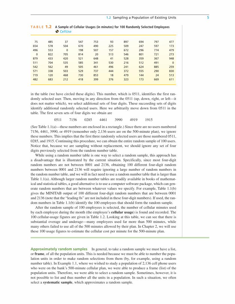
After the random sample of 100 employees is selected, the number of cellular minutes used

by each employee during the month (the employee’s cellular usage) is found and recorded. The

100 cellular-usage figures are given in Table 1.2. Looking at this table, we can see that there is

substantial overage and underage—many employees used far more than 500 minutes, while

many others failed to use all of the 500 minutes allowed by their plan. In Chapter 2, we will use

these 100 usage figures to estimate the cellular cost per minute for the 500-minute plan.

T A B L E 1.2 A Sample of Cellular Usages (in minutes) for 100 Randomly Selected Employees CellUse

75 485 37 547 753 93 897 694 797 477

654 578 504 670 490 225 509 247 597 173

496 553 0 198 507 157 672 296 774 479

0 822 705 814 20 513 546 801 721 273

879 433 420 521 648 41 528 359 367 948

511 704 535 585 341 530 216 512 491 0

542 562 49 505 461 496 241 624 885 259

571 338 503 529 737 444 372 555 290 830

719 120 468 730 853 18 479 144 24 513

482 683 212 418 399 376 323 173 669 611

Approximately random samples In general, to take a random sample we must have a list,

or frame, of all the population units. This is needed because we must be able to number the popu-

lation units in order to make random selections from them (by, for example, using a random

number table). In Example 1.1, where we wished to study a population of 2,136 cell phone users

who were on the bank’s 500-minute cellular plan, we were able to produce a frame (list) of the

population units. Therefore, we were able to select a random sample. Sometimes, however, it is

not possible to list and thus number all the units in a population. In such a situation, we often

select a systematic sample, which approximates a random sample.



Example 1.2 The Marketing Research Case: Rating a New Bottle Design4

The design of a package or bottle can have an important effect on a company’s bottom line. For

example, an article in the September 16, 2004, issue of USA Today reported that the introduction

of a contoured 1.5-L bottle for Coke drinks played a major role in Coca-Cola’s failure to meet

third-quarter earnings forecasts in 2004. According to the article, Coke’s biggest bottler, Coca-

Cola Enterprises, “said it would miss expectations because of the 1.5-liter bottle and the absence

of common 2-liter and 12-pack sizes . . . in supermarkets.’’5

In this case, a brand group is studying whether changes should be made in the bottle design

for a popular soft drink. To research consumer reaction to a new design, the brand group will use

the “mall intercept method,’’ in which shoppers at a large metropolitan shopping mall are inter-

cepted and asked to participate in a consumer survey. Each shopper will be exposed to the new

bottle design and asked to rate the bottle image. Bottle image will be measured by combining

consumers’ responses to five items, with each response measured using a seven-point “Likert

scale.” The five items and the scale of possible responses are shown in Figure 1.1. Here, since

we describe the least favourable response and the most favourable response (and we do not de-

scribe the responses between them), we say that the scale is “anchored” at its ends. Responses

to the five items will be summed to obtain a composite score for each respondent. It follows that

the minimum composite score possible is 5 and the maximum composite score possible is 35.

Furthermore, experience has shown that the smallest acceptable composite score for a success-

ful bottle design is 25.

In this situation, it is not possible to list and number each and every shopper at the mall while

the study is being conducted. Consequently, we cannot use random numbers (as we did in the

cell phone case) to obtain a random sample of shoppers. Instead, we can select a systematic

sample. To do this, every 100th shopper passing a specified location in the mall will be invited

to participate in the survey. Here, selecting every 100th shopper is arbitrary—we could select

every 200th, every 300th, and so forth. If we select every 100th shopper, it is probably reason-

able to believe that the responses of the survey participants are not related. Therefore, it is rea-

sonable to assume that the sampled shoppers obtained by the systematic sampling process make

up an approximate random sample.

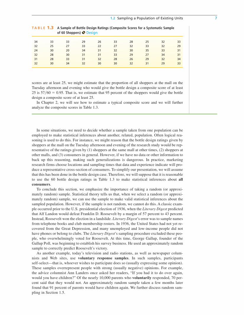
During a Tuesday afternoon and evening, a sample of 60 shoppers is selected by using the

systematic sampling process. Each shopper is asked to rate the bottle design by responding to

the five items in Figure 1.1, and a composite score is calculated for each shopper. The 60 com-

posite scores obtained are given in Table 1.3. Since these scores range from 20 to 35, we might

infer that most of the shoppers at the mall on the Tuesday afternoon and evening of the study

would rate the new bottle design between 20 and 35. Furthermore, since 57 of the 60 composite

4This case was motivated by an example in the book Essentials of Marketing Research, by W. R. Dillon, T. J. Madden, and N. H. Firtle (Burr Ridge, IL: Richard D. Irwin, 1993). The authors also wish to thank Professor L. Unger of the Department ofMarketing at Miami University for helpful discussions concerning how this type of marketing study would be carried out.

5Source: “Coke says earnings will come up short,” by Theresa Howard, USA Today, September 16, 2004, p. 801.

F I G U R E 1.1 The Bottle Design Survey Instrument

Strongly StronglyStatement Disagree Agree

The size of this bottle is convenient. 1 2 3 4 5 6 7

The contoured shape of this bottle is easy to handle. 1 2 3 4 5 6 7

The label on this bottle is easy to read. 1 2 3 4 5 6 7

This bottle is easy to open. 1 2 3 4 5 6 7

Based on its overall appeal, I like this bottle design. 1 2 3 4 5 6 7

Please circle the response that most accurately describes whether you agree or disagree with eachstatement about the bottle you have examined.



scores are at least 25, we might estimate that the proportion of all shoppers at the mall on the

Tuesday afternoon and evening who would give the bottle design a composite score of at least

25 is 57�60 � 0.95. That is, we estimate that 95 percent of the shoppers would give the bottle

design a composite score of at least 25.

In Chapter 2, we will see how to estimate a typical composite score and we will further

analyze the composite scores in Table 1.3.

T A B L E 1.3 A Sample of Bottle Design Ratings (Composite Scores for a Systematic Sample of 60 Shoppers) Design

34 33 33 29 26 33 28 25 32 33

32 25 27 33 22 27 32 33 32 29

24 30 20 34 31 32 30 35 33 31

32 28 30 31 31 33 29 27 34 31

31 28 33 31 32 28 26 29 32 34

32 30 34 32 30 30 32 31 29 33

In some situations, we need to decide whether a sample taken from one population can be

employed to make statistical inferences about another, related, population. Often logical rea-

soning is used to do this. For instance, we might reason that the bottle design ratings given by

shoppers at the mall on the Tuesday afternoon and evening of the research study would be rep-

resentative of the ratings given by (1) shoppers at the same mall at other times, (2) shoppers at

other malls, and (3) consumers in general. However, if we have no data or other information to

back up this reasoning, making such generalizations is dangerous. In practice, marketing

research firms choose locations and sampling times that data and experience indicate will pro-

duce a representative cross-section of consumers. To simplify our presentation, we will assume

that this has been done in the bottle design case. Therefore, we will suppose that it is reasonable

to use the 60 bottle design ratings in Table 1.3 to make statistical inferences about all

consumers.To conclude this section, we emphasize the importance of taking a random (or approxi-

mately random) sample. Statistical theory tells us that, when we select a random (or approxi-

mately random) sample, we can use the sample to make valid statistical inferences about the

sampled population. However, if the sample is not random, we cannot do this. A classic exam-

ple occurred prior to the U.S. presidential election of 1936, when the Literary Digest predicted

that Alf Landon would defeat Franklin D. Roosevelt by a margin of 57 percent to 43 percent.

Instead, Roosevelt won the election in a landslide. Literary Digest’s error was to sample names

from telephone books and club membership rosters. In 1936, the United States had not yet re-

covered from the Great Depression, and many unemployed and low-income people did not

have phones or belong to clubs. The Literary Digest’s sampling procedure excluded these peo-

ple, who overwhelmingly voted for Roosevelt. At this time, George Gallup, founder of the

Gallup Poll, was beginning to establish his survey business. He used an approximately random

sample to correctly predict Roosevelt’s victory.

As another example, today’s television and radio stations, as well as newspaper colum-

nists and Web sites, use voluntary response samples. In such samples, participants

self-select—that is, whoever wishes to participate does so (usually expressing some opinion).

These samples overrepresent people with strong (usually negative) opinions. For example,

the advice columnist Ann Landers once asked her readers, “If you had it to do over again,

would you have children?” Of the nearly 10,000 parents who voluntarily responded, 70 per-

cent said that they would not. An approximately random sample taken a few months later

found that 91 percent of parents would have children again. We further discuss random sam-

pling in Section 1.5.



CONCEPTS

Exercises for Sections 1.1 and 1.2

1.1 Define a population. Give an example of a population

that you might study when you start your career after

graduating from university.

1.2 Define what we mean by a variable, and explain the

difference between a quantitative variable and a quali-

tative (categorical) variable.

1.3 Below we list several variables. Which of these variables

are quantitative and which are qualitative? Explain.

a. The dollar amount on an accounts receivable invoice.

b. The net profit for a company in 2007.

c. The stock exchange on which a company’s stock is

traded.

d. The national debt of Canada in 2007.

e. The advertising medium (radio, television, Internet,

or print) used to promote a product.

1.4 Explain the difference between a census and a sample.

1.5 Explain each of the following terms:

a. Descriptive statistics. c. Random sample.

b. Statistical inference. d. Systematic sample.

1.6 Explain why sampling without replacement is preferred

to sampling with replacement.

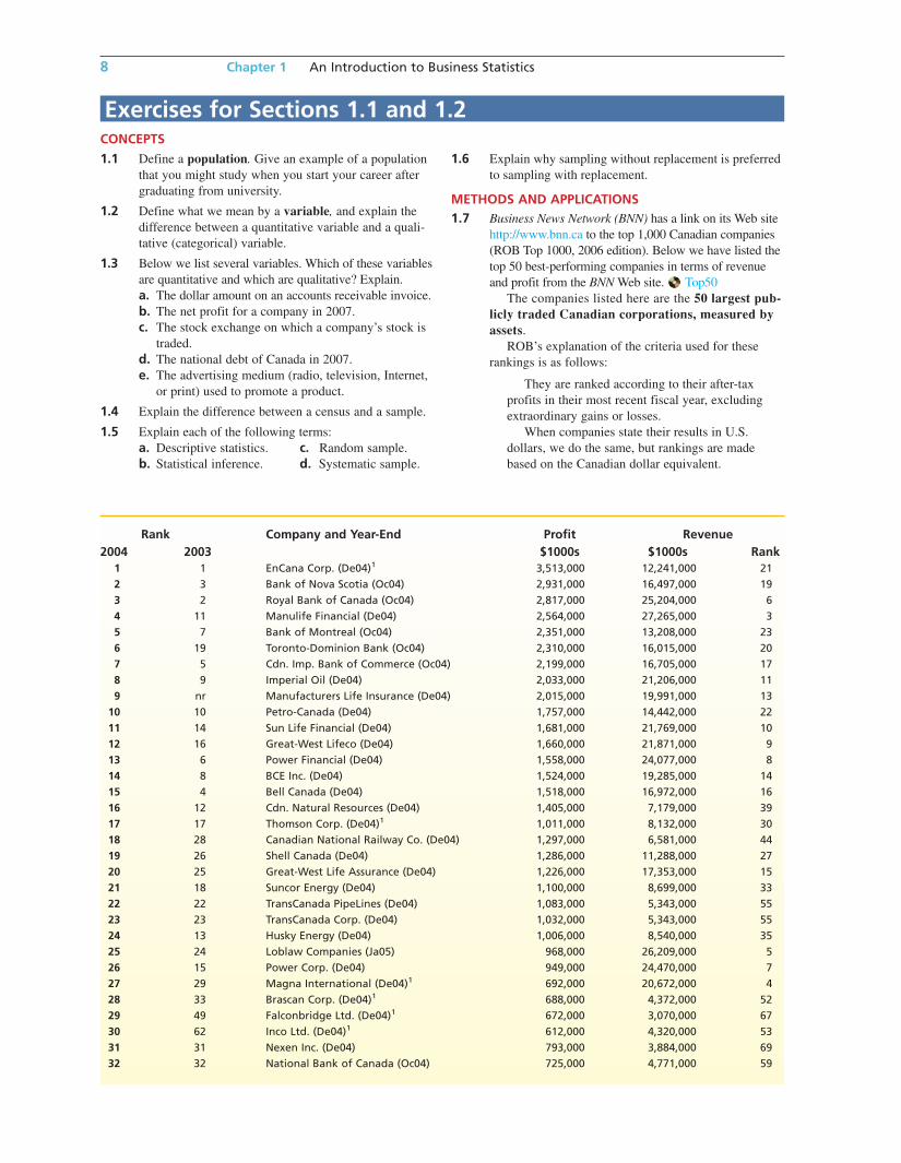
METHODS AND APPLICATIONS1.7 Business News Network (BNN) has a link on its Web site

http://www.bnn.ca to the top 1,000 Canadian companies

(ROB Top 1000, 2006 edition). Below we have listed the

top 50 best-performing companies in terms of revenue

and profit from the BNN Web site. Top50

The companies listed here are the 50 largest pub-

licly traded Canadian corporations, measured by

assets.

ROB’s explanation of the criteria used for these

rankings is as follows:

They are ranked according to their after-tax

profits in their most recent fiscal year, excluding

extraordinary gains or losses.

When companies state their results in U.S.

dollars, we do the same, but rankings are made

based on the Canadian dollar equivalent.

Rank Company and Year-End Profit Revenue2004 2003 $1000s $1000s Rank

1 1 EnCana Corp. (De04)1 3,513,000 12,241,000 21

2 3 Bank of Nova Scotia (Oc04) 2,931,000 16,497,000 19

3 2 Royal Bank of Canada (Oc04) 2,817,000 25,204,000 6

4 11 Manulife Financial (De04) 2,564,000 27,265,000 3

5 7 Bank of Montreal (Oc04) 2,351,000 13,208,000 23

6 19 Toronto-Dominion Bank (Oc04) 2,310,000 16,015,000 20

7 5 Cdn. Imp. Bank of Commerce (Oc04) 2,199,000 16,705,000 17

8 9 Imperial Oil (De04) 2,033,000 21,206,000 11

9 nr Manufacturers Life Insurance (De04) 2,015,000 19,991,000 13

10 10 Petro-Canada (De04) 1,757,000 14,442,000 22

11 14 Sun Life Financial (De04) 1,681,000 21,769,000 10

12 16 Great-West Lifeco (De04) 1,660,000 21,871,000 9

13 6 Power Financial (De04) 1,558,000 24,077,000 8

14 8 BCE Inc. (De04) 1,524,000 19,285,000 14

15 4 Bell Canada (De04) 1,518,000 16,972,000 16

16 12 Cdn. Natural Resources (De04) 1,405,000 7,179,000 39

17 17 Thomson Corp. (De04)1 1,011,000 8,132,000 30

18 28 Canadian National Railway Co. (De04) 1,297,000 6,581,000 44

19 26 Shell Canada (De04) 1,286,000 11,288,000 27

20 25 Great-West Life Assurance (De04) 1,226,000 17,353,000 15

21 18 Suncor Energy (De04) 1,100,000 8,699,000 33

22 22 TransCanada PipeLines (De04) 1,083,000 5,343,000 55

23 23 TransCanada Corp. (De04) 1,032,000 5,343,000 55

24 13 Husky Energy (De04) 1,006,000 8,540,000 35

25 24 Loblaw Companies (Ja05) 968,000 26,209,000 5

26 15 Power Corp. (De04) 949,000 24,470,000 7

27 29 Magna International (De04)1 692,000 20,672,000 4

28 33 Brascan Corp. (De04)1 688,000 4,372,000 52

29 49 Falconbridge Ltd. (De04)1 672,000 3,070,000 67

30 62 Inco Ltd. (De04)1 612,000 4,320,000 53

31 31 Nexen Inc. (De04) 793,000 3,884,000 69

32 32 National Bank of Canada (Oc04) 725,000 4,771,000 59



7 Historical Trivia: The Likert scale is named after Rensis Likert (1903–1981), who originally developed this numerical scale for measuring attitudes in hisPhD dissertation in 1932. [Source: Psychology in America: A Historical Survey, by E. R. Hilgard (San Diego, CA: Harcourt Brace Jovanovich, 1987).]

Consider the random numbers given in the random

number table of Table 1.1(a) on page 4. Starting in the

upper left corner of Table 1.1(a) and moving down the

two leftmost columns, we see that the first three two-

digit numbers obtained are

33 03 92

Starting with these three random numbers, and moving

down the two leftmost columns of Table 1.1(a) to find

more two-digit random numbers, use Table 1.1 to ran-

domly select five of these companies to be interviewed

in detail about their business strategies. Hint: Note

that the companies in the BNN list are numbered

from 1 to 50.

1.8 THE VIDEO GAME SATISFACTION RATING CASEVideoGame

A company that produces and markets video game

systems wishes to assess its customers’ level of

satisfaction with a relatively new model, the XYZ-

Box. In the six months since the introduction of the

model, the company has received 73,219 warranty

registrations from purchasers. The company will

randomly select 65 of these registrations and will

conduct telephone interviews with the purchasers.

Specifically, each purchaser will be asked to state their

level of agreement with each of the seven statements

listed on the survey instrument given in Figure 1.2.

Here the level of agreement for each statement is

measured on a seven-point Likert scale.7 Purchaser

33 180 Noranda Inc. (De04)1 551,000 7,002,000 32

34 21 Talisman Energy (De04) 663,000 6,479,000 45

35 30 Enbridge Inc. (De04) 652,200 6,843,700 43

36 36 PetroKazakhstan Inc. (De04)1 500,668 1,652,346 102

37 nr ING Canada (De04) 624,152 3,780,886 71

38 34 IGM Financial (De04) 617,096 2,119,071 104

39 82 Teck Cominco (De04) 617,000 3,452,000 78

40 314 IPSCO Inc. (De04)1 438,610 2,458,893 82

41 41 Telus Corp. (De04) 565,800 7,623,400 37

42 43 Canadian Oil Sands Trust (De04) 509,200 1,480,200 130

43 931 Gerdau Ameristeel (De04)1 337,669 3,154,390 65

44 27 George Weston (De04) 428,000 29,723,000 2

45 70 Norbord Inc. (De04)1 326,000 1,492,000 110

46 79 Canfor Corp. (De04) 420,900 4,120,000 64

47 38 Canadian Pacific Railway Ltd. (De04) 413,000 3,990,900 68

48 994 Potash Corp. of Saskatchewan (De04)1 298,600 3,328,200 61

49 46 Placer Dome (De04)1 291,000 1,946,000 90

50 100 Dofasco Inc. (De04) 376,900 4,235,400 62

1Figures are reported in U.S. dollars.nr: not ranked

Reprinted with permission from The Globe and Mail.

F I G U R E 1.2 The Video Game Satisfaction Survey Instrument

Strongly StronglyStatement Disagree Agree

The game console of the XYZ-Box is well designed. 1 2 3 4 5 6 7

The game controller of the XYZ-Box is easy to handle. 1 2 3 4 5 6 7

The XYZ-Box has high-quality graphics capabilities. 1 2 3 4 5 6 7

The XYZ-Box has high-quality audio capabilities. 1 2 3 4 5 6 7

The XYZ-Box serves as a complete entertainment centre. 1 2 3 4 5 6 7

There is a large selection of XYZ-Box games to choose from. 1 2 3 4 5 6 7

I am totally satisfied with my XYZ-Box game system. 1 2 3 4 5 6 7



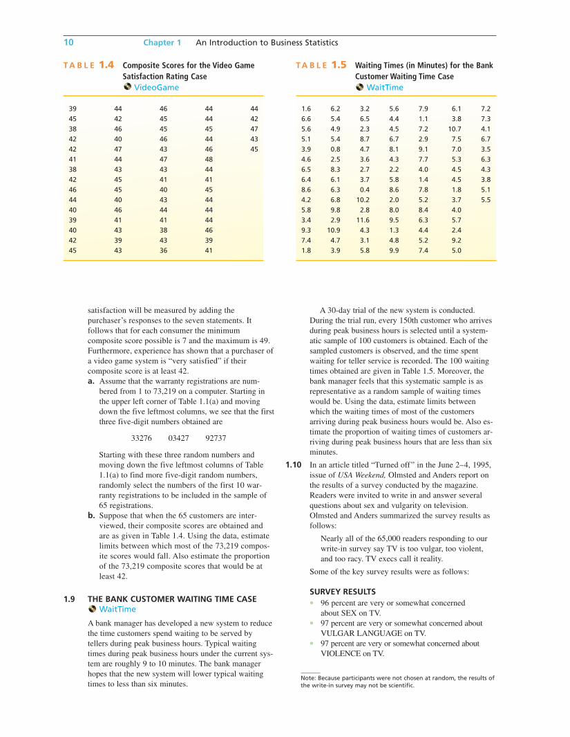
satisfaction will be measured by adding thepurchaser’s responses to the seven statements. Itfollows that for each consumer the minimumcomposite score possible is 7 and the maximum is 49.Furthermore, experience has shown that a purchaser ofa video game system is “very satisfied” if theircomposite score is at least 42.a. Assume that the warranty registrations are num-

bered from 1 to 73,219 on a computer. Starting inthe upper left corner of Table 1.1(a) and movingdown the five leftmost columns, we see that the firstthree five-digit numbers obtained are

33276 03427 92737

Starting with these three random numbers andmoving down the five leftmost columns of Table1.1(a) to find more five-digit random numbers,randomly select the numbers of the first 10 war-ranty registrations to be included in the sample of65 registrations.

b. Suppose that when the 65 customers are inter-viewed, their composite scores are obtained andare as given in Table 1.4. Using the data, estimatelimits between which most of the 73,219 compos-ite scores would fall. Also estimate the proportionof the 73,219 composite scores that would be atleast 42.

1.9 THE BANK CUSTOMER WAITING TIME CASEWaitTime

A bank manager has developed a new system to reducethe time customers spend waiting to be served bytellers during peak business hours. Typical waitingtimes during peak business hours under the current sys-tem are roughly 9 to 10 minutes. The bank managerhopes that the new system will lower typical waitingtimes to less than six minutes.

A 30-day trial of the new system is conducted.During the trial run, every 150th customer who arrivesduring peak business hours is selected until a system-atic sample of 100 customers is obtained. Each of thesampled customers is observed, and the time spentwaiting for teller service is recorded. The 100 waitingtimes obtained are given in Table 1.5. Moreover, thebank manager feels that this systematic sample is asrepresentative as a random sample of waiting timeswould be. Using the data, estimate limits betweenwhich the waiting times of most of the customersarriving during peak business hours would be. Also es-timate the proportion of waiting times of customers ar-riving during peak business hours that are less than sixminutes.

1.10 In an article titled “Turned off” in the June 2–4, 1995,issue of USA Weekend, Olmsted and Anders report onthe results of a survey conducted by the magazine.Readers were invited to write in and answer severalquestions about sex and vulgarity on television.Olmsted and Anders summarized the survey results asfollows:

Nearly all of the 65,000 readers responding to ourwrite-in survey say TV is too vulgar, too violent,and too racy. TV execs call it reality.

Some of the key survey results were as follows:

SURVEY RESULTS• 96 percent are very or somewhat concerned

about SEX on TV.• 97 percent are very or somewhat concerned about

VULGAR LANGUAGE on TV.• 97 percent are very or somewhat concerned about

VIOLENCE on TV.

T A B L E 1.4 Composite Scores for the Video GameSatisfaction Rating Case

VideoGame

39 44 46 44 44

45 42 45 44 42

38 46 45 45 47

42 40 46 44 43

42 47 43 46 45

41 44 47 48

38 43 43 44

42 45 41 41

46 45 40 45

44 40 43 44

40 46 44 44

39 41 41 44

40 43 38 46

42 39 43 39

45 43 36 41

T A B L E 1.5 Waiting Times (in Minutes) for the BankCustomer Waiting Time Case

WaitTime

1.6 6.2 3.2 5.6 7.9 6.1 7.2

6.6 5.4 6.5 4.4 1.1 3.8 7.3

5.6 4.9 2.3 4.5 7.2 10.7 4.1

5.1 5.4 8.7 6.7 2.9 7.5 6.7

3.9 0.8 4.7 8.1 9.1 7.0 3.5

4.6 2.5 3.6 4.3 7.7 5.3 6.3

6.5 8.3 2.7 2.2 4.0 4.5 4.3

6.4 6.1 3.7 5.8 1.4 4.5 3.8

8.6 6.3 0.4 8.6 7.8 1.8 5.1

4.2 6.8 10.2 2.0 5.2 3.7 5.5

5.8 9.8 2.8 8.0 8.4 4.0

3.4 2.9 11.6 9.5 6.3 5.7

9.3 10.9 4.3 1.3 4.4 2.4

7.4 4.7 3.1 4.8 5.2 9.2

1.8 3.9 5.8 9.9 7.4 5.0

Note: Because participants were not chosen at random, the results ofthe write-in survey may not be scientific.

bow83755_ch01_001-026.qxd 30/10/07 20:01 Page 10 Pinnacle 205:MHHE025:bow83755_ch01:

1.3 Sampling a Process 11

a. Note the disclaimer at the bottom of the survey re-

sults. In a write-in survey, anyone who wishes to par-

ticipate may respond to the survey questions.

Therefore, the sample is not random and we say that

the survey is “not scientific.” What kind of people

would be most likely to respond to a survey about TV

sex and violence? Do the survey results agree with

your answer?

b. If a random sample of the general population were

taken, do you think that its results would be the same?

Why or why not? Similarly, for instance, do you think

that 97 percent of the general population is “very or

somewhat concerned about violence on TV”?

c. Another result obtained in the write-in survey is as follows:

• Should “V-chips” be installed on TV sets so parents

could easily block violent programming?

YES 90% NO 10%

If you planned to start a business manufacturing and

marketing such V-chips (at a reasonable price), would

you expect 90 percent of the general population to desire

a V-chip? Why or why not?

8http://www.atla.org/pressroom/FACTS/frivolous/McdonaldsCoffeecase.aspx, Association of Trial Lawyers of America, January25, 2005.

1.3 Sampling a ProcessA population is not always defined to be a set of existing units. Often we are interested in study-

ing the population of all of the units that will be or could potentially be produced by a process.

A process is a sequence of operations that takes inputs (labour, materials, methods, machines,

and so on) and turns them into outputs (products, services, and the like).

Processes produce output over time. For example, this year’s Toyota Corolla manufacturing

process produces Toyota Corollas over time. Early in the model year, Toyota Canada might wish

to study the population of the city fuel efficiency of all Toyota Corollas that will be produced dur-

ing the model year. Or, even more hypothetically, Toyota Canada might wish to study the popula-

tion of the city fuel efficiency of all Toyota Corollas that could potentially be produced by this

model year’s manufacturing process. The first population is called a finite population because

only a finite number of cars will be produced during the year. Any population of existing units is

also finite. The second population is called an infinite population because the manufacturing

process that produces this year’s model could in theory always be used to build one more car. That

is, theoretically there is no limit to the number of cars that could be produced by this year’s

process. There are a multitude of other examples of finite or infinite hypothetical populations. For

instance, we might study the population of all waiting times that will or could potentially be ex-

perienced by patients of a hospital emergency room. Or we might study the population of all the

amounts of raspberry jam that will be or could potentially be dispensed into 500-mL jars by an auto-

mated filling machine. To study a population of potential process observations, we sample the

process—usually at equally spaced time points—over time. This is illustrated in the following case.

Example 1.3 The Coffee Temperature Case: Monitoring Coffee Temperatures

According to the Web site of the Association of Trial Lawyers of America,8 Stella Liebeck of

Albuquerque, New Mexico, was severely burned by McDonald’s coffee in February 1992.

Liebeck, who received third-degree burns over 6 percent of her body, was awarded $160,000

($US) in compensatory damages and $480,000 ($US) in punitive damages. A postverdict inves-

tigation revealed that the coffee temperature at the local Albuquerque McDonald’s had dropped

from about 85°C before the trial to about 70°C after the trial.

This case concerns coffee temperatures at a fast-food restaurant. Because of the possibility of

future litigation and to possibly improve the coffee’s taste, the restaurant wishes to study and

monitor the temperature of the coffee it serves. To do this, the restaurant personnel measure the

temperature of the coffee being dispensed (in degrees Celsius) at half-hour intervals from

10 A.M. to 9:30 P.M. on a given day. Table 1.6 gives the 24 temperature measurements obtained

in the time order that they were observed. Here time equals 1 at 10 A.M. and 24 at 9:30 P.M.



T A B L E 1.6 24 Coffee Temperatures Observed in Time Order (°C) CoffeeTemp

Coffee Coffee CoffeeTime Temperature Time Temperature Time Temperature

(10:00 A.M.) 1 73°C (2:00 P.M.) 9 71°C (6:00 P.M.) 17 70°C

2 76 10 68 18 77

3 69 11 75 19 68

4 67 12 72 20 72

(12:00 noon) 5 74 (4:00 P.M.) 13 67 (8:00 P.M.) 21 69

6 70 14 74 22 75

7 69 15 72 23 68

8 72 16 68 24 73

Examining Table 1.6, we see that the coffee temperatures range from 67°C to 77°C. Based on

this, is it reasonable to conclude that the temperature of most of the coffee that will or could

potentially be served by the restaurant will be between 67°C and 77°C? The answer is yes if the

restaurant’s coffee-making process operates consistently over time. That is, this process must be

in a state of statistical control.

A process is in statistical control if it does not exhibit any unusual process variations. Often

this means that the process displays a constant amount of variation around a constant, or

horizontal, level.

To assess whether a process is in statistical control, we sample the process often enough to

detect unusual variations or instabilities. The fast-food restaurant has sampled the coffee-making

process every half hour. In other situations, we sample processes with other frequencies—for

example, every minute, every hour, or every day. Using the observed process measurements, we

can then construct a runs plot (sometimes called a time series plot).

A runs plot is a graph of individual process measurements versus time.

Figure 1.3 shows the Excel outputs of a runs plot of the temperature data. (Some people call

such a plot a line chart when the plot points are connected by line segments as in the Excel

output.) Here we plot each coffee temperature on the vertical scale versus its corresponding

F I G U R E 1.3 Excel Runs Plots of Coffee Temperatures: The Process Is in Statistical Control

TEMP73766967

7069727168757267

74

12345

76

91011121314

8

A B D E F G H IC

80

70

75

65

60

˚C

1 3 5 7 9 11 13 15 17 19 21 23

Time



time index on the horizontal scale. For instance, the first temperature (73°C) is plotted versus

time equals 1, the second temperature (76°C) is plotted versus time equals 2, and so forth. The

runs plot suggests that the temperatures exhibit a relatively constant amount of variation around

a relatively constant level. That is, the centre of the temperatures can be pretty much repre-

sented by a horizontal line (constant level), and the spread of the points around the line stays

about the same (constant variation). Note that the plot points tend to form a horizontal band.

Therefore, the temperatures are in statistical control.

In general, assume that we have sampled a process at different (usually equally spaced) time

points and made a runs plot of the resulting sample measurements. If the plot indicates that the

process is in statistical control, and if it is reasonable to believe that the process will remain in

control, then it is probably reasonable to regard the sample measurements as an approximately

random sample from the population of all possible process measurements. Furthermore, since

the process remains in statistical control, the process performance is predictable. This allows us

to make statistical inferences about the population of all possible process measurements that will

or potentially could result from using the process. For example, assuming that the coffee-making

process will remain in statistical control, it is reasonable to conclude that the temperature of most

of the coffee that will be or could potentially be served will be between 67°C and 77°C.

To emphasize the importance of statistical control, suppose that another fast-food restaurant

observes the 24 coffee temperatures that are plotted versus time in Figure 1.4. These temperatures

range between 67°C and 80°C. However, we cannot infer from this that the temperature of most of

the coffee that will be or could potentially be served by this other restaurant will be between 67°C

and 80°C. This is because the downward trend in the runs plot of Figure 1.4 indicates that the

coffee-making process is out of control and will soon produce temperatures below 67°C. Another

example of an out-of-control process is illustrated in Figure 1.5. Here the coffee temperatures

seem to fluctuate around a constant level but with increasing variation (notice that the plotted tem-

peratures fan out as time advances). In general, the specific pattern of out-of-control behaviour

can suggest the reason for this behaviour. For example, the downward trend in the runs plot of

Figure 1.4 might suggest that the restaurant’s coffeemaker has a defective heating element.

Visually inspecting a runs plot to check for statistical control can be tricky. One reason is that

the scale of measurements on the vertical axis can influence whether the data appear to form

a horizontal band. For now, we will simply emphasize that a process must be in statistical con-

trol in order to make valid statistical inferences about the population of all possible process ob-

servations. Also, note that being in statistical control does not necessarily imply that a process is

capable of producing output that meets our requirements. For example, suppose that marketing

research suggests that the fast-food restaurant’s customers feel that coffee tastes best if its temper-

ature is between 67°C and 75°C. Since Table 1.6 indicates that the temperature of some of the coffee

it serves is not in this range (note that two of the temperatures are 67°C, one is 76°C, and another

is 77°C), the restaurant might take action to reduce the variation of the coffee temperatures.

F I G U R E 1.4 A Runs Plot of Coffee Temperatures:The Process Level Is Decreasing

F I G U R E 1.5 A Runs Plot of Coffee Temperatures:The Process Variation Is Increasing

TIME

TEM

P

50 10

70

80

65

60

15 20 25

TIME

TEM

P

50 10

70

80

65

60

15 20 25



Example 1.4 The Mass of the Loonie

In 1989, Mr. Steve Kopp, a lecturer in the Department of Statistical and Actuarial Sciences at theUniversity of Western Ontario, decided to weigh 200 one dollar coins (loonies) that were mintedin that year. He was curious about the distribution of the mass of the loonie.

From a production standpoint, the loonie would have to be minted within strict specifications.The loonie does in fact have specific minting requirements:

Composition: 91.5% nickel with 8.5% bronze platingMass (g): 7Diameter (mm): 26.5Thickness (mm): 1.75

A person at the Royal Canadian Mint might be interested in knowing if the minted coinsfall within an acceptable tolerance. Remember, these loonies cannot be too light or too heavy,as vending machines are set to accept coins according to mass and size. As a statistician, youmay be interested in testing a hypothesis about the mass of the coin. We will use this sampleof 200 loonies to ultimately draw conclusions about the entire population of loonies mintedin 1989. The steps used in the statistical process for making a statistical inference are asfollows:

1 Describe the practical problem of interest and the associated population or process tobe studied. We wish to ultimately determine whether or not the coins are being minted inan acceptable and consistent manner. The coin minter will use statistical processes on asample to study the population of coins that were minted during that year.

2 Describe the variable of interest and how it will be measured. The variable of interest isthe mass of the loonie (in grams). The mass was obtained using a highly sensitive scale thatgives masses in grams to four decimal places.

3 Describe the sampling procedure. A sample of 200 coins was obtained from a local bankin London, Ontario. The coins are packaged in rolls of 25, so eight rolls were obtained atrandom. These coins may or may not have come from the same production run, but we doknow that they were minted in the same year (1989). Each coin was carefully weighed, andthe masses are given in Table 1.7.

4 Describe the statistical inference of interest. The sample of 200 loonies will be used todetermine if the distribution of masses follows any specific type of distribution, and we arealso interested in knowing if the coins are being minted within the required mass specifi-cations.

5 Describe how the statistical inference will be made and evaluate the reliability of theinference. Figure 1.6 gives the MINITAB output of a plot of the 200 masses. Remember,we do not know if the coins were minted in different production runs, but we do know thatthey could not have all been minted at the same time, so this sample of coins was in factminted over a period of time. If it’s reasonable to believe that loonie masses will remainin control, we can make statistical inferences about the mass of the coin. For example, inTable 1.7 we see that the masses of the coins range between 6.8358 g and 7.2046 g, so wemight infer that most loonies would be somewhere between these two masses. In order todetermine the “typical” mass of the loonie population, we might try to determine the mid-point of this sample range. When we do this, we get 7.0202 g. Therefore, we might con-clude that the typical mass for the entire population of loonies minted is around 7.0202 g.According to specifications outlined on http://www.mint.ca, our sample of coins appearsto meet the required standard of a mass of 7 g for each loonie. More analysis would haveto be done to arrive at this conclusion, however. This estimate is intuitive, so we do not

The marketing research and coffee temperature cases are both examples of using thestatistical process to make a statistical inference. In the next case, we formally describe andillustrate this process.

Source: Coin image © 2007 RoyalCanadian Mint—All Rights Reserved.



T A B L E 1.7 Loonie Mass Data Loonies

7.0688 7.0196 7.008 7.0252 7.0912 6.9753 6.9720 7.0963

6.9651 6.9911 6.9156 7.0466 7.0948 7.0127 7.0470 7.0215

6.9605 7.0294 7.0050 7.0119 7.0929 7.0706 7.0459 6.9549

6.9797 7.0045 7.0898 7.0354 7.0186 6.9861 7.0339 6.9178

6.9861 6.9605 7.1322 6.9528 7.0648 6.9920 6.9334 7.0584

7.1227 6.9812 6.9873 7.0686 6.8479 7.0106 7.0340 7.0884

6.9861 7.0136 7.0572 6.8959 7.0079 7.0195 6.9888 7.0641

6.9692 7.0185 7.0158 7.0552 7.0478 7.0500 7.0919 7.0107

6.9018 7.1567 7.1135 6.9117 7.0346 7.0627 7.0561 6.8990

7.0574 6.9814 7.0016 7.0026 7.0212 7.0833 7.0343 7.0111

7.0467 7.0413 6.9892 7.0563 7.0374 7.0027 7.0012 7.2046

7.0386 6.9793 6.9074 7.0810 7.0076 7.0797 7.0132 6.9867

6.9799 7.0245 7.0461 6.9430 7.0934 7.0207 6.9364 6.9705

7.0326 7.0295 7.0024 6.9955 7.0184 7.0681 7.0046 7.0092

7.1380 7.0099 6.9936 6.9784 6.9475 7.0708 6.8821 7.0009

7.0908 6.9563 7.0364 6.9575 7.0118 7.0490 7.0426 7.0746

7.0335 6.9785 6.9005 7.1735 6.9034 6.9690 7.0137 6.9876

6.8788 7.0260 7.0216 7.0847 6.9481 6.9891 7.0943 6.9898

7.0654 6.9428 6.9986 6.8801 7.0640 7.0203 6.9521 7.0489

7.0610 7.0784 6.9741 6.9491 6.9541 6.9091 7.0732 6.9874

7.0057 6.9516 6.9477 7.0401 7.0017 7.0222 7.0941 6.8818

7.0277 7.0264 6.9862 7.0396 6.9685 7.0874 7.0024 7.0253

7.0438 7.0291 6.9582 7.0812 7.0780 6.9771 7.0463 7.0304

6.9977 6.9909 6.8358 7.0607 7.0652 7.0148 7.0909 6.9469

6.9531 6.9623 6.9785 6.8395 6.9618 7.0401 6.9994 7.0438

have any information about its reliability. In Chapter 2, we will study more precise ways

to both define and estimate a “typical” population value. In Chapters 3 through 7, we will

study tools for assessing the reliability of estimation procedures and for estimating “with

confidence.”

F I G U R E 1.6

Plot of Loonie Masses

Loo

nie

Mas

ses

1 200180160140120100806040206.8

6.9

7.0

7.1

7.2



Hour Measurement Hour Measurement1 3.005 10 3.005

2 3.020 11 3.015

3 2.980 12 2.995

4 3.015 13 3.020

5 2.995 14 3.000

6 3.010 15 2.990

7 3.000 16 2.985

8 2.985 17 3.020

9 3.025 18 2.985

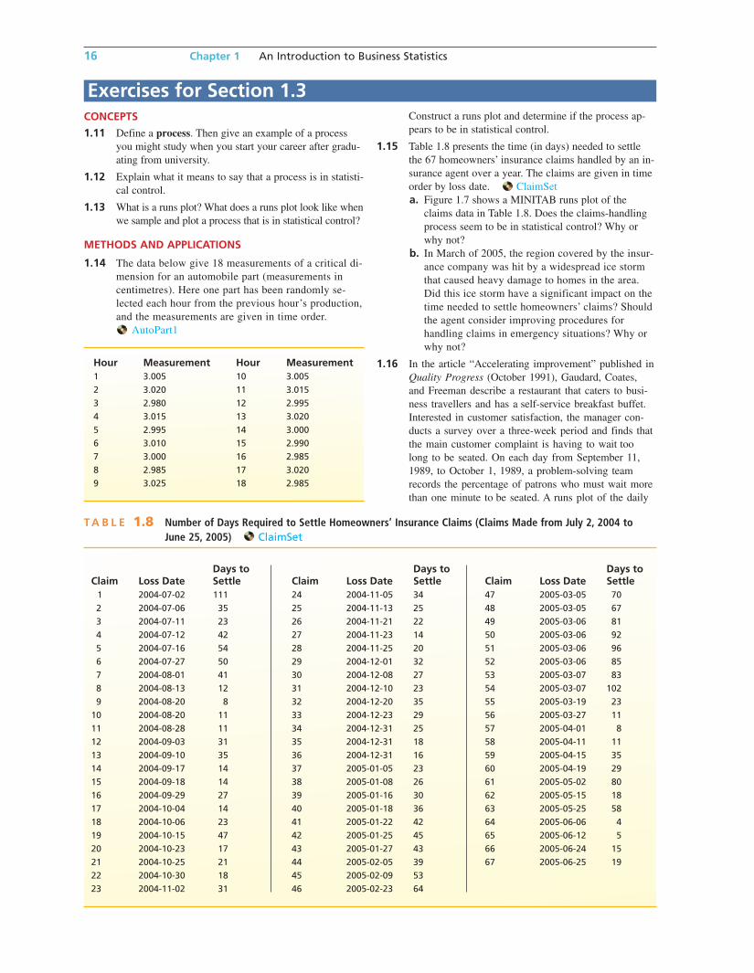
T A B L E 1.8 Number of Days Required to Settle Homeowners’ Insurance Claims (Claims Made from July 2, 2004 toJune 25, 2005) ClaimSet

Days to Days to Days toClaim Loss Date Settle Claim Loss Date Settle Claim Loss Date Settle

1 2004-07-02 111 24 2004-11-05 34 47 2005-03-05 70

2 2004-07-06 35 25 2004-11-13 25 48 2005-03-05 67

3 2004-07-11 23 26 2004-11-21 22 49 2005-03-06 81

4 2004-07-12 42 27 2004-11-23 14 50 2005-03-06 92

5 2004-07-16 54 28 2004-11-25 20 51 2005-03-06 96

6 2004-07-27 50 29 2004-12-01 32 52 2005-03-06 85

7 2004-08-01 41 30 2004-12-08 27 53 2005-03-07 83

8 2004-08-13 12 31 2004-12-10 23 54 2005-03-07 102

9 2004-08-20 8 32 2004-12-20 35 55 2005-03-19 23

10 2004-08-20 11 33 2004-12-23 29 56 2005-03-27 11

11 2004-08-28 11 34 2004-12-31 25 57 2005-04-01 8

12 2004-09-03 31 35 2004-12-31 18 58 2005-04-11 11

13 2004-09-10 35 36 2004-12-31 16 59 2005-04-15 35

14 2004-09-17 14 37 2005-01-05 23 60 2005-04-19 29

15 2004-09-18 14 38 2005-01-08 26 61 2005-05-02 80

16 2004-09-29 27 39 2005-01-16 30 62 2005-05-15 18

17 2004-10-04 14 40 2005-01-18 36 63 2005-05-25 58

18 2004-10-06 23 41 2005-01-22 42 64 2005-06-06 4

19 2004-10-15 47 42 2005-01-25 45 65 2005-06-12 5

20 2004-10-23 17 43 2005-01-27 43 66 2005-06-24 15

21 2004-10-25 21 44 2005-02-05 39 67 2005-06-25 19

22 2004-10-30 18 45 2005-02-09 53

23 2004-11-02 31 46 2005-02-23 64

CONCEPTS

1.11 Define a process. Then give an example of a process

you might study when you start your career after gradu-

ating from university.

1.12 Explain what it means to say that a process is in statisti-

cal control.

1.13 What is a runs plot? What does a runs plot look like when

we sample and plot a process that is in statistical control?

METHODS AND APPLICATIONS

1.14 The data below give 18 measurements of a critical di-

mension for an automobile part (measurements in

centimetres). Here one part has been randomly se-

lected each hour from the previous hour’s production,

and the measurements are given in time order.

AutoPart1

Exercises for Section 1.3Construct a runs plot and determine if the process ap-

pears to be in statistical control.

1.15 Table 1.8 presents the time (in days) needed to settle

the 67 homeowners’ insurance claims handled by an in-

surance agent over a year. The claims are given in time

order by loss date. ClaimSet

a. Figure 1.7 shows a MINITAB runs plot of the

claims data in Table 1.8. Does the claims-handling

process seem to be in statistical control? Why or

why not?

b. In March of 2005, the region covered by the insur-

ance company was hit by a widespread ice storm

that caused heavy damage to homes in the area.

Did this ice storm have a significant impact on the

time needed to settle homeowners’ claims? Should

the agent consider improving procedures for

handling claims in emergency situations? Why or

why not?

1.16 In the article “Accelerating improvement” published in

Quality Progress (October 1991), Gaudard, Coates,

and Freeman describe a restaurant that caters to busi-

ness travellers and has a self-service breakfast buffet.

Interested in customer satisfaction, the manager con-

ducts a survey over a three-week period and finds that

the main customer complaint is having to wait too

long to be seated. On each day from September 11,

1989, to October 1, 1989, a problem-solving team

records the percentage of patrons who must wait more

than one minute to be seated. A runs plot of the daily



9The source of Figure 1.8 is “Accelerating improvement,” by M. Gaudard, R. Coates, and L. Freeman, Quality Progress, October 1991, pp. 81–88. Copyright© 1991 American Society for Quality Control. Used with permission.

10This case is based on conversations by the authors with several employees working for a leading producer of trash bags. For purposes of confidentiality,we have withheld the company’s name.

F I G U R E 1.7 MINITAB Runs Plot of the InsuranceClaims Data for Exercise 1.15

F I G U R E 1.8 Runs Plot of Daily Percentages ofCustomers Waiting More Than OneMinute to Be Seated (for Exercise 1.16)

Claim

Day

s to

Set

tle

605040302010

100

75

50

25

0

Time Series Plot of Days to Settle9%

Perc

enta

ge

Wh

o W

aite

d

Day of Week (Sept. 11–Oct. 1, 1989)

M T W T F S S M T W T F S S M T W T F S S

8%7%6%5%4%3%2%1%

percentages is shown in Figure 1.8.9 What does the

runs plot suggest?

1.17 THE TRASH BAG CASE10 TrashBag

A company that produces and markets trash bags has

developed an improved 130-L bag. The new bag is

produced using a specially formulated plastic that is both

stronger and more biodegradable than previously used

plastics, and the company wishes to evaluate the strength

of this bag. The breaking strength of a trash bag is con-

sidered to be the mass (in kilograms) of a representative

trash mix that when loaded into a bag suspended in the

air will cause the bag to sustain significant damage (such

F I G U R E 1.9 Excel Runs Plot of Breaking Strengths for Exercise 1.17T A B L E 1.9 BreakingStrengths

TrashBag

22.0 23.9 23.0 22.5

23.8 21.6 21.9 23.6

24.3 23.1 23.4 23.6

23.0 22.6 22.3 22.2

22.9 22.7 23.5 21.3

22.5 23.1 24.2 23.3

23.2 24.1 23.2 22.4

22.0 23.1 23.9 24.5

23.0 22.7 23.3 22.4

22.8 22.8 22.5 23.4

StrengthA

22.023.824.323.0

22.523.222.023.022.823.921.623.122.6

22.9

A

15

12345

76

91011121314

8

22.723.124.123.122.722.8

1718192021

16

B D E F G H I JC

Runs Plot of Strength

Stre

ng

th

Time

1 6 11 16 21 26 31 3619

20

21

22

23

24

25

as ripping or tearing). The company has decided to carry

out a 40-hour pilot production run of the new bags. Each

hour, at a randomly selected time during the hour, a bag

is taken off the production line. The bag is then subjected

to a breaking strength test. The 40 breaking strengths ob-

tained during the pilot production run are given in Table

1.9, and an Excel runs plot of these breaking strengths is

given in Figure 1.9.

a. Do the 40 breaking strengths appear to be in statisti-

cal control? Explain.

b. Estimate limits between which most of the breaking

strengths of all trash bags would fall.



1.18 THE BANK CUSTOMER WAITINGTIME CASE WaitTime

Recall that every 150th customer arriving

during peak business hours was sampled

until a systematic sample of 100 customers

was obtained. This systematic sampling

procedure is equivalent to sampling from a

process. Figure 1.10 shows a MegaStat

runs plot of the 100 waiting times in Table

1.5. Does the process appear to be in sta-

tistical control? Explain.

F I G U R E 1.10 MegaStat Runs Plot of Waiting Times for Exercise 1.18

Runs Plot of Waiting Times

1 11

12

10

8

6

4

2

0

21 31 41 51 61 71 81 91

Customer

Wai

tin

g T

ime

1.4 Levels of Measurement: Nominal, Ordinal, Interval, and Ratio

In Section 1.1, we said that a variable is quantitative if its possible values are numbers that rep-

resent quantities (that is, “how much” or “how many”). In general, a quantitative variable is meas-

ured on a scale with a fixed unit of measurement between its possible values. For example, if we

measure employees’ salaries to the nearest dollar, then one dollar is the fixed unit of measurement

between different employees’ salaries. There are two types of quantitative variables: ratio and inter-

val. A ratio variable is a quantitative variable measured on a scale such that ratios of its values

are meaningful and there is an inherently defined zero value. Variables such as salary, height,

weight, time, and distance are ratio variables. For example, a distance of zero kilometres is “no dis-

tance at all,” and a town that is 30 km away is “twice as far” as a town that is 15 km away.

An interval variable is a quantitative variable where ratios of its values are not meaningful and

there is no meaningful zero. The 1 to 7 Likert scale example given earlier is an example of an in-

terval scale. The distance from 2 to 3 is the same as that from 5 to 6. The scale could also have been

–3 –2 –1 0 1 2 3

Here the zero is the midpoint and represents the same concept as the number 4 in the 1 to 7 scale.

In Section 1.1, we also said that if we simply record into which of several categories a popu-

lation (or sample) unit falls, then the variable is qualitative (or categorical). There are two types

of qualitative variables: ordinal and nominative (or nominal). An ordinal variable is a qualita-

tive variable for which there is a meaningful ordering, or ranking, of the categories. The meas-

urements of an ordinal variable may be nonnumerical or numerical. For example, a student may

be asked to rank their four favourite colours. The person may say that yellow (#1) is their most

favourite colour, then green (#2), red (#3), and blue (#4). If asked further, the person may say

they really adore yellow and green and that red and blue are “so-so” but that red is slightly bet-

ter than blue. This ranking does not have equal distances between points in that 1 to 2 is not the

same as 2 to 3. Only the order (of preference) is meaningful. In Chapter 13, we will learn how to

use nonparametric statistics to analyze an ordinal variable without considering the variable to

be somewhat quantitative and performing such arithmetic operations. In addition to these four

types of variables, data may also take the form of continuous or discrete values. Continuous vari-

ables are typically interval or ratio scale numbers and fall along a continuum so that decimals


1.5 A Brief Introduction to Surveys 19

make sense (such as salaries, age, mass, and height). In contrast, discrete variables are nom-

inal or ordinal and represent distinct groups in which decimals do not make sense (such as sex

categorization, living in urban or rural communities, and number of children in a household).

To conclude this section, we consider the second type of qualitative variable. A nominative

(or nominal) variable is a qualitative variable for which there is no meaningful ordering, or

ranking, of the categories. A person’s sex, the colour of a car, and an employee’s city of residence

are nominative (or nominal) variables.11

11Study Hint: To remember the levels of measurement, simply remember the French word for “black” (NOIR). This acronym is use-ful since it also puts the levels into order from simplest level of measurement (nominal or nominative) to most complex (ratio).

Exercises for Section 1.4CONCEPTS

1.19 Discuss the difference between a ratio variable and an

interval variable.

1.20 Discuss the difference between an ordinal variable and

a nominative (or nominal) variable.

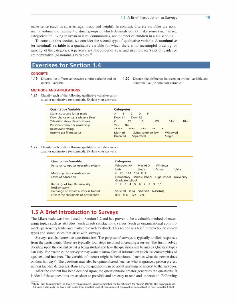
Qualitative Variable CategoriesStatistics course letter mark A B C D FDoor choice on Let’s Make a Deal Door #1 Door #2Television show classifications C C8 G PG 14� 18�

Personal computer ownership Yes NoRestaurant rating ***** **** *** ** *Income tax filing status Married Living common-law Widowed

Divorced Separated Single

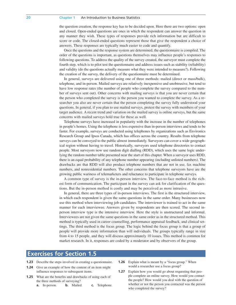
Qualitative Variable CategoriesPersonal computer operating system Windows XP Mac 05-X Windows

Unix Linux Other VistaMotion picture classifications G PG 14A 18A R ALevel of education Elementary Middle school High school University

Graduate school Rankings of top 10 university 1 2 3 4 5 6 7 8 9 10hockey teamsExchange on which a stock is traded S&P/TSX DJIA S&P 500 NASDAQFirst three characters of postal code B3J M1J T2K V7E

1.5 A Brief Introduction to SurveysThe Likert scale was introduced in Section 1.2 and has proven to be a valuable method of meas-

uring topics such as attitudes (such as job satisfaction), values (such as organizational commit-

ment), personality traits, and market research feedback. This section is a brief introduction to survey

types and some issues that arise with surveys.

Surveys are also known as questionnaires. The purpose of surveys is typically to elicit responses

from the participants. There are typically four steps involved in creating a survey. The first involves

deciding upon the content (what is being studied and how the questions will be asked). Question types

can vary. For example, the surveyor may want to know factual information (such as demographics of

age, sex, and income). The variable of interest might be behavioural (such as what the person does

on their holidays). The questions may also be opinion based (such as what fragrance a person prefers

in their laundry detergent). Basically, the questions can be about anything of interest to the surveyor.

After the content has been decided upon, the questionnaire creator generates the questions. It

is ideal if these questions are as short as possible and are easy to read and understand. Following

1.21 Classify each of the following qualitative variables as or-

dinal or nominative (or nominal). Explain your answers.

METHODS AND APPLICATIONS

1.22 Classify each of the following qualitative variables as or-

dinal or nominative (or nominal). Explain your answers.



the question creation, the response key has to be decided upon. Here there are two options: open

and closed. Open-ended questions are ones in which the respondent can answer the question in

any manner they wish. These types of responses provide rich information but are difficult to

score or code. The closed-ended questions represent those that give the respondent a choice of

answers. These responses are typically much easier to code and quantify.

Once the questions and the response system are determined, the questionnaire is compiled. The

order of the questions is important, as questions themselves may influence people’s responses to

following questions. To address the quality of the survey created, the surveyor must complete the

fourth step, which is to pilot test the questionnaire and address issues such as stability (reliability)

and validity (do the questions actually measure what they were intended to measure?). Following

the creation of the survey, the delivery of the questionnaire must be determined.

In general, surveys are delivered using one of three methods: mailed (direct or mass/bulk),

telephone, and in-person. Mailed surveys are relatively inexpensive and unobtrusive, but tend to

have low response rates (the number of people who complete the survey compared to the num-

ber of surveys sent out). Other concerns with mailing surveys is that you are never certain that

the person who completed the survey is the person you wanted to complete the survey. As a re-

searcher you also are never certain that the person completing the survey fully understood your

questions. In general, if you plan to use mailed surveys, pretest the survey with members of your

target audience. A recent trend and variation on the mailed survey is online surveys, but the same

concerns with mailed surveys hold true for these as well.

Telephone surveys have increased in popularity with the increase in the number of telephones

in people’s homes. Using the telephone is less expensive than in-person interviews and tends to be

faster. For example, surveys are conducted using telephones by organizations such as Environics

Research Group and Ipsos Canada, which has offices across the country. Results from telephone

surveys can be conveyed to the public almost immediately. Surveyors can cover a wide geograph-

ical region without having to travel. Historically, surveyors used telephone directories to contact

people. Most surveyors now use random digit dialling (RDD), which uses the same logic under-

lying the random number table presented near the start of this chapter. When a surveyor uses RDD,

there is an equal probability of any telephone number appearing (including unlisted numbers). The

drawbacks are that RDD will also produce telephone numbers that are not in use, fax machine

numbers, and nonresidential numbers. The other concerns that telephone surveyors have are the

growing public wariness of telemarketers and reluctance to participate in telephone surveys.

A common type of survey is the in-person interview. The face-to-face method is the rich-

est form of communication. The participant in the survey can ask for clarification of the ques-

tions. But the in-person method is costly and may be perceived as more intrusive.

In general, there are three types of in-person interviews. The first is the structured interview,

in which each respondent is given the same questions in the same order. Many businesses now

use this method when interviewing job candidates. The interviewer is trained to act in the same

manner for each interviewee. Answers given by respondents are then scored. The second in-

person interview type is the intensive interview. Here the style is unstructured and informal.

Interviewees are not given the same questions in the same order as in the structured method. This

method is typically used in career counselling, performance appraisal feedback, and clinical set-

tings. The third method is the focus group. The logic behind the focus group is that a group of

people will provide more information than will individuals. The groups typically range in size

from 4 to 15 people, and they will discuss approximately 10 issues. This method is common for

market research. In it, responses are coded by a moderator and by observers of the group.

Exercises for Section 1.51.23 Describe the steps involved in creating a questionnaire.

1.24 Give an example of how the content of an item might

influence responses to subsequent items.

1.25 What are the benefits and drawbacks of using each of

the three methods of surveying?

a. In-person. b. Mailed. c. Telephone.

1.26 Explain what is meant by a “focus group.” When

would a researcher use a focus group?

1.27 Explain how you would go about requesting that peo-

ple complete an online survey. How would you contact

the people? How would you deal with the question of

whether or not the person you contacted was the person

who completed the survey?


1.6 An Introduction to Survey Sampling 21

1.6 An Introduction to Survey SamplingRandom sampling is not the only type of sampling. Methods for obtaining a sample are called

sampling designs, and the sample we take is sometimes called a sample survey. In this section,

we explain three sampling designs that are alternatives to random sampling—stratified random

sampling, cluster sampling, and systematic sampling.

One common sampling design involves separately sampling important groups within a popu-

lation. Then the samples are combined to form the entire sample. This approach is the idea

behind stratified random sampling.

In order to select a stratified random sample, we divide the population into nonoverlapping

groups of similar units (people, objects, etc.). These groups are called strata. Then a random

sample is selected from each stratum, and these samples are combined to form the full sample.

It is wise to stratify when the population consists of two or more groups that differ with respect

to the variable of interest. For instance, consumers could be divided into strata based on sex, age,

language (e.g., speaks English, French, or other), or income.

As an example, suppose that a department store chain proposes to open a new store in a location

that would serve customers who live in a geographical region that consists of (1) an industrial city,

(2) a suburban community, and (3) a rural area. In order to assess the potential profitability of the

proposed store, the chain wishes to study the incomes of all households in the region. In addition,

the chain wishes to estimate the proportion and the total number of households whose members

would be likely to shop at the store. The department store chain feels that the industrial city, the sub-

urban community, and the rural area differ with respect to income and the store’s potential desir-

ability. Therefore, it uses these subpopulations as strata and takes a stratified random sample.

Taking a stratified sample can be advantageous because such a sample takes advantage of the

fact that units in the same stratum are similar to each other. It follows that a stratified sample can

provide more accurate information than a random sample of the same size. As a simple example,

if all of the units in each stratum were exactly the same, then examining only one unit in each stra-

tum would allow us to describe the entire population. Furthermore, stratification can make a sam-

ple easier (or possible) to select. Recall that, in order to take a random sample, we must have a

frame, or list, of all of the population units. Although a frame might not exist for the overall

population, a frame might exist for each stratum. For example, suppose nearly all the households

in the department store’s geographical region have telephones. Although there might not be a tele-

phone directory for the overall geographical region, there might be separate telephone directories

for the industrial city, the suburb, and the rural area from which samples could be drawn (although

recall some of the drawbacks of telephone surveying listed in the previous section).

Sometimes it is advantageous to select a sample in stages. This is a common practice when

selecting a sample from a very large geographical region. In such a case, a frame often does not

exist. For instance, there is no single list of all households in Canada. In this situation, we can

use multistage cluster sampling. To illustrate this procedure, suppose we wish to take a sample

of households from all households in Canada. We might proceed as follows:

Stage 1: Randomly select a sample of counties from all of the counties in Canada.

Stage 2: Randomly select a sample of townships in each county.

Stage 3: Randomly select a sample of households from each township.

We use the term cluster sampling to describe this type of sampling because at each stage we

“cluster” the households into subpopulations. For instance, in Stage 1 we cluster the households

into counties, and in Stage 2 we cluster the households in each county into townships. Also, no-

tice that the random sampling at each stage can be carried out because there are lists of (1) all

counties in Canada, (2) all townships in Canada, and (3) all households in each township.

As another example, consider another way of sampling the households in Canada. We might use

Stages 1 and 2 above to select counties and townships within the selected counties. Then, if there is

a telephone directory of the households in each township, we can randomly sample households from

each selected township by using its telephone directory. Because most households today have tele-

phones, and telephone directories are readily available, most national polls are now conducted by

telephone.



It is sometimes a good idea to combine stratification with multistage cluster sampling. Forexample, suppose a national polling organization wants to estimate the proportion of allregistered voters who favour a particular federal party. Because the federal party preferences ofvoters might tend to vary by geographical region, the polling organization might divide Canadainto regions (say, Atlantic Canada, Québec, Ontario, and Western Canada). The polling organiz-ation might then use these regions as strata and might take a multistage cluster sample from eachstratum (region).12

In order to select a random sample, we must number the units in a frame of all the popula-tion units. Then we use a random number table (or a random number generator on a computer)to make the selections. However, numbering all the population units can be quite time-consuming. Moreover, random sampling is used in the various stages of many complex sam-pling designs (requiring the numbering of numerous populations). Therefore, it is useful to havean alternative to random sampling. One such alternative is called systematic sampling. In or-der to systematically select a sample of n units without replacement from a frame of N units, wedivide N by n and round the result down to the nearest whole number. Calling the rounded re-sult �, we then randomly select one unit from the first � units in the frame—this is the first unitin the systematic sample. The remaining units in the sample are obtained by selecting every �thunit following the first (randomly selected) unit. For example, suppose we wish to sample apopulation of N � 14,327 members of an international allergists’ association to investigate howoften they have prescribed a particular drug during the last year. The association has a directorylisting the 14,327 allergists, and we wish to draw a systematic sample of 500 allergists from thisframe. Here we compute 14,327�500 � 28.654, which is 28 when rounded down. Therefore,we number the first 28 allergists in the directory from 1 to 28, and we use a random numbertable to randomly select one of the first 28 allergists. Suppose we select allergist number 19. Weinterview allergist 19 and every 28th allergist in the frame thereafter, so we choose allergists19, 47, 75, and so forth until we obtain our sample of 500 allergists. In this scheme, we mustnumber the first 28 allergists, but we do not have to number the rest because we can “countoff” every 28th allergist in the directory. Alternatively, we can measure the approximateamount of space in the directory that it takes to list 28 allergists. This measurement can thenbe used to select every 28th allergist.

In this book, we concentrate on showing how to analyze data produced by random sampling.However, if the order of the population units in a frame is random with respect to the character-istic under study, then a systematic sample should be (approximately) a random sample and wecan analyze the data produced by the systematic sample by using the same methods employedto analyze random samples. For instance, it would seem reasonable to assume that the alphabet-ically ordered allergists in a medical directory would be random (that is, have nothing to do withthe number of times the allergists prescribed a particular drug). Similarly, the alphabetically or-dered people in a telephone directory would probably be random with respect to many of the peo-ple’s characteristics that we might wish to study.

When we employ random sampling, we eliminate bias in the choice of the sample from aframe. However, a proper sampling design does not guarantee that the sample will produce ac-curate information. One potential problem is undercoverage.

Undercoverage occurs when some population units are excluded from the process of selectingthe sample.

This problem occurs when we do not have a complete, accurate list of all the population units.For example, although telephone polls today are common, some people in Canada do not havetelephones. In general, undercoverage usually causes some people to be underrepresented. If under-represented groups differ from the rest of the population with respect to the characteristicunder study, the survey results will be biased. A second potentially serious problem is nonre-

sponse.

12The analysis of data produced by multistage cluster sampling can be quite complicated. We explain how to analyze dataproduced by one- and two-stage cluster sampling in Appendix E (Part 2). This appendix also includes a discussion of anadditional survey sampling technique called ratio estimation. For a more detailed discussion of cluster sampling and ratioestimation, see Mendenhall, Schaeffer, and Ott (1986).

bow83755_ch01_001-026.qxd 11/6/07 4:26 PM Page 22 205:MHHE025:bow83755_ch01:

Chapter Summary 23

Nonresponse occurs when a population unit selected as part of the sample cannot be contacted

or refuses to participate.

In some surveys, 35 percent or more of the selected individuals cannot be contacted—even when

several callbacks are made. In such a case, other participants are often substituted for the people

who cannot be contacted. If the substitute participants differ from the originally selected partici-

pants with respect to the characteristic under study, the survey will again be biased. Third, when

people are asked potentially embarrassing questions, their responses might not be truthful. We

then have what we call response bias. Fourth, the wording of the questions asked can influence

the answers received. Slanted questions often evoke biased responses. For example, consider the

following question:

Which of the following best describes your views on gun control?

1 The government should take away our guns, leaving us defenceless against heavily armed

criminals.

2 We have the right to keep guns.

Exercises for Section 1.6CONCEPTS

1.28 When is it appropriate to use stratified random sampling?

What are strata, and how should strata be selected?

1.29 When is cluster sampling used? Why do we describe

this type of sampling by using the term cluster?

1.30 Explain each of the following terms:

a. Undercoverage.

b. Nonresponse.

c. Response bias.

1.31 Explain how to take a systematic sample of 100 com-

panies from the 1,853 companies that are members of

an industry trade association.

1.32 Explain how a stratified random sample is selected.

Discuss how you might define the strata to survey

student opinion on a proposal to charge all students a

$100 fee for a new university-run bus system that will

provide transportation between off-campus apartments

and campus locations.

1.33 Marketing researchers often use city blocks as clusters in

cluster sampling. Using this fact, explain how a market

researcher might use multistage cluster sampling to select

a sample of consumers from all cities with a population

of more than 10,000 in a region having many such cities.

CHAPTER SUMMARYThis chapter has introduced the idea of using sample data to

make statistical inferences—that is, drawing conclusions

about populations and processes by using sample data. We be-

gan by learning that a population is a set of existing units that

we wish to study. We saw that, since many populations are too

large to examine in their entirety, we often study a population

by selecting a sample, which is a subset of the population units.

Next we learned that, if the information contained in a sample

is to accurately represent the population, then the sample

should be randomly selected from the population, and we saw

how random numbers (obtained from a random number

table) can be used to select a random sample. We also learned

that selecting a random sample requires a frame (that is, a list

of all of the population units) and that, since a frame does not

always exist, we sometimes select a systematic sample.

We continued this chapter by studying processes. We

learned that to make statistical inferences about the population

of all possible values of a variable that could be observed when

using a process, the process must be in statistical control. We

learned that a process is in statistical control if it does not ex-

hibit any unusual process variations, and we demonstrated how

we might sample a process and how to use a runs plot to try to

judge whether a process is in control.

Next, in Section 1.4, we studied different types of quantita-

tive and qualitative variables. We learned that there are two

types of quantitative variables—ratio variables, which are

measured on a scale such that ratios of its values are meaning-

ful and there is an inherently defined zero value, and interval

variables, for which ratios are not meaningful and there is no

inherently defined zero value. We also saw that there are two

types of qualitative variables—ordinal variables, for which

there is a meaningful ordering of the categories, and nomina-

tive (or nominal) variables, for which there is no meaningful

ordering of the categories.

We concluded this chapter with Sections 1.5 and 1.6, which

discuss survey construction, types of survey methods, and

survey sampling. We introduced stratified random sam-

pling, in which we divide a population into groups (strata)

and then select a random sample from each group. We also in-

troduced multistage cluster sampling, which involves select-

ing a sample in stages, and we explained how to select a

systematic sample. Finally, we discussed some potential

problems encountered when conducting a sample survey—

undercoverage, nonresponse, response bias, and slanted

questions.

ww

w.m

cg

ra

wh

ill.ca

/o

lc/

bo

we

rm

an


GLOSSARY OF TERMScategorical (qualitative) variable: A variable with values that

indicate into which of several categories a population unit

belongs. (page 2)

census: An examination of all the units in a population. (page 2)

cluster sampling (multistage cluster sampling): A sampling

design in which we sequentially cluster population units into

subpopulations. (page 21)

descriptive statistics: The science of describing the important

aspects of a set of measurements. (page 2)

finite population: A population that contains a finite number

of units. (page 11)

frame: A list of all of the units in a population. This is needed

in order to select a random sample. (page 4)

infinite population: A population that is defined so that there

is no limit to the number of units that could potentially belong

to the population. (page 11)

interval variable: A quantitative variable such that ratios of its

values are not meaningful and for which there is not an inher-

ently defined zero value. (page 18)

measurement: The process of assigning a value of a variable

to each of the units in a population or sample. (page 2)

nominative (or nominal) variable: A qualitative variable for

which there is no meaningful ordering, or ranking, of the cate-

gories. (page 19)

nonresponse: A situation in which population units selected

to participate in a survey do not respond to the survey instru-

ment. (page 23)

ordinal variable: A qualitative variable for which there is a

meaningful ordering or ranking of the categories. (page 18)

population: A set of existing or potential units (people, ob-

jects, events, or the like) that we wish to study. (page 2)

process: A sequence of operations that takes inputs and turns

them into outputs. (page 11)

qualitative (categorical) variable: A variable with values

that indicate in which of several categories a population unit

belongs. (page 2)

quantitative variable: A variable with values that are num-

bers representing quantities. (page 2)

random number table: A table containing random digits that

is often used to select a random sample. (page 4)

random sample: A sample selected so that, on each selection

from the population, every unit remaining in the population on

that selection has the same chance of being chosen. (page 3)

ratio variable: A quantitative variable such that ratios of its

values are meaningful and for which there is an inherently de-

fined zero value. (page 18)

response bias: A situation in which survey participants do not

respond truthfully to the survey questions. (page 23)

runs plot: A graph of individual process measurements versus

time. (page 12)

sample: A subset of the units in a population. (page 2)

sampling with replacement: A sampling procedure in which

we place any unit that has been chosen back into the population

to give the unit a chance to be chosen on succeeding selections.

(page 3)

sampling without replacement: A sampling procedure in

which we do not place previously selected units back into the

population and, therefore, do not give these units a chance to be

chosen on succeeding selections. (page 3)

statistical control: A state in which a process does not exhibit

any unusual variations. Often this means that the process dis-

plays a uniform amount of variation around a constant, or hor-

izontal, level. (page 12)

statistical inference: The science of using a sample of meas-

urements to make generalizations about the important aspects

of a population. (page 3)

statistical process control (SPC): A method of analyzing

process data in which we monitor and study the process varia-

tion. The goal is to stabilize (and reduce) the amount of process

variation. (page 12)

strata: The subpopulations in a stratified sampling design.

(page 21)

stratified random sampling: A sampling design in which we

divide a population into nonoverlapping subpopulations and

then select a random sample from each subpopulation

(stratum). (page 21)

systematic sample: A sample taken by moving systematic-

ally through the population. For instance, we might ran-

domly select one of the first 200 population units and then

systematically sample every 200th population unit thereafter.

(page 6)

undercoverage: A situation in sampling in which some

groups of population units are underrepresented. (page 22)

variable: A characteristic of a population unit. (page 2)


SUPPLEMENTARY EXERCISES1.34 Some television stations attempt to gauge public opinion

by posing a question on the air and asking viewers to

call to give their opinions. Suppose that a particular

television station asks viewers whether they support or

oppose the federal gun registry. Viewers are to call one

of two toll-free numbers to register support or opposition.

When the results are tabulated, the station reports that

78 percent of those who called are opposed to the reg-

istry. What do you think of the sampling method used

by the station? Do you think that the percentage of the

entire population that opposes the registry is as high as

the 78 percent of the sample that was opposed?

1.35 Table 1.10 gives the “35 best companies to work for” as

rated on the Fortune magazine Web site on March 14,

2005. Use random numbers to select a random sample

of 10 of these companies. Justify that your sample is

random by carefully explaining how you obtained it.

List the random numbers you used and show how they

gave your random sample.

1.36 A bank wishes to study the amount of time it takes to

complete a withdrawal transaction from one of its

ABMs (automated banking machines). On a particular

day, 63 withdrawal transactions are observed between

10 A.M. and noon. The time required to complete each

transaction is given in Table 1.11. Figure 1.11 shows

an Excel runs plot of the 63 transaction times. Do the

transaction times seem to be in statistical control?

Why or why not? ABMTime

1.37 Figure 1.12 gives a runs plot of the Edmonton Oilers’

point percentages (number of points divided by total

ww

w.m

cg

ra

wh

ill.

ca

/o

lc/

bo

we

rm

an

bow83755_ch01_001-026.qxd 11/6/07 4:26 PM Page 24 205:MHHE025:bow83755_ch01:

Supplementary Exercises 25

Source: Fortune, March 14, 2005. Copyright © 2005 Time, Inc. All rights reserved.

Rank Company

1 Wegmans Food Markets2 W.L. Gore3 Republic Bancorp4 Genentech5 Xilinx6 J.M. Smucker7 S.C. Johnson & Son8 Griffin Hospital9 Alston & Bird

10 Vision Service Plan11 Starbucks12 Quicken Loans13 Adobe Systems14 CDW15 Container Store16 SAS Institute17 Qualcomm18 Robert W. Baird19 QuikTrip

Rank Company

20 HomeBanc Mortgage21 David Weekley Homes22 TD Industries23 Valero Energy24 Network Appliance25 JM Family Enterprises26 American Century

Investments27 Cisco Systems28 American Cast Iron Pipe29 Stew Leonard’s30 Whole Foods Market31 Baptist Health South

Florida32 Arnold & Porter33 Amgen34 American Fidelity

Assurance35 Goldman Sachs Group

T A B L E 1.10 Fortune’s 35 Best Companies to Work for in March 2005 (for Exercise 1.35)

ww

w.m

cg

ra

wh

ill.ca

/o

lc/

bo

we

rm

an

number of points available for the regular season)from the 1979/1980 season until the 2006/2007 season.Note that no games were played in the 2004/2005 seasondue to the lockout. The Oilers were one of the besthockey teams of the 1980s. However, many longtimeOilers fans believe that the 1987 trade of Paul Coffeyto the Pittsburgh Penguins was the beginning of theteam’s decline. That supposedly signalled the begin-ning of the end of the Stanley Cup Championship“dynasty” in Edmonton. Does the runs plot provideany evidence to support this opinion? Why or whynot? What else do you notice about the team’s pointpercentage starting in the 1999/2000 season? Can yougive any reasons for the sudden change?

1.38 THE TRASH BAG CASE TrashBag

Recall that the company will carry out a 40-hour pilot pro-duction run of the new bags and will randomly select onebag each hour to be subjected to a breaking strength test.a. Explain how the company can use random numbers

to randomly select the times during the 40 hours ofthe pilot production run at which bags will betested. Hint: Suppose that a randomly selected timewill be determined to the nearest minute.

b. Use the following random numbers (obtained fromTable 1.1) to select the times during the first fivehours at which the first five bags to be tested willbe taken from the production line: 61, 15, 64, 07,86, 87, 57, 64, 66, 42, 59, 51.

Transaction Time Transaction Time Transaction Time1 32 22 34 43 372 32 23 32 44 323 41 24 34 45 334 51 25 35 46 335 42 26 33 47 406 39 27 42 48 357 33 28 46 49 338 43 29 52 50 399 35 30 36 51 34

10 33 31 37 52 3411 33 32 32 53 3312 32 33 39 54 3813 42 34 36 55 4114 34 35 41 56 3415 37 36 32 57 3516 37 37 33 58 3517 33 38 34 59 3718 35 39 38 60 3919 40 40 32 61 4420 36 41 35 62 4021 32 42 33 63 39

T A B L E 1.11 ABM Transaction Times (in Seconds) for 63 Withdrawals ABMTime



F I G U R E 1.11 Excel Runs Plot of ABM Transaction Times for Exercise 1.36

ABM TIME32324151

3933433533333242

42

12345

76

91011121314

8

A B D E F G H IC

6050403020100

AB

M T

IME

0 10 20 30 40 50 60

TRANSACTION NUMBER

0.8

0.6

0.7

0.5

0.4

Point Percentage

1980 1988 19961984 1992

Year

Runs Plot of the Edmonton Oilers Point Percentages

2000 2004

0.3

F I G U R E 1.12 Runs Plot of the Edmonton Oilers’ Point Percentages from 1979/80 to 2006/07 (for Exercise 1.37)

ww

w.m

cg

ra

wh

ill.

ca

/o

lc/

bo

we

rm

an


An Introduction to Business Statistics - McGraw-Hill

Documents