An introduction to biostatistics: part 1Cavanr/IntroStat1.pdfAn introduction to biostatistics: part 1 Cavan Reilly September 4, 2019. Table of contents Introduction to data analysis

An introduction to biostatistics: part 1

Cavan Reilly

September 4, 2019

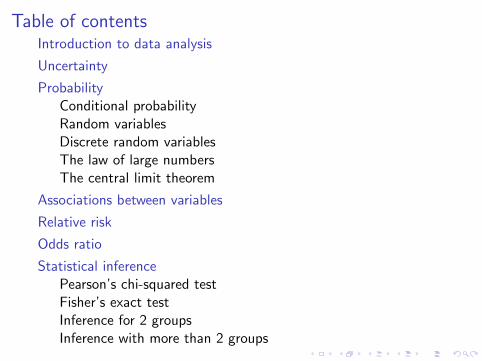
Table of contentsIntroduction to data analysis

Uncertainty

ProbabilityConditional probabilityRandom variablesDiscrete random variablesThe law of large numbersThe central limit theorem

Associations between variables

Relative risk

Odds ratio

Statistical inferencePearson’s chi-squared testFisher’s exact testInference for 2 groupsInference with more than 2 groups

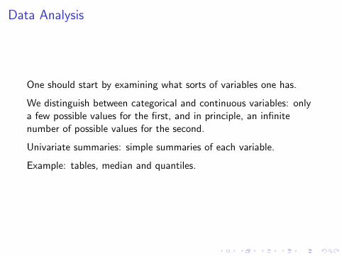
Data Analysis

One should start by examining what sorts of variables one has.

We distinguish between categorical and continuous variables: onlya few possible values for the first, and in principle, an infinitenumber of possible values for the second.

Univariate summaries: simple summaries of each variable.

Example: tables, median and quantiles.

Data Analysis

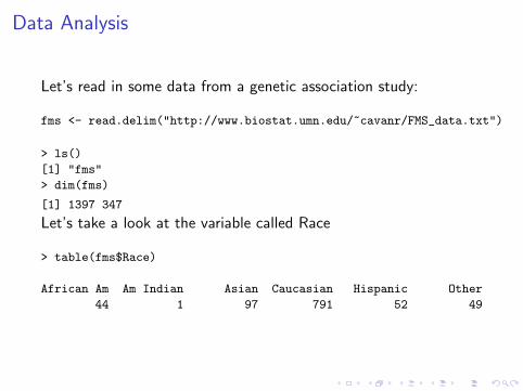
Let’s read in some data from a genetic association study:

fms <- read.delim("http://www.biostat.umn.edu/~cavanr/FMS_data.txt")

> ls()

[1] "fms"

> dim(fms)

[1] 1397 347

Let’s take a look at the variable called Race

> table(fms$Race)

African Am Am Indian Asian Caucasian Hispanic Other

44 1 97 791 52 49

Data Analysis

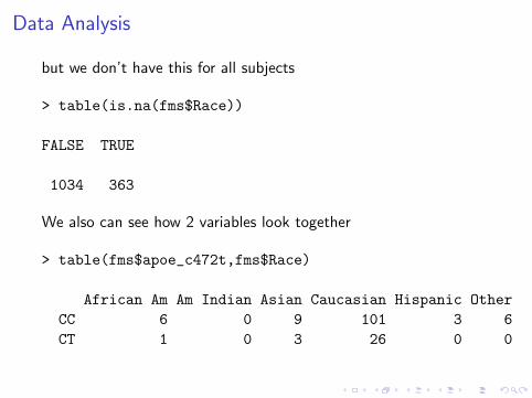
but we don’t have this for all subjects

> table(is.na(fms$Race))

FALSE TRUE

1034 363

We also can see how 2 variables look together

> table(fms$apoe_c472t,fms$Race)

African Am Am Indian Asian Caucasian Hispanic OtherCC 6 0 9 101 3 6CT 1 0 3 26 0 0

Uncertainty

If I collected a different data set I would produce differentsummaries.

To provide a way to think about this, we think of the data we seeas a realization of a random process: the data set we have is only 1of many we could have observed.

We model our observed data as values taken on by a randomvariable.

Probability

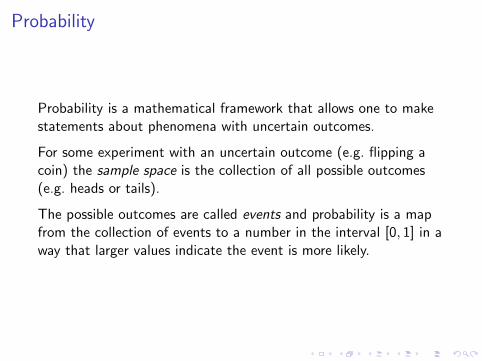
Probability is a mathematical framework that allows one to makestatements about phenomena with uncertain outcomes.

For some experiment with an uncertain outcome (e.g. flipping acoin) the sample space is the collection of all possible outcomes(e.g. heads or tails).

The possible outcomes are called events and probability is a mapfrom the collection of events to a number in the interval [0, 1] in away that larger values indicate the event is more likely.

Probability

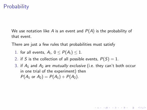
We use notation like A is an event and P(A) is the probability ofthat event.

There are just a few rules that probabilities must satisfy

1. for all events, Ai , 0 ≤ P(Ai ) ≤ 1.

2. if S is the collection of all possible events, P(S) = 1.

3. if A1 and A2 are mutually exclusive (i.e. they can’t both occurin one trial of the experiment) thenP(A1 or A2) = P(A1) + P(A2).

Probability

So, for example, if an experiment only has 2 possible outcomes andthey are equally likely then the probability of each is one half.

The odds on an event is the number of times you expect to see theevent happen for every time it doesn’t happen.

So if the probability of an event is kN the odds on that event are k

to the N − k .

> table(fms$apoe_c472t)

CC CT128 30

So the observed odds on CC is 128 to 30 and the observedprobability of seeing CC is 128/(128 + 30).

Conditional probability

Two events, A1 and A2 are independent ifP(A1 and A2) = P(A1)P(A2).

The conditional probability of event A1 given that event A2 hasoccurred is given by P(A1 and A2)/P(A2) and is denotedP(A1|A2).

So what is P(A1|A2) in terms of P(A2|A1)?

If 2 events are independent then P(A1|A2) = P(A1): this is theintuitive basis for understanding what independence means.

Random variables

A random variable is a quantity that takes on certain values withcertain probabilities.

For example, if I toss a coin and assign X the value of 0 if there isa head and 1 if there is a tail, then X is a random variable.

The distribution of a random variable is the values that the randomvariable takes and the probability that it takes those values.

We model the data we observe as the result of a randomizedexperiment and consequently as random variables.

Simulating random variables

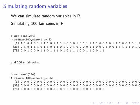
We can simulate random variables in R.

Simulating 100 fair coins in R

> set.seed(234)

> rbinom(100,size=1,p=.5)

[1] 1 1 0 1 0 1 1 1 1 0 1 1 1 1 0 0 0 1 0 1 1 1 1 1 0 0 1 0 1 1 1 0 0 1 1 1 1

[38] 0 1 0 1 1 1 0 1 1 0 1 1 0 1 0 0 1 0 0 0 0 1 1 0 0 0 1 0 0 1 1 1 1 1 0 1 0

[75] 0 0 1 0 0 0 1 1 0 1 1 1 0 1 0 1 1 1 0 0 1 1 0 0 1 1

and 100 unfair coins,

> set.seed(234)

> rbinom(100,size=1,p=.05)

[1] 0 0 0 0 0 0 0 0 0 0 0 0 0 0 0 0 0 0 0 0 0 0 0 0 0 0 0 0 0 0 0 0 0 0 0 0 0

[38] 0 0 0 0 0 0 0 0 0 0 0 0 0 0 0 0 0 0 0 0 0 0 0 0 0 0 0 0 0 0 0 0 0 0 0 0 0

[75] 0 0 0 0 0 0 0 0 0 0 0 0 0 1 0 0 0 0 0 0 0 1 0 0 0 0

Properties of random variables

The expectation of a random variable depends on its distributionand can be calculated as follows:

if X is the random variable then its expectation is given byEX =

∑k kP(X = k).

while the variance of a random variable is given byVarX =

∑k(k − EX )2P(X = k).

So if X is 1 with probability p and is otherwise 0 what is itsexpected value? Its variance?

There are a number of commonly used probability models that areencountered, both discrete and continuous.

Discrete random variables

The Bernoulli distribution: a single success or failure randomvariable. Distribution only depends on the probability of a success.

The binomial distribution: the number of successes in nindependent trials where each trial is a success or failure (and alltrials have the same success probability). Distribution depends onthe success probability and the total number of trials.

The multinomial distribution is a generalization of the Binomialdistribution to the case where each trial can have more than 2outcomes. Distribution depends on success probabilities andnumber of trials.

The multinomial distribution is a natural model for nucleic acidsequences (since each position is one of 4 possible nucleotides).

The law of large numbers

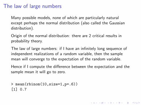
Many possible models, none of which are particularly naturalexcept perhaps the normal distribution (also called the Gaussiandistribution).

Origin of the normal distribution: there are 2 critical results inprobability theory.

The law of large numbers: if I have an infinitely long sequence ofindependent realizations of a random variable, then the samplemean will converge to the expectation of the random variable.

Hence if I compute the difference between the expectation and thesample mean it will go to zero.

> mean(rbinom(10,size=1,p=.6))[1] 0.7

The central limit theorem

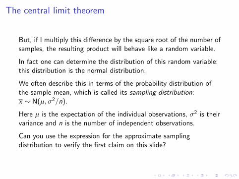
But, if I multiply this difference by the square root of the number ofsamples, the resulting product will behave like a random variable.

In fact one can determine the distribution of this random variable:this distribution is the normal distribution.

We often describe this in terms of the probability distribution ofthe sample mean, which is called its sampling distribution:x ∼ N(µ, σ2/n).

Here µ is the expectation of the individual observations, σ2 is theirvariance and n is the number of independent observations.

Can you use the expression for the approximate samplingdistribution to verify the first claim on this slide?

Continuous random variables

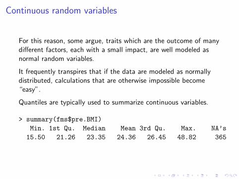
For this reason, some argue, traits which are the outcome of manydifferent factors, each with a small impact, are well modeled asnormal random variables.

It frequently transpires that if the data are modeled as normallydistributed, calculations that are otherwise impossible become“easy”.

Quantiles are typically used to summarize continuous variables.

> summary(fms$pre.BMI)Min. 1st Qu. Median Mean 3rd Qu. Max. NA’s15.50 21.26 23.35 24.36 26.45 48.82 365


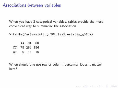
When you have 2 categorical variables, tables provide the mostconvenient way to summarize the association.

> table(fms$resistin_c30t,fms$resistin_g540a)

AA GA GGCC 75 281 356CT 0 11 10

When should one use row or column percents? Does it matterhere?


We frequently are interested in variables with 2 categories whereone category indicates health status (e.g. have cancer).

Often we would like to know if some other dichotomous variableincreases the likelihood that one has this health outcome (e.g.smoking).

The risk is the probability that one has a particular health outcome.

If this risk is modified by another dichotomous variable, then weare often interested in how the risk varies with this other variable.

Relative risk

One can look at the difference in risk,P(cancer|smoke)− P(cancer|don’t smoke), but for rare healthoutcomes this will always be a small number.

More commonly we look at the ratio rather than the difference-thisis called the relative risk.

To directly estimate P(cancer|smoke) we would need to set up astudy where we enrolled many smokers and follow them in aprospective study.

This is expensive and time consuming, it is much easier to recruitsubjects with cancer and ascertain if they smoke: a retrospectivestudy.

Odds ratio

Much like the relative risk is a ratio of probabilities, the odds ratiois a ratio of odds.

The big difference is that one can estimate the odds ratio usingdata from a retrospective study.

Moreover the odds ratio and relative risk are approximately equalwhen the event is rare.


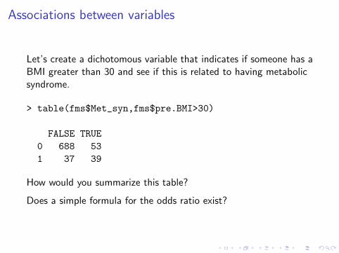
Let’s create a dichotomous variable that indicates if someone has aBMI greater than 30 and see if this is related to having metabolicsyndrome.

> table(fms$Met_syn,fms$pre.BMI>30)

FALSE TRUE0 688 531 37 39

How would you summarize this table?

Does a simple formula for the odds ratio exist?

Statistical inference

If I collected another data set in the same fashion as this one, doyou think we would find a positive association?

To address this question, we frequently pose the question asfollows: what is the probability that I would observe as big adifference as I have observed if there was not an associationbetween these 2 variables?


About 9% of the subjects have metabolic syndrome and about10% of subjects have a BMI greater than 30, so if these 2 variablesare independent then the probability of both of these propertiesbeing true is about 1%.

However we have observed about 5% of our subjects having a BMIover 30 and having metabolic syndrome: is this simply too large tocall chance variation?


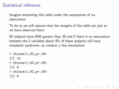
Imagine simulating this table under the assumption of noassociation.

To do so we will assume that the margins of the table are just aswe have observed them.

92 subjects have BMI greater than 30 and if there is no associationbetween the 2 variables about 9% of these subjects will havemetabolic syndrome, so conduct a few simulations

> rbinom(1,92,p=.09)[1] 10> rbinom(1,92,p=.09)[1] 6> rbinom(1,92,p=.09)[1] 8


These values are much smaller than our observed value of 39, infact looking at a million of these variables we are never even closeto the observed value of 39

> summary(rbinom(1000000,92,p=.09))Min. 1st Qu. Median Mean 3rd Qu. Max.0.000 6.000 8.000 8.278 10.000 24.000

So what we are seeing doesn’t even occur 1 in a million times ifthese 2 variables are independent.


The process of using observed data to make statements aboutunobserved data (e.g. data we will observe in the future) is calledstatistical inference.

Frequently hypothesis tests are used to produce estimates of theprobability of observing something more extreme than what wehave observed.

Such probabilities are called p-values and when a p-value is lessthan 0.05 we say that there is a statistically significant association.

To test for an association between 2 dichotomous variables oneuses a test procedure called Pearson’s χ2 test.

Pearson’s Chi-squared test

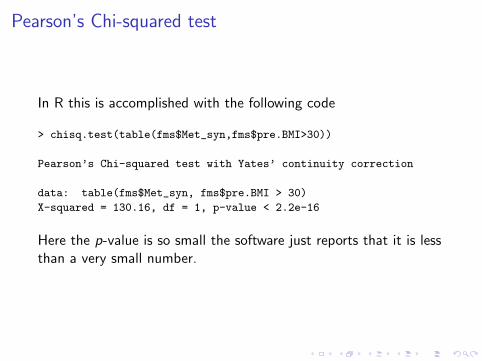
In R this is accomplished with the following code

> chisq.test(table(fms$Met_syn,fms$pre.BMI>30))

Pearson’s Chi-squared test with Yates’ continuity correction

data: table(fms$Met_syn, fms$pre.BMI > 30)

X-squared = 130.16, df = 1, p-value < 2.2e-16

Here the p-value is so small the software just reports that it is lessthan a very small number.


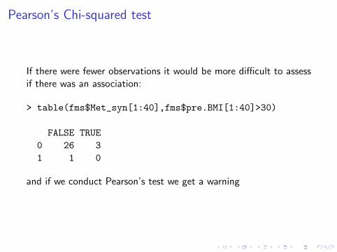
If there were fewer observations it would be more difficult to assessif there was an association:

> table(fms$Met_syn[1:40],fms$pre.BMI[1:40]>30)

FALSE TRUE0 26 31 1 0

and if we conduct Pearson’s test we get a warning


> chisq.test(table(fms$Met_syn[1:40],fms$pre.BMI[1:40]>30))

Pearson’s Chi-squared test with Yates’ continuity correction

data: table(fms$Met_syn[1:40], fms$pre.BMI[1:40] > 30)

X-squared = 9.1766e-32, df = 1, p-value = 1

Warning message:

In chisq.test(table(fms$Met_syn[1:40], fms$pre.BMI[1:40] > 30)) :

Chi-squared approximation may be incorrect

Fisher’s exact test

Pearson’s χ2 test, like many techniques in statistics, ultimatelyrelies on the central limit theorem and so is only an approximationthat is appropriate when the sample size is large.

Often times there are other techniques which are more appropriatewhen the sample size is small: here we can use a test calledFisher’s exact test.

Fisher’s exact test

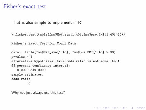
That is also simple to implement in R

> fisher.test(table(fms$Met_syn[1:40],fms$pre.BMI[1:40]>30))

Fisher’s Exact Test for Count Data

data: table(fms$Met_syn[1:40], fms$pre.BMI[1:40] > 30)

p-value = 1

alternative hypothesis: true odds ratio is not equal to 1

95 percent confidence interval:

0.0000 349.0909

sample estimates:

odds ratio

0

Why not just always use this test?

Associations between variables: one continuous variable

While we can always dichotomize a continuous variable andconduct analyses as we have above, this is suboptimal as itdisposes of information.

Boxplots are convenient visualization tools for comparing 2 or morecontinuous distributions.

pdf("bxplt-BMI.pdf")boxplot(fms$pre.BMI~fms$Met_syn)dev.off()

Causation: look at the distribution of the response variable as itdepends on the explanatory variable (this plot has this backwards).


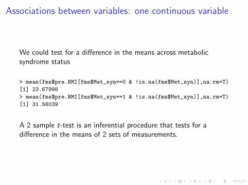
We could test for a difference in the means across metabolicsyndrome status

> mean(fms$pre.BMI[fms$Met_syn==0 & !is.na(fms$Met_syn)],na.rm=T)

[1] 23.67998

> mean(fms$pre.BMI[fms$Met_syn==1 & !is.na(fms$Met_syn)],na.rm=T)

[1] 31.56039

A 2 sample t-test is an inferential procedure that tests for adifference in the means of 2 sets of measurements.


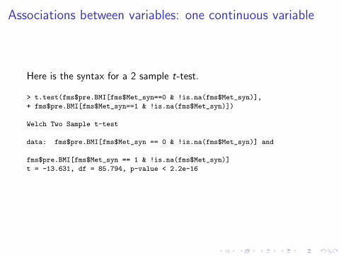
Here is the syntax for a 2 sample t-test.

> t.test(fms$pre.BMI[fms$Met_syn==0 & !is.na(fms$Met_syn)],

+ fms$pre.BMI[fms$Met_syn==1 & !is.na(fms$Met_syn)])

Welch Two Sample t-test

data: fms$pre.BMI[fms$Met_syn == 0 & !is.na(fms$Met_syn)] and

fms$pre.BMI[fms$Met_syn == 1 & !is.na(fms$Met_syn)]

t = -13.631, df = 85.794, p-value < 2.2e-16


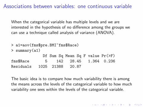
When the categorical variable has multiple levels and we areinterested in the hypothesis of no difference among the groups wecan use a technique called analysis of variance (ANOVA).

> a1=aov(fms$pre.BMI~fms$Race)> summary(a1)

Df Sum Sq Mean Sq F value Pr(>F)fms$Race 5 142 28.45 1.364 0.236Residuals 1025 21388 20.87

The basic idea is to compare how much variability there is amongthe means across the levels of the categorical variable to how muchvariability one sees within the levels of the categorical variable.

An introduction to biostatistics: part 1Cavanr/IntroStat1.pdfAn introduction to biostatistics: part 1 Cavan Reilly September 4, 2019. Table of contents Introduction to data analysis

Documents