AN INTRODUCTION TO BIOINFORMATICS ALGORITHMS NEIL C. JONES AND PAVEL A. PEVZNER

Welcome message from author
This document is posted to help you gain knowledge. Please leave a comment to let me know what you think about it! Share it to your friends and learn new things together.
Transcript
AN INTRODUCTION TO
BIOINFORMATICS ALGORITHMS
NEIL C. JONES AND PAVEL A. PEVZNER
Administrator
Note
Marked set by Administrator
An
Introduction
to
Bioinformatics
Algorithms
Sorin Istrail, Pavel Pevzner, and Michael Waterman, editors
Computational molecular biology is a new discipline, bringing together com-
putational, statistical, experimental, and technological methods, which is
energizing and dramatically accelerating the discovery of new technologies
and tools for molecular biology. The MIT Press Series on Computational
Molecular Biology is intended to provide a unique and effective venue for
the rapid publication of monographs, textbooks, edited collections, reference
works, and lecture notes of the highest quality.
Computational Molecular Biology: An Algorithmic Approach
Pavel A. Pevzner, 2000
Computational Methods for Modeling Biochemical Networks
James M. Bower and Hamid Bolouri, editors, 2001
Current Topics in Computational Molecular Biology
Tao Jiang, Ying Xu, and Michael Q. Zhang, editors, 2002
Gene Regulation and Metabolism: Postgenomic Computation Approaches
Julio Collado-Vides, editor, 2002
Microarrays for an Integrative Genomics
Isaac S. Kohane, Alvin Kho, and Atul J. Butte, 2002
Kernel Methods in Computational Biology
Bernhard Schölkopf, Koji Tsuda, and Jean-Philippe Vert, 2004
An Introduction to Bioinformatics Algorithms
Neil C. Jones and Pavel A. Pevzner, 2004
© 2004 Massachusetts Institute of Technology
All rights reserved. No part of this book may be reproduced in any form by any
electronic or mechanical means (including photocopying, recording, or information
storage and retrieval) without permission in writing from the publisher.
MIT Press books may be purchased at special quantity discounts for business or sales
promotional use. For information, please email [email protected] or
write to Special Sales Department, The MIT Press, 5 Cambridge Center, Cambridge,
MA 02142.
Typeset in 10/13 Lucida Bright by the authors using LATEX 2ε.
Printed and bound in the United States of America.
Library of Congress Cataloging-in-Publication Data
Jones, Neil C.
An introduction to bioinformatics algorithms/ by Neil C. Jones and Pavel A.
Pevzner.
p. cm.—(computational molecular biology series)
“A Bradford book.”
Includes bibliographical references and index (p. ).
ISBN 0-262-10106-8 (hc : alk. paper)
1. Bioinformatics. 2. Algorithms. I. Pevzner, Pavel. II. Title
QH324.2.J66 2004570’.285—dc22 2004048289
CIP
10 9 8 7 6 5 4 3 2 1

For my Grandfather, who lived to write and vice versa.
—NCJ
To Chop-up and Manny.
—PAP

Contents in Brief
Exh
aust
ive
Sear
ch
Gre
edy
Alg
orit
hm
s
Dyn
amic
Pro
gram
min
gA
lgor
ith
ms
Div
ide-
and
-Con
quer
Alg
orit
hm
s
Gra
ph
Alg
orit
hm
s
Com
bin
ator
ial P
atte
rnM
atch
ing
Clu
ster
ing
and
Tree
s
Hid
den
Mar
kov
Mod
els
Ran
dom
ized
Alg
orit
hm
s
Subject 4 5 6 7 8 9 10 11 12
Mapping DNA
Sequencing DNA
Comparing Sequences
Predicting Genes
Finding Signals
Identifying Proteins
Repeat Analysis
DNA Arrays
Genome Rearrangements
Molecular Evolution
Featuring historical perspectives from:
Russell Doolittle Chapter 3
David Haussler Chapter 11
Richard Karp Chapter 2
Webb Miller Chapter 7
Gene Myers Chapter 9
David Sankoff Chapter 5
Ron Shamir Chapter 10
Gary Stormo Chapter 4
Michael Waterman Chapter 6
Contents
Preface xv
1 Introduction 1
2 Algorithms and Complexity 7
2.1 What Is an Algorithm? 7
2.2 Biological Algorithms versus Computer Algorithms 14
2.3 The Change Problem 17
2.4 Correct versus Incorrect Algorithms 20
2.5 Recursive Algorithms 24
2.6 Iterative versus Recursive Algorithms 28
2.7 Fast versus Slow Algorithms 33
2.8 Big-O Notation 37
2.9 Algorithm Design Techniques 40
2.9.1 Exhaustive Search 41
2.9.2 Branch-and-Bound Algorithms 42
2.9.3 Greedy Algorithms 43
2.9.4 Dynamic Programming 43
2.9.5 Divide-and-Conquer Algorithms 48
2.9.6 Machine Learning 48
2.9.7 Randomized Algorithms 48
2.10 Tractable versus Intractable Problems 49
2.11 Notes 51
Biobox: Richard Karp 52
2.12 Problems 54
x Contents
3 Molecular Biology Primer 57
3.1 What Is Life Made Of? 57
3.2 What Is the Genetic Material? 59
3.3 What Do Genes Do? 60
3.4 What Molecule Codes for Genes? 61
3.5 What Is the Structure of DNA? 61
3.6 What Carries Information between DNA and Proteins? 63
3.7 How Are Proteins Made? 65
3.8 How Can We Analyze DNA? 67
3.8.1 Copying DNA 67
3.8.2 Cutting and Pasting DNA 71
3.8.3 Measuring DNA Length 72
3.8.4 Probing DNA 72
3.9 How Do Individuals of a Species Differ? 73
3.10 How Do Different Species Differ? 74
3.11 Why Bioinformatics? 75
Biobox: Russell Doolittle 79
4 Exhaustive Search 83
4.1 Restriction Mapping 83
4.2 Impractical Restriction Mapping Algorithms 87
4.3 A Practical Restriction Mapping Algorithm 89
4.4 Regulatory Motifs in DNA Sequences 91
4.5 Profiles 93
4.6 The Motif Finding Problem 97
4.7 Search Trees 100
4.8 Finding Motifs 108
4.9 Finding a Median String 111
4.10 Notes 114
Biobox: Gary Stormo 116
4.11 Problems 119
5 Greedy Algorithms 125
5.1 Genome Rearrangements 125
5.2 Sorting by Reversals 127
5.3 Approximation Algorithms 131
5.4 Breakpoints: A Different Face of Greed 132
5.5 A Greedy Approach to Motif Finding 136
5.6 Notes 137
Contents xi
Biobox: David Sankoff 139
5.7 Problems 143
6 Dynamic Programming Algorithms 147
6.1 The Power of DNA Sequence Comparison 147
6.2 The Change Problem Revisited 148
6.3 The Manhattan Tourist Problem 153
6.4 Edit Distance and Alignments 167
6.5 Longest Common Subsequences 172
6.6 Global Sequence Alignment 177
6.7 Scoring Alignments 178
6.8 Local Sequence Alignment 180
6.9 Alignment with Gap Penalties 184
6.10 Multiple Alignment 185
6.11 Gene Prediction 193
6.12 Statistical Approaches to Gene Prediction 197
6.13 Similarity-Based Approaches to Gene Prediction 200
6.14 Spliced Alignment 203
6.15 Notes 207
Biobox: Michael Waterman 209
6.16 Problems 211
7 Divide-and-Conquer Algorithms 227
7.1 Divide-and-Conquer Approach to Sorting 227
7.2 Space-Efficient Sequence Alignment 230
7.3 Block Alignment and the Four-Russians Speedup 234
7.4 Constructing Alignments in Subquadratic Time 238
7.5 Notes 240
Biobox: Webb Miller 241
7.6 Problems 244
8 Graph Algorithms 247
8.1 Graphs 247
8.2 Graphs and Genetics 260
8.3 DNA Sequencing 262
8.4 Shortest Superstring Problem 264
8.5 DNA Arrays as an Alternative Sequencing Technique 265
8.6 Sequencing by Hybridization 268
8.7 SBH as a Hamiltonian Path Problem 271
xii Contents
8.8 SBH as an Eulerian Path Problem 272
8.9 Fragment Assembly in DNA Sequencing 275
8.10 Protein Sequencing and Identification 280
8.11 The Peptide Sequencing Problem 284
8.12 Spectrum Graphs 287
8.13 Protein Identification via Database Search 290
8.14 Spectral Convolution 292
8.15 Spectral Alignment 293
8.16 Notes 299
8.17 Problems 302
9 Combinatorial Pattern Matching 311
9.1 Repeat Finding 311
9.2 Hash Tables 313
9.3 Exact Pattern Matching 316
9.4 Keyword Trees 318
9.5 Suffix Trees 320
9.6 Heuristic Similarity Search Algorithms 324
9.7 Approximate Pattern Matching 326
9.8 BLAST: Comparing a Sequence against a Database 330
9.9 Notes 331
Biobox: Gene Myers 333
9.10 Problems 337
10 Clustering and Trees 339
10.1 Gene Expression Analysis 339
10.2 Hierarchical Clustering 343
10.3 k-Means Clustering 346
10.4 Clustering and Corrupted Cliques 348
10.5 Evolutionary Trees 354
10.6 Distance-Based Tree Reconstruction 358
10.7 Reconstructing Trees from Additive Matrices 361
10.8 Evolutionary Trees and Hierarchical Clustering 366
10.9 Character-Based Tree Reconstruction 368
10.10 Small Parsimony Problem 370
10.11 Large Parsimony Problem 374
10.12 Notes 379
Biobox: Ron Shamir 380
10.13 Problems 384
Contents xiii
11 Hidden Markov Models 387
11.1 CG-Islands and the “Fair Bet Casino” 387
11.2 The Fair Bet Casino and Hidden Markov Models 390
11.3 Decoding Algorithm 393
11.4 HMM Parameter Estimation 397
11.5 Profile HMM Alignment 398
11.6 Notes 400
Biobox: David Haussler 403
11.7 Problems 407
12 Randomized Algorithms 409
12.1 The Sorting Problem Revisited 409
12.2 Gibbs Sampling 412
12.3 Random Projections 414
12.4 Notes 416
12.5 Problems 417
Using Bioinformatics Tools 419
Bibliography 421
Index 429
Preface
In the early 1990s when one of us was teaching his first bioinformatics class,
he was not sure that there would be enough students to teach. Although
the Smith-Waterman and BLAST algorithms had already been developed
they had not become the household names among biologists that they are
today. Even the term “bioinformatics” had not yet been coined. DNA arrays
were viewed by most as intellectual toys with dubious practical application,
except for a handful of enthusiasts who saw a vast potential in the technol-
ogy. A few bioinformaticians were developing new algorithmic ideas for
nonexistent data sets: David Sankoff laid the foundations of genome rear-
rangement studies at a time when there was practically no gene order data,
Michael Waterman and Gary Stormo were developing motif finding algo-
rithms when there were very few promoter samples available, Gene Myers
was developing sophisticated fragment assembly tools when no bacterial
genome has been assembled yet, and Webb Miller was dreaming about com-
paring billion-nucleotide-long DNA sequences when the 172, 282-nucleotide
Epstein-Barr virus was the longest GenBank entry. GenBank itself just re-
cently made a transition from a series of bound (paper!) volumes to an elec-
tronic database on magnetic tape that could be sent to scientists worldwide.
One has to go back to the mid-1980s and early 1990s to fully appreciate the
revolution in biology that has taken place in the last decade. However, bioin-
formatics has affected more than just biology—it has also had a profound
impact on the computational sciences. Biology has rapidly become a large
source of new algorithmic and statistical problems, and has arguably been
the target for more algorithms than any of the other fundamental sciences.
This link between computer science and biology has important educational
implications that change the way we teach computational ideas to biologists,
as well as how applied algorithmics is taught to computer scientists.

xvi Preface
For many years computer science was taught to only computer scientists,
and only rarely to students from other disciplines. A biology student in an al-
gorithms class would be a surprising and unlikely (though entirely welcome)
guest in the early 1990s. But these things change; many biology students
now take some sort of Algorithms 101. At the same time, curious computer
science students often take Genetics 101 and Bioinformatics 101. Although
these students are still relatively rare, keep in mind that the number of bioin-
formatics classes in the early 1990s was so small as to be considered nonexis-
tent. But that number is not so small now. We envision that undergraduate
bioinformatics classes will become a permanent component at every major
university. This is a feature, not a bug.
This is an introductory textbook on bioinformatics algorithms and the com-
putational ideas that have driven them through the last twenty years. There
are many important probabilistic and statistical techniques that we do not
cover, nor do we cover many important research questions that bioinfor-
maticians are currently trying to answer. We deliberately do not cover all
areas of computational biology; for example, important topics like protein
folding are not even discussed. The very first bioinformatics textbooks were
Waterman, 1995 (108), which contains excellent coverage of DNA statistics
and Gusfield, 1997 (44) which includes an encyclopedia of string algorithms.
Durbin et al., 1998 (31) and Baldi and Brunak, 1997 (7) emphasize Hidden
Markov Models and machine learning techniques; Baxevanis and Ouellette,
1998 (10) is an excellent practical guide to bioinformatics; Mount, 2001 (76)
excels in showing the connections between biological problems and bioin-
formatics techniques; and Bourne and Weissig, 2002 (15) focuses on protein
bioinformatics. There are also excellent web-based lecture notes for many
bioinformatics courses and we learned a lot about the pedagogy of bioinfor-
matics from materials on the World Wide Web by Serafim Batzoglou, Dick
Karp, Ron Shamir, Martin Tompa, and others.
Website
We have created an extensive website to accompany this book at
http://www.bioalgorithms.infoThis website contains a number of features that complement the book. For
example, though this book does not contain a glossary, we provide this ser-
vice, a searchable index, and a set of community message boards, at the
above web address. Technically savvy students can also download practical
Preface xvii
bioinformatics exercises, sample implementations of the algorithms in this
book, and sample data to test them with. Instructors and students may find
the prepackaged lecture notes on the website to be especially helpful. It is
our hope that this website be used as a repository of information that will
help introduce students to the diverse world of bioinformatics.
Acknowledgements
We are indebted to those who kindly agreed to be featured in the biograph-
ical sketches scattered throughout the book. Their insightful and heartfelt
responses definitely made these the most interesting part of this book. Their
life stories and views of the challenges that lay ahead will undoubtedly in-
spire students in the exploration of the unknown. There are many more sci-
entists whose bioboxes we would like to have in this book and it is only
the page limit (which turned out to be 200 pages too small) that prevented
us from commissioning more of them. Special thanks go to Ethan Bier who
inspired us to include biographical sketches in this book.
This book would not have been possible without the diligent teaching as-
sistants in bioinformatics courses taught during the winter and fall of 2003
and 2004: Derren Barken, Bryant Forsgren, Eugene Ke, Coleman Mosley, and
Degui Zhi all helped find technical errors, refine practical exercises, and de-
sign problems in the book. Helen Wu and John Allison spent many hours
making technical figures, which is a thankless task like no other. We are also
grateful to Vagisha Sharma who was kind enough to read the book from
cover to cover and provide insightful comments and, unfortunately, bugs in
the pseudocode. Steve Wasserman provided us with invaluable comments
from a biologist’s point of view that eventually led to new sections in the
book. Alkes Price and Haixu Tang pointed out ambiguities and helped clar-
ify the chapters on graphs and clustering. Ben Raphael and Patricia Jones
provided feedback on the early chapters and helped avoid some potential
misunderstandings. Dan Gilbert, of Dan Gilbert Art Group, Inc. kindly pro-
vided us with Triazzles to illustrate the problems of DNA sequence assembly.
Our special thanks go to Randall Christopher, the artist behind the website
www.kleemanandmike.com. Randall illustrated the book and designed
many unique graphical representations of some bioinformatics algorithms.
It has been a pleasure to work with Robert Prior of The MIT Press. With
sufficient patience and prodding, he managed to keep us on track. We also
appreciate the meticulous copyediting of G. W. Helfrich.
xviii Preface
Finally, we thank the many students in different undergraduate and grad-
uate bioinformatics classes at UCSD who provided comments on earlier ver-
sions of this book.
PAP would like to thank several people who taught him different aspects
of computational molecular biology. Andrey Mironov taught him that com-
mon sense is perhaps the most important ingredient of any applied research.
Mike Waterman was a terrific teacher at the time PAP moved from Moscow
to Los Angeles, both in science and in life. PAP also thanks Alexander Kar-
zanov, who taught him combinatorial optimization, which, surprisingly, re-
mains the most useful set of skills in his computational biology research. He
especially thanks Mark Borodovsky who convinced him to switch into the
field of bioinformatics in 1985, when it was an obscure discipline with an
uncertain future.
PAP also thanks his former students, postdocs, and lab members who
taught him most of what he knows: Vineet Bafna, Guillaume Bourque, Srid-
har Hannenhalli, Steffen Heber, Earl Hubbell, Uri Keich, Zufar Mulyukov,
Alkes Price, Ben Raphael, Sing-Hoi Sze, Haixu Tang, and Glenn Tesler.
NCJ would like to thank his mentors during undergraduate school— Toshi-
hiko Takeuchi, Harry Gray, John Baldeschwieler, and Schubert Soares—for
patiently but firmly teaching him that persistence is one of the more impor-
tant ingredients in research. Also, he thanks the admissions committee at the
University of California, San Diego who gambled on a chemist-turned-pro-
grammer, hopefully for the best.
Neil Jones and Pavel Pevzner
La Jolla, California, 2004
1 Introduction
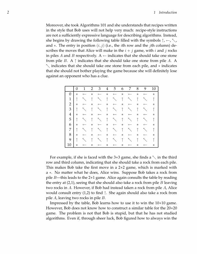
Imagine Alice, Bob, and two piles of ten rocks. Alice and Bob are bored one
Saturday afternoon so they play the following game. In each turn a player
may either take one rock from a single pile, or one rock from both piles. Once
the rocks are taken, they are removed from play; the player that takes the last
rock wins the game. Alice moves first.
It is not immediately clear what the winning strategy is, or even if there
is one. Does the first player (or the second) always have an advantage? Bob
tries to analyze the game and realizes that there are too many variants in
the game with two piles of ten rocks (which we will refer to as the 10+10
game). Using a reductionist approach, he first tries to find a strategy for the
simpler 2+2 game. He quickly sees that the second player—himself, in this
case—wins any 2+2 game, so he decides to write the “winning recipe”:
If Alice takes one rock from each pile, I will take the remaining rocks
and win. If Alice takes one rock, I will take one rock from the same
pile. As a result, there will be only one pile and it will have two rocks
in it, so Alice’s only choice will be to take one of them. I will take the
remaining rock to win the game.
Inspired by this analysis, Bob makes a leap of faith: the second player (i.e.,
himself) wins in any n+n game, for n ≥ 2. Of course, every hypothesis must
be confirmed by experiment, so Bob plays a few rounds with Alice. It turns
out that sometimes he wins and sometimes he loses. Bob tries to come up
with a simple recipe for the 3+3 game, but there are a large number of differ-
ent game sequences to consider, and the recipe quickly gets too complicated.
There is simply no hope of writing a recipe for the 10+10 game because the
number of different strategies that Alice can take is enormous.
Meanwhile, Alice quickly realizes that she will always lose the 2+2 game,
but she does not lose hope of finding a winning strategy for the 3+3 game.
2 1 Introduction
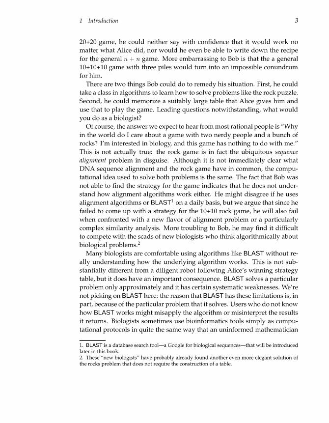
Moreover, she took Algorithms 101 and she understands that recipes written
in the style that Bob uses will not help very much: recipe-style instructions
are not a sufficiently expressive language for describing algorithms. Instead,
she begins by drawing the following table filled with the symbols ↑, ←, ,
and ∗. The entry in position (i, j) (i.e., the ith row and the jth column) de-
scribes the moves that Alice will make in the i + j game, with i and j rocks
in piles A and B respectively. A← indicates that she should take one stone
from pile B. A ↑ indicates that she should take one stone from pile A. A
indicates that she should take one stone from each pile, and ∗ indicates
that she should not bother playing the game because she will definitely lose
against an opponent who has a clue.
0 1 2 3 4 5 6 7 8 9 10
0 ∗ ← ∗ ← ∗ ← ∗ ← ∗ ← ∗
1 ↑ ↑ ↑ ↑ ↑ ↑
2 ∗ ← ∗ ← ∗ ← ∗ ← ∗ ← ∗
3 ↑ ↑ ↑ ↑ ↑ ↑
4 ∗ ← ∗ ← ∗ ← ∗ ← ∗ ← ∗
5 ↑ ↑ ↑ ↑ ↑ ↑
6 ∗ ← ∗ ← ∗ ← ∗ ← ∗ ← ∗
7 ↑ ↑ ↑ ↑ ↑ ↑
8 ∗ ← ∗ ← ∗ ← ∗ ← ∗ ← ∗
9 ↑ ↑ ↑ ↑ ↑ ↑
10 ∗ ← ∗ ← ∗ ← ∗ ← ∗ ← ∗
For example, if she is faced with the 3+3 game, she finds a in the third
row and third column, indicating that she should take a rock from each pile.
This makes Bob take the first move in a 2+2 game, which is marked with
a ∗. No matter what he does, Alice wins. Suppose Bob takes a rock from
pile B—this leads to the 2+1 game. Alice again consults the table by reading
the entry at (2,1), seeing that she should also take a rock from pile B leaving
two rocks in A. However, if Bob had instead taken a rock from pile A, Alice
would consult entry (1,2) to find ↑. She again should also take a rock from
pile A, leaving two rocks in pile B.
Impressed by the table, Bob learns how to use it to win the 10+10 game.
However, Bob does not know how to construct a similar table for the 20+20
game. The problem is not that Bob is stupid, but that he has not studied
algorithms. Even if, through sheer luck, Bob figured how to always win the
1 Introduction 3
20+20 game, he could neither say with confidence that it would work no
matter what Alice did, nor would he even be able to write down the recipe
for the general n + n game. More embarrassing to Bob is that the a general
10+10+10 game with three piles would turn into an impossible conundrum
for him.
There are two things Bob could do to remedy his situation. First, he could
take a class in algorithms to learn how to solve problems like the rock puzzle.
Second, he could memorize a suitably large table that Alice gives him and
use that to play the game. Leading questions notwithstanding, what would
you do as a biologist?
Of course, the answer we expect to hear from most rational people is “Why
in the world do I care about a game with two nerdy people and a bunch of
rocks? I’m interested in biology, and this game has nothing to do with me.”
This is not actually true: the rock game is in fact the ubiquitous sequence
alignment problem in disguise. Although it is not immediately clear what
DNA sequence alignment and the rock game have in common, the compu-
tational idea used to solve both problems is the same. The fact that Bob was
not able to find the strategy for the game indicates that he does not under-
stand how alignment algorithms work either. He might disagree if he uses
alignment algorithms or BLAST1 on a daily basis, but we argue that since he
failed to come up with a strategy for the 10+10 rock game, he will also fail
when confronted with a new flavor of alignment problem or a particularly
complex similarity analysis. More troubling to Bob, he may find it difficult
to compete with the scads of new biologists who think algorithmically about
biological problems.2
Many biologists are comfortable using algorithms like BLAST without re-
ally understanding how the underlying algorithm works. This is not sub-
stantially different from a diligent robot following Alice’s winning strategy
table, but it does have an important consequence. BLAST solves a particular
problem only approximately and it has certain systematic weaknesses. We’re
not picking on BLAST here: the reason that BLAST has these limitations is, in
part, because of the particular problem that it solves. Users who do not know
how BLAST works might misapply the algorithm or misinterpret the results
it returns. Biologists sometimes use bioinformatics tools simply as compu-
tational protocols in quite the same way that an uninformed mathematician
1. BLAST is a database search tool—a Google for biological sequences—that will be introducedlater in this book.2. These “new biologists” have probably already found another even more elegant solution ofthe rocks problem that does not require the construction of a table.
4 1 Introduction
might use experimental protocols without any background in biochemistry
or molecular biology. In either case, important observations might be missed
or incorrect conclusions drawn. Besides, intellectually interesting work can
quickly become mere drudgery if one does not really understand it.
Many recent bioinformatics books cater to this sort of protocol-centric prac-
tical approach to bioinformatics. They focus on parameter settings, specific
features of application, and other details without revealing the ideas behind
the algorithms. This trend often follows the tradition of biology books of
presenting material as a collection of facts and discoveries. In contrast, intro-
ductory books in algorithms usually focus on ideas rather than on the details
of computational recipes.
Since bioinformatics is a computational science, a bioinformatics textbook
should strive to present the principles that drive an algorithm’s design, rather
than list a stamp collection of the algorithms themselves. We hope that de-
scribing the intellectual content of bioinformatics will help retain your inter-
est in the subject. In this book we attempt to show that a handful of algorith-
mic ideas can be used to solve a large number of bioinformatics problems.
We feel that focusing on ideas has more intellectual value and represents
a better long-term investment: protocols change quickly, but the computa-
tional ideas don’t seem to.
We pursued a goal of presenting both the foundations of algorithms and
the important results in bioinformatics under the same cover. A more thor-
ough approach for a student would be to take an Introduction to Algorithms
course followed by a Bioinformatics course, but this is often an unrealistic ex-
pectation in view of the heavy course load biologists have to take. To make
bioinformatics ideas accessible to biologists we appeal to the innate algorith-
mic intuition of the student and try to avoid tedious proofs. The technical
details are hidden unless they are absolutely necessary.3
This book covers both new and old areas in computational biology. Some
topics, to our knowledge, have never been discussed in a textbook before,
while others are relatively old-fashioned and describe some experimental
approaches that are rarely used these days. The reason for including older
topics is twofold. First, some of them still remain the best examples for in-
troducing algorithmic ideas. Second, our goal is to show the progression of
ideas in the field, with the implicit warning that hot areas in bioinformatics
seem to come and go with alarming speed.
3. In some places we hide important computational and biological details and try to simplifythe presentation. We will unavoidably be blamed later for “trivializing” bioinformatics.
1 Introduction 5
One observation gained from teaching bioinformatics classes is that the
interest of computer science students, who usually know little of biology,
fades quickly when the students are introduced to biology without links to
computational issues. The same happens to biologists if they are presented
with seemingly unnecessary formalism with no links to real biological prob-
lems. To hold a student’s interest, it is necessary to introduce biology and
algorithms simultaneously. Our rather eclectic table of contents is a demon-
stration that attempts to reach this goal result in a somewhat interleaved or-
ganization of the material. However, we have tried to maintain a consistent
algorithmic theme (e.g., graph algorithms) throughout each chapter.
Molecular biology and computer science are complex fields whose termi-
nology and nomenclature can be formidable to the outsider. Bioinformatics
merges the two fields, and adds a healthy dose of statistics, combinatorics,
and other branches of mathematics. Like modern biologists who have to
master the dense language of mathematics and computer science, mathe-
maticians and computer scientists working in bioinformatics have to learn
the language of biology. Although the question of who faces the bigger chal-
lenge is a topic hotly debated over pints of beer, this is not the first “invasion”
of foreigners into biology; seventy years ago a horde of physicists infested bi-
ology labs, ultimately to revolutionize the field by deciphering the mystery
of DNA.
Two influential scientists are credited with crossing the barrier between
physics and biology: Max Delbrück and Erwin Schrödinger. Trained as
physicists, their entrances into the field of biology were remarkably different.
Delbrück, trained as an atomic physicist by Niels Bohr, quickly became an ex-
pert in genetics; in 1945 he was already teaching genetics to other biologists.4
Schrödinger, on the other hand, never turned into a “certified” geneticist and
remained somewhat of a biological dilettante. However, his book What Is
Life?, published in 1944, was influential to an entire generation of physicists
and biologists. Both James Watson (a biology student who wanted to be a
naturalist) and Francis Crick (a physicist who worked on magnetic mines)
switched careers to DNA science after reading Shrödinger’s book. Another
Nobel laureate, Sydney Brenner, even admitted to stealing a copy from the
public library in Johannesburg, South Africa.
Like Delbrück and Schrödinger, there is great variety in the biological
background of today’s computer scientists-turned-bioinformaticians. Some
of them have become experts in biology—though very few put on lab coats
4. Delbrück founded the famous phage genetics courses at Cold Spring Harbor Laboratory.
6 1 Introduction
and perform experiments—while others remain biological dilettantes. Al-
though there exists an opinion that every bioinformatician should be an ex-
pert in both biology and computer science, we are not sure that this is fea-
sible. First, it takes a lot of work just to master one of the two, so perhaps
understanding two in equal amounts is a bit much. Second, it is good to
recall that the first pioneers of DNA science were, in fact, self-proclaimed
dilettantes. James Watson knew almost no organic or physical chemistry be-
fore he started working on the double helix; Francis Crick, being a physicist,
knew very little biology. Neither saw any need to know about (let alone
memorize) the chemical structure of the four nucleotide bases when they
discovered the structure of DNA.5 When asked by Erwin Chargaff how they
could possibly expect to resolve the structure of DNA without knowing the
structures of its constituents, they responded that they could always look
up the structures in a book if the need arose. Of course, they understood the
physical principles behind a compound’s structure.
The reality is that even the most biologically oriented bioinformaticians are
experts only in some specific area of biology. Like Delbrück, who probably
would never have passed an exam in biology in the 1930s (when zoology and
botany remained the core of the mainstream biological curriculum), a typi-
cal modern-day bioinformatician is unlikely to pass the sequence of organic
chemistry, biochemistry, and structural biochemistry classes that a “real” bi-
ologist has to take. The question of how much biology a good computer
scientist–turned–bioinformatician has to know seems to be best answered
with “enough to deeply understand the biological problem and to turn it
into an adequate computational problem.” This book provides a very brief
introduction to biology. We do not claim that this is the best approach. For-
tunately, an interested reader can use Watson’s approach and look up the
biological details in the books when the need arises, or read pages 1 through
1294 of Alberts and colleagues’ (including Watson) book Molecular Biology of
the Cell (3).
This book is what we, as computer scientists, believe that a modern biolo-
gist ought to know about computer science if he or she would be a successful
researcher.
5. Accordingly, we do not present anywhere in this book the chemical structures of either nu-cleotides or amino acids. No algorithm in this book requires knowledge of their structure.
2 Algorithms and Complexity
This book is about how to design algorithms that solve biological problems.
We will see how popular bioinformatics algorithms work and we will see
what principles drove their design. It is important to understand how an
algorithm works in order to be confident in its results; it is even more impor-
tant to understand an algorithm’s design methodology in order to identify
its potential weaknesses and fix them.
Before considering any algorithms in detail, we need to define loosely
what we mean by the word “algorithm” and what might qualify as one.
In many places throughout this text we try to avoid tedious mathematical
formalisms, yet leave intact the rigor and intuition behind the important con-
cept.
2.1 What Is an Algorithm?
Roughly speaking, an algorithm is a sequence of instructions that one must
perform in order to solve a well-formulated problem. We will specify prob-
lems in terms of their inputs and their outputs, and the algorithm will be the
method of translating the inputs into the outputs. A well-formulated prob-
lem is unambiguous and precise, leaving no room for misinterpretation.
In order to solve a problem, some entity needs to carry out the steps spec-
ified by the algorithm. A human with a pen and paper would be able to do
this, but humans are generally slow, make mistakes, and prefer not to per-
form repetitive work. A computer is less intelligent but can perform simple
steps quickly and reliably. A computer cannot understand English, so al-
gorithms must be rephrased in a programming language such as C or Javain order to give specific instructions to the processor. Every detail must be
specified to the computer in exactly the right format, making it difficult to de-
8 2 Algorithms and Complexity
scribe algorithms; trifling details that a person would naturally understand
must be specified. If a computer were to put on shoes, one would need to
tell it to find a pair that both matches and fits, to put the left shoe on the left
foot, the right shoe on the right, and to tie the laces.1 In this book, however,
we prefer to simply leave it at “Put on a pair of shoes.”
However, to understand how an algorithm works, we need some way of
listing the steps that the algorithm takes, while being neither too vague nor
too formal. We will use pseudocode, whose elementary operations are sum-
marized below. Pseudocode is a language computer scientists often use to
describe algorithms: it ignores many of the details that are required in a pro-
gramming language, yet it is more precise and less ambiguous than, say, a
recipe in a cookbook. Individually, the operations do not solve any partic-
ularly difficult problems, but they can be grouped together into minialgo-
rithms called subroutines that do.
In our particular flavor of pseudocode, we use the concepts of variables,
arrays, and arguments. A variable, written as x or total, contains some nu-
merical value and can be assigned a new numerical value at different points
throughout the course of an algorithm. An array of n elements is an ordered
collection of n variables a1, a2, . . . , an. We usually denote arrays by bold-
face letters like a = (a1, a2, . . . , an) and write the individual elements as ai
where i is between 1 and n. An algorithm in pseudocode is denoted by a
name, followed by the list of arguments that it requires, like MAX(a, b) be-
low; this is followed by the statements that describe the algorithm’s actions.
One can invoke an algorithm by passing it the appropriate values for its ar-
guments. For example, MAX(1, 99) would return the larger of 1 and 99. The
operation return reports the result of the program or simply signals its end.
Below are brief descriptions of the elementary commands that we use in the
pseudocode throughout this book.2
Assignment
Format: a← b
Effect: Sets the variable a to the value b.
1. It is surprisingly difficult to write an unambiguous set of instructions on how to tie a shoelace.2. An experienced computer programmer might be confused by our not using “end if” or “endfor”, which is the conventional practice. We rely on indentation to demarcate blocks of pseu-docode.
2.1 What Is an Algorithm? 9
Example: b← 2
a← b
Result: The value of a is 2
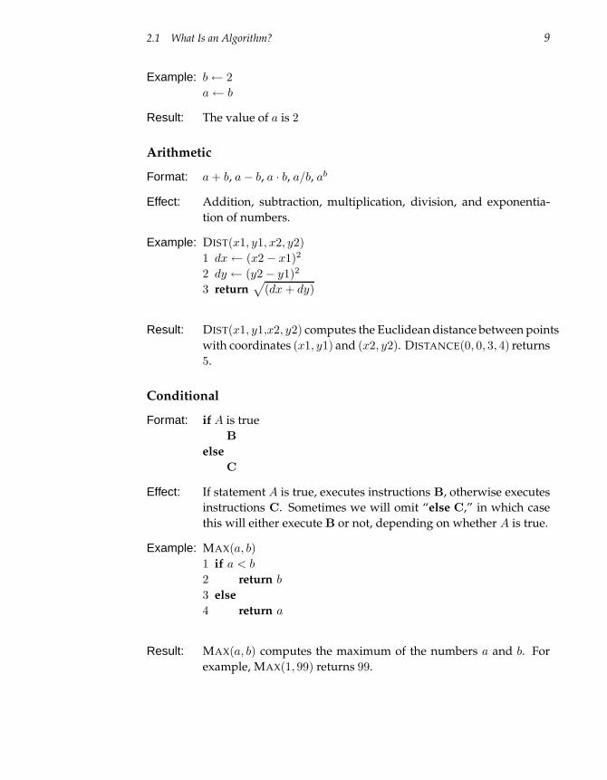
Arithmetic
Format: a + b, a− b, a · b, a/b, ab
Effect: Addition, subtraction, multiplication, division, and exponentia-
tion of numbers.
Example: DIST(x1, y1, x2, y2)
1 dx← (x2 − x1)2
2 dy ← (y2− y1)2
3 return√
(dx + dy)
Result: DIST(x1, y1,x2, y2) computes the Euclidean distance between points
with coordinates (x1, y1) and (x2, y2). DISTANCE(0, 0, 3, 4) returns
5.
Conditional
Format: if A is true
B
else
C
Effect: If statement A is true, executes instructions B, otherwise executes
instructions C. Sometimes we will omit “else C,” in which case
this will either execute B or not, depending on whether A is true.
Example: MAX(a, b)
1 if a < b
2 return b
3 else
4 return a
Result: MAX(a, b) computes the maximum of the numbers a and b. For
example, MAX(1, 99) returns 99.
10 2 Algorithms and Complexity
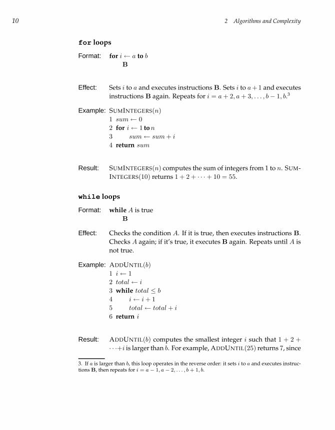
for loops
Format: for i← a to b
B
Effect: Sets i to a and executes instructions B. Sets i to a +1 and executes
instructions B again. Repeats for i = a + 2, a + 3, . . . , b− 1, b.3
Example: SUMINTEGERS(n)
1 sum← 0
2 for i← 1 to n
3 sum← sum + i
4 return sum
Result: SUMINTEGERS(n) computes the sum of integers from 1 to n. SUM-
INTEGERS(10) returns 1 + 2 + · · ·+ 10 = 55.
while loops
Format: while A is true
B
Effect: Checks the condition A. If it is true, then executes instructions B.
Checks A again; if it’s true, it executes B again. Repeats until A is
not true.
Example: ADDUNTIL(b)
1 i← 1
2 total ← i
3 while total ≤ b
4 i← i + 1
5 total ← total + i
6 return i
Result: ADDUNTIL(b) computes the smallest integer i such that 1 + 2 +
· · ·+i is larger than b. For example, ADDUNTIL(25) returns 7, since
3. If a is larger than b, this loop operates in the reverse order: it sets i to a and executes instruc-tions B, then repeats for i = a − 1, a − 2, . . . , b + 1, b.
2.1 What Is an Algorithm? 11
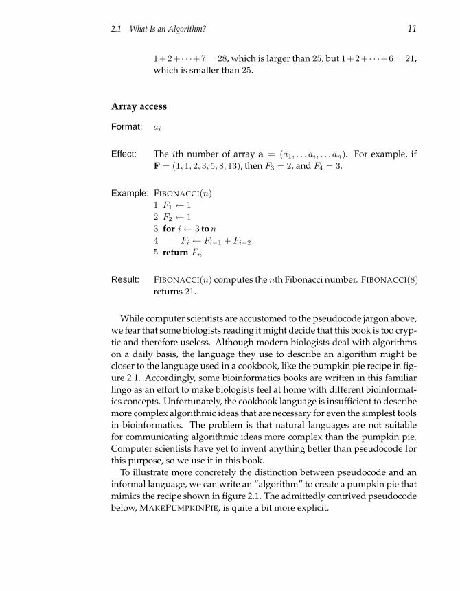
1+2+ · · ·+7 = 28, which is larger than 25, but 1+2+ · · ·+6 = 21,
which is smaller than 25.
Array access
Format: ai
Effect: The ith number of array a = (a1, . . . ai, . . . an). For example, if
F = (1, 1, 2, 3, 5, 8, 13), then F3 = 2, and F4 = 3.
Example: FIBONACCI(n)
1 F1 ← 1
2 F2 ← 1
3 for i← 3 to n
4 Fi ← Fi−1 + Fi−2
5 return Fn
Result: FIBONACCI(n) computes the nth Fibonacci number. FIBONACCI(8)
returns 21.
While computer scientists are accustomed to the pseudocode jargon above,
we fear that some biologists reading it might decide that this book is too cryp-
tic and therefore useless. Although modern biologists deal with algorithms
on a daily basis, the language they use to describe an algorithm might be
closer to the language used in a cookbook, like the pumpkin pie recipe in fig-
ure 2.1. Accordingly, some bioinformatics books are written in this familiar
lingo as an effort to make biologists feel at home with different bioinformat-
ics concepts. Unfortunately, the cookbook language is insufficient to describe
more complex algorithmic ideas that are necessary for even the simplest tools
in bioinformatics. The problem is that natural languages are not suitable
for communicating algorithmic ideas more complex than the pumpkin pie.
Computer scientists have yet to invent anything better than pseudocode for
this purpose, so we use it in this book.
To illustrate more concretely the distinction between pseudocode and an
informal language, we can write an “algorithm” to create a pumpkin pie that
mimics the recipe shown in figure 2.1. The admittedly contrived pseudocode
below, MAKEPUMPKINPIE, is quite a bit more explicit.
12 2 Algorithms and Complexity
1 12 cups canned or cooked pumpkin
1 cup brown sugar, firmly packed12 teaspoon salt2 teaspoons cinnamon1 teaspoon ginger2 tablespoons molasses3 eggs, slightly beaten12 ounce can of evaporated milk1 unbaked pie crust
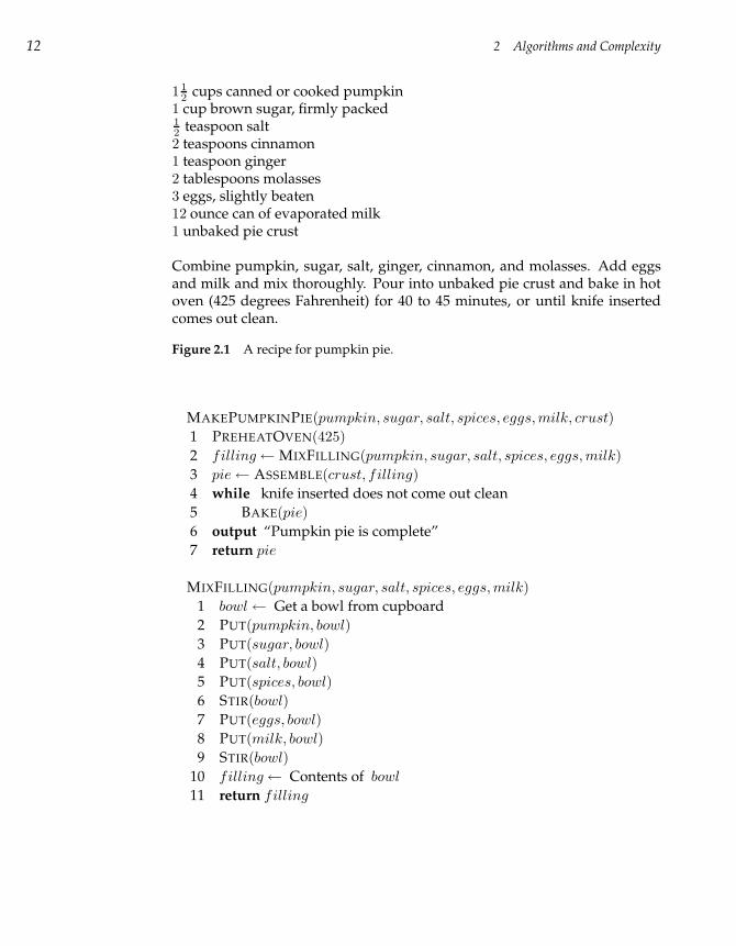
Combine pumpkin, sugar, salt, ginger, cinnamon, and molasses. Add eggsand milk and mix thoroughly. Pour into unbaked pie crust and bake in hotoven (425 degrees Fahrenheit) for 40 to 45 minutes, or until knife insertedcomes out clean.
Figure 2.1 A recipe for pumpkin pie.
MAKEPUMPKINPIE(pumpkin, sugar, salt, spices, eggs, milk, crust)
1 PREHEATOVEN(425)
2 filling← MIXFILLING(pumpkin, sugar, salt, spices, eggs, milk)
3 pie← ASSEMBLE(crust, filling)
4 while knife inserted does not come out clean
5 BAKE(pie)
6 output “Pumpkin pie is complete”
7 return pie
MIXFILLING(pumpkin, sugar, salt, spices, eggs, milk)
1 bowl ← Get a bowl from cupboard
2 PUT(pumpkin, bowl)
3 PUT(sugar, bowl)
4 PUT(salt, bowl)
5 PUT(spices, bowl)
6 STIR(bowl)
7 PUT(eggs, bowl)
8 PUT(milk, bowl)
9 STIR(bowl)
10 filling← Contents of bowl
11 return filling
2.1 What Is an Algorithm? 13
MAKEPUMPKINPIE calls (i.e., activates) the subroutine MIXFILLING, which
uses return to return the pie filling. The operation return terminates the ex-
ecution of the subroutine and returns a result to the routine that called it,
in this case MAKEPUMPKINPIE. When the pie is complete, MAKEPUMPKIN-
PIE notifies and returns the pie to whomever requested it. The entity pie in
MAKEPUMPKINPIE is a variable that represents the pie in the various stages
of cooking.
A subroutine, such as MIXFILLING, will normally need to return the re-
sult of some important calculation. However, in some cases the inputs to the
subroutine might be invalid (e.g., if you gave the algorithm watermelon in-
stead of pumpkin). In these cases, a subroutine may return no value at all
and output a suitable error message. When an algorithm is finished calculat-
ing a result, it naturally needs to output that result and stop executing. The
operation output displays information to an interested user.4
A subtle observation is that MAKEPUMPKINPIE does not in fact make a
pumpkin pie, but only tells you how to make a pumpkin pie at a fairly ab-
stract level. If you were to build a machine that follows these instructions,
you would need to make it specific to a particular kitchen and be tirelessly
explicit in all the steps (e.g., how many times and how hard to stir the fill-
ing, with what kind of spoon, in what kind of bowl, etc.) This is exactly
the difference between pseudocode (the abstract sequence of steps to solve
a well-formulated computational problem) and computer code (a set of de-
tailed instructions that one particular computer will be able to perform). We
reiterate that the function of pseudocode in this book is only to communicate
the idea behind an algorithm, and that to actually use an algorithm in this
book you would need to turn the pseudocode into computer code, which is
not always easy.
We will often avoid tedious details in the specification of an algorithm by
specifying parts of it in English (e.g., “Get a bowl from cupboard”), using op-
erations that are not listed in our description of pseudocode, or by omitting
certain details that are unimportant. We assume that, in the case of confusion,
the reader will fill in the details using pseudocode operations in a sensible
way.
4. Exactly how this is done remains beyond the scope of pseudocode and really does not matter.
14 2 Algorithms and Complexity
2.2 Biological Algorithms versus Computer Algorithms
Nature uses algorithm-like procedures to solve biological problems, for ex-
ample, in the process of DNA replication. Before a cell can divide, it must first
make a complete copy of all its genetic material.
DNA replication proceeds in phases, each of which requires an elaborate
cooperation between different types of molecules. For the sake of simplic-
ity, we describe the replication process as it occurs in bacteria, rather than
the replication process in humans or other mammals, which is quite a bit
more involved. The basic mechanism was proposed by James Watson and
Francis Crick in the early 1950s, but could only be verified through the in-
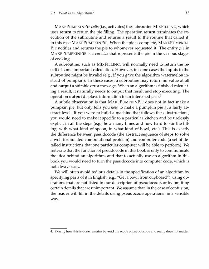
genious Meselson-Stahl experiment of 1957. The replication process starts
from a pair of complementary5 strands of DNA and ends up with two pairs
of complementary strands.6
1. A molecular machine (in other words, a protein complex) called a DNA
helicase, binds to the DNA at certain positions called replication origins.
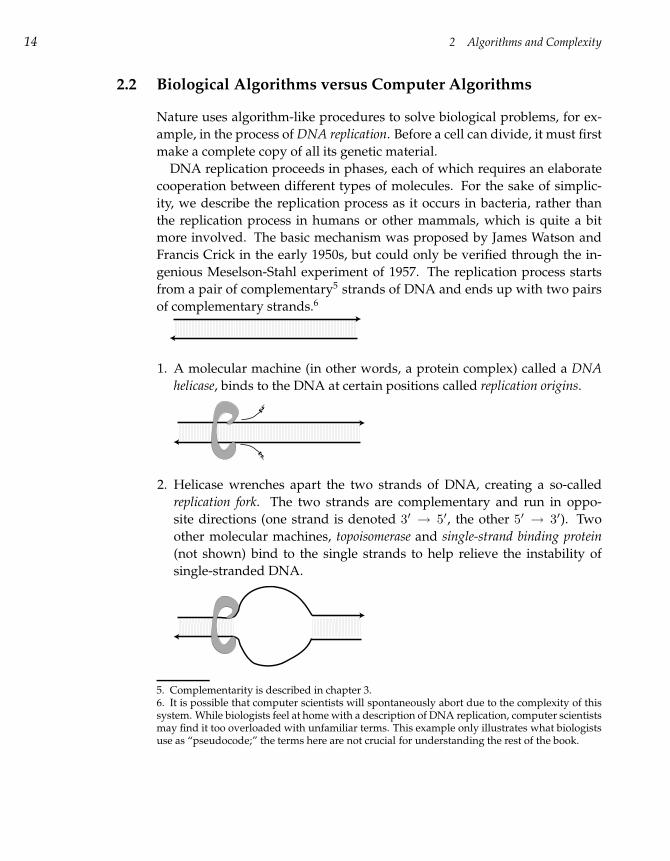
2. Helicase wrenches apart the two strands of DNA, creating a so-called
replication fork. The two strands are complementary and run in oppo-
site directions (one strand is denoted 3′ → 5′, the other 5′ → 3′). Two
other molecular machines, topoisomerase and single-strand binding protein
(not shown) bind to the single strands to help relieve the instability of
single-stranded DNA.
5. Complementarity is described in chapter 3.6. It is possible that computer scientists will spontaneously abort due to the complexity of thissystem. While biologists feel at home with a description of DNA replication, computer scientistsmay find it too overloaded with unfamiliar terms. This example only illustrates what biologistsuse as “pseudocode;” the terms here are not crucial for understanding the rest of the book.
2.2 Biological Algorithms versus Computer Algorithms 15
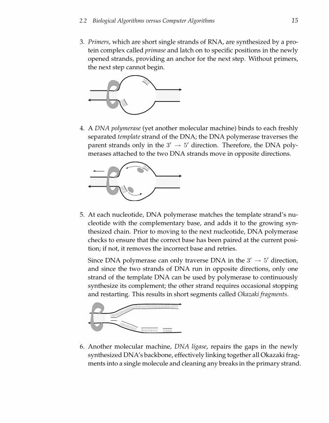
3. Primers, which are short single strands of RNA, are synthesized by a pro-
tein complex called primase and latch on to specific positions in the newly
opened strands, providing an anchor for the next step. Without primers,
the next step cannot begin.
4. A DNA polymerase (yet another molecular machine) binds to each freshly
separated template strand of the DNA; the DNA polymerase traverses the
parent strands only in the 3′ → 5′ direction. Therefore, the DNA poly-
merases attached to the two DNA strands move in opposite directions.
5. At each nucleotide, DNA polymerase matches the template strand’s nu-
cleotide with the complementary base, and adds it to the growing syn-
thesized chain. Prior to moving to the next nucleotide, DNA polymerase
checks to ensure that the correct base has been paired at the current posi-
tion; if not, it removes the incorrect base and retries.
Since DNA polymerase can only traverse DNA in the 3′ → 5′ direction,
and since the two strands of DNA run in opposite directions, only one
strand of the template DNA can be used by polymerase to continuously
synthesize its complement; the other strand requires occasional stopping
and restarting. This results in short segments called Okazaki fragments.
6. Another molecular machine, DNA ligase, repairs the gaps in the newly
synthesized DNA’s backbone, effectively linking together all Okazaki frag-
ments into a single molecule and cleaning any breaks in the primary strand.
16 2 Algorithms and Complexity
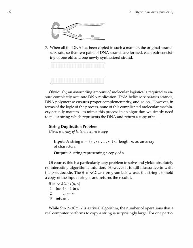
7. When all the DNA has been copied in such a manner, the original strands
separate, so that two pairs of DNA strands are formed, each pair consist-
ing of one old and one newly synthesized strand.
Obviously, an astounding amount of molecular logistics is required to en-
sure completely accurate DNA replication: DNA helicase separates strands,
DNA polymerase ensures proper complementarity, and so on. However, in
terms of the logic of the process, none of this complicated molecular machin-
ery actually matters—to mimic this process in an algorithm we simply need
to take a string which represents the DNA and return a copy of it.
String Duplication Problem:
Given a string of letters, return a copy.
Input: A string s = (s1, s2, . . . , sn) of length n, as an array
of characters.
Output: A string representing a copy of s.
Of course, this is a particularly easy problem to solve and yields absolutely
no interesting algorithmic intuition. However it is still illustrative to write
the pseudocode. The STRINGCOPY program below uses the string t to hold
a copy of the input string s, and returns the result t.
STRINGCOPY(s, n)
1 for i← 1 to n
2 ti ← si
3 return t
While STRINGCOPY is a trivial algorithm, the number of operations that a
real computer performs to copy a string is surprisingly large. For one partic-
2.3 The Change Problem 17
ular computer architecture, we may end up issuing thousands of instructions
to a computer processor. Computer scientists distance themselves from this
complexity by inventing programming languages that allow one to ignore
many of these details. Biologists have not yet invented a similar “language”
to describe biological algorithms working in the cell.
The amount of “intelligence” that the simplest organism, such as a bac-
terium, exhibits to perform any routine task—including replication—is amaz-
ing. Unlike STRINGCOPY, which only performs abstract operations, the bac-
terium really builds new DNA using materials that are floating near the repli-
cation fork. What would happen if it ran out? To prevent this, a bacterium
examines the surroundings, imports new materials from outside, or moves
off to forage for food. Moreover, it waits to begin copying its DNA until
sufficient materials are available. These observations, let alone the coordina-
tion between the individual molecules, lead us to wonder whether even the
most sophisticated computer programs can match the complicated behavior
displayed by even a single-celled organism.
2.3 The Change Problem
The first—and often the most difficult—step in solving a computational prob-
lem is to identify precisely what the problem is. By using the techniques
described in this book, you can then devise an algorithm that solves it. How-
ever, you cannot stop there. Two important questions to ask are: “Does it
work correctly?” and “How long will it take?” Certainly you would not be
satisfied with an algorithm that only returned correct results half the time,
or took 600 years to arrive at an answer. Establishing reasonable expecta-
tions for an algorithm is an important step in understanding how well the
algorithm solves the problem, and whether or not you trust its answer.
A problem describes a class of computational tasks. A problem instance is
one particular input from that class. To illustrate the difference between a
problem and an instance of a problem, consider the following example. You
find yourself in a bookstore buying a fairly expensive pen for $4.23 which
you pay for with a $5 bill (fig. 2.2). You would be due 77 cents in change, and
the cashier now makes a decision as to exactly how you get it.7 You would be
annoyed at a fistful of 77 pennies or 15 nickels and 2 pennies, which raises the
question of how to make change in the least annoying way. Most cashiers try
7. A penny is the smallest denomination in U.S. currency. A dollar is 100 pennies, a quarter is25 pennies, a dime is 10, and a nickel is 5.
18 2 Algorithms and Complexity
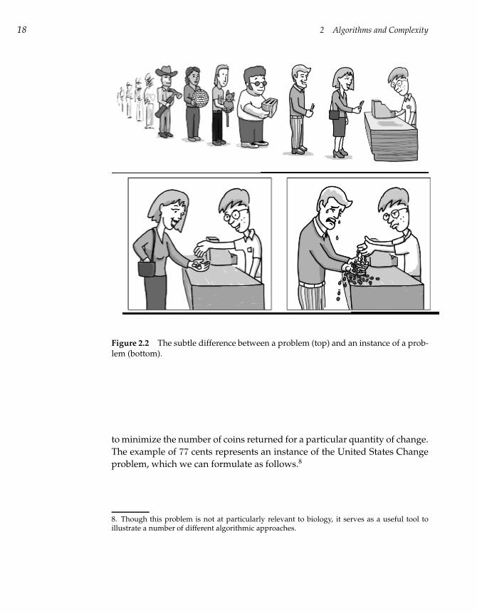
Figure 2.2 The subtle difference between a problem (top) and an instance of a prob-lem (bottom).
to minimize the number of coins returned for a particular quantity of change.
The example of 77 cents represents an instance of the United States Change
problem, which we can formulate as follows.8
8. Though this problem is not at particularly relevant to biology, it serves as a useful tool toillustrate a number of different algorithmic approaches.
2.3 The Change Problem 19
United States Change Problem:
Convert some amount of money into the fewest number of coins.
Input: An amount of money, M , in cents.
Output: The smallest number of quarters q, dimes d, nickels
n, and pennies p whose values add to M (i.e., 25q + 10d +
5n + p = M and q + d + n + p is as small as possible).
The algorithm that is used by cashiers all over the United States to solve
this problem is simple:
USCHANGE(M)
1 while M > 0
2 c← Largest coin that is smaller than (or equal to) M
3 Give coin with denomination c to customer
4 M ←M − c
A slightly more detailed description of this algorithm is:
USCHANGE(M)
1 Give the integer part of M/25 quarters to customer.
2 Let remainder be the remaining amount due the customer.
3 Give the integer part of remainder/10 dimes to customer.
4 Let remainder be the remaining amount due the customer.
5 Give the integer part of remainder/5 nickels to customer.
6 Let remainder be the remaining amount due the customer.
7 Give remainder pennies to customer.
A pseudocode version of the above algorithm is:
20 2 Algorithms and Complexity
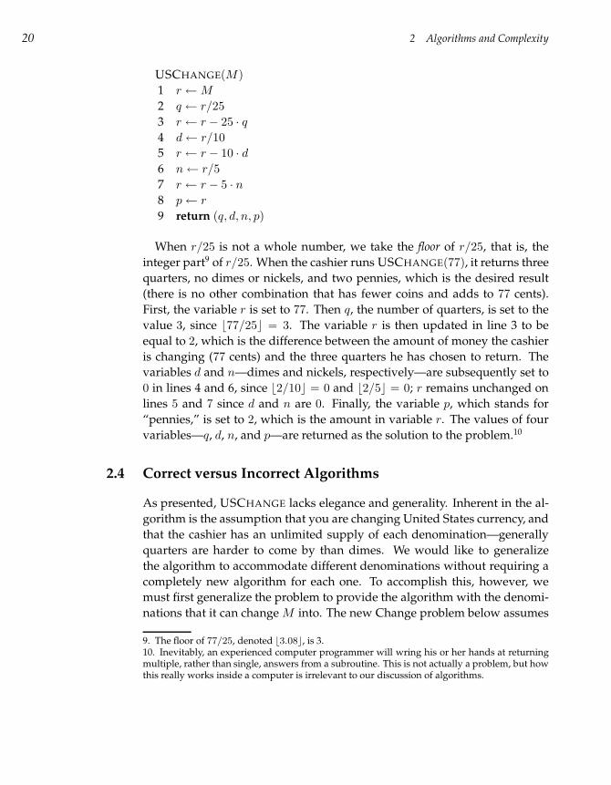
USCHANGE(M)
1 r ←M
2 q ← r/25
3 r ← r − 25 · q
4 d← r/10
5 r ← r − 10 · d
6 n← r/5
7 r ← r − 5 · n
8 p← r
9 return (q, d, n, p)
When r/25 is not a whole number, we take the floor of r/25, that is, the
integer part9 of r/25. When the cashier runs USCHANGE(77), it returns three
quarters, no dimes or nickels, and two pennies, which is the desired result
(there is no other combination that has fewer coins and adds to 77 cents).
First, the variable r is set to 77. Then q, the number of quarters, is set to the
value 3, since b77/25c = 3. The variable r is then updated in line 3 to be
equal to 2, which is the difference between the amount of money the cashier
is changing (77 cents) and the three quarters he has chosen to return. The
variables d and n—dimes and nickels, respectively—are subsequently set to
0 in lines 4 and 6, since b2/10c = 0 and b2/5c = 0; r remains unchanged on
lines 5 and 7 since d and n are 0. Finally, the variable p, which stands for
“pennies,” is set to 2, which is the amount in variable r. The values of four
variables—q, d, n, and p—are returned as the solution to the problem.10
2.4 Correct versus Incorrect Algorithms
As presented, USCHANGE lacks elegance and generality. Inherent in the al-
gorithm is the assumption that you are changing United States currency, and
that the cashier has an unlimited supply of each denomination—generally
quarters are harder to come by than dimes. We would like to generalize
the algorithm to accommodate different denominations without requiring a
completely new algorithm for each one. To accomplish this, however, we
must first generalize the problem to provide the algorithm with the denomi-
nations that it can change M into. The new Change problem below assumes
9. The floor of 77/25, denoted b3.08c, is 3.10. Inevitably, an experienced computer programmer will wring his or her hands at returningmultiple, rather than single, answers from a subroutine. This is not actually a problem, but howthis really works inside a computer is irrelevant to our discussion of algorithms.
2.4 Correct versus Incorrect Algorithms 21
that there are d denominations, rather than the four of the previous prob-
lem. These denominations are represented by an array c = (c1, . . . , cd). For
simplicity, we assume that the denominations are given in decreasing or-
der of value. For example, in the case of the United States Change prob-
lem, c = (25, 10, 5, 1), whereas in the European Union Change problem,
c = (20, 10, 5, 2, 1).
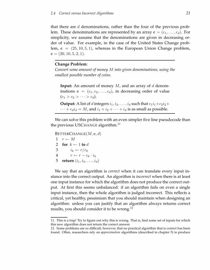
Change Problem:
Convert some amount of money M into given denominations, using the
smallest possible number of coins.
Input: An amount of money M , and an array of d denom-
inations c = (c1, c2, . . . , cd), in decreasing order of value
(c1 > c2 > · · · > cd).
Output: A list of d integers i1, i2, . . . , id such that c1i1+c2i2+
· · ·+ cdid = M , and i1 + i2 + · · ·+ id is as small as possible.
We can solve this problem with an even simpler five line pseudocode than
the previous USCHANGE algorithm.11
BETTERCHANGE(M, c, d)
1 r ←M
2 for k ← 1 to d
3 ik ← r/ck
4 r ← r − ck · ik5 return (i1, i2, . . . , id)
We say that an algorithm is correct when it can translate every input in-
stance into the correct output. An algorithm is incorrect when there is at least
one input instance for which the algorithm does not produce the correct out-
put. At first this seems unbalanced: if an algorithm fails on even a single
input instance, then the whole algorithm is judged incorrect. This reflects a
critical, yet healthy, pessimism that you should maintain when designing an
algorithm: unless you can justify that an algorithm always returns correct
results, you should consider it to be wrong.12
11. This is a trap! Try to figure out why this is wrong. That is, find some set of inputs for whichthis new algorithm does not return the correct answer.12. Some problems are so difficult, however, that no practical algorithm that is correct has beenfound. Often, researchers rely on approximation algorithms (described in chapter 5) to produce
22 2 Algorithms and Complexity
BETTERCHANGE is not a correct algorithm. Suppose we were changing 40
cents into coins with denominations of c1 = 25, c2 = 20, c3 = 10, c4 = 5,
and c5 = 1. BETTERCHANGE would incorrectly return 1 quarter, 1 dime,
and 1 nickel, instead of 2 twenty-cent pieces. As contrived as this may seem,
in 1875 a twenty-cent coin existed in the United States. Between 1865 and
1889, the U.S. Treasury even produced three-cent coins. How sure can we be
that BETTERCHANGE returns the minimal number of coins for our modern
currency, or for foreign countries? Determining the conditions under which
BETTERCHANGE is a correct algorithm is left as a problem at the end of this
chapter.
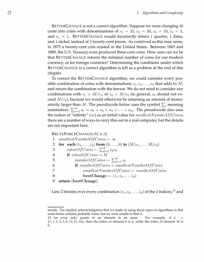
To correct the BETTERCHANGE algorithm, we could consider every pos-
sible combination of coins with denominations c1, c2, . . . , cd that adds to M ,
and return the combination with the fewest. We do not need to consider any
combinations with i1 > M/c1, or i2 > M/c2 (in general, ik should not ex-
ceed M/ck), because we would otherwise be returning an amount of money
strictly larger than M . The pseudocode below uses the symbol∑
, meaning
summation:∑m
i=1 ai = a1 + a2 + a3 + · · · + am. The pseudocode also uses
the notion of “infinity” (∞) as an initial value for smallestNumberOfCoins;
there are a number of ways to carry this out in a real computer, but the details
are not important here.
BRUTEFORCECHANGE(M, c, d)
1 smallestNumberOfCoins←∞
2 for each (i1, . . . , id) from (0, . . . , 0) to (M/c1, . . . , M/cd)
3 valueOfCoins←∑d
k=1 ikck
4 if valueOfCoins = M
5 numberOfCoins←∑d
k=1 ik6 if numberOfCoins < smallestNumberOfCoins
7 smallestNumberOfCoins← numberOfCoins
8 bestChange← (i1, i2, . . . , id)
9 return (bestChange)
Line 2 iterates over every combination (i1, i2, . . . , id) of the d indices,13 and
results. The implicit acknowledgment that we make in using those types of algorithms is thatsome better solution probably exists, but we were unable to find it.13. An array index points to an element in an array. For example, if c =1, 1, 2, 3, 5, 8, 13, 21, 34, then the index of element 8 is 6, while the index of element 34 is9.
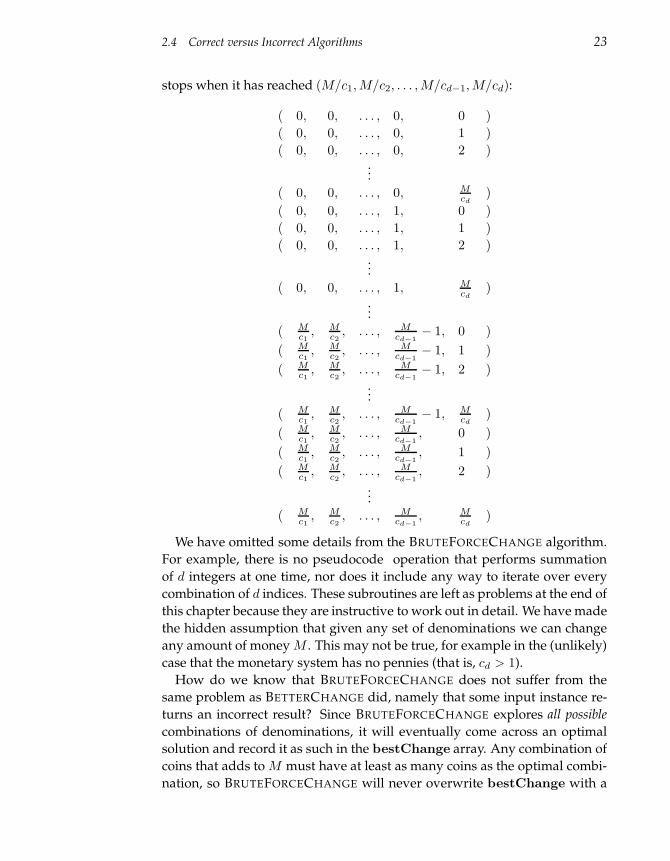
2.4 Correct versus Incorrect Algorithms 23
stops when it has reached (M/c1, M/c2, . . . , M/cd−1, M/cd):
( 0, 0, . . . , 0, 0 )
( 0, 0, . . . , 0, 1 )
( 0, 0, . . . , 0, 2 )...
( 0, 0, . . . , 0, Mcd
)
( 0, 0, . . . , 1, 0 )
( 0, 0, . . . , 1, 1 )
( 0, 0, . . . , 1, 2 )...
( 0, 0, . . . , 1, Mcd
)...
( Mc1
, Mc2
, . . . , Mcd−1− 1, 0 )
( Mc1
, Mc2
, . . . , Mcd−1− 1, 1 )
( Mc1
, Mc2
, . . . , Mcd−1− 1, 2 )
...
( Mc1
, Mc2
, . . . , Mcd−1− 1, M
cd)
( Mc1
, Mc2
, . . . , Mcd−1
, 0 )
( Mc1
, Mc2
, . . . , Mcd−1
, 1 )
( Mc1
, Mc2
, . . . , Mcd−1
, 2 )
...
( Mc1
, Mc2
, . . . , Mcd−1
, Mcd
)
We have omitted some details from the BRUTEFORCECHANGE algorithm.
For example, there is no pseudocode operation that performs summation
of d integers at one time, nor does it include any way to iterate over every
combination of d indices. These subroutines are left as problems at the end of
this chapter because they are instructive to work out in detail. We have made
the hidden assumption that given any set of denominations we can change
any amount of money M . This may not be true, for example in the (unlikely)
case that the monetary system has no pennies (that is, cd > 1).
How do we know that BRUTEFORCECHANGE does not suffer from the
same problem as BETTERCHANGE did, namely that some input instance re-
turns an incorrect result? Since BRUTEFORCECHANGE explores all possible
combinations of denominations, it will eventually come across an optimal
solution and record it as such in the bestChange array. Any combination of
coins that adds to M must have at least as many coins as the optimal combi-
nation, so BRUTEFORCECHANGE will never overwrite bestChange with a
24 2 Algorithms and Complexity
suboptimal solution.
We revisit the Change problem in future chapters to improve on this so-
lution. So far we have answered only one of the two important algorithmic
questions (“Does it work?”, but not “How fast is it?”). We shall see that
BRUTEFORCECHANGE is not particularly speedy.
2.5 Recursive Algorithms
Recursion is one of the most ubiquitous algorithmic concepts. Simply, an
algorithm is recursive if it calls itself.
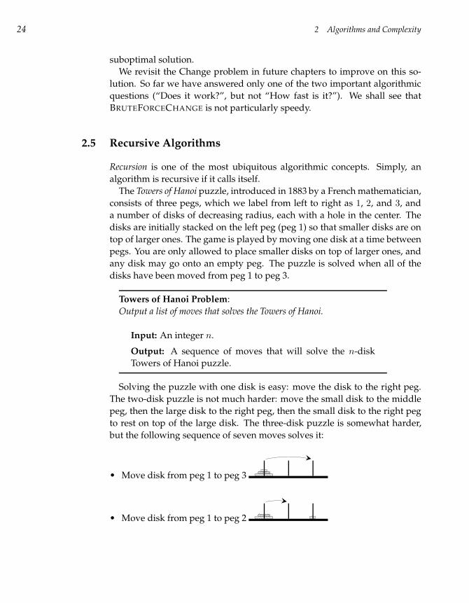
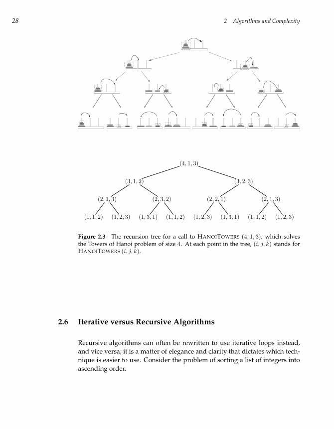
The Towers of Hanoi puzzle, introduced in 1883 by a French mathematician,
consists of three pegs, which we label from left to right as 1, 2, and 3, and
a number of disks of decreasing radius, each with a hole in the center. The
disks are initially stacked on the left peg (peg 1) so that smaller disks are on
top of larger ones. The game is played by moving one disk at a time between
pegs. You are only allowed to place smaller disks on top of larger ones, and
any disk may go onto an empty peg. The puzzle is solved when all of the
disks have been moved from peg 1 to peg 3.
Towers of Hanoi Problem:
Output a list of moves that solves the Towers of Hanoi.
Input: An integer n.
Output: A sequence of moves that will solve the n-disk
Towers of Hanoi puzzle.
Solving the puzzle with one disk is easy: move the disk to the right peg.
The two-disk puzzle is not much harder: move the small disk to the middle
peg, then the large disk to the right peg, then the small disk to the right peg
to rest on top of the large disk. The three-disk puzzle is somewhat harder,
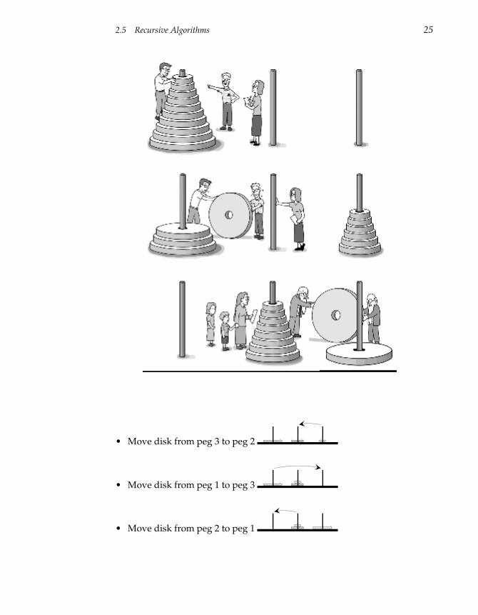
but the following sequence of seven moves solves it:
• Move disk from peg 1 to peg 3
• Move disk from peg 1 to peg 2
2.5 Recursive Algorithms 25
• Move disk from peg 3 to peg 2
• Move disk from peg 1 to peg 3
• Move disk from peg 2 to peg 1
26 2 Algorithms and Complexity
• Move disk from peg 2 to peg 3
• Move disk from peg 1 to peg 3
Now we will figure out how many steps are required to solve a four-disk
puzzle. You cannot complete this game without moving the largest disk.
However, in order to move the largest disk, we first had to move all the
smaller disks to an empty peg. If we had four disks instead of three, then
we would first have to move the top three to an empty peg (7 moves), then
move the largest disk (1 move), then again move the three disks from their
temporary peg to rest on top of the largest disk (another 7 moves). The whole
procedure will take 7 + 1 + 7 = 15 moves. More generally, to move a stack
of size n from the left to the right peg, you first need to move a stack of size
n − 1 from the left to the middle peg, and then from the middle peg to the
right peg once you have moved the nth disk to the right peg. To move a stack
of size n − 1 from the middle to the right, you first need to move a stack of
size n − 2 from the middle to the left, then move the (n − 1)th disk to the
right, and then move the stack of n− 2 from the left to the right peg, and so
on.
At first glance, the Towers of Hanoi problem looks difficult. However, the
following recursive algorithm solves the Towers of Hanoi problem with n
disks. The iterative version of this algorithm is more difficult to write and
analyze, so we do not present it here.
HANOITOWERS(n, fromPeg, toPeg)
1 if n = 1
2 output “Move disk from peg fromPeg to peg toPeg”
3 return
4 unusedPeg← 6− fromPeg − toPeg
5 HANOITOWERS(n− 1, fromPeg, unusedPeg)
6 output “Move disk from peg fromPeg to peg toPeg”
7 HANOITOWERS(n− 1, unusedPeg, toPeg)
8 return
The variables fromPeg, toPeg, and unusedPeg refer to the three different
pegs so that HANOITOWERS(n, 1, 3) moves n disks from the first peg to the
third peg. The variable unusedPeg represents which of the three pegs can
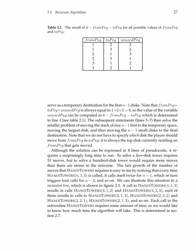
2.5 Recursive Algorithms 27
Table 2.1 The result of 6 − fromPeg − toPeg for all possible values of fromPegand toPeg.
fromPeg toPeg unusedPeg1 2 31 3 22 1 32 3 13 1 23 2 1
serve as a temporary destination for the first n−1 disks. Note that fromPeg+
toPeg+unusedPeg is always equal to 1+2+3 = 6, so the value of the variable
unusedPeg can be computed as 6 − fromPeg − toPeg which is determined
in line 4 (see table 2.1). The subsequent statements (lines 5–7) then solve the
smaller problem of moving the stack of size n−1 first to the temporary space,
moving the largest disk, and then moving the n − 1 small disks to the final
destination. Note that we do not have to specify which disk the player should
move from fromPeg to toPeg: it is always the top disk currently residing on
fromPeg that gets moved.
Although the solution can be expressed in 8 lines of pseudocode, it re-
quires a surprisingly long time to run. To solve a five-disk tower requires
31 moves, but to solve a hundred-disk tower would require more moves
than there are atoms in the universe. The fast growth of the number of
moves that HANOITOWERS requires is easy to see by noticing that every time
HANOITOWERS(n, 1, 3) is called, it calls itself twice for n − 1, which in turn
triggers four calls for n − 2, and so on. We can illustrate this situation in a
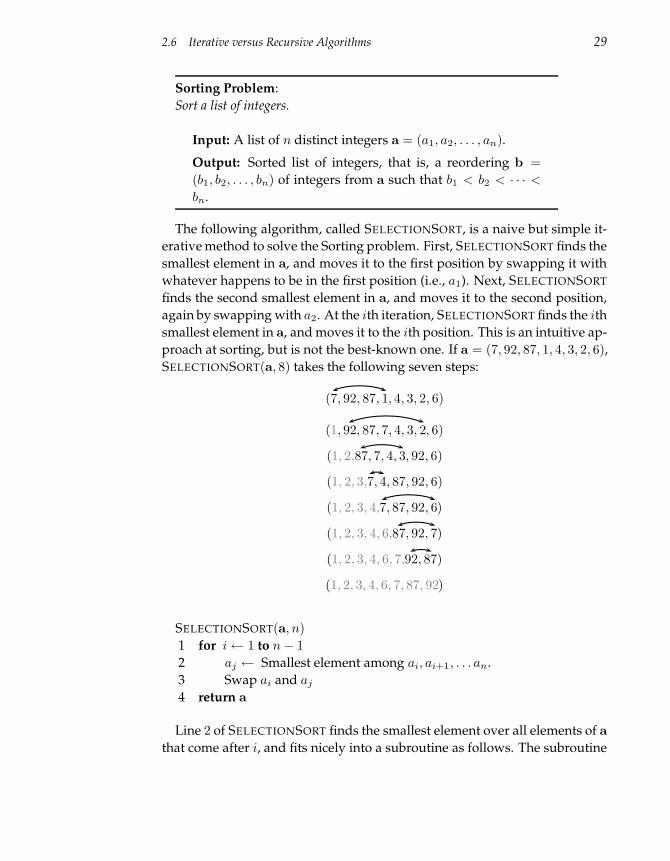
recursion tree, which is shown in figure 2.3. A call to HANOITOWERS(4, 1, 3)
results in calls HANOITOWERS(3, 1, 2) and HANOITOWERS(3, 2, 3); each of
these results in calls to HANOITOWERS(2, 1, 3), HANOITOWERS(2, 3, 2) and
HANOITOWERS(2, 2, 1), HANOITOWERS(2, 1, 3), and so on. Each call to the
subroutine HANOITOWERS requires some amount of time, so we would like
to know how much time the algorithm will take. This is determined in sec-
tion 2.7.
28 2 Algorithms and Complexity
(4, 1, 3)
(3, 1, 2)
(2, 1, 3)
(1, 1, 2) (1, 2, 3)
(2, 3, 2)
(1, 3, 1) (1, 1, 2)
(3, 2, 3)
(2, 2, 1)
(1, 2, 3) (1, 3, 1)
(2, 1, 3)
(1, 1, 2) (1, 2, 3)
Figure 2.3 The recursion tree for a call to HANOITOWERS (4, 1, 3), which solvesthe Towers of Hanoi problem of size 4. At each point in the tree, (i, j, k) stands forHANOITOWERS (i, j, k).
2.6 Iterative versus Recursive Algorithms
Recursive algorithms can often be rewritten to use iterative loops instead,
and vice versa; it is a matter of elegance and clarity that dictates which tech-
nique is easier to use. Consider the problem of sorting a list of integers into
ascending order.
2.6 Iterative versus Recursive Algorithms 29
Sorting Problem:
Sort a list of integers.
Input: A list of n distinct integers a = (a1, a2, . . . , an).
Output: Sorted list of integers, that is, a reordering b =
(b1, b2, . . . , bn) of integers from a such that b1 < b2 < · · · <
bn.
The following algorithm, called SELECTIONSORT, is a naive but simple it-
erative method to solve the Sorting problem. First, SELECTIONSORT finds the
smallest element in a, and moves it to the first position by swapping it with
whatever happens to be in the first position (i.e., a1). Next, SELECTIONSORT
finds the second smallest element in a, and moves it to the second position,
again by swapping with a2. At the ith iteration, SELECTIONSORT finds the ith
smallest element in a, and moves it to the ith position. This is an intuitive ap-
proach at sorting, but is not the best-known one. If a = (7, 92, 87, 1, 4, 3, 2, 6),
SELECTIONSORT(a, 8) takes the following seven steps:
(7, 92, 87, 1, 4, 3, 2, 6)
(1, 92, 87, 7, 4, 3, 2, 6)
(1, 2,87, 7, 4, 3, 92, 6)
(1, 2, 3,7, 4, 87, 92, 6)
(1, 2, 3, 4,7, 87, 92, 6)
(1, 2, 3, 4, 6,87, 92, 7)
(1, 2, 3, 4, 6, 7,92, 87)
(1, 2, 3, 4, 6, 7, 87, 92)
SELECTIONSORT(a, n)
1 for i← 1 to n− 1
2 aj ← Smallest element among ai, ai+1, . . . an.
3 Swap ai and aj
4 return a
Line 2 of SELECTIONSORT finds the smallest element over all elements of a
that come after i, and fits nicely into a subroutine as follows. The subroutine
30 2 Algorithms and Complexity
INDEXOFMIN(array, f irst, last) works with array and returns the index of
the smallest element between positions first and last by examining each
element from arrayfirst to arraylast.
INDEXOFMIN(array, f irst, last)
1 index← first
2 for k ← first + 1 to last
3 if arrayk < arrayindex
4 index← k
5 return index
For example, if a = (7, 92, 87, 1, 4, 3, 2, 6), then INDEXOFMIN(a, 1, 8) would
be 4, since a4 = 1 is smaller than any other element in (a1, a2, . . . , a8). Sim-
ilarly, INDEXOFMIN(a, 5, 8) would be 7, since a7 = 2 is smaller than any
other element in (a5, a6, a7, a8). We can now write SELECTIONSORT using
this subroutine.
SELECTIONSORT(a, n)
1 for i← 1 to n− 1
2 j ← INDEXOFMIN(a, i, n)
3 Swap elements ai and aj
4 return a
To illustrate the similarity between recursion and iteration, we could in-
stead have written SELECTIONSORT recursively (reusing INDEXOFMIN from
above):
RECURSIVESELECTIONSORT(a, f irst, last)
1 if first < last
2 index← INDEXOFMIN(a, f irst, last)
3 Swap afirst with aindex
4 a← RECURSIVESELECTIONSORT(a, f irst + 1, last)
5 return a
In this case, RECURSIVESELECTIONSORT(a, 1, n) performs exactly the same
operations as SELECTIONSORT(a, n).
It may seem contradictory at first that RECURSIVESELECTIONSORT calls it-
self to get an answer, but the key to understanding this algorithm is to realize
that each time it is called, it works on a smaller set of elements from the list
until it reaches the end of the list; at the end, it no longer needs to recurse.
2.6 Iterative versus Recursive Algorithms 31
The reason that the recursion does not continue indefinitely is because the al-
gorithm works toward a point at which it “bottoms out” and no longer needs
to recurse—in this case, when first = last.
As convoluted as it may seem at first, recursion is often the most natural
way to solve many computational problems as it was in the Towers of Hanoi
problem, and we will see many recursive algorithms in the coming chapters.
However, recursion can often lead to very inefficient algorithms, as this next
example shows.
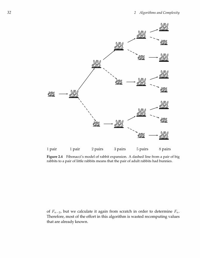
The Fibonacci sequence is a mathematically important, yet very simple,
progression of numbers. The series was first studied in the thirteenth century
by the early Italian mathematician Leonardo Pisano Fibonacci, who tried to
compute the number of offspring of a pair of rabbits over the course of a
year (fig. 2.4). Fibonacci reasoned that one pair of adult rabbits could create
a new pair of rabbits in about the same time that it takes bunnies to grow
into adults. Thus, in any given period, each pair of adult rabbits produces
a new pair of baby rabbits, and all baby rabbits grow into adult rabbits.14 If
we let Fn represent the number of rabbits in period n, then we can determine
the value of Fn in terms of Fn−1 and Fn−2. The number of adult rabbits
at time period n is equal to the number of rabbits (adult and baby) in the
previous time period, or Fn−1. The number of baby rabbits at time period
n is equal to the number of adult rabbits in Fn−1, which is Fn−2. Thus, the
total number of rabbits at time period n is the number of adults plus the
number of babies, that is, Fn = Fn−1 +Fn−2, with F1 = F2 = 1. Consider the
following problem:
Fibonacci Problem:
Calculate the nth Fibonacci number.
Input: An integer n.
Output: The nth Fibonacci number Fn = Fn−1 +Fn−2 (with
F1 = F2 = 1).
The simplest recursive algorithm, shown below, calculates Fn by calling
itself to compute Fn−1 and Fn−2. As figure 2.5 shows, this approach results
in a large amount of duplicated effort: in calculating Fn−1 we find the value
14. Fibonacci faced the challenge of adequately formulating the problem he was studying, oneof the more difficult parts of bioinformatics research. The Fibonacci view of rabbit life is overlysimplistic and inadequate: in particular, rabbits never die in his model. As a result, after just afew generations, the number of rabbits will be larger than the number of atoms in the universe.
32 2 Algorithms and Complexity
1 pair 1 pair 2 pairs 3 pairs 5 pairs 8 pairs
Figure 2.4 Fibonacci’s model of rabbit expansion. A dashed line from a pair of bigrabbits to a pair of little rabbits means that the pair of adult rabbits had bunnies.
of Fn−2, but we calculate it again from scratch in order to determine Fn.
Therefore, most of the effort in this algorithm is wasted recomputing values
that are already known.
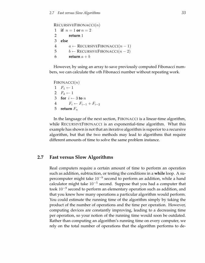
2.7 Fast versus Slow Algorithms 33
RECURSIVEFIBONACCI(n)
1 if n = 1 or n = 2
2 return 1
3 else
4 a← RECURSIVEFIBONACCI(n− 1)
5 b← RECURSIVEFIBONACCI(n− 2)
6 return a + b
However, by using an array to save previously computed Fibonacci num-
bers, we can calculate the nth Fibonacci number without repeating work.
FIBONACCI(n)
1 F1 ← 1
2 F2 ← 1
3 for i← 3 to n
4 Fi ← Fi−1 + Fi−2
5 return Fn
In the language of the next section, FIBONACCI is a linear-time algorithm,
while RECURSIVEFIBONACCI is an exponential-time algorithm. What this
example has shown is not that an iterative algorithm is superior to a recursive
algorithm, but that the two methods may lead to algorithms that require
different amounts of time to solve the same problem instance.
2.7 Fast versus Slow Algorithms
Real computers require a certain amount of time to perform an operation
such as addition, subtraction, or testing the conditions in a while loop. A su-
percomputer might take 10−9 second to perform an addition, while a hand
calculator might take 10−5 second. Suppose that you had a computer that
took 10−9 second to perform an elementary operation such as addition, and
that you knew how many operations a particular algorithm would perform.
You could estimate the running time of the algorithm simply by taking the
product of the number of operations and the time per operation. However,
computing devices are constantly improving, leading to a decreasing time
per operation, so your notion of the running time would soon be outdated.
Rather than computing an algorithm’s running time on every computer, we
rely on the total number of operations that the algorithm performs to de-
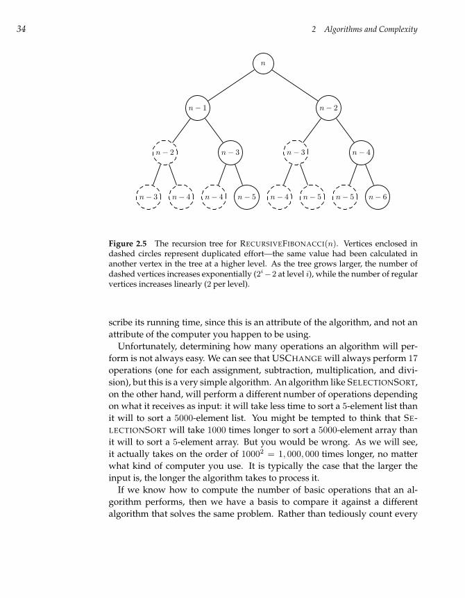
34 2 Algorithms and Complexity
n
n− 1
n− 2
n− 3 n− 4
n− 3
n− 4 n− 5
n− 2
n− 3
n− 4 n− 5
n− 4
n− 5 n− 6
Figure 2.5 The recursion tree for RECURSIVEFIBONACCI(n). Vertices enclosed indashed circles represent duplicated effort—the same value had been calculated inanother vertex in the tree at a higher level. As the tree grows larger, the number ofdashed vertices increases exponentially (2i−2 at level i), while the number of regularvertices increases linearly (2 per level).
scribe its running time, since this is an attribute of the algorithm, and not an
attribute of the computer you happen to be using.
Unfortunately, determining how many operations an algorithm will per-
form is not always easy. We can see that USCHANGE will always perform 17
operations (one for each assignment, subtraction, multiplication, and divi-
sion), but this is a very simple algorithm. An algorithm like SELECTIONSORT,
on the other hand, will perform a different number of operations depending
on what it receives as input: it will take less time to sort a 5-element list than
it will to sort a 5000-element list. You might be tempted to think that SE-
LECTIONSORT will take 1000 times longer to sort a 5000-element array than
it will to sort a 5-element array. But you would be wrong. As we will see,
it actually takes on the order of 10002 = 1, 000, 000 times longer, no matter
what kind of computer you use. It is typically the case that the larger the
input is, the longer the algorithm takes to process it.
If we know how to compute the number of basic operations that an al-
gorithm performs, then we have a basis to compare it against a different
algorithm that solves the same problem. Rather than tediously count every
2.7 Fast versus Slow Algorithms 35
multiplication and addition, we can perform this comparison by gaining a
high-level understanding of the growth of each algorithm’s operation count
as the size of the input increases. To illustrate this, suppose an algorithm A
performs 11n3 operations on an input of size n, and a different algorithm,
B, solves the same problem in 99n2 + 7 operations. Which algorithm, A or
B, is faster? Although, A may be faster than B for some small n (e.g., for
n between 0 and 9), B will become faster with large n (e.g., for all n ≥ 10).
Since n3 is, in some sense, a “faster-growing” function than n2 with respect
to n, the constants 11, 99, and 7 do not affect the competition between the
two algorithms for large n (see figure 2.6). We refer to A as a cubic algo-
rithm and to B as a quadratic algorithm, and say that A is less efficient than
B because it performs more operations to solve the same problem when n is
large. Thus, we will often be somewhat imprecise when we count operations
in algorithms—the behavior of algorithms on small inputs does not matter.
Let us estimate how long BRUTEFORCECHANGE will take on an input in-
stance of M cents, and denominations (c1, c2, . . . , cd). To calculate the total
number of operations in the for loop, we can take the approximate num-
ber of operations performed in each iteration and multiply this by the total
number of iterations. Since there are roughly Mc1· M
c2· · · M
cditerations, the for
loop performs on the order of d · Md
c1·c2···cdoperations, which dwarfs the other
operations in the algorithm.
This type of algorithm is often referred to as an exponential algorithm in
contrast to quadratic, cubic, or other polynomial algorithms. The expres-
sion for the running time of exponential algorithms includes a term like Md,
where d is a parameter of the problem (i.e., d may deliberately be made arbi-
trarily large by changing the input to the algorithm), while the running time
of a polynomial algorithm is bounded by a term like Mk where k is a con-
stant not related to the size of any parameters. For example, an algorithm
with running time M1 (linear), M2 (quadratic), M3 (cubic), or even M2005
is polynomial. Of course, an algorithm with running time M2005 is not very
practical, perhaps less so than some exponential algorithms, and much ef-
fort in computer science goes into designing faster and faster polynomial
algorithms. Since d may be large when the algorithm is called with a long
list of denominations [e.g., c = (1, 2, 3, 4, 5, . . . , 100)], we see that BRUTE-
FORCECHANGE can take a very long time to execute.
We have seen that the running time of an algorithm is often related to the
size of its input. However, the running time of an algorithm can also vary
among inputs of the same size. For example, suppose SELECTIONSORT first
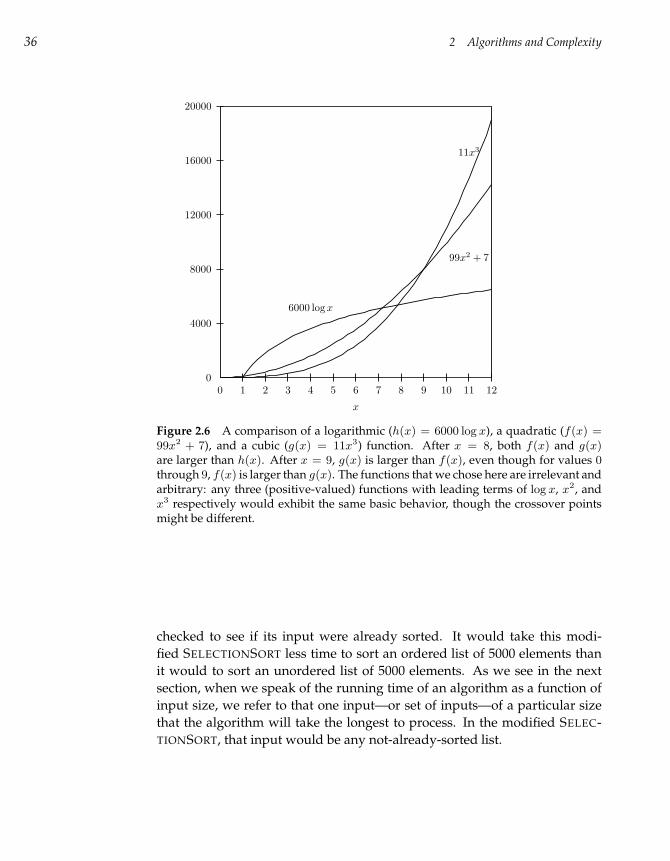
36 2 Algorithms and Complexity
0 1 2 3 4 5 6 7 8 9 10 11 120
4000
8000
12000
16000
20000
99x2 + 7
11x3
6000 logx
x
Figure 2.6 A comparison of a logarithmic (h(x) = 6000 log x), a quadratic (f(x) =99x2 + 7), and a cubic (g(x) = 11x3) function. After x = 8, both f(x) and g(x)are larger than h(x). After x = 9, g(x) is larger than f(x), even though for values 0through 9, f(x) is larger than g(x). The functions that we chose here are irrelevant andarbitrary: any three (positive-valued) functions with leading terms of log x, x2, andx3 respectively would exhibit the same basic behavior, though the crossover pointsmight be different.
checked to see if its input were already sorted. It would take this modi-
fied SELECTIONSORT less time to sort an ordered list of 5000 elements than
it would to sort an unordered list of 5000 elements. As we see in the next
section, when we speak of the running time of an algorithm as a function of
input size, we refer to that one input—or set of inputs—of a particular size
that the algorithm will take the longest to process. In the modified SELEC-
TIONSORT, that input would be any not-already-sorted list.
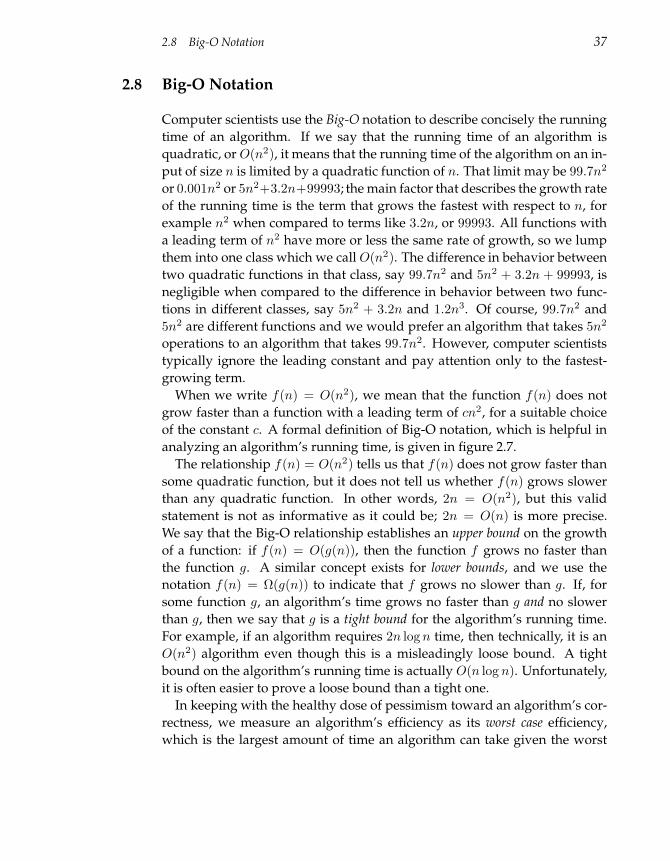
2.8 Big-O Notation 37
2.8 Big-O Notation
Computer scientists use the Big-O notation to describe concisely the running
time of an algorithm. If we say that the running time of an algorithm is
quadratic, or O(n2), it means that the running time of the algorithm on an in-
put of size n is limited by a quadratic function of n. That limit may be 99.7n2
or 0.001n2 or 5n2+3.2n+99993; the main factor that describes the growth rate
of the running time is the term that grows the fastest with respect to n, for
example n2 when compared to terms like 3.2n, or 99993. All functions with
a leading term of n2 have more or less the same rate of growth, so we lump
them into one class which we call O(n2). The difference in behavior between
two quadratic functions in that class, say 99.7n2 and 5n2 + 3.2n + 99993, is
negligible when compared to the difference in behavior between two func-
tions in different classes, say 5n2 + 3.2n and 1.2n3. Of course, 99.7n2 and
5n2 are different functions and we would prefer an algorithm that takes 5n2
operations to an algorithm that takes 99.7n2. However, computer scientists
typically ignore the leading constant and pay attention only to the fastest-
growing term.
When we write f(n) = O(n2), we mean that the function f(n) does not
grow faster than a function with a leading term of cn2, for a suitable choice
of the constant c. A formal definition of Big-O notation, which is helpful in
analyzing an algorithm’s running time, is given in figure 2.7.
The relationship f(n) = O(n2) tells us that f(n) does not grow faster than
some quadratic function, but it does not tell us whether f(n) grows slower
than any quadratic function. In other words, 2n = O(n2), but this valid
statement is not as informative as it could be; 2n = O(n) is more precise.
We say that the Big-O relationship establishes an upper bound on the growth
of a function: if f(n) = O(g(n)), then the function f grows no faster than
the function g. A similar concept exists for lower bounds, and we use the
notation f(n) = Ω(g(n)) to indicate that f grows no slower than g. If, for
some function g, an algorithm’s time grows no faster than g and no slower
than g, then we say that g is a tight bound for the algorithm’s running time.
For example, if an algorithm requires 2n log n time, then technically, it is an
O(n2) algorithm even though this is a misleadingly loose bound. A tight
bound on the algorithm’s running time is actually O(n log n). Unfortunately,
it is often easier to prove a loose bound than a tight one.
In keeping with the healthy dose of pessimism toward an algorithm’s cor-
rectness, we measure an algorithm’s efficiency as its worst case efficiency,
which is the largest amount of time an algorithm can take given the worst
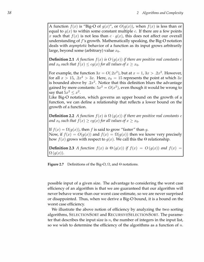
38 2 Algorithms and Complexity
A function f(x) is “Big-O of g(x)”, or O(g(x)), when f(x) is less than orequal to g(x) to within some constant multiple c. If there are a few pointsx such that f(x) is not less than c · g(x), this does not affect our overallunderstanding of f ’s growth. Mathematically speaking, the Big-O notationdeals with asymptotic behavior of a function as its input grows arbitrarilylarge, beyond some (arbitrary) value x0.
Definition 2.1 A function f(x) is O (g(x)) if there are positive real constants cand x0 such that f(x) ≤ cg(x) for all values of x ≥ x0.
For example, the function 3x = O(.2x2), but at x = 1, 3x > .2x2. However,for all x > 15, .2x2 > 3x. Here, x0 = 15 represents the point at which 3xis bounded above by .2x2. Notice that this definition blurs the advantagegained by mere constants: 5x2 = O(x2), even though it would be wrong tosay that 5x2 ≤ x2.Like Big-O notation, which governs an upper bound on the growth of afunction, we can define a relationship that reflects a lower bound on thegrowth of a function.
Definition 2.2 A function f(x) is Ω (g(x)) if there are positive real constants cand x0 such that f(x) ≥ cg(x) for all values of x ≥ x0.
If f(x) = Ω(g(x)), then f is said to grow “faster” than g.Now, if f(x) = O(g(x)) and f(x) = Ω(g(x)) then we know very preciselyhow f(x) grows with respect to g(x). We call this the Θ relationship.
Definition 2.3 A function f(x) is Θ (g(x)) if f(x) = O (g(x)) and f(x) =Ω (g(x)).
Figure 2.7 Definitions of the Big-O, Ω, and Θ notations.
possible input of a given size. The advantage to considering the worst case
efficiency of an algorithm is that we are guaranteed that our algorithm will
never behave worse than our worst case estimate, so we are never surprised
or disappointed. Thus, when we derive a Big-O bound, it is a bound on the
worst case efficiency.
We illustrate the above notion of efficiency by analyzing the two sorting
algorithms, SELECTIONSORT and RECURSIVESELECTIONSORT. The parame-
ter that describes the input size is n, the number of integers in the input list,
so we wish to determine the efficiency of the algorithms as a function of n.
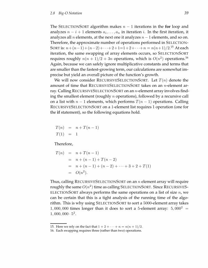
2.8 Big-O Notation 39
The SELECTIONSORT algorithm makes n − 1 iterations in the for loop and
analyzes n − i + 1 elements ai, . . . , an in iteration i. In the first iteration, it
analyzes all n elements, at the next one it analyzes n− 1 elements, and so on.
Therefore, the approximate number of operations performed in SELECTION-
SORT is: n+(n−1)+(n−2)+· · ·+2+1=1+2+· · ·+n = n(n+1)/2.15 At each
iteration, the same swapping of array elements occurs, so SELECTIONSORT
requires roughly n(n + 1)/2 + 3n operations, which is O(n2) operations.16
Again, because we can safely ignore multiplicative constants and terms that
are smaller than the fastest-growing term, our calculations are somewhat im-
precise but yield an overall picture of the function’s growth.
We will now consider RECURSIVESELECTIONSORT. Let T (n) denote the
amount of time that RECURSIVESELECTIONSORT takes on an n-element ar-
ray. Calling RECURSIVESELECTIONSORT on an n-element array involves find-
ing the smallest element (roughly n operations), followed by a recursive call
on a list with n − 1 elements, which performs T (n − 1) operations. Calling
RECURSIVESELECTIONSORT on a 1-element list requires 1 operation (one for
the if statement), so the following equations hold.
T (n) = n + T (n− 1)
T (1) = 1
Therefore,
T (n) = n + T (n− 1)
= n + (n− 1) + T (n− 2)
= n + (n− 1) + (n− 2) + · · ·+ 3 + 2 + T (1)
= O(n2).
Thus, calling RECURSIVESELECTIONSORT on an n element array will require
roughly the same O(n2) time as calling SELECTIONSORT. Since RECURSIVES-
ELECTIONSORT always performs the same operations on a list of size n, we
can be certain that this is a tight analysis of the running time of the algo-
rithm. This is why using SELECTIONSORT to sort a 5000-element array takes
1, 000, 000 times longer than it does to sort a 5-element array: 5, 0002 =
1, 000, 000 · 52.
15. Here we rely on the fact that 1 + 2 + · · · + n = n(n + 1)/2.16. Each swapping requires three (rather than two) operations.
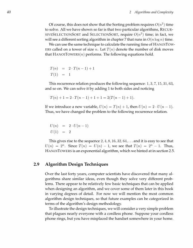
40 2 Algorithms and Complexity
Of course, this does not show that the Sorting problem requires O(n2) time
to solve. All we have shown so far is that two particular algorithms, RECUR-
SIVESELECTIONSORT and SELECTIONSORT, require O(n2) time; in fact, we
will see a different sorting algorithm in chapter 7 that runs in O(n log n) time.
We can use the same technique to calculate the running time of HANOITOW-
ERS called on a tower of size n. Let T (n) denote the number of disk moves
that HANOITOWERS(n) performs. The following equations hold.
T (n) = 2 · T (n− 1) + 1
T (1) = 1
This recurrence relation produces the following sequence: 1, 3, 7, 15, 31, 63,
and so on. We can solve it by adding 1 to both sides and noticing
T (n) + 1 = 2 · T (n− 1) + 1 + 1 = 2(T (n− 1) + 1).
If we introduce a new variable, U(n) = T (n) + 1, then U(n) = 2 · U(n − 1).
Thus, we have changed the problem to the following recurrence relation.
U(n) = 2 · U(n− 1)
U(1) = 2
This gives rise to the sequence 2, 4, 8, 16, 32, 64, . . . and it is easy to see that
U(n) = 2n. Since T (n) = U(n) − 1, we see that T (n) = 2n − 1. Thus,
HANOITOWERS is an exponential algorithm, which we hinted at in section 2.5.
2.9 Algorithm Design Techniques
Over the last forty years, computer scientists have discovered that many al-
gorithms share similar ideas, even though they solve very different prob-
lems. There appear to be relatively few basic techniques that can be applied
when designing an algorithm, and we cover some of them later in this book
in varying degrees of detail. For now we will mention the most common
algorithm design techniques, so that future examples can be categorized in
terms of the algorithm’s design methodology.
To illustrate the design techniques, we will consider a very simple problem
that plagues nearly everyone with a cordless phone. Suppose your cordless
phone rings, but you have misplaced the handset somewhere in your home.
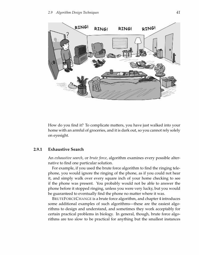
2.9 Algorithm Design Techniques 41
How do you find it? To complicate matters, you have just walked into your
home with an armful of groceries, and it is dark out, so you cannot rely solely
on eyesight.
2.9.1 Exhaustive Search
An exhaustive search, or brute force, algorithm examines every possible alter-
native to find one particular solution.
For example, if you used the brute force algorithm to find the ringing tele-
phone, you would ignore the ringing of the phone, as if you could not hear
it, and simply walk over every square inch of your home checking to see
if the phone was present. You probably would not be able to answer the
phone before it stopped ringing, unless you were very lucky, but you would
be guaranteed to eventually find the phone no matter where it was.
BRUTEFORCECHANGE is a brute force algorithm, and chapter 4 introduces
some additional examples of such algorithms—these are the easiest algo-
rithms to design and understand, and sometimes they work acceptably for
certain practical problems in biology. In general, though, brute force algo-
rithms are too slow to be practical for anything but the smallest instances
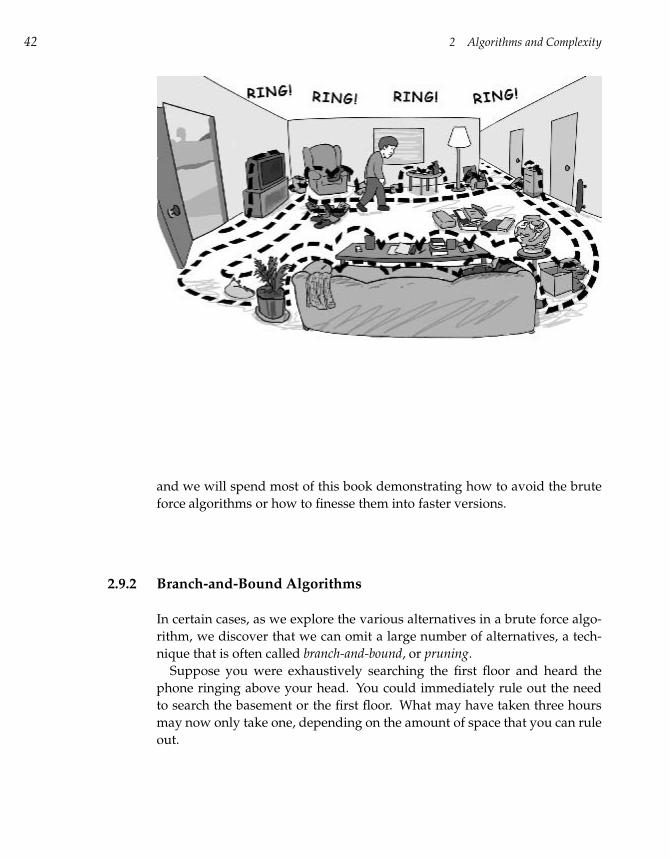
42 2 Algorithms and Complexity
and we will spend most of this book demonstrating how to avoid the brute
force algorithms or how to finesse them into faster versions.
2.9.2 Branch-and-Bound Algorithms
In certain cases, as we explore the various alternatives in a brute force algo-
rithm, we discover that we can omit a large number of alternatives, a tech-
nique that is often called branch-and-bound, or pruning.
Suppose you were exhaustively searching the first floor and heard the
phone ringing above your head. You could immediately rule out the need
to search the basement or the first floor. What may have taken three hours
may now only take one, depending on the amount of space that you can rule
out.
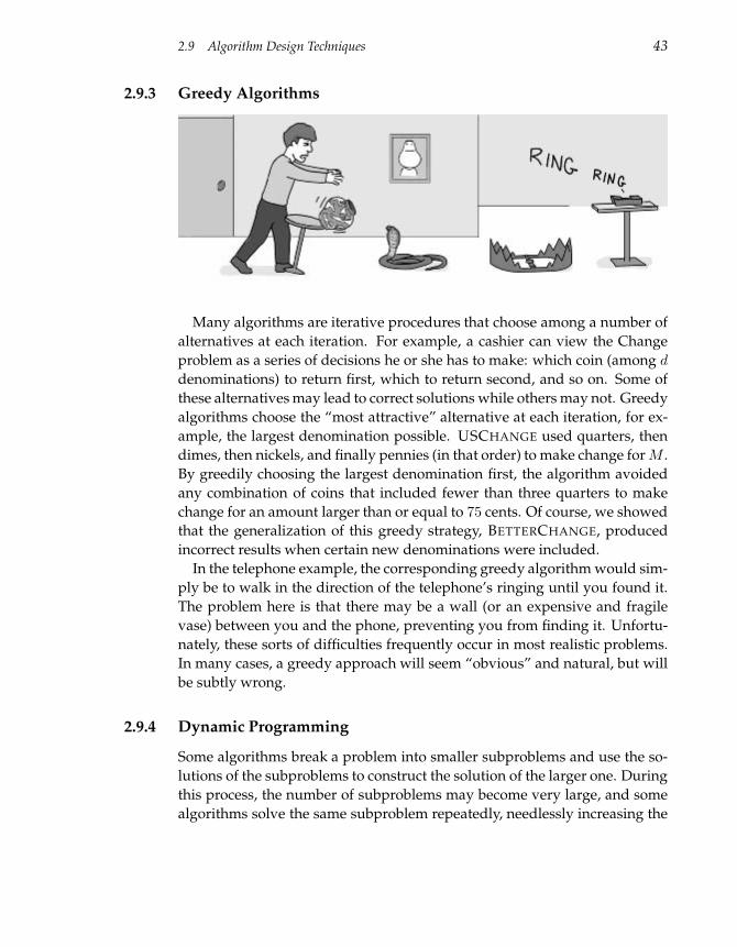
2.9 Algorithm Design Techniques 43
2.9.3 Greedy Algorithms
Many algorithms are iterative procedures that choose among a number of
alternatives at each iteration. For example, a cashier can view the Change
problem as a series of decisions he or she has to make: which coin (among d
denominations) to return first, which to return second, and so on. Some of
these alternatives may lead to correct solutions while others may not. Greedy
algorithms choose the “most attractive” alternative at each iteration, for ex-
ample, the largest denomination possible. USCHANGE used quarters, then
dimes, then nickels, and finally pennies (in that order) to make change for M .
By greedily choosing the largest denomination first, the algorithm avoided
any combination of coins that included fewer than three quarters to make
change for an amount larger than or equal to 75 cents. Of course, we showed
that the generalization of this greedy strategy, BETTERCHANGE, produced
incorrect results when certain new denominations were included.
In the telephone example, the corresponding greedy algorithm would sim-
ply be to walk in the direction of the telephone’s ringing until you found it.
The problem here is that there may be a wall (or an expensive and fragile
vase) between you and the phone, preventing you from finding it. Unfortu-
nately, these sorts of difficulties frequently occur in most realistic problems.
In many cases, a greedy approach will seem “obvious” and natural, but will
be subtly wrong.
2.9.4 Dynamic Programming
Some algorithms break a problem into smaller subproblems and use the so-
lutions of the subproblems to construct the solution of the larger one. During
this process, the number of subproblems may become very large, and some
algorithms solve the same subproblem repeatedly, needlessly increasing the
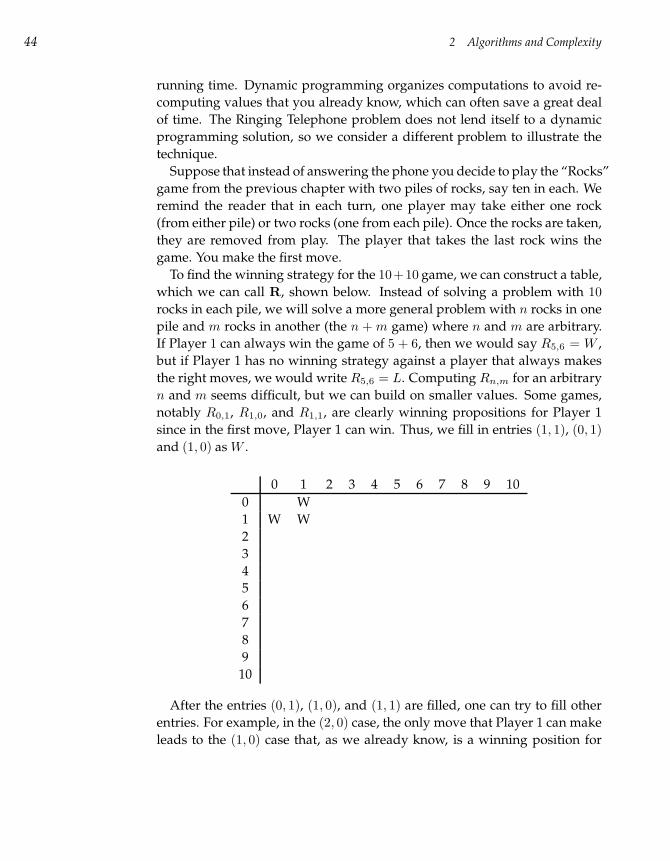
44 2 Algorithms and Complexity
running time. Dynamic programming organizes computations to avoid re-
computing values that you already know, which can often save a great deal
of time. The Ringing Telephone problem does not lend itself to a dynamic
programming solution, so we consider a different problem to illustrate the
technique.
Suppose that instead of answering the phone you decide to play the “Rocks”
game from the previous chapter with two piles of rocks, say ten in each. We
remind the reader that in each turn, one player may take either one rock
(from either pile) or two rocks (one from each pile). Once the rocks are taken,
they are removed from play. The player that takes the last rock wins the
game. You make the first move.
To find the winning strategy for the 10+10 game, we can construct a table,
which we can call R, shown below. Instead of solving a problem with 10
rocks in each pile, we will solve a more general problem with n rocks in one
pile and m rocks in another (the n + m game) where n and m are arbitrary.
If Player 1 can always win the game of 5 + 6, then we would say R5,6 = W ,
but if Player 1 has no winning strategy against a player that always makes
the right moves, we would write R5,6 = L. Computing Rn,m for an arbitrary
n and m seems difficult, but we can build on smaller values. Some games,
notably R0,1, R1,0, and R1,1, are clearly winning propositions for Player 1
since in the first move, Player 1 can win. Thus, we fill in entries (1, 1), (0, 1)
and (1, 0) as W .
0 1 2 3 4 5 6 7 8 9 10
0 W
1 W W
2
3
4
5
6
7
8
9
10
After the entries (0, 1), (1, 0), and (1, 1) are filled, one can try to fill other
entries. For example, in the (2, 0) case, the only move that Player 1 can make
leads to the (1, 0) case that, as we already know, is a winning position for
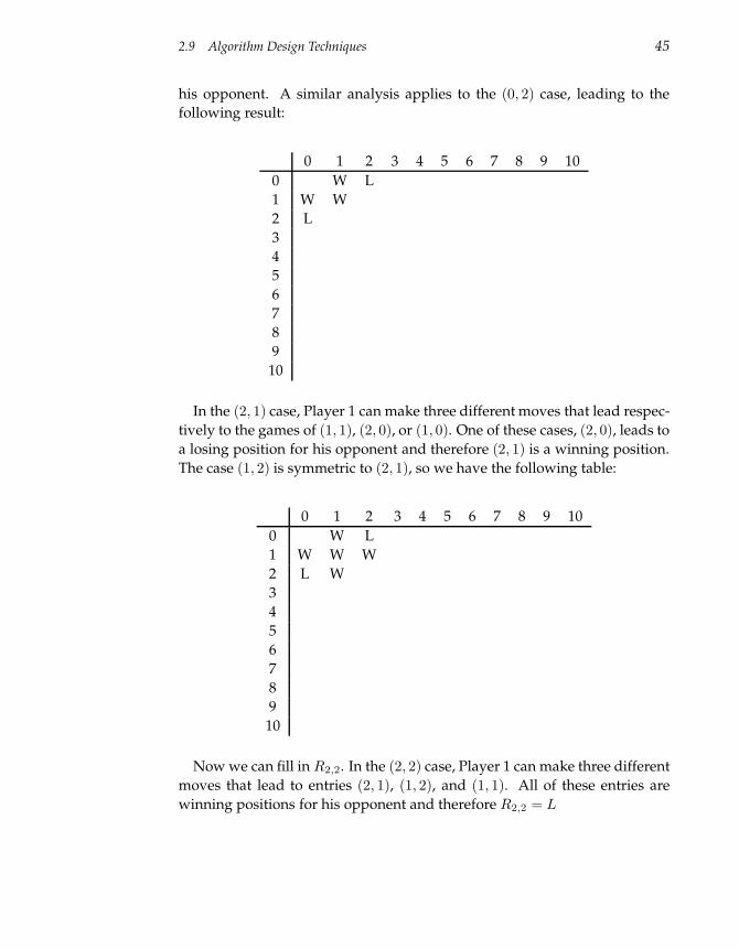
2.9 Algorithm Design Techniques 45
his opponent. A similar analysis applies to the (0, 2) case, leading to the
following result:
0 1 2 3 4 5 6 7 8 9 10
0 W L
1 W W
2 L
3
4
5
6
7
8
9
10
In the (2, 1) case, Player 1 can make three different moves that lead respec-
tively to the games of (1, 1), (2, 0), or (1, 0). One of these cases, (2, 0), leads to
a losing position for his opponent and therefore (2, 1) is a winning position.
The case (1, 2) is symmetric to (2, 1), so we have the following table:
0 1 2 3 4 5 6 7 8 9 10
0 W L
1 W W W
2 L W
3
4
5
6
7
8
9
10
Now we can fill in R2,2. In the (2, 2) case, Player 1 can make three different
moves that lead to entries (2, 1), (1, 2), and (1, 1). All of these entries are
winning positions for his opponent and therefore R2,2 = L
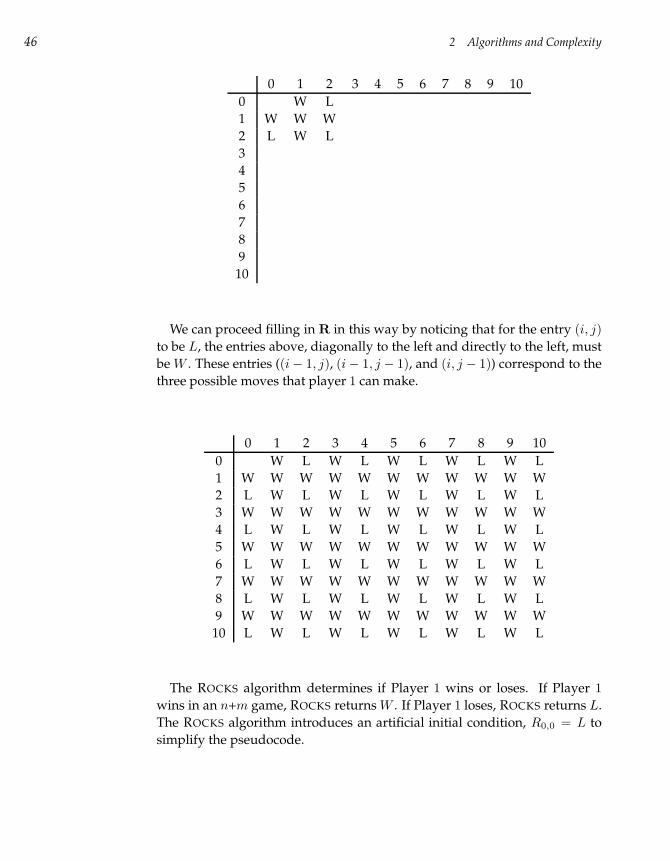
46 2 Algorithms and Complexity
0 1 2 3 4 5 6 7 8 9 10
0 W L
1 W W W
2 L W L
3
4
5
6
7
8
9
10
We can proceed filling in R in this way by noticing that for the entry (i, j)
to be L, the entries above, diagonally to the left and directly to the left, must
be W . These entries ((i− 1, j), (i− 1, j − 1), and (i, j − 1)) correspond to the
three possible moves that player 1 can make.
0 1 2 3 4 5 6 7 8 9 10
0 W L W L W L W L W L
1 W W W W W W W W W W W
2 L W L W L W L W L W L
3 W W W W W W W W W W W
4 L W L W L W L W L W L
5 W W W W W W W W W W W
6 L W L W L W L W L W L
7 W W W W W W W W W W W
8 L W L W L W L W L W L
9 W W W W W W W W W W W
10 L W L W L W L W L W L
The ROCKS algorithm determines if Player 1 wins or loses. If Player 1
wins in an n+m game, ROCKS returns W . If Player 1 loses, ROCKS returns L.
The ROCKS algorithm introduces an artificial initial condition, R0,0 = L to
simplify the pseudocode.
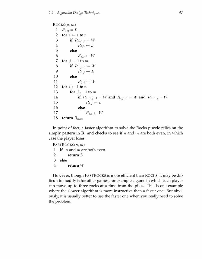
2.9 Algorithm Design Techniques 47
ROCKS(n, m)
1 R0,0 = L
2 for i← 1 to n
3 if Ri−1,0 = W
4 Ri,0 ← L
5 else
6 Ri,0 ←W
7 for j ← 1 to m
8 if R0,j−1 = W
9 R0,j ← L
10 else
11 R0,j ←W
12 for i← 1 to n
13 for j ← 1 to m
14 if Ri−1,j−1 = W and Ri,j−1 = W and Ri−1,j = W
15 Ri,j ← L
16 else
17 Ri,j ←W
18 return Rn,m
In point of fact, a faster algorithm to solve the Rocks puzzle relies on the
simply pattern in R, and checks to see if n and m are both even, in which
case the player loses.
FASTROCKS(n, m)
1 if n and m are both even
2 return L
3 else
4 return W
However, though FASTROCKS is more efficient than ROCKS, it may be dif-
ficult to modify it for other games, for example a game in which each player
can move up to three rocks at a time from the piles. This is one example
where the slower algorithm is more instructive than a faster one. But obvi-
ously, it is usually better to use the faster one when you really need to solve
the problem.
48 2 Algorithms and Complexity
2.9.5 Divide-and-Conquer Algorithms
One big problem may be hard to solve, but two problems that are half the
size may be significantly easier. In these cases, divide-and-conquer algorithms
fare well by doing just that: splitting the problem into smaller subproblems,
solving the subproblems independently, and combining the solutions of sub-
problems into a solution of the original problem. The situation is usually
more complicated than this and after splitting one problem into subprob-
lems, a divide-and-conquer algorithm usually splits these subproblems into
even smaller sub-subproblems, and so on, until it reaches a point at which
it no longer needs to recurse. A critical step in many divide-and-conquer
algorithms is the recombining of solutions to subproblems into a solution
for a larger problem. Often, this merging step can consume a considerable
amount of time. We will see examples of this technique in chapter 7.
2.9.6 Machine Learning
Another approach to the phone search problem is to collect statistics over the
course of a year about where you leave the phone, learning where the phone
tends to end up most of the time. If the phone was left in the bathroom
80% of the time, in the bedroom 15% of the time, and in the kitchen 5% of
the time, then a sensible time-saving strategy would be to start the search in
the bathroom, continue to the bedroom, and finish in the kitchen. Machine
learning algorithms often base their strategies on the computational analysis
of previously collected data.
2.9.7 Randomized Algorithms
If you happen to have a coin, then before even starting to search for the
phone, you could toss it to decide whether you want to start your search
on the first floor if the coin comes up heads, or on the second floor if the coin
comes up tails. If you also happen to have a die, then after deciding on the
second floor, you could roll it to decide in which of the six rooms on the sec-
ond floor to start your search.17 Although tossing coins and rolling dice may
be a fun way to search for the phone, it is certainly not the intuitive thing
to do, nor is it at all clear whether it gives you any algorithmic advantage
over a deterministic algorithm. We will learn how randomized algorithms
17. Assuming that you have a large house, of course.
2.10 Tractable versus Intractable Problems 49
help solve practical problems, and why some of them have a competitive
advantage over deterministic algorithms.
2.10 Tractable versus Intractable Problems
We have described a correct algorithm that solves the Change problem, but
requires exponential time to do so. This does not mean that all algorithms
that solve the Change problem will require exponential time. Showing that a
particular algorithm requires exponential time is much different than show-
ing that a problem cannot be solved by any algorithm in less than exponential
time. For example, we showed that RECURSIVEFIBONACCI required expo-
nential time to compute the nth Fibonacci number, while FIBONACCI solves
the same problem in linear O(n) time.18
We have seen that algorithms can be categorized according to their com-
plexity. In the early 1970s, computer scientists discovered that problems could
also be categorized according to their inherent complexity. It turns out that
some problems, such as listing every subset of an n-element set, require ex-
ponential time—no algorithm, no matter how clever, could possibly solve the
problem in less than exponential time. Other problems, such as sorting a list
of integers, require only polynomial time. Somewhere between the polyno-
mial problems and the exponential problems lies one particularly important
category of problems called the NP-complete problems. These are problems
18. There exists an algorithm even faster than O(n) to compute the n-th Fibonacci number; itdoes not calculate all of the Fibonacci numbers in the sequence up to n.
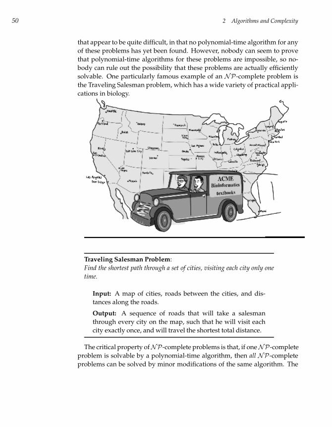
50 2 Algorithms and Complexity
that appear to be quite difficult, in that no polynomial-time algorithm for any
of these problems has yet been found. However, nobody can seem to prove
that polynomial-time algorithms for these problems are impossible, so no-
body can rule out the possibility that these problems are actually efficiently
solvable. One particularly famous example of an NP-complete problem is
the Traveling Salesman problem, which has a wide variety of practical appli-
cations in biology.
Traveling Salesman Problem:
Find the shortest path through a set of cities, visiting each city only one
time.
Input: A map of cities, roads between the cities, and dis-
tances along the roads.
Output: A sequence of roads that will take a salesman
through every city on the map, such that he will visit each
city exactly once, and will travel the shortest total distance.
The critical property ofNP-complete problems is that, if oneNP-complete
problem is solvable by a polynomial-time algorithm, then all NP-complete
problems can be solved by minor modifications of the same algorithm. The

2.11 Notes 51
fact that nobody has yet found that magic algorithm, after half a century
of research, suggests that it may not exist. However, this has not yet been
proven mathematically. It turns out that thousands of algorithmic prob-
lems are actually instances of the Traveling Salesman problems in disguise.19
Taken together, these problems form the class of NP-complete problems.
Despite the lack of mathematical proof, attempting to find a polynomial al-
gorithm for anNP-complete problem will likely result in failure and a whole
lot of wasted time. Unfortunately, proving that a problem really is NP-
complete, and not just superficially difficult, is somewhat of an undertaking.
In fact, it is not yet known whether or not some important bioinformatics
problems areNP-complete.
2.11 Notes
The word “algorithm” derived from the name of the ninth-century Arab
mathematician, al-Khwarizmi, of the court of Caliph Mamun in Baghdad.
al-Khwarizmi was a scholar in the House of Wisdom, where Greek scientific
works were translated; much of the mathematical knowledge in medieval
Europe was derived from Latin translations of his books. More recent books
on the general topic of algorithms are Knuth, 1998 (57); Aho, Hopcroft, and
Ullman, 1983 (1); and Cormen et al., 2001 (24).
The notion ofNP-completeness was proposed in the early 1970s by Steph-
en Cook (23), and Leonid Levin (65), and was further analyzed by Richard
Karp in 1972 (53) who demonstrated a rich variety of NP-complete prob-
lems. Garey and Johnson (39) authored an encyclopedic reference of NP-
complete problems.
19. Although these problems may have nothing in common with the Traveling Salesmanproblem—no cities, no roads, no distances—the Traveling Salesman problem can be convertedinto each one, and vice versa.
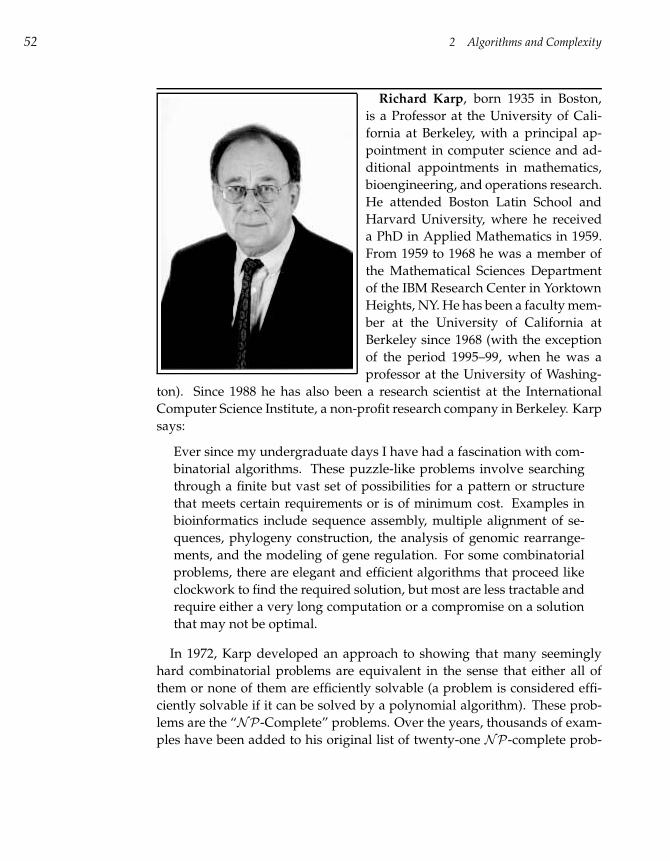
52 2 Algorithms and Complexity
Richard Karp, born 1935 in Boston,
is a Professor at the University of Cali-
fornia at Berkeley, with a principal ap-
pointment in computer science and ad-
ditional appointments in mathematics,
bioengineering, and operations research.
He attended Boston Latin School and
Harvard University, where he received
a PhD in Applied Mathematics in 1959.
From 1959 to 1968 he was a member of
the Mathematical Sciences Department
of the IBM Research Center in Yorktown
Heights, NY. He has been a faculty mem-
ber at the University of California at
Berkeley since 1968 (with the exception
of the period 1995–99, when he was a
professor at the University of Washing-
ton). Since 1988 he has also been a research scientist at the International
Computer Science Institute, a non-profit research company in Berkeley. Karp
says:
Ever since my undergraduate days I have had a fascination with com-
binatorial algorithms. These puzzle-like problems involve searching
through a finite but vast set of possibilities for a pattern or structure
that meets certain requirements or is of minimum cost. Examples in
bioinformatics include sequence assembly, multiple alignment of se-
quences, phylogeny construction, the analysis of genomic rearrange-
ments, and the modeling of gene regulation. For some combinatorial
problems, there are elegant and efficient algorithms that proceed like
clockwork to find the required solution, but most are less tractable and
require either a very long computation or a compromise on a solution
that may not be optimal.
In 1972, Karp developed an approach to showing that many seemingly
hard combinatorial problems are equivalent in the sense that either all of
them or none of them are efficiently solvable (a problem is considered effi-
ciently solvable if it can be solved by a polynomial algorithm). These prob-
lems are the “NP-Complete” problems. Over the years, thousands of exam-
ples have been added to his original list of twenty-one NP-complete prob-
2.11 Notes 53
lems, yet despite intensive effort none of these problems has been shown to
be efficiently solvable. Many computer scientists (including Karp) believe
that none of them ever will be.
Karp began working in bioinformatics circa 1991, attracted by the belief
that computational methods might reveal the secret inner workings of living
organisms. He says:
[I hoped] that my experience in studying combinatorial algorithms
could be useful in cracking those secrets. I have indeed been able to ap-
ply my skills in this new area, but only after coming to understand that
solving biological problems requires far more than clever algorithms:
it involves a creative partnership between biologists and mathematical
scientists to arrive at an appropriate mathematical model, the acquisi-
tion and use of diverse sources of data, and statistical methods to show
that the biological patterns and regularities that we discover could not
be due to chance. My recent work is concerned with analyzing the
transcriptional regulation of genes, discovering conserved regulatory
pathways, and analyzing genetic variation in humans.
There have been spectacular advances in biology since 1991, most no-
table being the sequencing of genomes. I believe that we are now
poised to understand—and possibly even reprogram— the gene reg-
ulatory networks and the metabolic networks that control cellular pro-
cesses. By comparing many related organisms, we hope to understand
how these networks evolved. Effectively, we are trying to find the ge-
netic basis of complex diseases so that we can develop more effective
modes of treatment.
54 2 Algorithms and Complexity
2.12 Problems
Problem 2.1
Write an algorithm that, given a list of n numbers, returns the largest and smallestnumbers in the list. Estimate the running time of the algorithm. Can you designan algorithm that performs only 3n/2 comparisons to find the smallest and largestnumbers in the list?
Problem 2.2
Write two algorithms that iterate over every index from (0, 0, . . . , 0) to (n1, n2, . . . , nd).Make one algorithm recursive, and the other iterative.
Problem 2.3
Is log n = O(n)? Is log n = Ω(n)? Is log n = Θ(n)?
Problem 2.4
You are given an unsorted list of n− 1 distinct integers from the range 1 to n. Write alinear-time algorithm to find the missing integer.
Problem 2.5
Though FIBONACCI(n) is fast, it uses a fair amount of space to store the array F.How much storage will it require to calculate the nth Fibonacci number? Modify thealgorithm to require a constant amount of storage, regardless of the value of n.
Problem 2.6
Prove that
Fn =1√5(φn − φ
n)
where Fn is the nth Fibonacci number, φ = 1+√
52
and φ = 1−√
52
.
Problem 2.7
Design an algorithm for computing the n-th Fibonacci number that requires less thanO(n) time. Hint: You probably want to use the result from problem 2.6. However,computing φn naively still requires O(n) time because each multiplication is a singleoperation.
Problem 2.8
Propose a more realistic model of rabbit life (and death) that limits the life span of rab-bits by k years. For example, if k = 2.5, then the corresponding sequence 1, 1, 2, 3, 4grows more slowly than the Fibonacci seqence. Write a recurrence relation and pseu-docode to compute the number of rabbits under this model. Will the number of rab-bits ever exceed the number of atoms in the universe (under these assumptions)?
Problem 2.9
Write an iterative (i.e., nonrecursive) algorithm to solve the Hanoi Tower problem.
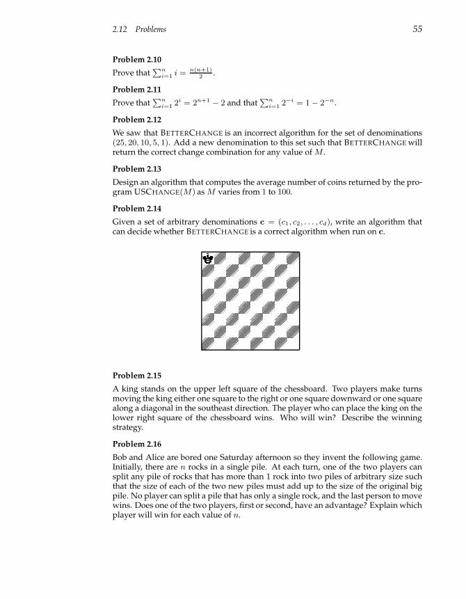
2.12 Problems 55
Problem 2.10
Prove thatPn
i=1 i = n(n+1)2
.
Problem 2.11
Prove thatPn
i=1 2i = 2n+1 − 2 and thatPn
i=1 2−i = 1− 2−n.
Problem 2.12
We saw that BETTERCHANGE is an incorrect algorithm for the set of denominations(25, 20, 10, 5, 1). Add a new denomination to this set such that BETTERCHANGE willreturn the correct change combination for any value of M .
Problem 2.13
Design an algorithm that computes the average number of coins returned by the pro-gram USCHANGE(M) as M varies from 1 to 100.
Problem 2.14
Given a set of arbitrary denominations c = (c1, c2, . . . , cd), write an algorithm thatcan decide whether BETTERCHANGE is a correct algorithm when run on c.
Problem 2.15
A king stands on the upper left square of the chessboard. Two players make turnsmoving the king either one square to the right or one square downward or one squarealong a diagonal in the southeast direction. The player who can place the king on thelower right square of the chessboard wins. Who will win? Describe the winningstrategy.
Problem 2.16
Bob and Alice are bored one Saturday afternoon so they invent the following game.Initially, there are n rocks in a single pile. At each turn, one of the two players cansplit any pile of rocks that has more than 1 rock into two piles of arbitrary size suchthat the size of each of the two new piles must add up to the size of the original bigpile. No player can split a pile that has only a single rock, and the last person to movewins. Does one of the two players, first or second, have an advantage? Explain whichplayer will win for each value of n.
56 2 Algorithms and Complexity
Problem 2.17
There are n bacteria and 1 virus in a Petri dish. Within the first minute, the virus killsone bacterium and produces another copy of itself, and all of the remaining bacteriareproduce, making 2 viruses and 2 · (n − 1) bacteria. In the second minute, each ofthe viruses kills a bacterium and produces a new copy of itself (resulting in 4 virusesand 2(2(n− 1) − 2) = 4n− 8 bacteria; again, the remaining bacteria reproduce. Thisprocess continues every minute. Will the viruses eventually kill all the bacteria? Ifso, design an algorithm that computes how many steps it will take. How does therunning time of your algorithm depend on n?
Problem 2.18
A very large bioinformatics department at a prominent university has a mix of 100professors: some are honest and hard-working, while others are deceitful and donot like students. The honest professors always tell the truth, but the deceitful onessometimes tell the truth and sometimes lie. You can ask any professors the followingquestion about any other professor: “Professor Y , is Professor X honest?” ProfessorY will answer with either “yes” or “no.” Design an algorithm that, with no more than198 questions, would allow you to figure out which of the 100 professors are honest(thus identifying possible research advisors). It is known that there are more honestthan dishonest professors.
Problem 2.19
You are given an 8 × 8 table of natural numbers. In any one step, you can eitherdouble each of the numbers in any one row, or subtract 1 from each of the numbersin any one column. Devise an algorithm that transforms the original table into a tableof all zeros. What is the running time of your algorithm?
Problem 2.20
There are n black, m green, and k brown chameleons on a deserted island. When twochameleons of different colors meet they both change their color to the third one (e.g.,black and green chameleons become brown). For each choice of n, m, and k decidewhether it is possible that after some time all the chameleons on the island are thesame color (if you think that it is always possible, check the case n = 1, m = 3, andk = 5).
3 Molecular Biology Primer
To understand bioinformatics in any meaningful way, it is necessary for a
computer scientist to understand some basic biology, just as it is necessary
for a biologist to understand some basic computer science. This chapter pro-
vides a short and informal introduction to those biological fundamentals.
We scanned existing bioinformatics books to find out how much biological
material was “relevant” to those books and we were surprised how little
biological knowledge was actually presented. It would be safe to say that
the minimum biological background one needs in order to digest a typical
bioinformatics book could fit into ten pages.1 In this chapter we give a brief
introduction to biology that covers most of the computational concepts dis-
cussed in bioinformatics books. Some of the sections in this chapter are not
directly related to the rest of the book, but we present them to convey the
fascinating story of molecular biology in the twentieth century.
3.1 What Is Life Made Of?
Biology at the microscopic level began in 1665 when a maverick and virtu-
oso performer of public animal dissections, Robert Hooke, discovered that
organisms are composed of individual compartments called cells. Cell the-
ory, further advanced by Matthias Schleiden and Theodor Schwann in the
1830s, marked an important milestone: it turned biology into a science be-
yond the reach of the naked eye. In many ways, the study of life became the
study of cells.
1. This is not to say that computer scientists should limit themselves to these ten pages. Moredetailed discussions can be found in introductory biology textbooks like Brown (17), Lewin (66),or Alberts (3).
58 3 Molecular Biology Primer
A great diversity of cells exist in nature, but they all have some common
features. All cells have a life cycle: they are born, eat, replicate, and die. Dur-
ing the life cycle, a cell has to make many important decisions. For example,
if a cell were to attempt to replicate before it had collected all of the neces-
sary nutrients to do so, the result would be a disaster. However, cells do not
have brains. Instead, these decisions are manifested in complex networks
of chemical reactions, called pathways, that synthesize new materials, break
other materials down for spare parts, or signal that the time has come to eat
or die. The amazingly reliable and complex algorithm that controls the life
of the cell is still beyond our comprehension.
One can envision a cell as a complex mechanical system with many mov-
ing parts. Not only does it store all of the information necessary to make a
complete replica of itself, it also contains all the machinery required to collect
and manufacture its components, carry out the copying process, and kick-
start its new offspring. In macroscopic terms, a cell would be roughly anal-
ogous to a car factory that could mine for ore, fabricate girders and concrete
pillars, and assemble an exact working copy of itself, all the while building
family sedans with no human intervention.
Despite the complexity of a cell, there seems to be a few organizing princi-
ples that are conserved across all organisms. All life on this planet depends
on three types of molecule: DNA, RNA, and proteins.2 Roughly speaking,
a cell’s DNA holds a vast library describing how the cell works. RNA acts
to transfer certain short pieces of this library to different places in the cell,
at which point those smaller volumes of information are used as templates
to synthesize proteins. Proteins form enzymes that perform biochemical re-
actions, send signals to other cells, form the body’s major components (like
the keratin in our skin), and otherwise perform the actual work of the cell.
DNA, RNA, and proteins are examples of strings written in either the four-
letter alphabet of DNA and RNA or the twenty-letter alphabet of proteins.
This meshes well with Schrödinger’s visionary idea about an “instruction
book” of life scribbled in a secret code. It took a long time to figure out that
DNA, RNA, and proteins are the main players in the cells. Below we give a
brief summary of how this was discovered.
2. To be sure, other types of molecules, like lipids, play a critical role in maintaining the cell’sstructure, but DNA, RNA, and proteins are the three primary types of molecules that biologistsstudy.
3.2 What Is the Genetic Material? 59
3.2 What Is the Genetic Material?
Schleiden’s and Schwann’s studies of cells were further advanced by the
discovery of threadlike chromosomes in the cell nucleii. Different organ-
isms have different numbers of chromosomes, suggesting that they might
carry information specific for each species. This fit well with the work of
the Augustinian monk Gregor Mendel in the 1860s, whose experiments with
garden peas suggested the existence of genes that were responsible for in-
heritance. Evidence that traits (more precisely, genes) are located on chro-
mosomes came in the 1920s through the work of Thomas Morgan. Unlike
Mendel, Morgan worked in New York City and lacked the garden space to
cultivate peas, so he instead used fruit flies for his experiments: they have
a short life span and produce numerous offspring. One of these offspring
turned out to have white eyes, whereas wild flies had red eyes. This one
white-eyed male fly born in Morgan’s “fly room” in New York City became
the cornerstone of modern genetics.
The white-eyed male fly was mated with its red-eyed sisters and the off-
spring were followed closely for a few generations. The analysis of offspring
revealed that white eyes appeared predominantly in males, suggesting that
a gene for eye color resides on the X chromosome (which partly determines
the gender of a fruit fly). Thus, Morgan suspected that genes were located
on chromosomes. Of course, Morgan had no idea what chromosomes were
themselves made of.
Morgan and his students proceeded to identify other mutations in flies and
used ever more sophisticated techniques to assign these mutations to certain
locations on chromosomes. Morgan postulated that the genes somehow re-
sponsible for these mutations were also positioned at these locations. His
group showed that certain genes are inherited together, as if they were a sin-
gle unit. For example, Morgan identified mutants with a black body color
(normal flies are gray) and mutants with vestigial wings. He proceeded to
cross black flies with vestigial wings with gray flies with normal wings, ex-
pecting to see a number of gray flies with vestigial wings, gray flies with
normal wings, black flies with vestigial wings, and black flies with normal
wings. However, the experiment produced a surprisingly large number of
normal flies (gray body, normal wings) and a surprisingly large number
of double mutants (black body, vestigial wings). Morgan immediately pro-
posed a hypothesis that such linked genes reside close together on a chromo-
some. Moreover, he theorized, the more tightly two genes are linked (i.e., the
more often they are inherited together), the closer they are on a chromosome.
60 3 Molecular Biology Primer
Morgan’s student Alfred Sturtevant pursued Morgan’s chromosome the-
ory and constructed the first genetic map of a chromosome that showed the
order of genes. Sturtevant studied three genes: cn, which determines eye
color; b, which determines body color; and vg, which determines wing size.
Sturtevant crossed double-mutant b and vg flies with normal flies and saw
that about 17% of the offspring had only a single mutation. However, when
Sturtevant crossed double-mutant b and cn flies he found that 9% of the off-
spring had only a single mutation. This implied that b and cn reside closer
together than b and vg; a further experiment with cn and vg mutants demon-
strated an 8% single mutation rate. Combined together, these three observa-
tions showed that b lies on one side of cn and vg on the other. By studying
many genes in this way, it is possible to determine the ordering of genes.
However, the nature of genes remained an elusive and abstract concept for
many years, since it was not clear how genes encoded information and how
they passed that information to the organism’s progeny.
3.3 What Do Genes Do?
By the early 1940s, biologists understood that a cell’s traits were inherent
in its genetic information, that the genetic information was passed to its
offspring, and that the genetic information was organized into genes that
resided on chromosomes. They did not know what the chromosomes were
made of or what the genes actually did to give rise to a cell’s traits. George
Beadle and Edward Tatum were the first to identify the job of the gene, with-
out actually revealing the true nature of genetic information. They worked
with the bread mold Neurospora, which can survive by consuming very sim-
ple nutrients like sucrose and salt. To be able to live on such a limited diet,
Neurospora must have some proteins (enzymes) that are able to convert these
simple nutrients into “real food” like amino acids and the other molecules
necessary for life. It was known that proteins performed this type of chemi-
cal “work” in the cell.
In 1941 Beadle and Tatum irradiated Neurospora with x-rays and examined
its growth on the usual “spartan” medium. Not surprisingly, some irradiated
Neurospora spores failed to grow on this diet. Beadle and Tatum conjectured
that x-rays introduced some mutations that possibly “destroyed” one of the
genes responsible for processing Neurospora’s diet into real food. Which par-
ticular gene was destroyed remained unclear, but one of the experiments
revealed that the irradiated Neurospora survived and even flourished when
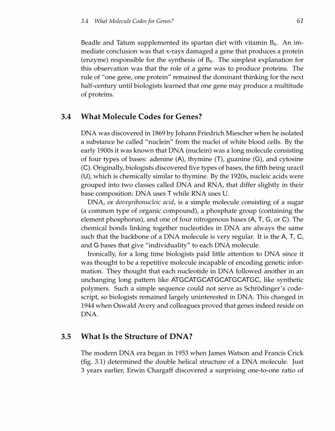
3.4 What Molecule Codes for Genes? 61
Beadle and Tatum supplemented its spartan diet with vitamin B6. An im-
mediate conclusion was that x-rays damaged a gene that produces a protein
(enzyme) responsible for the synthesis of B6. The simplest explanation for
this observation was that the role of a gene was to produce proteins. The
rule of “one gene, one protein” remained the dominant thinking for the next
half-century until biologists learned that one gene may produce a multitude
of proteins.
3.4 What Molecule Codes for Genes?
DNA was discovered in 1869 by Johann Friedrich Miescher when he isolated
a substance he called “nuclein” from the nuclei of white blood cells. By the
early 1900s it was known that DNA (nuclein) was a long molecule consisting
of four types of bases: adenine (A), thymine (T), guanine (G), and cytosine
(C). Originally, biologists discovered five types of bases, the fifth being uracil
(U), which is chemically similar to thymine. By the 1920s, nucleic acids were
grouped into two classes called DNA and RNA, that differ slightly in their
base composition: DNA uses T while RNA uses U.
DNA, or deoxyribonucleic acid, is a simple molecule consisting of a sugar
(a common type of organic compound), a phosphate group (containing the
element phosphorus), and one of four nitrogenous bases (A, T, G, or C). The
chemical bonds linking together nucleotides in DNA are always the same
such that the backbone of a DNA molecule is very regular. It is the A, T, C,
and G bases that give “individuality” to each DNA molecule.
Ironically, for a long time biologists paid little attention to DNA since it
was thought to be a repetitive molecule incapable of encoding genetic infor-
mation. They thought that each nucleotide in DNA followed another in an
unchanging long pattern like ATGCATGCATGCATGCATGC, like synthetic
polymers. Such a simple sequence could not serve as Schrödinger’s code-
script, so biologists remained largely uninterested in DNA. This changed in
1944 when Oswald Avery and colleagues proved that genes indeed reside on
DNA.
3.5 What Is the Structure of DNA?
The modern DNA era began in 1953 when James Watson and Francis Crick
(fig. 3.1) determined the double helical structure of a DNA molecule. Just
3 years earlier, Erwin Chargaff discovered a surprising one-to-one ratio of
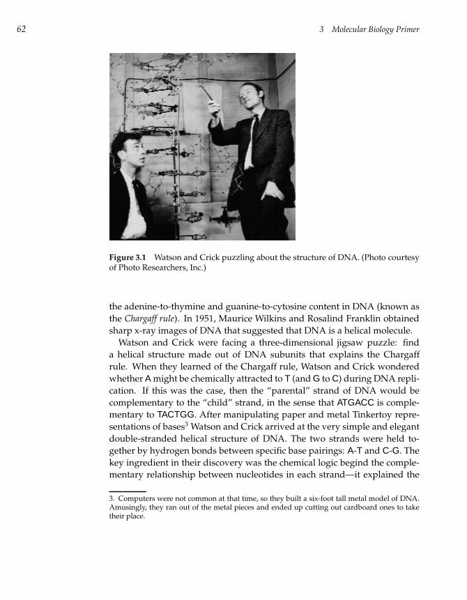
62 3 Molecular Biology Primer
Figure 3.1 Watson and Crick puzzling about the structure of DNA. (Photo courtesyof Photo Researchers, Inc.)
the adenine-to-thymine and guanine-to-cytosine content in DNA (known as
the Chargaff rule). In 1951, Maurice Wilkins and Rosalind Franklin obtained
sharp x-ray images of DNA that suggested that DNA is a helical molecule.
Watson and Crick were facing a three-dimensional jigsaw puzzle: find
a helical structure made out of DNA subunits that explains the Chargaff
rule. When they learned of the Chargaff rule, Watson and Crick wondered
whether A might be chemically attracted to T (and G to C) during DNA repli-
cation. If this was the case, then the “parental” strand of DNA would be
complementary to the “child” strand, in the sense that ATGACC is comple-
mentary to TACTGG. After manipulating paper and metal Tinkertoy repre-
sentations of bases3 Watson and Crick arrived at the very simple and elegant
double-stranded helical structure of DNA. The two strands were held to-
gether by hydrogen bonds between specific base pairings: A-T and C-G. The
key ingredient in their discovery was the chemical logic begind the comple-
mentary relationship between nucleotides in each strand—it explained the
3. Computers were not common at that time, so they built a six-foot tall metal model of DNA.Amusingly, they ran out of the metal pieces and ended up cutting out cardboard ones to taketheir place.
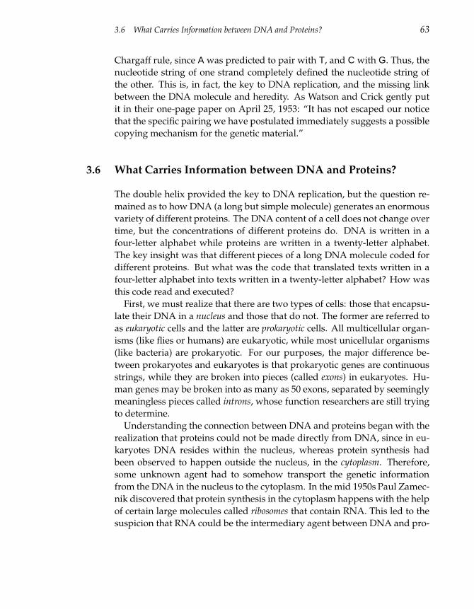
3.6 What Carries Information between DNA and Proteins? 63
Chargaff rule, since A was predicted to pair with T, and C with G. Thus, the
nucleotide string of one strand completely defined the nucleotide string of
the other. This is, in fact, the key to DNA replication, and the missing link
between the DNA molecule and heredity. As Watson and Crick gently put
it in their one-page paper on April 25, 1953: “It has not escaped our notice
that the specific pairing we have postulated immediately suggests a possible
copying mechanism for the genetic material.”
3.6 What Carries Information between DNA and Proteins?
The double helix provided the key to DNA replication, but the question re-
mained as to how DNA (a long but simple molecule) generates an enormous
variety of different proteins. The DNA content of a cell does not change over
time, but the concentrations of different proteins do. DNA is written in a
four-letter alphabet while proteins are written in a twenty-letter alphabet.
The key insight was that different pieces of a long DNA molecule coded for
different proteins. But what was the code that translated texts written in a
four-letter alphabet into texts written in a twenty-letter alphabet? How was
this code read and executed?
First, we must realize that there are two types of cells: those that encapsu-
late their DNA in a nucleus and those that do not. The former are referred to
as eukaryotic cells and the latter are prokaryotic cells. All multicellular organ-
isms (like flies or humans) are eukaryotic, while most unicellular organisms
(like bacteria) are prokaryotic. For our purposes, the major difference be-
tween prokaryotes and eukaryotes is that prokaryotic genes are continuous
strings, while they are broken into pieces (called exons) in eukaryotes. Hu-
man genes may be broken into as many as 50 exons, separated by seemingly
meaningless pieces called introns, whose function researchers are still trying
to determine.
Understanding the connection between DNA and proteins began with the
realization that proteins could not be made directly from DNA, since in eu-
karyotes DNA resides within the nucleus, whereas protein synthesis had
been observed to happen outside the nucleus, in the cytoplasm. Therefore,
some unknown agent had to somehow transport the genetic information
from the DNA in the nucleus to the cytoplasm. In the mid 1950s Paul Zamec-
nik discovered that protein synthesis in the cytoplasm happens with the help
of certain large molecules called ribosomes that contain RNA. This led to the
suspicion that RNA could be the intermediary agent between DNA and pro-
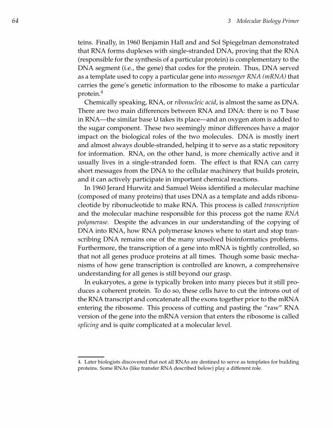
64 3 Molecular Biology Primer
teins. Finally, in 1960 Benjamin Hall and and Sol Spiegelman demonstrated
that RNA forms duplexes with single-stranded DNA, proving that the RNA
(responsible for the synthesis of a particular protein) is complementary to the
DNA segment (i.e., the gene) that codes for the protein. Thus, DNA served
as a template used to copy a particular gene into messenger RNA (mRNA) that
carries the gene’s genetic information to the ribosome to make a particular
protein.4
Chemically speaking, RNA, or ribonucleic acid, is almost the same as DNA.
There are two main differences between RNA and DNA: there is no T base
in RNA—the similar base U takes its place—and an oxygen atom is added to
the sugar component. These two seemingly minor differences have a major
impact on the biological roles of the two molecules. DNA is mostly inert
and almost always double-stranded, helping it to serve as a static repository
for information. RNA, on the other hand, is more chemically active and it
usually lives in a single-stranded form. The effect is that RNA can carry
short messages from the DNA to the cellular machinery that builds protein,
and it can actively participate in important chemical reactions.
In 1960 Jerard Hurwitz and Samuel Weiss identified a molecular machine
(composed of many proteins) that uses DNA as a template and adds ribonu-
cleotide by ribonucleotide to make RNA. This process is called transcription
and the molecular machine responsible for this process got the name RNA
polymerase. Despite the advances in our understanding of the copying of
DNA into RNA, how RNA polymerase knows where to start and stop tran-
scribing DNA remains one of the many unsolved bioinformatics problems.
Furthermore, the transcription of a gene into mRNA is tightly controlled, so
that not all genes produce proteins at all times. Though some basic mecha-
nisms of how gene transcription is controlled are known, a comprehensive
understanding for all genes is still beyond our grasp.
In eukaryotes, a gene is typically broken into many pieces but it still pro-
duces a coherent protein. To do so, these cells have to cut the introns out of
the RNA transcript and concatenate all the exons together prior to the mRNA
entering the ribosome. This process of cutting and pasting the “raw” RNA
version of the gene into the mRNA version that enters the ribosome is called
splicing and is quite complicated at a molecular level.
4. Later biologists discovered that not all RNAs are destined to serve as templates for buildingproteins. Some RNAs (like transfer RNA described below) play a different role.
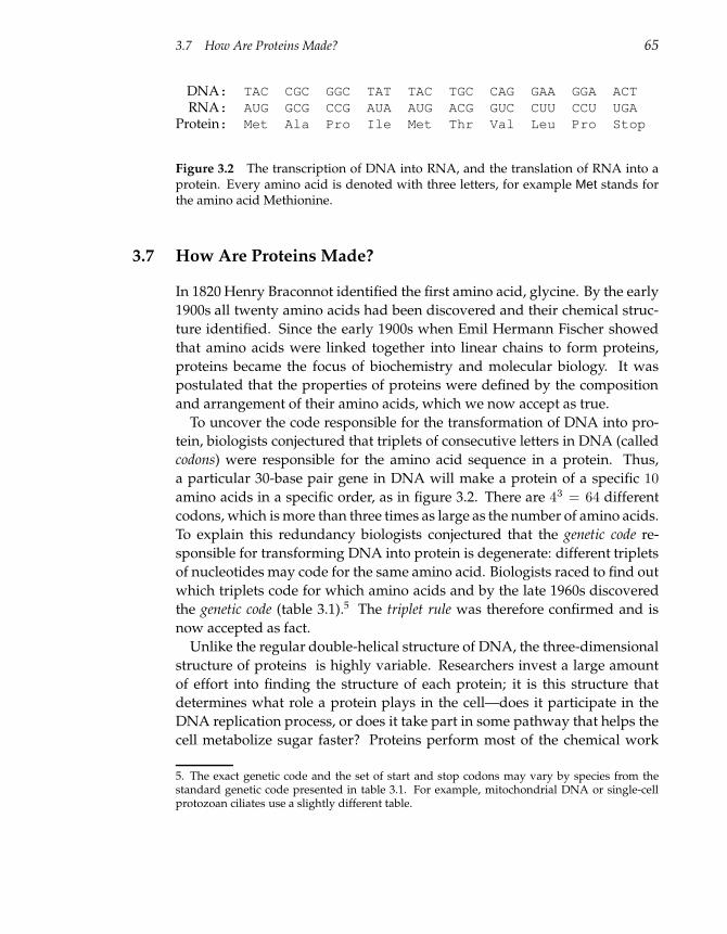
3.7 How Are Proteins Made? 65
DNA: TAC CGC GGC TAT TAC TGC CAG GAA GGA ACTRNA: AUG GCG CCG AUA AUG ACG GUC CUU CCU UGA
Protein: Met Ala Pro Ile Met Thr Val Leu Pro Stop
Figure 3.2 The transcription of DNA into RNA, and the translation of RNA into aprotein. Every amino acid is denoted with three letters, for example Met stands forthe amino acid Methionine.
3.7 How Are Proteins Made?
In 1820 Henry Braconnot identified the first amino acid, glycine. By the early
1900s all twenty amino acids had been discovered and their chemical struc-
ture identified. Since the early 1900s when Emil Hermann Fischer showed
that amino acids were linked together into linear chains to form proteins,
proteins became the focus of biochemistry and molecular biology. It was
postulated that the properties of proteins were defined by the composition
and arrangement of their amino acids, which we now accept as true.
To uncover the code responsible for the transformation of DNA into pro-
tein, biologists conjectured that triplets of consecutive letters in DNA (called
codons) were responsible for the amino acid sequence in a protein. Thus,
a particular 30-base pair gene in DNA will make a protein of a specific 10
amino acids in a specific order, as in figure 3.2. There are 43 = 64 different
codons, which is more than three times as large as the number of amino acids.
To explain this redundancy biologists conjectured that the genetic code re-
sponsible for transforming DNA into protein is degenerate: different triplets
of nucleotides may code for the same amino acid. Biologists raced to find out
which triplets code for which amino acids and by the late 1960s discovered
the genetic code (table 3.1).5 The triplet rule was therefore confirmed and is
now accepted as fact.
Unlike the regular double-helical structure of DNA, the three-dimensional
structure of proteins is highly variable. Researchers invest a large amount
of effort into finding the structure of each protein; it is this structure that
determines what role a protein plays in the cell—does it participate in the
DNA replication process, or does it take part in some pathway that helps the
cell metabolize sugar faster? Proteins perform most of the chemical work
5. The exact genetic code and the set of start and stop codons may vary by species from thestandard genetic code presented in table 3.1. For example, mitochondrial DNA or single-cellprotozoan ciliates use a slightly different table.
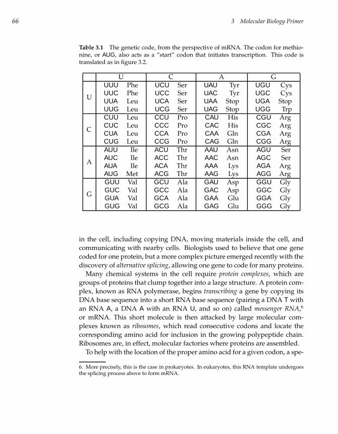
66 3 Molecular Biology Primer
Table 3.1 The genetic code, from the perspective of mRNA. The codon for methio-nine, or AUG, also acts as a “start” codon that initiates transcription. This code istranslated as in figure 3.2.
U C A G
U
UUU PheUUC PheUUA LeuUUG Leu
UCU SerUCC SerUCA SerUCG Ser
UAU TyrUAC TyrUAA StopUAG Stop
UGU CysUGC CysUGA StopUGG Trp
C
CUU LeuCUC LeuCUA LeuCUG Leu
CCU ProCCC ProCCA ProCCG Pro
CAU HisCAC HisCAA GlnCAG Gln
CGU ArgCGC ArgCGA ArgCGG Arg
A
AUU IleAUC IleAUA IleAUG Met
ACU ThrACC ThrACA ThrACG Thr
AAU AsnAAC AsnAAA LysAAG Lys
AGU SerAGC SerAGA ArgAGG Arg
G
GUU ValGUC ValGUA ValGUG Val
GCU AlaGCC AlaGCA AlaGCG Ala
GAU AspGAC AspGAA GluGAG Glu
GGU GlyGGC GlyGGA GlyGGG Gly
in the cell, including copying DNA, moving materials inside the cell, and
communicating with nearby cells. Biologists used to believe that one gene
coded for one protein, but a more complex picture emerged recently with the
discovery of alternative splicing, allowing one gene to code for many proteins.
Many chemical systems in the cell require protein complexes, which are
groups of proteins that clump together into a large structure. A protein com-
plex, known as RNA polymerase, begins transcribing a gene by copying its
DNA base sequence into a short RNA base sequence (pairing a DNA T with
an RNA A, a DNA A with an RNA U, and so on) called messenger RNA,6
or mRNA. This short molecule is then attacked by large molecular com-
plexes known as ribosomes, which read consecutive codons and locate the
corresponding amino acid for inclusion in the growing polypeptide chain.
Ribosomes are, in effect, molecular factories where proteins are assembled.
To help with the location of the proper amino acid for a given codon, a spe-
6. More precisely, this is the case in prokaryotes. In eukaryotes, this RNA template undergoesthe splicing process above to form mRNA.
3.8 How Can We Analyze DNA? 67
cial type of RNA, called transfer RNA (tRNA), performs a specific and elegant
function. There are twenty types of tRNAs, and twenty types of amino acids.
Each type of amino acid binds to a different tRNA, and the tRNA molecules
have a three-base segment (called an anticodon) that is complementary to the
codon in the mRNA. As in DNA base-pairing, the anticodon on the tRNA
sticks to the codon on the RNA, which makes the amino acid available to the
ribosome to add to the polypeptide chain. When one amino acid has been
added, the ribosome shifts one codon to the right, and the process repeats.
The process of turning an mRNA into a protein is called translation, since it
translates information from the RNA (written in a four-letter alphabet) into
the protein (written in 20-letter alphabet). All proteins, including the ones
necessary for this process, are produced by this process.
This flow of information,
DNA→ transcription→ RNA→ translation→ protein,
is emphatically referred to as the central dogma in molecular biology.
3.8 How Can We Analyze DNA?
Over the years, biologists have learned how to analyze DNA. Below we de-
scribe some important techniques for copying, cutting, pasting, measuring,
and probing DNA.
3.8.1 Copying DNA
Why does one need to copy DNA, that is, to obtain a large number of identi-
cal DNA fragments? From a computer science perspective, having the same
string in 109 copies does not mean much since it does not increase the to-
tal amount of information. However, most experimental techniques (like gel
electrophoresis, used for measuring DNA length) require many copies of the
same DNA fragment. Since it is difficult to detect a single molecule or even a
hundred molecules with modern instrumentation, amplifying DNA to yield
millions or billions of identical copies is often a prerequisite of further anal-
ysis.
One method, polymerase chain reaction or PCR, is the Gutenberg printing
press for DNA and is illustrated in figure 3.3. PCR amplifies a short (100-
to 500-nucleotide) DNA fragment and produces a large number of identical
DNA strings. To use PCR, one must know a pair of short (20- to 30-letter)
68 3 Molecular Biology Primer
strings in the DNA flanking the area of interest and design two PCR primers,
synthetic DNA fragments identical to these strings.
Suppose we want to generate a billion copies of a DNA fragment of 500
nucleotides, that we know happens to be flanked by the 20-mer nucleotide
sequence X on the left and the 20-mer nucleotide sequence Y on the right.
PCR repeats a cycle of three operations: denaturation, priming, and extension
to double the number of DNA fragments in every iteration. Therefore, after
thirty iterations of PCR we will have on the order of 230 DNA fragments,
which is more than a billion copies. To start PCR, we only need a single copy
of the target DNA, some artificially synthesized 20-nucleotide long DNA
fragment X (many copies), some 20-nucleotide long DNA fragment Y (many
copies), and billions of “spare” nucleotides (A,T,G,C).7 We also need a molec-
ular machine that will copy an existing DNA strand to produce a new DNA
strand, and for this purpose we hijack DNA polymerase. DNA polymerase
has an ability to add a complementary copy to a single-stranded DNA as
long as there is a primer (i.e., X and Y ) attached to the DNA strand and a
sufficient supply of spare nucleotides
The denaturation step simply amounts to heating double-stranded DNA
to separate it into two single strands (fig. 3.3 (top)). Priming is cooling down
the solution to allow primers X and Y to hybridize to their complemen-
tary positions in DNA (fig. 3.3 (middle)). In the extension step, DNA poly-
merase extends the primer to produce two double-stranded DNA copies
from single-stranded DNA (fig. 3.3 (bottom)). By repeatedly performing
these three steps, one achieves an exponential increase in the amount of
DNA, as shown in figure 3.4.
Another way to copy DNA is to clone it. In contrast to PCR, cloning does
not require any prior information about flanking primers. However, biolo-
gists usually have no control over which fragment of DNA gets amplified.
The process usually starts with breaking DNA into small pieces; to study
an individual piece, biologists obtain many identical copies of each piece
by cloning the pieces, and then try to select the individual piece of inter-
est. Cloning incorporates a fragment of DNA into a cloning vector, which is
a DNA molecule originating from a virus or bacterium. In this operation,
the cloning vector does not lose its ability for self-replication, but carries the
additional incorporated insert that the biologist plans to study. Vectors intro-
duce foreign DNA into host cells (such as bacteria) which reproduce in large
quantities. The self-replication process creates a large number of copies of the
7. X stands for the Watson-Crick complement of the 20-mer X.
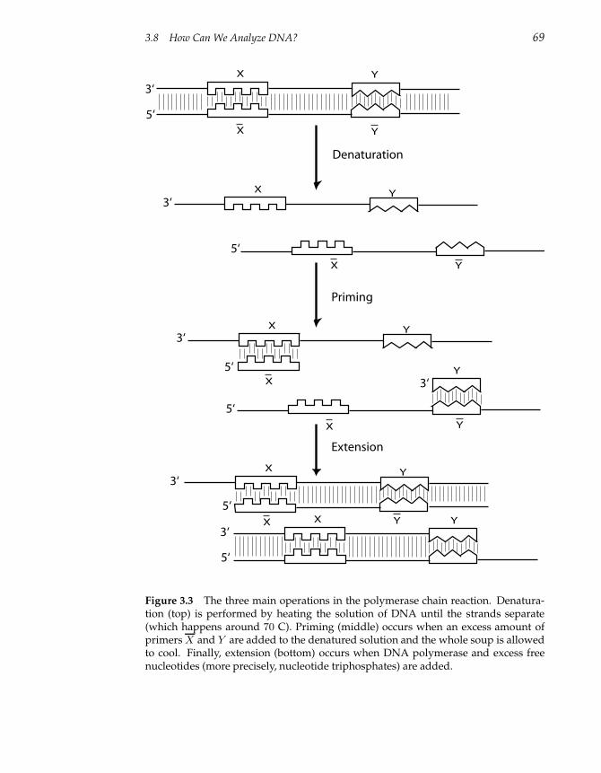
3.8 How Can We Analyze DNA? 69
X
X
Y
Y
X
X
X
Y
Y
X Y
X Y
X Y
Y
Y
X Y
X
Denaturation
Priming
Extension
3‘
3‘
3‘
3‘
5‘
3‘
5‘
3‘
5‘
5‘
5‘
5‘
Figure 3.3 The three main operations in the polymerase chain reaction. Denatura-tion (top) is performed by heating the solution of DNA until the strands separate(which happens around 70 C). Priming (middle) occurs when an excess amount ofprimers X and Y are added to the denatured solution and the whole soup is allowedto cool. Finally, extension (bottom) occurs when DNA polymerase and excess freenucleotides (more precisely, nucleotide triphosphates) are added.
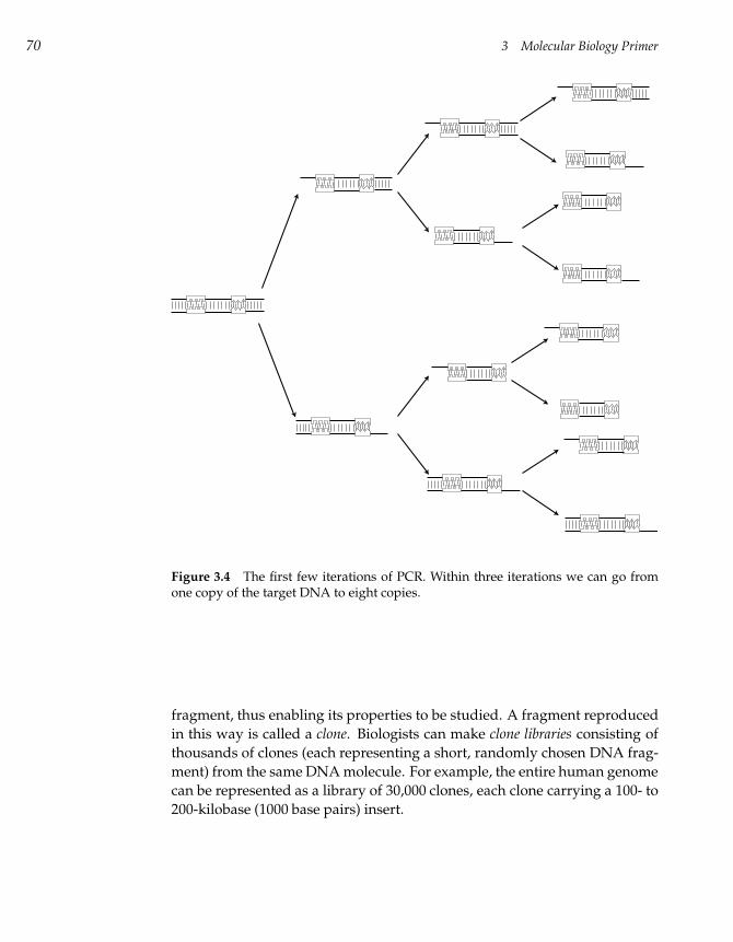
70 3 Molecular Biology Primer
Figure 3.4 The first few iterations of PCR. Within three iterations we can go fromone copy of the target DNA to eight copies.
fragment, thus enabling its properties to be studied. A fragment reproduced
in this way is called a clone. Biologists can make clone libraries consisting of
thousands of clones (each representing a short, randomly chosen DNA frag-
ment) from the same DNA molecule. For example, the entire human genome
can be represented as a library of 30,000 clones, each clone carrying a 100- to
200-kilobase (1000 base pairs) insert.
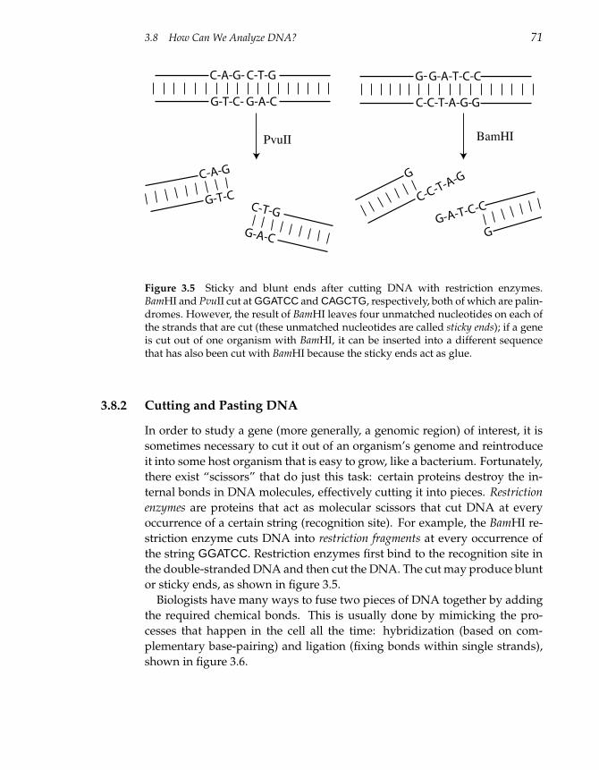
3.8 How Can We Analyze DNA? 71
G
C-C-T-A-G
G-A-T-C-C
G
G
C-C-T-A-G-
G-A-T-C-C
G
C-A-G
G-T-CC-T-G
G-A-C
C-A-G-
G-T-C-
C-T-G
G-A-C
PvuII BamHI
-
Figure 3.5 Sticky and blunt ends after cutting DNA with restriction enzymes.BamHI and PvuII cut at GGATCC and CAGCTG, respectively, both of which are palin-dromes. However, the result of BamHI leaves four unmatched nucleotides on each ofthe strands that are cut (these unmatched nucleotides are called sticky ends); if a geneis cut out of one organism with BamHI, it can be inserted into a different sequencethat has also been cut with BamHI because the sticky ends act as glue.
3.8.2 Cutting and Pasting DNA
In order to study a gene (more generally, a genomic region) of interest, it is
sometimes necessary to cut it out of an organism’s genome and reintroduce
it into some host organism that is easy to grow, like a bacterium. Fortunately,
there exist “scissors” that do just this task: certain proteins destroy the in-
ternal bonds in DNA molecules, effectively cutting it into pieces. Restriction
enzymes are proteins that act as molecular scissors that cut DNA at every
occurrence of a certain string (recognition site). For example, the BamHI re-
striction enzyme cuts DNA into restriction fragments at every occurrence of
the string GGATCC. Restriction enzymes first bind to the recognition site in
the double-stranded DNA and then cut the DNA. The cut may produce blunt
or sticky ends, as shown in figure 3.5.
Biologists have many ways to fuse two pieces of DNA together by adding
the required chemical bonds. This is usually done by mimicking the pro-
cesses that happen in the cell all the time: hybridization (based on com-
plementary base-pairing) and ligation (fixing bonds within single strands),
shown in figure 3.6.
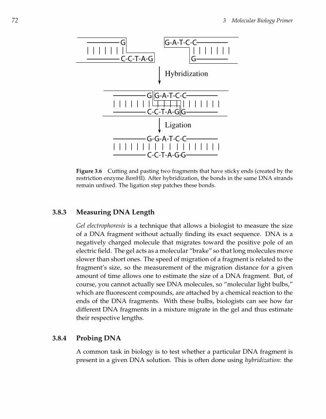
72 3 Molecular Biology Primer
G
C-C-T-A-G
G-A-T-C-C
G
G
C-C-T-A-G
G-A-T-C-C
G
G-
C-C-T-A-G-
G-A-T-C-C
G
Hybridization
Ligation
Figure 3.6 Cutting and pasting two fragments that have sticky ends (created by therestriction enzyme BamHI). After hybridization, the bonds in the same DNA strandsremain unfixed. The ligation step patches these bonds.
3.8.3 Measuring DNA Length
Gel electrophoresis is a technique that allows a biologist to measure the size
of a DNA fragment without actually finding its exact sequence. DNA is a
negatively charged molecule that migrates toward the positive pole of an
electric field. The gel acts as a molecular “brake” so that long molecules move
slower than short ones. The speed of migration of a fragment is related to the
fragment’s size, so the measurement of the migration distance for a given
amount of time allows one to estimate the size of a DNA fragment. But, of
course, you cannot actually see DNA molecules, so “molecular light bulbs,”
which are fluorescent compounds, are attached by a chemical reaction to the
ends of the DNA fragments. With these bulbs, biologists can see how far
different DNA fragments in a mixture migrate in the gel and thus estimate
their respective lengths.
3.8.4 Probing DNA
A common task in biology is to test whether a particular DNA fragment is
present in a given DNA solution. This is often done using hybridization: the
3.9 How Do Individuals of a Species Differ? 73
process of joining two complementary DNA strands into a single double-
stranded molecule. Biologists often use probes, which are single-stranded
DNA fragments 20 to 30 nucleotides long that have a known sequence and a
fluorescent tag. Hybridization of the probe to some unknown DNA fragment
of interest can show a biologist the presence of the probe’s complementary
sequence in the larger DNA fragment.8
We can also probe RNA using a DNA array to see if a gene is on or off.
A DNA array is essentially composed of “spots” bound to a solid support,
such as a glass slide. On each spot are many copies of the complement of one
gene’s mRNA transcript. If the mRNA content of a cell is poured onto this
slide, the mRNA will bind to the single-stranded spots and can be detected
with the light-bulb technique described eariler. As a result, biologists can
find out which genes are producing mRNA in a particular tissue under fixed
conditions.
3.9 How Do Individuals of a Species Differ?
The genetic makeup of an individual manifests itself in traits, such as hair
color, eye color, or susceptibility to malaria. Traits are caused by variations
in genes. A surprising observation is that, despite the near similarity of
genomes among all humans, no two individuals are quite the same. In fact,
the variations among the same gene across different individuals are limited
to a handful of different base pairs (if any). Roughly only 0.1% of the 3 billion
nucleotide human genome (or 3 million bases) are different between any two
individuals. Still, this leaves room for roughly 43,000,000 different genomes,
and is for all intents and purposes an endless diversity.
In other words, when we speak of “the” genome of a species, we are refer-
ring to some sort of “master” genome that is fairly representative of all the
possible genomes that an individual of that species could have. While spe-
cific individuals of the species may differ in some bases, the basic long DNA
sequence is roughly the same in all members of the species. Of course, this
handful of differences is critically important, and the large Human Diversity
Project is underway to understand how various individuals differ. This will
hopefully identify the mutations reponsible for a number of genetic diseases.
8. This is, essentially, a constant-time search of a database performed by molecular machines,something computer scientists only fantasize about!
74 3 Molecular Biology Primer
3.10 How Do Different Species Differ?
The genomes of different organisms may be vastly different and amazingly
similar.9 The human genome consists of about 3 billion bases, while the fly
genome has a scant 140 million bases. However, an analysis of the genomic
sequences for two vastly different organisms (fruit flies and humans) has
revealed that many genes in humans and flies are similar. Moreover, as many
as 99% of all human genes are conserved across all mammals! Some human
genes show strong similarity across not only mammals and flies but also
across worms, plants, and (worse yet) deadly bacteria. A species, then, is a
collection of individuals whose genomes are “compatible,” in the sense of
mating.
The likelihood that all currently living species could spontaneously de-
velop the same gene with the same function is quite low, so it seems reason-
able to assume that some process must exist that generates new species from
old ones. This process is called evolution. The theory that all living things
have evolved through a process of incremental change over millions of years
has been at the heart of biology since the publication in 1859 of Charles Dar-
win’s On the Origin of Species. However, only with the discovery of genomic
sequences were biologists able to see how these changes are reflected in the
genetic texts of existing species.
There are a number of sources for genetic variation across individuals in
a species. Errors in the replication of DNA, and bizarre biological processes
such as reverse transcription all cause the genomes of any two individuals in
a species to be subtly different. However, genetic differences are not entirely
spurious; many organisms have inherent processes that enforce genetic vari-
ation, so that no two individuals could be the same.10 Occasionally, a vari-
ation in an individual’s genome can produce a new trait, perhaps slightly
stronger teeth or longer fins. If the mutations in an individual are beneficial
in that individual’s environment, then that individual will be more likely
to be reproductively successful, passing along the mutation to its progeny.
If the mutations are harmful, then that individual will be less likely to re-
produce and the mutation will die out. This filtering of mutations is called
natural selection. Over many generations the more successful individuals will
become an increasingly large part of the population, to the end that the ben-
9. There are some genetic similarities between species that are rather surprising; we will exam-ine some of these similarities in later chapters.10. For example, chromosomes randomly crossover before they can make offspring. This occursin meiosis, a cell replication mechanism required for most multicellular organisms to reproduce.
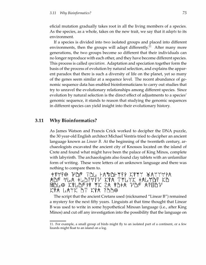
3.11 Why Bioinformatics? 75
eficial mutation gradually takes root in all the living members of a species.
As the species, as a whole, takes on the new trait, we say that it adapts to its
environment.
If a species is divided into two isolated groups and placed into different
environments, then the groups will adapt differently.11 After many more
generations, the two groups become so different that their individuals can
no longer reproduce with each other, and they have become different species.
This process is called speciation. Adaptation and speciation together form the
basis of the process of evolution by natural selection, and explains the appar-
ent paradox that there is such a diversity of life on the planet, yet so many
of the genes seem similar at a sequence level. The recent abundance of ge-
nomic sequence data has enabled bioinformaticians to carry out studies that
try to unravel the evolutionary relationships among different species. Since
evolution by natural selection is the direct effect of adjustments to a species’
genomic sequence, it stands to reason that studying the genomic sequences
in different species can yield insight into their evolutionary history.
3.11 Why Bioinformatics?
As James Watson and Francis Crick worked to decipher the DNA puzzle,
the 30 year-old English architect Michael Ventris tried to decipher an ancient
language known as Linear B. At the beginning of the twentieth century, ar-
chaeologists excavated the ancient city of Knossos located on the island of
Crete and found what might have been the palace of King Minos, complete
with labyrinth. The archaeologists also found clay tablets with an unfamiliar
form of writing. These were letters of an unknown language and there was
nothing to compare them to.
The script that the ancient Cretans used (nicknamed “Linear B”) remained
a mystery for the next fifty years. Linguists at that time thought that Linear
B was used to write in some hypothetical Minoan language (i.e., after King
Minos) and cut off any investigation into the possibility that the language on
11. For example, a small group of birds might fly to an isolated part of a continent, or a fewlizards might float to an island on a log.
76 3 Molecular Biology Primer
the tablets was Greek.12 In 1936, a fourteen-year-old boy, Michael Ventris,
went on a school trip to the Minoan exhibit in London and was fascinated
with the legend of the Minotaur and the unsolved puzzle of the Minoan lan-
guage. After seventeen years of code-breaking, Ventris decoded the Minoan
language at about the same time Watson and Crick deciphered the structure
of DNA.
Some Linear B tablets had been discovered on the Greek mainland. Not-
ing that certain strings of symbols appeared in the Cretan texts but did not
appear in Greek texts, Ventris made the inspired guess that those strings ap-
plied to cities on the island. Armed with these new symbols that he could
decipher, he soon unlocked much more text, and determined that the un-
derlying language of Linear B was, in fact, just Greek written in a different
alphabet. This showed that the Cretan civilization of the Linear B tablets had
been part of Greek civilization.
There were two types of clay tablets found at Crete: some written in Linear
B and others written in a different script named Linear A. Linear A appears to
be older than Linear B and linguists think that Linear A is the oldest written
language of Europe, a precursor of Greek. Linear A has resisted all attempts
at decoding. Its underlying language is still unknown and probably will
remain undecoded since it does not seem to relate to any other surviving
language in the world. Linear A and Linear B texts are written in alphabets
consisting of roughly ninety symbols.
Bioinformatics was born after biologists discovered how to sequence DNA
and soon generated many texts in the four-letter alphabet of DNA. DNA is
more like Linear A than Linear B when it comes to decoding—we still know
very little about the language of DNA. Like Michael Ventris, who mobilized
the mathematics of code-breaking to decipher Linear B, bioinformaticians
use algorithms, statistics, and other mathematical techniques to decipher the
language of DNA.
For example, suppose we have the genomic sequences of two insects that
we suspect are somewhat related, evolutionarily speaking—perhaps a fruit
fly (Drosophila melanogaster) and a malaria mosquito (Anopheles gamibae). Tak-
ing the Michael Ventris approach, we would like to know what parts of the
fruit fly genomic sequence are dissimilar and what parts are similar to the
mosquito genomic sequence. Though the means to find this out may not be
immediately obvious at this point, the alignment algorithms described later
12. For many years biologists thought that proteins rather than DNA represent the language ofthe cell, which was another mistaken assumption.
3.11 Why Bioinformatics? 77
in this book allow one to compare any two genes and to detect similarities
between them. Unfortunately, it will take an unbearably long time to do so
if we want to compare the entire fruit fly genome with the entire mosquito
genome. Rather than giving up on the question altogether, biologists com-
bined their efforts with algorithmists and mathematicians to come up with
an algorithm (BLAST) that solves the problem very quickly and evaluates
the statistical significance of any similarities that it finds.
Comparing related DNA sequences is often a key to understanding each
of them, which is why recent efforts to sequence many related genomes
(e.g., human, chimpanzee, mouse, rat) provide the best hope for understand-
ing the language of DNA. This approach is often referred to as comparative
genomics. A similar approach was used by the nineteenth century French
linguist Jean-François Champollion who decoded the ancient Egyptian lan-
guage.
The ancient Egyptians used hieroglyphs, but when the Egyptian religion
was banned in the fourth century as a pagan cult, knowledge of hieroglyph-
ics was lost. Even worse, the spoken language of Egyptian and its script
(known as demotic) was lost soon afterward and completely forgotten by the
tenth century when Arabic became the language of Egypt. As a result, a
script that had been in use since the beginning of the third millennium BC
turned into a forgotten language that nobody remembered.
During Napoleon’s Egyptian campaign, French soldiers near the city of
Rosetta found a stone (now known as the Rosetta stone) that was inscribed in
three different scripts. Many of Napoleon’s officers happened to be classi-
cally educated and one of them, a Lieutenant Bouchard, identified the three
bands of scripts as hieroglyphic, demotic, and ancient Greek. The last sen-
tence of the Greek inscription read: “This decree shall be inscribed on stelae
of hard rock, in sacred characters, both native and Greek.” The Rosetta stone
thus presented a comparative linguistics problem not unlike the comparative
genomics problems bionformaticians face today.
In recent decades biology has raised fascinating mathematical problems
and has enabled important biological discoveries. Biologists that reduce
bioinformatics to simply “the application of computers in biology” some-
times fail to recognize the rich intellectual content of bioinformatics. Bioin-
formatics has become a part of modern biology and often dictates new fash-
ions, enables new approaches, and drives further biological developments.
Simply using bioinformatics as a tool kit without a reasonable understand-
ing of the main computational ideas is not very different from using a PCR
kit without knowing how PCR works.

78 3 Molecular Biology Primer
Bioinformatics is a large branch of biology (or of computer science) and
this book presents neither a complete cross section nor a detailed look at
any one part of it. Our intent is to describe those algorithmic principles that
underlie the solution to several important biological problems to make it pos-
sible to understand any other part of the field.
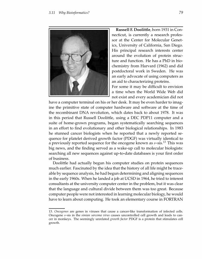
3.11 Why Bioinformatics? 79
Russell F. Doolittle, born 1931 in Con-
necticut, is currently a research profes-
sor at the Center for Molecular Genet-
ics, University of California, San Diego.
His principal research interests center
around the evolution of protein struc-
ture and function. He has a PhD in bio-
chemistry from Harvard (1962) and did
postdoctoral work in Sweden. He was
an early advocate of using computers as
an aid to characterizing proteins.
For some it may be difficult to envision
a time when the World Wide Web did
not exist and every academician did not
have a computer terminal on his or her desk. It may be even harder to imag-
ine the primitive state of computer hardware and software at the time of
the recombinant DNA revolution, which dates back to about 1978. It was
in this period that Russell Doolittle, using a DEC PDP11 computer and a
suite of home-grown programs, began systematically searching sequences
in an effort to find evolutionary and other biological relationships. In 1983
he stunned cancer biologists when he reported that a newly reported se-
quence for platelet derived growth factor (PDGF) was virtually identical toa previously reported sequence for the oncogene known as ν-sis.13 This was
big news, and the finding served as a wake-up call to molecular biologists:
searching all new sequences against up-to-date databases is your first order
of business.Doolittle had actually begun his computer studies on protein sequences
much earlier. Fascinated by the idea that the history of all life might be trace-
able by sequence analysis, he had begun determining and aligning sequences
in the early 1960s. When he landed a job at UCSD in 1964, he tried to interest
consultants at the university computer center in the problem, but it was clear
that the language and cultural divide between them was too great. Because
computer people were not interested in learning molecular biology, he would
have to learn about computing. He took an elementary course in FORTRAN
13. Oncogenes are genes in viruses that cause a cancer-like transformation of infected cells.Oncogene ν-sis in the simian sarcoma virus causes uncontrolled cell growth and leads to can-cer in monkeys. The seemingly unrelated growth factor PDGF is a protein that stimulates cellgrowth.
80 3 Molecular Biology Primer
programming, and, with the help of his older son, developed some simple
programs for comparing sequences. These were the days when one used
a keypunch machine to enter data on eighty-column cards, packs of which
were dropped off at the computer center with the hope that the output could
be collected the next day.
In the mid-1960s, Richard Eck and Margaret Dayhoff had begun the Atlas
of Protein Sequence and Structure, the forerunner of the Protein Identifica-
tion Resource (PIR) database. Their original intention was to publish an an-
nual volume of "all the sequences that could fit between two covers." Clearly,
no one foresaw the deluge of sequences that was to come once methods had
been developed for directly sequencing DNA. In 1978, for example, the entire
holding of the atlas, which could be purchased on magnetic tape, amounted
to 1081 entries. Realizing that this was a very biased collection of protein
sequences, Doolittle began his own database, which, because it followed the
format of the atlas, he called NEWAT ("new atlas"). At about the same time
he acquired a PDP11 computer, the maximum capacity of which was only
100 kilobytes, much of that occupied by a mini-UNIX operating system. With
the help of his secretary and his younger son (eleven years old at the time),
Doolittle began typing in every new sequence he could get his hands on,
searching each against every other sequence in the collection as they went.
This was in keeping with his view that all new proteins come from old pro-
teins, mostly by way of gene duplications. In the first few years of their small
enterprise, Doolittle & Son established a number of unexpected connections.
Doolittle admits that in 1978 he knew hardly anything about cancer viruses,
but a number of chance happenings put him in touch with the field. For
one, Ted Friedmann and Gernot Walter (who was then at the Salk Institute),
had sought Doolittle’s aid in comparing the sequences of two DNA tumor
viruses, simian virus 40 (SV40) and the polyoma virus. This led indirectly to
contacts with Inder Verma’s group at Salk, which was studying retroviruses
and had sequenced an “oncogene” called ν-mos in a retrovirus that caused
sarcomas in mice. They asked Doolittle to search it for them, but no signif-
icant matches were found. Not long afterward (in 1980), Doolittle read an
article reporting the nucleotide sequence of an oncogene from an avian sar-
coma virus—the famous Rous sarcoma virus. It was noted in that article that
the Salk team had provided the authors with a copy of their still unpublished
mouse sarcoma gene sequence, but no resemblances had been detected. In
line with his own project, Doolittle promptly typed the new avian sequence
into his computer to see if it might match anything else. He was astonished
to find that in fact a match quickly appeared with the still unpublished Salk
3.11 Why Bioinformatics? 81
sequence for the mouse retrovirus oncogene. He immediately telephoned
Inder Verma; "Hey, these two sequences are in fact homologous. These pro-
teins must be doing the same thing." Verma, who had just packaged up a
manuscript describing the new sequence, promptly unwrapped it and added
the new feature. He was so pleased with the outcome that he added Doolit-
tle’s name as one of the coauthors.
How was it that the group studying the Rous sarcoma virus had missed
this match? It’s a reflection on how people were thinking at the time. They
had compared the DNA sequences of the two genes without translating them
into the corresponding amino acid sequences, losing most of the information
as a result. It was another simple but urgent message to the community
about how to think about sequence comparisons.
In May of 1983, an article appeared in Science describing the characteri-
zation of a growth factor isolated from human blood platelets. Harry An-
toniades and Michael Hunkapiller had determined 28 amino acid residues
from the N-terminal end of PDGF. (It had taken almost 100,000 units of hu-
man blood to obtain enough of the growth factor material to get this much
sequence.) The article noted that the authors had conducted a limited search
of known sequences and hadn’t found any similar proteins.
By this time, Doolittle had modem access to a department VAX computer
where he now stored his database. He typed in the PDGF partial sequence
and set it searching. Twenty minutes later he had the results of the search;
human PDGF had a sequence that was virtually identical to that of an onco-
gene isolated from a woolly monkey. Doolittle describes it as an electrifying
moment, enriched greatly by his prior experiences with the other oncogenes.
He remembers remarking to his then fifteen-year old son, “Will, this exper-
iment took us five years and twenty minutes.” As it happened, he was not
alone in enjoying the thrill of this discovery. Workers at the Imperial Cancer
Laboratory in London were also sequencing PDGF, and in the spring of 1983
had written to Doolittle asking for a tape of his sequence collection. He had
sent them his newest version, fortuitously containing the ν-sis sequence from
the woolly monkey. Just a few weeks before the Science article appeared,
Antoniades and Hunkapiller replied with an effusive letter of thanks, not
mentioning just why the tape had been so valuable to them. Meanwhile,
Doolittle had written to both the PDGF workers and the ν-sis team, suggest-
ing that they compare notes. As a result, the news of the match was quickly
made known, and a spirited race to publication occurred, the report from
the Americans appearing in Science only a week ahead of the British effort
in Nature. Doolittle went on to make many other matches during the mid-

82 3 Molecular Biology Primer
1980s, including several more involving oncogenes. For example, he found a
relationship between the oncogene ν-jun and the gene regulator GCN4. He
describes those days as unusual in that an amateur could still occasionally
compete with the professionals. Although he continued with his interests in
protein evolution, he increasingly retreated to the laboratory and left bioin-
formatics to those more formally trained in the field.
4 Exhaustive Search
Exhaustive search algorithms require little effort to design but for many prob-
lems of interest cannot process inputs of any reasonable size within your
lifetime. Despite this problem, exhaustive search, or brute force algorithms
are often the first step in designing more efficient algorithms.
We introduce two biological problems: DNA restriction mapping and regula-
tory motif finding, whose brute force solutions are not practical. We further de-
scribe the branch-and-bound technique to transform an inefficient brute force
algorithm into a practical one. In chapter 5 we will see how to improve our
motif finding algorithm to arrive at an algorithm very similar to the popular
CONSENSUS motif finding tool. In chapter 12 we describe two randomized
algorithms, GibbsSampler and RandomProjections, that use coin-tossing to
find motifs.
4.1 Restriction Mapping
Hamilton Smith discovered in 1970 that the restriction enzyme HindII cleaves
DNA molecules at every occurrence, or site, of the sequences GTGCAC or
GTTAAC, breaking a long molecule into a set of restriction fragments. Shortly
thereafter, maps of restriction sites in DNA molecules, or restriction maps,
became powerful research tools in molecular biology by helping to narrow
the location of certain genetic markers.
If the genomic DNA sequence of an organism is known, then construc-
tion of a restriction map for HindII amounts to finding all occurrences of
GTGCAC and GTTAAC in the genome. Because the first bacterial genome
was sequenced twenty-five years after the discovery of restriction enzymes,
Administrator
Highlight
Administrator
Highlight
Administrator
Highlight
Administrator
Highlight
Administrator
Highlight
Administrator
Highlight
Administrator
Highlight
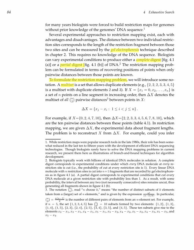
84 4 Exhaustive Search
for many years biologists were forced to build restriction maps for genomes
without prior knowledge of the genomes’ DNA sequence.1
Several experimental approaches to restriction mapping exist, each with
advantages and disadvantages. The distance between two individual restric-
tion sites corresponds to the length of the restriction fragment between those
two sites and can be measured by the gel electrophoresis technique described
in chapter 2. This requires no knowledge of the DNA sequence. Biologists
can vary experimental conditions to produce either a complete digest [fig. 4.1
(a)] or a partial digest [fig. 4.1 (b)] of DNA.2 The restriction mapping prob-
lem can be formulated in terms of recovering positions of points when only
pairwise distances between those points are known.
To formulate the restriction mapping problem, we will introduce some no-
tation. A multiset is a set that allows duplicate elements (e.g., 2, 2, 2, 3, 3, 4, 5
is a multiset with duplicate elements 2 and 3). If X = x1 = 0, x2, . . . , xn is
a set of n points on a line segment in increasing order, then ∆X denotes the
multiset of all(
n2
)
pairwise distances3 between points in X :
∆X = xj − xi : 1 ≤ i < j ≤ n .
For example, if X=0, 2, 4, 7, 10, then ∆X=2, 2, 3, 3, 4, 5, 6, 7, 8, 10, which
are the ten pairwise distances between these points (table 4.1). In restriction
mapping, we are given ∆X , the experimental data about fragment lengths.
The problem is to reconstruct X from ∆X . For example, could you infer
1. While restriction maps were popular research tools in the late 1980s, their role has been some-what reduced in the last ten to fifteen years with the development of efficient DNA sequencingtechnologies. Though biologists rarely have to solve the DNA mapping problems in currentresearch, we present them here as illustrations of branch-and-bound techniques for algorithmdevelopment.2. Biologists typically work with billions of identical DNA molecules in solution. A completedigest corresponds to experimental conditions under which every DNA molecule at every re-striction site is cut (i.e., the probability of cut at every restriction site is 1). Every linear DNAmolecule with n restriction sites is cut into n+1 fragments that are recorded by gel electrophore-sis as in figure 4.1 (a). A partial digest corresponds to experimental conditions that cut everyDNA molecule at a given restriction site with probability less than 1. As a result, with someprobability, the interval between any two (not necessarily consecutive) sites remains uncut, thusgenerating all fragments shown in figure 4.1 (b).3. The notation
`
nk
´
, read “n choose k,” means “the number of distinct subsets of k elements
taken from a (larger) set of n elements,” and is given by the expression n!(n−k)!k!
. In particular,`
n2
´
= n(n−1)2
is the number of different pairs of elements from an n-element set. For example,
if n = 5, the set 1, 2, 3, 4, 5 has`52
´
= 10 subsets formed by two elements: 1, 2, 1, 3,1, 4, 1, 5, 2, 3, 2, 4, 2, 5, 3, 4, 3, 5, and 4, 5. These ten subsets give rise to theelements x2 − x1, x3 − x1, x4 − x1, x5 − x1, x3 − x2, x4 − x2, x5 − x2, x4 − x3, x5 − x3, andx5 − x4.
Administrator
Highlight
Administrator
Highlight
Administrator
Highlight
Administrator
Highlight
Administrator
Highlight
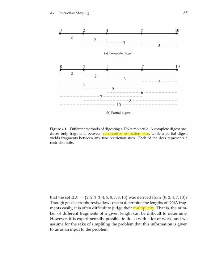
4.1 Restriction Mapping 85
0 2 4 7 10
22
33
(a) Complete digest.
0 2 4 7 10
22
33
45
67
810
(b) Partial digest.
Figure 4.1 Different methods of digesting a DNA molecule. A complete digest pro-duces only fragments between consecutive restriction sites, while a partial digestyields fragments between any two restriction sites. Each of the dots represents arestriction site.
that the set ∆X = 2, 2, 3, 3, 4, 5, 6, 7, 8, 10was derived from 0, 2, 4, 7, 10?
Though gel electrophoresis allows one to determine the lengths of DNA frag-
ments easily, it is often difficult to judge their multiplicity. That is, the num-
ber of different fragments of a given length can be difficult to determine.
However, it is experimentally possible to do so with a lot of work, and we
assume for the sake of simplifing the problem that this information is given
to us as an input to the problem.
Administrator
Highlight
Administrator
Highlight
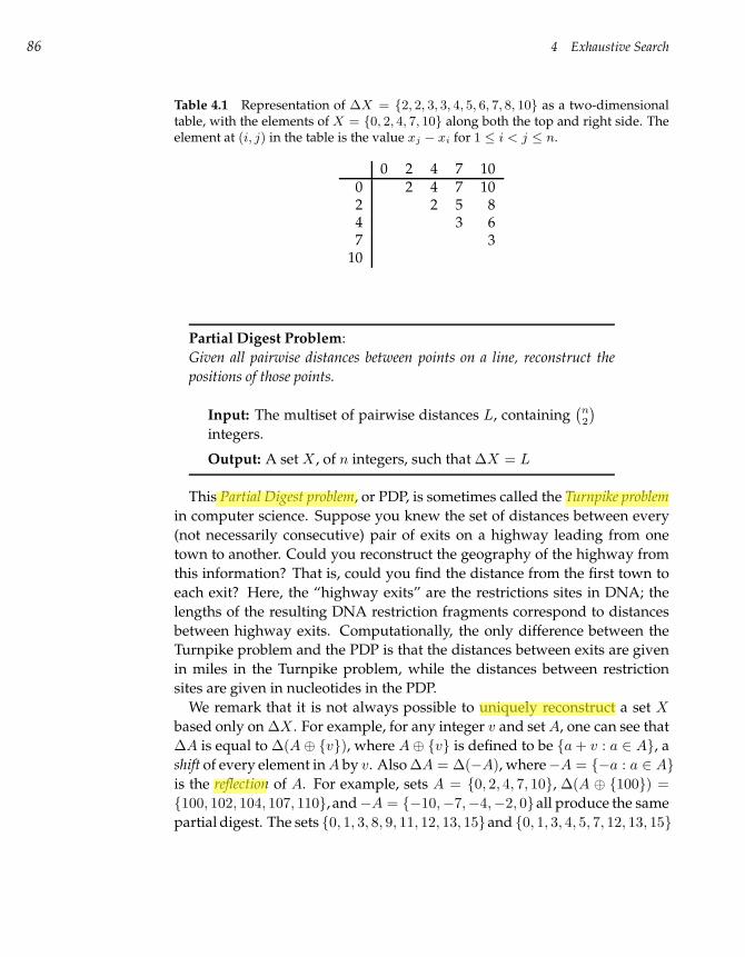
86 4 Exhaustive Search
Table 4.1 Representation of ∆X = 2, 2, 3, 3, 4, 5, 6, 7, 8, 10 as a two-dimensionaltable, with the elements of X = 0, 2, 4, 7, 10 along both the top and right side. Theelement at (i, j) in the table is the value xj − xi for 1 ≤ i < j ≤ n.
0 2 4 7 100 2 4 7 102 2 5 84 3 67 3
10
Partial Digest Problem:
Given all pairwise distances between points on a line, reconstruct the
positions of those points.
Input: The multiset of pairwise distances L, containing(
n2
)
integers.
Output: A set X , of n integers, such that ∆X = L
This Partial Digest problem, or PDP, is sometimes called the Turnpike problem
in computer science. Suppose you knew the set of distances between every
(not necessarily consecutive) pair of exits on a highway leading from one
town to another. Could you reconstruct the geography of the highway from
this information? That is, could you find the distance from the first town to
each exit? Here, the “highway exits” are the restrictions sites in DNA; the
lengths of the resulting DNA restriction fragments correspond to distances
between highway exits. Computationally, the only difference between the
Turnpike problem and the PDP is that the distances between exits are given
in miles in the Turnpike problem, while the distances between restriction
sites are given in nucleotides in the PDP.
We remark that it is not always possible to uniquely reconstruct a set X
based only on ∆X . For example, for any integer v and set A, one can see that
∆A is equal to ∆(A⊕ v), where A⊕ v is defined to be a + v : a ∈ A, a
shift of every element in A by v. Also ∆A = ∆(−A), where−A = −a : a ∈ A
is the reflection of A. For example, sets A = 0, 2, 4, 7, 10, ∆(A ⊕ 100) =
100, 102, 104, 107, 110, and−A = −10,−7,−4,−2, 0all produce the same
partial digest. The sets 0, 1, 3, 8, 9, 11, 12, 13, 15and 0, 1, 3, 4, 5, 7, 12, 13, 15
Administrator
Highlight
Administrator
Highlight
Administrator
Highlight
Administrator
Highlight
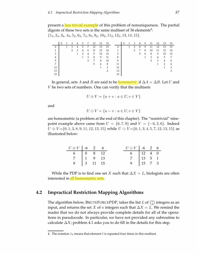
4.2 Impractical Restriction Mapping Algorithms 87
present a less trivial example of this problem of nonuniqueness. The partial
digests of these two sets is the same multiset of 36 elements4:
14, 24, 34, 43, 52, 62, 72, 83, 92, 102, 112, 123, 13, 14, 15.
0 1 3 4 5 7 12 13 15
0 1 3 4 5 7 12 13 15
1 2 3 4 6 11 12 14
3 1 2 4 9 10 12
4 1 3 8 9 11
5 2 7 8 10
7 5 6 8
12 1 3
13 2
15
0 1 3 8 9 11 12 13 15
0 1 3 8 9 11 12 13 15
1 2 7 8 10 11 12 14
3 5 6 8 9 10 12
8 1 3 4 5 7
9 2 3 4 6
11 1 2 4
12 1 3
13 2
15
In general, sets A and B are said to be homometric if ∆A = ∆B. Let U and
V be two sets of numbers. One can verify that the multisets
U ⊕ V = u + v : u ∈ U, v ∈ V
and
U V = u− v : u ∈ U, v ∈ V
are homometric (a problem at the end of this chapter). The “nontrivial” nine-
point example above came from U = 6, 7, 9 and V = −6, 2, 6. Indeed
U ⊕ V =0, 1, 3, 8, 9, 11, 12, 13, 15 while U V =0, 1, 3, 4, 5, 7, 12, 13, 15 as
illustrated below:
U ⊕ V -6 2 6
6 0 8 12
7 1 9 13
9 3 11 15
U V -6 2 6
6 12 4 0
7 13 5 1
9 15 7 3
While the PDP is to find one set X such that ∆X = L, biologists are often
interested in all homometric sets.
4.2 Impractical Restriction Mapping Algorithms
The algorithm below, BRUTEFORCEPDP, takes the list L of(
n2
)
integers as an
input, and returns the set X of n integers such that ∆X = L. We remind the
reader that we do not always provide complete details for all of the opera-
tions in pseudocode. In particular, we have not provided any subroutine to
calculate ∆X ; problem 4.1 asks you to do fill in the details for this step.
4. The notation 14 means that element 1 is repeated four times in this multiset.
Administrator
Highlight
Administrator
Highlight
Administrator
Highlight
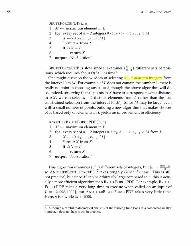
88 4 Exhaustive Search
BRUTEFORCEPDP(L, n)
1 M ← maximum element in L
2 for every set of n− 2 integers 0 < x2 < · · · < xn−1 < M
3 X ← 0, x2, . . . , xn−1, M
4 Form ∆X from X
5 if ∆X = L
6 return X
7 output “No Solution”
BRUTEFORCEPDP is slow since it examines(
M−1n−2
)
different sets of posi-
tions, which requires about O(Mn−2) time.5
One might question the wisdom of selecting n − 2 arbitrary integers from
the interval 0 to M . For example, if L does not contain the number 5, there is
really no point in choosing any xi = 5, though the above algorithm will do
so. Indeed, observing that all points in X have to correspond to some distance
in ∆X , we can select n − 2 distinct elements from L rather than the less
constrained selection from the interval (0, M). Since M may be large, even
with a small number of points, building a new algorithm that makes choices
of xi based only on elements in L yields an improvement in efficiency.
ANOTHERBRUTEFORCEPDP(L, n)
1 M ← maximum element in L
2 for every set of n− 2 integers 0 < x2 < · · · < xn−1 < M from L
3 X ← 0, x2, . . . , xn−1, M
4 Form ∆X from X
5 if ∆X = L
6 return X
7 output “No Solution”
This algorithm examines(
|L|n−2
)
different sets of integers, but |L| = n(n−1)2 ,
so ANOTHERBRUTEFORCEPDP takes roughly O(n2n−4) time. This is still
not practical, but since M can be arbitrarily large compared to n, this is actu-
ally a more efficient algorithm than BRUTEFORCEPDP. For example, BRUTE-
FORCEPDP takes a very long time to execute when called on an input of
L = 2, 998, 1000, but ANOTHERBRUTEFORCEPDP takes very little time.
Here, n is 3 while M is 1000.
5. Although a careful mathematical analysis of the running time leads to a somewhat smallernumber, it does not help much in practice.
Administrator
Highlight
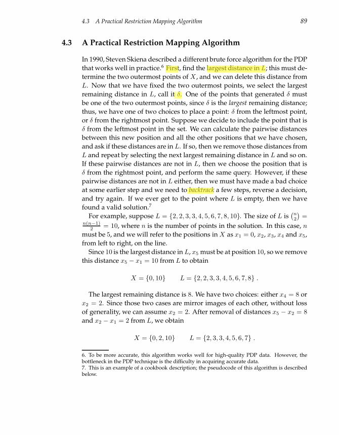
4.3 A Practical Restriction Mapping Algorithm 89
4.3 A Practical Restriction Mapping Algorithm
In 1990, Steven Skiena described a different brute force algorithm for the PDP
that works well in practice.6 First, find the largest distance in L; this must de-
termine the two outermost points of X , and we can delete this distance from
L. Now that we have fixed the two outermost points, we select the largest
remaining distance in L, call it δ. One of the points that generated δ must
be one of the two outermost points, since δ is the largest remaining distance;
thus, we have one of two choices to place a point: δ from the leftmost point,
or δ from the rightmost point. Suppose we decide to include the point that is
δ from the leftmost point in the set. We can calculate the pairwise distances
between this new position and all the other positions that we have chosen,
and ask if these distances are in L. If so, then we remove those distances from
L and repeat by selecting the next largest remaining distance in L and so on.
If these pairwise distances are not in L, then we choose the position that is
δ from the rightmost point, and perform the same query. However, if these
pairwise distances are not in L either, then we must have made a bad choice
at some earlier step and we need to backtrack a few steps, reverse a decision,
and try again. If we ever get to the point where L is empty, then we have
found a valid solution.7
For example, suppose L = 2, 2, 3, 3, 4, 5, 6, 7, 8, 10. The size of L is(
n2
)
=n(n−1)
2 = 10, where n is the number of points in the solution. In this case, n
must be 5, and we will refer to the positions in X as x1 = 0, x2, x3, x4 and x5,
from left to right, on the line.
Since 10 is the largest distance in L, x5 must be at position 10, so we remove
this distance x5 − x1 = 10 from L to obtain
X = 0, 10 L = 2, 2, 3, 3, 4, 5, 6, 7, 8 .
The largest remaining distance is 8. We have two choices: either x4 = 8 or
x2 = 2. Since those two cases are mirror images of each other, without loss
of generality, we can assume x2 = 2. After removal of distances x5 − x2 = 8
and x2 − x1 = 2 from L, we obtain
X = 0, 2, 10 L = 2, 3, 3, 4, 5, 6, 7 .
6. To be more accurate, this algorithm works well for high-quality PDP data. However, thebottleneck in the PDP technique is the difficulty in acquiring accurate data.7. This is an example of a cookbook description; the pseudocode of this algorithm is describedbelow.
Administrator
Highlight
Administrator
Highlight
Administrator
Highlight
Administrator
Highlight
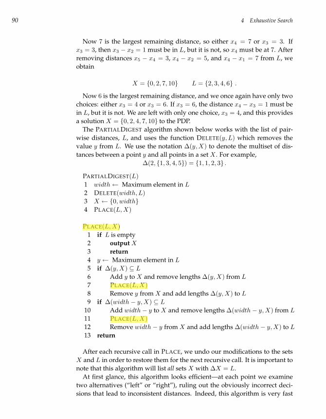
90 4 Exhaustive Search
Now 7 is the largest remaining distance, so either x4 = 7 or x3 = 3. If
x3 = 3, then x3 − x2 = 1 must be in L, but it is not, so x4 must be at 7. After
removing distances x5 − x4 = 3, x4 − x2 = 5, and x4 − x1 = 7 from L, we
obtain
X = 0, 2, 7, 10 L = 2, 3, 4, 6 .
Now 6 is the largest remaining distance, and we once again have only two
choices: either x3 = 4 or x3 = 6. If x3 = 6, the distance x4 − x3 = 1 must be
in L, but it is not. We are left with only one choice, x3 = 4, and this provides
a solution X = 0, 2, 4, 7, 10 to the PDP.
The PARTIALDIGEST algorithm shown below works with the list of pair-
wise distances, L, and uses the function DELETE(y, L) which removes the
value y from L. We use the notation ∆(y, X) to denote the multiset of dis-
tances between a point y and all points in a set X . For example,
∆(2, 1, 3, 4, 5) = 1, 1, 2, 3 .
PARTIALDIGEST(L)
1 width← Maximum element in L
2 DELETE(width, L)
3 X ← 0, width
4 PLACE(L, X)
PLACE(L, X)
1 if L is empty
2 output X
3 return
4 y ← Maximum element in L
5 if ∆(y, X) ⊆ L
6 Add y to X and remove lengths ∆(y, X) from L
7 PLACE(L, X)
8 Remove y from X and add lengths ∆(y, X) to L
9 if ∆(width− y, X) ⊆ L
10 Add width− y to X and remove lengths ∆(width − y, X) from L
11 PLACE(L, X)
12 Remove width− y from X and add lengths ∆(width− y, X) to L
13 return
After each recursive call in PLACE, we undo our modifications to the sets
X and L in order to restore them for the next recursive call. It is important to
note that this algorithm will list all sets X with ∆X = L.
At first glance, this algorithm looks efficient—at each point we examine
two alternatives (“left” or “right”), ruling out the obviously incorrect deci-
sions that lead to inconsistent distances. Indeed, this algorithm is very fast
Administrator
Highlight
Administrator
Highlight
Administrator
Highlight
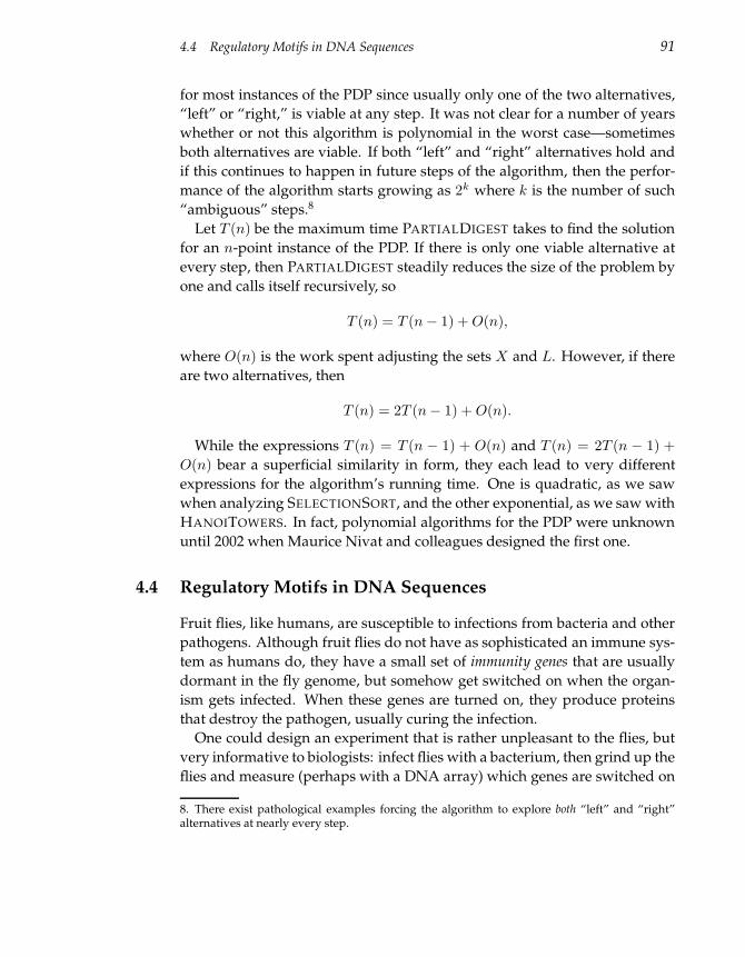
4.4 Regulatory Motifs in DNA Sequences 91
for most instances of the PDP since usually only one of the two alternatives,
“left” or “right,” is viable at any step. It was not clear for a number of years
whether or not this algorithm is polynomial in the worst case—sometimes
both alternatives are viable. If both “left” and “right” alternatives hold and
if this continues to happen in future steps of the algorithm, then the perfor-
mance of the algorithm starts growing as 2k where k is the number of such
“ambiguous” steps.8
Let T (n) be the maximum time PARTIALDIGEST takes to find the solution
for an n-point instance of the PDP. If there is only one viable alternative at
every step, then PARTIALDIGEST steadily reduces the size of the problem by
one and calls itself recursively, so
T (n) = T (n− 1) + O(n),
where O(n) is the work spent adjusting the sets X and L. However, if there
are two alternatives, then
T (n) = 2T (n− 1) + O(n).
While the expressions T (n) = T (n − 1) + O(n) and T (n) = 2T (n − 1) +
O(n) bear a superficial similarity in form, they each lead to very different
expressions for the algorithm’s running time. One is quadratic, as we saw
when analyzing SELECTIONSORT, and the other exponential, as we saw with
HANOITOWERS. In fact, polynomial algorithms for the PDP were unknown
until 2002 when Maurice Nivat and colleagues designed the first one.
4.4 Regulatory Motifs in DNA Sequences
Fruit flies, like humans, are susceptible to infections from bacteria and other
pathogens. Although fruit flies do not have as sophisticated an immune sys-
tem as humans do, they have a small set of immunity genes that are usually
dormant in the fly genome, but somehow get switched on when the organ-
ism gets infected. When these genes are turned on, they produce proteins
that destroy the pathogen, usually curing the infection.
One could design an experiment that is rather unpleasant to the flies, but
very informative to biologists: infect flies with a bacterium, then grind up the
flies and measure (perhaps with a DNA array) which genes are switched on
8. There exist pathological examples forcing the algorithm to explore both “left” and “right”alternatives at nearly every step.
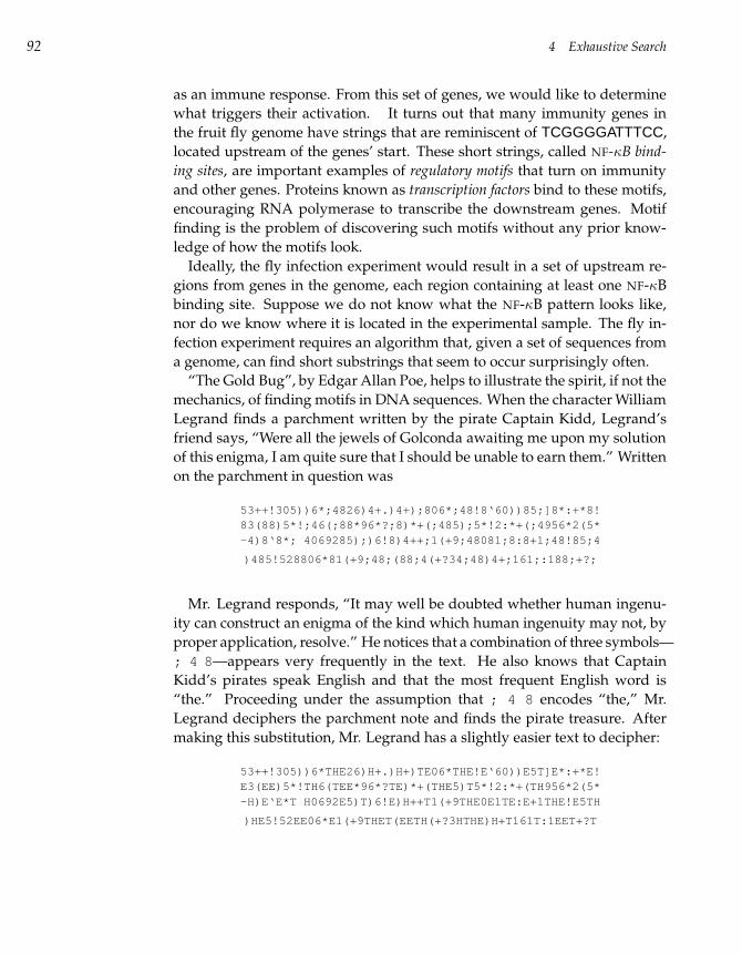
92 4 Exhaustive Search
as an immune response. From this set of genes, we would like to determine
what triggers their activation. It turns out that many immunity genes in
the fruit fly genome have strings that are reminiscent of TCGGGGATTTCC,
located upstream of the genes’ start. These short strings, called NF-κB bind-
ing sites, are important examples of regulatory motifs that turn on immunity
and other genes. Proteins known as transcription factors bind to these motifs,
encouraging RNA polymerase to transcribe the downstream genes. Motif
finding is the problem of discovering such motifs without any prior know-
ledge of how the motifs look.
Ideally, the fly infection experiment would result in a set of upstream re-
gions from genes in the genome, each region containing at least one NF-κB
binding site. Suppose we do not know what the NF-κB pattern looks like,
nor do we know where it is located in the experimental sample. The fly in-
fection experiment requires an algorithm that, given a set of sequences from
a genome, can find short substrings that seem to occur surprisingly often.
“The Gold Bug”, by Edgar Allan Poe, helps to illustrate the spirit, if not the
mechanics, of finding motifs in DNA sequences. When the character William
Legrand finds a parchment written by the pirate Captain Kidd, Legrand’s
friend says, “Were all the jewels of Golconda awaiting me upon my solution
of this enigma, I am quite sure that I should be unable to earn them.” Written
on the parchment in question was
53++!305))6*;4826)4+.)4+);806*;48!8‘60))85;]8*:+*8!83(88)5*!;46(;88*96*?;8)*+(;485);5*!2:*+(;4956*2(5*-4)8‘8*; 4069285);)6!8)4++;1(+9;48081;8:8+1;48!85;4
)485!528806*81(+9;48;(88;4(+?34;48)4+;161;:188;+?;
Mr. Legrand responds, “It may well be doubted whether human ingenu-
ity can construct an enigma of the kind which human ingenuity may not, by
proper application, resolve.” He notices that a combination of three symbols—
; 4 8—appears very frequently in the text. He also knows that Captain
Kidd’s pirates speak English and that the most frequent English word is
“the.” Proceeding under the assumption that ; 4 8 encodes “the,” Mr.
Legrand deciphers the parchment note and finds the pirate treasure. After
making this substitution, Mr. Legrand has a slightly easier text to decipher:
53++!305))6*THE26)H+.)H+)TE06*THE!E‘60))E5T]E*:+*E!E3(EE)5*!TH6(TEE*96*?TE)*+(THE5)T5*!2:*+(TH956*2(5*-H)E‘E*T H0692E5)T)6!E)H++T1(+9THE0E1TE:E+1THE!E5TH
)HE5!52EE06*E1(+9THET(EETH(+?3HTHE)H+T161T:1EET+?T
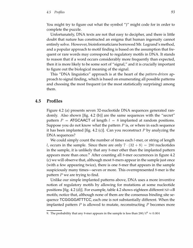
4.5 Profiles 93
You might try to figure out what the symbol “)” might code for in order to
complete the puzzle.
Unfortunately, DNA texts are not that easy to decipher, and there is little
doubt that nature has constructed an enigma that human ingenuity cannot
entirely solve. However, bioinformaticians borrowed Mr. Legrand’s method,
and a popular approach to motif finding is based on the assumption that fre-
quent or rare words may correspond to regulatory motifs in DNA. It stands
to reason that if a word occurs considerably more frequently than expected,
then it is more likely to be some sort of “signal,” and it is crucially important
to figure out the biological meaning of the signal.
This “DNA linguistics” approach is at the heart of the pattern-driven ap-
proach to signal finding, which is based on enumerating all possible patterns
and choosing the most frequent (or the most statistically surprising) among
them.
4.5 Profiles
Figure 4.2 (a) presents seven 32-nucleotide DNA sequences generated ran-
domly. Also shown [fig. 4.2 (b)] are the same sequences with the “secret”
pattern P = ATGCAACT of length l = 8 implanted at random positions.
Suppose you do not know what the pattern P is, or where in each sequence
it has been implanted [fig. 4.2 (c)]. Can you reconstruct P by analyzing the
DNA sequences?
We could simply count the number of times each l-mer, or string of length
l, occurs in the sample. Since there are only 7 · (32 + 8) = 280 nucleotides
in the sample, it is unlikely that any 8-mer other than the implanted pattern
appears more than once.9 After counting all 8-mer occurrences in figure 4.2
(c) we will observe that, although most 8-mers appear in the sample just once
(with a few appearing twice), there is one 8-mer that appears in the sample
suspiciously many times—seven or more. This overrepresented 8-mer is the
pattern P we are trying to find.
Unlike our simple implanted patterns above, DNA uses a more inventive
notion of regulatory motifs by allowing for mutations at some nucleotide
positions [fig. 4.2 (d)]. For example, table 4.2 shows eighteen different NF-κB
motifs; notice that, although none of them are the consensus binding site se-
quence TCGGGGATTTCC, each one is not substantially different. When the
implanted pattern P is allowed to mutate, reconstructing P becomes more
9. The probability that any 8-mer appears in the sample is less than 280/48 ≈ 0.004
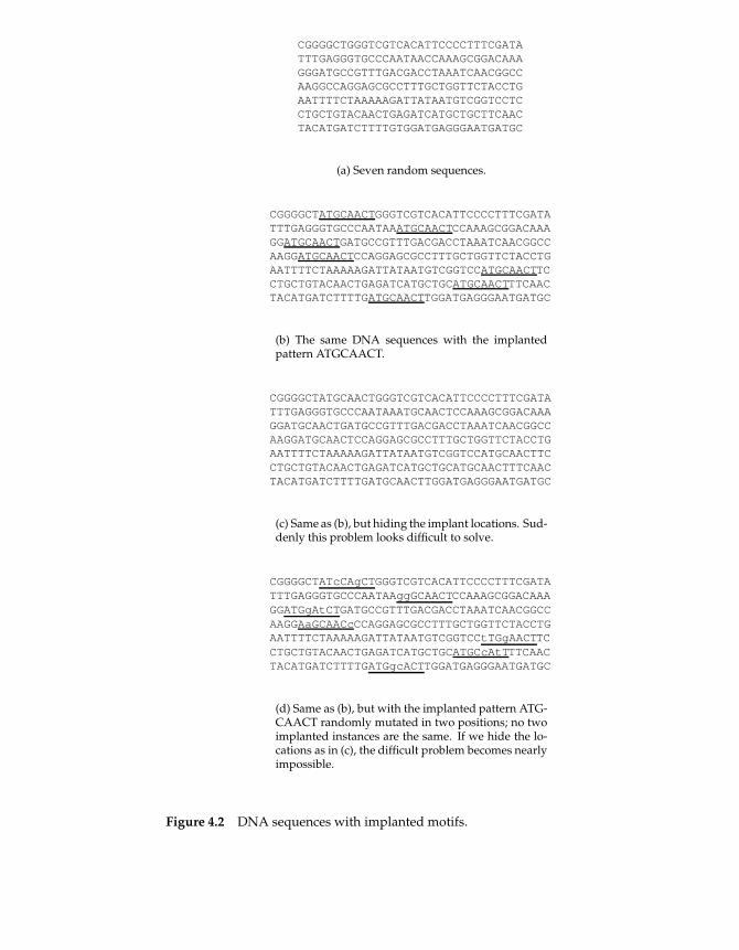
CGGGGCTGGGTCGTCACATTCCCCTTTCGATATTTGAGGGTGCCCAATAACCAAAGCGGACAAAGGGATGCCGTTTGACGACCTAAATCAACGGCCAAGGCCAGGAGCGCCTTTGCTGGTTCTACCTGAATTTTCTAAAAAGATTATAATGTCGGTCCTCCTGCTGTACAACTGAGATCATGCTGCTTCAACTACATGATCTTTTGTGGATGAGGGAATGATGC
(a) Seven random sequences.
CGGGGCTATGCAACTGGGTCGTCACATTCCCCTTTCGATATTTGAGGGTGCCCAATAAATGCAACTCCAAAGCGGACAAAGGATGCAACTGATGCCGTTTGACGACCTAAATCAACGGCCAAGGATGCAACTCCAGGAGCGCCTTTGCTGGTTCTACCTGAATTTTCTAAAAAGATTATAATGTCGGTCCATGCAACTTCCTGCTGTACAACTGAGATCATGCTGCATGCAACTTTCAACTACATGATCTTTTGATGCAACTTGGATGAGGGAATGATGC
(b) The same DNA sequences with the implantedpattern ATGCAACT.
CGGGGCTATGCAACTGGGTCGTCACATTCCCCTTTCGATATTTGAGGGTGCCCAATAAATGCAACTCCAAAGCGGACAAAGGATGCAACTGATGCCGTTTGACGACCTAAATCAACGGCCAAGGATGCAACTCCAGGAGCGCCTTTGCTGGTTCTACCTGAATTTTCTAAAAAGATTATAATGTCGGTCCATGCAACTTCCTGCTGTACAACTGAGATCATGCTGCATGCAACTTTCAACTACATGATCTTTTGATGCAACTTGGATGAGGGAATGATGC
(c) Same as (b), but hiding the implant locations. Sud-denly this problem looks difficult to solve.
CGGGGCTATcCAgCTGGGTCGTCACATTCCCCTTTCGATATTTGAGGGTGCCCAATAAggGCAACTCCAAAGCGGACAAAGGATGgAtCTGATGCCGTTTGACGACCTAAATCAACGGCCAAGGAaGCAACcCCAGGAGCGCCTTTGCTGGTTCTACCTGAATTTTCTAAAAAGATTATAATGTCGGTCCtTGgAACTTCCTGCTGTACAACTGAGATCATGCTGCATGCcAtTTTCAACTACATGATCTTTTGATGgcACTTGGATGAGGGAATGATGC
(d) Same as (b), but with the implanted pattern ATG-CAACT randomly mutated in two positions; no twoimplanted instances are the same. If we hide the lo-cations as in (c), the difficult problem becomes nearlyimpossible.
Figure 4.2 DNA sequences with implanted motifs.
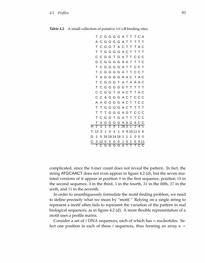
4.5 Profiles 95
Table 4.2 A small collection of putative NF-κB binding sites.
T C G G G G A T T T C A
A C G G G G A T T T T T
T C G G T A C T T T A C
T T G G G G A C T T T T
C C G G T G A T T C C C
G C G G G G A A T T T C
T C G G G G A T T C C T
T C G G G G A T T C C T
T A G G G G A A C T A C
T C G G G T A T A A A C
T C G G G G G T T T T T
C C G G T G A C T T A C
C C A G G G A C T C C C
A A G G G G A C T T C C
T T G G G G A C T T T T
T T T G G G A G T C C C
T C G G T G A T T T C C
T A G G G G A A G A C CA: 2 3 1 0 0 1 16 3 1 2 4 1
T: 12 3 1 0 4 1 0 9 15 11 5 6
G: 1 0 16 18 14 16 1 1 1 0 0 0
C: 3 12 0 0 0 0 1 5 1 5 9 11T C G G G G A T T T C C
complicated, since the 8-mer count does not reveal the pattern. In fact, the
string ATGCAACT does not even appear in figure 4.2 (d), but the seven mu-
tated versions of it appear at position 8 in the first sequence, position 19 in
the second sequence, 3 in the third, 5 in the fourth, 31 in the fifth, 27 in the
sixth, and 15 in the seventh.
In order to unambiguously formulate the motif finding problem, we need
to define precisely what we mean by “motif.” Relying on a single string to
represent a motif often fails to represent the variation of the pattern in real
biological sequences, as in figure 4.2 (d). A more flexible representation of a
motif uses a profile matrix.
Consider a set of t DNA sequences, each of which has n nucleotides. Se-
lect one position in each of these t sequences, thus forming an array s =
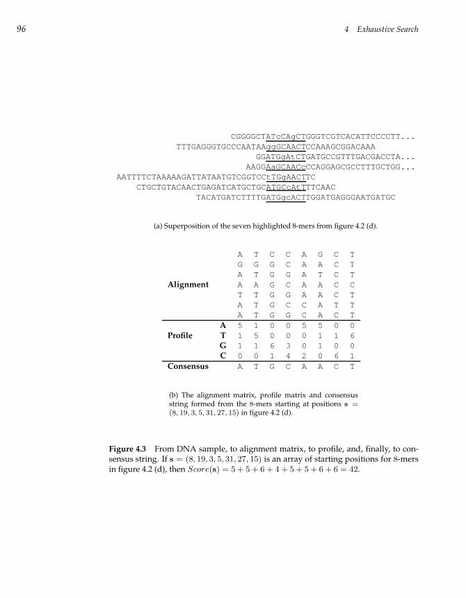
96 4 Exhaustive Search
CGGGGCTATcCAgCTGGGTCGTCACATTCCCCTT...TTTGAGGGTGCCCAATAAggGCAACTCCAAAGCGGACAAA
GGATGgAtCTGATGCCGTTTGACGACCTA...AAGGAaGCAACcCCAGGAGCGCCTTTGCTGG...
AATTTTCTAAAAAGATTATAATGTCGGTCCtTGgAACTTCCTGCTGTACAACTGAGATCATGCTGCATGCcAtTTTCAAC
TACATGATCTTTTGATGgcACTTGGATGAGGGAATGATGC
(a) Superposition of the seven highlighted 8-mers from figure 4.2 (d).
A T C C A G C TG G G C A A C TA T G G A T C T
Alignment A A G C A A C CT T G G A A C TA T G C C A T TA T G G C A C T
A 5 1 0 0 5 5 0 0Profile T 1 5 0 0 0 1 1 6
G 1 1 6 3 0 1 0 0C 0 0 1 4 2 0 6 1
Consensus A T G C A A C T
(b) The alignment matrix, profile matrix and consensusstring formed from the 8-mers starting at positions s =(8, 19, 3, 5, 31, 27, 15) in figure 4.2 (d).
Figure 4.3 From DNA sample, to alignment matrix, to profile, and, finally, to con-sensus string. If s = (8, 19, 3, 5, 31, 27, 15) is an array of starting positions for 8-mersin figure 4.2 (d), then Score(s) = 5 + 5 + 6 + 4 + 5 + 5 + 6 + 6 = 42.
4.6 The Motif Finding Problem 97
(s1, s2, . . . , st), with 1 ≤ si ≤ n − l + 1. The l-mers starting at these po-
sitions can be compiled into a t × l alignment matrix whose (i, j)th element
is the nucleotide in the si + j − 1th element in the ith sequence (fig. 4.3).
Based on the alignment matrix, we can compute the 4× l profile matrix whose
(i, j)th element holds the number of times nucleotide i appears in column
j of the alignment matrix, where i varies from 1 to 4. The profile matrix,
or profile, illustrates the variability of nucleotide composition at each posi-
tion for a particular choice of l-mers. For example, the positions 3, 7, and
8 are highly conserved, while position 4 is not. To further summarize the
profile matrix, we can form a consensus string from the most popular element
in each column of the alignment matrix, which is the nucleotide with the
largest entry in the profile matrix. Figure 4.3 shows the alignment matrix for
s = (8, 19, 3, 5, 31, 27, 15), the corresponding profile matrix, and the resulting
consensus string ATGCAACT.
By varying the starting positions in s, we can construct a large number of
different profile matrices from a given sample. We need some way of grading
them against each other. Some profiles represent high conservation of a pat-
tern while others represent no conservation at all. An imprecise formulation
of the Motif Finding problem is to find the starting positions s correspond-
ing to the most conserved profile. We now develop a specific measure of
conservation, or strength, of a profile.
4.6 The Motif Finding Problem
If P(s) denotes the profile matrix corresponding to starting positions s, then
we will use MP(s)(j) to denote the largest count in column j of P(s). For
the profile P(s) in figure 4.3, MP(s)(1) = 5, MP(s)(2) = 5, and MP(s)(8) = 6.
Given starting positions s, the consensus score is defined to be Score(s, DNA) =∑l
j=1 MP(s)(j). For the starting positions in figure 4.3, Score(s, DNA) =
5 + 5 + 6 + 4 + 5 + 5 + 6 + 6 = 42. Score(s, DNA) can be used to mea-
sure the strength of a profile corresponding to the starting positions s. A
consensus score of l · t corresponds to the best possible alignment, in which
each row of a column has the same letter. A consensus score of lt4 , however,
corresponds to the worst possible alignment, which has an equal mix of all
nucleotides in each column. In its simplest form, the Motif Finding prob-
lem can be formulated as selecting starting positions s from the sample that
98 4 Exhaustive Search
maximize Score(s, DNA).10
Motif Finding Problem:
Given a set of DNA sequences, find a set of l-mers, one from each
sequence, that maximizes the consensus score.
Input: A t×n matrix of DNA, and l, the length of the pattern
to find.
Output: An array of t starting positions s = (s1, s2, . . . , st)
maximizing Score(s, DNA).
Another view onto this problem is to reframe the Motif Finding problem
as the problem of finding a median string. Given two l-mers v and w, we can
compute the Hamming distance between them, dH(v, w), as the number of po-
sitions that differ in the two strings. For example, dH(ATTGTC, ACTCTC) =
2:
A T T G T C: X : X : :A C T C T C
Now suppose that s = (s1, s2, . . . , st) is an array of starting positions, and
that v is some l-mer. We will abuse our notation a bit and use dH(v, s) to
denote the total Hamming distance between v and the l-mers starting at posi-
tions s: dH(v, s) =∑t
i=1 dH(v, si), where dH(v, si) is the Hamming distance
between v and the l-mer that starts at si in the ith DNA sequence. We will
use TotalDistance(v, DNA) = mins(dH(v, s)) to denote the minimum possi-
ble total Hamming distance between a given string v and any set of starting
positions in the DNA. Finding TotalDistance(v, DNA) is a simple problem:
first one has to find the best match for v in the first DNA sequence (i.e., a po-
sition minimizing dH(v, s1) for 1 ≤ s1 ≤ n− l + 1), then the best match in the
10. Another approach is to maximize the entropy of the corresponding profile. Let P(s) = (pi,j),where pi,j is the count at element (i, j) of the 4 × l profile matrix. Entropy is defined as
lX
j=1
4X
i=1
pi,j
tlog
pi,j
t
where t is the number of sequences in the DNA sample. Although entropy is a more statisticallyadequate measure of profile strength than the consensus score, for the sake of simplicity we usethe consensus score in the examples below.
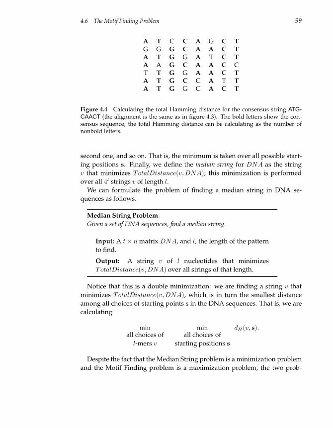
4.6 The Motif Finding Problem 99
A T C C A G C TG G G C A A C TA T G G A T C TA A G C A A C CT T G G A A C TA T G C C A T TA T G G C A C T
Figure 4.4 Calculating the total Hamming distance for the consensus string ATG-CAACT (the alignment is the same as in figure 4.3). The bold letters show the con-sensus sequence; the total Hamming distance can be calculating as the number ofnonbold letters.
second one, and so on. That is, the minimum is taken over all possible start-
ing positions s. Finally, we define the median string for DNA as the string
v that minimizes TotalDistance(v, DNA); this minimization is performed
over all 4l strings v of length l.
We can formulate the problem of finding a median string in DNA se-
quences as follows.
Median String Problem:
Given a set of DNA sequences, find a median string.
Input: A t× n matrix DNA, and l, the length of the pattern
to find.
Output: A string v of l nucleotides that minimizes
TotalDistance(v, DNA) over all strings of that length.
Notice that this is a double minimization: we are finding a string v that
minimizes TotalDistance(v, DNA), which is in turn the smallest distance
among all choices of starting points s in the DNA sequences. That is, we are
calculating
minall choices of
l-mers v
minall choices of
starting positions s
dH(v, s).
Despite the fact that the Median String problem is a minimization problem
and the Motif Finding problem is a maximization problem, the two prob-
100 4 Exhaustive Search
lems are computationally equivalent. Let s be a set of starting positions with
consensus score Score(s, DNA), and let w be the consensus string of the cor-
responding profile. Then
dH(w, s) = lt− Score(s, DNA).
For example, in figure 4.4, the Hamming distance between the consensus
string w and each of the seven implanted patterns is 2, and dH(w, s)=2 · 7 =
7 · 8− 42.
The consensus string minimizes dH(v, s) over all choices of v, i.e.,
dH(w, s) = minall choices of v
dH(v, s) = lt− Score(s, DNA)
Since t and l are constants, the smallest value of dH can also be obtained by
maximizing Score(s, DNA) over all choices of s:
minall choices of s
minall choices of v
dH(v, s) = lt− maxall choices of s
Score(s, DNA).
The problem on the left is the Median String problem while the problem on
the right is the Motif Finding problem.
In other words, the consensus string for the solution of the Motif Find-
ing problem is the median string for the input DNA sample. The median
string for DNA can be used to generate a profile that solves the Motif Find-
ing problem, by searching in each of the t sequences for the substring with
the smallest Hamming distance from the median string.
We introduce this formulation of the Median String problem to give more
efficient alternative motif finding algorithms below.
4.7 Search Trees
In both the Median String problem and the Motif Finding problem we have
to sift through a large number of alternatives to find the best one but we so
far lack the algorithmic tools to do so. For example, in the Motif Finding
problem we have to consider all (n− l + 1)t possible starting positions s:
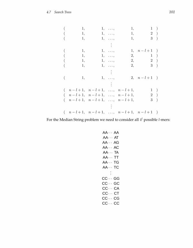
4.7 Search Trees 101
( 1, 1, . . . , 1, 1 )
( 1, 1, . . . , 1, 2 )
( 1, 1, . . . , 1, 3 )...
( 1, 1, . . . , 1, n− l + 1 )
( 1, 1, . . . , 2, 1 )
( 1, 1, . . . , 2, 2 )
( 1, 1, . . . , 2, 3 )...
( 1, 1, . . . , 2, n− l + 1 )...
( n− l + 1, n− l + 1, . . . , n− l + 1, 1 )
( n− l + 1, n− l + 1, . . . , n− l + 1, 2 )
( n− l + 1, n− l + 1, . . . , n− l + 1, 3 )...
( n− l + 1, n− l + 1, . . . , n− l + 1, n− l + 1 )
For the Median String problem we need to consider all 4l possible l-mers:
AA· · · AAAA· · · ATAA· · · AGAA· · · ACAA· · · TAAA· · · TTAA· · · TGAA· · · TC
...
CC· · · GGCC· · · GCCC· · · CACC· · · CTCC· · · CGCC· · · CC
102 4 Exhaustive Search
1111 1112 1121 1122 1211 1212 1221 1222 2111 2112 2121 2122 2211 2212 2221 2222
Figure 4.5 All 4-mers in the alphabet of 1, 2.
We note that this latter progression is equivalent to the following one if we
let 1 stand for A, 2 for T, 3 for G, and 4 for C:
(1, 1, . . . , 1, 1)
(1, 1, . . . , 1, 2)
(1, 1, . . . , 1, 3)
(1, 1, . . . , 1, 4)
(1, 1, . . . , 2, 1)
(1, 1, . . . , 2, 2)
(1, 1, . . . , 2, 3)
(1, 1, . . . , 2, 4)...
(4, 4, . . . , 3, 3)
(4, 4, . . . , 3, 4)
(4, 4, . . . , 4, 1)
(4, 4, . . . , 4, 2)
(4, 4, . . . , 4, 3)
(4, 4, . . . , 4, 4)
In general, we want to consider all kL L-mers in a k-letter alphabet. For the
Motif Finding problem, k = n−l+1, whereas for the Median String problem,
k = 4. Figure 4.5 shows all 24 4-mers in the two-letter alphabet of 1 and 2.
Given an L-mer from a k-letter alphabet, the subroutine NEXTLEAF (below)
demonstrates how to jump from an L-mer a = (a1a2 · · · aL) to the next L-
mer in the progression. Exactly why this algorithm is called NEXTLEAF will
become clear shortly.
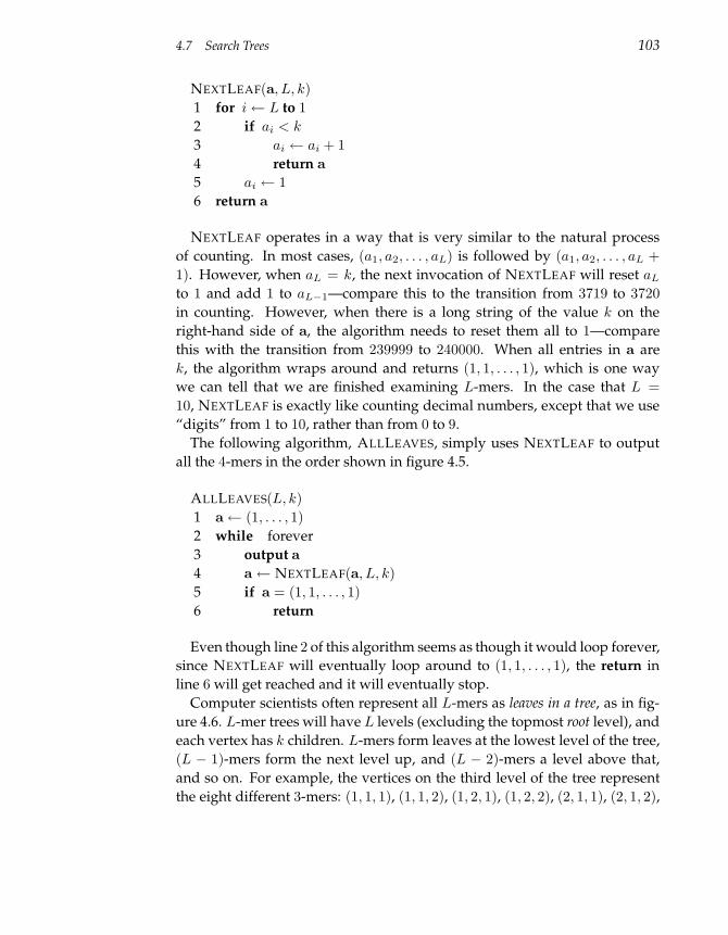
4.7 Search Trees 103
NEXTLEAF(a, L, k)
1 for i← L to 1
2 if ai < k
3 ai ← ai + 1
4 return a
5 ai ← 1
6 return a
NEXTLEAF operates in a way that is very similar to the natural process
of counting. In most cases, (a1, a2, . . . , aL) is followed by (a1, a2, . . . , aL +
1). However, when aL = k, the next invocation of NEXTLEAF will reset aL
to 1 and add 1 to aL−1—compare this to the transition from 3719 to 3720
in counting. However, when there is a long string of the value k on the
right-hand side of a, the algorithm needs to reset them all to 1—compare
this with the transition from 239999 to 240000. When all entries in a are
k, the algorithm wraps around and returns (1, 1, . . . , 1), which is one way
we can tell that we are finished examining L-mers. In the case that L =
10, NEXTLEAF is exactly like counting decimal numbers, except that we use
“digits” from 1 to 10, rather than from 0 to 9.
The following algorithm, ALLLEAVES, simply uses NEXTLEAF to output
all the 4-mers in the order shown in figure 4.5.
ALLLEAVES(L, k)
1 a← (1, . . . , 1)
2 while forever
3 output a
4 a← NEXTLEAF(a, L, k)
5 if a = (1, 1, . . . , 1)
6 return
Even though line 2 of this algorithm seems as though it would loop forever,
since NEXTLEAF will eventually loop around to (1, 1, . . . , 1), the return in
line 6 will get reached and it will eventually stop.
Computer scientists often represent all L-mers as leaves in a tree, as in fig-
ure 4.6. L-mer trees will have L levels (excluding the topmost root level), and
each vertex has k children. L-mers form leaves at the lowest level of the tree,
(L − 1)-mers form the next level up, and (L − 2)-mers a level above that,
and so on. For example, the vertices on the third level of the tree represent
the eight different 3-mers: (1, 1, 1), (1, 1, 2), (1, 2, 1), (1, 2, 2), (2, 1, 1), (2, 1, 2),
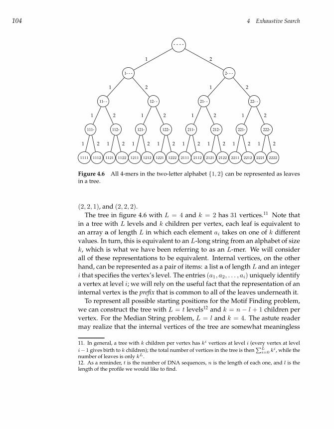
104 4 Exhaustive Search
- - - -
1- - -
1
11- -
1
111-
1
1111
1
1112
2
112-
2
1121
1
1122
2
12- -
2
121-
1
1211
1
1212
2
122-
2
1221
1
1222
2
2- - -
2
21- -
1
211-
1
2111
1
2112
2
212-
2
2121
1
2122
2
22- -
2
221-
1
2211
1
2212
2
222-
2
2221
1
2222
2
Figure 4.6 All 4-mers in the two-letter alphabet 1, 2 can be represented as leavesin a tree.
(2, 2, 1), and (2, 2, 2).
The tree in figure 4.6 with L = 4 and k = 2 has 31 vertices.11 Note that
in a tree with L levels and k children per vertex, each leaf is equivalent to
an array a of length L in which each element ai takes on one of k different
values. In turn, this is equivalent to an L-long string from an alphabet of size
k, which is what we have been referring to as an L-mer. We will consider
all of these representations to be equivalent. Internal vertices, on the other
hand, can be represented as a pair of items: a list a of length L and an integer
i that specifies the vertex’s level. The entries (a1, a2, . . . , ai) uniquely identify
a vertex at level i; we will rely on the useful fact that the representation of an
internal vertex is the prefix that is common to all of the leaves underneath it.
To represent all possible starting positions for the Motif Finding problem,
we can construct the tree with L = t levels12 and k = n − l + 1 children per
vertex. For the Median String problem, L = l and k = 4. The astute reader
may realize that the internal vertices of the tree are somewhat meaningless
11. In general, a tree with k children per vertex has ki vertices at level i (every vertex at level
i−1 gives birth to k children); the total number of vertices in the tree is thenPL
i=0 ki, while thenumber of leaves is only kL.12. As a reminder, t is the number of DNA sequences, n is the length of each one, and l is thelength of the profile we would like to find.
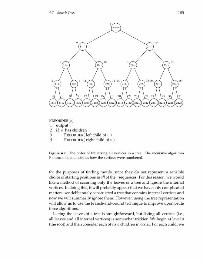
4.7 Search Trees 105
- - - -1
1- - -2
11- -3
111-4
1111
5
1112
6
112-7
1121
8
1122
9
12- -10
121-11
1211
12
1212
13
122-14
1221
15
1222
16
2- - -17
21- -18
211-19
2111
20
2112
21
212-22
2121
23
2122
24
22- -25
221-26
2211
27
2212
28
222-29
2221
30
2222
31
PREORDER(v)1 output v2 if v has children3 PREORDER( left child of v )4 PREORDER( right child of v )
Figure 4.7 The order of traversing all vertices in a tree. The recursive algorithmPREORDER demonstrates how the vertices were numbered.
for the purposes of finding motifs, since they do not represent a sensible
choice of starting positions in all of the t sequences. For this reason, we would
like a method of scanning only the leaves of a tree and ignore the internal
vertices. In doing this, it will probably appear that we have only complicated
matters: we deliberately constructed a tree that contains internal vertices and
now we will summarily ignore them. However, using the tree representation
wlll allow us to use the branch-and-bound technique to improve upon brute
force algorithms.
Listing the leaves of a tree is straightforward, but listing all vertices (i.e.,
all leaves and all internal vertices) is somewhat trickier. We begin at level 0
(the root) and then consider each of its k children in order. For each child, we
106 4 Exhaustive Search
again consider each of its k children and so on. Figure 4.7 shows the order of
traversing vertices for a tree with L = 4 and k = 2 and also gives an elegant
recursive algorithm to perform this process. The sequence of vertices that
PREORDER(root) would return on the tree of L = 4 and k = 2 would be as
follows:
(-,-,-,-)(1,-,-,-)(1,1,-,-)(1,1,1,-)(1,1,1,1)(1,1,1,2)(1,1,2,-)(1,1,2,1)(1,1,2,2)(1,2,-,-)(1,2,1,-)(1,2,1,1)(1,2,1,2)(1,2,2,-)(1,2,2,1)(1,2,2,2)(2,-,-,-)(2,1,-,-)(2,1,1,-)(2,1,1,1)(2,1,1,2)(2,1,2,-)(2,1,2,1)(2,1,2,2)(2,2,-,-)(2,2,1,-)(2,2,1,1)(2,2,1,2)(2,2,2,-)(2,2,2,1)(2,2,2,2)
Traversing the complete tree iteratively is implemented in the NEXTVER-
TEX algorithm, below. NEXTVERTEX takes vertex a = (a1, . . . , aL) at level i as
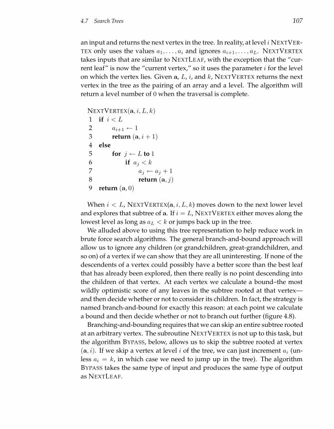
4.7 Search Trees 107
an input and returns the next vertex in the tree. In reality, at level i NEXTVER-
TEX only uses the values a1, . . . , ai and ignores ai+1, . . . , aL. NEXTVERTEX
takes inputs that are similar to NEXTLEAF, with the exception that the “cur-
rent leaf” is now the “current vertex,” so it uses the parameter i for the level
on which the vertex lies. Given a, L, i, and k, NEXTVERTEX returns the next
vertex in the tree as the pairing of an array and a level. The algorithm will
return a level number of 0 when the traversal is complete.
NEXTVERTEX(a, i, L, k)
1 if i < L
2 ai+1 ← 1
3 return (a, i + 1)
4 else
5 for j ← L to 1
6 if aj < k
7 aj ← aj + 1
8 return (a, j)
9 return (a, 0)
When i < L, NEXTVERTEX(a, i, L, k) moves down to the next lower level
and explores that subtree of a. If i = L, NEXTVERTEX either moves along the
lowest level as long as aL < k or jumps back up in the tree.
We alluded above to using this tree representation to help reduce work in
brute force search algorithms. The general branch-and-bound approach will
allow us to ignore any children (or grandchildren, great-grandchildren, and
so on) of a vertex if we can show that they are all uninteresting. If none of the
descendents of a vertex could possibly have a better score than the best leaf
that has already been explored, then there really is no point descending into
the children of that vertex. At each vertex we calculate a bound–the most
wildly optimistic score of any leaves in the subtree rooted at that vertex—
and then decide whether or not to consider its children. In fact, the strategy is
named branch-and-bound for exactly this reason: at each point we calculate
a bound and then decide whether or not to branch out further (figure 4.8).
Branching-and-bounding requires that we can skip an entire subtree rooted
at an arbitrary vertex. The subroutine NEXTVERTEX is not up to this task, but
the algorithm BYPASS, below, allows us to skip the subtree rooted at vertex
(a, i). If we skip a vertex at level i of the tree, we can just increment ai (un-
less ai = k, in which case we need to jump up in the tree). The algorithm
BYPASS takes the same type of input and produces the same type of output
as NEXTLEAF.
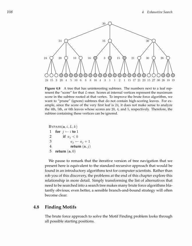
108 4 Exhaustive Search
30
24
24
24 15 3
20
20 4 5
10
10 6 3
16
16
8 16 4
3
3 1 1
15
2 1 15
30
21
17 21 23
30
15 27 30
26
26 18 19
Figure 4.8 A tree that has uninteresting subtrees. The numbers next to a leaf rep-resent the “score” for that L-mer. Scores at internal vertices represent the maximumscore in the subtree rooted at that vertex. To improve the brute force algorithm, wewant to “prune” (ignore) subtrees that do not contain high-scoring leaves. For ex-ample, since the score of the very first leaf is 24, it does not make sense to analyzethe 4th, 5th, or 6th leaves whose scores are 20, 4, and 5, respectively. Therefore, thesubtree containing these vertices can be ignored.
BYPASS(a, i, L, k)
1 for j ← i to 1
2 if aj < k
3 aj ← aj + 1
4 return (a, j)
5 return (a, 0)
We pause to remark that the iterative version of tree navigation that we
present here is equivalent to the standard recursive approach that would be
found in an introductory algorithms text for computer scientists. Rather than
rob you of this discovery, the problems at the end of this chapter explore this
relationship in more detail. Simply transforming the list of alternatives that
need to be searched into a search tree makes many brute force algorithms bla-
tantly obvious; even better, a sensible branch-and-bound strategy will often
become clear.
4.8 Finding Motifs
The brute force approach to solve the Motif Finding problem looks through
all possible starting positions.
4.8 Finding Motifs 109
BRUTEFORCEMOTIFSEARCH(DNA, t, n, l)
1 bestScore← 0
2 for each (s1, . . . , st) from (1, . . . , 1) to (n− l + 1, . . . , n− l + 1)
3 if Score(s, DNA) > bestScore
4 bestScore← Score(s, DNA)
5 bestMotif ← (s1, s2, . . . , st)
6 return bestMotif
There are n−l+1 choices for the first index (s1) and for each of those, there
are n− l+1 choices for the second index (s2). For each of those choices, there
are n − l + 1 choices for the third index, and so on. Therefore, the overall
number of positions is (n − l + 1)t, which is exponential in t, the number
of sequences. For each s, the algorithm calculates Score(s, DNA), which
requires O(l) operations. Thus, the overall complexity of the algorithm is
evaluated as O(lnt).
The only remaining question is how to write line 2 using standard pseu-
docode operations. This is particularly easy if we use NEXTLEAF from the
previous section. In this case, L = n − l + 1 and k = t. Rewriting BRUTE-
FORCEMOTIFSEARCH in this way we arrive at BRUTEFORCEMOTIFSEARCH-
AGAIN.
BRUTEFORCEMOTIFSEARCHAGAIN(DNA, t, n, l)
1 s← (1, 1, . . . , 1)
2 bestScore← Score(s, DNA)
3 while forever
4 s← NEXTLEAF(s, t, n− l + 1)
5 if Score(s, DNA) > bestScore
6 bestScore← Score(s, DNA)
7 bestMotif ← (s1, s2, . . . , st)
8 if s = (1, 1, . . . , 1)
9 return bestMotif
Finally, to prepare for the branch-and-bound strategy, we will want the
equivalent version, SIMPLEMOTIFSEARCH, which uses NEXTVERTEX to ex-
plore each leaf.
110 4 Exhaustive Search
SIMPLEMOTIFSEARCH(DNA, t, n, l)
1 s← (1, . . . , 1)
2 bestScore← 0
3 i← 1
4 while i > 0
5 if i < t
6 (s, i)← NEXTVERTEX(s, i, t, n− l + 1)
7 else
8 if Score(s, DNA) > bestScore
9 bestScore← Score(s, DNA)
10 bestMotif ← (s1, s2, . . . , st)
11 (s, i)← NEXTVERTEX(s, i, t, n− l + 1)
12 return bestMotif
Observe that some sets of starting positions can be ruled out immedi-
ately without iterating over them, based simply on the most optimistic es-
timate of their score. For example, if the first i of t starting positions [i.e.,
(s1, s2, . . . , si)] form a “weak” profile, then it may not be necessary to even
consider any starting positions in the sequences i + 1, i + 2, . . . , t, since the
resulting profile could not possibly be better than the highest-scoring profile
already found.
Given a set of starting positions s = (s1, s2, . . . , st), define the partial con-
sensus score, Score(s, i, DNA), to be the consensus score of the i× l alignment
matrix involving only the first i rows of DNA corresponding to starting po-
sitions (s1, s2, . . . , si,−,−, . . . ,−). In this case, a− indicates that we have not
chosen any value for that entry in s. If we have the partial consensus score for
s1, . . . , si, even in the best of circumstances the remaining t− i rows can only
improve the consensus score by (t − i) · l; therefore, the score of any align-
ment matrix with the first i starting positions (s1, . . . , si) could be at most
Score(s, i, DNA) + (t− i) · l. This implies that if Score(s, i, DNA) + (t− i) · l
is less than the currently best score, bestScore, then it does not make sense
to explore any of the remaining t − i sequences in the sample—with this
choice of (s1, . . . , si)—it would obviously result in wasted effort. Therefore,
the bound Score(s, i, DNA) + (t − i) · l could save us the trouble of looking
at (n− l + 1)t−i leaves.
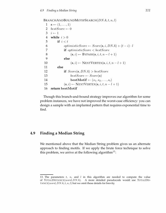
4.9 Finding a Median String 111
BRANCHANDBOUNDMOTIFSEARCH(DNA, t, n, l)
1 s← (1, . . . , 1)
2 bestScore← 0
3 i← 1
4 while i > 0
5 if i < t
6 optimisticScore← Score(s, i, DNA) + (t− i) · l
7 if optimisticScore < bestScore
8 (s, i)← BYPASS(s, i, t, n− l + 1)
9 else
10 (s, i)← NEXTVERTEX(s, i, t, n− l + 1)
11 else
12 if Score(s, DNA) > bestScore
13 bestScore← Score(s)
14 bestMotif ← (s1, s2, . . . , st)
15 (s, i)← NEXTVERTEX(s, i, t, n− l + 1)
16 return bestMotif
Though this branch-and-bound strategy improves our algorithm for some
problem instances, we have not improved the worst-case efficiency: you can
design a sample with an implanted pattern that requires exponential time to
find.
4.9 Finding a Median String
We mentioned above that the Median String problem gives us an alternate
approach to finding motifs. If we apply the brute force technique to solve
this problem, we arrive at the following algorithm13:
13. The parameters t, n, and l in this algorithm are needed to compute the valueof TOTALDISTANCE(word,DNA). A more detailed pseudocode would use TOTALDIS-TANCE(word,DNA, t, n, l) but we omit these details for brevity.
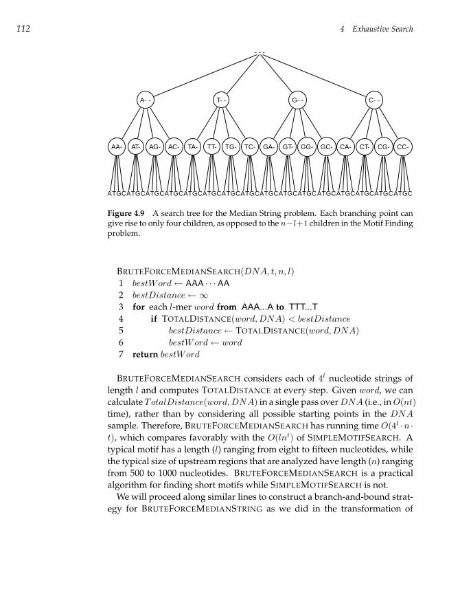
112 4 Exhaustive Search
- - -
A- -
AA-
ATGC
AT-
ATGC
AG-
ATGC
AC-
ATGC
T- -
TA-
ATGC
TT-
ATGC
TG-
ATGC
TC-
ATGC
G- -
GA-
ATGC
GT-
ATGC
GG-
ATGC
GC-
ATGC
C- -
CA-
ATGC
CT-
ATGC
CG-
ATGC
CC-
ATGC
Figure 4.9 A search tree for the Median String problem. Each branching point cangive rise to only four children, as opposed to the n−l+1 children in the Motif Findingproblem.
BRUTEFORCEMEDIANSEARCH(DNA, t, n, l)
1 bestWord← AAA · · ·AA
2 bestDistance←∞
3 for each l-mer word from AAA...A to TTT...T4 if TOTALDISTANCE(word, DNA) < bestDistance
5 bestDistance← TOTALDISTANCE(word, DNA)
6 bestWord← word
7 return bestWord
BRUTEFORCEMEDIANSEARCH considers each of 4l nucleotide strings of
length l and computes TOTALDISTANCE at every step. Given word, we can
calculate TotalDistance(word, DNA) in a single pass over DNA (i.e., in O(nt)
time), rather than by considering all possible starting points in the DNA
sample. Therefore, BRUTEFORCEMEDIANSEARCH has running time O(4l ·n ·
t), which compares favorably with the O(lnt) of SIMPLEMOTIFSEARCH. A
typical motif has a length (l) ranging from eight to fifteen nucleotides, while
the typical size of upstream regions that are analyzed have length (n) ranging
from 500 to 1000 nucleotides. BRUTEFORCEMEDIANSEARCH is a practical
algorithm for finding short motifs while SIMPLEMOTIFSEARCH is not.
We will proceed along similar lines to construct a branch-and-bound strat-
egy for BRUTEFORCEMEDIANSTRING as we did in the transformation of
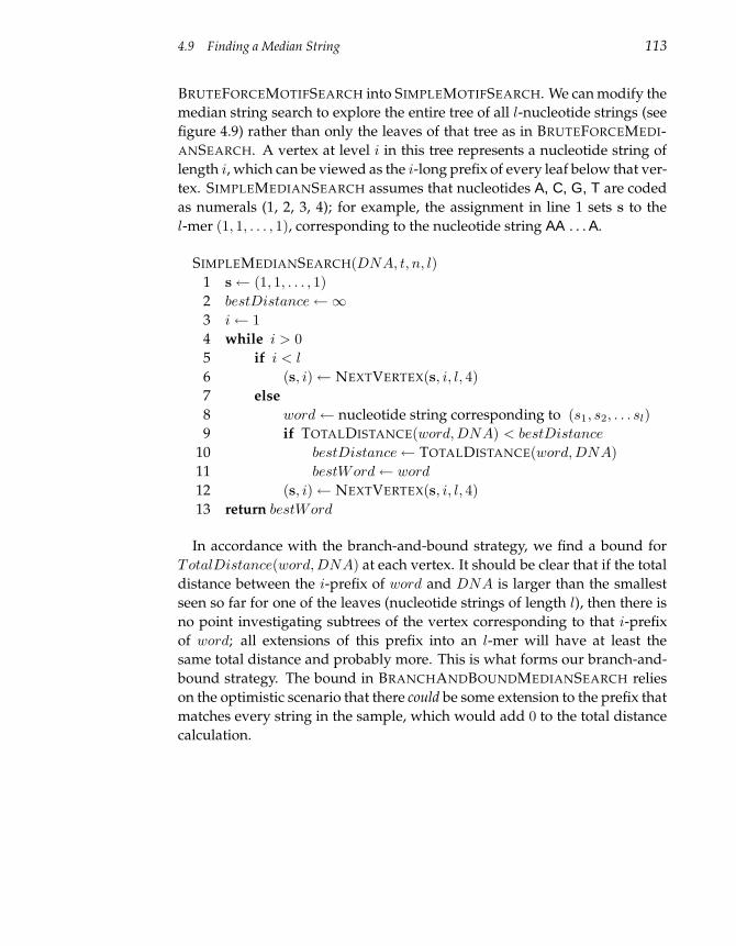
4.9 Finding a Median String 113
BRUTEFORCEMOTIFSEARCH into SIMPLEMOTIFSEARCH. We can modify the
median string search to explore the entire tree of all l-nucleotide strings (see
figure 4.9) rather than only the leaves of that tree as in BRUTEFORCEMEDI-
ANSEARCH. A vertex at level i in this tree represents a nucleotide string of
length i, which can be viewed as the i-long prefix of every leaf below that ver-
tex. SIMPLEMEDIANSEARCH assumes that nucleotides A, C, G, T are coded
as numerals (1, 2, 3, 4); for example, the assignment in line 1 sets s to the
l-mer (1, 1, . . . , 1), corresponding to the nucleotide string AA . . . A.
SIMPLEMEDIANSEARCH(DNA, t, n, l)
1 s← (1, 1, . . . , 1)
2 bestDistance←∞
3 i← 1
4 while i > 0
5 if i < l
6 (s, i)← NEXTVERTEX(s, i, l, 4)
7 else
8 word← nucleotide string corresponding to (s1, s2, . . . sl)
9 if TOTALDISTANCE(word, DNA) < bestDistance
10 bestDistance← TOTALDISTANCE(word, DNA)
11 bestWord← word
12 (s, i)← NEXTVERTEX(s, i, l, 4)
13 return bestWord
In accordance with the branch-and-bound strategy, we find a bound for
TotalDistance(word, DNA) at each vertex. It should be clear that if the total
distance between the i-prefix of word and DNA is larger than the smallest
seen so far for one of the leaves (nucleotide strings of length l), then there is
no point investigating subtrees of the vertex corresponding to that i-prefix
of word; all extensions of this prefix into an l-mer will have at least the
same total distance and probably more. This is what forms our branch-and-
bound strategy. The bound in BRANCHANDBOUNDMEDIANSEARCH relies
on the optimistic scenario that there could be some extension to the prefix that
matches every string in the sample, which would add 0 to the total distance
calculation.
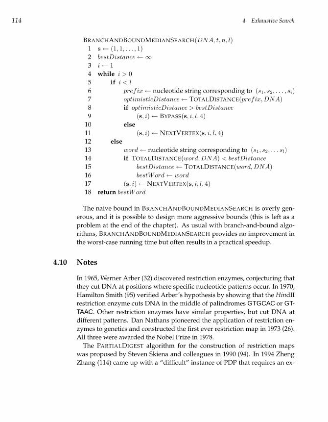
114 4 Exhaustive Search
BRANCHANDBOUNDMEDIANSEARCH(DNA, t, n, l)
1 s← (1, 1, . . . , 1)
2 bestDistance←∞
3 i← 1
4 while i > 0
5 if i < l
6 prefix← nucleotide string corresponding to (s1, s2, . . . , si)
7 optimisticDistance← TOTALDISTANCE(prefix, DNA)
8 if optimisticDistance > bestDistance
9 (s, i)← BYPASS(s, i, l, 4)
10 else
11 (s, i)← NEXTVERTEX(s, i, l, 4)
12 else
13 word← nucleotide string corresponding to (s1, s2, . . . sl)
14 if TOTALDISTANCE(word, DNA) < bestDistance
15 bestDistance← TOTALDISTANCE(word, DNA)
16 bestWord← word
17 (s, i)← NEXTVERTEX(s, i, l, 4)
18 return bestWord
The naive bound in BRANCHANDBOUNDMEDIANSEARCH is overly gen-
erous, and it is possible to design more aggressive bounds (this is left as a
problem at the end of the chapter). As usual with branch-and-bound algo-
rithms, BRANCHANDBOUNDMEDIANSEARCH provides no improvement in
the worst-case running time but often results in a practical speedup.
4.10 Notes
In 1965, Werner Arber (32) discovered restriction enzymes, conjecturing that
they cut DNA at positions where specific nucleotide patterns occur. In 1970,
Hamilton Smith (95) verified Arber’s hypothesis by showing that the HindII
restriction enzyme cuts DNA in the middle of palindromes GTGCAC or GT-TAAC. Other restriction enzymes have similar properties, but cut DNA at
different patterns. Dan Nathans pioneered the application of restriction en-
zymes to genetics and constructed the first ever restriction map in 1973 (26).
All three were awarded the Nobel Prize in 1978.
The PARTIALDIGEST algorithm for the construction of restriction maps
was proposed by Steven Skiena and colleagues in 1990 (94). In 1994 Zheng
Zhang (114) came up with a “difficult” instance of PDP that requires an ex-
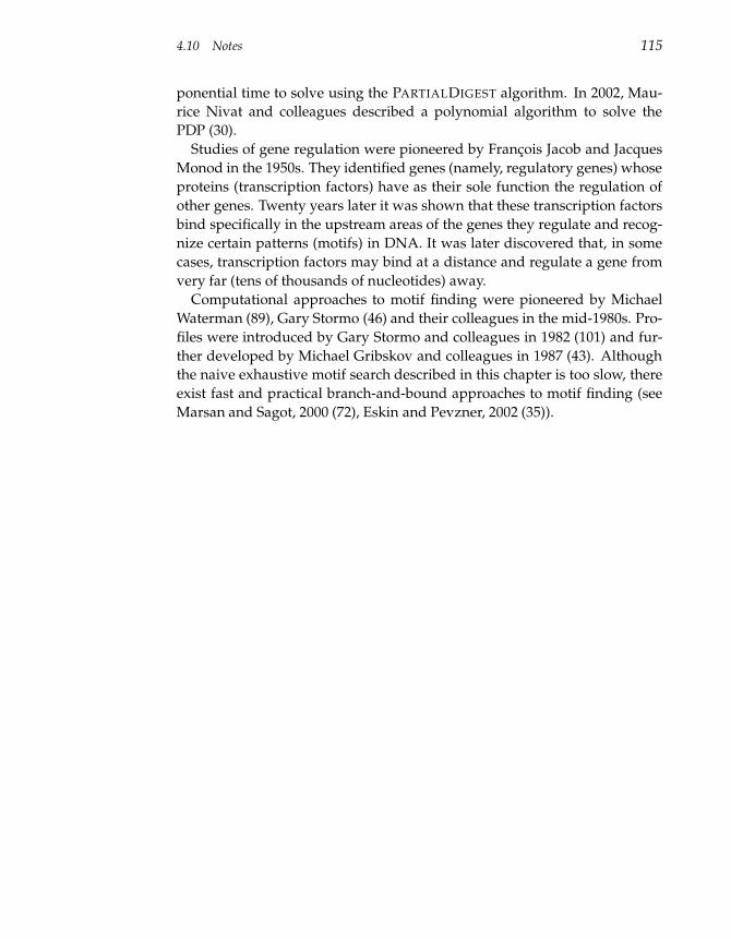
4.10 Notes 115
ponential time to solve using the PARTIALDIGEST algorithm. In 2002, Mau-
rice Nivat and colleagues described a polynomial algorithm to solve the
PDP (30).
Studies of gene regulation were pioneered by François Jacob and Jacques
Monod in the 1950s. They identified genes (namely, regulatory genes) whose
proteins (transcription factors) have as their sole function the regulation of
other genes. Twenty years later it was shown that these transcription factors
bind specifically in the upstream areas of the genes they regulate and recog-
nize certain patterns (motifs) in DNA. It was later discovered that, in some
cases, transcription factors may bind at a distance and regulate a gene from
very far (tens of thousands of nucleotides) away.
Computational approaches to motif finding were pioneered by Michael
Waterman (89), Gary Stormo (46) and their colleagues in the mid-1980s. Pro-
files were introduced by Gary Stormo and colleagues in 1982 (101) and fur-
ther developed by Michael Gribskov and colleagues in 1987 (43). Although
the naive exhaustive motif search described in this chapter is too slow, there
exist fast and practical branch-and-bound approaches to motif finding (see
Marsan and Sagot, 2000 (72), Eskin and Pevzner, 2002 (35)).
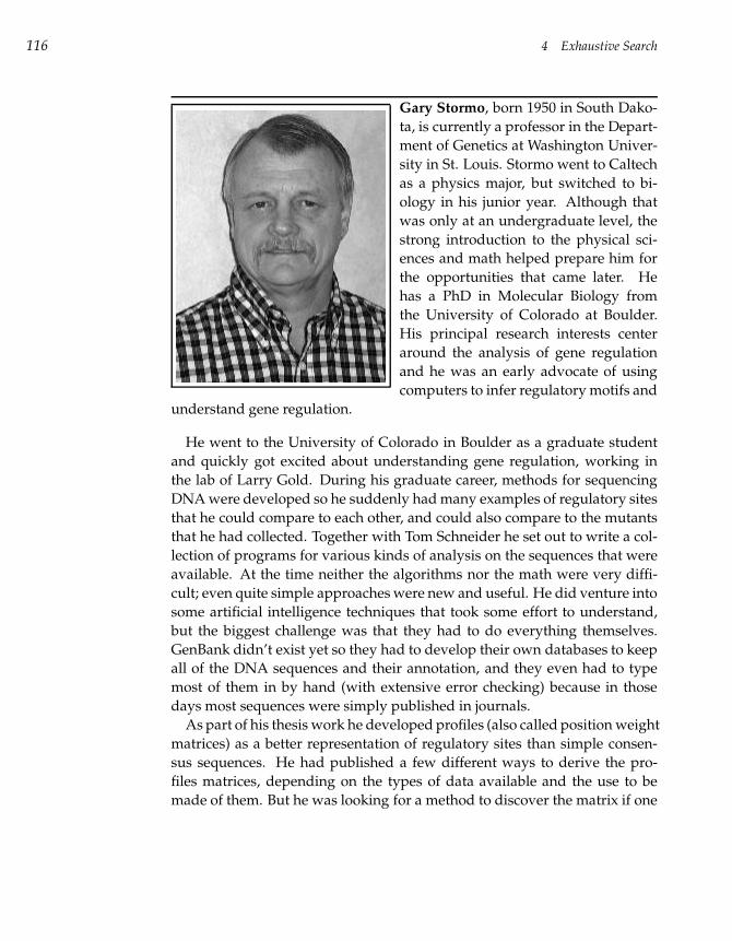
116 4 Exhaustive Search
Gary Stormo, born 1950 in South Dako-
ta, is currently a professor in the Depart-
ment of Genetics at Washington Univer-
sity in St. Louis. Stormo went to Caltech
as a physics major, but switched to bi-
ology in his junior year. Although that
was only at an undergraduate level, the
strong introduction to the physical sci-
ences and math helped prepare him for
the opportunities that came later. He
has a PhD in Molecular Biology from
the University of Colorado at Boulder.
His principal research interests center
around the analysis of gene regulation
and he was an early advocate of using
computers to infer regulatory motifs and
understand gene regulation.
He went to the University of Colorado in Boulder as a graduate student
and quickly got excited about understanding gene regulation, working in
the lab of Larry Gold. During his graduate career, methods for sequencing
DNA were developed so he suddenly had many examples of regulatory sites
that he could compare to each other, and could also compare to the mutants
that he had collected. Together with Tom Schneider he set out to write a col-
lection of programs for various kinds of analysis on the sequences that were
available. At the time neither the algorithms nor the math were very diffi-
cult; even quite simple approaches were new and useful. He did venture into
some artificial intelligence techniques that took some effort to understand,
but the biggest challenge was that they had to do everything themselves.
GenBank didn’t exist yet so they had to develop their own databases to keep
all of the DNA sequences and their annotation, and they even had to type
most of them in by hand (with extensive error checking) because in those
days most sequences were simply published in journals.
As part of his thesis work he developed profiles (also called position weight
matrices) as a better representation of regulatory sites than simple consen-
sus sequences. He had published a few different ways to derive the pro-
files matrices, depending on the types of data available and the use to be
made of them. But he was looking for a method to discover the matrix if one
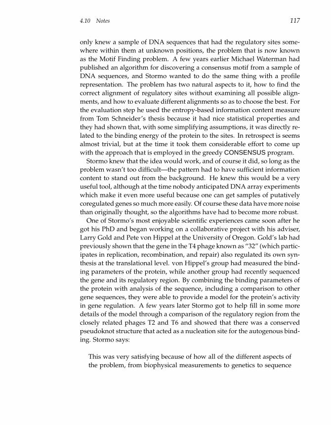
4.10 Notes 117
only knew a sample of DNA sequences that had the regulatory sites some-
where within them at unknown positions, the problem that is now known
as the Motif Finding problem. A few years earlier Michael Waterman had
published an algorithm for discovering a consensus motif from a sample of
DNA sequences, and Stormo wanted to do the same thing with a profile
representation. The problem has two natural aspects to it, how to find the
correct alignment of regulatory sites without examining all possible align-
ments, and how to evaluate different alignments so as to choose the best. For
the evaluation step he used the entropy-based information content measure
from Tom Schneider’s thesis because it had nice statistical properties and
they had shown that, with some simplifying assumptions, it was directly re-
lated to the binding energy of the protein to the sites. In retrospect is seems
almost trivial, but at the time it took them considerable effort to come up
with the approach that is employed in the greedy CONSENSUS program.
Stormo knew that the idea would work, and of course it did, so long as the
problem wasn’t too difficult—the pattern had to have sufficient information
content to stand out from the background. He knew this would be a very
useful tool, although at the time nobody anticipated DNA array experiments
which make it even more useful because one can get samples of putatively
coregulated genes so much more easily. Of course these data have more noise
than originally thought, so the algorithms have had to become more robust.
One of Stormo’s most enjoyable scientific experiences came soon after he
got his PhD and began working on a collaborative project with his adviser,
Larry Gold and Pete von Hippel at the University of Oregon. Gold’s lab had
previously shown that the gene in the T4 phage known as “32” (which partic-
ipates in replication, recombination, and repair) also regulated its own syn-
thesis at the translational level. von Hippel’s group had measured the bind-
ing parameters of the protein, while another group had recently sequenced
the gene and its regulatory region. By combining the binding parameters of
the protein with analysis of the sequence, including a comparison to other
gene sequences, they were able to provide a model for the protein’s activity
in gene regulation. A few years later Stormo got to help fill in some more
details of the model through a comparison of the regulatory region from the
closely related phages T2 and T6 and showed that there was a conserved
pseudoknot structure that acted as a nucleation site for the autogenous bind-
ing. Stormo says:
This was very satisfying because of how all of the different aspects of
the problem, from biophysical measurements to genetics to sequence
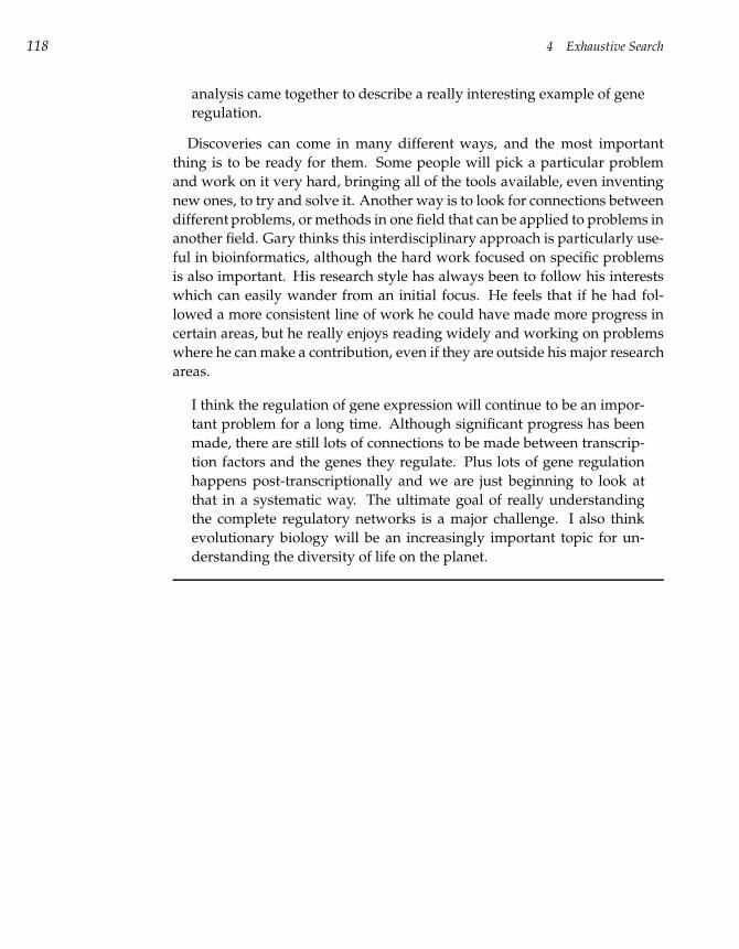
118 4 Exhaustive Search
analysis came together to describe a really interesting example of gene
regulation.
Discoveries can come in many different ways, and the most important
thing is to be ready for them. Some people will pick a particular problem
and work on it very hard, bringing all of the tools available, even inventing
new ones, to try and solve it. Another way is to look for connections between
different problems, or methods in one field that can be applied to problems in
another field. Gary thinks this interdisciplinary approach is particularly use-
ful in bioinformatics, although the hard work focused on specific problems
is also important. His research style has always been to follow his interests
which can easily wander from an initial focus. He feels that if he had fol-
lowed a more consistent line of work he could have made more progress in
certain areas, but he really enjoys reading widely and working on problems
where he can make a contribution, even if they are outside his major research
areas.
I think the regulation of gene expression will continue to be an impor-
tant problem for a long time. Although significant progress has been
made, there are still lots of connections to be made between transcrip-
tion factors and the genes they regulate. Plus lots of gene regulation
happens post-transcriptionally and we are just beginning to look at
that in a systematic way. The ultimate goal of really understanding
the complete regulatory networks is a major challenge. I also think
evolutionary biology will be an increasingly important topic for un-
derstanding the diversity of life on the planet.
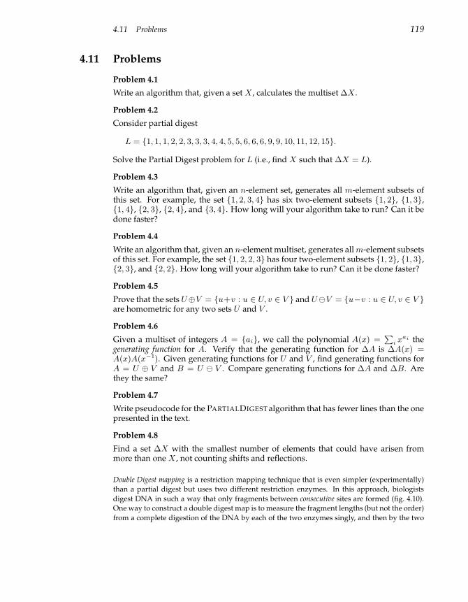
4.11 Problems 119
4.11 Problems
Problem 4.1
Write an algorithm that, given a set X, calculates the multiset ∆X.
Problem 4.2
Consider partial digest
L = 1, 1, 1, 2, 2, 3, 3, 3, 4, 4, 5, 5, 6, 6, 6, 9, 9, 10, 11, 12, 15.
Solve the Partial Digest problem for L (i.e., find X such that ∆X = L).
Problem 4.3
Write an algorithm that, given an n-element set, generates all m-element subsets ofthis set. For example, the set 1, 2, 3, 4 has six two-element subsets 1, 2, 1, 3,1, 4, 2, 3, 2, 4, and 3, 4. How long will your algorithm take to run? Can it bedone faster?
Problem 4.4
Write an algorithm that, given an n-element multiset, generates all m-element subsetsof this set. For example, the set 1, 2, 2, 3 has four two-element subsets 1, 2, 1, 3,2, 3, and 2, 2. How long will your algorithm take to run? Can it be done faster?
Problem 4.5
Prove that the sets U⊕V = u+v : u ∈ U, v ∈ V and UV = u−v : u ∈ U, v ∈ V are homometric for any two sets U and V .
Problem 4.6
Given a multiset of integers A = ai, we call the polynomial A(x) =P
ixai the
generating function for A. Verify that the generating function for ∆A is ∆A(x) =A(x)A(x−1). Given generating functions for U and V , find generating functions forA = U ⊕ V and B = U V . Compare generating functions for ∆A and ∆B. Arethey the same?
Problem 4.7
Write pseudocode for the PARTIALDIGEST algorithm that has fewer lines than the onepresented in the text.
Problem 4.8
Find a set ∆X with the smallest number of elements that could have arisen frommore than one X, not counting shifts and reflections.
Double Digest mapping is a restriction mapping technique that is even simpler (experimentally)
than a partial digest but uses two different restriction enzymes. In this approach, biologists
digest DNA in such a way that only fragments between consecutive sites are formed (fig. 4.10).
One way to construct a double digest map is to measure the fragment lengths (but not the order)
from a complete digestion of the DNA by each of the two enzymes singly, and then by the two
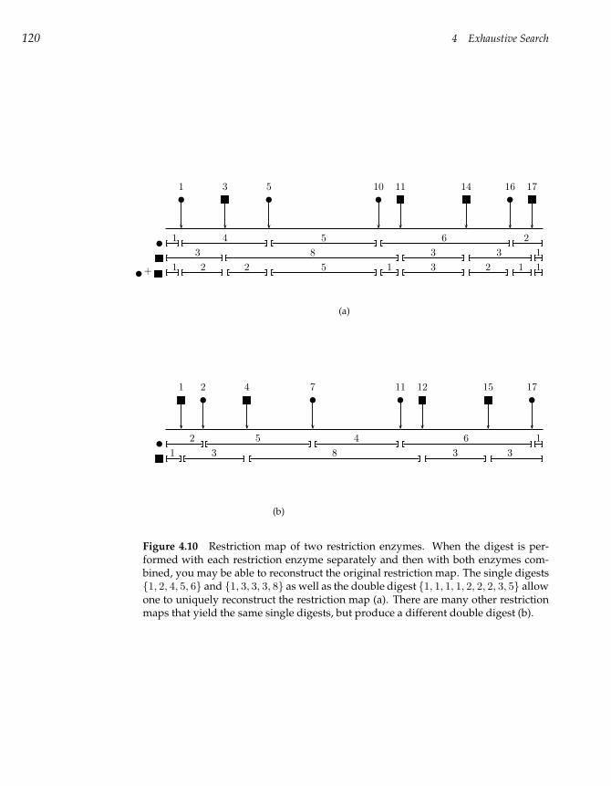
120 4 Exhaustive Search
1 3 5 10 11 14 16 17
1 4 5 6 2
3 8 3 3 1
+ 1 2 2 5 1 3 2 1 1
(a)
1 2 4 7 11 12 15 17
2 5 4 6 1
1 3 8 3 3
(b)
Figure 4.10 Restriction map of two restriction enzymes. When the digest is per-formed with each restriction enzyme separately and then with both enzymes com-bined, you may be able to reconstruct the original restriction map. The single digests1, 2, 4, 5, 6 and 1, 3, 3, 3, 8 as well as the double digest 1, 1, 1, 1, 2, 2, 2, 3, 5 allowone to uniquely reconstruct the restriction map (a). There are many other restrictionmaps that yield the same single digests, but produce a different double digest (b).
4.11 Problems 121
enzymes applied together. The problem of determining the positions of the cuts from fragment
length data is known as the Double Digest problem, or DDP.
Figure 4.10 shows “DNA” cut by two restriction enzymes, A (shown by a circle) and B (shown
by a square). Through gel electrophoresis experiments with these two restriction enzymes, a bi-
ologist can obtain information about the sizes of the restriction fragments generated by each in-
dividually. However, there are many orderings (maps) corresponding to these fragment lengths.
To find out which of the maps is the correct one, biologists cleave DNA by both enzymes at the
same time; this procedure is known as a double digest. The two maps presented in figure 4.10
produce the same single digests A and B but different double digests A+ B. The double digest
that fits experimental data corresponds to the correct map. The Double Digest problem is to find
a physical map, given three sets of fragment lengths: A, B, and A + B.
Problem 4.9
Devise a brute force algorithm for the DDP and suggest a branch-and-bound ap-proach to improve its performance.
Another technique used to build restriction maps leads to the Probed Partial Digest problem (PPDP).
In this method DNA is partially digested with a restriction enzyme, thus generating a collection
of DNA fragments between every two cutting sites. After this, a labeled probe that attaches to
the DNA between two cutting sites is hybridized to the partially digested DNA, and the sizes
of fragments to which the probe hybridizes are measured. In contrast to the PDP, where the in-
put consists of all partial fragments, the input for the PPDP consists of all partial fragments that
contain a given point (this point corresponds to the position of the labeled probe). The problem
is to reconstruct the positions of the sites from the multiset of measured lengths.
In the PPDP, we assume that the labeled probe is hybridized at position 0 and that A is the set
of restriction sites with negative coordinates while B is the set of restriction sites with positive
coordinates. The probed partial digest experiment provides the multiset b−a : a ∈ A, b ∈ B
and the problem is to find A and B given this set.
Problem 4.10
Design a brute force algorithm for the PPDP and suggest a branch-and-bound ap-proach to improve its performance.
Problem 4.11
The search trees in the text are complete k-ary trees: each vertex that is not a leaf hasexactly k children. It is also balanced: the number of edges in the path from the rootto any leaf is the same (this is sometimes referred to as the height of the tree). Find aclosed-form expression for the total number of vertices in a complete and balancedk-ary tree of height L.
Problem 4.12
Given a long text string T and one shorter pattern string s, find the first occurrenceof s in T (if any). What is the complexity of your algorithm?
Problem 4.13
Given a long text string T , one shorter pattern string s, and an integer k, find the firstoccurrence in T of a string (if any) s′ such that dH(s, s′) ≤ k. What is the complexityof your algorithm?
122 4 Exhaustive Search
Problem 4.14
Implement an algorithm that counts the number of occurrences of each l-mer in astring of length n. Run it over a bacterial genome and construct the distribution ofl-mer frequencies. Compare this distribution to that of a random string of the samelength as the bacterial genome.
Problem 4.15
The following algorithm is a cousin of one of the motif finding algorithms we haveconsidered in this chapter. Identify which algorithm is a cousin of ANOTHERMOTIF-SEARCH and find the similarities and differences between these two algorithms.
ANOTHERMOTIFSEARCH(DNA, t, n, l)
1 s← (1, 1, . . . , 1)
2 bestMotif ← FINDINSEQ(s, 1, t, n, l)
3 return bestMotif
FINDINSEQ(s, currentSeq, t, n, l)
1 bestScore← 0
2 for j ← 1 to n− l + 1
3 scurrentSeq ← j
4 if currentSeq 6= t
5 s← FINDINSEQ(s, currentSeq + 1, t, n, l)
6 if Score(s) > bestScore
7 bestScore← Score(s)
8 bestMotif ← s
9 return bestMotif
Problem 4.16
The following algorithm is a cousin of one of the motif finding algorithms we haveconsidered in this chapter. Identify which algorithm is a cousin of YETANOTHERMO-TIFSEARCH and find the similarities and differences between these two algorithms.

4.11 Problems 123
YETANOTHERMOTIFSEARCH(DNA, t, n, l)
1 s← (1, 1, . . . , 1)
2 bestMotif← FIND(s, 1, t, n, l)
3 return bestMotif
FIND(s, currentSeq, t, n, l)
1 i← currentSeq
2 bestScore← 0
3 for j ← 1 to n− l + 1
4 si ← j
5 bestPossibleScore← Score(s, i) + (t− i) · l6 if bestPossibleScore > bestScore
7 if currentSeq 6= t
8 s← FIND(s, currentSeq + 1, t, n, l)
9 if Score(s) > bestScore
10 bestScore← Score(s)
11 bestMotif ← s
12 return bestMotif
Problem 4.17
Derive a tighter bound for the branch-and-bound strategy for the Median String prob-lem. Hint: Split an l-mer w into two parts, u and v. Use TotalDistance(u, DNA) +TotalDistance(v,DNA) to bound TotalDistance(w,DNA).

5 Greedy Algorithms
The algorithm USCHANGE in chapter 2 is an example of a greedy strategy: at
each step, the cashier would only consider the largest denomination smaller
than (or equal to) M . Since the goal was to minimize the number of coins re-
turned to the customer, this seemed like a sensible strategy: you would never
use five nickels in place of one quarter. A generalization of USCHANGE, BET-
TERCHANGE also used what seemed like the best option and did not consider
any others, which is what makes an algorithm “greedy.” Unfortunately, BET-
TERCHANGE actually returned incorrect results in some cases because of its
short-sighted notion of “good.” This is a common characteristic of greedy
algorithms: they often return suboptimal results, but take very little time to
do so. However, there are a lucky few greedy algorithms that find optimal
rather than suboptimal solutions.
5.1 Genome Rearrangements
Waardenburg’s syndrome is a genetic disorder resulting in hearing loss and
pigmentary abnormalities, such as two differently colored eyes. The disease
was named after the Dutch ophthalmologist who first noticed that people
with two differently colored eyes frequently had hearing problems as well.
In the early 1990s, biologists narrowed the search for the gene implicated in
Waardenburg’s syndrome to human chromosome 2, but its exact location re-
mained unknown for some time. There was another clue that shed light on
the gene associated with Waardenburg’s syndrome, that drew attention to
chromosome 2: for a long time, breeders scrutinized mice for mutants, and
one of these, designated splotch, had pigmentary abnormalities like patches
of white spots, similar to those in humans with Waardenburg’s syndrome.
Through breeding, the splotch gene was mapped to one of the mouse chro-
Administrator
Highlight
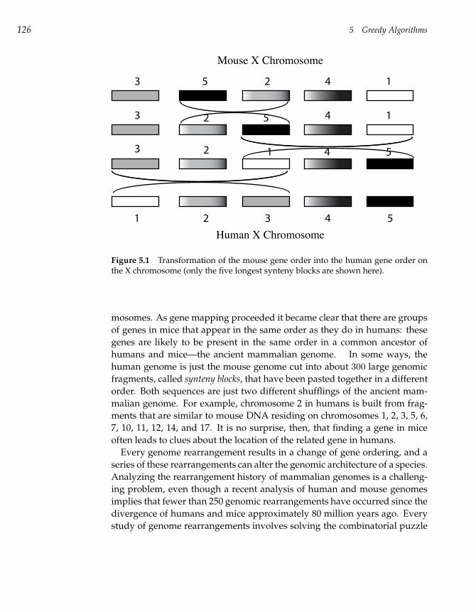
126 5 Greedy Algorithms
1 2 3 4 5
1
1
1
2
2
2
3
3
3
4
4
4
5
5
5
Human X Chromosome
Mouse X Chromosome
Figure 5.1 Transformation of the mouse gene order into the human gene order onthe X chromosome (only the five longest synteny blocks are shown here).
mosomes. As gene mapping proceeded it became clear that there are groups
of genes in mice that appear in the same order as they do in humans: these
genes are likely to be present in the same order in a common ancestor of
humans and mice—the ancient mammalian genome. In some ways, the
human genome is just the mouse genome cut into about 300 large genomic
fragments, called synteny blocks, that have been pasted together in a different
order. Both sequences are just two different shufflings of the ancient mam-
malian genome. For example, chromosome 2 in humans is built from frag-
ments that are similar to mouse DNA residing on chromosomes 1, 2, 3, 5, 6,
7, 10, 11, 12, 14, and 17. It is no surprise, then, that finding a gene in mice
often leads to clues about the location of the related gene in humans.
Every genome rearrangement results in a change of gene ordering, and a
series of these rearrangements can alter the genomic architecture of a species.
Analyzing the rearrangement history of mammalian genomes is a challeng-
ing problem, even though a recent analysis of human and mouse genomes
implies that fewer than 250 genomic rearrangements have occurred since the
divergence of humans and mice approximately 80 million years ago. Every
study of genome rearrangements involves solving the combinatorial puzzle
5.2 Sorting by Reversals 127
of finding a series of rearrangements that transform one genome into an-
other. Figure 5.1 presents a rearrangement scenario in which the mouse X chro-
mosome is transformed into the human X chromosome.1 The elementary
rearrangement event in this scenario is the flipping of a genomic segment,
called a reversal, or an inversion. One can consider other types of evolution-
ary events but in this book we only consider reversals, the most common
evolutionary events.
Biologists are interested in the most parsimonious evolutionary scenario,
that is, the scenario involving the smallest number of reversals. While there is
no guarantee that this scenario represents an actual evolutionary sequence, it
gives us a lower bound on the number of rearrangements that have occurred
and indicates the similarity between two species.2
Even for the small number of synteny blocks shown, it is not so easy to ver-
ify that the three evolutionary events in figure 5.1 represent a shortest series
of reversals transforming the mouse gene order into the human gene order
on the X chromosome. The exhaustive search technique that we presented
in the previous chapter would hardly work for rearrangement studies since
the number of variants that need to be explored becomes enormous for more
than ten synteny blocks. Below, we explore two greedy approaches that work
to differing degrees of success.
5.2 Sorting by Reversals
In their simplest form, rearrangement events can be modeled by a series
of reversals that transform one genome into another. The order of genes
(rather, of synteny blocks) in a genome can be represented by a permutation3
1. Extreme conservation of genes on X chromosomes across mammalian species provides anopportunity to study the evolutionary history of X chromosomes independently of the rest of thegenomes, since the gene content of X chromosomes has barely changed throughout mammalianevolution. However, the order of genes on X chromosomes has been disrupted several times. Inother words, genes that reside on the X chromosome stay on the X chromosome (but their ordermay change). All other chromosomes may exchange genes, that is, a gene can move from onechromosome to another.2. In fact, a sequence of reversals that transforms the X chromosome of mouse into the X chro-mosome of man does not even represent an evolutionary sequence, since humans are not de-scended from the present-day mouse. However, biologists believe that the architecture of the Xchromosome in the human-mouse ancestor is about the same as the architecture of the humanX chromosome.3. A permutation of a sequence of n numbers is just a reordering of that sequence. We willalways use permutations of consecutive integers: for example, 2 1 3 4 5 is a permutation of1 2 3 4 5.
128 5 Greedy Algorithms
π = π1π2 · · ·πn. The order of synteny blocks on the X chromosome in hu-
mans is represented in figure 5.1 by (1, 2, 3, 4, 5), while the ordering in mice
is (3, 5, 2, 4, 1).4
A reversal ρ(i, j) has the effect of reversing the order of synteny blocks
πiπi+1 · · ·πj−1πj
In effect, this transforms
π = π1 · · ·πi−1πiπi+1 · · ·πj−1πj−−−−−−−−−−−−→
πj+1 · · ·πn
into
π · ρ(i, j) = π1 · · ·πi−1πjπj−1 · · ·πi+1πi←−−−−−−−−−−−−
πj+1 · · ·πn
For example, if π = 1 2 4 3 7 5−−−→ 6, then π · ρ(3, 6) = 1 2 5 7 3 4←−−− 6. With this rep-
resentation of a genome, and a rigorous definition of an evolutionary event,
we are in a position to formulate the computational problem that mimics the
biological rearrangement process.
Reversal Distance Problem:
Given two permutations, find a shortest series of reversals that trans-
forms one permutation into another.
Input: Permutations π and σ.
Output: A series of reversals ρ1, ρ2, . . . , ρt transforming π
into σ (i.e., π · ρ1 · ρ2 · · · ρt = σ), such that t is minimum.
We call t the reversal distance between π and σ, and write d(π, σ) to denote
the reversal distance for a given π and σ. In practice, one usually selects the
second genome’s order as a gold standard, and arbitrarily sets σ to be the
identity permutation 1 2 · · · n. The Sorting by Reversals problem is similar to
the Reversal Distance problem, except that it requires only one permutation
as input.
4. In reality, genes and synteny blocks have directionality, reflecting whether they reside on thedirect strand or the reverse complement strand of the DNA. In other words, the synteny blockorder in an organism is really represented by a signed permutation. However, in this section weignore the directionality of the synteny blocks for simplicity.
5.2 Sorting by Reversals 129
Sorting by Reversals Problem:
Given a permutation, find a shortest series of reversals that transforms
it into the identity permutation.
Input: Permutation π.
Output: A series of reversals ρ1, ρ2, . . . , ρt transforming π
into the identity permutation such that t is minimum.
In this case, we call t the reversal distance of π and denote it as d(π). When
sorting a permutation π = 1 2 3 6 4 5, it hardly makes sense to move the
already-sorted first three elements of π. If we define prefix(π) to be the num-
ber of already-sorted elements of π, then a sensible strategy for sorting by
reversals is to increase prefix(π) at every step. This approach sorts π in 2
steps: 1 2 3 6 45 → 1 2 3 4 6 5→ 1 2 3 4 5 6. Generalizing this leads to an algo-
rithm that sorts a permutation by repeatedly moving its ith element to the
ith position.5
SIMPLEREVERSALSORT(π)
1 for i← 1 to n− 1
2 j ← position of element i in π (i.e., πj = i)
3 if j 6= i
4 π ← π · ρ(i, j)
5 output π
6 if π is the identity permutation
7 return
SIMPLEREVERSALSORT is an example of a greedy algorithm that chooses
the “best” reversal at every step. However, the notion of “best” here is rather
short-sighted—simply increasing prefix(π) does not guarantee the smallest
number of reversals. For example, SIMPLEREVERSALSORT takes five steps to
sort 6 1 2 3 4 5:
6 1 2 3 4 5→ 1 6 23 4 5→ 1 2 6 34 5→ 1 2 3 6 45→ 1 2 3 4 6 5→ 1 2 3 4 5 6
However, the same permutation can be sorted in just two steps:
6 1 2 3 4 5→ 5 4 3 2 16→ 1 2 3 4 5 6.
5. Note the superficial similarity of this algorithm to SELECTIONSORT in chapter 2.
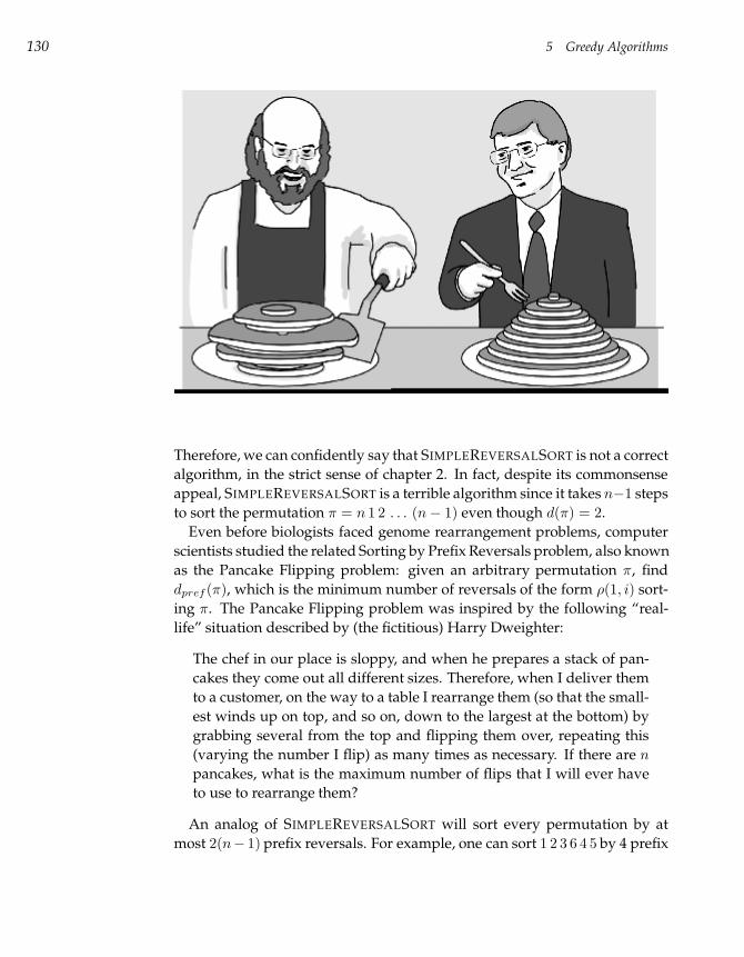
130 5 Greedy Algorithms
Therefore, we can confidently say that SIMPLEREVERSALSORT is not a correct
algorithm, in the strict sense of chapter 2. In fact, despite its commonsense
appeal, SIMPLEREVERSALSORT is a terrible algorithm since it takes n−1 steps
to sort the permutation π = n 1 2 . . . (n− 1) even though d(π) = 2.
Even before biologists faced genome rearrangement problems, computer
scientists studied the related Sorting by Prefix Reversals problem, also known
as the Pancake Flipping problem: given an arbitrary permutation π, find
dpref (π), which is the minimum number of reversals of the form ρ(1, i) sort-
ing π. The Pancake Flipping problem was inspired by the following “real-
life” situation described by (the fictitious) Harry Dweighter:
The chef in our place is sloppy, and when he prepares a stack of pan-
cakes they come out all different sizes. Therefore, when I deliver them
to a customer, on the way to a table I rearrange them (so that the small-
est winds up on top, and so on, down to the largest at the bottom) by
grabbing several from the top and flipping them over, repeating this
(varying the number I flip) as many times as necessary. If there are n
pancakes, what is the maximum number of flips that I will ever have
to use to rearrange them?
An analog of SIMPLEREVERSALSORT will sort every permutation by at
most 2(n− 1) prefix reversals. For example, one can sort 1 2 3 6 4 5 by 4 prefix
5.3 Approximation Algorithms 131
reversals (1 2 3 64 5 → 6 3 2 1 4 5 → 5 4 1 2 36 → 3 2 14 5 6 → 1 2 3 4 5 6) but
it is not clear whether there exists an even shorter series of prefix reversals
to sort this permutation. William Gates, an undergraduate student at Har-
vard in the mid-1970s, and Christos Papadimitriou, a professor at Harvard in
the mid-1970s, now at Berkeley, made the first attempt to solve this problem
and proved that any permutation can be sorted by at most 53 (n + 1) prefix
reversals. However, the Pancake Flipping problem remains unsolved.
5.3 Approximation Algorithms
In chapter 2 we mentioned that, for many problems, efficient polynomial
algorithms are still unknown and unlikely ever to be found. For such prob-
lems, computer scientists often find a compromise in approximation algorithms
that produce an approximate solution rather than an optimal one.6 The ap-
proximation ratio of algorithm A on input π is defined as A(π)OPT (π) , where A(π)
is the solution produced by the algorithm A and OPT (π) is the correct (op-
timal) solution of the problem.7 The approximation ratio, or performance guar-
antee of algorithm A is defined as its maximum approximation ratio over all
inputs of size n, that is, as
max|π|=n
A(π)
OPT (π).
We assume thatA is a minimization algorithm, i.e., an algorithm that attempts
to minimize its objective function. For maximization algorithms, the approx-
imation ratio is
min|π|=n
A(π)
OPT (π).
In essence, an approximation algorithm gives a worst-case scenario of just
how far off an algorithm’s output can be from some hypothetical perfect al-
gorithm. The approximation ratio of SIMPLEREVERSALSORT is at least n−12 ,
so a biologist has no guarantee that this algorithm comes anywhere close to
the correct solution. For example, if n is 1001, this algorithm could return
a series of reversals that is as large as 500 times the optimal. Our goal is
6. Approximation algorithms are only relevant to problems that have a numerical objectivefunction like minimizing the number of coins returned to the customer. A problem that doesnot have such an objective function (like the Partial Digest problem) does not lend itself to ap-proximation algorithms.7. Technically, an approximation algorithm is not correct, in the sense of chapter 2, since thereexists some input that returns a suboptimal (incorrect) output. The approximation ratio givesone an idea of just how incorrect the algorithm can be.
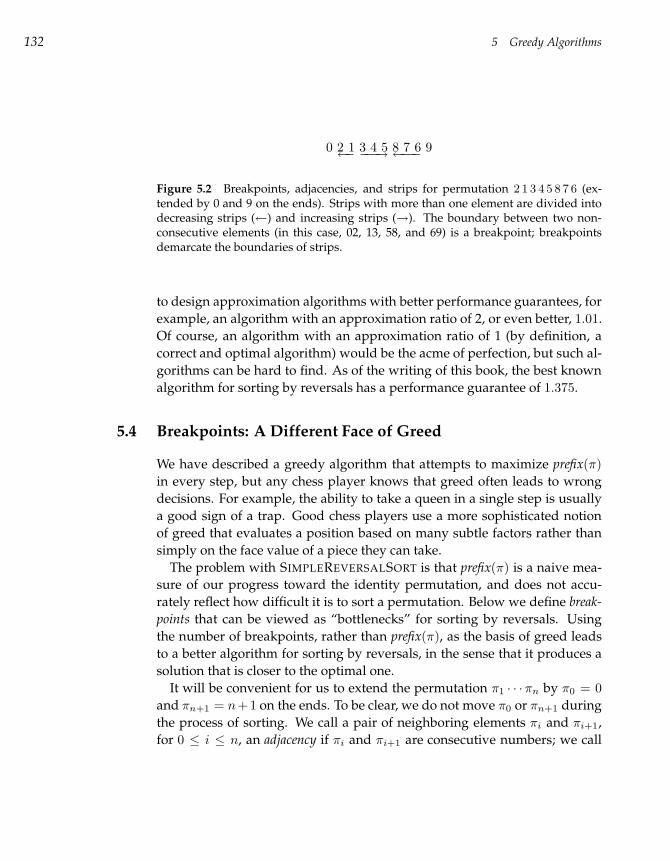
132 5 Greedy Algorithms
0 2 1←− 3 4 5−−−→ 8 7 6←−−− 9
Figure 5.2 Breakpoints, adjacencies, and strips for permutation 2 1 3 4 5 8 7 6 (ex-tended by 0 and 9 on the ends). Strips with more than one element are divided intodecreasing strips (←) and increasing strips (→). The boundary between two non-consecutive elements (in this case, 02, 13, 58, and 69) is a breakpoint; breakpointsdemarcate the boundaries of strips.
to design approximation algorithms with better performance guarantees, for
example, an algorithm with an approximation ratio of 2, or even better, 1.01.
Of course, an algorithm with an approximation ratio of 1 (by definition, a
correct and optimal algorithm) would be the acme of perfection, but such al-
gorithms can be hard to find. As of the writing of this book, the best known
algorithm for sorting by reversals has a performance guarantee of 1.375.
5.4 Breakpoints: A Different Face of Greed
We have described a greedy algorithm that attempts to maximize prefix(π)
in every step, but any chess player knows that greed often leads to wrong
decisions. For example, the ability to take a queen in a single step is usually
a good sign of a trap. Good chess players use a more sophisticated notion
of greed that evaluates a position based on many subtle factors rather than
simply on the face value of a piece they can take.
The problem with SIMPLEREVERSALSORT is that prefix(π) is a naive mea-
sure of our progress toward the identity permutation, and does not accu-
rately reflect how difficult it is to sort a permutation. Below we define break-
points that can be viewed as “bottlenecks” for sorting by reversals. Using
the number of breakpoints, rather than prefix(π), as the basis of greed leads
to a better algorithm for sorting by reversals, in the sense that it produces a
solution that is closer to the optimal one.
It will be convenient for us to extend the permutation π1 · · ·πn by π0 = 0
and πn+1 = n+1 on the ends. To be clear, we do not move π0 or πn+1 during
the process of sorting. We call a pair of neighboring elements πi and πi+1,
for 0 ≤ i ≤ n, an adjacency if πi and πi+1 are consecutive numbers; we call
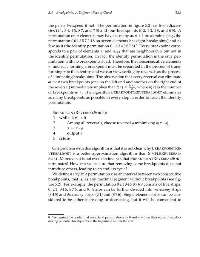
5.4 Breakpoints: A Different Face of Greed 133
the pair a breakpoint if not. The permutation in figure 5.2 has five adjacen-
cies (2 1, 3 4, 4 5, 8 7, and 7 6) and four breakpoints (0 2, 1 3, 5 8, and 6 9). A
permutation on n elements may have as many as n + 1 breakpoints (e.g., the
permutation 0 6 1 3 5 7 2 4 8 on seven elements has eight breakpoints) and as
few as 0 (the identity permutation 0 1 2 3 4 5 6 7 8).8 Every breakpoint corre-
sponds to a pair of elements πi and πi+1 that are neighbors in π but not in
the identity permutation. In fact, the identity permutation is the only per-
mutation with no breakpoints at all. Therefore, the nonconsecutive elements
πi and πi+1 forming a breakpoint must be separated in the process of trans-
forming π to the identity, and we can view sorting by reversals as the process
of eliminating breakpoints. The observation that every reversal can eliminate
at most two breakpoints (one on the left end and another on the right end of
the reversal) immediately implies that d(π) ≥ b(π)2 , where b(π) is the number
of breakpoints in π. The algorithm BREAKPOINTREVERSALSORT eliminates
as many breakpoints as possible in every step in order to reach the identity
permutation.
BREAKPOINTREVERSALSORT(π)
1 while b(π) > 0
2 Among all reversals, choose reversal ρ minimizing b(π · ρ)
3 π ← π · ρ
4 output π
5 return
One problem with this algorithm is that it is not clear why BREAKPOINTRE-
VERSALSORT is a better approximation algorithm than SIMPLEREVERSAL-
SORT. Moreover, it is not even obvious yet that BREAKPOINTREVERSALSORT
terminates! How can we be sure that removing some breakpoints does not
introduce others, leading to an endless cycle?
We define a strip in a permutation π as an interval between two consecutive
breakpoints, that is, as any maximal segment without breakpoints (see fig-
ure 5.2). For example, the permutation 0 2 1 3 4 5 8 7 6 9 consists of five strips:
0, 2 1, 3 4 5, 8 7 6, and 9. Strips can be further divided into increasing strips
(3 4 5) and decreasing strips (2 1) and (8 7 6). Single-element strips can be con-
sidered to be either increasing or decreasing, but it will be convenient to
8. We remind the reader that we extend permutations by 0 and n + 1 on their ends, thus intro-ducing potential breakpoints in the beginning and in the end.
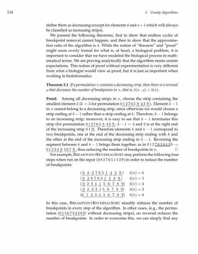
134 5 Greedy Algorithms
define them as decreasing (except for elements 0 and n+1 which will always
be classified as increasing strips).
We present the following theorems, first to show that endless cycles of
breakpoint removal cannot happen, and then to show that the approxima-
tion ratio of the algorithm is 4. While the notion of “theorem” and “proof”
might seem overly formal for what is, at heart, a biological problem, it is
important to consider that we have modeled the biological process in math-
ematical terms. We are proving analytically that the algorithm meets certain
expectations. This notion of proof without experimentation is very different
from what a biologist would view as proof, but it is just as important when
working in bioinformatics.
Theorem 5.1 If a permutation π contains a decreasing strip, then there is a reversal
ρ that decreases the number of breakpoints in π, that is, b(π · ρ) < b(π).
Proof: Among all decreasing strips in π, choose the strip containing the
smallest element k (k = 3 for permutation 0 1 2−−→ 7 6 5←−− 8←− 4 3←− 9−→). Element k − 1
in π cannot belong to a decreasing strip, since otherwise we would choose a
strip ending at k − 1 rather than a strip ending at k. Therefore, k − 1 belongs
to an increasing strip; moreover, it is easy to see that k − 1 terminates this
strip (for permutation 0 1 2−−→ 7 6 5←−− 8←− 4 3−→ 9−→, k − 1 = 2 and 2 is at the right end
of the increasing strip 0 1 2). Therefore elements k and k − 1 correspond to
two breakpoints, one at the end of the decreasing strip ending with k and
the other at the end of the increasing strip ending in k − 1. Reversing the
segment between k and k − 1 brings them together, as in 0 1 2 7 6 5 8 4 39 →
0 1 2 3 4−−−−→ 8←− 5 6 7−−→ 9−→, thus reducing the number of breakpoints in π. 2
For example, BREAKPOINTREVERSALSORT may perform the following four
steps when run on the input (0 8 2 7 6 5 1 4 3 9) in order to reduce the number
of breakpoints:
( 0−→ 8←− 2←− 7 6 5←−−− 1←− 4←− 3←− 9−→) b(π) = 6
( 0−→ 2←− 8 7 6 5←−−−− 1←− 4←− 3←− 9−→) b(π) = 5
( 0−→ 2 3 4−−−→ 1←− 5 6 7 8 9−−−−−−−−→) b(π) = 3
( 0−→ 4 3 2 1←−−−−− 5 6 7 8 9−−−−−−−−→) b(π) = 2
(0 1 2 3 4 5 6 7 8 9−−−−−−−−−−−−−−−−−−→) b(π) = 0
In this case, BREAKPOINTREVERSALSORT steadily reduces the number of
breakpoints in every step of the algorithm. In other cases, (e.g., the permu-
tation (0 1−→ 5 6 7−−→ 2 3 4−−→ 8 9−→) without decreasing strips), no reversal reduces the
number of breakpoints. In order to overcome this, we can simply find any
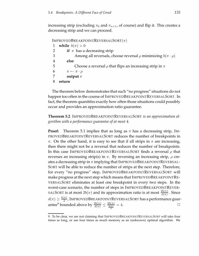
5.4 Breakpoints: A Different Face of Greed 135
increasing strip (excluding π0 and πn+1, of course) and flip it. This creates a
decreasing strip and we can proceed.
IMPROVEDBREAKPOINTREVERSALSORT(π)
1 while b(π) > 0
2 if π has a decreasing strip
3 Among all reversals, choose reversal ρ minimizing b(π · ρ)
4 else
5 Choose a reversal ρ that flips an increasing strip in π
6 π ← π · ρ
7 output π
8 return
The theorem below demonstrates that such “no progress” situations do not
happen too often in the course of IMPROVEDBREAKPOINTREVERSALSORT. In
fact, the theorem quanitifes exactly how often those situations could possibly
occur and provides an approximation ratio guarantee.
Theorem 5.2 IMPROVEDBREAKPOINTREVERSALSORT is an approximation al-
gorithm with a performance guarantee of at most 4.
Proof: Theorem 5.1 implies that as long as π has a decreasing strip, IM-
PROVEDBREAKPOINTREVERSALSORT reduces the number of breakpoints in
π. On the other hand, it is easy to see that if all strips in π are increasing,
then there might not be a reversal that reduces the number of breakpoints.
In this case IMPROVEDBREAKPOINTREVERSALSORT finds a reversal ρ that
reverses an increasing strip(s) in π. By reversing an increasing strip, ρ cre-
ates a decreasing strip in π implying that IMPROVEDBREAKPOINTREVERSAL-
SORT will be able to reduce the number of strips at the next step. Therefore,
for every “no progress” step, IMPROVEDBREAKPOINTREVERSALSORT will
make progress at the next step which means that IMPROVEDBREAKPOINTRE-
VERSALSORT eliminates at least one breakpoint in every two steps. In the
worst-case scenario, the number of steps in IMPROVEDBREAKPOINTREVER-
SALSORT is at most 2b(π) and its approximation ratio is at most 2b(π)d(π) . Since
d(π) ≥ b(π)2 , IMPROVEDBREAKPOINTREVERSALSORT has a performance guar-
antee9 bounded above by 2b(π)d(π) ≤
2b(π)b(π)
2
= 4. 2
9. To be clear, we are not claiming that IMPROVEDBREAKPOINTREVERSALSORT will take fourtimes as long, or use four times as much memory as an (unknown) optimal algorithm. We
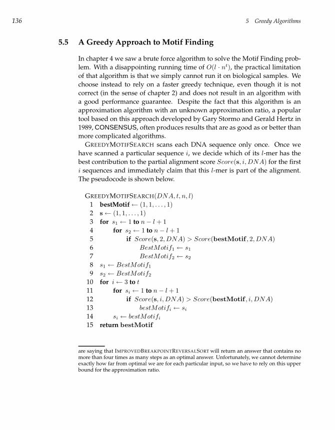
136 5 Greedy Algorithms
5.5 A Greedy Approach to Motif Finding
In chapter 4 we saw a brute force algorithm to solve the Motif Finding prob-
lem. With a disappointing running time of O(l · nt), the practical limitation
of that algorithm is that we simply cannot run it on biological samples. We
choose instead to rely on a faster greedy technique, even though it is not
correct (in the sense of chapter 2) and does not result in an algorithm with
a good performance guarantee. Despite the fact that this algorithm is an
approximation algorithm with an unknown approximation ratio, a popular
tool based on this approach developed by Gary Stormo and Gerald Hertz in
1989, CONSENSUS, often produces results that are as good as or better than
more complicated algorithms.
GREEDYMOTIFSEARCH scans each DNA sequence only once. Once we
have scanned a particular sequence i, we decide which of its l-mer has the
best contribution to the partial alignment score Score(s, i, DNA) for the first
i sequences and immediately claim that this l-mer is part of the alignment.
The pseudocode is shown below.
GREEDYMOTIFSEARCH(DNA, t, n, l)
1 bestMotif← (1, 1, . . . , 1)
2 s← (1, 1, . . . , 1)
3 for s1 ← 1 to n− l + 1
4 for s2 ← 1 to n− l + 1
5 if Score(s, 2, DNA) > Score(bestMotif , 2, DNA)
6 BestMotif1 ← s1
7 BestMotif2 ← s2
8 s1 ← BestMotif1
9 s2 ← BestMotif2
10 for i← 3 to t
11 for si ← 1 to n− l + 1
12 if Score(s, i, DNA) > Score(bestMotif , i, DNA)
13 bestMotifi ← si
14 si ← bestMotifi
15 return bestMotif
are saying that IMPROVEDBREAKPOINTREVERSALSORT will return an answer that contains nomore than four times as many steps as an optimal answer. Unfortunately, we cannot determineexactly how far from optimal we are for each particular input, so we have to rely on this upperbound for the approximation ratio.
5.6 Notes 137
GREEDYMOTIFSEARCH first finds the two closest l-mers—in the sense of
Hamming distance—in sequences 1 and 2 and forms a 2× l seed matrix. This
stage requires l(n − l + 1)2 operations. At each of the remaining t − 2 itera-
tions GREEDYMOTIFSEARCH extends the seed matrix into a matrix with one
more row by scanning the ith sequence (for 3 ≤ i ≤ t) each of the remaining
t−2 sequences and selecting the one l-mer that has the maximum Score(s, i).
This amounts to roughly l · (n− l + 1) operations in each iteration. Thus, the
running time of this algorithm is O(ln2 + lnt), which is vastly better than the
O(lnt) of SIMPLEMOTIFSEARCH or even the O(4lnt) of BRUTEFORCEMEDI-
ANSTRING. When t is small compared to n, GREEDYMOTIFSEARCH really
behaves as O(ln2), and the bulk of the time is actually spent locating the
l-mers from the first two sequences that are the most similar.
As you can imagine, because the sequences are scanned sequentially, it is
possible to construct input instances where GREEDYMOTIFSEARCH will miss
the optimal motif. One important difference between the popular CONSEN-SUS motif finding software tool and the algorithm presented here is that
CONSENSUS can scan the sequences in a random order, thereby making
it more difficult to construct inputs that elicit worst-case behavior. Another
important difference is that CONSENSUS saves a large number (usually at
least 1000) of seed matrices at each iteration rather than only the one that
GREEDYMOTIFSEARCH saves, making CONSENSUS less likely to miss the
optimal solution. However, no embellishment of this greedy approach will
be guaranteed to find an optimal motif.
5.6 Notes
The analysis of genome rearrangements in molecular biology was pioneered
by Theodosius Dobzhansky and Alfred Sturtevant who, in 1936, published
a milestone paper (102) presenting a rearrangement scenario for the species
of fruit fly. In 1984 Nadeau and Taylor (78) estimated that surprisingly few
genomic rearrangements (about 200) had taken place since the divergence of
the human and mouse genomes. This estimate, made in the pregenomic era
and based on a very limited data set, comes close to the recent postgenomic
estimates based on the comparison of the entire human and mouse DNA
sequences (85). The computational studies of the Reversal Distance prob-
lem were pioneered by David Sankoff in the early 1990s (93). The greedy
algorithm based on breakpoint elimination is from a paper (56) by John Ke-
cecioglu and David Sankoff. The best currently known algorithm for sorting

138 5 Greedy Algorithms
by reversals has an approximation ratio of 1.375 and was introduced by Piotr
Berman, Sridhar Hannenhalli and Marek Karpinski (13). The first algorith-
mic analysis of the Pancake Flipping problem was the work of William Gates
and Christos Papadimitriou in 1979 (40).
The greedy CONSENSUS algorithm was introduced by Gerald Hertz and
Gary Stormo, and further improved upon in 1999 in a later paper by the same
authors (47).
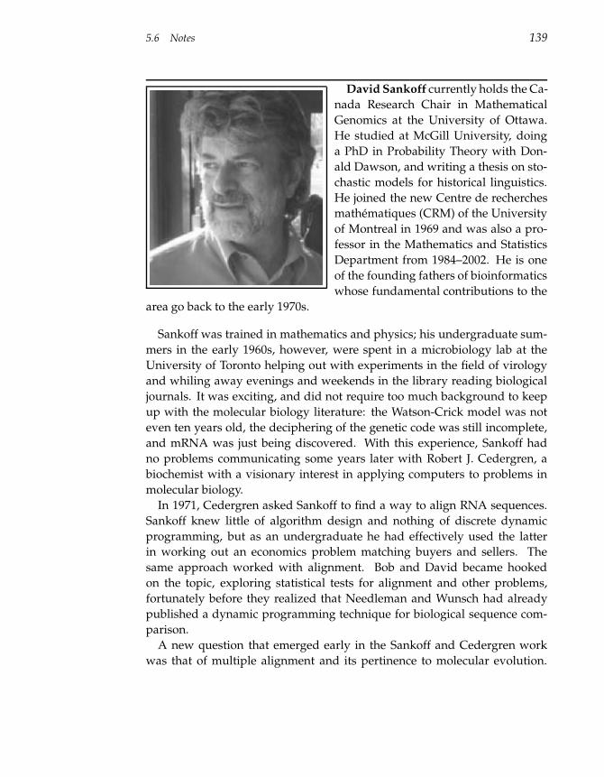
5.6 Notes 139
David Sankoff currently holds the Ca-
nada Research Chair in Mathematical
Genomics at the University of Ottawa.
He studied at McGill University, doing
a PhD in Probability Theory with Don-
ald Dawson, and writing a thesis on sto-
chastic models for historical linguistics.
He joined the new Centre de recherches
mathématiques (CRM) of the University
of Montreal in 1969 and was also a pro-
fessor in the Mathematics and Statistics
Department from 1984–2002. He is one
of the founding fathers of bioinformatics
whose fundamental contributions to the
area go back to the early 1970s.
Sankoff was trained in mathematics and physics; his undergraduate sum-
mers in the early 1960s, however, were spent in a microbiology lab at the
University of Toronto helping out with experiments in the field of virology
and whiling away evenings and weekends in the library reading biological
journals. It was exciting, and did not require too much background to keep
up with the molecular biology literature: the Watson-Crick model was not
even ten years old, the deciphering of the genetic code was still incomplete,
and mRNA was just being discovered. With this experience, Sankoff had
no problems communicating some years later with Robert J. Cedergren, a
biochemist with a visionary interest in applying computers to problems in
molecular biology.
In 1971, Cedergren asked Sankoff to find a way to align RNA sequences.
Sankoff knew little of algorithm design and nothing of discrete dynamic
programming, but as an undergraduate he had effectively used the latter
in working out an economics problem matching buyers and sellers. The
same approach worked with alignment. Bob and David became hooked
on the topic, exploring statistical tests for alignment and other problems,
fortunately before they realized that Needleman and Wunsch had already
published a dynamic programming technique for biological sequence com-
parison.
A new question that emerged early in the Sankoff and Cedergren work
was that of multiple alignment and its pertinence to molecular evolution.
140 5 Greedy Algorithms
Sankoff was already familiar with phylogeny problems from his work on lan-
guage families and participation in the early numerical taxonomy meetings
(before the schism between the parsimony-promoting cladists, led by Steve
Farris, and the more statistically oriented systematists). Combining phylo-
genetics with sequence comparison led to tree-based dynamic programming
for multiple alignment. Phylogenetic problems have cropped up often in
Sankoff’s research projects over the following decades.
Sankoff and Cedergren also studied RNA folding, applying several passes
of dynamic programming to build energy-optimal RNA structures. They
did not find the loop-matching reported by Daniel Kleitman’s group (later
integrated into a general, widely-used algorithm by Michael Zuker), though
they eventually made a number of contributions in the 1980s, in particular to
the problem of multiple loops and to simultaneous alignment and folding.
Sankoff says:
My collaboration with Cedergen also ran into its share of dead ends.
Applying multidimensional scaling to ribosome structure did not lead
very far, efforts to trace the origin of the genetic code through the phy-
logenetic analyses of tRNA sequences eventually petered out, and an
attempt at dynamic programming for consensus folding of proteins
was a flop.
The early and mid-1970s were nevertheless a highly productive time for
Sankoff; he was also working on probabilistic analysis of grammatical vari-
ation in natural languages, on game theory models for electoral processes,
and various applied mathematics projects in archaeology, geography, and
physics. He got Peter Sellers interested in sequence comparison; Sellers later
attracted attention by converting the longest common subsequence (LCS)
formulation to the edit distance version. Sankoff collaborated with promi-
nent mathematician Vaclav Chvatal on the expected length of the LCS of two
random sequences, for which they derived upper and lower bounds. Sev-
eral generations of probabilists have contributed to narrowing these bounds.
Sankoff says:
Evolutionary biologists Walter Fitch and Steve Farris spent sabbaticals
with me at the CRM, as did computer scientist Bill Day, generously
adding my name to a series of papers establishing the hardness of var-
ious phylogeny problems, most importantly the parsimony problem.
In 1987, Sankoff became a Fellow of the new Evolutionary Biology Pro-
gram of the Canadian Institute for Advanced Research (CIAR). At the very
5.6 Notes 141
first meeting of the CIAR program he was inspired by a talk by Monique
Turmel on the comparison of chloroplast genomes from two species of al-
gae. This led Sankoff to the comparative genomics–genome rearrangement
track that has been his main research line ever since. Originally he took a
probabilistic approach, but within a year or two he was trying to develop
algorithms and programs for reversal distance. A phylogeny based on the re-
versal distances among sixteen mitochondrial genomes proved that a strong
phylogenetic signal can be conserved in the gene order of even a miniscule
genome across many hundreds of millions of years. Sankoff says:
The network of fellows and scholars of the CIAR program, including
Bob Cedergren, Ford Doolittle, Franz Lang, Mike Gray, Brian Golding,
Mike Zuker, Claude Lemieux, and others across Canada; and a stellar
group of international advisors (such as Russ Doolittle, Michael Smith,
Marcus Feldman, Wally Gilbert) and associates (Mike Waterman, Joe
Felsenstein, Mike Steel and many others) became my virtual “home
department," a source of intellectual support, knowledge, and expe-
rience across multiple disciplines and a sounding board for the latest
ideas.
My comparative genomics research received two key boosts in the 1990s.
One was the sustained collaboration of a series of outstanding stu-
dents and postdocs: Guillaume Leduc, Vincent Ferretti, John Kece-
cioglu, Mathieu Blanchette, Nadia El-Mabrouk and David Bryant. The
second was my meeting Joe Nadeau; I already knew his seminal pa-
per with Taylor on estimating the number of conserved linkage seg-
ments and realized that our interests coincided perfectly while our
backgrounds were complementary.
When Nadeau showed up in Montreal for a short-lived appointment in
the Human Genetics Department at McGill, it took no more than an hour for
him and Sankoff to get started on a major collaborative project. They refor-
mulated the Nadeau-Taylor approach in terms of gene content data, freeing
it from physical or genetic distance measurements. The resulting simpler
model allowed them to thoroughly explore the mathematical properties of
the Nadeau-Taylor model and to experiment with the consequences of devi-
ating from it.
The synergy between the algorithmic and probabilistic aspects of com-
parative genomics has become basic to how Sankoff understands evolution.
The algorithmic is an ambitious attempt at deep inference, based on heavy
142 5 Greedy Algorithms
assumptions and the sophisticated but inflexible mathematics they enable.
The probabilistic is more descriptive and less explicitly revelatory of histor-
ical process, but the models based on statistics are easily generalized, their
hypotheses weakened or strengthened, and their robustness ascertained. In
Sankoff’s view, it is the playing out of this dialectic that makes the field of
whole-genome comparison the most interesting topic of research today and
for the near future.
My approach to research is not highly planned. Not that I don’t have
a vision about the general direction in which to go, but I have no spe-
cific set of tools that I apply as a matter of course, only an intuition
about what type of method or model, what database or display, might
be helpful. When I am lucky I can proceed from one small epiphany
to another, working out some of the details each time, until some clear
story emerges. Whether this involves stochastic processes, combina-
torial optimization, or differential equations is secondary; it is the bi-
ology of the problem that drives its mathematical formulation. I am
rarely motivated to research well-studied problems; instead I find my-
self confronting new problems in relatively unstudied areas; alignment
was not a burning preoccupation with biologists or computer scientists
when I started working on it, neither was genome rearrangement fif-
teen years later. I am quite pleased, though sometimes bemused, by the
veritable tidal wave of computational biologists and bioinformaticians
who have inundated the field where there were only a few isolated
researchers thirty or even twenty years ago.
5.7 Problems 143
5.7 Problems
Problem 5.1
Suppose you have a maximization algorithm, A, that has an approximation ratio of4. When run on some input π, A(π) = 12. What can you say about the true (correct)answer OPT = OPT (π)?
• OPT ≥ 3
• OPT ≤ 3
• OPT ≥ 12
• OPT ≤ 12
• OPT ≥ 48
• OPT ≤ 48
Problem 5.2
What is the approximation ratio of the BETTERCHANGE algorithm?
Problem 5.3
Design an approximation algorithm for the Pancake Flipping problem. What is itsapproximation ratio?
Problem 5.4
Perform the BREAKPOINTREVERSALSORT algorithm with π = 3 4 6 5 8 1 7 2 and showall intermediate permutations (break ties arbitrarily). Since BREAKPOINTREVERSAL-SORT is an approximation algorithm, there may be a sequence of reversals that isshorter than the one found by BREAKPOINTREVERSALSORT. Could you find such asequence of reversals? Do you know if it is the shortest possible sequence of rever-sals?
Problem 5.5
Find a permutation with no decreasing strips for which there exists a reversal thatreduces the number of breakpoints.
Problem 5.6
Can you find a permutation for which BREAKPOINTREVERSALSORT produces fourtimes as many reversals than the optimal solution of the Reversal Sorting problem?
A DNA molecule is not always shaped like a line segment. Some simple organisms have a
circular DNA molecule as a genome, where the molecule has no beginning and no end. These
circular genomes can be visualized as a sequence of integers written along the perimeter of a
circle. Two circular sequences would be considered equivalent if you could rotate one of the
circles and get the same sequence written on the other.
Problem 5.7
Devise an approximation algorithm to sort a circular genome by reversals (i.e., trans-form it to the identity circular permutation). Evaluate the algorithm’s performanceguarantee.
144 5 Greedy Algorithms
Problem 5.8
Devise a better algorithm (i.e., one with a better approximation ratio) for the Sortingby Reversals problem.
The swap sorting of permutation π is a transformation of π into the identity permutation by
exchanges of adjacent elements. For example, 3142 → 1342 → 1324 → 1234 is a three-step
swap sorting of permutation 3124.
Problem 5.9
Design an algorithm for swap sorting that uses the minimum number of swaps tosort a permutation.
Problem 5.10
Design an algorithm for swap sorting that uses the minimum number of swaps tosort a circular permutation.
Problem 5.11
How many permutations on n elements have a single breakpoint? How many per-mutations have exactly two breakpoints? How many permutations have exactly threebreakpoints?
Given permutations π and σ, a breakpoint between π and σ is defined as a pair of adjacent
elements πi and πi+1 in π that are separated in σ. For example, if π = 143256 and σ = 123465,
then π1 = 1 and π2 = 4 in π form a breakpoint between π and σ since 1 and 4 are separated
in σ. The number of breakpoints between π=01432567 and σ=01234657 is three (14, 25 and 67),
while the number of breakpoints between σ and π is also three (12, 46 and 57).
Problem 5.12
Prove that the number of breakpoints between π and σ equals the number of break-points between σ and π.
Problem 5.13
Given permutations π1 = 124356, π2 = 143256 and π3 = 123465, compute the num-ber of breakpoints between: (1) π1 and π2, (2) π1 and π3, and (3) π2 and π3.
Problem 5.14
Given the three permutations π1, π2, and π3 from the previous problem, find an an-
cestral permutation σ which minimizes the total breakpoint distanceP3
i=1 br(πi, σ)
between all three genomes and σ (br(πi, σ) is the number of breakpoints between πi
and σ).
Problem 5.15
Given three permutations π1, π2, and π3 from the previous problem, find an ancestral
permutation σ which minimizes the total reversal distanceP3
i=1 d(πi, σ) between allthree genomes and σ.
5.7 Problems 145
Analysis of genome rearrangements in multiple genomes corresponds to the following Multiple
Breakpoint Distance problem: : given a set of permutations π1, . . . , πk , find an ancestral permu-
tation σ such thatP
i=1,k br(πi, σ) is minimal, where br(πi, σ) is the number of breakpoints
between πi and σ.
Problem 5.16
Design a greedy algorithm for the Multiple Breakpoint Distance problem and evalu-ate its approximation ratio.
Problem 5.17
Alice and Bob have been assigned the task of implementing the BREAKPOINTREVER-SALSORT approximation algorithm.
• Bob wants to get home early so he decides to naively implement the algorithm,without putting any thought into performance improvements. What is the run-ning time of his program?
• Alice makes some changes to the algorithm and claims her algorithm achieves thesame approximation ratio as Bob’s (4) and runs in time O(n2). Give the pseu-docode for Alice’s algorithm.
• Not to be outdone, Bob gets a copy of Alice’s algorithm, and makes an improve-ment of his own. He claims that in the case where every strip is increasing, he canguarantee that there will be a decreasing strip in each of the next two steps (ratherthan one as in BREAKPOINTREVERSALSORT). Bob believes that this will give hisnew algorithm a better approximation ratio than the previous algorithms. Whatis Bob’s improvement, and what approximation ratio does it achieve?
Problem 5.18
Design an input for the GREEDYMOTIFSEARCH algorithm that causes the algorithmto output an incorrect result. That is, create a sample that has a strong pattern that ismissed because of the greedy nature of the algorithm. If optimalScore is the score ofthe strongest motif in the sample and greedyScore is the score returned by GREEDY-MOTIFSEARCH, how large can optimalScore/greedyScore be?

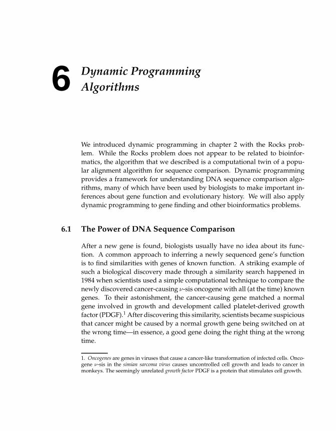
6 Dynamic Programming
Algorithms
We introduced dynamic programming in chapter 2 with the Rocks prob-
lem. While the Rocks problem does not appear to be related to bioinfor-
matics, the algorithm that we described is a computational twin of a popu-
lar alignment algorithm for sequence comparison. Dynamic programming
provides a framework for understanding DNA sequence comparison algo-
rithms, many of which have been used by biologists to make important in-
ferences about gene function and evolutionary history. We will also apply
dynamic programming to gene finding and other bioinformatics problems.
6.1 The Power of DNA Sequence Comparison
After a new gene is found, biologists usually have no idea about its func-
tion. A common approach to inferring a newly sequenced gene’s function
is to find similarities with genes of known function. A striking example of
such a biological discovery made through a similarity search happened in
1984 when scientists used a simple computational technique to compare the
newly discovered cancer-causing ν-sis oncogene with all (at the time) known
genes. To their astonishment, the cancer-causing gene matched a normal
gene involved in growth and development called platelet-derived growth
factor (PDGF).1 After discovering this similarity, scientists became suspicious
that cancer might be caused by a normal growth gene being switched on at
the wrong time—in essence, a good gene doing the right thing at the wrong
time.
1. Oncogenes are genes in viruses that cause a cancer-like transformation of infected cells. Onco-gene ν-sis in the simian sarcoma virus causes uncontrolled cell growth and leads to cancer inmonkeys. The seemingly unrelated growth factor PDGF is a protein that stimulates cell growth.
148 6 Dynamic Programming Algorithms
Another example of a successful similarity search was the discovery of the
cystic fibrosis gene. Cystic fibrosis is a fatal disease associated with abnormal
secretions, and is diagnosed in children at a rate of 1 in 3900. A defective gene
causes the body to produce abnormally thick mucus that clogs the lungs and
leads to lifethreatening lung infections. More than 10 million Americans are
unknowing and symptomless carriers of the defective cystic fibrosis gene;
each time two carriers have a child, there is a 25% chance that the child will
have cystic fibrosis.
In 1989 the search for the cystic fibrosis gene was narrowed to a region
of 1 million nucleotides on the chromosome 7, but the exact location of the
gene remained unknown. When the area around the cystic fibrosis gene was
sequenced, biologists compared the region against a database of all known
genes, and discovered similarities between some segment within this region
and a gene that had already been discovered, and was known to code for
adenosine triphosphate (ATP) binding proteins.2 These proteins span the cell
membrane multiple times as part of the ion transport channel; this seemed
a plausible function for a cystic fibrosis gene, given the fact that the disease
involves sweat secretions with abnormally high sodium content. As a result,
the similarity analysis shed light on a damaged mechanism in faulty cystic
fibrosis genes.
Establishing a link between cancer-causing genes and normal growth genes
and elucidating the nature of cystic fibrosis were only the first success stories
in sequence comparison. Many applications of sequence comparison algo-
rithms quickly followed, and today bioinformatics approaches are among
the dominant techniques for the discovery of gene function.
This chapter describes algorithms that allow biologists to reveal the simi-
larity between different DNA sequences. However, we will first show how
dynamic programming can yield a faster algorithm to solve the Change prob-
lem.
6.2 The Change Problem Revisited
We introduced the Change problem in chapter 2 as the problem of changing
an amount of money M into the smallest number of coins from denomina-
tions c = (c1, c2, . . . , cd). We showed that the naive greedy solution used by
cashiers everywhere is not actually a correct solution to this problem, and
ended with a correct—though slow—brute force algorithm. We will con-
2. ATP binding proteins provide energy for many reactions in the cell.
6.2 The Change Problem Revisited 149
sider a slightly modified version of the Change problem, in which we do
not concern ourselves with the actual combination of coins that make up
the optimal change solution. Instead, we only calculate the smallest number
of coins needed (it is easy to modify this algorithm to also return the coin
combination that achieves that number).
Suppose you need to make change for 77 cents and the only coin denomi-
nations available are 1, 3, and 7 cents. The best combination for 77 cents will
be one of the following:
• the best combination for 77− 1 = 76 cents, plus a 1-cent coin;
• the best combination for 77− 3 = 74 cents, plus a 3-cent coin;
• the best combination for 77− 7 = 70 cents, plus a 7-cent coin.
For 77 cents, the best combination would be the smallest of the above three
choices. The same logic applies to 76 cents (best of 75, 73, or 69 cents), and
so on (fig. 6.1). If bestNumCoinsM is the smallest number of coins needed to
change M cents, then the following recurrence relation holds:
bestNumCoinsM = min
bestNumCoinsM−1 + 1
bestNumCoinsM−3 + 1
bestNumCoinsM−7 + 1
In the more general case of d denominations c = (c1, . . . , cd):
bestNumCoinsM = min
bestNumCoinsM−c1 + 1
bestNumCoinsM−c2 + 1...
bestNumCoinsM−cd+ 1
This recurrence motivates the following algorithm:
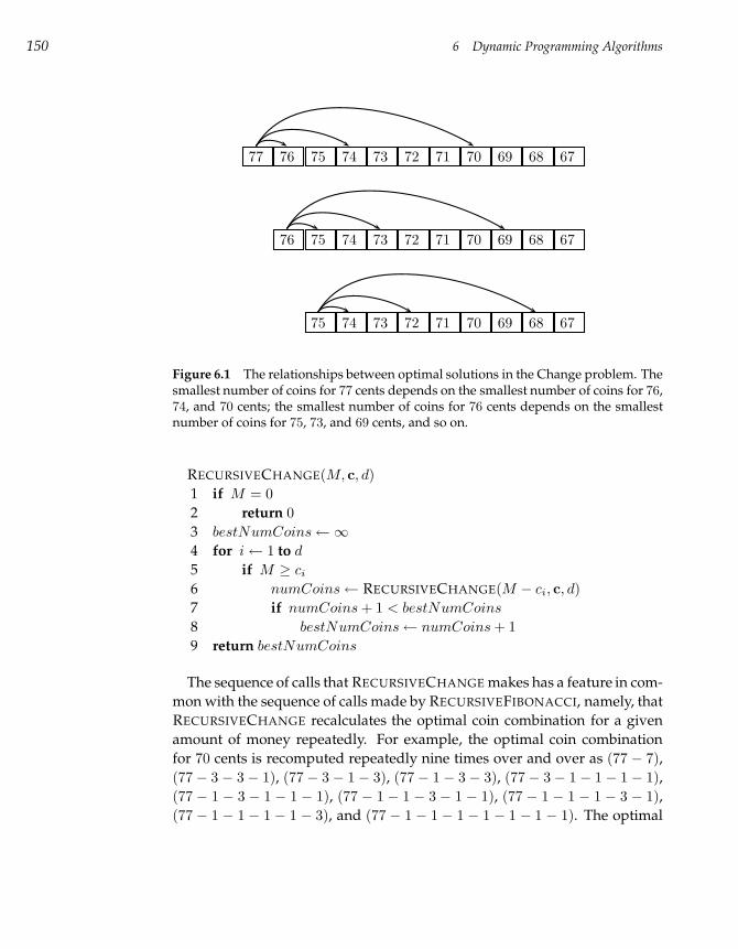
150 6 Dynamic Programming Algorithms
77 76 75 74 73 72 71 70 69 68 67
76 75 74 73 72 71 70 69 68 67
75 74 73 72 71 70 69 68 67
Figure 6.1 The relationships between optimal solutions in the Change problem. Thesmallest number of coins for 77 cents depends on the smallest number of coins for 76,74, and 70 cents; the smallest number of coins for 76 cents depends on the smallestnumber of coins for 75, 73, and 69 cents, and so on.
RECURSIVECHANGE(M, c, d)
1 if M = 0
2 return 0
3 bestNumCoins←∞
4 for i← 1 to d
5 if M ≥ ci
6 numCoins← RECURSIVECHANGE(M − ci, c, d)
7 if numCoins + 1 < bestNumCoins
8 bestNumCoins← numCoins + 1
9 return bestNumCoins
The sequence of calls that RECURSIVECHANGE makes has a feature in com-
mon with the sequence of calls made by RECURSIVEFIBONACCI, namely, that
RECURSIVECHANGE recalculates the optimal coin combination for a given
amount of money repeatedly. For example, the optimal coin combination
for 70 cents is recomputed repeatedly nine times over and over as (77 − 7),
(77 − 3 − 3 − 1), (77 − 3 − 1 − 3), (77 − 1 − 3 − 3), (77 − 3 − 1 − 1 − 1 − 1),
(77 − 1 − 3 − 1 − 1 − 1), (77 − 1 − 1 − 3 − 1 − 1), (77 − 1 − 1 − 1 − 3 − 1),
(77 − 1 − 1 − 1 − 1 − 3), and (77 − 1 − 1 − 1 − 1 − 1 − 1 − 1). The optimal
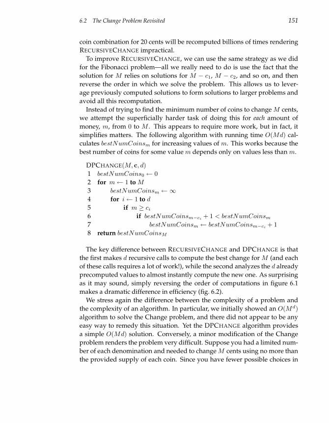
6.2 The Change Problem Revisited 151
coin combination for 20 cents will be recomputed billions of times rendering
RECURSIVECHANGE impractical.
To improve RECURSIVECHANGE, we can use the same strategy as we did
for the Fibonacci problem—all we really need to do is use the fact that the
solution for M relies on solutions for M − c1, M − c2, and so on, and then
reverse the order in which we solve the problem. This allows us to lever-
age previously computed solutions to form solutions to larger problems and
avoid all this recomputation.
Instead of trying to find the minimum number of coins to change M cents,
we attempt the superficially harder task of doing this for each amount of
money, m, from 0 to M . This appears to require more work, but in fact, it
simplifies matters. The following algorithm with running time O(Md) cal-
culates bestNumCoinsm for increasing values of m. This works because the
best number of coins for some value m depends only on values less than m.
DPCHANGE(M, c, d)
1 bestNumCoins0 ← 0
2 for m← 1 to M
3 bestNumCoinsm ←∞
4 for i← 1 to d
5 if m ≥ ci
6 if bestNumCoinsm−ci+ 1 < bestNumCoinsm
7 bestNumCoinsm ← bestNumCoinsm−ci+ 1
8 return bestNumCoinsM
The key difference between RECURSIVECHANGE and DPCHANGE is that
the first makes d recursive calls to compute the best change for M (and each
of these calls requires a lot of work!), while the second analyzes the d already
precomputed values to almost instantly compute the new one. As surprising
as it may sound, simply reversing the order of computations in figure 6.1
makes a dramatic difference in efficiency (fig. 6.2).
We stress again the difference between the complexity of a problem and
the complexity of an algorithm. In particular, we initially showed an O(Md)
algorithm to solve the Change problem, and there did not appear to be any
easy way to remedy this situation. Yet the DPCHANGE algorithm provides
a simple O(Md) solution. Conversely, a minor modification of the Change
problem renders the problem very difficult. Suppose you had a limited num-
ber of each denomination and needed to change M cents using no more than
the provided supply of each coin. Since you have fewer possible choices in
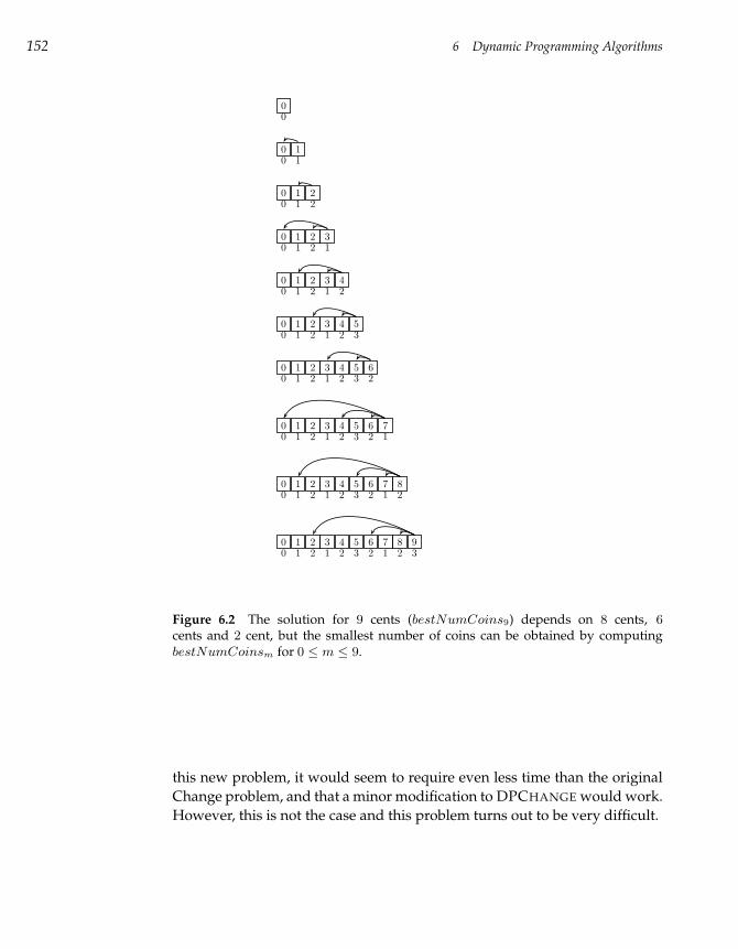
152 6 Dynamic Programming Algorithms
00
0 10 1
0 1 20 1 2
0 1 2 30 1 2 1
0 1 2 3 40 1 2 1 2
0 1 2 3 4 50 1 2 1 2 3
0 1 2 3 4 5 60 1 2 1 2 3 2
0 1 2 3 4 5 6 70 1 2 1 2 3 2 1
0 1 2 3 4 5 6 7 80 1 2 1 2 3 2 1 2
0 1 2 3 4 5 6 7 8 90 1 2 1 2 3 2 1 2 3
Figure 6.2 The solution for 9 cents (bestNumCoins9) depends on 8 cents, 6cents and 2 cent, but the smallest number of coins can be obtained by computingbestNumCoinsm for 0 ≤ m ≤ 9.
this new problem, it would seem to require even less time than the original
Change problem, and that a minor modification to DPCHANGE would work.
However, this is not the case and this problem turns out to be very difficult.
6.3 The Manhattan Tourist Problem 153
6.3 The Manhattan Tourist Problem
We will further illustrate dynamic programming with a surprisingly useful
toy problem, called the Manhattan Tourist problem, and then build on this
intuition to describe DNA sequence alignment.
Imagine a sightseeing tour in the borough of Manhattan in New York City,
where a group of tourists are determined to walk from the corner of 59th
Street and 8th Avenue to the Chrysler Building at 42nd Street and Lexing-
ton Avenue. There are many attractions along the way, but assume for the
moment that the tourists want to see as many attractions as possible. The
tourists are allowed to move either to the south or to the east, but even so,
they can choose from many different paths (exactly how many is left as a
problem at the end of the chapter). The upper path in figure 6.3 will take
the tourists to the Museum of Modern Art, but they will have to miss Times
Square; the bottom path will allow the tourists to see Times Square, but they
will have to miss the Museum of Modern Art.
The map above can also be represented as a gridlike structure (figure 6.4)
with the numbers next to each line (called weights) showing the number of
attractions on every block. The tourists must decide among the many possi-
ble paths between the northwesternmost point (called the source vertex) and
the southeasternmost point (called the sink vertex). The weight of a path from
the source to the sink is simply the sum of weights of its edges, or the overall
number of attractions. We will refer to this kind of construct as a graph, the
intersections of streets we will call vertices, and the streets themselves will
be edges and have a weight associated with them. We assume that horizontal
edges in the graph are oriented to the east like→while vertical edges are ori-
ented to the south like ↓. A path is a continuous sequence of edges, and the
length of a path is the sum of the edge weights in the path.3 A more detailed
discussion of graphs can be found in chapter 8.
Although the upper path in figure 6.3 is better than the bottom one, in the
sense that the tourists will see more attractions, it is not immediately clear if
there is an even better path in the grid. The Manhattan Tourist problem is to
find the path with the maximum number of attractions,4 that is, a longest path
3. We emphasize that the length of paths in the graph represent the overall number of attractionson this path and has nothing to do with the real length of the path (in miles), that is, the distancethe tourists travel.4. There are many interesting museums and architectural landmarks in Manhattan. However,it is impossible to please everyone, so one can change the relative importance of the types ofattractions by modulating the weights on the edges in the graph. This flexibility in assigningweights will become important when we discuss scoring matrices for sequence comparison.
154 6 Dynamic Programming Algorithms
(a path of maximum overall weight) in the grid.
Manhattan Tourist Problem:
Find a longest path in a weighted grid.
Input: A weighted grid G with two distinguished vertices:
a source and a sink.
Output: A longest path in G from source to sink.
Note that, since the tourists only move south and east, any grid positions
west or north of the source are unusable. Similarly, any grid positions south
or east of the sink are unusable, so we can simply say that the source vertex
is at (0, 0) and that the sink vertex at (n, m) defines the southeasternmost
corner of the grid. In figure 6.4 n = m = 4, but n does not always have
to equal m. We will use the grid shown in figure 6.4, rather than the one
corresponding to the map of Manhattan in figure 6.3 so that you can see a
nontrivial example of this problem.
The brute force approach to the Manhattan Tourist problem is to search
among all paths in the grid for the longest path, but this is not an option
for even a moderately large grid. Inspired by the previous chapter you may
be tempted to use a greedy strategy. For example, a sensible greedy strat-
egy would be to choose between two possible directions (south or east) by
comparing how many attractions tourists would see if they moved one block
south instead of moving one block east. This greedy strategy may provide re-
warding sightseeing experience in the beginning but, a few blocks later, may
bring you to an area of Manhattan you really do not want to be in. In fact,
no known greedy strategy for the Manhattan Tourist problem provides an
optimal solution to the problem. Had we followed the (obvious) greedy al-
gorithm, we would have chosen the following path, corresponding to twenty
three attractions.5
5. We will show that the optimal number is, in fact, thirty-four.
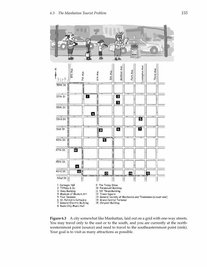
6.3 The Manhattan Tourist Problem 155
Figure 6.3 A city somewhat like Manhattan, laid out on a grid with one-way streets.You may travel only to the east or to the south, and you are currently at the north-westernmost point (source) and need to travel to the southeasternmost point (sink).Your goal is to visit as many attractions as possible.
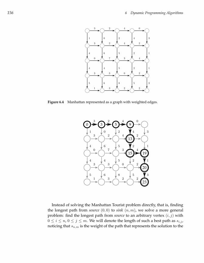
156 6 Dynamic Programming Algorithms
3 2 4 0
3 2 4 2
0 7 3 4
3 3 0 2
1 3 2 2
1
4
4
5
0
6
4
6
2
5
5
8
4
2
2
5
3
1
1
3
Figure 6.4 Manhattan represented as a graph with weighted edges.
3 2 4 0
3 2 4 2
0 7 3 4
3 3 0 2
1 3 2 2
1
4
4
5
0
6
4
6
2
5
5
8
4
2
2
5
3
1
1
3
0 3 5 9
13
15 19
20
23
Instead of solving the Manhattan Tourist problem directly, that is, finding
the longest path from source (0, 0) to sink (n, m), we solve a more general
problem: find the longest path from source to an arbitrary vertex (i, j) with
0 ≤ i ≤ n, 0 ≤ j ≤ m. We will denote the length of such a best path as si,j ,
noticing that sn,m is the weight of the path that represents the solution to the
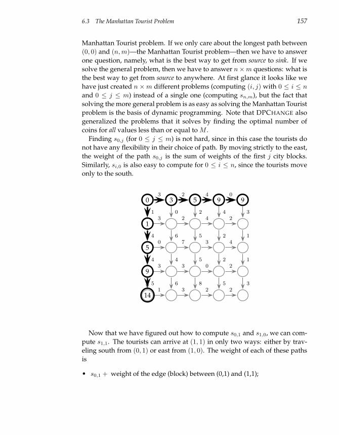
6.3 The Manhattan Tourist Problem 157
Manhattan Tourist problem. If we only care about the longest path between
(0, 0) and (n, m)—the Manhattan Tourist problem—then we have to answer
one question, namely, what is the best way to get from source to sink. If we
solve the general problem, then we have to answer n×m questions: what is
the best way to get from source to anywhere. At first glance it looks like we
have just created n ×m different problems (computing (i, j) with 0 ≤ i ≤ n
and 0 ≤ j ≤ m) instead of a single one (computing sn,m), but the fact that
solving the more general problem is as easy as solving the Manhattan Tourist
problem is the basis of dynamic programming. Note that DPCHANGE also
generalized the problems that it solves by finding the optimal number of
coins for all values less than or equal to M .
Finding s0,j (for 0 ≤ j ≤ m) is not hard, since in this case the tourists do
not have any flexibility in their choice of path. By moving strictly to the east,
the weight of the path s0,j is the sum of weights of the first j city blocks.
Similarly, si,0 is also easy to compute for 0 ≤ i ≤ n, since the tourists move
only to the south.
3 2 4 0
3 2 4 2
0 7 3 4
3 3 0 2
1 3 2 2
1
4
4
5
0
6
4
6
2
5
5
8
4
2
2
5
3
1
1
3
0 3 5 9 9
1
5
9
14
Now that we have figured out how to compute s0,1 and s1,0, we can com-
pute s1,1. The tourists can arrive at (1, 1) in only two ways: either by trav-
eling south from (0, 1) or east from (1, 0). The weight of each of these paths
is
• s0,1 + weight of the edge (block) between (0,1) and (1,1);
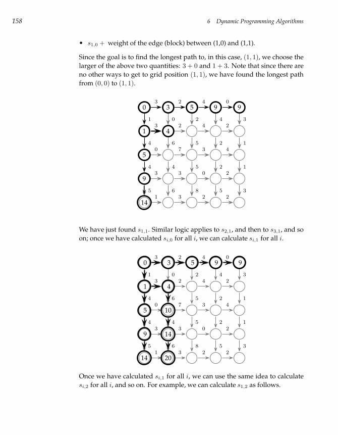
158 6 Dynamic Programming Algorithms
• s1,0 + weight of the edge (block) between (1,0) and (1,1).
Since the goal is to find the longest path to, in this case, (1, 1), we choose the
larger of the above two quantities: 3 + 0 and 1 + 3. Note that since there are
no other ways to get to grid position (1, 1), we have found the longest path
from (0, 0) to (1, 1).
3 2 4 0
3 2 4 2
0 7 3 4
3 3 0 2
1 3 2 2
1
4
4
5
0
6
4
6
2
5
5
8
4
2
2
5
3
1
1
3
0
4
3 5 9 9
1
5
9
14
We have just found s1,1. Similar logic applies to s2,1, and then to s3,1, and so
on; once we have calculated si,0 for all i, we can calculate si,1 for all i.
3 2 4 0
3 2 4 2
0 7 3 4
3 3 0 2
1 3 2 2
1
4
4
5
0
6
4
6
2
5
5
8
4
2
2
5
3
1
1
3
0
1
5
9
14
3
4
10
14
20
5 9 9
Once we have calculated si,1 for all i, we can use the same idea to calculate
si,2 for all i, and so on. For example, we can calculate s1,2 as follows.
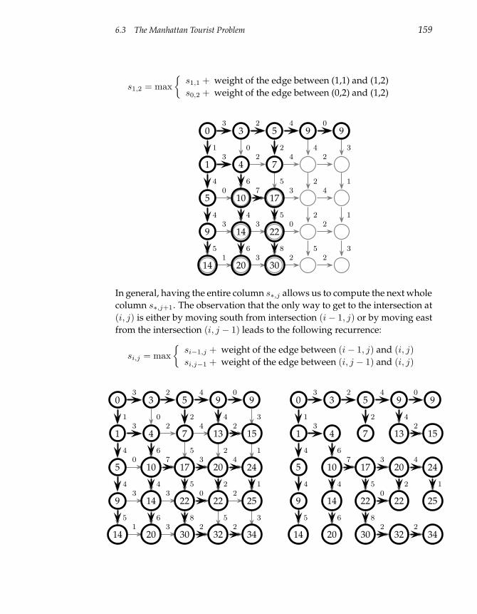
6.3 The Manhattan Tourist Problem 159
s1,2 = max
s1,1 + weight of the edge between (1,1) and (1,2)
s0,2 + weight of the edge between (0,2) and (1,2)
3 2 4 0
3 2 4 2
0 7 3 4
3 3 0 2
1 3 2 2
1
4
4
5
0
6
4
6
2
5
5
8
4
2
2
5
3
1
1
3
0
1
5
9
14
3
4
10
14
20
5
7
17
22
30
9 9
In general, having the entire column s∗,j allows us to compute the next whole
column s∗,j+1. The observation that the only way to get to the intersection at
(i, j) is either by moving south from intersection (i− 1, j) or by moving east
from the intersection (i, j − 1) leads to the following recurrence:
si,j = max
si−1,j + weight of the edge between (i− 1, j) and (i, j)
si,j−1 + weight of the edge between (i, j − 1) and (i, j)
3 2 4 0
3 2 4 2
0 7 3 4
3 3 0 2
1 3 2 2
1
4
4
5
0
6
4
6
2
5
5
8
4
2
2
5
3
1
1
3
0
1
5
9
14
3
4
10
14
20
5
7
17
22
30
9
13
20
22
32
9
15
24
25
34
3 2 4 0
3 2
7 3 4
0
2 2
1
4
4
5
6
4
6
2
5
8
4
2 1
0
1
5
9
14
3
4
10
14
20
5
7
17
22
30
9
13
20
22
32
9
15
24
25
34
160 6 Dynamic Programming Algorithms
This recurrence allows us to compute every score si,j in a single sweep of
the grid. The algorithm MANHATTANTOURIST implements this procedure.
Here,↓w is a two-dimensional array representing the weights of the grid’s
edges that run north to south, and→w is a two-dimensional array representing
the weights of the grid’s edges that run west to east. That is,↓wi,j is the weight
of the edge between (i, j − 1) and (i, j); and→wi,j is the weight of the edge
between (i, j − 1) and (i, j).
MANHATTANTOURIST(↓w,
→w, n, m)
1 s0,0 ← 0
2 for i← 1 to n
3 si,0 ← si−1,0+↓wi,0
4 for j ← 1 to m
5 s0,j ← s0,j−1+→w0,j
6 for i← 1 to n
7 for j ← 1 to m
8 si,j ← max
si−1,j+↓wi,j
si,j−1+→wi,j
9 return sn,m
Lines 1 through 5 set up the initial conditions on the matrix s, and line 8 cor-
responds to the recurrence that allows us to fill in later table entries based on
earlier ones. Most of the dynamic programming algorithms we will develop
in the context of DNA sequence comparison will look just like MANHAT-
TANTOURIST with only minor changes. We will generally just arrive at a
recurrence like line 8 and call it an algorithm, with the understanding that
the actual implementation will be similar to MANHATTANTOURIST.6
Many problems in bioinformatics can be solved efficiently by the applica-
tion of the dynamic programming technique, once they are cast as traveling
in a Manhattan-like grid. For example, development of new sequence com-
parison algorithms often amounts to building an appropriate “Manhattan”
that adequately models the specifics of a particular biological problem, and
by defining the block weights that reflect the costs of mutations from one
DNA sequence to another.
6. MANHATTANTOURIST computes the length of the longest path in the grid, but does not givethe path itself. In section 6.5 we will describe a minor modification to the algorithm that returnsnot only the optimal length, but also the optimal path.
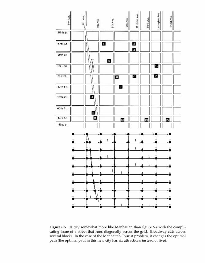
1 1
1
1 1
1 1
11
1 1
11
1
1
Figure 6.5 A city somewhat more like Manhattan than figure 6.4 with the compli-cating issue of a street that runs diagonally across the grid. Broadway cuts acrossseveral blocks. In the case of the Manhattan Tourist problem, it changes the optimalpath (the optimal path in this new city has six attractions instead of five).
162 6 Dynamic Programming Algorithms
Unfortunately, Manhattan is not a perfectly regular grid. Broadway cuts
across the borough (figure 6.5). We would like to solve a generalization of
the Manhattan Tourist problem for the case in which the street map is not
a regular rectangular grid. In this case, one can model any city map as a
graph with vertices corresponding to the intersections of streets, and edges
corresponding to the intervals of streets between the intersections. For the
sake of simplicity we assume that the city blocks correspond to directed edges,
so that the tourist can move only in the direction of the edge and that the
resulting graph has no directed cycles.7 Such graphs are called directed acyclic
graphs, or DAGs. We assume that every edge has an associated weight (e.g.,
the number of attractions) and represent a graph G as a pair of two sets, V
for vertices and E for edges: G = (V, E). We number vertices from 1 to
|V | with a single integer, rather than a row-column pair as in the Manhattan
problem. This does not change the generic dynamic programming algorithm
other than in notation, but it allows us to represent imperfect grids. An edge
from E can be specified in terms of its origin vertex u and its destination
vertex v as (u, v). The following problem is simply a generalization of the
Manhattan Tourist problem that is able to deal with arbitrary DAGs rather
than with perfect grids.
Longest Path in a DAG Problem:
Find a longest path between two vertices in a weighted DAG.
Input: A weighted DAG G with source and sink vertices.
Output: A longest path in G from source to sink.
Not surprisingly, the Longest Path in a DAG problem can also be solved
by dynamic programming. At every vertex, there may be multiple edges
that “flow in” and multiple edges that “flow out.” In the city analogy, any
intersection may have multiple one-way streets leading in, and some other
number of one-way streets exiting. We will call the number of edges entering
a vertex (i.e., the number of inbound streets) the indegree of the vertex (i.e.,
intersection), and the number of edges leaving a vertex (i.e., the number of
outbound streets) the outdegree of the vertex.
In the nicely regular case of the Manhattan problem, most vertices had
7. A directed cycle is a path from a vertex back to itself that respects the directions of edges. Ifthe resulting graph contained a cycle, a tourist could start walking along this cycle revisiting thesame attractions many times. In this case there is no “best” solution since a tourist may increasethe number of visited attractions indefinitely.
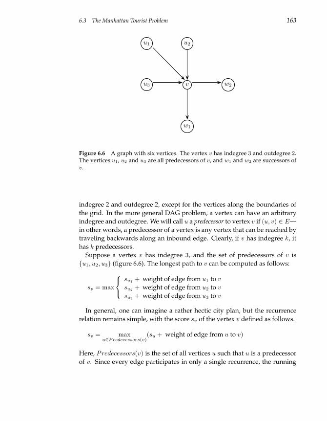
6.3 The Manhattan Tourist Problem 163
u1 u2
u3 v w2
w1
Figure 6.6 A graph with six vertices. The vertex v has indegree 3 and outdegree 2.The vertices u1, u2 and u3 are all predecessors of v, and w1 and w2 are successors ofv.
indegree 2 and outdegree 2, except for the vertices along the boundaries of
the grid. In the more general DAG problem, a vertex can have an arbitrary
indegree and outdegree. We will call u a predecessor to vertex v if (u, v) ∈ E—
in other words, a predecessor of a vertex is any vertex that can be reached by
traveling backwards along an inbound edge. Clearly, if v has indegree k, it
has k predecessors.
Suppose a vertex v has indegree 3, and the set of predecessors of v is
u1, u2, u3 (figure 6.6). The longest path to v can be computed as follows:
sv = max
su1 + weight of edge from u1 to v
su2 + weight of edge from u2 to v
su3 + weight of edge from u3 to v
In general, one can imagine a rather hectic city plan, but the recurrence
relation remains simple, with the score sv of the vertex v defined as follows.
sv = maxu∈Predecessors(v)
(su + weight of edge from u to v)
Here, Predecessors(v) is the set of all vertices u such that u is a predecessor
of v. Since every edge participates in only a single recurrence, the running
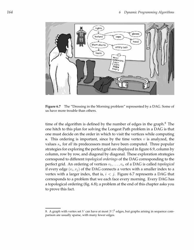
164 6 Dynamic Programming Algorithms
Figure 6.7 The “Dressing in the Morning problem” represented by a DAG. Some ofus have more trouble than others.
time of the algorithm is defined by the number of edges in the graph.8 The
one hitch to this plan for solving the Longest Path problem in a DAG is that
one must decide on the order in which to visit the vertices while computing
s. This ordering is important, since by the time vertex v is analyzed, the
values su for all its predecessors must have been computed. Three popular
strategies for exploring the perfect grid are displayed in figure 6.9, column by
column, row by row, and diagonal by diagonal. These exploration strategies
correspond to different topological orderings of the DAG corresponding to the
perfect grid. An ordering of vertices v1, . . . , vn of a DAG is called topological
if every edge (vi, vj) of the DAG connects a vertex with a smaller index to a
vertex with a larger index, that is, i < j. Figure 6.7 represents a DAG that
corresponds to a problem that we each face every morning. Every DAG has
a topological ordering (fig. 6.8); a problem at the end of this chapter asks you
to prove this fact.
8. A graph with vertex set V can have at most |V |2 edges, but graphs arising in sequence com-parison are usually sparse, with many fewer edges.
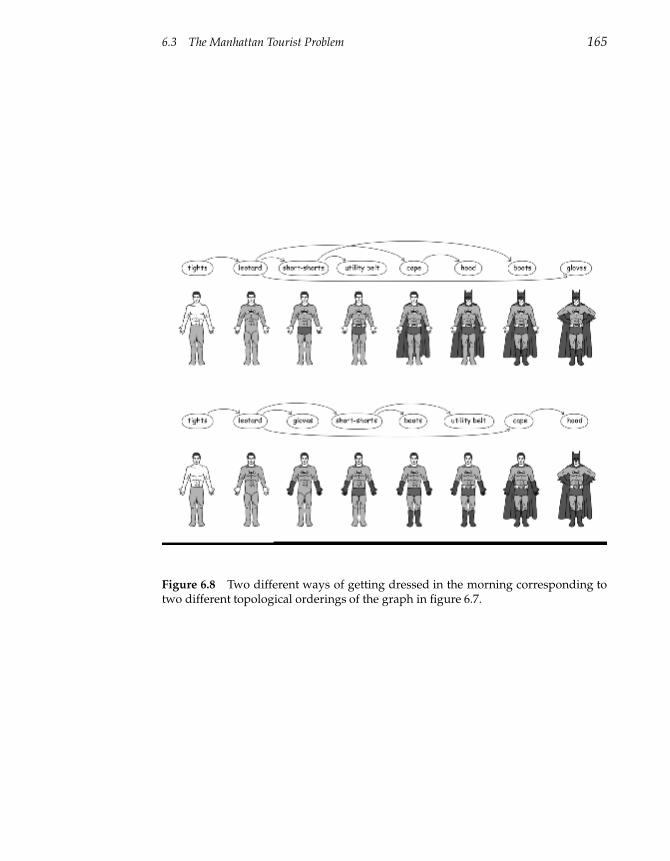
6.3 The Manhattan Tourist Problem 165
Figure 6.8 Two different ways of getting dressed in the morning corresponding totwo different topological orderings of the graph in figure 6.7.
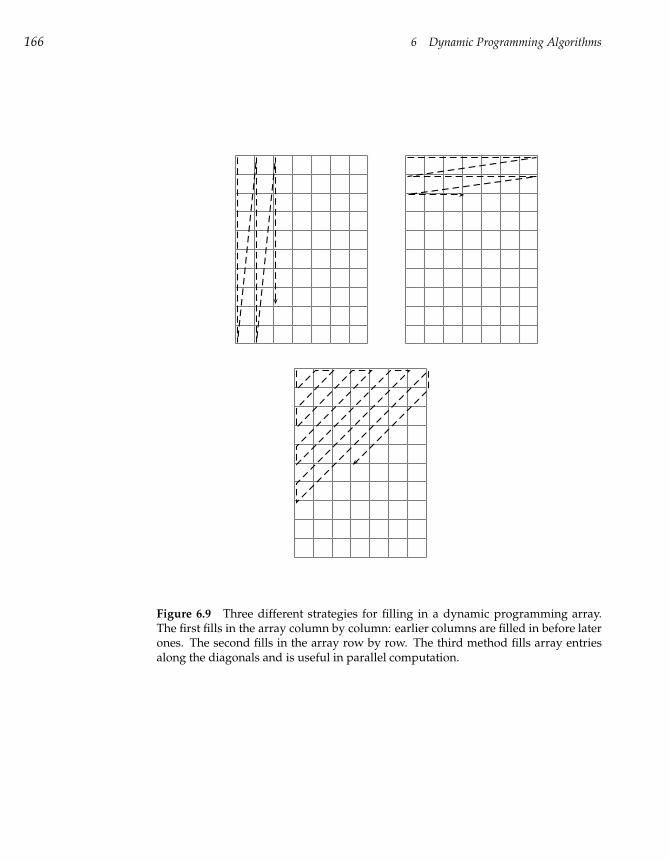
166 6 Dynamic Programming Algorithms
Figure 6.9 Three different strategies for filling in a dynamic programming array.The first fills in the array column by column: earlier columns are filled in before laterones. The second fills in the array row by row. The third method fills array entriesalong the diagonals and is useful in parallel computation.
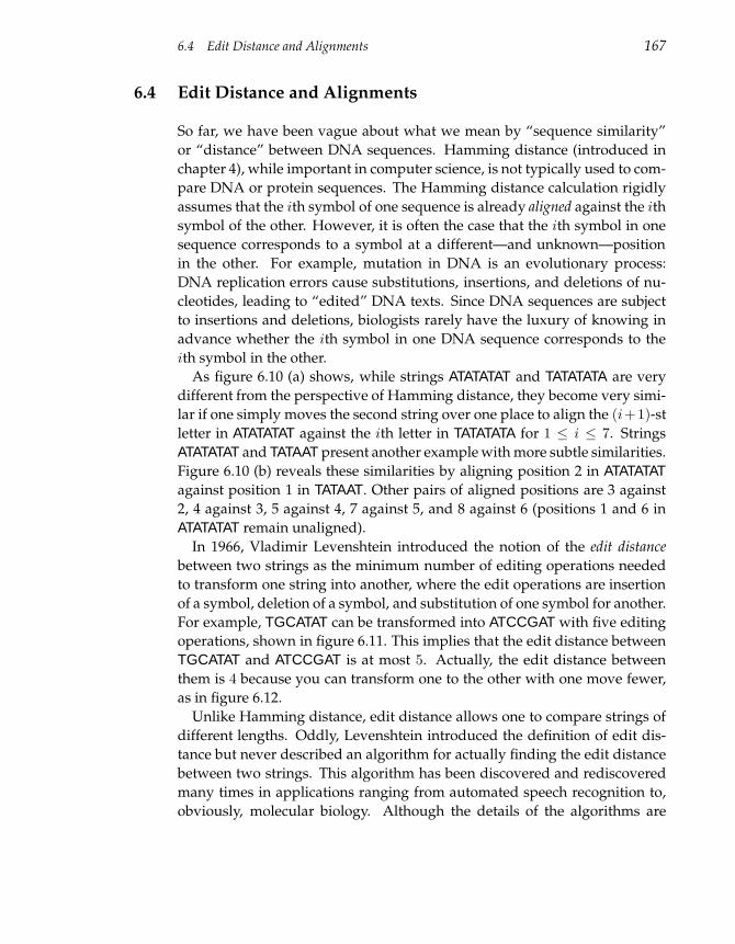
6.4 Edit Distance and Alignments 167
6.4 Edit Distance and Alignments
So far, we have been vague about what we mean by “sequence similarity”
or “distance” between DNA sequences. Hamming distance (introduced in
chapter 4), while important in computer science, is not typically used to com-
pare DNA or protein sequences. The Hamming distance calculation rigidly
assumes that the ith symbol of one sequence is already aligned against the ith
symbol of the other. However, it is often the case that the ith symbol in one
sequence corresponds to a symbol at a different—and unknown—position
in the other. For example, mutation in DNA is an evolutionary process:
DNA replication errors cause substitutions, insertions, and deletions of nu-
cleotides, leading to “edited” DNA texts. Since DNA sequences are subject
to insertions and deletions, biologists rarely have the luxury of knowing in
advance whether the ith symbol in one DNA sequence corresponds to the
ith symbol in the other.
As figure 6.10 (a) shows, while strings ATATATAT and TATATATA are very
different from the perspective of Hamming distance, they become very simi-
lar if one simply moves the second string over one place to align the (i+1)-st
letter in ATATATAT against the ith letter in TATATATA for 1 ≤ i ≤ 7. Strings
ATATATAT and TATAAT present another example with more subtle similarities.
Figure 6.10 (b) reveals these similarities by aligning position 2 in ATATATATagainst position 1 in TATAAT. Other pairs of aligned positions are 3 against
2, 4 against 3, 5 against 4, 7 against 5, and 8 against 6 (positions 1 and 6 in
ATATATAT remain unaligned).
In 1966, Vladimir Levenshtein introduced the notion of the edit distance
between two strings as the minimum number of editing operations needed
to transform one string into another, where the edit operations are insertion
of a symbol, deletion of a symbol, and substitution of one symbol for another.
For example, TGCATAT can be transformed into ATCCGAT with five editing
operations, shown in figure 6.11. This implies that the edit distance between
TGCATAT and ATCCGAT is at most 5. Actually, the edit distance between
them is 4 because you can transform one to the other with one move fewer,
as in figure 6.12.
Unlike Hamming distance, edit distance allows one to compare strings of
different lengths. Oddly, Levenshtein introduced the definition of edit dis-
tance but never described an algorithm for actually finding the edit distance
between two strings. This algorithm has been discovered and rediscovered
many times in applications ranging from automated speech recognition to,
obviously, molecular biology. Although the details of the algorithms are
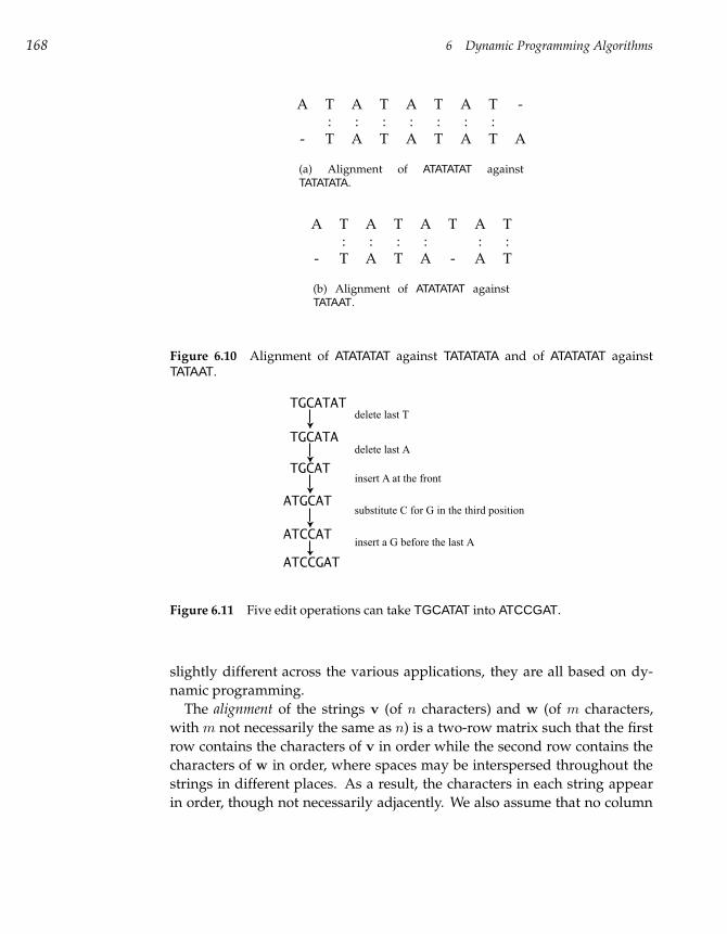
168 6 Dynamic Programming Algorithms
A T A T A T A T -: : : : : : :
- T A T A T A T A
(a) Alignment of ATATATAT againstTATATATA.
A T A T A T A T: : : : : :
- T A T A - A T
(b) Alignment of ATATATAT againstTATAAT.
Figure 6.10 Alignment of ATATATAT against TATATATA and of ATATATAT againstTATAAT.
TGCATAT
ATCCAT
TGCATA
TGCAT
ATGCAT
ATCCGAT
delete last T
delete last A
insert A at the front
substitute C for G in the third position
insert a G before the last A
Figure 6.11 Five edit operations can take TGCATAT into ATCCGAT.
slightly different across the various applications, they are all based on dy-
namic programming.
The alignment of the strings v (of n characters) and w (of m characters,
with m not necessarily the same as n) is a two-row matrix such that the first
row contains the characters of v in order while the second row contains the
characters of w in order, where spaces may be interspersed throughout the
strings in different places. As a result, the characters in each string appear
in order, though not necessarily adjacently. We also assume that no column
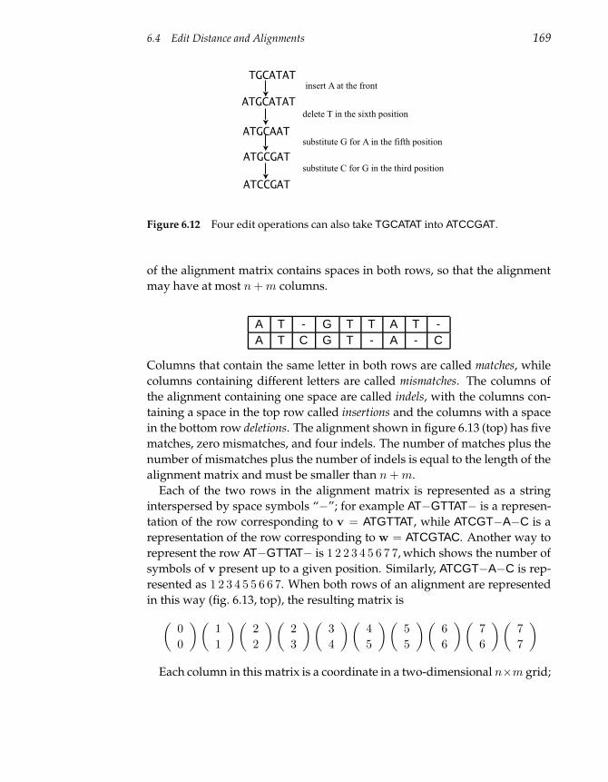
6.4 Edit Distance and Alignments 169
TGCATAT
ATCCGAT
ATGCATAT
ATGCAAT
ATGCGAT
delete T in the sixth position
substitute G for A in the fifth position
substitute C for G in the third position
insert A at the front
Figure 6.12 Four edit operations can also take TGCATAT into ATCCGAT.
of the alignment matrix contains spaces in both rows, so that the alignment
may have at most n + m columns.
A T - G T T A T -A T C G T - A - C
Columns that contain the same letter in both rows are called matches, while
columns containing different letters are called mismatches. The columns of
the alignment containing one space are called indels, with the columns con-
taining a space in the top row called insertions and the columns with a space
in the bottom row deletions. The alignment shown in figure 6.13 (top) has five
matches, zero mismatches, and four indels. The number of matches plus the
number of mismatches plus the number of indels is equal to the length of the
alignment matrix and must be smaller than n + m.
Each of the two rows in the alignment matrix is represented as a string
interspersed by space symbols “−”; for example AT−GTTAT− is a represen-
tation of the row corresponding to v = ATGTTAT, while ATCGT−A−C is a
representation of the row corresponding to w = ATCGTAC. Another way to
represent the row AT−GTTAT− is 1 2 2 3 4 5 6 7 7, which shows the number of
symbols of v present up to a given position. Similarly, ATCGT−A−C is rep-
resented as 1 2 3 4 5 5 6 6 7. When both rows of an alignment are represented
in this way (fig. 6.13, top), the resulting matrix is
(
0
0
)(
1
1
)(
2
2
)(
2
3
)(
3
4
)(
4
5
)(
5
5
)(
6
6
)(
7
6
)(
7
7
)
Each column in this matrix is a coordinate in a two-dimensional n×m grid;
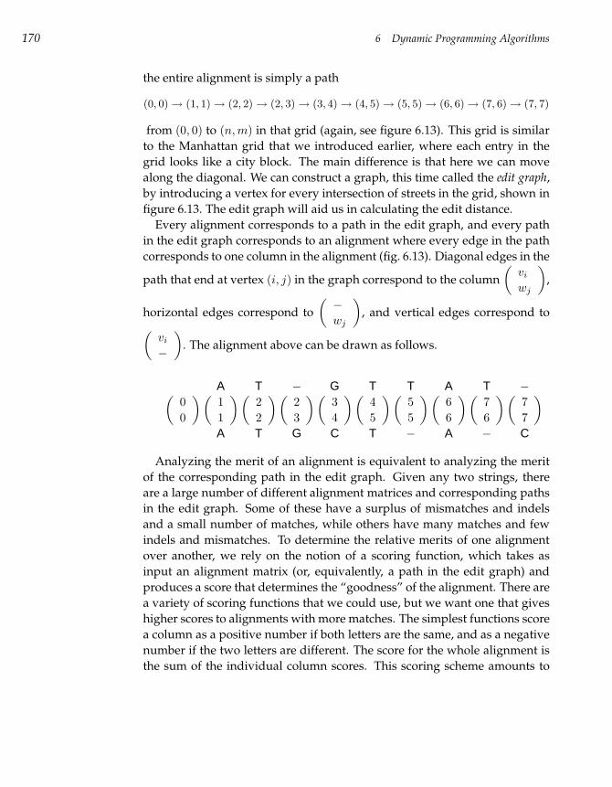
170 6 Dynamic Programming Algorithms
the entire alignment is simply a path
(0, 0)→ (1, 1)→ (2, 2)→ (2, 3)→ (3, 4)→ (4, 5)→ (5, 5)→ (6, 6)→ (7, 6)→ (7, 7)
from (0, 0) to (n, m) in that grid (again, see figure 6.13). This grid is similar
to the Manhattan grid that we introduced earlier, where each entry in the
grid looks like a city block. The main difference is that here we can move
along the diagonal. We can construct a graph, this time called the edit graph,
by introducing a vertex for every intersection of streets in the grid, shown in
figure 6.13. The edit graph will aid us in calculating the edit distance.
Every alignment corresponds to a path in the edit graph, and every path
in the edit graph corresponds to an alignment where every edge in the path
corresponds to one column in the alignment (fig. 6.13). Diagonal edges in the
path that end at vertex (i, j) in the graph correspond to the column
(
vi
wj
)
,
horizontal edges correspond to
(
−
wj
)
, and vertical edges correspond to
(
vi
−
)
. The alignment above can be drawn as follows.
(
0
0
)
A(
1
1
)
A
T(
2
2
)
T
−(
2
3
)
G
G(
3
4
)
C
T(
4
5
)
T
T(
5
5
)
−
A(
6
6
)
A
T(
7
6
)
−
−(
7
7
)
C
Analyzing the merit of an alignment is equivalent to analyzing the merit
of the corresponding path in the edit graph. Given any two strings, there
are a large number of different alignment matrices and corresponding paths
in the edit graph. Some of these have a surplus of mismatches and indels
and a small number of matches, while others have many matches and few
indels and mismatches. To determine the relative merits of one alignment
over another, we rely on the notion of a scoring function, which takes as
input an alignment matrix (or, equivalently, a path in the edit graph) and
produces a score that determines the “goodness” of the alignment. There are
a variety of scoring functions that we could use, but we want one that gives
higher scores to alignments with more matches. The simplest functions score
a column as a positive number if both letters are the same, and as a negative
number if the two letters are different. The score for the whole alignment is
the sum of the individual column scores. This scoring scheme amounts to
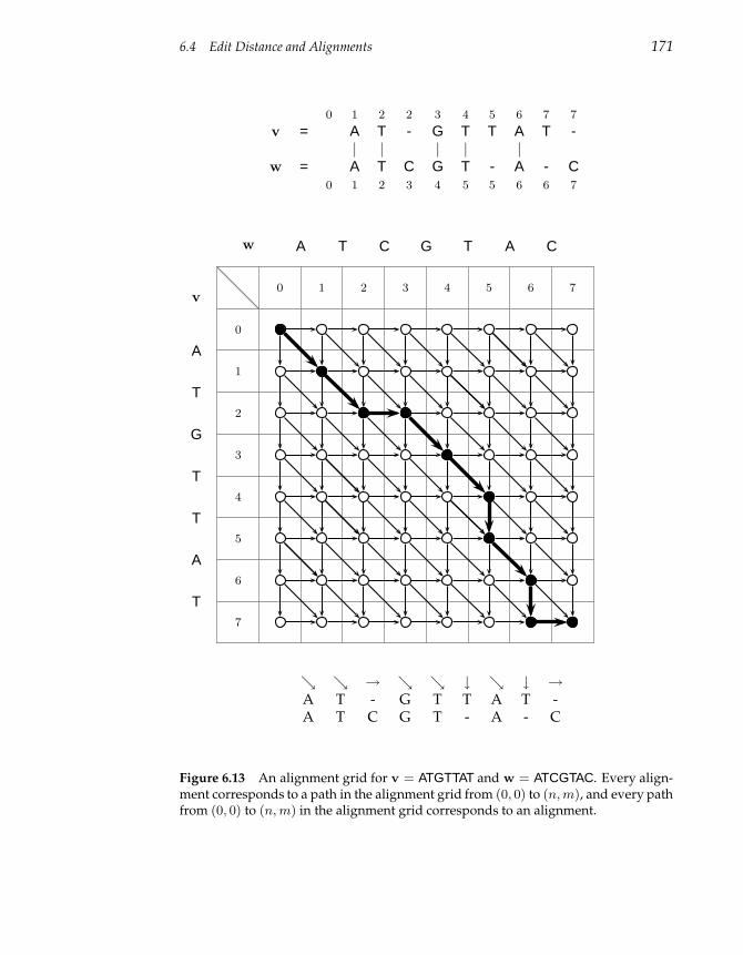
6.4 Edit Distance and Alignments 171
0 1 2 2 3 4 5 6 7 7
v = A T - G T T A T -| | | | |
w = A T C G T - A - C0 1 2 3 4 5 5 6 6 7
0
A
1
T
2
C
3
G
4
T
5
A
6
C
7
0
A1
T2
G3
T4
T5
A6
T7
v
w
→ ↓ ↓ →A T - G T T A T -A T C G T - A - C
Figure 6.13 An alignment grid for v = ATGTTAT and w = ATCGTAC. Every align-ment corresponds to a path in the alignment grid from (0, 0) to (n, m), and every pathfrom (0, 0) to (n, m) in the alignment grid corresponds to an alignment.
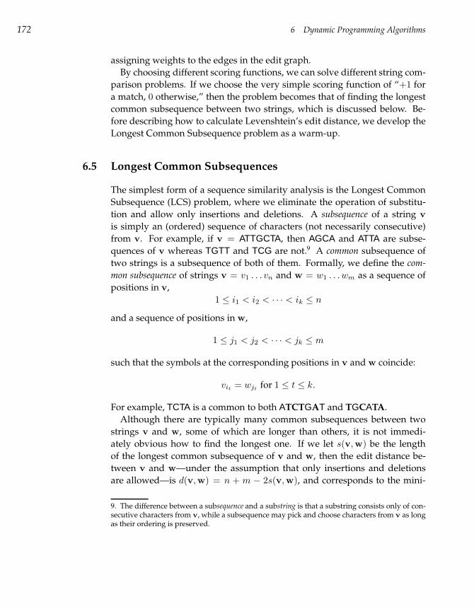
172 6 Dynamic Programming Algorithms
assigning weights to the edges in the edit graph.
By choosing different scoring functions, we can solve different string com-
parison problems. If we choose the very simple scoring function of “+1 for
a match, 0 otherwise,” then the problem becomes that of finding the longest
common subsequence between two strings, which is discussed below. Be-
fore describing how to calculate Levenshtein’s edit distance, we develop the
Longest Common Subsequence problem as a warm-up.
6.5 Longest Common Subsequences
The simplest form of a sequence similarity analysis is the Longest Common
Subsequence (LCS) problem, where we eliminate the operation of substitu-
tion and allow only insertions and deletions. A subsequence of a string v
is simply an (ordered) sequence of characters (not necessarily consecutive)
from v. For example, if v = ATTGCTA, then AGCA and ATTA are subse-
quences of v whereas TGTT and TCG are not.9 A common subsequence of
two strings is a subsequence of both of them. Formally, we define the com-
mon subsequence of strings v = v1 . . . vn and w = w1 . . . wm as a sequence of
positions in v,
1 ≤ i1 < i2 < · · · < ik ≤ n
and a sequence of positions in w,
1 ≤ j1 < j2 < · · · < jk ≤ m
such that the symbols at the corresponding positions in v and w coincide:
vit= wjt
for 1 ≤ t ≤ k.
For example, TCTA is a common to both ATCTGAT and TGCATA.
Although there are typically many common subsequences between two
strings v and w, some of which are longer than others, it is not immedi-
ately obvious how to find the longest one. If we let s(v,w) be the length
of the longest common subsequence of v and w, then the edit distance be-
tween v and w—under the assumption that only insertions and deletions
are allowed—is d(v,w) = n + m − 2s(v,w), and corresponds to the mini-
9. The difference between a subsequence and a substring is that a substring consists only of con-secutive characters from v, while a subsequence may pick and choose characters from v as longas their ordering is preserved.
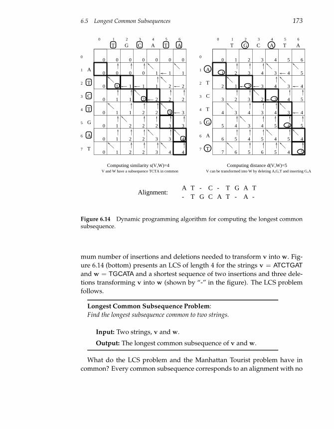
6.5 Longest Common Subsequences 173
A T - C - T G A T- T G C A T - A -
Alignment:
0
1
2
3
4
4
T G C A T A
A
T
C
T
G
A
T
0 1 2 3 4 5 6
0
1
2
3
4
5
6
7
1 2 3 4 5 6
1
2
3
4
5
6
7
2 3 4 3 4 5
2 3 4 3 4
2 3 3 4 5
3 4 3 4 4
4 3 4 5 4 5
5 4 5 4 5
6 5 6 5 5
V and W have a subsequence TCTA in common V can be transformed into W by deleting A,G,T and inserting G,AComputing similarity s(V,W)=4 Computing distance d(V,W)=5
0 0 0 0 0 0 0
0
0
0
0
0
0
0
0 0 1 1 1
1 1 1 1 22
1
1
1
1
1
1 2 2 2 2
1
2
2
2
2
2
2
2
2 3 3
2 3 3
3
3
3 4
4 4
T G C A T A
A
T
C
T
G
A
T
0 1 2 3 4 5 6
0
1
2
3
4
5
6
7
0
Figure 6.14 Dynamic programming algorithm for computing the longest commonsubsequence.
mum number of insertions and deletions needed to transform v into w. Fig-
ure 6.14 (bottom) presents an LCS of length 4 for the strings v = ATCTGATand w = TGCATA and a shortest sequence of two insertions and three dele-
tions transforming v into w (shown by “-” in the figure). The LCS problem
follows.
Longest Common Subsequence Problem:
Find the longest subsequence common to two strings.
Input: Two strings, v and w.
Output: The longest common subsequence of v and w.
What do the LCS problem and the Manhattan Tourist problem have in
common? Every common subsequence corresponds to an alignment with no
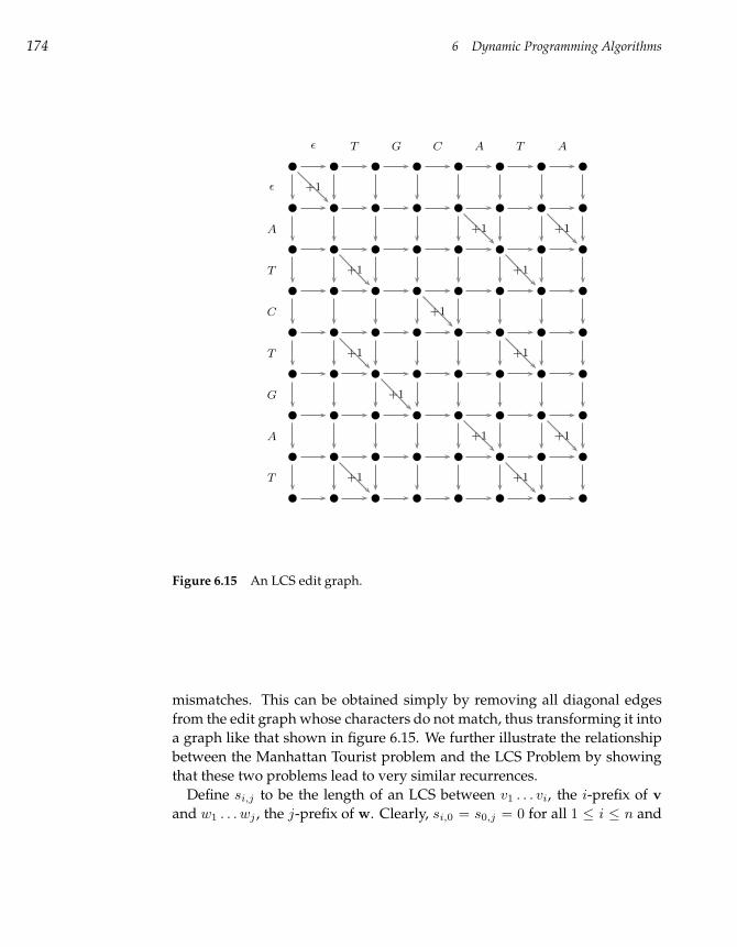
174 6 Dynamic Programming Algorithms
ε
A
T
C
T
G
A
T
ε T G C A T A
+1
+1 +1
+1 +1
+1
+1 +1
+1
+1 +1
+1 +1
Figure 6.15 An LCS edit graph.
mismatches. This can be obtained simply by removing all diagonal edges
from the edit graph whose characters do not match, thus transforming it into
a graph like that shown in figure 6.15. We further illustrate the relationship
between the Manhattan Tourist problem and the LCS Problem by showing
that these two problems lead to very similar recurrences.
Define si,j to be the length of an LCS between v1 . . . vi, the i-prefix of v
and w1 . . . wj , the j-prefix of w. Clearly, si,0 = s0,j = 0 for all 1 ≤ i ≤ n and
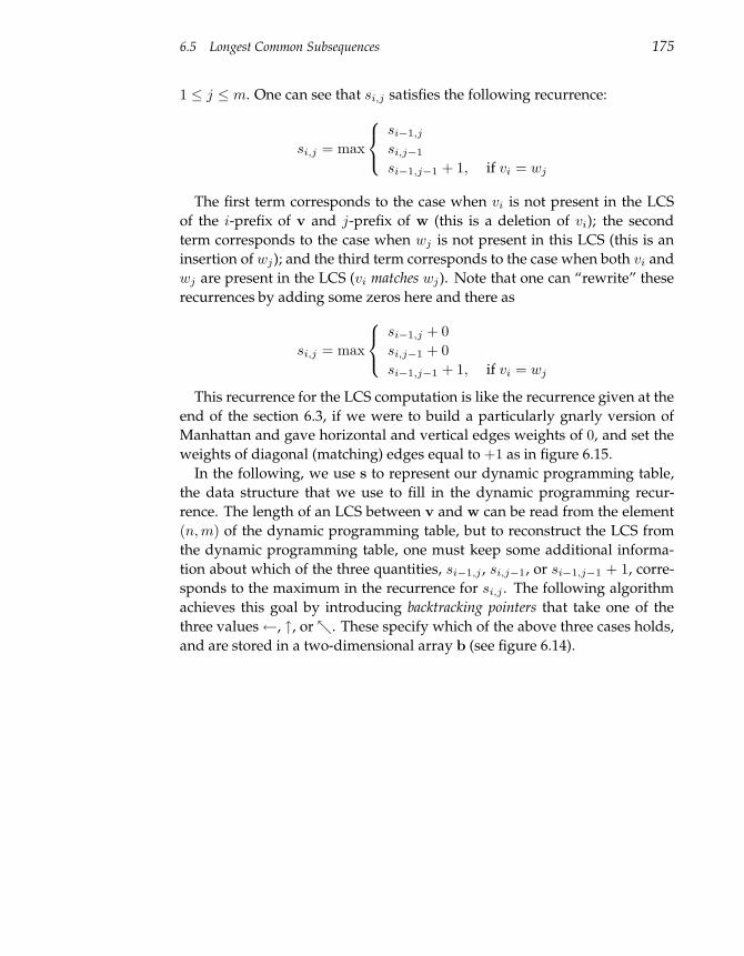
6.5 Longest Common Subsequences 175
1 ≤ j ≤ m. One can see that si,j satisfies the following recurrence:
si,j = max
si−1,j
si,j−1
si−1,j−1 + 1, if vi = wj
The first term corresponds to the case when vi is not present in the LCS
of the i-prefix of v and j-prefix of w (this is a deletion of vi); the second
term corresponds to the case when wj is not present in this LCS (this is an
insertion of wj); and the third term corresponds to the case when both vi and
wj are present in the LCS (vi matches wj). Note that one can “rewrite” these
recurrences by adding some zeros here and there as
si,j = max
si−1,j + 0
si,j−1 + 0
si−1,j−1 + 1, if vi = wj
This recurrence for the LCS computation is like the recurrence given at the
end of the section 6.3, if we were to build a particularly gnarly version of
Manhattan and gave horizontal and vertical edges weights of 0, and set the
weights of diagonal (matching) edges equal to +1 as in figure 6.15.
In the following, we use s to represent our dynamic programming table,
the data structure that we use to fill in the dynamic programming recur-
rence. The length of an LCS between v and w can be read from the element
(n, m) of the dynamic programming table, but to reconstruct the LCS from
the dynamic programming table, one must keep some additional informa-
tion about which of the three quantities, si−1,j , si,j−1, or si−1,j−1 + 1, corre-
sponds to the maximum in the recurrence for si,j . The following algorithm
achieves this goal by introducing backtracking pointers that take one of the
three values←, ↑, or. These specify which of the above three cases holds,
and are stored in a two-dimensional array b (see figure 6.14).
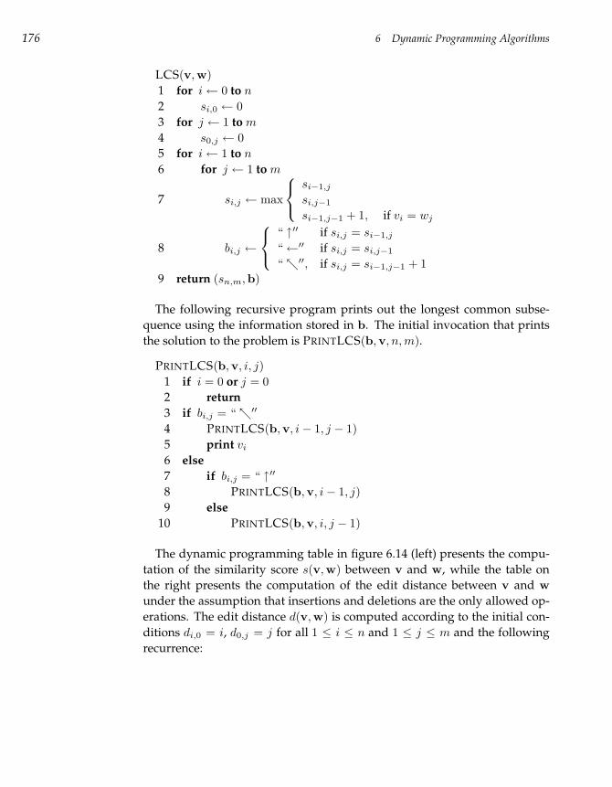
176 6 Dynamic Programming Algorithms
LCS(v,w)
1 for i← 0 to n
2 si,0 ← 0
3 for j ← 1 to m
4 s0,j ← 0
5 for i← 1 to n
6 for j ← 1 to m
7 si,j ← max
si−1,j
si,j−1
si−1,j−1 + 1, if vi = wj
8 bi,j ←
“ ↑′′ if si,j = si−1,j
“←′′ if si,j = si,j−1
“′′, if si,j = si−1,j−1 + 19 return (sn,m,b)
The following recursive program prints out the longest common subse-
quence using the information stored in b. The initial invocation that prints
the solution to the problem is PRINTLCS(b,v, n, m).
PRINTLCS(b,v, i, j)
1 if i = 0 or j = 0
2 return
3 if bi,j = “′′
4 PRINTLCS(b,v, i− 1, j − 1)
5 print vi
6 else
7 if bi,j = “ ↑′′
8 PRINTLCS(b,v, i− 1, j)
9 else
10 PRINTLCS(b,v, i, j − 1)
The dynamic programming table in figure 6.14 (left) presents the compu-
tation of the similarity score s(v,w) between v and w, while the table on
the right presents the computation of the edit distance between v and w
under the assumption that insertions and deletions are the only allowed op-
erations. The edit distance d(v,w) is computed according to the initial con-
ditions di,0 = i, d0,j = j for all 1 ≤ i ≤ n and 1 ≤ j ≤ m and the following
recurrence:
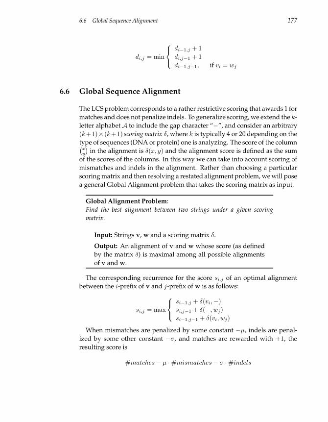
6.6 Global Sequence Alignment 177
di,j = min
di−1,j + 1
di,j−1 + 1
di−1,j−1, if vi = wj
6.6 Global Sequence Alignment
The LCS problem corresponds to a rather restrictive scoring that awards 1 for
matches and does not penalize indels. To generalize scoring, we extend the k-
letter alphabet A to include the gap character “−”, and consider an arbitrary
(k+1)× (k+1) scoring matrix δ, where k is typically 4 or 20 depending on the
type of sequences (DNA or protein) one is analyzing. The score of the column(
xy
)
in the alignment is δ(x, y) and the alignment score is defined as the sum
of the scores of the columns. In this way we can take into account scoring of
mismatches and indels in the alignment. Rather than choosing a particular
scoring matrix and then resolving a restated alignment problem, we will pose
a general Global Alignment problem that takes the scoring matrix as input.
Global Alignment Problem:
Find the best alignment between two strings under a given scoring
matrix.
Input: Strings v, w and a scoring matrix δ.
Output: An alignment of v and w whose score (as defined
by the matrix δ) is maximal among all possible alignments
of v and w.
The corresponding recurrence for the score si,j of an optimal alignment
between the i-prefix of v and j-prefix of w is as follows:
si,j = max
si−1,j + δ(vi,−)
si,j−1 + δ(−, wj)
si−1,j−1 + δ(vi, wj)
When mismatches are penalized by some constant −µ, indels are penal-
ized by some other constant −σ, and matches are rewarded with +1, the
resulting score is
#matches− µ ·#mismatches− σ ·#indels
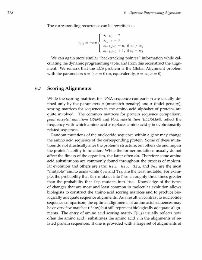
178 6 Dynamic Programming Algorithms
The corresponding recurrence can be rewritten as
si,j = max
si−1,j − σ
si,j−1 − σ
si−1,j−1 − µ, if vi 6= wj
si−1,j−1 + 1, if vi = wj
We can again store similar “backtracking pointer” information while cal-
culating the dynamic programming table, and from this reconstruct the align-
ment. We remark that the LCS problem is the Global Alignment problem
with the parameters µ = 0, σ = 0 (or, equivalently, µ =∞, σ = 0).
6.7 Scoring Alignments
While the scoring matrices for DNA sequence comparison are usually de-
fined only by the parameters µ (mismatch penalty) and σ (indel penalty),
scoring matrices for sequences in the amino acid alphabet of proteins are
quite involved. The common matrices for protein sequence comparison,
point accepted mutations (PAM) and block substitution (BLOSUM), reflect the
frequency with which amino acid x replaces amino acid y in evolutionarily
related sequences.
Random mutations of the nucleotide sequence within a gene may change
the amino acid sequence of the corresponding protein. Some of these muta-
tions do not drastically alter the protein’s structure, but others do and impair
the protein’s ability to function. While the former mutations usually do not
affect the fitness of the organism, the latter often do. Therefore some amino
acid substitutions are commonly found throughout the process of molecu-
lar evolution and others are rare: Asn, Asp, Glu, and Ser are the most
“mutable” amino acids while Cys and Trp are the least mutable. For exam-
ple, the probability that Ser mutates into Phe is roughly three times greater
than the probability that Trp mutates into Phe. Knowledge of the types
of changes that are most and least common in molecular evolution allows
biologists to construct the amino acid scoring matrices and to produce bio-
logically adequate sequence alignments. As a result, in contrast to nucleotide
sequence comparison, the optimal alignments of amino acid sequences may
have very few matches (if any) but still represent biologically adequate align-
ments. The entry of amino acid scoring matrix δ(i, j) usually reflects how
often the amino acid i substitutes the amino acid j in the alignments of re-
lated protein sequences. If one is provided with a large set of alignments of
6.7 Scoring Alignments 179
related sequences, then computing δ(i, j) simply amounts to counting how
many times the amino acid i is aligned with amino acid j. A “minor” compli-
cation is that to build this set of biologically adequate alignments one needs
to know the scoring matrix! Fortunately, in many cases the alignment of
very similar sequences is so obvious that it can be constructed even without
a scoring matrix, thus resolving this predicament. For example, if proteins
are 90% identical, even a naive scoring matrix (e.g., a matrix that gives pre-
mium +1 for matches and penalties−1 for mismatches and indels) would do
the job. After these “obvious” alignments are constructed they can be used
to compute a scoring matrix δ that can be used iteratively to construct less
obvious alignments.
This simplified description hides subtle details that are important in the
construction of scoring matrices. The probability of Ser mutating into Phein proteins that diverged 15 million years ago (e.g., related proteins in mouse
and rat) is smaller than the probability of the Ser → Phe mutation in pro-
teins that diverged 80 million years ago (e.g., related proteins in mouse and
human). This observation implies that the best scoring matrices to compare
two proteins depends on how similar these organisms are.
Biologists get around this problem by first analyzing extremely similar
proteins, for example, proteins that have, on average, only one mutation per
100 amino acids. Many proteins in human and chimpanzee fulfill this re-
quirement. Such sequences are defined as being one PAM unit diverged and to
a first approximation one can think of a PAM unit as the amount of time in
which an “average” protein mutates 1% of its amino acids. The PAM 1 scor-
ing matrix is defined from many alignments of extremely similar proteins as
follows.
Given a set of base alignments, define f(i, j) as the total number of times
amino acids i and j are aligned against each other, divided by the total num-
ber of aligned positions. We also define g(i, j) as f(i,j)f(i) , where f(i) is the
frequency of amino acid i in all proteins from the data set. g(i, j) defines
the probability that an amino acid i mutates into amino acid j within 1 PAM
unit. The (i, j) entry of the PAM 1 matrix is defined as δ(i, j) = log f(i,j)f(i)·f(j) =
log g(i,j)f(j) (f(i) · f(j) stands for the frequency of aligning amino acid i against
amino acid j that one expects simply by chance). The PAM n matrix can
be defined as the result of applying the PAM 1 matrix n times. If g is the
20 × 20 matrix of frequencies g(i, j), then gn (multiplying this matrix by it-
self n times) gives the probability that amino acid i mutates into amino acid
j during n PAM units. The (i, j) entry of the PAM n matrix is defined as
180 6 Dynamic Programming Algorithms
loggn
i,j
f(j) .
For large n, the resulting PAM matrices often allow one to find related
proteins even when there are practically no matches in the alignment. In this
case, the underlying nucleotide sequences are so diverged that their compar-
ison usually fails to find any statistically significant similarities. For example,
the similarity between the cancer-causing ν-sis oncogene and the growth fac-
tor PDGF would probably have remained undetected had Russell Doolittle
and colleagues not transformed the nucleotide sequences into amino acid
sequences prior to performing the comparison.
6.8 Local Sequence Alignment
The Global Alignment problem seeks similarities between two entire strings.
This is useful when the similarity between the strings extends over their en-
tire length, for example, in protein sequences from the same protein family.
These protein sequences are often very conserved and have almost the same
length in organisms ranging from fruit flies to humans. However, in many
biological applications, the score of an alignment between two substrings of
v and w might actually be larger than the score of an alignment between the
entireties of v and w.
For example, homeobox genes, which regulate embryonic development, are
present in a large variety of species. Although homeobox genes are very dif-
ferent in different species, one region in each gene—called the homeodomain—
is highly conserved. The question arises how to find this conserved area and
ignore the areas that show little similarity. In 1981 Temple Smith and Michael
Waterman proposed a clever modification of the global sequence alignment
dynamic programming algorithm that solves the Local Alignment problem.
Figure 6.16 presents the comparison of two hypothetical genes v and w of
the same length with a conserved domain present at the beginning of v and
at the end of w. For simplicity, we will assume that the conserved domains
in these two genes are identical and cover one third of the entire length, n, of
these genes. In this case, the path from source to sink capturing the similarity
between the homeodomains will include approximately 23n horizontal edges,
13n diagonal match edges (corresponding to homeodomains), and 2
3n vertical
edges. Therefore, the score of this path is
−2
3nσ +
1
3n−
2
3nσ = n
(
1
3−
4
3σ
)
6.8 Local Sequence Alignment 181
However, this path contains so many indels that it is unlikely to be the high-
est scoring alignment. In fact, biologically irrelevant diagonal paths from
the source to the sink will likely have a higher score than the biologically
relevant alignment, since mismatches are usually penalized less than indels.
The expected score of such a diagonal path is n(14 −
34µ) since every diagonal
edge corresponds to a match with probability 14 and mismatch with proba-
bility 34 . Since (1
3 −43σ) < (1
4 −34µ) for many settings of indel and mismatch
penalties, the global alignment algorithm will miss the correct solution of
the real biological problem, and is likely to output a biologically irrelevant
near-diagonal path. Indeed, figure 6.16 bears exactly this observation.
When biologically significant similarities are present in certain parts of
DNA fragments and are not present in others, biologists attempt to maxi-
mize the alignment score s(vi . . . vi′ , wj . . . wj′ ), over all substrings vi . . . vi′
of v and wj . . . wj′ of w. This is called the Local Alignment problem since the
alignment does not necessarily extend over the entire string length as it does
in the Global Alignment problem.
Local Alignment Problem:
Find the best local alignment between two strings.
Input: Strings v and w and a scoring matrix δ.
Output: Substrings of v and w whose global alignment, as
defined by δ, is maximal among all global alignments of all
substrings of v and w.
The solution to this seemingly harder problem lies in the realization that
the Global Alignment problem corresponds to finding the longest local path
between vertices (0, 0) and (n, m) in the edit graph, while the Local Align-
ment problem corresponds to finding the longest path among paths between
arbitrary vertices (i, j) and (i′, j′) in the edit graph. A straightforward and in-
efficient approach to this problem is to find the longest path between every
pair of vertices (i, j) and (i′, j′), and then to select the longest of these com-
puted paths.10 Instead of finding the longest path from every vertex (i, j)
to every other vertex (i′, j′), the Local Alignment problem can be reduced
to finding the longest paths from the source (0,0) to every other vertex by
10. This will result in a very slow algorithm with O(n4) running time: there are roughly n2
pairs of vertices (i, j) and computing local alignments starting at each of them typically takesO(n2) time.
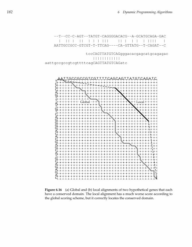
182 6 Dynamic Programming Algorithms
--T--CC-C-AGT--TATGT-CAGGGGACACG--A-GCATGCAGA-GAC| || | || | | | ||| || | | | | |||| |
AATTGCCGCC-GTCGT-T-TTCAG----CA-GTTATG--T-CAGAT--C
tccCAGTTATGTCAGgggacacgagcatgcagagac||||||||||||
aattgccgccgtcgttttcagCAGTTATGTCAGatc
A A T T GCCGCCG T CG T T T T C AGC AG T T A T G T C AGA T CTCCCAGTTATGTCAGGGGACACGAGCATGCAGAGAC
LocalGlobal
Figure 6.16 (a) Global and (b) local alignments of two hypothetical genes that eachhave a conserved domain. The local alignment has a much worse score according tothe global scoring scheme, but it correctly locates the conserved domain.
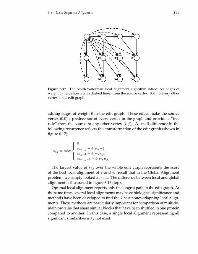
6.8 Local Sequence Alignment 183
Figure 6.17 The Smith-Waterman local alignment algorithm introduces edges ofweight 0 (here shown with dashed lines) from the source vertex (0, 0) to every othervertex in the edit graph.
adding edges of weight 0 in the edit graph. These edges make the source
vertex (0,0) a predecessor of every vertex in the graph and provide a “free
ride” from the source to any other vertex (i, j). A small difference in the
following recurrence reflects this transformation of the edit graph (shown in
figure 6.17):
si,j = max
0
si−1,j + δ(vi,−)
si,j−1 + δ(−, wj)
si−1,j−1 + δ(vi, wj)
The largest value of si,j over the whole edit graph represents the score
of the best local alignment of v and w; recall that in the Global Alignment
problem, we simply looked at sn,m. The difference between local and global
alignment is illustrated in figure 6.16 (top).
Optimal local alignment reports only the longest path in the edit graph. At
the same time, several local alignments may have biological significance and
methods have been developed to find the k best nonoverlapping local align-
ments. These methods are particularly important for comparison of multido-
main proteins that share similar blocks that have been shuffled in one protein
compared to another. In this case, a single local alignment representing all
significant similarities may not exist.
184 6 Dynamic Programming Algorithms
6.9 Alignment with Gap Penalties
Mutations are usually caused by errors in DNA replication. Nature fre-
quently deletes or inserts entire substrings as a unit, as opposed to deleting
or inserting individual nucleotides. A gap in an alignment is defined as a con-
tiguous sequence of spaces in one of the rows. Since insertions and deletions
of substrings are common evolutionary events, penalizing a gap of length x
as −σx is cruel and unusual punishment. Many practical alignment algo-
rithms use a softer approach to gap penalties and penalize a gap of x spaces
by a function that grows slower than the sum of penalties for x indels.
To this end, we define affine gap penalties to be a linearly weighted score
for large gaps. We can set the score for a gap of length x to be −(ρ + σx),
where ρ > 0 is the penalty for the introduction of the gap and σ > 0 is the
penalty for each symbol in the gap (ρ is typically large while σ is typically
small). Though this may seem to be complicating our alignment approach, it
turns out that the edit graph representation of the problem is robust enough
to accommodate it.
Affine gap penalties can be accommodated by adding “long” vertical and
horizontal edges in the edit graph (e.g., an edge from (i, j) to (i + x, j) of
length−(ρ+σx) and an edge from (i, j) to (i, j +x) of the same length) from
each vertex to every other vertex that is either east or south of it. We can then
apply the same algorithm as before to compute the longest path in this graph.
Since the number of edges in the edit graph for affine gap penalties increases,
at first glance it looks as though the running time for the alignment algorithm
also increases from O(n2) to O(n3), where n is the longer of the two string
lengths.11 However, the following three recurrences keep the running time
down:
↓si,j= max
↓si−1,j −σ
si−1,j − (ρ + σ)
→s i,j= max
→s i,j−1 −σ
si,j−1 − (ρ + σ)
11. The complexity of the corresponding Longest Path in a DAG problem is defined by thenumber of edges in the graph. Adding long horizontal and vertical edges imposed by affinegap penalties increases the number of edges by a factor of n.
6.10 Multiple Alignment 185
si,j = max
si−1,j−1 + δ(vi, wj)↓si,j→s i,j
The variable↓si,j computes the score for alignment between the i-prefix of
v and the j-prefix of w ending with a deletion (i.e., a gap in w), while the
variable→s i,j computes the score for alignment ending with an insertion (i.e.,
a gap in v). The first term in the recurrences for↓si,j and
→s i,j corresponds to
extending the gap, while the second term corresponds to initiating the gap.
Essentially,↓si,j and
→s i,j are the scores of optimal paths that arrive at vertex
(i, j) via vertical and horizontal edges correspondingly.
Figure 6.18 further explains how alignment with affine gap penalties can
be reduced to the Manhattan Tourist problem in the appropriate city grid. In
this case the city is built on three levels: the bottom level built solely with
vertical ↓ edges with weight −σ; the middle level built with diagonal edges
of weight δ(vi, wj); and the upper level, which is built from horizontal edges
→ with weight −σ. The lower level corresponds to gaps in sequence w, the
middle level corresponds to matches and mismatches, and the upper level
corresponds to gaps in sequence v. Also, in this graph there are two edges
from each vertex (i, j)middle at the middle level that connect this vertex with
vertex (i + 1, j)lower at the lower level and with vertex (i, j + 1)upper at the
upper level. These edges model a start of the gap and have weight −(ρ + σ).
Finally, one has to introduce zero-weight edges connecting vertices (i, j)lower
and (i, j)upper with vertex (i, j)middle at the middle level (these edges model
the end of the gap). In effect, we have created a rather complicated graph,
but the same algorithm works with it.
We have now introduced a number of pairwise sequence comparison prob-
lems and shown that they can all be solved by what is essentially the same
dynamic programming algorithm applied to a suitably built Manhattan-style
city. We will now consider other applications of dynamic programming in
bioinformatics.
6.10 Multiple Alignment
The goal of protein sequence comparison is to discover structural or func-
tional similarities among proteins. Biologically similar proteins may not ex-
hibit a strong sequence similarity, but we would still like to recognize resem-
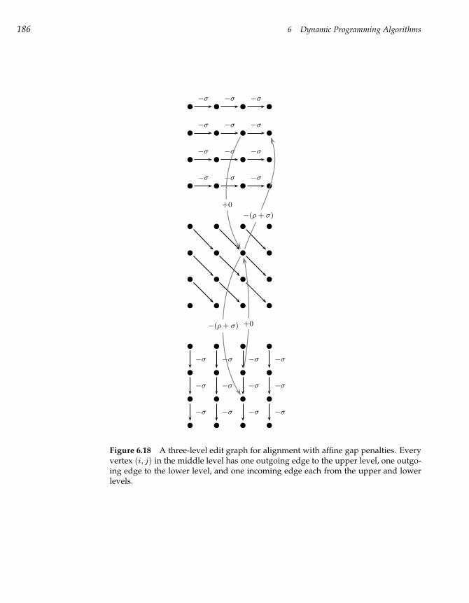
186 6 Dynamic Programming Algorithms
−σ −σ −σ −σ
−σ −σ −σ −σ
−σ −σ −σ −σ
−σ −σ −σ
−σ −σ −σ
−σ −σ −σ
−σ −σ −σ
−(ρ + σ)
−(ρ + σ)
+0
+0
Figure 6.18 A three-level edit graph for alignment with affine gap penalties. Everyvertex (i, j) in the middle level has one outgoing edge to the upper level, one outgo-ing edge to the lower level, and one incoming edge each from the upper and lowerlevels.
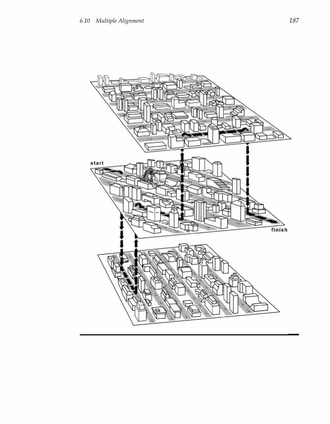
6.10 Multiple Alignment 187
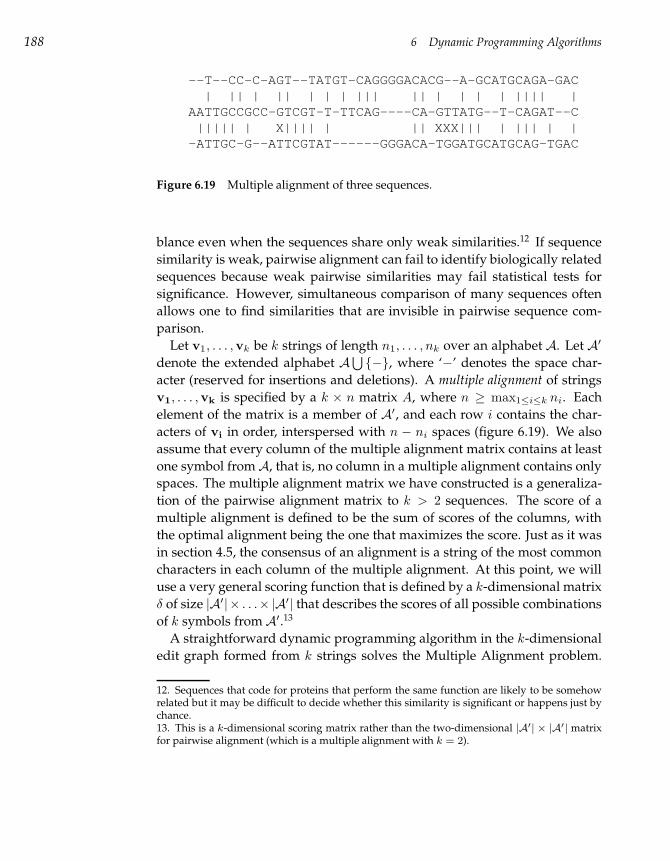
188 6 Dynamic Programming Algorithms
--T--CC-C-AGT--TATGT-CAGGGGACACG--A-GCATGCAGA-GAC| || | || | | | ||| || | | | | |||| |
AATTGCCGCC-GTCGT-T-TTCAG----CA-GTTATG--T-CAGAT--C||||| | X|||| | || XXX||| | ||| | |
-ATTGC-G--ATTCGTAT------GGGACA-TGGATGCATGCAG-TGAC
Figure 6.19 Multiple alignment of three sequences.
blance even when the sequences share only weak similarities.12 If sequence
similarity is weak, pairwise alignment can fail to identify biologically related
sequences because weak pairwise similarities may fail statistical tests for
significance. However, simultaneous comparison of many sequences often
allows one to find similarities that are invisible in pairwise sequence com-
parison.
Let v1, . . . ,vk be k strings of length n1, . . . , nk over an alphabet A. Let A′
denote the extended alphabet A⋃
−, where ‘−’ denotes the space char-
acter (reserved for insertions and deletions). A multiple alignment of strings
v1, . . . ,vk is specified by a k × n matrix A, where n ≥ max1≤i≤k ni. Each
element of the matrix is a member of A′, and each row i contains the char-
acters of vi in order, interspersed with n − ni spaces (figure 6.19). We also
assume that every column of the multiple alignment matrix contains at least
one symbol fromA, that is, no column in a multiple alignment contains only
spaces. The multiple alignment matrix we have constructed is a generaliza-
tion of the pairwise alignment matrix to k > 2 sequences. The score of a
multiple alignment is defined to be the sum of scores of the columns, with
the optimal alignment being the one that maximizes the score. Just as it was
in section 4.5, the consensus of an alignment is a string of the most common
characters in each column of the multiple alignment. At this point, we will
use a very general scoring function that is defined by a k-dimensional matrix
δ of size |A′|× . . .×|A′| that describes the scores of all possible combinations
of k symbols fromA′.13
A straightforward dynamic programming algorithm in the k-dimensional
edit graph formed from k strings solves the Multiple Alignment problem.
12. Sequences that code for proteins that perform the same function are likely to be somehowrelated but it may be difficult to decide whether this similarity is significant or happens just bychance.13. This is a k-dimensional scoring matrix rather than the two-dimensional |A′| × |A′| matrixfor pairwise alignment (which is a multiple alignment with k = 2).
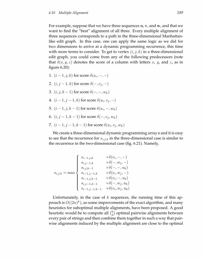
6.10 Multiple Alignment 189
For example, suppose that we have three sequences u, v, and w, and that we
want to find the “best” alignment of all three. Every multiple alignment of
three sequences corresponds to a path in the three-dimensional Manhattan-
like edit graph. In this case, one can apply the same logic as we did for
two dimensions to arrive at a dynamic programming recurrence, this time
with more terms to consider. To get to vertex (i, j, k) in a three-dimensional
edit graph, you could come from any of the following predecessors (note
that δ(x, y, z) denotes the score of a column with letters x, y, and z, as in
figure 6.20):
1. (i− 1, j, k) for score δ(ui,−,−)
2. (i, j − 1, k) for score δ(−, vj ,−)
3. (i, j, k − 1) for score δ(−,−, wk)
4. (i− 1, j − 1, k) for score δ(ui, vj ,−)
5. (i− 1, j, k − 1) for score δ(ui,−, wk)
6. (i, j − 1, k − 1) for score δ(−, vj , wk)
7. (i− 1, j − 1, k − 1) for score δ(ui, vj , wk)
We create a three-dimensional dynamic programming array s and it is easy
to see that the recurrence for si,j,k in the three-dimensional case is similar to
the recurrence in the two-dimensional case (fig. 6.21). Namely,
si,j,k = max
si−1,j,k +δ(vi,−,−)
si,j−1,k +δ(−, wj ,−)
si,j,k−1 +δ(−,−, uk)
si−1,j−1,k +δ(vi, wj ,−)
si−1,j,k−1 +δ(vi,−, uk)
si,j−1,k−1 +δ(−, wj , uk)
si−1,j−1,k−1 +δ(vi, wj , uk)
Unfortunately, in the case of k sequences, the running time of this ap-
proach is O((2n)k), so some improvements of the exact algorithm, and many
heuristics for suboptimal multiple alignments, have been proposed. A good
heuristic would be to compute all(
k2
)
optimal pairwise alignments between
every pair of strings and then combine them together in such a way that pair-
wise alignments induced by the multiple alignment are close to the optimal
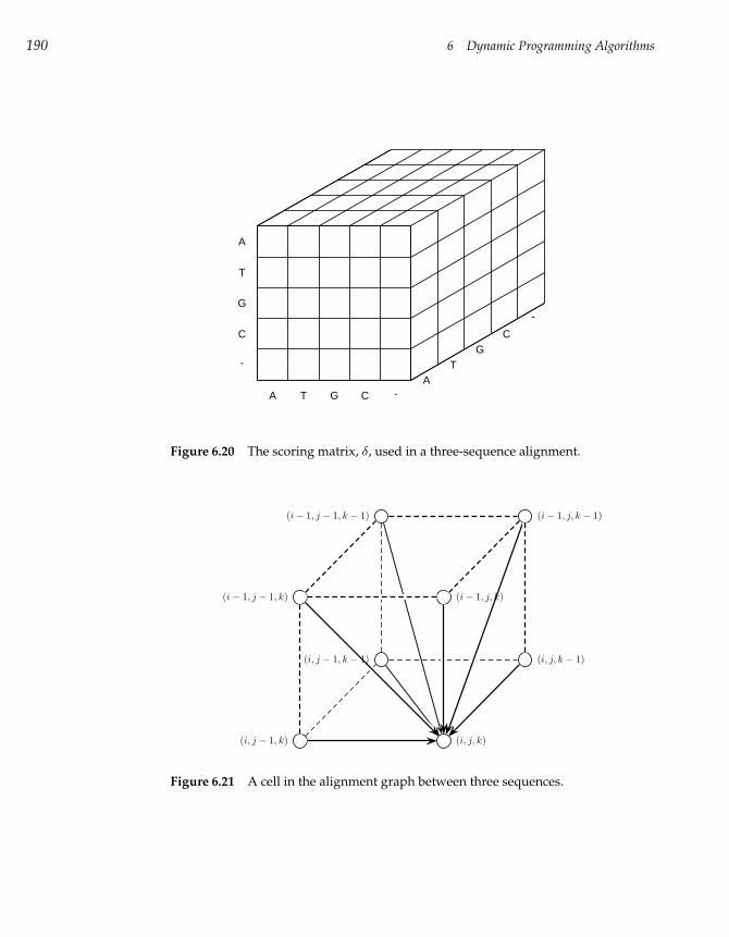
190 6 Dynamic Programming Algorithms
A T G C -
-
C
G
T
A
AT
GC
-
Figure 6.20 The scoring matrix, δ, used in a three-sequence alignment.
(i, j, k)
(i, j, k − 1)
(i, j − 1, k)
(i− 1, j − 1, k)
(i− 1, j − 1, k − 1)
(i− 1, j, k)
(i− 1, j, k − 1)
(i, j − 1, k − 1)
Figure 6.21 A cell in the alignment graph between three sequences.
6.10 Multiple Alignment 191
ones. Unfortunately, it is not always possible to combine optimal pairwise
alignments into a multiple alignment since some pairwise alignments may be
incompatible. For example, figure 6.22 (a) shows three sequences whose opti-
mal pairwise alignment can be combined into a multiple alignment, whereas
(b) shows three sequences that cannot be combined. As a result, some mul-
tiple alignment algorithms attempt to combine some compatible subset of
optimal pairwise alignments into a multiple alignment.
Another approach to do this uses one particularly strong pairwise align-
ment as a building block for the multiple k-way alignment, and iteratively
adds one string to the growing multiple alignment. This greedy progressive
multiple alignment heuristic selects the pair of strings with greatest similarity
and merges them together into a new string following the principle “once a
gap, always a gap.”14 As a result, the multiple alignment of k sequences is
reduced to the multiple alignment of k−1 sequences. The motivation for the
choice of the closest strings at the early steps of the algorithm is that close
strings often provide the most reliable information about a real alignment.
Many popular iterative multiple alignment algorithms, including the tool
CLUSTAL, use similar strategies.
Although progressive multiple alignment algorithms work well for very
close sequences, there are no performance guarantees for this approach. The
problem with progressive multiple alignment algorithms like CLUSTAL is
that they may be misled by some spuriously strong pairwise alignment, in
effect, a bad seed. If the very first two sequences picked for building multiple
alignment are aligned in a way that is incompatible with the optimal multiple
alignment, the error in this initial pairwise alignment will propagate all the
way through to the whole multiple alignment. Many multiple alignment
algorithms have been proposed, and even with systematic deficiencies such
as the above they remain quite useful in computational biology.
We have described multiple alignment for k sequences as a generalization
of the Pairwise Alignment problem, which assumed the existence of a k-
dimensional scoring matrix δ. Since such k-dimensional scoring matrices are
not very practical, we briefly describe two other scoring approaches that are
more biologically relevant. The choice of the scoring function can drastically
affect the quality of the resulting alignment, and no single scoring approach
is perfect in all circumstances.
The columns of a multiple alignment of k sequences describe a path of
14. Essentially, this principle states that once a gap has been introduced into the alignment itwill never close, even if that would lead to a better overall score.
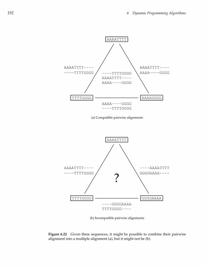
192 6 Dynamic Programming Algorithms
TTTTGGGG AAAAGGGG
AAAATTTT
AAAATTTT--------TTTTGGGG
AAAA----GGGG----TTTTGGGG
AAAATTTT----AAAA----GGGG----TTTTGGGG
AAAATTTT----AAAA----GGGG
(a) Compatible pairwise alignments
TTTTGGGG GGGGAAAA
AAAATTTT
AAAATTTT--------TTTTGGGG
----GGGGAAAATTTTGGGG----
----AAAATTTTGGGGAAAA----
?
(b) Incompatible pairwise alignments
Figure 6.22 Given three sequences, it might be possible to combine their pairwisealignment into a multiple alignment (a), but it might not be (b).
6.11 Gene Prediction 193
edges in a k-dimensional version of the Manhattan gridlike edit graph. The
weights of these edges are determined by the scoring function δ. Intuitively,
we want to assign higher scores to the columns with a low variation in let-
ters, such that high scores correspond to highly conserved sequences. For
example, in the Multiple Longest Common Subsequence problem, the score of
a column is set to 1 if all the characters in the column are the same, and 0 if
even one character disagrees.
In the more statistically motivated entropy approach, the score of a multiple
alignment is defined as the sum of the entropies of the columns, which are
defined to be15∑
x∈A′
px log px
where px is the frequency of letter x ∈ A′ in a given column. In this case,
the more conserved the column, the larger the entropy score. For example,
a column that has each of the 4 nucleotides present k4 times will have an
entropy score of 4 14 log 1
4 = −2, while a completely conserved column (as
in the multiple LCS problem) would have entropy 0. Finding the longest
path in the k-dimensional edit graph corresponds to finding the multiple
alignment with the largest entropy score.
While entropy captures some statistical notion of a good alignment, it can
be hard to design efficient algorithms that optimize this scoring function.
Another popular scoring approach is the Sum-of-Pairs score (SP-score). Any
multiple alignment A of k sequences v1, . . . ,vk forces a pairwise alignment
between any two sequences vi and vj of score sA(vi,vj).16 The SP-score for a
multiple alignment A is given by∑
1≤i<j≤k sA(vi,vj). In this definition, the
score of an alignment A is built from the scores of all pairs of strings in the
alignment.
6.11 Gene Prediction
In 1961 Sydney Brenner and Francis Crick demonstrated that every triplet of
nucleotides (codon) in a gene codes for one amino acid in the corresponding
protein. They were able to introduce deletions in DNA and observed that
deletion of a single nucleotide or two consecutive nucleotides in a gene dra-
matically alters its protein product. Paradoxically, deleting three consecutive
15. The correct way to define entropy is to take the negative of this expression, but the definitionabove allows us to deal with a maximization rather than a minimization problem.16. We remark that the resulting “forced” alignment is not necessarily optimal.
194 6 Dynamic Programming Algorithms
nucleotides results in minor changes in the protein. For example, the phrase
THE SLY FOX AND THE SHY DOG (written in triplets) turns into gibber-
ish after deleting one letter (THE SYF OXA NDT HES HYD OG) or two let-
ters (THE SFO XAN DTH ESH YDO G), but makes some sense after delet-
ing three nucleotides THE SOX AND THE SHY DOG. Inspired by this ex-
periment Charles Yanofsky proved that a gene and its protein product are
collinear, that is, the first codon in the gene codes for the first amino acid in
the protein, the second codon codes for the second amino acid (rather than,
say, the seventeenth), and so on. Yanofsky’s ingenious experiment was so
influential that nobody even questioned whether codons are represented by
continuous stretches in DNA, and for the subsequent fifteen years biologists
believed that a protein was encoded by a long string of contiguous triplets.
However, the discovery of split human genes in 1977 proved that genes are
often represented by a collection of substrings, and raised the computational
problem of predicting the locations of genes in a genome given only the ge-
nomic DNA sequence.
The human genome is larger and more complex than bacterial genomes.
This is not particularly surprising since one would expect to find more genes
in humans than in bacteria. However, the genome size of many eukaryotes
does not appear to be related to an organism’s genetic complexity; for exam-
ple, the salamander genome is ten times larger than the human genome. This
apparent paradox was resolved by the discovery that many organisms con-
tain not only genes but also large amounts of so-called junk DNA that does
not code for proteins at all. In particular, most human genes are broken into
pieces called exons that are separated by this junk DNA. The difference in the
sizes of the salamander and human genomes thus presumably reflects larger
amounts of junk DNA and repeats in the salamander genome.
Split genes are analogous to a magazine article that begins on page 1, con-
tinues on page 13, then takes up again on pages 43, 51, 74, 80, and 91, with
pages of advertising appearing in between. We do not understand why these
jumps occur. and a significant portion of the human genome is this junk “ad-
vertising” that separates exons.
More confusing is that the jumps between different parts of split genes
are inconsistent from species to species. A gene in an insect edition of the
genome will be organized differently than the related gene in a worm genome.
The number of parts (exons) may be different: the information that appears
in one part in the human edition may be broken up into two in the mouse
version, or vice versa. While the genes themselves are related, they may be
quite different in terms of the parts’ structure.
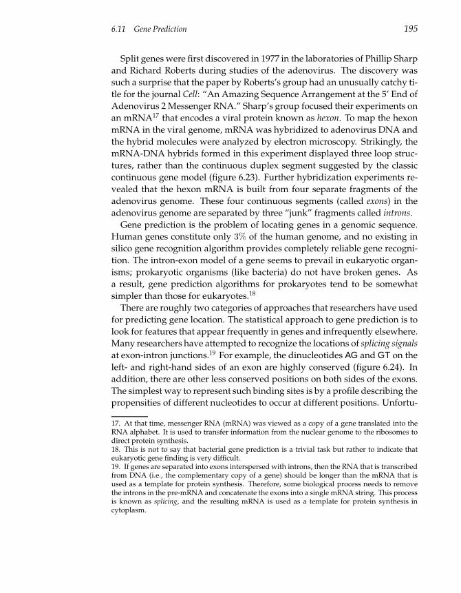
6.11 Gene Prediction 195
Split genes were first discovered in 1977 in the laboratories of Phillip Sharp
and Richard Roberts during studies of the adenovirus. The discovery was
such a surprise that the paper by Roberts’s group had an unusually catchy ti-
tle for the journal Cell: “An Amazing Sequence Arrangement at the 5’ End of
Adenovirus 2 Messenger RNA.” Sharp’s group focused their experiments on
an mRNA17 that encodes a viral protein known as hexon. To map the hexon
mRNA in the viral genome, mRNA was hybridized to adenovirus DNA and
the hybrid molecules were analyzed by electron microscopy. Strikingly, the
mRNA-DNA hybrids formed in this experiment displayed three loop struc-
tures, rather than the continuous duplex segment suggested by the classic
continuous gene model (figure 6.23). Further hybridization experiments re-
vealed that the hexon mRNA is built from four separate fragments of the
adenovirus genome. These four continuous segments (called exons) in the
adenovirus genome are separated by three “junk” fragments called introns.
Gene prediction is the problem of locating genes in a genomic sequence.
Human genes constitute only 3% of the human genome, and no existing in
silico gene recognition algorithm provides completely reliable gene recogni-
tion. The intron-exon model of a gene seems to prevail in eukaryotic organ-
isms; prokaryotic organisms (like bacteria) do not have broken genes. As
a result, gene prediction algorithms for prokaryotes tend to be somewhat
simpler than those for eukaryotes.18
There are roughly two categories of approaches that researchers have used
for predicting gene location. The statistical approach to gene prediction is to
look for features that appear frequently in genes and infrequently elsewhere.
Many researchers have attempted to recognize the locations of splicing signals
at exon-intron junctions.19 For example, the dinucleotides AG and GT on the
left- and right-hand sides of an exon are highly conserved (figure 6.24). In
addition, there are other less conserved positions on both sides of the exons.
The simplest way to represent such binding sites is by a profile describing the
propensities of different nucleotides to occur at different positions. Unfortu-
17. At that time, messenger RNA (mRNA) was viewed as a copy of a gene translated into theRNA alphabet. It is used to transfer information from the nuclear genome to the ribosomes todirect protein synthesis.18. This is not to say that bacterial gene prediction is a trivial task but rather to indicate thateukaryotic gene finding is very difficult.19. If genes are separated into exons interspersed with introns, then the RNA that is transcribedfrom DNA (i.e., the complementary copy of a gene) should be longer than the mRNA that isused as a template for protein synthesis. Therefore, some biological process needs to removethe introns in the pre-mRNA and concatenate the exons into a single mRNA string. This processis known as splicing, and the resulting mRNA is used as a template for protein synthesis incytoplasm.
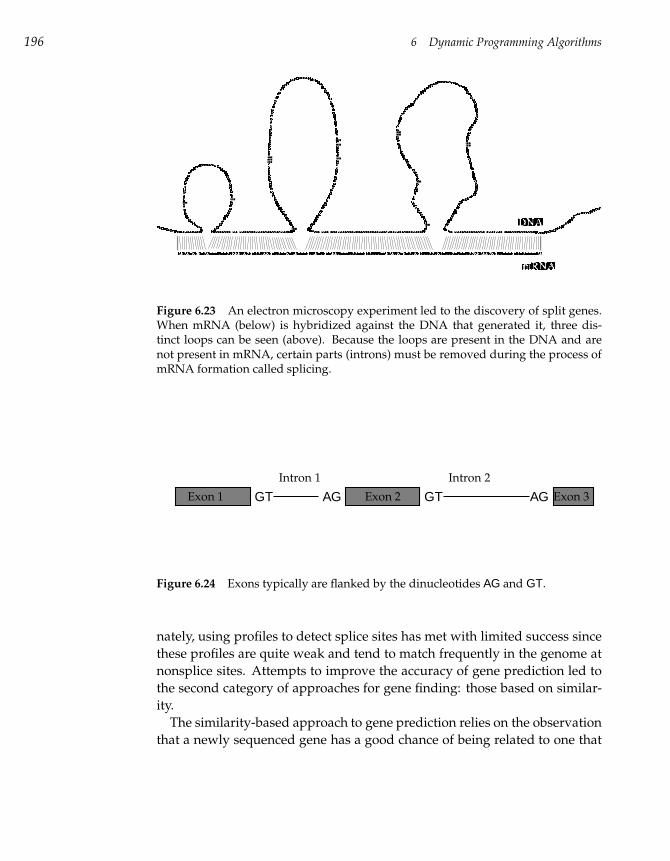
196 6 Dynamic Programming Algorithms
Figure 6.23 An electron microscopy experiment led to the discovery of split genes.When mRNA (below) is hybridized against the DNA that generated it, three dis-tinct loops can be seen (above). Because the loops are present in the DNA and arenot present in mRNA, certain parts (introns) must be removed during the process ofmRNA formation called splicing.
Exon 1
Intron 1
Exon 2
Intron 2
Exon 3GT AG GT AG
Figure 6.24 Exons typically are flanked by the dinucleotides AG and GT.
nately, using profiles to detect splice sites has met with limited success since
these profiles are quite weak and tend to match frequently in the genome at
nonsplice sites. Attempts to improve the accuracy of gene prediction led to
the second category of approaches for gene finding: those based on similar-
ity.
The similarity-based approach to gene prediction relies on the observation
that a newly sequenced gene has a good chance of being related to one that
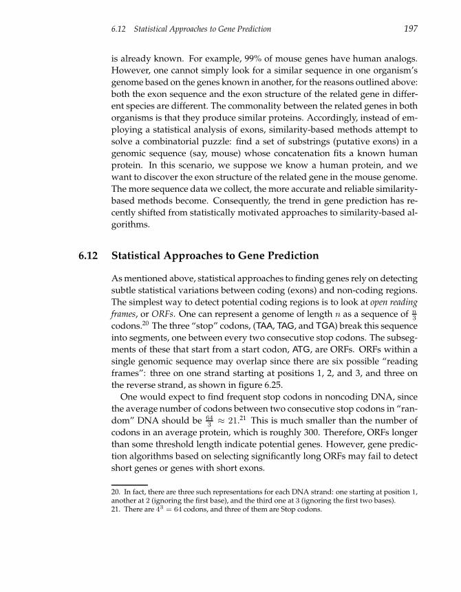
6.12 Statistical Approaches to Gene Prediction 197
is already known. For example, 99% of mouse genes have human analogs.
However, one cannot simply look for a similar sequence in one organism’s
genome based on the genes known in another, for the reasons outlined above:
both the exon sequence and the exon structure of the related gene in differ-
ent species are different. The commonality between the related genes in both
organisms is that they produce similar proteins. Accordingly, instead of em-
ploying a statistical analysis of exons, similarity-based methods attempt to
solve a combinatorial puzzle: find a set of substrings (putative exons) in a
genomic sequence (say, mouse) whose concatenation fits a known human
protein. In this scenario, we suppose we know a human protein, and we
want to discover the exon structure of the related gene in the mouse genome.
The more sequence data we collect, the more accurate and reliable similarity-
based methods become. Consequently, the trend in gene prediction has re-
cently shifted from statistically motivated approaches to similarity-based al-
gorithms.
6.12 Statistical Approaches to Gene Prediction
As mentioned above, statistical approaches to finding genes rely on detecting
subtle statistical variations between coding (exons) and non-coding regions.
The simplest way to detect potential coding regions is to look at open reading
frames, or ORFs. One can represent a genome of length n as a sequence of n3
codons.20 The three “stop” codons, (TAA, TAG, and TGA) break this sequence
into segments, one between every two consecutive stop codons. The subseg-
ments of these that start from a start codon, ATG, are ORFs. ORFs within a
single genomic sequence may overlap since there are six possible “reading
frames”: three on one strand starting at positions 1, 2, and 3, and three on
the reverse strand, as shown in figure 6.25.
One would expect to find frequent stop codons in noncoding DNA, since
the average number of codons between two consecutive stop codons in “ran-
dom” DNA should be 643 ≈ 21.21 This is much smaller than the number of
codons in an average protein, which is roughly 300. Therefore, ORFs longer
than some threshold length indicate potential genes. However, gene predic-
tion algorithms based on selecting significantly long ORFs may fail to detect
short genes or genes with short exons.
20. In fact, there are three such representations for each DNA strand: one starting at position 1,another at 2 (ignoring the first base), and the third one at 3 (ignoring the first two bases).21. There are 43 = 64 codons, and three of them are Stop codons.
198 6 Dynamic Programming Algorithms
Ala
Ala
Val
Arg Leu
Leu
Thr
Tyr
AUGGCACCGUCGGUGAGUAACGCAUUG
TACCGTGGCAGCCACTCATTGCGTAAC
Met
Met
Ala
Pro
Pro
Ser
SerSer
Val
Val Asp
Arg
Arg Arg
Leu Trp
Trp
His
His
Stop
Stop
StopGly Gly
GlyGly
Thr
Glu
Glu
Asn
Gln
Cys
Figure 6.25 The six reading frames for the sequence ATGCTTAGTCTG. The stringmay be read forward or backward, and there are three frame shifts in each direction.
Many statistical gene prediction algorithms rely on statistical features in
protein-coding regions, such as biases in codon usage. We can enter the fre-
quency of occurrence of each codon within a given sequence into a 64-element
codon usage array, as in table 6.1. The codon usage arrays for coding regions
are different than the codon usage arrays for non-coding regions, enabling
one to use them for gene prediction. For example, in human genes codons
CGC and AGG code for the same amino acid (Arg) but have very different
frequencies: CGC is 12 times more likely to be used in genes than AGG (ta-
ble 6.1). Therefore, an ORF that “prefers” CGC over AGG while coding for
Arg is a likely candidate gene. One can use a likelihood ratio approach22 to
compute the conditional probabilities of the DNA sequence in a window, un-
der the hypothesis that the window contains a coding sequence, and under
the hypothesis that the window contains a noncoding sequence. If we slide
this window along the genomic DNA sequence (and calculate the likelihood
22. The likelihood ratio technique allows one to test the applicability of two distinct hypotheses;when the likelihood ratio is large, the first hypothesis is more likely to be true than the secondone.
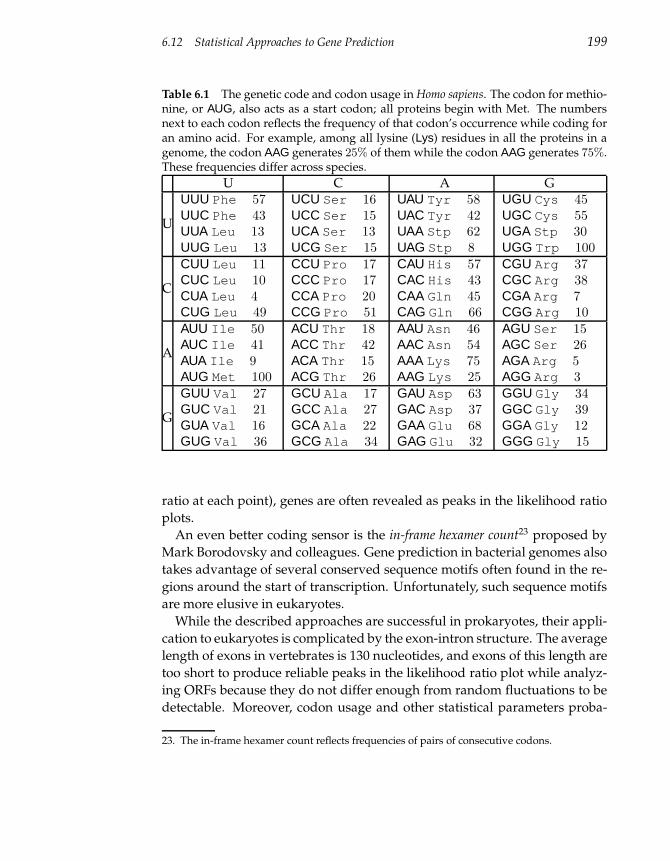
6.12 Statistical Approaches to Gene Prediction 199
Table 6.1 The genetic code and codon usage in Homo sapiens. The codon for methio-nine, or AUG, also acts as a start codon; all proteins begin with Met. The numbersnext to each codon reflects the frequency of that codon’s occurrence while coding foran amino acid. For example, among all lysine (Lys) residues in all the proteins in agenome, the codon AAG generates 25% of them while the codon AAG generates 75%.These frequencies differ across species.
U C A G
U
UUU Phe 57UUC Phe 43UUA Leu 13UUG Leu 13
UCU Ser 16UCC Ser 15UCA Ser 13UCG Ser 15
UAU Tyr 58UAC Tyr 42UAA Stp 62UAG Stp 8
UGU Cys 45UGC Cys 55UGA Stp 30UGG Trp 100
C
CUU Leu 11CUC Leu 10CUA Leu 4CUG Leu 49
CCU Pro 17CCC Pro 17CCA Pro 20CCG Pro 51
CAU His 57CAC His 43CAA Gln 45CAG Gln 66
CGU Arg 37CGC Arg 38CGA Arg 7CGG Arg 10
A
AUU Ile 50AUC Ile 41AUA Ile 9AUG Met 100
ACU Thr 18ACC Thr 42ACA Thr 15ACG Thr 26
AAU Asn 46AAC Asn 54AAA Lys 75AAG Lys 25
AGU Ser 15AGC Ser 26AGA Arg 5AGG Arg 3
G
GUU Val 27GUC Val 21GUA Val 16GUG Val 36
GCU Ala 17GCC Ala 27GCA Ala 22GCG Ala 34
GAU Asp 63GAC Asp 37GAA Glu 68GAG Glu 32
GGU Gly 34GGC Gly 39GGA Gly 12GGG Gly 15
ratio at each point), genes are often revealed as peaks in the likelihood ratio
plots.
An even better coding sensor is the in-frame hexamer count23 proposed by
Mark Borodovsky and colleagues. Gene prediction in bacterial genomes also
takes advantage of several conserved sequence motifs often found in the re-
gions around the start of transcription. Unfortunately, such sequence motifs
are more elusive in eukaryotes.
While the described approaches are successful in prokaryotes, their appli-
cation to eukaryotes is complicated by the exon-intron structure. The average
length of exons in vertebrates is 130 nucleotides, and exons of this length are
too short to produce reliable peaks in the likelihood ratio plot while analyz-
ing ORFs because they do not differ enough from random fluctuations to be
detectable. Moreover, codon usage and other statistical parameters proba-
23. The in-frame hexamer count reflects frequencies of pairs of consecutive codons.
200 6 Dynamic Programming Algorithms
bly have nothing in common with the way the splicing machinery actually
recognizes exons. Many researchers have used a more biologically oriented
approach and have attempted to recognize the locations of splicing signals
at exon-intron junctions. There exists a (weakly) conserved sequence of eight
nucleotides at the boundary of an exon and an intron (donor splice site) and a
sequence of four nucleotides at the boundary of an intron and exon (acceptor
splice site). Since profiles for splice sites are weak, these approaches have had
limited success and have been supplanted by hidden Markov model (HMM)
approaches24 that capture statistical dependencies between sites. A popular
example of this latter approach is GENSCAN, which was developed in 1997
by Chris Burge and Samuel Karlin. GENSCAN combines coding region and
splicing signal predictions into a single framework. For example, a splice site
prediction is more believable if signs of a coding region appear on one side
of the site but not on the other. Many such statistics are used in the HMM
framework of GENSCAN that merges splicing site statistics, coding region
statistics, and motifs near the start of the gene, among others. However, the
accuracy of GENSCAN decreases for genes with many short exons or with
unusual codon usage.
6.13 Similarity-Based Approaches to Gene Prediction
A similarity-based approach to gene prediction uses previously sequenced
genes and their protein products as a template for the recognition of un-
known genes in newly sequenced DNA fragments. Instead of employing
statistical properties of exons, this method attempts to solve the following
combinatorial puzzle: given a known target protein and a genomic sequence,
find a set of substrings (candidate exons) of the genomic sequence whose
concatenation (splicing) best fits the target.
A naive brute force approach to the spliced alignment problem is to find
all local similarities between the genomic sequence and the target protein
sequence. Each substring from the genomic sequence that exhibits sufficient
similarity to the target protein could be considered a putative exon.25 The
putative exons so chosen may lack the canonical exon-flanking dinucleotides
AG and GT but we can extend or shorten them slightly to make sure that
they are flanked by AG and GT. The resulting set may contain overlapping
24. Hidden Markov models are described in chapter 11.25. Putative here means that the sequence might be an exon, even though we have no proof ofthis.
6.13 Similarity-Based Approaches to Gene Prediction 201
substrings, and the problem is to choose the best subset of nonoverlapping
substrings as a putative exon structure.26
We will model a putative exon with a weighted interval in the genomic se-
quence, which is described by three parameters (l, r, w), as in figure 6.26.
Here, l is the left-hand position, r is the right-hand position, and w is the
weight of the putative exon. The weight w may reflect the local alignment
score for the genomic interval against the target protein sequence, or the
strength of flanking acceptor and donor sites, or any combination of these
and other measures; it reflects the likelihood that this interval is an exon. A
chain is any set of nonoverlapping weighted intervals. The total weight of a
chain is the sum of the weights of the intervals in the chain. A maximum chain
is a chain with maximum total weight among all possible chains. Below we
assume that the weights of all intervals are positive (w > 0).
Exon Chaining Problem:
Given a set of putative exons, find a maximum set of nonoverlapping
putative exons.
Input: A set of weighted intervals (putative exons).
Output: A maximum chain of intervals from this set.
The Exon Chaining problem for n intervals can be solved by dynamic pro-
gramming in a graph G on 2n vertices, n of which represent starting (left)
positions of intervals and n of which represent ending (right) positions of in-
tervals, as in figure 6.26. We assume that the set of left and right interval ends
is sorted into increasing order and that all positions are distinct, forming an
ordered array of vertices (v1, . . . v2n) in graph G.27 There are 3n− 1 edges in
this graph: there is an edge between each li and ri of weight wi for i from 1
to n, and 2n− 1 additional edges of weight 0 which simply connect adjacent
vertices (vi, vi+1) forming a path in the graph from v1 to v2n. In the algo-
rithm below, si represents the length of the longest path in the graph ending
at vertex vi. Thus, s2n is the solution to the Exon Chaining problem.
26. We choose nonoverlapping substrings because exons in real genes do not overlap.27. In particular, we are assuming that no interval starts exactly where another ends.
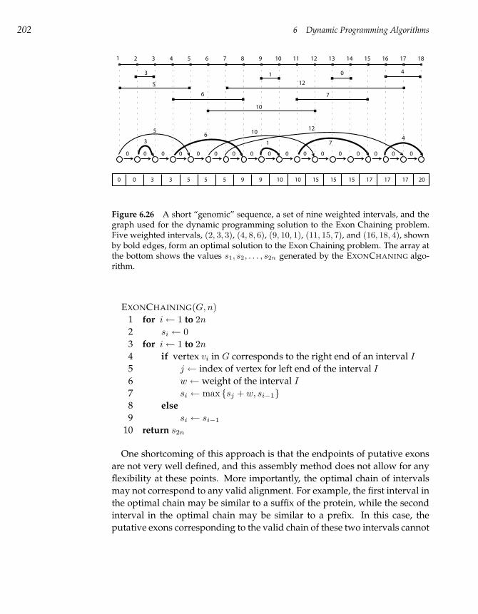
202 6 Dynamic Programming Algorithms
1 2 3 4 5 6 7 8 9 10 11 12 13 14 15 16 17 18
3
5
6 7
4
10
12
0
3
56
74
1012
0 0 0 0 0 0 0 0 0 0 0 0 0 0 0 0 0
1
1
0 0 3 3 5 5 5 9 9 10 15 1510 15 17 17 17 20
Figure 6.26 A short “genomic” sequence, a set of nine weighted intervals, and thegraph used for the dynamic programming solution to the Exon Chaining problem.Five weighted intervals, (2, 3, 3), (4, 8, 6), (9, 10, 1), (11, 15, 7), and (16, 18, 4), shownby bold edges, form an optimal solution to the Exon Chaining problem. The array atthe bottom shows the values s1, s2, . . . , s2n generated by the EXONCHANING algo-rithm.
EXONCHAINING(G, n)
1 for i← 1 to 2n
2 si ← 0
3 for i← 1 to 2n
4 if vertex vi in G corresponds to the right end of an interval I
5 j ← index of vertex for left end of the interval I
6 w ← weight of the interval I
7 si ← max sj + w, si−1
8 else
9 si ← si−1
10 return s2n
One shortcoming of this approach is that the endpoints of putative exons
are not very well defined, and this assembly method does not allow for any
flexibility at these points. More importantly, the optimal chain of intervals
may not correspond to any valid alignment. For example, the first interval in
the optimal chain may be similar to a suffix of the protein, while the second
interval in the optimal chain may be similar to a prefix. In this case, the
putative exons corresponding to the valid chain of these two intervals cannot
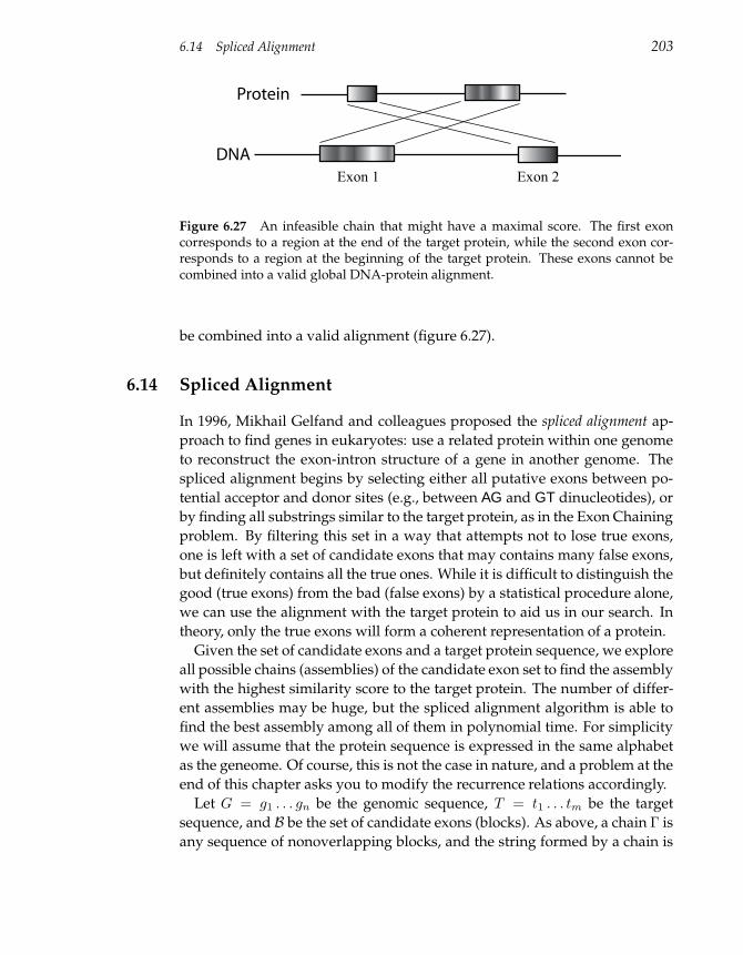
6.14 Spliced Alignment 203
DNA
Protein
Exon 1 Exon 2
Figure 6.27 An infeasible chain that might have a maximal score. The first exoncorresponds to a region at the end of the target protein, while the second exon cor-responds to a region at the beginning of the target protein. These exons cannot becombined into a valid global DNA-protein alignment.
be combined into a valid alignment (figure 6.27).
6.14 Spliced Alignment
In 1996, Mikhail Gelfand and colleagues proposed the spliced alignment ap-
proach to find genes in eukaryotes: use a related protein within one genome
to reconstruct the exon-intron structure of a gene in another genome. The
spliced alignment begins by selecting either all putative exons between po-
tential acceptor and donor sites (e.g., between AG and GT dinucleotides), or
by finding all substrings similar to the target protein, as in the Exon Chaining
problem. By filtering this set in a way that attempts not to lose true exons,
one is left with a set of candidate exons that may contains many false exons,
but definitely contains all the true ones. While it is difficult to distinguish the
good (true exons) from the bad (false exons) by a statistical procedure alone,
we can use the alignment with the target protein to aid us in our search. In
theory, only the true exons will form a coherent representation of a protein.
Given the set of candidate exons and a target protein sequence, we explore
all possible chains (assemblies) of the candidate exon set to find the assembly
with the highest similarity score to the target protein. The number of differ-
ent assemblies may be huge, but the spliced alignment algorithm is able to
find the best assembly among all of them in polynomial time. For simplicity
we will assume that the protein sequence is expressed in the same alphabet
as the geneome. Of course, this is not the case in nature, and a problem at the
end of this chapter asks you to modify the recurrence relations accordingly.
Let G = g1 . . . gn be the genomic sequence, T = t1 . . . tm be the target
sequence, and B be the set of candidate exons (blocks). As above, a chain Γ is
any sequence of nonoverlapping blocks, and the string formed by a chain is
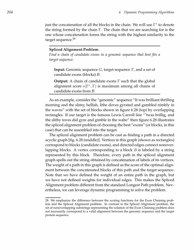
204 6 Dynamic Programming Algorithms
just the concatenation of all the blocks in the chain. We will use Γ∗ to denote
the string formed by the chain Γ. The chain that we are searching for is the
one whose concatenation forms the string with the highest similarity to the
target sequence.28
Spliced Alignment Problem:
Find a chain of candidate exons in a genomic sequence that best fits a
target sequence.
Input: Genomic sequence G, target sequence T , and a set of
candidate exons (blocks) B.
Output: A chain of candidate exons Γ such that the global
alignment score s(Γ∗, T ) is maximum among all chains of
candidate exons from B.
As an example, consider the “genomic” sequence “It was brilliant thrilling
morning and the slimy, hellish, lithe doves gyrated and gambled nimbly in
the waves” with the set of blocks shown in figure 6.28 (top) by overlapping
rectangles. If our target is the famous Lewis Carroll line “’twas brillig, and
the slithy toves did gyre and gimble in the wabe” then figure 6.28 illustrates
the spliced alignment problem of choosing the best “exons” (or blocks, in this
case) that can be assembled into the target.
The spliced alignment problem can be cast as finding a path in a directed
acyclic graph [fig. 6.28 (middle)]. Vertices in this graph (shown as rectangles)
correspond to blocks (candidate exons), and directed edges connect nonover-
lapping blocks. A vertex corresponding to a block B is labeled by a string
represented by this block. Therefore, every path in the spliced alignment
graph spells out the string obtained by concatenation of labels of its vertices.
The weight of a path in this graph is defined as the score of the optimal align-
ment between the concatenated blocks of this path and the target sequence.
Note that we have defined the weight of an entire path in the graph, but
we have not defined weights for individual edges. This makes the Spliced
Alignment problem different from the standard Longest Path problem. Nev-
ertheless, we can leverage dynamic programming to solve the problem.
28. We emphasize the difference between the scoring functions for the Exon Chaining prob-lem and the Spliced Alignment problem. In contrast to the Spliced Alignment problem, theset of nonoverlapping substrings representing the solution of the Exon Chaining problem doesnot necessarily correspond to a valid alignment between the genomic sequence and the targetprotein sequence.
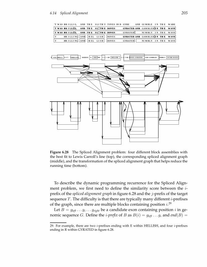
6.14 Spliced Alignment 205
’T W AS B R I L L I G, AND T H E S L I T H T OVE S DI D GYRE NDA GI M B L E I N T H E W AB E
T HR I L L I AND H E L H OVE SNG I SL D I N T H E W A EGYRAT E D VM B LNI Y
I NGYRAT E D T H E W A EVM B LNI Y
T HR I L L I AND H E L H OVE SNG I SL D
W AS BT R I L L I G, AND T H E S L T H E OVE SDW AS B R I L L I G, AND T H E S L T H E OVE ST D
W AS BT R I L L I G, AND T H E S L T H OVE SDW AS B R I L L I G, AND T H E S L T H E OVE ST D GYRAT NDAE DGYRAT NDAE D M B L EGA I N T H E W AVEI N T H E W A EVD
GYRAT NDAE DGYRAT NDAE D M B L EGA I N T H E W AVEI N T H E W A EVD
IT WAS BRILLI THRILLING MORNIN G, AND THE S L I MY HELLISH L I T HE DOVES GYRATED AND GAMBLED NIMBLY IN THE WAVESA N T
E
Y
Figure 6.28 The Spliced Alignment problem: four different block assemblies withthe best fit to Lewis Carroll’s line (top), the corresponding spliced alignment graph(middle), and the transformation of the spliced alignment graph that helps reduce therunning time (bottom).
To describe the dynamic programming recurrence for the Spliced Align-
ment problem, we first need to define the similarity score between the i-
prefix of the spliced alignment graph in figure 6.28 and the j-prefix of the target
sequence T . The difficulty is that there are typically many different i-prefixes
of the graph, since there are multiple blocks containing position i.29
Let B = gleft . . . gi . . . gright be a candidate exon containing position i in ge-
nomic sequence G. Define the i-prefix of B as B(i) = gleft . . . gi and end(B) =
29. For example, there are two i-prefixes ending with E within HELLISH, and four i-prefixesending in R within GYRATED in figure 6.28.
206 6 Dynamic Programming Algorithms
right (the words left and right are used here as indices). If the chain Γ =
(B1, B2, . . . , B) ends at block B, define Γ∗(i) to be the concatenation of all
candidate exons in the chain up to (and excluding) B, plus all the characters
in B up to i. That is, Γ∗(i) = B1 B2 · · · B(i).30 Finally, let
S(i, j, B) = maxall chains Γ ending in B
s(Γ∗(i), T (j)).
That is, given i, j, and a candidate exon B that covers position i, S(i, j, B)
is the score of the optimal spliced alignment between the i-prefix of G and
the j-prefix of T under the assumption that this alignment ends in block B.
The following recurrence allows us to efficiently compute S(i, j, B). For
the sake of simplicity we consider sequence alignment with linear gap penal-
ties for insertion or deletion equal to −σ, and use the scoring matrix δ for
matches and mismatches.
The dynamic programming recurrence for the Spliced Alignment problem
is broken into two cases depending on whether i is the starting vertex of
block B or not. In the latter case, the recurrence is similar to the canonical
sequence alignment:
S(i, j, B) = max
8
<
:
S(i− 1, j, B)− σ
S(i, j − 1, B)− σ
S(i− 1, j − 1, B) + δ(gi, tj)
On the other hand, if i is the starting position of block B, then
S(i, j, B) = max
8
>
<
>
:
S(i, j − 1, B)− σ
maxall blocks B′ preceding BS(end(B′), j − 1, B′) + δ(gi, tj),
maxall blocks B′ preceding BS(end(B′), j, B′)− σ,
After computing this three-dimensional table S(i, j, B), the score of the
optimal spliced alignment is
maxB
S(end(B), m, B),
where the maximum is taken over all possible blocks. One can further reduce
the number of edges in the spliced alignment graph by making a transfor-
30. The notation x y denotes concatenation of strings x and y.
6.15 Notes 207
mation of the graph in figure 6.28 (middle) into a graph shown in figure 6.28
(bottom). The details of the corresponding recurrences are left as a problem
at the end of this chapter.
The above description hides some important details of block generation.
The simplest approach to the construction of the candidate exon set is to gen-
erate all fragments between potential acceptor sites represented by AG and
potential donor sites represented by GT, removing possible exons with stop
codons in all three frames. However, this approach does not work well since
it generates many short blocks. Experiments with the spliced alignment al-
gorithm have shown that incorrect predictions are frequently associated with
the mosaic effect caused by very short potential exons. The difficulty is that
these short exons can be easily combined to fit any target protein, simply be-
cause it is easier to construct a given sentence from a thousand random short
strings than from the same number of random long strings. For example,
with high probability, the phrase “filtration of candidate exons” can be made
up from a sample of a thousand random two-letter strings (“fi,” “lt,” “ra,”
etc. are likely to be present in this sample). The probability that the same
phrase can be made up from a sample of the same number of random five-
letter strings is close to zero (even finding the string “filtr” in this sample is
unlikely). This observation explains the mosaic effect: if the number of short
blocks is high, chains of these blocks can replace actual exons in spliced align-
ments, thus leading to predictions with an unusually large number of short
exons. To avoid the mosaic effect, the candidate exons should be subjected
to some filtering procedure.
6.15 Notes
Although the first dynamic programming algorithm for DNA sequence com-
parison was published as early as 1970 by Saul Needleman and Christian
Wunsch (79), Russell Doolittle and colleagues used heuristic algorithms to
establish the similarity between cancer-causing genes and the PDGF gene in
1983 (28). When Needleman and Wunsch published their paper in 1970, they
did not know that a very similar algorithm had been published two years
earlier in a pioneering paper on automatic speech recognition (105) (though
the details of the algorithms are slightly different, they are both variations
of dynamic programming). Earlier still, Vladimir Levenshtein introduced
the notion of edit distance in 1966 (64), albeit without an algorithm for com-
puting it. The local alignment algorithm introduced by Temple Smith and
208 6 Dynamic Programming Algorithms
Michael Waterman in 1981 (96) quickly became the most popular alignment
tool in computational biology. Later Michael Waterman and Mark Eggert
developed an algorithm for finding the k best nonoverlapping local align-
ments (109). The algorithm for alignment with affine gap penalties was the
work of Osamu Gotoh (42).
The progressive multiple alignment approach, initially explored by Da-Fei
Feng and Russell Doolittle [Feng and Doolittle, 1987 (36)], resulted in many
practical algorithms, with CLUSTAL (48) one of the most popular.
The cellular process of splicing was discovered in the laboratories of Phillip
Sharp (12) and Richard Roberts (21). Applications of both Markov models
and in-frame hexamer count statistics for gene prediction were proposed by
Borodovsky and McInnich (14). Chris Burge and Samuel Karlin developed
an HMM approach to gene prediction that resulted in the popular GEN-SCAN algorithm in 1997 (20). In 1995 Snyder and Stormo (97) developed a
similarity-based gene prediction algorithm that amounts to the solution of a
problem that is similar to the Exon Chaining problem. The spliced alignment
algorithm was developed by Mikhail Gelfand and colleagues in 1996 (41).
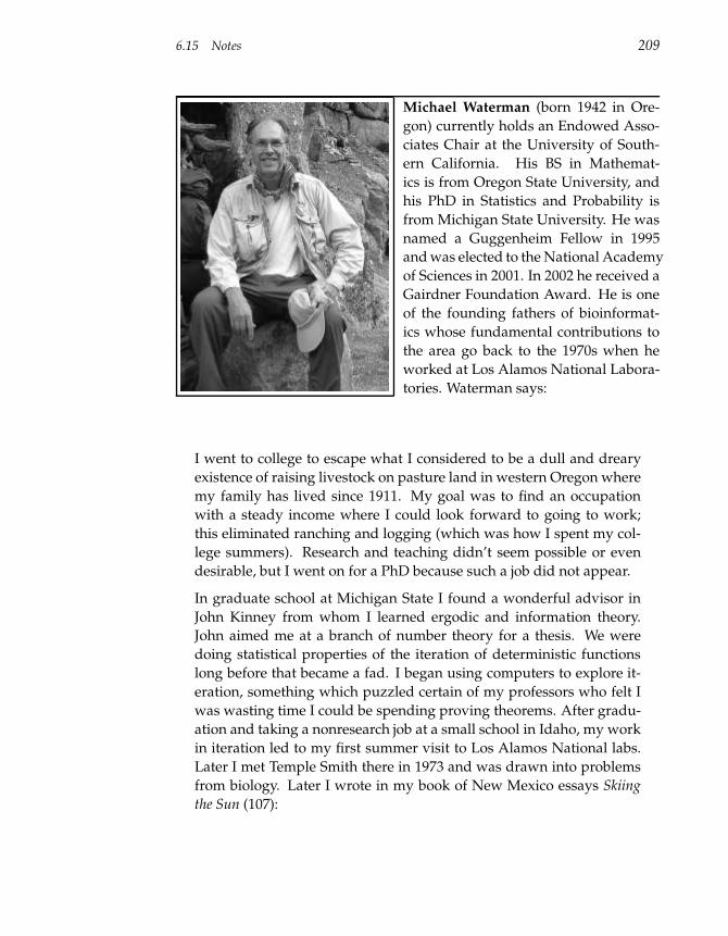
6.15 Notes 209
Michael Waterman (born 1942 in Ore-
gon) currently holds an Endowed Asso-
ciates Chair at the University of South-
ern California. His BS in Mathemat-
ics is from Oregon State University, and
his PhD in Statistics and Probability is
from Michigan State University. He was
named a Guggenheim Fellow in 1995
and was elected to the National Academy
of Sciences in 2001. In 2002 he received a
Gairdner Foundation Award. He is one
of the founding fathers of bioinformat-
ics whose fundamental contributions to
the area go back to the 1970s when he
worked at Los Alamos National Labora-
tories. Waterman says:
I went to college to escape what I considered to be a dull and dreary
existence of raising livestock on pasture land in western Oregon where
my family has lived since 1911. My goal was to find an occupation
with a steady income where I could look forward to going to work;
this eliminated ranching and logging (which was how I spent my col-
lege summers). Research and teaching didn’t seem possible or even
desirable, but I went on for a PhD because such a job did not appear.
In graduate school at Michigan State I found a wonderful advisor in
John Kinney from whom I learned ergodic and information theory.
John aimed me at a branch of number theory for a thesis. We were
doing statistical properties of the iteration of deterministic functions
long before that became a fad. I began using computers to explore it-
eration, something which puzzled certain of my professors who felt I
was wasting time I could be spending proving theorems. After gradu-
ation and taking a nonresearch job at a small school in Idaho, my work
in iteration led to my first summer visit to Los Alamos National labs.
Later I met Temple Smith there in 1973 and was drawn into problems
from biology. Later I wrote in my book of New Mexico essays Skiing
the Sun (107):
210 6 Dynamic Programming Algorithms
I was an innocent mathematician until the summer of 1974. It
was then than I met Temple Ferris Smith and for two months
was cooped up with him in an office at Los Alamos National
Laboratories. That experience transformed my research, my life,
and perhaps my sanity. Soon after we met, he pulled out a little
blackboard and started lecturing me about biology: what it was,
what was important, what was going on. Somewhere in there
by implication was what we should work on, but the truth be
told he didn’t know what that was either. I was totally confused:
amino acids, nucleosides, beta sheets. What were these things?
Where was the mathematics?
I knew no modern biology, but studying alignment and evolution was
quite attractive to me. The most fun was formulating problems, and
in my opinion that remains the most important aspect of our subject.
Temple and I spent days and weeks trying to puzzle out what we
should be working on. Charles DeLisi, a biophysicist who went on
to play a key role in jump-starting the Human Genome Project, was
in T-10 (theoretical biology) at the lab. When he saw the progress we
had made on alignment problems, he came to me and said there was
another problem which should interest me. This was the RNA folding
problem which was almost untouched. Tinoco had published the idea
of making a base-pair matrix for a sequence and that was it. By the fall
of 1974 I had seen the neat connection between alignment and folding,
and the following summer I wrote a long manuscript that defined the
objects of study, established some of their properties, explicitly stated
the basic problem of folding (which included free energies for all struc-
tural components), and finally gave algorithms for its solution. I had
previously wondered what such a discovery might feel like, and it was
wonderfully satisfying. However it felt entirely like exploration and
not a grand triumph of creation as I had expected. In fact I had always
wanted to be an explorer and regretted the end of the American fron-
tier; wandering about this new RNA landscape was a great joy, just as
I had thought when I was a child trying to transport myself by day-
dreams out of my family’s fields into some new and unsettled country.
6.16 Problems 211
6.16 Problems
In 1879, Lewis Carroll proposed the following puzzle to the readers of Vanity Fair: transform one
English word into another by going through a series of intermediate English words, where each
word in the sequence differs from the next by only one substitution. To transform head into tail
one can use four intermediates: head → heal → teal → tell → tall → tail. We say that two
words v and w are equivalent if v can be transformed into w by substituting individual letters
in such a way that all intermediate words are English words present in an English dictionary.
Problem 6.1
Find an algorithm to solve the following Equivalent Words problem.
Equivalent Words Problem:
Given two words and a dictionary, find out whether the words are equivalent.
Input: The dictionary, D (a set of words), and two words v and w
from the dictionary.
Output: A transformation of v into w by substitutions such that all
intermediate words belong to D. If no transformation is possible,
output “v and w are not equivalent.”
Given a dictionary D, the Lewis Carroll distance, dLC(v,w), between words v and w is defined
as the smallest number of substitutions needed to transform v into w in such a way that all
intermediate words in the transformation are in the dictionary D. We define dLC(v, w) = ∞ if
v and w are not equivalent.
Problem 6.2
Find an algorithm to solve the following Lewis Carroll problem.
Lewis Carroll Problem:
Given two words and a dictionary, find the Lewis Carroll distance between these
words.
Input: The dictionaryD, and two words v and w from the diction-
ary.
Output: dLC(v,w)
Problem 6.3
Find an algorithm to solve a generalization of the Lewis Carroll problem when inser-tions, deletions, and substitutions are allowed (rather than only substitutions).
212 6 Dynamic Programming Algorithms
Problem 6.4
Modify DPCHANGE to return not only the smallest number of coins but also the cor-rect combination of coins.
Problem 6.5
Let s(v,w) be the length of a longest common subsequence of the strings v and w andd(v,w) be the edit distance between v and w under the assumption that insertionsand deletions are the only allowed operations. Prove that d(v,w) = n+m−2s(v,w),where n is the length of v and m is the length of w.
Problem 6.6
Find the number of different paths from source (0, 0) to sink (n, m) in an n × mrectangular grid.
Problem 6.7
Can you find an approximation ratio of the greedy algorithm for the ManhattanTourist problem?
Problem 6.8
Let v = v1v2 · · · vn be a string, and let P be a 4×m profile. Generalize the sequencealignment algorithm for aligning a sequence against a profile. Write the correspond-ing recurrence (in lieu of pseudocode), and estimate the amount of time that youralgorithm will take with respect to n and m.
Problem 6.9
There are only two buttons inside an elevator in a building with 50 floors. The ele-vator goes 11 floors up if the first button is pressed and 6 floors down if the secondbutton is pressed. Is it possible to get from floor 32 to floor 33? What is the minimumnumber of buttons one has to press to do so? What is the shortest time one needsto get from floor 32 to floor 33 (time is proportional to the number of floors that arepassed on the way)?
Problem 6.10
A rook stands on the upper left square of a chessboard. Two players make turnsmoving the rook either horizontally to the right or vertically downward (as manysquares as they want). The player who can place the rook on the lower right squareof the chessboard wins. Who will win? Describe the winning strategy.
6.16 Problems 213
Problem 6.11
A queen stands on the third square of the uppermost row of a chessboard. Two play-ers take turns moving the queen either horizontally to the right or vertically down-ward or diagonally in the southeast direction (as many squares as they want). Theplayer who can place the queen on the lower right square of the chessboard wins.Who will win? Describe the winning strategy.
Problem 6.12
Two players play the following game with two “chromosomes” of length n and mnucleotides. At every turn a player can destroy one of the chromosomes and breakanother one into two nonempty parts. For example, the first player can destroy achromosome of length n and break another chromosome into two chromosomes oflength m
3and m− m
3. The player left with two single-nucleotide chromosomes loses.
Who will win? Describe the winning strategy for each n and m.
Problem 6.13
Two players play the following game with two sequences of length n and m nu-cleotides. At every turn a player can either delete an arbitrary number of nucleotidesfrom one sequence or an equal (but still arbitrary) number of nucleotides from bothsequences. The player who deletes the last nucleotide wins. Who will win? Describethe winning strategy for each n and m.
Problem 6.14
Two players play the following game with two sequences of length n and m nu-cleotides. At every turn a player must delete two nucleotides from one sequence(either the first or the second) and one nucleotide from the other. The player whocannot move loses. Who will win? Describe the winning strategy for each n and m.
Problem 6.15
Two players play the following game with a nucleotide sequence of length n. Atevery turn a player may delete either one or two nucleotides from the sequence. Theplayer who deletes the last letter wins. Who will win? Describe the winning strategyfor each n.
214 6 Dynamic Programming Algorithms
Problem 6.16
Two players play the following game with a nucleotide sequence of length n = nA +nT + nC + nG, where nA, nT , nC , and nG are the number of A,T,C, and G in thesequence. At every turn a player may delete either one or two nucleotides from thesequence. The player who is left with a uni-nucleotide sequence of an arbitrary length(i.e., the sequence containing only one of 4 possible nucleotides) loses. Who will win?Describe the winning strategy for each nA, nT , nC , and nG.
Problem 6.17
What is the optimal global alignment for APPLE and HAPPE? Show all optimal align-ments and the corresponding paths under the match premium +1, mismatch penalty−1, and indel penalty −1.
Problem 6.18
What is the optimal global alignment for MOAT and BOAST? Show all optimal align-ments and the corresponding paths under the scoring matrix below and indel penalty−1.
A B M O S TA 1 -1 -1 -2 -2 -3B 1 -1 -1 -2 -2
M 2 -1 -1 -2O 1 -1 -1S 1 -1T 2
Problem 6.19
Fill the global alignment dynamic programming matrix for strings AT and AAGT withaffine scoring function defined by match premium 0, mismatch penalty−1, gap open-ing penalty −1, and gap extension penalty −1. Find all optimal global alignments.
Problem 6.20
Consider the sequences v = TACGGGTAT and w = GGACGTACG. Assume that thematch premium is +1 and that the mismatch and indel penalties are −1.
• Fill out the dynamic programming table for a global alignment between v and w.Draw arrows in the cells to store the backtrack information. What is the score ofthe optimal global alignment and what alignment does this score correspond to?
• Fill out the dynamic programming table for a local alignment between v and w.Draw arrows in the cells to store the backtrack information. What is the score ofthe optimal local alignment in this case and what alignment achieves this score?
• Suppose we use an affine gap penalty where it costs−20 to open a gap, and −1 toextend it. Scores of matches and mismatches are unchanged. What is the optimalglobal alignment in this case and what score does it achieve?
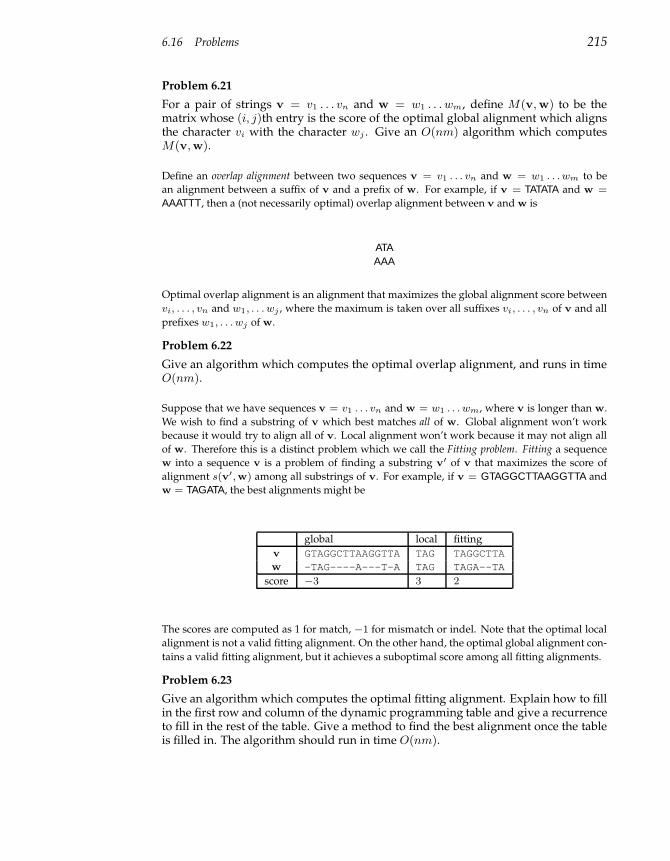
6.16 Problems 215
Problem 6.21
For a pair of strings v = v1 . . . vn and w = w1 . . . wm, define M(v, w) to be thematrix whose (i, j)th entry is the score of the optimal global alignment which alignsthe character vi with the character wj . Give an O(nm) algorithm which computesM(v,w).
Define an overlap alignment between two sequences v = v1 . . . vn and w = w1 . . . wm to be
an alignment between a suffix of v and a prefix of w. For example, if v = TATATA and w =
AAATTT, then a (not necessarily optimal) overlap alignment between v and w is
ATAAAA
Optimal overlap alignment is an alignment that maximizes the global alignment score between
vi, . . . , vn and w1, . . . wj , where the maximum is taken over all suffixes vi, . . . , vn of v and all
prefixes w1, . . . wj of w.
Problem 6.22
Give an algorithm which computes the optimal overlap alignment, and runs in timeO(nm).
Suppose that we have sequences v = v1 . . . vn and w = w1 . . . wm, where v is longer than w.
We wish to find a substring of v which best matches all of w. Global alignment won’t work
because it would try to align all of v. Local alignment won’t work because it may not align all
of w. Therefore this is a distinct problem which we call the Fitting problem. Fitting a sequence
w into a sequence v is a problem of finding a substring v′ of v that maximizes the score of
alignment s(v′,w) among all substrings of v. For example, if v = GTAGGCTTAAGGTTA and
w = TAGATA, the best alignments might be
global local fitting
v GTAGGCTTAAGGTTA TAG TAGGCTTAw -TAG----A---T-A TAG TAGA--TA
score −3 3 2
The scores are computed as 1 for match, −1 for mismatch or indel. Note that the optimal local
alignment is not a valid fitting alignment. On the other hand, the optimal global alignment con-
tains a valid fitting alignment, but it achieves a suboptimal score among all fitting alignments.
Problem 6.23
Give an algorithm which computes the optimal fitting alignment. Explain how to fillin the first row and column of the dynamic programming table and give a recurrenceto fill in the rest of the table. Give a method to find the best alignment once the tableis filled in. The algorithm should run in time O(nm).
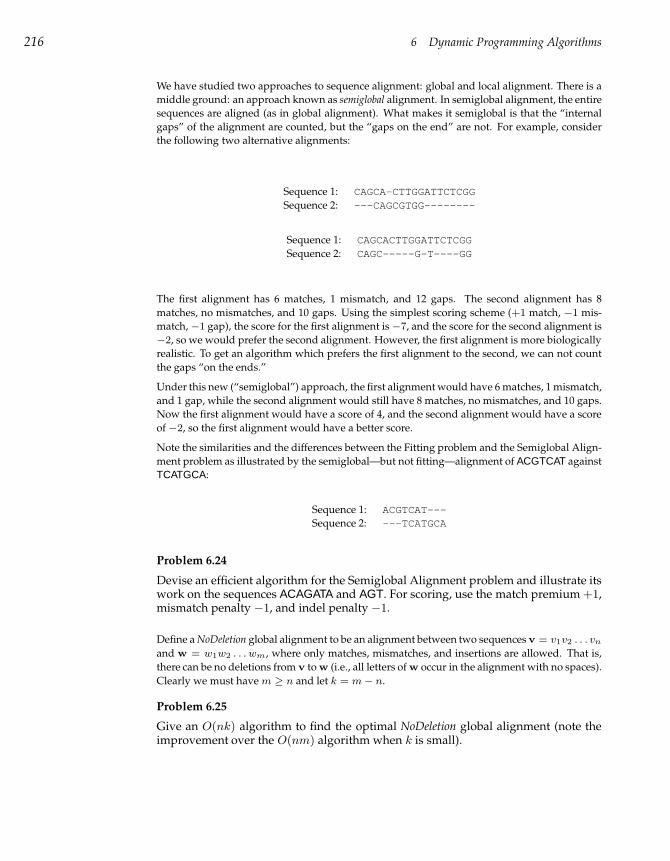
216 6 Dynamic Programming Algorithms
We have studied two approaches to sequence alignment: global and local alignment. There is a
middle ground: an approach known as semiglobal alignment. In semiglobal alignment, the entire
sequences are aligned (as in global alignment). What makes it semiglobal is that the “internal
gaps” of the alignment are counted, but the “gaps on the end” are not. For example, consider
the following two alternative alignments:
Sequence 1: CAGCA-CTTGGATTCTCGGSequence 2: ---CAGCGTGG--------
Sequence 1: CAGCACTTGGATTCTCGGSequence 2: CAGC-----G-T----GG
The first alignment has 6 matches, 1 mismatch, and 12 gaps. The second alignment has 8
matches, no mismatches, and 10 gaps. Using the simplest scoring scheme (+1 match, −1 mis-
match, −1 gap), the score for the first alignment is −7, and the score for the second alignment is
−2, so we would prefer the second alignment. However, the first alignment is more biologically
realistic. To get an algorithm which prefers the first alignment to the second, we can not count
the gaps “on the ends.”
Under this new (“semiglobal”) approach, the first alignment would have 6 matches, 1 mismatch,
and 1 gap, while the second alignment would still have 8 matches, no mismatches, and 10 gaps.
Now the first alignment would have a score of 4, and the second alignment would have a score
of −2, so the first alignment would have a better score.
Note the similarities and the differences between the Fitting problem and the Semiglobal Align-
ment problem as illustrated by the semiglobal—but not fitting—alignment of ACGTCAT against
TCATGCA:
Sequence 1: ACGTCAT---Sequence 2: ---TCATGCA
Problem 6.24
Devise an efficient algorithm for the Semiglobal Alignment problem and illustrate itswork on the sequences ACAGATA and AGT. For scoring, use the match premium +1,mismatch penalty −1, and indel penalty −1.
Define a NoDeletion global alignment to be an alignment between two sequences v = v1v2 . . . vn
and w = w1w2 . . . wm, where only matches, mismatches, and insertions are allowed. That is,
there can be no deletions from v to w (i.e., all letters of w occur in the alignment with no spaces).
Clearly we must have m ≥ n and let k = m − n.
Problem 6.25
Give an O(nk) algorithm to find the optimal NoDeletion global alignment (note theimprovement over the O(nm) algorithm when k is small).
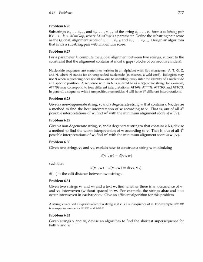
6.16 Problems 217
Problem 6.26
Substrings vi, . . . , vi+k and vi′ , . . . , vi′+k of the string v1, . . . , vn form a substring pairif i′−i+k > MinGap, where MinGap is a parameter. Define the substring pair scoreas the (global) alignment score of vi, . . . , vi+k and vi′ , . . . , vi′+k. Design an algorithmthat finds a substring pair with maximum score.
Problem 6.27
For a parameter k, compute the global alignment between two strings, subject to theconstraint that the alignment contains at most k gaps (blocks of consecutive indels).
Nucleotide sequences are sometimes written in an alphabet with five characters: A, T, G, C,
and N, where N stands for an unspecified nucleotide (in essence, a wild-card). Biologists may
use N when sequencing does not allow one to unambiguously infer the identity of a nucleotide
at a specific position. A sequence with an N is referred to as a degenerate string; for example,
ATTNG may correspond to four different interpretations: ATTAG, ATTTG, ATTGG, and ATTCG.
In general, a sequence with k unspecified nucleotides N will have 4k different interpretations.
Problem 6.28
Given a non-degenerate string, v, and a degenerate string w that contains k Ns, devise
a method to find the best interpretation of w according to v. That is, out of all 4k
possible interpretations of w, find w′ with the minimum alignment score s(w′,v).
Problem 6.29
Given a non-degenerate string, v, and a degenerate string w that contains k Ns, devise
a method to find the worst interpretation of w according to v. That is, out of all 4k
possible interpretations of w, find w′ with the minimum alignment score s(w′,v).
Problem 6.30
Given two strings v1 and v2, explain how to construct a string w minimizing
|d(v1, w)− d(v2,w)|
such thatd(v1, w) + d(v2,w) = d(v1,v2).
d(·, ·) is the edit distance between two strings.
Problem 6.31
Given two strings v1 and v2 and a text w, find whether there is an occurrence of v1
and v2 interwoven (without spaces) in w. For example, the strings abac and bbcoccur interwoven in cabbabccdw. Give an efficient algorithm for this problem.
A string x is called a supersequence of a string v if v is a subsequence of x. For example, ABLUEis a supersequence for BLUE and ABLE.
Problem 6.32
Given strings v and w, devise an algorithm to find the shortest supersequence forboth v and w.
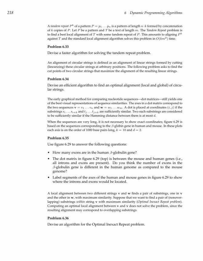
218 6 Dynamic Programming Algorithms
A tandem repeat P k of a pattern P = p1 . . . pn is a pattern of length n ·k formed by concatenation
of k copies of P . Let P be a pattern and T be a text of length m. The Tandem Repeat problem is
to find a best local alignment of T with some tandem repeat of P . This amounts to aligning P k
against T and the standard local alignment algorithm solves this problem in O(km2) time.
Problem 6.33
Devise a faster algorithm for solving the tandem repeat problem.
An alignment of circular strings is defined as an alignment of linear strings formed by cutting
(linearizing) these circular strings at arbitrary positions. The following problem asks to find the
cut points of two circular strings that maximize the alignment of the resulting linear strings.
Problem 6.34
Devise an efficient algorithm to find an optimal alignment (local and global) of circu-lar strings.
The early graphical method for comparing nucleotide sequences—dot matrices—still yields one
of the best visual representations of sequence similarities. The axes in a dot matrix correspond to
the two sequences v = v1 . . . vn and w = w1 . . . wm. A dot is placed at coordinates (i, j) if the
substrings si . . . si+k and tj . . . tj+k are sufficiently similar. Two such substrings are considered
to be sufficiently similar if the Hamming distance between them is at most d.
When the sequences are very long, it is not necessary to show exact coordinates; figure 6.29 is
based on the sequences corresponding to the β-globin gene in human and mouse. In these plots
each axis is on the order of 1000 base pairs long, k = 10 and d = 2.
Problem 6.35
Use figure 6.29 to answer the following questions:
• How many exons are in the human β-globulin gene?
• The dot matrix in figure 6.29 (top) is between the mouse and human genes (i.e.,all introns and exons are present). Do you think the number of exons in theβ-globulin gene is different in the human genome as compared to the mousegenome?
• Label segments of the axes of the human and mouse genes in figure 6.29 to showwhere the introns and exons would be located.
A local alignment between two different strings v and w finds a pair of substrings, one in v
and the other in w, with maximum similarity. Suppose that we want to find a pair of (nonover-
lapping) substrings within string v with maximum similarity (Optimal Inexact Repeat problem).
Computing an optimal local alignment between v and v does not solve the problem, since the
resulting alignment may correspond to overlapping substrings.
Problem 6.36
Devise an algorithm for the Optimal Inexact Repeat problem.
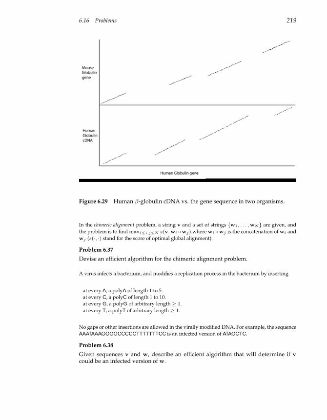
6.16 Problems 219
Figure 6.29 Human β-globulin cDNA vs. the gene sequence in two organisms.
In the chimeric alignment problem, a string v and a set of strings w1, . . . ,wN are given, and
the problem is to find max1≤i,j≤N s(v, wi wj) where wi wj is the concatenation of wi and
wj (s(·, ·) stand for the score of optimal global alignment).
Problem 6.37
Devise an efficient algorithm for the chimeric alignment problem.
A virus infects a bacterium, and modifies a replication process in the bacterium by inserting
at every A, a polyA of length 1 to 5.
at every C, a polyC of length 1 to 10.
at every G, a polyG of arbitrary length ≥ 1.
at every T, a polyT of arbitrary length ≥ 1.
No gaps or other insertions are allowed in the virally modified DNA. For example, the sequence
AAATAAAGGGGCCCCCTTTTTTTCC is an infected version of ATAGCTC.
Problem 6.38
Given sequences v and w, describe an efficient algorithm that will determine if v
could be an infected version of w.
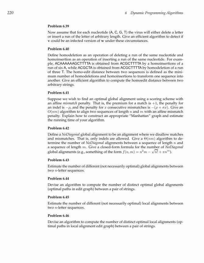
220 6 Dynamic Programming Algorithms
Problem 6.39
Now assume that for each nucleotide (A, C, G, T) the virus will either delete a letteror insert a run of the letter of arbitrary length. Give an efficient algorithm to detect ifv could be an infected version of w under these circumstances.
Problem 6.40
Define homodeletion as an operation of deleting a run of the same nucleotide andhomoinsertion as an operation of inserting a run of the same nucleotide. For exam-ple, ACAAAAAAGCTTTTA is obtained from ACGCTTTTA by a homoinsertions of arun of six A, while ACGCTA is obtained from ACGCTTTTA by homodeletion of a runof three T. The homo-edit distance between two sequences is defined as the mini-mum number of homodeletions and homoinsertions to transform one sequence intoanother. Give an efficient algorithm to compute the homoedit distance between twoarbitrary strings.
Problem 6.41
Suppose we wish to find an optimal global alignment using a scoring scheme withan affine mismatch penalty. That is, the premium for a match is +1, the penalty foran indel is −ρ, and the penalty for x consecutive mismatches is −(ρ + σx). Give anO(nm) algorithm to align two sequences of length n and m with an affine mismatchpenalty. Explain how to construct an appropriate “Manhattan” graph and estimatethe running time of your algorithm.
Problem 6.42
Define a NoDiagonal global alignment to be an alignment where we disallow matchesand mismatches. That is, only indels are allowed. Give a Θ(nm) algorithm to de-termine the number of NoDiagonal alignments between a sequence of length n anda sequence of length m. Give a closed-form formula for the number of NoDiagonal
global alignments (e.g., something of the form f(n, m) = n2m−√
n! + πnm).
Problem 6.43
Estimate the number of different (not necessarily optimal) global alignments betweentwo n-letter sequences.
Problem 6.44
Devise an algorithm to compute the number of distinct optimal global alignments(optimal paths in edit graph) between a pair of strings.
Problem 6.45
Estimate the number of different (not necessarily optimal) local alignments betweentwo n-letter sequences.
Problem 6.46
Devise an algorithm to compute the number of distinct optimal local alignments (op-timal paths in local alignment edit graph) between a pair of strings.
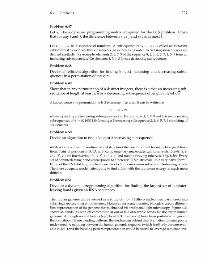
6.16 Problems 221
Problem 6.47
Let si,j be a dynamic programming matrix computed for the LCS problem. Provethat for any i and j, the difference between si+1,j and si,j is at most 1.
Let i1, . . . , in be a sequence of numbers. A subsequence of i1, . . . , in is called an increasing
subsequence if elements of this subsequence go in increasing order. Decreasing subsequences are
defined similarly. For example, elements 2, 6, 7, 9 of the sequence 8, 2, 1, 6, 5, 7, 4, 3, 9 form an
increasing subsequence, while elements 8, 7, 4, 3 form a decreasing subsequence.
Problem 6.48
Devise an efficient algorithm for finding longest increasing and decreasing subse-quences in a permutation of integers.
Problem 6.49
Show that in any permutation of n distinct integers, there is either an increasing sub-sequence of length at least
√n or a decreasing subsequence of length at least
√n.
A subsequence σ of permutation π is 2-increasing if, as a set, it can be written as
σ = σ1 ∪ σ2
where σ1 and σ2 are increasing subsequences of π. For example, 1, 5, 7, 9 and 2, 6 are increasing
subsequences of π = 821657439 forming a 2-increasing subsequence 2, 1, 6, 5, 7, 9 consisting of
six elements.
Problem 6.50
Devise an algorithm to find a longest 2-increasing subsequence.
RNAs adopt complex three-dimensional structures that are important for many biological func-
tions. Pairs of positions in RNA with complementary nucleotides can form bonds. Bonds (i, j)
and (i′, j′) are interleaving if i < i′ < j < j′ and noninterleaving otherwise (fig. 6.30). Every
set of noninterleaving bonds corresponds to a potential RNA structure. In a very naive formu-
lation of the RNA folding problem, one tries to find a maximum set of noninterleaving bonds.
The more adequate model, attempting to find a fold with the minimum energy, is much more
difficult.
Problem 6.51
Develop a dynamic programming algorithm for finding the largest set of noninter-leaving bonds given an RNA sequences.
The human genome can be viewed as a string of n (≈ 3 billion) nucleotides, partitioned into
substrings representing chromosomes. However, for many decades, biologists used a different
band representation of the genome that is obtained via traditional light microscopy. Figure 6.31
shows 48 bands (as seen on chromosme 4) out of 862 observable bands for the entire human
genome. Although several factors (e.g., local G/C frequency) have been postulated to govern
the formation of these banding patterns, the mechanism behind their formation remains poorly
understood. A mapping between the human genomic sequence (which itself only became avail-
able in 2001) and the banding pattern representation would be useful to leverage sequence level
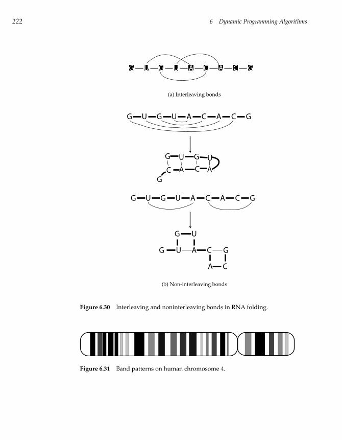
222 6 Dynamic Programming Algorithms
(a) Interleaving bonds
AA GG U G U CC
AA GG U G U CC
G
GG UU
C CA A
G U
G U
A C
A C
G
(b) Non-interleaving bonds
Figure 6.30 Interleaving and noninterleaving bonds in RNA folding.
Figure 6.31 Band patterns on human chromosome 4.
6.16 Problems 223
gene information against diseases that have been associated with certain band positions. How-
ever, until recently, no mapping between these two representations of the genome has been
known.
The Band Positioning problem is to find the starting and ending nucleotide positions for each
band in the genome (for simplicity we assume that all chromosomes are concatenated to form a
single coordinate system). In other words, the Band Positioning problem is to find an increasing
array start(b), that contains the starting nucleotide position for each band b in the genome. Each
band b begins at the nucleotide given by start(b) and ends at start(b + 1) − 1.31
A naive approach to this problem would be to use observed band width data to compute the
nucleotide positions. However, this solution is inaccurate because it assumes that band width is
perfectly correlated with its length in nucleotides. In reality, this correlation is often quite poor
and a different approach is needed.
In the last decade biologists have performed a large number of FISH (fluorescent in situ hybridiza-
tion) experiments that can help to solve the Band Positioning problem. FISH data consist of
pairs (x, b), where x is a position in the genome, and b is the index of the band that contains x .
FISH data are often subject to experimental error, so some FISH data points may contradict each
other.
Given a solution start(b) (1 ≤ b ≤ 862) of the Band Positioning problem, we define its FISH
quality as the number of FISH experiments that it supports, that is, the number of FISH experi-
ments (x, b) such that start(b) ≤ x < start(b + 1).
Problem 6.52
Find a solution to the Band Positioning problem that maximizes its FISH quality.
The FISH quality parameter ignores the width of the bands. A more adequate formulation is
to find an optimal solution of the Band Positioning problem that is consistent with band width
data, that is, the solution that minimizes
862X
b=1
|width(i) − (start(b + 1) − start(b))|
, where width(i) is the estimated width of the ith band.
Problem 6.53
Find an optimal solution of the Band Positioning problem that minimizes
862X
b=1
|width(i)− (start(b + 1)− start(b))|
Problem 6.54
Describe recurrence relations for multiple alignment of 4 sequences under the SP(sum-of-pairs) scoring rule.
31. For simplicity we assume that start(863) = n + 1 thus implying that the last 862th bandstarts at the nucleotide start(862) and ends at n.
224 6 Dynamic Programming Algorithms
Problem 6.55
Develop a likelihood ratio approach and design an algorithm that utilizes codon us-age arrays for gene prediction.
Problem 6.56
Consider the Exon Chaining problem in the case when all intervals have the sameweight. Design a greedy algorithm that finds an optimal solution for this limited caseof the problem.
Problem 6.57
Estimate the running time of the spliced alignment algorithm. Improve the runningtime by transforming the spliced alignment graph into a graph with a smaller numberof edges. This transformation is hinted at in figure 6.28.
Introns are spliced out of pre-mRNA during mRNA processing and biologists can perform
cDNA sequencing that provides the nucleotide sequence complementary to the mRNA. The
cDNA, therefore, represents the concatenation of exons of a gene. Consequently the exon-intron
structure can be determined by aligning the cDNA against the genomic DNA with the aligned
regions representing the exons and the large gaps representing the introns. This alignment can
be aided by the knowledge of the conserved donor and acceptor splice site sequences (GT at the
5’ splice site and AG at the 3’ splice site).
While a spliced alignment can be used to solve this cDNA Alignment problem there exists a faster
algorithm to align cDNA against genomic sequence. One approach is to introduce gap penalties
that would adequately account for gaps in the cDNA Alignment problem. When aligning cDNA
against genomic sequences we want to allow long internal gaps in the cDNA sequence. In
addition, long gaps that respect the consensus sequences at the intron-exon junctions are favored
over gaps that do not satisfy this property. Such gaps that exceed a given length threshold and
respect the donor and acceptor sites should be assigned a constant penalty. This penalty is lower
than the affine penalty for long gaps that do not respect the splice site consensus. The input to
the cDNA Alignment problem is genomic sequence v, cDNA sequence w, match, mismatch,
gap opening and gap extension parameters, as well as L (minimum intron length) and δL (fixed
penalty for gaps longer than L that respect the consensus sequences). The output is an alignment
of v and w where aligned regions represent putative exons and gaps in v represent putative
introns.
Problem 6.58
Devise an efficient algorithm for the cDNA Alignment problem.
The spliced alignment algorithm finds exons in genomic DNA by using a related protein as a
template. What if a template is not a protein but another (uninterpreted) genomic DNA se-
quence? Or, in other words, can (unannotated) mouse genomic DNA be used to predict human
genes?
Problem 6.59
Generalize the spliced alignment algorithm for alignment of one genomic sequenceagainst another.

6.16 Problems 225
Problem 6.60
For simplicity, the Spliced Alignment problem assumes that the genomic sequenceand the target protein sequence are both written in the same alphabet. Modify therecurrence relations to handle the case when they are written in different alphabets(specifically, proteins are written in a twenty letter alphabet, and DNA is written in afour letter alphabet).

7 Divide-and-Conquer Algorithms
As the name implies, a divide-and-conquer algorithm proceeds in two dis-
tinct phases: a divide phase in which the algorithm splits a problem instance
into smaller problem instances and solves them; and a conquer phase in
which it stitches the solutions to the smaller problems into a solution to the
bigger one. This strategy often works when a solution to a large problem
can be built from the solutions of smaller problem instances. Divide-and-
conquer algorithms are often used to improve the efficiency of a polynomial
algorithm, for example, by solving a problem in O(n log n) time that would
otherwise require quadratic time.
7.1 Divide-and-Conquer Approach to Sorting
In chapter 2 we introduced the Sorting problem, and developed an algorithm
that required O(n2) time to sort a list of integers. The divide-and-conquer
approach gives us a faster sorting algorithm.
Suppose that instead of a single list of n integers in an arbitrary order, we
have two lists, a of length n1 and b of length n2, each with approximately n/2
elements, but these two lists are both sorted. How could we make a sorted
list of n elements from these? A reasonable approach is to traverse each list
simultaneously as if each were a sorted stack of cards, picking the smaller
element on the top of either pile. The MERGE algorithm below combines two
sorted lists into a single sorted list in O(n1 + n2) time.
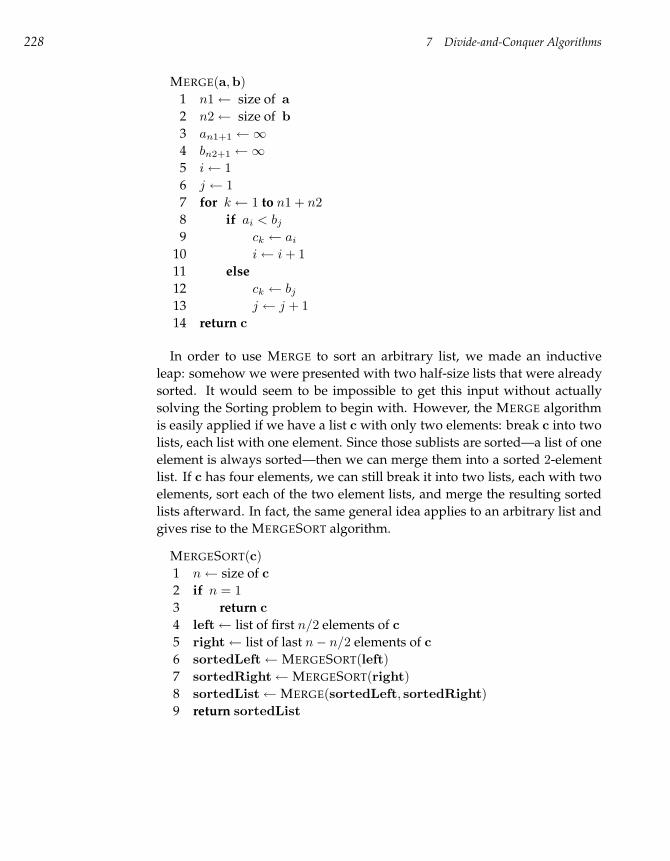
228 7 Divide-and-Conquer Algorithms
MERGE(a,b)
1 n1← size of a
2 n2← size of b
3 an1+1 ←∞
4 bn2+1 ←∞
5 i← 1
6 j ← 1
7 for k← 1 to n1 + n2
8 if ai < bj
9 ck ← ai
10 i← i + 1
11 else
12 ck ← bj
13 j ← j + 1
14 return c
In order to use MERGE to sort an arbitrary list, we made an inductive
leap: somehow we were presented with two half-size lists that were already
sorted. It would seem to be impossible to get this input without actually
solving the Sorting problem to begin with. However, the MERGE algorithm
is easily applied if we have a list c with only two elements: break c into two
lists, each list with one element. Since those sublists are sorted—a list of one
element is always sorted—then we can merge them into a sorted 2-element
list. If c has four elements, we can still break it into two lists, each with two
elements, sort each of the two element lists, and merge the resulting sorted
lists afterward. In fact, the same general idea applies to an arbitrary list and
gives rise to the MERGESORT algorithm.
MERGESORT(c)
1 n← size of c
2 if n = 1
3 return c
4 left← list of first n/2 elements of c
5 right← list of last n− n/2 elements of c
6 sortedLeft← MERGESORT(left)
7 sortedRight← MERGESORT(right)
8 sortedList← MERGE(sortedLeft, sortedRight)
9 return sortedList
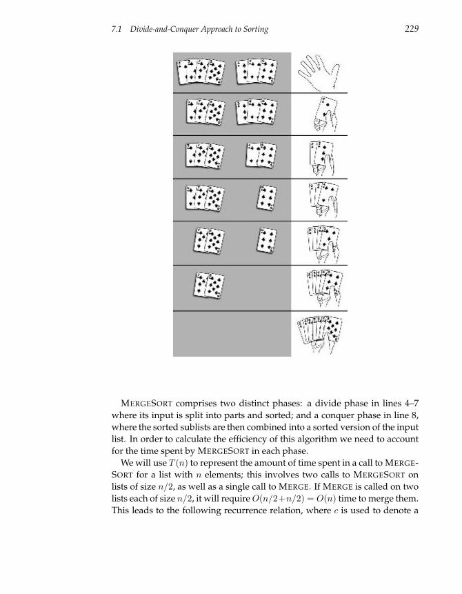
7.1 Divide-and-Conquer Approach to Sorting 229
MERGESORT comprises two distinct phases: a divide phase in lines 4–7
where its input is split into parts and sorted; and a conquer phase in line 8,
where the sorted sublists are then combined into a sorted version of the input
list. In order to calculate the efficiency of this algorithm we need to account
for the time spent by MERGESORT in each phase.
We will use T (n) to represent the amount of time spent in a call to MERGE-
SORT for a list with n elements; this involves two calls to MERGESORT on
lists of size n/2, as well as a single call to MERGE. If MERGE is called on two
lists each of size n/2, it will require O(n/2+n/2) = O(n) time to merge them.
This leads to the following recurrence relation, where c is used to denote a
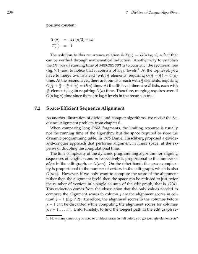
230 7 Divide-and-Conquer Algorithms
positive constant:
T (n) = 2T (n/2) + cn
T (1) = 1
The solution to this recurrence relation is T (n) = O(n log n), a fact that
can be verified through mathematical induction. Another way to establish
the O(n log n) running time of MERGESORT is to construct the recursion tree
(fig. 7.1) and to notice that it consists of log n levels.1 At the top level, you
have to merge two lists each with n2 elements, requiring O(n
2 + n2 ) = O(n)
time. At the second level, there are four lists, each with n4 elements, requiring
O(n4 + n
4 + n4 + n
4 ) = O(n) time. At the ith level, there are 2i lists, each withn2i elements, again requiring O(n) time. Therefore, merging requires overall
O(n log n) time since there are log n levels in the recursion tree.
7.2 Space-Efficient Sequence Alignment
As another illustration of divide-and-conquer algorithms, we revisit the Se-
quence Alignment problem from chapter 6.
When comparing long DNA fragments, the limiting resource is usually
not the running time of the algorithm, but the space required to store the
dynamic programming table. In 1975 Daniel Hirschberg proposed a divide-
and-conquer approach that performs alignment in linear space, at the ex-
pense of doubling the computational time.
The time complexity of the dynamic programming algorithm for aligning
sequences of lengths n and m respectively is proportional to the number of
edges in the edit graph, or O(nm). On the other hand, the space complex-
ity is proportional to the number of vertices in the edit graph, which is also
O(nm). However, if we only want to compute the score of the alignment
rather than the alignment itself, then the space can be reduced to just twice
the number of vertices in a single column of the edit graph, that is, O(n).
This reduction comes from the observation that the only values needed to
compute the alignment scores in column j are the alignment scores in col-
umn j − 1 (fig. 7.2). Therefore, the alignment scores in the columns before
j − 1 can be discarded while computing the alignment scores for columns
j, j + 1, . . . , m. Unfortunately, to find the longest path in the edit graph re-
1. How many times do you need to divide an array in half before you get to single-element sets?
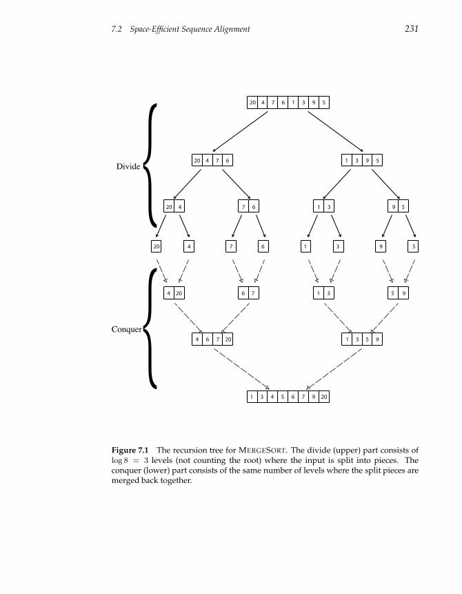
7.2 Space-Efficient Sequence Alignment 231
20
20
20
20
20
20
20
4
4
4
4
4
4
4
7
7
7
7
7
7
7
6
6
6
6
6
6
6
1
1
1
1
1
1
1
3
3
3
3
3
3
3
9
9
9
9
9
9
9
5
5
5
5
5
5
5
Divide
Conquer
Figure 7.1 The recursion tree for MERGESORT. The divide (upper) part consists oflog 8 = 3 levels (not counting the root) where the input is split into pieces. Theconquer (lower) part consists of the same number of levels where the split pieces aremerged back together.
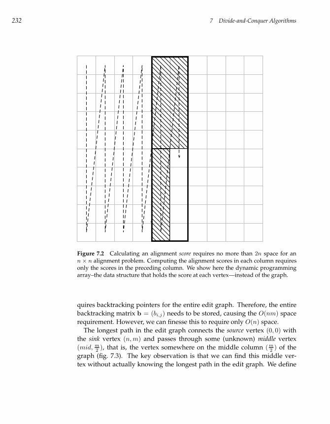
232 7 Divide-and-Conquer Algorithms
Figure 7.2 Calculating an alignment score requires no more than 2n space for ann× n alignment problem. Computing the alignment scores in each column requiresonly the scores in the preceding column. We show here the dynamic programmingarray–the data structure that holds the score at each vertex—instead of the graph.
quires backtracking pointers for the entire edit graph. Therefore, the entire
backtracking matrix b = (bi,j) needs to be stored, causing the O(nm) space
requirement. However, we can finesse this to require only O(n) space.
The longest path in the edit graph connects the source vertex (0, 0) with
the sink vertex (n, m) and passes through some (unknown) middle vertex
(mid, m2 ), that is, the vertex somewhere on the middle column (m
2 ) of the
graph (fig. 7.3). The key observation is that we can find this middle ver-
tex without actually knowing the longest path in the edit graph. We define
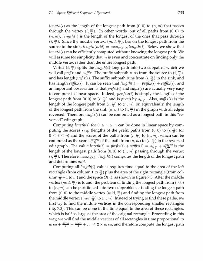
7.2 Space-Efficient Sequence Alignment 233
length(i) as the length of the longest path from (0, 0) to (n, m) that passes
through the vertex (i, m2 ). In other words, out of all paths from (0, 0) to
(n, m), length(i) is the length of the longest of the ones that pass through
(i, m2 ). Since the middle vertex, (mid, m
2 ), lies on the longest path from the
source to the sink, length(mid) = max0≤i≤n length(i). Below we show that
length(i) can be efficiently computed without knowing the longest path. We
will assume for simplicity that m is even and concentrate on finding only the
middle vertex rather than the entire longest path.
Vertex (i, m2 ) splits the length(i)-long path into two subpaths, which we
will call prefix and suffix. The prefix subpath runs from the source to (i, m2 ),
and has length prefix(i). The suffix subpath runs from (i, m2 ) to the sink, and
has length suffix(i). It can be seen that length(i) = prefix(i) + suffix(i), and
an important observation is that prefix(i) and suffix(i) are actually very easy
to compute in linear space. Indeed, prefix(i) is simply the length of the
longest path from (0, 0) to (i, m2 ) and is given by si, m
2. Also, suffix(i) is the
length of the longest path from (i, m2 ) to (n, m), or, equivalently, the length
of the longest path from the sink (n, m) to (i, m2 ) in the graph with all edges
reversed. Therefore, suffix(i) can be computed as a longest path in this “re-
versed” edit graph.
Computing length(i) for 0 ≤ i ≤ n can be done in linear space by com-
puting the scores si, m2
(lengths of the prefix paths from (0, 0) to (i, m2 ) for
0 ≤ i ≤ n) and the scores of the paths from (i, m2 ) to (n, m), which can be
computed as the score sreversei, m
2of the path from (n, m) to (i, m
2 ) in the reversed
edit graph. The value length(i) = prefix(i) + suffix(i) = si, m2
+ sreversei, m
2is the
length of the longest path from (0, 0) to (n, m) passing through the vertex
(i, m2 ). Therefore, max0≤i≤n length(i) computes the length of the longest path
and determines mid.
Computing all length(i) values requires time equal to the area of the left
rectangle (from column 1 to m2 ) plus the area of the right rectangle (from col-
umn m2 +1 to m) and the space O(n), as shown in figure 7.3. After the middle
vertex (mid, m2 ) is found, the problem of finding the longest path from (0, 0)
to (n, m) can be partitioned into two subproblems: finding the longest path
from (0, 0) to the middle vertex (mid, m2 ) and finding the longest path from
the middle vertex (mid, m2 ) to (n, m). Instead of trying to find these paths, we
first try to find the middle vertices in the corresponding smaller rectangles
(fig. 7.3). This can be done in the time equal to the area of these rectangles,
which is half as large as the area of the original rectangle. Proceeding in this
way, we will find the middle vertices of all rectangles in time proportional to
area + area2 + area
4 + . . . ≤ 2× area, and therefore compute the longest path
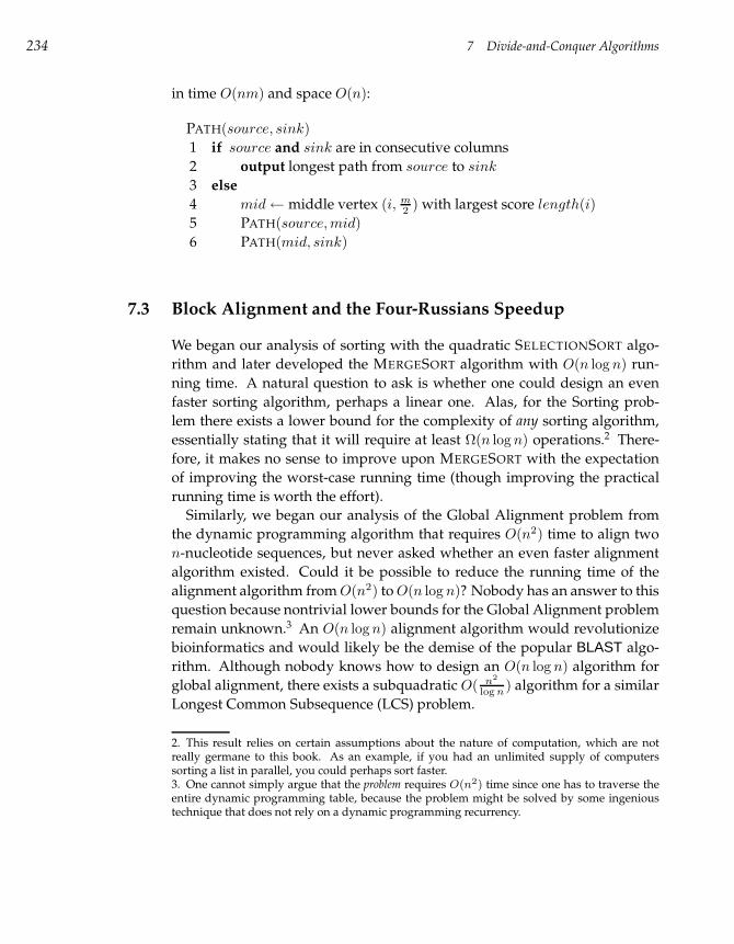
234 7 Divide-and-Conquer Algorithms
in time O(nm) and space O(n):
PATH(source, sink)
1 if source and sink are in consecutive columns
2 output longest path from source to sink
3 else
4 mid← middle vertex (i, m2 ) with largest score length(i)
5 PATH(source, mid)
6 PATH(mid, sink)
7.3 Block Alignment and the Four-Russians Speedup
We began our analysis of sorting with the quadratic SELECTIONSORT algo-
rithm and later developed the MERGESORT algorithm with O(n log n) run-
ning time. A natural question to ask is whether one could design an even
faster sorting algorithm, perhaps a linear one. Alas, for the Sorting prob-
lem there exists a lower bound for the complexity of any sorting algorithm,
essentially stating that it will require at least Ω(n log n) operations.2 There-
fore, it makes no sense to improve upon MERGESORT with the expectation
of improving the worst-case running time (though improving the practical
running time is worth the effort).
Similarly, we began our analysis of the Global Alignment problem from
the dynamic programming algorithm that requires O(n2) time to align two
n-nucleotide sequences, but never asked whether an even faster alignment
algorithm existed. Could it be possible to reduce the running time of the
alignment algorithm from O(n2) to O(n log n)? Nobody has an answer to this
question because nontrivial lower bounds for the Global Alignment problem
remain unknown.3 An O(n log n) alignment algorithm would revolutionize
bioinformatics and would likely be the demise of the popular BLAST algo-
rithm. Although nobody knows how to design an O(n log n) algorithm for
global alignment, there exists a subquadratic O( n2
log n) algorithm for a similar
Longest Common Subsequence (LCS) problem.
2. This result relies on certain assumptions about the nature of computation, which are notreally germane to this book. As an example, if you had an unlimited supply of computerssorting a list in parallel, you could perhaps sort faster.3. One cannot simply argue that the problem requires O(n2) time since one has to traverse theentire dynamic programming table, because the problem might be solved by some ingenioustechnique that does not rely on a dynamic programming recurrency.
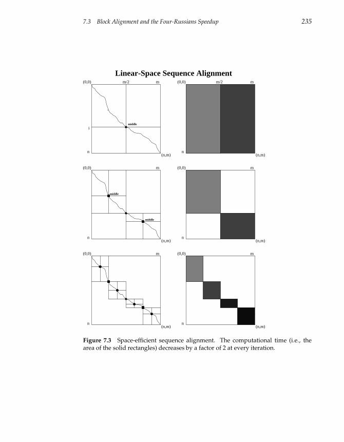
7.3 Block Alignment and the Four-Russians Speedup 235
(0,0)
n
m
(n,m)
(0,0)
n
m
(n,m)
i
(0,0)
n
m
(n,m)
(0,0)
n
m
(n,m)
(0,0)
n
m
(n,m)
(0,0)
n
m
(n,m)
m/2 m/2
middle
middle
middle
Linear-Space Sequence Alignment
Figure 7.3 Space-efficient sequence alignment. The computational time (i.e., thearea of the solid rectangles) decreases by a factor of 2 at every iteration.
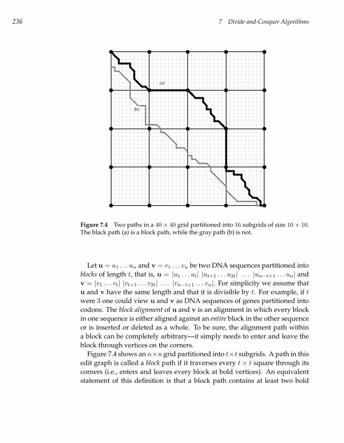
236 7 Divide-and-Conquer Algorithms
(a)
(b)
Figure 7.4 Two paths in a 40 × 40 grid partitioned into 16 subgrids of size 10 × 10.The black path (a) is a block path, while the gray path (b) is not.
Let u = u1 . . . un and v = v1 . . . vn be two DNA sequences partitioned into
blocks of length t, that is, u = |u1 . . . ut| |ut+1 . . . u2t| . . . |un−t+1 . . . un| and
v = |v1 . . . vt| |vt+1 . . . v2t| . . . |vn−t+1 . . . vn|. For simplicity we assume that
u and v have the same length and that it is divisible by t. For example, if t
were 3 one could view u and v as DNA sequences of genes partitioned into
codons. The block alignment of u and v is an alignment in which every block
in one sequence is either aligned against an entire block in the other sequence
or is inserted or deleted as a whole. To be sure, the alignment path within
a block can be completely arbitrary—it simply needs to enter and leave the
block through vertices on the corners.
Figure 7.4 shows an n×n grid partitioned into t×t subgrids. A path in this
edit graph is called a block path if it traverses every t × t square through its
corners (i.e., enters and leaves every block at bold vertices). An equivalent
statement of this definition is that a block path contains at least two bold
7.3 Block Alignment and the Four-Russians Speedup 237
vertices from every square that it passes through—it cannot, for example,
lop off a corner of a square. Block alignments correspond to block paths in
the edit graph and the Block Alignment problem is to find the highest-scoring,
or longest, block path through this graph. We will see below that when t
is on the order of the logarithm of the overall sequence length—neither too
small nor too large–we can solve this problem in less than quadratic n2 time.
Block Alignment Problem:
Find the longest block path through an edit graph.
Input: Two sequences, u and v partitioned into blocks of
size t.
Output: The block alignment of u and v with the maximum
score (i.e., the longest block path through the edit graph).
One can consider nt× n
tpairs of blocks (each pair defines a square in the
edit graph) and compute the alignment score βi,j for each pair of blocks
|u(i−1)·t+1 . . . ui·t| and |v(j−1)·t+1 . . . vj·t|. This amounts to solving nt× n
tmini
alignment problems of size t× t each and takes O(nt· n
t· t · t) = O(n2) time.
If si,j denotes the optimal block alignment score between the first i blocks of
u and the first j blocks of v, then
si,j = max
si−1,j − σblock
si,j−1 − σblock
si−1,j−1 + βi,j
,
where σblock is the penalty for inserting or deleting the entire block.4 The
indices i and j in this recurrence vary from 0 to nt
and therefore, the running
time of this algorithm is O(n2
t2) if we do not count time to precompute βi,j
for 0 ≤ i, j ≤ nt
. This approach allows one to solve the Block Alignment
problem for any value of t, but as we saw before, precomputing all βi,j takes
the same O(n2) time that the dynamic programming algorithm takes.
The speed reduction we promised is achieved by the Four-Russians tech-
nique when t is roughly log n.5 Instead of constructing nt× n
tminialignments
for all pairs of blocks from u and v we will construct 4t × 4t minialignments
4. In the simplest case σblock = σt , where σ is the penalty for the insertion or deletion of anucleotide.5. Since the Block Alignment problem takes a partitioned grid as input, the algorithm does notget to make a choice for the value of t.
238 7 Divide-and-Conquer Algorithms
for all pairs of t-nucleotide strings and store their alignment scores in a large
lookup table. At first glance this looks counterproductive, but if t = log n4
then 4t × 4t = n12 × n
12 = n, which is much smaller than n
t× n
t.
The resulting lookup table, which we will call Score, has only 4t × 4t = n
entries. Computing each of the entries takes O(log n · log n) time, so the over-
all running time to compute all entries of this table is only O(n · (log n)2).
We emphasize that the resulting two-dimensional lookup table Score is in-
dexed by a pair of t-nucleotide strings, thus leading to a slightly different
recurrence:
si,j = max
si−1,j − σblock
si,j−1 − σblock
si−1,j−1 + Score(ith block of v, jth block of u)
Since the time to precompute the lookup table Score in this case is rel-
atively small, the overall running time is dominated by the dynamic pro-
gramming step, for example, by the nt× n
taccesses it makes to the lookup
table. Since each access takes O(log n) time, the overall running time of this
algorithm is O( n2
log n).
7.4 Constructing Alignments in Subquadratic Time
So now we have an algorithm for the Block Alignment problem that is sub-
quadratic for convenient values of one of its input parameters, but it is not
clear whether similar ideas could be used to solve any of the problems from
chapter 6. In this section we show how to design a O( n2
log n) algorithm for
finding the longest common subsequence of two strings, again using the
Four-Russians speedup.
Unlike the block path in a partitioned edit graph, the path corresponding
to a longest common subsequence can traverse the edit graph arbitrarily and
does not have to pass through the bold vertices of figure 7.4. Therefore, pre-
computing the length of paths between the upper left corner and lower right
corner of every t× t subsequence is not going to help.
Instead we will select all vertices at the borders of the squares (shown by
bold vertices in figure 7.5) rather than just the vertices at the corners, as in
figure 7.4. This results in a significantly larger number of bold vertices than
in the case of block alignments but we can keep the number subquadratic.
Taken together, these vertices form nt
whole rows and nt
whole columns in
the edit graph; the total number of bold vertices is O(n2
t). We will perform
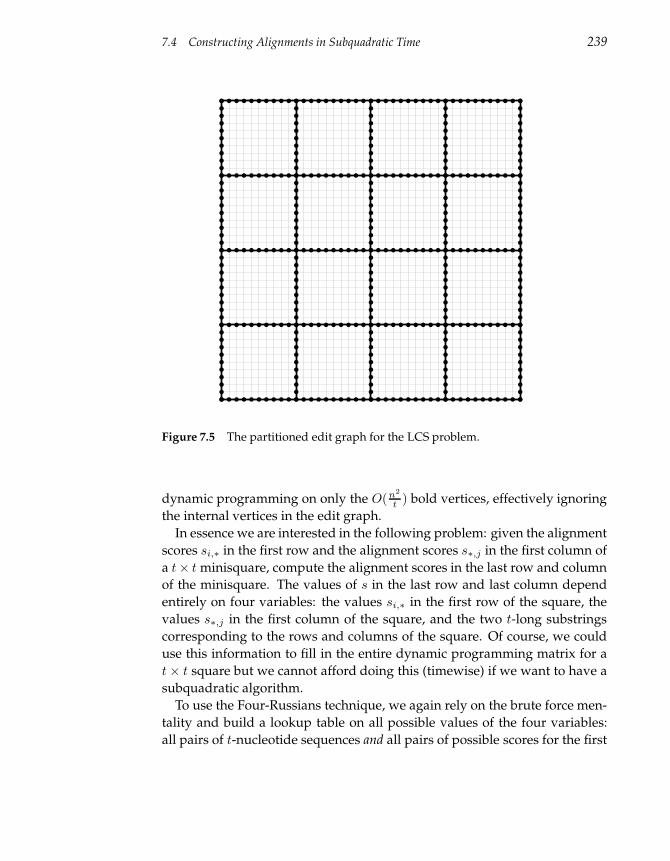
7.4 Constructing Alignments in Subquadratic Time 239
Figure 7.5 The partitioned edit graph for the LCS problem.
dynamic programming on only the O(n2
t) bold vertices, effectively ignoring
the internal vertices in the edit graph.
In essence we are interested in the following problem: given the alignment
scores si,∗ in the first row and the alignment scores s∗,j in the first column of
a t× t minisquare, compute the alignment scores in the last row and column
of the minisquare. The values of s in the last row and last column depend
entirely on four variables: the values si,∗ in the first row of the square, the
values s∗,j in the first column of the square, and the two t-long substrings
corresponding to the rows and columns of the square. Of course, we could
use this information to fill in the entire dynamic programming matrix for a
t× t square but we cannot afford doing this (timewise) if we want to have a
subquadratic algorithm.
To use the Four-Russians technique, we again rely on the brute force men-
tality and build a lookup table on all possible values of the four variables:
all pairs of t-nucleotide sequences and all pairs of possible scores for the first
240 7 Divide-and-Conquer Algorithms
row si,∗ and the first column s∗,j . For each such quadruple, we store the
precomputed scores for the last row and last column. However, this will be
an enormous table since there may be a large number of possible scores for
the first row and first column. Therefore, we perform some trickery. A care-
ful analysis of the LCS problem shows that the possible alignment scores in
the first row (or first column) are not entirely arbitrary: 0, 1, 2, 2, 2, 3, 4 is a
possible sequence of scores, but 0, 1, 2, 4, 5, 8, 9, 10 is not. Not only does the
progression of scores have to be monotonically increasing, but adjacent ele-
ments cannot differ by more than 1 (see problem 6.47). We can encode this as
a binary vector of differences; the above example 0, 1, 2, 2, 2, 3, 4 would be en-
coded as 1, 1, 0, 0, 1, 1.6 Thus, since there are 2t possible scores and 4t possible
strings, the entire lookup table will require 2t · 2t · 4t · 4t = 26t space. Again,
we set t = log n4 to make the size of the table collapse down to 26 log n
4 = n1.5.
Alas, this allows the precomputation step to be subquadratic, and the run-
ning time of the algorithm is dominated by the process of filling in the scores
for the bold vertices in figure 7.5 which takes O(
n2
log n
)
time.
7.5 Notes
MERGESORT was invented in 1945 by the legendary John von Neumann
while he was designing EDVAC, the world’s first stored-program electronic
computer. The idea of using a divide-and-conquer approach for sequence
comparison was proposed first by Daniel Hirschberg in 1975 for the LCS
problem (49), and then in 1988 by Eugene Myers and Webb Miller for the
Local Alignment problem (77). The Four-Russians speedup was proposed
by Vladimir Arlazarov, Efim Dinic, Mikhail Kronrod, and Igor Faradzev in
1970 (6) and first applied to sequence comparison by William Masek and
Michael Paterson (73).
6. (1, 1, 0, 0, 1, 1) is (1 − 0, 2 − 1, 2 − 2, 2 − 2, 3 − 2, 4 − 3).
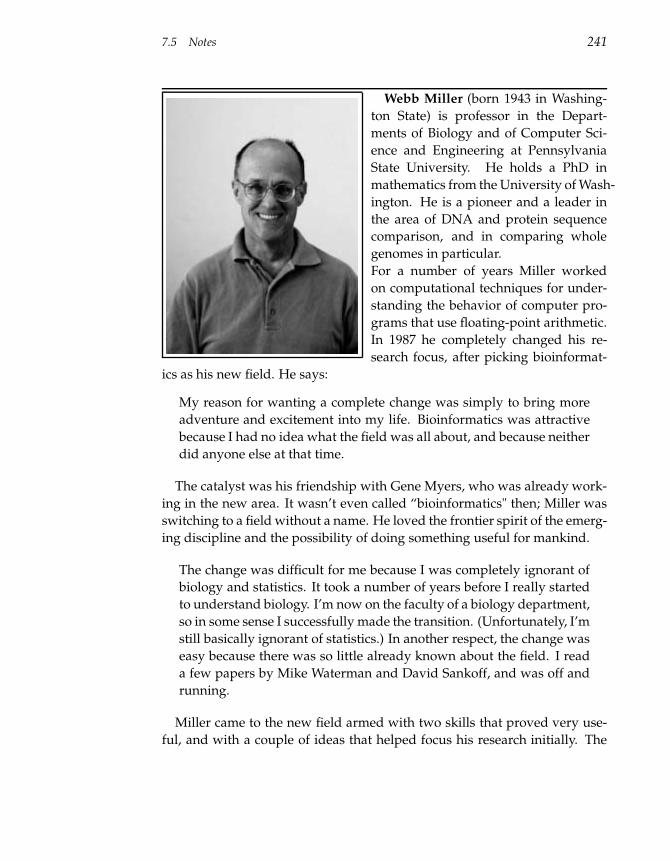
7.5 Notes 241
Webb Miller (born 1943 in Washing-
ton State) is professor in the Depart-
ments of Biology and of Computer Sci-
ence and Engineering at Pennsylvania
State University. He holds a PhD in
mathematics from the University of Wash-
ington. He is a pioneer and a leader in
the area of DNA and protein sequence
comparison, and in comparing whole
genomes in particular.
For a number of years Miller worked
on computational techniques for under-
standing the behavior of computer pro-
grams that use floating-point arithmetic.
In 1987 he completely changed his re-
search focus, after picking bioinformat-
ics as his new field. He says:
My reason for wanting a complete change was simply to bring more
adventure and excitement into my life. Bioinformatics was attractive
because I had no idea what the field was all about, and because neither
did anyone else at that time.
The catalyst was his friendship with Gene Myers, who was already work-
ing in the new area. It wasn’t even called “bioinformatics" then; Miller was
switching to a field without a name. He loved the frontier spirit of the emerg-
ing discipline and the possibility of doing something useful for mankind.
The change was difficult for me because I was completely ignorant of
biology and statistics. It took a number of years before I really started
to understand biology. I’m now on the faculty of a biology department,
so in some sense I successfully made the transition. (Unfortunately, I’m
still basically ignorant of statistics.) In another respect, the change was
easy because there was so little already known about the field. I read
a few papers by Mike Waterman and David Sankoff, and was off and
running.
Miller came to the new field armed with two skills that proved very use-
ful, and with a couple of ideas that helped focus his research initially. The
242 7 Divide-and-Conquer Algorithms
skills were his mathematical training and his experience writing computer
programs. The first idea that he brought to the field was that an optimal
alignment between two sequences can be computed in space proportional
to the length of the longer sequence. It is straightforward to compute the
score of an optimal alignment in that amount of space, but it is much less
obvious how to produce an alignment with that score. A very clever linear-
space alignment algorithm had been discovered by Dan Hirschberg around
1975. The other idea was that when two sequences are very similar and when
alignments are scored rather simply, an optimal alignment can be computed
much more quickly than by dynamic programming, using a greedy algo-
rithm. That idea was discovered independently by Gene Myers (with some
prodding from Miller) and Esko Ukkonen in the mid-1980s. Miller hoped
that these two ideas, or variants of them, would get him started in the new
field; he had “solutions in search of biological problems” rather than “bio-
logical problems in search of solutions.” Indeed, this is a common mode of
entry into bioinformatics for scientists trained in a quantitative field.
During his first decade in bioinformatics, Miller coauthored a few papers
about linear-space alignment methods. Finding a niche for greedy algo-
rithms took longer, but for comparing very similar DNA sequences, partic-
ularly when the difference between them is due to sequencing errors rather
than evolutionary mutations, they are quite useful; they deserve wider recog-
nition in the bioinformatics community than they now have.
The most successful of Miller’s bioinformatics projects have involved ideas
other than the ones he brought with him to the field. His most widely known
project was the collaboration to develop the BLAST program, where it was
David Lipman’s insights that drove the project in the right direction. How-
ever, it is Miller’s work on comparison methods for long DNA sequences that
brought him closer to biology and made Miller’s algorithms a household
name among teams of scientists analyzing mammalian and other whole-
genome sequences. Miller picked this theme as his Holy Grail around 1989,
and he has stuck with it ever since. When he started, there were only two
people in the world brave—or foolish—enough to publicly advocate sequenc-
ing the mouse genome and comparing it with the human genome: Miller
and his long-term collaborator, the biologist Ross Hardison. They occasion-
ally went so far as to tout the sequencing of several additional mammals.
Nowadays, it looks to everyone like the genome sequencing of mouse, rat,
chimpanzee, dog, and so on, was inevitable, but perhaps Miller’s many years
of working on programs to compare genome sequences made the inevitable
happen sooner.
7.5 Notes 243
What worked best for Miller was to envision an advance in bioinformat-
ics that would foster new biological discoveries – namely, that development
of methods to compare complete mammalian genome sequences would lead
to a better understanding of evolution and of gene regulation – and to do
everything he could think of to make it happen. This included developing
algorithms that would easily align the longest sequences he could find, and
helping Ross Hardison to verify experimentally that these alignments are
useful for studying gene regulation. When Miller and Hardison decided to
show how alignments and data from biological experiments could be linked
through a database, they learned about databases. When they wanted to set
up a network server to align DNA sequences, they learned about network
servers. When nobody in his lab was available to write software that they
needed, Miller wrote it himself. When inventing and analyzing a new al-
gorithm seemed important, he worked on it. The methods changed but the
biological motivation remained constant.
Miller has been more successful pursuing “a biological problem in search
of solutions than the other way around. His colleague, David Haussler, has
had somewhat the same experience; his considerable achievements bringing
hidden Markov models and other machine learning techniques to bioinfor-
matics have recently been eclipsed by his monumental success with the Hu-
man Genome Browser, which has directly helped a far wider community of
scientists.
The most exciting point so far in my career is today, with a new verte-
brate genome sequence coming my way every year. Some day, I hope
to look back with pride at my best achievement in bioinformatics, but
perhaps it hasn’t happened yet.
244 7 Divide-and-Conquer Algorithms
7.6 Problems
Problem 7.1
Construct the recursion tree for MERGESORT on the input (2, 5, 7, 4, 3, 6, 1, 8).
Problem 7.2
How much memory does MERGESORT need overall? Modify the algorithm to use aslittle as possible.
Problem 7.3
Suppose that you are given an array A of n words sorted in lexicographic order andwant to search this list for some arbitrary word, perhaps w (we write the number ofcharacters in w as |w|). Design three algorithms to determine if w is in the list: oneshould have O(n |w|) running time; another should have O(|w| log n) running timebut use no space (except for A and w); and the third should have O(|w|) running timebut can use as much additional space as needed.
Problem 7.4
We normally consider multiplication to be a very fast operation on a computer. How-ever, if the numbers that we are multiplying are very large (say, 1000 digits), thenmultiplication by the naive grade-school algorithm will take a long time. How longdoes it take? Write a faster divide-and-conquer algorithm for multiplication.
Problem 7.5
Develop a linear-space version of the local alignment algorithm.
Problem 7.6
Develop a linear-space version of global sequence alignment with affine gap penal-ties.
In the space-efficient approach to sequence alignment, the original problem of size n × n is
reduced to two subproblems of sizes i × n2
and (n − i) × n2
(for the sake of simplicity, we
assume that both sequences have the same length). In a fast parallel implementation of sequence
alignment, it is desirable to have a balanced partitioning that breaks the original problem into
subproblems of equal sizes.
Problem 7.7
Design a space-efficient alignment algorithm with balanced partitioning.
Problem 7.8
Design a divide-and-conquer algorithm for the Motif Finding problem and estimateits running time. Have you improved the running time of the exhaustive search algo-rithm?
Problem 7.9
Explore the possibilities of using a divide-and-conquer approach for the Median Stringproblem. Can you split the problem into subproblems? Can you combine the solu-tions of the subproblem into a solution to the main problem?
7.6 Problems 245
Problem 7.10
Devise a space-efficient dynamic programming algorithm for multiple alignment ofthree sequences. Write the corresponding recurrence relations. For three n-nucleotidesequences your algorithm should use at most quadratic O(n2) memory. Write therecursive algorithm that outputs the resulting alignment.
Problem 7.11
Design a linear-space algorithm for the Block Alignment problem.
Problem 7.12
Write a pseudocode for constructing the LCS in subquadratic time.

8 Graph Algorithms
Many bioinformatics algorithms may be formulated in the language of graph
theory. The use of the word “graph” here is different than in many physical
science contexts: we do not mean a chart of data in a Cartesian coordinate
system. In order to work with graphs, we will need to define a few concepts
that may not appear at first to be particularly well motivated by biological
examples, but after introducing some of the mathematical theory we will
show how powerful they can be in such bioinformatics applications as DNA
sequencing and protein identification.
8.1 Graphs
Figure 8.1 (a) shows two white and two black knights on a 3× 3 chessboard.
Can they move, using the usual chess knight’s moves,1 to occupy the posi-
tions shown in figure 8.1 (b)? Needless to say, two knights cannot occupy the
same square while they are moving.
Figure 8.2b represents the chessboard as a set of nine points. Two points
are connected by a line if moving from one point to another is a valid knight
move. Figure 8.2c shows an equivalent representation of the resulting dia-
gram that reveals that knights move around a “cycle” formed by points 1,
6, 7, 2, 9, 4, 3, and 8. Every knight’s move on the chessboard corresponds
to moving to a neighboring point in the diagram, in either a clockwise or
counterclockwise direction. Therefore the white-white-black-black knight
arrangement cannot be transformed into the alternating white-black-white-
black arrangement.
1. In the game of chess, knights (the “horses”) can move two steps in any of four directions (left,right, up, and down) followed by one step in a perpendicular direction, as shown in figure 8.1(c).
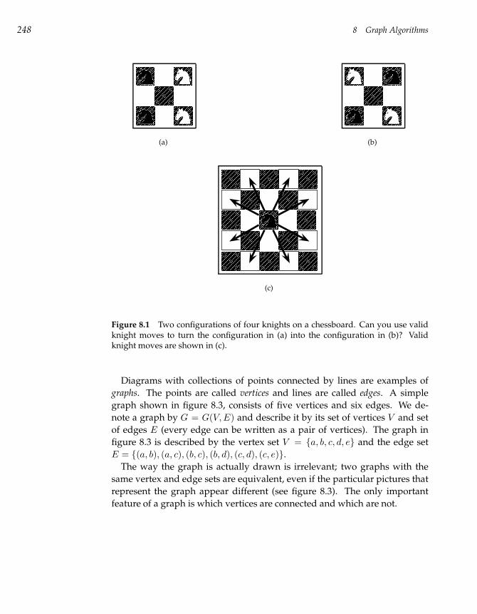
248 8 Graph Algorithms
(a) (b)
(c)
Figure 8.1 Two configurations of four knights on a chessboard. Can you use validknight moves to turn the configuration in (a) into the configuration in (b)? Validknight moves are shown in (c).
Diagrams with collections of points connected by lines are examples of
graphs. The points are called vertices and lines are called edges. A simple
graph shown in figure 8.3, consists of five vertices and six edges. We de-
note a graph by G = G(V, E) and describe it by its set of vertices V and set
of edges E (every edge can be written as a pair of vertices). The graph in
figure 8.3 is described by the vertex set V = a, b, c, d, e and the edge set
E = (a, b), (a, c), (b, c), (b, d), (c, d), (c, e).
The way the graph is actually drawn is irrelevant; two graphs with the
same vertex and edge sets are equivalent, even if the particular pictures that
represent the graph appear different (see figure 8.3). The only important
feature of a graph is which vertices are connected and which are not.
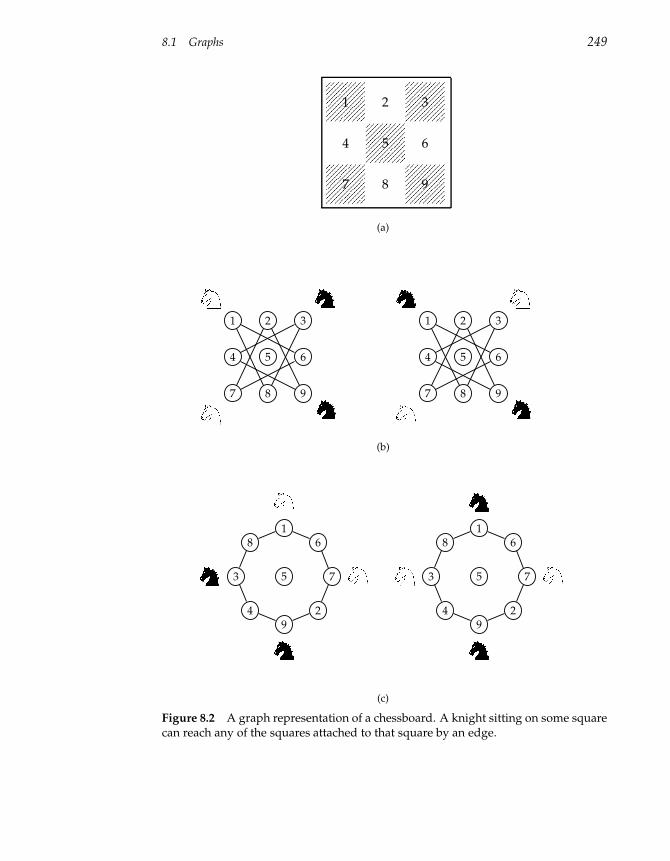
8.1 Graphs 249
1 2 3
4 5 6
7 8 9
(a)
1 2 3
4 5 6
7 8 9
1 2 3
4 5 6
7 8 9
(b)
61
8
3
49
2
75
61
8
3
49
2
75
(c)
Figure 8.2 A graph representation of a chessboard. A knight sitting on some squarecan reach any of the squares attached to that square by an edge.
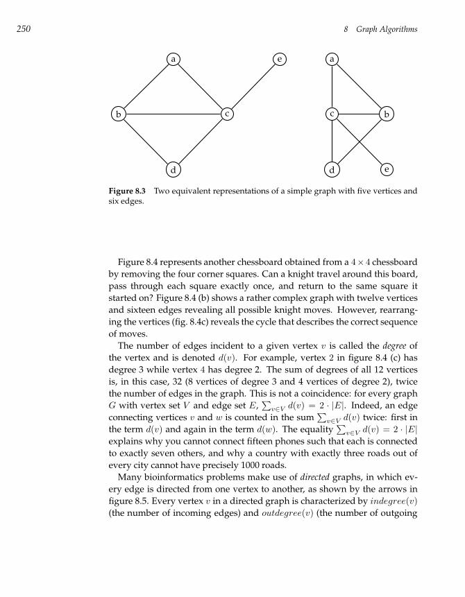
250 8 Graph Algorithms
a e
b c
d
a
c b
d e
Figure 8.3 Two equivalent representations of a simple graph with five vertices andsix edges.
Figure 8.4 represents another chessboard obtained from a 4×4 chessboard
by removing the four corner squares. Can a knight travel around this board,
pass through each square exactly once, and return to the same square it
started on? Figure 8.4 (b) shows a rather complex graph with twelve vertices
and sixteen edges revealing all possible knight moves. However, rearrang-
ing the vertices (fig. 8.4c) reveals the cycle that describes the correct sequence
of moves.
The number of edges incident to a given vertex v is called the degree of
the vertex and is denoted d(v). For example, vertex 2 in figure 8.4 (c) has
degree 3 while vertex 4 has degree 2. The sum of degrees of all 12 vertices
is, in this case, 32 (8 vertices of degree 3 and 4 vertices of degree 2), twice
the number of edges in the graph. This is not a coincidence: for every graph
G with vertex set V and edge set E,∑
v∈V d(v) = 2 · |E|. Indeed, an edge
connecting vertices v and w is counted in the sum∑
v∈V d(v) twice: first in
the term d(v) and again in the term d(w). The equality∑
v∈V d(v) = 2 · |E|
explains why you cannot connect fifteen phones such that each is connected
to exactly seven others, and why a country with exactly three roads out of
every city cannot have precisely 1000 roads.
Many bioinformatics problems make use of directed graphs, in which ev-
ery edge is directed from one vertex to another, as shown by the arrows in
figure 8.5. Every vertex v in a directed graph is characterized by indegree(v)
(the number of incoming edges) and outdegree(v) (the number of outgoing
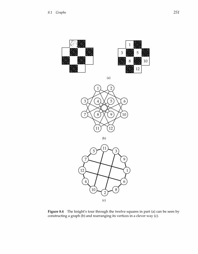
8.1 Graphs 251
(a)
1 2
3 4 5 6
7 8 9 10
11 12
1 2
3 4 5 6
7 8 9 10
11 12
(b)
1
9
311
5
7
12
4
102
8
6
(c)
Figure 8.4 The knight’s tour through the twelve squares in part (a) can be seen byconstructing a graph (b) and rearranging its vertices in a clever way (c).
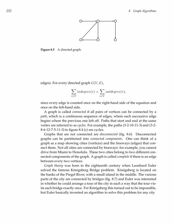
252 8 Graph Algorithms
Figure 8.5 A directed graph.
edges). For every directed graph G(V, E),
∑
v∈V
indegree(v) =∑
v∈V
outdegree(v),
since every edge is counted once on the right-hand side of the equation and
once on the left-hand side.
A graph is called connected if all pairs of vertices can be connected by a
path, which is a continuous sequence of edges, where each successive edge
begins where the previous one left off. Paths that start and end at the same
vertex are referred to as cycles. For example, the paths (3-2-10-11-3) and (3-2-
8-6-12-7-5-11-3) in figure 8.4 (c) are cycles.
Graphs that are not connected are disconnected (fig. 8.6). Disconnected
graphs can be partitioned into connected components. One can think of a
graph as a map showing cities (vertices) and the freeways (edges) that con-
nect them. Not all cities are connected by freeways: for example, you cannot
drive from Miami to Honolulu. These two cities belong to two different con-
nected components of the graph. A graph is called complete if there is an edge
between every two vertices.
Graph theory was born in the eighteenth century when Leonhard Euler
solved the famous Königsberg Bridge problem. Königsberg is located on
the banks of the Pregel River, with a small island in the middle. The various
parts of the city are connected by bridges (fig. 8.7) and Euler was interested
in whether he could arrange a tour of the city in such a way that the tour vis-
its each bridge exactly once. For Königsberg this turned out to be impossible,
but Euler basically invented an algorithm to solve this problem for any city.
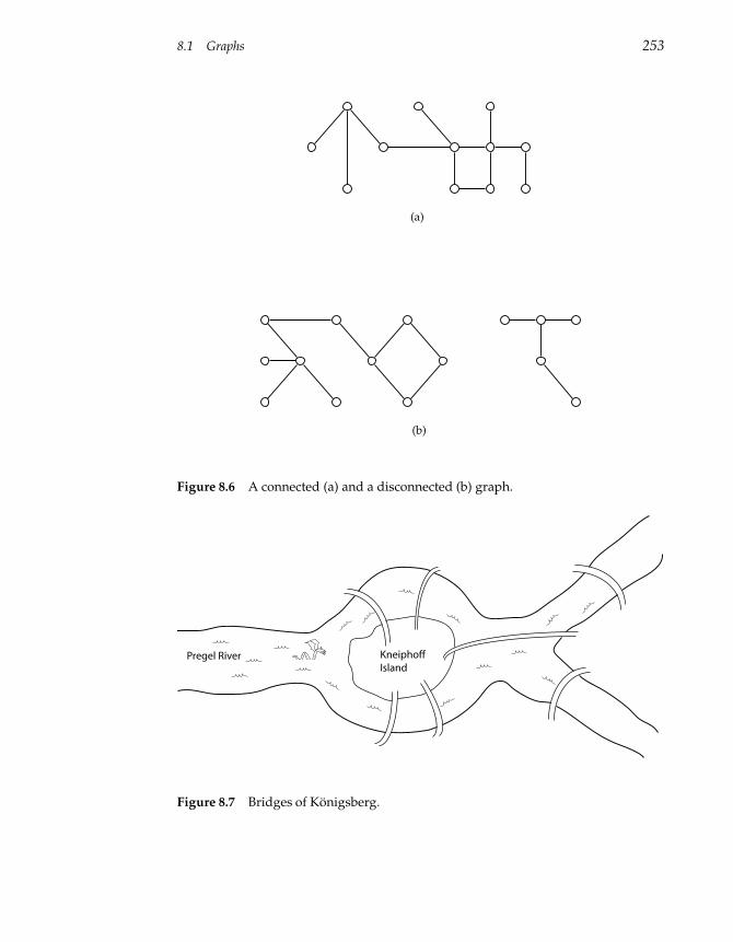
8.1 Graphs 253
(a)
(b)
Figure 8.6 A connected (a) and a disconnected (b) graph.
Kneiphoff
IslandPregel River
Figure 8.7 Bridges of Königsberg.
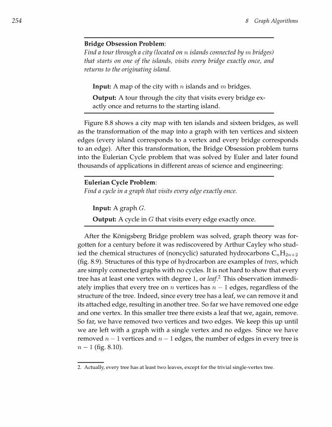
254 8 Graph Algorithms
Bridge Obsession Problem:
Find a tour through a city (located on n islands connected by m bridges)
that starts on one of the islands, visits every bridge exactly once, and
returns to the originating island.
Input: A map of the city with n islands and m bridges.
Output: A tour through the city that visits every bridge ex-
actly once and returns to the starting island.
Figure 8.8 shows a city map with ten islands and sixteen bridges, as well
as the transformation of the map into a graph with ten vertices and sixteen
edges (every island corresponds to a vertex and every bridge corresponds
to an edge). After this transformation, the Bridge Obsession problem turns
into the Eulerian Cycle problem that was solved by Euler and later found
thousands of applications in different areas of science and engineering:
Eulerian Cycle Problem:
Find a cycle in a graph that visits every edge exactly once.
Input: A graph G.
Output: A cycle in G that visits every edge exactly once.
After the Königsberg Bridge problem was solved, graph theory was for-
gotten for a century before it was rediscovered by Arthur Cayley who stud-
ied the chemical structures of (noncyclic) saturated hydrocarbons CnH2n+2
(fig. 8.9). Structures of this type of hydrocarbon are examples of trees, which
are simply connected graphs with no cycles. It is not hard to show that every
tree has at least one vertex with degree 1, or leaf.2 This observation immedi-
ately implies that every tree on n vertices has n − 1 edges, regardless of the
structure of the tree. Indeed, since every tree has a leaf, we can remove it and
its attached edge, resulting in another tree. So far we have removed one edge
and one vertex. In this smaller tree there exists a leaf that we, again, remove.
So far, we have removed two vertices and two edges. We keep this up until
we are left with a graph with a single vertex and no edges. Since we have
removed n− 1 vertices and n− 1 edges, the number of edges in every tree is
n− 1 (fig. 8.10).
2. Actually, every tree has at least two leaves, except for the trivial single-vertex tree.
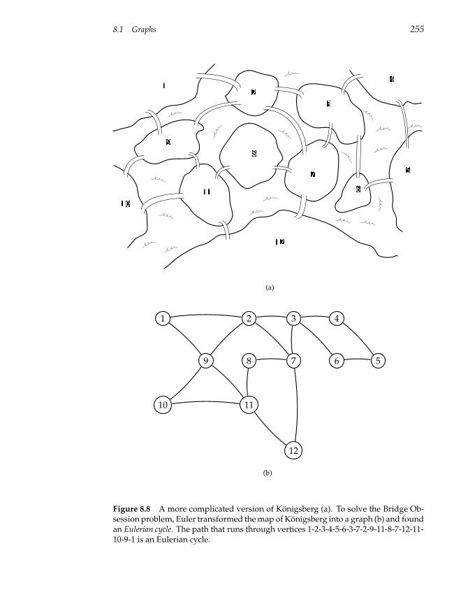
8.1 Graphs 255
(a)
1 2 3 4
9 8 7 6 5
10 11
12
(b)
Figure 8.8 A more complicated version of Königsberg (a). To solve the Bridge Ob-session problem, Euler transformed the map of Königsberg into a graph (b) and foundan Eulerian cycle. The path that runs through vertices 1-2-3-4-5-6-3-7-2-9-11-8-7-12-11-10-9-1 is an Eulerian cycle.
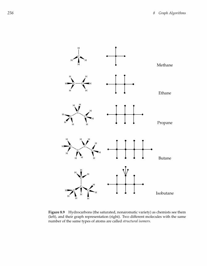
256 8 Graph Algorithms
C C
C
C
C
C
C
C
C
C
C
C
C
CH H
H
H
H
H
H
H
H
H
H
H
H
H
H H
HH
H
H
H
H H
H H
H
H
H
HH
H
H
H
H
H
HH
H
Methane
Ethane
Propane
!
"
#
$%&
'
(
)
*
+
,-.
/
0
1
2
3
456
7
8
9
:
;
<
Butane
=>
?
@
A
B
C
DEF
G
H
I
J
K
L
M
N
OP
Isobutane
Figure 8.9 Hydrocarbons (the saturated, nonaromatic variety) as chemists see them(left), and their graph representation (right). Two different molecules with the samenumber of the same types of atoms are called structural isomers.
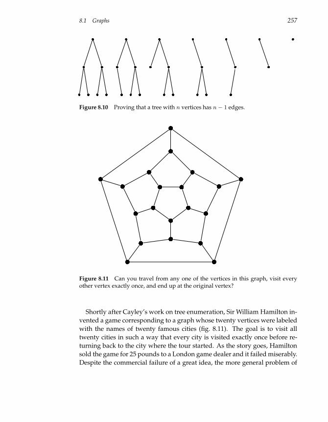
8.1 Graphs 257
!"
#
$
%&
'
()
*
+
,-
.
/0
Figure 8.10 Proving that a tree with n vertices has n− 1 edges.
1
2
3
4 5
6
7
8
9:
;<
=
>
?
@A
B
C
D
Figure 8.11 Can you travel from any one of the vertices in this graph, visit everyother vertex exactly once, and end up at the original vertex?
Shortly after Cayley’s work on tree enumeration, Sir William Hamilton in-
vented a game corresponding to a graph whose twenty vertices were labeled
with the names of twenty famous cities (fig. 8.11). The goal is to visit all
twenty cities in such a way that every city is visited exactly once before re-
turning back to the city where the tour started. As the story goes, Hamilton
sold the game for 25 pounds to a London game dealer and it failed miserably.
Despite the commercial failure of a great idea, the more general problem of
258 8 Graph Algorithms
finding “Hamiltonian cycles” in arbitrary graphs is of critical importance to
many scientific and engineering disciplines. The problem of finding Hamil-
tonian cycles looks deceivingly simple and somehow similar to the Eulerian
Cycle problem. However, it turns out to beNP-complete while the Eulerian
Cycle problem can be solved in linear time.3
Hamiltonian Cycle Problem:
Find a cycle in a graph that visits every vertex exactly once.
Input: A graph G.
Output: A cycle in G that visits every vertex exactly once (if
such a cycle exists).
Graphs, like many freeway maps, often give some sort of weight to every
edge, as in the Manhattan Tourist problem in chapter 6. The weight of an
edge may reflect, depending on the context, different attributes. For exam-
ple, the length of a freeway segment connecting two cities, the number of
tourist attractions along a city block, and the alignment score between two
amino acids are all natural weighting schemes. Weighted graphs are often
formally represented as an ordered triple, G = (V, E, w), where V is the set
of vertices in the graph, E is the set of edges, and w is a weight function de-
fined for every edge e in E (i.e., w(e) is a number reflecting the weight of edge
e). Given a weighted graph, one may be interested in finding some shortest
path between two vertices (e.g., a shortest path between San Diego and New
York). Though this problem may sound difficult if you were given a com-
plicated road map, it turns out that there exist fast algorithms to answer this
question.
Shortest Path Problem:
Given a weighted graph and two vertices, find the shortest distance
between them.
Input: A weighted graph, G = (V, E, w), and two distin-
guished vertices s and t.
Output: The shortest path between s and t in graph G.
3. The Hamiltonian Cycle problem is equivalent in complexity to the Traveling Salesman prob-lem mentioned in chapter 2 and is therefore NP-complete.
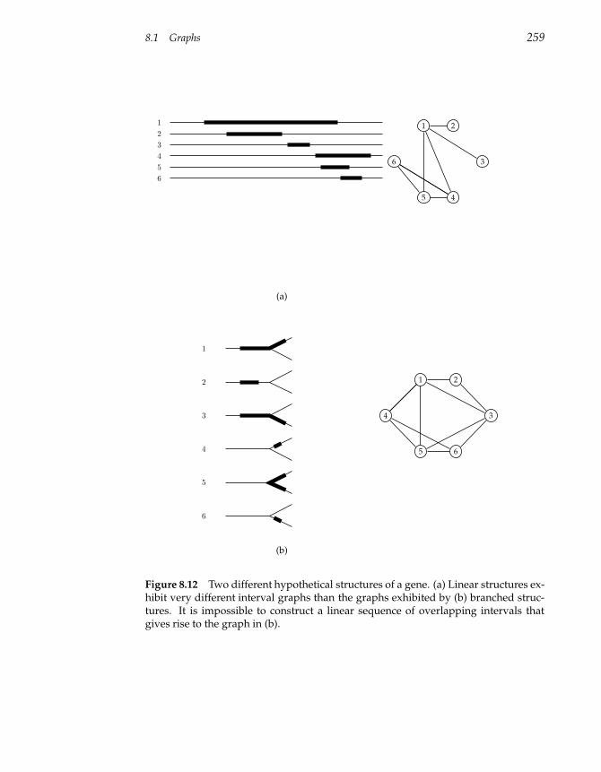
8.1 Graphs 259
1
2
3
4
5
6
1 2
6 3
5 4
(a)
1
2
3
4
5
6
1 2
4 3
5 6
(b)
Figure 8.12 Two different hypothetical structures of a gene. (a) Linear structures ex-hibit very different interval graphs than the graphs exhibited by (b) branched struc-tures. It is impossible to construct a linear sequence of overlapping intervals thatgives rise to the graph in (b).
260 8 Graph Algorithms
We emphasize that this problem is different—and somewhat more comp-
licated—than the Longest Path in a Directed Acyclic Graph (DAG) problem
that we considered in chapter 6.
Graphs are powerful tools in many applied studies and their role goes
well beyond analysis of maps of freeways. For example, at first glance, the
following “basketball” problem has nothing to do with graph theory:
Fifteen teams play a basketball tournament in which each team plays with each other team.
Prove that the teams can always be numbered from 1 to 15 in such a way that team 1 defeated
team 2, team 2 defeated team 3, ... , team 14 defeated team 15.
A careful analysis reduces this problem to finding a Hamiltonian path in a
directed graph on fifteen vertices.
8.2 Graphs and Genetics
Conceived by Euler, Cayley, and Hamilton, graph theory flourished in the
twentieth century to become a critical component of discrete mathematics.
In the 1950s, Seymour Benzer applied graph theory to show that genes are
linear.
At that time, it was known that genes behaved as functional units of DNA,
much like pearls on a necklace, but the chemical structure and organization
of the genes was not clear. Were genes broken into still smaller components?
If so, how were they organized? Prior to Watson and Crick’s elucidation
of the DNA double helix, it seemed a reasonable hypothesis that the DNA
content of genes was branched, as in figure 8.12, or even looped, rather than
linear. These two organizations have very different topological implications,
which Benzer exploited in an ingenious experiment.
Benzer studied a large number of bacteriophage4 T4 mutants, which hap-
pened to have a continuous interval deleted from an important gene. In their
“normal” state, nonmutant T4 phages will kill a bacterium. The mutant T4
phages that were missing a segment of their genome could not kill the bac-
terium. Different mutants had different intervals deleted from the gene, and
Benzer had to determine which interval had been deleted in each mutant.
Though Benzer did not know exactly where in the gene the mutant’s dele-
tion was, he had a way to test whether two deletions (i.e., their intervals)
overlapped, relying on how two phages with two different deletions behave
4. A bacteriophage is a virus that attacks bacteria.
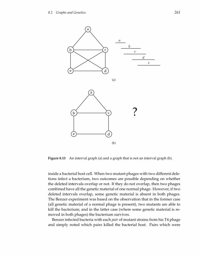
8.2 Graphs and Genetics 261
a
b c
e d
a
b
c
d
e
(a)
a
b c
e d
?
(b)
Figure 8.13 An interval graph (a) and a graph that is not an interval graph (b).
inside a bacterial host cell. When two mutant phages with two different dele-
tions infect a bacterium, two outcomes are possible depending on whether
the deleted intervals overlap or not. If they do not overlap, then two phages
combined have all the genetic material of one normal phage. However, if two
deleted intervals overlap, some genetic material is absent in both phages.
The Benzer experiment was based on the observation that in the former case
(all genetic material of a normal phage is present), two mutants are able to
kill the bacterium; and in the latter case (where some genetic material is re-
moved in both phages) the bacterium survives.
Benzer infected bacteria with each pair of mutant strains from his T4 phage
and simply noted which pairs killed the bacterial host. Pairs which were
262 8 Graph Algorithms
lethal to the host were mutants whose deleted intervals did not overlap. Ben-
zer constructed a graph5 where each strain was a vertex and two vertices
were connected when a double infection of a bacterial host was nonlethal.
He reasoned that if genes were linear [fig. 8.12 (a)], he would probably see
one type of graph, but if the genes were branched [fig. 8.12 (b)] he would see
another.
Given a set of n intervals on a line segment, the interval graph is defined
as a graph with n vertices that correspond to the intervals. There is an
edge between vertices v and w if and only if the intervals v and w over-
lap. Interval graphs have several important properties that make them easy
to recognize— for example, the graph in figure 8.13 (a) is an interval graph,
whereas the “house” graph in figure 8.13 (b) is not. Benzer’s problem was
equivalent to deciding whether the graph obtained from his bacteriophage
experiment represented an interval graph. Had the experiment resulted in a
graph like the “house” graph, then the genes could not have been organized
as linear structures. As it turned out, the graph was indeed an interval graph,
indicating that genes were composed of linearly organized functional units.
8.3 DNA Sequencing
Imagine several copies of a magazine cut into millions of pieces. Each copy
is cut in a different way, so a piece from one copy may overlap pieces from
another. Assuming that some large number of pieces are just sort of lost,
and the remaining pieces are splashed with ink, can you recover the original
text? This, essentially, is the problem of fragment assembly in DNA sequenc-
ing. Classic DNA sequencing technology allows one to read short 500- to
700-nucleotide sequences per experiment, each fragment corresponding to
one of the many magazine pieces. Assembling the entire genome from these
short fragments is like reassembling the magazine from the millions of tiny
slips of paper.6 Both problems are complicated by unavoidable experimental
errors—ink splashes on the magazine, and mistakes in reading nucleotides.
Furthermore, the data are frequently incomplete—some magazine pieces get
lost, while some DNA fragments never make it into the sequencing ma-
chine. Nevertheless, efforts to determine the DNA sequence of organisms
have been remarkably successful, even in the face of these difficulties.
5. It is not clear that he actually knew anything about graph theory at the time, but graph theo-rists eventually noticed his work.6. We emphasize that biologists reading these 500- to 700-nucleotide sequences have no ideawhere they are located within the entire DNA string.
8.3 DNA Sequencing 263
Two DNA sequencing methods were invented independently and simul-
taneously in Cambridge, England by Fred Sanger and in Cambridge, Mas-
sachusetts by Walter Gilbert. Sanger’s method takes advantage of how cells
make copies of DNA. Cells copy a strand of DNA nucleotide by nucleotide
in a reaction that adds one base at a time. Sanger realized that he could make
copies of DNA fragments of different lengths if he starved the reaction of
one of the four bases: a cell can only copy its DNA while it has all of the
bases in supply. For a sequence ACGTAAGCTA, starving at T would produce
a mixture of the fragments ACG and ACGTAAGC. By running one starvation
experiment for each of A, T, G, and C and then separating the resulting DNA
fragments by length, one can read the DNA sequence.7 Each of four star-
vation experiments produces a ladder of fragments of varying lengths called
the Sanger ladder.8 This approach culminated in the sequencing of a 5386-
nucleotide virus in 1977 and a Nobel Prize shortly thereafter. Since then the
amount of DNA sequence data has been increasing exponentially, particu-
larly after the launch of the Human Genome Project in 1989. By 2001, it had
produced the roughly 3 billion-nucleotide sequence of the human genome.
Within the past twenty years, DNA sequencing technology has been de-
veloped to the point where modern sequencing machines can sequence 500-
to 700-nucleotide DNA fragments, called sequencing reads. These reads then
have to be assembled into a continuous genome, which turns out to be a
very hard problem. Even though the DNA reading process has become quite
automated, these machines are not microscope-like devices that simply scan
500 nucleotides as if they were a sentence in a book. The DNA sequencing
machines measure the lengths of DNA fragments in the Sanger ladder, but
even this task is difficult; we cannot measure a single DNA fragment, but
must measure billions of identical fragments.
Shotgun sequencing starts with a large sample of genomic DNA. The sam-
ple is sonicated, a process which randomly partitions each piece of DNA in
the sample into inserts; the inserts that are smaller than 500 nucleotides are
removed from further consideration. Before the inserts can be read, each one
must be multiplied billions of times so that it is possible to read the ladders
produced by Sanger’s technique. To amplify the inserts, a sample is cloned
into a vector, and this vector used to infect a bacterial host. As the bacterium
reproduces, it creates a colony that contains billions of copies of the vector
7. Later Sanger found chemicals—so-called dideoxynucleotides—that could be inserted in placeof A, T, G, or C, and cause a growing DNA chain to end.8. The Sanger ladder for T shows the lengths of all sub-fragments ending at T and thereforereveals the set of positions where T occurs.
264 8 Graph Algorithms
and its associated insert. As a result, the cloning process results in the pro-
duction of a large sample of one particular insert that can then be sequenced
by the Sanger method. Usually, only the first 500 to 700 nucleotides of the in-
sert can be interpreted from this experiment. DNA sequencing is therefore a
two stage process including both experimental (reading 500–700 nucleotide
sequences form different inserts) and computational (assembling these reads
into a single long sequence) components.
8.4 Shortest Superstring Problem
Since every string, or read, that we sequence came from the much longer ge-
nomic string, we are interested in a superstring of the reads—that is, we want
a long string that “explains” all the reads we generated. However, there are
many possible superstrings to choose from—for example, we could concate-
nate all the reads together to get a (not very helpful) superstring. We choose
to be most interested in the shortest one, which turns out to be a reasonable
first approximation to the unknown genomic DNA sequence. With this in
mind, the simplest approximation of DNA sequencing corresponds to the
following problem.
Shortest Superstring Problem:
Given a set of strings, find a shortest string that contains all of them.
Input: Strings s1, s2, . . . , sn.
Output: A string s that contains all strings s1, s2, . . . , sn as
substrings, such that the length of s is as small as possible.
Figure 8.14 presents two superstrings for the set of all eight three-letter
strings in a 0–1 alphabet. The first (trivial) superstring is obtained by the
concatenation of all eight strings, while the second one is a shortest super-
string.
Define overlap(si, sj) to be the length of the longest prefix of sj that matches
a suffix of si. The Shortest Superstring problem can be cast as a Traveling
Salesman problem in a complete directed graph with n vertices correspond-
ing to strings s1, . . . , sn and edges of length −overlap(si, sj) (fig. 8.15). This
reduction, of course, does not lead to an efficient algorithm since the TSP is
NP-complete. Moreover it is known that the Shortest Superstring problem
is itselfNP-complete, so that a polynomial algorithm for this problem is un-
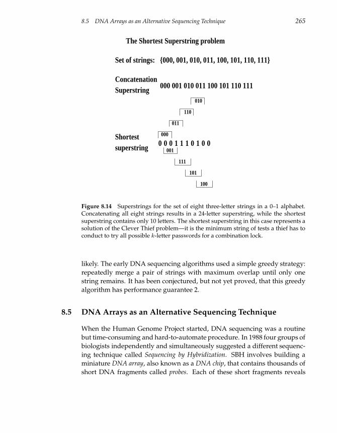
8.5 DNA Arrays as an Alternative Sequencing Technique 265
The Shortest Superstring problem
ConcatenationSuperstring
Set of strings: 000, 001, 010, 011, 100, 101, 110, 111
000 001 010 011 100 101 110 111
Shortest superstring 0 0 0 1 1 1 0 1 0 0
000
011
110
010
001
111
101
100
Figure 8.14 Superstrings for the set of eight three-letter strings in a 0–1 alphabet.Concatenating all eight strings results in a 24-letter superstring, while the shortestsuperstring contains only 10 letters. The shortest superstring in this case represents asolution of the Clever Thief problem—it is the minimum string of tests a thief has toconduct to try all possible k-letter passwords for a combination lock.
likely. The early DNA sequencing algorithms used a simple greedy strategy:
repeatedly merge a pair of strings with maximum overlap until only one
string remains. It has been conjectured, but not yet proved, that this greedy
algorithm has performance guarantee 2.
8.5 DNA Arrays as an Alternative Sequencing Technique
When the Human Genome Project started, DNA sequencing was a routine
but time-consuming and hard-to-automate procedure. In 1988 four groups of
biologists independently and simultaneously suggested a different sequenc-
ing technique called Sequencing by Hybridization. SBH involves building a
miniature DNA array, also known as a DNA chip, that contains thousands of
short DNA fragments called probes. Each of these short fragments reveals
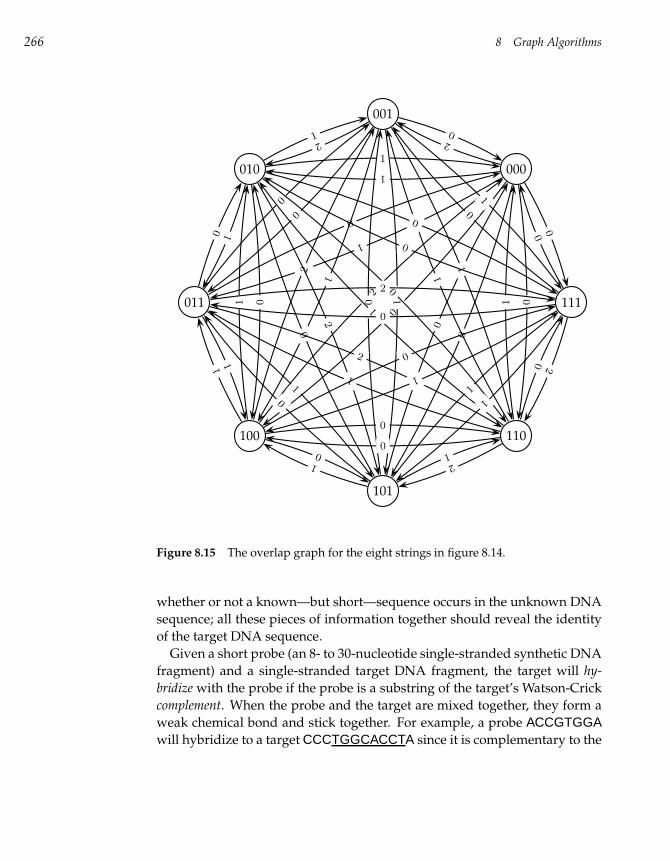
266 8 Graph Algorithms
000
001
010
011
100
101
110
111
2
0
1
1
1
0
00
0
0
02 0
1
21
12
1
1
00
1
0
1
0
10
0
1
2
0
0
0
0
1
1
0
1
1
2
1
2
0
0
1
0
1
00
21
0 2
1
1
Figure 8.15 The overlap graph for the eight strings in figure 8.14.
whether or not a known—but short—sequence occurs in the unknown DNA
sequence; all these pieces of information together should reveal the identity
of the target DNA sequence.
Given a short probe (an 8- to 30-nucleotide single-stranded synthetic DNA
fragment) and a single-stranded target DNA fragment, the target will hy-
bridize with the probe if the probe is a substring of the target’s Watson-Crick
complement. When the probe and the target are mixed together, they form a
weak chemical bond and stick together. For example, a probe ACCGTGGAwill hybridize to a target CCCTGGCACCTA since it is complementary to the
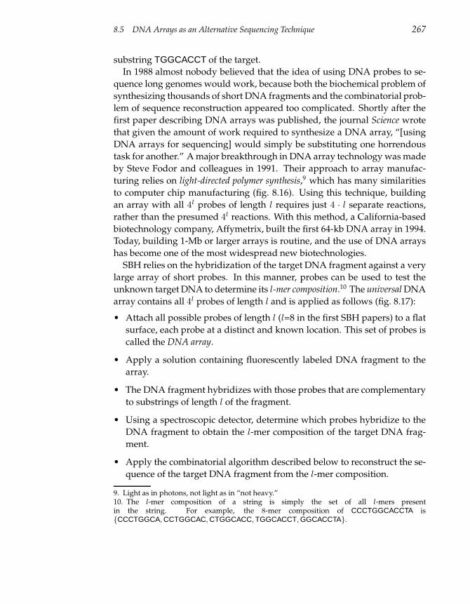
8.5 DNA Arrays as an Alternative Sequencing Technique 267
substring TGGCACCT of the target.
In 1988 almost nobody believed that the idea of using DNA probes to se-
quence long genomes would work, because both the biochemical problem of
synthesizing thousands of short DNA fragments and the combinatorial prob-
lem of sequence reconstruction appeared too complicated. Shortly after the
first paper describing DNA arrays was published, the journal Science wrote
that given the amount of work required to synthesize a DNA array, “[using
DNA arrays for sequencing] would simply be substituting one horrendous
task for another.” A major breakthrough in DNA array technology was made
by Steve Fodor and colleagues in 1991. Their approach to array manufac-
turing relies on light-directed polymer synthesis,9 which has many similarities
to computer chip manufacturing (fig. 8.16). Using this technique, building
an array with all 4l probes of length l requires just 4 · l separate reactions,
rather than the presumed 4l reactions. With this method, a California-based
biotechnology company, Affymetrix, built the first 64-kb DNA array in 1994.
Today, building 1-Mb or larger arrays is routine, and the use of DNA arrays
has become one of the most widespread new biotechnologies.
SBH relies on the hybridization of the target DNA fragment against a very
large array of short probes. In this manner, probes can be used to test the
unknown target DNA to determine its l-mer composition.10 The universal DNA
array contains all 4l probes of length l and is applied as follows (fig. 8.17):
• Attach all possible probes of length l (l=8 in the first SBH papers) to a flat
surface, each probe at a distinct and known location. This set of probes is
called the DNA array.
• Apply a solution containing fluorescently labeled DNA fragment to the
array.
• The DNA fragment hybridizes with those probes that are complementary
to substrings of length l of the fragment.
• Using a spectroscopic detector, determine which probes hybridize to the
DNA fragment to obtain the l-mer composition of the target DNA frag-
ment.
• Apply the combinatorial algorithm described below to reconstruct the se-
quence of the target DNA fragment from the l-mer composition.
9. Light as in photons, not light as in “not heavy.”10. The l-mer composition of a string is simply the set of all l-mers presentin the string. For example, the 8-mer composition of CCCTGGCACCTA isCCCTGGCA, CCTGGCAC, CTGGCACC, TGGCACCT, GGCACCTA.
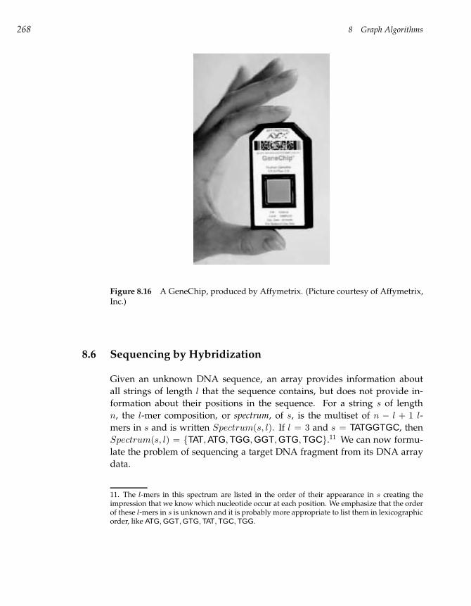
268 8 Graph Algorithms
Figure 8.16 A GeneChip, produced by Affymetrix. (Picture courtesy of Affymetrix,Inc.)
8.6 Sequencing by Hybridization
Given an unknown DNA sequence, an array provides information about
all strings of length l that the sequence contains, but does not provide in-
formation about their positions in the sequence. For a string s of length
n, the l-mer composition, or spectrum, of s, is the multiset of n − l + 1 l-
mers in s and is written Spectrum(s, l). If l = 3 and s = TATGGTGC, then
Spectrum(s, l) = TAT, ATG, TGG, GGT, GTG, TGC.11 We can now formu-
late the problem of sequencing a target DNA fragment from its DNA array
data.
11. The l-mers in this spectrum are listed in the order of their appearance in s creating theimpression that we know which nucleotide occur at each position. We emphasize that the orderof these l-mers in s is unknown and it is probably more appropriate to list them in lexicographicorder, like ATG, GGT, GTG, TAT, TGC, TGG.
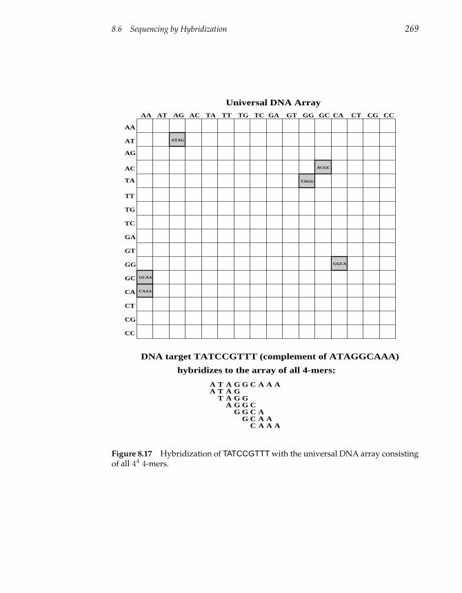
8.6 Sequencing by Hybridization 269
AA AT AG AC TA TT TG TC GA GT GG GC CA CT CG CC
AA
AG
AT
AC
TA
TT
TG
TC
GA
GT
GG
GC
CT
CG
CA
CC
ATAG
GCAA
TAGG
ACGC
GGCA
CAAA
DNA target TATCCGTTT (complement of ATAGGCAAA)
hybridizes to the array of all 4-mers:
A T G G C A A AA T G
T GGG
GGGG
CCCC
AAA
AA A
Universal DNA Array
AAAA
Figure 8.17 Hybridization of TATCCGTTT with the universal DNA array consistingof all 44 4-mers.
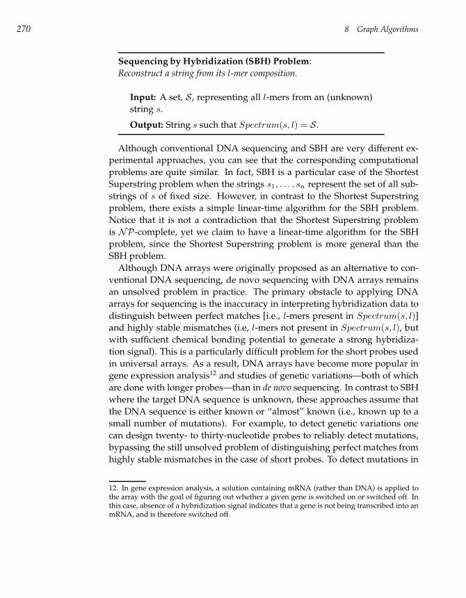
270 8 Graph Algorithms
Sequencing by Hybridization (SBH) Problem:
Reconstruct a string from its l-mer composition.
Input: A set, S, representing all l-mers from an (unknown)
string s.
Output: String s such that Spectrum(s, l) = S.
Although conventional DNA sequencing and SBH are very different ex-
perimental approaches, you can see that the corresponding computational
problems are quite similar. In fact, SBH is a particular case of the Shortest
Superstring problem when the strings s1, . . . , sn represent the set of all sub-
strings of s of fixed size. However, in contrast to the Shortest Superstring
problem, there exists a simple linear-time algorithm for the SBH problem.
Notice that it is not a contradiction that the Shortest Superstring problem
is NP-complete, yet we claim to have a linear-time algorithm for the SBH
problem, since the Shortest Superstring problem is more general than the
SBH problem.
Although DNA arrays were originally proposed as an alternative to con-
ventional DNA sequencing, de novo sequencing with DNA arrays remains
an unsolved problem in practice. The primary obstacle to applying DNA
arrays for sequencing is the inaccuracy in interpreting hybridization data to
distinguish between perfect matches [i.e., l-mers present in Spectrum(s, l)]
and highly stable mismatches (i.e, l-mers not present in Spectrum(s, l), but
with sufficient chemical bonding potential to generate a strong hybridiza-
tion signal). This is a particularly difficult problem for the short probes used
in universal arrays. As a result, DNA arrays have become more popular in
gene expression analysis12 and studies of genetic variations—both of which
are done with longer probes—than in de novo sequencing. In contrast to SBH
where the target DNA sequence is unknown, these approaches assume that
the DNA sequence is either known or “almost” known (i.e., known up to a
small number of mutations). For example, to detect genetic variations one
can design twenty- to thirty-nucleotide probes to reliably detect mutations,
bypassing the still unsolved problem of distinguishing perfect matches from
highly stable mismatches in the case of short probes. To detect mutations in
12. In gene expression analysis, a solution containing mRNA (rather than DNA) is applied tothe array with the goal of figuring out whether a given gene is switched on or switched off. Inthis case, absence of a hybridization signal indicates that a gene is not being transcribed into anmRNA, and is therefore switched off.
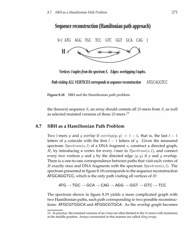
8.7 SBH as a Hamiltonian Path Problem 271
ATGS= TCC GTC GCA CAG TGC
Vertices: l-tuples from the spectrum S. Edges: overlapping l-tuples.
Path visiting ALL VERTICES corresponds to sequence reconstruction
AGG GGT
ATGCAGGTCC
H
Sequence reconstruction (Hamiltonian path approach)
Figure 8.18 SBH and the Hamiltonian path problem.
the (known) sequence S, an array should contain all 25-mers from S, as well
as selected mutated versions of these 25-mers.13
8.7 SBH as a Hamiltonian Path Problem
Two l-mers p and q overlap if overlap(p, q) = l − 1, that is, the last l − 1
letters of p coincide with the first l − 1 letters of q. Given the measured
spectrum Spectrum(s, l) of a DNA fragment s, construct a directed graph,
H , by introducing a vertex for every l-mer in Spectrum(s, l), and connect
every two vertices p and q by the directed edge (p, q) if p and q overlap.
There is a one-to-one correspondence between paths that visit each vertex of
H exactly once and DNA fragments with the spectrum Spectrum(s, l). The
spectrum presented in figure 8.18 corresponds to the sequence reconstruction
ATGCAGGTCC, which is the only path visiting all vertices of H :
ATG→ TGC→ GCA→ CAG→ AGG→ GGT→ GTC→ TCC
The spectrum shown in figure 8.19 yields a more complicated graph with
two Hamiltonian paths, each path corresponding to two possible reconstruc-
tions: ATGCGTGGCA and ATGGCGTGCA. As the overlap graph becomes
13. In practice, the mutated versions of an l-mer are often limited to the 3 l-mers with mutationsat the middle position. Arrays constructed in this manner are called tiling arrays.
272 8 Graph Algorithms
ATGS= TGC GTG GGC GCG CGT
H
ATGCGTGGCA
ATGGCGTGCA
TGG GCA
Multiple sequence reconstructions (Hamiltonian path approach)
Figure 8.19 Spectrum S yields two possible reconstructions corresponding to dis-tinct Hamiltonian paths.
larger, this approach ceases to be practically useful since the Hamiltonian
Path problem is NP-complete.
8.8 SBH as an Eulerian Path Problem
As we have seen, reducing the SBH problem to a Hamiltonian Path problem
does not lead to an efficient algorithm. Fortunately, reducing SBH to the
Eulerian Path problem in a directed graph,14 which leads to the simple linear-
time algorithm for sequence reconstruction mentioned earlier.
14. A directed path is a path v1 → v2 → . . . → vn from vertex v1 to vertex vn in which everyedge (vi, vi+1) is directed from vi to vi+1.
8.8 SBH as an Eulerian Path Problem 273
The reduction of the SBH problem to an Eulerian Path problem is to con-
struct a graph whose edges—rather than vertices—correspond to l-mers from
Spectrum(s, l), and then to find a path in this graph visiting every edge ex-
actly once. In this approach we build a graph G on the set of all (l− 1)-mers,
rather than on the set of all l-mers as in the previous section. An (l − 1)-mer
v is joined by a directed edge with an (l − 1)-mer w if the spectrum contains
an l-mer for which the first l − 1 nucleotides coincide with v and the last
l − 1 nucleotides coincide with w (fig. 8.20). Each l-mer from the spectrum
corresponds to a directed edge in G rather than to a vertex as it does in H ;
compare figures 8.19 and 8.20. Therefore, finding a DNA fragment contain-
ing all l-mers from the spectrum corresponds to finding a path visiting all
edges of G, which is the problem of finding an Eulerian path. Superficially,
finding an Eulerian path looks just as hard as finding a Hamiltonian path,
but, as we show below, finding Eulerian paths turns out to be simple.
We will first consider Eulerian cycles, that is, Eulerian paths in which the
first and the last vertices are the same. A directed graph G is Eulerian if
it contains an Eulerian cycle. A vertex v in a graph is balanced if the num-
ber of edges entering v equals the number of edges leaving v, that is, if
indegree(v) = outdegree(v). For any given vertex v in an Eulerian graph,
the number of times the Eulerian cycle enters v is exactly the same as the
number of times it leaves v. Thus, indegree(v) = outdegree(v) for every ver-
tex v in an Eulerian graph, motivating the following theorem characterizing
Eulerian graphs.
Theorem 8.1 A connected graph is Eulerian if and only if each of its vertices is
balanced.
Proof First, it is easy to see that if a graph is Eulerian, then each vertex must
be balanced. We show that if each vertex in a connected graph is balanced,
then the graph is Eulerian.
To construct an Eulerian cycle, we start from an arbitrary vertex v and form
any arbitrary path by traversing edges that have not already been used. We
stop the path when we encounter a vertex with no way out, that is, a ver-
tex whose outgoing edges have already been used in the path. In a balanced
graph, the only vertex where this can happen is the starting vertex v since for
any other vertex, the balance condition ensures that for every incoming edge
there is an outgoing edge that has not yet been used. Therefore, the resulting
path will end at the same vertex where it started, and with some luck will be
Eulerian. However, if the path is not Eulerian, it must contain a vertex w that
still has some number of untraversed edges. The cycle we just constructed
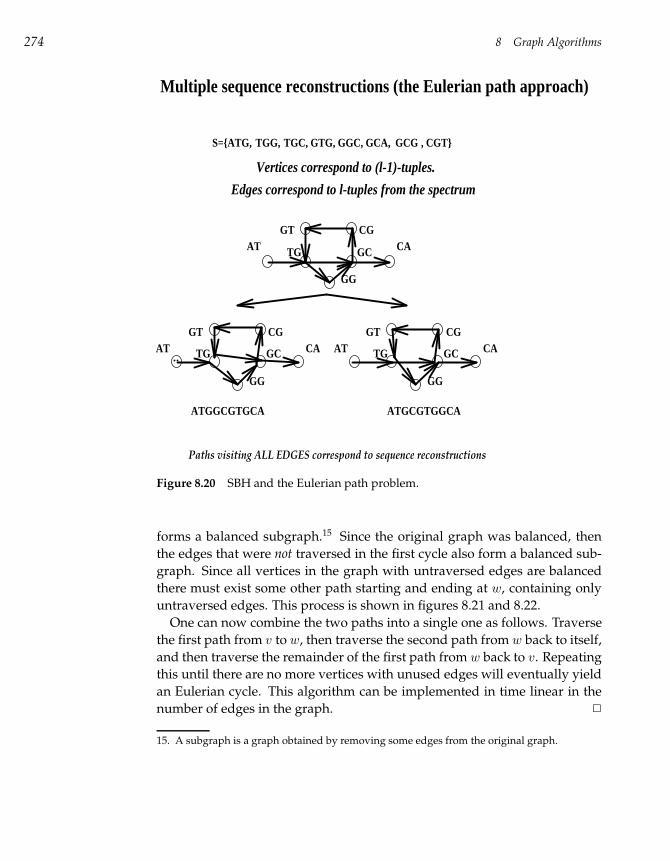
274 8 Graph Algorithms
AT CAGT CG
TG GC
GG
AT CAGT CG
TG GC
GG
ATGGCGTGCA ATGCGTGGCA
AT CAGT CG
TG GC
GG
Paths visiting ALL EDGES correspond to sequence reconstructions
S=ATG, TGG, GCGTGC, GTG, GGC, GCA,
Edges correspond to l-tuples from the spectrum
Vertices correspond to (l-1)-tuples.
, CGT
Multiple sequence reconstructions (the Eulerian path approach)
Figure 8.20 SBH and the Eulerian path problem.
forms a balanced subgraph.15 Since the original graph was balanced, then
the edges that were not traversed in the first cycle also form a balanced sub-
graph. Since all vertices in the graph with untraversed edges are balanced
there must exist some other path starting and ending at w, containing only
untraversed edges. This process is shown in figures 8.21 and 8.22.
One can now combine the two paths into a single one as follows. Traverse
the first path from v to w, then traverse the second path from w back to itself,
and then traverse the remainder of the first path from w back to v. Repeating
this until there are no more vertices with unused edges will eventually yield
an Eulerian cycle. This algorithm can be implemented in time linear in the
number of edges in the graph. 2
15. A subgraph is a graph obtained by removing some edges from the original graph.
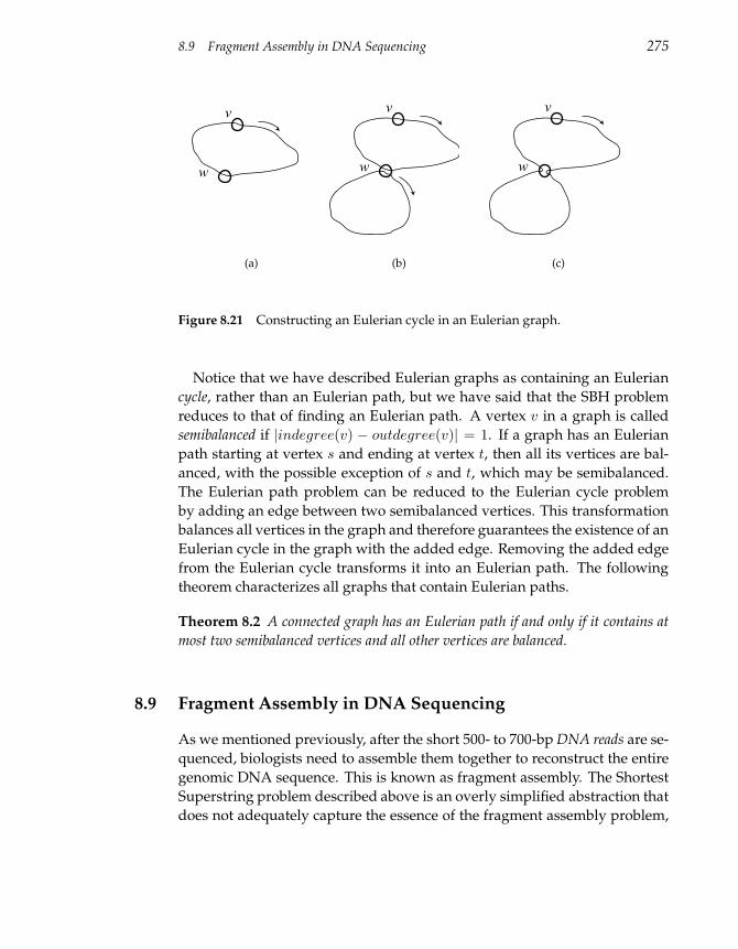
8.9 Fragment Assembly in DNA Sequencing 275
v
w
(a)
v
w
(b)
v
w
(c)
Figure 8.21 Constructing an Eulerian cycle in an Eulerian graph.
Notice that we have described Eulerian graphs as containing an Eulerian
cycle, rather than an Eulerian path, but we have said that the SBH problem
reduces to that of finding an Eulerian path. A vertex v in a graph is called
semibalanced if |indegree(v) − outdegree(v)| = 1. If a graph has an Eulerian
path starting at vertex s and ending at vertex t, then all its vertices are bal-
anced, with the possible exception of s and t, which may be semibalanced.
The Eulerian path problem can be reduced to the Eulerian cycle problem
by adding an edge between two semibalanced vertices. This transformation
balances all vertices in the graph and therefore guarantees the existence of an
Eulerian cycle in the graph with the added edge. Removing the added edge
from the Eulerian cycle transforms it into an Eulerian path. The following
theorem characterizes all graphs that contain Eulerian paths.
Theorem 8.2 A connected graph has an Eulerian path if and only if it contains at
most two semibalanced vertices and all other vertices are balanced.
8.9 Fragment Assembly in DNA Sequencing
As we mentioned previously, after the short 500- to 700-bp DNA reads are se-
quenced, biologists need to assemble them together to reconstruct the entire
genomic DNA sequence. This is known as fragment assembly. The Shortest
Superstring problem described above is an overly simplified abstraction that
does not adequately capture the essence of the fragment assembly problem,
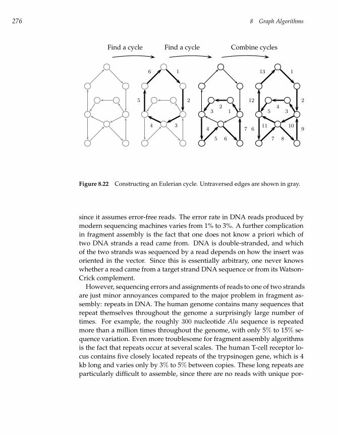
276 8 Graph Algorithms
Find a cycle
1
2
34
5
6
Find a cycle
12
3
4
5 6
7
Combine cycles
1
2
34
5
6
7 8
91011
12
13
Figure 8.22 Constructing an Eulerian cycle. Untraversed edges are shown in gray.
since it assumes error-free reads. The error rate in DNA reads produced by
modern sequencing machines varies from 1% to 3%. A further complication
in fragment assembly is the fact that one does not know a priori which of
two DNA strands a read came from. DNA is double-stranded, and which
of the two strands was sequenced by a read depends on how the insert was
oriented in the vector. Since this is essentially arbitrary, one never knows
whether a read came from a target strand DNA sequence or from its Watson-
Crick complement.
However, sequencing errors and assignments of reads to one of two strands
are just minor annoyances compared to the major problem in fragment as-
sembly: repeats in DNA. The human genome contains many sequences that
repeat themselves throughout the genome a surprisingly large number of
times. For example, the roughly 300 nucleotide Alu sequence is repeated
more than a million times throughout the genome, with only 5% to 15% se-
quence variation. Even more troublesome for fragment assembly algorithms
is the fact that repeats occur at several scales. The human T-cell receptor lo-
cus contains five closely located repeats of the trypsinogen gene, which is 4
kb long and varies only by 3% to 5% between copies. These long repeats are
particularly difficult to assemble, since there are no reads with unique por-
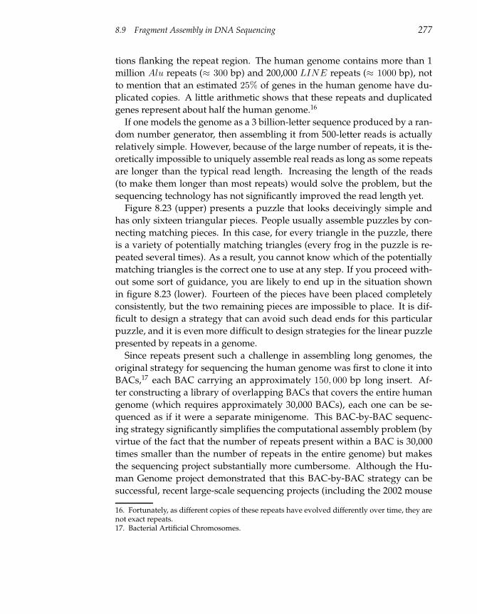
8.9 Fragment Assembly in DNA Sequencing 277
tions flanking the repeat region. The human genome contains more than 1
million Alu repeats (≈ 300 bp) and 200,000 LINE repeats (≈ 1000 bp), not
to mention that an estimated 25% of genes in the human genome have du-
plicated copies. A little arithmetic shows that these repeats and duplicated
genes represent about half the human genome.16
If one models the genome as a 3 billion-letter sequence produced by a ran-
dom number generator, then assembling it from 500-letter reads is actually
relatively simple. However, because of the large number of repeats, it is the-
oretically impossible to uniquely assemble real reads as long as some repeats
are longer than the typical read length. Increasing the length of the reads
(to make them longer than most repeats) would solve the problem, but the
sequencing technology has not significantly improved the read length yet.
Figure 8.23 (upper) presents a puzzle that looks deceivingly simple and
has only sixteen triangular pieces. People usually assemble puzzles by con-
necting matching pieces. In this case, for every triangle in the puzzle, there
is a variety of potentially matching triangles (every frog in the puzzle is re-
peated several times). As a result, you cannot know which of the potentially
matching triangles is the correct one to use at any step. If you proceed with-
out some sort of guidance, you are likely to end up in the situation shown
in figure 8.23 (lower). Fourteen of the pieces have been placed completely
consistently, but the two remaining pieces are impossible to place. It is dif-
ficult to design a strategy that can avoid such dead ends for this particular
puzzle, and it is even more difficult to design strategies for the linear puzzle
presented by repeats in a genome.
Since repeats present such a challenge in assembling long genomes, the
original strategy for sequencing the human genome was first to clone it into
BACs,17 each BAC carrying an approximately 150, 000 bp long insert. Af-
ter constructing a library of overlapping BACs that covers the entire human
genome (which requires approximately 30,000 BACs), each one can be se-
quenced as if it were a separate minigenome. This BAC-by-BAC sequenc-
ing strategy significantly simplifies the computational assembly problem (by
virtue of the fact that the number of repeats present within a BAC is 30,000
times smaller than the number of repeats in the entire genome) but makes
the sequencing project substantially more cumbersome. Although the Hu-
man Genome project demonstrated that this BAC-by-BAC strategy can be
successful, recent large-scale sequencing projects (including the 2002 mouse
16. Fortunately, as different copies of these repeats have evolved differently over time, they arenot exact repeats.17. Bacterial Artificial Chromosomes.
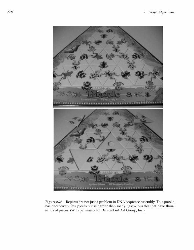
278 8 Graph Algorithms
Figure 8.23 Repeats are not just a problem in DNA sequence assembly. This puzzlehas deceptively few pieces but is harder than many jigsaw puzzles that have thou-sands of pieces. (With permission of Dan Gilbert Art Group, Inc.)
8.9 Fragment Assembly in DNA Sequencing 279
genome assembly) mainly follow the whole-genome assembly paradigm ad-
vocated by James Weber and Gene Myers in 1997. Myers led the fragment
assembly efforts at Celera Genomics, the company that announced the com-
pletion of a (draft) human genomic sequence in 2001.18 Weber and Myers
suggested a virtual increase in the length of a read, by pairing reads that
were separated by a fixed-size gap. This suggestion resulted in the so-called
mate-pair reads sequencing technique. In this method, inserts of length ap-
proximately L (where L is much longer than the length of a read) are se-
lected, and both ends of the insert are sequenced. This produces a pair of
reads called mates at a known (approximate) distance, L, from each other.
The insert length L is chosen in such a way that it is larger than the length of
most repeats in the human genome. The advantage of mate-pair reads is that
it is unlikely that both reads of the mate-pair will lie in a large-scale DNA re-
peat. Thus, the read that lies in a unique portion of DNA determines which
copy of a repeat its mate is in.
Most fragment assembly algorithms consist of the following three steps:
• Overlap: Finding potentially overlapping reads
• Layout: Finding the order of reads along DNA
• Consensus: Deriving the DNA sequence from the layout
The overlap problem is to find the best match between the suffix of one
read and the prefix of another. In the absence of sequencing errors, we could
simply find the longest suffix of one string that exactly matches the prefix of
another string. However, sequencing errors force us to use a variation of the
dynamic programming algorithm for sequence alignment. Since errors are
small (1% to 3%), the common practice is to filter out pairs of fragments that
do not share a significantly long common substring, an idea we will return
to in chapter 9 when we discuss combinatorial pattern matching.
Constructing the layout is the hardest step in fragment assembly. The dif-
ficulty is in deciding whether two fragments really overlap (i.e., their differ-
ences are caused by sequencing errors) or actually come from two different
copies of a repeat. Repeats represent a major challenge for whole-genome
shotgun sequencing and make the layout problem very difficult.
The final consensus step of fragment assembly amounts to correcting er-
rors in sequence reads. The simplest way to build the consensus is to report
18. The human genome sequence was sequenced in 2001 by both the publicly-funded HumanGenome Consortium and the privately-financed Celera Genomics. As a result, there exist twoslightly different versions of the human genome.
280 8 Graph Algorithms
the most frequent character in the layout constructed in the layout step. This
assumes that each position in the genome was represented by a sufficiently
large number of reads to ensure that experimental errors are reduced to mi-
nor noise.
8.10 Protein Sequencing and Identification
Few people remember that before DNA sequencing had even been seriously
suggested, scientists routinely sequenced proteins. Frederick Sanger was
awarded his first (of two) Nobel prize for determining the amino acid se-
quence of insulin, the protein needed by people suffering from diabetes. Se-
quencing the 52-amino acid bovine insulin in the late 1940s seemed more
challenging than sequencing an entire genome seems today. The compu-
tational problem facing protein sequencing at that time was similar to that
facing modern DNA sequencing; the main difference was in the length of
the sequenced fragments. In the late 1940s, biologists discovered how to ap-
ply the Edman degradation reaction to chop off one terminal amino acid at a
time from the end of a protein and read it. Unfortunately, this only works
for a few terminal amino acids before the results become impossible to in-
terpret. To get around this problem, Sanger digested insulin with proteases
(enzymes that cleave proteins) into peptides (short protein fragments) and se-
quenced each of the resulting fragments independently. He then used these
overlapping fragments to reconstruct the entire sequence, exactly like the
DNA sequencing “break—read the fragments—assemble” method today, as
shown in figure 8.24.
The Edman degradation reaction became the predominant protein sequenc-
ing method for the next twenty years, and by the late 1960s protein sequenc-
ing machines were on the market. Despite these advances, protein sequenc-
ing ceased to be of central interest in the field as DNA sequencing technol-
ogy underwent rapid improvements in the late 1970s. In DNA sequencing,
obtaining reads is relatively easy; it is the assembly that is difficult. In pro-
tein sequencing, obtaining reads is the primary problem, while assembly is
easy.19
Having DNA sequence data for a cell is critical to understanding the molec-
ular processes that the cell goes through. However, it is not the only impor-
19. Modern protein sequencing machines are capable of reading more than fifty residues froma peptide fragment. However, these machines work best when the protein is perfectly purified,which is hard to achieve in biological experiments.
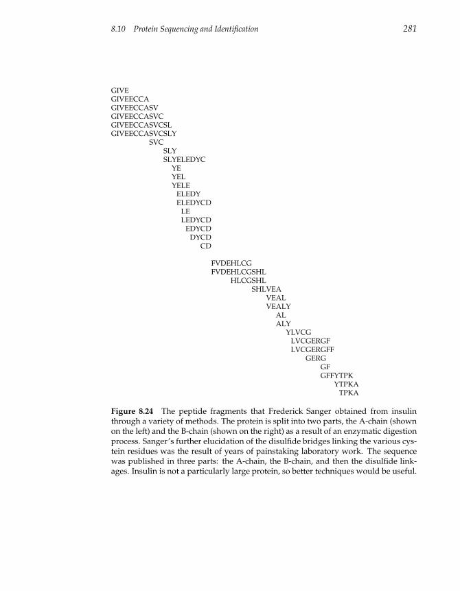
8.10 Protein Sequencing and Identification 281
GIVEGIVEECCAGIVEECCASVGIVEECCASVCGIVEECCASVCSLGIVEECCASVCSLY
SVCSLYSLYELEDYC
YEYELYELE
ELEDYELEDYCD
LELEDYCD
EDYCDDYCD
CD
FVDEHLCGFVDEHLCGSHL
HLCGSHLSHLVEA
VEALVEALY
ALALY
YLVCGLVCGERGFLVCGERGFF
GERGGFGFFYTPK
YTPKATPKA
Figure 8.24 The peptide fragments that Frederick Sanger obtained from insulinthrough a variety of methods. The protein is split into two parts, the A-chain (shownon the left) and the B-chain (shown on the right) as a result of an enzymatic digestionprocess. Sanger’s further elucidation of the disulfide bridges linking the various cys-tein residues was the result of years of painstaking laboratory work. The sequencewas published in three parts: the A-chain, the B-chain, and then the disulfide link-ages. Insulin is not a particularly large protein, so better techniques would be useful.
282 8 Graph Algorithms
tant component: one also needs to know what proteins the cell produces and
what they do. On the one hand, we do not yet know the full set of proteins
that cells produce, so we need a way to discover the sequence of previously
unknown proteins. On the other hand, it is important to identify which spe-
cific proteins interact in a biological system (e.g., those proteins involved in
DNA replication). Lastly, different cells in an organism have different reper-
toires of expressed proteins. Brain cells need different proteins to function
than liver cells do, and an important problem is to identify proteins that are
present or absent in each biological tissue under different conditions.
There are two types of computational problems motivated by protein se-
quencing. De novo protein sequencing is the elucidation of a protein’s sequence
in the case when a biological sample contains a protein that is either not
present in a database or differs from a canonical version present in a database
(e.g., mutated proteins or proteins with biochemical modifications). The
other problem is the identification of a protein that is present in a database;
this is usually referred to as protein identification. The main difference be-
tween protein sequencing algorithms and protein identification algorithms
is the difficulty of the underlying computational problems.
Perhaps the easiest way to illustrate the distinction between protein identi-
fication and sequencing is with a gedanken experiment. Suppose a biologist
wants to determine which proteins form the DNA polymerase complex in
rats. Having the complete rat genome sequence and knowing the location of
all the rat genes does not yet allow a biologist to determine what chemical
reactions occur during the DNA replication process. However, isolating a
rat’s DNA polymerase complex, breaking it apart, and sequencing the pro-
teins that form parts of the complex will yield a fairly direct answer to the
researcher’s question. Of course, if we presume that the biologist has the
complete rat genome sequence and all of its gene products, he may not actu-
ally have to sequence every amino acid in every protein in the DNA poly-
merase complex—just enough to figure out which proteins are present. This
is protein identification. On the other hand, if the researcher decides to study
an organism for which complete genome data are not available (perhaps an
obscure species of ant), then the researcher will need to perform de novo
protein sequencing.20
20. As usual with gedanken experiments, reality is more complicated. Even if the completegenomic sequence of a species is known and annotated, the repertoire of all possible proteinsusually is not, due to the myriad alternative splicings (different ways of constructing mRNAfrom the gene’s transcript) and post-translational modifications that occur in a living cell.
8.10 Protein Sequencing and Identification 283
For many problems, protein sequencing and identification remain the only
ways to probe a biological process. For example, gene splicing (see chap-
ter 6) is a complex process performed by the large molecular complex called
the spliceosome, which consists of over 100 different proteins complexed with
some functional RNA. Biologists want to determine the “parts list” of the
spliceosome, that is, the identity of proteins that form the complex. DNA
sequencing is not capable of solving this problem directly: even if all the
proteins in the genome were known, it is not clear which of them are parts
of the spliceosome. Protein sequencing and identification, on the other hand,
are very helpful in discovering this parts list. Recently, Matthias Mann and
colleagues purified the spliceosome complex and used protein sequencing
and protein identification techniques to find a detailed parts list for it.
Another application of these technologies is the study of proteins involved
in programmed cell death, or apoptosis. In the development of many organisms
cells must die at specific times. A cell dies if it fails to acquire certain survival
factors, and the death process can be initiated by the expression of certain
genes. In a developing nematode, for example, the death of individual cells
in the nervous system may be prevented by mutations in several genes that
are the subject of active investigation. DNA sequence data alone are not
sufficient to find the genes involved in programmed cell death, and until
recently, nobody knew the identity of these proteins. Protein analysis by mass
spectrometry allowed the sequencing of proteins involved in programmed cell
death, and the discovery of some proteins involved in the death-inducing
signaling complex.
The exceptional sensitivity of mass spectrometry has opened up new ex-
perimental and computational possibilities for protein studies. A protein can
be digested into peptides by proteases like trypsin. In a matter of seconds,
a tandem mass spectrometer breaks a peptide into even smaller fragments and
measures the mass of each. The mass spectrum of a peptide is a collection of
masses of these fragments. The protein sequencing problem is to derive the
sequence of a peptide given its mass spectrum. For an ideal fragmentation
process where every fragment of a peptide is generated, and in an ideal mass
spectrometer, the peptide sequencing problem is simple. However, the frag-
mentation process is not ideal, and mass spectrometers measure mass with
some imprecision. These details make peptide sequencing difficult.
A mass spectrometer works like a charged sieve. A large molecule (pep-
tide) gets broken into smaller fragments that have an electrical charge. These
fragments are then spun around and accelerated in a magnetic field until
they hit a detector. Because large fragments are harder to spin than small
284 8 Graph Algorithms
ones, one can distinguish between fragments with different masses based
on the amount of energy required to fling the different fragments around. It
happens that most molecules can be broken in several places, generating sev-
eral different ion types. The problem is to reconstruct the amino acid sequence
of the peptide from the masses of these broken pieces.
8.11 The Peptide Sequencing Problem
Let A = a1, a2, . . . , a20 be the set of amino acids, each with molecular
masses m(ai). A peptide P = p1 · · · pn is a sequence of amino acids, with par-
ent mass m(P ) =∑n
i=1 m(pi). We will denote the partial N-terminal peptide
p1, . . . , pi of mass mi =∑i
j=1 m(pj) as Pi and the partial C-terminal peptide
pi+1, . . . , pn of mass m(P )−mi as P−i , for 1 ≤ i ≤ n. Mass spectra obtained
by tandem mass spectrometry (MS/MS) consist predominantly of partial N-
terminal peptides and C-terminal peptides.21
A mass spectrometer typically breaks a peptide p1p2 · · · pn at different pep-
tide bonds and detects the masses of the resulting partial N-terminal and
C-terminal peptides.22 For example, the peptide GPFNA may be broken into
the N-terminal peptides G, GP, GPF, GPFN, and C-terminal peptides PFNA,
FNA, NA, A. Moreover, while breaking GPFNA into GP and FNA, it may
lose some small parts of GP and FNA, resulting in fragments of a lower mass.
For example, the peptide GP might lose a water (H2O), and the peptide FNA
might lose an ammonia (NH3). The resulting masses detected by the spec-
trometer will be equal to the mass of GP minus the mass of water (water
happens to weigh 1 + 1 + 16 = 18 daltons) , and the mass of FNA minus the
mass of ammonia (1 + 1 + 1 + 14 = 17 daltons). Peptides missing water and
ammonia are two different ion types that can occur in fragmenting a peptide
in a mass spectrometer.23
21. Every protein is a linear chain of amino acids, connected by a peptide bond. The peptidebond starts with a nitrogen (N) and ends with a carbon (C); therefore, every protein beginswith an “unstarted” peptide bond that begins with N and another “unfinished” peptide bondthat ends with C. An N-terminal peptide is a fragment of a protein that includes the “leftmost”end (i.e., the N-terminus). A C-terminal peptide is a fragment of a protein that includes the“rightmost” end (i.e., the C-terminus).22. Biologists typically work with billions of identical peptides in a solution. A mass spectrome-try machine breaks different peptide molecules at different peptide bonds (some peptide bondsare more prone to breakage than others). As a result, many N-terminal and C-terminal peptidemay be detected by a mass spectrometer.23. This is a simplified description of the complex and messy fragmentation process. In thissection we intentionally hide many of the technical details and focus only on the computationalchallenges.
8.11 The Peptide Sequencing Problem 285
Peptide fragmentation in a tandem mass spectrometer can be character-
ized by a set of numbers ∆ = δ1, . . . , δk representing the different types of
ions that correspond to the removal of a certain chemical group from a pep-
tide fragment. We will call ∆ the set of ion types. A δ-ion of an N-terminal
partial peptide Pi is a modification of Pi that has mass mi − δ, correspond-
ing to the loss of a (typically small) chemical group of mass δ when P was
fragmented into Pi. The δ-ion of C-terminal peptides is defined similarly.
The most frequent N-terminal ions are called b-ions (ion bi corresponds to Pi
with δ = −1) and the most frequent C-terminal ions are called y-ions (ion yi
corresponds to P−i with δ = 19), shown in figure 8.25 (a). Examples of other
frequent N-terminal ions are represented by b-H2O (a b-fragment that loses a
water) or y-NH3 and some others like b-H2O-NH3.
For tandem mass spectrometry, the theoretical spectrum T (P ) of peptide
P can be calculated by subtracting all possible ion types δ1, . . . , δk from the
masses of all partial peptides of P , such that every partial peptide generates
k masses in the theoretical spectrum, as in figure 8.25 (b).24
An experimental spectrum S = s1, . . . , sq is a set of numbers obtained in
a mass spectrometry experiment that includes masses of some fragment ions
as well as chemical noise.25 Note that the distinction between the theoretical
spectrum T (P ) and the experimental spectrum S is that you mathematically
generate T (P ) given the peptide sequence P , but you experimentally gener-
ate S without knowing what the peptide sequence is that generated it.
The match between the experimentally measured spectrum S and peptide
P is the number of masses in S that are equal to masses in T (P ). This is often
referred to as the shared peaks count. In reality, peptide sequencing algorithms
use more sophisticated objective functions than a simple shared peaks count,
incorporating different weighting functions for the matching masses. We
formulate the Peptide Sequencing problem as follows.
24. A theoretical spectrum of a peptide may contain as many as 2nk masses but it sometimescontains less since some of these masses are not unique.25. In reality, a mass spectrometer detects charged ions and measures mass-to-charge ratios. As aresult, an experimental spectrum contains the values m
zwhere m is the mass and z is an integer
(typically, 1 or 2) equal to the charge of a fragment ion. For simplicity we assume that z = 1through the remainder of this chapter.
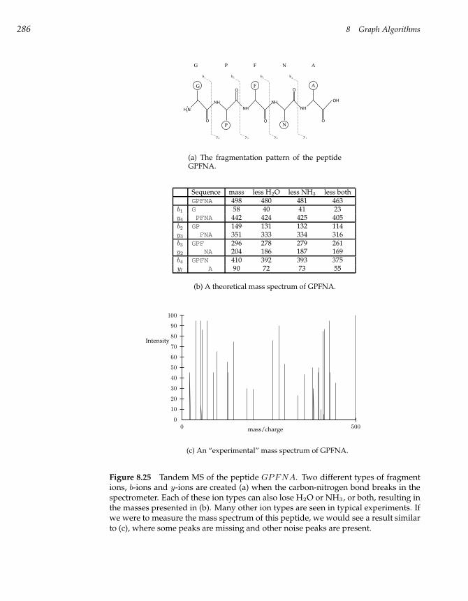
286 8 Graph Algorithms
O O O
OO
NH
NH
NH
NH
H N3
+
OH
G
G
P
P
F
F
N
N
A
A
b1 2 4
y4
b
y3
b3
y2
b
y1
(a) The fragmentation pattern of the peptideGPFNA.
Sequence mass less H2O less NH3 less bothGPFNA 498 480 481 463
b1 G 58 40 41 23y4 PFNA 442 424 425 405b2 GP 149 131 132 114y3 FNA 351 333 334 316b3 GPF 296 278 279 261y2 NA 204 186 187 169b4 GPFN 410 392 393 375yl A 90 72 73 55
(b) A theoretical mass spectrum of GPFNA.
0 5000
10
20
30
40
50
60
70
80
90
100
mass/charge
Intensity
(c) An “experimental” mass spectrum of GPFNA.
Figure 8.25 Tandem MS of the peptide GPFNA. Two different types of fragmentions, b-ions and y-ions are created (a) when the carbon-nitrogen bond breaks in thespectrometer. Each of these ion types can also lose H2O or NH3, or both, resulting inthe masses presented in (b). Many other ion types are seen in typical experiments. Ifwe were to measure the mass spectrum of this peptide, we would see a result similarto (c), where some peaks are missing and other noise peaks are present.
8.12 Spectrum Graphs 287
Peptide Sequencing Problem:
Find a peptide whose theoretical spectrum has a maximum match to a
measured experimental spectrum.
Input: Experimental spectrum S, the set of possible ion
types ∆, and the parent mass m.
Output: A peptide P of mass m whose theoretical spectrum
matches S better than any other peptide of mass m.
In reality, mass spectrometers measure both mass and intensity, which re-
flects the number of fragment ions of a given mass are detected in the mass
spectrometer. As a result, mass spectrometrists often represent spectra in two
dimensions, as in figure 8.25 (c), and refer to the masses in the spectrum as
“peaks.”26
8.12 Spectrum Graphs
There are two main approaches to solving the Peptide Sequencing prob-
lem that researchers have tried: either through exhaustive search among all
amino acid sequences of a certain length, or by analyzing the spectrum graph
which we define below. The former approach involves the generation of
all 20l amino acid sequences of length l and their corresponding theoretical
spectra, with the goal of finding a sequence with the best match between
the experimental spectrum and the sequence’s theoretical spectrum. Since
the number of sequences grows exponentially with the length of the pep-
tide, different branch-and-bound techniques have been designed to limit the
combinatorial explosion in these methods. Prefix pruning restricts the compu-
tational space to sequences whose prefixes match the experimental spectrum
well. The difficulty with the prefix pruning is that it frequently discards the
correct sequence if its prefixes are poorly represented in the spectrum.
The spectrum graph approach, on the other hand, does not involve gen-
erating all amino acid sequences, and leads to a fast algorithm for peptide
sequencing. In this approach, we construct a graph from the experimen-
tal spectrum. Assume for simplicity that an experimental spectrum S =
26. A match of a theoretical spectrum against an experimental spectrum with varying intensity,then, needs to reflect the intensity of the fragment ions. While accounting for intensities is im-portant for statistical analysis, it does not seriously affect the algorithmic details and we ignoreintensities in the remainder of this chapter.
288 8 Graph Algorithms
s1, . . . , sq consists of N-terminal ions and we will ignore the C-terminal
ions for a while. Every mass s ∈ S may have been created from a partial
peptide by one of the k different ion types. Since we do not know which ion
type from ∆ = (δ1, . . . , δk) created the mass s in the experimental spectrum,
we generate k different “guesses” for each of masses in the experimental
spectrum. Every guess corresponds to the hypothesis that s = x− δj , where
x is the mass of some partial peptide and 1 ≤ j ≤ k. Therefore, for every
mass s in the experimental spectrum, there are k guesses for the mass x of
some partial peptide: s + δ1, s + δ2, . . . , s + δk. As a result, each mass in the
experimental spectrum is transformed into a set of k vertices in the spectrum
graph, one for each possible ion type. The vertex for δi for the mass s is la-
beled with mass s + δi. We connect any two vertices u and v in the graph by
the directed edge (u, v) if the mass of v is larger than that of u by the mass of
a single amino acid. If we add a vertex at 0 and a vertex at the parent mass
m (connecting them to other vertices as before), then the Peptide Sequencing
problem can be cast as finding a path from 0 to m in the resulting DAG.27
In summary, the vertex set of the resulting spectrum graph is a set of num-
bers si + δj representing potential masses of N-terminal peptides adjusted
by the ion type δj . Every mass si of spectrum S generates k distinct ver-
tices Vi(s) = si + δ1, . . . , si + δk, though the sets Vi and Vj may overlap
if si and sj are close. The set of vertices in a spectrum graph is therefore
sinitial ∪ V1 ∪ · · · ∪ Vq ∪ sfinal, where sinitial = 0 and sfinal = m. The
spectrum graph may have at most qk + 2 vertices. We label the edges of
the spectrum graph by the amino acid whose mass is equal to difference be-
tween vertex masses. If we look at vertices as putative N-terminal peptides,28
the edge from u to v implies that the N-terminal sequence corresponding to
v may be obtained by extending the sequence at u by the amino acid that
labels (u, v).
A spectrum S of a peptide P = p1 . . . pn is called complete if S contains at
least one ion type corresponding to every N-terminal partial peptide Pi for
every 1 ≤ i ≤ n. The use of a spectrum graph is based on the observation
that for a complete spectrum there exists a path of length n+1 from sinitial to
sfinal in the spectrum graph that is labeled by P . This observation casts the
Peptide Sequencing problem as one of finding the “correct” path in the set
of all paths between two vertices in a directed acyclic graph. If the spectrum
27. In addition to the experimental spectrum, every mass spectrometry experiment always pro-duces the parent mass m of a peptide.28. Although we ignored C-terminal ions in this simplified construction of the spectrum graph,these ions can be taken into account by combining the spectrum S with its “reversed” version.
8.12 Spectrum Graphs 289
is complete, then the correct path that we are looking for is often the path
with the maximum number of edges, the familiar Longest Path in a DAG
problem.
Unfortunately, experimental spectra are frequently incomplete. Moreover,
even if the experimental spectrum is complete, there are often many paths
in the spectrum graph to choose from that have the same (or even larger)
length, preventing one from unambiguously reconstructing the peptide.
The problem with choosing a path with a maximum number of edges is
that it does not adequately reflect the “importance” of different vertices. For
example, a vertex in the spectrum graph obtained by a shift of +1 as si + 1
(corresponding to the most frequent b-ions) should be scored higher than a
vertex obtained by a shift of the rare b-H2O-NH3 ion (si+1−18−17 = si−34).
Further, whenever there are two peaks si and si′ such that si + δj=si′ + δj′ ,
the vertex corresponding to that mass should also get a higher score than a
vertex obtained by a single shift.
In the probabilistic approach to peptide sequencing, each ion type δi has
some probability of occurring, which we write as p(δi). Under the simplest
assumption, the probability that δi occurs for some partial peptide is inde-
pendent of whether δj also occurs for the same partial peptide. Under this
assumption, any given partial peptide may contribute as many as k masses in
the spectrum [this happens with probability∏k
i=1 p(δi)] and as few as 0 [this
happens with probability∏k
i=1(1 − p(δi))]. The probabilistic model below
scores the vertices of the spectrum graph based on these simple assumptions.
Suppose that an N-terminal partial peptide Pi with mass mi produces ions
δ1, . . . , δl (“present” ions of mass mi − δ1, mi − δ2, . . . , mi − δl ) but fails to
produce ions δl+1, . . . , δk (“missing” ions) in the experimental spectrum. All
l present ions will result in a vertex in the spectrum graph at mass mi, corre-
sponding to Pi. How should we score this vertex? A naive approach would
be to reward Pi for every ion type that explains it, suggesting a score of∏l
i=1 p(δi). However, this approach has the disadvantage of not consider-
ing the missing ions, so we combine those in by defining the score for the
partial peptide to be
(
l∏
i=1
p(δi)
)(
k∏
i=l+1
(1− p(δi))
)
.
However, there is some inherent probability of chemical noise, that is, it can
produce any mass (that has nothing to do with a peptide of interest) with
290 8 Graph Algorithms
certain probability pR. Therefore, we adjust the probabilistic score as
(
l∏
i=1
p(δi)
pR
)(
k∏
i=l+1
1− p(δi)
1− pR
)
.
8.13 Protein Identification via Database Search
De novo protein sequencing algorithms are invaluable for identification of
(both known and unknown) proteins, but they are most useful when work-
ing with complete or nearly complete high-quality spectra. Many spectra are
far from complete, and de novo peptide sequencing algorithms often pro-
duce ambiguous solutions for such spectra. If we had access to a database of
all proteins from a genome, then we would no longer need to consider all 20l
peptide sequences to interpret an MS/MS spectrum, but could instead limit
our search to peptides present in this database.
Currently, most proteins are identified by database search— effectively
looking the answer up in “the back of a book.” Indeed, an experimental
spectrum can be compared with the theoretical spectrum for each peptide
in such a database, and the entry in the database that best matches the ob-
served spectrum usually provides the sequence of the experimental peptide.
This forms the basis of the popular SEQUEST algorithm developed by John
Yates and colleagues. We formulate the Protein Identification problem as
follows.
Protein Identification Problem:
Find a protein from a database that best matches the experimental
spectrum.
Input: A database of proteins, an experimental spectrum S,
a set of ion types ∆, and a parent mass m.
Output: A protein of mass m from the database with the
best match to spectrum S.
Though the logic that SEQUEST uses to determine whether a database
entry matches an experimental spectrum is somewhat involved, the basic
approach of the algorithm is just a linear search through the database. One
drawback to MS/MS database search algorithms like SEQUEST is that pep-
tides in a cell are often slightly different from the “canonical” peptides present
8.13 Protein Identification via Database Search 291
in databases. The synthesis of proteins on ribosomes is not the final step in
a protein’s life: many proteins are subject to further modifications that reg-
ulate protein activities and these modifications may be either permanent or
reversible. For example, the enzymatic activity of some proteins is regulated
by the addition or removal of a phosphate group at a specific residue.29 Phos-
phorylation is a reversible process: protein kinases add phosphate groups while
phosphatases remove them.
Proteins form complex systems necessary for cellular signaling and meta-
bolic regulation, and are therefore often subject to a large number of bio-
chemical modifications (e.g., phosphorylation and glycosylation). In fact,
almost all protein sequences are modified after they have been constructed
from their mRNA template, and as many as 200 distinct types of modifica-
tions of amino acid residues are known. Since we are unable to predict these
post-translational modifications from DNA sequences, finding naturally occur-
ring modifications remains an important open problem. Computationally,
a chemical modification of the protein p1p2 · · · pi · · · pn at position i results
in increased mass of the N-terminal peptides Pi, Pi+1, . . . , Pn and increased
mass of the C-terminal peptides P−1 , P−
2 , . . . , P−i−1.
The computational analysis of modified peptides was also pioneered by
John Yates, who suggested an exhaustive search approach that (implicitly)
generates a virtual database of all modified peptides from a small set of po-
tential modifications, and matches the experimental spectrum against this
virtual database. It leads to a large combinatorial problem, even for a small
set of modification types.
Modified Protein Identification Problem:
Find a peptide from the database that best matches the experimental
spectrum with up to k modifications.
Input: A database of proteins, an experimental spectrum S,
a set of ion types ∆, a parent mass m, and a parameter k
capping the number of modifications.
Output: A protein of mass m with the best match to spec-
trum S that is at most k modifications away from an entry
in the database.
The major difficulty with the Modified Protein Identification problem is
29. Phosphorylation uses serine, threonine, or tyrosine residues to add a phosphate group.
292 8 Graph Algorithms
that very similar peptides P1 and P2 may have very different spectra S1 and
S2.30 Our goal is to define a notion of spectral similarity that correlates well
with sequence similarity. In other words, if P1 and P2 are a few modifica-
tions apart, the spectral similarity between S1 and S2 should be high. The
shared peaks count is, of course, an intuitive measure of spectral similarity.
However, this measure diminishes very quickly as the number of mutations
increases, thus leading to limitations in detecting similarities by database
search. Moreover, there are many correlations between the spectra of related
peptides, and only a small proportion of these correlations is captured by the
shared peaks count.
The spectral convolution algorithm, below, reveals potential peptide mod-
ifications without an exhaustive search and therefore does not require gener-
ating a virtual database of modified peptides.
8.14 Spectral Convolution
Let S1 and S2 be two spectra. Define the spectral convolution to be the multiset
S2S1 = s2 − s1 : s1 ∈ S1, s2 ∈ S2 and let (S2S1)(x) be the multiplicity
of element x in this multiset. In other words, (S2 S1)(x) is the number of
pairs (s1 ∈ S1, s2 ∈ S2) such that s2 − s1 = x (fig. 8.26).
The shared peak count that we introduced earlier in this chapter is the
number of masses common to both S1 and S2, and is simply (S2 S1)(0).
MS/MS database search algorithms that maximize the shared peak count
find a peptide in the database that maximizes (S2 S1)(0), where S2 is an
experimental spectrum and S1 is the theoretical spectrum of a peptide in
the database. However, if S1 and S2 correspond to peptides that differ by
k mutations or modifications, the value of (S2 S1)(0) may be too small to
determine that S1 and S2 really were generated by similar peptides. As a
result, the power of the shared peak count to discern that two peptides are
similar diminishes rapidly as the number of modifications increases—it is
bad at k = 1, and nearly useless for k > 1.
The peaks in the spectral convolution allow us to detect mutations and
modifications, even if the shared peak count is small. If peptides P2 and P1
(corresponding to spectra S2 and S1) differ by only one mutation (k = 1)
with amino acid difference δ = m(P2) −m(P1), then S2 S1 is expected to
have two approximately equal peaks at x = 0 and x = δ. If the mutation
30. P1 corresponds to a peptide from the database, while P2 corresponds to the modified ver-sion of P1, whose experimental spectrum is being used to search the database.
8.15 Spectral Alignment 293
occurs at position t in the peptide, then the peak at (S2 S1)(0) corresponds
to N-terminal peptides Pi for i < t and C-terminal peptides P−i for i ≥ t.
The peak at (S2 S1)(δ) corresponds to N-terminal peptides Pi for i ≥ t and
C-terminal peptides P−i for i < t.
Now assume that P2 and P1 are two substitutions apart, one with mass
difference δ′ and another with mass difference δ − δ′, where δ denotes the
difference between the parent masses of P1 and P2. These modifications
generate two new peaks in the spectral convolution at (S2 S1)(δ′) and at
(S2 S1)(δ − δ′). It is therefore reasonable to define the similarity between
spectra S1 and S2 as the overall height of the k highest peaks in S2 S1.
Although spectral convolution helps to identify modified peptides, it does
have a limitation. Let
S = 10, 20, 30, 40, 50, 60, 70, 80, 90, 100
be a spectrum of peptide P , and assume for simplicity that P produces only
b-ions. Let
S′ = 10, 20, 30, 40, 50, 55, 65, 75, 85, 95
and
S′′ = 10, 15, 30, 35, 50, 55, 70, 75, 90, 95
be two theoretical spectra corresponding to peptides P ′ and P ′′ from the
database. Which of the two peptides fits S better? The shared peaks count
does not allow one to answer this question, since both S′ and S′′ have five
peaks in common with S. Moreover, the spectral convolution also does not
answer this question, since both S S′ and S S′′ reveal strong peaks of
the same height at 0 and 5. This suggests that both P ′ and P ′′ can be ob-
tained from P by a single mutation with mass difference 5. However, a more
careful analysis shows that although this mutation can be realized for P ′ by
introducing a shift 5 after mass 50, it cannot be realized for P ′′. The major
difference between S′ and S′′ is that the matching positions in S′ come in
clumps while the matching positions in S′′ do not. Below we describe the
spectral alignment approach, which addresses this problem.
8.15 Spectral Alignment
Let A = a1, . . . , an be an ordered set of integers a1 < a2 < · · · < an.
A shift ∆i transforms A into a1, . . . ai−1, ai + ∆i, . . . , an + ∆i. That is, ∆i
alters all elements in the sequence except for the first i− 1 elements. We only
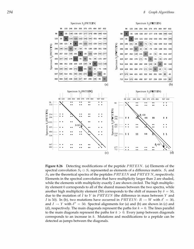
294 8 Graph Algorithms
98 133 246 254 355 375 476 484 597 632
98133
254
296
355
425
484
526
647682
δ=50
Spectrum S11(PRTEIINN))
Spe
ctru
m S
22(PR
TE
YYN
)
98 133 246 254 355 375 476 484 597 632
98133
284296
385425
514526
677712
δδ1 =30
δδ22=50
Spe
ctru
m S
22(PWW
TE
YYN
)
Spectrum S11(PRRTEIIN)
(c) (d)
98 133 246 254 355 375 476 484 597 632
98 00 − 35 − 148 − 156 − 257 − 277 − 378 − 386 − 499 − 534
133 35 00 − 133 − 121 − 222 − 242 − 343 − 351 − 464 − 499
254 156 121 88 00 − 101 − 121 − 222 − 230 − 343 − 378
296 198 163 50 42 − 59 − 79 − 180 − 188 − 301 − 336
355 257 222 109 101 00 − 20 − 121 − 129 − 242 − 277
425 327 292 179 171 70 50 − 51 − 59 − 172 − 207
484 386 351 238 230 129 109 88 00 − 113 − 148
526 428 393 280 272 171 151 50 42 − 71 − 106
647 549 514 401 393 292 272 171 163 50 15
682 584 549 436 428 327 307 206 198 85 50
98 133 246 254 355 375 476 484 597 632
98 00 − 35 − 148 − 156 − 257 − 277 − 378 − 386 − 499 − 534
133 35 00 − 133 − 121 − 222 − 242 − 343 − 351 − 464 − 499
284 186 151 38 30 − 71 − 91 − 192 − 200 − 313 − 348
296 198 163 50 42 − 59 − 79 − 180 − 188 − 301 − 336
385 287 252 139 131 30 10 − 91 − 99 − 212 − 247
425 327 292 179 171 70 50 − 51 − 59 − 172 − 207
514 416 381 268 260 159 139 38 30 − 83 − 118
526 428 393 280 272 171 151 50 42 − 71 − 106
677 579 544 431 423 322 302 201 193 80 45
712 614 579 466 458 357 337 236 228 115 80
Spectrum S11(PRTEIIN)
Spe
ctru
m S
22(PR
TE
YYN
)
Spectrum S11(PRRTEIIN)
Spe
ctru
m S
22(PWW
TE
YYN
)
(a) (b)
Figure 8.26 Detecting modifications of the peptide PRTEIN . (a) Elements of thespectral convolution S2 S1 represented as elements of a difference matrix. S1 andS2 are the theoretical spectra of the peptides PRTEIN and PRTEY N , respectively.Elements in the spectral convolution that have multiplicity larger than 2 are shaded,while the elements with multiplicity exactly 2 are shown circled. The high multiplic-ity element 0 corresponds to all of the shared masses between the two spectra, whileanother high multiplicity element (50) corresponds to the shift of masses by δ = 50,due to the mutation of I to Y in PRTEIN (the difference in mass between Y andI is 50). In (b), two mutations have occurred in PRTEIN : R → W with δ′ = 30,and I → Y with δ′′ = 50. Spectral alignments for (a) and (b) are shown in (c) and(d), respectively. The main diagonals represent the paths for k = 0. The lines parallelto the main diagonals represent the paths for k > 0. Every jump between diagonalscorresponds to an increase in k. Mutations and modifications to a peptide can bedetected as jumps between the diagonals.
8.15 Spectral Alignment 295
consider shifts that do not change the order of elements, that is, the shifts
with ∆i ≥ ai−1 − ai. The k-similarity, D(k), between sets A and B is defined
as the maximum number of elements in common between these sets after k
shifts. For example, a shift −56 transforms
S = 10, 20, 30, 40, 50, 60, 70, 80, 90, 100
into
S′ = 10, 20, 30, 40, 50,55,65,75,85,95 .
Therefore D(1) = 10 for these sets. The set
S′′ = 10, 15, 30, 35, 50, 55, 70, 75, 90, 95
has five elements in common with S (the same as S′) but there is no single
shift transforming S into S′′ (D(1) = 6). Below we analyze and solve the
following Spectral Alignment problem:
Spectral Alignment Problem:
Find the k-similarity between two sets.
Input: Sets A and B, which represent the two spectra, and a
number k (number of shifts).
Output: The k-similarity, D(k), between sets A and B.
One can represent sets A = a1, . . . , an and B = b1, . . . , bm as 0–1 ar-
rays a and b of length an and bm correspondingly. The array a will contain n
ones (at positions a1, . . . , an) and an− n zeros, while the array b will contain
m ones (at positions b1, . . . , bm) and bm −m zeros.31 In such a model, a shift
∆i < 0 is simply a deletion of ∆i zeros from a, while a shift ∆i > 0 is simply
an insertion of ∆i zeros in a. With this model in mind, the Spectral Align-
ment problem is simply to find the edit distance between a and b when the
elementary operations are deletions and insertions of blocks of zeros. As we
saw in chapter 6, these operations can be modeled by long horizontal and
vertical edges in a Manhattan-like graph. The only differences between the
traditional Edit Distance problem and the Spectral Alignment problem are a
somewhat unusual alphabet and the scoring of paths in the resulting graph.
The analogy between the Edit Distance problem and the Spectral Alignment
31. We remark that this is not a particularly dense encoding of the spectrum.
296 8 Graph Algorithms
problem leads us to frame spectral alignment as a type of longest path prob-
lem.
Define a spectral product A ⊗ B to be the an × bm two-dimensional matrix
with nm ones corresponding to all pairs of indices (ai, bj) and all remaining
elements zero. The number of ones on the main diagonal of this matrix de-
scribes the shared peaks count between spectra A and B, or in other words,
0-similarity between A and B. Figure 8.27 shows the spectral products S⊗S′
and S⊗S′′ for the example from the previous section. In both cases the num-
ber of ones on the main diagonal is the same, and D(0) = 5. The δ-shifted
peaks count is the number of ones on the diagonal that is δ away from the
main diagonal. The limitation of the spectral convolution is that it considers
diagonals separately without combining them into feasible mutation scenar-
ios. The k-Similarity between spectra is defined as the maximum number
of ones on a path through the spectral matrix that uses at most k + 1 di-
agonals, and the k-optimal spectral alignment is defined as the path that uses
these k + 1 diagonals. For example, 1-similarity is defined by the maximum
number of ones on a path through this matrix that uses at most two diago-
nals. Figure 8.27 demonstrates the notion that 1-similarity shows that S is
closer to S′ than to S′′; in the first case the optimal two-diagonal path covers
ten 1s (left matrix), versus six in the second case (right matrix). Figure 8.28
illustrates that the spectral alignment detects more and more subtle similar-
ities between spectra, simply by increasing k [compare figures 8.26 (c) and
(d)].32 Below we describe a dynamic programming algorithm for spectral
alignment.
Let Ai and Bj be the i-prefix of A and j-prefix of B, respectively. Define
Dij(k) as the k-similarity between Ai and Bj such that the last elements of
Ai and Bj are matched. In other words, Dij(k) is the maximum number of
ones on a path to (ai, bj) that uses at most k + 1 different diagonals. We say
that (i′, j′) and (i, j) are codiagonal if ai− ai′ = bj − bj′ and that (i′, j′) < (i, j)
if i′ < i and j′ < j. To take care of the initial conditions, we introduce a
fictitious element (0, 0) with D0,0(k) = 0 and assume that (0, 0) is codiagonal
with any other (i, j). The dynamic programming recurrence for Dij(k) is
then
Dij(k) = max(i′,j′)<(i,j)
Di′j′ (k) + 1, if (i′, j′) and (i, j) are codiagonal
Di′j′ (k − 1) + 1, otherwise.
The k-similarity between A and B is given by D(k) = maxij Dij(k).
32. To a limit, of course. When k is too large, the spectral alignment is not very useful.
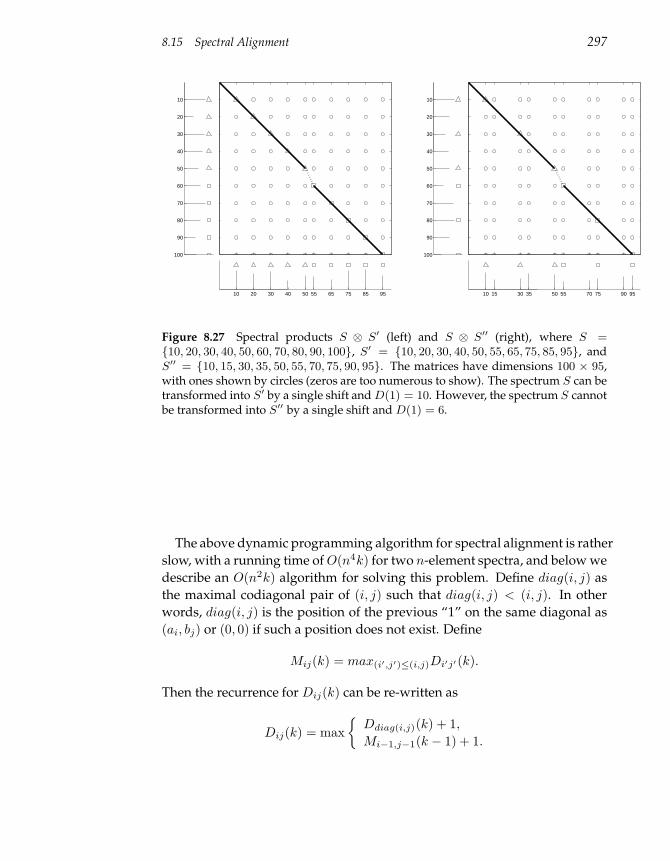
8.15 Spectral Alignment 297
10 20 30 40 50 55 65 75 85 95
10
20
30
40
50
60
70
80
90
100
10 15 30 35 50 55 70 75 90 95
10
20
30
40
50
60
70
80
90
100
Figure 8.27 Spectral products S ⊗ S′ (left) and S ⊗ S′′ (right), where S =10, 20, 30, 40, 50, 60, 70, 80, 90, 100, S′ = 10, 20, 30, 40, 50, 55, 65, 75, 85, 95, andS′′ = 10, 15, 30, 35, 50, 55, 70, 75, 90, 95. The matrices have dimensions 100 × 95,with ones shown by circles (zeros are too numerous to show). The spectrum S can betransformed into S′ by a single shift and D(1) = 10. However, the spectrum S cannotbe transformed into S′′ by a single shift and D(1) = 6.
The above dynamic programming algorithm for spectral alignment is rather
slow, with a running time of O(n4k) for two n-element spectra, and below we
describe an O(n2k) algorithm for solving this problem. Define diag(i, j) as
the maximal codiagonal pair of (i, j) such that diag(i, j) < (i, j). In other
words, diag(i, j) is the position of the previous “1” on the same diagonal as
(ai, bj) or (0, 0) if such a position does not exist. Define
Mij(k) = max(i′,j′)≤(i,j)Di′j′(k).
Then the recurrence for Dij(k) can be re-written as
Dij(k) = max
Ddiag(i,j)(k) + 1,
Mi−1,j−1(k − 1) + 1.
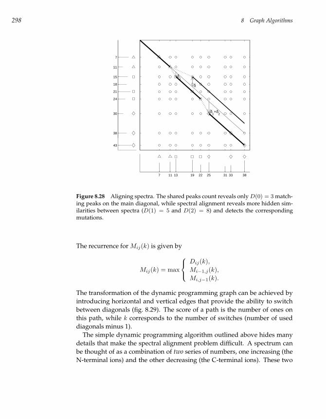
298 8 Graph Algorithms
δ1
δ
δ1+δ
2
7 11 13 19 22 25 31 33 38
7
11
15
18
21
24
30
38
43
Figure 8.28 Aligning spectra. The shared peaks count reveals only D(0) = 3 match-ing peaks on the main diagonal, while spectral alignment reveals more hidden sim-ilarities between spectra (D(1) = 5 and D(2) = 8) and detects the correspondingmutations.
The recurrence for Mij(k) is given by
Mij(k) = max
Dij(k),
Mi−1,j(k),
Mi,j−1(k).
The transformation of the dynamic programming graph can be achieved by
introducing horizontal and vertical edges that provide the ability to switch
between diagonals (fig. 8.29). The score of a path is the number of ones on
this path, while k corresponds to the number of switches (number of used
diagonals minus 1).
The simple dynamic programming algorithm outlined above hides many
details that make the spectral alignment problem difficult. A spectrum can
be thought of as a combination of two series of numbers, one increasing (the
N-terminal ions) and the other decreasing (the C-terminal ions). These two
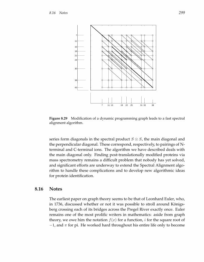
8.16 Notes 299
7 11 13 19 22 25 31 33 38
7
11
15
18
21
24
30
38
43
Figure 8.29 Modification of a dynamic programming graph leads to a fast spectralalignment algorithm.
series form diagonals in the spectral product S ⊗ S, the main diagonal and
the perpendicular diagonal. These correspond, respectively, to pairings of N-
terminal and C-terminal ions. The algorithm we have described deals with
the main diagonal only. Finding post-translationally modified proteins via
mass spectrometry remains a difficult problem that nobody has yet solved,
and significant efforts are underway to extend the Spectral Alignment algo-
rithm to handle these complications and to develop new algorithmic ideas
for protein identification.
8.16 Notes
The earliest paper on graph theory seems to be that of Leonhard Euler, who,
in 1736, discussed whether or not it was possible to stroll around Königs-
berg crossing each of its bridges across the Pregel River exactly once. Euler
remains one of the most prolific writers in mathematics: aside from graph
theory, we owe him the notation f(x) for a function, i for the square root of
−1, and π for pi. He worked hard throughout his entire life only to become
300 8 Graph Algorithms
blind. He commented: “Now I will have fewer distractions,” and proceeded
to write hundreds of papers more.
Graph theory was forgotten for a century, but was revived in the second
half of the nineteenth century by prominent scientists such as Sir William
Hamilton (who, among many other things, invented quaternions) and Gus-
tav Kirchhoff (who is responsible for Kirchhoff’s laws).
DNA arrays were proposed simultaneously and independently in 1988 by
Radoje Drmanac and colleagues in Yugoslavia (29), Andrey Mirzabenov and
colleagues in Russia (69), and Ed Southern in the United Kingdom (100).
The inventors of DNA arrays suggested using them for DNA sequencing,
and the original name for this technology was sequencing by hybridization.
A major breakthrough in DNA array technology was made by Steve Fodor
and colleagues in 1991 (38) when they adapted photolithography (a process
similar to computer chip manufacturing) to DNA synthesis. The Eulerian
path approach to SBH was described in (83).
Sanger’s approach to protein sequencing influenced work on RNA se-
quencing. Before biologists figured out how to sequence DNA, they rou-
tinely sequenced RNA. The first RNA sequencing project resulted in seventy-
seven ribonucleotides and took seven years to complete, though in 1965
RNA sequencing used the same “break—read the fragments—assemble” ap-
proach that is used for DNA sequencing today. For many years, DNA se-
quencing was done by first transcribing DNA to RNA and then sequencing
the RNA.
DNA sequencing methods were invented independently and simultane-
ously in 1977 by Frederick Sanger and colleagues (91) and Walter Gilbert and
colleagues (74). The overlap-layout-consensus approach to DNA sequenc-
ing was first outlined in 1984 (82) and further developed by John Kececioglu
and Eugene Myers in 1995 (55). DNA sequencing progressed to handle the
entire 1800 kb H. influenzae bacterium genome in the mid-1990s. In 1997, in-
spired by this breakthrough, James Weber and Eugene Myers (110) proposed
the whole-genome shotgun approach (first outlined by Jared Roach and col-
leagues in 1995 (87)) to sequence the entire human genome. The human
genome was sequenced in 2001 by J. Craig Venter and his team at Celera Ge-
nomics (104) with the whole genome shotgun approach, and independently
by Eric Lander and his colleagues at the Human Genome Consortium (62)
using the BAC-by-BAC approach.
Early approaches to protein sequencing by mass spectrometry were based
on manual peptide reconstruction and the assembly of those peptides into
protein sequences (51). The description of the spectrum graph approach pre-

8.16 Notes 301
sented in this chapter is from Vlado Dancik and colleagues (25). Searching
a database for the purposes of protein identification in mass spectrometry
was pioneered by Matthias Mann and John Yates in 1994 (71; 34). In 1995
Yates (112) extended his original SEQUEST algorithm to search for modified
peptides based on a virtual database of all modified peptides. The spectral
alignment algorithm was introduced five years later (84).
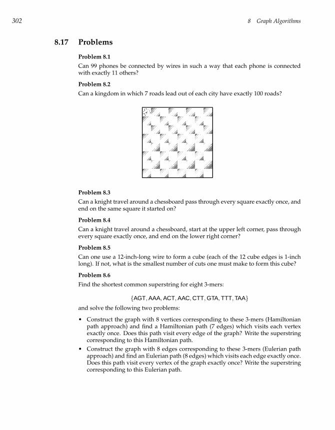
302 8 Graph Algorithms
8.17 Problems
Problem 8.1
Can 99 phones be connected by wires in such a way that each phone is connectedwith exactly 11 others?
Problem 8.2
Can a kingdom in which 7 roads lead out of each city have exactly 100 roads?
Problem 8.3
Can a knight travel around a chessboard pass through every square exactly once, andend on the same square it started on?
Problem 8.4
Can a knight travel around a chessboard, start at the upper left corner, pass throughevery square exactly once, and end on the lower right corner?
Problem 8.5
Can one use a 12-inch-long wire to form a cube (each of the 12 cube edges is 1-inchlong). If not, what is the smallest number of cuts one must make to form this cube?
Problem 8.6
Find the shortest common superstring for eight 3-mers:
AGT, AAA, ACT, AAC, CTT, GTA, TTT, TAAand solve the following two problems:
• Construct the graph with 8 vertices corresponding to these 3-mers (Hamiltonianpath approach) and find a Hamiltonian path (7 edges) which visits each vertexexactly once. Does this path visit every edge of the graph? Write the superstringcorresponding to this Hamiltonian path.
• Construct the graph with 8 edges corresponding to these 3-mers (Eulerian pathapproach) and find an Eulerian path (8 edges) which visits each edge exactly once.Does this path visit every vertex of the graph exactly once? Write the superstringcorresponding to this Eulerian path.
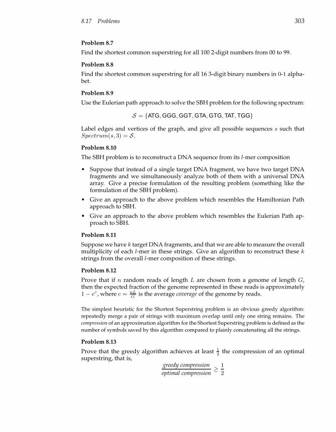
8.17 Problems 303
Problem 8.7
Find the shortest common superstring for all 100 2-digit numbers from 00 to 99.
Problem 8.8
Find the shortest common superstring for all 16 3-digit binary numbers in 0-1 alpha-bet.
Problem 8.9
Use the Eulerian path approach to solve the SBH problem for the following spectrum:
S = ATG, GGG, GGT, GTA, GTG, TAT, TGG
Label edges and vertices of the graph, and give all possible sequences s such thatSpectrum(s, 3) = S .
Problem 8.10
The SBH problem is to reconstruct a DNA sequence from its l-mer composition
• Suppose that instead of a single target DNA fragment, we have two target DNAfragments and we simultaneously analyze both of them with a universal DNAarray. Give a precise formulation of the resulting problem (something like theformulation of the SBH problem).
• Give an approach to the above problem which resembles the Hamiltonian Pathapproach to SBH.
• Give an approach to the above problem which resembles the Eulerian Path ap-proach to SBH.
Problem 8.11
Suppose we have k target DNA fragments, and that we are able to measure the overallmultiplicity of each l-mer in these strings. Give an algorithm to reconstruct these kstrings from the overall l-mer composition of these strings.
Problem 8.12
Prove that if n random reads of length L are chosen from a genome of length G,then the expected fraction of the genome represented in these reads is approximately1− ec, where c = nL
Gis the average coverage of the genome by reads.
The simplest heuristic for the Shortest Superstring problem is an obvious greedy algorithm:
repeatedly merge a pair of strings with maximum overlap until only one string remains. The
compression of an approximation algorithm for the Shortest Superstring problem is defined as the
number of symbols saved by this algorithm compared to plainly concatenating all the strings.
Problem 8.13
Prove that the greedy algorithm achieves at least 12
the compression of an optimalsuperstring, that is,
greedy compression
optimal compression≥ 1
2
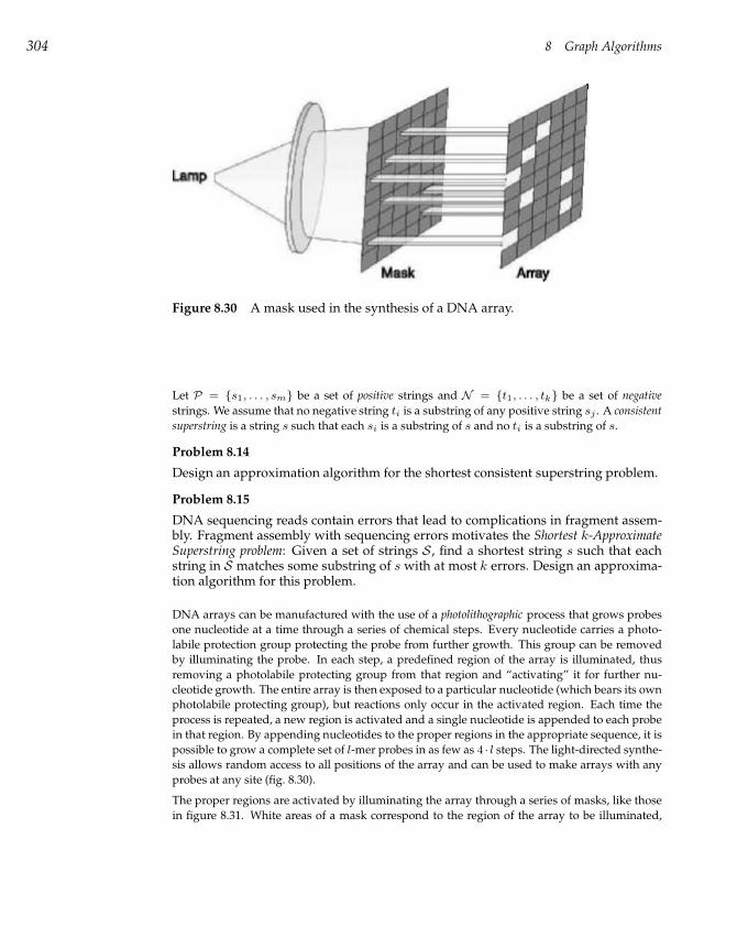
304 8 Graph Algorithms
Figure 8.30 A mask used in the synthesis of a DNA array.
Let P = s1, . . . , sm be a set of positive strings and N = t1, . . . , tk be a set of negative
strings. We assume that no negative string ti is a substring of any positive string sj . A consistent
superstring is a string s such that each si is a substring of s and no ti is a substring of s.
Problem 8.14
Design an approximation algorithm for the shortest consistent superstring problem.
Problem 8.15
DNA sequencing reads contain errors that lead to complications in fragment assem-bly. Fragment assembly with sequencing errors motivates the Shortest k-ApproximateSuperstring problem: Given a set of strings S , find a shortest string s such that eachstring in S matches some substring of s with at most k errors. Design an approxima-tion algorithm for this problem.
DNA arrays can be manufactured with the use of a photolithographic process that grows probes
one nucleotide at a time through a series of chemical steps. Every nucleotide carries a photo-
labile protection group protecting the probe from further growth. This group can be removed
by illuminating the probe. In each step, a predefined region of the array is illuminated, thus
removing a photolabile protecting group from that region and “activating” it for further nu-
cleotide growth. The entire array is then exposed to a particular nucleotide (which bears its own
photolabile protecting group), but reactions only occur in the activated region. Each time the
process is repeated, a new region is activated and a single nucleotide is appended to each probe
in that region. By appending nucleotides to the proper regions in the appropriate sequence, it is
possible to grow a complete set of l-mer probes in as few as 4 · l steps. The light-directed synthe-
sis allows random access to all positions of the array and can be used to make arrays with any
probes at any site (fig. 8.30).
The proper regions are activated by illuminating the array through a series of masks, like those
in figure 8.31. White areas of a mask correspond to the region of the array to be illuminated,
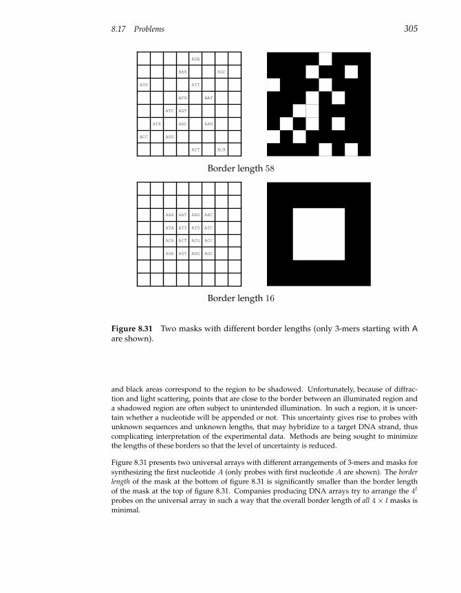
8.17 Problems 305
0 1 2 3 40
1
2
3
4
ACC
ATG
ATA
AGG
ATC
AAC
AGT
ACG
AAA
ACT
ATT
AGA
AAG
AAT
ACA
AGC
Border length 58
0 1 2 3 40
1
2
3
4
AGA
ACA
ATA
AAA
AGT
ACT
ATT
AAT
AGG
ACG
ATG
AAG
AGC
ACC
ATC
AAC
Border length 16
Figure 8.31 Two masks with different border lengths (only 3-mers starting with Aare shown).
and black areas correspond to the region to be shadowed. Unfortunately, because of diffrac-
tion and light scattering, points that are close to the border between an illuminated region and
a shadowed region are often subject to unintended illumination. In such a region, it is uncer-
tain whether a nucleotide will be appended or not. This uncertainty gives rise to probes with
unknown sequences and unknown lengths, that may hybridize to a target DNA strand, thus
complicating interpretation of the experimental data. Methods are being sought to minimize
the lengths of these borders so that the level of uncertainty is reduced.
Figure 8.31 presents two universal arrays with different arrangements of 3-mers and masks for
synthesizing the first nucleotide A (only probes with first nucleotide A are shown). The border
length of the mask at the bottom of figure 8.31 is significantly smaller than the border length
of the mask at the top of figure 8.31. Companies producing DNA arrays try to arrange the 4l
probes on the universal array in such a way that the overall border length of all 4 × l masks is
minimal.
306 8 Graph Algorithms
Problem 8.16
Find a lower bound on the overall border length of the universal array with 4l l-mers.
For two l-mers x and y, let dH(x, y) be the Hamming distance between x and y, that is, the
number of positions in which x and y differ. The overall border length of all masks equals
2P
dH(x, y), where the sum is taken over all pairs of neighboring probes on the array. This
observation establishes the connection between minimization of border length and Gray codes.
An l-bit Gray code is defined as a permutation of the binary numbers from 000 · · · 0 to 111 · · · 1,
each containing l binary digits, such that neighboring numbers have exactly one differing bit,
as do the first and last numbers. For example, the arrangement of sixteen 4-mers in a 4-bit Gray
code is shown below:
0 1 2 3 4 5 6 7 8 9 10 11 12 13 14 15
0 0 0 0 0 0 0 0 1 1 1 1 1 1 1 1
0 0 0 0 1 1 1 1 1 1 1 1 0 0 0 0
0 0 1 1 1 1 0 0 0 0 1 1 1 1 0 0
0 1 1 0 0 1 1 0 0 1 1 0 0 1 1 0
This Gray code can be generated recursively, starting with the 1-bit Gray code
G1 = 0, 1,
as follows. For an l-bit Gray code,
Gl = g1, g2, ..., g2l−1, g2l,
define an (l + 1)-bit Gray code as follows:
Gl+1 = 0g1, 0g2, ...,0g2l−1, 0g2l , 1g2l , 1g2l−1, ...,1g2, 1g1.
The elements of Gl are simply copied with 0s added to the front, then reversed with 1s added
to the front. Clearly, all elements in Gl+1 are distinct, and consecutive elements in Gl+1 differ
by exactly one bit. For example, the 2-bit Gray code is 00, 01, 11, 10, and the 3-bit Gray code
is 000, 001, 011, 010, 110, 111, 101, 100.
Problem 8.17
Design a Gray code for all 4-digit decimal numbers from 0000 to 9999.
We are interested in a two-dimensional Gray code composed of strings of length l over a four-
letter alphabet. In other words, we would like to generate a 2l-by-2l matrix in which each of
the 4l l-mers in a universal array is present at some position, and each pair of adjacent l-mers
(horizontally or vertically) differs in exactly one position. Constructing such a two-dimensional
Gray code is equivalent to minimizing the border length of the universal array.
Problem 8.18
Find the arrangement of probes on a universal array minimizing the border length.
Accurate determination of the peptide parent mass is very important in de novo peptide se-
quencing. An error in parent mass leads to systematic errors in the construction of the spectrum
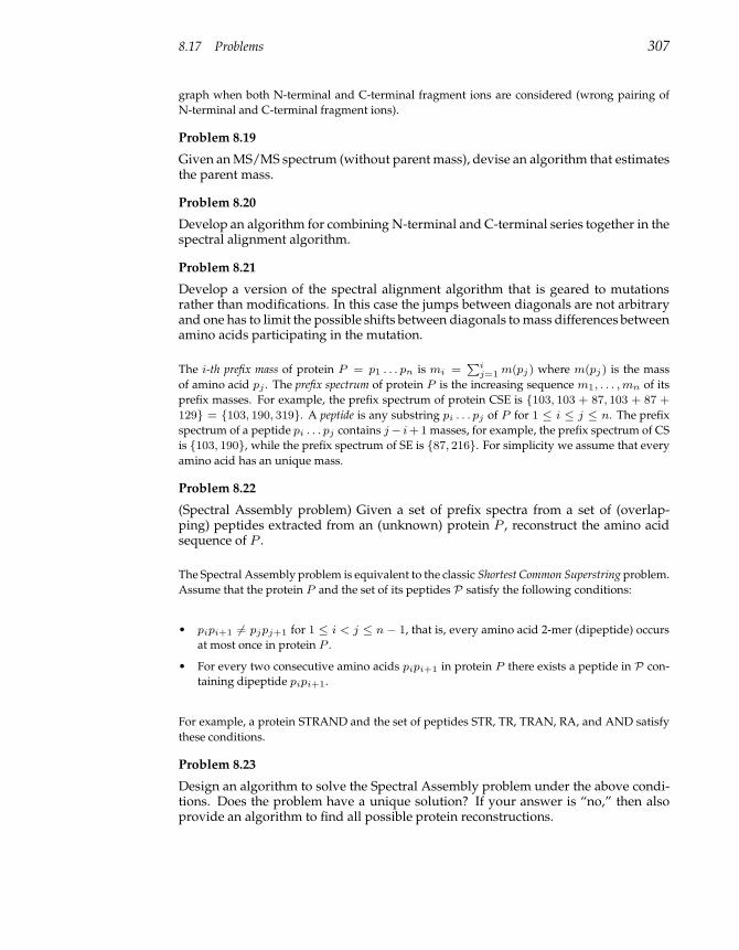
8.17 Problems 307
graph when both N-terminal and C-terminal fragment ions are considered (wrong pairing of
N-terminal and C-terminal fragment ions).
Problem 8.19
Given an MS/MS spectrum (without parent mass), devise an algorithm that estimatesthe parent mass.
Problem 8.20
Develop an algorithm for combining N-terminal and C-terminal series together in thespectral alignment algorithm.
Problem 8.21
Develop a version of the spectral alignment algorithm that is geared to mutationsrather than modifications. In this case the jumps between diagonals are not arbitraryand one has to limit the possible shifts between diagonals to mass differences betweenamino acids participating in the mutation.
The i-th prefix mass of protein P = p1 . . . pn is mi =Pi
j=1 m(pj) where m(pj) is the mass
of amino acid pj . The prefix spectrum of protein P is the increasing sequence m1, . . . , mn of its
prefix masses. For example, the prefix spectrum of protein CSE is 103, 103 + 87, 103 + 87 +
129 = 103, 190, 319. A peptide is any substring pi . . . pj of P for 1 ≤ i ≤ j ≤ n. The prefix
spectrum of a peptide pi . . . pj contains j − i+1 masses, for example, the prefix spectrum of CS
is 103, 190, while the prefix spectrum of SE is 87, 216. For simplicity we assume that every
amino acid has an unique mass.
Problem 8.22
(Spectral Assembly problem) Given a set of prefix spectra from a set of (overlap-ping) peptides extracted from an (unknown) protein P , reconstruct the amino acidsequence of P .
The Spectral Assembly problem is equivalent to the classic Shortest Common Superstring problem.
Assume that the protein P and the set of its peptides P satisfy the following conditions:
• pipi+1 6= pjpj+1 for 1 ≤ i < j ≤ n − 1, that is, every amino acid 2-mer (dipeptide) occurs
at most once in protein P .
• For every two consecutive amino acids pipi+1 in protein P there exists a peptide in P con-
taining dipeptide pipi+1.
For example, a protein STRAND and the set of peptides STR, TR, TRAN, RA, and AND satisfy
these conditions.
Problem 8.23
Design an algorithm to solve the Spectral Assembly problem under the above condi-tions. Does the problem have a unique solution? If your answer is “no,” then alsoprovide an algorithm to find all possible protein reconstructions.
308 8 Graph Algorithms
Problem 8.24
Extend this algorithm to solve the spectral assembly problem under the followingconditions:
• pipi+1 . . . pi+l−1 6= pjpj+1 . . . pj+l−1 for 1 ≤ i < j ≤ n− l +1, that is, every aminoacid l-mer (l-peptide) occurs at most once in protein P .
• For every l consecutive amino acids pipi+1 . . . pi+l−1 in protein P there exists apeptide in P containing l-peptide pipi+1 . . . pi+l−1.
Problem 8.25
Consider two proteins P1 and P2. The combined prefix spectrum of proteins P1 andP2 is defined as the union of their prefix spectra. Describe an algorithm for recon-structing P1 and P2 from their combined prefix spectrum. Give an example whensuch a reconstruction is non-unique. Generalize this algorithm for three and moreproteins.
When analyzing a protein p1 . . . pn, a mass spectrometer measures the masses of both the pre-
fix peptides p1 . . . pi and of the suffix peptides pi . . . pn, for 1 ≤ i ≤ n. The prefix-suffix
mass spectrum includes the masses of all prefix and suffix peptides. For example, CSE pro-
duces the following prefix-suffix spectrum 103, 129, 103 + 87, 129 + 87, 103 + 87 + 129 =
103, 129, 190, 216, 319 and it remains unknown which masses in the prefix-suffix spectrum
are derived from the prefix peptides and which are derived from the suffix peptides.
The prefix-suffix spectrum may contain as few as n masses (for palindromic peptides with every
suffix mass matched by a prefix mass) and as many as 2n−1 masses (if the overall peptide mass
is the only match between suffix and prefix masses).
Problem 8.26
Reconstruct a peptide given its prefix-suffix spectrum. Devise an efficient algorithmfor this problem under the assumption that the prefix-suffix spectrum of a peptide oflength n contains 2n− 1 masses.
In 1993 David Schwartz and colleagues developed the optical mapping technique for construction
of restriction maps. In optical mapping, single copies of DNA molecules are stretched and
attached to a glass under a microscope. When restriction enzymes are activated, they cleave
the DNA molecules at their restriction sites. The molecules remain attached to the surface, but
the elasticity of the stretched DNA pulls back the molecule ends at the cleaved sites. These can
be identified under the microscope as tiny gaps in the fluorescent line of the molecule. Thus a
“photograph” of the DNA molecule with gaps at the positions of cleavage sites gives a snapshot
of the restriction map.
Optical mapping bypasses the problem of reconstructing the order of restriction fragments,
but raises new computational challenges. The problem is that not all sites are cleaved in each
molecule and that some may incorrectly appear to be cut. In addition, inaccuracies in measur-
ing the length of fragments and the unknown orientation of each molecule (left to right or vice
versa) make the reconstruction difficult. In practice, data from many molecules are gathered to
build a consensus restriction map.
8.17 Problems 309
The input to the optical mapping problem is a 0-1 n × m matrix S = (sij) where each row
corresponds to a DNA molecule (straight or reversed), each column corresponds to a position
in that molecule, and sij = 1 if (and only if) there is a cut in position j of molecule i. The goal is
to reverse the orientation of a subset of molecules (subset of rows in S) and to declare a subset
of the t columns “real cut sites” so that the number of ones in cut site columns is maximized.
A naive approach to this problem is to find t columns with a large proportion of ones and
declare them potential cut sites. However, in this approach every real site will have a reversed
twin (since each “photograph” corresponds to either straight or reversed DNA molecules with
equal probabilities). Let w(i, j) be the number of molecules with both cut sites i and j present
(in either direct or reverse orientation). In a different approach, a graph on vertices 1, . . . , m
is constructed and two vertices are connected by an edge (i, j) of weight w(i, j).
Problem 8.27
Establish a connection between optical mapping and finding paths in graphs.

9 Combinatorial Pattern Matching
In chapter 5, we considered the Motif Finding problem, which is to find some
overrepresented pattern in a DNA sample. We are not given any particular
pattern to search for; rather we must infer it from the sample. Combinatorial
pattern matching, on the other hand, looks for exact or approximate occur-
rences of given patterns in a long text. Although pattern matching is in some
ways simpler than motif finding since we actually know what we are looking
for, the large size of genomes makes the problem, in practice, difficult. The
alignment techniques of chapter 6 become impractical for whole genomes,
particularly when one searches for approximate occurrences of many long
patterns at one time. In this chapter we develop a number of ways to make
pattern matching in a long string practical.
One recurring theme in this chapter is how to organize data into efficient
data structures, often a crucial part of solving a problem. For example, sup-
pose you were in a library with 2 million volumes in no discernible order
and you needed to find one particular title. The only way to guarantee find-
ing the title would be to check every book in the library. However, if the
books in the library were sorted by title, then the check becomes very easy.
A sorted list is only one of many types of data structures, and in this chapter
we discuss significantly more sophisticated ways of organizing data.
9.1 Repeat Finding
Many genetic diseases are associated with deletions, duplications, and rear-
rangements of long chromosomal regions. These are dramatic events that
affect the large-scale genomic architecture and may involve millions of nu-
cleotides. For example, DiGeorge syndrome, which commonly results in an
impaired immune system and heart defects, is associated with a large 3 Mb
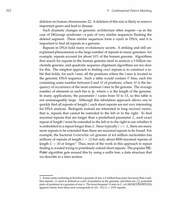
312 9 Combinatorial Pattern Matching
deletion on human chromosome 22. A deletion of this size is likely to remove
important genes and lead to disease.
Such dramatic changes in genomic architecture often require—as in the
case of DiGeorge syndrome—a pair of very similar sequences flanking the
deleted segment. These similar sequences form a repeat in DNA, and it is
important to find all repeats in a genome.
Repeats in DNA hold many evolutionary secrets. A striking and still un-
explained phenomenon is the large number of repeats in many genomes: for
example, repeats account for about 50% of the human genome. Algorithms
that search for repeats in the human genome need to analyze a 3 billion nu-
cleotide genome, and quadratic sequence alignment algorithms are too slow
for this. The simplest approach to finding exact repeats is to construct a ta-
ble that holds, for each l-mer, all the positions where the l-mer is located in
the genomic DNA sequence. Such a table would contain 4l bins, each bin
containing some number between 0 and M of positions, where M is the fre-
quency of occurrence of the most common l-mer in the genome. The average
number of elements in each bin is n4l , where n is the length of the genome.
In many applications, the parameter l varies from 10 to 13, so this table is
not unmanageably large. Although this tabulation approach allows one to
quickly find all repeats of length l, such short repeats are not very interesting
for DNA analysis. Biologists instead are interested in long maximal repeats,
that is, repeats that cannot be extended to the left or to the right. To find
maximal repeats that are longer than a predefined parameter L, each exact
repeat of length l must be extended to the left or to the right to see whether it
is embedded in a repeat longer than L. Since typically l << L, there are many
more repeats to be extended than there are maximal repeats to be found. For
example, the bacterial Escherichia coli genome of 4.6 million nucleotides has
millions of repeats of length l = 12 but only about 8000 maximal repeats of
length L = 20 or longer.1 Thus, most of the work in this approach to repeat
finding is wasted trying to pointlessly extend short repeats. The popular RE-Puter algorithm gets around this by using a suffix tree, a data structure that
we describe in a later section.
1. It may seem confusing at first that a genome of size 4.6 million base pairs has more than a mil-lion repeats. A repeat is defined as a pair of positions in the genome, and there are
`
n2
´
potentialpairs of positions in a genome of size n. The most frequent 12-mer in E. coli (ACGCCGCATCCG)appears ninety-four times and corresponds to (94 · 93)/2 = 4376 repeats.
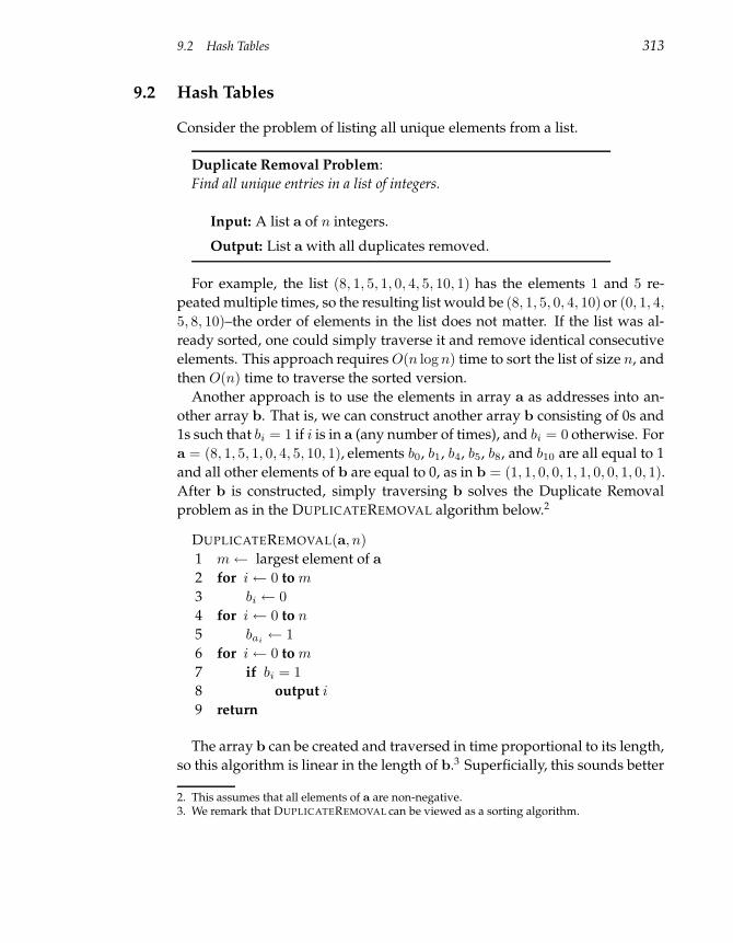
9.2 Hash Tables 313
9.2 Hash Tables
Consider the problem of listing all unique elements from a list.
Duplicate Removal Problem:
Find all unique entries in a list of integers.
Input: A list a of n integers.
Output: List a with all duplicates removed.
For example, the list (8, 1, 5, 1, 0, 4, 5, 10, 1) has the elements 1 and 5 re-
peated multiple times, so the resulting list would be (8, 1, 5, 0, 4, 10) or (0, 1, 4,
5, 8, 10)–the order of elements in the list does not matter. If the list was al-
ready sorted, one could simply traverse it and remove identical consecutive
elements. This approach requires O(n log n) time to sort the list of size n, and
then O(n) time to traverse the sorted version.
Another approach is to use the elements in array a as addresses into an-
other array b. That is, we can construct another array b consisting of 0s and
1s such that bi = 1 if i is in a (any number of times), and bi = 0 otherwise. For
a = (8, 1, 5, 1, 0, 4, 5, 10, 1), elements b0, b1, b4, b5, b8, and b10 are all equal to 1
and all other elements of b are equal to 0, as in b = (1, 1, 0, 0, 1, 1, 0, 0, 1, 0, 1).
After b is constructed, simply traversing b solves the Duplicate Removal
problem as in the DUPLICATEREMOVAL algorithm below.2
DUPLICATEREMOVAL(a, n)
1 m← largest element of a
2 for i← 0 to m
3 bi ← 0
4 for i← 0 to n
5 bai← 1
6 for i← 0 to m
7 if bi = 1
8 output i
9 return
The array b can be created and traversed in time proportional to its length,
so this algorithm is linear in the length of b.3 Superficially, this sounds better
2. This assumes that all elements of a are non-negative.3. We remark that DUPLICATEREMOVAL can be viewed as a sorting algorithm.
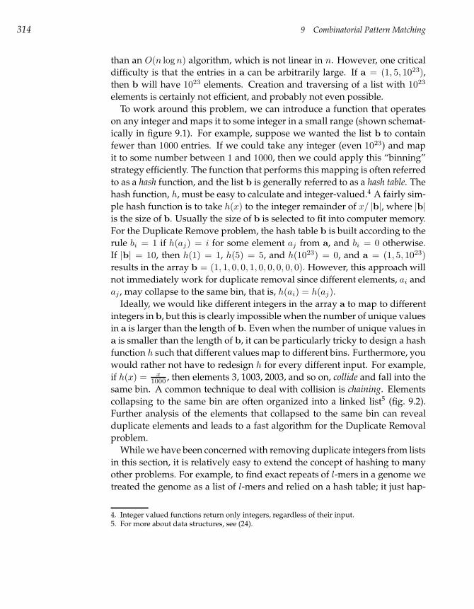
314 9 Combinatorial Pattern Matching
than an O(n log n) algorithm, which is not linear in n. However, one critical
difficulty is that the entries in a can be arbitrarily large. If a = (1, 5, 1023),
then b will have 1023 elements. Creation and traversing of a list with 1023
elements is certainly not efficient, and probably not even possible.
To work around this problem, we can introduce a function that operates
on any integer and maps it to some integer in a small range (shown schemat-
ically in figure 9.1). For example, suppose we wanted the list b to contain
fewer than 1000 entries. If we could take any integer (even 1023) and map
it to some number between 1 and 1000, then we could apply this “binning”
strategy efficiently. The function that performs this mapping is often referred
to as a hash function, and the list b is generally referred to as a hash table. The
hash function, h, must be easy to calculate and integer-valued.4 A fairly sim-
ple hash function is to take h(x) to the integer remainder of x/ |b|, where |b|
is the size of b. Usually the size of b is selected to fit into computer memory.
For the Duplicate Remove problem, the hash table b is built according to the
rule bi = 1 if h(aj) = i for some element aj from a, and bi = 0 otherwise.
If |b| = 10, then h(1) = 1, h(5) = 5, and h(1023) = 0, and a = (1, 5, 1023)
results in the array b = (1, 1, 0, 0, 1, 0, 0, 0, 0, 0). However, this approach will
not immediately work for duplicate removal since different elements, ai and
aj , may collapse to the same bin, that is, h(ai) = h(aj).
Ideally, we would like different integers in the array a to map to different
integers in b, but this is clearly impossible when the number of unique values
in a is larger than the length of b. Even when the number of unique values in
a is smaller than the length of b, it can be particularly tricky to design a hash
function h such that different values map to different bins. Furthermore, you
would rather not have to redesign h for every different input. For example,
if h(x) = x1000 , then elements 3, 1003, 2003, and so on, collide and fall into the
same bin. A common technique to deal with collision is chaining. Elements
collapsing to the same bin are often organized into a linked list5 (fig. 9.2).
Further analysis of the elements that collapsed to the same bin can reveal
duplicate elements and leads to a fast algorithm for the Duplicate Removal
problem.
While we have been concerned with removing duplicate integers from lists
in this section, it is relatively easy to extend the concept of hashing to many
other problems. For example, to find exact repeats of l-mers in a genome we
treated the genome as a list of l-mers and relied on a hash table; it just hap-
4. Integer valued functions return only integers, regardless of their input.5. For more about data structures, see (24).
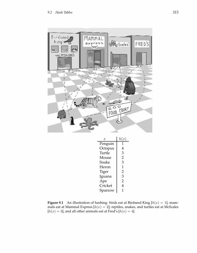
9.2 Hash Tables 315
x h(x)Penguin 1Octopus 4Turtle 3Mouse 2Snake 3Heron 1Tiger 2Iguana 3Ape 2Cricket 4Sparrow 1
Figure 9.1 An illustration of hashing: birds eat at Birdseed King [h(x) = 1]; mam-mals eat at Mammal Express [h(x) = 2]; reptiles, snakes, and turtles eat at McScales[h(x) = 3], and all other animals eat at Fred’s [h(x) = 4].
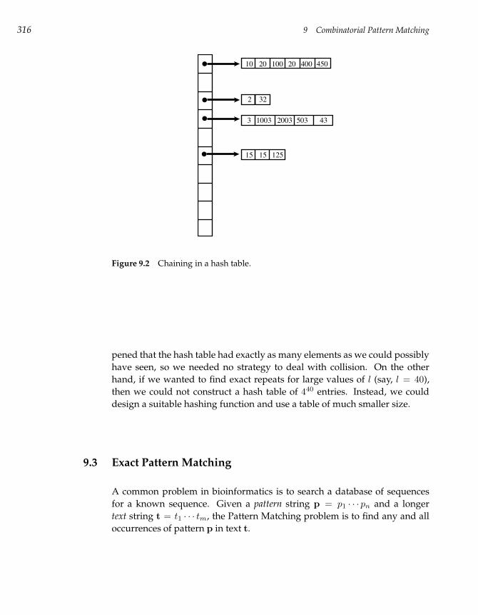
316 9 Combinatorial Pattern Matching
10 20 100 20 400 450
2 32
3 1003 2003 503 43
15 15 125
Figure 9.2 Chaining in a hash table.
pened that the hash table had exactly as many elements as we could possibly
have seen, so we needed no strategy to deal with collision. On the other
hand, if we wanted to find exact repeats for large values of l (say, l = 40),
then we could not construct a hash table of 440 entries. Instead, we could
design a suitable hashing function and use a table of much smaller size.
9.3 Exact Pattern Matching
A common problem in bioinformatics is to search a database of sequences
for a known sequence. Given a pattern string p = p1 · · · pn and a longer
text string t = t1 · · · tm, the Pattern Matching problem is to find any and all
occurrences of pattern p in text t.
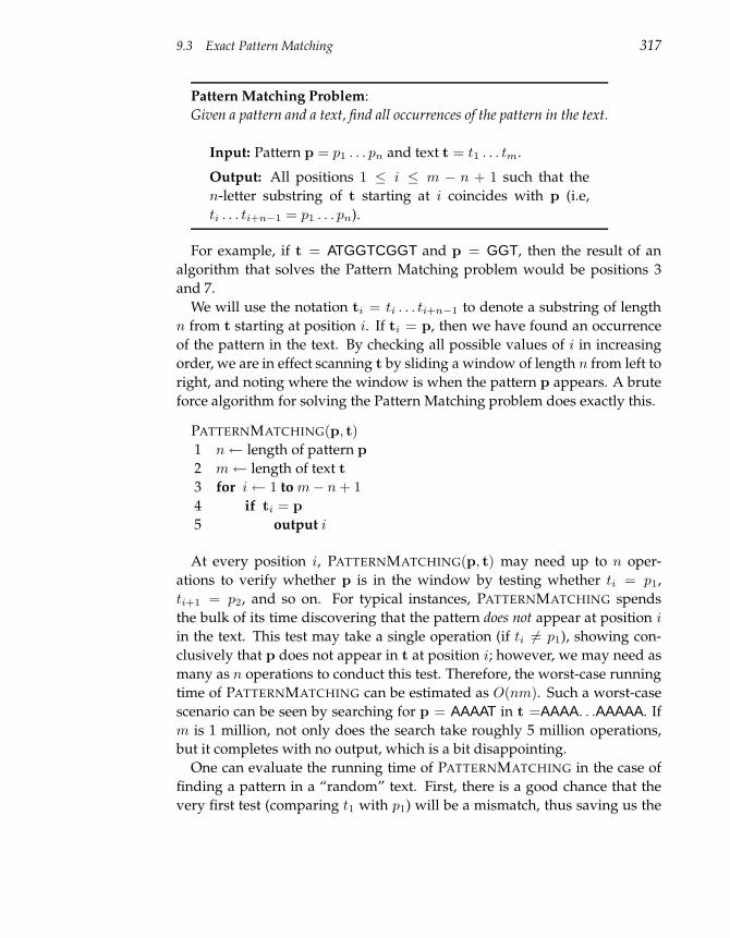
9.3 Exact Pattern Matching 317
Pattern Matching Problem:
Given a pattern and a text, find all occurrences of the pattern in the text.
Input: Pattern p = p1 . . . pn and text t = t1 . . . tm.
Output: All positions 1 ≤ i ≤ m − n + 1 such that the
n-letter substring of t starting at i coincides with p (i.e,
ti . . . ti+n−1 = p1 . . . pn).
For example, if t = ATGGTCGGT and p = GGT, then the result of an
algorithm that solves the Pattern Matching problem would be positions 3
and 7.
We will use the notation ti = ti . . . ti+n−1 to denote a substring of length
n from t starting at position i. If ti = p, then we have found an occurrence
of the pattern in the text. By checking all possible values of i in increasing
order, we are in effect scanning t by sliding a window of length n from left to
right, and noting where the window is when the pattern p appears. A brute
force algorithm for solving the Pattern Matching problem does exactly this.
PATTERNMATCHING(p, t)
1 n← length of pattern p
2 m← length of text t
3 for i← 1 to m− n + 1
4 if ti = p
5 output i
At every position i, PATTERNMATCHING(p, t) may need up to n oper-
ations to verify whether p is in the window by testing whether ti = p1,
ti+1 = p2, and so on. For typical instances, PATTERNMATCHING spends
the bulk of its time discovering that the pattern does not appear at position i
in the text. This test may take a single operation (if ti 6= p1), showing con-
clusively that p does not appear in t at position i; however, we may need as
many as n operations to conduct this test. Therefore, the worst-case running
time of PATTERNMATCHING can be estimated as O(nm). Such a worst-case
scenario can be seen by searching for p = AAAAT in t =AAAA. . .AAAAA. If
m is 1 million, not only does the search take roughly 5 million operations,
but it completes with no output, which is a bit disappointing.
One can evaluate the running time of PATTERNMATCHING in the case of
finding a pattern in a “random” text. First, there is a good chance that the
very first test (comparing t1 with p1) will be a mismatch, thus saving us the
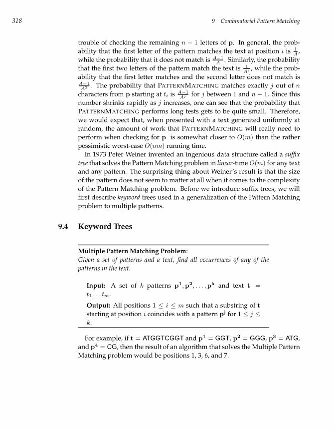
318 9 Combinatorial Pattern Matching
trouble of checking the remaining n − 1 letters of p. In general, the prob-
ability that the first letter of the pattern matches the text at position i is 1A
,
while the probability that it does not match is A−1A
. Similarly, the probability
that the first two letters of the pattern match the text is 1A2 , while the prob-
ability that the first letter matches and the second letter does not match isA−1A2 . The probability that PATTERNMATCHING matches exactly j out of n
characters from p starting at ti is A−1Aj for j between 1 and n − 1. Since this
number shrinks rapidly as j increases, one can see that the probability that
PATTERNMATCHING performs long tests gets to be quite small. Therefore,
we would expect that, when presented with a text generated uniformly at
random, the amount of work that PATTERNMATCHING will really need to
perform when checking for p is somewhat closer to O(m) than the rather
pessimistic worst-case O(nm) running time.
In 1973 Peter Weiner invented an ingenious data structure called a suffix
tree that solves the Pattern Matching problem in linear-time O(m) for any text
and any pattern. The surprising thing about Weiner’s result is that the size
of the pattern does not seem to matter at all when it comes to the complexity
of the Pattern Matching problem. Before we introduce suffix trees, we will
first describe keyword trees used in a generalization of the Pattern Matching
problem to multiple patterns.
9.4 Keyword Trees
Multiple Pattern Matching Problem:
Given a set of patterns and a text, find all occurrences of any of the
patterns in the text.
Input: A set of k patterns p1,p2, . . . ,pk and text t =
t1 . . . tm.
Output: All positions 1 ≤ i ≤ m such that a substring of t
starting at position i coincides with a pattern pj for 1 ≤ j ≤
k.
For example, if t = ATGGTCGGT and p1 = GGT, p2 = GGG, p3 = ATG,
and p4 = CG, then the result of an algorithm that solves the Multiple Pattern
Matching problem would be positions 1, 3, 6, and 7.
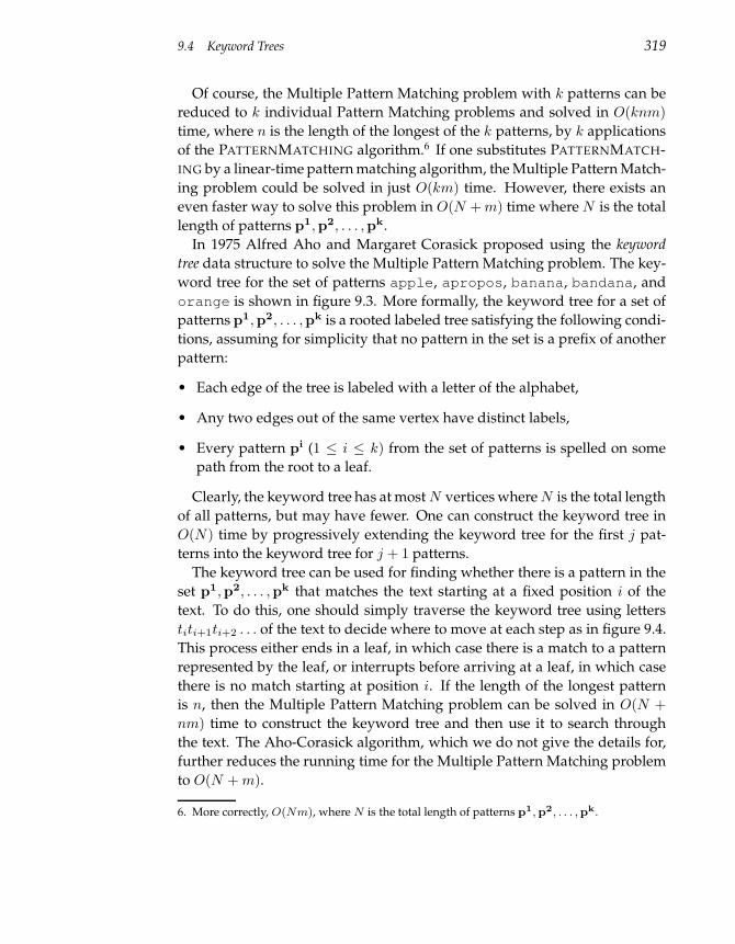
9.4 Keyword Trees 319
Of course, the Multiple Pattern Matching problem with k patterns can be
reduced to k individual Pattern Matching problems and solved in O(knm)
time, where n is the length of the longest of the k patterns, by k applications
of the PATTERNMATCHING algorithm.6 If one substitutes PATTERNMATCH-
ING by a linear-time pattern matching algorithm, the Multiple Pattern Match-
ing problem could be solved in just O(km) time. However, there exists an
even faster way to solve this problem in O(N + m) time where N is the total
length of patterns p1,p2, . . . ,pk.
In 1975 Alfred Aho and Margaret Corasick proposed using the keyword
tree data structure to solve the Multiple Pattern Matching problem. The key-
word tree for the set of patterns apple, apropos, banana, bandana, and
orange is shown in figure 9.3. More formally, the keyword tree for a set of
patterns p1,p2, . . . ,pk is a rooted labeled tree satisfying the following condi-
tions, assuming for simplicity that no pattern in the set is a prefix of another
pattern:
• Each edge of the tree is labeled with a letter of the alphabet,
• Any two edges out of the same vertex have distinct labels,
• Every pattern pi (1 ≤ i ≤ k) from the set of patterns is spelled on some
path from the root to a leaf.
Clearly, the keyword tree has at most N vertices where N is the total length
of all patterns, but may have fewer. One can construct the keyword tree in
O(N) time by progressively extending the keyword tree for the first j pat-
terns into the keyword tree for j + 1 patterns.
The keyword tree can be used for finding whether there is a pattern in the
set p1,p2, . . . ,pk that matches the text starting at a fixed position i of the
text. To do this, one should simply traverse the keyword tree using letters
titi+1ti+2 . . . of the text to decide where to move at each step as in figure 9.4.
This process either ends in a leaf, in which case there is a match to a pattern
represented by the leaf, or interrupts before arriving at a leaf, in which case
there is no match starting at position i. If the length of the longest pattern
is n, then the Multiple Pattern Matching problem can be solved in O(N +
nm) time to construct the keyword tree and then use it to search through
the text. The Aho-Corasick algorithm, which we do not give the details for,
further reduces the running time for the Multiple Pattern Matching problem
to O(N + m).
6. More correctly, O(Nm), where N is the total length of patterns p1, p2, . . . ,pk.
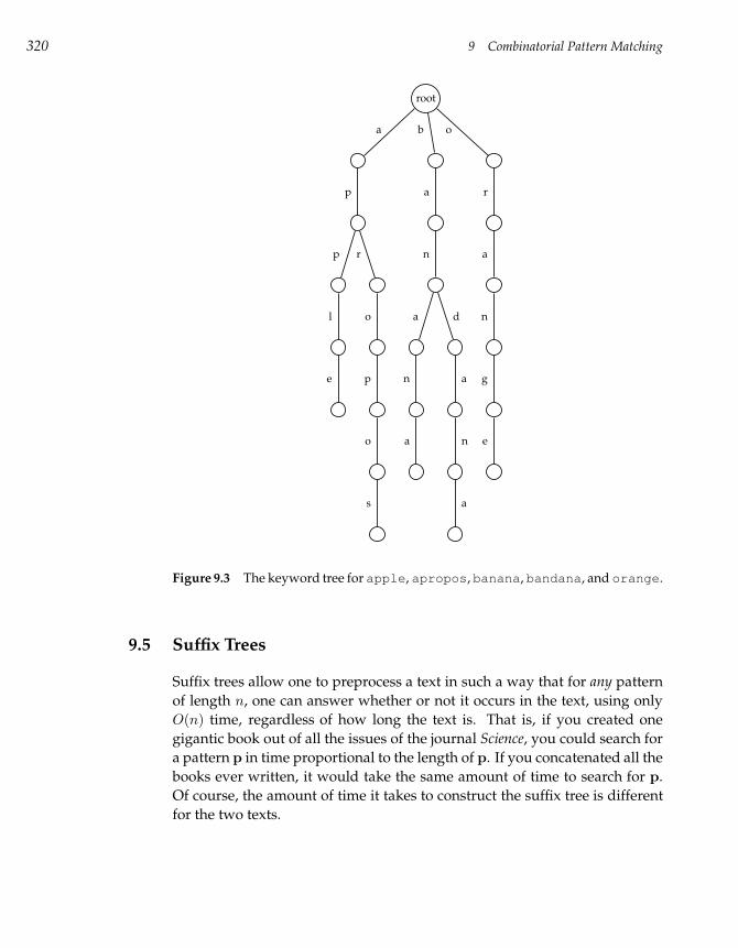
320 9 Combinatorial Pattern Matching
root
a
p
p
l
e
r
o
p
o
s
b
a
n
a
n
a
d
a
n
a
o
r
a
n
g
e
Figure 9.3 The keyword tree for apple, apropos, banana, bandana, and orange.
9.5 Suffix Trees
Suffix trees allow one to preprocess a text in such a way that for any pattern
of length n, one can answer whether or not it occurs in the text, using only
O(n) time, regardless of how long the text is. That is, if you created one
gigantic book out of all the issues of the journal Science, you could search for
a pattern p in time proportional to the length of p. If you concatenated all the
books ever written, it would take the same amount of time to search for p.
Of course, the amount of time it takes to construct the suffix tree is different
for the two texts.
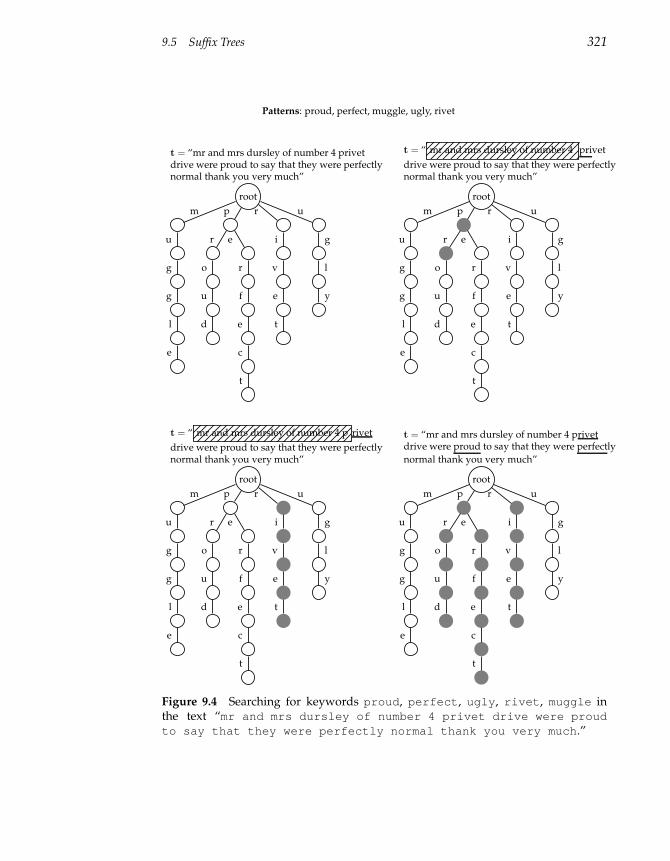
9.5 Suffix Trees 321
Patterns: proud, perfect, muggle, ugly, rivet
t = “mr and mrs dursley of number 4 privetdrive were proud to say that they were perfectlynormal thank you very much”
root
m
u
g
g
l
e
p
r
o
u
d
e
r
f
e
c
t
r
i
v
e
t
u
g
l
y
t = “ mr and mrs dursley of number 4 privet
drive were proud to say that they were perfectlynormal thank you very much”
root
m
u
g
g
l
e
p
r
o
u
d
e
r
f
e
c
t
r
i
v
e
t
u
g
l
y
t = “ mr and mrs dursley of number 4 p rivet
drive were proud to say that they were perfectlynormal thank you very much”
root
m
u
g
g
l
e
p
r
o
u
d
e
r
f
e
c
t
r
i
v
e
t
u
g
l
y
t = “mr and mrs dursley of number 4 privetdrive were proud to say that they were perfectly
normal thank you very much”
root
m
u
g
g
l
e
p
r
o
u
d
e
r
f
e
c
t
r
i
v
e
t
u
g
l
y
Figure 9.4 Searching for keywords proud, perfect, ugly, rivet, muggle inthe text “mr and mrs dursley of number 4 privet drive were proudto say that they were perfectly normal thank you very much.”
322 9 Combinatorial Pattern Matching
It turns out that a suffix tree for a text of length m can be constructed in
O(m) time, which leads immediately to a linear O(n + m) algorithm for the
Pattern Matching problem: construct the suffix tree for t, in O(m) time, and
then check whether p occurs in the tree, which requires O(n) time.
Figure 9.5 (a) shows the keyword tree for all six suffixes of the string AT-CATG: G, TG, ATG, CATG, TCATG, and ATCATG. The suffix tree of a text can
be obtained from the keyword tree of its suffixes by collapsing every path
of nonbranching vertices into a single edge, as in figure 9.5 (b). Although
one can use the keyword tree construction to build the suffix tree, it does not
lend itself to an efficient algorithm for the suffix trees construction. Indeed,
the keyword tree for k patterns can be constructed in O(N) time where N is
the total length of all these patterns. A text of length m has m suffixes vary-
ing in length from 1 to m and therefore the total length of these suffixes is
1+2+ · · ·+m = m(m+1)2 , quadratic in the length of the text. Weiner’s contri-
bution to the construction of suffix trees in O(m) time bypasses the keyword
tree construction step altogether.7
The suffix tree for a text t = t1 . . . tm is a rooted labeled tree with m leaves
(numbered from 1 to m) satisfying the following conditions8:
• Each edge is labeled with a substring of the text,9
• Each internal vertex (except possibly the root) has at least 2 children,
• Any two edges out of the same vertex start with a different letter,
• Every suffix of text t is spelled out on a path from the root to some leaf.
Suffix trees immediately lead to a fast algorithm for pattern matching. We
define the threading of a pattern p through a suffix tree T as the matching of
characters from p along the unique path in T until either all characters of p
are matched, which is a complete threading, or until no more matches are
possible, which is an incomplete threading. If the threading of a pattern is
complete, it ends at some vertex or edge of T and we define the p-matching
leaves as all of the leaves that are descendants of that vertex or edge. Every p-
matching leaf in the tree corresponds to an occurrence of p in t. An example
of a complete threading, and the p-matching leaves is shown in figure 9.6.
7. The linear-time algorithm for suffix tree construction is rather complicated and is beyond thescope of this book. See (44) for an excellent review of suffix trees.8. For simplicity we assume that the last letter of t does not appear anywhere in the text so thatno suffix string is a prefix of another suffix string. If this is not the case, we can add an extraletter (like $) to the end of the text to satisfy this condition.9. Note the difference between this and keyword trees.
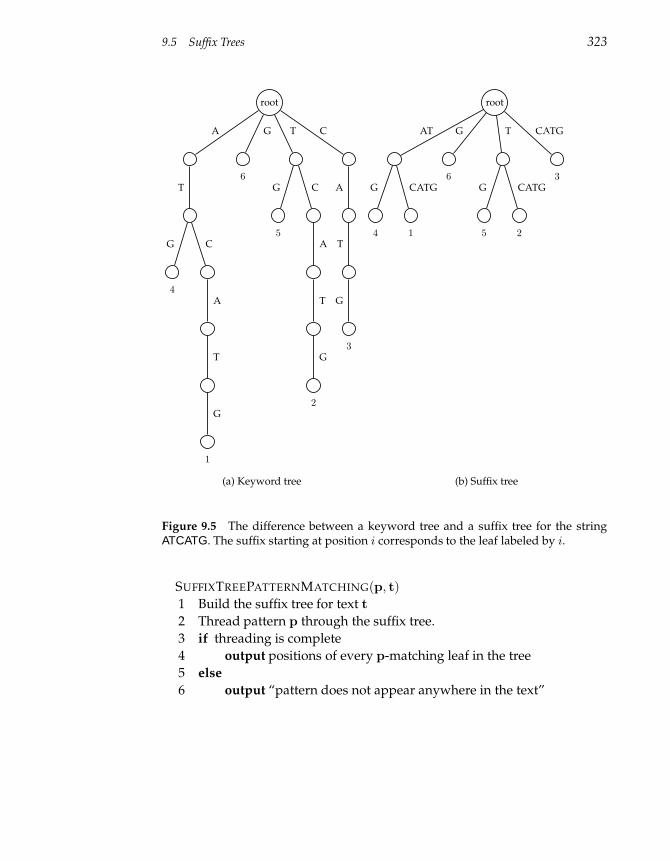
9.5 Suffix Trees 323
root
A
T
4
G C
A
T
1
G
6
G T
5
G C
A
T
2
G
C
A
T
3
G
(a) Keyword tree
root
AT
4
G
1
CATG6
G T
5
G
2
CATG3
CATG
(b) Suffix tree
Figure 9.5 The difference between a keyword tree and a suffix tree for the stringATCATG. The suffix starting at position i corresponds to the leaf labeled by i.
SUFFIXTREEPATTERNMATCHING(p, t)
1 Build the suffix tree for text t
2 Thread pattern p through the suffix tree.
3 if threading is complete
4 output positions of every p-matching leaf in the tree
5 else
6 output “pattern does not appear anywhere in the text”
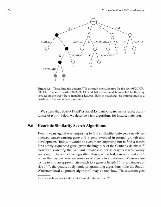
324 9 Combinatorial Pattern Matching
root
A
7
CATGG T
G
1
CATACATG
9
G5
ACATGG
T
6
ACATGG G
10
G
2
CATACATGG
G
3
CATACATGG
11
G
CAT
8
GG
4
ACATGG
Figure 9.6 Threading the pattern ATG through the suffix tree for the text ATGCATA-CATGG. The suffixes ATGCATACATGG and ATGG both match, as noted by the grayvertices in the tree (the p-matching leaves). Each p-matching leaf corresponds to aposition in the text where p occurs.
We stress that SUFFIXTREEPATTERNMATCHING searches for exact occur-
rences of p in t. Below we describe a few algorithms for inexact matching.
9.6 Heuristic Similarity Search Algorithms
Twenty years ago, it was surprising to find similarities between a newly se-
quenced cancer-causing gene and a gene involved in normal growth and
development. Today, it would be even more surprising not to find a match
for a newly sequenced gene, given the huge size of the GenBank database.10
However, searching the GenBank database is not as easy as it was twenty
years ago. The suffix tree algorithm above, while fast, can only find exact,
rather than approximate, occurrences of a gene in a database. When we are
trying to find an approximate match to a gene of length 103 in a database of
size 1010, the quadratic dynamic programming algorithms (like the Smith-
Waterman local alignment algorithm) may be too slow. The situation gets
10. The number of nucleotides in GenBank already exceeds 1010 .
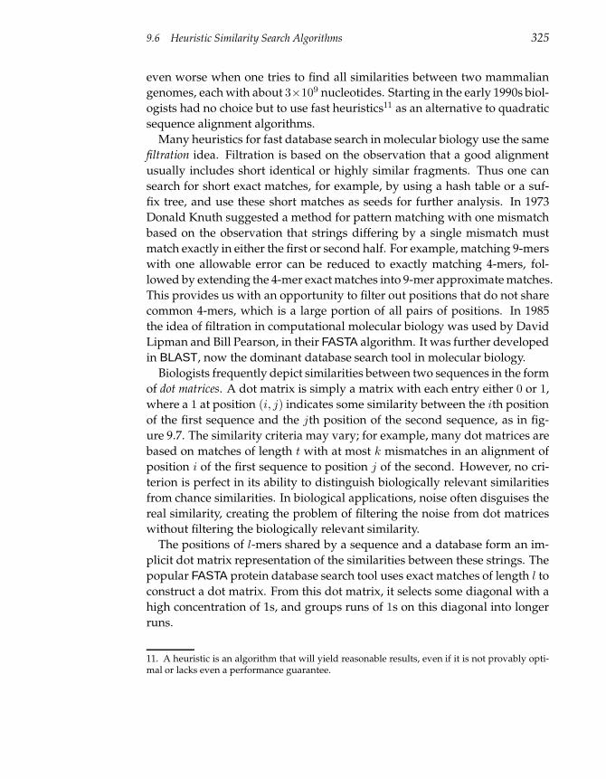
9.6 Heuristic Similarity Search Algorithms 325
even worse when one tries to find all similarities between two mammalian
genomes, each with about 3×10⁹ nucleotides. Starting in the early 1990s biol-
ogists had no choice but to use fast heuristics11 as an alternative to quadratic
sequence alignment algorithms.
Many heuristics for fast database search in molecular biology use the same
filtration idea. Filtration is based on the observation that a good alignment
usually includes short identical or highly similar fragments. Thus one can
search for short exact matches, for example, by using a hash table or a suf-
fix tree, and use these short matches as seeds for further analysis. In 1973
Donald Knuth suggested a method for pattern matching with one mismatch
based on the observation that strings differing by a single mismatch must
match exactly in either the first or second half. For example, matching 9-mers
with one allowable error can be reduced to exactly matching 4-mers, fol-
lowed by extending the 4-mer exact matches into 9-mer approximate matches.
This provides us with an opportunity to filter out positions that do not share
common 4-mers, which is a large portion of all pairs of positions. In 1985
the idea of filtration in computational molecular biology was used by David
Lipman and Bill Pearson, in their FASTA algorithm. It was further developed
in BLAST, now the dominant database search tool in molecular biology.
Biologists frequently depict similarities between two sequences in the form
of dot matrices. A dot matrix is simply a matrix with each entry either 0 or 1,
where a 1 at position (i, j) indicates some similarity between the ith position
of the first sequence and the jth position of the second sequence, as in fig-
ure 9.7. The similarity criteria may vary; for example, many dot matrices are
based on matches of length t with at most k mismatches in an alignment of
position i of the first sequence to position j of the second. However, no cri-
terion is perfect in its ability to distinguish biologically relevant similarities
from chance similarities. In biological applications, noise often disguises the
real similarity, creating the problem of filtering the noise from dot matrices
without filtering the biologically relevant similarity.
The positions of l-mers shared by a sequence and a database form an im-
plicit dot matrix representation of the similarities between these strings. The
popular FASTA protein database search tool uses exact matches of length l to
construct a dot matrix. From this dot matrix, it selects some diagonal with a
high concentration of 1s, and groups runs of 1s on this diagonal into longer
runs.
11. A heuristic is an algorithm that will yield reasonable results, even if it is not provably opti-mal or lacks even a performance guarantee.
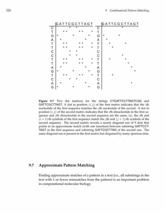
326 9 Combinatorial Pattern Matching
G A T T C G C T T A G TC * *T * * * * *G * * *A * *T * * * * *T * * * * *C * *C * *T * * * * *T * * * * *A * *G * * *T * * * * *C * *A * *G * * *
G A T T C G C T T A G TC *TG * *A *T * *T *CC *T * *T *A *G *T *CA *G
Figure 9.7 Two dot matrices for the strings CTGATTCCTTAGTCAG andGATTCGCTTAGT. A dot in position (i, j) of the first matrix indicates that the ithnucleotide of the first sequence matches the jth nucleotide of the second. A dot inposition (i, j) of the second matrix indicates that the ith dinucleotide in the first se-quence and jth dinucleotide in the second sequence are the same, i.e., the ith and(i + 1)-th symbols of the first sequence match the jth and (j + 1)-th symbols of thesecond sequence. The second matrix reveals a nearly diagonal run of 9 dots thatpoints to an approximate match (with one insertion) between substring GATTCCT-TAGT in the first sequence and substring GATTCGCTTAG of the second one. Thesame diagonal run is present in the first matrix but disguised by many spurious dots.
9.7 Approximate Pattern Matching
Finding approximate matches of a pattern in a text (i.e., all substrings in the
text with k or fewer mismatches from the pattern) is an important problem
in computational molecular biology.
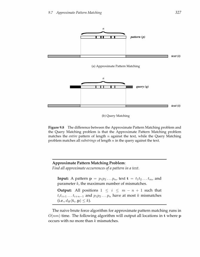
9.7 Approximate Pattern Matching 327
pattern (p)
text (t)
n(a) Approximate Pattern Matching
query (q)
text (t)
n(b) Query Matching
Figure 9.8 The difference between the Approximate Pattern Matching problem andthe Query Matching problem is that the Approximate Pattern Matching problemmatches the entire pattern of length n against the text, while the Query Matchingproblem matches all substrings of length n in the query against the text.
Approximate Pattern Matching Problem:
Find all approximate occurrences of a pattern in a text.
Input: A pattern p = p1p2 . . . pn, text t = t1t2 . . . tm, and
parameter k, the maximum number of mismatches.
Output: All positions 1 ≤ i ≤ m − n + 1 such that
titi+1 . . . ti+n−1 and p1p2 . . . pn have at most k mismatches
(i.e., dH(ti,p) ≤ k).
The naive brute force algorithm for approximate pattern matching runs in
O(nm) time. The following algorithm will output all locations in t where p
occurs with no more than k mismatches.
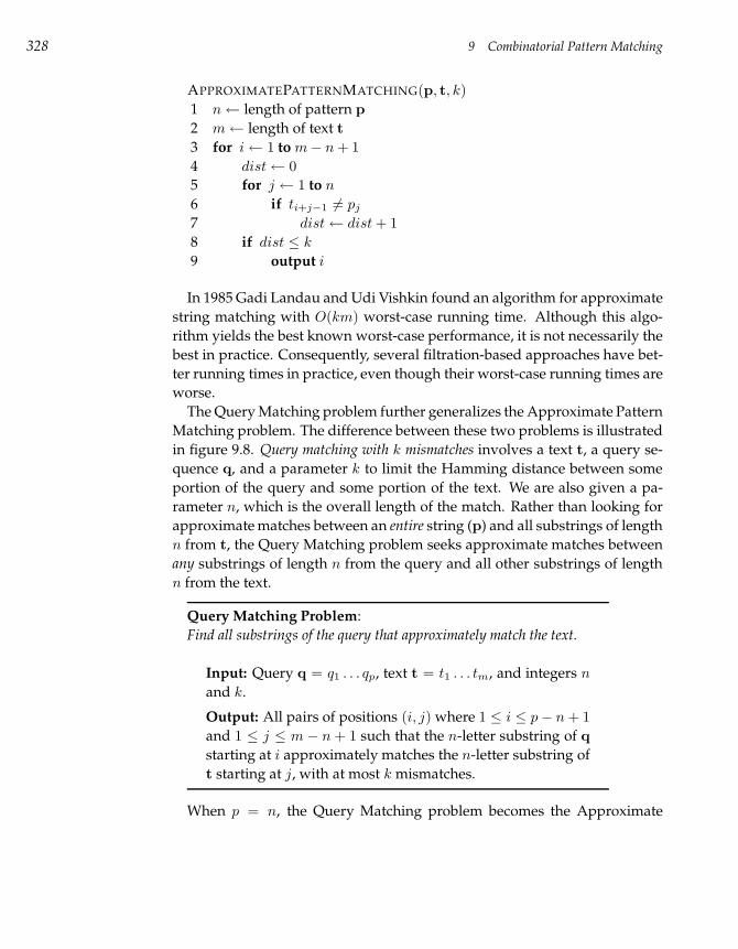
328 9 Combinatorial Pattern Matching
APPROXIMATEPATTERNMATCHING(p, t, k)
1 n← length of pattern p
2 m← length of text t
3 for i← 1 to m− n + 1
4 dist← 0
5 for j ← 1 to n
6 if ti+j−1 6= pj
7 dist← dist + 1
8 if dist ≤ k
9 output i
In 1985 Gadi Landau and Udi Vishkin found an algorithm for approximate
string matching with O(km) worst-case running time. Although this algo-
rithm yields the best known worst-case performance, it is not necessarily the
best in practice. Consequently, several filtration-based approaches have bet-
ter running times in practice, even though their worst-case running times are
worse.
The Query Matching problem further generalizes the Approximate Pattern
Matching problem. The difference between these two problems is illustrated
in figure 9.8. Query matching with k mismatches involves a text t, a query se-
quence q, and a parameter k to limit the Hamming distance between some
portion of the query and some portion of the text. We are also given a pa-
rameter n, which is the overall length of the match. Rather than looking for
approximate matches between an entire string (p) and all substrings of length
n from t, the Query Matching problem seeks approximate matches between
any substrings of length n from the query and all other substrings of length
n from the text.
Query Matching Problem:
Find all substrings of the query that approximately match the text.
Input: Query q = q1 . . . qp, text t = t1 . . . tm, and integers n
and k.
Output: All pairs of positions (i, j) where 1 ≤ i ≤ p− n + 1
and 1 ≤ j ≤ m − n + 1 such that the n-letter substring of q
starting at i approximately matches the n-letter substring of
t starting at j, with at most k mismatches.
When p = n, the Query Matching problem becomes the Approximate
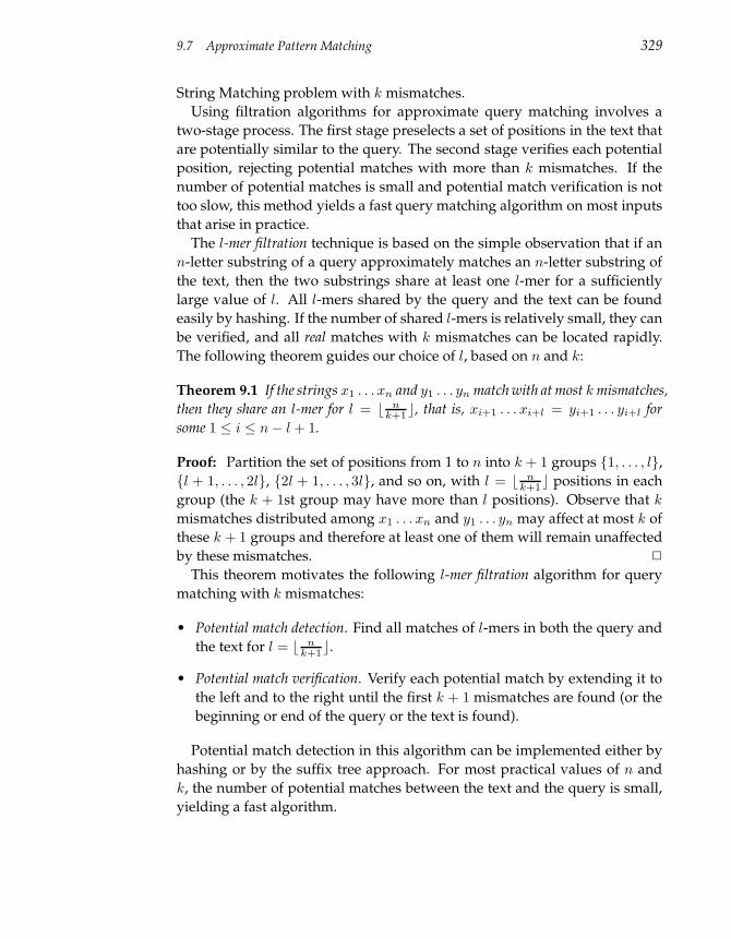
9.7 Approximate Pattern Matching 329
String Matching problem with k mismatches.
Using filtration algorithms for approximate query matching involves a
two-stage process. The first stage preselects a set of positions in the text that
are potentially similar to the query. The second stage verifies each potential
position, rejecting potential matches with more than k mismatches. If the
number of potential matches is small and potential match verification is not
too slow, this method yields a fast query matching algorithm on most inputs
that arise in practice.
The l-mer filtration technique is based on the simple observation that if an
n-letter substring of a query approximately matches an n-letter substring of
the text, then the two substrings share at least one l-mer for a sufficiently
large value of l. All l-mers shared by the query and the text can be found
easily by hashing. If the number of shared l-mers is relatively small, they can
be verified, and all real matches with k mismatches can be located rapidly.
The following theorem guides our choice of l, based on n and k:
Theorem 9.1 If the strings x1 . . . xn and y1 . . . yn match with at most k mismatches,
then they share an l-mer for l = b nk+1c, that is, xi+1 . . . xi+l = yi+1 . . . yi+l for
some 1 ≤ i ≤ n− l + 1.
Proof: Partition the set of positions from 1 to n into k + 1 groups 1, . . . , l,
l + 1, . . . , 2l, 2l + 1, . . . , 3l, and so on, with l = b nk+1c positions in each
group (the k + 1st group may have more than l positions). Observe that k
mismatches distributed among x1 . . . xn and y1 . . . yn may affect at most k of
these k + 1 groups and therefore at least one of them will remain unaffected
by these mismatches. 2
This theorem motivates the following l-mer filtration algorithm for query
matching with k mismatches:
• Potential match detection. Find all matches of l-mers in both the query and
the text for l = b nk+1c.
• Potential match verification. Verify each potential match by extending it to
the left and to the right until the first k + 1 mismatches are found (or the
beginning or end of the query or the text is found).
Potential match detection in this algorithm can be implemented either by
hashing or by the suffix tree approach. For most practical values of n and
k, the number of potential matches between the text and the query is small,
yielding a fast algorithm.
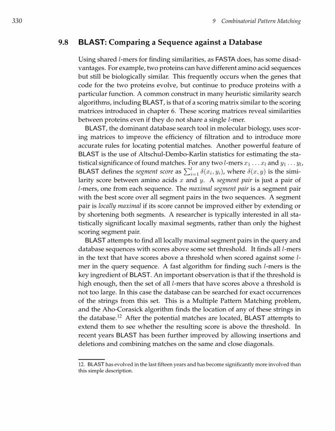
330 9 Combinatorial Pattern Matching
9.8 BLAST : Comparing a Sequence against a Database
Using shared l-mers for finding similarities, as FASTA does, has some disad-
vantages. For example, two proteins can have different amino acid sequences
but still be biologically similar. This frequently occurs when the genes that
code for the two proteins evolve, but continue to produce proteins with a
particular function. A common construct in many heuristic similarity search
algorithms, including BLAST, is that of a scoring matrix similar to the scoring
matrices introduced in chapter 6. These scoring matrices reveal similarities
between proteins even if they do not share a single l-mer.
BLAST, the dominant database search tool in molecular biology, uses scor-
ing matrices to improve the efficiency of filtration and to introduce more
accurate rules for locating potential matches. Another powerful feature of
BLAST is the use of Altschul-Dembo-Karlin statistics for estimating the sta-
tistical significance of found matches. For any two l-mers x1 . . . xl and y1 . . . yl,
BLAST defines the segment score as∑l
i=1 δ(xi, yi), where δ(x, y) is the simi-
larity score between amino acids x and y. A segment pair is just a pair of
l-mers, one from each sequence. The maximal segment pair is a segment pair
with the best score over all segment pairs in the two sequences. A segment
pair is locally maximal if its score cannot be improved either by extending or
by shortening both segments. A researcher is typically interested in all sta-
tistically significant locally maximal segments, rather than only the highest
scoring segment pair.
BLAST attempts to find all locally maximal segment pairs in the query and
database sequences with scores above some set threshold. It finds all l-mers
in the text that have scores above a threshold when scored against some l-
mer in the query sequence. A fast algorithm for finding such l-mers is the
key ingredient of BLAST. An important observation is that if the threshold is
high enough, then the set of all l-mers that have scores above a threshold is
not too large. In this case the database can be searched for exact occurrences
of the strings from this set. This is a Multiple Pattern Matching problem,
and the Aho-Corasick algorithm finds the location of any of these strings in
the database.12 After the potential matches are located, BLAST attempts to
extend them to see whether the resulting score is above the threshold. In
recent years BLAST has been further improved by allowing insertions and
deletions and combining matches on the same and close diagonals.
12. BLAST has evolved in the last fifteen years and has become significantly more involved thanthis simple description.
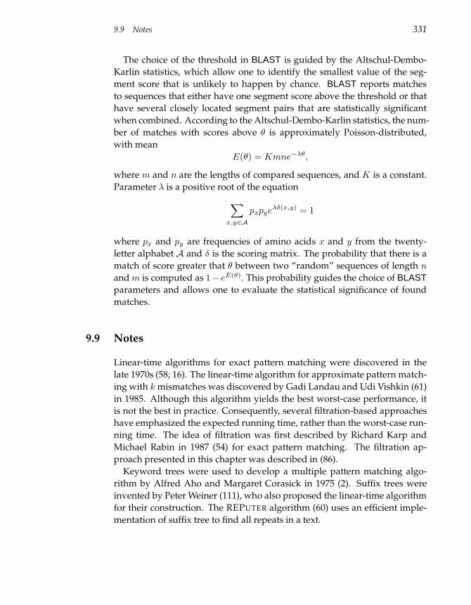
9.9 Notes 331
The choice of the threshold in BLAST is guided by the Altschul-Dembo-
Karlin statistics, which allow one to identify the smallest value of the seg-
ment score that is unlikely to happen by chance. BLAST reports matches
to sequences that either have one segment score above the threshold or that
have several closely located segment pairs that are statistically significant
when combined. According to the Altschul-Dembo-Karlin statistics, the num-
ber of matches with scores above θ is approximately Poisson-distributed,
with mean
E(θ) = Kmne−λθ,
where m and n are the lengths of compared sequences, and K is a constant.
Parameter λ is a positive root of the equation
∑
x,y∈A
pxpyeλδ(x,y) = 1
where px and py are frequencies of amino acids x and y from the twenty-
letter alphabet A and δ is the scoring matrix. The probability that there is a
match of score greater that θ between two “random” sequences of length n
and m is computed as 1− eE(θ). This probability guides the choice of BLASTparameters and allows one to evaluate the statistical significance of found
matches.
9.9 Notes
Linear-time algorithms for exact pattern matching were discovered in the
late 1970s (58; 16). The linear-time algorithm for approximate pattern match-
ing with k mismatches was discovered by Gadi Landau and Udi Vishkin (61)
in 1985. Although this algorithm yields the best worst-case performance, it
is not the best in practice. Consequently, several filtration-based approaches
have emphasized the expected running time, rather than the worst-case run-
ning time. The idea of filtration was first described by Richard Karp and
Michael Rabin in 1987 (54) for exact pattern matching. The filtration ap-
proach presented in this chapter was described in (86).
Keyword trees were used to develop a multiple pattern matching algo-
rithm by Alfred Aho and Margaret Corasick in 1975 (2). Suffix trees were
invented by Peter Weiner (111), who also proposed the linear-time algorithm
for their construction. The REPUTER algorithm (60) uses an efficient imple-
mentation of suffix tree to find all repeats in a text.

332 9 Combinatorial Pattern Matching
FASTA was developed by David Lipman and William Pearson in 1985 (67).
BLAST, the dominant database search tool in molecular biology, was devel-
oped by Steven Altschul, Warren Gish, Webb Miller, Gene Myers, and David
Lipman in 1990 (4). BLAST uses Altschul-Dembo-Karlin statistics (52; 27) to
estimate the statistical significance of found similarities. Currently there ex-
ist many variations and improvements of the BLAST tool, each tuned to a
particular application (5).
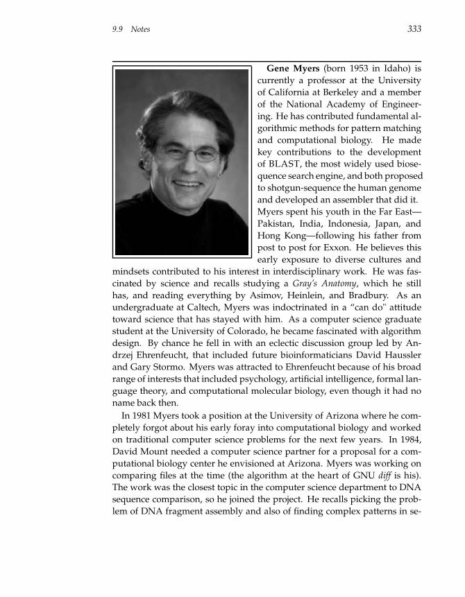
9.9 Notes 333
Gene Myers (born 1953 in Idaho) is
currently a professor at the University
of California at Berkeley and a member
of the National Academy of Engineer-
ing. He has contributed fundamental al-
gorithmic methods for pattern matching
and computational biology. He made
key contributions to the development
of BLAST, the most widely used biose-
quence search engine, and both proposed
to shotgun-sequence the human genome
and developed an assembler that did it.
Myers spent his youth in the Far East—
Pakistan, India, Indonesia, Japan, and
Hong Kong—following his father from
post to post for Exxon. He believes this
early exposure to diverse cultures and
mindsets contributed to his interest in interdisciplinary work. He was fas-
cinated by science and recalls studying a Gray’s Anatomy, which he still
has, and reading everything by Asimov, Heinlein, and Bradbury. As an
undergraduate at Caltech, Myers was indoctrinated in a “can do" attitude
toward science that has stayed with him. As a computer science graduate
student at the University of Colorado, he became fascinated with algorithm
design. By chance he fell in with an eclectic discussion group led by An-
drzej Ehrenfeucht, that included future bioinformaticians David Haussler
and Gary Stormo. Myers was attracted to Ehrenfeucht because of his broad
range of interests that included psychology, artificial intelligence, formal lan-
guage theory, and computational molecular biology, even though it had no
name back then.
In 1981 Myers took a position at the University of Arizona where he com-
pletely forgot about his early foray into computational biology and worked
on traditional computer science problems for the next few years. In 1984,
David Mount needed a computer science partner for a proposal for a com-
putational biology center he envisioned at Arizona. Myers was working on
comparing files at the time (the algorithm at the heart of GNU diff is his).
The work was the closest topic in the computer science department to DNA
sequence comparison, so he joined the project. He recalls picking the prob-
lem of DNA fragment assembly and also of finding complex patterns in se-
334 9 Combinatorial Pattern Matching
quences as topics for the proposal. A stellar review panel, including David
Sankoff, Temple Smith, and Rich Roberts, visited Arizona and were so im-
pressed with Myers’ preliminary work that he was invited to a meeting at
Waterville Valley, the first ever big bioinformatics meeting. Myers says:
I loved interacting with the biologists and the mathematicians and the
sense of excitement that something big was in the making. So in 1984
I became a computational biologist. Well, truthfully, a computer scien-
tist interested in problems motivated by computational biology. Over
the next twenty years that changed.
In the 1980s Myers worked a great deal with Webb Miller, another bioin-
formatics pioneer, and they developed some fundamental ideas for sequence
comparison, for example, linear-space alignment. He says:
It was Miller that mentored me and really helped me to develop as a
young researcher. I had been struggling with my ability to write and
with my confidence in the quality of my own work. Webb, ten years se-
nior to me, encouraged me and introduced me to the craft of technical
writing.
In 1989, Myers was working on how to find approximate matches to strings
in less than quadratic time in response to a challenge from Zvi Galil. He was
a smoker at the time and recalls talking with David Lipman outside the NIH
while on a cigarette break about his ideas. David, the coinventor of FASTA,
felt that a heuristic reformulation of the concepts would make for a fast and
practical protein search tool. Over the next few months, Miller and Myers
took turns coding different versions of the idea, with Lipman always driving
and challenging. As the work developed Steven Altschul contributed new
statistical work he had been doing with Sam Karlin, and Warren Gish, a real
code ace, built the final product. BLAST was published in 1990 and put on
the NCBI web server. It quickly became the most used tool in bioinformatics
and the most cited paper in science for several years after.
Myers did finally achieve his subquadratic algorithm in 1994 and contin-
ued to work on similarity search and fragment assembly. In 1994, at the same
meeting, Waterman and Idury, and Myers both presented fundamentally
new ideas for fragment assembly, one based on the idea of an Euler string
graph and the other on collapsing maximal uncontested interval subgraphs.
But despite being significant algorithmic advances, Phil Green’s beautifully
engineered and tuned PHRAP assembler became the mainstay of the ever
9.9 Notes 335
growing sequencing centers as they prepared for the assault on the human
genome. Myers thought he was out of the race. In 1995, Craig Venter and his
team shotgun sequenced Haemophilus influenzae, a 1.8 Mbp bacterium and
assembled it with a program written by the then very young Granger Sut-
ton. This was a rather startling success as most bioinformaticians viewed a
large clone, such as a BAC at 150 kbp, as the limit of what could be success-
fully shotgun-sequenced. Indeed the entire human genome program was
gearing up around the production of a collection of such BACs that spanned
the genome, and then shotgun-sequencing each of these in a hierarchical ap-
proach. Much of this impression was based on a misinterpretation of the
implication of a statistical theorem by Lander and Waterman about DNA
mapping. Myers says:
I recall beginning to rethink what this theorem was really saying about
shotgun-sequencing. At the same time, geneticist Jim Weber was think-
ing about shotgunning as a way to accelerate the Human Genome
Project, as he wanted to get to human genetic variation as quickly as
possible for his research. Weber called Lipman, looking for a bioinfor-
matician to help him put together a proposal. Lipman referred Weber
to me. I said yes, let’s think about it and in 1996 we began pushing the
idea and trying to publish simulation results showing that it was, in
principle, possible. The reaction to the proposal was incredibly nega-
tive; we were basically accused of being fools.
After several rejections, a very condensed version of their proposal and
Myers’ simulation was finally published in 1997 under the condition that a
rebuttal, by Phil Green, be published with it. Myers figured the proposal was
dead, but he continued to work on it at a simulation level with his students
because he found it intellectually interesting. He says:
I kept giving talks about it, hoping someone might get excited enough
to fund a $10 million pilot project. In 1998, Applied Biosystems, the
prime manufacturer of sequencing machines, and Craig Venter announced
that they would be forming a company to sequence the human genome
using a shotgun approach. To me it was as if someone had decided to
spend $300 million to try “my" project.
Myers had known Venter for ten years and quickly came to the decision
to join the company, Celera, at its inception in August 1998. With more re-
sources than he imagined, his problem became to deliver on the promise. He
says:
336 9 Combinatorial Pattern Matching
It was an incredible time of my life. I thought I could do it, but I didn’t
yet know I could do it. The pressure was incredible, but so was the
excitement.
A year and a half-million lines of code later a team of ten, including Granger
Sutton, achieved their first assembly of the Drosophila genome and presented
the results in October 1999. Myers had his 120 Mbp pilot project and it
was a success. The race for the human genome was then on. The Celera
team’s main obstacle was in how to scale up another 30-fold for the human
genome—computer memory and time were real problems. In 20,000 CPU
hours and a month’s time, a first assembly of the human genome was ac-
complished in May 2000. Subsequent refinements took place and the first
reconstructions of the genome were published by Celera and the public con-
sortium in February 2001. Today, whole-genome shotgun sequence is not
really debatable: it is the way that every genome is being sequenced. Myers
says:
Now at Berkeley, I have become fascinated with how cells work from
the level of particle systems and in particular how multicellular or-
ganisms develop. I figure the next great challenge is to “decode the
cell.” I am driven by the intellectual curiosity to have some sense of
understanding the cell as a system before the end of my career. Biol-
ogy drives what I do today; my skills as an algorithmist are tools to
this end as opposed to my primary focus, although I still get pretty
excited when I come up with a tricky new way to solve a particular
computational problem.
9.10 Problems 337
9.10 Problems
Problem 9.1
Derive the expectation and the variance of the number of occurrences of patterns AAand AT in a random text of length n. Are the expectations and variances for AA andAT the same?
Problem 9.2
Derive the expectation and the variance of the number of occurrences of a given pat-tern of length l in a random text of length n.
Let X be the set of all l-mers. Given an l-mer x and a text t, define x(t) as the number of
occurrences of x in t. Statistical distance between texts t and u is defined as
d(t, u) =
s
X
x∈X(x(t) − x(u))2.
Although statistical distance can be computed very fast, it can miss weak similarities that do not
preserve shared l-mers.
Problem 9.3
Evaluate an expected statistical distance between two random n-letter strings.
Problem 9.4
Prove that the average time that PATTERNMATCHING takes to check whether a pat-tern of length n appears at a given position in a random text is 2− n+1
An + n
An+1 (A isthe size of alphabet).
Problem 9.5
Write an efficient algorithm that will construct a keyword tree given a list of patterns
p1, p2, . . . ,pk.
Problem 9.6
Design an algorithm for a generalization of the Approximate Pattern Matching prob-lem in the case where the pattern can match a text with up to k mismatches, insertions,or deletions (rather than the mismatch-only model as before).
Problem 9.7
A string p = p1 . . . pn is a palindrome if it spells the same string when read backward,that is, pi = pn+1−i for 1 ≤ i ≤ n. Design an efficient algorithm for finding allpalindromes (of all lengths) in a text.
Problem 9.8
Design an efficient algorithm for finding the longest exact repeat within a text.
Problem 9.9
Design an efficient algorithm for finding the longest exact tandem repeat within atext.
338 9 Combinatorial Pattern Matching
Problem 9.10
Design an efficient algorithm for finding the longest exact repeat with at most onemismatch in a text.
Problem 9.11
Design an efficient algorithm for finding the longest string shared by two given texts.
Problem 9.12
Design an efficient algorithm for finding a shortest nonrepeated string in a text, thatis, a shortest string that appears in the text only once.
Problem 9.13
Design an efficient algorithm that finds a shortest string in text t1 that does not appearin text t2.
Problem 9.14
Implement an l-tuple filtration algorithm for the Query Matching problem.
10 Clustering and Trees
A common problem in biology is to partition a set of experimental data into
groups (clusters) in such a way that the data points within the same clus-
ter are highly similar while data points in different clusters are very differ-
ent. This problem is far from simple, and this chapter covers several algo-
rithms that perform different types of clustering. There is no simple recipe
for choosing one particular approach over another for a particular clustering
problem, just as there is no universal notion of what constitutes a “good clus-
ter.” Nonetheless, these algorithms can yield significant insight into data and
allow one, for example, to identify clusters of genes with similar functions
even when it is not clear what particular role these genes play. We conclude
this chapter with studies of evolutionary tree reconstruction, which is closely
related to clustering.
10.1 Gene Expression Analysis
Sequence comparison often helps to discover the function of a newly se-
quenced gene by finding similarities between the new gene and previously
sequenced genes with known functions. However, for many genes, the se-
quence similarity of genes in a functional family is so weak that one cannot
reliably derive the function of the newly sequenced gene based on sequence
alone. Moreover, genes with the same function sometimes have no sequence
similarity at all. As a result, the functions of more than 40% of the genes in
sequenced genomes are still unknown.
In the last decade, a new approach to analyzing gene functions has emerged.
DNA arrays allow one to analyze the expression levels (amount of mRNA pro-
duced in the cell) of many genes under many time points and conditions and
340 10 Clustering and Trees
to reveal which genes are switched on and switched off in the cell.1 The
outcome of this type of study is an n × m expression matrix I, with the n
rows corresponding to genes, and the m columns corresponding to differ-
ent time points and different conditions. The expression matrix I represents
intensities of hybridization signals as provided by a DNA array. In reality, ex-
pression matrices usually represent transformed and normalized intensities
rather than the raw intensities obtained as a result of a DNA array experi-
ment, but we will not discuss this transformation.
The element Ii,j of the expression matrix represents the expression level of
gene i in experiment j; the entire ith row of the expression matrix is called
the expression pattern of gene i. One can look for pairs of genes in an expres-
sion matrix with similar expression patterns, which would be manifested as
two similar rows. Therefore, if the expression patterns of two genes are sim-
ilar, there is a good chance that these genes are somehow related, that is,
they either perform similar functions or are involved in the same biological
process.2 Accordingly, if the expression pattern of a newly sequenced gene
is similar to the expression pattern of a gene with known function, a biolo-
gist may have reason to suspect that these genes perform similar or related
functions. Another important application of expression analysis is in the de-
ciphering of regulatory pathways; similar expression patterns usually imply
coregulation. However, expression analysis should be done with caution
since DNA arrays typically produce noisy data with high error rates.
Clustering algorithms group genes with similar expression patterns into clus-
ters with the hope that these clusters correspond to groups of functionally
related genes. To cluster the expression data, the n×m expression matrix is
often transformed into an n × n distance matrix d = (di,j) where di,j reflects
how similar the expression patterns of genes i and j are (see figure 10.1).3
The goal of clustering is to group genes into clusters satisfying the following
two conditions:
• Homogeneity. Genes (rather, their expression patterns) within a cluster
1. Expression analysis studies implicitly assume that the amount of mRNA (as measured by aDNA array) is correlated with the amount of its protein produced by the cell. We emphasize thata number of processes affect the production of proteins in the cell (transcription, splicing, trans-lation, post-translational modifications, protein degradation, etc.) and therefore this correlationmay not be straightforward, but it is still significant.2. Of course, we do not exclude the possibility that expression patterns of two genes may looksimilar simply by chance, but the probability of such a chance similarity decreases as we increasethe number of time points.3. The distance matrix is typically larger than the expression matrix since n m in most ex-pression studies.
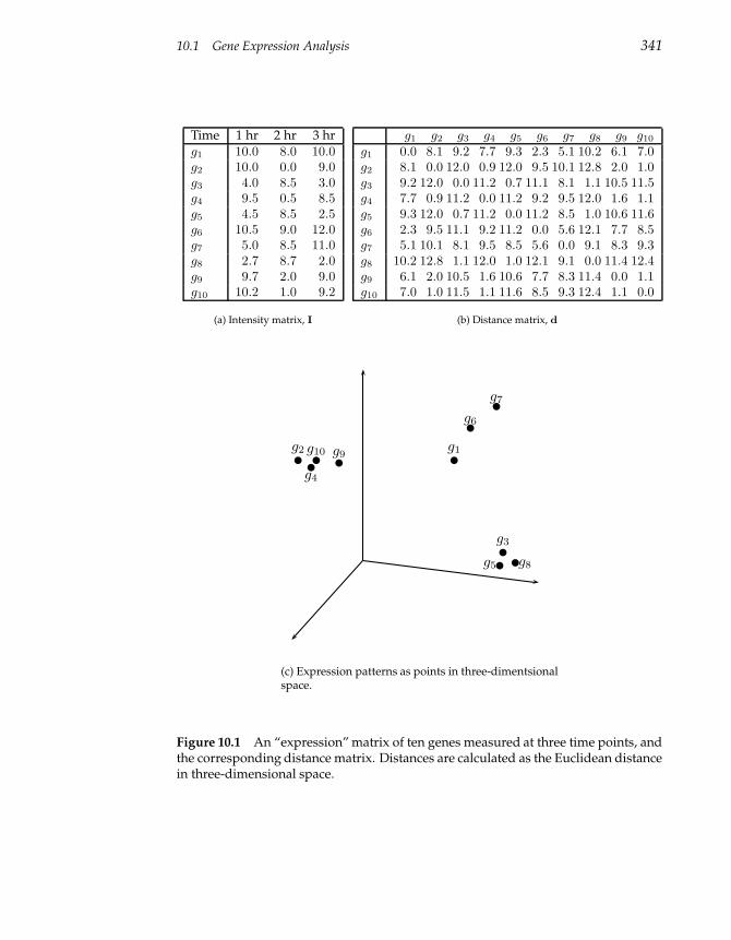
10.1 Gene Expression Analysis 341
Time 1 hr 2 hr 3 hrg1 10.0 8.0 10.0g2 10.0 0.0 9.0g3 4.0 8.5 3.0g4 9.5 0.5 8.5g5 4.5 8.5 2.5g6 10.5 9.0 12.0g7 5.0 8.5 11.0g8 2.7 8.7 2.0g9 9.7 2.0 9.0g10 10.2 1.0 9.2
(a) Intensity matrix, I
g1 g2 g3 g4 g5 g6 g7 g8 g9 g10
g1 0.0 8.1 9.2 7.7 9.3 2.3 5.1 10.2 6.1 7.0g2 8.1 0.0 12.0 0.9 12.0 9.5 10.1 12.8 2.0 1.0g3 9.2 12.0 0.0 11.2 0.7 11.1 8.1 1.1 10.5 11.5g4 7.7 0.9 11.2 0.0 11.2 9.2 9.5 12.0 1.6 1.1g5 9.3 12.0 0.7 11.2 0.0 11.2 8.5 1.0 10.6 11.6g6 2.3 9.5 11.1 9.2 11.2 0.0 5.6 12.1 7.7 8.5g7 5.1 10.1 8.1 9.5 8.5 5.6 0.0 9.1 8.3 9.3g8 10.2 12.8 1.1 12.0 1.0 12.1 9.1 0.0 11.4 12.4g9 6.1 2.0 10.5 1.6 10.6 7.7 8.3 11.4 0.0 1.1g10 7.0 1.0 11.5 1.1 11.6 8.5 9.3 12.4 1.1 0.0
(b) Distance matrix, d
g1g2
g3
g4
g5
g6
g7
g8
g9g10
(c) Expression patterns as points in three-dimentsionalspace.
Figure 10.1 An “expression” matrix of ten genes measured at three time points, andthe corresponding distance matrix. Distances are calculated as the Euclidean distancein three-dimensional space.
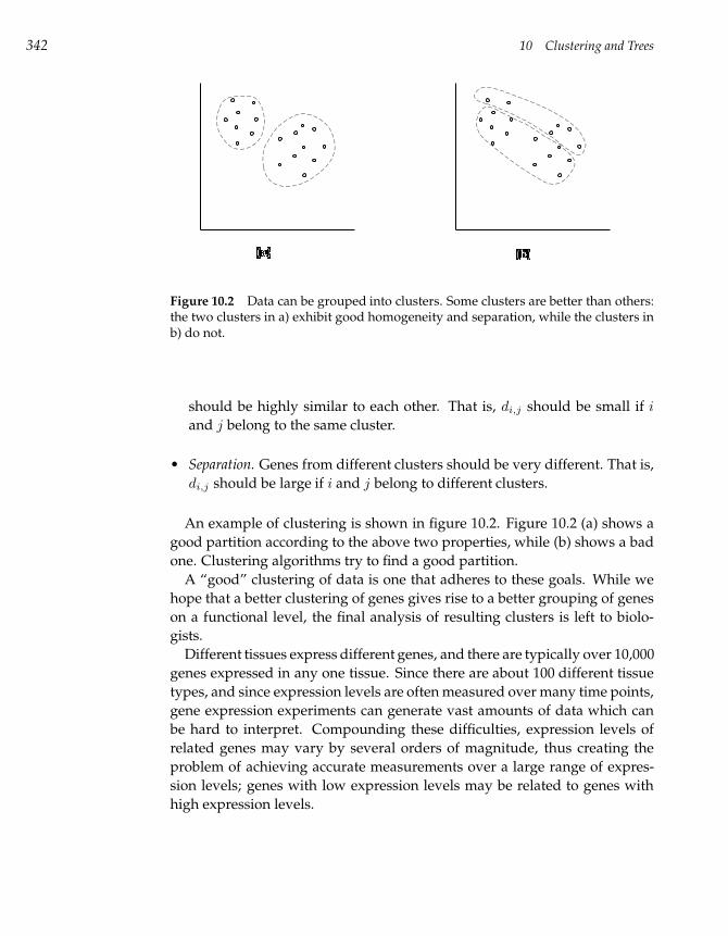
342 10 Clustering and Trees
Figure 10.2 Data can be grouped into clusters. Some clusters are better than others:the two clusters in a) exhibit good homogeneity and separation, while the clusters inb) do not.
should be highly similar to each other. That is, di,j should be small if i
and j belong to the same cluster.
• Separation. Genes from different clusters should be very different. That is,
di,j should be large if i and j belong to different clusters.
An example of clustering is shown in figure 10.2. Figure 10.2 (a) shows a
good partition according to the above two properties, while (b) shows a bad
one. Clustering algorithms try to find a good partition.
A “good” clustering of data is one that adheres to these goals. While we
hope that a better clustering of genes gives rise to a better grouping of genes
on a functional level, the final analysis of resulting clusters is left to biolo-
gists.
Different tissues express different genes, and there are typically over 10,000
genes expressed in any one tissue. Since there are about 100 different tissue
types, and since expression levels are often measured over many time points,
gene expression experiments can generate vast amounts of data which can
be hard to interpret. Compounding these difficulties, expression levels of
related genes may vary by several orders of magnitude, thus creating the
problem of achieving accurate measurements over a large range of expres-
sion levels; genes with low expression levels may be related to genes with
high expression levels.
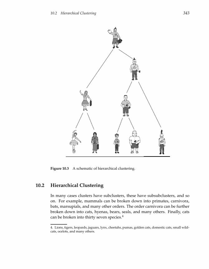
10.2 Hierarchical Clustering 343
Figure 10.3 A schematic of hierarchical clustering.
10.2 Hierarchical Clustering
In many cases clusters have subclusters, these have subsubclusters, and so
on. For example, mammals can be broken down into primates, carnivora,
bats, marsupials, and many other orders. The order carnivora can be further
broken down into cats, hyenas, bears, seals, and many others. Finally, cats
can be broken into thirty seven species.4
4. Lions, tigers, leopards, jaguars, lynx, cheetahs, pumas, golden cats, domestic cats, small wild-cats, ocelots, and many others.
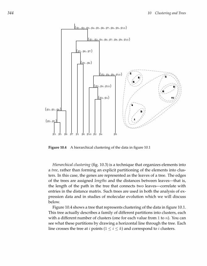
344 10 Clustering and Trees
g3 g5 g8 g7 g1 g6 g10 g2 g4 g9
g3, g5
g3, g5, g8
g2, g4
g2, g4, g10
g2, g4, g9, g10
g1, g6
g1, g6, g7
g1, g2, g4, g6, g7, g8, g9, g10
g1, g2, g3, g4, g5, g6, g7, g8, g9, g10
Figure 10.4 A hierarchical clustering of the data in figure 10.1
Hierarchical clustering (fig. 10.3) is a technique that organizes elements into
a tree, rather than forming an explicit partitioning of the elements into clus-
ters. In this case, the genes are represented as the leaves of a tree. The edges
of the trees are assigned lengths and the distances between leaves—that is,
the length of the path in the tree that connects two leaves—correlate with
entries in the distance matrix. Such trees are used in both the analysis of ex-
pression data and in studies of molecular evolution which we will discuss
below.
Figure 10.4 shows a tree that represents clustering of the data in figure 10.1.
This tree actually describes a family of different partitions into clusters, each
with a different number of clusters (one for each value from 1 to n). You can
see what these partitions by drawing a horizontal line through the tree. Each
line crosses the tree at i points (1 ≤ i ≤ k) and correspond to i clusters.
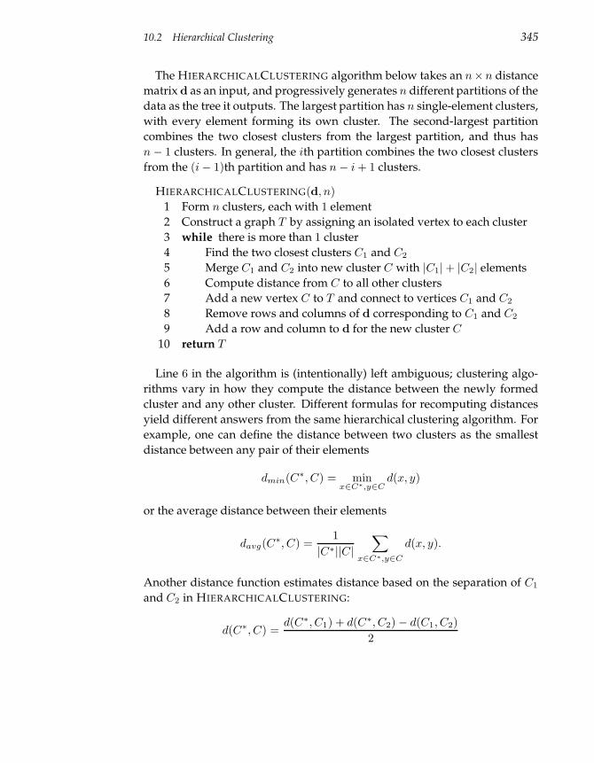
10.2 Hierarchical Clustering 345
The HIERARCHICALCLUSTERING algorithm below takes an n×n distance
matrix d as an input, and progressively generates n different partitions of the
data as the tree it outputs. The largest partition has n single-element clusters,
with every element forming its own cluster. The second-largest partition
combines the two closest clusters from the largest partition, and thus has
n− 1 clusters. In general, the ith partition combines the two closest clusters
from the (i− 1)th partition and has n− i + 1 clusters.
HIERARCHICALCLUSTERING(d, n)
1 Form n clusters, each with 1 element
2 Construct a graph T by assigning an isolated vertex to each cluster
3 while there is more than 1 cluster
4 Find the two closest clusters C1 and C2
5 Merge C1 and C2 into new cluster C with |C1|+ |C2| elements
6 Compute distance from C to all other clusters
7 Add a new vertex C to T and connect to vertices C1 and C2
8 Remove rows and columns of d corresponding to C1 and C2
9 Add a row and column to d for the new cluster C
10 return T
Line 6 in the algorithm is (intentionally) left ambiguous; clustering algo-
rithms vary in how they compute the distance between the newly formed
cluster and any other cluster. Different formulas for recomputing distances
yield different answers from the same hierarchical clustering algorithm. For
example, one can define the distance between two clusters as the smallest
distance between any pair of their elements
dmin(C∗, C) = minx∈C∗,y∈C
d(x, y)
or the average distance between their elements
davg(C∗, C) =1
|C∗||C|
∑
x∈C∗,y∈C
d(x, y).
Another distance function estimates distance based on the separation of C1
and C2 in HIERARCHICALCLUSTERING:
d(C∗, C) =d(C∗, C1) + d(C∗, C2)− d(C1, C2)
2
346 10 Clustering and Trees
In one of the first expression analysis studies, Michael Eisen and colleagues
used hierarchical clustering to analyze the expression profiles of 8600 genes
over thirteen time points to find the genes responsible for the growth re-
sponse of starved human cells. The HIERARCHICALCLUSTERING resulted
in a tree consisting of five main subtrees and many smaller subtrees. The
genes within these five clusters had similar functions, thus confirming that
the resulting clusters are biologically sensible.
10.3 k-Means Clustering
One can view the n rows of the n×m expression matrix as a set of n points
in m-dimensional space and partition them into k subsets, pretending that
k—the number of clusters—is known in advance.
One of the most popular clustering methods for points in multidimen-
sional spaces is called k-Means clustering. Given a set of n data points in
m-dimensional space and an integer k, the problem is to determine a set
of k points, or centers, in m-dimensional space that minimize the squared
error distortion defined below. Given a data point v and a set of k centers
X = x1, . . . xk, define the distance from v to the centers X as the distance
from v to the closest point in X , that is, d(v,X ) = min1≤i≤k d(v, xi). We will
assume for now that d(v, xi) is just the Euclidean5 distance in m dimensions.
The squared error distortion for a set of n points V = v1, . . . vn, and a set
of k centers X = x1, . . . xk, is defined as the mean squared distance from
each data point to its nearest center:
d(V ,X ) =
∑ni=1 d(vi,X )2
n
k-Means Clustering Problem:
Given n data points, find k center points minimizing the squared error
distortion.
Input: A set, V , consisting of n points and a parameter k.
Output: A set X consisting of k points (called centers) that
minimizes d(V ,X ) over all possible choices of X .
5. Chapter 2 contains a sample algorithm to calculate this when m is 2.
10.3 k-Means Clustering 347
While the above formulation does not explicitly address clustering n points
into k clusters, a clustering can be obtained by simply assigning each point to
its closest center. Although the k-Means Clustering problem looks relatively
simple, there are no efficient (polynomial) algorithms known for it. The Lloyd
k-Means clustering algorithm is one of the most popular clustering heuristics
that often generates good solutions in gene expression analysis. The Lloyd
algorithm randomly selects an arbitrary partition of points into k clusters and
tries to improve this partition by moving some points between clusters. In
the beginning one can choose arbitrary k points as “cluster representatives.”
The algorithm iteratively performs the following two steps until either it con-
verges or until the fluctuations become very small:
• Assign each data point to the cluster Ci corresponding to the closest clus-
ter representative xi (1 ≤ i ≤ k)
• After the assignments of all n data points, compute new cluster represen-
tatives according to the center of gravity of each cluster, that is, the new
cluster representative isP
v∈Cv
|C| for every cluster C.
The Lloyd algorithm often converges to a local minimum of the squared
error distortion function rather than the global minimum. Unfortunately, in-
teresting objective functions other than the squared error distortion lead to
similarly difficult problems. For example, finding a good clustering can be
quite difficult if, instead of the squared error distortion (∑n
i=1 d(vi,X )2), one
tries to minimize∑n
i=1 d(vi,X ) (k-Median problem) or max1≤i≤n d(vi,X ) (k-
Center problem). We remark that all of these definitions of clustering cost em-
phasize the homogeneity condition and more or less ignore the other impor-
tant goal of clustering, the separation condition. Moreover, in some unlucky
instances of the k-Means Clustering problem, the algorithm may converge
to a local minimum that is arbitrarily bad compared to an optimal solution (a
problem at the end of this chapter).
While the Lloyd algorithm is very fast, it can significantly rearrange every
cluster in every iteration. A more conservative approach is to move only one
element between clusters in each iteration. We assume that every partition
P of the n-element set into k clusters has an associated clustering cost, de-
noted cost(P ), that measures the quality of the partition P : the smaller the
clustering cost of a partition, the better that clustering is.6 The squared error
distortion is one particular choice of cost(P ) and assumes that each center
6. “Better” here is better clustering, not a better biological grouping of genes.
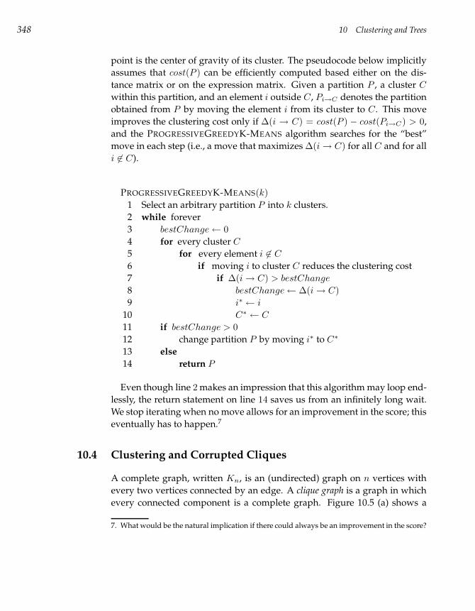
348 10 Clustering and Trees
point is the center of gravity of its cluster. The pseudocode below implicitly
assumes that cost(P ) can be efficiently computed based either on the dis-
tance matrix or on the expression matrix. Given a partition P , a cluster C
within this partition, and an element i outside C, Pi→C denotes the partition
obtained from P by moving the element i from its cluster to C. This move
improves the clustering cost only if ∆(i → C) = cost(P ) − cost(Pi→C) > 0,
and the PROGRESSIVEGREEDYK-MEANS algorithm searches for the “best”
move in each step (i.e., a move that maximizes ∆(i→ C) for all C and for all
i 6∈ C).
PROGRESSIVEGREEDYK-MEANS(k)
1 Select an arbitrary partition P into k clusters.
2 while forever
3 bestChange← 0
4 for every cluster C
5 for every element i 6∈ C
6 if moving i to cluster C reduces the clustering cost
7 if ∆(i→ C) > bestChange
8 bestChange← ∆(i→ C)
9 i∗ ← i
10 C∗ ← C
11 if bestChange > 0
12 change partition P by moving i∗ to C∗
13 else
14 return P
Even though line 2 makes an impression that this algorithm may loop end-
lessly, the return statement on line 14 saves us from an infinitely long wait.
We stop iterating when no move allows for an improvement in the score; this
eventually has to happen.7
10.4 Clustering and Corrupted Cliques
A complete graph, written Kn, is an (undirected) graph on n vertices with
every two vertices connected by an edge. A clique graph is a graph in which
every connected component is a complete graph. Figure 10.5 (a) shows a
7. What would be the natural implication if there could always be an improvement in the score?
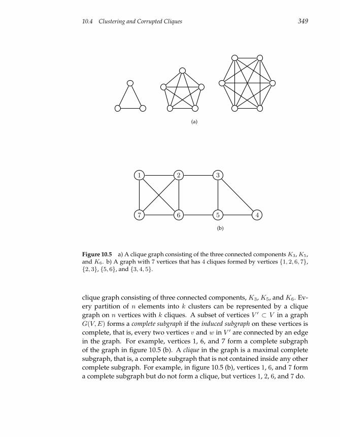
10.4 Clustering and Corrupted Cliques 349
(a)
1 2 3
7 6 5 4
(b)
Figure 10.5 a) A clique graph consisting of the three connected components K3, K5,and K6. b) A graph with 7 vertices that has 4 cliques formed by vertices 1, 2, 6, 7,2, 3, 5, 6, and 3, 4, 5.
clique graph consisting of three connected components, K3, K5, and K6. Ev-
ery partition of n elements into k clusters can be represented by a clique
graph on n vertices with k cliques. A subset of vertices V ′ ⊂ V in a graph
G(V, E) forms a complete subgraph if the induced subgraph on these vertices is
complete, that is, every two vertices v and w in V ′ are connected by an edge
in the graph. For example, vertices 1, 6, and 7 form a complete subgraph
of the graph in figure 10.5 (b). A clique in the graph is a maximal complete
subgraph, that is, a complete subgraph that is not contained inside any other
complete subgraph. For example, in figure 10.5 (b), vertices 1, 6, and 7 form
a complete subgraph but do not form a clique, but vertices 1, 2, 6, and 7 do.
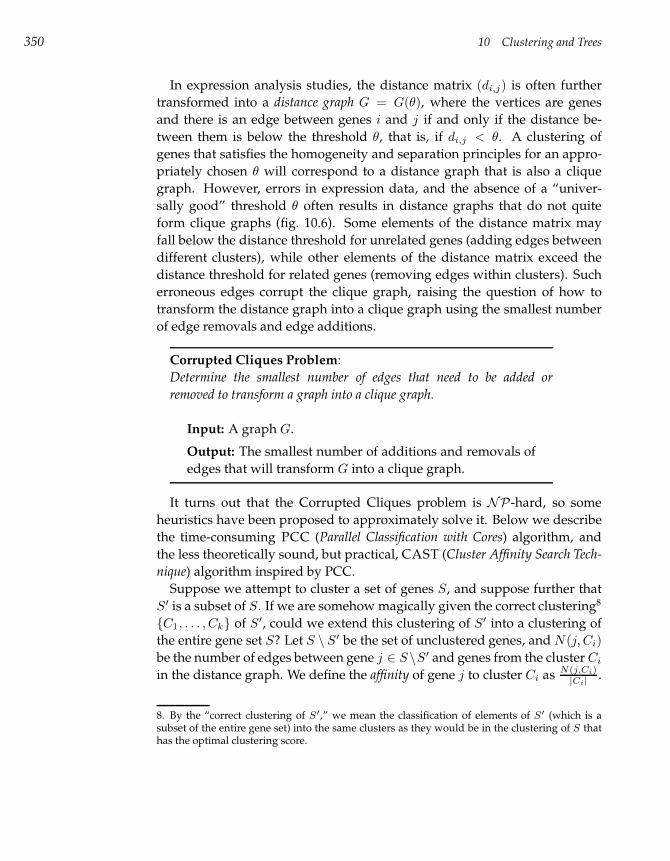
350 10 Clustering and Trees
In expression analysis studies, the distance matrix (di,j) is often further
transformed into a distance graph G = G(θ), where the vertices are genes
and there is an edge between genes i and j if and only if the distance be-
tween them is below the threshold θ, that is, if di,j < θ. A clustering of
genes that satisfies the homogeneity and separation principles for an appro-
priately chosen θ will correspond to a distance graph that is also a clique
graph. However, errors in expression data, and the absence of a “univer-
sally good” threshold θ often results in distance graphs that do not quite
form clique graphs (fig. 10.6). Some elements of the distance matrix may
fall below the distance threshold for unrelated genes (adding edges between
different clusters), while other elements of the distance matrix exceed the
distance threshold for related genes (removing edges within clusters). Such
erroneous edges corrupt the clique graph, raising the question of how to
transform the distance graph into a clique graph using the smallest number
of edge removals and edge additions.
Corrupted Cliques Problem:
Determine the smallest number of edges that need to be added or
removed to transform a graph into a clique graph.
Input: A graph G.
Output: The smallest number of additions and removals of
edges that will transform G into a clique graph.
It turns out that the Corrupted Cliques problem is NP-hard, so some
heuristics have been proposed to approximately solve it. Below we describe
the time-consuming PCC (Parallel Classification with Cores) algorithm, and
the less theoretically sound, but practical, CAST (Cluster Affinity Search Tech-
nique) algorithm inspired by PCC.
Suppose we attempt to cluster a set of genes S, and suppose further that
S′ is a subset of S. If we are somehow magically given the correct clustering8
C1, . . . , Ck of S′, could we extend this clustering of S′ into a clustering of
the entire gene set S? Let S \ S′ be the set of unclustered genes, and N(j, Ci)
be the number of edges between gene j ∈ S\S′ and genes from the cluster Ci
in the distance graph. We define the affinity of gene j to cluster Ci as N(j,Ci)|Ci|
.
8. By the “correct clustering of S′,” we mean the classification of elements of S′ (which is asubset of the entire gene set) into the same clusters as they would be in the clustering of S thathas the optimal clustering score.
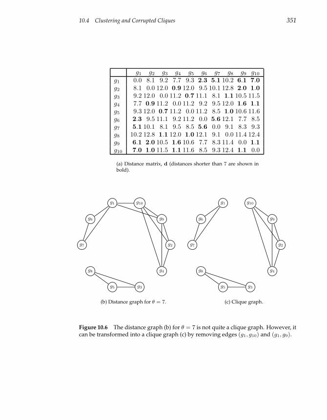
10.4 Clustering and Corrupted Cliques 351
g1 g2 g3 g4 g5 g6 g7 g8 g9 g10
g1 0.0 8.1 9.2 7.7 9.3 2.3 5.1 10.2 6.1 7.0g2 8.1 0.0 12.0 0.9 12.0 9.5 10.1 12.8 2.0 1.0g3 9.2 12.0 0.0 11.2 0.7 11.1 8.1 1.1 10.5 11.5g4 7.7 0.9 11.2 0.0 11.2 9.2 9.5 12.0 1.6 1.1g5 9.3 12.0 0.7 11.2 0.0 11.2 8.5 1.0 10.6 11.6g6 2.3 9.5 11.1 9.2 11.2 0.0 5.6 12.1 7.7 8.5g7 5.1 10.1 8.1 9.5 8.5 5.6 0.0 9.1 8.3 9.3g8 10.2 12.8 1.1 12.0 1.0 12.1 9.1 0.0 11.4 12.4g9 6.1 2.0 10.5 1.6 10.6 7.7 8.3 11.4 0.0 1.1g10 7.0 1.0 11.5 1.1 11.6 8.5 9.3 12.4 1.1 0.0
(a) Distance matrix, d (distances shorter than 7 are shown inbold).
g2
g9
g10g1
g6
g7
g8
g5 g3
g4
(b) Distance graph for θ = 7.
g2
g9
g10g1
g6
g7
g8
g5 g3
g4
(c) Clique graph.
Figure 10.6 The distance graph (b) for θ = 7 is not quite a clique graph. However, itcan be transformed into a clique graph (c) by removing edges (g1, g10) and (g1, g9).
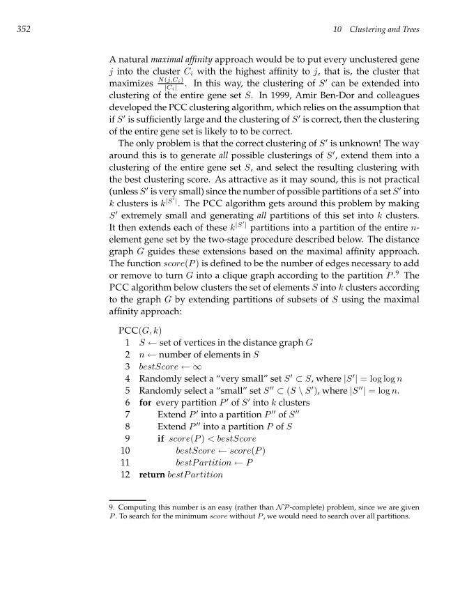
352 10 Clustering and Trees
A natural maximal affinity approach would be to put every unclustered gene
j into the cluster Ci with the highest affinity to j, that is, the cluster that
maximizes N(j,Ci)|Ci|
. In this way, the clustering of S′ can be extended into
clustering of the entire gene set S. In 1999, Amir Ben-Dor and colleagues
developed the PCC clustering algorithm, which relies on the assumption that
if S′ is sufficiently large and the clustering of S′ is correct, then the clustering
of the entire gene set is likely to to be correct.
The only problem is that the correct clustering of S′ is unknown! The way
around this is to generate all possible clusterings of S′, extend them into a
clustering of the entire gene set S, and select the resulting clustering with
the best clustering score. As attractive as it may sound, this is not practical
(unless S′ is very small) since the number of possible partitions of a set S′ into
k clusters is k|S′|. The PCC algorithm gets around this problem by making
S′ extremely small and generating all partitions of this set into k clusters.
It then extends each of these k|S′| partitions into a partition of the entire n-
element gene set by the two-stage procedure described below. The distance
graph G guides these extensions based on the maximal affinity approach.
The function score(P ) is defined to be the number of edges necessary to add
or remove to turn G into a clique graph according to the partition P .9 The
PCC algorithm below clusters the set of elements S into k clusters according
to the graph G by extending partitions of subsets of S using the maximal
affinity approach:
PCC(G, k)
1 S ← set of vertices in the distance graph G
2 n← number of elements in S
3 bestScore←∞
4 Randomly select a “very small” set S′ ⊂ S, where |S′| = log log n
5 Randomly select a “small” set S′′ ⊂ (S \ S′), where |S′′| = log n.
6 for every partition P ′ of S′ into k clusters
7 Extend P ′ into a partition P ′′ of S′′
8 Extend P ′′ into a partition P of S
9 if score(P ) < bestScore
10 bestScore← score(P )
11 bestPartition← P
12 return bestPartition
9. Computing this number is an easy (rather than NP-complete) problem, since we are givenP . To search for the minimum score without P , we would need to search over all partitions.
10.4 Clustering and Corrupted Cliques 353
The number of iterations that PCC requires is given by the number of par-
titions of set S′, which is k|S′| = klog log n = (log n)log2 k = (log n)c. The
amount of work done in each iteration is O(n2), resulting in a running time
of O(
n2(log n)c)
. Since this is too slow for most applications, a more practi-
cal heuristic called CAST is often used.
Define the distance between gene i and cluster C as the average distance
between i and all genes in the cluster C: d(i, C) =P
j∈Cd(i,j)
|C| . Given a thresh-
old θ, a gene i is close to cluster C if d(i, C) < θ and distant otherwise. The
CAST algorithm below clusters set S according to the distance graph G and
the threshold θ. CAST iteratively builds the partition P of the set S by find-
ing a cluster C such that no gene i 6∈ C is close to C, and no gene i ∈ C is
distant from C. In the beginning of the routine, P is initialized to an empty
set.
354 10 Clustering and Trees
CAST(G, θ)
1 S ← set of vertices in the distance graph G
2 P ← ∅
3 while S 6= ∅
4 v ← vertex of maximal degree in the distance graph G.
5 C ← v
6 while there exists a close gene i 6∈ C or distant gene i ∈ C
7 Find the nearest close gene i 6∈ C and add it to C.
8 Find the farthest distant gene i ∈ C and remove it from C.
9 Add cluster C to the partition P
10 S ← S \ C
11 Remove vertices of cluster C from the distance graph G
12 return P
Although CAST is a heuristic with no performance guarantee10 it per-
forms remarkably well with gene expression data.
10.5 Evolutionary Trees
In the past, biologists relied on morphological features, like beak shapes or
the presence or absence of fins to construct evolutionary trees. Today biol-
ogists rely on DNA sequences for the reconstruction of evolutionary trees.
Figure 10.7 represents a DNA-based evolutionary tree of bears and raccoons
that helped biologists to decide whether the giant panda belongs to the bear
family or the raccoon family. This question is not as obvious as it may at first
sound, since bears and raccoons diverged just 35 million years ago and they
share many morphological features.
For over a hundred years biologists could not agree on whether the giant
panda should be classified in the bear family or in the raccoon family. In 1870
an amateur naturalist and missionary, Père Armand David, returned to Paris
from China with the bones of the mysterious creature which he called simply
“black and white bear.” Biologists examined the bones and concluded that
they more closely resembled the bones of a red panda than those of bears.
Since red pandas were, beyond doubt, part of the raccoon family, giant pan-
das were also classified as raccoons (albeit big ones).
Although giant pandas look like bears, they have features that are unusual
for bears and typical of raccoons: they do not hibernate in the winter like
10. In fact, CAST may not even converge; see the problems at the end of the chapter.
10.5 Evolutionary Trees 355
other bears do, their male genitalia are tiny and backward-pointing (like rac-
coons’ genitalia), and they do not roar like bears but bleat like raccoons. As
a result, Edwin Colbert wrote in 1938:
So the quest has stood for many years with the bear proponents and the
raccoon adherents and the middle-of-the-road group advancing their
several arguments with the clearest of logic, while in the meantime the
giant panda lives serenely in the mountains of Szechuan with never a
thought about the zoological controversies he is causing by just being
himself.
The giant panda classification was finally resolved in 1985 by Steven O’Brien
and colleagues who used DNA sequences and algorithms, rather than be-
havioral and anatomical features, to resolve the giant panda controversy
(fig. 10.7). The final analysis demonstrated that DNA sequences provide an
important source of information to test evolutionary hypotheses. O’Brien’s
study used about 500,000 nucleotides to construct the evolutionary tree of
bears and raccoons.
Roughly at the same time that Steven O’Brien resolved the giant panda
controversy, Rebecca Cann, Mark Stoneking and Allan Wilson constructed
an evolutionary tree of humans and instantly created a new controversy. This
tree led to the Out of Africa hypothesis, which claims that humans have a
common ancestor who lived in Africa 200,000 years ago. This study turned
the question of human origins into an algorithmic puzzle.
The tree was constructed from mitochondrial DNA (mtDNA) sequences of
people of different races and nationalities.11 Wilson and his colleagues com-
pared sequences of mtDNA from people representing African, Asian, Aus-
tralian, Caucasian, and New Guinean ethnic groups and found 133 variants
of mtDNA. Next, they constructed the evolutionary tree for these DNA se-
quences that showed a trunk splitting into two major branches. One branch
consisted only of Africans, the other included some modern Africans and
some people from everywhere else. They concluded that a population of
Africans, the first modern humans, forms the trunk and the first branch of
the tree while the second branch represents a subgroup that left Africa and
later spread out to the rest of the world. All of the mtDNA, even samples
from regions of the world far away from Africa, were strikingly similar. This
11. Unlike the bulk of the genome, mitochondrial DNA is passed solely from a mother to herchildren without recombining with the father’s DNA. Thus it is well-suited for studies of recenthuman evolution. In addition, it quickly accumulates mutations and thus offers a quick-tickingmolecular clock.
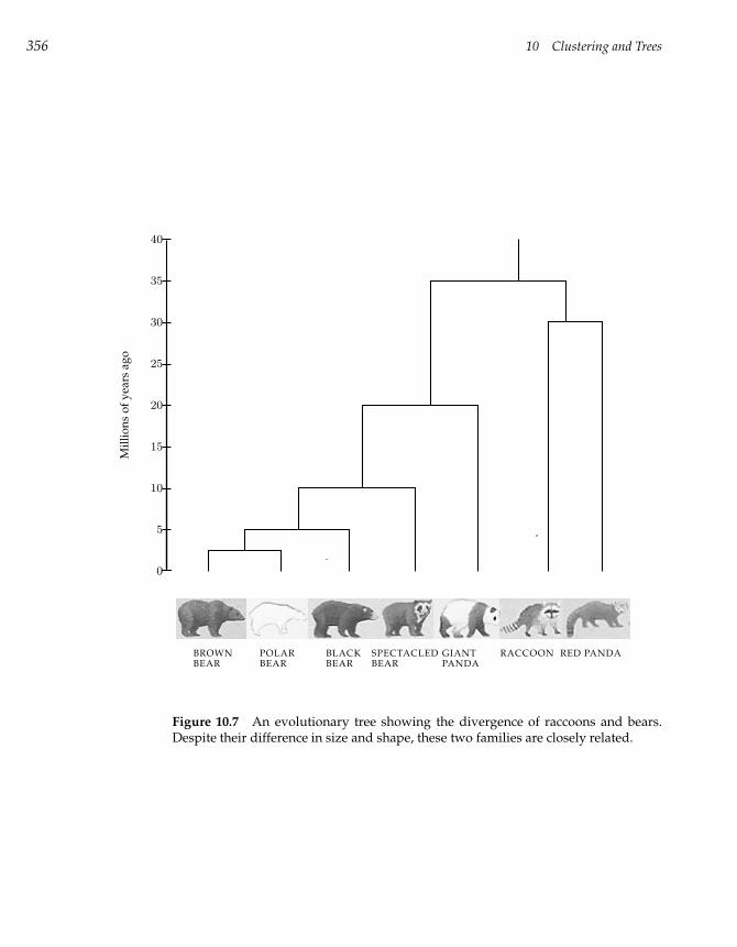
356 10 Clustering and Trees
BROWNBEAR
POLARBEAR
BLACKBEAR
SPECTACLEDBEAR
GIANTPANDA
RACCOON RED PANDA
40
35
30
25
20
15
10
5
0
Mil
lio
ns
of
yea
rsag
o
Figure 10.7 An evolutionary tree showing the divergence of raccoons and bears.Despite their difference in size and shape, these two families are closely related.
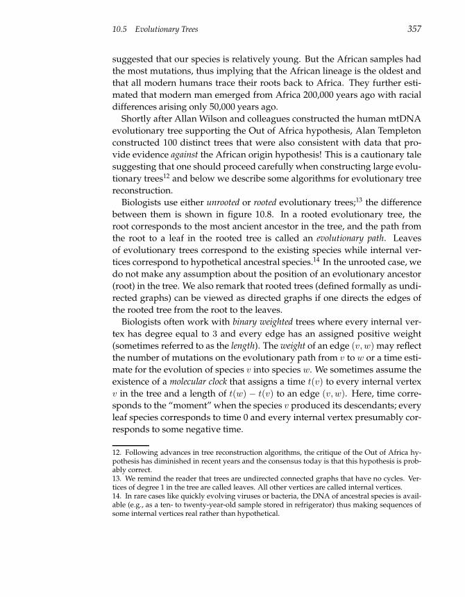
10.5 Evolutionary Trees 357
suggested that our species is relatively young. But the African samples had
the most mutations, thus implying that the African lineage is the oldest and
that all modern humans trace their roots back to Africa. They further esti-
mated that modern man emerged from Africa 200,000 years ago with racial
differences arising only 50,000 years ago.
Shortly after Allan Wilson and colleagues constructed the human mtDNA
evolutionary tree supporting the Out of Africa hypothesis, Alan Templeton
constructed 100 distinct trees that were also consistent with data that pro-
vide evidence against the African origin hypothesis! This is a cautionary tale
suggesting that one should proceed carefully when constructing large evolu-
tionary trees12 and below we describe some algorithms for evolutionary tree
reconstruction.
Biologists use either unrooted or rooted evolutionary trees;13 the difference
between them is shown in figure 10.8. In a rooted evolutionary tree, the
root corresponds to the most ancient ancestor in the tree, and the path from
the root to a leaf in the rooted tree is called an evolutionary path. Leaves
of evolutionary trees correspond to the existing species while internal ver-
tices correspond to hypothetical ancestral species.14 In the unrooted case, we
do not make any assumption about the position of an evolutionary ancestor
(root) in the tree. We also remark that rooted trees (defined formally as undi-
rected graphs) can be viewed as directed graphs if one directs the edges of
the rooted tree from the root to the leaves.
Biologists often work with binary weighted trees where every internal ver-
tex has degree equal to 3 and every edge has an assigned positive weight
(sometimes referred to as the length). The weight of an edge (v, w) may reflect
the number of mutations on the evolutionary path from v to w or a time esti-
mate for the evolution of species v into species w. We sometimes assume the
existence of a molecular clock that assigns a time t(v) to every internal vertex
v in the tree and a length of t(w) − t(v) to an edge (v, w). Here, time corre-
sponds to the “moment” when the species v produced its descendants; every
leaf species corresponds to time 0 and every internal vertex presumably cor-
responds to some negative time.
12. Following advances in tree reconstruction algorithms, the critique of the Out of Africa hy-pothesis has diminished in recent years and the consensus today is that this hypothesis is prob-ably correct.13. We remind the reader that trees are undirected connected graphs that have no cycles. Ver-tices of degree 1 in the tree are called leaves. All other vertices are called internal vertices.14. In rare cases like quickly evolving viruses or bacteria, the DNA of ancestral species is avail-able (e.g., as a ten- to twenty-year-old sample stored in refrigerator) thus making sequences ofsome internal vertices real rather than hypothetical.
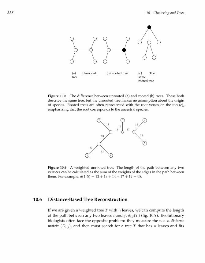
358 10 Clustering and Trees
(a) Unrootedtree
(b) Rooted tree (c) Thesamerooted tree
Figure 10.8 The difference between unrooted (a) and rooted (b) trees. These bothdescribe the same tree, but the unrooted tree makes no assumption about the originof species. Rooted trees are often represented with the root vertex on the top (c),emphasizing that the root corresponds to the ancestral species.
2 3 4
5
1 6
12
13
12
13
1416
17
13
12
Figure 10.9 A weighted unrooted tree. The length of the path between any twovertices can be calculated as the sum of the weights of the edges in the path betweenthem. For example, d(1, 5) = 12 + 13 + 14 + 17 + 12 = 68.
10.6 Distance-Based Tree Reconstruction
If we are given a weighted tree T with n leaves, we can compute the length
of the path between any two leaves i and j, di,j(T ) (fig. 10.9). Evolutionary
biologists often face the opposite problem: they measure the n × n distance
matrix (Di,j), and then must search for a tree T that has n leaves and fits
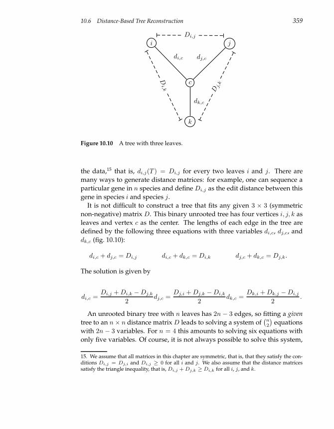
10.6 Distance-Based Tree Reconstruction 359
i j
c
k
di,c
dk,c
dj,c
Di,k
Di,j
Dj,
k
Figure 10.10 A tree with three leaves.
the data,15 that is, di,j(T ) = Di,j for every two leaves i and j. There are
many ways to generate distance matrices: for example, one can sequence a
particular gene in n species and define Di,j as the edit distance between this
gene in species i and species j.
It is not difficult to construct a tree that fits any given 3 × 3 (symmetric
non-negative) matrix D. This binary unrooted tree has four vertices i, j, k as
leaves and vertex c as the center. The lengths of each edge in the tree are
defined by the following three equations with three variables di,c, dj,c, and
dk,c (fig. 10.10):
di,c + dj,c = Di,j di,c + dk,c = Di,k dj,c + dk,c = Dj,k.
The solution is given by
di,c =Di,j + Di,k −Dj,k
2dj,c =
Dj,i + Dj,k −Di,k
2dk,c =
Dk,i + Dk,j −Di,j
2.
An unrooted binary tree with n leaves has 2n − 3 edges, so fitting a given
tree to an n× n distance matrix D leads to solving a system of(
n2
)
equations
with 2n − 3 variables. For n = 4 this amounts to solving six equations with
only five variables. Of course, it is not always possible to solve this system,
15. We assume that all matrices in this chapter are symmetric, that is, that they satisfy the con-ditions Di,j = Dj,i and Di,j ≥ 0 for all i and j. We also assume that the distance matricessatisfy the triangle inequality, that is, Di,j + Dj,k ≥ Di,k for all i, j, and k.
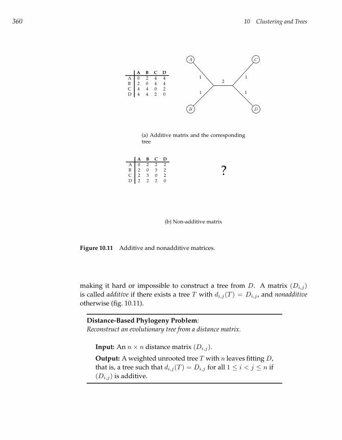
360 10 Clustering and Trees
A B C D
A 0 2 4 4B 2 0 4 4C 4 4 0 2D 4 4 2 0
A C
B D
1
1
1
1
2
(a) Additive matrix and the correspondingtree
A B C D
A 0 2 2 2B 2 0 3 2C 2 3 0 2D 2 2 2 0
?
(b) Non-additive matrix
Figure 10.11 Additive and nonadditive matrices.
making it hard or impossible to construct a tree from D. A matrix (Di,j)
is called additive if there exists a tree T with di,j(T ) = Di,j , and nonadditive
otherwise (fig. 10.11).
Distance-Based Phylogeny Problem:
Reconstruct an evolutionary tree from a distance matrix.
Input: An n× n distance matrix (Di,j).
Output: A weighted unrooted tree T with n leaves fitting D,
that is, a tree such that di,j(T ) = Di,j for all 1 ≤ i < j ≤ n if
(Di,j) is additive.
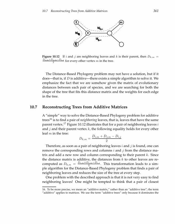
10.7 Reconstructing Trees from Additive Matrices 361
Figure 10.12 If i and j are neighboring leaves and k is their parent, then Dk,m =Di,m+Dj,m−Di,j
2for every other vertex m in the tree.
The Distance-Based Phylogeny problem may not have a solution, but if it
does—that is, if D is additive—there exists a simple algorithm to solve it. We
emphasize the fact that we are somehow given the matrix of evolutionary
distances between each pair of species, and we are searching for both the
shape of the tree that fits this distance matrix and the weights for each edge
in the tree.
10.7 Reconstructing Trees from Additive Matrices
A “simple” way to solve the Distance-Based Phylogeny problem for additive
trees16 is to find a pair of neighboring leaves, that is, leaves that have the same
parent vertex.17 Figure 10.12 illustrates that for a pair of neighboring leaves i
and j and their parent vertex k, the following equality holds for every other
leaf m in the tree:
Dk,m =Di,m + Dj,m −Di,j
2
Therefore, as soon as a pair of neighboring leaves i and j is found, one can
remove the corresponding rows and columns i and j from the distance ma-
trix and add a new row and column corresponding to their parent k. Since
the distance matrix is additive, the distances from k to other leaves are re-
computed as Dk,m =Di,m+Dj,m−Di,j
2 . This transformation leads to a sim-
ple algorithm for the Distance-Based Phylogeny problem that finds a pair of
neighboring leaves and reduces the size of the tree at every step.
One problem with the described approach is that it is not very easy to find
neighboring leaves! One might be tempted to think that a pair of closest
16. To be more precise, we mean an “additive matrix,” rather than an “additive tree”; the term“additive” applies to matrices. We use the term “additive trees” only because it dominates the
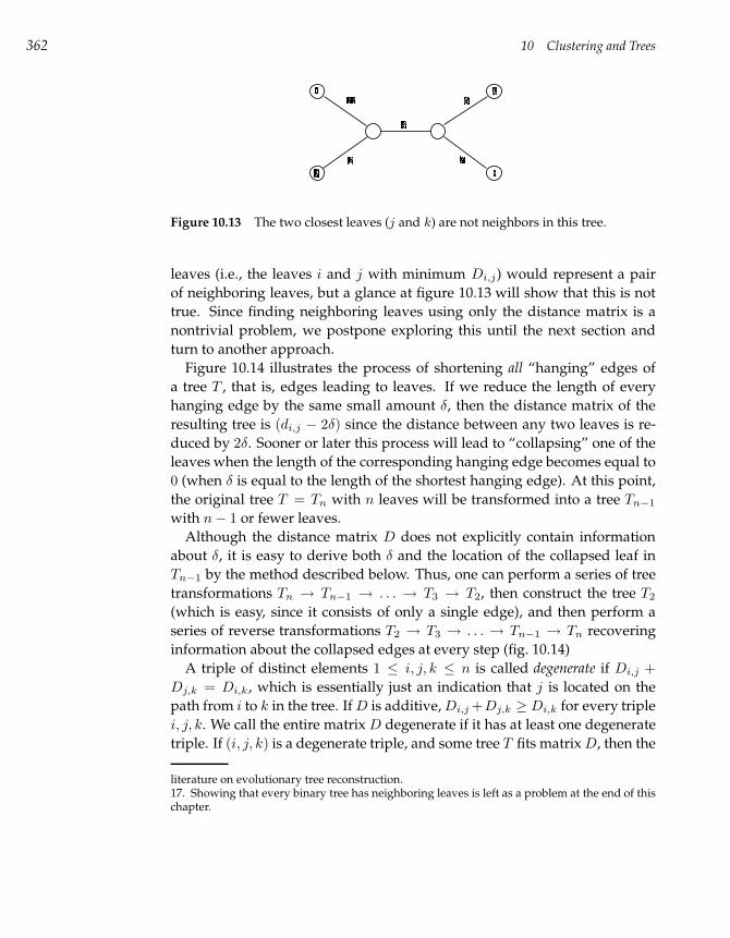
362 10 Clustering and Trees
Figure 10.13 The two closest leaves (j and k) are not neighbors in this tree.
leaves (i.e., the leaves i and j with minimum Di,j) would represent a pair
of neighboring leaves, but a glance at figure 10.13 will show that this is not
true. Since finding neighboring leaves using only the distance matrix is a
nontrivial problem, we postpone exploring this until the next section and
turn to another approach.
Figure 10.14 illustrates the process of shortening all “hanging” edges of
a tree T , that is, edges leading to leaves. If we reduce the length of every
hanging edge by the same small amount δ, then the distance matrix of the
resulting tree is (di,j − 2δ) since the distance between any two leaves is re-
duced by 2δ. Sooner or later this process will lead to “collapsing” one of the
leaves when the length of the corresponding hanging edge becomes equal to
0 (when δ is equal to the length of the shortest hanging edge). At this point,
the original tree T = Tn with n leaves will be transformed into a tree Tn−1
with n− 1 or fewer leaves.
Although the distance matrix D does not explicitly contain information
about δ, it is easy to derive both δ and the location of the collapsed leaf in
Tn−1 by the method described below. Thus, one can perform a series of tree
transformations Tn → Tn−1 → . . . → T3 → T2, then construct the tree T2
(which is easy, since it consists of only a single edge), and then perform a
series of reverse transformations T2 → T3 → . . . → Tn−1 → Tn recovering
information about the collapsed edges at every step (fig. 10.14)
A triple of distinct elements 1 ≤ i, j, k ≤ n is called degenerate if Di,j +
Dj,k = Di,k, which is essentially just an indication that j is located on the
path from i to k in the tree. If D is additive, Di,j +Dj,k ≥ Di,k for every triple
i, j, k. We call the entire matrix D degenerate if it has at least one degenerate
triple. If (i, j, k) is a degenerate triple, and some tree T fits matrix D, then the
literature on evolutionary tree reconstruction.17. Showing that every binary tree has neighboring leaves is left as a problem at the end of thischapter.
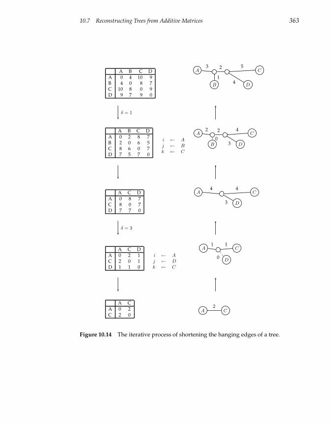
10.7 Reconstructing Trees from Additive Matrices 363
A B C DA 0 4 10 9B 4 0 8 7C 10 8 0 9D 9 7 9 0
A C
B D
3 2
4
5
1
δ = 1
A B C DA 0 2 8 7B 2 0 6 5C 8 6 0 7D 7 5 7 0
i ← Aj ← Bk ← C
A C
B D
2 2
3
4
0
A C DA 0 8 7C 8 0 7D 7 7 0
A C
D
4
3
4
δ = 3
A C DA 0 2 1C 2 0 1D 1 1 0
i ← Aj ← Dk ← C
A C
D
1
0
1
A CA 0 2C 2 0
A C2
Figure 10.14 The iterative process of shortening the hanging edges of a tree.
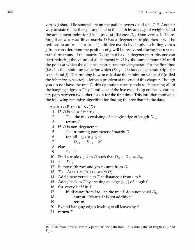
364 10 Clustering and Trees
vertex j should lie somewhere on the path between i and k in T .18 Another
way to state this is that j is attached to this path by an edge of weight 0, and
the attachment point for j is located at distance Di,j from vertex i. There-
fore, if an n × n additive matrix D has a degenerate triple, then it will be
reduced to an (n − 1) × (n − 1) additive matrix by simply excluding vertex
j from consideration; the position of j will be recovered during the reverse
transformations. If the matrix D does not have a degenerate triple, one can
start reducing the values of all elements in D by the same amount 2δ until
the point at which the distance matrix becomes degenerate for the first time
(i.e., δ is the minimum value for which (Di,j − 2δ) has a degenerate triple for
some i and j). Determining how to calculate the minimum value of δ (called
the trimming parameter) is left as a problem at the end of this chapter. Though
you do not have the tree T , this operation corresponds to shortening all of
the hanging edges in T by δ until one of the leaves ends up on the evolution-
ary path between two other leaves for the first time. This intuition motivates
the following recursive algorithm for finding the tree that fits the data.
ADDITIVEPHYLOGENY(D)
1 if D is a 2× 2 matrix
2 T ← the tree consisting of a single edge of length D1,2.
3 return T
4 if D is non-degenerate
5 δ ← trimming parameter of matrix D
6 for all 1 ≤ i 6= j ≤ n
7 Di,j ← Di,j − 2δ
8 else
9 δ ← 0
10 Find a triple i, j, k in D such that Dij + Djk = Dik
11 x← Di,j
12 Remove jth row and jth column from D.
13 T ← ADDITIVEPHYLOGENY(D)
14 Add a new vertex v to T at distance x from i to k
15 Add j back to T by creating an edge (v, j) of length 0
16 for every leaf l in T
17 if distance from l to v in the tree T does not equal Dl,j
18 output “Matrix D is not additive”
19 return
20 Extend hanging edges leading to all leaves by δ
21 return T
18. To be more precise, vertex j partitions the path from i to k into paths of length Di,j andDj,k .
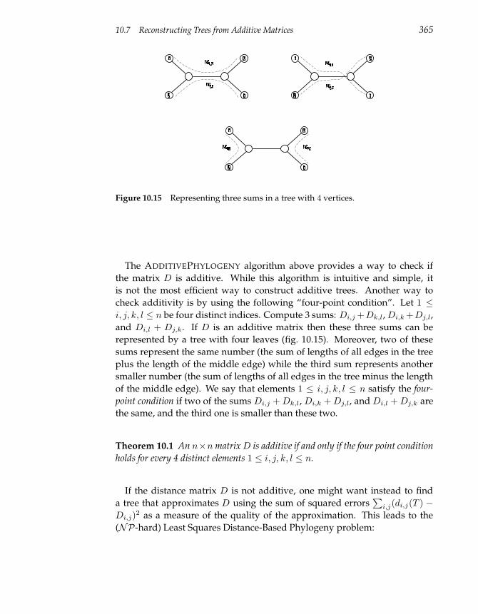
10.7 Reconstructing Trees from Additive Matrices 365
Figure 10.15 Representing three sums in a tree with 4 vertices.
The ADDITIVEPHYLOGENY algorithm above provides a way to check if
the matrix D is additive. While this algorithm is intuitive and simple, it
is not the most efficient way to construct additive trees. Another way to
check additivity is by using the following “four-point condition”. Let 1 ≤
i, j, k, l ≤ n be four distinct indices. Compute 3 sums: Di,j +Dk,l, Di,k +Dj,l,
and Di,l + Dj,k. If D is an additive matrix then these three sums can be
represented by a tree with four leaves (fig. 10.15). Moreover, two of these
sums represent the same number (the sum of lengths of all edges in the tree
plus the length of the middle edge) while the third sum represents another
smaller number (the sum of lengths of all edges in the tree minus the length
of the middle edge). We say that elements 1 ≤ i, j, k, l ≤ n satisfy the four-
point condition if two of the sums Di,j + Dk,l, Di,k + Dj,l, and Di,l + Dj,k are
the same, and the third one is smaller than these two.
Theorem 10.1 An n×n matrix D is additive if and only if the four point condition
holds for every 4 distinct elements 1 ≤ i, j, k, l ≤ n.
If the distance matrix D is not additive, one might want instead to find
a tree that approximates D using the sum of squared errors∑
i,j(di,j(T ) −
Di,j)2 as a measure of the quality of the approximation. This leads to the
(NP-hard) Least Squares Distance-Based Phylogeny problem:
366 10 Clustering and Trees
Least Squares Distance-Based Phylogeny Problem:
Given a distance matrix, find the evolutionary tree that minimizes
squared error.
Input: An n× n distance matrix (Di,j)
Output: A weighted tree T with n leaves minimizing∑
i,j(di,j(T )−Di,j)2 over all weighted trees with n leaves.
10.8 Evolutionary Trees and Hierarchical Clustering
Biologists often use variants of hierarchical clustering to construct evolution-
ary trees. UPGMA (Unweighted Pair Group Method with Arithmetic Mean) is a
particularly simple clustering algorithm. The UPGMA algorithm is a vari-
ant of HIERARCHICALCLUSTERING that uses a different approach to com-
pute the distance between clusters, and assigns heights to vertices of the con-
structed tree. Thus, the length of an edge (u, v) is defined to be the difference
in heights of the vertices v and u. The height plays the role of the molecular
clock, and allows one to “date” the divergence point for every vertex in the
evolutionary tree.
Given clusters C1 and C2, UPGMA defines the distance between them to
be the average pairwise distance: D(C1, C2) = 1|C1||C2|
∑
i∈C1
∑
j∈C2D(i, j).
At heart, UPGMA is simply another hierarchical clustering algorithm that
“dates” vertices of the constructed tree.
UPGMA(D, n)
1 Form n clusters, each with a single element
2 Construct a graph T by assigning an isolated vertex to each cluster
3 Assign height h(v) = 0 to every vertex v in this graph
4 while there is more than one cluster
5 Find the two closest clusters C1 and C2
6 Merge C1 and C2 into a new cluster C with |C1|+ |C2| elements
7 for every cluster C∗ 6= C
8 D(C, C∗) = 1|C|·|C∗|
∑
i∈C
∑
j∈C∗ D(i, j)
9 Add a new vertex C to T and connect to vertices C1 and C2
10 h(C)← D(C1,C2)2
11 Assign length h(C)− h(C1) to the edge (C1, C)
12 Assign length h(C)− h(C2) to the edge (C2, C)
13 Remove rows and columns of D corresponding to C1 and C2
14 Add a row and column to D for the new cluster C
15 return T
10.8 Evolutionary Trees and Hierarchical Clustering 367
UPGMA produces a special type of rooted tree19 that is known as ultra-
metric. In ultrametric trees the distance from the root to any leaf is the same.
We can now return to the “neighboring leaves” idea that we developed
and then abandoned in the previous section. In 1987 Naruya Saitou and
Masatoshi Nei developed an ingenious neighbor joining algorithm for phylo-
genetic tree reconstruction. In the case of additive trees, the neighbor joining
algorithm somehow magically finds pairs of neighboring leaves and pro-
ceeds by substituting such pairs with the leaves’ parent. However, neighbor
joining works well not only for additive distance matrices but for many oth-
ers as well: it does not assume the existence of a molecular clock and ensures
that the clusters that are merged in the course of tree reconstruction are not
only close to each other (as in UPGMA) but also are far apart from the rest.
For a cluster C, define u(C) = 1number of clusters−2
∑
all clusters C′ D(C, C′) as a
measure of the separation of C from other clusters.20 To choose which two
clusters to merge, we look for the clusters C1 and C2 that are simultaneously
close to each other and far from others. One may try to merge clusters that
simultaneously minimize D(C1, C2) and maximize u(C1)+ u(C2). However,
it is unlikely that a pair of clusters C1 and C2 that simultaneously minimize
D(C1, C2) and maximize u(C1) + u(C2) exists. As an alternative, one opts to
minimize D(C1, C2) − u(C1) − u(C2). This approach is used in the NEIGH-
BORJOINING algorithm below.
NEIGHBORJOINING(D, n)
1 Form n clusters, each with a single element
2 Construct a graph T by assigning an isolated vertex to each cluster
3 while there is more than one cluster
4 Find clusters C1 and C2 minimizing D(C1, C2)− u(C1)− u(C2)
5 Merge C1 and C2 into a new cluster C with |C1|+ |C2| elements
6 Compute D(C, C∗) = D(C1,C)+D(C2,C)2 to every other cluster C∗
7 Add a new vertex C to T and connect it to vertices C1 and C2
8 Assign length 12D(C1, C2) + 1
2 (u(C1)− u(C2)) to the edge (C1, C)
9 Assign length 12D(C1, C2) + 1
2 (u(C2)− u(C1)) to the edge (C2, C)
10 Remove rows and columns of D corresponding to C1 and C2
11 Add a row and column to D for the new cluster C
12 return T
19. Here, the root corresponds to the cluster created last.20. The explanation of that mysterious term “number of clusters − 2” in this formula is beyondthe scope of this book.
368 10 Clustering and Trees
10.9 Character-Based Tree Reconstruction
Evolutionary tree reconstruction often starts by sequencing a particular gene
in each of n species. After aligning these genes, biologists end up with an
n × m alignment matrix (n species, m nucleotides in each) that can be fur-
ther transformed into an n×n distance matrix. Although the distance matrix
could be analyzed by distance-based tree reconstruction algorithms, a cer-
tain amount of information gets lost in the transformation of the alignment
matrix into the distance matrix, rendering the reverse transformation of dis-
tance matrix back into the alignment matrix impossible. A better technique
is to use the alignment matrix directly for evolutionary tree reconstruction.
Character-based tree reconstruction algorithms assume that the input data are
described by an n×m matrix (perhaps an alignment matrix), where n is the
number of species and m is the number of characters. Every row in the matrix
describes an existing species and the goal is to construct a tree whose leaves
correspond to the n existing species and whose internal vertices correspond
to ancestral species. Each internal vertex in the tree is labeled with a charac-
ter string that describes, for example, the hypothetical number of legs in that
ancestral species. We want to determine what character strings at internal
nodes would best explain the character strings for the n observed species.
The use of the word “character” to describe an attribute of a species is
potentially confusing, since we often use the word to refer to letters from
an alphabet. We are not at liberty to change the terminology that biologists
have been using for at least a century, so for the next section we will re-
fer to nucleotides as states of a character. Another possible character might
be “number of legs,” which is not very informative for mammalian evolu-
tionary studies, but could be somewhat informative for insect evolutionary
studies.
An intuitive score for a character-based evolutionary tree is the total num-
ber of mutations required to explain all of the observed character sequences.
The parsimony approach attempts to minimize this score, and follows the
philosophy of Occam’s razor: find the simplest explanation of the data (see
figure 10.16).21
21. Occam was one of the most influential philosophers of the fourteenth century. Strong op-position to his ideas from theology professors prevented him from obtaining his masters degree(let alone his doctorate). Occam’s razor states that “plurality should not be assumed withoutnecessity,” and is usually paraphrased as “keep it simple, stupid.” Occam used this principle toeliminate many pseudoexplanatory theological arguments. Though the parsimony principle isattributed to Occam, sixteen centuries earlier Aristotle wrote simply that Nature operates in theshortest way possible.
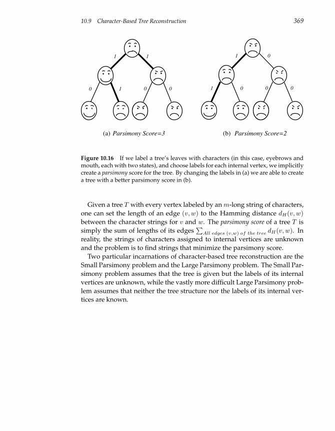
10.9 Character-Based Tree Reconstruction 369
1 1
0 1 0 0
1 0
1 0 0 0
Parsimony Score=3 Parsimony Score=2(a) (b)
Figure 10.16 If we label a tree’s leaves with characters (in this case, eyebrows andmouth, each with two states), and choose labels for each internal vertex, we implicitlycreate a parsimony score for the tree. By changing the labels in (a) we are able to createa tree with a better parsimony score in (b).
Given a tree T with every vertex labeled by an m-long string of characters,
one can set the length of an edge (v, w) to the Hamming distance dH(v, w)
between the character strings for v and w. The parsimony score of a tree T is
simply the sum of lengths of its edges∑
All edges (v,w) of the tree dH(v, w). In
reality, the strings of characters assigned to internal vertices are unknown
and the problem is to find strings that minimize the parsimony score.
Two particular incarnations of character-based tree reconstruction are the
Small Parsimony problem and the Large Parsimony problem. The Small Par-
simony problem assumes that the tree is given but the labels of its internal
vertices are unknown, while the vastly more difficult Large Parsimony prob-
lem assumes that neither the tree structure nor the labels of its internal ver-
tices are known.
370 10 Clustering and Trees
10.10 Small Parsimony Problem
Small Parsimony Problem:
Find the most parsimonious labeling of the internal vertices in an
evolutionary tree.
Input: Tree T with each leaf labeled by an m-character
string.
Output: Labeling of internal vertices of the tree T minimiz-
ing the parsimony score.
An attentive reader should immediately notice that, because the characters
in the string are independent, the Small Parsimony problem can be solved
independently for each character. Therefore, to devise an algorithm, we can
assume that every leaf is labeled by a single character rather than by a string
of m characters.
As we have seen in previous chapters, sometimes solving a more general—
and seemingly more difficult—problem may reveal the solution to the more
specific one. In the case of the Small Parsimony Problem we will first solve
the more general Weighted Small Parsimony problem, which generalizes the
notion of parsimony by introducing a scoring matrix. The length of an edge
connecting vertices v and w in the Small Parsimony problem is defined as the
Hamming distance, dH(v, w), between the character strings for v and w. In
the case when every leaf is labeled by a single character in a k-letter alphabet,
dH(v, w) = 0 if the characters corresponding to v and w are the same, and
dH(v, w) = 1 otherwise. One can view such a scoring scheme as a k × k
scoring matrix (δi,j) with diagonal elements equal to 0 and all other elements
equal to 1. The Weighted Small Parsimony problem simply assumes that the
scoring matrix (δi,j) is an arbitrary k× k matrix and minimizes the weighted
parsimony score∑
all edges (v, w) in the tree δv,w.
Weighted Small Parsimony Problem:
Find the minimal weighted parsimony score labeling of the internal
vertices in an evolutionary tree.
Input: Tree T with each leaf labeled by elements of a k-letter
alphabet and a k × k scoring matrix (δij).
Output: Labeling of internal vertices of the tree T minimiz-
ing the weighted parsimony score.
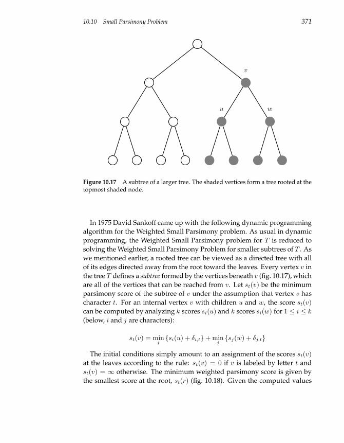
10.10 Small Parsimony Problem 371
v
u w
Figure 10.17 A subtree of a larger tree. The shaded vertices form a tree rooted at thetopmost shaded node.
In 1975 David Sankoff came up with the following dynamic programming
algorithm for the Weighted Small Parsimony problem. As usual in dynamic
programming, the Weighted Small Parsimony problem for T is reduced to
solving the Weighted Small Parsimony Problem for smaller subtrees of T . As
we mentioned earlier, a rooted tree can be viewed as a directed tree with all
of its edges directed away from the root toward the leaves. Every vertex v in
the tree T defines a subtree formed by the vertices beneath v (fig. 10.17), which
are all of the vertices that can be reached from v. Let st(v) be the minimum
parsimony score of the subtree of v under the assumption that vertex v has
character t. For an internal vertex v with children u and w, the score st(v)
can be computed by analyzing k scores si(u) and k scores si(w) for 1 ≤ i ≤ k
(below, i and j are characters):
st(v) = minisi(u) + δi,t+ min
jsj(w) + δj,t
The initial conditions simply amount to an assignment of the scores st(v)
at the leaves according to the rule: st(v) = 0 if v is labeled by letter t and
st(v) = ∞ otherwise. The minimum weighted parsimony score is given by
the smallest score at the root, st(r) (fig. 10.18). Given the computed values
372 10 Clustering and Trees
st(v) at all of the vertices in the tree, one can reconstruct an optimal assign-
ment of labels using a backtracking approach that is similar to that used in
chapter 6. The running time of the algorithm is O(nk).
In 1971, even before David Sankoff solved the Weighted Small Parsimony
problem, Walter Fitch derived a solution of the (unweighted) Small Parsi-
mony problem. The Fitch algorithm below is essentially dynamic program-
ming in disguise. The algorithm assigns a set of letters Sv to every vertex in
the tree in the following manner. For each leaf v, Sv consists of single letter
that is the label of this leaf. For any internal vertex v with children u and w,
Sv is computed from the sets Su and Sw according to the following rule:
Sv =
Su ∩ Sw, if Su and Sw overlap
Su ∪ Sw, otherwise
To compute Sv, we traverse the tree in post-order as in figure 10.19, starting
from the leaves and working toward the root. After computing Sv for all
vertices in the tree, we need to decide on how to assign letters to the internal
vertices of the tree. This time we traverse the tree using preorder traversal
from the root toward the leaves. We can assign root r any letter from Sr. To
assign a letter to an internal vertex v we check if the (already assigned) label
of its parent belongs to Sv. If yes, we choose the same label for v; otherwise
we label v by an arbitrary letter from Sv (fig. 10.20). The running time of this
algorithm is also O(nk).
At first glance, Fitch’s labeling procedure and Sankoff’s dynamic program-
ming algorithm appear to have little in common. Even though Fitch probably
did not know about application of dynamic programming for evolutionary
tree reconstruction in 1971, the two algorithms are almost identical. To reveal
the similarity between these two algorithms let us return to Sankoff’s recur-
rence. We say that character t is optimal for vertex v if it yields the smallest
score, that is, if st(v) = min1≤i≤k si(v). The set of optimal letters for a ver-
tex v forms a set S(v). If u and w are children of v and if S(u) and S(w)
overlap, then it is easy to see that S(v) = S(u)⋂
S(w). If S(u) and S(w) do
not overlap, then it is easy to see that S(v) = S(u)⋃
S(w). Fitch’s algorithm
uses exactly the same recurrence, thus revealing that these two approaches
are algorithmic twins.
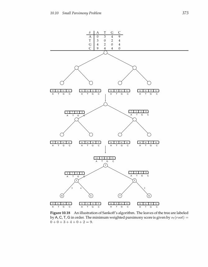
10.10 Small Parsimony Problem 373
δ A T G CA 0 3 4 9T 3 0 2 4G 4 2 0 4C 9 4 4 0
0 ∞ ∞ ∞
A T G C
∞ ∞ ∞ 0
A T G C
∞ 0 ∞ ∞
A T G C
∞ ∞ 0 ∞
A T G C
9 7 8 9
A T G C
0 ∞ ∞ ∞
A T G C
∞ ∞ ∞ 0
A T G C
7 2 2 8
A T G C
∞ 0 ∞ ∞
A T G C
∞ ∞ 0 ∞
A T G C
T
14 9 10 15
A T G C
T
9 7 8 9
A T G C
A
0 ∞ ∞ ∞
A T G C
3
C
∞ ∞ ∞ 0
A T G C
4
T
7 2 2 8
A T G C
T
∞ 0 ∞ ∞
A T G C
G
∞ ∞ 0 ∞
A T G C
2
Figure 10.18 An illustration of Sankoff’s algorithm. The leaves of the tree are labeledby A, C, T, G in order. The minimum weighted parsimony score is given by sT(root) =0 + 0 + 3 + 4 + 0 + 2 = 9.
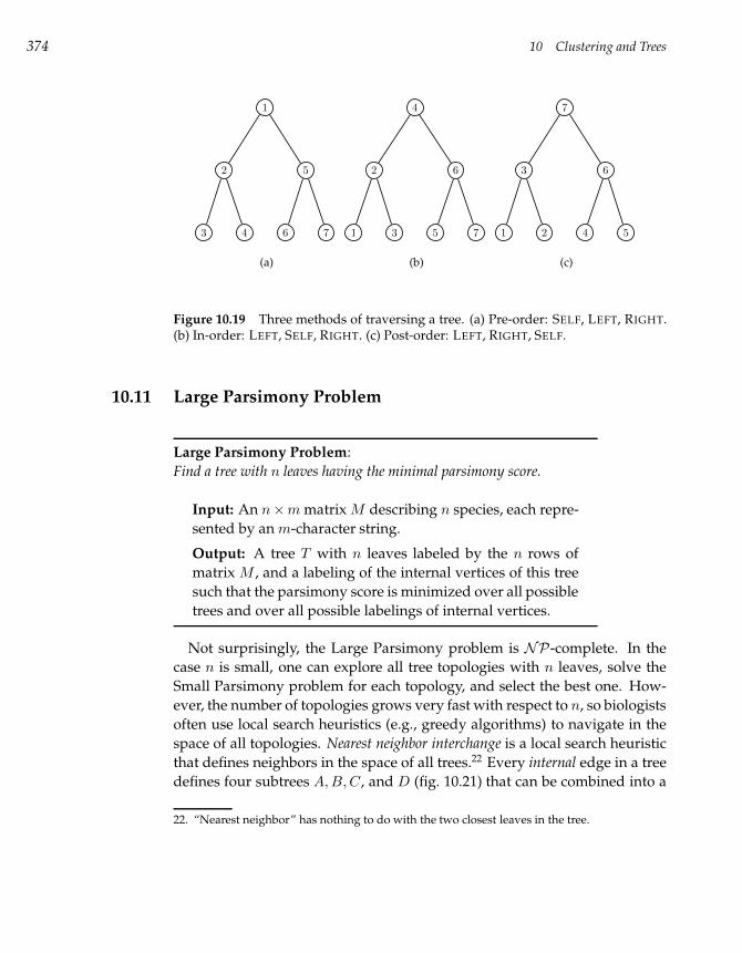
374 10 Clustering and Trees
1
2
3 4
5
6 7
(a)
4
2
1 3
6
5 7
(b)
7
3
1 2
6
4 5
(c)
Figure 10.19 Three methods of traversing a tree. (a) Pre-order: SELF, LEFT, RIGHT.(b) In-order: LEFT, SELF, RIGHT. (c) Post-order: LEFT, RIGHT, SELF.
10.11 Large Parsimony Problem
Large Parsimony Problem:
Find a tree with n leaves having the minimal parsimony score.
Input: An n×m matrix M describing n species, each repre-
sented by an m-character string.
Output: A tree T with n leaves labeled by the n rows of
matrix M , and a labeling of the internal vertices of this tree
such that the parsimony score is minimized over all possible
trees and over all possible labelings of internal vertices.
Not surprisingly, the Large Parsimony problem is NP-complete. In the
case n is small, one can explore all tree topologies with n leaves, solve the
Small Parsimony problem for each topology, and select the best one. How-
ever, the number of topologies grows very fast with respect to n, so biologists
often use local search heuristics (e.g., greedy algorithms) to navigate in the
space of all topologies. Nearest neighbor interchange is a local search heuristic
that defines neighbors in the space of all trees.22 Every internal edge in a tree
defines four subtrees A, B, C, and D (fig. 10.21) that can be combined into a
22. “Nearest neighbor” has nothing to do with the two closest leaves in the tree.
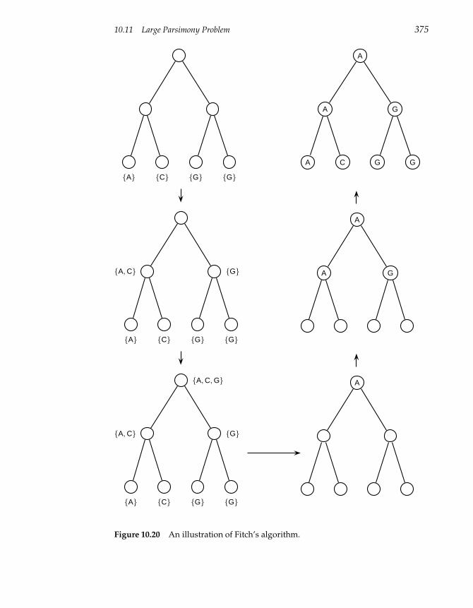
10.11 Large Parsimony Problem 375
A C G G
A, C
A C
G
G G
A, C, G
A, C
A C
G
G G
A
A
A C
G
G G
A
A G
A
Figure 10.20 An illustration of Fitch’s algorithm.
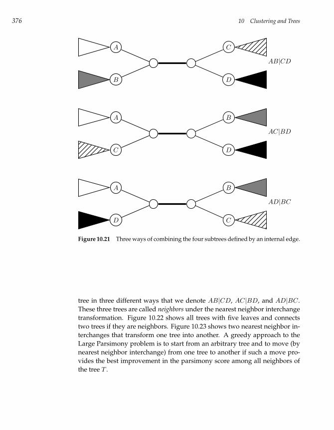
376 10 Clustering and Trees
A
B
C
D
AB|CD
A
C
B
D
AC|BD
A
D
B
C
AD|BC
Figure 10.21 Three ways of combining the four subtrees defined by an internal edge.
tree in three different ways that we denote AB|CD, AC|BD, and AD|BC.
These three trees are called neighbors under the nearest neighbor interchange
transformation. Figure 10.22 shows all trees with five leaves and connects
two trees if they are neighbors. Figure 10.23 shows two nearest neighbor in-
terchanges that transform one tree into another. A greedy approach to the
Large Parsimony problem is to start from an arbitrary tree and to move (by
nearest neighbor interchange) from one tree to another if such a move pro-
vides the best improvement in the parsimony score among all neighbors of
the tree T .
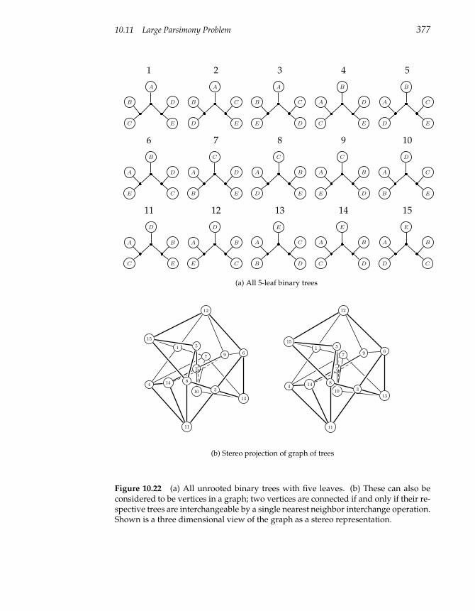
10.11 Large Parsimony Problem 377
1 2 3 4 5
A
BD
C E
A
BC
D E
A
BC
E D
B
AD
C E
B
AC
D E
6 7 8 9 10
B
AD
E C
C
AD
B E
C
AB
D E
C
AB
E D
D
AC
B E
11 12 13 14 15
D
AB
C E
D
A!B
"#
E C
E
A$C
%&
B D
E
A'B
()
C D
E
A*B
+,
D C
(a) All 5-leaf binary trees
2
1
3
14
9
5
10
11
4
7
13
8
15
12
6
2
1
314
9
5
10
11
4
7
13
8
15
12
6
(b) Stereo projection of graph of trees
Figure 10.22 (a) All unrooted binary trees with five leaves. (b) These can also beconsidered to be vertices in a graph; two vertices are connected if and only if their re-spective trees are interchangeable by a single nearest neighbor interchange operation.Shown is a three dimensional view of the graph as a stereo representation.
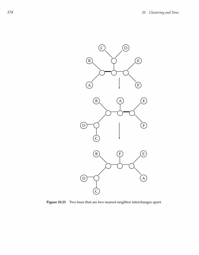
378 10 Clustering and Trees
C D
B E
A F
B A E
D F
C
B F E
D A
C
Figure 10.23 Two trees that are two nearest neighbor interchanges apart.
10.12 Notes 379
10.12 Notes
The literature on clustering can be traced back to the nineteenth century. The
k-Means clustering algorithm was introduced by Stuart Lloyd in 1957 (68),
popularized by MacQueen in 1965 (70), and has since inspired dozens of
variants. Applications of hierarchical clustering for gene expression analyses
were pioneered by Michael Eisen, Paul Spellman, Patrick Brown and David
Botstein in 1998 (33). The PCC and CAST algorithms were developed by
Amir Ben-Dor, Ron Shamir, and Zohar Yakhini in 1999 (11).
The molecular solution of the giant panda riddle was proposed by Stephen
O’Brien and colleagues in 1985 (81) and described in more details in O’Brien’s
book (80). The Out of Africa hypothesis was proposed by Rebecca Cann,
Mark Stoneking, and Allan Wilson in 1987. Even today it continues to be
debated by Alan Templeton and others (103).
The simple and intuitive UPGMA hierarchical clustering approach was
developed in 1958 by Charles Michener and Robert Sokal (98). The neighbor
joining algorithm was developed by Naruya Saitou and Masatoshi Nei in
1987 (90).
The algorithm to solve the Small Parsimony problem was developed by
Walter Fitch in 1971 (37), four years before David Sankoff developed a dy-
namic programming algorithm for the more general Weighted Small Parsi-
mony problem (92). The four-point condition was first formulated in 1965
(113), promptly forgotten, and rediscovered by Peter Buneman six years later (19).
The nearest neighbor interchange approach to exploring trees was proposed
in 1971 by David Robinson (88).
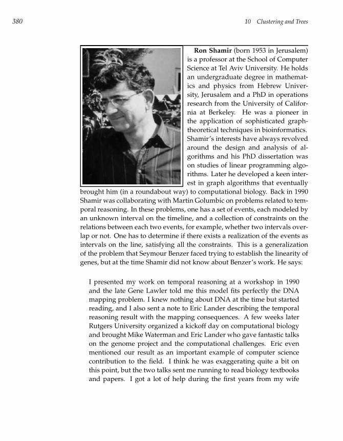
380 10 Clustering and Trees
Ron Shamir (born 1953 in Jerusalem)
is a professor at the School of Computer
Science at Tel Aviv University. He holds
an undergraduate degree in mathemat-
ics and physics from Hebrew Univer-
sity, Jerusalem and a PhD in operations
research from the University of Califor-
nia at Berkeley. He was a pioneer in
the application of sophisticated graph-
theoretical techniques in bioinformatics.
Shamir’s interests have always revolved
around the design and analysis of al-
gorithms and his PhD dissertation was
on studies of linear programming algo-
rithms. Later he developed a keen inter-
est in graph algorithms that eventually
brought him (in a roundabout way) to computational biology. Back in 1990
Shamir was collaborating with Martin Golumbic on problems related to tem-
poral reasoning. In these problems, one has a set of events, each modeled by
an unknown interval on the timeline, and a collection of constraints on the
relations between each two events, for example, whether two intervals over-
lap or not. One has to determine if there exists a realization of the events as
intervals on the line, satisfying all the constraints. This is a generalization
of the problem that Seymour Benzer faced trying to establish the linearity of
genes, but at the time Shamir did not know about Benzer’s work. He says:
I presented my work on temporal reasoning at a workshop in 1990
and the late Gene Lawler told me this model fits perfectly the DNA
mapping problem. I knew nothing about DNA at the time but started
reading, and I also sent a note to Eric Lander describing the temporal
reasoning result with the mapping consequences. A few weeks later
Rutgers University organized a kickoff day on computational biology
and brought Mike Waterman and Eric Lander who gave fantastic talks
on the genome project and the computational challenges. Eric even
mentioned our result as an important example of computer science
contribution to the field. I think he was exaggerating quite a bit on
this point, but the two talks sent me running to read biology textbooks
and papers. I got a lot of help during the first years from my wife
10.12 Notes 381
Michal, who happens to be a biologist and patiently answered all my
trivial questions.
This chance meeting with Gene Lawler and Eric Lander converted Shamir
into a bioinformatician and since 1991 he has been devoting more and more
time to algorithmic problems in computational biology. He still keeps an
interest in graph algorithms and often applies graph-theoretical techniques
to biological problems. In recent years, he has tended to combine discrete
mathematics techniques and probabilistic reasoning. Ron says:
I still worry about the complexity of the problems and the algorithms,
and would care about (and enjoy) the NP-hardness proof of a new
problem, but biology has trained me to be “tolerant” to heuristics when
the theoretical computer science methodologies only take you so far,
and the data require more.
Shamir was an early advocate of rigorous clustering algorithms in bioin-
formatics. Although clustering theory has been under development since the
1960s, his interest in clustering started in the mid-1990s as part of a collabora-
tion with Hans Lehrach of the Max Planck Institute in Berlin. Lehrach is one
of the fathers of the oligonucleotide fingerprinting technology that predates
the DNA chips techniques. Lehrach had a “factory” in Berlin that would
array thousands of unknown cDNA clones, and then hybridize them to k-
mer probes (typically 8-mers or 9-mers). This was repeated with dozens of
different probes, giving a fingerprint for each cDNA clone. To find which
clones correspond to the same gene, one has to cluster them based on their
fingerprints, and the noise level in the data makes accurate clustering quite
a challenge.
It was this challenge that brought Shamir to think about clustering. As
clustering theory is very heterogeneous and scattered over many different
fields, he set out to develop his algorithm first, before learning the literature.
Naturally, Shamir resorted to graph algorithms, modeled the clustered ele-
ments (clones in the fingerprinting application) as vertices, and connected
clones with highly similar fingerprints by edges. It was a natural next step to
repeatedly partition the graph based on minimum cuts (sets of edges whose
removal makes the graph disconnected) and hence his first clustering algo-
rithm was born. Actually the idea looked so natural to Shamir that he and
his student Erez Hartuv searched the literature for a long time just to make
sure it had not been published before. They did not find the same approach
382 10 Clustering and Trees
but found similar lines of thinking in works a decade earlier. According to
Shamir,
Given the ubiquity of clustering, I would not be surprised to unearth
in the future an old paper with the same idea in archeology, zoology,
or some other field.
Later, after considering the pros and cons of the approach, together with
his student Roded Sharan, Shamir improved the algorithm by adding a rig-
orous probabilistic analysis and created the popular clustering algorithm
CLICK. The publication of vast data sets of microarray expression profiles
was a great opportunity and triggered Shamir to further develop PCC and
CAST together with Amir Ben-Dor and Zohar Yakhini.
Shamir is one of the very few scientists who is regarded as a leader in
both algorithms and bioinformatics and who was credited with an important
breakthrough in algorithms even before he became a bioinformatician. He
says:
Probably the most exciting moment in my scientific life was my PhD re-
sult in 1983, showing that the average complexity of the Simplex algo-
rithm is quadratic. The Simplex algorithm is one of the most commonly
used algorithms, with thousands of applications in virtually all areas
of science and engineering. Since the 1950s, the Simplex algorithm was
known to be very efficient in practice and was (and is) used ubiqui-
tously, but worst-case exponential-time examples were given for many
variants of the Simplex, and none was proved to be efficient. This was
a very embarrassing situation, and resolving it was very gratifying.
Doing it together with my supervisors Ilan Adler (a leader in convex
optimization, and a student of Dantzig, the father of the Simplex algo-
rithm) and Richard Karp (one of the great leaders of theoretical com-
puter science) was extremely exciting. Similar results were obtained
independently at the same time by other research groups. There were
some other exhilarating moments, particularly those between finding
out an amazing new result and discovering the bug on the next day,
but these are the rewards and frustrations of scientific research.
Shamir views himself as not committed to a particular problem. One of
the advantages of scientific research in the university setting is the freedom
to follow one’s interests and nose, and not be obliged to work on the same
problem for years. The exciting rapid developments in biology bring about
10.12 Notes 383
a continuous flow of new problems, ideas, and data. Of course, one has to
make sure breadth does not harm the research depth. In practice, in spite of
this “uncommitted” ideology, Ron finds himself working on the same areas
for several years, and following the literature in these fields a while later. He
tends to work on several problem areas simultaneously but tries to choose
topics that are overlapping to some extent, just to save on the effort of under-
standing and following several fields. Shamir says:
In my opinion, an open mind, high antennae, a solid background in the
relevant disciplines, and hard work are the most important elements
of discovery. As a judge once said, “Inspiration only comes to the law
library at 3 AM". This is even more true in science. Flexibility and
sensitivity to the unexpected are crucial.
Shamir views the study of gene networks, that is, understanding how
genes, proteins, and other molecules work together in concert, as a long-
standing challenge.
384 10 Clustering and Trees
10.13 Problems
Problem 10.1
Determine the number of different ways to partition a set of n elements into k clus-ters.
Problem 10.2
Construct an instance of the k-Means Clustering problem for which the Lloyd algo-rithm produces a particularly bad solution. Derive a performance guarantee of theLloyd algorithm.
Problem 10.3
Find an optimal algorithm for solving the k-Means Clustering problem in the case ofk = 1. Can you find an analytical solution in this case?
Problem 10.4
Estimate the number of iterations that the Lloyd algorithm will require when k = 1.Repeat for k = 2.
Problem 10.5
Construct an example for which the CAST algorithm does not converge.
Problem 10.6
How do you calculate the trimming parameter δ in ADDITIVEPHYLOGENY?
Problem 10.7
Prove that a connected graph in which the number of vertices exceeds the number ofedges by 1 is a tree.
Problem 10.8
Some of 8 Hawaiian islands are connected by airlines. It is known one can reach everyisland from any other (probably with some intermediate stops). Prove that you canvisit all islands making no more than 12 flights.
Problem 10.9
Show that any binary tree with n leaves has 2n− 3 edges.
Problem 10.10
How many different unrooted binary trees on n vertices are there?
Problem 10.11
Prove that every binary tree has at least two neighboring leaves.
Problem 10.12
Design a backtracking procedure to reconstruct the optimal assignment of charactersin the Sankoff algorithm for the Weighted Small Parsimony problem.

10.13 Problems 385
Problem 10.13
While we showed how to solve the Weighted Small Parsimony problem using dy-namic programming, we did not show how to construct a Manhattan-like graph forthis problem. Cast the Weighted Small Parsimony problem in terms of finding a pathin an appropriate Manhattan-like directed acyclic graph.
Problem 10.14
The nearest neighbor interchange distance between two trees is defined as the minimumnumber of interchanges to transform one tree into another. Design an approximationalgorithm for computing the nearest neighbor interchange distance.
Problem 10.15
Find two binary trees with six vertices that are the maximum possible nearest neigh-bor interchange distance apart from each other.

11 Hidden Markov Models
Hidden Markov Models are a popular machine learning approach in bioinfor-
matics. Machine learning algorithms are presented with training data, which
are used to derive important insights about the (often hidden) parameters.
Once an algorithm has been suitably trained, it can apply these insights to
the analysis of a test sample. As the amount of training data increases, the ac-
curacy of the machine learning algorithm typically increases as well. The pa-
rameters that are learned during training represent knowledge; application
of the algorithm with those parameters to new data (not used in the train-
ing phase) represents the algorithm’s use of that knowledge. The Hidden
Markov Model (HMM) approach, considered in this chapter, learns some
unknown probabilistic parameters from training samples and uses these pa-
rameters in the framework of dynamic programming (and other algorithmic
techniques) to find the best explanation for the experimental data.
11.1 CG-Islands and the “Fair Bet Casino”
The least frequent dinucleotide in many genomes is CG. The reason for this
is that the C within CG is easily methylated, and the resulting methyl-C has
a tendency to mutate into T.1 However, the methylation is often suppressed
around genes in areas called CG-islands in which CG appears relatively fre-
quently. An important problem is to define and locate CG-islands in a long
genomic text.
Finding CG-islands can be modeled after the following toy gambling prob-
lem. The “Fair Bet Casino” has a game in which a dealer flips a coin and
1. Cells often biochemically modify DNA and proteins. Methylation is the most common DNAmodification and results in the addition of a methyl (CH3) group to a nucleotide position inDNA.
388 11 Hidden Markov Models
the player bets on the outcome (heads or tails). The dealer in this (crooked)
casino uses either a fair coin (heads or tails are equally likely) or a biased
coin that will give heads with a probability of 34 . For security reasons, the
dealer does not like to change coins, so this happens relatively rarely, with a
probability of 0.1. Given a sequence of coin tosses, the problem is to find out
when the dealer used the biased coin and when he used the fair coin, since
this will help you, the player, learn the dealer’s psychology and enable you
to win money. Obviously, if you observe a long line of heads, it is likely that
the dealer used the biased coin, whereas if you see an even distribution of
heads and tails, he likely used the fair one. Though you can never be certain
that a long string of heads is not just a fluke, you are primarily interested in
the most probable explanation of the data. Based on this sensible intuition,
we might formulate the problem as follows:
Fair Bet Casino Problem:
Given a sequence of coin tosses, determine when the dealer used a fair
coin and when he used a biased coin.
Input: A sequence x = x1 x2 x3 . . . xn of coin tosses (either
H or T ) made by two possible coins (F or B).
Output: A sequence π = π1 π2 π3 · · ·πn, with each πi being
either F or B indicating that xi is the result of tossing the
fair or biased coin, respectively.
Unfortunately, this problem formulation simply makes no sense. The am-
biguity is that any sequence of coins could possibly have generated the ob-
served outcomes, so technically π = FFF . . . FF is a valid answer to this
problem for every observed sequence of coin flips, as is π = BBB . . .BB. We
need to incorporate a way to grade different coin sequences as being better
answers than others. Below we explain how to turn this ill-defined problem
into the Decoding problem based on HMM paradigm.
First, we consider the problem under the assumption that the dealer never
changes coins. In this case, letting 0 denote tails and 1 heads, the question is
which of the two coins he used, fair (p+(0) = p+(1) = 12 ) or biased (p−(0) =
14 , p−(1) = 3
4 ). If the resulting sequence of tosses is x = x1 . . . xn, then the
11.1 CG-Islands and the “Fair Bet Casino” 389
probability that x was generated by a fair coin is2
P (x|fair coin) =n∏
i=1
p+(xi) =1
2n.
On the other hand, the probability that x was generated by a biased coin is
P (x|biased coin) =
n∏
i=1
p−(xi) =
(
1
4n−k
)(
3k
4k
)
=3k
4n.
Here k is the number of heads in x. If P (x|fair coin) > P (x|biased coin), then
the dealer most likely used a fair coin; on the other hand, we can see that if
P (x|fair coin)<P (x|biased coin), then the dealer most likely used a biased
coin. The probabilities P (x|fair coin)= 12n and P (x|biased coin) = 3k
4n become
equal at k = nlog2 3 . As a result, when k < n
log2 3 , the dealer most likely used
a fair coin, and when k > nlog2 3 , he most likely used a biased coin. We can
define the log-odds ratio as follows:
log2
P (x|fair coin)
P (x|biased coin)=
k∑
i=1
log2
p+(xi)
p−(xi)= n− k log2 3
However, we know that the dealer does change coins, albeit rarely. One ap-
proach to making an educated guess as to which coin the dealer used at each
point would be to slide a window of some width along the sequence of coin
flips and calculate the log-odds ratio of the sequence under each window. In
effect, this is considering the log-odds ratio of short regions of the sequence.
If the log-odds ratio of the short sequence falls below 0, then the dealer most
likely used a biased coin while generating this window of sequence; other-
wise the dealer most likely used a fair coin.
Similarly, a naive approach to finding CG-islands in long DNA sequences
is to calculate log-odds ratios for a sliding window of some particular length,
and to declare windows that receive positive scores to be potential CG-islands.
Of course, the disadvantage of this approach is that we do not know the
length of CG-islands in advance and that some overlapping windows may
classify the same nucleotide differently. HMMs represent a different proba-
bilistic approach to this problem.
2. The notation P (x|y) is shorthand for the “probability of x occurring under the assumptionthat (some condition) y is true.” The notation
Qni=1 ai means a1 · a2 · a3 · · · an.
390 11 Hidden Markov Models
11.2 The Fair Bet Casino and Hidden Markov Models
An HMM can be viewed as an abstract machine that has an ability to produce
some output using coin tossing. The operation of the machine proceeds in
discrete steps: at the beginning of each step, the machine is in a hidden state of
which there are k. During the step, the HMM makes two decisions: (1) “What
state will I move to next?” and (2) “What symbol—from an alphabet Σ—will
I emit?” The HMM decides on the former by choosing randomly among the k
states; it decides on the latter by choosing randomly among the |Σ| symbols.
The choices that the HMM makes are typically biased, and may follow arbi-
trary probabilities. Moreover, the probability distributions3 that govern which
state to move to and which symbols to emit change from state to state. In
essence, if there are k states, then there are k different “next state” distribu-
tions and k different “symbol emission” distributions. An important feature
of HMMs is that an observer can see the emitted symbols but has no ability to
see what state HMM is in at any step, hence the name Hidden Markov Mod-
els. The goal of the observer is to infer the most likely states of the HMM by
analyzing the sequences of emitted symbols. Since an HMM effectively uses
dice to emit symbols, the sequence of symbols it produces does not form any
readily recognizable pattern.
Formally, an HMM M is defined by an alphabet of emitted symbols Σ,
a set of (hidden) states Q, a matrix of state transition probabilities A, and a
matrix of emission probabilities E, where
• Σ is an alphabet of symbols;
• Q is a set of states, each of which will emit symbols from the alphabet Σ;
• A = (akl) is a |Q| × |Q| matrix describing the probability of changing to
state l after the HMM is in state k; and
• E = (ek(b)) is a |Q| × |Σ|matrix describing the probability of emitting the
symbol b during a step in which the HMM is in state k.
Each row of the matrix A describes a “state die”4 with |Q| sides, while
each row of the matrix E describes a “symbol die” with |Σ| sides. The Fair
3. A probability distribution is simply an assignment of probabilities to outcomes; in this case,the outcomes are either symbols to emit or states to move to. We have seen probability distribu-tions, in a disguised form, in the context of motif finding. Every column of a profile, when eachelement is divided by the number of sequences in the sample, forms probability distributions.4. Singular of “dice.”
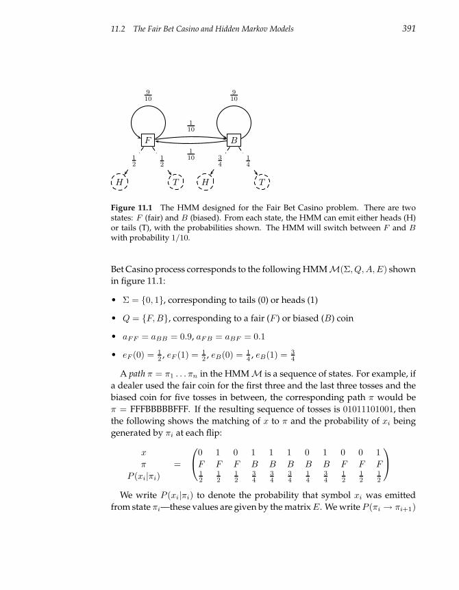
11.2 The Fair Bet Casino and Hidden Markov Models 391
F B
H T H T
12
12
34
14
110
110
910
910
Figure 11.1 The HMM designed for the Fair Bet Casino problem. There are twostates: F (fair) and B (biased). From each state, the HMM can emit either heads (H)or tails (T), with the probabilities shown. The HMM will switch between F and Bwith probability 1/10.
Bet Casino process corresponds to the following HMMM(Σ, Q, A, E) shown
in figure 11.1:
• Σ = 0, 1, corresponding to tails (0) or heads (1)
• Q = F, B, corresponding to a fair (F ) or biased (B) coin
• aFF = aBB = 0.9, aFB = aBF = 0.1
• eF (0) = 12 , eF (1) = 1
2 , eB(0) = 14 , eB(1) = 3
4
A path π = π1 . . . πn in the HMMM is a sequence of states. For example, if
a dealer used the fair coin for the first three and the last three tosses and the
biased coin for five tosses in between, the corresponding path π would be
π = FFFBBBBBFFF. If the resulting sequence of tosses is 01011101001, then
the following shows the matching of x to π and the probability of xi being
generated by πi at each flip:
x
π
P (xi|πi)
=
0 1 0 1 1 1 0 1 0 0 1
F F F B B B B B F F F12
12
12
34
34
34
14
34
12
12
12
We write P (xi|πi) to denote the probability that symbol xi was emitted
from state πi—these values are given by the matrix E. We write P (πi → πi+1)
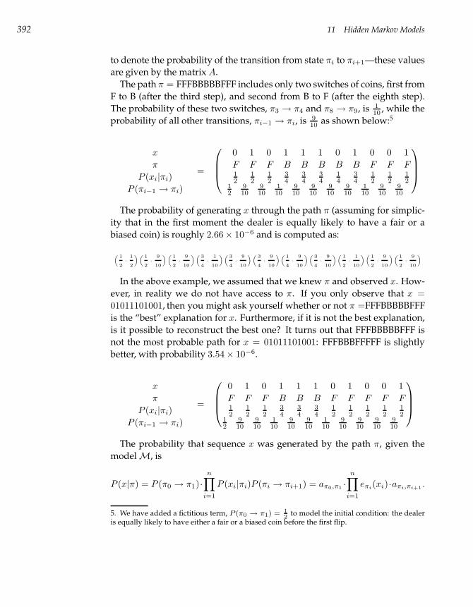
392 11 Hidden Markov Models
to denote the probability of the transition from state πi to πi+1—these values
are given by the matrix A.
The path π = FFFBBBBBFFF includes only two switches of coins, first from
F to B (after the third step), and second from B to F (after the eighth step).
The probability of these two switches, π3 → π4 and π8 → π9, is 110 , while the
probability of all other transitions, πi−1 → πi, is 910 as shown below:5
x
π
P (xi|πi)
P (πi−1 → πi)
=
0 1 0 1 1 1 0 1 0 0 1
F F F B B B B B F F F12
12
12
34
34
34
14
34
12
12
12
12
910
910
110
910
910
910
910
110
910
910
The probability of generating x through the path π (assuming for simplic-
ity that in the first moment the dealer is equally likely to have a fair or a
biased coin) is roughly 2.66× 10⁻⁶ and is computed as:
„ 1
2·
1
2
« „ 1
2·
9
10
« „ 1
2·
9
10
« „ 3
4·
1
10
« „ 3
4·
9
10
« „ 3
4·
9
10
« „ 1
4·
9
10
« „ 3
4·
9
10
« „ 1
2·
1
10
« „ 1
2·
9
10
« „ 1
2·
9
10
«
In the above example, we assumed that we knew π and observed x. How-
ever, in reality we do not have access to π. If you only observe that x =
01011101001, then you might ask yourself whether or not π =FFFBBBBBFFF
is the “best” explanation for x. Furthermore, if it is not the best explanation,
is it possible to reconstruct the best one? It turns out that FFFBBBBBFFF is
not the most probable path for x = 01011101001: FFFBBBFFFFF is slightly
better, with probability 3.54× 10⁻⁶.
x
π
P (xi|πi)
P (πi−1 → πi)
=
0 1 0 1 1 1 0 1 0 0 1
F F F B B B F F F F F12
12
12
34
34
34
12
12
12
12
12
12
910
910
110
910
910
110
910
910
910
910
The probability that sequence x was generated by the path π, given the
modelM, is
P (x|π) = P (π0 → π1)·n∏
i=1
P (xi|πi)P (πi → πi+1) = aπ0,π1 ·n∏
i=1
eπi(xi)·aπi,πi+1 .
5. We have added a fictitious term, P (π0 → π1) = 12
to model the initial condition: the dealeris equally likely to have either a fair or a biased coin before the first flip.
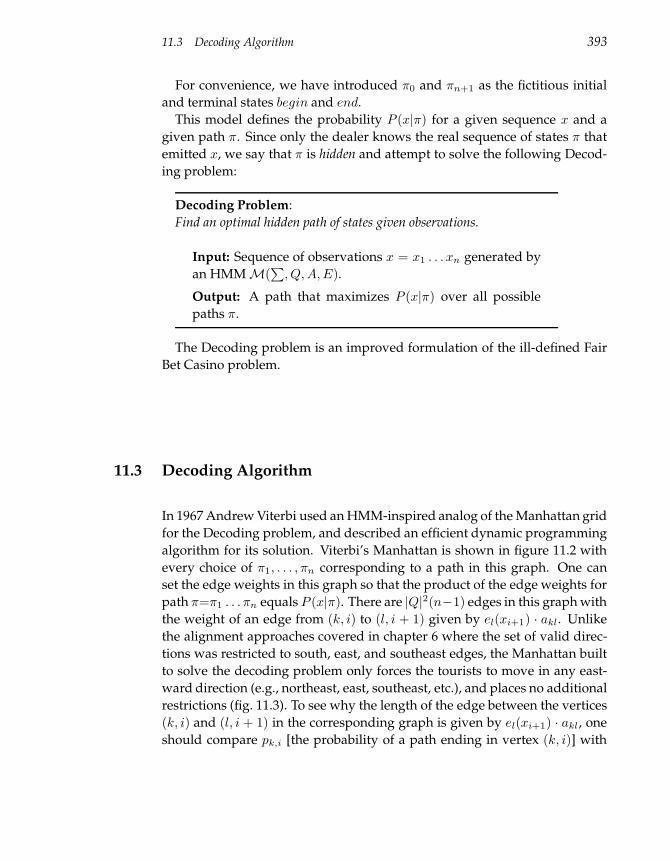
11.3 Decoding Algorithm 393
For convenience, we have introduced π0 and πn+1 as the fictitious initial
and terminal states begin and end.
This model defines the probability P (x|π) for a given sequence x and a
given path π. Since only the dealer knows the real sequence of states π that
emitted x, we say that π is hidden and attempt to solve the following Decod-
ing problem:
Decoding Problem:
Find an optimal hidden path of states given observations.
Input: Sequence of observations x = x1 . . . xn generated by
an HMMM(∑
, Q, A, E).
Output: A path that maximizes P (x|π) over all possible
paths π.
The Decoding problem is an improved formulation of the ill-defined Fair
Bet Casino problem.
11.3 Decoding Algorithm
In 1967 Andrew Viterbi used an HMM-inspired analog of the Manhattan grid
for the Decoding problem, and described an efficient dynamic programming
algorithm for its solution. Viterbi’s Manhattan is shown in figure 11.2 with
every choice of π1, . . . , πn corresponding to a path in this graph. One can
set the edge weights in this graph so that the product of the edge weights for
path π=π1 . . . πn equals P (x|π). There are |Q|2(n−1) edges in this graph with
the weight of an edge from (k, i) to (l, i + 1) given by el(xi+1) · akl. Unlike
the alignment approaches covered in chapter 6 where the set of valid direc-
tions was restricted to south, east, and southeast edges, the Manhattan built
to solve the decoding problem only forces the tourists to move in any east-
ward direction (e.g., northeast, east, southeast, etc.), and places no additional
restrictions (fig. 11.3). To see why the length of the edge between the vertices
(k, i) and (l, i + 1) in the corresponding graph is given by el(xi+1) · akl, one
should compare pk,i [the probability of a path ending in vertex (k, i)] with
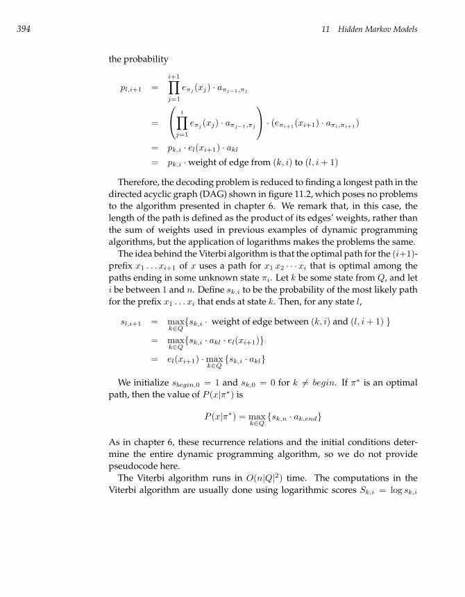
394 11 Hidden Markov Models
the probability
pl,i+1 =
i+1∏
j=1
eπj(xj) · aπj−1,πj
=
i∏
j=1
eπj(xj) · aπj−1,πj
· (eπi+1(xi+1) · aπi,πi+1)
= pk,i · el(xi+1) · akl
= pk,i ·weight of edge from (k, i) to (l, i + 1)
Therefore, the decoding problem is reduced to finding a longest path in the
directed acyclic graph (DAG) shown in figure 11.2, which poses no problems
to the algorithm presented in chapter 6. We remark that, in this case, the
length of the path is defined as the product of its edges’ weights, rather than
the sum of weights used in previous examples of dynamic programming
algorithms, but the application of logarithms makes the problems the same.
The idea behind the Viterbi algorithm is that the optimal path for the (i+1)-
prefix x1 . . . xi+1 of x uses a path for x1 x2 · · ·xi that is optimal among the
paths ending in some unknown state πi. Let k be some state from Q, and let
i be between 1 and n. Define sk,i to be the probability of the most likely path
for the prefix x1 . . . xi that ends at state k. Then, for any state l,
sl,i+1 = maxk∈Qsk,i · weight of edge between (k, i) and (l, i + 1)
= maxk∈Qsk,i · akl · el(xi+1)
= el(xi+1) ·maxk∈Qsk,i · akl
We initialize sbegin,0 = 1 and sk,0 = 0 for k 6= begin. If π∗ is an optimal
path, then the value of P (x|π∗) is
P (x|π∗) = maxk∈Qsk,n · ak,end
As in chapter 6, these recurrence relations and the initial conditions deter-
mine the entire dynamic programming algorithm, so we do not provide
pseudocode here.
The Viterbi algorithm runs in O(n|Q|2) time. The computations in the
Viterbi algorithm are usually done using logarithmic scores Sk,i = log sk,i
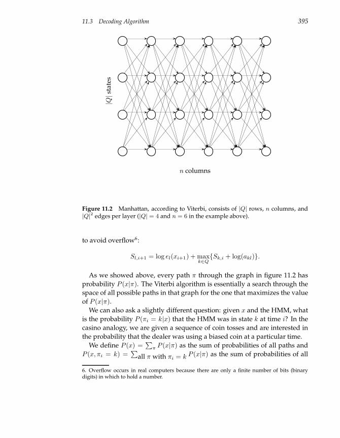
11.3 Decoding Algorithm 395
|Q|
stat
es
n columns
Figure 11.2 Manhattan, according to Viterbi, consists of |Q| rows, n columns, and|Q|2 edges per layer (|Q| = 4 and n = 6 in the example above).
to avoid overflow6:
Sl,i+1 = log el(xi+1) + maxk∈QSk,i + log(akl).
As we showed above, every path π through the graph in figure 11.2 has
probability P (x|π). The Viterbi algorithm is essentially a search through the
space of all possible paths in that graph for the one that maximizes the value
of P (x|π).
We can also ask a slightly different question: given x and the HMM, what
is the probability P (πi = k|x) that the HMM was in state k at time i? In the
casino analogy, we are given a sequence of coin tosses and are interested in
the probability that the dealer was using a biased coin at a particular time.
We define P (x) =∑
π P (x|π) as the sum of probabilities of all paths and
P (x, πi = k) =∑
all π with πi = k P (x|π) as the sum of probabilities of all
6. Overflow occurs in real computers because there are only a finite number of bits (binarydigits) in which to hold a number.
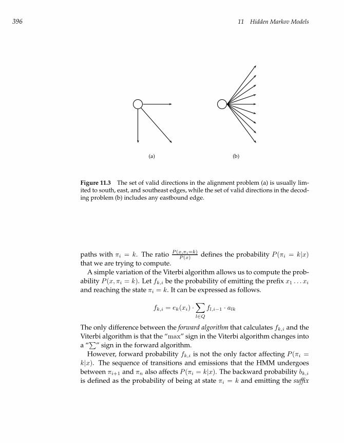
396 11 Hidden Markov Models
(a) (b)
Figure 11.3 The set of valid directions in the alignment problem (a) is usually lim-ited to south, east, and southeast edges, while the set of valid directions in the decod-ing problem (b) includes any eastbound edge.
paths with πi = k. The ratio P (x,πi=k)P (x) defines the probability P (πi = k|x)
that we are trying to compute.
A simple variation of the Viterbi algorithm allows us to compute the prob-
ability P (x, πi = k). Let fk,i be the probability of emitting the prefix x1 . . . xi
and reaching the state πi = k. It can be expressed as follows.
fk,i = ek(xi) ·∑
l∈Q
fl,i−1 · alk
The only difference between the forward algorithm that calculates fk,i and the
Viterbi algorithm is that the “max” sign in the Viterbi algorithm changes into
a “∑
” sign in the forward algorithm.
However, forward probability fk,i is not the only factor affecting P (πi =
k|x). The sequence of transitions and emissions that the HMM undergoes
between πi+1 and πn also affects P (πi = k|x). The backward probability bk,i
is defined as the probability of being at state πi = k and emitting the suffix
11.4 HMM Parameter Estimation 397
xi+1 . . . xn. The backward algorithm uses a similar recurrence:
bk,i =∑
l∈Q
el(xi+1) · bl,i+1 · akl
Finally, the probability that the dealer had a biased coin at moment i is given
by
P (πi = k|x) =P (x, πi = k)
P (x)=
fk(i) · bk(i)
P (x).
11.4 HMM Parameter Estimation
The preceding analysis assumed that we know the state transition and emis-
sion probabilities of the HMM. Given these parameters, it is easy for an in-
telligent gambler to figure out that the dealer in the Fair Bet Casino is using a
biased coin, simply by noticing that 0 and 1 have different expected frequen-
cies ( 38 vs 5
8 ). If the ratio of zeros to ones in a daylong sequence of tosses is
suspiciously low, then it is likely that the dealer is using a biased coin. Un-
fortunately, the most difficult problem in the application of HMMs is that the
HMM parameters are usually unknown and therefore need to be estimated
from data. It is more difficult to estimate the transition and emission prob-
abilities of an HMM than it is to reconstruct the most probable sequence of
states it went through when you do know the probabilities. In this case, we
are given the set of states, Q, but we do not know with what probability the
HMM moves from one state to another, or with what probability it emits any
particular symbol.
Let Θ be a vector combining the unknown transition and emission proba-
bilities of the HMMM. Given an observed symbol string x that the HMM
emitted, define P (x|Θ) as the maximum probability of x given the assign-
ment of parameters Θ. Our goal is to find
maxΘ
P (x|Θ).
Usually, instead of a single string x, we can obtain a sample of training se-
quences x1, . . . , xm, so a natural goal is to find
maxΘ
m∏
j=1
P (xj |Θ).
398 11 Hidden Markov Models
This results in a difficult optimization problem in the multidimensional pa-
rameter space Θ. Commonly used algorithms for this type of parameter op-
timization are heuristics that use local improvement strategies. If we know
the path π1 . . . πn corresponding to the observed states x1 . . . xn, then we can
scan the sequences and compute empirical estimates for transition and emis-
sion probabilities. If Akl is the number of transitions from state k to l and
Ek(b) is the number of times b is emitted from state k, then the reasonable
estimators are
akl =Akl
∑
q∈Q Akq
ek(b) =Ek(b)
∑
σ∈P Ek(σ)
.
However, we do not usually know the state sequence π = π1 . . . πn, and
in this case we can start from a wild guess for π1 . . . πn, compute empirical
estimates for transition and emission probabilities using this guess, and solve
the decoding problem to find a new, hopefully less wild, estimate for π. The
commonly used iterative local improvement strategy, called the Baum-Welch
algorithm, uses a similar approach to estimate HMM parameters.
11.5 Profile HMM Alignment
Given a family of functionally related biological sequences, one can search
for new members of the family from a database using pairwise alignments
between family members and sequences from the database. However, this
approach may fail to identify distantly related sequences because distant
cousins may have weak similarities that do not pass the statistical signifi-
cance test. However, if the sequence has weak similarities with many family
members, it is likely to belong to the family. The problem then is to somehow
align a sequence to all members of the family at once, using the whole set of
functionally related sequences in the search.
The simplest representation of a family of related proteins is given by their
multiple alignment and the corresponding profile.7 As with sequences, pro-
files can also be compared and aligned against each other since the dynamic
programming algorithm for aligning two sequences works if both of the in-
put sequences are profiles.
7. While in chapter 4 we defined profile element pij as a count of the nucleotide i in the jthcolumn of alignment matrix, biologists usually define pij as frequency of the nucleotide i in thejth column of the alignment matrix, that is, they divide all of the counts by t (see figure 11.4). Inorder to avoid columns that contain one or more letters with probabilities of 0, small numbers
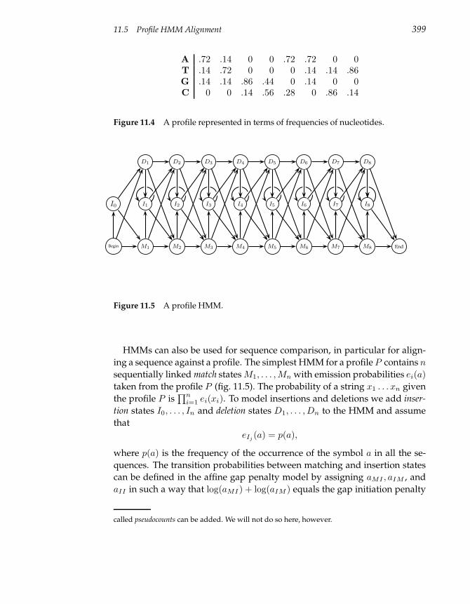
11.5 Profile HMM Alignment 399
A .72 .14 0 0 .72 .72 0 0T .14 .72 0 0 0 .14 .14 .86G .14 .14 .86 .44 0 .14 0 0C 0 0 .14 .56 .28 0 .86 .14
Figure 11.4 A profile represented in terms of frequencies of nucleotides.
Begin
I0
D1
I1
M1
D2
I2
M2
D3
I3
M3
D4
I4
M4
D5
I5
M5
D6
I6
M6
D7
I7
M7
D8
I8
M8 End
Figure 11.5 A profile HMM.
HMMs can also be used for sequence comparison, in particular for align-
ing a sequence against a profile. The simplest HMM for a profile P contains n
sequentially linked match states M1, . . . , Mn with emission probabilities ei(a)
taken from the profile P (fig. 11.5). The probability of a string x1 . . . xn given
the profile P is∏n
i=1 ei(xi). To model insertions and deletions we add inser-
tion states I0, . . . , In and deletion states D1, . . . , Dn to the HMM and assume
that
eIj(a) = p(a),
where p(a) is the frequency of the occurrence of the symbol a in all the se-
quences. The transition probabilities between matching and insertion states
can be defined in the affine gap penalty model by assigning aMI , aIM , and
aII in such a way that log(aMI) + log(aIM ) equals the gap initiation penalty
called pseudocounts can be added. We will not do so here, however.
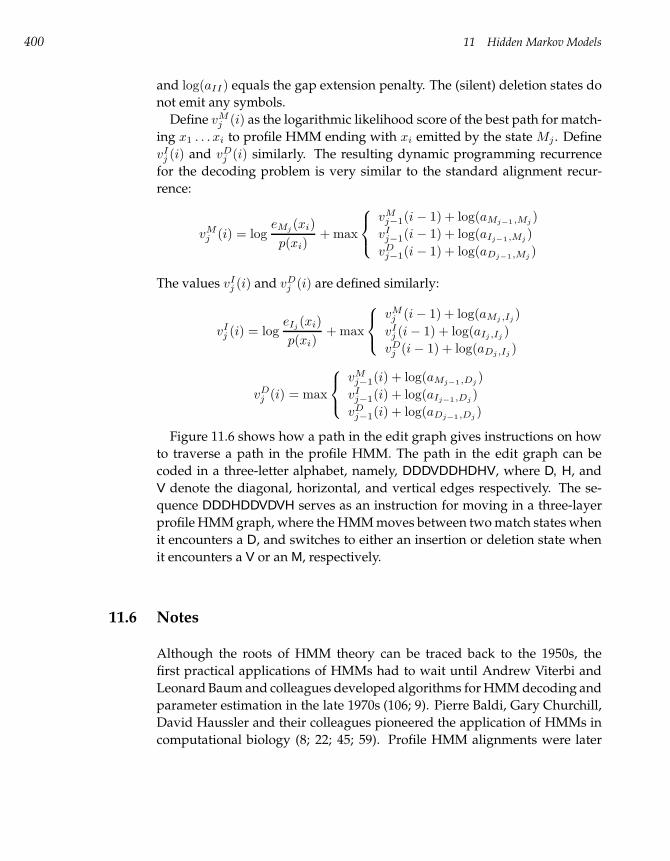
400 11 Hidden Markov Models
and log(aII) equals the gap extension penalty. The (silent) deletion states do
not emit any symbols.
Define vMj (i) as the logarithmic likelihood score of the best path for match-
ing x1 . . . xi to profile HMM ending with xi emitted by the state Mj . Define
vIj (i) and vD
j (i) similarly. The resulting dynamic programming recurrence
for the decoding problem is very similar to the standard alignment recur-
rence:
vMj (i) = log
eMj(xi)
p(xi)+ max
vMj−1(i− 1) + log(aMj−1,Mj
)
vIj−1(i− 1) + log(aIj−1,Mj
)
vDj−1(i− 1) + log(aDj−1,Mj
)
The values vIj (i) and vD
j (i) are defined similarly:
vIj (i) = log
eIj(xi)
p(xi)+ max
vMj (i− 1) + log(aMj ,Ij
)
vIj (i− 1) + log(aIj ,Ij
)
vDj (i− 1) + log(aDj ,Ij
)
vDj (i) = max
vMj−1(i) + log(aMj−1,Dj
)
vIj−1(i) + log(aIj−1,Dj
)
vDj−1(i) + log(aDj−1,Dj
)
Figure 11.6 shows how a path in the edit graph gives instructions on how
to traverse a path in the profile HMM. The path in the edit graph can be
coded in a three-letter alphabet, namely, DDDVDDHDHV, where D, H, and
V denote the diagonal, horizontal, and vertical edges respectively. The se-
quence DDDHDDVDVH serves as an instruction for moving in a three-layer
profile HMM graph, where the HMM moves between two match states when
it encounters a D, and switches to either an insertion or deletion state when
it encounters a V or an M, respectively.
11.6 Notes
Although the roots of HMM theory can be traced back to the 1950s, the
first practical applications of HMMs had to wait until Andrew Viterbi and
Leonard Baum and colleagues developed algorithms for HMM decoding and
parameter estimation in the late 1970s (106; 9). Pierre Baldi, Gary Churchill,
David Haussler and their colleagues pioneered the application of HMMs in
computational biology (8; 22; 45; 59). Profile HMM alignments were later
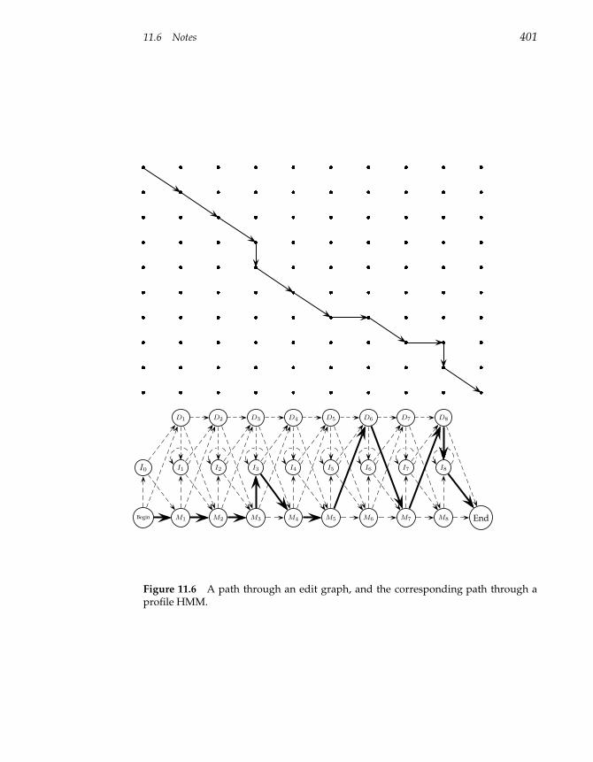
11.6 Notes 401
Begin
I0
D1
I1
M1
D2
I2
M2
D3
I3
M3
D4
I4
M4
D5
I5
M5
D6
I6
M6
D7
I7
M7
D8
I8
M8 End
!"#$%&'
()*+,-./01
23456789:;
<=>?@ABCDE
FGHIJKLMNO
PQRSTUVWXY
Z[\]_abc
Figure 11.6 A path through an edit graph, and the corresponding path through aprofile HMM.

402 11 Hidden Markov Models
used for developing Pfam, a database of protein domain families (99) and in
many other applications.
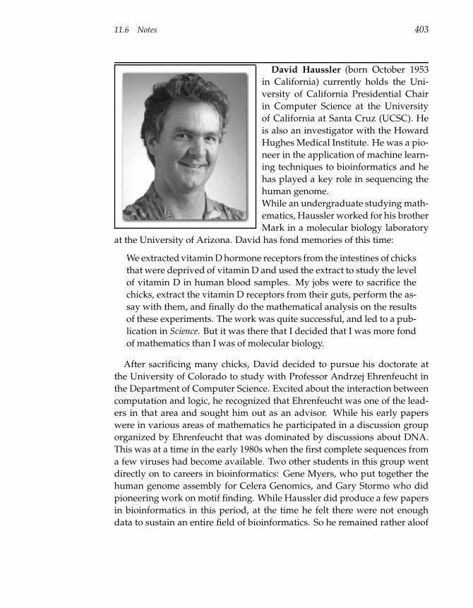
11.6 Notes 403
David Haussler (born October 1953
in California) currently holds the Uni-
versity of California Presidential Chair
in Computer Science at the University
of California at Santa Cruz (UCSC). He
is also an investigator with the Howard
Hughes Medical Institute. He was a pio-
neer in the application of machine learn-
ing techniques to bioinformatics and he
has played a key role in sequencing the
human genome.
While an undergraduate studying math-
ematics, Haussler worked for his brother
Mark in a molecular biology laboratory
at the University of Arizona. David has fond memories of this time:
We extracted vitamin D hormone receptors from the intestines of chicks
that were deprived of vitamin D and used the extract to study the level
of vitamin D in human blood samples. My jobs were to sacrifice the
chicks, extract the vitamin D receptors from their guts, perform the as-
say with them, and finally do the mathematical analysis on the results
of these experiments. The work was quite successful, and led to a pub-
lication in Science. But it was there that I decided that I was more fond
of mathematics than I was of molecular biology.
After sacrificing many chicks, David decided to pursue his doctorate at
the University of Colorado to study with Professor Andrzej Ehrenfeucht in
the Department of Computer Science. Excited about the interaction between
computation and logic, he recognized that Ehrenfeucht was one of the lead-
ers in that area and sought him out as an advisor. While his early papers
were in various areas of mathematics he participated in a discussion group
organized by Ehrenfeucht that was dominated by discussions about DNA.
This was at a time in the early 1980s when the first complete sequences from
a few viruses had become available. Two other students in this group went
directly on to careers in bioinformatics: Gene Myers, who put together the
human genome assembly for Celera Genomics, and Gary Stormo who did
pioneering work on motif finding. While Haussler did produce a few papers
in bioinformatics in this period, at the time he felt there were not enough
data to sustain an entire field of bioinformatics. So he remained rather aloof
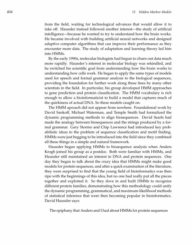
404 11 Hidden Markov Models
from the field, waiting for technological advances that would allow it to
take off. Haussler instead followed another interest—the study of artificial
intelligence—because he wanted to try to understand how the brain works.
He became involved with building artificial neural networks and designed
adaptive computer algorithms that can improve their performance as they
encounter more data. The study of adaptation and learning theory led him
into HMMs.
By the early 1990s, molecular biologists had begun to churn out data much
more rapidly. Haussler’s interest in molecular biology was rekindled, and
he switched his scientific goal from understanding how the brain works to
understanding how cells work. He began to apply the same types of models
used for speech and formal grammar analysis to the biological sequences,
providing the foundation for further work along these lines by many other
scientists in the field. In particular, his group developed HMM approaches
to gene prediction and protein classification. The HMM vocabulary is rich
enough to allow a bioinformaticist to build a model that captures much of
the quirkiness of actual DNA. So these models caught on.
The HMM aproach did not appear from nowhere. Foundational work by
David Sankoff, Michael Waterman, and Temple Smith had formalized the
dynamic programming methods to align biosequences. David Searls had
made the analogy between biosequences and the strings produced by a for-
mal grammar. Gary Stormo and Chip Lawrence had introduced key prob-
abilistic ideas to the problem of sequence classification and motif finding.
HMMs were just begging to be introduced into the field since they combined
all these things in a simple and natural framework.
Haussler began applying HMMs to biosequence analysis when Anders
Krogh joined his group as a postdoc. Both were familiar with HMMs, and
Haussler still maintained an interest in DNA and protein sequences. One
day they began to talk about the crazy idea that HMMs might make good
models for protein sequences, and after a quick examination of the literature,
they were surprised to find that the young field of bioinformatics was then
ripe with the beginnings of this idea, but no one had really put all the pieces
together and exploited it. So they dove in and built HMMs to recognize
different protein families, demonstrating how this methodology could unify
the dynamic programming, grammatical, and maximum-likelihood methods
of statistical inference that were then becoming popular in bioinformatics.
David Haussler says:
The epiphany that Anders and I had about HMMs for protein sequences
11.6 Notes 405
was certainly one of the most exciting moments in my career. How-
ever, I would have to say that the most exciting moment came later,
when my group participated in efforts to sequence the human genome,
and Jim Kent, then a graduate student at UCSC, was the first person
able to computationally assemble the public sequencing project’s data
to form a working draft. We raced with Gene Myers’ team at Celera
as they assembled their draft genome. On July 7, 2000, shortly after
Francis Collins and Craig Venter jointly announced in a White House
ceremony that their two teams had successfully assembled the human
genome, we released the public working draft onto the World Wide
Web. That moment on July 7, when the flood of A, C, T, and G of the
human genome sequence came across my computer screen, passing
across the net as they were to thousands of other people all over the
world, was the most exciting moment in my scientific life. For me, it
was symbolic of the entire Human Genome Project, both public and
private, and the boundless determination of the many scientists in-
volved. It seems unthinkable that out of a primordial soup of organic
molecules, life forms would eventually evolve whose cells would carry
their vital messages forward in DNA from generation to generation,
ever diversifying and expanding their abilities as this message became
more complex, until one day one of these species would accumulate
the facility to decode and share its own DNA message. Yet that day
had arrived.
Haussler’s approach to research has always been at the extreme interdisci-
plinary end of the spectrum. Most of his insights have come from the appli-
cation of perspectives of one field to problems encountered in another.
I’ve tried to stay focused on the big scientific questions, and never limit
my approach to conform to the norms of any well-established and nar-
row method of inquiry. I try to always listen carefully to the few best
scientists in all fields, rather than all the scientists in one field.
Haussler thinks that one key to discovery is picking the right problem.
Important scientific problems become ripe at particular times. Before that
they are unapproachable because the foundation required for their solution
has not been laid. After that they are no longer as important because the
heart of the problem has already been solved. Knowing when a scientific
problem is ripe for solution is a difficult art, however. Breadth of focus helps.
Luck doesn’t hurt either. Haussler says:
406 11 Hidden Markov Models
We have not even really begun to understand how a cell works, so there
are plenty of interesting problems left for bioinformaticians. Compu-
tational models for this problem probably won’t look anything like
what we have today. Problems associated with understanding how
cells form organs, bodies, and minds that function as they do is also
likely to keep anyone from being bored in this field for quite some time.
Applying what we learn to the practice of medicine will pose further
challenging problems. However, much foundational works remains
to be done before we can do justice to the loftiest of these problems.
One important piece of foundational work where bioinformatics will
play the key role is in understanding the evolutionary history of entire
genomes. With the full genome sequences of many different species,
we can begin to try to reconstruct the key events in the evolution of
our own genome using new comparative genomics approaches. This
will require more than raw genome data. It will demand the devel-
opment of new mathematics and algorithms appropriate to the task.
People have always been fascinated with origins, and the mystery of
our own origins has been paramount among these fascinations. Thus,
I anticipate no lack of interest in such investigations.
11.7 Problems 407
α
A
25
G
25
T
110
C
110
β
T
310
C
310
A
15
G
15
110
110
910
910
Figure 11.7 The HMM described in Problem 11.4.
11.7 Problems
Problem 11.1
The Decoding problem can be formulated as a longest path problem in a DAG. Thismotivates a question about a space-efficient version of the decoding algorithm. Doesthere exist a linear-space algorithm for the decoding problem?
Problem 11.2
To avoid suspicion, the dealer in the Fair Bet Casino keeps every coin for at least tentosses, regardless of whether it is fair or biased. Describe both the correspondingHMM and how to modify the decoding algorithm for this case.
Problem 11.3
Suppose you are given the dinucleotide frequences in CG-islands and the dinucleotidefrequencies outside CG-islands. Design an HMM for finding CG-islands in genomicsequences.
Problem 11.4
Figure 11.7 shows an HMM with two states α and β. When in the α state, it is morelikely to emit purines (A and G). When in the β state, it is more likely to emit pyrim-idines (C and T). Decode the most likely sequence of states (α/β) for sequence GGCT.Use log-scores, rather than straight probability scores.
Problem 11.5
Suppose a dishonest dealer has two coins, one fair and one biased; the biased coinhas heads probability 1/4. Assume that the dealer never switches the coins. Whichcoin is more likely to have generated the sequence HTTTHHHTTTTHTHHTT? It maybe useful to know that log2(3) = 1.585
408 11 Hidden Markov Models
Problem 11.6
Consider a different game where the dealer is not flipping a coin, but instead rollinga three-sided die with labels 1, 2, and 3. (Try not to think about what a three-sideddie might look like.) The dealer has two loaded dice D1 and D2. For each die Di, theprobability of rolling the number i is 1/2, and the probability of each of the other twooutcomes is 1/4. At each turn, the dealer must decide whether to (1) keep the samedie, (2) switch to the other die, or (3) end the game. He chooses (1) with probability1/2 and each of the others with probability 1/4. At the beginning the dealer choosesone of the two dice with equal probability.
• Give an HMM for this situation. Specify the alphabet, the states, the transitionprobabilities, and the emission probabilities. Include a start state start, and as-sume that the HMM begins in state start with probability 1. Also include an endstate end.
• Suppose that you observe the following sequence of die rolls: 1 1 2 1 2 2. Find asequence of states which best explains the sequence of rolls. What is the proba-bility of this sequence? Find the answer by completing the Viterbi table. Includebacktrack arrows in the cells so you can trace back the sequence of states. Some ofthe following facts may be useful:
log2(0) = −∞log2(1/4) = −2
log2(1/2) = −1
log2(1) = 0
• There are actually two optimal sequences of states for this sequence of die rolls.What is the other sequence of states?
12 Randomized Algorithms
Randomized algorithms make random decisions throughout their operation.
At first glance, making random decisions does not seem particularly help-
ful. Basing an algorithm on random decisions sounds like a recipe for dis-
aster, but an eighteenth-century French naturalist, Comte de Buffon, proved
the opposite by developing an algorithm to accurately compute π by ran-
domly dropping needles on a sheet of paper with parallel lines. The fact that
a randomized algorithm undertakes a nondeterministic sequence of opera-
tions often means that, unlike deterministic algorithms, no input can reli-
ably produce worst-case results. Randomized algorithms are often used in
hard problems where an exact, polynomial-time algorithm is not known. In
this chapter we will see how randomized algorithms solve the Motif Finding
problem.
12.1 The Sorting Problem Revisited
The QUICKSORT algorithm below is another fast and simple sorting tech-
nique. It selects an element m (typically, the first) from an array c and simply
partitions the array into two subarrays: csmall, containing all elements from
c that are smaller than m; and clarge containing all elements larger than m.
This partitioning can be done in linear time, and by following a divide-and-
conquer strategy, QUICKSORT recursively sorts each subarray in the same
way. The sorted list is easily created by simply concatenating the sorted
csmall, element m, and the sorted clarge.
Administrator
Highlight
410 12 Randomized Algorithms
QUICKSORT(c)
1 if c consists of a single element
2 return c
3 m← c1
4 Determine the set of elements csmall smaller than m
5 Determine the set of elements clarge larger than m
6 QUICKSORT(csmall)
7 QUICKSORT(clarge)
8 Combine csmall, m, and clarge into a single sorted array csorted
9 return csorted
It turns out that the running time of QUICKSORT depends on how lucky
we are with our selection of the element m. If we happen to choose m in such
a way that c is split into even halves (i.e., |csmall| = |clarge|), then
T (n) = 2T (n/2) + an,
where T (n) represents the time taken by QUICKSORT to sort an array of n
numbers, and an represents the time required to split the array of size n into
two parts; a is a positive constant. This is exactly the same recurrence we
saw in MERGESORT and we already know that it leads to O(n log n) running
time. However, if we choose m in such a way that it splits c unevenly (e.g.,
an extreme case occurs when csmall is empty and clarge has n− 1 elements),
then the recurrence looks like
T (n) = T (n− 1) + an
This is exactly the recurrence we saw for SELECTIONSORT and we already
know that it leads to O(n2) running time, something we want to avoid. In-
deed, QUICKSORT takes quadratic time to sort the array (n, n − 1, . . . , 2, 1).
Worse yet, it requires O(n2) time to process (1, 2, . . . , n− 1, n), which seems
unnecessary since the array is already sorted.
The QUICKSORT algorithm so far seems like a bad imitation of MERGE-
SORT. However, if we can choose a good “splitter” m that breaks an ar-
ray into two equal parts, we might improve the running time. To achieve
O(n log n) running time, it is not actually necessary to find a perfectly equal
(50/50) split. For example, a split into approximately equal parts of size,
say, 51/49 will also work. In fact, one can prove that the algorithm will
achieve O(n log n) running time as long as the sets csmall and clarge are both
12.1 The Sorting Problem Revisited 411
larger in size than n4 , which implies that, of n possible choices for m, at least
34n − 1
4n = 12n of them make good splitters! In other words, if we choose
m uniformly at random (i.e., every element of c has the same probability to
be chosen), there is at least a 50% chance that it will be a good splitter. This
observation motivates the following randomized algorithm:
RANDOMIZEDQUICKSORT(c)
1 if c consists of a single element
2 return c
3 Choose element m uniformly at random from c
4 Determine the set of elements csmall smaller than m
5 Determine the set of elements clarge larger than m
6 RANDOMIZEDQUICKSORT(csmall)
7 RANDOMIZEDQUICKSORT(clarge)
8 Combine csmall, m, and clarge into a single sorted array csorted
9 return csorted
RANDOMIZEDQUICKSORT is a very fast algorithm in practice but its worst-
case running time remains O(n2) since there is still a possibility that it selects
bad splitters. Although the behavior of a randomized algorithm varies on
the same input from one execution to the next, one can prove that its expected
running time is O(n log n).1
The key advantage of randomized algorithms is performance: for many
practical problems randomized algorithms are faster (in the sense of expected
running time) than the best known deterministic algorithms. Another attrac-
tive feature of randomized algorithms, as illustrated by RANDOMIZEDQUICK-
SORT and other algorithms in this chapter, is their simplicity.
We emphasize that RANDOMIZEDQUICKSORT, despite making random
decisions, always returns the correct solution of the sorting problem. The
only variable from one run to another is its running time, not the result. In
contrast, other randomized algorithms we consider in this chapter usually
produce incorrect (or, more gently, approximate) solutions. Randomized al-
gorithms that always return correct answers are called Las Vegas algorithms,
while algorithms that do not are called Monte Carlo algorithms. Of course,
computer scientists prefer Las Vegas algorithms to Monte Carlo algorithms
but the former are often difficult to come by. Although for some applications
1. The running time of a randomized algorithm is a random variable, and computer scientistsare often interested in the mean value of this random variable. This is referred to as the expectedrunning time.
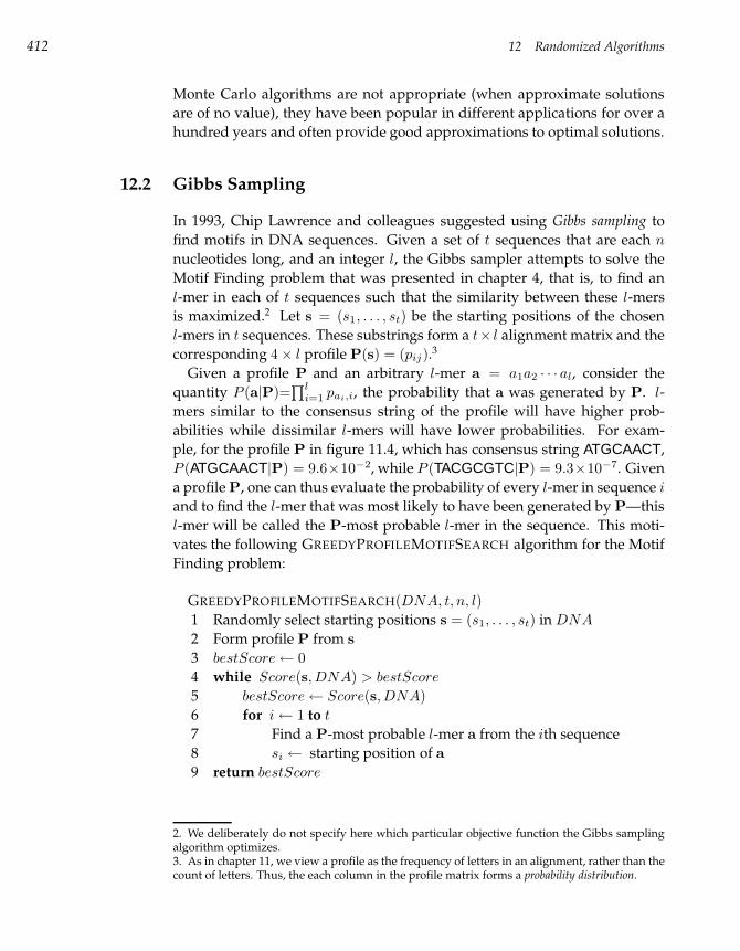
412 12 Randomized Algorithms
Monte Carlo algorithms are not appropriate (when approximate solutions
are of no value), they have been popular in different applications for over a
hundred years and often provide good approximations to optimal solutions.
12.2 Gibbs Sampling
In 1993, Chip Lawrence and colleagues suggested using Gibbs sampling to
find motifs in DNA sequences. Given a set of t sequences that are each n
nucleotides long, and an integer l, the Gibbs sampler attempts to solve the
Motif Finding problem that was presented in chapter 4, that is, to find an
l-mer in each of t sequences such that the similarity between these l-mers
is maximized.2 Let s = (s1, . . . , st) be the starting positions of the chosen
l-mers in t sequences. These substrings form a t× l alignment matrix and the
corresponding 4× l profile P(s) = (pij).3
Given a profile P and an arbitrary l-mer a = a1a2 · · · al, consider the
quantity P (a|P)=∏l
i=1 pai,i, the probability that a was generated by P. l-
mers similar to the consensus string of the profile will have higher prob-
abilities while dissimilar l-mers will have lower probabilities. For exam-
ple, for the profile P in figure 11.4, which has consensus string ATGCAACT,
P (ATGCAACT|P) = 9.6×10⁻², while P (TACGCGTC|P) = 9.3×10⁻⁷. Given
a profile P, one can thus evaluate the probability of every l-mer in sequence i
and to find the l-mer that was most likely to have been generated by P—this
l-mer will be called the P-most probable l-mer in the sequence. This moti-
vates the following GREEDYPROFILEMOTIFSEARCH algorithm for the Motif
Finding problem:
GREEDYPROFILEMOTIFSEARCH(DNA, t, n, l)
1 Randomly select starting positions s = (s1, . . . , st) in DNA
2 Form profile P from s
3 bestScore← 0
4 while Score(s, DNA) > bestScore
5 bestScore← Score(s, DNA)
6 for i← 1 to t
7 Find a P-most probable l-mer a from the ith sequence
8 si ← starting position of a
9 return bestScore
2. We deliberately do not specify here which particular objective function the Gibbs samplingalgorithm optimizes.3. As in chapter 11, we view a profile as the frequency of letters in an alignment, rather than thecount of letters. Thus, the each column in the profile matrix forms a probability distribution.
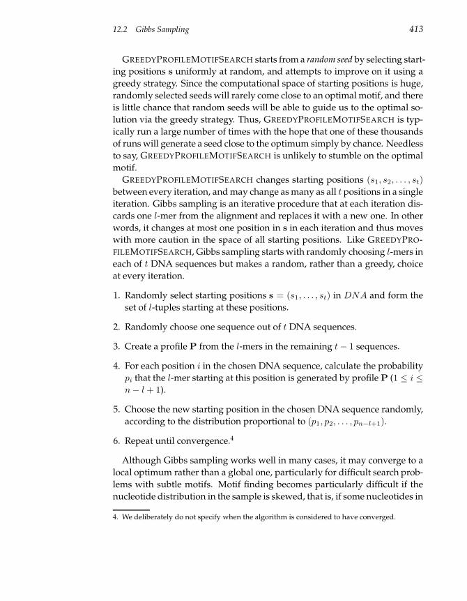
12.2 Gibbs Sampling 413
GREEDYPROFILEMOTIFSEARCH starts from a random seed by selecting start-
ing positions s uniformly at random, and attempts to improve on it using a
greedy strategy. Since the computational space of starting positions is huge,
randomly selected seeds will rarely come close to an optimal motif, and there
is little chance that random seeds will be able to guide us to the optimal so-
lution via the greedy strategy. Thus, GREEDYPROFILEMOTIFSEARCH is typ-
ically run a large number of times with the hope that one of these thousands
of runs will generate a seed close to the optimum simply by chance. Needless
to say, GREEDYPROFILEMOTIFSEARCH is unlikely to stumble on the optimal
motif.
GREEDYPROFILEMOTIFSEARCH changes starting positions (s1, s2, . . . , st)
between every iteration, and may change as many as all t positions in a single
iteration. Gibbs sampling is an iterative procedure that at each iteration dis-
cards one l-mer from the alignment and replaces it with a new one. In other
words, it changes at most one position in s in each iteration and thus moves
with more caution in the space of all starting positions. Like GREEDYPRO-
FILEMOTIFSEARCH, Gibbs sampling starts with randomly choosing l-mers in
each of t DNA sequences but makes a random, rather than a greedy, choice
at every iteration.
1. Randomly select starting positions s = (s1, . . . , st) in DNA and form the
set of l-tuples starting at these positions.
2. Randomly choose one sequence out of t DNA sequences.
3. Create a profile P from the l-mers in the remaining t− 1 sequences.
4. For each position i in the chosen DNA sequence, calculate the probability
pi that the l-mer starting at this position is generated by profile P (1 ≤ i ≤
n− l + 1).
5. Choose the new starting position in the chosen DNA sequence randomly,
according to the distribution proportional to (p1, p2, . . . , pn−l+1).
6. Repeat until convergence.4
Although Gibbs sampling works well in many cases, it may converge to a
local optimum rather than a global one, particularly for difficult search prob-
lems with subtle motifs. Motif finding becomes particularly difficult if the
nucleotide distribution in the sample is skewed, that is, if some nucleotides in
4. We deliberately do not specify when the algorithm is considered to have converged.
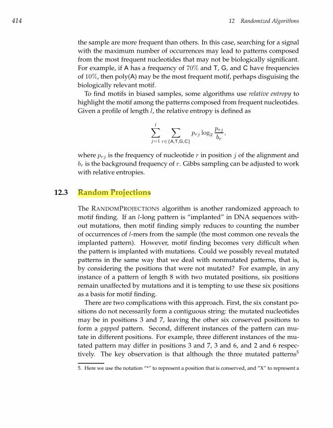
414 12 Randomized Algorithms
the sample are more frequent than others. In this case, searching for a signal
with the maximum number of occurrences may lead to patterns composed
from the most frequent nucleotides that may not be biologically significant.
For example, if A has a frequency of 70% and T, G, and C have frequencies
of 10%, then poly(A) may be the most frequent motif, perhaps disguising the
biologically relevant motif.
To find motifs in biased samples, some algorithms use relative entropy to
highlight the motif among the patterns composed from frequent nucleotides.
Given a profile of length l, the relative entropy is defined as
l∑
j=1
∑
r∈A,T,G,C
prj log2
prj
br
,
where prj is the frequency of nucleotide r in position j of the alignment and
br is the background frequency of r. Gibbs sampling can be adjusted to work
with relative entropies.
12.3 Random Projections
The RANDOMPROJECTIONS algorithm is another randomized approach to
motif finding. If an l-long pattern is “implanted” in DNA sequences with-
out mutations, then motif finding simply reduces to counting the number
of occurrences of l-mers from the sample (the most common one reveals the
implanted pattern). However, motif finding becomes very difficult when
the pattern is implanted with mutations. Could we possibly reveal mutated
patterns in the same way that we deal with nonmutated patterns, that is,
by considering the positions that were not mutated? For example, in any
instance of a pattern of length 8 with two mutated positions, six positions
remain unaffected by mutations and it is tempting to use these six positions
as a basis for motif finding.
There are two complications with this approach. First, the six constant po-
sitions do not necessarily form a contiguous string: the mutated nucleotides
may be in positions 3 and 7, leaving the other six conserved positions to
form a gapped pattern. Second, different instances of the pattern can mu-
tate in different positions. For example, three different instances of the mu-
tated pattern may differ in positions 3 and 7, 3 and 6, and 2 and 6 respec-
tively. The key observation is that although the three mutated patterns5
5. Here we use the notation “*” to represent a position that is conserved, and “X” to represent a
Administrator
Highlight
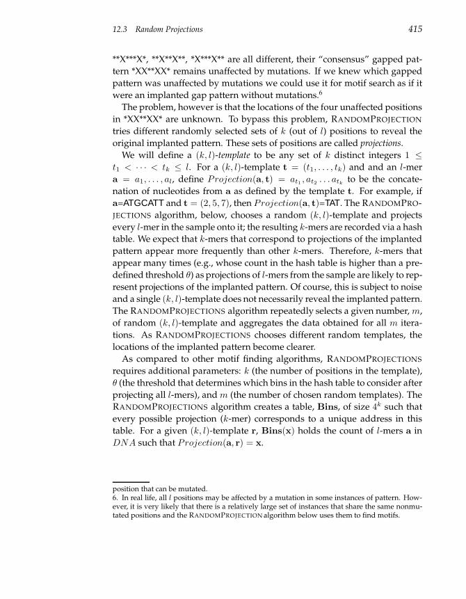
12.3 Random Projections 415
**X***X*, **X**X**, *X***X** are all different, their “consensus” gapped pat-
tern *XX**XX* remains unaffected by mutations. If we knew which gapped
pattern was unaffected by mutations we could use it for motif search as if it
were an implanted gap pattern without mutations.6
The problem, however is that the locations of the four unaffected positions
in *XX**XX* are unknown. To bypass this problem, RANDOMPROJECTION
tries different randomly selected sets of k (out of l) positions to reveal the
original implanted pattern. These sets of positions are called projections.
We will define a (k, l)-template to be any set of k distinct integers 1 ≤
t1 < · · · < tk ≤ l. For a (k, l)-template t = (t1, . . . , tk) and and an l-mer
a = a1, . . . , al, define Projection(a, t) = at1 , at2 . . . atkto be the concate-
nation of nucleotides from a as defined by the template t. For example, if
a=ATGCATT and t = (2, 5, 7), then Projection(a, t)=TAT. The RANDOMPRO-
JECTIONS algorithm, below, chooses a random (k, l)-template and projects
every l-mer in the sample onto it; the resulting k-mers are recorded via a hash
table. We expect that k-mers that correspond to projections of the implanted
pattern appear more frequently than other k-mers. Therefore, k-mers that
appear many times (e.g., whose count in the hash table is higher than a pre-
defined threshold θ) as projections of l-mers from the sample are likely to rep-
resent projections of the implanted pattern. Of course, this is subject to noise
and a single (k, l)-template does not necessarily reveal the implanted pattern.
The RANDOMPROJECTIONS algorithm repeatedly selects a given number, m,
of random (k, l)-template and aggregates the data obtained for all m itera-
tions. As RANDOMPROJECTIONS chooses different random templates, the
locations of the implanted pattern become clearer.
As compared to other motif finding algorithms, RANDOMPROJECTIONS
requires additional parameters: k (the number of positions in the template),
θ (the threshold that determines which bins in the hash table to consider after
projecting all l-mers), and m (the number of chosen random templates). The
RANDOMPROJECTIONS algorithm creates a table, Bins, of size 4k such that
every possible projection (k-mer) corresponds to a unique address in this
table. For a given (k, l)-template r, Bins(x) holds the count of l-mers a in
DNA such that Projection(a, r) = x.
position that can be mutated.6. In real life, all l positions may be affected by a mutation in some instances of pattern. How-ever, it is very likely that there is a relatively large set of instances that share the same nonmu-tated positions and the RANDOMPROJECTION algorithm below uses them to find motifs.
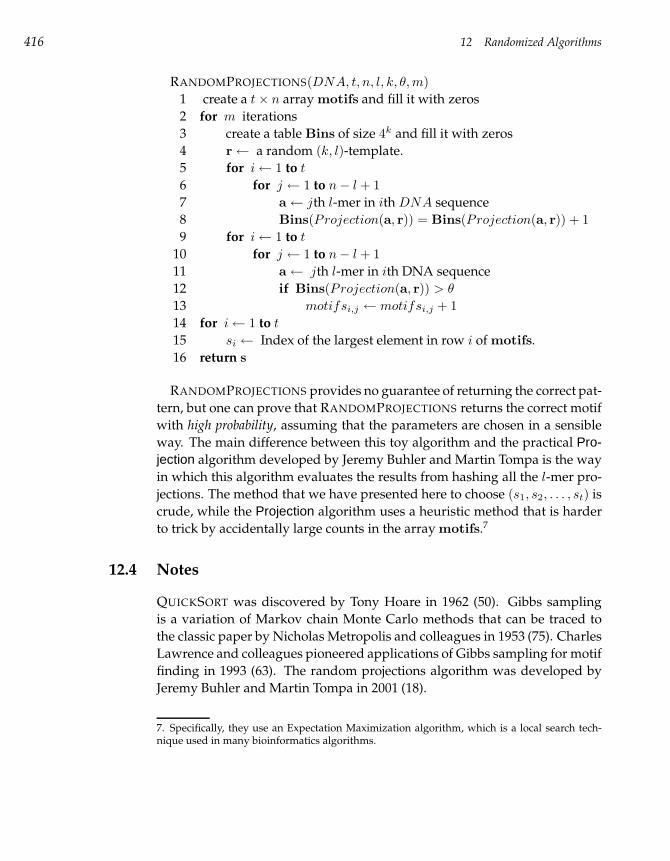
416 12 Randomized Algorithms
RANDOMPROJECTIONS(DNA, t, n, l, k, θ, m)
1 create a t× n array motifs and fill it with zeros
2 for m iterations
3 create a table Bins of size 4k and fill it with zeros
4 r← a random (k, l)-template.
5 for i← 1 to t
6 for j ← 1 to n− l + 1
7 a← jth l-mer in ith DNA sequence
8 Bins(Projection(a, r)) = Bins(Projection(a, r)) + 1
9 for i← 1 to t
10 for j ← 1 to n− l + 1
11 a← jth l-mer in ith DNA sequence
12 if Bins(Projection(a, r)) > θ
13 motifsi,j ← motifsi,j + 1
14 for i← 1 to t
15 si ← Index of the largest element in row i of motifs.
16 return s
RANDOMPROJECTIONS provides no guarantee of returning the correct pat-
tern, but one can prove that RANDOMPROJECTIONS returns the correct motif
with high probability, assuming that the parameters are chosen in a sensible
way. The main difference between this toy algorithm and the practical Pro-jection algorithm developed by Jeremy Buhler and Martin Tompa is the way
in which this algorithm evaluates the results from hashing all the l-mer pro-
jections. The method that we have presented here to choose (s1, s2, . . . , st) is
crude, while the Projection algorithm uses a heuristic method that is harder
to trick by accidentally large counts in the array motifs.7
12.4 Notes
QUICKSORT was discovered by Tony Hoare in 1962 (50). Gibbs sampling
is a variation of Markov chain Monte Carlo methods that can be traced to
the classic paper by Nicholas Metropolis and colleagues in 1953 (75). Charles
Lawrence and colleagues pioneered applications of Gibbs sampling for motif
finding in 1993 (63). The random projections algorithm was developed by
Jeremy Buhler and Martin Tompa in 2001 (18).
7. Specifically, they use an Expectation Maximization algorithm, which is a local search tech-nique used in many bioinformatics algorithms.
12.5 Problems 417
12.5 Problems
Problem 12.1
Show how to partition an array c into arrays csmall and clarge in QUICKSORT withoutrequesting additional memory.
Problem 12.2
Prove that QUICKSORT takes linear time to sort an array if all splits are chosen in such
a way that 13
<|clarge||csmall| < 3.
Problem 12.3
The Viterbi algorithm is a deterministic algorithm for solving the Decoding problem.Design a randomized algorithm for solving the Decoding problem that starts from arandomly chosen assignment of states and tries to improve it using coin tossing.
Problem 12.4
The k-Means clustering algorithm randomly selects an original partition into clustersand deterministically rearranges clusters afterward. Design a randomized version ofthe k-Means algorithm that uses coin tossing to rearrange clusters.
Problem 12.5
Design a randomized algorithm for solving the Large Parsimony problem that usescoin tossing to choose among the nearest neighbor interchanges available at everystep.
Problem 12.6
The Gibbs sampler algorithm “moves slowly” in the space of all starting positionsby changing starting position si in only one DNA sequence at every iteration. Incontrast, GREEDYPROFILEMOTIFSEARCH “moves fast” and may change positions si
in all DNA sequences. Describe a version of the Gibbs sampler that may changemany positions at every iteration. Explain the advantages and disadvantages of youralgorithm as compared to the Gibbs sampler described in the book.

Using Bioinformatics Tools (www.bioalgorithms.info)
No bioinformatics textbook would be complete without some application
of the theory; we hope that you will actually use the algorithmic principles
outlined in this text. To get you started, we have compiled a number of
challenging and useful practical exercises. Each of these exercises involves
using a computer and software to solve a biological question. Unfortunately,
the tools and techniques that bioinformaticians use change so quickly that
we could not hope to present these exercises in a static book form, so we
have made them available through the book’s website at
www.bioalgorithms.infoThe exercises cover a range of bioinformatics problems including motif
finding, sequence comparison, searching biological databases, applications
of HMMs, gene expression analysis, among others.
A large amount of supporting information can be found from the same
website. For example, we have made available many sets of lecture notes
that professors and students alike can use during a bioinformatics course,
a bulletin board to discuss sections of the book, a searchable index, and a
glossary.
419

Bibliography
[1] A. Aho, J. Hopcroft, and J. Ullman. Data Structures and Algorithms. Addison-Wesley,
Boston, 1983.
[2] A.V. Aho and M.J. Corasick. Efficient string matching: an aid to bibliographic search.
Communication of ACM, 18:333–340, 1975.
[3] B. Alberts, D. Bray, J. Lewis, M. Raff, K. Roberts, and J. Watson. Molecular Biology of
the Cell. Garland Publishing, New York, 1994.
[4] S. Altschul, W. Gish, W. Miller, E. Myers, and J. Lipman. Basic local alignment search
tool. Journal of Molecular Biology, 215:403–410, 1990.
[5] S.F. Altschul, T.L. Madden, A.A. Schaffer, J. Zhang, Z. Zhang, W. Miller, and D.J.
Lipman. Gapped BLAST and Psi-BLAST: A new generation of protein database
search programs. Nucleic Acids Research, 25:3389–3402, 1997.
[6] V.L. Arlazarov, E. A. Dinic, M. A. Kronrod, and I. A. Faradzev. On economical con-
struction of the transitive closure of an oriented graph. Soviet Math. Dokl., 11:1209–
1210, 1970.
[7] P. Baldi and S. Brunak. Bioinformatics: The Machine Learning Approach. MIT Press,
Cambridge, MA, 1997.
[8] P. Baldi, Y. Chauvin, T. Hunkapiller, and M. McClure. Hidden Markov models of
biological primary sequence information. Proceedings of the National Academy of
Sciences of the United States of America, 91:1059–1063, 1994.
[9] L. Baum, T. Petrie, G. Soules, and N. Weiss. A maximization technique occurring
in the statistical analysis of probabilistic functions of Markov Chains. Annals of
Mathematical Satistics, 41:164–171, 1970.
[10] A. Baxevanis and B.F. Ouellette. Bioinformatics: A Practical Guide to the Analysis of
Genes and Proteins. Wiley-Interscience, Hoboken, NJ, 1998.
[11] A. Ben-Dor, R. Shamir, and Z. Yakhini. Clustering gene expression patterns. Journal
of Computational Biology, 6:281–297, 1999.
422 Bibliography
[12] S.M. Berget, C. Moore, and P.A. Sharp. Spliced segments at the 5’ terminus of ade-
novirus 2 late mRNA. Proceedings of the National Academy of Sciences of the United
States of America, 74:3171–3175, 1977.
[13] P. Berman, S. Hannenhalli, and M. Karpinski. 1.375-approximation algorithm for
sorting by reversals. In European Symposium on Algorithms, volume 2461 of Lecture
Notes in Computer Science, pages 200–210, Rome, Italy, 2002. Springer-Verlag.
[14] M. Borodovsky and J. McIninch. Recognition of genes in DNA sequences with
ambiguities. BioSystems, 30:161–171, 1993.
[15] P. Bourne and H. Weissig (eds). Structural Bioinformatics. Wiley–Liss, Hoboken, NJ,
2002.
[16] R.S. Boyer and J.S. Moore. A fast string searching algorithm. Communication of ACM,
20:762–772, 1977.
[17] T. Brown. Genomes. John Wiley and Sons, New York, 2002.
[18] J. Buhler and M. Tompa. Finding motifs using random projections. In Proceed-
ings of the Fifth Annual International Conference on Computational Molecular Biology
(RECOMB-01), pages 69–76, Montreal, Canada, April, 2001.
[19] P. Buneman. The Recovery of Trees from Measures of Dissimilarity. Edinburgh Univer-
sity Press, Edinburgh, 1971.
[20] C. Burge and S. Karlin. Prediction of complete gene structures in human genomic
DNA. Journal of Molecular Biology, 268:78–94, 1997.
[21] L.T. Chow, R.E. Gelinas, T.R. Broker, and R.J. Roberts. An amazing sequence ar-
rangement at the 5’ ends of adenovirus 2 messenger RNA. Cell, 12:1–8, 1977.
[22] G. Churchill. Stochastic models for heterogeneous DNA sequences. Bulletin of Math-
ematical Biology, 51:79–94, 1989.
[23] S. A. Cook. The complexity of theorem-proving procedures. In Proceedings of the 3rd
annual ACM Symposium on Theory of Computing, pages 151–158, Shaker Heights,
OH, 1971. ACM Press.
[24] T. H. Cormen, C. L. Leieserson, R. L. Rivest, and C. Stein. Introduction to Algorithms.
MIT Press, Cambridge MA, 2001.
[25] V. Dancik, T. A. Addona, K. R. Clauser, J. E. Vath, and P. A. Pevzner. De novo
peptide sequencing via tandem mass spectrometry. Journal of Computational Biology,
6:327–342, 1999.
[26] K. J. Danna, G. H. Sack Jr., and D. Nathans. Studies of simian virus 40 DNA. VII. A
cleavage map of the SV40 genome. Journal of Molecular Biology, 78:363–376, 1973.
[27] A. Dembo and S. Karlin. Strong limit theorem of empirical functions for large ex-
ceedances of partial sums of i.i.d. variables. Annals of Probability, 19:1737–1755,
1991.
Bibliography 423
[28] R. F. Doolittle, M. W. Hunkapiller, L. E. Hood, S. G. Devare, K. C. Robbins, S. A.
Aaronson, and H. N. Antoniades. Simian sarcoma virus oncogene, ν-sis, is de-
rived from the gene (or genes) encoding a platelet-derived growth factor. Science,
221:275–277, 1983.
[29] R. Drmanac, I. Labat, I. Brukner, and R. Crkvenjakov. Sequencing of megabase plus
DNA by hybridization: Theory of the method. Genomics, 4:114–128, 1989.
[30] A. Duarat, Y. Gerard, and M. Nivat. The chords problem. Theoretical Computer
Science, 282:319–336, 2002.
[31] R. Durbin, S. Eddy, A. Krogh, and G. Mitchinson. Biological Sequence Analysis. Cam-
bridge University Press, Cambridge, England, 1998.
[32] D. Dussoix and W. Arber. Host specificity of infectious DNA from bacteriophage
lambda. Journal of Molecular Biology, 11:238–246, 1965.
[33] M. B. Eisen, P. T. Spellman, P. O. Brown, and D. Botstein. Cluster analysis and
display of genome-wide expression patterns. Proceedings of the National Academy of
Sciences of the United States of America, 95:14863–14868, 1998.
[34] J. K. Eng, A. L. McCormack, and J. R. Yates (III). An approach to correlate tandem
mass spectral data of peptides with amino acid sequences in a protein database. J
Am. Soc. Mass Spectrom., 5:976–989, 1995.
[35] E. Eskin and P. A. Pevzner. Finding composite regulatory patterns in DNA se-
quences. Bioinformatics, 18:S354–363, 2002.
[36] D. Feng and R. F. Doolittle. Progressive sequence alignment as a prerequisite to
correct phylogenetic trees. J. Mol. Evol., 60:351–360, 1987.
[37] W. M. Fitch. Toward defining the course of evolution: Minimum change for a spe-
cific tree topology. Systematic Zoology, 20:406–416, 1971.
[38] S.P.A. Fodor, J.L. Read, M.S. Pirrung, L. Stryer, A.T. Lu, and D. Solas. Light-directed
spatially addressable parallel chemical synthesis. Science, 251:767–773, 1991.
[39] M. R. Garey and D. S. Johnson. Computers and Intractability: A Guide to the Theory of
NP-completeness. W. H. Freeman and Co., 1979.
[40] W. Gates and C. Papadimitriou. Bounds for sorting by prefix reversals. Discrete
Mathematics, 27:45–57, 1979.
[41] M.S. Gelfand, A.A. Mironov, and P.A. Pevzner. Gene recognition via spliced se-
quence alignment. Proceedings of the National Academy of Sciences of the United States
of America, 93:9061–9066, 1996.
[42] O. Gotoh. An improved algorithm for matching biological sequences. Journal of
Molecular Biology, 162:705–708, 1982.
[43] M. Gribskov, M. McLachlan, and D. Eisenberg. Profile analysis: detection of dis-
tantly related proteins. Proceedings of the National Academy of Sciences of the United
States of America, 84:4355–4358, 1987.
424 Bibliography
[44] D. Gusfield. Algorithms on Strings, Trees, and Sequences. Computer Science and Compu-
tational Biology. Cambridge University Press, Cambridge, England, 1997.
[45] D. Haussler, A. Krogh, I. S. Mian, and K. Sjölander. Protein modeling using hidden
Markov models: Analysis of globins. In Proceedings of the Hawaii International Con-
ference on System Sciences, pages 792–802, Los Alamitos, CA, 1993. IEEE Computer
Society Press.
[46] G. Z. Hertz, G. W. Hartzell 3rd, and G. D. Stormo. Identification of consensus pat-
terns in unaligned DNA sequences known to be functionally related. Computer
Applications in Bioscience, 6:81–92, 1990.
[47] G.Z. Hertz and G.D. Stormo. Identifying DNA and protein patterns with statisti-
cally significant alignments of multiple sequences. Bioinformatics, 15:563–577, 1999.
[48] D.G. Higgins, J.D. Thompson, and T.J. Gibson. Using CLUSTAL for multiple se-
quence alignments. Methods in Enzymology, 266:383–402, 1996.
[49] D. Hirschberg. A linear space algorithm for computing maximal common subse-
quences. Communication of ACM, 18:341–343, 1975.
[50] C. A. R. Hoare. Quicksort. Computer Journal, 5:10–15, 1962.
[51] S. Hopper, R. S. Johnson, J. E. Vath, and K. Biemann. Glutaredoxin from rabbit bone
marrow. purification, characterization, and amino acid sequence determined by
tandem mass spectrometry. Journal of Biological Chemistry, 264:20438–20447, 1989.
[52] S. Karlin and S.F. Altschul. Methods for assessing the statistical significance of
molecular sequence features by using general scoring schemes. Proceedings of the
National Academy of Sciences of the United States of America, 87:2264–2268, 1990.
[53] R. M. Karp. Reducibility among combinatorial problems. In Complexity of Computer
Computations, pages 85–103, Yorktown Heights, NY, 1972. Plenum Press.
[54] R.M. Karp and M.O. Rabin. Efficient randomized pattern-matching algorithms.
IBM Journal of Research and Development, 31:249–260, 1987.
[55] J. Kececioglu and E.W. Myers. Combinatorial algorithms for DNA sequence assem-
bly. Algorithmica, 13:7–51, 1995.
[56] J. Kececioglu and D. Sankoff. Exact and approximation algorithms for the inversion
distance between two permutation. Algorithmica, 13:180–210, 1995.
[57] D. E. Knuth. The Art of Computer Programming. Addison-Wesley, 1998.
[58] D.E. Knuth, J.H. Morris, and V.R. Pratt. Fast pattern matching in strings. SIAM
Journal on Computing, 6:323–350, 1977.
[59] A. Krogh, M. Brown, I.S. Mian, K. Sjölander, and D. Haussler. Hidden Markov
models in computational biology: Applications to protein modeling. Journal of
Molecular Biology, 235:1501–1531, 1994.
Bibliography 425
[60] S. Kurtz, J. V. Choudhuri, E. Ohlebusch, C. Schleiermacher, J. Stoye, and
R. Giegerich. Reputer: the manifold applications of repeat analysis on a genomic
scale. Nucleic Acids Research, 29:4633–4642, 2001.
[61] G.M. Landau and U. Vishkin. Efficient string matching in the presence of errors.
In 26th Annual Symposium on Foundations of Computer Science, pages 126–136, Los
Angeles, October 1985.
[62] E. Lander et al. Initial sequencing and analysis of the human genome. Nature,
409:860–921, 2001.
[63] C.E. Lawrence, S.F. Altschul, M.S. Boguski, J.S. Liu, A.F. Neuwald, and J.C. Woot-
ton. Detecting subtle sequence signals: A Gibbs sampling strategy for multiple
alignment. Science, 262:208–214, 1993.
[64] V. I. Levenshtein. Binary codes capable of correcting deletions, insertions, and re-
versals. Cybernetics and Control Theory, 10:707–710, 1966.
[65] L. Levin. Universal sorting problems. Problems of Information Transmission, 9:265–
266, 1973.
[66] B. Lewin. Genes VII. Oxford University Press, Oxford, UK, 1999.
[67] D.J. Lipman and W.R. Pearson. Rapid and sensitive protein similarity searches.
Science, 227:1435–1441, 1985.
[68] S. P. Lloyd. Least squares quantization in PCM. IEEE Transactions on Information
Theory, 28:129–137, 1982.
[69] Y. Lysov, V. Florent’ev, A. Khorlin, K. Khrapko, V. Shik, and A. Mirzabekov. DNA
sequencing by hybridization with oligonucleotides. Doklady Academy Nauk USSR,
303:1508–1511, 1988.
[70] J. MacQueen. On convergence of k-means and partitions with minimum average
variance. Annals of Mathematical Statistics, 36:1084, 1965.
[71] M. Mann and M. Wilm. Error-tolerant identification of peptides in sequence
databases by peptide sequence tags. Analytical Chemistry, 66:4390–4399, 1994.
[72] L. Marsan and M. F. Sagot. Algorithms for extracting structured motifs using a
suffix tree with an application to promoter and regulatory site consensus identifi-
cation. Journal of Computational Biology, 7:345–362, 2000.
[73] W. J. Masek and M. S. Paterson. A faster algorithm computing string edit distances.
Journal of Computational System Science, 20:18–31, 1980.
[74] A. M. Maxam and W. Gilbert. A new method for sequencing DNA. Proceedings of
the National Academy of Sciences of the United States of America, 74:560–564, 1977.
[75] N. Metropolis, A. W. Rosenbluth, M. N. Rosenbluth, A. H. Teller, and E. Teller. Equa-
tion of state calculations by fast computing machines. Journal of Chemical Physics,
21:1087–1092, 1953.
426 Bibliography
[76] D. Mount. Bioinformatics: Sequence and Genome Analysis. Cold Spring Harbor Press,
Cold Spring Harbor, NY, 2001.
[77] E.W. Myers and W. Miller. Optimal alignments in linear space. Computer Applica-
tions in Biosciences, 4:11–17, 1988.
[78] J. Nadeau and B. Taylor. Lengths of chromosome segments conserved since diver-
gence of man and mouse. Proceedings of the National Academy of Sciences of the United
States of America, 81:814–818, 1984.
[79] S.B. Needleman and C.D. Wunsch. A general method applicable to the search for
similarities in the amino acid sequence of two proteins. Journal of Molecular Biology,
48:443–453, 1970.
[80] S. J. O’Brien. Tears of the Cheetah. Thomas Dunne Books, New York, 2003.
[81] S. J. O’Brien, W. G. Nash, D. E. Wildt, M. E. Bush, and R. E. Benveniste. A molecular
solution to the riddle of the giant panda’s phylogeny. Nature, 317:140–144, 1985.
[82] H. Peltola, H. Soderlund, and E. Ukkonen. SEQAID: A DNA sequence assembling
program based on a mathematical model. Nucleic Acids Research, 12:307–321, 1984.
[83] P.A. Pevzner. l-Tuple DNA sequencing: computer analysis. Journal of Biomolecular
Structure and Dynamics, 7:63–73, 1989.
[84] P.A. Pevzner, V. Dancik, and C.L. Tang. Mutation-tolerant protein identification by
mass-spectrometry. Journal of Computational Biology, 7:777–787, 2000.
[85] P.A. Pevzner and G. Tesler. Genome rearrangements in mammalian evolution:
Lessons from human and mouse genomes. Genome Research, 13:37–45, 2003.
[86] P.A. Pevzner and M.S. Waterman. Multiple filtration and approximate pattern
matching. Algorithmica, 13:135–154, 1995.
[87] J.C. Roach, C. Boysen, K. Wang, and L. Hood. Pairwise end sequencing: A unified
approach to genomic mapping and sequencing. Genomics, 26:345–353, 1995.
[88] D. F. Robinson. Comparison of labeled trees with valency three. Journal of Combina-
torial Theory (B), 11:105–119, 1971.
[89] J. R. Sadler, M. S. Waterman, and T. F. Smith. Regulatory pattern identification in
nucleic acid sequences. Nucleic Acids Research, 11:2221–2231, 1983.
[90] N. Saitou and M. Nei. The neighbor-joining method: A new method for reconstruct-
ing phylogenetic trees. Molecular Biological Evolution, 4:406–425, 1987.
[91] F. Sanger, S. Nicklen, and A. R. Coulson. DNA sequencing with chain-terminating
inhibitors. Proceedings of the National Academy of Sciences of the United States of Amer-
ica, 74:5463–5467, 1977.
[92] D. Sankoff. Minimal mutation trees of sequences. SIAM Journal of Applied Mathe-
matics, 28:35–42, 1975.
Bibliography 427
[93] D. Sankoff. Edit distances for genome comparisons based on non-local operations.
In Third Annual Symposium on Combinatorial Pattern Matching, volume 644 of Lecture
Notes in Computer Science, pages 121–135, Tucson, AZ, 1992. Springer-Verlag.
[94] S.S. Skiena, W.D. Smith, and P. Lemke. Reconstructing sets from interpoint dis-
tances. In Proceedings of Sixth Annual Symposium on Computational Geometry, pages
332–339, Berkeley, CA, June, 1990.
[95] H.O. Smith and K.W. Wilcox. A restriction enzyme from Hemophilus influenzae. I.
Purification and general properties. Journal of Molecular Biology, 51:379–391, 1970.
[96] T.F. Smith and M.S. Waterman. Identification of common molecular subsequences.
Journal of Molecular Biology, 147:195–197, 1981.
[97] E.E. Snyder and G.D. Stormo. Identification of protein coding regions in genomic
DNA. Journal of Molecular Biology, 248:1–18, 1995.
[98] R. R. Sokal and C. D. Michener. A statistical method for evaluating systematic rela-
tionships. University of Kansas Science Bulletin, 38:1409–1438, 1958.
[99] E.L. Sonnhammer, S.R. Eddy, and R. Durbin. Pfam: a comprehensive database of
protein domain families based on seed alignments. Proteins, 28:405–420, 1997.
[100] E. Southern. United Kingdom patent application GB8810400. 1988.
[101] G. Stormo, T. Schneider, L. Gold, and A. Ehrenfeucht. Use of the perceptron algo-
rithm to distinguish translational initiation sites in E. coli. Nucleic Acids Research,
10:2997–3011, 1982.
[102] A. H. Sturtevant and T. Dobzhansky. Inversions in the third chromosome of wild
races of Drosophila pseudoobscura, and their use in the study of the history of the
species. Proceedings of the National Academy of Sciences of the United States of America,
22:448–450, 1936.
[103] A. R. Templeton. Out of Africa again and again. Nature, 416:45–51, 2002.
[104] J.C. Venter et al. The sequence of the human genome. Science, 291:1304–1351, 2001.
[105] T.K. Vintsyuk. Speech discrimination by dynamic programming. Kibernetika, 4:52–
57, 1968.
[106] A. Viterbi. Error bounds for convolutional codes and an asymptotically optimal
decoding algorithm. IEEE Transactions on Information Theory, 13:260–269, 1967.
[107] M. S. Waterman. Skiing the Sun. (unpublished manuscript), 2004.
[108] M.S. Waterman. Introduction to Computational Biology. Chapman Hall, New York,
1995.
[109] M.S. Waterman and M. Eggert. A new algorithm for best subsequence alignments
with application to tRNA–rRNA comparisons. Journal of Molecular Biology, 197:723–
728, 1987.
428 Bibliography
[110] J. Weber and G. Myers. Whole genome shotgun sequencing. Genome Research,
7:401–409, 1997.
[111] P. Weiner. Linear pattern matching algorithms. In Proceedings of the 14th IEEE Sym-
posium on Switching and Automata Theory, pages 1–11, University of Iowa, October
1973.
[112] J. R. Yates III, J. K. Eng, A. L. McCormack, and D. Schieltz. Method to correlate
tandem mass spectra of modified peptides to amino acid sequences in the protein
database. Analytical Chemistry, 67:1426–1436, 1995.
[113] K. Zaretskii. Constructing a tree on the basis of a set of distances between the
hanging vertices. Uspekhi Mat. Nauk., 20:90–92, 1965.
[114] Z. Zhang. An exponential example for a partial digest mapping algorithm. Journal
of Computational Biology, 1:235–239, 1994.
Index
acceptor site, 200
additive matrix, 358
additive tree, see additive matrix
adjacency, 132
affine gap penalty, 184
Aho-Corasick algorithm, 328
algorithm, 7, 17
ADDITIVEPHYLOGENY, 362
ALLLEAVES, 103
APPROXIMATEPATTERNMATCHING,
326
approximation, 21, 131
approximation ratio, 131
Baum-Welch, 396
BETTERCHANGE, 21
BRANCHANDBOUNDMEDIANSEARCH,
114
BRANCHANDBOUNDMOTIFSEARCH,
111
BREAKPOINTREVERSALSORT, 133
BRUTEFORCECHANGE, 22
BRUTEFORCEMEDIANSEARCH, 112
BRUTEFORCEMOTIFSEARCH, 109
BRUTEFORCEPDP, 88
BYPASS, 108
CAST, 352
clustering, 338
correctness, 17, 20, 21
DPCHANGE, 151
DUPLICATEREMOVAL, 311
efficiency, 33, 151
EXONCHAINING, 202
FASTROCKS, 47
FIBONACCI, 33
Fitch’s, 370
GREEDYMOTIFSEARCH, 136
GREEDYPROFILEMOTIFSEARCH, 410
HANOITOWERS, 26
HIERARCHICALCLUSTERING, 343
IMPROVEDBREAKPOINTREVERSAL-
SORT, 135
incorrect, 21
BETTERCHANGE, 21
BREAKPOINTREVERSALSORT, 133
LCS, 176
MANHATTANTOURIST, 160
MERGE, 228
MERGESORT, 228
NEIGHBORJOINING, 365
NEXTLEAF, 103
NEXTVERTEX, 107
origins of, 51
PARTIALDIGEST, 90
PATH, 234
PATTERNMATCHING, 315
PCC, 350
PRINTLCS, 176
PROGRESSIVEGREEDYK-MEANS, 346
QUICKSORT, 408
RANDOMIZEDQUICKSORT, 409
RANDOMPROJECTIONS, 414
RECURSIVECHANGE, 150
430 Index
RECURSIVEFIBONACCI, 33
RECURSIVESELECTIONSORT, 30
ROCKS, 47
Sankoff’s, 369–370
SELECTIONSORT, 29
SIMPLEREVERSALSORT, 129
STRINGCOPY, 16
SUFFIXTREEPATTERNMATCHING, 321
UPGMA, 364
USCHANGE, 19
alignment, 168
Alu repeat, 276
amino acid, 65
anticodon, 67
apoptosis, 283
ATP binding proteins, 148
Avery, Oswald, 61
BAC, 277
backtracking pointers, 175
backward algorithm, 395
bacteriophage, 260
balanced partitioning, 244
balanced vertex, 273
Beadle, George, 60
Benzer, Seymour, 260
BLASTmaximal segment pair, 328
statistical significance, 328
block alignment, 234–237
BLOSUM matrix, 178
Bohr, Niels, 5
border length of mask, 304
Braconnot, Henry, 65
branch-and-bound algorithms, 42
breakpoint, 132
cells, 57
eukaryotic, 63
prokaryotic, 63
central dogma, 67
CG-island, 385
Chargaff rule, 62
Chargaff, Erwin, 61
chromosome, 59
cloning, 68
cloning vector, 68
CLUSTAL, 191
codon, 65
Start, 197
Stop, 197
complement, see Watson-Crick com-
plement
computer language, 7
CONSENSUS, 83, 136
consensus (in fragment assembly), 279
consensus string, 93
Crick, Francis, 5, 6, 61
cystic fibrosis, 148
DAG, see graph, DAG
David Haussler, 401
David Sankoff, 139
DDP, see problems, Double Digest Prob-
lem
degree, see vertex, degree
Delbrück, Max, 5
deletion, 169
divide-and-conquer algorithms, 48
DNA, 58
array, 265, 337
helicase, 14
nucleotides, 61
polymerase, 15
read, 275
reads, 263
repeat, 276
replication of, 14–16
discovery, 63
ligase, 15
Okazaki fragments, 15
primers and primase, 15
replication fork, 14
SSB, 14
Index 431
vector, 263
donor site, 200
dot matrix, 323
double helix, 61
Drosophila melanogaster, 59
dynamic programming, 43, 176
edge, 153, 248
edit distance, 167, 207
edit graph, 170
Edman degradation, 280
EDVAC, 240
emission probability, 388
entropy score, 193
Eulerian cycle, 258, 272–275
Eulerian graph, 273
evolution, 74
evolutionary character, 366
exhaustive search, 41
exon, 63, 194
experimental spectrum, 285
exponential algorithm, 35
FASTA, 323
Fibonacci numbers, 31
filtration
database search, 323, 327
of candidate exons, 207
Fischer, Emil Hermann, 65
fitting alignment, 215
floor function, 20
forward algorithm, 394
Four Russians technique, 237
four-point condition, 363
gap, 184
once a gap, always a gap, 191
gap penalty, 184
Gary Stormo, 116
Gates, William, 131
gel electrophoresis, 72, 85
gene, 60
Gene Myers, 331
generating function, 119
genes
immunity, 91
genetic code, 65
genetic linkage, 60
genome rearrangement, 126
reversal, 127, 128
reversal distance, 128–129
GENSCAN, 200
giant panda, 352
Gibbs sampling, 410
GibbsSampler, 83
Gilbert, Walter, 263
global alignment, 177
graph, 153, 248
clique, 346
complete, 252
connected, 252
connected component, 252
DAG (directed acyclic graph), 162
directed, 250
disconnected, 252
edge, see edge
interval, 262
path in a, see path
vertex, see vertex
greedy algorithms, 43
Hamiltonian cycle, 258, 272
Hamming distance, 98, 167
total, 98
hexamer count, 199
Hidden Markov Model, see HMM
hidden state, 388
hierarchical clustering, 342
HMM, 388
parameter estimation, 395
path, 389
profile HMM, 396–398
homeobox genes, 180
homometric sets, 87
Hooke, Robert, 57
432 Index
Human Diversity Project, 73
Hurwitz, Jerard, 64
hybridization, 72, 267
indel, 169
insert (DNA), 263
insertion, 169
insulin, 280
intron, 63, 195
ion type, 285
b-ion, 285
y-ion, 285
junk DNA, 194
k-similarity, 295
l-mer composition, 267
layout, 279
layout of DNA fragments, 279
Leonhard Euler, 299
Levenshtein distance, see edit distance
light-directed array synthesis, 303
likelihood ratio test, 198
LINE repeat, 277
Linear B, 75
local alignment, 181
machine learning, 48
mask for array synthesis, 303
mass spectrometry, 283
description, 283
MS/MS, see mass spectrometry, tan-
dem
tandem, 284
mass spectrum, 283
match, 169
mates, 279
maximization algorithm, 131
Mendel, Gregor, 59
Michael Waterman, 209
Miescher, Johann Friedrich, 61
minimization algorithm, 131
mismatch, 169
Morgan, Thomas, 59
mosaic effect, 207
multiple alignment, 188
multiset, 84
mutation, 184
mutations, 93
NF-κB binding motif, 92
nonadditive matrix, 358
ν-sis oncogene, 147
O-notation, 37
Occam’s razor, 366
open reading frame, 197
optical mapping, 307
ORF, see open reading frame
Out of Africa hypothesis, 353
overlap, 279
PAM matrix, 178
Papadimitriou, Christos, 131
path, 153, 252
cycle, 252
path length, 153
pattern-driven approach, 93
PCR, 67
PCR primer, 68
peptide
C-terminal, 284
N-terminal, 284
performance guarantee, 131
permutation, 127
Poe, Edgar Allan, 92
polynomial algorithm, 35
post-translational modification, 291, 338
glycosylation, 291
phosphorylation, 291
probe, 73
problem, 7
complexity, 151
input, 7
instance, 17
Index 433
output, 7
problems
k-Means Clustering Problem, 344
Approximate Pattern Matching Prob-
lem, 325
Block Alignment Problem, 237
Bridge Obsession Problem, 254
Change Problem, 21
Chimeric Alignment Problem, 219
Corrupted Cliques Problem, 348
Decoding Problem, 391
Distance-Based Phylogeny Problem,
358
Double Digest Problem, 121
Duplicate Removal Problem, 311
Equivalent Words Problem, 211
Eulerian Cycle Problem, 254
Exon Chaining Problem, 201
Fair Bet Casino Problem, 386
Fibonacci Problem, 31
Global Alignment Problem, 177
Hamiltonian Cycle Problem, 258
Inexact Repeat Problem, 218
Knights Tour problem, 250
Large Parsimony Problem, 372
Least Squares Distance-Based Phy-
logeny Problem, 364
Lewis Carroll Problem, 211
Local Alignment Problem, 181
Longest Common Subsequence Prob-
lem, 173
Longest Path in a DAG Problem, 162,
288, 289
Manhattan Tourist Problem, 154
Median String Problem, 99
Modified Protein Identification Prob-
lem, 291
Motif Finding Problem, 98
Multiple Breakpoint Distance Prob-
lem, 145
Multiple Pattern Matching Problem,
316
NP-complete, 49, 348, 372
Pancake Flipping Problem, 130
Partial Digest Problem, 86
Pattern Matching Problem, 315
Peptide Sequencing Problem, 287
Probed Partial Digest Problem, 121
Protein Identification Problem, 290
Query Matching Problem, 326
Reversal Distance Problem, 128
Sequencing by Hybridization (SBH)
Problem, 270
Shortest Path Problem, 258
Shortest Superstring Problem, 264
Small Parsimony Problem, 368
Sorting by Reversals Problem, 129
Sorting Problem, 29
Spectral Alignment Problem, 295
Spliced Alignment Problem, 204
String Duplication Problem, 16
Tandem Repeat Problem, 218
Towers of Hanoi Problem, 24
Traveling Salesman Problem, 50, 258,
264
Turnpike Problem, 86
United States Change Problem, 19
Weighted Small Parsimony Problem,
368
profile, 396
profile HMM alignment, 396
protein, 58
protein complex, 66
protein sequencing, 300
pseudocode, 8
argument, 8
array, 8
operations, 8–11
subroutine, 8, 13
variable, 8, 13
pumpkin pie, 11
quadratic algorithm, 35
randomized algorithms, 48
434 Index
RandomProjections, 83
rearrangement scenario, 127
red panda, 352
restriction enzyme, 71, 83
restriction fragment, 83
restriction fragments, 71
restriction map, 83
ribosome, 66
Richard Karp, 52
RNA, 58
folding, 221
messenger RNA (mRNA), 64
Rocks game, 1
Ron Shamir, 378
Rosetta stone, 77
Russell Doolittle, 79
Sanger, Frederick, 263, 280
SBH, see Sequencing by Hybridization
Schleiden, Matthias, 57
Schrödinger, Erwin, 5
Schwann, Theodor, 57
score of multiple alignment, 188
scoring matrix, 153, 178–180
semibalanced graph, 275
Sequencing by Hybridization, 265
SEQUEST, 290
shared peaks count, 285
shotgun sequencing, 263
simian sarcoma virus, 147
similarity score, 176
Smith, Hamilton, 83
Smith, Temple, 180
SP-score (Sum-of-Pairs), 193
spectral alignment, 293
spectral convolution, 292
spectral product, 296
spectrum graph, 287
spliced alignment graph, 205
splicing, 64, 195
alternative, 66
state transition probability, 388
statistical distance, 335
strip, 133
decreasing, 133
increasing, 133
Sturtevant, Alfred, 60
subsequence, 172
supersequence, 217
superstring, 264
synteny blocks, 126
Tatum, Edward, 60
test data, 385
theoretical spectrum, 285
tiling arrays, 271n
topological ordering, 164
Towers of Hanoi, 24
training data, 385
translation, 67
tree, see DAG
tree traversal
ALLLEAVES, 103
BYPASS, 108
in-order, 370
NEXTLEAF, 103
NEXTVERTEX, 107
post-order, 370
pre-order, 370
pruning, 107
triplet rule, 65
universal DNA array, 267
vertex, 153, 248
degree, 250
indegree, 162, 250
outdegree, 162, 252
predecessor, 163
von Neumann, John, 240
Waardenburg’s syndrome, 125
Waterman, Michael, 180
Watson, James, 5, 6, 61
Watson-Crick complement, 266

Index 435
Webb Miller, 241
weighted interval, 201
Weiss, Samuel, 64
worst case efficiency, 37
Zamecnik, Paul, 63
Related Documents