Noname manuscript No. (will be inserted by the editor) An Interior Point Method for Nonlinear Programming with Infeasibility Detection Capabilities Jorge Nocedal · Figen ¨ Oztoprak · Richard A. Waltz Received: date / Accepted: date Abstract This paper describes interior point methods for nonlinear programming endowed with infeasibility detection capabilities. The methods are composed of two phases, a main phase whose goal is to seek optimality, and a feasibility phase that aims exclusively at improving feasibility. A common characteristic of the algorithms is the use of a step-decomposition interior-point method in which the step is the sum of a normal component and a tangential component. The normal component of the step provides detailed information that allows the algorithm to determine whether it should be in main phase or feasibility phase. We give particular attention to the reliability of the switching mechanism between the two phases. The two algorithms proposed in this paper have been implemented in the knitro package as extensions of the knitro/cg and knitro/direct methods. Numerical results illustrate the performance of our methods on both feasible and infeasible problems. Keywords infeasibility detection · interior point · feasibility restoration Mathematics Subject Classification (2000) 90C30 · 90C51 1 Introduction This paper describes the design and implementation of interior point methods for nonlinear pro- gramming that are efficient when confronted with both feasible and infeasible problems. Our design is based on a step-decomposition approach in which the total step of the algorithm is the sum of a normal and a tangential component. The algorithms employ feasibility-improvement information J. Nocedal, corresponding author. E-mail: [email protected] Department of Electrical Engineering and Computer Science, Northwestern University, Evanston, IL, USA. This author was supported by National Science Foundation grant DMS-0810213 and by Department of Energy grant DE- FG02-87ER25047-A004. F. ¨ Oztoprak Sabanci University and Department of Electrical Engineering and Computer Science, Northwestern University, Evanston, IL, USA. This author was supported, in part, by National Science Foundation grant DMS-0810213. R.A. Waltz Daniel J. Epstein Department of Industrial and Systems Engineering, University of Southern California, Los Angeles, CA, USA. This author was supported by National Science Foundation grant CMMI-0728036.

Welcome message from author
This document is posted to help you gain knowledge. Please leave a comment to let me know what you think about it! Share it to your friends and learn new things together.
Transcript

Noname manuscript No.(will be inserted by the editor)
An Interior Point Method for Nonlinear Programming with Infeasibility
Detection Capabilities
Jorge Nocedal · Figen Oztoprak · Richard A. Waltz
Received: date / Accepted: date
Abstract This paper describes interior point methods for nonlinear programming endowed withinfeasibility detection capabilities. The methods are composed of two phases, a main phase whosegoal is to seek optimality, and a feasibility phase that aims exclusively at improving feasibility. Acommon characteristic of the algorithms is the use of a step-decomposition interior-point methodin which the step is the sum of a normal component and a tangential component. The normalcomponent of the step provides detailed information that allows the algorithm to determine whetherit should be in main phase or feasibility phase. We give particular attention to the reliability of theswitching mechanism between the two phases. The two algorithms proposed in this paper have beenimplemented in the knitro package as extensions of the knitro/cg and knitro/direct methods.Numerical results illustrate the performance of our methods on both feasible and infeasible problems.
Keywords infeasibility detection · interior point · feasibility restoration
Mathematics Subject Classification (2000) 90C30 · 90C51
1 Introduction
This paper describes the design and implementation of interior point methods for nonlinear pro-gramming that are efficient when confronted with both feasible and infeasible problems. Our designis based on a step-decomposition approach in which the total step of the algorithm is the sum ofa normal and a tangential component. The algorithms employ feasibility-improvement information
J. Nocedal, corresponding author.E-mail: [email protected] of Electrical Engineering and Computer Science, Northwestern University, Evanston, IL, USA. Thisauthor was supported by National Science Foundation grant DMS-0810213 and by Department of Energy grant DE-FG02-87ER25047-A004.
F. OztoprakSabanci University and Department of Electrical Engineering and Computer Science, Northwestern University,Evanston, IL, USA. This author was supported, in part, by National Science Foundation grant DMS-0810213.
R.A. WaltzDaniel J. Epstein Department of Industrial and Systems Engineering, University of Southern California, Los Angeles,CA, USA. This author was supported by National Science Foundation grant CMMI-0728036.
2 Jorge Nocedal et al.
provided by the normal component of the step to determine whether the algorithm should be ina feasibility or an optimality phase. Feasibility-improvement information of this type is not read-ily available in line search primal-dual methods [28,20,31,11,30,29,27], and this provides the mainmotivation for our choice of the step-decomposition approach.
Infeasible problems arise often in practice. They are sometimes generated by varying modelparameters to observe system response. They also arise when nonlinear optimization is a subproblemof another algorithm, such as branch-and-bound or branch-and-cut methods. In that context, theefficiency and reliability of the nonlinear optimization algorithm on feasible or infeasible problemsbecomes very important since the optimization solver is typically run thousands of times in thecourse of the solution of a master problem, with many infeasible subproblems generated.
Various infeasibility detection mechanisms have been proposed in the nonlinear programming lit-erature, with varying degrees of success. Let us begin by considering snopt [16] and filter [15], twoof the most popular active-set methods. snopt uses a switch that transforms the standard sequentialquadratic programming (SQP) algorithm into an SL1QP penalty method [14] when the problem isdeemed to be infeasible, badly scaled or degenerate. filter uses a more robust diagnostic — theinfeasibility of a trust region problem — to invoke a feasibility restoration phase whose objectiveis to minimize constraint violations. Both of these methods include a main mode and a feasibilitymode, together with a switching mechanism. SQP approaches based on a single optimization phaseare described by Gould and Robinson [19,18] and Byrd, Curtis and Nocedal [2], who propose anexact penalty SQP method that automatically varies its emphasis from optimality to feasibility, andvice versa, using so-called steering rules [6]. Another penalty-SQP method with a single optimizationphase is described by Yamashita and Yabe [32].
Sequential linear-quadratic programming (SLQP) methods have emerged as an attractive alter-native to SQP methods for solving problems with a large number of degrees of freedom. The methoddescribed by Chin and Fletcher [8] employs a filter and a feasibility restoration phase to deal withinfeasibility, whereas the SLQP method proposed by Byrd et al. [4], which is implemented in theknitro/active code, follows a penalty approach.
Interior point methods with infeasibility detection mechanisms have also been proposed in theliterature. loqo [28] employs a penalty approach, whereas ipopt [29] uses a filter and a feasibil-ity restoration phase. Curtis [2] proposes an interior-penalty method based on a single optimizationphase that balances the effects of the barrier and penalty functions through an extension of the steer-ing rules mentioned above. Methods based on augmented Lagrangian approaches, such as lancelot[10] and minos [25], are endowed with infeasibility detection mechanisms through the presence of aquadratic penalty term.
The interior point algorithms described in this paper contain an optimality mode and a feasibilitymode, but are distinct from other methods proposed in the literature. We have implemented them inthe knitro package [7], and report their performance on a large collection of feasible and infeasibleproblems.
The paper is divided into 7 sections. In Section 2, we present numerical results for several popularnonlinear programming solvers on a set of infeasible problems. Section 3 describes a mechanism fordetermining whether the algorithm should be in an optimality or feasibility phase. The proposedalgorithm is stated and discussed in Section 4, and numerical results on both feasible and infeasibleproblems are presented in Section 5. Our infeasibility detection approach is extended in Section 6to a primal-dual line search interior point method, and concluding remarks are given in Section 7.
Notation. Throughout the paper, ‖ · ‖ denotes the Euclidean norm unless stated otherwise. We let1 denote the vector of all ones, and employ superscripts, as in v(i), to indicate the components ofvector v.

An Interior Point Method for Nonlinear Programming with Infeasibility Detection Capabilities 3
2 Some Tests On Infeasible Problems
To serve as motivation for this paper, and to provide a snapshot of the state-of-the art in infeasibilitydetection in nonlinear programming, we present results of several popular solvers on a set of smalldimensional infeasible problems. Table 1 lists the problems and their characteristics; there n denotesthe number of variables and m the number of constraints. Test Set 1 is taken from [2], and Test Set2 was designed specifically for this study, and is described in [12].
Table 1 List of test problems
Test Set 1 Test Set 2
Problem n m Problem n m Problem n mISOLATED 2 4 BALLS 67 285 SOSQP1 MOD 200 201NACTIVE 2 3 COVERAGE 10 45 EIGMAXC TYPE2 22 23UNIQUE 2 2 PORTFOLIO 30 31 EIGMAXC TYPE3 22 23BATCH MOD 39 49 DEGEN 2 4 SENSITIVE 2 4ROBOT MOD 7 3 MCCORMCK MOD 251 3 LOCATE 20 110
POWELLBS MOD 4 8 PEIGEN 28 28
We tested the following solvers, which we group according to the type of algorithm they imple-ment:
a) snopt, filter, and knitro/active implement active set methods;b) loqo, knitro/direct, knitro/cg and ipopt implement interior point methods;c) lancelot , minos, and pennon [23] implement augmented Lagrangian methods.
The results are reported in Tables 2 and 3; they were obtained with the NEOS server using theAMPL interface. We do not provide detailed results for loqo or pennon because these two solverswere unable to detect infeasibility for any of the problems tested. For each solver, we report in Ta-bles 2 and 3 whether the code was able to detect that the problem was infeasible (Yes/No), as well asthe number of iterations needed to meet its default stop test. IP stands for interior point method; ALfor augmented Lagrangian method; and SLC for sequential linearly constrained Lagrangian method.For snopt, the number of iterations was determined by the number of Jacobian evaluations; forfilter, the number in parenthesis gives the total number of iterations in the feasibility restorationphase.
Table 2 Results for Test Set 1 (Infeasibility detection and number of iterations)
Solver Version Algorithm unique robot mod isolated batch mod nactive
SNOPT 7.2-10 SQP Y 138 Y 134 Y 83 Y 18 Y 130
FILTER 20020316 SQP Y 16(7) Y 23(22) Y 27(16) Y 6(2) Y 15(4)
KNITRO/ACT. 7.0 SLQP Y 18 Y 22 Y 18 Y 8 Y 12
KNITRO/CG 7.0 IP N 10000 Y 80 N 10000 Y 1315 Y 343
KNITRO/DIR. 7.0 IP Y 44 Y 148 Y 47 N 10000 Y 18
IPOPT 3.8.3 IP N 772 Y 44 Y 65 Y 97 Y 30
LANCELOT N.A. AL Y 23 Y 53 Y 16 N 1000 Y 21
MINOS 5.51 SLC N 0 Y 202 N 1 Y 200 Y 110
We observe from Tables 2 and 3 that, in these tests, the active set solvers filter and kni-tro/active are the most efficient and show the most consistent performance. filter performs

4 Jorge Nocedal et al.
Table 3 Results Test Set 2 (Infeasibility detection and number of iterations)
Solver locate balls coverage portfolio degen mccormck mod
SNOPT Y 34 Y 46 Y 175 Y 42 Y 17 N 118
FILTER Y 30(28) Y 63(62) Y 2(1) Y 11(10) Y 7(6) Y 13(9)
KNITRO/ACT. Y 20 Y 15 Y 1 Y 15 Y 26 Y 18
KNITRO/CG N 10000 Y 1661 N 10000 Y 447 N 10000 N 10000
KNITRO/DIR. N 10000 N 10000 Y 38 N 211 Y 15 Y 23
IPOPT Y 105 Y 816 Y 19 Y 47 Y 43 Y 63
LANCELOT N ?1 Y 808 Y 33 Y 651 Y 33 Y 24
MINOS Y 2104 Y 1458 N 46 N 30 Y 43 Y 462
Solver peigen powellbs mod sosqp1 mod2 eigmaxc type2 eigmaxc type3 sensitive
SNOPT Y 20 Y 95 N ?3 Y 12 Y 25 Y 11
FILTER Y 16(15) Y 2(1) Y 0(0) Y 8(7) Y 7(6) Y 12(7)
KNITRO/ACT. Y 18 Y 26 Y 3 Y 7 Y 16 Y 21
KNITRO/CG N 2590 N 10000 Y 5478 Y 258 Y 200 N 10000
KNITRO/DIR. N 648 N 43 Y 13 N 22 Y 575 Y 10
IPOPT Y 35 Y 81 Y 19 Y 18 Y 32 Y 22
LANCELOT N 1000 N 1000 Y 118 Y 35 Y 20 Y 41
MINOS Y 482 N 73 Y 100 Y 417 Y 464 Y 31
1 Execution failure without displaying an error message2 For this problem, AMPL option presolve was set to zero3 Exit with INFO=53 from snOptB, no Jacobian evaluations reported
well thanks to a carefully designed feasibility restoration phase. The strong performance of kni-tro/active was somewhat unexpected since the design of that algorithm was not guided by infea-sibility considerations [4]. However, an analysis of the equality constrained phase in knitro/activeshows that it is able to adapt itself so that the iteration gives sufficient emphasis to feasibility im-provement, when needed.
The performance of the interior point methods knitro/direct and knitro/cg are quite poor,which may not be surprising since these two algorithms do not contain any features for handlinginfeasibility. ipopt contains a feasibility restoration phase, but its performance is not consistentlysuccessful. The main motivation for this paper stems from the desire to build effective feasibilitydetection capabilities for interior point methods.
3 Infeasibility Certificates
The goal of this section is to describe a mechanism for determining whether the optimization al-gorithm should be in main (or optimality) mode or in feasibility mode. Our strategy is to rely oninformation provided by the normal component in a step decomposition method.
The nonlinear programming problem under consideration is stated as
minx
f(x)
s.t g(x) ≤ 0
h(x) = 0,
(3.1)
where f : Rn → R, g : Rn → Rm, and h : Rn → R
t are smooth functions. We define
w(x) =
[
g(x)+
h(x)
]
, with g(x)+ = max{g(x), 0}, (3.2)
so that ‖w‖ can serve as an infeasibility measure.

An Interior Point Method for Nonlinear Programming with Infeasibility Detection Capabilities 5
At an infeasible stationary point x of problem (3.1) we have that
‖w(x)‖ > 0 and θ(x) =
(
‖w(x)‖ − min‖d‖≤∆
∣
∣
∣
∣
∣
∣
∣
∣
[
[g(x) +Ag(x)d]+
h(x) +Ah(x)d
]∣
∣
∣
∣
∣
∣
∣
∣
)
= 0, (3.3)
for any ∆ > 0, where Ag(x) and Ah(x) denote the Jacobian matrices of g(x) and h(x), respectively.Therefore, we may suspect that the iterates of a nonlinear optimization algorithm approach aninfeasible stationary point if the sequence ‖w(xk)‖ remains bounded away from zero, while θ(xk)approaches zero. These two conditions can be encapsulated in an inequality of the form
θ(xk) ≤ δ‖w(xk)‖, for δ > 0.
We base our switching mechanisms between main and feasibility modes on a condition of this form,translated to the interior point framework that includes slacks.
As we discuss in the next section, a step-decomposition method provides an estimate of θ(x)at every iteration. This is not the case, however, in standard line search primal-dual interior pointmethods, since they do not solve a trust region problem of the type given in (3.3). Instead, thesealgorithms compute a search direction d that satisfies the constraint linearizations, but since the stepalong d may be significantly shortened due to the fraction to the boundary rule or the line search, itis difficult to measure the reduction in the constraints that can be achieved, to first order. In otherwords, it is difficult to employ a certificate of infeasibility such as (3.3) in a line search primal-dualmethod.
4 A Trust Region Interior Point Algorithm
In this section, we describe the interior point algorithm with infeasibility detection capabilities. Asalready mentioned, the algorithm contains a main mode whose goal is to satisfy the optimalityconditions of the nonlinear program (3.1), and a feasibility mode that aims exclusively at improvingfeasibility. In order to make use of the infeasibility certificates described in the previous section, weemploy a step-decomposition trust region interior point method of the type proposed in [5,3,1,22,9,21]. Specifically, we follow the algorithm described in [5,3], which is implemented in the knitro/cgoption of the knitro package [7]. We now give a brief overview of this method.
Introducing slacks, the nonlinear program (3.1) is transformed into
minx,s
f(x)
s.t g(x) + s = 0
h(x) = 0
s ≥ 0.
(4.1)
A solution to this problem is obtained by solving a series of barrier problems of the form
minx,s
ϕ(x, s)def= f(x)− µ
m∑
i=1
ln s(i)
s.t g(x) + s = 0,
h(x) = 0,
(4.2)
with µ→ 0.

6 Jorge Nocedal et al.
The step-decomposition approach is as follows. Given an iterate (xk, sk) and a trust region radius∆k, the algorithm first computes a normal step1 v = (vx, vs) by solving the subproblem
minv‖g(xk) + sk +Ag(xk)vx + vs‖2 + ‖h(xk) +Ah(xk)vx‖2
s.t. ‖(vx, S−1k vs)‖ ≤ ξ∆k
vs ≥ −ξκs,(4.3)
where Sk = diag{sik} is a scaling matrix for the slacks, the scalar ξ ∈ (0, 1) is a trust regioncontraction parameter and κ ∈ (0, 1) determines the fraction to the boundary rule; see [5]. (Typicalvalues for these parameters are ξ = 0.8, κ = 0.005.) The total step d = (dx, ds) of the algorithm isobtained by solving the subproblem
mind∇ϕ(xk, sk)
T d+ 12d
TWkd
s.t. Ag(xk)dx + ds = Ag(xk)vx + vs
Ah(xk)dx = Ah(xk)vx
‖(dx, S−1ds)‖ ≤ ∆k
ds ≥ −κs,
(4.4)
where Wk is a Hessian approximation; see [5]. The subproblems (4.3), (4.4) can be solved inexactlyas stipulated in [3]. The new iterate is given by
(xk+1, sk+1) = (xk, sk) + d, (4.5)
provided it yields sufficient reduction in the merit function φ; otherwise the step d is rejected, thetrust region radius ∆k is decreased and a new step is computed. We define the merit function as
φ(x, s; ν) = ϕ(x, s) + ν‖c(x, s)‖, (4.6)
where ν > 0 is a penalty parameter, and
c(x, s)def=
[
g(x) + sh(x)
]
. (4.7)
After the new iterate (4.5) is computed, the algorithm applies the slack reset
sk+1 ← max{sk+1,−g(xk)+},
which ensures that, at every iteration,
g(xk+1) + sk+1 ≥ 0. (4.8)
The Lagrange multipliers λk+1 = (λg, λh) are defined through a least squares approach. We refer to[5] for other details of the algorithm, such as the procedure for updating the penalty parameter ν in(4.6) and the trust region radius ∆k.
The main mode of the proposed algorithm employs the step-decomposition interior point methodjust outlined; the feasibility mode, which we describe next, can employ any interior point algorithm.
1 To save space, we write
v =
(
vxvs
)
= (vx, vs),
and similarly for other vectors containing x and s-components.

An Interior Point Method for Nonlinear Programming with Infeasibility Detection Capabilities 7
4.1 The Feasibility Phase
In the feasibility phase, the algorithm disregards the objective function f and aims exclusively atimproving feasibility. This goal is achieved by applying an interior point algorithm to the problem
minx‖w(x)‖1, (4.9)
where w(x) is the vector of constraint violations defined in (3.2). We reformulate (4.9) as a smoothproblem by introducing relaxation variables rg ∈ R
m, r+h , r−h ∈ R
t, as follows:
minx,r
rT1
s.t. g(x)− rg ≤ 0
h(x)− r+h + r−h = 0
r ≥ 0,
with r =
rgr+hr−h
. (4.10)
The corresponding barrier problem is given by
minx,r,s
ϕ(x, r, s)def= rT1− µ
2m+2t∑
i=1
ln s(i)
s.t. g(x)− rg + sg = 0
h(x)− r+h + r−h = 0
− r + sr = 0
with s =
[
sgsr
]
, (4.11)
where sg ∈ Rm and sr ∈ R
m+2t are the feasibility mode slacks, and µ ∈ R+ is the feasibility modebarrier parameter.
The Lagrangian for this problem is
L(x, r, s, λ) = rT1− µ
2m+2t∑
i=1
ln s(i) + λTg (g(x)− rg + sg) + λT
h
(
h(x)− r+h + r−h)
+ λTr (−r + sr) ,
with feasibility mode Lagrange multipliers λg ∈ Rm, λh ∈ R
t, and λr ∈ Rm+2t.
The first order optimality conditions for the barrier problem(4.11) are given by
F µ(x, r, s, λ) =
Ag(x)T λg +Ah(x)
T λh
1− λ− λr
Sgλg − µ1Srλr − µ1
g(x)− rg + sgh(x)− r+h + r−h−r + sr
= 0, (4.12)
where
Sg = diag(s(1)g , · · · , s(m)g ),
Sr = diag(s(1)r , · · · , s(m+2t)r ),
and λ =
λg
λh
−λh
.

8 Jorge Nocedal et al.
As mentioned previously, any interior point algorithm can be applied in the feasibility phase. Inour implementation, we employ the same step-decomposition method as in main mode. In order todescribe this method, it is convenient to introduce the following notation:
f(x, r) = rT1
g(x, r) =
[
g(x)− rg−r
]
, h(x, r) = h(x) + r+h − r−h .(4.13)
This allows us to write the barrier problem (4.11) in the same form as (4.2),
minx,r,s
f(x, r)− µ2m+2t∑
i=1
ln s(i)
s.t g(x, r) + s = 0
h(x, r) = 0,
(4.14)
and the application of the step-decomposition approach to (4.14) follows the discussion in the firstpart of this section.
4.2 Switching Conditions
We now describe in detail the conditions for determining when the algorithm is to be in main modeor feasibility mode. These conditions are motivated by the discussion in Section 3 and depend ontwo constants, δ > δ > 0, that are pre-selected. We recall that the constraint function c(x, s) isdefined in (4.7).
Principal Switching Conditions
[Main → Feasible ] Suppose that at a point (x, s) the algorithm is in main mode and has computeda step d = (dx, ds), and suppose that s ≥ −g(x) (see (4.8)).
If ||g(x) + s+Ag(x)dx + ds||+ ‖h(x) +Ah(x)dx‖ ≥ δ‖c(x, s)‖, (4.15)
then start feasibility mode.
[Feasible → Main ] Suppose that the algorithm is in feasibility mode and that it has computed astep d = (dx, dr, ds).
If ||g(x) + s+Ag(x)dx + ds||+ ‖h(x) +Ah(x)dx‖ ≤ δ‖c(x, s)‖, (4.16)
then return to main mode.
In our implementation, we choose δ = 0.9 and δ = 0.1. To make the algorithm less dependenton the choice of these two constants, our implementation includes additional conditions that aredesigned to avoid unnecessary cycling between the two phases; we describe these conditions inSection 4.5.
An Interior Point Method for Nonlinear Programming with Infeasibility Detection Capabilities 9
4.3 The Complete Algorithm
We describe the trust region interior point method through the pseudo-code given in the next pages.Algorithm 1 is the driver that controls the outer iterations, while Algorithms 2 and 3 describe inneriterations performed in the main phase (mode M) and the feasibility phase (mode F ), respectively.
The algorithm starts in mode M , assuming that the nonlinear program has a feasible solution. Insubsequent outer iterations, the algorithm updates the barrier parameter and proceeds to solve thenext barrier problem of the current mode – M or F (see Algorithm 1). The iterations of Algorithms 2and 3, solve the barrier problems (4.2) and (4.11), respectively, and generate the inner iterates,denoted by xk. We use counter l for the outer iterations of the algorithm, and denote the subsequenceof major iterates with {xkl
} ⊆ {xk}. The mode changes occur in Algorithms 2 and 3.As stated in Algorithm 1, the overall algorithm terminates in three cases:
1. Convergence to a stationary point of the nonlinear program (3.1). This is measured by the KKTerror for (3.1), which can be stated as
FM (xk, λk) =
∇fk + (λg)TkAg(xk) + (λh)
TkAh(xk)
g(xk)T (λg)k
g(xk)+
h(xk)
where (λg)k ≥ 0 ∈ Rm and (λh)k ∈ R
t are the Lagrange multipliers at iteration k.2. Convergence to a stationary point of the feasibility problem (4.10). This decision is based on the
KKT error for (4.10), which is given by
FF (xk, λk, rk) =
(λg)TkAg(xk) + (λh)
TkAh(xk)
(g(xk)− (rg)k)T(λg)k
(g(xk)− (rg)k)+
h(xk)− (r−h )k + (r+h )krTk (λr)k(−rk)+
1− λk − (λr)k
Here, λk, rk ≥ 0 are the Lagrange multipliers and the relaxation variables of (4.10) at iterationk, respectively. λ and λr are as defined in Section 4.1. When ‖w(x)‖ > 0 at a stationary pointof (4.10), we accept this as a certificate of local infeasibility and terminate.
3. The overall algorithm may converge to a point where the constraints of (3.1) do not satisfy thelinear independence constraint qualification (LICQ); see Theorem 3 in [3]. This is the third casewhen the algorithm terminates.
The termination criteria in Algorithms 2 and 3 correspond to the stationarity conditions of (4.2)and (4.11), respectively. In Algorithm 2, vpred(v) denotes the model prediction for the decrease in‖c(x, s)‖ provided by the normal step v. Similarly, pred(d) stands for the model prediction for thedecrease in the merit function (4.6) provided by the total step d. In Algorithm 3, they denote thecorresponding quantities for the feasibility phase problem (4.14).

10 Jorge Nocedal et al.
Algorithm 1: Solve NLP
Input: (x0, s0), µ1 > 0, γ ∈ (0, 1), {ǫl}l≥1 → 0, τ ≈ 01
l = 1, k0 = 0, (xk0, sk0
) = (x0, s0);2
mode = M ;3
while resource limits are not exceeded do4
if ‖FM (xkl, λkl
)‖ < τ then5
Convergence to a KKT point of the nonlinear program (3.1);6
Exit;7
else if ‖FF (xkl, λkl
, rkl)‖ < τ and ‖w(xk)‖ > τ then8
Convergence to an infeasible stationary point;9
Exit;10
else11
/*not a stationary point, solve the next barrier subproblem*/12
if mode = M then13
(xkl, skl
,mode) = Solve Main((xkl−1, skl−1
), µl, ǫl) (see Algorithm 2);14
else if mode = F then15
(xkl, skl
,mode) = Solve Feas((xkl−1, skl−1
), µl, ǫl) (see Algorithm 3);16
/*upon return, mode has been set to M or F*/17
if mode = M then18
if ||(∇fkl+ (λg)Tkl
Ag(xkl) + (λh)
TklAh(xkl
) , Skl(λg)kl
− µl1)|| ≥ ǫl then19
Convergence to a point failing to satisfy LICQ;20
Exit;21
Set µl+1 ∈ (0, γµl);22
else if mode = F then23
Set µl+1 ∈ (0, γµl);24
l = l + 1;25
4.4 Initialization of the Two Phases
In order to keep the description of Algorithms 2 and 3 brief, we did not state how various parametersand variables are initialized as the algorithm switches from one mode to the other. It is well knownthat interior point methods are very sensitive to the initialization of some of these parameters andthat it is difficult to find settings that work well on all problems. The following initialization ruleshave performed well in our experiments.
Feasibility Phase. Every time the feasibility phase is invoked, we perform the following initialization.
(a) The barrier parameter µ is set to the most recent main mode value, i.e., µ← µ.(b) The initial trust region radius is initialized to ∆ ← ∆
√n+m+ 2t/
√n, where ∆ is the trust
region from the main mode, m is the number of inequality constraints, t is the number of equalityconstraints, and the scaling
√n+m+ 2t/
√n accounts for the fact that there are more variables
in feasibility mode than in main mode and that we employ the ℓ2 norm in the trust regionconstraint.
(c) The penalty parameter is initialized as ν ← ν.(d) The slacks s and relaxation variables r are initialized to make the barrier constraints for the
feasibility mode initially feasible, while also decreasing the barrier objective as much as possiblefor the current xk. This involves an appropriate initialization of the auxiliary variables r and areset of the slacks s.

An Interior Point Method for Nonlinear Programming with Infeasibility Detection Capabilities 11
Algorithm 2: Solve Barrier Main
Input: (x0, s0), µ > 0, ǫ > 0, λ0, ∆0 > 0, η, ρ, β ∈ (0, 1), ν−1 > 0, δ > 01
while resource limits are not exceeded do2
if ||Fµ(xk, sk, λk)|| < ǫ then3
Return;4
Compute normal step, v = (vx, vs) by solving problem (4.3);5
/* If linearized constraint reduction is insufficient, switch to restoration mode*/6
if condition (4.15) holds then7
mode = F ;8
Set restoration mode slacks s, multipliers λ, and parameters µ, ∆ ;9
Solve Barrier Feas((xk, s), µ, ǫ) ;10
Compute total step, d = (dx, ds) by solving problem (4.4);11
Update penalty parameter, νk ≥ νk−1 so that predk(d) ≥ ρνkvpredk(v) ;12
if φ(xk, sk; νk)− φ(xk + dx, sk + ds; νk) < ηpredk(d) then13
∆k = β∆k;14
else15
xk+1 = xk + dx;16
sk+1 = max(sk + ds,−gk+1);17
Compute λk+1;18
Set ∆k+1 ≥ ∆k;19
k = k + 1;20
Algorithm 3: Solve Barrier Feas
Input: (x0, s0), µ > 0, ǫ > 0, λ0, ∆0 > 0, η, ρ, β ∈ (0, 1), ν−1 > 01
while resource limits are not exceeded do2
if ||F µ(xk, rk, sk, λk)|| < ǫ then3
Return;4
Compute total step, d = (dx, dr, ds) by using an interior point procedure ;5
if condition (4.16) holds then6
mode = M ;7
Adjust ν−1 if necessary, reset ∆;8
Reset main mode slacks s, and multipliers λ;9
Solve Barrier Main((xk, s), µ, ǫ);10
Update penalty parameter, νk ≥ νk−1 : predk(d) ≥ ρνkvpredk(v);11
if φ(xk, rk, sk)− φ(xk + dx, rk + dr, sk + ds) < ηpredk(d) then12
∆k = β∆k;13
else14
xk+1 = xk + dx, rk+1 = rk + dr;15
sk+1 = max(sk + ds,−gk+1);16
Compute λk+1;17
Set ∆k+1 ≥ ∆k;18
k = k + 1;19

12 Jorge Nocedal et al.
(e) λ = (λg, λh, λr), is computed as a least squares multiplier estimate; see [5, page 7].
Main Phase. When the algorithm returns from feasibility mode, the following initializations areperformed:
(a) The barrier parameter µ is set to its previous value in main mode, when the feasible mode waslast invoked.
(b) ∆← ∆, ν ← ν, s← s, i.e., these parameters inherit their values from the feasible mode.(c) λ = (λg, λh) is initialized via least squares approximation.
4.5 Additional Switching Conditions
The switching conditions described in section 4.2 have a solid theoretical underpinning, as they arebased on the stationarity conditions (3.3). Nevertheless, they can be sensitive to the choice of theconstants δ, δ in (4.15), (4.16). In order to make our switching conditions effective over a wide rangeof feasible and infeasible problems, we have found it useful to enhance them with the following rules.
[Main → Feasible ] The algorithm reverts to feasibility mode only if all the following conditions aresatisfied, in addition to (4.15):
1. At the current iterate (xk, sk) we have ‖wk‖ ≥ ζ‖wk−1‖ with ζ ∈ (0, 1) (we use ζ = 0.99).This condition ensures that we do not switch as long as we are making some minimal progressin reducing the overall infeasibility.
2. At least 3 iterations have been performed in main mode.3. The Principal Switching Conditions (4.15), (4.16), plus the conditions above, hold for two con-
secutive iterations. This safeguards against unnecessary switching as a result of one single un-productive iteration.
[Feasible → Main ]
1. Suppose that the feasibility phase was triggered at iteration j; then, we allow termination of thefeasibility phase at iteration k only if condition (4.16) and
‖w(xk)‖ ≤ (1− σ)‖w(xj)‖, with σ ∈ (0, 1)
are satisfied. This condition enforces that once we switch to feasibility phase, we do not returnto the optimization phase until we have achieved some predetermined decrease in the overallinfeasibility measure.
We have found that these additional switching rules prevent the algorithm from switching modestoo rapidly, and also make it unnecessary to try to adjust the values of the constants δ, δ (see (4.15),(4.16)) during the progression of the algorithm.
5 Numerical Experiments
Algorithm 1 has been implemented in the knitro/cg code, and has been tested on feasible andinfeasible problems.
In Table 4, we report the results for the infeasible problems listed in Table 1. The column underthe header knitro/cg gives the results with the earlier version of the code, specifically version 8.0 of

An Interior Point Method for Nonlinear Programming with Infeasibility Detection Capabilities 13
the knitro package with the options alg=2, presolve=0, maxiter=3000, maxtime real=500, andbar switchrule=1. knitro/cg/new denotes the new version endowed with infeasibility detectioncapabilities (i.e., Algorithm 1), using the same option settings, except for bar switchrule=2. Thecolumns ‘inf’, ‘F’, ‘itr’, ‘# switch’, and ‘sw.itr’ report whether the algorithm was successfulat detecting infeasibility (yes/no), the final value of the objective function, the total number ofiterations, the number of times the feasibility mode was started, and the iteration(s) at which thefeasibility mode was started, respectively. It is clear that the new algorithm has much improvedfeasibility detection capabilities.
Table 4 Results on Infeasible Problems
KNITRO/CG KNITRO/CG/NEW
problem n m inf F itr inf F itr # switch sw.itr
balls 67 285 Y 6.01 1331 Y 75.81 72 1 23
eigmaxc type2 22 23 Y -1.00 481 Y -1.00 25 1 13
isolated 2 4 N 0.00 3000 Y 0.00 14 1 10
nactive 2 3 Y -0.20 317 Y 0.00 16 1 12
powellbs modified 4 8 N 0.03 3000 Y 0.67 41 2 15,29
sosqp1 modified 200 201 N 1.94 3000 Y 0.00 21 1 13
batch 39 49 Y 255,187.40 122 Y 388,222.89 44 1 21
coverage 10 45 N 16.12 3000 Y 16.11 112 1 69
eigmaxc type3 22 23 Y -1.52 371 Y -1.26 19 1 9
mccormck modified 251 3 Y -118.34 103 Y 433.88 18 1 10
portfolio 30 31 Y 0.00 1009 Y 0.00 71 1 6
robot mod 7 3 Y 4.76 37 Y 5.77 16 1 5
unique 2 2 N 0.77 3000 Y 1.00 12 1 7
sensitive 2 4 N -391.57 3000 Y -367.79 16 1 7
locate 20 110 N 0.00 3000 Y 0.00 62 1 25
peigen 28 28 N 0.01 255 Y 0.03 22 1 11
degen 2 4 N 6.81 3000 Y 1.00 31 1 11
Next, we consider the performance of the new algorithm on feasible problems. We tested all theconstrained problems in the CUTEr set [17] using knitro/cg and knitro/cg/new, with the sameoption settings as above. The test set includes a total of 430 problems, and the results are given inAppendix A. Termination diagnostics are reported in Table 5, in order to observe if the infeasibilitydetection mechanism has a detrimental effect when the algorithm is applied to feasible problems,and in particular whether the new algorithm might converge more often than warranted to infeasiblestationary points. Table 5 indicates that this is not the case; in fact, out of the 430 problems, onlyonce did the new algorithm report infeasibility while the old algorithm converged to an optimalsolution. These result suggest that, overall, there is no loss of robustness when the new algorithm isapplied to feasible problems.
To examine in more detail the relative performance of knitro/cg and knitro/cg/new, weselected those problems from the CUTEr test set for which both methods obtained the same optimalobjective value, in the sense that
∣
∣
∣
∣
f(xCG)− f(xNEW)
max{f(xCG), f(xNEW)}
∣
∣
∣
∣
≤ 0.01,
where xCG and xNEW denote the final solutions for each method. 391 problems satisfied this condition,and the results are given in Figure 1 using the performance plots advocated by Morales [24] (which aremore informative than the Dolan-More performance profiles [13] when comparing only two solvers).

14 Jorge Nocedal et al.
Table 5 Terminations
knitro/cg knitro/cg/new number of problems
optimal infeasible 1
failure infeasible 1
failure optimal 4
optimal failure 4
optimal optimal 398
failure failure 20
unbounded unbounded 2
Total 430
For each problem i, Figure 1 plots the ratio
Ri = log2ITRNEW
ITRCG
, (5.1)
where ITRNEW and ITRCG denote the number of iterations required by the new and previous versionof the algorithm, respectively. The sign of Ri therefore identifies the method with better performance.For most problems the two methods required exactly the same number of iterations, something thatis clearly visible in Figure 1. For the remaining problems, the two methods appear to be equallyefficient.
In conclusion, our tests indicate that the new version of the algorithm is much more efficient oninfeasible problems, and is equally effective as the previous version when applied to feasible problems.
Fig. 1 Comparsion of the new and old versions of the trust region interior point algorithm (knitro/cg) in terms ofiterations, on 391 feasible problems. Each point in the x-axis corresponds to a problem, and the y-axis plots the ratio(5.1)

An Interior Point Method for Nonlinear Programming with Infeasibility Detection Capabilities 15
6 Application to a Line Search Method
The approach for handling infeasibility presented in the previous sections is based on a trust-regionmethod and is generally not applicable to line search primal-dual interior point methods. However,the line search algorithm implemented in knitro/direct contains a safeguarding technique uponwhich our infeasibility detection mechanism can be built. In this section, we discuss how to do so,and report numerical results on the problem sets tested in the previous section.
The algorithm in knitro/direct computes steps by solving the standard primal-dual systememployed in line search interior point methods; see e.g. [26, chap.19]. However, if the step computedin this manner cannot be guaranteed to be productive, the algorithm discards it and computes thenew iterate using the step-decomposition trust-region approach described in Section 4.
The decision to discard the primal-dual step is based on two criteria. First, if the steplengthparameter αk computed during the line search along the primal-dual direction is smaller than agiven threshold, this may be an indication that the algorithm is approaching an infeasible stationarypoint, or more generally, a point of near singularity of the primal-dual system. Second, if the inertiaof the primal dual system is such that the step is not guaranteed to be a descent direction for themerit function (i.e. if the Hessian of the Lagrangian is not positive definite in the tangent space ofthe constraints) then the primal-dual step must be modified. In these two cases, the primal-dualstep is discarded and the step decomposition approach of knitro/cg is invoked.
This framework allows us to easily incorporate the techniques of the previous section, as follows.If knitro/direct reverts to knitro/cg, we first check if the switching condition (4.15) holds forthe primal-dual trial step that was just computed. If so, then we invoke the feasible mode specifiedin Algorithm 3; otherwise we call the main mode of knitro/cg and check the switching conditionsafter the normal step computation. A precise description is given in Algorithm 4.
To see how Algorithm 4 performs in practice, we use the same test settings as in Section 5. Theresults in Table 6 show that the feasibility mode greatly improves the performance of the line searchalgorithm on infeasible problems, whereas Table 7 and Figure 2 indicate that this mechanism doesnot adversely affect the performance of the new algorithm on feasible problems.

16 Jorge Nocedal et al.
Algorithm 4: Knitro/Direct with Infeasibility Detection: Solve Barrier Main
Input: (x0, s0), µ > 0, ǫ > 0, λ0, ∆0 > 0, η, ρ, β ∈ (0, 1), ν−1 > 0, δ > 0, α0 > 01
while resource limits are not exceeded do2
if ||Fµ(xk, sk, λk)|| < ǫ then3
Return;4
stepReady=false;5
Factor the primal-dual system, record number of negative eigenvalues neig;6
if neig < l +m then7
Compute step d = (dx, ds, dλ) by solving the primal-dual system;8
Initialize αk, αλk;9
while stepReady=false and αk > αmink
do10
if φ(xk, sk; νk)− φ((xk, sk) + αk(dx, ds); νk) ≥ ηpredk(d) then11
xk+1 = xk + αkdx;12
sk+1 = max(sk + αkds,−gk+1);13
λk+1 = λk + αλkdλ;14
stepReady=true;15
k = k + 1;16
else17
Choose smaller values of αk, αλk;18
if stepReady=false and condition (4.15) holds then19
mode = F ;20
Set restoration mode slacks s, multipliers λ, and parameters µ, ∆ ;21
Solve Barrier Feas((xk, s), µ, ǫ) ;22
while stepReady=false do23
Compute normal step, v = (vx, vs) by solving problem (4.3);24
if condition (4.15) holds then25
mode = F ;26
Set restoration mode slacks s, multipliers λ, and parameters µ, ∆ ;27
Solve Barrier Feas((xk, s), µ, ǫ) ;28
Compute total step, d = (dx, ds) by solving problem (4.4);29
Update penalty parameter, νk ≥ νk−1 so that predk(d) ≥ ρνkvpredk(v) ;30
if φ(xk, sk; νk)− φ(xk + dx, sk + ds; νk) < ηpredk(d) then31
∆k = β∆k;32
else33
xk+1 = xk + dx;34
sk+1 = max(sk + ds,−gk+1);35
Compute λk+1;36
Set ∆k+1 ≥ ∆k;37
stepReady=true;38
k = k + 1;39
7 Final Remarks
Our numerical results suggest that the mechanism for endowing interior point methods with in-feasibility detection capabilities presented in this paper is effective in practice. In a future study,we analyze the convergence properties of this approach, paying close attention to the effect of theswitching rules between main and feasibility modes.

An Interior Point Method for Nonlinear Programming with Infeasibility Detection Capabilities 17
Table 6 Results on Infeasible Problems – Line Search Algorithm
KNITRO/DIR KNITRO/DIR/NEW
problem n m inf F itr inf F itr # switch sw.itr
balls 67 285 N 5.92 3000 Y 135,709,295.10 102 1 45
eigmaxc type2 22 23 N -1.00 17 Y -1.00 22 1 13
isolated 2 4 Y 0.00 145 Y 0.00 20 1 16
nactive 2 3 Y -0.20 18 Y 0.00 13 1 11
powellbs modified 4 8 Y 0.03 552 N -427.57 35 1 20
sosqp1 modified 200 201 Y 1.94 10 Y 0.00 14 1 10
batch mod 39 49 Y 255,185.36 291 Y 387,356.04 276 1 253
coverage 10 45 Y 15.97 63 Y 16.12 25 1 15
eigmaxc type3 22 23 N -1.44 3000 Y -1.26 103 1 54
mccormck modified 251 3 Y -73.80 24 Y 358.92 17 1 11
portfolio 30 31 N 0.00 38 N 0.00 208 1 7
robot mod 7 3 Y 4.79 39 Y 6.08 18 1 6
unique 2 2 Y 0.77 46 Y 1.00 29 1 25
sensitive 2 4 Y -374.56 26 Y -367.79 22 1 9
locate 20 110 N 0.00 3000 Y 0.00 963 1 939
peigen 28 28 N 0.00 3000 N 0.00 3000 0 -
degen 2 4 Y 5.65 15 Y 1.00 37 1 14
Table 7 Terminations–Line Search Algorithm
knitro/dir knitro/dir/new number of problems
optimal infeasible 1
infeasible optimal 1
failure infeasible 4
failure optimal 3
optimal failure 3
optimal optimal 410
failure failure 6
unbounded unbounded 1
infeasible infeasible 1
Total 430
We note, in closing, that it may be advantageous to apply a feasible interior point method infeasibility mode. By this we mean a method that ensures that inequality constraints that are satisfiedat one iteration remain satisfied during the rest of the run. This approach eliminates the need for therelaxation variables r introduced in (4.10), and defines the objective of the feasibility phase directionin terms of the set of violated constraints. Such an algorithm would keep updating this violated setso that once a constraint is satisfied, it cannot become infeasible at a later iteration. By providingadditional structure to the feasibility phase, this option could prove effective in practice.
Acknowledgment The authors would like to thank Richard Byrd for many useful suggestions duringthe course of this investigation.
References
1. J. V. Burke and S. P. Han. A robust sequential quadratic-programming method. Mathematical Programming,43(3):277–303, 1989.
2. R. B. Byrd, F. E. Curtis, and J. Nocedal. Infeasibility detection and sqp methods for nonlinear optimization.Technical Report 08/09, Optimization Center, Northwestern University, 2008.

18 Jorge Nocedal et al.
Fig. 2 Comparsion of the new and old versions of the line search interior point algorithm (knitro/direct) in termsof iterations, on 391 feasible problems. Each point in the x-axis corresponds to a problem, and the y-axis plots theratio (5.1)
3. R. H. Byrd, J.-Ch. Gilbert, and J. Nocedal. A trust region method based on interior point techniques for nonlinearprogramming. Mathematical Programming, 89(1):149–185, 2000.
4. R. H. Byrd, N. I. M. Gould, J. Nocedal, and R. A. Waltz. An algorithm for nonlinear optimization using linearprogramming and equality constrained subproblems. Mathematical Programming, Series B, 100(1):27–48, 2004.
5. R. H. Byrd, M. E. Hribar, and J. Nocedal. An interior point algorithm for large scale nonlinear programming.SIAM Journal on Optimization, 9(4):877–900, 1999.
6. R. H. Byrd, J. Nocedal, and R. A. Waltz. Steering exact penalty methods. Optimization Methods and Software,23(2), 2008.
7. R. H. Byrd, J. Nocedal, and R.A. Waltz. KNITRO: An integrated package for nonlinear optimization. In G. di Pilloand M. Roma, editors, Large-Scale Nonlinear Optimization, pages 35–59. Springer, 2006.
8. C. M. Chin and R. Fletcher. On the global convergence of an SLP-filter algorithm that takes EQP steps.Mathematical Programming, Series A, 96(1):161–177, 2003.
9. A. R. Conn, N. I. M. Gould, and Ph. Toint. Trust-region methods. MPS-SIAM Series on Optimization. SIAMpublications, Philadelphia, Pennsylvania, USA, 2000.
10. A. R. Conn, N. I. M. Gould, and Ph. L. Toint. An introduction to the structure of large scale nonlinear optimizationproblems and the LANCELOT project. In R. Glowinski and A. Lichnewsky, editors, Computing Methods in AppliedSciences and Engineering, pages 42–51, Philadelphia, USA, 1990. SIAM.
11. A. R. Conn, N. I. M. Gould, and Ph. L. Toint. A primal-dual algorithm for minimizing a nonconvex functionsubject to bound and linear equality constraints. In G. Di Pillo and F. Giannessi, editors, Nonlinear Optimizationand Related Topics (Erice, 1998), pages 15–49, Dordrecht, The Netherlands, 1997. Kluwer Academic Publishers.
12. F.E. Curtis and F. Oztoprak. A collection of infeasible nonlinear programming problems. Optimization Centertechnical report 2011/05, Northwestern University, 2011.
13. E. D. Dolan and J. J. More. Benchmarking optimization software with performance profiles. MathematicalProgramming, Series A, 91:201–213, 2002.
14. R. Fletcher. Practical Methods of Optimization. J. Wiley and Sons, Chichester, England, second edition, 1987.15. R. Fletcher and S. Leyffer. Nonlinear programming without a penalty function. Mathematical Programming,
91:239–269, 2002.16. P. E. Gill, W. Murray, and M. A. Saunders. SNOPT: An SQP algorithm for large-scale constrained optimization.
SIAM Journal on Optimization, 12:979–1006, 2002.17. N. I. M. Gould, D. Orban, and Ph. L. Toint. CUTEr and sifdec: A Constrained and Unconstrained Testing
Environment, revisited. ACM Trans. Math. Softw., 29(4):373–394, 2003.
An Interior Point Method for Nonlinear Programming with Infeasibility Detection Capabilities 19
18. N. I. M. Gould and D. P. Robinson. A second derivative SQP method: global convergence. Technical ReportRAL-TR-2009-001, Rutherford Appleton Laboratory, 2009.
19. N. I. M. Gould and D. P. Robinson. A second derivative SQP method: local convergence. Technical ReportRAL-TR-2009-002, Rutherford Appleton Laboratory, 2009.
20. S. Granville. Optimal reactive dispatch through interior point methods. IEEE Transactions on Power Systems,9(1):136–146, 1994.
21. M. Heinkenschloss and D. Ridzal. An inexact trust-region SQP method with applications to PDE-constrainedoptimization. In O. Steinbach and G. Of, editors, Numerical Mathematics and Advance Applications: Proceedingsof Enumath 2007, the 7th European Conference on Numerical Mathematics and Advanced Applications, Graz,Austria, September 2007, Heidelberg, 2008. Springer-Verlag. submitted.
22. M. Heinkenschloss and L. N. Vicente. Analysis of inexact trust-region SQP algorithms. SIAM Journal onOptimization, 12:283–302, 2001.
23. M. Kocvara. http://www2.am.uni-erlangen.de/˜kocvara/pennon/ampl-nlp-pp.html, 2003. Results of NLPproblems: performance profiles.
24. J. L. Morales. A numerical study of limited memory BFGS methods, 2002. Applied Mathematics Letters.25. B. A. Murtagh and M. A. Saunders. A projected lagrangian algorithm and its implementation for sparse nonlinear
constraints. Math. Prog. Study, 16:84–117, 1982.26. J. Nocedal and S. J. Wright. Numerical Optimization. Springer Series in Operations Research. Springer, 1999.27. R. Silva, M. Ulbrich, S. Ulbrich, and L. N. Vicente. A globally convergent primal-dual interior-point filter method
for nonlinear programming: new filter optimality measures and computational results. Technical Report 08-49,Department of Mathematics, University of Coimbra, 2009.
28. R. J. Vanderbei and D. F. Shanno. An interior point algorithm for nonconvex nonlinear programming. Compu-tational Optimization and Applications, 13:231–252, 1999.
29. A. Wachter and L. T. Biegler. On the implementation of a primal-dual interior point filter line search algorithmfor large-scale nonlinear programming. Mathematical Programming, 106(1):25–57, 2006.
30. R. A. Waltz, J. L. Morales, J. Nocedal, and D. Orban. An interior algorithm for nonlinear optimization thatcombines line search and trust region steps. Mathematical Programming, Series A, 107:391–408, 2006.
31. H. Yamashita. A globally convergent primal-dual interior-point method for constrained optimization. Optimiza-tion Methods and Software, 10(2):443–469, 1998.
32. Hiroshi Yamashita and Takahito Tanabe. A primal-dual exterior point method for nonlinear optimization. SIAMJournal on Optimization, 2007. Submitted for publication.

20 Jorge Nocedal et al.
A Complete Output of the Tests with Constrained CUTEr Problems
Table 8: Results with the new algorithm for feasible models
KNITRO/CG KNITRO/CG/NEW
problem n m F itr termination F itr termination
airport 84 42 4.80E+04 16 optimal 4.80E+04 16 optimal
aljazzaf 3 1 7.50E+01 56 optimal 7.50E+01 504 optimal
allinitc 3 1 3.05E+01 14 optimal 3.05E+01 14 optimal
alsotame 2 1 8.21E-02 7 optimal 8.21E-02 7 optimal
aug2d 20192 9996 1.69E+06 5 optimal 1.69E+06 5 optimal
aug2dc 20200 9996 1.82E+06 11 optimal 1.82E+06 11 optimal
aug2dcqp 20200 9996 6.50E+06 30 optimal 6.50E+06 40 optimal
aug2dqp 20192 9996 6.24E+06 29 optimal 6.24E+06 166 optimal
aug3d 3873 1000 5.54E+02 3 optimal 5.54E+02 3 optimal
aug3dc 3873 1000 7.71E+02 1 optimal 7.71E+02 1 optimal
aug3dcqp 3873 1000 9.93E+02 15 optimal 9.93E+02 15 optimal
aug3dqp 3873 1000 6.75E+02 23 optimal 6.75E+02 23 optimal
avion2 49 15 9.47E+07 19 optimal 9.47E+07 19 optimal
bigbank 1773 814 -4.21E+06 26 optimal -4.21E+06 26 optimal
biggsc4 4 7 -2.45E+01 20 optimal -2.45E+01 20 optimal
blockqp1 2005 1001 -9.96E+02 8 optimal -9.96E+02 8 optimal
blockqp2 2005 1001 -9.96E+02 6 optimal -9.96E+02 6 optimal
blockqp3 2005 1001 -4.97E+02 10 optimal -4.97E+02 10 optimal
blockqp4 2005 1001 -4.98E+02 6 optimal -4.98E+02 6 optimal
blockqp5 2005 1001 -4.97E+02 10 optimal -4.97E+02 10 optimal
bloweya 2002 1002 -4.47E-02 4 optimal -4.47E-02 4 optimal
bloweyb 2002 1002 -2.97E-02 5 optimal -2.97E-02 5 optimal
bloweyc 2002 1002 -2.99E-02 4 optimal -2.99E-02 4 optimal
brainpc0 6903 6898 3.82E-01 387 term feas 3.82E-01 387 term feas
brainpc1 6903 6898 1.69E+00 33 time limit 1.69E+00 33 time limit
brainpc2 13803 13798 8.50E-04 3000 itr limit 4.14E-04 183 optimal
brainpc3 6903 6898 4.14E-04 97 optimal 4.14E-04 97 optimal
brainpc4 6903 6898 4.37E-02 31 time limit 4.37E-02 31 time limit
brainpc5 6903 6898 4.23E-02 32 time limit 4.23E-02 32 time limit
brainpc6 6903 6898 1.83E-01 49 time limit 1.83E-01 49 time limit
brainpc7 6903 6898 3.62E-04 3000 itr limit 3.97E-04 396 term feas
brainpc8 6903 6898 3.76E-02 31 time limit 3.76E-02 31 time limit
brainpc9 6903 6898 4.26E-04 387 optimal 4.26E-04 387 optimal
britgas 450 360 3.84E-07 47 optimal 3.84E-07 47 optimal
bt1 2 1 -1.00E+00 7 optimal -1.00E+00 7 optimal
bt10 2 2 -1.20E+00 3 term infeas -1.20E+00 3 term infeas
bt11 5 3 8.25E-01 7 optimal 8.25E-01 7 optimal
bt12 5 3 6.19E+00 4 optimal 6.19E+00 4 optimal
bt13 5 1 4.00E-07 22 optimal 4.00E-07 22 optimal
bt2 3 1 3.26E-02 11 optimal 3.26E-02 11 optimal
bt3 5 3 4.09E+00 3 optimal 4.09E+00 3 optimal
bt4 3 2 -4.55E+01 5 optimal -4.55E+01 5 optimal
bt5 3 2 9.62E+02 5 optimal 9.62E+02 5 optimal
bt6 5 2 2.77E-01 9 optimal 2.77E-01 9 optimal
bt7 5 3 3.60E+02 10 optimal 3.60E+02 10 optimal
bt8 5 2 1.00E+00 10 optimal 1.00E+00 10 optimal
bt9 4 2 -1.00E+00 17 optimal -1.00E+00 17 optimal
byrdsphr 3 2 -4.68E+00 8 optimal -4.68E+00 8 optimal
cantilvr 5 1 1.34E+00 12 optimal 1.34E+00 12 optimal
catena 32 11 -2.31E+04 28 optimal -2.31E+04 28 optimal
catenary 496 166 -1.03E+09 3000 itr limit -1.39E+08 3000 itr limit
cb2 3 3 1.95E+00 10 optimal 1.95E+00 10 optimal
cb3 3 3 2.00E+00 8 optimal 2.00E+00 8 optimal
chaconn1 3 3 1.95E+00 7 optimal 1.95E+00 7 optimal
continued on the next page. . .

An Interior Point Method for Nonlinear Programming with Infeasibility Detection Capabilities 21
Table 8 -- cont’d
KNITRO/CG KNITRO/CG/NEW
problem n m F itr termination F itr termination
chaconn2 3 3 2.00E+00 7 optimal 2.00E+00 7 optimal
clnlbeam 1499 1000 3.45E+02 356 optimal 3.45E+02 356 optimal
concon 15 11 -6.23E+03 9 optimal -6.23E+03 9 optimal
congigmz 3 5 2.80E+01 24 optimal 2.80E+01 24 optimal
core1 65 50 9.11E+01 96 optimal 9.11E+01 415 optimal
core2 157 122 7.29E+01 59 optimal 7.29E+01 161 optimal
corkscrw 8997 7000 9.07E+01 412 optimal 9.07E+01 81 optimal
coshfun 61 20 -1.19E+20 43 unbounded -1.19E+20 43 unbounded
cresc100 6 200 5.69E-01 177 optimal 5.69E-01 177 optimal
cresc132 6 2654 4.48E+00 27 term infeas 6.85E-01 1279 optimal
cresc4 6 8 8.72E-01 46 optimal 8.72E-01 46 optimal
cresc50 6 100 5.94E-01 673 optimal 5.94E-01 673 optimal
csfi1 5 4 -4.91E+01 13 optimal -4.91E+01 13 optimal
csfi2 5 4 5.50E+01 64 optimal 5.50E+01 30 optimal
cvxqp1 1000 500 1.09E+06 9 optimal 1.09E+06 9 optimal
cvxqp2 10000 2500 8.18E+07 11 optimal 8.18E+07 11 optimal
cvxqp3 10000 7500 1.16E+08 18 optimal 1.16E+08 18 optimal
dallasl 837 598 -2.03E+05 156 optimal -2.03E+05 156 optimal
dallasm 164 119 -4.82E+04 88 optimal -4.82E+04 88 optimal
dallass 44 29 -3.24E+04 612 optimal -3.24E+04 612 optimal
deconvc 51 1 2.58E-03 50 optimal 1.60E+00 64 optimal
degenlpa 20 14 3.06E+00 24 optimal 3.06E+00 32 optimal
degenlpb 20 15 -4.50E+01 58 optimal -3.07E+01 23 optimal
demymalo 3 3 -3.00E+00 14 optimal -3.00E+00 14 optimal
dipigri 7 4 6.81E+02 8 optimal 6.81E+02 8 optimal
disc2 28 23 1.56E+00 25 optimal 1.56E+00 25 optimal
discs 33 66 1.20E+01 449 optimal 1.20E+01 1166 optimal
dittert 327 264 -2.00E+00 170 optimal -2.00E+00 170 optimal
dixchlng 10 5 2.47E+03 8 optimal 2.47E+03 8 optimal
dixchlnv 100 50 3.49E-13 17 optimal 3.49E-13 17 optimal
dnieper 57 24 1.87E+04 17 optimal 1.87E+04 17 optimal
dtoc1l 14985 9990 1.25E+02 9 optimal 1.25E+02 9 optimal
dtoc1na 1485 990 1.27E+01 9 optimal 1.27E+01 9 optimal
dtoc1nb 1485 990 1.59E+01 9 optimal 1.59E+01 9 optimal
dtoc1nc 1485 990 2.50E+01 16 optimal 2.50E+01 16 optimal
dtoc1nd 735 490 1.27E+01 16 optimal 1.27E+01 16 optimal
dtoc2 5994 3996 5.14E-01 249 optimal 5.14E-01 249 optimal
dtoc3 14996 9997 2.35E+02 4 optimal 2.35E+02 4 optimal
dtoc4 14996 9997 2.87E+00 3 optimal 2.87E+00 3 optimal
dtoc5 9998 4999 1.54E+00 3 optimal 1.54E+00 3 optimal
dtoc6 10000 5000 1.35E+05 12 optimal 1.35E+05 12 optimal
dual1 85 1 3.50E-02 25 optimal 3.50E-02 25 optimal
dual2 96 1 3.37E-02 15 optimal 3.37E-02 15 optimal
dual3 111 1 1.36E-01 34 optimal 1.36E-01 34 optimal
dual4 75 1 7.46E-01 14 optimal 7.46E-01 14 optimal
dualc1 9 13 6.16E+03 12 optimal 6.16E+03 12 optimal
dualc2 7 9 3.55E+03 8 optimal 3.55E+03 8 optimal
dualc5 8 1 4.27E+02 8 optimal 4.27E+02 8 optimal
dualc8 8 15 1.83E+04 13 optimal 1.83E+04 13 optimal
eg3 101 200 1.28E-01 22 optimal 1.28E-01 22 optimal
eigena2 110 55 8.25E+01 74 optimal 8.25E+01 74 optimal
eigenaco 110 55 0.00E+00 2 optimal 0.00E+00 2 optimal
eigenb2 110 55 1.60E+00 77 optimal 1.60E+00 77 optimal
eigenbco 110 55 9.00E+00 1 optimal 9.00E+00 1 optimal
eigenc2 462 231 7.72E+02 1663 term feas 7.72E+02 1663 term feas
eigencco 30 15 1.57E-16 10 optimal 1.57E-16 10 optimal
eigmaxa 101 101 -1.00E+00 8 optimal -1.00E+00 8 optimal
eigmaxb 101 101 -2.41E-02 23 optimal -2.41E-02 23 optimal
continued on the next page. . .

22 Jorge Nocedal et al.
Table 8 -- cont’d
KNITRO/CG KNITRO/CG/NEW
problem n m F itr termination F itr termination
eigmaxc 22 22 -1.00E+00 6 optimal -1.00E+00 6 optimal
eigmina 101 101 1.00E+00 10 optimal 1.00E+00 10 optimal
eigminb 101 101 9.67E-04 5 optimal 9.67E-04 5 optimal
eigminc 22 22 -1.13E-09 6 optimal -1.13E-09 6 optimal
expfita 5 21 1.15E-03 15 optimal 1.15E-03 15 optimal
expfitb 5 101 5.16E-03 14 optimal 5.16E-03 14 optimal
expfitc 5 501 5.74E+01 28 optimal 5.74E+01 28 optimal
extrasim 2 1 1.00E+00 5 optimal 1.00E+00 5 optimal
fccu 19 8 1.11E+01 0 optimal 1.11E+01 0 optimal
fletcher 4 4 1.95E+01 8 optimal 1.95E+01 8 optimal
gausselm 1495 3690 -1.77E+01 113 optimal -4.72E-01 3000 itr limit
genhs28 10 8 9.27E-01 2 optimal 9.27E-01 2 optimal
gigomez1 3 3 -3.00E+00 12 optimal -3.00E+00 12 optimal
gilbert 1000 1 4.82E+02 30 optimal 4.82E+02 30 optimal
goffin 51 50 1.00E-06 10 optimal 1.00E-06 10 optimal
gouldqp2 699 349 1.91E-04 7 optimal 1.91E-04 7 optimal
gouldqp3 699 349 2.07E+00 11 optimal 2.07E+00 11 optimal
gpp 250 498 1.44E+04 13 optimal 1.44E+04 13 optimal
gridneta 8964 6724 3.05E+02 12 optimal 3.05E+02 12 optimal
gridnetb 13284 6724 1.43E+02 3 optimal 1.43E+02 3 optimal
gridnetc 7564 3844 1.62E+02 18 optimal 1.62E+02 18 optimal
gridnete 7565 3844 2.07E+02 5 optimal 2.07E+02 5 optimal
gridnetf 7565 3844 2.42E+02 18 optimal 2.42E+02 18 optimal
gridneth 61 36 3.96E+01 5 optimal 3.96E+01 5 optimal
gridneti 61 36 4.02E+01 9 optimal 4.02E+01 9 optimal
grouping 100 125 1.39E+01 5 optimal 1.39E+01 5 optimal
hadamard 65 256 1.00E+00 13 optimal 1.00E+00 13 optimal
hager1 10000 5000 8.81E-01 2 optimal 8.81E-01 2 optimal
hager2 10000 5000 4.32E-01 1 optimal 4.32E-01 1 optimal
hager3 10000 5000 1.41E-01 1 optimal 1.41E-01 1 optimal
hager4 10000 5000 2.79E+00 7 optimal 2.79E+00 7 optimal
haifam 85 150 -4.50E+01 11 optimal -4.50E+01 11 optimal
haifas 7 9 -4.50E-01 17 optimal -4.50E-01 17 optimal
haldmads 6 42 3.42E-02 58 optimal 3.42E-02 58 optimal
hanging 288 180 -6.20E+02 19 optimal -6.20E+02 19 optimal
hatfldh 4 7 -2.45E+01 12 optimal -2.45E+01 12 optimal
himmelbi 100 12 -1.75E+03 19 optimal -1.75E+03 19 optimal
himmelbk 24 14 5.18E-02 20 optimal 5.18E-02 20 optimal
himmelp2 2 1 -6.21E+01 12 optimal -6.21E+01 12 optimal
himmelp3 2 2 -5.90E+01 11 optimal -5.90E+01 11 optimal
himmelp4 2 3 -5.90E+01 12 optimal -5.90E+01 12 optimal
himmelp5 2 3 -5.90E+01 17 optimal -5.90E+01 17 optimal
himmelp6 2 4 -5.90E+01 5 optimal -5.90E+01 5 optimal
hong 4 1 1.35E+00 10 optimal 1.35E+00 10 optimal
hs006 2 1 5.98E-16 7 optimal 5.98E-16 7 optimal
hs007 2 1 -1.73E+00 27 optimal -1.73E+00 27 optimal
hs008 2 2 -1.00E+00 5 optimal -1.00E+00 5 optimal
hs009 2 1 -5.00E-01 6 optimal -5.00E-01 6 optimal
hs010 2 1 -1.00E+00 11 optimal -1.00E+00 11 optimal
hs011 2 1 -8.50E+00 6 optimal -8.50E+00 6 optimal
hs012 2 1 -3.00E+01 7 optimal -3.00E+01 7 optimal
hs013 2 1 9.84E-01 15 optimal 9.84E-01 15 optimal
hs014 2 2 1.39E+00 6 optimal 1.39E+00 6 optimal
hs015 2 2 3.07E+02 9 optimal 3.07E+02 9 optimal
hs016 2 2 2.50E-01 11 optimal 2.50E-01 11 optimal
hs017 2 2 1.00E+00 9 optimal 1.00E+00 9 optimal
hs018 2 2 5.00E+00 9 optimal 5.00E+00 9 optimal
hs019 2 2 -6.96E+03 14 optimal -6.96E+03 39 optimal
continued on the next page. . .

An Interior Point Method for Nonlinear Programming with Infeasibility Detection Capabilities 23
Table 8 -- cont’d
KNITRO/CG KNITRO/CG/NEW
problem n m F itr termination F itr termination
hs020 2 3 4.02E+01 4 optimal 4.02E+01 4 optimal
hs021 2 1 -1.00E+02 5 optimal -1.00E+02 5 optimal
hs022 2 2 1.00E+00 6 optimal 1.00E+00 6 optimal
hs023 2 5 2.00E+00 7 optimal 2.00E+00 7 optimal
hs024 2 2 -1.00E+00 8 optimal -1.00E+00 8 optimal
hs026 3 1 6.37E-13 17 optimal 6.37E-13 17 optimal
hs027 3 1 4.00E-02 16 optimal 4.00E-02 16 optimal
hs028 3 1 1.97E-30 2 optimal 1.97E-30 2 optimal
hs029 3 1 -2.26E+01 7 optimal -2.26E+01 7 optimal
hs030 3 1 1.00E+00 3000 itr limit 1.00E+00 3000 itr limit
hs031 3 1 6.00E+00 4 optimal 6.00E+00 4 optimal
hs032 3 2 1.00E+00 9 optimal 1.00E+00 9 optimal
hs033 3 2 -4.59E+00 7 optimal -4.59E+00 7 optimal
hs034 3 2 -8.34E-01 9 optimal -8.34E-01 9 optimal
hs035 3 1 1.11E-01 8 optimal 1.11E-01 8 optimal
hs036 3 1 -3.30E+03 6 optimal -3.30E+03 6 optimal
hs037 3 1 -3.46E+03 6 optimal -3.46E+03 6 optimal
hs039 4 2 -1.00E+00 17 optimal -1.00E+00 17 optimal
hs040 4 3 -2.50E-01 3 optimal -2.50E-01 3 optimal
hs041 4 1 1.93E+00 8 optimal 1.93E+00 8 optimal
hs042 3 1 1.39E+01 3 optimal 1.39E+01 3 optimal
hs043 4 3 -4.40E+01 7 optimal -4.40E+01 7 optimal
hs044 4 6 -1.50E+01 6 optimal -1.50E+01 6 optimal
hs046 5 2 1.27E-11 17 optimal 1.27E-11 17 optimal
hs047 5 3 8.29E-11 16 optimal 8.29E-11 16 optimal
hs048 5 2 6.90E-31 2 optimal 6.90E-31 2 optimal
hs049 5 2 1.30E-08 15 optimal 1.30E-08 15 optimal
hs050 5 3 4.60E-25 8 optimal 4.60E-25 8 optimal
hs051 5 3 2.47E-32 2 optimal 2.47E-32 2 optimal
hs052 5 3 5.33E+00 2 optimal 5.33E+00 2 optimal
hs053 5 3 4.09E+00 4 optimal 4.09E+00 4 optimal
hs054 6 1 1.93E-01 5 optimal 1.93E-01 5 optimal
hs055 6 6 6.33E+00 4 optimal 6.33E+00 4 optimal
hs056 7 4 -3.46E+00 6 optimal -3.46E+00 6 optimal
hs057 2 1 3.06E-02 7 optimal 3.06E-02 7 optimal
hs059 2 3 -7.80E+00 13 optimal -7.80E+00 13 optimal
hs060 3 1 3.26E-02 7 optimal 3.26E-02 7 optimal
hs061 3 2 -1.44E+02 6 optimal -1.44E+02 6 optimal
hs062 3 1 -2.63E+04 6 optimal -2.63E+04 6 optimal
hs063 3 2 9.62E+02 17 optimal 9.62E+02 17 optimal
hs064 3 1 6.30E+03 14 optimal 6.30E+03 14 optimal
hs065 3 1 9.54E-01 9 optimal 9.54E-01 9 optimal
hs066 3 2 5.18E-01 9 optimal 5.18E-01 9 optimal
hs067 10 7 -1.16E+03 13 optimal -1.16E+03 13 optimal
hs070 4 1 1.75E-01 29 optimal 1.75E-01 29 optimal
hs071 4 2 1.70E+01 8 optimal 1.70E+01 8 optimal
hs072 4 2 7.28E+02 16 optimal 7.28E+02 16 optimal
hs073 4 3 2.99E+01 7 optimal 2.99E+01 7 optimal
hs074 4 4 5.13E+03 7 optimal 5.13E+03 7 optimal
hs075 4 4 5.17E+03 9 optimal 5.17E+03 9 optimal
hs076 4 3 -4.68E+00 6 optimal -4.68E+00 6 optimal
hs077 5 2 2.42E-01 11 optimal 2.42E-01 11 optimal
hs078 5 3 -2.92E+00 4 optimal -2.92E+00 4 optimal
hs079 5 3 7.88E-02 4 optimal 7.88E-02 4 optimal
hs080 5 3 5.39E-02 7 optimal 5.39E-02 7 optimal
hs081 5 3 5.39E-02 7 optimal 5.39E-02 7 optimal
hs083 5 3 -3.07E+04 7 optimal -3.07E+04 7 optimal
hs084 5 3 -5.28E+06 8 optimal -5.28E+06 8 optimal
continued on the next page. . .

24 Jorge Nocedal et al.
Table 8 -- cont’d
KNITRO/CG KNITRO/CG/NEW
problem n m F itr termination F itr termination
hs085 5 36 -1.91E+00 20 optimal -1.91E+00 20 optimal
hs086 5 6 -3.23E+01 8 optimal -3.23E+01 8 optimal
hs087 9 4 8.83E+03 12 optimal 8.83E+03 12 optimal
hs088 2 1 1.36E+00 37 optimal 1.36E+00 37 optimal
hs089 3 1 1.36E+00 39 optimal 1.36E+00 39 optimal
hs090 4 1 1.36E+00 2937 optimal 1.36E+00 2937 optimal
hs091 5 1 1.36E+00 51 optimal 1.36E+00 51 optimal
hs092 6 1 1.51E+00 3000 itr limit 1.36E+00 537 optimal
hs093 6 2 1.35E+02 5 optimal 1.35E+02 5 optimal
hs095 6 4 1.59E-02 21 optimal 1.59E-02 21 optimal
hs096 6 4 1.56E-02 33 optimal 1.56E-02 33 optimal
hs097 6 4 3.14E+00 22 optimal 3.14E+00 22 optimal
hs098 6 4 4.07E+00 12 optimal 4.07E+00 12 optimal
hs099 19 14 -8.31E+08 7 optimal -8.31E+08 7 optimal
hs100 7 4 6.81E+02 8 optimal 6.81E+02 8 optimal
hs100lnp 7 2 6.81E+02 8 optimal 6.81E+02 8 optimal
hs101 7 6 1.81E+03 522 optimal 1.81E+03 57 optimal
hs102 7 6 9.12E+02 2971 optimal 9.12E+02 86 optimal
hs103 7 6 5.44E+02 200 optimal 5.44E+02 49 optimal
hs104 8 6 3.95E+00 10 optimal 3.95E+00 10 optimal
hs106 8 6 7.05E+03 33 optimal 7.05E+03 65 optimal
hs107 9 6 5.06E+03 5 optimal 5.06E+03 5 optimal
hs108 9 13 -6.75E-01 19 optimal -6.75E-01 19 optimal
hs109 9 10 5.33E+03 794 optimal 5.33E+03 57 optimal
hs111 10 3 -4.78E+01 10 optimal -4.78E+01 10 optimal
hs111lnp 10 3 -4.78E+01 10 optimal -4.78E+01 10 optimal
hs112 10 3 -4.78E+01 6 optimal -4.78E+01 6 optimal
hs112x 10 4 -4.74E+01 3000 itr limit -4.59E+01 75 infeasible
hs113 10 8 2.43E+01 9 optimal 2.43E+01 9 optimal
hs114 10 11 -1.77E+03 20 optimal -1.77E+03 20 optimal
hs116 13 15 9.76E+01 31 optimal 9.76E+01 31 optimal
hs117 15 5 3.23E+01 17 optimal 3.23E+01 17 optimal
hs118 15 17 6.65E+02 14 optimal 6.65E+02 14 optimal
hs119 16 8 2.45E+02 11 optimal 2.45E+02 11 optimal
hs21mod 7 1 -9.60E+01 10 optimal -9.60E+01 10 optimal
hs268 5 5 1.56E-04 10 optimal 1.56E-04 10 optimal
hs35mod 2 1 2.50E-01 12 optimal 2.50E-01 12 optimal
hs44new 4 5 -1.50E+01 6 optimal -1.50E+01 6 optimal
hs99exp 28 21 -1.01E+09 38 optimal -1.01E+09 787 optimal
hubfit 2 1 1.69E-02 8 optimal 1.69E-02 8 optimal
hues-mod 10000 2 3.48E+07 48 optimal 3.48E+07 48 optimal
huestis 10000 2 3.48E+11 58 optimal 3.48E+11 469 optimal
hvycrash 201 150 -6.99E-02 138 optimal -6.56E-02 209 infeasible
kissing 127 903 8.43E-01 66 optimal 8.47E-01 319 optimal
kiwcresc 3 2 4.00E-08 9 optimal 4.00E-08 9 optimal
ksip 20 1000 5.76E-01 19 optimal 5.76E-01 19 optimal
lakes 90 78 7.35E+11 10 term infeas 3.51E+05 1688 optimal
launch 25 29 6.31E+00 3000 itr limit 4.11E-06 429 term infeas
lch 600 1 -4.29E+00 17 optimal -4.29E+00 17 optimal
lewispol 6 9 2.95E+00 9 optimal 2.95E+00 9 optimal
linspanh 72 32 -7.70E+01 7 optimal -7.70E+01 7 optimal
liswet1 10002 10000 3.61E+01 18 optimal 3.61E+01 18 optimal
liswet10 10002 10000 4.95E+01 34 optimal 4.95E+01 34 optimal
liswet11 10002 10000 4.95E+01 27 optimal 4.95E+01 27 optimal
liswet12 10002 10000 -3.31E+03 314 optimal -3.31E+03 314 optimal
liswet2 10002 10000 2.50E+01 23 optimal 2.50E+01 23 optimal
liswet3 10002 10000 2.50E+01 27 optimal 2.50E+01 27 optimal
liswet4 10002 10000 2.50E+01 27 optimal 2.50E+01 27 optimal
continued on the next page. . .

An Interior Point Method for Nonlinear Programming with Infeasibility Detection Capabilities 25
Table 8 -- cont’d
KNITRO/CG KNITRO/CG/NEW
problem n m F itr termination F itr termination
liswet5 10002 10000 2.50E+01 26 optimal 2.50E+01 26 optimal
liswet6 10002 10000 2.50E+01 29 optimal 2.50E+01 29 optimal
liswet7 10002 10000 4.99E+02 21 optimal 4.99E+02 21 optimal
liswet8 10002 10000 7.14E+02 123 optimal 7.14E+02 123 optimal
liswet9 10002 10000 1.96E+03 205 optimal 1.96E+03 205 optimal
loadbal 31 31 4.53E-01 10 optimal 4.53E-01 10 optimal
lootsma 3 2 1.41E+00 7 optimal 1.41E+00 7 optimal
lotschd 12 7 2.40E+03 10 optimal 2.40E+03 10 optimal
lsnnodoc 5 4 1.23E+02 9 optimal 1.23E+02 9 optimal
lsqfit 2 1 3.38E-02 7 optimal 3.38E-02 7 optimal
madsen 3 6 6.16E-01 10 optimal 6.16E-01 10 optimal
madsschj 81 158 -7.97E+02 72 optimal -7.97E+02 153 optimal
makela1 3 2 -1.41E+00 12 optimal -1.41E+00 12 optimal
makela2 3 3 7.20E+00 12 optimal 7.20E+00 12 optimal
makela3 21 20 7.56E-06 20 optimal 7.56E-06 20 optimal
makela4 21 40 2.27E-06 9 optimal 2.27E-06 9 optimal
manne 1094 730 -9.74E-01 164 optimal -9.74E-01 164 optimal
maratos 2 1 -1.00E+00 3 optimal -1.00E+00 3 optimal
matrix2 6 2 3.30E-06 13 optimal 3.30E-06 13 optimal
mconcon 15 11 -6.23E+03 9 optimal -6.23E+03 9 optimal
mifflin1 3 2 -1.00E+00 7 optimal -1.00E+00 7 optimal
mifflin2 3 2 -1.00E+00 11 optimal -1.00E+00 11 optimal
minc44 303 262 2.57E-03 81 optimal 2.57E-03 81 optimal
minmaxbd 5 20 1.16E+02 100 optimal 1.16E+02 77 optimal
minmaxrb 3 4 7.98E-08 10 optimal 7.98E-08 10 optimal
minperm 1113 1033 3.64E-04 180 optimal 3.64E-04 180 optimal
mistake 9 13 -1.00E+00 24 optimal -1.00E+00 24 optimal
model 60 32 5.74E+03 7 optimal 5.74E+03 7 optimal
mosarqp1 2500 700 -9.53E+02 10 optimal -9.53E+02 10 optimal
mosarqp2 900 600 -1.60E+03 9 optimal -1.60E+03 9 optimal
mwright 5 3 2.50E+01 7 optimal 2.50E+01 7 optimal
ncvxqp1 1000 500 -7.16E+07 49 optimal -7.16E+07 49 optimal
ncvxqp2 1000 500 -5.78E+07 45 optimal -5.78E+07 45 optimal
ncvxqp3 1000 500 -3.08E+07 58 optimal -3.14E+07 3000 itr limit
ncvxqp4 1000 250 -9.40E+07 45 optimal -9.40E+07 45 optimal
ncvxqp5 1000 250 -6.63E+07 47 optimal -6.64E+07 88 optimal
ncvxqp6 1000 250 -3.46E+07 81 optimal -3.55E+07 84 optimal
ncvxqp7 1000 750 -4.34E+07 33 optimal -4.34E+07 33 optimal
ncvxqp8 1000 750 -3.05E+07 47 optimal -3.05E+07 47 optimal
ncvxqp9 1000 750 -2.15E+07 44 optimal -2.15E+07 44 optimal
ngone 97 1273 -6.37E-01 39 optimal -6.41E-01 59 optimal
odfits 10 6 -2.38E+03 9 optimal -2.38E+03 9 optimal
oet1 3 1002 5.38E-01 44 optimal 5.38E-01 44 optimal
oet2 3 1002 8.72E-02 40 optimal 8.72E-02 40 optimal
oet3 4 1002 4.52E-03 26 optimal 4.52E-03 26 optimal
oet7 7 1002 2.10E-03 2341 optimal 2.10E-03 441 optimal
optcdeg2 1198 799 2.30E+02 23 optimal 2.30E+02 23 optimal
optcdeg3 1198 799 4.61E+01 16 optimal 4.61E+01 16 optimal
optcntrl 28 20 5.50E+02 13 optimal 5.50E+02 13 optimal
optctrl3 118 80 2.05E+03 9 optimal 2.05E+03 9 optimal
optctrl6 118 80 2.05E+03 9 optimal 2.05E+03 9 optimal
optmass 66 55 -1.90E-01 28 optimal -1.90E-01 37 optimal
optprloc 30 29 -1.64E+01 10 optimal -1.64E+01 10 optimal
orthrdm2 4003 2000 1.56E+02 6 optimal 1.56E+02 6 optimal
orthrds2 203 100 3.05E+01 27 term feas 3.05E+01 27 term feas
orthrega 517 256 1.66E+03 8 optimal 1.66E+03 8 optimal
orthregb 27 6 3.35E-15 2 optimal 3.35E-15 2 optimal
orthregc 10005 5000 1.90E+02 10 optimal 1.90E+02 10 optimal
continued on the next page. . .

26 Jorge Nocedal et al.
Table 8 -- cont’d
KNITRO/CG KNITRO/CG/NEW
problem n m F itr termination F itr termination
orthregd 10003 5000 1.52E+03 7 optimal 1.52E+03 7 optimal
orthrege 36 20 3.99E+00 32 optimal 3.99E+00 32 optimal
orthrgdm 10003 5000 1.51E+03 8 optimal 1.51E+03 8 optimal
orthrgds 10003 5000 1.77E+03 36 term feas 1.77E+03 36 term feas
pentagon 6 12 1.39E-04 13 optimal 1.39E-04 13 optimal
polak1 3 2 2.72E+00 9 optimal 2.72E+00 9 optimal
polak2 11 2 -2.05E+02 3000 itr limit -1.50E+04 3000 itr limit
polak3 12 10 5.93E+00 39 optimal 5.93E+00 39 optimal
polak4 3 3 1.37E-07 10 optimal 1.37E-07 10 optimal
polak5 3 2 5.00E+01 19 optimal 5.00E+01 19 optimal
polak6 5 4 -4.40E+01 1067 optimal -4.40E+01 66 optimal
portfl1 12 1 2.05E-02 9 optimal 2.05E-02 9 optimal
portfl2 12 1 2.97E-02 9 optimal 2.97E-02 9 optimal
portfl3 12 1 3.27E-02 9 optimal 3.27E-02 9 optimal
portfl4 12 1 2.63E-02 9 optimal 2.63E-02 9 optimal
portfl6 12 1 2.58E-02 8 optimal 2.58E-02 8 optimal
powell20 1000 1000 5.21E+07 434 optimal 5.21E+07 62 optimal
prodpl0 60 29 6.09E+01 13 optimal 6.09E+01 13 optimal
prodpl1 60 29 5.30E+01 12 optimal 5.30E+01 12 optimal
pt 2 501 1.78E-01 19 optimal 1.78E-01 19 optimal
qpcboei1 372 288 1.44E+07 129 optimal 1.44E+07 157 optimal
qpcboei2 143 125 8.29E+06 3000 itr limit 8.29E+06 3000 itr limit
qpcstair 385 356 6.20E+06 175 optimal 6.20E+06 130 optimal
qpnboei1 372 288 8.52E+06 189 optimal 8.46E+06 189 optimal
qpnboei2 143 125 1.27E+06 3000 itr limit 1.27E+06 3000 itr limit
qpnstair 385 356 5.15E+06 182 optimal 5.15E+06 133 optimal
reading1 10001 5000 -1.60E-01 15 optimal -1.60E-01 15 optimal
reading2 15001 10000 -1.19E-02 6 optimal -1.19E-02 6 optimal
robot 7 2 5.46E+00 6 optimal 5.46E+00 6 optimal
rosenmmx 5 4 -4.40E+01 13 optimal -4.40E+01 13 optimal
s332 2 100 2.99E+01 15 optimal 2.99E+01 15 optimal
s365mod 7 5 1.51E+01 3000 itr limit 9.77E+03 3000 itr limit
sawpath 589 782 1.82E+02 176 optimal 1.82E+02 176 optimal
simpllpa 2 2 1.00E+00 6 optimal 1.00E+00 6 optimal
simpllpb 2 3 1.10E+00 11 optimal 1.10E+00 11 optimal
sinrosnb 1000 999 -9.99E+04 0 optimal -9.99E+04 0 optimal
sipow1 2 10000 -1.00E+00 135 optimal -1.00E+00 135 optimal
sipow1m 2 10000 -1.00E+00 131 optimal -1.00E+00 131 optimal
sipow2 2 5000 -1.00E+00 15 optimal -1.00E+00 15 optimal
sipow2m 2 5000 -1.00E+00 15 optimal -1.00E+00 15 optimal
sipow3 4 9998 5.36E-01 27 optimal 5.36E-01 27 optimal
sipow4 4 10000 2.73E-01 23 optimal 2.73E-01 23 optimal
smbank 117 64 -7.13E+06 17 optimal -7.13E+06 17 optimal
smmpsf 720 263 1.05E+06 109 optimal 7.21E+08 3000 itr limit
snake 2 2 -3.93E+03 3000 itr limit -3.98E+03 3000 itr limit
sosqp2 20000 10001 -5.00E+03 24 optimal -5.00E+03 24 optimal
spanhyd 72 32 2.40E+02 12 optimal 2.40E+02 12 optimal
spiral 3 2 8.00E-07 128 optimal 8.00E-07 128 optimal
sreadin3 10000 5000 -4.67E-05 1 optimal -4.67E-05 1 optimal
sseblin 192 72 1.62E+07 130 optimal 1.62E+07 82 optimal
ssebnln 192 96 1.62E+07 302 optimal 1.62E+07 547 term feas
ssnlbeam 31 20 3.38E+02 15 optimal 3.38E+02 15 optimal
stancmin 3 2 4.25E+00 13 optimal 4.25E+00 13 optimal
static3 434 96 -2.66E+21 91 unbounded -2.66E+21 91 unbounded
steenbra 432 108 1.70E+04 192 optimal 1.70E+04 192 optimal
steenbrb 468 108 9.08E+03 386 optimal 9.11E+03 122 optimal
steenbrc 540 126 1.84E+04 420 optimal 1.87E+04 961 optimal
steenbrd 468 108 9.04E+03 446 optimal 9.14E+03 465 optimal
continued on the next page. . .

An Interior Point Method for Nonlinear Programming with Infeasibility Detection Capabilities 27
Table 8 -- cont’d
KNITRO/CG KNITRO/CG/NEW
problem n m F itr termination F itr termination
steenbre 540 126 2.75E+04 959 optimal 2.97E+04 641 optimal
steenbrf 468 108 2.83E+02 89 optimal 2.83E+02 191 optimal
steenbrg 540 126 2.75E+04 1162 optimal 2.74E+04 1290 optimal
supersim 2 2 6.67E-01 1 optimal 6.67E-01 1 optimal
svanberg 5000 5000 8.36E+03 17 optimal 8.36E+03 17 optimal
swopf 82 91 6.79E-02 13 optimal 6.79E-02 13 optimal
synthes1 6 6 7.59E-01 13 optimal 7.59E-01 13 optimal
tame 2 1 1.09E-15 4 optimal 1.09E-15 4 optimal
tfi2 3 10000 6.49E-01 22 optimal 6.49E-01 22 optimal
trainf 20000 10002 3.11E+00 78 optimal 3.11E+00 152 optimal
trainh 20000 10002 1.23E+01 42 optimal 1.23E+01 42 optimal
trimloss 142 72 9.06E+00 28 optimal 9.06E+00 28 optimal
try-b 2 1 1.00E-16 9 optimal 1.00E-16 9 optimal
twirism1 343 313 -1.01E+00 366 optimal -1.01E+00 1240 optimal
twobars 2 2 1.51E+00 7 optimal 1.51E+00 7 optimal
ubh1 17997 12000 1.12E+00 1806 optimal 1.12E+00 78 optimal
ubh5 19997 14000 7.48E-01 3000 itr limit 6.37E+01 3000 itr limit
vanderm1 100 99 3.33E-05 127 optimal 3.33E-05 127 optimal
vanderm2 100 99 3.06E-06 131 optimal 3.06E-06 131 optimal
vanderm3 100 99 2.29E-04 49 optimal 2.29E-04 49 optimal
vanderm4 9 8 1.36E-07 23 optimal 1.36E-07 23 optimal
womflet 3 3 6.05E+00 12 optimal 6.05E+00 12 optimal
yao 2000 1999 1.98E+02 71 optimal 1.98E+02 71 optimal
zecevic2 2 2 -4.12E+00 8 optimal -4.12E+00 8 optimal
zecevic3 2 2 9.73E+01 8 optimal 9.73E+01 8 optimal
zecevic4 2 2 7.56E+00 8 optimal 7.56E+00 8 optimal
zigzag 58 50 3.16E+00 32 optimal 3.16E+00 32 optimal
zy2 3 1 2.00E+00 6 optimal 2.00E+00 6 optimal

28 Jorge Nocedal et al.
B Complete Output of the Tests with Constrained CUTEr Problems - Line SearchAlgorithm
Table 9: Results with the new algorithm for feasible models - Line SearchAlgorithm
KNITRO/DIR KNITRO/DIR/NEW
problem n m F itr termination F itr termination
airport 84 42 4.80E+04 12 optimal 4.80E+04 12 optimal
aljazzaf 3 1 7.50E+01 50 optimal 7.50E+01 26 optimal
allinitc 3 1 3.05E+01 16 optimal 3.05E+01 16 optimal
alsotame 2 1 8.21E-02 6 optimal 8.21E-02 6 optimal
aug2d 20192 9996 1.69E+06 2 optimal 1.69E+06 2 optimal
aug2dc 20200 9996 1.82E+06 9 optimal 1.82E+06 9 optimal
aug2dcqp 20200 9996 6.50E+06 16 optimal 6.50E+06 16 optimal
aug2dqp 20192 9996 6.24E+06 16 optimal 6.24E+06 16 optimal
aug3d 3873 1000 5.54E+02 2 optimal 5.54E+02 2 optimal
aug3dc 3873 1000 7.71E+02 2 optimal 7.71E+02 2 optimal
aug3dcqp 3873 1000 9.93E+02 11 optimal 9.93E+02 11 optimal
aug3dqp 3873 1000 6.75E+02 11 optimal 6.75E+02 11 optimal
avion2 49 15 9.47E+07 23 optimal 9.47E+07 23 optimal
bigbank 1773 814 -4.21E+06 25 optimal -4.21E+06 25 optimal
biggsc4 4 7 -2.45E+01 11 optimal -2.45E+01 11 optimal
blockqp1 2005 1001 -9.96E+02 8 optimal -9.96E+02 8 optimal
blockqp2 2005 1001 -9.95E+02 6 optimal -9.95E+02 6 optimal
blockqp3 2005 1001 -4.97E+02 12 optimal -4.97E+02 12 optimal
blockqp4 2005 1001 -4.98E+02 8 optimal -4.98E+02 8 optimal
blockqp5 2005 1001 -4.97E+02 14 optimal -4.97E+02 14 optimal
bloweya 2002 1002 -4.55E-02 8 optimal -4.55E-02 8 optimal
bloweyb 2002 1002 -3.05E-02 8 optimal -3.05E-02 8 optimal
bloweyc 2002 1002 -3.04E-02 8 optimal -3.04E-02 8 optimal
brainpc0 6903 6898 3.40E-01 32 optimal 3.40E-01 32 optimal
brainpc1 6903 6898 4.14E-04 3000 itr limit 2.62E+16 273 infeasible
brainpc2 13803 13798 4.40E-04 50 optimal 4.40E-04 50 optimal
brainpc3 6903 6898 3.83E-04 3000 itr limit 4.22E-04 222 optimal
brainpc4 6903 6898 3.66E-04 3000 itr limit 7.21E+09 3000 itr limit
brainpc5 6903 6898 3.43E-04 3000 itr limit 8.35E+10 396 infeasible
brainpc6 6903 6898 3.56E-04 3000 itr limit 2.63E+09 3000 itr limit
brainpc7 6903 6898 3.64E-04 3000 itr limit 3.95E-04 164 optimal
brainpc8 6903 6898 3.69E-04 3000 itr limit 3.59E-04 256 optimal
brainpc9 6903 6898 3.74E-04 3000 itr limit 2.11E+09 78 infeasible
britgas 450 360 2.22E-06 22 optimal 2.22E-06 22 optimal
bt1 2 1 -1.00E+00 11 optimal -1.00E+00 11 optimal
bt10 2 2 -1.00E+00 6 optimal -1.00E+00 6 optimal
bt11 5 3 8.25E-01 7 optimal 8.25E-01 7 optimal
bt12 5 3 6.19E+00 3 optimal 6.19E+00 3 optimal
bt13 5 1 1.00E-08 11 optimal 1.00E-08 11 optimal
bt2 3 1 3.26E-02 12 optimal 3.26E-02 12 optimal
bt3 5 3 4.09E+00 2 optimal 4.09E+00 2 optimal
bt4 3 2 -4.55E+01 5 optimal -4.55E+01 5 optimal
bt5 3 2 9.62E+02 6 optimal 9.62E+02 6 optimal
bt6 5 2 2.77E-01 9 optimal 2.77E-01 9 optimal
bt7 5 3 3.60E+02 10 optimal 3.60E+02 10 optimal
bt8 5 2 1.00E+00 10 optimal 1.00E+00 10 optimal
bt9 4 2 -1.00E+00 23 optimal -1.00E+00 23 optimal
byrdsphr 3 2 -4.68E+00 8 optimal -4.68E+00 8 optimal
cantilvr 5 1 1.34E+00 12 optimal 1.34E+00 12 optimal
catena 32 11 -2.31E+04 6 optimal -2.31E+04 6 optimal
catenary 496 166 -3.48E+05 1624 optimal -3.48E+05 1766 optimal
continued on the next page. . .

An Interior Point Method for Nonlinear Programming with Infeasibility Detection Capabilities 29
Table 9 -- cont’d
KNITRO/DIR KNITRO/DIR/NEW
problem n m F itr termination F itr termination
cb2 3 3 1.95E+00 9 optimal 1.95E+00 9 optimal
cb3 3 3 2.00E+00 6 optimal 2.00E+00 6 optimal
chaconn1 3 3 1.95E+00 5 optimal 1.95E+00 5 optimal
chaconn2 3 3 2.00E+00 5 optimal 2.00E+00 5 optimal
clnlbeam 1499 1000 3.45E+02 16 optimal 3.45E+02 16 optimal
concon 15 11 -6.23E+03 6 optimal -6.23E+03 6 optimal
congigmz 3 5 2.80E+01 21 optimal 2.80E+01 21 optimal
core1 65 50 9.11E+01 17 optimal 9.11E+01 17 optimal
core2 157 122 7.29E+01 49 optimal 7.29E+01 274 optimal
corkscrw 8997 7000 9.07E+01 380 optimal 9.07E+01 116 optimal
coshfun 61 20 -7.73E-01 28 optimal -7.73E-01 28 optimal
cresc100 6 200 5.68E-01 365 optimal 5.69E-01 168 optimal
cresc132 6 2654 6.85E-01 798 optimal 6.23E+02 3000 itr limit
cresc4 6 8 -2.72E-01 3000 itr limit -2.75E-02 3000 itr limit
cresc50 6 100 5.93E-01 675 optimal 5.93E-01 675 optimal
csfi1 5 4 -4.91E+01 14 optimal -4.91E+01 14 optimal
csfi2 5 4 5.50E+01 20 optimal 5.50E+01 20 optimal
cvxqp1 1000 500 1.09E+06 10 optimal 1.09E+06 10 optimal
cvxqp2 10000 2500 8.18E+07 10 optimal 8.18E+07 10 optimal
cvxqp3 10000 7500 1.16E+08 9 optimal 1.16E+08 9 optimal
dallasl 837 598 -2.03E+05 245 optimal -2.03E+05 245 optimal
dallasm 164 119 -4.82E+04 103 optimal -4.82E+04 103 optimal
dallass 44 29 -3.24E+04 308 optimal -3.24E+04 308 optimal
deconvc 51 1 2.57E-03 44 optimal 2.57E-03 44 optimal
degenlpa 20 14 2.89E+00 23 optimal 2.89E+00 23 optimal
degenlpb 20 15 -6.98E+01 14 optimal -6.98E+01 14 optimal
demymalo 3 3 -3.00E+00 15 optimal -3.00E+00 15 optimal
dipigri 7 4 6.81E+02 6 optimal 6.81E+02 6 optimal
disc2 28 23 1.56E+00 20 optimal 1.56E+00 20 optimal
discs 33 66 1.53E+01 275 optimal 1.20E+01 164 optimal
dittert 327 264 -2.00E+00 32 optimal -2.00E+00 32 optimal
dixchlng 10 5 2.47E+03 9 optimal 2.47E+03 9 optimal
dixchlnv 100 50 2.71E-19 30 optimal 2.71E-19 30 optimal
dnieper 57 24 1.87E+04 32 optimal 1.87E+04 32 optimal
dtoc1l 14985 9990 1.25E+02 9 optimal 1.25E+02 9 optimal
dtoc1na 1485 990 1.27E+01 9 optimal 1.27E+01 9 optimal
dtoc1nb 1485 990 1.59E+01 11 optimal 1.59E+01 11 optimal
dtoc1nc 1485 990 2.50E+01 21 optimal 2.50E+01 21 optimal
dtoc1nd 735 490 1.26E+01 16 optimal 1.26E+01 16 optimal
dtoc2 5994 3996 5.25E-01 968 optimal 5.25E-01 968 optimal
dtoc3 14996 9997 2.35E+02 2 optimal 2.35E+02 2 optimal
dtoc4 14996 9997 2.87E+00 3 optimal 2.87E+00 3 optimal
dtoc5 9998 4999 1.54E+00 3 optimal 1.54E+00 3 optimal
dtoc6 10000 5000 1.35E+05 12 optimal 1.35E+05 12 optimal
dual1 85 1 3.50E-02 13 optimal 3.50E-02 13 optimal
dual2 96 1 3.37E-02 11 optimal 3.37E-02 11 optimal
dual3 111 1 1.36E-01 12 optimal 1.36E-01 12 optimal
dual4 75 1 7.46E-01 11 optimal 7.46E-01 11 optimal
dualc1 9 13 6.16E+03 12 optimal 6.16E+03 12 optimal
dualc2 7 9 3.55E+03 13 optimal 3.55E+03 13 optimal
dualc5 8 1 4.27E+02 7 optimal 4.27E+02 7 optimal
dualc8 8 15 1.83E+04 12 optimal 1.83E+04 12 optimal
eg3 101 200 1.28E-01 41 optimal 1.28E-01 41 optimal
eigena2 110 55 8.25E+01 36 optimal 8.25E+01 36 optimal
eigenaco 110 55 0.00E+00 3 optimal 0.00E+00 3 optimal
eigenb2 110 55 1.60E+00 78 optimal 1.60E+00 78 optimal
eigenbco 110 55 9.00E+00 1 optimal 9.00E+00 1 optimal
eigenc2 462 231 7.73E+02 1697 term feas 7.73E+02 1697 term feas
continued on the next page. . .
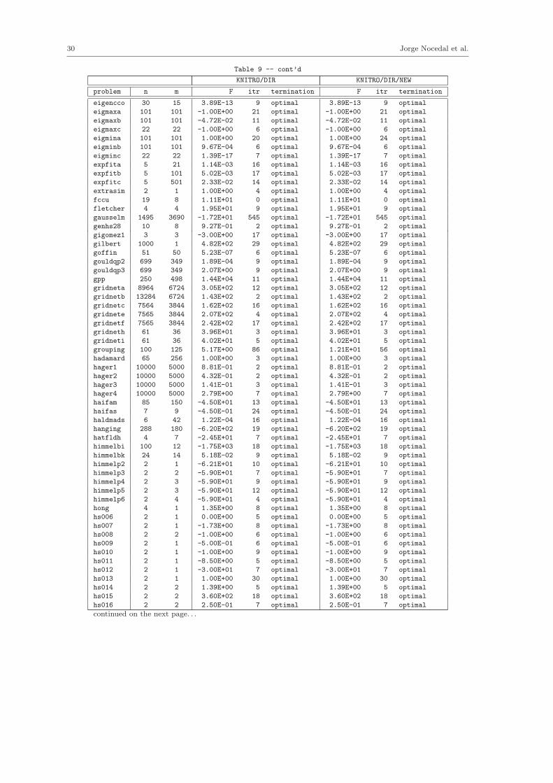
30 Jorge Nocedal et al.
Table 9 -- cont’d
KNITRO/DIR KNITRO/DIR/NEW
problem n m F itr termination F itr termination
eigencco 30 15 3.89E-13 9 optimal 3.89E-13 9 optimal
eigmaxa 101 101 -1.00E+00 21 optimal -1.00E+00 21 optimal
eigmaxb 101 101 -4.72E-02 11 optimal -4.72E-02 11 optimal
eigmaxc 22 22 -1.00E+00 6 optimal -1.00E+00 6 optimal
eigmina 101 101 1.00E+00 20 optimal 1.00E+00 24 optimal
eigminb 101 101 9.67E-04 6 optimal 9.67E-04 6 optimal
eigminc 22 22 1.39E-17 7 optimal 1.39E-17 7 optimal
expfita 5 21 1.14E-03 16 optimal 1.14E-03 16 optimal
expfitb 5 101 5.02E-03 17 optimal 5.02E-03 17 optimal
expfitc 5 501 2.33E-02 14 optimal 2.33E-02 14 optimal
extrasim 2 1 1.00E+00 4 optimal 1.00E+00 4 optimal
fccu 19 8 1.11E+01 0 optimal 1.11E+01 0 optimal
fletcher 4 4 1.95E+01 9 optimal 1.95E+01 9 optimal
gausselm 1495 3690 -1.72E+01 545 optimal -1.72E+01 545 optimal
genhs28 10 8 9.27E-01 2 optimal 9.27E-01 2 optimal
gigomez1 3 3 -3.00E+00 17 optimal -3.00E+00 17 optimal
gilbert 1000 1 4.82E+02 29 optimal 4.82E+02 29 optimal
goffin 51 50 5.23E-07 6 optimal 5.23E-07 6 optimal
gouldqp2 699 349 1.89E-04 9 optimal 1.89E-04 9 optimal
gouldqp3 699 349 2.07E+00 9 optimal 2.07E+00 9 optimal
gpp 250 498 1.44E+04 11 optimal 1.44E+04 11 optimal
gridneta 8964 6724 3.05E+02 12 optimal 3.05E+02 12 optimal
gridnetb 13284 6724 1.43E+02 2 optimal 1.43E+02 2 optimal
gridnetc 7564 3844 1.62E+02 16 optimal 1.62E+02 16 optimal
gridnete 7565 3844 2.07E+02 4 optimal 2.07E+02 4 optimal
gridnetf 7565 3844 2.42E+02 17 optimal 2.42E+02 17 optimal
gridneth 61 36 3.96E+01 3 optimal 3.96E+01 3 optimal
gridneti 61 36 4.02E+01 5 optimal 4.02E+01 5 optimal
grouping 100 125 5.17E+00 86 optimal 1.21E+01 56 optimal
hadamard 65 256 1.00E+00 3 optimal 1.00E+00 3 optimal
hager1 10000 5000 8.81E-01 2 optimal 8.81E-01 2 optimal
hager2 10000 5000 4.32E-01 2 optimal 4.32E-01 2 optimal
hager3 10000 5000 1.41E-01 3 optimal 1.41E-01 3 optimal
hager4 10000 5000 2.79E+00 7 optimal 2.79E+00 7 optimal
haifam 85 150 -4.50E+01 13 optimal -4.50E+01 13 optimal
haifas 7 9 -4.50E-01 24 optimal -4.50E-01 24 optimal
haldmads 6 42 1.22E-04 16 optimal 1.22E-04 16 optimal
hanging 288 180 -6.20E+02 19 optimal -6.20E+02 19 optimal
hatfldh 4 7 -2.45E+01 7 optimal -2.45E+01 7 optimal
himmelbi 100 12 -1.75E+03 18 optimal -1.75E+03 18 optimal
himmelbk 24 14 5.18E-02 9 optimal 5.18E-02 9 optimal
himmelp2 2 1 -6.21E+01 10 optimal -6.21E+01 10 optimal
himmelp3 2 2 -5.90E+01 7 optimal -5.90E+01 7 optimal
himmelp4 2 3 -5.90E+01 9 optimal -5.90E+01 9 optimal
himmelp5 2 3 -5.90E+01 12 optimal -5.90E+01 12 optimal
himmelp6 2 4 -5.90E+01 4 optimal -5.90E+01 4 optimal
hong 4 1 1.35E+00 8 optimal 1.35E+00 8 optimal
hs006 2 1 0.00E+00 5 optimal 0.00E+00 5 optimal
hs007 2 1 -1.73E+00 8 optimal -1.73E+00 8 optimal
hs008 2 2 -1.00E+00 6 optimal -1.00E+00 6 optimal
hs009 2 1 -5.00E-01 6 optimal -5.00E-01 6 optimal
hs010 2 1 -1.00E+00 9 optimal -1.00E+00 9 optimal
hs011 2 1 -8.50E+00 5 optimal -8.50E+00 5 optimal
hs012 2 1 -3.00E+01 7 optimal -3.00E+01 7 optimal
hs013 2 1 1.00E+00 30 optimal 1.00E+00 30 optimal
hs014 2 2 1.39E+00 5 optimal 1.39E+00 5 optimal
hs015 2 2 3.60E+02 18 optimal 3.60E+02 18 optimal
hs016 2 2 2.50E-01 7 optimal 2.50E-01 7 optimal
continued on the next page. . .
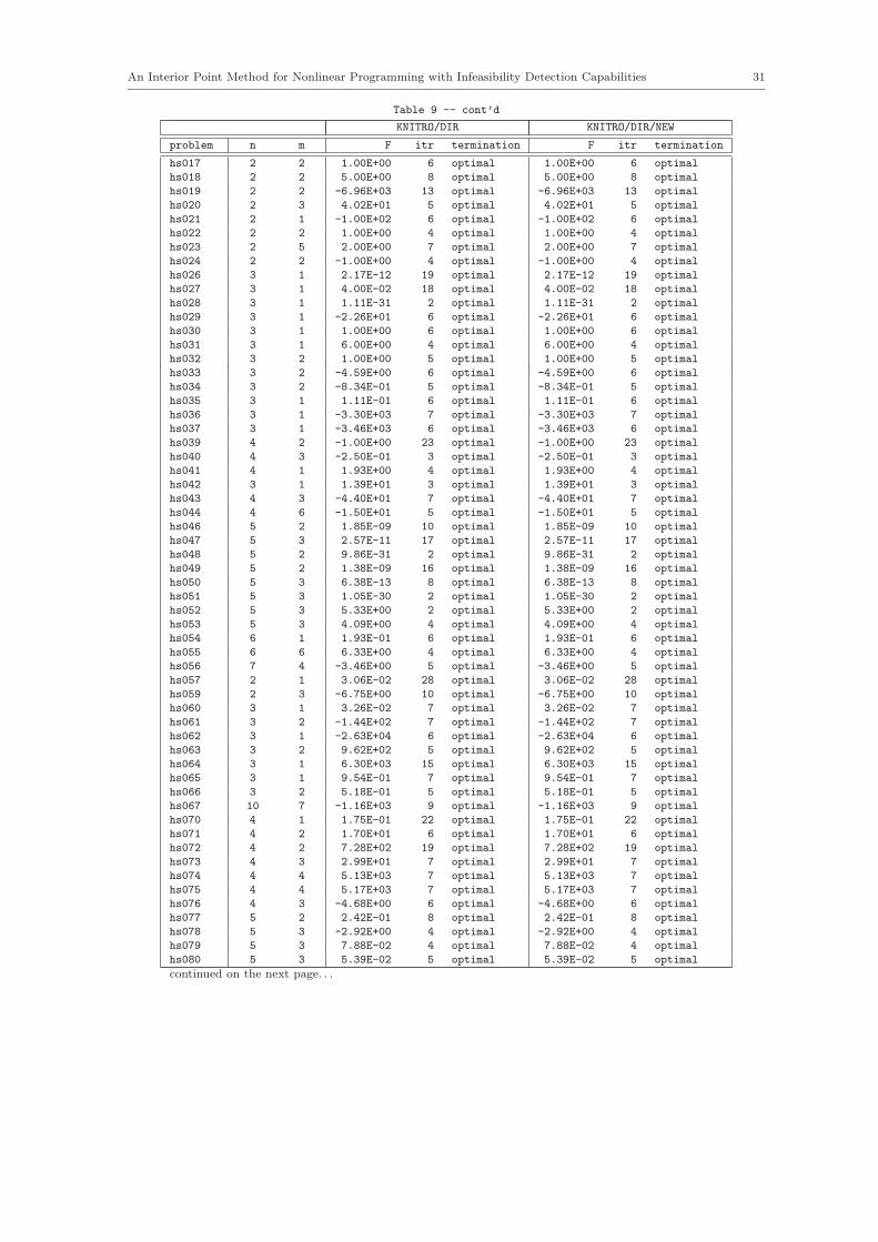
An Interior Point Method for Nonlinear Programming with Infeasibility Detection Capabilities 31
Table 9 -- cont’d
KNITRO/DIR KNITRO/DIR/NEW
problem n m F itr termination F itr termination
hs017 2 2 1.00E+00 6 optimal 1.00E+00 6 optimal
hs018 2 2 5.00E+00 8 optimal 5.00E+00 8 optimal
hs019 2 2 -6.96E+03 13 optimal -6.96E+03 13 optimal
hs020 2 3 4.02E+01 5 optimal 4.02E+01 5 optimal
hs021 2 1 -1.00E+02 6 optimal -1.00E+02 6 optimal
hs022 2 2 1.00E+00 4 optimal 1.00E+00 4 optimal
hs023 2 5 2.00E+00 7 optimal 2.00E+00 7 optimal
hs024 2 2 -1.00E+00 4 optimal -1.00E+00 4 optimal
hs026 3 1 2.17E-12 19 optimal 2.17E-12 19 optimal
hs027 3 1 4.00E-02 18 optimal 4.00E-02 18 optimal
hs028 3 1 1.11E-31 2 optimal 1.11E-31 2 optimal
hs029 3 1 -2.26E+01 6 optimal -2.26E+01 6 optimal
hs030 3 1 1.00E+00 6 optimal 1.00E+00 6 optimal
hs031 3 1 6.00E+00 4 optimal 6.00E+00 4 optimal
hs032 3 2 1.00E+00 5 optimal 1.00E+00 5 optimal
hs033 3 2 -4.59E+00 6 optimal -4.59E+00 6 optimal
hs034 3 2 -8.34E-01 5 optimal -8.34E-01 5 optimal
hs035 3 1 1.11E-01 6 optimal 1.11E-01 6 optimal
hs036 3 1 -3.30E+03 7 optimal -3.30E+03 7 optimal
hs037 3 1 -3.46E+03 6 optimal -3.46E+03 6 optimal
hs039 4 2 -1.00E+00 23 optimal -1.00E+00 23 optimal
hs040 4 3 -2.50E-01 3 optimal -2.50E-01 3 optimal
hs041 4 1 1.93E+00 4 optimal 1.93E+00 4 optimal
hs042 3 1 1.39E+01 3 optimal 1.39E+01 3 optimal
hs043 4 3 -4.40E+01 7 optimal -4.40E+01 7 optimal
hs044 4 6 -1.50E+01 5 optimal -1.50E+01 5 optimal
hs046 5 2 1.85E-09 10 optimal 1.85E-09 10 optimal
hs047 5 3 2.57E-11 17 optimal 2.57E-11 17 optimal
hs048 5 2 9.86E-31 2 optimal 9.86E-31 2 optimal
hs049 5 2 1.38E-09 16 optimal 1.38E-09 16 optimal
hs050 5 3 6.38E-13 8 optimal 6.38E-13 8 optimal
hs051 5 3 1.05E-30 2 optimal 1.05E-30 2 optimal
hs052 5 3 5.33E+00 2 optimal 5.33E+00 2 optimal
hs053 5 3 4.09E+00 4 optimal 4.09E+00 4 optimal
hs054 6 1 1.93E-01 6 optimal 1.93E-01 6 optimal
hs055 6 6 6.33E+00 4 optimal 6.33E+00 4 optimal
hs056 7 4 -3.46E+00 5 optimal -3.46E+00 5 optimal
hs057 2 1 3.06E-02 28 optimal 3.06E-02 28 optimal
hs059 2 3 -6.75E+00 10 optimal -6.75E+00 10 optimal
hs060 3 1 3.26E-02 7 optimal 3.26E-02 7 optimal
hs061 3 2 -1.44E+02 7 optimal -1.44E+02 7 optimal
hs062 3 1 -2.63E+04 6 optimal -2.63E+04 6 optimal
hs063 3 2 9.62E+02 5 optimal 9.62E+02 5 optimal
hs064 3 1 6.30E+03 15 optimal 6.30E+03 15 optimal
hs065 3 1 9.54E-01 7 optimal 9.54E-01 7 optimal
hs066 3 2 5.18E-01 5 optimal 5.18E-01 5 optimal
hs067 10 7 -1.16E+03 9 optimal -1.16E+03 9 optimal
hs070 4 1 1.75E-01 22 optimal 1.75E-01 22 optimal
hs071 4 2 1.70E+01 6 optimal 1.70E+01 6 optimal
hs072 4 2 7.28E+02 19 optimal 7.28E+02 19 optimal
hs073 4 3 2.99E+01 7 optimal 2.99E+01 7 optimal
hs074 4 4 5.13E+03 7 optimal 5.13E+03 7 optimal
hs075 4 4 5.17E+03 7 optimal 5.17E+03 7 optimal
hs076 4 3 -4.68E+00 6 optimal -4.68E+00 6 optimal
hs077 5 2 2.42E-01 8 optimal 2.42E-01 8 optimal
hs078 5 3 -2.92E+00 4 optimal -2.92E+00 4 optimal
hs079 5 3 7.88E-02 4 optimal 7.88E-02 4 optimal
hs080 5 3 5.39E-02 5 optimal 5.39E-02 5 optimal
continued on the next page. . .
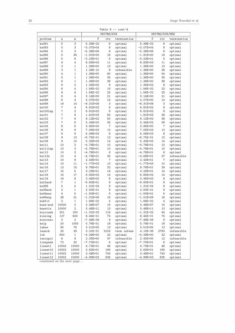
32 Jorge Nocedal et al.
Table 9 -- cont’d
KNITRO/DIR KNITRO/DIR/NEW
problem n m F itr termination F itr termination
hs081 5 3 5.39E-02 6 optimal 5.39E-02 6 optimal
hs083 5 3 -3.07E+04 8 optimal -3.07E+04 8 optimal
hs084 5 3 -5.28E+06 6 optimal -5.28E+06 6 optimal
hs085 5 36 -1.91E+00 16 optimal -1.91E+00 16 optimal
hs086 5 6 -3.23E+01 5 optimal -3.23E+01 5 optimal
hs087 9 4 8.83E+03 11 optimal 8.83E+03 11 optimal
hs088 2 1 1.36E+00 13 optimal 1.36E+00 13 optimal
hs089 3 1 1.28E-10 8 infeasible 1.36E+00 26 optimal
hs090 4 1 1.36E+00 60 optimal 1.36E+00 54 optimal
hs091 5 1 1.36E+00 35 optimal 1.36E+00 35 optimal
hs092 6 1 1.36E+00 38 optimal 1.36E+00 38 optimal
hs093 6 2 1.35E+02 6 optimal 1.35E+02 6 optimal
hs095 6 4 1.56E-02 19 optimal 1.56E-02 22 optimal
hs096 6 4 1.56E-02 25 optimal 1.56E-02 25 optimal
hs097 6 4 3.14E+00 21 optimal 3.14E+00 21 optimal
hs098 6 4 4.07E+00 14 optimal 4.07E+00 14 optimal
hs099 19 14 -8.31E+08 3 optimal -8.31E+08 3 optimal
hs100 7 4 6.81E+02 6 optimal 6.81E+02 6 optimal
hs100lnp 7 2 6.81E+02 8 optimal 6.81E+02 8 optimal
hs101 7 6 1.81E+03 92 optimal 1.81E+03 36 optimal
hs102 7 6 9.12E+02 50 optimal 9.12E+02 36 optimal
hs103 7 6 5.44E+02 35 optimal 5.44E+02 36 optimal
hs104 8 6 3.95E+00 7 optimal 3.95E+00 7 optimal
hs106 8 6 7.05E+03 12 optimal 7.05E+03 12 optimal
hs107 9 6 5.06E+03 8 optimal 5.06E+03 8 optimal
hs108 9 13 -6.75E-01 12 optimal -6.75E-01 12 optimal
hs109 9 10 5.33E+03 14 optimal 5.33E+03 14 optimal
hs111 10 3 -4.78E+01 10 optimal -4.78E+01 10 optimal
hs111lnp 10 3 -4.78E+01 10 optimal -4.78E+01 10 optimal
hs112 10 3 -4.78E+01 6 optimal -4.78E+01 6 optimal
hs112x 10 4 -4.74E+01 35 optimal -4.68E+01 37 infeasible
hs113 10 8 2.43E+01 7 optimal 2.43E+01 7 optimal
hs114 10 11 -1.77E+03 10 optimal -1.77E+03 10 optimal
hs116 13 15 9.76E+01 22 optimal 9.76E+01 29 optimal
hs117 15 5 3.23E+01 14 optimal 3.23E+01 14 optimal
hs118 15 17 6.65E+02 14 optimal 6.65E+02 14 optimal
hs119 16 8 2.45E+02 9 optimal 2.45E+02 9 optimal
hs21mod 7 1 -9.60E+01 9 optimal -9.60E+01 9 optimal
hs268 5 5 1.31E-04 9 optimal 1.31E-04 9 optimal
hs35mod 2 1 2.50E-01 9 optimal 2.50E-01 9 optimal
hs44new 4 5 -1.50E+01 5 optimal -1.50E+01 5 optimal
hs99exp 28 21 -1.01E+09 16 optimal -1.01E+09 16 optimal
hubfit 2 1 1.69E-02 4 optimal 1.69E-02 4 optimal
hues-mod 10000 2 3.48E+07 15 optimal 3.48E+07 15 optimal
huestis 10000 2 3.48E+11 13 optimal 3.48E+11 13 optimal
hvycrash 201 150 -1.31E-02 116 optimal -1.31E-02 44 optimal
kissing 127 903 8.45E-01 75 optimal 8.45E-01 75 optimal
kiwcresc 3 2 -7.49E-09 9 optimal -7.49E-09 9 optimal
ksip 20 1000 5.76E-01 18 optimal 5.76E-01 18 optimal
lakes 90 78 3.51E+05 13 optimal 3.51E+05 13 optimal
launch 25 29 3.31E-01 2102 term infeas 4.10E-06 2792 infeasible
lch 600 1 -4.29E+00 22 optimal -4.29E+00 22 optimal
lewispol 6 9 2.33E+00 47 infeasible 2.40E+00 12 infeasible
linspanh 72 32 -7.70E+01 6 optimal -7.70E+01 6 optimal
liswet1 10002 10000 4.73E+01 48 optimal 4.73E+01 48 optimal
liswet10 10002 10000 2.62E+01 165 optimal 2.62E+01 165 optimal
liswet11 10002 10000 3.49E+01 743 optimal 3.49E+01 743 optimal
liswet12 10002 10000 -4.99E+03 635 optimal -4.99E+03 635 optimal
continued on the next page. . .
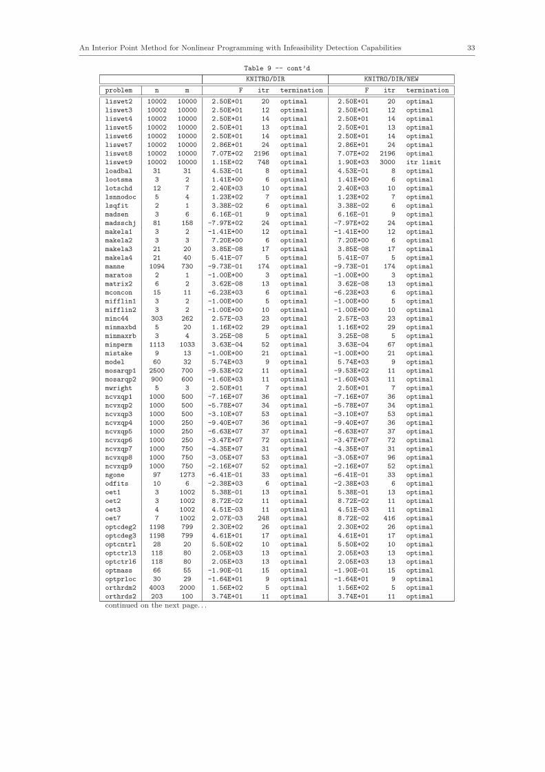
An Interior Point Method for Nonlinear Programming with Infeasibility Detection Capabilities 33
Table 9 -- cont’d
KNITRO/DIR KNITRO/DIR/NEW
problem n m F itr termination F itr termination
liswet2 10002 10000 2.50E+01 20 optimal 2.50E+01 20 optimal
liswet3 10002 10000 2.50E+01 12 optimal 2.50E+01 12 optimal
liswet4 10002 10000 2.50E+01 14 optimal 2.50E+01 14 optimal
liswet5 10002 10000 2.50E+01 13 optimal 2.50E+01 13 optimal
liswet6 10002 10000 2.50E+01 14 optimal 2.50E+01 14 optimal
liswet7 10002 10000 2.86E+01 24 optimal 2.86E+01 24 optimal
liswet8 10002 10000 7.07E+02 2196 optimal 7.07E+02 2196 optimal
liswet9 10002 10000 1.15E+02 748 optimal 1.90E+03 3000 itr limit
loadbal 31 31 4.53E-01 8 optimal 4.53E-01 8 optimal
lootsma 3 2 1.41E+00 6 optimal 1.41E+00 6 optimal
lotschd 12 7 2.40E+03 10 optimal 2.40E+03 10 optimal
lsnnodoc 5 4 1.23E+02 7 optimal 1.23E+02 7 optimal
lsqfit 2 1 3.38E-02 6 optimal 3.38E-02 6 optimal
madsen 3 6 6.16E-01 9 optimal 6.16E-01 9 optimal
madsschj 81 158 -7.97E+02 24 optimal -7.97E+02 24 optimal
makela1 3 2 -1.41E+00 12 optimal -1.41E+00 12 optimal
makela2 3 3 7.20E+00 6 optimal 7.20E+00 6 optimal
makela3 21 20 3.85E-08 17 optimal 3.85E-08 17 optimal
makela4 21 40 5.41E-07 5 optimal 5.41E-07 5 optimal
manne 1094 730 -9.73E-01 174 optimal -9.73E-01 174 optimal
maratos 2 1 -1.00E+00 3 optimal -1.00E+00 3 optimal
matrix2 6 2 3.62E-08 13 optimal 3.62E-08 13 optimal
mconcon 15 11 -6.23E+03 6 optimal -6.23E+03 6 optimal
mifflin1 3 2 -1.00E+00 5 optimal -1.00E+00 5 optimal
mifflin2 3 2 -1.00E+00 10 optimal -1.00E+00 10 optimal
minc44 303 262 2.57E-03 23 optimal 2.57E-03 23 optimal
minmaxbd 5 20 1.16E+02 29 optimal 1.16E+02 29 optimal
minmaxrb 3 4 3.25E-08 5 optimal 3.25E-08 5 optimal
minperm 1113 1033 3.63E-04 52 optimal 3.63E-04 67 optimal
mistake 9 13 -1.00E+00 21 optimal -1.00E+00 21 optimal
model 60 32 5.74E+03 9 optimal 5.74E+03 9 optimal
mosarqp1 2500 700 -9.53E+02 11 optimal -9.53E+02 11 optimal
mosarqp2 900 600 -1.60E+03 11 optimal -1.60E+03 11 optimal
mwright 5 3 2.50E+01 7 optimal 2.50E+01 7 optimal
ncvxqp1 1000 500 -7.16E+07 36 optimal -7.16E+07 36 optimal
ncvxqp2 1000 500 -5.78E+07 34 optimal -5.78E+07 34 optimal
ncvxqp3 1000 500 -3.10E+07 53 optimal -3.10E+07 53 optimal
ncvxqp4 1000 250 -9.40E+07 36 optimal -9.40E+07 36 optimal
ncvxqp5 1000 250 -6.63E+07 37 optimal -6.63E+07 37 optimal
ncvxqp6 1000 250 -3.47E+07 72 optimal -3.47E+07 72 optimal
ncvxqp7 1000 750 -4.35E+07 31 optimal -4.35E+07 31 optimal
ncvxqp8 1000 750 -3.05E+07 53 optimal -3.05E+07 96 optimal
ncvxqp9 1000 750 -2.16E+07 52 optimal -2.16E+07 52 optimal
ngone 97 1273 -6.41E-01 33 optimal -6.41E-01 33 optimal
odfits 10 6 -2.38E+03 6 optimal -2.38E+03 6 optimal
oet1 3 1002 5.38E-01 13 optimal 5.38E-01 13 optimal
oet2 3 1002 8.72E-02 11 optimal 8.72E-02 11 optimal
oet3 4 1002 4.51E-03 11 optimal 4.51E-03 11 optimal
oet7 7 1002 2.07E-03 248 optimal 8.72E-02 416 optimal
optcdeg2 1198 799 2.30E+02 26 optimal 2.30E+02 26 optimal
optcdeg3 1198 799 4.61E+01 17 optimal 4.61E+01 17 optimal
optcntrl 28 20 5.50E+02 10 optimal 5.50E+02 10 optimal
optctrl3 118 80 2.05E+03 13 optimal 2.05E+03 13 optimal
optctrl6 118 80 2.05E+03 13 optimal 2.05E+03 13 optimal
optmass 66 55 -1.90E-01 15 optimal -1.90E-01 15 optimal
optprloc 30 29 -1.64E+01 9 optimal -1.64E+01 9 optimal
orthrdm2 4003 2000 1.56E+02 5 optimal 1.56E+02 5 optimal
orthrds2 203 100 3.74E+01 11 optimal 3.74E+01 11 optimal
continued on the next page. . .

34 Jorge Nocedal et al.
Table 9 -- cont’d
KNITRO/DIR KNITRO/DIR/NEW
problem n m F itr termination F itr termination
orthrega 517 256 1.41E+03 21 optimal 1.41E+03 21 optimal
orthregb 27 6 3.35E-15 2 optimal 3.35E-15 2 optimal
orthregc 10005 5000 1.90E+02 11 optimal 1.90E+02 11 optimal
orthregd 10003 5000 1.52E+03 6 optimal 1.52E+03 6 optimal
orthrege 36 20 1.04E+01 46 optimal 1.04E+01 46 optimal
orthrgdm 10003 5000 1.51E+03 6 optimal 1.51E+03 6 optimal
orthrgds 10003 5000 1.78E+03 41 optimal 1.78E+03 41 optimal
pentagon 6 12 1.37E-04 10 optimal 1.37E-04 10 optimal
polak1 3 2 2.72E+00 6 optimal 2.72E+00 6 optimal
polak2 11 2 5.46E+01 8 optimal 5.46E+01 8 optimal
polak3 12 10 5.93E+00 20 optimal 5.93E+00 20 optimal
polak4 3 3 -2.30E-08 3 optimal -2.30E-08 3 optimal
polak5 3 2 5.00E+01 18 optimal 5.00E+01 18 optimal
polak6 5 4 -4.40E+01 12 optimal -4.40E+01 12 optimal
portfl1 12 1 2.05E-02 7 optimal 2.05E-02 7 optimal
portfl2 12 1 2.97E-02 7 optimal 2.97E-02 7 optimal
portfl3 12 1 3.27E-02 8 optimal 3.27E-02 8 optimal
portfl4 12 1 2.63E-02 7 optimal 2.63E-02 7 optimal
portfl6 12 1 2.58E-02 7 optimal 2.58E-02 7 optimal
powell20 1000 1000 5.21E+07 15 optimal 5.21E+07 15 optimal
prodpl0 60 29 6.09E+01 12 optimal 6.09E+01 12 optimal
prodpl1 60 29 5.30E+01 9 optimal 5.30E+01 9 optimal
pt 2 501 1.78E-01 13 optimal 1.78E-01 13 optimal
qpcboei1 372 288 1.44E+07 22 optimal 1.44E+07 22 optimal
qpcboei2 143 125 8.29E+06 33 optimal 8.29E+06 33 optimal
qpcstair 385 356 6.20E+06 24 optimal 6.20E+06 24 optimal
qpnboei1 372 288 8.52E+06 182 optimal 8.46E+06 148 optimal
qpnboei2 143 125 1.24E+06 1226 optimal 1.41E+33 3000 itr limit
qpnstair 385 356 5.15E+06 201 optimal 5.15E+06 84 optimal
reading1 10001 5000 -1.60E-01 15 optimal -1.60E-01 15 optimal
reading2 15001 10000 -1.14E-02 7 optimal -1.14E-02 7 optimal
robot 7 2 5.46E+00 6 optimal 5.46E+00 6 optimal
rosenmmx 5 4 -4.40E+01 7 optimal -4.40E+01 7 optimal
s332 2 100 2.99E+01 10 optimal 2.99E+01 10 optimal
s365mod 7 5 5.21E+01 13 optimal 5.22E+01 15 optimal
sawpath 589 782 3.91E+05 3000 itr limit 7.05E+04 3000 itr limit
simpllpa 2 2 1.00E+00 6 optimal 1.00E+00 6 optimal
simpllpb 2 3 1.10E+00 7 optimal 1.10E+00 7 optimal
sinrosnb 1000 999 -9.99E+04 0 optimal -9.99E+04 0 optimal
sipow1 2 10000 -1.00E+00 15 optimal -1.00E+00 15 optimal
sipow1m 2 10000 -1.00E+00 15 optimal -1.00E+00 15 optimal
sipow2 2 5000 -1.00E+00 16 optimal -1.00E+00 16 optimal
sipow2m 2 5000 -1.00E+00 19 optimal -1.00E+00 19 optimal
sipow3 4 9998 5.36E-01 13 optimal 5.36E-01 13 optimal
sipow4 4 10000 2.73E-01 12 optimal 2.73E-01 12 optimal
smbank 117 64 -7.13E+06 17 optimal -7.13E+06 17 optimal
smmpsf 720 263 1.05E+06 46 optimal 1.05E+06 46 optimal
snake 2 2 -3.51E+04 3000 itr limit -2.32E+03 3000 itr limit
sosqp2 20000 10001 -5.00E+03 15 optimal -5.00E+03 15 optimal
spanhyd 72 32 2.40E+02 9 optimal 2.40E+02 9 optimal
spiral 3 2 -2.91E-08 42 optimal -2.91E-08 42 optimal
sreadin3 10000 5000 -2.55E-05 1 optimal -2.55E-05 1 optimal
sseblin 192 72 1.62E+07 9 optimal 1.62E+07 9 optimal
ssebnln 192 96 1.62E+07 29 optimal 1.62E+07 29 optimal
ssnlbeam 31 20 3.38E+02 14 optimal 3.38E+02 14 optimal
stancmin 3 2 4.25E+00 9 optimal 4.25E+00 9 optimal
static3 434 96 -3.06E+21 99 unbounded -3.06E+21 99 unbounded
steenbra 432 108 1.70E+04 19 optimal 1.70E+04 19 optimal
continued on the next page. . .

An Interior Point Method for Nonlinear Programming with Infeasibility Detection Capabilities 35
Table 9 -- cont’d
KNITRO/DIR KNITRO/DIR/NEW
problem n m F itr termination F itr termination
steenbrb 468 108 9.24E+03 65 optimal 9.24E+03 65 optimal
steenbrc 540 126 2.04E+04 127 optimal 2.04E+04 127 optimal
steenbrd 468 108 9.65E+03 98 optimal 9.65E+03 98 optimal
steenbre 540 126 2.75E+04 825 optimal 2.75E+04 825 optimal
steenbrf 468 108 7.95E+02 279 optimal 2.85E+02 121 optimal
steenbrg 540 126 2.74E+04 45 optimal 2.74E+04 45 optimal
supersim 2 2 6.67E-01 2 optimal 6.67E-01 2 optimal
svanberg 5000 5000 8.36E+03 16 optimal 8.36E+03 16 optimal
swopf 82 91 6.79E-02 9 optimal 6.79E-02 9 optimal
synthes1 6 6 7.59E-01 9 optimal 7.59E-01 9 optimal
tame 2 1 0.00E+00 5 optimal 0.00E+00 5 optimal
tfi2 3 10000 6.49E-01 9 optimal 6.49E-01 9 optimal
trainf 20000 10002 3.10E+00 30 optimal 3.10E+00 30 optimal
trainh 20000 10002 1.23E+01 53 optimal 1.23E+01 53 optimal
trimloss 142 72 9.06E+00 19 optimal 9.06E+00 19 optimal
try-b 2 1 2.50E-17 9 optimal 2.50E-17 9 optimal
twirism1 343 313 -1.00E+00 2304 optimal -1.00E+00 89 optimal
twobars 2 2 1.51E+00 5 optimal 1.51E+00 5 optimal
ubh1 17997 12000 1.12E+00 5 optimal 1.12E+00 5 optimal
ubh5 19997 14000 1.12E+00 3 optimal 1.12E+00 3 optimal
vanderm1 100 99 3.30E-07 28 optimal 3.30E-07 28 optimal
vanderm2 100 99 3.29E-07 28 optimal 3.29E-07 28 optimal
vanderm3 100 99 3.75E-06 37 optimal 3.75E-06 37 optimal
vanderm4 9 8 2.21E-09 17 optimal 2.21E-09 17 optimal
womflet 3 3 6.05E+00 9 optimal 6.05E+00 9 optimal
yao 2000 1999 1.98E+02 36 optimal 1.98E+02 36 optimal
zecevic2 2 2 -4.12E+00 7 optimal -4.12E+00 7 optimal
zecevic3 2 2 9.73E+01 7 optimal 9.73E+01 7 optimal
zecevic4 2 2 7.56E+00 6 optimal 7.56E+00 6 optimal
zigzag 58 50 3.16E+00 16 optimal 3.16E+00 16 optimal
zy2 3 1 2.00E+00 5 optimal 2.00E+00 5 optimal
Related Documents