Mathematical Programming 43 (1989) 257-276 257 North-Holland AN INTERIOR POINT ALGORITHM FOR SEMI-INFINITE LINEAR PROGRAMMING M.C. FERRIS* and A.B, PHILPOTT** Cambridge University EngineeringDepartment, Cambridge, England Received 3 February 1986 Revised manuscript received 22 February 1988 We consider the generalization of a variant of Karmarkar's algorithm to semi-infiniteprogramming. The extension of interior point methods to infinite-dimensional linear programming is discussed and an algorithm is derived. An implementation of the algorithm for a class of semi-infinite linear programs is described and the results of a number of test problems are given. We pay particular attention to the problem of Chebyshev approximation. Some further results are given for an implementation of the algorithm applied to a discretization of the semi-infinite linear program, and a convergence proof is given in this case. Key words: Semi-infinite linear programming, discretizations, Karmarkar's method, Chebyshev approximation. 1. Introduction Much recent attention has been paid to Karmarkar's Projective Algorithm [8] for linear programming and the rescaling algorithm discovered independently by Dikin [4], Barnes [2], Cavalier and Soyster [3], and Vanderbei et al. [11]. These algorithms solve linear programs by constructing a sequence of points lying in the interior of the feasible region and converging to the optimal solution. Both algorithms make use of a transformation of variables, followed by a step in the direction of an appropriate projected gradient. In this paper we consider the generalization of this approach to solve linear programs posed over more abstract spaces. In particular, we consider a class of linear programs posed over a particular kind of pre-Hilbert space and describe a conceptual rescaling algorithm for members of this class. In order to show that this is not solely a theoretical exercise, we show that, for a class of semi-infinite linear programs, this approach can be applied in a straightforward manner to produce a rescaling algorithm for semi-infinite linear programming. We begin by describing a generalization of the rescaling algorithm [11] to an abstract space. Let S be any set and let W be a space of functions from S to ~q. It * Now at Department of Computer Sciences, University of Wisconsin, Madison, WI, USA. ** Now at Department of Theoretical and Applied Mechanics, University of Auckland, Auckland, New Zealand.

Welcome message from author
This document is posted to help you gain knowledge. Please leave a comment to let me know what you think about it! Share it to your friends and learn new things together.
Transcript
Mathematical Programming 43 (1989) 257-276 257 North-Holland
AN INTERIOR POINT ALGORITHM FOR SEMI-INFINITE LINEAR PROGRAMMING
M.C. FERRIS* and A.B, PHILPOTT**
Cambridge University Engineering Department, Cambridge, England
Received 3 February 1986 Revised manuscript received 22 February 1988
We consider the generalization of a variant of Karmarkar's algorithm to semi-infinite programming. The extension of interior point methods to infinite-dimensional linear programming is discussed and an algorithm is derived. An implementation of the algorithm for a class of semi-infinite linear programs is described and the results of a number of test problems are given. We pay particular attention to the problem of Chebyshev approximation. Some further results are given for an implementation of the algorithm applied to a discretization of the semi-infinite linear program, and a convergence proof is given in this case.
Key words: Semi-infinite linear programming, discretizations, Karmarkar's method, Chebyshev approximation.
1. Introduction
Much recent a t tent ion has been paid to Karmarkar ' s Projective Algor i thm [8] for
l inear p rogramming and the rescaling algori thm discovered i ndependen t ly by Dikin
[4], Barnes [2], Caval ier and Soyster [3], and Vanderbei et al. [11]. These algori thms
solve l inear programs by construct ing a sequence of points lying in the inter ior of
the feasible region and converging to the opt imal solution. Both algori thms make
use of a t ransformat ion of variables, fol lowed by a step in the direct ion of an
appropr ia te projected gradient.
In this paper we consider the general izat ion of this approach to solve l inear
programs posed over more abstract spaces. In part icular , we consider a class of
l inear programs posed over a part icular k ind of pre-Hilber t space and describe a
conceptual rescaling algori thm for members of this class. In order to show that this
is not solely a theoretical exercise, we show that, for a class of semi-infini te l inear
programs, this approach can be appl ied in a straightforward m a n n e r to produce a
rescaling algori thm for semi-infinite l inear programming.
We begin by describing a general izat ion of the rescaling algori thm [11] to an
abstract space. Let S be any set and let W be a space of funct ions from S to ~q. It
* Now at Department of Computer Sciences, University of Wisconsin, Madison, WI, USA. ** Now at Department of Theoretical and Applied Mechanics, University of Auckland, Auckland,
New Zealand.
2 5 8 M.C. Ferris, A.B. Philpott / Interior point algorithm
is clear that with suitable definitions of addition and scalar multiplication that W can
be given a vector space structure. Let U and Z be arbitrary vector spaces. Define
the space V to be the Cartesian product of U and W, i.e.
V = U O W .
We assume that V is a pre-Hilbert space with an inner product denoted by (-, -).
Members of U are denoted by u, members of W are denoted by w, and members of V are denoted by either (u, w) or (x, z). The generalization of the rescaling
algorithm which we describe below requires that the elements of W are regarded
at different times to have either the norm induced by the inner product (the IP
norm), or the supremum norm defined by
t/wllo = sup([I w(s)II~,l s c s}.
For example, the set of continuous functions on [0, 1] can be regarded at different times as a pre-Hilbert space with inner product defined by
;o ( f g)= f(s)g(s) ds
or as the Banach space C[0, 1] with the supremum norm. We define a convex cone W+ as follows:
W+={w6 W: wi(s)>-O, sc S, i= 1 , . . . , q},
and note that its interior W°+ (with respect to the supremum topology) is given by
We let
o W + = { w c W : wi(s)>O, scS , i = l , . . . , q } .
V+= U ® W+
and
o o V+ = U ® W+
and define a partial order "~>" on V by
~zt>7 fo r ( , y c V if and only if ~ - 7 c V + .
If we let 0 be the zero element of V then it is clear that
cV, ~/>0 if and only if ~ V + .
The set V+ is called the positive cone of V. We define ~: > 3' for ~, 3' c V to mean
that ( - 3' 6 V °, and we note that ( > 3' implies that s c i> 3/. We also assume that W °
is non-empty and having chosen a fixed element e of W ° let any (u, e) c V°+ be
called a preferred element of V.
M.C. Ferris, A .B . Philpott / Interior point algori thm 259
In what follows we shall confine our attention to linear programs which have the
following form.
LP minimize ((c, d), (u, w)),
V((u, w)) = b,
subject to (u, w) ~> 0,
(u,w)c v,
with c c U, d ~ W, b < Z, and T : V-~ Z being a continuous linear operator. For this class of infinite-dimensional linear programs we can specify an algorithm which is a generalization of the rescaling algorithm of [11]. At each step of the algorithm,
we define a V°+-invariant non-singular endomorphism of V which maps the current point (x, z) c V°+ to a preferred point (x, e) c V°+ which, with respect to the supremum
norm, is "far away" from the boundary of the positive cone. We then take a step in the transformed space along the direction of steepest descent of the transformed objective functional and apply the inverse of the endomorphism to give a new current point in the original space. The endomorphism is defined in terms of the current point (x, z) > 0 and a preferred point (x, e) as follows. Firstly, define z -~ by
,~--1 : ( Z I I , . . . , Zq 1)
with
z['(s) = ei(s) z,(s)'
and z* by
with
z*=(zL...,z~)
V s c S , i = l , . . . , q ,
z,(s) z* (S ) -eds ) , Vs~S , i = l , . . . , q .
Further we note that z -~, z* are elements of W °. For any w, v c W we define @: W x W-~ W b y
(w@v)i(s)=wi(s)vi(s), V, cS, i = l , . . . , q .
Clearly @ is commutative and associative and if w, r c W ° then so is w@ ~. We now define the following mappings in terms of the current point (x, z ) > O:
Fz((U, w ) ) : (u, z-'Qw),
F*~((u, w))= (u, z*Qw).
It is clear that F~* and Fz are linear mappings from V to itself. It is easy to see that
F=(V°_) ~ V ° and that F*(V °) ~ V °. It also follows from the definition of (3 that F* and Fz are mutual inverses.
260 M. C. Ferris, A.B. Philpott / Interior point algorithm
I f we make the assumption that for every (u, w) 6 V,
((c, d), (u, w)) = (F*z((e, d)), F~((u, w))),
then it follows that the solution to the problem given below has the same objective
functional value as the solution of LP (the constraints are unchanged since F* and
are mutual inverses).
minimize (F*((e, d)), Fz((U, w))),
T o F*z(F~((u , w ) ) ) = b,
subject to F*(Fz((U, w))) >~ O,
F*z(Fz((U, w)))c V,
where To F denotes the composition of T and F. Let us write y for z- l (~ w, so that (u, y) = Fz(u, w)). Since V and V+ are invariant under Fz and its inverse, it is clear
that this problem may be formulated as
SLP minimize (Fz*((c, d)), (u, y)),
To F~((u, y)) = t,,
subject to (u, y) ~> 0,
(u ,y ) ~ V.
The rescaling algorithm for LP can now be described as follows. Given a current point (x, z) feasible for LP and lying in V °, an iteration of the algorithm transforms V by the endomorphism Fz, mapping (x, z) to the preferred point (x, e). A step
from (x, e) is then computed so as to give a new point in Fz(V) with a smaller SLP objective functional value than that of (x, e); applying the inverse F* of Fz to V maps this new point to a new current point in V°+.
In the finite-dimensional case the rationale underlying the rescaling algorithm is discussed fully in [3] and [11]; the reasoning is similar in the abstract case. The
transformation Fz allows us to treat the current point as a preferred point which is chosen to be far away with respect to the supremum norm from the boundary of the positive cone. The direction of the step is given by the orthogonal projection of -F*z((C, d)) onto the kernel of T o F~*. A strictly positive step in this direction guarantees a strict decrease in the objective functionals of both the original problem and the scaled problem directly proportional to the length of the step. The orthogonal projection is necessary to ensure that the new current point satisfies the constraints
of LP. For the constructions described above to be possible we require a number of
assumptions which we now list before proceeding to describe the steps of the
algorithm explicitly.
Assumption 1. V = U ® W is a pre-Hilbert space with inner product ( . , .), where
U is a vector space and W is a space of functions S ~ q. T: V--~Z is a linear
mapping of V to a vector space Z.
M.C. Ferris, A.B. Philpott / Interior point algorithm
Assumption 2. There exists ¢~ ~ V with ~: > 0.
Assumption 3. For every (u, w) c V,
((c, d), (u, w)): (t:*z((C, d)), Fz((U, w))).
261
Assumption 4. For any choice of z E W, the kernel of the linear operator T o F* is a Hilbert space with respect to the norm induced by the inner product.
The algorithm Step O. Set k = O.
Step 1. Take a feasible point (x, z) ~k) > 0 and map it to a preferred point (x, e) using the map F~k~, i.e.
(X, e) =/~]~k~((x, z)(k)).
Step 2. Project the direction of steepest descent for the t ransformed linear func- tion, -F*¢~((c, d)), orthogonally onto the kernel of the linear operator ToF*~ to give (cv, zv).
Step 3. Find a step length a > 0 such that e + az e > 0, and let
z' = e + cezp.
Step 4. Invert the transformation to get (x, Z) (k+l), i.e.
(X, Z) (k+l) = F~z(k)( (X ~ - OlCp, Z') ).
Step 5. Check the termination criterion and stop if it is satisfied. Otherwise set k = k + 1 and return to Step 1.
It is pertinent at this point to make some remarks regarding the above assumptions. When U ® W = V = E ~ with the canonical inner product, the IP norm and the supremum norm are topologically equivalent, and V forms a Hilbert space with the convenient property that V°+ (the Cartesian product of U and the set of points in W with strictly positive components) is nonempty. We are therefore guaranteed not only the existence of a projected gradient vector by the Projection Theorem, but also the existence of a preferred element in V°+. When W is generalized to be a possibly infinite-dimensional space, the supremum norm and the IP norm are
unfortunately no longer topologically equivalent, and the Hilbert spaces (such as Lz[a, b]) with which we would like to work have canonical positive cones with empty interiors with respect to the Hilbert-space norm. For this reason it is necessary to make use of the supremum topology, and make Assumption 2, which amounts to choosing W so that V°+ is nonempty.
In fact the condition that V be a Hilbert space is stronger than necessary. We
require only that Assumption 4 above holds in order to ensure the existence of a projected direction of steepest descent. This assumption will hold in particular for
262 M.C. Ferris, A.B. Philpott / Interior point algorithm
spaces W and transformations T where ker(T o F*) is finite-dimensional for every
z in W. In the next section we shall describe a class of semi-infinite linear program-
ming problems for which this is true, and show how a rescaling algorithm to solve
members of this class can be constructed along the lines described above.
2. Semi-infinite linear programming
2.1. Problem formulation
In this section we consider the application of the algorithm to a class of semi-infinite linear pgramming problems. These have the following form.
minimize
subject to
where
cTx,
n al i (s )x j >I bl(s) if s E [11, /)1],
j = l
aqj(s)xj>~bq(s) if sc[ lq , Vq], ,]~ 1
aij(s), b i (s)cC°°[l i , vi], i - = l , . . . , q , j = l . . . . ,n, and c, x c E ' .
With a slight abuse of notation we will write this as
minimize c X x,
subject to A ( s ) x >~ b(s), Vs c S,
where
A(s ) = • ".. • b(s) = . . .
and c, x ~ ~". (Here S = [ll, vii for the ith equation.) In order to put the above linear
program into the form LP, we introduce a slack variable z~ ~ C°°[l~, v~] for each
constraint in the above system. The problem then becomes
minimize cVx,
subject to A ( s ) x - z ( s ) ~ - b ( s ) , V s ~ S ,
z ~ O ,
where x ~ ~ ' , z c l]~=~ C°~[I~, vii, which is exactly the form that we require if we set
U = ~ " and W = Z ~ - I ] ~ _ ~ C ~ [ l i , vi], and let T ( x , z ) = A ( . ) x - z ( . ) . The inner
product ( - , . ) is defined on V as
d), z)> I = d i ( s ) z , ( s ) ds . i~ 1 l i
M. C. Ferris, A.B. Philpott / lnterior point algorithm 263
We assume that e is given by ei ~ C~[li, vi] with ei(s) = 1, Vs c [1i, vi], i = 1, . , . . , q. We note that
((c, o), (x, z)) = cTx,
and see that
((c, d), (u, w)) = (F*((c, d)), Fz((U, w))),
since from the definition of the inner product given above we have that
((c, d), (u, w))= cTu + ~ d~(s)wi(s) ds i=1
= cTu + di (s )z i (s ) (1 /z i (s ) )wi(s) ds i= 1 I i
= (F*z((C, d)), F~((u, w))).
It is also evident that F*((c, 0)) = (c, 0), so that the direction of steepest descent for
the transformed linear function is -(c, 0). It remains to show how we can accomplish
the orthogonal projections within this framework which is dealt with in the next
section.
We note in closing this section that other forms of the semi-infinite linear program problem can be put into the LP framework with equal ease. In particular, if the
elements of R" are constrained in sign then we can redefine W and e in order to
force these elements away from the boundary of the positive cone at each step of
the algorithm.
2.2. A description of the implementation
Clearly, in Step 1 and Step 4 of the algorithm applied to the semi-infinite case, we
are effectively dividing and multiplying a positive function by a particular positive
function which has the property that it transforms the current point to the point
(x, e). In Step 2 of the algorithm we project a vector onto the kernel of T o F~*~k~.
Observe that this is a finite-dimensional subspace of V so we may accomplish this
by carrying out the following steps.
(i) Find a basis {Yi: i = 1 , . . . , n} of the kernel of T o F*ck~ where T is defined in Section 2.1. This is accomplished easily since we can construct the elements of the
basis as follows:
:r o F*~((u, w ) ) = :r(u, z* ~9 w)
= Au - (z* fi) w)
= Au - (z Q w)
since z * = z in this case. Thus, since any (u, w) in the kernel of To F~*¢~) has
2 6 4 M.C. Ferris, A.B. Philpott / Interior point algorithm
w = Au @ z -1, the elements of the basis are
yi = (ki, rf) for i , . . . , n,
where
and
k, = ( 0 , . . . , O, 1, 0 , . . . , O) ,
I in i t h p o s i t i o n
r i ( s ) = ( a , ( s ) / z l ( s ) , . . . , a q i ( s ) / z ~ ( s ) ) .
(ii) Orthonormalize this finite basis to give
{/3i = (g,, ti): i= 1 , . . . , n}.
This is accomplished by the modified Gram-Schmidt orthogonalization process, which is described in Goub and Van Loan [6].
It should be noted that the major work per iteration is in the calculation of the inner products (which are required for the Gram-Schmidt procedure). Each inner product requires q integrations, and the number of inner products needed per iteration is O(n2). Thus the total number of integrations per iteration is O(n2q).
It was decided to use Simpson's Rule to evaluate the integrals since it has a strong error bound and a simple implementation. In general the integrations cannot be carried out explicitly since even when the matrix A(s ) has polynomial entries, the integrand is a rational function. Most of the function evaluation in this process is
repetitive and so the cpu time can be decreased at the expense of using extra storage. Step 3 of the algorithm requires the evaluation of a step length c~ > 0 satisfying
e+ azp>O.
(rain) and This is evaluated by finding the minimum value of Zp(S) in [0, 1], say Zp , then setting
- - C[((mul ) OZ = (min--~,
Zp
where a(mul) is a constant multiplier constrained to lie in the interval (0, 1), and we assume that the minimum value of zp is negative, otherwise the problem is unbounded. (The choice of a~ul) is not entirely straightforward since the likelihood
of the algorithm terminating at a non optimal point increases as we increase a~mui). A further discussion of this point is made in Section 2.3.) For Step 5, the termination criterion chosen was to stop when two successive solutions differed by less than a prespecified tolerance.
M.C. Ferris, A.B. Philpott / Interior point algorithm 265
We now digress slightly to consider a Phase 1 procedure for the algorithm. At Step 0 we require a feasible solution, which is not always immediately available. We therefore consider the following problem, for some vector k,
FP minimize A,
subject to A ( s ) x + kA >I b(s) ,
A~>0.
I f we can find a solution to the above problem with A = 0 then we have a feasible
starting point for the main algorithm. It is easy to see that if we set every component of k to max i (max~ s (b~ (s))), then a feasible starting point to the algorithm is obtained by setting A(°> to some value greater than 1 and setting x to 0, thus forcing the corresponding slack functions to be greater than 0. It is then possible to solve the feasibility problem, FP, by the algorithm described above if we change Step 3 to read
Step 3. (For feasibility) Find the maximum step length fl > 0 such that
e+ [3Zp~O.
Let (Cp)A be the component of the projection % corresponding to the variable A.
(c,)~ < 0 since FP is bounded below. Then set
z' = e + olzp,
where
_ I - A / ( % ) ~ if A +/3(cp)~ <0 ,
a tamu~X/3 otherwise,
and O~mu I C ( 0 , 1) is a constant multiplier which ensures that the slack function remains strictly positive.
Note that this sets h to zero at the first instance that it becomes negative and that the variable A is assumed to lie in U and not in W. This enables the solution of
Phase 1 to be easily converted into a starting point for Phase 2, without a redefinition of the positive cone.
2.3. Chebyshev approximation
We consider the problem of approximating a given function f ( s ) with a finite set of approximating functions {ai(s): i = 1 , . . . , n}. This problem may be formulated in the L ~ norm,
n min max f ( s ) - ~, xiai(s) , x E ~ n s ~ S i=1
266 M.C. Ferris, A.B. Philpott / Interior point algorithm
or, wi th a c h a n g e o f n o t a t i o n ,
ra in m a x f ( s ) - a-r(s)x . x ~ n s ~ S
I t is we l l k n o w n tha t this is e q u i v a l e n t to the f o l l o w i n g semi - in f in i t e p r o g r a m .
m i n i m i z e h,
sub jec t to h + a T ( s ) x >~f(s) ,
h - a T ( s ) x >1 - f ( s ) .
It is c lea r to see tha t we can use the a l g o r i t h m d i scus sed in Sec t ion 1 i f we set
W = Z = C°°[0, 1 ] x C~°[0, 1],
a n d
U = N x N ".
Thus , a g e n e r a l e l e m e n t has the f o r m (h, x, z l ( s ) , z2(s)) w h e r e z i ( s ) is the s lack
f u n c t i o n a s s o c i a t e d wi th t he i th cons t ra in t .
Tile first p r o b l e m a t t e m p t e d was to a p p r o x i m a t e s 6 wi th the f u n c t i o n s ai(s) = s ~-1,
i = 1 . . . . , n. The resul ts a re g iven in Tab l e 1.
Table 1
Chebyshev approximation of s 6. Tolerance of solution is 10 ~; True solution is 4.88 x 10 - 4
c~(,1,~) Phase 1 Phase 2 Solution value CPU (s)
0.20 1 109 4.99 × 1 0 - 4 26.3 0.40 1 59 4.90x 10 4 14.5 0.60 1 45 5.63 × 10 -4 11.1 0.70 1 34 6.63 x 10 4 8.6 0.80 1 40 5.95 X 1 0 - 4 9.9 0.90 1 26 9.46 × 10 4 6.7 0.95 1 26 9.25 x 10 4 6.6 0.99 1 22 2.64× 10 3 5.7
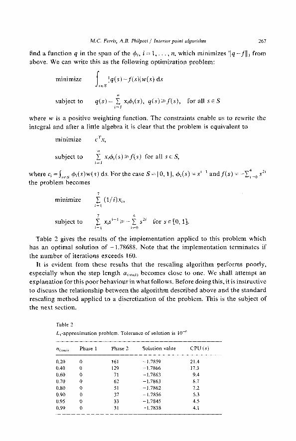
2.4. L l -approx imat ion
W e p r e s e n t s o m e less f a v o u r a b l e resul ts on the o n e - s i d e d L l - a p p r o x i m a t i o n p r o b l e m .
A c o m p l e t e d e s c r i p t i o n o f this p r o b l e m is g iven in G t a s h o f f a n d G u s t a f s o n [5]. Let
~bl, •. •, ~bn be an e x t e n d e d C h e b y s h e v sys tem o f o r d e r two. T h e p r o b l e m is t hen to
M.C. Ferris, A.B. Philpott / Interior point algorithm 267
find a func t ion q in the span of the qSi, i = 1 , . . . , n, which minimizes I I q - f i l l f rom
above. We can write this as the fol lowing op t imiza t i on p rob l em:
min imize f Iq(s ) - f ( s )[w(s) ds Js ~ S
n
subject to q(s) = ~ xi~5,(s), q(s) >~f(s), for all s c S
where w is a posi t ive weight ing funct ion. The cons t ra in ts enab le us to rewri te the
in tegral and after a l i t t le a lgebra it is c lear tha t the p r o b l e m is equiva len t to
min imize cr x,
subjec t to ~ xicbi(s) >~f(s) for all s ~ S, i - - I
where ci =Js~s qSi(s)w(s) ds. F o r the case S = [0, 1], cbi(s) = s i-1 and f ( s ) = - ~ = o s2i the p r o b l e m becomes
7
minimize ~ (1/i)x~, i = 1
7 4
subjec t to ~ xis i-1>1- ~ s 2~ for s c [0, 1]. i = 1 i ~ O
Table 2 gives the results o f the i m p l e m e n t a t i o n a p p l i e d to this p r o b l e m which
has an op t ima l so lu t ion o f -1 .78688. Note that the i m p l e m e n t a t i o n t e rmina tes i f
the n u m b e r of i te ra t ions exceeds 160.
I t is ev ident f rom these results tha t the resca l ing a lgor i thm per fo rms poor ly ,
espec ia l ly when the s tep length c~m~n becomes close to one. We shal l a t t empt an
exp l ana t i on for this p o o r behav iou r in wha t fol lows. Before do ing this, it is ins t ruct ive
to discuss the re la t ionsh ip be tween the a lgo r i thm desc r ibed above and the s t a n d a r d
rescal ing m e t h o d app l i ed to a d iscre t iza t ion of the p rob lem. This is the subjec t of
the next section.
Table 2
Ll-approximation problem. Tolerance of solution is 10 -6
c~mut ) Phase 1 Phase 2 Solution value CPU (s)
0.20 0 161 -1.7859 21.4 0.40 0 129 -1.7866 17.3 0.60 0 71 -1.7863 9.4 0.70 0 62 - 1.7863 8.7 0.80 0 51 -1.7862 7.2 0.90 0 37 -1.7856 5.3 0.95 0 33 -1.7845 4.5 0.99 0 31 -1.7838 4.1
268 M.C. Ferris, A.B. Philpott / Interior point algorithm
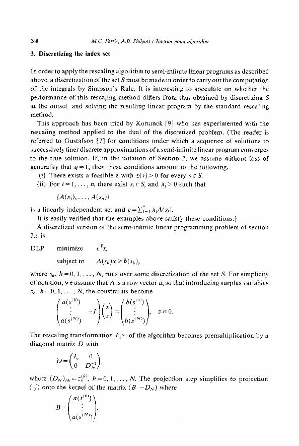
3. Diseretizing the index set
In order to apply the rescaling algorithm to semi-infinite linear programs as described above, a discretization of the set S must be made in order to carry out the computation of the integrals by Simpson's Rule. It is interesting to speculate on whether the
performance of this rescaling method differs from that obtained by discretizing S at the outset, and solving the resulting linear program by the standard rescaling method.
This approach has been tried by Kortanek [9] who has experimented with the rescaling method applied to the dual of the discretized problem. (The reader is referred to Gustafson [7] for conditions under which a sequence of solutions to successively finer discrete approximations of a semi-infinite linear program converges
to the true solution. If, in the notation of Section 2, we assume without loss of generality that q = 1, then these conditions amount to the following.
(i) There exists a feasible z with z(s)> 0 for every s c S. (ii) For i = 1 , . . . , n, there exist si c S, and ,~i > 0 such that
{A(sl),..., a(s,)}
is a linearly independent set and c=~7_1 Aim(si). It is easily verified that the examples above satisfy these conditions.)
A discretized version of the semi-infinite linear programming problem of section 2.1 is
DLP minimize cTx,
subject to A(sh)x >~ b(Sh),
where sh, h = 0, 1 , . . . , N, runs over some discretization of the set S. For simplicity
of notation, we assume that A is a row vector a, so that introducing surplus variables zh, h = 0, 1 . . . . , N, the constraints become
a(s'(N)) - I ( x ) \b(s'(N))J
The rescaling transformation F~k) of the algorithm becomes premultiplication by a diagonal matrix D with
0
where (DN)hh = z~h ~), h =0 , 1 , . . . , N. The projection step simplifies to projection (o c) onto the kernel of the matrix (B - D N ) where
M.C. Ferris, A.B. Philpott / Interior point algorithm 269
It is easily verified that the actual projection is given by
io
where v solves
( I . + B T D ; , 2 n ) ~ = - c .
Observe that (cI~) lies in the kernel of (B -DN) even though v may be computed inaccurately. Adler et al. [ 1 ] have exploited this fact in developing a fast implementa- tion of the rescaling algorithm by applying it to the dual of the linear program in standard form.
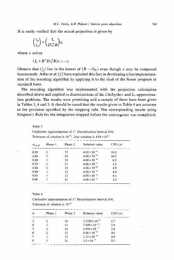
The rescaling algorithm was implemented with the projection calculation described above and applied to discretizations of the Chebyshev and Ll-approxima- tion problems. The results were promising and a sample of them have been given in Tables 3, 4 and 5. It should be noted that the results given in Table 4 are accurate to the precision specified by the stopping rule. The corresponding results using Simpson's Rule for the integration stopped before the convergence was completed.
Tab le 3
C h e b y s h e v a p p r o x i m a t i o n o f s 6. D i sc r e t i z a t i on in te rva l 0,01.
T o l e r a n c e o f s o l u t i o n is 10-6; T rue s o l u t i o n is 4.88 x 10 4
O~(mul ) P h a s e 1 Phase 2 S o l u t i o n va lue C P U (s)
0.20 1 72 4.92 X 1 0 - 4 19.9
0.40 1 34 4 . 9 0 x 10 4 10.2
0.60 1 22 4.89 x 10 -4 6.5
0.70 1 17 4 . 8 8 x 10 -4 5.5
0.80 1 15 4,88 x 10 -4 4.9
0.90 1 13 4,88 x 10 4 4.4
0.95 1 12 4.88 × 1 0 - 4 4.1
0.99 1 11 4.88 X 1 0 - 4 3.8
T a b l e 4
C h e b y s h e v a p p r o x i m a t i o n o f s". D i sc re t i za t i on in te rva l 0.01.
T o l e r a n c e o f so lu t ion is 1 0 - 6
n P h a s e 1 P h a s e 2 S o l u t i o n va lue C P U (s)
3 1 10 3 .1250 x 10 -2 1.7
4 1 11 7.809 x 10 -3 2.4
5 1 11 1 . 9 5 0 x 10 3 3.0
6 1 12 4.88 × 10 -4 4.1
7 1 12 1.22 x 1 0 - 4 4.9
8 1 11 3.1 x 10 -5 5.5
270 M.C. Ferris, A.B. Philpott / Interior point algorithm
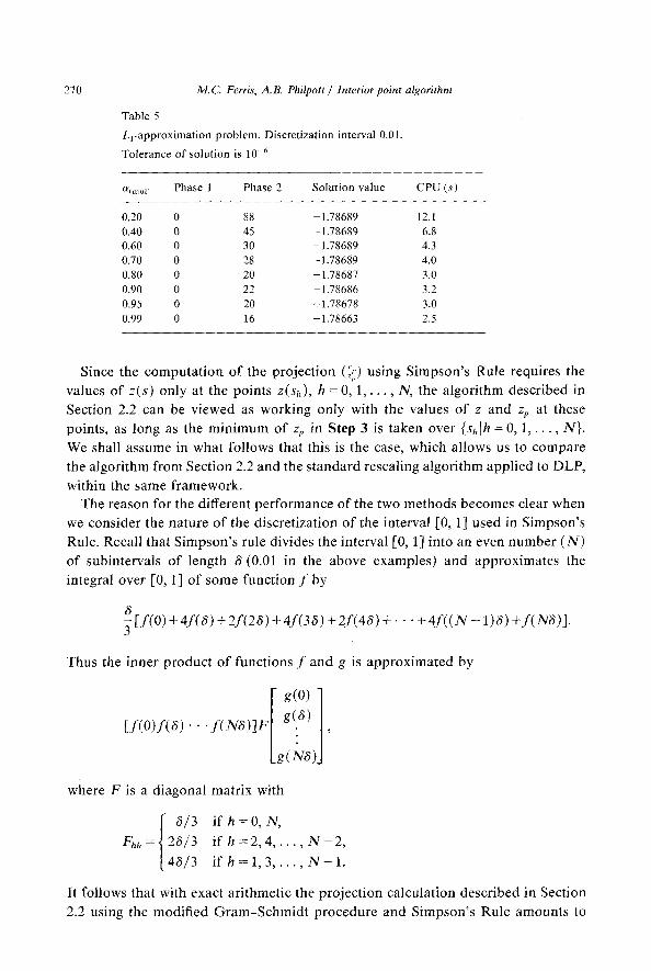
Table 5
Ll-approximation problem. Discretization interval 0.01.
Tolerance of solution is 10 -6
o+o~<m Phase 1 Phase 2 Solution value CPU (s)
0.20 0 88 -1.78689 12.1 0.40 0 45 -1.78689 6.8 0.60 0 30 -1.78689 4.3 0.70 0 28 -1.78689 4.0 0.80 0 20 -1.78687 3.0 0.90 0 22 - 1.78686 3.2 0.95 0 20 -1.78678 3.0 0.99 0 16 -1.78663 2.5
Since the computa t ion o f the project ion (z~;) using Simpson 's Rule requires the
values o f z(s) only at the points z(sh), h = 0 , l , . . . , N, the algori thm described in
Section 2.2 can be viewed as working only with the values o f z and zp at these
points, as long as the min imum of zp in Step 3 is taken over {Shlh =0 , 1 , . . . , N}.
We shall assume in what follows that this is the case, which allows us to compare
the algorithm from Section 2.2 and the s tandard rescaling algori thm applied to DLP,
within the same framework. The reason for the different per formance of the two methods becomes clear when
we consider the nature o f the discretization o f the interval [0, 1 ] used in Simpson's
Rule. Recall that Simpson 's rule divides the interval [0, 1] into an even number ( N )
o f subintervals o f length 6 (0.01 in the above examples) and approximates the
integral over [0, 1] o f some function f by
6 I f (0 ) + 4f (8) + 2f(28) + 4f(3 6) + 2f(48) + . • • + 4 f ( ( N - 1)8) + f ( N S ) ] .
Thus the inner p roduc t o f functions f and g is approximated by
r • / ,
[g(NS)J
where F is a diagonal matrix with
f 8 /3 i f h = 0 , N,
Fhh=~28/3 if h = 2 , 4 . . . . , N - 2 , / (4613 i f h = 1 , 3 , . . . , N - 1 .
It follows that with exact arithmetic the project ion calculation described in Section
2.2 using the modified Gra m -Sc hm i d t procedure and Simpson 's Rule amounts to
M.C. Ferris, A.B. Philpott / Interior point algorithm 271
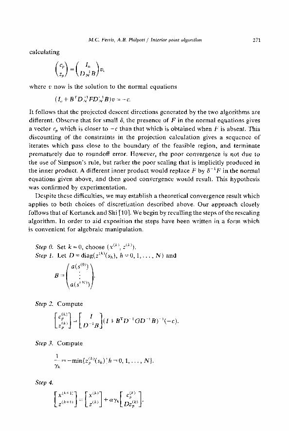
calculating
io
where v now is the solution to the normal equations
(I.+ BTD~'FD~B)v=-c.
It follows that the projected descent directions generated by the two algorithms are different. Observe that for small 6, the presence of F in the normal equations gives a vector cp which is closer to - c than that which is obtained when F is absent. This discounting of the constraints in the projection calculation gives a sequence of iterates which pass close to the boundary of the feasible region, and terminate prematurely due to roundoff error. However, the poor convergence is not due to the use of Simpson's rule, but rather the poor scaling that is implicitly produced in the inner product. A different inner product would replace F by 6-1F in the normal equations given above, and then good convergence would result. This hypothesis was confirmed by experimentation.
Despite these difficulties, we may establish a theoretical convergence result which applies to both choices of discretization described above. Our approach closely follows that of Kortanek and Shi [ 10]. We begin by recalling the steps of the rescaling algorithm. In order to aid exposition the steps have been written in a form which is convenient for algebraic manipulation.
Step O. Set k = 0, choose (x <k), z<k~). Step 1. Let D = diag(z(k)(sh), h = 0, 1 , . . . , N) and
Step 2. Compute
= ( I + B T D - ' G D - ' B ) - ' ( - ¢ ) . L~")J D '8
Step 3. Compute
1 = - - m i n { z ( f f ( S h ) l h = O, 1 , . . . , N } .
Yk
Step 4.
272 M.C. Ferris, A.B. Philpott / Interior point algorithm
Step 5. Set k = k + l , return to Step 1.
The algorithm stops in Step 2 if
z k,j =0,
in which case we declare optimality, or in Step 3 if yk ~< 0 which indicates unbounded-
ness. Here G is any diagonal positive definite matrix. Note that if G = I, then the algorithm corresponds to a standard discretization, and if G = F as defined in the
previous section, then the algorithm is that which uses Simpson's Rule. Observe
that G is independent of k, whereas D is not; its dependence on k has been
suppressed for notational convenience. It is useful to define at step k the vector
y(k) = [ D G - ~ D + BBT]-IBc.
This vector will be shown to converge to the optimal solution for the dual problem
to DLP which can be formulated as follows:
N DLP* maximize ~ b(Sh)Yh,
h=0
subject to BXy = c,
y>~O.
It is easy to demonstrate the following lemma.
Lemma 1. I f D L P has an optimal solution and the algorithm does not terminate then
.
Proof. For each k, we have by virtue of the definition of
(k) D-1Bc(p k) and - c = c~,k)+ T ~ 1 (k) that zp = B L, Gzp . It now follows from the definition o f X (k+l) that
cTx (k+l) cTx (k) rl c(k)2_~ - - - kLI 2 J
Since the algorithm does not terminate, Yk > 0 for every k, it is clear that cT.x "(k) is
a decreasing sequence bounded below by the optimal value of DLP. Thus cTx (k)
converges, and
2
M.C. Ferris, A.B. Philpott / Interior point algorithm 273
Let e = min{Ghh]h =0 , 1 , . . . , N}, so that
~(k),~Tz~_(k) (k) 2
which implies that
(k) 2 (k) T (k) ,/llc~ l{2+(z~ ) az~ ~>,/~IIG~>II=. (2) However ,
[[Z(k)[}2 ~ -min{z~*>(Sh)( h = O, 1 , . . . , N} = 1 . Yk
/ ,~(k)~,T f~ (k) Multiplying both sides o f (2) by ~/llc~k>H2+t,p ) uzp we find
-elZp ) uzp .
It follows immediately f rom (1) that
f l lira = 0. [] k ~ [ z(pk)J
x~ k> y(k) In order to demonstrate the convergence o f [=~] and we first prove the key
result:
Lemma 2. I f DLP has an optimal solution and the algorithm does not terminate then, for each h = 0, 1 . . . . . N,
lim inf Dh~ GhhZ(pk)(Sh) ~ O.
-1 k • Proof. Choose h, and let vk = Dhn Ghhzp(sh). Let u = lim inf Vk and suppose u > O.
Then there exists K such that for each k >~ K
U Ilim{vk, Vk+l, . . .}-- Ul < ~.
Thus, for each k >~ K, vk > u/2 > 0. N o w since D -1G is a positive definite diagonal matrix, it follows that z~k)(sh) > 0, for k >~ K. Thus, by the definition of D, for k >~ K,
z(k+l)(sh) = Z(k>(Sh)(1 + aykZ(f)(Sh) ) > z(k>(sh),
implying that lim infz(k)(Sh)> O. It follows immedaitely from Lemma 1 that Vk converges to zero which contradicts the assumpt ion u > O. []
We now proceed to the main convergence theorem.
Theorem I. Suppose that DLP has an optimal solution, and that the rescaling algorithm x(k)
does not terminate. Let H = {hIlim inf z<kt(Sh)> O} where [~k~] is the kth iterate of the algorithm, and let M be the matrix of corresponding columns of the ( N + 1) x ( N + 1)
x(k) identity matrix. I f (B - M) ) has rank N + 1, then any limit point [~] of {[~<k~]} k solves DLP and y(k> converges to a solution of DLP*.
2 7 4
Proof.
M.C. Ferris, A.B. Philpott / Interior point algorithm
(k) and y(k) it is easy to derive the relationship Using the definition of e(p k~, zp
f epk> l
Furthermore , for h ~ I4, lirn inf D ~ ) > 0, whence Lemmas 1 and 2 imply that
- ~ ( k ) lira Dhh GhhZp (Sh) = O. k~oc)
Thus, since limk~oo c(p k) = 0, it follows f rom (3) that
[ [01 lim - M T y(k)= . k~oC/
We can now invoke the s tandard argument of Kor tanek and Shi [10] to show that y(k) converges to some vector )5. Formally, y(k~ is bounded , since if not, then
[[y(k)[12Jk
is a bounded sequence having a limit point u satisfying
which contradicts the full rank assumption. Thus y(k) has limit points. Moreover , if Yl and Y2 are two such limit points then
which implies Yl = Y2, by the full rank assumption. Thus y(k) converges to )5. It is now sufficient to examine (3) to see that D ~Gz(p k) converges to -)5. By
Lemma 2, )5 ~> 0, and so )5 is feasible for DLP*. x@(m))
Returning to the primal problem, we consider the sequence {[7~l]}k and let {[~(k(.,))]},. be a subsequence converging to the limit point [~]. If, for any h, 2(sh)> O, then, by Lemma 1,
lim D~t~ ~ .(k(m))lo ~'JhhZ, p t.~h ) = O, m ~ o o
• " . ( k ( m ) ) which gives , l m , ~ Yh = 0, implying that 35 h = 0. By s tandard complementary slackness arguments, namely
N
c T x = f r B x = E ~h(b(Sh)+2(Sh)) h = 0
N
=- Z )shb(Sh), h = 0
it follows that [~] and )5 solve DLP and its dual respectively. []
M.C. Ferris, A.B. Philpott / Interior point algorithm 275
The above theorem shows that under suitable conditions the rescaling algorithm using Simpson's Rule to carry out the integrations will converge. In practice, however, choosing G = F gives poorer performance than choosing G = L For coarser discretizations (for example, N = 10) when both algorithms converge we have observed that choosing G = F takes approximately three times as many iterations
as choosing G = I. As remarked above, when the discretization is finer then rounding error gives termination at a non optimal point.
Kortanek [9] has proved that the (non optimal) iterates x (k~ of the rescaling algorithm when applied to a problem with optimal solution ~ satisfy
<~1 c Vx ~k~- C T ~ 2x/n
(k) for sufficiently large k. Here n is the number of variables in the problem and Cp
is the current projection of Dc. The proof relies on choosing k large enough to guarantee that the current estimate of the dual solution is close to the optimum. A similar proof for the algorithm described in Section 2.2 gives
~< 1 (4) cT x (k) -- cT ff 2~/N +1/z
where e =min{Ghh{ h : 0 , 1 , . . . , N} and / z = maX{Ghh [ h =0 , 1 , . . . , N}. It is tempting to suppose that the ratio e//~, which equals 0.25 when G = F, and
1.0 when G = 1 is responsible for the slower convergence of the rescaling method using Simpson's Rule. In fact, this is not the case, and experiments verified that scaling the matrix F by 1/6 improved the convergence to a level similar to that
obtained when G = L Further experimentation confirmed that the decrease expected in cTx by virtue
of (4) was often not obtained in the course of the algorithm. Examination of the estimates for the dual variables showed that these were quite different from their optimal values which indicates that the convergence rate obtained in (4) is accurate only in the immediate vicinity of the optimal solution.
Acknowledgement
The authors are grateful to a referee for suggestions concerning the discretization of the problem.
References
[1] 1. Adler, N.K. Karmarkar, M.G.C. Resende and G. Veiga. "An implementation of Karmarkar's algorithm for linear programming," Department of Industrial Engineering and Operations Research, University of California, Berkeley, CA 94720.
276 M.C. Ferris, A.B. Philpott / Interior point algorithm
[2] E.R. Barnes. "A variation on Karmarkar's algorithm for solving linear programming problems," Mathematical Programming 36 (1986) 174-182.
[3] T.M. Cavalier and A.L. Soyster, "'Some Computational Experience and a Modification of the Karmarkar Algorithm," ISME Working Paper 85-105, Pennsylvania State University, Pennsylvania (1985).
[4] 1.I. Dikin, "Iterative solution of problems of linear and quadratic programming," Soviet Mathematics Doklady 8(3) (1967) 674-675.
[5] K. Glashoff and S.-~. Gustafson, Linear Optimization and Approximation (Springer-Verlag, New York, 1983).
[6] G.H. Golub and C.F. Van Loan, Matrix Computations (The John Hopkins University Press, Bal- timore, Maryland, 1983).
[7] S.-~. Gustafson. "On numerical analysis in semi-infinite programming," in: R. Hettich, ed., Semi- Infinite Programming (Springer-Verlag, Berlin, 1979).
[8] N. Karmarkar, °'A new polynomial time algorithm for linear programming," Combinatorica 4 (1984) 373-395.
[9] K.O. Kortanek. "Vector-Supercomputer Experiments with the Linear Programming Scaling Algorithm," Working Paper 87-2, College of Business Adminstration, University of Iowa, Iowa City (1987).
[10] K.O. Kortanek and M. Shi. "Convergence results and numerical experiments on a linear program- ming hybrid algorithm," guropean Journal of Operational Research 32 (1987) 47-61.
[11] RJ. Vanderbei, M.S. Meketon and B.A. Freedman, "A modification of Karmarkar's algorithm," Algorithmica 1 (1986) 395-407.
Related Documents