An interactive boundary layer modelling methodology … · An interactive boundary layer modelling methodology for aerodynamic flows . by . Lelanie Smith . Submitted in partial. fulfilment

An interactive boundary layer modelling methodology for aerodynamic flows

by

Lelanie Smith

Submitted in partial fulfilment of the degree

Masters of Engineering

Department of Mechanical and Aeronautical Engineering

University of Pretoria

Supervisors: Prof Dr JP Meyer, Dr OF Oxtoby and Dr AG Malan

November 2011

i

ABSTRACT An interactive boundary layer modelling methodology for aerodynamic flows

Author: L. Smith

Supervisor: Prof J.P. Meyer

Co-supervisors: Dr O.F. Oxtoby

Dr A.G. Malan

Department: Mechanical and Aeronautical Engineering

Degree: Masters of Engineering (Aeronautical Engineering)

Computational fluid dynamics (CFD) simulation is a computational tool for exploring flow

applications in science and technology. Of central importance in many flow scenarios is the

accurate modelling of the boundary layer phenomenon. This is particularly true in the

aerospace industry, where it is central to the prediction of drag.

Modern CFD codes as applied to modelling aerodynamic flows have to be fast and efficient

in order to model complex realistic geometries. When considering viscous flows, the

boundary layer typically requires the largest part of computational resources. To simulate

boundary layer flow with most current CFD codes, requires extremely fine mesh spacing

normal to the wall and is consequently computationally very expensive. Boundary layer

modelling approaches offer considerable computational cost savings.

One boundary layer method which proved to be very accurate is the two-integral method of

Drela (1985). Coupling the boundary layer solution to inviscid external flow, however, is a

challenge due to the Goldstein singularity, which occurs as separation is approached.

This research proposed to develop a new method to couple Drela‟s two-integral equations to

a generic outer flow solver in an iterative fashion. The study introduced an auxiliary equation,

which was solved along with the displacement thickness to overcome the Goldstein

singularity without the need to solve the entire flow domain simultaneously. In this work, the

incompressible Navier-Stokes equations were used for the outer flow.

In the majority of previous studies, the boundary layer thickness was simulated using a wall

transpiration boundary condition at the interface between viscous and inviscid flows. This

boundary condition was inherently non-physical since it added extra mass into the system to

simulate the effects of the boundary layer. Here, this drawback was circumvented by the use

of a mesh movement algorithm to shift the surface of the body outward without regridding

the entire mesh. This replaced the transpiration boundary condition.

ii

The results obtained show that accurate modelling is possible for laminar incompressible

flow. The predicted solutions obtained compare well with similarity solutions in the case of

flat and inclined plates, and with the results of a NACA0012 airfoil produced by the validated

XFOIL code (Drela and Youngren, 2001).

Keywords: boundary layer, two-integral method, coupling, auxiliary velocity, displacement

thickness, mesh movement algorithm.

iii

ACKNOWLEDGEMENTS I wish to express my sincere gratitude to my supervisor, Dr OF Oxtoby, for his continual

support and insight, his guidance and unlimited patience, his friendship and commitment to

me and my project. It was an honour and privilege working with him and being exposed to

his infinite source of knowledge in the field of computational fluid dynamics.

I would also like to thank my co-supervisor Dr AG Malan, for his encouragement and

guidance during challenging phases of my project. Also for the use of Elemental, which he

has crafted and developed brilliantly.

I wish to express my deepest respect and gratitude to my other co-supervisor and academic

mentor Prof JP Meyer, for his continual support and advice on all levels of my academic

career. It is an absolute privilege to work with him and be associated with the Department of

Mechanical and Aeronautical Engineering which flourishes under his knowledgeable

guidance.

I would like to acknowledge the financial support of the University of Pretoria, NRF, TESP,

SOLAR Hub with the Stellenbosch University, EEDSM Hub and the CSIR.

Finally, I would like to thank my family for their support and encouragement. My dear

friends who inspire and motivate me to greatness. My fellow Master students for all the

entertainment and unconditional support. Lindi Maritz, Jeanette Schlebusch and Liesl Gouws

for their technical assistance. Zanete Osner for her continual supportive and loving care

during challenging phases of my project. My sincere gratitude to Carley and Alan Louw, and

all the students and fellow teachers at Yoga Connection for being a source of strength,

inspiration, energy and hours of guidance on a personal level.

“There is no such thing as a simple act of compassion or an inconsequential act of service. Everything we do for another person has infinite consequences”

– Caroline Myss

iv

TABLE OF CONTENTS

ABSTRACT .......................................................................................................................................... i

ACKNOWLEDGEMENTS ................................................................................................................ iii

LIST OF FIGURES ........................................................................................................................... vii

LIST OF TABLES .............................................................................................................................. ix

NOMENCLATURE ............................................................................................................................ x

CHAPTER 1: INTRODUCTION ........................................................................................................ 1

1.1 Background ........................................................................................................................... 1

1.2 Objectives ............................................................................................................................. 4

1.3 Structure of this dissertation ................................................................................................. 4

CHAPTER 2: BOUDARY LAYER MODELLING METHODS ....................................................... 6

2.1 Viscous region ...................................................................................................................... 7

2.1.1 Similarity solutions ............................................................................................................ 7

2.1.2 Numerical solutions of the boundary layer equations ....................................................... 9

2.1.3 Strong interaction and flow separation ............................................................................ 10

2.2 Out-of-boundary region (inviscid) ...................................................................................... 11

2.2.1 Summary of numerical approaches for inviscid flow equations ..................................... 12

2.3 Viscid-inviscid coupling ..................................................................................................... 13

2.3.1 Interactive boundary layer modelling techniques ............................................................ 14

2.3.2 Boundary conditions ........................................................................................................ 15

CHAPTER 3: MATHEMATICAL MODELLING ........................................................................... 18

3.1 Introduction ......................................................................................................................... 18

3.2 Conservation equations ....................................................................................................... 18

3.3 Governing equations for inviscid (out-of-boundary layer) flows ....................................... 19

3.4 Governing equations for boundary layer flow .................................................................... 20

3.5 Integral methods ................................................................................................................. 22

v

3.5.1 Two-equation integral boundary layer equations ............................................................ 23

3.5.2 Laminar closure equations ............................................................................................... 25

3.5.3 Goldstein singularity........................................................................................................ 28

3.6 Chapter summary ................................................................................................................ 29

CHAPTER 4: SOLUTION PROCEDURE ....................................................................................... 31

4.1 Introduction ......................................................................................................................... 31

4.2 Discretisation of the integral boundary layer equations ..................................................... 32

4.3 The Newton method............................................................................................................ 33

4.3.1 The algorithm for Newton‟s method for non-linear systems .......................................... 34

4.3.2 The linear system ............................................................................................................. 34

4.3.3 The Jacobian .................................................................................................................... 34

4.3.4 Initial condition................................................................................................................ 36

4.4 Inviscid flow solver ............................................................................................................ 36

4.4.1 Mesh generation .............................................................................................................. 37

4.5 Mesh moving algorithm ...................................................................................................... 38

4.6 Coupling and interaction method ........................................................................................ 38

4.7 Laminar wake singularity ................................................................................................... 39

4.8 Implementation into the code ............................................................................................. 40

4.9 Chapter summary ................................................................................................................ 41

CHAPTER 5: VERIFICATION AND VALIDATION ..................................................................... 42

5.1 Introduction ......................................................................................................................... 42

5.2 Results without inviscid (outer) flow interaction ................................................................ 42

5.2.1 Steady incompressible laminar flow over a flat plate...................................................... 42

5.2.2 Incompressible laminar flow over an inclined plate ........................................................ 44

5.3 Results when interacting with inviscid outer flow.............................................................. 45

5.3.1 Incompressible laminar flow over a flat plate ................................................................. 45

5.3.2 Incompressible laminar flow over an inclined plate ........................................................ 46

vi

5.3.3 Incompressible laminar flow over a NACA0012 airfoil ................................................. 49

5.4 Chapter summary ................................................................................................................ 56

CHAPTER 6: CONCLUSIONS ........................................................................................................ 57

6.1 Summary and discussion .................................................................................................... 57

6.2 Future suggestions .............................................................................................................. 59

REFERENCES .................................................................................................................................. 60

vii

LIST OF FIGURES

Figure 1: The boundary layer concept ....................................................................................... 7

Figure 2: Falkner-Skan wedges ................................................................................................. 8

Figure 3: Equivalent fictitious flow, (a) “solid” displacement, (b) transpiration velocity condition .................................................................................................................................. 16

Figure 4: Laminar closure relationship for the energy thickness shape parameter .................. 26

Figure 5: Laminar closure relationship for the skin friction coefficient .................................. 27

Figure 6: Laminar closure relationship for the dissipation coefficient .................................... 27

Figure 7: Comparison between the Blasius solution and the numerical solution ( 05.01 x ) 43

Figure 8: Convergence rate for the Blasius solution using different grid spacings with the dashed line depicting formal second-order accuracy. .............................................................. 44

Figure 9: Displacement thicknesses of flow over an inclined plate for various angles of attack.................................................................................................................................................. 45

Figure 10: Flat plate showing structured mesh ........................................................................ 46

Figure 11: Close-up of mesh movement for flat plate flow in Figure 11, magnified 200 times in x2-direction ........................................................................................................................... 46

Figure 12: Comparison between the two-integral solution and the Falkner-Skan similarity solution ..................................................................................................................................... 47

Figure 13: Pressure contours and unstructured mesh (β=0.4). Pressure values are in Pa ........ 48

Figure 14: Velocity distribution in m.s-1 for the entire flow field (β=0.4) .............................. 49

Figure 15: Mesh movement on the β=0.4 slope mesh, magnified 30 times ............................ 49

Figure 16: Comparison of the displacement thickness at different stages of convergence for the NACA0012 airfoil.............................................................................................................. 51

Figure 17: Comparison of velocity distribution for the NACA0012 airfoil ............................ 51

Figure 18: Shape factor at different stages of convergence ..................................................... 52

Figure 19: Skin friction coefficient at different stages of convergence ................................... 52

Figure 20: Comparison between the velocity specified and the velocity obtained from the boundary layer solution, after first iteration (top), intermediate (middle) and converged (bottom).................................................................................................................................... 53

viii

Figure 21: Mesh and velocity contours around a NACA0012 airfoil. Viscous-inviscid flow (top) and inviscid flow (bottom). Velocity distribution in m.s-1 ............................................ 54

Figure 22: Magnification of the flow across the leading edge of a NACA0012 airfoil. Velocity distribution in m.s-1 ................................................................................................... 55

Figure 23: Mesh movement around the NACA0012 airfoil .................................................... 56

ix

LIST OF TABLES

Table 1: Comparison between different mesh sizes for a flat plate ......................................... 43

Table 2: Comparison between different mesh sizes for angled plates ..................................... 44

Table 3: Numerical statistics surrounding convergence as shown in Figure 12. ..................... 48

x

NOMENCLATURE

c Artificial compressibility pseudo-acoustic velocity m.s-1

c Chord length m

CD Dissipation coefficient

Cf Skin friction coefficient

d Original grid position

f Force component N

h Enthalpy J.kg-1

h Height m

H Shape factor

H* Energy thickness shape factor

H** Density thickness

J Jacobian

k Thermal conductivity W.m-1.K-1

L Length m

M Mach number

n unit vector normal to the boundary

p Pressure N.m-2

Re Reynolds number

t Time s

u Velocity component m.s-1

U Free-stream velocity m.s-1

V Volume m3

V Volume flow rate m3.s-1

x Length m

Greek letters α Under-relaxation parameter

β Wedge angle radians

xi

δ Boundary layer thickness m

δ* Boundary layer displacement thickness m

δ** Boundary layer thickness m

ij Kronecker delta

Displacement grid position

Δ Difference

η Similarity coordinate

θ Momentum thickness m

μ Dynamic viscosity kg.m-1.s

ρ Density kg.m-3

τ Shear stress N.m-2

Kinematic viscosity m2.s-1

Subscripts

1, 2 Variables in the x- and y-directions, respectively

b Blowing

e Edge

i, j, k Nodal point indexing in the x-, y- and z-directions, respectively

k Kinematic

m Mid-point between nodes i and j

w Wall

θ Momentum thickness

∞ Free-stream value

Superscripts

m Exponent of the power law

~ Intermediate quantity

1

CHAPTER 1

INTRODUCTION

1.1 Background Computational fluid dynamics (CFD) is concerned with the numerical solution of equations

of fluid motion as well as the interaction of fluids and solid bodies. CFD today offers

software that allows the accurate simulation of transonic and turbulent flows. Modern CFD

codes are an increasingly valuable design tool in engineering, as well as a substantial research

tool in certain sciences. Since the 1970s, CFD codes have been used in the aerospace industry

to assist in designing and optimising aircraft and jet engine configurations and performance.

CFD has revolutionised airfoil design and analysis by its ability to optimise airfoil shapes to

specified requirements (Versteeg and Malalasekera, 2007).

An important engineering aspect of many flow problems is the behaviour of the fluid near a

solid boundary. Viscous flow moves from having completely irrotational motion away from

the boundary up to the surface of the body where the velocity reaches zero, because of the no-

slip condition at the wall. This change occurs in a very small layer adjacent to the surface of

the body, where normal and tangential forces exist not only between fluid layers but also

between the fluid and the wall. The physical property of fluid responsible for these forces is

viscosity. The layers in which viscous effects dominate are called boundary layers.

The boundary layer has to be resolved accurately in order to predict effects such as drag or

reversed flow leading to flow separation. The boundary layer is not only important to

2

determine appropriate shapes to minimise drag across a body and avoid separation but also to

simulate flow through blade cascades in compressors and turbines. Drag prediction is

important in the aerospace industry for economic reasons since it influences fuel burn costs

(Anderson, 2007). The boundary layer solution is imperative in certain cases of separation,

wakes and jet flows.

These effects are usually solved using the Navier-Stokes equations. When considering

viscous flows, the boundary layer typically requires the largest part of computational

resources. The reason for this is that, in boundary layer flows, gradients in velocity normal to

the boundary are a factor of Re greater than those parallel to the boundary, where Re is the

Reynolds number (White, 2006). Typically, Reynolds numbers in flow over an airfoil range

up to the order of 610 . This results in the need for small mesh spacing normal to the

boundary. The resulting fine meshes and stability limit on time-step size mean that the

boundary layer accounts for a great deal of computational cost. In addition, the need for

highly stretched elements on the boundary makes the process of meshing more specialised

and time-consuming. Boundary layer approaches, on the other hand, eliminate the need to

resolve the boundary layer.

To describe boundary layer flow over airfoils, there are various simplifications that can be

taken into account. The small thickness of the boundary layer prevalent in high Reynolds

number flows at moderate angles of attack permits certain approximations within the

boundary. First, the variation of the pressure normal to the wall is negligibly small. Second,

the variation of velocity along the wall is much smaller than the variation of velocity normal

to the wall.

Various researchers have recently achieved success in modelling boundary layers in a variety

of industrially relevant scenarios. Riziotis and Voutsinas (2008), for example, improved

prediction of aerodynamic performance in dynamic stall conditions of airfoils. Jie and Zhou

(2008) modeled transonic flow over complex three-dimensional aircraft configurations.

Sekar and Laschka (2005) determined minimum flutter speed in transonic flows and Szmelter

(2001) optimised transonic wings; Florea, Hall and Cizmas (1998) modelled cases of

unsteady viscous separated flow through subsonic compressors and Soize (1992) modelled

unsteady compressible flow in cascade blades at positive incidences.

3

In boundary layer modelling, flow is divided into two regions: an inviscid flow region, where

the flow is determined from flow models such as the Euler or full potential equations, and a

viscid region, where flow is governed by the boundary layer equations. Various viscid-

inviscid interaction techniques have been applied to find a composite solution of the

boundary layer equations coupled to an approximation of the outer inviscid flow. Interactive

boundary layer techniques can be extended to applications that include, multibody systems

and fluid-structure interactions (Cebeci and Cousteix, 2005).

The calculation of the boundary layer equations coupled to an inviscid solution offers an

attractive alternative to solving the Reynolds-averaged Navier-Stokes equations as well as to

the full Navier-Stokes equations. It is computationally far less expensive since it eliminates

the need to resolve the boundary layer.

However, a few difficulties are present with these methods. The main problem encountered

with interactive solution techniques is the so-called „strong interaction problem‟ (Wolles and

Hoeijmakers, 1998). Strong interactions exist in the region of the trailing edge or where flow

separation occurs, where neither the viscous nor the inviscid flow is dominant locally. It is in

these cases of trailing edge and separation regions that the so-called „Goldstein singularity‟

exists and where numerical interaction between the viscous and inviscid flow can fail or lack

robustness (Katz and Plotkin, 2001). The interactive problem can be thoroughly analysed

through the asymptotic triple-deck theory (Stewartson, 1974).

One way to overcome the Goldstein singularity is to solve the viscous and inviscid flow

regions simultaneously (Drela, 1985). However, this is computationally expensive and

effectively limits one to using a potential flow scheme for the inviscid flow solution. Other

existing interactive methods include the semi-inverse method of Le Balleur (1983) and the

quasi-simultaneous method of Veldman (1981).

Another important aspect when coupling the viscous and inviscid flow regions is that the

inviscid solution needs to be informed of the boundary layer displacement. This is usually

achieved by using a transpiration condition at the interface between the two flow regions

(Cebeci and Cousteix, 2005). The wall transpiration condition is a non-physical condition

where a fictitious velocity is induced into the boundary layer to simulate the effect of the

boundary layer.

4

1.2 Objectives The objective of this study is to develop a method of solving boundary layer flow coupled to

inviscid outer flow, which counters the difficulties described above. In order to achieve this,

the researcher aims to combine the following constituents:

an interactive solution technique to achieve computational efficiency and scaling for

large problem sizes, as well as modularity of inviscid and boundary layer solvers;

the use of a physical mass-conserving boundary condition, instead of the transpiration

velocity condition;

a coupling algorithm which circumvents the Goldstein singularity without the need for

a monolithic simultaneous solution;

The algorithm developed will be used with an existing computational fluid dynamics solver

to compute the influence of the boundary layer on the outer flow. The ultimate objective of

this study is to present a robust solver capable of accurately modelling the boundary layer

flow at a fraction of the computational cost of traditional CFD methods.

1.3 Structure of this dissertation Chapter 2 gives a detailed description of how the boundary layer theory concept and the

interactive boundary layer theory are modelled. This chapter also refers to the coupling

between viscous and inviscid flow, with possible anomalies that should be considered.

Chapter 3 discusses the governing equations starting from the inviscid flow outside the

boundary, to the different flow solutions for the boundary layer. The two-integral method of

Drela (1985) is completely explained as well as the different parameters that are added to

couple the viscous and inviscid flow with this method.

Chapter 4 details the complete solution procedure. The mesh movement and discretisation of

the governing equations are discussed, as well as the procedure that the solver follows to

calculate the boundary layer and move the mesh.

Chapter 5 gives verification and validation of the results obtained. First, the results of the

approximations to the similarity solution without coupling the viscous and inviscid flow are

considered, then with coupling and mesh movement.

5

Chapter 6 summarises and concludes the results. Recommendations for future work and

improvements are made.

6

CHAPTER 2 BOUDARY LAYER MODELLING METHODS

The concept of the boundary layer originated with Ludwig Prandtl in 1904, who reasoned

from experimental evidence that for sufficiently large Reynolds numbers, a thin region exists

near the wall where viscous effects are at least as important as inertial effects, no matter how

small the viscosity of the fluid might be. Prandtl‟s great achievement was to show the

practical importance the viscous part of the flow had on the flow solution, and which, up to

that point, had been neglected to simplify the Navier-Stokes equations. Prandtl deduced that a

reduced form of the governing equations could be employed under certain conditions. From

this, he derived the celebrated boundary layer equations, which hold under the following two

conditions:

1. The viscous layer must be thin relative to the characteristic streamwise dimension of the

object immersed in the flow, δ/L ≪1, where L is the characteristic length of the wall and δ

is the distance away from the wall at which velocity attains its free-stream value.

2. The largest viscous term must be the same approximate magnitude as any inertia term.

Note that when the boundary layer is thinner, the smaller the viscosity, or more generally, the

higher the Reynolds number.

7

Figure 1: The boundary layer concept

The boundary layer concept supposes that fluid flow can be divided into two unequally large

regions. As seen in Figure 1, in the bulk of the flow region, viscosity can be neglected; this

region is called the inviscid outer flow. The second region is the very thin boundary layer at

the wall where viscosity must be taken into account (Schlichting and Gersten, 2000). The

methods which were used to model these two regions, as well as the coupling between them

are discussed in the following section.

2.1 Viscous region Prandtl showed that the Navier-Stokes equations can be simplified for application in thin

boundary layers. By non-dimensionalising the equations and comparing the order of

magnitude of the various terms, he showed that several terms can be neglected. In Section

3.4, these terms will be mathematically shown as well as the simplification effects on the

Navier-Stokes equations to obtain the boundary layer equations. Since friction plays an

important role in the boundary layer, the friction terms in the equation cannot be neglected.

The resulting two-dimensional incompressible laminar boundary layer equations can be

solved either numerically or with similarity solutions. Numerical solution can either

incorporate the differential method, which solves the partial differential equations or the

integral method which solves the ordinary differentials that are already integrated in the x2-

direction (normal to the boundary). Further discussion of the mathematical formulation of

Prandtl‟s reasoning is given in Section 3.4.

2.1.1 Similarity solutions

Blasius in 1908, was the first to use Prandtl‟s boundary layer equations to treat flow along a

thin flat plate. Based on the premise that local velocity profiles all have the same

dimensionless shape along a plate, he introduced a new independent variable, called the

8

similarity variable. Using this variable he solved the continuity and momentum equations by

transforming the two partial differential equations into a single ordinary differential equation.

This method was further developed by Hiemenz and Howarth (Schlichting and Gersten,

2000). Hiemenz extended the solution to include stagnation point flow. Howarth extended the

Blasius series to unsymmetrical by using a power series expansion. A disadvantage of the

Blasius series is that it cannot solve past the singularity that occurs at the point of separation,

where the wall shear stress tends to zero. This singularity was characterised by Goldstein

(1947).

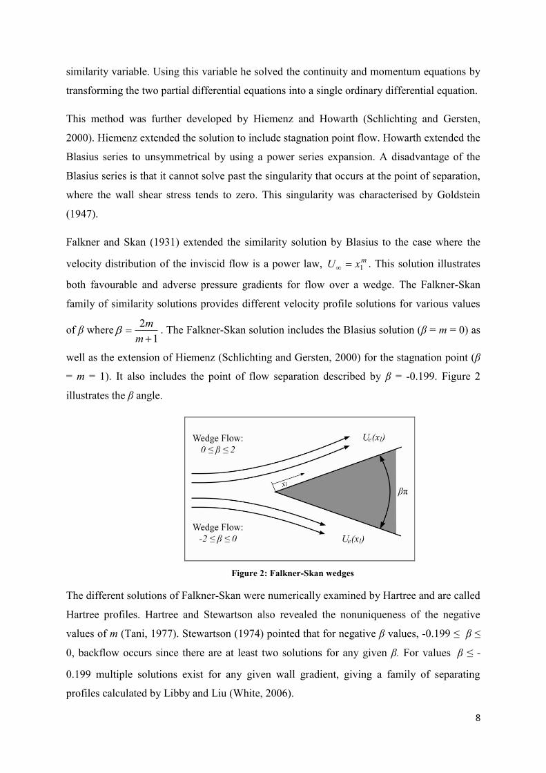
Falkner and Skan (1931) extended the similarity solution by Blasius to the case where the

velocity distribution of the inviscid flow is a power law, mxU 1 . This solution illustrates

both favourable and adverse pressure gradients for flow over a wedge. The Falkner-Skan

family of similarity solutions provides different velocity profile solutions for various values

of β where1

2

m

m . The Falkner-Skan solution includes the Blasius solution (β = m = 0) as

well as the extension of Hiemenz (Schlichting and Gersten, 2000) for the stagnation point (β

= m = 1). It also includes the point of flow separation described by β = -0.199. Figure 2

illustrates the β angle.

Figure 2: Falkner-Skan wedges

The different solutions of Falkner-Skan were numerically examined by Hartree and are called

Hartree profiles. Hartree and Stewartson also revealed the nonuniqueness of the negative

values of m (Tani, 1977). Stewartson (1974) pointed that for negative β values, -0.199 ≤ β ≤

0, backflow occurs since there are at least two solutions for any given β. For values β ≤ -

0.199 multiple solutions exist for any given wall gradient, giving a family of separating

profiles calculated by Libby and Liu (White, 2006).

9

The numerical investigations of Hartree, Leigh and Terrill show that integration cannot be

carried out past the separation point, further demonstrating the existence of the singularity

(White, 2006). Further, all of the above work is typically limited to non-curved surfaces. In

the case of airfoils, for example, numerical solution is to be sought.

2.1.2 Numerical solutions of the boundary layer equations Integral methods

In practical applications, an approximate solution of the boundary layer equations is usually

sufficient. Integral methods provide such an approximation. Von Karman and Pohlhausen

(Katz and Plotkin, 2001) were the first to introduce the integral method. Von Karman

proposed the momentum integral equation, obtained by integrating the momentum equation

across the boundary layer. The remaining independent variables, therefore, are parallel to the

wall. Pohlhausen applied this method to several cases using a fourth-order polynomial for

the velocity distribution to develop a set of solutions including the effect of the pressure

gradient inside the boundary layer.

In retarded flow regions, the approximation of Pohlhausen has less satisfactory results, for

which Thwaites (Katz and Plotkin, 2001) suggested a different approximation from

integrating the momentum integral equation. This method improves the original idea of

Holstein and Bohlen (Katz and Plotkin, 2001), rewriting the momentum integral equation in

terms of a better parameter. Thwaites looked at the entire collection of known analytical and

experimental results to see if they could be fit by a set of averaged one-parameter functions.

An integral formulation of the boundary layer equations is used when coupling viscous-

inviscid interactive flows. This is discussed in Section 2.3. Although the boundary layer

equations are simpler to solve than the complete Navier-Stokes equations, they are still non-

linear and thus pose some numerical difficulties. Special care is needed in regions where

singularities occur, such as in the neighbourhood of the trailing edge and separation regions.

Differential methods

There are several numerical methods for solving the boundary layer equations in differential

form. The Crank-Nicolson (Burden and Faires, 2005) and Keller box methods (Hirsch, 2001)

are the most convenient ones. Of the two, the Keller box method has significant advantages

over the other for two-dimensional boundary layer flows. Neither of these methods were

10

specifically designed to solve the boundary but were found to have the appropriate qualities

to do so accurately.

The box scheme, which is an implicit method with second-order accuracy, involves

transforming the momentum equation. Instead of it being a second-order partial differential

equation, it transforms into two first-order partial differential equations. This allows all the

derivatives in the boundary layer equations to be approximated by simple centred differences

(Keller, 1978) and two-point averages, using only values at the corners of the box. The box

scheme is a flexible numerical method and can solve cases in inverse flow as well as in

separation.

The use of differential methods is similar to solving the full Navier-Stokes equations in the

sense that they also require small grid spacing normal to the boundary to maintain

computational accuracy. In comparison with the integral methods, they are more general and

accurate but computationally more expensive (Cebeci and Cousteix, 2005).

2.1.3 Strong interaction and flow separation Similarity solutions (Falkner-Skan) and approximate solutions using an integral version of

the boundary layer momentum equation were discussed in the previous two sections. It was

briefly mentioned that Goldstein (1947) analytically showed that a singularity is present at

the trailing edge and that the boundary layer could not be integrated into the wake. The

source of this difficulty is the discontinuity in the boundary condition at the trailing edge

where shear stress approaches zero. Goldstein also pointed out that the pressure distribution

around the separation point must satisfy conditions associated with the existence of reverse

flow downstream of separation.

The trailing edge is a stagnant point in the inviscid flow. The solution shows a steep decrease

in surface speed as the trailing edge is approached, which corresponds to the sharp increase in

pressure. The strong adverse pressure gradient in the neighbourhood of the trailing edge will

lead to flow separation upstream of the edge. It appears that even in cases of flow without

separation (attached flow), the boundary layer equations cannot be integrated beyond a

trailing edge (Katz and Plotkin, 2001).

Goldstein (1947) derived a solution for the development of the near wake close to the trailing

edge of a finite flat plate. However, this solution did not provide details in the neighbourhood

of the trailing edge. Stewartson (1968) and Messiter (1970) independently derived a local

11

solution that provided the bridge between the Blasius solution upstream of the trailing edge

and the Goldstein near-wake solution downstream of the edge. Originally, this singularity

was thought to mean that Prandtl‟s boundary layer equations were invalid at these points,

however, Brown and Stewartson (1969) showed that a regular solution of the boundary layer

equations is possible in the vicinity of the singularity, if the pressure and outer flow velocity

are not prescribed in advance.

In the vicinity of these singularities, the boundary layer interacts strongly with the outer flow.

The structure of the flow field changes in these cases. Instead of the usual division between

inviscid flow and the boundary layer flow, there exists a three-layer hierarchical structure

referred to as „triple-deck theory‟ or asymptotic interaction theory (Stewartson, 1974). The

boundary layer here is divided into two further layers. The triple-deck theory replaces

Prandtl‟s theory near singular points. This analytical solution provides the displacement

interaction by an asymptotic matching of flows in three layers starting at the plate.

The methods of Thwaites and Pohlhausen, mentioned earlier, tie the local profile shape to the

local pressure gradient, making these one-equation integral methods unsuitable for flows with

strong interaction. The two-integral method developed by Drela (1985) eliminates this direct

link between profile shape and pressure gradient, improving the one-integral methods by

achieving treatment of strong interactive flow. However, the equations are still singular at

separation if an out-of-boundary layer velocity is specified. Interactive methods to

circumvent this are discussed in Section 2.3.

2.2 Out-of-boundary region (inviscid) Inviscid flow is characterised by the fact that there exist only normal pressure forces, but no

tangential shear forces between the adjacent layers of flow. Inviscid flow exists away from

the wall: this does not, however, mean that there is no viscosity in these regions – it merely

means that the effects of viscosity are negligible. These effects are small because the velocity

gradient is small and this then makes the viscous forces 22

2

xu

negligible compared with

the inertial forces, which are of the order of LU e

2

, where L is the characteristic length of the

wall.

12

2.2.1 Summary of numerical approaches for inviscid flow equations Navier-Stokes equations The full system of the time-dependent Navier-Stokes equations provides the most general

description of inviscid flow regions, but at the greatest computational expense.

Euler equations

The Euler equations describe the most general simplified version of the Navier-Stokes

equations, where all the shear stress and heat conduction terms are neglected. Prandtl‟s

boundary analysis shows that this is a valid approximation for flows at high Reynolds

numbers outside viscous regions, which develop near solid surfaces. This is because

convective effects essentially dominate flow here (Hirsch, 1995).

Euler codes are well established and can be enhanced by coupling to boundary layer

solutions. Szmelter (2001) uses an inviscid-viscid coupling with Euler flow to optimise

aerodynamic wings in viscous flow. It was also used by Jie and Zhou (2007) to determine

transonic flow over complex three-dimensional aircraft configurations.

Potential flow model The simplest inviscid approximation is that of the full potential model developed by Laplace

and Green (Hirsch, 1995). The basic assumption of the existence of a potential inviscid flow

is the condition of irrotationality, which is the condition of vanishing vorticity vector. The

potential flow model can accurately predict viscous regions when coupled to the boundary

layer equations, using an interactive approach. This model is useful for subsonic, low

transonic and fully supersonic regimes, but outside this range, the Euler equations are

advocated for the computation of inviscid flows.

Interactive approaches using the full potential flow model are those of Veldman (1981), Drela

(1985), Wolles and Hoeijmakers (1998), Sekar and Laschka (2005) and Riziotis and

Voutsinas (2008) to name a few. Each of these researchers used the full-potential inviscid

formulation coupled to a boundary layer (viscous) formulation to evaluate various

aerodynamic flow aspects, for example, viscous flow around an airfoil with separation,

dynamic stall and transonic dips of airfoils.

13

2.3 Viscid-inviscid coupling The so-called „viscid-inviscid interaction technique‟ has been applied to find an approximate

solution of the Navier-Stokes equations by solving a boundary layer model coupled to an

inviscid model.

Weak interaction

In design, it is common to obtain the pressure distribution about aerodynamic bodies from an

inviscid flow solution. The inviscid flow solution then provides the edge velocity distribution

needed as a boundary condition for solving the boundary layer equation to obtain the viscous

drag on the body. The interaction between the two models is accomplished using the

following procedure (Wolles and Hoeijmakers, 1998):

1. The displacement thickness is obtained by the boundary layer equations and is set as the

boundary condition of the inviscid flow.

2. The displacement that the boundary layer causes induces a reaction on the outer flow,

which then changes correspondingly.

3. This change then has a reaction on the boundary layer again; therefore, there is an

interaction between the boundary layer and the outer flow.

4. The viscous-inviscid interaction procedure continues iteratively until the change is

relatively small. In practice, however, convergence is obtained by severe under-relaxation

of the changes from one iterative cycle to another (Tannehill et al., 1997).

Strong interaction

It was stated in Section 2.1 that for the limiting regions of separation and in the

neighbourhood of the trailing edge, the boundary layer assumptions remain valid only if

pressure and external velocity are not specified. In these regions, the flow exhibits strong

interaction, and the weak interaction method described above will not converge. Instead, the

boundary layer must be solved in inverse mode, meaning external velocity is not specified, by

coupling the viscous and inviscid flows more tightly.

The inverse method was first developed by Catherall and Mangler (1966), who were the first

to integrate the boundary layer equations through a separation point. In their method, the

displacement thickness is prescribed as a boundary condition at the boundary layer edge as a

function along the surface to solve the pressure field. Using this technique, they could

integrate the boundary layer equations without encountering any numerical difficulties.

14

One problem associated with the inverse technique is the lack of prior knowledge of the

displacement thickness. This value must be obtained from solving the overall interactive

method between the inviscid and boundary layer flow. Interactive approaches are therefore

useful with separating flow where points of separation from the boundary occur. The next

section discusses methods used to overcome this difficulty.

2.3.1 Interactive boundary layer modelling techniques To avoid singularities for a viscid-inviscid interaction method, the correct treatment of the

interaction rather than an adaptation of the boundary layer model itself is required. There are

three basic approaches to solve the viscid-inviscid interaction problem.

In the quasi-simultaneous method of Veldman (1981), an interactive law, which models outer

flow, is solved simultaneously with the boundary layer equations. In this approach, the

external velocity and displacement thickness are treated as unknown quantities. While the

interactive law is only a simplified model for the outer flow, the true solution can then be

obtained through iterative refinement. The blowing velocity or transpiration velocity is then

used to simulate the boundary layer in this region.

The quasi-simultaneous method was designed using properties of the triple-deck structure. It

overcomes the Goldstein singularity by instantaneously informing the boundary layer of the

effect the changes in the boundary layer have on the inviscid solver. The interactive law is

then solved simultaneously with the boundary layer equations. Veldman (2009) analyses the

properties this interactive law ideally has. Coenen (2001) and Cebeci and Cousteix (2005)

employ the quasi-simultaneous method to model flow over two- and three-dimensional airfoil

and wing flows.

Secondly, semi-inverse methods were developed by Carter (1979) and Le Balleur (1983),

where coupling between inner and outer flow is achieved through a relaxation formula which

successively updates the displacement thickness distribution. In this method, the boundary

layer is solved in reverse, i.e. for a given displacement thickness, the velocity distribution at

the edge of the boundary layer, is computed. By then comparing this computed velocity with

the target distribution imposed by the inviscid flow, a relaxation formula is used to obtain

new estimates for the displacement thickness (Cebeci, 1999; Lagree, 2009).

15

The interactive solver of Szmelter (2001) uses the semi-inverse method of Le Balleur (1983)

to improve numerical stability. Jie and Zhou (2007) also used the semi-inverse method but

with a different relaxation formula by Carter (Veldman, 2009).

The fully simultaneous method of Drela and Giles (1987b), eliminates this sequential solution

of equations. Instead of solving the viscid and inviscid flow using an approximate interactive

law, the entire non-linear equation set is solved simultaneously as a coupled system using a

global Newton method. Drela developed the XFOIL code (Drela and Youngren, 2001) to

solve the interactive flow. This package has been thoroughly verified and validated for

different practical airfoil problems. The results obtained in this dissertation will be compared

with results obtained from the XFOIL 6.9 package.

Wolles and Hoeijmakers (1998), Sekar and Laschka (2005), Riziotis and Voutsinas (2008)

are some of the authors to have used the interactive method of Drela (1985). The fully

simultaneous method is more robust than the iterative methods. However, the quasi-

simultaneous method is simpler to implement and computationally less expensive. Also, the

quasi-simultaneous method has been shown to outperform the semi-inverse method in terms

of convergence speed (Lock and Williams, 1987). In this study, therefore, the methodology

which is proposed to overcome the singularity is based on the quasi-simultaneous philosophy.

That is, the approach taken is to solve an additional velocity equation along with the

displacement thickness, which while circumventing the singularity avoids the need to solve

the entire inviscid flow domain simultaneously.

2.3.2 Boundary conditions The boundary condition describing the displacement effect contains the information required

by the inviscid solver. This information is passed from the viscous solver to the inviscid

solver by one of two boundary conditions proposed by Lighthill (1958), namely the

transpiration velocity condition or the “solid” displacement surface condition. Both these

conditions require the real flow in the inviscid region to be replaced by an equivalent

fictitious inviscid flow to incorporate the viscous effects. It is done in such a manner that the

velocity components at the edge of the boundary layer are equal in both cases (Cebeci, 1999).

16

Figure 3: Equivalent fictitious flow, (a) “solid” displacement, (b) transpiration velocity condition

The transpiration condition of non-zero normal velocity at the surface, is based on the

concept that the displacement surface can be formed by distributing a blowing or suction

velocity on the body surface. The strength of the blowing or suction velocity bU ,2 is

determined from the boundary layer solutions according to

*,1

1,2 eb U

dxdU

where x1 is the surface distance along the body and δ* is the boundary displacement

thickness. The variation of bU ,2 on the body surface simulates the viscous effects in the

potential flow solution (Cebeci and Cousteix, 2005). A graphical representation can be seen

in Figure 3(b).

The “solid” displacement boundary condition displaces the inviscid flow by a distance equal

to the displacement thickness δ* formed by the boundary layer effects. The displacement

distance away from the surface represents the deficiency of mass with the boundary layer

(Cebeci and Cousteix, 2005). Figure 3(a) shows a graphical interpretation of this boundary

condition.

Historically, the transpiration model has been preferred. One reason cited for the use of the

transpiration condition is that the displacement model involves regridding the inviscid flow

field, making it computationally expensive. However, moving the mesh will have the same

effect without the necessity of regridding the inviscid flow field. Among the researchers who

used the transpiration condition are Veldman (1981), Szmelter (2001), Jie and Zhou (2007)

and Riziotis and Voutsinas (2008).

17

Wolles and Hoeijmakers (1998) developed a unique way to discretise the transpiration

velocity boundary condition, based on Hermite polynomial-interpolations, in their coupling

of the viscid-inviscid flow scheme to overcome numerical instabilities.

The displacement method has only been used in a few cases to model separation bubbles by

Gleyzes et al. (1985) and by Hafez et al. (1991) who modeled flow using a finite element

interactive method. To the author‟s knowledge, a displacement method by moving the mesh

has not been used in research until now.

The mesh movement algorithm used in this study is considered more physically realistic

since it avoids the addition of spurious mass into the system by the fictitious transpiration

velocity. It also avoids the complexity of calculating the effective blowing velocity necessary

to simulate the boundary layer. While it does add extra complexity in the need for a mesh

movement algorithm, many CFD solvers have this functionality built in anyway.

18

CHAPTER 3

MATHEMATICAL MODELLING

3.1 Introduction As seen in Chapter 2, finding exact solutions for the Navier-Stokes equations is generally

extremely difficult. The difficulty of solving the Navier-Stokes equations numerically

increases as the Reynolds number increases. However, in limiting cases of high Reynolds

numbers, where non-linear inertial terms vanish in a natural way, the Navier-Stokes equations

are considerably simplified. However, this limiting solution does not satisfy the no-slip

boundary condition at the surface. Therefore, to satisfy this condition, viscosity has to be

taken into account (Schlichting and Gersten, 2000).

Even though the boundary layer equations are considerably simpler and computationally less

expensive compared with the Navier-Stokes equations, their non-linearity still makes them

difficult to solve and causes methods such as super-positioning, which works well to solve

inviscid, incompressible, potential flow, to fail. Therefore the boundary lay will be solved

with the boundary layer equations and the out-of-boundary flow will be solved with the

inviscid Euler equations.

3.2 Conservation equations The fundamentals of fluid mechanics are described by the three conservation equations for

mass, momentum and energy. There are certain assumptions made about the fluid in order to

formulate these equations. The fluid is considered as a continuum, which means the smallest

19

volume element δV is still homogeneous. This, in turn, means that the dimensions of δV are

still very large when compared to the average distance between the molecules in the fluid.

The fluid is also assumed to be a Newtonian fluid, which means that a linear relationship

exists between the stress tensor and the rate of deformation tensor.

The resulting equations are:

Continuity

0

j

j

uxt [3.1]

Conservation of momentum (Newton’s second law)

ij

k

k

i

j

j

i

ji

iji

ji x

uxu

xu

xf

xpuu

xu

t

32

[3.2]

Conservation of energy (First law of thermodynamics)

j

iij

k

k

i

j

j

i

jj xu

xu

xu

xu

xTk

xDtDp

DtDh

32

[3.3]

The conservation laws for the three basic flow quantities, ρ, ρu and ρh are referred to as the

Navier-Stokes equations. These fundamentals may be used to calculate all flow properties

and characteristics over any object. They are also the core of the boundary layer equations.

3.3 Governing equations for inviscid (out-of-boundary layer) flows

With the inviscid flow approximation, the continuity equation [3.1] remains unchanged.

Neglecting viscosity, the Navier-Stokes equations reduce to the time-dependent Euler

equations:

0

iji

ji x

puux

ut

[3.4]

For a steady flow with no body forces, the Euler equations are reduced to:

i

jij x

puux

[3.5]

These equations are compressible and can be reduced to represent steady incompressible flow

when the density ρ is constant. Some of the terms within the momentum equation will be

neglected to simplify the boundary layer equations further for steady incompressible two-

dimensional laminar flow. The steady condition means that the flow is not dependent on time

20

and the incompressibility conditions mean that density and viscosity are constant. Under

these assumptions, the continuity equation reduces to:

02

2

1

1

xu

xu [3.6]

Here, u1 and u2 are the streamwise and normal velocity components, respectively. These

equations may be solved as described in Chapter 4.

3.4 Governing equations for boundary layer flow The boundary layer equations are a reduced form of the Navier-Stokes equations. Two length

scales are introduced near the wall, L, parallel to the wall, representing the length of the body

and δ, normal to the wall, representing the boundary layer thickness. The reduction occurs

based on the premise that the length scale δ is much smaller than L: δ L.

It has already been stated that the higher the Reynolds number, the thinner the boundary

layer, i.e. that boundary layer thickness will decrease with decrease in viscosity. The

boundary layer thickness is proportional to the square root of the kinematic viscosity, νδ~ .

Using this relation with the free-stream velocity U and characteristic length of the body L,

the dimensionally correct representation is obtained:

Re1~

L with

LURe [3.7]

The relationship shown in equation [3.7] shows that the larger the Reynolds number

becomes, the smaller the boundary layer thickness as compared with the characteristic length

of the body.

When considering flow over a flat plate (with plate normal in x2-direction), the Navier-Stokes

equation in the x1-direction is further reduced by noting that the second derivative of the

velocity component in the streamwise direction, 21

22

xu

, is negligible compared with the

corresponding derivative transverse to the main flow direction, 22

12

xu

.

The momentum equation then reduces to:

22

12

12

12

1

11

1xuv

xp

xuu

xuu

for the x1-direction. [3.8]

Typically to high Reynolds number flows, buoyancy effects within the flow do not contribute

to the acceleration of the flow in the x2-direction. The pressure gradient in the x2-direction is

21

then nearly zero, being only affected by these terms. For this reason, in the boundary layer

equations, the transverse pressure gradient is negligible, following as equation [3.9] (White,

2006):

02

xp for the x2-direction. [3.9]

Prandtl showed that pressure must be treated as a known variable in the boundary layer

analysis with 1xp assumed to be imposed on the boundary layer from an inviscid outer flow

analysis. That is, the free--stream outside the boundary layer, 1xUU ee , where x1 is the

coordinate parallel to the wall, is related to 1xp by Bernoulli‟s theorem for incompressible

flow (White, 2006).

Equation [3.9] states that pressure across the boundary, normal to the surface, is constant. It is

for this reason that the pressure is taken to be the inviscid pressure evaluated on the surface.

Application of the momentum equation [3.8] on the outer edge of the boundary is represented

as

11

11

1xp

xxUxU e

e

[3.10]

This equation can be substituted into equation [3.8], resulting in the pressure no longer being

unknown.

The following initial conditions apply to the boundary layer theory:

202

20,222

20,121

,0,0,0

xxxuxuxuxu

[3.11]

where denotes the shear stress in the x1-direction: 2

1

xuv

. [3.12]

The equations are subject to the boundary conditions:

1,111 0, xuxu w Wall motion [3.13]

1,212 0, xuxu w Mass flux [3.14]

11,211 , xUxxxu ee [3.15]

Here, u1,w(x1) simulates wall motion, u2,w(x1) simulates a mass flux (blowing) into the

boundary layer, ex ,2 denotes the „edge‟ of the boundary layer and Ue(x1) is the free-stream

velocity.

22

This set of equations can be solved exactly using similarity solutions, however, this is only

possible for simple geometries. Otherwise the equations have to be solved numerically using

the integral method for more complex flow problems. The numerical scheme that will be

developed for this study will, however, be tested against the similarity solutions for the flat,

inclined plates and a generated XFOIL solution for a NACA0012 airfoil.

3.5 Integral methods The integral solution of the boundary layer solutions is attributed to Von Karman. The

momentum integral method is a second method used to approximate the boundary layer

problem. Although it is an approximation solution, it does not depend on the similarity

assumption and it allows for significant changes in the shape of the boundary layer velocity

profile. Consequently, this method can be extended to any flow regime with complex

geometries and includes effects such as transition and separation (Katz and Plotkin, 2001).

The integral solution serves many engineering applications where it is not necessary to know

details of flow variables inside the boundary layer. For example, in the case of design

analysis, only the wall shear stress is needed to calculate the drag force on the surface and the

displacement thickness to allow for coupling with outer flow.

For a derivation of the integral momentum equation, consider Prandtl‟s boundary layer

equations [3.7] and [3.8]. Integrating equation [3.8] with respect to x2, from the wall, x2 = 0,

up to the boundary thickness, x2 = δ, transforms the equation into an ordinary differential

equation, known as the Von Karman integral momentum equation.

20 22

12

0 21

0 22

1220

1

11

1 dxxuvdx

xpdx

xuudx

xuu

[3.16]

Keeping in mind that x2 = δ in the boundary layer and that 2

1x

u

can be neglected as stated

before to obtain equation [3.8], and using the continuity equation to replace the derivatives of

u2 with those of u1, the equation [3.16] is reduced to:

we dx

dpdxudxdUdxu

dxd

1

0 211

20

21

1

1 [3.17]

where 02

1

2

xw x

u which is the wall shear stress.

23

This equation is further simplified by eliminating the pressure term 1

1dxdp

as per equation

[3.10]. Then using the momentum equations outside the boundary layer and rearranging the

terms, the following is obtained:

we

ee dxuU

dxdUdxuuU

dxd

0 211

20 111

[3.18]

where the nomenclature is as defined previously.

3.5.1 Two-equation integral boundary layer equations There are two very important requirements when formulating the two-equation integral

boundary layer equations. First, the type of viscous formulation employed in design analysis

has to have the capability of representing flow accurately within separation regions.

Secondly, the laminar and turbulent formulations must be compatible. It was with these

requirements in mind that the two-equation integral formulation based on dissipation closure

was developed for both laminar and turbulent flows (Drela and Giles, 1987a).

Drela and Giles substituted equations for momentum and displacement thickness into the

momentum integral equation [3.18] to obtain the momentum integral equation in terms of

momentum and displacement thickness. This method is referred to as the „two-integral

method‟. These equations can also be solved by using a variety of numerical schemes to

obtain approximations of the real solution.

The momentum and displacement thicknesses θ and * , and the skin friction coefficient Cf

are defined as follows:

d

Uu

Uu

ee

0

1 [3.19]

d

Uu

e

0

* 1 [3.20]

wee

f UC

2

2 [3.21]

where η denotes the similarity variable 21

Rexx .

Substituting these equations into equation [3.18], an ordinary differential equation is

obtained, which contains two-integral quantities: momentum thickness and boundary layer

24

thickness. Using the shape factor H, the friction coefficient Cf and Me as the edge Mach

number, a dimensionless version of the integral momentum equation is obtained:

1

121

1

1 22 dx

dUUxMH

Cxdxdx e

ee

f

[3.22]

where

*

H [3.23]

If equation [3.9] is first multiplied by u and then integrated, the kinetic energy integral

equation results:

1

12*

**

*1

1

*

*1 322

dxdU

UxMCx

dxdx e

eeD

[3.24]

The kinetic energy and density thicknesses * and ** , and dissipation coefficient CD, are

defined by:

d

Uu

Uu

ee

0

2* 1 [3.25]

d

Uu

ee

0

** 1 [3.26]

duU

Cee

D

03

1 [3.27]

These equations contain three different shape parameters: the shape parameter H, the energy

thickness shape parameter *H , which eliminates the direct link between the H and the local

external velocity Ue, and the density thickness shape factor **H .

They are defined as follows:

*

H

** H

**** H [3.28a-c]

Using these shape parameter definitions and subtracting equation [3.22] from equation [3.24],

the momentum and kinetic energy equations can be written as:

2

21

2

1

fe

ee

CdxdU

UMH

dxd

[3.29]

2

212 *

1

***

1

*f

De

e

CHC

dxdU

UHHH

dxdH

[3.30]

The two-integral equations [3.29] and [3.30] contain three unknowns, * , θ and Cf , and

cannot be solved without additional information. The necessary information is obtained from

25

an assumed velocity profile family, a function of the Falkner-Skan solution. In principle, this

profile defines the entire boundary layer velocity field Ue = 211 , xxu , which has the same

form anywhere along the boundary layer.

Different integral boundary layer methods make different choices for the local boundary layer

thickness and the shape of the local velocity profile. Examples of these methods are that of

Pohlhausen and that proposed by Thwaites, however, these are both one-integral systems

(Katz and Plotkin, 2001). Drela suggested a different set of closure equations when using the

two-integral boundary layer method (Drela, 1985), which is discussed next.

3.5.2 Laminar closure equations The integral boundary layer equations [3.29] and [3.30] are valid for both laminar and

turbulent boundary layers, as well as for free wakes. The fundamental difficulty with these

equations is that they contain more than two independent variables. Consequently, some

assumptions about the additional unknowns are to be made to obtain a solution.

The two dependent variables are defined as momentum and displacement thickness, θ and *

. Ue and Me relate to inviscid flow and therefore do not represent additional unknowns. The

undefined variables that remain are Cf, CD, *H and **H . The following functional

dependencies are assumed (Drela and Giles, 1987a).

ek

ek

MHHHMHHH,

Re,,****

**

Re,,

Re,,

ekDD

ekff

MHCCMHCC

Hk is the kinematic shape parameter defined with density taken as constant across the

boundary layer and solely depends on the velocity profile. Hk was developed as an empirical

expression by Whitfield in terms of the conventional shape parameter and edge Mach number

as follows:

2

2

0

0

113.0129.0

1

1

e

e

ee

ek M

MH

dUu

Uu

dUu

H

[3.31]

26

This expression assumes adiabatic flow and non-unity Prandtl number of air. It is accurate up

to Me = 3 and used for both laminar and turbulent flows (Drela, 1985). This equation

simplifies to HH k for incompressible flow.

To define the shape factor correlations, the velocity profiles of the Falkner-Skan solution

were used to carry out the numerical integration of the four length scales [3.19, 20] and [3.25,

26] to obtain analytical expressions of [3.28a-c]. This was done in order to reduce

computational cost associated with integration of the length scales at each x1 location

(Whitfield, 1978). For laminar flow, Drela used a finite differencing method to solve the

Falkner-Skan equations with prescribed shape parameter to obtain the following curve fits,

referred to as „laminar closure equations‟.

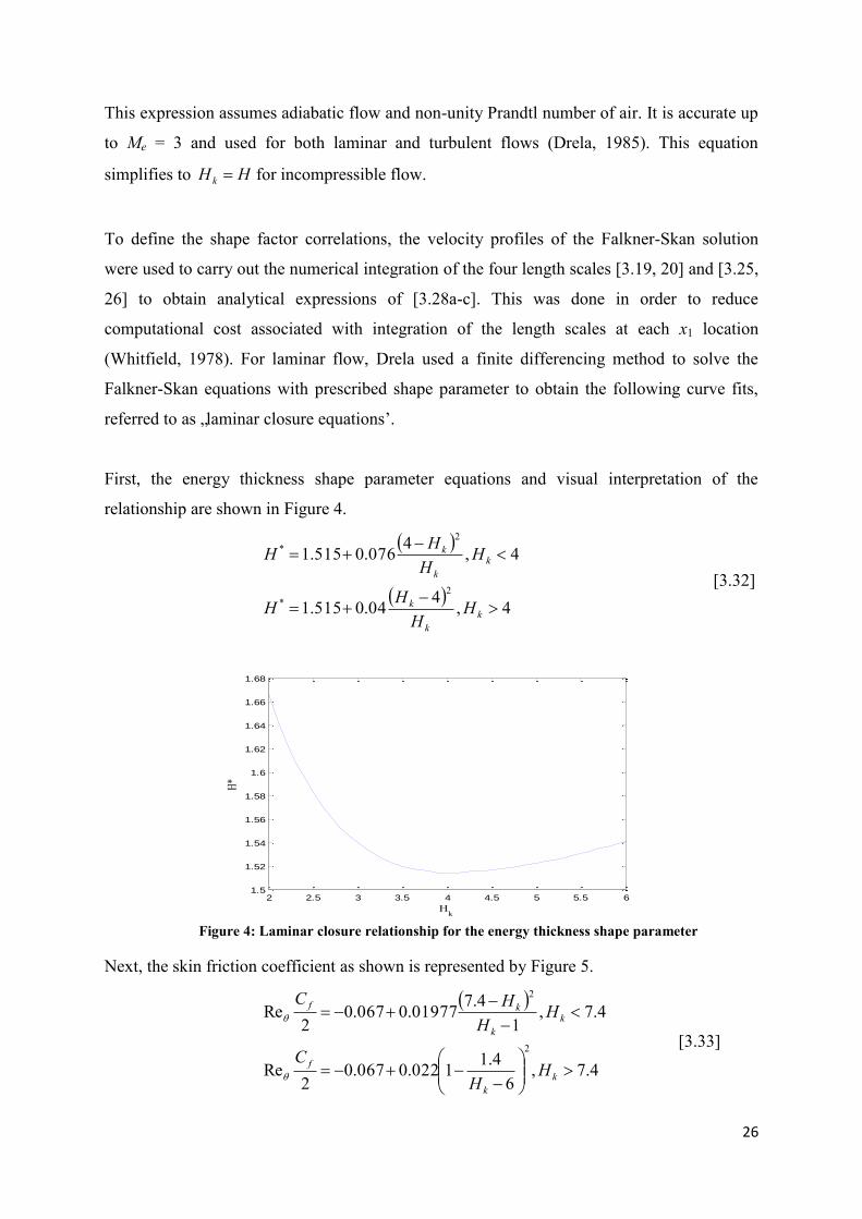
First, the energy thickness shape parameter equations and visual interpretation of the

relationship are shown in Figure 4.

4,404.0515.1

4,4076.0515.1

2*

2*

kk

k

kk

k

HH

HH

HHHH

[3.32]

Figure 4: Laminar closure relationship for the energy thickness shape parameter

Next, the skin friction coefficient as shown is represented by Figure 5.

4.7,6

4.11022.0067.02

Re

4.7,1

4.701977.0067.02

Re

2

2

kk

f

kk

kf

HH

C

HH

HC

[3.33]

2 2.5 3 3.5 4 4.5 5 5.5 61.5

1.52

1.54

1.56

1.58

1.6

1.62

1.64

1.66

1.68

H*

Hk

27

Figure 5: Laminar closure relationship for the skin friction coefficient

Last, the dissipation coefficient as shown below is given in Figure 6:

4,402.01

4003.0207.02Re

4,400205.0207.02Re

2

2

*

5.5*

kk

kD

kkD

HH

HHC

HHHC

[3.34]

Figure 6: Laminar closure relationship for the dissipation coefficient

The density thickness **H is derived by Whitfield and is defined as follows:

2** 251.08.0

064.0e

k

MH

H

[3.35]

This shape parameter is negligible for low subsonic flows and has only a small effect on

transonic flows (Drela, 1985). It is important to note the function shape of the closure

2 2.5 3 3.5 4 4.5 5 5.5 6-0.1

0

0.1

0.2

0.3

0.4

0.5

0.6

C fRe/2

Hk

2 2.5 3 3.5 4 4.5 5 5.5 60.18

0.2

0.22

0.24

0.26

0.28

0.3

2CdRe

/H*

Hk

28

equations [3.32 – 3.34]. They are smooth without discontinuities, which means numerically,

these functions will not cause any computational instabilities.

The level of accuracy of these correlations is a consequence of the fact that almost any

laminar velocity profile is very similar to the Falkner-Skan profile. This is true for measured

as well as computed solutions. This makes the empirical equations [3.32 – 3.34] very

accurate for all flows, especially in the incompressible case.

The integral boundary layer equations, after being simplified to two-dimensional steady

incompressible laminar flow are:

2

211

fe

e

CdxdU

UH

dxd

[3.36]

2

21 *

1

*

1

*f

De

e

CHC

dxdU

UHH

dxdH

[3.37]

For the purpose of this work, these equations will be discretised and solved by using

Newton‟s method, after which they will be connected to a solver which solves the inviscid

flow in the outer flow region.

3.5.3 Goldstein singularity The laminar closure equations reach a singularity at the point where Hk reaches 4, which is

where the function [3.32] reaches a minimum (Figure 4). This is referred to as the „Goldstein

singularity‟ at a boundary layer separation point. The vanishing derivative of *H causes a

singularity in equation [3.33], which can only be avoided if Ue adjusts to cause the rest of the

equation to tend to zero as well. Therefore, any boundary layer method with a prescribed Ue

that reaches separation will fail at this point.

This problem can be circumvented by solving the inviscid flow and boundary layer

simultaneously. Alternatively, elimination of this problem can be accomplished by allowing

the boundary layer to modify the inviscid flow solver it is interacting with by modifying Ue

via the displacement thickness. This process creates a negative feedback effect, which can

eliminate the singularity.

29

This can be achieved by assuming the boundary layer is growing on the wall of a two-

dimensional channel, which has a fixed specified total volume flow rate

V and a varying

specific height h(x1) (Drela, 2010).

The velocity can be written as

1*

11 xxhVxUe

, [3.38]

allowing the derivation of a differential equation for Ue:

*

11

*

1

hU

dxdh

dxd

dxdU

ee . [3.39]

Here, h(x1), the specific channel height, is calculated from the specified velocity by

1*

1,1 x

xUVxh estimate

spece

[3.40]

Where 1* xestimate is an estimated displacement thickness and Ue,spec is the velocity obtained

from the inviscid solution.

It is unavoidable that the final Ue will differ slightly from Ue,spec, although setting 1* xestimate

to the Blasius solution velocity distribution rather than zero can decrease this difference.

Also, although

V is an arbitrary value, it plays a role in the accuracy versus stability trade-

off. The greater the value of

V , the closer Ue will be to Ue,spec, but if it is set too high, the

Goldstein singularity is approached once again.

Equation [3.39] becomes an additional equation to solve with equations [3.36] and [3.37].

This allows the simultaneous solution of displacement thickness and velocity, circumventing

the singularity, while avoiding the need to solve the entire inviscid flow domain

simultaneously.

3.6 Chapter summary In this chapter, the general governing equations of fluid flow were presented. These equations

were used to derive the two-integral method of Drela (1985). Closure equations were derived

numerically from the similarity solutions of the Falkner-Skan equations and were discussed.

The velocity equations to overcome the Goldstein singularity that exists at the trailing edge

30

were also presented here. The solution procedure of the two-integral method will be

discussed in Chapter 4.

31

CHAPTER 4 SOLUTION PROCEDURE

4.1 Introduction The inviscid flow Euler and continuity equations [3.5 – 3.6] are solved in a two-dimensional

domain, while the boundary layer equations are solved on a one-dimensional grid. The

boundary layer equations involve coupled non-linear ordinary differential equations, which

were set up in Chapter 3 as:

11

22 dx

dUU

HC

dxd e

e

f [4.1]

1

**

1

*

12

2dxdU

UHH

CHC

dxdH e

e

fD

[4.2]

*

11

*

1

hU

dxdh

dxd

dxdU

ee [4.3]

where h is obtained as per [3.40].

Numerically solving the boundary layer equations as discussed in Chapter 3 is done as

follows:

The differencing method is selected as Crank-Nicolson for its second-order accuracy

and numerical stability.

A solution method for the system of ordinary differential equations is selected to

iteratively solve the set of non-linear equations (boundary layer equations). The

32

problem is treated as an initial value problem, solved point by point using Newton‟s

method.

The boundary layer solution is coupled with the inviscid flow solver using a mesh

movement algorithm. An under-relaxation parameter is used to ensure convergence.

The Goldstein singularity, which exists when 4H , is overcome by solving an

additional velocity equation suggested by Drela (2010).

The laminar wake, which is beyond the scope of this study, is treated with an

approximation function to simulate this region.

From equations [4.1 – 4.3], it is evident that the boundary layer equations are only solved in

the x1-direction. This is because, to obtain the Von Karman integral equations, the equations

are integrated in the x2-direction, leaving them dependent on x1 only.

For the inviscid flow, a two-dimensional domain of x1 and x2 is used to solve the complete

inviscid flow field. The one-dimensional mesh obtained to solve the boundary layer equations

is determined by the intersection between the inviscid flow mesh and the wall.

4.2 Discretisation of the integral boundary layer equations The approximate solution for the boundary equations here is obtained by solving them as an

initial value problem rather than simultaneously solving the whole complex system in one

step. Starting at a given initial value, approximations are obtained for the displacement

thickness * and momentum thickness θ. The initial starting value is obtained from the

similarity solution of Blasius for a flat plate.

There are two differential equations for the laminar incompressible flow that have to be

discretised, namely the momentum equation [4.1] and the shape parameter equation [4.2]. A

third velocity equation [4.3] is also discretised. The independent variables are * , θ and Ue.

Stepping through space by an amount 1x , the other points in the domain are solved using the

implicit Crank-Nicolson differencing method, with a non-linear equation solver such as

Newton‟s method. The Crank-Nicolson scheme is unconditionally stable while being second-

order accurate, therefore, there are no restriction on the step size and hence no restriction on

the mesh. The discretised form of the momentum equation is:

33

02

2 ,

,1

1,,

,,1

11

mf

i

ieie

me

mm

i

ii CxUU

UH

xf

, [4.4]

where Cf = Cf(Hk,Re) as given by [3.33] and the subscript m refers to a value halfway

between i and i – 1, for example, 121

21

iim .

The shape parameter equation is discretised as:

012

2,1

1,,

,

*,*,

,1

**

21

i

ieie

me

mmm

mfmmD

im x

UUU

HHC

HCx

HHf ii

, [4.5]

where Cf = Cf(Hk,Re) as given by [3.33], CD = CD(Hk,Re) as given by [3.34]. * HHk

and H** = 0 since it is incompressible attached flow.

Finally, the velocity equation, included to overcome the Goldstein singularity near the trailing

edge, is discretised as:

0

,1

1,,1

*1

**

,1

,3

i

ieieiiii

mmi

me

xUU

hhhx

Uf

, [4.6]

where h is the channel height as defined in equation [3.40].

4.3 The Newton method The Newton method is a well-established algorithm for solving non-linear scalar or vector

equations. It is fast to converge, if the initial approximation is close to the solution. Equations

[4.4 – 4.6] are solved as an initial value problem using a point-by-point local Newton method,

contrary to the method by Drela (1985), which uses a global Newton method to solve

simultaneously for all the points as well as the potential inviscid flow. Solving the equations

in this manner is much less computationally expensive since it does not solve the whole

monolithic system with each iteration. With the Newton method in this work, the exact

Jacobian matrix is determined at each iteration, by analytical differentiation of all the

governing discrete boundary layer equations [4.4 – 4.6].

The advantage of analytically determining the Jacobian matrix is that it avoids discretisation

errors, which can slow down or even stall convergence. It also saves computational effort

since the equations to be solved need only be evaluated once per iteration rather than for

every combination of equation and unknown, which is at least nine times in this case. This

produces a quadratic convergence rate, provided that a sufficiently accurate initial value is

34

known and the Jacobian inverse exists. The integral form of the boundary layer equations is

used to minimise the number of additional variables and hence the computation time.

4.3.1 The algorithm for Newton‟s method for non-linear systems To approximate the solution of a non-linear system of n unknowns, F(x) = 0, is given an

initial approximation of x, the following procedure is used:

At each step, the nn system xFyxJ is solved for y, where

j

iji x

xfxJ , for

ni 1 and nj 1 . Then x is set to x = x + y until y is sufficiently small, which then

gives x as the solution to the non-linear system.

The functional iteration procedure evolves from selecting 0x and generating

1111 kkkk xFxJxx for k = 1, 2, …, n.

4.3.2 The linear system In the present application, the vector function F referred to includes only the boundary layer

equations. These equations will be solved in the form of a linear system xFyxJ using

Gaussian elimination with partial pivoting (Burden and Faires, 2005). Gaussian elimination

with partial pivoting helps to reduce round-off errors, since it will demand that some rows

should interchange to ensure the pivot element is not zero. In larger systems, it is very

difficult to predict in advance when round-off errors can occur.

4.3.3 The Jacobian The Jacobian is defined as:

e

e

e

e

Ufff

Ufff

Ufff

UJ

33*

3

22*

2

11*

1

* ,,

where 1f , 2f and 3f are defined in equations [4.4 – 4.6].

The values in the Jacobian are as follows:

35

i

ieie

me

mf

xUU

UCf

,1

1,,

,*,

*1 1

21

41

[4.7]

i

ieie

me

mf

i xUU

UC

xf

,1

1,,

,

,

,1

1 1411

[4.8]

21,,

1,*

,1

,1 2441

ieie

iemm

ie

mf

e UUU

xUC

Uf

[4.9]

*

*,

*,

*

*,

*

*

,1*

2

442

mmfmfmmDm

i

m HCCHCHx

f

i

mmm

i

m

iee

eie

xH

xH

UUUU

i

i

,1

**

,1*

*

1,,

,, 11

[4.10]

*,,

*,

*

,1,1

*1

*2

442mmfmfmmDm

i

m

i

ii HCCHCHxx

HHf

i

mmm

i

m

iee

eie

xH

xH

UUUU

i

i

,1

**

,1

*

1,,

,,

211

[4.11]

21,,

*

,1

*,

*,2 14

4 ieie

emm

i

m

e

mfm

e

mD

e UUU

xH

UCH

UC

Uf i [4.12]

*,1

,1

*1

*2*

,1

,*

3

2 mmi

meiiii

mmi

me

hxU

hhhx

Uf

[4.13]

03

f [4.14]

iiiii

mmie xhh

hxUf

,11

*1

**

,1

3 12

1

[4.15]

The terms within the Jacobian depend on the shape parameter correlations [3.32 – 3.34], for

Cf, CD and *H . These derivatives were obtained analytically to ensure robustness and

efficiency of the overall system. The latter differs from other work.

36

4.3.4 Initial condition The local Newton method solved point by point needs an appropriate initial value to

converge. In addition, an initial value is needed for the Crank-Nicolson method and the

logical choice of zero cannot be used since fC and DC are singular there.

The initial value for displacement thickness * and momentum thickness are set according

to the similarity solution of Blasius (Drela, 1985). These are:

eUx1* 7208.1

[4.16]

eUx1664.0

[4.17]

The initial values obtained from this function are a sufficiently close approximation to solve

most boundary layer solutions (Drela, 1985). The value of 1x is set at the smallest value

possible to ensure convergence, while eU is set to the velocity at the first point.

The initial value for eU is set at speceU , , which is obtained from the inviscid solver. The

velocity function [4.3] is not used away from the singularity; instead eU is set equal to speceU ,

for 5.2H after which the velocity equation [4.3] is used to solve for eU .

4.4 Inviscid flow solver The flow solver is based on the Artificial-Compressibility Characteristic-Based split (CBS-

AC) scheme (Nithiarasu, 2003; Malan, Lewis and Nithiarasu, 2002; Malan and Lewis, 2011),

which is based on the original Chorin split and has similarities with other projection schemes

widely employed in incompressible flow calculation. Discretisation along characteristics and

a pressure-Poisson equation ensure a stable scheme. It can solve both compressible and

incompressible flows using a unified approach.

The scheme essentially contains three steps. In the first step, the intermediate velocity field is

established. In the second step, the pressure is obtained from a projected continuity equation.

Finally, the intermediate velocities are corrected to get the final velocity values. Any

additional scalar equation, such as temperature and concentration, can be added as a fourth

step.

37

The three steps of the CBS-AC algorithm can be written as:

Step 1: Intermediate momentum

n

ijjk

kj

ijij

j

niii Uu

xxut

xUu

xtUUU

2Re1~~

[4.18]

Where nini tUU , nn ttt 1 and ~ indicates an intermediate quantity. Further, t and n

respectively denote pseudo-solution time and iteration number. The higher-order term is due

to time discretisation using the characteristic concept and serves to stabilise the convective

term. Viscous terms are included although they are negligible for inviscid flow and the flow

solver is not required to resolve the boundary layer.

Step 2: Density or pressure

nnnn

nn ppc

pc

1

221 11

iiii

n

i

i

i

ni

xxp

xxpt

xU

xUt

2

2

2

1

~

1 [4.19]

Step 3: Momentum correction

i

n

ini

nii x

ptUUUU

2~1

[4.20]

Where 15.0 1 and 10 2 . For the explicit scheme, 02 is employed (Nithiarasu,

2003). Due to the artificial compressibility formulation, a finite value of c2 may be used.

4.4.1 Mesh generation Before a numerical solution for a physical process can be obtained, a grid must be

constructed. The physical domain is covered with a mesh to identify discrete volumes or

elements where conservation laws can be applied. A well-constructed mesh greatly improves

the quality of the solution (Tannehill et al., 1997). Generation of grids can be either

structured or unstructured.

In the case of the boundary layer, cell spacing normal to the wall must be very fine

(proportional to Re ) in order to capture the sharp gradients in this direction. The use of a

structured scheme allows a cell shape that is elongated in the flow direction. Alternatively,

38

the use of unstructured grids, for example, triangles in a two-dimensional problem, requires a

higher cell density in the boundary layer since the cells need to be as nearly equilateral as

possible to avoid grid-induced errors in the solution (Tannehill et al., 1997).

These are typical mesh generation problems when solving the viscous effects with the

Navier-Stokes equations. However, these problems can be avoided by using boundary layer

modelling, since it does not require mesh generation at all in the boundary layer.

4.5 Mesh moving algorithm The mesh movement routine is a simple interpolation function

21 1 rr [4.21]

where

2

3

22

3

1

23

2

dd

dr [4.22]

In this case, δ is the displacement of the grid point from its original position, 1d and 2d are

the closest distances from that point to the two closest boundaries and 1 and 2 are the

displacements of those two boundary points. This might seem like a crude approach but it is

sufficient for small displacements in aerodynamic applications and is selected for its

negligible computational cost.

4.6 Coupling and interaction method The interaction method between the solver and the different routines to calculate the

boundary and move the mesh happens as follows:

First, the CFD solver lets the flow solution converge to a point where the residual is less than

the specified tolerance divided by some factor, for example, 2. This factor is simply intended

to prevent an excessive number of mesh movements as convergence is approached, since

every time the mesh is moved, the residual increases slightly. Therefore, it is desirable to

decrease the residual more than necessary to ensure that even after the mesh is moved, the

system is still converged to the required tolerance.

Second, the solver uses the boundary layer thickness obtained from the boundary layer

solution to move boundary node i as follows:

)1(*)( 1

ni

ni xnx

i [4.23]

39

Where )(nix and )1( n

ix are the new and previous displacements of node i from its original

position, * is the computed boundary layer thickness, n is a unit vector normal to the

boundary and is an under-relaxation coefficient.

Coupling of the inviscid and viscous flow requires an under-relaxation parameter to ensure

stability of the numerical system. Essentially, the under-relaxation parameter only moves the

wall coordinates a fraction of the whole movement that is needed to move to the new position

specified by the boundary layer solver. It is a number between zero and one. If it is too close

to one, stability is sacrificed, whereas when it is close to zero, the system is very stable but

takes longer to converge. Ideally, the under-relaxation parameter is set as close to one as

possible without having numerical instabilities.

Following the mesh movement step, the mesh is repreprocessed and the residual is calculated

again. If this residual is less than the convergence tolerance, the program will give the

resulting output, otherwise it restarts from the beginning, repeating the process.

Preprocessing of a mesh for a finite volume method means calculating the volumes and edge

coefficients of dual cells. When the mesh is moved, this information changes and must be

recalculated. The boundary condition required for the inviscid solver at a solid wall is the

specification of the surface streamline position. This is equal to the displacement thickness δ*

calculated by the boundary layer routine.

4.7 Laminar wake singularity The velocity equation [4.3] (the discrete version of equation [3.47]) involves the fictitious

„channel height‟ h calculated as per equation [3.40]. As stated at the end of Section 3.5.3, the

selection of a smaller value of

V in equation [3.40] is more effective at removing the

singularity, but leads to computed velocities which differ markedly from the specified values,

and hence an inaccurate solution of the displacement thickness. Larger values of

V give more

accurate solutions, but less robustness against the Goldstein singularity.

In practice, it was found that an unacceptable amount of accuracy had to be sacrificed in

order for the iterative process to be robust in all situations. For example, the early cycles of

computing the boundary layer around the airfoil, where the initially imposed velocity

distribution is the inviscid solution with a large adverse pressure gradient near the trailing

edge, are particularly problematic.

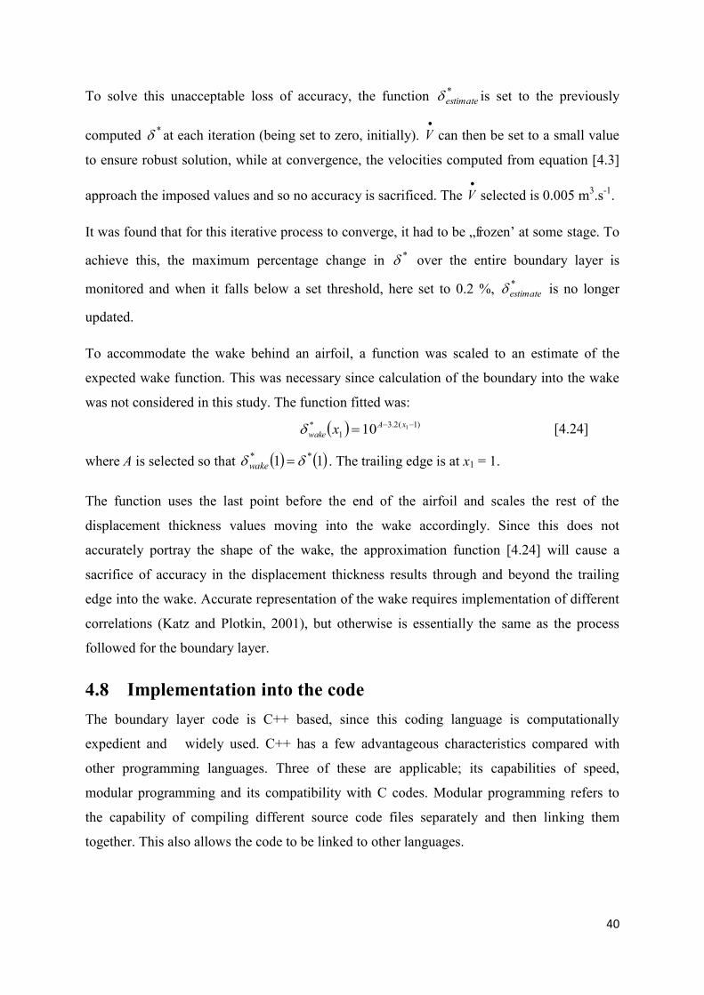
40

To solve this unacceptable loss of accuracy, the function *estimate is set to the previously

computed * at each iteration (being set to zero, initially).

V can then be set to a small value

to ensure robust solution, while at convergence, the velocities computed from equation [4.3]

approach the imposed values and so no accuracy is sacrificed. The

V selected is 0.005 m3.s-1.

It was found that for this iterative process to converge, it had to be „frozen‟ at some stage. To

achieve this, the maximum percentage change in * over the entire boundary layer is

monitored and when it falls below a set threshold, here set to 0.2 %, *estimate is no longer

updated.

To accommodate the wake behind an airfoil, a function was scaled to an estimate of the

expected wake function. This was necessary since calculation of the boundary into the wake

was not considered in this study. The function fitted was:

)1(2.31

* 110

xAwake x [4.24]

where A is selected so that 11 ** wake . The trailing edge is at x1 = 1.

The function uses the last point before the end of the airfoil and scales the rest of the

displacement thickness values moving into the wake accordingly. Since this does not

accurately portray the shape of the wake, the approximation function [4.24] will cause a

sacrifice of accuracy in the displacement thickness results through and beyond the trailing

edge into the wake. Accurate representation of the wake requires implementation of different

correlations (Katz and Plotkin, 2001), but otherwise is essentially the same as the process

followed for the boundary layer.

4.8 Implementation into the code The boundary layer code is C++ based, since this coding language is computationally

expedient and widely used. C++ has a few advantageous characteristics compared with

other programming languages. Three of these are applicable; its capabilities of speed,

modular programming and its compatibility with C codes. Modular programming refers to

the capability of compiling different source code files separately and then linking them

together. This also allows the code to be linked to other languages.

41

This approach to solve the boundary layer as a modular system, implies that it can be

integrated into any flow solver. It does not have to solve the inviscid flow together with the

boundary layer as one monolithic system. Also, the inviscid flow solver needs no knowledge

or extra parameters to understand or compute a fictitious transpiration velocity boundary

condition.

The only input the boundary layer code requires from the inviscid solver is the coordinates of

the nodes as well as the velocities at those nodes. It then calculates the displacement

thickness, auxiliary velocity and momentum thickness. The displacement thickness is then

returned to the inviscid code and used to calculate the new node point to which the mesh has

to move before the whole process starts again.

4.9 Chapter summary This chapter discussed the procedure followed to solve the boundary layer flow and the

interaction with the outer inviscid flow. The discretisation of the governing equations was

described as well as the interactive procedure by which it is coupled to the inviscid flow

solver. A local Newton method is used to solve the boundary layer flow, point by point, by

obtaining information about the velocity outside the boundary. The mesh is then moved to the

calculated boundary thickness and the process is repeated until convergence is reached. The

boundary condition at the edge of the boundary thickness is set to a slip condition. An under-

relaxation parameter ensures stability in the coupling condition. An additional velocity

equation adjusts the mesh movement to avoid the Goldstein singularity, which is encountered

before the trailing edge.

Chapter 5 follows with the results and discussion of the computational performance.

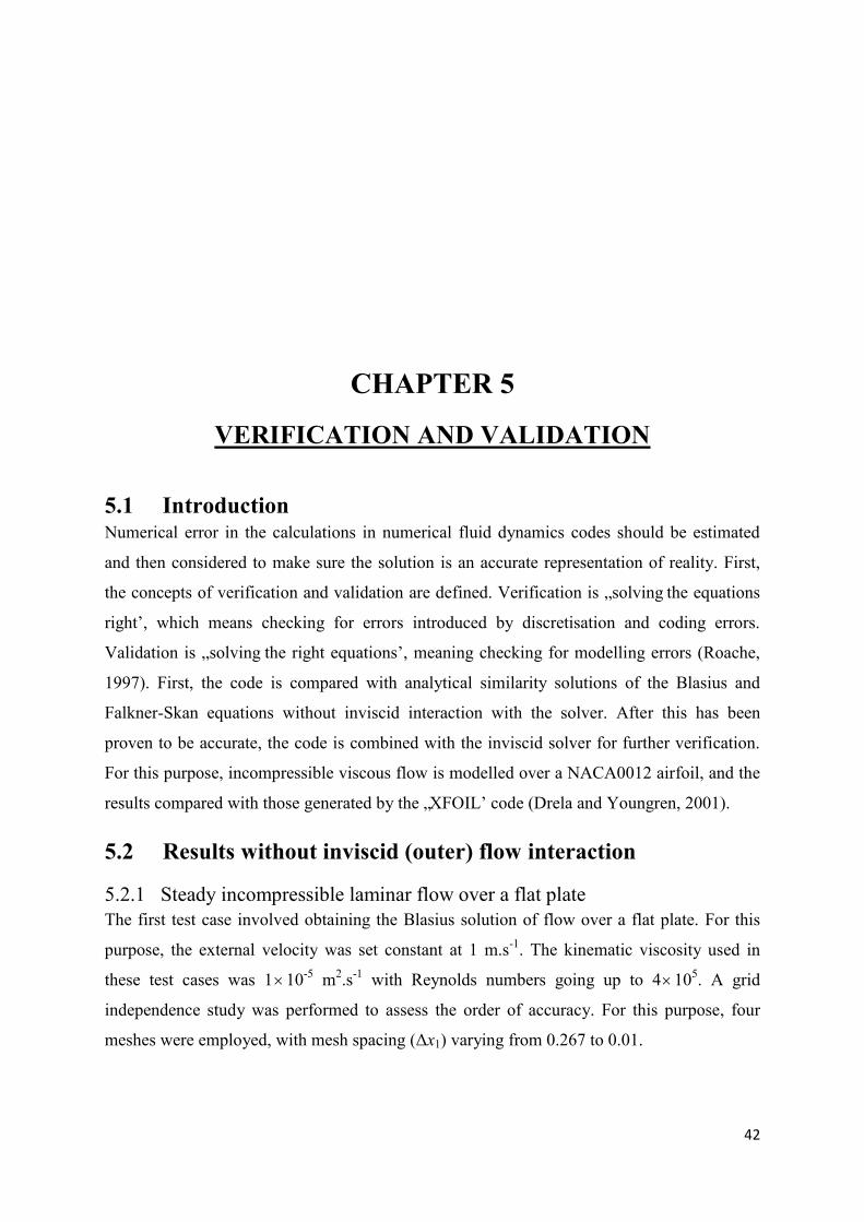
42

CHAPTER 5

VERIFICATION AND VALIDATION 5.1 Introduction Numerical error in the calculations in numerical fluid dynamics codes should be estimated

and then considered to make sure the solution is an accurate representation of reality. First,

the concepts of verification and validation are defined. Verification is „solving the equations

right‟, which means checking for errors introduced by discretisation and coding errors.

Validation is „solving the right equations‟, meaning checking for modelling errors (Roache,

1997). First, the code is compared with analytical similarity solutions of the Blasius and

Falkner-Skan equations without inviscid interaction with the solver. After this has been

proven to be accurate, the code is combined with the inviscid solver for further verification.

For this purpose, incompressible viscous flow is modelled over a NACA0012 airfoil, and the

results compared with those generated by the „XFOIL‟ code (Drela and Youngren, 2001).

5.2 Results without inviscid (outer) flow interaction

5.2.1 Steady incompressible laminar flow over a flat plate The first test case involved obtaining the Blasius solution of flow over a flat plate. For this

purpose, the external velocity was set constant at 1 m.s-1. The kinematic viscosity used in

these test cases was 110-5 m2.s-1 with Reynolds numbers going up to 4105. A grid

independence study was performed to assess the order of accuracy. For this purpose, four

meshes were employed, with mesh spacing (Δx1) varying from 0.267 to 0.01.

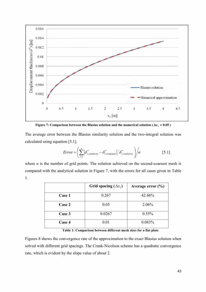
43

Figure 7: Comparison between the Blasius solution and the numerical solution ( 05.01 x )

The average error between the Blasius similarity solution and the two-integral solution was

calculated using equation [5.1].

nErrorn

isimilarityicomputedisimilarityi

1

*,

*,

*, [5.1]

where n is the number of grid points. The solution achieved on the second-coarsest mesh is

compared with the analytical solution in Figure 7, with the errors for all cases given in Table

1.

Grid spacing ( 1x ) Average error (%)

Case 1 0.267 42.46%

Case 2 0.05 2.06%

Case 3 0.0267 0.55%

Case 4 0.01 0.083%

Table 1: Comparison between different mesh sizes for a flat plate

Figures 8 shows the convergence rate of the approximation to the exact Blasius solution when

solved with different grid spacings. The Crank-Nicolson scheme has a quadratic convergence

rate, which is evident by the slope value of about 2.

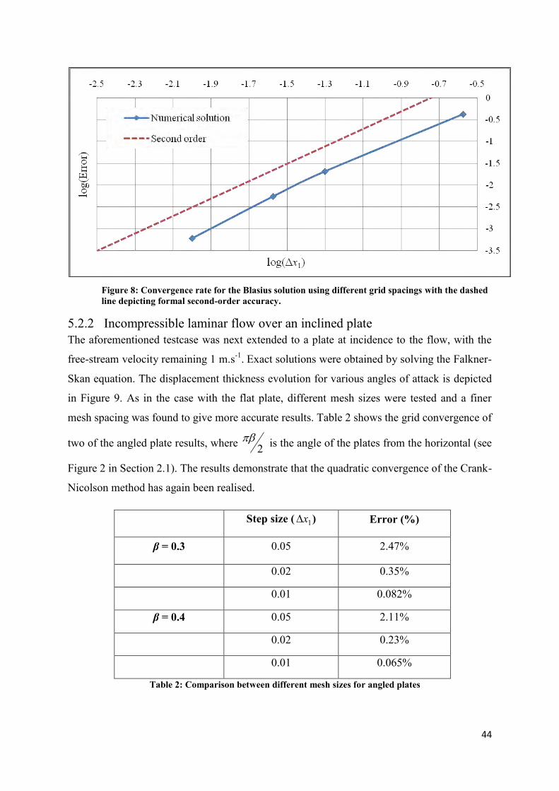
44

Figure 8: Convergence rate for the Blasius solution using different grid spacings with the dashed line depicting formal second-order accuracy.

5.2.2 Incompressible laminar flow over an inclined plate The aforementioned testcase was next extended to a plate at incidence to the flow, with the

free-stream velocity remaining 1 m.s-1. Exact solutions were obtained by solving the Falkner-

Skan equation. The displacement thickness evolution for various angles of attack is depicted

in Figure 9. As in the case with the flat plate, different mesh sizes were tested and a finer

mesh spacing was found to give more accurate results. Table 2 shows the grid convergence of

two of the angled plate results, where 2 is the angle of the plates from the horizontal (see

Figure 2 in Section 2.1). The results demonstrate that the quadratic convergence of the Crank-

Nicolson method has again been realised.

Step size ( 1x ) Error (%)

β = 0.3 0.05 2.47%

0.02 0.35%

0.01 0.082%

β = 0.4 0.05 2.11%

0.02 0.23%

0.01 0.065%

Table 2: Comparison between different mesh sizes for angled plates

45

Figure 9 shows the calculated displacement thickness for various plate angles. The numerical

and similarity solutions all agree to plotting accuracy.

Figure 9: Displacement thicknesses of flow over an inclined plate for various angles of attack

5.3 Results when interacting with inviscid outer flow 5.3.1 Incompressible laminar flow over a flat plate Having successfully validated the boundary layer modelling technology, viscous-inviscid

interaction problems were considered next. The first problem was again the laminar flow over

a flat plate at zero incidence. A structured mesh was employed as depicted in Figure 10. The

boundary condition at the leading edge of the flat plate was set to a fixed inflow velocity

parallel to the plate. The boundary condition at the trailing edge was set to an outflow

condition whereby velocity is extrapolated from inside the flow domain while pressure was

unconstrained. The boundary condition at the top of the domain was set to the fixed free-

stream velocity.

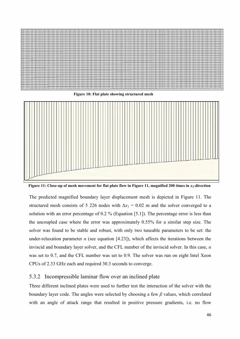
46

Figure 10: Flat plate showing structured mesh

Figure 11: Close-up of mesh movement for flat plate flow in Figure 11, magnified 200 times in x2-direction

The predicted magnified boundary layer displacement mesh is depicted in Figure 11. The

structured mesh consists of 5 226 nodes with Δx1 = 0.02 m and the solver converged to a

solution with an error percentage of 0.2 % (Equation [5.1]). The percentage error is less than

the uncoupled case where the error was approximately 0.55% for a similar step size. The

solver was found to be stable and robust, with only two tuneable parameters to be set: the

under-relaxation parameter α (see equation [4.23]), which affects the iterations between the

inviscid and boundary layer solver, and the CFL number of the inviscid solver. In this case, α

was set to 0.7, and the CFL number was set to 0.9. The solver was run on eight Intel Xeon

CPUs of 2.33 GHz each and required 30.3 seconds to converge.

5.3.2 Incompressible laminar flow over an inclined plate Three different inclined plates were used to further test the interaction of the solver with the

boundary layer code. The angles were selected by choosing a few β values, which correlated

with an angle of attack range that resulted in positive pressure gradients, i.e. no flow

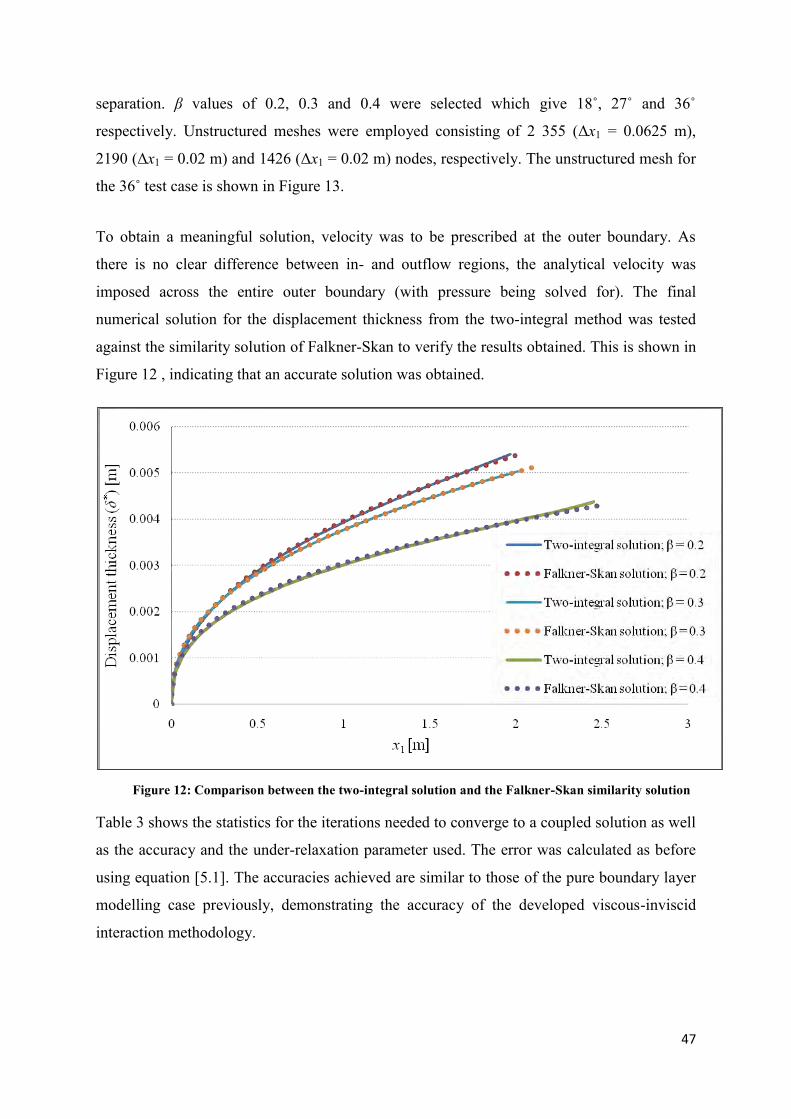
47

separation. β values of 0.2, 0.3 and 0.4 were selected which give 18˚, 27˚ and 36˚

respectively. Unstructured meshes were employed consisting of 2 355 (Δx1 = 0.0625 m),

2190 (Δx1 = 0.02 m) and 1426 (Δx1 = 0.02 m) nodes, respectively. The unstructured mesh for

the 36˚ test case is shown in Figure 13.

To obtain a meaningful solution, velocity was to be prescribed at the outer boundary. As

there is no clear difference between in- and outflow regions, the analytical velocity was

imposed across the entire outer boundary (with pressure being solved for). The final

numerical solution for the displacement thickness from the two-integral method was tested

against the similarity solution of Falkner-Skan to verify the results obtained. This is shown in

Figure 12 , indicating that an accurate solution was obtained.

Figure 12: Comparison between the two-integral solution and the Falkner-Skan similarity solution

Table 3 shows the statistics for the iterations needed to converge to a coupled solution as well

as the accuracy and the under-relaxation parameter used. The error was calculated as before

using equation [5.1]. The accuracies achieved are similar to those of the pure boundary layer

modelling case previously, demonstrating the accuracy of the developed viscous-inviscid

interaction methodology.

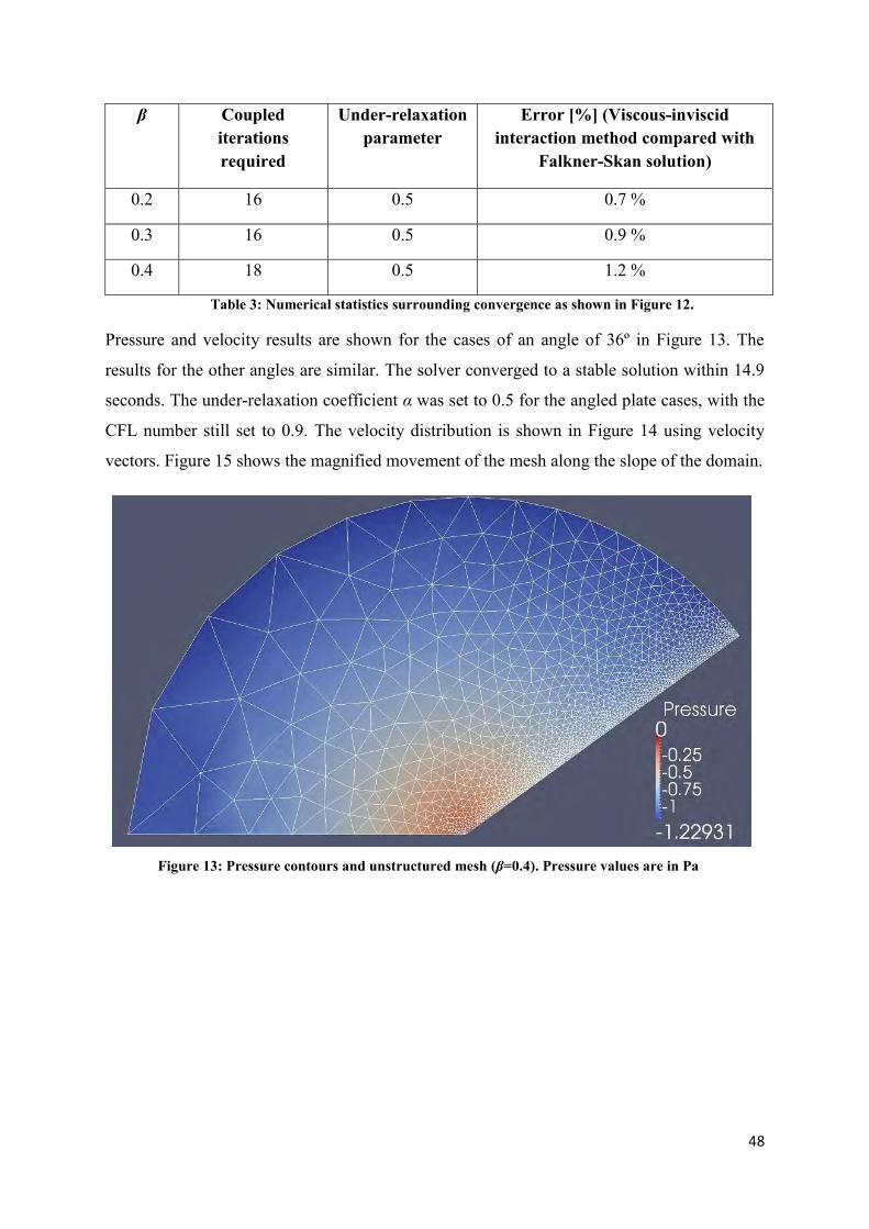
48

β Coupled iterations required

Under-relaxation parameter

Error [%] (Viscous-inviscid interaction method compared with

Falkner-Skan solution)

0.2 16 0.5 0.7 %

0.3 16 0.5 0.9 %

0.4 18 0.5 1.2 %

Table 3: Numerical statistics surrounding convergence as shown in Figure 12.

Pressure and velocity results are shown for the cases of an angle of 36º in Figure 13. The

results for the other angles are similar. The solver converged to a stable solution within 14.9

seconds. The under-relaxation coefficient α was set to 0.5 for the angled plate cases, with the

CFL number still set to 0.9. The velocity distribution is shown in Figure 14 using velocity

vectors. Figure 15 shows the magnified movement of the mesh along the slope of the domain.

Figure 13: Pressure contours and unstructured mesh (β=0.4). Pressure values are in Pa

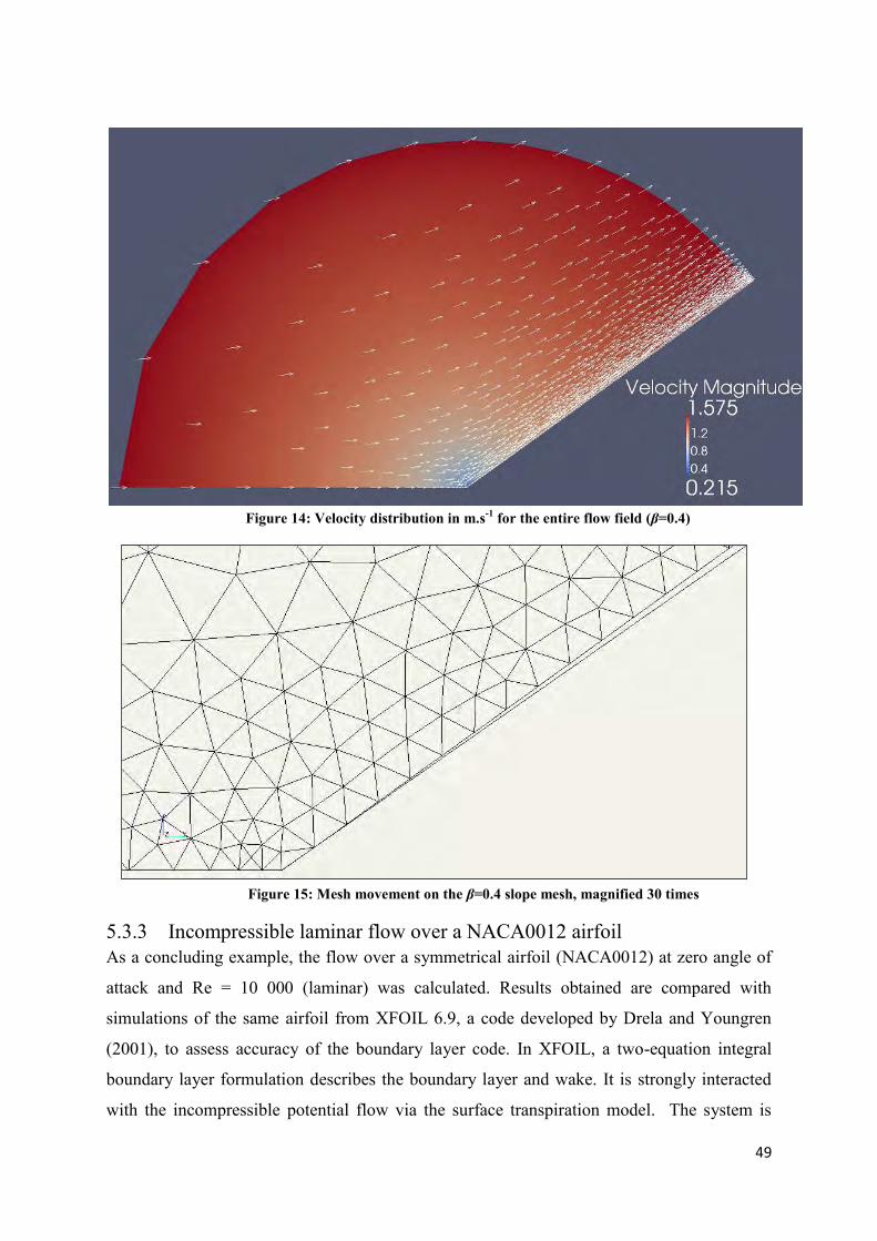
49

Figure 14: Velocity distribution in m.s-1 for the entire flow field (β=0.4)

Figure 15: Mesh movement on the β=0.4 slope mesh, magnified 30 times

5.3.3 Incompressible laminar flow over a NACA0012 airfoil As a concluding example, the flow over a symmetrical airfoil (NACA0012) at zero angle of

attack and Re = 10 000 (laminar) was calculated. Results obtained are compared with

simulations of the same airfoil from XFOIL 6.9, a code developed by Drela and Youngren

(2001), to assess accuracy of the boundary layer code. In XFOIL, a two-equation integral

boundary layer formulation describes the boundary layer and wake. It is strongly interacted

with the incompressible potential flow via the surface transpiration model. The system is

50

then solved using a full-Newton method, solving the whole flow field simultaneously (Drela

and Youngren, 2001), which differs from the method developed in this work. Further noting

that XFOIL is today a widely used commercial package, its results serve as meaningful

validation.

An unstructured computational mesh consisting of 12 064 nodes was employed (as shown in

Figure 20). The boundary conditions were set to slip velocity all around the domain. The

solver converged to a stable solution with an under-relaxation parameter of 0.1 and

converging to a solution within 72 viscous-inviscid iterations in 165 seconds using eight Intel

Xeon CPUs of 2.33 GHz each. The inviscid solver CFL number was maintained at 0.9.

Figure 16 shows the solution of the displacement thickness at different stages of convergence.

A slight inaccuracy in the vicinity of the trailing edge is evident, where the maximum

disparity between the codes of 13.2% occurs. The line name „intermediate‟ refers to a point in

convergence where there is a 10% difference between eU and speceU , (velocity obtained from

the inviscid solution). The velocity equation [4.3] suggested overcomes the Goldstein

singularity existing at the point of shear stress vanishing but a proper solution of the wake

would be required to ensure accurate calculation of the displacement thickness into the wake,

whereas in this work, a wake function was used to simulate the displacement thickness across

the trailing edge into the wake, as described in Section 4.7. The average difference in

predicted displacement thickness between the developed technology and that of XFOIL using

equation [5.1], is 3.95%. Figure 17 shows the velocity solution for the flow over the

NACA0012 airfoil. Both boundary layer thickness and boundary layer momentum thickness

(δ* and θ) grow towards the trailing edge and then slowly decrease in the near wake. Figure

18 depicts the shape factor (H) during different stages of convergence. The shape factor

begins at a value slightly lower than the Blasius value (H = 2.59) and grows gradually

towards the trailing edge. Recall that the singularity occurs at H = 4.

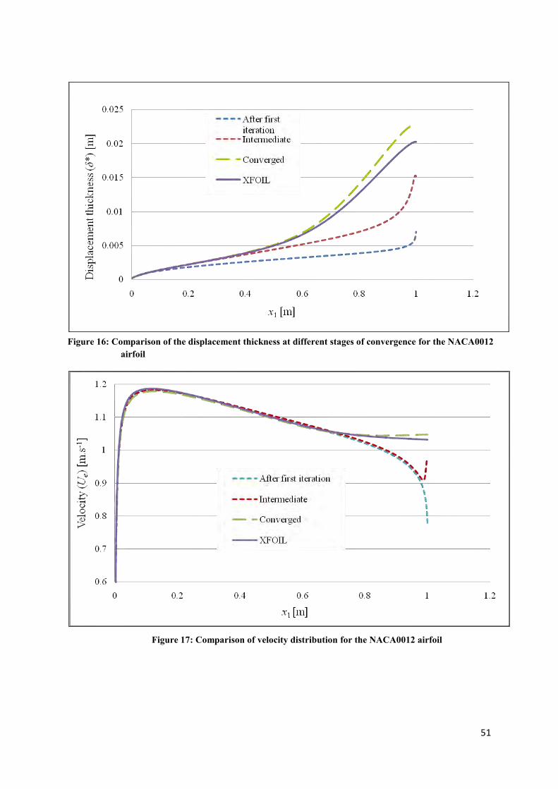
51

Figure 16: Comparison of the displacement thickness at different stages of convergence for the NACA0012

airfoil

Figure 17: Comparison of velocity distribution for the NACA0012 airfoil

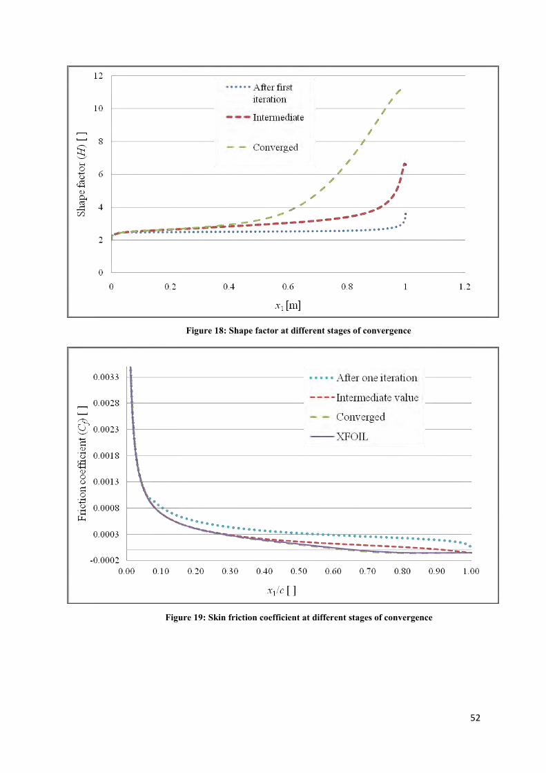
52

Figure 18: Shape factor at different stages of convergence

Figure 19: Skin friction coefficient at different stages of convergence

53

Figure 20: Comparison between the velocity specified and the velocity obtained from the boundary layer solution, after first iteration (top), intermediate (middle) and converged (bottom)

54

Figure 21: Mesh and velocity contours around a NACA0012 airfoil. Viscous-inviscid flow (top) and inviscid flow (bottom). Velocity distribution in m.s-1

Figure 19 depicts the friction coefficient (Cf) as calculated by equation [3.33] at different

stages of convergence, compared with the XFOIL values for a NACA0012 airfoil. The

friction coefficient is important since this dimensionless parameter relates to the friction drag

found in the boundary layer. The smaller the friction drag, the more economical the fuel-

55

usage of the aircraft. The Cf values converge to the XFOIL solution with an overall error of

4.7% and a maximum discrepancy of 7.7% to present an accurate value to use for estimating

the overall effects of the drag. Figure 20 shows the velocity that is computed by the auxiliary

boundary layer equation [4.3] (in order to avoid the Goldstein singularity) compared with the

velocity specified from the inviscid solver. It is compared at the different stages of

convergence, showing that the two velocities converge.

Figure 21 shows the unstructured mesh with velocity contours around the NACA0012 airfoil

for both the viscous-inviscid and only inviscid flow cases. The viscous-inviscid case also

shows the mesh movement depicted by the light grey area around the airfoil. The velocity

contours change significantly when the boundary layer solver is coupled to the inviscid flow

solver. Figure 22 presents a magnification of the velocity distribution around the leading edge

of the airfoil. The coupled solver is very robust when solving the stagnation point present at

the leading edge.

Figure 22: Magnification of the flow across the leading edge of a NACA0012 airfoil. Velocity distribution in m.s-1

Figure 23 displays the mesh movement around the airfoil compared with the boundary layer

thickness predicted by XFOIL 6.9 to an accuracy of 3.95%. It is evident that as the solver

reaches the trailing edge and into the wake, the accuracy decreases. This is due to the

assumed wake function (see Section 4.7).

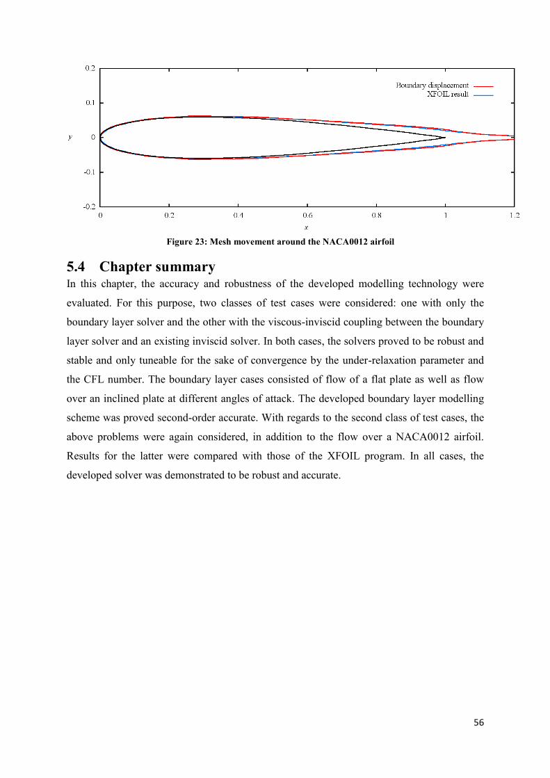
56

Figure 23: Mesh movement around the NACA0012 airfoil

5.4 Chapter summary In this chapter, the accuracy and robustness of the developed modelling technology were

evaluated. For this purpose, two classes of test cases were considered: one with only the

boundary layer solver and the other with the viscous-inviscid coupling between the boundary

layer solver and an existing inviscid solver. In both cases, the solvers proved to be robust and

stable and only tuneable for the sake of convergence by the under-relaxation parameter and

the CFL number. The boundary layer cases consisted of flow of a flat plate as well as flow

over an inclined plate at different angles of attack. The developed boundary layer modelling

scheme was proved second-order accurate. With regards to the second class of test cases, the

above problems were again considered, in addition to the flow over a NACA0012 airfoil.

Results for the latter were compared with those of the XFOIL program. In all cases, the

developed solver was demonstrated to be robust and accurate.

57

CHAPTER 6

CONCLUSIONS

6.1 Summary and discussion CFD codes are an important tool to visualise and predict flow phenomena. An important

engineering aspect of many flow problems is the behaviour of the fluid near a solid boundary.

Viscous flow moves from having completely irrotational motion away from the boundary up

to the surface of the body where the velocity reaches zero, because of the no-slip condition at

the wall. The result is viscous drag. Generally, these effects are solved using the Navier-

Stokes equations. However, to simulate boundary layer flow with most current CFD codes

requires extremely fine mesh spacing normal to the wall and is consequently computationally

very expensive. The boundary layer is not only important to determine appropriate shapes to

minimise drag across a body and thereby save fuel costs or to avoid separation but also to

simulate flow through blade cascades in compressors and turbines.

In the light of the above, for the purpose of this work, the flow domain is effectively divided

into two regions: the outer (inviscid) flow region and the boundary layer (viscous) region at

the surface. A novel viscous-inviscid modelling technology was developed, whereby the

viscous region was described by boundary layer equations while the outer region was solved

via an incompressible flow solver.

In the case of the viscous boundary layer region, the two-integral method of Drela (1985),was

used, obtaining the momentum integral equation in terms of momentum and displacement

thickness, to solve flow in the boundary layer and predict the displacement thickness. Drela‟s

58

method is able to solve limited cases of separation and forms the basis of most boundary

layer methods used by other researchers such as Wolles and Hoeijmakers (1998), Sekar and

Laschka (2005) and Riziotis and Voutsinas (2008). The boundary layer equations were then

discretised using the Crank-Nicolson differencing scheme (second-order implicit scheme) to

ensure stability. The Crank-Nicolson scheme is unconditionally stable and is an implicit

difference method, which has the advantage that the spacing of the grid lines is not limited by

stability constraints. These equations were solved point by point as an initial value problem

by a local Newton method, since this method is relatively fast to converge, if the initial

approximation is close to the solution.

The laminar closure equations reach a singularity at the point where Hk reaches 4, which is

referred to as the „Goldstein singularity‟ at a boundary layer separation point. One way, in

which the problem can be avoided is by solving the inviscid flow and boundary layer

simultaneously, however, this is computationally expensive. In this work, the problem was

eliminated by allowing the boundary layer to modify the inviscid flow solver it was

interacting with by modifying Ue via the displacement thickness. The process creates a

negative feedback effect, which eliminates the singularity. This is achieved by assuming that

the boundary layer is growing on the wall of a two-dimensional channel and solving for the

velocity by using an estimated displacement thickness that is updated continuously until the

percentage change between the previous and latest displacement thickness falls below a

threshold value (here taken as 0.2 %).

For the purpose of viscous-inviscid coupling, a new and novel method is proposed in this

work. It is designed to be both robust and computationally as cost-effective as the quasi-

simultaneous method, without requiring the selection of an interactive law. It is also

advantageous since prior information about the displacement thickness is not needed and the

complete flow field can be solved without solving a monolithic system. This is achieved by

moving the inviscid mesh at each iteration to reflect the boundary layer displacement. The

solution procedure is as follows: the flow solver converges to a solution where the residual is

less than the specified tolerance. The solver then uses the boundary layer thickness obtained

from the boundary layer solution to move the mesh to the outer edge of the boundary where a

slip boundary condition is imposed. The mesh is re-preprocessed and the flow is calculated

again until the residual is less than the convergence tolerance after the movement of the

mesh.

59

The developed modelling technology is thoroughly validated in terms of accuracy and

robustness via application to a number of test cases. Two classes of test cases were

considered: one with only the boundary layer solver and the other with the viscous-inviscid

coupling between the boundary layer solver and an existing inviscid solver. The first class of

boundary layer cases consisted of flow of a flat plate as well as flow over an inclined plate at

different angles of attack. The second class of test cases involved the same problems, in

addition to the flow over a NACA0012 airfoil (results for the latter were compared with those

of the XFOIL program). The developed boundary layer modelling scheme was proved

second-order accurate. In both cases, the solvers proved to be robust and stable and only

tuneable for the sake of convergence by the under-relaxation parameter and the CFL number.

6.2 Future suggestions The methodology developed can be extended in a straightforward manner to treat practical

airfoil design problems with transition to turbulent flows and even mild flow separation. The

following recommendations for further work are made to expand the range of problems that

the interaction method can solve and increase accuracy:

Expand the two-integral method to solve flow in the turbulent regime by adding the

additional parameters and equations given in the work of Drela (1985).

Expand the two-integral method to solve the transition regime, by adding an

amplification variable to the laminar viscous equation.

Solve the wake with the proper closure equations suggested by Drela (1985) to obtain a

more accurate solution for the boundary layer displacement past the trailing edge.

The inviscid solver is a separate module in this study, which has the potential to be

extended to compressible flow as well. Extending to a compressible outer flow solver

would allow transonic flow regimes to be modeled as well. This differs from Drela‟s

method (1985) which simultaneously solves the viscous flow linked with a more

limited potential flow model.

60

REFERENCES

Anderson, D.A. 2007. Fundamentals of aerodynamics. 4th ed. New York: McGraw-Hill.

Brown, S.N. & Stewartson, K. 1969. Laminar separation. Annual Review of Fluid Mechanics,

1:45 – 72.

Burden, R.L. & Faires, J.D. 2005. Numerical analysis. 8th ed. Belmont: Thompson

Brooks/Cole.

Catherall, D. & Mangler, K.W. 1966. The integration of the two-dimensional laminar

boundary layer equations past the point of vanishing skin friction. Journal of Fluid

Mechanics 26:163 – 182.

Cebeci, T. 1999. An engineering approach to the calculation of aerodynamic flows. Los

Angeles, CA: Horizon.

Cebeci, T. & Cousteix, J. 2005. Modelling and computation of boundary layer flows. Los

Angeles, CA: Horizon.

Coenen, E.G.M. 2001. Viscous-inviscid interaction with the quasi-simultaneous method for

2D and 3D airfoil flow. PhD thesis. Groningen: University of Groningen.

Drela, M. 1985. Two-dimensional transonic aerodynamic design and analysis using the Euler

equations. PhD thesis. Cambridge, MA: Department of Aeronautics and Astronautics.

Massachusettes Institute of Technology.

Drela M. 2010. Private communication.

Drela, M. & Giles, M.B. 1987a. Two-dimensional transonic aerodynamics design method.

American Institute of Aeronautics and Astronautics Journal, 25(9):1199 – 1206.

Drela, M. & Giles, M.B. 1987b. Viscous-Inviscid analysis of transonic and low Reynolds

number airfoils. American Institute of Aeronautics and Astronautics Journal,

25(10):347 – 1355.

Drela, M. & Youngren, H. 2001. XFOIL 6.9 User Primer. Cambridge, MA: Department of

Aeronautics and Astronautics. Massachusettes Institute of Technology.

61

Falkner, V.M. & Skan, S.W. 1931. Solution of the boundary layer equations. Philosophical

Magazine and Journal of Science, Series 7, 12(80):865 – 897.

Florea, R., Hall, K.C. & Cizmas, P.G.A. 1998. Reduced-order modelling of unsteady viscous

flow in a compressor cascade. American Institute of Aeronautics and Astronautics

Journal, 36(6):1039 – 1048.

Gleyzes, C., Cousteix, J. & Bonnet, J.L. 1985. Theoretical and experimental study of low

Reynolds number transitional separation bubbles. Conference on Low Reynolds

Number Airfoil Aerodynamics. United States. (June):137-152.

Goldstein, S. 1947. On laminar boundary layer flow near a position of separation. Journal of

Mechanics and Applied Mathematics, 1(1):43 – 69.

Hafez, M.M., Habashi, W.G. & Przybytkowski, S.M. 1991. Transonic viscous-inviscid

interaction by a finite element method. International Journal of Numerical Methods in

Fluids, 13:309 – 319.

Hirsch, C. 1995. Numerical computation of internal and external flows. Volume 2:

Computational methods for inviscid and viscous flows. Wiltshire:John Wiley.

Hirsch, C. 2001. Numerical computation of internal and external flows. Volume 1:

Fundamentals of numerical discretisation. Eastbourne:John Wiley.

Jie, L. & Zhou, Z. 2007. A structured mesh Euler and interactive boundary layer method for

wing/body configurations. Chinese Journal of Aeronautics, 21:19 – 27.

Katz, J. & Plotkin, A. 2001. Low speed aerodynamic. 2nd ed. New York:Cambridge

University Press.

Keller, H.B. 1978. Numerical methods in boundary layer theory. Annual Review of Fluid

Mechanics, 10:417 – 433.

Lagree, P.Y. 2009. Interactive boundary layer or inviscid-viscous interaction. Paris:Institut

Jean Le Rond d‟Alembert.

Le Balleur, J.C. 1983. Numerical viscous-inviscid interaction in steady and unsteady flows.

Proceedings of the Second Symposium, Numerical and Physical Aspects of

Aerodynamic Flow, 259 – 284.

62

Lock, R. & Williams, B. 1987. Viscous-inviscid interactions in external aerodynamics.

Progress Aerospace Science, 24:51 – 171.

Lighthill, M.J. 1958. On displacement thickness. Journal of Fluid Mechanics, 4:383 – 392.

Malan, A.G. & Lewis, R.W. 2011. An artificial compressibility CBS method for modelling

heat transfer and fluid flow in heterogeneous porous materials. International Journal

for Numerical Methods in Engineering, 86(7), In press.

Malan, A.G., Lewis, R.W. & Nithiarasu, P. 2002. An improved unsteady, artificial

compressibility, finite volume scheme for viscous incompressible flows: Part I.

Theory and Implementation. International Journal for Numerical Methods in

Engineering, 54(5):695 – 714.

Messiter, A.F. 1970. Boundary layer flow near the trailing edge of a flat plate. Journal of

Applied Mathematics, 18(1):241 – 257.

Nithiarasu, P. 2003. An efficient artificial compressibility (AC) scheme based on the

characteristics based split (CBS) method for incompressible flows. International

Journal for Numerical Methods in Engineering, 56:1815 – 1845.

Riziotis, V.A. & Voutsinas, S.G. 2008. Dynamic stall modelling on airfoils based on strong

viscous-inviscid interaction coupling. International Journal of Numerical Methods in

Fluids, 56:185 – 208.

Roache, R.J. 1997. Quantification of uncertainty in computational fluid dynamics. Annual

Review of Fluid Mechanics, 29:123 – 160.

Schlichting, H. & Gersten, K. 2000. Boundary layer theory 8th ed. Berlin:Springer-Verlag.

Sekar, W.K. & Laschka, B. 2005. Calculation of the transonic dip of airfoils using viscous-

inviscid aerodynamic interaction method. Aerospace Science and Technology, 9:661 –

671.

White, F.M. 2006. Viscous fluid flow. 3rd ed. Singapore:McGraw-Hill.

Whitfield, D.L. 1978. Analytical description of the complete turbulent boundary layer

velocity profile. American Institute of Aeronautics and Astronautics Papers 78-1158.

11th Fluid and Plasma Dynamics Conference. (July):12.

63

Soize, C. 1992. Strong coupling between inviscid fluid and boundary layer for airfoils with a

sharp edge. II. 2D unsteady case for isolated airfoil and straight blade cascade. La

Recherche Aerospatiale. 3:23 –53.

Stewartson, K. 1968. On the flow near the trailing edge of a flat plate II. Proceedings of the

Royal Society of London. Series A, Mathematical and Physical Sciences,

306(1486):275 – 290.

Stewartson, K. 1974. Multi-structured boundary layers on flat plates and related bodies.

Advances in Applied Mechanics, 14:145 – 293.

Szmelter, J. 2001. Multipoint Aerodynamic wing optimisation in viscous flow. Journal of

Aircraft, 38(5):860 – 867.

Tannehill, J.C., Anderson, D.A. & Pletcher, H.P. 1997. Computational fluid mechanics and

heat transfer 2nd ed. New York:Taylor and Francis.

Tani, I. 1977. History of boundary layer theory. Annual Reviews of Fluid Mechanics, 9:87 –

111.

Veldman, A.E.P. 1981. New, quasi-simultaneous method to calculate interacting boundary

layers. American Institute of Aeronautics and Astronautics Journal, 19:79 – 85.

Veldman, A.E.P. 2009. A simple interaction law for viscous-inviscid interaction. Journal of

Engineering Mathematics, 65:367 – 383.

Versteeg, H.K. & Malalasekera, W. 2007. An introduction to computational fluid dynamics:

The finite volume method. 2nd ed. Essex:Pearson Education.

White, F.M. 2006. Viscous fluid flow. 3rd ed. Singapore:McGraw-Hill.

Whitfield, D.L. 1978. Analytical description of the complete turbulent boundary layer

velocity profile. American Institute of Aeronautics and Astronautics Papers 78-1158.

11th Fluid and Plasma Dynamics Conference. (July):12.

Wolles, B.A. & Hoeijmakers, H.W.M. 1998. On viscid-inviscid interaction modelling for

airfoils as a numerical technique. American Institute of Aeronautics and Astronautics

Papers 98-0100. Netherlands:University of Twente.