An intelligent market making strategy in algorithmic trading

Front. Comput. Sci.

DOI 10.1007/s11704-014-3312-6

An intelligent market making strategy in algorithmic trading

Xiaodong LI1, Xiaotie DENG2,3, Shanfeng ZHU3,4, Feng WANG 5, Haoran XIE6

1 Department of Computer Science, City University of Hong Kong, Hong Kong, China

2 AIMS Lab, Department of Computer Science and Engineering, Shanghai Jiaotong University, Shanghai 200240, China

3 Shanghai Key Lab of Intelligent Information Processing, Fudan University, Shanghai 200433, China

4 School of Computer Science, Fudan University, Shanghai 200433, China

5 State Key Lab of Software Engineering, School of Computer Science, Wuhan University, Wuhan 430072, China

6 Department of Computer Science, Hong Kong Baptist University, Hong Kong, China

c© Higher Education Press and Springer-Verlag Berlin Heidelberg 2014

Abstract Market making (MM) strategies have played an

important role in the electronic stock market. However, the

MM strategies without any forecasting power are not safe

while trading. In this paper, we design and implement a two-

tier framework, which includes a trading signal generator

based on a supervised learning approach and an event-driven

MM strategy. The proposed generator incorporates the infor-

mation within order book microstructure and market news to

provide directional predictions. The MM strategy in the sec-

ond tier trades on the signals and prevents itself from profit

loss led by market trending. Using half a year price tick data

from Tokyo Stock Exchange (TSE) and Shanghai Stock Ex-

change (SSE), and corresponding Thomson Reuters news of

the same time period, we conduct the back-testing and simu-

lation on an industrial near-to-reality simulator. From the em-

pirical results, we find that 1) strategies with signals perform

better than strategies without any signal in terms of average

daily profit and loss (PnL) and sharpe ratio (SR), and 2) cor-

rect predictions do help MM strategies readjust their quoting

along with market trending, which avoids the strategies trig-

gering stop loss procedure that further realizes the paper loss.

Keywords algorithmic trading, market making strategy, or-

der book microstructure, news impact analysis, market simu-

lation

Received August 24, 2013; accepted January 16, 2014

E-mail: [email protected]

1 Introduction

A market maker refers to a bank or brokerage company that

participates in market nearly all the trading time and quotes

(bid and ask prices) for other stock buyers and sellers. When

people enter the market and want to trade a stock, market

makers are always there and provide liquidity. In doing so,

they are literally “making a market” for the stock [1]. With

the development of the algorithmic trading, the job of mak-

ing market is progressively transitioned to automated com-

puter programs. In particular, the market making (MM) strat-

egy has been playing an increasingly important role in the

real market. Due to the fast speed and high accuracy, the MM

strategy has become the key proprietary algorithmic trading

strategy. The MM strategy is doing the job of specialists who

quote for other traders, place passive or aggressive orders

in an order book, and dynamically readjust their quotes and

orders following market conditions and the strategy’s own

logic.

The profit of the MM strategy mainly comes from the

bouncing of stock prices. When the prices change within a

small range, orders frequently hit either strategy’s buy or sell

orders, which gives the strategy an amount of chances to cap-

ture the bid-ask spread and make profit. However, MM strate-

gies without any forecasting signal are not safe while trad-

ing. There are two main risks on MM. The first one refers to

informed traders or information asymmetry. Since the MM

2 Front. Comput. Sci.

strategy does not have 100% perfect information, there are

always traders with faster or better information who could

game with the MM strategy. This risk is especially severe for

illiquid stocks, where the strategy needs to detect and identify

whether the order is sent by an informed trader or not and set

larger bid-ask spread to compensate the risk [2]1) . The sec-

ond one is inventory imbalance or adverse selection led by

market trending. As illustrated by [3], when market price is

trending, the MM strategy with no pre-trending action will

accumulate risky inventory which brings loss to the strategy

in the worst case. Since the MM strategy is a fully automatic

program that both makes trading decisions to provide liquid-

ity, as well as takes actions to balance inventory and handle

risks, how to build an intelligent MM strategy has been an

attractive research issue on algorithmic trading.

There are many research papers in literature about MM

strategy [2,4–7]. To formulate, the proposed strategies could

be considered as a mapping from the strategy’s current state

θt and the market condition to the strategy’s action in next

step at+1,

f (θt, pt) �→ at+1. (1)

The market condition pt refers to events extracted from price

series. The strategy has to consider θt and pt, and takes corre-

sponding action at+1. Different from their approaches, we add

one more information source into MM strategy’s information

set, which is news event. And Formula (1) is changed to

f (θt, pt, nt) �→ at+1, (2)

where nt ∈ N is the news data set.

In this paper, we develop a trading signal generator and

a MM strategy, aiming at adaptively and progressively inte-

grating multiple market information sources to improve the

performance of the strategy. The first tier is a trading sig-

nal generator. We employ support vector machines (SVMs),

a successful nonparametric classifier, to classify patterns of

the order book and market news titles into either positive,

neutral, or negative categories. The second tier is the trad-

ing strategy. The predictions provided by the first tier are fed

into the MM strategy, where the strategy will then trade on

these signals. We back-tested this MM strategy with half a

year real market tick prices and news on a near-to-reality sim-

ulator. Experimental results show that the average daily profit

and loss (PnL) improves when the strategy has the help of

signals, and correct signals help the strategy quote along the

market trending and avoid the strategy triggering stop loss

utility in many cases.

The rest of this paper is organized as follows. Section 2 is a

brief literature review. Section 3 first shows our system archi-

tecture, and then illustrates in detail how to generate trading

signals from two information sources, and finally explains the

logic and work flow of the MM strategy. Section 4 describes

the back-testing setup and simulation results. Section 5 gives

our conclusion and describes our future work.

2 Related work

There are many works on MM strategy analysis. In our pro-

posed two-tier framework, there are mainly two research is-

sues. The first one is the signal generator, while the second

one is the trading strategy. In this section, we will briefly in-

troduce the current methodologies about these two issues.

2.1 Trading signal generation

Mining signals from market prices and news articles have

been studied in many previous works. For the mining of

price signals, Kim [8] used SVM to predict index prices and

claimed that the performance of SVM was better than back-

propagation neural networks. Similar result could be found

from the work of Cao and Tay [9, 10]. They applied SVM to

predict S&P 500 daily prices and also found that SVM had

better performance based on the metrics of normalized mean

square error and mean absolute error. Huang et al. [11] used

SVM to predict price directional movement of NIKKEI 225

index. After comparing SVM with linear discriminant anal-

ysis, quadratic discriminant analysis and back-propagation

neural networks, they drew the same conclusion.

Market news, which is traditionally processed by human

investors, has become an emerging and important informa-

tion source for machine learning models while forecasting.

The basic motivation is to analyze the statistical relation-

ship between word patterns and market responses. Fung et

al. [12] classified news articles into categories and predicted

newly released news articles’ directional impact based on the

trained model. AZFinText system, built by Schumaker and

Chen [13–16], was also able to give directional forecast of

prices.

One recent work shows that it would be better to use

two types of market information together [17]. Multi-kernel

SVM (MKSVM) is employed, and one sub-kernel handles

the information set of market prices while the other sub-

kernel deals with the instances of market news. Sub-kernels’

weights are learnt according to the predictability, and final

1) How to detect and identify orders’ properties is beyond the scope of this paper. Interested readers can refer to the references listed.

Xiaodong LI et al. An intelligent market making strategy in algorithmic trading 3

predictions are made by MKSVM. The experimental results

show that combination of information sets gives higher clas-

sification accuracy.

However, due to the small number of pieces of news re-

ported each day, most of the intra-day trading opportunities

(signals generated by prices only) are lost if the strategy only

trades when news appears. For example, on December 28,

2007, there are three pieces of news about 0005.HK (HSBC).

On the same day, there are hundreds of samples of order

book snapshots if we sample at one minute interval. If a strat-

egy only trades on the signals generated when both news and

prices are available, which has three times on December 28,

2007, the strategy will miss most other signals that could be

solely extracted from order book when there is no news re-

ported. In order to fully use the trading opportunities, it would

be better to let prices and news be modeled separately, and

combine the two signals within the logic of a trading strat-

egy.

2.2 MM strategy

Theoretical MM strategies have been proposed in many

previous works. Othman and Sandholm [4] ran an auto-

mated market maker on the Gates Hillman Prediction Market

(GHPM) which was designed and built to predict the opening

day of the Gates and Hillman Centers. Chen et al. [18] ana-

lyzed the strategic behaviors in a Fisher market and proved

that Leontief market had incentive ratio of 2. Abernethy et

al. [19] proposed a general framework for the design of secu-

rity markets over combinatorial of infinite state of outcome

spaces. Othman et al. [5] constructed a market maker that

was sensitive to market liquidity. Brahma et al. [2] proposed

a Bayersian market maker for binary outcome (or continu-

ous 0–1) markets that learned from the informational content

of trades. Bu et al. [20, 21] studied the strategies and arbi-

trage opportunities in auction and pari-mutual market. Das

and Magdon-Ismail [6] studied the profit-maximization prob-

lem of a monopolistic market maker who set two-sided prices

in an asset market. One theoretical analysis of market maker

behavior was proposed by Chakraborty and Kearns [7]. They

considered the characteristics of market prices — mean rever-

sion, and showed that the MM strategy made profit on mean

reverting stochastic processes.

There are several differences between our MM strategy and

those strategies reviewed:

1) The major difference is that we do not make any assump-

tion on whether strategy is trading with informed traders or

noise traders [2,5] which is the first kind of risks as described

in Section 1. In contrast, we use supervised machine learn-

ing algorithms to directly mine the trading signals from two

different information sources, i.e., order books and news, and

incorporate the directional predictions to guide the MM strat-

egy.

2) Our strategy is designed for real stock market instead

of either prediction market [4] or stock market with syntheti-

cally generated price series [2, 5, 7, 19].

The market rules, such as tick size (i.e., the minimum

increment/decrement when a buyer/seller bids/offers), trad-

ing hours (i.e., market open time, lunch break and market

close time), price limit (i.e., the highest/lowest price that a

buyer/seller can bid/offer) etc., are different from the virtual

markets, and all these rules need to be considered while im-

plementing the strategy. The whole system is further back-

tested with real market data.

3 An intelligent MM strategy

In this section, we firstly show an overall system architecture

of the trading platform, and then we introduce the work flow

of the MM strategy. As shown in Fig. 1, the whole platform

is composed of four parts:

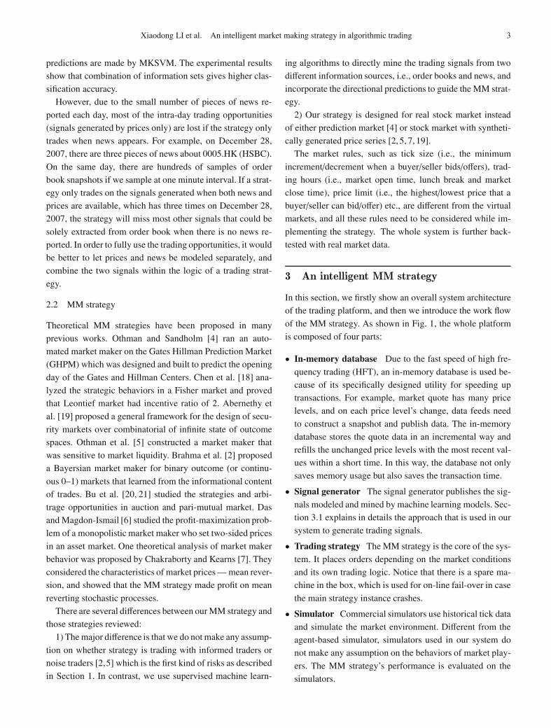
• In-memory database Due to the fast speed of high fre-

quency trading (HFT), an in-memory database is used be-

cause of its specifically designed utility for speeding up

transactions. For example, market quote has many price

levels, and on each price level’s change, data feeds need

to construct a snapshot and publish data. The in-memory

database stores the quote data in an incremental way and

refills the unchanged price levels with the most recent val-

ues within a short time. In this way, the database not only

saves memory usage but also saves the transaction time.

• Signal generator The signal generator publishes the sig-

nals modeled and mined by machine learning models. Sec-

tion 3.1 explains in details the approach that is used in our

system to generate trading signals.

• Trading strategy The MM strategy is the core of the sys-

tem. It places orders depending on the market conditions

and its own trading logic. Notice that there is a spare ma-

chine in the box, which is used for on-line fail-over in case

the main strategy instance crashes.

• Simulator Commercial simulators use historical tick data

and simulate the market environment. Different from the

agent-based simulator, simulators used in our system do

not make any assumption on the behaviors of market play-

ers. The MM strategy’s performance is evaluated on the

simulators.


Fig. 1 Architecture of the trading platform. The platform has four components: 1) in-memory database; 2) signal generator; 3) trading strategyand 4) simulator

As mentioned above, the main part of our MM strategy

process is composed of two components: signal generator

and trading strategy. In the following, we will show the de-

tailed information about these two components.

3.1 Signal generator

Order book information and market news articles are mod-

eled separately in signal modeling. We will refer to them as

order book signal (OBS) and news signal (NS) in the rest of

this paper.

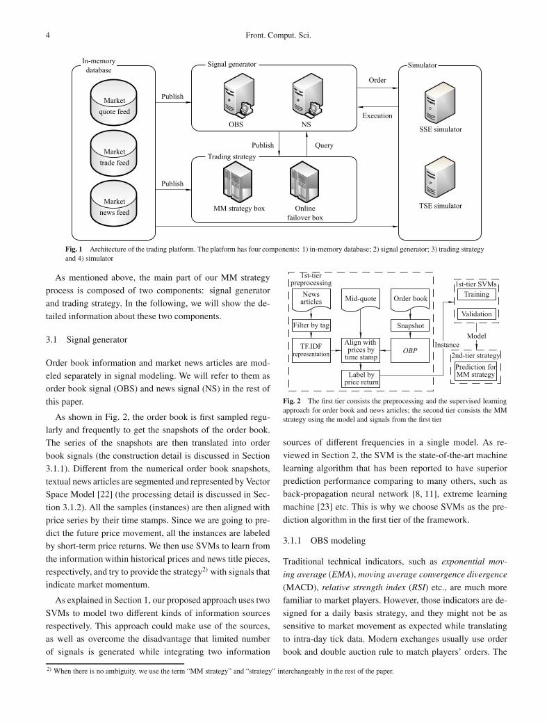
As shown in Fig. 2, the order book is first sampled regu-

larly and frequently to get the snapshots of the order book.

The series of the snapshots are then translated into order

book signals (the construction detail is discussed in Section

3.1.1). Different from the numerical order book snapshots,

textual news articles are segmented and represented by Vector

Space Model [22] (the processing detail is discussed in Sec-

tion 3.1.2). All the samples (instances) are then aligned with

price series by their time stamps. Since we are going to pre-

dict the future price movement, all the instances are labeled

by short-term price returns. We then use SVMs to learn from

the information within historical prices and news title pieces,

respectively, and try to provide the strategy2) with signals that

indicate market momentum.

As explained in Section 1, our proposed approach uses two

SVMs to model two different kinds of information sources

respectively. This approach could make use of the sources,

as well as overcome the disadvantage that limited number

of signals is generated while integrating two information

Fig. 2 The first tier consists the preprocessing and the supervised learningapproach for order book and news articles; the second tier consists the MMstrategy using the model and signals from the first tier

sources of different frequencies in a single model. As re-

viewed in Section 2, the SVM is the state-of-the-art machine

learning algorithm that has been reported to have superior

prediction performance comparing to many others, such as

back-propagation neural network [8, 11], extreme learning

machine [23] etc. This is why we choose SVMs as the pre-

diction algorithm in the first tier of the framework.

3.1.1 OBS modeling

Traditional technical indicators, such as exponential mov-

ing average (EMA), moving average convergence divergence

(MACD), relative strength index (RSI) etc., are much more

familiar to market players. However, those indicators are de-

signed for a daily basis strategy, and they might not be as

sensitive to market movement as expected while translating

to intra-day tick data. Modern exchanges usually use order

book and double auction rule to match players’ orders. The

2) When there is no ambiguity, we use the term “MM strategy” and “strategy” interchangeably in the rest of the paper.


information of order book, such as bid price (price at buy

side), ask price (price at sell side), bid size and ask size etc., is

broadcasted to investors. We consider such information more

useful and be able to provide more accurate insights of mar-

ket movement.

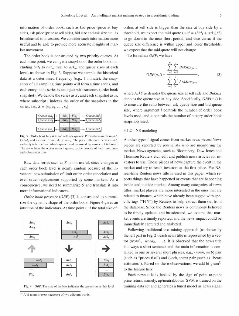
The order book is constructed by two priority queues. At

each time point, we can get a snapshot of the order book, in-

cluding bid1 to bidn, ask1 to askn, and queue sizes at each

level, as shown in Fig. 3. Suppose we sample the historical

data at a determined frequency (e.g., 1 minute), the snap-

shots of all sampling time points will form a time series, and

each entry in the series is an object with structure (order book

snapshot). We denote the series as S , and each snapshot as si,

where subscript i indexes the order of the snapshots in the

series, i.e., S = {s0, s1, . . . , sn}.

Fig. 3 Order book buy side and sell side queues. Prices decrease from bid1

to bidn and increase from ask1 to askn . The price difference between bid1

and ask1 is termed as bid-ask spread, and measured by number of tick-size.The arrow links the orders in each queue, by the priority of their limit priceand submission time

Raw data series such as S is not useful, since changes at

each order book level is nearly random because of the in-

vestors’ new submission of limit order, order cancelation and

even order replacement supported by some markets. As a

consequence, we need to summarize S and translate it into

more informational indicators.

Order book pressure (OBP) [3] is constructed to summa-

rize the dynamic shape of the order book. Figure 4 gives an

intuition of the indicators. At time point t, if the total size of

Fig. 4 OBP. The size of the box indicates the queue size at that level

orders at sell side is bigger than the size at buy side by a

threshold, we expect the mid quote (mid = (bid1 + ask1)/2)

to go down in the near short period, and vice versa; if the

queue size difference is within upper and lower thresholds,

we expect that the mid quote will not change.

To formalize OBP, we have

OBP(n, l) =

n∑

τ=0

l∑

j=1

BidSize j,t−τ

n∑

τ=0

l∑

i=1

AskSizei,t−τ

, (3)

where AskSize denotes the queue size at sell side and BidSize

denotes the queue size at buy side. Specifically, OBP(n, l) is

to measure the ratio between ask queue size and bid queue

size, where argument l controls the number of order book

levels used, and n controls the number of history order book

snapshots used.

3.1.2 NS modeling

Another type of signal comes from market news pieces. News

pieces are reported by journalists who are monitoring the

market. News agencies, such as Bloomberg, Dow Jones and

Thomson Reuters etc., edit and publish news articles for in-

vestors to use. Those pieces of news capture the event in the

market and try to reach investors at the first place. For NS,

real-time Reuters news title is used in this paper, which re-

ports things that have happened or events that are happening

inside and outside market. Among many categories of news

titles, market players are more interested in the ones that are

related to finance, which have already been tagged with spe-

cific tags (“FIN”) by Reuters to help extract them out from

the database. Since the Reuters news is commonly believed

to be timely updated and broadcasted, we assume that mar-

ket events are timely reported, and the news impact could be

immediately captured and analyzed.

Following traditional text mining approach (as shown by

the left part in Fig. 2), each news title is represented by a vec-

tor 〈word1, word2, . . . 〉. It is observed that the news title

is always a short sentence and the main information is con-

tained in one or several short phrases, e.g., 〈noun, verb〉 pair

(such as “prices rise”) and 〈verb, noun〉 pair (such as “beats

estimates”). Based on these observations, we add bi-gram3)

to the feature lists.

Each news title is labeled by the sign of point-to-point

price return, namely, up/neutral/down. SVM is trained on the

training data set and generates a tuned model as news signal

3) A bi-gram is every sequence of two adjacent words.


source. In the testing period, when out-of-sample news pieces

come in, SVM will give predictions.

3.2 Trading strategy

The MM strategy, which is quite different from execu-

tion strategies, such as direct market access (DMA), vol-

ume weighted average price (VWAP) etc., is a strategy that

does full time trading, quoting on both buy and sell sides,

managing bid-ask spread, and keeping its inventory from

bankruptcy. Similar to human specialist, the MM strategy

initially quotes at market open and dynamically changes the

quotes. Naturally, the key jobs for a MM strategy are 1) how

to manage orders (quotation), and 2) how to manage risk (bal-

ance cash and stocks).

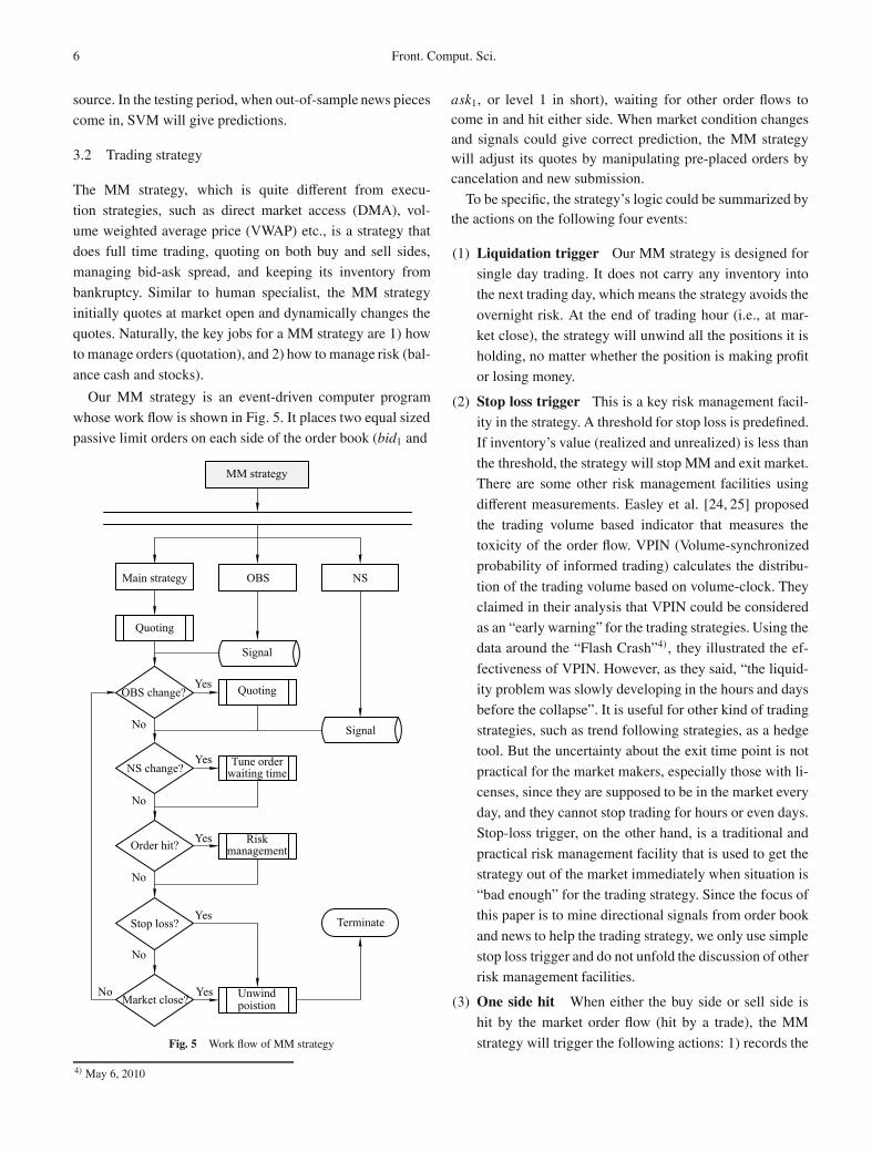
Our MM strategy is an event-driven computer program

whose work flow is shown in Fig. 5. It places two equal sized

passive limit orders on each side of the order book (bid1 and

Fig. 5 Work flow of MM strategy

ask1, or level 1 in short), waiting for other order flows tocome in and hit either side. When market condition changesand signals could give correct prediction, the MM strategywill adjust its quotes by manipulating pre-placed orders bycancelation and new submission.

To be specific, the strategy’s logic could be summarized bythe actions on the following four events:

(1) Liquidation trigger Our MM strategy is designed for

single day trading. It does not carry any inventory into

the next trading day, which means the strategy avoids the

overnight risk. At the end of trading hour (i.e., at mar-

ket close), the strategy will unwind all the positions it is

holding, no matter whether the position is making profit

or losing money.

(2) Stop loss trigger This is a key risk management facil-

ity in the strategy. A threshold for stop loss is predefined.

If inventory’s value (realized and unrealized) is less than

the threshold, the strategy will stop MM and exit market.

There are some other risk management facilities using

different measurements. Easley et al. [24, 25] proposed

the trading volume based indicator that measures the

toxicity of the order flow. VPIN (Volume-synchronized

probability of informed trading) calculates the distribu-

tion of the trading volume based on volume-clock. They

claimed in their analysis that VPIN could be considered

as an “early warning” for the trading strategies. Using the

data around the “Flash Crash”4) , they illustrated the ef-

fectiveness of VPIN. However, as they said, “the liquid-

ity problem was slowly developing in the hours and days

before the collapse”. It is useful for other kind of trading

strategies, such as trend following strategies, as a hedge

tool. But the uncertainty about the exit time point is not

practical for the market makers, especially those with li-

censes, since they are supposed to be in the market every

day, and they cannot stop trading for hours or even days.

Stop-loss trigger, on the other hand, is a traditional and

practical risk management facility that is used to get the

strategy out of the market immediately when situation is

“bad enough” for the trading strategy. Since the focus of

this paper is to mine directional signals from order book

and news to help the trading strategy, we only use simple

stop loss trigger and do not unfold the discussion of other

risk management facilities.

(3) One side hit When either the buy side or sell side is

hit by the market order flow (hit by a trade), the MM

strategy will trigger the following actions: 1) records the

4) May 6, 2010


fills/partial-fills in inventory, 2) calculates waiting time

for the un-hit order, and 3) adjusts quoting and places two

new limit orders when waiting time is over. Take hit of

buy side order for example, inventory is changing form

zero to non-zero since it records that one buy order got

hit. Since the strategy is risk neutral, the stock position

is risky if market price is trending down, and the sell or-

der waiting in the order book could not be sold at a price

higher than the buy price. To get rid of this inventory risk

and make money, the strategy needs to unwind this po-

sition at a higher (than buy price) price level. However,

this expectation could only be achieved when the market

is holding still or trending up, which means that market

should not be against our inventory. Therefore, risk is

translated to order’s waiting time. The longer the waiting

time is, the more risky it will be. If the strategy has the

ability to take higher risk, the waiting time of order could

be longer, and vice versa. The upper bound of the waiting

time is determined by signals prediction time horizon.

(4) Signal change If the signal sign changes, the strategy

will 1) cancel previous two limit orders, 2) adjust quot-

ing, and 3) place two new limit orders.

Assume we have already trained classifiers which can pre-

dict the future of an asset using order book information and

news respectively, i.e., within next TOBP time period and next

Tn, respectively, it tells the price movement will 1) go up, 2)

go down, or 3) stay still. Suppose the best bid and ask prices

at time t are pbt and pa

t . The quoting formula for our market

maker at time t + 1 is:

pb|at+1 = pb|a

t + (signOBP × μ + signn × η) × TickSize, (4)

where μ is a scalar factor that determines the number of ticks

the quoting formula is going to increase/decrease the bid/ask

levels when OBP signal changes. For different stocks, μ may

be different and should be determined and calibrated using

the historical data specifically, as shown in Section 4. η is

calculated by

η = σ ×√

TOBP

Tn, (5)

where σ is the daily volatility of prices. When Brownian pro-

cess is assumed, and Tn is usually longer than TOBP, η needs

to be scaled by the square root of the ratio of the time lengths.

And the final price that is set into the PRICE field of FIX pro-

tocol (Financial Information eXchange5), PRICE is the 44th

field of a FIX message.) is rounded to the nearest allowed

limit price.

Imagine that the price is trending up and signal correctly

gives a positive prediction, according to Eq. (4), pt+1 would

be pt + (μ + η) × TickSize which is greater than pt. It means

that the strategy will quote more aggressive bid price and

more passive ask price than time t. Conversely, if the price

is trending down, signal correctly gives negative signal, the

strategy will quote more passive bid price and pull down ask

bar by (μ+ η) ticks to place more aggressive ask price. There

will be no change of quote if the signal is neutral. The reason

why tick size appears in Eq. (4) is that for a specific market,

e.g., Tokyo Stock Exchange (TSE), equities use variant tick

sizes instead of consistent tick size, which enlarges the tick

size when the price is high and shrinks the tick size while the

price is low6) .

It could be observed that the proposed MM strategy has

two advantages: 1) the signal generators are working in sepa-

rate threads, which will speed up the responding speed of the

strategy; 2) unlike the strategies reviewed in Section 2, this

strategy does not either calculate the distribution of the in-

formed/noise traders, or calculate the probability of the trade

that is initiated by an informed or a noise trader. Since most

of the time, people cannot have the ground truth to verify the

assumption. In contrast, the proposed strategy integrates the

signals mined from two kinds of real historical data by a non-

parametric machine learning model. As long as the signals

are tuned to be more accurate, the strategy could avoid risks

and place the orders in right positions.

4 Experimental setup and back-testing simu-lation

As illustrated in the previous section, the performance of the

strategy relies on the quality of signals. In this section, we

first represent the setup of different signals and then simulate

our strategy on historical data.

4.1 Experiment universe

The main principles that determine which markets/stocks are

included into the experiment universe depend on two factors:

• High v.s. low stamp duty Real markets charge investors

stamp duties. Different markets’ stamp duties may have

different values by different rules. Since the stamp duty

will consume part of the investors’ profit, investors would

5) www.fixprotocol.org6) TSE tick size rules can be found here: http://www.tse.or.jp/english/faq/list/stockprice/p_e.html


prefer the market with low stamp duty to make more prof-

its.

• Liquid v.s. illiquid stocks The MM strategy prefers

stocks that are liquid, since liquid stocks are easier to trade

than illiquid stocks. The main profit of the MM strategy

comes from the bid-ask spread. The more times of the buy-

sell/short-buy round trades happen, the strategy will thus

make more profits. On the other side, the liquid stocks are

easier for simulator to simulate. Since the long queuing ef-

fect in the order book of illiquid stock, i.e., orders in the

queue of illiquid stocks will wait a long time to get filled,

the current simulator we use will overestimate the fill rate

for the illiquid stocks7) . To illustrate this point, we include

both liquid and illiquid stocks in the experiment universe

for comparison.

We have three candidate markets: TSE, Hong Kong StockExchange and Shanghai Stock Exchange (SSE). The first twomarkets are mature markets and the last one is an emerg-ing market. We want to test the strategy in both mature andemerging markets. Based on the principles, among the maturemarkets, we choose TSE since TSE has lower stamp duty, andamong the emerging markets we choose SSE.

The back-testing period starts from July 2011 to January2012, which lasts about six months and covers the inactiveand active trading seasons of 2011. We select one stock fromTSE, Toyota Motor Corp. (7203.T), and one other stock fromSSE, China Minsheng Banking Corp. Ltd. (600016.SS)8).7203.T and 600016.SS are quite liquid names with small bid-ask spread, which is appropriate for market making strategy.We also include one illiquid stock, Mizuho Financial GroupInc. (8411.T), for comparison, which illustrates the queu-ing effect in the order books of the illiquid stocks. Reuters

news is used in the experiment. As 7203.T and 8411.T are

constituents of .N225 (NEKKEI 225 index) and 600016.SS

is a constituent of .CSI300 (CSI 300 index), we include

news titles relevant to 7203.T, 8411.T, .N225, 600016.SS, and

.CSI300 for news signal setup.

4.2 OBS setup

Before training SVM for OBSs, we need to decide the length

of the training period, parameters calibration method and

training samples’ labeling.

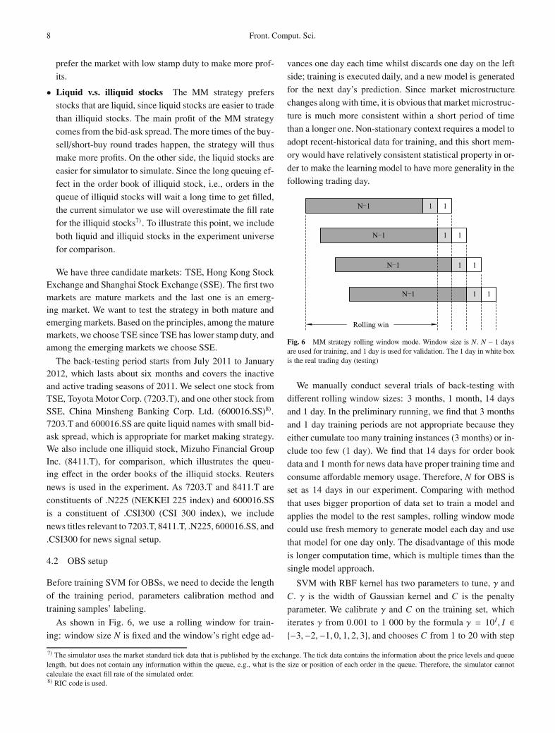
As shown in Fig. 6, we use a rolling window for train-

ing: window size N is fixed and the window’s right edge ad-

vances one day each time whilst discards one day on the left

side; training is executed daily, and a new model is generated

for the next day’s prediction. Since market microstructure

changes along with time, it is obvious that market microstruc-

ture is much more consistent within a short period of time

than a longer one. Non-stationary context requires a model to

adopt recent-historical data for training, and this short mem-

ory would have relatively consistent statistical property in or-

der to make the learning model to have more generality in the

following trading day.

Fig. 6 MM strategy rolling window mode. Window size is N. N − 1 daysare used for training, and 1 day is used for validation. The 1 day in white boxis the real trading day (testing)

We manually conduct several trials of back-testing with

different rolling window sizes: 3 months, 1 month, 14 days

and 1 day. In the preliminary running, we find that 3 months

and 1 day training periods are not appropriate because they

either cumulate too many training instances (3 months) or in-

clude too few (1 day). We find that 14 days for order book

data and 1 month for news data have proper training time and

consume affordable memory usage. Therefore, N for OBS is

set as 14 days in our experiment. Comparing with method

that uses bigger proportion of data set to train a model and

applies the model to the rest samples, rolling window mode

could use fresh memory to generate model each day and use

that model for one day only. The disadvantage of this mode

is longer computation time, which is multiple times than the

single model approach.

SVM with RBF kernel has two parameters to tune, γ and

C. γ is the width of Gaussian kernel and C is the penalty

parameter. We calibrate γ and C on the training set, which

iterates γ from 0.001 to 1 000 by the formula γ = 10I , I ∈{−3,−2,−1, 0, 1, 2, 3}, and chooses C from 1 to 20 with step

7) The simulator uses the market standard tick data that is published by the exchange. The tick data contains the information about the price levels and queuelength, but does not contain any information within the queue, e.g., what is the size or position of each order in the queue. Therefore, the simulator cannotcalculate the exact fill rate of the simulated order.8) RIC code is used.


size 1. This two-dimension grid search of parameter combi-

nations would iterate 7× 20 times. However, only calibrating

parameters on the training set may cause an over-fitting is-

sue, which makes the model have good performance on the

training set but poor performance on an unseen test set. To

overcome this issue and balance the bias and variance, we

pick the last day from the rolling window as the validation

set. The model is trained by rolling the training set excluding

validation day, and performance is evaluated on the validation

set. Parameter combination with the best performance on the

validation set is reserved. This method ensures that the model

has relatively good generality for future use.

Besides SVMs’ parameters, OBS has two other parameters

(shown in Eq. (3)): 1) OBS built-up time n and 2) order book

level l. Tick data is aggregated and sampled in minutes in

the experiment. Built-up time indicates how many historical

snapshots will signal use to calculate the signal value. Order

book level means how many bid/ask levels will signal use to

calculate the signal value. For instance, suppose current time

is t0, OBP(5,1) uses the last five minutes order book level 1

information to calculate the signal value at t0. In our available

data, we could get at most five levels. Fortunately, parame-

ters of signal do not need to calibrate, since SVM could take

a vector of OBPs with different parameters as input features.

We select built-up time from {1, 2, 3, 5, 10, 15} minutes and

order book level from 1 to 5. Therefore we form a vector of

6 × 5 = 30 OBP features.

Training instances should be labeled before use in the

classification. Point-to-point return, which calculates price

change ratio at two time points t0 and t0+Δ, is a good choice.

However, since tick price is not continuous (due to tick size),

point-to-point return needs to be further translated into tick

change, otherwise it would be hard for the strategy to deter-

mine the orders’ limit price. In our experiment, if mid quote

price’s increment in one minute exceeds μ ticks, where μ is

selected specific to each stock, instance is then labeled as pos-

itive, and vice versa; if mid price’s change does not exceed μ

ticks, instance is labeled as neutral. μ is calibrated among sev-

eral candidates, finally determined by the accuracy improve-

ment level of the model comparing with benchmark (random

signal, flip coin).

For each instance, it is classified into either positive, neu-

tral or negative class. The benchmark makes guesses on pre-

diction by randomly picking up positive, neutral or negative

based on label’s prior distribution in the training data set. As-

sume the distribution of three classes in the training data set

is P1, P0 and P−1, where P1+P0+P−1 = 1, then the accuracy

of benchmark will be P21 + P2

0 + P2−1. It is worth noting that

when μ becomes greater, more instances will fall into neutral

class, which implies that the distribution of three classes is

highly imbalanced and P0 is much greater than P1 and P−1.

In this case, the accuracy will become arbitrarily high. One

extreme case is that if μ covers the biggest price change in

training samples, then accuracy would equal 100%. Based on

the discussion, it is apparent that we do not need to calibrate

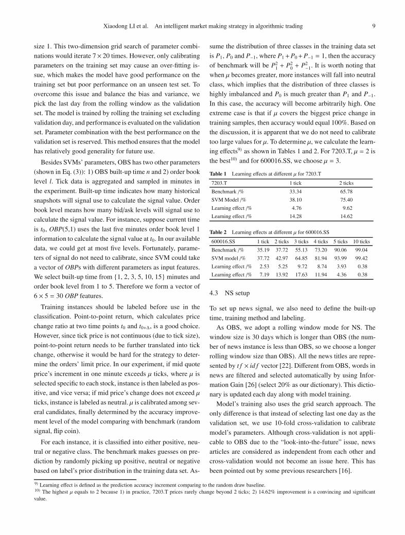
too large values for μ. To determine μ, we calculate the learn-

ing effects9) as shown in Tables 1 and 2. For 7203.T, μ = 2 is

the best10) and for 600016.SS, we choose μ = 3.

Table 1 Learning effects at different μ for 7203.T

7203.T 1 tick 2 ticks

Benchmark /% 33.34 65.78

SVM Model /% 38.10 75.40

Learning effect /% 4.76 9.62


Table 2 Learning effects at different μ for 600016.SS

600016.SS 1 tick 2 ticks 3 ticks 4 ticks 5 ticks 10 ticks

Benchmark /% 35.19 37.72 55.13 73.20 90.06 99.04

SVM model /% 37.72 42.97 64.85 81.94 93.99 99.42

Learning effect /% 2.53 5.25 9.72 8.74 3.93 0.38

Learning effect /% 7.19 13.92 17.63 11.94 4.36 0.38

4.3 NS setup

To set up news signal, we also need to define the built-up

time, training method and labeling.

As OBS, we adopt a rolling window mode for NS. The

window size is 30 days which is longer than OBS (the num-

ber of news instance is less than OBS, so we choose a longer

rolling window size than OBS). All the news titles are repre-

sented by t f × id f vector [22]. Different from OBS, words in

news are filtered and selected automatically by using Infor-

mation Gain [26] (select 20% as our dictionary). This dictio-

nary is updated each day along with model training.

Model’s training also uses the grid search approach. The

only difference is that instead of selecting last one day as the

validation set, we use 10-fold cross-validation to calibrate

model’s parameters. Although cross-validation is not appli-

cable to OBS due to the “look-into-the-future” issue, news

articles are considered as independent from each other and

cross-validation would not become an issue here. This has

been pointed out by some previous researchers [16].

9) Learning effect is defined as the prediction accuracy increment comparing to the random draw baseline.10) The highest μ equals to 2 because 1) in practice, 7203.T prices rarely change beyond 2 ticks; 2) 14.62% improvement is a convincing and significantvalue.


We label each piece of news with the sign of next n minutes

point-to-point tick change, thus each news is tagged as pos-

itive if the return is positive and vice versa. We use .CSI300

and .N225 indices, and calibrate point-to-point return for the

next 30, 60 and 120 minutes, which is longer than OBS. Re-

sults are shown in Table 3. We find that 60 minutes led to bet-

ter performance for both 7203.T and 600016.SS (600016.SS

performs also well at 30 minutes), and performance at 120

minutes is lower than expected and .CSI300 has fewer quali-

fied news titles at that time length.

Table 3 Calibration of news signal prediction time horizon

30 min 60 min 120 min

(Correct/total) (Correct/total) (Correct/total)

.N225&7203.T 50.24% 55.56% 45.32%

(206/410) (170/306) (92/203)

.CSI300&600016.SS 52.67% 53.73% 50.00%

(69/131) (36/67) (1/2)

4.4 Simulation

In order to compare the performance of MM strategy, we in-

clude two benchmarks and conduct five groups of simula-

tions. The first benchmark is MM strategy without any sig-

nal (naive signal), which means that the strategy does not

make prediction on price change. In another word, it uses the

same signal neutral from the market open to market close.

The other benchmark is MM strategy with random signal.

Random signal is generated by flipping a coin, either 1, 0

or −1 with equal possibility. It is expected that random signal

will hurt the strategy and lower the performance. Besides the

two benchmarks, we have another three simulations which

are “strategy with only OBS”, “strategy with only NS” and

“strategy with both OBS and NS”. Thus, we have five groups

of simulations.

To evaluate the performance, we record each day’s

PnL/Trade for MM strategy over all the back-testing days.

We then calculate the sharpe ratio (SR) whose formula is

SR =avg(PnL/Trade)dev(PnL/Trade)

. (6)

SR measures the profitability with the risk. If SR is greater

than 1, the strategy is making profit; if SR is less than 1, the

strategy is not profitable.

Tables 4 and 5 represent the simulation results of 7203.T

and 600016.SS over trading days from July 27, 2011 to Jan-

uary 20, 2012. The currency unit for 7203.T is Japanese Yen,

and for 600016.SS is Chinese Yuan.

From Tables 4 and 5, we can see that the strategy with ei-

ther OBS or NS has higher score on average daily PnL than

benchmark strategies do. While looking at SR column, we

find that the strategy with OBS or NS has higher SR than the

strategy with naive signal, and the strategy with both OBS

and NS has even higher score than the strategy with only

one of them. This observation is consistent both for 7203.T

and 600016.SS. Besides, the strategy with random signal has

lower score (<1) than the strategy with naive signal, which is

exactly what we have expected.

Table 4 Results of 7203.T, from 2011-07-27 to 2012-01-20

7203.T Max Min Avg Dev SR

Random signal 281.481 5 –1 060.000 0 46.879 5 51.706 8 0.906 6

Naive signal 143.761 0 –666.667 0 45.314 8 36.273 9 1.249 2

OBS 143.056 4 –270.833 0 56.573 0 26.196 2 2.159 6

NS 135.290 4 –171.429 0 56.416 9 23.231 9 2.428 4

OBS and NS 123.353 9 –186.667 0 60.060 6 17.851 1 3.364 5

Table 5 Results of 600016.SS, from 2011-07-27 to 2012-01-20

600016.SS Max Min Avg Dev SR

Random signal 1.736 5 –0.400 9 0.892 3 0.181 2 4.924 4

Naive signal 1.354 0 –0.366 7 0.997 8 0.171 4 5.821 2

OBS 1.373 1 0.488 9 1.002 5 0.130 8 7.761 4

NS 1.502 9 0.488 9 1.013 1 0.138 1 7.334 6

OBS and NS 1.435 5 0.488 9 1.014 9 0.128 6 7.795 6

To compare the performance of strategy on liquid and illiq-

uid stocks, we add one more stock, 8411.T, into our universe.

Table 6 presents the calibration of μ and the learning effect

for 8411.T, and Table 7 presents the simulation results for

8411.T. From the results, we can see that

• The random signal hurts the performance of the MM

strategy. In the SR column, the value of the random signal

benchmark is much lower than the other four models.

• The performance for the other four models are very sim-

ilar. Since 8411.T has a wide bid-ask spread, and the

mid quote rarely changes throughout the whole day trad-

ing, naive signal which always gives neutral prediction is

good enough for the strategy and it “predicts” correctly

most of the time.

• The SR for 8411.T is much higher than 7203.T and

600016.SS. This does not mean that running the MM

strategy on 8411.T can have much higher return than

7203.T. As mentioned before, 8411.T is an illiquid stock,

and the order in the bid/ask queue needs to wait for a long

time to get filled. In practice, the MM strategy cannot

have many buy-sell round trades each day for 8411.T.

The fill rate of illiquid stocks is overestimated in the

simulator because the simulator cannot properly simulate

the long queuing time with the current market tick data


quality.11) However, this bias does not affect the compar-

ison between the models.

Table 6 Learning effects at different μ for 8411.T

8411.T 1 tick 2 ticks

Benchmark /% 76.72 99.67

SVM model /% 82.42 99.90



Table 7 Results of 8411.T, from 2011-07-27 to 2012-01-20

8411.T Max Min Avg Dev SR

Random signal 100.221 2 96.648 0 99.592 4 0.476 2 209.142 3

Naive signal 100.000 0 97.140 0 99.776 0 0.368 8 270.519 2

OBS 100.000 0 97.140 0 99.778 0 0.368 8 270.519 5

NS 100.000 0 97.140 0 99.776 0 0.368 8 270.519 3

OBS and NS 100.000 0 97.140 0 99.779 6 0.368 8 270.519 5

4.5 Case study

Besides the comparison on SR, we also compare the perfor-

mance of MM strategies with different signal combinations

on the daily apple-to-apple basis. To be specific, we will show

cases in the simulation and dig into the trading days in this

subsection.

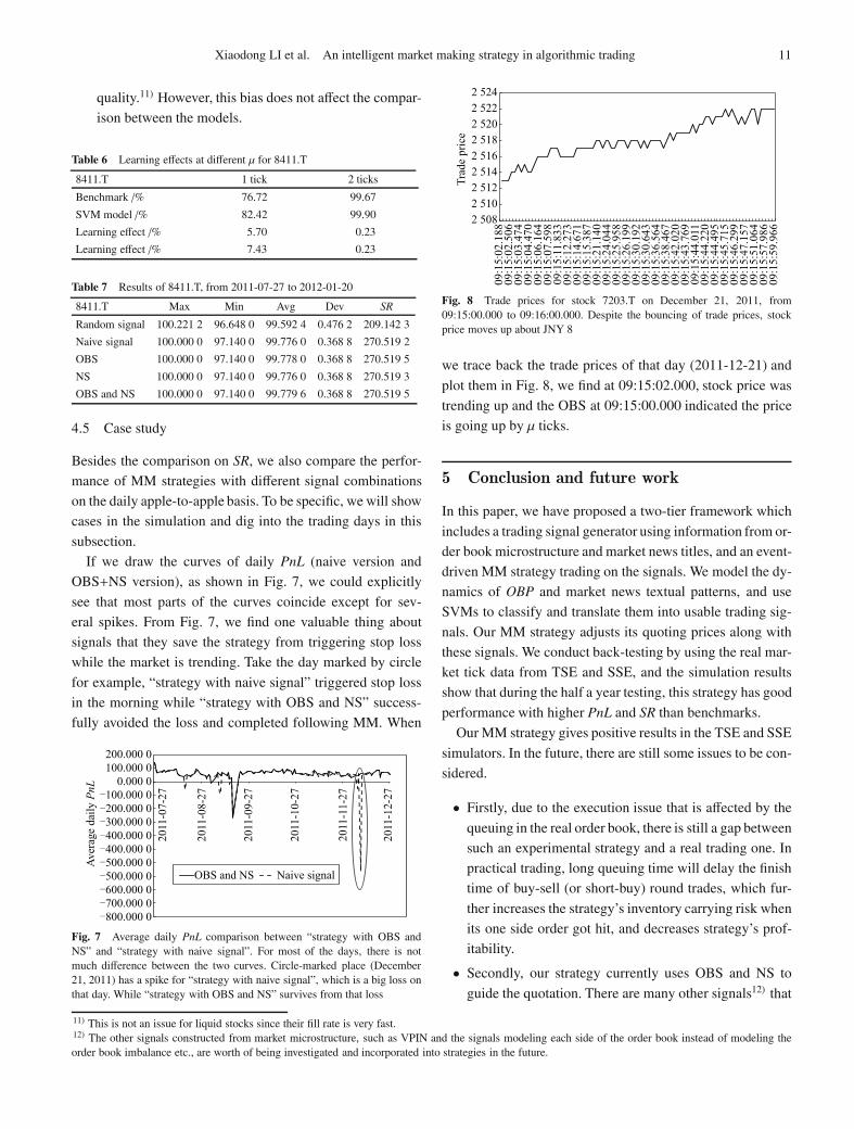
If we draw the curves of daily PnL (naive version and

OBS+NS version), as shown in Fig. 7, we could explicitly

see that most parts of the curves coincide except for sev-

eral spikes. From Fig. 7, we find one valuable thing about

signals that they save the strategy from triggering stop loss

while the market is trending. Take the day marked by circle

for example, “strategy with naive signal” triggered stop loss

in the morning while “strategy with OBS and NS” success-

fully avoided the loss and completed following MM. When

Fig. 7 Average daily PnL comparison between “strategy with OBS andNS” and “strategy with naive signal”. For most of the days, there is notmuch difference between the two curves. Circle-marked place (December21, 2011) has a spike for “strategy with naive signal”, which is a big loss onthat day. While “strategy with OBS and NS” survives from that loss

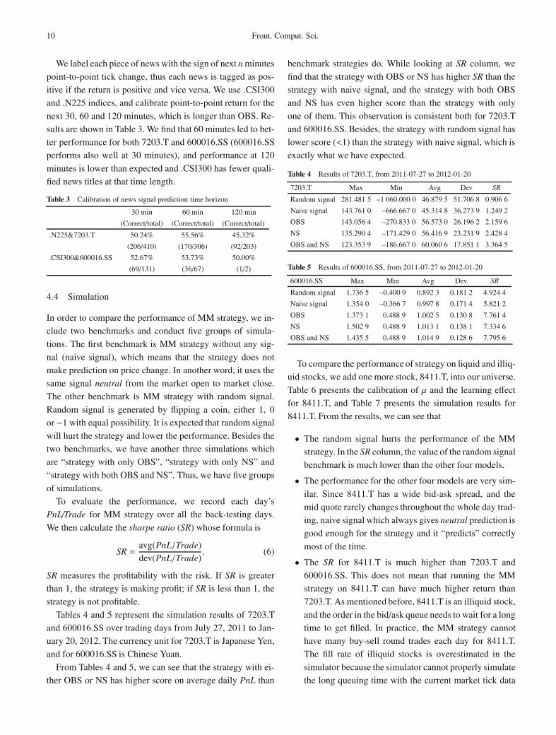
Fig. 8 Trade prices for stock 7203.T on December 21, 2011, from09:15:00.000 to 09:16:00.000. Despite the bouncing of trade prices, stockprice moves up about JNY 8

we trace back the trade prices of that day (2011-12-21) and

plot them in Fig. 8, we find at 09:15:02.000, stock price was

trending up and the OBS at 09:15:00.000 indicated the price

is going up by μ ticks.

5 Conclusion and future work

In this paper, we have proposed a two-tier framework which

includes a trading signal generator using information from or-

der book microstructure and market news titles, and an event-

driven MM strategy trading on the signals. We model the dy-

namics of OBP and market news textual patterns, and use

SVMs to classify and translate them into usable trading sig-

nals. Our MM strategy adjusts its quoting prices along with

these signals. We conduct back-testing by using the real mar-

ket tick data from TSE and SSE, and the simulation results

show that during the half a year testing, this strategy has good

performance with higher PnL and SR than benchmarks.

Our MM strategy gives positive results in the TSE and SSE

simulators. In the future, there are still some issues to be con-

sidered.

• Firstly, due to the execution issue that is affected by the

queuing in the real order book, there is still a gap between

such an experimental strategy and a real trading one. In

practical trading, long queuing time will delay the finish

time of buy-sell (or short-buy) round trades, which fur-

ther increases the strategy’s inventory carrying risk when

its one side order got hit, and decreases strategy’s prof-

itability.

• Secondly, our strategy currently uses OBS and NS to

guide the quotation. There are many other signals12) that

11) This is not an issue for liquid stocks since their fill rate is very fast.12) The other signals constructed from market microstructure, such as VPIN and the signals modeling each side of the order book instead of modeling theorder book imbalance etc., are worth of being investigated and incorporated into strategies in the future.


could be analyzed and included for the strategy’s use.

In the future study, we would like to investigate more on

the order book queuing theory and try to make the strategy

more practical. One possible approach is to establish the

stochastic relationship between the incoming flow (investors’

new orders) and outgoing flow (investors’ cancel orders and

market fill orders), and estimate the queuing time by the

stochastic process. Regarding the second issue, we will do a

further study on how to combine different signals and make

the strategy more effectively trade when more signals are

constructed based on the market microstructure.

Acknowledgements This work was supported by the National Natural Sci-ence Foundation of China (Grant Nos. 61173011, 61103125). Thanks forCharles River Advisors Ltd. who provide their commercial exchange sim-ulator for research use. Xiaotie Deng is supported by the National NaturalScience Foundation of China (Grant No. 61173011) and a 985 project ofShanghai Jiaotong University, China.

References

1. Radcliffe R. Investment: Concepts, Analysis, Strategy. Boston:

Addison-Wesley, 1997

2. Brahma A, Chakraborty M, Das S, Lavoie A, Magdon-Ismail M. A

bayesian market maker. In: Proceedings of the 13th ACM Conference

on Electronic Commerce. 2012, 215–232

3. O’hara M. Market Microstructure Theory. Cambridge, Mass.: Black-

well Publishers, 1995

4. Othman A, Sandholm T. Automated market-making in the large: the

gates hillman prediction market. In: Proceedings of the 11th ACM

Conference on Electronic Commerce. 2010, 367–376

5. Othman A, Sandholm T, Pennock D, Reeves D. A practical liquidity-

sensitive automated market maker. In: Proceedings of the 11th ACM

Conference on Electronic Commerce. 2010, 377–386

6. Das S, Magdon-Ismail M. Adapting to a market shock: optimal se-

quential market-making. Advances in Neural Information Processing

Systems, 2008, 361–368

7. Chakraborty T, Kearns M. Market making and mean reversion. In: Pro-

ceedings of the 12th ACM Conference on Electronic Commerce. 2011,

307–314

8. Kim K. Financial time series forecasting using support vector ma-

chines. Neurocomputing, 2003, 55(1–2): 307–319

9. Cao L, Tay F. Financial forecasting using support vector machines.

Neural Computing&Applications, 2001, 10(2): 184–192

10. Cao L. Support vector machines experts for time series forecasting.

Neurocomputing, 2003, 51: 321–339

11. Huang W, Nakamori Y, Wang S. Forecasting stock market movement

direction with support vector machine. Computers & Operations Re-

search, 2005, 32(10): 2513–2522

12. Fung G, Yu J, Lu H. The predicting power of textual information on

financial markets. IEEE Intelligent Informatics Bulletin, 2005, 5(1):

1–10

13. Schumaker R, Chen H. Textual analysis of stock market prediction us-

ing financial news articles. In: Proceedings of the 12th Americas Con-

ference on Information Systems. 2006, 185

14. Schumaker R, Chen H. A quantitative stock prediction system based on

financial news. Information Processing & Management, 2009, 45(5):

571–583

15. Schumaker R, Chen H. Textual analysis of stock market prediction us-

ing breaking financial news: the AZFin text system. ACM Transactions

on Information Systems, 2009, 27(2): 12

16. Schumaker R, Chen H. A discrete stock price prediction engine based

on financial news. Computer, 2010, 43(1): 51–56

17. Li X, Wang C, Dong J, Wang F, Deng X, Zhu S. Improving stock mar-

ket prediction by integrating both market news and stock prices. In:

Hameurlain A, Küng J, Wagner R, Liddle S W, Schewe K D, Zhou

X, eds. Database and Expert Systems Applications. Berlin: Springer,

2011, 279–293

18. Chen N, Deng X, Zhang J. How profitable are strategic behaviors in

a market? In: Demetrescu D, Halldórsson MM eds. Algorithms—

European Symposium on Algorithms. Berlin: Springer, 2011, 106–118

19. Abernethy J, Chen Y, Vaughan J. An optimization-based framework

for automated market-making. In: Proceedings of the 12th ACM Con-

ference on Electronic Commerce. 2011, 297–306

20. Bu T M, Deng X, Qi Q. Arbitrage opportunities across sponsored

search markets. Theoretical Computer Science, 2008, 407(1): 182–191

21. Bu T M, Deng X, Lin Q, Qi Q. Strategies in dynamic pari-mutual mar-

kets. In: Papadimitriou C, Zhang S, eds. Internet and Network Eco-

nomics. Berlin: Springer, 2008, 138–153

22. Salton G, McGill M J. Introduction to Modern Information Retrieval.

New York: McGraw-Hill Inc., 1986

23. Li X, Wang R, Cao J, Xie H. Empirical analysis: stock market predic-

tion via extreme learning machine. In: Proceedings of the 2013 Inter-

national Conference on Extreme Learning Machines. 2013, 1–12

24. Easley D, Prado L. d M M, O�Hara M. The microstructure of the “flash

crash”: flow toxicity, liquidity crashes, and the probability of informed

trading. The Journal of Portfolio Management, 2011, 37(2): 118–128

25. Abad D, Yagüe J. From pin to vpin: An introduction to order flow toxi-

city. The Spanish Review of Financial Economics, 2012, 10(2): 74–83

26. Han J, Kamber M, Pei J. Data Mining: Concepts and Techniques. San

Francisco: Morgan kaufmann, 2000

Xiaodong Li received the BSc degree

in computer science from Nanjing Uni-

versity, China. He is currently a PhD

student at City University of Hong

Kong, China. His research interests in-

clude data mining and algorithmic trad-

ing.


Xiaotie Deng is a chair professor in

the Department of Computer Science,

Shanghai Jiaotong University, China.

His research focus is on algorithmic

game theory, which deals with com-

putational issues on fundamental eco-

nomic problems such as Nash equilib-

rium, resource pricing and allocation

protocols such as auction and market

equilibrium, as well as theory and practice in internet market de-

sign.

Shanfeng Zhu received the BS and

MPhil degrees in computer science

from Wuhan University, China in 1996

and 1999, respectively, and the PhD in

computer science from the City Uni-

versity of Hong Kong, China in 2003.

He is currently an associate professor

of School of Computer Science, and

Shanghai Key Lab of Intelligent Infor-

mation Processing, Fudan University, China. Before joining Fudan

University in July 2008, he was a postdoctoral fellow at Kyoto Uni-

versity, Japan. His research focuses on developing and applying ma-

chine learning, data mining and algorithmic methods for informa-

tion retrieval, algorithmic trading, and bioinformatics. He is a mem-

ber of the CCF and the ACM.

Feng Wang received the MS and PhD

degrees in computer science in 2005

and 2008, respectively, both from

Wuhan University, China. She is cur-

rently an associate professor of School

of Computer Science, and State Key

Lab of Software Engineering of Wuhan

University, China. Her research inter-

ests include machine learning, intelli-

gent information retrieval, and algorithmic trading. She serves as a

reviewer for several IEEE transactions, other international journals

and conferences. She is a member of IEEE and ACM, and a senior

member of CCF.

Haoran Xie received the BEng degree

in software engineering from Beijing

University of Technology, China and

the MSc and PhD degrees in computer

science from City University of Hong

Kong, China. He is currently a senior

research assistant at Hong Kong Bap-

tist University, China. His research in-

terests include user modeling, person-

alization, social media, recommender systems, and financial data

mining.

An intelligent market making strategy in algorithmic trading

Documents