An integrated wind risk warning model for urban rail ...

An integrated wind risk warning model for urban rail transport in Shanghai, China

Article

Published Version

Creative Commons: Attribution 4.0 (CC-BY)

Open access

Han, Z., Tan, J., Grimmond, C. S. B., Ma, B., Yang, T. and Weng, C. (2020) An integrated wind risk warning model for urban rail transport in Shanghai, China. Atmosphere, 11 (1). 53. ISSN 2073-4433 doi: https://doi.org/10.3390/atmos11010053 Available at http://centaur.reading.ac.uk/88347/

It is advisable to refer to the publisher’s version if you intend to cite from the work. See Guidance on citing .Published version at: http://dx.doi.org/10.3390/atmos11010053

To link to this article DOI: http://dx.doi.org/10.3390/atmos11010053

Publisher: MDPI

All outputs in CentAUR are protected by Intellectual Property Rights law, including copyright law. Copyright and IPR is retained by the creators or other copyright holders. Terms and conditions for use of this material are defined in the End User Agreement .

www.reading.ac.uk/centaur

CentAUR

Central Archive at the University of Reading

Reading’s research outputs online

Atmosphere 2020, 11, 53; doi:10.3390/atmos11010053 www.mdpi.com/journal/atmosphere

Article

An Integrated Wind Risk Warning Model for Urban Rail Transport in Shanghai, China Zhihui Han 1,2,3, Jianguo Tan 2,4,5,*, C.S.B. Grimmond 6, Bingxin Ma 1, Tongxiao Yang 1 and Chunhui Weng 7

1 Shanghai Ecological Forecasting and Remote Sensing Center, Shanghai Meteorological Service, Shanghai 200030, China; [email protected] (Z.H.); [email protected] (B.M.); [email protected] (T.Y.)

2 Shanghai Key Laboratory of Meteorology and Health, Shanghai Meteorological Service, Shanghai 200030, China

3 State Key Laboratory for Disaster Reduction in Civil Engineering, Tongji University, Shanghai 200030, China

4 Shanghai Climate Center, Shanghai Meteorological Service, Shanghai 20003, China 5 Key Laboratory of Cities’ Mitigation and Adaptation to Climate Change in Shanghai, CMA, Shanghai

200030, China 6 Department of Meteorology, University of Reading, Reading RG6 6BB, UK; [email protected] 7 Shanghai Metro Operation Management Center, Shanghai 200030, China; [email protected] * Correspondence: [email protected]

Received: 7 November 2019; Accepted: 27 December 2019; Published: 1 January 2020

Abstract: The integrated wind risk warning model for rail transport presented has four elements: Background wind data, a wind field model, a vulnerability model, and a risk model. Background wind data uses observations in this study. Using the wind field model with effective surface roughness lengths, the background wind data are interpolated to a 30-m resolution grid. In the vulnerability model, the aerodynamic characteristics of railway vehicles are analyzed with CFD (Computational Fluid Dynamics) modelling. In the risk model, the maximum value of three aerodynamic forces is used as the criteria to evaluate rail safety and to quantify the risk level under extremely windy weather. The full model is tested for the Shanghai Metro Line 16 using wind conditions during Typhoon Chan-hom. The proposed approach enables quick quantification of real-time safety risk levels during typhoon landfall, providing sophisticated warning information for rail vehicle operation safety.

Keywords: rail transport; wind risk warning model; aerodynamic force; roughness length; wind field

1. Introduction

Rail transport is important in cities for both economic development and to alleviate congestion. Severe weather disruption of these systems can have significant economic and societal impacts on a region [1–3]. Daily, the Shanghai rail network (673 km of lines, 395 stations) is used by 11.8 million passengers [4]. Accidents associated with extreme weather (e.g., strong winds, heavy rainfall, low temperature, and high humidity) happen frequently and seriously affect the rail operation efficiency [5]. The main meteorological causes of rail service suspension in Shanghai are rainfall-induced waterlogging at the ground level and from strong winds for elevated lines [6]. For example, heavy precipitation, flooding, and strong winds of Typhoon HaiKui (August 2012) significantly disrupted rail transport, with rail, subway, and Maglev systems being suspended [7]. Although some knowledge exists on how to protect transport infrastructure from extreme weather, climate events,

Atmosphere 2020, 11, 53 2 of 16

and climate change, and to improve network performance [8–12], given the sensitivity of rail transport to extreme weather, more attention is warranted.

Urban rail transport involves many vehicles moving at high speed, making it vulnerable to aerodynamic forces induced by strong winds. These forces can influence the stability of carriages, and, under extreme conditions, lead to derailment, resulting in significant economic loss and casualties. For example, when the wind speed reached its maximum velocity of 41.8 m·s−1 (at 10 m) on 28 February 2007 in Xinjiang (China), 11 train carriages derailed, causing three deaths [13]. Studies of aerodynamic effects have largely used wind tunnel observations [14–16] and computational fluid dynamics (CFD) modelling [17,18]. Examples include: A scale model of a high speed passenger train at zero yaw in a wind tunnel was used to study the dependence of train skin friction drag and total aerodynamic drag on Reynolds number [14]; wind tunnel tests consider three types of rail vehicles in different configurations to identify the most critical wind conditions for running safety and the principal parameters influencing aerodynamic behavior [16]; and the stability, aerodynamic performance of a train, and the surrounding flow field in detail with numerical simulation [17]. Research on strong winds [19–21] and the effects of wind load on rail vehicle performance [22] have expanded considerably in the last decade, but much less attention has been given to the development of integrated systems of monitoring, forecasting, warning, and decision-making.

In this paper, an integrated wind risk warning model for rail transport (hereafter WR2) is introduced. It accounts for meteorological wind conditions, aerodynamic forces, and vehicle risk assessment. The study focuses on the transit vehicles used on the Shanghai Metro Line 16. The methodology uses CFD modeling with data that are available in most metropolitan areas of China (and many other countries). The approach proposed has considerable potential to improve network operation efficiency.

2. Meteorological Background

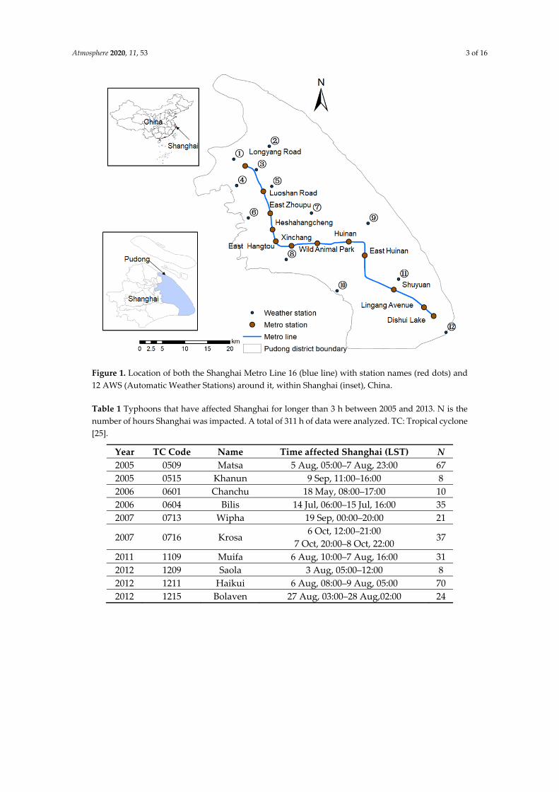
The coastal city of Shanghai is an important financial, direct-controlled municipality of China, with more than 24 million people [23]. Increasingly, Shanghai citizens rely on daily rail transport, especially between the suburbs and downtown. Here, we focused on the 58.96 km-long Metro Line 16 (45.22 km elevated) in the southeast of Shanghai (Figure 1). In this area, wind speeds are usually greater than elsewhere in the city [24]. Typhoons, strong gales associated with cold air, and strong convective weather systems all affect the operation and safety of this rail line. During typhoons that make landfall (Table 1), the wind roses for 12 automatic weather stations (AWS) near Metro Line 16 illustrate the wind from the NNE to SSE for 90% of the time (Figure 2).

Atmosphere 2020, 11, 53 3 of 16

Figure 1. Location of both the Shanghai Metro Line 16 (blue line) with station names (red dots) and 12 AWS (Automatic Weather Stations) around it, within Shanghai (inset), China.

Table 1 Typhoons that have affected Shanghai for longer than 3 h between 2005 and 2013. N is the number of hours Shanghai was impacted. A total of 311 h of data were analyzed. TC: Tropical cyclone [25].

Year TC Code Name Time affected Shanghai (LST) N 2005 0509 Matsa 5 Aug, 05:00–7 Aug, 23:00 67 2005 0515 Khanun 9 Sep, 11:00–16:00 8 2006 0601 Chanchu 18 May, 08:00–17:00 10 2006 0604 Bilis 14 Jul, 06:00–15 Jul, 16:00 35 2007 0713 Wipha 19 Sep, 00:00–20:00 21

2007 0716 Krosa 6 Oct, 12:00–21:00

7 Oct, 20:00–8 Oct, 22:00 37

2011 1109 Muifa 6 Aug, 10:00–7 Aug, 16:00 31 2012 1209 Saola 3 Aug, 05:00–12:00 8 2012 1211 Haikui 6 Aug, 08:00–9 Aug, 05:00 70 2012 1215 Bolaven 27 Aug, 03:00–28 Aug,02:00 24

Atmosphere 2020, 11, 53 4 of 16

Figure 2. Wind roses for 12 AWSs (automatic weather stations) around Shanghai Metro Line 16 (Figure 1) during the typhoons that affected the city between 2005 and 2013 (Table 1). Observations were made with Vaisala WA 15 wind sensors at 10 m above ground level (agl), samples at 1 min.

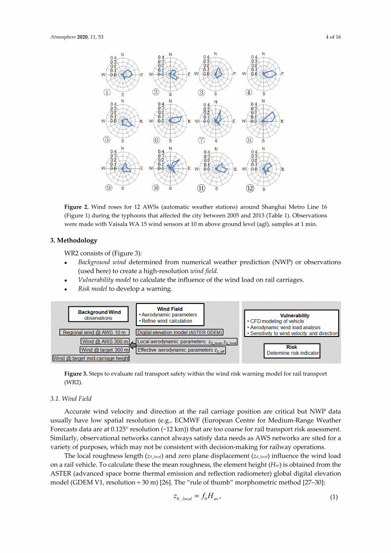
3. Methodology

WR2 consists of (Figure 3): Background wind determined from numerical weather prediction (NWP) or observations

(used here) to create a high-resolution wind field. Vulnerability model to calculate the influence of the wind load on rail carriages. Risk model to develop a warning.

Figure 3. Steps to evaluate rail transport safety within the wind risk warning model for rail transport (WR2).

3.1. Wind Field

Accurate wind velocity and direction at the rail carriage position are critical but NWP data usually have low spatial resolution (e.g., ECMWF (European Centre for Medium-Range Weather Forecasts data are at 0.125° resolution (~12 km)) that are too coarse for rail transport risk assessment. Similarly, observational networks cannot always satisfy data needs as AWS networks are sited for a variety of purposes, which may not be consistent with decision-making for railway operations.

The local roughness length (z0_local) and zero plane displacement (zd_local) influence the wind load on a rail vehicle. To calculate these the mean roughness, the element height (Hav) is obtained from the ASTER (advanced space borne thermal emission and reflection radiometer) global digital elevation model (GDEM V1, resolution = 30 m) [26]. The “rule of thumb” morphometric method [27–30]:

0 _ 0local avz f H= , (1)

Atmosphere 2020, 11, 53 5 of 16

_d local d avz f H= (2)

is used with the variability of building heights accounted for in the constants [31]: ƒ0 = 0.2 and ƒd =1.4. Rougher surfaces decrease the velocity (U) near the ground, as expressed in the logarithmic wind profile assuming neutral stability [32]:

0

( ) ln dz zuU zk z

∗ −=,

(3)

where u* is the friction velocity, k = 0.4 is von Karman’s constant, and z is the height above ground level (agl). Thus, given background wind data and the roughness parameters for the fetch over which the wind has blown as it approached the rail carriage, a local wind velocity can be estimated for any heights for which the log-law (Equation (3)) is applicable [31].

However, in urban environments, this may not be straightforward. In Shanghai, with more than 35,000 tall (>30 m) buildings, and over 1500 skyscrapers (>100 m) [23], there is hugely complex surface roughness, fetch, and thus wind fields. The rapid increase in the area of tall buildings between the year 2000 (2.59 km2 based on SRTM3 (Shuttle Radar Topography Mission) data (90 m resolution) [33]) and 2009 (30.09 km2 based on ASTER GDEM V1) means the surroundings of many AWS have changed. As these are not ‘traditional’ WMO sites [34] (e.g., influenced by a tall building in one direction and/or by trees in another), measurements may be unrepresentative of the regional, or background, wind field. Accounting for variations by direction may lead to more appropriate wind interpolation. To reduce the probability of physically unreasonable spatial inhomogeneity being generated during the interpolation, 10 m wind speeds (U10) were logarithmically raised to 300 m (U300):

_ln((300 ) / ) / ln((10 ) / )300 10 d,300 0_eff,300 d local 0_localU U z z z z= − − , (4)

where z0_eff,300 is the effective roughness length for winds at 300 m and zd,300 is the zero-plane displacement for winds at 300 m (Figure 4). These data are spatially interpolated using inverse weighting [35] and then logarithmically reduced to 70 m (U70):

ln((70 ) / ) / ln((300 ) / )70 300 d,70 0_eff,70 d,300 0_eff,300U U z z z z= − − , (5)

and from there to the mid-height of the carriage (zcar):

7 _ln(( ) / ) / ln((70 ) / )car 0 car d local 0_local d,70 0_eff,70U U z z z z z= − − , (6)

where z0_eff,70 is the effective roughness length for winds at 70 m, and zd,70 is the zero-plane displacement for winds at 70 m (Figure 4). The effective surface roughness length at a blending height, zr, is determined from [36]:

_/ exp( / ( ))0_eff r d mean rz z k C z=, (7)

where Cd_mean(zr) is the mean value of drag coefficients, Cd(zr), obtained by averaging the drag coefficient of an area:

2 2* 0( ) ( / ( )) ( / ln( / ))d r r r dC z u U z k z z z= = − , (8)

where zr is a reference height (i.e., 70, 300 m) to allow calculations for winds at 70 m (effective roughness length, z0_eff,70) and 300 m (z0_eff,300). Linear spatial averages are calculated for a height-fetch ratio of 1:50, i.e., 3480 and 15000 m squares (Figure 4), respectively, given the 30 m resolution.

Atmosphere 2020, 11, 53 6 of 16

Figure 4. Spatial variation in Shanghai based on ASTER GDEM V1 (NASA/METI 2009) data (resolution = 30 m) of: (a) local roughness length (z0_local) (Equation (1)); and effective roughness length (Equation (7)) for (b) 70 m agl (z0_eff,70) averaged over 3480 m; (c) for 300 m agl (z0_eff,300) for 15,000 m.

To determine the background wind, z0_eff,70 was calculated for 16 sectors (i.e., 22.5°, 1740 m extent) around each of the 119 AWS in Shanghai (Figure 5). The background wind field is interpolated from selected AWS across the whole area using the individual sectors for each AWS with z0_eff,70 ≤ 0.3 m. In the suburbs (beyond the pink area, Figure 4a), most stations meet the requirement in all 16 sectors; whereas within the urban area (pink, Figure 4a), frequently only a few sectors are usable (Figure 5). When the wind is from the north, 63 stations are used to interpolate the background wind field across the Shanghai province; whereas from the east 70, south 61, and west only 57 stations are used. The wind is interpolated every 10 min to provide a 30-m resolution gridded data set. Using the log-law with both the local and effective aerodynamic parameters, the wind speed is determined along the Metro line at zcar (train track ground level + centre height Hc of the vehicle). If this height is lower than where the log-law is applicable, then the within canopy exponential decrease [37] is applied.

Figure 5. All 119 AWS locations in Shanghai (●) and the wind directions the data were used to assess background wind based on criteria in Section 3.1: all directions (triangle), north (green), east (blue), south (grey), and west (red).

Atmosphere 2020, 11, 53 7 of 16

3.2. Vulnerability Model

3.2.1. Wind load Modeling

The Shanghai Metro Line 16 trains have three parts: Tail #1, Middle, and Tail #2 (hereafter T1, M, T2, respectively). T1 and T2 are the same length (LT) but are mirror images of each other. This enables the train to be driven in both directions. The front of each has an oblique angle of 25°, whereas the end that attaches to the M carriage is vertical (Figure 6). The M carriage has two vertical sides and length LM. The complete train is characterized by its length (L = 2LT + LM), width (W), height (H), and the carriage bottom to the rail track surface (Hb) distance (Figure 6).

Figure 6. (a) Model and mesh details in CFD (Computational Fluid Dynamics) simulation. The whole model domain is a 24-sided prism, with an externally tangent circle diameter of 30 L. The train model with two oblique faces of 25° lies in the center of the model domain, and its horizontal, longitudinal, and vertical lines are meshed with 30, 30, and 350 grids, respectively. (b) Relation between vehicle velocity (Uvehicle), wind velocity (Uwind), and resultant relative wind velocity (Urelative) for a train subjected to crosswinds. β is the yaw angle of the relative wind velocity, β0 the yaw angle of wind velocity. (c) Aerodynamic forces reference system: the aerodynamic lift force, FL, lateral (or side) aerodynamic force, FS, and overturning moment, FM. The dimensions refer to X and Y.

The wind load on the train at different wind attack angles is investigated using the commercial CFD software FLUENT. Here, a full-scale model of the train is established to simulate the interaction between the moving train and wind flow. Only the outer contour of the train is simulated, ignoring the influence of some details, such as the wheels, to obtain better grid simulations using fewer grids as is commonly done with CFD (e.g., Garcia et al. [38] simulated the train aerodynamics but ignored bogies, pantograph, spoiler, and the inter-car gap). Garcia et al. [38] concluded that CFD results are impacted if train underbody details are missing (cf. to observations) but less influenced by spoiler or bogies details. As we focus on aerodynamic (i.e., integrated facial) forces, the simplification is acceptable. The complete modelling domain is a 24-sided prism, with an externally tangent circle diameter of 30 L. The train model lies in the center of the modeling domain, and its horizontal, longitudinal, and vertical lines are meshed with 30, 30, and 350 grids, respectively (Figure 6). To control the grid quality, a sub-domain method is adopted to divide the computational domain into two parts: The exterior part shaped as a 24-sided hollow prism, and the interior part of the remaining region. To correctly reproduce the flow separation for the angle of attack, a finer spatial resolution is

Atmosphere 2020, 11, 53 8 of 16

used in the interior domain. In total, 2 million rectangular elements are generated with a minimum grid dimension on the train surface of 0.1 m, following the meshing scheme adopted by [16].

A velocity-inlet boundary condition is applied to the front planes along the windward direction and is characterized by a logarithmic wind profile, which represents a rural or sparse building terrain (z0 = 0.2 m). For the rear planes, the pressure outlet condition is set to a gauge value. For the train surface planes, the standard wall function is used to permit separated flow around a bluff body while the ground plane is a user defined fixed wall function to ensure the accuracy of numerical simulation [39]. The other planes are considered as symmetrical.

For moving rail vehicles with a crosswind, the pressure distribution, and thus the aerodynamic forces and momentum, are obviously related to the vehicle and wind properties. However, the actual wind that directly affects the wind load on the train is the relative wind velocity (Urelative) and its yaw angle (β) relative to the vehicle travel direction. This is the resultant of the vehicle and wind velocity vectors. In this paper, β is defined as the angle of attack. Figure 6 shows the relation between the vehicle velocity, Uvehicle, the wind velocity, Uwind, the relative wind velocity, Urelative, and their yaw angles, β0, β. However, in the CFD simulation, the train model is stationary, so Urelative = Uwind and thus β = β0. As the train is symmetric, only seven wind attack angles between 0° and 90° are simulated (interval = 15°).

The wind flow in the CFD simulation is considered as incompressible and the realizable k–ε turbulence model [40] is adopted. The SIMPLEC [41] velocity–pressure coupling method is used with the PRESTO [42] pressure and QUICK [43] momentum equations discretization methods.

Figure 7 shows the wind pressure coefficient distribution at angles of attack β = 0 °, 45° and 90°. The pressure coefficient Cpi (= pi(0.5ρUwind,Hc2)−1) is defined as the ratio of actual wind pressure to incoming flow pressure at a reference height (Hc), where pi is wind pressure of point i, ρ is air density, and Uwind,Hc is wind velocity at Hc (i.e. the centre height of the vehicle used here).

Figure 7. Wind pressure distribution coefficients of the rail train at angles of attack (a) 0°, (b) 45°, (c) 90° calculated with realizable k–ε turbulence model.

For β = 0°, the wind pressure coefficient distribution is obviously symmetric, with positive values on the whole front surface and the middle areas of the top, side, and bottom surfaces, with negative values on the areas close to windward of the top, side, and bottom surfaces, due to flow separation and reattachment. For β = 45°, the wind pressure coefficient on the front and side surfaces are positive, with the maximum occurring at the intersection of the two surfaces. All the wind pressure coefficients of the top, bottom, and side surfaces on the leeward side are negative. For β = 90°, the wind pressure coefficient distribution is also symmetric, with positive values on the only side surface facing inflow, and negative values on all the other surfaces.

3.2.2. Effect of Angle of Attack

Wind pressure on the rail vehicles can produce a group of forces, including aerodynamic drag force, aerodynamic lift force, trim moment, overturning moment, lateral aerodynamic force, and so on [16]. This paper focuses mainly on the aerodynamic lift force, FL, lateral (or side) aerodynamic force, FS, and overturning moment force, FM, which can directly influence the lateral stability of rail vehicles (Figure 6). The three aerodynamic forces are associated with wind and vehicle velocities, which are changing all the time. For the convenience of wind load calculation, the nondimensionalized coefficients of the three forces are defined:

Atmosphere 2020, 11, 53 9 of 16

2 2 2, , ,0.5 U 0.5 U 0.5 U

S L MS L M

wind Hc wind Hc wind Hc

F F FC C CA A A Hρ ρ ρ

= = =,

(9)

where A is the lateral projected area of the vehicle coach (front [T1] or back [T2] = 72.9 m2, middle [M] = 69.7 m2), ρ is the air density, and H is the height of the vehicle.

As expected, all the aerodynamic force coefficients change with the angle of attack (Figure 8). The lateral aerodynamic force (CS) and the overturning moment coefficients (CM) decrease from the front (T1) to the middle (M) to the back (T2) carriages. The largest CS and CM of the whole train are found between the T1 and M carriage. The aerodynamic lift force coefficient (CL,) of the M vehicle is slightly larger than the others.

In general, when the train is moving, the lateral wind has the greatest influence on the T1 vehicle, i.e., it is the most vulnerable to derailment. Given this, we focus on this vehicle. The aerodynamic force coefficients for T1 as a function of the wind angle of attack are derived from polynomial fits to the data in Figure 8:

2 20.00008 0.0198 0.0938 0.997LC Rβ β= − + − = , (10)

2 20.0001 0.0201 0.0113 0.984SC Rβ β= − + − = , (11)

2 20.0002 0.0246 0.0259 0.989MC Rβ β= − + − = . (12)

0 15 30 45 60 75 900.0

0.2

0.4

0.6

0.8

1.0

1.2

T1 M T2 WHOLE

Angle of attack (°)

CL

(a)

0 15 30 45 60 75 900.0

0.2

0.4

0.6

0.8

1.0

1.2

T1 M T2 WHOLE

Angle of attack (°)

CS

(b)

0 15 30 45 60 75 900.0

0.2

0.4

0.6

0.8

1.0

1.2

T1 M T2 WHOLE

Angle of attack (°)

CM

(c)

Figure 8. Aerodynamic force coefficients of rail vehicles versus angle of attack derived from Equation (9). (a) Aerodynamic lift force coefficient CL, (b) lateral (or side) aerodynamic force coefficient CS, (c) overturning moment coefficient CM ; for front (T1), middle (M), and back (T2) carriages, plus for the whole train (WHOLE).

3.2.3. Effect of Wind Direction, Wind Velocity, and Vehicle Velocity

To test the effect of wind direction on aerodynamic forces, we analysed the Dishui lake to East Huinan section of the Metro line (Figure 1), when the vehicle is travelling southeast at a velocity of 40 km·h-1. A wind velocity of 18 m·s−1 is used with the aerodynamic forces with respect to wind direction (Figure 9) obtained from Equations (9) to (12). This wind speed is chosen as the Shanghai Metro Operation Management Center sets a maximum vehicle velocity when the Beaufort Scale wind is eight (assumed here to be equivalent to 18 m·s−1).

Atmosphere 2020, 11, 53 10 of 16

0 45 90 135 180 225 270 315 3600

5

10

15

20

25

FM (kN

⋅m)

F L/F

S (kN

)

FL FS

Wind direction (°)

0

5

10

15

20

25 FM

Figure 9. Impact of wind direction when a vehicle is travelling southeast at 40 km·h−1 with a wind velocity of 18 m·s−1 on aerodynamic forces: aerodynamic lift force (FL, kN), lateral (or side) aerodynamic force (FS, kN), and overturning moment (FM, kN·m). Note that the meteorological convention for wind direction is used (i.e., northerly is 0°, increasing clockwise).

The aerodynamic lift force (FL), lateral aerodynamic force (FS), and overturning moment (FM) change in a similar manner with the wind direction. For the situation considered, all three aerodynamic forces have minimum values (0) at both 135° (southeast wind) and 315° (northwest wind), i.e., when the vehicle runs parallel to the wind direction and the wind angle of approach is 0°. However, the three aerodynamic forces maxima occur at different wind directions: For FL, at 56.25° and 213.75°; for FS, at 67.5° and 202.5°; and FM, at 78.75° and 191.25°. This analysis shows that wind direction has a considerable influence on the aerodynamic forces on rail vehicles. Thus, under conditions of known wind velocity and vehicle velocity, judgments can be made if the vehicle velocity should be reduced with respect to the prevailing wind direction. This approach has considerable potential to improve network operation efficiency.

The same scenario is used to evaluate the impact of wind velocity. As meteorological data analysis (Section 2) shows the prevailing wind direction along Metro Line 16 during landfall of a typhoon is most commonly NNE to SSE, here, we use 90°. The FL, FS, and FM increase gradually with wind velocity, with increasing rates with greater wind velocities (Figure 10). With a wind velocity of 18 m·s-1, the three forces are 13.3 kN, 15.8 kN, and 16.9 kN·m, respectively. However, if the wind velocity is doubled (i.e., 36 m·s-1), the three forces more than double: Increases of 2.39 (45.1 kN), 2.25 (51.3 kN), and 2.15 (53.2 kN·m) times, respectively.

0 5 10 15 20 25 30 35 40 45 500

20

40

60

80

100

FM (kN

⋅m)

FL FS

Wind velocity (m⋅s-1)

F L/FS (k

N)

0

20

40

60

80

100 FL

Figure 10. As in Figure 9 but the impact of wind velocity variations assuming an easterly wind (90°).

With the same conditions used to evaluate the effect of the rail vehicle velocity (Figure 11), the three forces increase approximately linearly, with FL having the slowest rate. When the vehicle

Atmosphere 2020, 11, 53 11 of 16

velocity is 40 km·h−1 (80 km·h−1), the three forces are 13.3 (17.0) kN, 15.8 (22.1) kN, and 16.9 (24.3) kN·m, respectively. Thus, if the vehicle velocity is doubled, the aerodynamic forces increase by 0.28, 0.40, and 0.44 times, respectively. As the vehicle aerodynamic forces are more sensitive to wind velocity than vehicle velocity, when wind velocity doubles, the vehicle velocity needs to be reduced by a greater factor to ensure stability.

0 20 40 60 80 100 12010

15

20

25

30

35

FM (kN

⋅m)

FL FS

Vehicle velocity (km⋅h-1)

F L/FS (k

N)

10

15

20

25

30

35 FM

Figure 11. As in Figure 9 but the impact of vehicle velocity.

3.3. Risk Model

The reason for developing WR2 is to have a tool that can be used to quickly, and automatically, control the velocity of rail vehicles to minimize (or avoid accidents) and to enhance the safety and efficiency of the system. Following discussions with the train operators, and investigation of real cases during strong winds, it was found that consistently all three aerodynamic forces influence the lateral stability of the vehicle and should be included in quantitative indicators of risk. The risk factor, R, defined as the maximum of the ratio of the three aerodynamic force to their corresponding threshold, is used to quantify risk under extreme winds:

[( ) , ( ) , ( ) ]S L Mside lift moment

S L M

F F FR MAX=Δ Δ Δ

, (13)

where FS, FL, and FM are the lateral aerodynamic force, aerodynamic lift force, and overturning moment, respectively, and ΔS, ΔL, ΔM are their thresholds, respectively. From a mechanics perspective, both FL and FS can affect the lateral force balance (FM is a resultant moment of FL and FS). Thus, there are complex cross effects between FL, FS, and FM. Given the Shanghai Metro Operation Management Center stipulate a maximum vehicle velocity at Beaufort Scale eight (~18 m·s−1) based on consideration of the comprehensive effects of all aerodynamic forces, the maximum aerodynamic forces when the vehicle runs at this maximum velocity are taken as the thresholds. Using Equations (9) to (12), ΔS is 1.7·104 N, ΔL is1.8·104 N, and ΔM is 1.9·104 N·m.

To calculate the risk factor, R, the steps are (Figure 3): (1) Obtain wind information for the rail vehicle from background AWS data interpolation (Section 3.1); (2) calculate the relative wind attack angle, β, and obtain the aerodynamic forces (Equations (9) to (12)); and (3) calculate the risk factor, R (Equation (13)).

4. Application

As the southern section of Shanghai Metro Line 16 (Figure 1) is exposed to typhoons almost every year, when these conditions prevail, rail vehicles must be slowed or stopped. Here, we applied WR2 using Typhoon Chan-hom wind conditions. This had Beaufort Scale winds of seven to nine (13.9 −24.4 m·s−1) in Shanghai, reaching 9 to 11 (20.8–30.3 m·s−1) along coastal areas with a maximum wind

Atmosphere 2020, 11, 53 12 of 16

velocity of 30.3 m·s−1 (AWS #12, Figure 1). The mean bias errors of the wind velocities (observed –simulated) at 10 m for the Wild Animal Park and Lingang Avenue metro stations (Figure 1) on 11 July 2015 (when Chan-hom made landfall) are 1.34 and 1.31 m·s−1, respectively (Figure 12); i.e., the model under-estimates. Figure 13 shows the risk distribution at 7:50 LST on 11 July 2015 based on the five rail transport risks classes (Table 2) associated with minimum wind velocities.

0 2 4 6 8 10 12 14 16 18 20 22 242468

1012141618

LST hour

Win

d ve

loci

ty (m

⋅s-1)

observed at Wild Animal Park simulated at Wild Animal Park observed at Lingang Avenue simulated at Lingang Avenue

Figure 12. Observed and simulated 10 min average wind velocities at Wild Animal Park and Lingang Avenue metro stations (Figure 1) on LST 11 July 2015 during Typhoon Chan-hom landfall.

The new WR2 model can quickly supply real-time safety risk level information during a typhoon. For the scenario considered, the risk level of the whole line is greater than “medium”. The risk around the Longyang and Huinan stations is the lowest, caused by the dense buildings with a large surface roughness length (Figure 14) that reduces the wind velocity and risk level (Table 2). However, the whole segment from Shuyuan to Dishui Lake stations, near the coast, is at “high” to “very high risk”. On this morning, trains were slowed down in the areas with high risk (Figure 13). This application shows that the method can provide finer scale warning information for rail vehicle operation safety, which should greatly improve the decision-making efficiency for the rail management during strong wind conditions, such as associated with typhoons.

Table 2 Wind risk scale (R, Equation 13) for rail transport and the minimum wind velocity at vehicle center height associated with each class.

Range 0 ＜ R ≤ 0.25 0.25 ＜ R ≤ 0.5 0.5 ＜ R ≤ 0.75 0.75 ＜ R ≤ 1 R ＞ 1 Risk Level Very low Low Medium High Very high

Minimum Wind Velocity (m·s−1) - 7.0 11.9 15.7 18.0

Atmosphere 2020, 11, 53 13 of 16

Figure 13. WR2 determined risk levels (see Table 2 values associated with the levels) of Shanghai Metro Line 16 during Typhoon Chan-hom landfall (7:50 LST 11 July 2015). See Figure 1 for location within Shanghai.

Figure 14. Spatial variation of local roughness length (z0_local) (Equation (1)) within 2 km along Shanghai Metro Line 16 based on ASTER GDEM V1 [26] data (resolution = 30 m).

Atmosphere 2020, 11, 53 14 of 16

If NWP data are used to provide the background wind conditions, WR2 can provide a forecast for rail vehicle operation safety, aiding both rail management and passenger expectations. NWP wind data from 925 hPa (~700 m, i.e., ~urban boundary layer height) are recommended for the background data to minimize the impact from surface structures. Accordingly, the wind field model needs to be modified slightly. The wind data at the target position can be extracted by reducing wind data from 925 hPa to Hc. Although WR2 has been available to the Shanghai Shentong Metro Group Co. since July 2016, with no typhoons in this area since then, it is not possible to assess the impact of it use on operations.

5. Conclusions

The wind risk warning model for rail transport (WR2) was developed by combining aerodynamic characteristics of rail vehicles with AWS wind data. The wind field interpolation uses an effective surface roughness length to enhance accuracy. Analysis of the aerodynamic characteristics of railway vehicles on Shanghai Metro Line 16 using CFD modelling showed that the lateral wind has the largest influence on the front carriage of a running train, and that wind direction has a large influence on the aerodynamic forces. Thus, if wind and vehicle velocities are known, judgments can be made about whether vehicle velocity should be limited (or not) with respect to the prevailing wind direction. This approach has considerable potential to improve network operation efficiency and safety. Critically, we recommend that the maximum value of the three aerodynamic forces is taken as the criteria for rail safety evaluation and propose the risk model to quantify risk under extreme windy weather.

WR2 can quantify quickly real-time safety risk levels during typhoon landfall, providing sophisticated warning information for rail vehicle operation safety. The risk model is sensitive to the wind direction and velocity, so the largest uncertainty is directly related to the surface aerodynamic parameters. The abrupt changes of wind speed and wind direction, when the train leaves the sheltered section or reverse, can affect the wind loading of the train, but at this time, the train normally runs at a low velocity, and the overall impact is not serious. As WR2 only considers the wind effect on rail vehicle safety, other risks related to fog, low (frozen) temperatures, etc., which can also cause serious accidents, need to be considered independently. As the wind load modeling is based on a prototype train, with the effects of infrastructure and noise barriers neglected, the results maybe conservative. Therefore, future research should consider these scenarios and involve wind tunnel tests to improve the wind load accuracy.

Given WR2’s simplicity, it has the potential to help evaluate planning decisions related to rail network operation efficiency (e.g., increase or decrease train velocity), site selection for rail lines and stations, and assessment for construction planning along existing rail lines.

Author Contributions: Formal analysis, Z.H. and T.Y.; investigation, Z.H., J.T., B.M. and C.W.; methodology, Z.H., J.T. and C.S.B.G.; resources, Z.H. and J.T.; validation, Z.H.; writing—original draft preparation, Z.H.; writing—review and editing, Z.H., J.T. and C.S.B.G. All authors have read and agreed to the published version of the manuscript.

Funding: This research was joint funded by the National Natural Science Foundation of China (grant number 41775019, 41875059), China Special Fund for Meteorological Research in the Public Interest (grant number GYHY201306023) , and the UK-China Research & Innovation Partnership Fund through the Met Office Climate Science for Service Partnership (CSSP) China as part of the Newton Fund.

Acknowledgments: We thank all the anonymous reviewers for their fair, exhaustive and competent comments on the manuscript.

Conflicts of Interest: The authors declare no conflict of interest.

References

1. Ludvigsen, J.; Klæboe, R. Extreme weather impacts on freight railways in Europe. Nat. Hazards. 2014, 70, 767–787.

Atmosphere 2020, 11, 53 15 of 16

2. Vajda, A.; Tuomenvirta, H.; Juga, I.; Nurmi, P.; Jokinen, P.; Rauhala, J. Severe weather affecting European transport systems: The identification, classification and frequencies of events. Nat. Hazards. 2014, 72, 169–188.

3. Jaroszweski, D.; Hooper, E.; Baker, C.; Chapman, L.; Quinn, A. The impacts of the 28 June 2012 storms on UK road and rail transport. Meteorol. Appl. 2015, 22, 470–476.

4. The Pujiang line began to operate on 31 March (in Chinese). Available online: http://www.shmetro.com/node49/201803/con115042.htm. (accessed on 20 June 2018).

5. Weng, C. Application of strong wind forecast on Shanghai rail transit elevated and ground metro lines (in Chinese). Urban Mass Transit. 2016, 19, 138–142.

6. Zhang,W. Rethink about work of ‘9.13’ rainstorm and ‘Feite’ typhoon (in Chinese). Urban Roads Bridges Flood Control. 2015, 36, 127–129.

7. “Haikui” slams Shanghai making suspension of high-speed rail and Maglev (in Chinese). Available online: http://bj.bendibao.com/news/201289/82662.shtm (accessed on 30 December 2019).

8. Suarez, P.; Anderson, W.; Mahal, V.; Lakshmanan, T.R. Impacts of flooding and climate change on urban transportation: A systemwide performance assessment of the Boston Metro Area. Transp. Res. Part, D. 2005, 10, 231–244.

9. Koetse, M.J.; Rietveld, P. The impact of climate change and weather on transport: An overview of empirical findings. Transp. Res. Part D. 2009, 14, 205–221.

10. Jaroszweski, D.; Chapman, L.; Petts, J. Assessing the potential impact of climate change on transportation: The need for an interdisciplinary approach. J. Transp. Geogr. 2010, 18, 331–335.

11. Ferranti, E.; Chapman, L.; Lowe, C.; Mcculloch, S.; Jaroszweski, D.; Quinn, A. Heat-related failures on southeast England’s railway network: Insights and implications for heat risk management. Weather Clim Soc. 2016, 8, 177–191.

12. Tsubaki, R.; Kawahara, Y.; Ueda, Y. Railway embankment failure due to ballast layer breach caused by inundation flows. Nat. Hazards. 2017, 87, 717–738.

13. A train in Xinjiang is struck by a thirteen-grade gale, causing carriages rollover and three people deaths (in Chinese). Available online: http://news.sina.com.cn/c/2007-02-28/083812389192.shtml. (accessed on 5 Jun 2013.

14. Brockie, N.J.W.; Baker, C.J. The Aerodynamic Drag of High Speed Trains. J. Wind Eng. Ind. Aerodyn. 1990, 34, 273–290.

15. Tian, H.; Gao, G. The analysis and evaluation on the aerodynamic behavior of 270 km/h high-speed train (in Chinese). China Railw. Sci. 2003, 24, 14–18.

16. Bocciolone, M.; Cheli, F.; Corradi, R.; Muggiasca, S.; Tomasini, G. Crosswind action on rail vehicles: Wind tunnel experimental analyses. J. Wind Eng. Ind. Aerodyn. 2008, 96, 584–610.

17. Carrarini, A. Reliability based analysis of the crosswind stability of railway vehicles. J. Wind Eng. Ind Aerodyn. 2006, 95, 493–509.

18. Xi,Y. Research on Aerodynamic Characteristics and Operation Safety of High-speed Trains under cross winds. PhD thesis, Beijing Jiaotong University, Beijing, China, 2012.

19. Huang, S.K.; Lindell, M.K.; Prater, C.S.; Wu, H.; Siebeneck, L.K. Household evacuation decision making in response to Hurricane Ike. Nat. Hazards Rev. 2012, 13, 283–296.

20. Meyer, R.; Broad, K.; Orlove, B.; Petrovic, N. Dynamic simulation as an approach to understanding hurricane risk response: Insights from the Storm view lab. Risk Anal. 2013, 33, 1532–1552.

21. Bostrom, A.; Morss, R.E.; Lazo, J.K.; Demuth, J.L.; Lazrus, H.; Hudson, R. A mental models study of hurricane forecast and warning production, communication, and decision-making. Weather Clim. Soc. 2016, 8, 111–129.

22. Baker, C.J.; Jones, J.; Lopez-Calleja, F.; Munday, J. Measurements of the cross-wind forces on trains. J. Wind Eng. Ind. Aerodyn. 2004, 92, 547–563. China, 2016.

23. Shanghai Statistics Bureau. 2016 Shanghai Statistical Yearbook (in Chinese); China Statistics Press, Beijing, China, 2016.

24. Shi, J.; Xu, J.; Tan, J.; Liu, J. Estimation of wind speeds for different recurrence intervals in Shanghai (in Chinese). Sci. Geogr. Sin. 2015, 35, 1191–1197.

25. WMO Typhoon Committee. Typhoon Committee Operational Manual Meteorological Component. 2012 ed. World Meteorological Organization, Tropical Cyclone Programme Report No. TCP-23, WMO/TD-No. 196.

Atmosphere 2020, 11, 53 16 of 16

26. NASA/METI. Advanced spaceborne thermal emission and reflection radiometer global digital elevation model: ASTER DEM V1. GDC Computer Network Information Center, Chinese Academy of Sciences. Available online: http://www.gscloud.cn. (accessed on 15 October 2016).

27. Garratt, J.R. The Atmospheric Boundary Layer. Cambridge University Press, Cambridge, UK, 1992. 28. Raupach, M.R. Drag and drag partition on rough surfaces. Bound.- Layer Meteorol. 1992, 60, 375–395. 29. Hanna, S.R.; Chang, J.C. Boundary layer parameterization for applied dispersion modeling over urban

areas. Bound.- Layer Meteorol. 1992, 58, 229–259. 30. Grimmond, C.S.B.; Oke, T.R. Aerodynamic properties of urban areas derived from analysis of surface form.

J. Appl. Meteorol. 1999, 38, 1262–1292. 31. Kent, C.W.; Grimmond, S.; Barlow, L.; Gatey, D.; Kotthaus, S.; Lindberg, F.; Halios, C.H. Evaluation of

urban local-scale aerodynamic parameters: Implications for the vertical profile of wind speed and for source areas. Bound.- Layer Meteorol. 2017, 164, 183–213.

32. Tennekes, H. The logarithmic wind profile. J. Atmos. Sci. 1973, 30, 234–238. 33. USGS. Shuttle Radar Topography Mission documentation: SRTM3. GDC Computer Network Information

Center, Chinese Academy of Sciences. http://www.gscloud.cn. (accessed on 30 October 2016). 34. WMO. Guide to meteorological instruments and methods of observation. 2014 ed. World Meteorological

Organization. https://library.wmo.int/opac/doc_num.php?explnum_id=3121. (accessed on 13 Oct 2016). 35. Shepard, D. A two-dimensional interpolation function for irregularly-spaced data. In Proceeding of the

23rd National Conference of the Association for Computing Machinery, Princeton, NJ, USA, 1968; pp. 517-524.

36. Wieringa, J. Roughness-dependent geographical interpolation of surface wind speed averages. Q. J. R. Meteorol. Soc. 1986, 112, 867–889.

37. Macdonald, R.W. Modeling the mean velocity profile in the urban canopy layer. Bound.- Layer Meteorol. 2000, 97, 25–45.

38. García, J.; Muñoz-Paniagua, J.; Jiménez, A.; Migoya, E.; Crespo, A. Numerical study of the influence of synthetic turbulent inflow conditions on the aerodynamics of a train. J. Fluids Structures. 2015, 56, 134–151.

39. Fang, P.; Gu, M.; Tan, J. Numerical wind fields based on the k-ε turbulent models in computational wind engineering (in Chinese). China J. Hydrodyn, 2010, 25, 475–483.

40. Shih, T.; Liou, W.W.; Shabbir, A.; Yang, Z.; Zhu, J. A new k–ε eddy viscosity model for high Reynolds number turbulent flows. Comput. Fluids. 1995, 24, 227–238.

41. Vandoormaal,J.P.; Raithby, G.D. Enhancements of the SIMPLE Method for Predicting Incompressible Fluid Flows. Numer. Heat Transfer appl. 1984, 7, 147–163.

42. Patankar, S.V. Numerical heat transfer and fluid flow. Taylor & Francis, NY, USA, 1980. 43. Leonard, B.P.; Mokhtari, S. ULTRA-SHARP non-oscillatory convection schemes for high-speed steady

multi-dimensional flow. NASA Technical Memorandum 102568 (ICOMP-90-12), 1990.

© 2020 by the authors. Licensee MDPI, Basel, Switzerland. This article is an open access article distributed under the terms and conditions of the Creative Commons Attribution (CC BY) license (http://creativecommons.org/licenses/by/4.0/).