An Institutional Frame to Compare Alternative Market ...

An Institutional Frame to Compare Alternative Market Designs in EU Electricity Balancing

Jean Michel Glachant, Marcello Saguan

January 2007

CWPE 0724& EPRG 0711

1

An Institutional Frame to Compare Alternative Market Designs in EU Electricity Balancing†

Jean Michel Glachant ‡, Marcelo Saguan §

January 21, 2007

Abstract

The so-called “electricity wholesale market” is, in fact, a sequence of several markets. The chain is closed with a provision for “balancing,” in which energy from all wholesale markets is balanced under the authority of the Transmission Grid Manager (TSO in Europe, ISO in the United States). In selecting the market design, engineers in the European Union have traditionally preferred the technical role of balancing mechanisms as “security mechanisms.” They favour using penalties to restrict the use of balancing energy by market actors.

While our paper in no way disputes the importance of grid security, nor the competency of engineers to elaborate the technical rules, we wish to attract attention to the real economic consequences of alternative balancing designs. We propose a numerical simulation in the framework of a two-stage equilibrium model. This simulation allows us to compare the economic properties of designs currently existing within the European Union and to measure their fallout. It reveals that balancing designs, which are typically presented as simple variants on technical security, are in actuality alternative institutional frameworks having at least four potential economic consequences: a distortion of the forward price; an asymmetric shift in the participants’ profits; an increase in the System Operator’s revenues; and inefficiencies.

Index Terms—Electricity Forward Market, Balancing Mechanism, Risk Aversion, Penalty,

Institutional Frame, Market Design. JEL Classification: D8; D23; L51; L94.

† This paper has been made with the support of the “ENERGIE” Project at SUPELEC (www.supelec.fr/ecole/eei/energie). We deeply thank P. Dessante, Energy Department at Supélec, France, for his exceptional help in making our project right.

‡ J.M. Glachant is permanent professor in economics at the University of Paris Sud, Faculté Jean-Monnet, 54 bd. Desgranges, 92331 Sceaux

Cedex, France (email: [email protected]; web site: www.grjm.net). § M. Saguan is engineer and researcher in electrical engineering and economics at both Supélec and University of Paris Sud, Paris, France

(email: [email protected]).

We wish to express our gratitude for the assistance and comments received from M. Massoni and C. Gence-Creux both at Commission de Régulation de l’Energie (CRE; French Energy Regulatory Commission), D. Finon (CIRED at CNRS), J. Bushnell (U. Berkeley), an anonymous referee at EPRG U. of Cambridge; as well as A. Rallet, Y. Perez, C. Hiroux and M. Mollard from ADIS or GRJM at Université Paris Sud. However, all the results, opinions, conclusions, recommendations, and (lamentably) errors remain the entire responsibility of the authors.

2

1 Introduction

The competitive electricity wholesale market is, in fact, a sequence of several markets. The

sequencing of these markets serves to organise the interactions between a number of modules, by

either merging or separating them. These notably include: a futures market, a “day ahead”

forward market, a congestion management mechanism, a reserves market, a balancing market,

sometimes an explicit market for transmission capacity, and sometimes also a market for

generation capacity. The precise configuration of this sequence comprises the overall

institutional arrangement of an electricity reform: its market design. Owing to the highly modular

nature of this sequence, distinctions between the institutional arrangements of electricity reforms

take the form of either numerous differences all along the sequence of modules, or of a few

variations within a single module.

Our paper shall focus on a single link in this chain, the last one: real-time energy balancing. In

this module, direct control over all operations of injecting or withdrawing power, from several

minutes or hours before real time until its actual implementation in real time, is placed under the

direct and exclusive authority of the transmission grid manager (TSO in Europe, ISO in the

United States). This module is of the greatest importance, both technically and economically,

since the impossibility of storing energy means that it has to be generated and consumed in “real

time.”

However, this “balancing” module is neither the best known of the electricity reforms, nor the

one with the greatest volume of activity. Of the competitive reforms in the European Union

(Glachant and Lévêque (2005)), the market modules that have received the most attention and

analysis are, first, the exchanges (PXs), in which short-term (day ahead or intraday) and long-

term (usually one month to one year = futures) energy contracts are traded and, also, OTC

markets which deal with the same timeframes (with or without brokers). Next are the congestion

management modules, which may be merged with, or separate from, day ahead markets, and

which sometimes take the form of explicit transmission capacity markets. All together, these

markets, which are the best known, account for over 95 percent of the volume of electricity

trading.

In reality, the effective importance of any element in the sequence of electricity market

modules is not necessarily determined by its volume of activity or by its visibility outside of the

3

world of electricity professionals. As everyone had the opportunity to learn during the California

crisis and the blackouts in New York and Rome, secondary mechanisms can be absolutely vital

under some conditions. It is widely understood by now that the electricity sector presents a

special combination of unique characteristics, such as: the impossibility of storing significant

quantities; the range of variation and uncertainty in consumption and generation; the short-term

price inelasticity of demand; and the constraint of ongoing real-time balancing of consumption

and generation.

Given these properties, one would guess that the institutional arrangements ensuring real-time

energy balancing must be much more than a technical security mechanism for the electrical

system, rather a centrepiece in the competitive structure. Aside from their physical role in

balancing global volumes of supply and demand, these arrangements also provide the sequence

of electricity markets with the only real-time price formation mechanisms. Since this real-time

energy is the only form of power that is physically tradable between wholesale market operators,

its price provides the “real” basis for the entire chain of forward prices, from futures through day

ahead, inclusively (Hirst (2001)).

In practice, competitive reforms apply two broad variants of balancing arrangements. These are

easily distinguished, with one being a “real-time market” and the other a “balancing

mechanism.” The principal difference between these two arrangements is that the “real-time

market” uses its market equilibrium price to impute a value to electricity in real time, while the

“balancing mechanism” imposes a penalty that creates a substantial gap between the purchase

and sales price of power.

This penalty, specific to balancing mechanisms, is incorporated into the prices of the observed

gap between the forecasted magnitudes of forward contracts (which are negotiated prior to real

time, especially day ahead and intraday) and the real magnitudes of consumption and generation

(measured continually by the Transmission Grid Operator as injections and withdrawals from the

grid).

The main argument used in the European Union to rationalise imposing such a penalty is an

engineering argument. The security of the electricity system, which is the top priority of the

transmission system operator (TSO), would be imperilled if real-time energy market prices were

used. Given that the primary electricity wholesale markets actually function as forward markets

(regardless of the timeframe under consideration, in particular futures and day ahead or intraday

4

markets), the argument advanced is that paying balancing power at its market value would

provide an incentive to market agents to intentionally create imbalances in their forward market

trading schedules. In this paper we will not examine this engineering argument regarding

security—an economic analysis frame thereof can be found in Joskow and Tirole (2004). We

treat the choices of the engineers of European Union’s TSOs in terms of network security as an

institutional given (ETSO (2003)). We do not propose an alternative security analysis or choice

of security measures.

We limit our labours to an economic evaluation of the institutional arrangements already in

place for balancing energy in real time. We are essentially comparing two types of existing

arrangements: the market arrangement using market prices, which will serve as a benchmark,

and the penalty-based balancing mechanism. This comparison has real empirical relevance

within the European Union, since France and Belgium implement balancing mechanisms that

rely on penalties (as does the United Kingdom, Newbery (2005)), while the real-time market

solution remains possible in the Netherlands. Moreover, France, Belgium, and the Netherlands

are three bordering countries on continental Europe that are currently engaged in discussions on

coordinating their PXs and on provisions for allocating interconnections. The fact that the

operation of these PXs and interconnections is linked to their balancing arrangements reinforces

the interest in such an assessment.

Our paper will not address the technical details of balancing arrangements. Rather, it will

concentrate on the economic properties of the two existing broad families of configuration

(balancing mechanism vs. real-time market), treating them as institutional, rather than purely

technical arrangements. With “institutional arrangement,” we mean a set of rules of the game for

economic agents that delimit their decision making powers, their information mechanisms, and

their incentive structures. These economic agents are, on the one hand, the TSO, who sets the

rules governing balancing, and, on the other hand, wholesale market participants (generators and

retailers) who react to these balancing rules.

Our work is based on the frame of a two-stage equilibrium model developed by Bessembinder

and Lemmon (2000). In this frame a first market stage which is the forward market (either day

ahead or intraday) is followed by a real-time stage. Each participant in these markets, whether

buyer or seller, forward or real-time, must confront substantial uncertainties, being forced to

make decisions on the first market (day ahead, etc.) before having all the relevant information.

5

Indeed, during the second, real-time, phase, a positive or negative randomness in consumption

kicks in and has repercussions on production under the authority of the TSO. Both the generators

and retailers in this market are characterised by risk aversion. They seek to maximise their utility

as of the closing of the first of the two markets, which thus serves as a market for hedging the

risks inherent in the nature of the second market. Since each of these two markets (forward and

real-time markets) has equilibrium, we can compute the quantities traded and the equilibrium

price of electricity on each (forward price and real-time price).

Within this framework, we define penalties—which transform “real-time markets” into a

“balancing mechanism”—in terms of a parameter modifying the price of positive and negative

imbalances in the power measured in real time. The TSO compares the volumes committed on

the day ahead (or intraday) market during the first stage with actual measurements of effective

consumption and generation during the second stage.

We also define the time of the “Gate Closure” as a parameter. This is when the TSO

definitively cuts off trades on forward markets and opens the second period, during which real-

time balancing occurs under its authority. The exact timing of this division between the two

markets dictates the set of information available to market participants, and thus impacts on the

level of uncertainty they must confront when making decisions. The uncertainty increases with

the length of the delay between the closure of the forward market and the real-time market. It

decreases as this delay shrinks. Numerical examples allow us to compare the economic

properties of the two families of institutional balancing arrangements (market vs. mechanism).

In a further variant on the model, we allow generators to use different technologies. One group

will dispose of a “flexible” technology, which can always respond to randomness after the

closing of the forward market. The other group uses an “inflexible” technology—which cannot.

In our analysis we will distinguish between, and assess, four major potential economic

consequences of the institutional diversity of balancing arrangements: (1°) a distortion of the

price on the forward market; (2°) an asymmetric shift in the participants’ welfare (especially

generators vs. retailers); (3°) an increase in the TSO’s revenues, and; (4°) inefficiencies.

The extent of the potential consequences of the different design alternatives draws our

attention to the fact that balancing arrangements are not exclusively technical security

provisions. Our paper reveals that engineers and regulators must account for economic analysis,

as long as several different balancing arrangements exist that are acceptable to those responsible

6

for the security of the grid.

Our paper is organised as follows. Section 2 explores the principal characteristics of the real-

time operation of electricity systems and the alternative designs of balancing arrangements.

Then, the prevalent balancing arrangements in place in Western continental Europe are briefly

presented. Section 3 introduces the two-stage equilibrium model, and develops numerical

simulations evaluating the potential economic consequences of the two different kinds of

balancing arrangements. Finally, Section 4 points out the economic significance of these

differences in balancing design (namely: shifts in prices, profits, and the technology mix in

generation), and concludes.

2 Balancing arrangements

2.1 Real-Time and balancing arrangements in electricity systems

Electricity systems are subject to a strong real-time constraint of permanent equilibrium

between injections (generation) and withdrawals (consumption). Even small deviations from the

equilibrium (imbalances) affect the frequency at which the system operates, which is expressed

in Hz, until a modification in generation or consumption allows the normal state to be re-

established. In fact, many aspects of the electricity system were designed to function at a

reference frequency—50 Hz in Europe. Divergences, even minor, from the reference frequency

can destabilise or damage components of the transmission system and result in harmful

consequences, such as blackouts (Wood and Wollenberg (1996)).

Permanent balancing of the electricity system is made all the more difficult by the fact that

electricity is very expensive to store (cf. the price of batteries). This absence of affordable

storage is compounded by many uncertainties, especially in consumption, which is virtually

always changing with no forewarning or commitment. As a result, electricity systems are

continually adjusting their generation to maintain equilibrium, and the precise conditions of

supply-demand equilibrium are only known when most of the uncertainties have disappeared.

This is why balancing must be operated as near as possible to real time.

Uncertainties can originate from errors in demand forecasts (in particular owing to

randomness in the climate or social events), errors in forecasts of output (as intermittence in

wind power, variability in thermal efficiency, outages, etc.), or incidents affecting the

transmission grid. Furthermore, intertemporal constraints on generation (cost or speed of starting

7

up, or shutting down, plants; cost or speed of adjusting output) can impede the ability of certain

plants to contribute to adjustments in generation for purposes of balancing. Flexibility in

generation depends, in particular, on the technology used. Not all technologies are equally able

to respond to short-term signals (from several hours to 15 minutes). Consequently, preparation

for real-time balancing begins before the actual moment of “real-time.”

The fundamental economic consequence resulting from these characteristics of balancing and

from flexibility in generation is that, in such a short timeframe (say, from one to three hours), we

cannot leave management of overall electricity equilibrium in the hands of a decentralised

market (Wilson (2002)). This is why operation of the real-time system, in a real-time framework,

is entrusted to a central authority who is responsible for the security of the system and enjoys

special power: the manager of the transmission grid (generally known as the TSO in Europe).

This is also why the rules of operation during this specific period are defined ex ante in a

balancing arrangement.

Nearly all balancing arrangements are based on a process that is organised into successive

steps (ETSO (2003); Stoft (2002)). In this process, one aggregates the positions of contracts

previously concluded on forward markets, and which have come to their day ahead or intraday

term, into the daily schedules. The daily schedules are transmitted to the TSO by authorised

representatives of the actors on these markets. These forward physical notifications are used by

the TSO to compute imbalances by comparison with actual measurements of injections and

withdrawals read off the transmission grid in real time. These discrepancies are subsequently

settled financially by those who are responsible for them, according to the provisions of the

balancing arrangements.

In practice, the first physical notification of schedules, made a day ahead, is solely indicative.

It can be modified until a fixed point in time, to wit the moment at which the TSO closes the

intraday window on forward trading. This is why the closing of the forward market by the TSO

is referred to as “Gate Closure.” At this precise moment, all schedules communicated to the TSO

become final. They serve for computing the imbalances to be submitted for financial settlement.

In this way, the timing of the gate closure demarks the closing of the forward markets and the

opening of the real-time framework under the exclusive operational authority of the TSO. The

temporal position of the gate closure is thus a key parameter of the design of the balancing

arrangement, determining the volume of information available for decisions made on forward

8

markets, and thus the level of uncertainty (Figure 1).

Quantity

Quantity

Prob

.

Prob

.

Gat

e clo

sure

Real

Tim

e

Forward Market Real-time Market or Mechanism

Time

Demand

Gat

e clo

sure

Real

Tim

e

Forward Market

Time

Demand

Real-time Market or Mechanism

Quantity

Quantity

Prob

.

Prob

.

Gat

e clo

sure

Real

Tim

e

Forward Market Real-time Market or Mechanism

Time

Demand

Gat

e clo

sure

Real

Tim

e

Forward Market

Time

Demand

Real-time Market or Mechanism

Figure 1 : Temporal position of gate closure.

This choice of temporal position of the gate closure occurs under several constraints. After the

closing of the forward markets, the TSO needs time to analyse the information gathered

(injections/withdrawals) and to compare this analysis with its own forecasts and with the general

state of the grid and the system in order to establish how to best ensure overall security. Other

constraints come into play for the participants in forward markets. For example, if the intraday

market (operating immediately prior to gate closure) is illiquid, not all participants will be able to

find counterparties to offer them additional contracts to modify their daily schedules.

Consequently, the effective position of gate closure may, in practice, be further ahead of real

time than the official position set out in the balancing arrangements.

Ever since the beginning of the electricity reforms, two different broad designs in balancing

arrangements have emerged. Broadly speaking, on one side we find reforms having adopted a

“real-time market” and relying on a single, real-time, price for power—this is most prevalent in

the United States. On the other side, the reforms more typical of Europe have opted for

“balancing mechanisms,” which may, or may not, be combined with bilateral contracts for

supplying the balancing (Boucher and Smeers (2002)). Within the framework of one or the other

of these designs, the system operator (TSO in EU; ISO in the United States) performs ongoing

adjustments to the electricity system using either supplies (offers and bids) made available on the

9

market or the balancing mechanisms, or by resorting to options negotiated in advance.1 The

supplies retained by the TSO are then paid on either a pay-as-bid or a marginal pricing basis. If

these supplies are inadequate to balance the system, in terms of either quantity or quality, the

systems operator may exercise previously acquired options on various categories of reserves.2

The principal difference between these two contrasting conceptions of balancing arrangements

lies in how they manage the settlement of imbalances.3 If the goal is to discourage imbalances (=

negative imbalances, demand for balancing electricity) by imposing a supplementary penalty on

the purchase price of balancing energy, the arrangement operates as a “balancing mechanism.”

This penalty may be explicit, such as a multiplicative factor applied to the supply cost of the

balancing mechanism, or implicit, integrated into the method by which the balancing price is

computed. In general, balancing mechanisms provide for at least two different prices for

imbalances. One price is applied to positive imbalances, in which energy supplied in excess of

the schedule is remunerated at below the marginal cost of systems balancing. Another price

exists for negative imbalances, in which energy supplies below the schedule are priced higher

than the marginal cost of systems balancing. Some balancing mechanisms use more than two

prices for imbalances. In particular, the sign of the overall imbalance in the system may be

compared to the sign of each individual imbalance. This gives rise to two cases. The sign of the

individual imbalance is the same as the sign for the entire system, in which case it will be

penalised more severely since it contributes to the global imbalance. Or, the individual sign may

be the opposite of the overall sign. Finally, the magnitude (absolute or relative) of the individual

imbalance may be used to distinguish between several bands of imbalances prices.

The main argument advanced in Europe in defence of imposing penalties on imbalances is that

market pricing could undermine the security of the electricity system. This is because

participants in forward markets would have an incentive to increase the risk exposure of the

electricity system by raising the amount of balancing power transacted during real time. In

practice, penalizing real-time imbalances also has the effect of transferring some of the risk and

the responsibility for balancing from the TSO to market participants. Since the penalty on

1 Balancing supplies are also frequently used to manage grid congestion. However, we do not consider congestion management in this article. 2 Reserve markets or mechanisms, bilateral contracts, or obligatory orders may be used to constitute reserves of power. We assume that all of

these arrangements function reasonably well, and that they do not interfere with the good functioning of energy markets. Consequently, we do not account for the arrangement put in place to constitute reserves.

3 Other design parameters are ignored here. These are: the basis on which imbalances are calculated (separation into distinct accounts for generation and consumption, or a single aggregate account, the unit of time on which imbalances are measured (10 min., 30 min., 1 hour), the transparency of the calculation of the price of imbalances, etc.

10

balancing is anticipated ex ante, additional balancing will be implemented by the operators on

the forward market before gate closure, and this will be observed by the TSO after gate closure.

We will not critique the logic underlying this reasoning since, in practice, it is the engineers of

the TSOs who select the rules governing security and balancing. We accept these rules as given.

We will limit our analysis to examining the economic consequences of the rules chosen by the

TSOs. Since these rules are not identical across all TSOs, it is possible to compare them, bearing

in mind that they are all meant to provide an acceptable level of security for at least one TSO.

However, for an economist, the use of penalties on a market, whether or not they are necessary

to ensure the security of the system, will inevitably have economic consequences. Here, in

particular, penalties modify the price of energy in real time, since it is this real-time price that

constitutes the very basis of the entire chain of forward prices and energy is not storable (Hirst

(2001) ; Boucher and Smeers (2002)). In fact, it is this real-time arrangement that provides the

only place on which physical energy can be traded between market participants. All other

markets, which shut down prior to gate closure, function as forward markets on which prices and

volumes are negotiated, but no energy actually changes hands. Consequently, it is of some

interest a priori to examine what economic consequences may arise during real time from the

imposition of a penalty on the price of real energy trades.

2.2 Balancing Arrangements in Western Europe

Since there is currently a movement toward the creation of harmonised regional markets in the

European Union, and France, Belgium, and the Netherlands are in the midst of discussions

toward this end, it is of particular interest to examine their example in depth (Glachant and

Leveque (2005)). A cursory look at the market design in these three bordering countries of

Western Europe reveals that France and Belgium use balancing mechanisms (with penalties or

an administrative fee), while an arrangement that resembles real-time markets prevails in the

Netherlands (ETS0 (2003)).4

In Belgium, the balancing arrangement truly is of a “mechanism,” and not a “market,” type.

Gate closure occurs a day ahead. There are 16 different types of imbalance prices. These prices

4 Balancing arrangements in England & Wales (under NETA or BETTA) use a dual-cash imbalance pricing. It is therefore considered as a

“mechanism” and penalties on imbalances arise from the complex manner imbalance prices are computed. See Henney (2002) for more detailed analysis of the E&W balancing arrangement.

11

depend on the sign of the individual imbalance (positive or negative), the sign of the global

imbalance (positive or negative), and the magnitude of the individual imbalance (above or below

a threshold). Prices on these imbalances are computed with respect to the day ahead price on two

markets outside of Belgium (APX in the Netherlands and PowerNext in France). Different levels

of penalties are applied to these day ahead prices on the exchanges. To illustrate, for imbalances

in excess of the threshold, the price of negative imbalances is fixed at between 110 and 175

per cent, and that of positive imbalances between 25 and 90 per cent, of the day ahead reference

price.5

The balancing arrangement in France also corresponds to a mechanism and not a market.

There is no rolling gate closure, and notifications from the generators are only accepted during

specific periods when the windows are open. The mechanism functions with four prices on

imbalances, which depend upon the relationship between the global sign of the system

imbalances and that of the individual imbalance. Imbalances with the same sign as that of the

system are settled with a penalty defined by a constant (k) applied to the mean purchase price of

energy to the TSO each half-hour. In 2005, this constant k was fixed at 15 per cent.6

In the Netherlands, the initial design of the balancing arrangement could match the definitions

of either mechanism or real-time market, depending on the value of the parameter on the

penalties. The price of the imbalance consists of an energy component, which is the marginal

cost of balancing energy, and a penalty, called the “incentive component.” The amount of the

penalty is fixed weekly, and it depends on the state of the system during the preceding weeks.

This value fell from a mean of approximately 2 euros per MWh in 2001 to around 0.5 euros in

2002, then was fixed at zero in 2003. Consequently, this same arrangement now functions more

like a real-time market: There are no more explicit penalties. Even though there are sometimes

two prices for imbalances with different signs…it is of interest to note that the initial

“mechanism” was able to metamorphose into a real-time market. Gate closure was set at one

hour before real time.7

5 Information from the Belgian TSO Elia. Website: www.elia.be. This description corresponds to balancing arrangements used in Belgium

until the end of 2005. In 2006 Belgian balancing mechanism was reformed and its new settings are quite similar to the French balancing mechanism.

6 Information from the French TSO RTE. Website: www.rte-france.com. 7 Information from the Dutch TSO Tennet. Website: www.tennet.nl.

12

3 Model and numerical simulations

3.1 The model

Interactions between forward and real-time markets in a context of uncertainty have been

examined by Bessembinder and Lemmon (2000), Siddiqui (2002), and Green & McDaniel

(1999).

Bessembinder and Lemmon use a two-stage approach to examine equilibrium in a perfectly

competitive market with risk averse agents. Retailers purchase energy from the forward and real

time markets and sell it to customers at a fixed unit price. The demand retailers face is stochastic

and price inelastic. Generators participate into forward and real-time markets as well and take

their production decisions in real time. Forward contract demand comes from the risk aversion of

agents. Risk aversion is formalized by setting market agents’ objective to maximize expected

utility function (a linear mean-variance utility function form : ][2][ ωω ππ VarAE − ). In this frame

equilibrium forward price depends on the statistical characteristics of real-time price (expected

value, variance and skewness). These analytical results are then used by Bessembinder and

Lemmon to “explain” actual forward premium (forward price minus expected real time price) on

two North American power markets (PJM and California). Siddiqui completes the Bessembinder

and Lemmon model by introducing a forward market for reserves. Then a two-stage equilibrium

approach is used to study three perfectly competitive markets: energy forward market, reserve

forward market and real-time market. Generators and retailers are supposed risk averse as well.

Demand is stochastic and cases of elastic and inelastic demand are developed. Siddiqui derives

analytical results relying equilibrium energy and reserves forward prices with statistical

characteristics of real-time price. The model is applied on the California Market to explain

forward premium prices. In Green and McDaniel, the interaction between a forward market and a

balancing mechanism is studied in a framework of perfect competition. Two types of pricing for

the balancing mechanism (pay-as-bid and marginal price) are addressed in the case of risk

neutral agents. None of these models account for the existence of penalties in real time, and a

single (flexible) generation technology is retained.

In this section we present a two-period equilibrium model to examine the consequences of

introducing a penalty during real time. We base our work on the Bessembinder & Lemmon

model and add some modifications. First, we introduce a real-time penalty to build our baseline

13

model. Second, we introduce a new technology, inflexible generators, into our extended model.

We simplify the empirical diversity of existing balancing arrangements by only distinguishing

between two types of arrangements. A “pure real-time market” arrangement, thus without

penalties, and a “balancing mechanism,” with penalties. Consequently, the level of penalties

applied to imbalances observed in real time is the parameter that transforms a real-time market

into a balancing mechanism. The temporal position of gate closure is, in turn, represented by a

parameter capturing the magnitude of the potential deviation from final demand (= the value of

the standard deviation of demand) at real time.

We also retain the assumption of perfectly competitive forward and real-time markets. We

analyse production decisions as being independent over time, between two successive sequences

of equilibria on two markets, on the basis that the impossibility of storing electricity makes the

two markets independent of each other. To simplify, we also assume that all uncertainty is

resolved in real time. Therefore, the only decisions made under uncertainty are on the forward

market, and this uncertainty is solely attributable to the stochastic nature of demand.

Making decisions on the forward market is thus risky. The fact that agents are risk averse

creates a demand for forward contracts to hedge against risks assumed up until real time (in a

context of absence of risk aversion and perfect competition, agents would have no reason to buy

on the forward market…). To model this behaviour, we assume that each agent maximises utility

over a profit function of the form ][2

][)]([ ωωωω πππ VarAEUE −≡ , where ω is a stochastic variable

describing the state of the world. The value of this variable is unknown to agents when they

make their decisions on forward markets, but will be revealed in real time.

In this simple model, we only have two retailers, retailer A and retailer B, each of whom faces

demands that are stochastic and inelastic in real time. We assume that these demands are

independent: They are uncorrelated. Thus, each retailer j (=A or =B) confronts demands that

may assume one of two states: a low level of demand ( lowjD , ) and a high level of demand ( highjD ,

), with probabilities p and )1( p− respectively.8 Thus, the expected values of the two retailers’

demands are: AD and BD . Total demand is the sum of the two individual demands of the

retailers.

There will thus be at most four possible states of the world of System Demand (Figure 2).

8 For the sake of simplicity, the same probability distribution, characterized by probabilities p and (1-p), is used for both retailers.

14

States of the world

(ω ) System Demand Demand A Demand B

1 lowBlowA DDD ,,1 += lowBD , lowAD ,

2 highBlowA DDD ,,2 += highBD ,

3 highAlowB DDD ,,3 += lowBD ,

highAD , 4

highBhighA DDD ,,4 +=

highBD ,

Figure 2 : States of the world of System Demand

On Figure 3 we see the distribution function of System Demand.9

Figure 3 : System demand distribution function.

We also assume that all agents know the distribution function of the stochastic variable, ω ,

and that the flexible generators have sufficient capacity to satisfy all possible demand (there are

no structural problems with generation capacity or providing for reserves). This simplified model

allows us to more easily study the consequences of introducing penalties in real time.

This section continues with a description of the agents and the TSO in Part 3.3.1 and a list of

variables and parameters in Part 3.3.2. Finally, Part 3.3.3 describes the baseline model, in which

generation technology is flexible for all producers. In the appendix we provide an overview of

the extended model with two types of generation technology: flexible and inflexible.

9 Note that the probability distribution function is asymmetric (p>0.5). In our numerical examples, an asymmetric distribution is used to

account for the convexity of the supply curve, which is ignored in our linear marginal cost model.

2p

2)1( p−

1D 2D 3D 4DωD

)1( pp −

)(ωprob

p

)1( p−

p

)1( p−

p

)1( p−

15

3.1.1 Market Participants and the TSO

In our two models, the baseline and extended model, we find four types of economic agents:

two types of generators (flexible and inflexible), retailers, and the TSO.

FLEXIBLE GENERATORS

There are FGN identical flexible producers. The can sell their electricity on the forward

market or in real time. Their cost function is quadratic: 2)( 2iii FGFGFGFG XXCT σ= . These

generators can make and change output decisions up to real time.

INFLEXIBLE GENERATORS

There are IGN identical inflexible producers. Owing to the nature of their generation

technology, they must make their output decisions before gate closure. Afterwards, they cannot

modify these decisions. Consequently, they only sell on the forward market. Their cost function

is quadratic: 2)( 2lll IGIGIGIG XXCT θ= .

RETAILERS

Retailers have no control over the real level of their clients’ consumption, which is stochastic

and inelastic in real time. Retailers buy electricity on the forward and real-time markets, and then

resell it to their clients at a price fixed in advance in a multi-period contract: CP . The exact

volume of electricity demand for which each retailer will be responsible in real time, ω,jD ,

remains unknown at the time of decision making on the forward market.

Since retailers’ forward purchases never exactly correspond to their clients’ actual

consumption, they will be in surplus or deficit positions at real time. They buy the corresponding

quantities from, or sell them to, the TSO, who manages the balancing. In the case of positive

imbalances, the TSO will pay retailers the real-time price (for a real-time market) or this price

reduced by k1 (for a balancing mechanism). In the case of negative imbalances, retailers pay

the price of the imbalance to the TSO, either at the market price (on a real-time market), or at

this price multiplied times k (on a balancing mechanism). When k = 1, the price of the

imbalance equals the real-time price, and the balancing arrangement is of the “real-time market”

16

type. When k > 1, the arrangement is of the “balancing mechanism” type.

TRANSMISSION SYSTEM OPERATOR (TSO)

The TSO is responsible for balancing the electricity system and, consequently, managing the

equilibrium between supply and demand in real time.

3.1.2 Variables and parameters

Parameters: • )(ωprob probability of state of the world ω , • ωD global electricity demand in state of the world ω , • FGσ slope of the marginal cost curve for flexible generators, • FGN number of flexible generators, • IGθ slope of the marginal cost curve for inflexible generators, • IGN number of inflexible generators, • k penalty coefficient, • FGA risk aversion coefficient for flexible generators, • RA risk aversion coefficient for retailers, • CP fixed price at which consumers buy from retailers.

Quantity variables: • F

FGiX quantity sold on the forward market by flexible generator i ,

• FIGl

X quantity sold on the forward market by inflexible generator l , • F

R jX quantity purchased by retailer j on the forward market,

• RTR j

X ω, quantity bought or sold by retailer j in real time (imbalance),

• RTFGi

X ω, quantity bought or sold by the flexible generator i in real time, •

iFGX quantity produced by flexible generator i , •

lIGX quantity produced by inflexible generator l . Price variables: • FP forward price, • RTPω real-time price for state of the world ω , • RT

jIP ω, price of retailer j’s real-time imbalances for state of the world ω .

17

3.1.3 Baseline Model

Here we solve the optimisation problem of the two types of market participants (generators

and retailers) by drawing on the market equilibrium presented in Bessembinder and Lemmon.

Since we have two markets (forward and real-time), there are two stages to the agents’

optimisation problem. In principle, these agents first take a position on the forward market on the

basis of forecasted real-time conditions. Subsequently, in real time, when the state of demand is

revealed, these agents conduct their real-time transactions in the absence of all uncertainty.

Our approach to modelling begins with agents’ real-time decision making, given that they

consider their positions on the forward market, and forward prices, to be given. Once we have

determined the optimal positions and the prices in real time for each state of the world, we will

be able to work backwards in time to establish optimal positions and equilibrium prices on

forward markets.

3.1.3.1 Real-time transactions

In real time, the state of the world ω occurs. Thus, there is no more uncertainty. Furthermore,

positions on the forward market have already been assumed and the forward price already

determined. Therefore, they can be treated as fixed. Consequently, we can compute real-time

positions and the real-time price, knowing that each agent seeks to maximise profit ωπ .

FLEXIBLE GENERATORS

Flexible generator i’s profit can be written:10

2,

**,, 2

)(iiiii FG

FGRTFG

RTFFG

FRTFGFG XXPXPX

σπ ωωωω −+=

Given that the output of the flexible generator must equal the quantity sold on the forward

market plus (minus) the quantities sold (bought) in real time, RTFG

FFGFG iii

XXX ωω ,, += , the necessary

first-order conditions are:

iXXPX

X FFG

RTFGFG

RTRTFG

RTFGFG

ii

i

ii ∀∀+−==∂

∂;)(0

)(,

,

,, ωσπ

ωωω

ωω

10 Variables designated with * are considered fixed.

18

and so: iXPX FFG

FG

RTRTFG ii

∀∀−= ;, ωσω

ω …………….…………………………………………( 1 )

RETAILERS

In real time, retailers buy (or sell) the difference between effective demand that actually

materialises, ω,jD , and their previous purchases on the forward market FR j

X . Consequently, the

quantities bought (or sold) in real time are:

jDXX jFR

RTR jj

∀∀−= ;,, ωωω …………………………………………………..………( 2 )

The price of imbalances depends on the sign and is defined by :

jX

kP

XkPIP

RTR

RT

RTR

RT

RTj

j

j

∀∀

>

≤= ;

)imbalance positive(0if 1

)imbalance negative(0if

,

,

, ωωω

ωω

ω ……………...…..…….( 3 )

where k is the penalty coefficient ( )1≥k . Notice that, if 1=k , then the price of imbalances

equals the price of energy. Figure 4 gives an example of computing the imbalance price.

kPIP RTRT22 =

RTP2

RTP1

Pric

e

Quantity1D 2D

Real-time and Imbalance Prices

kPIP

RTRT 1

1 =

Penalty

FRX

Negative Imbalance

Positive Imbalancek≤1

Real-time supply curve

kPIP RTRT22 =

RTP2

RTP1

Pric

e

Quantity1D 2D

Real-time and Imbalance Prices

kPIP

RTRT 1

1 =

Penalty

FRX

Negative Imbalance

Positive Imbalancek≤1

Real-time supply curve

Figure 4 : Example of energy and imbalance prices in real time11

11 This example corresponds to the case of a single retailer on the market (demand can only assume two states).

19

TSO

The TSO is responsible for managing the equilibrium and ensuring that the balancing

constraint is satisfied for this state of the world. Real-time market clearing conditions are defined

by : 12

ωωω ∀−= ∑∑j

RTR

i

RTFG ji

XX ,, ……………………………………………...…………….( 4 )

3.1.3.2 Forward Market

Returning now to the time at which positions were taken on the forward market, we can find

the equilibrium conditions on this market and the optimal quantities sold by each agent

participating in it.

Equilibrium conditions on the forward market are expressed by the following equation:

∑∑ =i

FFG

j

FR ij

XX ……………………………………………………………..………..( 5 )

From equations (2), (3), (4) and (5), we find that:

FG

FGRT

NDP σω ωω =∀ ……………….………………………………………..………..( 6 )

where ∑=j

jDD ωω , is global demand for the state of the world ω .

FLEXIBLE GENERATORS

On the forward market, we can express the profit of flexible generators as:

( )2,,, 2)( RT

FGFFG

FGRTFG

RTFFG

FFFGFG iiiiii

XXXPXPX ωωωωσ

π +−+=

The optimization program of flexible generators now consists of choosing FFGi

X so as to

maximised expected utility, ][2

][)]([ ,,, ωωωω πππiii FG

FGFGFG Var

AEUE −≡ , for a given forward price

FP , where ωω

ω πωπ ,, )(][iFGFG probE ∑= and ( )2,,, ][)(][ ωω

ωω ππωπ

iii FGFGFG EprobVar −=∑ .

Therefore, the first-order necessary conditions are:

[ ]i

X

XVarAXE

XXUE

FFG

FFGFG

FGFFGFG

FFG

FFGFG

i

iiii

i

ii ∀=∂

−∂

=∂

∂0

)]([2

)]([)(( ,,,

ωωω

πππ

12 The negative sign on this equation is attributable to the correspondence between the signs on the imbalances and the language used in

balancing mechanisms to define positive and negative imbalances from the perspective of the TSO.

20

From this equation, along with (1) and (6), we can derive:

][],[

][][ ,

RT

RTFG

RTFG

RTFFFG PVar

PCovPVarAPEPX i

iω

ωω

ω

ωρ

+−

= ……………………...……………..………..( 7 )

where ][ RTPE ω and ][ RTPVar ω are the expected value and the variance of the real-time price,

respectively, and ωρ ,iFG is generator i’s unhedged profit (i.e. with 0=FFGi

X , we have

22,, 2

1)0( ωωωσ

πρ DN

XFG

FGFFGFGFG iii

==≡ ). ],[ ,RT

FG PCovi ωωρ is the covariance between the unhedged

profit and the real-time price.

RETAILERS

Similarly, we can express retailer j’s profit: RTR

RTj

FR

Fj

CFRR jjjj

XIPXPDPX ωωωωπ ,,,, )( +−= . Retailer

j seeks to select FRj

X so as to maximise: ][2

][)]([ ,,, ωωωω πππjjj R

RRR Var

AEUE −≡

The first-order necessary conditions are:

( )j

X

XUEFR

FRR

j

jj ∀=∂

∂0

])([ ,ωπ

Using these equations and (4), we can write:

[ ]j

IPVar

IPCov

IPVarAPIPE

X RTj

RTjR

RTjR

FRTjF

Rj

j∀−

−=

][

],[

][ ,

,,

,

,

ω

ωω

ω

ω ρ…………………………..……..………..( 8 )

where ][ ,RTjIPE ω and ][ ,

RTjIPVar ω are the expected price of imbalances and the variance of this

price, respectively. ωρ ,jR is the unhedged profit of retailer j, (i.e.

ωωωωω πρ ,,,,, )0( jRTjj

CFRRR DIPDPX

jjj−==≡ ). ],[ ,, ωωρ jR IPCov

j is the covariance between retailer j’s

unhedged profit and the price of imbalances.

For the special case of no penalties ( 1=k ), we have:

[ ]j

PVar

PCov

PVarAPPEX RT

RTR

RTR

FRTFR

j

j∀−

−=

][

],[

][,

ω

ωω

ω

ωρ

…...………..……………………………..( 9 )

21

3.1.3.3 Equilibrium price

We can now use equations (3), (5) and (6), in conjunction with the optimal forward positions

(equations (7) and (8)), to determine the equilibrium forward price FP .

For example, solving the penalty-free case (k = 1) yields:

( )

+−×

++= 2

3

][][][][22

12

][ RTRTRTCRT

RFG

FGFG

FGRTF PVarPSkewPVarPPE

AAN

NPEP ωωωωω σ

Where ][ RTPE ω , ][ RTPVar ω , and ][ RTPSkew ω are the expected value, the variance, and the

skewness of the real-time price, respectively.

This result is equivalent to that of Bessembinder & Lemmon. When there is no penalty in real

time (the “real-time market” case), the forward price of electricity depends on expectations on

the real-time price, the statistical properties of total demand, and the parameters of generation

costs (variance and skewness of real-time prices).

To solve the cases with a penalty (k > 1) we must make an assumption regarding the sign of

the imbalances. Let highjFRlowj DXD

j ,, ≤≤ , then the prices of the imbalances can be defined for

every state of the world. This assumption must be confirmed in the numerical simulations.

Given the complexity of the equation, we will not provide an analytical solution. In the next

section, we present numerical simulations effected with Mathematica®.

3.2 Numerical simulations & Discussion

In this section, we use numerical simulations to examine the economic consequences of using

penalties in real time.

We shall look at three different cases:

• A benchmark case—this is the case of a real-time market (no penalty, k = 1),

• A case we call mechanism No.1, this is a balancing mechanism with a medium penalty of

(k = 1.2).

• A case we call mechanism No. 2, this is a balancing mechanism with a high penalty of

(k = 1.4).

Each of these three cases is examined for two types of gate closure (closing of the forward

22

market far from, or near to, real time). We represent the various temporal positions of the gate

closure in terms of their impact on the magnitude of the uncertainty affecting the decision

making. This is captured by modifying the magnitude of the standard deviation of the demand to

( 1SysStd =10) or ( 2SysStd =20).

All these cases are computed in the framework of our baseline model, within which all

generators are flexible: They can change their output decisions up to real time.

In our extended model, we also have inflexible generators (alongside flexible generators) who

must make output decisions before the closing of the forward market. In this case we only

compute results for an intermediary position of gate closure ( 1SysStd =15).13

3.2.1 Parameters

The parameters have to be determined. We simplify this task by borrowing parameters from

the Bessembinder & Lemmon simulations. In a future version of this model we will conduct

sensitivity analysis. However, we are already quite certain that the signs of the estimates will not

be affected, even if their absolute values change. All of these parameters are represented in Table

I. Table I : Parameters

Description Symbol Value Number of flexible generators FGN 10

Probability of low demand realization p 0.8

Risk aversion coefficient for flexible generators FGA 0.1

Risk aversion coefficient for retailers RA 0.02

Fixed Price to consumers CP 35

Coefficient of cost for flexible generators FGσ 3

Expected demand for retailer type A “Less Exposed” AD 200/3

Expected demand for retailer type B “More Exposed” BD 100/3

Demand standard deviation for retailer type A AStd 2SysStd

Demand standard deviation for retailer type B BStd 2SysStd

13 Only an intermediary position of gate closure is used in the extended model because the “inflexibility” of generators is defined considering

gate closure position. Therefore, it makes no sense comparing the extended model results for two different gate closure positions.

23

An asymmetric distribution was selected for demand (a positive coefficient of skewness:

(p>0.5) to account for the substantial convexity of the generators’ supply curve, which is not

explicitly incorporated in our model—marginal costs are linear despite quadratic cost functions).

To account for the various temporal positions of the gate closure, the different potential states

of individual demand are expressed as functions of the expected value and a standard deviation.

We have: pStdppDD jjlowj )1(, −−= and )1()1(, pStdppDD jjhighj −−+= . We can show that

][ ,ωjj DED = and ][ ,ωjj DVarStd = . The expected value of global demand is BASys DDD += ,

and its standard deviation, BASys StdStdStd += .

The characteristics of demand parameters were chosen to represent various types of agents

participating in the markets. In particular, type “A” retailers represent large net buyers (who thus

benefit from bulk discounts on their large orders) or retailers who are vertically integrated with

generators. Other retailers, called type “B”, represent small-scale net purchasers and those that

are not vertically integrated: AD > BD and 2SysBA StdStdStd == . This explains why the

ratio of the standard deviation of demand to the expected value of demand is greater for type B

retailers than for type A retailers AABB DStdDStd > .

Generators can only be vertically integrated or large-scale net sellers. Consequently, they can

easily handle an outage in a single one of their plants, and they do not have to deal with any in-

house risk resulting from their own output decisions.

In our extended model (with both flexible and inflexible generators), we set the number of inflexible generators at IGN =10. The coefficient on the flexible generators’ costs changes from

FGσ =3 to FGσ =6, and the cost coefficient for inflexible generators is fixed at IGσ =6. Thus, the global supply curve always corresponds to the supply curve in the first example.

3.2.2 Preliminary Results

Preliminary results from our baseline model (in which all producers are flexible) are presented

in Tables II and III.

The results from our extended model (with both flexible and inflexible generators) are

presented in Table IV.

24

Table II :

Baseline model results (only flexible generators) with near gate closure (standard deviation of system demand of 10)

Benchmark Case 1 Case 2 Near real-time gate closure (Stdsys=10)

No penalty (k=1)

Med. penalty (k=1.2)

High penalty (k=1.4)

Prices Forward price 29,49 29,64 30,11 Retailer type A 66,48 67,32 69,90 Retailer type B 33,14 33,98 36,57 Forward

Quantity Flexible Generators 99,62 101,30 106,47 Retailer type A 352,33 307,94 236,29 Retailer type B 168,61 129,27 73,14 Expected

Profit Flexible Generators 1464,06 1478,52 1526,22 Retailer type A 348,52 303,00 230,25 Retailer type B 164,81 124,33 67,09 Expected

Utility Flexible Generators 1461,48 1476,68 1525,03

TSO's expected revenue 0,00 69,27 149,35 Total Expect Utility 1974,8 1973,3 1971,7 Efficiency 100,00% 99,92% 99,84% Production Cost 1515,0 1515,0 1515,0

Cost and efficiency

Productive efficiency 100,00% 100,00% 100,00%

Table III : Baseline Model Results (only flexible generators)

with far gate closure (standard deviation of system demand of 20) Benchmark Case 1 Case 2

Far real-time gate closure (Stdsys=20) No penalty

(k=1)

Med. penalty (k=1.2)

High penalty (k=1.4)

Prices Forward price 28,91 31,57 33,83 Retailer type A 70,45 74,15 77,29 Retailer type B 37,12 40,82 43,96 Forward

QuantityFlexible Generators 107,58 114,97 121,24 Retailer type A 350,19 70,77 -189,77 Retailer type B 147,16 -43,55 -228,79 Expected

Profit Flexible Generators 1442,65 1740,53 2024,31 Retailer type A 311,50 21,14 -241,86 Retailer type B 108,47 -93,18 -280,88 Expected

Utility Flexible Generators 1423,00 1719,11 1985,94

TSO's expected revenue 0,00 172,25 334,25 Total Expect Utility 1843,0 1819,3 1797,4 Efficiency 100,00% 98,72% 97,53% Production Cost 1560,0 1560,0 1560,0

Cost and efficiency

Productive efficiency 100,00% 100,00% 100,00%

25

Table IV : Extended model results (flexible & inflexible generators)

with middle gate closure (standard deviation of system demand of 15) Benchmark Case 1 Case 2

Middle real-time gate closure (Stdsys=15) No penalty

(k=1)

Med. penalty (k=1.2)

High penalty (k=1.4)

Prices Forward price 29,9 31,5 32,8 Retailer type A 70,6 72,5 74,1 Retailer type B 37,2 39,2 40,7 Flexible Generators 57,9 59,2 60,2

Forward Quantity

Inflexible Generators 49,9 52,5 54,6 Retailer type A 270,1 85,2 -74,9 Retailer type B 101,5 -31,4 -148,8 Flexible Generators 813,7 922,0 1019,8

Expected Profit

Inflexible Generators 747,1 827,0 895,6 Retailer type A 212,6 22,4 -138,0 Retailer type B 44,0 -94,2 -211,9 Flexible Generators 790,9 893,6 977,9

Expected Utility

Inflexible Generators 747,1 827,0 895,6 TSO's expected revenue 0,0 125,9 227,9

Total Expect Utility 1794,7 1774,7 1751,5 Efficiency 100,00% 98,88% 97,59% Production Cost 1567,5 1571,3 1580,4

Cost and efficiency

Productive efficiency 100,00% 99,76% 99,18%

3.2.3 Discussion of the results

Four economic consequences appear in these numerical simulations: (1°) a distortion of the

forward price; (2°) an asymmetric shift in the welfare of market participants; (3°) an increase in

the TSO's revenues; and (4°) inefficiencies.

3.2.3.1 Distortion of forward prices and over-contracting

The use of penalties in real time changes the opportunity cost to participants on the forward

market. This results in distortions in the forward price. Figures 5 and 6 present modifications of

forward prices for the various cases under study.

Penalties increase the volatility of both the price of imbalances and the covariance between

retailers’ unhedged profits and these prices. This is why retailers prefer to buy more on forward

markets to hedge their profits. This creates tension on the forward market and results in a

distortion of the price on this market.

26

Forward Price Distorsion

20

22

24

26

28

30

32

34

36

Near real-time gate closure(Stdsys=10)

Far real-time gate closure(Stdsys=20)

Gate Closure Temporal Position

Forw

ard

Pric

e

No penalty (k=1)Med. penalty (k=1.2)High penalty (k=1.4)

Figure 5 : Influence of penalty on Forward Price in our baseline model (only flexible generation technology)

The distortion of the forward price may modify how the cost of hedging risks is allocated

between market participants and create a barrier to entry for some agents (cf. the next section).

Furthermore, these distortions may create the appearance of market power being exercised,

owing to the reappearance of a “price/cost” mark-up, even when the market is competitive

(Smeers (2005)).

Forward Price Distorsion

20

22

24

26

28

30

32

34

36

Middle real-time gate closure (Stdsys=15)Gate Closure Temporal Position

Forw

ard

Pric

e

No penalty (k=1)Med. penalty (k=1.2)High penalty (k=1.4)

Figure 6 : Influence of penalty on Forward Price in our extended model (with two generation technologies)

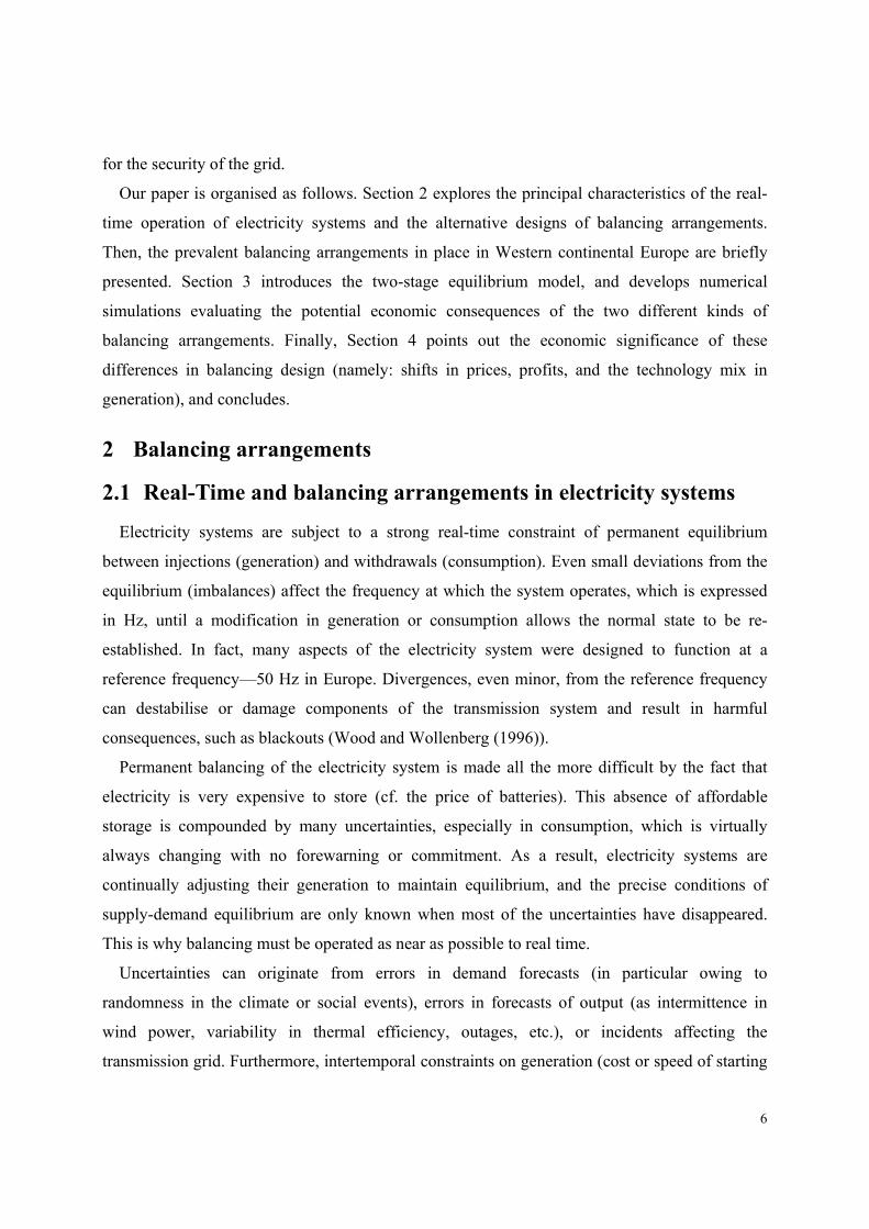
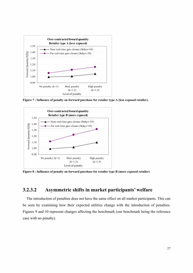
Another result of the penalties is over-contracting. Figures 7 and 8 illustrate this with the rate

of forward purchases by retailers and expected individual demand. We can see that retailers

almost always seek to buy more than the expected demand, and that this effect is exacerbated

when a penalty is imposed. Of course, over-contracting is greater when the retailer is more

exposed (= type B retailer).

27

Over-contracted foward quantityRetailer type A (less exposed)

0,90

1,00

1,10

1,20

1,30

1,40

1,50

No penalty (k=1) Med. penalty(k=1.2)

High penalty(k=1.4)

Level of penalty

Forw

ard

Qua

ntity

/E[D

j]

Near real-t ime gate closure (Stdsys=10)Far real-t ime gate closure (Stdsys=20)

Figure 7 : Influence of penalty on forward purchase for retailer type A (less exposed retailer).

Over-contracted foward quantityRetailer type B (more exposed)

0,90

1,00

1,10

1,20

1,30

1,40

1,50

No penalty (k=1) Med. penalty(k=1.2)

High penalty(k=1.4)

Level of penalty

Forw

ard

Qua

ntity

/E[D

j]

Near real-t ime gate closure (Stdsys=10)Far real-t ime gate closure (Stdsys=20)

Figure 8 : Influence of penalty on forward purchase for retailer type B (more exposed retailer)

3.2.3.2 Asymmetric shifts in market participants’ welfare

The introduction of penalties does not have the same effect on all market participants. This can

be seen by examining how their expected utilities change with the introduction of penalties.

Figures 9 and 10 represent changes affecting the benchmark (our benchmark being the reference

case with no penalty).

28

Expected utility changes (with respect to benchmark)Near real-time gate closure (Stdsys=10)

-80% -60% -40% -20% 0% 20%

Med. penalty(k=1.2)

High penalty(k=1.4)

Leve

l of p

enal

ties

Percentage of utility change

Flexible Generators

Retailer Type B

Retailer Type A

Figure 9 : Influence of penalty on welfare changes (with only flexible generators and near real-time gate closure).

Expected utility changes (with respect to benchmark)Far real-time gate closure (Stdsys=20)

-400% -300% -200% -100% 0% 100%

Med. penalty(k=1.2)

High penalty(k=1.4)

Leve

l of p

enal

ties

Percentage of utility change

Flexible Generators

Retailer Type B

Retailer Type A

Figure 10 : Influence of penalty on welfare changes (with only flexible generators and far real-time gate closure)

Two primary consequences are observed.

The first is a redistribution of welfare between retailers and generators. Net purchasers on the

forward market are retailers, and their welfare diminishes. Generators are net sellers, and their

welfare increases. It may be tempting to consider this transfer of welfare to correspond to a

service rendered by flexible generators in real time. However, in our extended model (both

flexible and inflexible technologies) we observe that inflexible generators also benefit from this

transfer. This shines the spotlight on the nature of the redistribution between buyers and sellers

on the forward market.

29

The second consequence is that penalties have a greater impact on small, vertically

disintegrated agents (Type B retailers) than on those that are large or integrated. Type B retailers

(which are both small and disintegrated) see their welfare fall twice as much, proportionally, as

type A retailers (which are large or vertically integrated in generation).

Therefore the use of penalties creates a barrier to entry to agents that are small or not vertically

integrated in generation. The balancing mechanism harms all agents who need to contend with

greater uncertainty (retailers or aggregators with small client bases, small generators, wind

generators, etc.). This barrier may deter some agents from entry, and thus undermine the

dynamics of competition.

3.2.3.3 Increased revenues for the TSO

Introduction of a penalty diverts revenues to the TSO (cf. Figures 11 and 12).

TSO's expected revenueBaseline Model (Only flexible generators)

0

50100

150200

250

300350

400

No penalty (k=1) Med. penalty(k=1.2)

High penalty(k=1.4)

Level of penalty

TSO

exp

ecte

d re

venu

e

Near real-t ime gateclosure (Stdsys=10)Far real-t ime gateclosure (Stdsys=20)

Figure 11 : Influence of penalty on TSO Revenue (only flexible generators)

The TSO’s revenues (flippantly referred to as the “beer fund”) increase with the level of the

penalties and the temporal distance of the gate closure. This revenue mechanism does not

provide the TSO with the right incentives to create the best design for the balancing arrangement,

for which the grid has a real need in real time. The fact that the TSO’s revenues automatically

increase when the level of the penalty rises and the gate closure moves ahead in time does not

provide any useful evidence regarding the exact improvement in the security.

30

TSO's expected revenueExtended Model (flexible & inflexible generators)

0

50

100

150

200

250

No penalty (k=1) Med. penalty(k=1.2)

High penalty(k=1.4)

Level of penalty

TSO

exp

ecte

d re

venu

e Middle real-t ime gateclosure (Stdsys=15)

Figure 12 : Influence of penalty on TSO Revenue (flexible and inflexible generators)

It is important to observe that the welfare of large generators also increases with the level of

the penalties. Since, in some countries, TSOs, large generators, and vertically integrated

generators may all be quite closely knit, and all have a great deal of say in choosing the market

design rules, we may fear that a poor initial choice of balancing arrangements may be followed

by a lengthy period in which these faulty bases are entrenched. This will make it very difficult to

improve this setup after the fact.

3.2.3.4 Inefficiencies

In our baseline model, in which all producers are flexible, efficiency in generation is not

undermined by the introduction of penalties. Inefficiencies that crop up are attributable to the

fact that penalties increase the volatility of profits and that, since market participants are risk

averse, their expected utility decreases (Figure 13).

Figure 14 reveals the impact of penalties in the model with two generation technologies

(flexible and inflexible). Here, inefficiencies in generation arise as inflexible producers make

poor output choices because of price distortions on the forward market. It is important to notice

that inflexible generators primarily take their cue from forward prices in deciding on output

levels. Another important consequence of introducing penalties into the dual technology model is

that real-time prices and imbalance prices are affected by excess generation from the inflexible.

31

EfficiencyBaseline Model (Only flexible generators)

97%

98%

99%

100%

101%

102%

Near real-t ime gate closure(Stdsys=10)

Far real-t ime gate closure(Stdsys=20)

Gate Closure Temporal Position

Effic

ienc

y

No penalty (k=1)Med. penalty (k=1.2)High penalty (k=1.4)

Figure 13 : Penalty decreasing efficiency in the baseline model (all generators being flexible)

EfficiencyExtended Model (flexible & inflexible generators)

97%

98%

99%

100%

101%

102%

Middle real-time gate closure (Stdsys=15)Gate Closure Temporal Position

Effic

ienc

y

No penalty (k=1)Med. penalty (k=1.2)High penalty (k=1.4)

Figure 14 : Penalty decreasing efficiency in the extended model (generators being flexible or inflexible)

4 Conclusion

We have examined the economic consequences of using penalties in balancing arrangements.

Running a few numerical simulations on the basis of a two-period equilibrium model, we have

found four principal economic consequences: (1°) a distortion of the forward price; (2°) an

asymmetric shift in the welfare of market participants that primarily impacts on small and

disintegrated agents; (3°) an increase in the TSO's revenues; and (4°) inefficiencies. The

magnitude of these consequences increases as the temporal position of the gate closure moves

away from real time.

Of course, the models we use are subject to several limitations, especially since they are based

32

on strong assumptions (perfect competition, no constraints on generation capacity, no constraints

on grid capacity, no reserves market, etc.). Therefore, we must seek to eliminate some of these

assumptions in future work. We shall also conduct a sensitivity analysis to see how the results

react to changes to the parameters.

Nonetheless, in light of these preliminary results, and given the current situation in which

countries in the western European Union continue to seek to improve and harmonise their market

designs, we wish to underline that economic consequences of this type cannot continue to be

ignored by decision makers…whether TSOs or regulators.

We do not deny that balancing provisions are extremely important for the security of the grid

and the good functioning of the electricity reforms. However, it is clear now that these balancing

arrangements are not technical security mechanisms. Rather, they are institutional arrangements

in which the TSO sets the rules of the game for other agents, with implications not only in real

time, but also on forward markets (day ahead and intraday).

In their choice of the temporal position of gate closure, TSOs define the structure of

information available to agents making decisions on forward markets, and by extension the level

of uncertainty entering into their decisions. With the combination of gate closure positions and

penalty levels, TSOs define the incentive system that applies to decisions made under uncertainty

by other agents who are risk averse. Moreover, these rules of the game have asymmetric impacts

on retailers and generators, on small, vertically disintegrated and large, vertically integrated

generators, and on flexible and inflexible generators. These rules may also function as barriers to

entry for small, disintegrated actors.

In conclusion, the security mechanisms that are TSO’s balancing arrangements are not neutral

in terms of their impacts on wholesale markets or the competitive dynamics on these markets.

Since there exist several alternative designs for balancing arrangements, it is not unreasonable to

expect TSOs and regulators to account for the economic consequences of the various models

when they establish the architecture of the wholesale market: either during the initial market

design, or during a later review in light of the experience accumulated in other countries.

Even though there currently exists a strong preference in Europe for conserving “balancing

mechanisms” and for delaying the implementation of “balancing markets,” it remains that the

time is right to conduct a comparative study of the existing balancing arrangements, since several

bordering countries are seeking to create closer links between their PXs and their provisions for

33

allocating interconnections in order to lay the foundation for a new regional market.

5 Appendices

Extended model with two generation technologies (flexible and inflexible) In this extension, we introduce a new generation technology, which is inflexible, alongside the

flexible technology of our baseline model. Inflexible generators must determine their level of

output within the uncertain framework of the forward market, since their output cannot be

adjusted beyond gate closure. They make decisions by observing the forward market.

To simplify, we assume that inflexible generators do not voluntarily take positions of

imbalance in real time. Consequently, they generate exactly the quantity that they sold on the

forward market (lIGX = F

IGlX ). The goal of the inflexible generator l is thus to select F

IGlX (or

lIGX )

so as to maximise profit. This profit function is given by:

2

2)( F

IGIGF

IGFF

IGIG llllXXPX θπ −= .

The first-order necessary condition is:

FIGIG

FFIG

FIGIG

l

l

ll XPX

Xθ

π−==

∂

∂0

)(

and so

IG

FFIG

PXl θ= …………………………………………………………………………………( 10 )

The conditions for equilibrium on the forward market (5) become:

∑∑∑ =+j

FR

l

FIG

i

FFG jli

XXX ……………………………………………………………….( 11 )

From equations (1), (2), (4), and (11), we find that:

ωσ

ωω ∀

−= ∑

FG

FG

l

FIG

RT

NXDP

l………………………………………………………….( 12 )

where ∑=j

jDD ωω , is global demand for the state of the world ω .

Thus, equation (7) becomes:

][],[

][][ ,

RT

RTFG

RTFG

RTFFFG PVar

PCovPVarAPEPX i

iω

ωω

ω

ωρ′

+−

= ………………………………………..……….( 13 )

34

where ωρ ,iFG′ is the unhedged profit of flexible generators (i.e. with 0=FFGi

X ), whence:

2,, )(

21)0( ∑−===′

l

FIGFG

FFGFGFG liii

XDX ωωω σπρ .

We can now use equations (3), (11) and (12), along with the optimal positions on the forward markets (equations (8), (10) and (13)), to find the market equilibria. ( FP , RTPω ).

6 References

Bessembinder, H. and Lemmon, M. (2000). “Equilibrium Pricing and Optimal Hedging in

Electricity Forward Markets,” Journal of Finance, Vol. 57, pp. 1347-1382, 2002.

Boucher, J. and Smeers, Y. (2002). “Towards a common European Electricity Market – Path in

the right direction…still far from an effective design,” Journal of Network Industries

3(4), 375-424, 2002.

ETSO (2003). “Current state of balance management in Europe,” available from ETSO website

(http://www.etso-net.org/upload/documents/BalanceManagemeninEurope.pdf), December 2003.

Glachant, J.M. and Leveque, F. (2005). “Electricity Single Market in the European Union:

What to do next?,” discussion paper of the European Union research project SESSA,

Sept 2005, (http://www.sessa.eu.com/ documents/bruxellesp/SESSA_report_wp1.pdf). Working

Paper CEEPR 2005-15 at MIT (web.mit.edu/ceepr). Main results presented at IDEI

conference, Toulouse, May 2005.

Green, R. and McDaniel, T. (1999). “Modelling Reta: A model of forward trading and the

balancing mechanism,” Department of Applied Economics Working Paper,

Cambridge.

Henney, A. (2002). “An Independent Review of NETA,” EEE Ltd. Publication, 21 November.

Hirst, E. (2001). “Real-time Balancing Operations and Markets: Key to Competitive Wholesale

Electricity Markets,” Edison Electric Institute, April 2001.

Joskow, P. and Tirole, J. (2004). “Reliability and Competitive Electricity Markets,” MIT

department of Economics working paper N° 2004-17, October 2004.

Newberry, D. (2005). “Refining Market Design,” discussion paper of the European Union

research project SESSA, Sept 2005,

(http://www.sessa.eu.com/documents/bruxellesp/SESSA_report_wp3.pdf).

35

Siddiqui, A. S. (2002). “Equilibrium Analysis of Forward Markets for Electricity and Reserves”.

PhD dissertation, University of California, Berkeley, 2002.

Smeers Y. (2005). “How well can one measure market power in restructured electricity

systems?” discussion paper of the European Union research project SESSA, Mai

2005, (http://www.sessa.eu.com/ documents/wp/D14.1_Smeers.pdf). Main results presented at

IDEI conference, Toulouse, May 2005.

Stoft, S. (2002). Power System Economics. IEEE Press, Wiley-Interscience.

Wilson R. (2002). “Architecture of electric power markets,” Econometrica, 70(4), 1299-1340.

Wood A.J. and Wollenberg B.F. (1996). Power generation, operation, and control. John Wiley

and Sons, New York ,1996.