HAL Id: tel-02489734 https://tel.archives-ouvertes.fr/tel-02489734 Submitted on 24 Feb 2020 HAL is a multi-disciplinary open access archive for the deposit and dissemination of sci- entific research documents, whether they are pub- lished or not. The documents may come from teaching and research institutions in France or abroad, or from public or private research centers. L’archive ouverte pluridisciplinaire HAL, est destinée au dépôt et à la diffusion de documents scientifiques de niveau recherche, publiés ou non, émanant des établissements d’enseignement et de recherche français ou étrangers, des laboratoires publics ou privés. An Information-Theoretic Approach to Distributed Learning. Distributed Source Coding Under Logarithmic Loss Yigit Ugur To cite this version: Yigit Ugur. An Information-Theoretic Approach to Distributed Learning. Distributed Source Cod- ing Under Logarithmic Loss. Information Theory [cs.IT]. Université Paris-Est, 2019. English. tel- 02489734

Welcome message from author
This document is posted to help you gain knowledge. Please leave a comment to let me know what you think about it! Share it to your friends and learn new things together.
Transcript
HAL Id: tel-02489734https://tel.archives-ouvertes.fr/tel-02489734
Submitted on 24 Feb 2020
HAL is a multi-disciplinary open accessarchive for the deposit and dissemination of sci-entific research documents, whether they are pub-lished or not. The documents may come fromteaching and research institutions in France orabroad, or from public or private research centers.
L’archive ouverte pluridisciplinaire HAL, estdestinée au dépôt et à la diffusion de documentsscientifiques de niveau recherche, publiés ou non,émanant des établissements d’enseignement et derecherche français ou étrangers, des laboratoirespublics ou privés.
An Information-Theoretic Approach to DistributedLearning. Distributed Source Coding Under
Logarithmic LossYigit Ugur
To cite this version:Yigit Ugur. An Information-Theoretic Approach to Distributed Learning. Distributed Source Cod-ing Under Logarithmic Loss. Information Theory [cs.IT]. Université Paris-Est, 2019. English. tel-02489734
UNIVERSITE PARIS-EST
Ecole Doctorale MSTIC
MATHEMATIQUES ET SCIENCES ET TECHNOLOGIES
DE L’INFORMATION ET DE LA COMMUNICATION
DISSERTATION
In Partial Fulfillment of the Requirements
for the Degree of Doctor of Philosophy
Presented on 22 November 2019 by:
Yigit UGUR
An Information-Theoretic Approach toDistributed Learning. Distributed Source
Coding Under Logarithmic Loss
Jury :
Advisor : Prof. Abdellatif Zaidi - Universite Paris-Est, France
Thesis Director : Prof. Abderrezak Rachedi - Universite Paris-Est, France
Reviewers : Prof. Giuseppe Caire - Technical University of Berlin, Germany
Prof. Gerald Matz - Vienna University of Technology, Austria
Dr. Aline Roumy - Inria, France
Examiners : Prof. David Gesbert - Eurecom, France
Prof. Michel Kieffer - Universite Paris-Sud, France


Acknowledgments
First, I would like to express my gratitude to my advisor Abdellatif Zaidi for his
guidance and support. It was a pleasure to benefit and learn from his knowledge and
vision through my studies.
I want to thank my colleague Inaki Estella Aguerri. I enjoyed very much collaborating
with him. He was very helpful, and tried to share his experience whenever I need.
My Ph.D. was in the context of a CIFRE contract. I appreciate my company Huawei
Technologies France for supporting me during my education. It was a privilege to be a
part of the Mathematical and Algorithmic Sciences Lab, Paris Research Center, and to
work with scientists coming from different parts of the world. It was a unique experience
to be within a very competitive international working environment.
During my Ph.D. studies, Paris gave me a pleasant surprise, the sincerest coincidence
of meeting with Ozge. I would like to thank her for always supporting me and sharing the
Parisian life with me.
Last, and most important, my deepest thanks are to my family: my parents Mustafa
and Kıymet, and my brother Kagan. They have been always there to support me whenever
I need. I could not have accomplished any of this without them. Their infinite love and
support is what make it all happen.
i

ii
Abstract
One substantial question, that is often argumentative in learning theory, is how to choose
a ‘good’ loss function that measures the fidelity of the reconstruction to the original.
Logarithmic loss is a natural distortion measure in the settings in which the reconstructions
are allowed to be ‘soft’, rather than ‘hard’ or deterministic. In other words, rather than
just assigning a deterministic value to each sample of the source, the decoder also gives an
assessment of the degree of confidence or reliability on each estimate, in the form of weights
or probabilities. This measure has appreciable mathematical properties which establish
some important connections with lossy universal compression. Logarithmic loss is widely
used as a penalty criterion in various contexts, including clustering and classification,
pattern recognition, learning and prediction, and image processing. Considering the high
amount of research which is done recently in these fields, the logarithmic loss becomes a
very important metric and will be the main focus as a distortion metric in this thesis.
In this thesis, we investigate a distributed setup, so-called the Chief Executive Officer
(CEO) problem under logarithmic loss distortion measure. Specifically, K ≥ 2 agents
observe independently corrupted noisy versions of a remote source, and communicate
independently with a decoder or CEO over rate-constrained noise-free links. The CEO also
has its own noisy observation of the source and wants to reconstruct the remote source to
within some prescribed distortion level where the incurred distortion is measured under
the logarithmic loss penalty criterion.
One of the main contributions of the thesis is the explicit characterization of the rate-
distortion region of the vector Gaussian CEO problem, in which the source, observations and
side information are jointly Gaussian. For the proof of this result, we first extend Courtade-
Weissman’s result on the rate-distortion region of the discrete memoryless (DM) K-encoder
CEO problem to the case in which the CEO has access to a correlated side information
iii

ABSTRACT
stream which is such that the agents’ observations are independent conditionally given
the side information and remote source. Next, we obtain an outer bound on the region of
the vector Gaussian CEO problem by evaluating the outer bound of the DM model by
means of a technique that relies on the de Bruijn identity and the properties of Fisher
information. The approach is similar to Ekrem-Ulukus outer bounding technique for the
vector Gaussian CEO problem under quadratic distortion measure, for which it was there
found generally non-tight; but it is shown here to yield a complete characterization of the
region for the case of logarithmic loss measure. Also, we show that Gaussian test channels
with time-sharing exhaust the Berger-Tung inner bound, which is optimal. Furthermore,
application of our results allows us to find the complete solutions of three related problems:
the quadratic vector Gaussian CEO problem with determinant constraint, the vector
Gaussian distributed hypothesis testing against conditional independence problem and
the vector Gaussian distributed Information Bottleneck problem.
With the known relevance of the logarithmic loss fidelity measure in the context
of learning and prediction, developing algorithms to compute the regions provided in
this thesis may find usefulness in a variety of applications where learning is performed
distributively. Motivated from this fact, we develop two type algorithms: i) Blahut-
Arimoto (BA) type iterative numerical algorithms for both discrete and Gaussian models
in which the joint distribution of the sources are known; and ii) a variational inference
type algorithm in which the encoding mappings are parameterized by neural networks
and the variational bound approximated by Monte Carlo sampling and optimized with
stochastic gradient descent for the case in which there is only a set of training data is
available. Finally, as an application, we develop an unsupervised generative clustering
framework that uses the variational Information Bottleneck (VIB) method and models the
latent space as a mixture of Gaussians. This generalizes the VIB which models the latent
space as an isotropic Gaussian which is generally not expressive enough for the purpose
of unsupervised clustering. We illustrate the efficiency of our algorithms through some
numerical examples.
Keywords: Multiterminal source coding, CEO problem, rate-distortion region, loga-
rithmic loss, quadratic loss, hypothesis testing, Information Bottleneck, Blahut-Arimoto
algorithm, distributed learning, classification, unsupervised clustering.
iv
Contents
Abstract . . . . . . . . . . . . . . . . . . . . . . . . . . . . . . . . . . . . . . . . iii
List of Figures . . . . . . . . . . . . . . . . . . . . . . . . . . . . . . . . . . . . . ix
List of Tables . . . . . . . . . . . . . . . . . . . . . . . . . . . . . . . . . . . . . xi
List of Tables . . . . . . . . . . . . . . . . . . . . . . . . . . . . . . . . . . . . . xii
Notation . . . . . . . . . . . . . . . . . . . . . . . . . . . . . . . . . . . . . . . . xiv
Acronyms . . . . . . . . . . . . . . . . . . . . . . . . . . . . . . . . . . . . . . . xvii
1 Introduction and Main Contributions 1
1.1 Main Contributions . . . . . . . . . . . . . . . . . . . . . . . . . . . . . . . 2
1.2 Outline . . . . . . . . . . . . . . . . . . . . . . . . . . . . . . . . . . . . . . 6
2 Logarithmic Loss Compression and Connections 11
2.1 Logarithmic Loss Distortion Measure . . . . . . . . . . . . . . . . . . . . . 11
2.2 Remote Source Coding Problem . . . . . . . . . . . . . . . . . . . . . . . . 13
2.3 Information Bottleneck Problem . . . . . . . . . . . . . . . . . . . . . . . . 15
2.3.1 Discrete Memoryless Case . . . . . . . . . . . . . . . . . . . . . . . 15
2.3.2 Gaussian Case . . . . . . . . . . . . . . . . . . . . . . . . . . . . . . 16
2.3.3 Connections . . . . . . . . . . . . . . . . . . . . . . . . . . . . . . . 17
2.4 Learning via Information Bottleneck . . . . . . . . . . . . . . . . . . . . . 21
2.4.1 Representation Learning . . . . . . . . . . . . . . . . . . . . . . . . 21
2.4.2 Variational Bound . . . . . . . . . . . . . . . . . . . . . . . . . . . 23
2.4.3 Finite-Sample Bound on the Generalization Gap . . . . . . . . . . . 24
2.4.4 Neural Reparameterization . . . . . . . . . . . . . . . . . . . . . . . 24
2.4.5 Opening the Black Box . . . . . . . . . . . . . . . . . . . . . . . . . 26
2.5 An Example Application: Text clustering . . . . . . . . . . . . . . . . . . . 28
v

CONTENTS
2.6 Design of Optimal Quantizers . . . . . . . . . . . . . . . . . . . . . . . . . 31
3 Discrete Memoryless CEO Problem with Side Information 35
3.1 Rate-Distortion Region . . . . . . . . . . . . . . . . . . . . . . . . . . . . . 36
3.2 Estimation of Encoder Observations . . . . . . . . . . . . . . . . . . . . . . 37
3.3 An Example: Distributed Pattern Classification . . . . . . . . . . . . . . . 39
3.4 Hypothesis Testing Against Conditional Independence . . . . . . . . . . . . 43
4 Vector Gaussian CEO Problem with Side Information 49
4.1 Rate-Distortion Region . . . . . . . . . . . . . . . . . . . . . . . . . . . . . 50
4.2 Gaussian Test Channels with Time-Sharing Exhaust the Berger-Tung Region 53
4.3 Quadratic Vector Gaussian CEO Problem with Determinant Constraint . . 55
4.4 Hypothesis Testing Against Conditional Independence . . . . . . . . . . . . 57
4.5 Distributed Vector Gaussian Information Bottleneck . . . . . . . . . . . . . 61
5 Algorithms 65
5.1 Blahut-Arimoto Type Algorithms for Known Models . . . . . . . . . . . . 65
5.1.1 Discrete Case . . . . . . . . . . . . . . . . . . . . . . . . . . . . . . 65
5.1.2 Vector Gaussian Case . . . . . . . . . . . . . . . . . . . . . . . . . . 71
5.1.3 Numerical Examples . . . . . . . . . . . . . . . . . . . . . . . . . . 72
5.2 Deep Distributed Representation Learning . . . . . . . . . . . . . . . . . . 75
5.2.1 Variational Distributed IB Algorithm . . . . . . . . . . . . . . . . . 78
5.2.2 Experimental Results . . . . . . . . . . . . . . . . . . . . . . . . . . 82
6 Application to Unsupervised Clustering 87
6.1 Proposed Model . . . . . . . . . . . . . . . . . . . . . . . . . . . . . . . . . 91
6.1.1 Inference Network Model . . . . . . . . . . . . . . . . . . . . . . . . 91
6.1.2 Generative Network Model . . . . . . . . . . . . . . . . . . . . . . . 92
6.2 Proposed Method . . . . . . . . . . . . . . . . . . . . . . . . . . . . . . . . 92
6.2.1 Brief Review of Variational Information Bottleneck for Unsupervised
Learning . . . . . . . . . . . . . . . . . . . . . . . . . . . . . . . . . 93
6.2.2 Proposed Algorithm: VIB-GMM . . . . . . . . . . . . . . . . . . . 95
6.3 Experiments . . . . . . . . . . . . . . . . . . . . . . . . . . . . . . . . . . . 99
6.3.1 Description of used datasets . . . . . . . . . . . . . . . . . . . . . . 99
vi
CONTENTS
6.3.2 Network settings and other parameters . . . . . . . . . . . . . . . . 99
6.3.3 Clustering Accuracy . . . . . . . . . . . . . . . . . . . . . . . . . . 100
6.3.4 Visualization on the Latent Space . . . . . . . . . . . . . . . . . . . 103
7 Perspectives 105
Appendices 107
A Proof of Theorem 1 109
A.1 Direct Part . . . . . . . . . . . . . . . . . . . . . . . . . . . . . . . . . . . 109
A.2 Converse Part . . . . . . . . . . . . . . . . . . . . . . . . . . . . . . . . . . 110
B Proof of Theorem 2 113
B.1 Direct Part . . . . . . . . . . . . . . . . . . . . . . . . . . . . . . . . . . . 113
B.2 Converse Part . . . . . . . . . . . . . . . . . . . . . . . . . . . . . . . . . . 114
C Proof of Proposition 3 119
D Proof of Proposition 4 123
E Proof of Converse of Theorem 4 125
F Proof of Proposition 5 (Extension to K Encoders) 129
G Proof of Theorem 5 135
H Proofs for Chapter 5 139
H.1 Proof of Lemma 3 . . . . . . . . . . . . . . . . . . . . . . . . . . . . . . . . 139
H.2 Proof of Lemma 5 . . . . . . . . . . . . . . . . . . . . . . . . . . . . . . . . 141
H.3 Derivation of the Update Rules of Algorithm 3 . . . . . . . . . . . . . . . . 142
H.4 Proof of Proposition 9 . . . . . . . . . . . . . . . . . . . . . . . . . . . . . 145
H.5 Proof of Proposition 10 . . . . . . . . . . . . . . . . . . . . . . . . . . . . . 146
H.6 Proof of Lemma 6 . . . . . . . . . . . . . . . . . . . . . . . . . . . . . . . . 147
I Supplementary Material for Chapter 6 149
I.1 Proof of Lemma 7 . . . . . . . . . . . . . . . . . . . . . . . . . . . . . . . . 149
I.2 Alternative Expression LVaDEs . . . . . . . . . . . . . . . . . . . . . . . . . 150
vii

CONTENTS
I.3 KL Divergence Between Multivariate Gaussian Distributions . . . . . . . . 151
I.4 KL Divergence Between Gaussian Mixture Models . . . . . . . . . . . . . . 151
viii
List of Figures
2.1 Remote, or indirect, source coding problem. . . . . . . . . . . . . . . . . . 13
2.2 Information Bottleneck problem. . . . . . . . . . . . . . . . . . . . . . . . . 15
2.3 Representation learning. . . . . . . . . . . . . . . . . . . . . . . . . . . . . 26
2.4 The evolution of the layers with the training epochs in the information plane. 27
2.5 Annealing IB algorithm for text clustering. . . . . . . . . . . . . . . . . . . 30
2.6 Discretization of the channel output. . . . . . . . . . . . . . . . . . . . . . 32
2.7 Visualization of the quantizer. . . . . . . . . . . . . . . . . . . . . . . . . . 32
2.8 Memoryless channel with subsequent quantizer. . . . . . . . . . . . . . . . 33
3.1 CEO source coding problem with side information. . . . . . . . . . . . . . 36
3.2 An example of distributed pattern classification. . . . . . . . . . . . . . . . 40
3.3 Illustration of the bound on the probability of classification error. . . . . . 43
3.4 Distributed hypothesis testing against conditional independence. . . . . . . 44
4.1 Vector Gaussian CEO problem with side information. . . . . . . . . . . . . 50
4.2 Distributed Scalar Gaussian Information Bottleneck. . . . . . . . . . . . . 63
5.1 Rate-distortion region of the binary CEO network of Example 2. . . . . . . 73
5.2 Rate-information region of the vector Gaussian CEO network of Example 3. 74
5.3 An example of distributed supervised learning. . . . . . . . . . . . . . . . . 81
5.4 Relevance vs. sum-complexity trade-off for vector Gaussian data model. . . 83
5.5 Two-view handwritten MNIST dataset. . . . . . . . . . . . . . . . . . . . . 84
5.6 Distributed representation learning for the two-view MNIST dataset. . . . 86
6.1 Variational Information Bottleneck with Gaussian Mixtures. . . . . . . . . 90
6.2 Inference Network . . . . . . . . . . . . . . . . . . . . . . . . . . . . . . . . 91
ix

LIST OF FIGURES
6.3 Generative Network . . . . . . . . . . . . . . . . . . . . . . . . . . . . . . . 92
6.4 Accuracy vs. number of epochs for the STL-10 dataset. . . . . . . . . . . . 101
6.5 Information plane for the STL-10 dataset. . . . . . . . . . . . . . . . . . . 102
6.6 Visualization of the latent space. . . . . . . . . . . . . . . . . . . . . . . . 103
x

List of Algorithms
1 Deterministic annealing-like IB algorithm . . . . . . . . . . . . . . . . . . . 29
2 BA-type algorithm to compute RD1CEO . . . . . . . . . . . . . . . . . . . . 70
3 BA-type algorithm for the Gaussian vector CEO . . . . . . . . . . . . . . . 71
4 D-VIB algorithm for the distributed IB problem [1, Algorithm 3] . . . . . . 80
5 VIB-GMM algorithm for unsupervised learning. . . . . . . . . . . . . . . . 96
6 Annealing algorithm pseudocode. . . . . . . . . . . . . . . . . . . . . . . . 98
xi

xii
List of Tables
2.1 The topics of 100 words in the the subgroup of 20 newsgroup dataset. . . . 30
2.2 Clusters obtained through the application of the annealing IB algorithm on
the subgroup of 20 newsgroup dataset. . . . . . . . . . . . . . . . . . . . . 30
4.1 Advances in the resolution of the rate region of the quadratic Gaussian
CEO problem. . . . . . . . . . . . . . . . . . . . . . . . . . . . . . . . . . . 57
5.1 DNN architecture for Figure 5.6. . . . . . . . . . . . . . . . . . . . . . . . 84
5.2 Accuracy for different algorithms with CNN architectures . . . . . . . . . . 86
6.1 Comparison of clustering accuracy of various algorithms (without pretraining).100
6.2 Comparison of clustering accuracy of various algorithms (with pretraining). 100
xiii

xiv
Notation
Throughout the thesis, we use the following notation. Upper case letters are used to
denote random variables, e.g., X; lower case letters are used to denote realizations of
random variables, e.g., x; and calligraphic letters denote sets, e.g., X . The cardinality
of a set X is denoted by |X |. The closure of a set A is denoted by A . The probability
distribution of the random variable X taking the realizations x over the set X is denoted
by PX(x) = Pr[X = x]; and, sometimes, for short, as p(x). We use P(X ) to denote
the set of discrete probability distributions on X . The length-n sequence (X1, . . . , Xn)
is denoted as Xn; and, for integers j and k such that 1 ≤ k ≤ j ≤ n, the sub-sequence
(Xk, Xk+1, . . . , Xj) is denoted as Xjk. We denote the set of natural numbers by N, and the
set of positive real numbers by R+. For an integer K ≥ 1, we denote the set of natural
numbers smaller or equal K as K = k ∈ N : 1 ≤ k ≤ K. For a set of natural numbers
S ⊆ K, the complementary set of S is denoted by Sc, i.e., Sc = k ∈ N : k ∈ K \ S.Sometimes, for convenience we use S defined as S = 0∪Sc. For a set of natural numbers
S ⊆ K; the notation XS designates the set of random variables Xk with indices in the
set S, i.e., XS = Xkk∈S . Boldface upper case letters denote vectors or matrices, e.g., X,
where context should make the distinction clear. The notation X† stands for the conjugate
transpose of X for complex-valued X, and the transpose of X for real-valued X. We denote
the covariance of a zero mean, complex-valued, vector X by Σx = E[XX†]. Similarly, we
denote the cross-correlation of two zero-mean vectors X and Y as Σx,y = E[XY†], and the
conditional correlation matrix of X given Y as Σx|y = E[(X− E[X|Y])(X− E[X|Y])†
],
i.e., Σx|y = Σx −Σx,yΣ−1y Σy,x. For matrices A and B, the notation diag(A,B) denotes
the block diagonal matrix whose diagonal elements are the matrices A and B and its
off-diagonal elements are the all zero matrices. Also, for a set of integers J ⊂ N and
a family of matrices Aii∈J of the same size, the notation AJ is used to denote the
xv

NOTATION
(super) matrix obtained by concatenating vertically the matrices Aii∈J , where the
indices are sorted in the ascending order, e.g, A0,2 = [A†0,A†2]†. We use N (µ,Σ) to
denote a real multivariate Gaussian random variable with mean µ and covariance matrix
Σ, and CN (µ,Σ) to denote a circularly symmetric complex multivariate Gaussian random
variable with mean µ and covariance matrix Σ.
xvi

Acronyms
ACC Clustering Accuracy
AE Autoencoder
BA Blahut-Arimoto
BSC Binary Symmetric Channel
CEO Chief Executive Officer
C-RAN Cloud Radio Acces Netowrk
DEC Deep Embedded Clustering
DM Discrete Memoryless
DNN Deep Neural Network
ELBO Evidence Lower Bound
EM Expectation Maximization
GMM Gaussian Mixture Model
IB Information Bottleneck
IDEC Improved Deep Embedded Clustering
KKT Karush-Kuhn-Tucker
KL Kullback-Leibler
LHS Left Hand Side
MDL Minimum Description Length
xvii

ACRONYMS
MIMO Multiple-Input Multiple-Output
MMSE Minimum Mean Square Error
NN Neural Network
PCA Principal Component Analysis
PMF Probability Mass Function
RHS Right Hand Side
SGD Stochastic Gradient Descent
SUM Successive Upper-bound Minimization
VaDE Variational Deep Embedding
VAE Variational Autoencoder
VIB Variational Information Bottleneck
VIB-GMM Variational Information Bottleneck with Gaussian Mixture Model
WZ Wyner-Ziv
xviii
Chapter 1
Introduction and Main
Contributions
The Chief Executive Officer (CEO) problem – also called as the indirect multiterminal
source coding problem – was first studied by Berger et al. in [2]. Consider the vector
Gaussian CEO problem shown in Figure 1.1. In this model, there is an arbitrary number
K ≥ 2 of encoders (so-called agents) each having a noisy observation of a vector Gaussian
source X. The goal of the agents is to describe the source to a central unit (so-called
CEO), which wants to reconstruct this source to within a prescribed distortion level. The
incurred distortion is measured according to some loss measure d : X × X → R, where Xdesignates the reconstruction alphabet. For quadratic distortion measure, i.e.,
d(x, x) = |x− x|2
the rate-distortion region of the vector Gaussian CEO problem is still unknown in general,
except in few special cases the most important of which is perhaps the case of scalar
sources, i.e., scalar Gaussian CEO problem, for which a complete solution, in terms of
characterization of the optimal rate-distortion region, was found independently by Oohama
in [3] and by Prabhakaran et al. in [4]. Key to establishing this result is a judicious
application of the entropy power inequality. The extension of this argument to the case of
vector Gaussian sources, however, is not straightforward as the entropy power inequality is
known to be non-tight in this setting. The reader may refer also to [5, 6] where non-tight
outer bounds on the rate-distortion region of the vector Gaussian CEO problem under
quadratic distortion measure are obtained by establishing some extremal inequalities that
1
CHAPTER 1. INTRODUCTION AND MAIN CONTRIBUTIONS
Xn PY0,Y1,...,YK |X
Encoder 1
Encoder 2
Encoder K
Yn1
Yn2
YnK
Decoder
R1
R2
RK
...
Xn
Yn0
Figure 1.1: Chief Executive Officer (CEO) source coding problem with side information.
are similar to Liu-Viswanath [7], and to [8] where a strengthened extremal inequality
yields a complete characterization of the region of the vector Gaussian CEO problem in
the special case of trace distortion constraint.
In this thesis, our focus will be mainly on the memoryless CEO problem with side
information at the decoder of Figure 1.1 in the case in which the distortion is measured
using the logarithmic loss criterion, i.e.,
d(n)(xn, xn) =1
n
n∑
i=1
d(xi, xi) ,
with the letter-wise distortion given by
d(x, x) = log( 1
x(x)
),
where x(·) designates a probability distribution on X and x(x) is the value of this
distribution evaluated for the outcome x ∈ X . The logarithmic loss distortion measure
plays a central role in settings in which reconstructions are allowed to be ‘soft’, rather
than ‘hard’ or deterministic. That is, rather than just assigning a deterministic value to
each sample of the source, the decoder also gives an assessment of the degree of confidence
or reliability on each estimate, in the form of weights or probabilities. This measure
was introduced in the context of rate-distortion theory by Courtade et al. [9, 10] (see
Chapter 2.1 for a detailed discussion on the logarithmic loss).
1.1 Main Contributions
One of the main contributions of this thesis is a complete characterization of the rate-
distortion region of the vector Gaussian CEO problem of Figure 1.1 under logarithmic
2

CHAPTER 1. INTRODUCTION AND MAIN CONTRIBUTIONS
loss distortion measure. In the special case in which there is no side information at the
decoder, the result can be seen as the counterpart, to the vector Gaussian case, of that by
Courtade and Weissman [10, Theorem 10] who established the rate-distortion region of
the CEO problem under logarithmic loss in the discrete memoryless (DM) case. For the
proof of this result, we derive a matching outer bound by means of a technique that relies
of the de Bruijn identity, a connection between differential entropy and Fisher information,
along with the properties of minimum mean square error (MMSE) and Fisher information.
By opposition to the case of quadratic distortion measure, for which the application of
this technique was shown in [11] to result in an outer bound that is generally non-tight,
we show that this approach is successful in the case of logarithmic distortion measure
and yields a complete characterization of the region. On this aspect, it is noteworthy
that, in the specific case of scalar Gaussian sources, an alternate converse proof may be
obtained by extending that of the scalar Gaussian many-help-one source coding problem
by Oohama [3] and Prabhakaran et al. [4] by accounting for side information and replacing
the original mean square error distortion constraint with conditional entropy. However,
such approach does not seem to lead to a conclusive result in the vector case as the entropy
power inequality is known to be generally non-tight in this setting [12, 13]. The proof
of the achievability part simply follows by evaluating a straightforward extension to the
continuous alphabet case of the solution of the DM model using Gaussian test channels
and no time-sharing. Because this does not necessarily imply that Gaussian test channels
also exhaust the Berger-Tung inner bound, we investigate the question and we show that
they do if time-sharing is allowed.
Besides, we show that application of our results allows us to find complete solutions to
three related problems:
1) The first is a quadratic vector Gaussian CEO problem with reconstruction constraint
on the determinant of the error covariance matrix that we introduce here, and for
which we also characterize the optimal rate-distortion region. Key to establishing
this result, we show that the rate-distortion region of vector Gaussian CEO problem
under logarithmic loss which is found in this paper translates into an outer bound
on the rate region of the quadratic vector Gaussian CEO problem with determinant
constraint. The reader may refer to, e.g., [14] and [15] for examples of usage of such
a determinant constraint in the context of equalization and others.
3
CHAPTER 1. INTRODUCTION AND MAIN CONTRIBUTIONS
2) The second is the K-encoder hypothesis testing against conditional independence
problem that was introduced and studied by Rahman and Wagner in [16]. In this
problem, K sources (Y1, . . . ,YK) are compressed distributively and sent to a detector
that observes the pair (X,Y0) and seeks to make a decision on whether (Y1, . . . ,YK)
is independent of X conditionally given Y0 or not. The aim is to characterize all
achievable encoding rates and exponents of the Type II error probability when the
Type I error probability is to be kept below a prescribed (small) value. For both
DM and vector Gaussian models, we find a full characterization of the optimal rates-
exponent region when (X,Y0) induces conditional independence between the variables
(Y1, . . . ,YK) under the null hypothesis. In both settings, our converse proofs show
that the Quantize-Bin-Test scheme of [16, Theorem 1], which is similar to the Berger-
Tung distributed source coding, is optimal. In the special case of one encoder, the
assumed Markov chain under the null hypothesis is non-restrictive; and, so, we find
a complete solution of the vector Gaussian hypothesis testing against conditional
independence problem, a problem that was previously solved in [16, Theorem 7] in the
case of scalar-valued source and testing against independence (note that [16, Theorem
7] also provides the solution of the scalar Gaussian many-help-one hypothesis testing
against independence problem).
3) The third is an extension of Tishby’s single-encoder Information Bottleneck (IB)
method [17] to the case of multiple encoders. Information theoretically, this problem
is known to be essentially a remote source coding problem with logarithmic loss
distortion measure [18]; and, so, we use our result for the vector Gaussian CEO
problem under logarithmic loss to infer a full characterization of the optimal trade-off
between complexity (or rate) and accuracy (or information) for the distributed vector
Gaussian IB problem.
On the algorithmic side, we make the following contributions.
1) For both DM and Gaussian settings in which the joint distribution of the sources
is known, we develop Blahut-Arimoto (BA) [19, 20] type iterative algorithms that
allow to compute (approximations of) the rate regions that are established in this
thesis; and prove their convergence to stationary points. We do so through a
variational formulation that allows to determine the set of self-consistent equations
4

CHAPTER 1. INTRODUCTION AND MAIN CONTRIBUTIONS
that are satisfied by the stationary solutions. In the Gaussian case, we show that the
algorithm reduces to an appropriate updating rule of the parameters of noisy linear
projections. This generalizes the Gaussian Information Bottleneck projections [21]
to the distributed setup. We note that the computation of the rate-distortion
regions of multiterminal and CEO source coding problems is important per-se as
it involves non-trivial optimization problems over distributions of auxiliary random
variables. Also, since the logarithmic loss function is instrumental in connecting
problems of multiterminal rate-distortion theory with those of distributed learning
and estimation, the algorithms that are developed in this paper also find usefulness
in emerging applications in those areas. For example, our algorithm for the DM CEO
problem under logarithm loss measure can be seen as a generalization of Tishby’s IB
method [17] to the distributed learning setting. Similarly, our algorithm for the vector
Gaussian CEO problem under logarithm loss measure can be seen as a generalization
of that of [21, 22] to the distributed learning setting. For other extension of the
BA algorithm in the context of multiterminal data transmission and compression,
the reader may refer to related works on point-to-point [23,24] and broadcast and
multiple access multiterminal settings [25,26].
2) For the cases in which the joint distribution of the sources is not known (instead only
a set of training data is available), we develop a variational inference type algorithm,
so-called D-VIB. In doing so: i) we develop a variational bound on the optimal
information-rate function that can be seen as a generalization of IB method, the
evidence lower bound (ELBO) and the β-VAE criteria [27, 28] to the distributed
setting, ii) the encoders and the decoder are parameterized by deep neural networks
(DNN), and iii) the bound approximated by Monte Carlo sampling and optimized
with stochastic gradient descent. This algorithm makes usage of Kingma et al.’s
reparameterization trick [29] and can be seen as a generalization of the variational
Information Bottleneck (VIB) algorithm in [30] to the distributed case.
Finally, we study an application to the unsupervised learning, which is a generative
clustering framework that combines variational Information Bottleneck and the Gaussian
Mixture Model (GMM). Specifically, we use the variational Information Bottleneck method
and model the latent space as a mixture of Gaussians. Our approach falls into the class
5
CHAPTER 1. INTRODUCTION AND MAIN CONTRIBUTIONS
in which clustering is performed over the latent space representations rather than the
data itself. We derive a bound on the cost function of our model that generalizes the
ELBO; and provide a variational inference type algorithm that allows to compute it. Our
algorithm, so-called Variational Information Bottleneck with Gaussian Mixture Model
(VIB-GMM), generalizes the variational deep embedding (VaDE) algorithm of [31] which
is based on variational autoencoders (VAE) and performs clustering by maximizing the
ELBO, and can be seen as a specific case of our algorithm obtained by setting s = 1.
Besides, the VIB-GMM also generalizes the VIB of [30] which models the latent space
as an isotropic Gaussian which is generally not expressive enough for the purpose of
unsupervised clustering. Furthermore, we study the effect of tuning the hyperparameter
s, and propose an annealing-like algorithm [32], in which the parameter s is increased
gradually with iterations. Our algorithm is applied to various datasets, and we observed a
better performance in term of the clustering accuracy (ACC) compared to the state of the
art algorithms, e.g., VaDE [31], DEC [33].
1.2 Outline
The chapters of the thesis and the content in each of them are summarized in what follows.
Chapter 2
The aim of this chapter is to explain some preliminaries for the point-to-point case before
presenting our contributions in the distributed setups. First, we explain the logarithmic
loss distortion measure, which plays an important role on the theory of learning. Then,
the remote source coding problem [34] is presented, which is eventually the Information
Bottleneck problem with the choice of logarithmic loss as a distortion measure. Later,
we explain the Tishby’s Information Bottleneck problem for the discrete memoryless [17]
and Gaussian cases [21], also present the Blahut-Arimoto type algorithms [19, 20] to
compute the IB curves. Besides, there is shown the connections of the IB with some well-
known information-theoretical source coding problems, e.g., common reconstruction [35],
information combining [36–38], the Wyner-Ahlswede-Korner problem [39,40], the efficiency
of investment information [41], and the privacy funnel problem [42]. Finally, we present the
learning via IB section, which includes a brief explanation of representation learning [43],
6
CHAPTER 1. INTRODUCTION AND MAIN CONTRIBUTIONS
finite-sample bound on the generalization gap, as well as, the variational bound method
which leads the IB to a learning algorithm, so-called the variational IB (VIB) [30] with
the usage of neural reparameterization and Kingma et al.’s reparameterization trick [29].
Chapter 3
In this chapter, we study the discrete memoryless CEO problem with side information
under logarithmic loss. First, we provide a formal description of the DM CEO model that
is studied in this chapter, as well as some definitions that are related to it. Then, the
Courtade-Weissman’s result [10, Theorem 10] on the rate-distortion region of the DM K-
encoder CEO problem is extended to the case in which the CEO has access to a correlated
side information stream which is such that the agents’ observations are conditionally
independent given the decoder’s side information and the remote source. This will be
instrumental in the next chapter to study the vector Gaussian CEO problem with side
information under logarithmic loss. Besides, we study a two-encoder case in which the
decoder is interested in estimation of encoder observations. For this setting, we find
the rate-distortion region that extends the result of [10, Theorem 6] for the two-encoder
multiterminal source coding problem with average logarithmic loss distortion constraints
on Y1 and Y2 and no side information at the decoder to the setting in which the decoder
has its own side information Y0 that is arbitrarily correlated with (Y1, Y2). Furthermore, we
study the distributed pattern classification problem as an example of the DM two-encoder
CEO setup and we find an upper bound on the probability of misclassification. Finally,
we look another closely related problem called the distributed hypothesis testing against
conditional independence, specifically the one studied by Rahman and Wagner in [16]. We
characterize the rate-exponent region for this problem by providing a converse proof and
show that it is achieved using the Quantize-Bin-Test scheme of [16].
Chapter 4
In this chapter, we study the vector Gaussian CEO problem with side information under
logarithmic loss. First, we provide a formal description of the vector Gaussian CEO
problem that is studied in this chapter. Then, we present one of the main results of the
thesis, which is an explicit characterization of the rate-distortion region of the vector
Gaussian CEO problem with side information under logarithmic loss. In doing so, we
7

CHAPTER 1. INTRODUCTION AND MAIN CONTRIBUTIONS
use a similar approach to Ekrem-Ulukus outer bounding technique [11] for the vector
Gaussian CEO problem under quadratic distortion measure, for which it was there found
generally non-tight; but it is shown here to yield a complete characterization of the region
for the case of logarithmic loss measure. We also show that Gaussian test channels with
time-sharing exhaust the Berger-Tung rate region which is optimal. In this chapter, we
also use our results on the CEO problem under logarithmic loss to infer complete solutions
of three related problems: the quadratic vector Gaussian CEO problem with a determinant
constraint on the covariance matrix error, the vector Gaussian distributed hypothesis
testing against conditional independence problem, and the vector Gaussian distributed
Information Bottleneck problem.
Chapter 5
This chapter contains a description of two algorithms and architectures that were developed
in [1] for the distributed learning scenario. We state them here for reasons of completeness.
In particular, the chapter provides: i) Blahut-Arimoto type iterative algorithms that allow
to compute numerically the rate-distortion or relevance-complexity regions of the DM and
vector Gaussian CEO problems that are established in previous chapters for the case in
which the joint distribution of the data is known perfectly or can be estimated with a high
accuracy; and ii) a variational inference type algorithm in which the encoding mappings
are parameterized by neural networks and the variational bound approximated by Monte
Carlo sampling and optimized with stochastic gradient descent for the case in which there
is only a set of training data is available. The second algorithm, so-called D-VIB [1], can
be seen as a generalization of the variational Information Bottleneck (VIB) algorithm
in [30] to the distributed case. The advantage of D-VIB over centralized VIB can be
explained by the advantage of training the latent space embedding for each observation
separately, which allows to adjust better the encoding and decoding parameters to the
statistics of each observation, justifying the use of D-VIB for multi-view learning [44,45]
even if the data is available in a centralized manner.
Chapter 6
In this chapter, we study an unsupervised generative clustering framework that combines
variational Information Bottleneck and the Gaussian Mixture Model for the point-to-point
8

CHAPTER 1. INTRODUCTION AND MAIN CONTRIBUTIONS
case (e.g., the CEO problem with one encoder). The variational inference type algorithm
provided in the previous chapter assumes that there is access to the labels (or remote
sources), and the latent space therein is modeled with an isotropic Gaussian. Here, we
turn our attention to the case in which there is no access to the labels at all. Besides, we
use a more expressive model for the latent space, e.g., Gaussian Mixture Model. Similar to
the previous chapter, we derive a bound on the cost function of our model that generalizes
the evidence lower bound (ELBO); and provide a variational inference type algorithm
that allows to compute it. Furthermore, we show how tuning the trade-off parameter s
appropriately by gradually increasing its value with iterations (number of epochs) results
in a better accuracy. Finally, our algorithm is applied to various datasets, including the
MNIST [46], REUTERS [47] and STL-10 [48], and it is seen that our algorithm outperforms
the state of the art algorithms, e.g., VaDE [31], DEC [33] in term of clustering accuracy.
Chapter 7
In this chapter, we propose and discuss some possible future research directions.
Publications
The material of the thesis has been published in the following works.
• Yigit Ugur, Inaki Estella Aguerri and Abdellatif Zaidi, “Vector Gaussian CEO
Problem Under Logarithmic Loss and Applications,” accepted for publication in
IEEE Transactions on Information Theory, January 2020.
• Yigit Ugur, Inaki Estella Aguerri and Abdellatif Zaidi, “Vector Gaussian CEO
Problem Under Logarithmic Loss,” in Proceedings of IEEE Information Theory
Workshop, pages 515 – 519, November 2018.
• Yigit Ugur, Inaki Estella Aguerri and Abdellatif Zaidi, “A Generalization of Blahut-
Arimoto Algorithm to Compute Rate-Distortion Regions of Multiterminal Source
Coding Under Logarithmic Loss,” in Proceedings of IEEE Information Theory Work-
shop, pages 349 – 353, November 2017.
• Yigit Ugur, George Arvanitakis and Abdellatif Zaidi, “Variational Information Bot-
tleneck for Unsupervised Clustering: Deep Gaussian Mixture Embedding,” Entropy,
vol. 22, no. 2, article number 213, February 2020.
9

10

Chapter 2
Logarithmic Loss Compression and
Connections
2.1 Logarithmic Loss Distortion Measure
Shannon’s rate-distortion theory gives the optimal trade-off between compression rate and
fidelity. The rate is usually measured in terms of the bits per sample and the fidelity of the
reconstruction to the original can be measured by using different distortion measures, e.g.,
mean-square error, mean-absolute error, quadratic error, etc., preferably chosen according
to requirements of the setting where it is used. The main focus in this thesis will be
on the logarithmic loss, which is a natural distortion measure in the settings in which
the reconstructions are allowed to be ‘soft’, rather than ‘hard’ or deterministic. That is,
rather than just assigning a deterministic value to each sample of the source, the decoder
also gives an assessment of the degree of confidence or reliability on each estimate, in the
form of weights or probabilities. This measure, which was introduced in the context of
rate-distortion theory by Courtade et al. [9, 10] (see also [49, 50] for closely related works),
has appreciable mathematical properties [51, 52], such as a deep connection to lossless
coding for which fundamental limits are well developed (e.g., see [53] for recent results
on universal lossy compression under logarithmic loss that are built on this connection).
Also, it is widely used as a penalty criterion in various contexts, including clustering and
classification [17], pattern recognition, learning and prediction [54], image processing [55],
secrecy [56] and others.
Let random variable X denote the source with finite alphabet X = x1, . . . , xn to
11

CHAPTER 2. LOGARITHMIC LOSS COMPRESSION AND CONNECTIONS
be compressed. Also, let P(X ) denote the reconstruction alphabet, which is the set
of probability measures on X . The logarithmic loss distortion between x ∈ X and its
reconstruction x ∈ P(X ), llog : X × P(X )→ R+, is given by
llog(x, x) = log1
x(x), (2.1)
where x(·) designates a probability distribution on X and x(x) is the value of this
distribution evaluated for the outcome x ∈ X . We can interpret the logarithmic loss
distortion measure as the remaining uncertainty about x given x. Logarithmic loss is also
known as the self-information loss in literature.
Motivated by the increasing interest for problems of learning and prediction, a growing
body of works study point-to-point and multiterminal source coding models under loga-
rithmic loss. In [51], Jiao et al. provide a fundamental justification for inference using
logarithmic loss, by showing that under some mild conditions (the loss function satisfying
some data processing property and alphabet size larger than two) the reduction in optimal
risk in the presence of side information is uniquely characterized by mutual information,
and the corresponding loss function coincides with the logarithmic loss. Somewhat related,
in [57] Painsky and Wornell show that for binary classification problems the logarithmic
loss dominates “universally” any other convenient (i.e., smooth, proper and convex) loss
function, in the sense that by minimizing the logarithmic loss one minimizes the regret
that is associated with any such measures. More specifically, the divergence associated
any smooth, proper and convex loss function is shown to be bounded from above by the
Kullback-Leibler divergence, up to a multiplicative normalization constant. In [53], the
authors study the problem of universal lossy compression under logarithmic loss, and
derive bounds on the non-asymptotic fundamental limit of fixed-length universal coding
with respect to a family of distributions that generalize the well-known minimax bounds
for universal lossless source coding. In [58], the minimax approach is studied for a problem
of remote prediction and is shown to correspond to a one-shot minimax noisy source
coding problem. The setting of remote prediction of [58] provides an approximate one-shot
operational interpretation of the Information Bottleneck method of [17], which is also
sometimes interpreted as a remote source coding problem under logarithmic loss [18].
Logarithmic loss is also instrumental in problems of data compression under a mutual
information constraint [59], and problems of relaying with relay nodes that are constrained
12
CHAPTER 2. LOGARITHMIC LOSS COMPRESSION AND CONNECTIONS
not to know the users’ codebooks (sometimes termed “oblivious” or nomadic processing)
which is studied in the single user case first by Sanderovich et al. in [60] and then by
Simeone et al. in [61], and in the multiple user multiple relay case by Aguerri et al. in [62]
and [63]. Other applications in which the logarithmic loss function can be used include
secrecy and privacy [56,64], hypothesis testing against independence [16,65–68] and others.
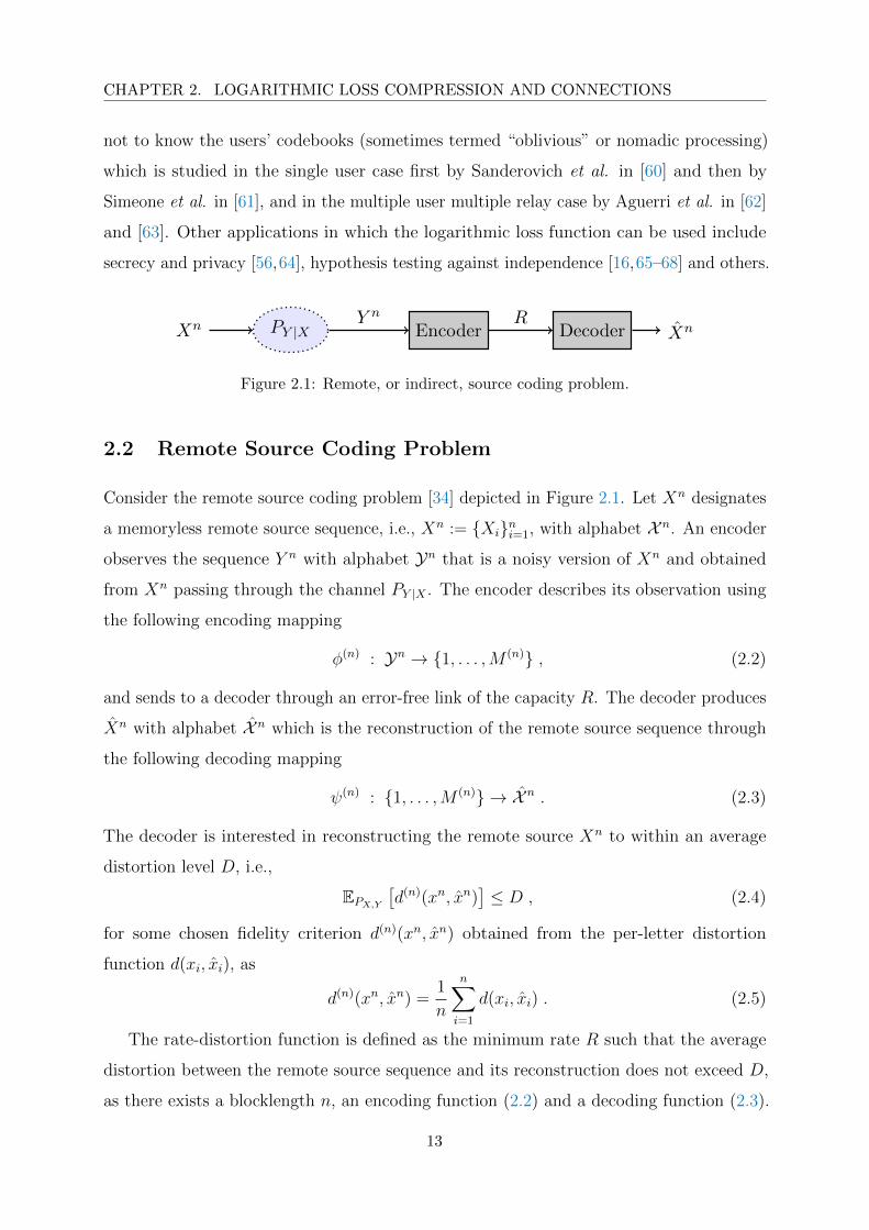
Xn PY |X Encoder DecoderY n R
Xn
Figure 2.1: Remote, or indirect, source coding problem.
2.2 Remote Source Coding Problem
Consider the remote source coding problem [34] depicted in Figure 2.1. Let Xn designates
a memoryless remote source sequence, i.e., Xn := Xini=1, with alphabet X n. An encoder
observes the sequence Y n with alphabet Yn that is a noisy version of Xn and obtained
from Xn passing through the channel PY |X . The encoder describes its observation using
the following encoding mapping
φ(n) : Yn → 1, . . . ,M (n) , (2.2)
and sends to a decoder through an error-free link of the capacity R. The decoder produces
Xn with alphabet X n which is the reconstruction of the remote source sequence through
the following decoding mapping
ψ(n) : 1, . . . ,M (n) → X n . (2.3)
The decoder is interested in reconstructing the remote source Xn to within an average
distortion level D, i.e.,
EPX,Y[d(n)(xn, xn)
]≤ D , (2.4)
for some chosen fidelity criterion d(n)(xn, xn) obtained from the per-letter distortion
function d(xi, xi), as
d(n)(xn, xn) =1
n
n∑
i=1
d(xi, xi) . (2.5)
The rate-distortion function is defined as the minimum rate R such that the average
distortion between the remote source sequence and its reconstruction does not exceed D,
as there exists a blocklength n, an encoding function (2.2) and a decoding function (2.3).
13

CHAPTER 2. LOGARITHMIC LOSS COMPRESSION AND CONNECTIONS
Remote Source Coding Under Logarithmic Loss
Here we consider the remote source coding problem in which the distortion measure is
chosen as the logarithmic loss.
Let ζ(y) = Q(·|y) ∈ P(X ) for every y ∈ Y . It is easy to see that
EPX,Y [llog(X,Q)] =∑
x
∑
y
PX,Y (x, y) log1
Q(x|y)
=∑
x
∑
y
PX,Y (x, y) log1
PX|Y (x|y)+∑
x
∑
y
PX,Y (x, y) logPX|Y (x|y)
Q(x|y)
= H(X|Y ) +DKL(PY |X‖Q)
≥ H(X|Y ) , (2.6)
with equality if and only of ζ(Y ) = PX|Y (·|y).
Now let the stochastic mapping φ(n) : Yn → Un be the encoder, i.e., ‖φ(n)‖ ≤ nR
for some prescribed complexity value R. Then, Un = φ(n)(Xn). Also, let the stochastic
mapping ψ(n) : Un → X n be the decoder. Thus, the expected logarithmic loss can be
written as
D(a)
≥ 1
n
n∑
i=1
EPX,Y [llog(Y, ψ(U))](b)
≥ H(X|U) , (2.7)
where (a) follows from (2.4) and (2.5), and (b) follows due to (2.6).
Hence, the rate-distortion of the remote source coding problem under logarithmic loss
is given by the union of all pairs (R,D) that satisfy
R ≥ I(U ;Y )
D ≥ H(X|U) ,(2.8)
where the union is over all auxiliary random variables U that satisfy the Markov chain
U −− Y −−X. Also, using the substitution ∆ := H(X)−D, the region can be written
equivalently as the union of all pairs (R,∆) that satisfy
R ≥ I(U ;Y )
∆ ≤ I(U ;X) .(2.9)
This gives a clear connection between the remote source coding problem under logarithmic
and the Information Bottleneck problem, which will be explained in the next section.
14
CHAPTER 2. LOGARITHMIC LOSS COMPRESSION AND CONNECTIONS
X PY |X Encoder DecoderY U
X
Figure 2.2: Information Bottleneck problem.
2.3 Information Bottleneck Problem
Tishby et al. in [17] present the Information Bottleneck (IB) framework, which can
be considered as a remote source coding problem in which the distortion measure is
logarithmic loss. By the choice of distortion metric as the logarithmic loss defined in (2.1),
the connection of the rate-distortion problem with the IB is studied in [18,52,69]. Next,
we explain the IB problem for the discrete memoryless and Gaussian cases.
2.3.1 Discrete Memoryless Case
The IB method depicted in Figure 2.2 formulates the problem of extracting the relevant
information that a random variable Y ∈ Y captures about another one X ∈ X such that
finding a representation U that is maximally informative about X (i.e., large mutual
information I(U ;X)), meanwhile minimally informative about Y (i.e., small mutual
information I(U ;Y )). The term I(U ;X) is referred as relevance and I(U ;Y ) is referred as
complexity. Finding the representation U that maximizes I(U ;X) while keeping I(U ;Y )
smaller than a prescribed threshold can be formulated as the following optimization
problem
∆(R) := maxPU|Y : I(U ;Y )≤R
I(U ;X) . (2.10)
Optimizing (2.10) is equivalent to solving the following Lagrangian problem
LIBs : max
PU|YI(U ;X)− sI(U ;Y ) , (2.11)
where LIBs can be called as the IB objective, and s designates the Lagrange multiplier.
For a known joint distribution PX,Y and a given trade-off parameter s ≥ 0, the optimal
mapping PU |Y can be found by solving the Lagrangian formulation (2.11). As shown
in [17, Theorem 4], the optimal solution for the IB problem satisfies the self-consistent
equations
p(u|y) = p(u)exp[−DKL(PX|y‖PX|u)]∑
u p(u) exp[−DKL(PX|y‖PX|u)](2.12a)
15

CHAPTER 2. LOGARITHMIC LOSS COMPRESSION AND CONNECTIONS
p(u) =∑
y
p(u|y)p(y) (2.12b)
p(x|u) =∑
y
p(x|y)p(y|u) =∑
y
p(x, y)p(u|y)
p(u). (2.12c)
The self consistent equations in (2.12) can be iterated, similar to Blahut-Arimoto algo-
rithm1, for finding the optimal mapping PU |Y which maximizes the IB objective in (2.11).
To do so, first PU |Y is initialized randomly, and then self-consistent equations (2.12) are
iterated until convergence. This process is summarized hereafter as
P(0)U |Y → P
(1)U → P
(1)X|U → P
(1)U |Y → . . .→ P
(t)U → P
(t)X|U → P
(t)U |Y → . . .→ P ?
U |Y .
2.3.2 Gaussian Case
Chechik et al. in [21] study the Gaussian Information Bottleneck problem (see also [22,
70,71]), in which the pair (X,Y) is jointly multivariate Gaussian variables of dimensions
nx, ny. Let Σx,Σy denote the covariance matrices of X,Y; and let Σx,y denote their
cross-covariance matrix.
It is shown in [21,22,70] that if X and Y are jointly Gaussian, the optimal representation
U is the linear transformation of Y and jointly Gaussian with Y 2. Hence, we have
U = AY + Z , Z ∼ N (0,Σz) . (2.13)
Thus, U ∼ N (0,Σu) with Σu = AΣyA† + Σz.
The Gaussian IB curve defines the optimal trade-off between compression and preserved
relevant information, and is known to have an analytical closed form solution. For a
given trade-off parameter s, the parameters of the optimal projection of the Gaussian IB
1Blahut-Arimoto algorithm [19, 20] is originally developed for computation of the channel capacity and the
rate-distortion function, and for these cases it is known to converge to the optimal solution. These iterative
algorithms can be generalized to many other situations, e.g., including the IB problem. However, it only converges
to stationary points in the context of IB.2One of the main contribution of this thesis is the generalization of this result to the distributed case. The
distributed Gaussian IB problem can be considered as the vector Gaussian CEO problem that we study in
Chapter 4. In Theorem 4, we show that the optimal test channels are Gaussian when the sources are jointly
multivariate Gaussian variables.
16

CHAPTER 2. LOGARITHMIC LOSS COMPRESSION AND CONNECTIONS
problem is found in [21, Theorem 3.1], and given by Σz = I and
A =
[0† ; 0† ; 0† ; . . . ; 0†
]0 ≤ s ≤ βc
1[α1v
†1 ; 0† ; 0† ; . . . ; 0†
]βc
1 ≤ s ≤ βc2[
α1v†1 ; α2v
†2 ; 0† ; . . . ; 0†
]βc
2 ≤ s ≤ βc3
......
, (2.14)
where v†1, . . . ,v†ny are the left eigenvectors of Σy|xΣ−1y sorted by their corresponding
ascending eigenvalues λ1, . . . , λny ; βci = 1
1−λi are critical s values; αi are coefficients defined
by αi =√
s(1−λi)−1
λiv†iΣyvi
; 0† is an ny dimensional row vectors of zeros; and semicolons separate
rows in the matrix A.
Alternatively, we can use a BA-type iterative algorithm to find the optimal relevance-
complexity tuples. By doing so, we leverage on the optimality of Gaussian test channel,
to restrict the optimization of PU|Y to Gaussian distributions, which are represented
by parameters, namely its mean and covariance (e.g., A and Σz). For a given trade-off
parameter s, the optimal representation can be found by finding its representing parameters
iterating over the following update rules
Σzt+1 =
(Σ−1
ut|x −(s− 1)
sΣ−1
ut
)−1
(2.15a)
At+1 = Σzt+1Σ−1ut|xA
t(I−Σx|yΣ−1
y
). (2.15b)
2.3.3 Connections
In this section, we review some interesting information theoretic connections that were
reported originally in [72]. For instance, it is shown that the IB problem has strong
connections with the problems of common reconstruction, information combining, the
Wyner-Ahlswede-Korner problem and the privacy funnel problem.
Common Reconstruction
Here we consider the source coding problem with side information at the decoder, also
called the Wyner-Ziv problem [73], under logarithmic loss distortion measure. Specifically,
an encoder observes a memoryless source Y and communicates with a decoder over a
rate-constrained noise-free link. The decoder also observes a statistically correlated side
17
CHAPTER 2. LOGARITHMIC LOSS COMPRESSION AND CONNECTIONS
information X. The encoder uses R bits per sample to describe its observation Y to the
decoder. The decoder wants to reconstruct an estimate of Y to within a prescribed fidelity
level D. For the general distortion metric, the rate-distortion function of the Wyner-Ziv
problem is given by
RWZY |X(D) = min
PU|Y : E[d(Y,ψ(U,X))]≤DI(U ;Y |X) , (2.16)
where ψ : U × X → Y is the decoding mapping.
The optimal coding coding scheme utilizes standard Wyner-Ziv compression at the
encoder, and the decoding mapping ψ is given by
ψ(U,X) = Pr[Y = y|U,X] . (2.17)
Then, note that with such a decoding mapping we have
E[llog(Y, ψ(U,X))] = H(Y |U,X) . (2.18)
Now we look at the source coding problem under the requirement such that the
encoder is able to produce an exact copy of the compressed source constructed by the
decoder. This requirement, termed as common reconstruction (CR), is introduced and
studied by Steinberg in [35] for various source coding models, including Wyner-Ziv setup
under a general distortion measure. For the Wyner-Ziv problem under logarithmic loss,
such a common reconstruction constraint causes some rate loss because the reproduction
rule (2.17) is not possible anymore. The Wyner-Ziv problem under logarithmic loss with
common reconstruction constraint can be written as follows
RCRY |X(D) = min
PU|Y : H(Y |U)≤DI(U ;Y |X) , (2.19)
for some auxiliary random variable U for which the Markov chain U −−Y −−X holds. Due
to this Markov chain, we have I(U ;Y |X) = I(U ;Y )− I(U ;X). Besides, observe that the
constrain H(Y |U) ≤ D is equivalent to I(U ;Y ) ≥ H(Y )−D. Then, we can rewrite (2.19)
as
RCRY |X(D) = min
PU|Y : I(U ;Y )≥H(Y )−DI(U ;Y )− I(U ;X) . (2.20)
Under the constraint I(U ;Y ) = H(Y )−D, minimizing I(U ;Y |X) is equivalent to maxi-
mizing I(U ;X), which connects the problem of CR readily with the IB.
In the above, the side information X is used for binning but not for the estimation at
the decoder. If the encoder ignores whether X is present at the decoder, the benefit of
binning is reduced – see the Heegard-Berger model with CR [74,75].
18
CHAPTER 2. LOGARITHMIC LOSS COMPRESSION AND CONNECTIONS
Information Combining
Here we consider the IB problem, in which one seeks to find a suitable representation
U that maximizes the relevance I(U ;X) for a given prescribed complexity level, e.g.,
I(U ;Y ) = R. For this setup, we have
I(Y ;U,X) = I(Y ;U) + I(Y ;X|U)
= I(Y ;U) + I(X;Y, U)− I(X;U)
(a)= I(Y ;U) + I(X;Y )− I(X;U) (2.21)
where (a) holds due the Markov chain U −− Y −−X. Hence, in the IB problem (2.11),
for a given complexity level, e.g., I(U ;Y ) = R, maximizing the relevance I(U ;X) is
equivalent of minimizing I(Y ;U,X). This is reminiscent of the problem of information
combining [36–38], where Y can be interpreted as a source transferred through two channels
PU |Y and PX|Y . The outputs of these two channels are conditionally independent given
Y ; and they should be processed in a manner such that, when combined, they capture as
much as information about Y .
Wyner-Ahlswede-Korner Problem
In the Wyner-Ahlswede-Korner problem, two memoryless sources X and Y are compressed
separately at rates RX and RY , respectively. A decoder gets the two compressed streams
and aims at recovering X in a lossless manner. This problem was solved independently by
Wyner in [39] and Ahlswede and Korner in [40]. For a given RY = R, the minimum rate
RX that is needed to recover X losslessly is given as follows
R?X(R) = min
PU|Y : I(U ;Y )≤RH(X|U) . (2.22)
Hence, the connection of Wyner-Ahlswede-Korner problem (2.22) with the IB (2.10) can
be written as
∆(R) = maxPU|Y : I(U ;Y )≤R
I(U ;X) = H(X) +R?X(R) . (2.23)
Privacy Funnel Problem
Consider the pair (X, Y ) where X ∈ X be the random variable representing the private
(or sensitive) data that is not meant to be revealed at all, or else not beyond some level ∆;
19

CHAPTER 2. LOGARITHMIC LOSS COMPRESSION AND CONNECTIONS
and Y ∈ Y be the random variable representing the non-private (or nonsensitive) data
that is shared with another user (data analyst). Assume that X and Y are correlated,
and this correlation is captured by the joint distribution PX,Y . Due to this correlation,
releasing data Y is directly to the data analyst may cause that the analyst can draw some
information about the private data X. Therefore, there is a trade-off between the amount
of information that the user keeps private about X and shares about Y . The aim is to find
a mapping φ : Y → U such that U = φ(Y ) is maximally informative about Y , meanwhile
minimally informative about X.
The analyst performs an adversarial inference attack on the private data X from the
disclosed data U . For a given arbitrary distortion metric d : X × X → R+ and the joint
distribution PX,Y , the average inference cost gain by the analyst after observing U can be
written as
∆C(d, PX,Y ) := infx∈X
EPX,Y [d(X, x)]− infX(φ(Y ))
EPX,Y [d(X, X)|U ] . (2.24)
The quantity ∆C was proposed as a general privacy metric in [76], since it measures the
improvement in the quality of the inference of the private data X due to the observation
U . In [42] (see also [77]), it is shown that for any distortion metric d, the inference cost
gain ∆C can be upper bounded as
∆C(d, PX,Y ) ≤ 2√
2L√I(U ;X) , (2.25)
where L is a constant. This justifies the use of the logarithmic loss as a privacy metric
since the threat under any bounded distortion metric can be upper bounded by an explicit
constant factor of the mutual information between the private and disclosed data. With
the choice of logarithmic loss, we have
I(U ;X) = H(X)− infX(U)
EPX,Y [llog(X, X)] . (2.26)
Under the logarithmic loss function, the design of the mapping U = φ(Y ) should strike a
right balance between the utility for inferring the non-private data Y as measured by the
mutual information I(U ;Y ) and the privacy threat about the private data X as measured
by the mutual information I(U ;X). That is refereed as the privacy funnel method [42],
and can be formulated as the following optimization
minPU|Y : I(U ;Y )≥R
I(U ;X) . (2.27)
Notice that this is an opposite optimization to the Information Bottleneck (2.10).
20

CHAPTER 2. LOGARITHMIC LOSS COMPRESSION AND CONNECTIONS
2.4 Learning via Information Bottleneck
2.4.1 Representation Learning
The performance of learning algorithms highly depends on the characteristics and properties
of the data (or features) on which the algorithms are applied. Due to this fact, feature
engineering, i.e., preprocessing operations – that may include sanitization and transferring
the data on another space – is very important to obtain good results from the learning
algorithms. On the other hand, since these preprocessing operations are both task- and
data-dependent, feature engineering is high labor-demanding and this is one of the main
drawbacks of the learning algorithms. Despite the fact that it can be sometimes considered
as helpful to use feature engineering in order to take advantage of human know-how
and knowledge on the data itself, it is highly desirable to make learning algorithms less
dependent on feature engineering to make progress towards true artificial intelligence.
Representation learning [43] is a sub-field of learning theory which aims at learning
representations by extracting some useful information from the data, possibly without using
any resources of feature engineering. Learning good representations aims at disentangling
the underlying explanatory factors which are hidden in the observed data. It may also be
useful to extract expressive low-dimensional representations from high-dimensional observed
data. The theory behind the elegant IB method may provide a better understanding of
the representation learning.
Consider a setting in which for a given data Y we want to find a representation U,
which is a function of Y (possibly non-deterministic) such that U preserves some desirable
information regarding to a task X in view of the fact that the representation U is more
convenient to work or expose relevant statistics.
Optimally, the representation should be as good as the original data for the task,
however, should not contain the parts that are irrelevant to the task. This is equivalent
finding a representation U satisfying the following criteria [78]:
(i) U is a function of Y, the Markov chain X−−Y −−U holds.
(ii) U is sufficient for the task X, that means I(U; X) = I(Y; X).
(iii) U discards all variability in Y that is not relevant to task X, i.e., minimal I(U; Y).
Besides, (ii) is equivalent to I(Y; X|U) = 0 due to the Markov chain in (i). Then, the
optimal representation U satisfying the conditions above can be found by solving the
21
CHAPTER 2. LOGARITHMIC LOSS COMPRESSION AND CONNECTIONS
following optimization
minPU|Y : I(Y;X|U)=0
I(U; Y) . (2.28)
However, (2.28) is very hard to solve due to the constrain I(Y; X|U) = 0. Tishby’s IB
method solves (2.28) by relaxing the constraint as I(U; X) ≥ ∆, which stands for that
the representation U contains relevant information regarding the task X larger than a
threshold ∆. Eventually, (2.28) boils down to minimizing the following Lagrangian
minPU|Y
H(X|U) + sI(U; Y) (2.29a)
= minPU|Y
EPX,Y
[EPU|Y [− logPX|U] + sDKL(PU|Y‖PU)
]. (2.29b)
In representation learning, disentanglement of hidden factors is also desirable in addition
to sufficiency (ii) and minimality (iii) properties. The disentanglement can be measured
with the total correlation (TC) [79,80], defined as
TC(U) := DKL(PU‖∏
j
PUj) , (2.30)
where Uj denotes the j-th component of U, and TC(U) = 0 when the components of U
are independent.
In order to obtain a more disentangled representation, we add (2.30) as a penalty
in (2.29). Then, we have
minPU|Y
EPX,Y
[EPU|Y [− logPX|U] + sDKL(PU|Y‖PU)
]+ βDKL
(PU‖
∏
j
PUj
), (2.31)
where β is the Lagrangian for TC constraint (2.30). For the case in which β = s, it is easy
to see that the minimization (2.31) is equivalent to
minPU|Y
EPX,Y
[EPU|Y [− logPX|U] + sDKL
(PU|Y‖
∏
j
PUj
)]. (2.32)
In other saying, optimizing the original IB problem (2.29) with the assumption of inde-
pendent representations, i.e., PU =∏
j PUj(uj), is equivalent forcing representations to be
more disentangled. Interestingly, we note that this assumption is already adopted for the
simplicity in many machine learning applications.
22

CHAPTER 2. LOGARITHMIC LOSS COMPRESSION AND CONNECTIONS
2.4.2 Variational Bound
The optimization of the IB cost (2.11) is generally computationally challenging. In the case
in which the true distribution of the source pair is known, there are two notable exceptions
explained in Chapter 2.3.1 and 2.3.2: the source pair (X, Y ) is discrete memoryless [17]
and the multivariate Gaussian [21,22]. Nevertheless, these assumptions on the distribution
of the source pair severely constrain the class of learnable models. In general, only a set of
training samples (xi, yi)ni=1 is available, which makes the optimization of the original IB
cost (2.11) intractable. To overcome this issue, Alemi et al. in [30] present a variational
bound on the IB objective (2.11), which also enables a neural network reparameterization
for the IB problem, which will be explained in Chapter 2.4.4.
For the variational distribution QU on U (instead of unknown PU), and a variational
stochastic decoder QX|U (instead of the unknown optimal decoder PX|U), let define
Q := QX|U , QU. Besides, for convenience let P := PU |Y . We define the variational IB
cost LVIBs (P,Q) as
LVIBs (P,Q) := EPX,Y
[EPU|Y [logQX|U ]− sDKL(PU |Y ‖QU)
]. (2.33)
Besides, we note that maximizing LIBs in (2.11) over P is equivalent to maximizing
LIBs (P) := −H(X|U)− sI(U ;Y ) . (2.34)
Next lemma states that LVIBs (P,Q) is a lower bound on LIB
s (P) for all distributions Q.
Lemma 1.
LVIBs (P,Q) ≤ LIB
s (P) , for all pmfs Q .
In addition, there exists a unique Q that achieves the maximum maxQ LVIBs (P,Q) =
LIBs (P), and is given by
Q∗X|U = PX|U , Q∗U = PU .
Using Lemma 1, the optimization in (2.11) can be written in term of the variational
IB cost as follows
maxPLIBs (P) = max
Pmax
QLVIBs (P,Q) . (2.35)
23

CHAPTER 2. LOGARITHMIC LOSS COMPRESSION AND CONNECTIONS
2.4.3 Finite-Sample Bound on the Generalization Gap
The IB method requires that the joint distribution PX,Y is known, although this is not the
case for most of the time. In fact, there is only access to a finite sample, e.g., (xi, yi)ni=1.
The generalization gap is defined as the difference between the empirical risk (average
risk over a finite training sample) and the population risk (average risk over the true joint
distribution).
It has been shown in [81], and revisited in [82], that it is possible to generalize the IB as
a learning objective for finite samples in the course of bounded representation complexity
(e.g., the cardinality of U). In the following, I(· ; ·) denotes the empirical estimate of the
mutual information based on finite sample distribution PX,Y for a given sample size of n.
In [81, Theorem 1], a finite-sample bound on the generalization gap is provided, and we
state it below.
Let U be a fixed probabilistic function of Y , determined by a fixed and known conditional
probability PU |Y . Also, let (xi, yi)ni=1 be samples of size n drawn from the joint probability
distribution PX,Y . For given (xi, yi)ni=1 and any confidence parameter δ ∈ (0, 1), the
following bounds hold with a probability of at least 1− δ,
|I(U ;Y )− I(U ;Y )| ≤(|U| log n+ log |U|)
√log 4
δ√2n
+|U| − 1
n(2.36a)
|I(U ;X)− I(U ;X)| ≤(3|U|+ 2) log n
√log 4
δ√2n
+(|X |+ 1)(|U|+ 1)− 4
n. (2.36b)
Observe that the generalization gaps decreases when the cardinality of representation U
get smaller. This means the optimal IB curve can be well estimated if the representation
space has a simple model, e.g., |U| is small. On the other hand, the optimal IB curve is
estimated badly for learning complex representations. It is also observed that the bounds
does not depend on the cardinality of Y . Besides, as expected for larger sample size n of
the training data, the optimal IB curve is estimated better.
2.4.4 Neural Reparameterization
The aforementioned BA-type algorithms works for the cases in which the joint distribution
of the data pair PX,Y is known. However, this is a very tight constraint which is very unusual
to meet, especially for real-life applications. Here we explain the neural reparameterization
and evolve the IB method to a learning algorithm to be able to use it with real datasets.
24
CHAPTER 2. LOGARITHMIC LOSS COMPRESSION AND CONNECTIONS
Let Pθ(u|y) denote the encoding mapping from the observation Y to the bottleneck
representation U, parameterized by a DNN fθ with parameters θ (e.g., the weights
and biases of the DNN). Similarly, let Qφ(x|u) denote the decoding mapping from the
representation U to the reconstruction of the label Y, parameterized by a DNN gφ with
parameters φ. Furthermore, let Qψ(u) denote the prior distribution of the latent space,
which does not depend on a DNN. By using this neural reparameterization of the encoder
Pθ(u|y), decoder Qφ(x|u) and prior Qψ(u), the optimization in (2.35) can be written as
maxθ,φ,ψ
EPX,Y
[EPθ(U|Y)[logQφ(X|U)]− sDKL(Pθ(U|Y)‖Qψ(U))
]. (2.37)
Then, for a given dataset consists of n samples, i.e., D := (xi,yi)ni=1, the optimization
of (2.37) can be approximated in terms of an empirical cost as follows
maxθ,φ,ψ
1
n
n∑
i=1
Lemps,i (θ, φ, ψ) , (2.38)
where Lemps,i (θ, φ, ψ) is the empirical IB cost for the i-th sample of the training set D, and
given by
Lemps,i (θ, φ, ψ) = EPθ(Ui|Yi)[logQφ(Xi|Ui)]− sDKL(Pθ(Ui|Yi)‖Qψ(Ui)) . (2.39)
Now, we investigate the possible choices of the parametric distributions. The encoder
can be chosen as a multivariate Gaussian, i.e., Pθ(u|y) = N (u;µθ,Σθ). So, it can be
modeled with a DNN fθ, which maps the observation y to the parameters of a multivariate
Gaussian, namely the mean µθ and the covariance Σθ, i.e., (µθ,Σθ) = fθ(y). The decoder
Qφ(x|u) can be a categorical distribution parameterized by a DNN fφ with a softmax
operation in the last layer, which outputs the probabilities of dimension |X |, i.e., x = gφ(u).
The prior of the latent space Qψ(u) can be chosen as a multivariate Gaussian (e.g., N (0, I))
such that the KL divergence DKL(Pθ(U|Y)‖Qψ(U)) has a closed form solution and is easy
to compute.
With the aforementioned choices, the first term of the RHS of (2.39) can be computed
using Monte Carlo sampling and the reparameterization trick [29] as
EPθ(Ui|Yi)[logQφ(Xi|Ui)] =1
m
m∑
j=1
logQφ(xi|ui,j) , ui,j = µθ,i+Σ12θ,i·εj , εj ∼ N (0, I) ,
where m is the number of samples for the Monte Carlo sampling step. The second term of
the RHS of (2.39) – the KL divergence between two multivariate Gaussian distributions –
25
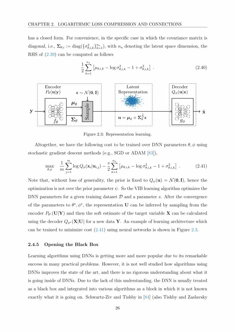
CHAPTER 2. LOGARITHMIC LOSS COMPRESSION AND CONNECTIONS
has a closed form. For convenience, in the specific case in which the covariance matrix is
diagonal, i.e., Σθ,i := diag(σ2θ,i,knuk=1), with nu denoting the latent space dimension, the
RHS of (2.39) can be computed as follows
1
2
nu∑
k=1
[µθ,i,k − log σ2
θ,i,k − 1 + σ2θ,i,k
]. (2.40)
y
EncoderPθ(u|y)
fθ
Sam
ple
µθ
Σθ
ε ∼ N (0, I)
gφ
DecoderQφ(u|x)
xu = µθ + Σ
12θ ε
LatentRepresentation
Figure 2.3: Representation learning.
Altogether, we have the following cost to be trained over DNN parameters θ, φ using
stochastic gradient descent methods (e.g., SGD or ADAM [83]),
maxθ,φ
1
m
m∑
j=1
logQφ(xi|ui,j)−s
2
nu∑
k=1
[µθ,i,k − log σ2
θ,i,k − 1 + σ2θ,i,k
]. (2.41)
Note that, without loss of generality, the prior is fixed to Qψ(u) = N (0, I), hence the
optimization is not over the prior parameter ψ. So the VIB learning algorithm optimizes the
DNN parameters for a given training dataset D and a parameter s. After the convergence
of the parameters to θ?, φ?, the representation U can be inferred by sampling from the
encoder Pθ?(U|Y) and then the soft estimate of the target variable X can be calculated
using the decoder Qφ?(X|U) for a new data Y. An example of learning architecture which
can be trained to minimize cost (2.41) using neural networks is shown in Figure 2.3.
2.4.5 Opening the Black Box
Learning algorithms using DNNs is getting more and more popular due to its remarkable
success in many practical problems. However, it is not well studied how algorithms using
DNNs improves the state of the art, and there is no rigorous understanding about what it
is going inside of DNNs. Due to the lack of this understanding, the DNN is usually treated
as a black box and integrated into various algorithms as a block in which it is not known
exactly what it is going on. Schwartz-Ziv and Tishby in [84] (also Tishby and Zaslavsky
26

CHAPTER 2. LOGARITHMIC LOSS COMPRESSION AND CONNECTIONS
in a preliminary work [82]) suggested to use an information-theoretical approach to ‘open
the black box’, where the IB principle is used to explain theory of deep learning. In [84],
it is proposed to analyze the information plane – where I(U ;X) versus I(U ;Y ) is plotted
– due to useful insights about the trade-off between prediction and compression.
(a) Tanh activation function. (b) ReLU activation function.
Figure 2.4: The evolution of the layers with the training epochs in the information plane. In the
x-axis, the mutual information between each layer and the input, i.e., I(Uk;Y ), is plotted. In the
y-axis, the mutual information between each layer and the label, i.e., I(Uk;X), is plotted. The
colors indicate training time in epochs. The curve on the far corresponds the mutual information
with the output layer; and the curve on the far right corresponds the mutual information with
the input layer. Figures are taken from [85].
Now consider a NN with K layers and let Uk be a random variable denoting the
representation, which is the output of k-th hidden layer. Then, the Markov chain
X −− Y −− U1 −− · · · −− UK −− X holds. In particular, a fully connected NN with
5 hidden layers with dimensions 12 – 10 – 7 – 5 – 4 – 3 – 2 is trained using SGD to make a
binary classification from a 12-dimensional input. All except the last layers are activated
with the hyperbolic tangent function (tanh); and sigmoid function is used for the last
(i.e., output) layer. In order to calculate the mutual information of layers with respect
to input and output variables, neuron’s tanh output activations are binned into 30 equal
intervals between -1 and 1. Then, these discretized values in each layer is used to calculate
the joint distributions PUi,Y and PUi,X over the 212 equally likely input patterns and true
output labels. Using these discrete joint distributions, the mutual informations I(Uk;Y )
27
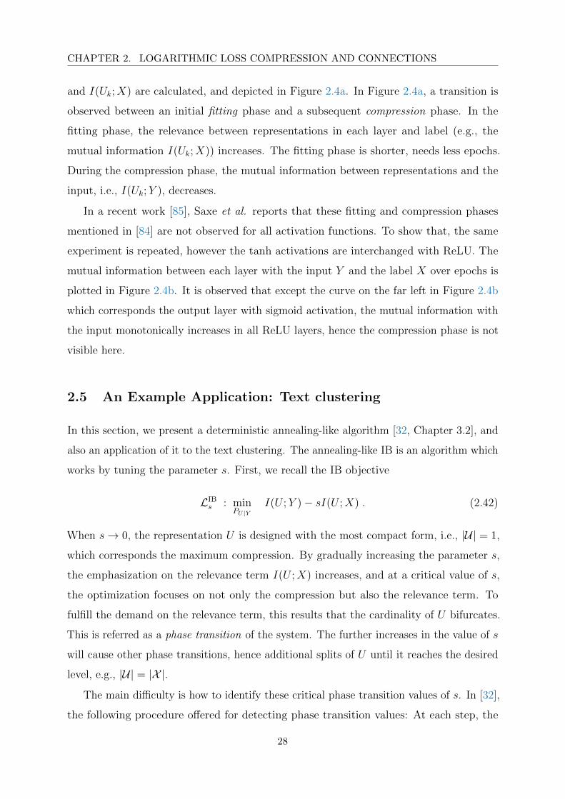
CHAPTER 2. LOGARITHMIC LOSS COMPRESSION AND CONNECTIONS
and I(Uk;X) are calculated, and depicted in Figure 2.4a. In Figure 2.4a, a transition is
observed between an initial fitting phase and a subsequent compression phase. In the
fitting phase, the relevance between representations in each layer and label (e.g., the
mutual information I(Uk;X)) increases. The fitting phase is shorter, needs less epochs.
During the compression phase, the mutual information between representations and the
input, i.e., I(Uk;Y ), decreases.
In a recent work [85], Saxe et al. reports that these fitting and compression phases
mentioned in [84] are not observed for all activation functions. To show that, the same
experiment is repeated, however the tanh activations are interchanged with ReLU. The
mutual information between each layer with the input Y and the label X over epochs is
plotted in Figure 2.4b. It is observed that except the curve on the far left in Figure 2.4b
which corresponds the output layer with sigmoid activation, the mutual information with
the input monotonically increases in all ReLU layers, hence the compression phase is not
visible here.
2.5 An Example Application: Text clustering
In this section, we present a deterministic annealing-like algorithm [32, Chapter 3.2], and
also an application of it to the text clustering. The annealing-like IB is an algorithm which
works by tuning the parameter s. First, we recall the IB objective
LIBs : min
PU|YI(U ;Y )− sI(U ;X) . (2.42)
When s→ 0, the representation U is designed with the most compact form, i.e., |U| = 1,
which corresponds the maximum compression. By gradually increasing the parameter s,
the emphasization on the relevance term I(U ;X) increases, and at a critical value of s,
the optimization focuses on not only the compression but also the relevance term. To
fulfill the demand on the relevance term, this results that the cardinality of U bifurcates.
This is referred as a phase transition of the system. The further increases in the value of s
will cause other phase transitions, hence additional splits of U until it reaches the desired
level, e.g., |U| = |X |.The main difficulty is how to identify these critical phase transition values of s. In [32],
the following procedure offered for detecting phase transition values: At each step, the
28
CHAPTER 2. LOGARITHMIC LOSS COMPRESSION AND CONNECTIONS
previous solution – which is found for the previous value of s – is taken as an initialization;
and each value of U is duplicated. Let u1 and u2 be such duplicated values of u. Then,
p(u1|y) = p(u|y)
(1
2+ α ε(u, y)
)
p(u2|y) = p(u|y)
(1
2− α ε(u, y)
),
(2.43)
where ε(u, x) is a random noise term uniformly selected in the range [−1/2, 1/2] and α
is a small scalar. Thus, the p(u1|y) and p(u2|y) is slightly perturbed values of p(u|y). If
these perturbed version of distributions are different enough, i.e., D( 1
2, 12
)
JS (PX|U1‖PX|U2) ≥ τ ,
where τ is a threshold value and DJS is the Jensen - Shannon divergence given by
D(π1,π2)JS (PX , QX) = π1DKL(PX‖PX) + π2DKL(QX‖PX), where PX = π1PX + π2QX ,
(2.44)
the corresponding value of s is a phase transition value and u is splitted into u1 and u2.
Otherwise, both perturbed values collapse to the same solution. Finally, the value of s
is increased and the whole procedure is repeated. This algorithm is called deterministic
annealing IB and stated in Algorithm 1. We note that tuning s parameter is very critical,
such that the step size in update of s should be chosen carefully, otherwise cluster splits
(phase transitions) might be skipped.
Algorithm 1 Deterministic annealing-like IB algorithm
1: input: pmf PX,Y , parameters α, τ, εs.
2: output: Optimal P ?U |Y . (soft partitions U of Y into M clusters)
3: initialization Set s→ 0 and |U| = 1, p(u|y) = 1, ∀y ∈ Y.
4: repeat
5: Update s, s = (1 + εs)sold.
6: Duplicate clusters according to (2.43).
7: Apply IB algorithm by using iteration rules (2.12).
8: Check for splits. If D( 1
2, 12)
JS (PX|U1‖PX|U2
) ≥ τ , then U ← U \ u ∪ u1, u2.9: until |U| ≥M .
Now, we apply the annealing-like algorithm to the 20 newsgroups dataset for word
clustering according to their topics. For convenience, we use a tiny version of 20 newsgroups
dataset, in which the most informative 100 words selected which come from 4 different
topics listed in Table 2.1. By using the the number of occurrences of words in topics, the
joint probability PX,Y is calculated. With the choice of parameters α = 0.005, εs = 0.001
29
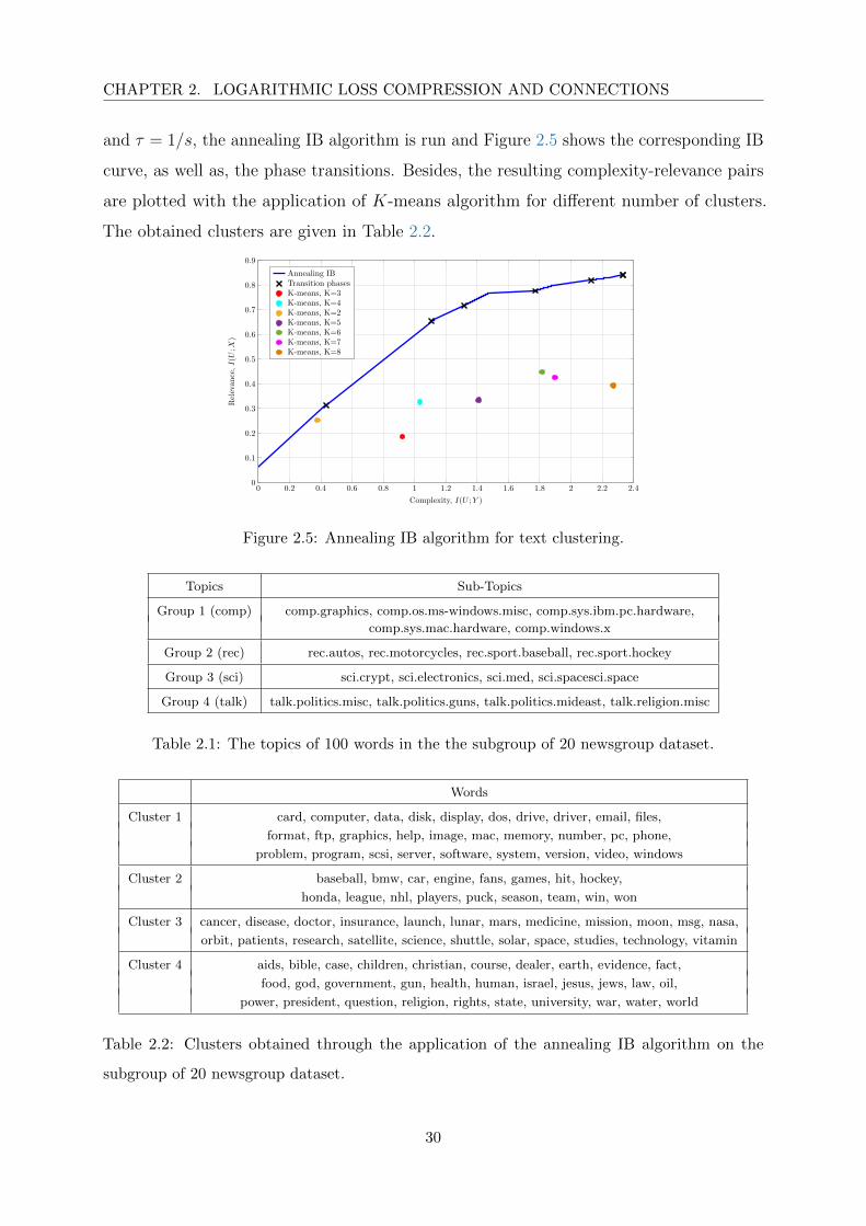
CHAPTER 2. LOGARITHMIC LOSS COMPRESSION AND CONNECTIONS
and τ = 1/s, the annealing IB algorithm is run and Figure 2.5 shows the corresponding IB
curve, as well as, the phase transitions. Besides, the resulting complexity-relevance pairs
are plotted with the application of K-means algorithm for different number of clusters.
The obtained clusters are given in Table 2.2.
0 0.2 0.4 0.6 0.8 1 1.2 1.4 1.6 1.8 2 2.2 2.40
0.1
0.2
0.3
0.4
0.5
0.6
0.7
0.8
0.9
Complexity, I(U ;Y )
Relevan
ce,I(U
;X)
Annealing IBTransition phasesK-means, K=3K-means, K=4K-means, K=2K-means, K=5K-means, K=6K-means, K=7K-means, K=8
Figure 2.5: Annealing IB algorithm for text clustering.
Topics Sub-Topics
Group 1 (comp) comp.graphics, comp.os.ms-windows.misc, comp.sys.ibm.pc.hardware,
comp.sys.mac.hardware, comp.windows.x
Group 2 (rec) rec.autos, rec.motorcycles, rec.sport.baseball, rec.sport.hockey
Group 3 (sci) sci.crypt, sci.electronics, sci.med, sci.spacesci.space
Group 4 (talk) talk.politics.misc, talk.politics.guns, talk.politics.mideast, talk.religion.misc
Table 2.1: The topics of 100 words in the the subgroup of 20 newsgroup dataset.
Words
Cluster 1 card, computer, data, disk, display, dos, drive, driver, email, files,
format, ftp, graphics, help, image, mac, memory, number, pc, phone,
problem, program, scsi, server, software, system, version, video, windows
Cluster 2 baseball, bmw, car, engine, fans, games, hit, hockey,
honda, league, nhl, players, puck, season, team, win, won
Cluster 3 cancer, disease, doctor, insurance, launch, lunar, mars, medicine, mission, moon, msg, nasa,
orbit, patients, research, satellite, science, shuttle, solar, space, studies, technology, vitamin
Cluster 4 aids, bible, case, children, christian, course, dealer, earth, evidence, fact,
food, god, government, gun, health, human, israel, jesus, jews, law, oil,
power, president, question, religion, rights, state, university, war, water, world
Table 2.2: Clusters obtained through the application of the annealing IB algorithm on the
subgroup of 20 newsgroup dataset.
30

CHAPTER 2. LOGARITHMIC LOSS COMPRESSION AND CONNECTIONS
2.6 Design of Optimal Quantizers
The IB method has been used in many fields, and in this section we present an application
in communications, which is an optimal quantizer design based on the IB method [86, 87].
The main idea is adapted from the deterministic IB, which was first proposed in [32]
for text clustering (which is presented in the previous section). Here, the IB method
compresses an observation Y to a quantized variable U while preserving the relevant
information with a random variable X. We consider the case in which the variable U is
quantized with q ∈ N bits, i.e., |U| = 2q. The aim is to find the deterministic quantizer
mapping PU |Y which maps the discrete observation Y to a quantized variable U which
maximizes the relevance I(U ;X) under a cardinality constraint |U|. This is equivalent to
finding the optimal clustering of Y which maximizes the mutual information I(U ;X).
So we initialize randomly by grouping Y into |U| clusters. The algorithm takes one of
the elements into a new cluster – so-called the singleton cluster. Due to this change, the
probabilities PX|U and PU are changed, and the new values are calculated using the IB
updates rules (2.12). Then, the deterministic IB is applied to decide on which one of the
original |U| clusters that the singleton cluster will be merged. The possible |U| choices
corresponds to merger costs given by
C(Ysing,Yk) = ψD(π1,π2)JS (PX|y‖PX|t) , k = 1, . . . , |U| , (2.45)
where D(π1,π2)JS is the Jensen - Shannon divergence given in (2.44) and
ψ = Pr(Y = y) + Pr(U = u) (2.46a)
π1 = Pr(Y = y)/ψ (2.46b)
π2 = Pr(U = u)/ψ . (2.46c)
The singleton cluster merges with the one which has a smaller merger cost.
The algorithm is a greedy algorithm, which repeats the draw and merge steps for all Y
until the obtained clusters are the same. Since the IB method does not converge to the
global optimum, it should be run several times and the clustering (quantization) should
be done with the best outcome, i.e., the mapping which maximize the IB cost (2.11).
Now we consider an example of finding the optimum channel quantizers for the binary
input additive white Gaussian noise (AWGN) channel [86, Section III], in which a code
31
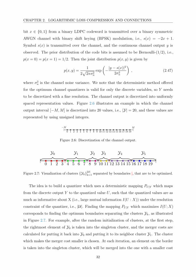
CHAPTER 2. LOGARITHMIC LOSS COMPRESSION AND CONNECTIONS
bit x ∈ 0, 1 from a binary LDPC codeword is transmitted over a binary symmetric
AWGN channel with binary shift keying (BPSK) modulation, i.e., s(x) = −2x + 1.
Symbol s(x) is transmitted over the channel, and the continuous channel output y is
observed. The prior distribution of the code bits is assumed to be Bernoulli-(1/2), i.e.,
p(x = 0) = p(x = 1) = 1/2. Then the joint distribution p(x, y) is given by
p(x, y) =1
2√
2πσ2n
exp
(−|y − s(x)|2
2σ2n
), (2.47)
where σ2n is the channel noise variance. We note that the deterministic method offered
for the optimum channel quantizers is valid for only the discrete variables, so Y needs
to be discretized with a fine resolution. The channel output is discretized into uniformly
spaced representation values. Figure 2.6 illustrates an example in which the channel
output interval [−M,M ] is discretized into 20 values, i.e., |Y| = 20, and these values are
represented by using unsigned integers.
−M|
0 1 2 3 4 5 6 7 8 9 10 11 12 13 14 15 16 17 18 19|M
Figure 2.6: Discretization of the channel output.
|0 1 2 3
|4 5 6 7
|8 9
|10 11
|12 13 14 15
|16 17 18 19
|Y0 Y1 Y2 Y3 Y4 Y5
Figure 2.7: Visualization of clusters Yk|U|k=1 separated by boundaries |, that are to be optimized.
The idea is to build a quantizer which uses a deterministic mapping PU |Y which maps
from the discrete output Y to the quantized value U , such that the quantized values are as
much as informative about X (i.e., large mutual information I(U : X)) under the resolution
constraint of the quantizer, i.e., |U|. Finding the mapping PU |Y which maximizes I(U ;X)
corresponds to finding the optimum boundaries separating the clusters Yk, as illustrated
in Figure 2.7. For example, after the random initialization of clusters, at the first step,
the rightmost element of Y0 is taken into the singleton cluster, and the merger costs are
calculated for putting it back into Y0 and putting it to its neighbor cluster Y1. The cluster
which makes the merger cost smaller is chosen. At each iteration, an element on the border
is taken into the singleton cluster, which will be merged into the one with a smaller cost
32

CHAPTER 2. LOGARITHMIC LOSS COMPRESSION AND CONNECTIONS
among the original and neighbor clusters. These steps are repeated until the resulting
cluster does not change anymore. This algorithm is detailed in [86, Algorithm 1].
In digital communication systems, a continuous channel output is fed into an analog-
to-digital converter to obtain a discrete valued sample – depicted in Figure 2.8. In theory,
it is assumed that the quantizer has a very high resolution so the effect of quantization is
generally ignored. However, this is not the case in real life. A few bits are desired in the
implementations, hence the quantizer becomes a bottleneck in the communication system.
X PY |XQuantizerPU |Y
YU
Figure 2.8: Memoryless channel with subsequent quantizer.
The state of the art low-density parity-check (LDPC) decoders execute the node
operations by processing the quasi-continuous LLRs, which makes belief propagation
decoding challenging. The IB method is proposed in [86] to overcome this complexity
issues. The main idea is to pass compressed but highly informative integer-valued messages
along the edges of a Tanner graph. To do so, Lewandowsky and Bauch use the IB
method [86], and construct discrete message passing decoders for LDPC codes; and they
showed that these decoders outperform state of the art decoders.
We close this section by mentioning the implementation issues of DNNs which are used
for many artificial intelligence (AI) algorithms. The superior success of DNNs comes at
the cost of high complexity (computational- and memory-wise). Although the devices,
e.g., smartphones, get more and more powerful compared to a few year ago with the
significant improvement of the chipsets, the implementation of DNNs is still a challenging
task. The proposed approach seems particularly promising for the implementation of DNN
algorithms on chipsets.
33

34

Chapter 3
Discrete Memoryless CEO Problem
with Side Information
In this chapter, we study the K-encoder DM CEO problem with side information shown
in Figure 3.1. Consider a (K + 2)-dimensional memoryless source (X, Y0, Y1, . . . , YK)
with finite alphabet X × Y0 × Y1 × . . .× YK and joint probability mass function (pmf)
PX,Y0,Y1,...,YK (x, y0, y1, . . . , yK). It is assumed that for all S ⊆ K := 1, . . . , K,
YS −− (X, Y0)−− YSc , (3.1)
forms a Markov chain in that order. Also, let (Xi, Y0,i, Y1,i, . . . , YK,i)ni=1 be a sequence of
n independent copies of (X, Y0, Y1, . . . , YK), i.e., (Xn, Y n0 , Y
n1 , . . . , Y
nK) ∼∏n
i=1 PX,Y0,Y1,...,YK
(xi, y0,i, y1,i, . . . , yK,i). In the model studied in this chapter, Encoder (or agent) k, k ∈ K,
observes the memoryless source Y nk and uses Rk bits per sample to describe it to the
decoder. The decoder observes a statistically dependent memoryless side information
stream, in the form of the sequence Y n0 , and wants to reconstruct the remote source Xn
to within a prescribed fidelity level. Similar to [10], in this thesis we take the reproduction
alphabet X to be equal to the set of probability distributions over the source alphabet
X . Thus, for a vector Xn ∈ X n, the notation Xj(x) means the jth-coordinate of Xn,
1 ≤ j ≤ n, which is a probability distribution on X , evaluated for the outcome x ∈ X . In
other words, the decoder generates ‘soft’ estimates of the remote source’s sequences. We
consider the logarithmic loss distortion measure defined as in (2.5), where the letter-wise
distortion measure is given by (2.1).
35
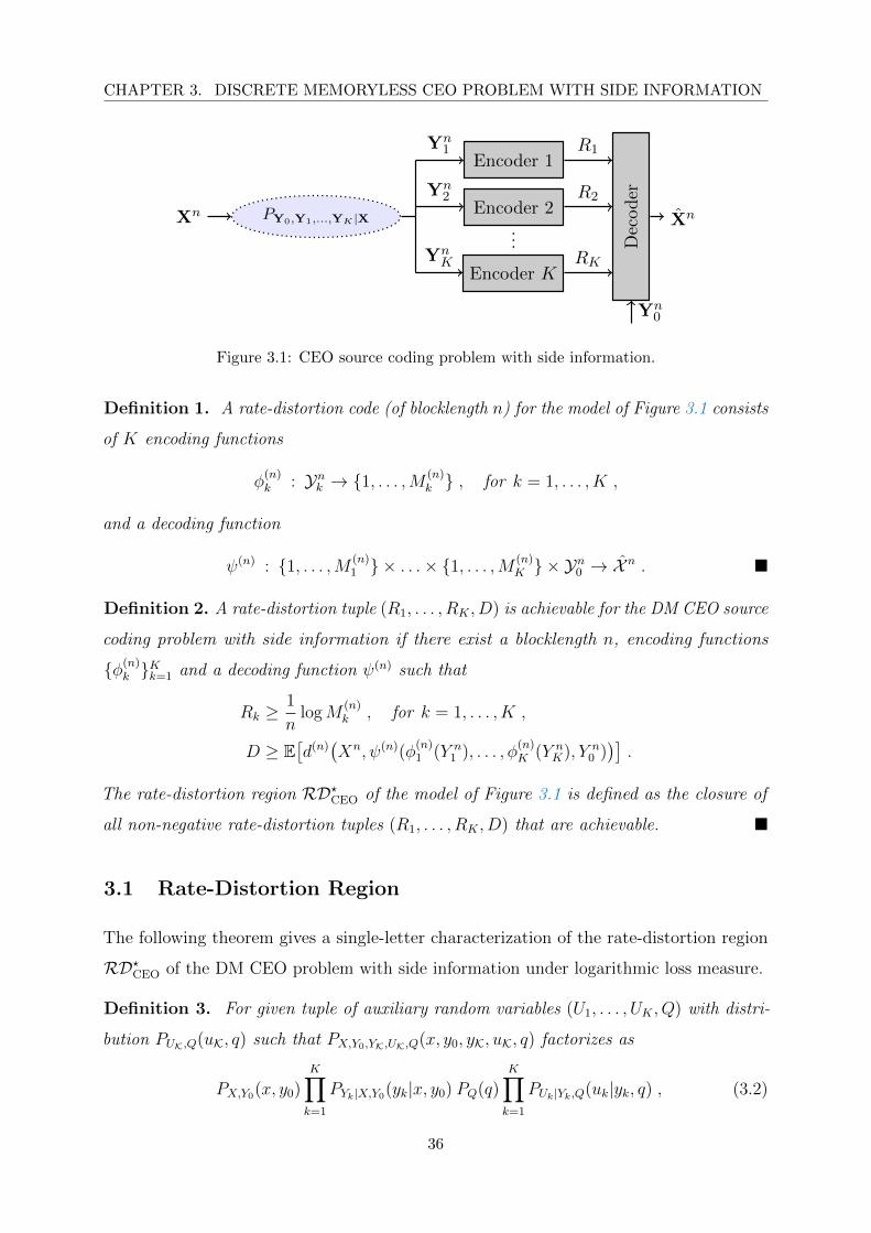
CHAPTER 3. DISCRETE MEMORYLESS CEO PROBLEM WITH SIDE INFORMATION
Xn PY0,Y1,...,YK |X
Encoder 1
Encoder 2
Encoder K
Yn1
Yn2
YnK
Decoder
R1
R2
RK
...
Xn
Yn0
Figure 3.1: CEO source coding problem with side information.
Definition 1. A rate-distortion code (of blocklength n) for the model of Figure 3.1 consists
of K encoding functions
φ(n)k : Ynk → 1, . . . ,M (n)
k , for k = 1, . . . , K ,
and a decoding function
ψ(n) : 1, . . . ,M (n)1 × . . .× 1, . . . ,M (n)
K × Yn0 → X n .
Definition 2. A rate-distortion tuple (R1, . . . , RK , D) is achievable for the DM CEO source
coding problem with side information if there exist a blocklength n, encoding functions
φ(n)k Kk=1 and a decoding function ψ(n) such that
Rk ≥1
nlogM
(n)k , for k = 1, . . . , K ,
D ≥ E[d(n)(Xn, ψ(n)(φ
(n)1 (Y n
1 ), . . . , φ(n)K (Y n
K), Y n0 ))].
The rate-distortion region RD?CEO of the model of Figure 3.1 is defined as the closure of
all non-negative rate-distortion tuples (R1, . . . , RK , D) that are achievable.
3.1 Rate-Distortion Region
The following theorem gives a single-letter characterization of the rate-distortion region
RD?CEO of the DM CEO problem with side information under logarithmic loss measure.
Definition 3. For given tuple of auxiliary random variables (U1, . . . , UK , Q) with distri-
bution PUK,Q(uK, q) such that PX,Y0,YK,UK,Q(x, y0, yK, uK, q) factorizes as
PX,Y0(x, y0)K∏
k=1
PYk|X,Y0(yk|x, y0) PQ(q)K∏
k=1
PUk|Yk,Q(uk|yk, q) , (3.2)
36

CHAPTER 3. DISCRETE MEMORYLESS CEO PROBLEM WITH SIDE INFORMATION
define RDCEO(U1, . . . , UK , Q) as the set of all non-negative rate-distortion tuples (R1, . . . ,
RK , D) that satisfy, for all subsets S ⊆ K,
∑
k∈SRk +D ≥
∑
k∈SI(Yk;Uk|X, Y0, Q) +H(X|USc , Y0, Q) .
Theorem 1. The rate-distortion region for the DM CEO problem under logarithmic loss
is given by
RD?CEO =⋃RDCEO(U1, . . . , UK , Q) ,
where the union is taken over all tuples (U1, . . . , UK , Q) with distributions that satisfy (3.2).
Proof. The proof of Theorem 1 is given in Appendix A.
Remark 1. To exhaust the region of Theorem 1, it is enough to restrict UkKk=1 and Q
to satisfy |Uk| ≤ |Yk| for k ∈ K and |Q| ≤ K + 2 (see [10, Appendix A]).
Remark 2. Theorem 1 extends the result of [10, Theorem 10] to the case in which the
decoder has, or observes, its own side information stream Y n0 and the agents’ observations
are conditionally independent given the remote source Xn and Y n0 , i.e., Y n
S −−(Xn, Y n0 )−−Y n
Sc
holds for all subsets S ⊆ K. The rate-distortion region of this problem can be obtained
readily by applying [10, Theorem 10], which provides the rate-distortion region of the model
without side information at decoder, to the modified setting in which the remote source
is X = (X,Y0), another agent (agent K + 1) observes YK+1 = Y0 and communicates
at large rate RK+1 = ∞ with the CEO, which wishes to estimates X to within average
logarithmic distortion D and has no own side information stream1.
3.2 Estimation of Encoder Observations
In this section, we focus on the two-encoder case, i.e., K = 2. Suppose the decoder wants
to estimate the encoder observations (Y1, Y2), i.e., X = (Y1, Y2). Note that in this case the
side information Y0 can be chosen arbitrarily correlated to (Y1, Y2) and is not restricted to
satisfy any Markov structure, since the Markov chain Y1 −− (X, Y0)−− Y2 is satisfied for
all choices of Y0 that are arbitrarily correlated with (Y1, Y2).
1Note that for the modified CEO setting the agents’ observations are conditionally independent given the
remote source X.
37

CHAPTER 3. DISCRETE MEMORYLESS CEO PROBLEM WITH SIDE INFORMATION
If a distortion of D bits is tolerated on the joint estimation of the pair (Y1, Y2), then
the achievable rate-distortion region can be obtained easily from Theorem 1, as a slight
variation of the Slepian-Wolf region, namely the set of non-negative rate-distortion triples
(R1, R2, D) such that
R1 ≥ H(Y1|Y0, Y2)−D (3.3a)
R2 ≥ H(Y2|Y0, Y1)−D (3.3b)
R1 +R2 ≥ H(Y1, Y2|Y0)−D . (3.3c)
The following theorem gives a characterization of the set of rate-distortion quadruples
(R1, R2, D1, D2) that are achievable in the more general case in which a distortion D1 is
tolerated on the estimation of the source component Y1 and a distortion D2 is tolerated
on the estimation of the source component Y2, i.e., the rate-distortion region of the
two-encoder DM multiterminal source coding problem with arbitrarily correlated side
information at the decoder.
Theorem 2. If X = (Y1, Y2), the component Y1 is to be reconstructed to within average
logarithmic loss distortion D1 and the component Y2 is to be reconstructed to within
average logarithmic loss distortion D2, the rate-distortion region RD?MT of the associated
two-encoder DM multiterminal source coding problem with correlated side information at
the decoder under logarithmic loss is given by the set of all non-negative rate-distortion
quadruples (R1, R2, D1, D2) that satisfy
R1 ≥ I(U1;Y1|U2, Y0, Q)
R2 ≥ I(U2;Y2|U1, Y0, Q)
R1 +R2 ≥ I(U1, U2;Y1, Y2|Y0, Q)
D1 ≥ H(Y1|U1, U2, Y0, Q)
D2 ≥ H(Y2|U1, U2, Y0, Q) ,
for some joint measure of the form PY0,Y1,Y2(y0, y1, y2)PQ(q)PU1|Y1,Q(u1|y1, q)PU2|Y2,Q(u2|y2, q).
Proof. The proof of Theorem 2 is given in Appendix B.
Remark 3. The auxiliary random variables of Theorem 2 are such that U1 −− (Y1, Q)−− (Y0, Y2, U2) and U2 −− (Y2, Q)−− (Y0, Y1, U1) form Markov chains.
38

CHAPTER 3. DISCRETE MEMORYLESS CEO PROBLEM WITH SIDE INFORMATION
Remark 4. The result of Theorem 2 extends that of [10, Theorem 6] for the two-encoder
source coding problem with average logarithmic loss distortion constraints on Y1 and Y2
and no side information at the decoder to the setting in which the decoder has its own side
information Y0 that is arbitrarily correlated with (Y1, Y2). It is noteworthy that while the
Berger-Tung inner bound is known to be non-tight for more than two encoders, as it is
not optimal for the lossless modulo-sum problem of Korner and Marton [88], Theorem 2
shows that it is tight for the case of three encoders if the observation of the third encoder
is encoded at large (infinite) rate.
In the case in which the sources Y1 and Y2 are conditionally independent given Y0, i.e.,
Y1 −− Y0−− Y2 forms a Markov chain, it can be shown easily that the result of Theorem 2
reduces to the set of rates and distortions that satisfy
R1 ≥ I(U1;Y1)− I(U1;Y0) (3.4)
R2 ≥ I(U2;Y2)− I(U2;Y0) (3.5)
D1 ≥ H(Y1|U1, Y0) (3.6)
D2 ≥ H(Y2|U2, Y0) , (3.7)
for some measure of the form PY0,Y1,Y2(y0, y1, y2)PU1|Y1(u1|y1)PU2|Y2(u2|y2).
This result can also be obtained by applying [89, Theorem 6] with the reproduction
functions therein chosen as
fk(Uk, Y0) := Pr[Yk = yk|Uk, Y0] , for k = 1, 2 . (3.8)
Then, note that with this choice we have
E[d(Yk, fk(Uk, Y0)] = H(Yk|Uk, Y0) , for k = 1, 2 . (3.9)
3.3 An Example: Distributed Pattern Classification
Consider the problem of distributed pattern classification shown in Figure 3.2. In this
example, the decoder is a predictor whose role is to guess the unknown class X ∈ X of
a measurable pair (Y1, Y2) ∈ Y1 × Y2 on the basis of inputs from two learners as well as
its own observation about the target class, in the form of some correlated Y0 ∈ Y0. It
is assumed that Y1 −− (X, Y0) −− Y2. The first learner produces its input based only
39
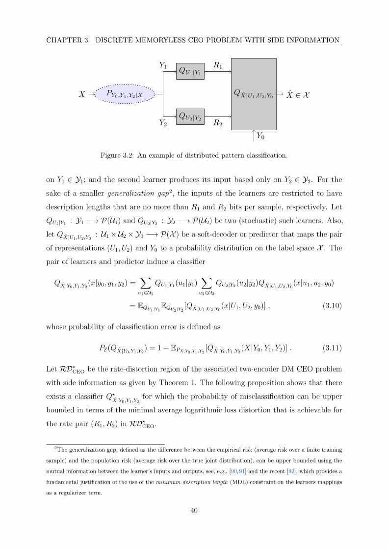
CHAPTER 3. DISCRETE MEMORYLESS CEO PROBLEM WITH SIDE INFORMATION
X PY0,Y1,Y2|X
QU1|Y1
QU2|Y2
QX|U1,U2,Y0
Y1
Y2
Y0
R1
R2
X ∈ X
Figure 3.2: An example of distributed pattern classification.
on Y1 ∈ Y1; and the second learner produces its input based only on Y2 ∈ Y2. For the
sake of a smaller generalization gap2, the inputs of the learners are restricted to have
description lengths that are no more than R1 and R2 bits per sample, respectively. Let
QU1|Y1 : Y1 −→ P(U1) and QU2|Y2 : Y2 −→ P(U2) be two (stochastic) such learners. Also,
let QX|U1,U2,Y0: U1 ×U2 ×Y0 −→ P(X ) be a soft-decoder or predictor that maps the pair
of representations (U1, U2) and Y0 to a probability distribution on the label space X . The
pair of learners and predictor induce a classifier
QX|Y0,Y1,Y2(x|y0, y1, y2) =
∑
u1∈U1
QU1|Y1(u1|y1)∑
u2∈U2
QU2|Y2(u2|y2)QX|U1,U2,Y0(x|u1, u2, y0)
= EQU1|Y1EQU2|Y2
[QX|U1,U2,Y0(x|U1, U2, y0)] , (3.10)
whose probability of classification error is defined as
PE(QX|Y0,Y1,Y2) = 1− EPX,Y0,Y1,Y2
[QX|Y0,Y1,Y2(X|Y0, Y1, Y2)] . (3.11)
Let RD?CEO be the rate-distortion region of the associated two-encoder DM CEO problem
with side information as given by Theorem 1. The following proposition shows that there
exists a classifier Q?X|Y0,Y1,Y2
for which the probability of misclassification can be upper
bounded in terms of the minimal average logarithmic loss distortion that is achievable for
the rate pair (R1, R2) in RD?CEO.
2The generalization gap, defined as the difference between the empirical risk (average risk over a finite training
sample) and the population risk (average risk over the true joint distribution), can be upper bounded using the
mutual information between the learner’s inputs and outputs, see, e.g., [90,91] and the recent [92], which provides a
fundamental justification of the use of the minimum description length (MDL) constraint on the learners mappings
as a regularizer term.
40
CHAPTER 3. DISCRETE MEMORYLESS CEO PROBLEM WITH SIDE INFORMATION
Proposition 1. For the problem of distributed pattern classification of Figure 3.2, there
exists a classifier Q?X|Y0,Y1,Y2
for which the probability of classification error satisfies
PE(Q?X|Y0,Y1,Y2
) ≤ 1− exp(− infD : (R1, R2, D) ∈ RD?CEO
),
where RD?CEO is the rate-distortion region of the associated two-encoder DM CEO problem
with side information as given by Theorem 1.
Proof. Let a triple mappings (QU1|Y1 , QU2|Y2 , QX|U1,U2,Y0) be given. It is easy to see that the
probability of classification error of the classifier QX|Y0,Y1,Y2as defined by (3.11) satisfies
PE(QX|Y0,Y1,Y2) ≤ EPX,Y0,Y1,Y2
[− logQX|Y0,Y1,Y2(X|Y0, Y1, Y2)] . (3.12)
Applying Jensen’s inequality on the right hand side (RHS) of (3.12), using the concavity
of the logarithm function, and combining with the fact that the exponential function
increases monotonically, the probability of classification error can be further bounded as
PE(QX|Y0,Y1,Y2) ≤ 1− exp
(− EPX,Y0,Y1,Y2
[− logQX|Y0,Y1,Y2(X|Y0, Y1, Y2)]
). (3.13)
Using (3.10) and continuing from (3.13), we get
PE(QX|Y0,Y1,Y2) ≤ 1− exp
(− EPX,Y0,Y1,Y2
[− logEQU1|Y1EQU2|Y2
[QX|U1,U2,Y0(X|U1, U2, Y0)]]
)
≤ 1− exp(− EPX,Y0,Y1,Y2
EQU1|Y1EQU2|Y2
[− log[QX|U1,U2,Y0(X|U1, U2, Y0)]]
),
(3.14)
where the last inequality follows by applying Jensen’s inequality and using the concavity
of the logarithm function.
Noticing that the term in the exponential function in the RHS of (3.14),
D(QU1|Y1 , QU1|Y1 , QX|U1,U2,Y0) := EPXY0Y1Y2
EQU1|Y1EQU2|Y2
[− logQX|U1,U2,Y0(X|U1, U2, Y0)] ,
is the average logarithmic loss, or cross-entropy risk, of the triple (QU1|Y1 , QU2|Y2 , QX|U1,U2,Y0);
the inequality (3.14) implies that minimizing the average logarithmic loss distortion leads
to classifier with smaller (bound on) its classification error. Using Theorem 1, the min-
imum average logarithmic loss, minimized over all mappings QU1|Y1 : Y1 −→ P(U1)
and QU2|Y2 : Y2 −→ P(U2) that have description lengths no more than R1 and R2 bits
per-sample, respectively, as well as all choices of QX|U1,U2,Y0: U1 × U2 × Y0 −→ P(X ), is
D?(R1, R2) = infD : (R1, R2, D) ∈ RD?CEO . (3.15)
41

CHAPTER 3. DISCRETE MEMORYLESS CEO PROBLEM WITH SIDE INFORMATION
Thus, the direct part of Theorem 1 guarantees the existence of a classifier Q?X|Y0,Y1,Y2
whose
probability of error satisfies the bound given in Proposition 1.
To make the above example more concrete, consider the following scenario where Y0
plays the role of information about the sub-class of the label class X ∈ 0, 1, 2, 3. More
specifically, let S be a random variable that is uniformly distributed over 1, 2. Also,
let X1 and X2 be two random variables that are independent between them and from S,
distributed uniformly over 1, 3 and 0, 2 respectively. The state S acts as a random
switch that connects X1 or X2 to X, i.e.,
X = XS . (3.16)
That is, if S = 1 then X = X1, and if S = 2 then X = X2. Thus, the value of S indicates
whether X is odd- or even-valued (i.e., the sub-class of X). Also, let
Y0 = S (3.17a)
Y1 = XS ⊕ Z1 (3.17b)
Y2 = XS ⊕ Z2 , (3.17c)
where Z1 and Z2 are Bernoulli-(p) random variables, p ∈ (0, 1), that are independent
between them, and from (S,X1, X2), and the addition is modulo 4. For simplification,
we let R1 = R2 = R. We numerically approximate the set of (R,D) pairs such that
(R,R,D) is in the rate-distortion region RD?CEO corresponding to the CEO network of
this example. The algorithm that we use for the computation will be described in detail in
Chapter 5.1.1. The lower convex envelope of these (R,D) pairs is plotted in Figure 3.3a
for p ∈ 0.01, 0.1, 0.25, 0.5. Continuing our example, we also compute the upper bound
on the probability of classification error according to Proposition 1. The result is given in
Figure 3.3b. Observe that if Y1 and Y2 are high-quality estimates of X (e.g., p = 0.01),
then a small increase in the complexity R results in a large relative improvement of the
(bound on) the probability of classification error. On the other hand, if Y1 and Y2 are
low-quality estimates of X (e.g., p = 0.25) then we require a large increase of R in order
to obtain an appreciable reduction in the error probability. Recalling that larger R implies
lesser generalization capability [90–92], these numerical results are consistent with the
fact that classifiers should strike a good balance between accuracy and their ability to
42
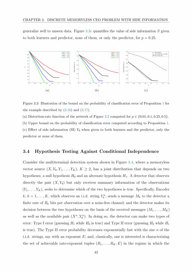
CHAPTER 3. DISCRETE MEMORYLESS CEO PROBLEM WITH SIDE INFORMATION
generalize well to unseen data. Figure 3.3c quantifies the value of side information S given
to both learners and predictor, none of them, or only the predictor, for p = 0.25.
0 0.2 0.4 0.6 0.8 1 1.2 1.40
0.1
0.2
0.3
0.4
0.5
0.6
0.7
0.8
0.9
1
R
D
p = 0.50p = 0.25p = 0.10p = 0.01
(a)
0 0.2 0.4 0.6 0.8 1 1.2 1.40
0.1
0.2
0.3
0.4
0.5
0.6
0.7
R
Upp
erB
ound
onPE
p = 0.50p = 0.25p = 0.10p = 0.01
(b)
0 0.2 0.4 0.6 0.8 1 1.2 1.40.1
0.2
0.3
0.4
0.5
0.6
0.7
0.8
0.9
R
Upp
erB
ound
onPE
SI nowhereSI at both Enc. and Dec.SI at only Dec.
(c)
Figure 3.3: Illustration of the bound on the probability of classification error of Proposition 1 for
the example described by (3.16) and (3.17).
(a) Distortion-rate function of the network of Figure 3.2 computed for p ∈ 0.01, 0.1, 0.25, 0.5.(b) Upper bound on the probability of classification error computed according to Proposition 1.
(c) Effect of side information (SI) Y0 when given to both learners and the predictor, only the
predictor or none of them.
3.4 Hypothesis Testing Against Conditional Independence
Consider the multiterminal detection system shown in Figure 3.4, where a memoryless
vector source (X, Y0, Y1, . . . , YK), K ≥ 2, has a joint distribution that depends on two
hypotheses, a null hypothesis H0 and an alternate hypothesis H1. A detector that observes
directly the pair (X, Y0) but only receives summary information of the observations
(Y1, . . . , YK), seeks to determine which of the two hypotheses is true. Specifically, Encoder
k, k = 1, . . . , K, which observes an i.i.d. string Y nk , sends a message Mk to the detector a
finite rate of Rk bits per observation over a noise-free channel; and the detector makes its
decision between the two hypotheses on the basis of the received messages (M1, . . . ,MK)
as well as the available pair (Xn, Y n0 ). In doing so, the detector can make two types of
error: Type I error (guessing H1 while H0 is true) and Type II error (guessing H0 while H1
is true). The Type II error probability decreases exponentially fast with the size n of the
i.i.d. strings, say with an exponent E; and, classically, one is interested is characterizing
the set of achievable rate-exponent tuples (R1, . . . , RK , E) in the regime in which the
43
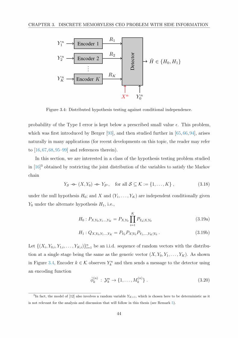
CHAPTER 3. DISCRETE MEMORYLESS CEO PROBLEM WITH SIDE INFORMATION
Y n1
Y n2
Y nK
Encoder 1
Encoder 2
Encoder K
... Det
ecto
r
R1
R2
RK
H ∈ H0, H1
Xn Y n0
Figure 3.4: Distributed hypothesis testing against conditional independence.
probability of the Type I error is kept below a prescribed small value ε. This problem,
which was first introduced by Berger [93], and then studied further in [65,66,94], arises
naturally in many applications (for recent developments on this topic, the reader may refer
to [16,67,68,95–99] and references therein).
In this section, we are interested in a class of the hypothesis testing problem studied
in [16]3 obtained by restricting the joint distribution of the variables to satisfy the Markov
chain
YS −− (X, Y0)−− YSc , for all S ⊆ K := 1, . . . , K , (3.18)
under the null hypothesis H0; and X and (Y1, . . . , YK) are independent conditionally given
Y0 under the alternate hypothesis H1, i.e.,
H0 : PX,Y0,Y1...,YK = PX,Y0
K∏
i=1
PYk|X,Y0 (3.19a)
H1 : QX,Y0,Y1...,YK = PY0PX|Y0PY1,...,YK |Y0 . (3.19b)
Let (Xi, Y0,i, Y1,i, . . . , YK,i)ni=1 be an i.i.d. sequence of random vectors with the distribu-
tion at a single stage being the same as the generic vector (X, Y0, Y1, . . . , YK). As shown
in Figure 3.4, Encoder k ∈ K observes Y nk and then sends a message to the detector using
an encoding function
φ(n)k : Ynk → 1, . . . ,M (n)
k . (3.20)
3In fact, the model of [12] also involves a random variable YK+1, which is chosen here to be deterministic as it
is not relevant for the analysis and discussion that will follow in this thesis (see Remark 5).
44
CHAPTER 3. DISCRETE MEMORYLESS CEO PROBLEM WITH SIDE INFORMATION
The pair (Xn, Y n0 ) is available at the detector which uses it together with the messages
from the encoders to make a decision between the two hypotheses based on a decision rule
ψ(n) : 1, . . . ,M (n)1 × . . .× 1, . . . ,M (n)
K × X n × Yn0 → H0, H1 . (3.21)
The mapping (3.21) is such that ψ(n)(m1, . . . ,mK , xn, yn0 ) = H0 if (m1, . . . ,mK , x
n, yn0 ) ∈An and H1 otherwise, with
An ⊆n∏
k=1
1, . . . ,M (n)k × X n × Yn0 ,
designating the acceptance region for H0. The encoders φ(n)k Kk=1 and the detector ψ(n)
are such that the Type I error probability does not exceed a prescribed level ε ∈ [0, 1], i.e.,
Pφ
(n)1 (Y n1 ),...,φ
(n)K (Y nK),Xn,Y n0
(Acn) ≤ ε , (3.22)
and the Type II error probability does not exceed β, i.e.,
Qφ
(n)1 (Y n1 ),...,φ
(n)K (Y nK),Xn,Y n0
(An) ≤ β . (3.23)
Definition 4. A rate-exponent tuple (R1, . . . , RK , E) is achievable for a fixed ε ∈ [0, 1]
and any positive δ if there exist a sufficiently large blocklength n, encoders φ(n)k Kk=1 and a
detector ψ(n) such that
1
nlogM
(n)k ≤ Rk + δ , for k = 1, . . . , K , (3.24a)
− 1
nlog β ≥ E − δ . (3.24b)
The rate-exponent region RHT is defined as
RHT :=⋂
ε>0
RHT,ε , (3.25)
where RHT,ε is the set of all achievable rate-exponent vectors for a fixed ε ∈ (0, 1].
We start with an entropy characterization of the rate-exponentRHT as defined by (3.25).
Let
R? =⋃
n
⋃
φ(n)k k∈K
R?(n, φ(n)
k k∈K), (3.26)
45
CHAPTER 3. DISCRETE MEMORYLESS CEO PROBLEM WITH SIDE INFORMATION
where
R?(n, φ(n)
k k∈K)
=
(R1, . . . , RK , E) s.t.
Rk ≥1
nlog |φ(n)
k (Y nk )| , for k = 1, . . . , K ,
E ≤ 1
nI(φ(n)
k (Y nk )k∈K;Xn|Y n
0 )
.
We have the following proposition, whose proof is essentially similar to that of [65, Theorem
5] and, hence, is omitted.
Proposition 2. RHT = R? .
Now, recall the CEO source coding problem under logarithmic loss of Figure 3.1 and
its rate-distortion region RD?CEO as given by Theorem 1 in the case in which the Markov
chain (3.1) holds. The following proposition states that RHT and RD?CEO can be inferred
from each other.
Proposition 3. (R1, . . . , RK , E) ∈ RHT if and only if (R1, . . . , RK , H(X|Y0) − E) ∈RD?CEO.
Proof. The proof of Proposition 3 appears in Appendix C.
The result of the next theorem follows easily by using Theorem 1 and Proposition 3.
Theorem 3. [100, Theorem 1] For the distributed hypothesis testing against conditional
independence problem of Figure 3.4, the rate-exponent region is given by the union of all
non-negative tuples (R1, . . . , RK , E) that satisfy, for all subsets S ⊆ K,
E ≤ I(USc ;X|Y0, Q) +∑
k∈S
(Rk − I(Yk;Uk|X, Y0, Q)
),
for some auxiliary random variables (U1, . . . , UK , Q) with distribution PUK,Q(uK, q) such
that PX,Y0,YK,UK,Q(x, y0, yK, uK, q) factorizes as
PX,Y0(x, y0)K∏
k=1
PYk|X,Y0(yk|x, y0) PQ(q)K∏
k=1
PUk|Yk,Q(uk|yk, q) .
46

CHAPTER 3. DISCRETE MEMORYLESS CEO PROBLEM WITH SIDE INFORMATION
Remark 5. In [16], Rahman and Wagner study the hypothesis testing problem of Fig-
ure 3.4 in the case in which X is replaced by a two-source (YK+1, X) such that, like in
our setup (which corresponds to YK+1 deterministic), Y0 induces conditional indepen-
dence between (Y1, . . . , YK , YK+1) and X under the alternate hypothesis H1. Under the
null hypothesis H0, however, the model studied by Rahman and Wagner in [16] assumes
a more general distribution than ours in which (Y1, . . . , YK , YK+1) are arbitrarily corre-
lated among them and with the pair (X, Y0). More precisely, the joint distributions of
(X, Y1, . . . , YK , YK+1) under the null and alternate hypotheses as considered in [16] are
H0 : PX,Y0,Y1...,YK ,YK+1= PY0PX,Y1,...,YK ,YK+1|Y0 (3.28a)
H1 : QX,Y0,Y1...,YK ,YK+1= PY0PX|Y0PY1,...,YK ,YK+1|Y0 . (3.28b)
For this model, they provide inner and outer bounds on the rate-exponent region which
do not match in general (see [16, Theorem 1] for the inner bound and [16, Theorem 2]
for the outer bound). The inner bound of [16, Theorem 1] is based on a scheme, named
Quantize-Bin-Test scheme therein, that is similar to the Berger-Tung distributed source
coding scheme [101, 102]; and whose achievable rate-exponent region can be shown through
submodularity arguments to be equivalent to the region stated in Theorem 3 (with YK+1 set
to be deterministic). The result of Theorem 3 then shows that if the joint distribution of
the variables under the null hypothesis is restricted to satisfy (3.19a), i.e., the encoders’
observations Ykk∈K are independent conditionally given (X, Y0), then the Quantize-Bin-
Test scheme of [16, Theorem 1] is optimal. We note that, prior to this work, for general
distributions under the null hypothesis (i.e., without the Markov chain (3.1) under this
hypothesis) the optimality of the Quantize-Bin-Test scheme of [16] for the problem of
testing against conditional independence was known only for the special case of a single
encoder, i.e., K = 1, (see [16, Theorem 3]), a result which can also be recovered from
Theorem 3.
47

48
Chapter 4
Vector Gaussian CEO Problem with
Side Information
In this chapter, we study the K-encoder vector Gaussian CEO problem with side in-
formation shown in Figure 4.1. The remote vector source X is complex-valued, has
nx-dimensions, and is assumed to be Gaussian with zero mean and covariance matrix
Σx 0. Xn = (X1, . . . ,Xn) denotes a collection of n independent copies of X. The
agents’ observations are Gaussian noisy versions of the remote vector source, with the
observation at agent k ∈ K given by
Yk,i = HkXi + Nk,i , for i = 1, . . . , n , (4.1)
where Hk ∈ Cnk×nx represents the channel matrix connecting the remote vector source
to the k-th agent; and Nk,i ∈ Cnk is the noise vector at this agent, assumed to be i.i.d.
Gaussian with zero-mean and independent from Xi. The decoder has its own noisy
observation of the remote vector source, in the form of a correlated jointly Gaussian side
information stream Yn0 , with
Y0,i = H0Xi + N0,i , for i = 1, . . . , n , (4.2)
where, similar to the above, H0 ∈ Cn0×nx is the channel matrix connecting the remote
vector source to the CEO; and N0,i ∈ Cn0 is the noise vector at the CEO, assumed to be
Gaussian with zero-mean and covariance matrix Σ0 0 and independent from Xi. In this
chapter, it is assumed that the agents’ observations are independent conditionally given
49
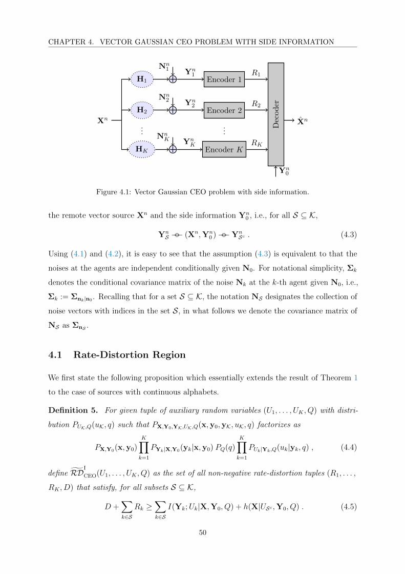
CHAPTER 4. VECTOR GAUSSIAN CEO PROBLEM WITH SIDE INFORMATION
Xn
H1
H2
HK
Nn1
Nn2
NnK
Encoder 1
Encoder 2
Encoder K
Yn1
Yn2
YnK
Decoder
R1
R2
RK
Yn0
Xn...
...
Figure 4.1: Vector Gaussian CEO problem with side information.
the remote vector source Xn and the side information Yn0 , i.e., for all S ⊆ K,
YnS −− (Xn,Yn
0 )−−YnSc . (4.3)
Using (4.1) and (4.2), it is easy to see that the assumption (4.3) is equivalent to that the
noises at the agents are independent conditionally given N0. For notational simplicity, Σk
denotes the conditional covariance matrix of the noise Nk at the k-th agent given N0, i.e.,
Σk := Σnk|n0 . Recalling that for a set S ⊆ K, the notation NS designates the collection of
noise vectors with indices in the set S, in what follows we denote the covariance matrix of
NS as ΣnS .
4.1 Rate-Distortion Region
We first state the following proposition which essentially extends the result of Theorem 1
to the case of sources with continuous alphabets.
Definition 5. For given tuple of auxiliary random variables (U1, . . . , UK , Q) with distri-
bution PUK,Q(uK, q) such that PX,Y0,YK,UK,Q(x,y0,yK, uK, q) factorizes as
PX,Y0(x,y0)K∏
k=1
PYk|X,Y0(yk|x,y0) PQ(q)K∏
k=1
PUk|Yk,Q(uk|yk, q) , (4.4)
define RDI
CEO(U1, . . . , UK , Q) as the set of all non-negative rate-distortion tuples (R1, . . . ,
RK , D) that satisfy, for all subsets S ⊆ K,
D +∑
k∈SRk ≥
∑
k∈SI(Yk;Uk|X,Y0, Q) + h(X|USc ,Y0, Q) . (4.5)
50
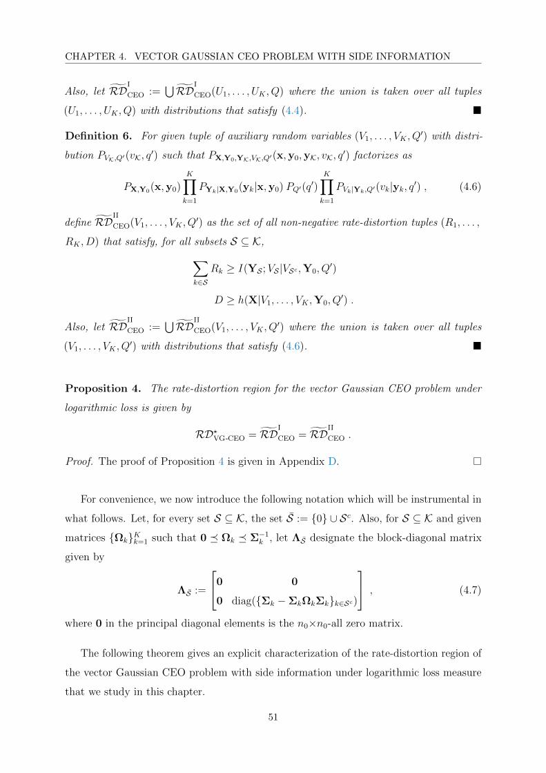
CHAPTER 4. VECTOR GAUSSIAN CEO PROBLEM WITH SIDE INFORMATION
Also, let RDI
CEO :=⋃ RDI
CEO(U1, . . . , UK , Q) where the union is taken over all tuples
(U1, . . . , UK , Q) with distributions that satisfy (4.4).
Definition 6. For given tuple of auxiliary random variables (V1, . . . , VK , Q′) with distri-
bution PVK,Q′(vK, q′) such that PX,Y0,YK,VK,Q′(x,y0,yK, vK, q′) factorizes as
PX,Y0(x,y0)K∏
k=1
PYk|X,Y0(yk|x,y0) PQ′(q′)K∏
k=1
PVk|Yk,Q′(vk|yk, q′) , (4.6)
define RDII
CEO(V1, . . . , VK , Q′) as the set of all non-negative rate-distortion tuples (R1, . . . ,
RK , D) that satisfy, for all subsets S ⊆ K,
∑
k∈SRk ≥ I(YS ;VS |VSc ,Y0, Q
′)
D ≥ h(X|V1, . . . , VK ,Y0, Q′) .
Also, let RDII
CEO :=⋃ RDII
CEO(V1, . . . , VK , Q′) where the union is taken over all tuples
(V1, . . . , VK , Q′) with distributions that satisfy (4.6).
Proposition 4. The rate-distortion region for the vector Gaussian CEO problem under
logarithmic loss is given by
RD?VG-CEO = RDI
CEO = RDII
CEO .
Proof. The proof of Proposition 4 is given in Appendix D.
For convenience, we now introduce the following notation which will be instrumental in
what follows. Let, for every set S ⊆ K, the set S := 0 ∪ Sc. Also, for S ⊆ K and given
matrices ΩkKk=1 such that 0 Ωk Σ−1k , let ΛS designate the block-diagonal matrix
given by
ΛS :=
0 0
0 diag(Σk −ΣkΩkΣkk∈Sc)
, (4.7)
where 0 in the principal diagonal elements is the n0×n0-all zero matrix.
The following theorem gives an explicit characterization of the rate-distortion region of
the vector Gaussian CEO problem with side information under logarithmic loss measure
that we study in this chapter.
51

CHAPTER 4. VECTOR GAUSSIAN CEO PROBLEM WITH SIDE INFORMATION
Theorem 4. The rate-distortion region RD?VG-CEO of the vector Gaussian CEO prob-
lem under logarithmic loss is given by the set of all non-negative rate-distortion tuples
(R1, . . . , RK , D) that satisfy, for all subsets S ⊆ K,
D +∑
k∈SRk ≥
∑
k∈Slog
1
|I−ΩkΣk|+ log
∣∣∣∣(πe)(Σ−1
x + H†SΣ−1nS
(I−ΛSΣ
−1nS
)HS
)−1∣∣∣∣ ,
for matrices ΩkKk=1 such that 0 Ωk Σ−1k , where S = 0 ∪ Sc and ΛS is as defined
by (4.7).
Proof. The proof of the direct part of Theorem 4 follows simply by evaluating the region
RDI
CEO as described by the inequalities (4.5) using Gaussian test channels and no time-
sharing. Specifically, we set Q = ∅ and p(uk|yk, q) = CN (yk,Σ1/2k (Ωk − I)Σ
1/2k ), k ∈ K.
The proof of the converse appears in Appendix E.
In the case in which the noises at the agents are independent among them and from
the noise N0 at the CEO, the result of Theorem 4 takes a simpler form which is stated in
the following corollary.
Corollary 1. Consider the vector Gaussian CEO problem described by (4.1) and (4.2) with
the noises (N1, . . . ,NK) being independent among them and with N0. Under logarithmic
loss, the rate-distortion region this model is given by the set of all non-negative tuples
(R1, . . . , RK , D) that satisfy, for all subsets S ⊆ K,
D +∑
k∈SRk ≥
∑
k∈Slog
1
|I−ΩkΣk|+ log
∣∣∣∣(πe)(Σ−1
x + H†0Σ−10 H0 +
∑
k∈ScH†kΩkHk
)−1
∣∣∣∣ ,
for some matrices ΩkKk=1 such that 0 Ωk Σ−1k .
Remark 6. The direct part of Theorem 4 shows that Gaussian test channels and no-time
sharing exhaust the region. For the converse proof of Theorem 4, we derive an outer
bound on the region RDI
CEO. In doing so, we use the de Bruijn identity, a connection
between differential entropy and Fisher information, along with the properties of MMSE
and Fisher information. By opposition to the case of quadratic distortion measure for
which the application of this technique was shown in [11] to result in an outer bound that
is generally non-tight, Theorem 4 shows that the approach is successful in the case of
logarithmic loss distortion measure as it yields a complete characterization of the region.
On this aspect, note that in the specific case of scalar Gaussian sources, an alternate
52
CHAPTER 4. VECTOR GAUSSIAN CEO PROBLEM WITH SIDE INFORMATION
converse proof may be obtained by extending that of the scalar Gaussian many-help-one
source coding problem by Oohama [3] and Prabhakaran et al. [4] through accounting for
additional side information at CEO and replacing the original mean square error distortion
constraint with conditional entropy. However, such approach does not seem conclusive in
the vector case, as the entropy power inequality is known to be generally non-tight in this
setting [12, 13].
Remark 7. The result of Theorem 4 generalizes that of [59] which considers the case of
only one agent, i.e., the remote vector Gaussian Wyner-Ziv model under logarithmic loss,
to the case of an arbitrarily number of agents. The converse proof of [59], which relies
on the technique of orthogonal transform to reduce the vector setting to one of parallel
scalar Gaussian settings, seems insufficient to diagonalize all the noise covariance matrices
simultaneously in the case of more than one agent. The result of Theorem 4 is also
connected to recent developments on characterizing the capacity of multiple-input multiple-
output (MIMO) relay channels in which the relay nodes are connected to the receiver
through error-free finite-capacity links (i.e., the so-called cloud radio access networks). In
particular, the reader may refer to [103, Theorem 4] where important progress is done,
and [62] where compress-and-forward with joint decompression-decoding is shown to be
optimal under the constraint of oblivious relay processing.
4.2 Gaussian Test Channels with Time-Sharing Exhaust the
Berger-Tung Region
Proposition 4 shows that the union of all rate-distortion tuples that satisfy (4.5) for all
subsets S ⊆ K coincides with the Berger-Tung inner bound in which time-sharing is used.
The direct part of Theorem 4 is obtained by evaluating (4.5) using Gaussian test channels
and no time-sharing, i.e., Q = ∅, not the Berger-Tung inner bound. The reader may
wonder: i) whether Gaussian test channels also exhaust the Berger-Tung inner bound for
the vector Gaussian CEO problem that we study here, and ii) whether time-sharing is
needed with the Berger-Tung scheme. In this section, we answer both questions in the
affirmative. In particular, we show that the Berger-Tung coding scheme with Gaussian
test channels and time-sharing achieves distortion levels that are not larger than any other
coding scheme. That is, Gaussian test channels with time-sharing exhaust the region
53
CHAPTER 4. VECTOR GAUSSIAN CEO PROBLEM WITH SIDE INFORMATION
RDII
CEO as defined in Definition 6.
Proposition 5. The rate-distortion region for the vector Gaussian CEO problem under
logarithmic loss is given by
RD?VG-CEO =⋃RDII
CEO(V G1 , . . . , V
GK , Q
′) ,
where RDII
CEO(·) is as given in Definition 6 and the superscript G is used to denote that
the union is taken over Gaussian distributed V Gk ∼ p(vk|yk, q′) conditionally on (Yk, Q
′).
Proof. For the proof of Proposition 5, it is sufficient to show that, for fixed Gaussian
conditional distributions p(uk|yk)Kk=1, the extreme points of the polytopes defined by (4.5)
are dominated by points that are in RDII
CEO and which are achievable using Gaussian
conditional distributions p(vk|yk, q′)Kk=1. Hereafter, we give a brief outline of proof for
the case K = 2. The reasoning for K ≥ 2 is similar and is provided in Appendix F.
Consider the inequalities (4.5) with Q = ∅ and (U1, U2) := (UG1 , U
G2 ) chosen to be Gaussian
(see Theorem 4). Consider now the extreme points of the polytopes defined by the obtained
inequalities:
P1 = (0, 0, I(Y1;UG1 |X,Y0) + I(Y2;UG
2 |X,Y0) + h(X|Y0))
P2 = (I(Y1;UG1 |Y0), 0, I(UG
2 ; Y2|X,Y0) + h(X|UG1 ,Y0))
P3 = (0, I(Y2;UG2 |Y0), I(UG
1 ; Y1|X,Y0) + h(X|UG2 ,Y0))
P4 = (I(Y1;UG1 |Y0), I(Y2;UG
2 |UG1 ,Y0), h(X|UG
1 , UG2 ,Y0))
P5 = (I(Y1;UG1 |UG
2 ,Y0), I(Y2;UG2 |Y0), h(X|UG
1 , UG2 ,Y0)) ,
where the point Pj is a a triple (R(j)1 , R
(j)2 , D(j)). It is easy to see that each of these
points is dominated by a point in RDII
CEO, i.e., there exists (R1, R2, D) ∈ RDII
CEO for
which R1 ≤ R(j)1 , R2 ≤ R
(j)2 and D ≤ D(j). To see this, first note that P4 and P5
are both in RDII
CEO. Next, observe that the point (0, 0, h(X|Y0)) is in RDII
CEO, which
is clearly achievable by letting (V1, V2, Q′) = (∅, ∅, ∅), dominates P1. Also, by using
letting (V1, V2, Q′) = (UG
1 , ∅, ∅), we have that the point (I(Y1;U1|Y0), 0, h(X|U1,Y0)) is
in RDII
CEO, and dominates the point P2. A similar argument shows that P3 is dominated
by a point in RDII
CEO. The proof is terminated by observing that, for all above corner
points, Vk is set either equal UGk (which is Gaussian distributed conditionally on Yk) or a
constant.
54
CHAPTER 4. VECTOR GAUSSIAN CEO PROBLEM WITH SIDE INFORMATION
Remark 8. Proposition 5 shows that for the vector Gaussian CEO problem with side
information under a logarithmic loss constraint, vector Gaussian quantization codebooks
with time-sharing are optimal. In the case of quadratic distortion constraint, however, a
characterization of the rate-distortion region is still to be found in general, and it is not
known yet whether vector Gaussian quantization codebooks (with or without time-sharing)
are optimal, except in few special cases such as that of scalar Gaussian sources or the
case of only one agent, i.e., the remote vector Gaussian Wyner-Ziv problem whose rate-
distortion region is found in [59]. In [59], Tian and Chen also found the rate-distortion
region of the remote vector Gaussian Wyner-Ziv problem under logarithmic loss, which they
showed achievable using Gaussian quantization codebooks that are different from those (also
Gaussian) that are optimal in the case of quadratic distortion. As we already mentioned,
our result of Theorem 4 generalizes that of [59] to the case of an arbitrary number of
agents.
Remark 9. One may wonder whether giving the decoder side information Y0 to the
encoders is beneficial. Similar to the well known result in Wyner-Ziv source coding of
scalar Gaussian sources, our result of Theorem 4 shows that encoder side information does
not help.
4.3 Quadratic Vector Gaussian CEO Problem with Determinant
Constraint
We now turn to the case in which the distortion is measured under quadratic loss. In this
case, the mean square error matrix is defined by
D(n) :=1
n
n∑
i=1
E[(Xi − Xi)(Xi − Xi)†] . (4.8)
Under a (general) error constraint of the form
D(n) D , (4.9)
where D designates here a prescribed positive definite error matrix, a complete solution is
still to be found in general. In what follows, we replace the constraint (4.9) with one on
the determinant of the error matrix D(n), i.e.,
|D(n)| ≤ D , (4.10)
55
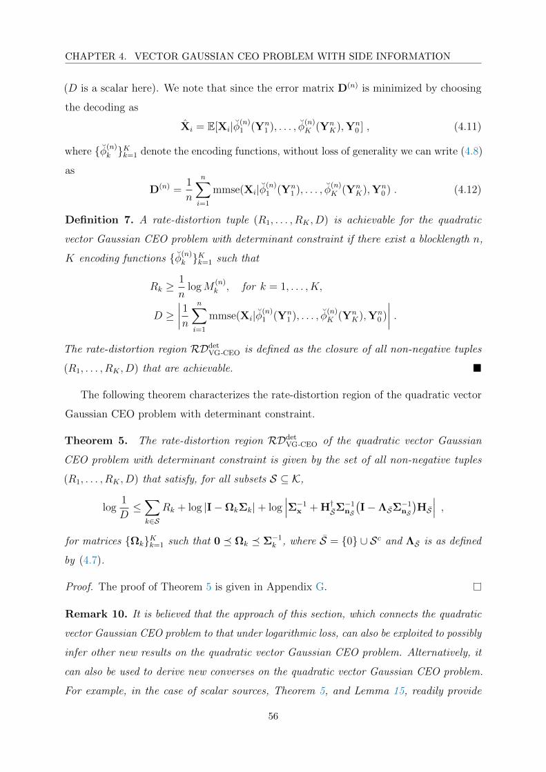
CHAPTER 4. VECTOR GAUSSIAN CEO PROBLEM WITH SIDE INFORMATION
(D is a scalar here). We note that since the error matrix D(n) is minimized by choosing
the decoding as
Xi = E[Xi|φ(n)1 (Yn
1 ), . . . , φ(n)K (Yn
K),Yn0 ] , (4.11)
where φ(n)k Kk=1 denote the encoding functions, without loss of generality we can write (4.8)
as
D(n) =1
n
n∑
i=1
mmse(Xi|φ(n)1 (Yn
1 ), . . . , φ(n)K (Yn
K),Yn0 ) . (4.12)
Definition 7. A rate-distortion tuple (R1, . . . , RK , D) is achievable for the quadratic
vector Gaussian CEO problem with determinant constraint if there exist a blocklength n,
K encoding functions φ(n)k Kk=1 such that
Rk ≥1
nlogM
(n)k , for k = 1, . . . , K,
D ≥∣∣∣∣1
n
n∑
i=1
mmse(Xi|φ(n)1 (Yn
1 ), . . . , φ(n)K (Yn
K),Yn0 )
∣∣∣∣ .
The rate-distortion region RDdetVG-CEO is defined as the closure of all non-negative tuples
(R1, . . . , RK , D) that are achievable.
The following theorem characterizes the rate-distortion region of the quadratic vector
Gaussian CEO problem with determinant constraint.
Theorem 5. The rate-distortion region RDdetVG-CEO of the quadratic vector Gaussian
CEO problem with determinant constraint is given by the set of all non-negative tuples
(R1, . . . , RK , D) that satisfy, for all subsets S ⊆ K,
log1
D≤∑
k∈SRk + log |I−ΩkΣk|+ log
∣∣∣Σ−1x + H†SΣ
−1nS
(I−ΛSΣ
−1nS
)HS
∣∣∣ ,
for matrices ΩkKk=1 such that 0 Ωk Σ−1k , where S = 0 ∪ Sc and ΛS is as defined
by (4.7).
Proof. The proof of Theorem 5 is given in Appendix G.
Remark 10. It is believed that the approach of this section, which connects the quadratic
vector Gaussian CEO problem to that under logarithmic loss, can also be exploited to possibly
infer other new results on the quadratic vector Gaussian CEO problem. Alternatively, it
can also be used to derive new converses on the quadratic vector Gaussian CEO problem.
For example, in the case of scalar sources, Theorem 5, and Lemma 15, readily provide
56

CHAPTER 4. VECTOR GAUSSIAN CEO PROBLEM WITH SIDE INFORMATION
an alternate converse proof to those of [3, 4] for this model. Similar connections were
made in [104, 105] where it was observed that the results of [10] can be used to recover
known results on the scalar Gaussian CEO problem (such as the sum rate-distortion region
of [106]) and the scalar Gaussian two-encoder distributed source coding problem. We
also point out that similar information constraints have been applied to log-determinant
reproduction constraints previously in [107].
Two-Encoder Rate Region K-Encoder Rate Region
Cooperative bound [trivial] Oohama ’98 [108], Prabhakaran et al. ’04 [4]
scalar
Wagner et al. ’08 [106] Tavildar et al. ’10 [109]
scalar, sum-rate scalar, tree-structure constraint
Rahman and Wagner ’15 [110] Ekrem and Ulukus ’14 [11]
vector vector, outer bound
Ugur et al. ’19
vector, determinant constraint
Table 4.1: Advances in the resolution of the rate region of the quadratic Gaussian CEO problem.
We close this section by presenting Table 4.1, where advances in the resolution of the
rate region of the quadratic Gaussian CEO problem is summarized.
4.4 Hypothesis Testing Against Conditional Independence
In this section we study the continuous case of the hypothesis testing problem presented in
Chapter 3.4. Here, (X,Y0,Y1, . . . ,YK) is a zero-mean Gaussian random vector such that
Y0 = H0X + N0 , (4.13)
where H0 ∈ Cn0×nx , X ∈ Cnx and N0 ∈ Cn0 are independent Gaussian vectors with zero-
mean and covariance matrices Σx 0 and Σ0 0, respectively. The vectors (Y1, . . . ,YK)
and X are correlated under the null hypothesis H0 and are independent under the alternate
hypothesis H1, with
H0 : Yk = HkX + Nk, for all k ∈ K (4.14a)
H1 : (Y1, . . . ,YK) independent from X conditionally given Y0 . (4.14b)
57
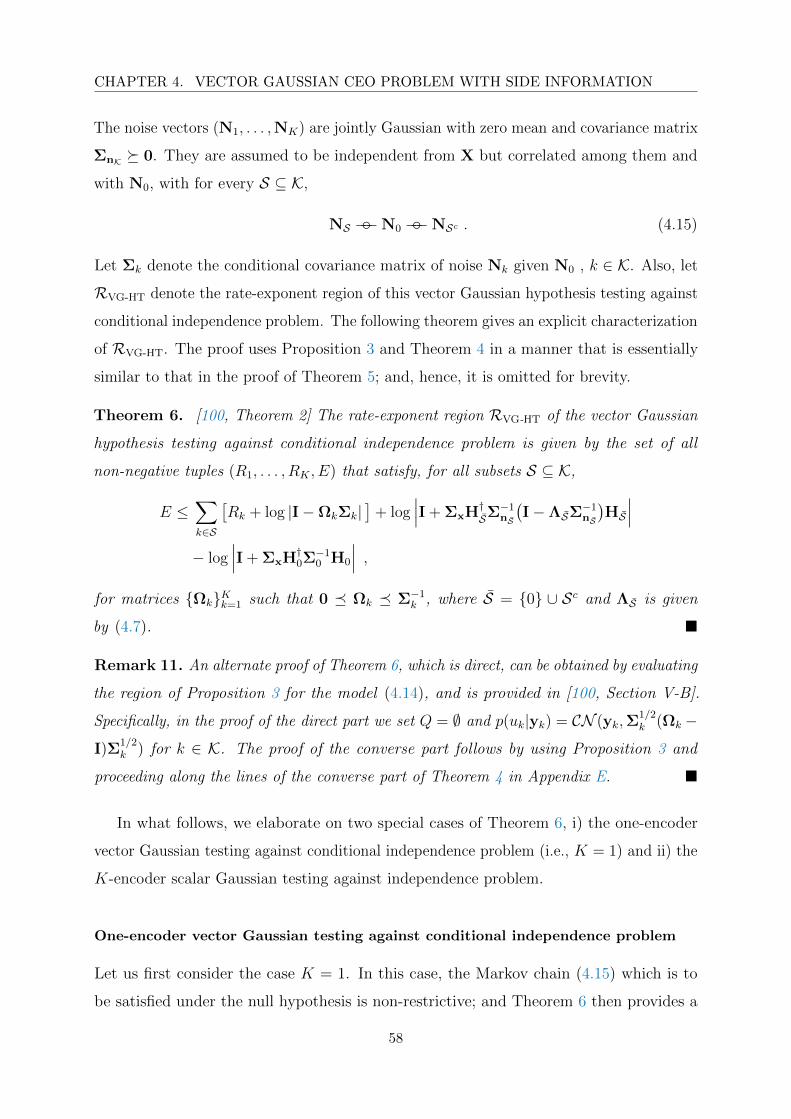
CHAPTER 4. VECTOR GAUSSIAN CEO PROBLEM WITH SIDE INFORMATION
The noise vectors (N1, . . . ,NK) are jointly Gaussian with zero mean and covariance matrix
ΣnK 0. They are assumed to be independent from X but correlated among them and
with N0, with for every S ⊆ K,
NS −−N0 −−NSc . (4.15)
Let Σk denote the conditional covariance matrix of noise Nk given N0 , k ∈ K. Also, let
RVG-HT denote the rate-exponent region of this vector Gaussian hypothesis testing against
conditional independence problem. The following theorem gives an explicit characterization
of RVG-HT. The proof uses Proposition 3 and Theorem 4 in a manner that is essentially
similar to that in the proof of Theorem 5; and, hence, it is omitted for brevity.
Theorem 6. [100, Theorem 2] The rate-exponent region RVG-HT of the vector Gaussian
hypothesis testing against conditional independence problem is given by the set of all
non-negative tuples (R1, . . . , RK , E) that satisfy, for all subsets S ⊆ K,
E ≤∑
k∈S
[Rk + log |I−ΩkΣk|
]+ log
∣∣∣I + ΣxH†SΣ−1nS
(I−ΛSΣ
−1nS
)HS
∣∣∣
− log∣∣∣I + ΣxH†0Σ
−10 H0
∣∣∣ ,
for matrices ΩkKk=1 such that 0 Ωk Σ−1k , where S = 0 ∪ Sc and ΛS is given
by (4.7).
Remark 11. An alternate proof of Theorem 6, which is direct, can be obtained by evaluating
the region of Proposition 3 for the model (4.14), and is provided in [100, Section V-B].
Specifically, in the proof of the direct part we set Q = ∅ and p(uk|yk) = CN (yk,Σ1/2k (Ωk −
I)Σ1/2k ) for k ∈ K. The proof of the converse part follows by using Proposition 3 and
proceeding along the lines of the converse part of Theorem 4 in Appendix E.
In what follows, we elaborate on two special cases of Theorem 6, i) the one-encoder
vector Gaussian testing against conditional independence problem (i.e., K = 1) and ii) the
K-encoder scalar Gaussian testing against independence problem.
One-encoder vector Gaussian testing against conditional independence problem
Let us first consider the case K = 1. In this case, the Markov chain (4.15) which is to
be satisfied under the null hypothesis is non-restrictive; and Theorem 6 then provides a
58

CHAPTER 4. VECTOR GAUSSIAN CEO PROBLEM WITH SIDE INFORMATION
complete solution of the (general) one-encoder vector Gaussian testing against conditional
independence problem. More precisely, in this case the optimal trade-off between rate and
Type II error exponent is given by the set of pairs (R1, E) that satisfy
E ≤ R1 + log |I−Ω1Σ1|
E ≤ log∣∣∣I + ΣxH†0,1Σ
−1n0,1
(I−Λ0,1Σ
−1n0,1
)H0,1
∣∣∣− log∣∣∣I + ΣxH†0Σ
−10 H0
∣∣∣ ,(4.16)
for some n1×n1 matrix Ω1 such that 0 Ω1 Σ−11 , where H0,1 = [H†0,H
†1]†, Σn0,1 is
the covariance matrix of noise (N0,N1) and
Λ0,1 :=
0 0
0 Σ1 −Σ1Ω1Σ1
, (4.17)
with the 0 in its principal diagonal denoting the n0×n0-all zero matrix. In particular, for
the setting of testing against independence, i.e., Y0 = ∅ and the decoder’s task reduced
to guessing whether Y1 and X are independent or not, the optimal trade-off expressed
by (4.16) reduces to the set of (R1, E) pairs that satisfy, for some n1×n1 matrix Ω1 such
that 0 Ω1 Σ−11 ,
E ≤ minR1 + log |I−Ω1Σ1| , log
∣∣∣I + ΣxH†1Ω1H1
∣∣∣. (4.18)
Observe that (4.16) is the counter-part, to the vector Gaussian setting, of the result of [16,
Theorem 3] which provides a single-letter formula for the Type II error exponent for the
one-encoder DM testing against conditional independence problem. Similarly, (4.18) is the
solution of the vector Gaussian version of the one-encoder DM testing against independence
problem which is studied, and solved, by Ahlswede and Csiszar in [65, Theorem 2]. Also,
we mention that, perhaps non-intuitive, in the one-encoder vector Gaussian testing against
independence problem swapping the roles of Y1 and X (i.e., giving X to the encoder and
the noisy (under the null hypothesis) Y1 to the decoder) does not result in an increase of
the Type II error exponent which is then identical to (4.18). Note that this is in sharp
contrast with the related1 setting of standard lossy source reproduction, i.e., the decoder
aiming to reproduce the source observed at the encoder to within some average squared
error distortion level using the sent compression message and its own side information,
1The connection, which is sometimes misleading, consists in viewing the decoder in the hypothesis testing
against independence problem considered here as one that computes a binary-valued function of (X,Y1).
59

CHAPTER 4. VECTOR GAUSSIAN CEO PROBLEM WITH SIDE INFORMATION
for which it is easy to see that, for given R1 bits per sample, smaller distortion levels
are allowed by having the encoder observe X and the decoder observe Y1, instead of the
encoder observing the noisy Y1 = H1X + N1 and the decoder observing X.
K-encoder scalar Gaussian testing against independence problem
Consider now the special case of the setup of Theorem 6 in which K ≥ 2, Y0 = ∅, and the
sources and noises are all scalar complex-valued, i.e., nx = 1 and nk = 1 for all k ∈ K. The
vector (Y1, . . . , YK) and X are correlated under the null hypothesis H0 and independent
under the alternate hypothesis H1, with
H0 : Yk = X +Nk, for all k ∈ K (4.19a)
H1 : (Y1, . . . , YK) independent from X . (4.19b)
The noises N1, . . . , NK are zero-mean jointly Gaussian, mutually independent and inde-
pendent from X. Also, we assume that the variances σ2k of noise Nk, k ∈ K, and σ2
x of X
are all positive. In this case, it can be easily shown that Theorem 6 reduces to
RSG-HT =
(R1, . . . , RK , E) : ∃ (γ1, . . . , γK) ∈ RK
+ s.t.
γk ≤1
σ2k
, ∀ k ∈ K
∑
k∈SRk ≥ E − log
((1 + σ2
x
∑
k∈Scγk)∏
k∈S[1− γkσ2
k]), ∀ S ⊆ K
.
(4.20)
The region RSG-HT as given by (4.20) can be used to, e.g., characterize the centralized
rate region, i.e., the set of rate vectors (R1, . . . , RK) that achieve the centralized Type II
error exponent
I(Y1, . . . , YK ;X) =K∑
k=1
logσ2x
σ2k
. (4.21)
We close this section by mentioning that, implicit in Theorem 6, the Quantize-Bin-
Test scheme of [16, Theorem 1] with Gaussian test channels and time-sharing is optimal
for the vector Gaussian K-encoder hypothesis testing against conditional independence
problem (4.14). Furthermore, we note that Rahman and Wagner also characterized
60

CHAPTER 4. VECTOR GAUSSIAN CEO PROBLEM WITH SIDE INFORMATION
the optimal rate-exponent region of a different2 Gaussian hypothesis testing against
independence problem, called the Gaussian many-help-one hypothesis testing against
independence problem therein, in the case of scalar valued sources [16, Theorem 7].
Specialized to the case K = 1, the result of Theorem 6 recovers that of [16, Theorem
7] in the case of no helpers; and extends it to vector-valued sources and testing against
conditional independence in that case.
4.5 Distributed Vector Gaussian Information Bottleneck
Consider now the vector Gaussian CEO problem with side information, and let the
logarithmic loss distortion constraint be replaced by the mutual information constraint
I(Xn;ψ(n)
(φ
(n)1 (Y n
1 ), . . . , φ(n)K (Y n
K), Y n0
))≥ n∆ . (4.22)
In this case, the region of optimal tuples (R1, . . . , RK ,∆) generalizes the Gaussian Infor-
mation Bottleneck Function of [21,22] as given by (4.24) to the setting in which the decoder
observes correlated side information Y0 and the inference is done in a distributed manner
by K learners. This region can be obtained readily from Theorem 4 by substituting therein
∆ := h(X) − D. The following corollary states the result, which was first established
in [1, 111].
Corollary 2. [111, Theorem 2] For the problem of distributed Gaussian Information
Bottleneck with side information at the predictor, the complexity-relevance region is given
by the union of all non-negative tuples (R1, . . . , RK ,∆) that satisfy, for every S ⊆ K,
∆ ≤∑
k∈S
[Rk + log |I−ΩkΣk|
]+ log
∣∣I + ΣxH†SΣ−1nS
(I−ΛSΣ
−1nS
)HS∣∣ ,
for matrices ΩkKk=1 such that 0 Ωk Σ−1k , where S = 0 ∪ Sc and ΛS is given
by (4.7).
In particular, if K = 1 and Y0 = ∅, with the substitutions Y := Y1, R := R1, H := H1,
Σ := Σ1, and Ω1 := Ω, the rate-distortion region of Theorem 4 reduces to the set of
2This problem is related to the Gaussian many-help-one problem [3,4, 106]. Here, different from the setup of
Figure 3.4, the source X is observed directly by a main encoder who communicates with a detector that observes
Y in the aim of making a decision on whether X and Y are independent or not. Also, there are helpers that
observe independent noisy versions of X and communicate with the detector in the aim of facilitating that test.
61
CHAPTER 4. VECTOR GAUSSIAN CEO PROBLEM WITH SIDE INFORMATION
rate-distortion pairs (R,D) that satisfy
D ≥ log∣∣(πe)
(Σ−1
x + H†ΩH)−1∣∣ (4.23a)
R +D ≥ log1
|I−ΩΣ| + log∣∣(πe)Σx
∣∣ , (4.23b)
for some matrix Ω such that 0 Ω Σ−1. Alternatively, by making the substitution
∆ := h(X)−D, the trade-off expressed by (4.23) can be written equivalently as
∆ ≤ log∣∣I + ΣxH†ΩH
∣∣ (4.24a)
∆ ≤ R + log∣∣I−ΩΣ
∣∣ , (4.24b)
for some matrix Ω such that 0 Ω Σ−1.
Expression (4.24) is known as the Gaussian Information Bottleneck Function [21, 22],
which is the solution of the Information Bottleneck method of [17] in the case of jointly
Gaussian variables. More precisely, using the terminology of [17], the inequalities (4.24)
describe the optimal trade-off between the complexity (or rate) R and the relevance (or
accuracy) ∆. The concept of Information Bottleneck was found useful in various learning
applications, such as for data clustering [112], feature selection [113] and others.
Furthermore, if in (4.1) and (4.2) the noises are independent among them and from N0,
the relevance-complexity region of Corollary 2 reduces to the union of all non-negative
tuples (R1, . . . , RK ,∆) that satisfy, for every S ⊆ K,
∆ ≤∑
k∈S
[Rk + log |I−ΩkΣk|
]+ log
∣∣I + Σx
(H†0Σ
−10 H0 +
∑
k∈ScH†kΩkHk
)∣∣ , (4.25)
for some matrices ΩkKk=1 such that 0 Ωk Σ−1k .
Example 1 (Distributed Scalar Gaussian Information Bottleneck). Consider a scalar
instance of the distributed Gaussian Information Bottleneck – that we study in this section
– depicted in Figure 4.2a where there are two agents and no side information, i.e., K = 2,
Y0 = ∅, nx = 1 and n1 = n2 = 1. The relevance-complexity region of this model is
given by (4.25) (wherein with the substitution H0 = 0). In particular, each encoder
observation Yk is the output of a Gaussian channel with SNR ρk, i.e., Yk =√ρkX +Nk,
where X ∼ N (0, 1), Nk ∼ N (0, 1), k = 1, 2. Furthermore, the model we consider
62

CHAPTER 4. VECTOR GAUSSIAN CEO PROBLEM WITH SIDE INFORMATION
here is symmetric, i.e., ρ1 = ρ2 = ρ and R1 = R2 = R. For this model, the optimal
relevance-complexity pairs (∆?, R) can be computed from
∆?(R, ρ) =1
2log(
1 + 2ρ exp(−4R)[exp(4R) + ρ−
√ρ2 + (1 + ρ) exp(4R)
]). (4.26)
X
h1
h2
N1
N2
Encoder 1
Encoder 2
Y1
Y2 Decoder
R
R
X
Yk =√ρX +Nk
X ∼ N (0, 1), Nk ∼ N (0, 1), k = 1, 2
(a) System model
0 0.5 1 1.5 2 2.5 3 3.5 4 4.5 50
0.2
0.4
0.6
0.8
1
1.2
1.4
1.6
R
∆
C-IB with R→∞C-IB (collaborative encoding)
D-IB (distributed encoding, Theorem 4)Independent point-to-point encoding
(b) Relevance vs. complexity trade-off.
Figure 4.2: Distributed Scalar Gaussian Information Bottleneck.
The Centralized IB (C-IB) upper bound is given by the pairs (∆cIB, R) achievable if (Y1, Y2)
are encoded jointly at a single encoder with complexity 2R, and given by
∆cIB(R, ρ) =1
2log (1 + 2ρ)− 1
2log (1 + 2ρ exp(−4R)) , (4.27)
which is an instance of the scalar Gaussian IB problem in [22].
The lower bound is given by the pairs (∆ind, R) achievable if (Y1, Y2) are encoded indepen-
dently at separate encoders, and given by
∆ind(R, ρ) =1
2log (1 + 2ρ− ρ exp(−2R))− 1
2log (1 + ρ exp(−2R)) . (4.28)
Figure 4.2b shows the optimal relevance-complexity region of tuples (∆?, R) obtained
from (4.26), as well as, the C-IB upper bounds ∆cIB(R, ρ) and ∆cIB(∞, ρ), and the lower
bound ∆ind(R, ρ) for the case in which the channel SNR is 10 dB, i.e., ρ = 10.
63

64
Chapter 5
Algorithms
This chapter contains a description of two algorithms and architectures that were developed
in [1] for the distributed learning scenario. We state them here for reasons of completeness.
In particular, the chapter provides: i) Blahut-Arimoto type iterative algorithms that allow
to compute numerically the rate-distortion or relevance-complexity regions of the DM and
vector Gaussian CEO problems for the case in which the joint distribution of the data is
known perfectly or can be estimated with a high accuracy; and ii) a variational inference
type algorithm in which the encoding mappings are parameterized by neural networks and
the bound approximated by Monte Carlo sampling and optimized with stochastic gradient
descent for the case in which there is only a set of training data is available.
5.1 Blahut-Arimoto Type Algorithms for Known Models
5.1.1 Discrete Case
Here we develop a BA-type algorithm that allows to compute the convex region RD?CEO
for general discrete memoryless sources. To develop the algorithm, we use the Berger-Tung
form of the region given in Proposition 11 for K = 2. The outline of the proposed method
is as follows. First, we rewrite the rate-distortion region RD?CEO in terms of the union of
two simpler regions in Proposition 6. The tuples lying on the boundary of each region are
parametrically given in Proposition 7. Then, the boundary points of each simpler region
are computed numerically via an alternating minimization method derived and detailed in
Algorithm 2. Finally, the original rate-distortion region is obtained as the convex hull of
the union of the tuples obtained for the two simple regions.
65
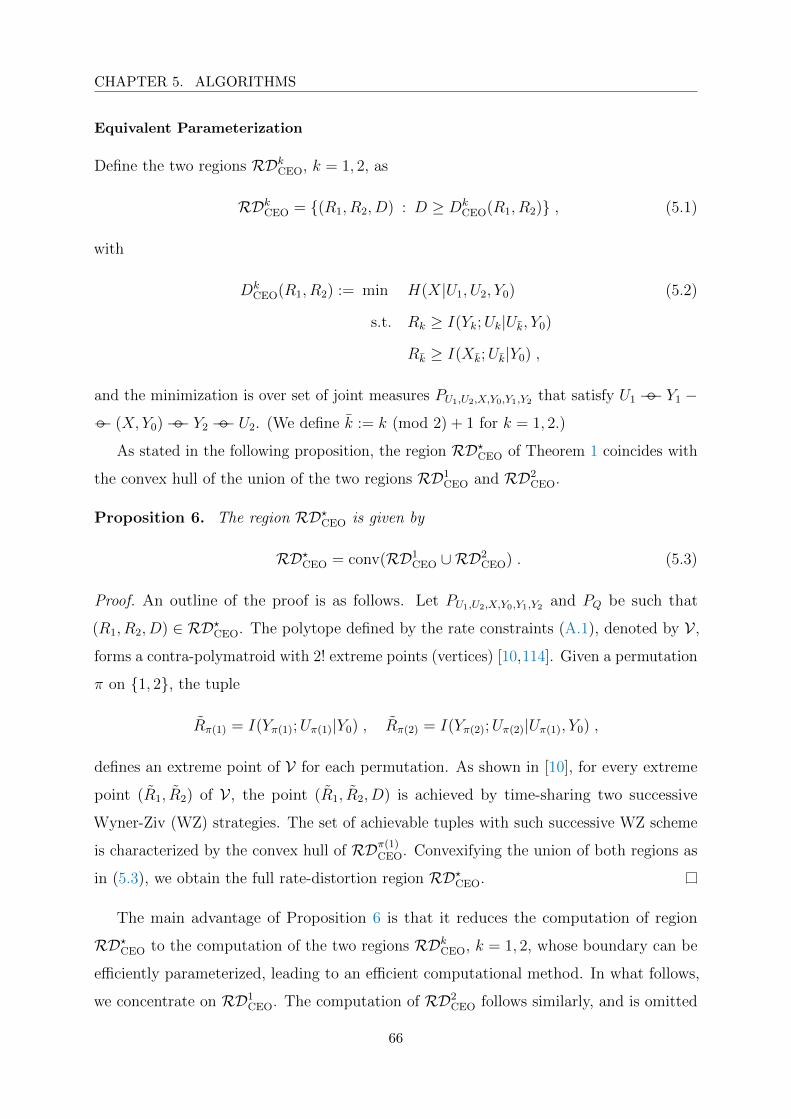
CHAPTER 5. ALGORITHMS
Equivalent Parameterization
Define the two regions RDkCEO, k = 1, 2, as
RDkCEO = (R1, R2, D) : D ≥ DkCEO(R1, R2) , (5.1)
with
DkCEO(R1, R2) := min H(X|U1, U2, Y0) (5.2)
s.t. Rk ≥ I(Yk;Uk|Uk, Y0)
Rk ≥ I(Xk;Uk|Y0) ,
and the minimization is over set of joint measures PU1,U2,X,Y0,Y1,Y2 that satisfy U1 −− Y1 −− (X, Y0)−− Y2 −− U2. (We define k := k (mod 2) + 1 for k = 1, 2.)
As stated in the following proposition, the region RD?CEO of Theorem 1 coincides with
the convex hull of the union of the two regions RD1CEO and RD2
CEO.
Proposition 6. The region RD?CEO is given by
RD?CEO = conv(RD1CEO ∪RD2
CEO) . (5.3)
Proof. An outline of the proof is as follows. Let PU1,U2,X,Y0,Y1,Y2 and PQ be such that
(R1, R2, D) ∈ RD?CEO. The polytope defined by the rate constraints (A.1), denoted by V ,
forms a contra-polymatroid with 2! extreme points (vertices) [10,114]. Given a permutation
π on 1, 2, the tuple
Rπ(1) = I(Yπ(1);Uπ(1)|Y0) , Rπ(2) = I(Yπ(2);Uπ(2)|Uπ(1), Y0) ,
defines an extreme point of V for each permutation. As shown in [10], for every extreme
point (R1, R2) of V, the point (R1, R2, D) is achieved by time-sharing two successive
Wyner-Ziv (WZ) strategies. The set of achievable tuples with such successive WZ scheme
is characterized by the convex hull of RDπ(1)CEO. Convexifying the union of both regions as
in (5.3), we obtain the full rate-distortion region RD?CEO.
The main advantage of Proposition 6 is that it reduces the computation of region
RD?CEO to the computation of the two regions RDkCEO, k = 1, 2, whose boundary can be
efficiently parameterized, leading to an efficient computational method. In what follows,
we concentrate on RD1CEO. The computation of RD2
CEO follows similarly, and is omitted
66
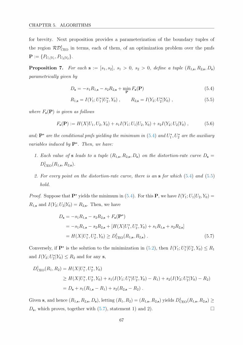
CHAPTER 5. ALGORITHMS
for brevity. Next proposition provides a parameterization of the boundary tuples of
the region RD1CEO in terms, each of them, of an optimization problem over the pmfs
P := PU1|Y1 , PU2|Y2.
Proposition 7. For each s := [s1, s2], s1 > 0, s2 > 0, define a tuple (R1,s, R2,s, Ds)
parametrically given by
Ds = −s1R1,s − s2R2,s + minPFs(P) (5.4)
R1,s = I(Y1;U?1 |U?
2 , Y0) , R2,s = I(Y2;U?2 |Y0) , (5.5)
where Fs(P) is given as follows
Fs(P) := H(X|U1, U2, Y0) + s1I(Y1;U1|U2, Y0) + s2I(Y2;U2|Y0) , (5.6)
and; P? are the conditional pmfs yielding the minimum in (5.4) and U?1 , U
?2 are the auxiliary
variables induced by P?. Then, we have:
1. Each value of s leads to a tuple (R1,s, R2,s, Ds) on the distortion-rate curve Ds =
D1CEO(R1,s, R2,s).
2. For every point on the distortion-rate curve, there is an s for which (5.4) and (5.5)
hold.
Proof. Suppose that P? yields the minimum in (5.4). For this P, we have I(Y1;U1|U2, Y0) =
R1,s and I(Y2;U2|Y0) = R2,s. Then, we have
Ds = −s1R1,s − s2R2,s + Fs(P?)
= −s1R1,s − s2R2,s + [H(X|U?1 , U
?2 , Y0) + s1R1,s + s2R2,s]
= H(X|U?1 , U
?2 , Y0) ≥ D1
CEO(R1,s, R2,s) . (5.7)
Conversely, if P? is the solution to the minimization in (5.2), then I(Y1;U?1 |U?
2 , Y0) ≤ R1
and I(Y2;U?2 |Y0) ≤ R2 and for any s,
D1CEO(R1, R2) = H(X|U?
1 , U?2 , Y0)
≥ H(X|U?1 , U
?2 , Y0) + s1(I(Y1;U?
1 |U?2 , Y0)−R1) + s2(I(Y2;U?
2 |Y0)−R2)
= Ds + s1(R1,s −R1) + s2(R2,s −R2) .
Given s, and hence (R1,s, R2,s, Ds), letting (R1, R2) = (R1,s, R2,s) yields D1CEO(R1,s, R2,s) ≥
Ds, which proves, together with (5.7), statement 1) and 2).
67
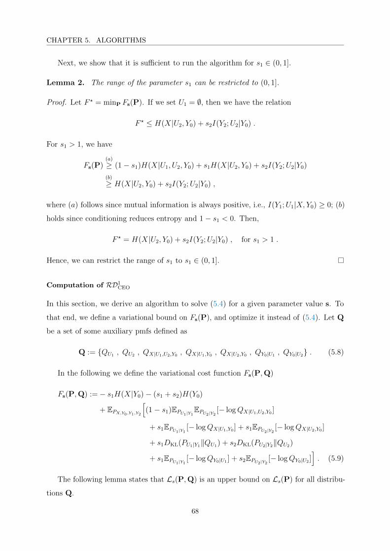
CHAPTER 5. ALGORITHMS
Next, we show that it is sufficient to run the algorithm for s1 ∈ (0, 1].
Lemma 2. The range of the parameter s1 can be restricted to (0, 1].
Proof. Let F ? = minP Fs(P). If we set U1 = ∅, then we have the relation
F ? ≤ H(X|U2, Y0) + s2I(Y2;U2|Y0) .
For s1 > 1, we have
Fs(P)(a)
≥ (1− s1)H(X|U1, U2, Y0) + s1H(X|U2, Y0) + s2I(Y2;U2|Y0)
(b)
≥ H(X|U2, Y0) + s2I(Y2;U2|Y0) ,
where (a) follows since mutual information is always positive, i.e., I(Y1;U1|X, Y0) ≥ 0; (b)
holds since conditioning reduces entropy and 1− s1 < 0. Then,
F ? = H(X|U2, Y0) + s2I(Y2;U2|Y0) , for s1 > 1 .
Hence, we can restrict the range of s1 to s1 ∈ (0, 1].
Computation of RD1CEO
In this section, we derive an algorithm to solve (5.4) for a given parameter value s. To
that end, we define a variational bound on Fs(P), and optimize it instead of (5.4). Let Q
be a set of some auxiliary pmfs defined as
Q := QU1 , QU2 , QX|U1,U2,Y0 , QX|U1,Y0 , QX|U2,Y0 , QY0|U1 , QY0|U2 . (5.8)
In the following we define the variational cost function Fs(P,Q)
Fs(P,Q) :=− s1H(X|Y0)− (s1 + s2)H(Y0)
+ EPX,Y0,Y1,Y2
[(1− s1)EPU1|Y1
EPU2|Y2[− logQX|U1,U2,Y0 ]
+ s1EPU1|Y1[− logQX|U1,Y0 ] + s1EPU2|Y2
[− logQX|U2,Y0 ]
+ s1DKL(PU1|Y1‖QU1) + s2DKL(PU2|Y2‖QU2)
+ s1EPU1|Y1[− logQY0|U1 ] + s2EPU2|Y2
[− logQY0|U2 ]]. (5.9)
The following lemma states that Ls(P,Q) is an upper bound on Ls(P) for all distribu-
tions Q.
68
CHAPTER 5. ALGORITHMS
Lemma 3. For fixed P, we have
Ls(P,Q) ≥ Ls(P) , for all Q .
In addition, there exists a Q that achieves the minimum minQ Fs(P,Q) = Fs(P), given by
QUk = PUk , QX|Uk,Y0 = PX|Uk,Y0 , QY0|Uk = PY0|Uk , for k = 1, 2 ,
QX|U1,U2,Y0 = PX|U1,U2,Y0 .(5.10)
Proof. The proof of Lemma 3 is given in Appendix H.1.
Using the lemma above, the minimization in (5.4) can be written in terms of the
variational cost function as follows
minPFs(P) = min
Pmin
QFs(P,Q) . (5.11)
Motivated by the BA algorithm [19,20], we propose an alternate optimization procedure
over the set of pmfs P and Q as stated in Algorithm 2. The main idea is that at iteration t,
for fixed P(t−1) the optimal Q(t) minimizing Fs(P,Q) can be found analytically; next, for
given Q(t) the optimal P(t) that minimizes Fs(P,Q) has also a closed form. So, starting
with a random initialization P(0), the algorithm iterates over distributions Q and P
minimizing Fs(P,Q) until the convergence, as stated below
P(0) → Q(1) → P(1) → . . .→ P(t) → Q(t) → . . .→ P? → Q? .
At each iteration, the optimal values of P and Q are found by solving a convex optimization
problems. We have the following lemma.
Lemma 4. Fs(P,Q) is convex in P and convex in Q.
Proof. The proof of Lemma 4 follows from the log-sum inequality.
For fixed P(t−1), the optimal Q(t) minimizing the variational bound in (5.9) can be
found from Lemma 3 and given by (5.10). For fixed Q(t), the optimal P(t) minimizing (5.9)
can be found by using the next lemma.
Lemma 5. For fixed Q, there exists a P that achieves the minimum minP Fs(P,Q),
where PUk|Yk is given by
p(uk|yk) = q(uk)exp[−ψk(uk, yk)]∑
ukq(uk) exp[−ψk(uk, yk)]
, for k = 1, 2 , (5.12)
69
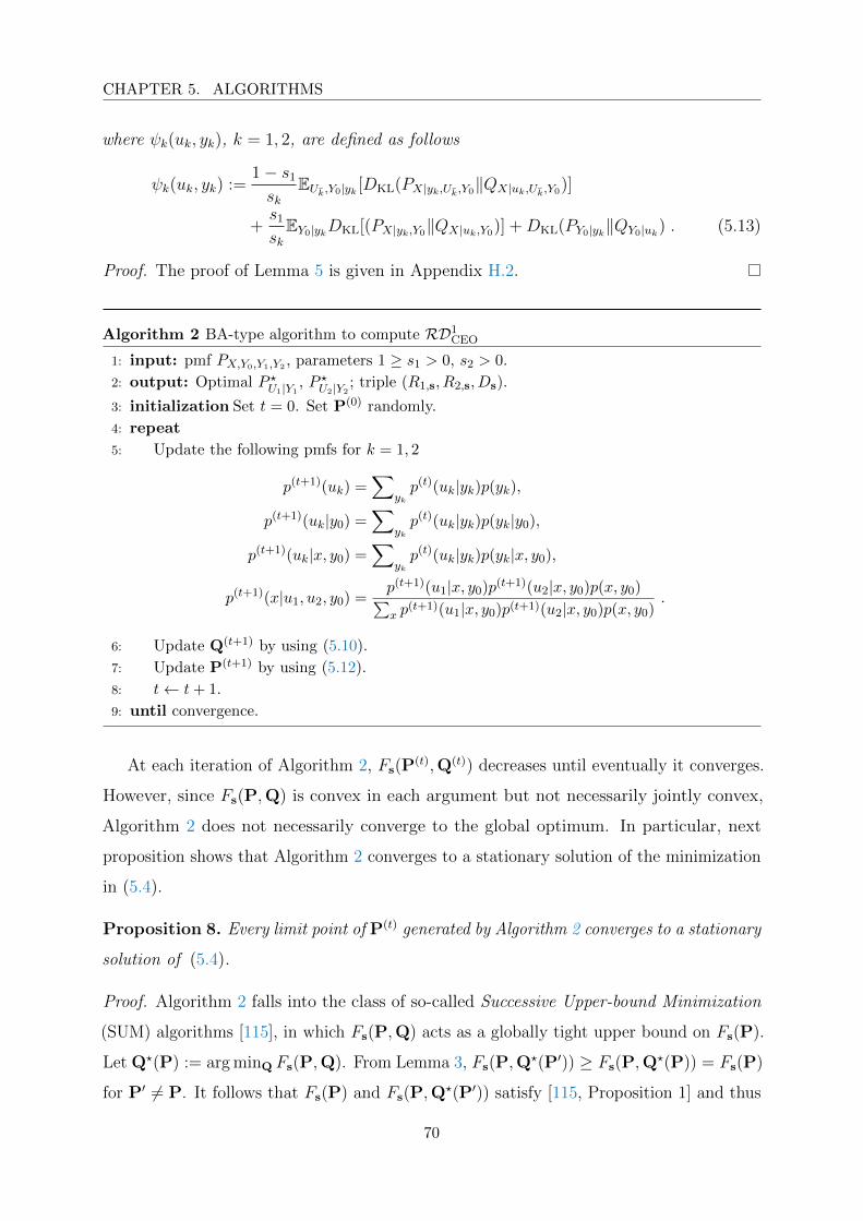
CHAPTER 5. ALGORITHMS
where ψk(uk, yk), k = 1, 2, are defined as follows
ψk(uk, yk) :=1− s1
skEUk,Y0|yk [DKL(PX|yk,Uk,Y0‖QX|uk,Uk,Y0)]
+s1
skEY0|ykDKL[(PX|yk,Y0‖QX|uk,Y0)] +DKL(PY0|yk‖QY0|uk) . (5.13)
Proof. The proof of Lemma 5 is given in Appendix H.2.
Algorithm 2 BA-type algorithm to compute RD1CEO
1: input: pmf PX,Y0,Y1,Y2, parameters 1 ≥ s1 > 0, s2 > 0.
2: output: Optimal P ?U1|Y1, P ?U2|Y2
; triple (R1,s, R2,s, Ds).
3: initialization Set t = 0. Set P(0) randomly.
4: repeat
5: Update the following pmfs for k = 1, 2
p(t+1)(uk) =∑
ykp(t)(uk|yk)p(yk),
p(t+1)(uk|y0) =∑
ykp(t)(uk|yk)p(yk|y0),
p(t+1)(uk|x, y0) =∑
ykp(t)(uk|yk)p(yk|x, y0),
p(t+1)(x|u1, u2, y0) =p(t+1)(u1|x, y0)p(t+1)(u2|x, y0)p(x, y0)∑x p
(t+1)(u1|x, y0)p(t+1)(u2|x, y0)p(x, y0).
6: Update Q(t+1) by using (5.10).
7: Update P(t+1) by using (5.12).
8: t← t+ 1.
9: until convergence.
At each iteration of Algorithm 2, Fs(P(t),Q(t)) decreases until eventually it converges.
However, since Fs(P,Q) is convex in each argument but not necessarily jointly convex,
Algorithm 2 does not necessarily converge to the global optimum. In particular, next
proposition shows that Algorithm 2 converges to a stationary solution of the minimization
in (5.4).
Proposition 8. Every limit point of P(t) generated by Algorithm 2 converges to a stationary
solution of (5.4).
Proof. Algorithm 2 falls into the class of so-called Successive Upper-bound Minimization
(SUM) algorithms [115], in which Fs(P,Q) acts as a globally tight upper bound on Fs(P).
Let Q?(P) := arg minQ Fs(P,Q). From Lemma 3, Fs(P,Q?(P′)) ≥ Fs(P,Q
?(P)) = Fs(P)
for P′ 6= P. It follows that Fs(P) and Fs(P,Q?(P′)) satisfy [115, Proposition 1] and thus
70

CHAPTER 5. ALGORITHMS
Fs(P,Q?(P′)) satisfies (A1)–(A4) in [115]. Convergence to a stationary point of (5.4)
follows from [115, Theorem 1].
Remark 12. Algorithm 2 generates a sequence that is non-increasing. Since this sequence
is lower bounded, convergence to a stationary point is guaranteed. This per-se, however,
does not necessarily imply that such a point is a stationary solution of the original problem
described by (5.4). Instead, this is guaranteed here by showing that the Algorithm 2 is of
SUM-type with the function Fs(P,Q) satisfying the necessary conditions [115, (A1)–(A4)].
5.1.2 Vector Gaussian Case
Computing the rate-distortion region RD?VG-CEO of the vector Gaussian CEO problem as
given by Theorem 4 is a convex optimization problem on ΩkKk=1 which can be solved
using, e.g., the popular generic optimization tool CVX [116]. Alternatively, the region can
be computed using an extension of Algorithm 2 to memoryless Gaussian sources as given
in the rest of this section.
Algorithm 3 BA-type algorithm for the Gaussian vector CEO
1: input: Covariance Σ(x,y0,y1,y2), parameters1 ≥ s1 > 0, s2 > 0.
2: output: Optimal pairs (A?k,Σz?
k), k = 1, 2.
3: initialization Set t = 0. Set randomly A0k and Σz0
k 0 for k = 1, 2.
4: repeat
5: For k = 1, 2, update the following
Σutk
= AtkΣyk
Atk†
+ Σztk
Σutk|(x,y) = At
kΣkAtk†
+ Σztk,
and update Σutk|(ut
k,y), Σut
2|y and Σytk|(ut
k,y) from their definitions by using the following
Σut1,u
t2
= At1H1ΣxH†2A
t†
2
Σutk,y
= AtkHkΣxH†0
Σyk,utk
= HkΣxH†kAtk
†.
6: Compute Σzt+1k
as in (5.16a) for k = 1, 2.
7: Compute At+1k as (5.16b) for k = 1, 2.
8: t← t+ 1.
9: until convergence.
For discrete sources with (small) alphabets, the updating rules of Q(t+1) and P(t+1) of
71
CHAPTER 5. ALGORITHMS
Algorithm 2 are relatively easy computationally. However, they become computationally
unfeasible for continuous alphabet sources. Here, we leverage on the optimality of Gaussian
test channels as shown by Theorem 4 to restrict the optimization of P to Gaussian
distributions, which allows to reduce the search of update rules to those of the associated
parameters, namely covariance matrices. In particular, we show that if P(t)Uk|Yk
, k = 1, 2, is
Gaussian and such that
Utk = At
kYk + Ztk , (5.14)
where Ztk ∼ CN (0,Σztk
), then P(t+1)Uk|Yk
is also Gaussian, with
Ut+1k = At+1
k Yk + Zt+1k , (5.15)
where Zt+1k ∼ CN (0,Σzt+1
k) and the parameters At+1
k and Σzt+1k
are given by
Σzt+1k
=
(1
skΣ−1
utk|(x,y0)− 1− s1
skΣ−1
utk|(utk,y0)+sk − s1
skΣ−1
utk|y0
)−1
(5.16a)
At+1k = Σzt+1
k
(1
skΣ−1
utk|(x,y0)Atk(I−Σyk|(x,y0)Σ
−1yk
)
)
−Σzt+1k
(1− s1
skΣ−1
utk|(utk,y0)Atk(I−Σyk|(utk,y0)Σ
−1yk
)
− sk − s1
skΣ−1
utk|y0Atk(I−Σyk|y0Σ
−1yk
)
). (5.16b)
The updating steps are provided in Algorithm 3. The proof of (5.16) can be found in
Appendix H.3.
5.1.3 Numerical Examples
In this section, we discuss two examples, a binary CEO example and a vector Gaussian
CEO example.
Example 2. Consider the following binary CEO problem. A memoryless binary source X,
modeled as a Bernoulli-(1/2) random variable, i.e., X ∼ Bern(1/2), is observed remotely
at two agents who communicate with a central unit decoder over error-free rate-limited
links of capacity R1 and R2, respectively. The decoder wants to estimate the remote source
X to within some average fidelity level D, where the distortion is measured under the
logarithmic loss criterion. The noisy observation Y1 at Agent 1 is modeled as the output
of a binary symmetric channel (BSC) with crossover probability α1 ∈ [0, 1], whose input is
72
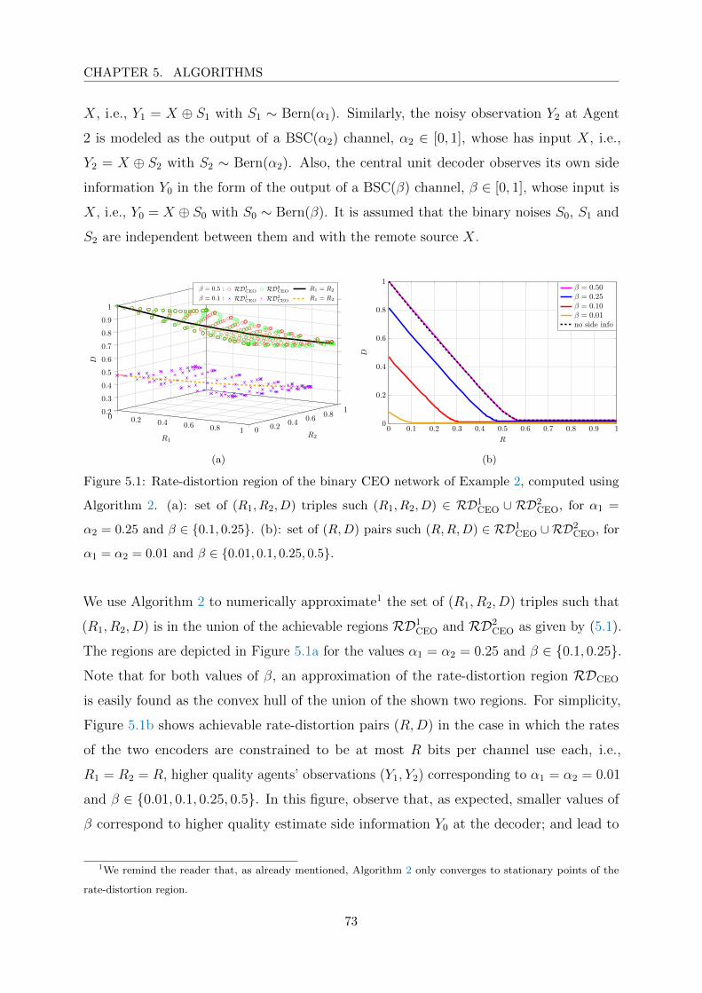
CHAPTER 5. ALGORITHMS
X, i.e., Y1 = X ⊕ S1 with S1 ∼ Bern(α1). Similarly, the noisy observation Y2 at Agent
2 is modeled as the output of a BSC(α2) channel, α2 ∈ [0, 1], whose has input X, i.e.,
Y2 = X ⊕ S2 with S2 ∼ Bern(α2). Also, the central unit decoder observes its own side
information Y0 in the form of the output of a BSC(β) channel, β ∈ [0, 1], whose input is
X, i.e., Y0 = X ⊕ S0 with S0 ∼ Bern(β). It is assumed that the binary noises S0, S1 and
S2 are independent between them and with the remote source X.
0 0.2 0.4 0.6 0.8 1 0 0.20.4
0.60.8
10.2
0.3
0.4
0.5
0.6
0.7
0.8
0.9
1
R1R2
D
β = 0.5 : RD1CEO RD2
CEO R1 = R2
β = 0.1 : RD1CEO RD2
CEO R1 = R2
(a)
0 0.1 0.2 0.3 0.4 0.5 0.6 0.7 0.8 0.9 10
0.2
0.4
0.6
0.8
1
R
D
β = 0.50β = 0.25β = 0.10β = 0.01no side info
(b)
Figure 5.1: Rate-distortion region of the binary CEO network of Example 2, computed using
Algorithm 2. (a): set of (R1, R2, D) triples such (R1, R2, D) ∈ RD1CEO ∪ RD2
CEO, for α1 =
α2 = 0.25 and β ∈ 0.1, 0.25. (b): set of (R,D) pairs such (R,R,D) ∈ RD1CEO ∪RD2
CEO, for
α1 = α2 = 0.01 and β ∈ 0.01, 0.1, 0.25, 0.5.
We use Algorithm 2 to numerically approximate1 the set of (R1, R2, D) triples such that
(R1, R2, D) is in the union of the achievable regions RD1CEO and RD2
CEO as given by (5.1).
The regions are depicted in Figure 5.1a for the values α1 = α2 = 0.25 and β ∈ 0.1, 0.25.Note that for both values of β, an approximation of the rate-distortion region RDCEO
is easily found as the convex hull of the union of the shown two regions. For simplicity,
Figure 5.1b shows achievable rate-distortion pairs (R,D) in the case in which the rates
of the two encoders are constrained to be at most R bits per channel use each, i.e.,
R1 = R2 = R, higher quality agents’ observations (Y1, Y2) corresponding to α1 = α2 = 0.01
and β ∈ 0.01, 0.1, 0.25, 0.5. In this figure, observe that, as expected, smaller values of
β correspond to higher quality estimate side information Y0 at the decoder; and lead to
1We remind the reader that, as already mentioned, Algorithm 2 only converges to stationary points of the
rate-distortion region.
73

CHAPTER 5. ALGORITHMS
smaller distortion values for given rate R. The choice β = 0.5 corresponds to the case of
no or independent side information at decoder; and it is easy to check that the associated
(R,D) curve coincides with the one obtained through exhaustive search in [10, Figure 3].
010
2030
40
010
2030
4015
16
17
18
19
20
R1R2
∆
RD1VG-CEO RD1
VG-CEO ∪RD2VG-CEO
RD2VG-CEO RD?
VG-CEO using CVX
(a)
0 10 20 30 40 5015
16
17
18
19
20
Rsum
∆
Joint encoding with Rsum →∞Joint encoding
Theorem 3 using CVX
Theorem 3 using Algorithm 2
(b)
Figure 5.2: Rate-information region of the vector Gaussian CEO network of Example 3. Numerical
values are nx = 3 and n0 = n1 = n2 = 4. (a): set of (R1, R2,∆) triples such (R1, R2, h(X) −∆) ∈ RD1
VG-CEO ∪ RD2VG-CEO, computed using Algorithm 3. (b): set of (Rsum,∆) pairs such
Rsum = R1 +R2 for some (R1, R2) for which (R1, R2, h(X)−∆) ∈ RD1VG-CEO ∪RD2
VG-CEO.
Example 3. Consider an instance of the memoryless vector Gaussian CEO problem as
described by (4.1) and (4.2) obtained by setting K = 2, nx = 3 and n0 = n1 = n2 =
4. We use Algorithm 3 to numerically approximate the set of (R1, R2,∆) triples such
(R1, R2, h(X) −∆) is in the union of the achievable regions RD1VG-CEO and RD2
VG-CEO.
The result is depicted in Figure 5.2a. The figure also shows the set of (R1, R2,∆) triples
such that (R1, R2, h(X) − ∆) lies in the region given by Theorem 4 evaluated for the
example at hand. Figure 5.2b shows the set of (Rsum,∆) pairs such Rsum := R1 +R2 for
some (R1, R2) for which (R1, R2, h(X)−∆) is in the union of RD1VG-CEO and RD2
VG-CEO.
The region is computed using two different approaches: i) using Algorithm 3 and ii) by
directly evaluating the region obtained from Theorem 4 using the CVX optimization tool
to find the maximizing covariance matrices (Ω1,Ω2) (note that this problem is convex
and so CVX finds the optimal solution). It is worth-noting that Algorithm 3 converges to
the optimal solution for the studied vector Gaussian CEO example, as is visible from the
figure. For comparisons reasons, the figure also shows the performance of centralized or
74
CHAPTER 5. ALGORITHMS
joint encoding, i.e., the case both agents observe both Y1 and Y2,
∆(Rsum) = maxPU|Y1,Y2
: I(U ;Y1,Y2|Y0)≤Rsum
I(U,Y0; X) . (5.17)
Finally, we note that the information/sum-rate function (5.17) can be seen an extension of
Chechik et al. Gaussian Information Bottleneck [21] to the case of side information Y0 at
the decoder. Figure 5.2b shows the loss in terms of information/sum-rate that is incurred
by restricting the encoders to operate separately, i.e., distributed Information Bottleneck
with side information at decoder.
5.2 Deep Distributed Representation Learning
Consider the K-encoder CEO problem under logarithmic loss that we studied in Chapter 3.
In this section, we study the case in which there is no side information, i.e., Y0 = ∅. The
K-encoder CEO source coding problem under logarithmic loss distortion is essentially a
distributed learning model, in which the decoder is interested in a soft estimate of X and
the inference is done in a distributed manner by K learners (encoders).
Let the logarithmic loss distortion constraint of the CEO problem be replaced by the
mutual information constraint
I(Xn;ψ(n)
(φ
(n)1 (Y n
1 ), . . . , φ(n)K (Y n
K)))≥ n∆ . (5.18)
In this case, the region RIDIB of optimal relevance-complexity tuples (R1, . . . , RK ,∆)
generalizes the Tishby’s Information Bottleneck [17] to the distributed case, which is called
as Distributed Information Bottleneck (DIB) problem [1]. Since these two problems are
equivalent, the region RIDIB can be characterized using the relevance-complexity region
RD?CEO given in Theorem 1 by substituting therein ∆ := H(X) − D. The following
corollary states the result.
Corollary 3. The relevance-complexity region RIDIB of the distributed learning problem
is given by the set of all non-negative relevance-complexity tuples (R1, . . . , RK ,∆) that
satisfy, for all subsets S ⊆ K,
∆ ≤∑
k∈S[Rk − I(Yk;Uk|X,Q)] + I(X;USc , Q) ,
75
CHAPTER 5. ALGORITHMS
for some auxiliary random variables (U1, . . . , UK , Q) with distribution PUK,Q(uK, q) such
that PX,YK,UK,Q(x, yK, uK, q) factorizes as
PX(x)K∏
k=1
PYk|X(yk|x) PQ(q)K∏
k=1
PUk|Yk,Q(uk|yk, q) .
Remark 13. The optimal relevance-complexity tuples (R1, . . . , RK ,∆) of the DIB prob-
lem – characterized by Corollary 3 – can be found by solving an optimization problem
on PUk|Yk,QKk=1 and PQ. Here, PUk|Yk,Q is the k-th stochastic encoding that maps the
observation Yk to a latent representation Uk such that Uk captures the relevant information
about X (similar to the single encoder IB problem), and PQ is the pmf of the time-sharing
variable Q among K encoders. The corresponding optimal decoding mapping is denoted by
PX|U1,...,UK ,Q for given PUk|Yk,QKk=1 and PQ.
For simplicity, the relevance is maximized under sum-complexity constraint, i.e., Rsum :=∑K
k=1Rk. The achievable relevance-complexity region under sum-complexity constraint is
defined by
RIsumDIB :=
(∆,Rsum) ∈ R2
+ : ∃(R1, . . . , RK) ∈ RK+ s.t.
(R1, . . . , RK ,∆) ∈ RIDIB andK∑
k=1
Rk = Rsum
.
The region RIsumDIB can be characterized as given in the following proposition.
Proposition 9. [100, Proposition 1] The relevance-complexity region under sum-complexity
constraint RIsumDIB is given by the convex-hull of all non-negative tuples (∆, Rsum) that satisfy
∆ ≤ ∆sumDIB(Rsum) where
∆sumDIB(Rsum) := max
Pmin
I(X;UK), Rsum −
K∑
k=1
I(Yk;Uk|X)
, (5.19)
in which the maximization is over the set of conditional pmfs P := PU1|Y1 , . . . , PUK |YK.
Proof. The proof of Proposition 9 is given in Appendix H.4.
Next proposition provides a parameterization of the boundary tuples (∆s, Rs) of the
region RIsumDIB in terms of a parameter s ≥ 0.
Proposition 10. For each tuple (∆, Rsum) on the boundary of the relevance-complexity
region RIsumDIB there exists s ≥ 0 such that (∆, Rsum) = (∆s, Rs), where
∆s :=1
1 + s
[(1 + sK)H(X) + sRs + max
PLDIBs (P)
](5.20)
76
CHAPTER 5. ALGORITHMS
Rs := I(X;U?K) +
K∑
k=1
[I(Yk;U?k )− I(X;U?
k )] , (5.21)
and P? is the set of pmfs that maximize the cost function
LDIBs (P) := −H(X|UK)− s
K∑
k=1
[H(X|Uk) + I(Yk;Uk)] . (5.22)
Proof. The proof of Proposition 10 is given in Appendix H.5.
From Proposition 10 it is easy to see that the boundary tuple (∆s, Rs) for a given
parameter s can be computed by finding the encoding mappings PUk|YkKk=1 that maximizes
the cost function LDIBs (P) in (5.22). Different boundary tuples of region RIsum
DIB can be
obtained by finding the encoding mappings maximizing (5.22) for different s values, and
computing (5.20) and (5.21) for the resulting solution.
For variational distributions QUk on Uk, k ∈ K (instead of unknown PUk), a variational
stochastic decoder QX|U1,...,UK (instead of the unknown optimal decoder PX|U1,...,UK ), and
K arbitrary decoders QX|Uk , k ∈ K, let define Q as follows
Q :=QX|U1,...,UK , QX|U1 , . . . , QX|UK , QX|U1 , . . . , QX|UK
.
In the following we define the variational DIB cost function LVDIBs (P,Q) as
LVDIBs (P,Q) := EPX,YK
[EPU1|Y1
× · · · × EPUK |YK[logQX|UK ]
+ sK∑
k=1
(EPUk|Yk [logQX|Uk ]−DKL(PUk|Yk‖QUk)
)].
(5.23)
The following lemma states that LVDIBs (P,Q) is a variational lower bound on the DIB
objective LDIBs (P) for all distributions Q.
Lemma 6. For fixed P, we have
LVDIBs (P,Q) ≤ LDIB
s (P) , for all Q .
In addition, there exists a Q that achieves the maximum maxQ LVDIBs (P,Q) = LDIB
s (P),
and is given by
Q?Uk
= PUk , Q?X|Uk = PX|Uk , k = 1, . . . , K ,
Q?X|U1,...,UK
= PX|U1,...,UK ,(5.24)
where PUk , PX|Uk and PX|U1,...,UK are computed from P.
77
CHAPTER 5. ALGORITHMS
Proof. The proof of Lemma 6 is given in Appendix H.6.
Using Lemma 6, it is easy to see that
maxPLDIBs (P) = max
Pmax
QLVDIBs (P,Q) . (5.25)
Remark 14. The variational DIB cost LVDIBs (P,Q) in (5.23) is composed of the cross-
entropy term that is average logarithmic loss of estimating X from all latent representations
U1, . . . , UK by using the joint decoder QX|U1,...,UK , and a regularization term. The regular-
ization term is consisted of: i) the KL divergence between encoding mapping PUk|Yk and the
prior QUk , that also seems in the single encoder case of the variational bound (see (2.33));
and ii) the average logarithmic loss of estimating X from each latent space Uk using the
decoder QX|Uk , that does not appear in the single encoder case.
5.2.1 Variational Distributed IB Algorithm
In the first part of this chapter, we present the BA-type algorithms which find P, Q
optimizing (5.25) for the cases in which the joint distribution of the data, i.e., PX,YK , is
known perfectly or can be estimated with a high accuracy. However, this is not the case
in general. Instead only a set of training samples (xi,y1,i, . . . ,yK,i)ni=1 is available.
For this case, we develop a method in which the encoding and decoding mappings are
restricted to a family of distributions, whose parameters are the outputs of DNNs. By
doing so, the variational bound (5.23) can be written in terms of the parameters of
DNNs. Furthermore, the bound can be computed using Monte Carlo sampling and the
reparameterization trick [29]. Finally, we use the stochastic gradient descent (SGD)
method to train the parameters of DNNs. The proposed method generalizes the variational
framework in [30,78,117–119] to the distributed case with K learners, and was given in [1].
Let Pθk(uk|yk) denote the encoding mapping from the observation Yk to the latent
representation Uk, parameterized by a DNN fθk with parameters θk. As a common example,
the encoder can be chosen as a multivariate Gaussian, i.e., Pθk(uk|yk) = N (uk;µθk ,Σθk).
That is the DNN fθk maps the observation yk to the parameters of the multivariate
Gaussian, namely the mean µθk and the covariance Σθk , i.e., (µθk ,Σθk) = fθ(yk). Similarly,
let QφK(x|uK) denote the decoding mapping from all latent representations U1, . . . ,UK to
the target variable X, parameterized by a DNN gφK with parameters φK; and let Qφk(x|uk)denote the regularizing decoding mapping from the k-th latent representations Uk to
78

CHAPTER 5. ALGORITHMS
the target variable X, parameterized by a DNN gφk with parameters φk, k = 1, . . . , K.
Furthermore, let Qψk(uk), k = 1, . . . , K, denote the prior of the latent space, which does
not depend on a DNN.
By restricting the coders’ mappings to a family of distributions as mentioned above,
the optimization of the variational DIB cost in (5.25) can be written as follows
maxP
maxQLVDIBs (P,Q) ≥ max
θ,φ,ψLNNs (θ,φ,ψ) , (5.26)
where θ := [θ1, . . . , θK ], φ := [φ1, . . . , φK , φK], ψ := [ψ1, . . . , ψK ] denote the parame-
ters of encoding DNNs, decoding DNNs, prior distributions, respectively; and the cost
LNNs (θ,φ,ψ) is given as
LNNs (θ,φ,ψ) := EPX,YK
[EPθ1 (U1|Y1) × · · · × EPθK (UK |YK)[logQφK(X|UK)]
+ sK∑
k=1
(EPθk (Uk|Yk)[logQφk(X|Uk)]−DKL(Pθk(Uk|Yk)‖Qψk(Uk))
)].
(5.27)
Furthermore, the cross-entropy terms in (5.27) can be computed using Monte Carlo
sampling and the reparameterization trick [29]. In particular, Pθk(uk|yk) can be sampled
by first sampling a random variable Zk with distribution PZk(zk), i.e., PZk = N (0, I),
then transforming the samples using some function fθk : Yk ×Zk → Uk parameterized by
θk, i.e., uk = fθk(yk, zk) ∼ Pθk(uk|yk). The reparameterization trick reduces the original
optimization to estimating θk of the deterministic function fθk ; hence, it allows us to
compute estimates of the gradient using backpropagation [29]. Thus, we have the empirical
DIB cost for the i-th sample in the training dataset as follows
Lemps,i (θ,φ,ψ) =
1
m
m∑
j=1
[logQφK(xi|u1,i,j, . . . ,uK,i,j) + s
K∑
k=1
logQφk(xi|uk,i,j)]
− sK∑
k=1
DKL(Pθk(Uk|yk)‖Qψk(Uk)) .
(5.28)
where m is the number of samples for the Monte Carlo sampling.
Finally, we train DNNs to maximize the empirical DIB cost over the parameters θ,φ
as
maxθ,φ
1
n
n∑
i=1
Lemps,i (θ,φ,ψ) . (5.29)
79
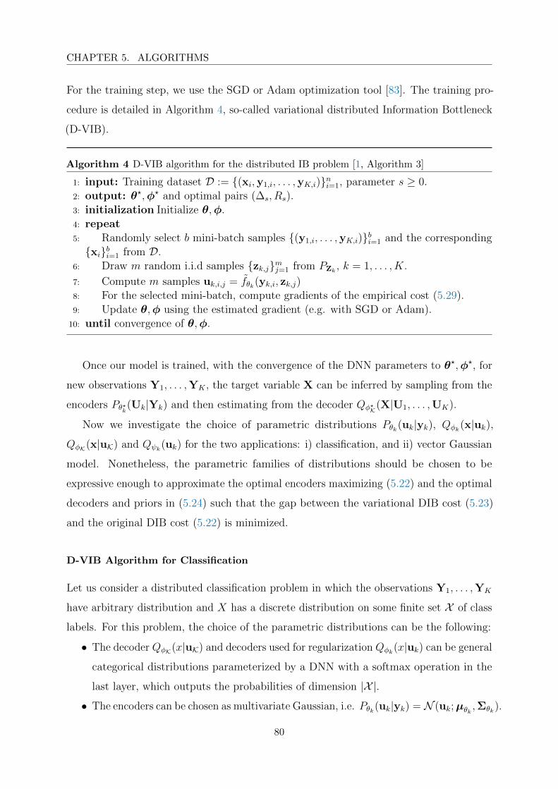
CHAPTER 5. ALGORITHMS
For the training step, we use the SGD or Adam optimization tool [83]. The training pro-
cedure is detailed in Algorithm 4, so-called variational distributed Information Bottleneck
(D-VIB).
Algorithm 4 D-VIB algorithm for the distributed IB problem [1, Algorithm 3]
1: input: Training dataset D := (xi,y1,i, . . . ,yK,i)ni=1, parameter s ≥ 0.2: output: θ?,φ? and optimal pairs (∆s, Rs).3: initialization Initialize θ,φ.4: repeat5: Randomly select b mini-batch samples (y1,i, . . . ,yK,i)bi=1 and the correspondingxibi=1 from D.
6: Draw m random i.i.d samples zk,jmj=1 from PZk , k = 1, . . . , K.
7: Compute m samples uk,i,j = fθk(yk,i, zk,j)8: For the selected mini-batch, compute gradients of the empirical cost (5.29).9: Update θ,φ using the estimated gradient (e.g. with SGD or Adam).
10: until convergence of θ,φ.
Once our model is trained, with the convergence of the DNN parameters to θ?,φ?, for
new observations Y1, . . . ,YK , the target variable X can be inferred by sampling from the
encoders Pθ?k(Uk|Yk) and then estimating from the decoder Qφ?K(X|U1, . . . ,UK).
Now we investigate the choice of parametric distributions Pθk(uk|yk), Qφk(x|uk),QφK(x|uK) and Qψk(uk) for the two applications: i) classification, and ii) vector Gaussian
model. Nonetheless, the parametric families of distributions should be chosen to be
expressive enough to approximate the optimal encoders maximizing (5.22) and the optimal
decoders and priors in (5.24) such that the gap between the variational DIB cost (5.23)
and the original DIB cost (5.22) is minimized.
D-VIB Algorithm for Classification
Let us consider a distributed classification problem in which the observations Y1, . . . ,YK
have arbitrary distribution and X has a discrete distribution on some finite set X of class
labels. For this problem, the choice of the parametric distributions can be the following:
• The decoder QφK(x|uK) and decoders used for regularization Qφk(x|uk) can be general
categorical distributions parameterized by a DNN with a softmax operation in the
last layer, which outputs the probabilities of dimension |X |.• The encoders can be chosen as multivariate Gaussian, i.e. Pθk(uk|yk) = N (uk;µθk ,Σθk).
80
CHAPTER 5. ALGORITHMS
• The priors of the latent space Qψk(uk) can be chosen as multivariate Gaussian (e.g.,
N (0, I)) such that the KL divergence DKL(Pθk(Uk|Yk)‖Qψk(Uk)) has a closed form
solution and is easy to compute [29,30]; or more expressive parameterizations can
also be considered [120,121].
y1
Encoder Pθ1(u1|y1)
fθ1
Sam
ple
µθ1
Σθ1
ε1 ∼ N (0, I)
y2
Encoder Pθ2(u2|y2)
fθ2
Sam
ple
µθ2
Σθ2
ε2 ∼ N (0, I)
u1 = µθ1+ Σ
12θ1ε1
u2 = µθ2+ Σ
12θ2ε2
Latent SpaceRepresentation
gφ1
µφ1
Σφ1
Decoder Qφ1(x|u1)
gφ2
µφ2
Σφ2
Decoder Qφ2(x|u2)
gφK
µφK
ΣφK
Decoder QφK(x|u1,u2)
x
Figure 5.3: An example of distributed supervised learning.
D-VIB Algorithm for Vector Gaussian Model
One of the main results of this thesis is that the optimal test channels are Gaussian for
the vector Gaussian model (see Theorem 4). Due to this, if the underlying data model is
multivariate vector Gaussian, then the optimal distributions P and Q are also multivariate
Gaussian. Hence, we consider the following parameterization, for k ∈ K,
Pθk(uk|yk) = N (uk;µθk ,Σθk) (5.30a)
QφK(x|uK) = N (x;µφK ,ΣφK) (5.30b)
Qφk(x|uk) = N (x;µφk ,Σφk) (5.30c)
Qψk(uk) = N (0, I) , (5.30d)
where µθk ,Σθk are the outputs of a DNN fθk that encodes the input Yk into a nuk-
dimensional Gaussian distribution; µφK ,ΣφK are the outputs of a DNN gφK with inputs
81
CHAPTER 5. ALGORITHMS
U1, . . . ,UK , sampled from N (uk;µθk ,Σθk); and µφk ,Σφk are the outputs of a DNN gφk
with the input Uk, k = 1, . . . , K.
5.2.2 Experimental Results
In this section, numerical results on the synthetic and real datasets are provided to
support the efficiency of the D-VIB Algorithm 4. We evaluate the relevance-complexity
trade-offs achieved by the BA-type Algorithm 3 and D-VIB Algorithm 4. The resulting
relevance-complexity pairs are compared to the optimal relevance-complexity trade-offs
and an upper bound, which is denoted by Centralized IB (C-IB). The C-IB bound is given
by the pairs (∆s, Rsum) achievable if (Y1, . . . , YK) are encoded jointly at a single encoder
with complexity Rsum = R1 + · · ·+RK , and can be obtained by solving the centralized IB
problem as follows
∆cIB(Rsum) = maxPU|Y1,...,YK
: I(U ;Y1,...,YK)≤Rsum
I(U ;X) . (5.31)
In the following experiments, the D-VIB Algorithm 4 is implemented by Adam opti-
mizer [29] over 150 epochs and minibatch size of 64. The learning rate is initialized with
0.001 and decreased gradually every 30 epochs with a decay rate of 0.5, i.e., learning rate
at epoch nepoch is given by 0.001 · 0.5bnepoch/30c.
Regression for Vector Gaussian Data Model
Here we consider a real valued vector Gaussian data model as in [1, Section VI-A].
Specifically, K = 2 encoders observe independently corrupted Gaussian noisy versions
of a nx-dimensional vector Gaussian source X ∼ N (x; 0, I), as Yk = HkX + Nk, where
Hk ∈ Rnk×nx represents the channel connecting the source to the k-th encoder and
Nk ∈ Rnk is the noise at this encoder, i.e., Nk ∼ N (0, I), k = 1, 2.
The optimal complexity-relevance trade-off for this model is characterized as in (4.25)
(wherein H0 = 0), and can be computed using two different approaches: i) using Al-
gorithm 3 and ii) by directly evaluating the region obtained from Theorem 4 using the
CVX optimization tool to find the maximizing covariance matrices (Ω1,Ω2) (note that
this problem is convex and so CVX finds the optimal solution). Furthermore, the C-IB
upper bound in (5.31) can be computed analytically (see (2.14)) since it is an instance of
Gaussian Information Bottleneck problem.
82

CHAPTER 5. ALGORITHMS
A synthetic dataset of n i.i.d. samples (xi,y1,i,y2,i)ni=1 is generated from the afore-
mentioned vector Gaussian model. Then, the proposed BA-type and D-VIB algorithms
are applied on the generated dataset for regression of the Gaussian target variable X. For
the case in which the covariance matrix Σx,y1,y2 of the data model is known, Algorithm 3
is used to compute the relevance-complexity pairs for different values of s. For the case in
which the covariance matrix Σx,y1,y2 is not known, Algorithm 4 is used to train the DNNs
determining the encoders and decoders for different value of s. The encoders and decoders
are parameterized with multivariate Gaussian as in (5.30). We use the following network
architecture: Encoder k, k = 1, 2, is modeled with DNNs with 3 hidden dense layers of 512
neurons with rectified linear unit (ReLU) activations; which is followed by a dense layer
without nonlinear activation to generate the outputs of Encoder k, i.e., µθk and Σθk of
size 512 and 512× 512. Each decoder is modeled with DNNs with 2 hidden dense layers
of 512 neurons with ReLU activations. The output of decoder 1, 2 and K is processed,
each, by a fully connected layer without nonlinear activation to generate µφk and Σφk ,
and µφK and ΣφK , of size 2 and 2× 2.
0 2 4 6 8 10 12
Sum-Complexity Rsum
0.0
0.1
0.2
0.3
0.4
0.5
0.6
Rel
evan
ce∆
C-IB with Rsum →∞D-IB Theorem 2
C-IB Upper Bound
D-VIB train n =30000
D-VIB test n=30000
BA-DIB Algorithm 3
Figure 5.4: Relevance vs. sum-complexity trade-off for vector Gaussian data model with K = 2
encoders, nx = 1, n1 = n2 = 3, and achievable pairs with the BA-type and D-VIB algorithms for
n = 40000. Figure is taken from [1].
Figure 5.4 shows the tuples (∆s, Rsum) resulting from the application of the BA-type
Algorithm 3. It is worth-noting that Algorithm 3 converges to the optimal solution obtained
directly by evaluation the region from (4.25). To apply the D-VIB algorithm, a synthetic
dataset of 40000 i.i.d. samples is generated, which is split into a training set of 30000
samples and a test set of 10000 samples. Figure 5.4 also shows the relevance-complexity
pairs resulting form the application of the D-VIB algorithm for different values of s in the
range (0, 10] calculated as in Proposition 10. For comparisons reasons, Figure 5.4 also
83
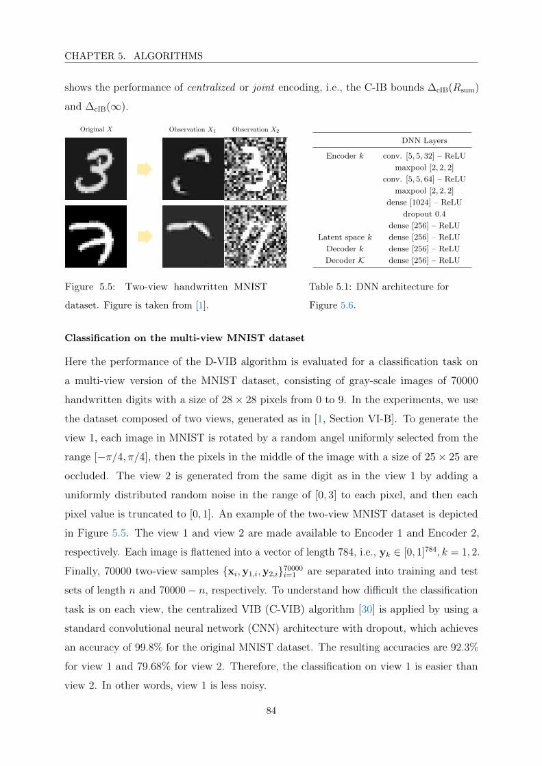
CHAPTER 5. ALGORITHMS
shows the performance of centralized or joint encoding, i.e., the C-IB bounds ∆cIB(Rsum)
and ∆cIB(∞).
0 10 20
0
5
10
15
20
25
0
5
10
15
20
25
Figure 5.5: Two-view handwritten MNIST
dataset. Figure is taken from [1].
DNN Layers
Encoder k conv. [5, 5, 32] – ReLU
maxpool [2, 2, 2]
conv. [5, 5, 64] – ReLU
maxpool [2, 2, 2]
dense [1024] – ReLU
dropout 0.4
dense [256] – ReLU
Latent space k dense [256] – ReLU
Decoder k dense [256] – ReLU
Decoder K dense [256] – ReLU
Table 5.1: DNN architecture for
Figure 5.6.
Classification on the multi-view MNIST dataset
Here the performance of the D-VIB algorithm is evaluated for a classification task on
a multi-view version of the MNIST dataset, consisting of gray-scale images of 70000
handwritten digits with a size of 28× 28 pixels from 0 to 9. In the experiments, we use
the dataset composed of two views, generated as in [1, Section VI-B]. To generate the
view 1, each image in MNIST is rotated by a random angel uniformly selected from the
range [−π/4, π/4], then the pixels in the middle of the image with a size of 25× 25 are
occluded. The view 2 is generated from the same digit as in the view 1 by adding a
uniformly distributed random noise in the range of [0, 3] to each pixel, and then each
pixel value is truncated to [0, 1]. An example of the two-view MNIST dataset is depicted
in Figure 5.5. The view 1 and view 2 are made available to Encoder 1 and Encoder 2,
respectively. Each image is flattened into a vector of length 784, i.e., yk ∈ [0, 1]784, k = 1, 2.
Finally, 70000 two-view samples xi,y1,i,y2,i70000i=1 are separated into training and test
sets of length n and 70000− n, respectively. To understand how difficult the classification
task is on each view, the centralized VIB (C-VIB) algorithm [30] is applied by using a
standard convolutional neural network (CNN) architecture with dropout, which achieves
an accuracy of 99.8% for the original MNIST dataset. The resulting accuracies are 92.3%
for view 1 and 79.68% for view 2. Therefore, the classification on view 1 is easier than
view 2. In other words, view 1 is less noisy.
84

CHAPTER 5. ALGORITHMS
Now we apply the D-VIB algorithm to the two-view MNIST dataset generated as
explained above. The CNN architecture is summarized in Table 5.1. For Encoder
k, k = 1, 2, we consider a nuk = 256 dimensional multivariate Gaussian distribution
parameterization, N (µθk ,Σθk), where µθk ,Σθk are the outputs of a DNN fθk consisting
of the concatenation of convolutional, dense and maxpool layers with ReLU activations
and a dropout. For the last layer of the encoder we use a linear activation. Then, the
latent representation uk, k = 1, 2, is sampled from N (µθk ,Σθk). The prior is chosen as
Qψk(uk) = N (0, I). Decoder k, k = 1, 2, and Decoder K takes uk and uK, respectively,
as an input. Each decoder is modeled with a DNN (gφk and gφK) with 2 hidden dense
layers of 256 neurons with ReLU activations. The output of each decoder is processed by
a fully connected layer, followed by a softmax, which outputs a normalized vector x of
size |X | = 10, corresponding to a distribution over the one-hot encoding of the digit labels
0, 1, . . . , 9 from the K observations, i.e., we have
Qφk(x|uk) = softmax(gφk(Uk)) , k = 1, . . . , K ,
QφK(x|uK) = softmax(gφK(U1, U2)) ,(5.32)
where softmax(p) for p ∈ Rd is a vector with i-th entry is calculated as [softmax(p)]i =
exp(pi)/d∑j=1
exp(pj), i = 1, . . . , d.
For given parameterization, the log-loss (reconstruction loss) terms are calculated by
using the cross-entropy criterion and the KL divergence terms can be computed as in (I.2).
The relevance-complexity pairs obtained from applying the D-VIB Algorithm 4 on
the two-view MNIST – consisting of a training set of n = 50000 samples – is depicted in
Figure 5.6a for 15 different values of s in the range [10−10, 1]. For comparisons reasons, the
figure also shows the C-IB upper bound for Rsum →∞ assuming that zero classification
error is possible, i.e., ∆cIB(∞) = log 10. During the training phase, it is observed that
higher sum-complexity results higher relevance, and that resulting relevance-complexity
pairs are very close to the theoretical limit. On the other hand, during the test phase,
the achievable relevance decreases for large values of sum-complexity. This is because
of the effect of the regularization such that the complexity constraint results in higher
generalization.
The accuracies of the D-VIB algorithm achieved by the joint (or main) estimator
QX|U1,U2 , as well as the regularizing decoders QX|Uk, k = 1, 2, are depicted in Figure 5.6b
85
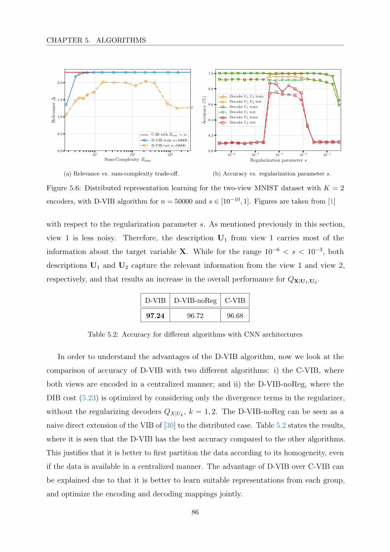
CHAPTER 5. ALGORITHMS
101 102 103
Sum-Complexity Rsum
0.0
0.5
1.0
1.5
2.0
Rel
evan
ce∆
C-IB with Rsum →∞D-VIB train n=50000
D-VIB test n=50000
(a) Relevance vs. sum-complexity trade-off.
10−9 10−7 10−5 10−3 10−1
Regularization parameter s
0.0
0.2
0.4
0.6
0.8
1.0
Acc
ura
cy(%
) Decoder U1, U2 train
Decoder U1, U2 test
Decoder U1 train
Decoder U1 test
Decoder U2 train
Decoder U2 test
(b) Accuracy vs. regularization parameter s.
Figure 5.6: Distributed representation learning for the two-view MNIST dataset with K = 2
encoders, with D-VIB algorithm for n = 50000 and s ∈ [10−10, 1]. Figures are taken from [1]
with respect to the regularization parameter s. As mentioned previously in this section,
view 1 is less noisy. Therefore, the description U1 from view 1 carries most of the
information about the target variable X. While for the range 10−6 < s < 10−3, both
descriptions U1 and U2 capture the relevant information from the view 1 and view 2,
respectively, and that results an increase in the overall performance for QX|U1,U2 .
D-VIB D-VIB-noReg C-VIB
97.24 96.72 96.68
Table 5.2: Accuracy for different algorithms with CNN architectures
In order to understand the advantages of the D-VIB algorithm, now we look at the
comparison of accuracy of D-VIB with two different algorithms: i) the C-VIB, where
both views are encoded in a centralized manner; and ii) the D-VIB-noReg, where the
DIB cost (5.23) is optimized by considering only the divergence terms in the regularizer,
without the regularizing decoders QX|Uk , k = 1, 2. The D-VIB-noReg can be seen as a
naive direct extension of the VIB of [30] to the distributed case. Table 5.2 states the results,
where it is seen that the D-VIB has the best accuracy compared to the other algorithms.
This justifies that it is better to first partition the data according to its homogeneity, even
if the data is available in a centralized manner. The advantage of D-VIB over C-VIB can
be explained due to that it is better to learn suitable representations from each group,
and optimize the encoding and decoding mappings jointly.
86
Chapter 6
Application to Unsupervised
Clustering
Clustering consists of partitioning a given dataset into various groups (clusters) based
on some similarity metric, such as the Euclidean distance, L1 norm, L2 norm, L∞ norm,
the popular logarithmic loss measure, or others. The principle is that each cluster should
contain elements of the data that are closer to each other than to any other element outside
that cluster, in the sense of the defined similarity measure. If the joint distribution of the
clusters and data is not known, one should operate blindly in doing so, i.e., using only
the data elements at hand; and the approach is called unsupervised clustering [122,123].
Unsupervised clustering is perhaps one of the most important tasks of unsupervised machine
learning algorithms currently, due to a variety of application needs and connections with
other problems.
Clustering can be formulated as follows. Consider a dataset that is composed of N
samples xiNi=1, which we wish to partition into |C| ≥ 1 clusters. Let C = 1, . . . , |C| be
the set of all possible clusters and C designate a categorical random variable that lies in
C and stands for the index of the actual cluster. If X is a random variable that models
elements of the dataset, given that X = xi induces a probability distribution on C, which
the learner should learn, thus mathematically, the problem is that of estimating the values
of the unknown conditional probability PC|X(·|xi) for all elements xi of the dataset. The
estimates are sometimes referred to as the assignment probabilities.
Examples of unsupervised clustering algorithms include the very popular K-means [124]
and Expectation Maximization (EM) [125]. The K-means algorithm partitions the data
87
CHAPTER 6. APPLICATION TO UNSUPERVISED CLUSTERING
in a manner that the Euclidean distance among the members of each cluster is minimized.
With the EM algorithm, the underlying assumption is that the data comprise a mixture
of Gaussian samples, namely a Gaussian Mixture Model (GMM); and one estimates the
parameters of each component of the GMM while simultaneously associating each data
sample with one of those components. Although they offer some advantages in the context
of clustering, these algorithms suffer from some strong limitations. For example, it is well
known that the K-means is highly sensitive to both the order of the data and scaling; and
the obtained accuracy depends strongly on the initial seeds (in addition to that, it does
not predict the number of clusters or K-value). The EM algorithm suffers mainly from
slow convergence, especially for high-dimensional data.
Recently, a new approach has emerged that seeks to perform inference on a transformed
domain (generally referred to as latent space), not the data itself. The rationale is that
because the latent space often has fewer dimensions, it is more convenient computationally
to perform inference (clustering) on it rather than on the high-dimensional data directly.
A key aspect then is how to design a latent space that is amenable to accurate low-
complexity unsupervised clustering, i.e., one that preserves only those features of the
observed high-dimensional data that are useful for clustering while removing all redundant
or non-relevant information. Along this line of work, we can mention [126], which utilized
Principal Component Analysis (PCA) [127, 128] for dimensionality reduction followed
by K-means for clustering the obtained reduced dimension data; or [129], which used
a combination of PCA and the EM algorithm. Other works that used alternatives for
the linear PCA include kernel PCA [130], which employs PCA in a non-linear fashion to
maximize variance in the data.
Tishby’s Information Bottleneck (IB) method [17] formulates the problem of finding a
good representation U that strikes the right balance between capturing all information
about the categorical variable C that is contained in the observation X and using the most
concise representation for it. The IB problem can be written as the following Lagrangian
optimization
minPU|X
I(X; U)− sI(C; U) , (6.1)
where s is a Lagrange-type parameter, which controls the trade-off between accuracy and
regularization. In [32, 131], a text clustering algorithm is introduced for the case in which
the joint probability distribution of the input data is known. This text clustering algorithm
88

CHAPTER 6. APPLICATION TO UNSUPERVISED CLUSTERING
uses the IB method with an annealing procedure, where the parameter s is increased
gradually. When s→ 0, the representation U is designed with the most compact form,
i.e., |U| = 1, which corresponds to the maximum compression. By gradually increasing
the parameter s, the emphasis on the relevance term I(C; U) increases, and at a critical
value of s, the optimization focuses on not only the compression, but also the relevance
term. To fulfill the demand on the relevance term, this results in the cardinality of U
bifurcating. This is referred as a phase transition of the system. The further increases
in the value of s will cause other phase transitions, hence additional splits of |U| until it
reaches the desired level, e.g., |U| = |C|.
However, in the real-world applications of clustering with large-scale datasets, the
joint probability distributions of the datasets are unknown. In practice, the usage of
Deep Neural Networks (DNN) for unsupervised clustering of high-dimensional data on a
lower dimensional latent space has attracted considerable attention, especially with the
advent of Autoencoder (AE) learning and the development of powerful tools to train them
using standard backpropagation techniques [29, 132]. Advanced forms include Variational
Autoencoders (VAE) [29, 132], which are generative variants of AE that regularize the
structure of the latent space, and the more general Variational Information Bottleneck
(VIB) of [30], which is a technique that is based on the Information Bottleneck method and
seeks a better trade-off between accuracy and regularization than VAE via the introduction
of a Lagrange-type parameter s, which controls that trade-off and whose optimization is
similar to deterministic annealing [32] or stochastic relaxation.
In this chapter, we develop an unsupervised generative clustering framework that
combines VIB and the Gaussian Mixture Model. Specifically, in our approach, we use
the Variational Information Bottleneck method and model the latent space as a mixture
of Gaussians. We derive a bound on the cost function of our model that generalizes the
Evidence Lower Bound (ELBO) and provide a variational inference type algorithm that
allows computing it. In the algorithm, the coders’ mappings are parameterized using
Neural Networks (NN), and the bound is approximated by Markov sampling and optimized
with stochastic gradient descent. Furthermore, we show how tuning the hyperparameter s
appropriately by gradually increasing its value with iterations (number of epochs) results
in a better accuracy. Furthermore, the application of our algorithm to the unsupervised
clustering of various datasets, including the MNIST [46], REUTERS [47], and STL-10 [48],
89

CHAPTER 6. APPLICATION TO UNSUPERVISED CLUSTERING
allows a better clustering accuracy than previous state-of-the-art algorithms. For instance,
we show that our algorithm performs better than the Variational Deep Embedding (VaDE)
algorithm of [31], which is based on VAE and performs clustering by maximizing the
ELBO. Our algorithm can be seen as a generalization of the VaDE, whose ELBO can be
recovered by setting s = 1 in our cost function. In addition, our algorithm also generalizes
the VIB of [30], which models the latent space as an isotropic Gaussian, which is generally
not expressive enough for the purpose of unsupervised clustering. Other related works,
which are of lesser relevance to the contribution of this paper, are the Deep Embedded
Clustering (DEC) of [33] and the Improved Deep Embedded Clustering (IDEC) of [133]
and [134]. For a detailed survey of clustering with deep learning, the readers may refer
to [135].
To the best of our knowledge, our algorithm performs the best in terms of clustering
accuracy by using deep neural networks without any prior knowledge regarding the labels
(except the usual assumption that the number of classes is known) compared to the
state-of-the-art algorithms of the unsupervised learning category. In order to achieve the
outperforming accuracy: (i) we derive a cost function that contains the IB hyperparameter
s that controls optimal trade-offs between the accuracy and regularization of the model;
(ii) we use a lower bound approximation for the KL term in the cost function, that does
not depend on the clustering assignment probability (note that the clustering assignment
is usually not accurate in the beginning of the training process); and (iii) we tune the
hyperparameter s by following an annealing approach that improves both the convergence
and the accuracy of the proposed algorithm.
Encoder
fθ
Decoder
gφ
U ∼∑c πc N (u;µc,Σc)
X X
Figure 6.1: Variational Information Bottleneck with Gaussian Mixtures.
90
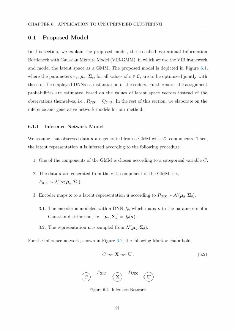
CHAPTER 6. APPLICATION TO UNSUPERVISED CLUSTERING
6.1 Proposed Model
In this section, we explain the proposed model, the so-called Variational Information
Bottleneck with Gaussian Mixture Model (VIB-GMM), in which we use the VIB framework
and model the latent space as a GMM. The proposed model is depicted in Figure 6.1,
where the parameters πc, µc, Σc, for all values of c ∈ C, are to be optimized jointly with
those of the employed DNNs as instantiation of the coders. Furthermore, the assignment
probabilities are estimated based on the values of latent space vectors instead of the
observations themselves, i.e., PC|X = QC|U. In the rest of this section, we elaborate on the
inference and generative network models for our method.
6.1.1 Inference Network Model
We assume that observed data x are generated from a GMM with |C| components. Then,
the latent representation u is inferred according to the following procedure:
1. One of the components of the GMM is chosen according to a categorical variable C.
2. The data x are generated from the c-th component of the GMM, i.e.,
PX|C ∼ N (x; µc, Σc).
3. Encoder maps x to a latent representation u according to PU|X ∼ N (µθ,Σθ).
3.1. The encoder is modeled with a DNN fθ, which maps x to the parameters of a
Gaussian distribution, i.e., [µθ,Σθ] = fθ(x).
3.2. The representation u is sampled from N (µθ,Σθ).
For the inference network, shown in Figure 6.2, the following Markov chain holds
C −−X−−U . (6.2)
C X UPX|C PU|X
Figure 6.2: Inference Network
91
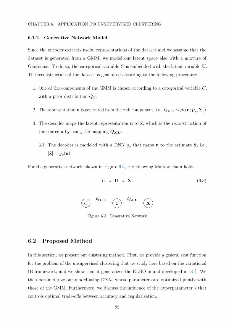
CHAPTER 6. APPLICATION TO UNSUPERVISED CLUSTERING
6.1.2 Generative Network Model
Since the encoder extracts useful representations of the dataset and we assume that the
dataset is generated from a GMM, we model our latent space also with a mixture of
Gaussians. To do so, the categorical variable C is embedded with the latent variable U.
The reconstruction of the dataset is generated according to the following procedure:
1. One of the components of the GMM is chosen according to a categorical variable C,
with a prior distribution QC .
2. The representation u is generated from the c-th component, i.e., QU|C ∼ N (u;µc,Σc).
3. The decoder maps the latent representation u to x, which is the reconstruction of
the source x by using the mapping QX|U.
3.1. The decoder is modeled with a DNN gφ that maps u to the estimate x, i.e.,
[x] = gφ(u).
For the generative network, shown in Figure 6.3, the following Markov chain holds
C −−U−−X . (6.3)
C U XQU|C QX|U
Figure 6.3: Generative Network
6.2 Proposed Method
In this section, we present our clustering method. First, we provide a general cost function
for the problem of the unsupervised clustering that we study here based on the variational
IB framework; and we show that it generalizes the ELBO bound developed in [31]. We
then parameterize our model using DNNs whose parameters are optimized jointly with
those of the GMM. Furthermore, we discuss the influence of the hyperparameter s that
controls optimal trade-offs between accuracy and regularization.
92
CHAPTER 6. APPLICATION TO UNSUPERVISED CLUSTERING
6.2.1 Brief Review of Variational Information Bottleneck for Unsupervised
Learning
As described in Chapter 6.1, the stochastic encoder PU|X maps the observed data x to a
representation u. Similarly, the stochastic decoder QX|U assigns an estimate x of x based
on the vector u. As per the IB method [17], a suitable representation U should strike
the right balance between capturing all information about the categorical variable C that
is contained in the observation X and using the most concise representation for it. This
leads to maximizing the following Lagrange problem
Ls(P) = I(C; U)− sI(X; U) , (6.4)
where s ≥ 0 designates the Lagrange multiplier and, for convenience, P denotes the
conditional distribution PU|X.
Instead of (6.4), which is not always computable in our unsupervised clustering setting,
we find it convenient to maximize an upper bound of Ls(P) given by
Ls(P) := I(X; U)− sI(X; U)(a)= H(X)−H(X|U)− s[H(U)−H(U|X)] , (6.5)
where (a) is due to the definition of mutual information (using the Markov chain C−−X−−U,
it is easy to see that Ls(P) ≥ Ls(P) for all values of P). Noting that H(X) is constant
with respect to PU|X, maximizing Ls(P) over P is equivalent to maximizing
L′s(P) : = −H(X|U)− s[H(U)−H(U|X)] (6.6)
= EPX
[EPU|X [logPX|U + s logPU − s logPU|X]
]. (6.7)
For a variational distribution QU on U (instead of the unknown PU) and a variational
stochastic decoder QX|U (instead of the unknown optimal decoder PX|U), let Q :=
QX|U, QU. Furthermore, let
LVBs (P,Q) := EPX
[EPU|X [logQX|U]− sDKL(PU|X‖QU)
]. (6.8)
Lemma 7. For given P, we have
LVBs (P,Q) ≤ L′s(P), for all Q .
In addition, there exists a unique Q that achieves the maximum maxQ LVBs (P,Q) = L′s(P),
and is given by
Q∗X|U = PX|U , Q∗U = PU .
93
CHAPTER 6. APPLICATION TO UNSUPERVISED CLUSTERING
Proof. The proof of Lemma 7 is given in Appendix I.1.
Using Lemma 7, maximization of (6.6) can be written in term of the variational IB
cost as follows
maxPL′s(P) = max
Pmax
QLVBs (P,Q) . (6.9)
Remark 15. As we already mentioned in the beginning of this chapter, the related work [31]
performs unsupervised clustering by combining VAE with GMM. Specifically, it maximizes
the following ELBO bound
LVaDE1 := EPX
[EPU|X [logQX|U]−DKL(PC|X‖QC)− EPC|X [DKL(PU|X‖QU|C)]
]. (6.10)
Let, for an arbitrary non-negative parameter s, LVaDEs be a generalization of the ELBO
bound (6.10) of [31] given by
LVaDEs := EPX
[EPU|X [logQX|U]− sDKL(PC|X‖QC)− sEPC|X [DKL(PU|X‖QU|C)]
].
(6.11)
Investigating the RHS of (6.11), we get
LVBs (P,Q) = LVaDE
s + sEPX
[EPU|X [DKL(PC|X‖QC|U)]
], (6.12)
where the equality holds since
LVaDEs = EPX
[EPU|X [logQX|U]− sDKL(PC|X‖QC)− sEPC|X [DKL(PU|X‖QU|C)]
](6.13)
(a)= EPX
[EPU|X [logQX|U]− sDKL(PU|X‖QU)− sEPU|X
[DKL(PC|X‖QC|U)
](6.14)
(b)= LVB
s (P,Q)− sEPX
[EPU|X
[DKL(PC|X‖QC|U)
]], (6.15)
where (a) can be obtained by expanding and rearranging terms under the Markov chain
C −−X−−U (for a detailed treatment, please look at Appendix I.2); and (b) follows from
the definition of LVBs (P,Q) in (6.8).
Thus, by the non-negativity of relative entropy, it is clear that LVaDEs is a lower bound
on LVBs (P,Q). Furthermore, if the variational distribution Q is such that the conditional
marginal QC|U is equal to PC|X, the bound is tight since the relative entropy term is zero
in this case.
94
CHAPTER 6. APPLICATION TO UNSUPERVISED CLUSTERING
6.2.2 Proposed Algorithm: VIB-GMM
In order to compute (6.9), we parameterize the distributions PU|X and QX|U using DNNs.
For instance, let the stochastic encoder PU|X be a DNN fθ and the stochastic decoder
QX|U be a DNN gφ. That is
Pθ(u|x) = N (u;µθ,Σθ) , where [µθ,Σθ] = fθ(x) ,
Qφ(x|u) = gφ(u) = [x] ,(6.16)
where θ and φ are the weight and bias parameters of the DNNs. Furthermore, the latent
space is modeled as a GMM with |C| components with parameters ψ := πc,µc,Σc|C|c=1,
i.e.,
Qψ(u) =∑
c
πc N (u;µc,Σc) . (6.17)
Using the parameterizations above, the optimization of (6.9) can be rewritten as
maxθ,φ,ψ
LNNs (θ, φ, ψ) (6.18)
where the cost function LNNs (θ, φ, ψ) given by
LNNs (θ, φ, ψ) := EPX
[EPθ(U|X)[logQφ(X|U)]− sDKL(Pθ(U|X)‖Qψ(U))
]. (6.19)
Then, for a given observations of N samples, i.e., xiNi=1, (6.18) can be approximated in
terms of an empirical cost as follows
maxθ,φ,ψ
1
n
n∑
i=1
Lemps,i (θ, φ, ψ) , (6.20)
where Lemps,i (θ, φ, ψ) is the empirical cost for the i-th observation xi, and given by
Lemps,i (θ, φ, ψ) = EPθ(Ui|Xi)[logQφ(Xi|Ui)]− sDKL(Pθ(Ui|Xi)‖Qψ(Ui)) . (6.21)
Furthermore, the first term of the RHS of (6.21) can be computed using Monte Carlo
sampling and the reparameterization trick [29]. In particular, Pθ(u|x) can be sampled
by first sampling a random variable Z with distribution PZ, i.e., PZ = N (0, I), then
transforming the samples using some function fθ : X × Z → U , i.e., u = fθ(x, z). Thus,
EPθ(Ui|Xi)[logQφ(Xi|Ui)] =1
M
M∑
m=1
log qφ(xi|ui,m) ,
with ui,m = µθ,i + Σ12θ,i · εm , εm ∼ N (0, I) ,
95

CHAPTER 6. APPLICATION TO UNSUPERVISED CLUSTERING
where M is the number of samples for the Monte Carlo sampling step.
The second term of the RHS of (6.21) is the KL divergence between a single component
multivariate Gaussian and a GMM with |C| components. An exact closed-form solution
for the calculation of this term does not exist. However, a variational lower bound
approximation [136] of it (see Appendix I.4) can be obtained as
DKL(Pθ(Ui|Xi)‖Qψ(Ui)) = − log
|C|∑
c=1
πc exp(−DKL(N (µθ,i,Σθ,i)‖N (µc,Σc)
). (6.22)
In particular, in the specific case in which the covariance matrices are diagonal, i.e.,
Σθ,i := diag(σ2θ,i,jnuj=1) and Σc := diag(σ2
c,jnuj=1), with nu denoting the latent space
dimension, (6.22) can be computed as follows
DKL(Pθ(Ui|Xi)‖Qψ(Ui))
= − log
|C|∑
c=1
πc exp
(− 1
2
nu∑
j=1
[(µθ,i,j − µc,j)2
σ2c,j
+ logσ2c,j
σ2θ,i,j
− 1 +σ2θ,i,j
σ2c,j
]), (6.23)
where µθ,i,j and σ2θ,i,j are the mean and variance of the i-th representation in the j-th
dimension of the latent space. Furthermore, µc,j and σ2c,j represent the mean and variance
of the c-th component of the GMM in the j-th dimension of the latent space.
Finally, we train DNNs to maximize the cost function (6.19) over the parameters θ, φ,
as well as those ψ of the GMM. For the training step, we use the ADAM optimization
tool [83]. The training procedure is detailed in Algorithm 5.
Algorithm 5 VIB-GMM algorithm for unsupervised learning.
1: input: Dataset D := xiNi=1, parameter s ≥ 0.2: output: Optimal DNN weights θ?, φ? and
GMM parameters ψ? = π?c , µ?c , Σ?c|C|c=1.
3: initialization Initialize θ, φ, ψ.4: repeat5: Randomly select b mini-batch samples xibi=1 from D.6: Draw m random i.i.d samples zjmj=1 from PZ.
7: Compute m samples ui,j = fθ(xi, zj)8: For the selected mini-batch, compute gradients of the empirical cost (6.20).9: Update θ, φ, ψ using the estimated gradient (e.g., with SGD or Adam).
10: until convergence of θ, φ, ψ.
96

CHAPTER 6. APPLICATION TO UNSUPERVISED CLUSTERING
Once our model is trained, we assign the given dataset into the clusters. As mentioned
in Chapter 6.1, we do the assignment from the latent representations, i.e., QC|U = PC|X.
Hence, the probability that the observed data xi belongs to the c-th cluster is computed
as follows
p(c|xi) = q(c|ui) =qψ?(c)qψ?(ui|c)
qψ?(ui)=
π?cN (ui;µ?c ,Σ
?c)∑
c π?cN (ui;µ?c ,Σ
∗c), (6.24)
where ? indicates optimal values of the parameters as found at the end of the training
phase. Finally, the right cluster is picked based on the largest assignment probability
value.
Remark 16. It is worth mentioning that with the use of the KL approximation as given
by (6.22), our algorithm does not require the assumption PC|U = QC|U to hold (which is
different from [31]). Furthermore, the algorithm is guaranteed to converge. However, the
convergence may be to (only) local minima; and this is due to the problem (6.18) being
generally non-convex. Related to this aspect, we mention that while without a proper
pre-training, the accuracy of the VaDE algorithm may not be satisfactory, in our case, the
above assumption is only used in the final assignment after the training phase is completed.
Remark 17. In [78], it is stated that optimizing the original IB problem with the assump-
tion of independent latent representations amounts to disentangled representations. It is
noteworthy that with such an assumption, the computational complexity can be reduced
from O(n2u) to O(nu). Furthermore, as argued in [78], the assumption often results only
in some marginal performance loss; and for this reason, it is adopted in many machine
learning applications.
Effect of the Hyperparameter
As we already mentioned, the hyperparameter s controls the trade-off between the relevance
of the representation U and its complexity. As can be seen from (6.19) for small values of
s, it is the cross-entropy term that dominates, i.e., the algorithm trains the parameters
so as to reproduce X as accurately as possible. For large values of s, however, it is most
important for the NN to produce an encoded version of X whose distribution matches the
prior distribution of the latent space, i.e., the term DKL(Pθ(U|X)‖Qψ(U)) is nearly zero.
97
CHAPTER 6. APPLICATION TO UNSUPERVISED CLUSTERING
In the beginning of the training process, the GMM components are randomly selected;
and so, starting with a large value of the hyperparameter s is likely to steer the solution
towards an irrelevant prior. Hence, for the tuning of the hyperparameter s in practice, it
is more efficient to start with a small value of s and gradually increase it with the number
of epochs. This has the advantage of avoiding possible local minima, an aspect that is
reminiscent of deterministic annealing [32], where s plays the role of the temperature
parameter. The experiments that will be reported in the next section show that proceeding
in the above-described manner for the selection of the parameter s helps in obtaining
higher clustering accuracy and better robustness to the initialization (i.e., no need for a
strong pretraining). The pseudocode for annealing is given in Algorithm 6.
Algorithm 6 Annealing algorithm pseudocode.
1: input: Dataset D := xini=1, hyperparameter interval [smin, smax].
2: output: Optimal DNN weights θ?, φ?, GMM parameters ψ? = π?c , µ?c , Σ?c|C|c=1,
assignment probability PC|X.
3: initialization Initialize θ, φ, ψ.
4: repeat
5: Apply VIB-GMM algorithm.
6: Update ψ, θ, φ.
7: Update s, e.g., s = (1 + εs)sold.
8: until s does not exceed smax.
Remark 18. As we mentioned before, a text clustering algorithm is introduced by Slonim et
al. [32, 131], which uses the IB method with an annealing procedure, where the parameter
s is increased gradually. In [32], the critical values of s (so-called phase transitions) are
observed such that if these values are missed during increasing s, the algorithm ends up
with the wrong clusters. Therefore, how to choose the step size in the update of s is very
important. We note that tuning s is also very critical in our algorithm, such that the step
size εs in the update of s should be chosen carefully, otherwise phase transitions might be
skipped that would cause a non-satisfactory clustering accuracy score. However, the choice
of the appropriate step size (typically very small) is rather heuristic; and there exists no
concrete method for choosing the right value. The choice of step size can be seen as a
trade-off between the amount of computational resource spared for running the algorithm
and the degree of confidence about scanning s values not to miss the phase transitions.
98

CHAPTER 6. APPLICATION TO UNSUPERVISED CLUSTERING
6.3 Experiments
6.3.1 Description of used datasets
In our empirical experiments, we apply our algorithm to the unsupervised clustering of
the following datasets.
MNIST: A dataset of gray-scale images of 70000 handwritten digits from 0 to 9 of
dimensions 28× 28 pixel each.
STL-10: A dataset of color images collected from 10 categories. Each category consists
of 1300 images of size of 96 × 96 (pixels) ×3 (RGB code). Hence, the original input
dimension nx is 27648. For this dataset, we use a pretrained convolutional NN model, i.e.,
ResNet-50 [137] to reduce the dimensionality of the input. This preprocessing reduces the
input dimension to 2048. Then, our algorithm and other baselines are used for clustering.
REUTERS10K: A dataset that is composed of 810000 English stories labeled with a
category tree. As in [33], 4 root categories (corporate/industrial, government/social,
markets, economics) are selected as labels and all documents with multiple labels are
discarded. Then, tf-idf features are computed on the 2000 most frequently occurring
words. Finally, 10000 samples are taken randomly, which are referred to as REUTERS10K
dataset.
6.3.2 Network settings and other parameters
We use the following network architecture: the encoder is modeled with DNNs with 3
hidden layers with dimensions nx− 500− 500− 2000−nu, where nx is the input dimension
and nu is the dimension of the latent space. The decoder consists of DNNs with dimensions
nu − 2000 − 500 − 500 − nx. All layers are fully connected. For comparison purposes,
we chose the architecture of the hidden layers as well as the dimension of the latent
space nu = 10 to coincide with those made for the DEC algorithm of [33] and the VaDE
algorithm of [31]. All except the last layers of the encoder and decoder are activated with
ReLU function. For the last (i.e., latent) layer of the encoder we use a linear activation;
and for the last (i.e., output) layer of the decoder we use sigmoid function for MNIST and
linear activation for the remaining datasets. The batch size is 100 and the variational
bound (6.20) is maximized by the Adam optimizer of [83]. The learning rate is initialized
99

CHAPTER 6. APPLICATION TO UNSUPERVISED CLUSTERING
with 0.002 and decreased gradually every 20 epochs with a decay rate of 0.9 until it reaches
a small value (0.0005 is our experiments). The reconstruction loss is calculated by using
the cross-entropy criterion for MNIST and mean squared error function for the other
datasets.
6.3.3 Clustering Accuracy
We evaluate the performance of our algorithm in terms of the so-called unsupervised
clustering accuracy (ACC), which is a widely used metric in the context of unsupervised
learning [135]. For comparison purposes, we also present those of algorithms from the
previous state-of-the-art.
MNIST STL-10
Best Run Average Run Best Run Average Run
GMM 44.1 40.5 (1.5) 78.9 73.3 (5.1)
DEC 80.6†
VaDE 91.8 78.8 (9.1) 85.3 74.1 (6.4)
VIB-GMM 95.1 83.5 (5.9) 93.2 82.1 (5.6)
† Values are taken from VaDE [31]
Table 6.1: Comparison of the clustering accuracy of various algorithms. The algorithms are
run without pretraining. Each algorithm is run ten times. The values in (·) correspond to the
standard deviations of clustering accuracies.
MNIST REURTERS10K
Best Run Average Run Best Run Average Run
DEC 84.3‡ 72.2‡
VaDE 94.2 93.2 (1.5) 79.8 79.1 (0.6)
VIB-GMM 96.1 95.8 (0.1) 81.6 81.2 (0.4)
‡ Values are taken from DEC [33]
Table 6.2: Comparison of the clustering accuracy of various algorithms. A stacked autoencoder
is used to pretrain the DNNs of the encoder and decoder before running algorithms (DNNs are
initialized with the same weights and biases of [31]). Each algorithm is run ten times. The values
in (·) correspond to the standard deviations of clustering accuracies.
100

CHAPTER 6. APPLICATION TO UNSUPERVISED CLUSTERING
0 50 100 150 200 250 300 350 400 450 5000.4
0.5
0.6
0.7
0.8
0.9
1
Epochs
ClusteringAccuracy
(ACC)
VIB-GMMVaDEDECGMM
Figure 6.4: Accuracy vs. number of epochs for the STL-10 dataset.
For each of the aforementioned datasets, we run our VIB-GMM algorithm for various
values of the hyperparameter s inside an interval [smin, smax], starting from the smaller
valuer smin and gradually increasing the value of s every nepoch epochs. For the MNIST
dataset, we set (smin, smax, nepoch) = (1, 5, 500); and for the STL-10 dataset and the
REUTERS10K dataset, we choose these parameters to be (1, 20, 500) and (1, 5, 100),
respectively. The obtained ACC accuracy results are reported in Table 6.1 and Table 6.2.
It is important to note that the reported ACC results are obtained by running each
algorithm ten times. For the case in which there is no pretraining1, Table 6.1 states the
accuracies of the best case run and average case run for the MNIST and STL-10 datasets.
It is seen that our algorithm outperforms significantly the DEC algorithm of [33], as well
as the VaDE algorithm of [31] and GMM for both the best case run and average case run.
Besides, in Table 6.1, the values in parentheses correspond to the standard deviations
of clustering accuracies. As seen, the standard deviation of our algorithm VIB-GMM
is lower than the VaDE; which can be expounded by the robustness of VIB-GMM to
non-pretraining. For the case in which there is pretraining, Table 6.2 states the accuracies
of the best case run and average case run for the MNIST and REUTERS10K datasets.
1In [31] and [33], the DEC and VaDE algorithms are proposed to be used with pretraining; more specifically,
the DNNs are initialized with a stacked autoencoder [138].
101

CHAPTER 6. APPLICATION TO UNSUPERVISED CLUSTERING
A stacked autoencoder is used to pretrain the DNNs of the encoder and decoder before
running algorithms (DNNs are initialized with the same weights and biases of [31]). It is
seen that our algorithm outperforms significantly the DEC algorithm of [33], as well as the
VaDE algorithm of [31] and GMM for both the best case run and average case run. The
effect of pretraining can be observed comparing Table 6.1 and Table 6.2 for MNIST. Using
a stacked autoencoder prior to running the VaDE and VIB-GMM algorithms results in a
higher accuracy, as well as a lower standard deviation of accuracies; therefore, supporting
the algorithms with a stacked autoencoder is beneficial for a more robust system. Finally,
for the STL-10 dataset, Figure 6.4 depicts the evolution of the best case ACC with
iterations (number of epochs) for the four compared algorithms.
0 2 4 6 8 10 12 14350
400
450
500
550
600
650
KL Divergence Loss, I(X;U)
Recon
structionLoss
epoch 1 - 10epoch 11 - 20epoch 21 - 50epoch 51 - 100epoch 100 - 500
Figure 6.5: Information plane for the STL-10 dataset.
Figure 6.5 shows the evolution of the reconstruction loss of our VIB-GMM algorithm
for the STL-10 dataset, as a function of simultaneously varying the values of the hyperpa-
rameter s and the number of epochs (recall that, as per the described methodology, we
start with s = smin, and we increase its value gradually every nepoch = 500 epochs). As
can be seen from the figure, the few first epochs are spent almost entirely on reducing
the reconstruction loss (i.e., a fitting phase), and most of the remaining epochs are spent
making the found representation more concise (i.e., smaller KL divergence). This is
reminiscent of the two-phase (fitting vs. compression) that was observed for supervised
learning using VIB in [84].
102
CHAPTER 6. APPLICATION TO UNSUPERVISED CLUSTERING
Remark 19. For a fair comparison, our algorithm VIB-GMM and the VaDE of [31]
are run for the same number of epochs, e.g., nepoch. In the VaDE algorithm, the cost
function (6.11) is optimized for a particular value of hyperparameter s. Instead of running
nepoch epochs for s = 1 as in VaDE, we run nepoch epochs by gradually increasing s to
optimize the cost (6.21). In other words, the computational resources are distributed over
a range of s values. Therefore, the computational complexity of our algorithm and the
VaDE are equivalent.
−100 −80 −60 −40 −20 0 20 40 60 80 100−100
−80
−60
−40
−20
0
20
40
60
80
100
(a) Initial accuracy = %10
−80 −60 −40 −20 0 20 40 60−80
−60
−40
−20
0
20
40
60
80
100
(b) 1-st epoch, accuracy = %41
−80 −60 −40 −20 0 20 40 60 80−80
−60
−40
−20
0
20
40
60
80
100
(c) 5-th epoch, accuracy = %66
−80 −60 −40 −20 0 20 40 60 80−80
−60
−40
−20
0
20
40
60
80
(d) Final, accuracy = %91.6
Figure 6.6: Visualization of the latent space before training; and after 1, 5 and 500 epochs.
6.3.4 Visualization on the Latent Space
In this section, we investigate the evolution of the unsupervised clustering of the STL-10
dataset on the latent space using our VIB-GMM algorithm. For this purpose, we find it
103

CHAPTER 6. APPLICATION TO UNSUPERVISED CLUSTERING
convenient to visualize the latent space through application of the t-SNE algorithm of [139]
in order to generate meaningful representations in a two-dimensional space. Figure 6.6
shows 4000 randomly chosen latent representations before the start of the training process
and respectively after 1, 5 and 500 epochs. The shown points (with a · marker in the figure)
represent latent representations of data samples whose labels are identical. Colors are used
to distinguish between clusters. Crosses (with an x marker in the figure) correspond to
the centroids of the clusters. More specifically, Figure 6.6a shows the initial latent space
before the training process. If the clustering is performed on the initial representations it
allows ACC accuracy of as small as 10%, i.e., as bad as a random assignment. Figure 6.6b
shows the latent space after one epoch, from which a partition of some of the points starts
to be already visible. With five epochs, that partitioning is significantly sharper and the
associated clusters can be recognized easily. Observe, however, that the cluster centers
seem still not to have converged. With 500 epochs, the ACC accuracy of our algorithm
reaches %91.6 and the clusters and their centroids are neater as visible from Figure 6.6d.
104
Chapter 7
Perspectives
The IB method is connected to many other problems [72], e.g., information combining, the
Wyner-Ahlswede-Korner problem, the efficiency of investment information, the privacy
funnel problem, and these connections are reviewed in Chapter 2.3.3. The distributed IB
problem that we study in this thesis can be instrumental to study the distributed setups
of these connected problems. Let us consider the distributed privacy funnel problem. For
example, a company, which operates over 2 different regions, needs to share some data –
that can be also used to draw some private data – with two different consultants for some
analysis. Instead of sharing all data with a single consultant, sharing the data related to
each region with different consultants who are experts for different regions may provide
better results. The problem is how to share the data with consultants without disclosing
the private data, and can be solved by exploring the connections of the distributed IB
with the privacy funnel.
This thesis covers the topics related to the problem of the source coding. However,
in the information theory it is known that there is a substantial relation – so-called the
duality – between the problems of the source and channel coding. This relation has been
used to infer solutions from one field (in which there are already known working techniques)
to the other one. Now, let consider the CEO problem in a different way, such that the
agents are deployed over an area and connected to the cloud (the central processor, or
the CEO) via finite capacity backhaul links. This problem is called as the Cloud - Radio
Access Networks (C-RAN). The authors in [62,63] utilize useful connections with the CEO
source coding problem under logarithmic loss distortion measure for finding the capacity
region of the C-RAN with oblivious relaying (for the converse proof).
105
CHAPTER 7. PERSPECTIVES
Considering the high amount of research which is done recently in machine learning field,
the distributed learning may become an important topic in the future. This thesis provides
a theoretical background of distributed learning by presenting an information-theoretical
connections, as well as, some algorithmic contributions (e.g., the inference type algorithms
for classification and clustering). We believe that our contribution can be beneficial to
understand the theory behind in the distributed learning area for the future research.
Like for the single-encoder IB problem of [17] and an increasing number of works that
followed, including [10, Section III-F], in our approach for the distributed learning problem
we adopted we have considered a mathematical formulation that is asymptotic (blocklength
n allowed to be large enough). In addition to that it leads to an exact characterization,
the result also readily provides a lower bound on the performance in the non-asymptotic
setting (e.g., one shot). For the latter setting known approaches (e.g., the functional
representation lemma of [140]) would lead to only non-matching inner and outer bounds
on the region of optimal trade-off pairs, as this is the case even for the single encoder
case [141].
One of the interesting problems left unaddressed in this thesis is the characterization of
the optimal input distributions under rate-constrained compression at the relays, where it
is known that discrete signaling sometimes outperforms Gaussian signaling for single-user
Gaussian C-RAN [60]. One may consider an extension to the frequency selective additive
Gaussian noise channel, in parallel to the Gaussian Information Bottleneck [142]; or
to the uplink Gaussian inference channel with backhaul links of variable connectivity
conditions [143]. Another interesting direction can be to find the worst-case noise for a
given input distribution, e.g., Gaussian, for the case in which the compression rate at each
relay is constrained. Finally, the processing constraint of continuous waveforms, such as
sampling at a given rate [144,145] with a focus on the logarithmic loss, is another aspect to
be mentioned, which in turn boils down to the distributed Information Bottleneck [1, 111].
106

Appendices
107

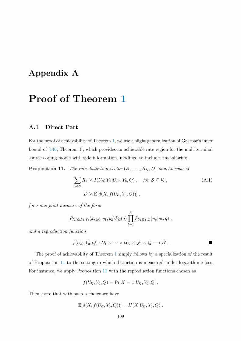
Appendix A
Proof of Theorem 1
A.1 Direct Part
For the proof of achievability of Theorem 1, we use a slight generalization of Gastpar’s inner
bound of [146, Theorem 1], which provides an achievable rate region for the multiterminal
source coding model with side information, modified to include time-sharing.
Proposition 11. The rate-distortion vector (R1, . . . , RK , D) is achievable if
∑
k∈SRk ≥ I(US ;YS |USc , Y0, Q) , for S ⊆ K , (A.1)
D ≥ E[d(X, f(UK, Y0, Q))] ,
for some joint measure of the form
PX,Y0,Y1,Y2(x, y0, y1, y2)PQ(q)K∏
k=1
PUk|Yk,Q(uk|yk, q) ,
and a reproduction function
f(UK, Y0, Q) : U1 × · · · × UK × Y0 ×Q −→ X .
The proof of achievability of Theorem 1 simply follows by a specialization of the result
of Proposition 11 to the setting in which distortion is measured under logarithmic loss.
For instance, we apply Proposition 11 with the reproduction functions chosen as
f(UK, Y0, Q) = Pr[X = x|UK, Y0, Q] .
Then, note that with such a choice we have
E[d(X, f(UK, Y0, Q))] = H(X|UK, Y0, Q) .
109

APPENDIX A. PROOF OF THEOREM 1
The resulting region can be shown to be equivalent to that given in Theorem 1 using
supermodular optimization arguments. The proof is along the lines of that of [10, Lemma
5] and is omitted for brevity.
A.2 Converse Part
We first state the following lemma, which is an easy extension of that of [10, Lemma 1]
to the case in which the decoder also observes statistically dependent side information.
The proof of Lemma 8 follows along the lines of that of [10, Lemma 1], and is therefore
omitted for brevity.
Lemma 8. Let T := (φ(n)1 (Y n
1 ), . . . , φ(n)K (Y n
K)). Then for the CEO problem of Figure 1.1
under logarithmic loss, we have nE[d(n)(Xn, Xn)] ≥ H(Xn|T, Y n0 ).
Let S be a non-empty set of K and Jk := φ(n)k (Y n
k ) be the message sent by Encoder k,
k ∈ K, where φ(n)k Kk=1 are the encoding functions corresponding to a scheme that achieves
(R1, . . . , RK , D).
Define, for i = 1, . . . , n, the following random variables
Uk,i := (Jk, Yi−1k ) , Qi := (X i−1, Xn
i+1, Yi−1
0 , Y n0,i+1) . (A.2)
We can lower bound the distortion D as
nD(a)
≥ H(Xn|JK, Y n0 )
=n∑
i=1
H(Xi|JK, X i−1, Y n0 )
(b)
≥n∑
i=1
H(Xi|JK, X i−1, Xni+1, Y
i−1K , Y n
0 )
=n∑
i=1
H(Xi|JK, X i−1, Xni+1, Y
i−1K , Y i−1
0 , Y0,i, Yn
0,i+1)
(c)=
n∑
i=1
H(Xi|UK,i, Y0,i, Qi) , (A.3)
where (a) follows due to Lemma 8; (b) holds since conditioning reduces entropy; and (c)
follows by substituting using (A.2).
110
APPENDIX A. PROOF OF THEOREM 1
Now, we lower bound the rate term as
n∑
k∈SRk
≥∑
k∈SH(Jk) ≥ H(JS) ≥ H(JS |JSc , Y n
0 ) ≥ I(JS ;Xn, Y nS |JSc , Y n
0 )
= I(JS ;Xn|JSc , Y n0 ) + I(JS ;Y n
S |Xn, JSc , Yn
0 )
= H(Xn|JSc , Y n0 )−H(Xn|JK, Y n
0 ) + I(JS ;Y nS |Xn, JSc , Y
n0 )
(a)
≥ H(Xn|JSc , Y n0 )− nD + I(JS ;Y n
S |Xn, JSc , Yn
0 )
=n∑
i=1
H(Xi|JSc , X i−1, Y n0 )− nD + I(JS ;Y n
S |Xn, JSc , Yn
0 )
(b)
≥n∑
i=1
H(Xi|JSc , X i−1, Xni+1, Y
i−1Sc , Y n
0 )− nD + I(JS ;Y nS |Xn, JSc , Y
n0 )
=n∑
i=1
H(Xi|JSc , X i−1, Xni+1, Y
i−1Sc , Y i−1
0 , Y0,i, Yn
0,i+1)− nD + I(JS ;Y nS |Xn, JSc , Y
n0 )
(c)=
n∑
i=1
H(Xi|USc,i, Y0,i, Qi)− nD + Θ , (A.4)
where (a) follows due to Lemma 8; (b) holds since conditioning reduces entropy; and (c)
follows by substituting using (A.2) and Θ := I(JS ;Y nS |Xn, JSc , Y n
0 ).
To continue with lower-bounding the rate term, we single-letterize the term Θ as
Θ = I(JS ;Y nS |Xn, JSc , Y
n0 )
(a)
≥∑
k∈SI(Jk;Y
nk |Xn, Y n
0 )
=∑
k∈S
n∑
i=1
I(Jk;Yk,i|Y i−1k , Xn, Y n
0 )
(b)=∑
k∈S
n∑
i=1
I(Jk, Yi−1k ;Yk,i|Xn, Y n
0 )
=∑
k∈S
n∑
i=1
I(Jk, Yi−1k ;Yk,i|X i−1, Xi, X
ni+1, Y
i−10 , Y0,i, Y
n0,i+1)
(c)=∑
k∈S
n∑
i=1
I(Uk,i;Yk,i|Xi, Y0,i, Qi) , (A.5)
where (a) follows due to the Markov chain Jk−−Y nk −− (Xn, Y n
0 )−−Y nS\k−−JS\k, k ∈ K; (b)
follows due to the Markov chain Yk,i −− (Xn, Y n0 )−− Y i−1
k ; and (c) follows by substituting
using (A.2).
111

APPENDIX A. PROOF OF THEOREM 1
Then, combining (A.4) and (A.5), we get
n∑
k∈SRk ≥
n∑
i=1
H(Xi|USc,i, Y0,i, Qi)− nD +∑
k∈S
n∑
i=1
I(Uk,i;Yk,i|Xi, Y0,i, Qi) . (A.6)
Summarizing, we have from (A.3) and (A.6)
nD ≥n∑
i=1
H(Xi|UK,i, Y0,i, Qi)
nD + n∑
k∈SRk ≥
n∑
i=1
H(Xi|USc,i, Y0,i, Qi) +∑
k∈S
n∑
i=1
I(Uk,i;Yk,i|Xi, Y0,i, Qi) .
We note that the random variables UK,i satisfy the Markov chain Uk,i −− Yk,i −−Xi −−YK\k,i −− UK\k,i, k ∈ K. Finally, a standard time-sharing argument completes the proof.
112
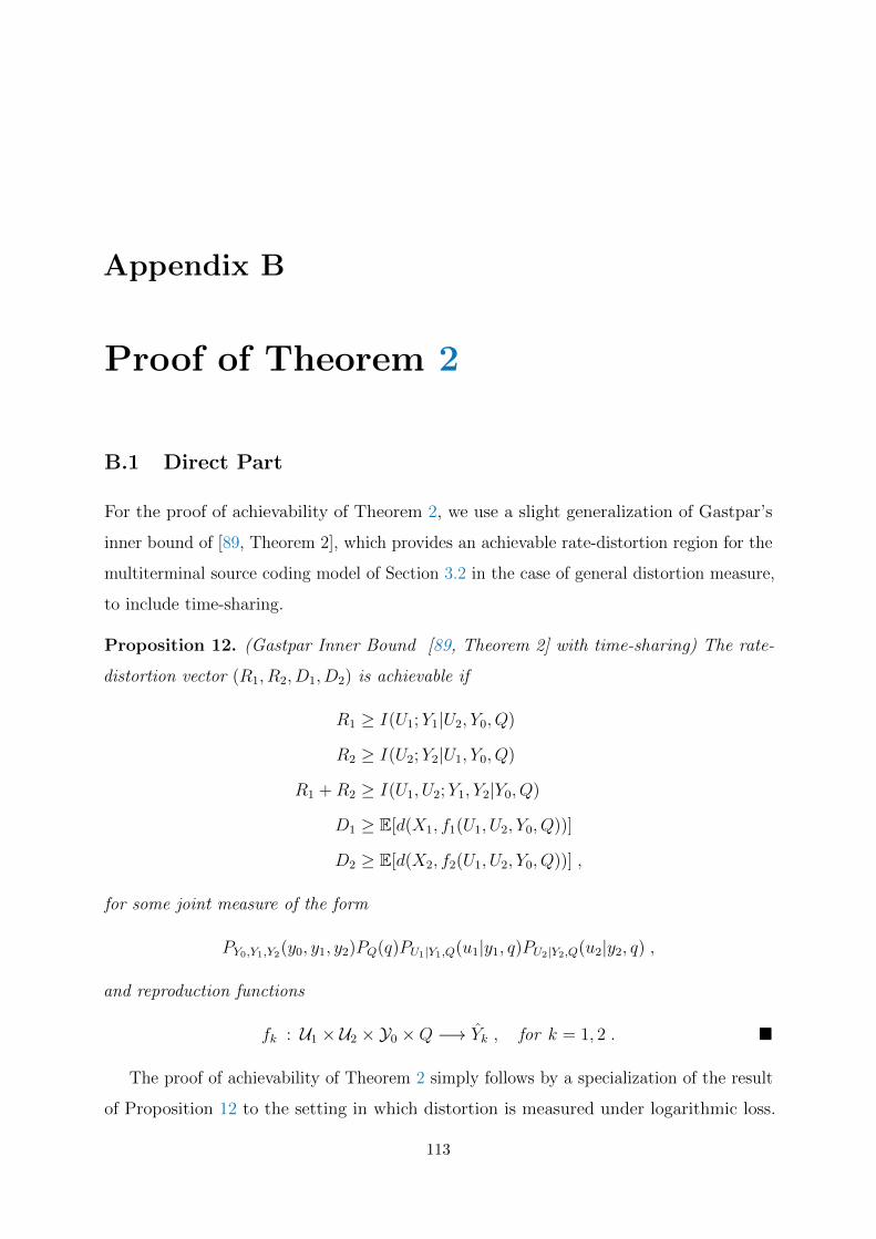
Appendix B
Proof of Theorem 2
B.1 Direct Part
For the proof of achievability of Theorem 2, we use a slight generalization of Gastpar’s
inner bound of [89, Theorem 2], which provides an achievable rate-distortion region for the
multiterminal source coding model of Section 3.2 in the case of general distortion measure,
to include time-sharing.
Proposition 12. (Gastpar Inner Bound [89, Theorem 2] with time-sharing) The rate-
distortion vector (R1, R2, D1, D2) is achievable if
R1 ≥ I(U1;Y1|U2, Y0, Q)
R2 ≥ I(U2;Y2|U1, Y0, Q)
R1 +R2 ≥ I(U1, U2;Y1, Y2|Y0, Q)
D1 ≥ E[d(X1, f1(U1, U2, Y0, Q))]
D2 ≥ E[d(X2, f2(U1, U2, Y0, Q))] ,
for some joint measure of the form
PY0,Y1,Y2(y0, y1, y2)PQ(q)PU1|Y1,Q(u1|y1, q)PU2|Y2,Q(u2|y2, q) ,
and reproduction functions
fk : U1 × U2 × Y0 ×Q −→ Yk , for k = 1, 2 .
The proof of achievability of Theorem 2 simply follows by a specialization of the result
of Proposition 12 to the setting in which distortion is measured under logarithmic loss.
113
APPENDIX B. PROOF OF THEOREM 2
For instance, we apply Proposition 12 with the reproduction functions chosen as
fk(U1, U2, Y0, Q) := Pr[Yk = yk|U1, U2, Y0, Q] , for k = 1, 2 .
Then, note that with such a choice we have
E[d(Yk, fk(U1, U2, Y0, Q)] = H(Yk|U1, U2, Y0, Q) , for k = 1, 2 .
B.2 Converse Part
We first state the following lemma, which is an easy extension of that of [10, Lemma 1]
to the case in which the decoder also observes statistically dependent side information.
The proof of Lemma 9 follows along the lines of that of [10, Lemma 1], and is therefore
omitted for brevity.
Lemma 9. Let T := (φ(n)1 (Y n
1 ), φ(n)2 (Y n
2 )). Then, for the multiterminal source coding
problem under logarithmic loss measure we have nE[d(Y nk , Y
nk )] ≥ H(Y n
k |T, Y n0 ) for k = 1, 2.
The proof of converse of Theorem 2 follows by Lemma 10 and Lemma 11 below, the
proofs of which follow relatively straightforwardly those in the proof of [10, Theorem 12].
Lemma 10. If a rate-distortion quadruple (R1, R2, D1, D2) is achievable for the model
of Section 3.2, then there exist a joint measure
PY0,Y1,Y2(y0, y1, y2)PQ(q)PU1|Y1,Q(u1|y1, q)PU2|Y2,Q(u2|y2, q) , (B.1)
and a D1 ≤ D1 which satisfies
D1 ≥ H(X1|U1, U2, Y,Q) (B.2a)
D2 ≥ D1 +H(X2|U1, U2, Y,Q)−H(X1|U1, U2, Y,Q) , (B.2b)
and
R1 ≥ H(Y1|U2, Y0, Q)−D1 (B.3a)
R2 ≥ I(U2;Y2|Y1, Y0, Q) +H(Y1|U1, Y0, Q)−D1 (B.3b)
R1 +R2 ≥ I(U2;Y2|Y1, Y0, Q) +H(Y1|Y0)−D1 . (B.3c)
114

APPENDIX B. PROOF OF THEOREM 2
Proof. Let J1 := φ(n)1 (Y n
1 ) and J2 := φ(n)2 (Y n
2 ), where the φ(n)1 and φ
(n)2 are the encoding
functions corresponding to a scheme that achieves (R1, R2, D1, D2). Define
D1 :=1
nH(Y n
1 |J1, J2, Yn
0 ) .
Also, define, for i = 1, . . . , n, the following random variables
U1,i := J1 , U2,i := (J2, Yn
2,i+1) , Qi := (Y i−11 , Y n
2,i+1, Yi−1
0 , Y n0,i+1) . (B.4)
First, note that by Lemma 9 we have nD1 ≥ H(Y n1 |J1, J2, Y
n0 ); and, so, D1 ≤ D1. Also,
we have
nD1 =n∑
i=1
H(Y1,i|J1, J2, Yi−1
1 , Y n0 )
(a)
≥n∑
i=1
H(Y1,i|J1, J2, Yi−1
1 , Y n2,i+1, Y
n0 )
=n∑
i=1
H(Y1,i|J1, J2, Yi−1
1 , Y n2,i+1, Y
i−10 , Y0,i, Y
n0,i+1)
(b)=
n∑
i=1
H(X1,i|U1,i, U2,i, Y0,i, Qi) ,
where (a) holds since conditioning reduces entropy; and (b) follows by substituting us-
ing (B.4).
We can lower bound the distortion D2 as
nD2 ≥ H(Y n2 |J1, J2, Y
n0 )
= H(Y n1 |J1, J2, Y
n0 ) + [H(Y n
2 |J1, J2, Yn
0 )−H(Y n1 |J1, J2, Y
n0 )]
= nD1 + Θ , (B.5)
where Θ := H(Y n2 |J1, J2, Y
n0 )−H(Y n
1 |J1, J2, Yn
0 ).
To continue with lower-bounding the distortion D2, we single-letterize the term Θ as
Θ =H(Y n2 |J1, J2, Y
n0 )−H(Y n
1 |J1, J2, Yn
0 )
=n∑
i=1
H(Y2,i|J1, J2, Yn
2,i+1, Yn
0 )−H(Y1,i|J1, J2, Yi−1
1 , Y n0 )
=n∑
i=1
I(Y i−11 ;Y2,i|J1, J2, Y
n2,i+1, Y
n0 ) +H(Y2,i|J1, J2, Y
i−11 , Y n
2,i+1, Yn
0 )
−n∑
i=1
I(Y n2,i+1;Y1,i|J1, J2, Y
i−11 , Y n
0 ) +H(Y1,i|J1, J2, Yi−1
1 , Y n2,i+1, Y
n0 )
115

APPENDIX B. PROOF OF THEOREM 2
(a)=
n∑
i=1
H(Y2,i|J1, J2, Yi−1
1 , Y n2,i+1, Y
n0 )−H(Y1,i|J1, J2, Y
i−11 , Y n
2,i+1, Yn
0 ) , (B.6)
where (a) follows by the Csiszar-Korner sum-identity
n∑
i=1
I(Y i−11 ;Y2,i|J1, J2, Y
n2,i+1, Y
n0 ) =
n∑
i=1
I(Y n2,i+1;Y1,i|J1, J2, Y
i−11 , Y n
0 ) .
Then, combining (B.5) and (B.6), we get
nD2 ≥ nD1 +n∑
i=1
H(Y2,i|J1, J2, Yi−1
1 , Y n2,i+1, Y
n0 )−H(Y1,i|J1, J2, Y
i−11 , Y n
2,i+1, Yn
0 )
= nD1 +n∑
i=1
H(Y2,i|J1, J2, Yi−1
1 , Y n2,i+1, Y
i−10 , Y0,i, Y
n0,i+1)
−H(Y1,i|J1, J2, Yi−1
1 , Y n2,i+1, Y
i−10 , Y0,i, Y
n0,i+1)
= nD1 +n∑
i=1
H(Y2,i|U1,i, U2,i, Y0,i, Qi)−H(Y1,i|U1,i, U2,i, Y0,i, Qi) ,
where the last equality follows by substituting using (B.4).
Rate R1 can be bounded easily as
nR1 ≥ H(J1) ≥ H(J1|J2, Yn
0 ) ≥ I(J1;Y n1 |J2, Y
n0 ) = H(Y n
1 |J2, Yn
0 )− nD1
=n∑
i=1
H(Y1,i|J2, Yn
1,i+1, Yn
0 )− nD1
(a)
≥n∑
i=1
H(Y1,i|J2, Yn
1,i+1, Yn
2,i+1, Yn
0 )− nD1
(b)=
n∑
i=1
H(Y1,i|J2, Yn
2,i+1, Yi−1
0 , Y0,i, Yn
0,i+1)− nD1
(c)
≥n∑
i=1
H(Y1,i|J2, Yi−1
1 , Y n2,i+1, Y
i−10 , Y0,i, Y
n0,i+1)− nD1
(d)=
n∑
i=1
H(Y1,i|U2,i, Y0,i, Qi)− nD1 ,
where (a) holds since conditioning reduces entropy; (b) follows since Y1,i−−(J2, Yn
2,i+1, Yn
0 )−− Y n
1,i+1 forms a Markov chain; (c) holds since conditioning reduces entropy; and (d)
follows by substituting using (B.4).
116

APPENDIX B. PROOF OF THEOREM 2
Now, we lower bound the rate R2 as
nR2 ≥ H(J2) ≥ H(J2|J1, Yn
0 ) = H(J2|J1, Yn
1 , Yn
0 ) + I(J2;Y n1 |J1, Y
n0 )
≥ I(J2;Y n2 |J1, Y
n1 , Y
n0 ) + I(J2;Y n
1 |J1, Yn
0 )
= I(J2;Y n2 |J1, Y
n1 , Y
n0 ) +H(Y n
1 |J1, Yn
0 )− nD1
(a)= I(J2;Y n
2 |Y n1 , Y
n0 ) +H(Y n
1 |J1, Yn
0 )− nD1
=n∑
i=1
I(J2;Y2,i|Y n1 , Y
n2,i+1, Y
n0 ) +H(Y1,i|J1, Y
i−11 , Y n
0 )− nD1
(b)
≥n∑
i=1
I(J2;Y2,i|Y n1 , Y
n2,i+1, Y
n0 ) +H(Y1,i|J1, Y
i−11 , Y n
2,i+1, Yn
0 )− nD1
(c)=
n∑
i=1
I(J2, Yn
1,i+1;Y2,i|Y i−11 , Y1,i, Y
n2,i+1, Y
n0 ) +H(Y1,i|J1, Y
i−11 , Y n
2,i+1, Yn
0 )− nD1
=n∑
i=1
I(J2, Yn
1,i+1, Yn
2,i+1;Y2,i|Y i−11 , Y1,i, Y
n2,i+1, Y
n0 ) +H(Y1,i|J1, Y
i−11 , Y n
2,i+1, Yn
0 )− nD1
(d)
≥n∑
i=1
I(J2, Yn
2,i+1;Y2,i|Y i−11 , Y1,i, Y
n2,i+1, Y
n0 ) +H(Y1,i|J1, Y
i−11 , Y n
2,i+1, Yn
0 )− nD1
(e)=
n∑
i=1
I(U2,i;Y2,i|Y1,i, Y0,i, Qi) +H(Y1,i|U1,i, Y0,i, Qi)− nD1 ,
where (a) holds since J1 is a deterministic function of Y n1 ; (b) holds since conditioning
reduces the entropy; (c) follows since Y n1,i+1−− (Y i−1
1 , Y1,i, Yn
2,i+1, Yn
0 )−−Y2,i forms a Markov
chain; (d) follows since conditioning reduces the entropy; and (e) follows by substituting
using (B.4).
The sum-rate R1 +R2 can be lower bounded similarly, as
n(R1 +R2) ≥ H(J1) +H(J2)
≥ H(J1|J2, Yn
0 ) +H(J2|Y n0 )
≥ I(J1;Y n1 |J2, Y
n0 ) + I(J2;Y n
1 , Yn
2 |Y n0 )
= I(J1;Y n1 |J2, Y
n0 ) + I(J2;Y n
1 |Y n0 ) + I(J2;Y n
2 |Y n1 , Y
n0 )
= I(J1, J2;Y n1 |Y n
0 ) + I(J2;Y n2 |Y n
1 , Yn
0 )
= H(Y n1 |Y n
0 )− nD1 + I(J2;Y n2 |Y n
1 , Yn
0 )
(a)=
n∑
i=1
I(J2;Y2,i|Y n1 , Y
n2,i+1, Y
n0 ) +H(Y1,i|Y0,i)− nD1
117

APPENDIX B. PROOF OF THEOREM 2
(b)=
n∑
i=1
I(J2, Yn
1,i+1;Y2,i|Y i−11 , Y1,i, Y
n2,i+1, Y
n0 ) +H(Y1,i|Y0,i)− nD1
=n∑
i=1
I(J2, Yn
1,i+1, Yn
2,i+1;Y2,i|Y i−11 , Y1,i, Y
n2,i+1, Y
n0 ) +H(Y1,i|Y0,i)− nD1
(c)
≥n∑
i=1
I(J2, Yn
2,i+1;Y2,i|Y i−11 , Y1,i, Y
n2,i+1, Y
n0 ) +H(Y1,i|Y0,i)− nD1
(d)=
n∑
i=1
I(U2,i;Y2,i|Y1,i, Y0,i, Qi) +H(Y1,i|Y0,i)− nD1 ,
where (a) follows since the source (Y n0 , Y
n1 , Y
n2 ) is memoryless; (b) follows since Y n
1,i+1 −−(Y i−1
1 , Y1,i, Yn
2,i+1, Yn
0 )−− Y2,i forms a Markov chain; (c) holds since conditioning reduces
the entropy; and (d) follows by substituting using (B.4).
Summarizing, the distortion pair (D1, D2) satisfies
D1 ≥1
n
n∑
i=1
H(X1,i|U1,i, U2,i, Y0,i, Qi)
D2 ≥ D1 +1
n
n∑
i=1
H(Y2,i|U1,i, U2,i, Y0,i, Qi)−H(Y1,i|U1,i, U2,i, Y0,i, Qi) ,
and the rate pair (R1, R2) satisfies
R1 ≥1
n
n∑
i=1
H(Y1,i|U2,i, Y0,i, Qi)−D1
R2 ≥1
n
n∑
i=1
I(U2,i;Y2,i|Y1,i, Y0,i, Qi) +H(Y1,i|U1,i, Y0,i, Qi)−D1
R1 +R2 ≥1
n
n∑
i=1
I(U2,i;Y2,i|Y1,i, Y0,i, Qi) +H(Y1,i|Y0,i)−D1 .
It is easy to see that the random variables (U1,i, U2,i, Qi) satisfy that U1,i −− (Y1,i, Qi)−− (Y0,i, Y2,i, U2,i) and U2,i −− (X2,i, Qi)−− (Y0,i, Y1,i, U1,i) form Markov chains. Finally, a
standard time-sharing argument proves Lemma 10.
The rest of the proof of converse of Theorem 2 follows using the following lemma, the
proof of which is along the lines of that of [10, Lemma 9] and is omitted for brevity.
Lemma 11. Let a rate-distortion quadruple (R1, R2, D1, D2) be given. If there exists a
joint measure of the form (B.1) such that (B.2) and (B.3) are satisfied, then the rate-
distortion quadruple (R1, R2, D1, D2) is in the region described by Theorem 2.
118
Appendix C
Proof of Proposition 3
We start with the proof of the direct part. Let a non-negative tuple (R1, . . . , RK , E) ∈ RHT
be given. Since RHT = R? , then there must exist a series of non-negative tuples
(R(m)1 , . . . , R
(m)K , E(m))m∈N such that
(R(m)1 , . . . , R
(m)K , E(m)) ∈ R? , for all m ∈ N, and (C.1a)
limm→∞
(R(m)1 , . . . , R
(m)K , E(m)) = (R1, . . . , RK , E) . (C.1b)
Fix δ′ > 0. Then, ∃ m0 ∈ N such that for all m ≥ m0, we have
Rk ≥ R(m)k − δ′ , for k = 1, . . . , K , (C.2a)
E ≤ E(m) + δ′ . (C.2b)
For m ≥ m0, there exist a series nmm∈N and functions φ(nm)k k∈K such that
R(m)k ≥ 1
nmlog |φ(nm)
k | , for k = 1, . . . , K , (C.3a)
E(m) ≤ 1
nmI(φ(nm)
k (Y nmk )k∈K;Xnm|Y nm
0 ) . (C.3b)
Combining (C.2) and (C.3) we get that for all m ≥ m0,
Rk ≥1
nmlog |φ(nm)
k (Y nmk )| − δ′ , for k = 1, . . . , K , (C.4a)
E ≤ 1
nmI(φ(nm)
k (Y nmk )k∈K;Xnm|Y nm
0 ) + δ′ . (C.4b)
The second inequality of (C.4) implies that
H(Xnm|φ(nm)k (Y nm
k )k∈K, Y nm0 ) ≤ nm(H(X|Y0)− E) + nmδ
′ . (C.5)
119

APPENDIX C. PROOF OF PROPOSITION 3
Now, consider the K-encoder CEO source coding problem of Figure 3.1; and let the
encoding function φ(nm)k at Encoder k ∈ K be such that φ
(nm)k := φ
(nm)k . Also, let the
decoding function at the decoder be
ψ(nm) : 1, . . . ,M (nm)1 × . . .× 1, . . . ,M (nm)
K × Ynm0 −→ X nm (C.6)
(m1, . . . ,mK , ynm0 ) −→ p(xnm|m1, . . . ,mK , y
nm0 ) . (C.7)
With such a choice, the achieved average logarithmic loss distortion is
E[d(nm)(Xnm , ψ(nm)(φ(nm)k (Y nm
k )k∈K, Y nm0 ))] =
1
nmH(Xnm|φ(nm)
k (Y nmk )k∈K, Y nm
0 ) .
(C.8)
Combined with (C.5), the last equality implies that
E[d(nm)(Xnm , ψ(nm)(φ(nm)k (Y
(nm)k )k∈K, Y nm
0 ))] ≤ nm(H(X|Y0)− E) + δ′ . (C.9)
Finally, substituting φ(nm)k with φ
(nm)k in (C.4), and observing that δ′ can be chosen
arbitrarily small in the obtained set of inequalities as well as in (C.9), it follows that
(R1, . . . , RK , H(X|Y0)− E) ∈ RD?CEO.
We now show the reverse implication. Let a non-negative tuple (R1, . . . , RK , H(X|Y0)−E) ∈ RD?CEO be given. Then, there exist encoding functions φ(n)k∈K and a decoding
function ψ(n) such that
Rk ≥1
nlog |φ(n)
k (Y nk )| , for k = 1, . . . , K , (C.10a)
H(X|Y0)− E ≥ E[d(n)(Xn, ψ(n)(φ(n)k (X
(n)k )k∈K, Y n
0 ))] . (C.10b)
Using Lemma 8 (see the proof of converse of Theorem 1 in Appendix A), the RHS of the
second inequality of (C.10) can be lower-bounded as
E[d(n)(Xn, ψ(n)(φ(n)k (X
(n)k )k∈K, Y n
0 ))] ≥ 1
nH(Xn|φ(n)
k (X(n)k )k∈K, Y n
0 ) . (C.11)
Combining the second inequality of (C.10) and (C.11), we get
H(Xn|ψ(n)(φ(n)k (X
(n)k )k∈K, Y n
0 )) ≤ n(H(X|Y0)− E) , (C.12)
from which it holds that
120

APPENDIX C. PROOF OF PROPOSITION 3
I(φ(n)k (X
(n)k )k∈K;Xn|Y n
0 ) = nH(X|Y0)−H(Xn|ψ(n)(φ(n)k (X
(n)k )k∈K, Y n
0 )) (C.13a)
≥ nE , (C.13b)
where the equality follows since (Xn, Y n0 ) is memoryless and the inequality follows by
using (C.12).
Now, using the first inequality of (C.10) and (C.13), it follows that (R1, . . . , RK , E) ∈R?(n, φ(n)
k k∈K)
. Finally, using Proposition 2, it follows that (R1, . . . , RK , E) ∈ RHT;
and this concludes the proof of the reverse part and the proposition.
121

122

Appendix D
Proof of Proposition 4
First let us define the rate-information region RI?CEO for discrete memoryless vector
sources as the closure of all rate-information tuples (R1, . . . , RK ,∆) for which there exist
a blocklength n, encoding functions φ(n)k Kk=1 and a decoding function ψ(n) such that
Rk ≥1
nlogM
(n)k , for k = 1, . . . , K ,
∆ ≤ 1
nI(Xn;ψ(n)(φ
(n)1 (Yn
1 ), . . . , φ(n)K (Yn
K),Yn0 )) .
It is easy to see that a characterization of RI?CEO can be obtained by using Theorem 1
and substituting distortion levels D therein with ∆ := H(X)−D. More specifically, the
region RI?CEO is given as in the following theorem.
Proposition 13. The rate-information region RI?CEO of the vector DM CEO problem
under logarithmic loss is given by the set of all non-negative tuples (R1, . . . , RK ,∆) that
satisfy, for all subsets S ⊆ K,
∑
k∈SRk ≥
∑
k∈SI(Yk;Uk|X,Y0, Q)− I(X;USc ,Y0, Q) + ∆ ,
for some joint measure of the form PY0,YK,X(y0,yK,x)PQ(q)∏K
k=1 PUk|Yk,Q(uk|yk, q).
The region RI?CEO involves mutual information terms only (not entropies); and, so,
using a standard discretization argument, it can be easily shown that a characterization of
this region in the case of continuous alphabets is also given by Proposition 13.
Let us now return to the vector Gaussian CEO problem under logarithmic loss that
we study in this section. First, we state the following lemma, whose proof is easy and is
omitted for brevity.
123

APPENDIX D. PROOF OF PROPOSITION 4
Lemma 12. (R1, . . . , RK , D) ∈ RD?VG-CEO if and only if (R1, . . . , RK , h(X) − D) ∈RI?CEO.
For vector Gaussian sources, the region RD?VG-CEO can be characterized using Proposi-
tion 13 and Lemma 12. This completes the proof of first equality RD?VG-CEO = RDI
CEO.
To complete the proof of Proposition 4, we need to show that two regions are equivalent,
i.e., RDI
CEO = RDII
CEO. To do that, it is sufficient to show that, for fixed conditional
distributions p(uk|yk, q)Kk=1, the extreme points of the polytope PD defined by (4.5) are
dominated by points that are in RDII
CEO that achieves distortion at most D. This is shown
in the proof of Proposition 5 in Appendix F.
124
Appendix E
Proof of Converse of Theorem 4
The proof of the converse of Theorem 4 relies on deriving an outer bound on the region
RDI
CEO given by Proposition 4. In doing so, we use the technique of [11, Theorem 8]
which relies on the de Bruijn identity and the properties of Fisher information; and extend
the argument to account for the time-sharing variable Q and side information Y0.
We first state the following lemma.
Lemma 13. [11, 147] Let (X,Y) be a pair of random vectors with pmf p(x,y). We have
log |(πe)J−1(X|Y)| ≤ h(X|Y) ≤ log |(πe)mmse(X|Y)| ,
where the conditional Fisher information matrix is defined as
J(X|Y) := E[∇ log p(X|Y)∇ log p(X|Y)†] ,
and the minimum mean squared error (MMSE) matrix is
mmse(X|Y) := E[(X− E[X|Y])(X− E[X|Y])†] .
Now, we derive an outer bound on (4.5) as follows. For each q ∈ Q and fixed pmf∏K
k=1 p(uk|yk, q), choose Ωk,qKk=1 satisfying 0 Ωk,q Σ−1k such that
mmse(Yk|X, Uk,q,Y0, q) = Σk −ΣkΩk,qΣk . (E.1)
Such Ωk,q always exists since, for all q ∈ Q, k ∈ K, we have
0 mmse(Yk|X, Uk,q,Y0, q) Σyk|(x,y0) = Σnk|n0 = Σk .
125
APPENDIX E. PROOF OF CONVERSE OF THEOREM 4
Then, for k ∈ K and q ∈ Q, we have
I(Yk;Uk|X,Y0, Q = q) = h(Yk|X,Y0, Q = q)− h(Yk|X, Uk,q,Y0, Q = q)
(a)
≥ log |(πe)Σk| − log |(πe)mmse(Yk|X, Uk,q,Y0, Q = q)|(b)= − log |I−Ωk,qΣk| , (E.2)
where (a) is due to Lemma 13; and (b) is due to (E.1).
For convenience, the matrix ΛS,q is defined as follows
ΛS,q :=
0 0
0 diag(Σk −ΣkΩk,qΣkk∈Sc)
. (E.3)
Then, for q ∈ Q and S ⊆ K, we have
h(X|USc,q,Y0, Q = q)(a)
≥ log |(πe)J−1(X|USc,q,Y0, q)|(b)= log
∣∣∣∣(πe)(Σ−1
x + H†SΣ−1nS
(I−ΛS,qΣ
−1nS
)HS
)−1∣∣∣∣ , (E.4)
where (a) follows from Lemma 13; and for (b), we use the connection of the MMSE and
the Fisher information to show the following equality
J(X|USc,q,Y0, q) = Σ−1x + H†SΣ
−1nS
(I−ΛS,qΣ
−1nS
)HS . (E.5)
In order to proof (E.5), we use de Bruijn identity to relate the Fisher information with
the MMSE as given in the following lemma.
Lemma 14. [11, 148] Let (V1,V2) be a random vector with finite second moments and
Z ∼ CN (0,Σz) independent of (V1,V2). Then
mmse(V2|V1,V2 + Z) = Σz −ΣzJ(V2 + Z|V1)Σz .
From MMSE estimation of Gaussian random vectors, for S ⊆ K, we have
X = E[X|YS ] + WS = GSYS + WS , (E.6)
where GS := ΣwSH†SΣ−1nS
, and WS ∼ CN (0,ΣwS ) is a Gaussian vector that is independent
of YS and
Σ−1wS
:= Σ−1x + H†SΣ
−1nS
HS . (E.7)
126

APPENDIX E. PROOF OF CONVERSE OF THEOREM 4
Now we show that the cross-terms of mmse (YSc |X, USc,q,Y0, q) are zero (similarly to [11,
Appendix V]). For i ∈ Sc and j 6= i, we have
E[(Yi − E[Yi|X, USc,q,Y0, q])(Yj − E[Yj|X, USc,q,Y0, q])
†]
(a)= E
[E[(Yi − E[Yi|X, USc,q,Y0, q])(Yj − E[Yj|X, USc,q,Y0, q])
†|X,Y0
]]
(b)= E
[E[(Yi − E[Yi|X, USc,q,Y0, q])|X,Y0
]E[(Yj − E[Yj|X, USc,q,Y0, q])
†|X,Y0
]]
= 0 , (E.8)
where (a) is due to the law of total expectation; (b) is due to the Markov chain Yk −−(X,Y0)−−YK\k.
Then, for k ∈ K and q ∈ Q, we have
mmse(GSYS
∣∣X, USc,q,Y0, q)
= GS mmse (YS |X, USc,q,Y0, q) G†S
(a)= GS
0 0
0 diag(mmse(Yk|X, USc,q,Y0, q)k∈Sc)
G†S
(b)= GSΛS,qG
†S , (E.9)
where (a) follows since the cross-terms are zero as shown in (E.8); and (b) follows due
to (E.1) and the definition of ΛS,q given in (E.3).
Finally, we obtain the equality (E.5) by applying Lemma 14 and noting (E.6) as follows
J(X|USc,q,Y0, q)(a)= Σ−1
wS−Σ−1
wSmmse
(GSYS
∣∣X, USc,q,Y0, q)Σ−1
wS
(b)= Σ−1
wS−Σ−1
wSGSΛS,qG
†SΣ−1wS
(c)= Σ−1
x + H†SΣ−1nS
HS −H†SΣ−1nS
ΛS,qΣ−1nS
HS
= Σ−1x + H†SΣ
−1nS
(I−ΛS,qΣ
−1nS
)HS ,
where (a) is due to Lemma 14; (b) is due to (E.9); and (c) follows due to the definitions of
Σ−1wS
and GS .
127
APPENDIX E. PROOF OF CONVERSE OF THEOREM 4
Next, we average (E.2) and (E.4) over the time-sharingQ and letting Ωk :=∑
q∈Q p(q)Ωk,q,
we obtain the lower bound
I(Yk; Uk|X,Y0, Q) =∑
q∈Qp(q)I(Yk; Uk|X,Y0, Q = q)
(a)
≥ −∑
q∈Qp(q) log |I−Ωk,qΣk|
(b)
≥ − log |I−∑
q∈Qp(q)Ωk,qΣk|
= − log |I−ΩkΣk| , (E.10)
where (a) follows from (E.2); and (b) follows from the concavity of the log-determinant
function and Jensen’s Inequality.
Besides, we can derive the following lower bound
h(X|USc ,Y0, Q) =∑
q∈Qp(q)h(X|USc,q,Y0, Q = q)
(a)
≥∑
q∈Qp(q) log
∣∣∣∣(πe)(Σ−1
x + H†SΣ−1nS
(I−ΛS,qΣ
−1nS
)HS
)−1∣∣∣∣
(b)
≥ log
∣∣∣∣(πe)(Σ−1
x + H†SΣ−1nS
(I−ΛSΣ
−1nS
)HS
)−1∣∣∣∣ , (E.11)
where (a) is due to (E.4); and (b) is due to the concavity of the log-determinant function
and Jensen’s inequality and the definition of ΛS given in (4.7).
Finally, the outer bound on RDI
CEO is obtained by applying (E.10) and (E.11) in (4.5),
noting that Ωk =∑
q∈Q p(q)Ωk,q Σ−1k since 0 Ωk,q Σ−1
k , and taking the union over
Ωk satisfying 0 Ωk Σ−1k .
128
Appendix F
Proof of Proposition 5
(Extension to K Encoders)
For the proof of Proposition 5, it is sufficient to show that, for fixed Gaussian distributions
p(uk|yk)Kk=1, the extreme points of the polytope PD defined by (4.5) are dominated by
points that are in RDII
CEO and which are achievable using Gaussian conditional distributions
p(vk|yk, q′)Kk=1. The proof is similar to [10, Appendix C, Lemma 6].
First, we characterize the extreme points of PD. Let the function f : 2K → R be such that
for all S ⊆ K,
f(S) = I(YS ;US |USc ,Y0, Q) + h(X|U1, . . . , UK ,Y0, Q)−D . (F.1)
It is easy to see that f(·) and the function S → [f(S)]+ := maxf(S), 0 are supermodular
functions. Also, for all subsets S ⊆ K, we have
f(S) = I(YS ;US |USc ,Y0, Q) + h(X|U1, . . . , UK ,Y0, Q)−D
(a)= I(YS ,X;US |USc ,Y0, Q) + h(X|U1, . . . , UK ,Y0, Q)−D
= I(YS ;US |X, USc ,Y0, Q) + I(X;US |USc ,Y0, Q) + h(X|U1, . . . , UK ,Y0, Q)−D
= I(YS ;US |X, USc ,Y0, Q) + h(X|USc ,Y0, Q)− h(X|US , USc ,Y0, Q)
+ h(X|U1, . . . , UK ,Y0, Q)−D
(b)=∑
k∈SI(Yk;Uk|X,Y0, Q) + h(X|USc ,Y0, Q)−D , (F.2)
where (a) follows using the Markov chain US−−YS−−X; and (b) follows by using the chain
129

APPENDIX F. PROOF OF PROPOSITION 5 (EXTENSION TO K ENCODERS)
rule and the Markov chain (Uk,Yk)−− (X,Y0, Q)−− (UK\k,YK\k). Then, by construction,
we have that PD is given by the set of (R1, . . . , RK) that satisfy for all subsets S ⊆ K,
∑
k∈SRk ≥ [f(S)]+ .
Proceeding along the lines of [103, Appendix B], we have that for a linear ordering
i1 ≺ i2 ≺ · · · ≺ iK on the set K, an extreme point of PD can be computed as follows
Rik = [f(i1, i2, . . . , ik)]+ − [f(i1, i2, . . . , ik−1)]+ , for k = 1, . . . , K .
All the K! extreme points of PD can be enumerated by looking over all linear orderings
i1 ≺ i2 ≺ · · · ≺ iK of K. Each ordering of K is analyzed in the same manner and, therefore,
for notational simplicity, the only ordering we consider is the natural ordering, i.e., ik = k,
in the rest of the proof. Then, by construction, we have
Rk =[ k∑
i=1
I(Yi;Ui|X,Y0, Q) + h(X|UKk+1,Y0, Q)−D
]+
−[ k−1∑
i=1
I(Yi;Ui|X,Y0, Q) + h(X|UKk ,Y0, Q)−D
]+.
(F.3)
Let j be the first index for which f(1, 2, . . . , j) > 0. Then it follows from (F.3) that
Rj =
j∑
k=1
I(Yk;Uk|X,Y0, Q) + h(X|UKj+1,Y0, Q)−D
= I(Yj;Uj|X,Y0, Q) +
j−1∑
k=1
I(Xk;Uk|X,Y0, Q) + h(X|UKj+1,Y0, Q)−D
+ h(X|UKj ,Y0, Q)− h(X|Uj, UK
j+1,Y0, Q)
(a)= f(1, 2, . . . , j − 1) + I(Yj;Uj|X, UK
j+1,Y0, Q) + I(X;Uj|UKj+1,Y0, Q)
= f(1, 2, . . . , j − 1) + I(Yj,X;Uj|UKj+1,Y0, Q)
(b)= f(1, 2, . . . , j − 1) + I(Yj;Uj|UK
j+1,Y0, Q)
= (1− θ)I(Yj;Uj|UKj+1,Y0, Q) ,
where (a) follows due to the Markov chain Uj −−Yj −−X−− UK\j and (F.2); (b) follows
due to the Markov chain Uj −−Yj −−X; and θ ∈ (0, 1] is defined as
θ :=−f(1, 2, . . . , j − 1)I(Yj;Uj|UK
j+1,Y0, Q)=D − h(X|UK,Y0, Q)− I(Yj−1
1 ;U j−11 |UK
j ,Y0, Q)
I(Yj;Uj|UKj+1,Y0, Q)
. (F.4)
130

APPENDIX F. PROOF OF PROPOSITION 5 (EXTENSION TO K ENCODERS)
Furthermore, for all indices k > j, we have
Rk = f(1, 2, . . . , k)− f(1, 2, . . . , k − 1)
= I(Yk;Uk|X,Y0, Q) + I(X;Uk|UKk+1,Y0, Q)
(a)= I(Yk;Uk|X, UK
k+1,Y0, Q) + I(X;Uk|UKk+1,Y0, Q)
= I(Yk,X;Uk|UKk+1,Y0, Q)
(b)= I(Yk;Uk|UK
k+1,Y0, Q) ,
where (a) follows due to the Markov chain Uk −−Yk −−X−− UK\k; and (b) follows due
to the Markov chain Uk −−Yk −−X.
Therefore, for the natural ordering, the extreme point (R1, . . . , RK) is given as
(R1, . . . , RK) =
(0, . . . , 0, (1− θ)I(Yj;Uj|UK
j+1,Y0, Q), I(Yj+1;Uj+1|UKj+2,Y0, Q),
. . . , I(YK ;UK |Y0, Q)
).
Next, we show that (R1, . . . , RK) ∈ PD is dominated by a point (R1, . . . , RK , D) ∈RDII
CEO that achieves a distortion D ≤ D.
We consider an instance of the CEO setup in which for a fraction θ ∈ (0, 1] of the time
the decoder recovers Unj+1, . . . , U
nK while encoders k = 1, . . . , j are inactive; and for the
remaining fraction (1 − θ) of the time the decoder recovers Unj , . . . , U
nK while encoders
k = 1, . . . , j − 1 are inactive. Then, the source X is decoded. Formally, we consider a pmf
p(q′)∏K
k=1 p(vk|yk, q′) for the CEO setup as follows. Let B denote a Bernoulli random
variable with parameter θ, i.e., B = 1 with probability θ and B = 0 with probability
1− θ. We let θ as in (F.4) and Q′ := (B,Q). Then, let the tuple of random variables be
distributed as follows
(Q′, VK) =
((1, Q), ∅, . . . , ∅, Uj+1, . . . , UK
), if B = 1 ,
((0, Q), ∅, . . . , ∅, Uj, . . . , UK
), if B = 0 .
(F.5)
Using Definition 6, we have (R1, . . . , RK , D) ∈ RDII
CEO, where
Rk = I(Yk;Vk|Vk+1, . . . , VK ,Y0, Q′) , for k = 1, . . . , K ,
D = h(X|V1, . . . , VK ,Y0, Q′) .
131
APPENDIX F. PROOF OF PROPOSITION 5 (EXTENSION TO K ENCODERS)
Then, for k = 1, . . . , j − 1, we have
Rk = I(Yk;Vk|Vk+1, . . . , VK ,Y0, Q′)
(a)= 0 = Rk , (F.6)
where (a) follows since Vk = ∅ for k < j independently of B.
For k = j, we have
Rj = I(Yj;Vj|Vj+1, . . . , VK ,Y0, Q′)
= θI(Yj;Uj|Uj+1, . . . , UK ,Y0, Q,B = 1)
+ (1− θ)I(Yj;Uj|Uj+1, . . . , UK ,Y0, Q,B = 0)
(a)= (1− θ)I(Yj;Uj|Uj+1, . . . , UK ,Y0, Q) = Rj , (F.7)
where (a) follows since Vj = ∅ for B = 0 and Vj = Uj for B = 1.
For k = j + 1, . . . , K, we have
Rk = I(Yk;Vk|Vk+1, . . . , VK ,Y0, Q′)
= θI(Yj;Uj|Uj+1, . . . , UK ,Y0, Q,B = 1)
+ (1− θ)I(Yj;Uj|Uj+1, . . . , UK ,Y0, Q,B = 0)
(a)= I(Yj;Uj|Uj+1, . . . , UK ,Y0, Q) = Rk , (F.8)
where (a) is due to Vj = Uj for k > j independently of B.
Besides, the distortion D satisfies
D = h(X|V1, . . . , VK ,Y0, Q′)
= θh(X|Uj+1, . . . , UK ,Y0, Q,B = 1) + (1− θ)h(X|Uj, . . . , UK ,Y0, Q,B = 0)
= h(X|UKj ,Y0, Q) + θI(X;Uj|UK
j+1,Y0, Q)
(a)= h(X|UK
j ,Y0, Q)
+D − h(X|UK,Y0, Q)− I(Yj−1
1 ;U j−11 |UK
j ,Y0, Q)
I(Yj,X;Uj|UKj+1,Y0, Q)
I(X;Uj|UKj+1,Y0, Q)
= h(X|UKj ,Y0, Q)
+D − h(X|UK,Y0, Q)− I(Yj−1
1 ;U j−11 |UK
j ,Y0, Q)
I(X;Uj|UKj+1,Y0, Q) + I(Yj;Uj|X, UK
j+1,Y0, Q)I(X;Uj|UK
j+1,Y0, Q)
≤D + h(X|UKj ,Y0, Q)− h(X|UK,Y0, Q)− I(Yj−1
1 ;U j−11 |UK
j ,Y0, Q)
132
APPENDIX F. PROOF OF PROPOSITION 5 (EXTENSION TO K ENCODERS)
=D + I(X;U j−11 |UK
j ,Y0, Q)− I(Yj−11 ;U j−1
1 |UKj ,Y0, Q)
(b)= D + I(X;U j−1
1 |UKj ,Y0, Q)− I(Yj−1
1 ,X;U j−11 |UK
j ,Y0, Q)
=D − I(Yj−11 ;U j−1
1 |X, UKj ,Y0, Q) ≤ D , (F.9)
where (a) follows from (F.4) and due to the Markov chain Uj −−Yj −−X; and (b) follows
due to the Markov chain US −−YS −−X for all subsets S ⊆ K.
Summarizing, using (F.6), (F.7), (F.8) and (F.9), it follows that the extreme point
(R1, R2, . . . , RK) ∈ PD is dominated by the point (R1, . . . , RK , D) ∈ RDII
CEO satisfy-
ing D ≤ D. Similarly, by considering all possible orderings each extreme point of PDcan be shown to be dominated by a point which lies in RDII
CEO. The proof is terminated
by observing that, for all extreme points, Vk is set either equal UGk (which is Gaussian
distributed conditionally on Yk) or a constant.
133

134
Appendix G
Proof of Theorem 5
We first present the following lemma, which essentially states that Theorem 4 provides an
outer bound on RDdetVG-CEO.
Lemma 15. If (R1, . . . , RK , D) ∈ RDdetVG-CEO, then (R1, . . . , RK , log(πe)nxD) ∈ RDI
CEO.
Proof. Let a tuple (R1, . . . , RK , D) ∈ RDdetVG-CEO be given. Then, there exist a blocklength
n, K encoding functions φ(n)k Kk=1 and a decoding function ψ(n) such that
Rk ≥1
nlogM
(n)k , for k = 1, . . . , K ,
D ≥∣∣∣∣1
n
n∑
i=1
mmse(Xi|φ(n)1 (Yn
1 ), . . . , φ(n)K (Yn
K),Yn0 )
∣∣∣∣ . (G.1)
We need to show that there exist (U1, . . . , UK , Q) such that
∑
k∈SRk + log(πe)nxD ≥
∑
k∈SI(Yk;Uk|X,Y0, Q) +h(X|USc ,Y0, Q) , for S ⊆ K . (G.2)
Let us define
∆(n) :=1
nh(Xn|φ(n)
1 (Yn1 ), . . . , φ
(n)K (Yn
K),Yn0 ) .
It is easy to justify that expected distortion ∆(n) is achievable under logarithmic loss (see
Proposition 4). Then, following straightforwardly the lines in the proof of Theorem 1
(see (A.6)), we have
∑
k∈SRk ≥
∑
k∈S
1
n
n∑
i=1
I(Yk,i;Uk,i|Xi,Y0,i, Qi) +1
n
n∑
i=1
h(Xi|USc,i,Y0,i, Qi)− ∆(n) . (G.3)
135
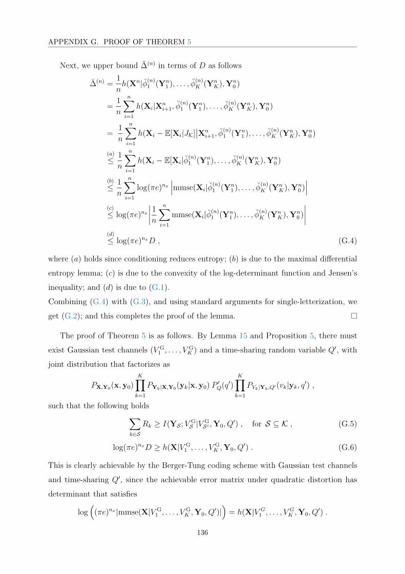
APPENDIX G. PROOF OF THEOREM 5
Next, we upper bound ∆(n) in terms of D as follows
∆(n) =1
nh(Xn|φ(n)
1 (Yn1 ), . . . , φ
(n)K (Yn
K),Yn0 )
=1
n
n∑
i=1
h(Xi|Xni+1, φ
(n)1 (Yn
1 ), . . . , φ(n)K (Yn
K),Yn0 )
=1
n
n∑
i=1
h(Xi − E[Xi|JK]∣∣Xn
i+1, φ(n)1 (Yn
1 ), . . . , φ(n)K (Yn
K),Yn0 )
(a)
≤ 1
n
n∑
i=1
h(Xi − E[Xi|φ(n)1 (Yn
1 ), . . . , φ(n)K (Yn
K),Yn0 )
(b)
≤ 1
n
n∑
i=1
log(πe)nx∣∣∣mmse(Xi|φ(n)
1 (Yn1 ), . . . , φ
(n)K (Yn
K),Yn0 )∣∣∣
(c)
≤ log(πe)nx∣∣∣∣1
n
n∑
i=1
mmse(Xi|φ(n)1 (Yn
1 ), . . . , φ(n)K (Yn
K),Yn0 )
∣∣∣∣
(d)
≤ log(πe)nxD , (G.4)
where (a) holds since conditioning reduces entropy; (b) is due to the maximal differential
entropy lemma; (c) is due to the convexity of the log-determinant function and Jensen’s
inequality; and (d) is due to (G.1).
Combining (G.4) with (G.3), and using standard arguments for single-letterization, we
get (G.2); and this completes the proof of the lemma.
The proof of Theorem 5 is as follows. By Lemma 15 and Proposition 5, there must
exist Gaussian test channels (V G1 , . . . , V
GK ) and a time-sharing random variable Q′, with
joint distribution that factorizes as
PX,Y0(x,y0)K∏
k=1
PYk|X,Y0(yk|x,y0) P ′Q(q′)K∏
k=1
PVk|Yk,Q′(vk|yk, q′) ,
such that the following holds
∑
k∈SRk ≥ I(YS ;V G
S |V GSc ,Y0, Q
′) , for S ⊆ K , (G.5)
log(πe)nxD ≥ h(X|V G1 , . . . , V
GK ,Y0, Q
′) . (G.6)
This is clearly achievable by the Berger-Tung coding scheme with Gaussian test channels
and time-sharing Q′, since the achievable error matrix under quadratic distortion has
determinant that satisfies
log(
(πe)nx|mmse(X|V G1 , . . . , V
GK ,Y0, Q
′)|)
= h(X|V G1 , . . . , V
GK ,Y0, Q
′) .
136

APPENDIX G. PROOF OF THEOREM 5
The above shows that the rate-distortion region of the quadratic vector Gaussian CEO
problem with determinant constraint is given by (G.6), i.e., RDII
CEO (with distortion
parameter log(πe)nxD). Recalling that RDII
CEO = RDI
CEO = RD?VG-CEO, and substituting
in Theorem 4 using distortion level log(πe)nxD completes the proof.
137

138
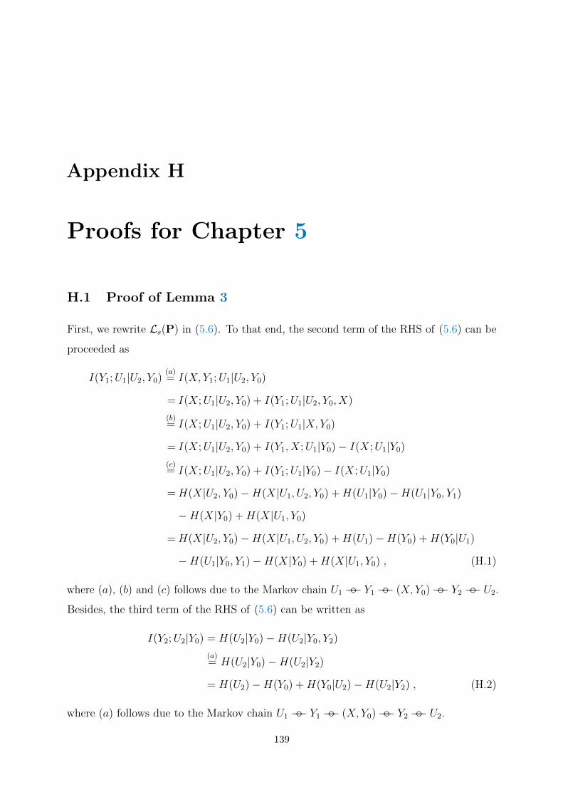
Appendix H
Proofs for Chapter 5
H.1 Proof of Lemma 3
First, we rewrite Ls(P) in (5.6). To that end, the second term of the RHS of (5.6) can be
proceeded as
I(Y1;U1|U2, Y0)(a)= I(X, Y1;U1|U2, Y0)
= I(X;U1|U2, Y0) + I(Y1;U1|U2, Y0, X)
(b)= I(X;U1|U2, Y0) + I(Y1;U1|X, Y0)
= I(X;U1|U2, Y0) + I(Y1, X;U1|Y0)− I(X;U1|Y0)
(c)= I(X;U1|U2, Y0) + I(Y1;U1|Y0)− I(X;U1|Y0)
=H(X|U2, Y0)−H(X|U1, U2, Y0) +H(U1|Y0)−H(U1|Y0, Y1)
−H(X|Y0) +H(X|U1, Y0)
=H(X|U2, Y0)−H(X|U1, U2, Y0) +H(U1)−H(Y0) +H(Y0|U1)
−H(U1|Y0, Y1)−H(X|Y0) +H(X|U1, Y0) , (H.1)
where (a), (b) and (c) follows due to the Markov chain U1 −− Y1 −− (X, Y0)−− Y2 −− U2.
Besides, the third term of the RHS of (5.6) can be written as
I(Y2;U2|Y0) = H(U2|Y0)−H(U2|Y0, Y2)
(a)= H(U2|Y0)−H(U2|Y2)
= H(U2)−H(Y0) +H(Y0|U2)−H(U2|Y2) , (H.2)
where (a) follows due to the Markov chain U1 −− Y1 −− (X, Y0)−− Y2 −− U2.
139

APPENDIX H. PROOFS FOR CHAPTER 5
By applying (H.1) and (H.2) in (5.6), we have
Fs(P) =− s1H(X|Y0)− (s1 + s2)H(Y0) + (1− s1)H(X|U1, U2, Y0)
+ s1H(X|U1, Y0) + s1H(X|U2, Y0) + s1H(U1)− s1H(U1|Y1)
+ s2H(U2)− s2H(U2|Y2) + s1H(Y0|U1) + s2H(Y0|U2)
=− s1H(X|Y0)− (s1 + s2)H(Y0)
− (1− s1)∑
u1u2xy0
p(u1, u2, x, y0) log p(x|u1, u2, y0)
− s1
∑
u1xy0
p(u1, x, y0) log p(x|u1, y0)− s1
∑
u2xy0
p(u2, x, y0) log p(x|u2, y0)
− s1
∑
u1
p(u1) log p(u1) + s1
∑
u1y1
p(u1, y1) log p(u1|y1)
− s2
∑
u2
p(u2) log p(u2) + s2
∑
u2y2
p(u2, y2) log p(u2|y2)
− s1
∑
u1y0
p(u1, y0) log p(y0|u1)− s2
∑
u2y0
p(u2, y0) log p(y0|u2) , (H.3)
Then, marginalizing (H.3) over variables X, Y0, Y1, Y2, and using the Markov chain U1 −−Y1 −− (X, Y0)−− Y2 −− U2, it is easy to see that Fs(P) can be written as
Fs(P) =− s1H(X|Y0)− (s1 + s2)H(Y0)
+ EPX,Y0,Y1,Y2
[(1− s1)EPU1|Y1
EPU2|Y2[− logPX|U1,U2,Y0 ]
+ s1EPU1|Y1[− logPX|U1,Y0 ] + s1EPU2|Y2
[− logPX|U2,Y0 ]
+ s1DKL(PU1|Y1‖PU1) + s2DKL(PU2|Y2‖PU2)
+ s1EPU1|Y1[− logPY0|U1 ] + s2EPU2|Y2
[− logPY0|U2 ]]. (H.4)
Hence, we have
Fs(P,Q)− Fs(P) = (1− s1)EU1,U2,Y0 [DKL(PX|U1,U2,Y0‖QX|U1,U2,Y0)]
+ s1EU1,Y0 [DKL(PX|U1,Y0‖QX|U1,Y0)] + s1EU2,Y0 [DKL(PX|U2,Y0‖QX|U2,Y0)]
+ s1DKL(PU1‖QU1) + s2DKL(PU2‖QU2)
+ s1EU1 [DKL(PY0|U1‖QY0|U1)] + s2EU2 [DKL(PY0|U2‖QY0|U2)]
≥ 0 ,
where it holds with equality if and only if (5.10) is satisfied. Note that we have the relation
1− s1 ≥ 0 due to Lemma 2. This completes the proof.
140
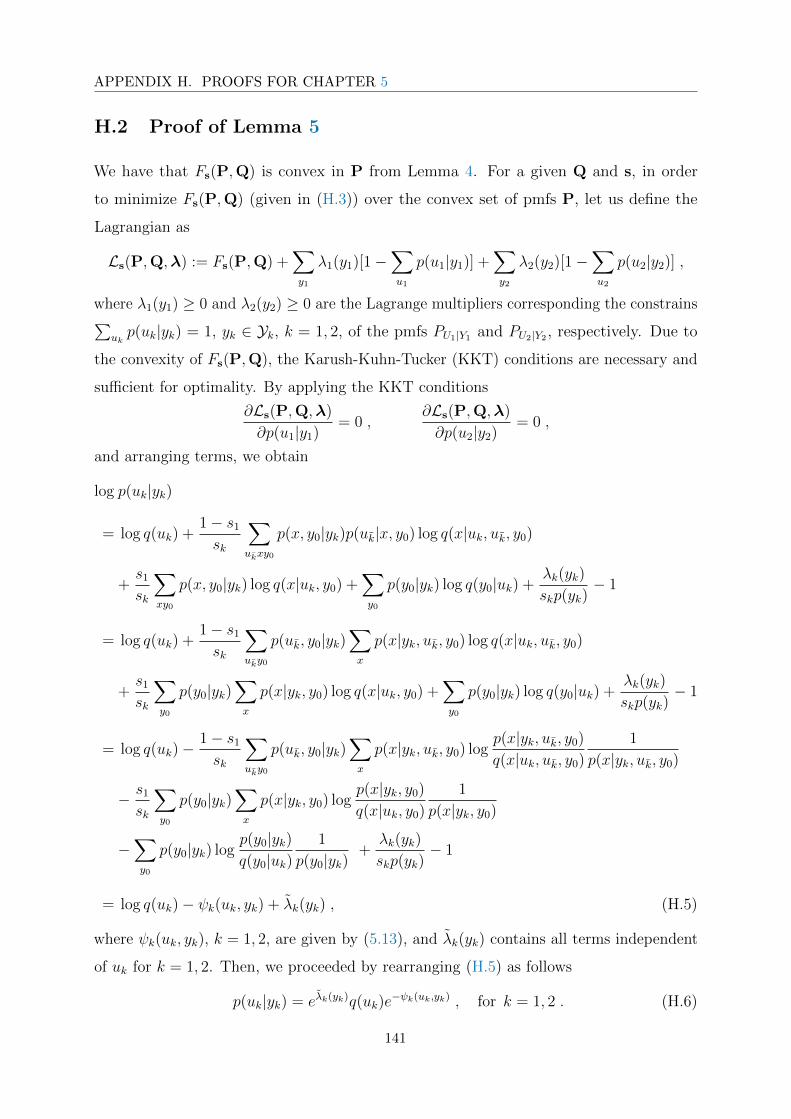
APPENDIX H. PROOFS FOR CHAPTER 5
H.2 Proof of Lemma 5
We have that Fs(P,Q) is convex in P from Lemma 4. For a given Q and s, in order
to minimize Fs(P,Q) (given in (H.3)) over the convex set of pmfs P, let us define the
Lagrangian as
Ls(P,Q,λ) := Fs(P,Q) +∑
y1
λ1(y1)[1−∑
u1
p(u1|y1)] +∑
y2
λ2(y2)[1−∑
u2
p(u2|y2)] ,
where λ1(y1) ≥ 0 and λ2(y2) ≥ 0 are the Lagrange multipliers corresponding the constrains∑
ukp(uk|yk) = 1, yk ∈ Yk, k = 1, 2, of the pmfs PU1|Y1 and PU2|Y2 , respectively. Due to
the convexity of Fs(P,Q), the Karush-Kuhn-Tucker (KKT) conditions are necessary and
sufficient for optimality. By applying the KKT conditions
∂Ls(P,Q,λ)
∂p(u1|y1)= 0 ,
∂Ls(P,Q,λ)
∂p(u2|y2)= 0 ,
and arranging terms, we obtain
log p(uk|yk)
= log q(uk) +1− s1
sk
∑
ukxy0
p(x, y0|yk)p(uk|x, y0) log q(x|uk, uk, y0)
+s1
sk
∑
xy0
p(x, y0|yk) log q(x|uk, y0) +∑
y0
p(y0|yk) log q(y0|uk) +λk(yk)
skp(yk)− 1
= log q(uk) +1− s1
sk
∑
uky0
p(uk, y0|yk)∑
x
p(x|yk, uk, y0) log q(x|uk, uk, y0)
+s1
sk
∑
y0
p(y0|yk)∑
x
p(x|yk, y0) log q(x|uk, y0) +∑
y0
p(y0|yk) log q(y0|uk) +λk(yk)
skp(yk)− 1
= log q(uk)−1− s1
sk
∑
uky0
p(uk, y0|yk)∑
x
p(x|yk, uk, y0) logp(x|yk, uk, y0)
q(x|uk, uk, y0)
1
p(x|yk, uk, y0)
− s1
sk
∑
y0
p(y0|yk)∑
x
p(x|yk, y0) logp(x|yk, y0)
q(x|uk, y0)
1
p(x|yk, y0)
−∑
y0
p(y0|yk) logp(y0|yk)q(y0|uk)
1
p(y0|yk)+
λk(yk)
skp(yk)− 1
= log q(uk)− ψk(uk, yk) + λk(yk) , (H.5)
where ψk(uk, yk), k = 1, 2, are given by (5.13), and λk(yk) contains all terms independent
of uk for k = 1, 2. Then, we proceeded by rearranging (H.5) as follows
p(uk|yk) = eλk(yk)q(uk)e−ψk(uk,yk) , for k = 1, 2 . (H.6)
141
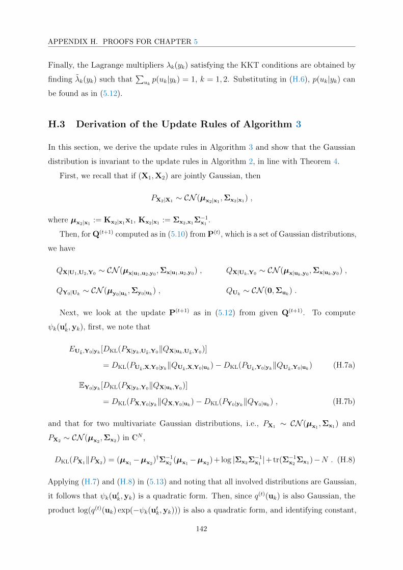
APPENDIX H. PROOFS FOR CHAPTER 5
Finally, the Lagrange multipliers λk(yk) satisfying the KKT conditions are obtained by
finding λk(yk) such that∑
ukp(uk|yk) = 1, k = 1, 2. Substituting in (H.6), p(uk|yk) can
be found as in (5.12).
H.3 Derivation of the Update Rules of Algorithm 3
In this section, we derive the update rules in Algorithm 3 and show that the Gaussian
distribution is invariant to the update rules in Algorithm 2, in line with Theorem 4.
First, we recall that if (X1,X2) are jointly Gaussian, then
PX2|X1 ∼ CN (µx2|x1,Σx2|x1) ,
where µx2|x1:= Kx2|x1x1, Kx2|x1 := Σx2,x1Σ
−1x1
.
Then, for Q(t+1) computed as in (5.10) from P(t), which is a set of Gaussian distributions,
we have
QX|U1,U2,Y0 ∼ CN (µx|u1,u2,y0,Σx|u1,u2,y0) , QX|Uk,Y0 ∼ CN (µx|uk,y0
,Σx|uk,y0) ,
QY0|Uk∼ CN (µy0|uk ,Σy0|uk) , QUk
∼ CN (0,Σuk) .
Next, we look at the update P(t+1) as in (5.12) from given Q(t+1). To compute
ψk(utk,yk), first, we note that
EUk,Y0|yk [DKL(PX|yk,Uk,Y0‖QX|uk,Uk,Y0)]
= DKL(PUk,X,Y0|yk‖QUk,X,Y0|uk)−DKL(PUk,Y0|yk‖QUk,Y0|uk) (H.7a)
EY0|yk [DKL(PX|yk,Y0‖QX|uk,Y0)]
= DKL(PX,Y0|yk‖QX,Y0|uk)−DKL(PY0|yk‖QY0|uk) , (H.7b)
and that for two multivariate Gaussian distributions, i.e., PX1 ∼ CN (µx1,Σx1) and
PX2 ∼ CN (µx2,Σx2) in CN ,
DKL(PX1‖PX2) = (µx1−µx2
)†Σ−1x2
(µx1−µx2
)+ log |Σx2Σ−1x1|+tr(Σ−1
x2Σx1)−N . (H.8)
Applying (H.7) and (H.8) in (5.13) and noting that all involved distributions are Gaussian,
it follows that ψk(utk,yk) is a quadratic form. Then, since q(t)(uk) is also Gaussian, the
product log(q(t)(uk) exp(−ψk(utk,yk))) is also a quadratic form, and identifying constant,
142
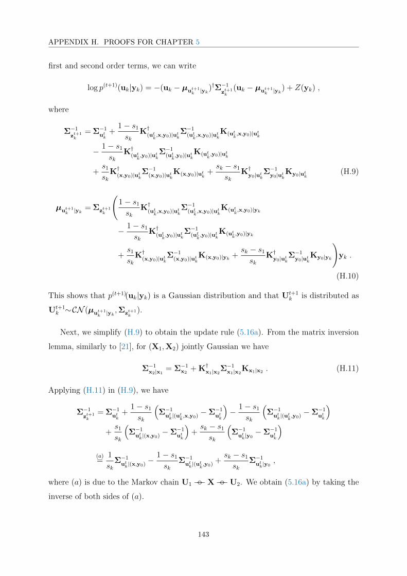
APPENDIX H. PROOFS FOR CHAPTER 5
first and second order terms, we can write
log p(t+1)(uk|yk) = −(uk − µut+1k |yk)
†Σ−1
zt+1k
(uk − µut+1k |yk) + Z(yk) ,
where
Σ−1
zt+1k
= Σ−1utk
+1− s1
skK†
(utk,x,y0)|utk
Σ−1(utk,x,y0)|utk
K(utk,x,y0)|utk
− 1− s1
skK†
(utk,y0)|utk
Σ−1(utk,y0)|utk
K(utk,y0)|utk
+s1
skK†
(x,y0)|utkΣ−1
(x,y0)|utkK(x,y0)|utk +
sk − s1
skK†
y0|utkΣ−1
y0|utkKy0|utk (H.9)
µut+1k |yk = Σzt+1
k
(1− s1
skK†
(utk,x,y0)|utk
Σ−1(utk,x,y0)|utk
K(utk,x,y0)|yk
− 1− s1
skK†
(utk,y0)|utk
Σ−1(utk,y0)|utk
K(utk,y0)|yk
+s1
skK†
(x,y0)|utkΣ−1
(x,y0)|utkK(x,y0)|yk +
sk − s1
skK†
y0|utkΣ−1
y0|utkKy0|yk
)yk .
(H.10)
This shows that p(t+1)(uk|yk) is a Gaussian distribution and that Ut+1k is distributed as
Ut+1k ∼CN (µut+1
k |yk ,Σzt+1k
).
Next, we simplify (H.9) to obtain the update rule (5.16a). From the matrix inversion
lemma, similarly to [21], for (X1,X2) jointly Gaussian we have
Σ−1x2|x1
= Σ−1x2
+ K†x1|x2Σ−1
x1|x2Kx1|x2 . (H.11)
Applying (H.11) in (H.9), we have
Σ−1
zt+1k
= Σ−1utk
+1− s1
sk
(Σ−1
utk|(utk,x,y0)−Σ−1
utk
)− 1− s1
sk
(Σ−1
utk|(utk,y0)−Σ−1
utk
)
+s1
sk
(Σ−1
utk|(x,y0)−Σ−1
utk
)+sk − s1
sk
(Σ−1
utk|y0−Σ−1
utk
)
(a)=
1
skΣ−1
utk|(x,y0)− 1− s1
skΣ−1
utk|(utk,y0)+sk − s1
skΣ−1
utk|y0,
where (a) is due to the Markov chain U1 −−X−−U2. We obtain (5.16a) by taking the
inverse of both sides of (a).
143

APPENDIX H. PROOFS FOR CHAPTER 5
Also from the matrix inversion lemma [21], for (X1,X2) jointly Gaussian we have
Σ−1x1
Σx1,x2Σ−1x2|x1
= Σ−1x1|x2
Σx1,x2Σ−1x2. (H.12)
Now, we simplify (H.10) to obtain the update rule (5.16b) as follows
µut+1k |yk = Σzt+1
k
(1− s1
skΣ−1
utkΣutk,(u
tk,x,y0)Σ
−1(utk,x,y0)|utk
Σ(utk,x,y0),ykΣ
−1yk
− 1− s1
skΣ−1
utkΣutk,(u
tk,y0)Σ
−1(utk,y0)|utk
Σ(utk,y0),ykΣ
−1yk
+s1
skΣ−1
utkΣutk,(x,y0)Σ
−1(x,y0)|utk
Σ(x,y0),ykΣ−1yk
+sk − s1
skΣ−1
utkΣutk,y0
Σ−1y0|utk
Σy0,ykΣ−1yk
)yk
(a)= Σzt+1
k
(1− s1
skΣ−1
utk|(utk,x,y0)Σutk,(u
tk,x,y0)Σ
−1(utk,x,y0)
Σ(utk,x,y0),ykΣ
−1yk
− 1− s1
skΣ−1
utk|(utk,y0)Σutk,(u
tk,y0)Σ
−1(utk,y0)
Σ(utk,y0),ykΣ
−1yk
+s1
skΣ−1
utk|(x,y0)Σutk,(x,y0)Σ
−1(x,y0)Σ(x,y0),ykΣ
−1yk
+sk − s1
skΣ−1
utk|y0Σutk,y0
Σ−1y0
Σy0,ykΣ−1yk
)yk
(b)= Σzt+1
k
(1− s1
skΣ−1
utk|(utk,x,y0)AtkΣyk,(u
tk,x,y0)Σ
−1(utk,x,y0)
Σ(utk,x,y0),ykΣ
−1yk
− 1− s1
skΣ−1
utk|(utk,y0)AtkΣyk,(u
tk,y0)Σ
−1(utk,y0)
Σ(utk,y0),ykΣ
−1yk
+s1
skΣ−1
utk|(x,y0)AtkΣyk,(x,y0)Σ
−1(x,y0)Σ(x,y0),ykΣ
−1yk
+sk − s1
skΣ−1
utk|y0AtkΣyk,y0Σ
−1y0
Σy0,ykΣ−1yk
)yk
(c)= Σzt+1
k
(1− s1
skΣ−1
utk|(utk,x,y0)Atk(Σyk −Σyk|(utk,x,y0))Σ
−1yk
− 1− s1
skΣ−1
utk|(utk,y0)Atk(Σyk −Σyk|(utk,y0))Σ
−1yk
+s1
skΣ−1
utk|(x,y0)Atk(Σyk −Σyk|(x,y0))Σ
−1yk
+sk − s1
skΣ−1
utk|y0Atk(Σyk −Σyk|y0)Σ−1
yk
)yk
144

APPENDIX H. PROOFS FOR CHAPTER 5
(d)= Σzt+1
k
(1
skΣ−1
utk|(x,y0)Atk(I−Σyk|(x,y0)Σ
−1yk
)
− 1− s1
skΣ−1
utk|(utk,y0)Atk(I−Σyk|(utk,y0)Σ
−1yk
)
+sk − s1
skΣ−1
utk|y0Atk(I−Σyk|y0Σ
−1yk
)
)yk ,
where (a) follows from (H.12); (b) follows from the relation Σuk,y0 = AkΣyk,y0 ; (c) is due
the definition of Σx1|x2 ; and (d) is due to the Markov chain U1 −−X−−U2. Equation
(5.16b) follows by noting that µut+1k |yk = At+1
k yk.
H.4 Proof of Proposition 9
For simplicity of exposition, the proof is given for the case K = 2 encoders. The
proof for K > 2 follows similarly. By the definition of RIsumDIB, the tuple (∆, Rsum) is
achievable if there exists some random variables X, Y1, Y2, U1, U2 with joint distribution
PX(x)∏K
k=1 PYk|X(yk|x)∏K
k=1 PUk|Yk(uk|yk) satisfying
∆ ≤ I(X;U1, U2) (H.13a)
∆ ≤ R1 − I(Y1;U1|X) + I(X;U2) (H.13b)
∆ ≤ R2 − I(Y2;U2|X) + I(X;U1) (H.13c)
∆ ≤ R1 +R2 − I(Y1;U1|X)− I(Y2;U2|X) (H.13d)
R1 +R2 ≤ Rsum . (H.13e)
The application of the Fourier-Motzkin elimination to project out R1 and R2 reduces (H.13)
to the following system of inequalities
∆ ≤ I(X;U1, U2) (H.14a)
2∆ ≤ Rsum − I(Y1;U1|X)− I(Y2;U2|X) + I(X;U1) + I(X;U2) (H.14b)
∆ ≤ Rsum − I(Y1;U1|X)− I(Y2;U2|X) . (H.14c)
We note that we have I(X;U1, U2) ≤ I(X;U1) + I(X;U2) due to the Markov chain
U1 −− Y1 −−X −− Y2 −− U2. Therefore, inequality (H.14b) is redundant as it is implied
by (H.14a) and (H.14c). This completes the proof.
145
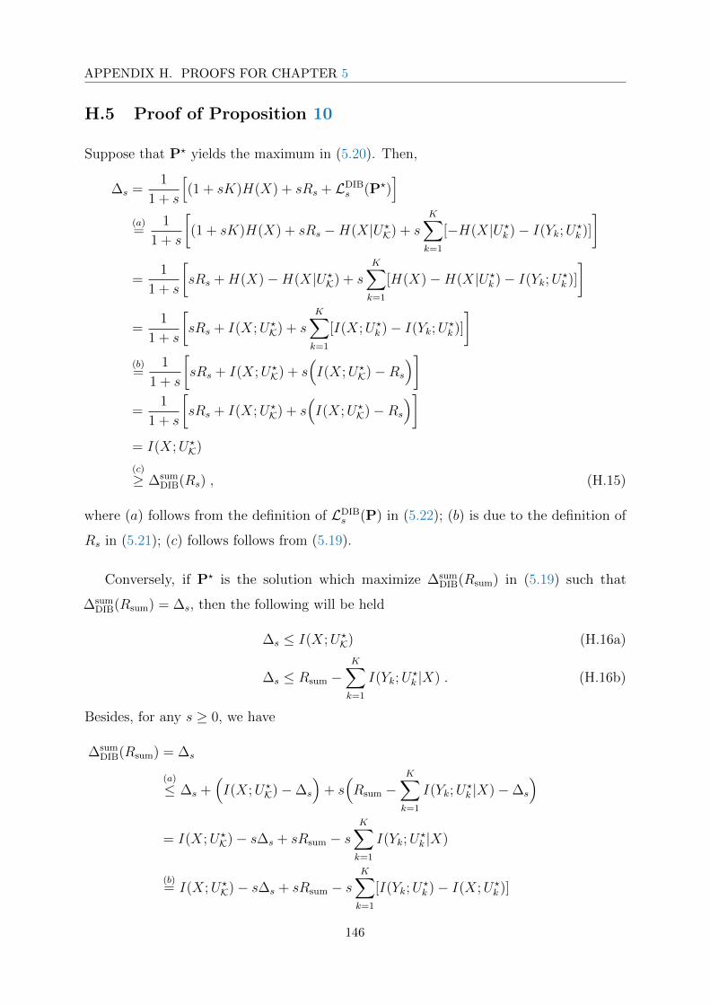
APPENDIX H. PROOFS FOR CHAPTER 5
H.5 Proof of Proposition 10
Suppose that P? yields the maximum in (5.20). Then,
∆s =1
1 + s
[(1 + sK)H(X) + sRs + LDIB
s (P?)]
(a)=
1
1 + s
[(1 + sK)H(X) + sRs −H(X|U?
K) + sK∑
k=1
[−H(X|U?k )− I(Yk;U
?k )]
]
=1
1 + s
[sRs +H(X)−H(X|U?
K) + s
K∑
k=1
[H(X)−H(X|U?k )− I(Yk;U
?k )]
]
=1
1 + s
[sRs + I(X;U?
K) + s
K∑
k=1
[I(X;U?k )− I(Yk;U
?k )]
]
(b)=
1
1 + s
[sRs + I(X;U?
K) + s(I(X;U?
K)−Rs
)]
=1
1 + s
[sRs + I(X;U?
K) + s(I(X;U?
K)−Rs
)]
= I(X;U?K)
(c)
≥ ∆sumDIB(Rs) , (H.15)
where (a) follows from the definition of LDIBs (P) in (5.22); (b) is due to the definition of
Rs in (5.21); (c) follows follows from (5.19).
Conversely, if P? is the solution which maximize ∆sumDIB(Rsum) in (5.19) such that
∆sumDIB(Rsum) = ∆s, then the following will be held
∆s ≤ I(X;U?K) (H.16a)
∆s ≤ Rsum −K∑
k=1
I(Yk;U?k |X) . (H.16b)
Besides, for any s ≥ 0, we have
∆sumDIB(Rsum) = ∆s
(a)
≤ ∆s +(I(X;U?
K)−∆s
)+ s(Rsum −
K∑
k=1
I(Yk;U?k |X)−∆s
)
= I(X;U?K)− s∆s + sRsum − s
K∑
k=1
I(Yk;U?k |X)
(b)= I(X;U?
K)− s∆s + sRsum − sK∑
k=1
[I(Yk;U?k )− I(X;U?
k )]
146
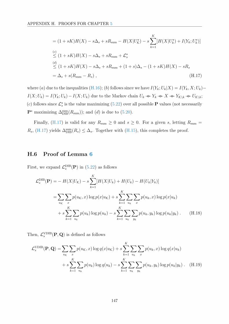
APPENDIX H. PROOFS FOR CHAPTER 5
= (1 + sK)H(X)− s∆s + sRsum −H(X|U?K)− s
K∑
k=1
[H(X|U?k ) + I(Yk;U
?k )]
(c)
≤ (1 + sK)H(X)− s∆s + sRsum + L?s(d)
≤ (1 + sK)H(X)− s∆s + sRsum + (1 + s)∆s − (1 + sK)H(X)− sRs
= ∆s + s(Rsum −Rs) , (H.17)
where (a) due to the inequalities (H.16); (b) follows since we have I(Yk;Uk|X) = I(Yk, X;Uk)−I(X;Uk) = I(Yk;Uk)− I(X;Uk) due to the Markov chain Uk−−Yk−−X −−YK\k−−UK\k;(c) follows since L?s is the value maximizing (5.22) over all possible P values (not necessarily
P? maximizing ∆sumDIB(Rsum)); and (d) is due to (5.20).
Finally, (H.17) is valid for any Rsum ≥ 0 and s ≥ 0. For a given s, letting Rsum =
Rs, (H.17) yields ∆sumDIB(Rs) ≤ ∆s. Together with (H.15), this completes the proof.
H.6 Proof of Lemma 6
First, we expand LDIBs (P) in (5.22) as follows
LDIBs (P) =−H(X|UK)− s
K∑
k=1
[H(X|Uk) +H(Uk)−H(Uk|Yk)]
=∑
uK
∑
x
p(uK, x) log p(x|uK) + sK∑
k=1
∑
uk
∑
x
p(uk, x) log p(x|uk)
+ sK∑
k=1
∑
uk
p(uk) log p(uk)− sK∑
k=1
∑
uk
∑
yk
p(uk, yk) log p(uk|yk) . (H.18)
Then, LVDIBs (P,Q) is defined as follows
LVDIBs (P,Q) =
∑
uK
∑
x
p(uK, x) log q(x|uK) + s
K∑
k=1
∑
uk
∑
x
p(uk, x) log q(x|uk)
+ sK∑
k=1
∑
uk
p(uk) log q(uk)− sK∑
k=1
∑
uk
∑
yk
p(uk, yk) log p(uk|yk) . (H.19)
147
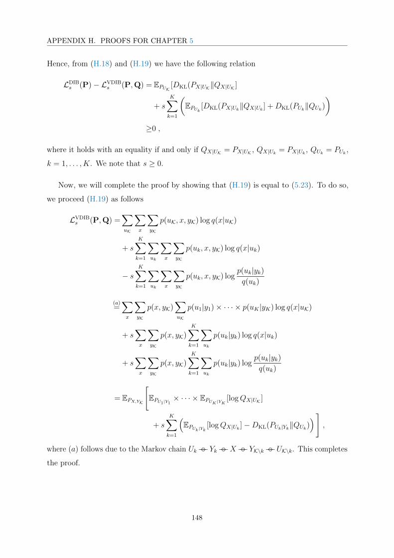
APPENDIX H. PROOFS FOR CHAPTER 5
Hence, from (H.18) and (H.19) we have the following relation
LDIBs (P)− LVDIB
s (P,Q) = EPUK[DKL(PX|UK‖QX|UK ]
+ sK∑
k=1
(EPUk [DKL(PX|Uk‖QX|Uk ] +DKL(PUk‖QUk)
)
≥0 ,
where it holds with an equality if and only if QX|UK = PX|UK , QX|Uk = PX|Uk , QUk = PUk ,
k = 1, . . . , K. We note that s ≥ 0.
Now, we will complete the proof by showing that (H.19) is equal to (5.23). To do so,
we proceed (H.19) as follows
LVDIBs (P,Q) =
∑
uK
∑
x
∑
yK
p(uK, x, yK) log q(x|uK)
+ sK∑
k=1
∑
uk
∑
x
∑
yK
p(uk, x, yK) log q(x|uk)
− sK∑
k=1
∑
uk
∑
x
∑
yK
p(uk, x, yK) logp(uk|yk)q(uk)
(a)=∑
x
∑
yK
p(x, yK)∑
uK
p(u1|y1)× · · · × p(uK |yK) log q(x|uK)
+ s∑
x
∑
yK
p(x, yK)K∑
k=1
∑
uk
p(uk|yk) log q(x|uk)
+ s∑
x
∑
yK
p(x, yK)K∑
k=1
∑
uk
p(uk|yk) logp(uk|yk)q(uk)
= EPX,YK
[EPU1|Y1
× · · · × EPUK |YK[logQX|UK ]
+ s
K∑
k=1
(EPUk|Yk [logQX|Uk ]−DKL(PUk|Yk‖QUk)
)],
where (a) follows due to the Markov chain Uk−−Yk−−X−−YK\k−−UK\k. This completes
the proof.
148
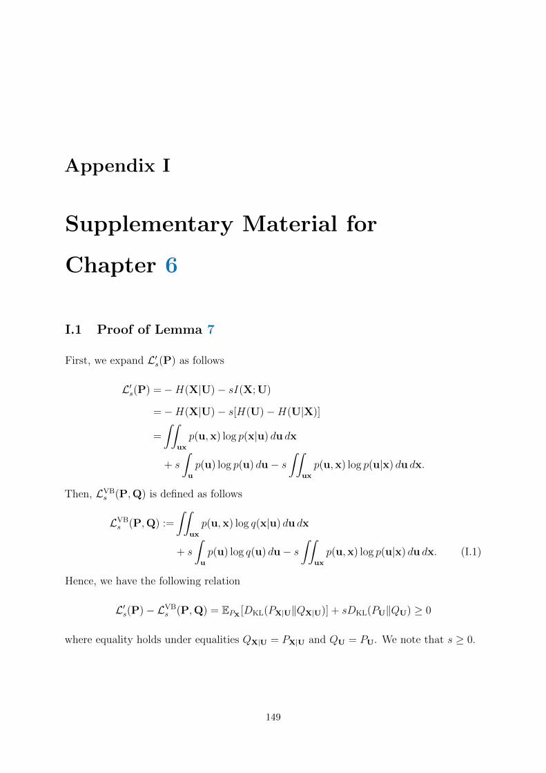
Appendix I
Supplementary Material for
Chapter 6
I.1 Proof of Lemma 7
First, we expand L′s(P) as follows
L′s(P) =−H(X|U)− sI(X; U)
=−H(X|U)− s[H(U)−H(U|X)]
=
∫∫
ux
p(u,x) log p(x|u) du dx
+ s
∫
u
p(u) log p(u) du− s∫∫
ux
p(u,x) log p(u|x) du dx.
Then, LVBs (P,Q) is defined as follows
LVBs (P,Q) :=
∫∫
ux
p(u,x) log q(x|u) du dx
+ s
∫
u
p(u) log q(u) du− s∫∫
ux
p(u,x) log p(u|x) du dx. (I.1)
Hence, we have the following relation
L′s(P)− LVBs (P,Q) = EPX
[DKL(PX|U‖QX|U)] + sDKL(PU‖QU) ≥ 0
where equality holds under equalities QX|U = PX|U and QU = PU. We note that s ≥ 0.
149
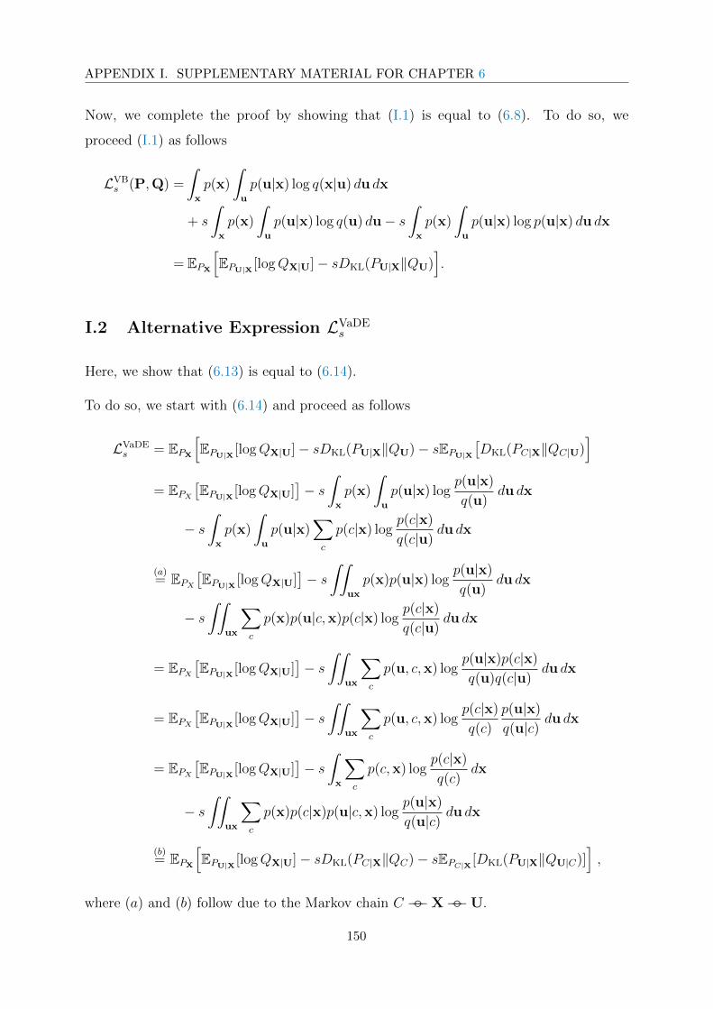
APPENDIX I. SUPPLEMENTARY MATERIAL FOR CHAPTER 6
Now, we complete the proof by showing that (I.1) is equal to (6.8). To do so, we
proceed (I.1) as follows
LVBs (P,Q) =
∫
x
p(x)
∫
u
p(u|x) log q(x|u) du dx
+ s
∫
x
p(x)
∫
u
p(u|x) log q(u) du− s∫
x
p(x)
∫
u
p(u|x) log p(u|x) du dx
= EPX
[EPU|X [logQX|U]− sDKL(PU|X‖QU)
].
I.2 Alternative Expression LVaDEs
Here, we show that (6.13) is equal to (6.14).
To do so, we start with (6.14) and proceed as follows
LVaDEs = EPX
[EPU|X [logQX|U]− sDKL(PU|X‖QU)− sEPU|X
[DKL(PC|X‖QC|U)
]
= EPX[EPU|X [logQX|U]
]− s
∫
x
p(x)
∫
u
p(u|x) logp(u|x)
q(u)du dx
− s∫
x
p(x)
∫
u
p(u|x)∑
c
p(c|x) logp(c|x)
q(c|u)du dx
(a)= EPX
[EPU|X [logQX|U]
]− s
∫∫
ux
p(x)p(u|x) logp(u|x)
q(u)du dx
− s∫∫
ux
∑
c
p(x)p(u|c,x)p(c|x) logp(c|x)
q(c|u)du dx
= EPX[EPU|X [logQX|U]
]− s
∫∫
ux
∑
c
p(u, c,x) logp(u|x)p(c|x)
q(u)q(c|u)du dx
= EPX[EPU|X [logQX|U]
]− s
∫∫
ux
∑
c
p(u, c,x) logp(c|x)
q(c)
p(u|x)
q(u|c) du dx
= EPX[EPU|X [logQX|U]
]− s
∫
x
∑
c
p(c,x) logp(c|x)
q(c)dx
− s∫∫
ux
∑
c
p(x)p(c|x)p(u|c,x) logp(u|x)
q(u|c) du dx
(b)= EPX
[EPU|X [logQX|U]− sDKL(PC|X‖QC)− sEPC|X [DKL(PU|X‖QU|C)]
],
where (a) and (b) follow due to the Markov chain C −−X−−U.
150
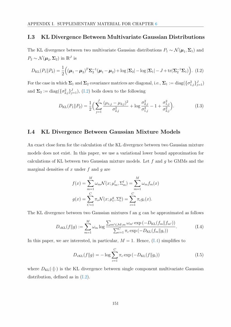
APPENDIX I. SUPPLEMENTARY MATERIAL FOR CHAPTER 6
I.3 KL Divergence Between Multivariate Gaussian Distributions
The KL divergence between two multivariate Gaussian distributions P1 ∼ N (µ1,Σ1) and
P2 ∼ N (µ2,Σ2) in RJ is
DKL(P1‖P2) =1
2
((µ1−µ2)TΣ−1
2 (µ1−µ2) + log |Σ2|− log |Σ1|−J + tr(Σ−12 Σ1)
). (I.2)
For the case in which Σ1 and Σ2 covariance matrices are diagonal, i.e., Σ1 := diag(σ21,jJj=1)
and Σ2 := diag(σ22,jJj=1), (I.2) boils down to the following
DKL(P1‖P2) =1
2
( J∑
j=1
(µ1,j − µ2,j)2
σ22,j
+ logσ2
2,j
σ21,j
− 1 +σ2
1,j
σ22,j
). (I.3)
I.4 KL Divergence Between Gaussian Mixture Models
An exact close form for the calculation of the KL divergence between two Gaussian mixture
models does not exist. In this paper, we use a variational lower bound approximation for
calculations of KL between two Gaussian mixture models. Let f and g be GMMs and the
marginal densities of x under f and g are
f(x) =M∑
m=1
ωmN (x;µfm,Σ
fm) =
M∑
m=1
ωmfm(x)
g(x) =C∑
C=1
πcN (x;µgc ,Σ
gc) =
C∑
c=1
πcgc(x).
The KL divergence between two Gaussian mixtures f an g can be approximated as follows
DvKL(f‖g) :=M∑
m=1
ωm log
∑m′∈M\m ωm′ exp (−DKL(fm‖fm′))∑C
c=1 πc exp (−DKL(fm‖gc)). (I.4)
In this paper, we are interested, in particular, M = 1. Hence, (I.4) simplifies to
DvKL(f‖g) = − logC∑
c=1
πc exp (−DKL(f‖gc)) (I.5)
where DKL(·‖·) is the KL divergence between single component multivariate Gaussian
distribution, defined as in (I.2).
151

152
Bibliography
[1] Inaki Estella Aguerri and Abdellatif Zaidi, “Distributed variational representation
learning,” IEEE Transactions on Pattern Analysis and Machine Intelligence, 2019.
[2] Toby Berger, Zhen Zhang, and Harish Viswanathan, “The CEO problem,” IEEE
Transactions on Information Theory, vol. 42, no. 3, pp. 887 – 902, May 1996.
[3] Yasutada Oohama, “Rate-distortion theory for Gaussian multiterminal source cod-
ing systems with several side informations at the decoder,” IEEE Transactions on
Information Theory, vol. 51, no. 7, pp. 2577 – 2593, July 2005.
[4] Vinod Prabhakaran, David Tse, and Kannan Ramachandran, “Rate region of the
quadratic Gaussian CEO problem,” in Proceedings of IEEE International Symposium
on Information Theory, June – July 2004, p. 117.
[5] Jun Chen and Jia Wang, “On the vector Gaussian CEO problem,” in Proceedings of
IEEE International Symposium on Information Theory, July – August 2011, pp. 2050 –
2054.
[6] Jia Wang and Jun Chen, “On the vector Gaussian L-terminal CEO problem,” in
Proceedings of IEEE International Symposium on Information Theory, July 2012, pp.
571 – 575.
[7] Tie Liu and Pramod Viswanath, “An extremal inequality motivated by multiterminal
information-theoretic problems,” IEEE Transactions on Information Theory, vol. 53,
no. 5, pp. 1839 – 1851, May 2007.
[8] Yinfei Xu and Qiao Wang, “Rate region of the vector Gaussian CEO problem with the
trace distortion constraint,” IEEE Transactions on Information Theory, vol. 62, no. 4,
pp. 1823 – 1835, April 2016.
153

BIBLIOGRAPHY
[9] Thomas A. Courtade and Richard D. Wesel, “Multiterminal source coding with an
entropy-based distortion measure,” in Proceedings of IEEE International Symposium
on Information Theory, July – August 2011, pp. 2040 – 2044.
[10] Thomas A. Courtade and Tsachy Weissman, “Multiterminal source coding under
logarithmic loss,” IEEE Transactions on Information Theory, vol. 60, no. 1, pp. 740 –
761, January 2014.
[11] Ersen Ekrem and Sennur Ulukus, “An outer bound for the vector Gaussian CEO
problem,” IEEE Transactions on Information Theory, vol. 60, no. 11, pp. 6870 – 6887,
November 2014.
[12] Saurabha Tavildar and Pramod Viswanath, “On the sum-rate of the vector Gaussian
CEO problem,” in Proceedings of 39-th Asilomar Conference on Signals, Systems, and
Computers, October – November 2005, pp. 3 – 7.
[13] Hanan Weingarten, Yossef Steinberg, and Shlomo Shamai (Shitz), “The capacity region
of the gaussian multiple-input multiple-output broadcast channel,” IEEE Transactions
on Information Theory, vol. 52, no. 9, pp. 3936 – 3964, September 2006.
[14] Daniel Perez Palomar, John M. Cioffi, and Miguel Angel Lagunas, “Joint Tx-Rx
beamforming design for multicarrier MIMO channels: A unified framework for convex
optimization,” IEEE Transactions on Signal Processing, vol. 51, no. 9, pp. 2381 – 2401,
September 2003.
[15] Anna Scaglione, Petre Stoica, Sergio Barbarossa, Georgios B. Giannakis, and Hemanth
Sampath, “Optimal designs for space-time linear precoders and decoders,” IEEE
Transactions on Signal Processing, vol. 50, no. 5, pp. 1051 – 1064, May 2002.
[16] Md. Saifur Rahman and Aaron B. Wagner, “On the optimality of binning for dis-
tributed hypothesis testing,” IEEE Transactions on Information Theory, vol. 58, no. 10,
pp. 6282 – 6303, October 2012.
[17] Naftali Tishby, Fernando C. Pereira, and William Bialek, “The information bottleneck
method,” in Proceedings of the 37-th Annual Allerton Conference on Communication,
Control and Computing, 1999, pp. 368 – 377.
154
BIBLIOGRAPHY
[18] Peter Harremoes and Naftali Tishby, “The information bottleneck revisited or how to
choose a good distortion measure,” in Proceedings of IEEE International Symposium
on Information Theory, June 2007, pp. 566 – 570.
[19] Richard E. Blahut, “Computation of channel capacity and rate-distortion functions,”
IEEE Transactions on Information Theory, vol. IT-18, no. 4, pp. 460 – 473, July 1972.
[20] Suguru Arimoto, “An algorithm for computing the capacity of arbitrary discrete
memoryless channels,” IEEE Transactions on Information Theory, vol. IT-18, no. 1,
pp. 14 – 20, January 1972.
[21] Gal Chechik, Amir Globerson, Naftali Tishby, and Yair Weiss, “Information bottleneck
for Gaussian variables,” Journal of Machine Learning Research, vol. 6, pp. 165 – 188,
January 2005.
[22] Andreas Winkelbauer and Gerald Matz, “Rate-information-optimal Gaussian channel
output compression,” in Proceedings of the 48-th Annual Conference on Information
Sciences and Systems, August 2014.
[23] Samuel Cheng, Vladimir Stankovic, and Zixiang Xiong, “Computing the channel capac-
ity and rate-distortion function with two-sided state information,” IEEE Transactions
on Information Theory, vol. 51, no. 12, pp. 4418 – 4425, December 2005.
[24] Mung Chiang and Stephen Boyd, “Geometric programming duals of channel capacity
and rate distortion,” IEEE Transactions on Information Theory, vol. 50, no. 2, pp. 245
– 258, February 2004.
[25] Frederic Dupuis, Wei Yu, and Frans M. J. Willems, “Blahut-Arimoto algorithms for
computing channel capacity and rate-distortion with side information,” in Proceedings
of IEEE International Symposium on Information Theory, June – July 2004, p. 181.
[26] Mohammad Rezaeian and Alex Grant, “A generalization of Arimoto-Blahut algorithm,”
in Proceedings of IEEE International Symposium on Information Theory, June – July
2004, p. 180.
[27] Irina Higgins, Loic Matthey, Arka Pal, Christopher Burgess, Xavier Glorot, Matthew
Botvinick, Shakir Mohamed, and Alexander Lerchner, “β-vae: Learning basic vi-
155

BIBLIOGRAPHY
sual concepts with a constrained variational framework,” in Proceedings of the 5-th
International Conference on Learning Representations, 2017.
[28] Alexander A. Alemi, Ben Poole, Ian Fischer, Ian Fischer, Joshua V. Dillon, Rif A.
Saurous, and Kevin Murphy, “Fixing a broken ELBO,” in Proceedings of the 35-th
International Conference on Machine Learning, 2018.
[29] Diederik P. Kingma and Max Welling, “Auto-encoding variational bayes,” in Proceed-
ings of the 2-nd International Conference on Learning Representations, 2014.
[30] Alexander A. Alemi, Ian Fischer, Joshua V. Dillon, and Kevin Murphy, “Deep
variational information bottleneck,” in Proceedings of the 5-th International Conference
on Learning Representations, 2017.
[31] Zhuxi Jiang, Yin Zheng, Huachun Tan, Bangsheng Tang, and Hanning Zhou, “Varia-
tional deep embedding: An unsupervised and generative approach to clustering,” in
Proceedings of the 26-th International Joint Conference on Artificial Intelligence, 2017,
pp. 1965 – 1972.
[32] Noam Slonim, The Information Bottleneck: Theory and Applications. PhD disserta-
tion, Hebrew University, 2002.
[33] Junyuan Xie, Ross Girshick, and Ali Farhadi, “Unsupervised deep embedding for
clustering analysis,” in Proceedings of the 33-rd International Conference on Machine
Learning, 2016, pp. 478 – 487.
[34] Hans S. Witsenhausen, “Indirect rate distortion problems,” IEEE Transactions on
Information Theory, vol. IT-26, no. 5, pp. 518 – 521, September 1980.
[35] Yossef Steinberg, “Coding and common reconstruction,” IEEE Transactions on
Information Theory, vol. 55, no. 11, pp. 4995 – 5010, November 2009.
[36] Ilan Sutskover, Shlomo Shamai (Shitz), and Jacob Ziv, “Extremes of information
combining,” IEEE Transactions on Information Theory, vol. 51, no. 4, pp. 1313 – 1325,
April 2005.
[37] Ingmar Land and Johannes Huber, “Information combining,” Foundations and Trends
in Communication and Information Theory, vol. 3, no. 3, pp. 227 – 330, November
2006.
156
BIBLIOGRAPHY
[38] Ingmar Land, Simon Huettinger, Peter A. Hoeher, and Johannes B. Huber, “Bounds
on information combining,” IEEE Transactions on Information Theory, vol. 51, no. 2,
pp. 612 – 619, February 2005.
[39] Aaron D. Wyner, “On source coding with side information at the decoder,” IEEE
Transactions on Information Theory, vol. 21, no. 3, pp. 294 – 300, May 1975.
[40] Rudolf Ahlswede and Janos Korner, “Source coding with side information and a
converse for degraded broadcast channels,” IEEE Transactions on Information Theory,
vol. 21, no. 6, pp. 629 – 637, November 1975.
[41] Elza Erkip and Thomas Cover, “The efficiency of investment information,” IEEE
Transactions on Information Theory, vol. 44, no. 3, pp. 1026 – 1040, May 1998.
[42] Ali Makhdoumi, Salman Salamatian, Nadia Fawaz, and Muriel Medard, “From the
information bottleneck to the privacy funnel,” in Proceedings of IEEE Information
Theory Workshop, November 2014, pp. 501 – 505.
[43] Yoshua Bengio, Aaron Courville, and Pascal Vincent, “Representation learning: A
review and new perspectives,” IEEE Transactions on Pattern Analysis and Machine
Intelligence, vol. 35, no. 8, pp. 1798 – 1828, August 2013.
[44] Chang Xu, Dacheng Tao, and Chao Xu, “A survey on multi-view learning,” arXiv:
1304.5634, 2013.
[45] Weiran Wang, Raman Arora, Karen Livescu, and Jeff Bilmes, “On deep multi-view
representation learning,” in Proceedings of the 32-nd International Conference on
Machine Learning, 2015.
[46] Yann Lecun, Leon Bottou, Yoshua Bengio, and Patrick Haffner, “Gradient-based
learning applied to document recognition,” in Proceedings of the IEEE, vol. 86, no. 11,
1998, pp. 2278 – 2324.
[47] David D. Lewis, Yiming Yang, Tony G. Rose, and Fan Li, “A new benchmark
collection for text categorization research,” The Journal of Machine Learning Research,
vol. 5, pp. 361 – 397, 2004.
157

BIBLIOGRAPHY
[48] Adam Coates, Andrew Ng, and Honglak Lee, “An analysis of single-layer networks in
unsupervised feature learning,” in Proceedings of the 14-th International Conference
on Artificial Intelligence and Statistics, 2011, pp. 215 – 223.
[49] Georg Pichler, Pablo Piantanida, and Gerald Matz, “Distributed information-theoretic
biclustering,” in Proceedings of IEEE International Symposium on Information Theory,
July 2016, pp. 1083 – 1087.
[50] Georg Pichler, Pablo Piantanida, and Gerald Matz, “A multiple description CEO
problem with log-loss distortion,” in Proceedings of IEEE International Symposium on
Information Theory, June 2017, pp. 111 – 115.
[51] Jiantao Jiao, Thomas A. Courtade, Kartik Venkat, and Tsachy Weissman, “Justifi-
cation of logarithmic loss via the benefit of side information,” IEEE Transactions on
Information Theory, vol. 61, no. 10, pp. 5357 – 5365, October 2015.
[52] Albert No and Tsachy Weissman, “Universality of logarithmic loss in lossy compres-
sion,” in Proceedings of IEEE International Symposium on Information Theory, June
2015, pp. 2166 – 2170.
[53] Yanina Shkel, Maxim Raginsky, and Sergio Verdu, “Universal lossy compression under
logarithmic loss,” in Proceedings of IEEE International Symposium on Information
Theory, June 2017, pp. 1157 – 1161.
[54] Nicolo Cesa-Bianchi and Gabor Lugosi, Prediction, Learning and Games. Cambridge
University Press, 2006.
[55] Thomas Andre, Marc Antonini, Michel Barlaud, and Robert M. Gray, “Entropy-based
distortion measure for image coding,” in Proceedings of IEEE International Conference
on Image Processing, October 2006, pp. 1157 – 1160.
[56] Kittipong Kittichokechai, Yeow-Khiang Chia, Tobias J. Oechtering, Mikael Skoglund,
and Tsachy Weissman, “Secure source coding with a public helper,” IEEE Transactions
on Information Theory, vol. 62, no. 7, pp. 3930 – 3949, July 2016.
[57] Amichai Painsky and Gregory Wornell, “On the universality of the logistic loss
function,” in Proceedings of IEEE International Symposium on Information Theory,
June 2018, pp. 936 – 940.
158
BIBLIOGRAPHY
[58] Cheuk Ting Li, Xiugang Wu, Ayfer Ozgur, and Abbas El Gamal, “Minimax learning
for remote prediction,” in Proceedings of IEEE International Symposium on Information
Theory, June 2018, pp. 541 – 545.
[59] Chao Tian and Jun Chen, “Remote vector Gaussian source coding with decoder side
information under mutual information and distortion constraints,” IEEE Transactions
on Information Theory, vol. 55, no. 10, pp. 4676 – 4680, October 2009.
[60] Amichai Sanderovich, Shlomo Shamai (Shitz), Yossef Steinberg, and Gerhard Kramer,
“Communication via decentralized processing,” IEEE Transactions on Information
Theory, vol. 54, no. 7, pp. 3008 – 3023, July 2008.
[61] Osvaldo Simeone, Elza Erkip, and Shlomo Shamai (Shitz), “On codebook information
for interference relay channels with out-of-band relaying,” IEEE Transactions on
Information Theory, vol. 57, no. 5, pp. 2880 – 2888, May 2011.
[62] Inaki Estella Aguerri, Abdellatif Zaidi, Giuseppe Caire, and Shlomo Shamai (Shitz),
“On the capacity of cloud radio access networks with oblivious relaying,” in Proceedings
of IEEE International Symposium on Information Theory, June 2017, pp. 2068 – 2072.
[63] Inaki Estella Aguerri, Abdellatif Zaidi, Giuseppe Caire, and Shlomo Shamai (Shitz),
“On the capacity of cloud radio access networks with oblivious relaying,” IEEE Trans-
actions on Information Theory, vol. 65, no. 7, pp. 4575 – 4596, July 2019.
[64] Flavio P. Calmon, Ali Makhdoumi, Muriel Medard, Mayank Varia, Mark Christiansen,
and Ken R. Duffy, “Principal inertia components and applications,” IEEE Transactions
on Information Theory, vol. 63, no. 8, pp. 5011 – 5038, July 2017.
[65] Rudolf Ahlswede and Imre Csiszar, “Hypothesis testing with communication con-
straints,” IEEE Transactions on Information Theory, vol. IT - 32, no. 4, pp. 533 – 542,
July 1986.
[66] Te Sun Han, “Hypothesis testing with multiterminal data compression,” IEEE Trans-
actions on Information Theory, vol. IT - 33, no. 6, pp. 759 – 772, November 1987.
[67] Chao Tian and Jun Chen, “Successive refinement for hypothesis testing and lossless
one-helper problem,” IEEE Transactions on Information Theory, vol. 54, no. 10, pp.
4666 – 4681, October 2008.
159

BIBLIOGRAPHY
[68] Sadaf Salehkalaibar, Michele Wigger, and Roy Timo, “On hypothesis testing against
conditional independence with multiple decision centers,” IEEE Transactions on
Communications, vol. 66, no. 6, pp. 2409 – 2420, June 2018.
[69] Ran Gilad-Bachrach, Amir Navot, and Naftali Tishby, “An information theoretic
tradeoff between complexity and accuracy,” in Proceedings of Conference on Learning
Theory, 2003, pp. 595 – 609.
[70] Andreas Winkelbauer, Stefan Farthofer, and Gerald Matz, “The rate-information trade-
off for Gaussian vector channels,” in Proceedings of IEEE International Symposium on
Information Theory, June 2014, pp. 2849 – 2853.
[71] Michael Meidlinger, Andreas Winkelbauer, and Gerald Matz, “On the relation between
the Gaussian information bottleneck and MSE-optimal rate-distortion quantization,”
in Proceedings of IEEE Workshop on Statistical Signal Processing, June 2014, pp. 89 –
92.
[72] Abdellatif Zaidi, Inaki Estella Aguerri, and Shlomo Shamai (Shitz), “On the informa-
tion bottleneck problems: Models, connections, applications and information theoretic
views,” Entropy, vol. 22, no. 2, p. 151, January 2020.
[73] Aaron D. Wyner and Jacob Ziv, “The rate-distortion function for source coding with
side information at the decoder,” IEEE Transactions on Information Theory, vol. IT –
22, no. 1, pp. 1 – 10, January 1976.
[74] Meryem Benammar and Abdellatif Zaidi, “Rate-distortion of a Heegard-Berger prob-
lem with common reconstruction constraint,” in Proceedings of International Zurich
Seminar on Communications, 2016, pp. 150 – 154.
[75] Meryem Benammar and Abdellatif Zaidi, “Rate-distortion function for a Heegard-
Berger problem with two sources and degraded reconstruction sets,” IEEE Transactions
on Information Theory, vol. 62, no. 9, pp. 5080 – 5092, September 2016.
[76] Flavio du Pin Calmon and Nadia Fawaz, “Privacy against statistical inference,” in
Proceedings of the 50-th Annual Allerton Conference on Communication, Control and
Computing, October 2012, pp. 1401 – 1408.
160

BIBLIOGRAPHY
[77] Shahab Asoodeh, Mario Diaz, Fady Alajaji, and Tamas Linder, “Information extrac-
tion under privacy constraints,” Information, vol. 7, no. 15, March 2016.
[78] Alessandro Achille and Stefano Soatto, “Information dropout: Learning optimal
representations through noisy computation,” IEEE Transactions on Pattern Analysis
and Machine Intelligence, vol. 40, no. 12, pp. 2897 – 2905, December 2018.
[79] Satosi Watanabe, “Information theoretical analysis of multivariate correlation,” IBM
Journal of Research and Development, vol. 4, no. 1, pp. 66 – 82, January 1960.
[80] Ricky T. Q. Chen, Xuechen Li, Roger Grosse, and David Duvenaud, “Isolating
sources of disentanglement in VAEs,” in Proceedings of the 32-nd Conference on Neural
Information Processing Systems, 2018.
[81] Ohad Shamir, Sivan Sabato, and Naftali Tishby, “Learning and generalization with
the information bottleneck,” in Proceedings of the 19-th International Conference on
Algorithmic Learning Theory, October 2008, pp. 92 – 107.
[82] Naftali Tishby and Noga Zaslavsky, “Deep learning and the information bottleneck
principle,” in Proceedings of IEEE Information Theory Workshop, April 2015.
[83] Diederik P. Kingma and Jimmy Ba, “Adam: A method for stochastic optimization,”
in Proceedings of the 3-rd International Conference on Learning Representations, 2015.
[84] Ravid Schwartz-Ziv and Naftali Tishby, “Opening the black box of deep neural
networks via information,” arXiv: 1703.00810, 2017.
[85] Andrew Michael Saxe, Yamini Bansal, Joel Dapello, Madhu Advani, Artemy Kolchin-
sky, Brendan Daniel Tracey, and David Daniel Cox, “On the information bottleneck
theory of deep learning,” in Proceedings of the 6-th International Conference on Learn-
ing Representations, 2018.
[86] Lewandowsky and Gerhard Bauch, “Information-optimum LDPC decoders based on
the information bottleneck method,” IEEE Access, vol. 6, pp. 4054 – 4071, 2018.
[87] Michael Meidlinger, Alexios Balatsoukas-Stimming, Andreas Burg, and Gerald Matz,
“Quantized message passing for LDPC codes,” in Proceedings of 49-th Asilomar Confer-
ence on Signals, Systems, and Computers, November 2015, pp. 1606 – 1610.
161

BIBLIOGRAPHY
[88] J. Korner and K. Marton, “How to encode the modulo-two sum of binary sources,”
IEEE Transactions on Information Theory, vol. 25, no. 02, pp. 219 – 221, March 1979.
[89] Michael Gastpar, “The Wyner-Ziv problem with multiple sources,” IEEE Transactions
on Information Theory, vol. 50, no. 11, pp. 2762 – 2768, November 2004.
[90] Daniel Russo and James Zou, “How much does your data exploration overfit? Con-
trolling bias via information usage,” arXiv: 1511.05219, 2015.
[91] Aolin Xu and Maxim Raginsky, “Information-theoretic analysis of generalization
capability of learning algorithms,” in Proceedings of the 31-st Conference on Neural
Information Processing Systems, 2017, pp. 2524 – 2533.
[92] Amir R. Asadi, Emmanuel Abbe, and Sergio Verdu, “Chaining mutual information
and tightening generalization bounds,” in Proceedings of the 32-nd Conference on
Neural Information Processing Systems, 2018.
[93] Toby Berger, “Decentralized estimation and decision theory,” in Proceedings of IEEE
Spring Workshop on Information Theory, 1979.
[94] Hossam M. H. Shalaby and Adrian Papamarcou, “Multiterminal detection with zero-
rate data compression,” IEEE Transactions on Information Theory, vol. 38, no. 2, pp.
254 – 267, March 1992.
[95] Wenwen Zhao and Lifeng Lai, “Distributed testing with zero-rate compression,” in
Proceedings of IEEE International Symposium on Information Theory, June 2015, pp.
2792 – 2796.
[96] Pierre Escamilla, Michele Wigger, and Abdellatif Zaidi, “Distributed hypothesis
testing with concurrent detections,” in Proceedings of IEEE International Symposium
on Information Theory, June 2018, pp. 166 – 170.
[97] Pierre Escamilla, Michele Wigger, and Abdellatif Zaidi, “Distributed hypothesis
testing with collaborative detection,” in Proceedings of the 56-th Annual Allerton
Conference on Communication, Control, and Computing, October 2018, pp. 512 – 518.
[98] Jiachun Liao, Lalitha Sankar, Flavio P. Calmon, and Vincent Y. F. Tan, “Hypothesis
testing under maximal leakage privacy constraints,” in Proceedings of IEEE Interna-
tional Symposium on Information Theory, June 2017, pp. 779 – 783.
162

BIBLIOGRAPHY
[99] Sreejith Sreekumar, Asaf Cohen, and Deniz Gunduz, “Distributed hypothesis testing
with a privacy constraint,” in Proceedings of IEEE Information Theory Workshop,
November 2018.
[100] Abdellatif Zaidi and Inaki Estella Aguerri, “Optimal rate-exponent region for a class
of hypothesis testing against conditional independence problems,” in Proceedings of
IEEE Information Theory Workshop, August 2019.
[101] Toby Berger, Multiterminal source coding. The Information Theory Approach to
Communications, CSIM Courses and Lectures, 1978, vol. 229.
[102] S. Y. Tung, Multiterminal source coding. PhD dissertation, Cornell University,
1978.
[103] Yuhan Zhou, Yinfei Xu, Wei Yu, and Jun Chen, “On the optimal fronthaul compres-
sion and decoding strategies for uplink cloud radio access networks,” IEEE Transactions
on Information Theory, vol. 62, no. 12, pp. 7402 – 7418, December 2016.
[104] Thomas A. Courtade, “Gaussian multiterminal source coding through the lens of
logarithmic loss,” in Information Theory and Applications Workshop, 2015.
[105] Thomas A. Courtade, “A strong entropy power inequality,” IEEE Transactions on
Information Theory, vol. 64, no. 4, pp. 2173 – 2192, April 2018.
[106] Aaron B. Wagner, Saurabha Tavildar, and Pramod Viswanath, “Rate region of
the quadratic Gaussian two-encoder source-coding problem,” IEEE Transactions on
Information Theory, vol. 54, no. 5, pp. 1938 – 1961, May 2008.
[107] Thomas A. Courtade and Jiantao Jiao, “An extremal inequality for long Markov
chains,” in Proceedings of the 52-nd Annual Allerton Conference on Communication,
Control and Computing, September 2014, pp. 763 – 770.
[108] Y. Oohama, “The rate-distortion function for the quadratic gaussian ceo problem,”
IEEE Transactions on Information Theory, vol. 44, no. 3, pp. 1057 – 1070, May 1998.
[109] Saurabha Tavildar, Pramod Viswanath, and Aaron B. Wagner, “The gaussian
many-help-one distributed source coding problem,” IEEE Transactions on Information
Theory, vol. 56, no. 1, pp. 564 – 581, January 2010.
163

BIBLIOGRAPHY
[110] Md. Saifur Rahman and Aaron B. Wagner, “Rate region of the vector gaussian
one-helper source-coding problem,” IEEE Transactions on Information Theory, vol. 61,
no. 5, pp. 2708 – 2728, May 2015.
[111] Inaki Estella Aguerri and Abdellatif Zaidi, “Distributed information bottleneck
method for discrete and Gaussian sources,” in Proceedings of International Zurich
Seminar on Information and Communication, February 2018.
[112] Noam Slonim and Naftali Tishby, “The power of word clusters for text classification,”
in Proceedings of 23-rd European Colloquium on Information Retrieval Research, 2001,
pp. 191 – 200.
[113] Yoram Baram, Ran El-Yaniv, and Kobi Luz, “Online choice of active learning
algorithms,” Journal of Machine Learning Research, vol. 5, pp. 255 – 291, March 2004.
[114] Jun Chen and Toby Berger, “Successive Wyner-Ziv coding scheme and its application
to the quadratic Gaussian CEO problem,” IEEE Transactions on Information Theory,
vol. 54, no. 4, pp. 1586 – 1603, April 2008.
[115] Meisam Razaviyayn, Mingyi Hong, and Zhi-Quan Luo, “A unified convergence
analysis of block successive minimization methods for nonsmooth optimization,” SIAM
Journal on Optimization, vol. 23, no. 2, pp. 1126 – 1153, June 2013.
[116] Michael Grant and Stephen Boyd, “CVX: Matlab software for disciplined convex
programming,” http://cvxr.com/cvx, March 2014.
[117] Matthew Chalk, Olivier Marre, and Gasper Tkacik, “Relevant sparse codes with
variational information bottleneck,” in Proceedings of the 30-th Conference on Neural
Information Processing Systems, 2016.
[118] Xue Bin Peng, Angjoo Kanazawa, Sam Toyer, Pieter Abbeel, and Sergey Levine,
“Variational discriminator bottleneck: Improving imitation learning, inverse rl, and gans
by constraining information flow,” in Proceedings of the 7-th International Conference
on Learning Representations, 2019.
[119] Bin Dai, Chen Zhu, and David P. Wipf, “Compressing neural networks using the
variational information bottleneck,” in Proceedings of the 35-th International Conference
on Machine Learning, 2018.
164

BIBLIOGRAPHY
[120] Diederik P. Kingma, Tim Salimans, Rafal Jozefowicz, Xi Chen, Ilya Sutskever, and
Max Welling, “Improved variational inference with inverse autoregressive flow,” in
Proceedings of 30-st Conference on Neural Information Processing Systems, 2016.
[121] George Papamakarios, Theo Pavlakou, and Iain Murray, “Masked autoregressive
flow for density estimation,” in Proceedings of 31-st Conference on Neural Information
Processing Systems, 2017.
[122] D. Sculley, “Web-scale K-means clustering,” in Proceedings of the 19-th International
Conference on World Wide Web, April 2010, pp. 1177 – 1178.
[123] Zhexue Huang, “Extensions to the K-means algorithm for clustering large datasets
with categorical values,” Data Mining and Knowledge Discovery, vol. 2, no. 3, pp. 283
– 304, September 1998.
[124] J. A. Hartigan and M. A. Wong, “Algorithm AS 136: A k-means clustering algorithm,”
Journal of the Royal Statistical Society, vol. 28, pp. 100 – 108, 1979.
[125] A. P. Dempster, N. M. Laird, and D. B. Rubin, “Maximum likelihood from incomplete
data via the EM algorithm,” Journal of the Royal Statistical Society, vol. 39, pp. 1 –
38, 1977.
[126] Chris Ding and Xiaofeng He, “K-means clustering via principal component analysis,”
in Proceedings of the 21-st International Conference on Machine Learning, 2004.
[127] Karl Pearson, “On lines and planes of closest fit to systems of points in space,”
Philosophical Magazine, vol. 2, no. 11, pp. 559 – 572, November 1901.
[128] Svante Wold, Kim Esbensen, and Paul Geladi, “Principal component analysis,”
Chemometrics and Intelligent Laboratory Systems, vol. 2, pp. 37 – 52, August 1987.
[129] Sam Roweis, “EM algorithms for PCA and SPCA,” in Advances in Neural Informa-
tion Processing Systems 10, 1997, pp. 626 – 632.
[130] Thomas Hofmann, Bernhard Scholkopf, and Alexander J. Smola, “Kernel methods
in machine learning,” The Annals of Statistics, vol. 36, pp. 1171 – 1220, June 2008.
[131] N. Slonim and N. Tishby, “Document clustering using word clusters via the infor-
mation bottleneck method,” in Proceedings of the 23-rd Annual International ACM
165

BIBLIOGRAPHY
SIGIR Conference on Research and Development in Information Retrieval, July 2000,
pp. 208 – 215.
[132] Danilo J. Rezende, Shakir Mohamed, and Daan Wierstra, “Stochastic backpropaga-
tion and approximate inference in deep generative models,” in Proceedings of the 31-st
International Conference on Machine Learning, 2014, pp. 1278 – 1286.
[133] Xifeng Guo, Long Gao, Xinwang Liu, and Jianping Yin, “Improved deep embedded
clustering with local structure preservation,” in Proceedings of the 26-th International
Joint Conference on Artificial Intelligence, 2017, pp. 1753 – 1759.
[134] Nat Dilokthanakul, Pedro A. M. Mediano, Marta Garnelo, Matthew C.H. Lee, Hugh
Salimbeni, Kai Arulkumaran, and Murray Shanahani, “Deep unsupervised clustering
with Gaussian mixture variational autoencoders,” arXiv: 1611.02648, 2017.
[135] Erxue Min, Xifeng Guo, Qiang Liu, Gen Zhang, Jianjing Cui, and Jun Long, “A
survey of clustering with deep learning: From the perspective of network architecture,”
IEEE Access, vol. 6, pp. 39 501 – 39 514, 2018.
[136] John R. Hershey and Peder A. Olsen, “Approximating the Kullback Leibler divergence
between Gaussian mixture models,” in Proceedings of IEEE International Conference
on Acoustics, Speech and Signal Processing, April 2007, pp. 317 – 320.
[137] Kaiming He, Xiangyu Zhang, Shaoqing Ren, and Jian Sun, “Deep residual learning
for image recognition,” in Proceedings of IEEE Conference on Computer Vision and
Pattern Recognition, 2016, pp. 770 – 778.
[138] Pascal Vincent, Hugo Larochelle, Isabelle Lajoie, Yoshua Bengio, and Pierre-Antoine
Manzagol, “Stacked denoising autoencoders: Learning useful representations in a deep
network with a local denoising criterion,” The Journal of Machine Learning Research,
vol. 11, pp. 3371 – 3408, December 2010.
[139] Laurens van der Maaten and Geoffrey Hinton, “Visualizing data using t-SNE,”
Journal of Machine Learning Research 9, pp. 2579 – 2605, November 2008.
[140] Cheuk Ting Li and Abbas El Gamal, “Strong functional representation lemma and
applications to coding theorems,” IEEE Transactions on Information Theory, vol. 64,
no. 11, pp. 6967 – 6978, November 2018.
166

BIBLIOGRAPHY
[141] Cheuk Ting Li, Xiugang Wu, Ayfer Ozgur, and Abbas El Gama, “Minimax learning
for remote prediction,” arXiv: 1806.00071, 2018.
[142] Adi Homri, Michael Peleg, and Shlomo Shamai (Shitz), “Oblivious fronthaul-
constrained relay for a Gaussian channel,” IEEE Transactions on Communications,
vol. 66, no. 11, pp. 5112 – 5123, November 2018.
[143] Roy Karasik, Osvaldo Simeone, and Shlomo Shamai (Shitz), “Robust uplink commu-
nications over fading channels with variable backhaul connectivity,” IEEE Transactions
on Wireless Communications, vol. 12, no. 11, pp. 5788 – 5799, November 2013.
[144] Yuxin Chen, Andrea J. Goldsmith, and Yonina C. Eldar, “Channel capacity under
sub-nyquist nonuniform sampling,” IEEE Transactions on Information Theory, vol. 60,
no. 8, pp. 4739 – 4756, August 2014.
[145] Alon Kipnis, Yonina C. Eldar, and Andrea J. Goldsmith, “Analog-to-digital com-
pression: A new paradigm for converting signals to bits,” IEEE Signal Processing
Magazine, vol. 35, no. 3, pp. 16 – 39, May 2018.
[146] Michael Gastpar, “On Wyner-Ziv networks,” in Proceedings of 37-th Asilomar
Conference on Signals, Systems, and Computers, November 2003, pp. 855 – 859.
[147] Amir Dembo, Thomas M. Cover, and Joy A. Thomas, “Information theoretic
inequalities,” IEEE Transactions on Information Theory, vol. 37, no. 6, pp. 1501 –
1518, November 1991.
[148] Daniel P. Palomar and Sergio Verdu, “Gradient of mutual information in linear
vector gaussian channels,” IEEE Transactions on Information Theory, vol. 52, no. 1,
pp. 141 – 154, January 2006.
167

168
Publications
[Y1] Yigit Ugur, Inaki Estella Aguerri, and Abdellatif Zaidi, “Vector Gaussian CEO
problem under logarithmic loss and applications,” accepted for publication in IEEE
Transactions on Information Theory, January 2020.
[Y2] Yigit Ugur, Inaki Estella Aguerri, and Abdellatif Zaidi, “A generalization of
Blahut-Arimoto algorithm to compute rate-distortion regions of multiterminal
source coding under logarithmic loss,” in Proceedings of IEEE Information Theory
Workshop, November 2017, pp. 349 – 353.
[Y3] Yigit Ugur, Inaki Estella Aguerri, and Abdellatif Zaidi, “Vector Gaussian CEO
problem under logarithmic loss,” in Proceedings of IEEE Information Theory
Workshop, November 2018, pp. 515 – 519.
[Y4] Yigit Ugur, George Arvanitakis, and Abdellatif Zaidi, “Variational information bot-
tleneck for unsupervised clustering: Deep Gaussian mixture embedding,” Entropy,
vol. 22, no. 2, p. 213, February 2020.
169
Related Documents