Working Paper Number 67 November 2006 Edition An Index of Donor Performance By David Roodman Abstract The Commitment to Development Index of the Center for Global Development rates 21 rich countries on the “development-friendliness” of their policies. It is revised and updated annu- ally. The component on foreign assistance combines quantitative and qualitative measures of official aid, and of fiscal policies that support private charitable giving. The quantitative measure uses a net transfers concept, as distinct from the net flows concept in the net Offi- cial Development Assistance measure of the Development Assistance Committee. The qualitative factors are: a penalty for tying aid; a discounting system that favors aid to poorer, better-governed recipients; and a penalty for “project proliferation.” The charitable giving measure is based on an estimate of the share of observed private giving to developing coun- tries that is attributable to a) lower overall taxes or b) specific tax incentives for giving. De- spite the adjustments, overall results are dominated by differences in quantity of official aid given. This is because while there is a seven-fold range in net concessional transfers/GDP among the scored countries, variation in overall aid quality across donors appears far lower, and private giving is generally small. Denmark, the Netherlands, Norway, and Sweden score highest while the largest donors in absolute terms, the United States and Japan, rank at or near the bottom. Standings by the 2006 methodology have been relatively stable since 1995. The Center for Global Development is an independent think tank that works to reduce global poverty and inequality through rigorous research and active engagement with the policy community. Use and dissemination of this Working Paper is encouraged, however reproduced copies may not be used for com- mercial purposes. Further usage is permitted under the terms of the Creative Commons License. The views ex- pressed in this paper are those of the author and should not be attributed to the directors or funders of the Center for Global Development. www.cgdev.org

Welcome message from author
This document is posted to help you gain knowledge. Please leave a comment to let me know what you think about it! Share it to your friends and learn new things together.
Transcript
Working Paper Number 67
November 2006 Edition An Index of Donor Performance
By David Roodman
Abstract
The Commitment to Development Index of the Center for Global Development rates 21 rich countries on the “development-friendliness” of their policies. It is revised and updated annu-ally. The component on foreign assistance combines quantitative and qualitative measures of official aid, and of fiscal policies that support private charitable giving. The quantitative measure uses a net transfers concept, as distinct from the net flows concept in the net Offi-cial Development Assistance measure of the Development Assistance Committee. The qualitative factors are: a penalty for tying aid; a discounting system that favors aid to poorer, better-governed recipients; and a penalty for “project proliferation.” The charitable giving measure is based on an estimate of the share of observed private giving to developing coun-tries that is attributable to a) lower overall taxes or b) specific tax incentives for giving. De-spite the adjustments, overall results are dominated by differences in quantity of official aid given. This is because while there is a seven-fold range in net concessional transfers/GDP among the scored countries, variation in overall aid quality across donors appears far lower, and private giving is generally small. Denmark, the Netherlands, Norway, and Sweden score highest while the largest donors in absolute terms, the United States and Japan, rank at or near the bottom. Standings by the 2006 methodology have been relatively stable since 1995.
The Center for Global Development is an independent think tank that works to reduce global poverty and inequality through rigorous research and active engagement with the policy community. Use and dissemination of this Working Paper is encouraged, however reproduced copies may not be used for com-mercial purposes. Further usage is permitted under the terms of the Creative Commons License. The views ex-pressed in this paper are those of the author and should not be attributed to the directors or funders of the Center for Global Development.
www.cgdev.org
An Index of Donor Performance
David Roodman1
Research Fellow, Center for Global Development
Center for Global Development
November 2006
Rich nations are often compared on how much they share their wealth with poorer countries. The
Nordics and the Netherlands, it is noted, are the most generous with foreign assistance, while the
United States gives among the least aid per unit of gross domestic product. Two major interna-
tional consensus documents issued in 2002, the reports of the International Conference on Fi-
nancing for Development, in Monterrey, Mexico, and the World Summit on Sustainable Devel-
opment, in Johannesburg, call on donors to move toward giving at least 0.7 percent of their na-
tional income in aid, as few now do. (UN 2002a, p. 9; UN 2002b, p. 52)
The measure of aid implicitly or explicitly referenced in all these comparisons and
benchmarks is “net overseas development assistance” (net ODA), which is a measure of aid
quantity defined by the donor-funded Development Assistance Committee (DAC) in Paris. DAC
counts total grants and concessional (low-interest) development loans given to developing coun-
tries, and subtracts principle repayments received on such loans (thus the “net”).2
Yet it is widely recognized that some dollars and euros of foreign aid do more good than
others. While some aid has funded vaccinations whose effectiveness can be measured in pennies
per life saved, other aid has handsomely paid donor-country consultants to write policy reports
that collect dust on shelves, or merely helped recipients make interest payments on old aid loans.
As a result, a simple quantity metric is hardly the last word on donor performance. 1 The author thanks Mark McGillivray, Simon Scott, and Paul Isenman for helpful comments on earlier drafts, Jean-Louis Grolleau for assistance with the data, and Alicia Bannon and Scott Standley for their contributions to the charitable giving section of this paper. 2 DAC considers a loan concessional if it has a grant element of at least 25 percent of the loan value, using a 10 per-cent discount rate.
This paper describes an index of donor performance that takes the standard quantity
measure as a starting point. It is motivated by the desire to incorporate determinants of aid im-
pact other quantity into the Commitment to Development Index (CDI) (Roodman 2006c; CGD
and FP 2006). The aid index was introduced in 2003 has been revised annually.3 At its heart, it is
an attempt to quantify aspects of aid quality. But it also departs from net ODA in its definition of
aid quantity, and in factoring in tax policies that support private giving.
Because this aid measure is designed to draw entirely from available statistics, primarily
the extensive DAC databases, many important aspects of aid quality are not reflected in the in-
dex—factors such as the realism of project designs and the effectiveness of structural adjustment
conditionality. Moreover, most variation in aid quality may occur within donor’s aid portfolios
rather than across donors. As a result, while there is a nearly sevenfold range in net aid trans-
fers/GDP among the 21 rich countries scored here, the calculations in this paper reveal nothing
like that sort of variation in aid quality across donors. Moreover, including private giving does
not change this picture because it appears to be much smaller than official giving in most coun-
tries. Thus the sheer quantity of official aid is still the dominant determinant of donors’ scores on
this index.
Still, the measure does highlight some interesting differences among donors, and does
somewhat rearrange the usual standings. Japan is especially hurt by the netting out of its large
amounts of interest received. Donors such as Australia and Italy are pulled low by the apparent
tendency to spread their small aid budgets thinly, over many projects.
In the last three decades or so, researchers have taken three broad approaches to cross-
country quantitative assessment of aid quality. Since at least the early 1970s, econometric studies
have been done of the determinants of donors’ aid allocations, factors such as recipient’s poverty
rate and level of oil exports (citations are below). Though often not evaluative in character, the
approach offers a way to measure one aspect of aid quality, selectivity, by looking at how re-
sponsive aid allocation is to recipient need and development potential. How best to integrate
such results with aid quantity into a single performance index is less obvious, however. Attempts
to create a single index began with Mark McGillivray (1989, 1994), who essentially computed
the weighted sum to each donor’s aid disbursements to all recipients, basing weights on recipient
3 Major changes since 2004 are: purging cancellation of old non-aid loans from gross aid; a new approach to penal-izing “project proliferation”; some simplifications in the selectivity weighting; and refinements to the computation of tax policy–induced private giving.
GDP/capita as an indicator of need. The third approach is the newest and most sophisticated.
Drawing on the literature on determinants of aid allocation, McGillivray, Leavy, and White
(2002), formally model allocation, giving donors utility functions that depend on the commercial
and geopolitical value of recipients, as well as on developmental need and potential. They then
compute optimal allocations and penalize donors to the extent they deviate from optima.
The donor performance measure described here is closest in spirit to McGillivray’s origi-
nal, but more ambitious than all previous approaches in the scope of information that it combines
into single index. It factors quality of recipient governance as well as poverty into the selectivity
scoring system, penalizes tying of aid, handles reverse flows (debt service) in a consistent way,
penalizes project proliferation (overloading recipient governments with the administrative bur-
den of many small aid projects), and rewards tax policies that encourage private charitable giving
to developing countries.
This paper details the calculations and illustrates them with 2004 data, which are the lat-
est available and the basis for the 2006 index. The first six sections describe the computations
involved in rating official aid programs: their final output is “quality-adjusted aid quantity” in
dollars, or simply “quality-adjusted aid.” They treat multilateral and bilateral donors in parallel,
so that the World Bank’s main concessional aid program, for instance, can be compared for se-
lectivity to Denmark’s aid program. The penultimate section describes how the quality-adjusted
aid of multilaterals is allocated back to the bilaterals that fund them, in order to give national
governments scores on official aid that reflect both their bilateral aid programs and their contri-
butions to multilaterals. The last section describes how the aid index factors in tax policies that
favor private charitable giving.
1. The first step: gross aid transfers
The starting point for the calculation of quality-adjusted official aid is gross disbursements of
ODA and Official Aid (OA), disaggregated by donor and recipient. In DAC terminology, OA is
concessional aid meeting the ODA definition, except that while ODA goes to countries conven-
tionally thought of as developing, OA goes to “Part II” countries—most European states that
emerged out of the Soviet bloc and richer non-DAC members such as Israel and Singapore. DAC
excludes OA from its most frequently cited statistics, perhaps out of concern that assistance to
such rich countries stretches the meaning of “aid.” I include OA because some Part II countries,
such as Ukraine, are poorer than many Part I countries.4 And since the selectivity adjustment de-
tailed below heavily discounts aid to the richest developing countries, there is less risk that
counting OA will misrepresent aid flows. For simplicity of exposition, I refer henceforth to both
ODA and OA as ODA.
DAC reports both commitments and disbursements of ODA, but its press releases nor-
mally focus on disbursement. Similarly, I use disbursements. Dudley and Montmarquette (1976)
argue that commitments better indicate donor policies, on the idea that recipient absorptive ca-
pacity limits largely explain any shortfalls in disbursements. But commitment-disbursement di-
vergences could reflect bottlenecks or unrealism on either side of the donor-recipient relation-
ship. Large and persistent gaps between commitments and disbursements may reflect a tendency
of certain donors to promise more than they can realistically deliver, or a failure to learn from
history that certain recipients cannot absorb aid as fast as donors hope. On balance, it seems best
to stick with disbursements and avoid the risk of rewarding donors for overpromising aid or sys-
tematically underestimating the capacity to absorb it.
The definition of gross disbursements used here differs in one respect from DAC’s. In re-
cent years, donors have formally cancelled billions of dollars in OOF loans to countries such as
Nigeria, Iraq, Pakistan, Cameroon, and the Democratic Republic of Congo (DRC). OOF or
“Other Official Finance” loans are ones with too small a concessional element to qualify as
ODA, or that are meant for military, export financing, or other non-development purposes. OOF
loan cancellations have run in the billions of dollars in recent years. The DRC, in fact, was the
world’s top ODA recipient in 2003, at just over $5 billion. It turns out that under a Paris Club
agreement, donors cancelled $4.5 billion in outstanding OOF loans to the DRC.
When OOF loans are cancelled, they are, in effect, retroactively recognized by the DAC
accounting system as ODA grants. This is a reasonable choice if the original purpose of the loan
was for development and it was merely disqualified as ODA because it was not concessional
enough. The DAC system books the transfer at the time it is officially recognized. It would be
more accurate to recognize the gradual transfer that occurs year by year as the loans become un-
collectible over time. The U.S. government does something like this, regularly assessing the
likely collectibility of its outstanding sovereign loans and taking on budget any drop in their ap-
4 See http://www.oecd.org/document/45/0,2340,en_2649_34447_2093101_1_1_1_1,00.html for lists of Part I and Part II countries.
parent value.5 DAC does not do this, perhaps in part because of the complexity, in part because
past years’ data would be constantly revised, and in part because accounting rules and appropria-
tions processes within some of the donor agencies, which govern DAC, create strong disincen-
tives for recognizing such losses.
Unfortunately, the resulting inaccuracies have been glaring in the last few years. The true,
current financial value of debt cancellation for countries such as the DRC is far less than the face
value. Even Pakistan, which received $1 billion in OOF debt relief in 2003, is a Highly Indebted
Poor Country going by the numbers. Much of its cancelled debt may therefore have been uncol-
lectible anyway, suggesting that the true value of the cancellation per se was far lower.6 Starting
in 2005, for which DAC data are not complete at this writing, large debt cancellations for Iraq
and Nigeria are also hitting the donors’ books, causing what DAC deputy director Richard Carey
(2005) has called a “debt bubble” in the ODA total.
The definition of gross disbursements used here therefore excludes forgiveness of non-
ODA loans. The reasoning is that the net transfers that do occur are not primarily a credit to cur-
rent policy. If a Carter Administration export credit to Zaire went bad in the early 1980s, and was
finally written off in 2003, the transfer that occurred does not for the most part reflect 2003 de-
velopment policy.
The starting point for purging OOF loan forgiveness is the formula for DAC’s standard
gross ODA:
Gross ODA = grants + ODA loans extended
The term "grants" on the right contains a subtlety relating to debt relief. When DAC accounts for
cancellation of ODA loans (not the OOF ones just discussed), it does so with two opposite trans-
actions. The first is a “debt forgiveness grant,” which is included under “grants.” The second is
an "offsetting entry for debt relief," which represents the immediate return of that grant in the
form of amortization. It is considered an ODA loan repayment. This mechanism prevents dou-
ble-counting of forgiven ODA loans, which were already fully counted as aid at disbursement.
Since the offsetting entry is considered a reflow, it does not enter gross ODA, but will surface in
net ODA in the next section. So canceling any loan, ODA or OOF, increases gross ODA. In fact,
5 The process occurs within the U.S. government’s Interagency Country Risk Assessment System. 6 Pakistan had an average ratio of present value of debt to exports of 189% during 2001–03 and an average ex-change-rate GDP/capita of $497. The corresponding HIPC thresholds are 150% and $885. But Pakistan is not con-sidered a HIPC because it is an IDA-IBRD blend country.

when donors and recipients reschedule debt, as under Paris Club agreements, the capitalization
of interest arrears is treated as a new aid flow, and is included in “ODA loans extended”, under
the subheading, “rescheduled debt.”7
Since the purpose here is to count only transactions that reflect current, actual transfers, I
exclude all debt forgiveness grants and capitalized interest, none of which involves actual move-
ment of money. I call the result “gross aid transfers” or simply “gross aid” to distinguish it from
gross ODA. Thus:
Gross aid = (grants – debt forgiveness grants) + (ODA loans extended – rescheduled debt)
This removes all debt forgiveness grants, for both ODA and non-ODA loans, from the definition
of gross aid. Now, the DAC definition of net ODA, discussed in the next section, does itself re-
move grants for ODA loan forgiveness, by counting those offsetting entries for debt relief in
ODA reflows. So in order to highlight the real departure of gross aid transfers and DAC account-
ing, I compare gross aid to DAC's Gross ODA net of offsetting entries for ODA loan forgive-
ness. Table 1 shows the 10 recipients most affected by changing the definition this way for 2004.
In all, forgiveness of non-ODA loans accounted for $5.2 billion of reported gross ODA.
Table 1. Gross ODA net of offsetting entries for ODA loan forgiveness vs. gross aid trans-fers, selected recipients, 2004 (million $)
Recipient
Gross ODA net of offsetting entries for ODA
loan forgiveness Gross aid Difference Congo, Dem. Rep. 1,846 1,056 791Angola 1,156 458 698Nicaragua 1,262 721 541Madagascar 1,277 760 517Cameroon 908 470 438Senegal 1,148 774 374Zambia 1,355 992 363Ghana 1,434 1,103 331Poland 1,544 1,252 292All Part I countries 92,540 87,302 5,238
Table 2 shows the implications from the donor perspective. Among bilaterals, the United
States gave the most gross aid to non-DAC governments and Japan came in second. Among mul-
tilaterals, the European Commission disbursed the most, followed by the World Bank’s Interna-
tional Development Association (IDA). Most of the calculations in the aid index are done for 7 In the previous edition of this paper, I asserted incorrectly that ODA loan forgiveness is netted out of gross ODA. I thank Nicolas Van de Sijpe for catching this problem.

each donor-recipient pair. The donor-level totals in Table 2, are not used in the calculations, but
are summaries for illustration. The final row of the table is an exception: it shows the figures for
one donor-recipient pair, the France and Senegal. I will continue the France-Senegal example in
order to illustrate the actual calculations at the level of the donor-recipient pair.
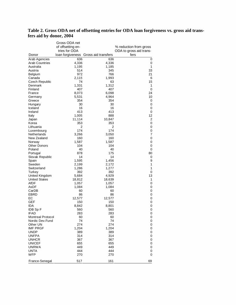
Table 2. Gross ODA net of offsetting entries for ODA loan forgiveness vs. gross aid trans-fers aid by donor, 2004
Donor
Gross ODA net of offsetting en-tries for ODA
loan forgiveness Gross aid transfers
% reduction from gross ODA to gross aid trans-
fers Arab Agencies 636 636 0Arab Countries 4,336 4,336 0Australia 1,195 1,185 1Austria 514 345 33Belgium 972 766 21Canada 2,115 1,993 6Czech Republic 74 63 15Denmark 1,331 1,312 1Finland 407 407 0France 8,073 6,098 24Germany 5,531 4,964 10Greece 354 354 0Hungary 30 30 0Iceland 16 16 0Ireland 413 413 0Italy 1,005 888 12Japan 11,114 10,847 2Korea 353 353 0Lithuania 2 2 0Luxembourg 174 174 0Netherlands 3,266 3,050 7New Zealand 160 160 0Norway 1,587 1,587 0Other Donors 104 104 0Poland 40 40 0Portugal 878 175 80Slovak Republic 14 14 0Spain 1,595 1,456 9Sweden 2,199 2,172 1Switzerland 1,286 1,277 1Turkey 392 392 0United Kingdom 5,684 4,929 13United States 18,812 18,639 1AfDF 1,057 1,057 0AsDF 1,084 1,084 0CarDB 60 60 0EBRD 86 86 0EC 12,577 12,577 0GEF 150 150 0IDA 8,842 8,801 0IDB Sp F 560 560 0IFAD 283 283 0Montreal Protocol 60 60 0Nordic Dev.Fund 74 74 0Other UN 274 274 0IMF PRGF 1,204 1,204 0UNDP 389 389 0UNFPA 314 314 0UNHCR 367 367 0UNICEF 655 655 0UNRWA 449 449 0UNTA 444 444 0WFP 270 270 0
France-Senegal 517 161 69
2. Subtracting debt service
The next step is to net debt service received out of gross aid transfers, in the belief that net trans-
fers are a better measure than gross of the cost to the donor’s treasury and benefit to the recipi-
ent. This departs somewhat from the approach of the DAC, whose net ODA statistic is net of
payments of principal, not interest. The rationale for the DAC approach is an analogy with the
capital flow concept of net foreign direct investment. Only return of capital is netted out of net
FDI, not repatriation of earnings. Similarly, only amortization is netted out of net ODA, not in-
terest, which can be seen as the donors’ “earnings” on aid investment. So the formula for net
ODA is simply:
Net ODA = Gross ODA – ODA loans received
(As mentioned in the previous section, ODA loans received does include offsetting entries for
forgiveness of ODA loans since they were counted in full as aid at disbursement.)
I find the FDI analogy inapt. In the case of FDI, return of capital can be expected to re-
duce the host country’s productive capital stock much more than repatriation of an equal amount
of profits. When the government of Ghana sends a check to the government of Japan for $1 mil-
lion, it hardly matters for either party whether it says “interest” or “principal” in the check’s
memo field, that is, whether the transaction enters the capital or current account. It seems
unlikely that interest and principal payments have different effects on Japan’s treasury or
Ghana’s capital stock and development.
Moreover, studies have found evidence of defensive lending on the part of bilateral and
multilateral lenders, whereby new loans go to servicing old ones (Ratha 2001; Birdsall, Claes-
sens, and Diwan 2002). To the extent that donors are lending to cover interest payments they re-
ceive on concessional loans, net ODA counts makes the circulation of money on paper look like
an aid increase. Much the same can be said for treating capitalization of interest arrears as new
aid.
For these reasons, the CDI aid index treats debt service uniformly. “Net aid transfers” is
defined as “gross aid transfers” less debt service actually received on ODA loans. (See Table 3.)
However, the design principle followed here, that only actual transfers be counted, introduces
another complexity. In DAC accounting, “interested received” includes interest on ODA loans
that has been forgiven, not actually paid. Forgiving interest generates two opposite transactions:
a debt forgiveness grant and a (forgiven) interest received transaction, which is included in total
interest received. Since the definition of gross aid used here excludes the debt forgiveness grant,
it must also exclude the return transaction for consistency; otherwise it will effectively penalize
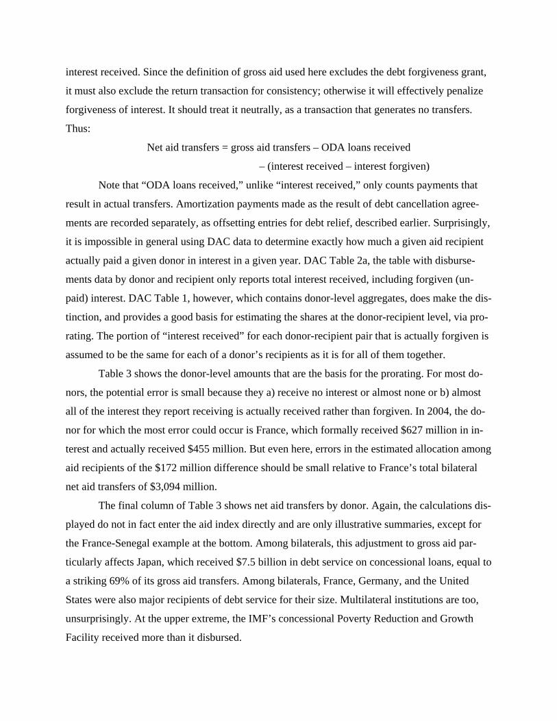
forgiveness of interest. It should treat it neutrally, as a transaction that generates no transfers.
Thus:
Net aid transfers = gross aid transfers – ODA loans received
– (interest received – interest forgiven)
Note that “ODA loans received,” unlike “interest received,” only counts payments that
result in actual transfers. Amortization payments made as the result of debt cancellation agree-
ments are recorded separately, as offsetting entries for debt relief, described earlier. Surprisingly,
it is impossible in general using DAC data to determine exactly how much a given aid recipient
actually paid a given donor in interest in a given year. DAC Table 2a, the table with disburse-
ments data by donor and recipient only reports total interest received, including forgiven (un-
paid) interest. DAC Table 1, however, which contains donor-level aggregates, does make the dis-
tinction, and provides a good basis for estimating the shares at the donor-recipient level, via pro-
rating. The portion of “interest received” for each donor-recipient pair that is actually forgiven is
assumed to be the same for each of a donor’s recipients as it is for all of them together.
Table 3 shows the donor-level amounts that are the basis for the prorating. For most do-
nors, the potential error is small because they a) receive no interest or almost none or b) almost
all of the interest they report receiving is actually received rather than forgiven. In 2004, the do-
nor for which the most error could occur is France, which formally received $627 million in in-
terest and actually received $455 million. But even here, errors in the estimated allocation among
aid recipients of the $172 million difference should be small relative to France’s total bilateral
net aid transfers of $3,094 million.
The final column of Table 3 shows net aid transfers by donor. Again, the calculations dis-
played do not in fact enter the aid index directly and are only illustrative summaries, except for
the France-Senegal example at the bottom. Among bilaterals, this adjustment to gross aid par-
ticularly affects Japan, which received $7.5 billion in debt service on concessional loans, equal to
a striking 69% of its gross aid transfers. Among bilaterals, France, Germany, and the United
States were also major recipients of debt service for their size. Multilateral institutions are too,
unsurprisingly. At the upper extreme, the IMF’s concessional Poverty Reduction and Growth
Facility received more than it disbursed.
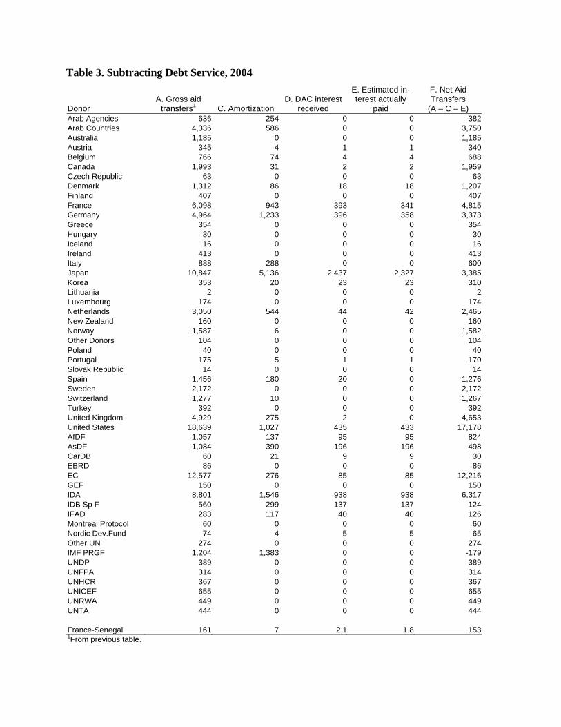
Table 3. Subtracting Debt Service, 2004
Donor A. Gross aid
transfers1 C. Amortization D. DAC interest
received
E. Estimated in-terest actually
paid
F. Net Aid Transfers
(A – C – E) Arab Agencies 636 254 0 0 382Arab Countries 4,336 586 0 0 3,750Australia 1,185 0 0 0 1,185Austria 345 4 1 1 340Belgium 766 74 4 4 688Canada 1,993 31 2 2 1,959Czech Republic 63 0 0 0 63Denmark 1,312 86 18 18 1,207Finland 407 0 0 0 407France 6,098 943 393 341 4,815Germany 4,964 1,233 396 358 3,373Greece 354 0 0 0 354Hungary 30 0 0 0 30Iceland 16 0 0 0 16Ireland 413 0 0 0 413Italy 888 288 0 0 600Japan 10,847 5,136 2,437 2,327 3,385Korea 353 20 23 23 310Lithuania 2 0 0 0 2Luxembourg 174 0 0 0 174Netherlands 3,050 544 44 42 2,465New Zealand 160 0 0 0 160Norway 1,587 6 0 0 1,582Other Donors 104 0 0 0 104Poland 40 0 0 0 40Portugal 175 5 1 1 170Slovak Republic 14 0 0 0 14Spain 1,456 180 20 0 1,276Sweden 2,172 0 0 0 2,172Switzerland 1,277 10 0 0 1,267Turkey 392 0 0 0 392United Kingdom 4,929 275 2 0 4,653United States 18,639 1,027 435 433 17,178AfDF 1,057 137 95 95 824AsDF 1,084 390 196 196 498CarDB 60 21 9 9 30EBRD 86 0 0 0 86EC 12,577 276 85 85 12,216GEF 150 0 0 0 150IDA 8,801 1,546 938 938 6,317IDB Sp F 560 299 137 137 124IFAD 283 117 40 40 126Montreal Protocol 60 0 0 0 60Nordic Dev.Fund 74 4 5 5 65Other UN 274 0 0 0 274IMF PRGF 1,204 1,383 0 0 -179UNDP 389 0 0 0 389UNFPA 314 0 0 0 314UNHCR 367 0 0 0 367UNICEF 655 0 0 0 655UNRWA 449 0 0 0 449UNTA 444 0 0 0 444 France-Senegal 161 7 2.1 1.8 153
1From previous table.
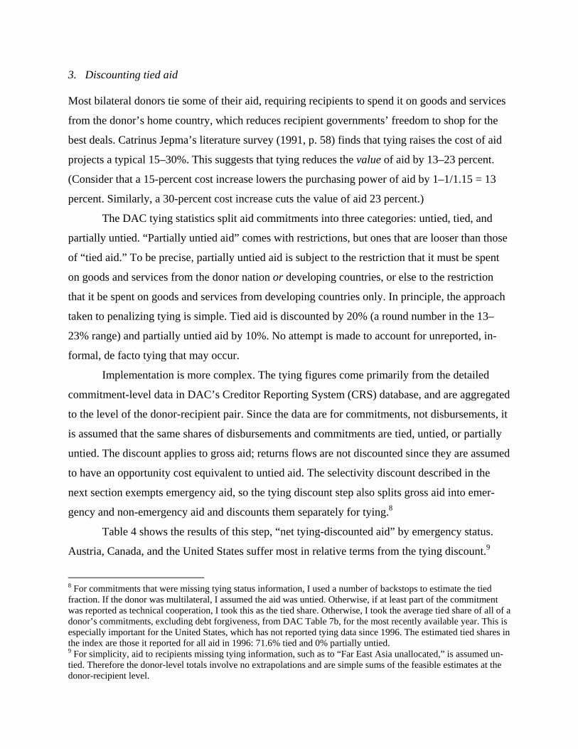
3. Discounting tied aid
Most bilateral donors tie some of their aid, requiring recipients to spend it on goods and services
from the donor’s home country, which reduces recipient governments’ freedom to shop for the
best deals. Catrinus Jepma’s literature survey (1991, p. 58) finds that tying raises the cost of aid
projects a typical 15–30%. This suggests that tying reduces the value of aid by 13–23 percent.
(Consider that a 15-percent cost increase lowers the purchasing power of aid by 1–1/1.15 = 13
percent. Similarly, a 30-percent cost increase cuts the value of aid 23 percent.)
The DAC tying statistics split aid commitments into three categories: untied, tied, and
partially untied. “Partially untied aid” comes with restrictions, but ones that are looser than those
of “tied aid.” To be precise, partially untied aid is subject to the restriction that it must be spent
on goods and services from the donor nation or developing countries, or else to the restriction
that it be spent on goods and services from developing countries only. In principle, the approach
taken to penalizing tying is simple. Tied aid is discounted by 20% (a round number in the 13–
23% range) and partially untied aid by 10%. No attempt is made to account for unreported, in-
formal, de facto tying that may occur.
Implementation is more complex. The tying figures come primarily from the detailed
commitment-level data in DAC’s Creditor Reporting System (CRS) database, and are aggregated
to the level of the donor-recipient pair. Since the data are for commitments, not disbursements, it
is assumed that the same shares of disbursements and commitments are tied, untied, or partially
untied. The discount applies to gross aid; returns flows are not discounted since they are assumed
to have an opportunity cost equivalent to untied aid. The selectivity discount described in the
next section exempts emergency aid, so the tying discount step also splits gross aid into emer-
gency and non-emergency aid and discounts them separately for tying.8
Table 4 shows the results of this step, “net tying-discounted aid” by emergency status.
Austria, Canada, and the United States suffer most in relative terms from the tying discount.9
8 For commitments that were missing tying status information, I used a number of backstops to estimate the tied fraction. If the donor was multilateral, I assumed the aid was untied. Otherwise, if at least part of the commitment was reported as technical cooperation, I took this as the tied share. Otherwise, I took the average tied share of all of a donor’s commitments, excluding debt forgiveness, from DAC Table 7b, for the most recently available year. This is especially important for the United States, which has not reported tying data since 1996. The estimated tied shares in the index are those it reported for all aid in 1996: 71.6% tied and 0% partially untied. 9 For simplicity, aid to recipients missing tying information, such as to “Far East Asia unallocated,” is assumed un-tied. Therefore the donor-level totals involve no extrapolations and are simple sums of the feasible estimates at the donor-recipient level.
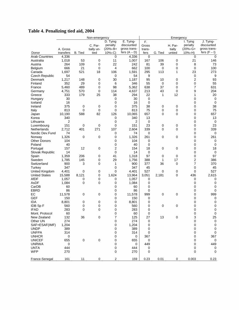
Table 4. Penalizing tied aid, 2004 Non-emergency Emergency
Donor A. Gross transfers B. Tied
C. Par-tially un-
tied
D. Tying penalty
(20%×B+ 10%×C)
E. Tying-discounted gross trans-fers (A – D)
F. Gross trans-fers G. Tied
H. Par-tially
untied
I. Tying penalty
(20%×G+ 10%×H)
J. Tying-discounted gross trans-fers (F – I)
Arab Countries 4,336 0 4,336 0 0 0Australia 1,018 53 0 11 1,007 167 106 0 21 146Austria 264 109 0 22 242 81 39 0 8 73Belgium 666 21 0 4 662 100 0 0 0 100Canada 1,697 521 18 106 1,591 295 113 1 23 273Czech Republic 54 0 54 9 0 9Denmark 1,217 148 0 30 1,187 95 10 0 2 93Finland 352 29 0 6 346 55 0 0 0 55France 5,460 489 0 98 5,362 638 37 0 7 631Germany 4,751 570 0 114 4,637 213 43 0 9 204Greece 333 179 25 38 294 22 1 12 1 20Hungary 30 0 30 0 0 0Iceland 16 0 16 0 0 0Ireland 375 0 0 0 375 38 0 0 0 38Italy 813 0 0 0 813 75 0 0 0 75Japan 10,190 588 82 126 10,065 657 0 0 0 657Korea 340 0 340 13 0 13Lithuania 2 0 2 0 0 0Luxembourg 151 0 0 0 151 23 0 0 0 23Netherlands 2,712 401 271 107 2,604 339 0 0 0 339Nordic Dev.Fund 74 0 74 0 0 0Norway 1,326 0 0 0 1,326 261 0 0 0 261Other Donors 104 0 104 0 0 0Poland 40 0 40 0 0 0Portugal 157 12 0 2 154 18 0 0 0 18Slovak Republic 14 0 14 0 0 0Spain 1,359 206 0 41 1,318 97 0 0 0 97Sweden 1,785 145 0 29 1,756 388 1 17 2 386Switzerland 900 3 0 1 900 377 36 0 7 370Turkey 347 0 347 45 0 45United Kingdom 4,401 0 0 0 4,401 527 0 0 0 527United States 15,588 8,121 0 1,624 13,964 3,051 2,181 0 436 2,615AfDF 1,057 0 0 0 1,057 0 0 0AsDF 1,084 0 0 0 1,084 0 0 0CarDB 60 0 60 0 0 0EBRD 86 0 86 0 0 0EC 11,578 0 0 0 11,578 999 0 0 0 999GEF 150 0 150 0 0 0IDA 8,801 0 0 0 8,801 0 0 0IDB Sp F 560 0 0 0 560 0 0 0 0 0IFAD 283 0 0 0 283 0 0 0Mont. Protocol 60 0 60 0 0 0New Zealand 132 36 0 7 125 27 13 0 3 25Other UN 274 0 274 0 0 0SAF+ESAF(IMF) 1,204 0 1,204 0 0 0UNDP 389 0 389 0 0 0UNFPA 314 0 314 0 0 0UNHCR 0 0 0 367 0 367UNICEF 655 0 0 0 655 0 0 0UNRWA 0 0 0 449 0 449UNTA 444 0 444 0 0 0WFP 270 0 270 0 0 0 France-Senegal 161 11 0 2 159 0.23 0.01 0 0.003 0.23
4. Adjusting for selectivity
It has long been argued that which country aid goes to is an important determinant of its effec-
tiveness (Easterly 2002, p. 35). Some countries need aid more than others. Some countries can
use it better than others. There is little empirically grounded consensus, however, on what pre-
cisely donors should select for.
For anyone measuring selectivity, two main challenges arise: choosing a mathematical
structure to distill numbers on recipient attributes and donor aid allocations into a metric; and
choosing the attributes that donors are expected to select for, such as low income, good policies,
or good governance. I will discuss my choices at the level of principle, then descend to the de-
tails of implementation.
Principles
The oldest approach to measuring selectivity—even if not always thought of as such—is the use
of cross-country regressions to explain donors’ aid allocations as a function of recipient charac-
teristics. Historically, these have included indicators of geopolitical importance (e.g, oil exports
or military expenditure), commercial links (trade with donors), and development need and poten-
tial (income, governance) (Kaplan 1975; Dudley and Montmarquette 1976; McKinley and Little
1979; Mosley 1981, 1985; Maizels and Nissanke 1984; Frey and Schneider 1986; Gang and
Lehman 1990; Schraeder, Hook, and Taylor 1998; Trumbull and Wall 1994; Alesina and Dollar
1998; Burnside and Dollar 2000; Collier and Dollar 2002; Birdsall, Claessens, and Diwan 2002).
In general, bilateral donors appear to be less sensitive to recipient need and potential than to stra-
tegic and commercial interests. More limited evidence suggests that multilaterals act oppositely.
Almost all the studies that check find a bias in favor of small countries, in the sense that the elas-
ticity of aid receipts with respect to population or GDP is statistically less than 1.
The cross-country regression approach to measuring selectivity is conceptually consis-
tent, but if used to evaluate donors it invites methodological challenges that it might be better to
avoid with a simpler approach. This is because it embodies an attempt to model donor decision-
making and predict the effects on allocations of marginal changes in recipient characteristics, all
else equal. (That is the meaning of regression coefficient estimates.) With modeling comes the
risk of misspecification. If a donor’s aid allocations fail to relate to the chosen variables via the
chosen functional form, the results may not be meaningful. For example, if a donor specializes in

one region, such as France in francophone Africa, its aid allocations will be highly nonlinear
with respect to most indicators of recipient appropriateness, and a linear regression may produce
strange results. Similarly if a donor specializes in the poorest nations. Results may also be sensi-
tive to the choice of regressors. The United States gives large amounts of aid to countries such as
Russia and Pakistan that appear too poorly governed to make good use of aid for development
but have obvious geopolitical value. As a result, regressions that control for geopolitical value
may yield a different coefficient on governance for the United States than regressions that do not.
This then raises the question of whether evaluations of selectivity should abstract from donors’
responsiveness to non-development concerns. Controlling for non-development concerns gives a
better picture of the effects of a hypothetical marginal change in an indicator of recipient devel-
opment potential. Not controlling for it gives a better picture of the general importance of devel-
opment potential in allocation. It is a question, in other words, of what is meant by “selectivity.”
The work of David Dollar and Victoria Levin (2004), used in the World Bank’s Global
Monitoring Report (2005b), stands in the regression tradition and faces some of these questions.
The authors estimate the elasticity of a donor’s aid disbursements with respect to recipient’s in-
come and governance. They do not control for commercial or geopolitical interests. They posit a
log-linear (elasticity-type) relationship between aid disbursements and recipient population,
GDP/capita, and “institutions/policies” as indicated by the World Bank’s Country Policy and In-
stitutional Assessment (CPIA). They do not control for donor interest variables. They do, how-
ever, abstract from small-country bias by controlling for population, even though Collier and
Dollar (2002) find that global aid could reduce poverty twice as fast if most of it were reallocated
to India.
The Dollar and Levin specification has a problem that is relatively specific to it, yet illus-
trates the general risk that comes with modeling. In the elasticity framework, the only recipients
that receive no aid are those with an extreme value on one of the determinants—e.g., infinite
GDP/capita or zero CPIA score. Since there are no such countries, an elasticity-based model pre-
dicts that every recipient receives aid from every donor. Rising income or falling governance
cause percentage reductions in aid, but never bring it to zero. Yet 1,523 out of the 4,914 the po-
tential donor-recipient pairs in the DAC database show zero disbursements for 2002 by my
count.10 The conflict between theory and reality appears when Dollar and Levin attempt, as it
were, to take the logarithms of these zeroes in order to perform their log-linear regressions. To
avoid infinities, they replace zeroes with a small number, $10,000 (actually, 0.01, since the fig-
ures are in millions of dollars). But in natural logs, 0.01 becomes –4.6. For comparison, the larg-
est gross flow in 2002, $1.3 billion from Japan to China, has a log of 7.2. If Dollar and Levin
were to replace zeroes with $100 (with a log of –9.2) or $1 (–13.8) they might reach quite differ-
ent results. An alternative specification that directly confronts the possibility that the distribution
of aid disbursements is truncated, such as tobit specification, may be more appropriate. Below, I
compare my results to theirs.
The second major approach to evaluating selectivity was initiated by McGillivray (1989,
1992). It is more radically empirical, eschewing any attempt to model allocation procedures or
estimate marginal effects, and lends itself more naturally to creating an index that reflects quan-
tity and selectivity. His index is, essentially, the weighted sum of a donor’s aid disbursements to
all recipients, where the weights are mathematically related to a recipient characteristic such as
GDP/capita. If the weights lie between 0 and 1, they can be thought of as discounts that penalize
or reward selection for desired characteristics. The ratio of the weighted sum to the unweighted
sum measures overall selectivity.11
Rao (1994, 1997) points out that donors can maximize their scores on McGillivray’s in-
dex by concentrating all their aid in the single poorest country. He argues that the source of this
perverse result is the failure of McGillivray’s index to consider recipients’ post-aid GDP/capita.
On the assumption that aid leads directly to GDP gains, if all aid went to the poorest country, that
country’s GDP/capita would rise rapidly and make it a less deserving recipient. He revised
McGillivray’s index to factor in both pre- and post-aid GDP. This introduced a notion of dimin-
ishing returns to aid: not diminishing returns to the effectiveness of aid in raising GDP/capita,
but diminishing returns to the value of doing so.
The third approach to assessing selectivity is the newest and most sophisticated. Drawing
on the cross-country literature on determinants of aid allocation, McGillivray, Leavy, and White 10 This excludes recipients lacking GDP, population, or (1999) CPIA data, and excludes three atypical donors: Arab Agencies, the Montreal Protocol fund, and the Caribbean Development Bank. 11 McGillivray’s original (1989) index summed aid/recipient population rather than total aid to each recipient. White (1992) questioned the implicit notion of donors “allocating” aid/recipient population: shifting $1 million in aid from small, poor Mali to large, poor India would reduce a donor’s score in McGillivray’s system because the aid would be lower per capita in India. In reply, McGillivray (1992) proposed using absolute aid rather than aid/capita, within the same basic framework.
(2002), formally model aid allocation. They endow donors with utility functions that depend on
their allocation of aid among recipients that are characterized by various commercial and geopo-
litical interest factors and levels of development need and potential. The authors incorporate di-
minishing returns to aid, compute optimal allocations, and penalize donors to the extent they de-
viate from their optima. The approach has several disadvantages from the point of view of the
CDI. It is conceptually complex. It is vulnerable to challenges analogous to those that apply to
the first approach, regarding proper specification. It rewards donors for pursuing geopolitical and
commercial interests (though this could be easily changed, to focus purely on recipient need, as
appropriate for the CDI). And it penalizes donors for aid allocations that are rather different from
the ideal ones even if they do not generate much lower utility. For example, if a donor at the op-
timal allocation shifts aid between two identical recipients, the marginal utility cost is zero, but
the marginal decline in the donor’s score would be non-zero.
The approach I take is closest to McGillivray’s original. For the purposes of the CDI, it
has the advantages of conceptual simplicity; it combines quantity and quality (selectivity) in a
natural way that minimizes questions about proper modeling specification. Since it does not
model with smooth functional forms, it does not inherently penalize sharp specialization in a cer-
tain region or income bracket. It can be combined with other discount factors, such as for tying
and project proliferation. It lends itself to a distinction between subflows of aid (emergency and
non-emergency). And it can handle net transfers even when they are negative, where some of the
common functional forms cannot. (Reverse flows, like zero flows, would bedevil the elasticity
approach of Dollar and Levin, for example.)
Here is a simple example of how the chosen system works. The selectivity formula intro-
duced here, it will emerge, assigns Mali a weight of 0.8 for non-emergency aid and Libya a 0.2,
for the 2004 data year. A donor whose aid program consisted of giving $1 million to each of
these countries would have selectivity-weighted aid of $1 million (0.8 × $1 million = $0.8 mil-
lion for Mali plus 0.2 × $1 million = $0.2 million for Libya). The donor’s “selectivity” is then the
ratio of its selectivity-weighted aid to its unweighted aid—in this case 0.5. This is also the aver-
age selectivity weight of the donor’s recipients, where the average is weighted by how much aid
the donor gives to each recipient.
One potentially counterintuitive result of this approach is that a donor that is constitution-
ally confined to a clientele with low selectivity weights comes off poorly even if it is in some
sense selective within that pool. The best example is the European Bank for Reconstruction and
Development (EBRD), which lends to the (relatively rich) nations of the former Eastern bloc.
But for purposes of comparing bilateral donors to each other, this is actually as it should be. As
will be described below, the “quality-adjusted aid quantities” of multilaterals are ultimately allo-
cated back as credits to the bilaterals. If Germany is to be more rewarded for giving aid to Ma-
lawi than Poland, it should also be more rewarded for doing the same indirectly—giving more to
the African Development Fund than the EBRD.
Having settled the question of mathematical form for measuring selectivity, there remains
the question of what donors are supposed to select for. The aid index uses two indicators. The
first is GDP/capita, converted to dollars on the basis of exchange rates.12 The second indicator is
the composite governance variable of Daniel Kaufman and Aart Kraay (Kaufmann, Kraay, and
Mastruzzi 2005), which is the most comprehensive governance indicator available. The KK
composite is an average of indicators on up to six dimensions, available data permitting: democ-
racy, political instability, rule of law, bureaucratic regulation, government effectiveness, and cor-
ruption. The six variables are themselves synthesized from several hundred primary variables
from more than a score of datasets. GDP/capita and the KK composite have several strengths for
measuring selectivity. They have wide coverage. They are updated regularly and made freely
available. And they reflect consensus views that a) the richer a country is, the less it needs aid;
and b) that institutional quality is a key determinant of development and, most likely, aid effec-
tiveness.
Before descending to the particulars of the selectivity discounting, it is worth reiterating
that two concepts are defined here relating to selectivity. The first, selectivity-weighted aid, is a
measure of aid allocations that blends quantity and quality, and is of primary interest for grading
performance. It possesses the desirable properties of linearity. If a country doubles its aid to
every recipient, its selectivity-adjusted aid score will double. If it runs two parallel aid programs,
the selectivity-adjusted aid total of the combination is the sum of those for the individual pro-
grams.
The second concept is the weighted-average selectivity score of a donor’s recipients—the
donor’s “selectivity.” This measure, it should be noted, behaves strangely when applied to do-
12 PPP-based GDP might seem more meaningful, but it is highly correlated with exchange-rate GDP in logs, so that it gives nearly the same results as used here, and is available for slightly few countries.
nors with net transfers much smaller than gross transfers. Consider this example. Donor X is a
development bank. It disburses nothing to Recipient Y, which has selectivity weight 0.6, but re-
ceives $1 million from Y in debt service, which is treated as negative aid. It disburses the $1 mil-
lion to Recipient Z, which has weight 0.8. Donor X’s selectivity-weighted aid is thus:
0.6 × (–$1 million) + 0.8 × ($1 million) = $0.2 million.
Its score is small but positive because it has transferred funds from a less appropriate to a more
appropriate aid “recipient”—perhaps an odd result, but meaningful. Now, what is the “selectiv-
ity” of Donor X?
selectivity-weighted net transfers / total net transfers = $0.2 million / 0 = ∞.
The donor has done some good for the developing world on net, according to the measure, with
zero net disbursal of funds. It is infinitely efficient.
This extreme example illustrates a counterintuitive result for donors whose net transfers
are much smaller than gross transfers (because of debt service). In these cases, the donor’s re-
ported “selectivity” can lie outside the range of most of its recipients’ selectivity weights. For
example, the IDB’s Fund for Special Operations disbursed $593 million in 2003. It received
$434 million in debt service, for a net aid of only $159 million. Yet it generally transferred funds
from countries deemed less appropriate for aid to those deemed more appropriate and so
achieves a selectivity score of 0.85 in 2003, it will emerge, which is higher than the selectivity
weight of any of its recipients. Mathematically, the 0.85 is a weighted average of selectivity fac-
tors between 0 and 1, where some of those weights (net transfers) are negative.
One can avoid such results by measuring selectivity of gross disbursements only, which I
call “gross selectivity.” In the abstract example above, Donor X has gross selectivity of $0.2 mil-
lion/$1 million = 0.2. This result seems more meaningful than infinity, but comes at the expense
of ignoring the debt service received from Recipient Y.
The sometimes-strange behavior of the version that includes reflows, “net selectivity,”
does not mean it is inherently flawed. Rather, it points up another subtlety in the question of
what is meant by selectivity. The picture conjured by the word “selectivity” is of a donor that
only sends funds outward. In fact, donors not only distribute their own money but redistribute
that of recipients. What does selectivity mean in such a context? Is a donor that bestows all its
net transfers on Malawi almost perfectly selective? Or is it falling far short of the ideal by failing
to transfer billions of dollars from Kuwait to Malawi?

The 2006 CDI deals with this problem with a compromise between principle and simplic-
ity. To avoid infinities, it segregates (tying-discounted) disbursements from reflows. It then ap-
plies the gross selectivity factor to disbursements, yielding selectivity-weighted disbursements,
and applies the same factor to reflows, implicitly assuming that the distribution of a donor’s dis-
bursements and reflows across recipients are same. It would be more accurate to separately com-
pute the “selectivity” of the donor’s reflows, but would also be more complicated, and tends to
generate extreme results in some cases.
Implementation
The flow to which selectivity weights are applied is the output of the previous steps in the con-
struction of the aid performance measure, namely “net tying-discounted aid” and debt service.
These quantities are multiplied by two discount factors. The first is linearly related to a country’s
KK governance score. The linear relationship is such that in the benchmark year of 2001, the
data year for the first edition of the CDI, the governance weight ranges exactly between 0 (for
the worst-governed country, the DRC) and 1 (for Chile). The second factor is a linear function of
a country’s log GDP/capita. In 2001, the United Arab Emirates (GDP/capita of $28,751) gets a 0
and the DRC (GDP/capita of $97), defines the upper end for the GDP/capita weights. This upper
end is not 1.0, as one might expect, but 1.84, a number chosen so that the highest combined se-
lectivity weight (the product of the governance and income factors) is 1.0 in the benchmark year
of 2001. Table 5 summarizes the weight computations. Kaufmann and Kraay have computed
their governance variables for even years since 1996, so the CDI scoring for odd years uses the
previous year’s KK data.
There are two exceptions to this weighting. First, emergency aid is exempted from the se-
lectivity discounting since it is often effective even in the poorest-governed countries. Second,
and new in 2006, is an exemption from the governance discount—the first discount factor—for
aid that is meant to improve governance, broadly defined. This sort of aid now receives a uni-
form governance discount of 50%—compared to the 75% discount it would otherwise get in,
say, the DRC or Afghanistan. It seems perverse to penalize donors for trying to improve govern-
ance where it is low. On the other hand, poor governance may indeed undermine the effective-
ness of aid meant to improve it. The choice of a uniform 50% discount seems like a minimally
arbitrary, middle-of-the-road response to the problem. Governance aid is defined as that assigned
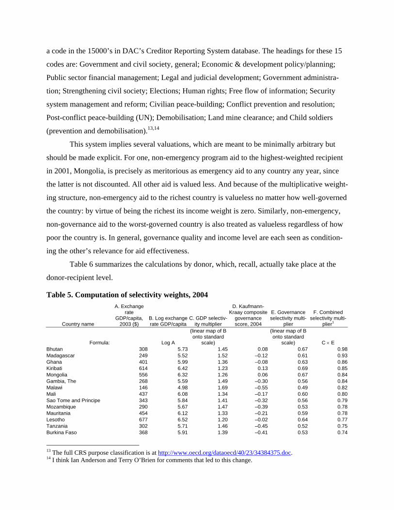
a code in the 15000’s in DAC’s Creditor Reporting System database. The headings for these 15
codes are: Government and civil society, general; Economic & development policy/planning;
Public sector financial management; Legal and judicial development; Government administra-
tion; Strengthening civil society; Elections; Human rights; Free flow of information; Security
system management and reform; Civilian peace-building; Conflict prevention and resolution;
Post-conflict peace-building (UN); Demobilisation; Land mine clearance; and Child soldiers
(prevention and demobilisation).13,14
This system implies several valuations, which are meant to be minimally arbitrary but
should be made explicit. For one, non-emergency program aid to the highest-weighted recipient
in 2001, Mongolia, is precisely as meritorious as emergency aid to any country any year, since
the latter is not discounted. All other aid is valued less. And because of the multiplicative weight-
ing structure, non-emergency aid to the richest country is valueless no matter how well-governed
the country: by virtue of being the richest its income weight is zero. Similarly, non-emergency,
non-governance aid to the worst-governed country is also treated as valueless regardless of how
poor the country is. In general, governance quality and income level are each seen as condition-
ing the other’s relevance for aid effectiveness.
Table 6 summarizes the calculations by donor, which, recall, actually take place at the
donor-recipient level.
Table 5. Computation of selectivity weights, 2004
Country name
A. Exchange rate
GDP/capita, 2003 ($)
B. Log exchange rate GDP/capita
C. GDP selectiv-ity multiplier
D. Kaufmann-Kraay composite
governance score, 2004
E. Governance selectivity multi-
plier
F. Combined selectivity multi-
plier1
Formula: Log A
(linear map of B onto standard
scale)
(linear map of B onto standard
scale) C × E Bhutan 308 5.73 1.45 0.08 0.67 0.98Madagascar 249 5.52 1.52 –0.12 0.61 0.93Ghana 401 5.99 1.36 –0.08 0.63 0.86Kiribati 614 6.42 1.23 0.13 0.69 0.85Mongolia 556 6.32 1.26 0.06 0.67 0.84Gambia, The 268 5.59 1.49 –0.30 0.56 0.84Malawi 146 4.98 1.69 –0.55 0.49 0.82Mali 437 6.08 1.34 –0.17 0.60 0.80Sao Tome and Principe 343 5.84 1.41 –0.32 0.56 0.79Mozambique 290 5.67 1.47 –0.39 0.53 0.78Mauritania 454 6.12 1.33 –0.21 0.59 0.78Lesotho 677 6.52 1.20 –0.02 0.64 0.77Tanzania 302 5.71 1.46 –0.45 0.52 0.75Burkina Faso 368 5.91 1.39 –0.41 0.53 0.74
13 The full CRS purpose classification is at http://www.oecd.org/dataoecd/40/23/34384375.doc. 14 I think Ian Anderson and Terry O’Brien for comments that led to this change.

Country name
A. Exchange rate
GDP/capita, 2003 ($)
B. Log exchange rate GDP/capita
C. GDP selectiv-ity multiplier
D. Kaufmann-Kraay composite
governance score, 2004
E. Governance selectivity multi-
plier
F. Combined selectivity multi-
plier1
Senegal 671 6.51 1.20 –0.18 0.60 0.72Benin 549 6.31 1.26 –0.29 0.56 0.71Uganda 259 5.56 1.50 –0.63 0.46 0.70India 650 6.48 1.21 –0.26 0.57 0.69Niger 261 5.56 1.50 –0.66 0.45 0.68Rwanda 225 5.41 1.55 –0.71 0.44 0.68Zambia 489 6.19 1.30 –0.52 0.50 0.65Guyana 1,030 6.94 1.06 –0.18 0.60 0.64Nicaragua 812 6.70 1.14 –0.32 0.56 0.63Sri Lanka 1,010 6.92 1.07 –0.24 0.58 0.62Guinea-Bissau 202 5.31 1.58 –0.87 0.39 0.62Ethiopia 113 4.73 1.77 –1.01 0.35 0.62Sierra Leone 188 5.24 1.61 –0.90 0.38 0.61Micronesia, Fed. Sts. 2,090 7.64 0.84 0.27 0.73 0.61Cape Verde 2,283 7.73 0.81 0.35 0.76 0.61Cambodia 343 5.84 1.41 –0.76 0.42 0.60Vietnam 547 6.30 1.27 –0.60 0.47 0.60Vanuatu 1,560 7.35 0.93 –0.06 0.63 0.59St. Vincent & the Grenadines 3,439 8.14 0.68 0.68 0.85 0.58Moldova 582 6.37 1.25 –0.64 0.46 0.57Namibia 2,711 7.91 0.75 0.35 0.76 0.57Eritrea 203 5.31 1.58 –0.98 0.36 0.57Philippines 1,002 6.91 1.07 –0.41 0.53 0.57Kenya 473 6.16 1.31 –0.74 0.43 0.56Jordan 1,996 7.60 0.85 0.03 0.66 0.56Nepal 248 5.51 1.52 –0.94 0.37 0.56Marshall Islands 1,871 7.53 0.87 –0.03 0.64 0.56Bolivia 1,005 6.91 1.07 –0.43 0.52 0.56Morocco 1,555 7.35 0.93 –0.19 0.59 0.55Egypt, Arab Rep. 987 6.89 1.08 –0.46 0.51 0.55Kyrgyz Republic 435 6.08 1.34 –0.80 0.41 0.55Dominica 3,883 8.26 0.64 0.68 0.85 0.55Armenia 1,187 7.08 1.02 –0.43 0.52 0.53Honduras 1,052 6.96 1.06 –0.51 0.50 0.53Maldives 2,219 7.70 0.82 –0.04 0.64 0.52Uruguay 3,854 8.26 0.64 0.54 0.81 0.52Suriname 2,540 7.84 0.78 0.05 0.67 0.52Chile 5,947 8.69 0.50 1.25 1.02 0.52Papua New Guinea 721 6.58 1.18 –0.72 0.44 0.51Costa Rica 4,651 8.44 0.58 0.77 0.88 0.51Thailand 2,558 7.85 0.77 0.03 0.66 0.51St. Lucia 4,439 8.40 0.60 0.68 0.85 0.51Comoros 563 6.33 1.26 –0.83 0.40 0.51China 1,270 7.15 1.00 –0.49 0.50 0.50El Salvador 2,398 7.78 0.79 –0.06 0.63 0.50Bulgaria 3,206 8.07 0.70 0.21 0.71 0.50Togo 392 5.97 1.37 –0.96 0.36 0.50Guinea 380 5.94 1.38 –0.97 0.36 0.50Bangladesh 402 6.00 1.36 –0.96 0.36 0.50Tonga 1,932 7.57 0.86 –0.26 0.57 0.49Dominican Republic 2,097 7.65 0.84 –0.25 0.58 0.48Botswana 5,283 8.57 0.54 0.80 0.89 0.48Belize 3,972 8.29 0.63 0.37 0.76 0.48Tunisia 2,827 7.95 0.74 –0.01 0.65 0.48Mauritius 4,965 8.51 0.56 0.66 0.85 0.48Jamaica 2,961 7.99 0.73 –0.05 0.64 0.46Grenada 4,879 8.49 0.57 0.54 0.81 0.46Tajikistan 297 5.69 1.46 –1.13 0.31 0.46Indonesia 1,082 6.99 1.05 –0.73 0.43 0.45Solomon Islands 462 6.14 1.32 –1.03 0.34 0.45Brazil 3,286 8.10 0.69 0.01 0.65 0.45

Country name
A. Exchange rate
GDP/capita, 2003 ($)
B. Log exchange rate GDP/capita
C. GDP selectiv-ity multiplier
D. Kaufmann-Kraay composite
governance score, 2004
E. Governance selectivity multi-
plier
F. Combined selectivity multi-
plier1
Romania 3,274 8.09 0.69 –0.01 0.65 0.45Ukraine 1,376 7.23 0.97 –0.63 0.46 0.45South Africa 4,792 8.47 0.57 0.43 0.78 0.45Latvia 5,897 8.68 0.51 0.71 0.86 0.44Cameroon 884 6.78 1.11 –0.87 0.39 0.44Fiji 2,986 8.00 0.72 –0.17 0.60 0.43Lithuania 6,181 8.73 0.49 0.77 0.88 0.43Georgia 1,084 6.99 1.05 –0.80 0.41 0.43Burundi 87 4.47 1.85 –1.40 0.23 0.43Paraguay 1,152 7.05 1.03 –0.78 0.42 0.43Peru 2,483 7.82 0.78 –0.35 0.55 0.43Malaysia 5,016 8.52 0.56 0.38 0.76 0.43Pakistan 604 6.40 1.23 –1.03 0.34 0.42Albania 2,141 7.67 0.83 –0.48 0.51 0.42Chad 457 6.13 1.32 –1.12 0.32 0.42Bosnia and Herzegovina 1,869 7.53 0.87 –0.58 0.48 0.42Lao PDR 397 5.98 1.37 –1.16 0.30 0.42Djibouti 1,420 7.26 0.96 –0.73 0.43 0.42Panama 4,467 8.40 0.59 0.16 0.70 0.42Macedonia, FYR 2,573 7.85 0.77 –0.39 0.53 0.41Yemen, Rep. 639 6.46 1.22 –1.05 0.34 0.41Poland 6,273 8.74 0.49 0.54 0.81 0.39Estonia 8,050 8.99 0.41 1.06 0.97 0.39Colombia 2,302 7.74 0.81 –0.55 0.49 0.39Azerbaijan 1,083 6.99 1.05 –0.96 0.36 0.38Syrian Arab Republic 1,282 7.16 0.99 –0.91 0.38 0.38Swaziland 2,117 7.66 0.83 –0.68 0.45 0.37Slovak Republic 7,578 8.93 0.43 0.74 0.87 0.37Ecuador 2,293 7.74 0.81 –0.65 0.46 0.37Guatemala 2,344 7.76 0.80 –0.65 0.46 0.37Nigeria 573 6.35 1.25 –1.21 0.29 0.36Turkey 4,384 8.39 0.60 –0.17 0.60 0.36Argentina 3,883 8.26 0.64 –0.34 0.55 0.35Central African Republic 319 5.76 1.44 –1.39 0.24 0.34Barbados 10,079 9.22 0.33 1.13 0.99 0.33Congo, Rep. 1,251 7.13 1.00 –1.12 0.32 0.32Mexico 6,441 8.77 0.48 0.04 0.66 0.32Oman 8,370 9.03 0.39 0.49 0.80 0.31Hungary 9,938 9.20 0.34 0.90 0.92 0.31Algeria 2,633 7.88 0.76 –0.82 0.41 0.31Kazakhstan 2,688 7.90 0.76 –0.82 0.41 0.31Croatia 7,605 8.94 0.42 0.24 0.72 0.31Iran, Islamic Rep. 2,415 7.79 0.79 –0.94 0.37 0.29Russian Federation 4,042 8.30 0.63 –0.63 0.46 0.29Uzbekistan 454 6.12 1.33 –1.46 0.21 0.28Czech Republic 10,443 9.25 0.32 0.74 0.87 0.28Gabon 5,304 8.58 0.54 –0.47 0.51 0.28Angola 1,745 7.46 0.90 –1.16 0.30 0.27Liberia 160 5.07 1.66 –1.63 0.16 0.27St. Kitts and Nevis 10,222 9.23 0.33 0.58 0.82 0.27Cote d'Ivoire 903 6.81 1.11 –1.38 0.24 0.26Zimbabwe 389 5.96 1.37 –1.54 0.19 0.26Belarus 2,211 7.70 0.82 –1.12 0.32 0.26Afghanistan 202 5.31 1.58 –1.64 0.16 0.26Sudan 501 6.22 1.29 –1.52 0.20 0.25Congo, Dem. Rep. 112 4.71 1.77 –1.70 0.14 0.25Antigua and Barbuda 11,754 9.37 0.29 0.77 0.88 0.25Lebanon 5,771 8.66 0.51 –0.55 0.49 0.25Malta 13,582 9.52 0.24 1.25 1.02 0.25Haiti 446 6.10 1.33 –1.59 0.18 0.23Seychelles 8,709 9.07 0.38 –0.15 0.61 0.23

Country name
A. Exchange rate
GDP/capita, 2003 ($)
B. Log exchange rate GDP/capita
C. GDP selectiv-ity multiplier
D. Kaufmann-Kraay composite
governance score, 2004
E. Governance selectivity multi-
plier
F. Combined selectivity multi-
plier1
Venezuela, RB 4,357 8.38 0.60 –0.97 0.36 0.22Trinidad and Tobago 11,529 9.35 0.29 0.30 0.74 0.22Libya 5,167 8.55 0.55 –0.94 0.37 0.20Turkmenistan 1,269 7.15 1.00 –1.53 0.19 0.19Korea, Rep. 14,042 9.55 0.23 0.61 0.83 0.19Saudi Arabia 9,730 9.18 0.35 –0.38 0.54 0.19Slovenia 16,008 9.68 0.19 0.99 0.95 0.18Equatorial Guinea 6,236 8.74 0.49 –1.15 0.31 0.15Bahrain 16,227 9.69 0.18 0.38 0.76 0.14Cyprus 19,847 9.90 0.12 0.87 0.91 0.11Israel 19,035 9.85 0.13 0.45 0.79 0.10Iraq 1,025 6.93 1.07 –1.88 0.09 0.10Hong Kong, China 23,778 10.08 0.06 1.31 1.04 0.06Singapore 24,576 10.11 0.05 1.62 1.13 0.06Kuwait 24,673 10.11 0.05 0.30 0.74 0.041To allow comparisons over time, the linear maps are designed so that selectivity weights fit exactly in the 0–1 range in a fixed ref-
erence year, 2001. In other years, weights can exceed these bounds.
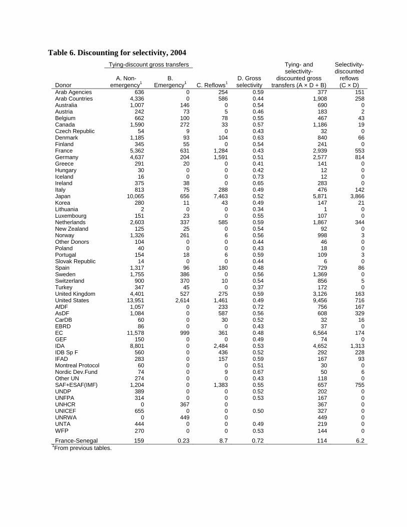
Table 6. Discounting for selectivity, 2004 Tying-discount gross transfers
Donor A. Non-
emergency1 B.
Emergency1 C. Reflows1 D. Gross selectivity
Tying- and selectivity-
discounted gross transfers (A × D + B)
Selectivity-discounted
reflows (C × D)
Arab Agencies 636 0 254 0.59 377 151Arab Countries 4,336 0 586 0.44 1,908 258Australia 1,007 146 0 0.54 690 0Austria 242 73 5 0.46 183 2Belgium 662 100 78 0.55 467 43Canada 1,590 272 33 0.57 1,186 19Czech Republic 54 9 0 0.43 32 0Denmark 1,185 93 104 0.63 840 66Finland 345 55 0 0.54 241 0France 5,362 631 1,284 0.43 2,939 553Germany 4,637 204 1,591 0.51 2,577 814Greece 291 20 0 0.41 141 0Hungary 30 0 0 0.42 12 0Iceland 16 0 0 0.73 12 0Ireland 375 38 0 0.65 283 0Italy 813 75 288 0.49 476 142Japan 10,065 656 7,463 0.52 5,871 3,866Korea 280 11 43 0.49 147 21Lithuania 2 0 0 0.34 1 0Luxembourg 151 23 0 0.55 107 0Netherlands 2,603 337 585 0.59 1,867 344New Zealand 125 25 0 0.54 92 0Norway 1,326 261 6 0.56 998 3Other Donors 104 0 0 0.44 46 0Poland 40 0 0 0.43 18 0Portugal 154 18 6 0.59 109 3Slovak Republic 14 0 0 0.44 6 0Spain 1,317 96 180 0.48 729 86Sweden 1,755 386 0 0.56 1,369 0Switzerland 900 370 10 0.54 856 5Turkey 347 45 0 0.37 172 0United Kingdom 4,401 527 275 0.59 3,126 163United States 13,951 2,614 1,461 0.49 9,456 716AfDF 1,057 0 233 0.72 756 167AsDF 1,084 0 587 0.56 608 329CarDB 60 0 30 0.52 32 16EBRD 86 0 0 0.43 37 0EC 11,578 999 361 0.48 6,564 174GEF 150 0 0 0.49 74 0IDA 8,801 0 2,484 0.53 4,652 1,313IDB Sp F 560 0 436 0.52 292 228IFAD 283 0 157 0.59 167 93Montreal Protocol 60 0 0 0.51 30 0Nordic Dev.Fund 74 0 9 0.67 50 6Other UN 274 0 0 0.43 118 0SAF+ESAF(IMF) 1,204 0 1,383 0.55 657 755UNDP 389 0 0 0.52 202 0UNFPA 314 0 0 0.53 167 0UNHCR 0 367 0 367 0UNICEF 655 0 0 0.50 327 0UNRWA 0 449 0 449 0UNTA 444 0 0 0.49 219 0WFP 270 0 0 0.53 144 0
France-Senegal 159 0.23 8.7 0.72 114 6.2
1From previous tables.
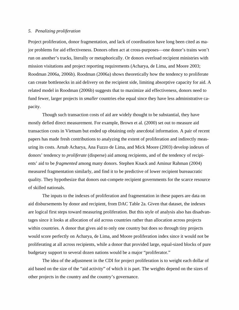
5. Penalizing proliferation
Project proliferation, donor fragmentation, and lack of coordination have long been cited as ma-
jor problems for aid effectiveness. Donors often act at cross-purposes—one donor’s trains won’t
run on another’s tracks, literally or metaphorically. Or donors overload recipient ministries with
mission visitations and project reporting requirements (Acharya, de Lima, and Moore 2003;
Roodman 2006a, 2006b). Roodman (2006a) shows theoretically how the tendency to proliferate
can create bottlenecks in aid delivery on the recipient side, limiting absorptive capacity for aid. A
related model in Roodman (2006b) suggests that to maximize aid effectiveness, donors need to
fund fewer, larger projects in smaller countries else equal since they have less administrative ca-
pacity.
Though such transaction costs of aid are widely thought to be substantial, they have
mostly defied direct measurement. For example, Brown et al. (2000) set out to measure aid
transaction costs in Vietnam but ended up obtaining only anecdotal information. A pair of recent
papers has made fresh contributions to analyzing the extent of proliferation and indirectly meas-
uring its costs. Arnab Acharya, Ana Fuzzo de Lima, and Mick Moore (2003) develop indexes of
donors’ tendency to proliferate (disperse) aid among recipients, and of the tendency of recipi-
ents’ aid to be fragmented among many donors. Stephen Knack and Aminur Rahman (2004)
measured fragmentation similarly, and find it to be predictive of lower recipient bureaucratic
quality. They hypothesize that donors out-compete recipient governments for the scarce resource
of skilled nationals.
The inputs to the indexes of proliferation and fragmentation in these papers are data on
aid disbursements by donor and recipient, from DAC Table 2a. Given that dataset, the indexes
are logical first steps toward measuring proliferation. But this style of analysis also has disadvan-
tages since it looks at allocation of aid across countries rather than allocation across projects
within countries. A donor that gives aid to only one country but does so through tiny projects
would score perfectly on Acharya, de Lima, and Moore proliferation index since it would not be
proliferating at all across recipients, while a donor that provided large, equal-sized blocks of pure
budgetary support to several dozen nations would be a major “proliferator.”
The idea of the adjustment in the CDI for project proliferation is to weight each dollar of
aid based on the size of the “aid activity” of which it is part. The weights depend on the sizes of
other projects in the country and the country’s governance.

Calculating “size weights” in a conceptually sound way turns out to be more complicated
than calculating selectivity weights. One reason is that the sizes of aid activities range over many
orders of magnitude, from $10,000 or smaller to $100 million or bigger. A linear map from this
range to a limited span needed for weights, such as [0, 1], would have to consign all projects
smaller than $5 million to near-0 weights. A map from log project size would work little better,
for while it would compress the high end, bringing $10 million and $100 million aid activities
closer together, it would explode the low end, generating large weight differences between
$1,000 and $10,000 projects. A second complication is that if there is such a thing as too small,
there is also such a thing as too big. As Radelet (2004) and Roodman (2006b) argue, large blocks
of program support are less appropriate for countries where governance is poor. In such coun-
tries, the oft-criticized transaction costs associated with aid activities—meetings with donors,
quarterly reports, etc.—also have the benefit of improving measurability of results and holding
recipients accountable for outcomes. This makes size fundamentally different from governance
and poverty, for which monotonic weighting functions are reasonable: to a first approximation,
the poorer or better governed the country, the more appropriate it seems for aid. In contrast, there
is in, in some theoretical sense, an optimal project size. It should depend on several factors, in-
cluding how big the receiving country is, how much aid it is receiving, and the quality of its gov-
ernance.
For these reasons, the new size weighting function in the CDI tends toward zero at both
the low and high ends, with a peak in between. More precisely, it is lognormal. This is the most
natural functional form for this situation because it has strictly positive support (and project size
is never negative), takes strictly positive values (so that size weights are never negative), and is
inherently compatible with the tendency of aid activity sizes to range over many orders of mag-
nitude, being a normal function of log project size.
As it happens, aid activities themselves tend to be lognormally distributed by size. Thus
the mathematical framework is one where a weighted sum of an approximately lognormal distri-
bution of aid activities is taken using weights from a separate lognormal function. Figure 1 illus-
trates. The heavy line shows the distribution of aid activities by size in a hypothetical country.
The most common size is at the peak of this curve. Because of the lognormal scale, however, the
average size, which is lifted by a few very large projects, is far to the right of the peak. The
dashed line shows one possible weighting curve. The weighting curve drawn here peaks at an
“optimal” size somewhat above the average project size, implying the belief that the average aid
dollar is going into aid activities that are too small, and is relatively wide, which indicates some
uncertainty about what the true optimal size is, and how much deviation from this optimum mat-
ters.
Applying such a weighting function to the distribution of projects hat donors fund forces
choices about the height, location, and width of each recipient’s size weighting curve. In a near-
vacuum of empirical evidence about the costs of proliferation, three principles hinted at above
shaped the choices. First, the actual distribution of aid activities by size is taken as a starting
point. Even though this is probably far from optimal in most countries, the choice serves o mini-
mize arbitrariness and puts some faith in donors’ judgments about where large or small projects
are most appropriate. Second is a bias toward larger projects. There is more consensus that the
proliferation of small projects in countries such as Tanzania and Mozambique is inefficient than
that $100,000,000 million loans from Japan and the Asian Development Bank to China are too
big, even though one might legitimately question the appropriateness of such carte blanche dis-
bursements to a relatively unaccountable, corrupt government. Thus the parameters chosen here
lead to formulas that tend to penalize projects on the small side of the observed distributions
more than those on the large side. Third is a bias toward agnosticism given the poor understand-
ing of these issues, toward preventing the differences among bilaterals’ overall proliferation
scores from being too great, manifest as a relatively wide weighting curve.
The choices can be stated precisely, as follows. The data source is the CRS database, for
which the unit of observation is the “aid activity,” which the CRS reporting guidelines describe
as follows:
An aid activity can take many forms. It could be a project or a programme, a cash transfer or de-livery of goods, a training course or a research project, a debt relief operation or a contribution to an NGO. (DAC 2002)
All aid activities in the CRS database are included, except for those coded as being donor admin-
istrative costs or debt forgiveness.
Since there are three degrees of freedom in the lognormal family of curves, which can be
thought of as height, width, and mode (highest-weighted project size), three constraints must be
imposed. The first constraint is that the weighting function must reach a peak value of 1.0, so
that only projects of “optimal” size go undiscounted. That fixes the height. To describe how the

mode is determined, let µ1 and σ1 be the mean and standard deviation of a recipient’s log aid ac-
tivity size. These are the standard parameters of the lognormal distribution. Let KK be the coun-
try’s Kaufmann-Kraay governance score (on which 0 is average). Then the mode of the weight-
ing function is decreed to occur at size For comparison, if the aid activities are per-
fectly lognormally distributed, their modal size is their median at and their average
size at
.22
11 σµ +eKK
,2
11 σµ −e ,1µe
2211 σµ +e (Aitchison and Brown 1963, p. 8). Thus for a country of average governance
(KK = 0), the “optimal aid activity size” is which is another step above the average—just
as far above the average as the average is above the median, in order of magnitude terms. This
choice is meant to be minimally arbitrary. Meanwhile, as a hypothetical country’s KK score
climbs from 0 to about standard deviation above the mean, to 1.0, the “optimal” project size ex-
actly doubles.
,2
1σµ +e
15 This choice is meant to be minimally arbitrary. Finally, the width of the weight-
ing curve, as measured by its standard deviation in log space, is set to twice that of the distribu-
tion of projects, that is, to 2σ1. A relatively broad weighting curve is meant to reflect uncertainty
about the true optimal size.
To simplify the calculations somewhat, the weighting is not done project by project.
Rather, the mean and standard deviation of log aid activity size of donor’s projects in each re-
cipient country are computed. The donor’s projects are then treated as if they are perfectly log-
normally distributed, thus fully characterized by these two numbers, and size-weighted aid is
calculated using a general formula for the integral of the product of two lognormal curves. (See
Appendix for details.)
As elsewhere, there are practical complications. Bilateral donors that do not report full
CRS commitments data, including Belgium, Spain, and Ireland, are assigned, recipient by recipi-
ent, the average weight for donors that do. But the multilaterals that do not provide CRS data are
assigned an average size weight of 1.0 for all recipients. Figure 2 shows that most of the multi-
laterals that do report get size weights near 1. Given this pattern, a figure near 1 is clearly appro-
priate for the only major multilateral not reporting, the IMF, which disburses in large blocks.
Both emergency and non-emergency aid are subject to the discount. For consistency, debt ser-
vice is discounted too, but by the average size weight for the full distribution of a recipient’s pro-
15 Scores on each of the 6 Kaufmann-Kraay components are standardized to have mean 0 and standard deviation 1. The composite has mean zero and standard deviation 0.93 (in 2002).
jects from all donors. This implicitly assumes that the opportunity cost of debt service is a set of
aid activities of a size that is not necessarily typical for the donor in that country, but is typical of
all donors. Note that this choice can heavily penalize a donor that disburses aid to a country
through small projects and then received comparable amounts of money in debt service. If the
debt service is discounted much less than the disbursements for size, a donor’s size-adjusted aid
can turn negative.
The approach does penalize very large projects in theory, especially in poorly governed
countries, but because the parameter choices create a bias toward large projects and a degree of
agnosticism, few large projects are actually discounted much. As a result, there is a strong posi-
tive correlation between a donor’s average project size across all recipients and its average size
weight in the CDI. (See Figure 2.) In sum, the approach has a well-defined and somewhat so-
phisticate theoretical foundation, but in practice, because of the conservative parameter choices,
the upshot is essentially a straightforward discount based on each donor’s average (log) project
size.
Summary calculations at the donor level are in Table 7. As before, the actual calculations
take place at the donor-recipient level. At that level, two size weights figure: one for the donor’s
own portfolio of projects in the recipient country, the other for all donors’ projects in each re-
cipient country, which is used for discounting debt service. Multilaterals such as the African and
Asian Development Funds and the IDA clearly come out ahead, as they commit aid in much lar-
ger blocks than other donors in the countries they assist. Among bilaterals, Denmark stands out.
Since this is the last adjustment for quality, the final column of Table 7 is labeled “net
quality-adjusted aid.” This is a dollar value that embodies both quantity and quality factors.
Since this is first calculated at the donor-recipient level, the next step is aggregating up to the do-
nor level.

Figure 1. Illustration of aid activity size weighting
$100 $1,000 $10,000 $100,000 $1,000,000 $10,000,000 $100,000,000
Projects by size Weights
Most common size
"Optimal" size
Average size
Figure 2. Average size weight in CDI versus average log aid activity commitment, 2003
Austria
Denmark
FranceGermany
Italy
Netherlands
NorwayPortugal
Sweden
Switzerland
United Kingdom
Finland
Canada
United States
Japan
Australia
New Zealand
IDAIDB Sp FAfDF
AsDF
EC
IFAD
.4.6
.81
Ave
rage
siz
e w
eigh
t
4 6 8 10Average log aid activity size
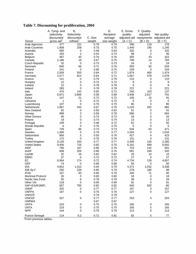
Table 7. Discounting for proliferation, 2004
Donor
A. Tying- and selectivity- discounted gross aid1
B. Selectivity-discounted
reflows1 C. Size weight
D. Recipient average
size weight
E. Gross quality-
adjusted aid (A × C)
F. Quality-adjusted
repayments (B × D)
Net quality-adjusted aid
(E + F) Arab Agencies 377 151 0.79 0.79 296 118 178 Arab Countries 1,908 258 0.75 0.75 1,440 195 1,245 Australia 690 0 0.48 0.63 332 0 332 Austria 183 2 0.53 0.74 98 2 96 Belgium 467 43 0.76 0.76 355 33 322 Canada 1,186 19 0.67 0.75 799 14 784 Czech Republic 32 0 0.73 0.73 24 0 24 Denmark 840 66 0.71 0.76 593 50 543 Finland 241 0 0.66 0.75 159 0 159 France 2,939 553 0.64 0.72 1,874 400 1,474 Germany 2,577 814 0.64 0.71 1,657 578 1,078 Greece 141 0 0.79 0.79 110 0 110 Hungary 12 0 0.74 0.74 9 0 9 Iceland 12 0 0.78 0.78 9 0 9 Ireland 283 0 0.78 0.78 221 0 221 Italy 476 142 0.50 0.72 240 103 137 Japan 5,871 3,866 0.58 0.68 3,408 2,617 791 Korea 147 21 0.72 0.72 106 15 91 Lithuania 1 0 0.72 0.72 0 0 0 Luxembourg 107 0 0.75 0.75 80 0 80 Netherlands 1,867 344 0.67 0.76 1,243 262 982 New Zealand 92 0 0.56 0.62 51 0 51 Norway 998 3 0.59 0.78 586 2 584 Other Donors 46 0 0.73 0.73 33 0 33 Poland 18 0 0.74 0.74 13 0 13 Portugal 109 3 0.48 0.72 52 2 50 Slovak Republic 6 0 0.76 0.76 5 0 5 Spain 729 86 0.73 0.73 534 63 471 Sweden 1,369 0 0.76 0.77 1,034 0 1,034 Switzerland 856 5 0.50 0.76 427 4 423 Turkey 172 0 0.76 0.76 131 0 131 United Kingdom 3,126 163 0.77 0.77 2,406 126 2,280 United States 9,456 716 0.65 0.70 6,191 499 5,692 AfDF 756 167 0.96 0.79 723 132 591 AsDF 608 329 0.96 0.76 581 249 332 CarDB 32 16 0.62 0.62 20 10 10 EBRD 37 0 0.72 0.72 27 0 27 EC 6,564 174 0.72 0.74 4,734 128 4,607 GEF 74 0 0.68 0.68 50 0 50 IDA 4,652 1,313 0.94 0.79 4,371 1,032 3,338 IDB Sp F 292 228 0.95 0.79 278 180 98 IFAD 167 93 0.96 0.76 160 71 90 Montreal Protocol 30 0 0.60 0.60 18 0 18 Nordic Dev.Fund 50 6 0.78 0.78 38 5 34 Other UN 118 0 0.69 0.69 81 0 81 SAF+ESAF(IMF) 657 755 0.82 0.82 540 620 -80 UNDP 202 0 0.77 0.77 157 0 157 UNFPA 167 0 0.76 0.76 127 0 127 UNHCR 0.79 0.79 UNICEF 327 0 0.77 0.77 253 0 253 UNRWA 0.67 0.67 UNTA 219 0 0.75 0.75 165 0 165 UNTA 219 0 0.75 0.75 165 0 165 WFP 144 0 0.79 0.79 113 0 113
France-Senegal 114 6.2 0.72 0.81 82 5 77 1From previous tables.
6. Aggregation to the donor level
In principle, this aggregation is matter of simple sums over recipients. But data problems intrude.
Not all aid in the DAC database is fully disaggregated by recipient country, partly because ad-
ministrative costs at headquarters are hard to allocate, partly because aid can support projects or
programs intended to benefit an entire region or continent. The United States, for example, gave
$2.435 billion in gross transfers in 2003 to “Least developed countries unspecified,” $130 mil-
lion to “Americas Unspecified,” and a separate $37 million to “North and Central America Unal-
located.” In addition, it is impossible to assign selectivity weights to some recipients for lack of
values for GDP/capita or the KK composite. These aid flows cannot be discounted for selectivity
without further assumptions. Similarly, some recipients, including recipient groups like those just
mentioned, have no commitments listed in the CRS database for some donors, so that no size
weight can be directly computed.
Leaving out aid that cannot be directly discounted for selectivity or size would understate
donors’ contributions. So such aid is incorporated as follows. For each sub-continental region, as
defined in the DAC database, such aid is discounted by the donor’s average selectivity and size
weights for aid that can be directly discounted. Once this discounting is done, all selectivity-
discounted aid to each region is summed. This procedure repeats at the level of the continent,
then the Part, then the aid recipient universe.16
7. Allocating multilateral quality-adjusted aid to bilaterals
Since the motivation for this exercise is to compare national governments, it is important to give
bilaterals credit for their contributions to multilateral institutions. This final step in computing
the index of official aid performance is done in a way that is the mirror image of the standard
DAC approach. In the DAC approach, each bilateral’s contribution to each multilateral is im-
puted forward to recipient countries based on the multilateral’s allocation across recipients in the
same year. So if Japan gives $50 million to the Asian Development Fund in some year, and 10%
of the AsDF’s net ODA goes to Indonesia that year, then 10% × $50 million = $5 million is im-
puted as Japan-Indonesia aid. In the CDI, the process runs the other way, because it is necessary
to transmit back the information about the multilaterals’ aid quality contained in their quality- 16 The DAC database divides Part II counties not into continents but into two major groups—former eastern bloc nations, and relatively rich non-DAC members. For the present calculations, these two groups are treated as “conti-nents.”

adjusted aid totals. So in the aid index, bilaterals receive credit for the aid programs of multilat-
erals in proportion to the bilaterals’ contributions to those multilaterals during the same year. For
example, since Germany accounted for 19.90% of net contributions to the IDA during 2004, it
receives credit for 19.90% of the IDA’s quality-adjusted aid of $3.338 billion, or $664 million.17
(See Table 8.)
The penultimate column of Table 8 is the final measure of official aid performance: qual-
ity-adjusted aid as a share of donor Gross National Income. GNI figures are converted to dollars
using market exchange rates, and are from the DAC.
Despite the quality adjustments, what most distinguishes donors from each other in this
index is still the sheer quantity of aid they disburse, especially when measured as true net trans-
fers. Denmark, the Netherlands, Norway, and Sweden are large donors by DAC’s net ODA
measure, and they score highest on this one too, with at least 0.29% of GNI for 2004. The two
largest donors by DAC’s standard net ODA measure, Japan and the United States score among
the lowest on this index, Japan at 0.04%, the United States at 0.06%. One reason for Japan’s low
score is that its true net transfers are much lower than its net ODA; at $6.433 billion, they put
Japan well behind France, Germany, and the United Kingdom.
The final column of Table 8 offers a quantitative measure of aid quality: the ratio of qual-
ity-adjusted aid to net aid transfers. U.S. aid quality is low despite large projects, because it
channels the lion’s share of its aid through its bilateral program, which features high tying and
low selectivity for poverty and good governance. Japanese aid quality also registers low, in part
because the tying penalty, computed as a fraction of gross aid, looms large relative to its much-
smaller net aid. The leaders are Sweden, Belgium, and the United Kingdom (all at 44%) and Ire-
land (at 47%).
Although the final scores are expressed as percentages of GNI, they should not be com-
pared to other variables so expressed, such as net ODA/GNI, only to each other. The selectivity
adjustment, for example, could have super-weighted aid to the most appropriate recipients rather
than discounting it to less appropriate ones. This equally meaningful choice would make little
difference for the relative results, but would raise scores across the board. 17 A few small multilaterals, such as the Central American Bank for Economic Integration receive contributions in but do not themselves report to DAC on their own aid allocations (examples include). This made it impossible to compute their quality-adjusted aid and allocate it back to bilaterals. To prevent contributions to these unscored mul-tilaterals from being dropped, a simple extrapolation was performed based on each bilateral’s ratio of quality-adjusted allocated back from scored multilaterals to contributions the donor made to those multilaterals.

I back-calculate this index of official aid performance to explore time-series as well as
cross-sectional variation in scores. What sets the starting point of the time frame is the availabil-
ity of the Kaufmann-Kraay governance variable—for even years in 1996–2004. For odd years, I
use the previous year’s score, except that 1995 calculations also use the 1996 KK scores. This
allows calculation of the index for 1995–2004. Total quality-adjusted aid/GNI of bilaterals de-
clined somewhat over this period. The simple average was 0.19% in 1995 and 0.15% in 2004,
and the correlation of 1995 and 2004 scores is 0.94.18 (See Figure 3.)
Aid quality (quality-adjusted aid/net aid transfers) is more volatile, and appears be fal-
ling. It averaged 456% in 1995 and 370% in 2003.19 The underlying reason appears to be slow
declines in selectivity for governance and increasing proliferation. This seems opposite in tenor
from the finding of Dollar and Levin (2004) of increasing selectivity since 1985.
Table 8. Allocating multilateral quality-adjusted aid to bilaterals, 2004
Net aid Quality-adjusted aid
Country Gross
aid Bilat-eral
Multi-lateral Total
Bi-later
al
Multi-lateral Total GNI
Ad-justed aid/GNI
Adjusted/ Net aid
(million $) ----- (million $) ----- ----- (million $) ----- (million $) ----- (%) ----- Australia 1,460 275 1,185 1,460 332 116 448 595,630 0.08 31Austria 771 427 340 766 96 176 272 290,943 0.09 36Belgium 1,509 743 688 1,431 322 310 633 357,207 0.18 44Canada 2,601 608 1,959 2,568 784 275 1,060 970,536 0.11 41Denmark 2,240 928 1,207 2,135 543 311 854 240,474 0.35 40Finland 747 340 407 747 159 100 259 185,126 0.14 35France 9,799 3,700 4,815 8,515 1,474 1,530 3,004 2,058,806 0.15 35Germany 9,634 4,670 3,373 8,043 1,078 1,950 3,028 2,729,147 0.11 38Greece 595 241 354 595 110 85 196 204,300 0.10 33Ireland 610 198 413 610 221 65 287 156,186 0.18 47Italy 3,289 2,401 600 3,001 137 822 959 1,669,301 0.06 32Japan 13,895 3,048 3,385 6,433 791 1,031 1,822 4,759,022 0.04 28Netherlands 4,753 1,703 2,465 4,168 982 683 1,665 573,127 0.29 40New Zealand 213 54 160 213 51 18 69 90,623 0.08 32Norway 2,249 662 1,582 2,244 584 211 795 251,528 0.32 35Portugal 395 219 170 389 50 86 136 164,404 0.08 35Spain 2,493 1,037 1,276 2,313 471 430 901 1,018,232 0.09 39Sweden 2,819 646 2,172 2,819 1,034 196 1,231 350,192 0.35 44Switzerland 1,647 370 1,267 1,637 423 177 600 376,621 0.16 37United Kingdom 8,237 3,308 4,653 7,961 2,280 1,247 3,527 2,179,558 0.16 44United States 22,161 3,522 17,178 20,700 5,692 1,726 7,418 11,656,110 0.06 36
18 These figures exclude Greece, which did not report to DAC for 1995, and may have given essentially no aid. 19 Figures exclude Greece.
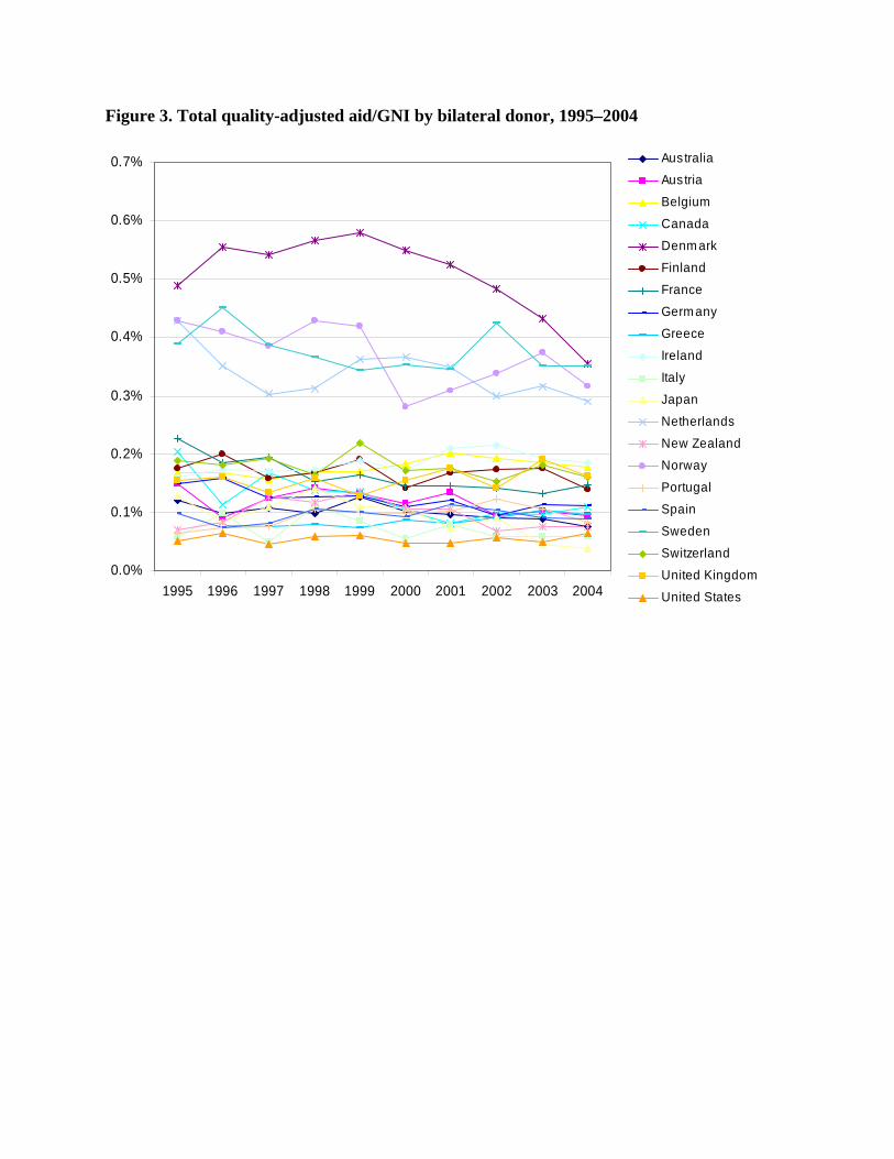
Figure 3. Total quality-adjusted aid/GNI by bilateral donor, 1995–2004
0.0%
0.1%
0.2%
0.3%
0.4%
0.5%
0.6%
0.7%
1995 1996 1997 1998 1999 2000 2001 2002 2003 2004
AustraliaAustria
Belgium
Canada
Denm ark
Finland
France
Germ any
Greece
Ireland
Italy
Japan
Netherlands
New Zealand
Norway
Portugal
Spain
Sweden
Switzerland
United Kingdom
United States
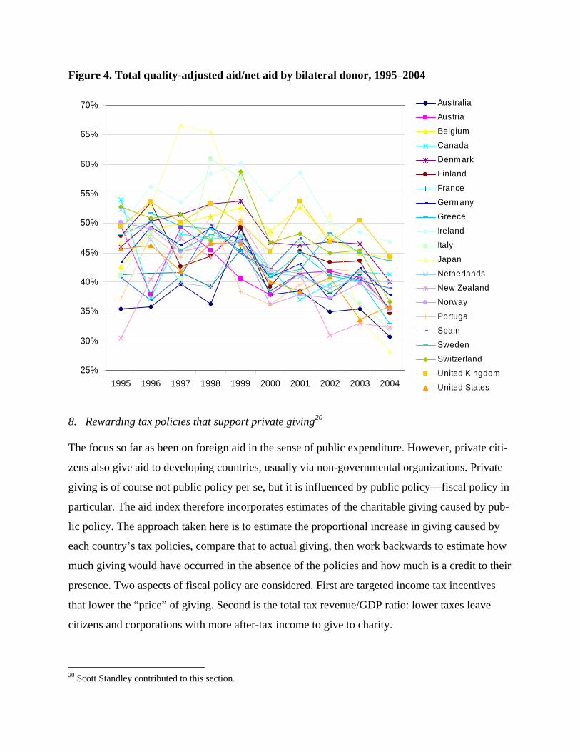
Figure 4. Total quality-adjusted aid/net aid by bilateral donor, 1995–2004
25%
30%
35%
40%
45%
50%
55%
60%
65%
70%
1995 1996 1997 1998 1999 2000 2001 2002 2003 2004
AustraliaAustria
Belgium
Canada
Denm ark
Finland
France
Germ any
Greece
Ireland
Italy
Japan
Netherlands
New Zealand
Norway
Portugal
Spain
Sweden
Switzerland
United Kingdom
United States
8. Rewarding tax policies that support private giving20
The focus so far as been on foreign aid in the sense of public expenditure. However, private citi-
zens also give aid to developing countries, usually via non-governmental organizations. Private
giving is of course not public policy per se, but it is influenced by public policy—fiscal policy in
particular. The aid index therefore incorporates estimates of the charitable giving caused by pub-
lic policy. The approach taken here is to estimate the proportional increase in giving caused by
each country’s tax policies, compare that to actual giving, then work backwards to estimate how
much giving would have occurred in the absence of the policies and how much is a credit to their
presence. Two aspects of fiscal policy are considered. First are targeted income tax incentives
that lower the “price” of giving. Second is the total tax revenue/GDP ratio: lower taxes leave
citizens and corporations with more after-tax income to give to charity.
20 Scott Standley contributed to this section.

The approach taken here will seem simplistic to some and too sophisticated to others. To
make the calculations practical, we make several simplifying assumptions. Each country’s tax
policies are complex and idiosyncratic. No two households are in exactly the same financial po-
sition, and so the tax codes present different incentives to different households. And of course
different people respond to the same incentives differently. On the other hand, the sophistication
of the calculations, such as it is, should not be read to imply that we see our estimates as beyond
improvement.
According to a survey reported in Roodman and Standley (2006), all but three index
countries—Austria, Finland, and Sweden—offer income tax incentives for charitable giving.
Australia, Belgium, Denmark, Germany, Greece, Ireland, Japan, Netherlands, Norway, Switzer-
land, the United Kingdom, and the United States allow partial or full deduction of charitable do-
nations from taxable income. Canada, France, Italy, New Zealand, Portugal, and Spain offer par-
tial credits—through the tax code, they reimburse a percentage of donations. These incentives
lower the price of giving in the sense that a dollar of forgone after-tax income buys more than a
dollar of charity. Charitable donations can fund the operations of non-profit groups working in
developing countries, such as Oxfam and CARE, or they can go to foundations that fund such
projects.
We translate the presence of a tax incentive into an estimate of the increase in charitable
giving in three steps. First, we express the tax measure as a price effect. For credits, this step is
straightforward. Canada’s 29% tax credit, for example, reduces the price of giving by 29%. For
deductions, we used a crude but available proxy for the marginal income tax rate faced by the
households with above-average incomes that appear to generate most charity. This proxy is the
marginal income tax rate for people at 167% of the income level of the average production
worker, from the OECD Tax Database. For example, the rate is 31.4% for the United States in
2003, so deductibility of charitable giving in the United States is treated as reducing the price by
31.4%. The second step is to factor in whether the deduction or credit is capped. In countries
where high-income, high-giving people account for most charity in the aggregate, caps can se-
verely limit the incentive effect in practice. Precisely how much, however, is hard to know, espe-
cially because there is little information about the distribution of giving by income group outside
the United States. Given the uncertainty, we factor caps in coarsely, by taking the simple average
of the below- and above-threshold price incentives. For most countries with caps, the above-

threshold price incentive is 0—there is no tax incentive to exceed the cap—so the price effect is
halved. The exception is Greece, which offers full deductibility up to €2,950 a year, then im-
poses a 10% tax above that limit. Since the Greece’s representative marginal income tax is
25.2%, the above-threshold price incentive is the difference between this and the special tax rate,
i.e., 15.2%. So the simple average of the below- and above-threshold rates for Greece is 20.2%.
(See Table 9.)
Finally, having estimated the price effect, we couple it with an estimate of the price elas-
ticity of giving. Research puts it at around 0.5 in the United States (Andreoni 2001). Thus, if a
representative individual in the United States faces a price effect of 31.4%, full deductibility of
charitable contributions multiplies giving by a factor of (1 – 0.314)–0.5 = 1.208, for a 20.8% in-
crease.
The procedure is similar for the effect of lower total taxes. When the overall tax ratio is
lower, individuals have more money to give to charity. Thus, while high marginal tax rates in-
crease the incentive to give when we look at the price effects of tax deductions, they decrease
the incentive to give when we look at income effects. Among the 21 scored countries, the tax
revenue/GDP ratio in 2000, the last year with data available for the first edition of the CDI,
ranged from 27.1% in Japan to 53.8% in Sweden (OECD 2004). To reward countries for lower
tax ratios, we need a baseline against which to define lowness. We choose Sweden’s 2000 tax
ratio, the highest. We combine this with an estimate of the income of elasticity of giving of 1.1
(Andreoni 2001). The United States, to continue the example, is treated as having reduced its to-
tal tax burden in 2003, the last year with data available for the 2006 CDI, from Sweden’s 2000
ratio of 53.8% to the actual 25.6%. (Sweden’s 2000 ratio is used every year for a consistent
benchmark.) This hypothetically raises the privately claimed share of GDP from 46.2% to
74.4%, an increase of 61.0%.21 As a result, the lower U.S. tax burden is estimated to multiply
charity by
,689.1538.01256.01 1.1
=⎟⎠⎞
⎜⎝⎛
−− for a 68.9% increase.
The two multipliers are then combined and divided into observed giving in order to esti-
mate giving in the absence of these favorable policies. Observed giving is “grants by NGOs” 21 Some share of the revenue funds transfer payments, which increase recipients’ disposable income and should therefore increase charitable giving. However, the transfer payments going to the high-income people that appear to account for most charity are probably relatively small.
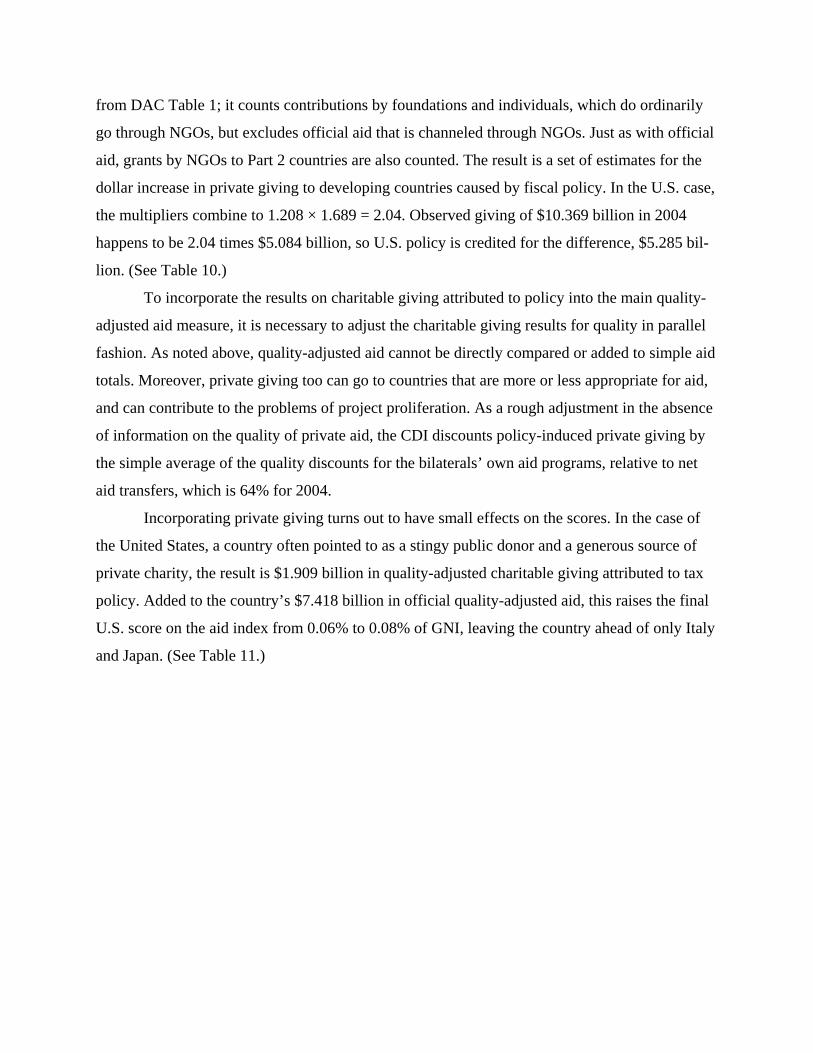
from DAC Table 1; it counts contributions by foundations and individuals, which do ordinarily
go through NGOs, but excludes official aid that is channeled through NGOs. Just as with official
aid, grants by NGOs to Part 2 countries are also counted. The result is a set of estimates for the
dollar increase in private giving to developing countries caused by fiscal policy. In the U.S. case,
the multipliers combine to 1.208 × 1.689 = 2.04. Observed giving of $10.369 billion in 2004
happens to be 2.04 times $5.084 billion, so U.S. policy is credited for the difference, $5.285 bil-
lion. (See Table 10.)
To incorporate the results on charitable giving attributed to policy into the main quality-
adjusted aid measure, it is necessary to adjust the charitable giving results for quality in parallel
fashion. As noted above, quality-adjusted aid cannot be directly compared or added to simple aid
totals. Moreover, private giving too can go to countries that are more or less appropriate for aid,
and can contribute to the problems of project proliferation. As a rough adjustment in the absence
of information on the quality of private aid, the CDI discounts policy-induced private giving by
the simple average of the quality discounts for the bilaterals’ own aid programs, relative to net
aid transfers, which is 64% for 2004.
Incorporating private giving turns out to have small effects on the scores. In the case of
the United States, a country often pointed to as a stingy public donor and a generous source of
private charity, the result is $1.909 billion in quality-adjusted charitable giving attributed to tax
policy. Added to the country’s $7.418 billion in official quality-adjusted aid, this raises the final
U.S. score on the aid index from 0.06% to 0.08% of GNI, leaving the country ahead of only Italy
and Japan. (See Table 11.)

Table 9. Computation of price incentive of tax policy, 2004
Country A. Tax
deduction?
B. Marginal income tax rate, 20041
(%)
C. Tax credit (%)
D. Deduction or credit capped?
Price incentive2
(%) Australia Yes 48.5 0.0 No 48.5 Austria No 31.7 0.0 No 0.0 Belgium Yes 45.1 0.0 No 45.1 Canada No 35.4 29.0 No 29.0 Denmark Yes 54.9 0.0 Yes 27.5 Finland No 43.7 0.0 No 0.0 France No 24.9 60.0 No 60.0 Germany Yes 47.5 0.0 No 47.5 Greece Yes 25.2 0.0 No 20.2 Ireland Yes 42.0 0.0 No 42.0 Italy No 36.4 19.0 No 19.0 Japan Yes 20.4 0.0 No 20.4 Netherlands Yes 52.0 0.0 No 52.0 New Zealand No 39.0 33.3 Yes 16.7 Norway Yes 41.5 0.0 Yes 20.7 Portugal No 24.0 25.0 No 25.0 Spain No 26.2 25.0 No 25.0 Sweden No 51.5 0.0 No 0.0 Switzerland Yes 25.1 0.0 No 25.1 United Kingdom Yes 22.0 0.0 No 22.0 United States Yes 31.4 0.0 No 31.4
1Marginal income tax rate for single individual at 167% income level of the average production worker. 2Formula is: Column B or C as appropriate, divided by 2 if there is a cap. Uniquely, Greece gives full deductibility up to a certain amount (2,950 euros) and imposes a low tax (10%) on contributions above the threshold. The tax incentive is therefore computed as the average of the below- and above-threshold incentives.
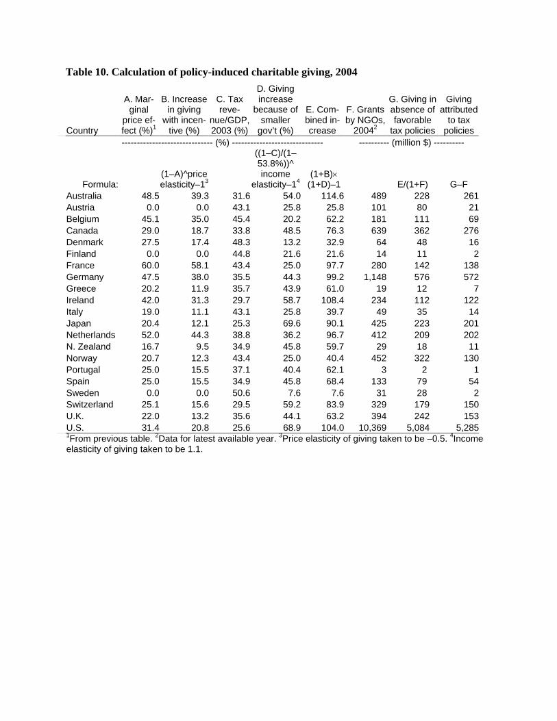
Table 10. Calculation of policy-induced charitable giving, 2004
Country
A. Mar-ginal
price ef-fect (%)1
B. Increase in giving
with incen-tive (%)
C. Tax reve-
nue/GDP, 2003 (%)
D. Giving increase
because of smaller
gov’t (%)
E. Com-bined in-crease
F. Grants by NGOs,
20042
G. Giving in absence of favorable
tax policies
Giving attributed
to tax policies
------------------------------ (%) ------------------------------ ---------- (million $) ----------
Formula: (1–A)^price elasticity–13
((1–C)/(1–53.8%))^ income
elasticity–14(1+B)×
(1+D)–1 E/(1+F) G–F Australia 48.5 39.3 31.6 54.0 114.6 489 228 261Austria 0.0 0.0 43.1 25.8 25.8 101 80 21Belgium 45.1 35.0 45.4 20.2 62.2 181 111 69Canada 29.0 18.7 33.8 48.5 76.3 639 362 276Denmark 27.5 17.4 48.3 13.2 32.9 64 48 16Finland 0.0 0.0 44.8 21.6 21.6 14 11 2France 60.0 58.1 43.4 25.0 97.7 280 142 138Germany 47.5 38.0 35.5 44.3 99.2 1,148 576 572Greece 20.2 11.9 35.7 43.9 61.0 19 12 7Ireland 42.0 31.3 29.7 58.7 108.4 234 112 122Italy 19.0 11.1 43.1 25.8 39.7 49 35 14Japan 20.4 12.1 25.3 69.6 90.1 425 223 201Netherlands 52.0 44.3 38.8 36.2 96.7 412 209 202N. Zealand 16.7 9.5 34.9 45.8 59.7 29 18 11Norway 20.7 12.3 43.4 25.0 40.4 452 322 130Portugal 25.0 15.5 37.1 40.4 62.1 3 2 1Spain 25.0 15.5 34.9 45.8 68.4 133 79 54Sweden 0.0 0.0 50.6 7.6 7.6 31 28 2Switzerland 25.1 15.6 29.5 59.2 83.9 329 179 150U.K. 22.0 13.2 35.6 44.1 63.2 394 242 153U.S. 31.4 20.8 25.6 68.9 104.0 10,369 5,084 5,2851From previous table. 2Data for latest available year. 3Price elasticity of giving taken to be –0.5. 4Income elasticity of giving taken to be 1.1.
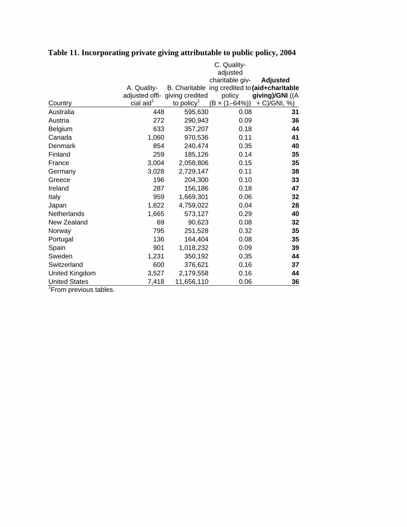
Table 11. Incorporating private giving attributable to public policy, 2004
Country
A. Quality-adjusted offi-
cial aid1
B. Charitable giving credited
to policy1
C. Quality-adjusted
charitable giv-ing credited to
policy (B × (1–64%))
Adjusted (aid+charitable giving)/GNI ((A
+ C)/GNI, %) Australia 448 595,630 0.08 31Austria 272 290,943 0.09 36Belgium 633 357,207 0.18 44Canada 1,060 970,536 0.11 41Denmark 854 240,474 0.35 40Finland 259 185,126 0.14 35France 3,004 2,058,806 0.15 35Germany 3,028 2,729,147 0.11 38Greece 196 204,300 0.10 33Ireland 287 156,186 0.18 47Italy 959 1,669,301 0.06 32Japan 1,822 4,759,022 0.04 28Netherlands 1,665 573,127 0.29 40New Zealand 69 90,623 0.08 32Norway 795 251,528 0.32 35Portugal 136 164,404 0.08 35Spain 901 1,018,232 0.09 39Sweden 1,231 350,192 0.35 44Switzerland 600 376,621 0.16 37United Kingdom 3,527 2,179,558 0.16 44United States 7,418 11,656,110 0.06 361From previous tables.

Appendix. Size weighting formula
This appendix derives the formula used to compute size-weighted aid for each donor-recipient
pair. It first derives a general formula for the integral of the product of two lognormal curves. In
the application in this paper, one curve represents the distribution of aid activities by size and the
other the weights applied to them based on size. This appendix then shows how the parameters
of the size weighting curve are mathematically determined.
Suppose we have two lognormal curves of the form:
( )
( )2
2
2
2
1
1
ln21
2
22
ln21
1
11
2
2
⎟⎟⎠
⎞⎜⎜⎝
⎛ −−
⎟⎟⎠
⎞⎜⎜⎝
⎛ −−
=
=
σµ
σµ
σπ
σπx
x
ex
Nxh
ex
Nxh
If u = ln x, then x = eu, du = dx/x, and the total integral of the product of the two curves is
.2
12
12
22
22
22
21
21
22
22
1
12
22
1
2
22
22
21
21
22
22
1
12
22
1
2
2
2
22
1
1
2
2
22
1
1
121121
21
21
21121
21
21
21
21
21
21
0
ln21
2
2ln
21
1
1
∫
∫
∫
∫
∞
∞−
⎟⎟
⎠
⎞
⎜⎜
⎝
⎛++⎟
⎟⎠
⎞⎜⎜⎝
⎛−+−⎟
⎟⎠
⎞⎜⎜⎝
⎛+−
∞
∞−
⎟⎟
⎠
⎞
⎜⎜
⎝
⎛++⎟
⎟⎠
⎞⎜⎜⎝
⎛+−⎟
⎟⎠
⎞⎜⎜⎝
⎛+−
∞
∞−
⎟⎟⎠
⎞⎜⎜⎝
⎛ −−⎟⎟
⎠
⎞⎜⎜⎝
⎛ −−
∞⎟⎟⎠
⎞⎜⎜⎝
⎛ −−⎟⎟
⎠
⎞⎜⎜⎝
⎛ −−
=
=
=
dueNN
duee
NN
duee
NN
dxex
Nex
N
uu
uu
u
uu
u
xx
σµ
σµ
σµ
σµ
σσ
σµ
σµ
σµ
σµ
σσ
σµ
σµ
σµ
σµ
σπσ
σπσ
σπσ
σπσπ
This arranges the exponent as a quadratic expression in u. Completing the square in that expres-
sion gives

.2
22
22
21
22
22
1
1
22
21
22
22
21
21
22
21
2
22
22
1
1
22
22
21
21
22
21
2
22
22
1
12
22
21
22
22
1
1
22
21
11
111
21
11
1
21
21
21
11
1
11
111
21
21
21
∫
∫
∞
∞−
⎟⎟⎟⎟⎟⎟
⎠
⎞
⎜⎜⎜⎜⎜⎜
⎝
⎛
+
−+
−+−
⎟⎟⎟⎟⎟⎟
⎠
⎞
⎜⎜⎜⎜⎜⎜
⎝
⎛
+++
⎟⎟⎠
⎞⎜⎜⎝
⎛−+
−−
∞
∞−
⎟⎟⎟⎟⎟⎟
⎠
⎞
⎜⎜⎜⎜⎜⎜
⎝
⎛
+++
⎟⎟⎠
⎞⎜⎜⎝
⎛−+
−
⎟⎟⎟⎟⎟⎟
⎠
⎞
⎜⎜⎜⎜⎜⎜
⎝
⎛
+
−+
−+−
= dueeNN
dueNN
u
u
σσ
σµ
σµ
σσσµ
σµ
σσ
σµ
σµ
σµ
σµ
σσ
σµ
σµ
σσ
σµ
σµ
σσ
σπσ
σπσ
The integral has been transformed into that of a normal curve, and evaluates to
.11
2
22
21 σσ
π
+
The whole expression is therefore
.2
112
2
22
21
2
22
22
1
1
22
22
21
21
22
22
21
21
22
21
2
22
22
1
1
11
1
21
22
21
21
11
1
21
22
21
21
21
⎟⎟⎟⎟⎟⎟
⎠
⎞
⎜⎜⎜⎜⎜⎜
⎝
⎛
+
⎟⎟⎠
⎞⎜⎜⎝
⎛−+
−+−
⎟⎟⎟⎟⎟⎟
⎠
⎞
⎜⎜⎜⎜⎜⎜
⎝
⎛
+++
⎟⎟⎠
⎞⎜⎜⎝
⎛−+
−−
+=
+
σσ
σµ
σµ
σµ
σµ
σµ
σµ
σσ
σµ
σµ
σσπ
σσ
πσπσ
eNN
eNN
Letting η1 = µ1/σ1, η2 = µ2/σ2, and ,ˆ 22
21 σσσ += this can be rewritten as
( ) ( ) .ˆ2
2
2
2
1
12
22
212
22
1 1ˆ2
1
21
021
⎟⎟
⎠
⎞
⎜⎜
⎝
⎛⎟⎟⎠
⎞⎜⎜⎝
⎛−+−+−∞
=∫ση
ση
σσσ
ηη
σπeNNdxxhxh (1)
In the present case, h1 is the distribution of aid activities by size, so N1, the number of aid
activities, is known, and µ1 and σ1 can be estimated from the data. To fix the three parameters of
h2, the size weighting function, we impose three constraints. First, we require that the peak value
of the weighting function is 1. In general, the mode of h2 is (Aitchison and Brown 1963),
at which it takes the value
222 σµ −e
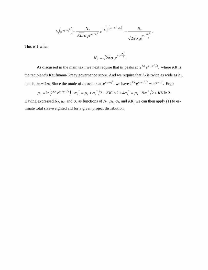
( ) ( ).
22
22
221
2
22 2
22
22
222
22
22
222
σµ
µσµσ
σµ
σµ
σπσπ −
−−−
−
− ==
e
Ne
eN
eh
This is 1 when
.2 222
22
2σ
µσπ
−= eN
As discussed in the main text, we next require that h2 peaks at ,2 2211 σµ +eKK where KK is
the recipient’s Kaufmann-Kraay governance score. And we require that h2 is twice as wide as h1,
that is, σ2 = 2σ1. Since the mode of h2 occurs at we have,2
22 σµ −e .22
222
11 2 σµσµ −+ = eeKK Ergo
( ) .2ln2942ln22ln 211
21
211
22
22
211 KKKKeKK ++=+++=+= + σµσσµσµ σµ
Having expressed N2, µ2, and σ2 as functions of N1, µ1, σ1, and KK, we can then apply (1) to es-
timate total size-weighted aid for a given project distribution.
References
Acharya, Arnab, Ana Fuzzo de Lima, and Mick Moore (2003), “The Proliferators—Transaction Costs and the Value of Aid,” mimeo. Aitchison, J., and J.A.C. Brown (1963), The Lognormal Distribution, Cambridge University Press, Cambridge. Alesina, Alberto, and David Dollar (1998), Who Gives Foreign Aid to Whom and Why?, Work-ing Paper 6612, National Bureau for Economic Research, Cambridge, MA, June. Andreoni, J. (2001), “Economics of Philanthropy,” International Encyclopedia of the Social & Behavioral Sciences, Elsevier Science Ltd, Oxford, U.K. Birdsall, Nancy, Stijn Claessens, and Ishac Diwan (2002), “Policy Selectivity Foregone: Debt and Donor Behavior in Africa,” Working Paper 17, Center for Global Development, Washing-ton, DC, October. Birdsall, Nancy, and David Roodman (2003), “The Commitment to Development Index: A Scorecard of Rich-Country Policies,” Center for Global Development, Washington, DC, April. Brown, Adrienne, Felix Naschold, Tim Conway and Adrian Fozzard (2000), “Aid Transaction Costs in Viet Nam,” Report for UNDP, December. Burnside, Craig and Dollar, David (2000), “Aid, Policies, and Growth.” American Economic Re-view, September, 90(4), pp. 847–68. Carey, Richard (2005), “Real or phantom aid?” DAC News, Paris, June–August. Center for Global Development and Foreign Policy (CGD and FP) (2006), “Ranking the Rich,” Foreign Policy, September/October. Collier, Paul and Dollar, David (2002). “Aid Allocation and Poverty Reduction.” European Eco-nomic Review, September, 45(1), pp. 1–26. Dollar, David, and Victoria Levin (2004), “The Increasing Selectivity of Foreign Aid,” draft, World Bank, Washington, DC, March 8, 2004. Dudley, Leonard, and Claude Montmarquette (1976), “A Model of the Supply of Bilateral For-eign Aid,” American Economic Review, March, 66(1), pp. 132–42.
Easterly, William (2002), “The Cartel of Good Intentions: Bureaucracy versus Markets in For-eign Aid,” Working Paper 4, Center for Global Development, Washington, DC, March.
Easterly, William, Ross Levine, and David Roodman (2004), “Aid, Policies, and Growth: Com-ment.” American Economic Review, June, 94(3).
Frey, Bruno S., and Friedrich Schneider (1986), “Competing Models of International Lending Activity,” Journal of Development Economics 20. Gang, Ira N., and James A. Lehman (1990), “New Directions or Not: USAID in Latin America,” World Development 18(5). Jepma, Catrinus J. (1991), The Tying of Aid OECD Development Centre, Paris. Kaplan, Stephen S. (1975) “The Distribution of Aid to Latin America: A Cross-national Aggre-gate Data and Time Series Analysis,” Journal of Developing Areas, October, 10. Kaufmann, Daniel, Aart Kraay, and Massimo Mastruzzi (2005), Governance Matters IV: Gov-ernance Indicators for 1996–2004, Policy Research Working Paper 3630, World Bank, Wash-ington, DC, May. Knack, Stephen, and Aminur Rahman (2004), “Donor Fragmentation and Bureaucratic Quality in Aid Recipients,” Policy Research Working Paper 3186, World Bank, Washington, DC, Janu-ary. Maizels, Alfred, and Machiko K. Nissanke (1984), “Motivations for Aid to Developing Coun-tries,” World Development 12 (9). McGillivray, Mark (1989), “The Allocation of Aid among Developing Countries: A Multi-Donor Analysis Using a Per Capita Aid Index,” World Development 17(4), pp. 561–68. ----------------------- (1992), “A Reply,” World Development 20(11), pp. 1699–1702. ----------------------- (2003), “Commitment to Development Index: A Critical Appraisal,” pre-pared for the Australian Agency for International Development, Canberra, November, http://www.ausaid.gov.au/publications/pdf/cdi_appraisal.pdf. McGillivray, Mark, Jennifer Leavy, and Howard White (2002), “Aid Principles and Policy: An Operational Basis for the Assessment of Donor Performance”, in B. Mak Arvin, ed., New Per-spectives on Foreign Aid and Economic Development, Praeger, Westport. McKinley, R.D., and R. Little (1979), “The US Aid Relationship: A Test of the Recipient Need and the Donor Interest Models,” Political Studies XXVII (2). Mosley, Paul (1981), “Models of the Aid Allocation Process: A Comment on McKinley and Lit-tle,” Political Studies XXIX (2). ----------------- (1985), “The Political Economy of Foreign Aid: A Model of the Market for a Pub-lic Good,” Economic Development and Cultural Change, January, 33 (2). Organisation for Economic Co-operation and Development (OECD) (2002), Reporting Direc-tives for the Creditor Reporting System, Paris.
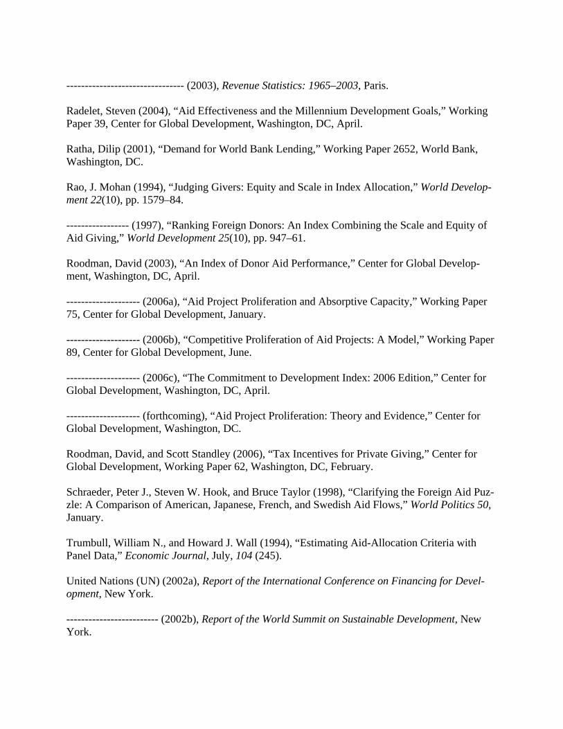
-------------------------------- (2003), Revenue Statistics: 1965–2003, Paris. Radelet, Steven (2004), “Aid Effectiveness and the Millennium Development Goals,” Working Paper 39, Center for Global Development, Washington, DC, April. Ratha, Dilip (2001), “Demand for World Bank Lending,” Working Paper 2652, World Bank, Washington, DC. Rao, J. Mohan (1994), “Judging Givers: Equity and Scale in Index Allocation,” World Develop-ment 22(10), pp. 1579–84. ----------------- (1997), “Ranking Foreign Donors: An Index Combining the Scale and Equity of Aid Giving,” World Development 25(10), pp. 947–61. Roodman, David (2003), “An Index of Donor Aid Performance,” Center for Global Develop-ment, Washington, DC, April. -------------------- (2006a), “Aid Project Proliferation and Absorptive Capacity,” Working Paper 75, Center for Global Development, January. -------------------- (2006b), “Competitive Proliferation of Aid Projects: A Model,” Working Paper 89, Center for Global Development, June. -------------------- (2006c), “The Commitment to Development Index: 2006 Edition,” Center for Global Development, Washington, DC, April. -------------------- (forthcoming), “Aid Project Proliferation: Theory and Evidence,” Center for Global Development, Washington, DC. Roodman, David, and Scott Standley (2006), “Tax Incentives for Private Giving,” Center for Global Development, Working Paper 62, Washington, DC, February. Schraeder, Peter J., Steven W. Hook, and Bruce Taylor (1998), “Clarifying the Foreign Aid Puz-zle: A Comparison of American, Japanese, French, and Swedish Aid Flows,” World Politics 50, January. Trumbull, William N., and Howard J. Wall (1994), “Estimating Aid-Allocation Criteria with Panel Data,” Economic Journal, July, 104 (245). United Nations (UN) (2002a), Report of the International Conference on Financing for Devel-opment, New York. ------------------------- (2002b), Report of the World Summit on Sustainable Development, New York.

White, Howard (1992), “The Allocation of Aid Among Developing Countries: A Comment on McGillivray’s Performance Index,” World Development 20(11), pp. 1697–98. World Bank (2005a), World Development Indicators, online database, Washington, DC. ------------------------- (2005b), Global Monitoring Report, Washington, DC.
Related Documents