An improved proximity force approximation for electrostatics

An improved proximity force approximation for electrostatics

Cesar D. Fosco1,2, Fernando C. Lombardo3, and Francisco D. Mazzitelli1,3

1 Centro Atomico Bariloche, Comision Nacional de

Energıa Atomica, R8402AGP Bariloche, Argentina

2 Instituto Balseiro, Universidad Nacional de Cuyo,

R8402AGP Bariloche, Argentina and

3 Departamento de Fısica Juan Jose Giambiagi, FCEyN UBA,

Facultad de Ciencias Exactas y Naturales, Ciudad Universitaria,

Pabellon I, 1428 Buenos Aires, Argentina - IFIBA

(Dated: today)

Abstract

A quite straightforward approximation for the electrostatic interaction between two perfectly

conducting surfaces suggests itself when the distance between them is much smaller than the

characteristic lengths associated to their shapes. Indeed, in the so called “proximity force ap-

proximation” the electrostatic force is evaluated by first dividing each surface into a set of small

flat patches, and then adding up the forces due two opposite pairs, the contribution of which are

approximated as due to pairs of parallel planes. This approximation has been widely and suc-

cessfully applied to different contexts, ranging from nuclear physics to Casimir effect calculations.

We present here an improvement on this approximation, based on a derivative expansion for the

electrostatic energy contained between the surfaces. The results obtained could be useful to dis-

cuss the geometric dependence of the electrostatic force, and also as a convenient benchmark for

numerical analyses of the tip-sample electrostatic interaction in atomic force microscopes.

PACS numbers:

1

arX

iv:1

201.

4783

v1 [

phys

ics.

clas

s-ph

] 2

3 Ja

n 20

12

I. INTRODUCTION

A standard problem in electromagnetism is to compute the electrostatic force between

conducting bodies, or its close relative: the calculation of the capacity of a system of con-

ductors. The simplest example is the case of parallel plates separated by a distance much

smaller than the characteristic size of the plates, which are held at a fixed electrostatic po-

tential difference. Albeit not as straightforwardly as in that example, some other systems

admit analytical exact solutions also; indeed, that is the case for two eccentric cylinders, for

a cylinder in front of a plane, and also for a sphere in front of a plane.

This problem is also of considerable practical relevance in Electrostatic Force Microscopy

(EFM) and its variants [1], which are based on the interaction between biased atomic force

microscopy (AFM) tips and a sample. The same applies to the experimental determination of

Casimir or gravitational forces between conducting bodies, as residual charges or potentials

produce unwanted forces that must be subtracted in order to determine the sought-after

force [2].

Of course the electrostatic force between bodies of arbitrary shape can, in principle, be

computed by solving numerically the Laplace equation with adequate boundary conditions.

However, analytic or semi-analytic methods are always welcome, as ways to improve the

understanding of the geometric dependence of the force, and also to be used as simple

benchmarks of fully numerical computations. For instance, in the context of EFM/AFM,

analytical models for the tips have been developed, and additional exactly solvable models

have been found, like the case of an hyperboloid in front of a plane [3]. Generalized image-

charge methods have also been proposed [4], in which the tip and the sample are replaced

by a set of fictitious charges, whose intensity and positions are found numerically.

An interesting analytical approach was introduced by B. Derjaguin in 1934, who de-

veloped an approximate method to compute the Van der Waals force between macroscopic

bodies assumed to be close to each other [5, 6]. The approximation assumes that the surfaces

of the bodies can be replaced by a set of flat patches and that at short distances the domi-

nant contributions correspond to pairs of patches (one on each surface) which are closest to

each other. Moreover, the interaction is supposed to be additive. In this way, it is possible

to compute the force between gently curved surfaces from the knowledge of the interaction

energy for flat surfaces, as long as the local curvature of the surfaces is much larger than

2

the minimum distance between bodies and when the surface normals in opposite patches

are almost parallel. Later on, the same idea was applied to nuclear physics, under the name

of Proximity Force Approximation (PFA) or Proximity Force Theorem, in order to compute

the interaction between nuclei [7, 8]. It has also been widely used to compute Casimir (or

retarded Van der Waals) forces between neutral macroscopic objects [2]. It should be clear

that, mutatis mutandis, the Derjaguin approximation and its ulterior developments can also

be applied to the analysis of electrostatic forces, at least between gently curved conducting

surfaces.

In spite of the simplicity and usefulness of the PFA, for many years there was a stumbling

block to its progress, since methods to asses its reliability, or to compute the next to leading

order (NTLO) correction were lacking. This situation left, as the only alternative of assessing

the PFA reliability, its comparison with the rather few examples for which an exact result

was available.

In an attempt to improve that situation, we have recently shown [9], in the context

of Casimir physics, that the PFA can be considered as the first term, in an expansion in

derivatives of the surfaces shapes, of the interaction energy. In this way, it is now possible

to improve the PFA by computing the NTLO corrections.

In this paper we carry out this program in the context of electrostatics. Our aim is

twofold: on the one hand, to show the potential usefulness of the improved PFA in computing

electrostatic forces. On the other hand, we believe that this attempt to present the improved

PFA in a simpler context, may help one to gain intuition about its applicability in more

complex scenarios.

II. PROXIMITY FORCE APPROXIMATION

Let us assume, for simplicity’s sake, that the system consists of a gently varying surface

in front of a plane (both perfect conductors). The plane is at z = 0, and we assume it to be

grounded. The curved surface is described by a single function z = ψ(x, y), and is assumed

to be at a constant electrostatic potential V . We shall use the notation x‖ = (x, y). The

electrostatic energy contained between surfaces is then given by:

U =ε02

∫d2x‖

∫ ψ(x‖)

0

dz |E|2 . (1)

3

The force between the conductors can be obtained by computing the variation of U under

a rigid displacement of one of the surfaces, while the capacity of the system is given by

C = 2U/V 2.

In the PFA, this system is replaced by a set of parallel plates (see Fig.1). The intensity

of the electric field between parallel plates separated by a distance ψ has the z-independent

value V/ψ. Therefore, the electrostatic energy is approximated by

UPFA =ε0V

2

2

∫d2x‖

1

ψ. (2)

When computing Van der Waals, nuclear or Casimir forces, the rather involved nature of

the interaction considered can render the interpretation of the approximations involved in

the PFA somewhat obscure. Here, on the contrary, the physical assumption is quite clear:

the electric field between opposite patches is regarded as constant and directed along the

line that joins both patches.

Eq.(2) can be used to estimate the electrostatic energy in many interesting situations.

To illustrate this point, let us consider a cylinder of length L and radius R in front of a

plane, and let us denote by a the minimum distance between surfaces. The function ψ, that

describes the part of the cylindrical surface which is closer to the plane, reads:

ψ(x) = a+R

(1−

√1− x2

R2

), (3)

with −xM < x < xM < R in order to cover the part of the cylinder which is closer to the

plane (the final result will not depend on xM). The PFA is expected to give an accurate

value of the electrostatic energy for R � a. Inserting Eq.(3) into Eq.(2), the integral can

be computed in terms of elementary functions. Expanding that result for a� R we obtain

U cpPFA ≈

ε0V2Lπ√2

√R

a, (4)

which is independent of xM . Note that, when the cylinder is close to the plane, the electro-

static force is proportional to a−3/2.

For this geometry, the exact electrostatic interaction energy is known [10]:

U cp =πLε0V

2

arccosh(1 + a

R

) . (5)

In the limit of a/R � 1, this exact electrostatic energy indeed reduces to the PFA result

given in Eq.(4). For later use, and to estimate the relevance of the corrections to the PFA,

4

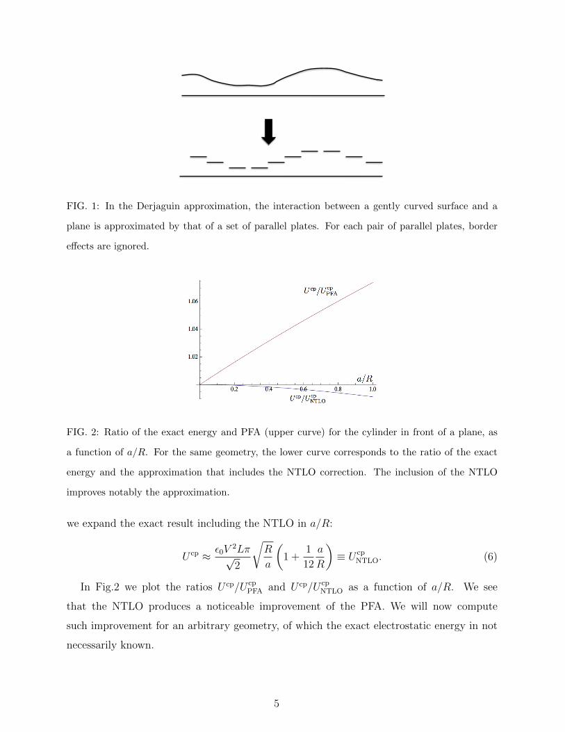
FIG. 1: In the Derjaguin approximation, the interaction between a gently curved surface and a

plane is approximated by that of a set of parallel plates. For each pair of parallel plates, border

effects are ignored.

FIG. 2: Ratio of the exact energy and PFA (upper curve) for the cylinder in front of a plane, as

a function of a/R. For the same geometry, the lower curve corresponds to the ratio of the exact

energy and the approximation that includes the NTLO correction. The inclusion of the NTLO

improves notably the approximation.

we expand the exact result including the NTLO in a/R:

U cp ≈ ε0V2Lπ√2

√R

a

(1 +

1

12

a

R

)≡ U cp

NTLO. (6)

In Fig.2 we plot the ratios U cp/U cpPFA and U cp/U cp

NTLO as a function of a/R. We see

that the NTLO produces a noticeable improvement of the PFA. We will now compute

such improvement for an arbitrary geometry, of which the exact electrostatic energy in not

necessarily known.

5

III. IMPROVING THE PFA: DERIVATIVE EXPANSION

In order to improve the PFA, we shall use the fact that the electrostatic energy may be

thought of as a functional of the shape of the surface. This functional will be, in general,

a non-local object, which becomes local when the surfaces are sufficiently close and parallel

to each other. To interpolate between those two situations, we shall therefore assume that

the electrostatic energy can be expanded in derivatives of ψ. Indeed, one can think of the

condition |∇ψ| � 1, as the existence of a small, dimensionless parameter. This translates

into the fact that the upper surface is almost parallel to the plane.

Including terms with up to two derivatives, the electrostatic energy has to be of the form:

UDE '∫d2x‖

[Veff(ψ) + Z(ψ)|∇ψ|2

], (7)

for some functions Veff and Z [11]. The result must be proportional to ε0V2, and must

reproduce UPFA for constant ψ. Moreover, as there are no other dimensional quantities

beyond ψ, dimensional analysis imply that both functions Veff and Z must be proportional

to ψ−1:

UDE 'ε0V

2

2

∫d2x‖

1

ψ(1 + βem|∇ψ|2) , (8)

where βem is the only (numerical) coefficient to be determined. Note that this coefficient is

independent of the nature of the surface being considered; therefore, it may be obtained once

and for all from its evaluation in a single case. Indeed, in order to obtain the coefficient βem,

the simplest approach, when an exact solution of the problem is available, would be to read

its value by expanding the exact solution. For instance, for the particular configuration of

a cylinder in front of a plane, one can insert Eq.(3) into Eq.(8), perform the integrals, and

expand the result in powers of a/R. Comparing this with the expansion of the exact result

given in Eq.(6), it is straightforward to show that βem = 1/3. Of course the same result

could have been obtained from any other particular example.

Nevertheless, the coefficient βem can also be computed from first principles, as described

in the next section.

IV. SOLVING THE LAPLACE EQUATION

It is perhaps more satisfying to prove that βem = 1/3 without assuming a particular

shape for the curved surface, but rather for a rather general class of surfaces. To that end it

6

will be sufficient to derive it by assuming that ψ(x‖) = a+ η(x‖) where a is the mean value

of ψ, and |η(x‖)| � 1. For this class of surfaces, the derivative expansion of the electrostatic

energy reads

UDE 'ε0V

2

2a

∫d2x‖

[1 +

(ηa

)2

+ βem|∇η|2 +O(η3)

], (9)

and therefore he coefficient βem can be read from the quadratic dependence of UDE on the

derivatives of η.

The electric field is given by E = −∇φ, where φ is the electrostatic potential, which

satisfies the Laplace equation with the appropriate boundary conditions on the surfaces:

∇2φ = 0, φz=0 = 0, φz=ψ = V. (10)

To proceed, we follow the approach of [12], to trade a simple boundary condition on

a complex surface into a complex boundary condition on a flat surface. We expand the

boundary condition on the upper surface as

V = φ(x‖, a+ η) = φ(x‖, a) + η∂zφ(x‖, a) +1

2η2∂2

zφ(x‖, a) + .... , (11)

and we expand the electrostatic potential as

φ = φ0 + φ1 + φ2 + . . . , (12)

where φ0 is the solution for parallel plates separated by a distance a, that is φ0 = V z/a,

and φi is assumed to be O(ηi).

Inserting Eq.(12) into Eq.(11), we see that φ1 and φ2 must satisfy the following boundary

conditions on z = a:

φ1(x‖, a) = −Vaη(x‖)

φ2(x‖, a) = −η(x‖)∂zφ1(x‖, a) . (13)

Thus, the initial problem has been converted into a problem of parallel plates for φ1 and φ2,

with more involved boundary conditions. Up to quadratic order, the electrostatic energy

reads

UDE 'ε02

∫d2x‖

∫ a+η

0

dz

[V 2

a2+ |∇φ1|2 + 2

V

a∂zφ1 + 2

V

a∂zφ2

]. (14)

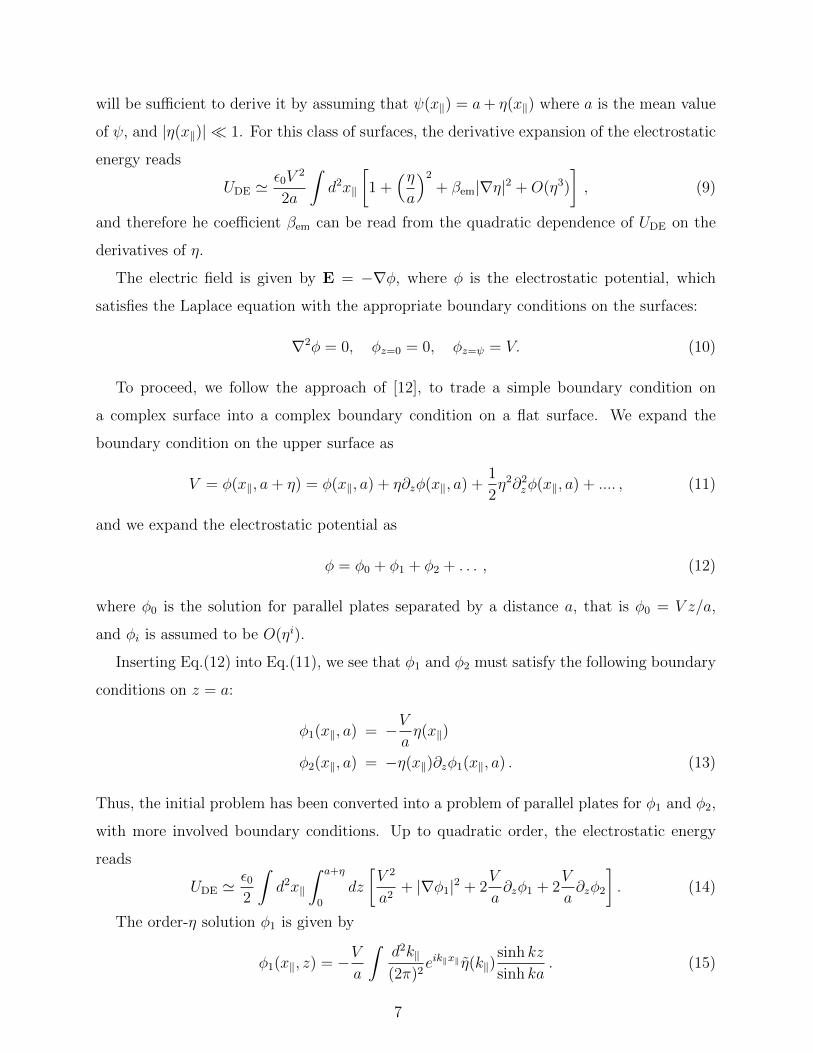
The order-η solution φ1 is given by

φ1(x‖, z) = −Va

∫d2k‖(2π)2

eik‖x‖ η(k‖)sinh kz

sinh ka. (15)

7

Indeed, it is simple to check that it satisfies both the Laplace equation and the correct

boundary condition (we are using the notation k ≡ |k‖|). The solution for φ2 is similar-

looking, although its explicit expression will not be necessary in order to evaluate the second-

order energy.

Using the solution Eq.(15) we obtain:∫d3x|∇φ1|2 =

V 2

a2

∫d2k‖(2π)2

|η(k‖)|2F (k‖), (16)

where

F (k‖) =

∫ a

0

dzk2

sinh2 ka(1 + 2 sinh2 kz) ' 1

a+ak2

3. (17)

(note that the integration in z runs up to a instead of a + η since the integrand is already

of order η2). Therefore, the term proportional to two derivatives of η reads

ε02

∫d3x|∇φ1|2 =

ε0V2

6a

∫d2x‖ |∇η|2 , (18)

which means that this term contributes to βem with a factor 1/3.

The other two terms in Eq.(14) can be computed in a similar fashion. For example:

2V

a

∫d3x ∂zφ2 '

2V

a

∫d2x‖ φ2(x‖, a) = −2V

a

∫d2x‖ η(x‖) ∂zφ1(x‖, a), (19)

and the explicit calculation gives a contribution 2/3 to βem.

There is a subtle point in the contribution to UDE proportional to ∂zφ1: being linear in

η, it is necessary to perform the integration in z up to a+ η:

2V

a

∫d2x‖

∫ a+η

0

dz ∂zφ1 =2V

a

∫d2x‖ φ1(x‖, a+ η) . (20)

Now we expand

φ1(x‖, a+ η) ' φ1(x‖, a) + η∂zφ1(x‖, a) , (21)

and substitute Eq.(21) into Eq.(20). The first term vanishes because the mean value of η is

zero. The calculation of the second term gives a contribution −2/3 to βem, that cancels a

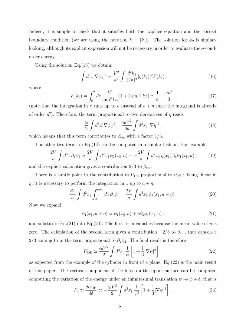
2/3 coming from the term proportional to ∂zφ2. The final result is therefore

UDE 'ε0V

2

2

∫d2x‖

1

ψ

[1 +

1

3|∇ψ|2

], (22)

as expected from the example of the cylinder in front of a plane. Eq.(22) is the main result

of this paper. The vertical component of the force on the upper surface can be computed

computing the variation of the energy under an infinitesimal translation ψ → ψ + δ, that is

Fz 'dUDE

dδ' −ε0V

2

2

∫d2x‖

1

ψ2

[1 +

1

3|∇ψ|2

]. (23)

8

V. TIP-SAMPLE ELECTROSTATIC INTERACTION

In this section we use the improved PFA to analyze the problem of the tip-sample elec-

trostatic force in an AFM. Typical geometries to model the interaction are sphere-plane,

paraboloid-plane, hyperboloid-plane, and sphere-ended cone in front of a plane, among oth-

ers [3]. In all these cases, it is possible to obtain the electrostatic force using the improved

PFA. The results will be accurate when the tip is sufficiently close to the sample.

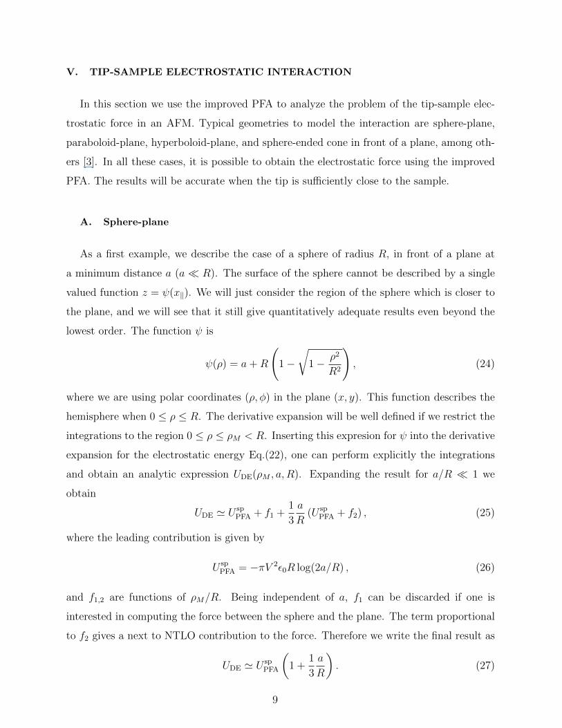
A. Sphere-plane

As a first example, we describe the case of a sphere of radius R, in front of a plane at

a minimum distance a (a� R). The surface of the sphere cannot be described by a single

valued function z = ψ(x‖). We will just consider the region of the sphere which is closer to

the plane, and we will see that it still give quantitatively adequate results even beyond the

lowest order. The function ψ is

ψ(ρ) = a+R

(1−

√1− ρ2

R2

), (24)

where we are using polar coordinates (ρ, φ) in the plane (x, y). This function describes the

hemisphere when 0 ≤ ρ ≤ R. The derivative expansion will be well defined if we restrict the

integrations to the region 0 ≤ ρ ≤ ρM < R. Inserting this expresion for ψ into the derivative

expansion for the electrostatic energy Eq.(22), one can perform explicitly the integrations

and obtain an analytic expression UDE(ρM , a, R). Expanding the result for a/R � 1 we

obtain

UDE ' U spPFA + f1 +

1

3

a

R(U sp

PFA + f2) , (25)

where the leading contribution is given by

U spPFA = −πV 2ε0R log(2a/R) , (26)

and f1,2 are functions of ρM/R. Being independent of a, f1 can be discarded if one is

interested in computing the force between the sphere and the plane. The term proportional

to f2 gives a next to NTLO contribution to the force. Therefore we write the final result as

UDE ' U spPFA

(1 +

1

3

a

R

). (27)

9

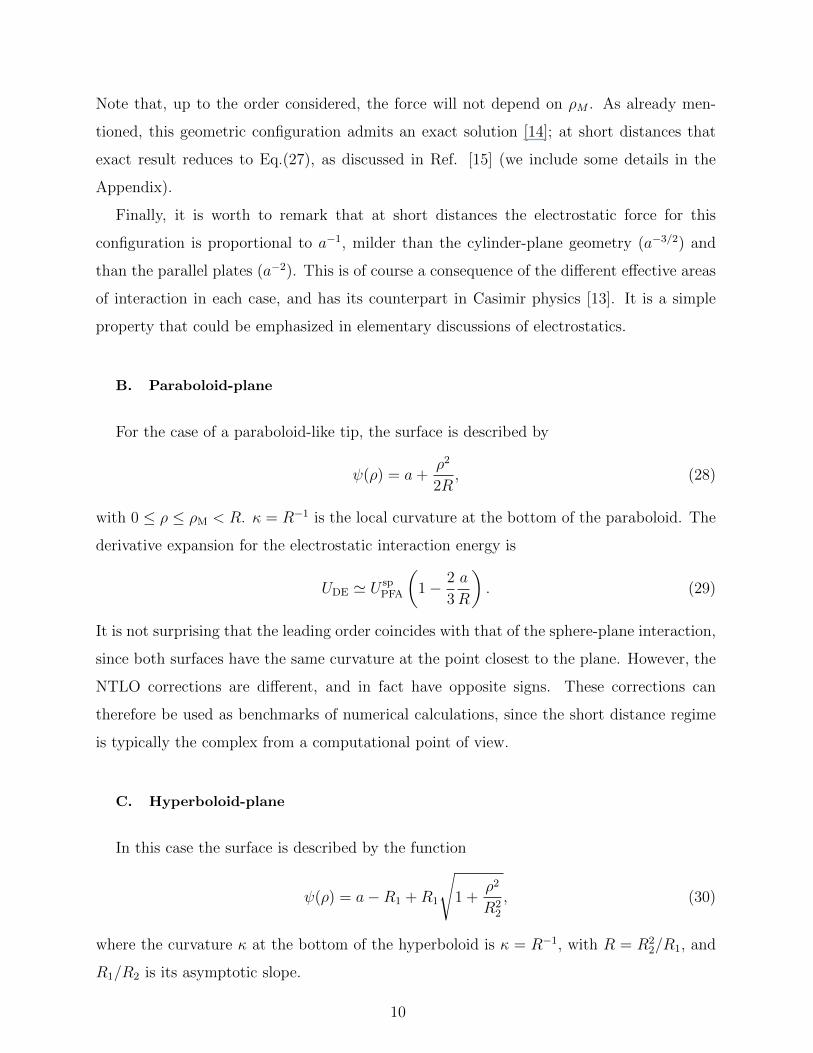
Note that, up to the order considered, the force will not depend on ρM . As already men-

tioned, this geometric configuration admits an exact solution [14]; at short distances that

exact result reduces to Eq.(27), as discussed in Ref. [15] (we include some details in the

Appendix).

Finally, it is worth to remark that at short distances the electrostatic force for this

configuration is proportional to a−1, milder than the cylinder-plane geometry (a−3/2) and

than the parallel plates (a−2). This is of course a consequence of the different effective areas

of interaction in each case, and has its counterpart in Casimir physics [13]. It is a simple

property that could be emphasized in elementary discussions of electrostatics.

B. Paraboloid-plane

For the case of a paraboloid-like tip, the surface is described by

ψ(ρ) = a+ρ2

2R, (28)

with 0 ≤ ρ ≤ ρM < R. κ = R−1 is the local curvature at the bottom of the paraboloid. The

derivative expansion for the electrostatic interaction energy is

UDE ' U spPFA

(1− 2

3

a

R

). (29)

It is not surprising that the leading order coincides with that of the sphere-plane interaction,

since both surfaces have the same curvature at the point closest to the plane. However, the

NTLO corrections are different, and in fact have opposite signs. These corrections can

therefore be used as benchmarks of numerical calculations, since the short distance regime

is typically the complex from a computational point of view.

C. Hyperboloid-plane

In this case the surface is described by the function

ψ(ρ) = a−R1 +R1

√1 +

ρ2

R22

, (30)

where the curvature κ at the bottom of the hyperboloid is κ = R−1, with R = R22/R1, and

R1/R2 is its asymptotic slope.

10

As in the previous examples, the derivative expansion of the electrostatic energy can be

computed in terms of elementary functions. The result is

UDE ' U spPFA

[1− (

2

3− R2

2

R21

)a

R

]. (31)

It is remarkable that sign of the NTLO correction depends on the parameters of the hyper-

boloid, and vanishes for the particular asymptotic slope R1/R2 =√

3/2.

VI. GENERALIZATIONS

The results presented so far can be generalized in several directions:

A. Beyond the next to leading order

It is in principle possible to extend the results in order to include more derivatives of the

shape function. For example, coming back to the case of a surface in front of a plane, the

improved PFA would be, including the next to NTLO corrections:

UDE =ε0V

2

2

∫d2x‖

1

ψ(1 +

1

3|∇ψ|2 + γ1|∇ψ|4 + γ2ψ|∇ψ|2∇2ψ

+ γ3ψ2∇2ψ∇2ψ + γ4ψ

2∂α∂βψ∂α∂βψ + γ5ψ3∇2∇2ψ), (32)

where γ1, γ2, ...γ5, are numerical coefficients that can be determined extending the calculation

of Section IV up to O(η4) [16].

The structure of the improved PFA is useful to analyze its range of validity: the NTLO

corrections are small when |∇ψ| � 1 or, in other words, when the curved surface is almost

parallel to the plane. Higher order corrections will be negligible when, in addition to this

condition, the scale of variation of the shape of the surface is much larger than the local

distance between surfaces.

B. Flat surface coated with a dielectric layer

The improved PFA can be extended to the case in which the sample (flat surface) is a

perfect conductor coated with a layer of width d of a material characterized with a constant

permittivity ε, as considered in the context of EFM [17]. Dimensional analysis implies that

11

the derivative expansion for the electrostatic energy will be of the form

UDE 'ε0V

2

2

∫d2x‖

1

ψ

[α(

ε

ε0,d

ψ) + β(

ε

ε0,d

ψ)|∇ψ|2

], (33)

for some functions α and β. We do not dwell here with the determination of the function

β, but just want to remark that α can be obtained by elementary considerations for a

parallel-plate capacitor with a dielectric layer:

α(ε

ε0,d

ψ) =

1

1− dψ

(1− ε0ε

). (34)

C. Two gently curved surfaces

For the case of the Casimir energy, the result of Ref.[9] has been generalized to the case

of two gently curved surfaces in Ref.[18]. This generalization can also be applied to the

electrostatic case. Let us assume that the surfaces are described by two functions ψ1(x‖)

and ψ2(x‖) that measure the height of the surfaces with respect to a reference plane Σ. The

derivative expansion for the electrostatic energy reads, in this case:

UDE[ψ1, ψ2] =ε0V

2

2

∫Σ

d2x‖1

ψ

[1 + β1|∇ψ1|2

+ β2|∇ψ2|2 + β×∇ψ1 · ∇ψ2 + β− z · ∇ψ1 ×∇ψ2) + · · ·], (35)

where ψ = |ψ2 − ψ1| is the height difference, and dots denote higher derivative terms.

As the energy must be invariant under the interchange of ψ1 and ψ2, β1 = β2 and β− = 0.

Moreover, in order to reproduce the previous result we must have β1 = β2 = 1/3. Finally,

the coefficient β× can be determined using the fact that the energy should be invariant under

a tilt of the reference surface Σ [18] or, alternatively, under a simultaneous rotation of both

surfaces. For an infinitesimal rotation of each surface with an angle ε in the plane (x, z) we

have δψi = ε(x + ψi∂xψi), for i = 1, 2. In order to simplify the calculation we can assume

that, initially, ψ1 = 0 and that ψ2 is only a function of x. Computing explicity the variation

of UDE to linear order in ε one can show that

δUDE = 0⇒ β× =1

3, (36)

and therefore

UDE[ψ1, ψ2] =ε0V

2

2

∫Σ

d2x‖1

ψ

[1 +

1

3

(|∇ψ1|2 + |∇ψ2|2 +∇ψ1 · ∇ψ2

)]. (37)

12

While the equality β1 = β2 is valid for any interaction (as long as the surfaces are

identical), the fact that β× = β1 is valid only for the particular case of the electrostatic

interaction, in which the leading term is proportional to ψ−1 (i.e. is not valid for the

Casimir energy, that is proportional to ψ−3 for parallel plates).

Computing the variation of the electrostatic energy Eq.(35) with respect to translations

or rotations of one of the surfaces, it is possible to obtain the vertical and lateral components

of the force, as well as the torque produced by the presence of the other surface.

VII. FINAL REMARKS

The PFA is a very useful approximation introduced by Derjaguin many years ago to

compute Van der Waals forces between macroscopic bodies. The approximation has been

subsequently widely used in rather different contexts, like nuclear physics and the Casimir

effect. Very recently, the approximation has been interpreted as the leading order in a

derivative expansion of the energy, and this interpretation allowed to compute, for the first

time, the NTLO corrections in a systematic way. In this paper we have pointed out that the

improved PFA is a powerful tool which may also be used to compute the electrostatic inter-

action between conducting surfaces. Indeed, with this improved approximation, it is possible

to compute the electrostatic force with high accuracy when the surfaces are sufficiently close

to each other.

Moreover, given the simplicity of the expressions for the energy and the force, the NTLO

could be used to test numerical methods aimed at a calculation of the force for arbitrary

surfaces.

Acknowledgements

This work was supported by ANPCyT, CONICET, UBA and UNCuyo.

Appendix

The electrostatic problem of a sphere of radius R in front of a plane can be solved exactly:

if the potential difference between the plane and the sphere is V , the electrostatic energy is

13

given by [14]

U sp = 2πε0RV2 sinh Γ

∑n≥1

1

sinh(nΓ), (38)

where cosh Γ = 1 + a/R. In order to obtain an analytic expression in the limit Γ → 0 we

write

S ≡∑n≥1

1

sinh(nΓ)= S −

∫ ∞1

dn

sinh(nΓ)+

1

Γln(coth Γ)

=γ

Γ+

1

Γln(coth Γ) +O(Γ), (39)

where γ = 0.5772. Replacing this expression into Eq.(38) and expanding the result for small

a/R we obtain

U sp ' −πε0aV 2 ln(2a/R)

{1 +

1

3

a

R+O

(a/R

ln(a/R)

)}, (40)

where we omited an irrelevant constant term. This result coincides, up to the NTLO, with

the one obtained using the derivative expansion Eq.(27).

[1] C. C. Williams, W. P. Hough, and A. Rishton, Appl. Phys. Lett. 55, 203 (1989); A. Gil, J.

Colchero, J. Gomez-Herrero, and A. M. Baro, Nanotechnology 14, 332 (2003); J. Hu, X.-D.

Xiao, and M. Salmeron, Appl. Phys. Lett. 67, 476 (1995).

[2] M. Bordag, G.L. Klimchitskaya, U. Mohideen, and V. M. Mostepanenko, Advances in the

Casimir Effect, Oxford University Press, Oxford, 2009.

[3] M. Lhernould, A. Delchambre, S. Regnier, P. Lambert, Applied Surface Science 253, 6203

(2007).

[4] G. Mesa and J. J. Saenz, Appl. Phys. Lett. 69, 1169 (1996); S. Gomez-Moivas, L. S. Froufe,

R. Carminati, J. J. Greffet, and J. J. Saenz, Nanotechnology 12, 496 (2001).

[5] B.V. Derjaguin, Koll. Z. 69, N2, 155 (1934); B. V. Derjaguin and I. I. Abrikosova, Sov. Phys.

JETP 3, 819 (1957); B. V. Derjaguin, Sci. Am. 203, 47 (1960).

[6] J.N. Israelachvili, Intermolecular and Surface Forces, Academic Press Inc., San Diego (1998).

[7] J. Blocki, J. Randrup, W. J. Swiatecki, and C. F. Tsang, Ann. Phys. NY 105, 427 (1977); J.

Blocki and W. J. Swiatecki, Ann. Phys. NY 132, 53 (1981).

[8] W. D. Myers and W. J. Swiatecki, Phys. Rev. C 62, 044610 (2000); I. Dutt and R. K. Puri,

Phys. Rev. C 81, 064609 (2010).

14

[9] C. Fosco, F. Lombardo and F. Mazzitelli, Phys. Rev. D 84, 105031 (2011).

[10] L. D. Landau and E.M. Lifshitz, Electrodynamics of continuous media, Pergamon Press, Ox-

ford (1984).

[11] We use the typical notation for the derivative expansion in Quantum Field Theory, in which

Veff is the effective potential and Z the wave function renormalization.

[12] L. H. Ford and A. Vilenkin, Phys. Rev. D 25, 2569 (1982).

[13] D. Dalvit, F. Lombardo, F. Mazzitelli, and R. Onofrio, Europhys. Lett. 67, 517 (2004).

[14] W. R. Smythe, Static and Dynamic Electricity, McGraw-Hill, New York (1968).

[15] F.D. Mazzitelli, F.C. Lombardo, and P. I. Villar, J. Phys.: Conf. Ser. 161, 012015 (2009).

[16] One could be tempted to obtain information about the coefficients γi from the exact result

of the cylinder in front of a plane. However, there is a subtle point here, because the next to

NTLO corrections for this geometry depend on the quantity xM introduced in Section II.

[17] K. S. Date, A. V. Kulkarni, and C. V. Dharmadhikari, e-Journal of Surface Science and

Nanotechnology 9, 206 (2011).

[18] G. Bimonte, T. Emig, R. L. Jaffe, M. Kardar, Casimir forces beyond the proximity approxi-

mation, arXiv:1110.1082.

15